arX

iv:1

903.

0289

9v2

[cs

.IT

] 2

2 O

ct 2

019

1

A General Construction and Encoder

Implementation of Polar CodesWei Song, Student Member, IEEE, Yifei Shen, Student Member, IEEE, Liping Li, Member, IEEE, Kai Niu,

Member, IEEE, and Chuan Zhang, Member, IEEE

Abstract—Similar to existing codes, puncturing and shorteningare two general ways to obtain an arbitrary code length and coderate for polar codes. When some of the coded bits are puncturedor shortened, it is equivalent to a situation in which the un-derlying channels of the polar codes are different. Therefore, thequality of bit channels with puncturing or shortening differ fromthe original qualities, which can greatly affect the construction ofpolar codes. In this paper, a general construction of polar codesis studied in two aspects: 1) the theoretical foundation of theconstruction; and 2) the hardware implementation of polar codesencoders. In contrast to the original identical and independentbinary-input, memoryless, symmetric (BMS) channels, theseunderlying BMS channels can be different. For binary erasurechannel (BEC) channels, recursive equations can be employedassuming independent BMS channels. For all other channel types,the proposed general construction of polar codes is based onthe existing Tal-Vardy’s procedure. The symmetric property andthe degradation relationship are shown to be preserved underthe general setting, rendering the possibility of a modification ofTal-Vardy’s procedure. Simulation results clearly show improvederror performance with re-ordering using the proposed newprocedures. In terms of hardware, a novel pruned folded encoderarchitecture is proposed which saves the computation for thebeginning frozen bits. Implementation results show the prunedencoder achieve 28% throughput improvement.

Index Terms—polar codes, construction, Tal-Vardy, prunedfolded encoder, throughput.

I. INTRODUCTION

POLAR codes are proposed by Arıkan in [1] and

achieve the capacity of binary-input, memoryless, output-

symmetric (BMS) channels with low encoding and decoding

complexity. Given N independent BMS channels W , polariza-

tion occurs through channel combining and splitting, resulting

in perfect bit channels or completely noisy bit channels as Napproaches infinity. The portion of the perfect bit channels

is exactly the symmetric capacity I(W ) of the underlying

channel W . Polar codes transmit information bits through

the perfect bit channels and fix the bits in the completely

noisy channels. Accordingly, the bits transmitted through the

completely noisy channels are called frozen bits.

This work was supported in part by the National Natural Science Foundationof China through grant 61501002, in part by the Natural Science Project ofMinistry of Education of Anhui through grant KJ2015A102, and in part bythe Talents Recruitment Program of Anhui University.

Wei Song and Liping Li are with the Key Laboratory of IntelligentComputing and Signal Processing, Ministry of Education, Anhui University,Hefei, China (liping li@ahu.edu.cn).

Yifei Shen and Chuan Zhang are with the National Mobile Com-munications Research Laboratory, Southeast University, Nanjing, China(chzhang@seu.edu.cn)

Kai Niu is with the Key Laboratory of Universal Wireless Communication,Ministry of Education, Beijing Univer- sity of Posts and Telecommunications,Beijing 100876, Peoples Republic of China (niukai@bupt.edu.cn)

The construction of polar codes (selecting the good bit

channels from all N bit channels) is presented in [1]–[7]. In

[1], Arıkan proposes Monte-Carlo simulations to sort the bit

channels with a complexity of O(SN logN) (S represents

the iterations of the Monte-Carlo simulations). In [2], [3],

density evolutions are used in the construction of polar codes.

Since the density evolution includes function convolutions,

its precisions are limited by the complexity. Bit channel

approximations are proposed in [4] with a complexity of

O(Nµ2 logµ) (µ is a user-defined parameter to control the

number of output alphabet at each approximation stage). In

[5]–[7], the Gaussian approximation (GA) is used to construct

polar codes in additive white Gaussian noise (AWGN) chan-

nels.

To achieve arbitrary code lengths and code rates, punc-

turing and shortening of polar codes are reported in [8]–

[14]. In [8], a channel-independent procedure is proposed

for puncturing that involves the minimum stopping set of

each bit. In [8], the punctured bits are unknown to decoders,

and it is therefore called the unknown puncturing type. The

quasi-uniform puncturing (QUP) algorithm is proposed in [9],

which simply punctures the reversed bits from 1 to P (P is

the number of bits to be punctured). The QUP puncturing

is the unknown puncturing. Re-ordering the bit channels

after puncturing with the GA method is proposed in [10],

and selecting the punctured bits from the frozen positions

is also proposed in [10]. The puncturing in [10] is also

the unknown puncturing. Another type of puncturing, called

known puncturing or shortening, is proposed in [11]–[14]. The

reversal quasi-uniform puncturing (RQUP) algorithm proposed

in [11] simply punctures the reversed bits from N − P + 1to N . The shortening in [12] is based on the column weights

of the generator matrices. A low-complexity construction of

shortened and punctured polar codes from a unified view is

proposed in [13]. In [14], an optimization algorithm to find a

shortening pattern and a set of frozen symbols for polar codes

is proposed.

Regardless of the puncturing or shortening pattern, a re-

ordering of bit channels is necessary when these operations are

performed. In AWGN channels, GA can be used to re-order

the bit channels when some of the coded bits are punctured

or shortened. Puncturing and shortening are equivalent to

the case in which the underlying channel corresponding to

the selected coded bit is no longer the underlying channel

W . As some of the underlying channels change, the bit

channels constructed from these underlying channels differ

from the original channels without puncturing or shortening.

Re-ordering of these new bit channels is necessary to avoid

deterioration of performance. However, the GA method is only

2

applicable to AWGN channels. New procedures are important

when studying puncturing or shortening of polar codes. This

is the motivation of the work in this paper.

To study the construction of polar codes in which some

of the coded bits are punctured or shortened, we first gen-

eralize this problem by considering the underlying channels

to be independent BMS channels (not necessarily identical

ones). For BEC channels, recursive equations are proposed

in [15] to calculate the Bhattacharyya parameter for each

bit channel. The construction complexity is the same as the

original complexity in [1]. For other channel types, the general

construction in this paper is based on Tal-Vardy’s procedures

in [4]. The symmetric property of polar codes, which is first

stated in [1], is proven to hold in the new setting in which the

underlying channels can differ. The degradation relationship

(the foundation of Tal-Vardy’s procedure) is also proven to

hold. Based on the theoretical analysis, a modification to

the Tal-Vardy algorithm [4] that is applicable to any BMS

channel is proposed to re-order the bit channels when some

of the underlying channels are independent BMS channels

(which, again, could be different channels). For continuous

output channels such as AWGN channels, conversion to

BMS channels can be performed first, and then the modified

Tal-Vardy algorithm can be applied analogous to the Tal-

Vardy algorithm itself. The general construction can therefore

be applied to re-order the bit channels with puncturing or

shortening. Depending on the puncture type, the punctured

channel must be equivalently modeled. Then, the recursion in

BEC channels or the modified Tal-Vardy’s procedure for all

other channels can be applied to re-order the bit channels.

Simulation results show that the re-ordering greatly improves

the error performance of polar codes.

Utilizing the property that the beginning of the source bits

are usually frozen bits (0s in other words), the encoding

throughput can be improved. With the increase of the code

length, the area of the encoder increases exponentially. Folding

[16] is a technique to reduce the area by multiplexing the

modules. By exploiting the same property between polar

encoding and the fast Fourier transformation (FFT), [17] first

applies the folding technique for the polar encoding based

on [18]. Folded systematic polar encoder is implemented in

[19]. Moreover, [20] designs an auto-generation folded polar

encoder, which could preprint the hardware code directly given

the length and the level of parallelism. Combining the property

of the puncturing mode, current folded encoder could be

pruned further. In this paper, a pruned folded polar encoder

is proposed. It avoids the beginning calculation of the frozen

‘0’ bits. Therefore, the latency could be reduced significantly.

Implementation results also proves the feasibility of the pruned

encoder, which provides 28% throughput improvement.

The remainder of this paper is organized as follows. In

Section II, we briefly introduce the basics of polar codes.

The general construction based on Tal-Vardy’s procedure is

presented in Section III. The numerical results for applying the

BEC construction and the general construction in Section III

are provided in Section IV. Section V proposes a pruned folded

polar encoder architecture and the results are compared with

the state-of-the-art. The paper ends with concluding remarks.

II. BACKGROUND ON POLAR CODES

A. Polarization Process

For a given BMS channel W : X −→ Y , its input alphabet,

output alphabet, and transition probability are X = {0, 1},Y , and W (y|x), respectively, where x ∈ X and y ∈ Y .

Two parameters represent the quality of a BMS channel W :

the symmetric capacity and the Bhattacharyya parameter. The

symmetric capacity can be expressed as

I(W ) =∑

y∈Y

∑

x∈X

1

2W (y|x) log

W (y|x)12W (y|0) + 1

2W (y|1). (1)

The Bhattacharyya parameter is

Z(W ) =∑

y∈Y

√

W (y|0)W (y|1) . (2)

The term GN is used to represent the generator matrix:

GN = BNF⊗n, where N = 2n is the code length (n > 1),

BN is the permutation matrix used for the bit-reversal opera-

tion, F , [ 1 01 1 ], and F⊗n denotes the nth Kronecker product

of F . The channel polarization is divided into two phases:

channel combing and channel splitting. The channel combing

refers to the combination of N copies of a given BMS W to

produce a vector channel WN , defined as

WN (yN1 |uN1 ) = WN (yN1 |u

N1 GN ). (3)

The channel splitting splits WN back into a set of N binary-

input channels W(i)N , defined as

W(i)N (yN1 , ui−1

1 |ui) =∑

uN

i+1∈XN−i

1

2N−1WN (yN1 |u

N1 ). (4)

The channel W(i)N is called bit channel i, which indicates

that it is the channel that bit i experiences from the channel

combining and splitting stages. Bit channel i can be viewed

as a BMS channel: X → (X i−11 ,YN

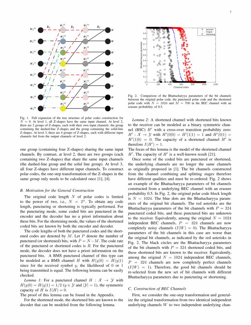
1 ).Polar codes can also be constructed recursively in a tree

structure [1]. The tree structure is expanded fully in Fig. 1

for N = 8. There are eight independent and identical BMS

channels W at the right-hand side. In Fig. 1, from right to

left, there are three levels: level one, level two, and level three,

each containing N/2 Z-shapes. A Z-shape is the basic one-

step transformation with the transition probability defined in

(4) with N = 2. This one-step transformation converts two

input channels to two output channels: the upper left channel

and the lower left channel. For bit channel i (1 ≤ i ≤ N ), the

binary expansion of i−1 is denoted as 〈i〉 = (b1, b2, ..., bn) (b1being the MSB). The bit bk at level k (1 ≤ k ≤ n) determines

whether bit channel i takes the upper left channel or the lower

left channel: If bk = 0, bit channel i takes the upper left

channel; otherwise, it takes the lower left channel. At level

k, there are 2n−k Z-shapes with the same input channels. For

example, in Fig. 1, at level 1, all Z-shapes have the same

input channels W . At level 2, there are two Z-shapes with the

same input channels: the two dashed-line Z-shapes have input

channels W(1)2 , and the two solid-line Z-shapes have input

channels W(2)2 . The Z-shapes are grouped with the same input

channels as one group in each level. Then, at level 1, there is

3

Fig. 1. Full expansion of the tree structure of polar codes construction forN = 8. At level 1, all Z-shapes have the same input channel. At level 2,there are 2 groups of Z-shapes, each with their own input channels: the groupcontaining the dashed-line Z-shapes and the group containing the solid-lineZ-shapes. At level 3, there are 4 groups of Z-shapes, each with different inputchannels fed from the output channels of level 2.

one group (containing four Z-shapes) sharing the same input

channels. By contrast, at level 2, there are two groups (each

containing two Z-shapes) that share the same input channels

(the dashed-line group and the solid line group). At level 3,

all four Z-shapes have different input channels. To construct

polar codes, the one-step transformation of the Z-shapes in the

same group only needs to be calculated once [1], [4].

B. Motivation for the General Construction

The original code length N of polar codes is limited

to the power of two, i.e., N = 2n. To obtain any code

length, puncturing or shortening is typically performed. For

the puncturing mode, some coded bits are punctured in the

encoder and the decoder has no a priori information about

these bits. For the shortening mode, the values of the shortened

coded bits are known by both the encoder and decoder.

The code lengths of both the punctured codes and the short-

ened codes are denoted by M . Let P denote the number of

punctured (or shortened) bits, with P = N−M . The code rate

of the punctured or shortened codes is R. For the punctured

mode, the decoder does not have a priori information on the

punctured bits. A BMS punctured channel of this type can

be modeled as a BMS channel H with H(y|0) = H(y|1)since for the received symbol y, the likelihood of 0 or 1being transmitted is equal. The following lemma can be easily

checked.

Lemma 1: For a punctured channel H : X → Y with

H(y|0) = H(y|1) = 1/2 (y ∈ Y and |Y| = 1), the symmetric

capacity of H is I(H) = 0.

The proof of this lemma can be found in the Appendix.

For the shortened mode, the shortened bits are known to the

decoder that can be modeled from the following lemma.

Channel index0 200 400 600 800 1000 1200

Bha

ttach

aryy

a pa

ram

eter

0

0.1

0.2

0.3

0.4

0.5

0.6

0.7

0.8

0.9

1punctureOrignalshortening

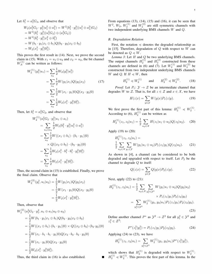
Fig. 2. Comparison of the Bhattacharyya parameters of the bit channelsbetween the original polar code, the punctured polar code and the shortenedpolar code with N = 1024 and M = 700 in the BEC channel with anerasure probability of 0.5.

Lemma 2: A shortened channel with shortened bits known

to the receiver can be modeled as a binary symmetric chan-

nel (BSC) H ′ with a cross-over transition probability zero:

H ′ : X → Y with H ′(0|0) = H ′(1|1) = 1 and H ′(0|1) =H ′(1|0) = 0. The capacity of a shortened channel H ′ is

therefore I(H ′) = 1.

The focus of this lemma is the model of the shortened channel

H ′. The capacity of H ′ is a well-known result [21].

Once some of the coded bits are punctured or shortened,

the underlying channels are no longer the same channels

as originally proposed in [1]. The bit channels constructed

from the channel combining and splitting stages therefore

have different qualities and must be re-ordered. Fig. 2 shows

an example of the Bhattacharyya parameters of bit channels

constructed from a underlying BEC channel with an erasure

probability 0.5. In Fig. 2, the original polar code block length

is N = 1024. The blue dots are the Bhattacharyya param-

eters of the original bit channels. The red asterisks are the

Bhattacharyya parameters of the bit channels with P = 324punctured coded bits, and these punctured bits are unknown

to the receiver. Equivalently, among the original N = 1024independent BEC channels, P = 324 channels are now

completely noisy channels (I(W ) = 0). The Bhattacharyya

parameters of the bit channels in this case are worse than

the original bit channels, as indicated by the red asterisks in

Fig. 2. The black circles are the Bhattacharyya parameters

of the bit channels with P = 324 shortened coded bits, and

these shortened bits are known to the receiver. Equivalently,

among the original N = 1024 independent BEC channels,

P = 324 channels are now completely perfect channels

(I(W ) = 1). Therefore, the good bit channels should be

re-selected from the new set of bit channels with different

Bhattacharyya parameters due to puncturing or shortening.

C. Construction of BEC Channels

First, we consider the one-step transformation and general-

ize the original transformation from two identical independent

underlying channels W to two independent underlying chan-

4

Fig. 3. General one-step transformation of polar codes where the underlyingchannels are independent BMS channels.

nels. The two independent channels can be different channels

as indicated in Fig. 3, where W and Q are two BMS channels.

With puncturing or shortening, Q can be a completely noisy

channel with I(Q) = 0 (puncturing) or a perfect channel

I(Q) = 1 (shortening). With the generalization in Fig. 3, the

synthesized channel W2 can be expressed as follows:

W2(y1, y2|u1, u2) = W (y1|u1 ⊕ u2)Q(y2|u2). (5)

The splitting channels W(1)2 and W

(2)2 can be expressed as

follows:

W(1)2 (y21 |u1) =

∑

u2

1

2W (y1|u1 ⊕ u2)Q(y2|u2), (6)

W(2)2 (y21 , u1|u2) =

1

2W (y1|u1 ⊕ u2)Q(y2|u2). (7)

Borrowing the notations from [15], the above one-step trans-

formation can be written as follows:

W(1)2 = W � Q, (8)

W(2)2 = W � Q. (9)

For BEC channels, the one-step transformation from W and

Q to W(1)2 ,W

(2)2 has the following Bhattacharyya parameters

[15]:

Z(W(1)2 ) = Z(W ) + Z(Q)− Z(W )Z(Q), (10)

Z(W(2)2 ) = Z(W )Z(Q). (11)

The construction of polar codes in BEC channels can be per-

formed by recursively employing these two equations where

the underlying channels are independent BMS channels.

III. GENERAL CONSTRUCTION BASED ON

THE TAL-VARDY PROCEDURE

Tal-Vardy’s construction of polar codes [4] is based on the

fact that polar codes can be constructed in n levels for a block

length N = 2n, as shown in Fig. 1. In each level, the one-step

transformation defined in (6) or (7) is performed. Note that

in the original one-step transformation in [1], the underlying

channels are identical: Q = W (also shown in Fig. 1). From

level k to level k + 1 (1 ≤ k ≤ n− 1), the size of the output

alphabet at least squares. The output channel in each level

is still a BMS channel. The idea in [4] is to approximate the

output BMS channel in each level by a new BMS channel with

a controlled output alphabet size. This size is denoted as µ,

which indicates that the output alphabet has at most µ symbols

in each level. With this controlled size, each approximated bit

channel can be evaluated in terms of the error probability,

As shown in [4], [15], the degradation relation is preserved

by the one-step channel transformation operation. In addition,

as shown by Proposition 6 of [4], the output of the approximate

procedure remains a BMS channel: taking an input BMS

channel, the output from the approximate process is still a

BMS channel. Therefore, the key to applying Tal-Vardy’s

approximate function to the general construction is that 1) the

output channels from (6) and (7) are still BMS channels; 2)

the degradation relation is preserved from (6) and (7).

In the following, we first prove that the output of the

generalized one-step transformation remains a BMS channel.

Then, the degradation relation from (6) and (7) is shown to be

preserved. The modification to Tal-Vardy’s algorithm follows.

A. Symmetric Property

Some notations are needed first. For a BMS channel W ,

it has a permutation π1 on Y with π−11 =π1 and W (y|1) =

W (π1(y)|0) for all y ∈ Y . Let π0 be the identity permutation

on Y . As in [1], a simpler expression x · y is used to replace

πx(y), for x ∈ X , and y ∈ Y .

Obviously, the equation W (y|x ⊕ a) = W (a · y|x) is

established for a ∈ {0, 1}, x ∈ X , and y ∈ Y . It is also

shown in [1] that W (y|x ⊕ a) = W (a · y|x). For xN1 ∈ X

N

and yN1 ∈ YN , let

xN1 · y

N1 , (x1 · y1, ..., xN · yN ). (12)

This is an element-wise permutation.

Proposition 1: For two independent BMS channels W and

Q, W 2=W ∗Q is also symmetric in the sense that

W 2(y21 |x21 ⊕ a21) = W 2(x2

1 · y21 |a

21), (13)

where a1, a2 ∈ {0, 1}.

Proof: Observe that W 2(y21 |x21 ⊕ a21) = W (y1|x1 ⊕

a1)Q(y2|x2 ⊕ a2). From the symmetric property of W and

Q, we also have

W (y1|x1 ⊕ a1) = W (x1 · y1|a1),

Q(y2|x2 ⊕ a2) = Q(x2 · y2|a2).

Therefore, W 2(y21 |x21 ⊕ a21) = W (x1 · y1|a1)Q(x2 · y2|a2),

which is exactly W 2(x21 · y

21 |a

21).

Proposition 2: For BMS channels W and Q, the channels

W2 defined in (5), W(1)2 defined in (6), and W

(2)2 defined in

(7), are also symmetric in the sense that

W2(y21 |u

21) = W2(a

21G2 · y

21 |u

21 ⊕ a21), (14)

W(1)2 (y21 |u1) = W

(1)2 (a21G2 · y

21 |u1 ⊕ a1), (15)

W(2)2 (y21 , u1|u2) = W

(2)2 (a21G2 · y

21 , u1 ⊕ a1|u2 ⊕ a2), (16)

where a1, a2 ∈ {0, 1}.

Proof: Let x21 = u2

1G2 and observe that

W2(y21 |u

21) = W (y1|x1)Q(y2|x2)

= W (x1 · y1|0)Q(x2 · y2|0)

= W2(x21 · y

21 |0

21).

5

Let b21 = a21G2, and observe that

W2(a21G2 · y

21 |u

21 ⊕ a21) = W 2(b21 · y

21 |(u

21 ⊕ a21)G2)

= W 2(b21 · y21 |(u

21G2)⊕ (a21G2))

= W 2(b21 · y21 |x

21 ⊕ b21)

= W (b1 · y1|x1 ⊕ b1)Q(b2 · y2|x2 ⊕ b2)

= W2(x21 · y

21 |0

21).

This proves the first result in (14). Next, we prove the second

claim in (15). With x1 = u1⊕u2 and x2 = u2, the bit channel

W(1)N can be written as follows:

W(1)2 (y21 |u1) =

∑

u2

1

2W2(y

21 |u

21)

=∑

u2

1

2W (y1|x1)Q(y2|x2) (17)

=∑

u2

1

2W (x1 · y1|0)Q(x2 · y2|0)

=∑

u2

1

2W2(x

21 · y

21 |0

21).

Then, let b21 = a21G2, and observe that

W(1)2 (a21G2 · y

21 |u1 ⊕ a1)

=∑

u2⊕a2

1

2W2(b

21 · y

21 |u

21 ⊕ a21)

=∑

u2

1

2W ((x1 ⊕ b1) · (b1 · y1)|0)

×Q((x2 ⊕ b2) · (b2 · y2)|0)

=∑

u2

1

2W2(x

21 · b

21 · b

21 · y

21 |0

21)

=∑

u2

1

2W2(x

21 · y

21 |0

21).

Thus, the second claim in (15) is established. Finally, we prove

the final claim. Observe that

W(2)2 (y21 , u1|u2) =

1

2W (y1|x1)Q(y2|x2)

=1

2W (x1 · y1|0)Q(x2 · y2|0)

=1

2W2(x

21 · y

21 |0

21).

Then, observe that

W(2)2 (a21G2 · y

21 , u1 ⊕ a1|u2 ⊕ a2)

=1

2W (b1 · y1|x1 ⊕ b1)Q(b2 · y2|x2 ⊕ b2)

=1

2W ((x1 ⊕ b1)·(b1 · y1)|0)×Q((x2 ⊕ b2)·(b2 ·y2)|0)

=1

2W (x1 · b1 · b1 · y1|0)Q(x2 · b2 · b2 · y2|0)

=1

2W (x1 · y1|0)Q(x2 · y2|0)

=1

2W2(x

21 · y

21 |0

21).

Thus, the third claim in (16) is also established.

From equations (13), (14), (15) and (16), it can be seen that

W 2, W2, W(1)2 and W

(2)2 are still symmetric channels with

two independent underlying BMS channels W and Q.

B. Degradation Relation

First, the notation 4 denotes the degraded relationship as

in [15]. Therefore, degradation of Q with respect to W can

be denoted as Q 4 W .

Lemma 3: Let H and Q be two underlying BMS channels.

The output channels H(1)2 and H

(2)2 constructed from these

channels are defined in (6) and (7). Let W(1)2 and W

(2)2 be

constructed from two independent underlying BMS channels

W and Q. If H 4 W , then

H(1)2 4 W

(1)2 and H

(2)2 4 W

(2)2 . (18)

Proof: Let P1: Y → Z be an intermediate channel that

degrades W to Z . That is, for all z ∈ Z and x ∈ X , we have

H(z|x) =∑

y∈Y

W (y|x)P1(z|y). (19)

We first prove the first part of this lemma: H(1)2 4 W

(1)2 .

According to (6), H(1)2 can be written as

H(1)2 (z1, z2|u1) =

1

2

∑

u2∈X

H(z1|u1 ⊕ u2)Q(z2|u2). (20)

Apply (19) to (20):

H(1)2 (z1, z2|u1) =

1

2

∑

u2∈X

∑

y1∈Y

W (y1|u1 ⊕ u2)P1(z1|y1)Q(z2|u2). (21)

As shown in [4], a channel can be considered to be both

degraded and upgraded with respect to itself. Let P2 be the

channel to degrade Q to itself:

Q(z|x) =∑

y∈Y

Q(y|x)P2(z|y). (22)

Next, apply (22) to (21):

H(1)2 (z1, z2|u1) =

1

2

∑

u2∈X

∑

y21∈Y2

W (y1|u1 ⊕ u2)Q(y2|u2)

× P1(z1|y1)P2(z2|y2)

=∑

y21∈Y2

W(1)2 (y1, y2|u1)P1(z1|y1)P2(z2|y2).

(23)

Define another channel P ∗ as Y2 → Z2 for all y21 ∈ Y2 and

z21 ∈ Z2:

P ∗(z21 |y21) = P1(z1|y1)P2(z2|y2). (24)

Applying (24) to (23), we have

H(1)2 (z1, z2|u1) =

∑

y21∈Y2

W(1)2 (y1, y2|u1)P

∗(z21 |y21),

which shows that H(1)2 is degraded with respect to W

(1)2 :

H(1)2 4 W

(1)2 . This proves the first part of this lemma. In the

6

same fashion, the second part of the lemma can be proven:

H(2)2 4 W

(2)2 .

Lemma 4: Let H and T be two underlying BMS channels.

The output channels H(1)2 and H

(2)2 are defined in (6) and

(7). Let W(1)2 and W

(2)2 be constructed from two independent

underlying BMS channels W and Q. If H 4 W and T 4 Q,

then

H(1)2 4 W

(1)2 and H

(2)2 4 W

(2)2 . (25)

The proof of this lemma is immediately available following

the proof of Lemma 3. Please note that the proof of Lemma 3

and Lemma 4 is provided in [22], where the increasing convex

ordering property is invoked. In this part, we provide another

way to prove the degradation preservation of the general one-

step polar transformation.

Proposition 3: Suppose there is a degrading (upgrading)

algorithm that approximates the BMS channel of the one-step

transformation defined in (6) or (7) with another BMS channel.

Apply the approximate algorithm to each of the n one-step

transformations. For the ith (1 ≤ i ≤ N ) bit channel, denote

the final approximate bit channel as W ′(i)N . Then, W ′(i)

N is

a BMS channel that is degraded (upgraded) with respect to

W(i)N .

Proof: From Proposition 1 and Proposition 2, it is shown

that the output of the one-step transformation is still a BMS

channel. From Lemma 3 and Lemma 4, it is shown that

the degradation relation is preserved with the transformation

defined in (6) and (7). Then with induction on each one-step

transformation, the final bit channel applying any degrading

(upgrading) algorithm is a degraded (upgraded) version of the

original bit channel.

In the following subsection, the approximate procedure is

chosen to be Tal-Vardy’s in [4].

C. Modified Tal-Vardy Algorithm

The Tal-Vardy algorithm is used to construct polar codes

in [4]. The algorithm can obtain an approximating bit-channel

with a specific size µ using the degrading merge function or

the upgrading merge function. The underlying channels are

assumed to be independent and identical BMS channels. In

this part, we propose a modification to Tal-Vardy’s approx-

imate procedure that can take independent BMS underlying

channels.

Fig. 4 shows an example of the general construction, indi-

cating the key difference of the construction problem with

the original construction. The labeling of the intermediate

channels in Fig. 4 is different from the labeling in Fig. 1. For

example, the four channels W(1)2 (these are output channels

of level one) in Fig. 1 are identical BMS channels, whereas

in Fig. 4, these channels could be independent but different

BMS channels. The superscript W(1)2 is changed to W

(1,j)2

to differentiate these channels, where j (1 ≤ j ≤ N ) is the

position of the channel counting from the top to the bottom

in that level. Originally, there are four channels W(1)2 located

at positions 1, 3, 5, and 7. These are now possibly different

channels: W(1,1)2 , W

(1,3)2 , W

(1,5)2 , and W

(1,7)2 in the general

construction. The labelling of the output channels at level 2

Fig. 4. The general construction of polar codes for N = 8. The initial N = 8bit channels are independent BMS channels W (1), W (2), . . . ,W (8). The

output channels of level 1 are labeled W(1,j)2 and W

(2,j)2 (1 ≤ j ≤ 8)

to indicate that they could be different. The same labeling is applied to theoutput channels of level 2.

follows the same fashion. Originally, two Z-shapes composed

of the four channels W(1)2 belong to the same group, thus

requiring only one calculation of the one-step transformation.

In the general construction, since W(1,1)2 , W

(1,3)2 , W

(1,5)2 , and

W(1,7)2 could be different, the two Z-shapes composed of them

need to be evaluated.

We use approximateFun(W,µ) to represent the de-

grading or the upgrading procedure in [4]. The vector Wcontains N sections: W = (W (1),W (2), . . . ,W (N)), with

W (i) representing the transition probability of the ith under-

lying channel. As in [4], suppose W (i) is sorted according

to the ascending order of the likelihood ratios. The modified

Tal-Vardy procedure is presented in Algorithm 1. Algorithm

2 locates the transition probabilities of the two underlying

channels for a given Z-shape at a given level.

D. Differences and Complexity Analysis Compared with Tal-

Vardy’s Procedure

Originally, the N independent underlying channels are

identical: N independent copies of BMS channel W . The Nindependent underlying channels of the general construction

in Section III-C can be different. The Z-shape (or the one-

step transformation) of the general construction takes the

form in Fig. 3. The main difference of the modified Tal-Vary

algorithm with the original algorithm lies in the number of

calculations of the one-step transformation. In the original Tal-

Vardy algorithm, all input channels to Z-shapes of the same

group are the same at each level, requiring one calculation

of the one-step transformation for each group (Please refer to

Section II-A for this discussion). Therefore, for the original

Tal-Vardy algorithm, the number of calculations of the one-

step transformation is 2k−1 for level k. Suppose all output

channels have size µ. Let us consider the approximate process

7

Algorithm 1 Modified Tal-Vardy Algorithm

Input: n: block length N = 2n

µ: the size of the output channel alphabet

W : transition probability of the underlying channel

W = (W (1),W (2), . . . ,W (N));Output: Pe;// The vector containing the error probability of

bit channels from 1 to N .

1: for i = 1 to n do

2: for j = 1 to N2 do

3: (Wu,Wb, k1, k2) =tran(W, i, j);4: // Obtain the transition probability defined in (6)

5: W0 ← calcTran_typeZero(Wu,Wb);6: // Merge W0 with a fixed output alphabet size µ7: W0a ← approximateFun(W0, µ);8: W (k1)←W0a;// put the merged output to the k1th

section of W9: // Obtain the transition probability defined in (7)

10: W1 ← calcTran_typeOne(Wu,Wb);11: // Merge W1 with a fixed output alphabet size µ.

12: W1a ← approximateFun(W1, µ);13: W (k2)←W1a;// put the merged output to the k2th

section of W .

14: end for

15: end for

16: Pe =calcErrorProb(W );// calculate the error prob-

ability of all bit channels according to their transition

probabilities.

Algorithm 2 Function (Wu,Wb, k1, k2) =tran(W, i, j)obtain the channel transition probability of the jth Z-shape

connection at level iInput: i: level i

j: the Z-shape index

W : transition probability of the underlying channel

W = (W (1),W (2), ...,W (N));Output: Wu: upper right channel corresponding to W in (6)

Wb: the bottom right channel corresponding to Q in (7).

k1: index of Wu in the vector Wk2: index of Wb in the vector W

1: pz = ⌈ j2i−1 ⌉;

2: k1 = (pz − 1)2i + j − (pz − 1)2i−1;

3: k2 = (pz − 1)2i + j − (pz − 1)2i−1 + 2i−1;

4: Wu = W (k1) = W (k1); // the k1th section of W5: Wb = W (k2) = W (k2); // the k2th section of W

by which all channels are stored from level n to level 1. All

N bit channels can be approximated at level n. At level k, the

memory space to store these channels is thus 2k−1 × 2 × µ,

leading to the largest memory space of 2n−1 × 2× µ = µN .

The total one-step transformation in n levels for the original

Tal-Vardy algorithm is therefore: 2n − 1 = N − 1, requiring

the approximate procedure to be applied 2(N − 1) times.

By contrast, in the modified Tal-Vardy algorithm, Z-shapes

in the same group in each level can have different input

channels, leading to a complete calculation of all one-step

transformations in each group. The approximate procedure is

TABLE ICOMPLEXITY COMPARISON

Largest

Memory Space

Number of Approximate

Procedures

Tal-Vardy µN 2(N − 1)

Modified Tal-Vardy µN logN N logN

applied to each of the one-step transformations in each level.

The total number of one-step transformations is N log2 N .

These one-step transformations require N logN approximate

procedures and µN logN memory space. Table I is a summary

of the complexity discussion.

IV. SIMULATION RESULTS OF THE GENERAL

CONSTRUCTION

In this section, the construction of polar codes in BEC

channels and the modified Tal-Vardy algorithm in Algorithm

1 for all other channels are used to construct polar codes

with puncturing and shortening, echoing our motivation of

this paper’s work in Section II-B. In the puncturing mode,

the receiver has no knowledge of the punctured bits. The

punctured coded bits are not transmitted and the corresponding

punctured channels are modeled as the channel in Lemma 1.

For BEC channels, this puncturing is equivalent to receiving an

erasure bit at the punctured position. In AWGN channels with

the BPSK modulation, it is equivalent to a received value of

zero at the punctured position. With shortening, the shortened

bits are known at the decoder side and are all set to zero in our

simulations. The transmission process is therefore modeled in

the following steps:

• Construction preparation:

– According to the puncturing/shortening mode, the

punctured/shortened coded bits are obtained.

– The corresponding channels are modeled as either

the channel in Lemma 1 or the channel in Lemma

2.

– The N underlying channels are obtained: N − Pchannels are independent and identical copies of the

original underlying channel W , and P channels are

either the channel from Lemma 1 or the channel from

Lemma 2.

– From these N underlying channels, the construc-

tion algorithm can be employed to re-order the bit

channels. For BEC channels, the recursive equations

in (10) and (11) can be employed to calculate the

Bhattacharyya parameters of the bit channels. For

AWGN channels, GA [9], [10] or the proposed

modified Tal-Vardy procedure can be employed to re-

order the bit channels. For all other BMS channels,

the proposed Tal-Vardy procedure can be employed

since GA is no longer applicable.

– Denote the information set as A and the frozen set as

A from the previous re-ordering of the bit channels.

• The decoding process:

– The N initial LR values can be calculated according

to their received symbols and their channel types:

8

the original underlying channel W , or the punc-

tured/shortened channel from Lemma 1/Lemma 2.

– The successive cancellation (SC) [1] decoding pro-

cess carries over from the initial LR values, the

information set A, and the frozen set A, just as in

the original SC decoding process.

Fig. 5 shows the error probability of polar codes with

N = 256 , R = 1/2 and R = 1/3 in the BEC channels. The

number of punctured (or shortened) bits is P = 70, resulting

in a final code length of M = 186. Define two vectors:

Vp = (1, 2, ..., P ) and Vs = (N−P+1, N−P+2, ..., N). The

punctured and shortened coded bits are bit-reversed versions

of Vp and Vs, respectively, as in [9], [11]. In Fig. 5, the

frame-error-rate (FER) performance is shown (a frame is a

code block) where the x-axis is the erasure probability of

the underlying BEC channels. The label with ‘puncture: No

re-ordering’ indicates that even with puncturing, the good

bit channels are selected from the original sorting of bit

channels as though there were no puncturing. The label

with ‘puncture: Re-ordering’ indicates that the bit channels

are re-selected from the Bhattacharyya parameters recursively

calculated according to equations (10) and (11). The label with

‘shorten: Re-ordering’ corresponds to the FER performance of

reordering bit channels when shortening is performed. The

initial Bhattacharyya parameters at the punctured positions

are set to one. The initial Bhattacharyya parameters at the

shortened positions are set to zero. It can be observed that re-

ordering bit channels with puncturing and shortening improves

the FER performance of the polar codes.

Fig. 6 shows the error performance of puncturing and

shortening in binary symmetric channels (BSC). Puncturing

and shortening are conducted in the same fashion as that

in the BEC channels with the same parameters. The x-axis

is the transition probability of the underlying BSC channels.

Originally, the bit channels are sorted according to Tal-Vardy’s

degrading merging procedure with µ = 256 [4] as though

there was no puncturing or shortening. The performance of

such a construction is shown in Fig. 6 by the lines with

asterisks (with legend ‘puncture: No re-ordering’). Applying

Algorithm 1 to re-order the bit channels, the output alphabet

size in each approximate process is still set as µ = 256. At

the punctured positions, the transition probabilities are set to

W (yi|0) = 0.5 and W (yi|1) = 0.5 (position i corresponds to a

punctured position). At the shortened positions, the transition

probabilities are W (yi|0) = 1 and W (yi|1) = 0 since the

shortened bits are set to zero. As shown in Fig. 6, if the bit

channels are not re-ordered, the FER performance is degraded

compared with the performance with re-ordering.

Note that polar codes with puncturing or shortening in BSC

channels can not be constructed using Gaussian approximation

[6], [7]. However, the proposed modified Tal-Vardy procedure

can be employed to construct polar codes with independent

BMS channels.

Fig. 7 shows the error performance of puncturing and short-

ening in AWGN channels. The underlying AWGN channel is

first converted to a BMS channel as in [4] with an output

alphabet size of 2048. Then, puncturing and shortening are

carried out in the same fashion as the BEC channel with the

Erasure Probability0.1 0.2 0.3 0.4 0.5 0.6 0.7

FE

R

10-5

10-4

10-3

10-2

10-1

100

puncture:No re-orderingpuncture:Re-orderingshorten:Re-ordering

R=1/2

R=1/3

Fig. 5. The error probability of polar codes in BEC channels. The originalcode length is N = 256. After puncturing and shortening, the code length isM = 186 with a code rate R = 1/2 and R = 1/3.

Transition Probability0 0.05 0.1 0.15

FE

R

10-5

10-4

10-3

10-2

10-1

100

puncture:No re-orderingpuncture:Re-orderingshorten:Re-ordering

R=1/2

R=1/3

Fig. 6. The error probability of polar codes in BSC channels. The originalcode length is N = 256. After puncturing and shortening, the code length isM = 186 with a code rate R = 1/2 and R = 1/3.

same puncturing and shortening parameters. The bit channels

are first sorted according to Tal-Vardy’s degrading merging

procedure with µ = 256 (assuming no puncturing or shorten-

ing). The FER performance of the polar code constructed from

this sorting is the lines with asterisks in Fig. 7 (corresponding

to a code rate of R = 1/2 and R = 1/4). Applying Algorithm

1, the bit channels are re-ordered, and the output alphabet size

is still µ = 256. At the punctured positions, the channels are

treated as receiving a zero (or with a LR of 1); at the shortened

positions, the channels are treated as a known channel with

an LR of infinity. As shown in Fig. 7, without re-ordering of

the bit channels, the FER performance is degraded compared

with the performance with re-ordering.

V. HARDWARE IMPLEMENTATION

In this section, a general folded polar encoder architecture

is studied. Based on that, a pruned architecture is proposed

which could reduce the latency and improve the throughput

significantly.

9

Eb/N0(dB)2 2.2 2.4 2.6 2.8 3 3.2 3.4 3.6 3.8 4

FE

R

10-4

10-3

10-2

10-1

100puncture:No re-orderingpuncture:Re-orderingshorten:Re-ordering

R=1/2

R=1/4

Fig. 7. The error performance of polar codes in AWGN channels. The originalcode length is N = 256. After puncturing and shortening, the code length isM = 186 with a code rate R = 1/2 and R = 1/4.

A. General Folded Polar Encoder

Folding is a transformation technique to reduce the hardware

area by multiplexing the processing time. When polar codes

are applied in ultra-reliable scenarios, the code length is long

and the hardware area is large. By exploiting the similarity

between polar encoding and the FFT, the folded polar encoders

are proposed in [17], [23].

Illuminated by [20], a general description of folded polar

encoder is summarized which requires less registers than [20].

The folded architecture could be represented by a general

equation. The folded polar encoder is composed of three basic

modules which are shown in Fig. 8. The XOR-or-PASS is the

arithmetic unit and is abbreviated as XP. The module SK is

the commutator with K/2 delays which switches the signal

flow. The PK is the permutation module with K inputs and

K outputs. Fig. 8 shows the case of P8.

XP

SK

K/2 D

K/2 D

P8

s

w

it

c

h

Fig. 8. Basic module of the folded polar encoder.

Suppose that the parallelism degree is L and the overall

architecture could be represented as below,

Arch=

log2 L−1∏

i=0

(

XP⊗L/2 ·P⊗2i

L/2i

)

·

log2(N/L)∏

i=1

(

S⊗L/22i

)

, (26)

where ∗⊗m means the module has m copies at each stage. For

example, when N = 16 and L = 4, the architecture is shown

in Fig. 9.

D

D

D

D

D D

D D

D D

D Ds

w

it

c

h

s

w

it

c

h

s

w

it

c

h

s

w

it

c

h

Fig. 9. The folded polar encoder architecture for N = 16 and L = 4.

Based on the equation, the hardware code of the folded

polar encoder could be generated automatically. In this paper,

this architecture is abbreviated as “auto encoder”.

B. Pruned Folded Polar Encoder

Based on the partial orders [3], [24], [25] of polar codes,

it can be concluded that the bit channels of polar codes with

large indices tend to be good bit channels; and those with small

indices tend to be frozen bit channels. Of course there are

regions where frozen and information bits are tangled together.

For example, in Fig. 10, the beginning part of the source bits

contains frozen bits (bits 0s) and the last part is the information

bits (bits 1s). With the puncturing such as [9], the first P bit

channels are punctured, meaning that there are consecutive Qfrozen bits 0 at the beginning of the source bits. The bottom

figure of Fig. 10 shows an example of the distribution of the

frozen and information bits. It is intuitive that the beginning

part of number of 0s (frozen bits) increases with puncturing.

1 64 128 192 256

1 64 128 192 256

Original polar codes with N=256 and R=1/2

Puncture polar codes with N=256, M=186 and R=1/2

Fig. 10. The bit distribution of original polar codes with N = 256 and R =1/2, and punctured polar codes with N = 256, M = 186 and R = 1/2. Thewhite part contains frozen bits (bits 0s) and the black lines are informationbits (bits 1s) in the two examples.

Since the XOR value of two ‘0’s is still ‘0’, the process for

the beginning bits could be avoided. In L-parallelism folded

polar encoder, the source bits enters the circuit in blocks of

length L. Define the latency as the first data-in to the first

data-out. The latency of the encoder is NL . According to the

bit distribution, denote C as the number of 0s at the beginning.

For the punctured polar code in Fig. 10, C = 95. The data-in

for these bits could be pruned. Herein, the latency could be

reduced to⌈

N−CL

⌉

. Correspondingly, the last⌈

CL

⌉

data-out

cycles should be combined to one cycle.

Take Fig. 9 as an example, label the data-in and data-out as

u1 to u4 and x1 to x4. The clock cycles of the original folded

polar encoder and pruned folded polar encoder are illustrated

in Table II. It can be seen that the latency of the original

encoder is 4 when pipelined, while the latency of the pruned

encoder is reduced to 3 when pipelined.

10

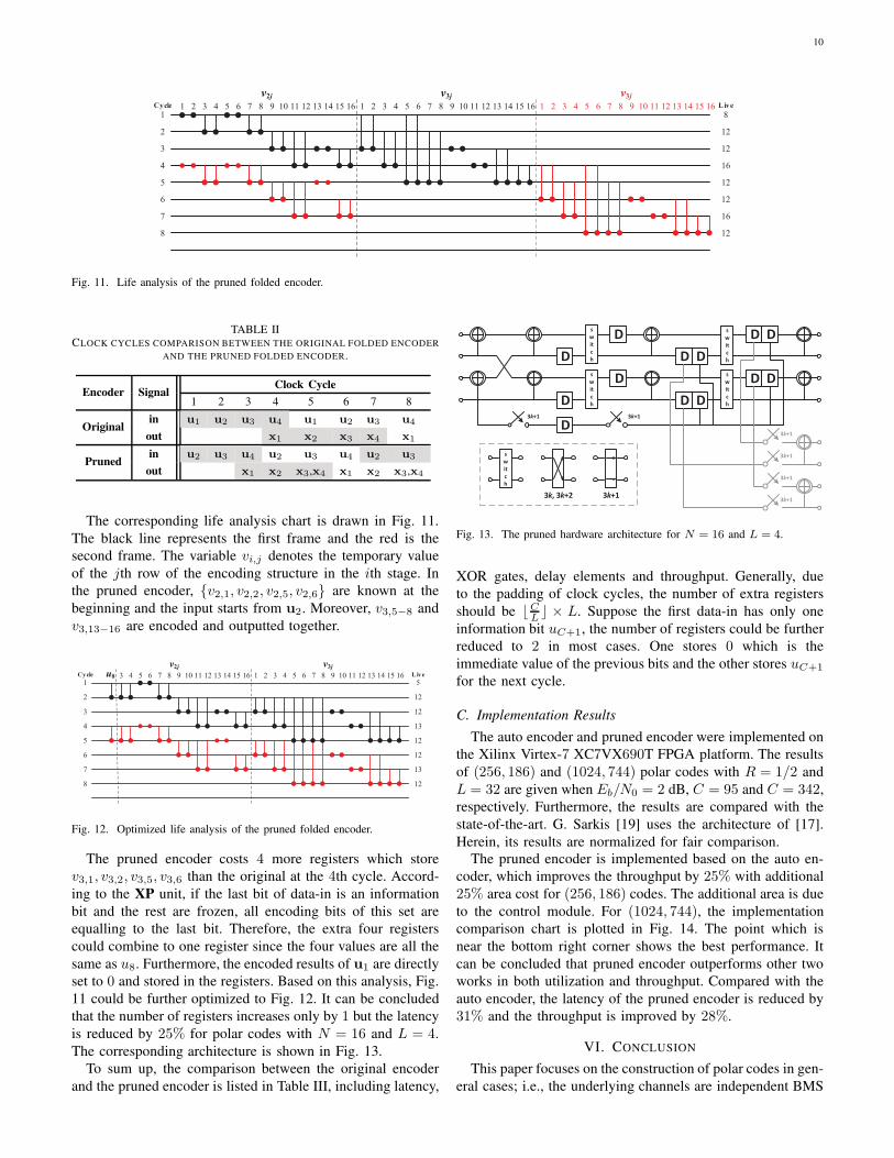
Fig. 11. Life analysis of the pruned folded encoder.

TABLE IICLOCK CYCLES COMPARISON BETWEEN THE ORIGINAL FOLDED ENCODER

AND THE PRUNED FOLDED ENCODER.

Clock CycleEncoder Signal

1 2 3 4 5 6 7 8

in u1 u2 u3 u4 u1 u2 u3 u4Original

out x1 x2 x3 x4 x1

in u2 u3 u4 u2 u3 u4 u2 u3Pruned

out x1 x2 x3,x4 x1 x2 x3,x4

The corresponding life analysis chart is drawn in Fig. 11.

The black line represents the first frame and the red is the

second frame. The variable vi,j denotes the temporary value

of the jth row of the encoding structure in the ith stage. In

the pruned encoder, {v2,1, v2,2, v2,5, v2,6} are known at the

beginning and the input starts from u2. Moreover, v3,5−8 and

v3,13−16 are encoded and outputted together.

Fig. 12. Optimized life analysis of the pruned folded encoder.

The pruned encoder costs 4 more registers which store

v3,1, v3,2, v3,5, v3,6 than the original at the 4th cycle. Accord-

ing to the XP unit, if the last bit of data-in is an information

bit and the rest are frozen, all encoding bits of this set are

equalling to the last bit. Therefore, the extra four registers

could combine to one register since the four values are all the

same as u8. Furthermore, the encoded results of u1 are directly

set to 0 and stored in the registers. Based on this analysis, Fig.

11 could be further optimized to Fig. 12. It can be concluded

that the number of registers increases only by 1 but the latency

is reduced by 25% for polar codes with N = 16 and L = 4.

The corresponding architecture is shown in Fig. 13.

To sum up, the comparison between the original encoder

and the pruned encoder is listed in Table III, including latency,

D

D

D

D

D D

D D

D D

D Ds

w

it

c

h

s

w

it

c

h

s

w

it

c

h

D3k+1 3k+1

3k+1

s

w

it

c

h

3k, 3k+2 3k+1

s

w

it

c

h3k+1

3k+1

3k+1

Fig. 13. The pruned hardware architecture for N = 16 and L = 4.

XOR gates, delay elements and throughput. Generally, due

to the padding of clock cycles, the number of extra registers

should be ⌊CL ⌋ × L. Suppose the first data-in has only one

information bit uC+1, the number of registers could be further

reduced to 2 in most cases. One stores 0 which is the

immediate value of the previous bits and the other stores uC+1

for the next cycle.

C. Implementation Results

The auto encoder and pruned encoder were implemented on

the Xilinx Virtex-7 XC7VX690T FPGA platform. The results

of (256, 186) and (1024, 744) polar codes with R = 1/2 and

L = 32 are given when Eb/N0 = 2 dB, C = 95 and C = 342,

respectively. Furthermore, the results are compared with the

state-of-the-art. G. Sarkis [19] uses the architecture of [17].

Herein, its results are normalized for fair comparison.

The pruned encoder is implemented based on the auto en-

coder, which improves the throughput by 25% with additional

25% area cost for (256, 186) codes. The additional area is due

to the control module. For (1024, 744), the implementation

comparison chart is plotted in Fig. 14. The point which is

near the bottom right corner shows the best performance. It

can be concluded that pruned encoder outperforms other two

works in both utilization and throughput. Compared with the

auto encoder, the latency of the pruned encoder is reduced by

31% and the throughput is improved by 28%.

VI. CONCLUSION

This paper focuses on the construction of polar codes in gen-

eral cases; i.e., the underlying channels are independent BMS

11

TABLE IIIXOR GATES, REGISTERS, LATENCY AND THROUGHPUT COMPARISONS BETWEEN ORIGINAL ENCODER AND PRUNED ENCODER.

XOR gates Registers Latency [cycle] Throughput [bit/cycle]

Original EncoderY. Hoo [17] L/2 log2 N N − L N/L L

Z. Zhong [20] L/2 log2 N 3N/2 − L 3N/2L − 1 2LN3N−2L

Pruned Encoder L/2(log2 N + C) N − L+ 2 ⌈N−CL

⌉ N/⌈N−CL

⌉

TABLE IVIMPLEMENTATION RESULTS COMPARISON WITH STATE-OF-THE-ART WORKS.

(N,C) (256, 186) (1024, 744)

Encoder Auto Encoder Pruned Encoder G. Sarkis [19] Z. Zhong [20] Auto Encoder Pruned Encoder

LUT 201 227 275 467 359 415

FF 134 192 789 312 207 324

Total 335 419 1064 779 566 739

Latency [cycle] 8 6 32 47 32 22

Max. Freq. [MHz] 415.8 390.75 401.23 407.05 392.17 359.18

Throughput [Gbps] 13.31 16.67 12.84 8.87 12.55 16.07

Throughput [Gb/s]8 10 12 14 16 18 20

Tot

al U

tiliz

atio

n

500

600

700

800

900

1000

1100

1200

G. Sarkis

Z. Zhong

Auto Encoder

Pruned Encoder

Fig. 14. Implementation comparison of state-of-the-art partially folded polarencoders.

channels. In terms of software, proofs are presented to show

that the symmetric property and the degradation relationship

are still preserved. From these theoretical aspects, a general

construction of polar codes based on Tal-Vardy’s algorithm

is proposed. The general construction can be applied to all

types of independent BMS channels. In terms of hardware, the

property of polar codes could optimize the hardware encoder

architecture. For the proposed pruned folded encoder, the

latency is reduced by 31% and throughput is improved by

28% when the length of code is 1024.

APPENDIX

PROOF OF LEMMA 1

The input alphabet is X = {0, 1}, and the output is Y ={y}. From Lemma 1, the transition probability is H(y|0) =H(y|1) = 1

2 . From (1), the symmetric capacity of this channel

H is

I(H) =∑

x∈X

1

2H(y|x) log

H(y|x)12H(y|0) + 1

2H(y|1)

=1

2H(y|0) log

H(y|0)12H(y|0) + 1

2H(y|1)

+1

2H(y|1) log

H(y|1)12H(y|0) + 1

2H(y|1)

= 0.

Therefore, the symmetric capacity of the channel H is I(H) =0.

REFERENCES

[1] E. Arıkan, “Channel polarization: A method for constructing capacity-achieving codes for symmetric binary-input memoryless channels,” IEEE

Trans. Inf. Theory, vol. 55, no. 7, pp. 3051–3073, Jul. 2009.[2] R. Mori and T. Tanaka, “Performance and construction of polar codes

on symmetric binary-input memoryless channels,” in Proc. IEEE Symp.

Inf. Theory (ISIT), June 2009, pp. 1496–1500.[3] ——, “Performance of polar codes with the construction using density

evolution,” IEEE Commun. Lett., vol. 13, no. 7, pp. 519–521, Jul. 2009.[4] I. Tal and A. Vardy, “How to construct polar codes,” IEEE Trans. Inf.

Theory, vol. 59, no. 10, pp. 6562–6582, Oct. 2013.

[5] P. Trifonov, “Efficient design and decoding of polar codes,” IEEE Trans.

Commun., vol. 60, no. 11, pp. 3221–3227, Nov. 2012.

[6] J. Dai, K. Niu, Z. Si, C. Dong, and J. Lin, “Does Gaussian approximationwork well for the long-length polar code construction?” IEEE Access,vol. 5, pp. 7950–7963, Apr. 2017.

[7] D. Wu, Y. Li, and Y. Sun, “Construction and block error rate analysisof polar codes over AWGN channel based on Gaussian approximation,”IEEE Commun. Lett., vol. 18, no. 7, pp. 1099–1102, Jul. 2014.

[8] A. Eslami and H. Pishro-Nik, “A practical approach to polar codes,” inProc. IEEE Symp. Inf. Theory (ISIT), Jul. 2011, pp. 16–20.

[9] K. Niu, K. Chen, and J. R. Lin, “Beyond turbo codes: Rate-compatiblepunctured polar codes,” in Proc. IEEE Inter. Conf. Commun. (ICC), Jun.2013, pp. 3423–3427.

[10] L. Zhang, Z. Zhang, X. Wang, Q. Yu, and Y. Chen, “On the puncturingpatterns for punctured polar codes,” in Proc. IEEE Symp. Inf. Theory

(ISIT), Jun. 2014, pp. 121–125.[11] K. Niu, J. Dai, K. Chen, J. Lin, K. Q. T. Zhang, and A. V. Vasilakos,

“Rate-compatible punctured polar codes: Optimal construction based onpolar spectra,” 2016. [Online]. Available: http://arxiv.org/abs/1612.01352

[12] R. Wang and R. Liu, “A novel puncturing scheme for polar codes,” IEEE

Commun. Lett., vol. 18, no. 12, pp. 2081–2084, Dec. 2014.[13] V. Bioglio, F. Gabry, and I. Land, “Low-complexity puncturing and

shortening of polar codes,” in Proc. IEEE Wireless Commun. Netw. Conf.

Workshops (WCNCW), Mar. 2017, pp. 1–6.[14] V. Miloslavskaya, “Shortened polar codes,” IEEE Trans. Inf. Theory,

vol. 61, no. 9, pp. 4852–4865, Sep. 2015.

12

[15] S. B. Korada, “Polar codes for channel and source coding,” PhD Thesis,2009.

[16] K. K. Parhi, VLSI digital signal processing systems: design and imple-

mentation. John Wiley & Sons, 2007.[17] H. Yoo and I.-C. Park, “Partially parallel encoder architecture for long

polar codes,” IEEE Trans. Circuits Syst. II, vol. 62, no. 3, pp. 306–310,Nov. 2015.

[18] M. Ayinala, M. Brown, and K. K. Parhi, “Pipelined parallel FFT archi-tectures via folding transformation,” IEEE Trans. VLSI Syst., vol. 20,no. 6, pp. 1068–1081, 2012.

[19] G. Sarkis, I. Tal, P. Giard, A. Vardy, C. Thibeault, and W. J. Gross,“Flexible and low-complexity encoding and decoding of systematic polarcodes,” IEEE Trans. Commun., vol. 64, no. 7, pp. 2732–2745, Jun. 2015.

[20] Z. Zhong, X. You, and C. Zhang, “Auto-generation of pipelined hardwaredesigns for polar encoder,” in Proc. IEEE China Semicond. Technol.

Inter. Conf. (CSTIC). IEEE, 2018, pp. 1–4.[21] T. M. Cover and J. A. Thomas, Elements of Information Theory, 2nd ed.

John Wiley & Sons Inc., 2006.[22] M. Alsan, “Re-proving channel polarization theorems: An extremality

and roburstness analysis,” PhD Thesis, 2015.[23] C. Zhang, J. Yang, X. You, and S. Xu, “Pipelined implementations of

polar encoder and feed-back part for SC polar decoder,” in Proc. IEEE

Int. Symp. Circuits Syst. (ISCAS), 2015, pp. 3032–3035.[24] C. Schurch, “A Partial Order For the Synthesized Channels of a Polar

Code,” in Proc. IEEE Symp. Inf. Theory (ISIT), July 2016, pp. 220–224.[25] W. Wang and L. Li, “Efficient Construction of Polar Codes,” in Proc.

IEEE Inter. Wireless Commun. Mobile Comput. Conf. (IWCMC), Jun.2017, pp. 1594–1598.