arX

iv:1

103.

2372

v3 [

stat

.ME

] 2

Nov

201

1

A general class of zero-or-one inflated beta regression models

Raydonal OspinaDepartamento de Estatıstica/CCENUniversidade Federal de Pernambuco

Cidade Universitaria, Recife/PE 50740-540, Brazil.e-mail: raydonal@de.ufpe.br

Silvia L.P. FerrariDepartamento de Estatıstica/IME

Universidade de Sao PauloRua do Matao 1010, Sao Paulo/SP 05508-090, Brazil.

e-mail: silviaferrari.usp@gmail.com

Abstract

This paper proposes a general class of regression models for continuous proportions when thedata contain zeros or ones. The proposed class of models assumes that the response variablehas a mixed continuous-discrete distribution with probability mass at zero or one. The betadistribution is used to describe the continuous component of the model, since its density hasa wide range of different shapes depending on the values of the two parameters that indexthe distribution. We use a suitable parameterization of the beta law in terms of its mean anda precision parameter. The parameters of the mixture distribution are modeled as functionsof regression parameters. We provide inference, diagnostic, and model selection tools for thisclass of models. A practical application that employs real data is presented.

Keywords and Phrases: Continuous proportions; Zero-or-one inflated beta distribution;Fractional data; Maximum likelihood estimation; Diagnostics; Residuals.

1 Introduction

Statistical modeling of continuous proportions has received close attention in the last few years.Some examples of proportions measured on a continuous scale include the fraction of incomecontributed to a retirement fund, the proportion of weekly hours spent on work-related activities,the fraction of household income spent on food, the percentage of ammonia escaping unconvertedfrom an oxidation plant, etc. Usual regression models, such as normal linear or nonlinear regressionmodels, are not suitable for such situations. Different strategies have been proposed for modelingcontinuous proportions that are perceived to be related to other variables. Regression modelsthat assume a beta distribution for the response variable are of particular interest.

It is well known that the beta distribution is very flexible for modeling limited range data,since its density has different shapes depending on the values of the two parameters that index

1

the distribution: left-skewed, right-skewed, “U ,” “J ,” inverted “J ,” and uniform (see Johnson,Kotz & Balakrishnan, 1995, §25.1). Beta regression models have been studied by Kieschnick &McCullough (2003), Ferrari & Cribari-Neto (2004), Espinheira, Ferrari & Cribari-Neto (2008a,2008b), Paolino (2001), Smithson & Verkuilen (2006), Korhonen et al. (2007), Simas, Barreto-Souza & Rocha (2010), and Ferrari & Pinheiro (2010), among others.

Oftentimes, proportions data include a non-negligeable number of zeros and/or ones. Whenthis is the case, the beta distribution does not provide a satisfactory description of the data, sinceit does not allow a positive probability for any particular point in the interval [0, 1]. A mixedcontinuous-discrete distribution might be a better choice. This approach has been consideredby Ospina & Ferrari (2010), who used the beta law to define the continuous component of thedistribution. The discrete component is defined by a Bernoulli or a degenerate distribution atzero or at one. The proposed distributions are usually referred to as zero-and-one inflated betadistributions (mixture of a beta and a Bernoulli distribution) and zero-inflated beta distributionsor one-inflated beta distributions (mixture of a beta and a degenerate distribution at zero or atone, depending on the case).

This paper is concerned with a general class of regression models for modeling continuousproportions when zeros or ones appear in the data. Such class of models is tailored for the situationwhere only one of the extremes (zero or one) is present in the dataset. We shall consider a mixtureof a beta distribution and a degenerate distribution at a fixed known point c, where c ∈ {0, 1}. Thebeta distribution is conveniently parameterized in terms of its mean and a precision parameter.We shall allow the mean and the precision parameter of the beta distribution and the probabilityof a point mass at c to be related to linear or non-linear predictors through smooth link functions.Inference, diagnostic, and selection tools for the proposed class of models will be presented. Closelyrelated to our work are the papers by Hoff (2007) and Cook, Kieschnick &McCullough (2008). Ourmodel, however, is more general and convenient than those proposed by these authors. It relaxeslinearity assumptions, allows all the parameters of the underlying distribution to be modeled asfunctions of unknown parameters and covariates, and uses a suitable parameterization of the betalaw. Unlike their papers, our article offers a comprehensive framework for the statistical analysisof continuous data observed on the standard unit interval with a point mass at one of its extremes.

The paper unfolds as follows. Section 2 presents a general class of zero-or-one inflated betaregression models. Section 3 discusses maximum likelihood estimation. Section 4 is devoted todiagnostic measures. Section 5 contains an application using real data and concluding remarksare given in Section 6. Some technical details are collected in two appendices.

2 Zero-or-one inflated beta regression models

The beta distribution with parameters µ and φ (0 < µ < 1 and φ > 0), denoted by B(µ, φ), hasthe density function

f(y;µ, φ) =Γ(φ)

Γ(µφ)Γ((1 − µ)φ)yµφ−1(1− y)(1−µ)φ−1, y ∈ (0, 1), (2.1)

where Γ(·) is the gamma function. The parameterization employed in (2.1) is not the usual one,but it is suitable for modeling purposes.

If y ∼ B(µ, φ), then E(y) = µ and Var(y) = µ(1 − µ)/(φ + 1). Hence, µ is the distributionmean and φ plays the role of a precision parameter, in the sense that, for a fixed µ, the largerthe value of φ, the smaller the variance of y. Since the beta distribution is very flexible, allowinga wide range of different forms, it is an attractive choice for modeling continuous proportions. A

2

possible shortcoming is that it is not appropriate for modeling datasets that contain observationsat the extremes (either zero or one). Our focus is on the case where only one of the extremesappears in the data—a situation often found in empirical research. It is then natural to modelthe data using a mixture of two distributions: a beta distribution and a degenerate distributionin a known value c, where c equals zero or one, depending on the case. Under this approach,we assume that the probability density function of the response variable y with respect to themeasure generated by the mixture1 is given by

bic(y;α, µ, φ) =

{α, if y = c,

(1− α)f(y;µ, φ), if y ∈ (0, 1),(2.2)

where f(y;µ, φ) is the beta density (2.1). Note that α is the probability mass at c and representsthe probability of observing zero (c = 0) or one (c = 1). If c = 0, the density (2.2) is called azero-inflated beta distribution, and if c = 1, the density is called a one-inflated beta distribution.

The mean of y and its variance can be written as

E(y) = αc+ (1− α)µ,

Var(y) = (1− α)µ(1 − µ)

φ+ 1+ α(1− α)(c − µ)2.

Note that E(y) is the weighted average of the mean of the degenerate distribution at c and themean of the beta distribution B(µ, φ) with weights α and 1 − α. Also, E(y | y ∈ (0, 1)) = µ andVar(y | y ∈ (0, 1)) = µ(1 − µ)/(1 + φ). Other properties of this distribution can be found inOspina & Ferrari (2010).

A general class of zero-or-one inflated beta regression models can be defined as follows. Lety1, . . . , yn be independent random variables such that each yt, for t = 1, . . . , n, has probabilitydensity function (2.2) with parameters α = αt, µ = µt, and φ = φt. We assume that αt, µt, andφt are defined as

h1(αt) = η1t = f1(vt, ρ),

h2(µt) = η2t = f2(xt, β),

h3(φt) = η3t = f3(zt, γ),

(2.3)

where ρ = (ρ1, . . . , ρp)⊤, β = (β1, . . . , βk)

⊤ and γ = (γ1, . . . , γm)⊤ are vectors of unknownregression parameters; (p + k + m < n), η1 = (η11, . . . , η1n)

⊤, η2 = (η21, . . . , η2n)⊤, and

η3 = (η31, . . . , η3n)⊤ are predictor vectors; and f1(·, ·), f2(·, ·), and f3(·, ·) are linear or nonlin-

ear twice continuously differentiable functions in the second argument, such that the derivativematrices V = ∂η1/∂ρ, X = ∂η2/∂β, and Z = ∂η3/∂γ have ranks p, k and m, respectively, for allρ, β, and γ.

Here vt = (vt1, . . . , vtp′), xt = (xt1, . . . , xtk′), and zt = (zt1, . . . , ztm′) are observations onp′ + k′ + m′ known covariates. We also assume that the link functions h1 : (0, 1) → R, h2 :(0, 1) → R, and h3 : (0,+∞) → R are strictly monotonic and twice differentiable. Variousdifferent link functions may be used. For µ and α one may choose h2(µ) = log{µ/(1 − µ)} (logitlink); h2(µ) = Φ−1(µ) (probit link), where Φ(·) denotes the standard normal distribution function;h3(µ) = log{− log(1 − µ)} (complementary log-log link); and h2(µ) = − log{− log(µ)} (log-log

1The probability measure P, corresponding to this distribution, defined over the measure space ((0, 1)∪{c},B),where B is the class of all Borelian subsets of (0, 1)∪{c}, is such that P << λ+δc, with λ representing the Lebesguemeasure, and δc is such that δc(A) = 1 if c ∈ A and δc(A) = 0 if c /∈ A and A ∈ B.

3

link), among others. Possible specifications for φ are h3(φ) = log φ (log link) and h3(φ) =√φ

(square-root link).Model (2.2)-(2.3) has a number of interesting features. The variance of yt is a function of

(αt, µt, φt) and, as a consequence, of the covariates values. Hence, non-constant response variancesare naturally accommodated by the model. Also, the role that the covariates and the parametersplay in the model is clear. For example, suppose c = 0. In this case, vt and ρ affect Pr(yt = 0), xtand β control E(yt | yt ∈ (0, 1)), and zt and γ influence the precision of the conditional distributionof yt, given that yt ∈ (0, 1). This feature can be very useful for modeling purposes. For instance,if the response is the individual mobile communications expenditure proportion (MCEP), model(2.2)-(2.3) allows the researcher to take into account that some individuals do not spend at allon MCEP and to separately assess the effects of the heterogeneity among consumers and non-consumers of mobile communications (in this connection, see Yoo, 2004).

Special cases. Model (2.2)-(2.3) embodies two general classes of models: the zero-inflated beta

regression model (c = 0) and the one-inflated beta regression model (c = 1), the first of whichis suitable when the data include zeros and the second, when ones appear in the dataset. Eachof them leads to a corresponding linear model when the predictors are linear functions of theparameters. In this case, we have p = p′, k = k′, m = m′, h1(αt) = v⊤t ρ, h2(µt) = x⊤t β andh3(φt) = z⊤t γ. Here, V = (v⊤1 , . . . , v

⊤n )

⊤, X = (x⊤1 , . . . , x⊤n )

⊤, and Z = (z⊤1 , . . . , z⊤n )

⊤. Also, thenonlinear beta regression model (Simas, Barreto-Souza & Rocha, 2010, and Ferrari & Pinheiro,2010) is a limiting case of our model obtained by setting αt = α→ 0. If, in addition, the predictorfor µt is linear and φt is constant through the observations, we arrive at the beta regression modeldefined by Ferrari & Cribari-Neto (2004).

3 Likelihood inference

The likelihood function for θ = (ρ⊤, β⊤, γ⊤)⊤ based on a sample of n independent observations is

L(θ) =

n∏

t=1

bic(yt;αt, µt, φ) = L1(ρ)L2(β, γ), (3.1)

where

L1(ρ) =

n∏

t=1

α1l{c}(yt)t (1− αt)

1−1l{c}(yt),

L2(β, γ) =∏

t:yt∈(0,1)

f(yt;µt, φt),

with 1lA(yt) being an indicator function that equals 1 if yt ∈ A, and 0, if yt /∈ A. Here, αt =h−11 (η1t), µt = h−1

2 (η2t), and φt = h−13 (η3t), as defined in (2.3), are functions of ρ, β, and γ,

respectively. Notice that the likelihood function L(θ) factorizes in two terms, the first of whichdepends only on ρ (discrete component), and the second, only on (β, γ) (continuous component).Hence, the parameters are separable (Pace & Salvan, 1997, p. 128) and the maximum likelihoodinference for (β, γ) can be performed separately from that for ρ, as if the value of ρ were known,and vice-versa.

The log-likelihood function is given by

ℓ(θ) = ℓ1(ρ) + ℓ2(β, γ) =

n∑

t=1

ℓt(αt) +∑

t:yt∈(0,1)

ℓt(µt, φt), (3.2)

4

whereℓt(αt) = 1l{c}(yt) log αt + (1− 1l{c}(yt)) log(1− αt), (3.3)

ℓt(µt, φt) = log Γ(φt)− log Γ(µtφt)− log Γ((1− µt)φt) + (µtφt − 1)y∗t + (φt − 2)y†t , (3.4)

y∗t = log{yt/(1 − yt)} and y†t = log(1 − yt) if yt ∈ (0, 1), and y∗t = 0 and y†t = 0 otherwise. We

have the following conditional moments of y∗t and y†t :

µ∗t = E(y∗t | yt ∈ (0, 1)) = ψ(µtφt)− ψ((1 − µt)φt),

µ†t = E(y†t | yt ∈ (0, 1)) = ψ((1 − µt)φt)− ψ(φt),

v∗t = Var(y∗t | yt ∈ (0, 1)) = ψ′(µtφt)− ψ′((1 − µt)φt),

v†t = Var(y†t | yt ∈ (0, 1)) = ψ′((1 − µt)φt)− ψ′(φt),

c∗† = Cov(y∗t , y†t | yt ∈ (0, 1)) = −ψ′((1− µt)φt),

(3.5)

with ψ(·) denoting the digamma function.2 Notice that ℓ1(ρ) represents the log-likelihood functionof a regression model for binary responses, in which the success probability for the tth observationis αt = h−1

1 (η1t) (McCullagh & Nelder 1989, §4.4.1). On the other hand, ℓ2(β, γ) is the log-likelihood function for (β, γ) in a nonlinear beta regression model based on the observationsthat fall in the interval (0, 1). Hence, the maximum likelihood (ML) estimation for this modelcan be accomplished by separately fitting a binomial regression model to the indicator variables1l{c}(yt), for t = 1, . . . , n, and a nonlinear beta regression model to the observations yt ∈ (0, 1),for t = 1, . . . , n.

The score function, obtained by the differentiation of the log-likelihood function with respectto the unknown parameters (see (A.1) – (A.3); Appendix A), is given by

U(θ) = (Uρ(ρ)⊤, Uβ(β, γ)

⊤, Uγ(β, γ)⊤)⊤,

whereUρ(ρ) = V⊤ADA∗(yc − α),

Uβ(β, γ) = X⊤(In − Y c)TΦ(y∗ − µ∗),

Uγ(β, γ) = Z⊤(In − Y c)H[M(y∗ − µ∗) + (y† − µ†)].

(3.6)

Here, y∗ = (y∗1, . . . , y∗n)

⊤, y† = (y†1, . . . , y†n)⊤, yc = (1l{c}(y1), . . . , 1l{c}(yn))

⊤, µ∗ = (µ∗1, . . . , µ∗n)

⊤,

µ† = (µ†1, . . . , µ†n)⊤, and α = (α1, . . . , αn)

⊤ are n-vectors and M = diag(µ1, . . . , µn), A =diag(1/α1, . . . , 1/αn), A∗ = diag(1/(1 − α1), . . . , 1/(1 − αn)), D = diag(1/h′1(α1),. . . , 1/h′1(αn)), Φ = diag(φ1, . . . , φn), T = diag(1/h′2(µ1), . . . , 1/h

′2(µn)), H = diag(1/h′3(φ1),

. . . , 1/h′3(φn)), and Yc = diag(1l{c}(y1), . . . , 1l{c}(yn)) are n×n diagonal matrices. Also, In repre-

sents the n× n identity matrix. The maximum likelihood estimators (MLEs) of ρ and (β⊤, γ⊤)⊤

are obtained as the solutions of the nonlinear systems Uρ(ρ) = 0 and (Uβ(β, γ)⊤, Uφ(β, γ))

⊤ = 0.There are not closed form expressions for these estimators, and their computations should beperformed numerically using a nonlinear optimization algorithm, e.g., some form of Newton’smethod (Newton-Raphson, Fisher’s scoring, BHHH, etc.) or a quasi-Newton algorithm such asBFGS. An iterative algorithm for maximum likelihood estimation is presented in Appendix B.For more details on nonlinear optimization, see Press et al. (1992).

2The digamma function is defined as ψ(x) = d log Γ(x)/dx, x > 0.

5

From the observed information matrix given in (A.4), it can be shown that the Fisher infor-mation matrix is

K(θ) =

Kρρ 0 00 Kββ Kβγ

0 Kγβ Kγγ

, (3.7)

where Kρρ = V⊤W1V, Kββ = X⊤W2X , Kγβ = K⊤βγ = X⊤W3Z, Kγγ = Z⊤W4Z with W1 =

(A∗ +A)D2, W2 = ΦT{V ∗A∗−1}TΦ, W3 = T{Φ(MV ∗ + C)A∗−1}H, and W4 = H{(M2V ∗ +2MC + V †)A∗−1}H. Notice that Kρβ = Kβρ

⊤ = 0 and Kργ = Kγρ⊤ = 0, thus indicating that

the parameters γ and (β⊤, γ⊤)⊤ are globally orthogonal (Cox & Reid, 1987) and their MLEs, ρand (β⊤, γ⊤)⊤, are asymptotically independent.

The inverse of Fisher’s information matrix is useful for computing asymptotic standard errorsof MLEs. From (3.7) and a standard formula for the inverse of partitioned matrices (Rao, 1973,p. 33), we have

K(θ)−1 =

Kρρ 0 00 Kββ Kβγ

0 Kγβ Kγγ

, (3.8)

whereKρρ = (V⊤W1V)−1, Kββ = {X⊤(W2−W3Z(Z⊤W4Z)−1Z⊤W3)X}−1, Kγβ = (Kβγ)⊤ =−(Z⊤W4Z)−1Z⊤W3X (X⊤(W2 − W3Z(Z⊤W4Z)−1Z⊤W3)X )−1, and Kγγ

= (Z⊤W4Z)−1 + (Z⊤W4Z)−1Z⊤W3X (X⊤(W2 − W3Z(Z⊤W4Z)−1Z⊤W3)X )−1

X⊤W3Z × (Z⊤W4Z)−1.

Fitting the model using the GAMLSS implementation. The zero-or-one inflated betadistribution has been incorporated in the GAMLSS framework (Rigby & Stasinopoulos, 2005);see Ospina (2006). GAMLSS allows the flexible modeling of each of the three parameters thatindex the distribution using parametric terms involving linear or nonlinear predictors, smoothnonparametric terms (e.g., cubic splines or loess), and random effects. Maximum (penalized)likelihood estimation is approached through a Newton-Raphson or Fisher scoring algorithm withthe backfitting algorithm for the additive components. Our approach consists of an application ofthe gamlss functions, which are fully documented in the gamlss package (Stasinopoulos & Rigby,2007; see also http://www.gamlss.org). The structure of the gamlss functions is familiar toreaders who are used to the R (or S-Plus) syntax (the glm function, in particular). The set ofgamlss packages can be freely downloaded from the R library at http://www.r-project.org/.

Large sample inference. If the model specified by (2.2) and (2.3) is valid and the usual reg-ularity conditions for maximum likelihood estimation are satisfied (Cox & Hinkley, 1974, p. 107),the MLEs of θ and K(θ), θ = (ρ⊤β⊤, γ)⊤ and K(θ), respectively, are consistent. Assuming that

I(θ) = limn→∞{n−1K(θ)} exists and is nonsingular, we have√n(θ − θ)

D→ Np+k+m(0, I(θ)−1),

whereD→ denotes convergence in distribution. Note that, if θl denotes the lth component of θ, it

follows that

(θl − θl){K(θ)ll

}−1/2 D→ N (0, 1),

where K(θ)ll is the lth diagonal element of K(θ)−1. A rigorous proof of the aforementionedasymptotic result can be obtained by extending arguments similar to those given in Fahrmeir &Kaufmann (1985).

Let K(ρ)ss, K(β)rr, and K(γ)RR be the estimated sth, rth and Rth diagonal elements of Kρρ,Kββ, and Kγγ , respectively. The asymptotic variances of ρs, βr, and γR are estimated by K(ρ)ss,

6

K(β)rr, andK(γ)RR, respectively. If 0 < ς < 1/2, and zς represents the ςth quantile of theN (0, 1)distribution, we have ρs± z1−ς/2(K(ρ)ss)1/2, βr± z1−ς/2(K(β)rr)1/2, and γR± z1−ς/2(K(γ)RR)1/2

as the limits of asymptotic confidence intervals (ACI) for ρs, βr, and γR, respectively, all withasymptotic coverage 100(1 − ς)%. Additionally, an approximate 100(1 − ς)% confidence intervalfor µ• = E(y), the mean response for the given covariates v and x, can be computed as

(µ• − z

1−ς/2s.e.(µ•), µ• + z

1−ς/2s.e.(µ•)

),

where c = 0 or c = 1, depending on the case; µ• = cα+(1− α)µ, with α = h−11 (η1); µ = h−1

2 (η2);

η1 = f1(v; ρ); η2 = f2(x; β); and

s.e.(µ•) =

√{(c− µ)/h′1(α)

}2v⊤Kρρv +

{(1− α)/h′2(µ)

}2x⊤Kββx.

Here, Kρρ and Kββ respectively equal Kρρ and Kββ, evaluated at θ.The likelihood ratio, Rao’s score, and Wald’s (W) statistics to test hypotheses on the param-

eters can be calculated from the log-likelihood function, the score vector, the Fisher informationmatrix, and its inverse given above. Their null distributions are usually unknown and the testsrely on asymptotic approximations. In large samples, a chi-squared distribution can be used asan approximation to the true null distributions. For testing the significance of the ith regressionparameter that models µ, one can use the signed square root of Wald’s statistic, βi/s.e.(βi), wheres.e.(βi) is the asymptotic standard error of the MLE of βi obtained from the inverse of Fisher’sinformation matrix evaluated at the maximum likelihood estimates. The limiting null distributionof the test statistic is standard normal. Significance tests on the γ’s and ρ’s can be performed ina similar fashion.

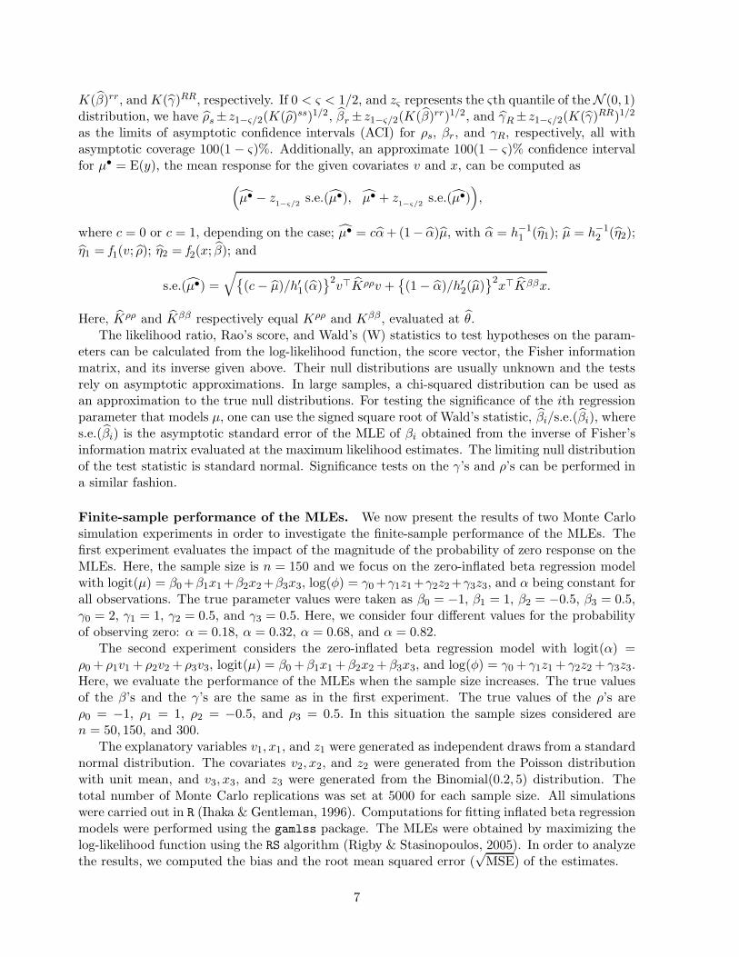
Finite-sample performance of the MLEs. We now present the results of two Monte Carlosimulation experiments in order to investigate the finite-sample performance of the MLEs. Thefirst experiment evaluates the impact of the magnitude of the probability of zero response on theMLEs. Here, the sample size is n = 150 and we focus on the zero-inflated beta regression modelwith logit(µ) = β0+β1x1+β2x2+β3x3, log(φ) = γ0+γ1z1+γ2z2+γ3z3, and α being constant forall observations. The true parameter values were taken as β0 = −1, β1 = 1, β2 = −0.5, β3 = 0.5,γ0 = 2, γ1 = 1, γ2 = 0.5, and γ3 = 0.5. Here, we consider four different values for the probabilityof observing zero: α = 0.18, α = 0.32, α = 0.68, and α = 0.82.

The second experiment considers the zero-inflated beta regression model with logit(α) =ρ0 + ρ1v1 + ρ2v2 + ρ3v3, logit(µ) = β0 +β1x1 +β2x2 + β3x3, and log(φ) = γ0 + γ1z1 + γ2z2 + γ3z3.Here, we evaluate the performance of the MLEs when the sample size increases. The true valuesof the β’s and the γ’s are the same as in the first experiment. The true values of the ρ’s areρ0 = −1, ρ1 = 1, ρ2 = −0.5, and ρ3 = 0.5. In this situation the sample sizes considered aren = 50, 150, and 300.

The explanatory variables v1, x1, and z1 were generated as independent draws from a standardnormal distribution. The covariates v2, x2, and z2 were generated from the Poisson distributionwith unit mean, and v3, x3, and z3 were generated from the Binomial(0.2, 5) distribution. Thetotal number of Monte Carlo replications was set at 5000 for each sample size. All simulationswere carried out in R (Ihaka & Gentleman, 1996). Computations for fitting inflated beta regressionmodels were performed using the gamlss package. The MLEs were obtained by maximizing thelog-likelihood function using the RS algorithm (Rigby & Stasinopoulos, 2005). In order to analyzethe results, we computed the bias and the root mean squared error (

√MSE) of the estimates.

7

Table 1 summarizes the numerical results of the first experiment. We note that, for a fixedsample size, the bias and the

√MSE of the estimators of the continuous component (β’s and γ’s)

increase with the expected proportion of zeros (α). This is to be expected, since the expectednumber of observations in (0, 1) decreases as α increases. Also, it is noteworthy that the bias andthe

√MSE of MLEs corresponding to the dispersion covariates tend to be much more pronounced

when compared with the MLEs of the parameters that model the mean response.

Table 1: Simulation results for the first experiment.

α = 0.18 α = 0.18 α = 0.18 α = 0.18

Estimator Bias√MSE Bias

√MSE Bias

√MSE Bias

√MSE

α 0.00052 0.03149 0.00022 0.03778 0.00086 0.03802 −0.00207 0.03097

β0 −0.00095 0.05213 −0.00176 0.07724 0.00032 0.11219 −0.00226 0.19777

β1 0.00176 0.04006 0.00207 0.04101 0.00354 0.07070 0.00452 0.11554

β2 −0.00048 0.02711 −0.00076 0.04308 −0.00427 0.08532 −0.00328 0.11987

β3 0.00014 0.03764 0.00024 0.05145 0.00073 0.08256 0.00089 0.12046

γ0 0.01241 0.21359 0.02668 0.25779 0.02892 0.43969 0.06437 0.71228

γ1 0.03158 0.13205 0.03203 0.14619 0.07302 0.30639 0.20369 0.51323

γ2 0.03088 0.12514 0.04288 0.16232 0.09854 0.30874 0.23140 0.68394

γ3 0.02745 0.15964 0.01527 0.17183 0.07067 0.32288 0.19891 0.69026

Table 2 presents simulation results for the second experiment. For the smallest sample sizeconsidered (n = 50), the estimation algorithm failed to converge in 1.3% of the samples. For largesample sizes the algorithm converged for all the samples. The estimated biases of the MLEs ofthe ρ’s (parameters of the discrete component) are markedly high for small samples. This is notsurprising; in standard logistic regression, the MLEs are considerably biased in small samples.For large samples, the bias of the ρ’s is negligible.

In the second experiment, the β’s and the γ’s are essentially estimated from the observationsin (0,1), which represent around 70% of the observations in our study. For all the sample sizesconsidered, the mean of the β’s and γ’s are close to the corresponding true values. Also, all theroot mean square errors decrease when the sample size increases, as expected.

4 Diagnostics

Likelihood-based inference depends on parametric assumptions, and a severe misspecification ofthe model or the presence of outliers may impair its accuracy. We shall introduce some types ofresiduals for detecting departures from the postulated model and outlying observations. Addi-tionally, we suggest some measures to assess goodness-of-fit.

Residuals. Residual analysis in the context of the zero-or-one inflated beta regression model(2.1)-(2.3) can be split into two parts. First, we focus on the residual analysis for the discrete andthe continuous component of the model separately. For this purpose, we propose a standardizedPearson residual based on Fisher’s scoring iterative algorithm for estimating ρ, β, and γ. Second,

8

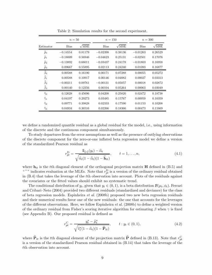
Table 2: Simulation results for the second experiment.

n = 50 n = 150 n = 300

Estimator Bias√MSE Bias

√MSE Bias

√MSE

ρ0 −0.14554 0.81179 −0.02398 0.38136 −0.01263 0.26529

ρ1 −0.18009 0.56946 −0.04623 0.25131 −0.02501 0.17076

ρ2 −0.13892 0.66011 −0.03437 0.24178 −0.01803 0.16958

ρ3 0.09667 0.55895 0.02113 0.24240 0.01093 0.16877

β0 0.00588 0.16190 0.00171 0.07288 0.00055 0.05272

β1 0.00588 0.10917 0.00146 0.04882 0.00027 0.03313

β2 −0.00211 0.09761 −0.00131 0.05057 0.00018 0.02872

β3 0.00140 0.12356 0.00104 0.05264 0.00063 0.03049

γ0 0.12628 0.45696 0.04208 0.25820 0.02472 0.18738

γ1 0.04197 0.29273 0.03485 0.15767 0.00959 0.10359

γ2 0.09771 0.39828 0.02333 0.17590 0.01153 0.10208

γ3 0.04934 0.36516 0.02266 0.18366 0.00473 0.11669

we define a randomized quantile residual as a global residual for the model, i.e., using informationof the discrete and the continuous component simultaneously.

To study departures from the error assumptions as well as the presence of outlying observationsof the discrete component for the zero-or-one inflated beta regression model we define a versionof the standardized Pearson residual as

rDpt =1l{c}(yt)− αt√

αt(1 − αt)(1 − htt), t = 1, . . . , n, (4.1)

where htt is the tth diagonal element of the orthogonal projection matrix H defined in (B.5) and“ ” indicates evaluation at the MLEs. Note that rDpt is a version of the ordinary residual obtainedin (B.4) that takes the leverage of the tth observation into account. Plots of the residuals againstthe covariates or the fitted values should exhibit no systematic trend.

The conditional distribution of yt, given that yt ∈ (0, 1), is a beta distribution B(µt, φt). Ferrariand Cribari–Neto (2004) provided two different residuals (standardized and deviance) for the classof beta regression models. Espinheira et al. (2008b) proposed two new beta regression residualsand their numerical results favor one of the new residuals: the one that accounts for the leveragesof the different observations. Here, we follow Espinheira et al. (2008b) to define a weighted versionof the ordinary residual from Fisher’s scoring iterative algorithm for estimating β when γ is fixed(see Appendix B). Our proposed residual is defined as

rCpt =y∗t − µ∗t√

v∗t (1− αt)(1− Ptt), t : yt ∈ (0, 1), (4.2)

where Ptt is the tth diagonal element of the projection matrix P defined in (B.13). Note that rCptis a version of the standardized Pearson residual obtained in (B.14) that takes the leverage of thetth observation into account.

9

To assess the overall adequacy of the zero-or-one inflated beta regression model to the dataat hand, we propose the randomized quantile residual (Dunn & Smyth, 1996). It is a randomizedversion of the Cox & Snell (1968) residual and given by

rqt = Φ−1(ut), t = 1, . . . , n, (4.3)

where Φ(·) denotes the standard normal distribution function, ut is a uniform random variableon the interval (at, bt], with at = limy↑yt BIc(yt; αt, µt, φt) and bt = BIc(yt; αt, µt, φt). Here,BIc(yt;αt, µt, φt) = αt1l[c,1](yt) + (1 − αt)F (yt;µt, φt), where F (·;µt, φt) is the cumulative dis-tribution function of the beta distribution B(µt, φt). In the zero-inflated beta regression model,ut is a uniform random variable on (0, αt] if yt = 0 and ut = BI0(yt; αt, µt, φt) if yt ∈ (0, 1). Onthe other hand, in the one-inflated beta regression model, ut is a uniform random variable on[αt, 1) if yt = 1 and ut = BI1(yt; αt, µt, φt) if yt ∈ (0, 1). Apart from sampling variability in αt, µt,and φt the r

qt are exactly standard normal in (at, bt] and the randomized procedure is introduced

in order to produce a continuous residual. The randomized quantile residuals can vary from onerealization to another. In practice, it is useful to make at least four achievements.

A plot of these residuals against the index of the observations (t) should show no detectablepattern. A detectable trend in the plot of some residual against the predictors may be suggestiveof link function misspecification. Also, normal probability plots with simulated envelopes are ahelpful diagnostic tool (Atkinson, 1985). Simulation results not presented here indicated thatthe randomized quantile residuals perform well in detecting whether the distribution assumptionis incorrect.

Global goodness-of-fit measure. A simple global goodness-of-fit measure is a pseudo R2, sayR2

p, defined by the square of the sample correlation coefficient between the outcomes, y1, . . . , yn,

and their corresponding predicted values, µ•1, . . . , µ•n, where µ

•t = E(yt) = cαt + (1 − αt)µt. A

perfect agreement between the y’s and µ•’s yields R2p = 1. Other pseudo R2’s are defined as

R2∗p = 1 − log L/ log L0 (McFadden, 1974) and R2

LR = 1 − (L0/L)2/n (Cox and Snell, 1989, p.

208-209), where L0 and L are the maximized likelihood functions of the null model and the fittedmodel, respectively. The ratio of the likelihoods or log-likelihoods may be regarded as measuresof the improvement, over the model with only three parameters (α, µ, and φ), achieved by themodel under investigation.

Influence measures. A well-known measure of the influence of each observation on the regres-sion parameter estimates is the likelihood displacement (Cook & Weisberg, 1982, Ch. 3). Thelikelihood displacement that results from removing the tth observation from the data is definedby

LDt =2

d{ℓ(θ)− ℓ(θ(t))},

where d is the dimension of θ and θ(t) is the MLE of θ obtained after removing the tth observationfrom the data. This definition does not consider that θ is actually split into two different typesof parameters: the parameters of the discrete component and the parameters of the continuouscomponent. Thus, it is more appropriate to consider the influence of the tth case on the estimationof ρ and (β, γ) separately. Therefore, we propose the following statistics:

LDDt =

2

p{ℓ1(ρ)− ℓ1(ρ(t))}, t = 0, 1, . . . , n

LDCt =

2

k +m{ℓ2(β, γ)− ℓ2(β(t), γ(t))}, t: yt ∈ (0, 1).

10

Simple approximations for LDDt and LDC

t are given by

LDDt ≈ cDtt =

htt

p(1− htt)(rDpt)

2, t = 0, 1, . . . , n

LDCt ≈ cCtt =

Ptt

(k +m)(1−Ptt)(rCpt)

2, t: yt ∈ (0, 1),

see Cook and Weisberg (1982, p. 191) and Wei (1998, p. 102). The approximations above arebased on the iterative scheme for evaluating the MLE of ρ, β, and γ (Appendix B) and Taylorexpansions of ℓ1(ρ(t)) and ℓ2(β(t), γ(t)) around ρ and (β, γ), respectively. The quantities cDtt and

cCtt can be useful to highlight influential cases. In practice, we recommend the plotting of cDtt andcCtt against t.

Model selection. Nested zero-or-one inflated beta regression models can be compared viathe likelihood ratio test, using twice the difference between the maximized log-likelihoods of afull model and a restricted model whose covariates are a subset of the full model. Informationcriteria, such as the generalized Akaike information criterion (GAIC), can be used for comparingnon-nested models. It is defined as

GAIC = D + d℘ , (4.4)

where D = −2ℓ is the global fitted deviance (Rigby & Stasinopoulus, 2005), ℓ is the maximizedlog-likelihood and d is the dimension of θ. It is possible to interpret the first term on the right-hand side of (4.4) as a measure of the lack of fit and the second term as a “penalty” for addingd parameters. The model with the smallest GAIC is then selected. The Akaike informationcriterion AIC (Akaike, 1974), the Schwarz Bayesian criterion SBC (Schwarz, 1978), and theconsistent Akaike information criterion (CAIC) are special cases of GAIC corresponding to ℘ = 2,℘ = log(n), and ℘ = log(n) + 1, respectively.

5 An application

This section contains an application of the zero-inflated beta regression model to real data.We analyze data on the mortality in traffic accidents of 200 randomly selected Brazilian mu-nicipal districts of the southeast region in the year 2002. The data were extracted from theDATASUS database available at www.datasus.gov.bt and IPEADATA database available atwww.ipeadata.gov.br. The response variable y is the proportion of deaths caused by trafficaccidents. The explanatory variables are the logarithm of the number of inhabitants of themunicipality (lnpop), the proportion of the population living in the urban area (propurb), theproportion of men in the population (propmen), the proportion of residents aged between 20 and29 years (prop2029), and the human development index of education of the municipal district(hdie). The main objective is to investigate the effect of the young population (prop2029) onthe proportion of deaths caused by traffic accidents after controlling for potential confoundingvariables. We report the summary statistics on each of these variables in Table 3.

Figure 1 presents a histogram and a box-plot of the response variable. The clump-at-zero(the bar with the dot above) in the histogram represents 39% of the data. We observe thatthe distribution of the data in (0,1) is asymmetric with an inverted “J” shape. Also, the box-plot reveals the presence of some outliers. Visual inspection suggests that a zero-inflated betadistribution may be a suitable model for the data.

11

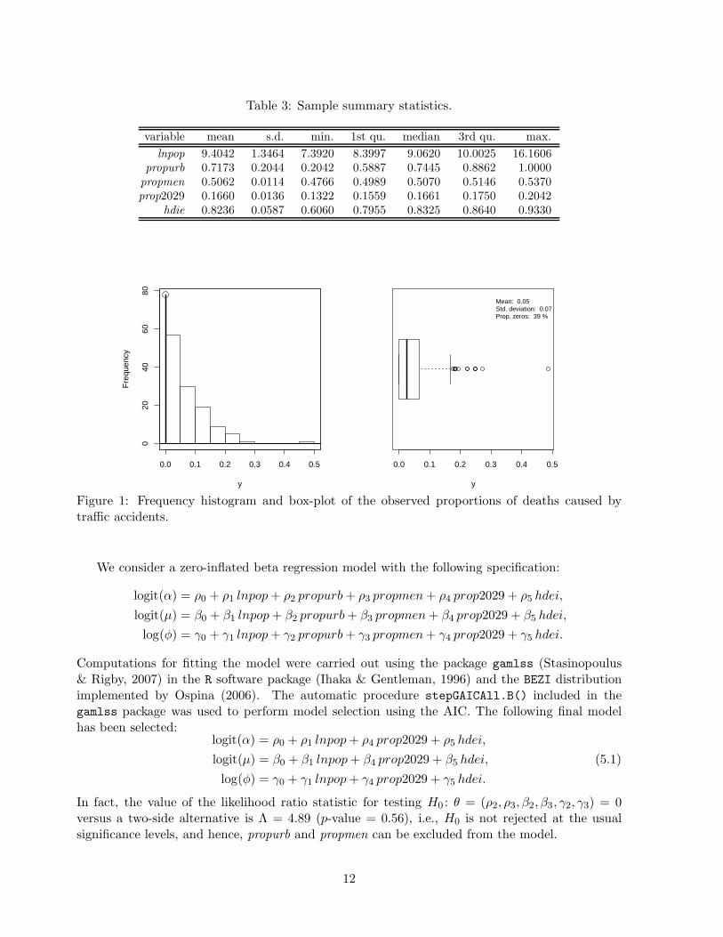
Table 3: Sample summary statistics.

variable mean s.d. min. 1st qu. median 3rd qu. max.

lnpop 9.4042 1.3464 7.3920 8.3997 9.0620 10.0025 16.1606propurb 0.7173 0.2044 0.2042 0.5887 0.7445 0.8862 1.0000propmen 0.5062 0.0114 0.4766 0.4989 0.5070 0.5146 0.5370prop2029 0.1660 0.0136 0.1322 0.1559 0.1661 0.1750 0.2042

hdie 0.8236 0.0587 0.6060 0.7955 0.8325 0.8640 0.9330

0.0 0.1 0.2 0.3 0.4 0.5

020

4060

80

y

Fre

quen

cy

0.0 0.1 0.2 0.3 0.4 0.5

y

Prop. zeros: 39 %

Mean: 0.05Std. deviation: 0.07

Figure 1: Frequency histogram and box-plot of the observed proportions of deaths caused bytraffic accidents.

We consider a zero-inflated beta regression model with the following specification:

logit(α) = ρ0 + ρ1 lnpop+ ρ2 propurb+ ρ3 propmen+ ρ4 prop2029 + ρ5 hdei,

logit(µ) = β0 + β1 lnpop+ β2 propurb+ β3 propmen+ β4 prop2029 + β5 hdei,

log(φ) = γ0 + γ1 lnpop+ γ2 propurb+ γ3 propmen+ γ4 prop2029 + γ5 hdei.

Computations for fitting the model were carried out using the package gamlss (Stasinopoulus& Rigby, 2007) in the R software package (Ihaka & Gentleman, 1996) and the BEZI distributionimplemented by Ospina (2006). The automatic procedure stepGAICAll.B() included in thegamlss package was used to perform model selection using the AIC. The following final modelhas been selected:

logit(α) = ρ0 + ρ1 lnpop+ ρ4 prop2029 + ρ5 hdei,

logit(µ) = β0 + β1 lnpop+ β4 prop2029 + β5 hdei,

log(φ) = γ0 + γ1 lnpop+ γ4 prop2029 + γ5 hdei.

(5.1)

In fact, the value of the likelihood ratio statistic for testing H0 : θ = (ρ2, ρ3, β2, β3, γ2, γ3) = 0versus a two-side alternative is Λ = 4.89 (p-value = 0.56), i.e., H0 is not rejected at the usualsignificance levels, and hence, propurb and propmen can be excluded from the model.

12

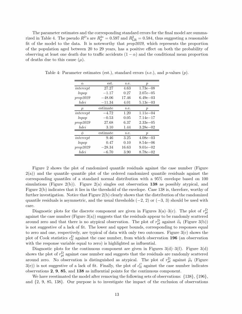
The parameter estimates and the corresponding standard errors for the final model are summa-rized in Table 4. The pseudo R2’s are R2∗

p = 0.597 and R2LR = 0.584, thus suggesting a reasonable

fit of the model to the data. It is noteworthy that prop2029, which represents the proportionof the population aged between 20 to 29 years, has a positive effect on both the probability ofobserving at least one death due to traffic accidents (1−α) and the conditional mean proportionof deaths due to this cause (µ).

Table 4: Parameter estimates (est.), standard errors (s.e.), and p-values (p).

α est. s.e. pintercept 27.27 4.63 1.73e−08lnpop −1.17 0.27 2.07e−05

prop2029 −48.06 17.46 6.49e−03hdei −11.34 4.01 5.13e−03

µ estimate s.e. pintercept −4.72 1.20 1.11e−04lnpop −0.53 0.05 7.14e−17

prop2029 27.68 6.37 2.33e−05hdei 3.10 1.44 3.28e−02

φ estimate s.e. pintercept 9.46 3.25 4.08e−03lnpop 0.47 0.10 8.54e−06

prop2029 −28.34 16.63 9.01e−02hdei −6.70 3.90 8.78e−02

Figure 2 shows the plot of randomized quantile residuals against the case number (Figure2(a)) and the quantile–quantile plot of the ordered randomized quantile residuals against thecorresponding quantiles of a standard normal distribution with a 95% envelope based on 100simulations (Figure 2(b)). Figure 2(a) singles out observation 138 as possibly atypical, andFigure 2(b) indicates that it lies in the threshold of the envelope. Case 138 is, therefore, worthy offurther investigation. Notice that Figure 2(b) clearly shows that the distribution of the randomizedquantile residuals is asymmetric, and the usual thresholds (−2, 2) or (−3, 3) should be used withcare.

Diagnostic plots for the discrete component are given in Figures 3(a)–3(c). The plot of rDptagainst the case number (Figure 3(a)) suggests that the residuals appear to be randomly scatteredaround zero and that there is no atypical observation. The plot of rDpt against αt (Figure 3(b))is not suggestive of a lack of fit. The lower and upper bounds, corresponding to responses equalto zero and one, respectively, are typical of data with only two outcomes. Figure 3(c) shows theplot of Cook statistics cDtt against the case number, from which observation 196 (an observationwith the response variable equal to zero) is highlighted as influential.

Diagnostic plots for the continuous component are given in Figures 3(d)–3(f). Figure 3(d)shows the plot of rDpt against case number and suggests that the residuals are randomly scattered

around zero. No observation is distinguished as atypical. The plot of rDpt against µt (Figure

3(e)) is not suggestive of a lack of fit. Finally, the plot of cCtt against the case number indicatesobservations 2, 9, 85, and 138 as influential points for the continuous component.

We have reestimated the model after removing the following sets of observations: {138}, {196},and {2, 9, 85, 138}. Our purpose is to investigate the impact of the exclusion of observations

13

0 50 100 150 200

−3

−2

−1

01

23

(a)

t

r tq

138

*

*

**

* * *

*

*

*

*

**

*

**

*

*

*

* **

*

*

**

* ***

** ****

**

*

**

* *

*

*

*

*

**

*

*

* **

*

*

**

*

* *

*

**

**

** **

*

*

*

**

*

* *

*

*

*

**

*

*

*

**

*

**

*

*

*

*

*

* *

**

*

*

*

*

**

*

** ***

*

*

*

*

*

*

*

**

***

*

***

*

**

*

*

*

*

**

*

**

* **

***

*

*

*

*

***

*

*

*

*

*

*

*

**

*

**

*

*

**

**

**

*

**

*

***

**

*

*

*

*

*

*

*

**

**

*

*

*

**

*

*

−3 −2 −1 0 1 2 3

−3

−2

−1

01

2

(b)

normal quantilesr tq

(b)

normal quantilesr tq

(b)

normal quantilesr tq

(b)

normal quantilesr tq

138

Figure 2: Quantile residual plots.

highlighted in the diagnostic plots on the inferences based on the estimated model. Table 5 givesrelative changes in the parameter estimates and the standard errors. Observation 138 alone isclearly influential for the estimation of the continuous component of the model, while observation196 solely impacts the inference on the discrete component, as expected. The joint exclusion ofcases 2, 9, 85, and 138 produces substantial changes in the parameter estimates of the continuouscomponent and only slight changes in the estimated model for the discrete part. Our findingssuggest that the proposed diagnostic tools are helpful for detecting atypical observations andinfluential cases and are able to indicate the component of the model, discrete or continuous, thatis affected by each influential observation.

6 Concluding remarks

We developed a general class of zero-or-one inflated beta regression models that can be usefulfor practitioners when modeling response variables in the standard unit interval, such as rates orproportions, with the presence of zeros or ones. Explicit formulas for the score function, Fisher’sinformation matrix, and its inverse are given. An iterative estimation procedure and its compu-tational implementation are discussed. Interval estimation for different population quantities ispresented. We also proposed a set of diagnostic tools that can be employed to identify departuresfrom the postulated model and the atypical and influential observations. These tools includepseudo R2’s, different residuals, influence measures, and model selection procedures. One partic-ularly interesting feature of the proposed diagnostic analysis is that it allows the practitioner toseparately identify influential cases on the discrete and the continuous components of the model.An application using real data was presented and discussed.

14

0 50 100 150 200

−4

−2

02

4(a)

t

r ptD

0.0 0.2 0.4 0.6 0.8

−4

−2

02

4

(b)

αtr ptD

0 50 100 150 200

0.00

0.10

0.20

(c)

t

c ttD

196

0 50 100 150 200

−4

−2

02

4

(d)

t

r ptC

0.00 0.10 0.20

−4

−2

02

4(e)

µt

r ptC

0 50 100 150 200

0.00

0.04

0.08

(f)

tc ttC 2

9 85

138

Figure 3: Diagnostic plots for the discrete component ((a)–(c)) and the continuous component((d)–(f)).

Acknowledgements

We gratefully acknowledge partial financial support from FAPESP/Brazil and CNPq/Brazil.

A Appendix A: Score vector and observed information matrix

Score vector. The elements of the score vector are given by

Us =∂ℓ(θ)

∂ρs=

n∑

t=1

∂ℓt(αt)

∂αt

∂αt

∂η1t

∂η1t∂ρs

=

n∑

t=1

1l{c}(yt)− αt

αt(1− αt)

1

h′1(αt)

∂η1t∂ρs

, (A.1)

Ur =∂ℓ(θ)

∂βr=

∑

t:yt∈(0,1)

∂ℓt(µt, φt)

∂µt

∂µt

∂η2t

∂η2t∂βr

=∑

t:yt∈(0,1)

φt(y∗t − µ∗

t )1

h′2(µt)

∂η2t∂βr

, (A.2)

UR =∂ℓ(θ)

∂γR=

∑

t:yt∈(0,1)

∂ℓt(µt, φt)

∂φt

∂φt∂η3t

∂η3t∂γR

=∑

t:yt∈(0,1)

[µt(y∗t − µ∗

t ) + (y†t − µ†t )]

1

h′3(φt)

∂η3t∂γR

, (A.3)

for s = 1, . . . , p; r = 1, . . . , k; and R = 1, . . . ,m.

15

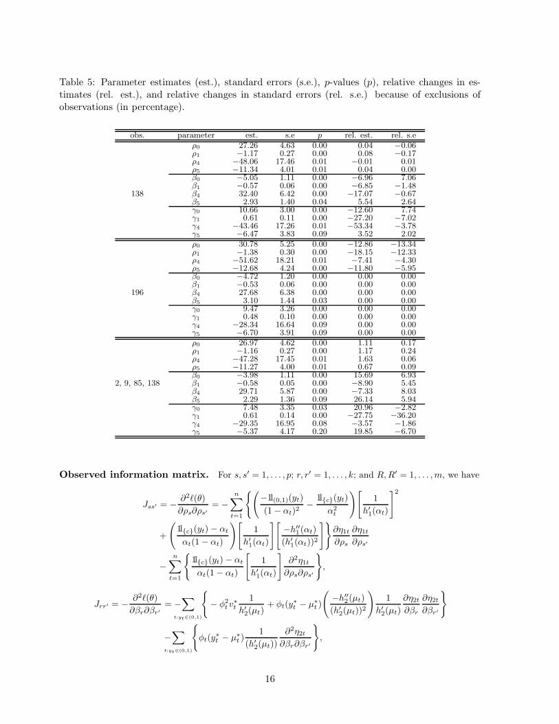
Table 5: Parameter estimates (est.), standard errors (s.e.), p-values (p), relative changes in es-timates (rel. est.), and relative changes in standard errors (rel. s.e.) because of exclusions ofobservations (in percentage).

obs. parameter est. s.e p rel. est. rel. s.eρ0 27.26 4.63 0.00 0.04 −0.06ρ1 −1.17 0.27 0.00 0.08 −0.17ρ4 −48.06 17.46 0.01 −0.01 0.01ρ5 −11.34 4.01 0.01 0.04 0.00β0 −5.05 1.11 0.00 −6.96 7.06β1 −0.57 0.06 0.00 −6.85 −1.48

138 β4 32.40 6.42 0.00 −17.07 −0.67β5 2.93 1.40 0.04 5.54 2.64γ0 10.66 3.00 0.00 −12.60 7.74γ1 0.61 0.11 0.00 −27.20 −7.02γ4 −43.46 17.26 0.01 −53.34 −3.78γ5 −6.47 3.83 0.09 3.52 2.02ρ0 30.78 5.25 0.00 −12.86 −13.34ρ1 −1.38 0.30 0.00 −18.15 −12.33ρ4 −51.62 18.21 0.01 −7.41 −4.30ρ5 −12.68 4.24 0.00 −11.80 −5.95β0 −4.72 1.20 0.00 0.00 0.00β1 −0.53 0.06 0.00 0.00 0.00

196 β4 27.68 6.38 0.00 0.00 0.00β5 3.10 1.44 0.03 0.00 0.00γ0 9.47 3.26 0.00 0.00 0.00γ1 0.48 0.10 0.00 0.00 0.00γ4 −28.34 16.64 0.09 0.00 0.00γ5 −6.70 3.91 0.09 0.00 0.00ρ0 26.97 4.62 0.00 1.11 0.17ρ1 −1.16 0.27 0.00 1.17 0.24ρ4 −47.28 17.45 0.01 1.63 0.06ρ5 −11.27 4.00 0.01 0.67 0.09β0 −3.98 1.11 0.00 15.69 6.93

2, 9, 85, 138 β1 −0.58 0.05 0.00 −8.90 5.45β4 29.71 5.87 0.00 −7.33 8.03β5 2.29 1.36 0.09 26.14 5.94γ0 7.48 3.35 0.03 20.96 −2.82γ1 0.61 0.14 0.00 −27.75 −36.20γ4 −29.35 16.95 0.08 −3.57 −1.86γ5 −5.37 4.17 0.20 19.85 −6.70

Observed information matrix. For s, s′ = 1, . . . , p; r, r′ = 1, . . . , k; and R,R′ = 1, . . . ,m, we have

Jss′ = − ∂2ℓ(θ)

∂ρs∂ρs′= −

n∑

t=1

{(−1l(0,1)(yt)

(1− αt)2− 1l{c}(yt)

α2t

)[1

h′1(αt)

]2

+

(1l{c}(yt)− αt

αt(1− αt)

)[1

h′1(αt)

][−h′′1(αt)

(h′1(αt))2

]}∂η1t∂ρs

∂η1t∂ρs′

−n∑

t=1

{1l{c}(yt)− αt

αt(1− αt)

[1

h′1(αt)

]∂2η1t∂ρs∂ρs′

},

Jrr′ = − ∂2ℓ(θ)

∂βr∂βr′= −

∑

t:yt∈(0,1)

{− φ2t v

∗t

1

h′2(µt)+ φt(y

∗t − µ∗

t )

(−h′′2(µt)

(h′2(µt))2

)1

h′2(µt)

∂η2t∂βr

∂η2t∂βr′

}

−∑

t:yt∈(0,1)

{φt(y

∗t − µ∗

t )1

(h′2(µt))

∂2η2t∂βr∂βr′

},

16

JrR = − ∂2ℓ(θ)

∂βr∂γR= −

∑

t:yt∈(0,1)

{[y∗t − µ∗

t − φt(µtv∗t + c∗†t )]

1

(h′2(µt))

∂η2t∂βr

1

(h′3(φt))

∂η3t∂γR

},

JRR′ = − ∂2ℓ(θ)

∂γR∂γR′

= −∑

t:yt∈(0,1)

{[−µ2

tv∗t − 2µtc

∗† − v†t ]1

(h′3(φt))+ [µt(y

∗t − µ∗

t ) + (y†t − µ†t)]

×(

−h′′3(φt)(h′3(φt))

2

)}1

(h′3(φt))

∂η3t∂γR

∂η3t∂γR′

−∑

t:yt∈(0,1)

{[µt(y

∗t − µ∗

t ) + (y†t − µ†t )]

1

(h′3(φt))

∂2η3t∂γR∂γR′

}.

The observed Fisher information matrix can now be written as

J(θ) =

Jρρ 0 00 Jββ Jβγ0 Jγβ Jγγ

, (A.4)

whereJρρ = V⊤{(A∗2(In − Y c) +A2Y c) +A∗A(Y c − α∗)D∗D}V⊤ − [(yc − α)⊤AD][V ],Jββ = X⊤{ΦTV ∗ + ST 2(Y ∗ −M∗)}(In − Y c)TΦX + [(y∗ − µ∗)⊤(In − Y c)TΦ][X ],

Jγβ = J⊤γβ = −X⊤{(Y ∗ −M∗)− Φ(MV ∗ + C)}(In − Y c)THZ,

Jγγ = Z⊤{H(M2V ∗ + 2MC + V †) + {M(Y ∗ −M∗) + (Y † −M†)}QH2}(In − Y c)HZ+ [((y∗ − µ∗)⊤M + (y† − µ†)⊤)(In − Y c)H ][Z],

with α∗ = diag(α1, . . . , αn), Y∗ = diag(y∗1 , . . . , y

∗n), Y

† = diag(y†1, . . . , y†t ), M∗ = diag(µ∗

1, . . . , µ∗n), M† =

diag(µ†1, . . . , µ

†n), and Q = diag(h′′3 (φ1), . . . , h

′′3(φn)); V is an n×p×p array with faces Vt = ∂2η1t/∂ρ∂ρ

⊤, Xis an n×k×k array with faces Xt = ∂2η2t/∂β∂β

⊤, and Z is an n×m×m array with faces Zt = ∂2η3t/∂γ∂γ⊤,

for t = 1, . . . , n. The column multiplication for three-dimensional arrays is indicated by the bracket operator

[·][·] as defined by Wei (1998, p. 188).

B Appendix B: Iterative algorithm for maximum likelihood es-

timation

MLEs for ρ and ϑ = (β⊤, φ)⊤ can be obtained by using a re-weighted least-squares algorithm. For ρ wehave

ρ(m+1) = (V(m)⊤W1

(m)V(m))−1V(m)W1

(m)y1(m), m = 0, 1, . . . , (B.1)

where W1 is defined in (3.7) and

y1 = Vρ+W1−1ADA∗(yc − α) (B.2)

is a local modified dependent variable. This cycle is repeated until convergence is achieved. Rewriting thisequation as

y1 = η1 − τ1 +W1−1ADA∗(yc − α), (B.3)

where η1 = f1(V ; ρ) and τ1 = f

1(V ; ρ) − Vρ, we can interpret (B.1) as an iterative process to fit a

generalized linear model with design matrix V , systematic part h1(αt) = η1t, tth diagonal element of thevariance function [W1

−1ADA∗]tt, t = 1, . . . , n, and offset τ1. The offset quantity is subtracted, at eachstep, from the predictor η1. The iterative process (B.1) may be performed, for instance, in the R package

17

by taking advantage of the library MASS (Venables & Ripley, 2002). This procedure allows us to extendthe diagnostic results of ordinary regression models to the discrete component of the zero-or-one inflated

beta regression model. Upon the converge of iterative process (B.1), we have ρ = (V⊤W1V)−1V⊤z, where

z = V ρ + W−11

ADA∗(yc − α). The ordinary residual for this re-weighted regression is

r∗ = W1/21

(z− η1) = W−1/21

ADA∗(yc − α).

Note that the tth element of r∗ is

r∗t =1l{c} − αt√αt(1− αt)

. (B.4)

By writing (V⊤W1V)ρ = V⊤z, it is possible to obtain the approximations E(r∗) ≈ 0 and Var(r∗) ≈(In −H), where In is the n× n identity matrix and

H = W11/2V(V⊤W1V)−1V⊤W1

1/2 (B.5)

is an orthogonal projection matrix onto the vector space spanned by the columns of V . The geometricinterpretation of H as a projection matrix is discussed by Moolgavark et al. (1984).

Now, let X∼, T∼, and W∼ be the (2n× (k + n)) and (2n× 2n), (2n× 2n) dimensional matrices

X∼=

(X 00 Z

), T∼=

((In − Y c)TΦ 0

0 (In − Y c)H

), W∼=

(W2 W3

W3 W4

), (B.6)

respectively, and y∼⊤= ((y∗ − µ∗)⊤, [M(y∗ − µ∗) + (y† − µ†)]⊤) be an 1 × 2n auxiliary vector. The score

vector corresponding to ϑ = (β⊤, γ⊤)⊤ can be written as

U(ϑ) = X∼⊤T∼y∼ . (B.7)

Fisher’s information matrix for the parameter vector ϑ is given by

K(ϑ) = X∼⊤W∼X∼ . (B.8)

Also, the iterative process for estimating ϑ takes the form

ϑ(m+1) = (X∼(m)⊤

W∼(m)X∼

(m))−1 X∼(m)

W∼(m)y∼

∗(m), (B.9)

where y∼∗(m) = X∼ ϑ + W∼

−1T∼y∼ and m = 0, 1, 2, . . . are the iterations that are performed until convergence,

which occurs when the distance between ϑ(m+1) and ϑ(m) becomes smaller than a given, small constant.The procedure is initialized by choosing suitable initial values for β and γ.

Assuming that γ is known, Fisher’s scoring iterative scheme used to estimating β can be written as

β(m+1) = (X (m)⊤W2(m)X (m))−1X (m)W2

(m)y2(m), (B.10)

where W2 is defined in (3.7) and y2 = Xβ +W2−1TΦ(y∗ − µ∗), with m = 0, 1, 2, . . . . Upon convergence,

we haveβ = (X⊤W2X )−1X⊤τ, (B.11)

where τ = X β + W−12T Φ(y∗ − µ∗). Then, β in (B.11) can be viewed as the least-squares estimate of

β obtained by regressing τ on X with weighting matrix W2. The ordinary residual of this re-weightedleast-squares regression is

r = (In − P)τ = W1/22

(τ − X β) = W−1/22

ΦT (y∗ − µ∗). (B.12)

Here,

P = W1/22X(X⊤W2X )−1X⊤W

1/22 (B.13)

18

is a projection matrix. Note that if all the quantities are evaluated at the true parameter, E(r) = 0 andVar(r) = (In−P). The P matrix is similar to the leverage matrix in standard linear regression models, andhence, we refer to it as the generalized leverage matrix. It is possible to show that In − P is symmetric,idempotent, and spans the residual r-space. This implies that a small 1 −Ptt indicates extreme points inthe design space of the continuous component of the zero-or-one inflated beta regression model. Note thatthe tth element of r is

rt =y∗ − µ∗

√v∗t (1 − αt)

. (B.14)

References

Akaike, H. (1974). A new look at the statistical model identification. IEEE. Transactions on Automatic

Control, 19, 716–723.

Atkinson, A. C. (1985). Plots, Transformations and Regression: An Introduction to Graphical Methods

of Diagnostic Regression Analysis. New York: Oxford University Press.

Cook, R. D. & Weisberg, S. (1982). Residuals and Influence in Regression. London: Chapman and Hall.

Cook, D. O., Kieschnick, R. & McCullough, B. D. (2008). Regression analysis of proportions in financewith self selection. Journal of Empirical Finance, 15, 860–867.

Cox, D. R. & Hinkley, D. V. (1974). Theoretical Statistics. London: Chapman and Hall.

Cox, D. R. & Reid, N. (1987). Parameter orthogonality and approximate conditional inference (withdiscussion). Journal of the Royal Statistical Society B, 49, 1–39.

Cox, D. & Snell, E. (1968). A general definition of residuals. Journal of the Royal Statistical Society B,30, 248–275.

Cox, D. R. & Snell, E. J. (1989). Analysis of Binary Data. London: Chapman and Hall.

Dunn, P. K. & Smyth, G. K. (1996). Randomized quantile residuals. Journal of Computational and

Graphical Statistics, 5, 236–244.

Espinheira, P. L., Ferrari, S. L. P. & Cribari–Neto, F. (2008a). Influence diagnostics in beta regression.Computational Statistics and Data Analysis, 52, 4417–4431.

Espinheira, P. L., Ferrari, S. L. P. & Cribari–Neto, F. (2008b). On beta regression residuals. Journal ofApplied Statistics, 35, 407–419.

Fahrmeir, L. & Kaufmann, H. (1985). Consistency and asymptotic normality of the maximum likelihoodestimator in generalized linear models. Annals of Statistics, 13, 342–368.

Ferrari, S. L. P. & Cribari–Neto, F. (2004). Beta regression for modelling rates and proportions. Journalof Applied Statistics, 7, 799–815.

Ferrari, S. L. P. & Pinheiro, E. C. (2010). Improved likelihood inference in beta regression. Journal of

Statistical Computation and Simulation. Available online. DOI: 10.1080/00949650903389993.

Hoff, A. (2007). Second stage DEA: Comparison of approaches for modelling the DEA score. European

Journal of Operational Research, 181, 425–435.

Ihaka, R. & Gentleman, R. (1996). R: A language for data analysis and graphics. Journal of Computa-

tional and Graphical Statistics, 5, 299–314.

19

Johnson, N., Kotz, S. & Balakrishnan, N. (1995). Continuous Univariate Distributions. 2nd ed. NewYork: John Wiley and Sons.

Kieschnick, R. &McCullough, B. D. (2003). Regression analysis of variates observed on (0,1): percentages,proportions, and fractions. Statistical Modelling, 3, 1–21.

Korhonen, L., Korhonen, K. T., Stenberg, P., Maltamo, M. & Rautiainen, M. (2007). Local models forforest canopy cover with beta regression. Silva Fennica, 41, 671–685.

McCullagh, P. & Nelder, J. A. (1989). Generalized Linear Models, 2nd ed. London: Chapman and Hall.

McFadden, D. (1974). Conditional logit analysis of qualitative choice behavior. In: P. Zarembka, ed.,Frontiers in Econometrics, 105–142. New York: Academic Press.

Ospina, R. (2006). The zero-inflated beta distribution for fitting a GAMLSS. Extra distributions to beused for GAMLSS modelling. Available at gamlss.dist package. http://www.gamlss.org.

Ospina, R. & Ferrari, S. L. P. (2010). Inflated beta distributions. Statistical Papers, 51, 111–126.

Pace, L. & Salvan, A. (1997). Principles of Statistical Inference from a Neo-Fisherian Perspective. Ad-vanced Series on Statistical Science and Applied Probability, Vol.4. Singapore: World Scientific.

Paolino, P. (2001). Maximum likelihood estimation of models with beta-distributed dependent variables.Political Analysis, 9, 325–346.

Press, W. H., Teulosky, S. A., Vetterling, W. T. & Flannery, B. P. (1992). Numerical Recipes in C: The

Art of Scientific Computing. 2nd ed. Prentice Hall: London.

Rao, C. R. (1973). Linear Statistical Inference and Its Applications, 2nd ed. New York: Wiley.

Rigby, R. A. & Stasinopoulos, D. M. (2005). Generalized additive models for location, scale and shape(with discussion). Applied Statistics, 54, 507–554.

Schwarz, G. (1978). Estimating the dimension of a mode. Annals of Statistics, 6, 461–464.

Simas, A. B., Barreto-Souza, W. & Rocha, A. V. (2010). Improved estimators for a general class of betaregression models. Computational Statistics & Data Analysis, 54, 348–366.

Smithson, M. & Verkuilen, J. (2006). A better lemon squeezer? Maximum likelihood regression with betadistributed dependent variables. Psychological Methods, 11, 54–71.

Stasinopoulos, D. M. & Rigby, R. A. (2007). Generalized additive models for location scale and shape(GAMLSS) in R. Journal of Statistical Software, 23, 1–43.

Venables, W. N. & Ripley, B. D. (2002). Modern Applied Statistics with S, 4th ed. New York: Springer.

Wei, B. C. (1998). Exponential Family Nonlinear Models. Singapore: Springer.

Yoo, S. (2004). A note on an approximation of the mobile communications expenditures distributionfunction using a mixture model. Journal of Applied Statistics, 31, 747–752.

20