This article appeared in a journal published by Elsevier. The attachedcopy is furnished to the author for internal non-commercial researchand education use, including for instruction at the authors institution

and sharing with colleagues.

Other uses, including reproduction and distribution, or selling orlicensing copies, or posting to personal, institutional or third party

websites are prohibited.

In most cases authors are permitted to post their version of thearticle (e.g. in Word or Tex form) to their personal website orinstitutional repository. Authors requiring further information

regarding Elsevier’s archiving and manuscript policies areencouraged to visit:

http://www.elsevier.com/copyright

Author's personal copy

A finite element formulation for the doublet mechanics modeling ofmicrostructural materials

Milos Kojic a,b,c,⇑, Ivo Vlastelica c,d, Paolo Decuzzi a, Vladimir T. Granik a, Mauro Ferrari a

a The Methodist Hospital Research Institute, 6670 Bertner Ave., Houston, TX 77030, United Statesb Harvard School of Public Health, 665 Huntington Ave., Boston, MA 02115, United Statesc Research and Development Center for Bioengineering, Sretenjskog Ustava 27, 34000 Kragujevac, Serbiad Metropolitan University, Tadeusa Koscuska 63, 11000 Belgrade, Serbia

a r t i c l e i n f o

Article history:Received 13 May 2010Received in revised form 15 December 2010Accepted 3 January 2011Available online 6 January 2011

Keywords:Doublet mechanics theoryMicrostructural discrete modelsMultiscale modelFinite element methodFlamant problemKelvin problem

a b s t r a c t

The doublet mechanics (DM) theory was developed [7,8] for modeling the behavior of solids where themicrostructure is important. Within the DM theory, solid bodies are discretized as an ensemble of parti-cles, with each pair of neighboring particles forming a ‘doublet’. Microstructural strains and stresses areintroduced through displacements and mutual interactions of the particles within the doublets. Thisdescription also includes a scale parameter, interpreted as the separation distance between two particlesin a doublet. The DM theory is consistent with other microstructural approaches and reduces to contin-uum mechanics in the case of non-scale formulation. Several problems in solid mechanics have been trea-ted analytically using DM [5].

In this work, DM is reformulated using a finite element approach with the aim of expanding even morethe potential applications of such an approach. As a first step in our development we considered themicrostructural elongation strains only, while the other two: shear and torsional are left for subsequentinvestigations. Two constitutive laws are considered: linear elastic and linear viscoelastic. A number ofsolved examples reveal the accuracy of the FE formulation developed for DM. The present numericalframework could be incorporated into various general numerical solution strategies, such as multi-scale-multidomain modeling, and further extended to include other constitutive relationships.

Published by Elsevier B.V.

1. Introduction

Solids can be mathematically modeled as either continuous ordiscrete media, primarily depending on the application. Modelsbased on the continuum assumption treat solids as a continuousdistribution of matter in space. This approach has been widelyused and has provided the foundation for overall great achieve-ments in various fields of engineering and science. However, whenthe characteristic length scale of the solid becomes comparablewith the grain or atomic size, or when the solid is intrinsically dis-crete, as granular materials, a different analysis including informa-tion on multiple scales is needed.

Discrete models for solids are more recent and are mainlydeveloped for microstructural problems. These include the latticedynamics model of crystals [4]; the molecular dynamics approach[19]; ab initio calculations and derivations [25]. The models

usually employ simplifications, such as regularity of particle dis-tribution, symmetry and periodicity. In practical engineeringapplications, for problems of micron size and up, those modelsare not of practical use because they require enormous computa-tional effort which cannot be handled with today’s computertechnology. In order to bridge the gap between discrete and con-tinuous models, a doublet mechanics (DM) theory has been intro-duced. Based on the original work by Granik [8], the DM theorywas further developed and applied to linear elastic geomechanicsin Granik and Ferrari [7], to viscoelasticity in Maddalena and Fer-rari [17] and other problems (a summary of the DM theory andapplications is given in Ferrari et al. [5]). We here cite more re-cent references where the DM theory has been successfullyimplemented: in Liu and Ferrari [15] a DM model was used tocompute spectral response for quantification of the physical prop-erties that determine the differences in the spectral signature ofnormal vs. malignant tissue; in Fang et al. [14] and Jin et al. [9]a dispersion analysis of wave propagation and its characterizationin viscoelastic cellular assemblies are presented; Sadd and Dai[20] compared the DM and FE solutions for micro-stress distribu-tions within a granular material and found good agreement

0045-7825/$ - see front matter Published by Elsevier B.V.doi:10.1016/j.cma.2011.01.001

⇑ Corresponding author at: The Methodist Hospital Research Institute, 6670Bertner Ave., Houston, TX 77030, United States.

E-mail address: mkojic@hsph.harvard.edu (M. Kojic).

Comput. Methods Appl. Mech. Engrg. 200 (2011) 1446–1454

Contents lists available at ScienceDirect

Comput. Methods Appl. Mech. Engrg.

journal homepage: www.elsevier .com/locate /cma

Author's personal copy

between the two; solutions for the stress and strain distributiondue to concentrated moving load on semiinfinite surface aregiven in Lin and Shen [13].

The DM model is general, suitable for applications in variousfields where microstructural material behavior is essential, suchas in geomechanics or in biomechanics (tissue and bone micro-structures, protein unfolding, etc.). Within the DM theory, a solidis discretized into particles (geometrical points in space) whichinteract among each other. A reference particle A (reference node)interacts with neighboring particles. Each couple of interactingparticles ABa represents a ‘doublet’. All doublets corresponding toa reference node make a bundle at the reference particle. The dou-blet is a ‘building block’ in the DM theory as it is the differentialvolume in continuum mechanics.

When the solid deforms, the discrete particles move so that thedisplacement field can be specified as in continuum mechanics.The displacement field includes translational and rotational de-grees of freedom. From a change of the relative positions betweenthe particles A and Ba and rotation along the direction ABa, the dou-blet mechanics strains for this doublet can be determined. Theelongation, shear and torsional strains are introduced, as describedin Ferrari et al. [5], and they are computed using geometrical rela-tions and Taylor series spatial expansion about the node A. The or-der M at which the series is truncated defines the order ofapproximation for the DM formulation. The case M = 1 representsthe scale free continuum mechanics description. For M > 1, theexpansion includes higher order spatial derivatives and the scaleparameter ga which, in geometrical terms, represents the initialdistance between the particles A and Ba, so that a multi-scale the-ory is formulated.

The DM theory is in agreement with other discrete theoriesand reduces to a standard continuum mechanics formulationwhen the characteristic length scale of the problem becomes suf-ficiently large. It relies on the ‘‘bottom-up’’ approach, with micro-structural constitutive relations, as opposed to Cosserat ormicropolar models with the ‘‘top-down’’ approach and largernumber of constitutive parameters than in the DM theory. Vari-ous mathematical schemes in modeling particulate or microstruc-tural materials have been used to develop macroscopicconstitutive parameters from the microstructure, as second-gradi-ent micropolar theory [21] or homogenization [18]; these macro-scopic parameters are further employed in common analysis ofsolids and structures.

Motivated by the generality of the DM theory and by the severalanalytical solutions already reported in the open literature, wehere present a FE formulation of the DM theory. The main idea ofthe presented mathematical formalism is to integrate the DMdescription into a FE framework, preserving kinematics of defor-mation and using the microstructural strains, stresses and consti-tutive laws. The FE formulation provides a basis for solution ofcomplex microstructural problems which cannot be obtained inanalytical form. The elongation microstrains are only consideredhere, as a first step and for comparison of the FE solutions withthose available in literature, where the elongation microstrainsare also employed. Although only the elongation microstrainsand microstresses are considered, these still give rise to contin-uum-level strains and stresses that include full elongation, shearand torsion effects. The presented mathematical formalism canfurther be extended to investigate the effects of other microstrainsand microstresses.

The basic DM relations are summarized in the next section andthen the FE formulation for linear and nonlinear problems is pre-sented. In Section 3, solutions of several examples demonstratethe accuracy of the FE procedure. In the last section we give con-cluding remarks about the presented formulation and highlightpossible further extension.

2. Basic relations in doublet mechanics

As stated above, only the elongation strains are considered,which can be calculated from the translational displacement field(rotational degrees of freedom are excluded). Hence, the displace-ment of a reference particle A is given as a function of the pointcoordinates xj, j = 1,2,3 and time, i.e. uA(xj, t) (see Fig. 1). Elongationstrain at a point A for a doublet ABa (a = 1,2, . . . ,n, where n is va-lence in case when the distribution of points form a Bravais lattice)can be expressed by using the Taylor series of order M (and specif-ically M = 2), as:

ea ¼XM

v¼1

gðv�1Þa

v!sa

j Tak1k2 ...kv

@k1k2 ...kv uj

@xk1@xk2� � � @xkv

� Tajk@uj

@xkþ ga

2Ta

jkm@2uj

@xk @xmsum on j; k;m

¼ 1;2;3; no sum on a; ð1Þ

where sai are unit vectors in initial configuration; ui is the displace-

ment; ga is the distance (scale parameter); and

Tajk ¼ sa

j sak and Ta

jkm ¼ saj s

aks

am ð2Þ

for M = 2. The approximation order M = 2 is adopted in all subse-quent derivations. No summation on a will be assumed if it is notstated otherwise; and summation on the repeated indices i, j,k, . . .

is implied (from 1 to 3). Components of the elongation strain are:

eai ¼ easa

i ¼ sai Ta

jk@uj

@xkþ ga

2sa

i Tajkm

@2uj

@xk @xm

¼ Taijk@uj

@xkþ ga

2Ta

ijkm@2uj

@xk @xm; ð3Þ

where

Taijkm ¼ sa

i saj s

aks

am: ð4Þ

Note that if the first order approximation (M = 1) is adopted, thestrains do not depend on ga and the usual continuum mechanics(CM) strains can be recovered. Also, note that the strain ea includesthe directional cosines of the doublet. From the above description,

Fig. 1. Representation of the solid by the DM model. (a) Material body; (b) The DMmiscrostructural model at a point A; (c) Kinematics of deformation of a doublet ABa.

M. Kojic et al. / Comput. Methods Appl. Mech. Engrg. 200 (2011) 1446–1454 1447

Author's personal copy

it follows that the characteristic length ga, the directional cosinessa

i and the valence n are the internal variables of the DM descrip-tion of the material.

Next, we introduce the microstructural stresses which arework-conjugate to the above microstructural strains. To each elon-gation strain ea corresponds the stress pa, therefore we can writethe components of the stress vector pa as

pai ¼ pasa

i � Tai pa: ð5Þ

These stresses and strains are related by a microstructural con-stitutive law. Here, the linear elastic and linear viscolelastic rela-tionships will be employed. In the case of linear elasticity, we have

pa ¼ Cabeb sum on b : b ¼ 1;2; . . . ;n; ð6Þ

while in the case of linear viscoelasticity, used in examples, thestress–strain relations can be written as

pa ¼ Cabeb þ Dab _eb sum on b : b ¼ 1;2; . . . ; n; ð7Þ

where Cab and Dab are the elastic and damping matrices, respec-tively; and _eb is the strain rate.

Finally, we give the relations between the macrostresses rij andthe microstresses pa at a material point (and the approximation forM = 2):

rij ¼Xn

a¼1

sai

XM

v¼1

ð�1Þvþ1 gv�1a

v!Ta

k1k2 ...kv

@v�1paj

@xk1@xk2� � � @xkv

�Xn

a¼1

sai s

aj pa � ga

2sa

m@pa

@xm

� �: ð8Þ

These relations are based on the equilibrium of a material element[5]. Note that to these elongation stresses correspond in general outelongation as well as shear macrostresses (see Example 1, Fig. 2b).

3. Finite element formulation

Here, a finite element formulation according to the doubletmechanics theory is presented. This displacement-based FE formu-lation follows a usual procedure given in the FE literature (cf.[1,10,12]). The DM description of material deformation givenabove – with kinematics of deformation and microstrains, micro-stresses and the corresponding constitutive relationships – is pre-served and built into the FE framework (and in our software PAK[11]). It is further assumed that displacements are small, i.e. theproblems are geometrically linear. We first derive the basic expres-sions assuming linear constitutive law and then extend the formu-lation to nonlinear constitutive relations.

The fundamental assumption is that the displacement fieldwithin a finite element is interpolated as

u ¼ NU ð9aÞ

or, in component form

ui ¼ NK UKi sum on K : K ¼ 1;2;3; . . . ;N; ð9bÞ

where ui is the displacement at a material point within the elementin direction of coordinate axis xi (i = 1,2,3); UK

i is the ith nodal dis-placement at node K; NK is the interpolation function correspondingto node K; and N is number of nodes of the finite element.

By substituting the interpolations (9) into Eq. (1), the micro-structural strains can be expressed as

ea ¼ BaU; ð10Þ

where the terms BaJj are:

BaJj ¼ Ta

jk@NJ

@xkþ ga

2Ta

jkm@2NJ

@xk @xm¼ sa

j sak@NJ

@xkþ ga

2sa

ksam

@2NJ

@xk @xm

!;

j ¼ 1;2;3; sum on k;m : k;m ¼ 1;2;3: ð11Þ

In the case of an elastic material, stresses can be expressedusing (6) and (10) in the form

pa ¼ Cabeb ¼ CabBbU sum on b : b ¼ 1;2; . . . ;n: ð12Þ

The virtual work per unit volume for the a doublet is

dWa ¼ deaT pa ¼ dUT BaT CabBbU

¼ dUT KaU no sum on a; sum on b : b ¼ 1;2; . . . ;n; ð13Þ

where, obviously, the stiffness matrix (per unit volume) for the dou-blet a is

Ka ¼ BaT CabBb sum on b: ð14Þ

Note that the matrix Ka is of dimensions 3N � 3N. Finally, the ma-trix of the finite element is:

KEL ¼Xn

a¼1

ZV

Ka dV ; ð15Þ

where V is the element volume. After assembling the elementmatrices, the solution for displacements is obtained from the bal-ance equation of the system (structure)

KsysUsys ¼ Fextsys; ð16Þ

where Ksys, Usys and Fextsys are the stiffness matrix, nodal displace-

ments and external forces of the system, respectively. In generatingthe FE model of a structure, appropriate boundary conditions mustbe imposed.

In an incremental analysis, the solution is obtained over incre-mental (time) steps, and equilibrium equation for a finite elementis

KELDU ¼ nþ1Fext � nFint; ð17Þ

where DU are increments of nodal displacements, n+1Fext is theexternal force vector for the element, which includes actions ofthe surrounding elements and those coming from other externalsources; and nFint is the element internal force. The left upper indi-ces n and n + 1 denote values at start and end of the step n. Theinternal force vector can be expressed as

nFint ¼Xn

a¼1

nFðaÞint ¼Xn

a¼1

ZV

BaT npa dV : ð18Þ

In the case of linear viscoelastic constitutive relations used below,the stresses are determined according to Eq. (7), with _eb ¼ Deb=Dt,where Deb is the strain increment and Dt is the time step size.The constitutive matrix (within the stiffness matrix KEL, see Eq.(14)) is

�Cab ¼ Cab þ 1Dt

Dab: ð19Þ

Note that for linear elastic law, we only have the first term on theright-hand side. The element balance equations are assembledand the system equations are solved for the increments ofdisplacements.

Finally, for the completeness of the presentation, we consider acase when constitutive relationships are nonlinear (as in [3]). Then,the stresses depend on strains (and, in general, on strain rates andhistory of deformation) so that an incremental-iterative schememust be employed. Instead of the linear equilibrium equation(17), the following relations can be derived (cf. [10])

1448 M. Kojic et al. / Comput. Methods Appl. Mech. Engrg. 200 (2011) 1446–1454

Author's personal copy

nþ1KELði�1ÞDUðiÞ ¼ nþ1Fext � nþ1Fintði�1Þ ð20Þ

corresponding to a load step n and equilibrium iteration i within thestep; DU(i) is the nodal displacement increment vector; and the leftupper index n + 1 indicates that the equilibrium is searched for theend of load step (implicit solution scheme). The displacement at endof load step is

nþ1UðiÞ ¼ nUþ DUð1Þ þ DUð2Þ þ � � � þ DUðiÞ; ð21Þ

where nU is the displacement at start of the step. The iteration stopswhen a convergence criterion is reached (e.g. jDU(i)j 6 e, where e is aselected numerical tolerance). Note that in the stiffness matrixn+1KEL(i�1), the constitutive matrix n+1C(i�1) is used, correspondingto the last known stress–strain state (iteration ‘‘i � 1’’). Likewise,in n+1Fint(i�1) enter stresses n+1p(i�1) – see Eq. (18). The incrementalequations are assembled and the iterative equations are solved foreach iteration. Note that the solution accuracy does not dependon the element stiffness matrix, but the number of iterations is re-duced if the proper, the so-called tangent matrices, are calculated(using the tangent constitutive matrix, cf. [12]).

In a case of large displacements, additional stiffness matrix, ageometrical stiffness matrix, may be included to increase the con-vergence rate [1,10,12], but that matrix is not specific for the DMmodel. Dynamic analysis can also be performed by the additionof inertial effects, where the material properties only enter throughmass density.

4. Examples

The examples are selected to demonstrate the accuracy of thepresented FE formulation as compared to the analytical solutionsavailable in the open literature. The examples include homogenousdeformations, the Flamant problem, the Kelvin problem, and aplate with a hole. All examples are 2D problems. The theoreticalrelations derived in the previous section are built into the gen-eral-purpose FE program PAK [11]. Several details are further givenwhich are important for the implementation of the above theory.

It is assumed that the valence is n = 3, hence three unit vectorssa are used and the indices a and b go from 1 to 3. The angle be-tween two adjacent unit vectors is 60� providing the isotropicmaterial response. The unit vectors are denoted as V1, V2, V3 inall figures. Also, the scale parameter is taken to be the same forall doublets and is denoted as g.

In order to incorporate the DM model within the commonlyused 4-node finite element for 2D analysis in PAK program, theinterpolation functions of the element-free Galerkin (EFG) type[2] are employed instead usual isoparametric functions. This isdue to the fact that the second derivatives (see Eq. (11)) are presentin the multiscale DM formulation, and the isoparametric interpola-tion functions for the linear 4-node element have zero secondderivatives. In the EFG interpolation functions, the linear base is as-sumed and the exponential weight functions are employed. Thedomain of influence of the weight function is bounded to one ele-ment, which also is the integration cell in the EFG terminology. De-tails about the interpolation functions and their derivatives aregiven in the Appendix.

We also have tested accuracy of the solutions when 8-node iso-parametric element, with quadratic interpolations, is used. Accu-racy and limitations of this element and 4-node element (withuse of the EFG interpolation functions) are given in Example 1.

The elastic and viscoelastic models are used. In the elastic con-stitutive relations (6), the isotropic-type microelastic matrix hastwo material constants A0 and B0:

Cab ¼ A0 for a ¼ b; and Cab ¼ B0 for a – b: ð22Þ

These constants can be related to the continuum isotropic elasticmaterial parameters Young’s modulus E and Poisson’s ratio m, as [5]:

A0 ¼E 1� mð Þ

1þ mð Þ 1� 2mð Þ ; B0

¼ Em1þ mð Þ 1� 2mð Þ for plane strain conditions ð23Þ

and

A0 ¼E

1� m2 ; B0 ¼Em

1� m2 for plane stress conditions: ð24Þ

The viscoelastic constitutive matrix Dab is taken to be diagonal andisotropic, with the constants:

Dab ¼ 1000 ½N s=l2�; for a ¼ b and Dab ¼ 0 for a – b: ð25Þ

In all examples we will use the following units: for length (l),for force (N), for Young’s modulus and stresses (N/l2).

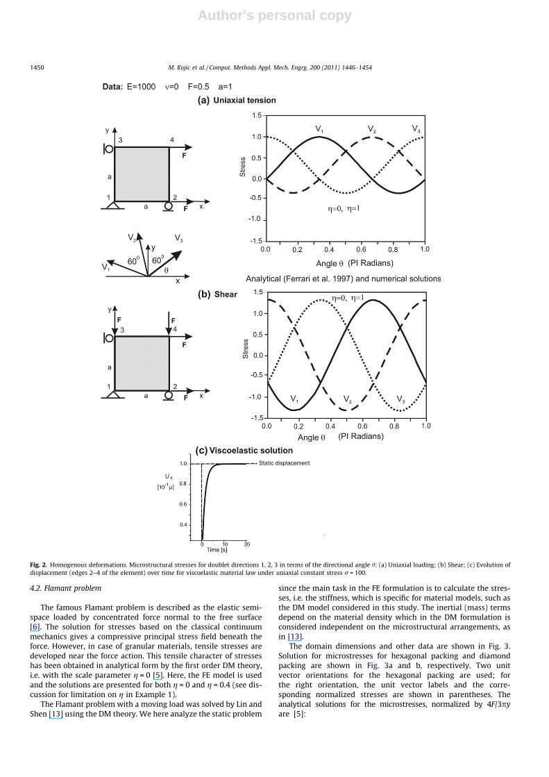
4.1. Homogenous deformations

Homogenous deformations are modeled by considering one4-node element, as shown in Fig. 2. The material is subjected touniaxial loading (Fig. 2a) or to equal tensional and compressiveforces (Fig. 2b). In the later case, the material experiencespure shear along the planes under 45� and 135� with respect tothe x-axis. The loading and boundary conditions are shown in thefigure.

The elastic solutions are obtained for various orientations of theunit vectors, specified by the angle h. The analytical and numerical(FE) solutions for microstresses along the doublet directions agreewith the analytical solutions [5]. It is interesting that the solutionsfor microstresses are practically the same for both values g = 0 andg = 1 of the scale parameter. The uniform macrostress distributionwithin the finite element is obtained.

We have investigated the effects of the second order terms,which include second derivatives and the scale parameter g, onaccuracy of stresses. This is performed by using various numbersof elements for the problem shown in Fig. 1a. We have found thatthe uniform and accurate stress field is obtained (error in the fieldless than 1%) if the parameter g, which has a dimension of length, isless or equal to the element side length. This bound on g is adoptedfor the other numerical examples.

An analysis of the solution accuracy was also carried out whenemploying 8-node isoprametric finite element. The solutions areaccurate with using the first order theory (g = 0). However, an or-der of magnitude smaller parameter g must be taken with respectto the 4-node element to obtain the same accuracy. This comesfrom the fact that the second derivatives of the isoparametric qua-dratic functions are mostly an order of magnitude higher than thefirst order derivatives, which leads to the conditions that the sec-ond order effects become more dominant (for g not sufficientlysmall). On the other hand, for the selected EFG parameters (seeAppendix), the second derivatives of the EFG interpolation func-tions are of the same order of magnitude or one order smaller thatthe first order terms, allowing larger values of the parameter g.

The viscoelastic material response under uniaxial constantstress r = 100 is shown in Fig. 2c. Therefore, in the incrementalequation (17) we only have nonzero external forces Fext

2x ¼ Fext4x ¼

ra=2 ¼ const: at nodes 1 and 2, while the internal forces are calcu-lated from Eq. (18) for each time step. The displacements are calcu-lated with the time step Dt = 0.5 s and agree with the analyticalsolution. The analytical solution for the displacement of the ele-ment side 2–4 loaded by forces is

Ux ¼ 0:1ð1� e�tÞ: ð26Þ

M. Kojic et al. / Comput. Methods Appl. Mech. Engrg. 200 (2011) 1446–1454 1449

Author's personal copy

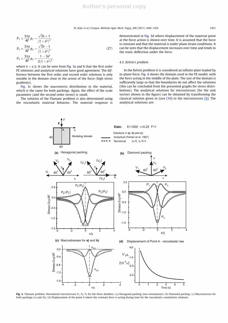
4.2. Flamant problem

The famous Flamant problem is described as the elastic semi-space loaded by concentrated force normal to the free surface[6]. The solution for stresses based on the classical continuummechanics gives a compressive principal stress field beneath theforce. However, in case of granular materials, tensile stresses aredeveloped near the force action. This tensile character of stresseshas been obtained in analytical form by the first order DM theory,i.e. with the scale parameter g = 0 [5]. Here, the FE model is usedand the solutions are presented for both g = 0 and g = 0.4 (see dis-cussion for limitation on g in Example 1).

The Flamant problem with a moving load was solved by Lin andShen [13] using the DM theory. We here analyze the static problem

since the main task in the FE formulation is to calculate the stres-ses, i.e. the stiffness, which is specific for material models, such asthe DM model considered in this study. The inertial (mass) termsdepend on the material density which in the DM formulation isconsidered independent on the microstructural arrangements, asin [13].

The domain dimensions and other data are shown in Fig. 3.Solution for microstresses for hexagonal packing and diamondpacking are shown in Fig. 3a and b, respectively. Two unitvector orientations for the hexagonal packing are used; forthe right orientation, the unit vector labels and the corre-sponding normalized stresses are shown in parentheses. Theanalytical solutions for the microstresses, normalized by 4F/3pyare [5]:

Fig. 2. Homogenous deformations. Microstructural stresses for doublet directions 1, 2, 3 in terms of the directional angle h: (a) Uniaxial loading; (b) Shear; (c) Evolution ofdisplacement (edges 2–4 of the element) over time for viscoelastic material law under uniaxial constant stress r = 100.

1450 M. Kojic et al. / Comput. Methods Appl. Mech. Engrg. 200 (2011) 1446–1454

Author's personal copy

P1 �3py4F

p1 ¼ffiffiffi3p

�xþ 1

1þ �x2ð Þ2;

P2 �3py4F

p2 ¼ffiffiffi3p

�x� 1

1þ �x2ð Þ2;

P3 �3py4F

p3 ¼1� 3�x2

2 1þ �x2ð Þ2;

ð27Þ

where �x ¼ x=y. It can be seen from Fig. 3a and b that the first orderFE solutions and analytical solutions have good agreement. The dif-ference between the first order and second order solutions is onlynotable in the domain close to the action of the force (high stressgradients).

Fig. 3c shows the macrostress distribution in the material,which is the same for both packings. Again, the effect of the scaleparameter (and the second order terms) is small.

The solution of the Flamant problem is also determined usingthe viscoelastic material behavior. The material response is

demonstrated in Fig. 3d where displacement of the material pointat the force action is shown over time. It is assumed that the forceis constant and that the material is under plane strain conditions. Itcan be seen that the displacement increases over time and tends tothe static deflection under the force.

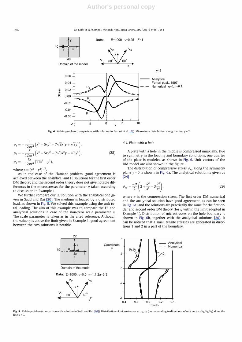
4.3. Kelvin’s problem

In the Kelvin problem it is considered an infinite plate loaded byin-plane force. Fig. 4 shows the domain used in the FE model, withthe force acting in the middle of the plate. The size of the domain issufficiently large so that the boundaries do not affect the solutions(this can be concluded from the presented graphs for stress distri-butions). The analytical solutions for microstresses (for the unitvectors shown in the figure) can be obtained by transforming theclassical solution given in Love [16] to the microstresses [5]. Theanalytical solutions are:

Fig. 3. Flamant problem. Normalized microstresses P1, P2, P3 for the three doublets: (a) Hexagonal packing (two orientations); (b) Diamond packing; (c) Macrostresses forboth packings (a) and (b); (d) Displacement of the point A where the constant force is acting during time for the viscoelastic constitutive relations.

M. Kojic et al. / Comput. Methods Appl. Mech. Engrg. 200 (2011) 1446–1454 1451

Author's personal copy

p1 ¼ �F

12pr4 x3 � 5xy2 þ 7ffiffiffi3p

x2yþffiffiffi3p

y3� �

;

p2 ¼ �F

12pr4 x3 � 5xy2 � 7ffiffiffi3p

x2y�ffiffiffi3p

y3� �

;

p3 ¼ �Fx

12pr4 11x2 � y2� �;

ð28Þ

where r ¼ ðx2 þ y2Þ1=2.As in the case of the Flamant problem, good agreement is

achieved between the analytical and FE solutions for the first orderDM theory; and the second order theory does not give notable dif-ferences in the microstresses for the parameter g taken accordingto discussion in Example 1.

We further compare our FE solution with the analytical one gi-ven in Sadd and Dai [20]. The medium is loaded by a distributedload, as shown in Fig. 5. We solved this example using the unit to-tal loading. The aim of this example was to compare the FE andanalytical solutions in case of the non-zero scale parameter g.The scale parameter is taken as in the cited reference. Althoughthe value g is above the limit given in Example 1, good agreementbetween the two solutions is notable.

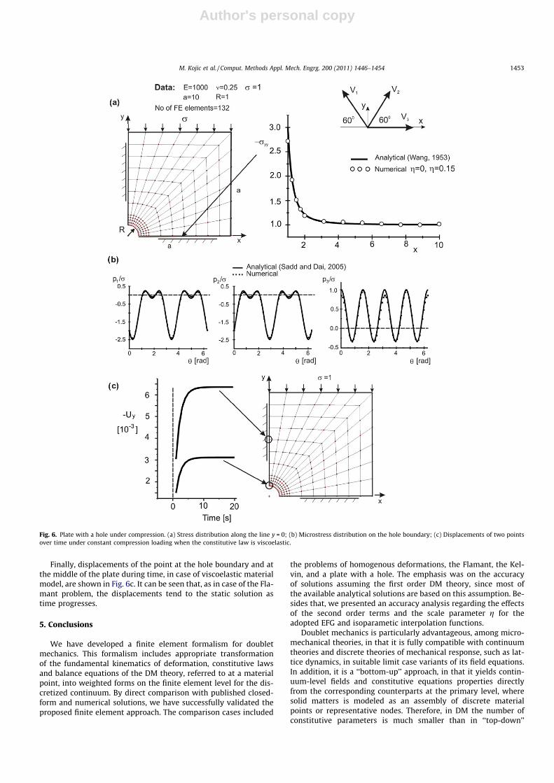
4.4. Plate with a hole

A plate with a hole in the middle is compressed uniaxially. Dueto symmetry in the loading and boundary conditions, one quarterof the plate is modeled as shown in Fig. 6. Unit vectors of theDM model are also shown in the figure.

The distribution of compressive stress ryy along the symmetryplane y = 0 is shown in Fig. 6a. The analytical solution is given as[24]

ryy ¼�r2

2þ R2

x2 þ 3R4

x4

!; ð29Þ

where r is the compression stress. The first order DM numericaland the analytical solution have good agreement, as can be seenin Fig. 6a; and the solutions are practically the same for the first or-der and second order DM theory (for g within the limit adopted inExample 1). Distribution of microstresses on the hole boundary isshown in Fig. 6b, together with the analytical solutions [20]. Itcan be noticed that a small tensile stresses are generated in direc-tions 1 and 2 in a part of the boundary.

Fig. 4. Kelvin problem (comparison with solution in Ferrari et al. [5]). Microstress distribution along the line y = 2.

Fig. 5. Kelvin problem (comparison with solution in Sadd and Dai [20]). Distribution of microstresses p1, p2, p3 (corresponding to directions of unit vectors V1, V2, V3) along theline x = 0.

1452 M. Kojic et al. / Comput. Methods Appl. Mech. Engrg. 200 (2011) 1446–1454

Author's personal copy

Finally, displacements of the point at the hole boundary and atthe middle of the plate during time, in case of viscoelastic materialmodel, are shown in Fig. 6c. It can be seen that, as in case of the Fla-mant problem, the displacements tend to the static solution astime progresses.

5. Conclusions

We have developed a finite element formalism for doubletmechanics. This formalism includes appropriate transformationof the fundamental kinematics of deformation, constitutive lawsand balance equations of the DM theory, referred to at a materialpoint, into weighted forms on the finite element level for the dis-cretized continuum. By direct comparison with published closed-form and numerical solutions, we have successfully validated theproposed finite element approach. The comparison cases included

the problems of homogenous deformations, the Flamant, the Kel-vin, and a plate with a hole. The emphasis was on the accuracyof solutions assuming the first order DM theory, since most ofthe available analytical solutions are based on this assumption. Be-sides that, we presented an accuracy analysis regarding the effectsof the second order terms and the scale parameter g for theadopted EFG and isoparametic interpolation functions.

Doublet mechanics is particularly advantageous, among micro-mechanical theories, in that it is fully compatible with continuumtheories and discrete theories of mechanical response, such as lat-tice dynamics, in suitable limit case variants of its field equations.In addition, it is a ‘‘bottom-up’’ approach, in that it yields contin-uum-level fields and constitutive equations properties directlyfrom the corresponding counterparts at the primary level, wheresolid matters is modeled as an assembly of discrete materialpoints or representative nodes. Therefore, in DM the number ofconstitutive parameters is much smaller than in ‘‘top-down’’

Fig. 6. Plate with a hole under compression. (a) Stress distribution along the line y = 0; (b) Microstress distribution on the hole boundary; (c) Displacements of two pointsover time under constant compression loading when the constitutive law is viscoelastic.

M. Kojic et al. / Comput. Methods Appl. Mech. Engrg. 200 (2011) 1446–1454 1453

Author's personal copy

approaches such as micropolar or Cosserat theories, and theconstitutive properties are often directly amenable to independentmeasurements. Thus, DM may be envisioned to find wide applica-bility in the mechanics of micro- and nano-structured media,especially for biomechanical problems, and for materials that aredesigned and assembled from elementary building blocks ofknown properties, per the dominant paradigm of ‘‘bottom-up’’nanotechnology. The presented finite element formulation of DMis proposed as computational aid for modeling, analysis, and designendeavors for these classes of materials and mechanics problems.

Acknowledgments

The authors acknowledge the following funding support:Department of Defense, W81XWH-07-2-0101; NASA NNJ06HE06A;and State of Texas, Emerging Technology Fund; Grants: OI144028and TR6209, Ministry of Science and Technological Developmentof Serbia.

Appendix

EFG interpolation functions and their derivatives.The interpolation functions used in Eq. (9) are specified as fol-

lows. They can be written as [2]

NKðrÞ ¼Xm

j¼1

ðA�1BÞjK pj; ðA:1Þ

where the vector p forms the so-called basis, which in a linear caseused in this paper and for 2D problems, is:

pTðx; yÞ ¼ ½1; x; y� ðA:2Þ

with the basis size m = 3. The terms of the matrices A and B are:

Aij ¼XN

I¼1

wIpIip

Ij ; BiK ¼ pK

i wK ; no sum on K; ðA:3Þ

where pKi is the ith component of the vector evaluated at node K;

and wK is a weight function corresponding to the FE node K. Theweight functions are defined in terms of the distance between apoint within the element and the FE node. The following exponen-tial weight functions are used:

wIðd2kI Þ ¼

exp � dI=cð Þ2k½ ��exp �ðdmax I=cÞ2k½ �1�exp �ðdmax I=cÞ2k½ � ; dI < dmax I;

0; dI P dmax I;

8<: ðA:4Þ

where dI is the distance from a material point to the node I; dmaxI isthe domain of influence for the weight function wI, calculated asdmaxI = dmaxc, where dmax = 2; parameter k = 1; and c can be ex-pressed as c = a � (max distance between element nodes), witha = 0.2. Values for parameters k, dmax and a are taken in accordancewith Belytschko [2], and our experience [22,23].

In order to evaluate the finite element matrices, it is necessaryto determine derivatives of the interpolation functions with re-spect to coordinates x and y. The derivatives of the interpolationfunctions (A.1) involve the derivatives of the inverse matrix A�1,calculated as:

A�1j �

@A@xj¼ �A�1A;jA

�1 ðA:5Þ

and

ðA�1Þ;kj �@2A�1

@xk@xj¼ �A�1

;k A;jA�1 � A�1A;kjA

�1 � A�1A;jA�1;k : ðA:6Þ

Hence, the derivatives of the inverse matrix are expressed in termsof the matrix products of the matrix derivatives A,j and A,kj, and theinverse matrix A�1.

References

[1] K.J. Bathe, Finite Element Procedures, Prentice-Hall, Inc., Englewood Cliffs, NJ,1996.

[2] T. Belytschko, Y.Y. Lu, L. Gu, Element-free Galerkin methods, Int. J. Numer.Methods Engrg. 37 (1994) 229–256.

[3] F. Cachoa, P.J. Elbischger, J.F. Rodriguez, M. Doblare, G.A. Holzapfel, Aconstitutive model for fibrous tissues considering collagen fiber crimp, Int. J.Non-Linear Mech. 42 (2007) 391–402.

[4] M.T. Dove, Introduction to Lattice Dynamics, Cambridge University Press,Cambridge, 1993.

[5] M. Ferrari, V. Granik, A. Imam, J. Nadeau, Advances in Doublet Mechanics,Springer, 1997.

[6] Flamant, Sur la repartition des pressions dans un solide rectangulaire chargétransversalment, C.R. Acad. Sci. Franc. 114 (1892) 1465–1468.

[7] V. Granik, M. Ferrari, Microstructural mechanics of granular media, Mech.Mater. 15 (1993) 301–322.

[8] V.T. Granik, Microstructural mechanics of granular media. 1. The principles oftheory, Report No. UCB/SEMM-1992/02, Dept. of Civil Engineering, Universityof California, Berkeley, March 1992.

[9] Y.F. Jin, C.Y. Xiong, J.Y. Fang, M. Ferrari, Characterization of wave dispersion inviscoelastic cellular assemblies by doublet mechanics, Chin. Phys. Lett. 26 (8)(2009) 084601-1–084601-4.

[10] M. Kojic, N. Filipovic, B. Stojanovic, N. Kojic, Computer Modeling inBioengineering – Theoretical Background, Examples and Software, JohnWiley and Sons, 2006.

[11] M. Kojic, R. Slavkovic, M. Zivkovic, N. Grujovic, N. Filipovic, Finite ElementProgram for Analysis of Solids, Fluids, Field and Coupled Problems andBiomechanics, Univ. Kragujevac and R&D Center for BioengineeringKragujevac, Serbia, 2008.

[12] M. Kojic, K.J. Bathe, Inelastic Analysis of Solids and Structures, Springer, Berlin– Heidelberg, 2005.

[13] S.S. Lin, Y.C. Shen, Stress fields of a half-plane caused by moving loads-resolved using doublet mechanics, Soil Dyn. Earthq. Engrg. 25 (2005) 893–904.

[14] J.Y. Fang, Z. Jue, F. Jing, M. Ferrari, Dispersion analysis of wave propagation incubic–tetrahedral assembly by doublet mechanics, Chin. Phys. Lett. 21 (2004)1562.

[15] J. Liu, M. Ferrari, Mechanical spectral signatures of malignant disease? A small-sample, comparative study of continuum vs. nano-biomechanical dataanalyses, Dis. Markers 18 (2002) 175–183.

[16] A.E.H. Love, A Treatise on the Mathematical Theory of Elasticity, Dover, NewYork, 1944.

[17] F. Maddalena, M. Ferrari, Viscoelasticity of granular materials, Mech. Mater.20/3 (1995) 241–250.

[18] S. Maghous, D. Bernaud, J. Freard, D. Garnier, Elastoplastic behavior of jointedrock masses as homogenized media and finite element analysis, Int. J. RockMech. Min. Sci. 45 (2008) 1273–1286.

[19] D.C. Rapaport, The Art of Molecular Dynamics Simulation, CambridgeUniversity Press, 2004.

[20] M.H. Sadd, Q. Dai, A comparison of micro-mechanical modeling of asphaltmaterials using finite elements and doublet mechanics, Mech. Mater. 37(2005) 641–662.

[21] A.S.J. Suiker, R. de Borst, C.S. Chang, Micro-mechanical modeling of granularmaterial. Part 1: Derivation of a second-gradient micro-polar constitutivetheory, Acta Mech. 149 (2001) 161–180.

[22] I. Vlastelica, Methods of Solving Elastoplastic Deformation of Non-Porous andPorous Metals in Fracture Mechanics: Ph.D. Thesis, Faculty of MechanicalEngineering, University of Kragujevac, Serbia, 2003 (in Serbian).

[23] I. Vlastelica, V. Isailovic, T. Djukic, N. Filipovic, M. Kojic, On accuracy of theelement-free Galerkin (EFG) method in modeling incompressible fluid flow, J.Serbian Soc. Comput. Mech. 2/1 (2008) 90–99.

[24] C.T. Wang, Applied Elasticity, McGraw-Hill Book Co., New York, 1953.[25] S. Yip (Ed.), Handbook of materials Modeling, Springer, 2005.

1454 M. Kojic et al. / Comput. Methods Appl. Mech. Engrg. 200 (2011) 1446–1454