Adsorption on interstellar analog surfaces: from atoms to ...
Upload
khangminh22Category
view
2download
0
HAL Id: tel-01158711https://tel.archives-ouvertes.fr/tel-01158711
Submitted on 1 Jun 2015
HAL is a multi-disciplinary open accessarchive for the deposit and dissemination of sci-entific research documents, whether they are pub-lished or not. The documents may come fromteaching and research institutions in France orabroad, or from public or private research centers.
L’archive ouverte pluridisciplinaire HAL, estdestinée au dépôt et à la diffusion de documentsscientifiques de niveau recherche, publiés ou non,émanant des établissements d’enseignement et derecherche français ou étrangers, des laboratoirespublics ou privés.
Distributed under a Creative Commons Attribution - NonCommercial| 4.0 InternationalLicense
A few experiments using cold atoms: dipolar quantumgases, guided atom optics, and quantum engineering
with single Rydberg atomsThierry Lahaye
To cite this version:Thierry Lahaye. A few experiments using cold atoms: dipolar quantum gases, guided atom optics,and quantum engineering with single Rydberg atoms. Atomic Physics [physics.atom-ph]. UniversitéParis 11, 2015. tel-01158711

Université Paris 11 Institut d’Optique Graduate School
Mémoire d’habilitation à diriger des recherches
présenté par
Thierry Lahaye
A few experiments using cold atoms:dipolar quantum gases, guided atom optics, andquantum engineering with single Rydberg atoms
Soutenue le 11 mai 2015devant le jury composé de :
M. C. Fabre . . . . . . . . . . . . . . . . . . . . . . . . . . Président du juryM. O. Gorceix . . . . . . . . . . . . . . . . . . . . . . . RapporteurM. P. Pillet . . . . . . . . . . . . . . . . . . . . . . . . . . RapporteurM. J. Vigué . . . . . . . . . . . . . . . . . . . . . . . . . . RapporteurM. A. Browaeys . . . . . . . . . . . . . . . . . . . . . ExaminateurM. J. Dalibard . . . . . . . . . . . . . . . . . . . . . . . ExaminateurM. T. Pfau . . . . . . . . . . . . . . . . . . . . . . . . . . . Examinateur

2
Acknowlegements
Writing a Mémoire d’habilitation à diriger des recherches is an interesting exercise in itself,allowing one to look back at the past and try to discern the logic at work in the first partof a research career. However, one of its main interests probably lies in the fact that it isabove all an ideal way to realize the importance of human relationships in research —asprobably in any human endeavor. I have been lucky, at all the stages of my research career,to interact with many outstanding individuals, who all have had a major impact not onlyon my research, but beyond that, on my conception of science. I am glad that some ofthem could make it to take part in my jury, or to attend the defense.
Let me start by thanking all the members of the jury for having bothered to readthis document in details, and asked many interesting questions. I now want to thankmore specifically people with whom I have worked more or less closely during the last 15years, and for that I will somehow follow the chronological order —maybe that’s a way tominimize the risk of forgetting someone!
I had my first real contact with research after my first year at ÉNS, when I spent onemonth as an intern in Jacques Vigué’s group, working on the early version of his atominterferometer and, more importantly, sharing his office. I could not have dreamed of abetter mentor in atomic physics. When I joined the LCAR many years later, Jacques wasthe director of the lab, and I greatly benefited from his help and advice at a time whennot-so-easy decisions had to be made. I want to thank him for that, and I only regret wecould not have more discussions about physics.
After my internship in John Doyle’s group at Harvard during my master, I was con-vinced to continue working in atomic physics. Joining the cold atom group at LabortoireKastler–Brossel of ÉNS for my PhD was thus an obvious choice. There, I had the oppor-tunity to benefit from two supervisors, Jean Dalibard and David Guéry-Odelin.
There is no way to emphasize enough the qualities that make Jean an ideal supervisor:not only he is the brilliant physicist and excellent teacher that everybody knows, but, andmaybe even more importantly, he also knows how to listen, guide, encourage a young stu-dent and allow him to gain confidence and become a scientist. I thank him for his numerouspieces of advice that were crucial, at several stages of my career. Through a day-to-dayclose supervision, David taught me during my PhD the basics of experimental cold atomsphysics, and countless interesting theoretical curiosities. I also want to thank the variouspost-docs and PhD students on the experiment: Christian Roos, Johnny Vogels, Gaël
3

Reinaudi, Zhaoying Wang, Antoine Couvert. . . They all had very different personalities,and contributed to making my PhD time a very enjoyable experience. Beyond the team, Iwant to thank all the members of the cold atom group. Attending the weekly group meet-ing, led by Claude Cohen-Tannoudji, Christophe Salomon, Jean Dalibard, Yvan Castin,Michèle Leduc, was the best AMO physics school one could dream of. Finally, I benefitedfrom the help of the technical services, and in particular I want to thank Jean-FrançoisPoint and Didier Courtiade.
After my PhD, I moved on to Stuttgart for a post-doc in Tilman Pfau’s group. Thesetwo and a half years were very productive, and played a major role in my maturation asa scientist. Tilman’s enthusiasm for physics, allied with an impressive ability to followvery closely all the progress in the lab, despite the size of the group, made my time in hisinstitute very enjoyable. I also want to thank him warmly for his understanding when I hadto spend a few weeks back in France with my wife and my new-born son. Not every ‘boss’would have had his attitude! In Stuttgart I also had the chance to interact with a wonderfulteam: Marco Fattori, Tobias Koch, Bernd Fröhlich, Jonas Metz, and Axel Griesmaier. Itwas a pleasure to tame the Chromium BEC machine with them. I also enjoyed a lot theinteractions with the other members of the institute, and in particular with Robert Löw,as well as with our theory colleagues Luis Santos and Hans-Peter Büchler. Many thanksalso to Karin Otter for having fought the central administration of the university for me.
I joined the LCAR in Toulouse in 2008. There, I worked very closely with RenaudMathevet. I have learned at lot from him, not only about all kinds of very valuabletechnical skills, but also a lot of physics, especially in optics, electronics, thermodynamics.I admire his vast culture, his energy for hard work, and his taste for always trying to explainphysics in the simplest (but rigorous) way. Working with him in the lab was a pleasure,and our work on the replication of Fizeau’s æther-drag experiment will remain a highlightof my time at LCAR. The cold atom team on the experiment was composed of GianlucaGattobigio, Pierrick Cheiney, Charlotte Fabre: with them we shared all the hard timesone encounters when building an experiment, but also the rewards when the setup wasrunning. I also thank François Vermersch who, supervised by David, did a lot of numericsto simulate our experiments. I also had the chance to interact with many other membersof the lab: Jacques, of course, but also Jean-Marc L’Hermite, Pierre Labastie. . . Specialthanks to Béatrice Chatel for having organized a lot of outreach activities for the generalpublic, in which I took part and which I enjoyed a lot. Among the staff of the technicalservices, I want to thank warmly Gilles Bailly and Stéphane Faure for all they have taughtme.
My final move was to Palaiseau, where I arrived at the beginning of 2012. This wasmade possible by several people whom I want to thank here: Jacques Vigué, Jean-MarcL’Hermite, Christian Chardonnet, Pascale Roubin, and Bertrand Girard. Working withAntoine Browaeys is a great privilege. His deep culture allied with strong modesty makesany scientific interaction with him a real pleasure. I appreciate a lot his way of managinghis team, in a way that makes everybody feel that his work is important for collective
4

achievements. When I joined the group, the Rydberg team was composed of Lucas Béguinand Aline Vernier. I consider myself very lucky to have had such a ‘dream team’ to startworking on single atoms. When both of them were about to leave the group, we had thepleasure to welcome, almost at the same time, the current members of another dreamteam: Sylvain Ravets, Henning Labuhn, and Daniel Barredo. Working for three yearswith all those five extremely talented students and post-docs, moreover in a very friendlyatmosphere, was extremely enjoyable, and led to many results. We also benefited from a lotof help by Florence Nogrette, who spent a long time developing the SLM system and then,when it became fun, had to let us play with it on the setup. Mondher Besbes helped us alot for the finite-element modeling of our electrodes, and I thank him for all the time he hasspent on that. Charles Adams spent a one-month sabbatical stay in our team in 2014 and itwas extremely enriching to interact with him. I also want to thank Yvan Sortais, not onlyfor being the group’s reference on optics, but also for many enjoyable discussions aboutphysics. Thanks also to Ronan Bourgain, Joseph Pellegrino, and Stephan Jennewein forinteresting interactions. Finally, let me thank all the technical and administrative servicesfor their efficiency and kindness, with special thanks to Christian Beurthe and AndréGuilbaud.
Finally, I want to express my gratitude to people that, while being outside of thefield of research itself, made it possible for me to undertake and/or pursue my passion forresearch. I had the chance to have several outstanding teachers, who contributed to myinterest in science, and knowledge in general. Among them, Henri Lluel stood out, and Ihad the great pleasure to show him our lab in Toulouse a few years ago. My parents haveno connections with science, but I know how much all they taught me as a kid turned outto be essential. Last but not least, I want to thank to my wife Irina and my son Maximefor reminding me constantly that there is life also outside of the lab.
5

6

Contents
Introduction 9
1 Dipolar quantum gases 111.1 Introduction . . . . . . . . . . . . . . . . . . . . . . . . . . . . . . . . . . . . 111.2 Realizing a purely dipolar quantum gas . . . . . . . . . . . . . . . . . . . . 141.3 Stability of a dipolar quantum gas . . . . . . . . . . . . . . . . . . . . . . . 161.4 Collapse dynamics of a dipolar quantum gas . . . . . . . . . . . . . . . . . . 191.5 Dipolar quantum gases in triple-well potentials . . . . . . . . . . . . . . . . 211.6 Recent achievements in the field of dipolar gases . . . . . . . . . . . . . . . 241.7 Published articles . . . . . . . . . . . . . . . . . . . . . . . . . . . . . . . . . 25
2 Guided atom optics 432.1 Introduction . . . . . . . . . . . . . . . . . . . . . . . . . . . . . . . . . . . . 432.2 A Zeeman slower based on permanent magnets . . . . . . . . . . . . . . . . 442.3 A Bragg reflector for guided matter waves . . . . . . . . . . . . . . . . . . . 472.4 Prospects . . . . . . . . . . . . . . . . . . . . . . . . . . . . . . . . . . . . . 492.5 Published articles . . . . . . . . . . . . . . . . . . . . . . . . . . . . . . . . . 50
3 Arrays of single Rydberg atoms 633.1 Introduction . . . . . . . . . . . . . . . . . . . . . . . . . . . . . . . . . . . . 633.2 Overview of the Chadoq experiment . . . . . . . . . . . . . . . . . . . . . . 653.3 Interactions between two single Rydberg atoms . . . . . . . . . . . . . . . . 703.4 Prospects: towards many atoms . . . . . . . . . . . . . . . . . . . . . . . . . 733.5 Published articles . . . . . . . . . . . . . . . . . . . . . . . . . . . . . . . . . 77
4 Administrative data 1114.1 Curriculum vitæ . . . . . . . . . . . . . . . . . . . . . . . . . . . . . . . . . 1114.2 Publications and conferences . . . . . . . . . . . . . . . . . . . . . . . . . . 114
4.2.1 Publication list . . . . . . . . . . . . . . . . . . . . . . . . . . . . . . 1144.2.2 Conferences . . . . . . . . . . . . . . . . . . . . . . . . . . . . . . . . 118
7
A Outreach 121A.1 Introduction . . . . . . . . . . . . . . . . . . . . . . . . . . . . . . . . . . . . 121A.2 A “laser fountain” for the 50th anniversary of the laser . . . . . . . . . . . . 122A.3 Yet another MOT video on Youtube . . . . . . . . . . . . . . . . . . . . . . 123A.4 A Paul trap for small particles . . . . . . . . . . . . . . . . . . . . . . . . . 124A.5 Fizeau’s “æther-drag” experiment made simple . . . . . . . . . . . . . . . . 125A.6 Measuring the eccentricity of the Earth orbit with a nail . . . . . . . . . . . 126A.7 Published articles . . . . . . . . . . . . . . . . . . . . . . . . . . . . . . . . . 127
Bibliography 149
8

Introduction
This Mémoire d’habilitation à diriger des recherches summarizes the research activitiesthat I have pursued over the last nine years, from my postdoc (included), to the presentday.
After my PhD at Laboratoire Kastler–Brossel of ENS Paris, under the joint super-vision of David Guéry-Odelin and Jean Dalibard, and entitled Evaporative cooling of amagnetically guided atomic beam, I joined in 2006 Tilman Pfau’s group, at Stuttgart Uni-versity, to work on dipolar quantum gases. More precisely, a Bose–Einstein condensateof chromium had been obtained in the group about one year before. Chromium has, inits ground state, a strong magnetic dipole moment of 6µB, where µB is the Bohr mag-neton, and thus, in addition to the short-range, isotropic contact interaction usually atwork in BECs, the long-range, anisotropic dipole-dipole interaction influences significantlythe properties of chromium BECs. However these dipolar effects remained a small pertur-bation as compared to the contact interactions. The group had also demonstrated thatseveral (relatively narrow) Feshbach resonances exist in the collisions of 52Cr atoms. Thisled to the possibility to use controlled magnetic fields in order to enhance the relativeeffects of the dipolar interactions, by tuning the contact interaction to zero close to aFeshbach resonance, and thus realize a purely dipolar quantum gas. This is exactly whatthe team achieved during my post-doc, during which we thus studied the properties ofpurely dipolar quantum gases, in particular their geometry-dependent stability and theircollapse dynamics when they are unstable.
In October 2008, I joined, as a CNRS researcher, the newly-founded cold atom groupof David Guéry-Odelin, at Laboratoire Collisions, Agrégats, Réactivité, in Toulouse. Thefirst months where devoted to preparing the new lab space, and then to moving, fromLKB to Toulouse, David’s experimental setup, which was a modified version of the onedeveloped during my PhD thesis, but now used for the all-optical generation of BECs of87Rb. We then rebuilt from scratch this setup in Toulouse, with some substantial changes.In the course of this rather technical work, a highlight was the development, led by RenaudMathevet, then an assistant professor in the group, of a Zeeman slower using a transversemagnetic field created by permanent magnets in a Halbach configuration. Once the BECapparatus was again operational, we chose to perform guided atom optics experiments:by outcoupling a BEC in a horizontal, single-beam dipole trap acting as waveguide, onegets a matterwave analogue of a pulsed laser, propagating in a “fiber” made of light. In
9
10
particular, we studied in details the reflection of such a matterwave on an attractive, one-dimensional optical lattice, the equivalent of the fiber Bragg gratings widely used in guidedphotonics. After a few years in Toulouse, I decided to reorient my research activity andmove to Laboratoire Charles Fabry of Institut d’Optique.
I thus joined Antoine Browaeys’ team in Palaiseau, in January 2012, to take the re-sponsibility of a setup still under construction, and funded by the ERC starting grant thatAntoine had just obtained. The long-term goal is to use the Rydberg blockade to engineerinteresting quantum states of a system of single atoms held in arrays of optical microtraps,or tweezers, with arbitrary geometries. Since then, we have moved forward towards thisgoal, by demonstrating single-atom loading in such arrays containing tens of tweezers, andby studying in great details the interactions between small numbers (two and three) ofsingle Rydberg atoms.
This manuscript is organized as follows. Chapter 1 deals with the main results ondipolar quantum gases; chapter 2 is devoted to the work performed in Toulouse; andchapter 3 reports on the experiments on single Rydberg atoms done in Palaiseau. Inthese chapters, I have tried to avoid repeating the details that one can readily find in thepublished papers (the main ones being reproduced in the text for convenience). I chose to(i) give a broad introduction to the field, suitable for non-specialists, (ii) provide sometimesinformation about some technical tricks that were important for the experiments, but weretoo technical for being discussed in published papers, and (iii) when applicable, try tolook, after a few years, at the possible impact of the results obtained. Chapter 3 on theRydberg experiments is obviously the most developed one, as it deals with my currentresearch interests. A final chapter, passage obligé of a HDR, summarizes administrativedata about my research career. I have decided to add an appendix about a part of mywork which, despite being small at the quantitative level, is important —and enjoyable—for me, namely outreach activities.

Chapter 1
Dipolar quantum gases
. . . Bien sûr, ce n’est pas la SeineCe n’est pas le Bois de VincennesMais c’est bien joli tout de même,À Vaihingen, à Vaihingen. . . 1
1.1 Introduction
The realization of Bose–Einstein condensates (BECs) of dilute atomic vapors in 1995,quickly followed by that of degenerate Fermi gases, has triggered a huge amount of theo-retical and experimental studies of the properties of quantum gases over the last twentyyears [100]. Despite the fact that such gases are extremely dilute, with densities n rarelyexceeding n ∼ 1014 cm−3, most of their striking properties, such as superfluidity for in-stance, are governed by binary interactions between the constituent atoms.
For the vast majority of atomic species, the actual interatomic potential between twoatoms can be replaced, at ultracold temperatures, by a contact pseudo-potential propor-tional to the scattering length a characterizing the two-body scattering problem. Forinstance, the mean-field description of the time-dependent behaviour of a BEC with amacroscopic wavefunction ψ relies on the Gross-Pitaevskii equation
i~∂ψ
∂t= − ~2
2m4ψ + V (r)ψ + g|ψ|2ψ, (1.1)
where V (r) is the external trapping potential, and
g = 4π~2a
m(1.2)
the interaction strength, proportional to the scattering length a. Here, and in all this chap-ter, we chose to normalize the macroscopic wavefunction ψ to the number N of particlesin the condensate: ∫
|ψ|2 dr = N. (1.3)
1Slightly adapted from Barbara, Göttingen (1964). For the reader not familiar with the geography ofStuttgart, let me mention that Vaihingen is the district of Stuttgart were the University campus is located.
11

12 Chapter 1. Dipolar quantum gases
Figure 1.1: (a): Two interacting magnetic dipoles. (b) Side-by-side dipoles repel each other, whilehead-to-tail ones attract each other (c).
More recently, ultracold atoms have been used to study strongly correlated systems,that cannot be described in a mean-field approach: for instance bosons in optical latticesrealize the Bose-Hubbard hamiltonian giving rise to the Mott transition, or fermions withinteractions that can be tuned via Feshbach resonances allow the study of the BEC–BCScross over [16]. However, in all those cases, the underlying interaction is still a short-range,isotropic contact interaction. The typical order of magnitude of the scattering length foran atom like 87Rb is a ∼ 100a0, where a0 is the Bohr radius. For the typical densitiesof quantum gases, the magnitude of the mean-field interaction gn is then on the order of10 kHz.
In principle, for paramagnetic atoms, another type of interaction plays a role: themagnetic dipole-dipole interaction (DDI) between the magnetic moments of the particles.For two atoms with parallel magnetic moments µ separated by r, the magnetic DDI takesthe familiar form
Udd = µ0µ2
4π1− 3 cos2 θ
r3 , (1.4)
where θ is the angle between the direction of the dipoles and the interatomic axis (Fig. 1.1a).The DDI is long-range as it decays as 1/r3, and anisotropic: two dipoles side by side repeleach other, while two dipoles in a head-to-tail configuration attract each other (Fig. 1.1band c). Due to these properties opposite to the ones of the contact interaction, quantumgases in which dipolar interactions play an important or even dominant role acquire uniquefeatures, and several pioneering articles in the early 2000’s studied the physics of dipolarBECs, which are governed by the non-local generalization of the Gross-Piteavskii equation(1.1):
i~∂ψ
∂t=[− ~2
2m4+ V (r) + g|ψ|2 +∫Udd(r − r′)|ψ(r′)|2 dr′
]ψ. (1.5)
Early theoretical proposals showed from equation (1.5) that the properties of a dipolarBEC are strikingly different from the ones of a contact-interacting condensate. As afirst example, the stability of the condensate was predicted to depend strongly on thetrapping geometry: for an oblate (i.e. pancake-shaped) BEC with the dipoles pointingout of the plane, the DDI is essentially repulsive, and the condensate is stable, while fora prolate (i.e. cigar-shaped) BEC with the dipoles aligned along the axis, the attractive
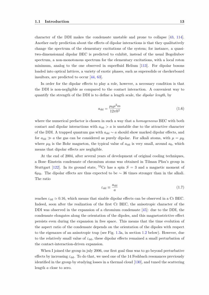
1.1 Introduction 13
character of the DDI makes the condensate unstable and prone to collapse [43, 114].Another early prediction about the effects of dipolar interactions is that they qualitativelychange the spectrum of the elementary excitations of the system; for instance, a quasi-two-dimensionnal dipolar BEC is predicted to exhibit, instead of the usual Bogoliubovspectrum, a non-monotonous spectrum for the elementary excitations, with a local rotonminimum, analog to the one observed in superfluid Helium [113]. For dipolar bosonsloaded into optical lattices, a variety of exotic phases, such as supersolids or checkerboardinsultors, are predicted to occur [44, 63].
In order for the dipolar effects to play a role, however, a necessary condition is thatthe DDI is non-negligible as compared to the contact interaction. A convenient way toquantify the strength of the DDI is to define a length scale, the dipolar length, by
add = µ0µ2m
12π~2 (1.6)
where the numerical prefactor is chosen in such a way that a homogeneous BEC with bothcontact and dipolar interactions with add > a is unstable due to the attractive characterof the DDI. A trapped quantum gas with add ∼ a should show marked dipolar effects, andfor add a the gas can be considered as purely dipolar. For alkali atoms, with µ = µB
where µB is the Bohr magneton, the typical value of add is very small, around a0, whichmeans that dipolar effects are negligible.
At the end of 2004, after several years of development of original cooling techniques,a Bose–Einstein condensate of chromium atoms was obtained in Tilman Pfau’s group inStuttgart [122]. In its ground state, 52Cr has a spin S = 3 and a magnetic moment of6µB. The dipolar effects are thus expected to be ∼ 36 times stronger than in the alkali.The ratio
εdd ≡adda
(1.7)
reaches εdd ' 0.16, which means that sizable dipolar effects can be observed in a Cr BEC.Indeed, soon after the realization of the first Cr BEC, the anisotropic character of theDDI was observed in the expansion of a chromium condensate [45]: due to the DDI, thecondensate elongates along the orientation of the dipoles, and this magnetostrictive effectpersists even during the expansion in free space. This means that the time evolution ofthe aspect ratio of the condensate depends on the orientation of the dipoles with respectto the eigenaxes of an anisotropic trap (see Fig. 1.3a, in section 1.2 below). However, dueto the relatively small value of εdd, these dipolar effects remained a small perturbation ofthe contact-interaction-driven expansion.
When I joined the group in july 2006, our first goal thus was to go beyond perturbativeeffects by increasing εdd. To do that, we used one of the 14 Feshbach resonances previouslyidentified in the group by studying losses in a thermal cloud [130], and tuned the scatteringlength a close to zero.
14 Chapter 1. Dipolar quantum gases
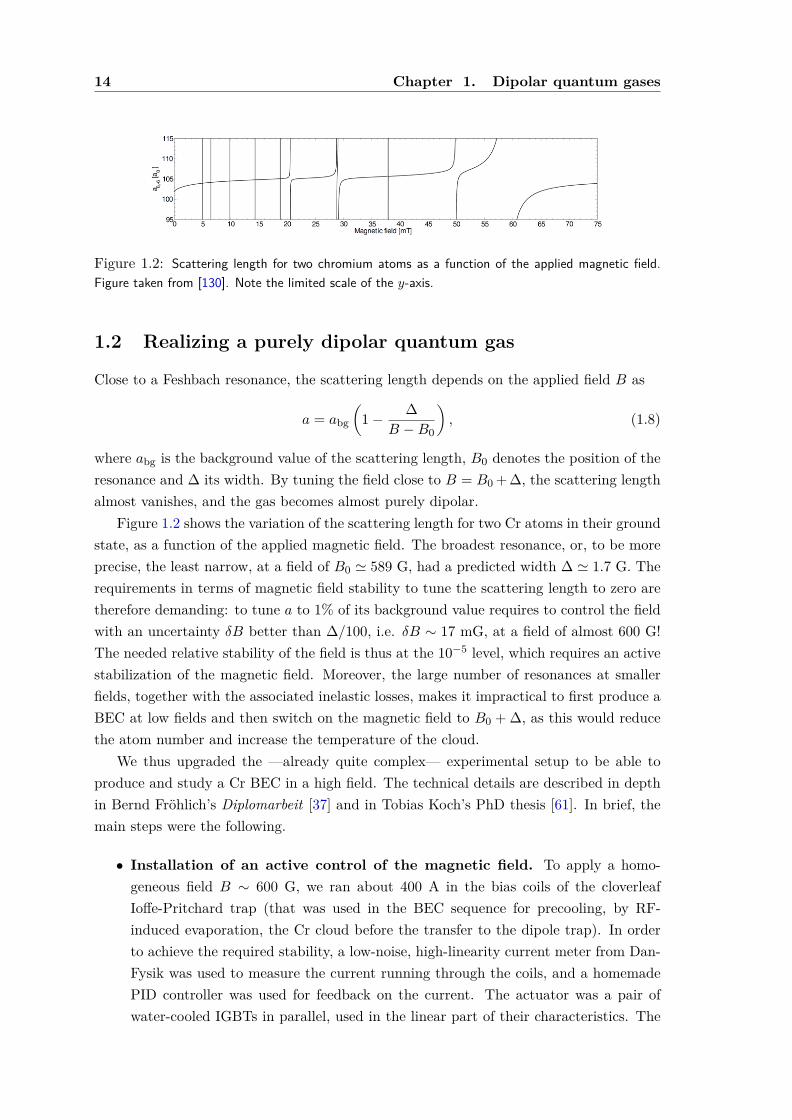
Figure 1.2: Scattering length for two chromium atoms as a function of the applied magnetic field.Figure taken from [130]. Note the limited scale of the y-axis.
1.2 Realizing a purely dipolar quantum gas
Close to a Feshbach resonance, the scattering length depends on the applied field B as
a = abg
(1− ∆
B −B0
), (1.8)
where abg is the background value of the scattering length, B0 denotes the position of theresonance and ∆ its width. By tuning the field close to B = B0 + ∆, the scattering lengthalmost vanishes, and the gas becomes almost purely dipolar.
Figure 1.2 shows the variation of the scattering length for two Cr atoms in their groundstate, as a function of the applied magnetic field. The broadest resonance, or, to be moreprecise, the least narrow, at a field of B0 ' 589 G, had a predicted width ∆ ' 1.7 G. Therequirements in terms of magnetic field stability to tune the scattering length to zero aretherefore demanding: to tune a to 1% of its background value requires to control the fieldwith an uncertainty δB better than ∆/100, i.e. δB ∼ 17 mG, at a field of almost 600 G!The needed relative stability of the field is thus at the 10−5 level, which requires an activestabilization of the magnetic field. Moreover, the large number of resonances at smallerfields, together with the associated inelastic losses, makes it impractical to first produce aBEC at low fields and then switch on the magnetic field to B0 + ∆, as this would reducethe atom number and increase the temperature of the cloud.
We thus upgraded the —already quite complex— experimental setup to be able toproduce and study a Cr BEC in a high field. The technical details are described in depthin Bernd Fröhlich’s Diplomarbeit [37] and in Tobias Koch’s PhD thesis [61]. In brief, themain steps were the following.
• Installation of an active control of the magnetic field. To apply a homo-geneous field B ∼ 600 G, we ran about 400 A in the bias coils of the cloverleafIoffe-Pritchard trap (that was used in the BEC sequence for precooling, by RF-induced evaporation, the Cr cloud before the transfer to the dipole trap). In orderto achieve the required stability, a low-noise, high-linearity current meter from Dan-Fysik was used to measure the current running through the coils, and a homemadePID controller was used for feedback on the current. The actuator was a pair ofwater-cooled IGBTs in parallel, used in the linear part of their characteristics. The

1.2 Realizing a purely dipolar quantum gas 15
large power dissipated in the IGBTs lead to numerous failures during the debuggingphase, and for a while, IGBTs almost became consumables! We finally reached astability in current better than 10−5, after realizing the importance of “tiny” detailssuch as the CMRR of differential amplifiers used in the PID controller, and usingAgilent power supplies with less noise than the ones initially installed.
• Achievement of BEC of Cr above 600 G. The high magnetic field was turnedon, in a few milliseconds, just after the optical pumping step that follows the transferof the cold Cr cloud from the magnetic trap to the optical dipole trap. At this stage,the density of the trapped sample is still low and the effect of inelastic losses is small.Forced evaporation in the crossed dipole trap is then performed2. Initial attemptsfailed due to the residual field curvature of the bias coils, which provided a veryweak radial trapping acting against gravity and preventing the evaporated atoms toleave the trap completely. We thus added a power supply providing a small oppositecurrent through the pinch coils to compensate for the residual curvature.
• Implementation of high-field imaging of the condensate. For initial exper-iments, we decided to image the BEC in high field in order to avoid crossing allresonances with the BEC before imaging. However, due to geometrical constraints,we could not use a σ+ polarization for imaging, which reduced the absorption cross-section by a factor of two. In later experiments on the dipolar collapse (see sec-tion 1.4), we decided to image in low field, as it turned out that with a sufficientlyfast switching off (on a timescale of ∼ 100 µs), losses were negligible.
Equipped with these tools, we managed to realize what we named a “quantum fer-rofluid”, i.e. a quantum gas with strong dipolar interactions [69]. This paper is reproducedat the end of the chapter (see page 26).
We first located the resonance, by measuring the scattering length a as a function of theapplied magnetic field B when approaching the resonance from above or from below (Fig. 1of [69] on page 26). In order to extract a, we studied the expansion of the condensate, whichis driven by contact and dipolar interactions. In the Thomas–Fermi regime, the density ofa contact-interacting BEC varies during free expansion in a self-similar way, keeping theshape of an inverted parabola. The time-dependent Gross–Pitaevskii equation reduces toa set of three ordinary differential equations governing the scaling parameters that givethe Thomas–Fermi radii of the BEC [20]. It can be shown that this property still holdsin the presence of dipole-dipole interactions [93]. This means that from a measurementof the atom number and of the Thomas–Fermi radii of the BEC after expansion, one caninfer in a rather simple way the scattering length a. By varying B around B0 = 589 G,we could vary a over more than one order of magnitude, an in particular reduce it to15% of the background value. In the vicinity of the resonance, inelastic three-body losses
2Having 400 A running in the bias coils for ∼ 10 seconds leads to significant thermal effects in the coils,but we could circumvent them by taking them into account in our calibration of the fields.

16 Chapter 1. Dipolar quantum gases
Figure 1.3: Anisotropic expansion of a Cr BEC. The aspect ratio of the cloud is plotted as a functionof the time of flight, for two orientations of the dipoles with respect to the trap axes. Solid symbolsare experimental data; the solid lines are the prediction of the scaling equations, without any adjustableparameter. (a): Perturbative effects obtained in the pioneering experiment of [45], at low fields, forεdd = 0.16. (b): In high field, but far from the resonance: the dipolar effects have a size similar to thecase (a). (c): Very close to the zero-crossing of the resonance, for εdd ' 0.75, the expansion dynamicsdepends drastically on the orientation of the dipoles. The inversion of ellipticity during time of flight,the usual “smoking gun” for BEC, can even be inhibited.
get enhanced, but the loss rates remain sufficiently small for the BEC to remain in aquasi-equilibrium state.
We could thus study how the aspect ratio of the condensate evolves when increasingthe dipolar parameter all the way to εdd ∼ 1. The anisotropic expansion of the conden-sate for two orientations of the dipoles with respect to the trap eigenaxes now shows verypronounced effects close to resonance (see Fig. 1.3). In particular, for strong dipolar in-teractions, the inversion of ellipticity of the BEC during time-of-flight, the usual “smokinggun” for BEC, can be inhibited.
This way of enhancing the relative effects of dipolar interactions by reducing the contactinteraction close to a zero-crossing of the scattering length was subsequently used in othergroups to observe very weak dipolar effects in alkali condensates : in 39K at LENS [35]and in 7Li at Rice [101]. However, there, the absolute strength of the dipolar interactionsis very weak, while in our case of a Cr condensate, dipolar effects can lead to dramaticeffects, as we now see.
1.3 Stability of a dipolar quantum gas
Due to the fact that the DDI has a partially attractive character, one expects that a ho-mogeneous purely dipolar condensate is unstable, and collapses. Indeed, a homogeneouscondensate with attractive contact interactions, i.e. with a scattering length a < 0, isunstable as the frequency of long-wavelength Bogoliubov excitations (phonons) is imagi-nary3.
3The Bogoliubov speed of sound is given by c =√gn/m, where g = 4π~2a/m, and becomes imaginary
when a < 0.
1.3 Stability of a dipolar quantum gas 17
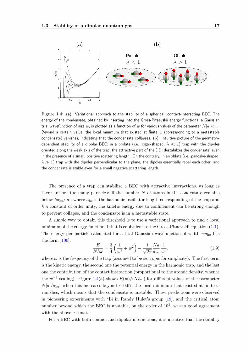
Figure 1.4: (a): Variational approach to the stability of a spherical, contact-interacting BEC. Theenergy of the condensate, obtained by inserting into the Gross-Pitaevskii energy functional a Gaussiantrial wavefunction of size w, is plotted as a function of w for various values of the parameter N |a|/aho.Beyond a certain value, the local minimum that existed at finite w (corresponding to a metastablecondensate) vanishes, indicating that the condensate collapses. (b): Intuitive picture of the geometry-dependent stability of a dipolar BEC: in a prolate (i.e. cigar-shaped, λ 1) trap with the dipolesoriented along the weak axis of the trap, the attractive part of the DDI destabilzes the condensate, evenin the presence of a small, positive scattering length. On the contrary, in an oblate (i.e. pancake-shaped,λ 1) trap with the dipoles perpendicular to the plane, the dipoles essentially repel each other, andthe condensate is stable even for a small negative scattering length.
The presence of a trap can stabilize a BEC with attractive interactions, as long asthere are not too many particles: if the number N of atoms in the condensate remainsbelow kaho/|a|, where aho is the harmonic oscillator length corresponding of the trap andk a constant of order unity, the kinetic energy due to confinement can be strong enoughto prevent collapse, and the condensate is in a metastable state.
A simple way to obtain this threshold is to use a variational approach to find a localminimum of the energy functional that is equivalent to the Gross-Pitaevskii equation (1.1).The energy per particle calculated for a trial Gaussian wavefunction of width waho hasthe form [100]:
E
N~ω= 3
4
( 1w2 + w2
)− 1√
2πNa
aho
1w3 , (1.9)
where ω is the frequency of the trap (assumed to be isotropic for simplicity). The first termis the kinetic energy, the second one the potential energy in the harmonic trap, and the lastone the contribution of the contact interaction (proportional to the atomic density, whencethe w−3 scaling). Figure 1.4(a) shows E(w)/(N~ω) for different values of the parameterN |a|/aho: when this increases beyond ∼ 0.67, the local minimum that existed at finite wvanishes, which means that the condensate is unstable. These predictions were observedin pioneering experiments with 7Li in Randy Hulet’s group [19], and the critical atomnumber beyond which the BEC is unstable, on the order of 103, was in good agreementwith the above estimate.
For a BEC with both contact and dipolar interactions, it is intuitive that the stability

18 Chapter 1. Dipolar quantum gases
Figure 1.5: Geometry-dependent stability of a dipolar BEC. Critical scattering length acrit, in unitsof the Bohr radius a0, below which the condensate becomes unstable, as a function of the trap aspectratio λ. The open squares are the experimental data; the thick solid line is the result of a verysimple variational calculation (see text and [62]), and the thin solid line is obtained by a numericalcalculation [18].
of the condensate in the presence of confinement depends strongly on the trap geometry,as can be seen on Fig. 1.4(b). Consider a BEC in a trap which is cylindrically symmetricaround the z axis, with the dipoles pointing along z. We denote by λ = ωz/ω⊥ the ratio ofthe axial to radial frequencies. In a prolate (i.e. cigar-shaped) trap (λ 1), the net effectof the dipolar interactions is attractive, one thus expects the instability of the BEC to occureven in the presence of a small, positive scattering length (smaller than add, as we shallsee). On the contrary, for an oblate (i.e. pancake-shaped) trap, the dipolar interactionhas a repulsive net effect, and the BEC is stable even with a weak (precisely, |a| < 2add)attractive contact interaction. This geometry-dependent stability is a distinctive feature ofthe dipolar BEC, and was studied theoretically in the pioneering work of [114], as well asin a number of subsequent papers (see e.g. references 4–7 of [62], reproduced on page 30).
We therefore investigated experimentally this geometry-dependent stability of a dipolarcondensate. The basic idea was to load the BEC in a trap of a given geometry, then, usingthe Feshbach resonance, to decrease the scattering length in about 10 ms to a final value,and see if the BEC was still stable. In order to be able to vary the aspect ratio λ over awide range, we decided to superimpose, onto the usual crossed optical dipole trap, a large-period, one-dimensional optical lattice obtained by crossing two beams with wavelengthλL = 1064 nm under a small angle θ = 4. This combined trap allowed us to vary λ overtwo orders of mangitude, while keeping the average trapping frequency almost constant.
For a given λ, we measured the number N of atoms in the BEC as a function of thefinal scattering length a of the ramp, and observed a sharp threshold below which the BEC
1.4 Collapse dynamics of a dipolar quantum gas 19
disappeared: only a dilute cloud survived. The critical value of the scattering length wasextracted by fitting the data to the empirical law N ∝ (a− acrit)β. We then studied howacrit depends on the aspect ratio λ. The results are shown as open squares on Fig. 1.5. Asexpected from the discussion above, we observe that for prolate traps, acrit ∼ add. For anoblate trap with λ ∼ 10, the critical scattering length is slightly negative. We thus couldrealize the first purely dipolar quantum gas.
To compare our experimental data for the variation of acrit as a function of λ withtheory, we performed a variational calculation using an anisotropic Gaussian trial wave-function in the Gross-Piteavskii energy functional with the non-local dipole-dipole term.The result of this two-parameter variational calculation is shown as a thick solid line onFig. 1.5. The agreement between the data and this very crude model is quite satisfactory.These results were published in [62], and are reproduced here on page 30. This paper mo-tivated a certain number of theoretical investigations; in particular, numerical solutions ofthe Gross-Pitaevskii equation, obtained in the group of John Bohn at JILA [18] were invery good agreement with our experimental data (thin line on Fig. 1.5).
1.4 Collapse dynamics of a dipolar quantum gas
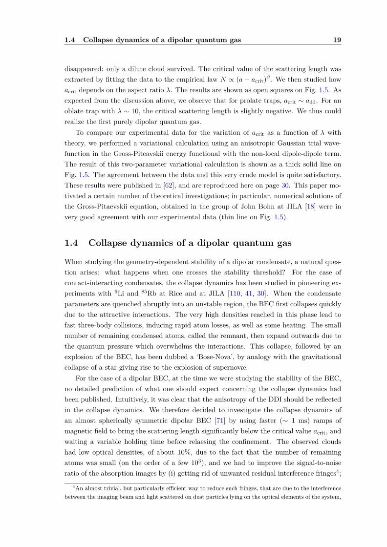
When studying the geometry-dependent stability of a dipolar condensate, a natural ques-tion arises: what happens when one crosses the stability threshold? For the case ofcontact-interacting condensates, the collapse dynamics has been studied in pioneering ex-periments with 6Li and 85Rb at Rice and at JILA [110, 41, 30]. When the condensateparameters are quenched abruptly into an unstable region, the BEC first collapses quicklydue to the attractive interactions. The very high densities reached in this phase lead tofast three-body collisions, inducing rapid atom losses, as well as some heating. The smallnumber of remaining condensed atoms, called the remnant, then expand outwards due tothe quantum pressure which overwhelms the interactions. This collapse, followed by anexplosion of the BEC, has been dubbed a ‘Bose-Nova’, by analogy with the gravitationalcollapse of a star giving rise to the explosion of supernovæ.
For the case of a dipolar BEC, at the time we were studying the stability of the BEC,no detailed prediction of what one should expect concerning the collapse dynamics hadbeen published. Intuitively, it was clear that the anisotropy of the DDI should be reflectedin the collapse dynamics. We therefore decided to investigate the collapse dynamics ofan almost spherically symmetric dipolar BEC [71] by using faster (∼ 1 ms) ramps ofmagnetic field to bring the scattering length significantly below the critical value acrit, andwaiting a variable holding time before relaesing the confinement. The observed cloudshad low optical densities, of about 10%, due to the fact that the number of remainingatoms was small (on the order of a few 103), and we had to improve the signal-to-noiseratio of the absorption images by (i) getting rid of unwanted residual interference fringes4;
4An almost trivial, but particularly efficient way to reduce such fringes, that are due to the interferencebetween the imaging beam and light scattered on dust particles lying on the optical elements of the system,

20 Chapter 1. Dipolar quantum gases
Figure 1.6: Collapse dynamics of a Cr BEC. (a): experimental images; (b): numerical simulationwithout any adjustable parameter. The dipoles are aligned along the horizontal axis of the figures.
(ii) averaging several images to decrease the effect of photon shot noise (iii) subtracting abroad thermal background.
The top row of Fig. 1.6 shows the observed density distribution after a fixed timeof flight, when varying the holding time. The dipoles are oriented along the horizontalaxis of the image. One clearly observes an anisotropic collapse, where the cloud, initallyelongated along the magnetization direction, evolves at longer times to display a cloverleaf-like pattern reminiscent of the d-wave symmetry of the DDI. At the same time, the numberof atoms in the condensate decreases abruptly during the collapse, by a factor ∼ 3.
In order to go beyond the mere observation of the collapse, the group of Masahito Uedain Tokyo collaborated with us to perform a complete numerical simulation of the dynamics,taking as inputs only the experimentally measured parameters. They performed a 3Dsimulation of the time-dependent, non-local Gross-Piteaevskii equation, where a loss termproportional to L3|ψ|4ψ was added to account for three-body losses (L3 is the measuredthree-body loss coefficient). Due to the wide variation in the condensate size during thecollapse dynamics, an algorithm with an adaptive grid size was needed. When we firstcompared the simulation results with the experimental data, a systematic shift in thetiming, of about 500 µs, was observed. We then realized that this had to do with eddycurrents induced in the vacuum chamber by the magnetic field ramp. After we measuredthe effects of eddy currents by Zeeman spectroscopy on the atom cloud, and included themin the simulation, we finally obtained an excellent agreement between the data and thesimulation, without any adjustable parameter, as can be seen on Fig. 1.6. In addition, thetime-dependence of the atom number in the BEC during collapse was also well reproducedby the numerics.
The simulation gave insight into phenomena that we could not access experimentally.In particular, it revealed the mechanism of the formation of the d-wave pattern duringthe collapse: due to the attractive interactions, the cloud initially collapses radially, andbecomes a very dense, needle-shaped cloud. Extremely fast three-body losses then occur,
turned out to simply reduce the diameter of the imaging beam impinging on all these elements to about1 mm. For this, it was enough to use an iris, conjugated with the plane of the atoms.
1.5 Dipolar quantum gases in triple-well potentials 21
leaving an almost non-interacting cloud, strongly confined in the radial direction, whichthus expands radially due to the quantum pressure. At the same time, axially, the cloudgoes on shrinking. This difference in the time scales between the axial and radial dynamicsis what explains the formation of the cloverleaf-like density distribution. It also leads to theformation of two vortex rings encircling the axial lobes of the cloud. However, observingthese vortex rings experimentally has remained elusive so far.
In a series of subsequent experiments, we then studied the collapse dynamics for varioustrap aspect ratios, including in the presence of the 1D optical lattice [80], which allowedus to confirm the coherent character of the remnant condensate. Here again, the collapsedynamics, which remains qualitatively similar to the one above, agrees very well with thesimulations.
1.5 Dipolar quantum gases in triple-well potentials
During my stay in Stuttgart, we often discussed informally in the group the theory paperspredicting exotic phases for dipolar bosons loaded in optical lattices [44]. These phasesarise due to the existence of dipolar interactions between the atoms residing on differentsites of the lattice. In particular, the possibility to observe supersolids, i.e. phases dis-playing at the same time off-diagonal and diagonal long-range order, appeared fascinating.Another interesting phase, revealing directly the long-range character of the dipolar in-teraction, is the checkerboard isolator, where an isolating phase is observed at half fillingon a square lattice, with a boson occupying one every second site. Unfortunately, even ina short-period optical lattice, the dipolar interaction between two single chromium atomsin nearest-neighbour sites is only of a few Hertz. This means that to observe these ex-otic phases, the tunneling rates and the contact interaction must be on the same orderof magnitude, or even smaller, implying very low temperatures. Thus, systems of polarmolecules seemed to be required to observe these predicted phases. Moreover, theoreticalstudies indicated that a large number of low-energy, metastable states occurred in suchsystems, implying that reaching the ground state would prove challenging [79].
We thus started to consider whether a different approach could allow us to studya minimalistic version of those exotic phases using Chromium atoms, and realized thatloading a Cr BEC with a mesoscopic number of atoms (N ∼ 102 to 103) in a triple-well potential would constitute a toy-model for these phases5: the ratio of interactionsto tunelling is enhanced by a factor N , and thus starts to be non-negligible for realisticparameters. These informal discussions finally gave birth to a theoretical proposal [72]written in collaboration with Luis Santos from Hannover.
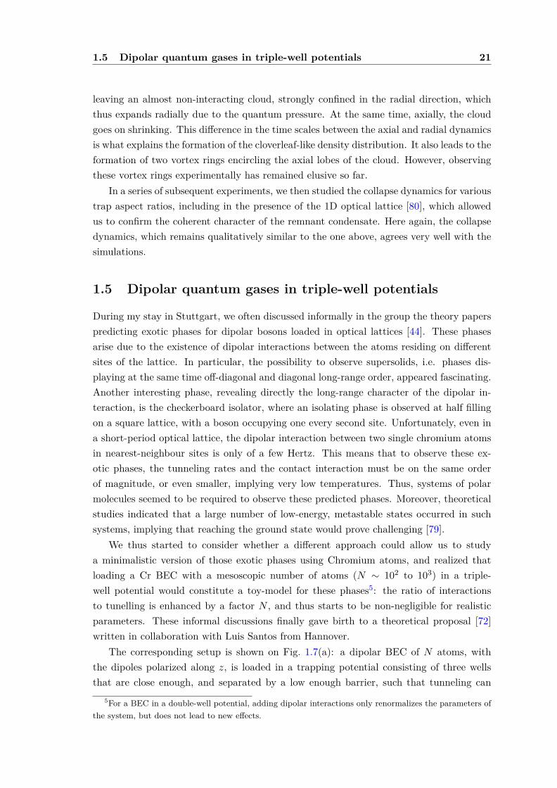
The corresponding setup is shown on Fig. 1.7(a): a dipolar BEC of N atoms, withthe dipoles polarized along z, is loaded in a trapping potential consisting of three wellsthat are close enough, and separated by a low enough barrier, such that tunneling can
5For a BEC in a double-well potential, adding dipolar interactions only renormalizes the parameters ofthe system, but does not lead to new effects.
22 Chapter 1. Dipolar quantum gases
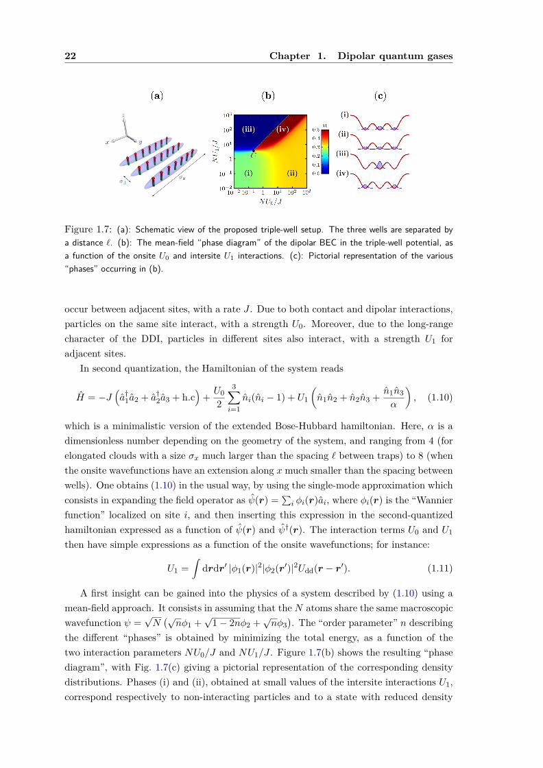
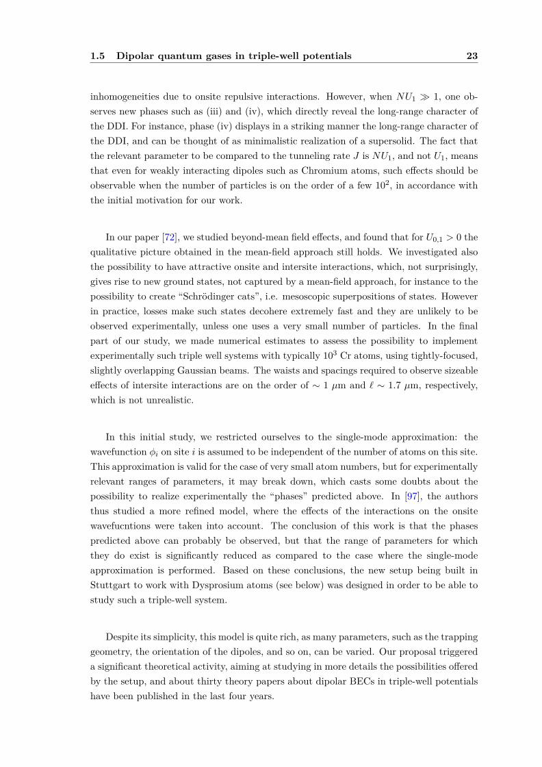
Figure 1.7: (a): Schematic view of the proposed triple-well setup. The three wells are separated bya distance `. (b): The mean-field “phase diagram” of the dipolar BEC in the triple-well potential, asa function of the onsite U0 and intersite U1 interactions. (c): Pictorial representation of the various“phases” occurring in (b).
occur between adjacent sites, with a rate J . Due to both contact and dipolar interactions,particles on the same site interact, with a strength U0. Moreover, due to the long-rangecharacter of the DDI, particles in different sites also interact, with a strength U1 foradjacent sites.
In second quantization, the Hamiltonian of the system reads
H = −J(a†1a2 + a†2a3 + h.c
)+ U0
2
3∑i=1
ni(ni − 1) + U1
(n1n2 + n2n3 + n1n3
α
), (1.10)
which is a minimalistic version of the extended Bose-Hubbard hamiltonian. Here, α is adimensionless number depending on the geometry of the system, and ranging from 4 (forelongated clouds with a size σx much larger than the spacing ` between traps) to 8 (whenthe onsite wavefunctions have an extension along x much smaller than the spacing betweenwells). One obtains (1.10) in the usual way, by using the single-mode approximation whichconsists in expanding the field operator as ψ(r) =
∑i φi(r)ai, where φi(r) is the “Wannier
function” localized on site i, and then inserting this expression in the second-quantizedhamiltonian expressed as a function of ψ(r) and ψ†(r). The interaction terms U0 and U1
then have simple expressions as a function of the onsite wavefunctions; for instance:
U1 =∫
drdr′ |φ1(r)|2|φ2(r′)|2Udd(r − r′). (1.11)
A first insight can be gained into the physics of a system described by (1.10) using amean-field approach. It consists in assuming that the N atoms share the same macroscopicwavefunction ψ =
√N(√nφ1 +
√1− 2nφ2 +
√nφ3
). The “order parameter” n describing
the different “phases” is obtained by minimizing the total energy, as a function of thetwo interaction parameters NU0/J and NU1/J . Figure 1.7(b) shows the resulting “phasediagram”, with Fig. 1.7(c) giving a pictorial representation of the corresponding densitydistributions. Phases (i) and (ii), obtained at small values of the intersite interactions U1,correspond respectively to non-interacting particles and to a state with reduced density
1.5 Dipolar quantum gases in triple-well potentials 23
inhomogeneities due to onsite repulsive interactions. However, when NU1 1, one ob-serves new phases such as (iii) and (iv), which directly reveal the long-range character ofthe DDI. For instance, phase (iv) displays in a striking manner the long-range character ofthe DDI, and can be thought of as minimalistic realization of a supersolid. The fact thatthe relevant parameter to be compared to the tunneling rate J is NU1, and not U1, meansthat even for weakly interacting dipoles such as Chromium atoms, such effects should beobservable when the number of particles is on the order of a few 102, in accordance withthe initial motivation for our work.
In our paper [72], we studied beyond-mean field effects, and found that for U0,1 > 0 thequalitative picture obtained in the mean-field approach still holds. We investigated alsothe possibility to have attractive onsite and intersite interactions, which, not surprisingly,gives rise to new ground states, not captured by a mean-field approach, for instance to thepossibility to create “Schrödinger cats”, i.e. mesoscopic superpositions of states. Howeverin practice, losses make such states decohere extremely fast and they are unlikely to beobserved experimentally, unless one uses a very small number of particles. In the finalpart of our study, we made numerical estimates to assess the possibility to implementexperimentally such triple well systems with typically 103 Cr atoms, using tightly-focused,slightly overlapping Gaussian beams. The waists and spacings required to observe sizeableeffects of intersite interactions are on the order of ∼ 1 µm and ` ∼ 1.7 µm, respectively,which is not unrealistic.
In this initial study, we restricted ourselves to the single-mode approximation: thewavefunction φi on site i is assumed to be independent of the number of atoms on this site.This approximation is valid for the case of very small atom numbers, but for experimentallyrelevant ranges of parameters, it may break down, which casts some doubts about thepossibility to realize experimentally the “phases” predicted above. In [97], the authorsthus studied a more refined model, where the effects of the interactions on the onsitewavefucntions were taken into account. The conclusion of this work is that the phasespredicted above can probably be observed, but that the range of parameters for whichthey do exist is significantly reduced as compared to the case where the single-modeapproximation is performed. Based on these conclusions, the new setup being built inStuttgart to work with Dysprosium atoms (see below) was designed in order to be able tostudy such a triple-well system.
Despite its simplicity, this model is quite rich, as many parameters, such as the trappinggeometry, the orientation of the dipoles, and so on, can be varied. Our proposal triggereda significant theoretical activity, aiming at studying in more details the possibilities offeredby the setup, and about thirty theory papers about dipolar BECs in triple-well potentialshave been published in the last four years.
24 Chapter 1. Dipolar quantum gases
1.6 Recent achievements in the field of dipolar gases
This final section summarizes briefly recent landmarks in the experimental study of dipolarquantum gases since 2008. This is not meant to be an exhaustive review, and manyimportant experimental and theoretical papers will not be mentioned.
After I left the group, the Cr team in Stuttgart studied the stability [88] and the in-TOF collapse dynamics [13] of a Cr BEC loaded in a 1D lattice where the effect of intersiteinteractions could be observed experimentally. In a series of impressive experiments in lowfield, the Villetaneuse group observed the anisotropic character of the DDI in the collectiveoscillations of the cloud [15] and in sound propagation [14], and made first steps in thestudy of quantum magnetism by loading a spinor Cr BEC in a 3D optical lattice [29].
Recently, the study of dipolar quantum gases using highly magnetic atoms has beenextended to two new species: the rare-earth elements Dysprosium (which has a magneticmoment of 10µB in its ground state) and Erbium (with a dipole moment of 7µB). Both haveattractive features, in particular a rich electronic level structure allowing the implemen-tation of new laser cooling schemes, and the existence of bosonic and fermionic isotopes.Bose–Einstein condensates [76] and degenerate Fermi gases (DFG) [75] of Dysprosium havebeen obtained in Ben Lev’s group, and similar results were reported in Erbium (7µB) inFrancesca Ferlaino’s group, with both a BEC [2] and a DFG [1]. These groups have alreadyreported exciting physics, with e.g. the observation of the d-wave collapse in Er [2], orthe achievement of Fermi degeneracy by direct evaporation of a polarized sample [1], thisbeing possible due to the long-range character of the DDI, which implies that, unlike forthe contact-interaction case, collisions between identical dipolar fermions do not freeze outat zero temperature. As mentioned above, the Stuttgart Cr setup has been rebuilt in viewof cooling and trapping Dy, with the goal, among other ones, to explore triple-well physics.Another Dy setup is currently being built at LKB/Collège de France, in the team of JeanDalibard and Sylvain Nascimbène, with the aim of studying topological superfluids.
Another promising platform to study dipolar quantum gases is to use polar molecules.There, one expects much stronger dipolar effects than in the case of magnetic dipoles, asthe interaction strength between two electric dipoles (on the order of one Debye) exceedsthat between two atomic magnetic moments (on the order of the Bohr magneton) by afactor ∼ 1/α2 where α ' 1/137 is the fine-structure constant. Moreover, the strength ofthe dipole-dipole interaction can be varied by tuning the strength of the electric field whichorients the molecules in the lab frame. In recent years, samples of ultracold polar fermionicmolecules, with densities such that the system is close to quantum degeneracy, have beenobtained in Jun Ye’s and Debbie Jin’s groups at JILA. Starting from an ultracold mixtureof fermionic 40K and bosonic 87Rb atoms, they created weakly-bound Feshabch molecules,and then transferred them to their ground state using two Raman lasers phase-lockedusing a frequency comb. Clear effects of the long-range, anisotropic interaction betweenthe molecules could be observed, e.g. in the rate of inelastic collisions [59]. More recently,loading the molecules in a 3D optical lattice allowed to implement a lattice spin model,
where the DDI yields spin-exchange interaction between the internal degrees of freedomof molecules pinned at the lattice sites [134].
Finally, Rydberg atoms open exciting prospects for the study of quantum many-bodysystems with dipolar interactions. A first approach is Rydberg dressing, which consists incoupling off-resonantly the ground state of the ultracold atoms of interest to a Rydbergstate. The dressed atoms then interact via a soft-core, long-range potential, while keepinga long lifetime [102]. Due to the prospects of achieving exotic states of matter, such assupersolids, Rydberg dressing is the subject of active experimental efforts, but remainsexperimentally challenging so far as one needs to minimize heating [5]. Another approachto study long-range-interacting quantum many-body systems consists in promoting cold,single atoms held in optical tweezers to Rydberg states: the interactions strengths can bevery large, on the order of tens of MHz for separations of a few microns, which allow tostudy coherent dynamics despite the limited lifetime of the Rydberg states, on the orderof ∼ 100 µs. This subject will be addressed in detail in chapter 3 of this manuscript.
1.7 Published articles
I list below the articles I have co-authored about dipolar quantum gases. The main onesare reproduced in the following pages.
• B. Fröhlich et al., Rev. Sci. Inst. 78, 043101 (2007);
• T. Lahaye et al., Nature 448, 672 (2007), reproduced on page 26;
• T. Koch et al., Nat. Phys. 4, 218 (2008), reproduced on page 30;
• T. Lahaye et al., Phys. Rev. Lett. 101, 080401 (2008), reproduced on page 35;
• J. Metz et al., New. J. Phys 11, 055032 (2009);
• T. Lahaye et al., Rep. Prog. Phys. 72, 126401 (2009). This is a review paperon the physics of dipolar bosonic quantum gases (41 pages, 368 references), writtenin collaboration with T. Pfau, L. Santos, C. Menotti and M. Lewenstein. It is notreprinted in this manuscript;
• T. Lahaye et al., Phys. Rev. Lett. 104, 170404 (2010), reproduced on page 39.
25

LETTERS
Strong dipolar effects in a quantum ferrofluidThierry Lahaye1, Tobias Koch1, Bernd Frohlich1, Marco Fattori1, Jonas Metz1, Axel Griesmaier1, Stefano Giovanazzi1
& Tilman Pfau1
Symmetry-breaking interactions have a crucial role in many areasof physics, ranging from classical ferrofluids to superfluid 3He andd-wave superconductivity. For superfluid quantum gases, a varietyof new physical phenomena arising from the symmetry-breakinginteraction between electric or magnetic dipoles are expected1.Novel quantum phases in optical lattices, such as chequerboardor supersolid phases, are predicted for dipolar bosons2,3. Dipolarinteractions can also enrich considerably the physics of quantumgases with internal degrees of freedom4–6. Arrays of dipolar part-icles could be used for efficient quantum information processing7.Here we report the realization of a chromium Bose–Einstein con-densate with strong dipolar interactions. By using a Feshbachresonance, we reduce the usual isotropic contact interaction, suchthat the anisotropic magnetic dipole–dipole interaction between52Cr atoms becomes comparable in strength. This induces achange of the aspect ratio of the atom cloud; for strong dipolarinteractions, the inversion of ellipticity during expansion (theusual ‘smoking gun’ evidence for a Bose–Einstein condensate)can be suppressed. These effects are accounted for by taking intoaccount the dipolar interaction in the superfluid hydrodynamicequations governing the dynamics of the gas, in the same way asclassical ferrofluids can be described by including dipolar terms inthe classical hydrodynamic equations. Our results are a first stepin the exploration of the unique properties of quantum ferrofluids.
A quantum ferrofluid is a superfluid quantum gas consisting ofpolarized dipoles, either electric or magnetic. The first option (usingpolarized electric dipoles) might be achieved for instance with polarmolecules in their vibrational ground state, aligned by an electricfield. Progress has been made recently in the slowing and trappingof polar molecules (see ref. 8 and references therein), but the densitiesand temperatures achieved to date are far away from the quantum-degenerate regime. The use of Feshbach resonances to create polarmolecules from two ultracold atomic species9 is a promising, activelyexplored alternative10; however it is a challenging task to bringthose heteronuclear molecules to their vibrational ground state11.Alternatively, atomic electric dipoles induced by dc fields12 or bylight13 could be used. The second option, chosen here, relies on themagnetic dipole–dipole interaction (MDDI) between atoms with alarge magnetic moment, such as chromium, for which a Bose–Einstein condensate (BEC) was achieved recently14. The relativestrength of the MDDI to the contact interaction is convenientlyexpressed by the dimensionless ratio
edd~m0 m2m
12 p B2að1Þ
where m is the atomic mass, a is the s-wave scattering length, m0 is thepermeability of a vacuum, " is h/2p, and m is the magnetic moment(numerical factors in edd are such that a homogenous BEC withedd . 1 is unstable against dipolar collapse). Chromium has a largedipole moment, m 5 6mB, and a background scattering length in the
fully polarized case of a < 100 a0 (mB is the Bohr magneton, and a0 theBohr radius), yielding15 edd < 0.16. Although this value is typically 36times larger than in standard alkali quantum gases, the MDDI is still asmall perturbation compared to the contact interaction. A perturb-ative mechanical effect of the MDDI has been demonstrated by ana-lysing the expansion of a chromium BEC from an anisotropic trap forvarious orientations of the dipoles16.
The existence of Feshbach resonances17 allows us to increase edd
and go beyond the perturbative limit. Indeed, close to a resonance,the scattering length varies with the applied magnetic field B as
a~abg 1D
BB0
ð2Þ
where abg is the background scattering length, B0 the resonance posi-tion, and D the resonance width. For B approaching B0 1 D, thescattering length tends to zero, thus enhancing edd. This gives thepossibility of reaching an MDDI-dominated quantum gas.
We report here the observation of strong dipolar effects in a chro-mium BEC in the vicinity of the broadest Feshbach resonance at
15. Physikalisches Institut, Universitat Stuttgart, Pfaffenwaldring 57, D-70550 Stuttgart, Germany.
0.1
1.0
10
–10 –8 –6 –4 –2 1086420
Sca
tter
ing
leng
th, a
/ab
g
Magnetic field, B − B0 (G)
a
a
b
b
c
c
d
d
B
A
z
By
Figure 1 | Tuning the chromium scattering length. A, Absorption images(field of view 260mm by 260mm) of the condensate after 5 ms of expansion,for different fields B above resonance (B 2 B0 is 2, 2.2, 2.7 and 9 G fora, b, c and d, respectively). Reducing a slows down the mean-field drivenexpansion. The change in aspect ratio for small a is a direct signature ofstrong MDDI. B, Variation of a across the resonance, inferred from themean-field energy released during expansion. The line is a fit to equation (2),yielding D 5 1.4 6 0.1 G.
Vol 448 | 9 August 2007 | doi:10.1038/nature06036
672Nature ©2007 Publishing Group
26
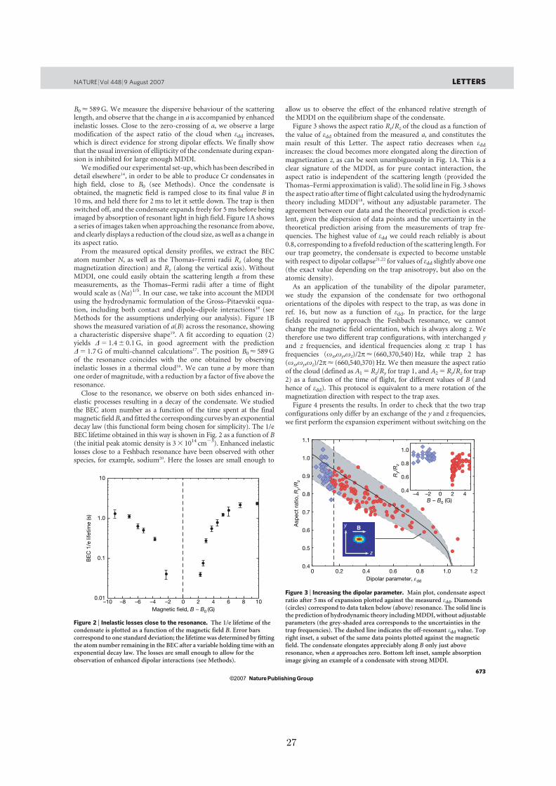
B0 < 589 G. We measure the dispersive behaviour of the scatteringlength, and observe that the change in a is accompanied by enhancedinelastic losses. Close to the zero-crossing of a, we observe a largemodification of the aspect ratio of the cloud when edd increases,which is direct evidence for strong dipolar effects. We finally showthat the usual inversion of ellipticity of the condensate during expan-sion is inhibited for large enough MDDI.
We modified our experimental set-up, which has been described indetail elsewhere14, in order to be able to produce Cr condensates inhigh field, close to B0 (see Methods). Once the condensate isobtained, the magnetic field is ramped close to its final value B in10 ms, and held there for 2 ms to let it settle down. The trap is thenswitched off, and the condensate expands freely for 5 ms before beingimaged by absorption of resonant light in high field. Figure 1A showsa series of images taken when approaching the resonance from above,and clearly displays a reduction of the cloud size, as well as a change inits aspect ratio.
From the measured optical density profiles, we extract the BECatom number N, as well as the Thomas–Fermi radii Rz (along themagnetization direction) and Ry (along the vertical axis). WithoutMDDI, one could easily obtain the scattering length a from thesemeasurements, as the Thomas–Fermi radii after a time of flightwould scale as (Na)1/5. In our case, we take into account the MDDIusing the hydrodynamic formulation of the Gross–Pitaevskii equa-tion, including both contact and dipole–dipole interactions18 (seeMethods for the assumptions underlying our analysis). Figure 1Bshows the measured variation of a(B) across the resonance, showinga characteristic dispersive shape19. A fit according to equation (2)yields D 5 1.4 6 0.1 G, in good agreement with the predictionD 5 1.7 G of multi-channel calculations17. The position B0 < 589 Gof the resonance coincides with the one obtained by observinginelastic losses in a thermal cloud16. We can tune a by more thanone order of magnitude, with a reduction by a factor of five above theresonance.
Close to the resonance, we observe on both sides enhanced in-elastic processes resulting in a decay of the condensate. We studiedthe BEC atom number as a function of the time spent at the finalmagnetic field B, and fitted the corresponding curves by an exponentialdecay law (this functional form being chosen for simplicity). The 1/eBEC lifetime obtained in this way is shown in Fig. 2 as a function of B(the initial peak atomic density is 3 3 1014 cm23). Enhanced inelasticlosses close to a Feshbach resonance have been observed with otherspecies, for example, sodium20. Here the losses are small enough to
allow us to observe the effect of the enhanced relative strength ofthe MDDI on the equilibrium shape of the condensate.
Figure 3 shows the aspect ratio Ry/Rz of the cloud as a function ofthe value of edd obtained from the measured a, and constitutes themain result of this Letter. The aspect ratio decreases when edd
increases: the cloud becomes more elongated along the direction ofmagnetization z, as can be seen unambiguously in Fig. 1A. This is aclear signature of the MDDI, as for pure contact interaction, theaspect ratio is independent of the scattering length (provided theThomas–Fermi approximation is valid). The solid line in Fig. 3 showsthe aspect ratio after time of flight calculated using the hydrodynamictheory including MDDI18, without any adjustable parameter. Theagreement between our data and the theoretical prediction is excel-lent, given the dispersion of data points and the uncertainty in thetheoretical prediction arising from the measurements of trap fre-quencies. The highest value of edd we could reach reliably is about0.8, corresponding to a fivefold reduction of the scattering length. Forour trap geometry, the condensate is expected to become unstablewith respect to dipolar collapse21,22 for values of edd slightly above one(the exact value depending on the trap anisotropy, but also on theatomic density).
As an application of the tunability of the dipolar parameter,we study the expansion of the condensate for two orthogonalorientations of the dipoles with respect to the trap, as was done inref. 16, but now as a function of edd. In practice, for the largefields required to approach the Feshbach resonance, we cannotchange the magnetic field orientation, which is always along z. Wetherefore use two different trap configurations, with interchanged yand z frequencies, and identical frequencies along x: trap 1 hasfrequencies (vx,vy,vz)/2p< (660,370,540) Hz, while trap 2 has(vx,vy,vz)/2p< (660,540,370) Hz. We then measure the aspect ratioof the cloud (defined as A1 5 Rz/Ry for trap 1, and A2 5 Ry/Rz for trap2) as a function of the time of flight, for different values of B (andhence of edd). This protocol is equivalent to a mere rotation of themagnetization direction with respect to the trap axes.
Figure 4 presents the results. In order to check that the two trapconfigurations only differ by an exchange of the y and z frequencies,we first perform the expansion experiment without switching on the
0.01
0.1
1.0
10
BE
C 1
/e li
fetim
e (s
)
–10 –8 –6 –4 –2 1086420Magnetic field, B − B0 (G)
Figure 2 | Inelastic losses close to the resonance. The 1/e lifetime of thecondensate is plotted as a function of the magnetic field B. Error barscorrespond to one standard deviation; the lifetime was determined by fittingthe atom number remaining in the BEC after a variable holding time with anexponential decay law. The losses are small enough to allow for theobservation of enhanced dipolar interactions (see Methods).
0.4
0.5
0.6
0.7
0.8
0.9
1.0
1.1
0 0.2 0.4 0.6 0.8 1.0 1.2
z
yAsp
ect
ratio
, Ry/
Rz
Dipolar parameter, εdd
0.4
0.6
0.8
1.0
–4 –2 0 2 4
Ry/
Rz
B − B0 (G)
B
Figure 3 | Increasing the dipolar parameter. Main plot, condensate aspectratio after 5 ms of expansion plotted against the measured edd. Diamonds(circles) correspond to data taken below (above) resonance. The solid line isthe prediction of hydrodynamic theory including MDDI, without adjustableparameters (the grey-shaded area corresponds to the uncertainties in thetrap frequencies). The dashed line indicates the off-resonant edd value. Topright inset, a subset of the same data points plotted against the magneticfield. The condensate elongates appreciably along B only just aboveresonance, when a approaches zero. Bottom left inset, sample absorptionimage giving an example of a condensate with strong MDDI.
NATURE | Vol 448 | 9 August 2007 LETTERS
673Nature ©2007 Publishing Group
27
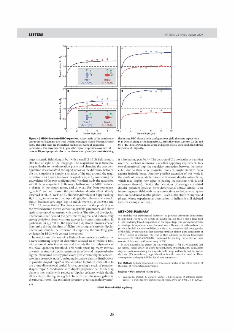
large magnetic field along z, but with a small (11.5 G) field along x(the line of sight of the imaging). The magnetization is thereforeperpendicular to the observation plane, and changing the trap con-figuration does not affect the aspect ratios, as the difference betweenthe two situations is simply a rotation of the trap around the mag-netization axis. Figure 4a shows the equality A1 5 A2, confirming theequivalence of the two configurations. We then study the expansionwith the large magnetic field B along z. In this case, the MDDI inducesa change in the aspect ratios, and A1 ? A2. Far from resonance,edd < 0.16 and we recover the perturbative dipolar effect alreadyobserved in ref. 16 (see Fig. 4b). However, for values of B approachingB0 1 D, edd increases and, correspondingly, the difference between A1
and A2 becomes very large (Fig. 4c and d, where edd is 0.5 6 0.1 and0.75 6 0.1, respectively). The lines correspond to the prediction ofthe hydrodynamic theory without adjustable parameters, and showagain a very good agreement with the data. The effect of the dipolarinteraction is far beyond the perturbative regime, and induces verystrong deviations from what one expects for contact interaction. Inparticular, for edd < 0.75, the aspect ratio A2 always remains smallerthan unity during the time of flight: the strong anisotropic dipolarinteraction inhibits the inversion of ellipticity, the ‘smoking gun’evidence for BECs with contact interaction.
In conclusion, the use of a Feshbach resonance to reduce thes-wave scattering length of chromium allowed us to realize a BECwith strong dipolar interaction, and to study the hydrodynamics ofthis novel quantum ferrofluid. This work opens up many avenuestowards the study of dipolar quantum gases beyond the perturbativeregime. Structured density profiles are predicted for dipolar conden-sates in anisotropic traps23, including biconcave density distributionsin pancake-shaped traps24. A clear direction for future work is thus touse a one-dimensional optical lattice, creating a stack of pancake-shaped traps. A condensate with dipoles perpendicular to the trapplane is then stable with respect to dipolar collapse, which shouldallow entry to the regime edd? 1. In particular, the investigation ofthe unusual, roton-like excitation spectrum predicted in this system25
is a fascinating possibility. The creation of Cr2 molecules by rampingover the Feshbach resonance is another appealing experiment. In atwo-dimensional trap, the repulsive interaction between the mole-cules, due to their large magnetic moment, might stabilize themagainst inelastic losses. Another possible extension of this work isthe study of degenerate fermions with strong dipolar interactions,which may display new types of pairing mechanisms (ref. 1, andreferences therein). Finally, the behaviour of strongly correlateddipolar quantum gases in three-dimensional optical lattices is aninteresting open field, with many connections to fundamental ques-tions in condensed-matter physics—such as the study of supersolidphases, whose experimental observation in helium is still debated(see, for example, ref. 26).
METHODS SUMMARY
We modified our experimental sequence14 to produce chromium condensates
in high field. For this, we switch on quickly (in less than 5 ms) a large field
(,600 G) during forced evaporation in the dipole trap. The low atomic density
at this stage of evaporation allows for small losses. The current in the coils used to
produce the field is actively stabilized; care is taken to ensure a high homogeneity
of the field. Evaporation is then resumed until an almost pure condensate of
3 3 104 atoms is obtained. The trap is then adjusted to obtain frequencies
(vx,vy,vz)/2p< (840,600,580) Hz (measured by exciting the centre of mass
motion of the cloud, with an accuracy of 5%).
In our data analysis to extract the scattering length a (Fig. 1), we assumed that
no external forces act on the atoms during the time of flight, that the condensate
stays in equilibrium during the magnetic field ramp, and finally that the hydro-
dynamic (Thomas–Fermi) approximation is valid even for small a. These
assumptions are largely fulfilled for all our parameters.
Full Methods and any associated references are available in the online version ofthe paper at www.nature.com/nature.
Received 4 May; accepted 15 June 2007.
1. Baranov, M., Dobrek, /L., Goral, K., Santos, L. & Lewenstein, M. Ultracold dipolargases — a challenge for experiments and theory. Phys. Scr. T102, 74–81 (2002).
db
0 108642Time of flight (ms)
0 108642Time of flight (ms)
z
y
Trap 1A1 = Rz/Ry
z
y
Trap 2A2 = Ry/Rz
B B
ca
0
0.5
1.0
1.5
2.0
z
y
Trap 1A1 = Rz/Ry
z
y
Trap 2A2 = Ry/Rz
B B
Asp
ect
ratio
s, A
1, A
2
0
0.5
1.0
1.5
2.0
Asp
ect
ratio
s, A
1, A
2
Figure 4 | MDDI-dominated BEC expansion. Aspect ratio of the condensateversus time of flight, for two traps with interchanged y and z frequencies (seetext). The solid lines are theoretical predictions without adjustableparameters. The error bar (in d) gives the typical dispersion over severalruns. a, Dipoles perpendicular to the observation plane (see inset sketching
the in-trap BEC shape); both configurations yield the same aspect ratio.b–d, Dipoles along z (see inset in b); edd takes the values 0.16 (b), 0.5 (c) and0.75 (d). The MDDI induces larger and larger effects, even inhibiting (d) theinversion of ellipticity.
LETTERS NATURE | Vol 448 | 9 August 2007
674Nature ©2007 Publishing Group
28
2. Goral, K., Santos, L. & Lewenstein, M. Quantum phases of dipolar bosons in opticallattices. Phys. Rev. Lett. 88, 170406 (2002).
3. Menotti, C., Trefzger, C. & Lewenstein, M. Metastable states of a gas of dipolarbosons in a 2D optical lattice. Phys. Rev. Lett. 98, 235301 (2007).
4. Kawaguchi, Y., Saito, H. & Ueda, M. Einstein–de Haas effect in dipolar Bose-Einstein condensates. Phys. Rev. Lett. 96, 080405 (2006).
5. Santos, L. & Pfau, T. Spin-3 chromium Bose-Einstein condensates. Phys. Rev. Lett.96, 190404 (2006).
6. Yi, S. & Pu, H. Spontaneous spin textures in dipolar spinor condensates. Phys. Rev.Lett. 97, 020401 (2006).
7. DeMille, D. Quantum computation with trapped polar molecules. Phys. Rev. Lett.88, 067901 (2002).
8. Doyle, J., Friedrich, B., Krems, R. V. & Masnou-Seeuws, F. (eds) Special issue onultracold molecules. Eur. Phys. J. D 31, 149–445 (2004).
9. Kohler, T., Goral, K. & Julienne, P. S. Production of cold moleculesvia magnetically tunable Feshbach resonances. Rev. Mod. Phys. 78, 1311–1361(2006).
10. Ospelkaus, C. et al. Ultracold heteronuclear molecules in a 3D optical lattice. Phys.Rev. Lett. 97, 120402 (2006).
11. Sage, J., Sainis, S., Bergeman, T. & DeMille, D. Optical production of ultracold polarmolecules. Phys. Rev. Lett. 94, 203001 (2005).
12. Marinescu, M. & You, L. Controlling atom-atom interaction at ultralowtemperatures by dc electric fields. Phys. Rev. Lett. 81, 4596–4599 (1998).
13. Giovanazzi, S., O’Dell, D. & Kurizki, G. Density modulations of Bose-Einsteincondensates via laser-induced interactions. Phys. Rev. Lett. 88, 130402 (2002).
14. Griesmaier, A., Werner, J., Hensler, S., Stuhler, J. & Pfau, T. Bose-Einsteincondensation of chromium. Phys. Rev. Lett. 94, 160401 (2005).
15. Griesmaier, A. et al. Comparing contact and dipolar interactions in a Bose-Einsteincondensate. Phys. Rev. Lett. 97, 250402 (2006).
16. Stuhler, J. et al. Observation of dipole-dipole interaction in a degenerate quantumgas. Phys. Rev. Lett. 95, 150406 (2005).
17. Werner, J., Griesmaier, A., Hensler, S., Stuhler, J. & Pfau, T. Observation ofFeshbach resonances in an ultracold gas of 52Cr. Phys. Rev. Lett. 94, 183201(2005).
18. Giovanazzi, S. et al. Expansion dynamics of a dipolar Bose-Einstein condensate.Phys. Rev. A 74, 013621 (2006).
19. Inouye, S. et al. Observation of Feshbach resonances in a Bose-Einsteincondensate. Nature 392, 151–154 (1998).
20. Stenger, J. et al. Strongly enhanced inelastic collisions in a Bose-Einsteincondensate near Feshbach resonances. Phys. Rev. Lett. 82, 2422–2425 (1999).
21. Santos, L., Shlyapnikov, G. V., Zoller, P. & Lewenstein, M. Bose-Einsteincondensation in trapped dipolar gases. Phys. Rev. Lett. 85, 1791–1794 (2000).
22. Goral, K., Rza?z?ewski, K. & Pfau, T. Bose-Einstein condensation with magnetic
dipole-dipole forces. Phys. Rev. A 61, 051601(R) (2000).23. Dutta, O. & Meystre, P. Ground-state structure and stability of dipolar
condensates in anisotropic traps. Phys. Rev. A 75, 053604 (2007).24. Ronen, S., Bortolotti, D. C. E. & Bohn, J. L. Radial and angular rotons in trapped
dipolar gases. Phys. Rev. Lett. 98, 030406 (2007).25. Santos, L., Shlyapnikov, G. V. & Lewenstein, M. Roton-maxon spectrum and
stability of trapped dipolar Bose-Einstein condensates. Phys. Rev. Lett. 90, 250403(2003).
26. Sasaki, S., Ishiguro, R., Caupin, F., Maris, H. J. & Balibar, S. Superfluidity of grainboundaries and supersolid behavior. Science 313, 1098–1100 (2006).
Acknowledgements We thank L. Santos for discussions and J. Stuhler forcontributions in the initial phases of the experiment. We acknowledge financialsupport by the German Science Foundation (SFB/TRR21) and the EU (Marie-Curiefellowship to T.L.).
Author Information Reprints and permissions information is available atwww.nature.com/reprints. The authors declare no competing financial interests.Correspondence and requests for materials should be addressed to T.L.([email protected]) or T.P. ([email protected]).
NATURE | Vol 448 | 9 August 2007 LETTERS
675Nature ©2007 Publishing Group
29

LETTERS
Stabilization of a purely dipolar quantumgas against collapse
T. KOCH, T. LAHAYE, J. METZ, B. FROHLICH, A. GRIESMAIER AND T. PFAU*5. Physikalisches Institut, Universitat Stuttgart, Pfaffenwaldring 57, 70550 Stuttgart, Germany*e-mail: [email protected]
Published online: 24 February 2008; doi:10.1038/nphys887
Although the phenomenon of Bose–Einstein condensation1 isa purely statistical effect that also appears in an ideal gas, thephysics of Bose–Einstein condensates (BECs) of dilute gases isconsiderably enriched by the presence of interactions amongthe atoms. In usual experiments with BECs, the only relevantinteraction is the isotropic and short-range contact interaction,which is described by a single parameter, the scattering lengtha. In contrast, the dipole–dipole interaction between particlespossessing an electric or magnetic dipole moment is of long-range character and anisotropic, which gives rise to newphenomena2,3. Most prominently, the stability of a dipolar BECdepends not only on the value of the scattering length, a, but alsostrongly on the geometry of the external trapping potential4–7.Here, we report on the experimental investigation of the stabilityof a dipolar BEC of 52Cr as a function of the scattering length andthe trap aspect ratio. We find good agreement with a universalstability threshold arising from a simple theoretical model. Usinga pancake-shaped trap with the dipoles oriented along the shortaxis of the trap, we are able to tune the scattering length to zero,stabilizing a purely dipolar quantum gas.
In the case of a homogeneous Bose–Einstein condensate (BEC)with pure contact interaction, the existence of a stable ground statedepends on the modulus and sign of the interaction. For repulsiveinteraction (a > 0), the BEC is stable, whereas for attractiveinteraction (a < 0), the BEC is unstable. This instability can beprevented by an external trapping potential. The tendency of the gasto shrink towards the centre of the trap is in that case counteractedby the repulsive quantum pressure arising from the Heisenberguncertainty relation. Detailed analysis8 shows that in a harmonictrap with mean frequency ω, a condensate is stable as long as thenumber of atoms N stays below a critical value Ncrit given by
Ncrit =kaho
|a|, (1)
where aho =√
h/(mω) is the harmonic oscillator length and k is aconstant of the order of 1/2. This scaling has been experimentallychecked in ref. 9 in a BEC of 85Rb. The dynamics of condensatesfor N ≥ Ncrit has been the subject of several experiments withcondensates of 7Li (refs 10,11) and 85Rb (ref. 12). In refs 13,14, the collapse of a Bose–Fermi mixture of 87Rb and 40K wasinvestigated. Some aspects of the dynamics such as the soliton trainformation in 7Li (ref. 15) and 85Rb (ref. 16) remain the subject ofongoing research.
Being anisotropic and long range, the dipole–dipole interaction(DDI) differs significantly from the contact interaction, whichchanges the stability conditions in a system with DDI present.
Considering a purely dipolar condensate with homogeneousdensity polarized by an external field, it is found that owing to theanisotropy of the DDI, the BEC is unstable, independent of howsmall the dipole moment is17. As in the pure contact case, a traphelps to stabilize the system. In the dipolar case, however, it is notonly the quantum pressure that prevents the collapse but also theanisotropy of the density distribution imprinted by the trap.
Consider a cylindrically symmetric harmonic trap
Vtrap(r,z) =1
2m
(ω2
r r2+ω2
z z2)
with the dipoles oriented along z, and r being the distance fromthe symmetry axis. As can be intuitively understood from Fig. 1a,in a pancake-shaped trap (aspect ratio l = ωz/ωr > 1), the dipolespredominantly repel each other and the BEC is stable. In contrast,a cigar-shaped trap (l < 1, Fig. 1b) leads to mainly attractive forcesand hence to a dipolar collapse. Following this simple argument,we expect that in the prolate case a positive scattering length a isneeded to stabilize the BEC, whereas in the oblate case, we caneven afford a slightly negative a. The dependence of the stabilityof a dipolar BEC on the trap aspect ratio l and scattering length ahas been extensively studied theoretically4–7, and is experimentallyinvestigated here.
Our measurements are carried out with a BEC of 52Cr (ref. 18),which is so far the only experimentally accessible quantum gas withobservable DDI19,20. To compare contact and dipolar interactions,we introduce a length scale characterizing the magnetic DDI
add =µ0µ
2m
12πh2 .
The numerical prefactor in add is chosen such that a homogeneouscondensate becomes unstable to local density perturbations fora ≤ add (ref. 21). As chromium has a magnetic dipole moment ofµ = 6µB (µB is the Bohr magneton), add ' 15a0, where a0 is theBohr radius. Far from Feshbach resonances, a takes its backgroundvalue abg '100a0 (ref. 22) and the BEC is stable for any l. To explorethe unstable regime, we thus reduce the scattering length a, whichin the vicinity of a Feshbach resonance scales as
a = abg
(1−
1B
B−B0
)with the applied magnetic field B.
To carry out the measurements, we produce a BEC ofapproximately 25,000 atoms at a magnetic field that is about 10 Gabove the broadest Feshbach resonance where the scattering lengthis approximately 85a0 and the BEC is stable. Once the BEC is
218 nature physics VOL 4 MARCH 2008 www.nature.com/naturephysics
© 2008 Nature Publishing Group
30

LETTERS
x
y
z
Oblate trap (λ > 1)
Prolate trap (λ < 1)
Optical lattice beams
Magnetic field coils
Dipole trap beam
Dipole trap beam
a
c
b
Figure 1 Intuitive picture of the trap geometry dependence of the stability of adipolar BEC. a,b, In an oblate trap (a), the dipoles mainly repel each other, whereasin a prolate trap (b), the interaction is predominantly attractive. c, The differenttrapping geometries are realized by the crossed optical dipole trap (red) and afurther one-dimensional optical lattice (green). The magnetic field is pointing alongthe symmetry axis z of our traps.
obtained20,23, we adiabatically shape the trapping potential to thedesired aspect ratio l. To be able to vary l over a wide range, wegenerate the trapping potential by a crossed optical dipole trap(ODT) and a superimposed one-dimensional optical lattice alongthe z direction (see Fig. 1c and Methods section).
We observe two effects when approaching the zero-crossing ofthe scattering length: the BEC shrinks in both directions owingto the decreasing scattering length and the ellipticity of the cloudchanges as a manifestation of the enhanced dipolar effects20. Finally,when we decrease the scattering length below some critical valueacrit, the BEC atom number (determined from a bimodal fit24 of thetime-of-flight absorption images) abruptly decreases (Fig. 2a,b).The disappearance of the BEC around the instability point is shownin Fig. 2c. Although slightly above acrit, we still see an almostpure BEC, for a ' acrit the density shows a bimodal distribution(an anisotropic, dense central peak surrounded by an isotropicgaussian cloud). Just below acrit, the BEC collapses and the densitydistribution becomes a unimodal, isotropic gaussian. Note that wedo not observe the formation of soliton trains as in refs 15,16. Thiscan be attributed to the fact that as our trap is much tighter thanin those references, the initial size of our BEC is smaller than anysingle soliton observed in refs 15,16.
The critical scattering length acrit where the condensate vanishesdepends strongly on the trap aspect ratio l. For an isotropic trap(Fig. 2a), the collapse occurs at a ' 15a0, whereas the pancake-shaped trap (Fig. 2b) can even stabilize a purely dipolar BEC(a ' 0). We repeated this experiment for six different traps (seeTable 1), thereby covering a range of two orders of magnitude in the
–10 0
N/1
04N
/104
10a/a0
20 30 40
–10 0 10a/a0
20 30 40
0
0
0.5
1.0
1.5
1.0
2.0
3.0 = 1.0λ
= 10λ
–5a0 –2a0 0a00
0.2
0.4 Optical density
a
c
b
Figure 2 Decrease of the BEC atom number N around the critical scatteringlength acrit. a,b, The critical point depends strongly on the aspect ratio l of the trap.The solid lines are fits to equation (2) used to determine the critical scattering lengthacrit (see text). c, Typical images of the atomic cloud around the critical scatteringlength for the trap with l = 10.
Table 1 Trap frequencies and aspect ratios of the traps used. The trap frequencieswere measured by either exciting the centre-of-mass motion or parametricheating and are accurate to about 10%. Traps 1–3 are provided only by thecrossed optical dipole trap, whereas for traps 4–6 the horizontal dipole trap beamand the optical lattice are used.
Trap ωr/ (2π ) (Hz) ωz/ (2π ) (Hz) ω/ (2π ) (Hz) l = ωz/ωr
1 1,300 140 620 0.112 890 250 580 0.283 480∗ 480 480 1.004 530 1,400 730 2.605 400 2,400 730 6.006 330 3,400 720 10.00∗Trap 3 is not cylindrically symmetric (see the Methods section) and has the trap frequencies ω x = 2π×610 Hz andω y = 2π×370 Hz.
trap aspect ratio l. To exclude three-body loss processes causing theabrupt decrease in the BEC atom number, we measured the lifetimeof the BEC for the different traps just above acrit and found the samelifetime (∼10 ms) for the different scattering lengths.
By fitting to the observed BEC atom numbers (Fig. 2a,b) thethreshold function
N = max[0,N0(a−acrit)
β], (2)
nature physics VOL 4 MARCH 2008 www.nature.com/naturephysics 219
© 2008 Nature Publishing Group
31

LETTERS
10–2 10–1
10–2 10–1 100 101 102 103
Trap aspect ratio = z / r
100 101
a crit
/a0
102 103
–30
–20
–10
0
10
20
λ ω ω
–0.4
–0.2
0
add
–2add
b
c
d
e
0.1 1 10 100
0.1 1 10 100
0.1 1 10 100
0.1 1 10 100
0.1
1
10
0.1
1
10
0.1
1
10
0.1
1
10
σ r
σ r
σz
σz
σz
σz
σ r
σ
ωσ
σ
r
<1
10
102
103
–
–E ( r , z )/Nh -
a b c
d e
Figure 3 Stability diagram of a dipolar BEC in the a–l plane. a, Experimental (green squares) and theoretical (green line) values of the critical scattering length acrit as afunction of the trap aspect ratio. The theory curve is obtained for 20,000 atoms and an average trap frequency ω = 2π×700 Hz (the average values we find for our sixtraps). The red curve (magnified in the inset) marks the stability threshold for a BEC with pure contact interactions using the same parameters. The asymptotic stabilityboundary (Nadd/aho 1) which for l → 0 (l → ∞) converges to add (−2add) is plotted in grey. The error bars in l and acrit result from the uncertainty (estimated onestandard deviation) in the trap frequency measurement and the calibration a (B ) of the scattering length. b–e, Behaviour of the energy landscape E (σ r , σz ). Lines of equalenergy are plotted for fixed l = 10 and four different values of the scattering length a (blue dots in a). For acrit < a < add (c) the collapsed prolate ground state emerges(σ r → 0 at finite σz ) and the BEC becomes metastable.
where N0, acrit and β are fitting parameters, we find the criticalscattering length acrit. The simple functional form (2) wasempirically chosen as it accounts for the fast decreasing BEC atomnumber at a ' acrit and for the slow decrease for a acrit. Theexponent β describing the steepness of the collapse was found tobe β ' 0.2 for all traps. The values of acrit that are plotted in Fig. 3amark the experimentally obtained stability threshold of a 52Cr BECin the plane (l, a). We observe a clear shift towards smaller aas l increases. For the most oblate trap (l = 10), we can reducethe scattering length to zero and hence access the purely dipolarregime experimentally.
To get a more quantitative insight into the collapse thresholdacrit(l), we numerically determine the critical scattering length(green curve in Fig. 3a). For this, we use a variational method tominimize the Gross–Pitaevskii energy functional1
E[Φ] =
∫ [h2
2m|∇Φ|
2+Vtrap|Φ|
2+
2πh2a
m|Φ|
4
+1
2|Φ|
2
∫Udd(r−r′)|Φ(r′)|2dr′
]dr, (3)
where
Udd(r) =µ0µ
2
4π
1−3cos2 θ
|r|3
is the interaction energy of two aligned magnetic dipoles µ, with rbeing the relative position of the dipoles and θ the angle between rand the direction z of polarization.
Similar to the work presented in refs 4–6 and 25, we usea cylindrically symmetric gaussian ansatz to evaluate the energyfunctional (3) with the radial and axial widths σr and σz asvariational parameters (see the Methods section). To obtainacrit, we lower the scattering length until the energy landscapeE(σr ,σz) does not contain any minimum for finite σr and σz
any more (Fig. 3b–e). Starting with large values a > add, we findthat E(σr ,σz) supports a global minimum for finite σr and σz
independently of l and thus the BEC is stable (Fig. 3b). Goingbelow a ∼ add, the absolute ground state is a collapsed infinitely thincigar-shaped BEC (σr → 0) and the possible existence of a furtherlocal minimum (corresponding to a metastable state) is determinedby the trap aspect ratio l (see Fig. 3c, where add > a > acrit andFig. 3d, where a = acrit). Finally, below a ∼−2add (Fig. 3e), the localminimum vanishes for any l and the BEC is always unstable6,7.
In spite of the simplicity of our model, we find good agreementbetween experiment and theory (Fig. 3a). We checked that thedifferent atom numbers and mean trap frequencies that we findfor the six traps modify the green curve by much less than theerror bars.
The behaviour of the critical scattering length acrit as a functionof the aspect ratio l can be understood considering the limitN add/aho 1, which is satisfied by our average experimental valueof N add/aho ' 23. Owing to their linear N-scaling, the kineticenergy and the potential energy (equations (5) and (6) in theMethods section) can be neglected and the total energy E(σr ,σz)is dominated by the interaction term
[Econtact +EDDI] ∝ N 2
[a
add
− f (κ)
].
The function f (ref. 25) of the cloud aspect ratio κ = σr/σz arisesfrom the DDI and is discussed in the Methods section.
In this regime, where the stability is solely governed by thecompetition between the contact and DDI, the critical scatteringlength (grey curve in Fig. 3a) is implicitly given by
acrit(l) = addf (κ(l)) . (4)
The asymptotic behaviour of the theory curve now becomesapparent: an extremely prolate (oblate) trap forces the cloud shapeto also be extremely prolate (oblate) and f takes its extremal
220 nature physics VOL 4 MARCH 2008 www.nature.com/naturephysics
© 2008 Nature Publishing Group
32
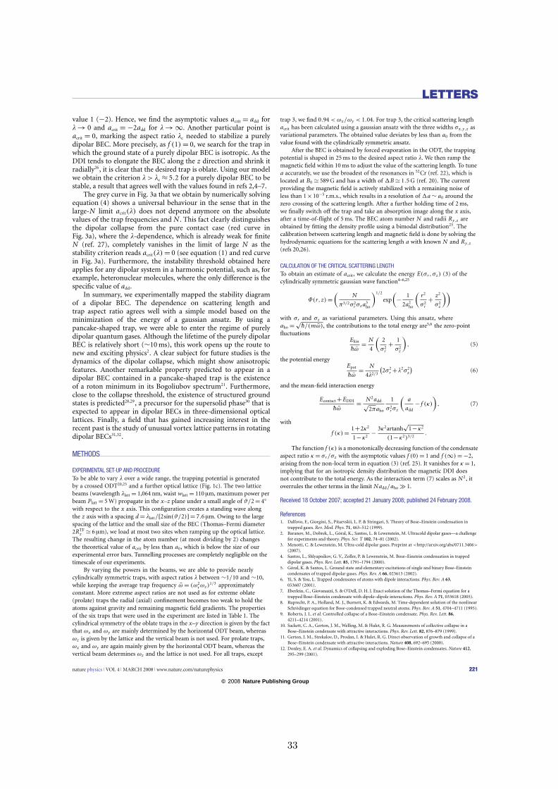
LETTERS
value 1 (−2). Hence, we find the asymptotic values acrit = add forl → 0 and acrit = −2add for l → ∞. Another particular point isacrit = 0, marking the aspect ratio lc needed to stabilize a purelydipolar BEC. More precisely, as f (1) = 0, we search for the trap inwhich the ground state of a purely dipolar BEC is isotropic. As theDDI tends to elongate the BEC along the z direction and shrink itradially26, it is clear that the desired trap is oblate. Using our modelwe obtain the criterion l > lc ≈ 5.2 for a purely dipolar BEC to bestable, a result that agrees well with the values found in refs 2,4–7.
The grey curve in Fig. 3a that we obtain by numerically solvingequation (4) shows a universal behaviour in the sense that in thelarge-N limit acrit(l) does not depend anymore on the absolutevalues of the trap frequencies and N . This fact clearly distinguishesthe dipolar collapse from the pure contact case (red curve inFig. 3a), where the l-dependence, which is already weak for finiteN (ref. 27), completely vanishes in the limit of large N as thestability criterion reads acrit(l) = 0 (see equation (1) and red curvein Fig. 3a). Furthermore, the instability threshold obtained hereapplies for any dipolar system in a harmonic potential, such as, forexample, heteronuclear molecules, where the only difference is thespecific value of add.
In summary, we experimentally mapped the stability diagramof a dipolar BEC. The dependence on scattering length andtrap aspect ratio agrees well with a simple model based on theminimization of the energy of a gaussian ansatz. By using apancake-shaped trap, we were able to enter the regime of purelydipolar quantum gases. Although the lifetime of the purely dipolarBEC is relatively short (∼10 ms), this work opens up the route tonew and exciting physics2. A clear subject for future studies is thedynamics of the dipolar collapse, which might show anisotropicfeatures. Another remarkable property predicted to appear in adipolar BEC contained in a pancake-shaped trap is the existenceof a roton minimum in its Bogoliubov spectrum21. Furthermore,close to the collapse threshold, the existence of structured groundstates is predicted28,29, a precursor for the supersolid phase30 that isexpected to appear in dipolar BECs in three-dimensional opticallattices. Finally, a field that has gained increasing interest in therecent past is the study of unusual vortex lattice patterns in rotatingdipolar BECs31,32.
METHODS
EXPERIMENTAL SET-UP AND PROCEDURETo be able to vary l over a wide range, the trapping potential is generatedby a crossed ODT20,23 and a further optical lattice (Fig. 1c). The two latticebeams (wavelength llatt = 1,064 nm, waist wlatt = 110 µm, maximum power perbeam Platt = 5 W) propagate in the x–z plane under a small angle of ϑ/2 = 4
with respect to the x axis. This configuration creates a standing wave alongthe z axis with a spacing d = llatt/[2sin(ϑ/2)] = 7.6 µm. Owing to the largespacing of the lattice and the small size of the BEC (Thomas–Fermi diameter2RTF
z ' 6 µm), we load at most two sites when ramping up the optical lattice.The resulting change in the atom number (at most dividing by 2) changesthe theoretical value of acrit by less than a0, which is below the size of ourexperimental error bars. Tunnelling processes are completely negligible on thetimescale of our experiments.
By varying the powers in the beams, we are able to provide nearlycylindrically symmetric traps, with aspect ratios l between ∼1/10 and ∼10,while keeping the average trap frequency ω = (ω2
r ωz )1/3 approximately
constant. More extreme aspect ratios are not used as for extreme oblate(prolate) traps the radial (axial) confinement becomes too weak to hold theatoms against gravity and remaining magnetic field gradients. The propertiesof the six traps that were used in the experiment are listed in Table 1. Thecylindrical symmetry of the oblate traps in the x–y direction is given by the factthat ωx and ωy are mainly determined by the horizontal ODT beam, whereasωz is given by the lattice and the vertical beam is not used. For prolate traps,ωx and ωy are again mainly given by the horizontal ODT beam, whereas thevertical beam determines ωz and the lattice is not used. For all traps, except
trap 3, we find 0.94 < ωx/ωy < 1.04. For trap 3, the critical scattering lengthacrit has been calculated using a gaussian ansatz with the three widths σx,y,z asvariational parameters. The obtained value deviates by less than a0 from thevalue found with the cylindrically symmetric ansatz.
After the BEC is obtained by forced evaporation in the ODT, the trappingpotential is shaped in 25 ms to the desired aspect ratio l. We then ramp themagnetic field within 10 ms to adjust the value of the scattering length. To tunea accurately, we use the broadest of the resonances in 52Cr (ref. 22), which islocated at B0 ' 589 G and has a width of 1B ' 1.5 G (ref. 20). The currentproviding the magnetic field is actively stabilized with a remaining noise ofless than 1×10⁻⁵ r.m.s., which results in a resolution of 1a ∼ a0 around thezero crossing of the scattering length. After a further holding time of 2 ms,we finally switch off the trap and take an absorption image along the x axis,after a time-of-flight of 5 ms. The BEC atom number N and radii Ry,z areobtained by fitting the density profile using a bimodal distribution23. Thecalibration between scattering length and magnetic field is done by solving thehydrodynamic equations for the scattering length a with known N and Ry,z
(refs 20,26).
CALCULATION OF THE CRITICAL SCATTERING LENGTHTo obtain an estimate of acrit, we calculate the energy E(σr ,σz ) (3) of thecylindrically symmetric gaussian wave function4–6,25
Φ(r,z) =
(N
π3/2σ2r σz a3
ho
)1/2
exp
(−
1
2a2ho
(r2
σ2r
+z2
σ2z
))with σr and σz as variational parameters. Using this ansatz, whereaho =
√h/(mω), the contributions to the total energy are5,6 the zero-point
fluctuationsEkin
hω=
N
4
(2
σ2r
+1
σ2z
), (5)
the potential energyEpot
hω=
N
4l2/3
(2σ2
r +l2σ2z
)(6)
and the mean-field interaction energy
Econtact +EDDI
hω=
N2add√
2πaho
1
σ2r σz
(a
add− f (κ)
), (7)
with
f (κ) =1+2κ2
1−κ2−
3κ2artanh√
1−κ2
(1−κ2)3/2.
The function f (κ) is a monotonically decreasing function of the condensateaspect ratio κ = σr /σz with the asymptotic values f (0) = 1 and f (∞) = −2,arising from the non-local term in equation (3) (ref. 25). It vanishes for κ = 1,implying that for an isotropic density distribution the magnetic DDI doesnot contribute to the total energy. As the interaction term (7) scales as N2, itoverrules the other terms in the limit N add/aho 1.
Received 18 October 2007; accepted 21 January 2008; published 24 February 2008.
References1. Dalfovo, F., Giorgini, S., Pitaevskii, L. P. & Stringari, S. Theory of Bose–Einstein condensation in
trapped gases. Rev. Mod. Phys. 71, 463–512 (1999).2. Baranov, M., Dobrek, L., Goral, K., Santos, L. & Lewenstein, M. Ultracold dipolar gases—a challenge
for experiments and theory. Phys. Scr. T 102, 74–81 (2002).3. Menotti, C. & Lewenstein, M. Ultra-cold dipolar gases. Preprint at <http://arxiv.org/abs/0711.3406>
(2007).4. Santos, L., Shlyapnikov, G. V., Zoller, P. & Lewenstein, M. Bose–Einstein condensation in trapped
dipolar gases. Phys. Rev. Lett. 85, 1791–1794 (2000).5. Goral, K. & Santos, L. Ground state and elementary excitations of single and binary Bose–Einstein
condensates of trapped dipolar gases. Phys. Rev. A 66, 023613 (2002).6. Yi, S. & You, L. Trapped condensates of atoms with dipole interactions. Phys. Rev. A 63,
053607 (2001).7. Eberlein, C., Giovanazzi, S. & O’Dell, D. H. J. Exact solution of the Thomas–Fermi equation for a
trapped Bose–Einstein condensate with dipole–dipole interactions. Phys. Rev. A 71, 033618 (2005).8. Ruprecht, P. A., Holland, M. J., Burnett, K. & Edwards, M. Time-dependent solution of the nonlinear
Schrodinger equation for Bose-condensed trapped neutral atoms. Phys. Rev. A 51, 4704–4711 (1995).9. Roberts, J. L. et al. Controlled collapse of a Bose–Einstein condensate. Phys. Rev. Lett. 86,
4211–4214 (2001).10. Sackett, C. A., Gerton, J. M., Welling, M. & Hulet, R. G. Measurements of collective collapse in a
Bose–Einstein condensate with attractive interactions. Phys. Rev. Lett. 82, 876–879 (1999).11. Gerton, J. M., Strekalov, D., Prodan, I. & Hulet, R. G. Direct observation of growth and collapse of a
Bose–Einstein condensate with attractive interactions. Nature 408, 692–695 (2000).12. Donley, E. A. et al. Dynamics of collapsing and exploding Bose–Einstein condensates. Nature 412,
295–299 (2001).
nature physics VOL 4 MARCH 2008 www.nature.com/naturephysics 221
© 2008 Nature Publishing Group
33

LETTERS
13. Modugno, G. et al. Collapse of a degenerate Fermi gas. Science 297, 2240–2243 (2002).14. Ospelkaus, C., Ospelkaus, S., Sengstock, K. & Bongs, K. Interaction-driven dynamics of 40K/87Rb
Fermi–Bose gas mixtures in the large particle number limit. Phys. Rev. Lett. 96, 020401 (2006).15. Strecker, K. E., Partridge, G. B., Truscott, A. G. & Hulet, R. G. Formation and propagation of
matter-wave soliton trains. Nature 417, 150–153 (2002).16. Cornish, S. L., Thompson, S. T. & Wieman, C. E. Formation of bright matter-wave solitons during
the collapse of attractive Bose–Einstein condensates. Phys. Rev. Lett. 96, 170401 (2006).17. Goral, K., Rzazewski, K. & Pfau, T. Bose–Einstein condensation with magnetic dipole–dipole forces.
Phys. Rev. A 61, 051601 (2000).18. Griesmaier, A., Werner, J., Hensler, S., Stuhler, J. & Pfau, T. Bose–Einstein condensation of chromium.
Phys. Rev. Lett. 94, 160401 (2005).19. Stuhler, J. et al. Observation of dipole–dipole interaction in a degenerate quantum gas. Phys. Rev.
Lett. 95, 150406 (2005).20. Lahaye, T. et al. Strong dipolar effects in a quantum ferrofluid. Nature 448, 672–675 (2007).21. Santos, L., Shlyapnikov, G. V. & Lewenstein, M. Roton-maxon spectrum and stability of trapped
dipolar Bose–Einstein condensates. Phys. Rev. Lett. 90, 250403 (2003).22. Werner, J. et al. Observation of Feshbach resonances in an ultracold gas of 52Cr. Phys. Rev. Lett. 94,
183201 (2005).23. Griesmaier, A. Generation of a dipolar Bose Einstein condensate. J. Phys. B 40, R91 (2007).24. Ketterle, W., Durfee, D. S. & Stamper-Kurn, D. M. in Bose–Einstein Condensation in Atomic Gases
(eds Inguscio, M., Stringari, S. & Wieman, C. E.) 67–176 (Proceedings of the International School ofPhysics Enrico Fermi, Course CXL, IOS Press, Amsterdam, 1999).
25. Giovanazzi, S., Gorlitz, A. & Pfau, T. Ballistic expansion of a dipolar condensate. J. Opt. B 5,208–211 (2003).
26. Giovanazzi, S. et al. Expansion dynamics of a dipolar Bose–Einstein condensate. Phys. Rev. A 74,013621 (2006).
27. Gammal, A., Frederico, T. & Tomio, L. Critical number of atoms for attractive Bose–Einsteincondensates with cylindrically symmetrical traps. Phys. Rev. A 64, 055602 (2001).
28. Ronen, S., Bortolotti, D. C. E. & Bohn, J. L. Radial and angular rotons in trapped dipolar gases. Phys.Rev. Lett. 98, 030406 (2007).
29. Dutta, O. & Meystre, P. Ground-state structure and stability of dipolar condensates in anisotropictraps. Phys. Rev. A 75, 053604 (2007).
30. Goral, K., Santos, L. & Lewenstein, M. Quantum phases of dipolar bosons in optical lattices. Phys.Rev. Lett. 88, 170406 (2002).
31. Cooper, N. R., Rezayi, E. H. & Simon, S. H. Vortex lattices in rotating atomic Bose gases with dipolarinteractions. Phys. Rev. Lett. 95, 200402 (2005).
32. Zhang, J. & Zhai, H. Vortex lattices in planar Bose–Einstein condensates with dipolar interactions.Phys. Rev. Lett. 95, 200403 (2005).
AcknowledgementsWe would like to thank L. Santos, G. V. Shlyapnikov and H.-P. Buchler for stimulating discussions andM. Fattori for his contributions in earlier stages of the experiment. We acknowledge financial supportby the German Science Foundation (SFB/TR 21 and SPP 1116) and the EU (Marie-Curie fellowshipcontract MEIF-CT-2006-038959 to T.L.).Correspondence and requests for materials should be addressed to T.P.
Author contributionsT.K., T.L., J.M. and B.F. carried out the experimental work and data analysis, T.K. and T.L. did thecalculations on the theoretical model and A.G. and T.P. were responsible for project planning.
Reprints and permission information is available online at http://npg.nature.com/reprintsandpermissions/
222 nature physics VOL 4 MARCH 2008 www.nature.com/naturephysics
© 2008 Nature Publishing Group
34
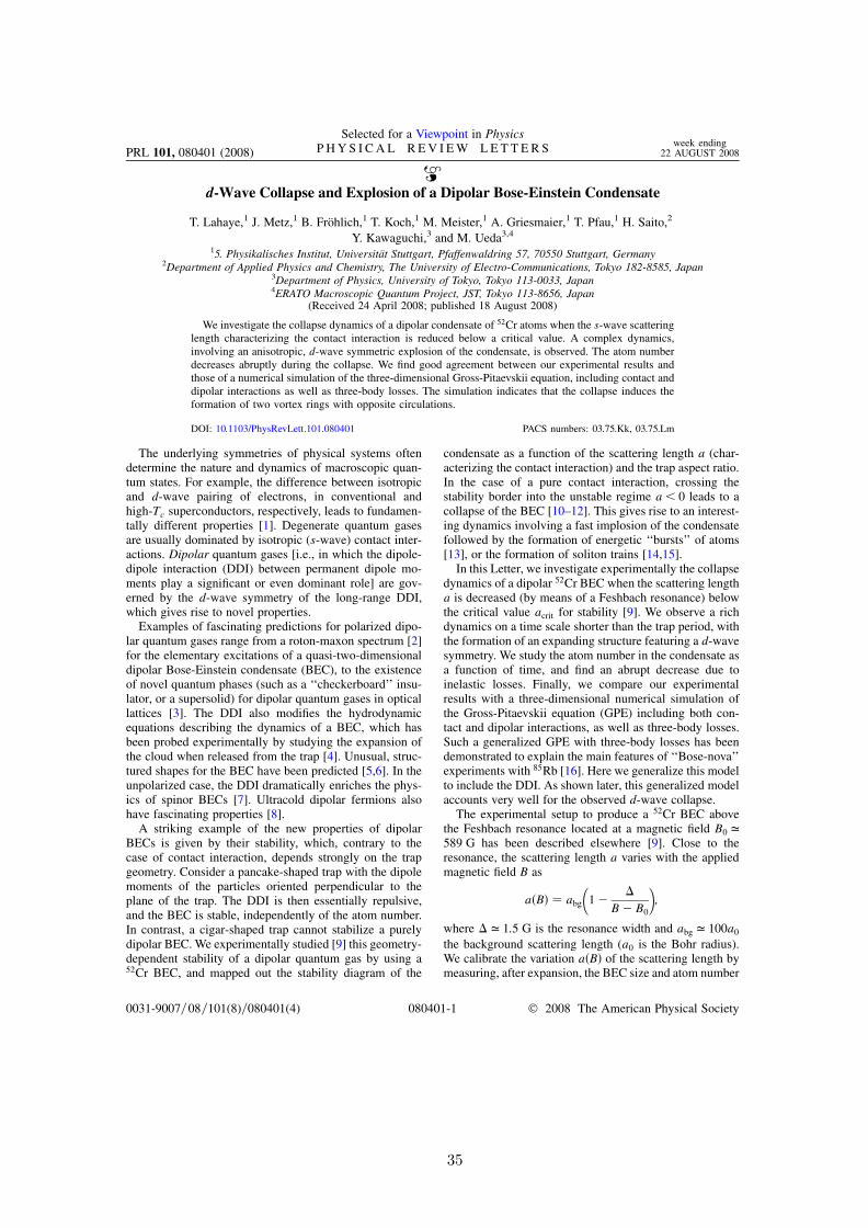
d-Wave Collapse and Explosion of a Dipolar Bose-Einstein Condensate
T. Lahaye,1 J. Metz,1 B. Frohlich,1 T. Koch,1 M. Meister,1 A. Griesmaier,1 T. Pfau,1 H. Saito,2
Y. Kawaguchi,3 and M. Ueda3,4
15. Physikalisches Institut, Universitat Stuttgart, Pfaffenwaldring 57, 70550 Stuttgart, Germany2Department of Applied Physics and Chemistry, The University of Electro-Communications, Tokyo 182-8585, Japan
3Department of Physics, University of Tokyo, Tokyo 113-0033, Japan4ERATO Macroscopic Quantum Project, JST, Tokyo 113-8656, Japan
(Received 24 April 2008; published 18 August 2008)
We investigate the collapse dynamics of a dipolar condensate of 52Cr atoms when the s-wave scatteringlength characterizing the contact interaction is reduced below a critical value. A complex dynamics,involving an anisotropic, d-wave symmetric explosion of the condensate, is observed. The atom numberdecreases abruptly during the collapse. We find good agreement between our experimental results andthose of a numerical simulation of the three-dimensional Gross-Pitaevskii equation, including contact anddipolar interactions as well as three-body losses. The simulation indicates that the collapse induces theformation of two vortex rings with opposite circulations.
DOI: 10.1103/PhysRevLett.101.080401 PACS numbers: 03.75.Kk, 03.75.Lm
The underlying symmetries of physical systems oftendetermine the nature and dynamics of macroscopic quan-tum states. For example, the difference between isotropicand d-wave pairing of electrons, in conventional andhigh-Tc superconductors, respectively, leads to fundamen-tally different properties [1]. Degenerate quantum gasesare usually dominated by isotropic (s-wave) contact inter-actions. Dipolar quantum gases [i.e., in which the dipole-dipole interaction (DDI) between permanent dipole mo-ments play a significant or even dominant role] are gov-erned by the d-wave symmetry of the long-range DDI,which gives rise to novel properties.
Examples of fascinating predictions for polarized dipo-lar quantum gases range from a roton-maxon spectrum [2]for the elementary excitations of a quasi-two-dimensionaldipolar Bose-Einstein condensate (BEC), to the existenceof novel quantum phases (such as a ‘‘checkerboard’’ insu-lator, or a supersolid) for dipolar quantum gases in opticallattices [3]. The DDI also modifies the hydrodynamicequations describing the dynamics of a BEC, which hasbeen probed experimentally by studying the expansion ofthe cloud when released from the trap [4]. Unusual, struc-tured shapes for the BEC have been predicted [5,6]. In theunpolarized case, the DDI dramatically enriches the phys-ics of spinor BECs [7]. Ultracold dipolar fermions alsohave fascinating properties [8].
A striking example of the new properties of dipolarBECs is given by their stability, which, contrary to thecase of contact interaction, depends strongly on the trapgeometry. Consider a pancake-shaped trap with the dipolemoments of the particles oriented perpendicular to theplane of the trap. The DDI is then essentially repulsive,and the BEC is stable, independently of the atom number.In contrast, a cigar-shaped trap cannot stabilize a purelydipolar BEC. We experimentally studied [9] this geometry-dependent stability of a dipolar quantum gas by using a52Cr BEC, and mapped out the stability diagram of the
condensate as a function of the scattering length a (char-acterizing the contact interaction) and the trap aspect ratio.In the case of a pure contact interaction, crossing thestability border into the unstable regime a < 0 leads to acollapse of the BEC [10–12]. This gives rise to an interest-ing dynamics involving a fast implosion of the condensatefollowed by the formation of energetic ‘‘bursts’’ of atoms[13], or the formation of soliton trains [14,15].
In this Letter, we investigate experimentally the collapsedynamics of a dipolar 52Cr BEC when the scattering lengtha is decreased (by means of a Feshbach resonance) belowthe critical value acrit for stability [9]. We observe a richdynamics on a time scale shorter than the trap period, withthe formation of an expanding structure featuring a d-wavesymmetry. We study the atom number in the condensate asa function of time, and find an abrupt decrease due toinelastic losses. Finally, we compare our experimentalresults with a three-dimensional numerical simulation ofthe Gross-Pitaevskii equation (GPE) including both con-tact and dipolar interactions, as well as three-body losses.Such a generalized GPE with three-body losses has beendemonstrated to explain the main features of ‘‘Bose-nova’’experiments with 85Rb [16]. Here we generalize this modelto include the DDI. As shown later, this generalized modelaccounts very well for the observed d-wave collapse.
The experimental setup to produce a 52Cr BEC abovethe Feshbach resonance located at a magnetic field B0 ’589 G has been described elsewhere [9]. Close to theresonance, the scattering length a varies with the appliedmagnetic field B as
aB abg
1
B B0
;
where ’ 1:5 G is the resonance width and abg ’ 100a0
the background scattering length (a0 is the Bohr radius).We calibrate the variation aB of the scattering length bymeasuring, after expansion, the BEC size and atom number
PRL 101, 080401 (2008)
Selected for a Viewpoint in PhysicsP H Y S I C A L R E V I E W L E T T E R S week ending
22 AUGUST 2008
0031-9007=08=101(8)=080401(4) 080401-1 © 2008 The American Physical Society
35

[9]. The reduction of a close to B0 is accompanied byinelastic losses. By measuring the 1=e lifetime and thedensity of the BEC close to resonance, we estimate thethree-body loss coefficient to be constant for the range ofscattering lengths (5 < a=a0 < 30) studied here, with avalue L3 2 1040 m6=s.
To study the collapse dynamics, we first create a BECof typically 20 000 atoms in a trap with frequenciesx;y;z’ 660;400;530Hz at a magnetic field 10 Gabove the Feshbach resonance, where the scattering lengthis a ’ 0:9abg. We then decrease a by ramping down B line-arly over 8 ms to a value ai 30a0 which still lies wellabove the critical value for collapse, measured to be atacrit ’ 15 3a0 [shaded area on Fig. 1(a)] for our pa-rameters [9]. This ramp is slow enough to be adiabatic( _a=a x;y;z), so that the BEC is not excited during it.After 1 ms waiting time, a is finally ramped down rapidlyto af 5a0, which is below the collapse threshold. Forthis, we ramp linearly in 1 ms the current It in the coilsproviding the magnetic field BI. However, due to eddycurrents in the metallic vacuum chamber, the actual valueof Bt and hence that of at change in time as depicted inblue on Fig. 1(a). To obtain this curve, we used Zeemanspectroscopy to measure the step response of Bt to a jumpin the current It (corresponding to a15 G change in B),and found that the resulting Bt is well described if _BB It holds, with ’ 0:5 ms. From this equation andthe measured It we determine the actual at.
After the ramp, we let the system evolve for an adjust-able time thold and then the trap is switched off. Note thatthe origin of thold corresponds to the end of the ramp in It.Because of eddy currents, thold 0 about 0.2 ms before the
time at which the scattering length crosses acrit. However,as we shall see below, even for thold < 0:2 ms a collapse(happening not in trap, but during the time of flight) isobserved, since during expansion the scattering lengthcontinues to evolve towards af . The large magnetic fieldalong z is rapidly turned off (in less than 300 s) after 4 msof expansion, and the condensate expands for another 4 msin an 11 G field pointing in the x direction, before beingimaged by absorption of a resonant laser beam propagatingalong x. Changing the direction of the field allows us to usethe maximum absorption cross section for the imaging (ifthe latter was done in high field, the absorption cross sec-tion would be smaller, thus reducing the signal to noiseratio of the images). We checked that this fast switchinghas no influence on the condensate dynamics. We observethat the atomic cloud has a clear bimodal structure, with abroad isotropic thermal cloud, well fitted by a Gaussian,and a much narrower, highly anisotropic central feature,interpreted as the remnant BEC [see Figs. 1(b) and 1(c)].
The upper row of Fig. 1(d) shows the time evolution ofthe condensate when varying thold. The images were ob-tained by averaging typically five absorption images takenunder the same conditions; the thermal background wassubtracted, and the color scale was adjusted separately foreach thold for a better contrast. From an initial shapeelongated along the magnetization direction z, the conden-sate rapidly develops a complicated structure with an ex-panding, torus-shaped part close to the z 0 plane.Interestingly, the angular symmetry of the condensate atsome specific times (e.g., at thold 0:5 ms) is reminiscentof the d-wave angular symmetry 1 3cos2 of the DDI.For larger values of thold, we observe that the condensate‘‘refocuses’’ due to the presence of the trap [17].
FIG. 1 (color). Collapse dynamics ofthe dipolar condensate. (a) Timing ofthe experiment. The red curve representsthe time variation of the scattering lengthat one would have in the absence ofeddy currents, while the blue curve isobtained by taking them into account(see text). (b) Sample absorption imageof the collapsed condensate for thold 0:4 ms, after 8 ms of time of flight,showing a ‘‘cloverleaf’’ pattern on topof a broad thermal cloud. This image wasobtained by averaging 60 pictures takenunder the same conditions. (c) Sameimage as (b) with the thermal cloudsubtracted. In (b) and (c) the field ofview is 270 m by 270 m. The greenarrow indicates the direction of the mag-netic field. (d) Series of images of thecondensate for different values of thold
(upper row) and results of the numericalsimulation without adjustable parameters(lower row); the field of view is 130 mby 130 m.
PRL 101, 080401 (2008) P H Y S I C A L R E V I E W L E T T E R Sweek ending
22 AUGUST 2008
080401-2
36
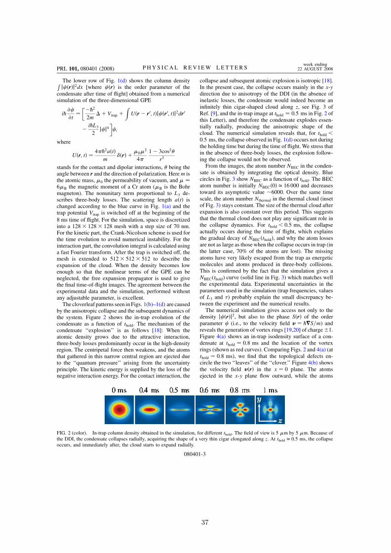
The lower row of Fig. 1(d) shows the column densityRj rj2dx [where r is the order parameter of the
condensate after time of flight] obtained from a numericalsimulation of the three-dimensional GPE
i@@ @t
@2
2m Vtrap
ZUr r0; tj r0; tj2dr0
i@L3
2j j4
;
where
Ur; t 4@2at
mr
02
41 3cos2
r3
stands for the contact and dipolar interactions, being theangle between r and the direction of polarization. Herem isthe atomic mass, 0 the permeability of vacuum, and 6B the magnetic moment of a Cr atom (B is the Bohrmagneton). The nonunitary term proportional to L3 de-scribes three-body losses. The scattering length at ischanged according to the blue curve in Fig. 1(a) and thetrap potential Vtrap is switched off at the beginning of the8 ms time of flight. For the simulation, space is discretizedinto a 128 128 128 mesh with a step size of 70 nm.For the kinetic part, the Crank-Nicolson scheme is used forthe time evolution to avoid numerical instability. For theinteraction part, the convolution integral is calculated usinga fast Fourier transform. After the trap is switched off, themesh is extended to 512 512 512 to describe theexpansion of the cloud. When the density becomes lowenough so that the nonlinear terms of the GPE can beneglected, the free expansion propagator is used to givethe final time-of-flight images. The agreement between theexperimental data and the simulation, performed withoutany adjustable parameter, is excellent.
The cloverleaf patterns seen in Figs. 1(b)–1(d) are causedby the anisotropic collapse and the subsequent dynamics ofthe system. Figure 2 shows the in-trap evolution of thecondensate as a function of thold. The mechanism of thecondensate ‘‘explosion’’ is as follows [18]: When theatomic density grows due to the attractive interaction,three-body losses predominantly occur in the high-densityregion. The centripetal force then weakens, and the atomsthat gathered in this narrow central region are ejected dueto the ‘‘quantum pressure’’ arising from the uncertaintyprinciple. The kinetic energy is supplied by the loss of thenegative interaction energy. For the contact interaction, the
collapse and subsequent atomic explosion is isotropic [18].In the present case, the collapse occurs mainly in the x-ydirection due to anisotropy of the DDI (in the absence ofinelastic losses, the condensate would indeed become aninfinitely thin cigar-shaped cloud along z, see Fig. 3 ofRef. [9], and the in-trap image at thold 0:5 ms in Fig. 2 ofthis Letter), and therefore the condensate explodes essen-tially radially, producing the anisotropic shape of thecloud. The numerical simulation reveals that, for thold <0:5 ms, the collapse observed in Fig. 1(d) occurs not duringthe holding time but during the time of flight. We stress thatin the absence of three-body losses, the explosion follow-ing the collapse would not be observed.
From the images, the atom number NBEC in the conden-sate is obtained by integrating the optical density. Bluecircles in Fig. 3 show NBEC as a function of thold. The BECatom number is initially NBEC0 ’ 16 000 and decreasestoward its asymptotic value 6000. Over the same timescale, the atom number Nthermal in the thermal cloud (insetof Fig. 3) stays constant. The size of the thermal cloud afterexpansion is also constant over this period. This suggeststhat the thermal cloud does not play any significant role inthe collapse dynamics. For thold < 0:5 ms, the collapseactually occurs during the time of flight, which explainsthe gradual decay of NBECthold, and why the atom lossesare not as large as those when the collapse occurs in trap (inthe latter case, 70% of the atoms are lost). The missingatoms have very likely escaped from the trap as energeticmolecules and atoms produced in three-body collisions.This is confirmed by the fact that the simulation gives aNBEC(thold) curve (solid line in Fig. 3) which matches wellthe experimental data. Experimental uncertainties in theparameters used in the simulation (trap frequencies, valuesof L3 and ) probably explain the small discrepancy be-tween the experiment and the numerical results.
The numerical simulation gives access not only to thedensity j rj2, but also to the phase Sr of the orderparameter (i.e., to the velocity field v @rS=m) andreveals the generation of vortex rings [19,20] of charge1.Figure 4(a) shows an in-trap isodensity surface of a con-densate at thold 0:8 ms and the location of the vortexrings (shown as red curves). Comparing Figs. 2 and 4(a) (atthold 0:8 ms), we find that the topological defects en-circle the two ‘‘leaves’’ of the ‘‘clover.’’ Figure 4(b) showsthe velocity field vr in the x 0 plane. The atomsejected in the x-y plane flow outward, while the atoms
FIG. 2 (color). In-trap column density obtained in the simulation, for different thold. The field of view is 5 m by 5 m. Because ofthe DDI, the condensate collapses radially, acquiring the shape of a very thin cigar elongated along z. At thold ’ 0:5 ms, the collapseoccurs, and immediately after, the cloud starts to expand radially.
PRL 101, 080401 (2008) P H Y S I C A L R E V I E W L E T T E R Sweek ending
22 AUGUST 2008
080401-3
37

near the z axis still flow inward, giving rise to the circula-tion. Thus, the vortex-ring formation is specific to thed-wave collapse induced by the DDI. Although the vortexrings are not observed directly in the experiment, theexcellent agreement between the experiment and simula-tion in Figs. 1 and 3 strongly suggests the creation of vortexrings during the collapse of the condensate.
In conclusion, we have investigated the collapse dynam-ics of a dipolar BEC. Contrary to the case of an isotropiccontact interaction, the DDI induces the formation of astructured cloud featuring a d-wave symmetry. The col-lapse dynamics is quantitatively reproduced by numericalsimulations of the GPE without any adjustable parameter.An interesting subject for future studies is the dependenceof the collapse dynamics on the trap geometry: one maywonder if the condensate would collapse in the same wayif initially trapped in a very anisotropic (e.g., pancake-shaped) trap. A natural extension of this work would in-
volve detecting, e.g., by interferometric methods [21,22],the vortex rings predicted by the simulation. Finally,whether one can nucleate stable vortex rings by initiatingthe collapse, and then changing a back to a value corre-sponding to a stable BEC, is a question which certainlydeserves further investigations.
We thank H. P. Buchler, S. Giovanazzi, L. Santos, andG. V. Shlyapnikov for useful discussions. We acknowledgesupport by the German Research Foundation (SFB/TRR 21and SPP 1116), the Landesstiftung Baden-Wurttenberg,and the EU (Marie-Curie Grant No. MEIF-CT-2006-038959 to T. L.). H. S., Y. K., and M. U. acknowledge sup-port by the Ministry of Education, Culture, Sports, Scienceand Technology of Japan (Grants-in-Aid for ScientificResearch No. 17071005 and No. 20540388, the 21st cen-tury COE program on ‘‘Nanometer-Scale QuantumPhysics’’) and by the Matsuo Foundation.
[1] C. C. Tsuei and J. R. Kirtley, Rev. Mod. Phys. 72, 969(2000).
[2] L. Santos, G. V. Shlyapnikov and M. Lewenstein, Phys.Rev. Lett. 90, 250403 (2003).
[3] K. Goral, L. Santos, and M. Lewenstein, Phys. Rev. Lett.88, 170406 (2002); C. Menotti, C. Trefzger, and M.Lewenstein, ibid. 98, 235301 (2007).
[4] K. Goral, K. Rzazewski, and T. Pfau, Phys. Rev. A 61,051601(R) (2000); L. Santos et al., Phys. Rev. Lett. 85,1791 (2000); S. Yi and L. You, Phys. Rev. A 63, 053607(2001); S. Giovanazzi, A. Gorlitz, and T. Pfau, J. Opt. B 5,S208 (2003); J. Stuhler et al., Phys. Rev. Lett. 95, 150406(2005); T. Lahaye et al., Nature (London) 448, 672 (2007).
[5] S. Ronen, D. C. E. Bortolotti, and J. L. Bohn, Phys. Rev.Lett. 98, 030406 (2007).
[6] O. Dutta and P. Meystre, Phys. Rev. A 75, 053604 (2007).[7] Y. Kawaguchi, H. Saito, and M. Ueda, Phys. Rev. Lett. 96,
080405 (2006); L. Santos and T. Pfau, ibid. 96, 190404(2006); S. Yi and H. Pu, ibid. 97, 020401 (2006); Y. Kawa-guchi, H. Saito, and M. Ueda, ibid. 97, 130404 (2006).
[8] M. A. Baranov, Phys. Rep. 464, 71 (2008).[9] T. Koch et al., Nature Phys. 4, 218 (2008).
[10] C. A. Sackett et al., Phys. Rev. Lett. 82, 876 (1999).[11] J. M. Gerton et al., Nature (London) 408, 692 (2000).[12] J. L. Roberts et al., Phys. Rev. Lett. 86, 4211 (2001).[13] E. A. Donley et al., Nature (London) 412, 295 (2001).[14] K. S. Strecker et al., Nature (London) 417, 150 (2002).[15] S. L. Cornish, S. T. Thompson, and C. E. Wieman, Phys.
Rev. Lett. 96, 170401 (2006).[16] M. Ueda and H. Saito, J. Phys. Soc. Jpn. 72, 127 (2003).[17] See EPAPS Document No. E-PRLTAO-101-008831 for a
movie of the collapse for 0 < thold < 1:6 ms. For moreinformation on EPAPS, see http://www.aip.org/pubservs/epaps.html.
[18] H. Saito and M. Ueda, Phys. Rev. A 65, 033624 (2002).[19] B. P. Anderson et al., Phys. Rev. Lett. 86, 2926 (2001).[20] N. S. Ginsberg, J. Brand, and L. V. Hau, Phys. Rev. Lett.
94, 040403 (2005).[21] M. R. Matthews et al., Phys. Rev. Lett. 83, 2498 (1999).[22] F. Chevy et al., Phys. Rev. A 64, 031601(R) (2001).
(b)(a)
x
y
z
y
z
FIG. 4 (color). Vortex rings predicted by the numerical simu-lation. (a) Isodensity surface of an in-trap condensate at thold 0:8 ms. The topological defects are shown by the red rings.(b) Velocity field of the atomic flow in the x 0 plane at thold 0:8 ms. The field of view is 2:5 m by 2:5 m; the color scalerepresents the velocity (red is faster).
0
5
10
15
20
25
0 0.4 0.8 1.2 1.6
NB
EC
/103
t hold /ms
0
20
40
60
80
100
0 0.4 0.8 1.2 1.6
Nth
erm
al/
103
t hold /ms
FIG. 3 (color online). Atom losses during collapse. Bluecircles: atom number NBEC in the condensate as a function ofthold. The solid curve is the result of the simulation for L3 2 1040 m6=s, without any adjustable parameter. Inset: theatom number Nthermal in the thermal cloud (red squares) remainsessentially constant during the collapse.
PRL 101, 080401 (2008) P H Y S I C A L R E V I E W L E T T E R Sweek ending
22 AUGUST 2008
080401-4
38
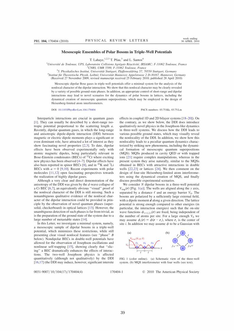
Mesoscopic Ensembles of Polar Bosons in Triple-Well Potentials
T. Lahaye,1,2,3 T. Pfau,3 and L. Santos4
1Universite de Toulouse, UPS, Laboratoire Collisions Agregats Reactivite, IRSAMC; F-31062 Toulouse, France2CNRS, UMR 5589, F-31062 Toulouse, France
35. Physikalisches Institut, Universitat Stuttgart, Pfaffenwaldring 57, 70550 Stuttgart, Germany4Institut fur Theoretische Physik, Leibniz Universitat Hannover, Appelstrasse 2 D-30167, Hannover, Germany
(Received 27 November 2009; revised manuscript received 25 February 2010; published 28 April 2010)
Mesoscopic dipolar Bose gases in triple-well potentials offer a minimal system for the analysis of the
nonlocal character of the dipolar interaction. We show that this nonlocal character may be clearly revealed
by a variety of possible ground-state phases. In addition, an appropriate control of short-range and dipolar
interactions may lead to novel scenarios for the dynamics of polar bosons in lattices, including the
dynamical creation of mesoscopic quantum superpositions, which may be employed in the design of
Heisenberg-limited atom interferometers.
DOI: 10.1103/PhysRevLett.104.170404 PACS numbers: 03.75.Kk, 03.75.Lm
Interparticle interactions are crucial in quantum gases[1]. They can usually be described by a short-range iso-tropic potential proportional to the scattering length a.Recently, dipolar quantum gases, in which the long-rangeand anisotropic dipole-dipole interaction (DDI) betweenmagnetic or electric dipole moments plays a significant oreven dominant role, have attracted a lot of interest as theyshow fascinating novel properties [2,3]. To date, dipolareffects have been observed experimentally only withatomic magnetic dipoles, being particularly relevant inBose-Einstein condensates (BECs) of 52Cr where excitingnew physics has been observed [4–7]. Dipolar effects havealso been reported in spinor BECs [8], and in 39K and 7LiBECs with a ¼ 0 [9,10]. Recent experiments with polarmolecules [11,12] open fascinating perspectives towardsthe realization of highly dipolar gases.
Although a very clear and direct demonstration of theanisotropy of the DDI was given by the d-wave collapse ofa Cr BEC [6,7], an equivalently obvious ‘‘visual’’ proof ofthe nonlocal character of the DDI is still missing. Such anonambiguous qualitative evidence of the nonlocal char-acter of the dipolar interaction could be provided in prin-ciple by the observation of novel quantum phases (super-solid, checkerboard) in optical lattices [13]. However, theunambiguous detection of such phases is far from trivial, asis the preparation of the ground state of the system due to alarge number of metastable states [14].
In this Letter, we investigate a minimal system, namely,a mesoscopic sample of dipolar bosons in a triple-wellpotential, which minimizes these restrictions, while stillpresenting clear visual nonlocal features (see ‘‘phase’’ Bbelow). Nondipolar BECs in double-well potentials haveallowed for the observation of Josephson oscillations andnonlinear self-trapping [15], showing clearly that ‘‘slic-ing’’ a BEC dramatically enhances the effects of interac-tions. The two-well Josephson physics is affectedquantitatively (although not qualitatively) by the DDI[16,17] (the DDI may induce, however, significant intersite
effects in coupled 1D and 2D bilayer systems [18–20]). Onthe contrary, as we show below, the DDI does introducequalitatively novel physics in the Josephson-like dynamicsin three-well systems. We discuss how the DDI leads tovarious possible ground states, which may visually revealthe nonlocality of the DDI. In addition, we show how thisnonlocality leads to a peculiar quantum dynamics charac-terized by striking new phenomena, including the dynami-cal formation of mesoscopic quantum superpositions(MQS). MQSs produced in cavity QED or with trappedions [21] require complex manipulations, whereas in thepresent system they arise naturally, similar to the MQSsobtained in BECs with attractive interactions in doublewells [22,23] or lattices [24]. We then comment on thedesign of four-site Heisenberg-limited atom interferome-ters using the dynamical creation of MQS, and finallydiscuss possible experimental scenarios.We consider N dipolar bosons in a three-well potential
VtrapðrÞ [Fig. 1(a)]. The wells are aligned along the y axis,
separated by a distance ‘ and an energy barrier V0. Thebosons are polarized by a sufficiently large external field,with a dipole moment d along a given direction. The latticepotential is strong enough compared to other energies (inparticular, the interaction energies) such that the on-sitewave functions i¼1;2;3ðrÞ are fixed, being independent of
the number of atoms per site. For a large enough V0 wemay assume iðrÞ ¼ ðr riÞ, where ri is the center ofsite i. In addition we may assume to be a Gaussian with
FIG. 1 (color online). (a) Schematic view of the three-wellsystem. (b) MQS interferometer with four wells (see text).
PRL 104, 170404 (2010) P HY S I CA L R EV I EW LE T T E R Sweek ending
30 APRIL 2010
0031-9007=10=104(17)=170404(4) 170404-1 2010 The American Physical Society
39
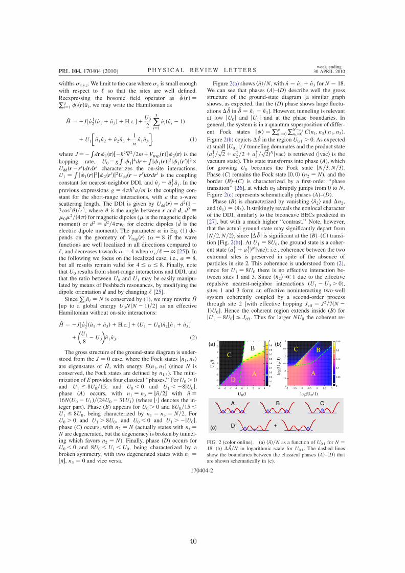
widthsx;y;z. We limit to the case wherey is small enough
with respect to ‘ so that the sites are well defined.
Reexpressing the bosonic field operator as c ðrÞ ¼P3i¼1 iðrÞai, we may write the Hamiltonian as
H ¼ J½ay2 ða1 þ a3Þ þ H:c: þU0
2
X3
i¼1
niðni 1Þ
þU1
n1n2 þ n2n3 þ 1
n1n3
; (1)
where J¼Rdr1ðrÞ½@
2r2=2mþVtrapðrÞ2ðrÞ is thehopping rate, U0¼g
Rj1j4drþRj1ðrÞj2j1ðr0Þj2
Uddðrr0Þdrdr0 characterizes the on-site interactions,U1 ¼
R j1ðrÞj2j2ðr0Þj2Uddðr r0Þdrdr0 is the coupling
constant for nearest-neighbor DDI, and nj ¼ ayj aj. In the
previous expressions g ¼ 4@2a=m is the coupling con-stant for the short-range interactions, with a the s-wavescattering length. The DDI is given by UddðrÞ ¼ d2ð13cos2Þ=r3, where is the angle between r and d, d2 0
2=ð4Þ for magnetic dipoles ( is the magnetic dipolemoment) or d2 d2=40 for electric dipoles ( d is theelectric dipole moment). The parameter in Eq. (1) de-pends on the geometry of VtrapðrÞ ( ¼ 8 if the wave
functions are well localized in all directions compared to‘, and decreases towards ¼ 4 when x=‘ ! 1 [25]). Inthe following we focus on the localized case, i.e., ¼ 8,but all results remain valid for 4 8. Finally, notethat U0 results from short-range interactions and DDI, andthat the ratio between U0 and U1 may be easily manipu-lated by means of Feshbach resonances, by modifying thedipole orientation d and by changing ‘ [25].
SinceP
ini ¼ N is conserved by (1), we may rewrite H[up to a global energy U0NðN 1Þ=2] as an effectiveHamiltonian without on-site interactions:
H ¼ J½ay2 ða1 þ a3Þ þ H:c: þ ðU1 U0Þn2½n1 þ n3þ
U1
8U0
n1n3: (2)
The gross structure of the ground-state diagram is under-stood from the J ¼ 0 case, where the Fock states jn1; n3iare eigenstates of H, with energy Eðn1; n3Þ (since N isconserved, the Fock states are defined by n1;3). The mini-
mization of E provides four classical ‘‘phases.’’ ForU0 > 0and U1 8U0=15, and U0 < 0 and U1 <8jU0j,phase (A) occurs, with n1 ¼ n3 ¼ b n=2c with n 16NðU0 U1Þ=ð24U0 31U1Þ (where bc denotes the in-teger part). Phase (B) appears for U0 > 0 and 8U0=15 U1 8U0, being characterized by n1 ¼ n3 ¼ N=2. ForU0 > 0 and U1 > 8U0, and U0 < 0 and U1 >jU0j,phase (C) occurs, with n2 ¼ N (actually states with ni ¼N are degenerated, but the degeneracy is broken by tunnel-ing which favors n2 ¼ N). Finally, phase (D) occurs forU0 < 0 and 8U0 <U1 <U0, being characterized by abroken symmetry, with two degenerated states with n1 ¼b nc, n3 ¼ 0 and vice versa.
Figure 2(a) shows hni=N, with n ¼ n1 þ n3 for N ¼ 18.We can see that phases ðAÞ–ðDÞ describe well the grossstructure of the ground-state diagram [a similar graphshows, as expected, that the (D) phase shows large fluctu-
ations in ¼ n1 n3]. However, tunneling is relevantat low jU0j and jU1j and at the phase boundaries. Ingeneral, the system is in a quantum superposition of differ-
ent Fock states jc i ¼ PNn1¼0
PNn1n3¼0 Cðn1; n3Þjn1; n3i.
Figure 2(b) depicts in the regionU0;1 > 0. As expectedat small jU0;1j=J tunneling dominates and the product state
ðay1=ffiffiffi2
p þ ay2=2þ ay3=ffiffiffi2
p ÞNjvaci is retrieved (jvaci is thevacuum state). This state transforms into phase (A), whichfor growing U0 becomes the Fock state jN=3; N=3i.Phase (C) remains the Fock state j0; 0i (n2 ¼ N), and theborder ðBÞ–ðCÞ is characterized by a first-order ‘‘phasetransition’’ [26], at which n2 abruptly jumps from 0 to N.Figure 2(c) represents schematically phases (A)–(D).Phase (B) is characterized by vanishing hn2i and n2,
and hn1i ¼ hn3i. It strikingly reveals the nonlocal characterof the DDI, similarly to the biconcave BECs predicted in[27], but with a much higher ‘‘contrast.’’ Note, however,that the actual ground state may significantly depart from
jN=2; N=2i, since jj is significant at the ðBÞ–ðCÞ transi-tion [Fig. 2(b)]. At U1 ¼ 8U0, the ground state is a coher-
ent state ðay1 þ ay3 ÞNjvaci; i.e., coherence between the two
extremal sites is preserved in spite of the absence ofparticles in site 2. This coherence is understood from (2),since for U1 ¼ 8U0 there is no effective interaction be-tween sites 1 and 3. Since hn2i 1 due to the effectiverepulsive nearest-neighbor interactions (U1 U0 > 0),sites 1 and 3 form an effective noninteracting two-wellsystem coherently coupled by a second-order processthrough site 2 [with effective hopping Jeff ¼ J2=7ðN 1ÞU0]. Hence the coherent region extends inside (B) forjU1 8U0j & Jeff . Thus for larger NU0 the coherent re-
0
0.1
0.2
0.3
0.4
0.5
0.6
0.7
0.8
0.9
1
-4 -3 -2 -1 0 1 2 3 4-4
-3
-2
-1
0
1
2
3
4
C
A
B
D
U /
J1
U /J0
(a)
0
0.05
0.1
0.15
0.2
0.25
-2 -1.5 -1 -0.5 0 0.5 1-2
-1.5
-1
-0.5
0
0.5
1
log(
U /
J)
1
log(U / J)0
C B
A
(b)
(c)
A B C
D +
FIG. 2 (color online). (a) hni=N as a function of U0;1 for N ¼18. (b) =N in logarithmic scale for U0;1. The dashed lines
show the boundaries between the classical phases ðAÞ–ðDÞ thatare shown schematically in (c).
PRL 104, 170404 (2010) P HY S I CA L R EV I EW LE T T E R Sweek ending
30 APRIL 2010
170404-2
40
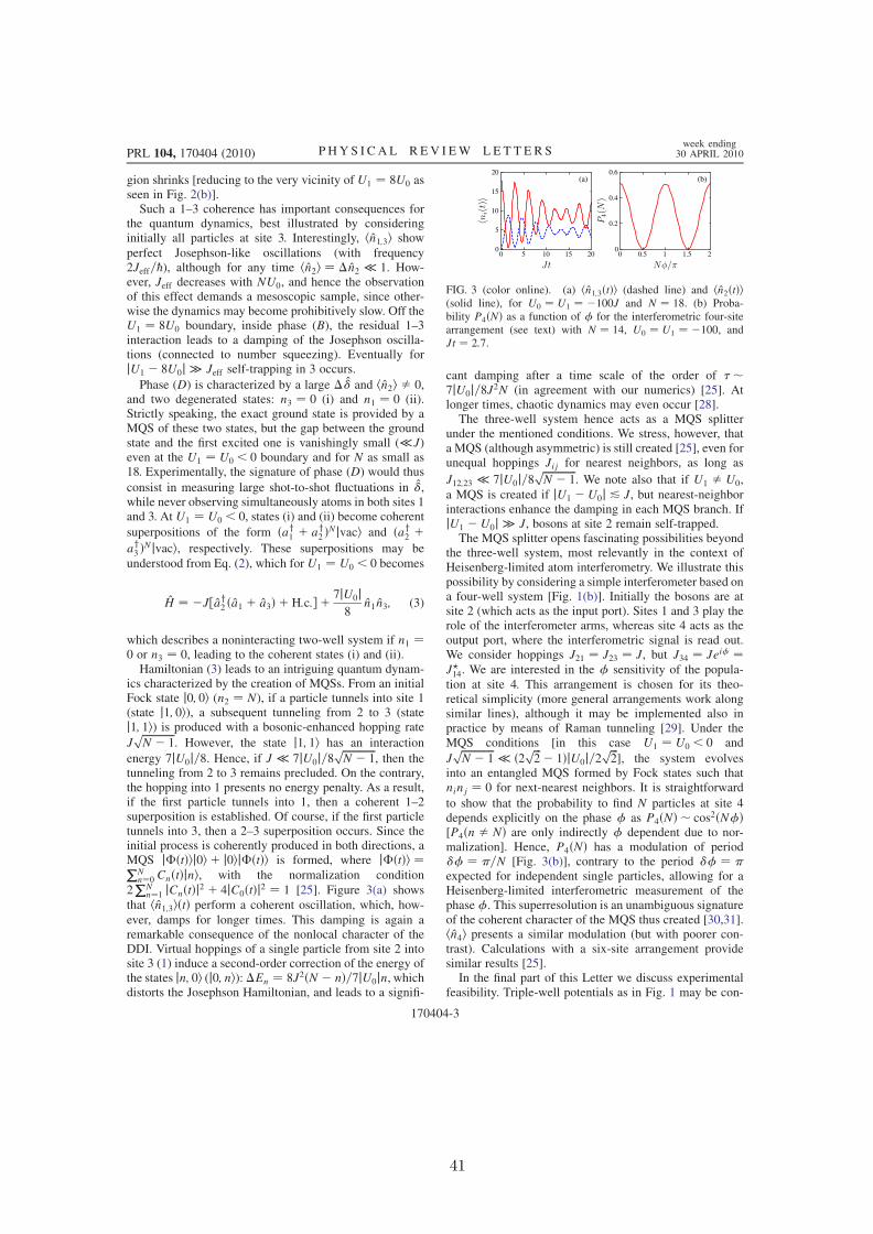
gion shrinks [reducing to the very vicinity of U1 ¼ 8U0 asseen in Fig. 2(b)].
Such a 1–3 coherence has important consequences forthe quantum dynamics, best illustrated by consideringinitially all particles at site 3. Interestingly, hn1;3i show
perfect Josephson-like oscillations (with frequency2Jeff=@), although for any time hn2i ¼ n2 1. How-ever, Jeff decreases with NU0, and hence the observationof this effect demands a mesoscopic sample, since other-wise the dynamics may become prohibitively slow. Off theU1 ¼ 8U0 boundary, inside phase (B), the residual 1–3interaction leads to a damping of the Josephson oscilla-tions (connected to number squeezing). Eventually forjU1 8U0j Jeff self-trapping in 3 occurs.
Phase (D) is characterized by a large and hn2i 0,and two degenerated states: n3 ¼ 0 (i) and n1 ¼ 0 (ii).Strictly speaking, the exact ground state is provided by aMQS of these two states, but the gap between the groundstate and the first excited one is vanishingly small (J)even at the U1 ¼ U0 < 0 boundary and for N as small as18. Experimentally, the signature of phase (D) would thus
consist in measuring large shot-to-shot fluctuations in ,while never observing simultaneously atoms in both sites 1and 3. At U1 ¼ U0 < 0, states (i) and (ii) become coherent
superpositions of the form ðay1 þ ay2 ÞNjvaci and ðay2 þay3 ÞNjvaci, respectively. These superpositions may be
understood from Eq. (2), which for U1 ¼ U0 < 0 becomes
H ¼ J½ay2 ða1 þ a3Þ þ H:c: þ 7jU0j8
n1n3; (3)
which describes a noninteracting two-well system if n1 ¼0 or n3 ¼ 0, leading to the coherent states (i) and (ii).
Hamiltonian (3) leads to an intriguing quantum dynam-ics characterized by the creation of MQSs. From an initialFock state j0; 0i (n2 ¼ N), if a particle tunnels into site 1(state j1; 0i), a subsequent tunneling from 2 to 3 (statej1; 1i) is produced with a bosonic-enhanced hopping rate
JffiffiffiffiffiffiffiffiffiffiffiffiffiN 1
p. However, the state j1; 1i has an interaction
energy 7jU0j=8. Hence, if J 7jU0j=8ffiffiffiffiffiffiffiffiffiffiffiffiffiN 1
p, then the
tunneling from 2 to 3 remains precluded. On the contrary,the hopping into 1 presents no energy penalty. As a result,if the first particle tunnels into 1, then a coherent 1–2superposition is established. Of course, if the first particletunnels into 3, then a 2–3 superposition occurs. Since theinitial process is coherently produced in both directions, aMQS jðtÞij0i þ j0ijðtÞi is formed, where jðtÞi ¼PN
n¼0 CnðtÞjni, with the normalization condition
2PN
n¼1 jCnðtÞj2 þ 4jC0ðtÞj2 ¼ 1 [25]. Figure 3(a) shows
that hn1;3iðtÞ perform a coherent oscillation, which, how-
ever, damps for longer times. This damping is again aremarkable consequence of the nonlocal character of theDDI. Virtual hoppings of a single particle from site 2 intosite 3 (1) induce a second-order correction of the energy ofthe states jn; 0i (j0; ni):En ¼ 8J2ðN nÞ=7jU0jn, whichdistorts the Josephson Hamiltonian, and leads to a signifi-
cant damping after a time scale of the order of 7jU0j=8J2N (in agreement with our numerics) [25]. Atlonger times, chaotic dynamics may even occur [28].The three-well system hence acts as a MQS splitter
under the mentioned conditions. We stress, however, thata MQS (although asymmetric) is still created [25], even forunequal hoppings Jij for nearest neighbors, as long as
J12;23 7jU0j=8ffiffiffiffiffiffiffiffiffiffiffiffiffiN 1
p. We note also that if U1 U0,
a MQS is created if jU1 U0j & J, but nearest-neighborinteractions enhance the damping in each MQS branch. IfjU1 U0j J, bosons at site 2 remain self-trapped.The MQS splitter opens fascinating possibilities beyond
the three-well system, most relevantly in the context ofHeisenberg-limited atom interferometry. We illustrate thispossibility by considering a simple interferometer based ona four-well system [Fig. 1(b)]. Initially the bosons are atsite 2 (which acts as the input port). Sites 1 and 3 play therole of the interferometer arms, whereas site 4 acts as theoutput port, where the interferometric signal is read out.We consider hoppings J21 ¼ J23 ¼ J, but J34 ¼ Jei ¼J?14. We are interested in the sensitivity of the popula-tion at site 4. This arrangement is chosen for its theo-retical simplicity (more general arrangements work alongsimilar lines), although it may be implemented also inpractice by means of Raman tunneling [29]. Under theMQS conditions [in this case U1 ¼ U0 < 0 and
JffiffiffiffiffiffiffiffiffiffiffiffiffiN 1
p ð2 ffiffiffi2
p 1ÞjU0j=2ffiffiffi2
p], the system evolves
into an entangled MQS formed by Fock states such thatninj ¼ 0 for next-nearest neighbors. It is straightforward
to show that the probability to find N particles at site 4depends explicitly on the phase as P4ðNÞ cos2ðNÞ[P4ðn NÞ are only indirectly dependent due to nor-malization]. Hence, P4ðNÞ has a modulation of period ¼ =N [Fig. 3(b)], contrary to the period ¼ expected for independent single particles, allowing for aHeisenberg-limited interferometric measurement of thephase. This superresolution is an unambiguous signatureof the coherent character of the MQS thus created [30,31].hn4i presents a similar modulation (but with poorer con-trast). Calculations with a six-site arrangement providesimilar results [25].In the final part of this Letter we discuss experimental
feasibility. Triple-well potentials as in Fig. 1 may be con-
(b)(a)
0 5 10 15 200
5
10
15
20
0 0.5 1 1.5 20
0.2
0.4
0.6
FIG. 3 (color online). (a) hn1;3ðtÞi (dashed line) and hn2ðtÞi(solid line), for U0 ¼ U1 ¼ 100J and N ¼ 18. (b) Proba-bility P4ðNÞ as a function of for the interferometric four-sitearrangement (see text) with N ¼ 14, U0 ¼ U1 ¼ 100, andJt ¼ 2:7.
PRL 104, 170404 (2010) P HY S I CA L R EV I EW LE T T E R Sweek ending
30 APRIL 2010
170404-3
41
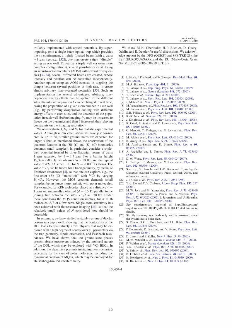
trollably implemented with optical potentials. By super-imposing, onto a single-beam optical trap which providesthe xz confinement, a tightly focused beam (with a waist1 m, see, e.g., [32]), one may create a tight ‘‘dimple’’acting as one well. To realize a triple well (or even morecomplex configurations), several possibilities exist. Usingan acousto-optic modulator (AOM) with several rf frequen-cies [33,34], several diffracted beams are created, whoseintensity and position can be controlled independently.Another option using an AOM consists in toggling thedimple between several positions at high rate, to createalmost arbitrary time-averaged potentials [35]. Such animplementation has several advantages: arbitrary, time-dependent energy offsets can be applied to the differentsites; the intersite separation ‘ can be changed in real time,easing the preparation of a given atom number in each well(e.g., by performing evaporative cooling with differentenergy offsets in each site), and the detection of the popu-lation in each well (before imaging, V0 may be increased tofreeze out the dynamics and then ‘ increased, thus relaxingconstraints on the imaging resolution).
We now evaluate J,U0, andU1 for realistic experimentalvalues. Although in our calculations we have just consid-ered N up to 36, similar ground states are expected forlarger N [but, as mentioned above, the observation of thequantum features at the ðBÞ–ðCÞ and ðDÞ–ðCÞ boundariesdemands small samples]. In particular, consider a triple-well potential formed by three Gaussian beams of waist1 m separated by ‘ ¼ 1:7 m. For a barrier heightV0=h ’ 2500 Hz, we obtain J=h 10 Hz, and the typicalvalue ofNU1=J is then10 forN ¼ 2000 52Cr atoms. Thevalue ofU0 can be tuned, for a fixed geometry, by means ofFeshbach resonances [4], so that one can explore, e.g., thefirst-order ðBÞ–ðCÞ ‘‘transition’’ with 52Cr by varyingU1=U0. However, the MQS creation demands smallsamples, being hence more realistic with polar molecules.For example, for KRb molecules placed at a distance ‘ ¼1 m and maximally polarized (d ¼ 0:5 D) parallel to thejoining line between the sites, U1=h ’ 70 Hz. Underthese conditions the MQS condition implies, for N ¼ 36molecules, J=h of a few hertz. Single-atom sensitivity hasbeen achieved with fluorescence imaging [36], so that therelatively small values of N considered here should bedetectable.
In summary, we have studied a simple system of dipolarbosons in a triple well, showing that the nonlocality of theDDI leads to qualitatively novel physics that may be ex-plored with a high degree of control over all parameters viathe trap geometry, dipole orientation, and Feshbach reso-nances. We have shown that the ground-state phasespresent abrupt crossovers induced by the nonlocal natureof the DDI, which may be explored with 52Cr BECs. Inaddition, the dynamics presents intriguing new scenarios,especially for the case of polar molecules, including thedynamical creation of MQSs, which may be employed forHeisenberg-limited interferometry.
We thank M.K. Oberthaler, H. P. Buchler, D. Guery-Odelin, and E. Demler for useful discussions. We acknowl-edge support by the DFG (QUEST and SFB/TRR 21), theESF (EUROQUASAR), and the EU (Marie-Curie GrantNo. MEIF-CT-2006-038959 to T. L.).
[1] I. Bloch, J. Dalibard, and W. Zwerger, Rev. Mod. Phys. 80,885 (2008).
[2] M.A. Baranov, Phys. Rep. 464, 71 (2008).[3] T. Lahaye et al., Rep. Prog. Phys. 72, 126401 (2009).[4] T. Lahaye et al., Nature (London) 448, 672 (2007).[5] T. Koch et al., Nature Phys. 4, 218 (2008).[6] T. Lahaye et al., Phys. Rev. Lett. 101, 080401 (2008).[7] J. Metz et al., New J. Phys. 11, 055032 (2009).[8] M.Vengalattore et al., Phys.Rev.Lett. 100, 170403 (2008).[9] M. Fattori et al., Phys. Rev. Lett. 101, 190405 (2008).[10] S. E. Pollack et al., Phys. Rev. Lett. 102, 090402 (2009).[11] K.-K. Ni et al., Science 322, 231 (2008).[12] J. Deiglmayr et al., Phys. Rev. Lett. 101, 133004 (2008).[13] K. Goral, L. Santos, and M. Lewenstein, Phys. Rev. Lett.
88, 170406 (2002).[14] C. Menotti, C. Trefzger, and M. Lewenstein, Phys. Rev.
Lett. 98, 235301 (2007).[15] M. Albiez et al., Phys. Rev. Lett. 95, 010402 (2005).[16] B. Xiong et al., Phys. Rev. A 79, 013626 (2009).[17] M. Asad-uz-Zaman and D. Blume, Phys. Rev. A 80,
053622 (2009).[18] A. Arguelles and L. Santos, Phys. Rev. A 75, 053613
(2007).[19] D.W. Wang, Phys. Rev. Lett. 98, 060403 (2007).[20] C. Trefzger, C. Menotti, and M. Lewenstein, Phys. Rev.
Lett. 103, 035304 (2009).[21] See, e.g., S. Haroche and J.-M. Raimond, Exploring the
Quantum (Oxford University Press, Oxford, 2006), andreferences therein.
[22] J. I. Cirac et al., Phys. Rev. A 57, 1208 (1998).[23] T.-L. Ho and C.V. Ciobanu, J. Low Temp. Phys. 135, 257
(2004).[24] M.W. Jack and M. Yamashita, Phys. Rev. A 71, 023610
(2005); P. Buonsante, V. Penna, and A. Vezzani, Phys.Rev. A 72, 043620 (2005); J. Javanainen and U. Shrestha,Phys. Rev. Lett. 101, 170405 (2008).
[25] See supplementary material at http://link.aps.org/supplemental/10.1103/PhysRevLett.104.170404 for moredetails.
[26] Strictly speaking, one deals only with a crossover, sincethe system has a finite size.
[27] S. Ronen, D. C. E. Bortolotti, and J. L. Bohn, Phys. Rev.Lett. 98, 030406 (2007).
[28] P. Buonsante, R. Franzosi, and V. Penna, Phys. Rev. Lett.90, 050404 (2003).
[29] D. Jaksch and P. Zoller, New J. Phys. 5, 56 (2003).[30] M.W. Mitchell et al., Nature (London) 429, 161 (2004).[31] P. Walther et al., Nature (London) 429, 158 (2004).[32] Y. R. P. Sortais et al., Phys. Rev. A 75, 013406 (2007).[33] Y. Shin et al., Phys. Rev. Lett. 92, 050405 (2004).[34] B. Frohlich et al., Rev. Sci. Instrum. 78, 043101 (2007).[35] K. Henderson et al., New J. Phys. 11, 043030 (2009).[36] R. Bucker et al., New J. Phys. 11, 103039 (2009).
PRL 104, 170404 (2010) P HY S I CA L R EV I EW LE T T E R Sweek ending
30 APRIL 2010
170404-4
42
Chapter 2
Guided atom optics
Parfois au fond de moi se ranimentL’eau verte du canal du MidiEt la brique rouge des Minimes.1
2.1 Introduction
I was hired at CNRS as a permanent researcher in October 2008, and joined the Cold Atomgroup recently founded at Laboratoire Collsions, Agrégats, Réactivité in Toulouse by DavidGuéry-Odelin, who had been appointed Professor at Université Paul Sabatier a few monthsearlier. At the time, David’s experimental setup was still located at Laboratoire Kastler-Brossel of the ENS, in Paris. The machine, based for a significant part on equipment builtduring my PhD thesis, was producing all-optical BECs of 87Rb and was used by a post-doc, Gianluca Gattobigio, and a PhD student, Antoine Couvert, to perform atom-opticsexperiments [27].
The group in Toulouse also included Renaud Mathevet, amaître de conférence who hadbeen working previously in the team of the now retired John Weiner, on nanolithographyusing laser-cooled Cesium atoms. Our early work with Renaud consisted in preparingthe lab space that had just been renovated to accommodate the experimental activity ofthe group. In parallel, the former nanolithography experiments were dismantled to makeroom for an extension of the lab space of the atom interferometry team, and, on my side,I finished some work, started in Stuttgart, related to dipolar gases.
In February 2009, we moved the BEC machine from ENS to Toulouse, and decided toreconstruct it without changes, so as to be operational as soon as possible. In retrospect,this probably was a mistake, as it turned out that several pieces of equipment, from thevacuum chamber to most of the lasers, finally had to be replaced in the end, while thedesign retained its initial shortcomings, such as a rather limited optical access and amoderate stability of the crossed optical dipole trap.
Two PhD students, Charlotte Fabre and Francois Vermersch, joined the team in1Claude Nougaro, Toulouse (1967).
43

44 Chapter 2. Guided atom optics
Figure 2.1: A quick summary of the early work of the cold atom group at LCAR in Toulouse. (a): Thelab just after the renovation was finished (January 2009). (b): The lab at the time when we obtainedthe first BEC in Toulouse (spring 2010). (c): The first atom optics paper from the group (end of 2011).
September 2009, and Gianluca Gattobigio prolonged his post-doc from Paris to Toulouse.We obtained a first BEC in April 2010, but the system was unreliable as the 1070 nm,300 W IPG fiber laser at the heart of the machine was slowly dying (its spatial modekept degrading week after week). After repair of the laser, stable operation of the ma-chine, giving BECs of up to 105 atoms every 5 seconds, was achieved at the end of 2010(figure 2.1).
As a follow-up of the studies performed at ENS, it was decided to continue guidedatom optics experiments, and we realized a Bragg reflector for guided matter waves [34].In parallel, in early 2010 a new experimental setup was designed, in view of replacingthe aging one moved from ENS. A PhD student, Pierrick Cheiney, joined the group inSeptember 2010 to work on this project. During the development of the setup, RenaudMathevet proposed to use permanent magnets for the construction of the Zeeman slower.This turned out to be a fruitful idea, that gave rise to the publication [22].
This chapter is organized as follows. I first describe in section 2.2 our Zeeman slowerbased on permanent magnets in a Halbach configuration. In section 2.3 I briefly summarizethe experimental demonstration of a Bragg reflector for guided matter waves. For details,the reader is referred to the successive PhD theses defended in the group [33, 127, 21].
2.2 A Zeeman slower based on permanent magnets in a Hal-bach configuration
More than thirty years after its first demonstration [99], the Zeeman slower remains one ofthe most widely used intense sources of slow atoms in experiments using cold or ultracoldatoms. Compared to alternative solutions, it is indeed a very robust system, which can
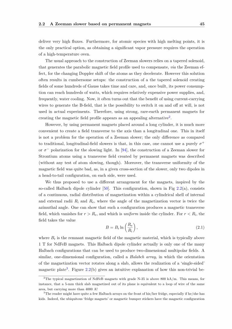
2.2 A Zeeman slower based on permanent magnets 45
deliver very high fluxes. Furthermore, for atomic species with high melting points, it isthe only practical option, as obtaining a significant vapor pressure requires the operationof a high-temperature oven.
The usual approach to the construction of Zeeman slowers relies on a tapered solenoid,that generates the parabolic magnetic field profile used to compensate, via the Zeeman ef-fect, for the changing Doppler shift of the atoms as they decelerate. However this solutionoften results in cumbersome setups: the construction of a the tapered solenoid creatingfields of some hundreds of Gauss takes time and care, and, once built, its power consump-tion can reach hundreds of watts, which requires relatively expensive power supplies, and,frequently, water cooling. Now, it often turns out that the benefit of using current-carryingwires to generate the B-field, that is the possibility to switch it on and off at will, is notused in actual experiments. Therefore, using strong, rare-earth permanent magnets forcreating the magnetic field profile appears as an appealing alternative2.
However, by using permanent magnets placed around a long cylinder, it is much moreconvenient to create a field transverse to the axis than a longitudinal one. This in itselfis not a problem for the operation of a Zeeman slower; the only difference as comparedto traditional, longitudinal-field slowers is that, in this case, one cannot use a purely σ+
or σ− polarization for the slowing light. In [94], the construction of a Zeeman slower forStrontium atoms using a transverse field created by permanent magnets was described(without any test of atom slowing, though). Moreover, the transverse uniformity of themagnetic field was quite bad, as, in a given cross-section of the slower, only two dipoles ina head-to-tail configuration, on each side, were used.
We thus proposed to use a different arrangement for the magnets, inspired by theso-called Halbach dipole cylinder [50]. This configuration, shown in Fig 2.2(a), consistsof a continuous, radial distribution of magnetization within a cylindrical shell of internaland external radii Ri and Re, where the angle of the magnetization vector is twice theazimuthal angle. One can show that such a configuration produces a magnetic transversefield, which vanishes for r > Re, and which is uniform inside the cylinder. For r < Ri, thefield takes the value
B = Br ln(ReRi
), (2.1)
where Br is the remnant magnetic field of the magnetic material, which is typically above1 T for NdFeB magnets. This Halbach dipole cylinder actually is only one of the manyHalbach configurations that can be used to produce two-dimensional multipolar fields. Asimilar, one-dimensional configuration, called a Halabch array, in which the orientationof the magnetization vector rotates along a slab, allows the realization of a ‘single-sided’magnetic plate3. Figure 2.2(b) gives an intuitive explanation of how this non-trivial be-
2The typical magnetization of NdFeB magnets with grade N-35 is above 800 kA/m. This means, forinstance, that a 5-mm thick slab magnetized out of its plane is equivalent to a loop of wire of the samearea, but carrying more than 4000 A!
3The reader might have quite a few Halbach arrays on the front of his/her fridge, especially if he/she haskids. Indeed, the ubiquitous ‘fridge magnets’ or magnetic bumper stickers have the magnetic configuration
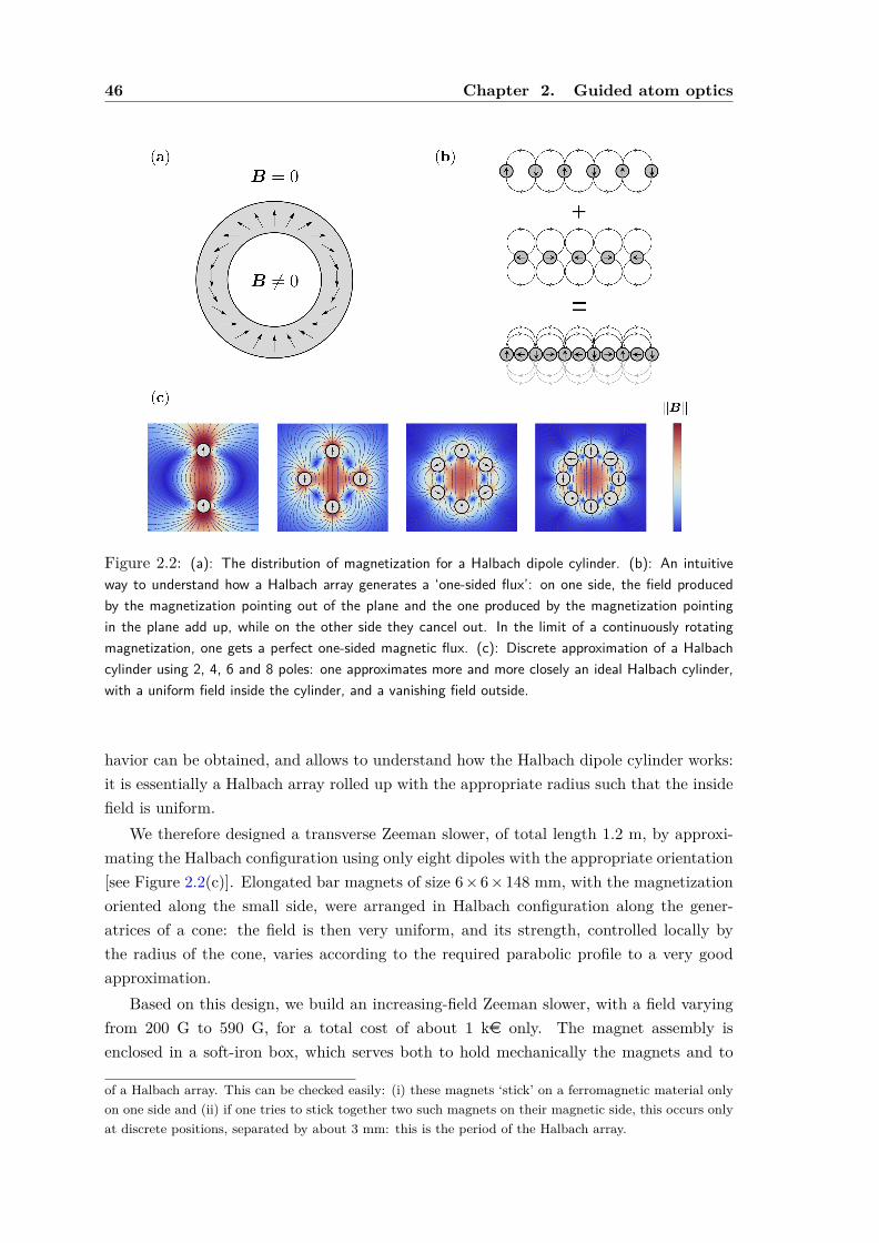
46 Chapter 2. Guided atom optics
Figure 2.2: (a): The distribution of magnetization for a Halbach dipole cylinder. (b): An intuitiveway to understand how a Halbach array generates a ‘one-sided flux’: on one side, the field producedby the magnetization pointing out of the plane and the one produced by the magnetization pointingin the plane add up, while on the other side they cancel out. In the limit of a continuously rotatingmagnetization, one gets a perfect one-sided magnetic flux. (c): Discrete approximation of a Halbachcylinder using 2, 4, 6 and 8 poles: one approximates more and more closely an ideal Halbach cylinder,with a uniform field inside the cylinder, and a vanishing field outside.
havior can be obtained, and allows to understand how the Halbach dipole cylinder works:it is essentially a Halbach array rolled up with the appropriate radius such that the insidefield is uniform.
We therefore designed a transverse Zeeman slower, of total length 1.2 m, by approxi-mating the Halbach configuration using only eight dipoles with the appropriate orientation[see Figure 2.2(c)]. Elongated bar magnets of size 6×6×148 mm, with the magnetizationoriented along the small side, were arranged in Halbach configuration along the gener-atrices of a cone: the field is then very uniform, and its strength, controlled locally bythe radius of the cone, varies according to the required parabolic profile to a very goodapproximation.
Based on this design, we build an increasing-field Zeeman slower, with a field varyingfrom 200 G to 590 G, for a total cost of about 1 ke only. The magnet assembly isenclosed in a soft-iron box, which serves both to hold mechanically the magnets and to
of a Halbach array. This can be checked easily: (i) these magnets ‘stick’ on a ferromagnetic material onlyon one side and (ii) if one tries to stick together two such magnets on their magnetic side, this occurs onlyat discrete positions, separated by about 3 mm: this is the period of the Halbach array.
2.3 A Bragg reflector for guided matter waves 47
avoid the leakage of stray magnetic fields outside the slower. An extra advantage of thisapproach is that the slower, made in two parts, can be fitted around the vacuum chamberafter the bake-out, allowing for high-temperature baking. We tested the slower not onlyby demonstrating the slowing down of an atomic beam, but also by loading a magneto-optical trap, with loading rates exceeding 1010 at/s when about 100 mW of cycling lightand 10 mW of repumper are used4. The results are detailed in [22]. Our design hasrecently been adapted for Sodium atoms, in an experiment under construction in the teamof Aurélien Perrin at LPL in Villetaneuse, and is, at the time of writing, being tested [95].
2.3 A Bragg reflector for guided matter waves
A few years after the realization of Bose–Einstein condensation in alkali gases in 1995, sev-eral pioneering experiments demonstrated the outcoupling of matterwaves from a trappedBEC, realizing what was to become known as atom lasers [81, 3, 49, 17]. The obtainedatom lasers were pulsed ones, with initially short bursts of atoms, and in later experimentsmuch longer pulses, with durations of up to ∼ 100 ms, that were called quasi-continuousatom lasers. In those beautiful illustrations of the wave nature of atoms, the outcoupledmatterwave was (i) propagating in free space, and (ii) falling under the influence of grav-ity. Both aspects are drawbacks in view of atom-optic experiments, as (i) gives rise to adecrease in brightness, while (ii) rapidly makes the de Broglie wavelength of the atomsvery small.
Therefore, in a second generation of experiments, the idea emerged to use an horizontaldipole trap beam as a waveguide for matterwaves, to keep the wave transversely confined,and prevent at the same time the acceleration of the atoms due to gravity. In the pioneeringwork of [47], atoms were outcoupled from a magnetic trap using a RF knife to transferthem to a magnetically-insensitive state, and then guided horizontally. This configuration,where light guides a wave of matter, realizes the complete opposite of the (much moreusual) guiding of light waves by matter along an optical fiber.
David Guéry-Odelin’s group at ENS had been pursuing for several years the studyof evaporative cooling of a magnetically guided atomic beam in view of achieving theoperation of a truly CW atom laser. Despite the achievement of the collisional regime forthe beam [73] and the demonstration of a gain of ten in phase-space density by RF-inducedevaporation [74], it appeared that the achievement of a CW atom laser by evaporation ofa beam would be extremely challenging technically. At about the time when I left ENS forStuttgart, it was thus decided to reorient the activities of the group towards the study ofguided, quasi-continuous atom lasers. An all-optical BEC of 87Rb was first obtained in acrossed optical dipole trap, and outcoupling was achieved by controlled spilling of the BECin the horizontal dipole trap beam. The group demonstrated that a careful control of theoutcoupling process allowed to obtain guided atom lasers with very few excited transverse
4The repumper frequency is swept at ∼ 10 kHz over a range of ∼ 2 GHz (otherwise, to get the sameflux out of the slower, higher repumping powers, on the order of 50 mW, are needed).

48 Chapter 2. Guided atom optics
Figure 2.3: (a): Bragg reflection on a sinusoidal grating. (b) Transmission coefficient through a800-site lattice, as a function of the incident velocity v and of the lattice depth U0. The white arrowsshow the Bragg condition v = nvr/2 obtained in the limit of a shallow lattice. (c) Atomic density alongthe guide after a propagation time tprop: experimental result (top panel) and simulation without anyadjustable parameter (bottom panel). The position of the Bragg reflector is shown by the white dashedline.
modes [28], i.e. a quasi-single-mode guided atom laser. The next logical step was then toimplement some atom-optical equivalents of mirrors, beamsplitters. . . .
In Toulouse, it was thus decided to pursue the exploration of guided atom optics,by trying to realize one of the simplest non-trivial atom-optical element, namely a dis-tributed Bragg reflector. Bragg mirrors and beamsplitters realized with optical standingwaves have been the workhorse of atom interferometry for three decades since their firstdemonstration in the 1980s [78]. Here, we studied how a matterwave packet interacts withan attractive periodic potential, of depth U0, and spacing d, obtained by superimposing aone-dimensional optical lattice along the axis of the guiding beam.
The presence of the lattice introduces a typical velocity scale, the recoil velocity vr =h/(md), and an energy scale Er = mv2
r /2. In usual atom-optics experiments with relativelyfast atoms, the periodic potential experienced by the atoms is very shallow as comparedto their kinetic energy, and reflection is obtained for the usual Bragg condition
2d sin θ = nλ, (2.2)
where n is an integer, d is the lattice spacing, and λ = h/(mv) is the de Broglie wavelengthof the particle, which impinges on the lattice at an angle θ (see Figure 2.3a). Here, weconsider a distributed Bragg reflector with the periodic modulation along the propagationaxis (θ = π/2), so the Bragg condition (2.2) reads simply v = nvr/2.
In our case, we deal with an ultraslow ‘beam’, and we thus need to revisit Braggreflection for lattice potentials that can be deep with respect to the kinetic energy of theincident particles. Figure 2.3b shows the calculated transmission coefficient for a 800-sitelattice, as a function of its depth U0 (in units of Er) and of the velocity v (in units ofvr) of the incident particle. For vanishing U0, one recovers full reflection when the Braggcondition v = nvr is fulfilled (white arrows). However, for a finite depth of the lattice,
2.4 Prospects 49
the transmission coefficient needs to be calculated by solving the Shrödinger equation ina sinusoidal potential. The Bloch theorem applies, and depending whether the incidentenergy lies within an allowed band or within a gap, the particle is transmitted or not. Foran infinite lattice, one thus expects the transmission coefficient to be either 0 or 1, and, inthe parameter plane (v, U0), the boundaries between the two situations can be obtainedby solving the Mathieu equation (dashed lines in Figure 2.3b). For a lattice with a finitenumber of sites, boundary effects change the picture only marginally at low velocities.
We experimentally implemented a Bragg reflector by intersecting two beams at anangle of about 80, thus making a longitudinal, one-dimensional lattice along the guide,with a lattice spacing of 650 nm and a Gaussian envelope with a 145 µm rms half-width.We produced an all-optical BEC 350 µm upstream, released it in the guide, and then gaveit a kick with a pulsed magnetic gradient, thus imparting it an initial mean velocity of10 to 15 mm/s. The wavepacket had a velocity dispersion of about 1.3 mm/s set by therepulsive interactions during the initial release of the BEC. The top panel of Figure 2.3cshows the atomic density along the guide, for increasing propagation times. On observesthat, when interacting with the lattice, the leading edge of the wavepacket (correspondingto high velocity components) is transmitted, while the trailing edge is reflected. The Braggreflector thus acts as a dichroic mirror for matter waves, with a sharp cutoff in velocityspace. The bottom panel is the result of a simulation of the time-dependent Schödingerequation without any adjustable parameter, and shows good agreement with the data. Wealso studied systematically the transmission of the reflector as a function of the depth ofthe optical lattice, and found good agreement with simulations.
2.4 Prospects
At the end of my time in Toulouse, we worked on a generalization of the Bragg reflector,using a time-dependent lattice: when its amplitude is modulated at a high frequency,new velocity classes can be reflected. We used this to demonstrate the principle of anotch velocity filter allowing to select very narrow velocity classes in a guided expandingcloud [24]. In another follow-up experiment, the team demonstrated the trapping of alaunched BEC in the lattice, with the periodic emission, via tunelling, of wavepacketswith a narrow velocity distribution [23].
In the future, it would be interesting to extend these studies along two directions:
• In the experiments described above, the effects of interparticle interactions are neg-ligible. A first subject of study would thus concern the propagation of matter wavestreams in the presence of significant interparticle interactions. In this case of non-linear guided atom optics, new interesting effects appear [84].
• The other natural extension of those studies would consist in going beyond proof-of-principle experiments, towards useful applications. An appealing experiment wouldconsist in realizing a matterwave interferometer using optically guided atoms, for
instance in a Mach–Zehnder geometry as proposed in [64]. For such studies, theintegrated matter wave circuits recently demonstrated in [108] appear as an idealplatform.
For both goals, the current setup is not well adapted: a more stable experiment, withmuch more optical access, is needed. Therefore the group is currently working on a newsetup, specially designed to overcome the above-mentioned shortcomings [12].
2.5 Published articles
Here, I list the articles I have co-authored about my work in LCAR; the main ones arereproduced in the following pages.
• C.M. Fabre et al., Phys. Rev. Lett. 107, 230401 (2011), reproduced on page 51.
• P. Cheiney et al., Rev. Sci. Inst. 82 063115 (2011) reproduced on page 56.
• P. Cheiney et al., Phys. Rev. A. 87, 013623 (2013).
50
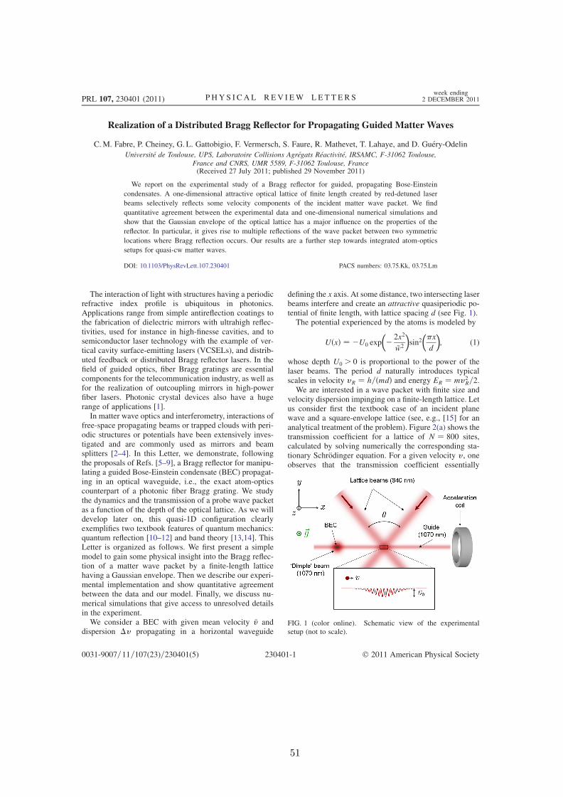
Realization of a Distributed Bragg Reflector for Propagating Guided Matter Waves
C.M. Fabre, P. Cheiney, G. L. Gattobigio, F. Vermersch, S. Faure, R. Mathevet, T. Lahaye, and D. Guery-Odelin
Universite de Toulouse, UPS, Laboratoire Collisions Agregats Reactivite, IRSAMC, F-31062 Toulouse,France and CNRS, UMR 5589, F-31062 Toulouse, France(Received 27 July 2011; published 29 November 2011)
We report on the experimental study of a Bragg reflector for guided, propagating Bose-Einstein
condensates. A one-dimensional attractive optical lattice of finite length created by red-detuned laser
beams selectively reflects some velocity components of the incident matter wave packet. We find
quantitative agreement between the experimental data and one-dimensional numerical simulations and
show that the Gaussian envelope of the optical lattice has a major influence on the properties of the
reflector. In particular, it gives rise to multiple reflections of the wave packet between two symmetric
locations where Bragg reflection occurs. Our results are a further step towards integrated atom-optics
setups for quasi-cw matter waves.
DOI: 10.1103/PhysRevLett.107.230401 PACS numbers: 03.75.Kk, 03.75.Lm
The interaction of light with structures having a periodicrefractive index profile is ubiquitous in photonics.Applications range from simple antireflection coatings tothe fabrication of dielectric mirrors with ultrahigh reflec-tivities, used for instance in high-finesse cavities, and tosemiconductor laser technology with the example of ver-tical cavity surface-emitting lasers (VCSELs), and distrib-uted feedback or distributed Bragg reflector lasers. In thefield of guided optics, fiber Bragg gratings are essentialcomponents for the telecommunication industry, as well asfor the realization of outcoupling mirrors in high-powerfiber lasers. Photonic crystal devices also have a hugerange of applications [1].
In matter wave optics and interferometry, interactions offree-space propagating beams or trapped clouds with peri-odic structures or potentials have been extensively inves-tigated and are commonly used as mirrors and beamsplitters [2–4]. In this Letter, we demonstrate, followingthe proposals of Refs. [5–9], a Bragg reflector for manipu-lating a guided Bose-Einstein condensate (BEC) propagat-ing in an optical waveguide, i.e., the exact atom-opticscounterpart of a photonic fiber Bragg grating. We studythe dynamics and the transmission of a probe wave packetas a function of the depth of the optical lattice. As we willdevelop later on, this quasi-1D configuration clearlyexemplifies two textbook features of quantum mechanics:quantum reflection [10–12] and band theory [13,14]. ThisLetter is organized as follows. We first present a simplemodel to gain some physical insight into the Bragg reflec-tion of a matter wave packet by a finite-length latticehaving a Gaussian envelope. Then we describe our experi-mental implementation and show quantitative agreementbetween the data and our model. Finally, we discuss nu-merical simulations that give access to unresolved detailsin the experiment.
We consider a BEC with given mean velocity v anddispersion v propagating in a horizontal waveguide
defining the x axis. At some distance, two intersecting laserbeams interfere and create an attractive quasiperiodic po-tential of finite length, with lattice spacing d (see Fig. 1).The potential experienced by the atoms is modeled by
UðxÞ ¼ U0 exp
2x2
~w2
sin2
x
d
; (1)
whose depth U0 > 0 is proportional to the power of thelaser beams. The period d naturally introduces typicalscales in velocity vR ¼ h=ðmdÞ and energy ER ¼ mv2
R=2.We are interested in a wave packet with finite size and
velocity dispersion impinging on a finite-length lattice. Letus consider first the textbook case of an incident planewave and a square-envelope lattice (see, e.g., [15] for ananalytical treatment of the problem). Figure 2(a) shows thetransmission coefficient for a lattice of N ¼ 800 sites,calculated by solving numerically the corresponding sta-tionary Schrodinger equation. For a given velocity v, oneobserves that the transmission coefficient essentially
FIG. 1 (color online). Schematic view of the experimentalsetup (not to scale).
PRL 107, 230401 (2011) P HY S I CA L R EV I EW LE T T E R Sweek ending
2 DECEMBER 2011
0031-9007=11=107(23)=230401(5) 230401-1 2011 American Physical Society
51

switches between 0 and 1 as a function of the depth of thelattice U0. It can be interpreted as follows. At the entrance,the incoming state of energy Ei ¼ mv2=2 is projected ontothe eigenstates of the lattice. The associated eigenenergiesdistribute into energy bands [13] whose position can beexpressed in terms of the characteristic functions of theMathieu equation [16,17] as depicted by the white dashedlines in Fig. 2(a). Reflection occurs if Ei lies in the gapbetween two allowed energy bands. Because of the finitelength of the lattice the energy bands are not strictlycontinuous and resolve into N separate states for vanishingincident velocity [17]. Undersampling of the image givesrise to the ‘‘foamy’’ aspect of the low-velocity side oftransmission bands. Obviously, the reflection by an attrac-tive potential is a purely quantum effect, with no classicalcounterpart.
A second interesting feature appears in the limit of avanishing potential depth U0. One still observes reflectionbut it occurs only for incident velocities of the form v ¼nvR=2 where n is an integer [see the white arrows inFig. 2(a)]. This corresponds to Bragg’s condition2d sin ¼ n [14], where ¼ =2 for retroreflection,and ¼ h=ðmvÞ is the incident de Broglie wavelength ofthe atoms: the reflection amplitude at each lattice site issmall, but constructive interference between all the re-flected waves results in a macroscopic reflected wavebuilding up. For the range of parameters of Fig. 2(a),quantum reflection by a single lattice well occurs onlyfor velocities that are very small as compared to vR [17]and thus cannot explain the observed features.
Figure 2(b) shows the result of the same calculation, butnow for the experimentally relevant case of a lattice having
a smooth Gaussian envelope. One clearly observes adrastic change in the dependence of the transmission co-efficient: for a fixed velocity v, the transmission is essen-
tially equal to one only below a critical value Uð1Þ0 of the
lattice depth, and then goes essentially to zero for increas-ing U0 (except for very narrow resonances). That criticalvalue corresponds to the smallest one at which total reflec-tion would occur for the square-envelope lattice. Almost noresurgence of the transmission is observed if U0 is furtherincreased, which gives a ‘‘sawtooth’’ appearance to theboundary between reflection and transmission.This can be understood as follows. We are in the slowly
varying envelope limit as ~w d. The amplitude of thelattice does not change appreciably over a few sites, andthus one can consider that, locally, the matter wave inter-
acts with a constant-amplitude lattice. WhenU0 ¼ Uð1Þ0 the
reflection condition is met at the center of the lattice, i.e.,at x ¼ 0. Then, for higher values of U0, there aresome locations xrefl, on both sides of the center, for
which UðxreflÞ ¼ Uð1Þ0 . In this case, reflection occurs at
x ¼ xrefl. If there were not a second, identical mirror atx ¼ xrefl, the transmission of the lattice would strictly
vanish for U0 >Uð1Þ0 . However, as in optics, the two local
Bragg mirrors actually constitute a Fabry-Perot resonator,analog to a VCSEL cavity for example, and transmissionexhibits sharp resonances which gives the same foamyaspect as in Fig. 2(a).We now come to the experimental realization. Our tech-
nique to produce all-optical BECs has been described indetail elsewhere [18]; in what follows we thus simply recallthe major steps. We produce an almost pure 87Rb conden-sate containing typically 5 104 atoms by forced evapo-ration over 4 s in a crossed optical dipole trap. It is made oftwo intersecting beams with a wavelength of 1070 nm. Ahorizontal one, with a waist of 50 m, to be used later as aguide for the BEC, defines the x direction. The second, the‘‘dimple’’ beam, of waist 150 m, propagates along thediagonal in the (x; z) plane, z being the vertical (Fig. 1).Spin distillation using a magnetic field gradient duringevaporation [18] results in the BEC being prepared in thestate jF ¼ 1; mF ¼ 0i. We then decrease adiabatically thepower in the dimple beam by a factor20 over 80 ms, thusbarely keeping a longitudinal confinement for the BEC,before switching it off abruptly to outcouple a wave packetin the horizontal guide. In this way, we produce a wavepacket with a minimal intrinsic longitudinal velocity dis-persion [19,20]. To set the wave packet in motion, we thenswitch on a coil, coaxial with the guide, that produces aninhomogeneous magnetic field. Through the quadraticZeeman effect the wave packet is accelerated in 15 ms toa final mean velocity v ¼ 11 mm=s. The residual accel-eration of the packet due to stray fields and beam curvatureis negligible (we measure an upper bound of 10 mm=s2).Centered 350 m downstream from the dimple location
x0, the optical lattice is produced at the intersection of two
FIG. 2 (color online). Intensity transmission coefficient of thelattice for an incident plane wave of velocity v, as a function ofthe lattice depth U0. (a) Square-envelope lattice with 800 sites.The white dashed lines are obtained from the Mathieu character-istic functions; white arrows show the velocities for which theBragg condition is fulfilled (see text). (b) Lattice with a Gaussianenvelope (1=e2 radius ~w ’ 230d). The vertical shaded stripecorresponds to the relevant velocity components in the wavepacket used for the measurements shown in Figs. 3 and 4. Theinsets on top of (a) and (b) illustrate the shape of the latticeenvelope, but the number of sites is reduced to N ¼ 20 forclarity.
PRL 107, 230401 (2011) P HY S I CA L R EV I EW LE T T E R Sweek ending
2 DECEMBER 2011
230401-2
52

beams with a wavelength L ¼ 840 nm (red-detuned withrespect to the 87Rb D1 and D2 lines) and a waist w ¼110 m, linearly polarized along z, crossing at an angle ’ 81. The lattice detuning is large enough so thatspontaneous emission does not play any role in our experi-mental time scales. The resulting lattice spacing is d ¼L=½2 sinð=2Þ ’ 650 nm, and the envelope 1=e2 radius is~w ¼ w= cosð=2Þ ’ 145 m. In a set of preliminary ex-periments we calibrate the potential depth U0 usingKapitza-Dirac (KD) diffraction [21,22]. A BEC is createdat the position of the lattice and exposed to the latticepotential for a short time KD, typically a few tens ofmicroseconds. The diffraction pattern of the BEC aftertime of flight as a function of KD is then compared tonumerical simulations of the process. A typical 35 mW perbeam results in U0 up to 15ER.
After being launched as described above, the wavepacket propagates in the horizontal guide for an adjustabletime tprop. Then all the lasers are switched off abruptly and
the cloud is imaged by absorption after a 10 ms time offlight. This gives access to the spatial density distributionnðx; tÞ ¼ jc ðx; tÞj2 of the wave packet with a resolution ofabout 10 m limited by the numerical aperture of ourcollection lens.
In a first set of experiments, the propagation time tprop ¼100 ms is sufficiently long so that the interaction with thelattice is completed. We measured in a separate experimentthe mean velocity v ’ 11 mm=s ’ 1:6vR and a rms veloc-ity spread v ’ 1:3 mm=s ’ 0:2vR corresponding to theshaded region of Fig. 2(b). For each lattice depth U0, anaverage image is generated from eight individual runs andthen integrated along the transverse direction y. Figure 3(a)is a stack of 55 such profiles. For sake of comparison,Fig. 3(b) is the result of a numerical simulation of the
wave packet dynamics using the one-dimensionalSchrodinger equation solved by the split-Fourier method;the initial condition is a Gaussian wave packet with theexperimentally measured momentum and position disper-sions [19]. There is no adjustable parameter and the overallagreement with experimental data means that our simple1D model captures most of the physics involved.Let us concentrate first on the transmitted part of the
wave packet (x > 0). If there were no lattice, the propaga-tion time tprop is long enough so that the initial size of the
wave packet is negligible with respect to its size afterpropagation. The spatial distribution of the wave packetwould then be a direct mapping of its initial velocitydistribution fðvÞ: nðx; tpropÞ / f½ðx x0Þ=tprop.One can then understand intuitively the main features of
Fig. 3 for the scattering of a wave packet, from the trans-mission coefficients shown in Fig. 2(b) for a plane wave. Inthe background of the shaded area of Fig. 2(b) representingthe wave packet one can see the transmitted and reflectedcomponents. In the presence of the lattice, the reflectedpart propagates backwards and is located, for the propaga-tion time chosen here, at a symmetrical position. Thisexplains why the transmitted and reflected wave packetsappear like a complementary mirrored image of each other.The sawtoothlike boundary, reminiscent of the transmis-sion diagram, is a fingerprint of the band structure insidethe lattice. However, the effect of the lattice potential is notlimited to the one of the sinusoidal component, responsiblefor the Bragg reflection described above. The spatiallyaveraged attractive potential also accelerates the wavepacket. The white dotted line in Fig. 3(b) shows the finalposition of a classical particle starting with velocity v fromposition x0 and propagating for a time tprop, taking into
account its acceleration by the spatially averaged latticepotential. The fair agreement with the data indicates thatthe slight curvature in the position of the wave packet as afunction of U0 simply arises from this classical effect.Beyond studying the asymptotic scattering states, it is
also possible to visualize the dynamics of the interaction byvarying tprop. Figure 4(a) displays such a time sequence
that fairly compares to the numerical simulation depictedin the same conditions in Fig. 4(b). One clearly observesthe spreading of the incident wave packet over the wholelattice for 30 & tprop & 45ms and its subsequent splitting
into a reflected and a transmitted one. Unfortunately, thedetails of the inner dynamics are washed out by the freeexpansion of the wave packet during the time-of-flightsequence and the finite resolution of the imaging system.Numerical simulations, properly checked against
the previous experimental results, are useful here. InFig. 4(c) we have deliberately suppressed the time-of-flightperiod and enhanced the optical resolution and the contrastwith respect to Fig. 4(b): one then clearly observes mul-tiple reflections of some components of the wave packet atsymmetric positions xrefl, with decreasing amplitude at
FIG. 3 (color online). (a) Measured density distribution of thewave packet (of initial mean velocity v ¼ 11 mm=s) after apropagation time tprop ¼ 100 ms, for different lattice depths U0.
Each horizontal line is the average of typically eight absorptionimages integrated along the y direction. The vertical whitedashed line shows the position of the center of the lattice.(b) Results of the simulation without any adjustable parameters.The finite resolution of the imaging system ( 10 m) isincluded. The dotted line is the expected position of the centerof the wave packet according to classical dynamics (see text).
PRL 107, 230401 (2011) P HY S I CA L R EV I EW LE T T E R Sweek ending
2 DECEMBER 2011
230401-3
53

each bounce. This ‘‘cavity-ring-down’’ behavior explainsthe formation of structures in the transmitted and reflectedwave packets as observed in Fig. 4(a) and especially visibleas a parallel lower stripe in the transmitted wave packet for50 & tprop & 75 ms. However, experimentally, observing
several bounces is not possible here due to the smallnumber of atoms involved.
In the same way, in images such as Fig. 3 the reflectedwave packet appears to be relatively smooth. It is actuallynot the case, as can be seen in simulations with fullresolution (Fig. 5). The lattice acts as a matter waveinterference filter with very narrow features due to thehigh number of lattice sites (foamy zones of Fig. 2).
Until now we have used a simple one-dimensional de-scription of the system. However, the system is actually farfrom being one dimensional, since the transverse quantumof energy @!? ’ h 90 Hz is much smaller than thetypical longitudinal energy scales, typically by 2 ordersof magnitude. Our simple one-dimensional model agreeswell with the experimental results as shown above becausecouplings between longitudinal and transverse degrees offreedom are weak (they are due only to experimental
imperfections such as misalignments of the lattice beamswith respect to the guide, for instance); some transverseexcitations can nevertheless be observed on our data [see,e.g., the long wavelength dipole oscillations in Fig. 4(a),especially for tprop * 30 ms]. Stronger couplings would be
expected to significantly alter the scattering properties ofthe structure [23,24].In conclusion, we have studied in detail the scattering of
a guided matter wave by a finite-length optical lattice in theslowly varying envelope limit. The experiments can beinterpreted in the framework of a local band structure,and the whole lattice can be seen as a cavity based onBragg mirrors.Major improvements are expected with the use of high
numerical aperture optics [25,26]. Drastically reducing thelength ~w of the lattice and thus generating a structureconsisting of only a few sites, possibly with a shapedenvelope, one could tailor almost arbitrarily the matterwave filter response. The latter can also be altered usinga moving optical lattice [27,28]. The transmission band ofthe filter could then be adjusted at will. Such setups wouldprove useful in measuring, for instance, the coherencelength [29] of guided atom lasers [30–32]. In a differentdirection, it would be appealing to study the effect ofinteratomic interactions [33] on the propagation of thewave packet, with the possible appearance of soliton trains[34] or atom-blockade effects [35]. This regime could bereached by using much higher transverse frequencies forthe guide, in order to enhance the effects of nonlinearities.We thank I. Carusotto for useful discussions, and
acknowledge support from Agence Nationale de laRecherche (GALOP project), Region Midi-Pyrenees, andInstitut Universitaire de France.
[1] B. E. A. Saleh and M.C. Teich, Fundamentals ofPhotonics (Wiley InterScience, New York, 2007).
[2] A. D. Cronin, J. Schmiedmayer, and D. E. Pritchard, Rev.Mod. Phys. 81, 1051 (2009).
[3] D. E. Pritchard et al., Ann. Phys. (Leipzig) 10, 35 (2001).[4] S. L. Rolston and W.D. Phillips, Nature (London) 416,
219 (2002).
FIG. 4 (color online). Time sequence showing the scattering ofa wave packet with mean velocity v ’ 11 mm=s on the opticallattice forU0 ’ 11ER. The white dashed lines in (a) and (b) showthe position of the center of the lattice. The time interval betweensuccessive images is 1 ms. (a) Experimental data. (b) Simulation,taking into account the finite imaging resolution as well as thetime of flight (TOF) period. (c) Same as (b) but without TOF norreduced resolution; the color scale is nonlinear in order toenhance contrast.
FIG. 5 (color online). (a) Calculated density and (b) velocitydistribution of a wave packet of initial mean velocity v ¼11 mm=s after a propagation time tprop ¼ 100 ms with full
resolution. The lattice depth is U0 ¼ 8ER.
PRL 107, 230401 (2011) P HY S I CA L R EV I EW LE T T E R Sweek ending
2 DECEMBER 2011
230401-4
54

[5] L. Santos and L. Roso, J. Phys. B 30, 5169 (1997).[6] L. Santos and L. Roso, Phys. Rev. A 58, 2407 (1998).[7] N. Friedman, R. Ozeri, and N. Davidson, J. Opt. Soc. Am.
B 15, 1749 (1998).[8] I. Carusotto, M. Artoni, and G. C. La Rocca, Phys. Rev. A
62, 063606 (2000).[9] T. Lauber et al., J. Phys. B 44, 065301 (2011).[10] C. Cohen-Tannoudji, B. Diu, and F. Laloe, Quantum
Mechanics (Wiley, New York, 1977).[11] F. Shimizu, Phys. Rev. Lett. 86, 987 (2001).[12] T.A. Pasquini et al., Phys. Rev. Lett. 93, 223201 (2004).[13] C. Kittel, Introduction to Solid-State Physics (Wiley, New
York, 1953).[14] N.W. Ashcroft and N.D. Mermin, Solid State Physics
(Saunders, Philadelphia, PA, 1976).[15] D.W. L. Sprung, H. Wu, and J. Martorell, Am. J. Phys. 61,
1118 (1993).[16] N.W. McLachlan, Theory and Application of Mathieu
Functions (Oxford University Press, Oxford, 1947).[17] See Supplemental Material at http://link.aps.org/
supplemental/10.1103/PhysRevLett.107.230401 for moredetails.
[18] A. Couvert et al., Europhys. Lett. 83, 50001 (2008).[19] Nonlinearities due to atom-atom interactions are negli-
gible for the dilute wave packets studied here, and thus arenot accounted for in the simulation (the chemical potentialof the BEC when it reaches the lattice is on the orderof 0:1ER, and thus negligible as compared to any
longitudinal energy scale). The only effect of interactionsis to set (in addition to the quantum pressure) the velocitydispersion of the wave packet in the initial stages of theexpansion in the guide, by conversion of the interactionenergy of the BEC into kinetic energy. For more details,see [20].
[20] F. Vermersch et al., Phys. Rev. A 84, 043618 (2011).[21] B. Gadway et al., Opt. Express 17, 19173 (2009).[22] J. H. Huckans et al., Phys. Rev. A 80, 043609 (2009).[23] G. L. Gattobigio, A. Couvert, B. Georgeot, and D. Guery-
Odelin, New J. Phys. 12, 085013 (2010).[24] G. L. Gattobigio, A. Couvert, B. Georgeot, and D. Guery-
Odelin, arXiv:1105.1971.[25] Y. R. P. Sortais et al., Phys. Rev. A 75, 013406 (2007).[26] K. Henderson et al., New J. Phys. 11, 043030 (2009).[27] L. Fallani et al., Phys. Rev. Lett. 91, 240405 (2003).[28] B. Eiermann et al., Phys. Rev. Lett. 91, 060402
(2003).[29] M. Kohl, T.W. Hansch, and T. Esslinger, Phys. Rev. Lett.
87, 160404 (2001).[30] W. Guerin et al., Phys. Rev. Lett. 97, 200402 (2006).[31] J. Billy et al., Ann. Phys. (Paris) 32, 17 (2007).[32] A. Bernard et al., New J. Phys. 13, 065015 (2011).[33] O. Morsch and M.K. Oberthaler, Rev. Mod. Phys. 78, 179
(2006).[34] I. Carusotto, D. Embriaco, and G. C. La Rocca, Phys. Rev.
A 65, 053611 (2002).[35] I. Carusotto, Phys. Rev. A 63, 023610 (2001).
PRL 107, 230401 (2011) P HY S I CA L R EV I EW LE T T E R Sweek ending
2 DECEMBER 2011
230401-5
55

REVIEW OF SCIENTIFIC INSTRUMENTS 82, 063115 (2011)
A Zeeman slower design with permanent magnetsin a Halbach configuration
P. Cheiney,1,2 O. Carraz,1,2 D. Bartoszek-Bober,3 S. Faure,1,2 F. Vermersch,1,2
C. M. Fabre,1,2 G. L. Gattobigio,1,2 T. Lahaye,1,2 D. Guéry-Odelin,1,2 and R. Mathevet1,2,a)
1Université de Toulouse, UPS - 118 route de Narbonne, F-31062 Toulouse, France2CNRS, UMR 5589, Laboratoire Collisions Agrégats Réactivité, IRSAMC - F-31062 Toulouse, France3Marian Smoluchowski Institute of Physics, Jagiellonian University, Cracow, Poland
(Received 13 January 2011; accepted 28 May 2011; published online 29 June 2011)
We describe a simple Zeeman slower design using permanent magnets. Contrary to common wire-wound setups, no electric power and water cooling are required. In addition, the whole system can beassembled and disassembled at will. The magnetic field is however transverse to the atomic motionand an extra repumper laser is necessary. A Halbach configuration of the magnets produces a highquality magnetic field and no further adjustment is needed. After optimization of the laser parameters,the apparatus produces an intense beam of slow and cold 87Rb atoms. With typical fluxes of (1–5)×1010 atoms/s at 30 m s−1, our apparatus efficiently loads a large magneto-optical trap with morethan 1010 atoms in 1 s, which is an ideal starting point for degenerate quantum gas experiments.© 2011 American Institute of Physics. [doi:10.1063/1.3600897]
I. INTRODUCTION
Nowadays, many atomic physics experiments study oruse quantum degenerate gases for which a large initial sam-ple of cold atoms is required. A wide variety of experimen-tal techniques has been developed for slowing and coolingatoms. Many of them rely on the radiation pressure fromquasi-resonant light. In particular, since their first realization,1
Zeeman slowers have become very popular for loadingmagneto-optical traps (MOT). These cold atom reservoirs arethen an ideal starting point to implement other techniques forfurther cooling.
Recently, several Zeeman slowers using permanent mag-nets have been built2 following the proposal of Ref. 3 (seealso Ref. 4 for a somewhat different approach formerly used).Here, we present an alternative design based on a Halbachconfiguration5 of the magnets and demonstrate fully satisfac-tory operation. Before going into details, let us emphasizesome advantages of the setup: simple machining and construction, compact, and
light,6 no electric power consumption nor water cooling, high fields with excellent transverse homogeneity, very smooth longitudinal profile and low stray mag-netic fields, easy to assemble and disassemble without vacuumbreaking, e.g., for high-temperature baking out.
This paper is organized as follows. In Sec. II, we first givethe basics of the theoretical framework and then compare ourpermanent magnets approach with the usual wire-wound tech-nique. Then we collect in Sec. III some information on mag-nets, shields, field calculations, and measurements useful tocharacterize our setup described in Sec. IV. We subsequently
a)Electronic mail: [email protected].
detail in Sec. V the whole experimental apparatus before wefinally present the Zeeman slower performances in Sec. VI.
II. ZEEMAN SLOWERS DESIGNS
A. Notations and field specifications
In a Zeeman slower, atoms are decelerated by scatteringphotons from a near resonant counter propagating laser. LetOz denote the mean atom and light propagation axis, andμ the linewidth and magnetic moment of the atomic transi-tion, k the light wave vector, m the atomic mass, and v(z)the velocity at z of an atom entering the field at z = 0. Tokeep atoms on resonance, changes in the Doppler shift kv(z)are compensated for by opposite changes of the Zeeman ef-fect μB(z) in an inhomogeneous magnetic field B(z).7 Weuse an increasing field configuration8 for better performancewith 87Rb.
As the scattering rate cannot exceed /2, the maximumachievable acceleration is
amax =
2
¯k
m. (1)
To keep a safety margin, the ideal magnetic field profile Bid(z)is calculated for only a fraction η = 0.75 of amax. Energy con-servation reads v(z)2 = v(0)2 − 2ηamaxz so that
Bid(z) = Bbias + B(1 −√
1 − z/L), (2)
where the length of the apparatus is L = v(0)2/2ηamax andμB/¯ = kv(0) assuming v(L) v(0). Here, v(0) definesthe capture velocity as, in principle, all velocity classes be-low v(0) are slowed down to v(L). A bias field Bbias is addedfor technical reasons discussed later on (Sec. IV C 1). Tomatch the resonance condition, lasers must be detuned fromthe atomic transition by
δ0 ≈ μ(Bbias + B)/h. (3)
0034-6748/2011/82(6)/063115/7/$30.00 © 2011 American Institute of Physics82, 063115-1
Downloaded 30 Jun 2011 to 130.120.228.133. Redistribution subject to AIP license or copyright; see http://rsi.aip.org/about/rights_and_permissions
56
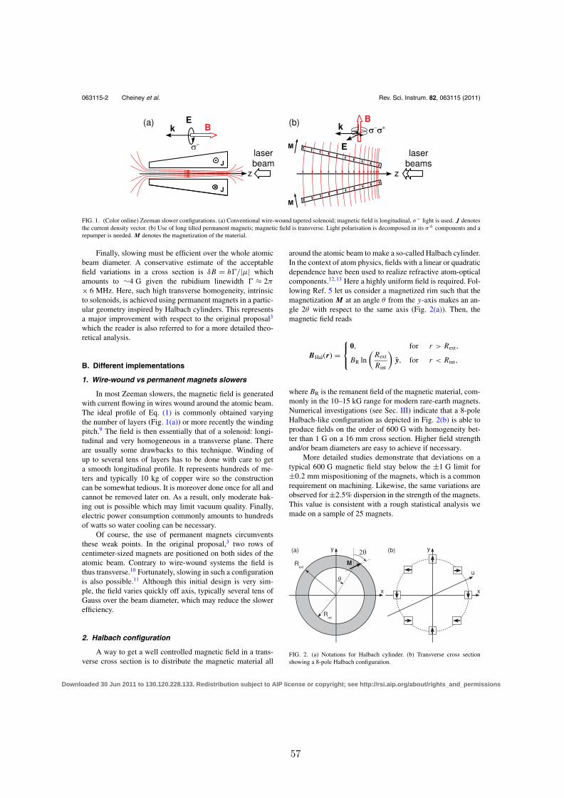
063115-2 Cheiney et al. Rev. Sci. Instrum. 82, 063115 (2011)
FIG. 1. (Color online) Zeeman slower configurations. (a) Conventional wire-wound tapered solenoid; magnetic field is longitudinal, σ− light is used. J denotesthe current density vector. (b) Use of long tilted permanent magnets; magnetic field is transverse. Light polarisation is decomposed in its σ± components and arepumper is needed. M denotes the magnetization of the material.
Finally, slowing must be efficient over the whole atomicbeam diameter. A conservative estimate of the acceptablefield variations in a cross section is δB = h/|μ| whichamounts to ∼4 G given the rubidium linewidth ≈ 2π
× 6 MHz. Here, such high transverse homogeneity, intrinsicto solenoids, is achieved using permanent magnets in a partic-ular geometry inspired by Halbach cylinders. This representsa major improvement with respect to the original proposal3
which the reader is also referred to for a more detailed theo-retical analysis.
B. Different implementations
1. Wire-wound vs permanent magnets slowers
In most Zeeman slowers, the magnetic field is generatedwith current flowing in wires wound around the atomic beam.The ideal profile of Eq. (1) is commonly obtained varyingthe number of layers (Fig. 1(a)) or more recently the windingpitch.9 The field is then essentially that of a solenoid: longi-tudinal and very homogeneous in a transverse plane. Thereare usually some drawbacks to this technique. Winding ofup to several tens of layers has to be done with care to geta smooth longitudinal profile. It represents hundreds of me-ters and typically 10 kg of copper wire so the constructioncan be somewhat tedious. It is moreover done once for all andcannot be removed later on. As a result, only moderate bak-ing out is possible which may limit vacuum quality. Finally,electric power consumption commonly amounts to hundredsof watts so water cooling can be necessary.
Of course, the use of permanent magnets circumventsthese weak points. In the original proposal,3 two rows ofcentimeter-sized magnets are positioned on both sides of theatomic beam. Contrary to wire-wound systems the field isthus transverse.10 Fortunately, slowing in such a configurationis also possible.11 Although this initial design is very sim-ple, the field varies quickly off axis, typically several tens ofGauss over the beam diameter, which may reduce the slowerefficiency.
2. Halbach configuration
A way to get a well controlled magnetic field in a trans-verse cross section is to distribute the magnetic material all
around the atomic beam to make a so-called Halbach cylinder.In the context of atom physics, fields with a linear or quadraticdependence have been used to realize refractive atom-opticalcomponents.12, 13 Here a highly uniform field is required. Fol-lowing Ref. 5 let us consider a magnetized rim such that themagnetization M at an angle θ from the y-axis makes an an-gle 2θ with respect to the same axis (Fig. 2(a)). Then, themagnetic field reads
BHal(r) =⎧⎨⎩
0, for r > Rext,
BR ln
(Rext
Rint
)y, for r < Rint,
where BR is the remanent field of the magnetic material, com-monly in the 10–15 kG range for modern rare-earth magnets.Numerical investigations (see Sec. III) indicate that a 8-poleHalbach-like configuration as depicted in Fig. 2(b) is able toproduce fields on the order of 600 G with homogeneity bet-ter than 1 G on a 16 mm cross section. Higher field strengthand/or beam diameters are easy to achieve if necessary.
More detailed studies demonstrate that deviations on atypical 600 G magnetic field stay below the ±1 G limit for±0.2 mm mispositioning of the magnets, which is a commonrequirement on machining. Likewise, the same variations areobserved for ±2.5% dispersion in the strength of the magnets.This value is consistent with a rough statistical analysis wemade on a sample of 25 magnets.
FIG. 2. (a) Notations for Halbach cylinder. (b) Transverse cross sectionshowing a 8-pole Halbach configuration.
Downloaded 30 Jun 2011 to 130.120.228.133. Redistribution subject to AIP license or copyright; see http://rsi.aip.org/about/rights_and_permissions
57
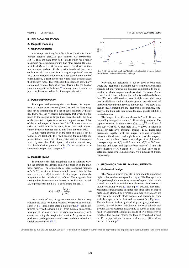
063115-3 Cheiney et al. Rev. Sci. Instrum. 82, 063115 (2011)
III. FIELD CALCULATIONS
A. Magnets modeling
1. Magnetic material
Our setup uses long 2a × 2b × 2c = 6 × 6 × 148 mm3
NdFeB magnets (HKCM, part number: Q148x06x06Zn-30SH). They are made from 30 SH grade which has a highermaximum operation temperature than other grades. Its rema-nent field BR = 10.8 kG is also lower. The device is thusmore compact and outer field extension is reduced. Such rare-earth material is very hard from a magnetic point of view sovery little demagnetization occurs when placed in the field ofother magnets, at least in our case where fields do not exceedthe kilogauss range. This makes field calculations particularlysimple and reliable. Even if an exact formula for the field ofa cuboid magnet can be found,14 in many cases, it can be re-placed with an ease to handle dipole approximation.
2. Dipole approximation
In the proposed geometry described below, the magnetshave a square cross section (2b = 2a) and the long mag-nets can be decomposed in a set of cubic magnets with side2a. Then, one easily checks numerically that when the dis-tance to the magnet is larger than twice the side, the fieldof the associated dipole is an accurate approximation of thatof the actual magnet to better than 2%.15 It is not a very re-strictive condition as in our case, 2a = 6 mm and magnetscannot be located nearer than 11 mm from the beam axis.
A full vector expression of the field of a dipole can befound in any textbook. It is well adapted for computer im-plementation. Even if the full magnetic system is then repre-sented by more than 1500 dipoles, calculations are still veryfast: the simulations presented in Sec. IV take less than 1 s ona conventional personal computer.14
B. Magnets layout
In principle, the field magnitude can be adjusted vary-ing the amount, the density and/or the position of the mag-netic material. The availability of very elongated magnets(c/a ≈ 25) directed us toward a simple layout. Only the dis-tance to the axis d(z) is varied. At first approximation, themagnets can be considered as infinite. The magnetic fieldstrength then decreases as the inverse of the distance squared.So, to produce the field B(z) a good ansatz for d(z) is
d(z) = d(L)
√B(L)
B(z). (4)
As a matter of fact, this guess turns out to be both veryefficient and close to a linear function. Numerical calculationsshow (Fig. 3) that a linear approximation of Eq. (4) can be op-timized to give a field within ±3 G from the ideal one over themost part of the slower. Such deviations are completely irrel-evant concerning the longitudinal motion. Magnets are thenpositioned on the generatrices of a cone and the mechanics isstraightforward (Sec. IV A).
FIG. 3. (Color online) Ideal (red/dotted) and calculated profiles, without(black/dashed) and with (blue/solid) end caps.
Naturally, the agreement is not so good at both endswhere the ideal profile has sharp edges, while the actual fieldspreads out and vanishes on distances comparable to the di-ameter on which magnets are distributed. The actual B isreduced which lowers the capture velocity and thus the beamflux. We made additional sections of eight extra cubic mag-nets in a Halbach configuration designed to provide localizedimprovement on the field profile at both ends (“end caps”). Asseen in Fig. 3, matching to the ideal profile is enhanced, espe-cially at the high field side where the ideal profile exhibits amarked increase.
The length of the Zeeman slower is L = 1184 mm cor-responding to eight sections of 148 mm-long magnets. Thecapture velocity is then v(0) = (2ηamaxL)1/2 ≈ 450 m s−1
and B = 388 G. A bias field Bbias = 200 G is added toavoid low-field level crossings around 120 G. These fieldparameters together with the magnet size and propertiesdetermine the distance and angle from axis of the magnets.In our case, the best choice was a slope of −15.9 mm/mcorresponding to d(0) = 49.5 mm and d(L) = 30.7 mm.Entrance and output end caps are both made of 10 mm-sidecubic magnets of N35 grade (BR = 11.7 kG). They are lo-cated on circles whose diameters are 94.0 mm and 66.0 mm,respectively.
IV. MECHANICS AND FIELD MEASUREMENTS
A. Mechanical design
The Zeeman slower consists in nine mounts supportingeight U-shaped aluminum profiles (Fig. 4). The U-shaped pro-files go through the mounts by means of square holes evenlyspaced on a circle whose diameter decreases from mount tomount according to Eq. (2) and Eq. (4) possibly linearized.Magnets are then inserted one after each other in the U-shapedprofiles and clamped by a small plastic wedge. End caps arefilled with the suitable block magnets and screwed togetherwith their spacer in the first and last mount (see Fig. 4(a)).The whole setup is then rigid and all parts tightly positioned.Indeed, as said before, calculations are very reliable andZeeman slower operation is known to be robust so there is noneed for adjustment. Mounts are made of two parts screwedtogether. The Zeeman slower can then be assembled aroundthe CF16 pipe without vacuum breaking, e.g., after bakingout the UHV setup.14
Downloaded 30 Jun 2011 to 130.120.228.133. Redistribution subject to AIP license or copyright; see http://rsi.aip.org/about/rights_and_permissions
58

063115-4 Cheiney et al. Rev. Sci. Instrum. 82, 063115 (2011)
(b) (c)
FIG. 4. (Color online) (a) Picture of the Zeeman slower: [M] mounts, [EC]output end cap screwed in last mount, [U] U-shaped profiles, [S] half part ofthe shield, [sp] 5 mm spacer between end cap and shield side. (b) Individualmount; [T] threading to screw the two parts of the mount together, [P] centralsquare milling in which CF16 pipe goes through. (c) Detail of a square holeto show U-shaped profiles insertion, magnets [m], and plastic wedge [W].Dimensions in mm.
B. Shielding
Stray magnetic fields might strongly affect atomicphysics experiments. Actually, the 8-pole configuration pro-duces very little field outside (see Fig. 6(a)), except of course,at both ends. However, to lower stray fields even further, wehave made a rectangular single-layer shield from a 1 mm-thick soft iron sheet wrapped around the mounts. Besides, me-chanical properties and protection are also improved. As seenin Fig. 5(a), the inner field is almost unaffected. On the con-trary, the outer magnetic field falls down much quicker all themore since the plateau around 0.5 G in Fig. 5(b) is probablyan artifact associated with the probe. In practice, no distur-bance is detected on the MOT and even on optical molasses125 mm downstream.14
C. Magnetic field and lasers characterization
1. Magnetic field
Magnetic field measurements are done with a home-made 3D probe using 3 Honeywell SS495 Hall effect
FIG. 5. (Color online) Calculated (red/gray) and measured (black) magneticfield profiles. (a) Scan along the beam axis. (b) Close up of the output region.In the calculation the shield is not taken into account. Dotted and dashed linesindicate the Zeeman slower and the shield physical ends. Log scale beforebreak.
FIG. 6. (a) Measured magnetic field without shield across the beam axis atz ∼ 460 mm along the u-direction of Fig. 2. (b) Close up of the central re-gion. Dashed lines indicate the atom beam extension and a 1 G magnetic fieldspan. Line to guide the eye. Log scale before break. The shield was removedto allow the probe to go through. With the shield, the inner field is almostunaffected and the outer field is below the probe sensitivity.
sensors.14 Figure 5 displays a longitudinal scan of the mag-netic field on the axis of the Zeeman slower with end caps andshield. It can be first noticed that the longitudinal profile is in-trinsically very smooth as the magnets make a uniform mag-netized medium throughout the Zeeman slower. After calibra-tion of the magnetic material actual remanent field, deviationsfrom the calculated profile are less than a few Gauss. Besides,one usually observes only localized mismatches attributed tothe dispersion in the strength of the magnets. The shield in-put and output sides flatten the inner field at both ends. Ofcourse the effect decreases when they get further apart but theZeeman slower should not be lengthened too much. A 5 mmspacer (tag [sp] in Fig. 4) is a good trade-off. Then, the actualmagnetic field measured parameters are Bbias = 200 G andB = 350 G only slightly smaller than the calculated value.
Figure 6 depicts a transverse cut of the magnetic field. Itis realized along the u-direction of Fig. 2 near the middle ofthe Zeeman slower (z ∼ 460 mm). The shield was removedto allow the probe to go through. It exhibits the two expectedfeatures: (i) little outer field and (ii) highly homogeneous in-ner field. In the vicinity of the axis, the measured profile ishowever less flat than expected. This is mainly due to the fi-nite size of the probe. Anyway, magnetic field deviations staywithin a Gauss or so in the region of interest. With the shield,the outer field is below probe sensitivity.
2. Lasers
The Zeeman slower operates between the 52S1/2 and52 P3/2 states of 87Rb around λ = 780 nm (D2 line). Foran increasing-field Zeeman slower, a closed σ− transitionis required,8 F = 2, m F = −2 ↔ F ′ = 3, m F ′ = −3 in ourcase. However, the magnetic field is here perpendicular to thepropagation axis. Thus, any incoming polarization state pos-sesses a priori π and σ± components: it is not possible to cre-ate a pure σ− polarization state (see Fig. 1 and Ref. 16). In ad-dition to laser power losses, the π and σ+ components excitethe m F ′ = −2 and −1 states from which spontaneous emis-sion populates F = 1 ground state levels. Repumping light isthus necessary between the F = 1 and F ′ = 2 manifolds. Thedetrimental effect of the unwanted polarization components isminimized when the incoming polarization is perpendicular tothe magnetic field since there is no π contribution in that case.We measured a 20 (FWHM) acceptance for the polarizationalignment.
Downloaded 30 Jun 2011 to 130.120.228.133. Redistribution subject to AIP license or copyright; see http://rsi.aip.org/about/rights_and_permissions
59
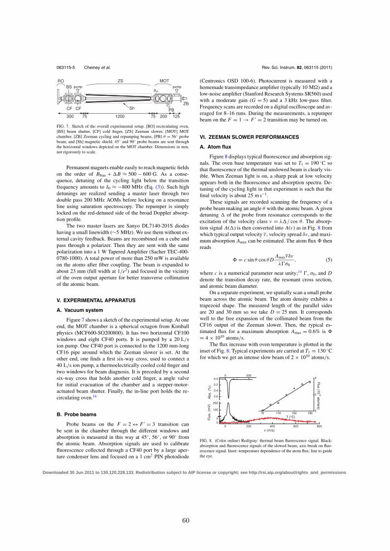
063115-5 Cheiney et al. Rev. Sci. Instrum. 82, 063115 (2011)
FIG. 7. Sketch of the overall experimental setup. [RO] recirculating oven,[BS] beam shutter, [CF] cold finger, [ZS] Zeeman slower, [MOT] MOTchamber, [ZB] Zeeman cycling and repumping beams, [PB] θ = 56 probebeam, and [Sh] magnetic shield. 45 and 90 probe beams are sent throughthe horizontal windows depicted on the MOT chamber. Dimensions in mm,not rigorously to scale.
Permanent magnets enable easily to reach magnetic fieldson the order of Bbias + B ≈ 500 − 600 G. As a conse-quence, detuning of the cycling light below the transitionfrequency amounts to δ0 ≈ −800 MHz (Eq. (3)). Such highdetunings are realized sending a master laser through twodouble pass 200 MHz AOMs before locking on a resonanceline using saturation spectroscopy. The repumper is simplylocked on the red-detuned side of the broad Doppler absorp-tion profile.
The two master lasers are Sanyo DL7140-201S diodeshaving a small linewidth (∼5 MHz). We use them without ex-ternal cavity feedback. Beams are recombined on a cube andpass through a polarizer. Then they are sent with the samepolarization into a 1 W Tapered Amplifier (Sacher TEC-400-0780-1000). A total power of more than 250 mW is availableon the atoms after fiber coupling. The beam is expanded toabout 23 mm (full width at 1/e2) and focused in the vicinityof the oven output aperture for better transverse collimationof the atomic beam.
V. EXPERIMENTAL APPARATUS
A. Vacuum system
Figure 7 shows a sketch of the experimental setup. At oneend, the MOT chamber is a spherical octagon from Kimballphysics (MCF600-SO200800). It has two horizontal CF100windows and eight CF40 ports. It is pumped by a 20 L/sion pump. One CF40 port is connected to the 1200 mm-longCF16 pipe around which the Zeeman slower is set. At theother end, one finds a first six-way cross, used to connect a40 L/s ion pump, a thermoelectrically cooled cold finger andtwo windows for beam diagnosis. It is preceded by a secondsix-way cross that holds another cold finger, a angle valvefor initial evacuation of the chamber and a stepper-motor-actuated beam shutter. Finally, the in-line port holds the re-circulating oven.14
B. Probe beams
Probe beams on the F = 2 ↔ F ′ = 3 transition canbe sent in the chamber through the different windows andabsorption is measured in this way at 45, 56, or 90 fromthe atomic beam. Absorption signals are used to calibratefluorescence collected through a CF40 port by a large aper-ture condenser lens and focused on a 1 cm2 PIN photodiode
(Centronics OSD 100-6). Photocurrent is measured with ahomemade transimpedance amplifier (typically 10 M) and alow-noise amplifier (Stanford Research Systems SR560) usedwith a moderate gain (G = 5) and a 3 kHz low-pass filter.Frequency scans are recorded on a digital oscilloscope and av-eraged for 8–16 runs. During the measurements, a repumperbeam on the F = 1 → F ′ = 2 transition may be turned on.
VI. ZEEMAN SLOWER PERFORMANCES
A. Atom flux
Figure 8 displays typical fluorescence and absorption sig-nals. The oven base temperature was set to T1 = 190 C sothat fluorescence of the thermal unslowed beam is clearly vis-ible. When Zeeman light is on, a sharp peak at low velocityappears both in the fluorescence and absorption spectra. De-tuning of the cycling light in that experiment is such that thefinal velocity is about 25 m s−1.
These signals are recorded scanning the frequency of aprobe beam making an angle θ with the atomic beam. A givendetuning of the probe from resonance corresponds to theexcitation of the velocity class v = λ/ cos θ . The absorp-tion signal A() is then converted into A(v) as in Fig. 8 fromwhich typical output velocity v , velocity spread δv , and maxi-mum absorption Amax can be estimated. The atom flux thenreads
= c sin θ cos θ DAmaxvδv
λσ0, (5)
where c is a numerical parameter near unity;14 , σ0, and Ddenote the transition decay rate, the resonant cross section,and atomic beam diameter.
On a separate experiment, we spatially scan a small probebeam across the atomic beam. The atom density exhibits atrapezoid shape. The measured length of the parallel sidesare 20 and 30 mm so we take D = 25 mm. It correspondswell to the free expansion of the collimated beam from theCF16 output of the Zeeman slower. Then, the typical es-timated flux for a maximum absorption Amax = 0.6% is
= 4 × 10¹⁰ atoms/s.The flux increase with oven temperature is plotted in the
inset of Fig. 8. Typical experiments are carried at T1 = 130 Cfor which we get an intense slow beam of 2 × 10¹⁰ atoms/s.
FIG. 8. (Color online) Red/gray: thermal beam fluorescence signal. Black:absorption and fluorescence signals of the slowed beam; axis break on fluo-rescence signal. Inset: temperature dependence of the atom flux; line to guidethe eye.
Downloaded 30 Jun 2011 to 130.120.228.133. Redistribution subject to AIP license or copyright; see http://rsi.aip.org/about/rights_and_permissions
60

063115-6 Cheiney et al. Rev. Sci. Instrum. 82, 063115 (2011)
FIG. 9. (a) Final velocity as a function of Zeeman cycling light detuning(I = 4.7 mW cm−2). Line: linear fit, the slope is 0.95 m s−1/MHz. (b) Atomflux as a function of final velocity.
Finally, we measured little influence of the entrance endcap on the atom flux and a moderate increase, 10 ± 5%, withthe output one.
B. Velocity distribution
Naturally, the Zeeman cycling light detuning strongly af-fects the atom beam velocity distribution (Fig. 9). A lineardependence of the final velocity in the detuning is observed.The actual slope is on the order of that expected from a simplemodel dv/dδ = 2π/k = 0.78 m s−1/MHz but slightly higherand intensity-dependent.17
Besides, the atom flux is roughly constant for final ve-locities above 40 m s−1. Below this value, the flux measuredin the chamber 125 mm downstream decreases. Indeed, thebeam gets more divergent and atoms are lost in collisions withthe walls of the vacuum chamber.
C. Needed laser powers
Figure 10 demonstrates that comparable amounts of cy-cling and repumper light are necessary. With a total power of100 mW we get a non-critical operation of the Zeeman slowerat its best flux and a final velocity of 30 m s−1, well suitedfor efficient MOT loading. The equivalent intensity is about24 mW cm−2. However, as we shall see now, a lot of powercan be saved with a more elaborate strategy.
D. Repumper
In the results reported until now, repumping and cyclinglight have the same polarization: linear and perpendicular to
FIG. 10. (Color online) (a) Atom flux as a function of cycling and repumperbeams powers. (b) Cross section along the white dotted line corresponding toa total available power of 100 mW. Power ratio is measured with a scanningFabry-Perot interferometer.
FIG. 11. (Color online) (a) Atom flux as a function of repumper frequency. f is the beat note frequency of the repumper with an auxiliary laser lockedon the F = 2 → F ′ = 3 resonance line; red/gray circles/black squares: re-pumper polarization perpendicular/parallel to the magnetic field. (b) Atomflux as a function of repumper power (log scale) when its frequency is fixed(black) or swept (red/gray) across the full spectrum of left panel.
the magnetic field, a state commonly referred to as linear σ
recalling that it is a superposition of σ± states.16 If no com-mon amplification in a tapered amplifier is used, polariza-tions are likely to be orthogonal. The repumper polarizationis then parallel to the magnetic field i.e., a π state. Whenthe repumper frequency is varied as in Fig. 11(a) very dif-ferent spectra for the two configurations are observed. Effi-cient repumping occurs with more or less well defined peaksspread over about 2 GHz and roughly centered around theF = 1 → F ′ = 2 transition. This means that several depump-ing/repumping pathways are involved, probably occurring atlocalized places along the Zeeman slower.
It is not easy to get a simple picture of what is happening:a complete ab initio simulation of the internal dynamics is notsimple due to the large number of Zeeman sublevels (24 in to-tal for all the ground and excited states), the multiple levelcrossings occurring in the 50–200 G range, and high lightintensities. However, one can overcome this intricate inter-nal dynamics by sweeping quickly (typically around 8 kHz)the repumper frequency over all the observed peaks. With alow-pass filter, the central frequency remains locked on theside of the Doppler profile. Doing so, we get a slightly higherflux for significantly less repumper power, typically 10 mW(Fig. 11(b)).
E. MOT loading
A final demonstration of the Zeeman slower efficiency isgiven by monitoring the loading of a MOT. It is made from3 retroreflected beams 28 mm in diameter (FW at 1/e2). Weuse 10–20 mW and 1–3 mW of cycling and repumper lightper beam. When the Zeeman slower is on with a final veloc-ity of 30 m s−1, a quasi-exponential loading is observed withcharacteristic time τ ∼ 320 ms for magnetic field gradientson the order of 15–20 G cm−1. After 1 s or so, the cloudgrowth is complete. From absorption spectroscopy, we de-duce a density n = 1.4 × 10¹⁰ atoms cm−3. The typical cloudsize is 12 mm so we estimate the atom number to be on theorder of N = 2 × 10¹⁰. These figures are consistent with theabove measurements of an atom flux of several 1010 atoms/sand nearly unity capture efficiency. As expected, thanks to thehigh magnetic field in the slower, the Zeeman beams are fardetuned and do not disturb the MOT.
Downloaded 30 Jun 2011 to 130.120.228.133. Redistribution subject to AIP license or copyright; see http://rsi.aip.org/about/rights_and_permissions
61
063115-7 Cheiney et al. Rev. Sci. Instrum. 82, 063115 (2011)
VII. CONCLUSION
We have presented a simple and fast to build, robustZeeman slower based on permanent magnets in a Halbachconfiguration. Detailed characterization shows it is anefficient and reliable source for loading a MOT with morethan 1010 atoms in 1 s. Without power nor cooling water con-sumption, the apparatus produces homogeneous and smoothhigh fields over the whole beam diameter and low strayfields. It also simplifies high-temperature bakeout. We thusbelieve it to be a very attractive alternative to wire-woundsystems.
ACKNOWLEDGMENTS
We thank J. M. Vogels for his major contribution to thedesign of the recirculation oven and D. Comparat for use-ful bibliography indications. This work was supported by theAgence Nationale pour la Recherche (ANR-09-BLAN-0134-01), the Région Midi-Pyrénées, and the Institut Universitairede France.
1W. D. Phillips and H. Metcalf, Phys. Rev. Lett. 48, 596 (1982).2Y. Ovchinnikov, J. McCelland, D. Comparat, and G. Reinaudi, privatecommunications (February 2011).
3Y. B. Ovchinnikov, Opt. Commun. 276, 261 (2007).4S. N. Bagayev, V. I. Baraulia, A. E. Bonert, A. N. Goncharov, M. R.Seydaliev, and A. S. Tychkov, Laser Phys. 11, 1178 (2001).
5K. Halbach, Nucl. Instrum. Methods 169, 1 (1980).61200 mm long, 120 × 130 mm2 cross section; dural holders, magnets andshield weights are, respectively, 5.0, 2.5, and 4.5 kg. It takes half a day ofwork to put parts together once machining is done.
7W. D. Phillips, Rev. Mod. Phys. 70, 721 (1998).8T. E. Barrett, S. W. Dapore-Schwartz, M. D. Ray, and G. P. Lafyatis, Phys.Rev. Lett. 67, 3483 (1991).
9S. C. Bell, M. Junker, M. Jasperse, L. D. Turner, Y.-J. Lin, I. B. Spielman,and R. E. Scholten, Rev. Sci. Instrum. 81, 013105 (2010).
10We could not find a configuration that produces a longitudinal magneticfield of several hundreds of Gauss with a reasonable amount of magneticmaterial.
11P. Melentiev, P. Borisov, and V. Balykin, JETP 98, 667 (2004).12W. G. Kaenders, F. Lison, I. Müller, A. Richter, R. Wynands, and D.
Meschede, Phys. Rev. A 54, 5067 (1996).13D. Patterson and J. M. Doyle, J. Chem. Phys. 126, 154307 (2007).14See supplementary material at http://dx.doi.org/10.1063/1.3600897 for
more information on the magnetic field for a cuboid calculation, the fluxcalculation, the oven design and for pictures of the setup. A movie of MOTloading, Mathematica programs for field calculations and technical draw-ings (.dxf) are available at http://www.coldatomsintoulouse.com/rm/.
15Convergence can be much slower for cuboids with different aspect ratios.16G. Grynberg, A. Aspect, and C. Fabre, Introduction to Quantum Optics,
From the Semi-classical Approach to Quantized Light (Cambridge Univer-sity Press, Cambridge, England, 2010).
17V. S. Bagnato, C. Salomon, E. J. Marega, and S. C. Zilio, J. Opt. Soc. Am.B 8, 497 (1991).
Downloaded 30 Jun 2011 to 130.120.228.133. Redistribution subject to AIP license or copyright; see http://rsi.aip.org/about/rights_and_permissions
62
Chapter 3
Arrays of single Rydberg atoms
J’entrai pas au crid’«À nous deux Paris »en Île-de-France. . . 1
3.1 Introduction
Over the last thirty years, tremendous progress has been done in the manipulation of singlequantum objects, such as single photons or single ions, allowing the actual realization inthe lab of what was considered as Gedankenexperimente by the founding fathers of quan-tum mechanics. These remarkable achievements were honored by the award of the NobelPrize in Physics in 2012 to Serge Haroche and David Wineland [51, 132]. The degreeof control achieved nowadays, using a variety of different experimental platforms such astrapped ions, ultracold atoms, single photons, superconducting circuits, NV centers, quan-tum dots. . . , together with the motivation of applications such as quantum informationprocessing [89], quantum metrology [42], and quantum simulation [39], has given birthto a whole new field that can be called quantum engineering. Among all the exploredplatforms, the ones using Rydberg atoms appear to be extremely promising.
Rydberg states of atoms correspond to highly excited atomic states, with a principalquantum number n 1. This gives Rydberg atoms exaggerated properties. They havea size scaling as n2 and thus a very large electric dipole moment: the matrix element ofthe dipole moment operator between two adjacent states is on the order of n2ea0 wherea0 is the Bohr radius, and e the elementary charge. Moreover, they have long lifetimes(scaling as n3 for low angular momentum states). Rydberg atoms, due to their similaritieswith hydrogen, have played a very important role in the early days of quantum mechanicsand atomic physics. The advent of tunable lasers at the end of the seventies triggereda regain of interest in the physics of Rydberg atoms, which were an ideal testbed forstudying coherent interactions between atoms and the electromagnetic field [32]. Thissecond ‘golden age’ of Rydberg physics culminated in the cavity QED experiments by the
1Georges Brassens, Les ricochets (1976).
63
64 Chapter 3. Arrays of single Rydberg atoms
Haroche group [52], among others.Due to their very strong electric dipoles, two Rydberg atoms separated by a distance R
interact very strongly with each other via the dipolar interaction, either at first order (onethen deals with a resonant dipole-dipole interaction U = C3/R
3, where C3 scales as n4)or at second-order (in this case, one deals with the van der Waals interaction U = C6/R
6
where C6 scales as n11). Figure 3.1a, taken from Ref. [111], shows that interactions betweentwo Rydberg atoms with n ∼ 100 and separated by a few microns are about twelve ordersof magnitude higher than between ground-state atoms, reaching several MHz.
These exaggerated properties of Rydberg states are at the origin of the third ‘goldenage’ of Rydberg physics, which started some fifteen years ago. Pioneering proposals [58, 77]were put forward in the early 2000s’, following early experimental studies of interactionsin cold Rydberg gases [4, 85], and suggested to use cold Rydberg atoms for quantuminformation processing. The basic mechanism at work is the Rydberg blockade (figure 3.1b).Consider that for a single atom, one couples, using a resonant laser, the ground state |g〉to the Rydberg state |r〉 with a Rabi frequency Ω. Now suppose that two atoms are closeto each other, such that, due to interactions, the collective state |rr〉 undergoes a shiftU ~Ω. Then, when one shines the same resonant laser on the pair of atoms, the systemcan be resonantly excited from |gg〉 to |rg〉 or |gr〉, but a second excitation to |rr〉 is off-resonant and thus strongly suppressed: this is the essence of the Rydberg blockade. Onereadily shows that in this case, the system undergoes a collective Rabi oscillation, with anenhanced Rabi frequency Ω
√2, between |gg〉 and the entangled state
(|rg〉+ eiφ |gr〉
)/√
2(the phase φ has a well-defined value, that depends on the relative positions of the atomsand on the wavevectors of the lasers used for Rydberg excitation). This can be extendedto N atoms: if all atoms are close enough such that the interaction between any two atomsexceeds the single-atom Rabi coupling Ω (i.e. the sample size is smaller than the so-calledblockade radius), then the system oscillates at a frequency Ω
√N between the collective
ground state and a W-state where a single Rydberg excitation is delocalized over the Natoms.
Following these proposals, Rydberg blockade effects were experimentally observed incold atomic ensembles, first in MOTs [124, 120] and then in BECs [55] and optical lat-tices [115] (for a more complete list of references, see e.g. Refs. [26, 68]). However, insuch ensembles one deals in general with (i) a sample larger than the blockade radius, and(ii) with fluctuating atom numbers, which makes the observation of collective Rabi oscil-lations difficult. This was solved in 2009 by our group and by the group of Mark Saffman:using two individual atoms trapped by optical tweezers separated by a controlled distance,Rydberg blockade and collective enhancement were observed [38, 125]. These works weresoon extended by using the blockade to create entanglement of two atoms in the groundstate [131] and to realize a C–NOT gate [56].
Based on these successful demonstrations, it appeared very promising to try and extendthose studies to a larger number of individual atoms held in arrays of optical microtraps,thus creating an appealing platform not only for quantum information processing [111],
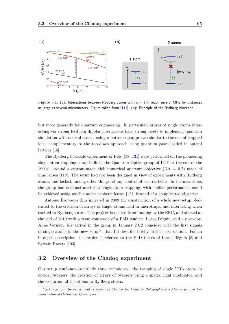
3.2 Overview of the Chadoq experiment 65
Figure 3.1: (a): Interactions between Rydberg atoms with n ∼ 100 reach several MHz for distancesas large as several micrometers. Figure taken from [111]. (b): Principle of the Rydberg blockade.
but more generally for quantum engineering. In particular, arrays of single atoms inter-acting via strong Rydberg dipolar interactions have strong assets to implement quantumsimulation with neutral atoms, using a bottom-up approach similar to the one of trappedions, complementary to the top-down approach using quantum gases loaded in opticallattices [16].
The Rydberg blockade experiment of Refs. [38, 131] were performed on the pioneeringsingle-atom trapping setup built in the Quantum Optics group of LCF at the end of the1990s’, around a custom-made high numerical aperture objective (NA = 0.7) made ofnine lenses [118]. The setup had not been designed in view of experiments with Rydbergatoms, and lacked, among other things, of any control of electric fields. In the meantime,the group had demonstrated that single-atom trapping, with similar performance, couldbe achieved using much simpler aspheric lenses [121] instead of a complicated objective.
Antoine Browaeys thus initiated in 2009 the construction of a whole new setup, ded-icated to the creation of arrays of single atoms held in microtraps, and interacting whenexcited to Rydberg states. The project benefited from funding by the ERC, and started atthe end of 2010 with a team composed of a PhD student, Lucas Béguin, and a post-doc,Aline Vernier. My arrival in the group in January 2012 coincided with the first signalsof single atoms in the new setup2, that I’ll describe briefly in the next section. For anin-depth description, the reader is referred to the PhD theses of Lucas Béguin [8] andSylvain Ravets [103].
3.2 Overview of the Chadoq experiment
Our setup combines essentially three techniques: the trapping of single 87Rb atoms inoptical tweezers, the creation of arrays of tweezers using a spatial light modulator, andthe excitation of the atoms to Rydberg states.
2In the group, the experiment is known as Chadoq, for Contrôle Holographique d’Atomes pour la Dé-monstration d’Opérations Quantiques.

66 Chapter 3. Arrays of single Rydberg atoms
Figure 3.2: (a): Schematic view of the experimental setup. (b): The fluorescence signal of a singleatom, showing a characteristic telegraph-like behavior. (c): A gallery of fluorescence signals correspond-ing to individual atoms trapped in arrays of optical tweezers created with the SLM.
Single-atom trapping
Figure 3.2(a) shows a schematic view of our experimental setup. The heart of the ma-chine consists of two commercial aspheric lenses (N.A. = 0.5, focal length 10 mm, workingdistance 7 mm) that are facing each other inside the vacuum chamber, and with whichwe focus a laser beam at 850 nm down to a 1/e2 radius of about 1 µm. This creates anoptical dipole trap, with a typical depth of about 1 mK for a power of about 3 mW. Thetransverse and longitudinal frequencies are about 80 kHz and 15 kHz respectively.
We load this conservative microtrap from a low-density optical molasses created aroundit. From time to time, an atom undergoing diffusion in the molasses enters the microtrapand is cooled down by the molasses beams while being captured in the tweezers, so thatit remains trapped there. Now, if a second atom enters the trap, a light-assisted collisionoccurs and results in the loss of both atoms; due to the small volume of the trap, this occurson a timescale of a few tens of microseconds, much faster than the rate of entry of atomsinto the tweezers at low molasses density. Therefore, observed with a time resolution ofseveral milliseconds, the trap occupation alternates randomly between zero and one: oneobtains a single-atom source, albeit a non-deterministic one, the probability for the trapto contain a single atom being 50%. The rate at which the toggling occurs can be variedeasily by varying the density of the optical molasses cloud (e.g. by adding a very weak
3.2 Overview of the Chadoq experiment 67
magnetic field gradient, turning the molasses into a low-density MOT).We observe this loading dynamics by collecting, using the same aspheric lens, the
fluorescence emitted at 780 nm by the atom, separating it from the trapping light with adichroic mirror, and imaging it on a sensitive detector. Figure 3.2(b) shows a typical signal,obtained by collecting the emitted photons for 20 ms on a fiberized avalanche photodiode.One observes two well-defined fluorescence levels, a low one and a high one, correspondingrespectively to the absence and to the presence of one atom in the microtrap. By defininga threshold, one thus unambiguously triggers an experimental sequence as soon as the trapis loaded.
Creating arrays of microtraps
In order to create arrays of optical tweezers, we use a spatial light modulator (SLM)to imprint an arbitrary phase on the trapping beam prior to focusing [92]. Despite thefact that the SLM only permits to manipulate the phase of the laser beam, and not itsamplitude, the use of the Gershberg-Saxton (GS) algorithm [40] allows one to obtaina good approximation of any desired target intensity pattern in the focal plane of thelens. This allows us to create arbitrary, two-dimensional arrays of microtraps as shownin figure 3.2(c). The versatility of the SLM is also used for improving the quality of ourarrays of traps [92]:
• Despite the care with which the optical setup was designed and built, we still havesmall residual optical aberrations, which degrade the quality of large arrays. Bymeasuring them using a Shack-Hartman sensor, and adding to the SLM phase patternthe opposite of the measured wavefront distortion, we drastically improve the qualityof the microtraps (in particular their depth).
• In large arrays, despite the fact that the target intensity corresponds to an array withall traps of the same intensity, the ones obtained in practice show a relatively largedispersion in the observed trap intensities (of up to a factor of two). This would provedetrimental for loading single atoms with 50% probability in the traps. We solvethis problem by implementing an active improvement of the uniformity of the arraysof traps. For a given array, we first calculate an initial phase pattern for the SLMusing the GS algorithm. We then measure, at the output of the vacuum chamber,the intensity of each tweezers on a CCD camera conjugated with the atoms’ plane.Some traps are too dim, while others are too intense. We use this information tocalculate a new target intensity, where the intensity of the traps that were previouslytoo intense is reduced, and vice-versa. We use this new target intensity as an inputfor the GS algorithm, while keeping, as the initial guess for the phase, the previouslycalculated grating. Iterating this procedure for about 20 times allows us to obtainfor instance arrays of 100 traps with an rms deviation of the intensities below 1.5%.
We thus have a very satisfactory way, using the SLM, to generate high quality, arbitrary2D arrays of microtraps. However, the SLM refreshing rate being of only a few tens

68 Chapter 3. Arrays of single Rydberg atoms
of Hz at most, these arrays are, for all practical purposes, static on the timescales of theexperiment. For many experiments however, it is desirable to have the possibility to singleout temporarily at least one atom among all the ones confined in the array. For thispurpose, we have included in our setup an extra addressing beam [66]. The principle isstraightforward: we superimpose onto the trapping beam an extra beam at 850 nm (with afrequency shift of a few hundreds of MHz with respect to the trap beam), whose intensityand position can be controlled fast using two crossed AOMs, and which is focused to a1/e2 radius of about 1.3 µm at the position of the atoms. This beam introduces an extralight shift on the selected atom when it is in the ground state, which can be used for manyapplications:
• We can selectively excite to Rydberg states either only the selected atom, either all ofthem but this one. In [66] we demonstrated this addressing, without any measurablecross-talk between atoms separated by 3 µm.
• We can manipulate collective quantum states. For instance, using the Rydbergblockade we first prepare two atoms in the ‘super-radiant’ state∣∣∣ψ+
⟩= |gr〉+ |rg〉√
2. (3.1)
We then illuminate the second atom with the addressing beam for a carefully chosentime so as it acquires a phase-shift of π when in |g〉 (the 850 nm beam induces anegligible light shift on the Rydberg state |r〉), and we thus obtain, again as shownin [66], the ‘sub-radiant’ state
∣∣ψ−⟩ = |gr〉 − |rg〉√2
. (3.2)
• Finally, we plan to use this addressing beam as a movable tweezers [11], that shouldallow us to drag atoms along in the array, for instance to sort out a disordered array.
Manipulating Rydberg atoms
For exciting the atoms to Rydberg states (figure 3.3(a)), we use a standard two-photontransition, with a first photon at 795 nm, detuned by ∆ = 2π × 740 MHz above the∣∣∣5S1/2, F = 2
⟩↔
∣∣∣5P1/2, F = 2⟩
line, and a second photon in the blue, at 474 nm, to
excite Rydberg states∣∣∣nD3/2,mj = 3/2
⟩(with 50 6 n 6 100). Both lasers are stabilized
using an ultrastable ULE cavity, resulting in a global linewidth that we estimate to beabout 30 kHz. The Rabi frequencies ΩR and ΩB on those two transitions are typically ofa few tens of MHz, resulting in an effective Rabi coupling Ω = ΩRΩB/(2∆) of typically1 MHz (beyond Rabi frequencies of 5 MHz, we start to suffer strongly from spontaneousemission from the intermediate 5P1/2 state).
We detect the successful Rydberg excitation of an atom in a rather crude, but actuallyquite effective, way: an atom excited to a Rydberg state with n > 50 has a radiative decay

3.2 Overview of the Chadoq experiment 69
Figure 3.3: (a): The two-photon Rydberg excitation scheme and an example of a single-atom Rabioscillation between the ground state and the Rydberg state
∣∣82D3/2,mj = 3/2⟩. (b): Finite-element
method simulation of the set of electrodes placed around the aspheric lenses. In the given configuration,we apply an electric field along the z-direction. (c): Rydberg blockade with two atoms separated by4 µm and excited to |r〉 =
∣∣62D3/2,mj = 3/2⟩. The top panel shows a Rabi oscillation for a single
atom, to calibrate the Rabi frequency Ω. The middle panel shows the probability Pgr + Prg to exciteonly one atom to the Rydberg state, clearly showing the collective enhancement of the Rabi frequencyby a factor
√2. Finally, the bottom panel showing the probability Prr to excite both atoms to |r〉
illustrates strikingly the blockade. Figure adapted from [9].
time to the ground state in excess of 100 µs, and is not trapped (actually it is slightlyrepelled) by the optical tweezers. Due to its finite thermal velocity (about 70 nm/µs forour typical T ' 50 µK), it thus has ample time to escape the trapping region beforedecaying back to the ground state. This means that at the end of a sequence, when weswitch on again the tweezers and the MOT beams to induce fluorescence, a Rydberg atommanifests itself as a missing atom in the trap. We repeat an excitation sequence for about100 times and then reconstruct the various probabilities for each atom of the array to beeither in |g〉 or in |r〉. An example of a Rabi oscillation between the ground state and theRydberg state
∣∣∣82D3/2,mj = 3/2⟩is shown in Figure 3.3(a).
For a sequence without a Rydberg excitation pulse, a ground-state atom as a non-zero,but small, probability ε ' 3% to be lost (essentially due to collisions with the backgroundgas), and thus to be mistakenly inferred to be in a Rydberg state. This distorts themeasured populations, but this can be corrected for if needed, following the procedure

70 Chapter 3. Arrays of single Rydberg atoms
described in [119]. The converse detection error (i.e. recapturing an atom that actuallywas excited transiently to a Rydberg state) can be estimated to be well below 1%, andthus negligible at our level of accuracy.
Rydberg atoms are extremely sensitive to electric fields (their static polarizability scalesas n7 with the principal quantum number n). We have thus designed our setup to mini-mize stray fields, and to allow for compensating them: (i) the aspheric lenses are coatedwith transparent, conductive 200 nm-thick layer of indium-tin oxide (ITO); (ii) eight in-dependent electrodes placed around the lenses allow for applying controlled fields pointingin any direction [figure 3.3(b)]. Using Stark spectroscopy on a single atom, we measured aresidual field of about 150 mV/cm without compensation, that could be corrected to bet-ter than 5 mV/cm by applying appropriate voltages on the electrodes. We also used theelectrodes to tune electrically the interactions between the atoms at a Förster resonance(see section 3.3 below).
A final, very useful tool to manipulate Rydberg atoms is microwave radiation, whichcouples together various Rydberg states. In [6] for instance, we used a microwave antennaplaced outside the vacuum chamber, above the top viewport, to induce transitions atabout 9.1 GHz between the states 62D3/2 and 63P1/2. More recently, we extended thisto the 20.1 GHz transition 62D3/2 ↔ 64P1/2. This degree of freedom allows to tune thestrength of the interactions (see 3.3). Moreover, due to the giant dipole matrix elementsbetween Rydberg states, a very moderate microwave power is enough to drive fast Rabioscillations, in the range of several MHz, between the chosen levels.
As a first test of our experimental setup, we performed two-atom blockade experiments,and observed the collective Rabi oscllations and the suppression of double excitations of anunprecedented quality, as can be seen on figure 3.3(c). However, in order to perform a moresensitive assessment of the quality of our apparatus, we embarked on detailed quantitativemeasurements of the different types of interactions existing between two atoms in Rydbergstates.
3.3 Interactions between two single Rydberg atoms
At the large interatomic distances R > 3 µm and the principal quantum numbers n < 100that are relevant for our experiments, the size ∼ n2a0 of the electronic wavefunction ofRydberg states is negligible as compared to R. Thus the interaction between atoms isessentially given by the dipole-dipole Hamiltonian
Vddi = 14πε0
d1 · d2 − 3(d1 · n)(d2 · n)R3 , (3.3)
where n is the unit vector joining the positions of the two atoms, and di is the electric dipolemoment operator of atom i. One can easily check that higher-order terms in the multipoleexpansion, such as dipole-quadrupole interactions, quadrupole-quadrupole interactions,and so on are completely negligible for our experimental parameters.
3.3 Interactions between two single Rydberg atoms 71
The perturbative effects of this interaction Hamiltonian on a pair of atoms dependson which Rydberg states the atoms are prepared in, and on the distance R between them.Let us assume first that both atoms are prepared in the same state, e.g. a D state; weshall denote this pair state as |dd〉 for short. As atomic eigenstates have a definite parity,the average value of the dipole moment (an odd-parity operator) in the state |d〉 vanishes.This means that (3.3) has no effect to first order of perturbation theory. Therefore, thedipolar interaction manifests itself only at second-order, giving rise to an energy shift ofthe level |dd〉 given by the usual expression
∆E =∑φ,φ′
|〈φφ′|Vddi|dd〉|2
2Ed − Eφ − Eφ′, (3.4)
where |φ〉 , |φ′〉 denote single-atom states that are dipole-coupled to |d〉. This shift, beingsecond-order in (3.3), scales as C6/R
6, and is nothing else but the van der Waals inter-action. It is straightforward to evaluate how the C6 coefficient scales with the principalquantum number n: the dipole matrix elements for an atom scale as n2, whence a n8
scaling of the numerators in (3.4); the energy denominators, on the other hand, scale asn−3, and thus C6 ∼ n11, an extraordinarily fast scaling.
This perturbative treatment fails when the interatomic distance R becomes too small,such that the couplings ∼ C3/R
3 between different pair states start to be on the sameorder as the energy difference between them. In this case, one generally needs to diago-nalize numerically the full Hamiltonian. However, in some cases, a single pair state has anenergy very close to the energy of the original |dd〉 state, and the situation becomes verysimple as one deals with essentially two coupled levels. This phenomenon has been calledin the Rydberg community a Förster resonance, due to its analogy with the phenomenonof fluorescence resonance energy transfer in photochemistry, that was understood quanti-tatively in 1948 by Theodor Förster [36, 25]. The two coupled pair states have in generaldifferent polarizabilities, and therefore, by applying a small electric field, one can tunethem into exact resonance. The dipole-dipole interaction then leads to new eigenstates,that are symmetric and antisymmetric combinations of the initial pair states, and that aresplit by an interaction energy scaling as 1/R3.
Finally, another way to observe a resonant dipole-dipole interaction between two Ryd-berg atoms is to prepare them initially in two different, dipole-coupled states, for examplea P and a D state. Then, the two pair states |dp〉 and |pd〉 are automatically alwaysresonant, and the resonant dipole-dipole interaction scaling as C3/R
3 is observed.In a series of experiments aiming at benchmarking our experimental setup, we have
measured quantitatively these different variants of the dipolar interaction between a pair ofindividual atoms located at controlled positions. As compared to studies using ensembles ofatoms where interaction effects tend to be averaged over all the pairwise atomic separations(see [26] and references therein), we could (i) measure directly the scaling with distanceand the angular dependence of the interaction, and (ii) observe its coherent characterin time-resolved experiments. We have successively studied van der Waals interactions,
72 Chapter 3. Arrays of single Rydberg atoms
Förster resonances, and resonant dipole-dipole interaction between two different Rydbergstates:
• In [9], we measured the van der Waals interaction between two atoms preparedin the state
∣∣∣nD3/2,mj = 3/2⟩
(and with the internuclear axis aligned along thequantization axis) as a function of their distance R, for principal quantum num-bers n = 53, 62, 82. For that, we worked in a partial blockade regime, where thesingle-atom Rabi frequency Ω is comparable to the interaction U . The dynamicsof the populations of the four two-atom states |gg〉 , |rg〉 , |gr〉 , |rr〉 then depends onboth Ω (which is measured in a calibration experiment with only one atom) and onU . Fitting the observed dynamics with U as the only adjustable parameter allowsone to extract an accurate value of the interaction. In [7], we studied the angulardependence of the van der Waals interaction, which is isotropic for S states butanisotropic for D states.
• In [105], we studied the∣∣∣59D3/2, 59D3/2
⟩↔∣∣∣61P1/2, 57F5/2
⟩Förster resonance of
87Rb, using our ability to apply arbitrary electric fields using our electrodes to tunethe pair states into resonance. We first performed a spectroscopic study to determinethe exact value of the electric field giving rise to the avoided crossing between thetwo pair states, and checked that the splitting at resonance indeed scales as 1/R3
with distance. In a second step, we studied the interaction in the time domain,by preparing first the system in |dd〉, and then switching abruptly (with a risetimeof about 10 ns) the electric field to resonance, for an adjustable time T . A finaloptical readout pulse then allowed us to measure the probability for the pair ofatoms to be in |dd〉, showing coherent oscillations between the two coupled pairstates, at a frequency ∝ C3/R
3. In a subsequent experiment, we measured theangular dependence of the dipolar interaction at resonance, clearly observing thecharacteristic variation 1 − 3 cos2 θ of the interaction with the angle θ between theinternuclear axis and the quantization axis [104]. As compared to earlier studiesof Förster resonances in disordered ensembles comprising a large number of atoms[112, 86, 128, 106, 107, 90, 91], our pristine system consisting of only two atoms atcontrolled positions makes it possible to study directly the spatial dependence of theinteraction and to observe its coherent character.
• Finally, in [6] we studied the resonant dipole-dipole interaction between two atomsprepared in different Rydberg states, namely |↑〉 ≡
∣∣∣62D3/2,mj = 3/2⟩and |↓〉 ≡∣∣∣63P1/2,mj = 1/2
⟩. The dipole-dipole interaction then couples the states |↑↓〉 and
|↓↑〉, with a strength scaling as C3/R3. Here again, in contrast to experiments in
disordered atomic ensembles [4, 85, 126, 48, 10], we could measure the R-dependenceof the interaction. In this case, we extended our measurements all the way up toR = 50 µm, a very large distance on the atomic scale. When considering the twocoupled Rydberg states as the two eigenstates of a pseudo-spin 1/2, the dipole-dipole Hamiltonian can be recast in the form of an XY spin Hamiltonian (i.e. a

3.4 Prospects: towards many atoms 73
Figure 3.4: Log-log plot of the measured interactions energies E between two single Rydberg atomsseparated by a distance R, in the van der Waals regime (green points, data taken from [9]), at a Försterresonance (red points, data taken from [105]), and for the resonant dipole-dipole interaction betweentwo distinct Rydberg states (blue points, data taken from [6]). The solid lines are the theoretical values,without any adjustable parameters.
spin-exchange Hamiltonian), so this study can be considered as the demonstrationof an elementary building block for the quantum simulation of spin Hamiltonians.
Figure 3.4 summarizes, on the same log-log plot, the distance dependence of the inter-action energies we have measured for two Rydberg atoms with n ' 60, in the various casesof the van der Waals interactions (green), resonant dipolar interaction at a Förster reso-nance (red), and the resonant dipolar interaction between two different states (blue). Thesolid lines correspond to ab-initio calculations of the interactions, without any adjustableparameters. The excellent agreement between data and calculations shows that the levelof control achieved with our setup is encouraging in view of experiments involving moreatoms.
3.4 Prospects: towards many atoms
The next step is to extend our studies to many atoms, ideally several tens of particles.Over the last year, we have already made significant progress along those lines.
Understanding technical imperfections
We have first studied systems of three atoms, observing both van der Waals blockade [7]and resonant dipole-dipole interaction [6]. In the latter case, we studied the propagationof a single spin excitation in a three atom-chain initially prepared in |↑↓↓〉, and obtainedclear experimental evidence for long-range hopping of the excitation (see figure 3.5).

74 Chapter 3. Arrays of single Rydberg atoms
Figure 3.5: Long-range hopping of a spin excitation along a three-atom chain [6]. (a) Theoreticalcalculations for the ideal case where the system is initially in |↑↓↓〉. (b) Experimental data (points) andsolution of a model without any adjustable parameters, taking into account the independently measuredexperimental imperfections (solid line).
One of the main interest of those two studies was to understand quantitatively someof the technical limitations of our experimental approach. A first issue is the finite tem-perature of the atoms in the tweezers (around 50 µK), which leads to (i) shot-to-shotfluctuations in the distances between the particles, and therefore in their interactions, and(ii) to a residual motion of the atoms during the interaction time (which occurs in freeflight). Both effects contribute to dephasing in the dynamics, and might be detrimentalwhen the number of atoms scales up. Raman sideband cooling of neutral atoms held inoptical tweezers similar to ours was demonstrated recently in [60, 123], which means thatthis limitation can be circumvented in principle. A second issue is related to the statedetection, which shows small errors as described above, due to the probability ε 6= 0 tolose a ground-state atom during the sequence and thus to infer incorrectly that it was ina Rydberg state. Here again however, this can be corrected following the ideas of [119],which are routinely implemented in ion-trap based quantum simulations (see e.g. [57]).
Loading the microtrap arrays
One major limitation of our approach so far is that the loading of microtraps by singleatoms is non-deterministic. The average time for an array of N traps to be fully loaded,starting from an empty array, increases exponentially with N , roughly as 2N as N →∞.In practice, we could perform experiments with up to 9 atoms [65], but then the dutycycle of the experiment becomes very long, with a single shot every minute on average,which requires acquisition times of several hours to record the dynamics of the system withsufficient statistics. Except for some experiments in which one could content oneself witha sparse (50%) loading of the arrays, we will thus need to investigate quasi-deterministic

3.4 Prospects: towards many atoms 75
loading schemes in the near future. Several approaches have been suggested or evendemonstrated at the level of a proof of principle:
• In [46], a blue-detuned ‘collision beam’ was used to ensure that in a tweezers loadedwith several 85Rb atoms, light-assisted collisions gave rise to the loss of only oneatom out of the two involved in the collision. This allowed the authors to achievesingle-atom loading probabilities in excess of 80% in a microtrap. It remains to bechecked whether this approach works for 87Rb, and for large arrays of tweezers.
• Another possibility is to use the Rydberg blockade itself, by loading initially eachtweezers with a few atoms, exciting only one of them to a Rydberg state using theRydberg blockade, and removing the remaining ground-state atoms with a push-out beam. Preliminary results by the Wisconsin group, reported in [31], achievedonly a modest increase in the single-atom loading probability of the tweezers, whichreached about 60%, too low for the method to be of a practical interest so far. Theidea however probably deserves to be investigated further.
• Finally, a different approach to the loading of an array of N traps would consistin starting with a larger array containing 2N traps, loading it sparsely to have∼ N single atoms, and then sorting the atoms, using a movable optical tweezers, tofully load the N traps of the array of interest. This is certainly quite challengingtechnically, but this type of approach has already been demonstrated in similarsetups [82, 117].
Future experiments
With the current status of the setup, several appealing directions for future experimentsbecome realistic.
A first one deals with basic demonstrations of building blocks for quantum informationprocessing. Having already demonstrated Rydberg blockade with up to about ten atoms, anatural follow-up experiment will be to demonstrate the generation of entangled W stateswhere the qubit is encoded in two hyperfine levels of the ground state of the atom, as wasdone for two atoms in [131]. In particular, what kind of fidelities can be achieved, andwhat limits it when we scale up the number of qubits, remains an open question. Such astudy can then be generalized to the generation of other classes of entangled states, such asfor instance GHZ states, still using the Rydberg blockade but with slightly more involvedprotocols that amount to implementing collective C-NOT gates [83, 87].
Another line of research deals with quantum simulation [129], in particular of spinHamiltonians. A system of atoms interacting via van der Waals interactions when in theRydberg state can be described by an Ising-type Hamiltonian
HIsing =∑i<j
C6|ri − rj |6
σ(i)z σ(j)
z (3.5)
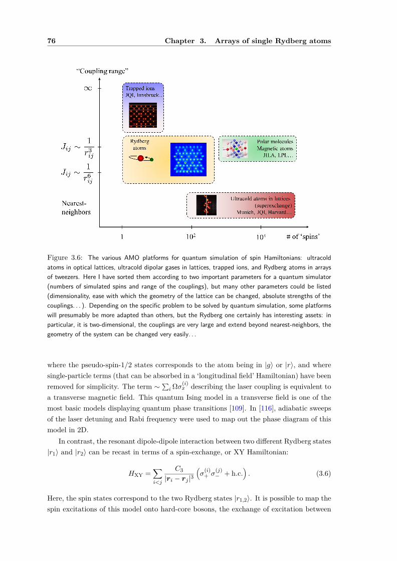
76 Chapter 3. Arrays of single Rydberg atoms
Figure 3.6: The various AMO platforms for quantum simulation of spin Hamiltonians: ultracoldatoms in optical lattices, ultracold dipolar gases in lattices, trapped ions, and Rydberg atoms in arraysof tweezers. Here I have sorted them according to two important parameters for a quantum simulator(numbers of simulated spins and range of the couplings), but many other parameters could be listed(dimensionality, ease with which the geometry of the lattice can be changed, absolute strengths of thecouplings. . . ). Depending on the specific problem to be solved by quantum simulation, some platformswill presumably be more adapted than others, but the Rydberg one certainly has interesting assets: inparticular, it is two-dimensional, the couplings are very large and extend beyond nearest-neighbors, thegeometry of the system can be changed very easily. . .
where the pseudo-spin-1/2 states corresponds to the atom being in |g〉 or |r〉, and wheresingle-particle terms (that can be absorbed in a ‘longitudinal field’ Hamiltonian) have beenremoved for simplicity. The term ∼
∑i Ωσ(i)
x describing the laser coupling is equivalent toa transverse magnetic field. This quantum Ising model in a transverse field is one of themost basic models displaying quantum phase transitions [109]. In [116], adiabatic sweepsof the laser detuning and Rabi frequency were used to map out the phase diagram of thismodel in 2D.
In contrast, the resonant dipole-dipole interaction between two different Rydberg states|r1〉 and |r2〉 can be recast in terms of a spin-exchange, or XY Hamiltonian:
HXY =∑i<j
C3|ri − rj |3
(σ
(i)+ σ
(j)− + h.c.
). (3.6)
Here, the spin states correspond to the two Rydberg states |r1,2〉. It is possible to map thespin excitations of this model onto hard-core bosons, the exchange of excitation between

3.5 Published articles 77
two atoms corresponding to (long-range) hopping of the corresponding bosons. Our three-atom spin chain experiment [6] corresponds to the smallest non-trivial instance of thismodel. In future work, in collaboration with Thomas Pohl’s group in Dresden, we planto find pairs of states for which the resonant dipole-dipole interaction and the (alwayspresent) van der Waals interaction are comparable in strength. In this case, one realizesa XXZ Heisenberg Hamiltonian, with some couplings slowly decaying as 1/R3, which isexpected to display new, exotic properties [53, 96].
I thus believe that our system will be an interesting platform for the simulation of spinHamiltonians, complementary to the other approaches using the tools of atomic physics,namely ultracold atoms or molecules in optical lattices and trapped ions (see e.g. [54] andreferences therein), as illustrated on Figure 3.6.
In the long run, one can envision to use the rich internal structure of Rydberg states toimplement more complex Hamiltonians. For instance one could use two types of excitationsto implement the equivalent of a Hubbard model with two species of hard-core bosons.The dipole-dipole interaction then naturally introduces a spin-orbit coupling for the motionof these excitations, which opens interesting perspectives for the quantum simulation oftopological matter displaying e.g. edge states, that we could image directly [98].
3.5 Published articles
Below is a list of the articles I have co-authored about our work on Rydberg atoms.
• L. Béguin et al., Phys. Rev. Lett. 110, 263201 (2013), reproduced on page 78.
• F. Nogrette et al., Phys. Rev. X 4, 021034 (2014), reproduced on page 83.
• D. Barredo et al., Phys. Rev. Lett. 112, 183002 (2014), reproduced on page 92.
• H. Labuhn et al., Phys. Rev. A. 90, 023415 (2014), reproduced on page 97.
• S. Ravets et al., Nature Phys. 10, 914 (2014), reproduced on page 101.
• D. Barredo et al., Phys. Rev. Lett. 114, 113002 (2015), reproduced on page 105.
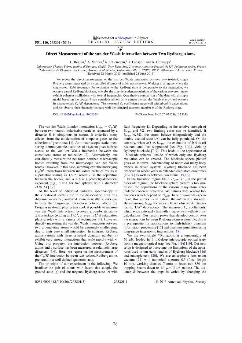
Direct Measurement of the van der Waals Interaction between Two Rydberg Atoms
L. Beguin,1 A. Vernier,1 R. Chicireanu,2 T. Lahaye,1 and A. Browaeys1
1Laboratoire Charles Fabry, Institut d’Optique, CNRS, Univ Paris Sud, 2 avenue Augustin Fresnel, 91127 Palaiseau cedex, France2Laboratoire de Physique des Lasers, Atomes et Molecules, Universite Lille 1, CNRS; 59655 Villeneuve d’Ascq cedex, France
(Received 22 March 2013; published 24 June 2013)
We report the direct measurement of the van der Waals interaction between two isolated, single
Rydberg atoms separated by a controlled distance of a few micrometers. Working in a regime where the
single-atom Rabi frequency for excitation to the Rydberg state is comparable to the interaction, we
observe partial Rydberg blockade, whereby the time-dependent populations of the various two-atom states
exhibit coherent oscillations with several frequencies. Quantitative comparison of the data with a simple
model based on the optical Bloch equations allows us to extract the van der Waals energy, and observe
its characteristic C6=R6 dependence. The measured C6 coefficients agree well with ab initio calculations,
and we observe their dramatic increase with the principal quantum number n of the Rydberg state.
DOI: 10.1103/PhysRevLett.110.263201 PACS numbers: 34.20.Cf, 03.67.Bg, 32.80.Ee
The van der Waals–London interaction UvdW ¼ C6=R6
between two neutral, polarizable particles separated by adistance R is ubiquitous in nature. It underlies manyeffects, from the condensation of nonpolar gases to theadhesion of gecko toes [1]. At a macroscopic scale, mea-suring thermodynamic quantities of a system gives indirectaccess to the van der Waals interaction between theconstituent atoms or molecules [2]. Alternatively, onecan directly measure the net force between macroscopicbodies resulting from the microscopic van der Waalsforces. However, in this case, summing over the underlyingC6=R
6 interactions between individual particles results ina potential scaling as 1=L, where L is the separationbetween the bodies, and < 6 is a geometry-dependentexponent (e.g., ¼ 1 for two spheres with a diameterD L) [1,2].
At the level of individual particles, spectroscopy ofthe vibrational levels close to the dissociation limit of adiatomic molecule, analyzed semiclassically, allows oneto infer the long-range interaction between atoms [3].Progress in atomic physics has made it possible to measurevan der Waals interactions between ground-state atomsand a surface (scaling as 1=L3, or even 1=L4 if retardationplays a role) with a variety of techniques [4]. However,directly measuring the van der Waals interaction betweentwo ground-state atoms would be extremely challenging,due to their very small interaction. In contrast, Rydbergatoms (atoms with large principal quantum number n)exhibit very strong interactions that scale rapidly with n.Using this property, the interaction between Rydbergatoms and a surface has been measured at relatively largedistances [5,6]. Here, we report on the measurement ofthe C6=R
6 interaction between two isolated Rydberg atomsprepared in a well defined quantum state.
The principle of our experiment is the following. Weirradiate the pair of atoms with lasers that couple theground state jgi and the targeted Rydberg state jri with
Rabi frequency . Depending on the relative strength ofUvdW and @, two limiting cases can be identified. IfUvdW @, the atoms behave independently and thedoubly excited state jrri can be fully populated. On thecontrary, when @ UvdW, the excitation of jrri is offresonant and thus suppressed [see Fig. 1(a)], yieldingRydberg blockade [7–9]. This leads to the appearance of‘‘blockade spheres’’ inside of which only one Rydbergexcitation can be created. The blockade sphere picturegives an intuitive understanding of nontrivial many-bodyeffects in driven systems. Rydberg blockade has beenobserved in recent years in extended cold atom ensembles[10–14] as well as between two atoms [15,16].In the transition region @UvdW, i.e., in the partial
blockade regime, the blockade sphere picture is too sim-plistic: the populations of the various many-atom statesundergo coherent collective oscillations with several fre-quencies which depend on UvdW. In our two-atom experi-ment, this allows us to extract the interaction strength.By measuring UvdW for various R, we observe its charac-teristic 1=R6 dependence. The measured C6 coefficients,which scale extremely fast with n, agree well with ab initiocalculations. Our results prove that detailed control overthe interactions between Rydberg atoms is possible; this isa prerequisite for applications to high-fidelity quantuminformation processing [17] and quantum simulation usinglong-range interatomic interactions [18].We use two single 87Rb atoms at a temperature of
50 K, loaded in 1 mK-deep microscopic optical trapsfrom a magneto-optical trap [see Fig. 1(b)] [19]. Our newsetup is designed to overcome the limitations of the appa-ratus used in our early studies of Rydberg blockade [16]and entanglement [20]. We use an aspheric lens undervacuum [21] with numerical aperture 0.5 (focal length10 mm, working distance 7 mm) to focus two 850 nmtrapping beams down to 1:1 m (1=e2 radius). The dis-tance R between the traps is varied by changing the
PRL 110, 263201 (2013)
Selected for a Viewpoint in PhysicsPHY S I CA L R EV I EW LE T T E R S
week ending28 JUNE 2013
0031-9007=13=110(26)=263201(5) 263201-1 2013 American Physical Society
78

incidence angle of the beams on the lens. We calibrate R bymeasuring the displacement of an image of the trap whenchanging the incidence of the trapping beams. The result-ing uncertainty is below 5% [22].
The aspheric lens used to focus the trapping beamsalso collects the atom fluorescence from each trap onseparate photon counters. The two-photon excitationfrom jgi ¼ j5S1=2; F ¼ 2; mF ¼ 2i to the Rydberg state
jri ¼ jnD3=2; mj ¼ 3=2i [see the inset of Fig. 1(b)],
described in Ref. [23], yields coherent oscillations withsingle-atom Rabi frequencies =ð2Þ in the range from500 kHz to 5 MHz [see Fig. 2(a)]. The excitation pulse hasa duration (during which the traps are off), and the laserfrequencies are adjusted so that the (light-shift corrected)one-atom detuning is ’ 0. After excitation, we infer thestate of each atom by detecting its presence or absence inits respective trap (atoms in jri are slightly antitrapped bythe optical potential, which results in their loss). We thusreconstruct the populations Pij of the two-atom states jiji
(i, j taking the values g, r), by repeating each sequenceabout 100 times [23].Our setup was designed to minimize residual electric
fields detrimental to Rydberg state manipulations: (i) theaspheric lens surface facing the atoms is coated with aconductive 200 nm-thick indium-tin-oxide layer; (ii) eightindependent electrodes allow us to apply electric fieldsalong any direction [24]. Using Stark spectroscopy onthe j62D3=2; mj ¼ 3=2i state, we determine that with all
electrodes grounded, a residual field of 150 mV=cm(pointing essentially along x) was present. After applyingappropriate correction voltages, the residual field is below5 mV=cm. This cancellation is critical to the success ofthe experiment: small (transverse) stray fields mix jri withother Rydberg states not coupled to light, or exhibitingForster zeros [25], thus degrading the blockade.Figures 2(b)–2(e) shows the probabilities Prg þ Pgr to
excite only one atom, and Prr to excite both, versus thearea of the excitation pulse, for various R and , inthe case n ¼ 62. In Fig. 2(b), the atoms are far apart(R ’ 15 m) and thus almost independent. Indeed, theprobability Prr of exciting both atoms is nearly equal tothe product P1;rP2;r [see Fig. 2(a)], where Pi;r is the
probability for atom i to be in jri, obtained in a controlexperiment with only trap i. In this case Prg þ Pgr is
expected to oscillate at frequency 2 between 0 and 1=2,close to what we observe. On the contrary, in Fig. 2(e), theatoms are close (R ’ 4:0 m) and ’ 2 1:9 MHz issmall enough for almost perfect blockade to occur: atall times, Prr is negligible (Prr < 0:06, with an averageof 0.036), and thus differs substantially from the productof the single-atom excitation probabilities expected forindependent atoms. At the same time, Prg þ Pgr oscillates
at ð1:49 0:07Þ, close to the expected collective
frequencyffiffiffi2
p [16].
In between those regimes [see Figs. 2(c) and 2(d)],blockade is only partial: Prg þ Pgr and Prr show a more
complex behavior, revealing nontrivial two-atom states.We model this dynamics by solving the optical Blochequations (OBEs) [26,27]. Each atom i (i ¼ 1, 2) is con-sidered as a two-level atom with ground state jgii andnD3=2 Rydberg state jrii, coupled by a near-resonant
laser with Rabi frequency (in practice, for our data,the atoms experience, within 5%, the same). In the basisfjggi; jgri; jrgi; jrrig, and using the rotating wave approxi-mation, the Hamiltonian is
H¼
0 @=2 @=2 0
@=2 @ 0 @=2
@=2 0 @ @=2
0 @=2 @=2 UvdW2@
0BBBBB@
1CCCCCA: (1)
We omit diagonal terms corresponding to interactionbetween ground-state atoms (for R ¼ 1 m the van derWaals interaction is in the 108 Hz range, and the
FIG. 1 (color online). (a) Principle of the Rydberg blockade.The single-atom Rabi frequency is . (b) Experimental setup.Two single atoms are trapped in microscopic optical trapsseparated by R. Eight electrodes (four of which, facing theones displayed here, are not shown) provide electric field con-trol. Inset: two-photon excitation scheme (the intermediate-statedetuning is ’ 2 740 MHz).
PRL 110, 263201 (2013) P HY S I CA L R EV I EW LE T T E R Sweek ending28 JUNE 2013
263201-2
79
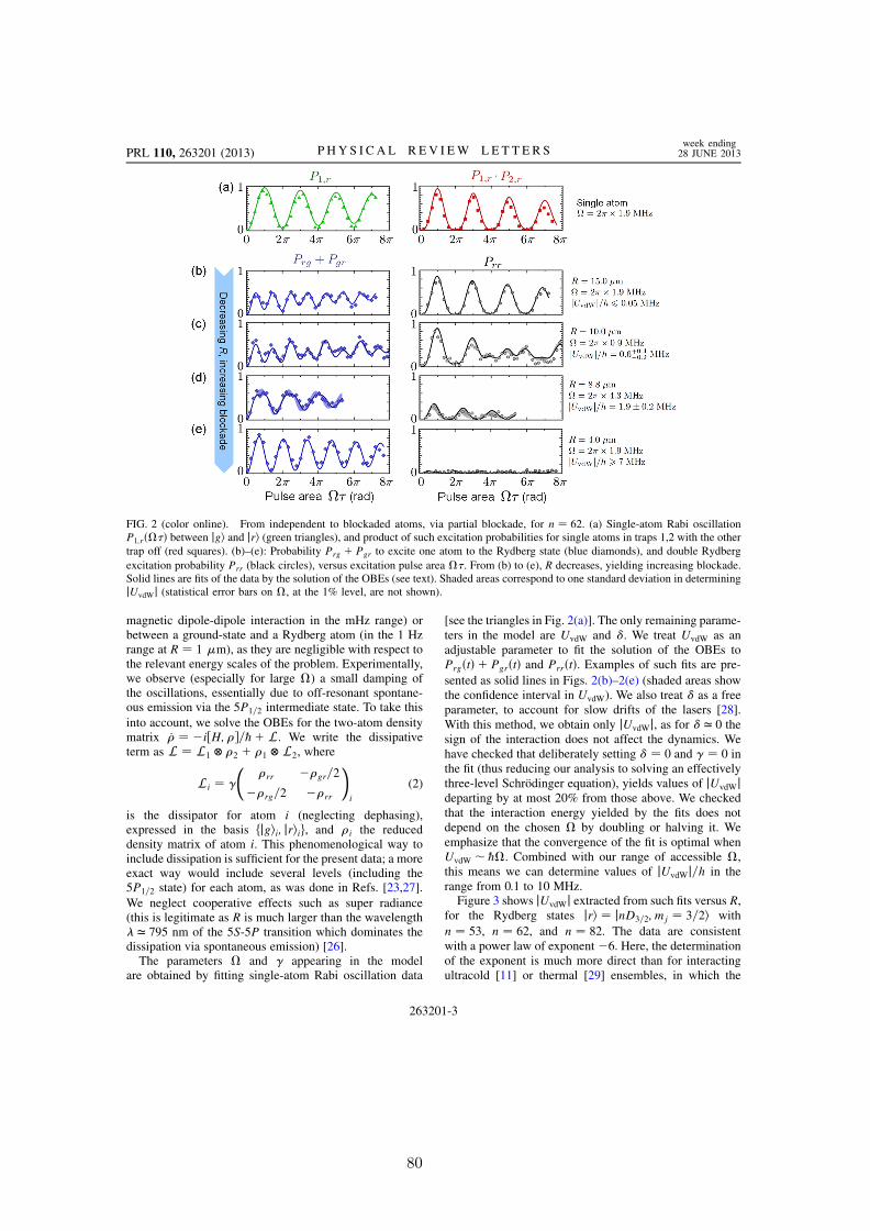
magnetic dipole-dipole interaction in the mHz range) orbetween a ground-state and a Rydberg atom (in the 1 Hzrange at R ¼ 1 m), as they are negligible with respect tothe relevant energy scales of the problem. Experimentally,we observe (especially for large ) a small damping ofthe oscillations, essentially due to off-resonant spontane-ous emission via the 5P1=2 intermediate state. To take this
into account, we solve the OBEs for the two-atom densitymatrix _ ¼ i½H;=@þL. We write the dissipativeterm as L ¼ L1 2 þ 1 L2, where
Li ¼ rr gr=2
rg=2 rr
!i
(2)
is the dissipator for atom i (neglecting dephasing),expressed in the basis fjgii; jriig, and i the reduceddensity matrix of atom i. This phenomenological way toinclude dissipation is sufficient for the present data; a moreexact way would include several levels (including the5P1=2 state) for each atom, as was done in Refs. [23,27].
We neglect cooperative effects such as super radiance(this is legitimate as R is much larger than the wavelength ’ 795 nm of the 5S-5P transition which dominates thedissipation via spontaneous emission) [26].
The parameters and appearing in the modelare obtained by fitting single-atom Rabi oscillation data
[see the triangles in Fig. 2(a)]. The only remaining parame-ters in the model are UvdW and . We treat UvdW as anadjustable parameter to fit the solution of the OBEs toPrgðtÞ þ PgrðtÞ and PrrðtÞ. Examples of such fits are pre-
sented as solid lines in Figs. 2(b)–2(e) (shaded areas showthe confidence interval in UvdW). We also treat as a freeparameter, to account for slow drifts of the lasers [28].With this method, we obtain only jUvdWj, as for ’ 0 thesign of the interaction does not affect the dynamics. Wehave checked that deliberately setting ¼ 0 and ¼ 0 inthe fit (thus reducing our analysis to solving an effectivelythree-level Schrodinger equation), yields values of jUvdWjdeparting by at most 20% from those above. We checkedthat the interaction energy yielded by the fits does notdepend on the chosen by doubling or halving it. Weemphasize that the convergence of the fit is optimal whenUvdW @. Combined with our range of accessible ,this means we can determine values of jUvdWj=h in therange from 0.1 to 10 MHz.Figure 3 shows jUvdWj extracted from such fits versus R,
for the Rydberg states jri ¼ jnD3=2; mj ¼ 3=2i with
n ¼ 53, n ¼ 62, and n ¼ 82. The data are consistentwith a power law of exponent6. Here, the determinationof the exponent is much more direct than for interactingultracold [11] or thermal [29] ensembles, in which the
FIG. 2 (color online). From independent to blockaded atoms, via partial blockade, for n ¼ 62. (a) Single-atom Rabi oscillationP1;rðÞ between jgi and jri (green triangles), and product of such excitation probabilities for single atoms in traps 1,2 with the other
trap off (red squares). (b)–(e): Probability Prg þ Pgr to excite one atom to the Rydberg state (blue diamonds), and double Rydberg
excitation probability Prr (black circles), versus excitation pulse area . From (b) to (e), R decreases, yielding increasing blockade.Solid lines are fits of the data by the solution of the OBEs (see text). Shaded areas correspond to one standard deviation in determiningjUvdWj (statistical error bars on , at the 1% level, are not shown).
PRL 110, 263201 (2013) P HY S I CA L R EV I EW LE T T E R Sweek ending28 JUNE 2013
263201-3
80

random distribution of atoms smears out the interaction Rdependence. Our results illustrate the dramatic dependenceof UvdW with n: for instance, changing n from 53 to 62 atgiven R yields a fiftyfold increase in UvdW. Fitting the databy jUvdWj ¼ jC6jExpt:=R6 with jC6jExpt: as an adjustable
parameter, we obtain the values of Table I.To compare our measurements to the theoretical expres-
sions of jUvdWj (solid lines in Fig. 3), we diagonalize theinteraction Hamiltonian, considering only the leading, elec-tric dipole interaction term. From the quantum defectsreported in Ref. [30], we compute radial wave functionsusing the Numerov algorithm [31]. We restrict theHamiltonian to a two-atom basis jn1l1j1mj1; n2l2j2mj2icomprising only states close in energy (up to h5GHz)from the jnD3=2; mj ¼ 3=2; nD3=2; mj ¼ 3=2i state, and
satisfying jn n1;2j 4. This corresponds to (sparse) ma-
trices up to ’ 103 103 [32].At the large distances relevant here, the dipole-dipole
interaction simply shifts the two-atom levels by a quantityC6=R
6 that can be obtained from second-order perturbationtheory. At shorter distances, mixing between adjacentlevels occurs [25], altering the 1=R6 character of the inter-action (this can be seen for n ¼ 53 when R< 4 m).We obtain the jC6jTh: coefficients of Table I by fitting thenumerically obtained interactions at distances 15<R<20 m. Our results are in good agreement with second-order perturbation theory calculations [33]. We get anestimate of the uncertainty in jC6jTh: by adding random,uniformly distributed relative errors of 0:5% to radialmatrix elements appearing in the Hamiltonian. The relativeuncertainty is larger (10%) for n ¼ 53, due to cancella-tions of terms with opposite signs. Taking into account
error bars, the agreement between our measurement andthe calculated C6 is very good. It appears from Fig. 3 thatfor the largest values of UvdW, our experimental determi-nation systematically lies below the theory. An explanationmight be that mechanical effects induced by interactionslead to a modification of the dynamics, as recently sug-gested [34]. Our present analysis neglects these effects andmay lead to an underestimation of the actual interaction.Including these effects is left to future work.In summary, we have directly measured the van der
Waals interaction between two isolated Rydberg atoms.The level of control demonstrated here opens excitingperspectives in multiatom systems, for observinggeometry-dependent effects due to the anisotropy of thedipolar interaction [35], or the nonadditivity of van derWaals interactions [36]. It is also a prerequisite forgenerating high-fidelity, many-atom entanglement usingRydberg blockade, as well as for quantum simulation oflong-range interacting spin systems.We thank A. Guilbaud, P. Roth, C. Beurthe, F. Moron,
and F. Nogrette for technical assistance, C. Evellin forcontributions at the early stage of this work, Y. R. P.Sortais for invaluable advice in the design of the setup,H. Labuhn and S. Ravets for a careful reading of themanuscript, and J. Vigue for useful discussions. L. B. ispartially supported by the DGA.We acknowledge financialsupport by the EU (ERC Stg Grant ARENA, AQUTEIntegrating Project, and Initial Training NetworkCOHERENCE), and by Region Ile-de-France (LUMATand Triangle de la Physique).
[1] J. N. Israelachvili, Intermolecular And Surface Forces
(Academic, New York, 2010).[2] P. C. Hiemenz and R. Rajagopalan, Principles of Colloid
and Surface Chemistry (Marcel Dekker, New York, 1997).[3] R. J. Le Roy and R.B. Bernstein, J. Chem. Phys. 52, 3869
(1970).[4] See, e.g., A. Aspect and J. Dalibard, Seminaire Poincare 1,
67 (2002), and references therein.[5] A. Anderson, S. Haroche, E. A. Hinds, W. Jhe, and D.
Meschede, Phys. Rev. A 37, 3594 (1988).[6] V. Sandoghdar, C. I. Sukenik, E. A. Hinds, and S. Haroche,
Phys. Rev. Lett. 68, 3432 (1992).[7] D. Jaksch, J. I. Cirac, P. Zoller, R. Cote, and M.D. Lukin,
Phys. Rev. Lett. 85, 2208 (2000).
FIG. 3 (color online). Magnitude jUvdWj of the interactionenergy between atoms in jnD3=2; mj ¼ 3=2i, extracted from
the fits of Fig. 2, versus R, for n ¼ 53 (blue), n ¼ 62 (red),and n ¼ 82 (green). Error bars are one standard deviation inthe fitted jUvdWj. Solid lines: ab initio theoretical expectations(see text) without any adjustable parameter. Shaded areas: 5%systematic uncertainty in R.
TABLE I. Experimental and theoretical jC6j coefficients forn ¼ 53, 62, and 82.
n jC6jExptðGHz m6Þ jC6jThðGHz m6Þ53 13:7 1:2 16:9 1:762 730 20 766 1582 8500 300 8870 150
PRL 110, 263201 (2013) P HY S I CA L R EV I EW LE T T E R Sweek ending28 JUNE 2013
263201-4
81

[8] M.D. Lukin, M. Fleischhauer, and R. Cote, Phys. Rev.Lett. 87, 037901 (2001).
[9] D. Comparat and P. Pillet, J. Opt. Soc. Am. B 27, A208(2010).
[10] K. Singer, M. Reetz-Lamour, T. Amthor, L. G. Marcassa,and M. Weidemuller, Phys. Rev. Lett. 93, 163001(2004).
[11] R. Heidemann, U. Raitzsch, V. Bendkowsky, B. Butscher,R. Low, L. Santos, and T. Pfau, Phys. Rev. Lett. 99, 163601(2007).
[12] J. D. Pritchard, D. Maxwell, A. Gauguet, K. J. Weatherill,M. P. A. Jones, and C. S. Adams, Phys. Rev. Lett. 105,193603 (2010).
[13] Y. O. Dudin and A. Kuzmich, Science 336, 887 (2012).[14] P. Schauss, M. Cheneau, M. Endres, T. Fukuhara, S. Hild,
A. Omran, T. Pohl, C. Gross, S. Kuhr, and I. Bloch, Nature(London) 491, 87 (2012).
[15] E. Urban, T. A. Johnson, T. Henage, L. Isenhower,D. D. Yavuz, T. G. Walker, and M. Saffman, Nat. Phys.5, 110 (2009).
[16] A. Gaetan, Y. Miroshnychenko, T. Wilk, A. Chotia,M. Viteau, D. Comparat, P. Pillet, A. Browaeys, andP. Grangier, Nat. Phys. 5, 115 (2009).
[17] M. Saffman, T.G. Walker, and K. Mølmer, Rev. Mod.Phys. 82, 2313 (2010).
[18] H. Weimer, M. Muller, I. Lesanovsky, P. Zoller, andH. P. Buchler, Nat. Phys. 6, 382 (2010).
[19] N. Schlosser, G. Reymond, I. Protsenko, and P. Grangier,Nature (London) 411, 1024 (2001).
[20] T. Wilk, A. Gaetan, C. Evellin, J. Wolters, Y.Miroshnychenko, P. Grangier, and A. Browaeys, Phys.Rev. Lett. 104, 010502 (2010).
[21] Y. R. P. Sortais et al., Phys. Rev. A 75, 013406 (2007).[22] The dispersion in the interatomic distances due to the
finite temperature has negligible effects. For T¼50K,
the transverse size in our traps (of radial frequency!r 2 100 kHz) is 100 nm (longitudinal sizeonly contributes to second order).
[23] Y. Miroshnychenko, A. Gaetan, C. Evellin, P. Grangier,D. Comparat, P. Pillet, T. Wilk, and A. Browaeys, Phys.Rev. A 82, 013405 (2010).
[24] R. Low, H. Weimer, J. Nipper, J. B Balewski, B. Butscher,H. P. Buchler, and T. Pfau, J. Phys. B 45, 113001(2012).
[25] T.G. Walker and M. Saffman, Phys. Rev. A 77, 032723(2008).
[26] C. Ates, T. Pohl, T. Pattard, and J.M. Rost, Phys. Rev. A76, 013413 (2007).
[27] X. L. Zhang, A. T. Gill, L. Isenhower, T. G. Walker, andM. Saffman, Phys. Rev. A 85, 042310 (2012).
[28] For our data, the best-fit value of =ð2Þ lies in the range300 kHz, compatible with observed frequency drifts ofthe excitation lasers over the acquisition of a full data set(a few hours).
[29] T. Baluktsian, B. Huber, R. Low and T. Pfau, Phys. Rev.Lett. 110, 123001 (2013).
[30] W. Li, I. Mourachko, M.W. Noel, and T. F. Gallagher,Phys. Rev. A 67, 052502 (2003).
[31] M. L. Zimmerman, M.G. Littman, M.M. Kash, and D.Kleppner, Phys. Rev. A 20, 2251 (1979).
[32] At the large distances used to extract C6, only a few tens ofstates contribute significantly. However, to obtain thecorrect short-distance behavior,103 states are necessary.
[33] A. Reinhard, T. C. Liebisch, B. Knuffman, and G. Raithel,Phys. Rev. A 75, 032712 (2007).
[34] W. Li, C. Ates, and I. Lesanovsky, arXiv:1303.3212.[35] T. J. Caroll, K. Claringbould, A. Goodsell, M. J. Lim, and
M.W. Noel, Phys. Rev. Lett. 93, 153001 (2004).[36] D. Cano and J. Fortagh, Phys. Rev. A 86, 043422
(2012).
PRL 110, 263201 (2013) P HY S I CA L R EV I EW LE T T E R Sweek ending28 JUNE 2013
263201-5
82
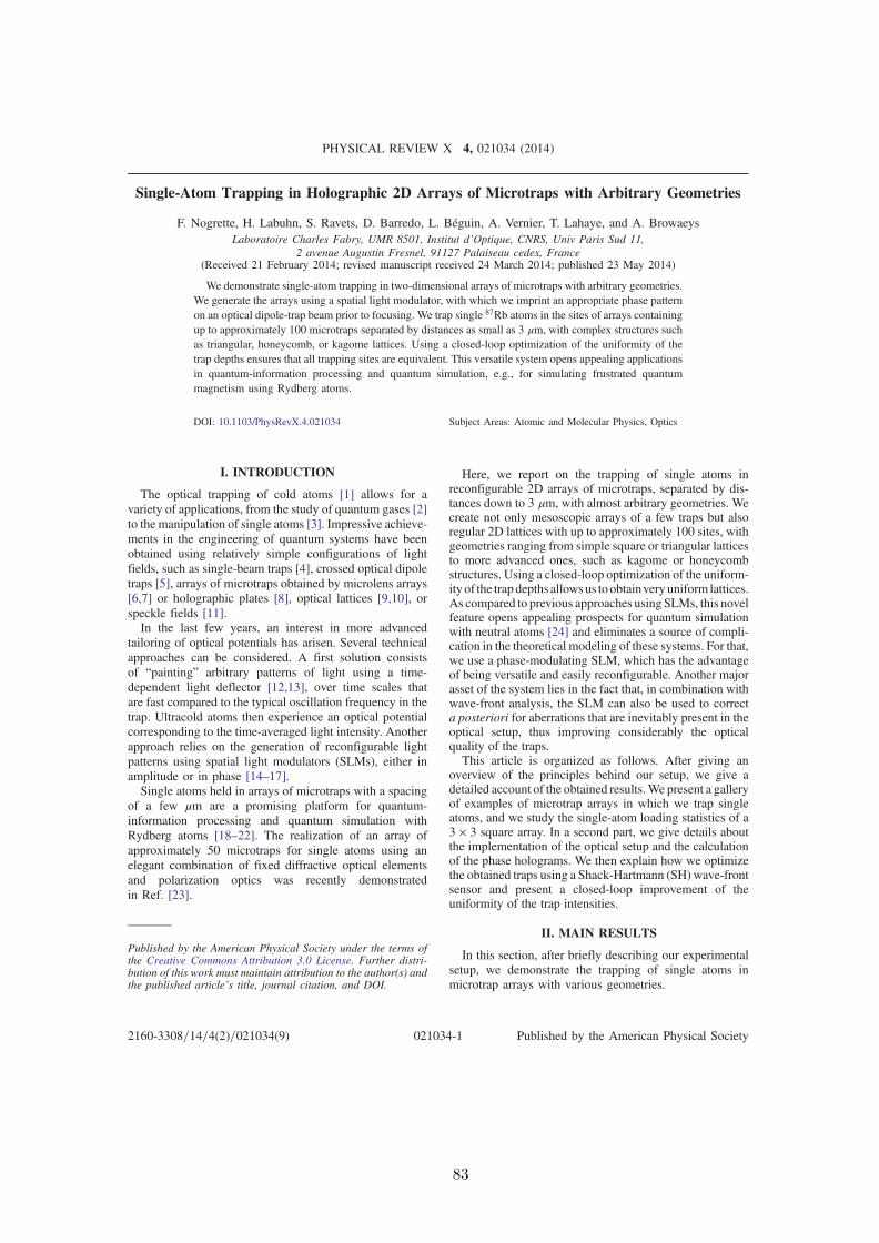
Single-Atom Trapping in Holographic 2D Arrays of Microtraps with Arbitrary Geometries
F. Nogrette, H. Labuhn, S. Ravets, D. Barredo, L. Béguin, A. Vernier, T. Lahaye, and A. BrowaeysLaboratoire Charles Fabry, UMR 8501, Institut d’Optique, CNRS, Univ Paris Sud 11,
2 avenue Augustin Fresnel, 91127 Palaiseau cedex, France(Received 21 February 2014; revised manuscript received 24 March 2014; published 23 May 2014)
We demonstrate single-atom trapping in two-dimensional arrays of microtraps with arbitrary geometries.We generate the arrays using a spatial light modulator, with which we imprint an appropriate phase patternon an optical dipole-trap beam prior to focusing. We trap single 87Rb atoms in the sites of arrays containingup to approximately 100 microtraps separated by distances as small as 3 μm, with complex structures suchas triangular, honeycomb, or kagome lattices. Using a closed-loop optimization of the uniformity of thetrap depths ensures that all trapping sites are equivalent. This versatile system opens appealing applicationsin quantum-information processing and quantum simulation, e.g., for simulating frustrated quantummagnetism using Rydberg atoms.
DOI: 10.1103/PhysRevX.4.021034 Subject Areas: Atomic and Molecular Physics, Optics
I. INTRODUCTION
The optical trapping of cold atoms [1] allows for avariety of applications, from the study of quantum gases [2]to the manipulation of single atoms [3]. Impressive achieve-ments in the engineering of quantum systems have beenobtained using relatively simple configurations of lightfields, such as single-beam traps [4], crossed optical dipoletraps [5], arrays of microtraps obtained by microlens arrays[6,7] or holographic plates [8], optical lattices [9,10], orspeckle fields [11].In the last few years, an interest in more advanced
tailoring of optical potentials has arisen. Several technicalapproaches can be considered. A first solution consistsof “painting” arbitrary patterns of light using a time-dependent light deflector [12,13], over time scales thatare fast compared to the typical oscillation frequency in thetrap. Ultracold atoms then experience an optical potentialcorresponding to the time-averaged light intensity. Anotherapproach relies on the generation of reconfigurable lightpatterns using spatial light modulators (SLMs), either inamplitude or in phase [14–17].Single atoms held in arrays of microtraps with a spacing
of a few μm are a promising platform for quantum-information processing and quantum simulation withRydberg atoms [18–22]. The realization of an array ofapproximately 50 microtraps for single atoms using anelegant combination of fixed diffractive optical elementsand polarization optics was recently demonstratedin Ref. [23].
Here, we report on the trapping of single atoms inreconfigurable 2D arrays of microtraps, separated by dis-tances down to 3 μm, with almost arbitrary geometries. Wecreate not only mesoscopic arrays of a few traps but alsoregular 2D lattices with up to approximately 100 sites, withgeometries ranging from simple square or triangular latticesto more advanced ones, such as kagome or honeycombstructures. Using a closed-loop optimization of the uniform-ity of the trapdepths allowsus toobtainveryuniform lattices.As compared to previous approaches using SLMs, this novelfeature opens appealing prospects for quantum simulationwith neutral atoms [24] and eliminates a source of compli-cation in the theoretical modeling of these systems. For that,we use a phase-modulating SLM, which has the advantageof being versatile and easily reconfigurable. Another majorasset of the system lies in the fact that, in combination withwave-front analysis, the SLM can also be used to correcta posteriori for aberrations that are inevitably present in theoptical setup, thus improving considerably the opticalquality of the traps.This article is organized as follows. After giving an
overview of the principles behind our setup, we give adetailed account of the obtained results.We present a galleryof examples of microtrap arrays in which we trap singleatoms, and we study the single-atom loading statistics of a3 × 3 square array. In a second part, we give details aboutthe implementation of the optical setup and the calculationof the phase holograms. We then explain how we optimizethe obtained traps using a Shack-Hartmann (SH) wave-frontsensor and present a closed-loop improvement of theuniformity of the trap intensities.
II. MAIN RESULTS
In this section, after briefly describing our experimentalsetup, we demonstrate the trapping of single atoms inmicrotrap arrays with various geometries.
Published by the American Physical Society under the terms ofthe Creative Commons Attribution 3.0 License. Further distri-bution of this work must maintain attribution to the author(s) andthe published article’s title, journal citation, and DOI.
PHYSICAL REVIEW X 4, 021034 (2014)
2160-3308=14=4(2)=021034(9) 021034-1 Published by the American Physical Society
83
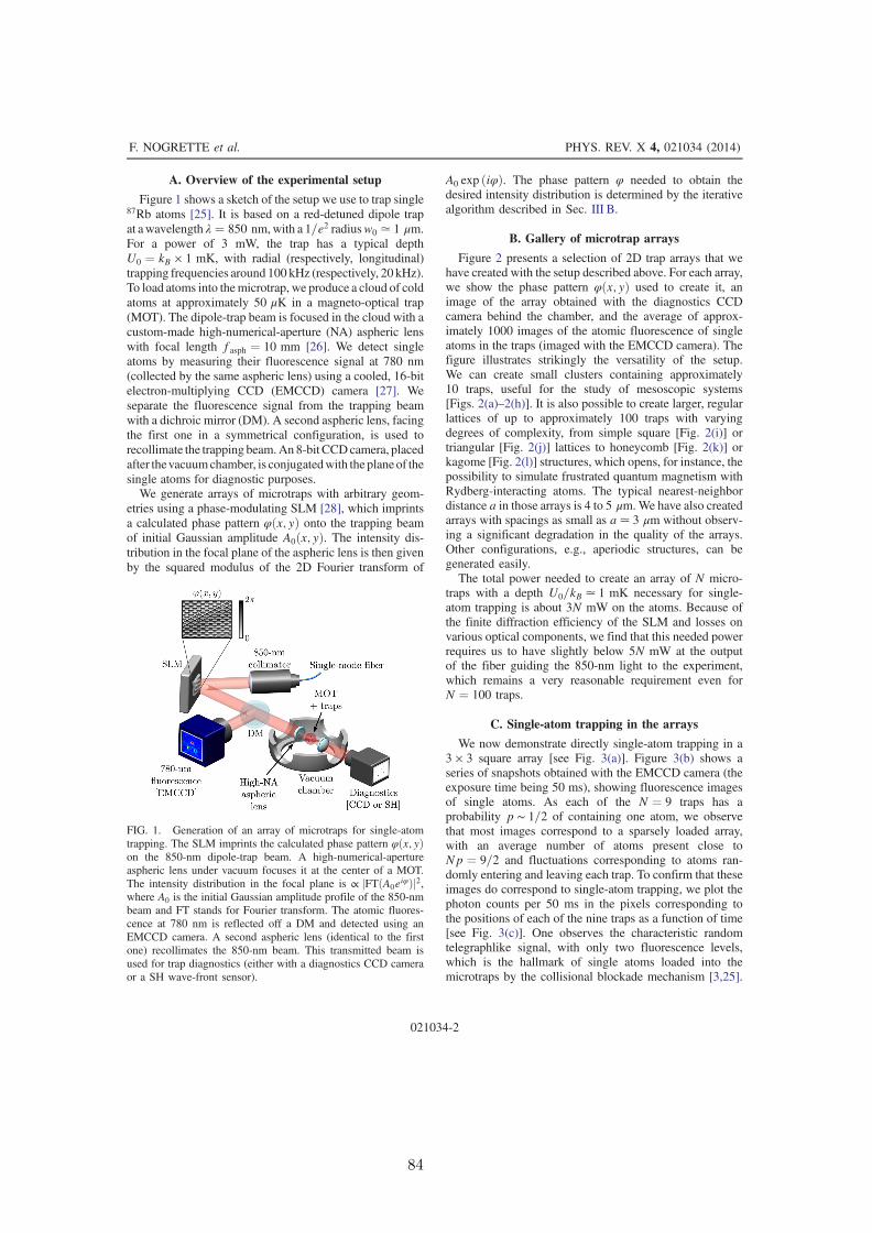
A. Overview of the experimental setup
Figure 1 shows a sketch of the setup we use to trap single87Rb atoms [25]. It is based on a red-detuned dipole trapat awavelength λ ¼ 850 nm,with a 1=e2 radiusw0 ≃ 1 μm.For a power of 3 mW, the trap has a typical depthU0 ¼ kB × 1 mK, with radial (respectively, longitudinal)trapping frequencies around 100 kHz (respectively, 20 kHz).To load atoms into themicrotrap, we produce a cloud of coldatoms at approximately 50 μK in a magneto-optical trap(MOT). The dipole-trap beam is focused in the cloud with acustom-made high-numerical-aperture (NA) aspheric lenswith focal length fasph ¼ 10 mm [26]. We detect singleatoms by measuring their fluorescence signal at 780 nm(collected by the same aspheric lens) using a cooled, 16-bitelectron-multiplying CCD (EMCCD) camera [27]. Weseparate the fluorescence signal from the trapping beamwith a dichroic mirror (DM). A second aspheric lens, facingthe first one in a symmetrical configuration, is used torecollimate the trapping beam.An8-bit CCDcamera, placedafter thevacuumchamber, is conjugatedwith the plane of thesingle atoms for diagnostic purposes.We generate arrays of microtraps with arbitrary geom-
etries using a phase-modulating SLM [28], which imprintsa calculated phase pattern φðx; yÞ onto the trapping beamof initial Gaussian amplitude A0ðx; yÞ. The intensity dis-tribution in the focal plane of the aspheric lens is then givenby the squared modulus of the 2D Fourier transform of
A0 exp ðiφÞ. The phase pattern φ needed to obtain thedesired intensity distribution is determined by the iterativealgorithm described in Sec. III B.
B. Gallery of microtrap arrays
Figure 2 presents a selection of 2D trap arrays that wehave created with the setup described above. For each array,we show the phase pattern φðx; yÞ used to create it, animage of the array obtained with the diagnostics CCDcamera behind the chamber, and the average of approx-imately 1000 images of the atomic fluorescence of singleatoms in the traps (imaged with the EMCCD camera). Thefigure illustrates strikingly the versatility of the setup.We can create small clusters containing approximately10 traps, useful for the study of mesoscopic systems[Figs. 2(a)–2(h)]. It is also possible to create larger, regularlattices of up to approximately 100 traps with varyingdegrees of complexity, from simple square [Fig. 2(i)] ortriangular [Fig. 2(j)] lattices to honeycomb [Fig. 2(k)] orkagome [Fig. 2(l)] structures, which opens, for instance, thepossibility to simulate frustrated quantum magnetism withRydberg-interacting atoms. The typical nearest-neighbordistance a in those arrays is 4 to 5 μm.We have also createdarrays with spacings as small as a≃ 3 μm without observ-ing a significant degradation in the quality of the arrays.Other configurations, e.g., aperiodic structures, can begenerated easily.The total power needed to create an array of N micro-
traps with a depth U0=kB ≃ 1 mK necessary for single-atom trapping is about 3N mW on the atoms. Because ofthe finite diffraction efficiency of the SLM and losses onvarious optical components, we find that this needed powerrequires us to have slightly below 5N mW at the outputof the fiber guiding the 850-nm light to the experiment,which remains a very reasonable requirement even forN ¼ 100 traps.
C. Single-atom trapping in the arrays
We now demonstrate directly single-atom trapping in a3 × 3 square array [see Fig. 3(a)]. Figure 3(b) shows aseries of snapshots obtained with the EMCCD camera (theexposure time being 50 ms), showing fluorescence imagesof single atoms. As each of the N ¼ 9 traps has aprobability p ∼ 1=2 of containing one atom, we observethat most images correspond to a sparsely loaded array,with an average number of atoms present close toNp ¼ 9=2 and fluctuations corresponding to atoms ran-domly entering and leaving each trap. To confirm that theseimages do correspond to single-atom trapping, we plot thephoton counts per 50 ms in the pixels corresponding tothe positions of each of the nine traps as a function of time[see Fig. 3(c)]. One observes the characteristic randomtelegraphlike signal, with only two fluorescence levels,which is the hallmark of single atoms loaded into themicrotraps by the collisional blockade mechanism [3,25].
FIG. 1. Generation of an array of microtraps for single-atomtrapping. The SLM imprints the calculated phase pattern φðx; yÞon the 850-nm dipole-trap beam. A high-numerical-apertureaspheric lens under vacuum focuses it at the center of a MOT.The intensity distribution in the focal plane is ∝ jFTðA0eiφÞj2,where A0 is the initial Gaussian amplitude profile of the 850-nmbeam and FT stands for Fourier transform. The atomic fluores-cence at 780 nm is reflected off a DM and detected using anEMCCD camera. A second aspheric lens (identical to the firstone) recollimates the 850-nm beam. This transmitted beam isused for trap diagnostics (either with a diagnostics CCD cameraor a SH wave-front sensor).
F. NOGRETTE et al. PHYS. REV. X 4, 021034 (2014)
021034-2
84

By analyzing each of the nine traces, we find that theoccupation probability pi of each trap i is close to 1=2. (Wefind probabilities pi ranging from 0.43 to 0.57, with anaverage p ¼ 0.53.)Figure 3(d) is a histogram of the number of atoms
trapped in the 3 × 3 array, obtained by analyzing approx-imately 2500 images [23]. For an array of N independenttraps, if each trap has the same probability p to be filled, theprobability Pn to have n atoms in the array is given by thebinomial distribution
Pn ¼N!
n!ðN − nÞ!pnð1 − pÞN−n: (1)
The dots in Fig. 3(d) correspond to Eq. (1) with N ¼ 9 andp ¼ p and show good agreement with the data. Therefore,the assumption that all traps are loaded with the sameprobability is a good approximation for estimating theprobability of a given configuration to occur.
III. DETAILED IMPLEMENTATION
In the preceding section, we focused on giving a detailedpresentation of the results obtained. However, obtainingarrays of traps with as high a quality as what is demon-strated in Figs. 2 and 3 requires some care in theimplementation of the setup. In this section, we detailthe implementation of both the hardware and the softwareparts of the system.
FIG. 2. A gallery of microtrap arrays with different geometries. For each panel, we show the calculated phase pattern φ used to createthe array (left), an image of the resulting trap arrays taken with the diagnostics CCD (middle), and the average of approximately 1000fluorescence images of single atoms loaded into the traps (right).
SINGLE-ATOM TRAPPING IN HOLOGRAPHIC 2D ARRAYS … PHYS. REV. X 4, 021034 (2014)
021034-3
85

A. Optical layout
Our SLM has an active area of 12 × 18 mm2, with aresolution of 600 × 800 pixels. It is illuminated by acollimated Gaussian beam with a 6.7-mm 1=e2 radiuscoming from a polarization-maintaining, single-mode fiberconnected to a collimator with a focal length f ¼ 75 mm.As diffraction-limited operation of the aspheric lens isobtained for an infinite-to-focus conjugation, with a pupildiameter D ¼ 10 mm, we use an afocal telescope with atransverse magnification my ¼ −0.8 to adapt the SLMactive area to the aspheric lens aperture, while maintainingthe collimation of the beam.The implementation of the full system (vacuum chamber,
dichroic mirror for fluorescence detection, components forgenerating the microtrap array) results in a relatively long
distance (l≃ 500 mm) between the SLM and the asphericlens. This leads to the following problem [see Fig. 4(a)]:When generating off-axis traps, the beam diffracted by theSLM impinges on the lens off center, giving rise to clippingand field aberrations. These effects decrease the quality ofarrays with a large number of microtraps. We circumventthis problem using pupil conjugation: We take advantageof the extra degree of freedom given by the position ofthe telescope to conjugate the plane of the SLM with theaspheric lens, as shown in Fig. 4(b).The optimization of the system is done with an optical
design software. The simulation includes all the compo-nents from the optical fiber to the focal plane of the asphericlens in the vacuum chamber. The lenses of the telescopeand the lens of the collimator are near-infrared achromaticdoublets used at low numerical aperture and small fields.The performance of the system over a field of 30 × 30 μm2
in the microtrap plane is satisfactory: The Strehl ratio, i.e.,the ratio of the actual peak intensity over the theoreticalpeak intensity for a diffraction-limited system [29], ispredicted to be S ≥ 0.88 by the calculation.For the phase-pattern calculation described below, we
replace the telescope and the aspheric lens by a singleequivalent lens with an effective focal length feff ¼fasph=jmyj ¼ 12 mm and an effective pupil in the SLMplane with diameter Deff ¼ 12 mm.
B. Gerchberg-Saxton algorithm
We use the Gerchberg-Saxton (GS) algorithm [30] tocalculate the phase pattern φðx; yÞ required to obtain anintensity distribution in the lens focal plane close to a desiredtarget intensity It. For the sake of completeness, we brieflyrecall below the essential steps of the algorithm (see Fig. 5).
FIG. 3. Single-atom trapping in a 3 × 3 array. (a) Image of thetraps, separated by 4 μm, obtained with the diagnostics CCDcamera. (b) Sample fluorescence images of single atoms trappedin the array. The exposure time is 50ms. (c) Photon counts per 50msat the pixels corresponding to each of the nine trap positions,as a function of time. The random, telegraphlike signal with onlytwo fluorescence levels is the signature of single-atom trapping.(d) Histogram of the occurrences of images with n atoms trapped(with 0 ≤ n ≤ 9) over a set of approximately 2500 images. The reddotscorrespond to thebinomialdistribution [Eq. (1)]withp ¼ 0.53.
FIG. 4. Pupil conjugation. (a) Without a telescope, for a givenfield y ≠ 0, the dipole-trap beam is clipped and not centered onthe aspheric lens. (b) The implemented telescope adapts the sizeof the beam to the aspheric lens pupil; by conjugating the SLMaperture to the entrance pupil of the aspheric lens, the beam iswell centered, whatever the field.
F. NOGRETTE et al. PHYS. REV. X 4, 021034 (2014)
021034-4
86
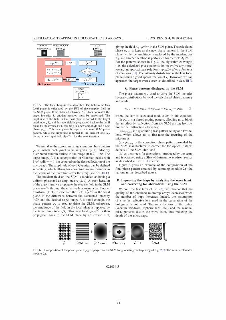
We initialize the algorithm using a random phase patternφ0 in which each pixel value is given by a uniformlydistributed random variate in the range ð0; 0.2Þ × 2π. Thetarget image It is a superposition of Gaussian peaks with1=e2 radii w ¼ 1 μm centered on the desired location of themicrotraps. The amplitude of each Gaussian can be definedseparately, which allows for correcting nonuniformities inthe depths of the microtraps over the array (see Sec. III E).The incident field on the SLM is modeled as having a
uniform phase and an amplitude A0ðx; yÞ. At each iterationof the algorithm, we propagate the electric field in the SLMplane A0eiφn through the effective lens using a fast Fouriertransform (FFT) to calculate the field Af
neiφfn in the focal
plane. If the difference between the calculated intensityjAf
nj2 and the desired target image It is small enough, thephase pattern φn is used to drive the SLM; otherwise,the amplitude of the field in the focal plane is replaced bythe target amplitude
ffiffiffiffi
Itp
. This new fieldffiffiffiffi
Itp
eiφfn is then
propagated back to the SLM plane by an inverse FFT,
giving the field Anþ1eiφnþ1 in the SLM plane. The calculatedphase φnþ1 is kept as the new phase pattern in the SLMplane, while the amplitude is replaced by the incident oneA0, and another iteration is performed for the field A0eiφnþ1 .For the patterns shown in Fig. 2, the algorithm converges(i.e., the calculated phase patterns do not evolve any more)toward an approximate solution, typically after a few tensof iterations [31]. The intensity distribution in the lens focalplane is then a good approximation of It. However, we canapproach the target even closer, as described in Sec. III E.
C. Phase patterns displayed on the SLM
The phase pattern φtot used to drive the SLM includesseveral contributions beyond the calculated phase pattern φand reads
φtot ¼ φþ φblaze þ φFresnel þ φfactory þ φSH; (2)
where the sum is calculated modulo 2π. In this equation,(i) φblaze is a blazed grating pattern, allowing us to block
the zeroth-order reflection from the SLM arising from itsnonperfect diffraction efficiency;(ii) φFresnel is a quadratic phase pattern acting as a Fresnel
lens, which allows us to fine-tune the focusing of themicrotraps;(iii) φfactory is the correction phase pattern provided by
the SLM manufacturer to correct for the optical flatnessdefects of the SLM chip; and(iv) φSH corrects for aberrations introduced by the setup
and is obtained using a Shack-Hartmann wave-front sensoras described in Sec. III D below.Figure 6 gives an example of the composition of the
final phase pattern obtained by summing (modulo 2π) thevarious terms described above.
D. Improving the traps by analyzing the wave frontand correcting for aberrations using the SLM
Without the last term of Eq. (2), we observe that thequality of the obtained microtrap arrays decreases whenthe number of traps increases. Indeed, the assumptionof a perfect effective lens used in the calculation of thehologram is not valid. The imperfections of the optics(vacuum windows, aspheric lens, etc.) and the residualmisalignments distort the wave front, thus reducing thedepth of the microtraps.
FIG. 5. The Gerchberg-Saxton algorithm. The field in the lensfocal plane is calculated by the FFT of the complex field inthe SLM plane. If the obtained intensity jAf
nj2 does not match thetarget intensity It, another iteration must be performed: Theamplitude of the field in the focal plane is forced to the targetamplitude
ffiffiffiffi
Itp
, and this new field is propagated back to the pupilplane by the inverse FFT, resulting in a new amplitude and a newphase φnþ1. This new phase is kept as the next SLM phasepattern, while the amplitude is forced to the incident one A0,giving a new input field A0eiφnþ1 for the next iteration.
FIG. 6. Composition of the phase pattern φtot displayed on the SLM for generating the trap array of Fig. 2(c). The sum is calculatedmodulo 2π.
SINGLE-ATOM TRAPPING IN HOLOGRAPHIC 2D ARRAYS … PHYS. REV. X 4, 021034 (2014)
021034-5
87

1. Wave-front measurement
In order to correct for the above-mentioned imperfections,we measure the wave front with a Shack-Hartmann sensorand use the resultingφSH to drive the SLM [32].We performthis measurement at the exit of the vacuum chamber, wherethe trapping beam has been recollimated by the secondaspheric lens (see Fig. 1). The wave-front sensor [33]analyzes the wave front corresponding to a single trapcentered in the field where the phase pattern displayed onthe SLM is φblaze þ φfactory. The measured rms deviationfrom a flat wave front is δrms ¼ 0.15λ (tilt and focus termsbeing removed). After applying the correction phase φSH tothe SLM, wemeasure δrms ¼ 0.014λ. Figure 7 illustrates theimpact of the phase corrections on the trap pattern (asmeasured by the diagnostics CCD camera) for a 4 × 4 array:A comparison between Figs. 7(a) and 7(b) suggests that thecorrection increases the trap depth by a factor close to 2.This wave-front measurement includes the aberrations
induced by the recollimating aspheric lens and the secondvacuum window (see Fig. 1). An independent wave-frontmeasurement on the trapping beam before the chamberyields δrms ¼ 0.05λ without correction, showing that theoptics of the vacuum chamber account for most of thewave-front aberrations. Applying directly the measuredφSH on the SLM thus “overcorrects” aberrations, and onemight fear that at the location of the atoms, the effect of thecorrection is actually detrimental. It is therefore desirableto check directly the actual effect of the correction on the
atoms. For this purpose, we directly measure the trap depthand frequency with single atoms.
2. Impact on the trap depth
We measure the trap depth using light-shift spectroscopywith a single atom [34,35]. For that, we shine a σþ-polarized probe that is quasiresonant with the transitionj5S1=2; F ¼ 2; mF ¼ 2i → j5P3=2; F ¼ 3; mF ¼ 3i on theatom and we record the number of fluorescence photonsscattered by the atom as a function of probe detuning. Theshift of the resonance with respect to its free-space valuegives directly the trap depth U0 [36]. Figure 8(a), obtainedon the central trap of a 3 × 1 array with a 4-μm separation,shows that including the Shack-Hartmann correctionactually increases the trap depth by about 50%.
3. Impact on the trap frequency
Another important parameter of the trap is the trappingfrequency. In order to determine the transverse trappingfrequency seen by the atoms, we excite the breathing mode,as in Refs. [25,37]. For that purpose, the microtrap isswitched off for a few microseconds, during which the atomleaves the center of the trap. When the trap is switched onagain for a time ΔThold, the atom oscillates in the trap, witha radial frequency ωr [38]. If the trap is then switched offagain for a short time, the probability to recapture the atomafterward depends on its kinetic energy at the time of thelast switch-off, and thus oscillates at 2ωr.
FIG. 7. Effect of the Shack-Hartmann correction pattern φSH. ACCD image of 4 × 4microtraps is shown (a) only with the factorycorrection and (b) with both the factory and the Shack-Hartmannpatterns applied. (c) Intensity profiles along the dashed lines on(a) and (b), with (blue curve) and without (orange curve) thecorrection φSH. The arrays are created with the same calculatedphase φ. The laser power and the exposure time of the CCDcamera are the same for both cases.
FIG. 8. (a) Trap depth U0=kB as a function of the trap power,with (blue diamonds) and without (orange disks) Shack-Hartmann correction. With the latter, the trap depth increasesby about 50%. (b) Recapture probabilities for an atom oscillatingin the trap as a function of the hold time ΔThold. The trapfrequency increases by about 30% when the Shack-Hartmanncorrection pattern is added to the SLM.
F. NOGRETTE et al. PHYS. REV. X 4, 021034 (2014)
021034-6
88

Figure 8(b) shows the results of such a measurement,for a power of 2.8 mW per trap, again in the 3 × 1 array.The measured trap frequencies are ωr ¼ 2π × 68.0 kHzbefore correction and ωr ¼ 2π × 86.5 kHz with the Shack-Hartmann correction applied to the SLM. The increase intrapping frequency comes essentially from the increaseddepth of the corrected traps.Using the single atom as a diagnostics tool, we could, in
principle, test whether one can improve even further thetrap quality by applying to the SLM a phase αφSH (where0 ≤ α ≤ 1 is an adjustable parameter), in the hope ofcorrecting only the aberrations “seen” by the atom, i.e.,not the aberrations induced by the second lens and thesecond viewport. A test for α ¼ 1=2 (which would yield thebest correction if both lenses and windows introduce equalaberrations) gives results slightly worse than for α ¼ 1, andin the following, we thus keep this choice.
E. Closed-loop optimization of the uniformityof the trap depths in the array
An important figure of merit to assess the quality of thearrays is the uniformity of the trap depths. Figure 9(a)
shows the distribution of the trap intensities, inferred froman analysis of an image of the array obtained with thediagnostics CCD camera, for a 10 × 10 square lattice with aspacing a ¼ 4 μm. In this case, the phase applied to theSLM is obtained by running the GS algorithm with a targetimage It for which all traps have the same intensity. Oneobserves a dispersion in the trap depths of 19% rms(the minimal and maximal values being Imin ¼ 61 andImax ¼ 148, where the average intensity of all traps isnormalized to I ¼ 100). This variation in trap depths isdetrimental for loading optimally the trap array with singleatoms. Indeed, if the trap depth is too low, one still trapssingle atoms, but with a probability of occupancy signifi-cantly lower than 1=2. Conversely, if the trap is too deep,one enters a regime in which the probability to have morethan one atom is not negligible [36].A way to compensate for this imperfection is to use the
image of the trap array obtained with the diagnostics CCDto calculate a new target image where the new trap intensityI0i of trap i is scaled according to the measured one Ii as
I0i ¼I
1 −Gð1 − Ii=IÞ; (3)
where I is the average intensity of all traps and G anadjustable “gain.” In other words, traps that are too weakget enhanced in the new target image, while the brightestones get dimmed. We then run again the GS algorithm withthis new target image as an input and with the previouslyobtained phase pattern φ as the initial guess for the phase(see Fig. 10). We observe that the distribution of the trapintensities decreases quite drastically after a few iterations.Choosing G≃ 0.7 gives the best performance. (Lowervalues decrease the convergence speed, while higher valuesyield overshoots in the correction.) Figure 9(b) shows the
FIG. 9. Improving the uniformity of trap depths in a 10 × 10square array. (a) Histogram of the maximal intensity levels of themicrotraps Ii, measured with the diagnostics CCD camera (seethe inset), for the trap array obtained after a single use of the GSalgorithm and a target image where all traps have the sameintensity. The standard deviation is 19%. (b) Same as (a) but afterthe closed-loop optimization of the uniformity of the trapintensities. The standard deviation is now 1.4%.
FIG. 10. Closed-loop algorithm used for improving the uni-formity of trap depths. From the various trap intensities measuredwith the CCD camera (red profile), we calculate a new targetintensity It following Eq. (3): The brightest traps are dimmed,while the dimmest ones are enhanced. We then use this adaptedtarget as the input for a new iteration of the GS algorithm, withthe previously calculated phase as the initial condition.
SINGLE-ATOM TRAPPING IN HOLOGRAPHIC 2D ARRAYS … PHYS. REV. X 4, 021034 (2014)
021034-7
89

resulting histogram of trap intensities for the 10 × 10square lattice, after 20 iterations. The array is now veryuniform, with trap intensities varying between 96% and103% of I (peak to peak). This improvement corresponds toa 15-fold reduction in the dispersion of the trap depths.The single-atom trapping demonstrated in the arrays of
Figs. 2 and 3 could be achieved only after this closed-loopoptimization is implemented and illustrates strikingly theefficiency of the method. We believe that such an opti-mization, which takes full advantage of the reconfigurablecharacter of the SLM, could prove useful in order to createvery uniform lattices with arbitrary structures for quantumsimulation with ultracold atoms.
IV. CONCLUSION AND OUTLOOK
The simple setup described above is a versatile toolfor creating arrays of microtraps with almost arbitrarygeometries. We have demonstrated single-atom loading insuch arrays, which opens exciting possibilities to engineerinteresting few-atom entangled states using, e.g., a Rydbergblockade [39], especially in combination with dynamicaladdressability using moving optical tweezers [40].For arrays with a large number of traps, a current
limitation of the system is the nondeterministic characterof the single-atom loading of the microtraps: As each traphas a probability 1=2 of being filled with an atom, anN-traparray has, at any given time, only an exponentially smallprobability 1=2N to be fully loaded. Implementing quasi-deterministic loading schemes will thus be needed to takefull advantage of the setup, which implies increasing theloading probability p per trap beyond 1=2. A first approachtoward this goal consists in using the Rydberg blockade:Loading probabilities of p ∼ 60% have been recentlydemonstrated in a single microtrap [41]. Alternatively,using a blue-detuned “collision beam,” relatively highloading probabilities, already in excess of 90%, have beenachieved [42]. This scheme opens the possibility to fullyload an array of 20 traps with a probability of more than10%. Testing both approaches on our setup will be thesubject of future work.In combination with the recently demonstrated Raman-
sideband cooling of single atoms trapped in opticaltweezers [43,44], a similar system with smaller distancesbetween microtraps—which could be achieved using high-numerical-aperture objectives such as the ones used inquantum-gas microscopes [45]—could then become aninteresting alternative approach to study the many-bodyphysics of ultracold atoms in engineered optical potentials,without using traditional optical lattices [46].
ACKNOWLEDGMENTS
We thank Yvan Sortais for invaluable advice about theoptical design and for a careful reading of the manuscript,André Guilbaud for technical assistance, and Bruno Viaris,
Laurence Pruvost, and Zoran Hadzibabic for fruitful dis-cussions. We are grateful to Lionel Jacubowiez, ThierryAvignon, and Samuel Bucourt for the loan of ImagineOptic Shack-Hartmann wave-front sensors. This workwas supported financially by the EU [ERC Stg GrantARENA, AQUTE Integrating Project, FET-Open XtrackProject HAIRS, and EU Marie-Curie Program ITNCOHERENCE FP7-PEOPLE-2010-ITN-265031 (H. L.)],by the DGA (L. B.), and by Région Île-de-France (LUMATand Triangle de la Physique, LAGON Project).
[1] R. Grimm, M. Weidemüller, and Yu. B. Ovchinnikov,Optical Dipole Traps for Neutral Atoms, Adv. At. Mol.Opt. Phys. 42, 95 (2000).
[2] M. Lewenstein, A. Sampera, and V. Ahufinger, UltracoldAtoms in Optical Lattices: Simulating Quantum Many-BodySystems (Oxford University Press, Oxford, England, 2012).
[3] N. Schlosser, G. Reymond, I. Protsenko, and P. Grangier,Sub-Poissonian Loading of Single Atoms in a MicroscopicDipole Trap, Nature (London) 411, 1024 (2001).
[4] G. Cennini, G. Ritt, C. Geckeler, and M. Weitz, Bose-Einstein Condensation in a CO2-Laser Optical Dipole Trap,Appl. Phys. B 77, 773 (2003).
[5] M. D. Barrett, J. A. Sauer, and M. S. Chapman, All-OpticalFormation of an Atomic Bose-Einstein Condensate, Phys.Rev. Lett. 87, 010404 (2001).
[6] R. Dumke, M. Volk, T. Müther, F. B. J. Buchkremer, G.Birkl, and W. Ertmer, Micro-optical Realization of Arraysof Selectively Addressable Dipole Traps: A Scalable Con-figuration for Quantum Computation with Atomic Qubits,Phys. Rev. Lett. 89, 097903 (2002).
[7] M. Schlosser, S. Tichelmann, J. Kruse, and G. Birkl,Scalable Architecture for Quantum Information Processingwith Atoms in Optical Microstructures, Quantum Inf.Process. 10, 907 (2011).
[8] R. Newell, J. Sebby, and T. G. Walker, Dense Atom Cloudsin a Holographic Atom Trap, Opt. Lett. 28, 1266 (2003).
[9] I. Bloch, Ultracold Quantum Gases in Optical Lattices,Nat. Phys. 1, 23 (2005).
[10] K. D. Nelson, X. Li, and D. S. Weiss, Imaging Single Atomsin a Three-Dimensional Array, Nat. Phys. 3, 556 (2007).
[11] J. Billy, V. Josse, Z. Zuo, A. Bernard, B. Hambrecht, P.Lugan, D. Clément, L. Sanchez-Palencia, P. Bouyer, and A.Aspect, Direct Observation of Anderson Localization ofMatter Waves in a Controlled Disorder, Nature (London)453, 891 (2008).
[12] F. K. Fatemi, M. Bashkansky, and Z. Dutton, DynamicHigh-Speed Spatial Manipulation of Cold Atoms UsingAcousto-optic and Spatial Light Modulation, Opt. Express15, 3589 (2007).
[13] K. Henderson, C. Ryu, C. MacCormick, and M. G. Boshier,Experimental Demonstration of Painting Arbitrary andDynamic Potentials for Bose-Einstein Condensates, NewJ. Phys. 11, 043030 (2009).
[14] A. L. Gaunt and Z. Hadzibabic, Robust Digital Holographyfor Ultracold Atom Trapping, Sci. Rep. 2, 721 (2012).
F. NOGRETTE et al. PHYS. REV. X 4, 021034 (2014)
021034-8
90

[15] A. L. Gaunt, T. F. Schmidutz, I. Gotlibovych, R. P. Smith,and Z. Hadzibabic, Bose-Einstein Condensation of Atomsin a Uniform Potential, Phys. Rev. Lett. 110, 200406(2013).
[16] V. Boyer, C. M. Chandrashekar, C. J. Foot, and Z. J. Laczik,Dynamic Optical Trap Generation Using FLC SLMs for theManipulation of Cold Atoms, J. Mod. Opt. 51, 2235(2004).
[17] S. Bergamini, B. Darquié, M. Jones, L. Jacubowiez, A.Browaeys, and P. Grangier, Holographic Generation ofMicrotrap Array for Single Atoms by Use of a Program-mable Phase Modulator, J. Opt. Soc. Am. B 21, 1889(2004).
[18] M. Saffman, T. Walker, and K. Mølmer, QuantumInformation with Rydberg Atoms, Rev. Mod. Phys. 82,2313 (2010).
[19] E. Urban, T. A. Johnson, T. Henage, L. Isenhower, D. D.Yavuz, T. G. Walker, and M. Saffman, Observation ofRydberg Blockade between Two Atoms, Nat. Phys. 5, 110(2009).
[20] A. Gaëtan, Y. Miroshnychenko, T. Wilk, A. Chotia, M.Viteau, D. Comparat, P. Pillet, A. Browaeys, and P.Grangier, Observation of Collective Excitation of TwoIndividual Atoms in the Rydberg Blockade Regime, Nat.Phys. 5, 115 (2009).
[21] L. Béguin, A. Vernier, R. Chicireanu, T. Lahaye, and A.Browaeys, Direct Measurement of the van der WaalsInteraction between Two Rydberg Atoms, Phys. Rev. Lett.110, 263201 (2013).
[22] D. Barredo, S. Ravets, H. Labuhn, L. Béguin, A. Vernier, F.Nogrette, T. Lahaye, and A. Browaeys, Demonstration ofStrong Rydberg Blockade in Three-Atom Systems withAnisotropic Interactions, Phys. Rev. Lett. 112, 183002(2014).
[23] M. J. Piotrowicz, M. Lichtman, K. Maller, G. Li, S. Zhang,L. Isenhower, and M. Saffman, Two-Dimensional Lattice ofBlue-Detuned Atom Traps Using a Projected GaussianBeam Array, Phys. Rev. A 88, 013420 (2013).
[24] I. Bloch, J. Dalibard, and S. Nascimbène, Quantum Sim-ulations with Ultracold Quantum Gases, Nat. Phys. 8, 267(2012).
[25] Y. R. P. Sortais, H. Marion, C. Tuchendler, A. M. Lance, M.Lamare, P. Fournet, C. Armellin, R. Mercier, G. Messin, A.Browaeys, and P. Grangier, Diffraction Limited Optics forSingle AtomManipulation, Phys. Rev. A 75, 013406 (2007).
[26] We use a D-ZLaF52LA aspheric lens from LightPathtechnologies. It is optimized at 780 nm for an infinite-to-focus conjugation with a numerical aperture NA ¼ 0.54.When used at 850 nm, its performance is maintained for areduced aperture NA ¼ 0.44, i.e., D ¼ 10 mm.
[27] We use a Andor iXon Ultra, which can be used in anEMCCD mode. However, due to the relatively high photonyield (approximately 300 photons per 50-ms time bin), here,we do not need to use the electron multiplier to detect singleatoms.
[28] Reflective liquid crystal on silicon, Hamamatsu X10468-02.[29] H. Gross, Handbook of Optical Systems (Wiley-VCH,
Weinheim, 2007), Vol. 3.
[30] R. W. Gerchberg and W. O. Saxton, A Practical Algorithmfor the Determination of Phase from Image and DiffractionPlane Pictures, Optik (Stuttgart) 35, 237 (1972).
[31] We have implemented the algorithm using MATLAB. Withoutany attempt to optimize the code, convergence takes lessthan one minute on a personal computer.
[32] C. López-Quesada, J. Andilla, and E. Martín-Badosa,Correction of Aberration in Holographic Optical TweezersUsing a Shack-Hartmann Sensor, Appl. Opt. 48, 1084(2009).
[33] We use a HASO4 First from Imagine Optic.[34] M. K. Tey, Z. Chen, S. A. Aljunid, B. Chng, F. Huber, G.
Maslennikov, and C. Kurtsiefer, Strong Interaction betweenLight and a Single Trapped Atom without the Need for aCavity, Nat. Phys. 4, 924 (2008).
[35] C. Y. Shih and M. S. Chapman, Nondestructive Light-ShiftMeasurements of Single Atoms in Optical Dipole Traps,Phys. Rev. A 87, 063408 (2013).
[36] L. Béguin, Ph.D. thesis, Institut d’Optique Graduate School,2013.
[37] H. Engler, T. Weber, M. Mudrich, R. Grimm, and M.Weidemüller, Very Long Storage Times and EvaporativeCooling of Cesium Atoms in a Quasielectrostatic DipoleTrap, Phys. Rev. A 62, 031402 (2000).
[38] The longitudinal confinement is much weaker than in theradial direction, so for short switch-off times, the longi-tudinal motion of the atom is only weakly excited.
[39] M. Müller, I. Lesanovsky, H. Weimer, H. P. Büchler, and P.Zoller, Mesoscopic Rydberg Gate Based on Electromag-netically Induced Transparency, Phys. Rev. Lett. 102,170502 (2009).
[40] J. Beugnon, C. Tuchendler, H. Marion, A. Gaëtan, Y.Miroshnychenko, Y. R. P. Sortais, A. M. Lance, M. P. A.Jones, G. Messin, A. Browaeys, and P. Grangier, Two-Dimensional Transport and Transfer of a Single AtomicQubit in Optical Tweezers, Nat. Phys. 3, 696 (2007).
[41] M. Ebert, A. Gill, M. Gibbons, X. Zhang, M. Saffman, andT. G. Walker, Atomic Fock State Preparation UsingRydberg Blockade, Phys. Rev. Lett. 112, 043602 (2014).
[42] A. V. Carpentier, Y. H. Fung, P. Sompet, A. J. Hilliard, T. G.Walker, and M. F. Andersen, Preparation of a Single Atomin an Optical Microtrap, Laser Phys. Lett. 10, 125501(2013).
[43] A. M. Kaufman, B. J. Lester, and C. A. Regal, Cooling aSingle Atom in an Optical Tweezer to Its Quantum GroundState, Phys. Rev. X 2, 041014 (2012).
[44] J. D. Thompson, T. G. Tiecke, A. S. Zibrov, V. Vuletić, andM. D. Lukin, Coherence and Raman Sideband Cooling of aSingle Atom in an Optical Tweezer, Phys. Rev. Lett. 110,133001 (2013).
[45] W. S. Bakr, J. I. Gillen, A. Peng, S. Foelling, and M.Greiner, A Quantum Gas Microscope for Detecting SingleAtoms in a Hubbard Regime Optical Lattice, Nature(London) 462, 74 (2009).
[46] A. M. Kaufman, B. J. Lester, C. M. Reynolds, M. L. Wall,M. Foss-Feig, K. R. A. Hazzard, A. M. Rey, and C. A.Regal, Hong-Ou-Mandel Atom Interferometry in Tunnel-Coupled Optical Tweezers, arXiv:1312.7182.
SINGLE-ATOM TRAPPING IN HOLOGRAPHIC 2D ARRAYS … PHYS. REV. X 4, 021034 (2014)
021034-9
91

Demonstration of a Strong Rydberg Blockade in Three-Atom Systemswith Anisotropic Interactions
D. Barredo, S. Ravets, H. Labuhn, L. Béguin, A. Vernier, F. Nogrette, T. Lahaye, and A. BrowaeysLaboratoire Charles Fabry, Institut d’Optique, CNRS, Univ Paris Sud,
2 avenue Augustin Fresnel, 91127 Palaiseau cedex, France(Received 17 February 2014; published 8 May 2014)
We study the Rydberg blockade in a system of three atoms arranged in different two-dimensionalgeometries (linear and triangular configurations). In the strong blockade regime, we observe high-contrast,coherent collective oscillations of the single excitation probability and an almost perfect van der Waalsblockade. Our data are consistent with a total population in doubly and triply excited states below 2%. Inthe partial blockade regime, we directly observe the anisotropy of the van der Waals interactions betweenjnDi Rydberg states in the triangular configuration. A simple model that only uses independently measuredtwo-body van der Waals interactions fully reproduces the dynamics of the system without any adjustableparameter. These results are extremely promising for scalable quantum information processing andquantum simulation with neutral atoms.
DOI: 10.1103/PhysRevLett.112.183002 PACS numbers: 32.80.Ee, 03.67.Bg, 34.20.Cf
Engineering quantum many-body systems with a highdegree of control and tunable interactions is an active fieldof research as it is a prerequisite for quantum informationprocessing [1] and quantum simulation [2]. Recently,significant achievements have been obtained towards thisgoal, e.g., using trapped ions for simulating quantummagnetism [3–5]. Another platform considered for suchtasks consists of systems of neutral Rydberg atoms inter-acting via the strong and controllable long-range dipole-dipole interaction, which is responsible for the Rydbergblockade [6–9]. Through this mechanism, multiple exci-tations with a resonant narrow-band laser are inhibitedwithin a blockade sphere by Rydberg-Rydberg interac-tions. The dipole blockade provides a way to realize fastquantum gates and to entangle particles, as demonstratedfor two atoms [10,11]. This mechanism can in principle beextended to an ensemble of N atoms, with fascinatingapplications in quantum state engineering [12].Although the picture of a blockade sphere has been
remarkably successful at describing many recent experi-ments [13–22], some theoretical works question this simpleapproach. Even for the case of N ¼ 3, some situationshave been identified where nearly resonant dipole-dipoleinteractions [23], the nonadditivity of the van der Waalspotentials [24], or the anisotropy of the interactions [25]lead to the breakdown or reduction of the blockade.In this Letter, we show that, for experimentally relevant
parameters, the Rydberg blockade is robust in ensembles ofthree atoms. In particular, we consider two differentarrangements, namely, a line and an equilateral triangle.We observe an almost perfect van der Waals blockade andthe coherent collective behavior of Rydberg excitations inboth configurations. To go beyond this observation andunderstand the dynamics of the system in detail, we
measure the angular dependence of the effective interactionenergy Veff between two single-atoms excited to jri≡jnD3=2; mj ¼ 3=2i Rydberg states. Using the measuredtwo-body interaction strength we demonstrate that it ispossible to fully reproduce the three-atom excitationdynamics in both the full and partial blockade regimes,with a model based on a master equation with no adjustableparameters. With the degree of experimental control dem-onstrated here, many theoretical proposals envisioningquantum simulation using Rydberg atoms become realistic.We consider three atoms, with ground jgii and Rydberg
jrii states coupled with Rabi frequencies Ωi, and interact-ing via pairwise interactions Vij. The system is thusdescribed by the Hamiltonian [26]
H ¼X3
i¼1
ℏΩi
2ðσðiÞrg þ σðiÞgr Þ þ
X
i<j
VijσðiÞrr σ
ðjÞrr ; (1)
where σðiÞrg ¼ jriihgij, σðiÞgr ¼ jgiihrij, and σðiÞrr ¼ jriihrij. Allparameters of the Hamiltonian can be tuned by a properchoice of the experimental settings. In particular, choosingjri ¼ jnD3=2i gives an extra degree of freedom to tune Vij
due to the anisotropy of the interaction. In what follows allRabi couplings Ωi ≡Ω are equal within 5%.A strong blockade is obtained if the interaction strengths
Vij between atom pairs are much greater than the atom-light coupling ℏΩ [Fig. 1(a)]. In this regime, the statescarrying double and triple Rydberg excitations are off-resonant with the light field and the system can be describedas a two-level model involving the collective states jgggiand jΦ1ri¼ðjggriþjgrgiþjrggiÞ= ffiffiffi
3p
, coupled by an effec-tive Rabi frequency
ffiffiffi3
pΩ. Here, jijki≡ ji1ijj2ijk3i stands
PRL 112, 183002 (2014) P HY S I CA L R EV I EW LE T T ER Sweek ending9 MAY 2014
0031-9007=14=112(18)=183002(5) 183002-1 © 2014 American Physical Society
92
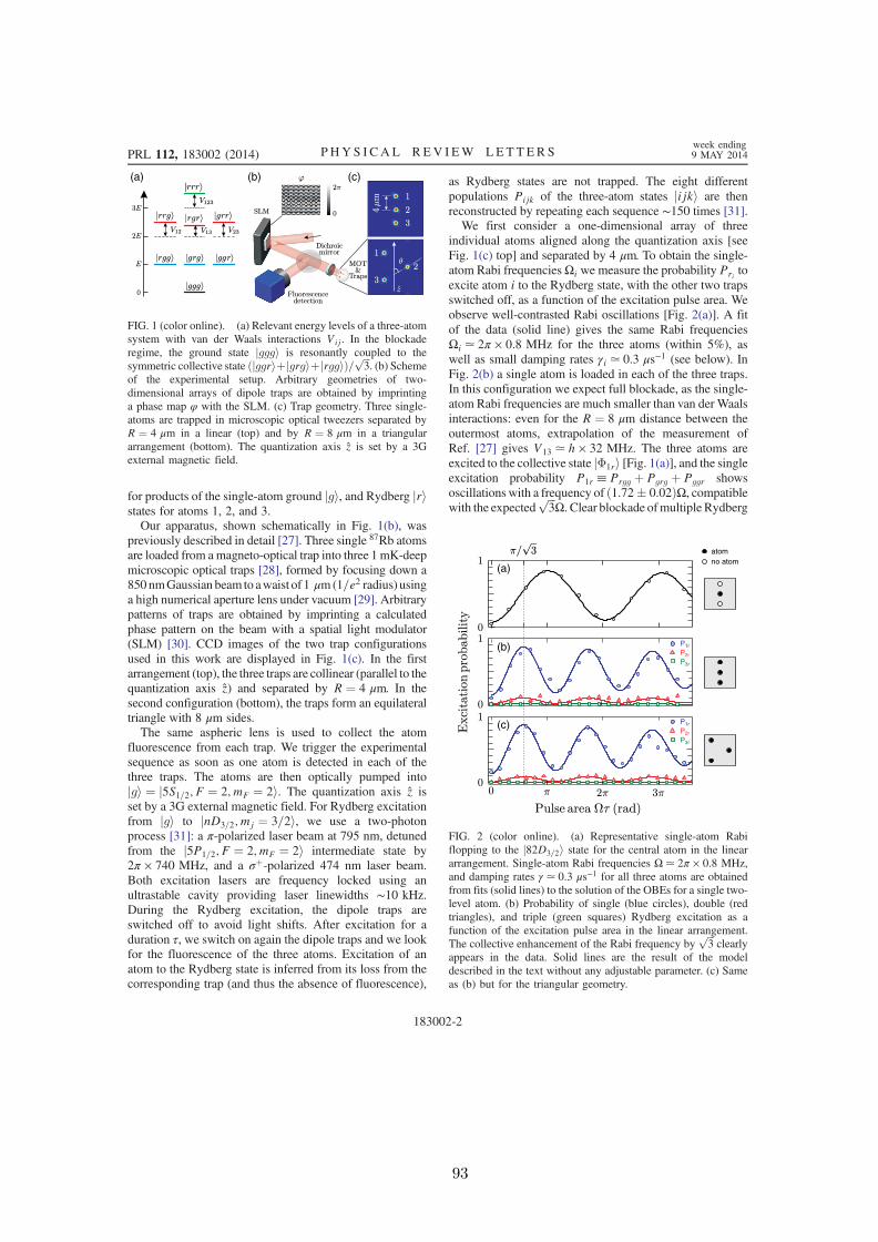
for products of the single-atom ground jgi, and Rydberg jristates for atoms 1, 2, and 3.Our apparatus, shown schematically in Fig. 1(b), was
previously described in detail [27]. Three single 87Rb atomsare loaded from amagneto-optical trap into three 1 mK-deepmicroscopic optical traps [28], formed by focusing down a850nmGaussian beam to awaist of1 μm(1=e2 radius) usinga high numerical aperture lens under vacuum [29]. Arbitrarypatterns of traps are obtained by imprinting a calculatedphase pattern on the beam with a spatial light modulator(SLM) [30]. CCD images of the two trap configurationsused in this work are displayed in Fig. 1(c). In the firstarrangement (top), the three traps are collinear (parallel to thequantization axis z) and separated by R ¼ 4 μm. In thesecond configuration (bottom), the traps form an equilateraltriangle with 8 μm sides.The same aspheric lens is used to collect the atom
fluorescence from each trap. We trigger the experimentalsequence as soon as one atom is detected in each of thethree traps. The atoms are then optically pumped intojgi ¼ j5S1=2; F ¼ 2; mF ¼ 2i. The quantization axis z isset by a 3G external magnetic field. For Rydberg excitationfrom jgi to jnD3=2; mj ¼ 3=2i, we use a two-photonprocess [31]: a π-polarized laser beam at 795 nm, detunedfrom the j5P1=2; F ¼ 2; mF ¼ 2i intermediate state by2π × 740 MHz, and a σþ-polarized 474 nm laser beam.Both excitation lasers are frequency locked using anultrastable cavity providing laser linewidths ∼10 kHz.During the Rydberg excitation, the dipole traps areswitched off to avoid light shifts. After excitation for aduration τ, we switch on again the dipole traps and we lookfor the fluorescence of the three atoms. Excitation of anatom to the Rydberg state is inferred from its loss from thecorresponding trap (and thus the absence of fluorescence),
as Rydberg states are not trapped. The eight differentpopulations Pijk of the three-atom states jijki are thenreconstructed by repeating each sequence ∼150 times [31].We first consider a one-dimensional array of three
individual atoms aligned along the quantization axis [seeFig. 1(c) top] and separated by 4 μm. To obtain the single-atom Rabi frequenciesΩi we measure the probability Pri toexcite atom i to the Rydberg state, with the other two trapsswitched off, as a function of the excitation pulse area. Weobserve well-contrasted Rabi oscillations [Fig. 2(a)]. A fitof the data (solid line) gives the same Rabi frequenciesΩi ≃ 2π × 0.8 MHz for the three atoms (within 5%), aswell as small damping rates γi ≃ 0.3 μs−1 (see below). InFig. 2(b) a single atom is loaded in each of the three traps.In this configuration we expect full blockade, as the single-atom Rabi frequencies are much smaller than van der Waalsinteractions: even for the R ¼ 8 μm distance between theoutermost atoms, extrapolation of the measurement ofRef. [27] gives V13 ≃ h × 32 MHz. The three atoms areexcited to the collective state jΦ1ri [Fig. 1(a)], and the singleexcitation probability P1r ≡ Prgg þ Pgrg þ Pggr showsoscillations with a frequency of ð1.72 0.02ÞΩ, compatiblewith the expected
ffiffiffi3
pΩ. Clear blockade ofmultiple Rydberg
(a) (b) (c)
FIG. 1 (color online). (a) Relevant energy levels of a three-atomsystem with van der Waals interactions Vij. In the blockaderegime, the ground state jgggi is resonantly coupled to thesymmetric collective state ðjggriþjgrgiþjrggiÞ= ffiffiffi
3p
. (b) Schemeof the experimental setup. Arbitrary geometries of two-dimensional arrays of dipole traps are obtained by imprintinga phase map φ with the SLM. (c) Trap geometry. Three single-atoms are trapped in microscopic optical tweezers separated byR ¼ 4 μm in a linear (top) and by R ¼ 8 μm in a triangulararrangement (bottom). The quantization axis z is set by a 3Gexternal magnetic field.
P1r
P2r
P3r
atom
P1r
P2r
P3r
(a)
(b)
(c)
FIG. 2 (color online). (a) Representative single-atom Rabiflopping to the j82D3=2i state for the central atom in the lineararrangement. Single-atom Rabi frequencies Ω≃ 2π × 0.8 MHz,and damping rates γ ≃ 0.3 μs−1 for all three atoms are obtainedfrom fits (solid lines) to the solution of the OBEs for a single two-level atom. (b) Probability of single (blue circles), double (redtriangles), and triple (green squares) Rydberg excitation as afunction of the excitation pulse area in the linear arrangement.The collective enhancement of the Rabi frequency by
ffiffiffi3
pclearly
appears in the data. Solid lines are the result of the modeldescribed in the text without any adjustable parameter. (c) Sameas (b) but for the triangular geometry.
PRL 112, 183002 (2014) P HY S I CA L R EV I EW LE T T ER Sweek ending9 MAY 2014
183002-2
93

excitations is observed in the data, as the populationsP2r ¼ Prrg þ Prgr þ Pgrr (P3r ¼ Prrr) of doubly (triply)excited states are almost totally suppressed in the system,with P2r (P3r) never exceeding 9% (1%).We now show that the actual blockade is even better than
suggested by these values. Indeed, each atom has a smallprobability ε to be lost during the sequence, independentlyof its internal state [32]. An independent measurement of theloss probability gives ε ¼ ð5 1Þ%. Since in our detectionscheme an atom loss is interpreted as an excitation to theRydberg state, the observed double excitation P2r differsfrom the actual one ~P2r and, to first order in ε, it reads [32]
P2r ¼ ð1 − εÞ ~P2r þ 2ε ~P1r: (2)
If the blockade were perfect, one would have ~P2r ¼ 0, andthe measured P2r would thus oscillate between 0 and 2ε, inphase with P1r. From the data on Fig. 2(b) we can extract anupper bound of ∼2% on ~P2r [32].To gain more insight into the quality of the blockade for
our experimental parameters, we simulate the dynamics ofthe system with Hamiltonian (1). A sum of independentsingle atom dissipators,
L½ρ ¼X
i
γi2ð2σðiÞgr ρσðiÞrg − σðiÞrr ρ − ρσðiÞrr Þ; (3)
is used to account for a small experimental damping γi ofthe oscillations (mainly due to off-resonant spontaneousemission through the intermediate state j5P1=2i; all the γiare equal within 10%). The results of the simulation, withno adjustable parameter, are represented by solid lines inFig. 2(b), where the loss-error correction (2) is included.The very good agreement with the data further supports thequality of the blockade. Our results are compatible with theprediction of the model of double excitation probability~Pðtheo.Þ2r ∼ 10−3 for the same experimental parameters.
Although proving experimentally that the double excitationis that low would require a more detailed study ofsystematic effects, this figure is very encouraging forhigh-fidelity generation of three-atom jWi states.In the results discussed so far, we only considered a one-
dimensional configuration. For scalability to a large num-ber of atoms, however, two-dimensional arrays of traps arepreferable. In this case, some atom pairs necessarily havean internuclear axis not aligned along the quantization axisand the anisotropy of the interaction comes into play, whichmight eventually prevent a perfect blockade [23–25]. Toinvestigate this effect we study the blockade in an equi-lateral triangle configuration. Here, the anisotropic char-acter of the D-state orbital plays a role and the interactionenergies between atom pairs V12 ≃ V23 are weaker thanV13, although the atoms are equally separated. Despite this,Fig. 2(c) shows that the strength of the blockade is notreduced in the triangular geometry. Double and tripleexcitation probabilities are inhibited and the single
excitation probability oscillates at ∼ffiffiffi3
pΩ. This result opens
encouraging prospects for achieving strong blockade overtwo-dimensional arrays of atoms.In order to observe directly the anisotropy of the inter-
action [33]wemeasured the interaction energybetween atompairs separated by R ¼ 12 μm as a function of the angle θbetween the internuclear axis and the quantization axis z. Theprocedure to extract the effective interaction energy Veff issimilar to the one introduced in Ref. [27]. Working in thepartial blockade regime (ℏΩ ∼ Veff ), wemodel the excitationdynamics through the solution of the optical Bloch equations(OBE) involving two-level atoms. Strictly speaking, tomodel two atoms in the jnD3=2i state and θ ≠ 0, one wouldneed to consider all 49 Zeeman sublevels with their differentvan der Waals couplings [34]. So as to keep the modeltractable, even for large number of atoms, we model thesystem in the simplest nontrivial way, retaining only onesingle doubly excited state jrriwith an effective energy shiftVeffðθÞ. All input parameters are obtained from single-atomRabi oscillation experiments. The measured dynamics of thetwo-atomsystemare then fittedwith the solutionof theOBEswithVeff as the only fitting parameter. Amore detailed studyof the angular dependence of the van der Waals interaction,taking into account the full Zeeman structure of the atompair,is beyond the scope of this Letter and will be the subject offuture work.The result of this approach is shown in Fig. 3 for the
j82D3=2i state. The anisotropy of the effective interaction isevident. The energy shift shows a maximum around θ ¼ 0
FIG. 3 (color online). Angular dependence of the effectiveinteraction energy Veff for two atoms in j82D3=2i at R ¼ 12 μm,with θ the angle between the internuclear axis and the quantiza-tion axis z. Red squares indicate the measured energy shifts V13,V23, and V12 used for the simulation of three-atom dynamics inthe partial blockade regime (see Fig. 4). In the inset, the angulardependence of the interaction for the spherically symmetricj82S1=2i state is shown for comparison. Error bars representone standard deviation confidence intervals in the fits.
PRL 112, 183002 (2014) P HY S I CA L R EV I EW LE T T ER Sweek ending9 MAY 2014
183002-3
94

and decreases for larger angles. A relative change ofinteraction strength by a factor ∼3 is measured when θvaries from θ ¼ 0 to θ ¼ 60°. In contrast, for a sphericallysymmetric S-Rydberg state, the interaction energy is iso-tropic (see inset of Fig. 3) [35] . For theD state, we observean unexpected, slight asymmetry in the angular dependenceof Veff , probably due to small systematic effects [36] .The angular dependence of Veff manifests itself in the
interaction dynamics of the three atoms in the triangularconfiguration. By increasing the sides of the triangle toR ¼ 12 μm, the effective interaction energies becomeðV12; V23; V13Þ≃ h × ð0.9; 1.1; 2.6Þ MHz (see red squaresin Fig. 3), and the blockade is only partial for our chosenRabi frequency Ω. In Fig. 4 we show the populations ofdoubly (Prrg, Prgr, Pgrr) and triply (Prrr) excited statesfor two different Rabi frequencies. In the first data set[Fig. 4(a)], Ω ¼ 2π × 0.8 MHz and the anisotropy in thebinary interaction (V12 ≠ V13) is directly observed in thedynamics: the probability Prgr to detect double excitationof atoms 1 and 3 is almost totally suppressed, while it isappreciable for Prrg and Pgrr. Those two curves showalmost the same dynamics, as expected. Triple excitationsare totally blocked in this regime. For comparison, we showalso the dynamics when a slightly higher Rabi frequencyΩ ¼ 2π × 1.6 MHz is used [Fig. 4(b)]. This corresponds toa partial blockade regime where V13 > ℏΩ > V12. In thiscase, even triple excitations are not completely blockaded.Prrg and Pgrr also exhibit similar behavior, while Prgrshows different dynamics. The populations of states carry-ing only single excitations also show the anisotropy [32].Many-body effects have largely been recognized to play
a key role in the modeling of systems in physics and
chemistry [37]. In the case of Rydberg atoms they havebeen invoked to explain anomalous broadenings of Försterresonances [38,39]. To understand the evolution of thepopulation of the states during excitation and to investigateto what extent few-atom many-body physics can bedescribed from pairwise interactions we perform again asimulation using the OBEs for the three-atom system. In themodel, with no adjustable parameters, the measured inter-action energies at θ ¼ 0 and θ ¼ 60° (red squares in Fig. 3)are introduced. As shown by the solid lines in Fig. 4, thesimulation (where atom loss correction is included) fullyreproduces the experimental data. The fact that the simu-lation can accurately describe the evolution of the triplyexcited state Prrr suggests that, for our choice of param-eters, the pairwise addition of van der Waals level shiftsV123 ¼ V12 þ V13 þ V23 is valid to a very good approxi-mation. However, this additivity of the potential may nothold in the case of resonant dipole-dipole interactions.There, quantum interference between different many-bodyinteraction channels can influence the dynamics [23]. Allthese processes can be studied for Rydberg atoms close toFörster resonance and will be the subject of future work.Another interesting line of research will consist in studyingthe recently predicted Borromean trimers bound by thedipole-dipole interaction [40].In summary, we have investigated the dynamics of a
system of three Rydberg atoms in both full and partialblockade regimes. We observe a strong van der Waalsblockade of the excitations and coherent Rabi oscillationsfor two different spatial configurations. For the sameexperimental parameters in the equilateral triangle arrange-ment, the anisotropy of the interaction potential betweenjnDi states does not prevent the observation of a strong vanderWaals blockade, which is a prerequisite for the scalabilityof quantum information processing proposals using two-dimensional arrays of dipole traps. The strong blockadeachieved and the small damping of the oscillations pave theway for the generation ofmany-atom entanglement with highfidelity through the Rydberg blockade [12]. In the partialblockade regime, the angular dependence of the interactionenergy shift between two atoms has been measured for thej82D3=2i and j82S1=2i Rydberg states. Furthermore, we haveshown that with the measured effective energy shifts it ispossible to reproduce the three-atom dynamics with highaccuracy. This result demonstrates that one can confidentlyscale those studies for two-dimensional arrays of more than afew atoms, enabling the quantum simulation of large-size,long-range interacting spin systems.
We thank Daniel Cano for interesting discussions.This work was supported financially by the EU [ERCStg Grant ARENA, AQUTE Integrating project, FET-OpenXtrack project HAIRS, EU Marie-Curie program ITNCOHERENCE FP7-PEOPLE-2010-ITN-265031 (H.L.)],by the DGA (L.B.), and by Région Île-de-France(LUMAT and Triangle de la Physique, LAGON project).
(a) (b)
FIG. 4 (color online). Probabilities of detection of doubleRydberg excitation Prrg, Prgr, Pgrr, and triple excitation Prrrversus excitation pulse area Ωτ for driving Rabi frequenciesΩ ¼ 2π × 0.8 MHz (a), and Ω ¼ 2π × 1.6 MHz (b) in thetriangular configuration. The distance between the traps isR ¼ 12 μm. The ratio between effective pairwise interactionenergies is V13=V12 ∼ 3 for θ ¼ 60°. Solid lines are the solutionof the OBEs without any adjustable parameter.
PRL 112, 183002 (2014) P HY S I CA L R EV I EW LE T T ER Sweek ending9 MAY 2014
183002-4
95

[1] M. A. Nielsen, I. L. Chuang, Quantum Computationand Quantum Information (Cambridge University Press,Cambridge, England, 2000).
[2] R. Feynman, Int. J. Theor. Phys. 21, 467 (1982).[3] B. P. Lanyon et al., Science 334, 57 (2011).[4] J. W. Britton, B. C. Sawyer, A. C. Keith, C.-C. Joseph
Wang, J. K. Freericks, H. Uys, M. J. Biercuk, and J. J.Bollinger, Nature (London) 484, 489 (2012).
[5] R. Islam, C. Senko, W. C. Campbell, S. Korenblit, J. Smith,A. Lee, E. E. Edwards, C.-C. J. Wang, J. K. Freericks, andC. Monroe, Science 340, 583 (2013).
[6] H. Weimer, M. Müller, I. Lesanovsky, P. Zoller and H. P.Büchler, Nat. Phys. 6, 382 (2010).
[7] D. Jaksch, J. I. Cirac, P. Zoller, S. L. Rolston, R. Côté, andM. D. Lukin, Phys. Rev. Lett. 85, 2208 (2000).
[8] M. D. Lukin, M. Fleischhauer, R. Cote, L. M. Duan, D.Jaksch, J. I. Cirac, and P. Zoller, Phys. Rev. Lett. 87, 037901(2001).
[9] D. Comparat and P. Pillet, J. Opt. Soc. Am. B 27, A208(2010).
[10] T.Wilk,A.Gaëtan,C.Evellin, J.Wolters,Y.Miroshnychenko,P. Grangier, and A. Browaeys, Phys. Rev. Lett. 104, 010502(2010).
[11] L. Isenhower, E. Urban, X. L. Zhang, A. T. Gill, T. Henage,T. A. Johnson, T. G. Walker, and M. Saffman, Phys. Rev.Lett. 104, 010503 (2010).
[12] M. Saffman, T. G. Walker, and K. Mølmer, Rev. Mod. Phys.82, 2313 (2010).
[13] K. Singer, M. Reetz-Lamour, T. Amthor, L. G. Marcassa,and M. Weidemüller, Phys. Rev. Lett. 93 163001(2004).
[14] R. Heidemann, U. Raitzsch, V. Bendkowsky, B. Butscher,R. Löw, L. Santos, and T. Pfau, Phys. Rev. Lett. 99, 163601(2007).
[15] J. D. Pritchard, D. Maxwell, A. Gauguet, K. J. Weatherill,M. P. A. Jones, and C. S. Adams, Phys. Rev. Lett. 105,193603 (2010).
[16] Y. O. Dudin and A. Kuzmich, Science 336, 887 (2012).[17] Y. O. Dudin, L. Li, F. Bariani, and A. Kuzmich, Nat. Phys.
8, 790 (2012).[18] P. Schauss, M. Cheneau, M. Endres, T. Fukuhara, S. Hild,
A. Omran, T. Pohl, C. Gross, S. Kuhr, and I. Bloch, Nature(London) 491, 87 (2012).
[19] E. Urban, T. A. Johnson, T. Henage, L. Isenhower, D. D.Yavuz, T. G. Walker, and M. Saffman, Nat. Phys. 5, 110(2009).
[20] A. Gaëtan, Y. Miroshnychenko, T. Wilk, A. Chotia, M.Viteau, D. Comparat, P. Pillet, A. Browaeys, and P.Grangier, Nat. Phys. 5, 115 (2009).
[21] G. Günter, H. Schempp, M. Robert-de-Saint-Vincent, V.Gavryusev, S. Helmrich, C. S. Hofmann, S. Whitlock, andM. Weidemuller, Science 342, 954 (2013).
[22] A. M. Hankin, Y.-Y. Jau, L. P. Parazzoli, C. W. Chou, D. J.Armstrong, A. J. Landahl, and G.W. Biedermann, Phys.Rev. A 89, 033416 (2014).
[23] T. Pohl and P. R. Berman, Phys. Rev. Lett. 102, 013004(2009).
[24] D. Cano and J. Fortágh, Phys. Rev. A 86, 043422 (2012).[25] J. Qian, X.-D. Zhao, L. Zhou, and W. Zhang, Phys. Rev. A
88, 033422 (2013).[26] I. Lesanovsky, Phys. Rev. Lett. 106, 025301 (2011).[27] L. Béguin, A. Vernier, R. Chicireanu, T. Lahaye, and A.
Browaeys, Phys. Rev. Lett. 110, 263201 (2013).[28] N. Schlosser, G. Reymond, I. Protsenko and P. Grangier,
Nature (London) 411, 1024 (2001).[29] Y. R. P. Sortais et al., Phys. Rev. A 75, 013406 (2007).[30] F. Nogrette et al., arXiv:1402.5329 [Phys. Rev. X (to be
published)].[31] Y. Miroshnychenko, A. Gaëtan, C. Evellin, P. Grangier, D.
Comparat, P. Pillet, T. Wilk, and A. Browaeys, Phys. Rev. A82, 013405 (2010).
[32] See Supplemental Material at http://link.aps.org/supplemental/10.1103/PhysRevLett.112.183002 for de-tailed error-loss analysis and full system dynamics.
[33] T. J. Carroll, K. Claringbould, A. Goodsell, M. J. Lim, andM.W. Noel, Phys. Rev. Lett. 93, 153001 (2004).
[34] A. Reinhard, T. C. Liebisch, B. Knuffman, and G. Raithel,Phys. Rev. A 75, 032712 (2007).
[35] For excitation to the S state, the polarizations of the795 nm (474 nm) lasers are π (σ−).
[36] However, the observed asymmetry has a negligible impacton the three-atom dynamics that we study in the rest of theLetter.
[37] R. A. DiStasio, O. A. von Lilienfeld, and A. Tkatchenko,Proc. Natl. Acad. Sci. U.S.A. 109, 14791 (2012).
[38] W. R. Anderson, J. R. Veale, T. F. Gallagher, Phys. Rev.Lett. 80, 249 (1998).
[39] I. Mourachko, D. Comparat, F. de Tomasi, A. Fioretti, P.Nosbaum, V. Akulin, and P. Pillet, Phys. Rev. Lett. 80, 253(1998).
[40] M. Kiffner, W. Li, and D. Jaksch, Phys. Rev. Lett. 111,233003 (2013).
PRL 112, 183002 (2014) P HY S I CA L R EV I EW LE T T ER Sweek ending9 MAY 2014
183002-5
96
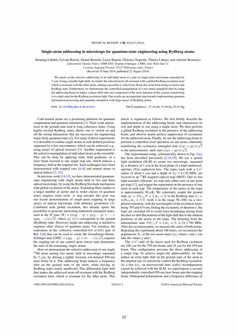
PHYSICAL REVIEW A 90, 023415 (2014)
Single-atom addressing in microtraps for quantum-state engineering using Rydberg atoms
Henning Labuhn, Sylvain Ravets, Daniel Barredo, Lucas Beguin, Florence Nogrette, Thierry Lahaye, and Antoine BrowaeysLaboratoire Charles Fabry, UMR 8501, Institut d’Optique, CNRS, Univ Paris Sud 11,
2 avenue Augustin Fresnel, 91127 Palaiseau cedex, France(Received 19 June 2014; published 22 August 2014)
We report on the selective addressing of an individual atom in a pair of single-atom microtraps separated by3 μm. Using a tunable light shift, we render the selected atom off-resonant with a global Rydberg excitation laserwhich is resonant with the other atom, making it possible to selectively block this atom from being excited to theRydberg state. Furthermore we demonstrate the controlled manipulation of a two-atom entangled state by usingthe addressing beam to induce a phase shift onto one component of the wave function of the system, transferringit to a dark state for the Rydberg excitation light. Our results are an important step towards implementing quantuminformation processing and quantum simulation with large arrays of Rydberg atoms.
DOI: 10.1103/PhysRevA.90.023415 PACS number(s): 37.10.Gh, 32.80.Ee, 03.67.Bg
Cold neutral atoms are a promising platform for quantumcomputation and quantum simulation [1]. Their weak interac-tions in the ground state lead to long coherence times. Usinghighly excited Rydberg states allows one to switch on andoff the strong interactions that are necessary for engineeringmany-body quantum states [2]. For many of those experimentsit is desirable to confine single atoms at well-defined positionsseparated by a few micrometers, which can be achieved, e.g.,using arrays of optical tweezers [3]. Another requirement isthe selective manipulation of individual atoms in the ensemble.This can be done by applying static field gradients, or alaser beam focused to one single trap site, which induces afrequency shift at the targeted site. Such techniques have beendemonstrated with trapped ions [4–6] and neutral atoms inoptical lattices [7–13].
In previous work [14,15], we have demonstrated quantum-state engineering with single atoms held in two and threeoptical microtraps, by using the Rydberg blockade mechanismwith global excitation of the atoms. Extending these studies toa larger number of atoms and to wider classes of quantumstates requires extra tools. A step towards this goal wasour recent demonstration of single-atom trapping in largearrays of optical microtraps with arbitrary geometries [3].Combined with global excitation, this already opens thepossibility to generate interesting multiatom entangled states,such as the W state |W 〉 = (|rgg · · · g〉 + |grg · · · g〉 + · · · +|ggg · · · r〉)/√N , where |g〉 (|r〉) corresponds to the ground(Rydberg) state. However, single-site addressing is needed toengineer other classes of quantum states. For instance, therealization of the collective controlled-NOT (CNOT) gate ofRef. [16] that can be used to create the Greenberger-Horne-Zeilinger state |GHZ〉 = (|gg · · · g〉 + |rr · · · r〉)/√2, requiresthe singling out of one control atom whose state determinesthe state of the remaining, target, atoms.
Here we demonstrate the selective addressing of one single87Rb atom among two atoms held in microtraps separatedby 3 μm, by shining a tightly focused, red-detuned 850-nmlaser beam on it. This addressing beam induces a frequencyshift on the ground state of the atom, while leaving itsRydberg states nearly unaffected. This differential light shiftthus makes the addressed atom off-resonant with the Rydbergexcitation laser, which is resonant for the other atom. This
article is organized as follows. We first briefly describe theimplementation of the addressing beam, and characterize itssize and depth in situ using a single atom. We then performa global Rydberg excitation in the presence of the addressingbeam, and observe nearly perfect suppression of excitationsfor the addressed atom. Finally, we use the addressing beam toperform a controlled local operation on one atom, coherentlytransferring the symmetric entangled state (|rg〉 + |gr〉)/√2to the antisymmetric, dark state (|rg〉 − |gr〉)/√2.
Our experimental setup, schematically shown in Fig. 1(a),has been described previously [3,14,15]. We use a spatiallight modulator (SLM) to create two microtraps, separatedby a distance of 3 μm in the focal plane of a high-numerical-aperture (NA) aspherical lens. The traps, each with a 1/e2
radius of about 1 μm and a depth of U0 ≈ h×20 MHz, arefocused in an 87Rb magneto-optical trap (MOT). Due to fastlight-assisted collisions, we trap only either zero or one atomper trap [17], and trigger the experiment on the presence of oneatom in each trap. The temperature of the atoms in the trapsis approximately 50 μK. We coherently couple the groundstate |g〉 = |5S1/2,F = 2,mf = 2〉 to the Rydberg state |r〉 =|nD3/2,mj = 3/2〉 (with n in the range 50–100) via a two-photon transition, with the wavelengths of the excitation lasersbeing 795 and 474 nm. During the excitation, of duration τ , thetraps are switched off to avoid extra broadening arising fromthe shot-to-shot fluctuations of the light shift due to the randompositions of the atoms in the traps. The detuning from theintermediate state |5P1/2,F = 2,mf = 2〉 is 2π×740 MHz.After the excitation pulse, we measure the states of both atoms.Repeating the experiment about 100 times, we reconstruct thepopulations Pij of the two-atom states |ij 〉, where i and j cantake the values g and r .
The 1/e2 radii of the lasers used for Rydberg excitationare 100 μm for the 795-nm beam, and 18 μm for the 474-nmbeam. This configuration prevents the direct addressing ofa single trap. To achieve single-site addressability, we thusinduce an extra light shift on the ground state of the atom atthe targeted site, to selectively control the Rydberg excitation.As a fast (i.e., on microsecond time scales) reconfigurationcannot be achieved with the SLM, we superimpose a second,independently controlled 850-nm laser beam onto the trappingbeam. Orthogonal polarizations and a frequency difference of
1050-2947/2014/90(2)/023415(4) 023415-1 ©2014 American Physical Society
97

HENNING LABUHN et al. PHYSICAL REVIEW A 90, 023415 (2014)
SLMtrap beam
addressing beam
AOM x
traps
PBS
AOM y
telescope
(a)
(b)
(c)
474 nm beam
E
x
I
x
−2 0 2−5−4−3−2−1
0
ΔE/
h [M
Hz]
Δ x [µm]
795 nm beam
FIG. 1. (Color online) (a) Sketch of the experimental setup. Thetwo microtraps are created by a red-detuned 850-nm laser beamon which an appropriate phase is imprinted using a spatial lightmodulator (SLM), and focused by a high-NA aspheric lens in aMOT. The addressing beam is superimposed onto the trap beam bya polarizing beam-splitter cube (PBS), and focused down on thetargeted atom by the same aspheric lens. The two perpendicularAOMs can be used for precise dynamical x-y positioning of theaddressing beam. A telescope is used to conjugate the AOM planewith the aspheric lens, to avoid clipping when the addressing beamis deflected. (b) The light shift E of the ground state of the targetedsingle atom is directly proportional to the intensity I of the addressingbeam at the position x of the atom. (c) Measured light shift E asa function of the distance x between the addressing beam andthe targeted trap, yielding a 1/e2 radius of the addressing beam ofw0 1.3 μm.
about 200 MHz prevent interference between the trapping andaddressing beams. The addressing beam has a 1/e2 radius ofw0 1.3 μm in the focus, slightly larger than the trap size.This choice results from a trade-off between two oppositerequirements, namely, minimizing alignment sensitivity andinhomogeneous light shifts (which favors a large w0) andminimizing cross-talk (which implies choosing a small w0).For a perfectly Gaussian beam with w0 1.3 μm, one expectstheoretically that if one atom is addressed by a light shift of10 MHz, the second atom 3 μm away experiences a lightshift of only 0.2 kHz, which is negligible as compared tothe other relevant frequencies in the experiment. An electro-optic modulator enables fast (about 10 ns) switching of theaddressing beam. In addition, two acousto-optic modulators(AOMs) can be used for dynamical x-y positioning of theaddressing beam with respect to the targeted trap.
In a first experiment, we measure the intensity profile of theaddressing beam in situ by performing Rydberg spectroscopyon a single atom. For different positions x of the addressingbeam with respect to the targeted atom, we scan the frequencyof the Rydberg excitation lasers. As mainly the ground stateexperiences a light shift E proportional to the addressingbeam intensity, the resonance frequency for Rydberg excitationis shifted by E [see Fig. 1(b)]. Figure 1(c) shows themeasured light shift as a function of x. A Gaussian fitgives a 1/e2 radius w0 = 1.3 ± 0.1μm. The residual lightshift experienced by the nearby atom 3 μm away is belowthe resolution of our experiment.
We observe that for large light shifts, the probability oflosing an atom during the sequence increases. We attribute thiseffect to the following: due to the finite temperature, the atomnever sits exactly at the intensity maximum of the addressingbeam. The fast switching on and off of the addressing beamthus imparts kinetic energy to the atom. This increase in kineticenergy becomes more and more important as the intensity ofthe addressing beam gets larger. For large enough intensities inthe addressing beam, this effect thus increases the probabilityfor the atom to leave the trapping region during the experiment.However, for light shifts below 40 MHz, this loss probabilityremains below 1%, and is thus negligible.
We now perform a Rydberg blockade experiment with twosingle atoms in order to demonstrate single-site addressability(Fig. 2). In Ref. [18], site-resolving excitation beams were usedto demonstrate blockade with two atoms separated by 10 μm.Here, we use a global excitation scheme in combination withthe addressing beam, and obtain similar results, albeit with adistance between the atoms of only 3 μm. For both atoms, theground state |g〉 is coupled to the Rydberg state |r〉 = |59D3/2〉with a Rabi frequency 2π×1 MHz [Fig. 2(a)]. If theatoms were independent, they would both undergo Rabioscillations between |g〉 and |r〉 with the Rabi frequency .The strong dipole-dipole interaction Udd between the Rydbergstates forbids a double excitation of the atoms if Udd .This condition is largely fulfilled for the parameters chosenhere: the interaction energy of two atoms in |59D3/2〉, separatedby 3 μm, is approximately h×300 MHz. We thus excite onlythe superposition state |s〉 = (|rg〉 + eik·r |gr〉)/√2, whosecoupling to the two-atom ground state |gg〉 is
√2 [18,19]
(here, k is the vector sum of the wave vectors of the excitationlasers, and r is the position of atom 2 with respect to atom 1).This results in Prg and Pgr oscillating between 0 and 1/2 with afrequency
√2, as can be seen in Fig. 2(b). Another signature
of the blockade is the suppression of double excitation Prr 0[see bottom panel in Fig 2(b)].
If we shine the addressing beam on atom 2, we observe astrong suppression of the excitation probability for the states|gr〉 and |rr〉 [see Fig. 2(c)], as atom 2 is never excited tothe Rydberg state |r〉. At the same time, atom 1 shows Rabioscillations between |g〉 and |r〉 with the single-atom Rabifrequency . The small residual excitation probability of atom2 that we observe is fully accounted for by the errors in ourstate detection [15], meaning that cross-talk between the twotraps is negligible.
Finally, we show that we can also use the addressing beamto directly manipulate a two-atom quantum state. Withoutany addressing, the excitation to the state |rr〉 is completely
023415-2
98

SINGLE-ATOM ADDRESSING IN MICROTRAPS FOR . . . PHYSICAL REVIEW A 90, 023415 (2014)
1 mota 2 mota 1 mota 2 mota
0
10
10
10
1
0
E
0
(b)
(a)
(c)
FIG. 2. (Color online) (a) Two atoms, separated by 3 μm, areilluminated by light that resonantly couples the ground state |g〉 to|r〉 = |59D3/2〉 with the single-atom Rabi frequency . The timeevolution of the populations of the two-atom states |gg〉, |gr〉, |rg〉,and |rr〉 are shown, (b) without any addressing and (c) with atom 2addressed with a light shift of E h×10 MHz. Solid lines are fitsby damped sine curves. The vertical solid lines mark the pulse areasτ corresponding to a π pulse for the nonaddressed case (blue) andthe addressed case (red). The black dashed lines show the expectedmeasured populations for a perfect blockade of atom 2, taking intoaccount state-detection errors.
suppressed in the Rydberg blockade regime (Udd ). Byapplying an excitation pulse of duration π/(
√2) we thus pre-
pare the atoms in the state |ψ(0)〉 = (|gr〉 + eik·r |rg〉)/√2. Wethen illuminate atom 2 with the addressing beam [Fig. 3(a)].Its energy is shifted by E when in the ground state, while itsRydberg state remains unaffected [see Fig. 2(a)]. After a timeT the state of the system has therefore evolved to
|ψ(T )〉 = 1√2
(|gr〉 + e−iE T/eik·r |rg〉). (1)
The antisymmetric dark state |ψ(Tπ )〉= (|gr〉− eik·r |rg〉)/√2 (with Tπ = π/E) is not coupled to the ground state
0 50 100 150 200 2500.0
0.2
0.4
0.6
0.8
1.0
100
4
8
2 3 4 5
f [M
Hz]
P [mW]
Tt
dipoletrap
dipoletrap
de-excitationpulse
addressingbeam
excitationpulse
(a)
(b)
FIG. 3. (Color online) (a) Pulse sequence for the phase manipu-lation: while the dipole trap is switched off, the atoms are excited tothe state |s〉 = (|gr〉 + eik·r |rg〉)/√2. The addressing beam inducesa light shift E on the ground state of atom 2, thus changing therelative phase evolution between |gr〉 and |rg〉. This is followed bya global deexcitation pulse. (b) Population of the two-atom groundstate |gg〉 after the deexcitation pulse, as a function of the addressingpulse length T , for a laser power in the addressing beam P =1.5 mW (blue diamonds) and P = 3.5 mW (red circles). Solid linesare fits by damped sine curves of frequency f . Inset: oscillationfrequency f as a function of the power P of the addressing beam,showing the expected linear dependence. For this experiment we usethe Rydberg state |82D3/2〉.
|gg〉. The probability of deexciting the atoms to |gg〉 isthus expected to oscillate between 0 and 1 with a frequencyf = E/h.
Figure 3(b) shows the probability Pgg of deexciting theatoms back to |gg〉 versus the duration T of the addressingpulse. We observe the expected oscillation of the final ground-state population Pgg . Due to the finite Rydberg excitationefficiency (about 90% for our parameters), we measure acontrast of the oscillations that is lower than 1. In addition,the finite temperature of the atoms in the experiment leads toa small motion of the atoms during the sequence, implyingthat (i) the phase k · r imprinted by the excitation pulse is notexactly canceled out by the deexcitation pulse [20]; and (ii) thelight shift E experienced by atom 2 fluctuates from shot toshot. Averaged over many runs, both effects lead to a decreasedcontrast and a finite damping of the observed oscillations. Totake these effects into account, we fitted the data with a dampedsine curve of the form Pgg(T ) = A + B exp(−γ t) cos(2πf T ),with the oscillation frequency f and the damping rate γ asadjustable parameters. Repeating the experiment for differentpowers of the addressing beam, we obtain the expected lineardependence of f with the applied light shift on the atom [seeinset of Fig. 3(b)]. This demonstrates our ability to performsome controlled local operations on qubits in a quantumregister.
023415-3
99

HENNING LABUHN et al. PHYSICAL REVIEW A 90, 023415 (2014)
In conclusion, we have shown that we can selectivelyprevent one single atom in a pair of single-atom trapsfrom being resonant with Rydberg excitation lasers, with nomeasurable cross-talk with a neighboring atom as close as3 μm. We also demonstrated the use of the addressing beam toperform a local operation in a system of two atoms. Our schemeis easily scalable to a larger number of traps. These techniqueswill prove useful for a variety of applications in quantumsimulation and quantum information processing with Rydbergatoms. For instance, they open the possibility of selectivelyaddressing a single qubit in a larger ensemble, e.g., as a control
atom for realizing collective quantum gates [16], or to excitea single atom to a different Rydberg state, allowing the studyof the transfer of excitations along a Rydberg chain [21].
We thank Yvan Sortais for helpful advice about the opticaldesign. We acknowledge financial support by the EU [ERC StgGrant ARENA, AQUTE Integrating Project, FET-Open XtrackProject HAIRS, and EU Marie-Curie Program ITN COHER-ENCE Grant No. FP7-PEOPLE-2010-ITN-265031 (H.L.)],by DGA (L.B.), and by Region Ile-de-France (LUMAT andTriangle de la Physique, LAGON Project).
[1] I. Bloch, J. Dalibard, and S. Nascimbene, Nat. Phys. 8, 267(2012).
[2] M. Saffman, T. G. Walker, and K. Mølmer, Rev. Mod. Phys. 82,2313 (2010).
[3] F. Nogrette, H. Labuhn, S. Ravets, D. Barredo, L. Beguin,A. Vernier, T. Lahaye, and A. Browaeys, Phys. Rev. X 4, 021034(2014).
[4] H. C. Nagerl, D. Leibfried, H. Rohde, G. Thalhammer,J. Eschner, F. Schmidt-Kaler, and R. Blatt, Phys. Rev. A 60,145 (1999).
[5] H. Haffner, W. Hansel, C. F. Roos, J. Benhelm, D. Chek-al-kar,M. Chwalla, T. Korber, U. D. Rapol, M. Riebe, P. O. Schmidt,C. Becher, O. Guhne, W. Dur, and R. Blatt, Nature 438, 643(2005).
[6] C. Monroe and J. Kim, Science 339, 1164 (2013).[7] R. Dumke, M. Volk, T. Muther, F. B. J. Buchkremer, G. Birkl,
and W. Ertmer, Phys. Rev. Lett. 89, 097903 (2002).[8] M. Saffman, Opt. Lett. 29, 1016 (2004).[9] M. Karski, L. Forster, J.-M. Choi, A. Steffen, N. Belmechri,
W. Alt, D. Meschede, and A. Widera, New J. Phys. 12, 065027(2010).
[10] C. Weitenberg, M. Endres, J. F. Sherson, M. Cheneau, P. Schauß,T. Fukuhara, I. Bloch, and S. Kuhr, Nature (London) 471, 319(2011).
[11] M. Schlosser, S. Tichelmann, J. Kruse, and G. Birkl,Quantum Inf. Process. 10, 907 (2011).
[12] T. Fukuhara, A. Kantian, M. Endres, M. Cheneau, P. Schauß,S. Hild, D. Bellem, U. Schollwock, T. Giamarchi, C. Gross,I. Bloch, and S. Kuhr, Nat. Phys. 9, 235 (2013).
[13] J. H. Lee, E. Montano, I. H. Deutsch, and P. S. Jessen,Nat. Commun. 4, 2027 (2013).
[14] L. Beguin, A. Vernier, R. Chicireanu, T. Lahaye, andA. Browaeys, Phys. Rev. Lett. 110, 263201 (2013).
[15] D. Barredo, S. Ravets, H. Labuhn, L. Beguin, A. Vernier,F. Nogrette, T. Lahaye, and A. Browaeys, Phys. Rev. Lett. 112,183002 (2014).
[16] M. Muller, I. Lesanovsky, H. Weimer, H. P. Buchler, andP. Zoller, Phys. Rev. Lett. 102, 170502 (2009).
[17] Y. R. P. Sortais, H. Marion, C. Tuchendler, A. M. Lance,M. Lamare, P. Fournet, C. Armellin, R. Mercier, G. Messin,A. Browaeys, and P. Grangier, Phys. Rev. A 75, 013406(2007).
[18] E. Urban, T. A. Johnson, T. Henage, L. Isenhower, D. D. Yavuz,T. G. Walker, and M. Saffman, Nat. Phys. 5, 110 (2009).
[19] A. Gaetan, Y. Miroshnychenko, T. Wilk, A. Chotia, M. Viteau,D. Comparat, P. Pillet, A. Browaeys, and P. Grangier, Nat. Phys.5, 115 (2009).
[20] T. Wilk, A. Gaetan, C. Evellin, J. Wolters, Y. Miroshnychenko,P. Grangier, and A. Browaeys, Phys. Rev. Lett. 104, 010502(2010).
[21] S. Wuster, C. Ates, A. Eisfeld, and J. M. Rost, Phys. Rev. Lett.105, 053004 (2010).
023415-4
100
LETTERSPUBLISHED ONLINE: 26 OCTOBER 2014 | DOI: 10.1038/NPHYS3119
Coherent dipole–dipole coupling between twosingle Rydberg atoms at an electrically-tunedFörster resonanceSylvain Ravets, Henning Labuhn, Daniel Barredo, Lucas Béguin, Thierry Lahayeand Antoine Browaeys*
Resonant energy transfers, the non-radiative redistribution ofan electronic excitation between two particles coupled by thedipole–dipole interaction, lie at the heart of a variety of phe-nomena1, notably photosynthesis. In 1948, Förster establishedthe theory of fluorescence resonant energy transfer (FRET)between broadband, nearly-resonant donors and acceptors2.The 1/R6 scaling of the energy transfer rate, where R is thedistance between particles, enabled widespread use of FRETas a ‘spectroscopic ruler’ for determining nanometric distancesin biomolecules3. The underlying mechanism is a coherentdipolar coupling between particles, as recognized in the earlydays of quantum mechanics4, but this coherence has not beendirectly observed so far. Here we study, spectroscopically andin the time domain, the coherent, dipolar-induced exchange ofexcitations between two Rydberg atoms separated by up to15µm, and brought into resonance by applying an electric field.Coherent oscillation of the system between two degeneratepair states then occurs at a frequency scaling as 1/R3, thehallmark of resonant dipole–dipole interactions5. Our resultsnot only demonstrate, at the fundamental level of two atoms,the basic mechanism underlying FRET, but also open excitingprospects for active tuning of strong, coherent interactions inquantum many-body systems.
The possibility to tune at will coherent interactions inmany-bodysystems by changing external parameters is one of the key toolsenabling quantum simulation. For instance, in ultracold quantumgases, such tuning can be achieved by magnetically-inducedFeshbach resonances6,7. Rydberg atoms are another promisingplatform for the quantum simulation of complex many-bodyproblems, owing to the strong interactions associated with theirlarge principal quantum numbers8. They have proved to be anefficient tool for characterizing non-radiative exchange of energyin resonant collisional processes9, studying collective effects10and engineering quantum states of matter11. The observation ofRydberg blockade between individual atoms12,13, where the stronginteraction between Rydberg states inhibits multiple excitationswithin a blockade sphere, opens the way towards the developmentof Rydberg quantum simulators14. An appealing tool for thoseapplications is the possibility to tune the strength of the interactionsby external electric fields using Förster resonances15–23. So far, owingto inhomogeneities in the atomic ensembles used in experiments,only indirect evidence for the coherent character of the interactionhas been obtained24,25.
Here, we study a system of two single atoms at a Försterresonance. We first perform a spectroscopic measurement of theenergies of the two-atom states as a function of the applied electricfield, and observe directly the avoided crossing between pair statesinduced by the dipole–dipole interaction. The splitting at resonanceis observed to scale as 1/R3 as a function of the distance R betweenthe atoms. In a second experiment, we prepare the system in agiven pair state away from resonance, and switch to resonance fora controlled time, revealing the coherent oscillation between thetwo degenerate pair states induced by the dipolar interaction. Theseresults open the way to real-time tuning of interactions for quantumsimulation with Rydberg atoms11,14.
Two atoms located at positions R1 and R2 interact through thedipole–dipole interaction
Vdip=1
4πε0
(µ1 · µ2−3(µ1 ·n)(µ2 ·n)
R3
)
where µi is the electric dipole moment of atom i (i = 1, 2),R=R2−R1 and n= R/R. When the two atoms are prepared inthe same state, Vdip usually has no effect to first order, as theaverage value of the dipolemoment vanishes in an atomic eigenstate.Second-order perturbation theory gives rise to an energy shift ofthe atom pair, which results in the van der Waals interaction26
UvdW∝R−6. However, resonance effects between two Rydberg atomscan occur when two pair states are degenerate5, and in this case thedipolar interaction manifests itself at first order. Such a resonance,called a ‘Förster resonance’ in analogy with the FRETmechanism atwork in photochemistry, can be achieved using small electric fieldsto Stark-tune the energy of the pair states.
In this work, we use the states |p〉 = |61P1/2, mJ = 1/2〉,|d〉=|59D3/2,mJ =3/2〉 and |f 〉 = |57F5/2,mJ = 5/2〉 of 87Rb. Thepair states |dd〉, |pf 〉 and |fp〉 are almost degenerate (Fig. 1a): theirFörster defect∆0= (Epf −Edd)/h, in the absence of an electric field,is only 8.5MHz (h is Planck’s constant). Using the differential Starkeffect between |dd〉 and |pf 〉, they can be brought to exact resonanceby applying an electric field Fres'32mV cm−1 (Fig. 1b). The smallelectric fields at play ensure that we work in a regime of induceddipoles (even for the highly polarizable f state), as opposed to therigid dipoles obtained for larger electric fields. At resonance, theeigenstates of the interacting system are |±〉= (|dd〉 ± |pf 〉)/
√2,
where |pf 〉 = (|pf 〉 + |fp〉)/√2. If the system is initially prepared
in |dd〉, it thus oscillates between the two degenerate electronic
Laboratoire Charles Fabry, UMR 8501, Institut d’Optique, CNRS, Univ Paris Sud 11, 2 avenue Augustin Fresnel, 91127 Palaiseau Cedex, France.*e-mail: [email protected]
914 NATURE PHYSICS | VOL 10 | DECEMBER 2014 | www.nature.com/naturephysics
© 2014 Macmillan Publishers Limited. All rights reserved
101

NATURE PHYSICS DOI: 10.1038/NPHYS3119 LETTERS
Vdip
p p
d d
f f
2E
E
0
0 20 40 60−20
−10
0
10
20Fres
E/h
(MH
z)
F (mV cm−1)
ΔE
ΔE
xyElectrodes
z
F
|dd⟩
|dd⟩
|dd⟩
|+⟩
|−⟩
|pf⟩∼
|pf⟩∼
|pf⟩∼
|dg⟩∼
|gg⟩
δ
a
c
d
b
R
Trappingbeam
Figure 1 | Principle of the experiment. a, The pair states |dd〉 and |pf〉 are coupled by the dipolar interaction at a Förster resonance. b, Stark eect of the pairstates. In the absence of coupling, the two pair-state energy levels (dotted lines) vary when an external electric field F is applied, and cross each other forF=Fres. The coupled system (solid lines) undergoes an avoided crossing at resonance (vertical dashed line). c, Experimental set-up. Two individual 87Rbatoms are trapped in microscopic optical tweezers separated by a distance R. Eight independent electrodes allow the application of a tunable electric field Falong the internuclear axis z. d, Structure of the coupled levels at resonance. We scan the excitation laser (blue arrow) to perform a two-atom excitationfrom |gg〉 to |dd〉 via the intermediate, one-excitation state |dg〉=(|dg〉+|gd〉)/
√2. The detuning between the laser frequency and the position of |dd〉 in the
absence of interactions (grey horizontal line) is denoted by δ.
10
20
Prr
P rr
0
−10
−200 20 40
Field F (mV cm−1)60
0.6 0.5
0.0
10
5 10 151
−20 −10 0 10 20
0.5
0.4
0.3
0.2
0.1
0.0
ΔE/h
ΔE/h
(MH
z)
a b
c /(2 ) (MHz) πδ
R = 8.1 mμ R = 8.1 μm
R (μm)
/(
2) (
MH
z)
δπ
Figure 2 | Spectroscopy at the Förster resonance. a, Two-atom excitation spectrum where the population of doubly-Rydberg-excited states, Prr , is plottedas a function of δ and F, showing the avoided crossing between the resonant pair states. The white dashed line indicates the position of the Försterresonance. b, Spectrum Prr(δ) at resonance for R=8.1 µm. A representative error bar (one standard error in the measurement of Prr) is shown. A doubleGaussian (solid line) is fit to the data. c, Double-logarithmic plot of the splitting1E between the peaks, at resonance, as a function of R. Error bars are onestandard deviation in the determination of1E in the fit by a double Gaussian. The solid line shows a fit by a power law, giving an exponent−3.2±0.2.
configurations with a frequency given by the dipolar coupling2√2C3/R3 (where C3
√2/R3= 〈dd|Vdip|pf 〉). In particular, after
half a period of interaction, the system has evolved to the entangledstate |pf 〉.
Our experimental set-up has been described previously26,27. Wetrap two single laser-cooled atoms in optical tweezers separated bya controlled distance R of a few micrometres (Fig. 1c). A set of eight
independent electrodes allows us to apply a controlled electric fieldF aligned with the internuclear axis28. A 3G magnetic field, alsoaligned along z , is used to split the Zeeman sublevels. We opticallypump the atoms in the ground state |g 〉 = |5S1/2, F = 2,mF = 2〉(with an efficiency >90%), which we couple, with an effective RabifrequencyΩ , to the Rydberg state |d〉 using a two-photon transition(using two lasers of wavelengths 795 nm and 474 nm, withπ andσ+
NATURE PHYSICS | VOL 10 | DECEMBER 2014 | www.nature.com/naturephysics 915
© 2014 Macmillan Publishers Limited. All rights reserved
102
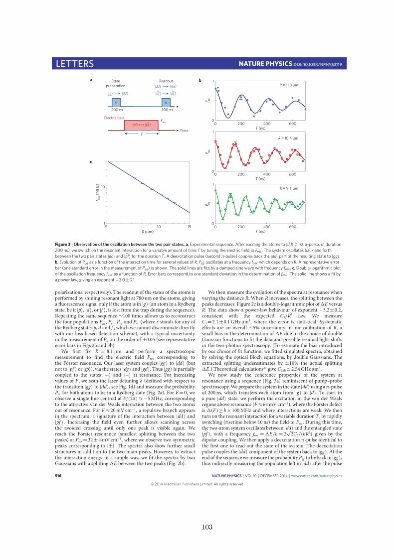
LETTERS NATURE PHYSICS DOI: 10.1038/NPHYS3119
TimeT
Electric fieldFres
State preparation
Readout
5 10 151
10
T (ns)
P ggP gg
P gg
00 200 400 600
T (ns)0 200 400 600
T (ns)0 200 400 600
1
0
1
0
1
200 ns 200 ns
|dd⟩ |gg⟩
|gg⟩ |dd⟩
|dd⟩
ππf os
c (M
Hz)
R (μm)
R = 11.3 μm
R = 10.4 μm
c
ba
R = 9.1 μm
|pf ⟩ |pf ⟩∼ ∼
|pf ⟩∼
Figure 3 | Observation of the oscillation between the two pair states. a, Experimental sequence. After exciting the atoms to |dd〉 (first π-pulse, of duration200 ns), we switch on the resonant interaction for a variable amount of time T by tuning the electric field to Fres. The system oscillates back and forthbetween the two pair states |dd〉 and |pf〉 for the duration T. A deexcitation pulse (second π-pulse) couples back the |dd〉 part of the resulting state to |gg〉.b, Evolution of Pgg as a function of the interaction time for several values of R. Pgg oscillates at a frequency fosc which depends on R. A representative errorbar (one standard error in the measurement of Pgg) is shown. The solid lines are fits by a damped sine wave with frequency fosc. c, Double-logarithmic plotof the oscillation frequency fosc as a function of R. Error bars correspond to one standard deviation in the determination of fosc. The solid line shows a fit bya power law, giving an exponent−3.0±0.1.
polarizations, respectively). The readout of the states of the atoms isperformed by shining resonant light at 780 nm on the atoms, givinga fluorescence signal only if the atom is in |g 〉 (an atom in a Rydbergstate, be it |p〉, |d〉, or |f 〉, is lost from the trap during the sequence).Repeating the same sequence ∼100 times allows us to reconstructthe four populations Pgg , Pgr , Prg and Prr (where r stands for any ofthe Rydberg states p, d and f , which we cannot discriminate directlywith our loss-based detection scheme), with a typical uncertaintyin the measurement of Pij on the order of ±0.05 (see representativeerror bars in Figs 2b and 3b).
We first fix R = 8.1 µm and perform a spectroscopicmeasurement to find the electric field Fres corresponding tothe Förster resonance. Our laser system couples |gg 〉 to |dd〉 (butnot to |pf 〉 or |fp〉), via the states |dg 〉 and |gd〉. Thus |gg 〉 is partiallycoupled to the states |+〉 and |−〉 at resonance. For increasingvalues of F , we scan the laser detuning δ (defined with respect tothe transition |gg 〉 to |dd〉, see Fig. 1d) and measure the probabilityPrr for both atoms to be in a Rydberg state (Fig. 2a). For F=0, weobserve a single line centred at δ/(2π)≈−5MHz, correspondingto the attractive van der Waals interaction between the two atomsout of resonance. For F ≈20mV cm−1, a repulsive branch appearsin the spectrum, a signature of the interaction between |dd〉 and|pf 〉. Increasing the field even further allows scanning acrossthe avoided crossing until only one peak is visible again. Wereach the Förster resonance (smallest splitting between the twopeaks) at Fres=32±4mV cm−1, where we observe two symmetricpeaks corresponding to |±〉. The spectra also show further smallstructures in addition to the two main peaks. However, to extractthe interaction energy in a simple way, we fit the spectra by twoGaussians with a splitting1E between the two peaks (Fig. 2b).
We then measure the evolution of the spectra at resonance whenvarying the distance R. When R increases, the splitting between thepeaks decreases. Figure 2c is a double-logarithmic plot of1E versusR. The data show a power-law behaviour of exponent −3.2±0.2,consistent with the expected C3/R3 law. We measureC3=2.1±0.1GHz µm3, where the error is statistical. Systematiceffects are an overall ∼5% uncertainty in our calibration of R, asmall bias in the determination of 1E due to the choice of doubleGaussian functions to fit the data and possible residual light-shiftsin the two-photon spectroscopy. (To estimate the bias introducedby our choice of fit function, we fitted simulated spectra, obtainedby solving the optical Bloch equations, by double Gaussians. Theextracted splitting underestimates by '10% the actual splitting1E.) Theoretical calculations29 give C3,th'2.54GHz µm3.
We now study the coherence properties of the system atresonance using a sequence (Fig. 3a) reminiscent of pump–probespectroscopy.We prepare the system in the state |dd〉 using aπ-pulseof 200 ns, which transfers each atom from |g 〉 to |d〉. To start ina pure |dd〉 state, we perform the excitation in the van der Waalsregime above resonance (F≈64mV cm−1), where the Förster defectis 1(F)≥h× 100MHz and where interactions are weak. We thenturn on the resonant interaction for a variable durationT , by rapidlyswitching (risetime below 10 ns) the field to Fres. During this time,the two-atom system oscillates between |dd〉 and the entangled state|pf 〉, with a frequency fosc =1E/h= 2
√2C3/(hR3) given by the
dipolar coupling. We then apply a deexcitation π-pulse identical tothe first one to read out the state of the system. The deexcitationpulse couples the |dd〉 component of the system back to |gg 〉. At theend of the sequencewemeasure the probabilityPgg to be back in |gg 〉,thus indirectly measuring the population left in |dd〉 after the pulse
916 NATURE PHYSICS | VOL 10 | DECEMBER 2014 | www.nature.com/naturephysics
© 2014 Macmillan Publishers Limited. All rights reserved
103
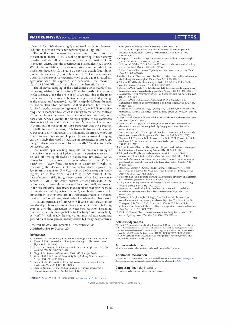
NATURE PHYSICS DOI: 10.1038/NPHYS3119 LETTERSof electric field. We observe highly contrasted oscillations between|dd〉 and |pf 〉, with a frequency depending on R (Fig. 3b).
The oscillations between two states are a direct proof ofthe coherent nature of the coupling underlying Förster energytransfer, and also allow a more accurate determination of theinteraction energy than the spectroscopic method described above.We fit the oscillation by a damped sine wave to extract theoscillation frequency fosc. Figure 3c shows a double-logarithmicplot of the values of fosc as a function of R. The data shows apower-law behaviour of exponent −3.0± 0.1, again in excellentagreement with the expected R−3 behaviour. The measuredC3=2.39±0.03GHz µm3 is also close to the theoretical value.
The observed damping of the oscillations comes mainly fromdephasing, arising from two effects. First, shot-to-shot fluctuationsin the distance R (on the order of δR' 170 nm), due to the finitetemperature of the atoms in the tweezers, give rise to dephasing,as the oscillation frequency fosc∝1/R3 is slightly different for eachrealization. This effect dominates at short distances: for instance,for R'9µm, the corresponding spread δfosc/fosc=3δR/R in relativefrequencies reaches ∼6%, which is enough to reduce the contrastof the oscillations by more than a factor of two after only fouroscillation periods. Second, the voltages applied to the electrodesalso fluctuate from shot to shot by a few mV, inducing fluctuationsin F and thus in the detuning 1(F) from resonance (by a fractionof a MHz for our parameters). This has negligible impact for smallR, but appreciably contributes to the damping for large R, where thedipolar interaction is weaker. In principle, both sources of dampingcan be strongly decreased by technical improvements in the set-up,using colder atoms as demonstrated recently30,31 and more stablevoltage sources.
Our results open exciting prospects for real-time tuning ofinteractions in systems of Rydberg atoms, in particular to switchon and off Ryberg blockade on nanosecond timescales. As anillustration, in the above experiment, when switching F from64mVcm−1 (away from resonance) to 32mV cm−1 (right onresonance), the blockade shift between two atoms separated byR=10 µm varies from U =UvdW ∼ h× 0.2MHz (van der Waalsregime) up to U = 1E/2 ∼ h × 4MHz (C3/R3 regime). If thepair of atoms initially in |gg 〉 were driven with a Rabi frequencyΩ/(2π)∼ 1MHz, one would observe a strong blockade in thesecond case, whereas blockade would be almost totally suppressedin the first situation. This means that, simply by changing the valueof the electric field by a few mVcm−1, we obtain a twenty-foldenhancement of the interaction, and the blockade radius is increasedby a factor∼2 in real time, a feature hard to achieve by other means.
A natural extension of this work will consist in measuring theangular dependence of resonant interactions29, in view of tailoringeven further the interactions between two particles. Extendingour results beyond two particles, to few-body32 and many-bodysystems15,16,23, will enable the study of transport of excitations andgeneration of entanglement in fully controlled many-body systems.
Received 30 May 2014; accepted 8 September 2014;published online 26 October 2014
References1. Andrews, D. L. & Demidov, A. A. Resonance Energy Transfer (Wiley, 1999).2. Förster, T. Zwischenmolekulare Energiewanderung und Fluoreszenz. Ann.
Phys. 437, 55–75 (1948).3. Stryer, L. & Haugland, R. P. Energy transfer: A spectroscopic ruler. Proc. Natl
Acad. Sci. USA 58, 719–726 (1967).4. Clegg, R. M. Reviews in Fluorescence 2006 1–45 (Springer, 2006).5. Walker, T. G. & Saffman, M. Zeros of Rydberg–Rydberg Föster interactions.
J. Phys. B 38, S309–S319 (2005).6. Inouye, S. et al. Observation of Feshbach resonances in a Bose–Einstein
condensate. Nature 392, 151–154 (1998 ).7. Chin, C., Grimm, R., Julienne, P. & Tiesinga, E. Feshbach resonances in
ultracold gases. Rev. Mod. Phys. 82, 1225–1286 (2010).
8. Gallagher, T. F. Rydberg Atoms (Cambridge Univ. Press, 2005).9. Safinya, K. A., Delpech, J. F., Gounand, F., Sandner, W. & Gallagher, T. F.
Resonant Rydberg-atom–Rydberg-atom collisions. Phys. Rev. Lett. 47,405–408 (1981).
10. Comparat, D. & Pillet, P. Dipole blockade in a cold Rydberg atomic sample.J. Opt. Soc. Am. B 27, A208–A232 (2010).
11. Saffman, M., Walker, T. G. & Mølmer, K. Quantum information with Rydbergatoms. Rev. Mod. Phys. 82, 2313–2363 (2010).
12. Urban, E. et al. Observation of Rydberg blockade between two atoms. NaturePhys. 5, 110–114 (2009).
13. Gaëtan, A. et al. Observation of collective excitation of two individual atoms inthe Rydberg blockade regime. Nature Phys. 5, 115–118 (2009).
14. Weimer, H., Müller, M., Lesanovsky, I., Zoller, P. & Büchler, H. P. A Rydbergquantum simulator. Nature Phys. 6, 382–388 (2010).
15. Anderson, W. R., Veale, J. R. & Gallagher, T. F. Resonant dipole–dipole energytransfer in a nearly frozen Rydberg gas. Phys. Rev. Lett. 80, 249–252 (1998).
16. Mourachko, I. et al.Many-body effects in a frozen Rydberg gas. Phys. Rev. Lett.80, 253–256 (1998).
17. Anderson, W. R., Robinson, M. P., Martin, J. D. D. & Gallagher, T. F.Dephasing of resonant energy transfer in a cold Rydberg gas. Phys. Rev. A 65,063404 (2002).
18. Mudrich, M., Zahzam, N., Vogt, T., Comparat, D. & Pillet, P. Back and forthtransfer and coherent coupling in a cold Rydberg dipole gas. Phys. Rev. Lett. 95,233002 (2005).
19. Vogt, T. et al. Electric-field induced dipole blockade with Rydberg atoms. Phys.Rev. Lett. 99, 073002 (2007).
20. Reinhard, A., Younge, K. C. & Raithel, G. Effect of Förster resonances onthe excitation statistics of many-body Rydberg systems. Phys. Rev. A 78,060702(R) (2008).
21. Van Ditzhuijzen, C. S. E. et al. Spatially resolved observation of dipole–dipoleinteraction between Rydberg atoms. Phys. Rev. Lett. 100, 243201 (2008).
22. Ryabtsev, I. I., Tretyakov, D. B., Beterov, I. I. & Entin, V. M. Observation of theStark-tuned Förster resonance between two Rydberg atoms. Phys. Rev. Lett.104, 073003 (2010).
23. Günter, G. et al. Observing the dynamics of dipole-mediated energy transportby interaction-enhanced imaging. Science 342, 954–956 (2013).
24. Nipper, J. et al.Highly resolved measurements of Stark-tuned Försterresonances between Rydberg atoms. Phys. Rev. Lett. 108, 113001 (2012).
25. Nipper, J. et al. Atomic pair-state interferometer: Controlling and measuringan interaction-induced phase shift in Rydberg-atom pairs. Phys. Rev. X 2,031011 (2012).
26. Béguin, L., Vernier, A., Chicireanu, R., Lahaye, T. & Browaeys, A. Directmeasurement of the van der Waals interaction between two Rydberg atoms.Phys. Rev. Lett. 110, 263201 (2013).
27. Nogrette, F. et al. Single-atom trapping in holographic 2D arrays of microtrapswith arbitrary geometries. Phys. Rev. X 4, 021034 (2014).
28. Löw, R. et al. An experimental and theoretical guide to strongly interactingRydberg gases. J. Phys. B 45, 113001 (2012).
29. Reinhard, A., Cubel Liebisch, T., Knuffman, B. & Raithel, G. Level shiftsof rubidium Rydberg states due to binary interactions. Phys. Rev. A 75,032712 (2007).
30. Kaufman, A. M., Lester, B. J. & Regal, C. A. Cooling a single atom in anoptical tweezer to its quantum ground state. Phys. Rev. X 2, 041014 (2012).
31. Thompson, J. D., Tiecke, T. G., Zibrov, A. S., Vuletić, V. & Lukin, M. D.Coherence and Raman sideband cooling of a single atom in an optical tweezer.Phys. Rev. Lett. 110, 133001 (2013).
32. Gurian, J. H. et al. Observation of a resonant four-body interaction in coldcesium Rydberg atoms. Phys. Rev. Lett. 108, 023005 (2012).
AcknowledgementsWe thank C. S. Adams for enlightening discussions, F. Nogrette for technical assistanceand M. Besbes for finite-element calculations of the electric field configuration. Thiswork was supported financially by the EU (ERC Stg Grant ARENA, FET-Open Xtrackproject HAIRS, EU Marie-Curie program ITN COHERENCE FP7-PEOPLE-2010-ITN-265031 (H.L.)), by the DGA (L.B.), and by Région Île-de-France (LUMAT andTriangle de la Physique, LAGON project).
Author contributionsAll authors contributed extensively to the work presented in this paper.
Additional informationReprints and permissions information is available online at www.nature.com/reprints.Correspondence and requests for materials should be addressed to A.B.
Competing financial interestsThe authors declare no competing financial interests.
NATURE PHYSICS | VOL 10 | DECEMBER 2014 | www.nature.com/naturephysics 917
© 2014 Macmillan Publishers Limited. All rights reserved
104

Coherent Excitation Transfer in a Spin Chain of Three Rydberg Atoms
Daniel Barredo, Henning Labuhn, Sylvain Ravets, Thierry Lahaye, and Antoine BrowaeysLaboratoire Charles Fabry, UMR 8501, Institut d’Optique, CNRS, Université Paris Sud 11,
2 avenue Augustin Fresnel, 91127 Palaiseau cedex, France
Charles S. AdamsJoint Quantum Centre (JQC) Durham-Newcastle, Department of Physics, Durham University,
Durham DH1 3LE, United Kingdom(Received 23 September 2014; revised manuscript received 21 November 2014; published 19 March 2015)
We study coherent excitation hopping in a spin chain realized using highly excited individuallyaddressable Rydberg atoms. The dynamics are fully described in terms of an XY spin Hamiltonian with along range resonant dipole-dipole coupling that scales as the inverse third power of the lattice spacing,C3=R3. The experimental data demonstrate the importance of next neighbor interactions which are manifestas revivals in the excitation dynamics. The results suggest that arrays of Rydberg atoms are ideally suitedto large scale, high-fidelity quantum simulation of spin dynamics.
DOI: 10.1103/PhysRevLett.114.113002 PACS numbers: 32.80.Ee, 03.67.Bg, 05.50.+q
Spin Hamiltonians, introduced in the early days ofquantum mechanics to explain ferromagnetism, are widelyused to study quantum magnetism [1]. Assemblies ofinteracting, localized spins are a paradigm of quantummany-body systems, where the interplay between inter-actions and geometry-induced frustration creates a wealthof intriguing quantum phases.Many other phenomena, suchas coherent energy transfer, photochemistry, or photosyn-thesis [2], can also be described using spin Hamiltonians.However, despite this fundamental significance, exactanalytical solutions are known only for the simplest cases,and numerical simulations of strongly correlated spinsystems are notoriously difficult.For those reasons, quantum simulation of spin
Hamiltonians by controllable systems raises great interest.Recently, various approaches were followed to simulatespin systems using tools of atomic physics [3], such as coldatoms [4–6] or polar molecules [7] in optical lattices,interacting via weak exchange or dipole-dipole inter-actions, or trapped ions with engineered effective inter-actions [8–10]. As compared to their condensed-mattercounterparts, the spin couplings can be long range, whichgives rise to new properties [11–14].Rydberg atoms are a promising alternative platform for
quantum simulation [15,16]. In particular, they allowimplementing various spin-1=2 Hamiltonians on two-dimensional lattices with strong couplings, in the MHzrange [17,18]. Rydberg systems interacting through vander Waals interactions can be described by Ising-type
Hamiltonians H ¼ PijVijσ
ziσ
zj where σz is the z-Pauli
matrix acting in the (pseudo-) spin Hilbert space, andVij ∼ jri − rjj−6, where ri denotes the position of atom i[17–21]. On the other hand, spin-exchange, or XY, spinHamiltonians of the form H ¼ P
ijVijðσþi σ−j þ σ−i σþj Þ,
where σ ¼ σx iσy are spin-flip operators andVij ∼ jri − rjj−3, can be realized by using two differentRydberg states, interacting directly via the resonant dipole-dipole interaction. However, in this case, only incoherenttransfer of excitations has been observed so far, due tothe random atomic positions in the ensembles used inexperiments [22–27].In this Letter, we study the coherent dynamics of a
spin excitation in a chain of three Rydberg atoms. Thedipole-dipole interaction between atoms is given by theXY Hamiltonian [28]
H ¼ 1
2
X
i≠j
C3
R3ijðσþi σ−j þ σ−i σ
þj Þ; ð1Þ
where Rij ¼ jri − rjj is the distance between atoms i and j.We calibrate the spin-spin coupling between two Rydbergatoms by investigating the temporal evolution of twoRydberg atoms prepared in the state j↑↓i, as a functionof distance R between the atoms, up to R≃ 50 μm. Wethen use three Rydberg atoms prepared in j↑↓↓i and studythe propagation of the excitation through this minimalisticspin chain, observing the effect of long-range hopping ofthe excitation. The agreement between experimental dataand the XY model without adjustable parameters validatesour setup as a future quantum simulator for systems ofmany spins in arbitrary two-dimensional arrays.The experimental setup, shown in Fig. 1(a), is detailed in
Ref. [30]. Briefly, we focus a red-detuned trapping beam
Published by the American Physical Society under the terms ofthe Creative Commons Attribution 3.0 License. Further distri-bution of this work must maintain attribution to the author(s) andthe published article’s title, journal citation, and DOI.
PRL 114, 113002 (2015) P HY S I CA L R EV I EW LE T T ER Sweek ending
20 MARCH 2015
0031-9007=15=114(11)=113002(5) 113002-1 Published by the American Physical Society
105

with an aspheric lens into a magneto-optical trap of 87Rb, toa waist ≃1 μm. Multiple traps at arbitrary distances arecreated by imprinting an appropriate phase on the trappingbeam with a spatial light modulator [31]. Because of fastlight-assisted collisions in the small trapping volume, atmost one atom is present in each trap. The temperature ofthe trapped atoms is approximately 50 μK. A 6 G magneticfield defines the quantization axis [32].We encode the two spin states in the Rydberg states
j↑i ¼ j62D3=2; mj ¼ 3=2i and j↓i ¼ j63P1=2; mj ¼ 1=2i[see Fig. 1(b)]. We trigger an experiment when an atom isdetected in each trap. To prepare the atoms in a desiredspin state, we first optically pump them in jgi ¼ j5S1=2;F ¼ 2; mF ¼ 2i. We then switch off the traps to avoidinhomogeneous light shifts, and excite the atoms toj↑i ¼ j62D3=2; mJ ¼ 3=2i via a two-photon transition(wavelengths 795 and 474 nm, with polarizations π andσþ, respectively), detuned from the intermediate statej5P1=2; F ¼ 2; mF ¼ 2i by Δ≃ 2π × 740 MHz. Fromthe j↑i state the atom can be transferred to j↓i ¼j63P1=2; mj ¼ 1=2i using resonant microwaves at≃9.131 GHz, emitted by an antenna outside the vacuumchamber.To read out the state of an atom at the end of a sequence,
we switch on the excitation lasers, coupling only j↑i backto the ground state. We then turn on the dipole traps torecapture ground-state atoms, while atoms in Rydbergstates remain untrapped, and detect atoms in jgi byfluorescence. Therefore if we detect an atom in its trapat the end of a sequence, we assume it was in j↑i, while aloss corresponds to the j↓i state. We reconstruct all the 2N
probabilities Pi1…ik…iN of having ik atom in trap k, withik ¼ 0 or 1, for our N-trap system (with N ¼ 1; 2, or 3) byrepeating the experiment typically 100 times. For instancefor N ¼ 3, P100 is the probability to recapture an atomin trap 1, while recapturing none in traps 2 and 3. Thestatistical error on the determination of the probabilitiesis below 5%. Figure 1(c) illustrates the coherent spin mani-pulation for a single atom, by showing Rabi oscillationsbetween j↑i and j↓i: the probability P1 to recapture theatom oscillates with a frequency ΩMW ≃ 2π × 4.6 MHz.In 4 μs, we induce more than 35 spin flips withoutobserving noticeable damping.We first use two atoms, aligned along the quantization
axis, to directly measure the coupling between two spinsas a function of their distance. The sequence is shown inFig. 2(a). We illuminate atom 1 with an addressing beam[33] which induces a 20 MHz light shift, making it offresonant to the global Rydberg excitation. Atom 2 isexcited to j↑i, and then transferred to j↓i using micro-waves. Subsequently, atom 1 is optically excited to the j↑istate with the addressing beam switched off (atom 2 in j↓iis not affected by the Rydberg excitation pulse). We letthe system evolve for an adjustable time τ and read out the
(a) (b)
(c) 0
E
0 1 2 30
1
Trapbeam
Asphericlenses
Microwaveantenna
FIG. 1 (color online). (a) Individual 87Rb atoms in microtrapsaligned along the quantization axis, defined by a B ¼ 6 Gmagnetic field. (b) Excitation lasers couple the ground statejgi¼ j5S1=2;F¼ 2;mF ¼ 2i and the Rydberg state j↑i¼ j62D3=2;mJ ¼ 3=2i with an effective Rabi frequency Ωopt. Microwavescouple j↑i to j↓i ¼ j63P1=2; mJ ¼ 1=2i, with Rabi frequencyΩMW. (c) Microwave-driven Rabi oscillation of a single atombetween j↑i and j↓i, yielding ΩMW ¼ 2π × 4.6 MHz.
FIG. 2 (color online). (a) Sequence to observe spin exchangebetween two atoms. (b) Excitation hopping between states j↑↓i(blue disks) and j↓↑i (red disks) of two atoms separated byR ¼ 30 μm. Solid lines are sinusoidal fits, with frequency 2E=h.(c) Interaction energy E (circles) versus R. Error bars are smallerthan the symbols size. The line shows the theoretical predictionC3=R3 with Cth
3 ¼ 7965 MHz μm3. The shaded area correspondsto our systematic 5% uncertainty in the calibration of R.
PRL 114, 113002 (2015) P HY S I CA L R EV I EW LE T T ER Sweek ending
20 MARCH 2015
113002-2
106
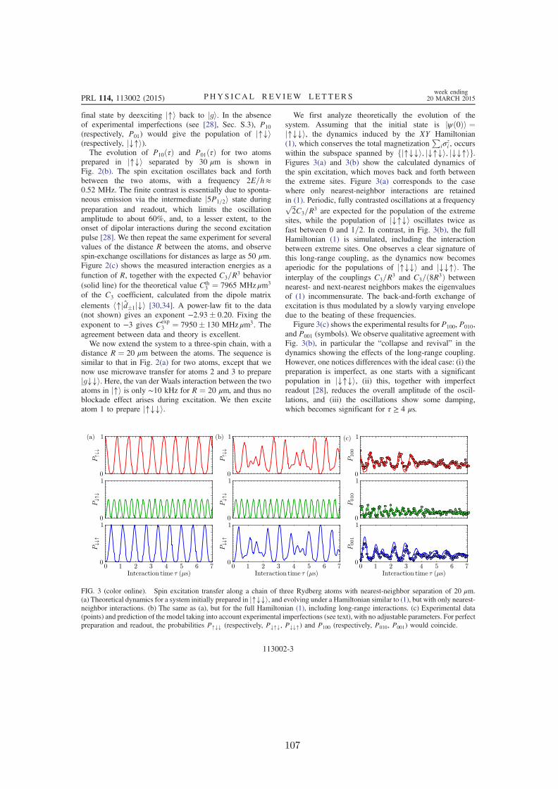
final state by deexciting j↑i back to jgi. In the absenceof experimental imperfections (see [28], Sec. S.3), P10
(respectively, P01) would give the population of j↑↓i(respectively, j↓↑i).The evolution of P10ðτÞ and P01ðτÞ for two atoms
prepared in j↑↓i separated by 30 μm is shown inFig. 2(b). The spin excitation oscillates back and forthbetween the two atoms, with a frequency 2E=h≈0.52 MHz. The finite contrast is essentially due to sponta-neous emission via the intermediate j5P1=2i state duringpreparation and readout, which limits the oscillationamplitude to about 60%, and, to a lesser extent, to theonset of dipolar interactions during the second excitationpulse [28]. We then repeat the same experiment for severalvalues of the distance R between the atoms, and observespin-exchange oscillations for distances as large as 50 μm.Figure 2(c) shows the measured interaction energies as afunction of R, together with the expected C3=R3 behavior(solid line) for the theoretical value Cth
3 ¼ 7965 MHz μm3
of the C3 coefficient, calculated from the dipole matrixelements h↑jd1j↓i [30,34]. A power-law fit to the data(not shown) gives an exponent −2.93 0.20. Fixing theexponent to −3 gives Cexp
3 ¼ 7950 130 MHz μm3. Theagreement between data and theory is excellent.We now extend the system to a three-spin chain, with a
distance R ¼ 20 μm between the atoms. The sequence issimilar to that in Fig. 2(a) for two atoms, except that wenow use microwave transfer for atoms 2 and 3 to preparejg↓↓i. Here, the van der Waals interaction between the twoatoms in j↑i is only ∼10 kHz for R ¼ 20 μm, and thus noblockade effect arises during excitation. We then exciteatom 1 to prepare j↑↓↓i.
We first analyze theoretically the evolution of thesystem. Assuming that the initial state is jψð0Þi ¼j↑↓↓i, the dynamics induced by the XY Hamiltonian(1), which conserves the total magnetization
Piσ
zi , occurs
within the subspace spanned by fj↑↓↓i; j↓↑↓i; j↓↓↑ig.Figures 3(a) and 3(b) show the calculated dynamics ofthe spin excitation, which moves back and forth betweenthe extreme sites. Figure 3(a) corresponds to the casewhere only nearest-neighbor interactions are retainedin (1). Periodic, fully contrasted oscillations at a frequencyffiffiffi2
pC3=R3 are expected for the population of the extreme
sites, while the population of j↓↑↓i oscillates twice asfast between 0 and 1=2. In contrast, in Fig. 3(b), the fullHamiltonian (1) is simulated, including the interactionbetween extreme sites. One observes a clear signature ofthis long-range coupling, as the dynamics now becomesaperiodic for the populations of j↑↓↓i and j↓↓↑i. Theinterplay of the couplings C3=R3 and C3=ð8R3Þ betweennearest- and next-nearest neighbors makes the eigenvaluesof (1) incommensurate. The back-and-forth exchange ofexcitation is thus modulated by a slowly varying envelopedue to the beating of these frequencies.Figure 3(c) shows the experimental results for P100, P010,
and P001 (symbols). We observe qualitative agreement withFig. 3(b), in particular the “collapse and revival” in thedynamics showing the effects of the long-range coupling.However, one notices differences with the ideal case: (i) thepreparation is imperfect, as one starts with a significantpopulation in j↓↑↓i, (ii) this, together with imperfectreadout [28], reduces the overall amplitude of the oscil-lations, and (iii) the oscillations show some damping,which becomes significant for τ ≥ 4 μs.
FIG. 3 (color online). Spin excitation transfer along a chain of three Rydberg atoms with nearest-neighbor separation of 20 μm.(a) Theoretical dynamics for a system initially prepared in j↑↓↓i, and evolving under a Hamiltonian similar to (1), but with only nearest-neighbor interactions. (b) The same as (a), but for the full Hamiltonian (1), including long-range interactions. (c) Experimental data(points) and prediction of the model taking into account experimental imperfections (see text), with no adjustable parameters. For perfectpreparation and readout, the probabilities P↑↓↓ (respectively, P↓↑↓, P↓↓↑) and P100 (respectively, P010, P001) would coincide.
PRL 114, 113002 (2015) P HY S I CA L R EV I EW LE T T ER Sweek ending
20 MARCH 2015
113002-3
107

Imperfect preparation and readout stem from the factthat, in addition to the spontaneous emission via theintermediate state during the optical pulses, the Rabifrequency for optical excitation (≃5.3 MHz) of atom 1from jgi to j↑i is not much higher than the interaction(≃0.92 MHz for R ¼ 20 μm). Thus, during the excitationof atom 1, the spin excitation already has a significantprobability to hop to atom 2. The damping essentially arisesfrom the finite temperature of the atoms, which leads tochanges in the interatomic distances, and thus in thecouplings.To go beyond this qualitative understanding of the
limitations of our “quantum simulator,” we add all knownexperimental imperfections to the XY model [28]. Theresult, shown by solid lines on Fig. 3(c) accuratelyreproduces the data with no free parameters. To obtainthese curves, we simulate the full sequence, i.e., all threeoptical (de-) excitation pulses with or without the address-ing beam, the microwave pulse, and evolution time, bysolving the optical Bloch equations describing the dynam-ics of the internal states of the atoms, restricted to threestates: jgi, j↑i, and j↓i. Dissipation comes from both off-resonant excitation of the intermediate j5P1=2i state duringthe optical excitation pulse, and from the finite lifetimesof the Rydberg states (101 and 135 μs for j↑i and j↓i,respectively [35]). The former effect is treated as aneffective damping of the jgi ↔ j↑i transition, present onlyduring the optical pulses, and with a damping rate chosen tomatch the damping of single-atom Rabi oscillations per-formed to calibrate the excitation Rabi frequency Ωopt [17].We then account for the thermal motion of the atoms.
A first consequence of the finite temperature (T ≃ 50 μK)is that at the beginning of the sequence, the atoms haverandom positions (the transverse rms extension of thethermal motion in each microtrap, of radial frequency90 kHz, is about 120 nm) and random velocities(70 nm=μs rms).During the sequence, the traps are switchedoff and the atoms are thus in free flight with their initialvelocity. When solving the optical Bloch equations, we thusfirst draw the initial positions r0i and velocities v0i of eachatom i according to a thermal distribution, and use time-dependent dipolar couplings C3=jðr0i þ v0i tÞ − ðr0j þ v0j tÞj3in Eq. (1) [36]. We then average the results over 100realizations. This yields a dephasing of the oscillations,resulting in a significant contrast reduction at long times.A second effect of the temperature is that an atom has a
small probability εðtÞ to leave the trap region during theexperiment. In this case, we mistakenly infer that itwas in a Rydberg state at the end of the sequence. Thisleads to a small distortion of the measured populations Pijk
(i; j; k ¼ 0; 1) [37], that we compute from the actual onesas described in [17]. We measure εðtÞ (which increases withthe duration t of the sequence, from ∼1% at t ¼ 0 up to∼20% for t ¼ 7 μs) in a calibration experiment, and then
use it to calculate the expected populations from thesimulated ones [28].Figure 4 shows how those two consequences of the finite
temperature contribute to the observed damping in thedynamics of P001: both have sizable effects, but thedephasing due to fluctuations in the coupling dominatesat long times. Reducing the atomic temperature using, e.g.,Raman cooling [38,39] would render those effects negli-gible for our time scales, and allow the realization of anearly ideal quantum simulator of spin dynamics.In summary, we have measured the dynamics of a spin
excitation in a minimal spin chain of three Rydberg atoms.The evolution of the system is accurately described byan XY Hamiltonian without any adjustable parameters. Theobtained results are encouraging in view of scaling upthe system to a larger number of spins. In particular, theresidual motion of the atoms and the level of detectionerrors would already allow us to observe unambiguouslythe back-and-forth propagation of an excitation over achain of ∼20 atoms [28]. However, so far, experimentswith more than ∼5 atoms are hampered by the stochasticloading of the traps by single atoms [31]. In future work,we will thus explore various quasideterministic loadingschemes that have been demonstrated at the level of asingle [40,41] or a few [42,43] traps. Once this is achieved,our system will allow us to study the equivalent of anassembly of hard-core bosons on a 2D lattice with long-range, anisotropic hopping. We will also study dipolarinteractions involving more than only two Rydberg statesat an electrically tuned Förster resonance [44]. Oursystem will be ideal to study exotic phases and frustrationin quantum magnetism, excitation hopping in complexnetworks [45,46], or quantum walks with long-rangehopping [47].
We acknowledge financial support by the EU [ERC Stg.Grant ARENA, AQUTE Integrating Project, FET-OpenXtrack Project HAIRS, and EU Marie-Curie Program ITNCOHERENCE FP7-PEOPLE-2010-ITN-265031 (H. L.)],and by Région Île-de-France (LUMAT and Triangle de laPhysique, projects LAGON and COLISCINA during thestay of C. S. A. at LCF). C. S. A. also acknowledgessupport from the U.K. EPSRC and Durham University.
FIG. 4 (color online). Influence of the temperature on P001ðτÞ:simulated dynamics at zero temperature (black dashed line), andadding either only atom loss (green dotted line), or only atomicmotion (blue solid line).
PRL 114, 113002 (2015) P HY S I CA L R EV I EW LE T T ER Sweek ending
20 MARCH 2015
113002-4
108

[1] A. Auerbach, Interacting Electrons and Quantum Magnet-ism (Springer-Verlag, New York, 1994).
[2] E. Collini, Chem. Soc. Rev. 42, 4932 (2013).[3] M. Lewenstein, A. Sanpera, and V. Ahufinger, Ultracold
Atoms in Optical Lattices: Simulating Quantum Many-BodySystems (Oxford University Press, Oxford, U.K, 2012).
[4] J. Simon, W. S. Bakr, R. Ma, M. E. Tai, P. M. Preiss, andM. Greiner, Nature (London) 472, 307 (2011).
[5] T. Fukuhara, P. Schauß, M. Endres, S. Hild, M. Cheneau,I. Bloch, and C. Gross, Nature (London) 502, 76 (2013).
[6] A. de Paz, A. Sharma, A. Chotia, E. Maréchal, J. H.Huckans, P. Pedri, L. Santos, O. Gorceix, L. Vernac, andB. Laburthe-Tolra, Phys. Rev. Lett. 111, 185305 (2013).
[7] B. Yan, S. A. Moses, B. Gadway, J. P. Covey, K. R. A.Hazzard, A. M. Rey, D. S. Jin, and J. Ye, Nature (London)501, 521 (2013).
[8] K. Kim, M. S. Chang, S. Korenblit, R. Islam, E. E. Edwards,J. K. Freericks, G. D. Lin, L. M. Duan, and C. Monroe,Nature (London) 465, 590 (2010).
[9] P. Richerme, Z.-X. Gong, A. Lee, C. Senko, J. Smith, M.Foss-Feig, S. Michalakis, A. V. Gorshkov, and C. Monroe,Nature (London) 511, 198 (2014).
[10] P. Jurcevic, B. P. Lanyon, P. Hauke, C. Hempel, P. Zoller,R. Blatt, and C. F. Roos, Nature (London) 511, 202 (2014).
[11] P. Hauke, F. M. Cucchietti, A. Müller-Hermes, M.-C.Bañuls, J. I. Cirac, and M. Lewenstein, New J. Phys. 12,113037 (2010).
[12] D. Peter, S. Müller, S. Wessel, and H. P. Büchler, Phys. Rev.Lett. 109, 025303 (2012).
[13] K. R. A. Hazzard, M. van den Worm, M. Foss-Feig, S. R.Manmana, E. Dalla Torre, T. Pfau, M. Kastner, and A. M.Rey, Phys. Rev. A 90, 063622 (2014).
[14] M. Avellino, A. J. Fisher, and S. Bose, Phys. Rev. A 74,012321 (2006).
[15] M. Saffman, T. G. Walker, and K. Mølmer, Rev. Mod. Phys.82, 2313 (2010).
[16] H. Weimer, M. Müller, I. Lesanovsky, P. Zoller, and H.-P.Büchler, Nat. Phys. 6, 382 (2010).
[17] D. Barredo, S. Ravets, H. Labuhn, L. Béguin, A. Vernier, F.Nogrette, T. Lahaye, and A. Browaeys, Phys. Rev. Lett. 112,183002 (2014).
[18] P. Schauß, J. Zeiher, T. Fukuhara, S. Hild, M. Cheneau, T.Macrì, T. Pohl, I. Bloch, and C. Gross, arXiv:1404.0980.
[19] H. Weimer, R. Löw, T. Pfau, and H. P. Büchler, Phys. Rev.Lett. 101, 250601 (2008).
[20] T. Pohl, E. Demler, and M. D. Lukin, Phys. Rev. Lett. 104,043002 (2010).
[21] I. Lesanovsky, Phys. Rev. Lett. 106, 025301 (2011).[22] I. Mourachko, D. Comparat, F. de Tomasi, A. Fioretti, P.
Nosbaum, V. M. Akulin, and P. Pillet, Phys. Rev. Lett. 80,253 (1998).
[23] W. R. Anderson, J. R. Veale, and T. F. Gallagher, Phys. Rev.Lett. 80, 249 (1998).
[24] C. S. E. van Ditzhuijzen, A. F. Koenderink, J. V. Hernández,F. Robicheaux, L. D. Noordam, and H. B. van Linden vanden Heuvell, Phys. Rev. Lett. 100, 243201 (2008).
[25] G. Günter, H. Schempp, M. Robert-de-Saint-Vincent, V.Gavryusev, S. Helmrich, C. S. Hofmann, S. Whitlock, andM. Weidemüller, Science 342, 954 (2013).
[26] S. Bettelli, D. Maxwell, T. Fernholz, C. S. Adams, I.Lesanovsky, and C. Ates, Phys. Rev. A 88, 043436 (2013).
[27] D. Maxwell, D. J. Szwer, D. Paredes-Barato, H. Busche,J. D. Pritchard, A. Gauguet, K. J. Weatherill, M. P. A. Jones,and C. S. Adams, Phys. Rev. Lett. 110, 103001 (2013).
[28] See Supplemental Material at http://link.aps.org/supplemental/10.1103/PhysRevLett.114.113002, whichincludes Ref. [29], for extra details about the simulationof the spin chain dynamics.
[29] C. Tuchendler, A. M. Lance, A. Browaeys, Y. R. P. Sortais,and P. Grangier, Phys. Rev. A 78, 033425 (2008).
[30] L. Béguin, A. Vernier, R. Chicireanu, T. Lahaye, and A.Browaeys, Phys. Rev. Lett. 110, 263201 (2013).
[31] F. Nogrette, H. Labuhn, S. Ravets, D. Barredo, L. Béguin,A. Vernier, T. Lahaye, and A. Browaeys, Phys. Rev. X 4,021034 (2014).
[32] The stray electric field is below 5 mV=cm. Note that as (1)conserves the excitation number, the system is quite immuneto decoherence due to global fluctuations in electric ormagnetic fields.
[33] H. Labuhn, S. Ravets, D. Barredo, L. Béguin, F. Nogrette,T. Lahaye, and A. Browaeys, Phys. Rev. A 90, 023415(2014).
[34] A. Reinhard, T. C. Liebisch, B. Knuffman, and G. Raithel,Phys. Rev. A 75, 032712 (2007).
[35] I. I. Beterov, I. I. Ryabtsev, D. B. Tretyakov, and V. M.Entin, Phys. Rev. A 79, 052504 (2009).
[36] Here, we neglect mechanical effects due to the interactionsbetween Rydberg atoms during the interaction time. Using aclassical model we estimate that these induce a displacementin R below 30 nm for τ ≤ 7 μs and are therefore negligible.
[37] C. Shen and L.-M. Duan, New J. Phys. 14, 053053 (2012).[38] A. M. Kaufman, B. J. Lester, and C. A. Regal, Phys. Rev. X
2, 041014 (2012).[39] J. D. Thompson, T. G. Tiecke, A. S. Zibrov, V. Vuletić, and
M. D. Lukin, Phys. Rev. Lett. 110, 133001 (2013).[40] T. Grünzweig, A. Hilliard, M. McGovern, and M. F.
Andersen, Nat. Phys. 6, 951 (2010).[41] M. Ebert, A. Gill, M. Gibbons, X. Zhang, M. Saffman, and
T. G. Walker, Phys. Rev. Lett. 112, 043602 (2014).[42] Y. Miroshnychenko, W. Alt, I. Dotsenko, L. Förster, M.
Khudaverdyan, D. Meschede, D. Schrader, and A.Rauschenbeutel, Nature (London) 442, 151 (2006).
[43] M. Schlosser, J. Kruse, C. Gierl, S. Teichmann, S.Tichelmann, and G. Birkl, New J. Phys. 14, 123034 (2012).
[44] S. Ravets, H. Labuhn, D. Barredo, L. Béguin, T. Lahaye,and A. Browaeys, Nat. Phys. 10, 914 (2014).
[45] S. Wüster, C. Ates, A. Eisfeld, and J. M. Rost, Phys. Rev.Lett. 105, 053004 (2010).
[46] S. Mostarda, F. Levi, D. Prada-Gracia, F. Mintert, and F.Rao, arXiv:1312.1833.
[47] R. Côté, A. Russell, E. E. Eyler, and P. L. Gould, New J.Phys. 8, 156 (2006).
PRL 114, 113002 (2015) P HY S I CA L R EV I EW LE T T ER Sweek ending
20 MARCH 2015
113002-5
109

110 Chapter 3. Arrays of single Rydberg atoms
Chapter 4
Administrative data
In this last chapter, I first give a detailed CV, and then list my publications and mycontributions in conferences.
4.1 Curriculum vitæ
Personal data
Born 14 September 1979 in Toulouse.Married, one child.French nationality.
Career
Oct. 2012–present: Researcher (CR1) at CNRS, Laboratoire Charles Fabry, UMR 8501,Palaiseau.Jan. 2012–Oct. 2012: Researcher (CR2) at CNRS, Laboratoire Charles Fabry, UMR8501, Palaiseau.Oct. 2008– Dec. 2011: Researcher (CR2) at CNRS, LCAR, UMR 5589, Toulouse.2006–2008: Post-doctoral researcher, University of Stuttgart (Germany), in TilmanPfau’s group.2003–2005: Teaching assistant (allocataire-moniteur), Université Paris 6.1999–2003: Student at École Normale Supérieure, Paris.
Education
2002–2005: PhD thesis in the Cold Atom group of Laboratoire Kastler Brossel, ENS,Paris, under the supervision of D. Guéry-Odelin and J. Dalibard, with honors (MentionTrès Honorable). Title of the thesis: Evaporative cooling of a mgnetically guided atomicbeam.
111

112 Chapter 4. Administrative data
2001–2002: DEA of quantum physics, ENS, Paris: with honors (“mention TB”), rankjoint 1st.1999–2001: studies in Physics at ENS, Paris [2000: “Licence”, with honors (“mentionTB”); 2001: “Maîtrise”, with honors (“mention TB”)].1999: Admitted at École Polytechnique (ranked 1) and ENS Paris (ranked 4).1997–1999: Classes préparatoires PCSI–PC?, Lycée Pierre de Fermat, Toulouse.1997: Baccalauréat S, with honors (“félicitations du jury”).
Awards
2009: Louis Armand Prize of the French Academy of Sciences “for the realization of thefirst purely dipolar quantum gas”.2006: Individual Marie Curie EU fellowship.
Teaching experience
2012–: Lectures on Quantum mechanics at the “Préparation à l’Agrégation de Physique”,ENS Cachan.2008–2010: Teaching assistant for the lecture “Photons and Atoms” by Claude Fabre, atthe Master 2 of Quantum Physics, ENS Paris.2006–2007: Advanced Physical Laboratory, international master programme, Universityof Stuttgart.2005–2006: Oral exams (“colles”) in Physics, MPSI, Lycée Louis-le-Grand, Paris.2003–2006: Teaching assistant (“moniteur”), University Paris 6.
Co-supervision of PhD students
Jan. 2013–now: Co-supervision of the PhD thesis of Henning Labuhn. Defense plannedfor December 2015.Jan. 2013–now: Co-supervision of the PhD thesis of Sylvain Ravets, Development oftools for quantum engineering using individual atoms: optical nanofibers and controlledRydberg interactions, defended on 16 December 2014. S. Ravets is now pursuing a six-month post-doctoral stay in our group.Jan. 2012–Dec. 2013: Co-supervision of the PhD thesis of Lucas Béguin, Measurementof the van der Waals interaction between two Rydberg atoms, defended on 13 December2013. Lucas Béguin is now a postdoctoral researcher in Philip Treutlein’s group (Basel,Switzerland).Sept. 2010–Dec. 2011: Co-supervision of the PhD thesis of Pierrick Cheiney, Diffusiond’ondes de matière sur des potentiels complexes. Pierrick Cheiney is now a postdoctoralresearcher in Leticia Tarruell’s group (ICFO, Spain).Sept. 2009–Dec. 2011: Co-supervision of the PhD thesis of Charlotte Fabre, Miroirsde Bragg pour ondes de matière et apport de la supersymétrie aux potentiels exponentiels.

4.1 Curriculum vitæ 113
Charlotte Fabre is now a professeur agrégée in classes préparatoires.
Co-supervision of post-docs
May 2013–now: co-supervision of the post-doc of Daniel Barredo.Jan. 2012–may 2013: co-supervision of the post-doc of Aline Vernier, who is nowIngénieur de Recherche at LOA, ENSTA, Palaiseau.
Supervision of undergraduate students
June 2014: Supervision of the L3 internship of Kevin Roux (IOGS).June 2013: Supervision of the L3 internship of Vincent Lienhard (ENS Cachan).July 2012: Supervision of the L3 internship of Pierre-Yves Perrin (IOGS).July 2010: Supervision of the L3 internship of Clement Lao-Thiane (IOGS).Jan.–March 2010: Co-supervision of the M2 internship of Pierrick Cheiney (M2 Mé-canique quantique, ENS Ulm).July 2009: Supervision of the L3 internship of Sebastien Garcia (ENS Ulm).May–June 2009: Co-supervision of the M1 internship of Sven Badoux (Université PaulSabatier).April–June 2009: Co-supervision of the M2 internship of Charlotte Fabre (M2 Sciencesde la matière, Université Paul Sabatier).Oct 2007–July 2008: Supervision of the master thesis of Alaksei Charnukha (Univer-sität Stuttgart).July 2007–July 2008: Supervision of the diplomarbeit of Maximilian Meister (Univer-sität Stuttgart).July 2006–July 2007: Supervision of the diplomarbeit of Bernd Fröhlich (UniversitätStuttgart).Jan.–march 2006: Co-supervision of the M2 internship of Antoine Couvert (M2 Mé-canique quantique, ENS Ulm).
Tasks of general interest
• 2015—: Membre nommé of the Conseil de laboratoire of LCF.
• Referee for Physical Review Letters, Physical Review A, EuroPhysics Letters, OpticsExpress, Journal of Physics B, New Journal of Physics.
• Referee for the IFRAF (Institut Francilien de Recherche sur les Atomes Froids), forthe French Agency of Research (ANR), for the Austrian Science Fund.
• Organizer of the weekly colloquium of LCAR (september 2010–september 2011).
• Co-organizer of a parallel session Condensed-matter with cold atoms at the CongrèsGénéeral de la Societe Française de Physique (Bordeaux, France, 4–8 july 2011).

114 Chapter 4. Administrative data
• Co-organizer, with A. Browaeys, C. S. Adams, and J. V. Porto, of a Les Houchessummer school entitled “Current trends in atomic physics”, in July 2016.
• Webmaster of the website of the cold atom group LCAR (2008–2011).
• Outreach: editions 2009 to 2013 of Fête de la Science at LCAR and then LCF, 50th
anniversary of the laser in Toulouse, supervision of CPGE students for their TIPE. . .
4.2 Publications and conferences
4.2.1 Publication list
Refereed publications
1. D. Barredo, H. Labuhn, S. Ravets, T. Lahaye, A. Browaeys, and C. S. Adams,Coherent Excitation Transfer in a “Spin Chain” of Three Rydberg AtomsPhys. Rev. Lett. 114, 113002 (2015).
2. S. Ravets, H. Labuhn, D. Barredo, L. Béguin, T. Lahaye, and A. Browaeys,Coherent dipole–dipole coupling between two single Rydberg atoms at an electrically-tuned Förster resonanceNature Phys. 10, 914 (2014).
3. H. Labuhn, S. Ravets, D. Barredo, L. Béguin, F. Nogrette, T. Lahaye, and A.Browaeys,Single-atom addressing in microtraps for quantum-state engineering using RydbergatomsPhys. Rev. A 90, 023415 (2014).
4. F. Nogrette, H. Labuhn, S. Ravets, D. Barredo, L. Béguin, A. Vernier, T. Lahaye,and A. Browaeys,Single-Atom Trapping in Holographic 2D Arrays of Microtraps with Arbitrary Ge-ometriesPhys. Rev. X 4, 021034 (2014).
5. D. Barredo, S. Ravets, H. Labuhn, L. Béguin, A. Vernier, F. Nogrette, T. Lahaye,and A. Browaeys,Demonstration of a Strong Rydberg Blockade in Three-Atom Systems with AnisotropicInteractionsPhys. Rev. Lett. 112, 183002 (2014).
6. L. Béguin, A. Vernier, R. Chicireanu, T. Lahaye and A. Browaeys,Direct measurement of the van der Waals interaction between two Rydberg atomsPhys. Rev. Lett 110, 263201 (2013).
4.2 Publications and conferences 115
7. P. Cheiney, C. M. Fabre, F. Vermersch, G. L. Gattobigio, R. Mathevet, T. Lahayeand D. Guéry-OdelinMatter wave scattering on an amplitude-modulated optical latticePhys. Rev. A. 87, 013623 (2013).
8. T. LahayeMeasuring the eccentricity of the Earth’s orbit with a nail and a piece of plywoodEur. J. Phys. 33 1167 (2012).
9. T. Lahaye, P. Labastie and R. MathevetFizeau’s “aether-drag” experiment in the undergraduate laboratoryAm. J. Phys. 80 497 (2012).
10. C.M. Fabre, P. Cheiney, G.L. Gattobigio, F. Vermersch, S. Faure, R. Mathevet, T.Lahaye and D. Guéry-OdelinRealization of a distributed Bragg reflector for propagating guided matter wavesPhys. Rev. Lett. 107, 230401 (2011).
11. P. Cheiney, O. Carraz, D. Bartoszek-Bober, S. Faure, F. Vermersch, C.M. Fabre,G.L. Gattobigio, T. Lahaye, D. Guéry-Odelin, and R. MathevetZeeman slowers made simple with permanent magnets in a Halbach configurationRev. Sci. Inst. 82 063115 (2011).
12. T. Lahaye, T. Pfau, and L. SantosMesoscopic ensembles of polar bosons in triple-well potentialsPhys. Rev. Lett. 104, 170404 (2010) ; Erratum, Phys. Rev. Lett. 105, 239904(2010).
13. T. Lahaye, C. Menotti, L. Santos, M. Lewenstein and T. PfauThe physics of dipolar bosonic quantum gasesRep. Prog. Phys. 72, 126401 (2009).
14. J. Metz, T. Lahaye, B. Fröhlich, A. Griesmaier, T. Pfau, H. Saito, Y. Kawaguchiand M. UedaCoherent collapses of dipolar Bose-Einstein condensates for different trap geometriesNew J. Phys. 11, 055032 (2009).
15. T. Lahaye, J. Metz, B. Fröhlich, T. Koch, M. Meister, A. Griesmaier, T. Pfau, H.Saito, Y. Kawaguchi and M. Uedad-wave collapse and explosion of a dipolar Bose-Einstein condensatePhys. Rev. Lett. 101, 080401 (2008).
16. T. Koch, T. Lahaye, J. Metz, B. Fröhlich, A. Griesmaier and T. PfauStabilization of a purely dipolar quantum gas against collapseNature Phys. 4, 218 (2008).

116 Chapter 4. Administrative data
17. G. Reinaudi, T. Lahaye, Z. Wang, and D. Guéry-OdelinStrong saturation absorption imaging of dense clouds of ultracold atomsOpt. Lett. 32, 3143 (2007).
18. T. Lahaye, T. Koch, B. Fröhlich, M. Fattori, J. Metz, A. Griesmaier, S. Giovanazziand T. PfauStrong dipolar effects in a quantum ferrofluidNature 448, 672 (2007).
19. B. Fröhlich, T. Lahaye, B. Kaltenhäuser, H. Kübler, S. Müller, T. Koch, M. Fattoriand T. PfauTwo-frequency acousto-optic modulator driver to improve the beam-pointing stabilityduring intensity rampsRev. Sci. Instrum. 78, 043101 (2007).
20. T. LahayeRefroidissement par évaporation d’un jet atomique guidé magnétiquementAnn. Phys. Fr. 31-1, 1 (2006).
21. G. Reinaudi, Z. Wang, A. Couvert, T. Lahaye and D. Guéry-OdelinA moving magnetic mirror to slow down a bunch of atomsEur. Phys. J. D 40, 405 (2006).
22. T. Lahaye, G. Reinaudi, Z. Wang, A. Couvert, and D. Guéry-OdelinTransport of atom packets in a train of Ioffe-Pritchard trapsPhys. Rev. A 74, 033622 (2006).
23. T. Lahaye and D. Guéry-OdelinKinetics of the evaporative cooling of an atomic beamPhys. Rev. A. 73, 063622 (2006).
24. G. Reinaudi, T. Lahaye, A. Couvert, Z. Wang and D. Guéry-OdelinEvaporation of an atomic beam on a material surfacePhys. Rev. A 73, 035402 (2006).
25. T. Lahaye, Z. Wang, G. Reinaudi, S. P. Rath, J. Dalibard and D. Guéry-OdelinEvaporative cooling of a Rubidium atomic beamPhys. Rev. A 72, 033411 (2005).
26. T. Lahaye and D. Guéry-OdelinDiscrete-step evaporation of an atomic beamEur. Phys. J. D 33, 67 (2005).
27. T. Lahaye, J. M. Vogels, K. Guenter, Z. Wang, J. Dalibard, and D. Guéry-OdelinRealization of a magnetically guided atomic beam in the collisional regimePhys. Rev. Lett. 93, 093003 (2004).
4.2 Publications and conferences 117
28. D. Guéry-Odelin and T. LahayeDynamics of a trapped ultracold two-dimensional atomic gasComptes Rendus Physique 5, 55 (2004).
29. J. M. Vogels, T. Lahaye, C. Roos, J. Dalibard, and D. Guéry-OdelinHow to reach the collisional regime on a magnetically guided atomic beam?J. Phys. IV France 116, 259 (2004).
30. C. F. Roos, P. Cren, T. Lahaye, J. Dalibard, and D. Guéry-OdelinInjection of a cold atomic beam into a magnetic guideLaser Physics 13, 607 (2003).
31. T. Lahaye, P. Cren, C. Roos, and D. Guéry-OdelinPropagation of guided cold atomsCommun. Nonlinear Sci. 8, 315 (2003).
32. D. Egorov, T. Lahaye, W. Schöllkopf, B. Friedrich, and J. M. DoyleBuffer-gas cooling of atomic and molecular beamsPhys. Rev. A 66, 043401 (2002).
33. R. Delhuille, C. Champenois, M. Büchner, L. Jozefowski, T. Lahaye, R. Mathevet,A. Miffre, C. Rizzo, C. Robillard, G. Trénec, and J. ViguéSome theoretical and experimental aspects of three-gratings Mach-Zehnder atom in-terferometersC. R. Acad. Sci. Paris 2 IV, 587 (2001).
Books
1. D. Guéry-Odelin and T. LahayeClassical mechanics illustrated by modern physics, 42 problems with solutionsEnglish translation of 2., Imperial College Press (december 2010).
2. D. Guéry-Odelin and T. LahayeLa mécanique classique illustrée par la physique contemporaine, 42 exercices andproblèmes corrigésForeword by Jean Dalibard. Éditions Ellipses (september 2008).
Book chapters
1. A. Browaeys and T. LahayeInteracting Cold Rydberg Atoms: a Toy Many-Body System,In Niels Bohr 1913–2013, Séminaire Poincaré XVII, 125 (2013).
2. D. Guéry-Odelin and T. LahayeBasics on Bose-Einstein condensationIn K. L. Chuan et al., "Ultracold gases and quantum information", Proceedings of

118 Chapter 4. Administrative data
Les Houches in Singapore 2009 summer school, 70 pages, Oxford University Press(2011).
3. T. Lahaye, J. Metz, T. Koch, B. Fröhlich, A. Griesmaier and T. PfauA purely dipolar quantum gasIn ATOMIC PHYSICS 21, proceedings of ICAP 2008, arXiv:0808.3876.
4. C. Menotti, M. Lewenstein, T. Lahaye and T. Pfau,Dipolar interaction in ultra-cold atomic gasesChapter of the volume “Dynamics and Thermodynamics of systems with long rangeinteractions: theory and experiments”, A. Campa, A. Giansanti, G. Morigi, F. SylosLabini Eds., AIP Conference proceedings 970 (2008).
4.2.2 Conferences
1. IARPA’s workshop on Multi-Qubit Coherent Operations, New-York City, NY, USA,3–6 February 2015: invited talk Quantum engineering in arrays of single Rydbergatoms.
2. Workshop Second International Workshop on Ultracold Rydberg Physics Recife, Brazil,5–8 October 2014: invited talk Small systems of interacting Rydberg atoms.
3. Workshop Long-range interactions in quantum systems, Palaiseau, France, 23–26September 2014: invited talk Resonant dipole-dipole interactions in systems of singleRydberg atoms.
4. Workshop of the ITN Coherence, Granada, Spain, 10–12 September 2014: invitedtalk Small systems of interacting Rydberg atoms.
5. Workshop Networks of Rydberg atoms, Oxford, UK, 9–10 January 2014: invited talkRydberg blockade experiments in small arrays of single atoms.
6. Invited talk in the company ImagineOptic, Orsay, France, 5 December 2013: Arraysof microtraps for single-atom trapping.
7. Workshop Façonner la lumière, ENS Ulm, Paris, France, 7 November 2013: invitedtalk Arrays of microtraps for quantum information processing using the Rydbergblockade.
8. QuPa workshop, Institut Henri Poincaré, Paris, France, 19 September 2013: invitedtalk Rydberg atoms for quantum information processing.
9. ICQT 2013, Moscow, Russia, 20–24 July 2013: poster Direct measurement of thevan der Waals interaction between two Rydberg atoms.
10. DAMOP 2013, Quebec City, Canada, 3–7 June 2013: invited talk (‘Hot Topicssession’) Direct measurement of the van der Waals interaction between two Rydbergatoms.
4.2 Publications and conferences 119
11. Invited talk at the seminar of the students of the Solid-state physics Master 2 pro-gram, LPS, Orsay, 28 November 2012: Entangling Neutral Atoms using the RydbergBlockade.
12. First workshop of the GDR Information Quantique, Fondements et Applications,23–25 March 2011, Nice, France: poster Mesoscopic ensembles of polar bosons intriple-well potentials.
13. Conference Atom Lasers, 4–9 April 2010, Les Houches, France: invited talk TowardsCW atom lasers by evaporation of guided beams: a review.
14. Workshop Dipolar quantum gases, 30 September–2 October 2009, Stuttgart, Ger-many: invited talk Mesoscopic dipolar BECs in triple well potentials.
15. Conference Bose-Einstein Condensation 2009, 5–11 September 2009, San Feliu deGuixols, Spain: poster All-optical guided atom lasers.
16. Workshop Control of quantum correlations in tailored matter: Common perspectivesof mesoscopic systems and quantum gases, 3–6 December 2008, Reisensburg, Ger-many: invited talk Experiments with dipolar BECs.
17. Workshop Dipolar gases, 25 june 2008, Villetaneuse, France: invited talk Recentexperiments with a dipolar BEC.
18. Conference Theory of Quantum Gases and Quantum Coherence, 3–7 June 2008,Grenoble, France: invited talk Experiments with dipolar BECs.
19. Conference Nonlinear phenomena in quantum degenerate gases, 1–5 April 2008,Toledo, Spain: invited talk Nonlinear dynamics of a dipolar BEC.
20. Joint International Conference IFRAF–CO.CO.MAT Control of quantum correla-tions in tailored matter: Common perspectives of mesoscopic systems and quantumgases, 3–7 October 2007, Reisensburg, Germany. Invited talk Strong dipolar inter-actions in a BEC.
21. Summer school Novel Quantum Phases and Non-equilibrium Phenomena in ColdAtom Gases, 27 August–7 September 2007, International Centre for TheoreticalPhysics, Trieste, Italy: invited talk Experiments with dipolar quantum gases.
22. Annual DPG meeting, 19–23 March 2007, Düsseldorf, Germany. Talk Strong dipolareffects in a Chromium BEC close to a Feshbach resonance.
23. ConferenceQuo vadis BEC?, 27–29 October 2006, Berlin, Germany. Poster ChromiumBEC: a dipolar quantum gas.
24. 38th EGAS Conference (European Group on Atomic Systems) 7–10 June 2006, Ischia,Italy. Contributed talk Evaporative cooling of a magnetically guided atomic beam.
120 Chapter 4. Administrative data
25. First IFRAF Workshop (Institut Francilien de Recherche sur les Atomes Froids),IHP, Paris, France, 4 May 2006: invited talk Evaporative cooling of a magneticallyguided atomic beam: the prospects of using a conveyor belt for atoms.
26. VIIth Workshop on Quantum Optics and Foundations of Quantum Mechanics, Bil-bao, Spain, 14 December 2005: invited talk Evaporative cooling of a magneticallyguided atomic beam: towards a cw coherent source for atom optics.
27. Group seminar in Prof. Tilman Pfau’s group, Stuttgart, Germany, 26 October 2005:Evaporative cooling of a magnetically guided atomic beam.
28. Group seminar in Prof. Markus Oberthaler’s group, Heidelberg, Germany, 24 Octo-ber 2005: Evaporative cooling of a magnetically guided atomic beam.
29. Group seminar in Prof. Rudi Grimm’s group, Innsbruck, Austria, 22 September2005: Evaporative cooling of a magnetically guided atomic beam: towards a cw atomlaser.
30. Mesoscopic Phenomena in Ultracold Matter: From Single Atoms to Coherent Ensem-bles, 11–15 October 2004, Dresden, Germany. Poster Realization of a magneticallyguided beam in the collisional regime.
31. Young Atom Opticians Conference, 3–8 June 2003, Amsterdam, the Netherlands.Poster Magnetically guided beams: a first step towards a cw atom laser.
32. Atomic Physics Gordon Conference, 17–22 June 2001, Williamstown, MA, USA.Poster Buffer-gas cooling of a rubidium atomic beam.
Appendix A
Outreach
Il s’enfermait tout’ la journéeAu fond d’son atelierPour fair’ des expériences1
A.1 Introduction
In this chapter, I give a brief description of the outreach activities I have been involved withsince I was hired at CNRS, which consisted essentially in the realization of demonstrationexperiments, either for the general public or for undergraduate students. I personally findthis “popularization” of physics extremely enriching, and even though I devote only a verysmall part of my time to such work, I decided, essentially for my own personal records,to include a short description of it in this Mémoire d’habilitation. The work describedhere was performed at LCAR, most notably because there I benefited from extremelyenriching interactions with two passionate popularizers of physics: Béatrice Chatel andRenaud Mathevet. Without them, most of what is described below would not have beendone.
This chapter is organized as follows. I first describe two realizations directed towardsthe general public: a “laser fountain”, made for the celebration of the 50th anniversary ofthe laser that B. Chatel organized during the 2010 science festival La Novela in Toulouse,and a small video of the operation of a Rb magneto-optical trap, that was posted onYoutube. The rest of the chapter is devoted to the realization of experiments triggeredby undergraduate students working on their TIPE2. I first describe the construction andoperation of a Paul trap for small anthracene particles, then I report on a replication ofthe famous “æther-drag” experiment performed by Fizeau in 1851, and finally I show thatone can measure the eccentricity of the Earth orbit with very modest equipment. The lasttwo experiments gave rise to a publication in the American Journal of Physics [70] and
1Boris Vian, La Java des bombes atomiques (1955).2Travaux d’Initiative Personnelle Encadrés: a small research project by students of Classes préparatoires,
on a theme chosen by themselves, and that can include the realization of experiments.
121
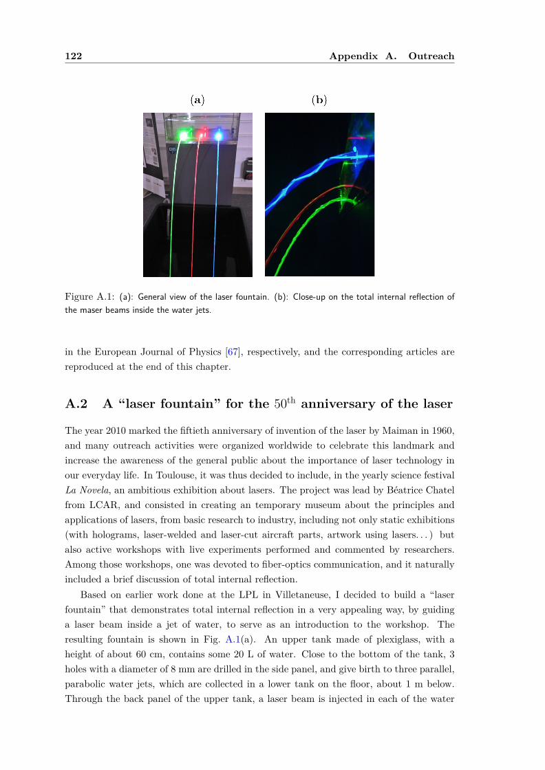
122 Appendix A. Outreach
Figure A.1: (a): General view of the laser fountain. (b): Close-up on the total internal reflection ofthe maser beams inside the water jets.
in the European Journal of Physics [67], respectively, and the corresponding articles arereproduced at the end of this chapter.
A.2 A “laser fountain” for the 50th anniversary of the laser
The year 2010 marked the fiftieth anniversary of invention of the laser by Maiman in 1960,and many outreach activities were organized worldwide to celebrate this landmark andincrease the awareness of the general public about the importance of laser technology inour everyday life. In Toulouse, it was thus decided to include, in the yearly science festivalLa Novela, an ambitious exhibition about lasers. The project was lead by Béatrice Chatelfrom LCAR, and consisted in creating an temporary museum about the principles andapplications of lasers, from basic research to industry, including not only static exhibitions(with holograms, laser-welded and laser-cut aircraft parts, artwork using lasers. . . ) butalso active workshops with live experiments performed and commented by researchers.Among those workshops, one was devoted to fiber-optics communication, and it naturallyincluded a brief discussion of total internal reflection.
Based on earlier work done at the LPL in Villetaneuse, I decided to build a “laserfountain” that demonstrates total internal reflection in a very appealing way, by guidinga laser beam inside a jet of water, to serve as an introduction to the workshop. Theresulting fountain is shown in Fig. A.1(a). An upper tank made of plexiglass, with aheight of about 60 cm, contains some 20 L of water. Close to the bottom of the tank, 3holes with a diameter of 8 mm are drilled in the side panel, and give birth to three parallel,parabolic water jets, which are collected in a lower tank on the floor, about 1 m below.Through the back panel of the upper tank, a laser beam is injected in each of the water

A.3 Yet another MOT video on Youtube 123
Figure A.2: A screen capture of the MOT video on Youtube.
jets3, and undergoes several total internal reflections at the water/air interface, as can beseen in Fig. A.1(b).
The upper tank gets empty in a few minutes. In order for the fountain to run contin-uously, a pump was switched on automatically when the water level was below a presetvalue, and pumped back the water to the upper tank until it was almost full. At thispoint, the pump turned off again. The turbulence created in the tank by the pump diedout in a few tens of seconds. This, in combination with the great care taken in machiningthe orifices to make them very smooth, allowed for water jets without any roughness, andmade it possible to observe many total internal reflections. The fountain encountered bigsuccess among the public, from toddlers to adults. . .
This fountain was reused several times at LCAR for the Fête de la Science. I laterbuilt a smaller version, working on similar principles, for the entrance hall of the institute.
A.3 Yet another MOT video on Youtube
During the process of testing the permanent-magnet Zeeman slower described in sec-tion 2.2, we used a 87Rb magneto-optical trap that was loaded by the slowed beam. I tooka movie of the corresponding MOT dynamics, showing a few typical phenomena that onecan observe visually with a MOT: loading it, turning the MOT into an optical molasseswhen switching off the magnetic field gradient, moving the zero of magnetic field usingshim coils, observing the MOT decay due to background-gas collisions. We decided toshare the video on Youtube4 with a short text describing the various phases of the movie(see Fig. A.2). Four years later, the video has been viewed some 3,700 times. This videoalso proved to be very useful in talks for the general public, as a means to show how acloud of cold atoms actually looks like in the lab, making the subject less abstract.
3I used three relatively cheap, 20 mW diode-pumped solid-state lasers from SDL, one red, one green,and one blue.
4https://www.youtube.com/watch?v=eAIDL_2xN8M.
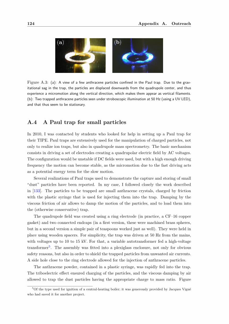
124 Appendix A. Outreach
Figure A.3: (a): A view of a few anthracene particles confined in the Paul trap. Due to the grav-itational sag in the trap, the particles are displaced downwards from the quadrupole center, and thusexperience a micromotion along the vertical direction, which makes them appear as vertical filaments.(b): Two trapped anthracene particles seen under stroboscopic illumination at 50 Hz (using a UV LED),and that thus seem to be stationary.
A.4 A Paul trap for small particles
In 2010, I was contacted by students who looked for help in setting up a Paul trap fortheir TIPE. Paul traps are extensively used for the manipulation of charged particles, notonly to realize ion traps, but also in quadrupole mass spectrometry. The basic mechanismconsists in driving a set of electrodes creating a quadrupolar electric field by AC voltages.The configuration would be unstable if DC fields were used, but with a high enough drivingfrequency the motion can become stable, as the micromotion due to the fast driving actsas a potential energy term for the slow motion.
Several realizations of Paul traps used to demonstrate the capture and storing of small“dust” particles have been reported. In my case, I followed closely the work describedin [133]. The particles to be trapped are small anthracene crystals, charged by frictionwith the plastic syringe that is used for injecting them into the trap. Damping by theviscous friction of air allows to damp the motion of the particles, and to load them intothe (otherwise conservative) trap.
The quadrupole field was created using a ring electrode (in practice, a CF–16 coppergasket) and two connected endcaps (in a first version, these were machined brass spheres,but in a second version a simple pair of teaspoons worked just as well). They were held inplace using wooden spacers. For simplicity, the trap was driven at 50 Hz from the mains,with voltages up to 10 to 15 kV. For that, a variable autotransformer fed a high-voltagetransformer5. The assembly was fitted into a plexiglass enclosure, not only for obvioussafety reasons, but also in order to shield the trapped particles from unwanted air currents.A side hole close to the ring electrode allowed for the injection of anthracene particles.
The anthracene powder, contained in a plastic syringe, was rapidly fed into the trap.The triboelectric effect ensured charging of the particles, and the viscous damping by airallowed to trap the dust particles having the appropriate charge to mass ratio. Figure
5Of the type used for ignition of a central-heating boiler; it was generously provided by Jacques Viguéwho had saved it for another project.

A.5 Fizeau’s “æther-drag” experiment made simple 125
A.3(a) shows the trapping of about five anthracene particles, which appear as verticalfilaments. This is due to the due to the gravitational sag experienced by the particlesin the trap: the particles are displaced downwards from the center of the quadrupolefield, and thus experience a micromotion along the vertical axis. Figure A.3(b) shows twoparticles illuminated by a UV6 LED fed by short current pulses with a repetition rate of50 Hz, allowing the stroboscopic observation of the particles, which appear motionless inthis case. Using the measured value of the gravitational sag and knowing the parametersof the trap, a semi-quantitative measurement of the charge-to-mass ratio of the anthraceneparticles could be performed by the students.
A.5 Fizeau’s “æther-drag” experiment made simple
This work was also triggered by students who contacted Pierre Labastie, asking for helpin setting up a replication of Fizeau’s 1851 “æther-drag” experiment for their TIPE. Aquick description of this famous experiment often occurs in textbooks on special relativity,as it is a nice way to illustrate the relativistic addition of velocities. Of course, Fizeau’smotivation in 1851 was different: his work was a test of an hypothesis made in 1818 byFresnel to “explain” the negative result of experiments performed by Arago with the goalto observe the dependence of the speed of light on the motion of the observer.
Fresnel’s “partial æther-drag” formula gives, in the lab frame, the velocity V of lightpropagating in a transparent medium with refractive index n, which is itself moving witha velocity v in the lab frame:
V = c
n+(
1− 1n2
)v. (A.1)
In contrast, a naive application of the usual (Galilean) addition of velocities (“total drag”)would give V = c/n+ v. In the limit of a medium becoming extremely dilute, such as ina gas whose pressure vanishes, the latter formula would give V = c + v, while Fresnel’sequation predicts V = c, a much more reasonable result as in this case one expects no effectof such a dilute gas on the propagation of light. The experiment by Fizeau confirmed thevalidity of Fresnel’s formula, and played a role in later developments of the electrodynamicsof moving media, that finally culminated with the birth of special relativity.
Fizeau’s extremely clever idea is to use an interferometer (which is actually a Sagnac-type interferometer), inside which a U-shaped tube with flowing water is inserted (seeFigs. 1 and 2 of the article [70] reproduced below on page 128). The two paths of theinterferometer are the same, but in one of them the light co-propagates with the water flow,while, in the other, light and water are counter-propagating. This clever trick allows oneto reject common-mode phase-shifts due to turbulent flow in the tubes7. The position ofthe interference fringes that are observed at the output of the interferometer then dependlinearly on the velocity of the water flow, and on the length of the interferometer. For
6When irradiated by UV light, anthracene particles fluoresce in the blue.7In many textbooks, this crucial point is overlooked, and the interferometric arrangements that are
shown would not allow for the observation of the effect.

126 Appendix A. Outreach
reasonable water velocities of a few meters per second, a fringe displacement of about onefringe requires an interaction length of a few meters.
The difficulty of the experiment thus lies in the realization of a water circulation systemcompatible with the observation of interference fringes. Together with Renaud Mathevet,we built an inexpensive but robust setup, based on standard plumbing hardware. We usedinitially a green solid-state laser as a light source, but, for the fun of it, we also used whitelight as in the original experiments. We found good agreement with theory, discarding theGalilean addition of velocities. We finally decided to publish a detailed description of oursetup in the American Journal of Physics.
A.6 Measuring the eccentricity of the Earth orbit with anail
In this last section, I briefly describe an experiment which somehow departs from myfield of optics or particle trapping, and rather deals with astronomy. It also originatedfrom discussions with students about possible subjects for a TIPE, but finally I did it toentertain myself, essentially at home (as the reader will see, little equipment is needed).In the end I also published a paper about it, this time in the European Journal of Physics,and so, for completeness, I include a brief description of this work here.
It is well-known that the Sun’s maximal altitude in the sky (reached at noon) displaysstrong seasonal variations, due to the obliquity of the Earth’s rotation axis. However, it isless known that the exact time at which this maximum occurs also varies during the year,by a few minutes. The difference between the true local noon and the official noon givenby clocks is called the equation of time. This difference is due to the combination of twoeffects :
• the obliquity on the ecliptic makes the projection of the Sun on the celestial equatormove non-uniformly;
• the eccentricity of the Earth orbit gives rise, via Kepler’s second law, to a non-uniform apparent motion of the Sun on the celestial equator.
Huyghens was the first to give correct expressions for the equation of time in the sev-enteenth century, although the irregularity of the apparent motion of the Sun had beenknown since Antiquity.
What I reported on in [67] was a very basic way to measure the equation of time, usingan elementary homemade sundial consisting of a nail protruding from a plywood base.The length of the shadow of the nail when placed in the sunlight allows one to computethe elevation of the Sun. One then just needs to plot the altitude of the Sun over timeduring the the course of a day, and extract from this data the maximal altitude and thetime at which this maximum is reached. Repeating this every few days over a full yeargives a good determination of the variation of the equation of time during the year, which
in turns allows for determining the eccentricity of the Earth orbit. I obtained a value of(1.7± 0.1) %, to be compared to the published value 1.6711 %. Besides being a lot of fun,performing this work was also a good reminder about the fact that one does not alwaysneed fancy equipment to measure something with a reasonable accuracy.
A.7 Published articles
Here, I list the two peer-reviewed educational articles I have co-authored:
• T. Lahaye, P. Labastie, and R. Mathevet, Am. J. Phys 80, 497 (2012), reproducedon page 128. I should point out here a few typos introduced in the copy-editingprocess, and that we unfortunately did not spot when proofreading the paper. Onpage 498, in the denominator of the first fraction of Eq. (1), a factor c is missing. Onpage 499, in the second column, the numerical values of the velocities disappearedin two instances. They should read 4 and 6 m/s, respectively.
• T. Lahaye, Eur. J. Phys 33, 1167 (2012) reproduced on page 137.
127

Fizeau’s “aether-drag” experiment in the undergraduate laboratory
Thierry Lahaye and Pierre LabastieUniversite de Toulouse, UPS, Laboratoire Collisions Agregats Reactivite, IRSAMC; F-31062 Toulouse,France and CNRS, UMR 5589, F-31062 Toulouse, France
Renaud MathevetUniversite de Toulouse, UPS, Laboratoire Collisions Agregats Reactivite, IRSAMC; F-31062 Toulouse,France; CNRS, UMR 5589, F-31062 Toulouse, France; and Laboratoire National des Champs MagntiquesIntenses, UPR3228 CNRS/INSA/UJF/UPS, F-31400, Toulouse, France
(Received 16 December 2011; accepted 10 February 2012)
We describe a simple realization of Fizeau’s “aether-drag” experiment. Using an inexpensive setup,
we measure the phase shift induced by moving water in a laser interferometer and find good agreement
with the relativistic prediction or, in the terms of 19th century physics, with Fresnel’s partial-drag
theory. This appealing experiment, particularly suited for an undergraduate laboratory project,
not only allows a quantitative measurement of a relativistic effect on a macroscopic system but also
constitutes a practical application of important concepts of optics, data acquisition and processing, and
fluid mechanics. VC 2012 American Association of Physics Teachers.
[http://dx.doi.org/10.1119/1.3690117]
I. INTRODUCTION
In introductory courses and textbooks dealing with specialrelativity, Fizeau’s “aether-drag” experiment often appearssimply as an application of the law of composition of veloc-ities, sometimes in the form of an exercise.1 However, AlbertEinstein himself declared that Fizeau’s measurement of thespeed of light in moving water was, together with stellar aber-ration, one of the experimental results that had influenced himmost in the development of relativity.2 In spite of this highpraise, introductory expositions of Fizeau’s experiment,including a discussion of its historical development and thedetails of the experimental setup, are often lacking. Moreover,many textbooks actually show incorrect experimental arrange-ments that would not allow for the observation of the effect inpractice. Here, we show that one can actually performFizeau’s experiment with rather modest equipment, and thatsuch a project illustrates in an appealing way not only relativ-istic kinematics but also interesting aspects of wave optics,data acquisition and processing, and even fluid mechanics.
This article is organized as follows. We first review brieflythe historical background of Fizeau’s experiment, a “test” ofspecial relativity carried out more than half a century beforerelativity was born! For completeness, we recall in Sec. III thederivation of the expected fringe shift in both the relativisticand non-relativistic frameworks, following the usual textbooktreatment of the problem. We then turn to the main point ofthe paper, namely, how to reproduce the experiment in anundergraduate laboratory. Section IV is devoted to thedescription of our apparatus, starting with an emphasis on theexperimental trade-offs one needs to address in the designphase. Finally, we discuss in Sec. V the results obtained, firstwith water as a moving medium and then with air, in order todiscriminate between relativistic and non-relativistic predic-tions. The use of a white-light source instead of a laser is pre-sented in Appendix A, with a discussion of the possibleadvantages and drawbacks. Appendix B establishes a usefulfluid mechanics formula using dimensional analysis.
II. HISTORICAL BACKGROUND
Since Fizeau’s aether-drag experiment is a landmark amongthe various experimental and theoretical developments leading
to special relativity, it is worthwhile to recall briefly the his-tory of these developments. An extensive historical study ofthe subject is beyond the scope of this paper. Here, we merelyrecall the main steps that led to Fizeau’s aether drag experi-ment, as well as the major subsequent developments.3
We begin our reminder in the 17th century, at a time whenthe nature of light was a matter of harsh debate, as evidencedby the famous controversy between Christiaan Huygens andIsaac Newton. The speed of light in a vacuum c was knownto be finite since the work of Ole Romer in 1676.4 However,the measurement of the speed of light in a material mediumof refractive index n was considered a crucial test becauseHuygens’ wave theory implies that the speed of light in themedium is c/n, while Newton’s corpuscular theory predicts itto be nc. Newton’s views prevailed until the beginning of the19th century, when interference experiments by ThomasYoung and polarization experiments by Etienne Malus firmlyestablished the wave theory.
An important event was the measurement by FrancoisArago of the deviation of light from a distant star by a prismin 1810.5 The idea of Arago is that if the speed of the lightcoming from distant stars is increased or decreased by theEarth’s velocity, Newton’s theory predicts that the deviationby a prism should be different from what would be observedif the source was terrestrial. He, therefore, tried to detect thisdifference and found a null result. This experiment seems tobe the first in a long series that showed the impossibility ofdetecting the relative motion of light with respect to theEarth.6
Arago soon became friends with Augustin Fresnel, whohad a mathematically sound theory of light waves, and askedhim if the wave theory could explain the null result he hadfound. Fresnel’s answer came a few years later.7 His demon-stration is based on the hypothesis of an absolute aether as asupport of light waves, associated with a partial drag bytransparent media. That is, if the medium of index n moveswith speed v, the aether inside the medium moves only atspeed ð1 n2Þ v. The value of Fresnel’s drag coefficient1 n2 precisely gives a null result for the Arago experi-ment. However, his demonstration, using some supposedelastic properties of the aether, is not so convincing bymodern standards.6
497 Am. J. Phys. 80 (6), June 2012 http://aapt.org/ajp VC 2012 American Association of Physics Teachers 497
128

The first Earth-based direct measurement of the speed oflight was realized by Hippolyte Fizeau in 1849, by means ofa rotating cogwheel. This kind of time-of-flight techniquewas soon improved by Leon Foucault who, using a rotatingmirror, succeeded in showing that the speed of light is lowerin water than in air.8,9 Nevertheless, such absolute measure-ments were far from accurate enough to measure the smallchange of the speed of light in moving media.
This is where Fizeau’s aether-drag experiment enters thescene. As we shall see, this experiment is based on a muchmore sensitive differential measurement using the interfero-metric arrangement shown in Fig. 1. The experiment wasperformed in 1851 and almost immediately reported to theFrench academy of science, and then translated into Eng-lish.10 Fizeau measured an effect in agreement with Fresnel’stheory to within a few percent, which unambiguously ruledout concurrent theories postulating total aether drag.
Many experiments of increasing precision were thenundertaken to try to demonstrate the influence of Earth’smotion on light propagation, but all gave null results. It soonbecame apparent that Fresnel’s partial drag did not allow themeasurement of any absolute motion of Earth to first order inv/c. In what would now be called a review paper,11 EleuthereMascart concludes in 1874 (our translation): “the generalconclusion of this memoir would be […] that the translationmotion of the Earth is of no appreciable consequence on op-tical phenomena produced with terrestrial sources or solarlight, that those phenomena do not allow to appreciate theabsolute motion of a body and that only relative motions canbe attained.”
In 1881 Albert Michelson designed a new interferometer,which, according to existing theories, could detect Earth’sdisplacement respective to aether because the expected effectwas proportional to ðv=cÞ2. His first measurement was atmost half of the expected fringe shift. He then improved theapparatus with Edward Morley. The two physicists graduallybecame convinced of a null result. In 1886 they decided toredo Fizeau’s experiment—the only experiment with a posi-tive result, and one that had yet to be reproduced. With acareful design of the hydraulics and an improved design forthe interferometer,12 they confirmed Fizeau’s result, andFresnel’s aether drag, with much higher precision. However,in their celebrated experiment of 1887,13 the measured shiftwas at most 0.01 fringe instead of an expected 0.4. The twoexperiments were thus incompatible according to existingtheories, Fizeau’s needing a partial drag and Michelson-Morley’s needing a total drag of aether.
History then accelerated. In the late 1880 s, George Fitz-gerald proposed the concept of length contraction. In 1895,Hendrick Lorentz published his theory of electromagnetic
media, in which he derived Fresnel’s formula from first prin-ciples. At the beginning of the 20th century, it became evi-dent that time dilation was also necessary to account for allelectromagnetic phenomena. After Albert Einstein publishedthe theory of special relativity in 1905, Max Laue, in 1907,derived Fresnel’s drag coefficient from the relativistic addi-tion of velocities.14 All experiments, being either of first(Fizeau) or second (Michelson-Morley) order in v/c, werethen explained by a single theory with no need for an aetherwith such special properties.
In the relativistic framework, one can also account for theeffects of dispersion, already predicted by Lorentz in 1895.Although the supplementary term makes only a few percentcorrection, Pieter Zeeman, in his 1914–1927 experiments,succeeded in measuring it.15,16 More recently, this experi-ment was performed in liquids, solids, and gases using ringlasers17 and confirmed the value of the dispersion term towithin 15%.18 Fizeau’s experiment has also been success-fully transposed to neutron matter waves.19
Thus, as may not be commonly understood, Fizeau’saether-drag experiment was a crucial turning point betweenold and modern conceptions of light and space-time. Webelieve this makes its replication particularly valuable froma pedagogical point of view.
III. THEORETICAL BACKGROUND
In this section, we recall the derivation of the phase differ-ence Du induced by the motion, with velocity v, of the me-dium of refractive index n in the interferometric arrangementshown in Fig. 2, which is essentially the one used by Michel-son and Morley in 1886.12 Let us consider first the casewhere water and monochromatic light of vacuum wave-length k propagate in the same direction [shown as light gray(green online) in Fig. 2]. In the reference frame where wateris at rest, the phase velocity of light is c/n. In the laboratoryframe, using the relativistic composition of velocities, thephase velocity of light is
vþ ¼c=nþ v
1þ ðv=nÞ=c2¼ c=nþ v
1þ v=ðncÞ : (1)
The phase accumulated by light over the propagation dis-tance of 2‘ is thus
Fig. 1. (Color online) Sketch of the interferometer used by Fizeau (adapted
from Michelson, Studies in Optics. Copyright VC 1995 by Dover). For the sake
of clarity, the two counter-propagating beams are drawn in different gray levels
(colors). S: source; O: observer; M: mirror; Wi: windows; Li: lenses; BS: beam
splitter; DS: double slit.
Fig. 2. (Color online) Sketch of the experimental setup (see text for details).
Mi: mirror; Wi: windows; BS: beam splitter. The two counter-propagating
beams are drawn in different gray levels (colors) for clarity.
498 Am. J. Phys., Vol. 80, No. 6, June 2012 Lahaye, Labastie, and Mathevet 498
129
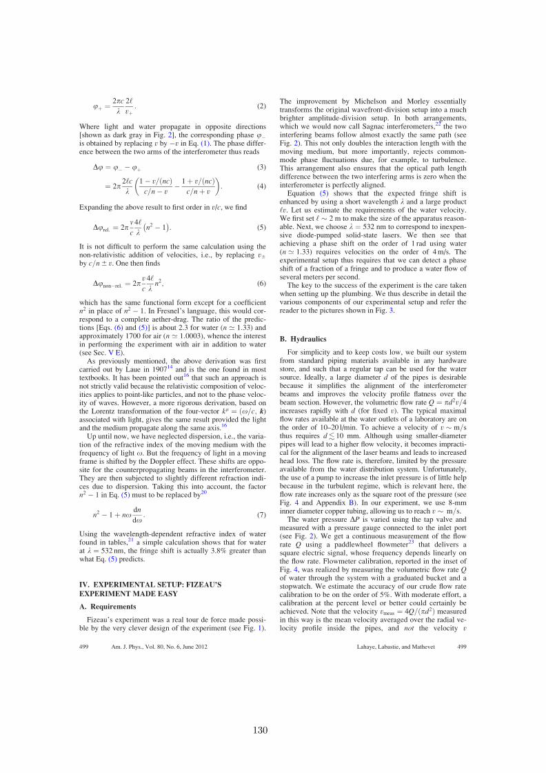
uþ ¼2pc
k2‘
vþ: (2)
Where light and water propagate in opposite directions[shown as dark gray in Fig. 2], the corresponding phase uis obtained by replacing v by v in Eq. (1). The phase differ-ence between the two arms of the interferometer thus reads
Du ¼ u uþ (3)
¼ 2p2‘c
k1 v=ðncÞ
c=n v 1þ v=ðncÞ
c=nþ v
: (4)
Expanding the above result to first order in v/c, we find
Durel: ¼ 2pv
c
4‘
kn2 1
: (5)
It is not difficult to perform the same calculation using thenon-relativistic addition of velocities, i.e., by replacing v6
by c=n 6 v. One then finds
Dunonrel: ¼ 2pv
c
4‘
kn2; (6)
which has the same functional form except for a coefficientn2 in place of n2 1. In Fresnel’s language, this would cor-respond to a complete aether-drag. The ratio of the predic-tions [Eqs. (6) and (5)] is about 2.3 for water (n ’ 1:33) andapproximately 1700 for air (n ’ 1:0003), whence the interestin performing the experiment with air in addition to water(see Sec. V E).
As previously mentioned, the above derivation was firstcarried out by Laue in 190714 and is the one found in mosttextbooks. It has been pointed out16 that such an approach isnot strictly valid because the relativistic composition of veloc-ities applies to point-like particles, and not to the phase veloc-ity of waves. However, a more rigorous derivation, based onthe Lorentz transformation of the four-vector kl ¼ ðx=c; k)associated with light, gives the same result provided the lightand the medium propagate along the same axis.16
Up until now, we have neglected dispersion, i.e., the varia-tion of the refractive index of the moving medium with thefrequency of light x. But the frequency of light in a movingframe is shifted by the Doppler effect. These shifts are oppo-site for the counterpropagating beams in the interferometer.They are then subjected to slightly different refraction indi-ces due to dispersion. Taking this into account, the factorn2 1 in Eq. (5) must to be replaced by20
n2 1þ nxdn
dx: (7)
Using the wavelength-dependent refractive index of waterfound in tables,21 a simple calculation shows that for waterat k ¼ 532 nm, the fringe shift is actually 3.8% greater thanwhat Eq. (5) predicts.
IV. EXPERIMENTAL SETUP: FIZEAU’S
EXPERIMENT MADE EASY
A. Requirements
Fizeau’s experiment was a real tour de force made possi-ble by the very clever design of the experiment (see Fig. 1).
The improvement by Michelson and Morley essentiallytransforms the original wavefront-division setup into a muchbrighter amplitude-division setup. In both arrangements,which we would now call Sagnac interferometers,22 the twointerfering beams follow almost exactly the same path (seeFig. 2). This not only doubles the interaction length with themoving medium, but more importantly, rejects common-mode phase fluctuations due, for example, to turbulence.This arrangement also ensures that the optical path lengthdifference between the two interfering arms is zero when theinterferometer is perfectly aligned.
Equation (5) shows that the expected fringe shift isenhanced by using a short wavelength k and a large product‘v. Let us estimate the requirements of the water velocity.We first set ‘ 2 m to make the size of the apparatus reason-able. Next, we choose k ¼ 532 nm to correspond to inexpen-sive diode-pumped solid-state lasers. We then see thatachieving a phase shift on the order of 1 rad using water(n ’ 1:33) requires velocities on the order of 4 m/s. Theexperimental setup thus requires that we can detect a phaseshift of a fraction of a fringe and to produce a water flow ofseveral meters per second.
The key to the success of the experiment is the care takenwhen setting up the plumbing. We thus describe in detail thevarious components of our experimental setup and refer thereader to the pictures shown in Fig. 3.
B. Hydraulics
For simplicity and to keep costs low, we built our systemfrom standard piping materials available in any hardwarestore, and such that a regular tap can be used for the watersource. Ideally, a large diameter d of the pipes is desirablebecause it simplifies the alignment of the interferometerbeams and improves the velocity profile flatness over thebeam section. However, the volumetric flow rate Q ¼ pd2v=4increases rapidly with d (for fixed v). The typical maximalflow rates available at the water outlets of a laboratory are onthe order of 10–20 l/min. To achieve a velocity of v m=sthus requires d. 10 mm. Although using smaller-diameterpipes will lead to a higher flow velocity, it becomes impracti-cal for the alignment of the laser beams and leads to increasedhead loss. The flow rate is, therefore, limited by the pressureavailable from the water distribution system. Unfortunately,the use of a pump to increase the inlet pressure is of little helpbecause in the turbulent regime, which is relevant here, theflow rate increases only as the square root of the pressure (seeFig. 4 and Appendix B). In our experiment, we use 8-mminner diameter copper tubing, allowing us to reach v m=s.
The water pressure DP is varied using the tap valve andmeasured with a pressure gauge connected to the inlet port(see Fig. 2). We get a continuous measurement of the flowrate Q using a paddlewheel flowmeter23 that delivers asquare electric signal, whose frequency depends linearly onthe flow rate. Flowmeter calibration, reported in the inset ofFig. 4, was realized by measuring the volumetric flow rate Qof water through the system with a graduated bucket and astopwatch. We estimate the accuracy of our crude flow ratecalibration to be on the order of 5%. With moderate effort, acalibration at the percent level or better could certainly beachieved. Note that the velocity vmeas ¼ 4Q=ðpd2Þ measuredin this way is the mean velocity averaged over the radial ve-locity profile inside the pipes, and not the velocity v
499 Am. J. Phys., Vol. 80, No. 6, June 2012 Lahaye, Labastie, and Mathevet 499
130
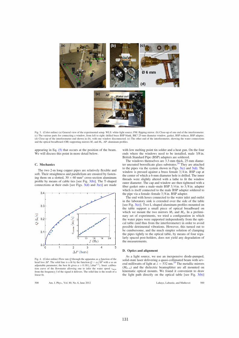
appearing in Eq. (5) that occurs at the position of the beam.We will discuss this point in more detail below.
C. Mechanics
The two 2-m long copper pipes are relatively flexible andsoft. Their straightness and parallelism are ensured by fasten-ing them on a slotted, 30 60 mm2 cross-section aluminumprofile by means of cable ties [see Fig. 3(b)]. The T-shapedconnections at their ends [see Figs. 3(d) and 3(e)] are made
with low melting point tin solder and a heat gun. On the fourends where the windows need to be installed, male 3/8 in.British Standard Pipe (BSP) adapters are soldered.
The windows themselves are 3.3-mm thick, 25-mm diame-ter uncoated borosilicate glass substrates.24 They are attachedto the pipes via the system shown in Figs. 3(c) and 3(d). Thewindow is pressed against a brass female 3=4 in: BSP cap atthe center of which a 6-mm diameter hole is drilled. The innerthreads were slightly altered with a lathe to fit the windowouter diameter. The cap and window are then tightened with afiber gasket onto a male–male BSP 3=4 in: to 3=8 in: adapterwhich is itself connected to the male BSP adapter soldered tothe pipe via a female–female 3=8 in: BSP adapter.
The end with hoses connected to the water inlet and outletin the laboratory sink is extended over the side of the table[see Fig. 3(e)]. Two L-shaped aluminum profiles mounted onthe table support a small piece of optical breadboard onwhich we mount the two mirrors M3 and M4. In a prelimi-nary set of experiments, we tried a configuration in whichthe water pipes were supported independently from the opti-cal table (and thus from the interferometer) in order to avoidpossible detrimental vibrations. However, this turned out tobe cumbersome, and the much simpler solution of clampingthe pipes tightly to the optical table, by means of four regu-larly spaced post-holders, does not yield any degradation ofthe measurements.
D. Optics and alignment
As a light source, we use an inexpensive diode-pumped,solid-state laser delivering a quasi-collimated beam with sev-eral milliwatts of light at k ¼ 532 nm.25 The metallic mirrors(M04) and the dielectric beamsplitter are all mounted onkinematic optical mounts. We found it convenient to drawthe light path directly on the optical table [see Fig. 3(b)]
Fig. 4. (Color online) Flow rate Q through the apparatus as a function of the
head loss DP. The solid line is a fit by the function Q ¼ affiffiffiffiffiffiffiDPp
with a as an
adjustable parameter; the best fit gives a ’ 0:18 L=ðsbar1=2Þ. Inset: calibra-
tion curve of the flowmeter allowing one to infer the water speed vmeas
from the frequency f of the signal it delivers. The solid line is the result of a
linear fit.
Fig. 3. (Color online) (a) General view of the experimental setup. WLS: white-light source; FM: flipping mirror. (b) Close-up of one end of the interferometer.
(c) The various parts for connecting a window, from left to right: drilled brass BSP blank, BK7 25-mm diameter window, gasket, BSP reducer, BSP adapter.
(d) Close-up of the interferometer end shown in (b), with one window disconnected. (e) The other end of the interferometer, showing the water connections
and the optical breadboard (OB) supporting mirrors M3 and M4. AP: aluminum profiles.
500 Am. J. Phys., Vol. 80, No. 6, June 2012 Lahaye, Labastie, and Mathevet 500
131

before mounting the mirrors and the beamsplitter, as thisconsiderably simplifies the alignment of the interferometer.
To align the interferometer, we begin with four small dia-phragms (diameter 2 mm) positioned just in front of thecenters of the windows W14. The tubing system is thenremoved, and one walks the beam using M1, BS, and M2 sothat beams W1W4 and W2W3 pass through the diaphragms.Using M3 and/or M4, one then aligns the returning beamonto the incoming one. After a few iterations, one obtains aquasi-perfect superposition of the beams and observes analmost flat intensity profile in the interference field. Whentilting slightly one of the mirrors (e.g., M3), nice straight par-allel fringes appear.
Now the pipes can be repositioned and clamped onto thetable. Water is set to flow, and one makes sure that no airbubbles are trapped inside the pipes, especially close to thewindows where the diameter is larger. If so, they can beremoved by loosening the cap while the water is flowing.
Instead of the expected fringe pattern, one usuallyobserves caustics and diffuse reflections on the inner sidesof the pipes. Indeed, due to the soldering, the parallelism ofthe windows cannot be ensured. When a beam strikesthe window at a small angle from the normal, its path isslightly deviated. This deviation is only partially compen-sated at the inner glass/water interface, so the interferometermust be realigned. After a few iterations, the fringes return(see Fig. 5).
V. EXPERIMENTAL RESULTS
A. Data acquisition
For quantitative measurements of the fringe shift, we usean inexpensive webcam,26 whose objective lens and IR filterhave been removed in order to directly expose the CMOS de-tector chip to the fringe pattern. Using the micrometerscrews of mirror M2, for instance, the fringes are set parallelto one of the axes of the camera chip. From the webcamsoftware, the gamma correction is adjusted to get a linear
response of the detector.27 The integration time and light in-tensity are adjusted to use the full dynamic range of the web-cam, taking care not to saturate any pixels.
An important point for later data processing is that, priorto acquiring a series of images, one needs to locate the posi-tion of the central fringe on the camera. For this, it is conven-ient to wobble mirror M2, for example. The fringe spacingvaries, and the fringes move symmetrically away from thecentral one which is dark and does not move. Once the posi-tion x0 of the central fringe has been located, the webcam isroughly centered on it to limit systematic errors due tochanges in the fringe spacing. The fringe spacing is thenadjusted to get about ten fringes on the detector chip. Toofew fringes will not allow for an accurate measurement ofthe fringe position offset and period. On the other hand, ifthe fringes are too narrow, the resolution of the camera willlimit accuracy.
B. Data processing
We process the images in the following way. We sum upthe values of all pixels in a column, and thus obtain a one-dimensional intensity distribution I(x), where x (in pixels)denotes the position along an axis perpendicular to thefringes (see Fig. 5). We then fit the data using
IðxÞ ¼ I0 þ I1 sin2pðx x0Þ
Kþ Du
; (8)
where I0; I1;K, and Du are adjustable parameters, and x0 isthe (fixed) position of the central fringe, determined asexplained above.
C. Experimental results with water
Acquisition and processing are repeated for various watervelocities. Figure 6 shows the experimentally measuredphase difference Du as a function of the measured water ve-locity vmeas. The origin of phases has been chosen to vanishat zero velocity. As can be seen in the figure, we take fivemeasurements for each velocity to improve the statistics andto get an estimate of the variance. Negative velocities were
Fig. 5. (Color online) Sample images of the fringe pattern obtained from the
camera for (a) v¼ –5.7 m/s, (b) v¼ 0.8 m/s, and (c) v¼ 5.7 m/s. The white
dashed line shows the position x0 of the central fringe for v¼ 0. (d) Process-
ing of the image shown in (c)—the dots are the vertically integrated inten-
sities and the (red) solid curve is the best fit to Eq. (8).
Fig. 6. (Color online) Experimental results using water as the moving me-
dium. Circles: data; thin solid line: linear fit, giving a slope of 0:274 6 0:003
rad s/m; thick solid line: relativistic prediction from Eq. (5); dashed line:
non-relativistic prediction from Eq. (6).
501 Am. J. Phys., Vol. 80, No. 6, June 2012 Lahaye, Labastie, and Mathevet 501
132

obtained simply by exchanging the inlet and outlet ports ofthe tubing system. No data could be recorded for velocitiesbelow 1 m/s. Indeed, when the velocity is low, turbulence inthe pipes is not fully developed, which leads to low spatialand temporal frequency fluctuations and very unstable pic-tures. We also could not take data for zero velocity becausein this case the inlet or outlet valve must be closed; such asituation produces undue stress on the tubing system so thatlight can no longer properly exit the system. For this reason,the alignment procedure must be performed with water flow-ing in the pipes.
We observe a clear linear dependence of Du on vmeas. Alinear fit (thin solid line) gives a slope of 0:274 6 0:003rad s/m. The non-relativistic prediction of Eq. (6) (dashedline) has slope 0.563 rad s/m, which does not match theexperimental results at all. The relativistic prediction givenby Eq. (5) (thick solid line) has slope 0.248 rad s/m and is inmuch better agreement with the experimental data. However,there appears to be a slight systematic error in the data com-pared with the prediction. As stated earlier, this comes fromthe fact that we measure the mean velocity vmeas averagedover the velocity profile inside the pipes, whereas the veloc-ity v appearing in Eq. (5) is the velocity at the position of thebeam, i.e., on the axis of the pipes.
To understand how vmeas is related to v, let v(r) denote theradial dependence of the velocity in the pipes of radius R andlet vmax ¼ vð0Þ. Because the beam is well centered on thepipe by construction, we can safely assume that v ¼ vmax.We must therefore multiply the theoretical prediction by thecorrection factor
vmax
vmeas
¼ pR2vmaxÐ R0
2prvðrÞdr: (9)
A theoretical model for the radial dependence v(r) is thusrequired. In the laminar regime (Poiseuille flow), v(r) wouldhave the parabolic shape shown as the dashed curve inFig. 7, which, using Eq. (9), gives a correction factor equalto 2. However, for v& 1 m/s, one can check that the Reyn-olds number Re ¼ vd=& 104, making the flow turbulent.Here, 106m2=s denotes the kinematic viscosity ofwater. Under these conditions, there is no simple rigorousanalytic expression for the velocity profile. However, for therange of Reynolds numbers used here, experimentally meas-ured flow profiles are well reproduced12 by the empirical lawvðrÞ ¼ vmaxð1 r2=R2Þ1=6
, corresponding to the much flattervelocity profile shown as the solid curve in Fig. 7. In the tur-bulent regime, Eq. (9) then gives a correction factor of 1.16.The relativistic prediction (5) multiplied by this correctionfactor, and including the 3.8% correction due to dispersion,yields a slope of 0.299 rad s/m (not shown in Fig. 6). Theagreement between the experimental and theoretical valuesis thus at the level of 8%.
D. Discussion
Based on our data, we conclude that the non-relativisticprediction is clearly ruled out by our measurements. Never-theless, the rather good agreement with the relativistic pre-diction must not be over interpreted. Indeed, it is difficult toput an accurate error bar on the result, as several systematiceffects should be studied carefully for such a purpose.First, the systematic errors are dominated by our flowratemeasurement. A more careful calibration should thus be per-
formed in order to improve the accuracy. Second, the factorof 1.16 due to the shape of the velocity profile should bemeasured specifically for our system. A final source ofuncertainty is the determination of the actual length ‘ appear-ing in Eq. (5). In practice, the flow makes a right-angle turnat each end of the pipes, so the velocity will presumably beaffected up and downstream on length scales on the order ofthe pipe diameter d. This implies a correction of order d=‘(on the percent level), but again, an accurate estimation isdifficult.
In the end, due to a slight distortion of the tubing when thevelocity (and thus the pressure) is varied, the fringe spacingchanges by a small amount. As mentioned, an important fea-ture of the Sagnac-like interferometric arrangement usedhere is that it operates at low interference order p. This iscrucial in order to be sure that when the water is flowinginside the pipes, the observed shift of the fringes does arisefrom the aether drag effect and not from a slight change inthe fringe spacing. As an example, let us assume that using adifferent interferometric setup, one observes an interferencepattern with ten fringes, corresponding to interference orders,say p1 ¼ 104 to p2 ¼ p1 þ 10. If, as is likely, the fringe spac-ing changes by a quantity as small as 104 in relative valuewhen the water velocity varies, one would observe that ourten fringes would shift, almost as a whole, by as much as onefull fringe! For the data presented in the paper, we havemeasured that the fringe period K does not vary by morethan 5% over the full range of velocities, yielding negligibleerrors due to the low interference orders used here.
E. Experimental results with air
In his original paper,10 Fizeau states that he performed theexperiment with air as a moving medium and that “themotion of the air does not produce any sensible displacementof the fringes,” in agreement with the partial drag prediction(5). On the contrary, the non-relativistic prediction (6) pre-dicts a measurable shift.
It is thus interesting to repeat the experiment using airinstead of water. We do so by using a standard compressedair outlet, as available in most laboratories. One actuallyneeds very moderate pressures in order to achieve relatively
Fig. 7. (Color online) Dashed curve: Poiseuille’s velocity profile for laminar
flow given by vðrÞ ¼ vmaxð1 r2=R2Þ. Solid curve: velocity profile for tur-
bulent flow, modeled here by the empirical form vðrÞ ¼ vmaxð1 r2=R2Þ1=6.
502 Am. J. Phys., Vol. 80, No. 6, June 2012 Lahaye, Labastie, and Mathevet 502
133

high velocities for the air flow in the 8-mm diameter pipes:only 0.2 bar typically yields vmeas ’ 35m=s. Measuring theair velocity is not as straightforward as with water; we foundit convenient to use a hot-wire anemometer28 placed in aD¼ 18 mm inner-diameter pipe at the outlet of the d¼ 8 mmpipes. The velocity vmeas in the interaction region of the in-terferometer is then deduced from the measured velocityvanem at the anemometer position via volumetric flow conser-vation vmeas ¼ vanemðD=dÞ2. This assumes incompressibleflow, which is valid since the air velocity is much smallerhere than the speed of sound.29
Figure 8 shows the measured phase shifts (circles) alongwith the predictions of Eqs. (5) and (6). We cannot clearlyidentify the reason(s) behind the seemingly oscillatorybehavior of the measured fringe shift with velocity. In anycase, the non-relativistic prediction is clearly ruled out bythe measurements, which are clearly compatible with the rel-ativistic calculation.
VI. CONCLUSION AND OUTLOOK
Using rather modest equipment, we have shown thatFizeau’s “aether-drag” experiment can be reproduced in theundergraduate laboratory at a quantitative level. It not onlymakes a nice practical introduction to the sometimes abstractconcepts of special relativity but also constitutes an interest-ing application of several branches of experimental physics.
Immediate improvements of the setup described in thispaper would consist of (i) calibrating the flowrate more care-fully and (ii) increasing the stiffness of the tubing system. Anatural extension of this work, suitable for a long-term stu-dent project, would consist of trying to study the systematiceffects in detail—for example, the determination of theeffective length ‘. One way to measure this effect would beto start from the full pipe length and then repeat the experi-ment for shorter and shorter pipe lengths. The effect can thenbe evaluated by measuring the dependence of the slopeDu=v on the pipe length.
A more ambitious extension, suitable for advanced under-graduates, would illustrate more modern optical techniques.For instance, one may use a ring cavity of moderately highfinesse (say F 100 –1000) and measure the variation of
the resonance frequencies of the two counterpropagatingmodes when the velocity of the medium is varied. A gain insensitivity by a factor F is then expected. Such techniques,with ultra-high finesse cavities, are currently used to mea-sure, for example, non-reciprocity effects in the propagationof light with amazing sensitivities.30
ACKNOWLEDGMENTS
The authors thank Eric Desmeules for instigating this pro-ject and his students Melodie Andrieu and Laurane Bou-langer for help in setting up a preliminary version of theapparatus during their “TIPE” project (the data shown inFigs. 4 and 6 were essentially acquired by them). The authorsthank Jacques Vigue for useful discussions. David Guery-Odelin created the conditions that made this project possible.R.M. dedicates his contribution to Jose-Philippe Perez forinspiring discussions over the years. Funding by CNRS isacknowledged.
APPENDIX A: USING A WHITE-LIGHT SOURCE
INSTEAD OF A LASER
We have also performed this experiment using a white-light source instead of a laser. The source is a 1-mm diameteriris illuminated by a 55-W halogen lamp (the type used forcar headlights) and a condenser lens. The resulting divergingbeam is collimated by a 100-mm focal length lens and super-imposed onto the path of the laser beam using two mirrors.The second mirror, located between M0 and M1, is a flippingmirror so that one can switch easily between the laser andthe white light sources [see Fig. 3(a)]. Once the interferome-ter has been aligned with the laser, white-light fringes arereadily observed. Naturally, if the iris is opened the luminos-ity is increased at the expense of spatial coherence, and thecontrast in the picture is lost. The fringes are then localizedin the vicinity of mirror M3. A color image as in Fig. 9(a) isthen recovered using a converging lens that conjugates M3
and the detector plane.The advantages of using a white source is that (i) the position
of the dark central fringe can be found without ambiguity as thecontrast of the colored fringes vanishes rapidly away from thezero path-length difference and (ii) compared to using a laser,unwanted interference fringes (due to scattering on dust particlesfor example) as well as speckle, are suppressed. There are,
Fig. 8. (Color online) Experimental results using air as the moving medium.
Circles: data; solid line: relativistic prediction from Eq. (5); dashed line:
non-relativistic prediction from Eq. (6).
Fig. 9. (Color online) (a) A sample white-light fringe pattern. (b) Composite
image of 22 fringe patterns obtained for different water velocities v. One
clearly observes the linear shift of the central fringe position as a function of v.
503 Am. J. Phys., Vol. 80, No. 6, June 2012 Lahaye, Labastie, and Mathevet 503
134

however, a certain number of drawbacks. Besides the reducedluminosity, making quantitative comparisons with theory isobviously much more difficult than in the monochromatic case.Indeed, one would need to measure the light spectrum, as wellas the wavelength-dependent reflectivity (including phaseshifts)introduced by the beamsplitter in order to model quantitativelythe fringe pattern. For instance, we have observed that using ametallic beamsplitter instead of the dielectric one significantlyalters the colors and the contrast of the fringe pattern obtained inwhite light.
We made a composite of 22 images taken for variouswater velocities v. The result, shown in Fig. 9(b), clearlyshows that the fringe positions shift linearly with velocity.However, a quantitative analysis of such an image is noteasy, and the motivation behind this figure is mainly foraesthetics.
APPENDIX B: TURBULENT HEAD LOSS IN A
CIRCULAR PIPE: DIMENSIONAL ANALYSIS
APPROACH
In the standard introductory physics curriculum, the com-putation of the head loss in a circular pipe is done usingPoiseuille’s equation, valid for laminar flow. It is much lesscommon to present the case of turbulent flow to undergradu-ate students. Reference to the Moody diagram, giving theso-called friction factor as a function of Reynolds numberand pipe roughness, can be found in engineering-orientedtextbooks, but may appear as quite involved to beginningphysics students. In this appendix, we show how dimensionalanalysis can be used to infer a plausible expression for theturbulent head loss, at least for its dependence on flow rateand pipe diameter, two parameters that are crucial for thedesign of our experimental setup.
We consider the head loss DP for the flow of a fluid ofdensity q and kinematic viscosity in a circular pipe of di-ameter d and length l, flowing with a volumetric flow rate Q.Let us make two assumptions. First, for an infinitely longpipe, only the pressure gradient DP=l is physically relevant.And second, the limit of very large Reynolds number corre-sponds formally to the limit ! 0. In this case, the viscosity should not appear explicitly in the expression for the headloss. Under these conditions, we expect the functional formfor the head loss to be
DP
l¼ AqaQbDc; (B1)
where A is a dimensionless constant and ða; b; cÞ the expo-nents to be determined. Equating the dimensions on bothsides of this equation yields three equations for the expo-nents, which can be solved to give
DP
l¼ A
qQ2
D5: (B2)
This expression agrees well with empirical formulae used inan engineering context if one chooses A 3 102, andthis is typically what one would find using the friction factorobtained in a Moody diagram31,32 for our Reynolds numbers.For example, the value of the coefficient a obtained when fit-ting the flow rate data of Fig. 4 yields A ’ 2:5 102, ingood agreement with the previous estimate.
1E. F. Taylor and J. A. Wheeler, Spacetime Physics: Introduction to SpecialRelativity, 2nd ed. (W. H. Freeman & Company, New York, 1992).
2R. S. Shankland, “Conversations with Albert Einstein,” Am. J. Phys. 31,
47–57 (1963).3For a detailed account, see O. Darrigol, “The genesis of the Theory of
Relativity,” Seminaire Poincare, 1, 1–22 (2005), available online at
www.bourbaphy.fr/darrigol2.pdf, and references therein.4O. Romer, “Demonstration touchant le mouvement de la lumiere trouve
par M. Romer de l’Academie Royale des Sciences,” J. des Scavans,
233–236 (1676). An English translation appeared quickly in Philos. Trans.
12, 893–894 (1677), available online at http://dx.doi.org/10.1098/
rstl.1677.0024.5Arago gave an account of the results to the French Academy of Sciences,
but the text was not published until 1853, in F. Arago, “Memoire sur la
vitesse de la lumiere,” C. R. Acad. Sci. 36, 38–49 (1853), available online
at http://gallica.bnf.fr/ark:/12148/bpt6k2993z/f42.image.6For a modern account see R. Ferraro and D. M. Sforza, “Arago (1810):
The first experimental result against the ether,” Eur. J. Phys. 26, 195–204
(2005).7A. Fresnel, “Lettre de M. Fresnel a M. Arago, sur l’influence du
mouvement terrestre dans quelques phenomenes d’optique,” Ann.
Chim. Phys. 9, 57–66 (1818), available online at http://www.google.
com/books?id¼nZc5AAAAcAAJ.8L. Foucault, Sur les vitesses relatives de la lumiere dans l’air et dans l’eau(Bachelier, Paris, 1853), available online at http://www.bibnum.education.
fr/files/foucault-texte.pdf.9A. A. Michelson, Studies in Optics (Dover, New York, 1995).
10H. Fizeau, “Sur les hypotheses relatives a l’ether lumineux, et sur une ex-
perience qui paraıt demontrer que le mouvement des corps change la
vitesse avec laquelle la lumiere se propage dans leur interieur,” C. R.
Acad. Sci. 33, 349–355 (1851); translated into English in H. Fizeau, “On
the effect of the motion of a body upon the velocity with which it is trav-
ersed by light,” Philos. Mag. 4th series 2, 568–571 (1851). A longer
account, with the same title, was published in H. Fizeau, Ann. Chim. Phys.
57, 385–404 (1859), and translated in H. Fizeau, Philos. Mag. 4 th series
19, 245–260 (1860).11E. Mascart, “Sur les modifications qu’eprouve la lumiere par suite du
mouvement de la source lumineuse et du mouvement de l’observateur,”
Ann. Sci. Ec. Normale Super. (2 nd series) 3, 363–420 (1874), available
online at http://www.numdam.org/numdam-bin/feuilleter?j¼asens.12A. A. Michelson and E. W. Morley, “Influence of Motion of the Medium
on the Velocity of Light,” Am. J. Sci. 31, 377–386 (1886).13A. A. Michelson and W. Morley, “On the relative motion of the Earth and
the luminiferous ether,” Am. J. Sci. 34, 333–345 (1887).14M. Laue, “Die Mitfuhrung des Lichtes durch bewegte Korper nach dem
Relativitatsprinzip,” Ann. Phys. 328, 989–990 (1907).15P. Zeeman, “Fresnel’s coefficient for light of different colors (first part),”
Proc. Roy. Acad. Sci. Amsterdam 17, 445–451 (1914); “Fresnel’s coeffi-
cient for light of different colours (second part),” ibid. 18, 398–408
(1915). This experiment was recently revisited by Lerche who claims, on
the basis of ignored systematic effects, that Zeeman’s experiments are
inconclusive.16
16I. Lerche, “The Fizeau effect: Theory, experiment, and Zeeman’s
measurements,” Am. J. Phys. 45, 1154–1164 (1977).17W. M. Macek, J. R. Schneider, and R. M. Salamon, “Measurement of Fres-
nel Drag with the Ring Laser,” J. Appl. Phys. 35, 2556–2557 (1964).18H. R. Bilger and A. T. Zavodny, “Fresnel Drag in a Ring Laser: Measure-
ment of the Dispersive Term,” Phys. Rev. A 5, 591–599 (1972).19A. Klein et al., “Neutron Propagation in Moving Matter: The Fizeau
Experiment with Massive Particles,” Phys. Rev. Lett. 46, 1551–1554
(1981).20J. D. Jackson, Classical Electrodynamics, 3rd ed. (Wiley, New-York,
1998), chap. 11.21P. Schiebener, J. Straub, J. M. H. Levelt Sengers, and J. S. Gallagher,
“Refractive index of water and steam as function of wavelength, tempera-
ture and density,” J. Phys. Chem. Ref. Data 19, 677–717 (1990).22E. Hecht, Optics, 4th ed. (Addison-Wesley, San Franciso, 2002),
pp. 412–413.23Gems sensors rotoflow 155421 BSPP-RS.24Edmund Optics, model 43892.25Shangai Dream Lasers SDL-532-005T.26Philips SPZ5000 webcam.27This linearity can be checked by using a powermeter (or a calibrated
photodiode) and a set of neutral density filters to attenuate the laser beam.
504 Am. J. Phys., Vol. 80, No. 6, June 2012 Lahaye, Labastie, and Mathevet 504
135

One then readily verifies that for a proper setting of the webcam’s gamma,
the pixel counts are proportional to the light intensity on the detector.28Testo 425 hot-wire anemometer.29Corrections due to the compressibility of air are on the order of ðv=vsÞ2,
where v is the flow velocity and vs ’ 340 m=s the speed of sound in air. For
our parameters, compressibility thus amounts to an error of about 1% at most,
and is completely negligible with respect to other sources of uncertainty.
30B. Pelle, H. Bitard, G. Bailly, and C. Robilliard, “Magnetoelectric direc-
tional nonreciprocity in gas-phase molecular nitrogen,” Phys. Rev. Lett.
106, 193003 (2011).31E. Guyon, J.-P. Hulin, L. Petit, C. D. Mitescu, Physical Hydrodynamics
(Oxford U.P., Oxford, 2001).32T. E. Faber, Fluid Dynamics for Physicists (Cambridge U.P., Cambridge,
1995).
505 Am. J. Phys., Vol. 80, No. 6, June 2012 Lahaye, Labastie, and Mathevet 505
136
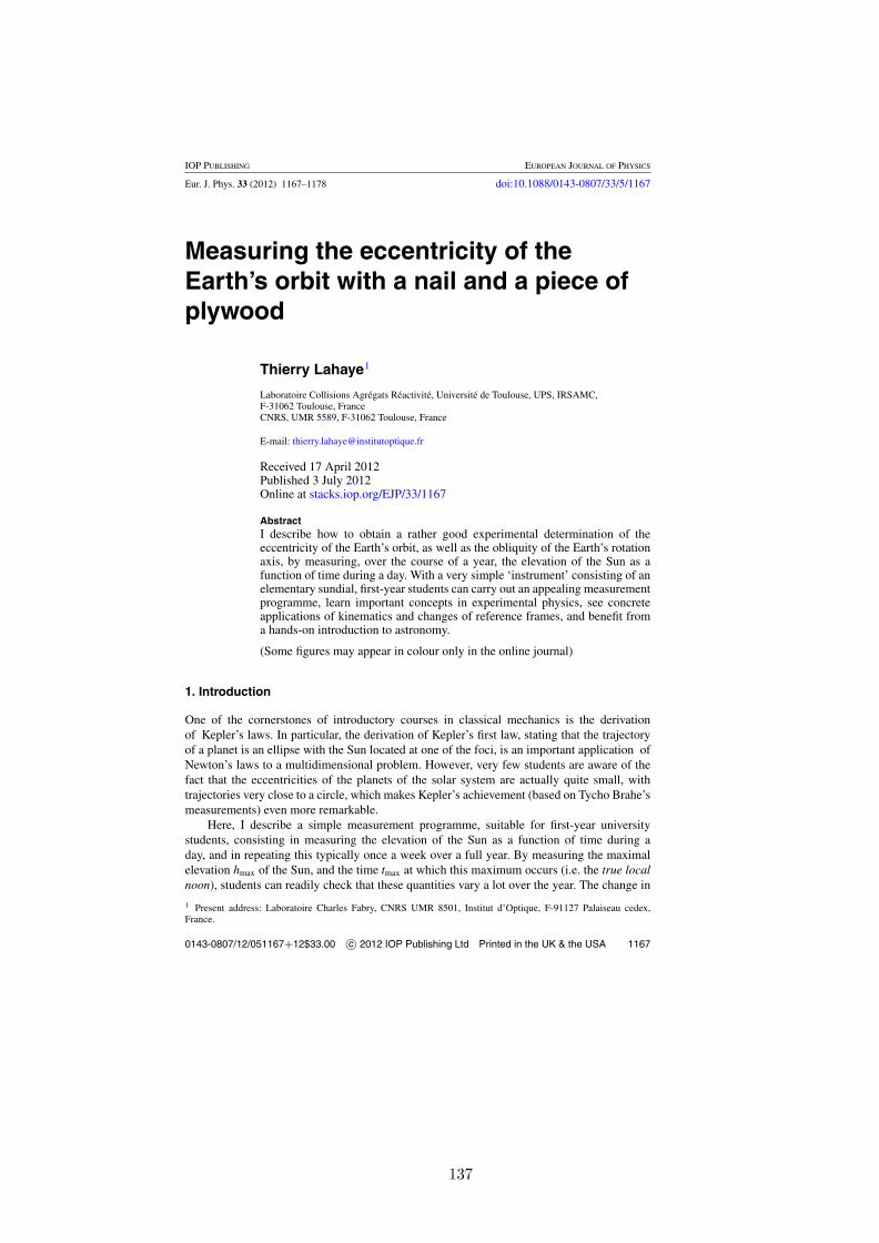
IOP PUBLISHING EUROPEAN JOURNAL OF PHYSICS
Eur. J. Phys. 33 (2012) 1167–1178 doi:10.1088/0143-0807/33/5/1167
Measuring the eccentricity of theEarth’s orbit with a nail and a piece ofplywood
Thierry Lahaye1
Laboratoire Collisions Agregats Reactivite, Universite de Toulouse, UPS, IRSAMC,F-31062 Toulouse, FranceCNRS, UMR 5589, F-31062 Toulouse, France
E-mail: [email protected]
Received 17 April 2012Published 3 July 2012Online at stacks.iop.org/EJP/33/1167
AbstractI describe how to obtain a rather good experimental determination of theeccentricity of the Earth’s orbit, as well as the obliquity of the Earth’s rotationaxis, by measuring, over the course of a year, the elevation of the Sun as afunction of time during a day. With a very simple ‘instrument’ consisting of anelementary sundial, first-year students can carry out an appealing measurementprogramme, learn important concepts in experimental physics, see concreteapplications of kinematics and changes of reference frames, and benefit froma hands-on introduction to astronomy.
(Some figures may appear in colour only in the online journal)
1. Introduction
One of the cornerstones of introductory courses in classical mechanics is the derivationof Kepler’s laws. In particular, the derivation of Kepler’s first law, stating that the trajectoryof a planet is an ellipse with the Sun located at one of the foci, is an important application ofNewton’s laws to a multidimensional problem. However, very few students are aware of thefact that the eccentricities of the planets of the solar system are actually quite small, withtrajectories very close to a circle, which makes Kepler’s achievement (based on Tycho Brahe’smeasurements) even more remarkable.
Here, I describe a simple measurement programme, suitable for first-year universitystudents, consisting in measuring the elevation of the Sun as a function of time during aday, and in repeating this typically once a week over a full year. By measuring the maximalelevation hmax of the Sun, and the time tmax at which this maximum occurs (i.e. the true localnoon), students can readily check that these quantities vary a lot over the year. The change in
1 Present address: Laboratoire Charles Fabry, CNRS UMR 8501, Institut d’Optique, F-91127 Palaiseau cedex,France.
0143-0807/12/051167+12$33.00 c© 2012 IOP Publishing Ltd Printed in the UK & the USA 1167
137

1168 T Lahaye
Figure 1. Schematic view of the elementary sundial.
hmax is essentially related to the obliquity ε of the Earth over the ecliptic, and thus allows forquite an accurate determination of ε (as well as that of the latitude of observation). The changeof tmax over a year gives an experimental determination of the equation of time E(t), i.e. thedifference between the mean local noon and the true local noon, and allows for a determinationof the eccentricity e of the Earth’s orbit [1]. This is a rewarding result for students to realizethat with such simple measurements, they can obtain good experimental values for the abovequantities, and that with careful observations one can perform ‘science without instruments’as did the astronomers of various antique civilizations [2, 3].
I have organized this paper as follows. I first describe how to measure in a simple waythe elevation of the Sun versus time over a day, with an accuracy of about 1. Then I give theresults I obtained for hmax(t) and E(t) by repeating the measurement about once a week forone year, starting in August 2010. I show how one can extract the obliquity ε of the Earth’saxis and the eccentricity e of its orbit by fitting the experimental data with simple, analyticexpressions. Finally, possible extensions of the work are proposed. Appendix A contains abrief reminder on basic notions of spherical astronomy, and should be read first by readersnot familiar with these notions. In the remaining appendices, the derivation of the analyticexpressions used for fitting the data is given, so that the paper is self-contained.
2. Measurements
We are interested in studying the motion of the Earth around the Sun. Using the relativity ofmotion, we can thus simply measure the apparent motion of the Sun on the celestial sphere,i.e. the time dependence of two angles that define the position of the Sun in the sky.
As we shall see, for our purpose, it is sufficient to measure the elevation of the Sun (alsocalled altitude, or height) above the horizon, i.e. the angle h shown in figure 1. This can bedone very simply by measuring the length s of the shadow of a vertical gnomon (i.e. a rod witha sharp point) of length . Then the elevation of the Sun is given by h = arctan(/s).
Contrary to the case where one would measure also the azimuthal position of the Sun,here, the orientation of the horizontal base does not need to be fixed. One of the advantages of
138
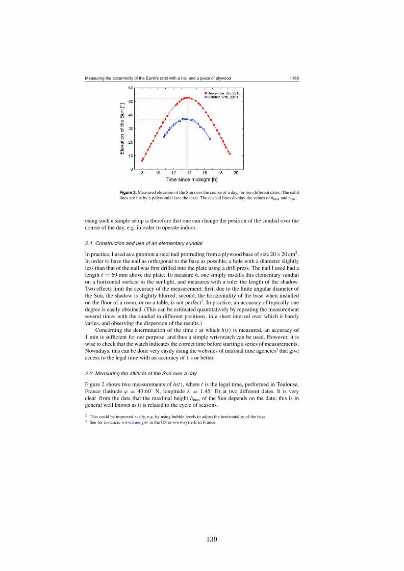
Measuring the eccentricity of the Earth’s orbit with a nail and a piece of plywood 1169
Figure 2. Measured elevation of the Sun over the course of a day, for two different dates. The solidlines are fits by a polynomial (see the text). The dashed lines display the values of hmax and tmax.
using such a simple setup is therefore that one can change the position of the sundial over thecourse of the day, e.g. in order to operate indoor.
2.1. Construction and use of an elementary sundial
In practice, I used as a gnomon a steel nail protruding from a plywood base of size 20×20 cm2.In order to have the nail as orthogonal to the base as possible, a hole with a diameter slightlyless than that of the nail was first drilled into the plate using a drill press. The nail I used had alength = 69 mm above the plate. To measure h, one simply installs this elementary sundialon a horizontal surface in the sunlight, and measures with a ruler the length of the shadow.Two effects limit the accuracy of the measurement: first, due to the finite angular diameter ofthe Sun, the shadow is slightly blurred; second, the horizontality of the base when installedon the floor of a room, or on a table, is not perfect2. In practice, an accuracy of typically onedegree is easily obtained. (This can be estimated quantitatively by repeating the measurementseveral times with the sundial in different positions, in a short interval over which h barelyvaries, and observing the dispersion of the results.)
Concerning the determination of the time t at which h(t) is measured, an accuracy of1 min is sufficient for our purpose, and thus a simple wristwatch can be used. However, it iswise to check that the watch indicates the correct time before starting a series of measurements.Nowadays, this can be done very easily using the websites of national time agencies3 that giveaccess to the legal time with an accuracy of 1 s or better.
2.2. Measuring the altitude of the Sun over a day
Figure 2 shows two measurements of h(t), where t is the legal time, performed in Toulouse,France (latitude ϕ = 43.60 N, longitude λ = 1.45 E) at two different dates. It is veryclear from the data that the maximal height hmax of the Sun depends on the date; this is ingeneral well known as it is related to the cycle of seasons.
2 This could be improved easily, e.g. by using bubble levels to adjust the horizontality of the base.3 See for instance, www.time.gov in the US or www.syrte.fr in France.
139
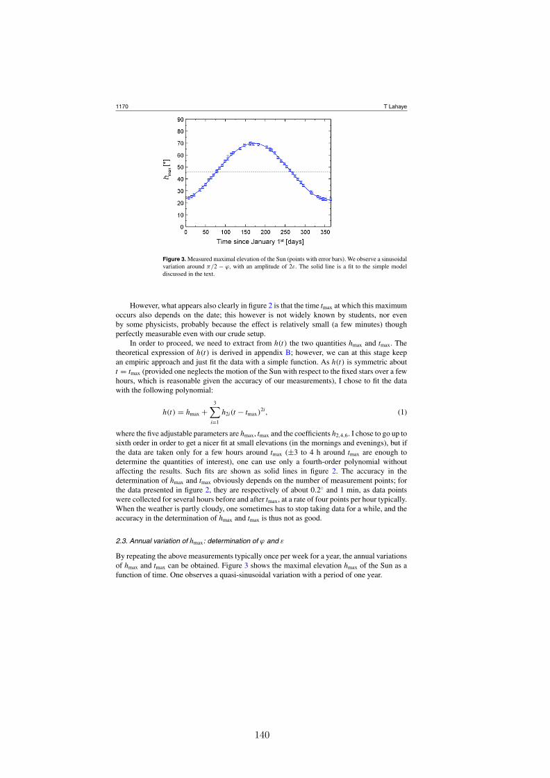
1170 T Lahaye
Figure 3. Measured maximal elevation of the Sun (points with error bars). We observe a sinusoidalvariation around π/2 − ϕ, with an amplitude of 2ε. The solid line is a fit to the simple modeldiscussed in the text.
However, what appears also clearly in figure 2 is that the time tmax at which this maximumoccurs also depends on the date; this however is not widely known by students, nor evenby some physicists, probably because the effect is relatively small (a few minutes) thoughperfectly measurable even with our crude setup.
In order to proceed, we need to extract from h(t) the two quantities hmax and tmax. Thetheoretical expression of h(t) is derived in appendix B; however, we can at this stage keepan empiric approach and just fit the data with a simple function. As h(t) is symmetric aboutt = tmax (provided one neglects the motion of the Sun with respect to the fixed stars over a fewhours, which is reasonable given the accuracy of our measurements), I chose to fit the datawith the following polynomial:
h(t) = hmax +3∑
i=1
h2i(t − tmax)2i, (1)
where the five adjustable parameters are hmax, tmax and the coefficients h2,4,6. I chose to go up tosixth order in order to get a nicer fit at small elevations (in the mornings and evenings), but ifthe data are taken only for a few hours around tmax (±3 to 4 h around tmax are enough todetermine the quantities of interest), one can use only a fourth-order polynomial withoutaffecting the results. Such fits are shown as solid lines in figure 2. The accuracy in thedetermination of hmax and tmax obviously depends on the number of measurement points; forthe data presented in figure 2, they are respectively of about 0.2 and 1 min, as data pointswere collected for several hours before and after tmax, at a rate of four points per hour typically.When the weather is partly cloudy, one sometimes has to stop taking data for a while, and theaccuracy in the determination of hmax and tmax is thus not as good.
2.3. Annual variation of hmax: determination of ϕ and ε
By repeating the above measurements typically once per week for a year, the annual variationsof hmax and tmax can be obtained. Figure 3 shows the maximal elevation hmax of the Sun as afunction of time. One observes a quasi-sinusoidal variation with a period of one year.
140

Measuring the eccentricity of the Earth’s orbit with a nail and a piece of plywood 1171
(a) (b)
Figure 4. (a) Measured equation of time E (points with error bars). The solid line is a fit to thesimple model of the equation of time given in the appendix. (b) Combining the effects of the Earth’sobliquity (E1(t), dotted line) and of the eccentricity of the Earth’s orbit (E2(t), dashed line) givesthe full expression of the equation of time E(t) (solid line).
The qualitative explanation for this phenomenon is simple, and is usually part of geographycourses in elementary education, but I repeat it here for completeness. Due to the obliquity ε
of the Earth’s rotation axis, the angle between the Earth’s axis and the line joining the centre ofthe Earth to the Sun varies between π/2−ε (at the summer solstice, when the Earth’s axis leanstowards the Sun) and π/2 + ε (at the winter solstice). Correspondingly, the angular distancebetween the Sun and the celestial pole varies with a period of one year and an amplitude of ε.This induces a similar variation of hmax, around a mean value which depends on the observer’slatitude. For a quantitative treatment, the reader is referred to appendix C.
2.4. Annual variation of tmax: determination of e
We now turn to a more subtle measurement concerning the variation of tmax, which definesthe true local noon. It is convenient to convert the measured values into a quantity called theequation of time, that we shall denote by E, defined as the difference between the mean localnoon and the true local noon (our measured tmax). The former is obtained from the legal noon,given by clocks (corrected if necessary by 1 h in summer due to daylight saving time) by adding(subtracting) 4 min for each degree of longitude west (east) from the reference meridian ofthe corresponding time zone. For instance, in Toulouse (longitude λ = 1.45 E), one needs tosubtract tmax from 13.00 h in winter time and 14.00 h in summer time, and then subtract another5.8 min to correct for the longitude, to obtain the equation of time E. For instance, on 17 October(see figure 2), we have tmax = 13.66 h, thus giving E = 60(14 − 13.66) − 5.8 = 14.6 min.
Figure 4 gives the results obtained by measuring E(t) over a year. One observes a non-trivial behaviour, the equation of time varying between a maximum of about 16 min in autumnand a minimum of about −15 min in winter, and vanishing at four different dates.
Physically, the origin of the equation of time lies in the fact that the duration of the truesolar day, i.e. the time elapsed between two successive transits of the Sun across the observer’smeridian, is not constant over a year. The solar day would have a constant duration if, alongthe year, the Sun moved on the celestial sphere (i) at constant angular velocity and (ii) alongthe celestial equator (this defines the so-called mean Sun; the time between two transits of themean Sun defines the mean solar day of 86 400 s). However, these two assumptions are both
141

1172 T Lahaye
wrong: since the Sun moves along the ecliptic, which is inclined with respect to the equatordue to the obliquity ε of the Earth’s axis, the motion of its projection on the equator is irregular.(It coincides with the mean Sun at the time of the equinox, then lags behind the mean Sun for aquarter of the year, catches up at the solstice and then is ahead of the mean Sun for another threemonths.) This contribution E1 to the equation of time thus has a six month period. Moreover,via Kepler’s second law of areal velocity (see appendix D) the angular velocity of the apparentmotion of the Sun is not constant over the year due to the fact that the Earth’s orbit is notcircular: for instance, when the Earth–Sun distance is smaller (in January), the Sun moves fasteralong the ecliptic. This contribution E2 to E(t) has obviously a one-year period. Combiningthese two contributions explains the temporal variation of the equation of time (see figure 4(b);appendix D gives the derivation of the analytical expressions of E1 and E2).
3. Exploiting the data
3.1. Obliquity of the Earth
It is easy to show (see appendix C) that to a very good approximation, one has
hmax = π
2− ϕ + ε sin
(2π
T(t − t0)
), (2)
where ϕ is the latitude of the place of observation, ε is the obliquity of the Earth’s axis, Tis the duration of the year and t0 is the date of the vernal equinox. When fitting the data byequation (2) with the four previous quantities as adjustable parameters, we obtain⎧⎪⎪⎨
⎪⎪⎩
ϕ = 43.8 ± 0.2,ε = 23.5 ± 0.1,T = 374 ± 6 d,
t0 = 78 ± 1 d, i.e. 19 March,
(3)
which is close to the accepted values (respectively, 43.60, 23.44, 365.25 d and 20 March.)Note that by repeating the measurements over the course of several years, a much moreaccurate determination of the duration T of the year could be achieved.
3.2. Eccentricity of the Earth’s orbit
We show in appendix D that a good approximation of the equation of time is given by
E(t) = d
2π
[1 − cos ε
2sin
(4π
T(t − t0)
)− 2e sin
(2π
T(t − t1)
)](4)
where d is the duration of a day (i.e. 1440 min), e is the eccentricity of the Earth’s orbit and t1is the date of perihelion passage.
Fitting the data shown in figure 4 by equation (4) with e and t1 as adjustable parameters(and using the values determined above for ε, T and t0), we obtain
e = 0.017 ± 0.001,
t1 = 1 ± 5 d, i.e. 1 January,(5)
again in relatively good agreement with the values e = 0.0167 and t1 = 3 d found in theliterature.
4. Conclusion and outlook
I have shown that with very modest equipment, one can measure with reasonable accuracysome of the orbital elements of the Earth, and in particular its eccentricity, despite its relatively
142

Measuring the eccentricity of the Earth’s orbit with a nail and a piece of plywood 1173
small value. The above measurements can be the basis of further activities for students. Amongthem, one can list the following ones, given here under the form of exercises:
• Use equation (B.4) of appendix B to calculate the length of daytime as a function of thelatitude along the year and compare it to the one obtained from the ephemerides given incalendars.
• Show that the duration of a solar day is (1 + dE/dt) × 86 400 s. What are its minimal andmaximal values?
• Using a sundial with a fixed base, check experimentally that the azimuthal position of theSun when it reaches its highest elevation is always the same (i.e. South) throughout theyear4.
• Still with a fixed-base sundial, plot experimentally the curve traced out over the year by theend of the shadow at the mean local noon. This eight-shaped curve is called an analemaand is sometimes encountered on sundials in order to allow for a computation of the legaltime from the measured solar time.
Acknowledgments
I thank Maxime Lahaye and Irina Lahaye for help in taking the data, Giovanni Luca Gattobigiofor discussions, and Lucas Beguin, Antoine Browaeys and Renaud Mathevet for usefulsuggestions that helped me improve the manuscript.
Appendix A. A quick reminder on spherical astronomy
This section consists in a minimalist reminder about basic terms and notions of sphericalastronomy needed for the understanding of the paper. The reader is referred to the first sectionsof [2] for a similar but more exhaustive reminder. A very detailed and accessible introductionto spherical astronomy can be found online in the celestial mechanics lecture notes of [4], orin standard textbooks about spherical astronomy [5].
To an Earth-bound observer O (that we assume, for definiteness, located in the northernhemisphere), celestial bodies appear to move on a sphere centred on himself, the celestialsphere (figure A1(a)). The local vertical points towards the zenith Z; the great circleperpendicular to the vertical is the horizon. Over a day, ‘fixed’ stars appear to rotate aroundthe north celestial pole P (close to the star Polaris). The great circle going through Z and Pcrosses the horizon in two points defining the South S and the North N; the two other cardinalpoints on the horizon (East E and West W ) are deduced from S and N by a 90 rotation aroundthe vertical axis.
The position of celestial bodies can be specified in spherical coordinates by two angles,once a reference system has been chosen. Two reference systems are particularly useful: thehorizon system, in which measurements are made in practice, and which is dependent on theobserver’s location on Earth, and the equatorial system, which is defined by the directions of‘fixed’ stars.
• In the horizon system (figure A1(b)), the local vertical, pointing towards the zenith, ischosen as the z-axis. The position of a point on the celestial sphere is specified using the
4 Note that with a fixed-base sundial, the determination of the equation of time can be much more accurate than withthe method used in this paper. Indeed, in that case one needs to determine the time tmax at which the solar azimuth ψvanishes (i.e. when the Sun is South and crosses the observer’s meridian), which can be done with a high precision asit varies linearly in time: the determination of such a zero-crossing is much more accurate than that of the position ofa maximum.
143

1174 T Lahaye
(a) (b)
(c) (d)
Figure A1. Geometry of the celestial sphere. (a) Important points, axes and circles on the celestialsphere. (b) Definition of the coordinates in the horizon system. (c) Definition of the coordinatesin the equatorial system. (d) Definition of the coordinates of the Sun in the equatorial systemduring its motion along the ecliptic.
altitude (or elevation) h (angle between the radius vector of the point and the horizon), andthe azimuth ψ , counted along the horizon, starting from the South and counted positivetowards the West (note that other conventions exist for the choice of the azimuth origin).
• In the equatorial system (figure A1(c)), OP is chosen as the polar axis. The intersectionof the plane perpendicular to OP with the celestial sphere defines the celestial equator.The position of a point on the celestial sphere is given by the declination δ (angle from thecelestial equator to the body) and the hour angle H (counted along the celestial equator,from the south to the equatorial projection of the body).
The equatorial system is obtained by rotating the horizon system around OE by an angleπ/2 −ϕ, where ϕ is the (geographical) latitude of the point of observation; for instance, at theNorth pole (ϕ = π/2) the equatorial and horizon systems coincide.
Finally, the ecliptic is the great circle along which the apparent annual motion of the Sun(traditionally denoted by the astronomical symbol ) takes place on the celestial sphere. It isinclined on the celestial equator by the obliquity ε of the Earth’s axis.
The angular position of the Sun along the ecliptic is given by the ecliptic longitude λ,whose origin is taken at the vernal point V (the point where the ecliptic crosses the celestialequator, and where the Sun is located at the time of the spring equinox in the Northern
144

Measuring the eccentricity of the Earth’s orbit with a nail and a piece of plywood 1175
hemisphere). The angular distance on the celestial equator between V and the projection ofthe Sun on the equator is the Sun’s right ascension α.
Appendix B. Expression of h(t) over a day
From the definitions given above, in the equatorial coordinate system (x′, y′, z′), the coordinatesof the Sun read
S′ =⎛⎝ x′ = cos δ cos H
y′ = − cos δ sin Hz′ = sin δ
⎞⎠ , (B.1)
with δ being the declination and H the hour angle of the Sun. In the horizon system (x, y, z),they read
S =⎛⎝ x = cos h cos ψ
y = − cos h sin ψ
z = sin h
⎞⎠ , (B.2)
where h is the altitude of the Sun and ψ is its azimuth. Since the equatorial system is deducedfrom the horizon system by a rotation of angle π/2 − ϕ around the (Oy) = (Oy′) axis, the(x, y, z) coordinates are obtained by multiplying the (x′, y′, z′) ones by the following rotationmatrix:
R =⎛⎝sin ϕ 0 − cos ϕ
0 1 0cos ϕ 0 sin ϕ
⎞⎠ . (B.3)
From the last component of the relation S = RS′ we obtain
sin h = cos ϕ cos δ cos H + sin ϕ sin δ (B.4)
which gives the elevation of the Sun as a function of time (i.e. the hour angle H) for the givenlocation and declination of the Sun.
Appendix C. A simple model for hmax(t)
From equation (B.4) above, we find immediately that the elevation of the Sun becomes maximalwhen cos H = 1 and reaches the value hmax fulfilling
sin hmax = cos ϕ cos δ + sin ϕ sin δ = cos(ϕ − δ), (C.1)
whence
hmax = π
2− ϕ + δ. (C.2)
We now need to express the time dependence of the declination of the Sun. Using figure A1,one can show (see equation (D.5) below) that sin δ = sin ε sin λ, which can be simplifiedto δ ε sin λ to a very good approximation (even though ε 23, the maximal error dueto this approximation is smaller than 0.3, i.e. negligible as compared with our experimentaluncertainties). Making further simplification that the solar ecliptic longitude λ increaseslinearly in time (i.e. assuming here that the eccentricity of the Earth’s orbit is e = 0), wehave λ = 2π(t − t0)/T , with t0 being the date of the spring equinox. Combining this simplesinusoidal approximation for δ(t) and equation (C.2) finally yields equation (2) of the maintext.
145

1176 T Lahaye
Appendix D. A simple model for the equation of time
Following e.g. [1], a good approximation of the theoretical expression of the equation of timecan be obtained in the following way. If the eccentricity of the Earth’s orbit were e = 0, andif the obliquity of the Earth were ε = 0, one would have E = 0. We can thus expect thatby calculating separately the small contributions E1 and E2 of both the obliquity and of theeccentricity, and adding them, a good approximation of E is obtained: one basically expandsE to the lowest orders in e and ε.
We first calculate the contribution E1 to E arising from the nonzero value of the obliquity.Here, we can neglect the ellipticity of the Earth’s orbit, and assume that the motion of the Sunaround the Earth takes place on a circle, and thus, using Kepler’s second law, at a constantangular velocity. The longitude λ of the Sun along the ecliptic (see figure A1(d)) thusincreases linearly in time as
λ = 2π
T(t − t0), (D.1)
where T is the length of a year and t0 is the date of the vernal (i.e. spring) equinox. Howeverthe mean Sun is a fictitious body that moves at constant angular velocity along the celestialequator, not the ecliptic. The difference between λ and α, once converted to time via thecorrespondence 1 ↔ 4 min, thus gives the obliquity contribution to the equation of time:
E1 = (4 min/) × (λ − α) (D.2)
(for readability, from now on I shall drop the subscript ). We thus have to express α
as a function of λ, and then use (D.1) to obtain E1(t). To find the relation between α
and λ, we introduce the equatorial frame with the origin at the centre of the celestialsphere, the z-axis pointing towards the celestial pole, and the x-axis towards the vernalpoint V , and another, ecliptic frame obtained from the former by a rotation of the angleε around Ox (see figure A1(d)). The coordinates of the Sun in the equatorial frame are(cos δ cos α, cos δ sin α, sin δ), and in the ecliptic frame (cos λ, sin λ, 0). Since the rotationmatrix from the equatorial to the ecliptic frame reads⎛
⎝1 0 00 cos ε sin ε
0 − sin ε cos ε
⎞⎠ , (D.3)
one can relate (α, δ) to λ, and we obtain
tan α = tan λ cos ε, (D.4)
sin δ = sin ε sin λ. (D.5)
Therefore, using (D.4)
λ − α = λ − arctan(cos ε tan λ). (D.6)
From this expression it may not be obvious to see the time dependence (in particular theperiodicity) of E1. We can obtain a better understanding (and a convenient expression) bynoting that cos ε is actually close to 1 (for ε = 23.44, we have cos ε 0.9174). If one Taylorexpands f (x, A) = x−arctan(A tan x) around A = 1, one obtains f (x, A) (1−A) sin(2x)/2,and thus, putting everything together, we obtain our final expression for E1:
E1(t) d
2π
1 − cos ε
2sin
(4π
T(t − t0)
). (D.7)
where d is the duration of a day. The dotted line in figure 4(b) shows E1(t).
146
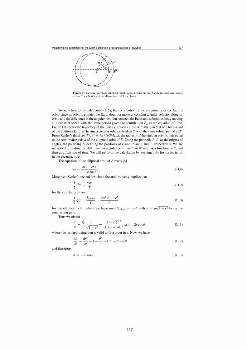
Measuring the eccentricity of the Earth’s orbit with a nail and a piece of plywood 1177
Figure D1. Circular (grey) and elliptical (black) orbits around the Sun S with the same semi-majoraxis a. The ellipticity of the ellipse is e = 0.3 for clarity.
We now turn to the calculation of E2, the contribution of the eccentricity of the Earth’sorbit: since its orbit is elliptic, the Earth does not move at constant angular velocity along itsorbit, and the difference in the angular position between the Earth and a fictitious body movingat a constant speed with the same period gives the contribution E2 to the equation of time.Figure D1 shows the trajectory of the Earth E (black ellipse with the Sun S at one focus) andof the fictitious Earth E ′ having a circular orbit centred on S, with the same orbital period as E.From Kepler’s third law T 2/a3 = 4π2/(GMSun), the radius r of the circular orbit is thus equalto the semi-major axis a of the elliptical orbit of E. Using the perihelia P, P′ as the origins ofangles, the polar angles defining the positions of P and P′ are θ and θ ′, respectively. We areinterested in finding the difference in angular positions ϑ ≡ θ ′ − θ , as a function of θ , andthen as a function of time. We will perform the calculation by keeping only first-order termsin the eccentricity e.
The equation of the elliptical orbit of E reads [6]
rE = a(1 − e2)
1 + e cos θ. (D.8)
Moreover, Kepler’s second law about the areal velocity implies that
1
2a2θ ′ = πa2
T(D.9)
for the circular orbit and
1
2r2
Eθ ′ = Sellipse
T= πa2
√1 − e2
T(D.10)
for the elliptical orbit, where we have used Sellipse = πab with b = a√
1 − e2 being thesemi-minor axis.
Thus we obtain
θ ′
θ= r2
E
a2
1√1 − e2
= (1 − e2)3/2
(1 + e cos θ )2 1 − 2e cos θ, (D.11)
where the last approximation is valid to first order in e. Now, we have
dϑ
dθ= dθ ′
dθ− 1 = θ ′
θ− 1 −2e cos θ (D.12)
and therefore
ϑ = −2e sin θ. (D.13)
147

1178 T Lahaye
Since we are keeping only the first-order terms in e, we can replace θ by θ ′ = 2π(t − t1)/T inthe above equation, where t1 is the time of perihelion passage. We finally obtain the followingexpression for E2:
E2(t) −de
πsin
(2π
T(t − t1)
). (D.14)
The dashed line in figure 4(b) shows E2(t). Combining (D.7) and (D.14), we find expression(4) given in the text (solid line in figure 4(b)).
References
[1] Rees W G 1991 Eur. J. Phys. 12 96[2] Gutzwiller M C 1998 Rev. Mod. Phys. 70 589[3] Krisciunas K 2010 Am. J. Phys. 78 834[4] Tatum J B 2012 Celestial Mechanics (Lecture Notes) http://orca.phys.uvic.ca/∼tatum[5] See e.g. Woolard E W and Clemence G M 1966 Spherical Astronomy (New York: Academic)[6] Goldstein H 1950 Classical Mechanics (Reading, MA: Addison Wesley)
148

Bibliography
[1] K. Aikawa, A. Frisch, M. Mark, S. Baier, R. Grimm, and F. Ferlaino. ReachingFermi degeneracy via universal dipolar scattering. Phys. Rev. Lett., 112:010404,2014.
[2] K. Aikawa, A. Frisch, M. Mark, S. Baier, A. Rietzler, R. Grimm, and F. Ferlaino.Bose–Einstein condensation of Erbium. Phys. Rev. Lett., 108:210401, 2012.
[3] B. P. Anderson and M. A. Kasevitch. Macroscopic quantum interference from atomictunnel array. Science, 282:1686, 1998.
[4] W. R. Anderson, J. R. Veale, and T. F. Gallagher. Resonant dipole-dipole energytransfer in a nearly frozen Rydberg gas. Phys. Rev. Lett., 80:249, 1998.
[5] J. B. Balewski, A. T. Krupp, A. Gaj, S. Hofferberth, R. Löw, and T. Pfau. Ry-dberg dressing: understanding of collective many-body effects and implications forexperiments. New J. Phys., 16:063012, 2014.
[6] D. Barredo, H. Labuhn, S. Ravets, T. Lahaye, A. Browaeys, and C. S. Adams. Coher-ent excitation transfer in a “spin chain” of three Rydberg atoms. arXiv:1408.1055,2014.
[7] D. Barredo, S. Ravets, H. Labuhn, L. Béguin, A. Vernier, F. Nogrette, T. Lahaye,and A. Browaeys. Demonstration of a strong Rydberg blockade in three-atom sys-tems with anisotropic interactions. Phys. Rev. Lett., 112:183002, 2014.
[8] L. Béguin. Measurement of the van der Waals interaction between two Rydbergatoms. PhD thesis, University Paris 11, 2013.
[9] L. Béguin, A. Vernier, R. Chicireanu, T. Lahaye, and A. Browaeys. Direct mea-surement of the van der Waals interaction between two Rydberg atoms. Phys. Rev.Lett., 110:263201, 2013.
[10] S. Bettelli, D. Maxwell, T. Fernholz, C. S. Adams, I. Lesanovsky, and C. Ates.Exciton dynamics in emergent Rydberg lattices. Phys. Rev. A, 88:043436, 2013.
[11] J. Beugnon, C. Tuchendler, H. Marion, A. Gaëtan, Y. Miroshnychenko, Y. R. P.Sortais, A. M. Lance, M. P. A. Jones, G. Messin, A. Browaeys, and P. Grangier.
149
Two-dimensional transport and transfer of a single atomic qubit in optical tweezers.Nature Phys., 3:696, 2007.
[12] J. Billy. Private communication, 2013.
[13] J. Billy, E. A. L. Henn, S. Müller, T. Maier, H. Kadau, A. Griesmaier, M. Jona-Lasinio, L. Santos, and T. Pfau. Deconfinement-induced collapse of a coherent arrayof dipolar Bose–Einstein condensates. Phys. Rev. A, 86:051603, 2012.
[14] G. Bismut, B. Laburthe-Tolra, E. Maréchal, P. Pedri, O. Gorceix, and L. Vernac.Anisotropic excitation spectrum of a dipolar quantum Bose gas. Phys. Rev. Lett.,109:155302, 2012.
[15] G. Bismut, B. Pasquiou, E. Maréchal, P. Pedri, L. Vernac, O. Gorceix, andB. Laburthe-Tolra. Collective excitations of a dipolar Bose–Einstein condensate.Phys. Rev. Lett., 105:040404, 2010.
[16] I. Bloch, J. Dalibard, and W. Zwerger. Many-body physics with ultracold gases.Rev. Mod. Phys., 80:885, 2008.
[17] I. Bloch, T. W. Hänsch, and T. Esslinger. Atom laser with a CW output coupler.Phys. Rev. Lett., 82:3008, 1999.
[18] J. L. Bohn, R. M. Wilson, and S. Ronen. How does a dipolar Bose–Einstein con-densate collapse? Las. Phys., 19:547, 2009.
[19] C. C. Bradley, C. A. Sackett, and R. G. Hulet. Bose–Einstein condensation oflithium: Observation of limited condensate number. Phys. Rev. Lett., 78:985, 1997.
[20] Y. Castin and R. Dum. Bose–Einstein condensates in time-dependent traps. Phys.Rev. Lett., 77:5315, 1996.
[21] P. Cheiney. Matter wave scattering on complex potentials. PhD thesis, UniversityPaul Sabatier, Toulouse, 2013.
[22] P. Cheiney, O. Carraz, D. Bartoszek-Bober, S. Faure, F. Vermersch, C. M. Fabre,G. L. Gattobigio, T. Lahaye, D. Guéry-Odelin, and R. Mathevet. A Zeemanslower design with permanent magnets in a Halbach configuration. Rev. Sci. In-str., 82:063115, 2011.
[23] P. Cheiney, F. Damon, G. Condon, B. Georgeot, and D. Guéry-Odelin. Realizationof tunnel barriers for matter waves using spatial gaps. EPL, 103:50006, 2013.
[24] P. Cheiney, C. M. Fabre, F. Vermersch, G. L. Gattobigio, R. Mathevet, T. Lahaye,and D. Guéry-Odelin. Matter-wave scattering on an amplitude-modulated opticallattice. Phys. Rev. A, 87:013623, 2013.
[25] R. M. Clegg. The history of FRET. Reviews in Fluorescence, 2006:1, 2006.
150
[26] D. Comparat and P. Pillet. Dipole blockade in a cold rydberg atomic sample. J.Opt. Soc. Am. B, 27:A208, 2010.
[27] A. Couvert. Production et étude de lasers à atomes guidés, et de leur interactionavec des défauts contrôlés. PhD thesis, University Paris 6, 2010.
[28] A. Couvert, M. Jeppesen, T. Kawalec, G. Reinaudi, R. Mathevet, and D. Guéry-Odelin. A quasi-monomode guided atom laser from an all-optical Bose–Einsteincondensate. EPL, 83:50001, 2008.
[29] A. de Paz, A. Sharma, A. Chotia, E. Maréchal, J. H. Huckans, P. Pedri, L. Santos,O. Gorceix, L. Vernac, and B. Laburthe-Tolra. Nonequilibrium quantum magnetismin a dipolar lattice gas. Phys. Rev. Lett., 111:185305, 2013.
[30] E. A. Donley, N. R. Claussen, S. L. Cornish, J. L. Roberts, E. A. Cornell, and C. E.Wieman. Dynamics of collapsing and exploding Bose–Einstein condensates. Nature,412:295, 2001.
[31] M. Ebert, A. Gill, M. Gibbons, X. Zhang, M. Saffman, and T. G. Walker. AtomicFock state preparation using Rydberg blockade. Phys. Rev. Lett., 112:043602, 2014.
[32] C. Fabre. Etude théorique et expérimentale de l’interaction d’un atome très excitéavec le rayonnement. Application à la spectroscopie des états de Rydberg du sodium.PhD thesis, Université Pierre et Marie Curie - Paris VI, 1980.
[33] C. M. Fabre. Miroirs de Bragg pour ondes de matière et apport de la supersymétrieaux potentiels exponentiels. PhD thesis, University Paul Sabatier, Toulouse, 2012.
[34] C. M. Fabre, P. Cheiney, G. L. Gattobigio, F. Vermersch, S. Faure, R. Mathevet,T. Lahaye, and D. Guéry-Odelin. Realization of a distributed Bragg reflector forpropagating guided matter waves. Phys. Rev. Lett., 107:230401, 2011.
[35] M. Fattori, C. D’Errico, G. Roati, M. Zaccanti, M. Jona-Lasinio, M. Modugno,M. Inguscio, and G. Modugno. Atom interferometry with a weakly interacting Bose–Einstein condensate. Phys. Rev. Lett., 100:080405, 2008.
[36] T. Förster. Zwischenmolekulare Energiewanderung und Fluoreszenz. Ann. Phys.,437:55, 1948.
[37] B. Fröhlich. Strong dipolar effects in a chromium Bose–Einstein condensate. Diplo-marbeit, Universität Stuttgart, 2007.
[38] A. Gaetan, Y. Miroshnychenko, T. Wilk, A. Chotia, M. Viteau, D. Comparat, P. Pil-let, A. Browaeys, and P. Grangier. Observation of collective excitation of two indi-vidual atoms in the Rydberg blockade regime. Nat. Phys., 5:115, 2009.
[39] M. Georgescu, I. S. Ashhab, and F. Nori. Quantum simulation. Rev. Mod. Phys.,86:153, 2014.
151

[40] R.W. Gerchberg and W. O. Saxton. A practical algorithm for the determination ofphase from image and diffraction plane pictures. Optik, 35:237, 1972.
[41] J. M. Gerton, D. Strekalov, I. Prodan, and R. G. Hulet. Direct observation of growthand collapse of a Bose–Einstein condensate with attractive interactions. Nature,408:692, 2000.
[42] V. Giovannetti, S. Lloyd, and L. Maccone. Advances in quantum metrology. NaturePhot., 5:222, 2011.
[43] K. Góral, K. Rzazewski, and T. Pfau. Bose–Einstein condensation with magneticdipole-dipole forces. Phys. Rev. A, 61:051601, 2000.
[44] K. Góral, L. Santos, and M. Lewenstein. Quantum phases of dipolar bosons inoptical lattices. Phys. Rev. Lett., 88:170406, 2002.
[45] A. Griesmaier, J. Werner, S. Hensler, J. Stuhler, and T. Pfau. Bose–Einstein con-densation of Chromium. Phys. Rev. Lett., 94:160401, 2005.
[46] T. Grünzweig, A. Hilliard, M. McGovern, and M. F. Andersen. Near-deterministicpreparation of a single atom in an optical microtrap. Nature Phys., 6:951, 2010.
[47] W. Guerin, J.-F. Riou, J. P. Gaebler, V. Josse, P. Bouyer, and A. Aspect. Guidedquasicontinuous atom laser. Phys. Rev. Lett., 97:200402, 2006.
[48] G. Günter, H. Schempp, M. Robert-de Saint-Vincent, V. Gavryusev, S. Helmrich,C.S. Hofmann, S. Whitlock, and M. Weidemller. Observing the dynamics of dipole-mediated energy transport by interaction-enhanced imaging. Science, 342:954, 2013.
[49] E. W. Hagley, L. Deng, M. Kozuma, J. Wen, K. Helmerson, S. L. Rolston, and W. D.Phillips. A well-collimated quasi-continuous atom laser. Science, 283:1706, 1999.
[50] K. Halbach. Design of permanent multipole magnets with oriented rare earth cobaltmaterial. Nucl. Instr. Meth., 169(1), 1980.
[51] S. Haroche. Nobel lecture: Controlling photons in a box and exploring the quantumto classical boundary. Rev. Mod. Phys., 85:1083, 2013.
[52] S. Haroche and J.-M. Raimond. Exploring the Quantum — Atoms, Cavities, andPhotons. Oxford University Press, 2006.
[53] P. Hauke, F. M. Cucchietti, A. Müller-Hermes, M.-C. Bañuls, J. I. Cirac, andM. Lewenstein. Complete devil’s staircase and crystal-superfluid transitions in adipolar XXZ spin chain: a trapped ion quantum simulation. New Journal of Physics,12:113037, 2010.
[54] K. R. A. Hazzard, M. van den Worm, M. Foss-Feig, S. R. Manmana, E. G.Dalla Torre, T. Pfau, M. Kastner, and A. M. Rey. Quantum correlations and entan-glement in far-from-equilibrium spin systems. Phys. Rev. A, 90:063622, 2014.
152

[55] R. Heidemann, U. Raitzsch, V. Bendkowsky, B. Butscher, R. Löw, L. Santos, andT. Pfau. Evidence for coherent collective Rydberg excitation in the strong blockaderegime. Phys. Rev. Lett., 99:163601, 2007.
[56] L. Isenhower, E. Urban, X. L. Zhang, A. T. Gill, T. Henage, T. A. Johnson, T. G.Walker, and M. Saffman. Demonstration of a neutral atom controlled-not quantumgate. Phys. Rev. Lett., 104:010503, 2010.
[57] R. Islam, C. Senko, W. C. Campbell, S. Korenblit, J. Smith, A. Lee, E. E. Edwards,C.-C. J. Wang, J. K. Freericks, and C. Monroe. Emergence and frustration of mag-netism with variable-range interactions in a quantum simulator. Science, 340:583,2013.
[58] D. Jaksch, J. I. Cirac, P. Zoller, S. L. Rolston, R. Côté, and M. D. Lukin. Fastquantum gates for neutral atoms. Phys. Rev. Lett., 85:2208, 2000.
[59] D. Jin and J. Ye. Polar molecules in the quantum regime. Physics Today, 64:27,2011.
[60] A. M. Kaufman, B. J. Lester, and C. A. Regal. Cooling a single atom in an opticaltweezer to its quantum ground state. Phys. Rev. X, 2:041014, 2012.
[61] T. Koch. Enhancing the dipolar character of a Bose-Einstein condensate: From per-turbative effects to a purely dipolar quantum gas. PhD thesis, Universität Stuttgart,2008.
[62] T. Koch, T. Lahaye, J. Metz, B. Fröhlich, A. Griesmaier, and T. Pfau. Stabilizationof a purely dipolar quantum gas against collapse. Nat. Phys., 4:218, 2008.
[63] D. L. Kovrizhin, G. V. Pai, and S. Sinha. Density wave and supersolid phases ofcorrelated bosons in an optical lattice. Europhys. Lett., 72:162, 2005.
[64] H. Kreutzmann, U. V. Poulsen, M. Lewenstein, R. Dumke, W. Ertmer, G. Birkl,and A. Sanpera. Coherence properties of guided-atom interferometers. Phys. Rev.Lett., 92:163201, 2004.
[65] H. Labuhn and et al. Collective excitation of a mesoscopic number of atoms in theRydberg blockade regime, 2015. In preparation.
[66] H. Labuhn, S. Ravets, D. Barredo, L. Béguin, F. Nogrette, T. Lahaye, andA. Browaeys. Single-atom addressing in microtraps for quantum-state engineeringusing Rydberg atoms. Phys. Rev. A, 90:023415, 2014.
[67] T. Lahaye. Measuring the eccentricity of the Earth’s orbit with a nail and a pieceof plywood. Eur. J. Phys., 33:1167, 2012.
[68] T. Lahaye and A. Browaeys. Interacting cold Rydberg atoms: a toy many-bodysystem. Séminaire Poincaré, 17:125, 2013.
153
[69] T. Lahaye, T. Koch, B. Fröhlich, M. Fattori, J. Metz, A. Griesmaier, S. Giovanazzi,and T. Pfau. Strong dipolar effects in a quantum ferrofluid. Nature, 448:672, 2007.
[70] T. Lahaye, P. Labastie, and R. Mathevet. Fizeau’s “aether-drag” experiment in theundergraduate laboratory. Am. J. Phys., 80:497, 2012.
[71] T. Lahaye, J. Metz, B. Fröhlich, T. Koch, M. Meister, a. Griesmaier, T. Pfau,H. Saito, Y. Kawaguchi, and M. Ueda. d-wave collapse and explosion of a dipolarBose–Einstein condensate. Phys. Rev. Lett., 101:080401, 2008.
[72] T. Lahaye, T. Pfau, and L. Santos. Mesoscopic ensembles of polar bosons in triple-well potentials. Phys. Rev. Lett., 104:170404, 2010.
[73] T. Lahaye, J. Vogels, K. Günter, Z. Wang, J. Dalibard, and D. Guéry-Odelin. Real-ization of a magnetically guided atomic beam in the collisional regime. Phys. Rev.Lett., 93:093003, 2004.
[74] T. Lahaye, Z. Wang, G. Reinaudi, S. Rath, J. Dalibard, and D. Guéry-Odelin.Evaporative cooling of a guided rubidium atomic beam. Phys. Rev. A, 72(3):033411,2005.
[75] M. Lu, N. Q. Burdick, and B. L. Lev. Quantum degenerate dipolar Fermi gas. Phys.Rev. Lett., 108:215301, 2012.
[76] M. Lu, N. Q. Burdick, S. H. Youn, and B. L. Lev. Strongly dipolar Bose–Einsteincondensate of Dysprosium. Phys. Rev. Lett., 107:190401, 2011.
[77] M. D. Lukin, M. Fleischhauer, R. Cote, L. M. Duan, D. Jaksch, J. I. Cirac, andP. Zoller. Dipole blockade and quantum information processing in mesoscopic atomicensembles. Phys. Rev. Lett., 87:037901, 2001.
[78] P. Martin, B. Oldaker, A. Miklich, and D. Pritchard. Bragg scattering of atoms froma standing light wave. Phys. Rev. Lett., 60:515, 1988.
[79] C. Menotti, C. Trefzger, and M. Lewenstein. Metastable states of a gas of dipolarbosons in a 2D optical lattice. Phys. Rev. Lett., 98:235301, 2007.
[80] J. Metz, T. Lahaye, B. Fröhlich, A. Griesmaier, T. Pfau, H. Saito, Y. Kawaguchi,and M. Ueda. Coherent collapses of dipolar Bose–einstein condensates for differenttrap geometries. New J. Phys., 11:055032, 2009.
[81] M.-O. Mewes, M. R. Andrews, D. M. Kurn, D. S. Durfee, C. G. Townsend, andW. Ketterle. Output coupler for Bose–Einstein condensed atoms. Phys. Rev. Lett.,78:582, 1997.
[82] Y. Miroshnychenko, W. Alt, I. Dotsenko, L. Förster, M. Khudaverdyan,D. Meschede, D. Schrader, and A. Rauschenbeutel. Quantum engineering: An atom-sorting machine. Nature, 442:151, 2006.
154
[83] D. Møller, L. B. Madsen, and K. Mølmer. Quantum gates and multiparticle entan-glement by Rydberg excitation blockade and adiabatic passage. Phys. Rev. Lett.,100:170504, 2008.
[84] O. Morsch and M. Oberthaler. Dynamics of Bose–Einstein condensates in opticallattices. Rev. Mod. Phys., 78:179, 2006.
[85] I. Mourachko, D. Comparat, F. de Tomasi, A. Fioretti, P. Nosbaum, V. M. Akulin,and P. Pillet. Many-body effects in a frozen Rydberg gas. Phys. Rev. Lett., 80:253,1998.
[86] M. Mudrich, N. Zahzam, T. Vogt, D. Comparat, and P. Pillet. Back and forthtransfer and coherent coupling in a cold Rydberg dipole gas. Phys. Rev. Lett.,95:233002, 2005.
[87] M. Müller, I. Lesanovsky, H. Weimer, H. P. Büchler, and P. Zoller. MesoscopicRydberg gate based on electromagnetically induced transparency. Phys. Rev. Lett.,102:170502, 2009.
[88] S. Müller, J. Billy, E. A. L. Henn, H. Kadau, A. Griesmaier, M. Jona-Lasinio,L. Santos, and T. Pfau. Stability of a dipolar Bose–Einstein condensate in a one-dimensional lattice. Phys. Rev. A, 84:053601, 2011.
[89] M. A. Nielsen and I. L. Chuang. Quantum Computation and Quantum Information.Cambridge University Press, 2000.
[90] J. Nipper, J. B. Balewski, A. T. Krupp, B. Butscher, R. Löw, and T. Pfau. Highlyresolved measurements of Stark-tuned Förster resonances between Rydberg atoms.Phys. Rev. Lett., 108:113001, 2012.
[91] J. Nipper, J. B. Balewski, A. T. Krupp, S. Hofferberth, R. Löw, and T. Pfau. Atomicpair-state interferometer: Controlling and measuring an interaction-induced phaseshift in Rydberg-atom pairs. Phys. Rev. X, 2:031011, 2012.
[92] F. Nogrette, H. Labuhn, S. Ravets, D. Barredo, L. Béguin, A. Vernier, T. Lahaye,and A. Browaeys. Single-atom trapping in holographic 2d arrays of microtraps witharbitrary geometries. Phys. Rev. X, 4:021034, 2014.
[93] D. H. J. O’Dell, S. Giovanazzi, and C. Eberlein. Exact hydrodynamics of a trappeddipolar Bose–Einstein condensate. Phys. Rev. Lett., 92:250401, 2004.
[94] Y. B. Ovchinnikov. A permanent Zeeman slower for Sr atomic clock. Eur. Phys. J.Special Topics, 163:95, 2008.
[95] A. Perrin. Private communication, 2012.
[96] D. Peter, S. Müller, S. Wessel, and H. P. Büchler. Anomalous behavior of spinsystems with dipolar interactions. Phys. Rev. Lett., 109:025303, 2012.
155
[97] D. Peter, K. Pawlowski, T. Pfau, and K. Rzazewski. Mean-field description of dipolarbosons in triple-well potentials. J. Phys. B, 45:225302, 2012.
[98] D. Peter, N. Y. Yao, N. Lang, S. D. Huber, M. D. Lukin, and H.-P. Büchler.Topological flat bands with Chern number C = 2 by dipolar exchange interactions.arXiv:1410.5667, 2014.
[99] W. D. Phillips and H. Metcalf. Laser deceleration of an atomic beam. Phys. Rev.Lett., 48:596, 1982.
[100] L. P. Pitaevskii and S. Stringari. Bose-Einstein condensation. Clarendon Press,Oxford, 2003.
[101] S. E. Pollack, D. Dries, M. Junker, Y. P. Chen, T. A. Corcovilos, and R. G. Hulet.Extreme tunability of interactions in a 7Li Bose–Einstein condensate. Phys. Rev.Lett., 102:090402, 2009.
[102] G. Pupillo, A. Micheli, M. Boninsegni, I. Lesanovsky, and P. Zoller. Strongly corre-lated gases of Rydberg-dressed atoms: Quantum and classical dynamics. Phys. Rev.Lett., 104:223002, 2010.
[103] S. Ravets. Development of tools for quantum engineering using individual atoms:optical nanofibers and controlled Rydberg interactions. PhD thesis, University Paris11, 2014.
[104] S. Ravets and et al. Measurement of the angular dependence of the dipolar interac-tion between two Rybderg atoms at a Förster resonance, 2015. In preparation.
[105] S. Ravets, H. Labuhn, D. Barredo, L. Béguin, T. Lahaye, and A. Browaeys. Coherentdipole-dipole coupling between two single Rydberg atoms at an electrically-tunedFörster resonance. Nature Phys., 10:914, 2014.
[106] A. Reinhard, K. C. Younge, and G. Raithel. Effect of Förster resonances on theexcitation statistics of many-body Rydberg systems. Phys. Rev. A, 78:060702, 2008.
[107] I. I. Ryabtsev, D. B. Tretyakov, I. I. Beterov, and V. M. Entin. Observation ofthe Stark-tuned Förster resonance between two Rydberg atoms. Phys. Rev. Lett.,104:073003, 2010.
[108] C. Ryu and M. G. Boshier. Integrated coherent matter wave circuits.arXiv:1410.8814, 2014.
[109] S. Sachdev. Quantum phase transitions. Cambridge University Press, 1999.
[110] C. A. Sackett, J. M. Gerton, M. Welling, and R. G. Hulet. Measurements of collectivecollapse in a Bose–Einstein condensate with attractive interactions. Phys. Rev. Lett.,82:876, 1999.
156

[111] M. Saffman, T. G. Walker, and K. Mølmer. Quantum information with Rydbergatoms. Rev. Mod. Phys., 82:2313, 2010.
[112] K. A. Safinya, J. F. Delpech, F. Gounand, W. Sandner, and T. F. Gallagher. Reso-nant Rydberg-atom-Rydberg-atom collisions. Phys. Rev. Lett., 47:405, 1981.
[113] L. Santos, G. V. Shlyapnikov, and M. Lewenstein. Roton-maxon spectrum andstability of trapped dipolar Bose–Einstein condensates. Phys. Rev. Lett., 90:250403,2003.
[114] L. Santos, G. V. Shlyapnikov, P. Zoller, and M. Lewenstein. Bose–Einstein conden-sation in trapped dipolar gases. Phys. Rev. Lett., 85:1791, 2000.
[115] P. Schauß, M. Cheneau, M. Endres, T. Fukuhara, S. Hild, A. Omran, T. Pohl,C. Gross, S. Kuhr, and I. Bloch. Observation of spatially ordered structures in atwo-dimensional Rydberg gas. Nature, 491:87, 2012.
[116] P. Schauß, J. Zeiher, T. Fukuhara, S. Hild, M. Cheneau, T. Macrì, T. Pohl,I. Bloch, and C. Gross. Dynamical crystallization in a low-dimensional Rydberggas. arXiv:1404.0980, 2014.
[117] M. Schlosser, J. Kruse, C. Gierl, S. Teichmann, S. Tichelmann, and G. Birkl. Fasttransport, atom sample splitting and single-atom qubit supply in two-dimensionalarrays of optical microtraps. New J. Phys., 14:123034, 2012.
[118] N. Schlosser, G. Reymond, I. Protsenko, and P. Grangier. Sub-poissonian loading ofsingle atoms in a microscopic dipole trap. Nature, 411:1024, 2001.
[119] C. Shen and L.-M. Duan. Correcting detection errors in quantum state engineeringthrough data processing. New J. Phys., 14:053053, 2012.
[120] K. Singer, M. Reetz-Lamour, T. Amthor, L. G. Marcassa, and M. Weidemüller.Suppression of excitation and spectral broadening induced by interactions in a coldgas of Rydberg atoms. Phys. Rev. Lett., 93:163001, 2004.
[121] Y. R. P. Sortais, H. Marion, C. Tuchendler, A. M. Lance, M. Lamare, P. Fournet,C. Armellin, R. Mercier, G. Messin, A. Browaeys, and P. Grangier. Diffraction-limited optics for single-atom manipulation. Phys. Rev. A, 75:013406, 2007.
[122] J. Stuhler, A. Griesmaier, T. Koch, M. Fattori, T. Pfau, S. Giovanazzi, P. Pedri,and L. Santos. Observation of dipole-dipole interaction in a degenerate quantumgas. Phys. Rev. Lett., 95:150406, 2005.
[123] J. D. Thompson, T. G. Tiecke, A. S. Zibrov, V. Vuletić, and M. D. Lukin. Coherenceand Raman sideband cooling of a single atom in an optical tweezer. Phys. Rev. Lett.,110:133001, 2013.
157
[124] D. Tong, S. M. Farooqi, J. Stanojevic, S. Krishnan, Y. P. Zhang, R. Côté, E. E.Eyler, and P. L. Gould. Local blockade of Rydberg excitation in an ultracold gas.Phys. Rev. Lett., 93:063001, 2004.
[125] E. Urban, T. A. Johnson, T. Henage, L. Isenhower, D. D. Yavuz, T. G. Walker,and M. Saffman. Observation of Rydberg blockade between two atoms. Nat. Phys.,5:110, 2009.
[126] C. S. E. van Ditzhuijzen, A. F. Koenderink, J. V. Hernández, F. Robicheaux, L. D.Noordam, and H. B. van Linden van den Heuvell. Spatially resolved observationof dipole-dipole interaction between Rydberg atoms. Phys. Rev. Lett., 100:243201,2008.
[127] F. Vermersch. Etudes numériques sur la production, la diffusion et la manipulationd’ondes de matière. PhD thesis, University Paul Sabatier, Toulouse, 2013.
[128] T. Vogt, M. Viteau, A. Chotia, J. Zhao, D. Comparat, and P. Pillet. Electric-fieldinduced dipole blockade with Rydberg atoms. Phys. Rev. Lett., 99:073002, 2007.
[129] H. Weimer, M. Müller, I. Lesanovsky, P. Zoller, and H.-P. Büchler. A Rydbergquantum simulator. Nat. Physics, 6:382, 2010.
[130] J. Werner, A. Griesmaier, S. Hensler, J. Stuhler, T. Pfau, A. Simoni, and E. Tiesinga.Observation of Feshbach resonances in an ultracold gas of 52Cr. Phys. Rev. Lett.,94:183201, 2005.
[131] T. Wilk, A. Gaëtan, C. Evellin, J. Wolters, Y. Miroshnychenko, P. Grangier, andA. Browaeys. Entanglement of two individual neutral atoms using Rydberg blockade.Phys. Rev. Lett., 104:010502, 2010.
[132] D. J. Wineland. Nobel lecture: Superposition, entanglement, and raisingSchrödinger’s cat. Rev. Mod. Phys., 85:1103–1114, 2013.
[133] H. Winter and H. W. Ortjohann. Simple demonstration of storing macroscopicparticles in a Paul trap. Am. J. Phys., 59:807, 1991.
[134] B. Yan, S. A. Moses, B. Gadway, J. P. Covey, K. R. A. Hazzard, A. M. Rey, D. S. Jin,and J. Ye. Observation of dipolar spin-exchange interactions with lattice-confinedpolar molecules. Nature, 501:521, 2013.
158
Copyright © 2022 FDOKUMEN