b i o s y s t em s e ng i n e e r i n g 1 0 9 ( 2 0 1 1 ) 7 7e8 9

Avai lab le a t www.sc iencedi rec t .com

journa l homepage : www.e lsev ie r . com/ loca te / i ssn /15375110

Research Paper

A dynamic data-based model describing nephropathiaepidemica in Belgium

Sara Amirpour Haredasht a, Jose Miguel Barrios b, Piet Maes c, Willem W. Verstraeten b,f,g,Jan Clement c, Genevieve Ducoffre d, Katrien Lagrou e, Marc Van Ranst c, Pol Coppin b,Daniel Berckmans a, Jean-Marie Aerts a,*aMeasure, Model & Manage Bioresponses (M3-BIORES), Department of Biosystems, Katholieke Universiteit Leuven,

Kasteelpark Arenberg 30, B-3001 Leuven, BelgiumbM3-BIORES, Department of Biosystems, Katholieke Universiteit Leuven, Willem de Croylaan 34, B-3001 Leuven, Belgiumc Laboratory of Clinical Virology, Rega Institute, Katholieke Universiteit Leuven, Minderbroedersstraat 10, B-3000 Leuven, BelgiumdScientific Institute of Public Health, Epidemiology, Juliette Wytsmanstraat 14, B-1050 Brussels, BelgiumeDepartment of Experimental Laboratory Medicine, Katholieke Universiteit Leuven, Herestraat 49, B-3000 Leuven, BelgiumfRoyal Netherlands Meteorological Institute, Climate Observations, PO Box 201, NL-3730 AE, De Bilt, The NetherlandsgEindhoven University of Technology, Applied Physics, PO Box 513, 5600 MB, Eindhoven, The Netherlands

a r t i c l e i n f o

Article history:

Received 11 August 2010

Received in revised form

8 February 2011

Accepted 11 February 2011

Published online 31 March 2011

* Corresponding author. Tel.: þ32 16 321434;E-mail address: jean-marie.aerts@biw.ku

1537-5110/$ e see front matter ª 2011 IAgrEdoi:10.1016/j.biosystemseng.2011.02.004

Nephropathia epidemica (NE) is a human infection caused by Puumala virus (PUUV), which

is naturally carried and shed by bank voles (Myodes glareolus). Population dynamics and

infectious diseases in general, such as NE, have often been modelled with mechanistic SIR

(Susceptible, Infective and Remove with immunity) models. Precipitation and temperature

have been found to be indicators of NE, however most SIR models do not take them into

account. The objective of this paper was to develop a dynamic model of incidences of NE in

Belgium by taking into account climatological data. A multipleeinput, single-output (MISO)

transfer function was used to model the incidence of NE. In a first step, the NE cases were

modelled based on data from 1996 until 2003 with an R2T of 0.68. In the next step the MISO

model was validated for incidences of NE in Belgium from 2003 to 2008 (R2T of 0.54). The

output of the MISO models was the number of NE cases in Belgium over the time period

1996 until 2008 and the inputs were average measured monthly precipitation (mm), and

temperature (�C) as well as estimated carrying capacity (vole ha�1).

The monthly values of carrying capacity (K ) were estimated for the whole period by

using an existing mechanistic SIR model. K is related to the variation in seed production in

Northern Europe, which has an effect on the population of bank voles.

In the future, such modelling approaches may be used to predict and monitor forth-

coming NE cases based on climate and vegetation data as a tool for prevention of NE cases.

ª 2011 IAgrE. Published by Elsevier Ltd. All rights reserved.

fax: þ32 16 321480.leuven.be (J.-M. Aerts).. Published by Elsevier Ltd. All rights reserved.

Nomenclature

Bank vole dynamics

S susceptible vole density, vole ha�1

In newly infected vole density, vole ha�1

Ic chronically infected vole density, vole ha�1

P overall density of the vole population, i.e.

S þ In þ Ic, vole ha�1

b(t) birth rate at time t, y�1

m natural mortality rate, y�1

k(t) induced density-dependent effect and seasonal

variation on mortality rates, ha y�1 vole�1

K(t) carrying capacity, vole ha�1

bn transmission rate using density-dependent

transmission during the acute excretion phase,

vole�1 y�1

bc transmission rate using frequency-dependent

transmission during the chronic excretion phase,

y�1

3 indirect contamination rate (ground to rodents),

ha�1 y�1

s inverse of duration of high excretion period, y�1

Soil contamination dynamics

G contaminated proportion of the soil litter surface

4n ground contamination rate by newly infected

voles (rodents to ground), ha vole y�1

4c ground contamination rate by chronically infected

voles, ha vole y�1

d ground decontamination rate, ha�1 y�1

Human contamination dynamics

WSv susceptible number of workers in the village

WSf susceptible number of workers in the forest

HSv other inhabitants in the village

HSf other inhabitants in the forest

If infected individuals (workers and other

inhabitants combined) in the forest

Iv infected individuals in the village

R recovered individuals

rw worker frequency of displacements in the forest,

person�1 y�1

rh other inhabitant frequency of trip in the forest,

person�1 y�1

r inverse of standard time spent in the forest on

each visit, person�1 y�1

3w contamination rate for professionals, ha�1 y�1

3h contamination rate for other inhabitants, ha�1 y�1

u recovery rate from NE, person�1 y�1

Dynamic data-based model

H(t) number of NE cases reported in Belgium per

month, cases month�1

t discrete-time instants with a measurement

interval of 1 month, month

T(t) inputs of the model: average monthly

temperature, �CP(t) inputs of the model: average monthly

precipitation, mm

K(t) inputs of the model: average monthly carrying

capacity, vole ha�1

nti the number of the time delays between each input

i and their first effects on the output

A(z�1) is the denominator polynomial and equals to

1þ a1z�1 þ a2z�2 þ.þ anaz�na

Bi(z�1) are the numerator polynomials and equals to

b0i þ b1iz�1 þ b2iz

�2 þ.þ bnbiz�nbi, cases �C�1,

cases mm�1, cases ha vole �1 (depending on the

input i)

aj the model parameters to be estimated

bi the model parameters to be estimated, cases �C�1,

cases mm�1, cases ha vole�1(depending on the

input i)

z�1 the backward shift operator, defined as

z�1y ðkÞ ¼ y ðk� 1Þna the orders of the respective polynomials

nbi the orders of the respective polynomials

3(t) additive noise, cases

s_ 2

variance of the model residuals, cases2

sy2 variance of themeasured output around its mean,

cases2

b i o s y s t em s e n g i n e e r i n g 1 0 9 ( 2 0 1 1 ) 7 7e8 978

1. Introduction 1999; Clement, Maes, & Van Ranst, 2007) or remaining unno-

Hantavirusesare rodentor insectivore-bornevirusesandsome

of themare recognizedascausesofhumanhaemorrhagic fever

withrenal syndrome (HFRS). InwesternandcentralEuropeand

in western Russia one of the most important hantavirus is

Puumala virus (PUUV), which is transmitted to humans by

infected red bank voles (Myodes glareolus). PUUV causes

a general mild form of haemorrhagic fever with renal

syndromecallednephropathiaepidemica (NE) (Clement,Maes,

& Van Ranst, 2006).

In general, only 13% of all PUUV infections are sero-diag-

nosed, the others being interpreted as ‘a bad flu’ (Brummer-

Korvenkontio, Vapalahti, Henttonen, Koskela, & Vaheri,

ticed. HFRS, including NE, is now the most underestimated

cause of infectious acute renal failure worldwide, so the offi-

cially registered NE is only the tip of the iceberg.

Mechanistic models play an important role in analysing

the spread and control of infectious diseases (Anderson &

May, 1979; May & Anderson, 1979). Many attempts have

been made to build mathematical models describing the

dynamics of the bank voles’ population and spread and

survival of PUUV (Allen, Langlais, & Phillips, 2003; Sauvage,

Langlais, & Pontier, 2007; Sauvage, Langlais, Yoccoz, &

Pontier, 2003; Wolf, Sauvage, Pontier, & Langlais, 2006).

These models are typically based on components such as an

epidemiological compartment structure, the nature of the

b i o s y s t em s e ng i n e e r i n g 1 0 9 ( 2 0 1 1 ) 7 7e8 9 79

incidence, a demographical structure of the population, and

the interaction between the demographical structure and the

epidemiological incidence of the disease.

Mathematical models, such as the model of Sauvage et al.

(2007), developed to describe the population dynamics of

infectious disease are often dealing with the ecology of the

interaction between host and parasite. The dynamics of

animal population and disease behaviour involve four main

factors as described by these models: the host providing

a habitat for parasites, the degree to which parasites reduce

host mortality, the extent to which the host acquires immu-

nity, and the necessity of transmission from one host to the

next (Anderson & May, 1979). In reality, in wild animals, such

as bank voles, disease risk depends on many biological

complications. The population dynamics of host and infection

do not just depend on the abundance and nature of the

infections but are also influenced by the environmental

factors related to the abundance of hosts (bank voles) and

environmental factors related to the spread of the parasites

(PUUV).

Although these mechanistic models have important

scientific merits, they also have limitations. Often, these

models just show the demographic variability of the pop-

ulation without considering the environment and its impact

on the target population.

Taking into account the role of the climate and vegetation

conditions can assist in (i) a better understanding of the

transmission characteristics of the disease, (ii) making fore-

casts about the epidemics of the disease based on expected

trends in future climatological and environmental conditions

and (iii) analysing crucial data that influence the occurrence of

the disease. Therefore, models that consider the dynamics of

climate and of vegetation conditions may play an important

role in improving detection, control and planning of the inci-

dence of some infectious diseases.

The transmission dynamics of PUUV are very complex.

They involve the interaction between environment, tree

biology, the bank vole’s population cycle and human risk

behaviour (Bennet et al., 2006). It is not surprising that the

bank vole’s population dynamics, spread, and survival of

PUUV are complex. Consequently, mechanistic models

describing these complex interactions turn out to be compli-

cated although they are still an idealisation of reality which is

much more complex than the equations. These mechanistic

models can be compared with data-based mathematical

procedures, where the model is inferred, and the model

parameters are directly estimated from experimental data,

using more objective statistically-based methods (e.g. Costa,

Borgonovo, Leroy, Berckmans, & Guarino, 2009; Ferentinos &

Albright, 2003; Rastetter, 1987; Thanh, Vranken, Van Brecht,

& Berckmans, 2007; Ushada & Murase, 2006). The most

straightforward way to obtain a model based on experiments

is to describe the data statistically with some mathematical

relationships (Meinzer, 1982). Living organisms in general

respond dynamically to changes in their physical micro-

environment. Many attempts have already been made to

model these biological responses of living organisms to their

physical micro-environment (Aerts, Steppe, Boonen, Lemeur,

& Berckmans, 2007; Aerts, Wathes, & Berckmans, 2003; Cho

& Mostaghim, 2009).

Because of the dynamic nature of the bank vole’s pop-

ulation, a dynamic systems approach might be a valuable

alternative to mechanistic models to investigate the under-

lying mechanisms. The resulting dynamic data-based models

of this type are often simple in structure, inherently stochastic

in form and are characterised by the minimum number of

parameters required to justify the dynamic information

content of the available data (Young, 1984).

In order to predict the NE incidence in humans, it is there-

fore necessary to havemore knowledge about the dynamics of

hantavirus infections aswell as the bank vole’s population and

their interactions with their natural environment. Several

studies have been carried out to develop a tool for predicting

the epidemic years of NE incidence in Belgium, based on

environmental factors. Clement et al. (2009) showed, through

statistical analysis, that it was possible to predict the epidemic

years based on the precipitation and temperature of the

previous years. Tersago, Servais, Heyman, Ducoffre, and Leirs

(2009) showed a relation between annual NE incidence, based

on tree ecology, and the average air temperature and precipi-

tation of summer and autumn, by using a generalised linear

model (GLM). Both studies related the incidence of NE cases to

the mast year phenomenon that has a direct influence on the

number of bank voles in the forest.

We hypothesised that combining a data-based modelling

approach with a mechanistic SIR model would allow the

dynamics of the NE cases to be modelled with a compact

model structure that takes into account climatological data. In

this study, we aimed to build a multiple-input, single-output

(MISO) transfer function to model the incidence of NE cases in

Belgium from 1996 till 2003 as a function of measured average

monthly air temperature (�C),monthly precipitation (mm) and

carrying capacity (vole ha�1) estimated from the mechanistic

SIR model described by Sauvage et al. (2007). To validate the

data-basedmodel, we usedmeasurements of the NE cases, air

temperature, precipitation and carrying capacity from 2003

until 2008.

The outbreaks and spread of hantavirus have been ques-

tioned and studied for many years. An important added value

of modelling NE cases is that it can be used as a tool in future

to study themechanism bywhich the virus spreads, to predict

the future course of an occurrence and to evaluate strategies

to control the epidemics.

2. Materials and methods

2.1. Data

2.1.1. Nephropathia epidemica infectionsThe Scientific Institute of Public Health (IPH, Brussels) in

Belgium provided NE data. In Belgium, the weekly numbers of

NE cases per postal code (a spatial entity smaller than the

municipality) were available from 1994 until 2008.

2.1.2. Climate dataThe Royal Meteorological Institute of Belgium (RMI, Ukkel),

which is located in thecentre of Belgium,provideddailydataon

air temperature (�C) and precipitation (mm) from 1996 to 2008.

b i o s y s t em s e n g i n e e r i n g 1 0 9 ( 2 0 1 1 ) 7 7e8 980

To be capable of capturing the dynamics of the NE cases,

we calculated monthly average precipitation (mm) and

average temperatures (�C) based on the daily reported climate

data for Ukkel.

2.1.3. Tree seed production categoriesThe Tree Seed Centre of the Ministry of the Walloon Region

supplied categories of seed production of beech andnative oak

species (Quercus robur, Quercus petraea). Tree seed production

for each tree species is divided into four categories: “very good

year” (the species is fruiting throughout the Walloon territory

and practically all trees are bearing seed in high quantities),

“goodyear” (the species is fruiting throughout the territory, but

the trees are bearing much less seed and some trees do not

fruit), “moderate year” (there is a reduced number of trees

bearing seeds and sometimes only located in a portion of the

territory) and “low year” (years without fructification in

significant quantities).

2.2. Epidemiological model

The population SIR model presented here is based on the

equations proposed by Sauvage et al. (2007). Their model

consists of two sub-models. The first sub-model (bank vole’s

population sub-model) describes the bank vole’s demography

and infection and the second sub-model (human population

sub-model) describes the access of humans to the forest and

the dynamics of the subsequent human infections. In the

model, the bank voles contaminate the environment which

then spreads the virus into the human population.

The first sub-model describes the bank vole’s demography

and illustrates the interaction between the trees’ biology by

the K(t) factor (Eq. (5)),the bank vole’s population cycle and

environmental contamination (G). The humans sub-model

illustrates the interaction between the environment (G) and

human risk behaviour. The transmission of the PUUV to

humans occurs by inhalation of air-suspended particles of

urine, faeces, or saliva from infected bank voles (Lee et al.,

1981; Nozum, Rossi, Stephenson, & Leduc, 1988).

2.2.1. Bank vole’s population sub-modelThe epidemic model with one viral infection is implemented

using themodel of Sauvage et al. (2007). Themodel consists of

three differential equations with states S, In and Ic defined as

“susceptible vole density” (vole ha�1), “newly infected vole

density” (vole ha�1) and “chronically infected vole density”

(vole ha�1) respectively. The model equations are:

dSdt

¼bðSþInþIcÞ�ðmþkðSþInþIcÞÞS��bnInþ

bcIcP

�S�eGS (1)

Indt

¼�bnIn þ

bcIcP

�Sþ eGS� sIn � ðmþ kðSþ In þ IcÞÞIn (2)

Icdt

¼ sIn � ðmþ kðSþ In þ IcÞÞIc (3)

The model parameters are described in the Nomenclature

section as defined by Sauvage et al. (2007).

Parameters b and k are functions of time. Parameter b rep-

resented birth rate and k integrated the seasonal variations

linked to the reproductive season or the possiblemulti-annual

variations of the environmental carrying capacity, which is

responsible for multi-annual fluctuations of the bank vole

population density.

The function used to express the birth rate b(t) by Sauvage

et al. (2007) is:

b ¼ j20sinð2pðt� 0:15ÞÞj þ 20sinð2p� 0:15Þ (4)

Another point which needs further explanation is the

parameter k(t), the density-dependent effect and seasonal

variation onmortality rate. It corresponds to themean growth

rate of the bank vole population divided by the forest carrying

capacity:

k ðtÞ ¼ ð10�mÞ=K ðtÞ (5)

where K(t) is the environment carrying capacity.

Throughout the text, b (bn and bc) refers to a direct trans-

mission rate and e (e, ew and eh) to an indirect one. bn was the

direct transmission rate from newly infected rodents. bc was

the transmission rate from chronically infected voles, and is

directly affected by the number of different neighbours met

per vole per year. The direct transmission contact rates, bn and

bc, are unknown in bank vole populations. They were cali-

brated using the estimate from Begon et al. (1998) for the bank

voleecowpox system.

We took a conservative indirect contact rate assuming that

on average each point of the area is visited once every 73 days,

i.e. 5 (¼365/73) visits per unit of area per year (Sauvage et al.,

2007).

Site contamination/decontamination dynamics allowed

the spread of infection from voles to humans. The modelling

process was similar to that used by Berthier, Langlais, Auger,

and Pontier (2000).

dGdt

¼ ð4nIn þ 4cIcÞð1� GÞ � dG (6)

where 4n, the proportion of territory contaminated by one

newly infectious individual per year, and 4c, the equivalent

rate for chronically infected voles, were estimated from

Rozenfeld, Le Boulenge, and Rasmont (1987). The value of 4n is

higher than that of 4c because newly infected voles release

virus in higher quantities and through more routes than do

chronically infected voles do. Rozenfeld et al. (1987) showed

a strategic choice of scentmarks deposited bymale bank voles

on their territory borders, their feeding point’s area and even

their rivals’ burrows. These marked areas are more probably

explored by other bank voles. The ground decontamination

rate (d ) in the Sauvage model is taken as 30 ha-1 y-1 as it is

basedon the reciprocal of the virus survival time in the ground,

which is about 12 days (Kallio, 2003), calculated as 365/12.

The initial condition of S(0), In(0) and Ic(0) are non-negative.

The total population size is P ¼ S þ In þ Ic, which satisfied the

differential equations.

2.2.2. Human population sub-modelThe dynamics of NE infection in humans were written using

a SIR (Susceptible, Infective andRemovewith immunity)model

with indirect transmission and for a two-host sub-population,

forest workersW and others H (Sauvage et al., 2007).

b i o s y s t em s e ng i n e e r i n g 1 0 9 ( 2 0 1 1 ) 7 7e8 9 81

dWSv

dt¼ �rwWSv þ rWSf (7)

dHSv

dt¼ �rhHSv þ rHSf (8)

dWSf

dt¼ rwWSv � ew GWSf � rWSf (9)

dHSf

dt¼ rwHSv � ehGHSf � rHSf (10)

dIfdt

¼ �ewWSf þ ehHSf

�G� rIf (11)

dIvdt

¼ rIf � gIv (12)

dR

dt¼ gIv (13)

In the human population sub-model, G describes the

threshold value of the index of environment contamination

required for humans to become infected. The model param-

eters are described in the Nomenclature section.

We consider a threshold for human contamination as it is

described for tularaemia in both animals and humans (Patrick,

2001). Such a threshold results in zero values for ew and eh

when G� 0.08. This threshold is based on the assumption that

humans breathe 1.5 m further above the forest litter than the

voles. Moreover, the high host specificity of hantaviruses

(Monroe et al., 1999) should reduce the effective infectivity of

k ðtÞ ¼ ð4ndIn=dtþ 4cdIc=dt� 4nðBnIn þ BcIc=PÞS� 4neGS� ð4c � 4cÞsIn �mÞ�ðdG=d ðtÞ þ dGÞ=1� G

=P ðtÞ 15)

the virus when humans are exposed to infectious aerosols, as

is the case, for example, for tularaemia (Patrick, 2001). Ifrepresents the number of people acquiring the virus in the

forest. Iv and If represent the actual numbers of diseased

people in the forest and town respectively at the considered

moment. As NE is contracted only once in a lifetime, the

infected people (If and Iv) were removed from the system and

accumulate in the R class (Eq. (13)) as they recover. The R class

equals the total number of NE cases since the beginning of the

simulation.

2.3. Calculation of carrying capacity

Carrying capacity of a biological species K(t) in an environ-

ment is the population size of the species that the environ-

ment can sustain given the food, habitat, water and other

necessities available in the environment (Sayre, 2008).

The environmental carrying capacity K(t) of the bank voles

follows the variation in seed production in the northern part of

Europe. K(t) is one of the driving factors responsible for multi-

annual fluctuations of the bank vole’s population density

(Sauvage et al., 2003). It has beendemonstrated that increasing

amounts of beech and oak fruits, in so-called mast years,

increases bank vole numbers, and that this is associated with

outbreaks of NE in northwest Europe (Clement et al., 2009).

Recently, many attempts have been made to predict mast

years by analysing meteorological data and to link the

occurrence of the mast year to NE cases (Bennet et al., 2006;

Clement et al., 2009; Linard et al., 2007; Tersago et al., 2009).

However, none of these approaches quantified the environ-

mental carrying capacity K(t).

In our research, we estimated the carrying capacity by

using the mechanistic model described in Sauvage et al.

(2007). First, we calculated the ground contamination rate

from the human’s sub-model based on the number of cases in

Belgium from 1996 until 2007. As explained for the human

population sub-model, the numbers of infection cases in

humans is calculated in the mechanistic model by summing

Eqs. (11) and (12). In order to quantify the carrying capacity

based on the human cases, Eqs. (11) and (12) were replaced in

the mechanistic model by the known NE cases in Belgium on

a monthly basis from 1996 until 2007. In order to calculate the

equations, the human cases in Belgium were defined as

a Fourier transform function. By using themechanisticmodel,

the ground contamination rate, G(t) was defined based on

human cases by Eqs. (11) and (12) as:

G ðtÞ ¼ d�If þ Iv

�ð1þ gÞdt

��eWWSf þ ehHSf

�(14)

k(t) is calculated from the bank vole’s population sub-

model. The k(t) value was derived from Eqs. (2), (3) and (6). The

final formula was:

The equations were solved by using the ODE45 function in

Matlab� (R2008a, MathWorks Inc., US). The ODE45 function is

used to solve ordinary differential equations. The human

cases were described using the Fourier transform function in

Matlab�.

The estimated carrying capacity (Eq. (5)) was used in a next

step as one of the inputs in the data-based modelling phase.

2.4. Dynamic data-based modelling

The objective of the next step was to quantify the dynamics of

the incidence of NE in Belgium and to relate it with environ-

mental data. First, a multiple-input, single-output (MISO)

transfer function (TF) was used to model the incidence of the

disease from 1996 until 2008 as function of the climatology

data of temperature and precipitation only. The model

structure used could be described as follows (Young, 1984):

H ðtÞ ¼ BT ðz�1ÞA ðz�1Þ Tðt� ntTÞ þ BP ðz�1Þ

A ðz�1Þ P ðt� ntPÞ þ e ðtÞ (16)

where H(t) is the number of NE cases reported in Belgium

per month; t represents discrete-time instants with

b i o s y s t em s e n g i n e e r i n g 1 0 9 ( 2 0 1 1 ) 7 7e8 982

a measurement interval of 1 month; T(t) and P(t) represent the

two inputs of the model, namely average monthly air

temperature (�C) and average monthly precipitation (mm)

respectively; nti is the number of the time delays between each

input i and their first effects on the output; A(z�1) is the

denominator polynomial and equals

1þ a1z�1 þ a2z�2 þ.þ anaz�na; Bi(z�1) are the numerator

polynomials linked with the inputs i and are equal to

b0i þ b1iz�1 þ b2iz�2 þ.þ bnbiz�nbi; aj, bi are the model param-

eters to be estimated; z�1 is the backward shift operator,

defined as z�1y ðkÞ ¼ y ðk� 1Þ; na, nbi are the orders of the

respective polynomials; and e(t) is additive noise, a serially

uncorrelated sequence of random variables with variance s2

that accounts for measurement noise, modelling errors and

effects of unmeasured inputs to the process (assumed to be

a zero mean).

Second, the MISO model was extended with carrying

capacity as a third input variable. The carrying capacity was

estimated from a mechanistic model as described above. The

model structure can be described as follows (Young, 1984):

HðtÞ¼BT ðz�1ÞAðz�1ÞTðt�ntTÞ þBP ðz�1Þ

Aðz�1ÞPðt�ntPÞ þBk ðz�1ÞAðz�1ÞKðt�ntkÞþeðtÞ

(17)

where K(t) is the average monthly carrying capacity

(vole ha�1). The available time series of the three inputs and

the output of the MISO model are shown in Fig. 1.

1996 1997 1998 1999 2000 2001 20

50

100 O

Num

ber o

f NE

case

s

0

20

0

5

1995 1996 1997 1998 1999 2000 20

50

100

Ave

rage

tem

pera

ture

°C

Pre

cipi

taio

n m

mC

arry

ing

capa

city

rode

nt-1

Fig. 1 e Time series of availab

The model parameters were estimated using a refined

instrumental variable approach with the Captain toolbox in

Matlab� (Taylor, Pedregal, Young, & Tych, 2007; Young, 1984).

For each data set, themodel parameters of Eqs. (16) and (17)

were estimated. The resulting models were evaluated by the

coefficient of determination (R2T; Young & Lees, 1993).

The ability to estimate the parameters of a TF model

represents only one side of the model identification problem.

Equally important is the problem of objective model order

identification. This involves the identification of the best

choice of orders of the polynomials A(z�1) and Bi(z�1). The

process of model order identification can be assisted by

the use of well-chosen statistical measures that indicate the

presence of over-parameterisation. A good identification

procedure used to select the most appropriate model order

[na, nbi] is based on the minimisation of the Young Identifi-

cation Criterion (YIC; Young & Lees, 1993).

The YIC is a heuristic statistical criterion that consists of

two terms. The first term provides a normalised measure

of how well the model fits the data. The smaller the variance

of the model residuals in relation to the variance of the

measured output, the more negative this term becomes. The

second term is a normalised measure of how well the model

parameter estimates are defined. This term tends to become

less negative when the model is over-parameterised (more

complex) and the parameter estimates are poorly defined.

Consequently, the model that minimises YIC provides a good

002 2003 2004 2005 2006 2007 2008

utput

Year Inputs

001 2002 2003 2004 2005 2006 2007

Year

le input and output data.

b i o s y s t em s e ng i n e e r i n g 1 0 9 ( 2 0 1 1 ) 7 7e8 9 83

compromise between goodness of fit and parametric effi-

ciency (which is equivalent to complexity).

After YIC, the standard errors on the parameter estimates

were calculated as the root of the diagonal elements of the

covariance matrix. Based on the standard errors, the 95%

confidence interval (CI95%) for each parameter estimated (q_)

could be calculated as:

CI95% ¼ q_ � t0:025;N�npSE ðq_ Þ (18)

where t0.05,N-np is the value given by the two-tailed student t

distribution with N the number of data used to estimate the

parameters and np the number of parameters. In this study,

the value for t0.05,N�np was approximately 2. This means that

the parameter estimation was considered to be reliable when

the observed value of the parameter estimate was at least

twice the value of its standard error (meaning that the

parameter value was significantly different from 0).

Thirdly, the model stability was calculated for the selected

TF models as part of the model evaluation. Stability was

determined by quantifying the poles (roots of the A(z�1)

polynomial) of the models. The model is considered to be

stable when all the poles lie within the unity circle in the

complex plane or z-plane (Young & Wang, 1987).

In order to identify the models for the whole period,

different combinations for na, nbt, nbp, nbk, ntT, ntP and ntKwere calculated.More specifically for theMISOmodelwith two

inputs, na ranged from 1 to 4, nbT and nbP ranged from 1 to 4,

and ntT and ntP ranged from 0 to 4. Therefore, to identify the

first MISO model of two inputs and one output, in total 1600

(4� 4� 4� 5� 5) possible TFmodelswere calculated. The total

number of possible TFmodels for the secondMISOmodelwith

three inputs and one outputwas 6400 (4� 4� 4� 4� 5� 5� 1).

The delay ntk was predetermined to be 12 (only one value). It

was assumed that there is 12-month time delay between the

carrying capacity and the incidence of the NE cases, as sug-

gested by Sauvage et al. (2007). All these models were ranked

based on YIC (from low to high values). Only the first 20 best

models as indicated by YIC were selected for further evalua-

tion. Based on the resulting 20 models, the TF order identifi-

cation wasmade on the basis of the goodness of fit, expressed

as the coefficient of determination R2T, the stability of the

resulting model and the confidence interval of the estimated

model parameters. This approach was used to identify one

final model (i.e. model structure with specific model parame-

ters) for the whole period from 1996 until 2003. The identified

model was validated by applying the model to inputeoutput

data from2003 to 2008.Validationcanbedefinedas theprocess

that determines the accuracy with which a model represents

a real system (Young & Lees, 1993).

3. Results

The first aim of this study was to quantify the dynamics of the

incidence of NE in Belgium and to relate it to climatological

data (average monthly temperature and precipitation only).

When applying the modelling approach to the period from

1996 until 2008, the YIC criterion selected models that were

predominantly third order (na ¼ 3, Eq. (16)). Comparing the

resulting models for the period 1996e2003, there was one

model structure that (i) was selected by YIC as being one of the

20 best models, and (ii) was stable (all poles within the unit-

circle in the z-plane). This model structure was described by

na ¼ 3, nbT ¼ 1, nbP ¼ 1, ntT ¼ 0 and ntP ¼ 0. The resulting TF

model structure is represented in Eq. (19).

H ðtÞ ¼ bTz�1

1þ a1z�1 þ a2z�2 þ a3z�3T ðtÞ

þ bPz�1

1þ a1z�1 þ a2z�2 þ a3z�3P ðtÞ (19)

However, looking at themodelling results in Fig. 2, it is clear

that the model was not able to describe the periodic peaks in

NE cases (1996, 1999, 2001, 2003, 2005).

In an attempt to improve the data-based model, because

the climatological data alone were not able to explain the

dynamics of NE cases and since carrying capacity is ameasure

for, among other things, food availability for the bank voles,

we introduced the variable ‘carrying capacity’ as a third input.

Elasticity and sensitivity analyses were done for the SIR

(Susceptible, Infective and Remove with immunity) mecha-

nistic model and revealed that slight differences in the forest

carrying capacity values used in the model create very large

gradient in the predicted epidemic pattern in humans

(Sauvage et al., 2007). Therefore, it could be expected that

introduction of this variable could help explain the different

dynamics in the years considered. As described before, the

value of carrying capacity was estimated from the mecha-

nistic SIR model of Sauvage et al. (2007). The incidence of NE

cases per year versus the average estimated carrying capacity

(vole ha�1) is shown in Fig. 3. As demonstrated in previous

studies conducted by Clement et al. (2009), Sauvage et al.

(2007) and Tersago et al. (2009), high NE incidence were asso-

ciated with abundance of food in the previous autumn.

As can be seen in Fig. 3, there is an unexpected increase in

the number of NE cases in 2005. This pattern of increased NE

cases continued in the following years, as 163 cases were

confirmed in 2006 and again 298 in 2007. Until 2005, each

epidemic year (>100 NE cases annually) was followed by at

least one non-epidemic year with <60 annual NE cases

(Clement et al., 2009, 2010; Tersago et al., 2009).

Fig. 3 indicates further the category of seed production of

annual beech and native oak fruiting in southern Belgium.

Analysis of Tersago et al. (2009) confirmed the data in Fig. 3,

which showed that each peak year for number of NE cases is

preceded by a year with high seed production of at least native

oak, or beech or both. The extreme NE outbreak in 2005 was

probably a result of a heat wave occurring 2 years earlier in

summer 2003 (Tersago et al., 2009). Higher temperature from

summer to autumn in 2006 and 2007 increased the green

biomass of herbaceous plants that constituted a high

percentage of the bank vole’s diet. High temperature during

the reproductive season increases bank vole’s reproduction

and decreases the use of resources to maintain the high

metabolic rate of bank voles (Tersago et al., 2009). As a result,

from 2005 until 2008, the higher carrying capacity did not

coincide with seed production of beech and oak trees.

As described earlier we estimated in total 6400 models for

the case of three inputs and selected the 20 best models based

1996 1997 1998 1999 2000 2001 2002 2003 2004 2005 2006 2007 20080

10

20

30

40

50

60

70

Year

Num

ber o

f NE

cas

es

Fig. 2 e The resulting model (——) of the data-based MISO model with 2 inputs (average monthly temperature and

precipitation) versus measured (–�–) number of NE cases in Belgium from January 1996 till September 2007.

b i o s y s t em s e n g i n e e r i n g 1 0 9 ( 2 0 1 1 ) 7 7e8 984

on YIC. The models that were selected were predominantly

third order (na ¼ 3). Comparing the resulting models for the

period 1996e2003, there was one model structure that (i) was

selected by YIC as being one of the 20 best models, (ii)

described the data accurately (R2T ¼ 0.69), and (iii) was stable

(all poles within the unit-circle in the z-plane) This model

structure was described by na ¼ 3, nbT ¼ 2, nb2 ¼ 2, nbK ¼ 2,

ntT ¼ 0, ntP ¼ 3 and ntK3 ¼ 12. The resulting TFmodel structure

is represented in Eq. (20).

H ðtÞ ¼ b0Tz�1 þ b1Tz�1

1þ a1z�1 þ a2z�2 þ a3z�3T ðtÞ

þ b0Pz�1 þ b1Pz�1

1þ a1z�1 þ a2z�2 þ a3z�3Pðt� 3Þ

þ b0Kz�1 þ b1Kz�1

1þ a1z�1 þ a2z�2 þ a3z�3Kðt� 12Þ (20)

The specific values for the model parameters (a1, a2, a3, b0T,

b1T, b0P, b1P, b0K, b1K) are presented in Table 1. As can be seen in

the table, the standard deviations on the parameter estimates

were small compared to the absolute parameter values,

providing confidence in the parameter estimates. The

modelling results for the period 1996e2003 are shown in Fig. 4.

The second part of the data set (January 2003 until

September 2007) was used for validation to determine

whether the model parameters and structure described in

Table 1 were adequate for the rest of the data set. The model

validation results are presented in Fig. 5. The model described

the data with a R2T of 0.54.

To evaluate the performance of the model further, for

both data sets the hypothesis that the slope of the

regression line of modelled versus measured data equalled

one and the intercept equalled zero was tested. A linear

regression analysis was performed. The result of this anal-

ysis is shown in Fig. 6 for the first data set and Fig. 7 for the

second (validation) data set. It is clear that the first data set

(1996e2003) was better modelled (slope of 0.74 and intercept

of 4.27), compared to the second part of the data set with

a slope of 0.68 and an intercept of 6.67. However, for both

data sets the null hypothesis was rejected as the values of

one for the slope and zero for the intercept were outside the

95% confidence interval (the CI95% of the slopes equalled to

0.74 � 0.12 and 0.68 � 0.18 for first and second data set

respectively and the CI95% of the intercepts equalled to

4.27 � 1.32, 6.67 � 3.86 for the first and second data set

respectively).

When looking at the modelling results in general, it could

be observed that the model described the data quite well, but

when looking in more detail it is clear that the model showed

particularly good results for the epidemic months in which

the data were more dynamic. To evaluate the performance of

the model in these more dynamic periods, we applied the

same analysis for each dataset, as reported above, for the

months with more than 10 NE cases. The results of this

analysis are shown in Figs. 8 and 9.

Using the 95% confidence interval, the null hypothesis was

now accepted for the two data sets. The 95% confidence

interval for the slope of the first data set was 0.86 � 0.24 and

for the second data set it was 0.75 � 0.26. The 95% confidence

interval for the intercept of the first data set was 2.26 � 4.64

and for the second data set it was 4.43 � 6.83.

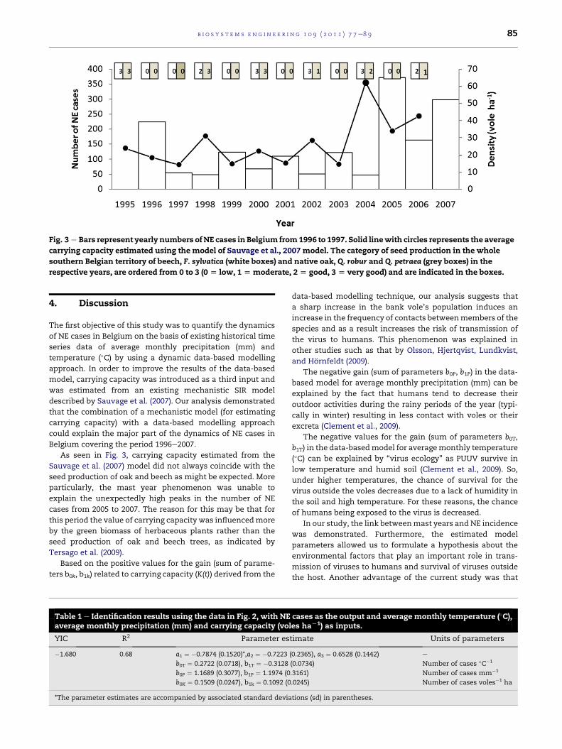
Fig. 3 e Bars represent yearly numbers ofNE cases in Belgium from1996 to 1997. Solid linewith circles represents the average

carrying capacity estimated using the model of Sauvage et al., 2007 model. The category of seed production in the whole

southern Belgian territory of beech, F. sylvatica (white boxes) and native oak, Q. robur and Q. petraea (grey boxes) in the

respective years, are ordered from 0 to 3 (0 [ low, 1[ moderate, 2[ good, 3 [ very good) and are indicated in the boxes.

b i o s y s t em s e ng i n e e r i n g 1 0 9 ( 2 0 1 1 ) 7 7e8 9 85

4. Discussion

The first objective of this study was to quantify the dynamics

of NE cases in Belgium on the basis of existing historical time

series data of average monthly precipitation (mm) and

temperature (�C) by using a dynamic data-based modelling

approach. In order to improve the results of the data-based

model, carrying capacity was introduced as a third input and

was estimated from an existing mechanistic SIR model

described by Sauvage et al. (2007). Our analysis demonstrated

that the combination of a mechanistic model (for estimating

carrying capacity) with a data-based modelling approach

could explain the major part of the dynamics of NE cases in

Belgium covering the period 1996e2007.

As seen in Fig. 3, carrying capacity estimated from the

Sauvage et al. (2007) model did not always coincide with the

seed production of oak and beech as might be expected. More

particularly, the mast year phenomenon was unable to

explain the unexpectedly high peaks in the number of NE

cases from 2005 to 2007. The reason for this may be that for

this period the value of carrying capacity was influencedmore

by the green biomass of herbaceous plants rather than the

seed production of oak and beech trees, as indicated by

Tersago et al. (2009).

Based on the positive values for the gain (sum of parame-

ters b0k, b1k) related to carrying capacity (K(t)) derived from the

Table 1 e Identification results using the data in Fig. 2, with NEaverage monthly precipitation (mm) and carrying capacity (vol

YIC R2 Parameter es

�1.680 0.68 a1 ¼ �0.7874 (0.1520)*,a2 ¼ �0.7223

b0T ¼ 0.2722 (0.0718), b1T ¼ �0.3128

b0P ¼ 1.1689 (0.3077), b1P ¼ 1.1974 (0

b0K ¼ 0.1509 (0.0247), b1k ¼ 0.1092 (0

*The parameter estimates are accompanied by associated standard devia

data-based modelling technique, our analysis suggests that

a sharp increase in the bank vole’s population induces an

increase in the frequency of contacts betweenmembers of the

species and as a result increases the risk of transmission of

the virus to humans. This phenomenon was explained in

other studies such as that by Olsson, Hjertqvist, Lundkvist,

and Hornfeldt (2009).

The negative gain (sum of parameters b0P, b1P) in the data-

based model for average monthly precipitation (mm) can be

explained by the fact that humans tend to decrease their

outdoor activities during the rainy periods of the year (typi-

cally in winter) resulting in less contact with voles or their

excreta (Clement et al., 2009).

The negative values for the gain (sum of parameters b0T,

b1T) in the data-basedmodel for averagemonthly temperature

(�C) can be explained by “virus ecology” as PUUV survive in

low temperature and humid soil (Clement et al., 2009). So,

under higher temperatures, the chance of survival for the

virus outside the voles decreases due to a lack of humidity in

the soil and high temperature. For these reasons, the chance

of humans being exposed to the virus is decreased.

In our study, the link betweenmast years and NE incidence

was demonstrated. Furthermore, the estimated model

parameters allowed us to formulate a hypothesis about the

environmental factors that play an important role in trans-

mission of viruses to humans and survival of viruses outside

the host. Another advantage of the current study was that

cases as the output and average monthly temperature (�C),es haL1) as inputs.

timate Units of parameters

(0.2365), a3 ¼ 0.6528 (0.1442) e

(0.0734) Number of cases �C�1

.3161) Number of cases mm�1

.0245) Number of cases voles�1 ha

tions (sd) in parentheses.

1996 1997 1998 1999 2000 2001 2002 20030

5

10

15

20

25

30

35

Year

Num

ber o

f NE

cas

es

Fig. 4 e The resulting model simulation (——) of the data-based MISO model with 3 inputs (average monthly temperature,

precipitation and estimated carrying capacity) versus measured (–�–) number of NE cases in Belgium from January 1996 till

January 2003. The model described the data with the R2T of 0.68.

2003 2004 2005 2006 2007 20080

10

20

30

40

50

60

70

Year

Num

ber o

f NE

cas

es

Fig. 5 e The simulation result (——) versus measured (–�–) number of NE cases in Belgium from January 2003 till January

2008.

b i o s y s t em s e n g i n e e r i n g 1 0 9 ( 2 0 1 1 ) 7 7e8 986

Fig. 8 e The MISO model result for epidemic months (>10

NE cases) versus number of NE cases in Belgium from

January 1996 till January 2003 (circles). The solid line

represents the regression line of the modelled versus

measured data.

Fig. 6 e The MISO model result versus number of NE cases

in Belgium from January 1996 till January 2003 (circles).

The solid line represents the regression line of the

modelled versus measured data.

b i o s y s t em s e ng i n e e r i n g 1 0 9 ( 2 0 1 1 ) 7 7e8 9 87

employing a data-based modelling approach allowed us to

quantify and predict the dynamics of NE cases on a monthly

basis. To the authors’ knowledge, this is the first time this has

been reported.

A study in Sweden performed a time series analysis for NE

cases in relation to bank vole’s population dynamics and the

North Atlantic Oscillation (NAO) index. Within this research,

no relationshipwas foundbetween theNAOand thenumberof

NE cases over two time series, totalling 37 years (Palo, 2009).

The analysis included a long-term data set on host abundance

(25 years). The incidence of Puumala virus infections in the

host was not measured. In order to model the dynamics of NE

cases, a multivariate stepwise model was applied with vole

index, winter mortality and NAO index at different time lags.

The analysis showed that only vole index contributed signifi-

cantly to the model of human NE. The authors acknowledged

that the NAO may be too coarse a measurement and that

temperature and precipitation individually may be better

predictors of NE incidence. In our study, we used average

measuredoutside temperatureandprecipitationaspredictors.

Fig. 7 e The simulation result versus number of NE cases in

Belgium from January 2003 till January 2008 (circles). The

solid line represents the regression line of the modelled

versus measured data.

Furthermore,weused theestimatedcarrying capacitywhich is

an indicator for abundance of bank voles in the forest. Our

model could describe the dynamics of NE in a more accurate

way despite the fact that Palo (2009) had a longer time series as

well asmeasurements of the temporal bank voles fluctuations.

In the study of Palo (2009), the NE cases were modelled with

a coefficient of determination (R2) between measured and

modelled data of 0.39. In our study, the R2T valuewas 0.68when

applying the model to the training data set. In contrast to the

work of Palo (2009) we also validated our model on a separate

dataset, resulting inaR2T valueof 0.54.AlthoughtheR2

T values in

our study were not very high, they were considerably higher

than values found by other researchers for similar modelling

approaches.

In another study, NE epidemics have been explained by

rodent host abundance (Olsson et al., 2009). The explanation is

based on the strong positive correlation and reported

temporal patterns linking bank voles’ abundance and NE

cases in Sweden. In the study a linear regression analysis was

Fig. 9 e The model simulation for epidemic months (>10

NE cases) versus number of NE cases in Belgium from

January 2003 till January 2008 (circles). The solid line

represents the regression line of the modelled versus

measured data.

b i o s y s t em s e n g i n e e r i n g 1 0 9 ( 2 0 1 1 ) 7 7e8 988

performed in the NE cases in Sweden (per year) from 1989

until 2007 based on the autumn bank voles trapping indices.

The NE cases (per year) were modelled with a coefficient of

determination (R2) between measured and modelled data of

0.63 but no validation was performed. In our study we

managed tomodel the NE cases in Belgium on amonthly basis

with a R2T of 0.68 without using any data about the cyclic phase

of the bank vole fluctuations, bank vole abundance, or PUUV

dynamics in the bank vole populations. Knowledge about the

dynamics of the bank vole population and NE cases was

introduced into our approach via the mechanistic model of

Sauvage et al. (2007). This can be considered as useful when

there is a lack of the trapping data.

Although the modelling results look promising when

comparedwith the available literature, several limitations can

be identified which are related to the applied modelling

methodology. The first limitation we faced when identifying

the data-based model was that the NE data in Belgium cover

a period of only 11 years. Although the number of sampleswas

theoretically sufficient to estimate the model parameters of

the model structure used, as indicated by the acceptable

standard errors on the parameter estimates (Table 1), a data-

set covering a longer period would be expected to improve the

modelling results. Another limitation is the quantification of

the carrying capacity. As shown in the work of Sauvage et al.

(2007), carrying capacity is one of the key factors in the

transmission of the disease. However, today there is no clear

way of quantifying this critical factor. Furthermore, it should

be noticed that the climatological values used as inputs in the

data-based model were measured at the weather station in

Ukkel, which is located close to Brussels, near to the centre of

Belgium. Since we used these climatological data tomodel the

NE cases for the whole country, it might be expected that

taking into account spatial characteristics of the climatolog-

ical data could potentially improve the modelling results.

In contrast to the mechanistic modelling approach, data-

based modelling techniques identify the dynamic character-

istics of processes based onmeasured data and as such are not

based on a priori knowledge. As a result, the choice of the

different input variables for explaining the output of the

considered system is crucial. Howeverwe know fromprevious

work (e.g. Sauvage et al., 2007; Tersago et al., 2009) that

climatological data and carrying capacity are important vari-

ables explaining the NE cases.

Based on the earlier critical reflection, several suggestions

can be made for improving this dynamic modelling concept.

Firstly, carrying capacity estimated from the mechanistic

model may be estimated from the vegetation index values

derived from satellite images. Using this method, carrying

capacity could be estimated more directly, provided that the

relationship between the information in the satellite images

(such as broad leaved forest phenology, e.g. Barrios et al., 2010)

and the carrying capacity can be established. Another way to

estimate the carrying capacity is the use of regression models

to investigate the effect of meteorological data and vegetation

indexes on carrying capacity. Secondly, the knowledge that is

described in mechanistic models could be used to explain the

modelparametersof thedynamicdata-basedmodels inamore

physically/physiologically meaningful way. Thirdly, in future

work the data-basedmodelling approachmay be improved by

integration of estimated bank vole population dynamics

measured in thefield.This couldgive thepossibility toquantify

the carrying capacity based on field measurements instead of

epidemiological models. Finally, it is expected that linking the

data-based modelling approach with existing mechanistic

models, such as the model of Sauvage et al. (2007), will create

added value since such data-based mechanistic models can

take advantage of the fact that they combine mechanistic

process knowledge with measured information (e.g. vegeta-

tion indexes, climatologicaldata, etc.)whichmakes themmore

understandable from a biological/ecological point of view, but

at the same time allows real-timemeasured information to be

taken into account to predict future NE outbreaks.

In this study we have focused on the temporal patterns in

the evolution of the emergence of the NE incidence. The

observed spatial features of NE incidence could be the subject

of future research.

5. Conclusion

The objective of this study was to quantify the dynamics of NE

cases using a dynamic data-based modelling approach.

Combining amechanisticmodel as described by Sauvage et al.

(2007) and a data-based modelling approach proved to be

valuable for describing the dynamics of NE cases in Belgium

on a monthly basis from 1996 until 2003 (R2T of 0.68).

The identified data-basedmodel was validated by applying

it to the inputeoutput data from 2003 to 2007.The validation

data were fitted with R2T of 0.54 and it was seen that the model

performedwell in simulating themonthly dynamics of the NE

cases in Belgium.

The results of the current study help to define significant

environmental factors on the spread of the disease. Deter-

mining a dynamic data-based model for NE which includes

factors such as vegetation coverage and abundance of food for

bank voles’ may provide an expert tool to predict (and aid

prevention of) the incidence of NE cases by making use of

remote sensing tools for measuring broad leaved forest

phaenology andmonitoring the vegetation dynamics together

with climatological data.

Acknowledgement

We are grateful to Professor James Taylor for reviewing the

modelling results of this study. This research has been sup-

ported by the Katholieke Universiteit Leuven (project IDO/07/

005). Piet Maes is supported by a postdoctoral grant from the

‘Fonds voorWetenschappelijk Onderzoek (FWO)-Vlaanderen’.

r e f e r e n c e s

Aerts, J.-M., Steppe, K., Boonen, C., Lemeur, R., & Berckmans, D.(2007). Simulation of sap flow in a beech tree by means ofa dynamic data-based model as influenced by a solar eclipse.Biosystems Engineering, 98(4), 446e454.

b i o s y s t em s e ng i n e e r i n g 1 0 9 ( 2 0 1 1 ) 7 7e8 9 89

Aerts, J.-M., Wathes, C. M., & Berckmans, D. (2003). Dynamic data-based modelling of heat production and growth of broilerchickens: development of an integrated management system.Biosystems Engineering, 84(3), 257e266.

Allen, L. J., Langlais, M., & Phillips, C. J. (2003). The dynamics oftwo viral infections in a single host population withapplications to hantavirus. Mathematical Biosciences, 186(2),191e217.

Anderson, R. M., & May, R. M. (1979). Population biology ofinfectious diseases: part I. Nature, 280, 361e367.

Barrios, J. M., Verstraeten, W.W., Maes, P., Clement, J., Aerts, J.-M.,Amirpour Haredasht, S., et al. (2010). Satellite derived forestphenology and its relation with nephropathia epidemica inBelgium. International Journal of Environmental Research and PublicHealth, 7(6), 2486e2500.

Begon, M., Feore, S., Bown, K., Chantrey, J., Jones, T., & Bennett, M.(1998). Population and transmission dynamics of cowpox inbank voles: testing fundamental assumptions. Ecology Letters,1(2), 82e86.

Bennet, E., Clement, J., Sansom, P., Hall, I., Leach, S., & Medlock, J.M. (2006). Environmental and ecological potential for enzooticcycles of Puumala hantavirus in Great Britain. Epidemiology andInfection, 4(1), 1e8.

Berthier, K., Langlais, M., Auger, P., & Pontier, D. (2000). Dynamicsof a feline virus with two transmission modes withinexponentially growing host populations. The Royal Society, 267(1457), 2049e2056.

Brummer-Korvenkontio, M., Vapalahti, O., Henttonen, H.,Koskela, P., & Vaheri, A. (1999). Epidemiological study ofnephropathia epidemica in Finland 1989e96. ScandinavianJournal of Infectious Diseases, 31, 427e435.

Cho, J., & Mostaghim, S. (2009). Dynamic agricultural non-pointsource assessment tool (DANSAT): model application.Biosystems Engineering, 102(4), 500e515.

Clement, J., Maes, P., & Van Ranst, M. (2006). Hantaviruses in theold and new world. Perspectives in Medical Virology, 16, 161e177,(Emerging viruses in human populations).

Clement, J., Maes, P., & Van Ranst, M. (2007). Acute kidney injuryin emerging, non-tropical infections. Acta Clinica Belgica, 62(6),387e395.

Clement, J., Maes, P., van Ypersele de Strihou, C., van derGroen, G., Barrios, J. M., Verstraeten, W. W., et al. (2010).Beechnuts and outbreaks of nephropathia epidemica (NE): ofmast, mice and men. Nephrology, Dialysis, Transplantation, 25(6), 1740e1746.

Clement, J., Vercauteren, J., Verstraeten, W. W., Ducoffre, G.,Barrios, J.M., Vandamme,A.M., et al. (2009). Relating increasinghantavirus incidences to the changing climate: the mastconnection. International Journal of Health Geographics, 8(1).

Costa, A., Borgonovo, F., Leroy, T., Berckmans, D., & Guarino, M.(2009). Dust concentration variation in relation to animalactivity in a pig barn. Biosystems Engineering, 1(104), 118e124.

Ferentinos, K. P., & Albright, L. D. (2003). Fault detection anddiagnosis in deep-trough hydroponics using intelligentcomputational tools. Biosystems Engineering, 84(1), 13e30.

Kallio, E. (2003). Stability of Puumala-virus outside the host. In:2nd European meeting on viral zoonoses. St Raphae.

Lee, H. W., French, G. R., Lee, P. W., Baek, L. J., Tsuchiya, K., &Foulke, R. S. (1981). Observations on natural and laboratoryinfection of rodents with the etiologic agent of Koreanhemorrhagic fever. The American Society of Tropical Medicine andHygiene, 30(2), 477e482.

Linard, C., Lamarque, P., Heyman, P., Ducoffre, G., Luyasu, V.,Tersago, K., et al. (2007). Determinants of the geographicdistribution of Puumala virus and Lyme borreliosis infectionsin Belgium. International Journal of Health Geographics, 6(15).

May, R. M., & Anderson, R. M. (1979). Population biology ofinfectious diseases: part II. Nature, 280.

Meinzer, F. C. (1982). Models of steady state and dynamic gasexchange responses to vapour pressure and light in Douglasfir (Pseudotsuga menziesii) saplings. Oecologia, 55(3), 403e408.

Monroe, M., Morzunov, S. P., Johnson, A. M., Bowen, M. D.,Artsob, H., Yates, T., et al. (1999). Genetic diversity anddistribution of Peromyscus-borne hantaviruses in NorthAmerica. Emerging Infectious Diseases, 5, 75e86.

Nozum, E. O., Rossi, C. A., Stephenson, E. H., & Leduc, J. W. (1988).Aerosol transmission of hantaan and related viruses tolaboratory rats. The American Journal of Tropical Medicine andHygiene, 38(3), 636e640.

Olsson, G. E., Hjertqvist, M., Lundkvist, A., & Hornfeldt, B. (2009).Predicting high risk for human hantavirus infections, Sweden.Emerging Infectious Diseases, 15(1), 104e106.

Palo, R. T. (2009). Time series analysis performed on nephropathiaepidemica in humans of northern Sweden in relation to bankvole population dynamic and the NAO index. Zoonoses andPublic Health, 56(3), 150e156.

Patrick, W. (2001). Biological warfare scenarios. In S. I. Layne, T. J.Beugelsdijk, & C. K. Patel (Eds.), Firepower in the lab automationin the fight against infectious diseases and bioterrorism(pp. 215e224). Washington: Joseph Henry Press.

Rastetter, E. B. (1987). Analysis of community interactions usinglinear transfer function models. Ecological Modelling, 36(1e2),101e117.

Rozenfeld, F. M., Le Boulenge, E., & Rasmont, R. (1987). Urinemarking by male bank voles (Clethrionomys glareolus Schreber,1780; Microtidae, Rodentia) in relation to their social rank.Canadian Journal of Zoology, 65, 2594e2601.

Sauvage, F., Langlais, M., & Pontier, D. (2007). Predicting theemergence of human hantavirus disease using a combinationof viral dynamics and rodent demographic patterns.Epidemiology and Infection, 135, 46e56.

Sauvage, F., Langlais, M., Yoccoz, N. G., & Pontier, D. (2003,January). Modelling hantavirus in fluctuating populations ofbank voles: the role of indirect transmission on viruspersistence. The Journal of Animal Ecology, 1e13.

Sayre, N. F. (2008). The genesis, history, and limits of carrying.Annals of the Association of American Geographer, 98(1), 120e134.

Taylor, C. J., Pedregal, D. J., Young, P. C., & Tych, W. (2007).Environmental time series analysis and forecasting with thecaptain toolbox. Environmental Modelling & Software, 22(6),797e814.

Tersago, K., Servais, A., Heyman, P., Ducoffre, G., & Leirs, H.(2009). Hantavirus disease (nephropathia epidemica) inBelgium: effects of tree seed production and climate.Epidemiology Infection, 137, 250e256.

Thanh, V. T., Vranken, E., Van Brecht, A., & Berckmans, D. (2007).Data-based mechanistic modelling for controlling in threedimensions the temperature distribution in a room filled withobstacles. Biosystems Engineering, 98(1), 54e65.

Ushada, M., & Murase, H. (2006). Identification of a moss growthsystem using an artificial neural network model. BiosystemsEngineering, 94(2), 179e189.

Wolf, C., Sauvage, F., Pontier, D., & Langlais, M. (2006). A multi-patch epidemic model with periodic demography, direct andindirect transmission and variable maturation rate.Mathematical Population Studies, 13, 153e177.

Young, P. C. (1984). Recursive estimation and time series analysis.Berlin: Springer-Verlag.

Young, P. C., & Lees, M. (1993). The active mixing volume: a newconcept in modelling environmental systems. In V. Barnet, R.Turkman, & K. Feridun (Eds.), Statistics for the environment (pp.2e43). Chichester: John Wiley.

Young, P. C., & Wang, C. (1987). ldentification and estimation ofmultivariable dynamic systems. In J. O’Reilly (Ed.),Multivariable control for industrial applications (pp. 244e270).London: Peter.