A dynamic approach for evaluating coarse scale satellite soil moisture products

HESSD7, 7263–7303, 2010

Soil moisturevalidation

A. Loew and F. Schlenz

Title Page

Abstract Introduction

Conclusions References

Tables Figures

J I

J I

Back Close

Full Screen / Esc

Printer-friendly Version

Interactive Discussion

Discussion

Paper

|D

iscussionP

aper|

Discussion

Paper

|D

iscussionP

aper|

Hydrol. Earth Syst. Sci. Discuss., 7, 7263–7303, 2010www.hydrol-earth-syst-sci-discuss.net/7/7263/2010/doi:10.5194/hessd-7-7263-2010© Author(s) 2010. CC Attribution 3.0 License.

Hydrology andEarth System

SciencesDiscussions

This discussion paper is/has been under review for the journal Hydrology and EarthSystem Sciences (HESS). Please refer to the corresponding final paper in HESSif available.

A dynamic approach for evaluating coarsescale satellite soil moisture productsA. Loew1 and F. Schlenz2

1Max-Planck-Institute for Meteorology, KlimaCampus, Hamburg, Germany2Department of Geography, University of Munich, Munich, Germany

Received: 15 August 2010 – Accepted: 18 August 2010 – Published: 24 September 2010

Correspondence to: A. Loew ([email protected])

Published by Copernicus Publications on behalf of the European Geosciences Union.

7263

http://www.hydrol-earth-syst-sci-discuss.net

http://www.hydrol-earth-syst-sci-discuss.net/7/7263/2010/hessd-7-7263-2010-print.pdf

http://www.hydrol-earth-syst-sci-discuss.net/7/7263/2010/hessd-7-7263-2010-discussion.html

http://creativecommons.org/licenses/by/3.0/

HESSD7, 7263–7303, 2010



Title Page



Tables Figures

J I

J I

Back Close

Full Screen / Esc



Discussion

Paper

|D

iscussionP

aper|

Discussion

Paper

|D

iscussionP

aper|

Abstract

Validating coarse scale remote sensing soil moisture products requires a comparisonof gridded data to point-like ground measurements. The necessary aggregation of insitu measurements to the footprint scale of a satellite sensor (>100 km2) introducesuncertainties in the validation of the satellite soil moisture product. Observed differ-5

ences between the satellite product and in situ data are therefore partly attributable tothese aggregation uncertainties. The present paper investigates different approachesto disentangle the error of the satellite product from the uncertainties associated tothe up-scaling of the reference data. A novel approach is proposed, which allows forthe quantification of the remote sensing soil moisture error using a temporally adaptive10

technique. It is shown that the point-to-area sampling error can be estimated within0.0084 [m3/m3].

1 Introduction

There is ample evidence that atmospheric and climate processes are significantly con-ditioned by the availability of water in the soils (Fast and McCorcle, 1991; Clark and15

Arritt, 1995; Koster et al., 2004). Soil moisture is an essential climate variable that hasimportance for the interactions between the land surface and atmosphere. It is thus anessential variable in climate research and numerical weather forecast as well as landsurface hydrology. Satellite remote sensing has been demonstrated to provide usefulinformation on soil moisture dynamics at various temporal and spatial scales (Zribi and20

Dechambre, 2002; Bindlish and Barros, 2000; Wigneron et al., 2004, 2003; Loew et al.,2006; Schwank et al., 2005; Owe et al., 2008). Two dedicated satellite soil moisturemissions have been designed to provide global information on soil moisture dynamics.The European Soil Moisture and Ocean Salinity mission (SMOS) (Kerr et al., 2001)was launched in November 2009 and is the first dedicated soil moisture mission ever25

built. The NASA Soil Moisture Active Passive mission (SMAP) (NRC, 2007) is planned

7264





HESSD7, 7263–7303, 2010



Title Page



Tables Figures

J I

J I

Back Close

Full Screen / Esc



Discussion

Paper

|D

iscussionP

aper|

Discussion

Paper

|D

iscussionP

aper|

to be launched in 2014. These satellite missions will provide information on soil mois-ture dynamics at global scale and with coarse spatial resolution (�100 km2). A criticalaspect of the missions success is the validation of their soil moisture products to verifyif they meet pre-defined accuracy requirements. This validation exercise is complicatedby the scale mismatch between the satellite footprint and local in situ measurements5

of soil moisture which serve as a reference.A large number of continuous soil moisture measurements would be needed to deter-

mine the soil moisture dynamics at the footprint scale (Yoo, 2002; Brocca et al., 2007;Famiglietti et al., 2008) with an accuracy better than 0.04 [m3/m3], which is the typicalaccuracy requirement for satellite soil moisture missions (Walker and Houser, 2004).10

Characteristic soil moisture patterns develop that remain stable at different temporaland spatial scales (Vachaud et al., 1985; Vinnikov et al., 1996). The analysis of tempo-rally stable soil moisture patterns has been used for the development of concepts forthe upscaling of local soil moisture measurements to larger scales that could be usedfor the validation of satellite soil moisture products (Cosh et al., 2004, 2006). A differ-15

ent concept for the evaluation of the error of satellite soil moisture products has beeninvestigated by Miralles and Crow (2010). They applied the so called triple collocation(TC) method to quantify the uncertainty of soil moisture data sets using data from threeindependent sources. They showed that this technique provides a useful alternative toaddress the satellite soil moisture validation problem and that it is possible to quantify20

the soil moisture error with an accuracy of 0.0064 [m3/m3] for their test site.The objective of the present paper is to contrast the potential of these different tech-

niques for the validation of coarse scale soil moisture products. The potential synergiesof combining in situ soil moisture information with distributed land surface modelingfor the validation of satellite products is evaluated. A temporally dynamic validation25

approach is proposed which applies the TC method for monthly temporal slices andprovides a framework for the quantification of the uncertainties of a satellite based soilmoisture product. The novelty of the approach is that it provides uncertainty estimatesof soil moisture products at rather short timescales and is able to identify periods where

7265





HESSD7, 7263–7303, 2010



Title Page



Tables Figures

J I

J I

Back Close

Full Screen / Esc



Discussion

Paper

|D

iscussionP

aper|

Discussion

Paper

|D

iscussionP

aper|

either the satellite measurements or the in situ measurements don’t provide reliable in-formation on the large scale soil moisture dynamics. The method is verified on a coresoil moisture validation site situated in Southern Germany using AMSR-E soil moistureproducts.

2 Methodology5

A key question for the validation of remote sensing soil moisture data products is anappropriate accuracy assessment of the data products. Typically, the root mean squaredifference (RMSD) is used to predefine the accuracy requirements of a satellite soilmoisture product (Walker and Houser, 2004; Kerr, 2007). It is defined as

RMSD=√〈(x−y)2〉 (1)10

whereas x and y correspond to vectors of collocated satellite and in-situ observa-tions respectively. Angled brackets indicate ensemble averaging. The user requirementfor global satellite soil moisture products is currently defined with RMSD≤0.04 [m3/m3](Walker and Houser, 2004; Kerr et al., 2001). However as by its definition, the RMSD isvery sensitive to a bias between in situ reference data and the satellite product. Even15

if a product would perfectly reproduce the relative temporal soil moisture dynamics itwould show a large RMSD if the estimates or used reference data are biased. Biasesin remote sensing based soil moisture estimates might result from a variety of sources,like e.g. imperfect characterization of the land surface in the retrieval scheme of vari-able sensitivity of the observation system to soil moisture dynamics (van de Griend20

et al., 2003; Loew, 2008).On the other hand, regular in situ soil moisture measurements are typically based on

a relative small number of samples compared to the footprint scale of a satellite sensor.The monitoring of soil moisture dynamics using a very high number of observations islimited to dedicated campaigns (Famiglietti et al., 2008). Existing regular soil moisture25

7266





HESSD7, 7263–7303, 2010



Title Page



Tables Figures

J I

J I

Back Close

Full Screen / Esc



Discussion

Paper

|D

iscussionP

aper|

Discussion

Paper

|D

iscussionP

aper|

networks like the Oklahoma Mesonet network (www.mesonet.org) (Brock et al., 1995),the REMEDHUS network in Spain (Ceballos et al., 2002) or the SMOSHYD validationsite (Loew et al., 2009a) provide in situ data from only a few stations � 10 for an areacorresponding to the footprint of dedicated soil moisture missions like SMOS.

Ground based soil moisture measurements are very local as soil moisture probes5

used for regular measurements are typically only representative for very small vol-umes in the order of 10−4 m3 (for a comparison of different measurement techniquessee Walker et al., 2004). Currently, no global in situ soil moisture monitoring net-work exists. First efforts to collect reference data of in situ soil moisture was madeby Robock et al. (2000). More recently, a research community driven in situ soil mois-10

ture network bank has been initiated to collect and distribute harmonized and qualityproofed in situ soil moisture data (http://www.ipf.tuwien.ac.at/insitu/)

As the spatial variability in the footprint of a satellite sensor can be large, the mis-match between in situ measurements and the satellite footprint scale results in largeuncertainties for the validation of satellite soil moisture products.15

An appropriate validation approach therefore needs to take into account the inherentuncertainties that are associated with the upscaling of local scale soil moisture mea-surements to a larger scale. Two different approaches will be introduced in the followingand their potential will be investigated in the further analysis of the paper.

2.1 Temporal stable soil moisture patterns20

The concept of temporal stability was introduced by Vachaud et al. (1985) as a meanto represent large scale soil moisture dynamics using a measurement network of afew sites only. The fundamental assumption of the method is that characteristic soilmoisture patterns persist, which can be used to develop time-invariant relationshipsbetween local (θ) and large scale (θ) soil moisture dynamics in the spatial domain R25

7267





www.mesonet.org

http://www.ipf.tuwien.ac.at/insitu/

HESSD7, 7263–7303, 2010



Title Page



Tables Figures

J I

J I

Back Close

Full Screen / Esc



Discussion

Paper

|D

iscussionP

aper|

Discussion

Paper

|D

iscussionP

aper|

with an area A which is given by

θj =A−1∫Rθjdr ≈

1N

N∑i=1

θi j +ε (2)

and can be approximated by a discrete number of N measurements. The index ispecifies the in situ measurements at point P with coordinates (x,y) and ε is the errorof Eq. (2) due to the discrete approximation. The number of required measurements5

to obtain a specific accuracy might vary, depending on the heterogeneity of the studyarea. Brocca et al. (2007) used a statistical approach to infer the number of requiredsamples for different spatial scales and concluded that 15 to 35 measurement sitesare needed to estimate θ with an absolute error of 0.02 [m3/m3] for a study area witha size of 10.000 m2. As the variability of soil moisture is also dependent on the soil10

moisture dynamic itself, the number of required samples might vary as a function of θ(Vereecken et al., 2007). Famiglietti et al. (2008) provide an analysis of a large numberof soil moisture measurements from different campaigns and at various scales. Theyconclude that the number of measurements required to estimate θ with an accuracybetter than 0.04 [m3/m3] (95% confidence level) is larger than N = 20 for a scale of15

50 km with decreasing sample numbers for very dry or wet conditions.A point i is considered to be temporally stable if its soil moisture dynamics is in good

agreement with the spatial average. The relative soil moisture difference at time j isgiven as

δi j =θi j − θj

θj

(3)20

The expected value of δi and its standard deviation is then obtained from M timesas

δi =1M

M∑j=1

δi j (4)

7268





HESSD7, 7263–7303, 2010



Title Page



Tables Figures

J I

J I

Back Close

Full Screen / Esc



Discussion

Paper

|D

iscussionP

aper|

Discussion

Paper

|D

iscussionP

aper|

σ(δi )=

√√√√ 1M−1

M∑j=1

(δi j − δi )2 (5)

A point which is representative for the large scale soil moisture dynamics thereforecorresponds to small values of |δi | and σ(δi ). If stable relationships between the localand large scale soil moisture dynamics exist, these can be used for the upscaling oflocal measurements to the larger scale (Brocca et al., 2010).5

Spatially persistent soil moisture patterns have been analyzed using ground mea-surements (Vachaud et al., 1985; Grayson and Western, 1998; Cosh et al., 2004;Martinez-Fernnandez and Ceballos, 2005; Teuling et al., 2006), models (Loew andMauser, 2008) or remote sensing observations (Wagner et al., 2008). Techniquesto dissaggregate coarse scale remote sensing observations using prior knowledge of10

persistent soil moisture fields have been developed (Loew and Mauser, 2008; Wagneret al., 2008).

The temporal stability approach assumes that a specific location can be found wherethe relationship between local and large scale soil moisture dynamics is time-invariant.It will be evaluated in Sect. 4 if this assumption is applicable for the data used in the15

present study and contrasted against the triple collocation approach introduced next.

2.2 Triple collocation method

The triple collocation (TC) method was originally developed to estimate the errors ofsea wind and wave height estimates derived from buoy, model and satellite data (Stof-felen, 1998; Caires and Sterl, 2003). It estimates the uncertainties of observations of a20

geophysical quantity using time series of three independent data sets.Scipal et al. (2009) was the first to apply the TC method to quantify uncertainties of

surface soil moisture data, using data from two different remote sensing soil moistureproducts and ERA-40 reanalysis data. The method was then used for validation ofremote sensing surface soil moisture observations using sparse in situ networks by25

Miralles and Crow (2010).7269





HESSD7, 7263–7303, 2010



Title Page



Tables Figures

J I

J I

Back Close

Full Screen / Esc



Discussion

Paper

|D

iscussionP

aper|

Discussion

Paper

|D

iscussionP

aper|

The implementation of the TC method in the present study follows the analyticalsolution provided by Caires and Sterl (2003). The method and used notation is brieflyintroduced in the following.

It is assumed that three temporally collocated time series of n observations (xi , yi ,zi , i =1...n) of an arbitrary physical quantity Ti , i =1...n exist. Their respective random5

errors (ex, ey , ez) are assumed to have zero mean. The true measurements (X,Y,Z)of T , corresponding to the observations (xi , yi , zi ) are related to T as

x=X +ex =α0+β0T +exy = Y +ey =α1+β1T +eyz=Z+ex =α2+β2T +ez

(6)

where the subscripts have been dropped for easier notation. Removing the mean fromeach of the variables and denoting the anomalies as x∗, y∗, z∗, T ∗, their relationship is10

given by

x∗ =α0+β0T∗+ex

y∗ =α1+β1T∗+ey

z∗ =α2+β2T∗+ez

(7)

If we assume that the errors of the data sets are uncorrelated, 〈exey 〉 = 〈exez〉 =〈eyez〉= 0, and independent of T , 〈Tex〉= 〈Tey 〉= 〈Tez〉= 0, we can remove the un-known deterministic variable T ∗ using a simple elimination procedure (see for details,15

Caires and Sterl, 2003) and obtain

β1 =β0〈y∗z∗〉/〈x∗z∗〉

β2 =β0〈y∗z∗〉/〈x∗y∗〉

(8)

where angled brackets 〈·〉 denote ensemble averaging. The variances of the obser-vation errors are then obtained as

7270





HESSD7, 7263–7303, 2010



Title Page



Tables Figures

J I

J I

Back Close

Full Screen / Esc



Discussion

Paper

|D

iscussionP

aper|

Discussion

Paper

|D

iscussionP

aper|

var (ex) = 〈e2x〉= 〈(x∗)2〉−〈x∗y∗〉〈x∗z∗〉/〈y∗z∗〉 (9)

= 〈(x∗)2−〈x∗y∗〉β0

β1〉

var (ey ) = 〈e2y 〉= 〈(y∗)2〉−〈x∗y∗〉〈y∗z∗〉/〈x∗z∗〉

= 〈(y∗)2−〈x∗y∗〉β1

β0〉

var (ez) = 〈e2z〉= 〈(z∗)2〉−〈x∗z∗〉〈y∗z∗〉/〈x∗y∗〉5

= 〈(z∗)2−〈y∗z∗〉β0

β1〉

Finally the coefficients α1 and α2 are estimated as

α1 = 〈y〉−β1(〈x〉−α0

)α2 = 〈z〉−β2

(〈x〉−α0

) (10)

Note, that only four of the six coefficients can be derived using x,y,z. Defining oneobservation (e.g. x) as a reference, α1, α2, β1 and β2 can be estimated. Typically it is10

assumed that the reference is a bias free estimator of the deterministic variable (Scipalet al., 2009; Caires and Sterl, 2003), thus α0 =0 and β0 =1. However, in a strict sense,this assumption might not be valid. In fact, it will be shown that the ground stations inthe present study are not a bias free estimator of the large scale soil moisture content.

Further, modeled soil moisture as well as satellite retrievals typically exhibit their15

own characteristics and are therefore typically rescaled before any inter-comparison(Reichle et al., 2004; Albergel et al., 2010). In that sense, the estimation of α andβ parameters corresponds to a similar rescaling of the original data sets. However,the estimation of the errors is independent of the chosen model parameters as can beseen from Eq. (9).20

7271





HESSD7, 7263–7303, 2010



Title Page



Tables Figures

J I

J I

Back Close

Full Screen / Esc



Discussion

Paper

|D

iscussionP

aper|

Discussion

Paper

|D

iscussionP

aper|

3 Study area and data

Three different soil moisture data sets are used in the present study. These are basedon ground observations, land surface model simulations and remote sensing soil mois-ture estimates. The datasets and their characteristics are described after a brief intro-duction to the study area.5

3.1 Study area

The study area is located in the Upper Danube catchment area which is situated inSouthern Germany (Fig. 1). A remote sensing soil moisture validation site has beenestablished in a small sub-catchment (Vils), situated in the Northeast of the city of Mu-nich (Loew et al., 2009a). The site is most suitable for validation of coarse resolution10

microwave remote sensing data as the microwave signal is not affected by open wa-ter water bodies or large urban areas which might have a considerable effect on themicrowave signal (Loew, 2008).

To perform a cross comparison between the different data sets, these are repro-jected to a common, equal area grid. The Icosahedral Snyder Equal Area projection15

(ISEA4H9) is used as the reference projection (Sahr et al., 2003) which has a gridspacing of 12.5 km. The same grid is used as a reference grid for the Soil Moisture andOcean Salinity Mission (SMOS). Each grid node has a unique identifier which will beused in the following to identify ground stations, model grid cells and satellite footprints.

3.2 Soil moisture data20

3.2.1 Soil moisture measurements

Half-hourly measurements of soil moisture profiles are available since mid of 2007from five stations in the test site. Soil moisture measurements are made using Time-Domain-Reflectrometry (TDR) probes at depth of 5, 10, 20 and 40 cm. Surface soil

7272





HESSD7, 7263–7303, 2010



Title Page



Tables Figures

J I

J I

Back Close

Full Screen / Esc



Discussion

Paper

|D

iscussionP

aper|

Discussion

Paper

|D

iscussionP

aper|

moisture at 5 cm is measured by two different probes independently. The stationscover an area of approximately 40×40 km2.

3.2.2 Land surface model

The PROMET land surface model is used in the present study to simulate the surfaceenergy and water fluxes (Mauser and Schaedlich, 1998) on an hourly basis. The model5

consists of a kernel model which is based on five sub-modules (radiation balance,soil model, vegetation model, aerodynamic model, snow model) to simulate the actualwater and energy fluxes and a spatial data modeler, which provides and organizesthe spatial input data on the field-, micro and macro-scale. Soil moisture dynamic issimulated using a modified version of the Richards equation for flow in unsaturated10

media (Philip, 1957). The soil water retention model of Brooks and Corey (1964) isused to relate soil moisture content to soil suction head. A detailed description of themodel is given by Mauser and Bach (2009). The soil water model has been validatedin different test sites using in-situ soil moisture measurements of soil moisture profiles(Pauwels et al., 2008).15

PROMET model simulations are made on 1 km2 grid. The meteorological forcing isobtained from a dense network of stations which are collocated with the in situ soilmoisture network. Model simulations at 1 km2 scale are made from 1st of November2007 until end of 2009. The high resolution model simulations are then aggregatedto estimate the expected large scale soil moisture dynamics at the footprint scale of a20

satellite sensor (see Fig. 1).

3.2.3 Satellite soil moisture

Remote sensing soil moisture data are obtained from a globally available data setbased on the Advance Microwave Scanning Radiometer (AMSR-E), provided by theVU University Amsterdam together with NASA Goddard Space Flight Centre (Owe25

et al., 2008). AMSR-E is a passive microwave scanning radiometer, operating at six

7273





HESSD7, 7263–7303, 2010



Title Page



Tables Figures

J I

J I

Back Close

Full Screen / Esc



Discussion

Paper

|D

iscussionP

aper|

Discussion

Paper

|D

iscussionP

aper|

different wavelengths within the microwave spectrum (6.925, 10.65, 18.7, 23.8, 36.5,and 89 GHz). The large area coverage (swath width: 1445 km) of the sensor allows fora frequent coverage of the globe in the order of three days with increasing frequenciesat higher latitudes. The spatial resolution of the different channels is varying from 5 km(89 GHz) to 56 km (6.925 GHz) (Njoku et al., 2003).5

Soil moisture retrievals are based on the solution of a microwave radiative transfermodel which solves simultaneously for the surface soil moisture content and vegetationoptical depth without a priori information (Meesters et al., 2005). The flexible approachallows in general for the retrieval of soil moisture from a variety of frequencies. TheC-band (6.925 GHz) data product is used in the present study as it is expected to have10

the highest sensitivity to surface soil moisture dynamics from the AMSR-E channels.The data set is available since 2002. The data product has been validated over alarge range of study areas with high correlations with in situ observations in semi aridregions (r = 0.79, RMSE=0.03 [m3/m3] for the Murrumbidgee Soil Moisture Monitor-ing Network in Australia, Draper et al., 2007; r = 0.83, RMSE=0.06 [m3/m3] for the15

REMEDHUS soil moisture network in Spain, Wagner et al., 2007) and somewhat lowerin agricultural areas (r =0.78, RMSE=0.06 [m3/m3] for the SMOS REX site in France,Rudiger et al., 2009).

Only data from the daytime ascending overpass (01:30 p.m.) are used as thesewere found to be less noisy than the nighttime observations (Loew et al., 2009b). As20

the sensitivity of the AMSR-E observations to soil moisture decreases with increasingoptical depth of the vegetation layer, only data with an optical depth τ < 0.8 are usedfor the further analysis. A single AMSR-E time series, located in the center of the testsite (ISEA ID #2027099) is used in the study.

4 Soil moisture variability and stability25

The variability of the in situ soil moisture data is analyzed in the following. The in-vestigations are limited to the period from 01/05 to 30/10 of the years 2008 and 2009

7274





HESSD7, 7263–7303, 2010



Title Page



Tables Figures

J I

J I

Back Close

Full Screen / Esc



Discussion

Paper

|D

iscussionP

aper|

Discussion

Paper

|D

iscussionP

aper|

to cover a large variability in soil moisture and vegetation conditions, while avoidinginterference by snow and frozen soil conditions.

4.1 Soil moisture variability

The average soil moisture θ for the investigated area is calculated from the stationdata. As the number of stations (N = 5) is rather small to sufficiently represent θ this5

will introduce an uncertainty in the estimation of θ (Famiglietti et al., 2008; Brocca et al.,2010). Figure 2 shows time series of θ and its standard deviation for the years 2008and 2009. Both soil moisture curves show a dynamical range between 0.2 [m3/m3] and0.4 [m3/m3]. The standard deviation varies between 0.025 and 0.1 [m3/m3].

4.2 Temporal stability analysis10

A temporal stability analysis (Sect. 2.1), is conducted for each of the stations, using θas the reference. For each station and year, the statistic for δ is calculated using Eq. (4)and Eq. (5). Results are summarized for each station and year in Fig. 3. Considerabledifferences are observed between the years. The station Steinbeissen (Neusling) doesbest represent the large scale soil moisture dynamics in 2008 (2009) according to the15

δ metric.The linear relationship between θj and θ was estimated using a least square ap-

proach with θ as the dependent variable. The regression coefficients are given inTable 2. By removing this linear trend, we obtain the random upscaling error for eachstation (estation). Considerable differences are observed between the two years. The20

different stations do not show a consistent relationship to the large scale soil mois-ture dynamics. While all stations show significant correlations with the large area soilmoisture dynamics over a certain time period, they might not be used to predict thespatial mean soil moisture dynamics consistently over a longer time period. The rea-son for these differences are small scale differences in precipitation dynamics, which25

are mostly related to convective events that are local.

7275





HESSD7, 7263–7303, 2010



Title Page



Tables Figures

J I

J I

Back Close

Full Screen / Esc



Discussion

Paper

|D

iscussionP

aper|

Discussion

Paper

|D

iscussionP

aper|

However at smaller timescales, a single station might be a good predictor for thelarge scale soil moisture dynamics. We will therefore investigate the potential of usinga temporally dynamic approach to assess the soil moisture validation problem usingthe triple collocation technique. First, the triple collocation will be applied on an annualbasis to provide comparable results with the analysis in the present section. We will5

then relax the method by applying it on shorter timescales to adapt it to temporallystable soil moisture patterns at shorter timescales.

5 Triple collocation analysis

5.1 Data preparation

The triple collocation method requires all data sets to be temporally collocated. They10

are therefore binned to daily values and spatially collocated on the ISEA grid. Satel-lite data which were recorded during precipitation events were not considered for theinter-comparison, as the rainfall and interception in the canopy can deteriorate themicrowave signal (Saleh et al., 2007). Data from different stations were used as a ref-erence (x) and compared against the spatially averaged soil moisture from PROMET15

(y) and AMSR-E soil moisture data (z). The different experiments for the various sta-tions are summarized in Table 1. It is assumed that the model and satellite data arerepresentative for the same spatial domain, while the ground measurements are ex-pected to provide an uncertain proxy for θ over the same area. We aim to obtain arobust estimate for esat to quantify the accuracy of the satellite data.20

The triple collocation analysis will be either made for the entire investigation period(01/05–30/10) or for a 30 day moving window from the beginning to the end of theinvestigation period with steps of 15 days. As the triple collocation relies on a signifi-cant correlation between the three different data sets we first calculate the correlationbetween each pair of x,y,z. In case of negative correlation, the data are not ana-25

lyzed. Scipal et al. (2009) further screened the data by applying a threshold of 0.2

7276





HESSD7, 7263–7303, 2010



Title Page



Tables Figures

J I

J I

Back Close

Full Screen / Esc



Discussion

Paper

|D

iscussionP

aper|

Discussion

Paper

|D

iscussionP

aper|

to the obtained correlation coefficient which corresponds to a significant correlation atthe 95% level for time series with a large number of samples. However, as we re-strict our analysis to much shorter timescales, we explicitly calculate the significance(pxy ,pxz,pyz) of the correlation between the variables according to a t-test (Press et al.,1992).5

5.2 Analysis results

The TC analysis is made in two parts. First, results from a yearly analysis are presented(static approach) and then results from the TC analysis at shorter time scales (dynamicapproach) are presented.

5.2.1 Static approach10

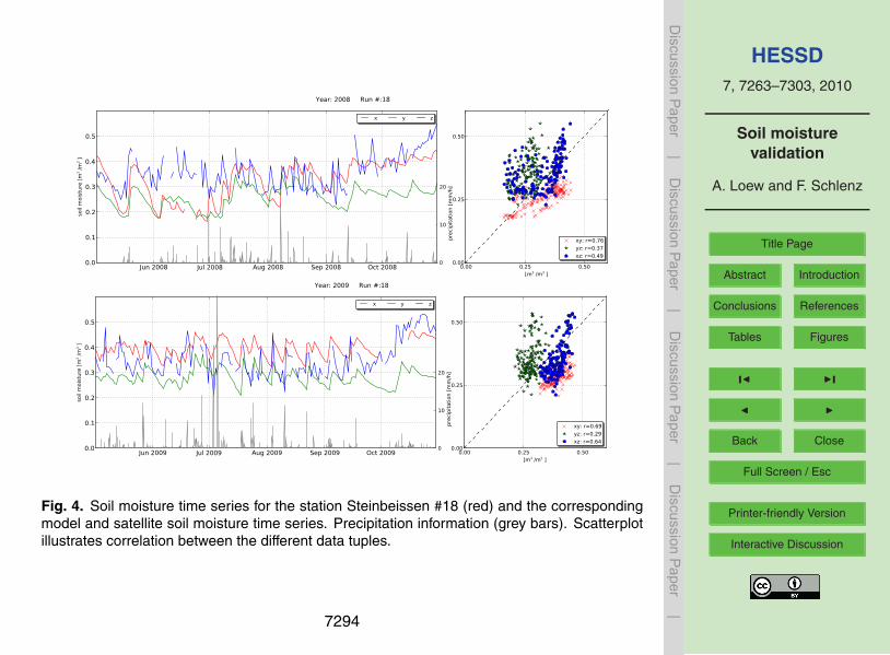
The static approach exploits the full time series for the estimation of the error variances,which is similar to the approach of Scipal et al. (2009). The estimated errors for themodel simulated and satellite soil moisture show consistent results for the differentexperiments (Table 3). The model errors (emodel) range between 0.0176 and 0.0285(0.0075 and 0.0238) [m3/m3] for 2008 (2009). The AMSR-E soil moisture error esat15

ranges between 0.047 and 0.0659 [m3/m3] which is in the same order than resultsobtained from previous studies (Draper et al., 2007; Wagner et al., 2007). The robustresults for the satellite product error for different stations indicate that the selection of aparticular station seems to have minor impact on the uncertainty estimates.

All stations show significant correlations between the in situ measurements and the20

model simulations as well as the satellite retrievals. Further it is observed that thecorrelation between the station and the satellite data is in general higher than the cor-relation between the model and the satellite data.

As the same model and satellite data are used for all simulations, differences inthe error estimates result only from differences between the ground stations. Their25

representativity for the large scale soil moisture dynamics changes throughout the yearas was shown previously.

7277





HESSD7, 7263–7303, 2010



Title Page



Tables Figures

J I

J I

Back Close

Full Screen / Esc



Discussion

Paper

|D

iscussionP

aper|

Discussion

Paper

|D

iscussionP

aper|

The estimated gains (β1,β2) vary between 0.22 and 0.86 which would have beenexpected due to the lower spatially aggregated soil moisture variability at larger scalescompared to local measurements. Different gains are observed for the same stationin different years. A comparison of the estimated error for each station (estat) with theactual estimate of the station error (estation) shows that they are in the range between5

0.0248 and 0.0356 [m3/m3] for estations and 0.0097 and 0.0489 [m3/m3] for estat (Ta-ble 3).

Considerable differences are observed between the two years for the various sta-tions. These results indicate that data from the different stations can not be used toupscale the local soil moisture measurements in a consistent way as their representa-10

tiveness for the larger area is changing with time, which is consistent with the resultsof the temporal stability analysis. This indicates that temporally adaptive methods areneeded for the inter-comparison of the in situ soil moisture data with the footprint scalesoil moisture estimates. This is at least valid for the data used in the present analysis.We will therefore investigate in the following if a dynamic collocation approach, applied15

on shorter timescales, might be used as an alternative for the soil moisture validationproblem.

5.2.2 Dynamic approach

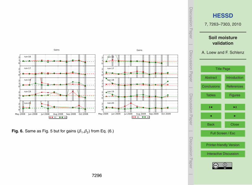
A temporal window of dt = 30 days is used for the dynamic triple analysis which re-duces the number of collocated data points and thus the degree of freedom for the20

correlation between the data tuples. The results of all different 30-day intervals aresummarized in Fig. 5 – Fig. 7. These show the temporal variability of r , e and β. Datasets, where the correlation for at least one out of the three data tuples (xy , xz, yz) wasnot significant at the 95% level are marked with gray bars. Dashed lines correspond toe, r , β as estimated from the static approach and are provided for comparison.25

The estimated satellite product errors are in general lower for the dynamic approachthan they are for the static TC analysis. The obtained values for esat are consistentbetween the different stations and show a similar temporal dynamic. This indicates

7278





HESSD7, 7263–7303, 2010



Title Page



Tables Figures

J I

J I

Back Close

Full Screen / Esc



Discussion

Paper

|D

iscussionP

aper|

Discussion

Paper

|D

iscussionP

aper|

that the choice of the reference station has a minor effect on the calculation of esat andthat they provide a robust estimate of the uncertainty of the satellite data product.

In a large number of sample intervals non-significant correlations are found. Ingeneral, one can differentiate between time intervals where all stations show a non-significant correlation between at least one of the data tuples and those where a single5

station indicates a correlation at a low significance level. As an example, Fig. 8 showsdetails of the analyzed time series for the stations #17 (Lochheim) and #18 (Steinbeis-sen) for consecutive time periods in 2008.

All three data sets capture well the decrease of soil moisture until mid of May 2008and the increase due to the precipitation between 16th and 19th of May 2008 (a).10

Highly significant correlations are found between all data tuples. Frequent precipitationin the first half of June results in a couple of data gaps for the satellite data due tothe precipitation masking, decreasing especially the correlation between the satellitedata and model results (b). The following time period is dominated by low soil moisturedynamics until end of June (c). The satellite data capture in general this low variability,15

but no significant correlations with neither the PROMET model simulations nor the insitu data are found for this period for both stations. The satellite soil moisture producthas large noise compared to the small soil moisture signal. The satellite data capturethe increase of soil moisture after 10th of July 2008 (d) for both stations although thereare data gaps during this rain period. However, no significant correlations are found20

between the in situ data and the satellite product for station #18 (p=0.74), while signif-icant correlations are found for station #17 (e). This station is the only one that showsno significant correlations during that time period (see also Fig. 7). In this case, thelack of a significant correlation is caused by a data gap in the in situ soil moisture datafrom 17th to 23th of June which has been identified by the TC method.25

5.2.3 Effect of temporal sampling

The temporal window used for the dynamic TC analysis determines how many datapoints are used in the analysis and thus determines the degree of freedom for the

7279





HESSD7, 7263–7303, 2010



Title Page



Tables Figures

J I

J I

Back Close

Full Screen / Esc



Discussion

Paper

|D

iscussionP

aper|

Discussion

Paper

|D

iscussionP

aper|

correlation. The previous analysis with dt = 30 days did show that an analysis onshort time scales is feasible and helps to make an appropriate error assessment of thesatellite data. The significance of the correlations between the time series has beenshown to be a useful tool for the detection of gaps and artefact’s in the time series.However, large parts of the time series show no significant correlation at the 95% level5

in these cases.On the other hand, the yearly analysis did show significant correlations for all data

tuples as a larger time interval results in a higher degree of freedom for the correla-tion threshold. A further analysis using dt= 60 [days] (not shown here) did show veryconsistent results for the satellite error as estimated from different stations. The esti-10

mated satellite error was smaller than the one obtained from the yearly analysis, butdid show less temporal variability than the one obtained using dt=30 [days]. However,the low soil moisture variability in the mid of June 2008 does still affect this analysisand non-significant correlations are identified for all stations during that time periodusing dt = 60 [days] which provides additional information on the lack of significant15

information on soil moisture dynamics in the remote sensing data.

5.2.4 Accuracy of error assessment

To assess the reliability of these estimates, we compare esat against the reference errorestation. The latter is an approximation to the actual uncertainties in representing largescale soil moisture dynamics using a single station, as has been discussed previously.20

In case that the TC method provides good predictive skills for the actual error of astation it should also provide reliable estimates of the error of the satellite product.

Figure 9 shows the results of the error analysis for the two years. Each point corre-sponds to a single triple collocation result of a 30 day period and a single station. Thedifferent number of points per station and year results from the fact that only periods25

with significant correlations (95% confidence) between the data sets have been used.The root mean square difference (RMSD) between the estimated and reference error is0.00841 (0.00835) [m3/m3] in 2008 (2009). These results are very close to the results

7280





HESSD7, 7263–7303, 2010



Title Page



Tables Figures

J I

J I

Back Close

Full Screen / Esc



Discussion

Paper

|D

iscussionP

aper|

Discussion

Paper

|D

iscussionP

aper|

obtained by (Miralles and Crow, 2010) who found that the triple collocation methodscould provide error estimates with an accuracy between 0.00694 [m3/m3] and 0.0150[m3/m3] using data from different test sites. It is very encouraging that the obtainederror estimates are close to those estimated from the in situ data only as well as tothose obtained by (Miralles and Crow, 2010) who conducted their study in completely5

different test sites with different soil moisture dynamics.

6 Discussion and conclusions

The present study did investigate different approaches for the inter-comparison ofcoarse scale remote sensing soil moisture data with in situ reference information onsoil moisture dynamics. The TC method was successfully applied to quantify the un-10

certainties of AMSR-E soil moisture data in the Upper Danube catchment. While tem-porary persistent soil moisture patterns could be identified in the test site, no single soilmoisture station was found to provide a robust proxy for the large scale soil moisturedynamics within the test site.

Combining single location in situ data with land surface model simulations and re-15

mote sensing soil moisture estimates using the (static) TC method did provide consis-tent estimates of the error of the satellite soil moisture product. The rescaling of thesoil moisture data in the TC analysis compensates for systematic differences betweenthe various data sets. The spatially averaged long term AMSR-E soil moisture RMSEwas estimated as 0.057 [m3/m3]. The such obtained satellite product uncertainties are20

very valuable to provide a general estimate of the quality of the data product from auser’s point of view.

The analysis of satellite soil moisture products at shorter timescales providesadditional quantitative information on the temporal dynamics of its error. The proposed(dynamic) TC method compensates for the lack of representativeness of a single soil25

moisture station by taking into account the temporal varying relationships between insitu and satellite soil moisture dynamics.

7281





HESSD7, 7263–7303, 2010



Title Page



Tables Figures

J I

J I

Back Close

Full Screen / Esc



Discussion

Paper

|D

iscussionP

aper|

Discussion

Paper

|D

iscussionP

aper|

Consistent satellite error estimates were obtained using data from different soil mois-ture stations as a reference. The such obtained errors were smaller than those esti-mated from the long term (static) TC approach which indicates that the satellite productcan have a higher accuracy in specific periods than those estimated from the annualanalysis. Significant correlations between the used soil moisture data sets were found5

at these shorter timescales as well. The significance of these correlations providesimportant additional information on the quality of the error estimates. It could be shownthat increasing uncertainties of the satellite soil moisture product are reflected in adecrease of the significance of the correlation. Time periods with higher errors of thesatellite data product could be clearly identified when the analysis from several stations10

did show non-significant correlations. In case that only a single station did show a non-significant correlation, we could show that this is an indicator for a reduced quality ofthe reference data. Thus, there is a strong need for using multiple in situ soil moisturestations for the validation of remote sensing satellite products in a test site as theseprovide complementary information for the evaluation of the TC results.15

In practice, periods without significant soil moisture information could not be iden-tified without appropriate reference soil moisture information. The obtained error es-timates therefore represent a lower boundary of the possible range of soil moistureerrors, while the annual TC method (static) provides the upper limit. The actual soilmoisture error is therefore likely to range somewhere in between these two extremes.20

The dynamic TC method thus provides additional information on the accuracy of thesatellite data product as well as the reference soil moisture data which is in particu-lar useful for improving the validation and further development of remote sensing soilmoisture products. The accuracy of the calculated soil moisture errors for the used soilmoisture stations was estimated as 0.0084 [m3/m3].25

The triple collocation method provides a useful framework for the quantification oferrors of satellite soil moisture products. The proposed extension to shorter timescalesmakes it a useful tool for a more detailed quantitative analysis of satellite soil moisturetime series and their validation. The method is in general applicable to time series of

7282





HESSD7, 7263–7303, 2010



Title Page



Tables Figures

J I

J I

Back Close

Full Screen / Esc



Discussion

Paper

|D

iscussionP

aper|

Discussion

Paper

|D

iscussionP

aper|

different satellites as well as different geophysical variables. A further evaluation of themethod in other test sites as well as an extension of the method to SMOS soil moisturedata products is foreseen.Acknowledgements. Alexander Loew was supported through the Cluster of Excellence CliSAP(EXC177), University of Hamburg, funded through the German Science Foundation (DFG)5

which is gratefully acknowledged. Field data collection and model simulations were conductedin the SMOSHYD project, funded by the German Aerospace Center (50EE0731). AMSR-Esoil moisture products were obtained from the Vrije Universiteit Amsterdam.

The service charges for this open access publication10

have been covered by the Max Planck Society.

References

Albergel, C., Calvet, J.-C., Mahfouf, J.-F., Rudiger, C., Barbu, A. L., Lafont, S., Roujean, J.-L.,Walker, J. P., Crapeau, M., and Wigneron, J.-P.: Monitoring of water and carbon fluxes usinga land data assimilation system: a case study for southwestern France, Hydrol. Earth Syst.15

Sci., 14, 1109–1124, doi:10.5194/hess-14-1109-2010, 2010. 7271Bindlish, R. and Barros, A. P.: Multifrequency Soil Moisture Inversion from SAR Measurements

with the Use of IEM, Remote Sens. Environ., 71, 67–88, 2000. 7264Brocca, L., Morbidelli, R., Melone, F., and Moramarco, T.: Soil moisture spatial variability in

experimental areas of central Italy, J. Hydrol., 333, 356–73, doi:10.1016/j.jhydrol.2006.09.20

004, 2007. 7265, 7268Brocca, L., Melone, F., Moramarco, T., and Morbidelli, R.: Spatial-temporal variability of soil

moisture and its estimation across scales, Water Resour. Res., 46, W02516+, doi:10.1029/2009WR008016, 2010. 7269, 7275

Brock, F., Crawford, K. C., Elliott, R. L., Cuperus, G. W., Stadler, S. J., Johnson, H. L., and Eilts,25

M. D.: The Oklahoma Mesonet: A Technical Overview, J. Atmos. Ocean. Technol., 12, 5–19,1995. 7267

Brooks, R. and Corey, A.: Hydraulic properties of porous media, Tech. rep., Hydrology paper 3.Colorado State University, Fort Collins, Colorado, 1964. 7273

Caires, S. and Sterl, A.: Validation of ocean wind and wave data using triple collocation, J.30

Geophys. Res., 108, C3, doi:10.1029/2002JC001491, 2003. 7269, 7270, 72717283





HESSD7, 7263–7303, 2010



Title Page



Tables Figures

J I

J I

Back Close

Full Screen / Esc



Discussion

Paper

|D

iscussionP

aper|

Discussion

Paper

|D

iscussionP

aper|

Ceballos, A., Martinez-Fernandez, J., Santos, F., and Alonso, P.: Soil-water behaviour of sandysoils under semi-arid conditions in the Duero Basin (Spain), J. Arid Environ., 51, 501–519,2002. 7267

Clark, C. and Arritt, R.: Numerical simulations of the effect of soil moisture and vegetation coveron the development of deep convection, J. Appl. Meteorol., 34, 2029–2045, 1995. 72645

Cosh, M. H., Jackson, T. J., Bindlish, R., and Prueger, J. H.: Watershed scale temporal andspatial stability of soil moisture and its role in validating satellite estimates, Remote Sens.Environ., 92, 427–435, 2004. 7265, 7269

Cosh, M. H., Jackson, T. J., Starks, P., and Heathman, G.: Temporal stability of surface soilmoisture in the Little Washita River watershed and its applications in satellite soil moisture10

product validation, J. Hydrol., 323, 168–177, 2006. 7265Draper, C., Walker, J., Steinle, P., de Jeu, R., and Holmes, T.: Remotely sensed soil mois-

ture over Australia from AMSR-E, Proceedings, MODSIM 2007International Congress onModelling and Simulation, Christchurch, New Zealand, Modelling and Simulation Society ofAustralia and New Zealand, 2007. 7274, 727715

Famiglietti, J. S., Ryu, D., Berg, A. A., Rodell, M., and Jackson, T. J.: Field observationsof soil moisture variability across scales, Water Resour. Res., 44, W01423+, doi:10.1029/2006WR005804, 2008. 7265, 7266, 7268, 7275

Fast, J. D. and McCorcle, M. D.: The effect of heterogeneous soil moisture on a summerbaroclinic circulation in the central United States, Mon. Weather Rev., 119, 2140–2167, 1991.20

7264Grayson, R. and Western, A.: Towards areal estimation of soil water content from point mea-

surements: time and space stability of mean response, J. Hydrol., 207, 68–82, 1998. 7269Kerr, Y. H.: Soil moisture from space: Where are we?, Hydrogeol. J., 15, 117–120, 2007. 7266Kerr, Y. H., Waldteufel, P., Wigneron, J.-P., Martinuzzi, J.-M., Font, J., and Berger, M.: Soil25

Moisture Retrieval from Space: The Soil Moisture and Ocean Salinity (SMOS) Mission, IEEET. Geosci. Remote Sens., 39(8), 1729–1735, 2001. 7266

Kerr, Y. H., Waldteufel, P., Wigneron, J.-P., Martinuzzi, J.-M., Font, J., and Berger, M.: SoilMoisture Retrieval from Space: The Soil Moisture and Ocean Salinity (SMOS) Mission, IEEET. Geosci. Remote Sens., 39(8), 1729–1735, 2001. 726430

Koster, R., Dirmeyer, P., Guo, Z., Bonan, G., Chan, E., and Cox, P.: Regions of strong couplingbetween soil moisture and precipitation, Science, 305, 1138–1140, 2004. 7264

Loew, A.: Impact of surface heterogeneity on surface soil moisture retrievals from passive

7284





HESSD7, 7263–7303, 2010



Title Page



Tables Figures

J I

J I

Back Close

Full Screen / Esc



Discussion

Paper

|D

iscussionP

aper|

Discussion

Paper

|D

iscussionP

aper|

microwave data at the regional scale: the Upper Danube case, Remote Sens. Environ., 112,231–248, doi:10.1016/j.rse.2007.04.009, 2008. 7266, 7272

Loew, A. and Mauser, W.: On the disaggregation of passive microwave soil moisture data usinga priori knowledge of temporal persistent soil moisture fields, IEEE T. Geosci. Remote Sens.,46, 819–834, 2008. 72695

Loew, A., Ludwig, R., and Mauser, W.: Derivation of surface soil moisture from ENVISAT ASARWideSwath and Image mode data in agricultural areas, IEEE T. Geosci. Remote Sens.,44(4), 889–899, 2006. 7264

Loew, A., DallAmico, J., Schlenz, F., and Mauser, W.: The Upper Danube soil moisture val-idation site: measurements and activities, in: Proc. Earth Observation and Water Cycle10

conference, Frascati (Rome), 18–20 November 2009, ESA-SP-674, 2009a. 7267, 7272Loew, A., Holmes, T., and de Jeu, R.: The European heat wave 2003: early indicators from

multisensoral microwave remote sensing?, J. Geophys. Res., 114, D05103, doi:10.1029/2008JD010533, 2009b. 7274

Martinez-Fernnandez, J. and Ceballos, A.: Mean soil moisture estimation using temporal sta-15

bility analysis, J. Hydrol., 312, 28–38, 2005. 7269Mauser, W. and Bach, H.: PROMET – Large scale distributed hydrological modelling to study

the impact of climate change on the water flows of mountain watersheds, J. Hydrol., 376,362–377, doi:{10.1016/j.jhydrol.2009.07.046}, 2009. 7273

Mauser, W. and Schaedlich, S.: Modelling the spatial distribution of evapotranspiration using20

remote sensing data and PROMET, J. Hydrol., 213, 250–267, 1998. 7273Meesters, A. G. C. A., deJeu, R., and Owe, M.: Analytical Derivation of the Vegetation Optical

Depth From the Microwave Polarization Difference Index, IEEE Geosci. Remote Sens. Lett.,2(2), 121–123, 2005. 7274

Miralles, D. and Crow, W.: A technique for estimating spatial sampling errors in coarse-scale25

soil moisture estimated derived point-scale observations, Geophys. Res. Lett., in review,2010. 7265, 7269, 7281

Njoku, E., Jackson, T., Lakshmi, V., Chan, T., and Nghiem, S.V.: Soil moisture retrieval fromAMSRE, IEEE T. Geosci. Remote Sens., 41, 215–229, 2003. 7274

NRC: NASA Soil Moisture Active/Passive (SMAP) mission concept, United States National30

Research Council Earth Science Decadal Survey (NRC, 2007), 400 pp, 2007. 7264Owe, M., de Jeu, R., and Holmes, T.: Multi-Sensor Historical Climatology of Satellite-Derived

Global Land Surface Moisture, J. Geophys. Res., 113, F01002, doi:1029/2007JF000769,

7285





HESSD7, 7263–7303, 2010



Title Page



Tables Figures

J I

J I

Back Close

Full Screen / Esc



Discussion

Paper

|D

iscussionP

aper|

Discussion

Paper

|D

iscussionP

aper|

2008. 7264, 7273Pauwels, V. R. N., Timmermans, W., and Loew, A.: Comparison of the estimated water and

energy budgets of a large winter wheat field during AgriSAR 2006 by multiple sensors andmodels, J. Hydrol., 349, 425–440, 2008. 7273

Philip, J.: The theory of infiltration: 1. The infiltration equation and its solution, Soil Sci., 83,5

345–357, 1957. 7273Press, W., Teukolsky, S., Vetterling, W., and Flannery, B.: Numerical recipes in FORTRAN: the

art of scientific computing, Cambridge Univ Pr, 935 pp., 1992. 7277Reichle, R., Koster, R., Dong, J., and Berg, A.: Global Soil Moisture from Satellite Observations,

Land Surface Models, and Ground Data: Implications for Data Assimilation, J. Hydrol., 5,10

430–442, 2004. 7271Robock, A., Vinnikov, K. Y., Srinivasan, G., Entin, J. K., Hollinger, S. E., Speranskaya, N. A.,

Liu, S., and Namkha, A.: The Global Soil Moisture Data Bank, B. Am. Meteorol. Soc., 1281–1299, 2000. 7267

Rudiger, C., Calvet, J. C., Gruhier, C., Holmes, T., de Jeu, R., and Wagner, W.: An Intercompar-15

ison of ERS-Scat, AMSR-E Soil Moisture Observations with Model Simulations over France,J. Hydrol., 10, 431–447, 2009. 7274

Sahr, K., White, D., and Kimerling, A. J.: Geodesic Discrete Global Grid Systems, Cartographyand Geographic Information Science, 30, 121–134, 2003. 7272

Saleh, K., Wigneron, J., Waldteufel, P., deRosnay, P., Schwank, M., Calvet, J., and Kerr, Y.:20

Estimates of surface soil moisture under grass covers using L-band radiometry, RemoteSens. Environ., 109, 42–53, 2007. 7276

Schwank, M., Matzler, C., Guglielmetti, M., and Fluher, H.: L-Band Radiometer Measurementsof Soil Water Under Growing Clover Grass, IEEE T. Geosci. Remote Sens., 43, 2225–2237,2005. 726425

Scipal, K., Holmes, T., deJeu, R., and Wagner, W.: A Possible Solution for the Problem ofEstimating the Error Structure of Global Soil Moisture Datasets, Geophys. Res. Lett., 35,L24403, doi:10.1029/2008GL035599, 2009. 7269, 7271, 7276, 7277

Stoffelen, A.: Toward the true near-surface wind speed: Error modeling and calibration usingTriple Collocation, J. Geophys. Res., 103, 7755–7766, 1998. 726930

Teuling, A. J., Uijlenhoet, R., Hupet, F., van Loon, E. E., and Troch, P. A.: Estimating spatialmean root-zone soil moisture from point-scale observations, Hydrol. Earth Syst. Sci., 10,755–767, doi:10.5194/hess-10-755-2006, 2006. 7269

7286





HESSD7, 7263–7303, 2010



Title Page



Tables Figures

J I

J I

Back Close

Full Screen / Esc



Discussion

Paper

|D

iscussionP

aper|

Discussion

Paper

|D

iscussionP

aper|

Vachaud, G., Passerat de Silans, A., Balabanis, P., and Vauclin, M.: Temporal stability of spa-tially measured soil water probability density function, Soil Sci. Soc. Am. J., 49, 822–828,1985. 7265, 7267, 7269

van de Griend, A., Wigneron, J., and Waldteufel, P.: Consequences of surface heterogeneity forparameter retrieval from 1.4 GHz multiangle SMOS observations, IEEE T. Geosci. Remote5

Sens., 41, 803–811, 2003. 7266Vereecken, H., Kamai, T., Harter, T., Kasteel, R., Hopmans, J., and Vanderborght, J.: Explaining

soil moisture variability as a function of mean soil moisture: A stochastic unsaturated flowperspective, Geophys. Res. Lett., 34, doi:10.1029/2007GL031813, 2007. 7268

Vinnikov, K. Y., Robock, A., Speranskaya, N. A., and Schlosser, C. A.: Scale of temporal and10

spatial variability of midlatitude soil moisture, J. Geophys. Res., 101, 7163–7174, 1996. 7265Wagner, W., Naeimi, V., Scipal, K., deJeu, R., and Martınez-Fernandez, J.: Soil moisture from

operational meteorological satellites, Hydrogeol. J., 15, 121–131, 2007. 7274, 7277Wagner, W., Pathe, C., Doubkova, M., Sabel, D., Bartsch, A., Hasenauer, S., Bloeschl, G.,

Martinez-Fernandez, J., and Loew, A.: Temporal stability of soil moisture and radar backscat-15

ter observed by the Advanced Synthetic Aperture Radar (ASAR), Sensors Journal, 8, 1174–1197, 2008. 7269

Walker, J. P. and Houser, P. R.: Requirements of a global near-surface soil moisture satellitemission: accuracy, repeat time, and spatial resolution, Adv. Water Resour., 27, 785–801,2004. 7265, 726620

Walker, J. P., Willgoose, G. R., and Kalma, J. D.: In situ measurement of soil moisture: acomparison of techniques, J. Hydrol., 293, 85–99, 2004. 7267

Wigneron, J., Calvet, J., de Rosnay, P., Kerr, Y., Waldteufel, P., Saleh, K., Escorihuela, M., andKruszewski, A.: Soil moisture retrievals from biangular L-band passive microwave observa-tions, IEEE T. Geosci. Remote Sens., 1, 277–281, 2004. 726425

Wigneron, J.-P., Calvet, J.-C., Pellarin, T., Van de Griend, A. A., Berger, M., and Ferrazzoli,P.: Retrieving near-surface soil moisture from microwave radiometric observations: currentstatus and future plans, Remote Sens. Environ., 85, 489–506, 2003. 7264

Yoo, C.: A ground validation problem of remotely sensed soil moisture data, Stoch. Env. Res.Risk A., 16, 175–187, doi:10.1007/s00477-002-0092-6, 2002. 726530

Zribi, M. and Dechambre, M.: A new empirical model to retrieve soil moisture and roughnessfrom C-band radar data, Remote Sens. Environ., 84, 42–52, 2002. 7264

7287





HESSD7, 7263–7303, 2010



Title Page



Tables Figures

J I

J I

Back Close

Full Screen / Esc



Discussion

Paper

|D

iscussionP

aper|

Discussion

Paper

|D

iscussionP

aper|

Table 1. List of soil moisture stations, IDs of closest ISEA grid point and assigned experimentnumber.

Station ISEA Name lat/lon experimentnumber [deg]

118 2026587 Engersdorf 48.45/12.63 16

74 2026585 Lochheim 48.27/12.49 17

16 2026588 Steinbeissen 48.61/12.73 18

14 2027101 Neusling 48.69/12.88 19

49 2027611 Frieding 48.34/12.83 20

7288





HESSD7, 7263–7303, 2010



Title Page



Tables Figures

J I

J I

Back Close

Full Screen / Esc



Discussion

Paper

|D

iscussionP

aper|

Discussion

Paper

|D

iscussionP

aper|

Table 2. Correlation parameters between the soil moisture time series of a station as comparedagainst the corresponding spatial average.

Station Experiment ISEA2008 2009

gain offset corr estation gain offset corr estation

Steinbeissen 18 2026588 0.77 9.03 0.93 3.19 0.96 −3.1 0.80 5.25Engersdorf 16 2026587 0.93 −1.2 0.89 4.82 0.56 10.5 0.78 8.80Lochheim 17 2026585 0.71 4.50 0.93 8.16 0.57 16.6 0.84 5.47Neusling 19 2027101 1.35 −3.9 0.84 7.03 1.03 0.82 0.74 3.60Frieding 20 2027611 0.72 12.6 0.90 5.95 0.51 19.8 0.72 7.87

7289





HESSD7, 7263–7303, 2010



Title Page



Tables Figures

J I

J I

Back Close

Full Screen / Esc



Discussion

Paper

|D

iscussionP

aper|

Discussion

Paper

|D

iscussionP

aper|

Table 3. Summary of soil moisture errors as estimated using triple collocation method fordifferent stations: estimated errors esat, emodel, esat, correlation (r), gains β and offsets α of therelationships given by Eq. (6). Upscaling errors for the station used as variable x is shown forcomparison (estation). Errors are given as [m3/m3] × 100.

Year Exp. estation estat emodel esat rxy rxz ryz β1 α1 β2 α2

2008

16 2.83 2.68 2.66 5.96 0.88 0.51 0.37 0.55 4.86 0.48 16.917 3.23 4.49 2.85 5.80 0.85 0.53 0.35 0.34 11.6 0.32 22.018 2.66 0.97 2.82 5.87 0.76 0.48 0.36 0.43 11.9 0.41 21.919 3.23 1.19 2.49 5.92 0.78 0.42 0.36 0.95 −0.7 0.78 13.620 3.56 4.89 1.76 5.44 0.74 0.46 0.51 0.55 9.29 0.53 21.4

2009

16 2.92 4.87 1.38 4.88 0.47 0.17 0.27 0.72 −2.7 0.51 11.717 2.52 1.56 2.29 6.20 0.63 0.42 0.25 0.24 20.5 0.39 24.018 2.48 2.00 2.17 5.63 0.68 0.64 0.32 0.39 12.5 0.94 −2.019 2.80 2.06 2.38 4.70 0.60 0.43 0.18 0.36 16.1 0.48 19.120 3.13 4.02 0.75 6.50 0.75 0.23 0.28 0.55 12.6 0.40 24.2

7290





HESSD7, 7263–7303, 2010



Title Page



Tables Figures

J I

J I

Back Close

Full Screen / Esc



Discussion

Paper

|D

iscussionP

aper|

Discussion

Paper

|D

iscussionP

aper|

5°E 10°E 15°E

5°E 10°E 15°E

50°N

55°N

50°N

55°N

12.3 12.4 12.5 12.6 12.7 12.8 12.9 13.0 13.1longitude [deg]

48.1

48.2

48.3

48.4

48.5

48.6

48.7

latit

ude

[deg

]

2028122

20286352026584

2027097

2027610

2028123

20286362026585

2027098

2027611

20281242026073

2026586

2027099

2027612

20281252026074

2026587

2027100

20276132025562

2026075

2026588

2027101

20276142025563

2026076

2026589

Neusling (#14)

Frieding (#49)

Steinbeissen (#16)

Engersdorf (#118)

Lochheim (#74)

Fig. 1. Location of test site (left) and details of used in situ stations and their mapping to theISEA grid. The polygons correspond to ISEA grid cells used for the analysis of land surfacemodel simulations. The circle corresponds to the AMSR-E like footprint size.

7291





HESSD7, 7263–7303, 2010



Title Page



Tables Figures

J I

J I

Back Close

Full Screen / Esc



Discussion

Paper

|D

iscussionP

aper|

Discussion

Paper

|D

iscussionP

aper|

Jun 2008 Jul 2008 Aug 2008 Sep 2008 Oct 20080.0

0.1

0.2

0.3

0.4

0.5

0.6

soil

moi

stur

e [m

3/m

3]


0.1

0.2

0.3

0.4

0.5

0.6

soil

moi

stur

e [m

3/m

3]

Fig. 2. Temporal evolution of large scale mean soil moisture content θ as calculated from theaverage of all ground stations. Greyed area correspond to ±1σθ.

7292





HESSD7, 7263–7303, 2010



Title Page



Tables Figures

J I

J I

Back Close

Full Screen / Esc



Discussion

Paper

|D

iscussionP

aper|

Discussion

Paper

|D

iscussionP

aper|

Steinbeissen(2026588)

Engersdorf(2026587)

Lochheim(2026585)

Neusling(2027101)

Frieding(2027611)

0.4

0.2

0.0

0.2

0.4

2008 δ

Steinbeissen(2026588)

Engersdorf(2026587)

Lochheim(2026585)

Neusling(2027101)

Frieding(2027611)

station #

0.4

0.2

0.0

0.2

0.4

2009 δ

Fig. 3. Boxplot of the relative difference δ between soil moisture observations of a single stationand the spatial mean θ. Boundaries of the boxes correspond to the 25% and 75% quartilesand the line indicates the median value. Whiskers indicate extreme values

7293





HESSD7, 7263–7303, 2010



Title Page



Tables Figures

J I

J I

Back Close

Full Screen / Esc



Discussion

Paper

|D

iscussionP

aper|

Discussion

Paper

|D

iscussionP

aper|


0.1

0.2

0.3

0.4

0.5

soil

moi

stur

e [m

3/m

3]

x y z

0.00 0.25 0.50[m3 /m3 ]

0.00

0.25

0.50

xy: r=0.76yz: r=0.37xz: r=0.49

0

10

20

prec

ipita

tion

[mm

/h]

Year: 2008 Run #:18


0.1

0.2

0.3

0.4

0.5

soil

moi

stur

e [m

3/m

3]

x y z

0.00 0.25 0.50[m3 /m3 ]

0.00

0.25

0.50

xy: r=0.69yz: r=0.29xz: r=0.64

0

10

20

prec

ipita

tion

[mm

/h]

Year: 2009 Run #:18

Fig. 4. Soil moisture time series for the station Steinbeissen #18 (red) and the correspondingmodel and satellite soil moisture time series. Precipitation information (grey bars). Scatterplotillustrates correlation between the different data tuples.

7294





HESSD7, 7263–7303, 2010



Title Page



Tables Figures

J I

J I

Back Close

Full Screen / Esc



Discussion

Paper

|D

iscussionP

aper|

Discussion

Paper

|D

iscussionP

aper|

0.000.250.500.751.00 run-16

0.000.250.500.751.00 run-17

0.000.250.500.751.00 run-18

0.000.250.500.751.00 run-19

May 2008 Jun 2008 Jul 2008 Aug 2008 Sep 2008 Oct 20080.000.250.500.751.00 run-20

xy yz xz

Correlation

0.000.250.500.751.00 run-16

0.000.250.500.751.00 run-17

0.000.250.500.751.00 run-18

0.000.250.500.751.00 run-19

May 2009 Jun 2009 Jul 2009 Aug 2009 Sep 2009 Oct 20090.000.250.500.751.00 run-20

xy yz xz

Correlation

Fig. 5. Correlation coefficients for dynamic TC analysis with dT = 30 days for relationshipbetween station and model (xy, red), model and satellite (yz,green) and station and satellite(xz, blue). Dates correspond to center of analyzed time period. Grey bars indicate caseswhere at least one of the correlations was not significant at the 95% level

7295





HESSD7, 7263–7303, 2010



Title Page



Tables Figures

J I

J I

Back Close

Full Screen / Esc



Discussion

Paper

|D

iscussionP

aper|

Discussion

Paper

|D

iscussionP

aper|

012 run-16

012 run-17

012 run-18

012 run-19

May 2008 Jun 2008 Jul 2008 Aug 2008 Sep 2008 Oct 2008

012 run-20

b1 b2

Gains

012 run-16

012 run-17

012 run-18

012 run-19

May 2009 Jun 2009 Jul 2009 Aug 2009 Sep 2009 Oct 2009

012 run-20

b1 b2

Gains

Fig. 6. Same as Fig. 5 but for gains (β1,β2) from Eq. (6.)

7296





HESSD7, 7263–7303, 2010



Title Page



Tables Figures

J I

J I

Back Close

Full Screen / Esc



Discussion

Paper

|D

iscussionP

aper|

Discussion

Paper

|D

iscussionP

aper|

0.02.55.07.5 run-16

0.02.55.07.5 run-17

0.02.55.07.5 run-18

0.02.55.07.5 run-19

May 2008 Jun 2008 Jul 2008 Aug 2008 Sep 2008 Oct 20080.02.55.07.5 run-20

sx sy sz

Errors

0.02.55.07.5 run-16

0.02.55.07.5 run-17

0.02.55.07.5 run-18

0.02.55.07.5 run-19

May 2009 Jun 2009 Jul 2009 Aug 2009 Sep 2009 Oct 20090.02.55.07.5 run-20

sx sy sz

Errors

Fig. 7. Same as Fig. 5 but for estimated errors of station (sx, red), model (sy, green) andsatellite (sz, blue).

7297





HESSD7, 7263–7303, 2010



Title Page



Tables Figures

J I

J I

Back Close

Full Screen / Esc



Discussion

Paper

|D

iscussionP

aper|

Discussion

Paper

|D

iscussionP

aper|

May 04 2009 May 10 2009 May 16 2009 May 22 2009 May 28 20090.0

0.1

0.2

0.3

0.4

0.5

soil

moi

stur

e [m

3/m

3]

x y z

0.00 0.25 0.50[m3 /m3 ]

0.00

0.25

0.50

xy: r=0.61 (p=1.00)yz: r=0.46 (p=0.99)xz: r=0.40 (p=0.97)

0

10

20

prec

ipita

tion

[mm

/h]

Year: 2009 Run #:17

May 04 2009 May 10 2009 May 16 2009 May 22 2009 May 28 20090.0

0.1

0.2

0.3

0.4

0.5

soil

moi

stur

e [m

3/m

3]

x y z

0.00 0.25 0.50[m3 /m3 ]

0.00

0.25

0.50

xy: r=0.45 (p=0.93)yz: r=0.48 (p=0.99)xz: r=0.51 (p=0.99)

0

10

20

prec

ipita

tion

[mm

/h]

Year: 2009 Run #:18

Fig. 8a. Details of soil moisture time series for stations Lochheim #17 and Steinbeissen #18(red), model (green) and satellite (blue). Correlations r between the time series and theirrespective significance p are provided. Information on precipitation dynamics is provided.

7298





HESSD7, 7263–7303, 2010



Title Page



Tables Figures

J I

J I

Back Close

Full Screen / Esc



Discussion

Paper

|D

iscussionP

aper|

Discussion

Paper

|D

iscussionP

aper|

May 19 2009 May 25 2009 May 31 2009 Jun 06 2009 Jun 12 20090.0

0.1

0.2

0.3

0.4

0.5

soil

moi

stur

e [m

3/m

3]

x y z

0.00 0.25 0.50[m3 /m3 ]

0.00

0.25

0.50

xy: r=0.85 (p=1.00)yz: r=0.59 (p=1.00)xz: r=0.55 (p=1.00)

0

10

20

prec

ipita

tion

[mm

/h]

Year: 2009 Run #:17

May 19 2009 May 25 2009 May 31 2009 Jun 06 2009 Jun 12 20090.0

0.1

0.2

0.3

0.4

0.5

soil

moi

stur

e [m

3/m

3]

x y z

0.00 0.25 0.50[m3 /m3 ]

0.00

0.25

0.50

xy: r=0.76 (p=1.00)yz: r=0.62 (p=1.00)xz: r=0.59 (p=1.00)

0

10

20

prec

ipita

tion

[mm

/h]

Year: 2009 Run #:18

Fig. 8b. Continued.

7299





HESSD7, 7263–7303, 2010



Title Page



Tables Figures

J I

J I

Back Close

Full Screen / Esc



Discussion

Paper

|D

iscussionP

aper|

Discussion

Paper

|D

iscussionP

aper|

Jun 02 2009 Jun 08 2009 Jun 14 2009 Jun 20 2009 Jun 26 20090.0

0.1

0.2

0.3

0.4

0.5

soil

moi

stur

e [m

3/m

3]

x y z

0.00 0.25 0.50[m3 /m3 ]

0.00

0.25

0.50

xy: r=0.92 (p=1.00)yz: r=0.30 (p=0.93)xz: r=0.67 (p=1.00)

0

10

20

prec

ipita

tion

[mm

/h]

Year: 2009 Run #:17

Jun 02 2009 Jun 08 2009 Jun 14 2009 Jun 20 2009 Jun 26 20090.0

0.1

0.2

0.3

0.4

0.5

soil

moi

stur

e [m

3/m

3]

x y z

0.00 0.25 0.50[m3 /m3 ]

0.00

0.25

0.50

xy: r=0.89 (p=1.00)yz: r=0.26 (p=0.80)xz: r=0.47 (p=0.99)

0

10

20

prec

ipita

tion

[mm

/h]

Year: 2009 Run #:18

Fig. 8c. Continued.

7300





HESSD7, 7263–7303, 2010



Title Page



Tables Figures

J I

J I

Back Close

Full Screen / Esc



Discussion

Paper

|D

iscussionP

aper|

Discussion

Paper

|D

iscussionP

aper|

Jun 17 2009 Jun 23 2009 Jun 29 2009 Jul 05 2009 Jul 11 20090.0

0.1

0.2

0.3

0.4

0.5

soil

moi

stur

e [m

3/m

3]

x y z

0.00 0.25 0.50[m3 /m3 ]

0.00

0.25

0.50

xy: r=0.83 (p=1.00)yz: r=0.19 (p=0.66)xz: r=0.12 (p=0.42)

0

10

20

prec

ipita

tion

[mm

/h]

Year: 2009 Run #:17

Jun 17 2009 Jun 23 2009 Jun 29 2009 Jul 05 2009 Jul 11 20090.0

0.1

0.2

0.3

0.4

0.5

soil

moi

stur

e [m

3/m

3]

x y z

0.00 0.25 0.50[m3 /m3 ]

0.00

0.25

0.50

xy: r=0.82 (p=1.00)yz: r=0.13 (p=0.46)xz: r=0.24 (p=0.76)

0

10

20

prec

ipita

tion

[mm

/h]

Year: 2009 Run #:18

Fig. 8d. Continued.

7301





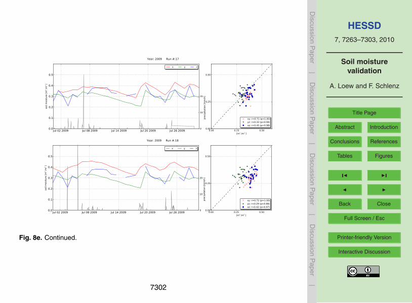
HESSD7, 7263–7303, 2010



Title Page



Tables Figures

J I

J I

Back Close

Full Screen / Esc



Discussion

Paper

|D

iscussionP

aper|

Discussion

Paper

|D

iscussionP

aper|

Jul 02 2009 Jul 08 2009 Jul 14 2009 Jul 20 2009 Jul 26 20090.0

0.1

0.2

0.3

0.4

0.5

soil

moi

stur

e [m

3/m

3]

x y z

0.00 0.25 0.50[m3 /m3 ]

0.00

0.25

0.50

xy: r=0.71 (p=1.00)yz: r=0.33 (p=0.94)xz: r=0.45 (p=0.98)

0

10

20

prec

ipita

tion

[mm

/h]

Year: 2009 Run #:17

Jul 02 2009 Jul 08 2009 Jul 14 2009 Jul 20 2009 Jul 26 20090.0

0.1

0.2

0.3

0.4

0.5

soil

moi

stur

e [m

3/m

3]

x y z

0.00 0.25 0.50[m3 /m3 ]

0.00

0.25

0.50

xy: r=0.72 (p=1.00)yz: r=0.29 (p=0.86)xz: r=0.42 (p=0.97)

0

10

20

prec

ipita

tion

[mm

/h]

Year: 2009 Run #:18

Fig. 8e. Continued.

7302





HESSD7, 7263–7303, 2010



Title Page



Tables Figures

J I

J I

Back Close

Full Screen / Esc



Discussion

Paper

|D

iscussionP

aper|

Discussion

Paper

|D

iscussionP

aper|

0.00 0.02 0.04 0.06 0.08 0.10station error [m3 /m3 ]

0.00

0.02

0.04

0.06

0.08

0.10

estim

ated

sta

tion

erro

r [m

3/m

3]

2008 rmse: 0.00841 [m3 /m3 ]

0.00 0.02 0.04 0.06 0.08 0.10station error [m3 /m3 ]

0.00

0.02

0.04

0.06

0.08

0.10

estim

ated

sta

tion

erro

r [m

3/m

3]

2009 rmse: 0.00835 [m3 /m3 ]

Fig. 9. Comparison of the estimated station error (estat) with the reference soil moisture error(estation) for the years 2008 and 2009 using periods with significant correlations between all soilmoisture data sets.

7303





A dynamic approach for evaluating coarse scale satellite soil moisture products

Documents

Transcript of A dynamic approach for evaluating coarse scale satellite soil moisture products