Atmospheric Environment 38 (2004) 1425–1436

ARTICLE IN PRESS

AE International – Europe

*Correspond

E-mail addr

1352-2310/$ - se

doi:10.1016/j.at

A development of ozone abatement strategies for the Grenoblearea using modeling and indicators

O. Couacha, F. Kirchnera,*, R. Jimeneza, I. Balina, S. Peregob, H. van den Bergha

aAir Pollution Laboratory (LPAS), Swiss Federal Institute of Technology (EPFL), CH-1015 Lausanne, Switzerlandb IBM Suisse, Altstetterstrasse 124, 8010 Zurich, Suisse (Switzerland)

Received 28 July 2003; received in revised form 20 November 2003; accepted 1 December 2003

Abstract

The Grenoble metropolitan area, located in the French Alps, regularly has periods of high ozone concentrations

during the summertime. Grenoble is located in a Y shaped convergence of three deep valleys, some 3000m above sea

level, with typical wind pattern. During the summer of 1999, a major field campaign GRENOble PHOTochemistry

(GRENOPHOT) was held in order to obtain measurements necessary for air quality model validation. The air quality

model METeorological PHOtochemistry MODel (METPHOMOD) is used to investigate the dynamic characteristics of

air pollution in the Grenoble area during the GRENOPHOT field campaign. The meteorological and atmospheric

chemistry simulations were validated using both ground and vertical profile measurements (e.g. lidar) performed during

the observation period (25–27 July) when the measured ozone concentrations reached 95 ppb. Both the spatial as well as

the temporal variability of the simulated ozone concentrations were in good agreement with the measured values. The

highest ozone values were found, in the southern zone, some 20 km downwind of the city center. It was found that

about 32 ppb of fresh ozone are generated in the Grenoble plume. For developing ozone abatement strategies it is

important to know whether in a specific area the ozone production is limited by VOC or NOx: Several indicators wereproposed for distinguishing between VOC and NOx limitation. The morning Y ¼ tVOC

HO =tNOx

HO (the ratio of the lifetimes

of OH against losses by reacting with VOC and NOx) was applied and the afternoon indicator was k¼ ½H2O2�=½HNO3�:The Y indicator gives information about the effect of changes in the emissions on the ozone formation in the air parcel

which passes there, whereas k provides information about the sensitivity of ozone formation in the aging plume. A

combination of both indicators can be used to obtain a comprehensive view of the ozone formation in the Grenoble

area. These results are confirmed by the investigation of the air mass regime with the time evolution of the ozone

isopleths at the maximums locations (south and north west valleys).

r 2003 Elsevier Ltd. All rights reserved.

Keywords: Indicators; Ozone production regimes; Mountains area; Grenoble

1. Introduction

In order to reduce the occurrence of ozone peaks in

urban regions, suitable combinations of NOx and VOC

emissions are necessary. The assessment of an urban

ozone strategy can be undertaken by application of a

validated photochemical model. The photochemical

ing author. Tel.: +41-22-693-61-38.

ess: frank.kirchner@epfl.ch (F. Kirchner).

e front matter r 2003 Elsevier Ltd. All rights reserve

mosenv.2003.12.001

airshed model METPHOMOD (Perego, 1999) was

applied and validated over the city of Grenoble, France,

and the surrounding region during an Intensive Ob-

servation Period (IOP) from 25 to 27 July in the context

of the GRENOPHOT field campaign (Couach et al.,

2002; Quaglia et al., 2000). The difference between the

base case and simulations with reductions in NOx and

VOC emissions are presented and analyzed in this study.

Finally, a combination of the indicator Y ¼ tVOCOH =tNOx

OH

(the ratio of the lifetimes of OH against losses due to

d.

ARTICLE IN PRESS

Rural stations

y = 0.668x + 24.947R2 = 0.575

0

20

40

60

80

100

0 20 40 60 80 100

Ozone measured

Ozo

ne s

imul

ated

Suburb stations

y = 0.6594x + 17.478R2 = 0.4237

0

20

40

60

80

100

0 20 40 60 80 100

Ozone measured

Ozo

ne s

imul

ated

urban stations

y = 0.8582x + 1.9022R2 = 0.6398

0

20

40

60

80

100

0 20 40 60 80 100

Ozone measured

Ozo

ne s

imul

ated

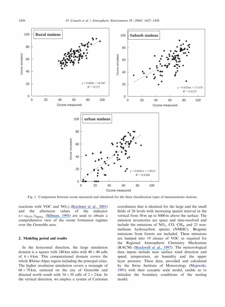
Fig. 1. Comparison between ozone measured and simulated for the three classification types of measurements stations.

O. Couach et al. / Atmospheric Environment 38 (2004) 1425–14361426

reactions with VOC and NOx) (Kirchner et al., 2001)

and the afternoon values of the indicator

k¼ cH2O2=cHNO3

(Sillman, 1995) are used to obtain a

comprehensive view of the ozone formation regimes

over the Grenoble area.

2. Modeling period and results

In the horizontal direction, the large simulation

domain is a square with 240 km sides with 40� 40 cells

of 6� 6 km. This computational domain covers the

whole Rh #one-Alpes region including the principal cities.

The higher resolution simulation covers a rectangle of

68� 78 km, centered on the city of Grenoble and

directed north–south with 34� 39 cells of 2� 2 km. In

the vertical direction, we employ a system of Cartesian

coordinates that is identical for the large and the small

fields of 26 levels with increasing spatial interval in the

vertical from 50m up to 8000m above the surface. The

emission inventories are space and time-resolved and

include the emissions of NOx; CO, CH4, and 23 non-

methane hydrocarbon species (NMHC). Biogenic

emissions from forests are included. These emissions

are lumped into 19 classes of VOC as required for

the Regional Atmospheric Chemistry Mechanism

(RACM) (Stockwell et al., 1997). The meteorological

data inputs include near surface wind direction and

speed, temperature, air humidity and the upper

layer pressure. These data, provided and calculated

by the Swiss Institute of Meteorology (Majewski,

1991) with their synoptic scale model, enable us to

initialize the boundary conditions of the nesting

model.

ARTICLE IN PRESS

(A) (B)

(C)

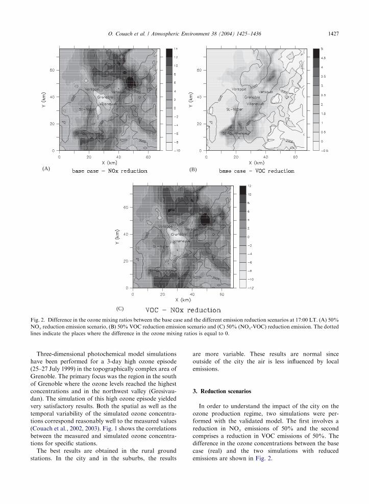
Fig. 2. Difference in the ozone mixing ratios between the base case and the different emission reduction scenarios at 17:00 LT. (A) 50%

NOx reduction emission scenario, (B) 50% VOC reduction emission scenario and (C) 50% (NOx-VOC) reduction emission. The dotted

lines indicate the places where the difference in the ozone mixing ratios is equal to 0.

O. Couach et al. / Atmospheric Environment 38 (2004) 1425–1436 1427

Three-dimensional photochemical model simulations

have been performed for a 3-day high ozone episode

(25–27 July 1999) in the topographically complex area of

Grenoble. The primary focus was the region in the south

of Grenoble where the ozone levels reached the highest

concentrations and in the northwest valley (Gresivau-

dan). The simulation of this high ozone episode yielded

very satisfactory results. Both the spatial as well as the

temporal variability of the simulated ozone concentra-

tions correspond reasonably well to the measured values

(Couach et al., 2002, 2003). Fig. 1 shows the correlations

between the measured and simulated ozone concentra-

tions for specific stations.

The best results are obtained in the rural ground

stations. In the city and in the suburbs, the results

are more variable. These results are normal since

outside of the city the air is less influenced by local

emissions.

3. Reduction scenarios

In order to understand the impact of the city on the

ozone production regime, two simulations were per-

formed with the validated model. The first involves a

reduction in NOx emissions of 50% and the second

comprises a reduction in VOC emissions of 50%. The

difference in the ozone concentrations between the base

case (real) and the two simulations with reduced

emissions are shown in Fig. 2.

ARTICLE IN PRESS

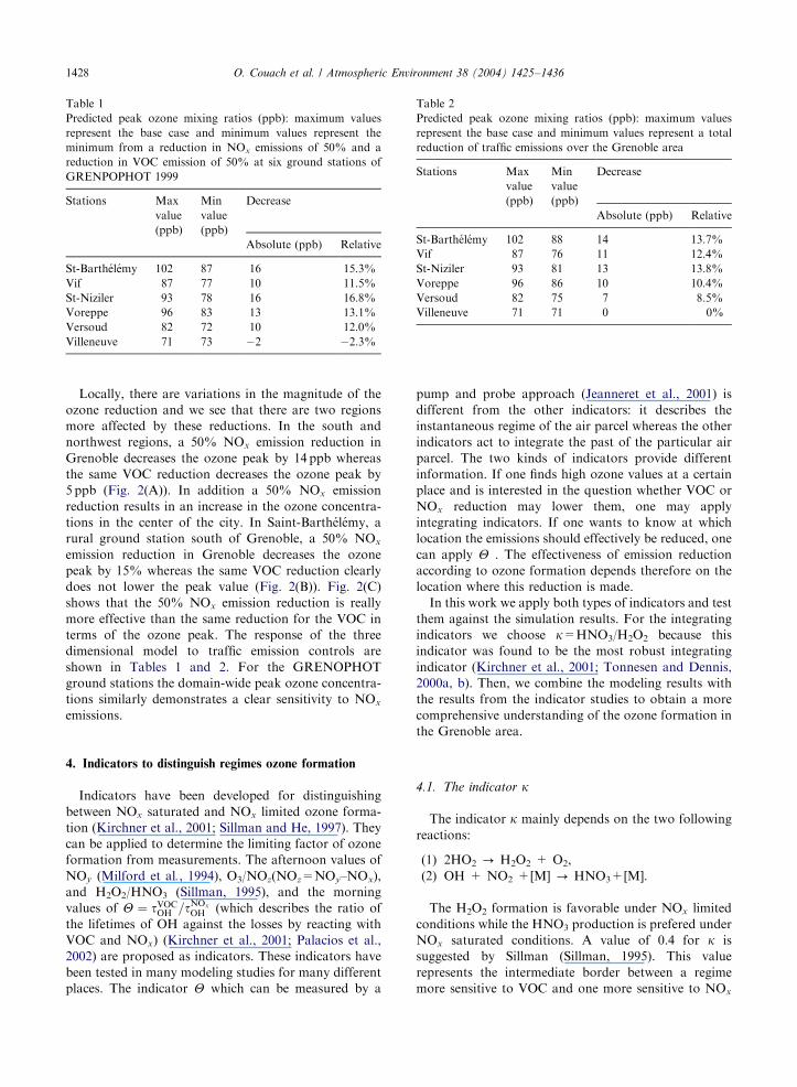
Table 1

Predicted peak ozone mixing ratios (ppb): maximum values

represent the base case and minimum values represent the

minimum from a reduction in NOx emissions of 50% and a

reduction in VOC emission of 50% at six ground stations of

GRENPOPHOT 1999

Stations Max

value

(ppb)

Min

value

(ppb)

Decrease

Absolute (ppb) Relative

St-Barth!el!emy 102 87 16 15.3%

Vif 87 77 10 11.5%

St-Niziler 93 78 16 16.8%

Voreppe 96 83 13 13.1%

Versoud 82 72 10 12.0%

Villeneuve 71 73 �2 �2.3%

Table 2

Predicted peak ozone mixing ratios (ppb): maximum values

represent the base case and minimum values represent a total

reduction of traffic emissions over the Grenoble area

Stations Max

value

(ppb)

Min

value

(ppb)

Decrease

Absolute (ppb) Relative

St-Barth!el!emy 102 88 14 13.7%

Vif 87 76 11 12.4%

St-Niziler 93 81 13 13.8%

Voreppe 96 86 10 10.4%

Versoud 82 75 7 8.5%

Villeneuve 71 71 0 0%

O. Couach et al. / Atmospheric Environment 38 (2004) 1425–14361428

Locally, there are variations in the magnitude of the

ozone reduction and we see that there are two regions

more affected by these reductions. In the south and

northwest regions, a 50% NOx emission reduction in

Grenoble decreases the ozone peak by 14 ppb whereas

the same VOC reduction decreases the ozone peak by

5 ppb (Fig. 2(A)). In addition a 50% NOx emission

reduction results in an increase in the ozone concentra-

tions in the center of the city. In Saint-Barth!el!emy, a

rural ground station south of Grenoble, a 50% NOx

emission reduction in Grenoble decreases the ozone

peak by 15% whereas the same VOC reduction clearly

does not lower the peak value (Fig. 2(B)). Fig. 2(C)

shows that the 50% NOx emission reduction is really

more effective than the same reduction for the VOC in

terms of the ozone peak. The response of the three

dimensional model to traffic emission controls are

shown in Tables 1 and 2. For the GRENOPHOT

ground stations the domain-wide peak ozone concentra-

tions similarly demonstrates a clear sensitivity to NOx

emissions.

4. Indicators to distinguish regimes ozone formation

Indicators have been developed for distinguishing

between NOx saturated and NOx limited ozone forma-

tion (Kirchner et al., 2001; Sillman and He, 1997). They

can be applied to determine the limiting factor of ozone

formation from measurements. The afternoon values of

NOy (Milford et al., 1994), O3/NOz(NOz=NOy–NOx),

and H2O2/HNO3 (Sillman, 1995), and the morning

values of Y ¼ tVOCOH =tNOx

OH (which describes the ratio of

the lifetimes of OH against the losses by reacting with

VOC and NOx) (Kirchner et al., 2001; Palacios et al.,

2002) are proposed as indicators. These indicators have

been tested in many modeling studies for many different

places. The indicator Y which can be measured by a

pump and probe approach (Jeanneret et al., 2001) is

different from the other indicators: it describes the

instantaneous regime of the air parcel whereas the other

indicators act to integrate the past of the particular air

parcel. The two kinds of indicators provide different

information. If one finds high ozone values at a certain

place and is interested in the question whether VOC or

NOx reduction may lower them, one may apply

integrating indicators. If one wants to know at which

location the emissions should effectively be reduced, one

can apply Y . The effectiveness of emission reduction

according to ozone formation depends therefore on the

location where this reduction is made.

In this work we apply both types of indicators and test

them against the simulation results. For the integrating

indicators we choose k=HNO3/H2O2 because this

indicator was found to be the most robust integrating

indicator (Kirchner et al., 2001; Tonnesen and Dennis,

2000a, b). Then, we combine the modeling results with

the results from the indicator studies to obtain a more

comprehensive understanding of the ozone formation in

the Grenoble area.

4.1. The indicator k

The indicator k mainly depends on the two following

reactions:

(1)

2HO2 - H2O2 + O2,

(2)

OH + NO2 +[M] - HNO3+[M].

The H2O2 formation is favorable under NOx limited

conditions while the HNO3 production is prefered under

NOx saturated conditions. A value of 0.4 for k is

suggested by Sillman (Sillman, 1995). This value

represents the intermediate border between a regime

more sensitive to VOC and one more sensitive to NOx

ARTICLE IN PRESSO. Couach et al. / Atmospheric Environment 38 (2004) 1425–1436 1429

and it is valid for moderately polluted conditions with

80–150 ppb O3 (Sillman and He, 2002).

4.2. The indicator Y

Three-dimensional simulations were performed to test

the behavior of the indicator Y for different times 8:00,

10:00 and 12:00 LT. The indicator was tested by

increasing the NOx emissions in the whole area. Between

8:00 and 9:00 LT the mean value of NOx emissions over

the whole modeling domain was 12mol km�2 h�1. For

test case 1 in the first 2min after 8:00 LT the

same amount of 12mol km�2 NOx emissions was

additionally emitted from each surface grid cell.

Together with the additional NOx in each grid cell

either Tracer A or Tracer B was emitted, depending

on the value of the indicator Y ¼ tVOCOH =tNOx

OH at 8:00 LT

in that grid cell. Tracer A was emitted from those

grid cells where Y was below 0.2, tracer B from the

other grid cells. The emission rate was 12mol km�2 h�1

and therefore identical with the one of the

additional emitted NOx. Both tracers are chemi-

cally inert. During the following hours of the simula-

tion the tracers provide two important pieces of

information:

* The kind of the tracer provides information on the

origin of the air parcel.* The sum of all tracers provides information on the

amount of NOx that has been additionally emitted to

this air parcel.

-10

-5

0

5

10

150 2 4

H2O2

ozo

ne

red

uct

ion

(pp

b)

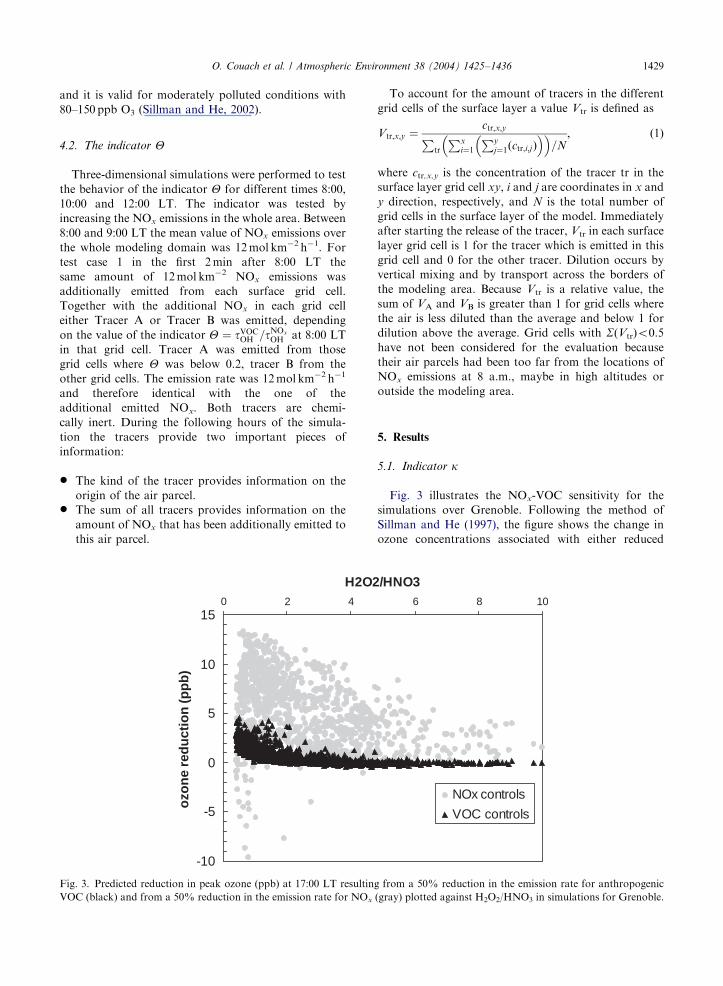
Fig. 3. Predicted reduction in peak ozone (ppb) at 17:00 LT resultin

VOC (black) and from a 50% reduction in the emission rate for NOx

To account for the amount of tracers in the different

grid cells of the surface layer a value Vtr is defined as

Vtr;x;y ¼ctr;x;yP

tr

Pxi¼1

Pyj¼1ðctr;i;jÞ

� �� �=N

; ð1Þ

where ctr,x,y is the concentration of the tracer tr in the

surface layer grid cell xy, i and j are coordinates in x and

y direction, respectively, and N is the total number of

grid cells in the surface layer of the model. Immediately

after starting the release of the tracer, Vtr in each surface

layer grid cell is 1 for the tracer which is emitted in this

grid cell and 0 for the other tracer. Dilution occurs by

vertical mixing and by transport across the borders of

the modeling area. Because Vtr is a relative value, the

sum of VA and VB is greater than 1 for grid cells where

the air is less diluted than the average and below 1 for

dilution above the average. Grid cells with S(Vtr)o0.5

have not been considered for the evaluation because

their air parcels had been too far from the locations of

NOx emissions at 8 a.m., maybe in high altitudes or

outside the modeling area.

5. Results

5.1. Indicator k

Fig. 3 illustrates the NOx-VOC sensitivity for the

simulations over Grenoble. Following the method of

Sillman and He (1997), the figure shows the change in

ozone concentrations associated with either reduced

6 8 10

/HNO3

NOx controls

VOC controls

g from a 50% reduction in the emission rate for anthropogenic

(gray) plotted against H2O2/HNO3 in simulations for Grenoble.

ARTICLE IN PRESS

noon

0% 20% 40% 60% 80% 100%

-18 to -10

-10 to -3

-3 to +3

+3 to +10

+10 to +18

Tracer B (NOx saturated)

Tracer A (NOx limited)

> 0.2

< 0.2

Number ofgrid cells

Number ofgrid cellsconsidered

Mean tracermixing ratioppb

33

476

589

201

26

33

365

284

201

26

4.03

3.97

4.83

7.65

11.89

noon

0% 20% 40% 60% 80% 100%

-18 to -10

-10 to -3

-3 to +3

+3 to +10

+10 to +18

Tracer B (NOx saturated)

Tracer A (NOx limited)

> 0.2

< 0.2

Number ofgrid cells

Number ofgrid cellsconsidered

Mean tracermixing ratioppb

33

476

589

201

26

33

365

284

201

26

4.03

3.97

4.83

7.65

11.89

Number ofgrid cells

Number ofgrid cellsconsidered

Mean tracermixing ratioppb

33

476

589

201

26

33

365

284

201

26

4.03

3.97

4.83

7.65

11.89

5 p.m.

0% 20% 40% 60% 80% 100%

0 to +3

+3 to +5

+5 to +8

+8 to +15

+15 to +20

Tracer

Number ofgrid cells

Number ofgrid cells considered

Mean tracermixing ratioppb

13

254

533

216

290

13

254

533

156

3

4.58

2.85

1.72

1.25

1.12

5 p.m.

0% 20% 40% 60% 80% 100%

0 to +3

+3 to +5

+5 to +8

+8 to +15

+15 to +20

Tracer

Number ofgrid cells

Number ofgrid cells considered

Mean tracermixing ratioppb

13

254

533

216

290

13

254

533

156

3

4.58

2.85

1.72

1.25

1.12

Number ofgrid cells

Number ofgrid cells considered

Mean tracermixing ratioppb

13

254

533

216

290

13

254

533

156

3

4.58

2.85

1.72

1.25

1.12

3 p.m.

0% 20% 40% 60% 80% 100%

-5 to -2

-2 to 2

+2 to +8

+8 to +15

+15 to +24

Number ofgrid cells

Number ofgrid cells considered

Mean tracermixing ratioppb

12

320

645

348

1

12

320

564

50

1

3.91

2.84

2.03

3.05

6.44

3 p.m.

0% 20% 40% 60% 80% 100%

-5 to -2

-2 to 2

+2 to +8

+8 to +15

+15 to +24

Number ofgrid cells

Number ofgrid cells considered

Mean tracermixing ratioppb

12

320

645

348

1

12

320

564

50

1

3.91

2.84

2.03

3.05

6.44

Number ofgrid cells

Number ofgrid cells considered

Mean tracermixing ratioppb

12

320

645

348

1

12

320

564

50

1

3.91

2.84

2.03

3.05

6.44

∆ ∆ O

3 (pp

b)∆ ∆

O3 (

ppb)

∆ ∆ O

3 (pp

b)

Tracer

Tracer

Fig. 4. Comparison between the tracer (tracer A in black Yo0.2 (NOx limited) and tracer B in white Y>0.2 (NOx saturated)) mixing

ratios and the changes in the ozone formation at noon and 15:00 LT due to additional NOx and tracer emissions emitted at 08:00 LT in

the Grenoble simulation.

O. Couach et al. / Atmospheric Environment 38 (2004) 1425–14361430

ARTICLE IN PRESS

noon

0% 20% 40% 60% 80% 100%

-18 to -14

-14 to -2

-2 to +3

+3 to +10

+10 to +18

< 0.2

Number ofgrid cells

Number ofgrid cellsconsidered

Mean tracermixing ratioppb

110

344

477

391

4

103

258

266

391

4

10.63

11.45

12.94

18.97

18.06

noon

0% 20% 40% 60% 80% 100%

-18 to -14

-14 to -2

-2 to +3

+3 to +10

+10 to +18

Number ofgrid cells

Number ofgrid cellsconsidered

Mean tracermixing ratioppb

110

344

477

391

4

103

258

266

391

4

10.63

11.45

12.94

18.97

18.06

Number ofgrid cells

Number ofgrid cellsconsidered

Mean tracermixing ratioppb

110

344

477

391

4

103

258

26

1

4

10.6

11.45

12.94

18.97

18.06

3 p.m.

0% 20% 40% 60% 80% 100%

-8 to -2

-2 to 2

+2 to +8

+8 to +15

+15 to +24

Tracer

Number ofgrid cells

Number ofgrid cellsconsidered

Mean tracermixing ratioppb

17 17 9.66

3 p.m.

0% 20% 40% 60% 80% 100%

-8 to -2

-2 to 2

+2 to +8

+8 to +15

+15 to +24

Tracer

Number ofgrid cells

Number ofgrid cellsconsidered

Mean tracermixing ratioppb

17 17 9.66

Number ofgrid cells

Number ofgrid cellsconsidered

Mean tracermixing ratioppb

17

403

584

320

2

17

403

501

87

2

9.66

6.89

4.88

7.72

12.48

5 p.m.

0% 20% 40% 60% 80% 100%

-2 to +2

+2 to +4

+4 to +8

+8 to +15

+15 to +24

Tracer

Number ofgrid cells

Number ofgrid cellsconsidered

Mean tracermixing ratioppb

21

194

21

3

7.64

5.99

5 p.m.

0% 20% 40% 60% 80% 100%

-2 to +2

+2 to +4

+4 to +8

+8 to +15

+15 to +24

Tracer

Number ofgrid cells

Number ofgrid cellsconsidered

Mean tracermixing ratioppb

21

194

21

3

7.64

5.99

Number ofgrid cells

Number ofgrid cellsconsidered

Mean tracermixing ratioppb

21

38

58

13

194

21

388

578

32

3

7.64

6.34

4.16

2.68

5.99

∆ ∆ O

3 (pp

b)∆ ∆

O3 (

ppb)

∆ ∆ O

3 (pp

b)

Tracer

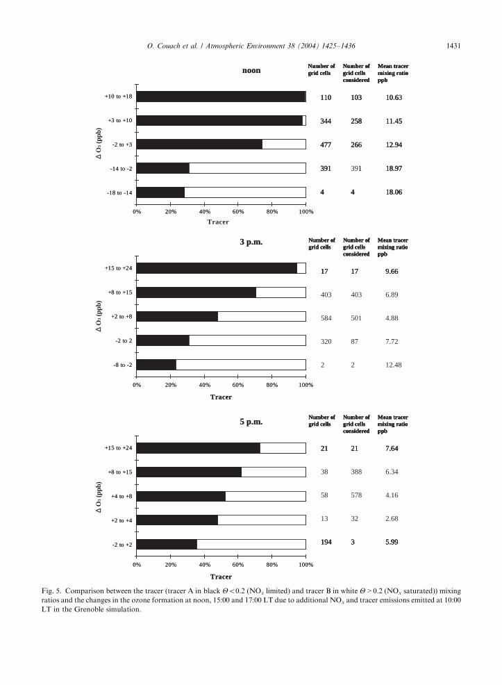
Fig. 5. Comparison between the tracer (tracer A in black Yo0.2 (NOx limited) and tracer B in white Y>0.2 (NOx saturated)) mixing

ratios and the changes in the ozone formation at noon, 15:00 and 17:00 LT due to additional NOx and tracer emissions emitted at 10:00

LT in the Grenoble simulation.

O. Couach et al. / Atmospheric Environment 38 (2004) 1425–1436 1431

ARTICLE IN PRESS

3 p.m.

0% 20% 40% 60% 80% 100%

-8 to -2

-2 to +2

+2 to +8

+8 to +15

+15 to +20

Number ofgrid cells

Number ofgrid cellsconsidered

Mean tracermixing ratioppb

23

389

620

260

34

23

389

34

9.59

6.58

4.17

5.26

7.02

3 p.m.

0% 20% 40% 60% 80% 100%

-8 to -2

-2 to +2

+2 to +8

+8 to +15

+15 to +20

Number ofgrid cells

Number ofgrid cellsconsidered

Mean tracermixing ratioppb

23

389

620

260

34

23

389

34

9.59

6.58

4.17

5.26

7.02

Number ofgrid cells

Number ofgrid cellsconsidered

Mean tracermixing ratioppb

23

389

620

260

34

23

389

486

158

34

9.59

6.58

4.17

5.26

7.02

5 p.m.

0% 20% 40% 60% 80% 100%

-2 to +2

+2 to +4

+4 to +8

+8 to +15

+15 to +22

Number ofgrid cells

Number ofgrid cellsconsidered

Mean tracermixing ratioppb

61

383

528

238

116

61

383

508

1

6.91

5.16

3.62

3.29

2.16

5 p.m.

0% 20% 40% 60% 80% 100%

-2 to +2

+2 to +4

+4 to +8

+8 to +15

+15 to +22

Number ofgrid cells

Number ofgrid cellsconsidered

Mean tracermixing ratioppb

61

383

528

238

116

61

383

1

6.91

5.16

3.62

3.29

2.16

Number ofgrid cells

Number ofgrid cellsconsidered

Mean tracermixing ratioppb

61

383

528

238

116

61

383

109

1

6.91

5.16

3.62

3.29

2.16

∆ ∆ O

3 (pp

b)∆ ∆

O3 (

ppb)

Tracer

Tracer

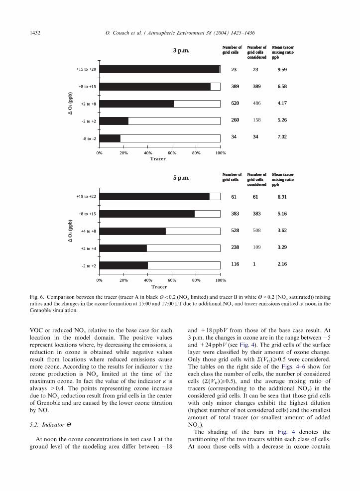
Fig. 6. Comparison between the tracer (tracer A in black Yo0.2 (NOx limited) and tracer B in white Y>0.2 (NOx saturated)) mixing

ratios and the changes in the ozone formation at 15:00 and 17:00 LT due to additional NOx and tracer emissions emitted at noon in the

Grenoble simulation.

O. Couach et al. / Atmospheric Environment 38 (2004) 1425–14361432

VOC or reduced NOx relative to the base case for each

location in the model domain. The positive values

represent locations where, by decreasing the emissions, a

reduction in ozone is obtained while negative values

result from locations where reduced emissions cause

more ozone. According to the results for indicator k the

ozone production is NOx limited at the time of the

maximum ozone. In fact the value of the indicator k is

always >0.4. The points representing ozone increase

due to NOx reduction result from grid cells in the center

of Grenoble and are caused by the lower ozone titration

by NO.

5.2. Indicator Y

At noon the ozone concentrations in test case 1 at the

ground level of the modeling area differ between �18

and +18ppbV from those of the base case result. At

3 p.m. the changes in ozone are in the range between �5

and +24 ppbV (see Fig. 4). The grid cells of the surface

layer were classified by their amount of ozone change.

Only those grid cells with S(Vtr)X0.5 were considered.

The tables on the right side of the Figs. 4–6 show for

each class the number of cells, the number of considered

cells (S(Vtr)X0.5), and the average mixing ratio of

tracers (corresponding to the additional NOx) in the

considered grid cells. It can be seen that those grid cells

with only minor changes exhibit the highest dilution

(highest number of not considered cells) and the smallest

amount of total tracer (or smallest amount of added

NOx).

The shading of the bars in Fig. 4 denotes the

partitioning of the two tracers within each class of cells.

At noon those cells with a decrease in ozone contain

ARTICLE IN PRESSO. Couach et al. / Atmospheric Environment 38 (2004) 1425–1436 1433

high amounts of the tracer B and therefore originate

from grid cells for which the indicator Y indicates NOx

saturation at 8:00 LT. In contrast the air parcels with the

largest ozone increases contain only small amounts of

tracer B but high amounts of A. In the following hours

transport and mixing lowers the contrast between the

different air parcels but nevertheless also at 15:00 LT the

grid cells with the highest ozone increase contain at least

80% of tracer A.

In test case 2 we emitted the additional NOx and the

tracers at 10:00 LT, instead of 8:00 LT. The tracers A

and B were emitted according to the values of Y at 10:00

LT. Everything else was as in test case 1. Fig. 5 shows

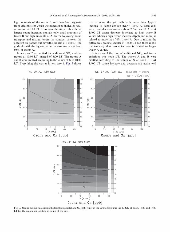
Fig. 7. Ozone mixing ratios isopleths [ppb] (grayscale) and Ox [ppb] (l

LT for the maximum location in south of the city.

that at noon the grid cells with more than 3 ppbV

increase of ozone contain nearly 100% A. Grid cells

with ozone decrease contain about 70% tracer B. Also at

15:00 LT ozone decrease is related to high tracer B

values whereas high ozone increase (8 ppb and more) is

related to more than 70% tracer A. Due to mixing the

differences become smaller at 17:00 LT but there is still

the tendency that ozone increase is related to larger

tracer A values.

In test case 3 the time of additional NOx and tracer

emissions was noon LT. The tracers A and B were

emitted according to the values of Y at noon LT. At

15:00 LT ozone increase and decrease are again well

ine) in the Grenoble plume the 27 July at noon, 15:00 and 17:00

ARTICLE IN PRESS

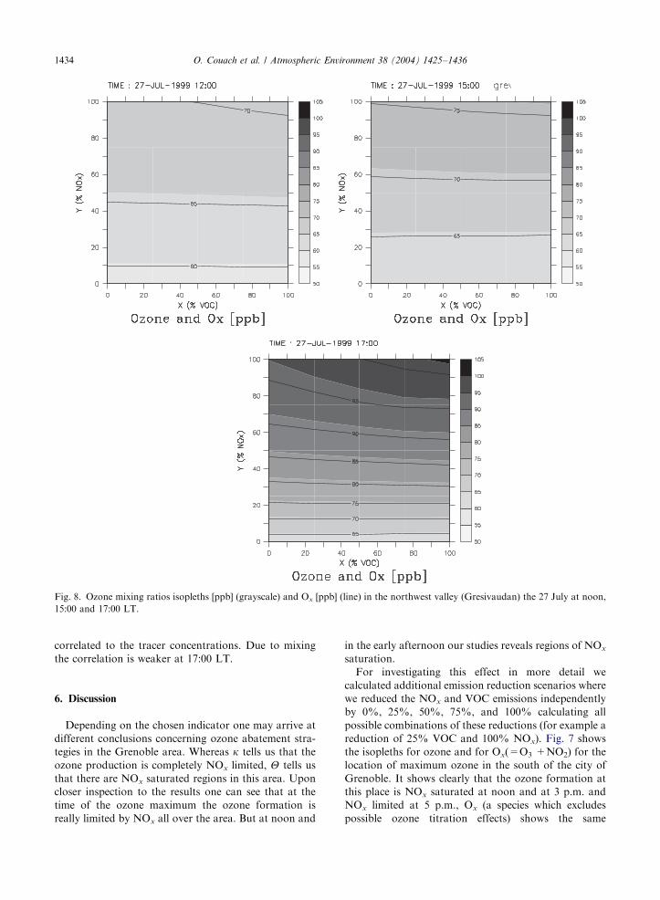
Fig. 8. Ozone mixing ratios isopleths [ppb] (grayscale) and Ox [ppb] (line) in the northwest valley (Gresivaudan) the 27 July at noon,

15:00 and 17:00 LT.

O. Couach et al. / Atmospheric Environment 38 (2004) 1425–14361434

correlated to the tracer concentrations. Due to mixing

the correlation is weaker at 17:00 LT.

6. Discussion

Depending on the chosen indicator one may arrive at

different conclusions concerning ozone abatement stra-

tegies in the Grenoble area. Whereas k tells us that the

ozone production is completely NOx limited, Y tells us

that there are NOx saturated regions in this area. Upon

closer inspection to the results one can see that at the

time of the ozone maximum the ozone formation is

really limited by NOx all over the area. But at noon and

in the early afternoon our studies reveals regions of NOx

saturation.

For investigating this effect in more detail we

calculated additional emission reduction scenarios where

we reduced the NOx and VOC emissions independently

by 0%, 25%, 50%, 75%, and 100% calculating all

possible combinations of these reductions (for example a

reduction of 25% VOC and 100% NOx). Fig. 7 shows

the isopleths for ozone and for Ox(=O3 +NO2) for the

location of maximum ozone in the south of the city of

Grenoble. It shows clearly that the ozone formation at

this place is NOx saturated at noon and at 3 p.m. and

NOx limited at 5 p.m., Ox (a species which excludes

possible ozone titration effects) shows the same

ARTICLE IN PRESS

Fig. 9. Spatial control ozone production regimes calculated with the Y indicator (bold line) over the Grenoble area the 27 July at

08:00, 10:00 and noon LT. Tick line show the highway and thin lines show the topography.

O. Couach et al. / Atmospheric Environment 38 (2004) 1425–1436 1435

dependence. Fig. 8 shows that the situation at the place

of the ozone maximum in the North of the city of

Grenoble is completely different. Here we find NOx

limitation all the time.

Ozone abatement strategies have to consider all these

spatial and temporal changes in the limitation of

maximum ozone values. A combination of the results

of the indicator studies and of the emission reduction

scenarios gives us a comprehensive view of the situation.

The indicator k tells us that the NOx emissions in that

region must be lowered in order to decrease the

maximum ozone concentrations. But from the reduction

scenarios we know that reducing only NOx will lead to

increasing ozone values at some locations at noon and in

the early afternoon. For finding the places where the

NOx reduction must be accompanied by VOC reduc-

tions in order to avoid increasing ozone concentrations

in the early afternoon we can use the results from the

indicatorY. The study shows that the indicatorY works

well and that there is a strong correlation between the Y

values at the place and the time of emission and the

change in the ozone several hours later.

Fig. 9 presents the distribution of NOx sensitive and

NOx saturated areas according to the indicator values of

Y. At the NOx saturated locations the NOx reduction

must be accompanied by VOC reduction. Fig. 9 shows

that the areas with indicator values below or above 0.2

do not considerably change between 8 a.m. and noon.

That means that by this method for each location a

specific regime can be attributed and therefore location

specific emission reductions can be developed.

7. Conclusion

Three-dimensional photochemical model simulations

have been performed for a 3 day episode in the

topographically complex area of Grenoble and base

case was validated. Based on the model scenarios over

Grenoble and on the combination of the indicators Y

ARTICLE IN PRESSO. Couach et al. / Atmospheric Environment 38 (2004) 1425–14361436

and k one can say that the region of the maximum ozone

is NOx limited. Nevertheless this study shows also that

some areas are NOx saturated before the time of the

ozone maximum. Applying the indicator Y allowed the

identification of the locations where NOx reduction

must be accompanied by VOC reduction in order to

avoid increasing ozone concentrations at noon and in

the early afternoon.

References

Couach, O., Balin, I., Jim!enez, R., Perego, S., Kirchner, F.,

Ristori, P., Simeonov, V., Quaglia, P., Vestri, V., Clappier,

A., Calpini, B., Van den Bergh, H., 2002. Study of a

photochemical episode over the Grenoble area using a

mesoscale model and intensive measurements. Pollution

Atmosph!erique 174, 277–295.

Couach, O., Balin, I., Jim!enez, R., Ristori, P., Kirchner, F.,

Perego, S., Simeonov, V., Calpini, B., Van den Bergh, H.,

2003. Ozone and planetary boundary layer dynamics on a

complex topography area of Grenoble by measurements

and modeling. Atmospheric Chemical and Physics (3),

549–562.

Jeanneret, F., Kirchner, F., Clappier, A., van den Bergh, H.,

Calpini, B., 2001. Total VOC reactivity in the planetary

boundary layer. Part one: estimation by a new experimental

technique. Journal of Geophysical Research 106 (D3),

3083–3093.

Kirchner, F., Jeanneret, F., Clappier, A., Kr .uger, B., Van den

Bergh, H., Calpini, B., 2001. Total VOC reactivity in the

planetary boundary layer 2. A new indicator for determin-

ing the sensitivity of the ozone production to VOC

and NOx. Journal of Geophysical Research 106 (D3),

3095–3110.

Majewski, D., 1991. The Europa Modell of the Wetterdienst,

ECMWF Seminar on Numerical Methods in Atmospheric

Models, Vol. 2, pp. 147–191.

Milford, J., Gao, D., Sillman, S., Blossey, P., Russel, A.G.,

1994. Total reactive nitrogen (NOy) as an indicator for the

sensitivity of ozone to NOx and hydrocarbons. Journal of

Geophysical Research 99, 3533–3542.

Palacios, M., Kirchner, F., Martilli, A., Clappier, A., Martin,

F., Rogriguez, M.E., 2002. Response of selected chemical

mechanisms in effects of ozone control strategies applied to

the greater Madrid area. Atmospheric Environment 36,

5323–5333.

Perego, S., 1999. Metphomod—a numerical mesoscale model

for simulation of regional photosmog in complex terrain:

model description and application during Pollumet 1993

(Switzerland). Meteorology and Atmospheric Physics (70),

43–69.

Quaglia, P., Couach, O., Balin, J., Simeonov, V., Lazzarotto,

B., Van den Bergh, H., Calpini, B., 2000. Air pollution

measurements during the Grenoble campaign. In: Eurotrac

Symposium, Garmish-Partenkirchen.

Sillman, S., 1995. The use of NOy, H2O2, and HNO3 as

indicators for ozone-NOx-hydrocarbon sensitivity in urban

locations. Journal of Geophysical Research 100 (D7),

14175–14188.

Sillman, S., He, D., 1997. The use of photochemical indicators

to evaluate ozone-NOx-hydrocarbon sensitivity: case studies

from Atlanta, New York and Los Angeles. Journal of the

Air and Waste Management Association 47, 1030–1040.

Sillman, S., He, D., 2002. Some theoretical results concerning

O3-NOx-VOC chemistry and NOx-VOC indicators. Journal

of Geophysical Research 107 (D22), 4659–4673.

Stockwell, W.R., Kirchner, F., Kuhn, M., Seefeld, S., 1997. A

new mechanism for regional atmospheric chemistry

modeling. Journal of Geophysical Research 102 (D22),

25847–25879.

Tonnesen, G.S., Dennis, R.G., 2000a. Analysis of radical

propagation efficiency to assess ozone sensitivity to hydro-

carbons and NOx, 2, Long-lived species as indicators of

ozone concentration sensitivity. Journal of Geophysical

Research 105, 9227–9241.

Tonnesen, G.S., Dennis, R.L., 2000b. Analysis of radical

propagation efficiency to assess ozone sensitivity to hydro-

carbons and NOx, 1 Local indicators of instantaneous odd

oxygen production sensitivity. Journal of Geophysical

Research 105, 9213–9225.