This article was downloaded by: [GROUPE ESC TOULOUSE], [Professor Uche Okongwu]On: 08 July 2011, At: 05:08Publisher: Taylor & FrancisInforma Ltd Registered in England and Wales Registered Number: 1072954 Registered office: Mortimer House,37-41 Mortimer Street, London W1T 3JH, UK

Production Planning & ControlPublication details, including instructions for authors and subscription information:http://www.tandfonline.com/loi/tppc20

A decision support system for optimising the orderfulfilment processUche Okongwu a , Matthieu Lauras a b , Lionel Dupont b & Vérane Humez ba Department of Industrial Organisation, Logistics and Technology, Université de Toulouse,Toulouse Business School, 20 Boulevard Lascrosses, 31068 Toulouse Cedex 7, Franceb Department of Industrial Engineering, Université de Toulouse, Mines Albi, Route de Teillet,81013 Albi Cedex 9, France

Available online: 1 January 2011

To cite this article: Uche Okongwu, Matthieu Lauras, Lionel Dupont & Vérane Humez (2011): A decision support system foroptimising the order fulfilment process, Production Planning & Control, DOI:10.1080/09537287.2011.566230

To link to this article: http://dx.doi.org/10.1080/09537287.2011.566230

PLEASE SCROLL DOWN FOR ARTICLE

Full terms and conditions of use: http://www.tandfonline.com/page/terms-and-conditions

This article may be used for research, teaching and private study purposes. Any substantial or systematicreproduction, re-distribution, re-selling, loan, sub-licensing, systematic supply or distribution in any form toanyone is expressly forbidden.

The publisher does not give any warranty express or implied or make any representation that the contentswill be complete or accurate or up to date. The accuracy of any instructions, formulae and drug doses shouldbe independently verified with primary sources. The publisher shall not be liable for any loss, actions, claims,proceedings, demand or costs or damages whatsoever or howsoever caused arising directly or indirectly inconnection with or arising out of the use of this material.

Production Planning & Control2011, 1–18, iFirst

A decision support system for optimising the order fulfilment process

Uche Okongwua, Matthieu Laurasab*, Lionel Dupontb and Verane Humezb

aDepartment of Industrial Organisation, Logistics and Technology, Universite de Toulouse, Toulouse Business School,20 Boulevard Lascrosses, 31068 Toulouse Cedex 7, France; bDepartment of Industrial Engineering, Universite de Toulouse,

Mines Albi, Route de Teillet, 81013 Albi Cedex 9, France

(Final version received 7 February 2011)

Many authors have highlighted gaps at the interfaces between supply chains (SCs) and demand chains. Generally,the latter tends primarily to be ‘agile’ by maximising effectiveness and responsiveness while the former tends to be‘lean’ by maximising efficiency. When, in the SC, disruptions (that lead to stock-out situations) occur aftercustomer orders have been accepted, managers are faced with the problem of maximising customer satisfactionwhile taking into consideration the conflicting objectives of the supply and demand sides of the order fulfilmentprocess. This article proposes a cross-functional multi-criteria decision-making (advanced available-to-promise)tool that provides different strategic options from which a solution can be chosen. It also proposes a performancemeasurement system to support the decision-making and improvement process. The results of some experimentaltests show that the model enables to make strategic decisions on the degree of flexibility required to achieve thedesired level of customer service.

Keywords: supply chain; demand chain; advanced available-to-promise; order fulfilment process; agility; lean

1. Introduction

In today’s highly globalised economy and competitiveenvironment, most businesses are market-driven.Firms therefore look for new concepts, techniquesand tools that would enable them to manage theirdemand and supply chains (SCs) in order to improvecustomer satisfaction, competitiveness and profitabil-ity. Customer satisfaction would lead to customerloyalty, which is one of the factors necessary toguarantee the sustainability of any business. In orderto guarantee sustainable growth, companies aim tokeep existing customers while gaining new ones. To dothis, they do not have to be highly competitive only oncost and quality, but also on the reliability and speed ofdelivering customer orders. The order fulfilment pro-cess (OFP) is therefore one of the most importantprocesses within an organisation and is considered byLin and Shaw (1998) as one of the three pillars of acompany, the other two being the product develop-ment process and the customer service process.

Croxton et al. (2001) break the OFP into twocomponents: the strategic process, which ‘considers themanufacturing, logistics and marketing requirementsnecessary to design the distribution network’ and theoperational process, which ‘defines the specific stepsrelated to the way customer orders are generated andcommunicated, recorded, processed, documented,

picked, delivered, and handled after delivery’. This

article develops a model that enables to measure the

performance of the operational process, on the basis of

which decisions can be made in order to improve thestrategic process. Though not explicit in the activities

described by Lin and Shaw (1998) and Croxton et al.

(2001), the OFP can be broken down into two phases:

. The first phase comprises the order promising

activity (also referred to as ‘availability

check’), which verifies the availability of

resources in order to promise to the customer

a given quantity that will be delivered on a

given date. Readers interested in the details ofthis phase should refer to the work done by

Chen et al. (2008).. The second phase comprises the execution (or

order fulfilment) activity, where the order is

actually delivered as promised.

In an ideal situation, customer orders would be

delivered as promised. In reality, operational disrup-

tions such as machine breakdowns, material shortage

and quality defects can lead to stock-out situations. If

these disruptions occur at the first phase, then some ofthe customer orders may simply not be accepted. But,

if they occur at the second phase, then some of the

already accepted customer orders may not be fulfilled.

*Corresponding author. Email: matthieu.lauras@mines-albi.fr

ISSN 0953–7287 print/ISSN 1366–5871 online

� 2011 Taylor & Francis

DOI: 10.1080/09537287.2011.566230

http://www.informaworld.com

Dow

nloa

ded

by [

GR

OU

PE E

SC T

OU

LO

USE

], [

Prof

esso

r U

che

Oko

ngw

u] a

t 05:

08 0

8 Ju

ly 2

011

This article considers the second phase of the OFP andlooks at how best already accepted customer orderscan be fulfilled in stock-out situations. This entailsdeveloping a decision-making tool as well as a set ofindicators to measure and improve the performance ofthe OFP. Within the OFP, the order management(OM) activity consists in analysing orders and manag-ing backlog in order to determine if, how and whenorders can be delivered. Its main objectives are twodimensional (Lin and Shaw 1998):

. delivering qualified products to fulfil customerorders at the right time and right place;

. achieving agility to handle uncertainties frominternal or external environments.

In practice, there are techniques that enable theOM activity to partly achieve these goals by choosingbetween different alternatives. As they will be discussedin Section, these techniques are available-to-promise(ATP), advanced available-to-promise (AATP), cap-able-to-promise (CTP) and profitable-to-promise(PTP). However, in the case of stock-out, they areinsufficient for decision making in the face of certainvariables such as unknown availability, product sub-stitution and specific operations.

An OFP involves generating, filling, delivering andservicing customer orders (Croxton 2003). It is acomplex process because it is composed of severalactivities, executed by different functional entities, andheavily interdependent among the tasks, resources andentities involved in the process (Lin and Shaw 1998).Even though it has a clear global objective to provideto the customer the right product, at the right time, atthe right place at the right price, each functional entitythat participates in this process generally tries toachieve their own individual objectives. These objec-tives are often antagonistic. For example, in the case ofstock-out, distribution may prefer to ship everything inone batch on a later date; the sales department maywant to send backorders separately; marketing maynot want to sell some products separately; manufactur-ing may not want to change their schedule; and ofcourse, the customer would want to be delivered aspromised.

This article therefore also aims to look at how theconflicting objectives of the different functional entitiescan be taken into consideration in the decision supportsystem that is used to manage the OFP.

In the following section, we will discuss theliterature concerning decision support systems usedto support the OFP. We will go on to develop anddiscuss the set of indicators that will be used tomeasure the performance of the OFP based on ourmodel. Then, our advanced ATP model is described

and applied to a practical case. Finally, we will discuss

the results, before drawing some conclusions that willinclude perspectives for further research.

2. Decision support systems

2.1. Conventional order fulfilment techniques

There are several techniques that support the OFP andmore precisely the OM activity. The most commonly

used is probably ATP. In the 11th edition of theAPICS dictionary (2005), the American Production

and Inventory Control Society defined ATP as ‘theuncommitted portion of a company’s inventory andplanned production maintained in the master produc-

tion schedule to support customer order promising’.This promising mechanism is suitable for make-to-

stock (MTS) production systems where finished goods(FG) are produced based on demand forecast and keptin inventory before orders are received from customers.

In make-to-order (MTO), as well as in assemble-to-

order (ATO) and engineer-to-order (ETO) strategies,delivery dates have to be set based on available

capacity and material constraints in order to avoid‘over promising’ and ‘under promising’ on job orders.Techniques used to achieve this goal are referred to

as CTP.A third technique, referred to as PTP, is used when

profitability is taken into consideration in addition tocapacity and material constraints. Kirche et al. (2005)

define PTP as ‘the ability to respond to a customerorder by determining how profitable it is to accept this

order’. The analysis of a PTP system allows thebusiness to find out if a particular order will be

profitable to make, considering the raw material costs,process costs, inventory costs and other costs againstthe price the customer is willing to pay. In the case of

MTS, PTP works on the data from distributionplanning, while in the case of ATO, MTO and ETO,

it works on the data from production planning.This article deals with an MTS strategy, where the

customer is delivered from FG inventory and sched-uled production.

As pointed out by Chen et al. (2002), ATP consists

in simply monitoring the uncommitted portion ofcurrent and future available FG. Note that if nopromise can be found for an order, the SC will not be

able to fulfil the order within the allocation planninghorizon (Kilger and Schneeweiss 2000). It is therefore

more or less static. In Section 1, we mentioned that theOFP is composed of two phases: order promising andorder fulfilment, ATP techniques are mostly used for

the first phase, as described by Xiong et al. (2006).

2 U. Okongwu et al.

Dow

nloa

ded

by [

GR

OU

PE E

SC T

OU

LO

USE

], [

Prof

esso

r U

che

Oko

ngw

u] a

t 05:

08 0

8 Ju

ly 2

011

This article looks essentially at the order fulfilmentphase. In other words, the issue is: what happens whenorders have been promised, but the available quantitiesare not sufficient to fulfil these orders in the rightquantities and at the promised due dates?

2.2. Advanced order fulfilment techniques

Given the limitations of ATP models, some authorshave proposed to develop AATP models in order toenhance the responsiveness of order promising and thereliability of order fulfilment (Pibernik 2005). Chenet al. (2002) define AATP as ‘a decision-makingmechanism that can dynamically handle the uncertaintyand unanticipated changes related to suppliers andcustomers, as well as production processes’. In otherwords, AATP directly links available resources (i.e. rawmaterials, FG and work-in-progress) as well as produc-tion and distribution capacities with customer orders inorder to improve overall performance by bridging thegap between the forecast-driven SC and the order-driven demand chain (DC). Two characteristics used byPibernik (2005) to classify AATP models are:

. the availability level: FG inventory or supplychain resources (SCR; materials and capacity);

. the operating mode: real time (RT; orders areprocessed as they arrive) or batch mode(orders are received over a given timewindow and processed together).

Four AATP types are derived from these twocharacteristics as given in Table 1. These are: RT/FG,RT/SCR, batch time (BT)/FG and BT/SCR.

For each of these types, conventional ATP func-tionalities are searched along three dimensions: time,customer and product. Some additional advanced ATPfunctionalities are currently discussed by researchers(Kilger and Schneeweiss 2000, Pibernik 2005). Theyrefer mainly to strategies applied to an anticipatedshortage of FG or SCR. Based on these functionalities,three different strategies can be supported by AATP

models (Kilger and Schneeweiss 2000, Pibernik 2005,Siala et al. 2006):

. AATP with substitute products: in certaincases substitute products can be deliveredwithin the given delivery time window inplace of the product originally ordered bythe customer;

. Multi-location AATP: if the customer ordercannot be fulfilled with the FG or SCR in agiven location, available FG and resources canbe sourced from other locations;

. AATP with partial delivery: if the orderedquantity is not available within the givendelivery time window, the customer order canbe fulfilled with two or more partial deliveries.

In the AATP planning mechanism, these differentstrategies can be combined in any possible sequence orin such a way that all feasible solutions are determinedand assessed simultaneously (Pibernik 2005).

Some authors have attempted to develop modelsconsidering one or two of the four AATP types(Table 1), as well as none or just one of the threestrategies mentioned above. For example, Chen et al.(2002) developed a BT/SCR AATP model and consid-ered two strategies (substitute raw materials and multi-sources). Pibernik (2005) presented two AATP types(RT/FG and BT/FG) using an optimisation approachand took only one strategy (partial delivery) intoaccount. Siala et al. (2006) proposed a multi-locationRT/FG AATP model that also considers substituteproducts. Pibernik (2006) presented a RT/FG AATPmodel for a single product.

No author seems to have developed a model thatsimultaneously considers all three strategies (productsubstitution, partial delivery and multi-location sourc-ing). This is what we try to achieve in this article.Table 2 positions the contribution of this article withrespect to the two phases of the OFP, as well as to the

Table 2. Decision-making tools classified according to theOFP phase.

Phase 1:availability check

Phase 2: orderfulfilment

Conventional tools(ATP, CTPand PTP)

Zschorn (2006) Chen et al. (2002)Lin and Chen (2005)Xiong et al. (2003)Jeong et al. (2002)

Advancedtools (AATP)

Siala et al. (2006) Our proposedmodel

Pibernik (2006)Pibernik (2005)Chen et al. (2002)

Table 1. Types of AATP models.

Operating mode

Availability level

FG SCR

RT RT/FG RT/SCRBT BT/FG BT/SCR

Source: Adapted from Pibernik (2005).Notes: FG, finished goods; SCR, supply chain resources; RT,real time and BT, batch time.

Production Planning & Control 3

Dow

nloa

ded

by [

GR

OU

PE E

SC T

OU

LO

USE

], [

Prof

esso

r U

che

Oko

ngw

u] a

t 05:

08 0

8 Ju

ly 2

011

work of other authors. Moreover, none has studied theimpact of the different functional entities involved inthe OFP. In other words, the models of the above-mentioned authors consider essentially a single stake-holder’s point of view, that of the customer (Pibernik2005) or that of the distribution centre (Siala et al.2006). This article tries to bridge the gap between theconflicting objectives of the two sides.

We would like the reader to note that the acronymAATP is also used for allocated ATP by some authorssuch as Lee et al. (2006) and Herbert (2009). These areATP systems that enable materials in short supplyto be assigned to customer segments according to apre-determined allocation policy. This is not thedefinition of AATP adopted in this article.

3. Performance measurement system

Some authors (Bourne et al. 2003, Chan et al. 2006)have reviewed the frameworks for developing andimplementing a performance measurement system.Examples are Balanced Scorecard (Kaplan andNorton 1996), Activity Based Costing/Management(Cokins 1989), Supply Chain Operations Reference(Supply Chain Council 2008), Performance Prism(Neely et al. 2002) or ECOGRAI (Ducq andVallespir 2005). This article does not intend to reviewthese methods but simply to adopt one of them and useit to structure the development of performance indica-tors for the application of our model.

In this article, we have adopted the ECOGRAImethod because it explicitly shows the link between theperformance indicators and the decision variables. It iscomposed of six steps (Ducq and Vallespir 2005).Step 1 consists in modelling the control and controlledstructures. The aim is to determine the physical systemfor which the performance will be analysed, as well asthe decision centres of the management system inwhich the decisions are made to control and improvethe performance. Step 2 aims to identify the objectivesof the decision centres identified. Step 3 consists inidentifying the decision variables that correspond toeach objective of the decision centres. In step 4, theperformance indicators are defined. An informationsystem for the performance indicators is designed instep 5 and its integration into the company’s informa-tion system is done in step 6. In this article, only steps1–4 are presented.

3.1. Modelling the control structure

Most firms aim to manage both their DC and their SCsuch as to: (1) maximise the satisfaction of the ultimate

customer by delivering quickly and responsively error-free products at a relatively low price, and (2) minimiseoperational cost by eliminating non-value-added activ-ities and reducing lead times, thereby creating value forstakeholders. Christopher (1992) defined a SC as ‘thenetwork of organisations that are involved, throughupstream and downstream linkages, in the differentprocesses and activities that produce value in the formof products and services delivered to the ultimateconsumer’. The downstream linkages constitute theDC, which is defined by Hoover et al. (2001) as ‘thechain of activities that communicate demand frommarkets to suppliers’. From this definition, the SC canbe referred to as the upstream linkages, which encom-pass all the activities involved in fulfilling the demandby supplying products and/or services to the market.

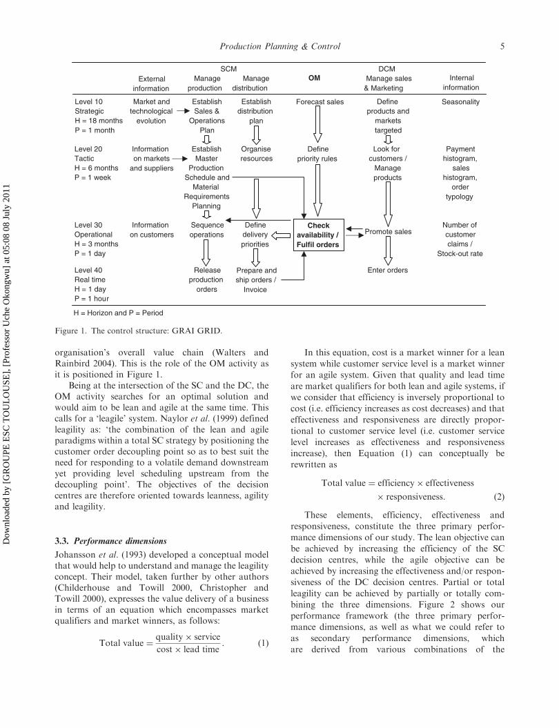
The integration of the SC and DC processes entailsdeveloping the communication, co-operation andcoordination capabilities of the functional entitiesinvolved. To achieve this, the OFP and more preciselythe OM activity has to be executed properly. Figure 1shows the ECOGRAI control structure, which identi-fies the key functions involved in the OFP. Vertically,this structure clearly shows the activities of eachfunction at different horizons (strategic, tactical andoperational) and the relationship between the functionscan be seen horizontally.

The OM function serves as a ‘bridge’ between theSC and the DC and highlights the availability check/order fulfilment decision centre, which constitutes thecentral axis in this article.

3.2. Objectives of decision centres

Though there are different definitions of demand chainmanagement (DCM) and supply chain management(SCM) in the literature, some authors argue that SCMis termed DCM to reflect the fact that the chain (ornetwork) is driven by the market, and not by suppliers(Rainbird 2004). It could be said that SCM laysemphasis on efficiency (which consists in minimisingoperational cost) while DCM lays emphasis on effec-tiveness (which consists in maximising flexibility andresponsiveness), but tries more to reconcile bothefficiency and effectiveness (Walters 2006a). It followsthat the decision centres on the supply side of the OMactivity would aim to be ‘lean’ (efficient) by eliminatingwastes while those on the demand side would aim to be‘agile’ (flexible and responsive) by providing speedyresponse to market changes. A firm is best placed tocreate value and exploit market opportunities whenthere is an effective combination of SC capabilities(efficiency) and DC effectiveness to maximise the

4 U. Okongwu et al.

Dow

nloa

ded

by [

GR

OU

PE E

SC T

OU

LO

USE

], [

Prof

esso

r U

che

Oko

ngw

u] a

t 05:

08 0

8 Ju

ly 2

011

organisation’s overall value chain (Walters andRainbird 2004). This is the role of the OM activity asit is positioned in Figure 1.

Being at the intersection of the SC and the DC, theOM activity searches for an optimal solution andwould aim to be lean and agile at the same time. Thiscalls for a ‘leagile’ system. Naylor et al. (1999) definedleagility as: ‘the combination of the lean and agileparadigms within a total SC strategy by positioning thecustomer order decoupling point so as to best suit theneed for responding to a volatile demand downstreamyet providing level scheduling upstream from thedecoupling point’. The objectives of the decisioncentres are therefore oriented towards leanness, agilityand leagility.

3.3. Performance dimensions

Johansson et al. (1993) developed a conceptual modelthat would help to understand and manage the leagilityconcept. Their model, taken further by other authors(Childerhouse and Towill 2000, Christopher andTowill 2000), expresses the value delivery of a businessin terms of an equation which encompasses marketqualifiers and market winners, as follows:

Total value ¼quality� service

cost� lead time: ð1Þ

In this equation, cost is a market winner for a lean

system while customer service level is a market winner

for an agile system. Given that quality and lead time

are market qualifiers for both lean and agile systems, if

we consider that efficiency is inversely proportional to

cost (i.e. efficiency increases as cost decreases) and that

effectiveness and responsiveness are directly propor-

tional to customer service level (i.e. customer service

level increases as effectiveness and responsiveness

increase), then Equation (1) can conceptually be

rewritten as

Total value ¼ efficiency� effectiveness

� responsiveness: ð2Þ

These elements, efficiency, effectiveness and

responsiveness, constitute the three primary perfor-

mance dimensions of our study. The lean objective can

be achieved by increasing the efficiency of the SC

decision centres, while the agile objective can be

achieved by increasing the effectiveness and/or respon-

siveness of the DC decision centres. Partial or total

leagility can be achieved by partially or totally com-

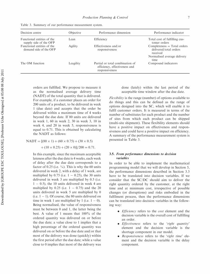
bining the three dimensions. Figure 2 shows our

performance framework (the three primary perfor-

mance dimensions, as well as what we could refer to

as secondary performance dimensions, which

are derived from various combinations of the

SCM DCMInternal

informationOM Manage Manage Manage sales External

information production distribution & Marketing

H = Horizon and P = Period

Level 10 Market and technological

evolution

Establish Sales &

OperationsPlan

Establish distribution

plan

Defineproducts and

markets targeted

Forecast sales SeasonalityStrategic H = 18 months P = 1 month

Informationon markets

and suppliers

Establish Master

ProductionSchedule and

Material Requirements

Planning

Definepriority rules

Organiseresources

Level 20 Tactic H = 6 months P = 1 week

Look for customers /

Manageproducts

Payment histogram,

sales histogram,

ordertypology

Level 30 Operational H = 3 months P = 1 day

Informationon customers

Sequenceoperations

Definedelivery priorities

Number of customer claims /

Stock-out rate

Check availability / Fulfil orders

Promote sales

Release production

orders

Prepare and ship orders /

Invoice

Enter ordersLevel 40 Real time H = 1 day P = 1 hour

Figure 1. The control structure: GRAI GRID.

Production Planning & Control 5

Dow

nloa

ded

by [

GR

OU

PE E

SC T

OU

LO

USE

], [

Prof

esso

r U

che

Oko

ngw

u] a

t 05:

08 0

8 Ju

ly 2

011

primary dimensions). The secondary dimensions are:total agility (effectiveness, responsiveness and flexibil-ity); partial effective leagility (efficiency, effectivenessand flexibility); partial responsive leagility (efficiency,responsiveness and flexibility) and total leagility (effi-ciency, effectiveness, responsiveness and flexibility).

3.4. From performance dimensions to performanceindicators

Indicators are needed to measure the performancedimensions (efficiency, effectiveness and responsive-ness) that we mentioned in Section 3.3. Many authors(Holweg 2005, Walters 2006b, Reichhart and Holweg2007, Stevenson and Spring 2007, Zokaei and Hines2007) have emphasised the vagueness, the multidimen-sionality and the interdependency in the definitions ofthese performance dimensions, which sometimes makethem difficult to measure in practice. We do not intendto review the literature of these terms, but simply toadopt a strict and clear definition of each of them, suchas to be able to define the various strategies that will beused in our AATP model. We will adopt the followingrestrictive and 1-D (or single factor) definitions:

. Efficiency is doing things right (Zokaei andHines 2007) and this can be defined as the costof fulfilling customer orders. Although effi-ciency is generally measured with respect tothe best possible way of doing something,some authors define it in relative terms as thebest of all possible ways of doing something(Bescos and Dobler 1995, Mas-Colell et al.1995, Halley and Guilhon 1997). Some of

these authors go further to suggest that it can

best be measured in financial terms in order to

reflect the primary goal of profit-making

organisations. Walters (2006b) suggests that

efficiency should be measured from a broad

perspective that encompasses customer needs,

rather than from a narrow perspective that

considers only the supply’s short-term cost

reduction objectives. Therefore, if we consider

the OFP as being composed of the following

elements: order preparation, transportation,

substitution, delay, shortage (undelivered

quantity), efficiency can be measured as the

total cost of the five elements, expressed

simply in financial values.. Effectiveness is doing the right thing (Zokaei

and Hines 2007) and this can be defined as

fulfilling orders exactly as they are requested

by customers (i.e. the completeness of cus-

tomer orders). It is measured in terms of the

percentage of the order that is fulfilled within

the time frame that is acceptable by the

customer. Its value can go from 0% to

100%, the latter being the best. Zero per

cent means that nothing is delivered within the

time frame acceptable by the customer and

100% means that all the ordered quantity was

delivered within the acceptable time frame,

with or without substitute products. This

performance criterion is the ‘completeness

percentage’.. Responsiveness is doing things quickly and this

can be defined as the speed at which customer

Efficiencyx

Total leagility(x, y, z)

Effectivenessz

Partial leagility (x, y)

Partial leagility

(x, z)

Total agility (y, z)

Partial agility (y)

Lean

(x)Par t i a l

agi l i ty(z

Responsivenessy)

Figure 2. Decision variables.

6 U. Okongwu et al.

Dow

nloa

ded

by [

GR

OU

PE E

SC T

OU

LO

USE

], [

Prof

esso

r U

che

Oko

ngw

u] a

t 05:

08 0

8 Ju

ly 2

011

orders are fulfilled. We propose to measure it

as the normalised average delivery time

(NADT) of the total quantity that is delivered.

For example, if a customer places an order for

200 units of a product, to be delivered in week

1 (due date) and accepts that the order be

delivered within a maximum time of 4 weeks

beyond the due date. If 80 units are delivered

in week 1, 60 in week 2, 30 in week 3, 10 in

week 4, and 20 in week 5, responsiveness is

equal to 0.71. This is obtained by calculating

the NADT as follows:

NADT ¼ ½ð80� 1Þ þ ð60� 0:75Þ þ ð30� 0:5Þ

þ ð10� 0:25Þ þ ð20� 0Þ�=200 ¼ 0:71:

In this example, since the maximum acceptable

lateness after the due date is 4 weeks, each week

of delay after the due date corresponds to a

factor of 0.25 (i.e. ¼). This is why the 60 units

delivered in week 2, with a delay of 1 week, are

multiplied by 0.75 (i.e. 1 � 0.25), the 30 units

delivered in week 3 are multiplied by 0.5 (i.e.

1 � 0.5), the 10 units delivered in week 4 are

multiplied by 0.25 (i.e. 1 � 0.75) and the 20

units delivered in week 5 are multiplied by 0

(i.e. 1 � 1). Of course, the 80 units delivered on

time in week 1 are multiplied by 1 (i.e. 1 � 0).

Being normalised, the value of responsiveness

must be between 0 and 1, the latter being the

best. A value of 1 means that 100% of the

ordered quantity was delivered on or before

the due date; a value close to 1 implies that a

high percentage of the ordered quantity was

delivered on or before the due date and/or that

most of the delivery was done (quickly) within

the first period after the due date; while a value

close to 0 implies that most of the delivery was

done (lately) within the last period of the

acceptable time window after the due date.

Flexibility is the range (number) of options available todo things and this can be defined as the range ofoptions designed into the SC, which will enable it tofulfil customer orders. It is measured in terms of thenumber of substitutes for each product and the numberof sites from which each product can be shipped(multi-site shipment). These flexibility elements shouldhave a positive impact on effectiveness and respon-siveness and could have a positive impact on efficiency.A summary of the performance measurement system ispresented in Table 3.

3.5. From performance dimensions to decisionvariables

In order to be able to implement the mathematicalprogramming model that we will develop in Section 5,the performance dimensions described in Section 3.3have to be translated into decision variables. If weconsider that the SC/DC should aim to deliver theright quantity ordered by the customer, at the righttime and at minimum cost, irrespective of possiblechanges (or disruptions) and risks embodied in thefulfilment process, then the performance dimensionscan be translated into decision variables in the follow-ing way:

. Efficiency refers to the cost element and thedecision variable is the overall cost of fulfillingan order.

. Effectiveness refers to the ‘right quantity’element and the decision variable is theshortage component in our model.

. Responsiveness refers to the ‘right time’ ele-ment and the decision variable is the delaycomponent.

Table 3. Summary of our performance measurement system.

Decision centre Objective Performance dimension Performance indicator

Functional entities of thesupply side of the OFP

Lean Efficiency Total cost of fulfilling cus-tomer orders

Functional entities of thedemand side of the OFP

Agility Effectiveness and/orresponsiveness

Completeness ¼ Total ordersdelivered/total ordersreceived

Normalised average deliverytime

The OM function Leagility Partial or total combination ofefficiency, effectiveness andresponsiveness

Compound indicators

Production Planning & Control 7

Dow

nloa

ded

by [

GR

OU

PE E

SC T

OU

LO

USE

], [

Prof

esso

r U

che

Oko

ngw

u] a

t 05:

08 0

8 Ju

ly 2

011

. Flexibility can be considered as the elementthat enables the system to adapt to changesand the decision variable is the substitutioncomponent.

We note that, in our model, all these variables willbe expressed in terms of cost in order to facilitate theproblem-solving process by using a common unit (thatis relevant) to support the decision maker. In otherwords, our model calculates the cost of shortages anddelays, and then tries to minimise them, with the aim ofmaximising the overall efficiency of the OFP. In thismodel, coefficients are used to vary the impact of thedecision variables on the objective function in order toobtain and study different strategic configurations aswill be discussed later in Section 5.2.

4. Research assumptions and hypotheses

In this section, we will describe the hypotheses of ourmodel and the associated symbols used in it.

4.1. The customer

The first hypothesis considers that an order is com-posed of n different lines (multi-references order). Eachline can be defined by a product p and a quantity Dp.The product p is positioned on the line p.

The customer wants to be delivered at a due date,DD. There is a delay as soon as the effective deliverydate is beyond the DD. The latest delivery dateauthorised by the customer is referred to as thedeadline, DL. Beyond this DL, the customer willrefuse the backorder. If not all ordered quantity isdelivered, there is a shortage cost, CShp.

We also consider a delay cost, CDVp. This costdepends on the laps of time between DD and theeffective delivery date, as well as on the quantitydelivered late. There is also a delay penalty, which isconsidered as a fixed cost, CDF.

An order can be delivered in several instalments.Nshipmax stands for the maximum number of ship-ments for an order. We consider that there are twoshipments as soon as an order is delivered from twodifferent sources s or prepared from a unique sourcebut at two different dates.

Given that an order line p can be delivered inseveral instalments, Nsplitmaxp stands for the maxi-mum number of splits authorised by the customer, fora given line. We consider that a line is split if and whenthe overall quantity of the line is delivered in severalshipments. Two different cases must therefore beconsidered: the total quantity is shipped from a solesource at different dates or the total quantity is shipped

from different sources. No particular cost has beenassociated with this in order not to penalise thesupplier twice. Actually, as soon as a line is split, thewhole order will be delivered late (entailing therefore adelay cost) or delivered from different sources (entail-ing therefore an increase in the transportation cost).

4.2. Substitute products

In this study, we have envisaged the possibility of usinga substitute product in place of the product inshortage. Consequently, the original product p can besubstituted by a set of products Sp. We consider thatP (group of demanded products) and S (group ofsubstitute products) are disjoined. Then, let us considerRr as the set of products of P that r can replace. Thecost of substitution (denoted by QSp) depends only onthe quantity of the substitute. We note that allproducts (original or substitute) can be deliveredfrom different sources s.

4.3. Preparation and shipments

One shipment from a sourcing site s implies apreparation cost (CP) that includes a fixed part CPFs

(which depends on the sourcing site) and a variablepart CPVps that depends also on the sourcing site, aswell as on the quantity of product p picked.

A transportation cost is also considered. This costis defined as a variable cost, CTVgs that depends on theweight of the quantity shipped and the distancebetween the sourcing site s and the customer. Aproduct p gets a weight Wp. This cost is directlyproportional to the distance between the source andthe customer. But since this article studies the case ofonly one customer, our model does not include anyvariable (index) c for customer. Therefore, for a givendistance, the transportation cost is determined just fordifferent weight brackets of the ordered quantity.Generally, there are two cases:

(1) A fixed cost for each weight bracket. Forexample, if the shipping cost of a quantitybetween 0 and 5 kg is 8 euros and that of aquantity between 5 and 10 kg is 10 euros, theshipping of a quantity of 6 kg and a quantity of9 kg will both cost 10 euros.

(2) A degressive cost for each weight bracket. Forexample, if for a weight between 0 and 5 kg, thecost is 2E/kg and for a weight between 5 and10 kg, it is 1.5E/kg, the shipping cost of aquantity of 6 kg will be 9E (6� 1.5E) and thatof a quantity of 9 kg will be 13.5E (9� 1.5E).

8 U. Okongwu et al.

Dow

nloa

ded

by [

GR

OU

PE E

SC T

OU

LO

USE

], [

Prof

esso

r U

che

Oko

ngw

u] a

t 05:

08 0

8 Ju

ly 2

011

In this case, transporters are encouraged to

search for economy of scale.

In this study, we consider only the second option.

5. Proposed model

5.1. AATP model

Here, we define the elements used in our AATP model.

The model is based on an OFP viewed from the

receiving end rather than from the shipping end. The

notations used as indexes, parameters and variables are

summarised in Table 4. All variables are expressed with

respect to the delivery date. In this case, pickup dates

are equal to delivery dates minus lead times. Moreover,

it is assumed that all picked-up quantities are delivered.As discussed in Section 3.5, the objective function

(3) tries to minimise the total cost of the system

(preparation costs CP, transportation costs CT, delay

costs CD, substitution costs CS and shortage costs

CSh). We propose to balance the different costs of the

system in order to be able to reflect the strategy of the

network. The aim is to minimise the total cost:

Minimise ½cðCPÞ � CPþ cðCTÞ � CT

þ cðCDÞ � CDþ cðCSÞ � CSþ cðCShÞ � CSh�, ð3Þ

where c is the balancing coefficient for cost.The different costs are defined below.

Order preparation cost (CP):

CP ¼Xs

Xt

DCUst

!� CPFs

þXp

Xs

Xt

Xpst þXi2Sp

Yipst

!" #� CPVps ð4Þ

Transportation cost (CT):

Case 1: a fixed cost for each weight bracket

CT ¼Xt

Xs

Xg

DELstg � CTVgs ð5:1Þ

Case 2: a degressive cost for each weight bracket

CT ¼Xt

Xs

Xg

PFstg � CTVgs ð5:2Þ

Delay cost (CD):

CD ¼ OD � CDFþXt¼DL

t¼DD

Xp

Qpt � CDVp � ðt�DDÞ:

ð6Þ

Substitution cost (CS):

CS ¼Xp

QSp � CSVp: ð7Þ

Shortage cost (CSh):

CSh ¼Xp

shortagep � CShp: ð8Þ

The above objective function is solved subjectto 22 constraint functions that are listed inTable 5.

5.2. Implementing the order fulfilment strategies

In our model, we have considered the OFP as beingcomposed of the following decision variables: orderpreparation, transportation, substitution, delay andshortage (undelivered quantity). With respect to theprinciples described in Section 3.5, the performancedimensions (delivery strategies) developed inSection 3.3 can be implemented in the following way:

(1) Efficiency: a similar coefficient should be puton all the cost elements in the objectivefunction stated in Equation (3), with theexception of the substitution cost (non-flexiblecondition), the objective being to minimise theglobal cost of the order fulfilment.

(2) Effectiveness: a higher coefficient should be puton shortage, the objective being to maximisethe completeness of the orders by minimisingshortages.

(3) Responsiveness: a higher coefficient is put ondelay, the objective being to deliver as quicklyas possible. In a way, quick delivery enables tominimise the risk of shortage. So, a mediumcoefficient could also be put on shortage.

(4) Agility (effectiveness and responsiveness in aflexible environment): a high coefficient is puton shortage (for effectiveness) and delay (forresponsiveness).

(5) Partial effective leagility (efficiency and effec-tiveness in a flexible environment): a highcoefficient is put on shortage (for effectiveness)and the coefficients put on order preparation,transportation, substitution and delay shouldbe balanced (for efficiency).

(6) Partial responsive leagility (efficiency andresponsiveness in a flexible environment): ahigh coefficient is put on delay (for responsive-ness) and the coefficients put on order prepa-ration, transportation, substitution andshortage should be balanced (for efficiency).

Production Planning & Control 9

Dow

nloa

ded

by [

GR

OU

PE E

SC T

OU

LO

USE

], [

Prof

esso

r U

che

Oko

ngw

u] a

t 05:

08 0

8 Ju

ly 2

011

(7) Leagility (Efficiency, effectiveness and respon-siveness in a flexible environment): coefficientsshould be balanced between all the fiveelements.

These scenarios represent the extreme strategiesderived from the conceptual framework presented in

Section 3.3 and do not constitute a complete experi-

mental plan. In our future research, it will be interest-

ing to study the impact of a larger panel of order

fulfilment strategies.We note that, since the cost elements of the

objective function (Equation 3) are weighted using

Table 4. Indexes, parameters and variables of our model.

Notations Explanation

Indexes used in our modelp Product index, p¼ 1. . . n, n is the total number of lines in the orderq All products (order or substitute)r Substitute product (replacement product) indexs Source (distribution centre) index, s¼ 1. . . S, S is the number of sourcest Time period index, t¼ 1, . . . ,T, T is the planning horizong Weight bracket index, g¼ 1, . . . ,G, G is the number of weight brackets

Parameters of our modelATPqst Quantity of product q that can be shipped from site s, between dates 1 and tCDF Fixed penalty if there is a delay of at least one period within the order delivery time window

(for DD5 t5DL)CDVp Cost of delay for one period for product p (for DD5 t5DL)CPFs Fixed preparation cost for site sCPVqs Preparation cost for product q on site sCShp Cost of shortage for product pCSVp Cost of substitution for product pCTVgs Transportation cost for a delivery within weight bracket g, from site s to customerDD Due dateDL DeadlineDp Demand of product p in a given orderkmaxg Superior limit of weight bracket gkming Inferior limit of weight bracket gNshipmax Maximum number of shipments allowedNsplitmaxp Maximum number of splits allowed for a given order line pRPr Set of products for which r can be a substituteSp Set of substitute products for product pT Planning horizonTLs Delivery time from site s to customerWq Weight of one product q

Variables of our modelDCUst Variable linked to the use of source s for a delivery on date t (distribution centre using),

DCUst¼ 1 if site s is used, 0 otherwiseDELstg Binary variable linked to weight bracket g of a delivery from site s on date t, DELstg¼ 1 if

there is a delivery within the weight bracket g from site s on date t, 0 otherwiseOD Binary variable linked to the due date (order delay), OD¼ 1 if there is a delay, 0 otherwisePEst Weight of the delivery sent from s on date tPFstg Weight of the delivery within the weight bracket g. PEstg¼PEst if DELstg¼ 1 PEstg¼ 0 if

DELstg¼ 0ORpst Binary variable linked to the quantity of product delivered on date t from site s to fill line pQpt Quantity of product delivered on date t to fill line p (product p or substitute)QSp Quantity of product p substitutedRpst Quantity of product delivered on date t from site s to fill the line p (product p or substitute)Shortagep Final backorder quantity of product pXCpst Total quantity of product p picked on site s and delivered on date tXpst Quantity of product p picked on site s (on date t – DLs) and delivered on date tXRCrst Total quantity of substitute product r picked on site s and delivered on date tXRrst Quantity of substitute product r picked on site s and delivered on date tYrpst (r2Sp) Quantity of product r substituted to p, picked on site s and delivered on date t

10 U. Okongwu et al.

Dow

nloa

ded

by [

GR

OU

PE E

SC T

OU

LO

USE

], [

Prof

esso

r U

che

Oko

ngw

u] a

t 05:

08 0

8 Ju

ly 2

011

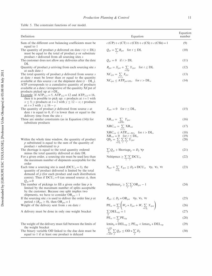
Table 5. The constraint functions of our model.

Definition EquationEquationnumber

Sum of the different cost balancing coefficients must beequal to 1

c (CP)þ c (CT)þ c (CD)þ c (CS)þ c (CSh)¼ 1 (9)

The quantity of product p delivered on date t (t5DL)must be equal to the total of product p or substituteproduct r delivered from all sourcing sites s

Qpt ¼PsRpst for t � DL (10)

The customer does not allow any deliveries after the dateDL

Qpt ¼ 0 if t4DL (11)

Quantity of product p arriving from each sourcing site sat each date t

Rpst ¼ Xpst þPr2Sp

Yrpst for t � DL (12)

The total quantity of product p delivered from source sat date t must be lower than or equal to the quantityavailable at this source s at the shipment date (t – DLs).ATP corresponds to a cumulative quantity of productsavailable at a date t irrespective of the quantity XCpst ofproducts picked up at t-DLs

XCpst ¼Pi¼1,t

Xpsi (13)

XCpst � ATPpst-DLs for t4DLs (14)

Example: If ATP111¼ 5, ATP112¼ 12 and ATP113¼ 16,then it is possible to pick up: x products at t¼ 1 withx � 5; y products at t¼ 2 with y � 12� x; z productsat t¼ 3 with z � 16� y

The quantity of product p delivered from source s atdate t is equal to 0, if t is lower than or equal to thedelivery time from the site s

Xpst ¼ 0 for t � DLs (15)

These are similar constraints (as in Equation (14)) forsubstitute products

XRrst ¼P

i2RPr

Yipst (16)

XRCrst ¼Pi¼1,t

XRrsi (17)

XRCrst � ATPrst�DLs for t4DLs (18)XRrst ¼ 0 for t � DLs (19)

Within the whole time window, the quantity of productp substituted is equal to the sum of the quantity ofproduct r substituted to p

QSp ¼Pr2Sp

Ps

PtYrpst (20)

The shortage is equal to the total quantity orderedminus the total quantity delivered at date DL

PtQpt þ Shortagep ¼ Dp 8p (21)

For a given order, a sourcing site must be used less thanthe maximum number of shipments acceptable for theorder

Nshipmax �Ps

PtDCUst (22)

Each time a sourcing site is used (DCUst¼ 1), thequantity of product delivered is limited by the totaldemand of p (for each product and each distributioncentre). Thus if DCUs¼ 0 (an unused source s), thenQpt¼ 0

Xpst þPi2Sp

Yipst � Dp �DCUst 8p, 8s, 8t (23)

The number of pickings to fill a given order line p islimited by the maximum number of splits acceptableby the customer. Because one split implies twoshipments, we have to consider ORpst� 1

Nsplitmaxp �Ps

PtORpst � 1 (24)

If the sourcing site s is used to deliver the order line p atperiod t (Rpst4 0), then ORpst¼ 1

Rpst � Dp �ORpst 8p, 8s, 8t (25)

Weight of the delivery sent from s on date t PEst ¼Pp

Wp � Xpst þWr

Pr2Sp

Yrpst

!(26)

A delivery must be done in only one weight bracketPgDELstg ¼ 1 (27)

PEst ¼PgPEstg (28)

The weight of the delivery must fall between the limits ofthe weight bracket

kming �DELstg � PEstg 5kmaxg �DELstg (29)

The binary variable OD linked to the due date must beequal to 1 if at least one product is delayed

Pt¼DL

t¼DD

PpQpt � OD �

PpDp (30)

Production Planning & Control 11

Dow

nloa

ded

by [

GR

OU

PE E

SC T

OU

LO

USE

], [

Prof

esso

r U

che

Oko

ngw

u] a

t 05:

08 0

8 Ju

ly 2

011

coefficients, the total cost does not correspond to the

real logistics cost. Indeed, our model being a decision-

making tool that aims to find a trade-off between the

different performance dimensions (efficiency, effective-

ness and responsiveness), the difference between the

real logistics cost and the total cost of the objective

function can be regarded, from a strategic decision-

making point of view, as a trade-off cost. Slack and

Lewis (2008) define trade-offs in operations as the way

firms are willing to sacrifice one performance objective

to achieve excellence in another. From the strategic

cost management perspective, this trade-off cost could

be referred to as a structural or executional cost that

enables the firm to minimise the negative impact of the

actions of one business function on another business

function (Anderson and Dekker 2009a,b). Logue

(1975) argues that, in the assessment of market

efficiency, the chief cost of dealing with a market-

maker is the difference between the theoretical but

unobservable equilibrium price and the transaction

price. In a similar way, we therefore argue that the

difference between the real logistics cost and the

objective function cost (which is the equilibrium cost)

corresponds to the strategic price that the firm has to

pay in order to maximise (or optimise) the customer’s

satisfaction.

6. Numerical application

6.1. Presentation

We carried out two experiments, which enabled us totest on the one hand non-flexible strategies (efficiency,effectiveness and responsiveness) and on the otherhand, flexible strategies (total agility, partial effectiveleagility, partial responsive leagility and total leagility).For the non-flexible strategies, substitution and multi-sourcing capabilities are not taken into considerationwhile for the flexible strategies, flexibility is added tothe system by allowing the substitution of products andby using a second sourcing site.

Each strategy is implemented using a set of valuesrelative to the five cost balancing coefficients – c(CP),c(CT), c(CD), c(CS) and c(CSh). Based on the perfor-mance framework that we proposed in Section 3.3 andusing the values of the three performance indicators:NADT (responsiveness), total cost (efficiency) andcompleteness (Effectiveness), the results obtained areexpressed in the form of a 3-D surface graphicalpresentation (see the figures in the discussions thatfollow). Each result is represented by a point withcoordinates as NADT, total cost (normalised in orderto obtain a value between [0;1]) and completeness.

We consider an order placed by a customer at t¼ 0.This order is composed of three different products –M, N and O – and the demand is 100 units for each.The due date is week 1. But in week 1, there is ashortage of all these products. The customer does notwant to receive his order in more than three instal-ments and the order line of product M cannot be splitmore than once. The latest delivery date acceptable bythe customer is week 5. The set of data used to performthe first experiment (without flexibility) is shown inTable 6.

Regarding the second experiment, products MSand NS are added as substitutes for products M and N,respectively. In addition, a second sourcing plan S2 isopened and some inventories (for all the products) areintroduced. The set of data used to perform this secondexperiment (with flexibility) is shown in Table 7. Weassume that all products shipped in a given week aredelivered the same week.

6.2. Results and discussion of experiment 1

Given the absence of flexibility, the coefficient c(CS) isequal to 0 (no substitution). All the results are shownin Figure 3.

As discussed in Section 3, the efficiency strategy isbased on the minimisation of the total cost. Thesolution obtained turns out to be the most economic,with a total cost of $17160. The efficiency objective isclearly illustrated by the fact that the delivery planincludes in week 1, a quantity of 18 units of product O(and not the 20 units available) such as to benefit froma lower transportation cost in week 2. Actually, the

Table 6. Data for experiment 1 of the single-order case.

Items from source S1

M N O

Price $100 $160 $100Period1 50 30 202 50 100 203 50 100 904 90 100 1005 100 100 100

CostCPVps 3 4.5 3CPFs 200 200 200CDF 10 10 10CDVp 25 40 25CShp 200 360 200

Weight 1 0.7 0.5

12 U. Okongwu et al.

Dow

nloa

ded

by [

GR

OU

PE E

SC T

OU

LO

USE

], [

Prof

esso

r U

che

Oko

ngw

u] a

t 05:

08 0

8 Ju

ly 2

011

two units of product O that are added to the 70 unitsof product N allow the weight group to be changedfrom [0, 50] to [50, 200], thereby minimising thetotal cost.

In line with its aim to maximise the completenesspercentage of the customer order, the effectivenessstrategy gives a delivery plan that enables to deliver allthe products within the time window of 5 weeks

Figure 3. Results of experiment 1 of the single-order case.

Table 7. Data for experiment 2 of the single-order case.

Items from source S1 Items from source S2

Period M N O MS NS Period M N O MS NS

1 50 30 20 0 10 1 20 40 0 10 302 50 100 20 0 10 2 30 40 50 10 303 50 100 90 0 10 3 50 60 50 10 304 90 100 100 0 10 4 50 60 50 10 305 100 100 100 0 10 5 50 60 50 10 30

Cost CostCPVps 3 4.5 3 4 5.5 CPVps 4 5.5 4 5 6.5CPFs 200 200 200 200 200 CPFs 200 200 200 200 200CDF 10 10 10 10 10 CDF 10 10 10 10 10CDVp 25 40 25 25 40 CDVp 25 40 25 25 40CShp 200 360 200 CShp 200 360 200

Weight 1 0.7 0.5 1 0.7 Weight 1 0.7 0.5 1 0.7Transport Transport0–50 kg $10 0–50 kg $1250–200 kg $8 50–200 kg $10Above 200 kg $5 Above 200 kg $7

Production Planning & Control 13

Dow

nloa

ded

by [

GR

OU

PE E

SC T

OU

LO

USE

], [

Prof

esso

r U

che

Oko

ngw

u] a

t 05:

08 0

8 Ju

ly 2

011

acceptable by the customer. However, compared to the

efficiency strategy, the relatively small improvement

(4%) in completeness might not be sufficient to

compensate for the 8% increase in total cost and the

7% decrease in NADT.The responsiveness strategy implies quickness and

aims to deliver all the ordered quantity as soon as the

products are available. This strategy enables to obtainthe solution with the best NADT value – all the

products are shipped within 3 weeks whereas in the

other two strategies (efficiency and effectiveness) 4 and

5 weeks are, respectively, required to fulfil the order.

Here again, this strategy would be adopted only in

exceptional cases since, compared to the other two

strategies, the relatively small improvement (5% and12.5% with respect to efficiency and effectiveness,

respectively) in NADT may not counterbalance the

large increase (24% and 15%, respectively) in total

cost, as well as the decrease (16% and 20%, respec-

tively) in completeness.In this experiment, the efficiency strategy turns out

to be outstanding compared to the effectiveness and

responsiveness strategies. This is however understand-able given the absence of flexibility (only one sourcing

site and no substitutes products). Nevertheless, these

two strategies can be adopted under specific circum-

stances where the quickness and completeness of the

delivery of the customer order is much more important

than the cost of delivering the order. For example, in

the healthcare industry, a hospital (the customer) willmost likely want its order of certain medication to be

delivered quickly and completely at a higher cost if that

will enable to save the life of a patient suffering from

chronic cancer. We can therefore say that the results of

this experiment enable us to emphasise two interesting

aspects of our model. Firstly, by assigning different

balancing coefficients to the different components of

an OFP, the total cost of the OFP can be minimisedwhile meeting the contractually agreed requirements of

the customer. Secondly, by varying the balancing

coefficients, the supplier can modulate the different

performance objectives (efficiency, effectiveness and

responsiveness) in order to adapt to the customer’s

expectations at different times and under specific

circumstances. In other words, the supplier canconstantly adapt its strategy depending on the

market contextual conditions and requirements.

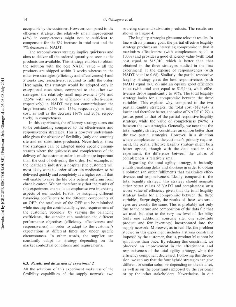
6.3. Results and discussion of experiment 2

All the solutions of this experiment make use of the

flexibility capabilities of the supply network: two

sourcing sites and substitute products. The results areshown in Figure 4.

The leagility strategies give some relevant results. Inline with its primary goal, the partial effective leagilitystrategy produces an interesting compromise in that itmaximises effectiveness (with completeness equal to100%) and provides a good efficiency value (with totalcost equal to $15,010, which is better than thatobtained in the three strategies studied in the firstexperiment) at the expense of responsiveness (withNADT equal to 0.68). Similarly, the partial responsiveleagility strategy gives the best responsiveness (withNADT equal to 0.79) and an equally good efficiencyvalue (with total cost equal to $15,144), while effec-tiveness drops significantly to 80%. The total leagilitystrategy looks for a compromise between the threevariables. This explains why, compared to the twopartial leagility strategies, the total cost ($12,424) islower and therefore better, the value of NADT (0.79) isjust as good as that of the partial responsive leagilitystrategy, while the value of completeness (96%) isbetween the two strategies. Generally, we note that thetotal leagility strategy constitutes an option better thanthe two partial strategies. However, in a situationwhere completeness is the customer’s primary require-ment, the partial effective leagility strategy might be abetter option, though with the data used in thisexperiment, the difference between the values ofcompleteness is relatively small.

Regarding the total agility strategy, it basicallyentails penalising delay and shortage in order to obtaina solution (an order fulfilment) that maximises effec-tiveness and responsiveness. Ideally, compared to thetotal leagility strategy, this strategy should generateeither better values of NADT and completeness or aworse value of efficiency given that the total leagilitystrategy looks for a compromise between the threevariables. Surprisingly, the results of these two strat-egies are exactly the same. This is probably not onlydue to the nature and composition of the data file thatwe used, but also to the very low level of flexibility(only one additional sourcing site, one substituteproduct and few inventory) incorporated into thesupply network. Moreover, as in real life, the problemstudied in this experiment includes a strong constraintimposed by the customer, that is, product M cannot besplit more than once. By relaxing this constraint, weobserved an improvement in the effectiveness andresponsiveness of the total agility strategy, while theefficiency component decreased. Following this discus-sion, we can say that the four hybrid strategies can givedifferent or similar solutions depending on the data set,as well as on the constraints imposed by the customeror by the other stakeholders. Nevertheless, in our

14 U. Okongwu et al.

Dow

nloa

ded

by [

GR

OU

PE E

SC T

OU

LO

USE

], [

Prof

esso

r U

che

Oko

ngw

u] a

t 05:

08 0

8 Ju

ly 2

011

further research, we will endeavour to add moreflexibility to the system in order to observe a moresignificant difference between the total agility and totalleagility strategies.

The results of this second experiment clearly showthat the conflicting objectives of the different actors ofa SC can be traded off against each other while tryingto minimise the overall cost of fulfilling customerorders. By varying the cost balancing coefficients, asupplier can therefore adopt different order fulfilmentstrategies that would enable it not only to respond (inthe most efficient way possible) to the various expec-tations of its stakeholders, but also to modulate itsstrategy such as to constantly react to the changingstrategic behaviour of its competitors.

7. Coherence analysis – step 4 of the ECOGRAI

method

We present in this section the internal study ofcoherence for the OM decision-making centre as it ispositioned in the GRAI grid (Figure 1). This step of

the ECOGRAI method aims to analyse the impact ofthe different decision variables on the different perfor-mance dimensions. As presented in Table 8, thisanalysis enables to establish the links between thethree sets {objectives, decision variables, performanceindicators}. Table 8 shows:

. at the top, the three objectives of the OMdecision centre;

. in the middle, the four performanceindicators;

. at the bottom, the seven decision variableswhich enable us to improve the system. Thesevariables correspond to each of the fivecoefficients in the objective function of ourAATP model plus the two variables whichenable us to improve flexibility.

Table 8 was completed with the results obtained inthe different numerical applications presented earlier.A strong link ‘objective–indicator’ shows that theperformance indicator clearly measures the degree towhich the objective is attained. A strong link ‘variable–indicator’ shows that an action on the variable has a

Figure 4. Results of experiment 2 of the single-order case.

Production Planning & Control 15

Dow

nloa

ded

by [

GR

OU

PE E

SC T

OU

LO

USE

], [

Prof

esso

r U

che

Oko

ngw

u] a

t 05:

08 0

8 Ju

ly 2

011

significant effect on the evolution of the value of theindicator.

In conclusion, the performed experiments enabled

us to observe that:

. each objective is connected to at least oneindicator and one decision variable;

. each variable is connected to at least one

objective and one indicator;. each indicator is connected to at least one

objective and one variable.

Our {objective, decision variables, performanceindicators} proposal for the OM decision-making

centre therefore seems coherent.

8. Conclusion

In an OFP, if there is stock-out after acceptingcustomer orders and promising due delivery dates,

managers are faced with the difficult and challengingtask of maximising customers’ satisfaction while rec-

onciling the conflicting objectives of the differentfunctional entities that constitute the supply and

demand sides of the OFP. Whereas some authorshave provided partial answers to these problems, we

have proposed in this article a model composed of amore comprehensive multi-criteria decision-making

AATP tool and a performance measurement frame-work to support the decision-making process. This

model was tested on a single-order theoretical case.The results showed a lot of consistency and coherence

between the performance indicators and the decisionvariables. They particularly would enable companies to

make some strategic decisions in terms of the degree of

flexibility required to achieve the desired level ofcustomer service.

Though our model constitutes a significant firststep towards solving the multi-dimensional problemsencountered in order fulfilment in stock-out situations,the simulation is based on the fulfilment of a singleorder and therefore does not allow us to evaluateflexibility and agility on a large scale and scope. To dothis, we will in our further research carry out exper-

iments over several weeks of incoming customersorders. This will also enable us to investigate theimprovement of the overall performance for an orderportfolio (i.e. with several customers orders). In otherwords, we will try to find out whether fulfilling aspecific order in a way that is not the most economicalprovides other forms of benefit such as being able tosatisfy more customers? Also, our model needs to betested on a company which already possesses a

significant degree of flexibility in its SC. Furtherresearch should also include a sensitivity analysis onthe balancing coefficients, as well as some practicalinsights on how managers can adjust and adapt themodel to their own strategies. It will also be interestingto apply our model to other industrial sectors in orderto observe possible changes in the decision variablesand performance indicators.

The ultimate goal of this article is to enhance thecreation of a governing body that could use our modelas a decision support system to arbitrate between the

conflicting objectives of the different stakeholders in asupply network.

All these perspectives are geared towards a realapplication in a European cosmetic company. Theresearch study is performed in order to develop adecision support system to optimise its OM process

Table 8. Internal coherence analysis (step 4 of the ECOGRAI method).

OM function Decision centre OM 30 Internal coherence analysis

Objectives O1: To minimise the delivery costs ** – – **O2: To deliver on time – ** – **O3: To deliver the right products – – ** *

Performance indicators PI 1: Totalcost

PI 2:NADT

PI 3: Percentage ofcompleteness

PI 4: Degreeof flexibility

Decisionvariables

DV 1: To penalise the transportation cost ** – – –DV 2: To penalise the distribution cost ** – – –DV 3: To penalise the substitution cost ** – – *DV 4: To penalise the delay cost ** ** – –DV 5: To penalise the shortage cost ** * ** –DV 6: To add a source – – – **DV 7: To add products of substitution – – – **

Note: **Strong link; *weak link and (–) no link.

16 U. Okongwu et al.

Dow

nloa

ded

by [

GR

OU

PE E

SC T

OU

LO

USE

], [

Prof

esso

r U

che

Oko

ngw

u] a

t 05:

08 0

8 Ju

ly 2

011

(about 2000 orders and 11,000 order lines per day) instock-out situations.

Notes on contributors

Uche Okongwu is a Professor of SCMat Toulouse Business School, France.He holds an MSc degree inMechanical Engineering and a PhDin Industrial Management. AtToulouse Business School, he hasheld many faculty positions, such asdirector of an MBA program inAerospace Management and director

of a graduate program in SCM. He has published articles ininternational journals and his current research interestfocuses on development and performance measurement ofSCM systems. He is also an independent consultant on SCMissues and industrial organisation.

Matthieu Lauras is an AssociateProfessor of SCM at the IndustrialEngineering Department of theUniversity of Toulouse – Mines Albi,France. He is also an AffiliateProfessor at Toulouse BusinessSchool, France and co-director of theAgilea consulting and training com-pany, France. His research interest is

focused on performance, integration and management ofSC processes. His research activities concern not onlytraditional industrial sectors, but also the humanitariansector. He has published several papers in journals andinternational conferences in the field of SCM and perfor-mance assessment.

Lionel Dupont is a full Professor inproduction and operations manage-ment. He is the Director of theIndustrial Engineering Departmentof the University of Toulouse –Mines Albi, France. His researchworks cover manufacturing systemsconfiguration, design, planning andscheduling and SCM. He also worked

in many different industrial sectors some of which areautomotive, information technology and pharmaceutical. Hehas published a book on industrial engineering and manyarticles with practical applications.

Verane Humez holds her PhD at theIndustrial Engineering Department ofthe University of Toulouse – MinesAlbi, France. She worked on custo-mer-driven SCs and more precisely onthe integration of DCs and SCs, usingreal data from a pharmaceutical SC tovalidate her models. Now, she is aprocurement support manager atAirbus Military, France.

References

Anderson, S.W. and Dekker, H.C., 2009a. Strategic cost

management in supply chains, Part 1: structural cost

management. Accounting Horizons, 23 (2), 201–220.Anderson, S.W. and Dekker, H.C., 2009b. Strategic cost

management in supply chains, Part 2: executional cost

management. Accounting Horizons, 23 (3), 289–305.APICS, 2005. American Production and Inventory Control

Society Dictionary. 11th ed. Alexandria: APICS.Bescos, P.L. and Dobler, P., 1995. Controle de gestion et

management. Paris: Montchrestien.Bourne, M., et al., 2003. Implementing performance mea-

surement systems literature review. International Journal of

Business Performance Management, 5 (1), 1–24.

Chan, F.T.S., Chan, H.K., and Qi, H.J., 2006. A review of

performance measurement systems for supply chain

management. International Journal of Business

Performance Management, 8 (2–3), 110–131.Chen, J.H., Lin, J.T., and Wu, Y.S., 2008. Order promising

rolling planning with ATP/CTP reallocation mechanism.

IESM, 7 (1), 57–65.

Chen, C-Y., Zhao, Z., and Ball, M.O., 2002. A model for

batch advanced available-to-promise. Production and

Operations Management, 11 (4), 424–440.Childerhouse, P. and Towill, D.R., 2000. Engineering supply

chains to match customer requirements. Logistics

Information Management, 13 (6), 337–345.Christopher, M., 1992. Logistics and supply chain manage-

ment. London: Pitman.Christopher, M. and Towill, D.R., 2000. Supply chain

migration from lean and functional to agile and custo-

mised. Supply Chain Management: An International

Journal, 5 (4), 206–213.Cokins, G., 1989. Activity-based cost management: an

executive’s guide, Edition hardcover. New York, USA:

Cross and Lynch.Croxton, K.L., 2003. The order fulfilment process. The Inter-

national Journal of Logistics Management, 14 (1), 19–32.Croxton, K.L., Garcia-Dastugue, S.J., and Lambert, D.M.,

2001. The supply chain management processes. The

International Journal of Logistics Management, 2 (12),

13–36.

Ducq, Y. and Vallespir, B., 2005. Definition and aggregation

of a performance measurement system in three aeronau-

tical workshops using the ECOGRAI method. The

Production Planning and Control, 16 (2), 163–177.Halley, A. and Guilhon, A., 1997. Logistics behaviour of

small enterprises: performance, strategy and definition.

International Journal of Physical Distribution and Logistics

Management, 16 (8), 475–495.Herbert, M., 2009. Customer segmentation, allocation

planning and order promising in make-to-stock produc-

tion. OR Spectrum, 31 (1), 229–256.Holweg, M., 2005. An investigation into supplier respon-

siveness: empirical evidence from the automotive industry.

The International Journal of Logistics Management, 16 (1),

96–119.

Production Planning & Control 17

Dow

nloa

ded

by [

GR

OU

PE E

SC T

OU

LO

USE

], [

Prof

esso

r U

che

Oko

ngw

u] a

t 05:

08 0

8 Ju

ly 2

011

Hoover, W., et al., 2001. Managing the demand-supply chain.New York: Wiley.

Jeong, B., et al., 2002. An available to promise system forTFT LCD manufacturing in supply chain. Computer &Industrials Engineering, 43, 191–212.

Johansson, H.J., et al., 1993. Business Process Reengineering:

Breaking Strategies for Market Dominance. Chichester:John Wiley & Sons.

Kaplan, R.S. and Norton, D.P., 1996. The balanced

scorecard: translating strategy into action. Boston:Harvard Business School Press.

Kilger, C. and Schneeweiss, L., 2000. Demand fulfilment and

ATP. In: H. Stadtler and C. Kilger, eds, Supply chainmanagement and advanced planning: concepts, models,software and case studies. Berlin: Springer, 135–148.

Kirche, E.T., Kadipasaoglu, S.N., and Khumawala, B.M.,

2005. Maximizing supply chain profits with effective ordermanagement: integration of Activity-Based Costing andTheory of Constraints with mixed-integer modelling.

International Journal of Production Research, 43 (7),1297–1311.

Lee, Y.H., et al., 2006. Production quantity allocation for

order fulfilment in the supply chain: a neutral networkbased approach. Production Planning and Control, 17 (4),378–389.

Lin, J.T. and Chen, J.H., 2005. Enhance order promisingwith ATP allocation planning considering material andcapacity constraints. Journal of Chinese Institute ofIndustrial Engineers, 22 (4), 282–292.

Lin, F.R. and Shaw, M.J., 1998. Reengineering the orderfulfilment process in supply chain networks. TheInternational Journal of Flexible Manufacturing System,

10, 197–229.Logue, D.E., 1975. Market-making and the assessmentof market efficiency. The Journal of Finance, 30 (1),

115–123.Mas-Colell, A., Whinston, M.D., and Green, J.R., 1995.Microeconomic theory. New York: Oxford University

Press, 150.Naylor, J.B., Naim, M.M., and Berry, D., 1999. Leagility:interfacing the lean and agile manufacturing paradigm inthe total supply chain. International Journal of Production

Economics, 62, 107–118.Neely, A., Adams, C., and Kennerley, M., 2002. Theperformance prism: The scorecard for measuring and

managing business success. New Jersey: Prentice Hall.Pibernik, R., 2005. Advanced available to promise: classifi-cation, selected methods and requirements for operations

and inventory management. International Journal ofProduction Economics, 93–94, 239–252.

Pibernik, R., 2006. Managing stock-outs effectively withorder fulfilment systems. Journal of ManufacturingTechnology Management, 17 (6), 721–736.

Rainbird, M., 2004. Demand and Supply Chains: the value

catalyst. International Journal of Physical Distribution andLogistics Management, 34 (3/4), 230–250.

Reichhart, A. and Holweg, M., 2007. Creating the Customer-

Responsive Supply Chain: a reconciliation of concepts.International Journal of Operations and ProductionManagement, 27 (11), 1145–1172.

Siala, M., Campagne, J.P. and Ghedira, K., 2006.Proposition d’une nouvelle approche pour la gestion dudisponible dans les chaıne logistiques. MOSIM’06, Rabat,Maroc, Avril.

Slack, N. and Lewis, M., 2008. Operations strategy. 2nd ed.England: Pearson Education Limited.

Stevenson, M. and Spring, M., 2007. Flexibility from the

supply chain perspective: definition and review.International Journal of Operations and ProductionManagement, 27 (7), 685–713.

Supply Chain Council, 2008. Supply Chain OperationsReference model-SCOR, Version 9.0. USA and Europe:Supply Chain Council.

Walters, D., 2006a. Effectiveness and efficiency: the role ofsupply chains management. The International Journal ofLogistics Management, 17 (1), 75–94.

Walters, D., 2006b. Demand chain effectiveness – supply

chain efficiencies: a role for enterprise informationmanagement. Journal of Enterprise InformationManagement, 19 (3), 246–261.

Walters, D. and Rainbird, M., 2004. The demand chain as anintegral component of the value chain. Journal ofConsumer Marketing, 21 (7), 465–475.

Xiong, M., et al., 2003. A web-enhanced dynamic BOMbased available to promise system. International Journal ofProduction Economics, 84, 133–147.

Xiong, M.H., et al., 2006. A DSS approach to managingcustomer enquiries for SMEs at the customer enquirystage. International Journal of Production Economics, 103,332–346.

Zokaei, K. and Hines, P., 2007. Achieving consumer focus insupply chains. International Journal of PhysicalDistribution and Logistics Management, 37 (3), 223–247.

Zschorn, L., 2006. An extended model of ATP to increaseflexibility of delivery. International Journal of ComputerIntegrated Manufacturing, 19 (5), 434–442.

18 U. Okongwu et al.

Dow

nloa

ded

by [

GR

OU

PE E

SC T

OU

LO

USE

], [

Prof

esso

r U

che

Oko

ngw

u] a

t 05:

08 0

8 Ju

ly 2

011