A dynamic programming model for optimising feeding ... - Helda

A G R I C U L T U R A L A N D F O O D S C I E N C E

A dynamic programming model for optimising feeding and slaughter decisions

regarding fattening pigsJarkko K. Niemi

MTT Agrifood Research Finland, Economic Research, Luutnantintie 13, FI-00410 Helsinki, Finland

e-mail: [email protected]

ACADEMIC DISSERTATION

To be presented, with the permission of the Faculty of Agriculture and Forestry of the University of Helsinki,

for public criticism in Auditorium XII, Unioninkatu 34, Helsinki, on April 21st, 2006, at 12 o’clock.

Supervisors: Docent Kyösti Pietola Economic Research MTT Agrifood Research Finland

Professor Matti Ylätalo Department of Economics and Management University of Helsinki, Finland Reviewers: Professor Ruud Huirne Business Economics Group Wageningen University, The Netherlands Professor Anders Ringgaard Kristensen Department of Large Animal Sciences Royal Veterinary and Agricultural University, Denmark

Opponents: Professor Pekka Ilmakunnas Department of Economics Helsinki School of Economics, Finland

Professor Asko Mäki-Tanila Biotechnology and Food Research MTT Agrifood Research Finland


PrefaceSeveral persons have contributed to this thesis and supported me. I take this opportunity to thank those people. First, I wish to express my gratitude to my two supervisors, Docent Kyösti Pietola (MTT Eco-nomic Research) and Professor Matti Ylätalo (University of Helsinki). Docent Pietola encouraged me to start post-graduate studies, supported me throughout, and assisted me in my efforts to deal with a variety of methodological and theoretical issues. Professor Ylätalo supported me during my studies in several ways, provided guidance during my research, and made constructive comments on this study. In addition, I would like to express my gratitude to Marja-Liisa Sévon-Aimonen (MTT Animal Production Research), who provided biological data and helped me to formalise the model.

I thank Professor Ruud Huirne (Wageningen University, The Netherlands) and Professor Anders Ring-gaard Kristensen (Royal Veterinary and Agricultural University, Denmark) for their careful pre-examina-tion of the thesis and for their many valuable comments. I am also grateful to Professor Pekka Ilmakunnas (Helsinki School of Economics) and Professor Asko Mäki-Tanila (MTT Biotechnology and Food Re-search) who agreed to be my public examiner.

I wish to acknowledge my colleagues at MTT Economic Research as well as several people who have participated in this research project at MTT Animal Production Research: Esa Mäntysaari (Ph.D.), Hilkka Siljander-Rasi (M.Sc.), Ismo Stranden (Ph.D.), Jarmo Valaja (Ph.D.) and Kaarina Vuori (M.Sc.). I also thank Saara Raulo (Ph.D.) (the National Veterinary and Food Research Institute) and Marie-Josée Mangen (Ph.D.) (Agricultural Economics Research Institute, The Netherlands) for suggestions concerning early versions of Chapter 7. I am also grateful to the supervisors of the research project “Economic comparison of feeding strategies in pigs” for their remarks.

This study is based on research projects which were funded by Ministry of Agriculture and Forestry, MTT Agrifood Research Finland and Raisio Group Plc., with additional support provided by the Finnish Animal Breeding Association (FABA). In addition, the August Johannes and Aino Tiura Foundation of Agricultural Research, the Science and Research Foundation of the Finnish Association of Academic Agronomists as well as the Finnish Cultural Foundation provided financial support for this thesis. I gratefully acknowledge the funding and information provided by these organisations. I am also grateful to MTT for giving me the op-portunity to work on this topic and for providing me with excellent facilities for this study.

I thank Emeritus Professor Henry Fullenwider (Ph.D.) for reading the manuscript for English-language usage. I’m also grateful to the editorial board of Agricultural and Food Science for accepting this study for publication in their journal.

Finally, I wish to express my gratitude to my friends and relatives for their support. Warm thanks go to my parents Erkki and Raila, who have encouraged and supported me throughout my life. My warmest thanks go to my wife Sari for her love, care and understanding, and to our sons, Ville and Jere, who have always brought sunshine into my life.

Kurikka, February 2006 Jarkko Niemi

4


ContentsAbstract ........................................................................................................................ 6

1 Introduction ............................................................................................................. 7 1.1 Background of the study .................................................................................. 7 1.2 Modelling feeding and the timing of slaughter decisions ................................ 8 1.3 Objectives and structure of the study ............................................................... 10

2 Previous studies on pig production management and optimisation ........................ 11 2.1 Production and pricing of pig meat in Finland ................................................. 11 2.2 Features of optimised pig management ............................................................ 12 2.2.1 The planning horizon ............................................................................. 12 2.2.2 Choosing the optimal feeding patterns .................................................. 12 2.2.3 The optimality of slaughter timing ........................................................ 16 2.2.4 Uncertainty of slaughter income ............................................................ 19 2.3 Methods for optimising pig fattening ............................................................... 20 2.3.1 The optimality of an allocation .............................................................. 20 2.3.2 Production and cost functions ................................................................ 21 2.3.3 Convex and concave sets and functions ................................................. 22 2.3.4 Dynamic programming .......................................................................... 24 2.4 Scope and method of the study ........................................................................ 26

3 A dynamic programming model for pig fattening ................................................... 29 3.1 Model specification problems .......................................................................... 29 3.2 The optimisation problem ................................................................................ 31 3.3 Decomposing the control variables .................................................................. 32 3.4 The pig growth model ...................................................................................... 33 3.5 Restricting pig growth ...................................................................................... 35 3.6 One-period returns function ............................................................................. 36

4 Precision feeding – a benchmark scenario .............................................................. 37 4.1 Data and scenarios ............................................................................................ 37 4.2 Estimation method ............................................................................................ 41 4.3 Results .............................................................................................................. 44 4.4 Summary .......................................................................................................... 49

5 Adjusting pig production management to market conditions ................................. 50 5.1 Data and scenarios ............................................................................................ 50 5.1.1 Price movements .................................................................................... 50 5.1.2 Quality price premiums .......................................................................... 52 5.2 Results .............................................................................................................. 52 5.2.1 The effects of price changes .................................................................. 52 5.2.2 Elasticity estimates for price movements .............................................. 56 5.2.3 The effects of quality price premiums ................................................... 58 5.3 Summary .......................................................................................................... 61

5


6 The value and management implications of animal genetics .................................. 63 6.1 Data and scenarios ............................................................................................ 63 6.2 Results .............................................................................................................. 66 6.2.1 The effects of animal genotype .............................................................. 66 6.2.2 Split-sex feeding .................................................................................... 69 6.3 Summary .......................................................................................................... 72

7 The importance of slaughter timing ........................................................................ 74 7.1 Data and scenarios ............................................................................................ 74 7.1.1 The case of exogenously delayed slaughter ........................................... 74 7.1.2 Modelling the value of slaughter timing ................................................ 76 7.2 Results .............................................................................................................. 78 7.2.1 Adjusted feeding patterns when the slaughter is delayed ...................... 78 7.2.2 Income losses in the event of a short slaughter delay ............................ 79 7.2.3 Income losses in the event of a long slaughter delay ............................. 82 7.3 Summary .......................................................................................................... 83

8 Conclusions and discussion ..................................................................................... 85 8.1 Management implications ................................................................................ 85 8.2 Policy implications ........................................................................................... 89 8.3 Suggestions for further research ....................................................................... 91

References .................................................................................................................... 93Selostus ........................................................................................................................ 98

Appendices Appendix A. Computer code of the basic model Appendix B. Sensitivity analysis of two-phase feeding Appendix C. Feeding patterns of female pigs and castrated male pigs Appendix D. Sensitivity analysis for genotype scenarios

6


A dynamic programming model for optimising feeding and slaughter decisions

regarding fattening pigs Jarkko K. Niemi

MTT Agrifood Research Finland, Economic Research, e-mail: [email protected]

Costs of purchasing new piglets and of feeding them until slaughter are the main variable expenditures in pig fattening. They both depend on slaughter intensity, the nature of feeding patterns and the technological constraints of pig fattening, such as genotype. Therefore, it is of interest to examine the effect of production technology and changes in input and output prices on feeding and slaughter decisions. This study examines the problem by using a dynamic programming model that links genetic characteristics of a pig to feeding decisions and the timing of slaughter and takes into account how these jointly affect the quality-adjusted value of a carcass. The state of nature and the genotype of a pig are known in the analysis.

The results suggest that producer can benefit from improvements in the pig’s genotype. Animals of im-proved genotype can reach optimal slaughter maturity quicker and produce leaner meat than animals of poor genotype. In order to fully utilise the benefits of animal breeding, the producer must adjust feeding and slaughter patterns on the basis of genotype.

The results also suggest that the producer can benefit from flexible feeding technology. Typically, such a technology provides incentives to feed piglets with protein-rich feed. When the pig approaches slaughter maturity, the share of protein-rich feed in the diet gradually decreases and the amount of energy-rich feed increases. Generally, the optimal slaughter weight is within the weight range that pays the highest price per kilogram of pig meat.

The optimal feeding pattern and the optimal timing of slaughter depend on price ratios. Particularly, an increase in the price of pig meat provides incentives to increase the growth rates up to the pig’s biological maximum by increasing the amount of energy in the feed. Price changes and changes in slaughter premium can also have large income effects.

Key words: barley, carcass composition, dynamic programming, feeding, genotypes, pig fattening, preci-sion agriculture, productivity, slaughter weight, soybeans

7


Vol. 15 (2006): Supplement 1.

1 Introduction

1.1 Background of the studyDecisions related to feeding regimen and slaugh-ter timing in pig meat production have vital sig-nificance because they affect economic perform-ance of pig farms and more broadly, the economic performance of the pork industry. Both decisions can significantly affect the value of pigs sold for slaughter and the income flows of a pig farm, es-pecially as the prices of feed and of piglets are the major variable production expenses. Tuppi (2004), for instance, estimates that on ProAgria Rural Advisory Centres’ sample farms specialised in pig fattening, the average feed cost in 2003 was 22% (€39 per pig) and the purchase cost of pig-lets was 32% (€57 per pig) of the total produc-tion cost of pig meat. Taken together, these two items account for 93% of the total material cost incurred in bringing a pig to slaughter. Therefore, changes in the allocation of feeds, the length of the fattening period, and factors that determine the optimality of these decisions, can have large impact on production cost and profitability of pig fattening.

The effects of prices and technological con-straints on production management and the value of a capacity unit are inextricably related to choice of feeding patterns and to slaughter decisions. The genetic production potential of an animal (i.e. gen-otype) can have a particularly large impact on the market value of a carcass and as well as on input efficiency of feeds. It is known that the pig’s re-quirements for protein (Fuller et al. 1989) and en-ergy (Whittemore 1983) depend on its maturity stage and genotype (Boland et al. 1999). Hence, producer can benefit from using feeding schemes that have two or more phases, each of which has a different feed composition (two or three-phase feeding), as opposed to schemes that have the same feed composition (one-phase feeding) throughout the fattening period (Boland et al. 1999, Campos 2003, p. 80) and from adjusting the timing of slaughter of pigs in a batch according to their

weight and leanness (Kure 1997, Chapter 4). Stud-ies even suggest that providing an efficient supply of nutrients according to the pig’s genetic growth potential requires continuous rather than discrete adjustment of feed ratios (Glen 1983). The benefits of continuous adjustments are, however, quite un-known.

Studies suggest that improvements in genotype can significantly increase returns to pig farming. Since a pig’s genotype and carcass leanness are correlated and since carcass is priced according to its weight and leanness, increases in returns have been observed above all to improvements that in-crease the growth rate of lean meat (Boland et al. 1993). Full utilisation of production potential of improved genotypes can require the adjustment of slaughter and feeding patterns accordingly (cf. Boland et al. 1999). Therefore, it is important to examine how genotype affects pig production management, and how management and genotype jointly affect the value of a capacity unit. This can be important particularly when aiming at obtaining unbiased assessment of economic advantages of a particular animal breeding strategy.

An example of a segregated feeding pattern is the case where the producer has an option to group pigs into batches according to their sex, and there-after to optimise feeding and slaughter decisions separately for both sexes (split-sex feeding). Since feeding and slaughter decisions frequently involve interactions (Chavas et al. 1985), it is important to take into account also the income that simultane-ous adjustment of feeding and slaughter decisions can contribute to the capacity unit through im-proved carcass quality as a result of the enhance-ment of the genetic characteristics of the animal. This aspect is often omitted and an inflexible feed-ing technology is used instead.

Successful pig management entails the ability to find solutions to problems arising from uncer-tainty and biological variation. Pigs are often managed as groups where individuals may have different growth patterns. This causes variation in carcass value, with the results that it becomes op-

8


Niemi, J.K. Optimising feeding and slaughter decisions regarding pigs

timal to adjust the timing of slaughter of pigs ac-cording to their weight and leanness (cf. Kure 1997, Roemen and de Klein 2000). Measurement of carcass quality can also be inaccurate and affect the optimal timing of marketing (Jorgensen 1993, Boland et al. 1996). Furthermore, it may take time to observe changes in growth rates of pigs (White et al. 2004), and manager may not always reach desired carcass composition (Parsons et al. 2004). Studies such as Jorgensen (1993), Boland et al. (1996) and Kure (1997) have carefully examined the impacts of uncertainty and biological varia-tion in pig fattening. Less work has been done to analyse the connections between feeding and slaughter decisions and carcass quality. Hence, this study emphasises these linkages and shows how to estimate to the value of genetic improve-ments by taking their management effects into ac-count.

From an economic point of view, price ratios of inputs and outputs largely determine the opti-mality of feeding and slaughter decisions for a given production technology (Dent et al. 1970, Sonka et al. 1976, Jolly et al. 1980, Glen 1983, Chavas et al. 1985, Broekmans 1992, Rydstedt and Andersson 1993, Kure 1997, Boland et al. 1999). The factors affecting the optimal pig production management patterns include price adjustments that depend on carcass weight and leanness (Boland et al. 1993). Although a producer can ben-efit from adjusting feeding and/or slaughter pat-terns according to the markets, studies have gener-ally found that input substitution is inelastic with respect to input and output prices. Income, on the other hand, has responded very elastically to changes in input and/or output prices (Chavas et al. 1985, Boland et al. 1993, Sipiläinen and Ryhä-nen 1996, Kure 1997).

Feeding and slaughter decisions are also in-volved in several policy issues such as the subsi-dising of pig fattening and regulations affecting the choice of inputs, outputs and production tech-nology. An example of a regulatory problem in-volving the need to evaluate the impact of regula-tions on production is whether to prohibit the use of genetically modified (GMO) soy meal in feeds. GMO soy meal is less expensive than non-GMO

soy meal. Dros and Kriesch (2003, p. 10–11), for instance, have reported approximately a 10% price difference. The price gap is expected to increase over time. Regulations prohibiting the use of GMO soy meal therefore imply higher feed costs to do-mestic producers than to foreign competitors with less stringent regulations. Thus, estimates of the effects of regulations require taking into account to which extent producers can make adjustments to production through input substitution.

Another important policy issue is decoupling subsidies from production. The slaughter premium paid for each slaughtered carcass affects the timing of slaughter, because the amount of premiums paid to the producer depends on slaughter intensity. The premium is also known to have an impact on pro-ducer income (Sipiläinen and Ryhänen 1996). De-coupling the slaughter premium from production so that producer has no obligation to produce meat is the equivalent of removing it from the optimisa-tion problem. Since the decoupled premium is ex-ogenous, decoupling can decrease the profitability of high slaughter intensity. Decoupling can in-crease the value of existing production capacity but decrease producer incentives to invest in new production capacity. This is so because decoupled payment is independent of production capacity. Hence, more consideration could be given to giv-ing the producer incentives to invest in new pro-duction capacity.

1.2 Modelling feeding and the timing of slaughter decisions

Economic optimisation of feeding and slaughter decisions requires simultaneous analysis of both decisions. This is mainly due to two aspects. The first is that feeding decisions, conditional on the genotype of an animal, affect both carcass value and daily growth rates (Chavas et al. 1985, Kennedy 1986, p. 11, Burt 1993). Hence, making the optimal feeding decisions requires information on how a pig of a particular genotype responds to

9



feeds and how feeding affects the market value of a carcass. The second aspect is that economically optimal production decisions take both allocation of inputs and the timing of replacement of an asset into account (Burt 1965, 1993, Dillon and Ander-son 1990, p. 87–88). No matter how the problem of the optimal timing of marketing of an animal is solved, the general principle is simple: It is opti-mal to market a pig when the marginal net revenue from fattening an additional day is equal to the op-portunity cost of replacement (Chavas et al. 1985, p. 639, Dillon and Anderson 1990, p. 87–94, Bo-land et al. 1993, p. 148). In other words, the re-placement pig can contribute higher profit than the current pig (for analytical solution, see Chavas et al. (1985, p. 639)).

In this study, pig fattening is examined with a structural-form optimisation model that is based on characterisation of the growth mechanism of pigs. An optional approach would be to estimate a reduced-form pig growth model. Discussion on how to feed fattening pigs includes solving wheth-er it is optimal to feed the pig according to its bio-logical growth potential (ad libitum feeding) (Dil-lon and Anderson 1990, p. 113). The problem is economically relevant because, as Boland et al. (1999) note, maximisation of live weight growth only does not recognise the impact of diminishing returns on inputs. Even when the growth rates are exogenously given, it is useful to solve feed ratios by maximising profits rather than weight gain.

The benefits of restricting the supply of feed below stomach capacity are related to a carcass merit based meat pricing scheme (Boland et al. 1993, Boland et al. 1996, Sipiläinen and Ryhänen 1996) and to the fact that restricting the feed sup-ply gives the producer the option to extract the quality price premium from the markets at the cost of decreased growth rate. Although pig growth it-self is a complex process, the principle of how to control carcass quality through feeding is quite simple. As the amount of protein in feed increases, carcass becomes leaner (i.e. the share of red meat in the carcass increases) and its value (€ per kg) increases. As the amount of energy in feed increas-es, carcass becomes fattier, and as the total amount of feed increases, the daily weight gain increases

and the pig reaches the specified live weight quick-er than before the increase. Therefore, the daily feed allowance significantly affects carcass quality (Whittemore 1998, p. 48–52).

The growth of a pig and constraints related to its growth can be characterised using a set of equa-tions (Emmans 1995, p. 113N). The idea is to split the pig’s live weight into energy, protein, water and ash and then to model the growth of the com-ponents separately. As Emmans and Kyriazakis (1999) summarise, this can be a very useful form of simplifying pig growth, because most important processes of pig growth can be reduced to a func-tion of either an energy or a protein component. The genotype of a pig plays an important part in this functional approach. In this study, the geno-type of a pig refers to the maximum rate at which the amount of lean and fatty tissue in the pig’s body can increase (i.e. the growth potential). Lean tissue refers to the protein component and meas-ures the amount of all fat-free components in the body, whereas fatty tissue refers to the energy component and measures all fat in the body.

When the Gompertz function characterises the maximum growth pattern of a pig, the parameter known as mature weight measures the weight that an animal can reach when it matures, and the pa-rameter known as maturing rate measures the maximum daily weight gain of a tissue component (Whittemore 1998, p. 59–68, Emmans and Kyria-zakis 1999; see also Black 1988, Boland et al. 1993, Sevón-Aimonen 2001). Clearly, these two parameters are of interest when estimating the val-ue of genetic improvements. Generally, an increase in the rate of daily weight gain is associated with an increase in maturing rate, whereas an increase in carcass leanness is associated with an increase in the mature weight of lean tissue. Both increases, however, result in a higher rate of daily weight gain (Whittemore 1998, p. 59–68, Emmans and Kyriazakis 1999).

Mature weight is conceptually different from slaughter weight. Mature weight depends on the pig’s genotype, whereas the producer decides the slaughter weight. Since slaughter pigs are valued according to their weight and carcass leanness, in-creasing the probability for the slaughter to be de-

10



layed can provide a producer with incentives to minimise reductions in the value of a carcass by marketing the pigs prematurely. Yet, little attention has been paid on examination of the economic im-pacts of delayed timing of slaughter, and of the op-tions available to an individual producer to adjust pig farming to delayed slaughter. This problem is common, because slaughterhouses are generally responsible for the collection of animals for slaughter, and an individual producer cannot al-ways fully control the date of slaughter. Thus, failed co-ordination of the production chain can alter the value of a carcass and the quality of the industry’s product.

Similar problem can occur also in special cir-cumstances, such as when animal disease regula-tions expose farms to the risk of a long exogenous delay in the timing of slaughter. Then, producer’s problem is to consider the options to minimise in-come losses through adjusting feeding patterns. The problem of premature slaughter is interesting also from society’s point of view because prema-ture slaughter can have externalities for a large number of farms in the event of an animal disease outbreak, and because it can increase society’s ex-posure to additional disease losses.

1.3 Objectives and structure of the study

This study focuses on modelling the production technology of pig fattening in cases where produc-er can observe the technology and state of nature of pig and control feeding and slaughter of a pig accordingly. The objective is to examine changes in pig producer’s production decisions and income when production technology and input and output prices change. In more detail, the goal of this study is to estimate:• How much the producer can benefit from using

a flexible feeding technology (‘precision feed-ing’), which allows him/her to continuously control feed ratios and carcass quality, instead

of inflexible two-phase feeding technology (Chapter 4)

• How the optimal feeding and slaughter policies and the value of a capacity unit change when carcass quality premiums, slaughter premiums or the prices of pig meat, feed and piglets change in a given production technology (Chapter 5)

• How much the producer can benefit from changes in production technology such that the genotype of an animal is improved, and how these technological improvements affect the optimal feeding and slaughter patterns (Chap-ter 6)

• How much the producer can benefit from opti-mising the timing of slaughter, and how he/she can minimise income losses when there is a possibility that the production technology al-lows timing of slaughter to be delayed (Chap-ter 7)These problems are studied by modelling the

producer’s decision making in a finite horizon re-cursive dynamic programming (Bellman, 1957) framework. Dynamic programming provides an efficient tool for linking feeding and feed compo-nents to carcass quality and for optimising feeding and the timing of slaughter simultaneously. The value of a capacity unit depends on both volume and quality of pig meat produced, which is condi-tional on quality price premiums paid according to the share of red meat in the carcass. The scope of this study is practical in the sense that the model characterises the growth mechanism of a pig (cf. Lucas’s critique of the validity of macroeconomic models (Sargent 1987, p. 40–41)).

The main contribution of this study to the lit-erature of pig production management is the dy-namic approach that explicitly takes into account carcass quality while simultaneously optimising feeding and slaughter decisions. The model esti-mates the optimal feeding and slaughter patterns and corresponding value functions over time and over subsequent fattening periods. The term fat-tening period refers to the time that is used to feed an individual piglet until slaughter maturity. The model is normalised for a capacity unit. The value of a capacity unit refers to the compensation that

11



the producer receives for fixed inputs and other variable inputs than feed cost and cost of replace-ment piglets. The results are based on the data from growth experiments on Finnish low-fat York-shire and Landrace crossbreed pigs, literature and meat market records in 2001–2003. The results are conditional on model formulation factors such as producer’s ability to control carcass quality of an individual pig and that states of nature (i.e. geno-type, carcass composition, prices) are known each period. Hence, the main goal of this thesis is to analyse how changes in model parameters, such as market information, animal genotype or feeding technology, affect feeding and slaughter patterns and the value of a capacity unit rather than to esti-

mate absolute feed levels and the timing of slaugh-ter or the parameters themselves.

This study is organised as follows. Chapter 2 discusses the optimisation of pig fattening in gen-eral, and results obtained in previous studies. Chapter 3 presents the modelling framework used in this study. Each of the four research problems given above is examined separately, one at a time, in Chapters 4–7. More detailed description of the problem in question is given in the beginning of each of these Chapters, followed by scenario and data description, the results and a summary at the end of the Chapter. Finally, Chapter 8 draws con-clusions and discusses the results.

2 Previous studies on pig production management and optimisation

2.1 Production and pricing of pig meat in Finland

Approximately 2.3 million fattening pigs are slaughtered in Finland per year. The average car-cass weight of a slaughtered pig in the past few years has been 82–84 kg. Thus, the annual amount of pig meat produced by fattening pigs in Finland has been 162–187 million kg (Tike 2005). Finnish pig farms house approximately 520,000 fattening pigs (>50 kg) and almost 300,000 young pigs at 20–50 kg live weight, of which most become fat-tening pigs (Tike 2004b). Since 1995, the price of pig meat has been less volatile in Finland than in most member countries of European Union (EU). Both increases and decreases in the EU average price seem to diffuse into Finnish meat markets with lags, and the difference between the highest and the lowest meat price is generally smaller in Finland than in such countries as Denmark, Ger-

many, the Netherlands or Spain, which produce large amounts of pig meat (Eurostat 2004).

The producer price of pig meat in Finland is adjusted according to carcass weight and the share of red meat in the carcass. The advantage of car-cass component based pricing is that it sends pig meat producers an observable price signal reflect-ing the value of carcass quality at later stages of the marketing chain (Boland et al. 1996, p. 46). Carcass leanness upon slaughter is graded accord-ing to the SEUROP classification scheme com-monly used in European Union. The measurement is carried out with a Hennessy grading probe 4 measure or a pork fat thickness analyser. In 2003, 40.6% of the carcasses qualified as class S (more than 60% red meat), 54.6% as class E (55–59% red meat), and 4.6% as class U (50–54% red meat) carcasses. The share of carcasses in class S was higher in 2003 than in any of the years from 1999–2002 (Tike 2004a).

Major slaughterhouses in Finland use similar principles when pricing pig meat, but the quality

12



premiums or discounts may differ from slaughter-house to slaughterhouse. The producer price con-sists of the base price, where no quality adjust-ments apply, and quality premiums or discounts that depend on carcass weight and leanness. In ad-dition, the base price can be differentiated accord-ing to producer category. For instance, producers contracted to produce a certified quality generally receive a higher base price than producers without a contract.

Often, the base price is paid for carcasses con-taining 59–59.9% lean meat and being within cer-tain weight range (such as 75–80 kg). Each addi-tional percentage point of red meat increases above (below) the reference receives an additional pre-mium (discount). Each kilogram of carcass weight that is below or above the target weight range, re-sults in a price discount. The discount increases as the carcass is lighter or heavier. For instance, when the discount is €0.02 per additional kg and the car-cass weight is 2 kg above the target, the price per kg is discounted €0.04 below the base price.

2.2 Features of optimised pig management

2.2.1 The planning horizon

Farm management is often defined as the alloca-tion of limited resources to maximise the farm’s satisfaction. The management functions include planning the allocation, implementing the plans, and finally controlling the activities. Agricultural producers can have different objectives in the short run and in the long run. Planning in the short run involves the operational planning and implemen-tation of a chosen strategy whereas strategic plan-ner expands decisions to long run planning and to fundamental issues of firm operations (Boehlje and Eidman 1984, p. 6–27 and 242–261). Interme-diate length horizon planning is known as tactical planning. Feeding and slaughter decisions, for in-stance, can be adjusted at relatively short intervals

whereas investments in costly new production technology require planning for a period of several years, because the new technology can increase ef-ficiency of input use and thus contribute value added in the long run.

Management decisions can be represented as a cyclical process (Figure 1) in which strategic, tac-tical and operational decisions combine to affect the implementation and control of management plans. After the plans have been developed, the managers are concerned with implementing the plans, controlling and monitoring the outcome over time, as well as with adjusting the plans if conditions change. The decisions examined in this study mainly relate to strategic and operational de-cision-making.

2.2.2 Choosing the optimal feeding patterns

The biological basis of examining the optimality of feeding patterns is usually the partitioning of the nutritional needs of the growing pig into additive parts, the maintenance needs being met first, fol-lowed by growth needs. In addition, nutritional needs can be separated into protein (i.e. amino ac-ids), energy and minerals needs. If an animal con-sumes just enough nutrients to meet the mainte-nance requirements, then no growth occurs. Thus, nutritional information is critical in the dynamic modelling of animal growth. Furthermore, the

Strategic planning

Tactical planning

Operational planning

Implementation

Control

Fig. 1. The management cycle (Huirne 1990).

13



amount of feed an animal can eat is limited by its stomach capacity (a genetic constraint) (cf. Black 1995, Emmans 1995, Whittemore 1998, Sevón-Aimonen 2001). Therefore, it is important to know whether the actual growth meets the poten-tial. If not, then other factors, such as feed avail-ability, restrict growth (Emmans and Kyriazakis 1999).

Both maximum rate of protein retention at dif-ferent stages of growth and mature weights of the animal can differ by sex (Whittemore et al. 1988, Emmans and Kyriazakis 1999, Sevón-Aimonen 2001). Similarly, changes in such factors as quality of feed, housing environment, animal health, diet composition, the number of pigs in a pen, and floor allowance can affect the growth rates obtained with a given amount of feed (Kornegay and Knot-ter 1984, Heikkonen 1997, Whittemore 1998). Animals having the freedom to choose their diet may prefer, for instance, large amounts of energy feed (such as barley) and dislike diets that contain a very high or very low share of protein (Arsenos et al. 2000). In addition, the producer can control feed intake causing the pig to eat less that its stom-ach capacity allows and hence, reducing growth rates below the genetic potential.

Studying potential and actual growth rates re-quires knowledge of growth as a function of weight and feed intake, and of growth potential. When carcass leanness needs to be taken into account, growth needs to be further separated into energy and protein needs (cf. Chavas et al. 1985, Glen 1983, Boland et al. 1993, Emmans 1995, Kure 1997, Sevón-Aimonen 2001). According to Whit-temore (1998, p 50), the ratio of fat growth to lean growth responds quite steadily to increased use of feeds when growth of fatty and lean tissue is re-stricted below the maximum. When lean growth reaches its maximum, the growth rate of fatty tis-sue increases with respect to the growth rate of lean tissue. Even if feeding is initially restricted so that tissue grows below the potential, the pig can have the capacity to partly compensate for reduced weight gain afterwards if the amount of feed is in-creased up to the level where the pig can utilise the nutrients up to its growth potential (Valaja et al. 1992, Kyriazakis and Emmans 1999).

Finnish feeding recommendations advise that young piglets be fed with a protein-rich diet. As the recommended amount of energy in feed in-creases almost every week, pigs approaching slaughter maturity are fed with energy-rich feed. The daily amount of energy supplied to young pigs increases by 0.2 fodder units each week. At later stages of growth, an increase of 0.1 fodder units is typical, and eventually the amount supplied stabi-lises at a constant level. In addition, the recom-mendations suggest discretionary reduction of the share of protein in feed once or twice during the fattening period. The first reduction is recom-mended at 55 kg live weight and the second at 80 kg live weight (MTT 2004).

Changes in recommended feeding patterns are linked to the fact that economically optimal feed-ing decisions change as growth rates change (Fig-ure 2). Figure 2 illustrates the fact that an increase in the daily feed allowance affects the three factors measured in the vertical axis, viz. the share of red meat in the carcass, the amount of daily weight gain and the feed cost per additional kilogram of meat for a given feed allowance. The daily weight gain increases when feed allowance increases, but the marginal weight gain is smaller when the al-lowance is large than when it is small. This can be due, for instance, to limits in stomach capacity and the fact that the daily weight gain starts to decrease when the animal becomes mature enough. Simul-taneously, the average feed cost per kilogram of marketed meat decreases. At a certain inflection point, and thereafter, the efficiency of converting feed into meat decreases and average feed cost in-creases. Furthermore, increasing a feed allowance causes trade-off between carcass leanness and dai-ly weight gain. The shaded box between the two vertical lines illustrates the region where an eco-nomically optimal feed allowance is likely to be found. The optimum is where the feed allowance and the three components are suitably balanced. In general, if the daily feed allowance is excessively high (low), then decreasing (increasing) it results in higher returns to producer. The exact location of the profit-maximising optimum in the shaded re-gion, however, depends on such factors as feed and piglet prices.

14



Optimal region

fodder units of feedper pig per day

*)Share of red meat

*)Daily weight gain

*)Feed consumption

The

amou

ntof

mea

sure

dva

riabl

es*)

Fig. 2. The impact of daily feed allowance (fodder units per pig per day) on feed consumption (fodder units per additional kilo-gram of meat), daily weight gain (kg), the share of red meat in car-cass at slaughter (%), and the re-gion where the economically op-timal daily feed allowance with respect to the combination of the three factors can be found (Source: Danske slagterier 2001, p. 1).

Since interactions frequently occur between feed inputs, it is important to consider different in-put combinations over a feasible operational range. Both static and dynamic analyses of the optimal feeding patterns suggest that it is optimal to de-crease the share of protein in feed as the pig grows. Dent et al. (1970) examined the effect of feed in-take in different combinations on pig growth and economic outcomes using static regression analy-sis. They observed that response of lean meat and live weight gain to both lysine and protein intake was almost linear for young pigs. Response of live weight gain to increased amount of energy was continuous though diminishing in the later stages of growth, and a connection between low response to protein and low intake of energy was observed. In early stages of growth, lean growth showed positive though a diminishing response to energy.

As the ratio of energy intake to dietary lysine decreases along the iso-growth line, the cost of producing a daily weight gain simultaneously de-creases. Thus, under conditions orientated purely to achieving live-weight gain at the minimum feed cost, nutrient combinations should be selected to-wards the high energy-low lysine end of the iso-growth curve (Dent et al. 1970, p. 202). These re-sults, however, do not permit the construction of a

continuous growth curve. Sonka et al. (1976), ob-served a similar change in the feeding pattern as the pig grows. They estimated that the optimal share of protein in the diet varies between 12–18% depending on the growth stage of the animal as well as on input prices. Sonka et al. (1976, p. 473) also observed that when the price of protein is low in comparison with the price of corn, the cost ad-vantage of using low amounts of protein decreas-es.

Chavas et al. (1985) estimated the optimal feeding pattern of fattening pigs using optimal control theory1. They concluded that pig meat pro-ducers have incentives to feed high protein ration for young pigs, but to use lower protein ration in the finishing phase. The result was quite robust to changes in relative prices. They observed that the marginal product of each nutrient had a negative relationship with respect to the level of the other nutrient. They also observed a diminishing mar-ginal utility of growth with respect to feed intake.

1 For further details on the method, see for instance, Kamien and Schwartz (1992, p. 109–243), Seierstad and Sydsaeter (1993, p. 69–410) or Bertsekas (1995a, p. 97–112).

15



Chavas et al. (1985) have characterised the op-timal feeding pattern as follows. The amount of soybean meal increases until the pig reaches ap-proximately 73 kg live weight. Thereafter, the amount of soybean meal in feed decreases. The amount of corn, on the other hand, increases dur-ing the fattening period. During the finishing stage, the amount of corn increases very rapidly and the share of protein in feed decreases linearly. In addi-tion, Chavas et al. (1985) computed positive cross-price elasticity estimates with soybean meal and corn. Thus, the feeds were substitutes for each other. When the price of one feed increased by one percent the amount of the substitute feed increased less than 0.15%. Increasing the price of a piglet by one percent, however, increased the demand for corn by 1.84% and the demand for soybean meal by 0.94%.

Glen (1983), studied another dynamic pro-gramming application by optimising feeding pat-terns of fattening pigs for the entire fattening pe-riod. The pigs had a specified slaughter weight. Glen (1983) divided feeding and live weight into energy and protein (for development of the pig growth model see Whittemore and Fawcett (1976), and for use of the growth model to determine the least costly feed ratio see Fawcett et al. (1978)). Glen (1983) estimated that with a diet consisting of soy and barley it is optimal to increase the amount of feed throughout the fattening period. The optimal diet for 20 kg piglet contained 9.7% soy whereas the optimal diet for 25–50 kg pig con-tained 19.3–21.6% soy. Thereafter, on pigs heavier than 50 kg, the share of soy decreased approxi-mately to 2%. Also Boland et al. (1999) showed that it is economically optimal to decrease the share of protein in feed when the pig approaches the optimal slaughter maturity.

Using a production and cost theoretical ap-proach, Sipiläinen and Ryhänen (1996, p.157–200) estimated that at the price ratios observed in 1993–1996, and at the price ratios estimated for 2000, a producer could achieve a higher income per slaughtered pig by using unrestricted feeding in-stead of restricted feeding. When the analysis fo-cused on maximising the daily surplus, the result was more ambiguous. At price ratios for 1996, re-

stricted feeding yielded a higher surplus than unre-stricted feeding, whereas at price ratios for 1995, this was the case only for castrated male pigs. In general, these results suggest that castrated male pigs benefited more, in terms of returns, from re-stricted feeding than female pigs.

Kure (1997, p. 71–72) also showed substantial income effects of changes in input and output pric-es. An increase of 10% in the base price of pig meat increased annual net revenues by 81.7% and decreased the optimal slaughter weight by 2 kg. A similar increase in feed prices decreased annual net revenues by 40% and slaughter weight by 0.2 kg.

Studies suggest that a producer can increase profits by adjusting the composition and amount of feed according to the pig’s current needs. The ad-justment can be done continuously or, as Boland et al. (1999) and Campos (2003, p. 73–100) illus-trate, in phases. The advantage of allowing adjust-ment of feeding patterns in economic analysis is that it recognises the impact of diminishing returns on feed ratios (Boland et al. 1999). In other words, using two- or three-phase feeding instead of a sin-gle feed ration increases the cost of replacement (i.e. opportunity cost of feeding) (Campos 2003, p. 98). This is due to the fact that under two or three-phase feeding, the loss of nutrients and the cost of an additional day of fattening period are smaller than under one-phase feeding.

Wet feeds, for instance, allow producers more flexibility than dry feeds in adjusting feeding pat-terns. Use of wet feeds can also decrease the amount of wasted feed. Thus, using a flexible feed-ing technology, such as wet feeds, can improve the efficiency of inputs use and both increase and sta-bilise income (Campos 2003, p. 61–66, Campos and Andersson 2003, p. 41–42). As adjustments include reducing the share of protein in feed in ac-cordance with the pig’s needs, the adjustments can also reduce environmental externalities such as nutrient leakages (Boland et al. 1998, Campos 2003, p. 20–21, 83–84 and 98–100). Hence, fewer nutrients are excreted and higher returns for pro-ducers are obtainable under flexible feeding tech-nology than under inflexible feeding technology (Boland et al. 1999).

16



2.2.3 The optimality of slaughter timingEconomically optimal production decisions take both allocation of inputs and the timing of replace-ment of an asset into account (Burt 1965, 1993, Dillon and Anderson 1990, p. 87–88). The prob-lem of timing is related to the fact that extracting an output from a resource system exchanges a fu-ture loss for an immediate gain, whereas allocating an input into a resource system exchanges an im-mediate loss for a future gain (Kennedy 1986, p. 11). Several studies have elaborated on the opti-mality of the timing of slaughter or on the timing of marketing pigs for slaughter (Jolly et al. 1980, Chavas et al. 1985, Giesen et al. 1988, Broekmans 1992, Boland et al. 1993, Burt 1993, Rydstedt and Andersson 1993, Lloyd et al. 1994, Kure 1997, Toft 2000, Roemen and de Klein 2000, Campos 2003). Chavas et al. (1985, p. 639, for further ap-plication, see Campos and Andersson 2003, p. 32–35) derive a principle that it is optimal to keep the animal until the age at which the marginal net rev-enue is equal to the opportunity cost of replace-ment. Furthermore, Burt (1993) provides a solu-tion to the dynamic and simultaneous replacement and feeding problem under input and output price uncertainty by extending Hotelling’s replacement and depreciation theory to pig fattening. Another approach is to make feeding and slaughter deci-sions that maximise average profit per unit of time

(cf. Dillon and Anderson 1990, p. 87–94, Boland et al. 1993, p. 148).

The concept of retention pay-off, despite the fact that it is used for reproduction animals (sows), illustrates the basic idea of the optimal timing of replacement of an animal as a function of time (Figure 3). The optimal timing for replacement is at time t2, when average revenue equals marginal revenue (R2). Any deviation from the optimal tim-ing may result in a loss. Replacing (cf. slaughter-ing) the animals at the optimal time yields higher revenues than replacing them at a later time be-cause the replacement animal can provide higher income than the current animal would provide in the future if no replacement took place. As early replacement leaves some of the current animal’s production potential unused, replacement prior to t2 is also non-optimal. When the replacement ani-mal is non-identical to the current animal, the opti-mum may shift away from t2 (Huirne et al. 1993, Huirne at al. 1997, p. 86).

Sipiläinen and Ryhänen (1996) estimated that increasing the price of pig meat 10% above the price of 1996 would decrease the optimal slaugh-ter weight from 81.6 kg to 79.5 kg. Simultaneous-ly, producer’s daily surplus would increase by 32%. If feed price increased by 10%, the optimal slaughter weight would decrease by 2.1 kg and producer’s income would decrease by 12%. If the price of a piglet increased by 10%, the optimal

Time

Marginal revenue

Average revenueNetrevenue

t1 t2 t3

R1

R2

R3

Fig. 3. The optimal time for re-placement as a function of time in a situation without an alternative opportunity (t3), and in situations of an identical (t2) and a non-identical (improved) (t1) replace-ment animal (Huirne et al. 1997, p. 86).

17



slaughter weight would increase by 6.9 kg and producer’s income would decrease by 18%. In other cases, the effect of piglet price on slaughter weight was smaller. In the above cases, feeding was restricted and the carcass quality premiums and discounts applied for carcasses containing less than 59% or more than 61% red meat. When the base leanness (implies no discounts or premiums) was 59–60%, the optimal slaughter weight was generally 76.6 kg, whereas income effects were similar to the previous case. Finally, removing the slaughter premium increased the optimal slaughter weight (Sipiläinen and Ryhänen 1996, p. 191).

Giesen et al. (1988) developed a model that op-timised delivery of pigs to the slaughter according to their weight in an all-in/all-out production sys-tem. Their results indicated that producer can ex-tract positive returns by using such an optimisation model. Ross (1980) analysed production function in order to maximise pig meat producer profits. He showed that the optimal slaughter weight varies within relatively narrow range and is generally close to the maximum carcass index. Jolly et al. (1980, p. 809) also provided evidence that market weights of slaughter pigs are rather insensitive to changes in feed or meat prices and that net farm income re-sponds sluggishly to changes in slaughter weights.

Kure (1997) analysed the marketing manage-ment of a pig fattening farm. Specifically, he stud-ied how to select and when to market individual pigs from batches, and when to deliver the remain-ing pigs of a batch for slaughter (i.e. terminate the batch). Kure (1997) concluded that selection of the timing of slaughter based on carcass leanness and weight is only slightly superior to selection based on pig’s live weight only. Therefore, very little fi-nancial leeway was left for on-farm leanness meas-urement. The leeway, however, may depend on the meat quality premiums and discounts.

Kure (1997) noticed that pig meat producers can benefit from marketing individual pigs of a batch according to their weight. In other words, fast-growing pigs should be marketed before they suffer from discounts in meat price due to excess weight, whereas slowly growing pigs should be kept until they reach sufficient live weight. The optimal delivery patterns were affected by the var-

iance of pig traits as well as by the flexibility of piglet supply. The terminal weight of a batch in-creased a little when the variance between traits increased (Kure 1997, Chapter 4). Thus, when a producer has to market a group of pigs of different qualities, he/she benefits from marketing fast-growing pigs when they are close to the upper limit of the target weight range and slowly grow-ing pigs at a lower weight. Similar result has been confirmed in several studies (cf. Jorgensen 1993, Rantala 2004, Toft et al. 2005), which is due to the fact that producers can compensate for the value of lost growth potential of slowly growing pigs by increased rotation of animal stock and improved productivity of replacement pigs.

Roemen and de Klein (2000) used a Markov decision model to study the production problem of how to organise delivery of groups of pigs. They took into account that each group consists of sub-groups of pigs with different growth rates and that meat prices vary in time stochastically and interde-pendently. They concluded that the optimal deliv-ery pattern depends on the combination of pig’s age and pig meat price. They concluded that pigs in a larger pig group should be delivered if the ani-mals are sufficiently close to the delivery weight and if the price is in the preferred price set. Other-wise it is optimal to postpone the delivery.

Chavas et al. (1985) estimated the optimal marketing time of fattening pigs using the optimal control theory. The results suggest that the optimal marketing time is very close to the maximum of the price premium function. Thus, they conclude that, in a continuous pig operation, the presence of a price premium or discount can be very effective in influencing the marketing weight of pigs. How-ever, they emphasise that further research is re-quired to study the relationship between quality-adjusted market signals and producer response in terms of carcass quality characteristics. The quali-ty price adjustment of Chavas et al. (1985) was based on a quadratic function of live weight, which may not reflect the Finnish policy of basing meat pricing on carcass merit.

In contrast to previous studies that neglect op-portunity cost of replacement, Chavas et al. (1985) and Boland et al. (1999) observed that the age and

18



weight of a pig upon marketing increased with in-put prices and decreased with output prices. The timing of marketing and the marketing weight re-sponded quite elastically to changes in piglet price, at least when compared to other input prices. Boland et al. (1999) conclude that under optimised feeding, an increase in feed prices has a larger im-pact on average net revenues than on the marginal cost of the timing of replacement. Chavas et al. (1985) and Boland et al. (1999) also observe that prices of inputs and the price of pig meat have a strong impact on producer income. In analyses such as those done by Boland et al. (1993) and Kure (1997), input allocation has responded less elastically to price changes, and income effects have been more elastic than in the analysis of Cha-vas et al. (1985). Boland et al. (1993), for instance, report elasticity estimates of decision variables with respect to price changes to be less than 0.25, whereas income elasticity estimates with respect to price changes are 2.35 or larger. On gilts, in-come elasticity with respect to the price of pig meat is as high as 12.79. The impacts of quality adjustments are also quite large.

Female and male pigs have different growth rates and thus require different time periods to reach slaughter maturity. Female pigs have higher yields of lean meat than male pigs. Thus, produc-ers may benefit from marketing female and male pigs separately (Boland et al. 1993, Boland et al. 1996). This view is supported by Sipiläinen and Ryhänen (1996, p. 186), who estimated that, de-pending on the combination of feeding pattern (re-stricted/unrestricted), price ratios and meat quality premiums and discounts, the optimal slaughter weight of female pigs can be higher, lower or the same as the optimal slaughter weight of castrated male pigs. These results emphasise the importance of technological options, such as separate facilities for pig groups, separation of feeding patterns or genotype of pigs (cf. Chavas et al. 1985, p. 643, Boland et al. 1993, p. 161). Some studies (e.g. Jolly et al. 1980), however, estimate that penalties from simultaneous non-optimal marketing of gilts and barrows are small.

Returns to management under alternative pric-ing systems vary widely. Boland et al. (1993) ob-

served that pigs of lean genotype had heavier opti-mal slaughter weight than pigs of fatty genotype. The heaviest weights were close to the limit above which weight price discounts applied. Further-more, pigs priced according to carcass merits were heavier upon slaughter and they required a longer fattening period, but also contributed higher in-come than pigs priced according to live weight. In addition, pricing based on six size components of hams and loins resulted in slightly heavier pigs than standard carcass merit pricing. The difference was larger for fatty pigs than for lean pigs. The explanation is largely in the efficiency of convert-ing a kilogram of feed into lean meat, because lean pigs and barrows have higher lean and feed effi-ciency than fatty pigs and gilts. The interpretation of the feed efficiency ratio is, however, problem-atic because the choice of diet, length of fattening period and slaughter weight affect the ratio. De-spite improved feed efficiency per kilogram of pig meat, profits can fall if slaughter weight simultane-ously falls (Campos and Andersson 2003, p. 43). Despite this drawback, the positive impact of car-cass merits on producer profits increases when the genetic background of pigs is conducive to the production of leaner meat (Boland et al. 1993).

Rydstedt and Andersson (1993) developed a dynamic optimisation model to estimate the batch slaughter pattern that maximises pig meat produc-er income over a given planning horizon. They showed that although slaughter weights differ sea-sonally and an increase in the price of pig meat increases incentives for adjusting the timing of marketing, pig meat producers have insufficient incentives to keep capacity units idle in order to produce pigs specifically for Christmas markets. Only a large increase (+20%) in the price of pig meat over time resulted in seasonal synchronisa-tion of the timing of marketing. Thus, they con-cluded that producing at full capacity is among the most important factors affecting profitability of pig fattening operations.

Few of the studies mentioned above have si-multaneously optimised decisions on how to feed and slaughter fattening pigs. Recent studies con-ducted with other animals provide more examples of joint dynamic optimisation of feeding and re-

19



placement decisions. Mourits et al. (1999, 2000) optimised nutrition and timing of insemination of dairy heifers using stochastic dynamic program-ming and the hierarchic Markov process technique. Nielsen et al. (2004) optimised winter feed levels, grazing strategy and slaughter policy of organic steer production in Denmark, using a multi-level hierarchic Markov process. Pihamaa and Pietola (2002) used dynamic programming to optimise feeding and slaughter patterns of beef cattle in Fin-land. Vargas et al. (2001) also paid attention to feeding strategies in their dynamic programming model. However, while decisions on replacing the dairy herd were optimised, their model did not ex-plicitly optimise feeding decisions. Earlier work on dynamic optimisation of feeding and timing of marketing include Talpaz et al. (1988) and Kennedy et al. (1976) for broilers, and Kennedy (1972), Yager et al. (1980) and Feinerman and Siegel (1988) for beef cattle. The first three studies have deterministic optimisation models, Yager et al. (1980) presents stochastic optimisation model for beef cows, and Feinerman and Siegel (1988) has a farm-level optimisation model for beef feedlots.

2.2.4 Uncertainty of slaughter incomeIt is known that volatility and uncertainty of in-come can affect optimal production decisions. Broekmans (1992) observed differences in the du-ration of the fattening period when evaluating the effect of price fluctuations on delivery patterns for slaughter pigs. Broekmans (1992) concluded a producer has more incentives for a longer fatten-ing period under fixed prices than under uncertain prices. An exception was the case where the prices were favourable (i.e. low feed prices and/or high pig meat price). When prices became uncertain, producer maximised the net present value of future income flow by slaughtering the pigs as soon as possible, i.e. when prices were still favourable. This was earlier than when prices were fixed and deterministic (Broekmans 1992). The result, how-ever, can depend on the current market conditions so that expectations on whether prices will fall or rise can affect the timing of slaughter.

Another source of income uncertainty is that producers cannot always accurately assess current quality of pigs. Accuracy of carcass assessment can affect the optimal timing of marketing (Jor-gensen 1993, Boland et al. 1996) and incentives for preferring genotypes that conduce to carcass leanness at the farm level (Boland et al. 1996). When the number of pigs per pen increases, chanc-es to control animal quality decrease. Thus, ani-mals can be delivered at an inappropriate weight and producer can suffer income losses compared to the case of perfect information. Ignoring possi-ble sources of uncertainty can result in overestima-tion of the value of information. The effect of un-certainty over the pig’s actual weight may not be large in all the cases, however, and depends on the problem under investigation (Jorgensen 1993).

Recent advances in precision farming have filled some of the information gaps in swine pro-duction. These include visual analysis of pigs and on-line weighing of animals that are ready for de-livery (see e.g. Schofield et al. 1999, Kristensen 2003) as well as individual-specific feeding tech-nology. Jorgensen (1993) recognised that the opti-mal delivery policy is relatively robust to varia-tions in weighing precision. Weighing precision was measured through variance of weighing. When the pen had more than 16 pigs, the variation was large enough so that improved weighing precision left only very little financial leeway for invest-ments in weighing equipments. Nevertheless, in-creasing the weighing precision could increase slaughter weights at most by 4 kg. An increase in both the variance of pig quality and weighing pre-cision could decrease the net present value of pig fattening by almost 5% (Jorgensen 1993).

Among the potential benefits of real-time per-formance measurement of pigs are characterisa-tion of growth response to nutrients in the context of specific pig and farm types, and optimisation of pig performance with reference to a given target (cf. Whittemore 2004). White et al. (2004) ob-served that visual image analysis was able to de-tect a change in pig state after 3–5 days fattening period with 80% confidence, and after 8–10 days fattening period with 95% confidence. The results of Parsons et al. (2004), however, suggest that

20



real-time control of weight gain and leanness of pig can be challenging. Parsons et al. (2004), com-pared pig groups that were fed in order to reach 50 kg or 60 kg liveweight and groups that were fed in order to reach 12 mm or 16 mm backfat thickness. They found that it is possible to control carcass quality to some extent. They also found that the proposed management could not reach the target leanness, particularly the 16 mm back fat target.

The final example of income uncertainty is that by Toft et al. (2005), who show that the optimal delivery policy depends on such risk factors as the possibility of animal disease. When disease pres-sure increases, producer can benefit from market-ing a larger share of animals at earlier growth stages. This is due to the fact that the producer can slow down the epidemic by early delivery, which reduces the potential shortfall in weight gain due to the disease. Another explanation may be in the expectation that the next batch will be more pro-ductive than the current (infected) batch. There-fore, the opportunity cost of replacement decreases when the number of infected pigs in the current batch increases, and the producer accepts a small immediate loss if he/she expects to gain rewards in the future. Thus, the optimal disease control policy includes delivery policy (Toft et al. 2005, p. 11–12). This result emphasises the importance of con-sidering slaughter decisions simultaneously with most other pig herd management problems.

2.3 Methods for optimising pig fattening

2.3.1 The optimality of an allocation

In the past, the analysis of agricultural production response has heavily relied on static analysis (Heady and Dillon 1972, Kennedy 1986). Live-stock production processes, however, are never instantaneous or static, but occur in a dynamic set-ting in which time can have a decisive impact on outcomes. The major difference between dynamic

and static optimisation is the time aspect: while dynamic optimisation takes into account the inter-temporal nature of the problem, static optimisation generally focuses on a single-period optimal solu-tion. Occasionally, a mixture of both methods is used. Linear programming, for instance, can solve least cost ratios within dynamic programming ap-plications (Glen 1983, Bertsekas 1995b, p. 51).

Several ways to model production dynamics have been presented. One approach discussed by Dillon and Anderson (1990, p. 87–94) is to specify production response as a function of time and total input used during the response period. Another ap-proach is to characterise production as a dynamic process that follows differential or difference equa-tions. The latter approach allows us to examine a biological process in greater detail than the first approach, but it also has high requirements for data accuracy. No matter which approach is cho-sen, it is important to pay attention to the charac-terisation of dynamic processes. Chavas et al. (1985, p. 640) have criticised some earlier analy-ses of pig growth because their ability to character-ise growth response continuously for all stages of pig growth is impaired due to static bias, and hence they do not facilitate determination of the optimal timing of slaughter and replacement.

The fundamental idea of both dynamic and static optimisation is to find the resource allocation that maximises a given objective, such as maxim-ising the value of a capacity unit. A standard ap-proach to obtain the optimal resource allocation for a constrained optimisation problem is to for-mulate the maximisation problem into a La-grangean form and then to characterise the first-order conditions. In general, the optimal resource allocation is such that increasing or decreasing the amount of a particular resource cannot yield addi-tional profits. In other words, marginal revenue is zero (Gravelle and Rees 1992, p. 12–42, Mas-Colell et al. 1995, p. 956–964).

In a static framework, the optimal allocation of inputs is such that the marginal rate of technical substitution equals the input price ratio (Dillon and Anderson 1990, p. 11–25, Mas-Colell et al. 1995, p. 129–143). Since the static criteria omit the op-portunity cost of replacement, the result may differ

21



in the dynamic framework. Chavas et al. (1985, p. 639) derive a result where the optimal resource allocation in pig fattening is at the point, where the marginal rate of technical substitution between two inputs with respect to growth function equals the ratio of net marginal value product of the two inputs. The ratio at time t is equal to the marginal value of the current product minus input cost. Therefore, both growth rate function and produc-tion function play a role in the optimality condi-tions.

The optimal solution holds only momentarily and can be altered by any deviation in any param-eter. On the other hand, when prices change but relative prices remain constant, the optimal solu-tion to the problem can remain. Thus, the optimal allocation of resources primarily depends on rela-tive prices whereas the financial outcome (such as profit) may depend also on the absolute prices (Mas-Colell et al. 1995, p. 50–57 and 129–143). In pig farming, the optimal feeding and slaughter de-cisions can change over time when markets change (Chavas et al. 1985). The aspect of shifting price ratios is particularly important in dynamic optimi-sation, because it takes into account how future decisions and dynamics of production affect cur-rent optimal decisions and vice versa.

2.3.2 Production and cost functionsIn order to find a global solution to an optimisation problem, the problem has to meet certain condi-tions. These necessary conditions are embodied in the Weirstrass Theorem. The conditions are that the objective function is continuous, and that the feasible set is non-empty, closed and bounded (Gravelle and Rees 1992, p. 25–26). These four conditions are important although in discrete time models the objective function is often a discrete approximation of a continuous function. Without boundedness, for instance, the solution can be infi-nite (Bertsekas 1995b, p. 9–11). Because the con-ditions are closely related to the properties of the functions that characterise underlying processes, Chapter 2.3. briefly examines the issues that fre-quently arise in production economics.

One of the fundamental ideas of production economics is that a relationship exists between in-puts z and outputs y. Generally, the relationship is written in a convenient mathematical form called the production function y=f(z). Thus, a corre-spondence between y and z exists (Chambers 1988, p. 7–9). When modelling pig growth, the corre-spondence generally means that growth potential and growth rate can be measured using factors such as the amounts of feed, composition of the diet, live weight and carcass composition as ex-planatory factors. Several models based on such detailed or simplified biological understanding of pig growth have been developed (e.g. Sonka et al. 1976, Whittemore and Fawcett 1976, Glen 1983, Chavas et al. 1985, Black et al. 1986, Emmans 1995, Sevón-Aimonen 2001, Lizardo et al. 2002).

A set of assumptions often ensures that the pro-duction function will have the desired properties (Varian 1984, Chambers 1988, Gravelle and Rees 1992, Mas-Colell et al. 1995). The production function has the property of being (strictly) monot-onic. This implies that output does not decrease when the amount of inputs increases. In addition, the input requirement set V(y) is preferably con-cave, which implies that the production function is strictly quasi-concave. Convexity of the produc-tion possibilities set, on the other hand, is required for the law of the diminishing marginal rate of technical substitution. An alternative requirement is the law of diminishing marginal productivity. Further properties of the production function in-clude that a positive output requires the use of scarce inputs; the production possibilities set is closed and nonempty; that the production function is finite, nonnegative, real valued and single-val-ued for all finite and nonnegative inputs; and that the production function is everywhere continuous or twice-continuously differentiable. The last property rules out discontinuous jumps in the pro-duction technology (Chambers 1988, p. 9–18).

As an example of the property of the law of diminishing marginal productivity, we may con-sider a producer who keeps on increasing the amount of feed fed to a pig. For small amounts of feed, the growth rate of a pig increases when the amount of feed increases. After having enough

22



feed, the pig cannot eat more feed and thus the growth rate no longer increases even if the amount of feed fed increases. The law of diminishing mar-ginal returns holds for a concave production func-tion, because the second derivative of such a func-tion is negative. The law implies that the amount of output gained by using an additional unit of in-put starts decreasing after the marginal product has reached its maximum, whereas the average prod-uct per unit of input reaches the maximum when the marginal product drops below the average product. The marginal product, however, is posi-tive until the total output reaches the maximum (Intriligator 2002, p. 179–189).

The cost of producing a certain amount of out-put is another issue that is of interest in the eco-nomic analysis. Hence, the cost function:

(1) c(p,y) = minz≥0

{pz:z ∈ V(y)},

where p is a vector of strictly positive exogenous input prices, and pz is the inner product. As Equa-tion 1 illustrates, the cost function represents the minimum cost of producing a given level of output at a given time and given input and output prices (Varian 1984, p. 21, Chambers 1988, p. 50–59). According to Varian (1984, p. 37), the cost func-tion summarises all economically relevant infor-mation about the production technology of the firm. Cost functions also have desirable properties, such as concavity and non-decreasingness in pric-

es. Concavity is a direct consequence of the funda-mental inequality of cost minimisation, and sug-gests that the shape of the cost curve with respect to prices is similar to that of an upturned bowl (Varian 1984, p. 44–46, Chambers 1988, p. 50–59).

2.3.3 Convex and concave sets and functions

The properties of production and cost functions can have important implications for optimisation. The property of convexity is closely related to the concepts of half space and hyperplane. A half space is the set of all points lying on one side of a hyperplane in a real space. Graphically this means that drawing a line (hyperplane) across the real space creates half spaces both below and above the line. Since all half spaces and hyperplanes are con-vex sets, a closed convex set can be defined using hyperplanes that support the set. For a convex set it holds that the line az+(1–a)z’, where 0<a<1, can connect any two points in the set so that all points lying on the connecting line belong to the convex set. For a non-convex set, the points at the con-necting line can lie outside the set (Figure 4) (Mas-Colell et al. 1995, p. 947–949).

The production possibilities set should be a closed convex set in order to guarantee that the

z z’

az+(1-a)z’

z z’

az+(1-a)z’

Fig. 4. Convex and non-convex sets (Mas-Colell et al. 1995, p. 947). a) Convex technology b) Non-convex technology.

23



technology has no ‘holes’ in the boundary of the production possibilities frontier. The requirement is essentially a mathematical requirement that can-not always be contradicted by observable data (Chambers 1988, p. 252). Output y in Figure 5 il-lustrates, for instance, the daily weight gain of a pig when it is given amount z of feeds. Then, Fig-ure 5a can illustrate a flexible feeding technology and Figure 5b two-phase feeding technology. The optimal resource allocation lies on the frontier of the production possibilities set, such as at the inter-section of z* and y* in Figure 5a. The kink in Figure 5b suggests that there is a region where increasing the use of input z yields no additional output de-spite the fact that higher output is available.

If production function is concave, then the im-plicit cost function (i.e. the cost of deviating from the optimal bounded resource allocation (Gravelle and Rees 1992, p. 36–39)) is convex in y. Convex-ity of the implicit cost function for a twice-con-tinuously differentiable cost function is equivalent to the traditional neoclassical assumption of rising marginal cost, which is usually taken as a neces-sary condition for a stable equilibrium to exist (Chambers 1988, p. 138–140). Furthermore, if the objective function is quasi-concave and the feasi-ble set is convex, then the function has concave contours, and a local maximum is also a global maximum (Gravelle and Rees 1992, p. 22–28).

The defining property of a concave function is known as Jensen’s inequality (Mas-Colell p. 185–186 and 931). The inequality theorem says that the expected value of a concave function f, defined in

a convex set, is no smaller when using the total amount az1+(1–a)z2 of inputs to obtain an output than the expected value of outputs obtained when using inputs z1 and z2 separately:

(2) f(az1+(1–a)z2) ≥ a f(z1) +(1–a) f(z2),where 0<a<1.

The inequality theorem implies that when a producer deviates from the optimal solution, he/she suffers losses and cannot increase the value of a capacity unit. Thus, non-convexity (or linearity) of production technology can have the result that the optimal solution fluctuates over time. This phe-nomenon is known as the bang-bang control (e.g. Intriligator 2002, p. 358). Figure 6 illustrates the case where the costs are either convex or non-con-vex. pyy is income from selling the output y at price py, whereas c(pz,y) is production cost as a function of output y and input prices pz. A producer who is a rational profit maximiser never chooses the re-gion y*< y< y1 if y* and y1 are available. Rather, such an individual hops over this non-convex re-gion (broken line) (Chambers 1988, p. 142, Grav-elle and Rees 1992, p. 204–205). Observationally equivalent convex technology would, between y* and y1, follow the broken line instead of the solid line.

Lack of sufficient concavity or convexity is probably the most common reason for the conver-gence problems of optimisation models. An exam-ple of such a problem is that the optimal solution varies between y* and y1 when the profits are equal

T

zz*

y

y*

a) Convex technology b) Non-convex technology

z

y

T

Fig. 5. Illustration of a convex (a) and a non-convex (b) production technology (Chambers 1988, p. 253).

24



at both y* and y1. Although pigs can respond to changes in feeding by changing their eating behav-iour (Whittemore et al. 2002), large fluctuations in daily feed allowance should be avoided. Optimisa-tion models often assume decreasing marginal en-ergetic efficiency above maintenance require-ments. However, this assumption has been criti-cised for its lack of empirical support (Emmans and Kyriazakis 1995). From the biological point of view the criticism can be justified, while from the economic point of view such assumptions can be also due to the way the problem is formulated, such as taking into account the amount of wasted feed (cf. Campos 2003).

2.3.4 Dynamic programmingThe literature provides a number of techniques for solving the dynamic optimisation problems that were examined in the previous chapters. The tech-niques have differences as well as similarities. Of these techniques, dynamic programming (Glen 1983) and optimal control (Chavas et al. 1985) have been applied to pig fattening.

Dynamic programming (Bellman 1957) was developed in the 1950’s by Richard Bellman for the planning of military logistics. It has been fruit-

fully applied to both discrete and continuous time problems in economics and management (for ex-amples, see Glen 1983, Kennedy 1986, Ljunqvist and Sargent 2000, Stokey and Lucas 1989). The fundamental principle of dynamic programming is Bellman’s principle of optimality (Bellman 1957, p. 83): ”An optimal policy has the property that, whatever the initial state and optimal first decision may be, the remaining decisions constitute an op-timal policy with regards to the state resulting from the first decision.”

Elements defining a dynamic programming problem are (Kennedy 1986):1) A sequence of decisions ut, t=1,…,T2) a set of states xt for t=1,…,T where a decision

has to be made, 3) a transformation (or transition) function g(xt,

ut), and4) a stage return function Rt(xt, ut) that gives in-

stantaneous returns for each decision at each stage and point of time.

5) A set of constraints that may restrict free choice of choosing the optimal sequence of decision variables.Modifying the notation of Kennedy (1986,

p. 27–31) for the purposes of this study, the deci-sion problem of how to use resource xt (such as production facilities) can be considered as the problem of maximising recursively the value Vt(xt) of the resource with respect to the decision varia-ble ut:

(3) Vt(xt) = maxut

{Rt(xt, ut)+βVt+1(xt+g(xt, ut))}, for t=T,…,1, subject to VT(xT)=F(xT) and x1=∞x1,

where Vt(xt) is the maximised value of the resource at stage t=T,…,1, index t indicates the stage (such as time) under consideration, Rt(xt,ut) is the func-tion giving the instantaneous stage return, β is the discount factor, Vt+1 is the maximised value of the resource in the next stage, g(xt, ut) is the transition equation that defines both autonomous and con-trolled changes from the current stage xt of the re-source to the next-period stage xt+1 of the resource when the decision ut is taken, VT(xT)=F(xT) is the terminal value of the resource at the end of the

Fig. 6. Profit maximisation with non-convex costs (Cham-bers 1988, p. 142).

y

pyyc(pz,y)

y*

c(pz,y)

pyy

y1

25



planning horizon, and x1 is the given initial state of the resource.

The rules that summarise the optimality condi-tions for control problems are, in general, referred to as the maximum principle. In dynamic program-ming, the principle of optimality implies the Mark-ovian property, which says that the future state of the resource depends only on the current state of the resource and the current decision (Ljunqvist and Sargent 2000, p. 1). Thus, past events do not affect the optimal future decisions that maximise the value function in Equation 3. This emphasises the importance of defining the state so that it in-cludes all information that is relevant for choosing ut optimally at a given xt. The principle of optimal-ity holds also for other separable objective func-tions besides additive functions (Nemhauser 1966, p. 34–39).

The Markovian property is also related to the recursivity of the decision problem. Recursivity refers to the fact that the decision problem is split into small pieces over time and the pieces have in-tertemporal connections. Recursive methods are a very powerful approach to economic dynamics as they focus on the trade-off between the current pe-riod’s utility and a continuation value for utility in all future periods (Ljunqvist and Sargent 2000, p. xxiv). Since determining Vt+1(xt+1) enables Vt(xt) to be determined, the value function is recursive (Kennedy 1986, p. 27). Due to the recursive nature of the optimal policy (i.e. a sequence of decisions over time), sequential decision problems can be solved by using backwards recursion. Thus, it is possible to obtain feedback from future decisions in order to optimise current decisions so that they depend only on the current state of nature.

Recursivity can have important managerial im-plications. Uncertainty in decision making is known to decrease the utility of a risk-averse deci-sion maker (e.g. Mas-Colell et al. 1995, p. 193–194). Such an uncertainty can arise, for instance, from inability to observe the current quality of a pig. On the other hand, Brealey and Myers (2003, p. 578) note that the option value of having the op-portunity to adjust decisions over time always ex-ceeds its minimum value (except when stock price is zero). Hence, if producer has an option to re-

spond to changes in the state of nature over time, then he/she can benefit from taking this option into account when the future development of the proc-ess is uncertain. The argument is based on an op-tions approach and recursivity of decision-making (for details, see Dixit and Pindyck 1994, Chapter 2). An applied example could be that if producer observes that pigs are growing poorly, then a re-cursive model allows producer to adjust feeding patterns or to replace pigs prematurely with pigs that are expected to be more productive than the current pigs. Under uncertainty this option yields higher returns than the case where feeding and slaughter decisions are chosen deterministically in the beginning according to the average case, and producer cannot respond to his/her observations of pig growth. Therefore, benefits from flexible feed-ing technology under uncertainty could be even larger in a dynamic adjustment model than in a de-terministic model.

Dynamic programming can solve both analyti-cal and numerical decision problems. Analytically a dynamic programming problem can be solved by using the Hamiltonian or the Lagrange method. An analytical solution to the problem includes differ-entiating the objective function with respect to the decision variable ut and with respect to a change in state of nature over time (a time derivative) as a consequence of the current state and current deci-sion. The problem is to find a solution where forth-coming returns and instantaneous returns are bal-anced so that no additional aggregate returns to the resource are available by adjusting sequence of de-cisions (for details, see Kennedy 1986 p. 10–23, Ljunqvist and Sargent 2000, p. 35–36, or Stokey and Lucas 1989, p. 66–102). Using the repeated substitution method, and by starting from the ter-minal period T, the optimal solution can be ob-tained stepwise for each moment of the time hori-zon. The solution for the ‘terminal’ period is known as the transversality condition (Intriligator 2002, p. 315–317).

Common techniques used to solve numerical dynamic programming optimisation problems are value function iteration and policy iteration. In the policy improvement algorithm (Howard 1960), the first step is to choose a policy from a decision pos-

26



sibilities set, and then solve for the value of the resource under the chosen policy. The second step is to choose an alternative policy and to solve for the value of the resource under the alternative pol-icy. The third step is to compare alternative poli-cies and choose the policy with the highest value unless a policy with a higher value of the resource is available by repeating the second step (policy improvement) (Ljunqvist and Sargent 2000, p. 32–33 and p. 633–635, Bertsekas 1995b, p. 35–49).

Value function iteration includes policy itera-tion. Value function iteration is suitable for solving both finite-horizon and infinite-horizon problems. It maximises the internal rate of return by solving the Bellmann equation explicitly and recursively. One of the differences between value iteration and policy iteration is how they handle time. Policy it-eration optimises the control variable over (gener-ally) infinite time horizon whereas value function iteration requires a sufficiently long finite time ho-rizon in order to have stable solutions. Initiating the value function iteration requires giving a start-ing vector, such as VT(xT)=0 (Ljunqvist and Sar-gent 2000, p. 32). The idea is to iterate the solution to the Bellman equation over time for a sufficiently large number of successive iterations t* (note that the time can run virtually, from the future to the past). Ultimately, the optimal decision vector be-comes the same for iteration t* and for all subse-quent iterations (Ljunqvist and Sargent 2000, p. 32, Bertsekas 1995b, p. 19–34). In other words, the optimal control policy converges so that in-creasing t* does not alter the decision vector (Stokey and Lucas 1989, p. 332). Ultimately Vt(xt) also converges to V(x) if t* is large enough (Kennedy 1986, p. 30).

The discount factor is important in determining t*, because a discrete change in the value function depends on how much additional value the optimal decision contributes to the asset in comparison with the depreciation of the asset over time. Thus, a large discount rate implies faster convergence than small discount rate (Bertsekas 1995b, p. 25–27). The contraction mapping theorem proves that the solu-tion to the optimisation problem is feasible only if the discount factor has a value that is between zero and one (Stokey and Lucas 1989, p. 49–55).

One drawback of dynamic programming is that complex models having several state or decision variables frequently face excess computational burdens. This problem is known as “the curse of dimensionality” (Bellman and Dreyfus 1962, p. 323). Although advances in information tech-nology have facilitated the analysis of complex farm decision problems, most applications still re-quire considerable amounts of computational ca-pacity. Several approaches, such as the Hierarchi-cal Markov process (HMP) (Kristensen 1987), which omits the states of nature that are ‘useless’ in terms of the flow of the underlying process, have been developed to solve the problem of di-mensionality. One of the largest HMP applications was reported by Houben et al. (1994), who consid-ered 6,821,724 states of nature. Kure (1997, p. 83–98) also proposes an option to solve efficiently a recursive dynamic programming model in pig fat-tening.

Dynamic programming has similarities with optimal control theory (for an application see Cha-vas et al. 1985). In optimal control problems, the variables are also divided into state variables and control variables. The control influences the objec-tive function directly through its own value and indirectly through its impact on the evolution of the state variable over time (Kamien and Schwartz 1992, p. 121–123, Seierstad and Sydsaeter 1993, p. 74–75). Despite the fact that the optimal solu-tion is a function of time, the method applies also to problems involving constraints on the state vari-ables or on the derivatives of the functions sought (cf. Kamien and Schwartz 1992, p. 121–123, Seierstad and Sydsaeter 1993, p. 73–73 and 194–219, Bertsekas 1995a, p. 110–112).

2.4 Scope and method of the study

Until now, this study has focused on the result and research approaches of previous studies. This chapter proposes an approach and a method that is

27



designed to solve the problems identified in Chap-ter 1.3. Since the focus of this study is on econom-ics, which examines how scarce resources should be allocated (Black 1997, p. 137), a natural start-ing point is to maximise the utility of a pig meat producer with respect to decision variables. In this study, the measure of utility is the value Vt(xt) of a capacity unit at a given moment t and given state of nature xt of a capacity unit. The value of a ca-pacity unit is a suitable measure because it is the net present value of the most important variable income flows that depend on feeding and slaughter decisions and genotype of a pig.

The goal of the study is to examine how a pro-ducer can maximise the value of a capacity unit by simultaneously optimising feeding and slaughter patterns so that the quality of a carcass is taken into account (White region inside the shaded box in Figure 7). Both exogenous and endogenous fac-tors determine how much utility producers can re-ceive from pig farming over time. Exogenous fac-tors set limits for pig fattening operations, whereas endogenous factors can be chosen by an individual producer himself/herself. Endogenous factors in-clude such decisions as which feeds to use, how much to use, when to market pigs for slaughter and what kind of animals to buy. Nevertheless, exoge-nous factors largely determine which decisions are optimal for an individual producer. Exogenous factors include, for instance, prices of inputs and outputs, quality premiums paid for lean meat, sub-

sidy rates, animal welfare regulations, and biologi-cal constraints of animals, such as their genetic quality and the nature of their growth process (Fig-ure 7).

The factors that producer can control can im-ply considerable adjustment costs. In other words, it may not be profitable to change decisions once they are taken even if markets no longer provide incentives for choosing the action again. For in-stance, when a producer has invested in a capacity unit, it is costly for him/her to keep the unit idle as long as the slaughter income exceeds variable cost of production (cf. Ross 1980). Similarly, even if the prices are currently unfavourable, it can be profitable to put effort into animal breeding in the long run. Since the value of a capacity unit gives information on a producer’s incentives to invest in new production capacity in the long run, this study indirectly examines also pig farm investment deci-sions. In conclusion, a producer can optimise feed-ing and slaughter patterns conditional on exoge-nous constraints and the dynamics of the produc-tion process.

Studies (see Chapter 2.2) suggest that optimi-sation methods are powerful tools for analysing the optimality of feeding and slaughter decisions. As Chavas et al. (1985), Dillon and Anderson (1990, p. 113), Boland et al. (1999) and some oth-ers suggest, the method of study needs to be able to take into account the dynamic and sequential na-ture of pig fattening, as well as the requirements

Endo

geno

usfa

ctor

s Objective:max V(xt)

The choiceof feedingpattern

The timingof slaughter

Long term objectives:- Technology- Breeding strategy

Markets-Meat price-Input prices

Agricultural policy& regulations

Exogenous shocksto pig farming

Biologicallimitations

Farm-specificconstraints

Other exogenousfactors

Fig. 7. The scope of this study is to examine feeding and slaughter decisions that maximise the value of a capacity unit (V(xt)), condi-tional on exogenous and prede-termined factors such as market conditions and technology, and the effects that changes in these factors have on the decisions.

28



that economic efficiency enforces on the optimal feeding decisions. While being theoretically strong, the major disadvantage of static production function analysis is that it can hardly take into ac-count the timing of allocation of resources. Opti-mal control theory and dynamic programming, on the other hand, emphasise the time aspect.

Agricultural resource management decisions frequently have irreversible effects on the resource itself or on the cost of reversal. This irreversibility and uncertainty may significantly affect the value of a decision (Dixit and Pindyck 1994). Hence, one of the advantages of dynamic programming is the option to take into account information gained from the underlying process over time and to re-vise production decisions according to this infor-mation. In dynamic programming, the optimal se-quence of decisions takes into account the effects that current decisions have on future decisions. With rotating modifications, similar feedback is obtainable also from an optimal control problem (Chavas et al. 1985, p. 643).

One of the differences between the two meth-ods is that the optimal solution of dynamic pro-gramming depends only on the current state of nature, whereas the optimal solution of the optimal control is a function of the state of nature and time. Although a dynamic programming problem is more general than the classical calculus of varia-tions problem, the maximum principles of the two methods have much in common (Intriligator 2002, p. 330–334). Both principles can be defined for discrete-time and continuous-time problems. A discrete-time formulation is appropriate for most practical resource problems in agriculture, because outputs are frequently obtained and inputs applied periodically (Kennedy 1986, p. 11).

As the optimal solution in dynamic program-ming depends only on the state variable and not

explicitly on time, dynamic programming can be a more convenient method for solving discrete time models than optimal control method. Dynamic programming can have generality and simplicity for numerical solution of low dimension problems because concavity/convexity assumptions are not required and inequality and integer constraints can simplify computation (Burt 1982, p. 383–384). Lack of sufficient concavity or convexity can, however, result in instability of the optimal control policy at certain points of the state space (e.g. In-triligator 2002, p. 358). Furthermore, the solution to the value function, the state variables and the control variables can freely choose any functional form.

For analytical problems optimal control can be more useful than dynamic programming, as the maximum principle can solve the control variables and the co-state variables separately (Intriligator 2002, p. 355–357). Dynamic programming is, however, suitable for solving hardly tractable problems possibly containing nonlinear functions and sequential aspects (Kennedy 1986, p. 6, In-triligator 2002, p. 365). Pig fattening involves both nonlinear growth functions and sequential slaugh-ter decisions. Dynamic programming is also tech-nically attractive for solving the problem at hand numerically, because it requires placing fewer re-strictions on the state variables rather than using optimal control. Dynamic programming has prov-en to be useful in simultaneous optimisation of feeding and slaughter decisions in cattle (Feiner-man and Siegel 1988, Mourits et al. 1999, Pihamaa and Pietola 2002, Nielsen et al. 2004) and broilers (Kennedy et al. 1976, Talpaz et al. 1988). Dynamic programming can therefore provide a useful ap-proach for optimising feeding and slaughter deci-sions in pig fattening as well.

29



3.1 Model specification problemsThe objective of this study is to examine how pro-duction technology and input and output prices may affect pig production management and in-come in cases where the state of nature and pig’s growth pattern are known. Rather than to estimate feeding levels, the goal is to study how the value of a capacity unit changes and how the optimal feed-ing and slaughter patterns should be adjusted when pig genotype or market price changes. The analy-sis should therefore focus on comparing differ-ences between alternative scenarios, because the results arise from differences in model parameters rather than from absolute values of the parameters. The goal is also to study how much producer can benefit from using a flexible feeding technology, which allows him/her to control feed ratios and carcass quality continuously, instead of two-phase feeding technology. The main issue is whether it is profitable to invest in technology where feeds can be supplied according to the current state of the pig. Dynamic optimisation of feeding and slaugh-ter decisions is suitable method for estimation of such a flexible production technology.

The problems are approached by modelling the pig management problem under a specific produc-tion technology. The studies reviewed in Chapter 2 suggest that such a modelling problem ought to take several biological and economic aspects into account. These include characterisation of pig growth, markets, and uncertainty related to deci-sions. Economic analyses traditionally separate feeding and slaughter decisions. Chavas et al. (1985), Kure (1997) and Boland et al. (1999) how-ever argue that feeding and slaughter decisions should be optimised simultaneously. This issue is of great importance because it is linked to carcass quality and value.

As opposed to studies that use predictive em-pirical models (such as Kure 1997), this study is mainly based on a characterisation of the pig’s growth mechanism (cf. studies such as Glen 1983)

and it uses information obtained from literature and growth experiments. The advantage of the structural form model is that it can explicitly char-acterise the mechanism of how feeding and slaugh-ter decisions and genotype of a pig affect growth, carcass quality and carcass value, and how chang-es in meat price quality premiums, input and meat prices and genotype affect optimal decisions. Tak-ing into account simultaneity of decisions causes trade-offs, such that there is insufficient computa-tional power to take into account stochastic aspects that have been elaborated in empirical models. The novelty of this study is therefore in that it explic-itly analyses the simultaneity of feeding decisions and slaughter decisions and their links to pig geno-type and carcass quality.

Studies (e.g. Glen 1983, Boland et al. 1993, Kure 1997, Sevón-Aimonen 2001) have used growth functions to characterise pig growth as a function of pig’s age. Growth functions are often used in a mechanical growth model to characterise pig genotype in terms of stomach capacity (cf. Glen 1983, Black et al. 1986, Emmans 1995). The functions can separate growth into components that can characterise carcass leanness, weight and market value. This characterisation can be inter-preted as a production technology, and input use can be optimised accordingly. In this study, growth of an individual pig under unrestricted feeding is based on stomach capacity.

Another important issue that needs to be taken into account in modelling pig growth is feed sup-ply. Feed supply should be adjusted according to the maturity stage of a pig because requirements for protein, energy and other nutrients change as the pig grows (MTT 2004). In addition, producer can minimise feed costs and nutrient leakages by controlling feed supply (Boland et al. 1998, Cam-pos 2003). Studies reviewed in Chapter 2 suggest that it is justified to separate feed supply into com-ponents. It is economically important to take into account options to control carcass quality through feed supply because producer can (in suitable con-ditions) benefit from controlling carcass quality

3 A dynamic programming model for pig fattening

30



(cf. Chavas et al. 1985, Sipiläinen and Ryhänen 1996). This study therefore allows producer to control both feed supply and carcass quality through feeding decisions. This is in contrast with many previous studies that assume that growth fol-lows function based on the stomach capacity.

Previous studies have related time to the dy-namics of the growth process of production ani-mals (Glen 1983, Chavas et al. 1985, Kure 1997, Sevón-Aimonen 2001, Nielsen et al. 2004) and to the timing of replacement and marketing decisions (Giesen et al. 1988, Huirne et al. 1993, Kure 1997, Mourits et al. 1999, Roemen and de Klein 2000, Toft et al. 2005). These relationships emphasise the irreversible nature of time. For instance, past feeding decisions cannot be undone. The analysis conducted in this study assumes that producer can control feeding and slaughter decisions daily ac-cording to the current quality of the pig. This is justified because this study focuses on characteris-ing production technology, where time has an im-portant role. Daily adjustment is justified also be-cause textbooks (cf. Dixit and Pindyck 1994, p. 335, Hayashi 2000, p. 121) suggest the use of high-frequency data when estimating variables that are of interest. Low-frequency data that has long time steps could alter slaughter decisions be-cause the value of marketing a pig now versus marketing it in the subsequent period is affected by the length of the time step, especially if it is large.

Even if production decisions are made each day, it should be noted that in practice it can be very difficult to control carcass quality with de-sired accuracy in a group of pigs (cf. Hansen 1992, Parsons et al. 2004). It can take time to observe how growth rates change after adjusting feeding (White et al. 2004) and producer may not reach very high lean percentages of carcass through feeding (Parsons et al. 2004). The model therefore imposes restrictions, such that the pig has limited ability to utilise very large amounts of feed or diets with very high protein content.

When modelling pig production technology it is also important to take uncertainty into account. Market uncertainty related to future prices of in-puts and outputs affects production decisions be-cause it makes returns to a capacity unit uncertain

(e.g. Burt 1992, Broekmans 1992). Market uncer-tainty can be dealt with by modelling the impact of uncertainty or removing the uncertainty. The ap-proach taken in this study is to remove the uncer-tainty from the model by allowing producer to make fixed-price meat marketing contracts such as futures contracts. The approach is justified because pig meat producer prices in Finland are quite sta-ble in the short run when compared to most other EU countries, and because slaughterhouses that buy slaughter pigs and trade piglets in Finland pro-vide also price lists that remain in effect until a specified delivery date.

Decisions in pig fattening may also include biological uncertainty and variation. Uncertainty arises, for instance, when a heterogeneous group of pigs needs to be fed and managed but their ge-netic characteristics are unknown. Variation can arise when growth rates of pigs in a group differ. Studies (e.g. Jorgensen 1993, Kure 1997) suggest that these factors decrease returns to pig fattening. Models should therefore take into account the fact that biological variation within a pig group can be large and that producer cannot fully observe geno-type of a pig or state of nature of a pig.

Studies such as Jorgensen (1993), Boland et al. (1996) and Kure (1997) have explored the effects of biological uncertainty and variation in pig fat-tening in a detailed manner. Less work has been done to characterise simultaneous optimisation of feeding and slaughter timing of pigs, and their link to the carcass quality. Simultaneous analyses have been conducted on other animals (see e.g. Talpaz et al. 1988, Mourits et al. 1999, Pihamaa and Pie-tola 2002, Nielsen et al. 2004). Chavas et al. (1985), Kure (1997) and Boland et al. (1999) argue that feeding and slaughter decisions interact and should be optimised jointly. The contribution of this study to the literature of pig management lies in its ability to take into account simultaneity of feeding and slaughter decisions and link them to carcass quality. The issue is of great importance because carcass quality determines quality premi-ums paid for a carcass.

The analysis conducted in this study assumes that producer can observe production technology (e.g. genotype) and state of a pig and control

31



growth of an individual pig accordingly. This ap-proach is chosen because models of the growth of group of heterogeneous pigs are very liable to the curse of dimensionality (Bellman and Dreyfus 1962, p. 323). In other words, computational bur-den of such a stochastic model becomes excessive (see Chapter 4.2). However, the theoretical model can be extended to cases where production tech-nology and growth rates are unknown. The impacts of the underlying assumptions on the results are discussed in Chapter 8.

The dynamic programming model that is intro-duced in Chapter 3 is a recursive optimisation model. The model takes into account that producer can optimise current decisions according to the current state of nature and expected returns, and adjust his/her decisions in the forthcoming periods if necessary on the basis of additional information on production incentives. Hence, the model is also well suited to solve stochastic optimisation prob-lems such as the one presented in Chapter 7. As Dixit and Pindyck (1994, Chapter 2) and Brealey and Myers (2003, p. 578) illustrate, the ability to apply a model with a recursive structure gives an option to adjust decisions after observing the state of nature and thus guides to the optimal decisions and higher returns. The model is solved numeri-cally by iterating on the Bellman equation (for de-tails, see Chapters 2.3.4 and 4.2). Value function iteration is used because it maximises internal rate of return to the capacity unit and solves the opti-mal feeding and slaughter decisions recursively. This method it is suitable for solving infinite-hori-zon problems. It can also be used effectively when the planning horizon is finite (as is often the case for individual producers).

Decision and state variables of the model are evaluated discretely, at given nodes of the state and control space. The state and control spaces are piecewise linear because linear interpolation is carried out between the nodes (cf. Keane and Wolpin 1994). The model described in Chapter 3 could be solved for continuous space as well be-cause functions of the model are generally contin-uous. The model is normalised for a capacity unit, the results are estimated for a period of approxi-mately 5 years, and other costs than feeding cost

and the cost of replacement piglets are excluded from the analysis. The impact of these constant factors vanishes when alternative scenarios are compared (for details, see Robinson and Barry 1996, p. 66). Hence, even if these constant factors affect the value function, they do not affect the ranking of the scenarios.

3.2 The optimisation problemThis chapter focuses on modelling the pig meat producer’s decision problem using dynamic pro-gramming (DP). The model developed here will be applied to solve specific decision problems in Chapters 4–7. The goal of the pig meat producer is to find a management policy that maximises the expected net present value of a capacity unit. The objective includes controlling carcass quality so that the value of a capacity unit is also maximised when the timing of slaughter is exogenously deter-mined. The value to be maximised is the discount-ed net income from selling the animals for slaugh-ter plus related slaughter subsidy minus by the cost of producing ready-to-slaughter animals over a given planning horizon. In order to reach the ob-jective, producer controls the feeding and slaugh-ter decisions simultaneously.

The economic model of the problem follows a Bellman equation of the form:

(4) Vt(xt) = maxut

{Rt (xt,ut) + βVt+1(xt+1)},

t = 0,1,…,T

subject to: xt+1 = g(xt,ut) (transition equations) x0 given (initial state given) VT+1(xT+1)given (the terminal value),

where the optimal value function Vt is the function of the current state vector xt; t is the time index that measures time in days; ut is the control vector; Rt(.) is the one-period return function; β is the dis-count factor; Vt+1(xt+1) is the next-period value function; g(.) is the transition equation, VT+1(xT+1) is the value of a capacity unit after the terminal period T, and x0 is the state of nature in the begin-

32



ning of the planning horizon. The transition equa-tion determines the connection between the cur-rent state of nature and the next-period state of nature for a given control. The transition equation consists of the pig growth model, the constraints that genotype imposes on the growth model, and other constraints and controls that may affect evo-lution of the state of nature over time. Although the Bellman equation above is deterministic, the model can be extended to have stochastic features by attaching an expectations operator so that the next period’s value function is uncertain.

The state vector xt includes input and output prices and animal weight measures. The effects of price uncertainty are not considered in this study because prices have a fixed value that is exoge-nously given to the producer in each scenario. Prices are nevertheless included as state variables in the model because they give information that is relevant for making optimal decisions in each sce-nario. The weight measures contain three compo-nents, viz. the weight of lean tissue xt

lean, the weight of fatty tissue xt

fat and the animal’s live weight xt

weight. The live weight is not an independent state variable, because the two tissue components deter-mine the live weight component. Live weight vari-able is, however, used in Equations 6–12 as an auxiliary variable. Live weight is obtained as a function of lean and fatty tissues (cf. Glen 1983, Sevón-Aimonen 2001):

(5) xtweight =

(xtlean + xt

fat + θ51(xtlean)

θ53 + θ52(xtlean)

θ54)/0.95,

where θ5j, j=1,2,3,4, are parameters for the at-tached variables. The measure of live weight first combines the amounts of lean tissue , fatty tissue , water and ash in the body to give empty weight. Dividing the empty weight by 0.95 then yields the live weight (see e.g. Whittemore 1998, p. 57). The weight of water in the body is estimated using a simple allometric function of live weight (param-eters θ51 and θ53). A similar function also estimates the weight of ash in the body (parameters θ52 and θ54). Therefore, lean tissue measures the amount of fat-free components (i.e. the amount of protein) in the body, and fatty tissue measures the amount of fat (i.e. the amount of energy) in the body. Hence,

producer produces two outputs: lean meat and by-products.

The control vector ut decomposes into three generic control variables, viz. the decision to slaughter the animal ut

cull, the amount of digestible protein supplied in the feeds ut

prot, and the amount of digestible energy supplied in the feeds ut

ener. The decision to sell the pig for slaughter is a binary choice variable. It takes the value of one when the animal is slaughtered instantaneously in period t, and the value of zero when feeding of the animal is continued. After slaughter, the animal is replaced by a newly weaned piglet whenever t<T. After the terminal period T, the value function equals the value of the slaughtered animal (i.e. the value of the carcass). The time unit of the model is one day.

3.3 Decomposing the control variables

Pigs use protein and energy supplied in feed to grow lean and fatty tissue. The control variable ut

ener measures the net energy (MJ) supplied in the feeds, whereas the control variable ut

prot measures the amount of digestible protein supplied in the feeds in terms of lysine. Of the 22 commonly found amino acids, 9 are essential to the pig (Whit-temore 1998, p. 339). Because lysine is often the first amino acid in the diet to limit the protein syn-thesis, the amount of protein in feed is measured by its lysine contents. Other amino acids besides lysine are supplied in amounts that do not restrict protein growth (cf. Glen 1983, p. 513–515). This approach helps to avoid the problem known as the curse of dimensionality. The mixture of amino ac-ids is balanced so that at least 7% of digestible pro-tein ut

prot supplied in the feeds is lysine (Agricul-tural Research Council 1981). In addition, the pig can utilise 70% of supplied protein after absorp-tion (Fuller et al. 1989).

The two generic control variables utprot and

utener determine the growth of lean and fatty tissues,

33



whereas the feeds used in farms generally contain both protein and energy. Therefore, producer con-trols the two generic control variables via the amounts of three feeds: barley ut

barley, soy meal utsoy

and synthetic amino acids utamino.

Producer can choose feeding and slaughter pat-terns simultaneously and separately for each day within the boundaries set by the pig’s natural growth and feed uptake characteristics. This means that the producer can apply unrestricted feeding, where the animal grows according to its growth potential. Alternatively, he/she may restrict the amount of protein feed, energy feed, or both so that the daily weight gain is below the animal’s growth potential. Hence, producer can control the value and quality of the carcass within limits set by the pig’s growth potential (Whittemore 1998, p. 48–52).

3.4 The pig growth modelThe pig growth model measures how pig growth responds to the amount of nutrients supplied in the feeds. The growth model presented in this chapter is subject to the restriction that the stomach capac-ity of a pig does not restrict growth. This restric-tion is introduced into the optimisation model in Chapter 3.5. The model measures the amounts of protein and energy deposited into the body each day. This is also referred to below as the growth of lean and fatty tissue. The model takes into account interactions between the tissue components despite the fact that lean and fatty tissue growth are meas-ured using separate equations. The next-period states of nature given in Equations 6 and 7 are linked to each other such that xt

fat affects xt+1lean and

xtlean affects xt+1

fat. Therefore, for a given control, the Markov property is satisfied for the system of growth equations and two state variables.

Lean tissue growth is a function of the digesti-ble protein given in the feeds and the current live weight composition of the animal. Protein reten-tion is constrained by the fact that the pig needs amino acids in a balanced mixture. Thus, when a

necessary amino acid is lacking, growth of protein tissue cannot increase unless the amount of that particular amino acid increases. The result is use-ful, because the mixture of amino acids can be de-fined so that only one amino acid rations protein growth (Moughan 1995, p.75–76). The producer can partly substitute synthetic amino acid supple-mentation for amino acids required in feed (Valaja et al. 1993). For instance, adding lysine in solid or crystalline form when lysine restricts protein growth increases the daily weight gain and cost ef-ficiency of feed conversion and can also increase carcass leanness (Valaja 1992). Supplementation at later stages of growth may sometimes level off the benefits of supplementation gained during the early stages of growth (Valaja et al. 1996).

The transition equation for lean tissue utilises the growth rate of protein in body:

(6) xt+1lean = xt

lean – θ61xtweight

θ63 + θ62ut

prot, when utcull = 0,

where θ6j, j=1,2,3, are parameters (coefficients) for the attached decision and state variables. Parame-ters θ61 and θ63 measure the amount of lysine re-quired for body maintenance as a function of live weight, and parameter θ62 refers to the amount of lean tissue that one unit of lysine given in the feeds can grow. The ileal digestible lysine required for body maintenance is at least 36 mg lysine per kg live weight per day (Fuller et al. 1989, p. 255). The parameter values are summarised in Table 1. When ut

cull = 1, the pig is replaced with a newly weaned piglet, and Equation 6 reduces to xt+1

lean = x0lean.

The next problem is to define growth of fatty tissue. Partitioning of energy is affected by such factors as composition and amount of feed, hous-ing conditions, herd health, live weight and carcass composition and stocking density (for an over-view, see Black et al. 1986, Emmans 1999). Black (1995) has illustrated that metabolisable energy is used with an efficiency of 100% when providing heat to maintain body temperature below her lower critical temperature. It is therefore important for models to be capable of predicting which nutrients are to be used for particular purposes and to apply the appropriate energetic efficiencies. Then the model effectively becomes a “net energy model”

34



in which the efficiency of energy use depends on diet composition, genotype and housing environ-ment of an animal as well as on the fat and lean tissue composition of the carcass.

In this study, the utilisation of energy is sepa-rated into three parts, viz. energy required for maintenance, protein synthesis, and growth of fat-ty tissue. Because heavy animals require more maintenance energy than light animals, mainte-nance energy (mener(xt

lean, xtfat, ut

ener)) is a function of live weight. As one of the three state variables is redundant, maintenance energy is ultimately a function of the amount of protein and fatty tissue. Consumption of energy for maintenance is based on Collin et al. (2001). The estimate includes the energy required for fasting heat production and heat production due to physical activity.

In order to optimise feed conversion to lean tis-sue, producers aim to achieve high lean growth rates without excessive fat deposition (Kanis 1988, Boland et al. 1993, Williams et al. 1994). Animals with reduced feed intake achieve lower lean growth rates, grow slower, and allocate a higher percentage of their energy intake to maintenance. When energy intake increases above that needed for maximum lean growth, the ratio of fat:lean deposition, backfat thickness, and efficiency of feed conversion into lean tissue increase (for a review, see Schinckel and de Lange 1996). To evaluate alternative manage-ment or genetic changes that affect energy intake, the relationship between energy intake and protein accretion must be characterised. Computing the slope of protein accretion on (energy) feed intake is a common way for describing the partitioning of energy between lean and fat growth (cf. Campbell et al. 1983). An optional way to express the rela-tionship between protein accretion and energy in-take is to use the ratio of lipid to protein deposition (cf. Whittemore and Fawcett 1976).

The energy required for protein growth mprot(xt

lean, xtfat, ut

ener) is such that it maintains the protein level and is a function of the amount of fatty and lean tissue. Energy that is left after main-tenance and protein growth goes to the growth of fatty tissue. The model utilises the net energy ap-proach (NE) to growth of fatty tissue because the Finnish feed classification is based on net energy

(MTT 2004). This means that energy is supplied to the pig as metabolizable energy (ME). An alterna-tive would be to handle feeds in the form of digest-ible energy (DE) (Patience 1996). As noted above, the difference is that the net energy approach in-corporates the effects of feed quality, environmen-tal and animal specific factors in the transforma-tion process whereas in the DE approach, energy is supplied only to digestion process.

The energy required for lean growth is param-eterised as follows. First, let ∆xt

lean and ∆xtfat denote

the growth potential of lean and fatty tissues for a given current state of nature. These parameters re-flect the maximum daily growth rate as a function of the state variable. They are derived in Equations 8, 9 and 10 by differentiating the Gompertz growth func-tion (Equation 8) with respect to time. Second, de-fine a constant that measures the energy required for the growth of a given amount of protein tissue. Third, define a slope that increases the amount of energy required for lean growth when the growth of fatty tissue decreases and the growth of lean tissue re-mains constant.

The slope for the energy required for lean growth is computed by first allowing ∆xt

lean to de-crease by 60% below the growth potential, and thereafter measuring the change in energy required for lean growth when the growth of fatty tissue de-viates below the reference value ∆xt

fat. The devia-tion is obtained from the amount of energy availa-ble for growth. Finally, the change in the growth of lean tissue is compared to the aggregate growth of both tissue components and weighted with the en-ergy that is available for growth after subtracting maintenance energy. The parameters are approxi-mated by converting the estimates of Quiniou (1999) to the net energy. The conversion is solved numerically so that the daily weight gain is the same in both the net energy approach and the di-gestible energy approach. Thereafter, the require-ment is linearly interpolated and extrapolated for animals having different values of the weight measures. The complexity of deriving the slope is due to the fact that the desired change of energy tissue growth in terms of net energy is observable only indirectly as a function of the weight meas-ures.

35



The foregoing steps produce the transition equation for fatty tissue on the conditions that feeding is continued (for details, see appendix A, p. 108–109):

(7) xt+1fat = xt

fat + θ71utener –

θ72(xtweight)

θ73 – mprot(xt

lean, xtfat, ut

ener)

where mprot(xtlean, xt

fat, utener) = θ74∆xt

lean +

θ75∆xtlean

(ut

ener – θ79(xtweigth)θ73),

θ76∆xtlean + θ77∆xt

fat – θ78(xtweigth)

θ73

where θ7j denote parameters for j=1,…,9, and ∆xt

lean and ∆xtfat refer to the daily growth potential

of xtlean and xt

fat, respectively. Parameter θ71 in Equation 7 refers to how many megajoules of en-ergy are converted into fatty tissue, the term θ72(xt

weight)θ73 refers to the energy used for mainte-nance as a function of live weight, whereas mprot(xt

lean, xtfat, ut

ener) measures the energy used in protein growth. It is a function of a constant θ74∆xt

lean, which quantifies the demand for energy for protein synthesis as a function of the amount of lean tissue in the basic situation and of a slope that adjusts demand for energy used in protein synthe-sis according to the current state of nature and the current growth rates. The slope is due to the fact that potential growth of lean tissue starts decreas-ing at a lower live weight that potential growth of fatty tissue. When ut

cull = 1, the pig is replaced with a newly weaned piglet, and Equation 7 reduces to xt+1

fat = x0fat.

3.5 Restricting pig growthWith respect to growth, the producer can distin-guish the cases of unrestricted growth and restrict-ed growth. Restricted growth (and restricted feed-ing) requires that the producer endogenously re-stricts the supply of nutrients in feed so that giving additional units of energy or protein to the animal can yield additional daily weight gain (see the growth model in Chapter 3.4). In the event of un-restricted growth (and unrestricted feeding) no

such condition holds. In other words, unrestricted growth equals the animal’s growth potential that, due to limited stomach capacity, cannot be exceed-ed by increasing the amount of feeds given to the animal. Thus, feeding the pig in excess of its stom-ach capacity brings no monetary compensation. The growth terms could also be reversed as, in the event of unrestricted feeding, genotype restricts growth instead of feed supply. In addition to the upper growth limit, animal can have limits for the minimum growth of tissue for given time period (Whittemore 1998, p. 69). The minimum growth can be implicitly set, for instance, for animal wel-fare reasons. Like unrestricted growth, growth po-tential can also be separated into lean and fatty tis-sue.

Under unrestricted feeding, the weight of both lean and fatty tissue follows the Gompertz func-tion. The literature often characterises the Gom-pertz function as the functional form that best ap-proximates the growth of pigs. The Gompertz function represents a sigmoidal (S-shaped) weight curve. The weight of a young animal grows slowly but the growth rate accelerates rapidly. After an in-flection point, the growth decelerates (e.g. Whit-temore 1998, p. 59–76). Formally, the function is:

(8) xτi = α iexp(–kiexp(–ϕ iτ))

where i={lean, fat}. The subscript τ is the age of the animal measured in days, and αi, ki, and ϕi are parameters. Parameters αi and ϕi are usually re-ferred to as adult weight and maturing rate (Em-mans and Kyriazakis 1999). Equation 8 is not di-rectly applicable to the model, because the state variable is specified differently than in Equations 4–7. Utilising Equation 8 in the model requires transforming it so that is consistent with the equa-tions given in Chapter 3.3.

To give the Gompertz weight function a form that is consistent with that of a transition equation, a logarithmic transformation of Equation 8 is done first. Thus, the expression lnxτ

i = lnαi – kiexp(–ϕiτ). Next, the transformation is differentiated with re-spect to time (i.e. ∂lnxτ

i/∂τ). Then, the time deriva-tive is added to the current state, and the change is discretised as a relative change with respect to xτ

i.

36



Thus, the next-period state variable is the current state plus the growth rate of a tissue component during a time period. Finally, the terms are rear-ranged to obtain the next-period state for cases where the animal is not slaughtered in period t. Therefore, the transition equation under unrestrict-ed feeding is:

(9) xiτ+1 = x i

t(1 + ∂lnxτi/∂τ)

≅ x iτ (1 + kiϕiexp(–ϕiτ))

= x iτ (1 + ϕilnαi – ϕilnαi + when uτ

cull = 0, ϕikiexp(–ϕiτ)) and = x i

τ (γ i – ϕilnx iτ),

xiτ+1 = xi

0 when uτcull =1,

where γ i = 1 + ϕilnαi.

The superscript i and parameters αi, ki and ϕi refer to the parameters as used in Equation 8. Since the next-period state no longer depends explicitly on age, Equation 9 can take the form of a general transition equation when τ is replaced with t. Therefore, the transition equation for those cases where the pig utilises feeds up to its biological growth potential is x i

t+1 = x it(γ i – ϕ ilnx i

t). When the animal is slaughtered at age τ (i.e. uτ

cull = 1), Equa-tion 9 simplifies to x i

t+1 = x i0 , because the next-pe-

riod state then corresponds a newly weaned pig-let.

The feed uptake function for Equation 9 fol-lows the Gompertz function. It should be noted that energy tissue of a pig grows according to Equation 9 only if energy supply from feeds is suf-ficiently large to produce a weight gain in Equa-tion 7 that is at least as high the growth potential in Equation 9. The same applies to the growth of lean tissue and supply of protein. Therefore, Equation 9 is subject to the condition that pig growth in Equa-tions 6 and 7 is at least as high as the growth poten-tial.

Equation 9 also includes an expression for the daily growth potential of tissue component i={lean,fat}. This expression was utilised in Equa-tion 7. The expression is the time derivative that indicates the difference between the current state variable and value of the state variable in the next period. The result corresponds to the maximum daily growth of a tissue component that was used

when deriving the energy required for protein growth. For both lean and fatty tissue, the daily growth potential in Equation 7 follows:

(10) ∆xit+1 = ϕixi

t(lnαi – lnxit) when ut

cull = 0.

In addition to having a maximum growth po-tential, the growth of fatty and lean tissue can also have minimum values (Whittemore 1998, p. 68–75). In this study, no weight loss is allowed in ei-ther of the components. In addition, the ratio of the growth of fatty tissue with respect to the growth of lean tissue is restricted from below by factor λ. According to Whittemore (1998, p. 69), some fat is required in the body. The minimum target of fat:lean tissue ratio in a young pig is at least 1. The ratio, however, depends on the genotype of a pig. Physiologically, even ratio 0.3 may suffice to sus-tain life. A similar target ratio holds for the ani-mal’s growth rates. The minimum ratio of fatty to lean tissue varies according to the animal’s matu-rity stage and genetic characteristics, and no gen-eral cut-off values are available for a minimum ratio of fatty to lean tissue. Whittemore (1998, p. 68–70 and p. 557–558), however, provides esti-mates of λ that can be used in modelling. This study utilises the estimates for commercial female and castrated male pigs.

3.6 One-period returns functionOver the continuation region ut

cull = 0, instantane-ous returns are equivalent to the variable cost of feeding the animal. The feed cost is the sum of the products of feed prices pt

soy, ptbarley and pt

amino and feed quantities ut

soy, utbarley and ut

amino. When the pig is slaughtered, a producer obtains a return from marketing the pig for slaughter (salvage value) and incurs an expenditure from purchasing a new pig-let. Instantaneous cash flows are evaluated dis-cretely at the same points of the state and control space where control and state variables are evalu-ated. Hence, Equation 11 gives the instantaneous cash flow:

37



(11) Rt(xt,ut) = –(1 – utcull)(ut

soyptsoy + ut

barleyptbarley +

utaminopt

amino) + utcull(φ(xt

weight)ptmeat(xt

fat,xtlean)

– ptweaner + pt

subsidy),

where the current state vector xt includes animal weight measures as defined above and exogenous prices (p’s). The quality-adjusted price of meat, pt

meat(xtfat,xt

lean), depends on the relative amounts of fatty and lean tissues as the slaughterhouses adjust the price for meat quality. pt

weaner denotes the price of a weaned piglet, and pt

subsidy is the slaughter pre-mium received for each slaughtered pig. Other in-put costs, such as veterinary and electricity costs, also affect the profitability of pig farming. These costs are assumed to be constant over time. Time-constant costs affect the value of a capacity unit, but they do not affect optimal feeding and slaugh-ter patterns. Moreover, the impact of time-constant costs vanishes when value functions of alternative scenarios are compared. The function φ(xt

weight) gives the amount of marketable meat as a function of the pig’s live weight.

The yield of marketable meat of carcass live weight is computed with the formula:

(12) φ(xtweight) = (1 – (θ121 – θ122xt

weight)/100)xtweight ,

where θ121 and θ122 are parameters of the percent-age function. The percentage yield of meat at

slaughter is generally 73–75% (e.g. Partanen et al. 1998, Perttilä et al. 2002, Partanen et al. 2003).

The price of pig meat ptmeat(xt

fat,xtlean) follows

current quality-adjusted meat pricing practices in Finland. The principle quality components subject to the adjustment are the share of red meat (Hen-nessy-scale) in the carcass and carcass weight upon slaughter. Although the share of red meat is not included in the instantaneous returns function, it implicitly affects the quality price premiums paid to producers. The following formula gives the share of red meat:

(13) ρ(xtlean,xt

fat) = θ131 + θ132xtlean – θ133xt

fat,

where θ131, θ132 and θ133 are parameters of the func-tion.

The complete functional characterisation of the model is a combination of several equations. Because these equations take various functional forms, it is not possible to fully certify that the concavity of production function will hold global-ly true. The amount of feed required for an addi-tional unit of growth, for instance, is approximate-ly linear. According to Jensen’s inequality theorem (for details, see Mas-Colell et al. 1995, p. 185–186), lack of sufficient concavity exposes the mod-el to the risk of having an unstable ‘bang-bang’ control pattern (Intriligator 2002, p. 358).

4 Precision feeding – a benchmark scenario

4.1 Data and scenariosThe theoretical optimisation model developed in Chapter 3 is now applied to empirical data in order to examine the research problems. This chapter fo-cuses on the first research problem, which is to es-timate how much a pig meat producer can benefit from using a flexible feeding technology in com-parison with the two-phase feeding. This chapter

also introduces the basic scenario by giving back-ground information and by defining numerical val-ues for each of the model parameters. The basic scenario is presented in terms of the “average pig”. This implies that the pigs in a group are homoge-neous throughout the fattening period and that they are managed similarly. It is used as a benchmark and subsequent scenarios are compared to it. Char-acteristics of the average pig will serve as bench-marks that facilitate an analysis of the adjustments

38



that changes in price ratios or genetic characteris-tics cause in the optimal feeding and slaughter pat-terns and in the value of a capacity unit. The vari-ous components of the sensitivity analysis are pre-sented in Chapters 5–7.

The potential benefits of increased flexibility of feeding technology (Boland et al. 1999, Cam-pos 2003, p. 80) lie in the ability of a flexible feed-ing technology to take into account the marginal value of the pig’s carcass quality and its biological nutrient requirements at various stages of growth in greater detail than an inflexible technology. As these requirements depend on animal’s stage of maturity and genotype, it is important to consider the benefits from using precision feeding technolo-gies.

Estimating the benefits of precision feeding in-cludes comparing results achieved with alternative combinations of feeding and slaughter patterns, and then choosing the patterns that maximise the value of a capacity unit for a given genotype of a pig and for a given feeding technology. Thereafter, the solution to the problem includes comparing the results of the benchmark scenario and the two-phase feeding scenario in order to observe the ef-fect of the technology. This approach is designed to allow a producer to apply the results to any con-venient precision feeding technique. The tech-niques range from animal specific feeding ma-chines to having two feed stocks and two feed pipes that mix feed immediately prior to feeding.

Of the model variables, the generic control variable of slaughtering the pig ut

cull is a binary de-cision variable having the value ut

cull = 1 at slaugh-ter and value ut

cull = 0 otherwise. Producer can de-liver pigs to slaughter every day. After the delivery, the pen is kept empty 24 hours so that the new pig-let enters the capacity unit on the day after slaugh-ter. The importance of optimising the timing of slaughter is examined in Chapter 7. The amount ut

barley of barley in the diet is measured as grams per day, whereas the amount ut

soy of soy meal used in these computations is a ratio of kilograms of soy to kilograms of barley. These feeds are used because they are among the most important feed ingredi-ents used to fatten pigs in Finland. One kilogram of soy meal supplies 403 g digestible protein, 23.9

g digestible lysine and 8.44 MJ energy. The corre-sponding values for one kilogram of barley are 81 g digestible protein, 2.6 g lysine and 9.07 MJ en-ergy (MTT 2004).

Synthetic amino acids supply only digestible amino acids. At first, the supplement ut

amino in-cludes lysine. When the amount of synthetic lysine increases above 0.8 g per kilogram of barley, the supplement also includes threonine. Finally, when the amount of synthetic amino acid supplement in-creases above 2 g lysine and 1 g threonine per kilo-gram of barley, the supplement also includes me-thionine. The price of the supplement is adjusted accordingly. The maximum supplement is limited to 2.7 g lysine, 1.3 g threonine and 0.8 g methio-nine per kilogram of barley. Balancing the mix of amino acids such that lysine always limits protein synthesis implies that when a feed contains less than 5% soy meal, pigs cannot fully utilise a lysine supplement above 2 g per kilogram of barley.

In the subsequent economic analysis, the pa-rameters of the growth model (see Table 1) are taken as given and known to the decision maker. Hence, the problem is not to estimate these param-eters but to estimate how genotype and market pa-rameters affect pig production management and the value of a capacity unit. Other parameters ex-cept the constraints on growth potential and the parameters of energy to protein growth are inde-pendent of genotype. The parameter values of ma-turing rate and mature weight are means of the parameter values of female and castrated male pigs, respectively (Table 1). Marja-Liisa Sevón-Aimonen, a researcher in the MTT Animal Pro-duction Research unit, has estimated the parame-ters based on a dataset of animal experiments pre-sented by Sévon-Aimonen (2001). The experi-ments were conducted at the Agri-Food Research Finland (MTT) Pig Research station in Hyvinkää on pigs obtained from 22 litters.

The pigs in the experiment were born between December 1998 and March 1999. Dams were crossbreeds of Finnish Yorkshire and Landrace and genetically at the same level as sows in pro-duction stock. Sires were purebred AI-boars of the same breeds. In total 14 piglets were dissected and chemically analysed at the age of 3 days in order to

39



estimate the initial body composition of their live littermates. One female and one castrated male piglet from 22 litters were weaned at the age of 5 weeks and reared until the age of 168 days. Live weight was recorded weekly. Pigs were fed ac-cording to appetite in groups of two pigs, applying three-phase feeding (200 g, 160 and 150 g crude protein and 13.3, 10.2 and 8.9 g lysine per kg dry matter in phase I, II and III, respectively). Half of the carcass of each pig was dissected using same method as used in the Finnish station test proce-dure (see e.g. Faba 2004). Carcasses were dissect-ed to three fractions and their chemical composi-tion was analysed. Based on the experiments pre-sented by Sévon-Aimonen (2001), the parameters of the growth curves were estimated in 2004 for this study, with minor corrections2 for the present study, at the animal level and with the non-linear least squares method. The estimates of maturing rate reported in Table 1 are identical to those pre-sented by Sévon-Aimonen (2001), and the differ-ence between the estimates of mature weight is less than 2%. Despite considerable genetic varia-bility within a group of pigs, the estimates are ex-pected to be consistent. Sévon-Aimonen (2001), for instance, reported that the pigs in any given group are heterogenous particularly with respect to mature weight of fatty tissue.

Information on parameter values of Equations 6 and 7 was also obtained from Marja-Liisa Sevón-Aimonen. In addition, loss ratio of meat upon slaughter and share of red meat in carcass were es-timated from the growth experiment data. In the basic scenario, where characteristics of female and male pigs are pooled, the minimum fat to lean growth ratio is λ = 1. This represents the ratio of commercial castrated male pigs as described in Whittemore (1998, p. 70).

In addition to the production function, prices (Table 2) are an important element of the model. The base price of pig meat and input prices in the benchmark scenario are the averages of minimum and maximum prices observed in the Finnish meat

markets between January 2001 and June 2003. This period includes extreme fluctuations of the price of pig meat. The prices of pig meat, piglets (estimated price for a 25 kg piglet) and barley are based on statistics provided by the Information Centre of Ministry of Agriculture and Forestry (Tike 2002, 2003). The piglet price is linked to the price of pig meat, and the price of barley includes a treatment cost of approximately €0.01. The av-erage price of pig meat was €0.04–0.05 below the prices of the benchmark scenario in January and March 2005 (Tike 2005, Tike 2005b). In February and March 2005, however, the price of piglets as well as to the price of barley was 5–10% lower than in the benchmark scenario (Käytännön Maa-mies 2005, p. 70–75).

The marginal quality adjustments for the price of pig meat are continuous linear approximations of actual slaughterhouse price lists. The actual price lists apply discrete marginal quality adjust-ments. Linearisation improves the continuity and concavity properties of the model. Linear adjust-ments also illustrate producer’s valuation of the meat quality as a continuous variable. The slopes of adjustments in the benchmark scenario were ob-tained from selected Finnish slaughterhouse price lists. The base price is paid for carcasses that weigh 75–85 kg and contain 59% red meat. The marginal discount for the meat price is €0.02 for each ad-ditional kilogram deviating from the target weight range. Each additional percentage below 59% re-sults in additional price discount of €0.02 per kilo-gram of meat. Each additional percentage above 59% results in price premium of €0.02 per kilo-gram of meat.

The prices of synthetic amino acids in Table 2 were obtained from Raisio Group Plc.3, one of the major feed manufacturers in Finland. The price of soy meal was derived from the Chicago Board of Trade futures price (USD) (Futurestrading 2003) by converting it to euros at the official exchange rates4 (Bank of Finland, 2003), and adding a con-

2 The estimation results are still unpublished. Detailed estimates are available from Marja-Liisa Sévon-Aimo-nen.

3 Eeva-Liisa Paju, Raisio Group Plc., personal commu-nication 3 October 2003

4 €1 equals to $0.85–1.15.

40



Table 1. The values of parameters used in the basic scenario, their standard error and a brief description of the variables related to the parameters.

Parameter Description of related variable Value Standard error

θ51 Weight of water in the carcass1) 5.107 0.652*(1000θ53/1000)

θ52 Weight of ash in the carcass1) 0.195 0.026*(1000θ54/1000)

θ53 Weight of water in the carcass1) 0.871 0.006

θ54 Weight of ash in the carcass1) 0.951 0.016

θ61 Lysine for maintenance2) 0.000 NA

θ62 Conversion of one kilogram of lysine to protein tissue3) 8.333 NA

θ63 Lysine for maintenance2) 0.75 NA

θ71 Conversion of one MJ of energy to fatty tissue4) 0.025 NA

θ72 Energy for body maintenance5) 0.026 NA

θ73 Energy for body maintenance5) 0.6 NA

θ74 Energy for protein growth at the potential6) 0.24 NA

θ75 Adjustment of energy to protein growth based on the level of lean tissue6) 0.36 NA

θ76 Adjustment of energy to protein growth based on the level of lean tissue6) 23.6 NA

θ77 Adjustment of energy to protein growth based on the level of fatty tissue6) 39.3 NA

θ78 Subtraction of maintenance energy from energy used to protein growth6) 0.102 NA

θ79 Subtraction of maintenance energy from energy used to protein growth6) 1.02 NA

αfat Mature weight of fatty tissue1) 52.85 15

ϕfat Maturing rate of fatty tissue1) 0.014 0.002

αlean Mature weight of lean tissue1) 29.69 5.3

ϕlean Maturing rate of lean tissue1) 0.014 0.002

θ121 Loss of meat at slaughter (constant)1) 30.81 NA

θ122 The effect of live weight on the loss of meat at slaughter1) 0.04 NA

θ131 The share of red meat in the carcass (constant)1) 56 3.005

θ132 Increase in the share of red meat due to lean tissue1) 0.749 0.19

θ133 Decrease in the share of red meat due to fatty tissue1) 0.443 0.048

NA not available.1) Estimated from the growth experiment data by Marja-Liisa Sévon-Aimonen, MTT Animal Production Research. For

details, see Sévon-Aimonen (2001).2) Fuller et al. (1989).3) Agricultural Research Council (1981) and Fuller et al. (1989).4) One kilogram of fat contains 39.3 MJ energy and one kilogram of protein contains 23.6 MJ energy (e.g. Whittemore

1998, p. 281).5) Collin et al. (2001).6) Derived using the results of Quiniou et al. (1999) and estimation results from the Finnish growth experiment.

stant transportation cost to the futures price. In ad-dition, producers receive a slaughter premium for each pig of at least 61 kg carcass weight upon slaughter. The premium varies according to region and year (Anonymous 2001, Anonymous 2002a,

Anonymous 2002b, Anonymous 2002c, Anony-mous 2002d, MMM 2004, p. 100–103, MKL 2003, p. 32). In 2005, the slaughter premium was lower than in the benchmark scenario.

41



Table 2. Price parameters

Price parameter Symbol Parameter value

Pig meat, €/kg 1) ptmeat 1.39

+/– Price for each additional red meat percentage 0.02

– Discount for each kilogram of excess weight 0.02

Slaughter premium, €/carcass 2) ptsubsidy 21.92

Piglet, €/piece3) ptweaner 61.07

Barley, €/kg ptbarley 0.11

Soy meal, €/kg ptsoy 0.31

Lysine, €/kg ptlysine 2.36

Methionine €/kg ptmethionine 2.63

Threonine, €/kg ptthreonine 5.25

Daily discount rate4) β 99.98%

1) The base price that is paid for a carcass weighting 76-85 kg and containing 59% red meat. Any deviation from these values results in a price premium or discount.

2) Paid for carcasses weighing at least 61 kg upon slaughter.3) Estimated price of a 25 kg piglet.4) Daily discount rate used in the analysis corresponds to 6% annual interest rate.

4.2 Estimation method

The optimisation problem is modelled in an opti-mal stopping framework by finite horizon recur-sive dynamic programming. The optimal controls and the value function are solved numerically by iterating on the Bellman equation. The iteration procedure utilises the value function iteration (for details, see Ljunqvist and Sargent 2000, p. 32) and the grid search method. The model optimises feed-ing and slaughter patterns conditional on the as-sumption that producer continues production. The value function indicates whether it is more profit-able to exit the industry than to continue produc-tion. Producer should continue production only if the sum of the value function minus the omitted production costs is positive.

Before initialising the procedure, the length of the planning horizon T is set long enough so that the feeding and slaughter patterns converge during the iteration process. The procedure locally line-arises the state and control spaces. It sets up dis-crete state and control spaces such that the state and control variables are evaluated at given points of the space (i.e. at given nodes). When initialised

at time t = T, the procedure selects a state of nature (a node) from all possible combinations (nodes) of lean and fatty tissue of a pig. Next, the procedure computes returns for all feasible values of the con-trol variable and thereafter chooses the option that maximises returns for the particular node. The re-turns are the sum of the t+1-period value function and the instantaneous returns function (Equation 4; maximised returns) for particular values of con-trol variables. Connections between the states of nature over time are obtained from the transition equations. Similar computations of returns and choices of the optimal decision are repeated sepa-rately for all state nodes at time t = T. Thereafter, the next-period value function is updated to corre-spond the current value function, and time index t is updated one period backwards in time (i.e. t = T–1). Then, the steps of computing the returns and choosing the optimal control values are repeated for all state nodes at time t, after which the value function is again updated and the time index pro-ceeds one step backwards in time. These steps are repeated until the time index becomes t = 0. The final step is to print out the optimal decision path and the value function over time when initial state of nature is given. Appendix A provides further de-

42



Define: - Input parameters- Control and state variables and their discrete spaces- The terminal value function- set t=T

Trace the optimal control path using the optimised feeding and slaughter patterns

Solve the optimal decision rules:

2. Compute returns for all feasible control options at the given node

4. Set t=t-1

3. Find the maximum returns for the given node

Repeat untilall nodes at thave beenevaluated

1. Select a state of nature (a node) to be evaluated at the moment t

Repeatuntilt=0

Fig. 8. Flow chart of the optimisation model. The model solves the optimal decisions and the value function when the cur-rent state of nature is given and time runs from t = T,..,0.

tails and the computer code of the optimisation procedure.

The state space of a model needs to be suffi-ciently large in order to find the optimal path of control variables, and it needs to be sufficiently fine across states so that the state and the control spaces do not themselves impose boundaries to the optimal solutions. When testing the model in year 2004, the grid was defined by first running the model with a rather coarse grid and then refining the grid using the results as a refinement indicator (cf. Kennedy 1986, p. 105). Care was taken to en-sure that neither the optimal state nor the optimal control space ever reached the maximal or mini-mal values given in the state and control space. Some coarseness still remains because a very fine grid required considerable amount of computation capacity, but the remaining error has no impact on qualitative results, and only a small impact on the numerical results.

The iterations are performed with a model (see Appendix A) developed in Gauss 6.0 for Windows

programming language (Aptech Systems 2003). The optimal decisions are solved for a time hori-zon of 1800 days (5 years). Within this period, the optimal feeding and slaughter patterns converged to the reported patterns, whereas the value func-tion required a much longer time period to con-verge. The value function was left unconverged because increasing the duration of the planning horizon did not alter the optimal control patterns but it did require more computational capacity than the current model. Kennedy (1986, p. 56) ar-gues that convergence of the optimal decisions for successive iterations is a good indication that the number of iterations (i.e. t*) is sufficient. Conver-gence of control variables was tested in two ways: 1) by verifying in selected scenarios that a signifi-cant increase in the time horizon (until the value function had converged) had no impact on the con-trol patterns, and 2) that the model repeated the optimal feeding and slaughter pattern for at least 2–3 pigs close to the present. The results are there-fore suitable for comparison and ranking of sce-

43



narios, whereas the value functions reported in this study are underestimated.

The amount of barley is evaluated at 50 g dis-crete ranges and the amount of soy is evaluated at the ranges of 20 g soy per kilogram of barley. The optimal level of amino acid supplement is iterated on a daily basis so that the other control variables are at the optimum. Then, the level is fixed at the “optimal” level with respect to the amount of bar-ley. This approach keeps the number of control variables low enough in order to minimise the curse of dimensionality (Bellman and Dreyfus 1962, p. 323). The states of fatty and lean tissue are both evaluated approximately at 500 g ranges (37 nodes for xt

lean and 52 nodes for xtfat). The state-

control space approximates continuous space be-cause linear interpolation is carried out between the nodes. For more details, see the end of Step 4 in Appendix A. The curse of dimensionality can be a problem even if the state space is currently quite small, because control nodes and state nodes must be evaluated on all possible combinations of con-trol and state nodes and at each day of the planning horizon. Only slaughter decision is a binary con-trol variable. If feeding decisions are not opti-mised, then a standard PC could solve an individ-ual optimisation scenario in less that 60 seconds.

The optimal feeding and slaughter patterns are plotted graphically for individual pigs. In order to filter fluctuations of the optimal flexible feeding pattern due to the concavity problems, a polyno-mial approximation of the optimised feeding pat-tern is estimated for a single pig. The approxima-tion is a model that explains the daily amounts of soy meal and barley for each day of the fattening period. It utilises the fact that any nonlinear func-tion can be expressed using Taylor series expan-sion. In other words, the nonlinear function is lin-earised locally (Pindyck and Rubinfeld 1998, p. 267–268, Intriligator 2002, p. 329). Approxima-tions have a functional form that is flexible enough to graphically illustrate the optimal feeding pattern of a single pig over time. The approximation takes the following form:

(14) utf = θ f

141 + θ f142t + θ f

143t2 + θ f

144t3,

where f = {soy, barley},

where t is the time index, the term utf denotes the

optimal amount of marketable feed f in period t and for feed type f indicated by the superscript, and θ f

14j, j = 1,2,3,4, are parameters to be estimated. Since approximation is carried out only for the first fattened and slaughtered pig, the time index t in Equation 14 counts the number of days elapsed from the beginning of the fattening period. When t = 1, the pig has a live weight of 25 kg (see Tables 1 and 2). All approximations are estimated using ordinary least squares regression and the Matlab econometrics toolbox (LeSage 2000).

The computations are carried out using the ac-tual numerical results. Hence, the approximations in Equation 14 are only to help graphical presenta-tion of the optimal feeding patterns. The layout of the Figures that illustrate the optimal feeding pat-terns is the following. The optimised pattern (thin broken line) is visible behind the approximation (solid black line), and behind that is the approxi-mation of the benchmark scenario (grey line). When the broken or grey lines are invisible, the invisible parts of the line are graphically identical to the continuous black line (polynomial approxi-mation). Therefore, the Figures also show any er-ror caused by the approximation.

The optimal solutions are characterised numer-ically as well. Monetary results over different time periods are converted to equivalent annual income (Brealey and Myers 2003, Chapter 6) using the re-sults for the pig that is closest to the present. This approximates the value function by carrying out a project appraisal type comparison. Monetary re-sults given for a 5-year planning period can be converted to annual values by multiplying them by 0.228.

The test of whether a producer can benefit from applying a continuously adjusting feeding policy instead of a two-phase feeding policy is carried out by comparing the results of flexible feeding policy to the result of the two-phase feeding. In the event of the two-phase feeding, a producer can choose the share of soy meal only twice for each slaugh-tered pig. The producer can adjust the amount of premixed feed (i.e. fixed shares of barley, soy meal and amino acid supplement) each day, choose the live weight at which the share of soy meal in feed

44



changes, and choose the timing of slaughter. The shares of soy meal and the switching weight are constant throughout the planning horizon. The op-timal two-phase feeding is iterated using a proce-dure which estimates the value of a capacity unit under optional soy feeding patterns and optional switching weights.

4.3 ResultsDecision rules converge to the optimal feeding and slaughter policy gradually. Convergence refers

here to results where the optimal feeding and slaughter decisions at time t = 0 became stable over time and are unaffected by an increase in T. Convergence does not refer to the full convergence of both value function and control patterns. In the benchmark scenario, convergence suggests that it is optimal to slaughter the pig at 115 kg live weight after a feeding period of 105 days. Figure 9 illus-trates the regions of converged control patterns (Figures 9a and 9b), corresponding values of the state variables (Figures 9c, 9d and 9e) and the val-ue of a capacity (Figures 9f) unit for a finite plan-ning horizon of 1800 days (approximately 5 years). The convergence region is indicated by the narrow

a) Share of soy meal in feed

0

5

10

15

20

25

1 201 401 601 801 1001 1201 1401 1601 1801

time in days

% of feed

b) Amount of barley in feed

0.00.51.01.52.02.53.03.5

1 201 401 601 801 1001 1201 1401 1601 1801

time in days

kg feed per day

c) Amount of lean tissue

0

5

10

15

20

25

1 201 401 601 801 1001 1201 1401 1601 1801

time in days

kg

d) Amount of fatty tissue

0

5

10

15

20

25

1 201 401 601 801 1001 1201 1401 1601 1801

time in days

kg

e) Live weight of a pig

0

20

40

60

80

100

120

1 201 401 601 801 1001 1201 1401 1601 1801

time in days

kg

f) Value function

0100200300400500600700800

1 201 401 601 801 1001 1201 1401 1601 1801

time in days

€ per capacity unit

Fig. 9. Convergence regions (indicated by a small box having a width equal to the optimal length of the fattening period (i.e. 105 days) in each graph a-f) of the optimal control policy, defined for the optimal feeding patterns (Figures a and b), the amount of lean tissue (c), amount of fatty tissue (d), live weight (e), and the value value of a capacity unit (f) over the entire optimisation period. When the amount of barley drops to zero, the pig is slaughtered and replaced with a new pig-let.

45



box in each figure. As subsequent Figures report more detailed results, the purpose of Figure 9 is only to indicate the convergence of control pat-terns. In the subsequent analysis, feeding and growth patterns are reported for the converged policy only. The value of a capacity unit refers to the value of the value function at date t = 0 (Figure 9f). Annual approximations of the value function are based on the converged feeding and slaughter policy.

Figure 10 reports the optimal amount of barley in the feed and the polynomial approximation thereof. The approximation estimates the optimal amount of barley quite well. The performance of the third-order approximation is quite similar, for instance, to that of the fourth-order approximation. The results suggest that the optimal diet of young pigs is protein-rich, whereas pigs close to slaugh-ter maturity have an energy-rich diet. In total, the pig eats 31.1 kg soy meal and 225.4 kg barley dur-ing the fattening period. The model recommends feeding 1.25 kg barley per day to 25 kg piglets. Thereafter, the amount of barley increases at a de-celerating rate. During the last 30 days of the fat-tening period, the amount of barley stabilises to 2.6–2.7 kg per day. Before slaughter, the amount of barley even decreases a little. Peaks in the dot-ted line in Figure 10 as well as subsequent figures are due to the fact that the production function is non-convex. In other words, production function does not imply globally decreasing marginal returns to input use (see discussion in Chapter 2.3.3).

The optimal amino acid supplements are 2.7 g of lysine, 0.8 g of methionine and 1.3 g of threo-nine per kilogram of barley. The efficiency of the lysine supplement decreases linearly when the share of soy in feed drops below 5% at the end of the fattening period. This means that when the share of soy meal drops to zero only 2 g of the sup-plement is available for growth. The adjustment allows only lysine to limit the protein synthesis. The optimal level of daily supplement is generally quite constant.

In pigs of 25 kg live weight, the share of soy meal is approximately 20% of the total amount of feed. Thereafter, the share of soy meal gradually decreases. After 85 days of fattening, the share drops below 6% (Figure 11). Since both the amount of soy meal and the amount of barley affect the percentage share of soy meal in feed, converting the share of soy to kilograms of soy meal changes the pattern. During the first three weeks after 25 kg liveweight, the amount of soy increases from the initial amount of 330 g per day to 390 g per day. For the next three weeks, the amount of soy meal remains at approximately 400 g per day. Thereaf-ter, the amount of soy meal decreases gradually until three weeks before the slaughter, when it sta-bilises at close to 150 g per day.

As Figures 12 and 13 indicate, the estimated feeding patterns in the benchmark scenario differ from the Finnish feeding standards. Optimised feeding patterns, however, are conditional on the relative prices of pig meat, feeds and other inputs,

0.0

0.5

1.0

1.5

2.0

2.5

3.0

3.5

1 11 21 31 41 51 61 71 81 91 101

time in days

kg feed per day

BarleyFit of barley

Fig. 10. The optimal amount of barley (kg per day) fed during the fattening period; the polynomial approximation (Fit) for the opti-mal amount of barley.

46



and formulation of the model. For small piglets (25–29 kg live weight) the model recommends an approximately 15% higher level of energy than the standard energy-rich diet. After 20 days fattening period (at 40 kg live weight), the model recom-mends energy feeding that is close to the stand-ards, whereas after 40 days of fattening (at 59 kg live weight and thereafter), the model suggests ad-justing the amount of energy below the standards (Figure 12). Thus, the pig eats, on the average, 2.40 fodder units per day. This is 0.05 fodder units less than even in the standard low energy diet.

On pigs having less than 50 kg live weight, the optimal amount of lysine with respect to the amount of energy is close to the feeding standards (9.5 g lysine per fodder unit; see Figure 13). There-after, the amount of lysine decreases gradually so

that it reaches the level of 7 g lysine per fodder unit at 100 kg live weight (85 days after 25 kg live weight). Thus, the model suggests a higher level of lysine in the middle of the fattening period than that recommended by MTT (2004).

The model recommends slaughtering the pig at 115 kg live weight. Slaughter yields 85 kg of meat, of which 61.3% is red meat. Carcass leanness is above the average of Finnish pigs, because 59.4% of fattening pigs slaughtered in Finnish slaughter-houses in 2003 contained red meat less than 60.0% (Tike 2004a). Therefore, the model recommends controlling the feeding and the timing of slaughter so that the producer benefits from the price pre-mium paid for lean carcasses.

The result of the optimal feeding policy is that the lean tissue grows according to the growth po-

0

5

10

15

20

25

1 11 21 31 41 51 61 71 81 91 101

time in days

% of feed

Soy Fit of soy

Fig. 11. The optimal share of soy meal (% of the total amount of feed) for the fattening period of a single pig, and polynomial ap-proximation (Fit of soy) of the optimal share of soy meal.

0.0

0.5

1.0

1.5

2.0

2.5

3.0

3.5

1 11 21 31 41 51 61 71 81 91 101

time in days

fodder units per day

High level

Low level

The model

Fig. 12. The amount of energy (fodder units per day) optimised by the model and as recommend-ed by MTT (2004) for the stand-ard energy-rich (high level) and low energy (low level) diets.

47



0

2

4

6

8

10

12

1 11 21 31 41 51 61 71 81 91 101

time in days

g lysine per fodder unit

Two-phasefeeding

Three-phasefeeding

The modelFig. 13. The amount of lysine (g per fodder unit) estimated by the model and as recommended in Finnish two-phase and three-phase feeding standards (MTT 2004).

tential whereas the growth of fatty tissue is re-stricted below the potential. The average daily weight gain of lean tissue is 147 g, the average daily weight gain of fatty tissue is 167 g, and the average daily weight gain of the carcass is 868 g. The daily weight gain is high during the early stag-es of growth, and reaches the maximum value (ap-proximately 950 g per day) just before the growth of lean tissue starts decelerating (Figure 14). Re-stricting energy feeding strongly reduces the growth of live weight and fatty tissue in the second half of the fattening period, and helps to increase carcass leanness.

The model estimates the value of a capacity unit to be €687.41. The value of a capacity unit refers to the value of the value function on the first day of the planning horizon. It is the net present

value of income flows to the capacity unit ob-tained under optimal feeding and slaughter pat-terns and discounted over the five years period. Each pig that is slaughtered under the optimal feeding and slaughter policy contributes €44.21 in value to the capacity unit. The annual equiva-lent value added is €150.33 per capacity unit. The optimised results are conditional on the growth parameters given in Table 1 and on the prices giv-en in Table 2 on pages 40–41. Since piglets and feeds generally pay more than 90% of the total variable cost of pig fattening (excl. cost of labour), the figures are mainly compensation for capital and labour inputs. The model optimises the cost of feed for a single fattened pig at €36.60, and the value of a slaughtered pig and slaughter premium at €142.21.

0.0

0.2

0.4

0.6

0.8

1.0

1.2

1 11 21 31 41 51 61 71 81 91 101

time in days

kg/day

Lean tissue+fattytissue+water+ashLean tissue+fattytissueLean tissue

Fig. 14. The average daily growth of lean tissue, lean and fatty tis-sue, and live weight (includes fatty tissue, lean tissue, water and ash) for each 10 day period.

48



A two-phase feeding technology restricts the producer to adjusting the share of soy meal in feed discretely only once during the fattening period. The model suggests that it is optimal to switch the share of soy from 17% to 6% at 75 kg live weight. The amount of barley increases from the initial amount of 1.4 kg to 2.2 kg just before adjusting the soy content of the feed. Then, the optimal amount of barley jumps to 3.0 kg, after which it gradually decreases to 2.6 kg (Figure 15). The value of a ca-pacity unit, however, remains almost constant when the feed composition is adjusted at 65–75 kg live weight, or even at 55–85 kg live weight. When adjusting the composition at 45–55 kg live weight, the feed is richer in soy meal than Figure 15 indi-cates (see Appendix B).

The optimal shares of lysine in feed in the two-phase feeding are 8.9 g per fodder unit during the first phase and 6.8 g per fodder unit during the sec-ond phase. After adjusting the feed composition, the share of energy in feed increases above the level of flexible feeding technology. Under two-phase feeding, the pig is slaughtered after 101 days

of fattening, at a carcass weight of 85.3 kg with the carcass containing 60.8% red meat.

The value of a capacity unit over the 5-year pe-riod decreases from €687.41 per capacity unit un-der the flexible feeding technology to €678.23 per capacity unit under two-phase feeding. The model estimates annual returns from using the flexible feeding technology instead of the two-phase feed-ing technology at €1.70 per capacity unit. The fig-ure takes into account that the producer optimises both feed ratios and the timing of slaughter under the constraint that the share of soy meal in feed can be adjusted only once during the fattening period. Therefore, the optimal feeding patterns differ in Figure 15 from the recommendations (MTT 2004). The benefits of flexible feeding technology, how-ever, depend on price ratios. When the price of pig meat increases to €1.62, the optimal flexible diet changes more rapidly over time than is illustrated in Figure 15. Simultaneously, annual returns from the flexible feeding technology increase (see Ap-pendix B).

0

5

10

15

20

25

1 11 21 31 41 51 61 71 81 91 101

time in days

% of feed

Two-phase feeding

0.0

0.5

1.0

1.5

2.0

2.5

3.0

3.5

1 11 21 31 41 51 61 71 81 91 101

time in days

kg feed per day

Benchmark

Fig. 15. The amount of barley (kg per day, left panel) and the share of soy meal (% of the total amount of feed, right panel) in feed under optimised two-phase feeding and as approximated in the benchmark sce-nario.

49



4.4 Summary

The model indicates that pig meat producer can achieve higher returns per capacity unit when us-ing a flexible feeding technology (precision feed-ing), which allows the adjustment of slaughter tim-ing and feed ratios according to the pig’s growth, than those offered by less flexible two-phase feed-ing. The model allows producer to improve the ef-ficiency of input use and provides more options to control carcass quality under precision feeding than under phase feeding. The model is flexible also in the sense that it allows the producer to choose the date when pigs are delivered to slaugh-ter. Based on the prices given in Table 2, an aver-age pig contributed €150.33 value per year to the capacity unit. This was €1.70 more than under op-timised two-phase feeding. This figure takes into account that producer optimised the two feeding phases, the timing at switching the feed, and the timing of slaughter.

Under flexible feeding technology, the optimal diet of a young pig is characterised by protein-rich feed. While pig grows, the amount of barley in feed increases, but at decreasing rate. Although young pigs require protein-rich feed to grow and to maintain carcass leanness, they also require quite large amounts of energy in order to keep the daily weight gain at a high level. Heavier pigs, on the other hand, need a large amount of energy for body maintenance and growth of tissue. During the last weeks before the slaughter, the amount of barley stabilises at 2.6–2.7 kg per day. Although the amount of soy meal increases in the beginning of the fattening period, the share of soy meal in feed decreases throughout the fattening period. Thus, the diet gradually changes from being a protein-rich diet to an energy-rich diet.

The optimal feeding pattern restricts growth so that lean tissue grows in accordance with the growth potential and fatty tissue grows, on the av-erage, 80 g (30%) below the potential. The adjust-ment of feeding is more tightly controlled when the pig is close to the optimal slaughter maturity than when it is young. As restricting growth de-creases daily weight gain, the pig reaches the opti-

mal slaughter weight later than when it is fed ac-cording to the growth potential. The optimal tim-ing of slaughter is such that the slaughterhouse price scheme gives no price discount to the carcass due to excessively low or high carcass weight. If other quality factors are held constant, a slightly higher slaughter weight would result in a price dis-count. The impact of restricting slaughter timing is examined in Chapter 7.

Under two-phase feeding, the model optimises the switch of the feed ratios approximately at 65–75 kg live weight, whereas according to Finnish feeding recommendations the second phase begins already at 55 kg live weight. The optimal two-phase feeding is rich in protein during the early stages of growth (17% soy meal in feed in the first phase), and thereafter rich in energy (6% soy meal in feed in the second phase). In the first phase, the amount of protein is lower than the amount of pro-tein in the protein-rich diet recommended by MTT (2004). The optimal diet also includes decreasing the amount of energy with the approach of optimal slaughter maturity.

In two-phase feeding the amount of energy in feed increases and the growth of fatty tissue in-creases when feed ratios change. As lean growth potential at the time of change is still quite high, the increase is necessary in order to maintain the level of lean growth with the new energy-rich feed. The producer also benefits from continuing the first phase until 65–75 kg live weight. The share of red meat in the carcass, and hence the price of pig meat, is lower under the two-phase feeding tech-nology than under the flexible feeding technology. The growth rate of fatty tissue, however, is higher under two-phase feeding than under flexible feed-ing technology. This decreases the length of the fattening period and increases the volume of an-nual meat production per capacity unit.

The logic of the results is robust and holds quite generally, despite the fact that the results pre-sented in this study are conditional on prices and on the formulation of the optimisation model. This implies that the steepness and height of the feeding curves can vary depending on current markets and genotype of an animal. Hence, the results give best information on how changes in the model variables

50



(such as feeding technology) affect production management and the value of a capacity unit.

Because the model at hand can use energy and protein for growth almost linearly after subtracting maintenance requirements, the optimal feed con-trol occasionally fluctuates between the limiting constraints (‘bang-bang-control’, (cf. Intriligator 2002, p. 358)). This shows up as kinks in the feed-ing curves. The problem is related particularly to the question of whether it is profitable to produce low-fat meat. The problem is due to the numerical iteration techniques and to the problem known as Jensen’s inequality (Mas-Colell p. 185–186 and

p. 931). The inequality problem implies that a model having a convex production function, such as the Gompertz function, can produce a result in-dicating that it is optimal to split the total amount, say 4 kg, of feed given to animal on subsequent days into two portions, such that a larger amount, say 2.5 kg, of the energy-rich feed is given to the animal on the first day, and a smaller amount, say 1.5 kg, of the energy-rich feed is given to the ani-mal on the second day. In the absence of the ine-quality problem, the amount of feed could be the same on both days. On the average, the inequality problem is cancelled out.

5 Adjusting pig production management to market conditions

5.1 Data and scenarios

5.1.1 Price movements

The objective of Chapter 5 is to explore the prob-lem of how the optimal feeding and slaughter pat-terns change when prices of pig meat, feeds, pig-lets, carcass quality premiums or slaughter premi-um change (the second research problem). This problem is important because changes in the input and output prices of pig fattening can affect the optimality of feeding patterns and the timing of slaughter (Chavas et al. 1985, Kure 1997, Sipiläi-nen and Ryhänen 1996, p. 157–200). Therefore, the analysis of production decisions with respect to changes in relative prices can provide informa-tion on how producers can adjust production deci-sions according to markets and how market move-ments affect producer income.

The problem of price and subsidy ratios is in-teresting also from society’s point of view, because ethical and economic policy choices influence pro-ducer’ decisions. Regulations can, for instance, force producers to use non-genetically modified

feed ingredients. Since non-genetically modified soy meal is more expensive than genetically modi-fied soy meal (e.g. Dros and Kriesch 2003, p. 10–11), such regulations can affect the competitive-ness of domestic meat production by increasing the production cost of pig meat. Decoupling the slaughter premium, on the other hand, is the equiv-alent of completely removing the premium from the optimisation problem. Therefore, decoupling can affect producer incentives to invest in new production capacity in the long run even if pro-ducer can obtain an equivalent income as an in-come transfer. The problem arises because decou-pled transfer is independent of maintaining pro-duction.

The effects of price changes are analysed by estimating the marginal change in slaughter and feeding decisions and the value of a capacity unit when the parameter value of one of the variables changes (ceteris paribus). In other words, all prices are first fixed to exactly the same values as in the benchmark scenario. Then, one of the prices is re-laxed and adjusted to an optional value. Finally, the optimal feeding and slaughter patterns and the value function are estimated under the flexible

51



feeding technology as described in Chapter 4.2. Thus, the only difference between the benchmark scenario and a market scenario is the difference in the specific price variable.

The market scenarios focus on changes in the prices of pig meat, piglets or feeds, as well as to changes in slaughter premium. The parameter val-ues of the market scenarios are based on the same data as the prices in the benchmark scenario (see Chapter 4.1 and Table 3). Parameter values are ob-tained by adjusting the selected price to the highest price or price ratio observed in the data. In some scenarios, for instance when the variable is the price of pig meat, the relative price change can be quite large. In addition, one of the scenarios in-creases all feed prices by 10%, but maintains feed price ratios, and another scenario decreases the price of soy meal by 10%. Changes in slaughter premium are analysed in two scenarios. In the first scenario, the premium increases from the premium paid for pigs slaughtered in subsidy regions A/B

and to the premium paid for pigs slaughtered in northern parts of the region C in 2003 (MKL 2003). In the second scenario, the premium is removed from the optimisation problem (i.e. decoupled).

After optimising feeding and slaughter patterns with the prices given in Table 3, each scenario is compared to the benchmark scenario. Thereafter, own price and cross-price elasticity estimates for supply of pig meat, slaughter intensity, input use and changes in the value of a capacity unit are computed. Elasticity estimates are computed uti-lising the results provided by the optimisation model, and information on a given price parame-ter. Elasticity estimates are used to illustrate which factors have most significant impact on input use, output and producer income. They are useful for instance when information on how the impacts of changes in various feed prices need to be com-pared. An elasticity estimate indicates a percent-age change in the observed variable when one of the prices increases by a percentage point and oth-

Table 3. Price parameters used in the market scenarios.

Price of Pig meat1) Piglet2) Premium3) Barley4) Soy meal5) Lysine6) Methionine6) Threonine6)

€/kg €/piece €/carcass €/kg €/kg €/kg €/kg €/kgScenario pt

meat ptweaner pt

subsidy ptbarley pt

soy ptlysine pt

methionine ptthreonine

Benchmark 1.39 61.07 21.92 0.11 0.31 2.36 2.63 5.25

Price of pig meat increases4) 1.62 61.07 21.92 0.11 0.31 2.36 2.63 5.25

Slaughter premium increases3) 1.39 61.07 28.54 0.11 0.31 2.36 2.63 5.25

Slaughter premium removed 1.39 61.07 0 0.11 0.31 2.36 2.63 5.25

Price of piglets increases4) 1.39 67.96 21.92 0.11 0.31 2.36 2.63 5.25

Price of barley increases4) 1.39 61.07 21.92 0.12 0.31 2.36 2.63 5.25

Price of soy increases5) 1.39 61.07 21.92 0.11 0.34 2.36 2.63 5.25

Price of soy decreases by 10% 1.39 61.07 21.92 0.11 0.28 2.36 2.63 5.25

All feed prices increase 10% 1.39 61.07 21.92 0.12 0.34 2.59 2.89 5.781) The price paid for a carcass weighting 76–85 kg and containing 59% red meat. Any deviation from this quality results

in price adjustment. An additional percentage point of red meat increases, and an additional kilogram of carcass weight decreases the price by €0.02. The price is from Tike (2002, 2003).

2) Estimated price of a 25 kg piglet. Estimated from Tike (2002, 2003).3) Slaughter premium paid for carcasses over 61 kg upon slaughter in 2003. Based on MKL (2003, p. 32). For further

details, see Anonymous (2002a), Anonymous (2002c), Anonymous (2002d), Anonymous (2002b), Anonymous (2001), MMM (2004, p. 100–103).

4) Based on Tike (2002, 2003).5) Estimated from Futurestrading (2003).6) Eeva-Liisa Paju, Raisio Group Plc, personal communication, 3 October 2003.

52



er prices remain constant. An elasticity estimate εij for the change in quantity Qi of decision variable i with respect to the change of price Pj of input or output j is obtained using the formula (Chambers 1988, p. 135, Gravelle and Rees 1992, p. 367):

(15) εij = ∆Qi|Pj =

∂lnQi , ∆Pj Qi ∂lnPj

where ∆Qi denotes the change in the amount of the decision variable i when the price Pj of input or output j changes by ∆Pj euro. The elasticity esti-mates are normalised for a capacity unit.

Changes in the supply of pig meat are meas-ured on the basis if the optimal slaughter weights, the amount of pig meat produced per year per ca-pacity unit, and the time required to reach slaugh-ter maturity. In addition, elasticity estimates meas-ure changes in the share of red meat in the slaugh-tered carcass. When computing elasticity esti-mates, the amount of feed input is evaluated as the total amount of barley or soy meal fed to an indi-vidual pig. Elasticity estimates also measure how price changes affect the value of a capacity unit, where the value is evaluated in terms of annual re-turns under optimised feeding and slaughter pat-terns. These data and corresponding price changes are obtained from the model as differences be-tween the scenarios.

5.1.2 Quality price premiumsChapter 5 estimates the marginal effects that changes in the quality premiums of pig meat have on optimal feeding and slaughter decisions and the value of a capacity unit. The marginal quality ad-justments reflect the value of improved or reduced carcass quality. Quality adjustments are of interest to both producers and meat processors. Producers can optimise the allocation of feeds, slaughter weight and carcass fatness according to the premi-ums whereas processors can control the volume and quality of pig meat through quality premiums and discounts. Thus, information on how price quality adjustments affect carcass weights can be useful when markets distortions occur or when the market needs to be balanced.

The marginal effects of meat quality price ad-justments are analysed experimentally as in the event of price ratios in Chapter 5.1.1. Analysing the impacts of quality adjustments on optimal feeding and slaughter patterns is similar to chang-ing the slope of the adjustment for excess carcass weight, the share of red meat, or both, and position of the slope with respect to the benchmark scenar-io (ceteris paribus). This is due to the fact that quality price adjustments are linear approxima-tions of discrete pricing schemes. The effects of a red meat premium are analysed by increasing or decreasing the premium paid for each additional percentage of red meat. The effects of price adjust-ments based on carcass weight are analysed by in-creasing or decreasing the marginal discount per each additional kilogram that deviates from the target weight range. In addition, an option to de-crease slaughter weights by shifting the location of the target weight range is examined (Table 4).

5.2 Results

5.2.1 The effects of price changesThe results suggest that market movements affect the allocation of feeds and the timing of slaughter (Figures 16–21, Table 5). When the price of pig meat increases from €1.39 to €1.62 (ceteris pari-bus), the optimal share of soy meal in feed de-creases and the amount of barley in feed increases. Young pigs, however, are fed with almost the same diet in both cases. The total amount of soy meal fed during the fattening period decreases by 9.92 kg, and the total amount of barley increases by 14.28 kg. After a 93 days fattening period, the pig eats 3.4 kg barley and 30 g soy meal in the €1.62 scenario (Figure 16). Synthetic amino acids are supplied at the same ratio with respect to the amount of barley in both cases. Because the share of energy in the diet increases, the growth of fatty tissue almost reaches the growth potential when the price of pig meat is €1.62.

When the price of pig meat increases from €1.39 to €1.62, the time required to reach slaugh-

53



Table 4. Meat pricing schemes in quality-adjusted meat pricing scenarios

Red meat premium1) Weight discount2) Target weight2)

Scenario € per % € per kg carcass weight, kg

No adjustment 0 0 none

Lean price is €0.01 0.01 0.02 85

Benchmark; lean price is €0.02 and weight price discount is €0.02 0.02 0.02 85

Lean price is €0.03 0.03 0.02 85

Lean price is €0.04 0.04 0.02 85

No weight price discount 0.02 0 none

Target weight decreases by 5 kg 0.02 0.02 80

1) Red meat premium and lean price both refer to the same price adjustment, viz. price premium based on the share of red meat in carcass.

2) Target weight is an upper bound above which the weight discount applies. The lower bound is 10 kg below the upper bound. The discount scheme is a linear approximation of a discrete scheme. Each additional kilogram deviating from the target weight range results in additional price discount.

ter maturity decreases by 11 days. Simultaneously, the optimal slaughter weight decreases by 830 g. In addition, the share of red meat in the carcass decreases by 3.2%. Although the carcass suffers from a price discount due to low share of red meat, the value of a capacity unit increases by €303.34 over a period of 5 years (€68.31 additional income

per year) (Table 5). One of the reasons for these large positive income effects is that increasing the growth rate of pigs increases the amount of annu-ally marketed meat by 31.3 kg per capacity unit.

A higher slaughter premium is paid to produc-ers in the northern parts of Finland than in south-ern parts of Finland. When the slaughter premium

0

5

10

15

20

25

1 11 21 31 41 51 61 71 81 91 101time in days

€ 1.62 Fit of €1.62

0.0

0.5

1.0

1.5

2.0

2.5

3.0

3.5

1 11 21 31 41 51 61 71 81 91 101

time in days

kg feed per day

€ 1.39

% of feed

Fig. 16. The amount of barley (kg per day, left panel) and the share of soy meal (% of the total amount of feed, right panel) when the price of pig meat is either €1.39 (benchmark scenario) or €1.62. The fit of €1.62 represents a polynomial approximation of the optimised €1.62 scenario.

54



increases from €22 to €28, the amount of soy meal fed during the fattening period decreases by 5.23 kg and the amount of barley increases by 1.07 kg. When the premium is €28, the amount of bar-ley, however, is sharply reduced the last two weeks before the slaughter (Figure 17). When the slaugh-ter premium increases from €22 to €28, length of the fattening period decreases by 7 days and the optimal slaughter weight decreases by 1.6 kg. Due to the energy-richer diet, the share of red meat in the carcass decreases by 1.5%. In addition, the value of a capacity unit increases by €97.08 over the period of 5 years (€12.58 additional income per year) (Table 5).

When the slaughter premium is completely re-moved, the total amount of soy meal fed during the fattening period increases by 2.42 kg and the total amount of barley decreases by 7.21 kg. The opti-mal feeding patterns are graphically very close to the scenario where the piglet price increases (see Figure 18), because the minimum fat to lean growth ratio is then a binding constraint. Removing the slaughter premium increases the length of the fat-tening period by one day. In addition, the optimal

slaughter weight decreases, and the share of red meat upon slaughter increases. The most signifi-cant change occurs in the value of a capacity unit, which decreases by €307.53 (–45%) (Table 5).

When the price of piglets increases from €61 to €68, the total amount of soy meal fed during the fattening period increases by 1.62 kg, and the amount of barley fed during the fattening period decreases by 3.16 kg. The largest increase in the protein content of the feed is observed in the mid-dle of the fattening period (Figure 18). Increasing the piglet price increases the length of the fattening period by one day, but has no significant effect on the optimal slaughter weight. Therefore, the share of red meat increases by 0.4% compared to the benchmark scenario. The result that changes in the price of piglets have only a small impact on the optimal decisions is affected by the facts that the meat pricing scheme guides slaughter weights and that fat-to-lean growth rate constraint mitigates against increasing carcass leanness. Finally, the value of a capacity unit over the 5-year period de-creases by €98.04 (€23.22 less income per year) compared to the benchmark scenario (Table 5).

0

5

10

15

20

25

1 11 21 31 41 51 61 71 81 91 101

time in days

% of feed

€ 28 Fit of €28

0.0

0.5

1.0

1.5

2.0

2.5

3.0

3.5

1 11 21 31 41 51 61 71 81 91 101

time in days

kg feed per day

€ 22

Fig. 17. The amount of barley (kg per day, left panel) and the share of soy meal (% of the total amount of feed, right panel) when slaughter premium is either €22 (benchmark scenario) or €28. The fit of €28 represents a polynomial approximation of the €28 scenario.

55



When the price of barley increases from €0.11 to €0.12, the amount of soy meal fed during the fattening period increases by 1.46 kg, whereas the amount of barley decreases by 2.40 kg. Both opti-mised and approximated feeding patterns are graphically almost identical to those presented in Figure 18 for the case of increased price of piglets. Changes in the timing of slaughter, slaughter weight and carcass leanness are also of the same magnitude than in the case where the price of pig-let increased. The value of a capacity unit decreas-es by €22.10 over the period of 5 years (€4.99 less income per year) (Table 5).

When the price of soy meal increases from €0.31 to €0.34, the total amount of soy meal fed during the feeding period decreases by 2.43 kg and the total amount of barley increases by 1.14 kg. The share of soy meal in feed decreases, particu-larly in the second half of the fattening period (Figure 19). The length of the fattening period de-creases by 3 days and the optimal slaughter weight decreases by 0.6 kg. The shift towards energy-rich

feed decreases the share of red meat in the carcass by 0.7%. The value of a capacity unit decreases by €13.47 over the period of 5 years (€3.24 less in-come per year) (Table 5). In contrast to this, the scenario with a 10% decrease in the price of soy meal generates approximately €3.33 less income per capacity unit per year than the benchmark sce-nario.

When the prices of all feeds increase by 10%, the diet becomes richer in protein. The amount of soy meal in feed increases by 0.94 kg, whereas the amount of barley decreases by 0.56 kg. The feed-ing curves also shift only marginally. Particularly at the early stages of the fattening period, the curves are graphically almost the same as in the benchmark scenario. When the prices of all feeds increase by 10%, the length of the fattening period decreases by one day and the share of red meat in the carcass increases by 0.2%. The value of a ca-pacity unit decreases by €55.15 over the period of five years (€4.47 less income per year) compared to the benchmark scenario.

0

5

10

15

20

25

1 11 21 31 41 51 61 71 81 91 101

time in days

% of feed

Fit of €68

0.0

0.5

1.0

1.5

2.0

2.5

3.0

3.5

1 11 21 31 41 51 61 71 81 91 101

time in days

kg feed per day

€ 61 € 68

Fig. 18. The amount of barley (kg per day, left panel) and the share of soy meal (% of the total amount of feed, right panel) when the price of piglets is either €61 (benchmark scenario) or €68. The fit of €68 represents a polynomial approximation of the €68 scenario.

56



0

5

10

15

20

25

1 11 21 31 41 51 61 71 81 91 101

time in days

% of feed

€ 0.31 Fit of €0.34

0.0

0.5

1.0

1.5

2.0

2.5

3.0

3.5

1 11 21 31 41 51 61 71 81 91 101

time in days

kg feed per day

€ 0.31

Fig. 19. The amount of barley (kg per day, left panel) and the share of soy meal (% of the total amount of feed, right panel) when the price of soy meal is either €0.31 (benchmark scenario) or €0.34. The fit of €0.34 represents a polynomial approximation of the €0.34 scenario.

Table 5. Time required to reach the optimal slaughter maturity (duration of fattening period in days), carcass weight upon slaughter, share of red meat in the slaughtered carcass, and value of a capacity unit (value function of a capacity unit) over the 5-year period in the market scenarios.

Scenario Duration Carcass weight Red meat Value function

days kg % € for the 5-year period

Benchmark 105 85 61.3 687

High price of pig meat 94 84.2 58.1 991

Slaughter premium removed 106 84.4 62 380

High slaughter premium 98 83.4 59.8 784

High piglet price 106 85 61.7 589

High barley price 106 85.1 61.7 665

High soy meal price 102 84.4 60.7 674

The price of soy meal decreases by 10% 106 85.1 61.6 700

High price of all feeds 106 85.2 61.6 632

5.2.2 Elasticity estimates for price movements

Elasticity estimates allow the comparison of fac-tors that are measured using different scales. Ta-ble 6 reports own and cross-price elasticity esti-mates for major decisions involved in the market

scenarios. Each line reports the percentage change in the amount of the decision variable given in the second line when the price given in the first column increases by one percentage point. A one percent increase in the price of pig meat, for in-stance, increases the amount of annually pro-duced meat (kg per capacity unit) by 0.66 per-cent.

57



Length of fattening period is a discrete varia-ble. It measures the intensity at which producer makes slaughter and replacement decisions. The length of the fattening period decreases by 0.72% when the price of pig meat increases by one per-centage point. A one per cent increase in the slaughter premium shortens the fattening period only by 0.26% and one percent increase in the price of soy meal shortens the period by 0.31%. Changes in other input prices than that of soy meal increase the length of the fattening period only marginally.

Even if the length of the fattening period can be quite elastic with respect to price changes, slaughter weights respond very inelastically to price changes. Therefore, a larger supply effect is observed indirectly in the annual amount of pig meat produced. The annual production volume per capacity unit increases most elastically when the price of pig meat increases (elasticity estimate 0.66). This is due to several simultaneous changes in feeding and slaughter decisions. Furthermore, increasing either the price of soy meal or the slaughter premium by one per cent increases the amount of pig meat produced per annum by ap-proximately 0.2%. Another supply effect is ob-served in the share of red meat, which responds most elastically to changes in the price of pig meat.

The share of red meat, however, responds very in-elastically to changes in the input prices.

The amount of soy meal fed during the fatten-ing period increases elastically when the price of pig meat increases. A one percent increase in the price of soy meal decreases the amount of soy meal by 0.6% whereas an increase in the price of barley has approximately an opposite effect. The same factors that decrease the length of the fatten-ing period also decrease the amount of soy meal fed to a pig.

The amount of barley increases almost unit elastically when the price of pig meat increases. The amount of barley responds less elastically to changes in feed prices than the amount of soy meal. When the price of barley increases by one percent, the amount of soy meal fed during the fat-tening period decreases by 0.33% and the amount of barley increases by 0.37%. An increase in all feed prices results in similar but less elastic chang-es in feeding than an increase in the price of barley only.

Table 6 also shows elasticity estimates for pro-ducer income changes with respect to market movements. Income effects are measured using the value of the capacity unit. Producer incomes increase very elastically when the price of pig meat increases, but inelastically when slaughter premi-

Table 6. Elasticity estimates of use of feeds, time required to reach slaughter maturity (duration), slaughter weight (weight), annual amount of meat produced (meat yield), share of red meat in the slaughtered carcass (%), and pig meat producer income effect (i.e. annual contribution to the value function) with respect to changes in the price of meat, feeds or piglets or in the slaughter premium.

Percentage change in1)

1% increase in the price of Duration Weight Meat yield Red meat Soy meal Barley Income effect

Pig meat –0.72 –0.06 0.66 –0.36 –1.78 1.12 2.44

Piglet 0.09 –0.01 –0.1 0.06 0.39 –0.22 –1.57

Barley 0.16 0 –0.15 0.09 0.6 –0.33 –0.55

Soy meal –0.31 –0.07 0.24 –0.12 –0.56 0.37 –0.23

All feeds 0.1 0.03 –0.07 0.04 0.22 –0.13 –0.93

Slaughter premium –0.26 –0.07 0.19 –0.09 –0.44 0.28 0.54

1) The estimates are normalised for a capacity unit and computed from the converged feeding and slaughter patterns. The estimates are bounded from below so that the growth of fatty tissue with respect to the growth of lean tissue must exceed a given threshold value and from above so that the daily weight gain cannot exceed the pig’s growth potential. The estimates are valid upon price increase and near the parameters used in the market scenarios.

58



um increases. Producer income decreases most elastically when the price of piglets increases. Al-though income responds almost unit elastically to an increase in all feed prices, an increase only in the price of barley or soy meal decreases incomes quite inelastically.

5.2.3 The effects of quality price premiums

Producers can benefit from adjusting feeding pat-terns and the timing of slaughter when marginal quality price adjustments increase (Table 7 on page 61). When both the red meat adjustment and the excess live weight adjustments are removed (i.e. set equal to zero), the amount of barley fed during the fattening period increases by 55.87 kg (25%) and the amount of soy meal decreases by 10.01 kg (–32%) (Figure 20) compared to the benchmark scenario (Figure 13). Due to the use of energy-rich feed ration when no quality adjustments are ap-plied, both fatty and lean tissue grow according to

the growth potential. Thus, producer maximises daily weight gain.

Removing the quality price adjustments in-creases the optimal slaughter weight by 6.9 kg and decreases the length of the fattening period by one day compared to the benchmark scenario. Simulta-neously, the annual amount of meat produced in-creases by 26.8 kg. Removing the quality price adjustment increases the value of a capacity unit by €26.80 (4%) over the 5-year period (Table 7), or €6.67 per year.

When the price premium based on the share of red meat in the carcass decreases from €0.02 to €0.01, the amount of barley fed during the fatten-ing period increases by 16.62 kg (7%), and the amount of soy meal decreases by 10.36 kg (–33%) (Figure 21). Simultaneously, the length of the fat-tening period decreases by 11 days, the optimal slaughter weight decreases by 0.5 kg (–1%), and the share of red meat decreases by 3.4%. Although the value of a capacity unit decreases somewhat, the converged slaughter and feeding patterns can contribute slightly higher income after the price premium based on the share of red meat in the car-

0

5

10

15

20

25

1 11 21 31 41 51 61 71 81 91 101

time in days

% of feed

Fit of no adjustments

0.0

0.5

1.0

1.5

2.0

2.5

3.0

3.5

1 11 21 31 41 51 61 71 81 91 101

time in days

kg feed per day

Benchmark No adjustments

Fig. 20. The amount of barley (kg per day, left panel) and the share of soy meal (% of the total amount of feed, right panel) in the benchmark scenario and in the scenario where no marginal meat quality adjust-ments to the price of pig meat are applied. Fit of no adjustments represents a polynomial approximation of the no adjustments scenario.

59



cass has decreased from €0.02 to €0.01. Changes in the daily weight gains are similar to the case where the price quality adjustments were com-pletely removed. The length of the fattening period becomes dominant in the slaughter decision when the price premium based on the share of red meat in the carcass decreases from €0.02 to €0.01, and thus the amount of annually produced meat in-creases by 32.5 kg and the carcass becomes fattier (Table 7).

When the price adjustment based on the share of red meat in the carcass increases from €0.02 to €0.03, the amount of barley fed during the fatten-ing period decreases by 6.87 kg (–3%) and the amount of soy meal increases by 2.49 kg (8%). The amount of barley decreases particularly after one third of the fattening period has passed where-as the share of soy meal in feed increases also for young pigs (Figure 22). When the price premium for red meat increases from €0.02 to €0.03, the optimal share of red meat in the carcass increases by 0.6%. Producers also gain returns from produc-ing lean meat, because the value of a capacity unit

increases by €31.42 (–5%) over the 5 years period (€10.01 additional income per year) when the amount of the red meat premium increases from €0.02 to €0.03.

Increasing the price adjustment based on the share of red meat from €0.02 to €0.04 results in almost similar changes in feeding and slaughter patterns than observed in the event of an increase from €0.02 to €0.03. Adjustments of feeding are only little larger when the red meat premium in-creases from €0.02 to €0.04 than those reported in Figure 22, because the minimum ratio of fat to lean growth is a binding constraint in both cases. Furthermore, when the red meat adjustment in-creases from €0.02 to €0.04, the value of a capac-ity unit over the 5-year period increases €65.49 above the benchmark scenario (€18.55 additional income per year) (Table 7).

An increase or a decrease in the discount due to excess carcass weight generally results in negligi-ble changes in feeding patterns, timing of slaugh-ter, slaughter weight, carcass leanness and value function. Nevertheless, the existence of a discount

0.0

0.5

1.0

1.5

2.0

2.5

3.0

3.5

1 11 21 31 41 51 61 71 81 91 101time in days

kg feed per day

0

5

10

15

20

25

1 11 21 31 41 51 61 71 81 91 101time in days

% of feed

Lean price €0.01 Fit of lean price €0.01Lean price €0.02

Fig. 21. The amount of barley (kg per day, left panel) and the share of soy meal (% of the total amount of feed, right panel) when the marginal price adjustment based on the share of red meat in the carcass is either €0.02 (lean price €0.02) or €0.01 (lean price €0.01). The fit of lean price €0.01 represents a polyno-mial approximation of the lean price €0.01 scenario.

60



0

5

10

15

20

25

1 11 21 31 41 51 61 71 81 91 101

time in days

% of feed

Fit of lean price €0.03

0.0

0.5

1.0

1.5

2.0

2.5

3.0

3.5

1 11 21 31 41 51 61 71 81 91 101

time in days

kg feed per day

Lean price €0.02 Lean price €0.03

Fig. 22. The amount of barley (kg per day, left panel) and the share of soy meal (% of the total amount of feed, right panel) when the marginal price adjustment based on the share of red meat in the carcass is either €0.02 (lean price €0.02) or €0.03 (lean price €0.03). The fit of the lean price of €0.03 represents a polynomial approximation of the lean price €0.03 scenario.

scheme due to excess carcass weight is an impor-tant signal in determining the slaughter weight. Completely removing the weight discount increas-es the optimal slaughter weight by 6.0 kg com-pared to the benchmark scenario. Simultaneously, the length of the fattening period increases by 9 days and the share of red meat decreases by 0.3%. Thus, the annual amount of pig meat produced per capacity unit increases by 20.7 kg. The target weight above 91.0 kg results in exactly the same slaughter weight as no weight discount at all. Re-moving the weight discount from the benchmark scenario decreases the total amount of soy meal fed during the fattening period by 0.1 kg and in-creases the amount of barley by 33.2 kg. There-fore, the share of protein in feed decreases and the amount of barley increases during the second half of the fattening period. The changes increase the value of the capacity unit by €6.7 over the period of 5 years.

When the target weight range moves 5 kg downwards from 85 kg to 80 kg, the total amount of soy meal fed during the fattening period de-creases by 0.24 kg (–1%), and the total amount of

barley decreases by 21.84 kg (–10%). These changes are mainly due to the fact that the fatten-ing period becomes 7 days shorter and slaughter weight decreases by 4.5 kg. In other words, chang-es in the composition of feed given to pigs of a certain weight are marginal, but the shorter fatten-ing period implies that more emphasis is put on the protein-rich diet that is fed at the early stages of the fattening period. In addition, the value of a ca-pacity unit decreases by €11.47 over the 5-year period (€1.63 less income per year).

If the target weight shifts from 85 kg to 80 kg and simultaneously either the discount, due to ex-cess carcass weight changes, or the premium, due to the share of red meat changes, then the optimal timing of slaughter falls close to 80 kg carcass weight. The changes in feeding patterns are mainly due to the shorter fattening period and minor ad-justments before the slaughter, because feeding patterns during the first 85 days of the fattening period are very similar at both target weights. Therefore, removing the difference between the benchmark scenario and the scenario where only the target weight range shifts downwards confirms

61



that the effects that quality price adjustments have on carcass quality management are similar to those reported in Table 7.

The meat pricing scheme used in the bench-mark scenario is a linear approximation of an ac-tual meat pricing scheme that measures carcass weight and leanness on a discrete scale. As optimi-sation with the discrete price scheme resulted in estimates that were similar to those reported in this chapter, linearisation causes no significant bias to the results. A discrete price scheme can, however, affect management patterns. This is the case when the pricing scheme has a large flat region, where no adjustments apply. A scheme that paid no pre-mium for carcasses containing 58–60% red meat, for instance, increased the amount of barley in feed. The growth of fatty tissue then reached growth potential, the fattening period became shorter and the share of red meat in the carcass de-creased when compared to the benchmark scenar-io.

5.3 SummaryThe results presented in Chapter 5.2 indicate that pig meat producers can adjust feeding and slaugh-ter patterns to market conditions by controlling the share of protein and the amount of energy in feed,

and the timing of slaughter. In other words, the op-timal feeding patterns and the timing of slaughter correlate and are strongly linked to carcass quality, particularly carcass leanness. It is generally opti-mal to grow lean tissue according to the potential and control carcass quality by adjusting the growth rate of fatty tissue and the timing of slaughter. Re-ducing the growth of fatty tissue decreases the amount of barley in the feed and increases the use of soy meal. Hence, the protein lost when reducing the amount of barley is replaced by protein ob-tained from soy meal.

When the daily amount of feed is a function of time, it is possible to characterise marginal chang-es in feeding patterns due to price movements by the steepness and concavity of the slopes of the curves for the amount of barley and for the share of soy meal in the feed. When the growth of fatty tissue is controlled and incentives for unrestricted feeding decrease, the producer at first increases the daily growth rate at the early stages of growth. When incentives to maximise live weight gain fur-ther increase, the producer gradually starts increas-ing the growth rates as well when pigs are close to the optimal slaughter maturity.

Comparisons of the optimal feeding and slaughter patterns give information on how price changes affect pig management decisions, but the optimal levels of feeding patterns in Figures 16–22 should be interpreted with the normative approach of the study in mind. The elasticity estimates re-

Table 7. Time required to reach slaughter maturity (duration), carcass weight upon slaughter, share of red meat in the slaughtered carcass, and the value of a capacity unit (value function) over a 5-year period under alternative meat quality pricing scenarios.

Duration Carcass weight Red meat Value function

days kg % €/5 years

No price premiums on carcass quality 104 91.9 57.5 714

Lean price is €0.01 94 84.5 58 685

Benchmark (lean price is €0.02 and excess weight price discount is €0.02) 105 85 61.3 687

Lean price is €0.03 106 84.5 62 719

Lean price is €0.04 106 84.4 62 753

Excess weight price discount is €0.00 114 91 61.1 694

Target weight decreases 5 kg 98 80.6 61.3 676

62



ported in Table 6 suggest that producer responds to the increasing price of pig meat (ceteris paribus) by increasing the daily weight gain and decreasing the length of the fattening period. A one percent increase in the price of pig meat shortens the fat-tening period by 0.72%. As the amount of annually produced pig meat then increases, an increase in the price of pig meat price emphasises the volume of production. Increasing the daily weight gain re-quires increasing the amount of energy in feed, which decreases the share of red meat in carcass. Although the producer suffers from a price dis-count due to fatty carcass, the increase in the pro-duction volume and in the base price of pig meat increases the value of a capacity unit.

Slaughter returns increase when slaughter pre-mium increases. Consequently, when the slaughter premium increases by one percent, the amount of meat produced per capacity unit per year increases by 0.19%, and length of the fattening period de-creases by 0.26%. Since the optimal slaughter weight is quite unaffected by the length of the fat-tening period, the diet becomes richer in energy when the slaughter premium increases. When the slaughter premium is removed from the optimisa-tion problem, annual meat production per capacity unit decreases by 5 kg and the value of a capacity unit drops to one half of the benchmark value.

In general, producers respond to rising price of a feed by decreasing the amount of that particular feed and replacing the lost nutrients by increasing use of other feeds. This substitution effect is small-er when the prices of all feeds increase than when only the prices of selected feeds increases. Chang-es in feed prices have only a marginal effect on the length of the fattening period, slaughter weight and the share of red meat in slaughtered carcass. Nevertheless, increasing feed prices decreases the value of the capacity unit. On the other hand, when the price of soy meal drops by 10%, the producer is able to substitute soy meal for barley and syn-thetic amino acids. This together with decreased price of feed results in a €3.33 increase in the an-nual income of a capacity unit.

An increase in piglet price decreases incentives for maximising daily weight gain of a pig instead of its carcass value. Thus, an increase in the piglet

price increases the length of the fattening period and decreases the annual meat yield per capacity unit. As the changes required adjustments in the growth rates, a one percent increase in the piglet price increases the amount of soy meal fed during the fattening period by 0.39%, and decreases the amount of barley by 0.22%. Qualitatively, these impacts are equal to decreasing slaughter premi-um. Management patterns are affected by the fat-to-lean growth ratio constraint. Relaxing this con-straint would increase choice elasticities somewhat with respect to changes in the piglet price.

Although the pig management that maximises the value of a capacity unit implicitly controls car-cass quality, the optimal slaughter weight depends primarily on the target weight range. In most sce-narios, the optimal slaughter weight is close to the point at which additional carcass weight reduces the price of pig meat. Therefore, decreasing the target weight range also decreases the optimal slaughter weight.

Quality premiums based on the share of red meat in the carcass have more complex effects on carcass quality than weight discounts do. When the premium paid for an additional percentage point of red meat increases, the share of red meat in the carcass quickly increases. Since producing leaner carcasses requires decreasing the growth of fatty tissue, the optimal amount of barley in feed decreases. Protein content lost when decreasing the amount of barley is then replaced in favour of increased use of soy meal. Since growth rates then decrease, the length of the fattening period also in-creases. Therefore, an increase in the relative price premium paid for lean carcasses increases the share of red meat in the carcass at slaughter but decreases the amount of meat produced per capac-ity unit per year. Nevertheless, the value of a ca-pacity unit responds sluggishly to options in the feeding patterns.

Changes in the price variables generally result in large income effects. Income effects are meas-ured based on the value of a capacity unit. Particu-larly, when the price of pig meat is high, producers are able to earn high returns, whereas low prices result in significantly smaller returns. A one per-cent increase in the price of pig meat increases

63




Chapter 6 focuses on the third research problem, which was to examine the effects of genotype on the optimal slaughter and feeding patterns, and the potential benefits related to animals of improved genotype. The problem is related the producer’s ability to control genotype quality through animal breeding in the long run. Improvements in genetic characteristics of an animal are known to be able improve economic performance of pig meat pro-duction (Chavas et al. 1985, Boland et al. 1993). Even if improvements are once implemented, the potential for further improvements still exists.

In the following analysis, the genotype of an animal is measured with parameters of mature weight and maturing rate. The parameters are re-lated to the pig’s genetic carcass composition and to the biological maximum of the daily weight gain of lean tissue, fatty tissue and live weight (see Equation 9 in Chapter 3.5). Maturing rate refers to the maximum rate of daily weight gain of a pig, whereas mature weight refers to the biological maximum weight that it can reach when it reaches maturity. An increase in either of the parameters, however, increases the maximum daily weight gain of the pig when other factors are held constant (Emmans and Kyriazakis 1999). Although the av-erage increase in live weight gain within a speci-fied weight range can be the same in both cases, the shapes of the growth curves can be very differ-ent, and two pigs of equal live weight can have different amounts of lean and fatty tissue depend-ing on their mature weight and maturing rate.

The problem confronting animal breeders is whether it is optimal to improve mature weight, maturing rate, or both. The problem is compli-cated by the fact that maturing rate correlates negatively with mature weight. When the maxi-mum daily growth rate is a function of time, the effects of mature weight and maturing rate on the growth rates of fatty tissue, lean tissue, and pig’s live weight can be determined on the basis of the concavity and height of the growth curve. When mature weight is constant and maturing rate in-creases, the daily growth rate increases, particu-larly at early stages of growth. Hence, the pig can quickly reach the specified slaughter weight. The growth rate of a pig having high maturing rate can be very high for a short period around the inflec-tion point, but thereafter the daily weight gain of the pig can decrease rapidly compared to that of a pig having low maturing rate. The daily weight gain can still be higher on a pig having high ma-turing rate than on a pig having low maturing rate (Whittemore 1998, p. 67, Emmans and Kyriaza-kis 1999).

An increase in the mature weight of a pig in-creases both its daily growth rate and the biologi-cal maximum weight that it can reach when it be-comes adult (e.g. Schinckel and de Lange 1996, Whittemore 1998, p. 59–68, Emmans and Kyria-zakis 1999). Since an increase in mature weight only increases the growth rate throughout the fat-tening period, it can have a larger impact on the growth rate of older pigs than an increase in matur-ing rate. In contrast to this, the growth rate of young pigs can increase less than in the event of an increase in maturing rate.

producer income by 2.44%, whereas a one percent increase in the slaughter premium increases pro-ducer income by 0.54%. Producer income responds inelastically also to changes in the prices of other

inputs besides piglet price. Despite adjusting feed-ing and slaughter patterns, a one percent increase in the price of piglet decreases producer income by 1.57%.

6 The value and management implications of animal genetics

64



An animal’s genotype affects its potential to utilise energy and protein. It follows that full utili-sation of the economic potential of animals of im-proved genotype can require adjustments in pig management patterns. Particularly, this may re-quire adjusting the feeding and slaughter patterns according to genotype. Thus, it is essential to take into account the effects of efficient input allocation in order to obtain consistent estimates of the value of animal breeding strategies.

The value of genotype and the effects of ge-netic differences on the optimal feeding and slaughter patterns are analysed in six scenarios. The scenarios are, in general, derived from the benchmark scenario by changing the parameter value of maturing rate, mature weight, or both, so that desired marginal changes in genotype are ob-tained. The changes have implications for the ini-tial weights of lean and fatty tissue, which depend on these two parameters (Table 8). Prices, subsidy rates and estimation methods used in the genotype scenarios are the same as in the benchmark sce-nario unless otherwise mentioned.

The first set of scenarios compares animals that have either improved maturing rate or improved mature weight. In other words, these scenarios ex-amine the effects of an improvement in a single ge-netic characteristic on the value of a capacity unit. In both scenarios, the biological maximum of pig’s daily liveweight gain between 20–120 kg live weight is approximately 1.07 kg. This is 100 g more than the daily weight gain potential in the bench-mark scenario. In the improved mature weight sce-nario, the growth potential increases steadily at all stages of the growth. In the improved maturing rate scenario, the maximum growth of a young piglet increases more than the maximum growth of a pig that is close to the optimal slaughter maturity. Hence, the growth curve has increased concavity with respect to time. At the maximum growth rate, the pig having an improved mature weight can reach approximately the same share of red meat than the pig having an improved maturing rate.

The second set of scenarios includes a com-parison between pigs having a low K-index and a high K-index. The K-index is based on a progeny test. It measures the fertility of a sow using the

characteristics of piglets and variation of the char-acteristics. Both maturing rate and mature weight contribute to the index value, since daily weight gain, feed conversion, and meat quality all affect the value of the K-index (Faba 2004). In general, fatty and slowly growing pigs tend to have a low K-index. Lean and rapidly growing pigs tend to have a high K-index. The difference between high and low K-index pigs in the analysis is 10 K-index points. The difference in the average daily weight gain potential of the two genotypes is 38 g per day between 25–120 kg liveweight. Parameter values of K-index scenarios are based on the estimates for high and low breeding class reported by Sévon-Aimonen (2001).

Animal breeding has progressed at the rate of approximately 4–6 K-index points per year. Thus, an improvement of 10 K-index points can be reached in 1.7–3.5 years5, 6. According to Faba (2000), the daily weight gain of pigs that partici-pated in the progeny test increased in 1990–1999, on the average, 7.9 g per year in Yorkshire pigs and 8.7 g in landrace pigs (genetically trended esti-mate). Simultaneously, feed conversion, which measures the amount of feed required to produce an additional kilogram of meat, decreased by 0.024 fodder units per kilogram per year (genetically trended estimate). The share of red meat increased by 0.37% per year in Yorkshire pigs and by 0.29% per year in landrace pigs (Faba 2000).

At the rate reported in Faba (2000), improving the daily weight gain of pigs by 100 g requires 11–13 years of genetic progress. Nevertheless, it is possible to change the growth curve to have simi-lar shape as the scenarios in Table 8 in 3.5 years by breeding either mature weight or maturing rate only. Due to the strong negative correlation be-tween mature weight and maturing rate, this could imply significant drawbacks in the other compo-nent of the growth curve, and hence, smaller in-crease in the daily weight gain5.

The direct cost of animal breeding in Finland is approximately €1.75 million per year. At the rate of 12 g additional daily weight gain per year, the

5 Marja-Liisa Sevón-Aimonen, MTT Animal Production Research, personal communication, 12 November 2004.

65



cost of animal breeding equals at least €145,833 per additional gram of weight gain, or at least €291,666 per additional point of K-index6.

The third set of scenarios (split-sex feeding) focuses on the animal’s phenotype and the benefits of flexible feeding technology on female and cas-trated male pigs. Since phenotype is an observable feature, producer can visually conclude genetic characteristics typical to each pig. Castrated male pigs, for instance, are fattier and grow faster than female pigs when they are fed according to the bi-ological growth potential. Therefore, female pig-lets can have improved carcass composition when compared to castrated male piglets at the same live weight. Due to genetic variations among pigs, pro-ducers may benefit from a flexible feeding tech-nology that allows pigs to be grouped into batches according to their gender and then, to feed and slaughter female and castrated male pigs separate-ly (cf. Kure 1997, Boland et al. 1999). Thus, the name split-sex feeding.

Split-sex feeding scenarios solve the optimal feeding and slaughter patterns of female and cas-trated male pigs separately for both sexes. There-after, the analysis focuses on the effects of manag-ing pigs as a group where both sexes are fed and slaughtered similarly (pooled-sex feeding). Pooled feeding and slaughter patterns are selected so that the optimal feeding and slaughter pattern is either female or castrated male pig’s optimal feeding and slaughter pattern. Pooled feeding takes into ac-count differences between genotypes of pigs. It is conditional on the fact that pigs are provided con-ditions where feeding has no significant impact on their behaviour. The benefits of split-sex feeding are examined under two price scenarios, where the base price of pig meat is either €1.39 or €1.62 (otherwise prices are identical). These scenarios are run separately for both sexes. In pooled-sex feeding, the benefits are normalised so that both sexes contribute 50% of returns for a capacity unit. The parameter values of female and castrated male pigs were estimated from growth experiment data by Marja-Liisa Sévon-Aimonen, MTT Animal Production Research (see Chapter 4.1).

6 Matti Puonti, Finnish Animal Breeding Association, personal communication, 15 November 2004.

Table 8. The parameter values of mature weight (β lean and β fat), maturing rate (α i) and the initial amounts of lean (x0lean)

and fatty tissues (x0fat), and average daily weight gain potential (ADG between 25-120 kg) of an individual pig for split-

sex feeding and genotype scenarios1).

Parameter

Scenario α i 2) β lean β fat x0lean x0

fat ADG

Benchmark 0.014 29.875 55.499 3.775 3.041 0.969

Female pig 3) 0.014 30.625 50.984 3.818 2.829 0.943

Castrated male pig 0.015 29.124 60.015 3.743 3.198 0.987

Low K-index 0.014 29.95 58.76 3.759 3.119 0.953

High K-index 0.014 30.93 53.87 3.797 2.931 0.991

Improved mature weight 0.014 33.045 63.941 3.775 3.041 1.072

Improved maturing rate 0.016 29.875 55.499 3.775 3.041 1.067

1) Parameter values of castrated male pig and female pig scenarios were estimated from the growth experiment data. The benchmark scenario was constructed from these two scenarios (see Chapter 4.1). Parameter values of K-index scenarios were obtained from Sévon-Aimonen (2001). The benchmark scenario was constructed from these two scenarios (see Chapter 4.1). Other scenarios were constructed from the benchmark scenario by adjusting the parameter values of the benchmark scenario in order to obtain desired marginal change in comparison with the benchmark scenario.

2) The value of the maturing rate parameter α i, where i={lean, fat}, is the same for both tissue components.3) Female pigs have a minimum fat to lean growth ratio 0.9, whereas for castrated male pigs the ratio is 1.0 (Whittemore

1998, p. 90).

66



6.2 Results

6.2.1 The effects of animal genotype When mature weight increases so that the average daily growth potential of live weight between 20–120 kg live weight increases 100 g above the benchmark scenario, the pig eats 5.28 kg (17%) more soy meal and 20.84 kg (–9%) less barley dur-ing the fattening period than in the benchmark sce-nario. As suggested by the increased concavity of the curve representing the share of soy meal in feed (Figure 23), the share of soy meal in feed increases particularly in the middle of the fattening period. The changes in feeding patterns are linked to the increased growth potential of lean tissue and to the result that the optimal slaughter maturity is reached 9 days earlier than in the benchmark scenario.

The increase in mature weight has only a small impact on the optimal slaughter weight, whereas the optimal share of red meat in the carcass in-creases by 0.4% compared to the benchmark sce-

nario. When compared to the benchmark scenario, the increase in mature weight increases the value of a capacity unit by €91.70 (13%) over the 5-year period. This implies that the converged slaughter and feeding policy contributes annually €25.05 in additional value to the capacity unit (Table 9).

When the maturing rate increases so that the daily live weight growth potential increases, on the average 100 g above the benchmark scenario (be-tween 20–120 kg live weight) the amount of soy meal fed during the fattening period increases by 3.04 kg (10%), whereas the amount of barley de-creases by 17.42 kg (–8%). The curve illustrating the daily amount of barley shifts upwards, whereas the share of soy meal in feed increases at the early stages of growth, but decreases when pigs ap-proach optimal slaughter maturity (Figure 24). Thus, the pattern of protein feeding is linked to the genotype of the animal.

Despite the fact that the fattening period is 10 days shorter in the increased maturing rate scenar-io than in the benchmark scenario, differences in carcass quality at slaughter are negligible. The

0

5

10

15

20

25

1 11 21 31 41 51 61 71 81 91 101

time in days

% of feed

Fit of mature weight

0.0

0.5

1.0

1.5

2.0

2.5

3.0

3.5

1 11 21 31 41 51 61 71 81 91 101

time in days

kg feed per day

Benchmark Improved mature weight

Fig. 23. The amount of barley (kg per day, left panel) and the share of soy meal (% of the total amount of feed, right panel) in the benchmark scenario and in the scenario where an increase in mature weight in-creases the maximum daily weight gain by 100 g above the benchmark scenario. The fit of the mature weight is a polynomial approximation of the improved mature weight scenario.

67



higher growth rate of the pig in the increased ma-turing rate scenario than in the benchmark scenario implies that the value of a capacity unit increases by €84.93 (12%) over the 5 years period (Table 9). Under converged feeding and slaughter patterns this also means that the improved maturing rate increases the value annually contributed to a ca-pacity unit by €23.54 when compared to the benchmark scenario. The increase is somewhat less than in the event of increased mature weight.

Pricing meat on the basis of carcass merit in-creases the economic importance of carcass com-position. Therefore, if the price of pig meat in-creases or if the red meat premium decreases (ce-teris paribus), benefits from genetic improvements of growth rate can increase compared to those fig-ures reported in Table 9. In addition, the minimum requirement for the fat to lean growth ratio can in-fluence the optimal feeding patterns and the value of a capacity unit. The sensitivity analysis in Ap-pendix D, however, shows that the value of im-proved mature weight is higher than the value of improved maturing rate.

Genetic improvements that increase the K-in-dex of a pig affect maturing rate, mature weight and the initial composition of the pig. Pigs having a high K-index are fed 2.37 kg more soy meal and 9.37 kg less barley during the fattening period than in the benchmark scenario. Even if differences in energy feeding of pigs of a given age are quite small, high K-index pigs can eat more protein than benchmark pigs (Figure 25). The fattening period is 4 days shorter for pigs having high K-index than in the benchmark scenario. Pigs having a high K-index contribute €38 (6%) more value to the ca-pacity unit than pigs in the benchmark scenario (Table 9).

Pigs having a low K-index are fed with 0.44 kg less soy meal and 5.25 kg more barley during the fattening period than in the benchmark scenario. The share of soy meal in feed decreases below the benchmark scenario, particularly when the pig is young (Figure 26). Since pigs having a high K-in-dex are leaner and grow faster than the pigs having a low K-index, differences in feeding patterns due to K-index value of pig show up particularly in the

0

5

10

15

20

25

1 11 21 31 41 51 61 71 81 91 101

time in days

% of feed

Fit of maturating ratio

0.0

0.5

1.0

1.5

2.0

2.5

3.0

3.5

1 11 21 31 41 51 61 71 81 91 101

time in days

kg feed per day

Benchmark Improved maturating ratio

Fig. 24. The amount of barley (kg per day, left panel) and the share of soy meal (% of the total amount of feed, right panel) in the benchmark scenario and in the scenario where an increase in maturing rate in-creases the daily weight gain potential by 100 g. The fit of the maturing rate represents a polynomial ap-proximation of the improved maturing rate scenario.

68



0

5

10

15

20

25

1 11 21 31 41 51 61 71 81 91 101

time in days

% of feed

High K-index Fit of high K-index

0.0

0.5

1.0

1.5

2.0

2.5

3.0

3.5

1 11 21 31 41 51 61 71 81 91 101

time in days

kg feed per day

Benchmark

Fig. 25. The amount of barley (kg per day, left panel) and the share of soy meal (% of the total amount of feed, right panel) in the benchmark scenario and in the scenario where the pig has a high K-index. The fit of the K-index is a polynomial approximation of the high K-index scenario.

share of soy meal in feed (Figures 26 and 27). The fattening period of pigs of low K-index is a few days longer than the period in the benchmark sce-nario. Pigs having a low K-index contribute €26

(-4%) less value to the capacity unit than the pigs in the benchmark scenario. The equivalent annual value of a genetic improvement of 10 K-index points is €14.51 per capacity unit.

0

5

10

15

20

25

1 11 21 31 41 51 61 71 81 91 101

time in days

% of feed

Fit of low K-index

0.0

0.5

1.0

1.5

2.0

2.5

3.0

3.5

1 11 21 31 41 51 61 71 81 91 101

time in days

kg feed per day

Benchmark Low K-index

Fig. 26. The amount of barley (kg per day, left panel) and the share of soy meal (% of the total amount of feed, right panel) in the benchmark scenario and in the scenario where the pig has a low K-index. The fit of the low K-index is a polynomial approximation of the low K-index scenario.

69



6.2.2 Split-sex feeding7

In this study, the differences between female and castrated male pigs are considered in the form of differences in mature weight and maturing rate. Female piglets are leaner than castrated male pigs at the same live weight, but castrated male pigs have the potential to grow at a faster rate than fe-male pigs. When the producer optimises the feed-ing and slaughter patterns of female pigs (the grey line in Figure 27; see also Figure A4 in Appendix C), the total amount of soy meal fed during the fat-tening period is 2.49 kg (8%) higher, and the amount of barley is 8.58 kg (–4%) lower than in the benchmark scenario. The share of soy meal in feed increases throughout the fattening period, ex-cluding the last few weeks before slaughter. The length of the fattening period is the same in both cases, but female pig has a lower slaughter weight than in the benchmark scenario. In addition, the share of red meat in female pigs is 0.8% lower than

in the benchmark scenario. The value of a capacity unit over the 5-year period is €8.12 higher than in the benchmark scenario (€2.75 per year) (Table 10).

The optimal feeding patterns of a castrated male pig (the grey line in Figure 28; see also Fig-ure A5 in Appendix C) and the benchmark pig are quite similar. The total amount of soy meal fed to a castrated male pig during the fattening period is 0.18 kg lower, and the amount of barley is 2.40 kg higher in the castrated male pig scenario than in the benchmark scenario. Thus, the difference is mainly due to the fact that the fattening period is longer on castrated male pigs than in the bench-mark scenario. The value of a capacity unit with a castrated male pig over the 5-year period is €13.08 lower than in the benchmark scenario (Table 10). The constraint on the minimum fat-to-lean growth ratio is binding, particularly during the medium stages of growth.

The diet fed to female pigs is richer in protein than that fed to castrated male pigs. In addition, the fattening period is shorter for female pigs than for castrated male pigs. This is due to the fact that the initial state of nature is different for female pigs than for castrated male pigs. Female pigs gain an advantage through the length of the fattening pe-riod because of their leanness and because of the price premium paid for lean carcasses. The effect

Table 9. Time required to reach slaughter maturity (duration), carcass weight upon slaughter, share of red meat in the slaughtered carcass, and value of a capacity unit (value function) over the period of 5 years under alternative genotype scenarios1).



Benchmark 105 85 61.3 687

Improved mature weight2) 96 85.2 61.7 779

Improved maturing rate2) 95 84.8 61.3 772

High K- index3) 101 85 61.6 725

Low K-index3) 109 85.3 61.4 661

1) The changes in the genotype are observed through the parameter values of mature weight (βlean and βfat) and maturing rate (αi).

2) The scenarios increase the average biological maximum daily weight gain by 100 g between 20 and 120 kg live weight when compared to the bechmark scenario.

3) The difference between pigs of high K-index and pigs of low K-index in 10 K-index points.

7 Part of the material reported in this chapter was pre-sented in preliminarily form at the European Workshop for Decision Problems in Agriculture and Natural Resources held 27–28 September 2004 in Silsoe, United Kingdom.

70



Table 10. Time required to reach slaughter maturity (duration), carcass weight upon slaughter, share of red meat in the slaughtered carcass, and value function over the period of 5 years in the benchmark scenario, the female pig scenario and the castrated male pig scenario when the price of pig meat is set at €1.39.



Benchmark 105 85 61.3 687

Female pig 105 84.3 62.1 696

Castrated male pig 107 85.2 61.3 674

of initial leanness is also visible in the feeding curves (Figures 27 and 28), where female pigs can utilise high levels of protein at early stages of growth.

When the price of pig meat increases from €1.39 to €1.62, which is the only difference be-tween scenarios in Tables 10 and 11, producer has incentives to grow pigs almost according to their growth potential. The price increase leads the pro-ducer to reduce the amount of soy meal fed to the female pig during the fattening period by 9.11 kg, and to increase the amount of barley by 17.50 kg (Figure 27). For castrated male pigs, the price change leads the producer to reduce the total amount of soy meal fed during the fattening period by 12.42 kg and to increase the amount of barley by 12.52 kg (Figure 28). For castrated male pigs the price increase leads the producer to decrease the length of the fattening period almost twice as much as for female pigs. Thus, after this price in-crease, the fattening period is 5 days shorter for castrated male pigs than for female pigs (Table 11).

The share of red meat in the carcass decreases more for castrated male pigs than for female pigs when the price of pig meat increases from €1.39 to €1.62. In addition, the value of a capacity unit increases more than 43% for both sexes (Tables 10 and 11). Differences in the daily amounts of feeds between the sexes are larger when the base price of pig meat is €1.62 than when the price is €1.39. Particularly at the higher price and a few weeks before the optimal slaughter time, the diet fed to female pigs is richer in protein than that fed to cas-trated male pigs (Figures 27 and 28). Thus, when

the price of pig meat is high, the producer can fully utilise the growth potential of castrated male pigs, and still benefit from the leanness of female pigs.

In pooled-sex feeding, the producer feeds all pigs using the same feeding and slaughter pattern instead of first separating them by sex and then feeding and slaughtering both sexes separately. Pooled-sex feeding patterns in Table 12 are the same optimal feeding and slaughter patterns that were reported in Tables 10 and 11 with the excep-tion that each of the patterns is applied simultane-ously on both female and castrated male pigs. Un-der pooled-sex feeding both female and castrated male pigs contribute 50% of their returns to a ca-pacity unit.

When feeding and slaughter patterns are pooled, it is optimal to feed and slaughter female and castrated male pigs according to the optimal policy for female pigs. When the price of pig meat is €1.39, the producer’s expected annual benefits from split-sex feeding are €1.89 per capacity unit. Then, only castrated male pigs suffer from ineffi-cient input allocation. Similarly, when the price of pig meat is €1.62, the expected benefits from split-sex feeding are €1.55 per capacity unit per year. If the producer uses the optimal feeding patterns of castrated male pig, then expected value of a capac-ity unit is significantly lower than when using the optimal female pig’s feeding policy.

When the price of pig meat is €1.39, losses from pooled-sex feeding are mainly due to the fact that castrated male pig is slaughtered prematurely; and when the price of pig meat is €1.62, due to the fact that the slaughter of castrated male pig delays. Thus, income from the castrated male pig then suf-

71



0

20

25

1 11 21 31 41 51 61

time in days

% of feed

Fit of €1.62

0.0

0.5

1.0

1.5

2.0

2.5

3.0

3.5

1 11 21 31 41 51 61 71 81 91 101

time in days

kg feed per day

€1.39

5

10

15

71 81 91 101

€1.62

Fig. 27. The amount of barley (kg per day, left panel) and the share of soy meal (% of the total amount of feed, right panel) for female pigs, when the base price of pig meat is either €1.39 or €1.62. The fit of €1.62 represents a polynomial approximation of the scenario where pig meat price is €1.62 and the pig is female pig.

0

5

10

15

20

25

1 11 21 31 41 51 61 71 81 91 101

time in days

% of feed

Fit of €1.62

10.0

0.5

1.0

1.5

2.0

2.5

3.0

3.5

1 11 21 31 41 51 61 71 81 91 101

time in days

kg feed per day

€1.39 €1.62

Fig. 28. The amount of barley (kg per day, left panel) and the share of soy meal (% of the total amount of feed, right panel) for castrated male pigs, when the base price of pig meat is either €1.39 or €1.62. The fit of €1.62 represents a polynomial approximation of the scenario where pig meat price is €1.62 and the pig is castrated male pig.

fers from a quality price discount due to low car-cass weight or due to fatty and overweight carcass. Nevertheless, producer can reduce an increase in carcass fatness due to pooled feeding patterns, be-

cause the optimal feeding pattern of female pigs is characterised by protein-rich feeding.

The optimal feeding and slaughter patterns can exist between the two options considered in Table

72



Table 11. Time required to reach slaughter maturity (duration), carcass weight upon slaughter, share of red meat in the slaughtered carcass, and value function over the period of 5 years for the benchmark scenario, female pig, and castrated male pig when the price of pig meat is set at €1.62.



Benchmark at €1.62 94 84.2 58.1 991

Female pig 97 84.4 59.4 994

Castrated male pig 92 83.7 57.1 979

Table 12. The expected value of a capacity unit when all the units have female pigs or castrated male pigs, or when half of the units have female pigs, and when the price of pig meat is either €1.39 or €1.62.1)

Scenario Share of female pigs Value Optimal policy

% of capacity units €/year

Price of pig meat is €1.39

Female pig 100 152.56 female

Castrated male pig 0 143.56 castrated male

Split-sex feeding 50 148.06 both separately

Pooled feeding 50 146.17 female

Price of pig meat is €1.62

Female pig 100 220.48 female

Castrated male pig 0 217.27 castrated male

Split-sex feeding 50 218.88 both separately

Pooled feeding 50 217.33 female

1) The values are not directly comparable to the estimates reported in other tables.

12. An analysis where producer can shift the feed ratios and the timing of slaughter marginally from the female pig’s optimal pattern towards castrated male pig’s optimal pattern resulted approximately in 50% lower benefits in both scenarios reported in Table 12. In such a case, the optimal pattern is also close to female pig’s patterns. The analysis suggest that when the restricted feeding is applied, the quality of a carcass is valuable, and the timing of pooled slaughter is particularly important. The choice of feeding pattern at the margin is particu-larly important when the pigs are fed according to their growth potential. Then, differences in feed-ing patterns between sexes are larger and the daily weight gain is larger than when energy supply is restricted. Furthermore, energy-rich feeding can reduce carcass value through excess weight and fatness more than protein-rich feeding.

6.3 Summary

Producers are able to gain additional value from the capacity unit by improving the genetic proper-ties of fattening pigs. In order to gain full advan-tage from such improvements, the feeding and slaughter patterns are adjusted according to geno-type. When maturing rate or mature weight of an animal increases, the total amount of barley fed during the fattening period generally decreases and the total amount of soy meal increases. The changes in feeding patterns are mainly due to the facts that the growth curve, which is a function of time, either shifts upwards or becomes steeper, or that the concavity of the curve increases.

Changes in mature weight and maturing rate affect feeding patterns differently. When mature

73



weight increases, the concavity of the curve illus-trating the share of soy meal (or protein) in the feed as a function of the animal’s age increases. In addition, the share of soy meal in the feed then re-mains high until the inflection point of the growth curve is passed. Thereafter the share of soy meal in the feed decreases rapidly. When the maturing rate increases, the curve illustrating the share of soy meal in the feed approaches linearity, and steep-ness of the curve increases. In other words, the share of protein in the feed is high for young pigs, but decreases quickly when pigs become older.

An increase in mature weight or maturing rate shortens the fattening period, whereas the slaugh-ter weights are almost unaffected. In addition, an increase in mature weight increases carcass lean-ness and carcass value. At prices used in the bench-mark scenario, the model estimates that a 100 g increase in the daily weight gain increases the val-ue of a capacity unit by 12–13% (€85–95 per ca-pacity unit over the period of 5 years). In general, an increase in mature weight benefits the producer slightly more than an increase in mature weight.

In addition, pigs having a higher K-index con-tribute higher value to the capacity unit than pigs having low K-index. The value of improving ge-netic characteristics of a pig by 10 K-index points is €64 per capacity unit over a period of 5 years. In feeding patterns, the most significant difference is that particularly at the beginning of the fatten-ing period, pigs having a high K-index require feed richer in protein than that required by pigs having low K-index. In addition, pigs having a high K-index are able to reach the optimal slaugh-ter maturity 8 days earlier than pigs having a low K-index.

The optimal diet of the female pigs is richer in protein than the diet of the castrated male pigs. Fe-male pigs eat more soy meal than castrated male pigs, whereas castrated male pigs eat more barley than female pigs. In addition, the share of soy meal decreases at a slower rate for the female pigs than for the castrated male pigs. The differences in feeding are more visible when the producer has in-centives to feed the pig according to its growth potential than when feed supply is restricted below the stomach capacity.

Pig genotype also affects the optimal timing of slaughter. When the price of pig meat is €1.62, the pigs are fed according to their growth potential, and the female pigs are slaughtered 5 days later than the castrated male pigs. On the other hand, when prices of the benchmark scenario are used, the castrated male pigs are slaughtered 2 days later than the female pigs. This is affected by the ini-tially higher fat content and higher growth poten-tial of a castrated male pig than of a female pig. If the initial composition is the same for both sexes, the fattening period of female pigs would be long-er than the period of castrated male pigs. The dif-ference in pig’s genetic characteristics is also ob-servable in the share of red meat in the carcass. Despite restricting the growth rates of both the fe-male pigs and the castrated male pigs, the female pigs have higher share of red meat upon slaughter. The difference in carcass leanness is even larger when the pigs are fed according to growth poten-tial than when the feeding is restricted.

The producer benefits from separating the feeding and slaughter patterns of the female and the castrated male pigs. The benefits are estimated at €1.89 when the price of pig meat is €1.39, and at €1.55 when the price of pig meat is €1.62. The benefits increase when separating feeding and slaughter by sex is able to improve the accuracy of the timing of slaughter with respect to the slaugh-ter weight or carcass leanness, or when the separa-tion improves precision of nutrient supply. There-fore, when pooled-sex feeding results in either premature or delayed slaughter, the benefits of split-sex feeding increase if a quality-adjusted price premium is related to the change. In addition, when the feeding and slaughter patterns signifi-cantly increase carcass fatness, producer suffers price discounts due to fatty carcass, and the bene-fits from precision feeding increase. Thus, when feeding patterns are pooled, using the optimal feeding patterns of the female pigs to feed both sexes rather than the optimal feeding patterns of the castrated male pigs contribute higher returns to the capacity unit.

Although carcass merits based meat pricing emphasises the value of carcass composition, sen-sitivity analysis provides results that are in line

74




7.1.1 The case of exogenously delayed slaughter

In the previous chapters, a producer was able to fully control the timing of slaughter. Due to exog-enous constraints, however, a producer may not always control the exact delivery date of pigs. This may result in slaughter delays beyond the opti-mum. The delay can be relatively short, such as few days, or quite long, such as several weeks. This chapter examines the last research problem, the importance of the timing of slaughter, using two examples: a short delay of the timing of slaughter (slaughterhouse logistics problem) and a long delay of the timing of slaughter (animal movement restrictions problem).

In the first example, a slaughterhouse organises the transport of pigs for slaughter so that the trans-port date can be any date in a given interval. This can result in short delays in the timing of slaughter of individual pigs, because the slaughter date is ex-ogenously given to the producer and because it is revealed only after, or upon, marketing the ani-

mals. As a carcass becomes heavier when the tim-ing of slaughter is postponed and a heavy carcass generally contains more fat than a light carcass (Whittemore 1998, p. 53), delayed slaughter re-sults in quality price discounts and decreases in value. If the expected delay of the timing of slaugh-ter increases, producer losses can increase also for other reasons than reduced carcass quality. For in-stance, pigs in overpopulated pens can suffer from increased stress, behavioural problems, respiratory diseases and mortality, or reduced weight gain (cf. Kornegay and Knotter 1984, Heikkonen 1998). Fortunately, producers can reduce decreases in carcass value by restricting feeding so that growth rates decrease. Restricted feeding, however, pro-vides only limited options for minimising a de-crease in carcass value unless information on delay is available well before the optimal timing of slaughter.

The problem of delayed slaughter is interest-ing, because delayed slaughter can reduce the quality of meat, and hence reduce income. Re-duced meat quality decreases the quality of the meat processor’s raw material and hence affects the competitiveness of the industry. The problem is largely a co-ordination problem. If co-ordination fails, the quality of pig meat can be low despite the fact that the slaughterhouse can control the meat supply via quality premiums and discounts. There-fore, it is important to have information on how pig meat producers can take the probability for de-layed slaughter into account, and how this affects the value of a capacity unit. When both the pro-ducer and the slaughterhouse have sufficient infor-mation for determining the exact slaughter date,

with those of basic genotype scenarios. Sensitivity analysis (see Appendix D) illustrates that if the price of pig meat increases or if the price of red meat decreases (ceteris paribus), the benefits from

genetic improvements may increase. In addition to the growth potential, the minimum requirement for fat-to-lean growth affects the optimal feeding patterns as well as the value of growth.

7 The importance of slaughter timing8

8 This chapter is based on model similar to Niemi, J.K., Pietola, K. & Sevón-Aimonen, M.-L. 2004. Hog producer income losses under contagious animal disease restric-tions. Acta Agriculturae Scandinavica Section C – Food Economics 1: 185–194. This chapter extends the analysis and includes a revised meat pricing system in contrast with the earlier paper.

75



they can fully optimise the timing of slaughter and the quality of meat.

The second example involves government ani-mal disease regulations, which can result in long delays of the timing of slaughter. Contagious dis-eases, such as classical swine fever and foot and mouth disease, can cause catastrophic losses to in-dividual livestock producers, producers as a group, other stakeholders, as well as to taxpayers (Saatkamp et al. 2000). The European Union is therefore prepared to eradicate most contagious diseases quickly once they are introduced into member countries. Standard procedures applied to eradicate highly contagious animal diseases and prevent further spread of the infections include culling infected herds, disinfecting the premises and imposing restrictions on animal movement (e.g. European Council 2001). Restrictions on ani-mal movement can force producers to feed ready-to-slaughter pigs even if the farm is uninfected. Farms can be quarantined, for instance, due to sus-picion of the presence of a contagious animal dis-ease on the farm itself or in the immediate vicinity. Animal movement restrictions are still necessary, because they can prevent new infections in cases where infected animals are transported without ob-serving signs of an infection.

Although individual producers may face losses due to disease eradication measures, such meas-ures can benefit society or producers collectively as a group (Mangen et al. 2002). Furthermore, eco-nomic incentives can affect the outcome of an eradication policy (cf. Kuchler and Hamm 2000). These observations imply that cost efficient eradi-cation of a contagious animal disease requires choosing policies that minimise losses to society, conditional on the requirement that all agents (such as pig meat producers) who can avoid infecting their herd or can otherwise reduce the outbreak have incentives to do so.

The problem of authorities is to design com-pensation schemes that provide all producers in-centives to choose preferred management practices and thus avoid the problem of moral hazard (for further details on the moral hazard problem, see Salanié (2005, p. 119–160)). An example of a flawed compensation scheme suffering from moral

hazard problems would be a scheme that provides individual producer with incentives to minimise losses due to maintenance feeding by increasing the probability of having his/her herd infected in order to gain quick access to slaughter. Even if such behaviour is prohibited by law, producer may have incentives to behave so that he/she uninten-tionally increases the probability of spreading the disease into his/her herd or from his/her herd to other herds. Another example could be a producer who minimises the risk of losing animals by mar-keting them for slaughter prematurely (cf. swine influenza application by Toft et al. (2005) who find the optimal slaughter pattern and animal disease policy to correlate). When such decisions are made under uncertainty, information on increased ani-mal disease risk could increase the number of ani-mal transports throughout the country.

Even if the producer cannot fully determine the exact timing of the slaughter in the above exam-ples, he/she can minimise the losses due to delayed timing of slaughter. First, the producer can try to decrease the animal’s growth rate and to slow down the increase in carcass fatness by adjusting feeding. Therefore, unbiased estimates of producer income losses due to delayed slaughter require in-formation on the expected duration of the delay even when the timing of culling is exogenously de-termined. Second, the producer can take into ac-count the probability of delayed timing of slaugh-ter and consider marketing the pigs prematurely. In the event of animal disease restrictions, this entails either the moral hazard problem or the sufficiently large probability that the farm will be placed under restrictions.

If an exogenous date of slaughter cannot be re-vealed to producer until after he/she has chosen when to market the pigs, then he/she has to decide under uncertainty whether to market pigs prema-turely. In other words, events resulting in delayed slaughter may never come to pass even if a deci-sion is made to slaughter9 pigs prematurely. There-

9 In the event of measures taken to eradicate an animal disease, ‘cull’ should be used instead of the term ‘slaugh-ter’ whenever government authorities order animals to be culled and disposed of.

76



fore, the decision has to be made according to ex-pected outcomes. Producer then minimises losses from possible delay of the timing of slaughter ei-ther by allowing a certain loss due to premature slaughter or by running the risk of losses due to delayed slaughter. As Kure (1997) observes, the cost of early slaughter increases if the supply of new piglets to the capacity unit is fixed in such a way that the capacity unit temporarily becomes idle.

7.1.2 Modelling the value of slaughter timing

The scenarios include two options, viz. exoge-nously delayed slaughter and premature slaughter. The options are studied by imposing restrictions on the timing of slaughter. The producer’s problem is to maximise the expected value of a capacity unit. Therefore, when the slaughter date is exoge-nously given, the objective includes minimising losses due to reduced carcass quality. In the first option, the producer feeds the pig until slaughter becomes feasible and then slaughters the pig pro-vided that it is mature enough. In the second op-tion, the producer slaughters the pig immediately and the capacity unit then remains idle for a speci-fied number of days. Both cases are modelled in the event of a short delay and long delay, and opti-misation is conditional on the expected duration of the restrictions imposed on slaughter. Finally, the discussion extends the analysis to how uncertainty regarding the imposition the restrictions affects the maximised value of a capacity unit when producer must choose either premature slaughter or delayed slaughter (which may never turn out to be delayed) before uncertainty is revealed.

The problem is modelled by introducing sto-chasticity into the optimisation problem and re-stricting the slaughter of an individual pig so that it is exogenously given. The economic model now follows a Bellman equation of the form:

(16) Vt(xt) = maxut {Rt(xt,ut) + βEt(Vt+1(xt+1))},

t = 0,1,…,T

subject to: xt+1 = g(xt,ut,εt) (transition equations) x0 given (initial state given) VT+1(xT+1) given (the terminal value),

where the value function Vt is the function of the current state vector xt, t is the time index, ut is the control vector, Rt(.) is the instantaneous net return function, β is the discount factor, Et is the expecta-tions operator, Vt+1(.) denotes the next-period value function, and g(.) is a function determining the transition equation. The only differences between Equations 4 and 16 are the expectations operator, the possibility of removing restrictions on slaugh-ter indicated by εt in the transition equation, and the fact that the state vector now includes informa-tion on slaughter restrictions. This modification implies that instantaneous returns in Equation 16 are certain, whereas future returns are uncertain.

After carrying out the expectations operation, the next-period value function becomes:

(17) Et(Vt+1(xt+1)) = Prt+1Vt+1cull(xt+1) +

(1 – Prt+1)Vt+1feed(xt+1), t = 0,1,…,T,

where Prt+1 denotes the probability that the slaugh-ter becomes feasible before the next-period t+1, Vt+1

cull(xt+1) denotes the state-specific next-period value function when the slaughter is feasible, and Vt+1

feed(xt+1) denotes the state-specific next-period value function when the restrictions on the slaugh-ter continue. The difference in the two state-spe-cific value functions is that only Vt+1

cull(xt+1) allows the producer to slaughter the animals. Therefore, the expectations operator is the weighted sum of two state-specific value functions and the weights are the corresponding probabilities that a delay will occur. Under restricted slaughter, the binary slaughter variable is exogenously restricted at ut

cull = 0. Thus, the optimal choice is nested and conditional such that uncertainty over outcomes arises from the unobservability of the state of na-ture. As opposed to the studies where instantane-ous returns are unobservable, in this study instan-taneous returns are observable to the producer. Hence, the state-specific expected value of future net returns is not observable in the current period t, but it is observable in the future (cf. Rust 1987, Keane and Wolpin 1994).

77



Producer income losses arise not only as a con-sequence of delayed slaughter timing, but also by overcrowding pens as a results of the delay. There-fore, the instantaneous return function (Equation 11) of a capacity unit becomes:

(18) Rt(xt,ut) = – (1 – utcull)(ut

soyptsoy + ut

barleyptbarley +

utaminopt

amino) + utcull(φ(xt

weight)ptmeat(xt

fat,xtlean) –

Ctpcc(xt

weight) – Ctmor(xt

weight) – ptweaner + pt

subsidy),

where exogenous prices (p’s), the price of pig meat (pt

meat(xtfat,xt

lean)), and the measure of meat yield are used as in Equation 11. The function Ct

pcc(xtweight)

gives the value of excess meat lost through partial carcass condemnations, and Ct

mor(xtweight) gives

losses due to increased mortality. In addition, the animals consume more feed when slaughter is de-layed. Economic effects of farm overpopulation are estimated as a function of the pig’s live weight using the basic formula of allometry. In other words, overpopulation losses occur when the opti-mal (unrestricted) slaughter weight is exceeded and the losses increase with live weight because heavy animals require more pen area than light animals. The model is normalised for an average pig. The average pig represents an individual pig or a group of homogeneous pigs.

Using the results obtained by Heikkonen (1998), Ct

mor(xtweight) triggers when the pen area re-

quirement per overweight pig is at least 10% more than the area allocated for pigs at the optimal slaughter weight. The cost of mortality is a quad-ratic function of live weight such that each addi-tional kilogram of live weight increases the cost by €0.0125 and that the cost per unit of live weight increases simultaneously by €0.0015. Additional meat lost in partial carcass condemnations is esti-mated based on Tuovinen (1994). Using the base price of pig meat, the value of condemned meat increases at the rate of €0.0498 per each addition-al unit of the allocation factor (xt

weight)0.67. The loss factors are scaled according to the quality-adjusted price of pig meat.

The model is applied to unrestricted slaughter and to restricted (i.e. delayed) slaughter scenarios. The losses are normalised by estimating them over a planning horizon of 5 years. This underestimates

the losses because it takes more than 5 years for the value function to converge. It does not affect the difference between delayed slaughter and pre-mature slaughter scenarios, because both scenarios discount income flows obtained after lifting the re-strictions similarly. Restrictions on slaughter are imposed and the losses are estimated only for the delayed slaughter of the pig that currently com-prises the capacity unit. When slaughter becomes feasible in the next period, producer slaughters the pig (provided that it is mature enough to be slaugh-tered) and thereafter follows an unrestricted opti-mal slaughter policy. Since producer can have in-centives to reduce the amount of feed to such an extent that animal welfare is endangered, the mini-mum daily weight gain of a pig must remain above 0.5 kg. The limit is based on discussions with vet-erinarians and animal scientists.

Restrictions on slaughter are imposed, or op-tionally, the pigs are slaughtered prematurely at different live weights. The weights and corre-sponding dates are 93 kg (4 weeks before the opti-mal slaughter date), 99 kg (3 weeks before the op-timal slaughter date), 105 kg (2 weeks before the optimal slaughter date), 111 kg (1 week before the optimal slaughter date), and 116 kg (at the optimal slaughter date). Therefore, the expected delay of slaughter depends on both the age of an animal when the restrictions are imposed and on the ex-pected duration of the restriction period.

The expected duration of the restriction period follows a jump process and can be either certain or uncertain. Expected duration computed as in Dixit and Pindyck (1994, p. 85–87), is 0–66 days begin-ning from t = 0. In uncertain cases, the maximum duration is 120 days. In the event of slaughter-house logistics problems, restrictions are imposed for 0–31 days. When the expected duration of the restrictions is certain (deterministic), the slaughter date is known after imposing the restrictions. When the expected duration is uncertain (stochas-tic), the probabilities for the slaughter to become feasible before the next day are 33% for the sce-nario with an expected duration of 3 days, 10% for the scenario with 10 days expected duration, 5.9% for the scenario with 17 days expected duration, 4.2% for the scenario with 24 days expected dura-

78



tion, and 3.2% for the scenario with 31 days ex-pected duration.

In the event of animal disease restrictions, the minimum duration of the restriction period is 45 days. This represents the estimated minimum du-ration for a farm located in the protection zone of a classical swine fever outbreak (European Council 2001). After a restriction period of 45 days, prob-abilities for the slaughter to become feasible be-fore the next day are 50% for the scenario with an expected duration of 47 days, 14% for the scenario with an expected duration of 52 days, 7.1% for the scenario with an expected duration of 59 days, and 4.8% for the scenario with an expected duration of 66 days.

In premature slaughter scenarios, the animals are slaughtered prematurely and the capacity unit remains idle until the slaughter restrictions expire. Thus, supply for piglets is fixed, and expected du-ration of the idle capacity follows a similar jump process as in the expected duration of the restric-tions. These scenarios also allow the case to be examined in which new piglets are obtained im-mediately after premature slaughter. Producer in-come from premature slaughter equals the return that he/she receives when marketing the pig at the moment the restrictions on slaughter are imposed.

7.2 Results

7.2.1 Adjusted feeding patterns when the slaughter is delayed

Producers can minimise income losses due to de-layed slaughter by adjusting feeding patterns. This chapter illustrates adjusted feeding pattern using selected examples and parameter values of the benchmark scenario. In the example, the restric-tions are imposed at 99 kg live weight (21 days before the optimal slaughter date). Expected dura-tion of the restrictions is certain and it is set at ei-ther 24 or 31 days.

When restrictions are imposed for 24 days, the model recommends decreasing the share of soy

meal in feed and the amount of barley in feed be-low the levels of the benchmark scenario immedi-ately after obtaining the information on restrictions and thereafter, maintaining the reduced feed lev-els. When the restrictions are imposed for 31 days, the results suggest decreasing the share of soy meal in the feed more than in the 24 days scenario (Figure 29). If the expected duration of the restric-tion period were more than 31 days, restricting of soy feeding would be stronger than in the scenarios in Figure 29. If the expected duration were long enough, all protein could be supplied through the least expensive feed (barley). On the other hand, if the restrictions are imposed on animals heavier than 99 kg for 24 days, then the optimal slaughter date is closer to the present than in the 99 kg sce-nario and therefore, the amount of soy meal is re-duced more than as illustrated in the 24 days sce-nario in Figure 29. The kinks in the feeding curves are due to the fact that the underlying production function is non-convex. This causes irregularity of control variables at certain nodes of the state space. In addition, discretisation of the model has a very small impact on the curves.

Even if Figure 29 illustrates the patterns of re-stricted feeding, there are additional options to de-crease growth rates. This is the case when the pro-ducer has incentives to feed the pigs according to the growth potential, as in the scenario where the price of pig meat was €1.62 (see Chapter 5). This is due to the fact that under unrestricted feeding daily growth rates are higher than under restricted feeding. In the scenario where the price of pig meat was €1.62 the pig reached the optimal slaughter weight approximately two weeks after 99 kg live weight, and the optimal diet contained 3.0–3.5 kg barley and 2–4% soy meal. Therefore, introducing a delay beyond the optimal timing of slaughter would result in stronger adjustments than in the example given in Figure 29.

When the pig is initially fed according to its growth potential, and slaughter is restricted, for instance, for 24 days, the producer can decrease the amount of barley and increase the share of soy meal in feed so that the feeding patterns approxi-mately follow the 24 days scenario illustrated in Figure 29. Therefore, the amount of soy meal (kg

79



0

5

10

15

20

25

1 11 21 31time in days

24 days 31 days

0.0

0.5

1.0

1.5

2.0

2.5

3.0

3.5

1 11 21 31time in days

kg feed per day

No delay

% of feed

Fig. 29. The amount of barley (kg per day, left panel) and the share of soy meal (% of the total amount of feed, right panel) in feed when slaughter is not delayed and when the pig can be slaughtered either 24 days or 31 days after 99 kg live weight (the live weight at day zero of the Figure).

per day) increases somewhat. When the duration of the restriction period increases, the share of soy meal in feed decreases, and the share of red meat and daily weight gain further decreases. The result for increased share of soy meal in feed is valid for scenarios where expected duration of the restric-tion period is short and the animals are young such that producer is able to adjust the slaughter weight close to the target weight. Thus, if information on the delayed timing of slaughter is obtained just few days before the optimal slaughter date, producer has hardly any options to adjust the slaughter weight below the target weight.

7.2.2 Income losses in the event of a short slaughter delay

Producers suffer income losses when the timing of slaughter is exogenously delayed beyond the opti-mum. The losses increase when the expected delay increases. The results suggest that the loss due to an additional day of delay is smaller when the ex-pected delay is short than when expected delay is long. When expected duration of the restriction pe-riod is certain, information on restrictions is ob-

tained at 116 kg, and the timing of slaughter is de-layed by 3 days, the producer suffers €3.44 income loss due to decreased carcass quality and mainte-nance feeding. When the delay increases to 10 days, the loss increases to €9.76, and when the de-lay increases to 17 days, the loss increases to €16.42 (Figure 30).

The timing of the arrival of information on de-lay is important. When restrictions on slaughter are imposed on young pigs, the producer has more time to minimise losses though feeding than when the restrictions are imposed on pigs that are ap-proaching slaughter maturity. Therefore, income losses increase when the pigs affected by the re-strictions become larger. When restrictions on slaughter are imposed for 10 days at 111 kg live weight, income losses due to delayed slaughter are €4.21 per capacity unit. When the same restric-tions are imposed at 116 kg, the losses per capacity unit are €5.55 higher than in the 111 kg case. On the other hand, when the restrictions are imposed so that slaughter becomes feasible 3 days after the optimal slaughter date and the restrictions are im-posed at 111 kg live weight, the loss is €0.77 high-er than when the restrictions are imposed at 116 kg (Figure 30).

80



4.45

4.27 8.

87

4.12 9.

11

15.0

4

4.21

9.79

16.1

6 23.0

3

3.44

9.76

16.4

2 23.4

9 31.0

7

0

10

20

30

40

50

60

3 10 17 24 31

Expected duration of the delay

€/animal

Delay imposed at 93 kg





Fig. 30. Expected income losses when the timing of slaughter is delayed and expected duration of the delay is known in advance. Information about the delay is re-ceived when the pig’s live weight is either 93 kg, 99 kg, 105 kg, 111 kg or 116 kg, and the slaughter is allowed 3–31 days after the pos-sibility of a delay is observed.

0.00 0.70 3.

43 7.56 12

.31

0.01 1.38 5.

14 10.1

3 15.5

7

0.07 2.

72 7.73

13.6

1 19.7

2

0.69 5.

54

11.8

4 18.6

7 25.5

3

3.46

10.1

0 17.3

7 24.9

0 32.2

7

0

10

20

30

40

50

60

3 10 17 24 31


€/animal






Fig. 31. Expected income losses when the timing of slaughter may be delayed and the expected du-ration of the delay is uncertain. Information about the delay is re-ceived when the pig’s live weight is 93 kg, 99 kg, 105 kg, 111 kg or 116 kg, and the slaughter is ex-pected to become feasible 3–31 days after being notified of the possible delay.

When the exact timing of delayed slaughter is uncertain, i.e. when the expected duration of the restriction period is uncertain, producer income losses generally increase. This holds particularly for the cases where pigs are young and the expect-ed duration of the restriction period increases. Un-certainty implies that the pig can be delivered for slaughter before or after the expected duration of the restriction period expires. Thus, when restric-tions are imposed for 10 days for instance, the pro-ducer is expected to suffer income losses in all scenarios (Figure 31).

When expected duration of restrictions in-creases, or when pigs facing the restrictions be-come younger, the introduction of uncertainty over the expected duration of the restriction period in-creases the losses. For example, uncertainty in-creases losses by €0.69 per capacity unit when restrictions are imposed for 3 days at 111 kg live weight, and by €0.02 per capacity unit when the

restrictions are imposed at 116 kg (slaughter de-lays with certainty). If the expected duration of the restriction period increases to 10 days, for instance in the 111 kg scenario, then the losses increase by €1.33 when uncertainty over expected duration is introduced. Thus, the cost of uncertainty increases when the probability of delayed slaughter increas-es (Figure 31).

Instead of taking the risk of delayed slaughter due to logistic problems, producer has an option to market the pigs for slaughter prematurely. Then producer allows certain losses due to premature slaughter in order to avoid losses due to delayed slaughter. When a pig is slaughtered at the optimal slaughter weight, producer receives €143.67 in-come from marketing the pig for slaughter. The figure includes income from the meat and slaugh-ter subsidy but excludes the cost of a replacement animal. In scenarios where the pig is slaughtered prematurely, returns from the slaughter are

81



€138.37 when the pig is slaughtered at 111 kg live weight (one week before the optimal slaughter date), €131.85 when the pig is slaughtered at 105 kg live weight (two weeks before the optimal slaughter date), €121.70 when the pig is slaugh-tered at 99 kg live weight (three weeks before the optimal slaughter date), and €108.94 when the pig is slaughtered at 93 kg live weight (four weeks be-fore the optimal slaughter date).

A prematurely slaughtered carcass is lighter than a carcass slaughtered at the optimal slaughter weight. In addition, the producer obtains more in-come from subsequent pigs when a new piglet is obtained immediately after the slaughter than when a new piglet is obtained after lifting the re-strictions. When the producer slaughters the pig prematurely at 111 kg live weight and obtains a new piglet immediately, his/her income loss is €0.36 per capacity unit. Similarly, slaughter at 105 kg live weight results in €1.11 income loss. The quality-adjusted price of pig meat decreases rapidly when the weight of a slaughtered pig falls below the target weight range. Therefore, estimat-ed income loss from slaughter at 99 kg is €5.55 and at 93 kg it is €12.59.

When a producer slaughters a pig prematurely and the capacity unit remains idle until the restric-tions imposed on slaughter are lifted (i.e. piglet supply is fixed), his/her income loss is the higher the longer the expected duration of the restriction period is. Since additional losses depend only on

discounted future returns, each additional day of the restriction period increases the losses almost linearly in the very short run. An additional week of idle production capacity increases the losses by €2.89–€2.92 in all scenarios where the expected duration is certain (Figure 32).

When uncertainty about the expected duration of idle production capacity is introduced (Figure 33), the capacity unit can remain idle for a shorter, a longer or for exactly the same time than when expected duration is certain (Figure 32). Introduc-ing uncertainty over the expected duration of the idle production capacity decreases producer’s ex-pected income losses because he/she can then ben-efit from a possibility to restock the capacity unit before the expected duration expires. When ex-pected duration is 17 days or fewer, the difference between deterministic and stochastic scenarios is less than €0.10 per capacity unit. Introducing un-certainty over the expected duration of idle capac-ity decreases expected losses in the 24 days sce-nario by €0.45 per capacity unit, and in the 31 days scenario by €1.45 per capacity unit. Increas-ing the expected duration of idle production capac-ity from 3 days to 10 days increases the losses by €2.91 per capacity unit. Thereafter, the value of each additional week decreases so that increasing expected duration for instance from 24 to 31 days increases the losses only by €1.89 per capacity unit.

13.4

2

16.3

3

19.2

5

22.1

5

25.0

5

6.38 9.

29 12.2

1

15.1

1

18.0

1

1.93 4.

85 7.76 10

.67

13.5

7

1.18 4.

10 7.01 9.

92 12.8

2

0.81 3.

73 6.64 9.

55 12.4

5

0

10

20

30

40

50

60

3 10 17 24 31

Expected duration of idle capacity

€/animal

Slaughter at 93 kg

Slaughter at 99 kg

Slaughter at 105 kg

Slaughter at 111 kg

Slaughter at 116 kg

Fig. 32. Expected income losses when a pig is slaughtered prema-turely and a replacement piglet is acquired only after a delay. The expected duration of the idle pro-duction capacity is known in ad-vance. Live weight upon prema-ture slaughter is 93 kg, 99 kg, 105 kg, 111 kg or 116 kg, and the ex-pected duration of idle produc-tion capacity is 3–31 days.

82


Niemi, J.K. Optimising feeding and slaughter decisions regarding pigs13

.42

16.3

3

19.1

9

21.7

0

23.6

0

6.38 9.

29 12.1

5

14.6

6

16.5

6

1.93 4.

85 7.70 10

.22

12.1

1

1.18 4.

09 6.95 9.

47 11.3

6

0.81 3.

72 6.58 9.

10 10.9

9

0

10

20

30

40

50

60

3 10 17 24 31


€/animal

Slaughter at 93 kg

Slaughter at 99 kg

Slaughter at 105 kg

Slaughter at 111 kg

Slaughter at 116 kg

Fig. 33. Expected income losses when the pig is slaughtered pre-maturely and the replacement piglet is acquired only after a de-lay. The expected duration of the idle production capacity is uncer-tain. Live weight upon premature slaughter is 93 kg, 99 kg, 105 kg, 111 kg or 116 kg, and the expect-ed duration of idle production capacity is 1–31 days.

12.5

6

15.9

3 21.0

2 26.0

2

17.2

4

20.8

8 26.3

1 31.5

7

22.5

8

26.5

3 32.2

4 37.7

0

28.9

1

33.0

8 38.9

8 44.5

5

34.9

9

39.2

6 45.2

4 50.8

8

0

10

20

30

40

50

60

47 52 59 66


€/animal






Fig. 34. Expected income losses when the timing of culling can be delayed and the expected dura-tion of the delay is uncertain, but at least 45 days. Information about the delay is observed when the pig’s live weight is 93 kg, 99 kg, 105 kg, 111 kg or 116 kg, and slaughter is expected to become feasible 45–66 days after the ob-serving the potential for delay.

7.2.3 Income losses in the event of a long slaughter delay

The effect of uncertainty on producer’s income losses is important in the event of a long restriction period. When animal disease regulations prohibit transport of animals for slaughter for several weeks, producer’s income losses increase signifi-cantly compared to losses with shorter delays. When the expected duration of the restrictions im-posed on the timing of slaughter increases by one day, the producer’s expected income losses in-crease by €0.67–0.85 per additional day. The cost effect of each additional day increases when the pig’s live weight increases, and decreases when the expected duration of the restriction period in-creases.

For example, when the restrictions are imposed at 93 kg live weight and the expected duration of the restriction period increases from 47 to 52 days, producer income losses increase by €3.37 (€0.67 per additional day) per capacity unit. A similar in-crease in expected duration of the restrictions at 116 kg live weight increases the losses by €4.27 (€0.85 per additional day). On the other hand, when the restrictions are imposed at 93 kg live weight and the expected duration of the restriction period increases from 52 to 59 days, the losses in-crease by €5.09 (€0.73 per additional day) (Fig-ure 34).

The losses due to delayed slaughter are signifi-cantly related to the fact that a producer can mini-mise a decrease in carcass quality by adjusting feeding. The losses increase if the feeding technol-ogy used on the farm does not allow adjustment of

83



feeding or if the adjustments are costly. In the 99 kg 24 days scenario, for instance, the adjustments have the potential to reduce the losses from €6.85 to €4.27 per capacity unit. In other words, adjust-ments have the potential to decrease the losses by 38%, compared to the situation where producer has no option to adjust feeding. This result is based on an additional simulation where producer fol-lows the same feeding pattern as he/she would have followed if no restriction on slaughter were imposed. For the time after optimal slaughter, the feeding pattern remains the same as immediately before the optimal slaughter date. The adjustments decrease price discounts due to excess carcass weight. Thus, relative benefits of restricted feeding can be quite large when producer has an option to control the value of a carcass.

When the animals are slaughtered prematurely in the response to animal disease restrictions (Fig-ure 35), a large share of the losses is due to the large expected duration of idle production capacity (cf. Figure 33 vs. Figure 35). Even if the low value of a carcass contributes losses, relative differences in losses of alternative expected duration and live weight scenarios are smaller in Figure 35 than in Figure 33 (slaughterhouse logistics problem).

7.3 SummaryIf slaughter of a pig is delayed beyond the opti-mum, then producer can minimise the losses due

to the delay by adjusting feeding patterns accord-ing to the expected duration of the delay. The ad-justment minimises price discounts due to excess carcass weight and may help to reduce decrease in carcass fatness. If producer can foresee the delay well before it realises and the slaughter moment and the delay is just few days, then the delay has little impact on the optimal feeding patterns. The impact that a delay has on feeding patterns and the value function can be large if information on the delay is obtained close to the optimal unrestricted slaughter timing. On the other hand, if the delivery schedule is fixed such that slaughter is allowed e.g. every 7 days, then the model usually recommends that the growth rates of fatty tissue be adjusted so that the slaughter weight at the fixed date is close to the optimum of the flexible delivery schedule, to reduce slaughter weight a little, or both.

When the timing of slaughter is delayed for a short time, the producer reduces the amount of en-ergy in feed in order to decrease the growth rate of fatty tissue. Simultaneously, the share of soy meal in feed increases if producer initially has incen-tives to feed the pig according to its growth poten-tial and if the pig can be slaughtered close to the target weight range. This result is due to the fact that when the pig is fed according to growth poten-tial, the initial amount of energy feed is higher than when restricted feeding is initially applied. Feed-ing adjustments decrease the daily weight gain and thus minimise the meat price discounts due to the fact that the slaughter weight exceeds the target weight and due to the low share of red meat in car-cass.

31.6

6

33.7

2

36.3

5

37.7

1

24.6

2

26.6

8

29.3

1

30.6

7

20.1

8

22.2

4

24.8

6

26.2

3

19.4

2

21.4

8

24.1

1

25.4

8

19.0

5

21.1

1

23.7

4

25.1

1

0

10

20

30

40

50

60

47 52 59 66


€/animal

Slaughter at 93 kg

Slaughter at 99 kg

Slaughter at 105 kg

Slaughter at 111 kg

Slaughter at 116 kg

Fig. 35. Expected income losses when the pig is slaughtered pre-maturely and the replacement piglet is acquired only after a de-lay. Expected duration of idle production capacity is uncertain, but at least 45 days. Live weight upon premature slaughter is 93 kg, 99 kg, 105 kg, 111 kg or 116 kg, and the expected dura-tion of idle production capacity is 47–66 days.

84



When expected duration of the delay increases or when animals under slaughter restrictions ap-proach the optimal slaughter time, the share of soy meal in feed increases. Since both daily gain of live weight and growth of lean tissue then de-crease, the adjustment minimises price discounts due to heavy carcass and losses due to costly pro-tein feeding. The degree of restricting is con-strained by the minimum fat to lean growth ratio and a minimum daily weight gain of 0.5 kg. Hence, inflexibility of feeding technology constrains feed-ing decisions.

Even if flexible feeding technology provides potential to reduce producer income losses due to exogenously delayed timing of slaughter, the re-maining losses are still considerable. When restric-tions are imposed at 93–116 kg live weight for 3–31 days, and the expected duration of the restric-tion period is certain, the losses range from zero to €31.07. When uncertainty over the expected dura-tion is introduced, the losses for similar scenarios range from zero to € 32.27 per capacity unit. Fi-nally, when animal disease restrictions are imposed at 93–116 kg live weight for 47–66 days, the losses due to maintenance feeding range from €12.56 to €50.88 per capacity unit.

The losses increase rapidly when information on delay of the timing of slaughter is provided closer to the slaughter optimal moment. Similarly, the losses increase when expected duration of the delay increases, and when uncertainty over ex-pected duration of the restriction period is intro-duced. In such cases, the losses can be very large or quite small depending on whether slaughter is allowed before the expected duration expires. In all scenarios, the major determinant for the losses is that quality-adjusted value of pig meat decreases when pigs become overweight.

A producer is able to avoid delayed slaughter when he/she has an option to slaughter the pigs prematurely. The value of a prematurely slaugh-tered carcass is lower than the value of an opti-mally slaughtered carcass. When the pigs are slaughtered at 93–116 kg live weight, the capacity unit remains idle for 3–31 days, and expected du-

ration of the idle capacity is certain, the losses range from €0.81 to €25.05 per capacity unit. When uncertainty over the expected duration is in-troduced, the losses for similar scenarios range from €0.81 to €23.60 per capacity unit. Finally, when animal disease restrictions are imposed at 93–116 kg live weight, such that the capacity unit remains idle for 47–66 days, the losses range from €19.05 to €37.71 per capacity unit.

Losses due to premature slaughter increase as prematurely slaughtered animals are younger. Losses increase also as the expected duration of idle capacity unit increases. Therefore, a fixed or restricted piglet supply increases producer’s in-come losses. If the optimal slaughter is not feasible (or is unlikely) upon a possibility for a premature slaughter, then an option for premature slaughter can have positive value.

Since differences in expected losses between delayed slaughter and premature slaughter scenar-ios are considerable, even a small probability that slaughter will be delayed is able to provide incen-tives for premature slaughter. In the event of a slaughterhouse logistics problem, such that ex-pected duration of the restriction period is certain, the results of 111 kg scenario provide producer in-centives to slaughter the pigs prematurely if the idleness of capacity unit is expected to last at least 10 days. The same applies in the 105 kg and 31 days scenario. Premature slaughter at 105 kg mini-mises losses even when expected duration of the restriction period is 17 days, provided that the ca-pacity unit is restocked immediately. When ex-pected duration of the restriction period is uncer-tain, incentives for premature slaughter increase, particularly in the 99 kg, 105 kg and 111 kg sce-narios.

In the event of an animal disease related re-striction on the timing of slaughter, producer has incentives to market the pigs prematurely when restrictions are imposed on pigs of 105 kg live weight or heavier. Also when the restrictions are imposed at 99 kg live weight and expected dura-tion of the restriction period is 66 days, there are incentives for premature slaughter.

85



This chapter draws general conclusions focusing first on herd management aspects and then on the policy implications of the results. The contribution of this study to the literature of pig management is that the analysis takes into account simultaneity of feeding and slaughter decisions, which are tradi-tionally separated in economic analyses, and links them explicitly to carcass quality. In addition to having an option to control composition and amount of feed, the model allows producer to con-trol carcass quality. Hence, it focuses on character-ising production technology. The issue is econom-ically important, because carcass quality deter-mines quality price premiums paid for a carcass and it can therefore have large impact on returns to capacity unit.

The analysis is carried out with a structural-form optimisation model that characterises the growth mechanism of a pig. In other words, the focus is on its nutritional requirements. It should be noted that the result of this study give informa-tion on the mechanism of adjusting feeding and slaughter patterns in cases where producer knows the state of nature and genotype of a pig (i.e. pro-duction technology). The implications of uncer-tainty and biological variability in pig management have been explored in detail in previous studies (see e.g. Broekmans 1992, Burt 1993, Jorgensen 1993, Boland et al. 1996, Kure 1997, Roemen and de Klein 2000, White et al. 2004).

The conclusions focus on where the results give best information, viz. comparing the results between scenarios and understanding the effects that changes in the parameters of the mechanical growth model have on the outcomes. The results can be used to compare and rank reported scenari-os despite the fact that the value function estimated for a period of 1800 days underestimates the true value of a capacity unit over a longer time period. The validity of the comparison is due to the re-quirement that benchmark scenario and other sce-narios challenging it should be compared with the same units of measure (Robinson and Barry 1996,

p. 66). In individual scenarios, the value function and management patterns should be evaluated conditional on the underlying data and on the fact that in the model producer can control feeding and slaughter according to pig’s genotype. These data give information on the markets, interest rate, planning horizon, production technology, geno-type and other factors that are taken into account in the analysis and that affect the results.

8.1 Management implicationsThe results suggest that pig meat producers have substantial opportunities to increase returns from pig farming by improving and utilising genetic production potential of their stock. In order to fully utilise this production potential, producer must ad-just feeding and slaughter decisions particularly with respect to genotype of an animal, maturity stage, and market conditions. Hence, he/she can benefit from increased flexibility of feeding tech-nology. Previous studies support this view (Glen 1983, Chavas et al. 1985, Boland et al. 1999, Cam-pos 2003).

The benefits of precision feeding arise from the ability of technological flexibility to avoid wasting nutrients while still fully utilising the economic potential of the genotype. The benefits can be par-ticularly large if the initial technology is very in-flexible, such as one-phase feeding. Another criti-cal factor that affects the benefits is the extent to which flexible feeding technology improves pro-ducer options to control carcass quality. If im-provements are large (small) then benefits can also be large (small). The aggregate returns at the farm level are quite large despite the fact that individual returns per animal can be small. Therefore, addi-tional returns obtained from using a flexible feed-ing technology can suffice to cover the cost of in-troducing the precision feeding technology. If

8 Conclusions and discussion

86



technological options for precision feeding are available at a cost-efficient price, producers should consider them as an option to conventional tech-nologies.

When examined according to the maturity stage of a pig of given genotype, the optimal preci-sion feeding pattern is generally in line with the results of previous studies (Dent et al. 1970, Sonka et al. 1976, Glen 1983, Chavas et al. 1985). The degree of adjustment during the fattening period is, however, larger in this study than in similar studies. Chavas et al. (1985), for instance, estimat-ed that the share of protein in feed remains con-stant until the finishing period, after which it de-creases linearly, whereas in this study, the share of protein in feed decreases throughout the fattening period. In addition, Chavas et al. (1985) observed no decrease in the amount of energy-rich feed at the end of the fattening period. These differences are due to differences in feed characteristics and functional specifications, and due to the fact that this study splits animal’s live weight into fatty and lean tissue. Animal’s genotype may also have driv-en a wedge between the results of the two studies.

The optimal management solutions can have important practical implications, because the mod-el can explicitly link feed components to carcass composition and meat quality. Application of feed-ing and slaughter patterns presented in this study requires that producer has sufficient information on the state of nature and genotype of a pig (i.e. the ability to monitor pigs well) and that he/she can control its growth. The general principles of pro-tein and energy feeding are applicable regardless of whether premix or other feeds are used instead of soy meal, barley or amino acid supplements. In-dependent of genotypes, the optimal feed ration for young pigs is rich in protein. When pigs ap-proach their optimal slaughter maturity, the opti-mal daily allowance of both energy and feed bulk increases, and the share of protein in feed decreas-es.

This study supports the view that feeding af-fects carcass leanness even if the pig’s genotype largely determines differences in leanness. The analysis focuses on cases where producer can ob-serve genotype and state of nature of a pig and ad-

just feeding and slaughter patterns accordingly. Comparison with the studies of Hansen (1992) and Parsons et al. (2004) suggests that this approach can give an optimistic view on how accurately pro-ducer can observe genotypes of animals and how he/she can reach desired profit-maximising carcass composition through continuous adjustment of feeding. The model used in this study eliminates extreme carcass quality control options by allow-ing producer not to feed very large amounts of feed or diets having very high protein content. At 110 kg live weight the difference in carcass lean-ness between pigs fed with protein-rich feed and energy-rich feed in this study is therefore 2.9%. In the study of Parsons et al. (2004), the difference in carcass leanness at 110 kg live weight between pigs fed with protein-rich feed and energy-rich feed is approximately 2.2%. The results are in line with the results of Affentranger et al. (1996), Ram-aekers et al. (1996) and Quiniou et al. (1999), who observed restricted energy feeding to be able to in-crease the share of lean meat tissue in carcass by 2-3% when compared to energy-rich diets, such as ad libitum feeding.

In contrast with some previous studies, this study emphasises that obtaining full benefits from genetic improvements requires adjusting the feed-ing patterns according to genotype. The results suggest that pigs having a genetic tendency to high growth rates of lean tissue should be fed with a feed that is richer in protein than the feed of pigs having tendency to high growth rates of fatty tis-sue. The segregation between genotypes can con-tinue until late stages of growth because pigs hav-ing high mature weight of lean tissue have poten-tial to utilise large amounts of protein-rich feed until very late stages of the fattening period. Kure (1997) and Boland et al. (1999) also observed that segregated management is at least as economical as pooled pig management.

Returns to segregated feeding increase when the genetic differences between the growth rates of lean tissue of animals increase. This is due to the fact that producers can avoid quality-adjusted price discounts due to the carcass weight and carcass leanness, particularly when genetic differences are large. Therefore, in pooled feeding it is important

87



to group pigs so that pigs in a pen have no large differences in their growth potential and that the pigs can maintain carcass leanness around slaugh-ter weight. It is also likely that a group of pigs should follow the same feeding regimen as the animal that has the highest lean growth potential, because otherwise the genetic potential of these animals might not be fully utilised. In order to reach this conclusion, producer should have suffi-cient information on genotypes of pigs, genotypes should be similar enough, and he/she should pro-vide pigs an environment in which restricted feed-ing has insignificant impact on their behaviour.

In two-phase feeding, the composition of the diet is adjusted discretely. This can result either in decreased daily weight gain or in supplying nutri-ents that cannot be utilised. The major technologi-cal advantage of precision feeding is that it can avoid such large changes in the composition of the diet. Therefore, genotype constraints that control the quality of carcass are more restricting under two-phase feeding than under a flexible feeding technology, and precision feeding can provide a producer with improved tools to adjust manage-ment patterns to changing meat markets and ani-mal qualities.

The results suggest that improvements in ani-mal’s genotype can contribute large economic benefits to the capacity unit. This result is in line with the findings of Chavas et al. (1985), Boland et al. (1993) and Pietola and Sévon-Aimonen (2002). Even if the price of pig meat affects the value of genetic improvements, relative returns to improved genotypes are quite independent of the price of pig meat. The benefits of genetic improvements are related to the fact that increased growth rates in-crease slaughter density and decrease the amount of feed required to produce a kilogram of pig meat. Above all, genetic improvements that increase lean growth can provide value added. This is in line with the results of earlier studies (Boland et al. 1993, Boland et al. 1996), although these findings emphasise the amount of feed required for a kilo-gram of lean meat more strongly than those of pre-vious studies.

If measures to increase mature weight and ma-turing rate both carry the same cost in animal

breeding programmes, then the results encourage producers to focus on improving mature weight rather than maturing rate. Even if carcass quality matters, the benefits of improved genotypes seem to relate to the growth rates. This is due to the fact that the difference between increasing the mature weight and the maturing rate is in the way that the daily growth rates increase. It could also be benefi-cial to aim at improving simultaneously both ma-ture weight and maturing rate. Simultaneous in-creases in both properties could lead to piglets having high growth rates and the continuation of the high lean growth on pigs approaching slaugh-ter. This could allow producer to gain synergetic benefits from both improvements. In fact, Emmans and Kyriazakis (1999) suggest that animal breed-ing programmes aiming at leaner pigs often result in improvements in both mature weight and matur-ing rate of lean tissue.

Although the optimal management patterns de-pend on the genotype of an animal and the options available to producers to monitor and control growth, the results suggest that revisions in feed-ing recommendations to increase the amount of lysine in the first phase of three-phase feeding, and to expand switching the feed ration at no sooner than 55 kg live weight are economically justified (cf. Tuori et al. 2002 vs. MTT 2004). Nevertheless, the results reported here suggest that the producer can obtain higher returns per capacity unit per year when further adjusting feed composition and by continuing the protein-rich diet until 65–75 kg live weight. If the phase is switched within this weight range, the value of a capacity unit is quite stable. This could be due to the fact that the inflection point of the Gompertz function is within this range. Another explanation could be that energetic effi-ciency of feed is almost linear in the feasible re-gion (cf. Black 1995, Emmans and Kyriazakis 1995). Boland et al. (1999) also noted that the rev-enue curves are flat near the optimum.

These results support the observation by Boland et al. (1999) that the maximisation of weight gain only is not a valid criterion for choos-ing the optimal management practices in pig fat-tening. This is due to the fact that restricted feed-ing is generally the optimal feeding pattern in this

88



study. Sipiläinen and Ryhänen (1996) also come to the same conclusion. The problem is related to the fact that producer’s incentives to enhance output quality increase when either the profitability of marketing a fixed quantity of output decreases or the profitability of high marketing frequency de-creases. This is the case when the price of output quantity decreases, the price of output quality in-creases, or the production cost of high quality out-put decreases. In other words, in order to produce leaner meat, the producer must decrease the daily weight gain below the potential by reducing the growth of fatty tissue. This requires increasing the share of soy meal in feed in order to maintain the amount of protein in feed. Thus, less meat is pro-duced per day.

Output quality is at the core of the logic behind adjusting feeding and slaughter decisions to suit market conditions. The outcome is that elasticity estimates of the length of the fattening period and of the annual volume of meat production correlate negatively and they can have widely different val-ues. Our elasticity estimates have signs similar to those of Chavas et al. (1985) and Boland et al. (1993). Even if the producer responds inelastically to changes in most input and output prices, the re-sponses here are generally more elastic than those reported in previous studies. This is due to the fact that the connection between decomposition of feed and decomposition of carcass quality is made ex-plicit in this study but not in all previous studies. Also the fact that the state and genotype of a pig are known in this study, and the fact that there are differences between studies in costs that are taken into account may have increased responses.

The comparison above holds particularly for the length of the fattening period and for manage-ment responses with respect to the price of pig meat. Chavas et al. (1985), for instance, report that management patterns respond more elastically than in this study only in response to an increase in the price of piglet. Low management response with respect to the price of piglet in this study could be due to the impact of the minimum fat-to-lean growth rate constraint and the meat pricing scheme. Elasticity estimates also show commonly accepted input substitution effects. This implies

that the producer can optimise production by re-placing an input, which price increases, with other inputs. The substitution effect is larger when the price of a single input increases than when the price of a group of inputs, such as all feeds, in-creases.

In contrast to Kure (1997), who found little fi-nancial leeway for taking on-farm measures to op-timise carcass leanness, this study suggests that the benefits of optimising carcass leanness can be quite large, particularly under suitable market con-ditions. One explanation for this could be that this study emphasises the importance of managerial ef-forts to utilise improved growth rates and carcass quality premiums while allowing considerable flexibility in feeding technology. Methodological differences may also have driven a wedge between the results of the two studies. This study used known biological characteristics along with opti-mised feeding and slaughter patterns of a pig, whereas Kure (1997) included biological variation of pigs into his model and optimised marketing de-cisions for a group of pigs. Our results suggest that the choice between restricted and unrestricted en-ergy feeding is particularly critical for the price of red meat with respect to the price of pig meat. When this price ratio falls below 0.013 in the benchmark scenario, the profitability of producing lean meat quickly decreases, and hence maximis-ing production volumes can be more important than the quality of pig meat. Also large flat regions in the quality-adjusted price scheme provide in-centives to maximise daily weight gain.

Even if carcass leanness matters, our results clearly show that the optimal timing of slaughter is when carcass weight is close to the upper limit of the target weight range. Hence, the optimal slaugh-ter weight is quite fixed. Several studies share this insight (Jolly et al. 1980, Ross 1980, Kure 1997).

An exception to the slaughter rule becomes rel-evant when producer cannot fully control for the timing of slaughter of an individual animal. When there is a risk that slaughter will be delayed be-yond the optimum, producer has incentives to slaughter prematurely the pigs that are within the target weight range. For such animals, even a small probability (>5%) of delayed slaughter, or that an

89



expected delay will be extended, can result that premature slaughter will maximise the value of a capacity unit. Thus, the optimal delivery policy is affected by risk factors that can reduce slaughter income, such as the risk that the slaughterhouse might be late in transporting the animals. The gen-eral result regarding marketing income risk is in line with that reported for various risk manage-ment problems (e.g. Broekmans 1992, Toft et al. 2005).

As the option of premature marketing may be unavailable, the results suggest an optional way to minimise losses due to maintenance feeding. This option, which previous studies do not examine, is to reduce the amount of energy in feed immedi-ately after obtaining the information on the delay. Thus, when producer can control carcass quality, he/she can minimise income losses from excess carcass weight and decreasing carcass leanness. In addition, if excess weight gain is sufficiently large (i.e. the delay is long), then he/she minimises the weight gain and the losses due to costly mainte-nance and protein feeding.

8.2 Policy implicationsThe results support the view that changes in input prices and output prices have large income effects to producers. Several studies share this result (Chavas et al. 1985, Boland et al 1993, Sipiläinen and Ryhänen 1996, Kure 1997, Boland et al. 1999). These results join those of prior research in show-ing that providing a producer with the option of dynamically adjusting management decisions can result in higher management response elasticities and lower income elasticities with respect to price changes than when no such option exists. The elas-ticity estimates imply that depressions and peaks in the price of pig meat have a particularly strong impact on producer income. Therefore, producers and policy makers should extract value added from the markets whenever it is available.

The results suggest that completely decoupling the slaughter premium from production decreases

producer incentives to invest in new production capacity (i.e. it decreases returns to cover the in-vestment cost), because the producer has no obli-gation to produce pig meat if he/she desires to have the decoupled payment. As a result, the net income that depends on the number of capacity units de-creases significantly. Therefore, decoupling can increase the number of producers that do not invest in new production capacity but exit the industry, and thus decoupling can decrease the amount of pig meat produced in Finland in the long run. On the other hand, when the production capacity is given or when the payment is dependent on the ca-pacity unit (e.g. when investments are subsidised), decoupling can have only a small impact on pro-duction capacity. Then decoupling can even in-crease producer income, because he/she can ex-tract additional income from adjusting meat qual-ity and still obtain a decoupled income transfer as long as the income from markets exceeds the vari-able cost of production (cf. the exit criterion by Ross (1980)).

The results suggest that the slaughter premium has a rather small impact on output per capacity unit as long as the producer has no incentive to change his/her behaviour by adjusting the length of the fattening period. Although a slaughter pre-mium fulfils the conditions required for a lump sum transfer (for details, see Mas-Colell et al. 1995, p. 524) better than a price support, an in-crease in slaughter premium increases producer incomes inelastically.

Another important policy issue arises in con-nection with regulations that prohibit producers from using certain inputs. If domestic regulations prohibit the use of genetically modified soy meal and foreign regulations do not, domestic producers have to pay a higher input price for soy feed than some of their competitors. The results suggest that pig meat producers as a group suffer approximate-ly €2 million per year (€0.01 per kilogram of pig meat) in higher production costs when using ge-netically non-modified feed instead of less expen-sive modified feed. Hence, farms having high in-put prices suffer from this competitive disadvan-tage when compared to farms benefiting from low input prices even though they can substitute barley

90



and synthetic amino acids for soy meal. From the economic point of view, such regulations will re-sult in reduced demand for domestic products when some consumers shift to less expensive for-eign products. Thus, regulations that increase pro-duction costs in Finland decrease the competitive-ness of the Finnish pig meat industry and increase pig meat imports, unless producers can obtain val-ue added from the markets.

The findings of this study suggest that efforts made to increase the competitiveness of pig meat production, particularly by increasing the techno-logical productivity of pig fattening, provide value added. For instance, 10% increase in the K-index of a pig increases the value of a capacity init by approximately the same percentage. Hence, the average rate of genetic progress raises the quality-adjusted value of a capacity unit (ceteris paribus) by almost 6% per year. On the other hand, assum-ing that the total number of capacity units with im-proved pigs is 600,000, improving the daily weight gain potential by 100 g at fixed prices, and equals approximately €150 million per year in additional returns to Finnish pig meat producers as a group. Even if this large benefit requires adjustments in both genetics and management, the benefits seem to exceed the costs. The advantage of these tech-nologies is that they provide more or less perma-nent improvements in the efficiency of input use whereas the breeding effort is required only once (although breeding takes several years). These technologies, however, provide only a temporary competitive advantage to producers because pro-ducers with high costs can obtain the same tech-nology over time. Thus, maintaining the competi-tive advantage requires continuous effort.

One of the options to improve the genotype of pigs is to improve the productivity of sows. Al-though this study focuses on pig fattening, some implications relate to piglet production. For in-stance, if it is possible to decrease the price of a piglet by increasing the number of weaned piglets per sow, then pig meat producers can gain a com-petitive advantage from having access to less ex-pensive inputs. Such an increase can be profitable even if decreasing the piglet price implies minor reductions in the daily growth potential of pigs or

leanness of carcasses compared to other options. From the pig meat producer’s point of view, the decrease in the growth potential or leanness (cete-ris paribus) cannot be very large because, as Cha-vas et al. (1985) and Boland et al. (1999) already noted, the technological and economic possibili-ties of animal genetics are very large.

The results suggest that quality adjustments of the price of pig meat provide slaughterhouses with an efficient tool to control carcass quality. This finding is due to the fact that whenever a carcass weight-based price discount exists, it is dominant in optimising slaughter weights. Boland et al. (1993), Sipiläinen and Ryhänen (1996) and Kure (1997) also show that meat pricing affects the slaughter weights. In contrast to previous studies, this study suggests that the most effective way to control the supply of pig meat is to adjust simulta-neously both the target weight and price premium paid for red meat. This is so because as the produc-er’s incentives to increase carcass leanness in-crease, the length of the fattening period increases, and the annual production volume of pig meat per capacity unit also increases. Particularly, produc-ers who introduce a flexible feeding technology have increased options to control carcass quality. Hence, the efficiency of lean meat pricing in con-trolling meat quantities depends how flexible pro-ducers are in controlling carcass quality of a pig. Full utilisation of quality-adjusted pricing schemes also requires that both producers and slaughter-houses have sufficient and symmetric information on how incomes and pig management respond to changes in quality premiums.

Since the producer cannot always fully control the timing of slaughter, failures to optimise the timing of slaughter can reduce the performance of quality-adjusted pricing schemes. This is due to the fact that the producer can minimise income losses due to delayed slaughter by marketing the animals prematurely. The result holds particularly when pigs are within the target weight range and producer cannot reduce growth rates enough through feeding. Therefore, it is important to have well defined rules for the timing of collection of animals for slaughter. Such rules can provide pro-ducer higher income and enhance the quality of

91



meat sold to slaughterhouses. The rules could in-clude definition of the date at which pigs are col-lected for slaughter if the producer markets them today.

In the event of contagious animal diseases, transporting animals can reduce the effectiveness of a disease eradication policy if the transports in-crease the risk of additional infections. Because the expected delay of the timing of slaughter can be very lengthy, even a small probability of a delay can provide the producer with incentives to mini-mise potential costs. In infection areas, premature slaughter implies either a moral hazard problem or that producer suspects that animal movement re-strictions will be imposed on his/her farm. In such circumstances, the producer can increase society’s expected losses by marketing the animals in ad-vance, before the restrictions are imposed. Kuchler and Hamm (2000) and Toft et al. (2005) also have suggested, although in a different context, that management patterns are correlated with animal disease control policies. Hence, any compensation independent of whether it is obtained from the markets or from the government should be condi-tional on non-infectious management practices. Thus the compensation scheme should provide the producer sufficient incentives to minimise the probability of his/her herd being infected.

Asymmetric information or the increased risk of infection in regions having an intensive contact structure can exacerbate the incentive problem. One solution to the incentives’ problem could be to take the effect of a reduction in the price of pig meat due to decreased carcass quality into account, and thus losses due to maintenance feeding, when designing compensation and restriction schemes for heavy animals. Another option could be to of-fer the producer an option to sell the animals in a buy-out scheme for economic welfare reasons dur-ing the restriction period. This would both allow epidemiologically safe culling and stabilise pro-ducer income. This study, however, does not focus on the question of whether society should organise such an income stabilisation scheme. In each case, special attention should be paid to producers keep-ing heavy animals (>100 kg) in stock, because they would be better off to interrupt farming in-

stead of continuing. Furthermore, as Meuwissen (1999) and Meuwissen et al. (2003) note, the groups which are responsible for actions and their consequences should be agreed before the emer-gency situation occurs in order to avoid misunder-standings and actions due to missing or imperfect information.

8.3 Suggestions for further research

The approach used in this study allows us to solve numerically a general dynamic programming problem that cannot be solved analytically. The postulated model takes into account the dynamic and simultaneous nature of pig meat production as suggested by Chavas et al. (1985). It maximises internal rate of return to the capacity unit and al-lows producer to adjust production according to the current pig quality. One major advantage of the structural-form model presented here is that it can explicitly link feed components with carcass com-position and meat quality. As opposed to reduced-form models, this analysis examines marginal changes in cases where genotype and state of a pig is known. The implications of such issues as het-erogeneity of a pig group and unknown production technology have been examined in previous stud-ies (such as Jorgensen 1993, Boland et al. 1996, Kure 1997, White et al. 2004). Further studies could extend this analysis to deal with cases in-volving unknown genotypes.

The results are conditional on the functions, prices and growth parameters that are used in the model, and on the ability of producer to control carcass quality of individual pigs on a daily basis. They give information to producers and policy planners on how pig management patterns and the value of a capacity unit change in reaction to changes in relative prices, animal quality, animal growth rates, technology and constraints related to pig fattening. This information provides them with alternatives to adjust feeding regimens instead of

92



ignoring these variables by adhering to globally applicable optimal feed levels.

One of the potential future applications of this model is in the analysis of production and market-ing contracts in pig production. The model can be extended to include the effects of price uncertainty, price volatility, and other production costs than piglet and feed costs even if the current analysis excludes these effects (for a pig management ap-plication under price uncertainty, see Burt 1993). Another extension might involve analyses in which prices of inputs and outputs are mutually correlat-ed and vary simultaneously but price sets are ran-dom. According to statistics presented in Tike (2003) and elsewhere, however, the price of pig meat in Finland is quite stable. In 2001–2003 the standard deviation of the change in the average price of pig meat over the period of 3 months was approximately €0.036. Furthermore, as some slaughterhouses announce prices in advance for a given period, producers may have quite consistent price expectations in the short run. This helps in planning and implementing feeding patterns.

The fact that the results are estimated only for a period of 5 years underestimates the value func-tions. This kind of normalisation has no impact on which scenario producer prefers if he/she is al-lowed to choose between them, because the sce-narios are compared using the same units of meas-ure. However, it would be more useful to extend the length of the estimation period such that the value function also converges.

As choice of functional forms is important for modelling, assumptions regarding concavity and decreasing marginal product are occasionally dis-cussed in the literature. Concavity can be particu-larly important when the choice is made between restricted and unrestricted feeding. In pig fatten-ing, the main problem is that biological studies generally postulate pigs to respond linearly or al-most linearly to increasing amounts of feed in the diet (cf. Black 1995). This can result in a corner solution or unstable decision variables in optimisa-tion models. Hence, it increases the importance of growth restrictions. Nevertheless, Emmans and Kyriazakis (1995) critisise the lack of empirical biological evidence to support the assumption that

marginal energetic efficiency decreases above maintenance requirements.

As the growth equations used in this model are combinations of several functions, it is impossible to ensure that the production function is globally concave. This concavity problem resulted in ir-regular shapes of optimised feeding curves in some scenarios. These irregularities were probably due to the fact that marginal returns from producing an additional unit of lean meat or fatty meat were, in some cases, non-decreasing. A simulation of pig growth in selected scenarios using optional man-agement patterns, however, verifies that under given model formulation, any potential bias of es-timated management patterns is negligible. Boland et al. (1999, p. 92) also noted that their model was not globally concave. For this reason, they per-formed a heuristic matrix test. The results of this test allowed them to conclude that their optimal solution is likely to be also a global optimum. One optional modelling approach to ensure concavity of the production function could be to estimate the transition equations so that they have well defined microeconomic form, such as in Chavas et al. (1985) or Campos (2003).

Another issue related to model validity is the consistency of growth parameters. In empirical studies where feeding is unrestricted (ad libitum), it is important to know whether the pig’s growth potential actually restricts pig’s growth. If not, then feeding (or some other factor, such as climate) actually limits the growth, and the data cannot be used to estimate the pig’s growth potential. The parameters used in this study, however, are expect-ed to be valid. One of the strengths of this study is that the parameters of the model are known. In other words, the problem was to estimate pig pro-duction management patterns conditional on pa-rameters, not to determine the parameters them-selves. Therefore, the results provide the best in-formation on how the producer can adjust manage-ment decisions when the values of the parameters change. Future applications could also examine the case where the genotype and the state of nature of a pig are unknown. As the results of Parsons et al. (2004) suggest, this could affect producer’s op-tions to control carcass quality. Taking into ac-

93



count the case of unobservable parameters would allow a comparison between full-information man-agement pattern and a limited-information man-agement pattern. The uncertainty aspect includes at least two scenarios. In the first scenario, pro-ducer is unable to observe the true current state of nature. In the second scenario, he/she is unable to observe the next-period state of nature (i.e. sto-chastic growth pattern).

This study estimated the optimal feeding and slaughter patterns for an individual pig. Although the results provide information on how non-opti-mal management affects the value of a capacity unit, further research is needed to extend the anal-ysis to large heterogeneous groups of pigs. The problem is interesting because, as Kure (1997) and Jorgensen (1993) point out, variation of the pig’s genetic characteristics can decrease the value of information about large groups of pigs. Taking into account heterogeneity of pigs is important and it requires including the distribution of the states of nature in the model. Such an extension is analyti-cally equivalent to optimising the current model, but it exposes the model to the problem of the curse of dimensionality. Unexploited opportunities may also exist to reduce the problem of the curse of dimensionality by using a more efficient dy-namic programming algorithm or by enhancing the technical performance of the current program. One option to improve the computational efficien-

cy of the model could be an approach in which the terminal value of an infinite process is received af-ter marketing the current batch, and where the so-lution to the optimisation problem is obtained by repeating a procedure that updates the terminal value (for details, see Kure 1997).

Further research is also needed on appetite control. Chavas et al. (1985, p. 642) discuss a sim-ilar problem. Information is required particularly on how low the ratios of protein to energy in feed can be under suitable markets without affecting the efficiency of feed conversion. Such information could give further insights into the benefits of re-stricted feeding, and the results of this study could be validated with a growth experiment.

When optimising production, producers fre-quently use feed inputs efficiency as a measure. Feed efficiency is the ratio of the amount of feed required to produce one kilogram of meat. Feed efficiency is unable to take the interaction between carcass quality and feeding adequately into ac-count (cf. discussion by Boland et al. 1993, Cam-pos and Andersson 2003, p. 43). This study sug-gests that the problem is that when feeding is re-stricted, feed efficiency is lower than when feeding is unrestricted. Even if restricted feeding is opti-mal, the feed efficiency may indicate that the pro-duction is inefficient. Consequently, the measure should be further improved so that it takes the rela-tive shares of lean and fatty tissue into account.

References

Affentranger, P., Gerwig, C., Seewer, G.J.F., Schwörer, D. & Künzi, N. 1996. Growth and carcass characteristics as well as meat and fat quality of three types of pigs under different feeding regimens. Livestock Production Scien-ce 45: 187–196.

Anonymous 2001. Laki maa- ja puutarhatalouden kansalli-sista tuista 28.12.2001/1559. Cited 11 November 2004. Available on the Internet: http://www.finlex.fi/fi/laki/alkup/2001/20011559.

Anonymous 2002a. Valtioneuvoston asetus 1083/2002 vuodelta 2002 maksettavasta pohjoisesta tuesta anne-tun valtioneuvoston asetuksen muuttamisesta. Cited

11 November 2004. Available on the Internet: http://www.finlex.fi/fi/laki/alkup/2002/20021083.

Anonymous 2002b. Valtioneuvoston asetus 212/2002 vuodelta 2002 maksettavasta Etelä-Suomen kansalli-sesta tuesta annetun valtioneuvoston asetuksen 5 §:n muuttamisesta. Cited 11 November 2004. Available on the Internet: http://www.finlex.fi/fi/laki/alkup/2002/ 20020212.

Anonymous 2002c. Valtioneuvoston asetus vuodelta 2002 maksettavasta pohjoisesta tuesta. Cited 11 November 2004. Available on the Internet: http://www.finlex.fi/fi/laki/alkup/2002/20020023.

94



Anonymous 2002d. Valtioneuvoston asetus vuodelta 2002 maksettavasta pohjoisesta tuesta annetun valtioneu-voston asetuksen muuttamisesta. Cited 11 November 2004. Available on the Internet: http://www.finlex.fi/fi/laki/alkup/2002/20020213.

Arsenos, G., Emmans, G.C. & Kyriazakis, I. 2000. Variation between individuals and the consequences for diet se-lection by groups of animals. Animal Behaviour 60: 811–820.

Agricultural Research Council 1981. The nutrient require-ments of pig. Farnham Royal: Commonwealth Agricul-tural Bureaux. 307 p.

Aptech Systems 2003. Gauss for Windows, programming language, v. 6.0. Maple Valley, WA: Aptech Systems inc.

Bank of Finland 2003. Official exchange rates. Cited 11 No-vember 2004. Available on the Internet:www.suomen-pankki.fi.

Bellmann, R. 1957. Dynamic programming. New Jersey: Princeton University Press. 339 p.

Bellman, R.E. & Dreyfus S.E. 1962. Applied dynamic pro-gramming. New Jersey: Princeton University Press. 363 p.

Bertsekas, D.P. 1995a. Dynamic programming and optimal control. Volume 1. Belmont: Athena Scientific. 387 p.

Bertsekas, D.P. 1995b. Dynamic programming and optimal control. Volume 2. Belmont: Athena Scientific. 292 p.

Black, J. 1997. A dictionary of economics. New York: Oxford University Press. 512 p.

Black, J.L. 1995. Modelling energy metabolism in the pig – critical evaluation of a simple reference model. In: Moughan, J.P., Verstegen, M.W.A. and Visser-Reyn-eveld, M.I. (eds.). Modelling growth in the pig. Wagenin-gen: Wageningen Pers. EAAP (European Association of Animal Production) publication 78: 87–12.

Black, J.L. 1988. Animal growth and its regulation. Journal of Animal Science 66 (supplement 3): 1–22.

Black, J.L., Campbell, R.G., Williams, I.H., James, K.J. & Davies, G.T. 1986. Simulation of energy and amino acid utilisation in the pig. Research and Development in Agriculture 3: 121–145.

Boehlje, M.D. & Eidman, V.R. 1984. Farm Management. New York: John Wiley & Sons. 806 p.

Boland, M.A. Foster, K.A. & Preckel, P.V. 1998. Economic analysis of phosphorous-reducing technologies in pork production. Journal of Agricultural and Resource Eco-nomics 23: 468–482.

Boland, M.A., Foster, K.A. & Preckel, P.V. 1999. Nutrition and the economics of swine management. Journal of Applied and Agricultural Economics 31: 83–96

Boland, M.A., Foster, K.A., Preckel, P.V. & Schnickel, A.P. 1996. Analyzing pork carcass evaluation technologies in a swine bioeconomic model. Journal of Production Agriculture 9: 45–49.

Boland, M.A., Preckel, P.V. & Schnickel, A.P. 1993. Optimal hog slaughter weights under alternative pricing sys-tems. Journal of Applied and Agricultural Economics 25: 148–163.

Brealey, R.A. & Myers, S.C. 2003. Principles of corporate finance. Boston: Irwin McGraw-Hill. 1071 p.

Broekmans, J.E. 1992. Influence of price fluctuations on delivery strategies for slaughter pigs. Dina Notat 7: 1–

28. Cited 9 August 2004. Available on the Internet: ftp://ftp.dina.kvl.dk/pub/Staff/Anders.R.Kristensen/dina-re-ports/notat7/notat7.pdf

Burt, O.R. 1965. Optimal replacement under risk. Journal of Farm Economics 47: 324–346.

Burt, O.R. 1982. Dynamic programming: Has its day ar-rived? Western Journal of Agricultural Economics 7: 381–394.

Burt, O.R. 1993. Decision rules for the dynamic animal feeding problem. American Journal of Agricultural Eco-nomics 75: 190–202.

Campbell, R.G., Taverner, M.R. & Curic, D.M. 1983. The in-fluence of feeding level from 20 to 45 kg live weight on the performance and body composition of female and entire male pigs. Animal Production 36:193.

Campos, M. 2003. The economics of technologies in Swed-ish pig production. Doctoral thesis. Agra Universitatis Agriculturae Sueciae: Agraria 236. 101p.

Campos, M. & Andersson, H. 2003. The value of animal welfare improving technologies in Swedish pig produc-tion. In: Campos, M. The economics of technologies in Swedish pig production. Doctoral thesis. Agra Universi-tatis Agriculturae Sueciae: Agraria 236: 29–49.

Chambers, R.G. 1988. Applied production analysis – A dual approach. Cambridge: Cambridge University Press. 331 p.

Chavas, J.P., Klieberstein, J. & Crenshaw, T.D. 1985. Model-ling dynamic agricultural response: The case of swine production. American Journal of Agricultural Econom-ics 67: 636–646.

Collin, A., van Milgren, J., Dubois, S. & Noblet, J. 2001. Ef-fect of high temperature and feeding level on energy utilization in piglets. Journal of Animal Science 79: 1849–1857.

Danske slagterier 2001. Fokus på fodringstrategi til slagtes-vin. Copenhagen: Danske Slagterier. 4 p. Cited 11 No-vember 2004. Available on the Internet:www.dan-skeslagterier.dk.

Dent, J.B., Blair, R., English, P.R. & Raeburn, J.R. 1970. Protein, lysine and feed intake level effects on pig growth III. Regression analysis and economic aspects. Journal of Agricultural Science, Cambridge 75: 189–205.

Dillon, J.L. & Anderson, J. 1990. The analysis of response in crop and livestock production. 3rd edition. New York: Pergamon Publishing. 251 p.

Dixit, A.K. & Pindyck, R.S. 1994. Investment under uncer-tainty. New Jersey: Princeton University Press. 468 pp.

Dros, J.M. & Kriesch, M. 2003. GMO free soy for Europe – Quick scan on demand and arguments. Amsterdam: Aidenvironment. 76 p. Cited 13 November 2004. Avail-able on the Internet: http://www.genet-info.org/-docu-ments/GM%20_free_Soy_for_Europe.pdf.

Emmans, G.C. 1995. Ways of describing pig growth and food intake using equations. Pig News and Information 16: 113–116.

Emmans, G.C. 1999. Energy flows. In: Kyriazakis, I. (ed.). A quantitative biology of the pig. Wallingford, Oxon, UK: CAB International. p. 363–377.

Emmans, G.C. & Kyriazakis, I. 1995. The idea of optimisa-tion in animals: uses and dangers. Livestock Produc-tion Science 44: 189–197.

95



Emmans, G. C., & I. Kyriazakis. 1999. Growth and body composition. In: Kyriazakis, I. (ed.). A quantitative biol-ogy of the pig. Wallingford, Oxon, UK: CAB Internation-al. p.181–197.

European Council 2001. Council directive 2001/89/EC of 23 October 2001 on Community measures for the con-trol of classical swine fever. Official Journal of the Euro-pean Communities L316: 5–35.

Eurostat 2004. NewCronos database. Cited 12 May 2004. Available on the Internet: http://europa.eu.int/comm/eurostat/newcronos/reference/display.do?screen=welcomeref&open=/agric/agri&language=en&product=EU_MAIN_TREE&root=EU_MAIN_TREE&scrollto=0

Faba 2000. Kotieläinjalostuksen tilastokirja 2000 – Animal breeding statistics 2000. Vantaa, Finland: The Finnish Animal Breeding Association. 65 p. Cited 12 November 2004. Available on the Internet: http://www.faba.fi/leh-det/julkaisut/tilastokirja.pdf.

Faba 2004. Kantakoe. Cited 11 November 2004. Cited 25 August 2004. Available on the Internet: http://www.faba.fi/palvelut/sikatilat/kantakoe/.

Fawcett, R.H., Whittemore, C.T. & Rowland, C.M. 1978. To-wards the optimal nutrition of fattening pigs: Part II – Least cost growth and use of chemical value on diet formula-tion. Journal of Agricultural Economics 29: 175–182.

Feinerman, E. & Siegel, P.B. 1988. A dynamic farm-level planning model for beef feedlot production marketing. Journal of Agricultural Economics 39: 413–429.

Fuller, M.F., McWilliam, R., Wang, T.C. & Giles, L.R. 1989. The optimum dietary amino acid pattern for growing pigs. 2. Requirements for maintenance and for tissue protein accretion. British Journal of Nutrition 62, 255–267.

Futurestrading 2003. Chicago board of trade futures price quotations for soy meal. Cited 7 October 2004. Availa-ble on the Internet: www.futurestrading.com.

Giesen, G.W.J., Baltussen, W.H.M., & Oenema, J. 1988. Optimalisering van het afleveren van mestvarkens. Den Haag: Lanbouw-Economisch Institut. 74 p. (In Dutch).

Glen, J.J. 1983. A dynamic programming model for pig pro-duction. Journal of Operational Research Society vol. 34, 6, 511–519.

Gravelle, H. & Rees, R. 1992. Microeconomics. 2nd edition. London: Longman group. 752 p.

Heady, E.O. & Dillon, J.L. 1972. Agricultural production functions. 5th edition. Ames: Iowa State University Press. 667 p.

Hayashi, F. 2000. Econometrics. New Jersey: Princeton University Press. 683 p.

Heikkonen, H. 1998. Kasvatustiheyden vaikutus lihasikojen päiväkasvuun, sairastuvuuteen ja lääkityksen tarpee-seen. Syventävien opintojen tutkielma. Helsinki: Hel-singin yliopisto, Eläinlääketieteellinen tiedekunta, Koti-eläinhygienia. 41 p.

Houben, E.H.M, Huirne, R.M.B., Dijkhuizen, A.A. & Kristen-sen, A.R. 1994. Optimal replacement of mastitic cows determined by hierarchic Markov process. Journal of Dairy Science 77: 2975–2994.

Howard, R.A. 1960. Dynamic programming and Markov processes. Cambridge, Massachusetts: MIT Press. 136 p.

Huirne, R.B.M. 1990. Computerized management support for swine breeding farms. PhD thesis. Wageningen: De-partment of Farm Management, Wageningen Agricul-tural University. 165 p.

Huirne, R.B.M., Dijkhuizen, A.A., van Beek, P. & Hendriks, Th.H.B. 1993. Stochastic dynamic programming to support sow replacement decisions. European Journal of Operational Research 67: 161–171.

Huirne, R.B.M., Dijkhuizen, A.A., van Beek, P. & Renkema, J.A. 1997. Dynamic programming to optimize treatment and replacement decisions. In: Dijkhuizen, A.A. & Mor-ris, R.S. Animal health economics: principles and ap-plications. Sydney: Post Graduate Foundation in Vet-erinary Science. p. 85–97.

Intriligator, M.D. 2002. Mathematical optimisation and eco-nomic theory. Classics in applied mathematics 39. Philadelphia: Society for industrial and applied mathe-matics. 508 p.

Jolly, R.W., Sather, A.P., Patterson, R.D., Sonntag, B.H., Martin, A.H. & Freeden, H.T. 1980. Alternative market weights for swine: production economics. Journal of Animal Science 51: 804–810.

Jorgensen, E. 1993. The influence of weighting precision on delivery in slaughter pig production. Acta Agriculturae Scandinavica, Section A: Animal Science 43: 181–189.

Kamien, M.I. & Schwartz, N.L. 1992. Dynamic optimization: The calculus of variations and optimal control in eco-nomics and management. Advanced Textbooks in Eco-nomics 31. Amsterdam: Elsevier Science B.V. 377 p.

Kanis, E. 1988. Food intake capacity in relation to breeding and feeding of growing pigs. PhD thesis. Wageningen: University of Wageningen. 129 p.

Käytännön Maamies 2005. Hintaseuranta. p. 71–75.Keane, M.P. & Wolpin, K.I. 1994. The solution and estima-

tion of discrete choice dynamic programming models by simulation and interpolation: Monte Carlo evidence. The Review of Economics and Statistics 76: 648–672.

Kennedy 1972 A model for determining optimal marketing and feeding policies of beef cattle. Journal of Agricul-tural Economics 23: 147–160.

Kennedy, J.O.S. 1986. Dynamic programming: Applications to agriculture and natural resources. London: Elsevier Applied Science Publishers. 341 p.

Kennedy, J.O.S., Rofe, B.H., Grieg, I.D. & Hardaker, J.B. 1976. Optimal feeding policies for broiler production: an application of dynamis programming. Australian Jour-nal of Agricultural Economics 20: 19–32.

Kornegay, E.T. & Notter, D.R. 1984. Effects of floor space and number of pigs per pen on performance. Pig News and Information 5: 23–33.

Kristensen, A. R. 1987. Optimal replacement and ranking of dairy cows determined by a hierarchic Markov process. Livestock Production Science 16: 131–144.

Kristensen, A.R. 2003. Information from on-line weight as-sessment for optimal selection of slaughter pigs from market. In: EFITA 2003 Conference, 5–9 July 2003, De-brecen, Hungary. p. 754–759. Cited 11 June 2004. Available on the Internet: http://www.date.hu/efita2003/mainstream.php.

Kuchler, F. & Hamm, S. 2000. Animal disease incidence and indempity eradication programs. Agricultural Econom-ics 22: 299–308.

96



Kure, H. 1997. Marketing management support in slaughter pig production. PhD thesis. Copenhagen: The Royal Veterinary and Agricultural University. 108 p. Cited 9 August 2004. Available on the Internet: http://www.dina.kvl.dk/publications/all_publications.html.

Kyriazakis, I. & Emmans, G.C. 1999. Voluntary food intake and diet selection. In: Kyriazakis, I. (ed.). A quantitative biology of the pig. Wallingford, Oxon, UK: CAB Interna-tional. p. 363–377.

LeSage 2004. Econometrics toolbox for Matlab. Cited 11 November 2004. Available on the Internet: http://www.spatial-econometrics.com.

Lizardo, R., van Milgren, J., Mourot, J., Noblet J. & Bon-neau, M. 2002. Nutritional model of fatty acid composi-tion in the growing finishing pig. Livestock Production Science 75: 167–182.

Ljunqvist, L. & Sargent, T.J. 2000. Recursive Macroeco-nomic theory. Cambridge: MIT Press. 701 p.

Lloyd, F.W., Harsh, S.B., Kaneene, J.B., Schwad, G.D., Thacker, B.J. & Thulin, A.J. 1994. Development of a computerized systems model for health management decision support in growing hogs. Preventive Veteri-nary Medicine 19: 249–265

Mangen, M-J, Nielen, M. & Burrell, A.M. 2002. Simulated effect of pig-population density on epidemic size and choice of control strategy for classical swine fever epi-demics in The Netherlands. Preventive Veterinary Medicine 56: 141–163.

Mas-Colell, A., Whinston, M.D. & Green, J.R. 1995. Micro-economic theory. New York: Oxford University Press. 981 p.

Meuwissen, M.P.M. 1999. Insurance as a risk management tool for European agriculture. PhD thesis. Wageningen: Wageningen Agricultural University. 117 pp.

Meuwissen, M.P.M., Van Asseldonk, M.A.P.M. & Huirne, R.B.M. 2003. Alternative risk financing instruments for livestock epidemics. Agricultural Systems 75: 305–322.

Moughan, P.J. 1995. Modelling metabolism in the pig – First principles. In: Moughan, J.P., Verstegen, M.W.A. & Visser-Reyneveld, M.I. (eds.). Modelling growth in the pig. Wageningen: Wageningen Pers. EAAP (European Association of Animal Production) publication 78: 59–70.

Mourits, M.C.M., Galligan, D.T., Dijkhuizen, A.A. & Huirne, R.B.M. 2000. Optimization of dairy heifer management decisions based on production conditions of Pennsyl-vania. Journal of Dairy Science 83: 1989–1997.

Mourits, M.C.M., Huirne, R.B.M., Dijkhuizen, A.A., Kris-tensen, A.R. & Galligan, D.T. 1999. Economic optimiza-tion of dairy heifer management decisions. Agricultural Systems 21: 17–31.

MKL 2003. Mallilaskelmia maataloudesta 2003. Vantaa, Finland: Maaseutukeskusten liitto. 43 p.

MMM 2004. Hakuopas 2004. Helsinki: Ministry of Agricul-ture and Forestry. 167 p. Cited 11 November 2004. Available on the Internet: http://www.mmm.fi/tuet/ohjeet_oppaat_tiedonannot/oppaat/2004/Hakuopas_2004.pdf.

MTT 2004. Rehutaulukot ja ruokintasuositukset 2004: mä-rehtijät – siat – siipikarja – turkiseläimet – hevoset. Feed tables and feeding recommendations 2004.

MTT:n selvityksiä 86. 82 p. Cited 20 January 2005. Available on the Internet: http://www.mtt.fi/mtts/pdf/mtts86.pdf

Nemhauser, G.L. 1966. Introduction to dynamic program-ming. New York: John Wiley. 256 p.

Nielsen, B.K., Kristensen, A.R. & Thamsborg, S.M. 2004. Optimal decisions in organic steer production – a mod-el including winter feed level, grazing strategy and slaughtering policy. Livestock Production Science 88: 239–250.

Partanen, K., Siljander-Rasi, H., Alaviuhkola, T. & van Gilse van der Pals, N. 1998. Utilisation of reactive lysine from meat and bone meals of different ash content by grow-ing-finishing pigs. Agricultural and Food Science in Fin-land 7: 1–12.

Partanen, K., Alaviuhkola, T, Siljander-Rasi, H. & Suomi, K. 2003. Faba beans in diets for growing-finishing pigs. Agricultural and Food Science in Finland 12: 35–48.

Parsons, D.J., Schofield, C.P., Green, D.M. & Whittemore, C.T. 2004. Real-time control of pig growth through an integrated management system. In: Proceedings of EWDA-04 European workshop for decision problems in agriculture and natural resources. Silsoe, England, 27–28 September 2004. p. 109–120.

Patience, J.F. 1996. Precision in swine feeding programs: An integrated approach. Animal Feed Science Techno-logy 59: 137–145.

Perttilä, S., Siljander-Rasi, H., Partanen, K., Alaviuhkola, T., Suomi, K. & Valaja, J. 2002. Apparent ileal amino acid digestibility and the nutritive value of the triticale culti-vars Moreno and Ulrika for growing-finishing pigs. Agri-cultural and Food Science in Finland 11: 93–105.

Pietola, K. & Sevón-Aimonen, M.-L. 2002. Eläinjalostus tuottaa lisäarvoa Suomen sikatalouteen. In: toim. An-neli Hopponen. Maataloustieteen Päivät 2002 [verkko-julkaisu]. Suomen maataloustieteellisen seuran tiedote 18: [4 p.]. Cited 11 November 2004. Available on the Internet: http://www.agronet.fi/maataloustieteellinen-seura/julkaisut/esit/50pietola.pdf

Pihamaa, P. & Pietola, K. 2002. Optimal beef cattle man-agement under agricultural policy reforms in Finland. Agricultural and Food Science in Finland 11: 3–12.

Pindyck, R.S. & Rubinfeld, D.L. 1998. Econometric models and economic forecasts. 4th edition. Boston: Irwin Mc-Graw-Hill. 634 p.

Quiniou, N., Noblet, J., Dourmad, J.-Y. & van Milgren, J. 1999. Influence of energy supply on growth character-istics and consequences for growth modelling. Live-stock Production Science 60: 317–328.

Ramaekers, P.J.L., Swinkels, J.W.G.M., Huiskes, J.H., Ver-stegen, M.W.A. , Den Hartog, L.A. & Van der Peet-Schwering, C.M.C. 1996. Performance and carcass traits of individual pigs housed in groups as affected by ad libitum and restricted feeding. Livestock Production Science 47: 43–50.

Rantala, J. 2004. Missä painossa siat teuraaksi? Lihatalous 62 (6): 18–19.

Roemen, J. & de Klein, J. 2000.An optimal marketing strat-egy for porkers with differences in growth rates and dependent prices. In: Plà, L.M. & Pomar, J. (eds.). Pro-ceedings of the international symposium on pig herd management modelling and information technoloqies

97



related. Lleida: Institut de Recerca i Technologia Agro-alimentaries & Universitat de Lleida. p. 107–116.

Ross, R.W. 1980. The use of a production function to max-imise profits in feeder hog enterprise. Canadian Jour-nal of Agricultural Economics 28: 33–37.

Rust, J. 1987. Optimal replacement of GMC bus engines: An empirical model of Harold Zurcher. Econometrica 55: 999–1033.

Robinson, L.J. & Barry, P.J. 1996. Present value models and investment analysis. Northport, Alabama: The Aca-demic Page. 661 p.

Rydstedt, C. & Andersson, H. 1993. Optimala strategier i specialiserad slaktsvinsproduction. Uppsala: Swedish university of agricultural sciences. Report 62. 48 p.

Saatkamp, H, Berentsen, P.B.M & Horst, H.S. 2000. Eco-nomic aspects of the control of classical swine fever outbreaks in the European Union. Veterinary Microbiol-ogy 73: 221–237

Salanié, B. 2005. The economics of contracts: a primer. Cambridge, Massachusetts: The MIT Press. 244 p.

Sargent, T.J. 1987. Dynamic macroeconomic theory. Cam-bridge: Harvard University Press. 369 p.

Schinckel, A.P. & de Lange, C.F.M. 1996. Characterization of growth parameters needed as inputs for pig growth models. Journal of Animal Science 74: 2021–2036.

Schofield, C.P., Marchant, J.A., White, R.P., Brandl, N. & Wilson, M. 1999. Monitoring pig growth using a proto-type imaging system. Journal of Agricultural Engineer-ing Research 72: 205–210.

Seierstad, A. & Sudsaetter, K. 1993. Optimal control theory with economic applications. Amsterdam: Elsevier sci-ence publishers B.V. 445 p.

Sevón-Aimonen, M.-L. 2001. The parameters of growth curve and composition of growth for Finnish pigs. In: Book of Abstracts of the 52nd Annual Meeting of the European Association for Animal Production: Book of abstracts No. 7. Budapest, Hungary 26–29 August 2001. Wageningen: Wageningen Pers. p. 290.

Sipiläinen, T. & Ryhänen, M. 1996. EU-jäsenyyden vaikutus sianlihan tuotantoon. In: Ylätalo, M. (ed.). Maatalousyri-tysten sopeutuminen EU:ssa vallitseviin hintasuhteisiin – Tuotanto- ja kustannusteoreettinen tarkastelu kasvin-viljelyyn ja kotieläintuotantoon sovellettuna. Helsinki: University of Helsinki. Department of Economics and Management Publications 12. p.157–200.

Sonka, S.T., Heady, E.O. & Dahm, P.F. 1976. Estimation of gain isoquants and a decision model application for swine production. American Journal of Agricultural Economics 58: 466–474.

Stokey, N.L. & Lucas, R.E. with the collaboration of Pres-cott, E.C. 1989. Recursive methods in economic dy-namics. Cambridge: Harvard University Press. 588 p.

Talpaz, H., Hurwitz, S., de la Torre, J.R. & Sharpe, P.J.H. 1988. Economic optimization of a growth trajectory for broilers. American Journal of Agricultural Economics 80: 382–390.

Tike 2002. Tietokappa. Helsinki: Information Centre of the Ministry of Agriculture and Forestry. Monthly Review of Agricultural Statistics 3/2002. 47 p.


Tike 2004a. Quality classification of slaughter animals 2003. Helsinki: Information Centre of the Ministry of Ag-riculture and Forestry. Agricultural Statistical Bulletin 3/2004.

Tike 2004b. Kotieläinten lukumäärät 1.12.2003. The number of livestock at 1.12.2003. Helsinki: Information Centre of the Ministry of Agriculture and Forestry. Agricultural Statistical Bulletin 4/2004. 12 p.


Tike 2005b. Teurastamotilasto. Maaliskuu 2005. Helsinki: Information Centre of the Ministry of Agriculture and Forestry. 1 p.

Toft, N, Kristensen, A.R. & Jorgensen, E. 2005. A frame-work for decision support related to infectious diseases in slaughter pig fattening units. Agricultural Systems 85: 120–137.

Toft, N. 2000. Elements of support systems in pig produc-tion. PhD thesis. Copenhagen: The Royal Veterinary and Agricultural University. Dina research report no. 90. 92 p. Cited 9 August 2004. Available on the Internet: http://www.dina.kvl.dk/publications/all_publications.html

Tuppi, K. 2004. Tuotanto- ja talousseurannan tulokset 2003. Sikatalouden tulosseminaari, Tampere 10.6.2004. Pro-Agria Maaseutukeskusten liitto ja MTT sikatalous.

Tuori, M., Kuoppala, K., Valaja, J., Aimonen, E., Saarisalo, E. & Huhtanen, P. 2002. Rehutaulukot ja ruokintasuosi-tukset: märehtijät–siat–siipikarja-turkiseläimet-hevoset. Helsinki: University of Helsinki. 88 p. Cited 17 August 2004. Available on the Internet: http://www.mtt.fi.

Tuovinen, V.K, Gröhn, Y.K., Straw, B.E. & Boyd, R.D. 1992. Feeder unit environmental factors associated with par-tial carcass condemnations in market swine. Preven-tive Veterinary Medicine 12: 175–195.

Valaja, J. 1992. The effect of supplementation of liquid lysine to barley distillers solids diet on the performance and carcass quality of pigs. Agricultural and Food Sci-ence in Finland 1: 599–567.

Valaja, J., Alaviuhkola, T. & Suomi, K. 1993. Reducing crude protein content with supplementation of synthetic lysine and threonine in barley-rapeseed meal-pea diet for growing pigs. Agricultural and Food Science in Finland 2: 117–123.

Valaja, J., Alaviuhkola, T., Suomi, K. & Immonen, I. 1992. Compensatory growth after feed restriction during the rearing period in pigs. Agricultural and Food Science in Finland 1: 15–20.

Valaja, J., Siljander-Rasi, H., Alaviuhkola, T. & Rantanen, A. 1996. Lysine supplementation of barley wet distillers’ solids diets for growing pigs. Agricultural and Food Sci-ence in Finland 5: 157–166.

Vargas, B., Herrero, M. & van Arendonk, J.A.M. 2001. Inter-actions between optimal replacement policies and feeding strategies in dairy herds. Livestock Production Science 69: 17–31.

Varian, H.R. 1984. Microeconomic analysis. New York: W. W. Norton & Company 506 p.

White, R.P., Schofield, C.P., Green, D.M., Parsons, D.J. & Whittemore, C.T. 2004. The effectiveness of a visual image analysis (VIA) system for monitoring the per-

98



formance of growing/finishing pigs. Animal Science 78: 409–418.

Whittemore, C. T. 1983. Development of recommended en-ergy and protein allowances for young pigs. Agricultural Systems 11: 159–186.

Whittemore, C.T. 1998. The science and practice of pig pro-duction. Essex: Longman group. 661 p.

Whittemore, C.T. 2004. Production control systems for pigs. London swine conference, Ontario, April 2004. 8 p.

Whittemore, E.C., Kyriazakis, I., Tolkamp, B.J. & Emmans, G.C. 2002. The short term feeding behaviour of grow-ing pigs fed foods in different bulk content. Physiology & Behaviour 76: 131–141.

Whittemore, C.T. & Fawcett, R.H. 1976. Theoretical aspect of a flexible model to simulate protein and lipid growth in pigs. Animal Production 22: 87–96.

Whittemore, C.T., Tullis, J.B. & Emmans, G.C. 1988. Protein growth in pigs. Animal Production 46: 437–455.

Williams, N.H., Cline, T.R., Schinckel, A. P. & Jones, D. J. 1994. The impact of ractopamine, energy intake, and dietary fat on finisher pig growth performance and car-cass merit. Journal of Animal Science 72:3152–3162.

Yager, W.A., Green, R.C. & Burt, O. 1980. Optimal policies for marketing cull cows. American Journal of Agricultu-ral Economics 62: 456–467.

SELOSTUSDynaamisen ohjelmoinnin malli lihasikojen optimaalisen tuotantokierron

ja ruokinnan määrittämiseksiJarkko K. Niemi

MTT (Maa- ja elintarviketalouden tutkimuskeskus), Taloustutkimus

Tässä tutkimuksessa tarkasteltiin tarkennetun ruokinnan ja eläinaineksen perinnöllisen laadun parantamisen ta-loudellisia hyötyjä suomalaisilla lihasioilla. Tarkenne-tulla ruokinnalla tarkoitetaan sialle annettavan rehun määrän ja koostumuksen sovittamista sian kasvunvai-heen, perinnöllisten tekijöiden ja hintasuhteiden mukaan niin, että sika voi hyödyntää mahdollisimman tehok-kaasti rehussa olevan energian ja valkuaisen. Lihasiko-jen taloudellisesti optimaaliseen ruokintaan vaikuttavat monet eri tekijät, kuten sian perimä, markkinatilanne ja sika-aineksen vaihtelu. Tämä tutkimus tarjoaa ensisijas-sa tietoa siitä, miten sianlihan tuottaja voi sopeuttaa sian ruokintaa ja teurastuksen ajoitusta tuotantopanosten ja lihan hintasuhteiden, eläimen perinnöllisen tason (mm. päiväkasvu ja ruhon rasvoittumisherkkyys) ja tuotanto-teknologian joustavuuden muuttuessa. Tutkimustuloksia tulisikin tarkastella ensisijaisesti vertaamalla tarkastel-tuja skenaarioita keskenään, sillä tulokset johtuvat erois-ta skenaarioiden lähtötiedoissa.

Tutkimusmenetelmänä käytettiin numeerista dynaa-misen ohjelmoinnin mallia. Malli simuloi yksittäisen sian päiväkasvua ja optimoi ruokinnassa käytettävän re-hun koostumuksen ja määrän sekä teurastuksen ajoituk-sen annettujen lähtötietojen (rehujen, porsaan ja lihan hinnat, rehujen laatu, sian perimä) määräämissä rajoissa. Sian teuraspaino, ruhon koostumus teurastushetkellä ja

ruokinta optimoitiin niin, että ne antoivat sikapaikalle mahdollisimman suuren tuoton. Tarkastelussa käytetty ruokinta perustui ohra-soijarouhe-aminohappotäyden-nys-seokseen, jonka määrä ja koostumus optimoitiin erikseen kasvatusjakson jokaiselle päivälle. Ruokinta- ja teurastuspäätöksiä määritettäessä otettiin huomioon se, miten sian perimän, ruokinnan ja teurastuksen ajoituk-sen välinen yhteys vaikuttaa ruhon laatuun ja sikapaikan tuottoarvoon. Lisäksi otettiin huomioon se, miten sian syöntikyky ja ravinteiden tarve rajoittavat tuottajan mahdollisuuksia valita rehun koostumus ja rehuannok-sen määrä.

Tulokset viittaavat siihen, että lihasikaa kannattaa pääsääntöisesti ruokkia rajoitetulla energiaruokinnalla. Siksi on tärkeää, että rehu sisältää sian tarpeeseen näh-den riittävästi valkuaista. Optimoidun ruokinnan mukai-sesti toimittaessa nuorta lihasikaa ruokitaan korkean valkuaispitoisuuden omaavalla rehulla ja lähes teuras-kypsää sikaa korkean energiapitoisuuden omaavalla re-hulla. Perusskenaariossa (luku 4) soijarouheen osuus rehussa laskee joustavasti niin, että 25 kg painavan por-saan rehuannoksessa soijarouhetta on noin 20 % ja teu-raskypsällä sian annoksessa vajaat 5 %. Samalla ohran määrä rehussa lisääntyy. Porsaan rehuannos sisältää 1,25 kg ohraa päivässä ja teuraskypsän sian rehuannos noin 2,60 kg ohraa päivässä. Tutkimuksen perusskenaariossa

99



ohran määrä vakiintuu 2,6–2,7 kg:an päivässä päivässä jo noin kuukausi ennen teurastusta. Lisäksi sialle anne-taan aminohappotäydennyksenä 2,7 g lysiiniä, 0,8 g me-tioniinia ja 1,3 g treoniinia/1 kg ohraa.

Perusskenaariossa sika saavuttaa 115 kg teuraspai-non (vastaa noin 85 kg ruhopainoa) 105 päivässä. Pe-russkenaariossa sikapaikka tuottaa vuodessa noin 150 € korvauksen tuotantoon sitoutuneelle työlle, pääomalle ja muille tuotannontekijöille kuin porsaille ja rehulle. Tar-kennettuun kaksivaiheruokintaan verrattuna joustava ruokintateknologia antaa 1,70 € lisätuoton sikapaikkaa kohti vuodessa. Tämän ohella lisätuottoja saadaan sika-kohtaiseen ruokintaan siirtymisestä ja kaksivaiheruokin-nan tarkentamisesta. Tarkennetussa kaksivaiheruokin-nassa sikoja ruokitaan alkukasvatusrehulla 65–75 kg elopainoon asti ja rehun määrää (muttei koostumusta) muutetaan sian kasvun mukaisesti.

Lähtötietojen vaikutusta tuloksiin tarkasteltiin ver-taamalla perusskenaarion (luku 4) tuloksia vaihtoehtois-ten skenaarioiden (luvut 5–7) tuloksiin. Tulosten mu-kaan taloudellisesti optimaalinen lihasian ruokinta riip-puu markkinatilanteesta. Malli suosittaa ruokkimaan si-kaa vapaalla ruokinnalla ja energiavaltaisella rehulla silloin, kun sianlihan hinta on korkea suhteessa punai-sesta lihasta maksettavaan laatulisään. Tällöin ruokinta maksimoi sian päiväkasvun. Muissa tapauksissa malli suosittaa rajoittamaan energiaruokintaa. Tällöin ruho kasvaa lihakkaammaksi kuin vapaalla ruokinnalla. Ra-joitetun ruokinnan kannattavuus johtuukin siitä, että tuotantokierron pidentymisestä huolimatta tuottaja voi lisätä sikapaikan tuottoa nostamalla ruhon laatukorjattua arvoa ruokinnan avulla. Rehun valkuaispitoisuutta kan-nattaa lisätä myös silloin, kun kaikkien rehujen hinnat tai teuraspalkkio laskevat. Sen sijaan vain rehun oman hinnan noustessa sitä kannattaa korvata muilla rehuilla. Energiaruokintaa vähennettäessä tulisi huolehtia siitä, että rehun sisältämän valkuaisen määrä ei laske energia-pitoisen rehun määrää vähennettäessä. Toisin sanoen energiapitoisen rehun määrää vähennettäessä myös re-huannoksen sisältämän valkuaisen määrä vähenee, mikä tulisi korvata lisäämällä valkuaispitoisen rehun määrää.

Taloudellisesti optimaalinen lihasian ruokinta riip-puu myös sika-aineksen perimästä (genotyypistä). Tu-losten mukaan sikoja, joilla on perinnöllinen taipumus nopeaan päiväkasvuun ja jotka rasvoittuvat helposti, kannattaa ruokkia energiapitoisemmalla rehulla kuin si-koja, joilla on taipumus hitaaseen päiväkasvuun ja jotka säilyttävät lihakkuutensa melko hyvin. Tässä tutkimuk-sessa ei kuitenkaan tarkastella tilanteita, joissa peräk-käisten sikaerien perinnöllinen taso vaihtelee voimak-kaasti. Lihakkuutensa hyvin säilyttävillä sioilla rehun

valkuaispitoisuus pidetään melko korkea jopa yli kasva-tusjakson puolivälin, ja ohran määrä rehussa nousee melko suoraviivaisesti. Sen sijaan samaan päiväkasvuun yltävillä sioilla, joiden valkuaisen kasvukyky laskee no-peasti, rehun valkuaispitoisuus laskee melko nopeasti siitäkin huolimatta, että ne tarvitsevat alkukasvatuksessa runsaasti valkuaispitoista rehua.

Tulokset viittaavat siihen, että nopeakasvuiset ja vä-härasvaiset siat voivat antaa hidaskasvuisiin ja helposti rasvoittuviin sikoihin verrattuna jopa yli 20 euron lisä-tuoton lihasikapaikkaa kohti vuodessa. Perusskenaarion hintasuhteilla esimerkiksi 10 K-indeksipisteen parannus sian perimässä tuottaa vuodessa 14,51 € lisätuoton sika-paikkaa kohti. Sian biologisen maksimipäiväkasvun noustessa elopainovälillä 20–120 kg keskimäärin 100 g saadaan sikapaikkaa kohti kohti vuodessa 23,54 € lisä-tuotto. Lisätuotto on hieman suurempi, mikäli päiväkas-vua nostettaessa panostetaan niin sanotun aikuistumis-suhteen sijasta aikuispainon nostamiseen. Hyödyt johtu-vat osittain siitä, että keskimääräistä korkeamman ai-kuispainon omaavat siat ovat rasvattomampia kuin muut siat. Koska geneettinen parannus on jokseenkin pysyvä, edellä mainittuja lisätuottoja voidaan saada pitkältä ai-kaväliltä. Eläinjalostuksen tulosten täysimääräinen hyö-dyntäminen kuitenkin edellyttää tuotantopanosten käy-tön tehostamista sian perintötekijöiden mukaan. Tämä johtuu erityisesti siitä, että nopeakasvuisen ja vähäras-vaisen sian tuotanto-ominaisuudet saadaan täysin hyö-dynnettyä vain, mikäli lihakkaan ruhon tuottamiseen tarvittavan valkuaisen määrää rehussa muutetaan sian kasvukyvyn mukaan.

Tulokset viittaavat siihen, että sika kannattaa teuras-taa teuraspainon ollessa mahdollisimman lähellä kor-keimman hintaportaan yläpäätä. Siten lihan hinnoittelun muuttuessa myös optimaalinen teuraspaino muuttuu. Jos teurastus jostain syystä uhkaa viivästyä niin että sika kasvaa ”ylipainoiseksi”, tuottajan kannattaa markkinoi-da sika ennenaikaisesti. Tulos johtuu siitä, että ylipainoi-sen sian lihasta maksetaan alennettua kilohintaa. Mikäli sika voidaan teurastaa ennenaikaisesti korkeimman hin-taportaan sisällä, tuottaja välttää lihan hintaan tehtävän laatuvähennyksen ja ennenaikaisen teurastuksen mene-tys jää melko pieneksi. Tämä pätee erityisesti silloin, kun uusi sikaerä saadaan ilman tavanomaista pitempää viivettä heti teurastuksen jälkeen. Jos teurastus kuiten-kin viivästyy, tuottaja voi minimoida laatutappioiden riskin vähentämällä energiaruokintaa. Tällöin hän estää ruhoa rasvoittumasta. Lisäksi tuottaja voi vähentää re-hun kokonaismäärää, jolloin hän minimoi ruhon painon vuoksi lihan hintaan tehtävän laatuhintavähennyksen suuruuden.


Appendix A: Computer code of the basic model

100

This appendix illustrates functioning of the com-puter code. The optimisation problem is solved recursively by iterating on the Bellman’s equation. The iteration is carried out by discretising the state and control spaces, and thereafter solving the opti-mal controls separately at each point of the state space and at every period of the planning horizon. As Figure A1 illustrates, the model is defined in a three dimensional state space. One of the dimen-

The

amou

ntof

lean

tissu

e(x

tlean

)

The amount of fatty tissue (xtfat)

� (xtfat, xt

lean)

The

amou

ntof

soy

mea

l(u t

soy )

The amount of barley (utbarley)

The amount of amino acid

supplementation (u taminos )

Fig. A1. The typical model is defined in a three dimensional state space, where one dimension is redundant due to the rela-tionship xt

weight(xtfat,xt

lean), and in a four dimensional control space, where feed allocations determine three of the dimensions and the binary slaughter variable determines the fourth dimension.

The solutions are obtained using backwards re-cursion. This implies that the model solves the op-timal controls of the final period t = T first. There-after, the model solves the optimal optimal control for each period t = t–1 until the time index reaches period t = 0. At each combination of the points of the state space and the time space, the solution en-tails that the model evaluates the value of a capac-

sions, the live weight of an animal, is a function of the other state variables, and hence redundant. In addition, the state vector includes several scalars such as input and output prices. Furthemore, the typical model is defined in a four dimensional con-trol space, where three of the control variables re-late to the feed levels. The fourth control variable is the binary slaughter variable, which collapses other controls to scalar when executed.

ity unit for all feasible values of the control varia-bles. After the optimal solutions are obtained, the model prints out the optimal control patterns and the value function throughout the time (Figure A2). The computer code below follows a pattern similar to that shown in Figure A2. The text be-tween /* and */ is commented text separated from the computer code.


Appendix A: Computer code of the basic model

101

Initialisation

Step 1: Define input parameters:-Meat pricing scheme and input prices-Feed characteristics-Animal’s genetic characteristics-State and control variables and initial states of nature

Step 2: Set up space grids:-State spaces (lean tissue, fatty tissue, live weight)-Control spaces (barley, soy meal, amino acid supplementation, binary slaughter variable)-Quality adjusted meat price and loss ratio of meat upon slaughter at each state of nature

Step 3: Specify the terminal value function

Step 5: Trace the optimal control paths:-Give the initial state of nature for t=1-Use the optimal feeding and slaughter decisions from step 4 to simulate pig growth-For each t=1,…,T, find the corresponding values of the value function-Print the optimal paths of the state variables, the optimal controls and the value function over time

Terminate computation and save the results reported at step 5

Step 4: Solve the optimal decision rules:-Set up computational variables and matrices and begin with t=T

For each control node, repeat:-Compute instantaneous returns at each node of the control space-Solve daily growth of tissue components and live weight-Consider whether the constraints are binding at any control-Solve the next-period state of nature for each node of the control spaces-Find the next-period value function and the value of a capacity unit

Repeat step 4 for each time period t=T,…,0

For each given state of nature:-Solve the controls that maximise the value of a capacity unit-Save the optimal controls and corresponding value function

Rep

eatf

or a

llst

ate

node

s

t=t-1

if t>0if t=0

If all state nodes at time t evaluated

Figure A2.Fig. A2. Flow diagram of the model.

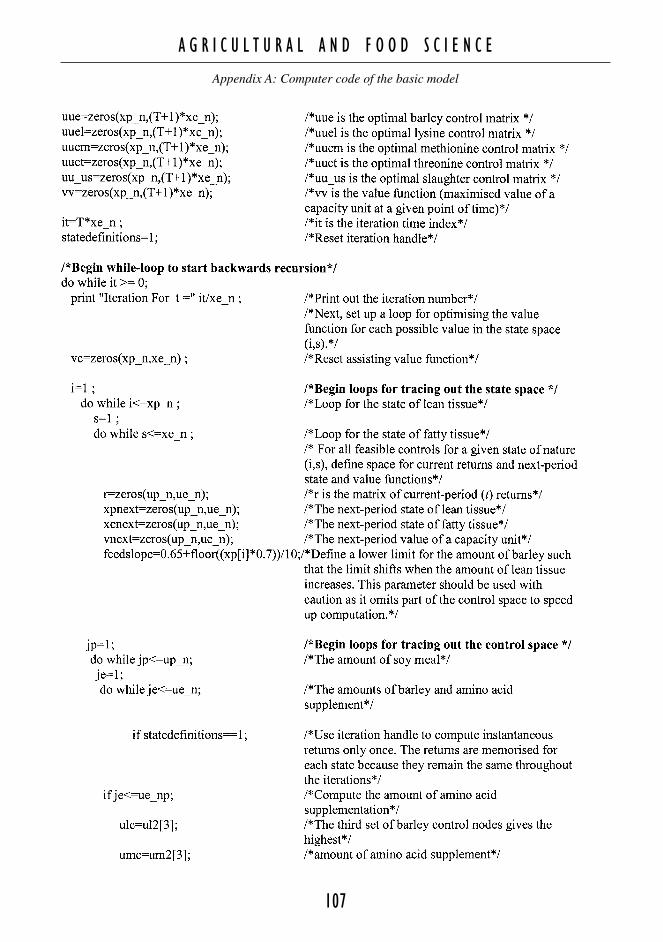
116


Appendix B: Sensitivity analysis of two-phase feeding

This appendix presents a sensitivity analysis of the two-phase feeding technology. Table A1 illustrates the value of a capacity unit and an approximation of the optimal share of soy meal in both phases of the two-phase feeding when the feed ration is switched at live weight of 45–120 kg. As the pig is always slaughtered below 120 kg live weight, switching at 120 kg live weight in practice is the equivalent of using the same feed ration throughout the fattening period (i.e. one-phase feeding). In addition, Figure

Table A1. The value function and approximated optimal share of soy meal in feed under two-phase feeding before (first phase) and after (second phase) switching the feed ratios, when the share of soy meal is adjusted once at 45–120 kg live weight.

Switching weight kg

First phase% soy meal

Second phase% soy meal

Value function€

45 19% 9% 67355 18% 7% 67765 18% 7% 67875 17% 6% 67885 15% 6% 67795 14% 4% 673

120*) 14% 4% 658

*) Switching the feed ratios at 120 kg live weight is equal to one-phase feeding, because the pig is slaughtered at 116 kg live weight.

Table A2. The value function and approximated optimal share of soy meal in feed under two-phase feeding before (first phase) and after (second phase) switching the feed ratios, when the share of soy meal is adjusted once at 45–120 kg live weight, and the price of pig meat is €1.62.

Switching weight kg

First phase% soy meal

Second phase% soy meal

Value function€

45 17% 7% 97455 15% 7% 97665 15% 6% 97975 15% 6% 97885 14% 4% 97795 11% 4% 973120*) 9% 2% 965

*) Switching the feed ratios at 120 kg live weight is equal to one-phase feeding, because the pig is slaughtered at 116 kg live weight.

A3 represents the optimal feeding patterns under two-phase feeding and flexible feeding technology, when producer has incentives to feed the pig ac-cording to its natural growth potential. This scenario is parameterised as the market scenario where the price of pig meat was €1.62. In other words, when the price of pig meat is €1.62 the value of a capac-ity unit for the two-phase feeding in Figure A3 is €979 over the period of 5 years. The corresponding value for the flexible feeding technology is €991.

0

2

4

6

8

10

12

14

16

18

20

1 11 21 31 41 51 61 71 81 91 101

time in days

Two phase

0.0

0.5

1.0

1.5

2.0

2.5

3.0

3.5

1 11 21 31 41 51 61 71 81 91 101

time in days

kg feed per day

Flexible

% of feed

Fig. A3. The amount of barley (kg per day, left panel) and the share of soy meal (% of the total amount of feed, right panel) in feed under two-phase feeding and as approximated in the benchmark scenario of the flexible feeding technology. The price of pig meat in both scenarios is €1.62.

117


Appendix C: Feeding patterns of female pigs and castrated male pigs

0

5

10

15

20

25

1 11 21 31 41 51 61 71 81 91 101

time in days

% of feed

Fit of castrated male pig

0.0

0.5

1.0

1.5

2.0

2.5

3.0

3.5

1 11 21 31 41 51 61 71 81 91 101

time in days

kg feed per day

Benchmark Castrated male pig

This appendix presents the optimised feeding pat-terns for female and castrated male pigs, and their position with respect to the benchmark scenario. The Figures are based on optimising feeding and slaughter patterns separately for female pigs and castrated male pigs. The only difference between these scenarios and the benchmark scenario is that

the parameters of the growth potential of the pig and the minimum fat-to-lean growth constraint are given gender-specific values. The price of pig meat in these scenarios is €1.39. The polynomial ap-proximations presented in Figures A4 and A5 cor-respond to the €1.39 curves reported in Figures 28 and 29 in Chapter 6.

1 11 21 31 41 51 61 71 81 91 101

time in days

Female pig Fit of female pig

0.0

0.5

1.0

1.5

2.0

2.5

3.0

3.5

1 11 21 31 41 51 61 71 81 91 101

time in days

kg feed per day

Benchmark

0

5

10

15

20

25% of feed

Fig. A4. The amount of barley (kg per day, left panel) and the share of soy meal (% of the total amount of feed, right panel) in the benchmark scenario and in the female pig scenario. The fit of female pig represents a polynomial approximation of the female pig scenario.

Fig. A5. The amount of barley (kg per day, left panel) and the share of soy meal (% of the total amount of feed, right panel) in the benchmark scenario and in the castrated male pig scenario. The fit of castrated male pig represents a polynomial approximation of the castrated male pig scenario.

118


Appendix D: Sensitivity analysis for genotype scenarios

This appendix presents sensitivity analyses with respect to constraints used in the model, and additional analyses of the effects of price changes. The results below utilise the growth parameters of the genotype and split-sex feeding scenarios. The price ratios are exactly the same as those used in corresponding market scenarios in Chapter 5. In addition, Figures A6 and A7 represent changes in feeding patterns when the constraint on the mini-mum growth ratio of fat to lean is reduced by 0.2 units below the initial values for female and cas-

trated male pigs. The reduced ratios are for pigs of improved genotype (Whittemore 1998, p. 68–70 and 557–558). In other words, the change allows the producer to increase the degree of restricting of feeding. The change increases the convexity of the optimal feeding pattern. As the constraint is locally binding in the benchmark scenario, the change in-creases the share of soy meal in feed and decreases the amount of barley. Notably, the pattern of change in feed ratios is larger for young pigs than for pigs close to the optimal slaughter maturity.

0

5

10

15

20

25

1 11 21 31 41 51 61 71 81 91 101

time in days

% of feed

Min ratio 0.8 Fit of min ratio 0.8

0.0

0.5

1.0

1.5

2.0

2.5

3.0

3.5

1 11 21 31 41 51 61 71 81 91 101

time in days

kg feed per day

Min ratio 1

Fig. A6. The effect of reducing the minimum growth ratio from 1 to 0.8 on the optimal feeding patterns for castrated male pigs.

The effects of changes in the minimum fat to lean growth ratio on the numerical results are re-ported in Table A3 for all genotype and split-sex feeding scenarios. The results utilise price ratios similar to those in the benchmark scenario. Tables A4 and A5 represent sensitivity analyses with re-

spect to price changes for female and castrated male pigs when changes in price ratios are similar to the market scenarios. Tables A6, A7, A8 and A9 repeat similar sensitivity analyses for pigs having a low K-index, a high K-index, improved maturing rate and improved mature weight.

119



Fig. A7. The effect of reducing the minimum growth ratio from 0.9 to 0.7 on the optimal feeding patterns for female pigs.

0

5

10

15

20

25

1 11 21 31 41 51 61 71 81 91 101

time in days

% of feed

Min ratio 0.7 Fit of min ratio 0.7

0.0

0.5

1.0

1.5

2.0

2.5

3.0

3.5

1 11 21 31 41 51 61 71 81 91 101

time in days

kg feed per day

Min ratio 0.9

Table A3. Time required to reach slaughter maturity, carcass weight upon slaughter, share of red meat in the slaughtered carcass, and value function over the period of 5 years under alternative growth ratio constraints in genotype and split-sex feeding scenarios.

Scenario Time to slaughter Carcass weight Red meat Value function


Castrated male pig, ratio is 1 107 85.6 61.3 674

Castrated male pig, ratio is 0.8 107 84.5 61.9 676

Female pig, ratio is 0.9 104 84.3 62.1 696

Female pig, ratio is 0.7 108 85.1 63 698

Improved mature weight, ratio is 1 95 85.2 61.7 779

Improved mature weight, ratio is 0.8 98 85.1 63 784

Improved maturing rate ratio is 1 94 84.8 61.3 772

Improved maturing rate, ratio is 0.8 95 84 62.1 775

Low K-index, ratio is 1 108 85.3 61.4 661

Low K-index, ratio is 0.8 108 83.8 62.2 664

High K-index, ratio is 1 100 85 61.6 725

High K-index, ratio is 0.8 104 85.1 62.9 729

120



Table A4. Time required to reach slaughter maturity, carcass weight upon slaughter, share of red meat in the slaughtered carcass, and value function over the period of 5 years for castrated male pigs under alternative price parameters. The price ratios used in the scenarios correspond to those used in the market scenarios in Chapter 5.


days kg % € per 5 years

Benchmark price ratios 107 85.6 61.3 674


High price of piglet 107 85.1 61.7 578

High price of barley 107 85.3 61.5 652

High price of soy 103 84.8 60.5 661



Table A5. Time required to reach slaughter maturity, carcass weight upon slaughter, share of red meat in the slaughtered carcass, and value function over the period of 5 years for female pigs under alternative price parameters. The price ratios used in the scenarios correspond to those used in the market scenarios in Chapter 5.










Table A6. Time required to reach slaughter maturity, carcass weight upon slaughter, share of red meat in the slaughtered carcass, and value function over the period of 5 years under alternative price parameters for pigs having improved mature weight. The price ratios used in the scenarios correspond to those used in the market scenarios in Chapter 5.





High price of piglet 95 85 61.8 671





121



Table A7. Time required to reach slaughter maturity, carcass weight upon slaughter, share of red meat in the slaughtered carcass, and value function over the period of 5 years under alternative price parameters for pigs having improved maturing rate. The price ratios used in the scenarios correspond to those used in the market scenarios in Chapter 5.




High price of pig meat 85 84.6 58 1107

High price of piglet 96 85 61.8 664





Table A8. Time required to reach slaughter maturity, carcass weight upon slaughter, share of red meat in the slaughtered carcass, and value function over the period of 5 years under alternative price parameters for pigs having a low K-index. The price ratios used in the scenarios correspond to those used in the market scenarios in Chapter 5.






High price of barley 108 85 61.6 639

High price of soy 104 83.6 61 648

High price of all feeds 108 85 61.6 607


Table A9. Time required to reach slaughter maturity, carcass weight upon slaughter, share of red meat in the slaughtered carcass, and value function over the period of 5 years under alternative price parameters for pigs having a low K-index. The price ratios used in the scenarios correspond to those used in the market scenarios in Chapter 5.



Benchmark price ratios 100 85 61.6 725







A dynamic programming model for optimising feeding ... - Helda

Documents

Transcript of A dynamic programming model for optimising feeding ... - Helda