
Optimising Airline Maintenance Scheduling Decisions
252
Optimising Airline Maintenance Scheduling Decisions David Torres Sanchez, B.Sc.(Hons.), M.Res Submitted for the degree of Doctor of Philosophy at Lancaster University. August 2019
-
Upload
khangminh22 -
Category
Documents
-
view
2 -
download
0
Transcript of Optimising Airline Maintenance Scheduling Decisions

Optimising Airline
Maintenance Scheduling
Decisions
David Torres Sanchez, B.Sc.(Hons.), M.Res
Submitted for the degree of Doctor of
Philosophy at Lancaster University.
August 2019

Abstract
Airline maintenance scheduling (AMS) studies how plans or schedules are constructed
to ensure that a fleet is efficiently maintained and that airline operational demands
are met. Additionally, such schedules must take into consideration the different regu-
lations airlines are subject to, while minimising maintenance costs. In this thesis, we
study different formulations, solution methods, and modelling considerations, for the
AMS and related problems to propose two main contributions.
First, we present a new type of multi-objective mixed integer linear programming
formulation which challenges traditional time discretisation. Employing the concept
of time intervals, we efficiently model the airline maintenance scheduling problem
with tail assignment considerations. With a focus on workshop resource allocation
and individual aircraft flight operations, and the use of a custom iterative algorithm,
we solve large and long-term real-world instances (16000 flights, 529 aircraft, 8 main-
tenance workshops) in reasonable computational time. Moreover, we provide evidence
to suggest, that our framework provides near-optimal solutions, and that inter-airline
cooperation is beneficial for workshops.
Second, we propose a new hybrid solution procedure to solve the aircraft recovery
I

II
problem. Here, we study how to re-schedule flights and re-assign aircraft to these, to
resume airline operations after an unforeseen disruption. We do so while taking op-
erational restrictions into account. Specifically, restrictions on aircraft, maintenance,
crew duty, and passenger delay are accounted for. The flexibility of the approach al-
lows for further operational restrictions to be easily introduced. The hybrid solution
procedure involves the combination of column generation with learning-based hyper-
heuristics. The latter, adaptively selects exact or metaheuristic algorithms to generate
columns. The five different algorithms implemented, two of which we developed, were
collected and released as a Python package (Torres Sanchez, 2019a). Findings suggest
that the framework produces good quality recovery solutions and is scalable to larger
networks.

Acknowledgements
I would like thank Dr Burak Boyaci, for our regular meetings and constant stream
of exciting ideas, Professor Konstantinos Zografos, and my industrial supervisor, Dr
Richard Standing from R2 Data Labs (Rolls-Royce), for their patience, guidance, and
feedback throughout.
I thank the EPSRC funded Statistics and Operational Research (STOR-i) Centre
for Doctoral Training and Rolls-Royce Holdings plc. I thank everyone involved in
STOR-i, students and others, but especially Professors Jonathan Tawn, Idris Eckley
and Kevin Glazebrook for their continued support and very useful pieces of advice.
STOR-i has managed to create a friendly research environment which has led to me
really enjoying my time here.
Last but not least, I thank my family (far and close) for putting up with coffee-
fuelled writing mode Dave. Sin vosotros no estarıa donde estoy.
III

IV
Para mis padres.

Declaration
I declare that the work in this thesis has been done by myself and has not been
submitted elsewhere for the award of any other degree.
A version of Chapter 3 is being reviewed for publication as: Torres Sanchez, D.,
Boyacı, B., Zografos, K. G. (n.d.). ‘An Optimisation Framework for Airline Fleet
Maintenance Scheduling with Tail Assignment Considerations’. Transportation Re-
search Part B: Methodological.
A version of Chapter 4 is to be submitted for publication as: Torres Sanchez, D.,
Boyacı, B., Zografos, K. G. (Forthcoming). ‘A Hybrid Solution Procedure for the
Aircraft Recovery Problem with Operational Restrictions’.
A version of Appendix B.3 is being reviewed for publication as: Torres Sanchez,
D. (Under review). ‘cspy: A Python package with a collection of algorithms for the
(Resource) Constrained Shortest Path problem’. Journal of Open Source Software.
The word count for this thesis is 40558 words.
David Torres Sanchez
August 2019
V

Contents
Abstract I
Acknowledgements III
Declaration V
List of Abbreviations XI
List of Algorithms XII
List of Figures XV
List of Tables XVII
1 Introduction 1
1.1 Problem Description . . . . . . . . . . . . . . . . . . . . . . . . . . . 3
1.1.1 Airline Maintenance Scheduling Problem with Tail Assignment
Considerations . . . . . . . . . . . . . . . . . . . . . . . . . . 4
1.1.2 Aircraft Recovery Problem with Multiple Operational Restrictions 7
1.2 Thesis Contents and Contributions . . . . . . . . . . . . . . . . . . . 8
VI

CONTENTS VII
2 Extended Literature Review 14
2.1 General Scheduling Problems . . . . . . . . . . . . . . . . . . . . . . 14
2.1.1 Classification of Machine Scheduling Problems . . . . . . . . . 15
2.1.2 Classification of Project Planning Problems and the RCPSP . 16
2.1.3 Long-term RCPSP formulations . . . . . . . . . . . . . . . . . 21
2.1.4 A Formulation for the Preemptive RCPSP . . . . . . . . . . . 28
2.2 Maintenance Scheduling . . . . . . . . . . . . . . . . . . . . . . . . . 34
2.2.1 Prognostic-Based Models . . . . . . . . . . . . . . . . . . . . . 36
2.2.2 Modelling Scheduling Problems in Other Industries . . . . . . 49
2.3 Airline Scheduling and Recovery . . . . . . . . . . . . . . . . . . . . . 51
2.3.1 Tail Assignment and Aircraft Recovery . . . . . . . . . . . . . 53
2.3.2 Integrated and Semi-Integrated Airline Scheduling and Recovery 60
2.4 Methodology for Chapter 4 . . . . . . . . . . . . . . . . . . . . . . . . 73
2.4.1 Column Generation . . . . . . . . . . . . . . . . . . . . . . . . 73
2.4.2 Shortest Path Problem with Resource Constraints . . . . . . . 78
2.4.3 Hyper-heuristics . . . . . . . . . . . . . . . . . . . . . . . . . . 86
3 An Optimisation Framework for Airline Fleet Maintenance Schedul-
ing with Tail Assignment Considerations 88
3.1 Introduction . . . . . . . . . . . . . . . . . . . . . . . . . . . . . . . . 88
3.2 Literature Review . . . . . . . . . . . . . . . . . . . . . . . . . . . . . 92
3.3 The Proposed Modelling Approach . . . . . . . . . . . . . . . . . . . 100
3.3.1 Assumptions . . . . . . . . . . . . . . . . . . . . . . . . . . . . 100

CONTENTS VIII
3.3.2 Concepts . . . . . . . . . . . . . . . . . . . . . . . . . . . . . . 101
3.3.3 Airline Fleet Maintenance Scheduling with Violations . . . . . 102
3.3.4 Airline Fleet Maintenance Scheduling with Tail Assignment . 110
3.4 Solution Methodology . . . . . . . . . . . . . . . . . . . . . . . . . . 116
3.4.1 Preprocessing Routine . . . . . . . . . . . . . . . . . . . . . . 116
3.4.2 Solution Procedure . . . . . . . . . . . . . . . . . . . . . . . . 118
3.5 Model Application and Computational Tests . . . . . . . . . . . . . . 125
3.5.1 Single Workshop Case . . . . . . . . . . . . . . . . . . . . . . 127
3.5.2 Multi-workshop Case . . . . . . . . . . . . . . . . . . . . . . . 135
3.6 Conclusions . . . . . . . . . . . . . . . . . . . . . . . . . . . . . . . . 140
4 A Hybrid Solution Procedure for the Aircraft Recovery Problem
with Operational Restrictions 142
4.1 Introduction . . . . . . . . . . . . . . . . . . . . . . . . . . . . . . . . 142
4.2 Literature Review . . . . . . . . . . . . . . . . . . . . . . . . . . . . . 145
4.3 Modelling . . . . . . . . . . . . . . . . . . . . . . . . . . . . . . . . . 153
4.3.1 Definitions . . . . . . . . . . . . . . . . . . . . . . . . . . . . . 153
4.3.2 Aircraft Recovery Problem Formulation . . . . . . . . . . . . . 154
4.3.3 Column Generation . . . . . . . . . . . . . . . . . . . . . . . . 154
4.4 Solution Methodology . . . . . . . . . . . . . . . . . . . . . . . . . . 163
4.4.1 Network Generation . . . . . . . . . . . . . . . . . . . . . . . 163
4.4.2 Hybrid Solution Procedure . . . . . . . . . . . . . . . . . . . . 165
4.5 Computational Experiments . . . . . . . . . . . . . . . . . . . . . . . 177

CONTENTS IX
4.6 Conclusions . . . . . . . . . . . . . . . . . . . . . . . . . . . . . . . . 185
5 Thesis Conclusions, Limitations and Further Work 188
A Appendix for Chapter 3 193
A.1 Extension: Airline Maintenance Scheduling with Flight Re-Scheduling 193
A.2 Supplementary Proofs . . . . . . . . . . . . . . . . . . . . . . . . . . 194
A.3 Interval Generation . . . . . . . . . . . . . . . . . . . . . . . . . . . . 196
B Appendix for Chapter 4 201
B.1 Functions Employed in Metaheuristic Algorithms . . . . . . . . . . . 201
B.1.1 Algorithm 3 . . . . . . . . . . . . . . . . . . . . . . . . . . . . 201
B.1.2 Algorithms 5 and 6 . . . . . . . . . . . . . . . . . . . . . . . . 202
B.1.3 Algorithm 7 . . . . . . . . . . . . . . . . . . . . . . . . . . . . 203
B.2 Parameters in the Computational Tests . . . . . . . . . . . . . . . . . 204
B.3 cspy: A Python package with a collection of algorithms for the (Re-
source) Constrained Shortest Path problem . . . . . . . . . . . . . . . 206
B.3.1 Introduction . . . . . . . . . . . . . . . . . . . . . . . . . . . . 206
B.3.2 Algorithms . . . . . . . . . . . . . . . . . . . . . . . . . . . . 207
B.4 Features . . . . . . . . . . . . . . . . . . . . . . . . . . . . . . . . . . 208
B.5 Example . . . . . . . . . . . . . . . . . . . . . . . . . . . . . . . . . . 209
Bibliography 213

List of Abbreviations
AMS : Airline Maintenance Scheduling
AR : Aircraft Recovery
CBM : Condition-based Maintenance
CM : Corrective Maintenance
FH : Flying Hours
GRASP : Greedy Randomised Adaptive Search Procedure
IP : Integer Program
LP : Linear Program
MCNF : Multi-Commodity Network Flow
MIP : Mixed Integer Program
MMILP : Multi-Objective Mixed Integer Linear Program
MOPs : Maintenance Opportunities
MR : Maintenance Requirement
X

LIST OF ABBREVIATIONS XI
PM : Preventive Maintenance
PRCPSP : Preemptive Resource Constrained Project Scheduling Problem
RCPSP : Resource Constrained Project Scheduling Problem
REF : Resource Extension Function
RR : Rolls-Royce
RUL : Remaining Useful Life
SPPRC: Shortest Path Problem with Resource Constraints
TA : Tail Assignment
TSN : Time-Space Network

List of Algorithms
1 Column Generation Algorithm. . . . . . . . . . . . . . . . . . . . . . 77
2 Generic monodirectional labelling algorithm for the SPPRC. . . . . . 82
3 Bidirectional labelling algorithm with dynamic halfway point for the
SPPRC (Tilk et al., 2017). . . . . . . . . . . . . . . . . . . . . . . . . 85
4 Solution procedure with conflicting period selection and interval splitting.124
5 Tabu Search for the SPPRC. . . . . . . . . . . . . . . . . . . . . . . . 171
6 Greedy Elimination Algorithm for the SPPRC. . . . . . . . . . . . . . 172
7 Adapted GRASP for the SPPRC (Ferone et al., 2019). . . . . . . . . 174
8 Reinforcement Learning – Great-Deluge Hyper-heuristic (Ozcan et al.,
2010) . . . . . . . . . . . . . . . . . . . . . . . . . . . . . . . . . . . . 175
XII

List of Figures
1.1 Connections between areas in Chapter 2 and the rest of the thesis. . . 9
2.1 An activity broken down into two subactivities. . . . . . . . . . . . . 29
2.2 Example of a feasible preemptive schedule showing the processing of
activities for two resources R1 (left) and R2 (right). . . . . . . . . . . 32
2.3 Example of a feasible non-preemptive schedule showing the processing
of activities for two resources R1 (left) and R2 (right). . . . . . . . . . 33
2.4 Failure rate (r) evolving through time (t) after performing PM inter-
ventions at times ti for i = 1, 2, 3, 4 (assuming λ ≥ 1). . . . . . . . . . 38
2.5 Sequential modelling of the airline scheduling problem (Bae, 2010). . 52
2.6 Hyper-heuristic algorithm. . . . . . . . . . . . . . . . . . . . . . . . . 87
3.1 Stages of the airline scheduling problem. . . . . . . . . . . . . . . . . 93
3.2 Time-Space Network (TSN) example. . . . . . . . . . . . . . . . . . . 94
3.3 Timeline showing the deconstruction of three MOPs into sets of con-
secutive intervals. . . . . . . . . . . . . . . . . . . . . . . . . . . . . . 104
3.4 Flow chart outlining the process of the iterative algorithm. . . . . . . 117
XIII

LIST OF FIGURES XIV
3.5 Conflicting period selection. . . . . . . . . . . . . . . . . . . . . . . . 119
3.6 Interval splitting stage for a 9 hour MOP using binary segmentation
for three iterations. . . . . . . . . . . . . . . . . . . . . . . . . . . . 122
3.7 Resource profiles for the Bangkok workshop for the first and last (4th)
iterations of the interval splitting stage using Method 3. . . . . . . . . 134
3.8 Result comparison (objectives 3.3.21, 3.3.22) for Method 3 vs tradi-
tional discretisation for different time steps. . . . . . . . . . . . . . . 134
3.9 Computational comparison for Method 3 applied to different multi-
workshop cases. . . . . . . . . . . . . . . . . . . . . . . . . . . . . . . 137
3.10 Maintenance schedules produced by using Method 3 for each aircraft
and workshop in the first multi-workshop case. . . . . . . . . . . . . . 139
4.1 Time-Space Network (TSN) example (Torres Sanchez et al., n.d.). . . 147
4.2 Generation of Time-Space Networks. . . . . . . . . . . . . . . . . . . 165
4.3 Hybrid Solution Procedure. . . . . . . . . . . . . . . . . . . . . . . . 167
4.4 Comparison between hyper-heuristics HH1 and HH2. . . . . . . . . . 182
4.5 Trend between network size (per instance) and percentage of flights
cancelled (using HH2). . . . . . . . . . . . . . . . . . . . . . . . . . . 184
4.6 Performance comparison for each instance using the exact algorithm
(A1), a random non-learning based method (rHH1), and the hybrid
solution procedure (mHH2). . . . . . . . . . . . . . . . . . . . . . . . 184
A.1 Example of edge labelling for flights between airports sp and sq. . . . 197
A.2 Incident edges with source and sink functions. . . . . . . . . . . . . . 197
List of Tables
2.1 Computational results including makespan (MS) and computational
times (T) for Model 2.1.4, psplib benchmark results, Model 2.1.2, and
the preprocessing stage. . . . . . . . . . . . . . . . . . . . . . . . . . 34
2.2 Forward and backward labelling notation. . . . . . . . . . . . . . . . 83
3.1 Typical maintenance frequencies in calendar months (MO), flying hours
(FH), or flight cycles (FC) (Cook and Tanner, 2008; Martins, 2016). . 90
3.2 Summary of selected literature. MS = inclusion of maintenance schedul-
ing, FH = use of legal remaining flying hours, RC = workshop resource
considerations, H = time horizon (days), Sched. Type = scheduling
type, Airlines = number of airlines considered, W = number of work-
shops considered, F = number of flights (in largest test instance), A =
number of aircraft (in largest test instance), T = computational time
(of largest test instance). . . . . . . . . . . . . . . . . . . . . . . . . . 99
3.3 Maintenance regulation parameter values for two check types (1 and 2)
and two aircraft types (A320 and F100). . . . . . . . . . . . . . . . . 126
XV

LIST OF TABLES XVI
3.4 Sample resource demands and limit capacities for four types of re-
sources (ri for i = 1, 2, 3, 4) and two maintenance types (1 and 2). . . 126
3.5 Objective function breakdown for the Bangkok workshop. The best
method in each iteration is highlighted in green. . . . . . . . . . . . . 132
3.6 Comparison across 5 workshops during the interval splitting stage for
the three different splitting methods. . . . . . . . . . . . . . . . . . . 133
3.7 Method comparison for the 4-workshop case. . . . . . . . . . . . . . . 136
4.1 Flight range according to flight length (Eurocontrol, 2011). . . . . . . 143
4.2 Summary of selected AR literature. Air. = aircraft type flight range
considerations, Maint. = maintenance regulations considerations, Pass.
= passenger delay restrictions considerations, SPPRC = use of shortest
path problem with resource constraints, HH = use of hyper-heuristics,
Opt. = optimal integer solution obtained, F = number of flights in
largest test instance, A = number of aircraft in largest test instance, T
= computational time of largest test instance. . . . . . . . . . . . . . 152
4.3 Test instances.1 F = # of flights, A = # of aircraft, T = # of aircraft
types, H = length of planning horizon in days, TSN= size of time-space
network (# of nodes, # of arcs). . . . . . . . . . . . . . . . . . . . . . 178
4.4 Algorithms used in solution procedure. . . . . . . . . . . . . . . . . . 178
4.5 Usage count of metaheuristics for the two hyperheuristics (HH1, HH2)
using different utility functions. . . . . . . . . . . . . . . . . . . . . . 179

LIST OF TABLES XVII
4.6 Computational results of the hybrid solution procedure using hyper-
heuristic HH1. . . . . . . . . . . . . . . . . . . . . . . . . . . . . . . . 180
4.7 Computational results of the hybrid solution procedure using hyper-
heuristic HH2. . . . . . . . . . . . . . . . . . . . . . . . . . . . . . . . 181
B.1 Different aircraft types in test instances with their respective operating
costs. . . . . . . . . . . . . . . . . . . . . . . . . . . . . . . . . . . . . 205
B.2 Parameters for computational tests. . . . . . . . . . . . . . . . . . . . 205
Chapter 1
Introduction
The industrial partner for this PhD project, Rolls-Royce Holdings plc (RR), is a
market leader in the civil aerospace business sector; powering more than 13,000 engines
around the world and 35 types of commercial aircraft (Rolls-Royce Holdings plc,
2015). Besides producing jet engines, RR provides several so-called digital service
solutions that range from the detection of operational deficiencies of the engines to
the suggestion of tentative maintenance schedules for the management of an airlines’
fleet. RR has to cater the appropriate support for all stages of an engines’ lifecycle to
meet with the service offering requested by the customer. In particular, the services
related to this research project are those linked to the scheduling of maintenance
for which current services have been found to yield suboptimal plans that induce
significant losses. The objectives of this thesis are, to develop optimisation-based
mathematical models and solution algorithms to optimise the aircraft maintenance
schedules, and, additionally, to provide innovative airline scheduling tools to broaden
the digital service solutions offering.
1

CHAPTER 1. INTRODUCTION 2
Motivated by these objectives, research has been carried out around several areas
of the literature. One such stream is the airline maintenance scheduling (AMS)
literature. Due to the constant interaction between aircraft maintenance activities
and airline operations, a facet of particular interest lies in the interaction between the
currently disjoint AMS and tail assignment (TA) problems. The latter, refers to the
assignment of aircraft to different, already scheduled, flight legs. The two individual
components of the problem are of interest to researchers, as they each compose highly
complex optimisation problems. Additionally, sets of constraints and regulations have
to be included. Typically, these problems are treated separately and solved sequen-
tially (Cordeau et al., 2001). That is, the optimal solution from the TA problem
becomes input for the AMS problem. Clearly, the solution of one subproblem does
not take into consideration the restrictions of the subsequent subproblem, leading
to suboptimal overall solutions, often far from optimality. Nonetheless, considering
them in conjunction (keeping in mind tractability), captures the interactions between
the two problems, avoids the suboptimality issue, and, maximises aircraft availability
while minimising unnecessary maintenance costs and meeting minimum safety reg-
ulations as established by the regulatory agencies (civil aviation authority, federal
aviation administration or similar).
Another area of interest is the aircraft recovery (AR) literature. With main-
tenance and other operational restrictions in mind, the aim of the AR problem is to
recover airline operations from an unexpected disruption. This involves the generation
of new flight schedules such that the alterations to the initial plans are minimised.

CHAPTER 1. INTRODUCTION 3
1.1 Problem Description
The increasing customer demand for care packages plus other services, which make
up for 53% of the total underlying revenue in RR’s civil aerospace business sector,
has driven to an exploration and revision of the current systems in place (Rolls-Royce
Holdings plc, 2015). The combination of AMS and TA will lead to optimal mainte-
nance decisions which RR believe can significantly increase their revenue aftermarket
growth. As for their customers, it is estimated that around 69% of the direct oper-
ating costs are engine influenced costs (Rolls-Royce Holdings plc, 2016). Hence, this
approach will have a great financial impact on customers as well, not only for the
aircraft availability but also in the long-term effect of efficient aircraft maintenance.
In an increasingly larger aviation intelligence market, a brand-new AR learning-
based service is bound to have an impact (IATA, 2019). Striving towards one of
RR’s aims to “Take Care for our customers to the next level” by strengthening their
aerospace digital service solutions offering.
In this thesis, we present two new scheduling tools that enable customers to access,
maintenance scheduling and workshop services, through our AMS tool; and, aircraft
recovery solutions, through our AR learning-based tool.
The individual characteristics of the problems were gathered across several meet-
ings with Dr Richard Standing and other experts from RR including: fuel consultants,
the principal business analyst, and past airline practitioners. They can be summarised
as two problems with different characteristics. The problems are discussed in the next
two sections.

CHAPTER 1. INTRODUCTION 4
1.1.1 Airline Maintenance Scheduling Problem with Tail As-
signment Considerations
The first problem considered in this thesis, subject of Chapter 3, considers the AMS
problem with TA considerations and can be labelled as large-scale, medium-term,
time-dependent and prognostic.
The problem is large-scale due to the multiple aspects. Aside from the time
dimension, another factor of significant influence is the fleet size and characteristics.
Each aircraft belongs to a certain fleet type, hence, has different specifications and
passenger restrictions which limit the authorised flight legs. Additionally, each air-
craft has a corresponding set of operations history (e.g. the number of flying hours,
the number of operations, maintenance details) that need to be considered. Mainte-
nance workshop constraints also introduce further size considerations. Such workshop
constraints include, capacity, costs, demand, manpower, and inventory. Notably, man-
power or maintenance crew introduces several complications. Restrictions apply to
each technician as they can only perform operations on the levels they have been
certified for.
The planning horizon for the problem is a medium-term 1-3 months. The reason
for the planning horizon to have been modified from the usual operational level found
in the literature (1 to 7 days), is to capture the interactions between the components
of the model and to gain insights into which tactical decisions should be made. Such
tactical decisions will favour an overall profit in the long-term by guiding the decisions
towards the exploration of alternatives and co-operation options.

CHAPTER 1. INTRODUCTION 5
The time-dependent element, sometimes referred to as dynamicity, comes natu-
rally from the scheduling setting. In optimisation problems, time-dependence can be
modelled using either a discrete or a continuous time representation. These choices
bring different benefits. As can be found in the reviews of scheduling approaches for
chemical processes, Floudas and Lin (2004, 2005) among others, it is apparent that
traditional continuous time representations provider higher quality solutions, however,
they are more computationally expensive (to the extent that they become intractable
for large instances). Since our problem is large, a time discretisation method is em-
ployed. In order to improve the quality of the solutions and avoid suboptimality
issues, an appropriate solution algorithm is developed that makes the discretisation
more granular.
The trade-off between performing different types of interventions at certain work-
shops and the outcome in terms of improved aircraft condition, cost and time required,
can be included using prognostic modelling. This allows the up-to-date “health”-
state of the aircraft and deterioration to be utilised when making scheduling deci-
sions. The updated legal remaining flying hours can be used to account for aircraft
“health”-state. Hence, aircraft have to monitored throughout the planning horizon
to determine whether they are suitable for operating a certain flight, or not; in which
case the aircraft can be exchanged for a suitable one.
Current Industrial Practice
Aircraft maintenance requirements are covered by civil aviation authorities. In short,
they provide a set of limitations on aircraft use between different types of maintenance

CHAPTER 1. INTRODUCTION 6
interventions. Not considering short-term types, maintenance interventions consist
of four medium/long-term airframe checks (A, B, C and D) and three long-term
off-wing/major maintenance (engine, landing gear, and auxiliary power unit). The
limitations imposed by regulations are a certain number of flying hours, cycles, or
months between different maintenance interventions. These vary depending on the
aircraft type (Cook and Tanner, 2008). For more information see Section 3.1.
In practice, according to practitioners, maintenance operators constrain them-
selves by time, not by scope. That is, if an aircraft has been brought in for a non-
major check, type A, for example, they will perform as many operations as possible
to make the aircraft available by the end of the set downtime. If they are unable
to perform all the desirable tasks but the aircraft is safely functional, they will add
these to the list of deferred operations to avoid introducing any further delays into
the system. The operations in the list will be fixed at a later stage or workshop. For
our purposes, two maintenance intervention types will be used, on-wing, check types
A and C. Check type B is excluded as it is running out of practice (Qantas, 2016).
For the AMS problem, RR currently employ two pieces of software: SCAF and
StaggerLite, which can be described as a forecaster and a schedule planner, re-
spectively (Rolls-Royce Holdings plc, 2017). The SCAF model employs AnyLogic, a
customisable simulation tool, to predict engine failure rate evolution across time and
usage. To do this, SCAF uses relevant data about each aircraft. Some factors that have
been found to be influential include: the number of operations, the age of the aircraft,
the number of cycles (takeoffs and landings), and the number of flying hours. The

CHAPTER 1. INTRODUCTION 7
output of the SCAF model is then fed into the StaggerLite model which, using the
OptiQuest optimisation tool, arranges a feasible maintenance schedule according to
several maintenance requirements, available time slots and objective function criteria.
The total computational time for an average size airline ranges from 40 minutes to
1 hour to produce a 2 to 4 week schedule. Unfortunately, this procedure leads to
suboptimal schedules which are then not presented in an interpretable way to the
maintenance operators and engineers. Moreover, it does not take into account the
effect that these interventions may have on TA.
1.1.2 Aircraft Recovery Problem with Multiple Operational
Restrictions
The second problem considered in this thesis, subject of Chapter 4, considers the
AR problem with operational considerations and can be labelled as combinatorial,
short-term, and learning-based.
The nature of the problem is combinatorial. Generating new flight schedules
around a given disruption, involves selecting from all the possible flight paths. We
use column generation to solve the problem efficiently. Moreover, considering multi-
ple operational restrictions reduces the number of feasible flight paths. Among the
most important operational restrictions are: aircraft type, maintenance, crew duty,
and passenger delay. Aircraft type restrictions ensure that aircraft operate suitable
flight ranges according to their specifications. Maintenance restrictions, as previously
discussed, involve limiting the number of flying hours between certified maintenance

CHAPTER 1. INTRODUCTION 8
interventions. Crew duty restrictions involve several rules including enforced rest pe-
riods and maximum duty durations. Passenger delay restrictions set maximum delay
thresholds after which passengers have the right to reparations by the airline. For
more details on operational restrictions, see Section 4.1.
The problem is short-term or operational. The aim of the problem is to resume
airline operations in minimal time while also minimising the inconveniences for crew
and passengers. Hence, an operational planning horizon (1 to 10 days) is appropriate
and commonly used for this type of problem.
To provide an aviation intelligence solution, the problem is learning-based. For
this purpose, the exploration of an interaction between statistics and operational
research is required. To incorporate a learning-based mechanism into a column gen-
eration setting, selection hyper-heuristics can be employed. These choose different
algorithms to generate columns, which can then be evaluated and learning can be
done by comparing the performance and quality of the columns.
1.2 Thesis Contents and Contributions
In Chapter 2, we include an extended literature review, with topics of interest for
Chapters 3 and 4. Figure 1.1 summarises the links and overlaps between the different
sections in Chapter 2 and their use in the rest of the thesis. Hence, justifying the
areas visited by either a direct link or an important theoretical relation.
The extended literature review in Chapter 2, starts with an introduction to the
general scheduling problem, Section 2.1 (Traditional Scheduling Problems), which in-

CHAPTER 1. INTRODUCTION 9
SchedulingProblems
RCPSP
MachineScheduling
Long termRCPSP
PRCPSP
Maintenance
Prognostics
AirlineScheduling
and Recovery
Tail As-signment
AircraftRecovery
SolutionMethods
IterativeAlgorithms
ColumnGeneration
SPPRC
Hyper-heuristics
Chapter3
Chapter4
Figure 1.1: Connections between areas in Chapter 2 and the rest of the thesis.

CHAPTER 1. INTRODUCTION 10
cludes a classification scheme for different types of machine and project scheduling
problems. Also, as a minor contribution, we present a new formulation for the preemp-
tive resource constrained project scheduling problem (preemptive RCPSP), a special
kind of project scheduling which generalises some of the machine scheduling problems.
The following sections review two streams of the literature, Maintenance Scheduling
and Prognostics (Section 2.2), and Airline Scheduling and Recovery (Section 2.3).
As can be seen in Figure 1.1, Maintenance Scheduling lies partly inside Scheduling
Problems, intersecting with Airline Scheduling, and, partly outside, where prognostic
considerations are. Airline Scheduling and Recovery, which contains Tail Assignment
and Aircraft Recovery (Section 2.3.1), is fully within Scheduling Problems. Integrated
and Semi-Integrated Airline Scheduling and Recovery (in Section 2.3.2) considers the
intersection between two or more components of the Airline Scheduling and Recovery
problems. This section also includes a discussion of more sophisticated approaches to
model the problem such as multi-objective robust optimisation, artificial neural net-
works, and multi-layered networks. Section 2.4, reviews several areas related to the
methodology employed in Chapter 4. Precisely, we study a common solution method
for combinatorial optimisation problems, Column Generation, and a related well-
known subproblem, the shortest path problem with resource constraints (SPPRC).
Also, a brief overview of Hyper-heuristic search methods is provided.
Chapter 3, as displayed with red dashed arrows in Figure 1.1, couples several
concepts for a considerable contribution: a concept from the Long Term RCPSP
literature, the intersection between Maintenance Scheduling and Tail Assignment,

CHAPTER 1. INTRODUCTION 11
the use of Prognostics, and a problem-specific iterative algorithm. The abstract for
this chapter is given below.
Fierce competition between airlines has led to the need of minimising the operating
costs while also ensuring quality of service. Given the large proportion of operating
costs dedicated to aircraft maintenance, cooperation between airlines and their respec-
tive maintenance provider is paramount. In this research, we propose a framework to
develop commercially viable and maintenance feasible flight and maintenance sched-
ules. Such framework involves two multi-objective mixed integer linear programming
formulations and an iterative algorithm. The first formulation, the airline fleet main-
tenance scheduling with violations, minimises the number of maintenance regulation
violations and the number of not airworthy aircraft; subject to limited workshop
resources and current maintenance regulations on individual aircraft flying hours.
The second formulation, the airline fleet maintenance scheduling with tail assignment
allows aircraft to be assigned to different flights. In this case, subject to similar con-
straints as the first formulation, six lexicographically ordered objective functions are
minimised. Namely, the number of violations, maximum resource level, number of
tail re-assignments, number of maintenance interventions, overall resource usage, and
number of not airworthy aircraft. The iterative algorithm ensures fast computational
times while providing good quality solutions. Additionally, by tracking aircraft and
using precise flying hours between maintenance opportunities we ensure that the air-
craft are airworthy at all times. Computational tests on real flight schedules over a
30-day planning horizon show that even with multiple airlines and workshops (16000
flights, 529 aircraft, 8 maintenance workshops) our solution approach can construct

CHAPTER 1. INTRODUCTION 12
near-optimal maintenance schedules within minutes.
On the other hand, Chapter 4, as shown with blue dashed arrows in Figure 1.1,
models the intersection between Aircraft Recovery and Maintenance Scheduling with
the use of Column Generation with the SPPRC and Hyper-heuristics. The abstract
for this chapter is given below.
The unforeseen disruption of airline services often leads to significant additional
costs. Aircraft recovery models enable the resumption of services in minimal time
while minimising the additional costs incurred. Therefore, solutions must provide an
efficient re-planning of scheduled services that mitigates the impact on passengers
and crew while respecting a set of regulations for operations. Such regulations impose
restrictions on aircraft, maintenance, crew, and passenger delay. The aircraft recov-
ery problem is a hard combinatorial optimisation problem, hence, these restrictions
cannot be modelled with ease. In this paper, we develop a hybrid solution proce-
dure, based on column generation and hyper-heuristics, that allows us to consider
such operational restrictions while providing solutions to real-world test instances in
reasonable computational time. Such solutions, minimise the number of flights that
are cancelled and the total operating costs. The operational restrictions are taken into
account in the subproblems, i.e. when generating columns. Specifically, this is done
by modelling the subproblems as shortest path problems with resource constraints,
with appropriately defined weights and resources, one for each operational restriction.
The hyper-heuristic algorithms learns from the selection of three different metaheuris-
tic algorithms to generate columns. The learning process allows the hyper-heuristic

CHAPTER 1. INTRODUCTION 13
to adapt as the problem develops, selecting the most effective metaheuristic for each
subproblem. Furthermore, an exact bidirectional labelling algorithm with dynamic
halfway point is used to generate columns with non-negative reduced costs, thus,
guaranteeing optimal solutions for the LP relaxation of the aircraft recovery problem.
Lastly, Chapter 5 provides the concluding remarks for the thesis and potential
research directions. Additionally, Appendix A provides supplementary materials for
Chapter 3, an extension that accounts for flight re-scheduling, some additional proofs,
and the theoretical motivation behind the interval-based formulations. Appendix B
provides extra materials for Chapter 4, functions used in the pseudo-code for each
algorithm, parameters used in the computational tests, and the high-level paper about
the Python package developed.

Chapter 2
Extended Literature Review
This chapter contains a review of the literature necessary for Chapters 3 and 4. Par-
ticularly, we include an introduction to general scheduling problems (machine
scheduling and project planning), an overview of maintenance scheduling and
prognostics, an exploration of airline scheduling and recovery, and a break-
down of the areas employed in the methodology for Chapter 4.
2.1 General Scheduling Problems
Since the late ‘50s, scheduling problems have been researched thoroughly. There were
mainly developed and motivated around two applications: machine scheduling
and project planning. Machine scheduling deals with the combinatorial problem
that arises from considering a large number of scheduling situations in which one
or more machines are available for processing a particular number of jobs. Project
planning refers to the programming of different activities that need completion for
14
CHAPTER 2. EXTENDED LITERATURE REVIEW 15
a given project. Various types of projects are, for example, a school timetable, a
construction, a business expansion, or a software development process. These usually
are accompanied by some precedence and resource constraints. Such resources can be
broadly defined as “production units” and range from raw materials to machinery or
even manpower and are taken as inputs for the project planning problem. Brucker
and Knust (2012) gave a very comprehensive study to both of these problems.
2.1.1 Classification of Machine Scheduling Problems
Depending on the machine environment or on the characteristics of the jobs there are
several classes of machine scheduling problems. As it shall be discussed later, these
can be generalised under a special type of project scheduling problem.
The simplest machine scheduling model is for a single machine. That is, there are
n jobs J = {1, 2, . . . , n} (order of which is assumed to be given), with certain known
processing times pj, and which have to be processed on a single machine. Under the
assumption that only one job can be processed at a time, this case is known as the
single machine scheduling problem. The next simplest case is when a set of jobs
have to be processed on multiple independent and identical machines with the same
processing times. However, if the machines are not identical, then the processing time
for job j on machine Mk becomes pjk. If a machine is allowed to process more than
one different job, then any machine in the subset of machines µj ∈ {M1, . . . ,Mm} can
be used to process it, unless that machine is being used to process another job. All
of these cases (subject, again, to the single job per machine assumption) are grouped
under the parallel machine scheduling problem. More precisely, when jobs occupy
CHAPTER 2. EXTENDED LITERATURE REVIEW 16
all machines in their respective µj simultaneously, then the problem is classed as a
multi-processor task scheduling problem.
By studying the characteristics of different jobs, more classes of machine scheduling
problems arise; shop scheduling problems. In shop scheduling problems, jobs consist
of a sequence of operations that have to be processed on different machines. Formally,
job j consists of nj operations O1j, . . . , Onjj; that must be processed sequentially (in
some order) and in one machines from the subset, µOij∈ {M1, . . . ,Mu} (for 1 ≤ u ≤ m
and 1 ≤ i ≤ nj). If there is a precedence relation between operations but jobs are
independent of each other, then the problem is classed as a job-shop problem. If
there is an order for both, the operations and the jobs, then the problem becomes
a flow-shop problem. Further, if there is an order for the jobs but not for the
operations, then the problem is classed as a open-shop problem.
2.1.2 Classification of Project Planning Problems and the
RCPSP
Project planning is heavily conditioned by the specifications on the resources and ac-
tivities. These are grouped under the more appropriate term, resource-constrained
project scheduling problem (RCPSP). For a recent and thorough review, we refer
the reader to Habibi et al. (2018). The generality of the RCPSP allows it to have a
wide range of applications where the aim is to schedule some activities or jobs, such
that precedence and resource constraints are satisfied, and a certain objective function
is optimised. As for the objective functions, for example, the project duration, the
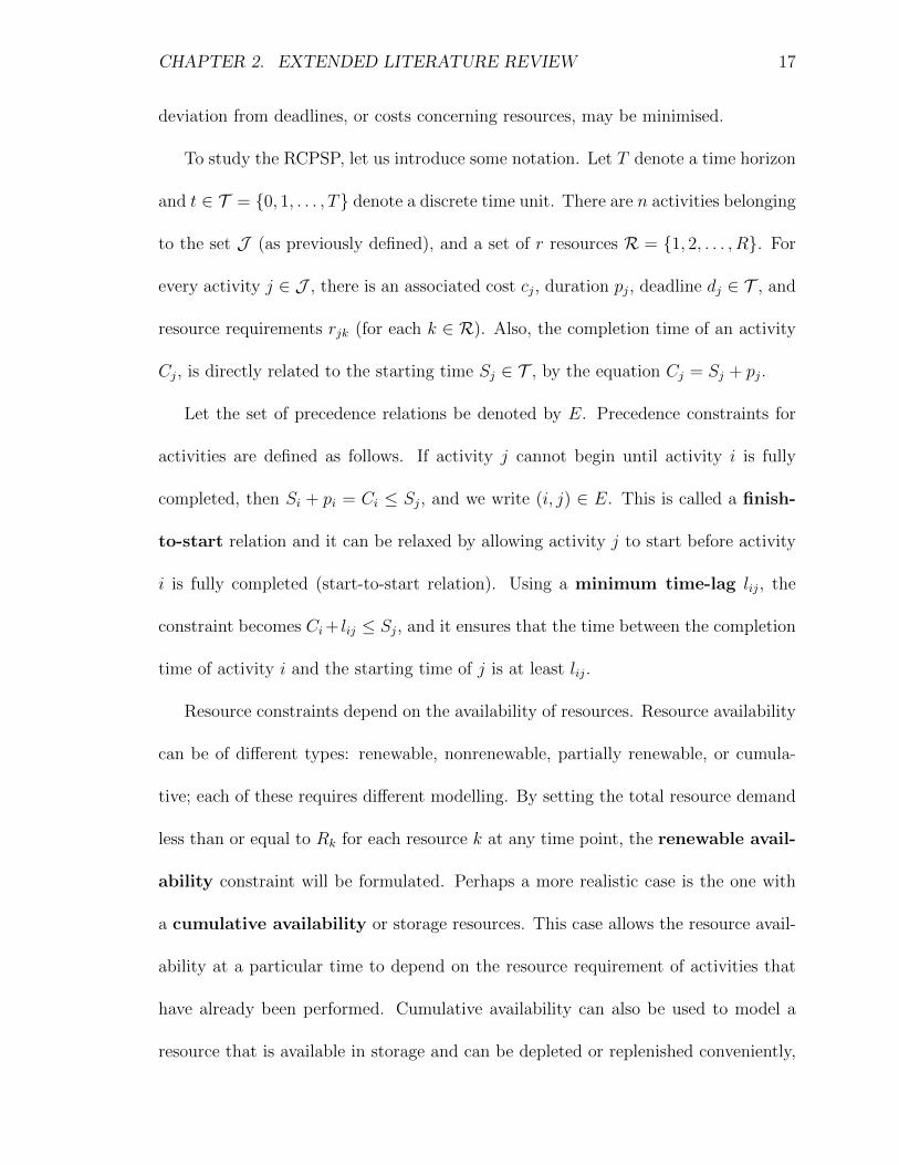
CHAPTER 2. EXTENDED LITERATURE REVIEW 17
deviation from deadlines, or costs concerning resources, may be minimised.
To study the RCPSP, let us introduce some notation. Let T denote a time horizon
and t ∈ T = {0, 1, . . . , T} denote a discrete time unit. There are n activities belonging
to the set J (as previously defined), and a set of r resources R = {1, 2, . . . , R}. For
every activity j ∈ J , there is an associated cost cj, duration pj, deadline dj ∈ T , and
resource requirements rjk (for each k ∈ R). Also, the completion time of an activity
Cj, is directly related to the starting time Sj ∈ T , by the equation Cj = Sj + pj.
Let the set of precedence relations be denoted by E. Precedence constraints for
activities are defined as follows. If activity j cannot begin until activity i is fully
completed, then Si + pi = Ci ≤ Sj, and we write (i, j) ∈ E. This is called a finish-
to-start relation and it can be relaxed by allowing activity j to start before activity
i is fully completed (start-to-start relation). Using a minimum time-lag lij, the
constraint becomes Ci+ lij ≤ Sj, and it ensures that the time between the completion
time of activity i and the starting time of j is at least lij.
Resource constraints depend on the availability of resources. Resource availability
can be of different types: renewable, nonrenewable, partially renewable, or cumula-
tive; each of these requires different modelling. By setting the total resource demand
less than or equal to Rk for each resource k at any time point, the renewable avail-
ability constraint will be formulated. Perhaps a more realistic case is the one with
a cumulative availability or storage resources. This case allows the resource avail-
ability at a particular time to depend on the resource requirement of activities that
have already been performed. Cumulative availability can also be used to model a
resource that is available in storage and can be depleted or replenished conveniently,

CHAPTER 2. EXTENDED LITERATURE REVIEW 18
perhaps incurring additional costs. Let resource demands r−jk and r+jk, represent the
depleted and replenished amount, respectively, of resource k when activity j is per-
formed. By introducing a dummy starting activity 0 and dummy terminating activity
n + 1 the initial and final amount of resource k can be modelled by r+0k and r+n+1,k,
respectively. For each resource k, there is a lower bound (safety stock) Rk and upper
bound (maximum capacity) Rk. The constraints to ensure the accumulated inventory
for every resource stays within its bounds is given by,
Rk ≤∑
{j| Sj+pj≤t}
r+jk −∑
{j| Sj≤t}
r−jk ≤ Rk, ∀ t ∈ T , k ∈ R .
Furthermore, in the case when there are some processing alternatives for activity j
(e.g. using more than one machine to process it), the problem becomes multi-mode.
For this extension, processing alternatives may be grouped in the set Mj of modes
(conceptually the same as the µj seen in the machine scheduling problem) and the
processing time and resource usage of activity j will depend on the mode m ∈ Mj.
These can be denoted by pjm and rjkm, respectively.
Formulation of the RCPSP
After studying the necessary considerations and classifications of the problem, a basic
formulation can be presented. For the sake of illustration, a RCPSP model with
minimum time-lag, renewable resources, and a generic cost function is presented. Let
xjt be the binary decision variable for this problem; it is equal to 1 if activity j starts
at time period t, and it is 0 otherwise. The RCPSP can be formulated as follows,

CHAPTER 2. EXTENDED LITERATURE REVIEW 19
Model 2.1.1. A discrete-time formulation for the RCPSP (Brucker et al., 1999)
minx
∑t∈T
∑j∈J
cj(t)xjt (2.1.1a)
Subject to∑t∈T
xjt = 1, ∀ j ∈ J (2.1.1b)∑t∈T
txit + pi︸ ︷︷ ︸Ci
+lij ≤∑t∈T
txjt︸ ︷︷ ︸Sj
∀ (i, j) ∈ E (2.1.1c)
∑j∈J
t∑u=t−pi+1
rjkxju ≤ Rk ∀ k ∈ R, t ∈ T (2.1.1d)
xjt ∈ {0, 1} ∀ j ∈ J , t ∈ T (2.1.1e)
The generic time-dependent cost function cj(t), used in the objective function
2.1.1a, can take any of the following forms,
(i) Makespan: to minimise the total project time, we can set cj(t) = 0 for all
activities j ∈ J \ {n+ 1}, and cn+1(t) = t;
(ii) Maximum lateness: to minimise the maximum difference between the com-
pletion time and the deadline, we can use the same cj(t) as for objective (i),
and additionally, set lj,n+1 = pj − dj for all activities j ∈ J ;
(iii) Earliness/tardiness costs: to minimise costs associated with early/late ac-
tivities, we can set cj(t) = αj max {0, dj − Cj}+βj max {0, Cj − dj}, where αj
and βj are the additional costs associated with earliness and tardiness for each
activity j;
(iv) Weighted number of late activities: to minimise the weighted number of
late activities, we can use the same cost function as for objective (iii) with
CHAPTER 2. EXTENDED LITERATURE REVIEW 20
αj = 0.
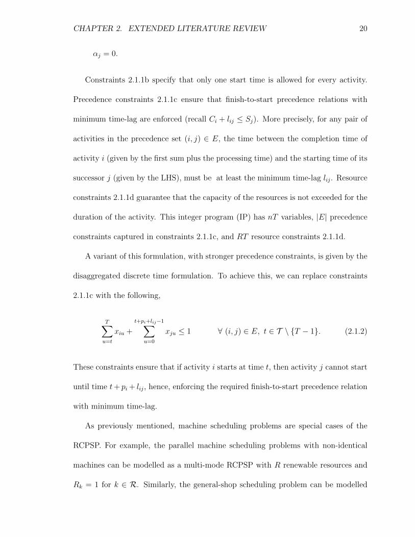
Constraints 2.1.1b specify that only one start time is allowed for every activity.
Precedence constraints 2.1.1c ensure that finish-to-start precedence relations with
minimum time-lag are enforced (recall Ci + lij ≤ Sj). More precisely, for any pair of
activities in the precedence set (i, j) ∈ E, the time between the completion time of
activity i (given by the first sum plus the processing time) and the starting time of its
successor j (given by the LHS), must be at least the minimum time-lag lij. Resource
constraints 2.1.1d guarantee that the capacity of the resources is not exceeded for the
duration of the activity. This integer program (IP) has nT variables, |E| precedence
constraints captured in constraints 2.1.1c, and RT resource constraints 2.1.1d.
A variant of this formulation, with stronger precedence constraints, is given by the
disaggregated discrete time formulation. To achieve this, we can replace constraints
2.1.1c with the following,
T∑u=t
xiu +
t+pi+lij−1∑u=0
xju ≤ 1 ∀ (i, j) ∈ E, t ∈ T \ {T − 1}. (2.1.2)
These constraints ensure that if activity i starts at time t, then activity j cannot start
until time t+ pi + lij, hence, enforcing the required finish-to-start precedence relation
with minimum time-lag.
As previously mentioned, machine scheduling problems are special cases of the
RCPSP. For example, the parallel machine scheduling problems with non-identical
machines can be modelled as a multi-mode RCPSP with R renewable resources and
Rk = 1 for k ∈ R. Similarly, the general-shop scheduling problem can be modelled
CHAPTER 2. EXTENDED LITERATURE REVIEW 21
as the RCPSP with m+ n renewable resources, Rk = 1 for all resources k. Of these,
the first m correspond to the machines and the remaining resources account for the
fact that different operations of job j cannot be processed at the same time. The
total number of activities will be∑n
j=1 = nj and operation Oij requires one unit of
machine resource µij and one unit of job resource m+ j.
2.1.3 Long-term RCPSP formulations
Given the nature the problem considered in Chapter 3, the long-term RCPSP liter-
ature is worth considering. Particularly, Kone et al. (2011) introduced a formulation
that challenged the classical discretisation of time by indexing variables with some
pre-defined time intervals. They refer to this type of formulation as an “event-based
RCPSP”. More formally, these events correspond to start or end times of activi-
ties. Their formulation, for long-term planning horizons, involves considerably fewer
variables than the formulations indexed by time. It should be noted that they inde-
pendently developed the same idea as Sousa and Wolsey (1992). Kone et al. (2013)
later extended the event-based formulation to account for non-renewable resources.
More authors have used a similar indexation of time. Naber (2017) removed the as-
sumption regarding fixed resources per activity in the RCPSP by allowing flexible
resource usage. Kopanos et al. (2014) presented two new types of continuous time
formulations and provided a computational study comparing the performance of other
similar RCPSP formulations.

CHAPTER 2. EXTENDED LITERATURE REVIEW 22
On/Off Event-based Formulation (Kone et al., 2011)
To study the “event-based RCPSP” formulations by Kone et al. (2011), let us alter the
notation used in the previous section to match the one employed by the authors. Let
the RCPSP be defined by (A, p,E,R,B, b). Where A is a set of activities (including
dummy start and end activities, i.e. A = {0, 1, . . . , n, n+1}), p is a vector of durations,
E is the precedence relation, R is a set of renewable resources, B is a vector of resource
availabilities, and b is a matrix of demands. For the event-based formulation we require
a set of events E = {0, 1, . . . , n}, where n is the number of activities. Each of these
correspond to either the start or the end of an activity. Making use of this event set
Kone et al. (2011) introduced two event-indexed formulations for the RCPSP. The
first formulation, the Start/End event-based (SEE) formulation, is a simplification
of the formulation by Zapata et al. (2008) for the multi-mode multi-project RCPSP.
The SEE formulation requires two variables for each event, which allows tracking of
the start and end events for each activity. The formulation we are going to discuss
in more detail is the On/Off event-based (OOE) formulation as it only requires one
variable per event. It receives its name due to the definition of the variables used as
they either represent the start or the end of an activity. With this definition it is more
difficult to identify when an activity starts and ends; for this purpose, the authors
include some “contiguity” (transitivity) constraints and a continuous variable to track
event times. Apart from being able to deal with long-term planning horizons, another
advantage of these formulations is that they can deal with rational processing times
for activities.

CHAPTER 2. EXTENDED LITERATURE REVIEW 23
To study the OOE formulation in more detail, let the event indexed binary vari-
able zie, take the value 1 if an activity i starts at event e or if it is still being processed
immediately after event e; and it is 0 otherwise. The authors introduce a contin-
uous variable te in order to account for time/date of event e. In terms of project
completion time, the worst case would be if the processing times for all activities is
disjoint, meaning that all the te variables will be different. However, depending on
resource availability, the start/end of different activities may correspond to the same
events, which makes some of these times equal. Moreover, the authors work under
the following assumptions,
1. Fixed and renewable resources;
2. Non-preemptive schedule;
3. Activities make use of all the resources they require when being processed.
The problem can be formulated as follows,

CHAPTER 2. EXTENDED LITERATURE REVIEW 24
Model 2.1.2. OOE formulation Kone et al. (2011).
min Cmax (2.1.3a)
Subject to∑e∈E
zie ≥ 1; ∀i (2.1.3b)
Cmax ≥ te + (zie − zi,e−1)pi; ∀ i, e; (2.1.3c)
t0 = 0; (2.1.3d)
te+1 ≥ te; ∀ e 6= n− 1 ∈ E (2.1.3e)
tf ≥ te + ((zie − zi,e−1)− (zif − zi,f−1)− 1) pi; ∀ (e, f, i) ∈ E2 × A, f > e(2.1.3f)
e−1∑e′=0
zie′ ≤ e(1− (zie − zi,e−1)); ∀ e ∈ E \ {0} (2.1.3g)
n−1∑e′=e
zie′ ≤ (n− e)(1 + (zie − zi,e−1)); ∀ e ∈ E \ {0} (2.1.3h)
zie +e−1∑e′=0
zje′ ≤ 1 + (1− zie)e; ∀ e, ∀ (i, j) ∈ E (2.1.3i)
n−1∑i=0
bikzie ≤ Bk; ∀ e, k (2.1.3j)
te ≥ 0; ∀ e; (2.1.3k)
zie ∈ {0, 1}; ∀ i, e; (2.1.3l)
The OOE formulation involves O(n2) binary variables, O(n) continuous variables,
and O(n3 + (|R|+ |E|)n) constraints.
The objective function 2.1.3a, employs a makespan criteria and a corresponding
continuous variable subject to constraints 2.1.3c. Constraints 2.1.3b ensure that ev-
ery activity is processed at least once. Constraints 2.1.3d initialise the time variable
for the first event while constraints 2.1.3e ensure that it remains nondecreasing. Con-
straints 2.1.3f link binary and continuous variables in a form that poses a lower bound
for the time of any later event. That is, if activity i starts immediately after event e
(zie = 1∧zi,e−1 = 0) and ends at event f (zi,f−1 = 1∧zi,f = 0), then the time of event f

CHAPTER 2. EXTENDED LITERATURE REVIEW 25
is at least equal to the time of event e plus the processing time of activity i. Any other
combination of values for the binary variables yields a redundant constraint. Con-
straints 2.1.3g and 2.1.3h are called contiguity constraints, more commonly referred
to as transitivity, and ensure that zie remains equal to 1 for the total processing time
of activity i. Constraints 2.1.3i ensure precedence relations are satisfied. Constraints
2.1.3j ensure that the resource limits are not violated. The last two constraints, 2.1.3k
and 2.1.3l define the variables.
If the earliest start (ESi) and latest start (LSi) times for activities are known, the
following constraints can be included,
ESizie ≤ te ≤ LSi(zie − zi,e−1) + LSn(1− (zie − zi,e−1)) ∀ i, e . (2.1.4)
These constraints are crucial for the performance of the model, hence, if the ear-
liest/latest start times are not known, preprocessing steps can be implemented in
order to compute them (Demassey et al., 2005).
Kone et al. (2011) included a computational comparison of the OOE formula-
tion against three other well-known formulations. The discrete time formulation, the
disaggregated discrete time formulation, and the flow-based continuous-time formula-
tion; as well as their own SEE. Testing on different data sets with different properties
clearly showed that the OOE outperforms the other formulations on instance sets
with a long time horizon and high processing rates of activities.

CHAPTER 2. EXTENDED LITERATURE REVIEW 26
RCPSP with consumption and production of resources (Kone et al., 2013)
Kone et al. (2013), extended the OOE formulation (Kone et al., 2011) for a more
complex problem; the RCPSP with consumption and production of resources (RCP-
SP/CPR). They showed that the revised event-based formulation still outperformed
all other types. The formulation borrows most of the constraints from Model 2.1.2
but also introduces several continuous variables to account for the stock level with
consumption/production of different resources for each activity. To avoid confusion
in the notation for the resources we change R to P , as the former previously denoted
renewable resources. The continuous variables required are,
sep : stock level of resource p ∈ P at event e;
uiep : amount of resource p ∈ P consumed by activity i at event e;
piep : amount of resource p ∈ P produced by activity i at event e.
The RCPSP/CPR formulation involves objective 2.1.3a and constraints 2.1.3b to
2.1.3l from Model 2.1.2, as well as some constraints regarding the consumption of
resources. The formulation is as follows,

CHAPTER 2. EXTENDED LITERATURE REVIEW 27
Model 2.1.3. RCPSP/CPR Kone et al. (2013)
Constraints2.1.3a to 2.1.3l
uiep ≥ c−ip(zie − zi,e−1); ∀ i, e, p; (2.1.5a)
uiep ≤ c−ipzie; ∀ i, e, p; (2.1.5b)
uiep ≤ c−ip(1− zi,e−1); ∀ i, e, p; (2.1.5c)
piep ≥ c+ip(zi,e−1 − zie); ∀ i, e, p; (2.1.5d)
piep ≤ c+ipzi,e−1; ∀ i, e, p; (2.1.5e)
piep ≤ c+ip(1− zi,e); ∀ i, e, p; (2.1.5f)
sep = se−1,p +∑i∈A
piep −∑i∈A
uiep; ∀ i, e, p; (2.1.5g)
n−1∑i=0
bipzie ≤ sep; ∀ e, p; (2.1.5h)
sep, uiep, piep ≥ 0; ∀ i, e, p. (2.1.5i)
Here, c−ip and c−ip denote the minimum and maximum amount of resource p required
to perform activity i, respectively. The combination of constraints 2.1.5a, 2.1.5b, and
2.1.5c ensure that the value of variable uiep is equal to c−ip if activity i starts being
processed at event e for any resource p, and is 0 otherwise. So, the only combination
that leads to uiep = c−ip is zie = 1 ∧ zi,e−1 = 0. Similarly, constraints 2.1.5d, 2.1.5e,
and 2.1.5f ensure the production variable is equal to c+ip if activity i finishes being
processed at event e for any resource p, and is 0 otherwise. In this case, the only
combination that leads to piep = c+ip is zie = 0 ∧ zi,e−1 = 1. Constraints 2.1.5g ensure
the stock level se,p, for each event e and resource p is updated utilising the stock level
from the previous event se−1,p, plus the resource produced by each activity minus
the consumption by each activity. Constraints 2.1.5h limit the resources available at
each event with the corresponding stock level. Lastly, constraints 2.1.5i define the
variables.

CHAPTER 2. EXTENDED LITERATURE REVIEW 28
2.1.4 A Formulation for the Preemptive RCPSP
The literature for the preemptive RCPSP (PRCPSP) is very limited. Afshar-Nadjafi
(2014) studied different preemption penalty costs and a weighted earliness-tardiness
in the objective function of the PRCPSP. Afshar-Nadjafi and Arani (2014) published
similar results for the multi-mode case. Coffman et al. (2015) explored the smallest
time between events (shift) in an optimal schedule for parallel machine scheduling
problem with preemptions allowed at non-integer (rational) times. Additionally, in
this article, authors introduced an alternative definition for events to account for
preemptions, these are identified as an activity start, interruption, resumption, or
completion; let us adopt such definition. More recently, Creemers (2019) showed
the impact of allowing preemptions in a stochastic project scheduling setting. They
presented a computational study (using psplib instances Kolisch and Sprecher, 1997)
where they compared the benefit in preemption when compared to other well-known
RCPSP formulations.
We wish to extend the OOE formulation from Kone et al. (2011) (discussed in
Section 2.1.3) to allow preemptions. For this purpose, we require to introduce some
notation. Let p−i be a value that represents the minimum time allowed to be spent on
activity i, with p−i < pi (see Figure 2.1). This can also be thought of as the amount of
time after starting/resuming an activity in which we cannot complete/interrupt said
activity. From this, the fraction ni =⌊pi/p
−i
⌋determines the maximum number of
subactivities activity i can be broken into. Hence,
∑i∈A
⌊pip−i
⌋=∑i∈A
ni = N ,

CHAPTER 2. EXTENDED LITERATURE REVIEW 29
determines the new number of events. That is, E = {0, 1, . . . , N}. Furthermore, we
impose the assumption, that two subactivities can only be processed in parallel if they
do not divide the same activity.
p−i p−i
pi1 pi2
Figure 2.1: An activity broken down into two subactivities.
With these definitions, we can change constraints 2.1.3f to,
p−i ((zie − zi,e−1)− (zif − zi,f−1)− 1) ≤ tf− te ≤ pi ∀ (e, f) ∈ E2 (f > e), ∀ i ∈ A .
(2.1.6)
These constraints bound elapsed times between events. The upper bound is the total
processing time pi. While the lower bound is set to be the minimum time allowed,
p−i .
To monitor the progress of individual subactivities throughout the project, let
us introduce a new continuous time variable, aie, which represents the amount of
processing time that has been dedicated to activity i by event e. In terms of the
variables introduced for Model 2.1.2, for a single process of each activity, we may
write the processing variable as follows,
aie =
ai,e−1 + te − te−1, if zie = 1 ∨ zi,e−1 = 1
ai,e−1, otherwise
∀ i, e.
With 0 ≤ aie ≤ pi ∀ e ∈ E ; ai0 = ai,−1 = 0 ∀ i ∈ A; and aiN = pi ∀ i ∈ A. By
using some big-M constraints, this definition is equivalent to the following activity

CHAPTER 2. EXTENDED LITERATURE REVIEW 30
processing constraints,
ai0 = ai,−1 = 0 ∀ i; (2.1.7a)
ai,e−1 ≤ ai,e ∀ i, e; (2.1.7b)
aie ≤ ai,e−1 +M (zie + zi,e−1) ∀ i, e; (2.1.7c)
aie ≥ ai,e−1 + (te − te−1)−M(1− zie) ∀ i, e; (2.1.7d)
aie ≥ ai,e−1 + (te − te−1)−M(1− zi,e−1) ∀ i, e; (2.1.7e)
aiN = pi ∀ i; (2.1.7f)
0 ≤ aie ≤ pi ∀ e ∈ E ∀ i, e. (2.1.7g)
Constraints 2.1.7a initialise the dummy activity processing variable ai,−1, and the one
corresponding first event ai0. Constraints 2.1.7b ensure that the processing variable in
nondecreasing. Constraints 2.1.7c to 2.1.7e ensure that if either zie = 1 or zi,e−1 = 1
the processing variable is recursively updated, otherwise, due to M , they become
redundant. That is, if zie = 1 ∨ zi,e−1 = 1, aie is updated with ai,e−1, the already
processed time for activity i, plus the time elapsed, te − te−1, between events e − 1
and e. In fact, since constraints 2.1.6 bound te − te−1 with pi, for the same effect
we can replace M with pi. Constraints 2.1.7f ensure that every activity is processed
to completion and least by the last event N . Constraints 2.1.7g bound the activity
processing variable.
As for the objective function for the event-based PRCPSP we have similar options
to those for the simpler version of the problem. In our notation, we have
(i) Makespan: minCmax = tN .
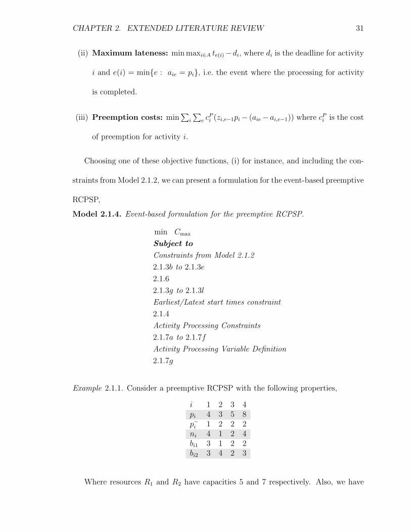
CHAPTER 2. EXTENDED LITERATURE REVIEW 31
(ii) Maximum lateness: min maxi∈A te(i)−di, where di is the deadline for activity
i and e(i) = min{e : aie = pi}, i.e. the event where the processing for activity
is completed.
(iii) Preemption costs: min∑
i
∑e c
Pi (zi,e−1pi− (aie− ai,e−1)) where cPi is the cost
of preemption for activity i.
Choosing one of these objective functions, (i) for instance, and including the con-
straints from Model 2.1.2, we can present a formulation for the event-based preemptive
RCPSP,
Model 2.1.4. Event-based formulation for the preemptive RCPSP.
min Cmax
Subject to
Constraints from Model 2.1.2
2.1.3b to 2.1.3e
2.1.6
2.1.3g to 2.1.3l
Earliest/Latest start times constraint
2.1.4
Activity Processing Constraints
2.1.7a to 2.1.7f
Activity Processing Variable Definition
2.1.7g
Example 2.1.1. Consider a preemptive RCPSP with the following properties,
i 1 2 3 4pi 4 3 5 8p−i 1 2 2 2ni 4 1 2 4bi1 3 1 2 2bi2 3 4 2 3
Where resources R1 and R2 have capacities 5 and 7 respectively. Also, we have

CHAPTER 2. EXTENDED LITERATURE REVIEW 32
the following two precedence relations E = {(2, 3), (3, 4)} of types finish-to-start and
start-to-start, respectively. Meaning that activity 3 cannot start before the end of
activity 2, and that activity 4 cannot start before the start of activity 3.
In this case, from the values above, we see that activity 2, for example, has to be
processed in a single go (n2 = 1). The others have at most 4 subactivities. Thus,
N = n1 +n2 +n3 +n4 = 11. A feasible solution for the scheduling of this project can
be seen in Figure 2.2, with the corresponding values for the variables,
e = 0: t0 = 0, z20 = 1 a20 = 0e = 1: t1 = 0, z21 = z11 = 1 a21 = a11 = 0e = 2: t2 = 3, z32 = 1 a22 = a12 = 3, a32 = 0e = 3: t3 = 3, z33 = z43 = 1 a33 = a43 = 0e = 4: t4 = 8, z44 = 1 a34 = a44 = 5e = 5: t5 = 8, z45 = z15 = 1 a45 = 5, a15 = 3e = 6: t6 = 9, z46 = 1 a45 = 6, a16 = 4e = 7: t7 = 11, a47 = 8.
With Cmax = 11. The remaining variables are equal to 0. The Gantt chart of the
two resources considered R1 and R2 is presented in Figure 2.2. It is worth noting that,
in comparison with the non-preemptive case, solution in Figure 2.3, the makespan is
reduced by 1.
3 8 9 11
12345
24
1a3 1b
3 8 9 11
1234567
1a
2 4
3 1b
Figure 2.2: Example of a feasible preemptive schedule showing the processing ofactivities for two resources R1 (left) and R2 (right).

CHAPTER 2. EXTENDED LITERATURE REVIEW 33
1 3 8 12
12345
2 3
4
1
1 3 8 12
1234567
4
13
2
Figure 2.3: Example of a feasible non-preemptive schedule showing the processing ofactivities for two resources R1 (left) and R2 (right).
Implementation and Computational Tests
To solve Model 2.1.4 efficiently, one has to implement some preprocessing steps. We
apply the well-known local constraint programming (CP) algorithm for the estimation
of earliest/latest start times, ESi/LSi, from Demassey et al. (2005). After implement-
ing the preprocessing algorithm, we tested Model 2.1.4, allowing a single preemption,
using the well-known psplib library instances (Kolisch and Sprecher, 1997). Partic-
ularly, we used the j30 data set with 30 activities (parameter 1 instances 1-10, i.e.
j301 1 to j301 10).1 Since we are only allowing one preemption, for each activity i,
we set,
p−i =⌊pi
2
⌋.
Hence,
N =∑i∈A
⌊pip−i
⌋=∑i∈A
⌊pibpi/2c
⌋≤ 2|A| ,
that is, as one would expect, the number of events is at most twice the number of
activities.
A computational comparison between three different formulations is given in Table
1Companion code avilable at https://github.com/torressa/prcpsp.

CHAPTER 2. EXTENDED LITERATURE REVIEW 34
2.1. We include the results for Model 2.1.4, the psplib benchmark results, and the
results for the OOE formulation (Model 2.1.2). We compare the makespan (MS) and
the computational times (T) for the ten instances (Inst.) studied. Additionally, the
local constraint programming algorithm is efficient, as shown by the low computational
times for the preprocessing stage. As expected, the makespan for our preemptive
formulation, Model 2.1.4, is on average 11.6% lower than the benchmark results with
a slight increment in the solution times. When compared with solutions obtained with
Model 2.1.2, our formulation shows an average decrease of 0.8% for the makespan,
with a lower average computational time.
Table 2.1: Computational results including makespan (MS) and computational times(T) for Model 2.1.4, psplib benchmark results, Model 2.1.2, and the preprocessingstage.
Model2.1.4
BenchmarkModel2.1.2
PreprocessingStage
Inst. MS T (s) MS T (s) MS T (s) T (s)
1 38 6.21 43 0.3 38 5.32 0.172 42 4.35 47 0.11 42 0.87 0.143 43 2.49 47 0.12 44 300 0.124 55 5.48 62 0.64 55 0.91 0.095 31 6.97 39 0.48 33 300 0.146 38 3.1 48 0.04 38 1.96 0.157 60 5.99 60 0.01 60 0.67 0.128 53 3.97 53 0.03 53 0.91 0.19 42 4.37 49 0.1 42 0.76 0.210 37 5.99 45 0.04 37 1.07 0.2
2.2 Maintenance Scheduling
Traditionally, machine maintenance was performed on a run-to-failure basis. In the
late ‘50s and early ‘60s, with the recent developments in operational research, preven-
CHAPTER 2. EXTENDED LITERATURE REVIEW 35
tive maintenance (PM) was introduced and maintenance planning was formulated
as any other ordinary scheduling optimisation problem. Tasks are to be performed
(inspections and perhaps unexpected repairs), with a certain frequency and some ca-
pacity and workforce constraints. While these models do reduce system failure and
dangerous accidents; they are labour intensive, do not account for the uncertainty of
failure, and induce several unnecessary costs. The next step was towards prognos-
tic models as they mitigate these issues by using the current “health”-state of the
machine as an impetus factor to predict when failures are likely to occur and how to
best avoid them. Conditioning the modelling on the current state of the system is
where a relatively recent and active research area comes into play: condition-based
maintenance (CBM).
In the airline framework, around “80% of the inspection and access activities do
not lead to a repair”– Papakostas et al. (2010). This highlights the need to challenge
and consider current maintenance scheduling models to reduce unnecessary inspec-
tions. Although some airlines are shifting to a more effective scheme through the use
of sensors and more sophisticated analysis of the data, many still schedule mainte-
nance periodically according to the opinion of their experts. This leads to suboptimal
schedules vulnerable to the very likely introduction of delays and additional costs
when demanding an unscheduled repair.
The techniques and approaches concerning the scheduling of different maintenance
interventions, focussing mainly on the aircraft related, will be summarised in this sec-
tion. As already mentioned in Section 1.1, there are considerable savings to be made
from more efficient maintenance programmes. Furthermore, the improvements made

CHAPTER 2. EXTENDED LITERATURE REVIEW 36
can then be applied to other industries and areas that require such efficiency analysis
like nuclear plants, automotive and other machinery operated in high-performance
environments (e.g. hydraulic structures, brake linings, pipelines or cutting tools).
2.2.1 Prognostic-Based Models
Being able to replace optimally, at the most appropriate moment in time, the neces-
sary components of the machine is essential to plan the maintenance workload and
inventory reducing losses and general inefficiencies. By introducing the remaining
useful life (RUL) of a system, prognostics can be defined to be the capability of
predicting the changes in RUL. The RUL is, as its name suggests, the time until
the system cannot perform its usual operations. Specifically, taking into account the
current RUL of a system for every decision point is modelled under CBM.
Heng et al. (2009) and Jardine et al. (2006) presented very useful summaries on
some of the current prognostic-based approaches and their corresponding benefits and
drawbacks. Especially relevant to jet engines, in the former, the authors reviewed the
methods for predicting rotating machinery failures. Besides, they both agreed that
the most efficient and accurate models are CBM models. In this context, maintenance
tasks are usually classified into three categories, proactive maintenance (inspections),
PM or corrective maintenance (CM). CBM models recommend maintenance deci-
sions based on the information collected through non-intrusive monitoring or updated
historical data. CBM models also attempt to keep unnecessary operations (inspec-
tions and PM) to a minimum by performing an intervention exclusively when there is
significant evidence of abnormal behaviour. A CBM program, thus, can help to reduce

CHAPTER 2. EXTENDED LITERATURE REVIEW 37
maintenance associated costs by reducing the number of unnecessary operations.
Jayabalan and Chaudhuri (1992) developed one of the first prognostic-based mod-
els. The authors introduced two types of maintenance interventions, which correspond
to PM and CM. For each of these operations performed, a constant improvement fac-
tor γ, regarding the failure rate of the system is used. That is, every time a PM
intervention is performed at a particular time ti, the measure that quantifies the fail-
ure rate (e.g. the age of the system), is reduced by ti − ti/γ. As time increases, the
cost of performing a corrective replacement also increases. Interventions of this type
are assumed to restore the system to as-good-as-new state. Therefore, the authors
employed a threshold such that if the failure rate reaches a certain level λmax, either
a PM or CM operation will be performed. Based on the objective of minimising the
total maintenance costs, one operation is chosen every time this occurs. Using this
method and resting on several assumptions (intervention durations can be assumed to
be negligible), the authors formulated a cost model and presented a recursive equation
to calculate the time for the n-th intervention tn. It is given by the following equation,
tn = tn−1 +
(1− 1
γ
)n−1t1 =
n∑i=1
(1− 1
γ
)i−1t1 ,
where t1 is the time when the system reaches the maximum failure rate λmax, for the
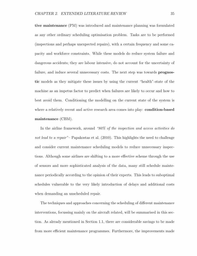
first time. For the case when γ ≥ 1, depicted in Figure 2.4, the successive maintenance
intervals are of decreasing length. The times between the interventions decreases as
the system deteriorates faster after every intervention. At each of these points ti, a
cost problem is solved to determine whether a PM or a CM should be performed. In
the case a CM is required to minimise the total cost, the failure rate will drop to 0
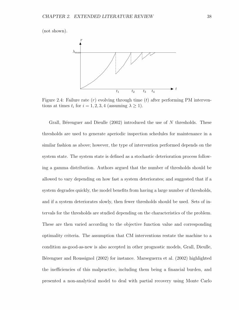
CHAPTER 2. EXTENDED LITERATURE REVIEW 38
(not shown).
λmax
t
r
t1 t3t2 t4
Figure 2.4: Failure rate (r) evolving through time (t) after performing PM interven-tions at times ti for i = 1, 2, 3, 4 (assuming λ ≥ 1).
Grall, Berenguer and Dieulle (2002) introduced the use of N thresholds. These
thresholds are used to generate aperiodic inspection schedules for maintenance in a
similar fashion as above; however, the type of intervention performed depends on the
system state. The system state is defined as a stochastic deterioration process follow-
ing a gamma distribution. Authors argued that the number of thresholds should be
allowed to vary depending on how fast a system deteriorates; and suggested that if a
system degrades quickly, the model benefits from having a large number of thresholds,
and if a system deteriorates slowly, then fewer thresholds should be used. Sets of in-
tervals for the thresholds are studied depending on the characteristics of the problem.
These are then varied according to the objective function value and corresponding
optimality criteria. The assumption that CM interventions restate the machine to a
condition as-good-as-new is also accepted in other prognostic models, Grall, Dieulle,
Berenguer and Roussignol (2002) for instance. Marseguerra et al. (2002) highlighted
the inefficiencies of this malpractice, including them being a financial burden, and
presented a non-analytical model to deal with partial recovery using Monte Carlo
CHAPTER 2. EXTENDED LITERATURE REVIEW 39
simulations.
CBM-based Formulation for Fighter Aircraft Maintenance (Li et al., 2016)
One of the current CBM model formulations for fighter aircraft is the one given by Li
et al. (2016). This formulation combined the “health”-state monitoring and several
uncertainty measures in a single model. It is standard practice in the aircraft-related
literature to take such “health”-state to be the legal remaining flying hours (Sarac
et al., 2006). By updating the estimated remaining available flying hours for an in-
dividual aircraft, i.e. the RUL, according to certain historical information about the
aircraft, the authors proposed a way to model the problem. The uncertainties included
in this model account for the maintenance and flight durations drawn from uniform
and normal distributions, respectively. The assumption that flight duration, mainte-
nance task durations, and even the departure delay come from normal distributions
(with different parameters) is a conventional assumption in the literature. Based on
the work by Mueller and Chatterji (2002)who, additionally, showed that departure
delay can be modelled using a Poisson distribution.
Since Li et al. (2016) focused on scheduling maintenance for fighter aircraft, they
use different types of flight operations, encapsulated by grouping the flights by “sor-
ties”. This is due to various sorties or missions (e.g. transport, reconnaissance,
bomber, fighter, or special operations) require different engine functions and ma-
noeuvres.
To study the formulation in Li et al. (2016), the introduction of their notation is
required. Let us define some sets and parameters,

CHAPTER 2. EXTENDED LITERATURE REVIEW 40
F : Set of all aircraft i ∈ F , |F| = n represents the number of aircraft;
J : Set of all sortie types j ∈ J , |J | represents the number of unique sortie types;
lj : Duration of sortie type j ∈ J ;
hmax : Maximum number of flying hours between maintenance interventions;
htj : Life of aircraft i ∈ F remaining at period t;
k : Average number of time period required to complete maintenance;
bi : Flying hours remaining on aircraft i ∈ F at the beginning of the time horizon;
M : Maximum number of aircraft that can be in maintenance at any given period t
without penalty.
The decision binary variables are xtij and mti for the aircraft and maintenance
respectively and are defined as follows,
xtij : 1, if aircraft i ∈ F flies sorties type j ∈ J in period t ∈ T ; 0, otherwise;
mti : 1 if aircraft i ∈ F enters maintenance in period t ∈ T ; 0, otherwise.
Time is taken be discrete, with a time horizon denoted by T , thus t ∈ T =
{1, . . . , T}. The discrete-time unit for this model is half-days, that is, when t goes up
by a single unit this corresponds to an increase in 12 hours. The problem can now be
formulated as follows,

CHAPTER 2. EXTENDED LITERATURE REVIEW 41
Model 2.2.1. Time-discrete MIP with CBM considerations (Li et al., 2016)
minm
max∑i
∑τ=t−k
(mτi −M), ∀ t ∈ [k + 1, T ] (2.2.1a)
Subject to
h1i = bi , ∀ i ∈ F (2.2.1b)∑j
xtijlj + ht+1i ≤ hti + hmaxm
ti , ∀ t ∈ T , i ∈ F (2.2.1c)∑
j
xtijlj + ht+1i ≤ hti , ∀ t ∈ T , i ∈ F (2.2.1d)
hmaxmti ≤ ht+1
i ≤ hmax , ∀ t ∈ T , i ∈ F (2.2.1e)
hmaxmti ≤ hmax − hti , ∀ t ∈ T , i ∈ F (2.2.1f)∑
j
xtij ≤ 1, ∀ t ∈ T , i ∈ F (2.2.1g)∑i
xtij ≤ 1, ∀ t ∈ T , j ∈ J (2.2.1h)∑j
xt+yij +mti ≤ 1, ∀ t ∈ [1, T − k + 1], y ∈ [0, k − 1], i ∈ F
(2.2.1i)
mti +mt+y
i ≤ 1, ∀ t ∈ [1, T − k], y ∈ [1, k], i ∈ F , t ∈ T (2.2.1j)
hti ≥ 0; xti, mti ∈ {0, 1}, ∀ t ∈ T , i ∈ F (2.2.1k)
The objective function 2.2.1a, minimises the maximum number of aircraft in ser-
vice during any average maintenance duration period and ensures this does not exceed
the maintenance capacity M . Constraints 2.2.1b initialise the remaining flying hours
for each aircraft. This initialisation is critical, otherwise, the formulation leads to a
contradiction. To include stochasticity, the model draws each initial number of flying
hours bi, from a uniform distribution with certain parameters. The authors draw from
a U(0, 200). Constraints 2.2.1c, 2.2.1d, and 2.2.1e update the remaining flying hours
for aircraft i for the next time period t + 1, depending on sorties flown and whether
maintenance is currently being performed or has been performed. Constraints 2.2.1f
guarantee that maintenance has to be performed when the remaining flying hours for

CHAPTER 2. EXTENDED LITERATURE REVIEW 42
an aircraft reaches the fixed level hmax. Constraints 2.2.1g enforce that at most one
sortie per aircraft. Constraints 2.2.1h ensure that no sortie is assigned to more than
one aircraft. Both constraints 2.2.1i and 2.2.1j force the downtime of an aircraft to
be sufficient to allow the completion of maintenance, this involves the maintenance
duration uncertainty captured by k. That is, if maintenance is to be performed for
aircraft i at time period t, so mti = 1, then maintenance cannot be performed again
until after a period greater than the average duration of said maintenance operation,
mt+yi = 0 for y ∈ [1, k]. Similarly, if mt
i = 1, then aircraft i cannot be allocated
to operate any sortie j until after a period greater that the average duration of a
maintenance task and therefore∑
j xt+yij = 0. The authors assumed that maintenance
duration k, follows a N (3, 1). Lastly, constraints 2.2.1k define the domains of the
decision variables.
In the case study presented, with time horizon T = 50 (or 25 days), n = 200 air-
craft, two types of sorties (|J | = 2), and M = 0, the model minimises the maximum
number of aircraft undergoing maintenance at any given period. Although the com-
putational times were quite promising, the model presented several limitations. The
remaining flying hours were disregarded for the end of the time horizon. Nonethe-
less, one would not expect most of the aircraft to become non-operational for the
next planning period. Moreover, the “health”-state or condition of the aircraft was
included by constraints which do not account for the possible relationship between
the different factors in operations history. Finally, letting M = 0 with the objective
function as formulated, leads to aircraft with low remaining flying hours being held
at the base without operating any sorties.
CHAPTER 2. EXTENDED LITERATURE REVIEW 43
Alternative Generation for Aircraft Maintenance Planning (Papakostas
et al., 2010)
A different modelling approach, which removes the issues previously discussed for the
formulation by Li et al. (2016), was given by Papakostas et al. (2010). By combining
the decision-making and alternative generation approach from Chryssolouris et al.
(1992), and the set-partitioning based IP formulation from Sarac et al. (2006); the
authors presented a CBM methodology for the scheduling of aircraft maintenance
tasks at an operational level or short-term planning horizon.
Chryssolouris et al. (1992) introduced a generic decision-making framework for
the allocation of different resources, in a manufacturing system, to production tasks.
Such framework involved the application of a simulation approach at every “decision
point”. Here, decision points are defined as points in time when tasks are completed.
Notably, they develop an algorithm for the generation of alternatives for every decision
point.
In the airline operator setting, as proposed by Papakostas et al. (2010), the
decision-making steps at every decision point are as follows,
Step 1. Identify required maintenance tasks.
Step 2. Determine decision criteria and weights for evaluating alternative.
Step 3. Generate alternatives.
Step 4. Determine the consequences of the different alternatives and their utility.
In this case, a decision point is defined as a point in time when an aircraft has landed
CHAPTER 2. EXTENDED LITERATURE REVIEW 44
and there are several components to be scheduled for maintenance. In step 1, for the
identification of the required maintenance tasks involved with a certain alternative,
a set of constraints for maintenance and time requirements have to be imposed and
updated to form the decision-making criteria in step 2. Such constraints include, a
number of suitable airports for each task, manpower available to perform each task,
and flight arrival and departure times. The authors borrowed parts of the formulation
by Sarac et al. (2006) to achieve this. In step 3, alternatives are defined as allocations
of maintenance interventions to suitable resources either at the current or successive
workshops. For the alternative generation, it is important to establish a maximum
number of alternatives (MNA) to be considered and a sampling rate (the number of
times a single alternative is considered). The methodology proposed generates MNA
alternatives for every decision point (using the algorithm by Chryssolouris et al.,
1992), and each one of these alternatives is simulated SR times.
To present a schedule from these feasible alternatives, the authors introduced an
utility measure for every alternative in step 4. Several factors influence such utility
measure. These include the cost, operational risk, flight delay and RUL; each of
which has an individual weight (step 2). Once this has been calculated for the MNA
alternatives (each simulated SR times), the tasks can be ordered by the utility. Thus,
it can effectively be seen which tasks should be performed first. Each of these factors
can be calculated as outlined below.
Cost criterion. The cost criterion depends on several independent costs for each
workshop. The cost of performing task Ty (out of the total number of tasks Y ) at

CHAPTER 2. EXTENDED LITERATURE REVIEW 45
workshop i of airport j, is summarised in the following formula
Cost = (E + L + OH)×O + C
where E = equipment rate, L = labour rate, OH = overhead rate, O = time required
for the completion of a task, and C = procurement cost associated with the same task
(parts and additional materials). All of these are dependant on the type of task Ty
and on the workshop i of airport j, denoted with Rij.
The cost of an alternative k, Alk, is given by
Cost(Alk) = c1,k =
∑SRs=1
∑Yy=1 Cost(Ty, Rij)s
SR
where the cost function Cost(Ty, Rij)s, dependent on task type and airport workshop,
is evaluated for each s-th sample of the alternative.
Operational risk criterion. The operational risk accounts for the stochasticity
of events: desirable and undesirable. Desirable events are taken as the scheduled
events. Unwanted or undesirable events include additional hiring or equipment failure
and can be regarded as considering the worst case scenario. The overall uncertainty
can be included by taking the expected value of the gain of a certain maintenance
task allocation. The formula, therefore, sums the desirable costs (as calculated from
the cost criterion) times its corresponding success probability, plus the undesirable

CHAPTER 2. EXTENDED LITERATURE REVIEW 46
costs times the probability of these events happening. The formula is given by,
Risk(Ty, Rij) = Cost(Ty, Rij) · SP(Ty, Rij) + UnDV(Ty, Rij) · UnDP(Ty, Rij) .
The cost of an unscheduled or undesirable event UnDV is taken to be twice as much as
the desirable scheduled event cost. Both the success probability (SP) and undesirable
probability (UnDP) can be taken from two separate Weibull distributions according
to the updated failure state of the aircraft. Using Weibull analysis is common practice
when estimating lifetimes and failures for different types of machinery.
The total operational risk for an alternative k is the average over all the samples,
hence,
Risk(Alk) = c2,k =
∑SRs=1
∑Yy=1 Risk(Ty, Rij)s
SR.
Flight delay criterion. The possible future flight delay depends on three inde-
pendent stochastic events. The duration of flights, the duration of a maintenance task
and departure delay. With this in mind, the authors draw the probabilities for each of
these events from different normal distributed random variables with different mean
and variance. Delay in a certain flight leg l will be introduced by unsuccessful delivery
of a maintenance intervention (usually because of lack of resource availability) or by
weather conditions or extreme events. Delays will then be propagated throughout the
day, influencing future departure and arrival times.
The flight delay for a certain alternative is given by
FD(Alk) = c3,k =
∑SRs=1
∑Yy=1
{max[ATl,s − AT due
l , 0] + max[DTl,s −DT duel , 0]
}SR

CHAPTER 2. EXTENDED LITERATURE REVIEW 47
where ATl,s−AT duel is the difference between the actual arrival time and the planned
arrival time and the second term is the equivalent for departure times. Note the
similarity between this criterion and the earliness/tardiness cost, objective function
(iii), discussed in Section 2.1.2.
RUL criterion. The remaining useful life criterion simply corresponds to a health
assessment prediction for an aircraft quantified by the remaining flying hours. This
figure can be calculated from a stochastic model that takes into account the inter-
dependence of the components which are monitored through different sensors. This
quantity is taken as initially known and consequently updated. By considering the
change in RUL when different tasks are performed, the RUL for an alternative k can
be calculated as,
RUL(Alk) = c4,k =
∑SRs=1
∑Yy=1wry|RUL(Ty, Rij)s|
SR,
where RUL(Ty, Rij) is the remaining useful life of task Ty when it is allocated to
resource Rij. A weight wry, is associated to each task y, such that the relative
importance (with respect to the other tasks) of performing a certain task is captured.
These weights can be reassigned at step 2 after a historical data set has been gathered
and examined.
Utility measure. Once all the criteria have been calculated, they can be nor-
malised and according to a fixed set of criteria weights, wc, attributed to the utility
gain for each criterion (c = 1, 2, 3, 4), the total utility can be quantified. These cri-
teria weights, assigned in step 2 of the decision-making process, can be initialised

CHAPTER 2. EXTENDED LITERATURE REVIEW 48
according to some given priorities and then be updated according to how the sys-
tem responds. For the case study in the paper, these were taken as 30% for the
cost, 20% for the operational risk, 10% for the flight delay and 40% for the RUL
(w1 = 0.3, w2 = 0.2, w3 = 0.1 and w4 = 0.4). The utility for alternative k is given by
Ut(Alk) =4∑c=1
wccmaxc − cc,kcmaxc − cmin
c
.
Where, cmaxc and cmin
c correspond to the maximum and minimum values of criterion c
over all the alternatives. This provides the normalisation,
Ut(Alk) ∈ [0, 1] ∀ k ∈ {1, . . . ,MNA}.
The alternative with the best utility will, ultimately, provide the best possible allo-
cation of all tasks at current or successive airport workshops for all aircraft under
examination. Given how the utility function is defined, a greater utility implies the
weighted minimisation over all criteria.
The computational analysis for the case study included a MNA of 49 alternatives
and a sampling rate, a simulation rate (SR) of 10, and provided a solution within 20
minutes. If the alternative with the highest utility is chosen, the solution is guaranteed
to provide an optimal, feasible and robust schedule. The repeated sampling from the
different distributions for each of the sampling stages, provides a robust solution.
CHAPTER 2. EXTENDED LITERATURE REVIEW 49
2.2.2 Modelling Scheduling Problems in Other Industries
This section outlines some of the strategies several authors have adopted for other
problems in the literature. Initially, problems where resource allocation plays a cru-
cial role are reviewed, specifically, applied to cloud computing and virtualised data
centres. As briefly mentioned, prognostic models can also be applied in the context
of electronics, production plants, gas turbines, cars, and general systems subject to
vibrations.
Urgaonkar et al. (2010) addressed the power management issues for the so-called
virtualised data centres by employing Lyapunov optimisation to ensure optimal alloca-
tion of resources. The dynamic resource allocation is an appropriate way of modelling
for this problem, as at any point in time there are a different number of applications
that compete for the available processing servers. Furthermore, these applications are
heterogeneous, that is, they have individual processing requirements (time and mem-
ory). In the context seen for the RCPSP, what was referred to as jobs or requests, can
now be taken as the processing of applications, and the resources are servers. The aim
of the authors was to develop an algorithm that provided a robust resource allocation
solution while coping with time-varying workloads. The algorithm exploited queuing
data from the arrivals of processing requests to infer about future arrival processes.
The arrival of processes were taken from a random stochastic process with a certain
time average rate; however, no assumption was made for the distribution of these. The
authors employed queuing dynamics and backlog information to estimate the arrival
process. For the inclusion of the power management element, the model was designed

CHAPTER 2. EXTENDED LITERATURE REVIEW 50
to adapt to electricity consumption variations from different CPU speeds and usages.
The power-frequency relationship that derivates from dynamic voltage and frequency
scaling for the CPU’s is non-linear. By using Lyapunov optimisation, the authors not
only dealt with the complexity and non-linearity of the problem effectively, but also
derived analytical performance guarantees of the algorithm.
Christer et al. (1998) employed a statistical approach to model the prediction of
faults for an extrusion press. Assuming some distributional properties for the faults,
the authors implemented a planned PM approach. The aim was to reduce the costs
and interruptions to the production process. The fault origination process was mod-
elled by a homogeneous Poisson process. This makes expected number of failures easy
to calculate. To make the model more realistic, the authors used available historical
data to make the expected number of failures increase over time as the extrusion
press deteriorates. The delay time concept plays a crucial role in the modelling of
PM planning in this model. It is defined as the time between when a fault is detected
and the time that the machine fails. Combining the updated proportion of failures
(after some inference from the data), an explicit distribution function for the delay
time was given. More specifically, the cumulative distribution function for the delay
time was shown to be a weighted sum of uniform and exponential distributions.
Some authors have applied artificial intelligence techniques for finding prognostic
predictions. Neural networks for example, have been implemented on prognostic pre-
dictions for gas turbines by DePold and Gass (1998) and for cars by Jhwei et al. (2008).
A brief discussion on the use of artificial neural networks for airline crew scheduling
is given further on, in Section 2.3.2. Also, wavelet theory has been employed for

CHAPTER 2. EXTENDED LITERATURE REVIEW 51
condition monitoring and fault diagnostics (Peng and Chu, 2004).
2.3 Airline Scheduling and Recovery
The airline scheduling problem consists of several steps with different planning hori-
zons corresponding to airlines’ planning stages. These are, flight scheduling, fleet
assignment, tail assignment, and, crew scheduling. These stages are traditionally
modelled is by solving them sequentially, the output of one stage is input for the
next. This scheme is summarised in Figure 2.5. Firstly, a flight schedule needs to be
provided, usually 12 months in advance, according to demand and other restrictions
an airline wishes to apply. Different fleet types are then assigned to certain routes or
flight legs in a way that maximises the revenue, and that does not violate safety or
maintenance regulations. This stage is referred to as the fleet assignment problem,
and is usually solved for a 12-week horizon. Given the allocation of fleet types to
flights, the next stage determines a 1-4 week sequence of flights to be flown by each
aircraft. The solution must ensure that each flight is flown exactly once, each aircraft
is maintained as per regulations, and capacity constraints for fleet types are satisfied
(Cadarso et al., 2016). Some authors refer to this stage as the tail assignment (TA)
problem or aircraft routing/rotation. At the final stage, crew scheduling uses the
solution from the fleet assignment to provide a 1-4 week schedule for the airline crew;
allocating flight legs, working hours, and satisfying duty regulations.
In contrast, the airline recovery problem considers the same steps but in an op-
erational setting. In this scenario it is assumed that pre-operational plans have been

CHAPTER 2. EXTENDED LITERATURE REVIEW 52
Flight Scheduling
Fleet Assignment
Aircraft Routing
Crew Scheduling
12 months inadvance
12 weeks inadvance
1-4 weeks inadvance
1-4 weeks inadvance
Figure 2.5: Sequential modelling of the airline scheduling problem (Bae, 2010).
unpredictably disrupted, therefore, the aim is to propose alternative plans that al-
low a fast resumption of airline operations while reducing the impact caused by the
deviation from the original pre-operational schedule. Such impact can be quanti-
fied by introduced passenger delay, or additional recovery costs (e.g. crew costs and
regulation fines). Given the nature of the problem, the time horizon for these prob-
lems is significantly reduced to an operational horizon, between 1-10 days. The steps
in airline recovery are, flight recovery (sometimes schedule recovery), fleet recovery,
aircraft recovery (AR), crew recovery, and, additionally, passenger recovery. The
latter, not present in the airline planning stages, consists on the rerouting of pas-
sengers, by using different means of transportation if necessary, to deliver them to
their destination. The characteristics of the remaining problems is the same as their

CHAPTER 2. EXTENDED LITERATURE REVIEW 53
pre-operational counterpart, but with disruption considerations. Moreover, the order,
when solving them sequentially, is also the same.
In the coming sections, we describe, in detail, the literature for some components
of the airline scheduling and recovery problems. Specifically, in Section 2.3.1, we
focus on the TA and AR problems, and, in Section 2.3.2, we provide a review of the
integrated airline scheduling and recovery literature.
2.3.1 Tail Assignment and Aircraft Recovery
TA, sometimes also referred to as aircraft rotation, is a combinatorial optimisation
problem that deals with the assignment of individual aircraft to different flight legs.
AR, considers the same problem but with flight cancellation and delay considerations.
There are three main types of formulation for these problems, string-based mod-
els, time-space network (TSN) models, and multi-commodity network flow
(MCNF) models.
String-based models are a type of formulation that formulates the TA problem
using strings, i.e. sequences of connected flights that begin and end at a maintenance
workshop, and, that satisfy flow balance and maintenance regulations (Barnhart et al.,
1998).
TSN models were introduced by Jarrah et al. (1993) for AR problem and then
used by Clarke et al. (1997) for the TA problem. As its name suggests, in a TSN, each
airport is represented by a time line where nodes show every departure/arrival at the
corresponding point in the airport time line, and arcs show flights and connections.
MCNF models, introduced by Feo and Bard (1989) for the TA problem, and first

CHAPTER 2. EXTENDED LITERATURE REVIEW 54
used by Arguello (1997) for the AR problem, are based on a fleet-flow time-space
network (layered TSN models). Here, each aircraft represents separate commodities
and flow has to be preserved. The formulation, typically, includes capacity constraints
(passengers and fleet) and conservation of aircraft, flight, and airport flow.
For convenience and brevity, let us study each of the three different formulations
for the TA problem.
String-based Formulation (Barnhart et al., 1998)
The first string-based formulation was presented by Barnhart et al. (1998) for the TA
problem. To study this formulation, let us introduce their notation,
F : Set of flights indexed by i;
K : Set of fleet indexed by k;
Gk : Set of ground connections for fleet k indexed by j;
S : Set of strings indexed by s;
S−i : Set of augmented strings ending with flight i;
S+i : Set of augmented strings starting with flight i;
ais : Parameter which is equal to 1 if flight i is contained in string s, 0 otherwise;
cks : Parameter representing the cost of assigning string s to fleet k.
Two variables are necessary, xks is a binary variable which is equal to 1 if string s is
flown by fleet k; or, 0 otherwise. The continuous variable, yk(·) is equal to the number of

CHAPTER 2. EXTENDED LITERATURE REVIEW 55
aircraft of fleet k on the ground at the station between certain events in the subscript.
For instance, the number of aircraft of fleet k on the ground at the station between
the predecessor event of i and the arrival (departure) of i are denoted by yk(e−,k
i,a ,eki,a)(yk(e−,k
i,d ,eki,d)
); and, between the arrival (departure) of i and its successor, by yk
(eki,a,e+,ki,a )(
yk(eki,d,e
+,ki,d )
).
Model 2.3.1. String-based formulation for the TA problem (Barnhart et al., 1998).
min∑k
∑s
cksxks (2.3.1a)
Subject to∑k
∑s
aisxks = 1 ∀ i (2.3.1b)∑
s∈S+i
xks − yk(e−,ki,d ,e
ki,d)
+ yk(eki,d,e
+,ki,d )
= 0 ∀ i, k (2.3.1c)
−∑s∈S−i
xks − yk(e−,ki,a ,e
ki,a)
+ yk(eki,a,e
+,ki,a )
= 0 ∀ i, k (2.3.1d)
∑s
rksxks +
∑j∈Gk
rkj ykj ≤ Nk ∀ k (2.3.1e)
ykj ≥ 0 ∀ k, j ∈ Gk (2.3.1f)
xks ∈ {0, 1} ∀ s, k (2.3.1g)
The objective function 2.3.1a minimises the cost of the strings assigned. Con-
straints 2.3.1b ensure that each flight is in exactly one string. Constraints 2.3.1c
and 2.3.1d assure that the flow of aircraft of arriving and departing from a certain
location is conserved. Constraints 2.3.1e enforce that the total number of fleet k, the
sum of the aircraft flying (first term) plus the ones on the ground (second term), does
not exceed the size of the fleet k, Nk. This employs two additional parameters, rks
and pkj , which represent the number of aircraft in fleet k flying and on the ground,
respectively, at a certain point in time. The point in time when these parameters

CHAPTER 2. EXTENDED LITERATURE REVIEW 56
are measured, authors argued, does not make a difference due to the flow constraints.
Lastly, constraints 2.3.1f and 2.3.1g define the variables.
Some influential works employ the string-based formulation for the TA problem,
Cohn and Barnhart (2003); Sarac et al. (2006); Papadakos (2009), among others. Ma-
her (2015) has used this type of formulation to solve the integrated airline recovery
problem (discussed in more detail in Section 2.3.2). However, string-based formula-
tions have a major disadvantage, generating all possible strings becomes intractable
even for small instances.
Time-Space Network Formulation (Clarke et al., 1997)
The time-space network formulation was offered for the TA problem by Clarke et al.
(1997). To discuss the formulation in more detail, let G = (N,A) be a graph with
a set of nodes N and arcs A. For each arc i ∈ A let us denote the head and tail
functions as h(i) and t(i), respectively. Let vij denote the through value of flight j
following i; if, either i or j is a ground arc, then it takes the value 0. We require
a binary variable, xij, which is equal to 1 if flight i is connected to flight j, and 0
otherwise.

CHAPTER 2. EXTENDED LITERATURE REVIEW 57
Model 2.3.2. TSN formulation for the TA problem (Clarke et al., 1997).
max∑
{i,j∈A: h(i)=t(j), i6=j}
vijxij (2.3.2a)
Subject to∑{j: h(j)=t(i), i 6=j}
xij = 1 ∀ i ∈ A (2.3.2b)
∑{i: h(i)=t(j), i 6=j}
xij = 1 ∀ j ∈ A (2.3.2c)
∑{i∈S, j∈A\S: h(i)=t(j)}
xij ≥ 1 ∀ S ⊂ A with 2 ≤ |S| ≤ |A| − 2 (2.3.2d)
∑{i∈P ′, j∈A\f(i): h(i)=t(j)}
xij ≥ 1 ∀ P ⊂ P k, k ∈ K (2.3.2e)
xij ∈ {0, 1} ∀(i, j) ∈ A× A (2.3.2f)
The objective function 2.3.2a, maximises the through value for all connecting
flights. Constraints 2.3.2b ensure that exactly one connection is chosen between each
flight i and its corresponding neighbours j, i.e. h(j) = t(i). Conversely, constraints
2.3.2c ensure that for every flight j there is exactly one connection to its corresponding
neighbours i, i.e. h(i) = t(j). Constraints 2.3.2d (subtour elimination constraints)
ensure that no cycles are present in the solution. Constraints 2.3.2e ensure that no
path, P , out the set of paths with maintenance violations for maintenance of type k,
Pk, is allowed. Constraints 2.3.2f define the domains of the variables.
TSN models have been widely applied to the TA and AR problems (Thengvall
et al., 2000, 2001; Løve et al., 2001; Hicks et al., 2005; Bratu and Barnhart, 2006;
Orhan et al., 2012; Haouari et al., 2013; Liang and Chaovalitwongse, 2013; Safaei and
Jardine, 2018; Khaled et al., 2018).

CHAPTER 2. EXTENDED LITERATURE REVIEW 58
Multi-Commodity Network Flow Formulation (Feo and Bard, 1989)
The multi-commodity network flow formulation was proposed for the TA problem
by Feo and Bard (1989). In order to study it in more detail, let us introduce their
notation,
D : Set of days with D = {1, . . . , nD}, indexed by d;
A : Set of airports with A = {1, . . . , nA}, indexed by j or k. Let j(d) represent the
airport j on the evening of day d;
K : Set of aircraft with K = {1, . . . , nK}, indexed by i;
cj : Unit cost for performing maintenance at airport j;
pj : Maintenance capacity for airport j (in number of aircraft).
The variable xij(d)k(d+1) is equal to 1 if aircraft i is in city j on the evening of
day d, and in city k on the evening of day d + 1; 0 otherwise. The variable wij(d) is
equal to 1 if aircraft i receives maintenance at city j at the end of day d. The MCNF
formulation is as follows,

CHAPTER 2. EXTENDED LITERATURE REVIEW 59
Model 2.3.3. MCNF formulation for the TA problem (simplified) (Feo and Bard,1989).
min
nA∑j=1
nK∑i=1
nD∑d=1
cjwij(d) (2.3.3a)
Subject to∑j(d−1)
xij(d−1)k(d) −∑j(d+1)
xij(d)k(d+1) = 0 ∀ i, k(d) (2.3.3b)
nK∑i=1
xij(d)k(d+1) = 1 ∀ d, (j(d), k(d+ 1)) ∈ F (2.3.3c)
np∑i=1
wij(d) ≤ pj ∀ d, j(d) (2.3.3d)
wij(d) −∑k(d−1)
xij(d−1)k(d) ≤ 0 ∀ i, k(d) (2.3.3e)
xij ∈ {0, 1} ∀(i, j) ∈ A× A (2.3.3f)
The objective function 2.3.3a minimises the total maintenance cost. Constraints
2.3.3b ensure the conservation of flow for each aircraft (commodity) and airport-day
pair. Constraints 2.3.3c ensure that the number of aircraft assigned to a flight is
exactly one. Constraints 2.3.3d restrict the number of aircraft that can have mainte-
nance at an airport i on day d. Constraints 2.3.3e represent the conservation of flow
for maintenance. Constraints 2.3.3f define the domains of the variable. Authors in-
cluded some additional constraints for maintenance which we have omitted to simplify
the formulation.
The MCNF formulation has been chosen by multiple authors to solve the TA and
AR problems (Bard et al., 2001; Yan and Tseng, 2002; Sriram and Haghani, 2003;
Mercier et al., 2005; Eggenberg et al., 2010).
CHAPTER 2. EXTENDED LITERATURE REVIEW 60
2.3.2 Integrated and Semi-Integrated Airline Scheduling and
Recovery
The airline scheduling problem involves solving an array of problems that facilitate
airlines’ daily operation. Similarly, the airline recovery problem solves a closely re-
lated sequence of problems that consider the mitigation of the effects caused by an
unforeseen disruption. As discussed in section 2.3, the common problems are, flight
scheduling/recovery, fleet assignment/recovery, tail assignment or aircraft recovery,
and crew scheduling/recovery. Airline recovery additionally considers passenger re-
covery. Clearly, when solved sequentially, the solution to one problem does not take
into consideration the restrictions of the subsequent problems. Even though this se-
quential approach reduces the computational complexity, due to the interdependence
of each stage, the solution provided is suboptimal, often far from optimality. Models
have been developed to breach this gap and provide better quality results, which con-
sider the combination of two or more stages into a single problem. Despite initially
being considered computationally intractable (Hane et al., 1993), many fruitful and
tractable models have emerged. Models are grouped under the labels integrated or
semi-integrated, depending on whether all stages are integrated or not.
Integrated Airline Scheduling
The first semi-integrated model, integrating fleet assignment and aircraft routing, was
presented by Desaulniers et al. (1997). In this paper, assuming the flight origin/des-
tination information is given, authors introduced the use of time-windows on flight

CHAPTER 2. EXTENDED LITERATURE REVIEW 61
departures for the fleet assignment problem. The problem is modelled using two
equivalent formulations: a set partitioning type formulation (Model 1) and a time
constrained MCNF formulation (Model 2). Distinct solution approaches were used
for the two different formulations. Column generation, benefiting from the equiva-
lence of the formulations, is used to solve both the first and second models to achieve
lower and upper bounds respectively. With these bounds the optimal solution is ob-
tained via branch-and-bound on Model 2. Apart from providing a solution within a
reasonable time, for the largest number of aircraft considered the total CPU time was
at most 1 hour, these solutions provided a significant improvement in the profit.
The semi-integrated model by Yan and Tseng (2002) integrated flight scheduling,
fleet assignment and aircraft routing. Similarly, as the previous authors, they used an
integer MCNF formulation. In this model, all the flight legs are considered as optional
legs and are selected as required. An algorithm is developed to solve the problem. It
is based on Lagrangian relaxation, the network simplex method, the least cost flow
augmenting algorithm, and the flow decomposition algorithm. Given the computer
processors used at the time of the study, the solution times for this algorithm are very
high rounding 160 hours for moderately sized problems.
Sriram and Haghani (2003) presented a semi-integrated model for fleet assignment
and aircraft routing. The optimisation formulation presented, extended from the pi-
oneering work by Feo and Bard (1989), included heterogeneity of the fleet and two
types of maintenance checks. The result was an integer MCNF formulation which
accounted for maintenance checks A and B. The objective of the model is the min-
imisation of the costs associated with maintenance and invalid fleet assignment. The
CHAPTER 2. EXTENDED LITERATURE REVIEW 62
heuristic solution procedure provided, constructs schedules using a search technique
based on depth-search first and random search. Establishing a maximum number
of iterations terminates the heuristic solution procedure and provides a near-optimal
solution. This solution method provided good quality solutions for a problem with 58
flights and 75 airports in 5 minutes of computational time.
Yan et al. (2004) addressed the issues that arise when general airline crew schedul-
ing models are applied to maintenance crew. The authors presented a MIP formulation
that solved the short-term maintenance manpower scheduling problem. The objective
of the model is to minimise the total manpower required. The constraints ensure that
the demand for maintenance intervention types for each type of aircraft is met at
every time period, taking into account the certificates that technicians possess. The
certification system increases the complexity of the problem. Furthermore, authors
included several models to allow for different flexible strategies, these include shifts,
squad size, and working hours. The solution method developed includes splitting
the initial problem into two subproblems, which are dealt with individually using a
custom algorithm that efficiently selects “certificate combinations”. Given an initial
feasible schedule, the algorithm (which is based on implicate enumeration) generates
different certificate combinations which are selected by the minimum man-hour re-
quirement. The procedure is repeated until a certain level of precision has been met.
The algorithm was tested on a data set for 6 days, 6 types of aircraft (51 in total) with
481 maintenance items. The most complex model, taking all the flexible strategies
criteria, provided a solution only 5% off optimality in under 11 minutes CPU time.
For the combination of aircraft routing and crew scheduling Mercier and Soumis

CHAPTER 2. EXTENDED LITERATURE REVIEW 63
(2005) provided a compact semi-integrated MIP formulation. The primary focus of
this MIP is in crew scheduling, under the assumption that the fleet assignment prob-
lem has been solved. The three-phase algorithm presented to compute solutions,
combined Benders’ decomposition method with a dynamic constraint generation pro-
cedure. The optimal solutions were shown to allow some degree of flexibility on the
departure times. This induced considerable cost reductions and with no flight re-
timing, the CPU time for a single processor, on 510 flight legs, is just over 8 minutes.
The effect of flight re-timing is also considered in the study and significantly increased
the solution times to up to 36 hours. Flight re-timing is a way of balancing the fact
that flight schedules are used as an input and allowed for flights to be rescheduled
within certain time limits (for instance, ± 5 minutes).
A model that puts more emphasis on maintenance scheduling is given by Pa-
padakos (2009). The formulation, based on the string-based MIP by Cohn and Barn-
hart (2003) integrated fleet assignment, aircraft routing, and crew scheduling. Two
solution approaches were proposed one that just used Benders’ decomposition and
a novel “three-phase algorithm”. The latter used a Benders’ decomposition method
(accelerated by the Magnanti-Wong method) combined with accelerated column gen-
eration. A case study examined data sets from an European airline (372 legs per day)
and a North American airline (over 2100 legs per day), both composed of 6 types
of aircraft and either central hub or hub-and-spoke network structure. These
simply relate to the different connection types that airlines may have, for instance, a
small airline is likely to have a central hub type network structure if the aircraft can
only be serviced in one workshop. Low-cost airlines, on the other hand, typically have

CHAPTER 2. EXTENDED LITERATURE REVIEW 64
a hub-and-spoke network. Using these data sets, authors compared their two algo-
rithms to the best-known method in the semi-integrated literature, which is given by
Mercier et al. (2005). Out of the two heuristic algorithms, the more computationally
expensive one, the three-phase algorithm provided the best solutions. However, both
algorithms outperformed the best-known method. The largest instance considered,
required a CPU time of 16.5 hours and did not reach optimality.
Cacchiani and Salazar-Gonzalez (2016) concentrated on providing an exact solu-
tion for the problem of a particular real-world regional carrier. The MIP formulation
proposed integrated fleet assignment, aircraft routing, and crew scheduling. This for-
mulation takes maintenance into account but in a simple single machine scheduling
type framework with some restrictive assumptions. Conditioned by the case study,
the assumptions are that maintenance is only performed: at night, every 3 days, and
in a single workshop. Similarly, as in the previous model, the authors developed a
three-phase solution algorithm. Phase I obtains a lower bound on the solution by im-
plementing column generation. Phase II derives an upper bound by heuristic methods
(either a combination of Lagrangian relaxation and column generation or Benders’ de-
composition). Finally, Phase III uses a branch-and-price algorithm, similar to the one
by Sarac et al. (2006), to achieve optimality. To speed up the algorithm, the authors
employed an efficient way of completing the first stage of the algorithm with a new
type of bounding cut. The case study visited was for the regional carrier provider
Binter Canarias. Flying around the Canary Islands and as far as Marrakech-Menara,
with up to 172 flights, the aircraft used are powered by turboprop engines. Although
the meteorological conditions they are subjected to are sometimes extreme (the Ca-

CHAPTER 2. EXTENDED LITERATURE REVIEW 65
nary Islands are known for their strong winds) the flights are short, between 30 and 70
minutes. The solution times for the largest case took approximately 2 hours. More-
over, the authors compared their algorithm with the heuristic algorithm currently in
use by the airline company. The heuristic algorithm (previously developed by one of
the authors, Salazar-Gonzalez, 2014), was found to provide faster computational times
in most instances; however, the exact method was found to improve the optimality
of the solution significantly. Regarding the objective function, between a 4.37% and
23.56% improvement were observed.
Cadarso et al. (2016) addressed the influence of competition to flight schedules,
airline revenues, and destinations. It is usually assumed that demand is deterministic
and invariant to airline changes and competition. However, this assumption leads to
overestimates in the number of passengers served. In particular, the paper studied the
effect of competition with high-speed rail services. The authors developed two mod-
els: one exclusively for market demand (Model 1) and another for scheduling (Model
2). Model 1 uses a nested logit model with a range of parameters suitably defined
to estimate the influence of competitors. The estimation takes place using maxi-
mum likelihood estimation and a historic data set from a Spanish airline, IBERIA,
and high-speed rail services. Model 2 is an integrated model for frequency planning,
approximate timetable development, and fleet assignment. It uses a nonlinear MIP
formulation with dynamic time discrete intervals (number of time periods considered
are lower for uncongested airports). The formulation takes the results from the mar-
ket demand, Model 1, as input parameters. Model 2, therefore, takes airport slots
availabilities, fleet size, average fares, demand, and competitors schedules as inputs.

CHAPTER 2. EXTENDED LITERATURE REVIEW 66
The authors referred to Model 2 as the integrated airline scheduling under competi-
tion model. The case study considered data from IBERIA (hub-and-spoke network)
with 23 airports and 104 routes. Using a standard computer, optimal solutions were
found (with at most 1% optimality gap) in under 2 seconds. Authors also included
an assessment using standard statistics (F-tests, t-tests, and hypothesis testing) that
assessed the fit of Model 1. The schedules produced by Model 2 were found to be
reasonably close to the original decisions made by the airline.
The fact that fuel costs are a driving factor in airlines’ expenditure motivated the
authors in Gurkan et al. (2016). In this paper, the authors proposed an operational
and robust mixed integer nonlinear formulation that integrated flight scheduling, fleet
assignment, and aircraft routing with special attention on cruise speed control for
the fuel consumption element. The type of aircraft used and duration of trips were
considered. To remove the non-linearity introduced by the fuel consumption formula,
authors presented a conic reformulation. Authors developed a discrete approximation
and cruise speed control algorithm (Heuristic 1), and a multi-stage triplet search
algorithm (Heuristic 2). A computational study revealed that, on average, Heuristic
1 provided better solutions while Heuristic 2 was faster.
Integrated Airline Recovery
When compared to its pre-operational equivalent, the integrated airline recovery lit-
erature is more limited. The first approach that integrated all stages of the airline
recovery problem was proposed by Lettovsky (1997). In practice, however, the author
only applied the framework to the crew recovery problem (Lettovsky et al., 2000).

CHAPTER 2. EXTENDED LITERATURE REVIEW 67
Abdelghany et al. (2008) published a decision support tool for airlines schedule
recovery that allowed the integration of aircraft and crew recovery. The approach,
which consists of several interacting components including preprocessing, simulation,
and a “greedy optimisation strategy” was run on a rolling horizon basis. The simula-
tion component accounted for delay propagation of a given disruption across a flight
network, hence, predicted the disrupted flights. The greedy optimisation strategy,
based on an efficient MIP, provided solutions for the semi-integrated airline recovery
problem. The test instances considered, 1100 flights and 552 aircraft, were solved in
reasonable computational times.
Petersen et al. (2012) were the first to implement a framework that integrated all
components for an integrated airline recovery. Closely related to the work by Let-
tovsky (1997), authors introduced a model that integrated all problems. A solution
procedure was implemented that provided a balance between solving the fully inte-
grated model and tractability. Their procedure, which revolved around some custom
preprocessing and an efficient solution algorithm, provided globally optimal solution
to the flight and passenger recovery problems. To limit the scope of the problem,
in an attempt to make it tractable, authors proposed two main preprocessing steps.
First, the identification of what authors referred to as disruptable flights. These are,
given a disruption (e.g. airport closure), flights that are either directly affected or are
candidates for disruption. The latter, are identified as flights that are not directly
affected by the disruption, but their delay/cancellation is likely to be beneficial for
the whole recovery process. Second, to create flight delay copies authors introduced
event-driven delays. Given a maximum delay window and some airport constraints

CHAPTER 2. EXTENDED LITERATURE REVIEW 68
(e.g. gate or slot restrictions), flight delay copies are generated to avoid these re-
strictions. Hence, significantly limiting the number of copies for a given flight. The
solution algorithm, an iterative Benders’ decomposition algorithm, solved the passen-
ger and flight recovery problems to optimality. For the other components, aircraft
and crew, LP-relaxations were solved, on which branching is performed to achieve
integrality. The computational tests presented, for a US-based carrier, daily recov-
ery solutions for 800 flights in under 30 minutes. Moreover, the authors introduced a
combined Benders’ decomposition and column generation algorithm (column-and-row
generation) for the crew recovery problem.
Maher (2016) presented a solution algorithm that solved the semi-integrated air-
line recovery problem (flight, aircraft, and crew). The solution algorithm extended
the generic column-and-row generation, by Muter et al. (2013), which enabled its
efficient application on the semi-integrated airline recovery formulation. For the com-
putational tests, different disruption scenarios were generated using two test instances
with different network structures. A central hub instance (262 flights, 48 aircraft),
and hub-and-spoke instance (441 flights, 123 aircraft). Using the proposed solution
approach, computational times shown were an average of 427 seconds for the central
hub instances and 400 seconds for the hub-and-spoke instances. Moreover, tests report
the computational benefit of the column-and-row generation algorithm over a column
generation algorithm. This framework was extended by the same author to account
for passenger recovery in Maher (2015). Hence, providing a solution procedure for
the fully integrated airline recovery problem.
CHAPTER 2. EXTENDED LITERATURE REVIEW 69
Marla et al. (2016) proposed a semi-integrated (aircraft and crew recovery) TSN-
based model that, additionally, considered a new step: flight planning. This additional
step, which involved the calculation flight trajectories, allowed the consideration of
several supplementary factors in the decision making process; the most influential one
being fuel burn. Authors included flight planning by generating flight copies at each
departure time for each alternative cruise speed. The evaluation of these flight copies
is then outsourced to a separate tool, which provides information about the resulting
fuel burn and other flight specific details. The results are combined in the scenario
generation with a passenger delay simulator, as an input to the formulation of the
approximate semi-integrated formulation. The computational tests, for an EU-based
airline with 250 daily flights were solved with a time limit of 2 minutes, hence, the
problem was not solved to optimality.
Arıkan et al. (2017), extending previous work by Arıkan et al. (2016), presented
a semi-integrated (aircraft, crew and passenger recovery) modelling approach which
also included some flight planning considerations. Particularly, authors accounted
for the effect of cruise speed by modelling its effects on the fuel costs. Due to the
fuels costs constraints being nonlinear, the authors formulated the problem using
a conic quadratic mixed integer programming formulation. Preprocessing routines
are included to ensure problem sizes are manageable. These ensure that the proposed
flight network representations (similar to those introduced by Desaulniers et al., 1997)
remain manageable and the scope of the recovery is limited. Computational tests
revealed that reasonable test instances (288 flights) can be solved within 10 minutes.

CHAPTER 2. EXTENDED LITERATURE REVIEW 70
Alternative Approaches for Airline Scheduling and Recovery
Some more infrequent models for the different stages of airline scheduling throughout
the literature can be found in this section. Specifically, discussed here is the mod-
elling of passenger recovery through a multiplex network (Cardillo et al., 2013); semi-
integration of flight scheduling and fleet assignment through robust multi-objective
optimisation (Burke et al., 2010); and crew scheduling through Potts mean field tech-
niques (Lagerholm et al., 2000).
By modelling a network from European Air Transport Network using a multi-
plex graph and an algorithm for re-scheduling under random failures (disturbances),
Cardillo et al. (2013) developed a robust passenger recovery model. The idea of a mul-
tiplex graph in this context represents the operations of different airlines as a network
on multiple layers (where each layer represents one airline). Superposition of networks
gives an accurate visualisation of the air traffic busiest airports as a whole and also
in the individual layers. The multiplex network is constructed by the summation of a
layer-measure for the number of edges incident to a vertex, providing a global degree
for each vertex. The layer-measure allows for the calculation of the probability that
a given terminal will be selected as origin or destination. This is set to be the ratio of
the global degree of the vertex over the sum of the global degree over all the vertices
in the multiplex graph. For the inclusion of a random failure, the authors introduced
a hopping distance which is simply the minimum distance between two airports across
all the layers (disregarding the airline). To model disturbances, a random set of edges
is removed. Authors outlined an algorithm for re-scheduling by using current active

CHAPTER 2. EXTENDED LITERATURE REVIEW 71
paths and re-routing passengers to different flights and if necessary, airlines (satisfying
a load constraint), until all passengers complete their initial journey.
There are two central methods in the optimisation framework to address uncer-
tainty: stochastic programming and robust optimisation. Stochastic program-
ming requires alternating scenarios for uncertain data by drawing from appropriate
distributions. However, if the distributions are unknown then there is a challenge to
estimate and assess the fit on the data. Robust optimisation, on the other hand, only
requires the uncertain quantity of interest to lay between some known intervals. By
such a deterministic management of uncertainty, this approach focuses on providing
a robust schedule. In the airline scheduling context, models of this type consider-
ably reduce the number of build-up delays by making the schedule stable against
disturbances.
Burke et al. (2010) applied robust optimisation with multiple objectives to solve
a semi-integrated model for the flight scheduling and fleet assignment problems. Au-
thors argued that the simultaneous consideration of these, within a robust optimisa-
tion setting, provides schedules that lead to a better operational performance, also
accounting for an optimal trade-off between the multiple objectives according to the
priority attributed to these. For the solution algorithm, authors applied a multi-meme
memetic algorithm, a hybridisation of the genetic algorithm with local search. It is
initialised, either randomly or by a biased set of criteria, and then produces an approx-
imate Pareto front which is improved upon in consequent iterations. Authors revealed
that, the flexibility provided by the robust objectives at the operational level ensures

CHAPTER 2. EXTENDED LITERATURE REVIEW 72
good quality solutions for longer term schedules. The computational tests used a
relatively small data set from the KLM Royal Dutch Airlines and the University of
Nottingham’s high-performance computing facility to run the experiments.
Lee et al. (2006) modelled the flight scheduling problem as a multi-objective pro-
gramming problem, which was solved using a multi-objective genetic algorithm. To
make the solution robust, airlines selected the initial values for the parameters rep-
resenting the measures of robustness (e.g. perturbation allowed for flight departure
times), these were then optimised according to the objectives. The computational
times for the algorithm were around 90 hours on an outdated computer.
Several artificial intelligence approaches can also be applied to the airline schedul-
ing problem and other resource allocation problems. Lagerholm et al. (2000) proposed
the use of artificial neural networks for the modelling of the crew scheduling problem.
Specifically, authors developed an approach based on the so-called mean field Potts
approach. Utilising the fact that feedback artificial neural network methods can be
applied to solve set partitioning problems, and since the crew scheduling problem
may be transformed into a set partitioning problem, an algorithm is presented for
this problem. The algorithm is based on first, narrowing down the solution space by
using an advanced reduction technique that removes a large part of the suboptimal
solutions, and then, using a mean field approach based on a Potts neuron encoding.
They highlighted the benefits and applications to other complex combinatorial prob-
lems. A computational case study was presented showing that the crew scheduling
problem can be solved on a large flight network (1000 flights and 50 airports) in just
over 10 minutes.
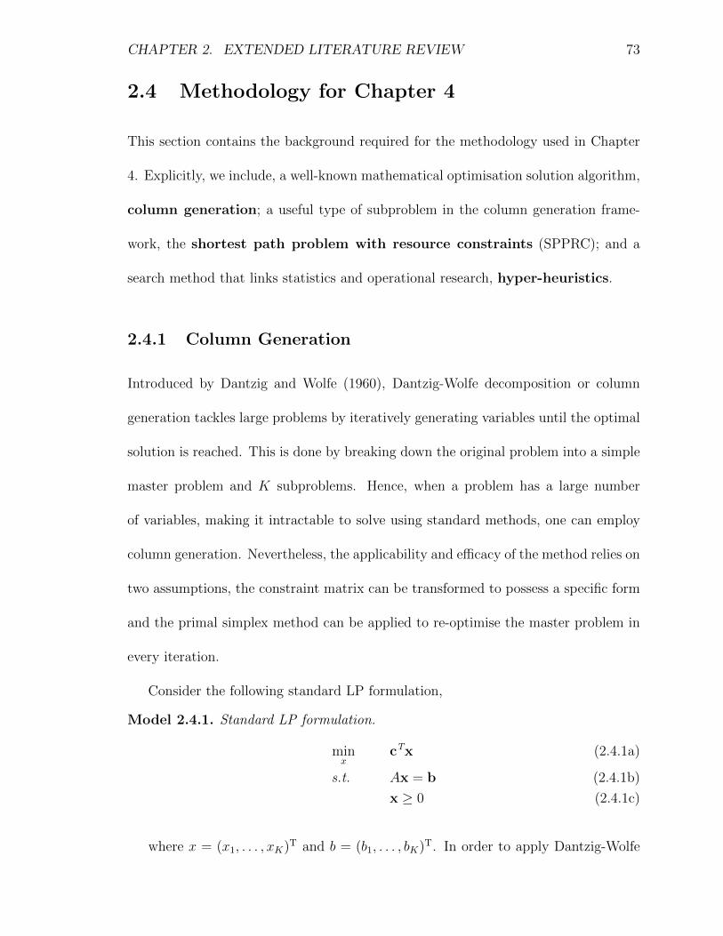
CHAPTER 2. EXTENDED LITERATURE REVIEW 73
2.4 Methodology for Chapter 4
This section contains the background required for the methodology used in Chapter
4. Explicitly, we include, a well-known mathematical optimisation solution algorithm,
column generation; a useful type of subproblem in the column generation frame-
work, the shortest path problem with resource constraints (SPPRC); and a
search method that links statistics and operational research, hyper-heuristics.
2.4.1 Column Generation
Introduced by Dantzig and Wolfe (1960), Dantzig-Wolfe decomposition or column
generation tackles large problems by iteratively generating variables until the optimal
solution is reached. This is done by breaking down the original problem into a simple
master problem and K subproblems. Hence, when a problem has a large number
of variables, making it intractable to solve using standard methods, one can employ
column generation. Nevertheless, the applicability and efficacy of the method relies on
two assumptions, the constraint matrix can be transformed to possess a specific form
and the primal simplex method can be applied to re-optimise the master problem in
every iteration.
Consider the following standard LP formulation,
Model 2.4.1. Standard LP formulation.
minx
cTx (2.4.1a)
s.t. Ax = b (2.4.1b)
x ≥ 0 (2.4.1c)
where x = (x1, . . . , xK)T and b = (b1, . . . , bK)T. In order to apply Dantzig-Wolfe

CHAPTER 2. EXTENDED LITERATURE REVIEW 74
decomposition, the constraint matrix, A, has to retain a specific form. Let Bk and Ak
for k = 1, . . . , K be submatrices with appropriate dimensions, then, A has a special
structure as depicted below,
B0 B1 B2 . . . BK
A1
A2
. . .
AK
.
This structure, called the block angular structure, provides the necessary submatrices
to reformulate the problem into a master problem and K subproblems. The top row,
which corresponds to the constraints of the master problem, i.e.∑K
k=1Bkxk = b0, are
referred to as the coupling constraints. The subproblems, with constraints of the form
Akxk = bk for k = 1, . . . , K; do not all have to be solved.
To reformulate the master problem, Minkowski’s representation theorem can be
employed. The theorem states that extreme points or rays are represented by a set
of points which lay on the boundary of a convex region.
Theorem 2.4.1 (Minkowski’s representation theorem, Minkowski, 1953). If P =
{x : Ax = b, x ≥ 0} is a feasible (bounded or unbounded) region, then we can
represent any point x ∈ P as a linear combination of its extreme points or rays, x(j),
x =∑j
λjx(j) as long as
∑j
δjλj = 1 and λj ≥ 0

CHAPTER 2. EXTENDED LITERATURE REVIEW 75
where
δj =
1, if x(j) is an extreme point (case that P is bounded)
0, if x(j) is an extreme ray (case that P is unbounded).
Hereby, each column of the master problem can be made to represent a solution,
as a linear combination of extreme points and rays, of each of the subproblems. The
model can be reformulated as follows,
Model 2.4.2. Standard LP Reformulation using Theorem 2.4.1.
minx0,λkj
cT0 x0 +K∑k=1
pk∑j=1
(cTk x
(j)k
)λkj (2.4.2a)
s.t. B0x0 +K∑k=1
pk∑j=1
(Bkx
(j)k
)λkj = b0 (2.4.2b)
pk∑j=1
δkjλkj = 1 k = 1, . . . , K (2.4.2c)
x0, λkj ≥ 0 (2.4.2d)
In practice, this reformulation can not be applied directly, as the number of λ–
variables becomes very large because the number of extreme points and rays for every
subproblem is also large. However, the fact that many of these variable will end
up being non-basic may be exploited by the column generation algorithm. So that,
only the variables with a negative reduced cost, therefore likely to become basic, are
explored. With this consideration, the restricted master problem (RMP) may be
reformulated as,

CHAPTER 2. EXTENDED LITERATURE REVIEW 76
Model 2.4.3. Restricted Master Problem.
minx0,λ′
cT0 x0 + cTλ′ (2.4.3a)
s.t. B0x0 +Bλ′ = b0 (2.4.3b)
∆λ′ = 1 (2.4.3c)
x0, λ′ ≥ 0. (2.4.3d)
The dimensions of this problem evolve as variables are added when the subprob-
lems are solved. If a subproblem k has been solved, the variable λk,j can be included
if its reduced cost is negative. The master problem is extended by introducing the
column and its corresponding cost coefficient. This procedure is repeated until the
objective function of the original LP is improved or no more variables with negative
reduced costs are found.
Let the dual variables for constraints 2.4.3b and 2.4.3c be denoted by π1 and π(k)2
respectively. To determine which new column should be introduced to the master
problem, a reduced cost LP needs to be solved for each subproblem under consid-
eration. Assuming the subproblem k is bounded, the reduced cost LP gives the K
formulations for the subproblems as,
Model 2.4.4. Reduced cost LP.
minxk
σk =(cTk − πT
1 Bk
)xk − π(k)
2 (2.4.4a)
s.t. Bkxk = bk (2.4.4b)
xk ≥ 0. (2.4.4c)
Now, the most significant xk to enter the master problem are those found to
maximise the reduced cost LP. So, if σ∗k < 0 then the new column, λk,j, can be
introduced to the master problem with its corresponding cost coefficient, cTk x∗k.
The pseudo-code for the column generation algorithm is given in Algorithm 1. It

CHAPTER 2. EXTENDED LITERATURE REVIEW 77
consists on iteratively solving the RMP, and one of the K subproblems at a time. The
subproblem is solved by solving the corresponding reduced cost LP. Hence, if, after
solving the k-th subproblem, we see that objective is negative, then, the corresponding
variable has a negative reduced cost, and we generate and add the column to the RMP.
We repeat the process, moving on to the next subproblem until no negative reduced
cost is obtained. Moreover, the initialisation involves checking the subproblems and
generating the first columns. If any of the subproblems happens to be infeasible, then
the master problem is also infeasible. Otherwise, an initial feasible solution can be
easily constructed from the optimal solutions to these.
Algorithm 1 Column Generation Algorithm.
1: INPUTS: RPM (Model 2.4.3), K subproblems (Model 2.4.4)2: Initialisations: stop = False.3: while stop is False do4: Solve RPM;5: for k = 1, . . . , K do6: Solve subproblem k7: if σ∗k < 0 then8: Update the restricted master problem by adding proposal x∗k.
9: Introduce column
(cTk x
∗k
Bkx∗k
).
10: end if11: end for12: if No proposal generated then13: stop = True. . Optimality has been reached.14: end if15: end while
This algorithm is extremely versatile and has been used to solve multiple types
of problems. However, if the original problem is a MIP and optimal solutions are
sought, column generation has to be embedded in a branching algorithm to form the
so-called branch-and-price algorithm.

CHAPTER 2. EXTENDED LITERATURE REVIEW 78
2.4.2 Shortest Path Problem with Resource Constraints
In the applied column generation framework, particularly in scheduling related lit-
erature, the shortest path problem with resource constraints (SPPRC) is commonly
employed to generate variables as a subproblem. It consists, as its name suggests, in
finding, among all paths, the shortest path from source to sink nodes, that satisfies a
set of constraints for a defined set of resources.
The SPPRC was first introduced by Desrochers (1986) as a subproblem for the bus
driver scheduling problem. It has been widely applied in a variety of different settings
including: the vehicle routing problem with time windows, the technician routing and
scheduling problem, the capacitated arc-routing problem, on-demand transportation
systems, and airport ground movement (Desrochers and Soumis, 1988; Feillet et al.,
2004; Irnich and Villeneuve, 2006; Righini and Salani, 2008; Bode and Irnich, 2014;
Chen et al., 2016; Garaix et al., 2010; Tilk et al., 2017; Zamorano and Stolletz, 2017).
To discuss the SPPRC in more detail, let us define some notation. Let G = (N,A)
denote a directed graph with set of nodes N and arcs A. Let R = {1, . . . , R} denote
the set of resources, and L = (L1, . . . , LR) and L = (L1, . . . , L
R) denote vectors
for minimum and maximum resources, respectively. For each arc i, we denote the
associated weight by wi, and the vector of resource consumption by fi = (f 1i , . . . , f
Ri ).
Each component in the vector is called a resource extension function (REF) (Irnich
and Desaulniers, 2005). For an example of how these can be applied see Section 4.3.3.
For a given path, p, between a given pair of nodes, we denote the set of connections
by A(p), the total weight of the path by w(p), and the resource consumed along the

CHAPTER 2. EXTENDED LITERATURE REVIEW 79
path by f(p) = (f 1(p), . . . , fR(p)). Where,
w(p) =∑i∈A(p)
wi ; f r(p) =∑i∈A(p)
f ri .
The path is said to be resource feasible if L ≤ f(p) ≤ L, i.e. Lr ≤ f r(p) ≤ Lr
for
every resource r.
Solution Algorithms
There are a number of algorithms for the standard shortest path problems. Among
some of the most historically relevant algorithms are greedy algorithms, Dijkstra’s al-
gorithm (which is restricted to graphs with non-negative edge weights) and Bellman-
Ford algorithm, and best-first search, A* search algorithm (which uses a heuristic
function to provide faster solutions). Nevertheless, these algorithms cannot be used
directly to solve the SPPRC. The reason for this is the need to compare the resources
consumed when obtaining the different paths. This is done through the use of la-
belling algorithms. Simply put, labels carry information about the different resources
under consideration, allowing comparisons between different potential paths. Alter-
natively, as introduced in Chapter 4, standard algorithms can be employed to provide
approximate but fast solutions for the SPPRC. This is done by iteratively solving
a standard shortest path problem and modifying the graph so as to force resource
feasibility.
Many exact algorithms to solve the SPPRC are dynamic programming (DP)
labelling algorithms. These build paths in a systematic fashion by starting at a
CHAPTER 2. EXTENDED LITERATURE REVIEW 80
source node and traversing the graph considering all feasible directions. Labels are
created in order to efficiently compare different paths and discard the dominated or
“suboptimal” ones.
Irnich and Desaulniers (2005) presented an exact DP algorithm, the monodirec-
tional forward labelling algorithm (sometimes called unidirectional), based on the
pioneering work by Desrochers and Soumis (1988). Boland et al. (2006) published a
state augmenting algorithm that used a monodirectional labelling algorithm to find an
elementary path (one without repeating nodes). Righini and Salani (2006) introduced
a bidirectional labelling algorithm for the SPPRC. The bidirectional algorithm is
an extension of the monodirectional algorithm that supports search from both ends of
the graph, hence reducing the computational efforts. Moreover, they used bounding
in order to mitigate label explosion. This typical phenomenon occurs simply due to
the nature of the algorithm and the need to store the non-dominated labels of all
partial paths. More recently, Tilk et al. (2017) released a bidirectional labelling al-
gorithm with dynamic halfway point. Based on previous works (Righini and Salani,
2006; Pecin et al., 2017), the bidirectional search is bounded for both directions and
these bounds are dynamically updated as the search in either direction advances.
Some heuristic algorithms to solve the SPPRC are also based on DP. Additionally,
metaheuristic algorithms have been developed to find fast and promising solutions
to the SPPRC. DP heuristics have been developed by several authors (Feillet et al.,
2004; Lozano et al., 2015). Local search or metaheuristics, in this setting, start with a
given path and perform a series of moves (node/arc: deletion, insertion, or exchange)
to obtain another feasible path with lower cost. Metaheuristics implemented for
CHAPTER 2. EXTENDED LITERATURE REVIEW 81
the SPPRC include trajectory-based, Tabu search (Desaulniers et al., 2008) and
greedy randomised adaptive search procedure (GRASP) (Ferone et al., 2019),
and nature-inspired, hybrid particle swarm algorithm (Marinakis et al., 2017).
For more information on metaheuristic algorithms for the SPPRC, including two new
algorithms, see Section 4.4.2.
We now proceed with a discussion of two exact labelling algorithms.
Monodirectional Forward Labelling Algorithm
Algorithm 2 shows a generic version of the monodirectional forward labelling algo-
rithm (Irnich and Desaulniers, 2005). It uses a set of unprocessed paths U and a set
of processed paths P, which change dynamically with every iteration. After an appro-
priate initialisation, in line 3, an unprocessed path is selected, say Q and subsequently
removed from the set of unprocessed paths, line 4. In lines 5 to 10, all the feasible one
node extensions are computed and checked for resource feasibility. In lines 7 and 8,
if the extension is resource feasible, then it is added to the set of unprocessed paths
U, and the original path is added to the set of processed paths P. After this, if we
wish to eliminate some suboptimal paths, dominance relations can be applied to both
unprocessed and processed paths.
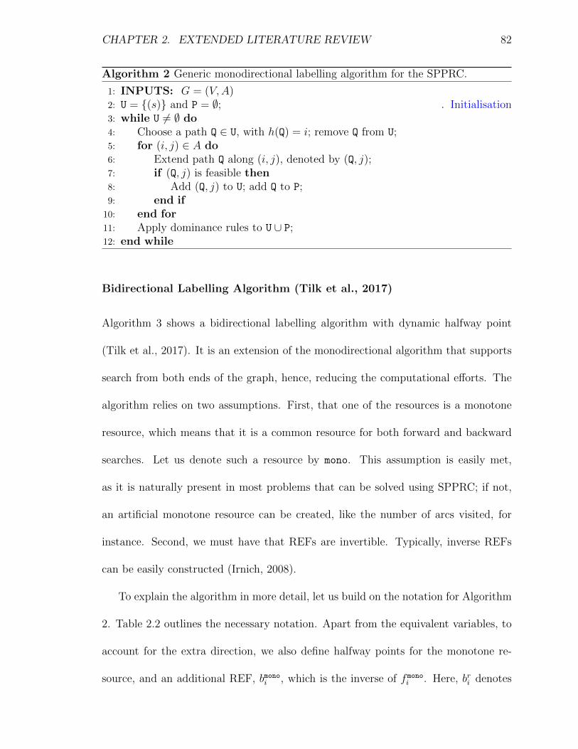
CHAPTER 2. EXTENDED LITERATURE REVIEW 82
Algorithm 2 Generic monodirectional labelling algorithm for the SPPRC.
1: INPUTS: G = (V,A)2: U = {(s)} and P = ∅; . Initialisation3: while U 6= ∅ do4: Choose a path Q ∈ U, with h(Q) = i; remove Q from U;5: for (i, j) ∈ A do6: Extend path Q along (i, j), denoted by (Q, j);7: if (Q, j) is feasible then8: Add (Q, j) to U; add Q to P;9: end if
10: end for11: Apply dominance rules to U ∪ P;12: end while
Bidirectional Labelling Algorithm (Tilk et al., 2017)
Algorithm 3 shows a bidirectional labelling algorithm with dynamic halfway point
(Tilk et al., 2017). It is an extension of the monodirectional algorithm that supports
search from both ends of the graph, hence, reducing the computational efforts. The
algorithm relies on two assumptions. First, that one of the resources is a monotone
resource, which means that it is a common resource for both forward and backward
searches. Let us denote such a resource by mono. This assumption is easily met,
as it is naturally present in most problems that can be solved using SPPRC; if not,
an artificial monotone resource can be created, like the number of arcs visited, for
instance. Second, we must have that REFs are invertible. Typically, inverse REFs
can be easily constructed (Irnich, 2008).
To explain the algorithm in more detail, let us build on the notation for Algorithm
2. Table 2.2 outlines the necessary notation. Apart from the equivalent variables, to
account for the extra direction, we also define halfway points for the monotone re-
source, and an additional REF, bmonoi , which is the inverse of f monoi . Here, bri denotes

CHAPTER 2. EXTENDED LITERATURE REVIEW 83
the backward REF for any arc i and resource r. Arc extensions, along arc (i, j), for
partial paths Q (from s to i) and Q’ (from t to j) are {s, . . . , i, j} denoted with (Q, j),
and {t, . . . , j, i} denoted with (Q’, i), respectively. Where s and t denote source and
sink nodes respectively. If the the forward REF is assumed to be non-decreasing, then
its inverse, the backward REF, has to be non-increasing (and vice-versa). Further-
more, let Qmono and Q’mono stand for the cumulative monotone resource consumption
for the forward and backward partial paths.
Table 2.2: Forward and backward labelling notation.
Forward Backward
Unprocessed paths F B
Halfway point formono
HF HB
Partial Path Q = {s, . . . , i} Q’ = {t, . . . , j}REF f monoi bmonoi
Extended path alongarc (i, j)
(Q, j) (Q’, i)
REF arc extension f monoi ≤ f monoj bmonoi ≤ bmonoj
(non-decreasing) (non-increasing)Cumulative REF f mono(Q) = Qmono bmono(Q’) = Q’mono
The algorithm requires some inputs, a directed graph G = (V,A), and the halfway
point for the forward and backward search HF and HB, respectively. For the monotone
resource mono, recall the lower and upper bounds are denoted by Lmono and Lmono
.
Depending on the values for the halfway points, the algorithm behaves in different
ways,
HF = HB > Lmono
: Monodirectional forward labelling algorithm;
HF = HB < Lmono: Monodirectional backward labelling algorithm;
Lmono < HF = HB < Lmono
: Bidirectional labelling algorithm with static halfway point;

CHAPTER 2. EXTENDED LITERATURE REVIEW 84
Lmono = HB < HF = Lmono
: Bidirectional labelling algorithm with dynamic halfway point.
Once Algorithm 3 is initialised, in line 2, and direction settled, in line 4, we proceed
either a forward or backward search in a very similar fashion as Algorithm 2. After
choosing a path from the unprocessed set of paths, lines 6 or 16, we check if the
halfway point has been reached, lines 7 or 17, if not, then we proceed to extend the
selected path in the traditional way, lines 8-12 or 18-22. After this, we update the
value of the halfway point to reduce the size of the search in the opposite direction.
That is, in the forward search, in line 13, we update HB to a higher value if we have
searched past it. Conversely, in the backward search, in line 23, we update HF to
a lower value if we have searched past it. The algorithm carries on in this fashion,
updating the direction of search in every iteration. It terminates when no more paths
remain to be processed in any direction.

CHAPTER 2. EXTENDED LITERATURE REVIEW 85
Algorithm 3 Bidirectional labelling algorithm with dynamic halfway point for theSPPRC (Tilk et al., 2017).
1: INPUTS: G = (V,A), L, L;2: Initialisations: HF= L
mono, HB= Lmono, F = {(s)}, B = {(t)}, and P = ∅;
3: . See Appendix B.1.1 for functions employed4: while F 6= ∅ or B 6= ∅ do5: direction = getDirection(F, B)6: if direction = forward then . Forward labelling7: Choose a path Q ∈ F, with h(Q) = i; remove Q from F;8: if Qres ≤ HF then9: for (i, j) ∈ A do
10: Extend path Q along (i, j), denoted by (Q, j); . Path extension step11: if (Q, j) is feasible then Add (Q, j) to F; add Q to P;12: end if13: end for14: HB = max{HB,min{Qres, HF}}15: end if16: else if direction = backward then . Backward labelling17: Choose a path Q’ ∈ B, with t(Q’) = j; remove Q’ from B;18: if Q’res > HB then19: for (i, j) ∈ A do20: Extend path Q’ along (i, j), denoted by (Q’, i);21: if (Q’, i) is feasible then Add (Q’, i) to B; add Q to P;22: end if23: end for24: HF = min{HF,max{Q’res, HB}}25: end if26: else . If no direction27: break28: end if29: Apply dominance rules to F ∪ B ∪ P;30: end while
CHAPTER 2. EXTENDED LITERATURE REVIEW 86
2.4.3 Hyper-heuristics
Hyper-heuristic search methods incorporate different machine learning techniques to
automate the solution of an evolving set of optimisation problems, hence, being able
to adapt to the challenges in a suitable fashion to produce promising solutions. With
a set of low-level heuristics or metaheuristics, hyper-heuristic methods exploit the
combination or selection of these to generate improved solutions.
Combination or generation hyper-heuristics combine basic components of dif-
ferent heuristic methods to construct new heuristics. Heuristic methods frequently
consist of problem-dependent simple local search operations. For example, in a generic
scheduling setting, some simple local search operations, that add activities to a sched-
ule under construction, could be: add the activity with longest/shortest processing
time, add a random activity, try all the possible candidate activities (not already
present in the current schedule) and add the one that best suites the current schedule
(e.g. minimises a certain cost function, or satisfies a certain constraint).
Figure 2.6 shows a scheme for a selection hyper-heuristic. Given a problem
specific input and three different heuristics(or metaheuristics) H1, H2, H3, in each
iteration the hyper-heuristic algorithm selects one heuristic (based on the ranking),
applies it on the problem under consideration, evaluates its performance, and updates
the ranks of all heuristics based on the performance.
Hyper-heuristic methods model an interaction between statistics and operational
research, and have received attention from researchers from both communities. This
has led to a wide array of applications including (and not limited to) scheduling prob-

CHAPTER 2. EXTENDED LITERATURE REVIEW 87
lems, e.g. educational timetabling (Burke et al., 2007), nurse rostering (Burke et al.,
2003); the travelling salesman problem (Keller and Poli, 2007; Runka, 2009); vehi-
cle routing problems (Ochoa et al., 2012); and knapsack problems, mutidimensional
(Allen et al., 2009), and 0/1 (Kumar et al., 2008). Furthermore, there are recent
theoretical publications that study computational complexity of different methods,
Doerr et al. (2018), for instance. Given the scope of the area, we refer the reader to
the recent and thorough review by Burke et al. (2013), and Burke et al. (2019). In
Chapter 4 we employ a learning-based hyper-heuristic to adaptively select different
metaheuristic algorithms in a column generation framework.
INPUT
Heuristic selection
H2H1 H3
Update
EvaluateApply Rank
Figure 2.6: Hyper-heuristic algorithm.

Chapter 3
An Optimisation Framework forAirline Fleet MaintenanceScheduling with Tail AssignmentConsiderations
3.1 Introduction
There are a number of operational decisions associated with airlines, from ticket prices
to flight times, crew rosters, and aircraft maintenance. When making these decisions,
airlines have to take into account their own economic interests influenced by demand,
costs, and sometimes even the actions of their competitors. In such a competitive en-
vironment, airlines aim to minimise their operating costs while providing competitive
services. Significant proportion of operating costs are dedicated to maintenance. For
instance, 20.5% of the average direct operating cost per medium-haul trip are ded-
icated to maintenance on an Airbus A330-200 (Aircraft Analysis & Fleet Planning,
2005). Therefore, it is of paramount importance to develop decision making tools that
will allow airlines to optimise their aircraft maintenance decisions.
Maintenance types are classified according to: short, medium and long-term in-
88

CHAPTER 3. AIRLINE FLEET MAINTENANCE SCHEDULING 89
terventions. Short-term or line maintenance does not require modelling or advanced
planning as they are carried out as standard procedures at airport gates. Medium
and long-term maintenance interventions include:
1. Airframe checks (A, B, C and D);
2. Engine performance restoration (EPR) and life limited parts replacement (ELR);
3. Landing gear overhaul (LG), and;
4. Auxiliary power unit (APU) performance restoration.
Civil Aviation Authorities Regulations impose that maintenance has to be per-
formed after a certain number of months (MO), flying hours (FH), or flight cycles
(FC), at certified maintenance workshops. In the medium-term, A checks have to be
performed every 80-100 FH (every 7 to 9 days), requiring 10-20 man-hours, while B
checks typically occur every 500-600 FH (every two months), requiring 100-300 man-
hours (Department for BIS, 2016). However, in practice, Type B checks are included
as part of a longer A check, or a bundle of A checks (Qantas, 2016). Long-term
maintenance, including C and D checks, LG, EPR, ELR, and APU are performed
once every 1–6 years and can last over 10 days (Ackert, 2011). It is worth noting that
there is a large variability in the duration of maintenance checks due to the fact that
different aircraft types have different maintenance requirements.
Table 3.1 shows the frequency of the four airframe checks for various aircraft types.
As one would expect, the time between checks increases for more modern aircraft and
B checks disappear, being contained in longer A checks. Maintenance is performed

CHAPTER 3. AIRLINE FLEET MAINTENANCE SCHEDULING 90
before any of the three criteria (MO, FH or FC) is met. For instance, for the B737-
200, a C check is performed after 18 MO, 6000 FH, or 3000 FC, whichever occurs first.
The justification for this practice is to ensure coverage of overused aircraft operating
short-haul flights. In these cases, FC are accumulated faster than FH (Cook and
Tanner, 2008). Moreover, usual frequencies of long-term maintenance, for the A320,
for instance, are 13500 FC for both the EPR and the ELR, 120 MO/20000 FC for the
LG, and 75000 FH for the APU (Ackert, 2011).
Table 3.1: Typical maintenance frequencies in calendar months (MO), flying hours(FH), or flight cycles (FC) (Cook and Tanner, 2008; Martins, 2016).
Aircraft A check B check C check D check
B737-300 275 FH 825 FH 18 MO 48 MOB737-400 275 FH 825 FH 18 MO 48 MOB737-500 275 FH 825 FH 18 MO 48 MOB737-800 500 FH n/a 4000-6000 FH 96-144 MOB757-200 500-600 FH n/a 18 MO/6000 FH/3000 FC 72 MO
F100 500 FH n/a 5000 FH 12000 FHB767-300ER 600 FH n/a 18 MO/6000 FH 72 MO
B747-400 600 FH n/a 18 MO/7500 FH 72 MOA319 600 FH n/a 18-20 MO/6000 FH/3000 FC 72 MOA320 600 FH n/a 18-20 MO/6000 FH/3000 FC 72 MO
For maintenance to be performed effectively, there is an essential underlying pro-
cess, airline fleet maintenance scheduling (AMS). The AMS problem deals with the
construction of a schedule that minimises maintenance costs, resource usage, and the
disruption to airline operations, while satisfying current safety regulations by differ-
ent civil aviation authorities (Sriram and Haghani, 2003). Given the frequency of the
maintenance checks, the decision horizon for medium-term maintenance should be a
month, and, at least, six months for long-term maintenance.
A challenge for the AMS problem is to allocate maintenance-related resources

CHAPTER 3. AIRLINE FLEET MAINTENANCE SCHEDULING 91
in a cost-effective fashion. These resources are geographically dispersed throughout
distant and distinct maintenance workshops. Some examples of resources include
limited specialised tools, spare parts, and certified technicians. Additionally, regulated
checks depend on the state of the aircraft and employ different resources.
The major contribution of this paper is the framework that deals with the re-
quirements introduced by 30-day planning horizon instances, with multiple airlines
and workshops, and tight resource availabilities. Such framework can be broken down
into three steps. Firstly, the preprocessing step identifies maintenance opportunities
(MOPs). These opportunities arise when flights have large turnaround times dur-
ing which aircraft can be maintained. This preprocessing allows us to formulate and
solve the problem efficiently. Next, in the case when not enough MOPs are found,
we identify when these occur and we reassign aircraft to different flights to generate
more MOPs. In other words, we re-solve the tail assignment (TA) problem. Lastly,
to preserve tractability and improve the quality of solutions, we provide a two-stage
iterative algorithm. The first stage adjusts the size of the TA problem appropriately.
The second stage makes the timeline more granular to improve resource allocation.
Further contributions introduced by this work are: the presentation of a new type
of multi-objective optimisation formulation for the AMS which copes with single and
multi-workshop cases, the focus on workshop resource allocation, the consideration
of different fleet types and their respective maintenance requirements, and, the intro-
duction of a solution framework that solves problems of realistic size in short time.
Showing the potential of this framework which promotes cooperation between airlines.

CHAPTER 3. AIRLINE FLEET MAINTENANCE SCHEDULING 92
The remainder of this paper is organised as follows: Section 3.2, discusses the
relevant literature. Section 3.3 presents the proposed modelling approaches and the
corresponding underlying concepts. The first model, minimises the number of mainte-
nance regulation violations, adhering to the criteria presented in Table 3.1. The second
model solves a reduced TA problem within the AMS considering violations. Section
3.4 presents the solution methodology and the model application. Computational ex-
periments are given in Section 3.5, while Section 3.6 summarises the conclusions and
provides recommendations for future research.
3.2 Literature Review
The airline planning process or airline scheduling problem involves several stages:
flight scheduling, sometimes referred to as schedule design; fleet assignment, which
assigns fleet types to flights (Hane et al., 1993); tail assignment (TA), sometimes called
aircraft routing or aircraft rotation and involves assigning individual aircraft to flights
(Clarke et al., 1997); maintenance scheduling (MS); and, finally, crew scheduling.
These were traditionally modelled by formulating each stage separately and solving
them sequentially, i.e. the output of one stage is the input for the next. Figure 3.1
presents the order of solving the different types of problems identified above (solid
lines), along with some common feedback loops (dashed lines) and the associated
typical planning horizons.
The sequential modelling and solution of the airline scheduling problem does not
take into consideration the restrictions of the subsequent problems. The benefit of the

CHAPTER 3. AIRLINE FLEET MAINTENANCE SCHEDULING 93
sequential approach is the reduction in computational complexity. Even though the
sequential feedback system is a close approximation, the solution can be improved
by modelling the interdependence of each stage in an integrated model (Cordeau
et al., 2001). Integrated models have been developed to provide better quality results
and consider the combination of two or more stages into a single problem (Desaulniers
et al., 1997; Clarke et al., 1997; Barnhart et al., 1998; Cohn and Barnhart, 2003; Sriram
and Haghani, 2003; Mercier et al., 2005; Sarac et al., 2006; Liang and Chaovalitwongse,
2013; Safaei and Jardine, 2018). In particular, MS is frequently contained within the
TA, in which case it is called aircraft maintenance routing (AMR) problem (Gopalan
and Talluri, 1998).
FlightScheduling
Fleet As-signment
Tail Assign-ment (TA)
CrewScheduling
MaintenanceSchedul-ing (MS)
1-4 weeksin advance
1-7 daysin advance
12 monthsin advance
12 monthsin advance
Figure 3.1: Stages of the airline scheduling problem.
The most common types of mixed integer programming formulations for the inte-
grated airline scheduling problem can be classified into three groups,
String-based models: a type of formulation that models the problem using strings,
i.e. sequences of connected flights that begin and end at a maintenance work-
shop, and, that satisfy flow balance and maintenance regulations (Desaulniers
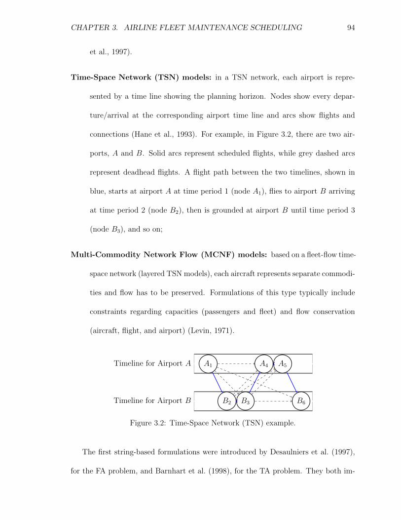
CHAPTER 3. AIRLINE FLEET MAINTENANCE SCHEDULING 94
et al., 1997).
Time-Space Network (TSN) models: in a TSN network, each airport is repre-
sented by a time line showing the planning horizon. Nodes show every depar-
ture/arrival at the corresponding airport time line and arcs show flights and
connections (Hane et al., 1993). For example, in Figure 3.2, there are two air-
ports, A and B. Solid arcs represent scheduled flights, while grey dashed arcs
represent deadhead flights. A flight path between the two timelines, shown in
blue, starts at airport A at time period 1 (node A1), flies to airport B arriving
at time period 2 (node B2), then is grounded at airport B until time period 3
(node B3), and so on;
Multi-Commodity Network Flow (MCNF) models: based on a fleet-flow time-
space network (layered TSN models), each aircraft represents separate commodi-
ties and flow has to be preserved. Formulations of this type typically include
constraints regarding capacities (passengers and fleet) and flow conservation
(aircraft, flight, and airport) (Levin, 1971).
Timeline for Airport B
Timeline for Airport A A1 A4 A5
B2 B3 B6
Figure 3.2: Time-Space Network (TSN) example.
The first string-based formulations were introduced by Desaulniers et al. (1997),
for the FA problem, and Barnhart et al. (1998), for the TA problem. They both im-

CHAPTER 3. AIRLINE FLEET MAINTENANCE SCHEDULING 95
plemented a branch and bound scheme as their solution method. Even though they
included maintenance regulations, workshop resources or flying hours (FH) were not
considered. Sarac et al. (2006); Cohn and Barnhart (2003); Papadakos (2009) used
the same type of formulation for the AMR problem. Papadakos (2009) produced
a computational case study for a medium-sized data set (700 flights, 167 aircraft).
The heuristic algorithm used required 16 hours to solve the problem under consider-
ation. Sarac et al. (2006) implemented a branch-and-price algorithm and used legal
remaining FH to influence decisions. Aside from the excessive solution times, string-
based formulations are not capable of generating all strings even for small instances.
Furthermore, these models do not include resource usage for maintenance activities.
The TSN formulation, introduced by Hane et al. (1993), has been used widely
within the integrated airline scheduling framework, (Clarke et al., 1997; Hicks et al.,
2005; Orhan et al., 2012; Haouari et al., 2013; Liang and Chaovalitwongse, 2013).
However, given that TSNs do not allow individual aircraft to be tracked, aggregated
maintenance constraints are implemented. This means that models are forced to, for
instance, minimise total weekly maintenance operations. More recently, Safaei and
Jardine (2018) examined the AMR problem with generalised maintenance constraints
and legal remaining FH considerations. They used test instances for a single air-
line. The computational study, for a relatively large data set (7 days, 772 flights, 18
aircraft), solutions show financial impact but computational times are not provided.
Using the MCNF formulation, introduced by Levin (1971), the problem can be
solved using column generation (Yan and Tseng, 2002; Sriram and Haghani, 2003;
Mercier et al., 2005). Particularly, Sriram and Haghani (2003), presented some influ-
CHAPTER 3. AIRLINE FLEET MAINTENANCE SCHEDULING 96
ential work, based on the TA formulation by Feo and Bard (1989), which solved the
AMR incorporating A and B checks. They used a heuristic algorithm that solved a
small test instance (58 flights, 75 airports) in 5 minutes.
All the publications mentioned thus far are limited to daily or weekly schedules and
assume cyclical repetitions of the flights and hence maintenance operations. Khaled
et al. (2018), however, considered individual maintenance requirements for a 30-day
plan. They used an improved TSN formulation for the AMR problem, which allowed
them to effectively schedule A checks, constrained by individual aircraft legal remain-
ing FH. They assumed that maintenance is generally performed at night. Due to the
type of formulation, solution times increased noticeably for a large number of flights
(timed out at 3 hours for 1494 flights and a single airline). Li et al. (2016), dealt
with the AMR problem for fighter jets. This formulation, which relied on a single
workshop assumption, also employed legal remaining FH to determine the frequency
of maintenance. Further assumptions included: no resource considerations, only one
type of maintenance, and the disregard of aircraft “health” at the end of the planning
horizon. The test set considered is of 25 days and 200 aircraft but no solution times
are provided. In addition, the timeline is discretised by splitting each day into two 12
hour intervals, clearly, this incurs a huge loss in accuracy.
In different context, we find formulations that account for long-term planning
horizons; specifically, in the resource constrained project scheduling problem (RCPSP)
literature. The RCPSP is a generalisation of machine scheduling problem where jobs
are scheduled according to some predefined order, or precedence, subject to different

CHAPTER 3. AIRLINE FLEET MAINTENANCE SCHEDULING 97
resource demands and capacity constraints. Usually, the objective is to minimise
the duration of the project (collection of ordered jobs), commonly, under a non-
preemption assumption (jobs have to processed fully) (Kone et al., 2011; Brucker and
Knust, 2012; Kopanos et al., 2014; Naber, 2017). The reader may refer to a recent
and thorough review article by Habibi et al. (2018). On the long-term RCPSP, Kone
et al. (2011) proposed two formulations which they named “event-based RCPSP”
formulations. Events correspond to start and/or end times of activities. Since their
formulations involve fewer variables than the formulations indexed by time, they have
the capacity to deal with longer planning horizons.
As can be seen in the summary of the literature in Table 3.2, no publications
have addressed the long-term AMS problem with multiple airlines, workshops and
resource considerations, while providing fast solution times. Additionally, we take
into account individual aircraft maintenance requirements and their respective flight
operations. The key contributions of the present paper are,
Reassignment. We include the option of reassigning some flights to obtain longer
maintenance opportunities.
Efficient resource allocation. Maintenance models do not always consider the dif-
ferent resources available throughout maintenance workshops. Therefore, we
incorporate workshop resource restrictions.
Individual aircraft considerations. Different aircraft may have different mainte-
nance duration and requirements, and different accumulation of FH. Hence, we
include this in our model.

CHAPTER 3. AIRLINE FLEET MAINTENANCE SCHEDULING 98
Long-term planning horizon. Short-term, or operational planning, is not suitable
for most aircraft maintenance. Further, personnel and equipment hire are sig-
nificantly expensive. Thus, it is extremely useful for maintenance operators to
plan longer in advance.
Two-stage iterative algorithm. We employ a two-stage algorithm that provides
good solutions for large instances in reasonable computational time.
Single and multi-workshop tests cases. Our generic framework, allows us to model
both single and multi-workshop cases.
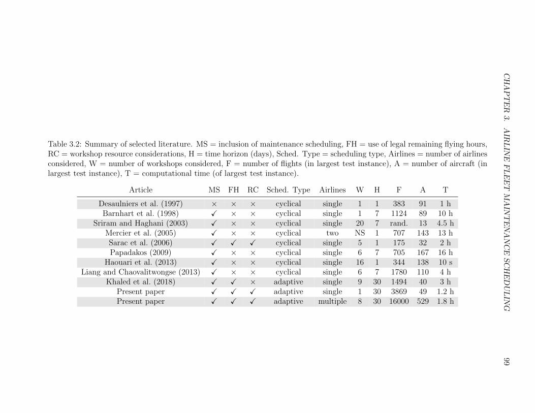
CHAPTER
3.AIR
LIN
EFLEET
MAIN
TENANCESCHEDULIN
G99
Table 3.2: Summary of selected literature. MS = inclusion of maintenance scheduling, FH = use of legal remaining flying hours,RC = workshop resource considerations, H = time horizon (days), Sched. Type = scheduling type, Airlines = number of airlinesconsidered, W = number of workshops considered, F = number of flights (in largest test instance), A = number of aircraft (inlargest test instance), T = computational time (of largest test instance).
Article MS FH RC Sched. Type Airlines W H F A T
Desaulniers et al. (1997) × × × cyclical single 1 1 383 91 1 hBarnhart et al. (1998) X × × cyclical single 1 7 1124 89 10 h
Sriram and Haghani (2003) X × × cyclical single 20 7 rand. 13 4.5 hMercier et al. (2005) X × × cyclical two NS 1 707 143 13 hSarac et al. (2006) X X X cyclical single 5 1 175 32 2 hPapadakos (2009) X × × cyclical single 6 7 705 167 16 h
Haouari et al. (2013) X × × cyclical single 16 1 344 138 10 sLiang and Chaovalitwongse (2013) X × × cyclical single 6 7 1780 110 4 h
Khaled et al. (2018) X X × adaptive single 9 30 1494 40 3 hPresent paper X X X adaptive single 1 30 3869 49 1.2 hPresent paper X X X adaptive multiple 8 30 16000 529 1.8 h

CHAPTER 3. AIRLINE FLEET MAINTENANCE SCHEDULING 100
3.3 The Proposed Modelling Approach
In order to be able to adequately model the problem, we first state the necessary
assumptions, highlight the concepts used and define the appropriate notation. After
this, we propose two multi-objective mixed integer linear programming (MMILP)
formulations that schedule different types of maintenance for a medium/long-term
planning horizon e.g. airframe checks A and C. To check if regulation requirements
are being fulfilled, we employ different maintenance requirement (MR) variables for
each type of maintenance and aircraft type, which vary with flying hours (FH).
In the first formulation, given an input flight schedule, we aim to determine
whether a feasible maintenance schedule exists. We call this the airline fleet main-
tenance scheduling (AMS) formulation. If a feasible maintenance schedule does not
exist, we seek to minimise the number of infeasibilities, or violations. Such violations
represent the cases when the limit imposed by the regulations on the FH are exceeded.
To minimise the violations, we introduce the second formulation which extends the
AMS formulation to account for an appropriate tail assignment (TA) problem.
3.3.1 Assumptions
To ease the formulation of the problem, we make some modelling assumptions.
1. Maintenance can only be performed in the pre-identified maintenance opportu-
nities (MOPs);
2. Maintenance can be done at any workshop, if the aircraft has a MOP there;
unless otherwise specified by an airline;

CHAPTER 3. AIRLINE FLEET MAINTENANCE SCHEDULING 101
3. Maintenance cannot be preempted;
4. To extend MOPs, we may reassign flights to different aircraft, i.e. we may modify
the airlines’ preferred TA;
5. Resources can be shared amongst different airlines at the maintenance work-
shops.
3.3.2 Concepts
The integrated airline scheduling literature reveals that the models used for short-
term planning are not easily scalable for our 30-day planning horizon. Additionally,
not much attention is paid to either resource usage for maintenance activities or air-
craft health-state monitoring. However, as mentioned in the literature review section,
Kone et al. (2011) presented a formulation for the long-term resource constrained
project scheduling problem (RCPSP) that challenged the classical discretisation of
time. Instead, they index the variables using some pre-defined “events”.
Kone et al. (2011), independently formalised the same idea as Sousa and Wolsey
(1992), and refer to this type of formulation as an “event-based RCPSP”. Events
represent either the start or the end of an activity. Compared to traditional time
indexation, their formulations involve considerably fewer variables, therefore, being
ideal for problems with long planning horizons. Kone et al. (2013) extended the
formulation to account for non-renewable resources. More authors have used a similar
indexation of continuous time. Naber (2017) focused on removing the assumption
regarding fixed resources per activity in the RCPSP by allowing flexibility of resource
usage.
CHAPTER 3. AIRLINE FLEET MAINTENANCE SCHEDULING 102
In the present paper, events represent turnaround times, the time between arrival
and departure, at a certain maintenance workshop where the total time is sufficient to
perform at least one type of maintenance. We regard these as MOPs. Thus, provided
with a flight schedule, MOPs are easily identified and pose no restrictive assumption
on the aircraft or airlines considered. For more information on how these are created,
see Section 3.4.1.
3.3.3 Airline Fleet Maintenance Scheduling with Violations
The AMS with violations model, checks, subject to regulations, whether a feasible
maintenance schedule exists given a flight schedule. Violations of regulations, contrary
to most other works, are not included as constraints but as an objective which we
try to minimise. Hence, the impasse that infeasibilities bring is avoided and more
conclusions can be inferred about the process. First, the necessary sets, parameters
and variables are defined, then, we introduce the MMILP formulation.
Notation
To formulate the problem, we introduce the following notation. The set of all aircraft is
denoted by K and indexed with k. In order to distinguish aircraft by type and airline,
we introduce the set T with function t : K → T ; t(k) maps a specific aircraft k ∈ K
to its corresponding fleet type and airline. Each aircraft has its own corresponding
MOPs contained in the set MOPk which we can index with j. Moreover, we can
subdivide each MOP into time intervals. These provide an alternative discretisation
of time and represent either the start or end time of some MOP. All time intervals
are contained in the set I, indexed by i. Each element, i, has a start and end time,
CHAPTER 3. AIRLINE FLEET MAINTENANCE SCHEDULING 103
denoted with sti and eti respectively, and a maintenance workshop W i. Some common
maintenance checks are collected in the set C, indexed by c. Resources are contained
in the set R. The demand for resource r ∈ R varies per check c ∈ C, this is denoted
by brc. Moreover, the duration of maintenance may vary within aircraft types. Hence,
for an aircraft k, of type t(k), we define the duration of a single check c ∈ C to take
∆t(k),c time units to complete.
For convenience, we can identify the following subsets. Let Ik be the subset of
intervals where aircraft k is available for maintenance. Similarly, let Ki be the subset
of aircraft available for maintenance at interval i. The resources available at the
maintenance workshop of interval i, W i, are contained in the set RW i ⊆ R.
Each MOP can be represented by a set of consecutive intervals. For j ∈ MOPk,
we can identify the corresponding intervals as i ∈MOP jk ⊆ Ik. This idea is illustrated
in Figure 3.3, where an example for an aircraft k with three MOPs is shown. The
numbering indicates the interval number. Each of MOP is labelled with a different
j = 1, 2, 3. It is worth noting that every interval is assigned to exactly one MOP. We
can identify the interval sets Ik = {1, 2, 3, 7, 8, 11, 12} ⊂ I = {1, . . . , 12}. Thus, given
the definition of MOPs, intervals in I \ Ik = {4, 5, 6, 9, 10} must belong to another
aircraft (not pictured). Moreover, if i is part of a MOP for aircraft k, i ∈ Ik, we
can say that aircraft k is not flying at interval i, hence, is available for maintenance.
Conversely, if i is not part of any MOP for aircraft k, i /∈ Ik, we can say that aircraft
k is flying at interval i.
In order to employ FH accurately in the model, we introduce two additional pa-
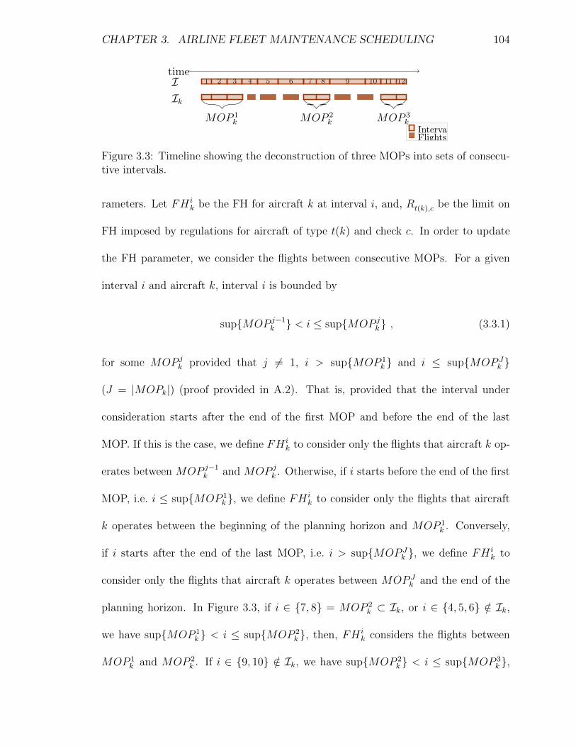
CHAPTER 3. AIRLINE FLEET MAINTENANCE SCHEDULING 104
1 2 3 4 5 6 7 8 9 10 11 12timeIIk
MOP 1k MOP 2
k MOP 3k
IntervalsFlights
Figure 3.3: Timeline showing the deconstruction of three MOPs into sets of consecu-tive intervals.
rameters. Let FH ik be the FH for aircraft k at interval i, and, Rt(k),c be the limit on
FH imposed by regulations for aircraft of type t(k) and check c. In order to update
the FH parameter, we consider the flights between consecutive MOPs. For a given
interval i and aircraft k, interval i is bounded by
sup{MOP j−1k } < i ≤ sup{MOP j
k} , (3.3.1)
for some MOP jk provided that j 6= 1, i > sup{MOP 1
k } and i ≤ sup{MOP Jk }
(J = |MOPk|) (proof provided in A.2). That is, provided that the interval under
consideration starts after the end of the first MOP and before the end of the last
MOP. If this is the case, we define FH ik to consider only the flights that aircraft k op-
erates between MOP j−1k and MOP j
k . Otherwise, if i starts before the end of the first
MOP, i.e. i ≤ sup{MOP 1k }, we define FH i
k to consider only the flights that aircraft
k operates between the beginning of the planning horizon and MOP 1k . Conversely,
if i starts after the end of the last MOP, i.e. i > sup{MOP Jk }, we define FH i
k to
consider only the flights that aircraft k operates between MOP Jk and the end of the
planning horizon. In Figure 3.3, if i ∈ {7, 8} = MOP 2k ⊂ Ik, or i ∈ {4, 5, 6} /∈ Ik,
we have sup{MOP 1k } < i ≤ sup{MOP 2
k }, then, FH ik considers the flights between
MOP 1k and MOP 2
k . If i ∈ {9, 10} /∈ Ik, we have sup{MOP 2k } < i ≤ sup{MOP 3
k },

CHAPTER 3. AIRLINE FLEET MAINTENANCE SCHEDULING 105
then, FH ik considers the flights between MOP 2
k and MOP 3k .
Using the previous two parameters, we can define the deterioration that a certain
number of FH incurs on an aircraft for a specific check type. For an interval i, check
c and aircraft k, the deterioration parameter is defined as,
DRikc =
FH ik
Rt(k),c
. (3.3.2)
In the next subsection, we provide the notation needed to describe the proposed
mathematical model. However, it is useful to discuss two of the variables in detail. To
account for the legal remaining FH, we define a variable, wikc ∈ [0, 1], that tracks the
MR at the beginning of interval i, for check type c and aircraft k. Where a value close
to 0 represents that no maintenance is required, and a value close to 1 represents that
maintenance is urgently required. This variable is updated by using the deterioration
parameter DRikc. We define a binary variable to identify regulation violations, vikc
gets the value 1 if the regulation for check c is violated at interval i by aircraft k,
while it is 0 otherwise.
Definitions
Sets
C: Set of checks indexed by c;
I: Set of intervals indexed by i;
Ik: Set of intervals where aircraft k is available for maintenance, Ik ⊆ I;
K: Set of all aircraft indexed by k;

CHAPTER 3. AIRLINE FLEET MAINTENANCE SCHEDULING 106
Ki: Set of aircraft available for maintenance at interval i, Ki ⊆ K;
MOPk: Set of MOPs for aircraft k, indexed by j;
MOP jk : Set of intervals that constitute the j-th MOP for aircraft k, MOP j
k ⊆ Ik;
R: Set of resources indexed by r;
RW i: Set of resources available at the workshop of interval i, W i, RW i ⊆ R;
T : Set of aircraft types with t : K → T .
Parameters
brc: Demand of resource r to process check c;
DRikc: Deterioration (per flying hour) at interval i for check c and aircraft k;
∆t(k),c: Duration of check c for an aircraft of type t(k);
sti/eti: Start/end time of interval i ∈ I.
Variables
Bir: The capacity for resource r at interval i.
wikc: A continuous variable with values between 0 and 1 to represent the MR for
aircraft k for check c at the beginning of interval i. 0 means that the aircraft re-
quires no maintenance, 1 means that the aircraft requires maintenance urgently.
mikc: 1, if a maintenance check c for aircraft k starts/continues at the beginning of
interval i; 0, otherwise.

CHAPTER 3. AIRLINE FLEET MAINTENANCE SCHEDULING 107
vikc: 1, if regulation for check c is being violated at interval i for aircraft k; 0, otherwise.
zikc: 1, if there is a change between the consecutive variables, mikc and mi−1
kc ; 0, other-
wise.
Formulation
Model 3.3.1. Interval MMILP formulation for AMS with violations.
min∑k
∑c
∑i
vikc (3.3.3)
min∑k
∑c
wsup{Ik}kc (3.3.4)
Subject to
Maintenance Requirement
vikc = 0 ∀k, c, i /∈ Ik; (3.3.5)
mikc = 0 ∀k, c, i /∈ Ik; (3.3.6)
wikc ≥ wi−1kc +DRikc
(1−mi
kc
)−mi
kc − vikc ∀k, c, i 6= inf{I}; (3.3.7)
wsup{MOP j
k}kc ≤ DR
inf{MOP j+1k }
kc ∀k, c, j 6= |MOPk|; (3.3.8)
Maintenance∑c
mikc ≤ 1 ∀k, i ∈ Ik; (3.3.9)∑
i′∈MOP jk
(eti′ − sti′)mi′
kc ≥ ∆t(k),cmikc ∀k, c, j, i ∈MOP j
k ; (3.3.10)
Transitivity Constraints
zinf{MOP j
k}kc ≥ m
inf{MOP jk}
kc ∀k, c, j; (3.3.11)
zikc ≥ mikc −mi−1
kc ∀k, c, j; i, i− 1 ∈MOP jk ; (3.3.12)∑
i∈MOP jk
zikc ≤ 1 ∀k, c, j; (3.3.13)
Resources∑k∈Ki
∑c
brcmikc ≤ Bi
r ∀i, r ∈ RW i ; (3.3.14)
Variables
wikc ∈ [0, 1] ∀k, c, i; (3.3.15)
Bir ∈ R+ ∀k, i, r ∈ RW i ; (3.3.16)
mikc, z
ikc, v
ikc ∈ {0, 1} ∀k, c, i. (3.3.17)

CHAPTER 3. AIRLINE FLEET MAINTENANCE SCHEDULING 108
The proposed formulation is a MMILP with two lexicographically ordered objec-
tive functions. The functions involved minimise the following objectives (in order of
importance), the number of violations, and the total MR at the last interval. Objec-
tive 3.3.3 minimises the number of regulation violations. Objective 3.3.4 minimises
the total MR at the end of the planning horizon. Recall that a value close to 0 for
the wikc variable indicates that the aircraft requires no maintenance; hence, minimis-
ing wsup{Ik}kc corresponds to minimising the amount of maintenance required by each
individual aircraft at the end of the planning horizon.
The first two MR constraints 3.3.5 and 3.3.6 ensure that neither a violation nor
maintenance occur when an aircraft is operating flights. Precisely, constraints 3.3.5
and 3.3.6 ensure that if aircraft k is flying at interval i, i.e. i /∈ Ik, then, for any check
c, neither a violation nor maintenance intervention may occur.
Constraints 3.3.7 enforce a recurrence relation for the MR variable. For time
interval i, aircraft k, and check type c, we update the MR variable depending on
whether or not aircraft k is flying at interval i. If aircraft k is not flying at interval
i, i.e. i ∈ Ik and i ∈ MOP jk for some j; the current MR, wikc, is updated using
the previous MR, wi−1kc , plus the appropriate deterioration, DRikc (the deterioration
incurred by the flights between MOP j−1k and MOP j
k , as defined in equation 3.3.2),
or drops to 0 if either a violation or maintenance occur. Please recall that the first
priority objective minimises the number of violations. On the other hand, if aircraft
k is flying at interval i, i.e. i /∈ Ik, then, by constraints 3.3.5 and 3.3.6, mikc = 0 and
vikc = 0, hence, the recurrence relation is enforced.
Constraints 3.3.8 ensure that the MR variable at the end of a MOP stays within

CHAPTER 3. AIRLINE FLEET MAINTENANCE SCHEDULING 109
the regulation limits (captured within the deterioration parameter) at least until the
next MOP. That is, for a given aircraft k, check type c and MOP j (with j 6= |MOPk|),
the MR at the end of the MOP, wsup{MOP j
k}kc , should remain feasible to operate the
upcoming flights between MOP jk and MOP j+1
k . Using the definition of the deteri-
oration parameter, this is encapsulated in DRinf{MOP j+1
k }kc , since, by equation 3.3.1,
sup{MOP jk} < inf{MOP j+1
k } ≤ sup{MOP j+1k }.
Constraints 3.3.9 and 3.3.10 enforce the maintenance restrictions. Constraints
3.3.9 assure that no more than one maintenance type is scheduled for the same in-
terval. Constraints 3.3.10 guarantee that the aircraft is available for the minimum
time required for each maintenance type. More precisely, the sum of the duration of
consecutive intervals has to be greater than the minimum prespecified duration of the
check.
Transitivity constraints, 3.3.11, 3.3.12, and 3.3.13, ensure that if we decide to
maintain in MOP jk , preemptions are not allowed (proof provided in A.2). Constraints
3.3.11 initialise the auxiliary variable using the first interval in the MOP. Constraints
3.3.12 establish that when a maintenance starts, i.e. the difference between consecutive
maintenance variables is 1, the auxiliary variable is 1. Constraints 3.3.13 ensure that
at most one auxiliary variable is 1, or, equivalently we cannot start a maintenance
more than once. Hence, wherever we terminate maintenance, all auxiliary variables
thereafter must be 0.
Constraints 3.3.14 ensure that a maintenance intervention of some type is only
scheduled if there are sufficient resources available at the workshop. The total number
of checks over all aircraft present at a given interval cannot exceed the capacity for

CHAPTER 3. AIRLINE FLEET MAINTENANCE SCHEDULING 110
each resource. The last four constraints 3.3.15 – 3.3.17 define the domains of the
variables.
3.3.4 Airline Fleet Maintenance Scheduling with Tail Assign-ment
In this section we extend the AMS formulation previously discussed, to include reas-
signment variables for the periods where regulations are being violated. In order to
determine where this occurs, we solve Model 3.3.1, and identify which violation vari-
ables, vikc, have the value 1. Using this information we efficiently select reassignable
and preassigned flights which allow us to solve the joint AMS and TA problem.
Notation
To formulate the AMS with TA, we first expand the notation introduced for Model
3.3.1. All flights are contained in the set F , which we can index with f . More
precisely, it contains flight legs (sequence of multiple flights) between MOPs. Also,
let If be the subset of intervals at which flight f ∈ F occurs, and Kf be the subset
of aircraft free to operate flight f .
Additionally, for a given interval i, we can identify the set of flights that either,
depart at the end of interval i, or, arrive at the start of interval i. Let us denote the
departure set with
F idep = {f : f ∈ F , inf{If} = i} ,
and, the arrival set with
F iarr = {f : f ∈ F , sup{If} = i} .

CHAPTER 3. AIRLINE FLEET MAINTENANCE SCHEDULING 111
In order to control the number of reassignment variables, we can identify the
subsets of flights which are reassignable and those which are fixed or preassigned.
Such that, if a flight is reassignable, then we can reassign it to another aircraft; in
contrast, if a flight is preassigned, then it is operated by the preassigned aircraft. Let
FR ⊂ F and FR ⊂ F be two (disjoint) subsets (with FR ∪ FR = F), that contain
those flights which are reassignable and preassigned, respectively. Also, let Of for
flight f ∈ FR, with Of ⊆ Kf , contain the aircraft preassigned to flight f . To preserve
efficiency and minimise the changes in the airlines’ preferred TA, instead of setting
all flights to be reassignable, we select an appropriate subset of flights. More details
on the selection process can be found in Section 3.4.2.
We can redefine the deterioration parameter in terms of flights, DRfkc, which repre-
sents the deterioration for the operation of flight f for check c and aircraft k. Similarly,
as for the previous model,
DRfkc =
FHf
Rt(k),c
,
where FHf are the FH that correspond to flight f . Lastly, the violation variable
can also be expressed in terms of flights, vfkc gets the value 1 if a regulation is being
violated before flight f for aircraft k and check c, while it is 0 otherwise.
Definitions
Sets
F : Set of all flights indexed by f ;
FR: Set of reassignable flights, FR ⊂ F ;
FR: Set of preassigned flights, FR ⊂ F ;
CHAPTER 3. AIRLINE FLEET MAINTENANCE SCHEDULING 112
F idep: Set of flights which are scheduled to depart at the end of interval i;
F iarr: Set of flights which are scheduled to arrive at the start of interval i;
If : Set of intervals occupied by flight f , If ⊆ I;
Kf : Set of aircraft available to operate flight f , Kf ⊆ K;
Of : Set of aircraft preassigned to operate flight f ∈ FR, Of ⊆ Kf .
Parameters
DRfkc: Deterioration for the operation of flight f for check c and aircraft k.
Variables
afk: 1, if the flight f is (re)assigned to aircraft k; 0, otherwise.
Br: The maximum capacity for resource r.
vfkc: 1, if the regulation for check c is being violated before flight f for aircraft k; 0,
otherwise.

CHAPTER 3. AIRLINE FLEET MAINTENANCE SCHEDULING 113
Formulation
Model 3.3.2. Interval MMILP formulation for AMS with TA.
min∑f
∑k∈Kf
∑c
vfkc (3.3.18)
min∑r
Br (3.3.19)
min∑f
∑k∈Kf\Of
afk (3.3.20)
min∑k
∑c
∑i
(eti − sti
)mikc (3.3.21)
min∑i
∑r
(eti − sti
)Bir (3.3.22)
min∑k
∑c
wsup{Ik}kc (3.3.23)
Subject to
Preassigned Flights
afk = 1 ∀f ∈ FR, k ∈ Of ; (3.3.24)∑c
vfkc = 0 ∀f ∈ FR, k ∈ Of ; (3.3.25)
Maintenance Requirement
wikc ≥ wi−1kc +∑
f∈Fiarr
(DRf
kcafk − v
fkc
)−mi
kc ∀k, c, i 6= inf{I}; (3.3.26)
wsup{MOP j
k}kc ≤
∑f∈F
sup{MOPjk}
dep
DRfkca
fk ∀k, c, j; (3.3.27)
Reassignment
mi+1kc ≤ 1−
∑f∈Fi
dep
afk ∀k, c, i 6= sup{I}; (3.3.28)
∑k
afk = 1 ∀f ; (3.3.29)
Maintenance
Constraints 3.3.6, 3.3.9 and 3.3.10
Transitivity Constraints
Constraints 3.3.11− 3.3.13
Resources
Constraints 3.3.14
Bir ≤ Br ∀i, r ∈ RW i ; (3.3.30)
(3.3.31)

CHAPTER 3. AIRLINE FLEET MAINTENANCE SCHEDULING 114
Variables
afk ∈ {0, 1} ∀k, f ; (3.3.32)
vfkc ∈ {0, 1} ∀k, c, f ; (3.3.33)
Br ∈ R+ ∀r (3.3.34)
Constraints 3.3.15− 3.3.17
The proposed formulation is a MMILP with six lexicographically ordered objective
functions. The functions involved minimise the following objectives (in the order of
importance), the number of violations, maximum resource level, number of reassigned
flights, number of maintenance interventions, overall resource usage, and total MR.
Objective 3.3.18, with largest priority, minimises the number of regulation violations.
Objective 3.3.19 minimises the sum of maximum level for each resource. Objective
3.3.20 minimises the number of strictly reassigned flights (i.e. assigned to an aircraft
different from the one in the input TA), thus minimising the number of changes in
the airlines’ preferred TA. Objective 3.3.21 minimises the number of maintenance
interventions weighted with the duration of intervals. Objective 3.3.22 minimises the
resource level per interval, again, weighted with the duration of intervals. Finally, as
in the previous model, with least priority, objective 3.3.23, minimises the total MR
at the last interval.
Constraints 3.3.24 ensure that if flight f is preassigned to aircraft k ∈ Of , then
afk = 1. Similarly, constraints 3.3.25 ensure that if flight f is preassigned to aircraft
k ∈ Of , then a violation cannot occur vfkc = 0 for any check c.
The MR constraints are a simple extension of those in Model 3.3.1. Constraints
3.3.26 enforce a recurrence relation where the current MR, wikc, is updated using the

CHAPTER 3. AIRLINE FLEET MAINTENANCE SCHEDULING 115
previous MR, wi−1kc , plus a deterioration term if the aircraft has been assigned the
flights prior to the interval under consideration, or drops to 0 if either a violation or
maintenance occurs. In the case when flight f is reassignable, i.e. f ∈ FR, and if
flight f is not reassigned to aircraft k, afk = 0, then, the MR is only updated if a
violation or maintenance occurs. On the other hand, in the case of either, flight f
being reassigned to aircraft k, or, flight f being preassigned to aircraft k (f ∈ FR
and k ∈ Of ), we have, afk = 1. Thus, by constraints 3.3.25 and 3.3.28, vfkc = 0 and
mikc = 0, thus, the MR is deteriorated according to the appropriate deterioration,
DRfkc. Therefore, the recurrence relation is enforced.
Constraints 3.3.27 ensure that the MR remains feasible for the operation of any of
the flights that depart the end of interval i. That is, for a given aircraft k, check type
c and MOP j, the MR at the end of the MOP, wsup{MOP j
k}kc , should remain feasible to
operate whichever flights are assigned to aircraft k departing at the end of the MOP.
Such flights are contained in F sup{MOP jk}
dep .
As for the reassignment, constraints 3.3.28 ensures that maintenance is not per-
formed if an aircraft departs. More specifically, if an aircraft k is reassigned and due
to depart on a flight after interval i 6= sup{I}, then, at interval i+1 (after the aircraft
has departed) maintenance cannot be performed, hence, mi+1kc = 0. Constraints 3.3.29
ensure that all flights have exactly one aircraft assigned to them.
Constraints 3.3.30 establish the value for the maximum resource level for each
resource. The remaining constraints, (maintenance, transitivity and resource con-
straints) as well as variable definitions, can be borrowed from Model 3.3.1. The last
constraints 3.3.32–3.3.34, define the domains of the extra variables.

CHAPTER 3. AIRLINE FLEET MAINTENANCE SCHEDULING 116
3.4 Solution Methodology
The solution approach chosen only requires flight schedules, and resource capacities
and demands for maintenance services. To improve the efficiency of the solutions,
after a preprocessing routine, we implement an iterative algorithm. The algorithm is
displayed in Figure 3.4 and pseudocode presented in Algorithm 4. The algorithm con-
sists of two stages, conflicting period selection and interval splitting. The conflicting
period selection stage involves selecting the sets of reassignable and preassigned flights
and resolving. This stage terminates when all the violations are removed or when the
size of the conflicting periods cannot be increased any further. During subsequent
iterations, the interval splitting stage identifies intervals where maintenance occurs,
splits them and resolves the problem. Splitting time intervals allows the model to
assign more maintenance to the existing schedule since it makes time intervals more
granular.
3.4.1 Preprocessing Routine
Flight schedules are crucial for the model as they give the initial tail assignment (TA)
and accurate flying hours (FH) in order to update the maintenance requirement (MR)
throughout the planning horizon. We obtained flight schedules from Flightradar24 AB
(2018) using pyflightdata, the Python module (Allamraju, 2014). We gathered data
globally for an extended period. Following the data gathering stage, we preprocess
the flight schedule data. Preprocessing involves filtering schedules through the nearest
airport to the maintenance workshops under consideration. After this, we identify
airlines and aircraft types of interest so we can track and update the aircraft’s FH

CHAPTER 3. AIRLINE FLEET MAINTENANCE SCHEDULING 117
appropriately. This gives a reduced network with accurate FH for each aircraft. For
eight maintenance workshops over a 30-day planning horizon (between dates 14/11/16
and 15/12/16), prior to preprocessing, we have 23927 flights and 1643 aircraft of two
types (Airbus A320 and Fokker 100). Then, we proceed to identify maintenance
opportunities (MOPs) i.e. turnaround times sufficient to perform at least the shortest
maintenance type. We choose a turnaround time of at least 5 hours to allow for at
least a short maintenance intervention. Using aircraft MOPs, we generate intervals
by identifying all start and end times of the MOPs and storing them in an ordered
set.
PreprocessingRoutine
INPUTDATA
SolveModel 3.3.1
FeasibleMaintenance
Schedule?
SolveModel 3.3.2
ConflictingPeriod Selection
GoodResource
Allocation?
IntervalSplitting
STOPProposedSchedule
NOYES
YES
NO
Figure 3.4: Flow chart outlining the process of the iterative algorithm.
As part of this stage, we pre-determine which variables are not required in the

CHAPTER 3. AIRLINE FLEET MAINTENANCE SCHEDULING 118
model, hence, for efficiency, they are not created. Specifically, all the variables involved
in constraints 3.3.5 and 3.3.6 in Model 3.3.1, and constraints 3.3.24, 3.3.25, and 3.3.28
in Model 3.3.2, have known values and it is unnecessary to create them. Therefore,
in practice, since the reassignment variables that involve preassigned flights are not
present in Model 3.3.2, when MR constraints involve preassigned flights, we simply
use MR constraints from Model 3.3.1. For this reason, the number of reassignment
variables is determined by selecting the sets of reassignable and preassigned flights.
3.4.2 Solution Procedure
To ensure efficiency and solution accuracy, we propose an iterative solution procedure
which has two stages, conflicting period selection, and interval splitting. The aim of
the conflicting period selection stage is to, by using the identification of regulation
violations, select the number of reassignment variables. In each iteration, if the regula-
tion violations involved have not been removed, we increase the size of the conflicting
period (which determines the number of reassignment variables) and resolve Model
3.3.2. In the interval splitting stage, once all infeasibilites have been removed or all
reassignment variables have been introduced, we split intervals where maintenance
takes place and resolve Model 3.3.2. This ensures flexibility as it allows the additional
generated intervals to be allocated to different aircraft.
Conflicting Period Selection
An illustration of the conflicting period selection stage is given in Figure 3.5. For
a certain violation, say at interval i, with {k1, k2, k3, . . . , kK} ∈ Ki, we select the

CHAPTER 3. AIRLINE FLEET MAINTENANCE SCHEDULING 119
initial conflicting period as shown in red with j i(1) as the upper bound, as the next
interval where Ki ⊆ Kji
(1) . We classify flights either in the reassignable subset (FR),
if they are involved in the conflict, or in the preassigned subset (FR), otherwise. This
regulates the number of reassignment variables, and keeps the solution process of
Model 3.3.2 efficient. If in the new solution, interval i still has a violation, we increase
the size of the conflicting period to reach j i(2), the next interval where Ki ⊆ Kj
i(2) .
Again, we update the sets of reassignable and preassigned flights and resolve the
problem. If the violation has not been removed, we move on to the next interval
with matching aircraft. We continue this process until the violation is removed or the
end of the planning horizon is reached, in which case, all the reassignment variables,
corresponding to violation i, would have been introduced.
i
k1k2k3...
kK
violation j i(1) j i
(2)
conflicting period 2
confl
ictin
gpe
riod
1
. . .
endofplanninghorizo
n
Figure 3.5: Conflicting period selection.
In order to identify the conflicting period, we have to identify where violations
occur. For the first iteration, the set V that contain all intervals for which at least
one violation occurs is given by,
V =
{i : i ∈ I,
∑k
∑c
vikc ≥ 1
},
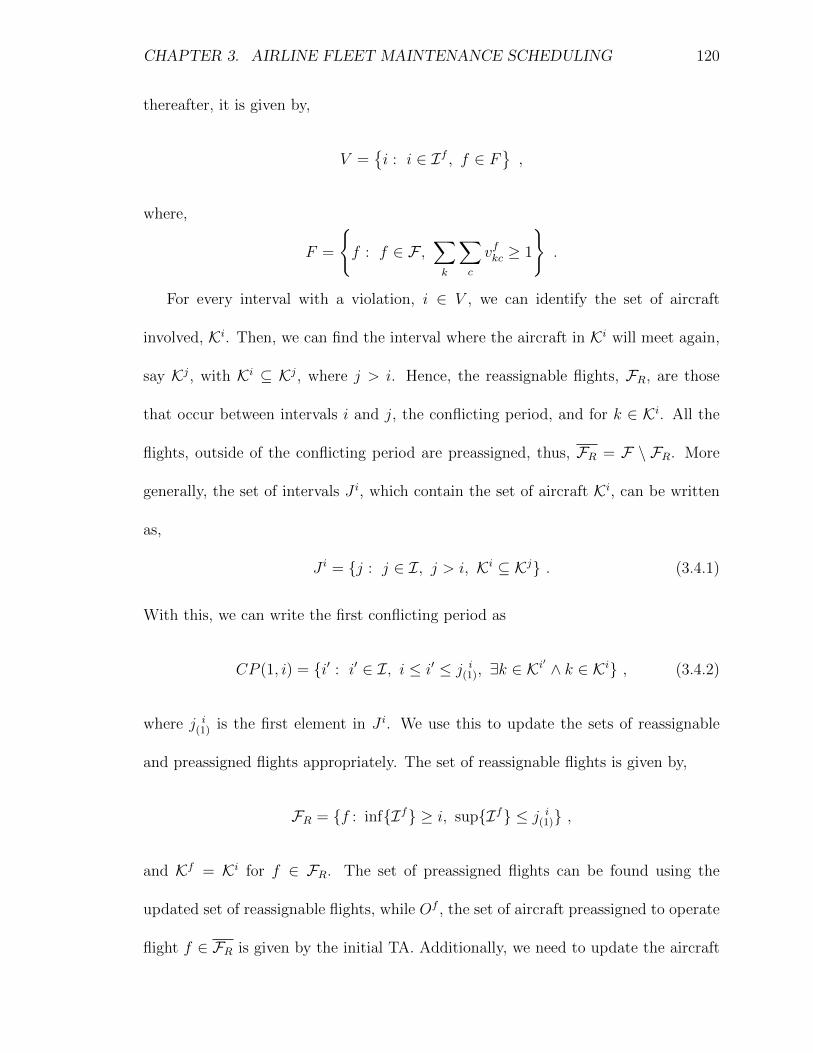
CHAPTER 3. AIRLINE FLEET MAINTENANCE SCHEDULING 120
thereafter, it is given by,
V ={i : i ∈ If , f ∈ F
},
where,
F =
{f : f ∈ F ,
∑k
∑c
vfkc ≥ 1
}.
For every interval with a violation, i ∈ V , we can identify the set of aircraft
involved, Ki. Then, we can find the interval where the aircraft in Ki will meet again,
say Kj, with Ki ⊆ Kj, where j > i. Hence, the reassignable flights, FR, are those
that occur between intervals i and j, the conflicting period, and for k ∈ Ki. All the
flights, outside of the conflicting period are preassigned, thus, FR = F \ FR. More
generally, the set of intervals J i, which contain the set of aircraft Ki, can be written
as,
J i = {j : j ∈ I, j > i, Ki ⊆ Kj} . (3.4.1)
With this, we can write the first conflicting period as
CP (1, i) = {i′ : i′ ∈ I, i ≤ i′ ≤ j i(1), ∃k ∈ Ki
′ ∧ k ∈ Ki} , (3.4.2)
where j i(1) is the first element in J i. We use this to update the sets of reassignable
and preassigned flights appropriately. The set of reassignable flights is given by,
FR = {f : inf{If} ≥ i, sup{If} ≤ j i(1)} ,
and Kf = Ki for f ∈ FR. The set of preassigned flights can be found using the
updated set of reassignable flights, while Of , the set of aircraft preassigned to operate
flight f ∈ FR is given by the initial TA. Additionally, we need to update the aircraft

CHAPTER 3. AIRLINE FLEET MAINTENANCE SCHEDULING 121
present at the intervals in the conflicting period. Thus, we set
Ki′ = Ki′ ∪ Ki for i′ ∈ CP (1, i) .
By solving Model 3.3.2 after these updates, we can reassign the flights to any of the
aircraft involved in the conflict. In the next iterations, if the violation is removed, then
without loss of generality, we may assume that the remaining schedule can remain
unchanged. However, if solving Model 3.3.2 has not led to the elimination of the
violation, we expand the conflicting period and resolve. For this, we use CP (m, i),
for m = 2, . . . , |J i|, which uses the m-th element of J i, j i(m). Similarly, to update the
set of reassignable flights, we set,
FR = {f : inf{If} ≥ i, sup{If} ≤ j i(m)} ,
with, Kf = Ki for f ∈ FR, and,
Ki′ = Ki′ ∪ Ki for i′ ∈ CP (m, i) .
With the set of preassigned flights and aircraft being updated as previously, using the
new set of reassignable flights. We do this for every interval with a violation i ∈ V ,
until either the violation is eliminated or the end of the planning horizon is reached.
Interval Splitting
The interval splitting stage favours the redistribution of resources by using a more
granular timeline with each iteration. Resources are occupied for the duration of the
interval if maintenance is being performed. When long intervals occur, given the non-
preemption assumption, resources can be held even after the maintenance has been

CHAPTER 3. AIRLINE FLEET MAINTENANCE SCHEDULING 122
finalised (exceeding the minimum maintenance duration). Therefore, we consider the
effect of splitting intervals, using different criteria, and resolving the problem. For
example, in Figure 3.6, given the intervals, in the first iteration we have a MOP of 9
hours. Suppose that the maintenance scheduled for this MOP only takes 8 hours. So,
in the first iteration, the last hour of the last interval is being wastefully allocated.
Splitting, therefore, allows for the resources to be allocated to different aircraft. By
splitting in half, in iteration 3, we see that the last hour is no longer being held.
3h 2h 4h
iteration
1
2
3
MOP
Figure 3.6: Interval splitting stage for a 9 hour MOP using binary segmentation forthree iterations.
Let us define three simple splitting methods. Suppose, after solving the problem,
we have mikc = 1, so we split interval i using the following,
1. Binary segmentation (split in half);
2. Golden ratio (split by Golden ratio);
3. Minimum cut (split that allows at least the shortest type of maintenance).
Methods 1 and 2 are well-known and are regularly employed in search algorithms
(Nocedal and Wright, 2006). Method 3 splits intervals that allows the shortest type
of maintenance. Going back to the example in Figure 3.6, recall that the duration of
the maintenance is 8 hours, splitting using Method 3 would produce a single split at
the 8th hour in the second iteration.

CHAPTER 3. AIRLINE FLEET MAINTENANCE SCHEDULING 123
To compare the splitting methods and identify good solutions, we compute an
accuracy measure representing the usage of MOPs. The accuracy measure can be
expressed as the ratio of the minimum time required for a check over the actual time
scheduled for the check. That is,
A =
∑c
∑k
∑j ∆t(k),c∑
c
∑k
∑j
∑i∈MOP j
k(eti − sti)mi
kc
. (3.4.3)
Given constraints 3.3.10, which specify that maintenance scheduled should be at least
of the minimum required duration; we have that A ≤ 1. Therefore, a schedule that
has an accuracy value close to 1, is one that does not schedule more maintenance than
strictly required, and is, thus, efficient.
Algorithm
As outlined in Figure 3.4 and in the pseudocode of Algorithm 4, the algorithm requires
some inputs. Specifically, a set of intervals, set of aircraft, FH for each aircraft,
maintenance regulations and durations, and, resource capacities and demands. Once
these are provided, in the first iteration, Model 3.3.1 is solved. If there are violations;
i.e. there is no feasible maintenance schedule or, equivalently, V 6= ∅; we implement
the conflicting period selection stage and resolve Model 3.3.2 until the violations have
been removed. After this, we iterate the interval splitting stage and resolve Model
3.3.2 until either, the resource allocation is good enough, equivalently, A ≥ 1 − ε
(where ε is the tolerance), or, no more intervals are added.

CHAPTER 3. AIRLINE FLEET MAINTENANCE SCHEDULING 124
Algorithm 4 Solution procedure with conflicting period selection and interval split-ting.
1: Initialisations iter, A = 0 . Iteration counter and accuracy measure2: ε = 0.01 . Set Tolerance3: maxiter = 50 . Maximum number of iterations4: Intervals = I . Interval set5: V, CP, oldIntervals = [ ]6: while iter < maxiter and A < 1− ε do7: if iter = 0 then8: Solve Model 3.3.1 . For the first iteration9: else
10: Solve Model 3.3.2 . For iterations ≥ 111: end if12: Update V and A13: if V is not empty then . If violations have not been removed14: SelectCP(V ) . Call function to update conflicting periods15: else16: which = {i : i ∈ I,
∑k
∑cm
ikc ≥ 1}
17: oldIntervals = Intervals
18: SplitIntervals(which, Intervals) . Call function to split intervals19: if |Intervals| = |oldIntervals| then . No intervals have been added20: Break . Stop the algorithm21: end if22: end if23: Increment iter24: end while25: function SelectCP(V ) . Updates the conflicting periods for all violations26: for i in V do27: Compute J i
28: if i not in CP then . If the violation is new29: CP = CP ∪ CP(1,i) . Update CP with first conflicting period30: else . If violation has occurred at a previous iteration31: for m in 2→ |J i| do . Iterate through elements in Ji32: if CP(m-1,i) in CP then . Find already used CP
33: CP = CP \ CP(m-1,i) . Remove it from conflicting periods34: CP = CP ∪ CP(m,i)
35: Break36: end if37: end for38: end if39: end for40: Intervals = Intervals ∪ CP . Update intervals41: end function42: function SplitIntervals(which, Intervals) . Splits intervals in which
43: for i in which do44: Using Method 1, 2, or 3; split i into i1 and i245: Intervals= Intervals\{i} ∪ {i1, i2} . Update Intervals
46: end for47: end function

CHAPTER 3. AIRLINE FLEET MAINTENANCE SCHEDULING 125
3.5 Model Application and Computational Tests
We tested the iterative algorithm using flight schedules obtained for the maintenance
workshops under consideration over the 30-day period selected. The results shown in
this section use preprocessed flight data between dates 14/11/16 and 15/12/16 (see
Section 3.4.1 for more information on the data gathering and preprocessing). The
iterative algorithm was written in Python, using Gurobi Optimization version 8.1
(2019) to solve the models. Two computational studies are presented, one for the
single workshop case (five workshops treated independently) and one for the multi-
workshop case (up to eight workshops treated simultaneously).
As for the experimental set-up, we restrict the interval splitting stage of the al-
gorithm such that the resulting intervals are at least 5 seconds long. Solution times
for each iteration are limited to 500 seconds for each objective. The parameters used
for the computational tests include the standard duration and frequencies for the reg-
ulated medium-term maintenance checks, as mentioned in Section 3.1. Specifically,
according to Table 3.1, for the two types of aircraft under consideration, the values of
regulation parameter, Rt(k),c, is given in Table 3.3. Here, we see the type of aircraft
(Airbus A320 and Fokker 100), check type (c = 1 or 2) and the corresponding main-
tenance regulation parameter values, Rt(k),c. Using these values, c = 1 corresponds
to an A check and c = 2 corresponds to a C check. Resource demand and capacities,
shown in Table 3.4, vary for four different types of renewable resources. A realistic
interpretation of resources is as follows, r1 – number of hangar bays, r2 – certified
technicians, r3, r4 – different types of specialised tools. The value for the tolerance, ε,

CHAPTER 3. AIRLINE FLEET MAINTENANCE SCHEDULING 126
which determines the required accuracy level as A ≥ 1−ε, is set to be 0.01. The initial
maintenance requirement (MR) variable is sampled from a Uniform distribution as
follows,
winf{Ik}kc ∼ Unif(0, 0.3) ∀k, c.
Sensitivity analysis around the chosen value produces distinct maintenance schedules
and resource profiles but does not affect the computational performance of the algo-
rithm. For instance, higher values lead to more maintenance being scheduled towards
the start of the planning horizon; conversely, lower values lead to more maintenance
being scheduled towards the end of the planning horizon.
Table 3.3: Maintenance regulation parameter values for two check types (1 and 2)and two aircraft types (A320 and F100).
t(k) c = 1 c = 2
Airbus A320 Rt(k),c =600FH Rt(k),c =6000FH
Fokker 100 Rt(k),c =500FH Rt(k),c =5000FH
Table 3.4: Sample resource demands and limit capacities for four types of resources(ri for i = 1, 2, 3, 4) and two maintenance types (1 and 2).
r br1 br2 Bir
r1 1 1 25r2 3 5 25r3 2 3 25r4 1 2 25
In addition, the formulations are solved using lexicographic ordered objectives
with priorities as suggested by airline practitioners. In the order of importance, the
objectives which are minimised, namely,
1. the number of violations (objective 3.3.18),

CHAPTER 3. AIRLINE FLEET MAINTENANCE SCHEDULING 127
2. the maximum resource level (objective 3.3.19),
3. the number of strictly reassigned flights (objective 3.3.20),
4. the weighted number of maintenance interventions (objective 3.3.21),
5. the weighted overall resource usage (objective 3.3.22),
6. the total MR at the end of the planning horizon (objective 3.3.23).
Given that we are seeking for a maintenance feasible schedule, assigning the number
of violations, in any but the highest priority level leads to infeasible maintenance
schedules. Apart from this, as tests revealed, the order of the other objectives does
not affect the integrity of the solutions or the computational times.
3.5.1 Single Workshop Case
In the case when maintenance workshops can be treated independently, we can solve
the problem for each workshop individually. This situation can occur, for example,
due to the geographical location of the workshops or upon a particular airlines’ request
or restrictions. In this case, we implement the algorithm in parallel for each mainte-
nance workshop under consideration. It is worth noting that due to the preprocessing
routine, which leads to considering only flights with large turnaround times and just
two specific aircraft types, the number of flights and aircraft are significantly reduced
compared those seen in ordinary operations; for more information see Section 3.4.1.
The details for the five workshops, are as follows,

CHAPTER 3. AIRLINE FLEET MAINTENANCE SCHEDULING 128
Atlanta Hartsfield-Jackson International Airport: with 1048 flights and 115
aircraft, produces 389 intervals;
Bangkok Suvarnabhumi Airport: with 3869 flights and 49 aircraft, produces 843
intervals;
Cairo International Airport: with 781 flights and 34 aircraft, produces 279 inter-
vals;
Dubai International Airport: with 223 flights and 11 aircraft, produces 63 inter-
vals;
Tokyo Haneda International Airport: with 978 flights and 10 aircraft, produces
162 intervals.
In all cases under consideration, after a single iteration of the conflicting period
selection stage, violations are removed and the interval splitting stage begins. In order
to compare the three splitting methods, we study four different aspects, namely, the
final number of intervals, total run times, accuracy measure, and objective function
value. Table 3.5 breaks down the objective function for the largest workshop, while
the results for the workshops under consideration are shown in Table 3.6. Specifically,
Table 3.6 shows the accuracy measure plots per iteration, final number of intervals,
and total run times. In the accuracy measure plots, as shown in the legend, Method
1 is represented with solid lines, Method 2 with dashed lines, and Method 3 with
dot-dashed lines.
The trend with the number of intervals per iteration is increasing for all methods,

CHAPTER 3. AIRLINE FLEET MAINTENANCE SCHEDULING 129
which is expected. The final number of intervals, as shown in Table 3.6 , is the number
of intervals at the last iteration. Method 3 offers the least final number of intervals
throughout, which is reflected in its solution times. Method 1 reveals a higher number
of intervals than Method 2.
The run times for the largest workshop, Bangkok, using Method 3 takes 72 minutes
to terminate the algorithm. For the remaining, small to medium-sized workshops, it
takes between 0.36 seconds to 4 minutes to reach a good solution. Computational
times for Method 1 and Method 2 (both significantly larger than Method 3) with the
latter showing lower solution times.
The accuracy measure per iteration appears as a plot in the second column in
Table 3.6. As can be seen, the accuracy measure evolves differently depending on the
workshop. It takes a varying number of iterations across workshops for the algorithm
to terminate. In all cases, more clear for Atlanta and Dubai, the required level of
accuracy (0.99) is not reached; the algorithm terminates due to no more intervals
being created. For the cases of Tokyo and Dubai, using Method 3, terminates the
algorithm in very few iterations; whereas the rest take slightly more. Between Methods
1 and 2, both provide very similar quality solutions.
A breakdown of the different components of the objective function value for the
Bangkok workshop is given in Table 3.5. The table shows the different values for each
objective per iteration and for the corresponding splitting method. In each iteration,
the best method is shown in green. This is determined by comparing objectives
in decreasing order of priority until differing objectives are found, and one method
presents an objective value lower than the rest. Note that objectives 3.3.18 (number

CHAPTER 3. AIRLINE FLEET MAINTENANCE SCHEDULING 130
of violations) and 3.3.20 (number of reassigned flights) remain constant. Objectives
3.3.21 (weighted number of maintenance interventions) and 3.3.22 (weighted overall
resource usage) decrease, while objectives 3.3.19 (maximum resource level) and 3.3.23
(total MR at the end of the planning horizon) show some fluctuation. The decrease
in the fourth and fifth priority objectives is due to them being the only ones weighted
with the duration of the intervals, and, therefore, are the only ones that are decreasing
as the duration of maintenance interventions also decrease. The first iteration is the
starting point where no splitting has occurred, hence, objectives have the same values
throughout the three splitting methods. In the second iteration, Method 2 is better
than Method 3 as it presents the same first three priority objectives (Obj. 3.3.18 -
3.3.20) and a lower value in the fourth priority objective (Obj. 3.3.21). Iterations
thereafter show that Method 3 dominates with a lower second priority objective (Obj.
3.3.19). Additionally, Method 3 provides healthier fleet overall, as suggested by the
consistently lower value of objective 3.3.23.
Due to its good solution times, lowest objective values, and overall higher accuracy
measure we can claim that, for the single workshop case, the interval splitting stage
performs better using Method 3. Furthermore, it is worth noting that the aircraft
are, also, kept in a healthier state at the end of the planning horizon. For this reason,
we present more detailed results using Method 3 for the largest workshop (Bangkok).
Figure 3.7 shows two resource profiles (first and last iteration) for resource r1 at the
Bangkok workshop. From Figure 3.7a to Figure 3.7b, we see that the resource profiles
become considerably less populated and thinner. This means that the resource usage
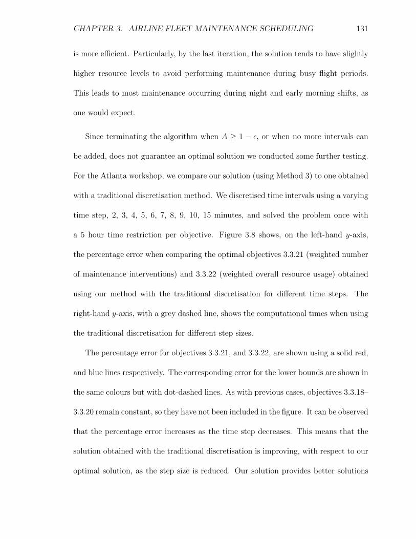
CHAPTER 3. AIRLINE FLEET MAINTENANCE SCHEDULING 131
is more efficient. Particularly, by the last iteration, the solution tends to have slightly
higher resource levels to avoid performing maintenance during busy flight periods.
This leads to most maintenance occurring during night and early morning shifts, as
one would expect.
Since terminating the algorithm when A ≥ 1 − ε, or when no more intervals can
be added, does not guarantee an optimal solution we conducted some further testing.
For the Atlanta workshop, we compare our solution (using Method 3) to one obtained
with a traditional discretisation method. We discretised time intervals using a varying
time step, 2, 3, 4, 5, 6, 7, 8, 9, 10, 15 minutes, and solved the problem once with
a 5 hour time restriction per objective. Figure 3.8 shows, on the left-hand y-axis,
the percentage error when comparing the optimal objectives 3.3.21 (weighted number
of maintenance interventions) and 3.3.22 (weighted overall resource usage) obtained
using our method with the traditional discretisation for different time steps. The
right-hand y-axis, with a grey dashed line, shows the computational times when using
the traditional discretisation for different step sizes.
The percentage error for objectives 3.3.21, and 3.3.22, are shown using a solid red,
and blue lines respectively. The corresponding error for the lower bounds are shown in
the same colours but with dot-dashed lines. As with previous cases, objectives 3.3.18–
3.3.20 remain constant, so they have not been included in the figure. It can be observed
that the percentage error increases as the time step decreases. This means that the
solution obtained with the traditional discretisation is improving, with respect to our
optimal solution, as the step size is reduced. Our solution provides better solutions

CHAPTER 3. AIRLINE FLEET MAINTENANCE SCHEDULING 132
for step sizes of 8 minutes and above (hence the negative percentage error values).
The optimal solution for a time step of 4 minutes (the smallest available as 2 and
3 minutes timed-out) shows only 0.6% improvement for both objectives. While for
the lower bounds for the smallest time step (2 minutes) show 6.6% improvement in
objective 3.3.21, and 8% in objective 3.3.22. Nevertheless, our solution gives a value
20% lower over all step sizes for the second priority objective (objective 3.3.19). Thus,
given the priority of the objectives, Method 3 dominates all the solutions studied
produced using traditional discretisation, thus, producing near optimal solutions.
The dashed line in Figure 3.8, plotted against the right-hand y-axis, reveals that
implementing a traditional time discretisation comes at a huge computational cost.
Specifically, the discretisation with the smallest time step (2 minutes) is around 188
times slower than our solution. The reason why our method is significantly more
efficient is because it only makes time intervals more granular when it is required and
where the solution is more sensitive.
Table 3.5: Objective function breakdown for the Bangkok workshop. The best methodin each iteration is highlighted in green.
Iteration Method / Obj.Obj.
3.3.18Obj.
3.3.19Obj.
3.3.20Obj.
3.3.21Obj.
3.3.22Obj.
3.3.231 Method 1 0 70 3 305 2184 54
Method 2 0 70 3 305 2184 54Method 3 0 70 3 305 2184 54
2 Method 1 0 70 3 216 1559 62Method 2 0 70 3 209 1509 52Method 3 0 70 3 210 1523 60
3 Method 1 0 77 3 179 1304 66Method 2 0 77 3 179 1303 60Method 3 0 70 3 173 1258 60
4 Method 1 0 77 3 169 1231 71Method 2 0 77 3 169 1234 101Method 3 0 70 3 169 1233 55

CHAPTER 3. AIRLINE FLEET MAINTENANCE SCHEDULING 133
Table 3.6: Comparison across 5 workshops during the interval splitting stage for thethree different splitting methods.
Table 6: Comparison across 5 workshops during the interval splitting stage for the three different splitting methods.
Station Accuracy Measure (per iteration) Features Splitting Methods
Atlanta
� � � �
����
����
����
����
����
�������� �������� ��������
Method 1 Method 2 Method 3
Final #intervals
3343 3187 551
Total CPUtime (min)
60 52 4
Bangkok
� � � �
����
����
����
���� Final #intervals 2713 2653 919
Total CPUtime (min) 105 95 72
Cairo
� � � � � � �
���
���
���
���
��� Final #intervals 3431 3117 349
Total CPUtime (min) 68 47 5.5
Dubai
� � � � �
���
���
���
���
��� Final #intervals 473 457 85
Total CPUtime (s) 6.6 4.4 0.36
Tokyo
� � � � � �
���
���
���
���
Final #intervals 845 771 189
Total CPUtime (min) 234 72 3.3
23

CHAPTER 3. AIRLINE FLEET MAINTENANCE SCHEDULING 134
15-11
17-11
19-11
21-11
23-11
25-11
27-11
29-11
01-12
03-12
05-12
07-12
09-12
11-12
13-12
Date
0
1
2
3
4
5
6
Resource Level
Resource profile at Bangkok for resource r1, iteration 1
Maximum
Mean
(a) Resource profile for the first iteration.
15-11
17-11
19-11
21-11
23-11
25-11
27-11
29-11
01-12
03-12
05-12
07-12
09-12
11-12
13-12
Date
0
1
2
3
4
5
6
Resource Level
Resource profile at Bangkok for resource r1, iteration 4
Maximum
Mean
(b) Resource profile for the last iteration.
Figure 3.7: Resource profiles for the Bangkok workshop for the first and last (4th)iterations of the interval splitting stage using Method 3.
234567891015Step Size (min)
−1.1−0.50.00.6
2.0
4.0
6.06.6
8.0
% Erro
r
Obj. 21Obj. 22
LB of Obj. 21LB of Obj. 22
CPU Time
100
200
300
400
500
600
700
CPU Time (m
in)
Figure 3.8: Result comparison (objectives 3.3.21, 3.3.22) for Method 3 vs traditionaldiscretisation for different time steps.

CHAPTER 3. AIRLINE FLEET MAINTENANCE SCHEDULING 135
3.5.2 Multi-workshop Case
To allow for interdependence between airlines and workshops, we consider several
multi-workshop cases. Here, the algorithm solves the problem for all the workshops
simultaneously. The first multi-workshop case considers four of the workshops used
in the single workshop case. Using Atlanta, Cairo, Dubai and Tokyo, we produce
a multi-workshop test set with 3002 flights and 167 aircraft, which produces 900
intervals. The interdependence for this case, due to their close proximity, is between
Cairo and Dubai.
After a single iteration of the conflicting period selection, all violations are re-
moved. Hence, the interval splitting stage begins. Table 3.7 shows, the intervals,
computational time and accuracy measure value for each of the splitting methods. In
each iteration, the best method is shown in green. As with the single workshop, this
is determined by comparing objectives in decreasing order of priority until differing
objectives are found, and one method presents an objective value lower than the rest.
To avoid repetition, these have not been included due to their resemblance with the
results in the single workshop case. The computational times reveal that Method 3
is the fastest (with a total of 1158 intervals and 9 minutes), followed by Method 2
(with a total of 4812 intervals and 58 minutes) and then Method 1 (with a total of
5020 intervals and 62 minutes). The highest accuracy measure, however, is no longer
associated with Method 3, but with Method 1.
Given that it shows lowest solution times and objective values, provides a health-
ier fleet, and exhibits an acceptable accuracy measure we suggest that, for the multi-

CHAPTER 3. AIRLINE FLEET MAINTENANCE SCHEDULING 136
Table 3.7: Method comparison for the 4-workshop case.
Iteration Method Intervals CPU time(s)
AccuracyMeasure
1 Method 1 900 59 0.72Method 2 900 57 0.72Method 3 900 61 0.72
2 Method 1 1384 610 0.86Method 2 1390 414 0.83Method 3 1076 123 0.84
3 Method 1 2556 1252 0.93Method 2 2586 1258 0.92Method 3 1134 148 0.90
4 Method 1 5020 1777 0.99Method 2 4812 1739 0.98Method 3 1158 200 0.94
workshop case, the interval splitting stage should be implemented using Method 3.
However, if more accuracy is sought, one can resort to Method 1 at the expense of
higher computational times. When compared with the average accuracy measure
obtained individually for the four workshops, Method 1 shows a 6% increase. This
suggests that modelling interdependence between workshops, or, inter-airline cooper-
ation, leads to more efficient allocation of resources.
Figure 3.10 shows the maintenance schedules produced using Method 3 for the four
workshops involved in the multi-workshop test set. The x-axis represents the date and
the y-axis shows each individual aircraft tail number. Hence, the plot shows when in
the planning horizon a specific aircraft is being served, which type of maintenance it
is receiving, and where the maintenance is taking place. Note that only one check 2
(c = 2 which corresponds to a C check) is scheduled in the busiest workshop, Atlanta,
on the first day (14/12). The rest of the maintenance shown are checks c = 1 which
correspond to A checks.

CHAPTER 3. AIRLINE FLEET MAINTENANCE SCHEDULING 137
4 5 6 7 8Number of Workshops
20
40
60
80
100
CPU
time (m
in)
Computational Time Comparison
1000
2000
3000
4000
5000
Numbe
r of Interva
ls
CPU Time (min)Number of Intervals
Figure 3.9: Computational comparison for Method 3 applied to different multi-workshop cases.
To study the scalability of the framework, four additional multi-workshop cases
were created. They include, a 5 workshop case with 6871 flights and 216 aircraft,
a 6 workshop case with 9681 flights and 260 aircraft, a 7 workshop case with 12402
flights and 429 aircraft, and, the largest, an 8 workshop case with 16000 flights and
529 aircraft. Additional to the five workshops considered in the single workshop case,
the 8 workshop case considers workshops based in Abu Dhabi International Airport,
Beijing Capital International Airport, and, Madrid Barajas Airport. These cases were
solved using Method 3 and until the algorithm was terminated; the least accuracy
level achieved was of 0.97. The resulting computational comparison, in Figure 3.9,
shows the computational times (red line on the left-hand y-axis) and final number of
intervals (grey dashed line on the right-hand y-axis) for the different multi-workshop
cases. The evolution of the CPU time and number of intervals seems to increase

CHAPTER 3. AIRLINE FLEET MAINTENANCE SCHEDULING 138
linearly with the number of workshops; the 8 multi-workshop case finalises with 5292
intervals and in 108 minutes. Therefore, it is possible that the framework is scalable
for larger data sets. Clearly, this depends on the size and number of flights introduced
each new workshop. Nonetheless, given the size of the largest instance considered, we
have managed to demonstrate the computational efficiency and the potential of this
framework.

CHAPTER 3. AIRLINE FLEET MAINTENANCE SCHEDULING 139
Air
craf
tT
ail
Num
ber
s
N206FRN207FRN667AWN324USN630NKN425UAN902NKN303FRN636NKN414UAN473UAN422UAN111USN646NKN663AWN675AWN656AWN629NKN616NKN219FRN235FRN202FRN125UWN230FRN661AWN104UWN102UWN203FRN619NKN434UAN201FRN651AWN218FRN232FRN220FRN316USN221FRN365NWN320USN655AWN119USN114UWN426UAN367NWN659AWN110UWN601NKN652AWN466UAN649AWN312USN228FRN122USN644NKN229FRN645NKN321USN449UAN642NKN643NKN338NWN638NKN452UAN123UWN668AWN372NWN904NKN660AWN326USN637NKN423UAN901NKN331NWN327NWN347NWN635NKN903NKN208FRN665AWN653AWN214FRN678AWN315USN647AWN462UAN657AWN109UWN374NWN127UWN369NWN485UAN318USN601AWN624NKN361NWN672AWN357NWN366NWN355NWN112USN454UAN359NWN464UAN358NWN333NWN117UWN627NKN345NWN620NKN490UAN622NKN341NWN639NKN650AWN628NK
Check 2
Atlanta
D-AIULD-AIUKD-AIUHD-AIUDD-AIUBD-AIUASU-GBFSU-BPVSU-BPUSU-GBGJY-AYR
SU-NMCSU-GBZD-AIZCD-AIZBD-AIZFD-AIZED-AIZJ
SU-GCAD-AIZMD-AIPCD-AIZZSU-BSNSU-GCBSU-BQJSU-BQKSU-BQMSU-GCDSU-TCFSU-BQCSU-NMASU-NMBJY-AYSJY-AYX
Cairo
A7-AHUA7-AHWAP-BLIEP-IEBVT-IFWJY-AYQJY-AYRJY-AYSJY-AYUJY-AYXAP-BLY
Dubai
13-11
15-11
17-11
19-11
21-11
23-11
25-11
27-11
29-11
01-12
03-12
05-12
07-12
09-12
11-12
13-12
15-12
Date
JA8997JA8654JA8609JA8946JA8947JA8400JA8396JA8300JA8313JA8304
Tokyo
Figure 3.10: Maintenance schedules produced by using Method 3 for each aircraft andworkshop in the first multi-workshop case.
CHAPTER 3. AIRLINE FLEET MAINTENANCE SCHEDULING 140
3.6 Conclusions
We have solved the airline fleet maintenance scheduling problem considering tail as-
signment. Previous studies that tackle a similar problem have modelled a short-term
planning horizon and tend to be computationally expensive even for moderately sized
data sets. By using aircraft individual legal remaining flying hours and our interval
based formulations, we tackle the problem while providing solutions in reasonable
time. We present two multi-objective mixed integer linear programming formulations
for this purpose. The first acts as a feasibility check for an input flight schedule and
provides an initial set of variables for the tail assignment. If a feasible maintenance
schedule was not found, the second formulation employs the location of the regulation
violations to formulate a combined maintenance and tail assignment problem. This
explores the different options across an aircraft journey and decides on the optimal
allocation of flights, maintenance and resources. Additionally, our approach accounts
for multiple resources and for generic types of maintenance.
In order to improve solutions, we implement a heuristic algorithm that consists of
two stages: conflicting period selection and interval splitting. The conflicting period
selection stage increases the size of the tail assignment problem gradually until we
are able to produce a feasible maintenance schedule. After this, the interval splitting
stage improves resource allocation.
Test results show that the algorithm is efficient, since it can solve large instances
in reasonable computational time, for a 30-day planning horizon and provides good
quality solutions. We solved a multi-workshop test case with 8 workshops, 16000
CHAPTER 3. AIRLINE FLEET MAINTENANCE SCHEDULING 141
flights and 429 aircraft in under 2h. Highlighting the importance of developing new
efficient formulations. Solutions present airlines with alternatives to their initial tail
assignment during the planning stage. These solutions focus on satisfying maintenance
regulations and keeping the aircraft healthy, while remaining commercially viable for
the airlines. Results promote inter-airline cooperation, which allows for workshop
resource sharing between airlines, since it provides a more efficient resource allocation
per workshop.
Some limitations are worth noting. Stopping the iterative algorithm when the
accuracy measure is maximal does not guarantee an optimal solution. Clearly, if con-
tinued indefinitely, the algorithm would reach the optimal solution, however, applying
the stopping criterion gives a good quality solution in reasonable time. We compared
the solution obtained using our method to the one obtained using a traditional dis-
cretisation with a small time step. This revealed that our solution is better and around
188 times faster, however, the theoretical proof remains to be done. Additionally, we
have not considered the complications that may arise from some of the long-term
maintenance types. In some cases, for example with life limited replacements, the
inclusion of inventory control for spares and those being fixed would be paramount.
Further work includes the implementation of a rolling horizon and the application of
clustering for maintenance workshops with intersecting flights.

Chapter 4
A Hybrid Solution Procedure for
the Aircraft Recovery Problem
with Operational Restrictions
4.1 Introduction
To encourage smooth running of airline operations, at the planning stage, airlines
aim to create a schedule that suits them while respecting operational constraints.
Even though, good pre-operational planning models exist, unplanned events often
occur, affecting these plans. Hence, re-planning around the disruptions is paramount
to resume ordinary operations (IATA, 2019). The airline recovery problem studies
this problem and provides strategies to solve it. One the components of the airline
recovery problem, at the operational stage, is the aircraft recovery (AR) problem.
Other stages include, schedule, crew and passenger recovery (Clausen et al., 2010).
142

CHAPTER 4. AIRCRAFT RECOVERY PROBLEM 143
Table 4.1: Flight range according to flight length (Eurocontrol, 2011).
Flight Range Aircraft Type Distance Time
Short-haul flight Turboprop/narrow-body ≤ 1500 km Under 3 hoursMedium-haul flight Narrow/wide-body ≥ 1500 and ≤ 4000 km 3 to 6 hours
Long-haul flight Wide-body ≥ 4000 km 6 to 12 hours
The AR problem deals with the re-assignment of aircraft to flights, or flight legs,
subject to operational restrictions, such that the cancelled and/or delayed flights are
minimised. Operational restrictions may include, aircraft, maintenance, crew, and
passenger disruption.
Aircraft types restrict the flights that certain aircraft are allowed to operate. There
are three main types of aircraft: turboprop, narrow-body, and wide-body. The main
difference among these is the passenger capacity and the flight range they operate.
For instance, a turboprop aircraft, used for regional flights, is unsuitable to oper-
ate medium-haul flights. Convention for the classification of flights is given by the
flight distance, or equivalently, the flight time. Flight range, and the link to aircraft
types, is summarised in Table 4.1 which specifies the restriction for each aircraft type.
Moreover, there are aircraft that operate mixed ranges, including: short/medium-
haul, medium/long-haul, short/long-haul, and short/medium/long-haul; the last two
are the rarest with a 0.2% and 0.9% of an international fleet (the sample included a
mixed fleet from 67 airlines between 2008 and 2009, Eurocontrol, 2011).
Maintenance requirements are covered by several civil aviation authorities which
provide a set of guidelines on how much an aircraft can be used between maintenance
operations. Typically, regulations impose four medium/long-term airframe checks
(A, B, C and D) and three long-term off-wing maintenance (engine, landing gear, and

CHAPTER 4. AIRCRAFT RECOVERY PROBLEM 144
auxiliary power unit). These have to be performed after a certain number of flying
hours, cycles, or months depending on the aircraft type (Cook and Tanner, 2008).
Crew restrictions are dominated by duty rules. Duty rules, as outlined by Barnhart
et al. (2003), rely on regulations that balance working and resting hours for crew.
Firstly, crew duty periods (shifts) must end at the respective crew-base airport. The
most important rules that crew duties must adhere to are, (1) the maximum duty
length (i.e. time away from the crew-base), and (2) the maximum consecutive duty
hours without breaks Barnhart et al. (2003); Maher (2015).
Passenger disruption restrictions are different for cancellations and delays. Under
EU law, passengers have the right to some reparation (care, re-routing, or compen-
sation) from airlines if certain thresholds are exceeded. As established by European
Parliament and Council of the European Union (2004), for delays, passengers have
the right to reparation if (i) their short-haul flight is delayed by two hours or more, (ii)
their medium/long-haul-haul flight within the EU, or their medium-haul flight outside
the EU, is delayed by three hours or more, or (iii) their flight, not falling under (i)
or (ii), i.e. other long-haul flights, is delayed by four hours or more. For cancellations
due to “extraordinary” circumstances, airlines are exempt from providing passengers
with reparation. Given that the disruptions considered for the AR problem are of this
type, passenger restrictions for cancellations are not considered.
In this paper, we develop a generic framework that solves the AR problem by
generating flight schedules that minimise flight cancellations and operational costs,
subject to a number of operational constraints. This is done by using a new hybrid

CHAPTER 4. AIRCRAFT RECOVERY PROBLEM 145
solution procedure with several components. We solve the AR problem using col-
umn generation. To generate columns, we model the subproblems using the shortest
path problem with resource constraints (SPPRC). Such resource constraints allow
us to model the different restrictions outlined above, namely, aircraft, maintenance,
crew and passenger delay, while keeping the algorithm computationally efficient. To
solve each SPPRC we use a reinforced learning hyper-heuristic which selects, out of
a set of metaheuristic algorithms, the most appropriate one to apply based on past
performance. In addition, once the metaheuristics stop generating columns with neg-
ative reduced cost, we employ an exact bidirectional labelling algorithm with dynamic
halfway point (Tilk et al., 2017) to guarantee optimal solutions for the LP relaxation
of the AR problem.
The remainder of this paper is organised as follows: Section 4.2, discusses the
relevant literature. Section 4.3 presents the proposed modelling approaches and the
corresponding underlying concepts. Section 4.4 presents the solution methodology
which includes preprocessing steps and a detailed breakdown of our hybrid solution
procedure. Computational experiments are given in Section 4.5, while Section 4.6
summarises the conclusions and provides recommendations for future research direc-
tions.
4.2 Literature Review
The aircraft recovery (AR) problem deals with the operational assignment of aircraft
to flights to recover from a so-called disruption. A disruption can be a series of unfore-
seen factors (e.g. air traffic controller strike, drone sighting) that leads to significantly

CHAPTER 4. AIRCRAFT RECOVERY PROBLEM 146
reduced airline operations. Such assignment must, therefore, quickly propose a so-
lution that minimises cancellations while respecting ordinary regulations and restric-
tions. Intrinsically linked to the AR problem, is the pre-operational planning stage
equivalent, the tail assignment (TA) problem (sometimes called aircraft rotation). It
is a well-known combinatorial optimisation problem that deals with the assignment
of individual aircraft to different flight legs without delay or cancellation consider-
ations. Traditionally, there are three main types of formulation for these problems,
string-based models, time-space network (TSN) models, and multi-commodity
network flow (MCNF) models.
String-based models are a type of formulation that formulates the AR or TA
problems using strings, i.e. sequences of connected flights that begin and end at a
maintenance workshop, and that satisfy flow balance and maintenance regulations.
Barnhart et al. (1998) introduced the use of string-based formulations for the TA
problem. Some influential works employ the string-based formulation for the TA
problem (Cohn and Barnhart, 2003; Sarac et al., 2006; Papadakos, 2009). Maher
(2015) modelled the integrated airline recovery problem (including the AR problem)
using a string-based formulation and solved it using a column-and-row generation
algorithm.
Figure 4.1 shows a simple TSN, the blue arcs represent a flight path through the
network: starting at airport A at time period 1, then flying to airport B at time
period 2, then grounded at airport B until time period 3, and so on. The dashed
arcs, represent non-scheduled connections. In TSNs, each airport is represented

CHAPTER 4. AIRCRAFT RECOVERY PROBLEM 147
by a time line where nodes represent every departure/arrival at the corresponding
airport time line. Arcs represent flights and connections between the different time
lines. TSNs were first introduced by Jarrah et al. (1993) for the AR problem, and
were made known by Clarke et al. (1997) for the TA problem. TSN models have
been widely applied (Thengvall et al., 2000, 2001; Løve et al., 2001; Hicks et al.,
2005; Bratu and Barnhart, 2006; Orhan et al., 2012; Haouari et al., 2013; Liang and
Chaovalitwongse, 2013; Marla et al., 2016; Safaei and Jardine, 2018; Khaled et al.,
2018).
Timeline for Airport B
Timeline for Airport A A1 A4 A5
B2 B3 B6
Figure 4.1: Time-Space Network (TSN) example (Torres Sanchez et al., n.d.).
MCNF models are based on a fleet-flow time-space network (layered TSN models),
where each aircraft represents separate commodities and flow has to be preserved.
The formulation, typically, includes capacity constraints (passengers and fleet) and
conservation of aircraft, flight, and airport flow (Feo and Bard, 1989). The MCNF
formulation, first employed for the AR problem by Arguello (1997), has been chosen
by multiple authors (Bard et al., 2001; Yan and Tseng, 2002; Sriram and Haghani,
2003; Mercier et al., 2005; Eggenberg et al., 2010).
Varied solution approaches have been applied to solve the different formulations for
the AR and TA problems. Column generation or branch-and-price, for instance, has
been used by Barnhart et al. (1998); Gronkvist (2005); Sarac et al. (2006); Eggenberg

CHAPTER 4. AIRCRAFT RECOVERY PROBLEM 148
et al. (2010); Maher et al. (2014, 2018); Liang et al. (2018), among others. Par-
ticularly, Liang et al. (2018) combined column generation with a basic multi-label
algorithm (which solved each subproblem as a shortest path problem in a connection
network) and applied it to solve the AR problem with airport capacity constraints
and maintenance considerations. Even though, this framework is computationally
efficient, it is restrictive for further operational considerations. Several metaheuris-
tic algorithms have also been used for the AR problem, greedy randomised adaptive
search procedure (GRASP) (Arguello et al., 1997), local search (Løve et al., 2001),
multi-objective genetic algorithm (Liu et al., 2008), and large neighbourhood search
(Bisaillon et al., 2011). The latter, algorithm that earned the authors first prize at
the ROADEF challenge 2009 (Palpant et al., 2009), was applied to the aircraft and
passenger recovery problem.
In the applied column generation framework, particularly in the scheduling related
literature, the shortest path problem with resource constraints (SPPRC) is commonly
employed to generate columns. It consists, as its name suggests, in finding, among all
paths, the shortest path (from source to sink nodes) that satisfies a set of constraints
for a defined set of resources. The SPPRC was first introduced by Desrochers (1986)
as a subproblem for the bus driver scheduling problem and has, since then, been widely
studied and applied in a variety of settings including (but not limited to): the vehicle
routing problem with time windows, the technician routing and scheduling problem,
the capacitated arc-routing problem, on-demand transportation systems, and airport
ground movement (Desrochers and Soumis, 1988; Feillet et al., 2004; Irnich and Vil-

CHAPTER 4. AIRCRAFT RECOVERY PROBLEM 149
leneuve, 2006; Righini and Salani, 2008; Bode and Irnich, 2014; Chen et al., 2016;
Garaix et al., 2010; Tilk et al., 2017; Zamorano and Stolletz, 2017). Its ability to
model complex cost functions as simple resource constraints and the variety of algo-
rithms to solve it, make it a versatile and flexible method (Irnich and Desaulniers,
2005). For the AR problem, the idea of applying the SPPRC was previously sketched
by Eggenberg et al. (2010). They solved the problem using column generation, where
the subproblems were solved using the SPPRC. However, a single resource was in-
cluded (to account for maintenance) and computational experiments appear to be
incomplete (no computational times given).
Several algorithms have been developed to solve the SPPRC exactly. The most
common exact algorithms are dynamic programming (DP) labelling algorithms. These
methods build paths in a systematic fashion by starting at a source node and traversing
the graph considering all feasible directions. Labels are created in order to efficiently
compare different paths and discard the suboptimal ones. Irnich and Desaulniers
(2005) presented an exact algorithm based on DP, the monodirectional forward la-
belling algorithm, based on the pioneering work by Desrochers and Soumis (1988).
Boland et al. (2006) published a state augmenting algorithm that uses a monodirec-
tional labelling algorithm to find an elementary path (one without repeating nodes).
Righini and Salani (2006) introduced a bidirectional labelling algorithm for the SP-
PRC. The bidirectional algorithm is an extension of the monodirectional algorithm
that supports search from both ends of the graph, hence, reducing the computa-
tional efforts. Moreover, they use bounding to mitigate label explosion. This typical
phenomenon occurs due to the nature of the algorithm and the need to store the

CHAPTER 4. AIRCRAFT RECOVERY PROBLEM 150
non-dominated labels of all partial paths. More recently, Tilk et al. (2017) released
a bidirectional labelling algorithm with dynamic halfway point. Based on previous
works (Righini and Salani, 2006; Pecin et al., 2017), the bidirectional search is bounded
for both directions and these bounds are dynamically updated as the search in either
direction advances. The algorithm has been shown to be significantly more efficient
that monodirectional ones (Gschwind et al., 2018).
Even with some of the most recent algorithms, solving an instance of the SP-
PRC exactly can be slow, thus, heuristic algorithms have been developed to find fast
and promising shortest paths. These are mostly based on either DP or local search
methods (metaheuristics). DP heuristics have been implemented by several authors.
Feillet et al. (2004) presented a label correcting algorithm. Lozano et al. (2015) de-
veloped a pulse algorithm. Local search or metaheuristics start with a given path and
perform a series of moves (node/arc: deletion, insertion, or exchange) to obtain an-
other feasible path with lower cost. Metaheuristics implemented include Tabu search
(Desaulniers et al., 2008), GRASP (Ferone et al., 2019), and hybrid particle swarm
algorithm (Marinakis et al., 2017). Ferone et al. (2019) used GRASP in conjunction
with a branch and bound scheme to solve the related: constrained shortest path tour
problem.
When several low-level heuristics or metaheuristics are available to solve a certain
problem, hyper-heuristic algorithms exploit the combination or selection of these to
generate improved solutions. Figure 2.6 shows a scheme for a selective hyper-heuristic.
Given some problem specific input and three different heuristics, in each iteration, the
hyper-heuristic algorithm selects one heuristic (based on the ranking), applies it on the

CHAPTER 4. AIRCRAFT RECOVERY PROBLEM 151
problem under consideration, evaluates its performance, and updates the ranks of all
heuristics based on the performance. Given the scope of the area, we refer the reader
to the recent and thorough review by Burke et al. (2013), and Burke et al. (2019).
Specifically related to column generation, Li et al. (2015) combined a selection hyper-
heuristic algorithm with column generation for the bus driver scheduling problem. To
the extent of our knowledge, no other authors have combined hyper-heuristics with
column generation.
The contributions of the present paper are (also outlined in Table 4.2),
• Hybrid Solution Procedure. We combine a reinforcement learning selection
hyper-heuristic with column generation.
• Generic Modelling. The SPPRC allows for complex and generic operational
constraints. We cater for aircraft, maintenance, crew duty, and passenger de-
lay restrictions, but scope for more considerations is possible e.g. crew budget
constraints, strategic delay costs, or airport capacity.
• SPPRC Algorithms. We implement four metaheuristic algorithms (two pre-
sented in this paper and two recent ones) and an exact algorithm (bidirectional
labelling algorithm with dynamic halfway point) to efficiently solve instances of
the SPPRC. These have been released as a Python package (Torres Sanchez,
2019a).
• Computational Efficiency. Our hybrid solution procedure was tested on six
different real-world tests instances with different sizes, producing solutions in
minutes.

CHAPTER
4.AIR
CRAFT
RECOVERY
PROBLEM
152
Table 4.2: Summary of selected AR literature. Air. = aircraft type flight range considerations, Maint. = maintenance regulationsconsiderations, Pass. = passenger delay restrictions considerations, SPPRC = use of shortest path problem with resourceconstraints, HH = use of hyper-heuristics, Opt. = optimal integer solution obtained, F = number of flights in largest testinstance, A = number of aircraft in largest test instance, T = computational time of largest test instance.
Article Air. Maint. Crew Pass. SPPRC HH Opt. F A T
Arguello (1997) × × × × × × × 42 16 10 sThengvall et al. (2000) X × × X × × × 42 16 10 sThengvall et al. (2001) X × × X × × × 1434 332 3.5 h
Løve et al. (2001) X × × × × × × 340 80 6 sBard et al. (2001) × × × × × × × 162 27 3 min
Bratu and Barnhart (2006) X × X X × × × 1063 302 1.4 hLiu et al. (2008) × × × × × × × 140 19 n/a
Eggenberg et al. (2010) × × × X X × × 608 85 50 minBisaillon et al. (2011) × X × X × × × 1423 256 n/a
Maher (2015) × X X X × × X 262 48 20 minLiang et al. (2018) × X × × × × × 638 4 6 min
Present paper X X X X X X × 658 28 69 min

CHAPTER 4. AIRCRAFT RECOVERY PROBLEM 153
4.3 Modelling
To formulate the aircraft recovery (AR) problem, we introduce the following notation.
Let J be the set of all flights, indexed by j. Let K be the set of aircraft, indexed by
k. Let S be the set of schedules, indexed by s, with each schedule having a certain
cost, cs, associated with it. Each schedule is composed of a series of flights, which can
be denoted with J s, hence, j ∈ J s means that flight j is present in schedule s. We
can define the cost of a schedule as the sum of the costs of the flights that compose it.
Flight costs take into account operational and delay costs; see Section 4.3.3 for more
information.
Let the parameter dsjk, be equal to 1 if flight j is assigned to aircraft k in schedule
s, and it is 0 otherwise. Finally, we define an assignment variable, xsk gets the value
1 if schedule s is assigned to aircraft k, while it is 0 otherwise.
4.3.1 Definitions
Sets
J : Set of flights indexed by j, with J = {1, . . . , J};
K : Set of all aircraft indexed by k, with K = {1, . . . , K};
S : Set of schedules indexed by s.
J s : Set of flights in schedule s, with J s ⊆ J ;
Parameters
cs : Cost of schedule s;
dsjk : Parameter equal to 1 if flight j is assigned to aircraft k in schedule s, 0 otherwise.
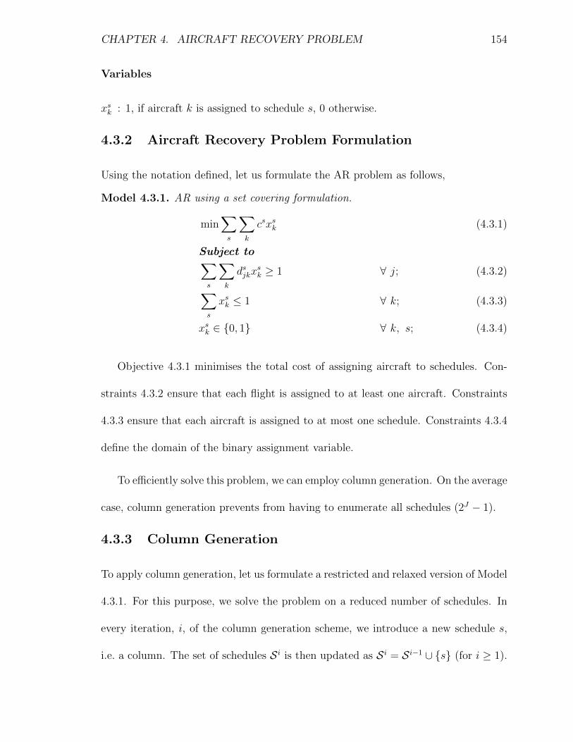
CHAPTER 4. AIRCRAFT RECOVERY PROBLEM 154
Variables
xsk : 1, if aircraft k is assigned to schedule s, 0 otherwise.
4.3.2 Aircraft Recovery Problem Formulation
Using the notation defined, let us formulate the AR problem as follows,
Model 4.3.1. AR using a set covering formulation.
min∑s
∑k
csxsk (4.3.1)
Subject to∑s
∑k
dsjkxsk ≥ 1 ∀ j; (4.3.2)∑
s
xsk ≤ 1 ∀ k; (4.3.3)
xsk ∈ {0, 1} ∀ k, s; (4.3.4)
Objective 4.3.1 minimises the total cost of assigning aircraft to schedules. Con-
straints 4.3.2 ensure that each flight is assigned to at least one aircraft. Constraints
4.3.3 ensure that each aircraft is assigned to at most one schedule. Constraints 4.3.4
define the domain of the binary assignment variable.
To efficiently solve this problem, we can employ column generation. On the average
case, column generation prevents from having to enumerate all schedules (2J − 1).
4.3.3 Column Generation
To apply column generation, let us formulate a restricted and relaxed version of Model
4.3.1. For this purpose, we solve the problem on a reduced number of schedules. In
every iteration, i, of the column generation scheme, we introduce a new schedule s,
i.e. a column. The set of schedules S i is then updated as S i = S i−1 ∪ {s} (for i ≥ 1).
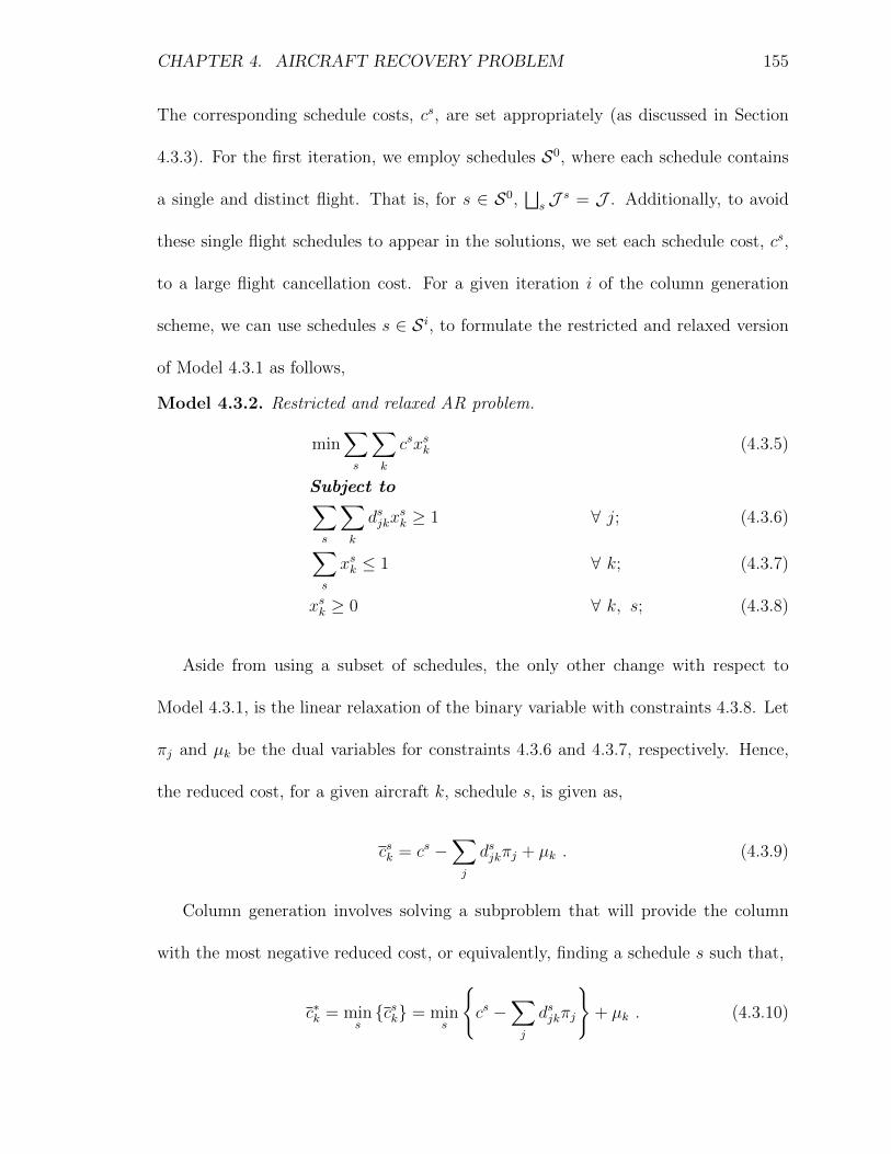
CHAPTER 4. AIRCRAFT RECOVERY PROBLEM 155
The corresponding schedule costs, cs, are set appropriately (as discussed in Section
4.3.3). For the first iteration, we employ schedules S0, where each schedule contains
a single and distinct flight. That is, for s ∈ S0,⊔s J s = J . Additionally, to avoid
these single flight schedules to appear in the solutions, we set each schedule cost, cs,
to a large flight cancellation cost. For a given iteration i of the column generation
scheme, we can use schedules s ∈ S i, to formulate the restricted and relaxed version
of Model 4.3.1 as follows,
Model 4.3.2. Restricted and relaxed AR problem.
min∑s
∑k
csxsk (4.3.5)
Subject to∑s
∑k
dsjkxsk ≥ 1 ∀ j; (4.3.6)∑
s
xsk ≤ 1 ∀ k; (4.3.7)
xsk ≥ 0 ∀ k, s; (4.3.8)
Aside from using a subset of schedules, the only other change with respect to
Model 4.3.1, is the linear relaxation of the binary variable with constraints 4.3.8. Let
πj and µk be the dual variables for constraints 4.3.6 and 4.3.7, respectively. Hence,
the reduced cost, for a given aircraft k, schedule s, is given as,
csk = cs −∑j
dsjkπj + µk . (4.3.9)
Column generation involves solving a subproblem that will provide the column
with the most negative reduced cost, or equivalently, finding a schedule s such that,
c∗k = mins{csk} = min
s
{cs −
∑j
dsjkπj
}+ µk . (4.3.10)

CHAPTER 4. AIRCRAFT RECOVERY PROBLEM 156
Hence, generating a column for aircraft k corresponds to solving a subproblem and
creating a schedule s with its corresponding flights. Specifically, each subproblem is
modelled by employing the shortest path problem with resource constraints (SPPRC).
Given that airlines’ operational factors can be taken on an individual aircraft basis,
we can model them in the subproblems as independent resource constraints.
Subproblems: Shortest Path Problem with Resource Constraints
To solve the subproblems for each aircraft k, given in Equation 4.3.10, we make use of
the SPPRC. To model the subproblems accurately, let us define a network with some
specific properties. Let G = (N,A) be directed activity-on-arc or a TSN where the
set of nodes N represents the airports under consideration at different time points,
and the arcs, A, correspond to connections. Let G have a single source and sink nodes
with no incoming or outgoing connections respectively. For two nodes i, j ∈ N there
is an arc, i.e connection, g = (i, j) ∈ A, if and only if it corresponds to a scheduled
connection (flight or ground with g ∈ J ), or a non-scheduled connection (g /∈ J ). We
distinguish two types of non-scheduled connections: a flight delay copy, a delayed
copy of a scheduled flight; and a non-scheduled ground connection. See Section
4.4.1 for more details.
For any connection g, let wg denote the weight, hg and tg denote the head and tail
nodes (respectively), ag and dg denote the arrival and departure times (respectively),
rg denote the flight range, and lastly, let Tg denote the type of connection (scheduled:
flight or ground connection, non-scheduled: flight delay copy or ground connection).
Additionally, every connection has a corresponding operational cost. For a sub-

CHAPTER 4. AIRCRAFT RECOVERY PROBLEM 157
problem k and any scheduled connection, the operating cost is defined to be propor-
tional to a standard operating cost cstk . Where cstk is either, the standard total oper-
ating cost (per unit time) for aircraft k, if the connection corresponds to a flight, or 0
otherwise. The costs associated with non-scheduled connections (per unit time) are,
codk for flight delay copies (operating costs under delay), and cgwk for ground connections
(ground waiting costs). See Appendix B.2 for the values used in the computational
tests.
To define resource consumption and constraints, let R = {1, . . . , R} be a set of
resources. Let L = (L1, . . . , LR) and L = (L1, . . . , L
R) be vectors for minimum and
maximum resources, respectively. For each connection g, we denote the associated
weight by wg, and the resource consumption vector by fg = (f 1g , . . . , f
Rg ). Each com-
ponent in this vector is referred to as a resource extension function (REF) (Irnich
and Desaulniers, 2005). For a given path, p, we denote the set of connections by
A(p), the weight of the path by w(p), and the resource consumed along the path by
f(p) = (f 1(p), . . . , fR(p)), where,
w(p) =∑g∈A(p)
wg ; f r(p) =∑g∈A(p)
f rg . (4.3.11)
To define the weight wg, for an arc g and subproblem k, we use,
wg =
cstk (ag − dg)− πg if g ∈ J
cstk (ag − dg) + codk (dg − dj)− πj if g /∈ J ∧ COND0
cgwk (ag − dg) if g /∈ J ∧ COND′0
; (4.3.12)
where πg is the dual variable for constraints 4.3.7. Here, condition COND0 is true

CHAPTER 4. AIRCRAFT RECOVERY PROBLEM 158
only if Tg corresponds to a flight delay copy of a scheduled flight j, where,
j = sup {j ∈ J : hj = hg, tj = tg, and dj < dg} . (4.3.13)
Condition COND′0 is true only if Tg corresponds to a non-scheduled ground con-
nection. Hence, Equation 4.3.12 defines the weights of scheduled and non-scheduled
connections separately. For a given subproblem k and any scheduled connection g,
the weight is proportional to the standard operating cost for aircraft k (cstk ) times the
duration of the connection, minus the corresponding dual value. Note that this may
lead to negative weights. For a given subproblem k and any non-scheduled connection
g, if the connection corresponds to a flight delay copy, then the weight is equal to the
standard operating cost (cstk ) times the duration of the connection, plus the operating
cost under delay (codk ) times the delay with respect to the original flight, minus the
dual value of the original flight. If the non-scheduled connection corresponds to a
non-scheduled ground connection, then the weight is equal to the ground waiting cost
(cgwk ) times the duration of the connection.
Using these definitions, generating a column for each aircraft k corresponds to a
schedule t produced by the connections of a path produced by solving an appropriate
SPPRC. Such path is one that minimises delay while satisfying operational restric-
tions. That is, finding a path in G, p, which minimises w(p) subject to resource
constraints L ≤ f(p) ≤ L, i.e. Lr ≤ f r(p) ≤ Lr
for every resource r. To evaluate
the column, the reduced cost can be calculated by updating the parameters dtjk, and
using Equation 4.3.9. If the reduced cost is negative, the column is added with a cost
ct. To minimise operational costs, ct is set to be equal to the total operating costs of

CHAPTER 4. AIRCRAFT RECOVERY PROBLEM 159
the schedule.
Resource Extension Functions
To take airline operational factors into account, we define appropriate resource ex-
tension functions (REFs) employed in the SPPRC. For this purpose, it is convenient
to define some attributes for connections and aircraft. Each connection g, in a TSN,
G, has attributes regarding the arrival and departure airports (hg, tg), departure and
arrival times (dg, ag), and flight range (rg). Each aircraft k has an attribute rk that
represents the range that a certain aircraft type can operate. Let us define a set of
seven resources,
R = {mono, air, maint, crew-d1, crew-d2, pass, non-s} ,
corresponding to: an artificial monotone resource (required for the exact algorithm,
see Section 4.4.2); operational restrictions: aircraft, maintenance, crew (duty restric-
tions 1 and 2 from Section 4.1), and passenger delay; and an additional restriction for
non-scheduled connections.
We can define REFs for each resource. For extending partial path pi (a path from
source to node i) along arc g = (i, j), resulting in partial path pj (a path from source
to node j passing through node i), we can set the resource consumption vector, f(pj),
according to the following REFs.
For the artificial monotone resource,
f mono(pj) = f mono(pi) + 1 (4.3.14)

CHAPTER 4. AIRCRAFT RECOVERY PROBLEM 160
For aircraft restrictions,
f air(pj) =
1 if not COND1
0 otherwise
; (4.3.15)
where condition COND1 depends on the range of the aircraft under consideration,
rk. If rk is short-haul or long-haul, then COND1 is true only if rg corresponds to the
same range. If rk is short/medium-haul, then COND1 is true only if rg is at most a
medium-haul flight.
For maintenance restrictions,
f maint(pj) =
f maint(pi) if hg = tg
0 if COND2
f maint(pi) + (ag − dg) otherwise
; (4.3.16)
where condition COND2 is true only if the origin and destination airports, hg = tg,
corresponds to a hub airport and the turnaround time, ag−dg, is at least long enough
for the shortest type of maintenance allowed. We denote this quantity with maintMin.
For crew duty restrictions 1 and 2,
f crew-d1(pj) =
f crew-d1(pi) + (ag − dg) if hg 6= tg
f crew-d1(pi) if not COND′2
0 if COND′2
; (4.3.17)

CHAPTER 4. AIRCRAFT RECOVERY PROBLEM 161
and
f crew-d2(pj) =
f crew-d2(pj) + (ag − dg) if hg 6= tg
f crew-d2(pi) if not COND3
0 if COND3
. (4.3.18)
Where condition COND′2 is true only if the arrival and departure airport, hg =
tg, corresponds to a hub airport. Condition COND3 is true only if the origin and
destination airports, hg = tg, corresponds to a hub airport and the turnaround time,
ag − dg, is at least long enough for the shortest crew duty break. We denote this
quantity with breakMin.
For the passenger delay restrictions,
f pass(pj) =
1 if COND4
0 otherwise
; (4.3.19)
where condition COND4 is true only if g /∈ J , corresponding to a flight delay copy
of flight j (defined by Equation 4.3.13), and either of the following hold: if rg is
short-haul, dg − dj ≥ 2; if rg is medium-haul, dg − dj ≥ 3; or if rg is long-haul,
dg − dj ≥ 4.
Lastly, for non-scheduled connection restrictions,
f non-s(pj) =
1 if g ∈ J
f non-s(pi)− 1 otherwise
. (4.3.20)
With these definitions, we can set the minimum and maximum resource levels for
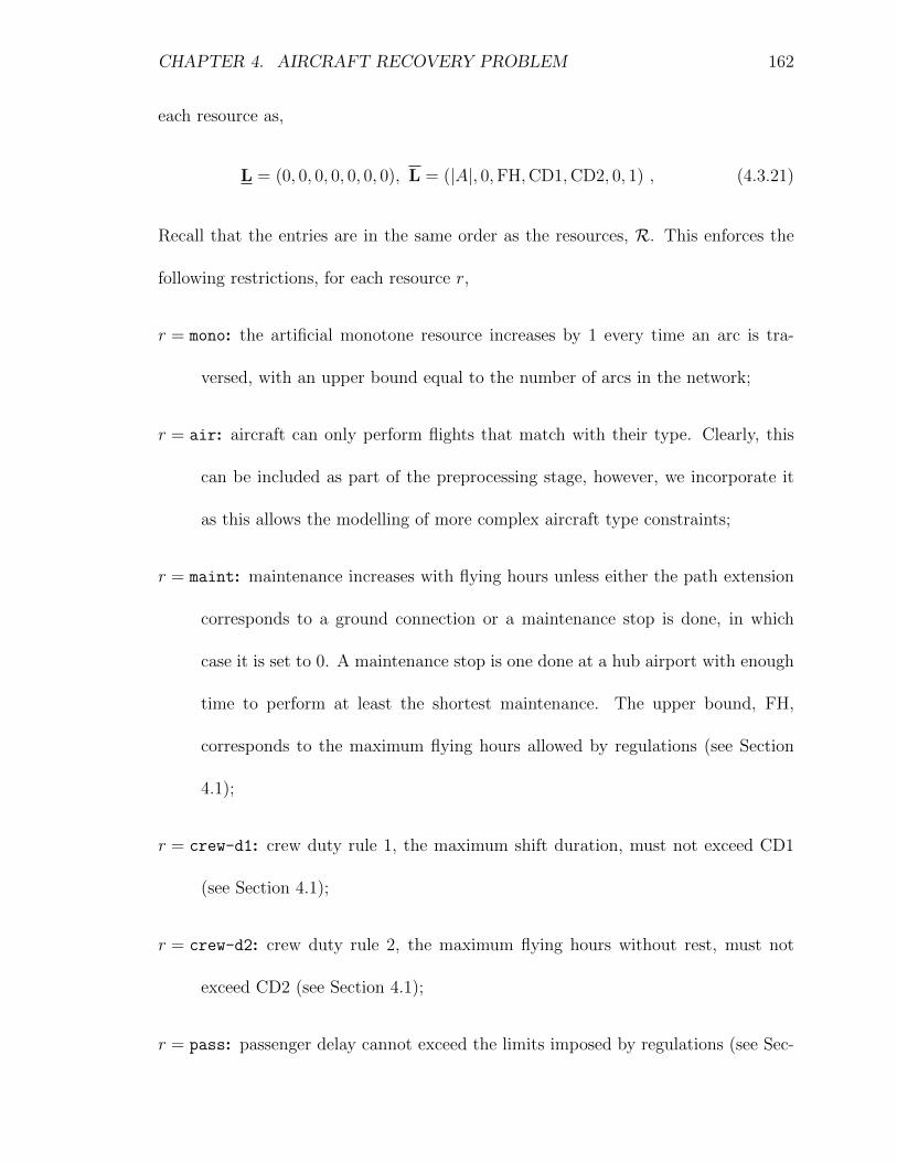
CHAPTER 4. AIRCRAFT RECOVERY PROBLEM 162
each resource as,
L = (0, 0, 0, 0, 0, 0, 0), L = (|A|, 0,FH,CD1,CD2, 0, 1) , (4.3.21)
Recall that the entries are in the same order as the resources, R. This enforces the
following restrictions, for each resource r,
r = mono: the artificial monotone resource increases by 1 every time an arc is tra-
versed, with an upper bound equal to the number of arcs in the network;
r = air: aircraft can only perform flights that match with their type. Clearly, this
can be included as part of the preprocessing stage, however, we incorporate it
as this allows the modelling of more complex aircraft type constraints;
r = maint: maintenance increases with flying hours unless either the path extension
corresponds to a ground connection or a maintenance stop is done, in which
case it is set to 0. A maintenance stop is one done at a hub airport with enough
time to perform at least the shortest maintenance. The upper bound, FH,
corresponds to the maximum flying hours allowed by regulations (see Section
4.1);
r = crew-d1: crew duty rule 1, the maximum shift duration, must not exceed CD1
(see Section 4.1);
r = crew-d2: crew duty rule 2, the maximum flying hours without rest, must not
exceed CD2 (see Section 4.1);
r = pass: passenger delay cannot exceed the limits imposed by regulations (see Sec-

CHAPTER 4. AIRCRAFT RECOVERY PROBLEM 163
tion 4.1);
r = non-s: enforces that no two consecutive non-scheduled connections are in a path.
A scheduled flight sets the resource to 1, otherwise, it is set to its previous
value minus 1. Since the minimum for this resource is 0, and two consecutive
non-scheduled connections will produce a value of -1, the required relation is
enforced.
See Appendix B.2 for the values of FH, CD1, and CD2 used in the computational
tests.
4.4 Solution Methodology
The hybrid solution procedure relies on several interacting components. Namely, the
generation and update of a specific type of network and the combination of column
generation with hyper-heuristics. In this section, we examine the different compo-
nents of the hybrid solution procedure in detail. Particularly, we study the different
algorithms employed in the column generation scheme, exact and metaheuristic, and
adapt a reinforcement learning–great-deluge hyper-heuristic to create two column
generation-specific hyper-heuristics.
4.4.1 Network Generation
Flight schedules allow us to construct the necessary TSN network for the subprob-
lems. The TSN network, G, as defined in Section 4.3.3, is constructed as follows. A
node is included for every airport under consideration at each different time point.
We include two artificial nodes that represent the source and sink nodes, with no in-

CHAPTER 4. AIRCRAFT RECOVERY PROBLEM 164
coming or outgoing arcs respectively. Arcs are split by scheduled flights/ground arcs
(those present in the initial flight schedule), and non-scheduled connections which we
generate. Non-scheduled connections are generated between all airports with a prior
existing flight (flight delay copies) and all ground arcs. Another type on non-scheduled
connection are ferry or empty flights (sometimes positioning). However, ferrying is
not always considered in the AR problem (Clausen et al., 2010), alternatively, some
authors that account for crew recovery considered crew deadhead flights (where crew
travel along with passengers), Maher (2015), for instance. Kenan et al. (2018) solved
an extension to the TA problem (with maintenance) allowing ferry flights. They re-
ported that the appearance of these types of connections in the solutions occurred
only upon the decrease of the allocated ferrying costs (provided by an airline) and
resulted in a small increase in profit. Thengvall et al. (2001) solved the AR problem
using a TSN and also including ferry flights. Results showed that the number of ferry
flights in the solution decrease as the recovery horizon increases. Additionally, the
recovery horizons in this work were under 24 hours. Given that the recovery hori-
zons considered in this research are at least 2 days, we do not account for ferrying;
nonetheless, flight delays and cancellations are included.
Figure 4.2 shows a two airport example of a TSN with two different routes. Given
the routes in the pre-operational flight schedules (blue and red arcs), non-scheduled
connections are generated (dashed arcs) for flight delay copies and ground arcs. More-
over, due to airline restrictions, flight delay copies are not generated prior to the orig-
inal flight. For instance, a copy for the blue flight B3 to A4 is only generated after,
creating the flight delay copy B4 to A5, but not B2 to A3. This creates a cross-hatched

CHAPTER 4. AIRCRAFT RECOVERY PROBLEM 165
pattern between connected airports. Generating delay copies in this fashion, avoids
creating additional arcs (as with most of the traditional methods), but fits more nat-
urally into the original pre-operational plans. Clearly, larger networks benefit from
more flight delay copies and therefore, more options when creating routes; hence,
leading to better quality solutions. On the other hand, small networks provide less
flight delay copies and typically correlate with worse quality solutions. See Section
4.5 for more information.
Timeline for Airport B
Timeline for Airport A A1 A2 A3 A4 A5 A6
B2 B3 B4 B5 B6
Figure 4.2: Generation of Time-Space Networks.
4.4.2 Hybrid Solution Procedure
There are several components in our hybrid solution procedure. Figure 4.3 outlines the
three main parts. The TSN component (in yellow), as previously discussed in Section
4.4.1, generates the initial TSN based on an input flight schedule, then, once the duals
have been obtained from the solution of Model 4.3.2, we update the connection weights
as discussed in Section 4.3.3. The column generation component (in purple), has three
processes that involve, solving Model 4.3.2, generating a column and checking whether
a proposed column has negative reduced cost. To solve the subproblems, we make
use of the hyper-heuristic component of the solution procedure (in grey). Here, we
select, out of a set of heuristics H, an algorithm H to solve the subproblem for aircraft

CHAPTER 4. AIRCRAFT RECOVERY PROBLEM 166
k, hence, generating a column. Then, we evaluate the performance of the heuristic
based on past performance and the cost of the column provided. If the column for
aircraft k has negative reduced cost, then we add it to Model 4.3.2 and resolve the
problem. Otherwise, we check whether all subproblems have been solved using an
exact algorithm, A. If not, then we update the hyper-heuristic accordingly depending
on which hyper-heuristic we are using. Broadly, this involves using the exact algorithm
if all heuristics have produced a non-negative reduced cost for k, and updating the set
of heuristics H in different ways (see Section 4.4.2 for a more detailed explanation).
If all subproblems have been solved using the exact algorithm and produced columns
with non-negative reduced costs, we exit the loop.
We now proceed to describe the different components of the hybrid solution proce-
dure. Particularly, we focus on the exact and metaheuristic algorithms implemented
for solving the subproblems and on the hyper-heuristics used to select and evaluate
the metaheuristic algorithms.
Exact Algorithm
To solve the SPPRC exactly, we implement a bidirectional labelling algorithm with
dynamic halfway point (Tilk et al., 2017). It is an extension of the monodirectional
algorithm that supports search from both ends of the graph, hence, reducing the
computational efforts. The algorithm relies on two assumptions. Firstly, one of the
resources must be a monotone resource. Such a resource is common for forward and
backward searches. Let us denote such a resource by mono. The assumption is easily
met, as a monotone resource typically present in most applications e.g. time; if not, an

CHAPTER 4. AIRCRAFT RECOVERY PROBLEM 167
INPUT
GenerateTSN
Update TSN
Col
um
nG
ener
atio
n
Hyp
erh
euri
stic
TS
N
SolveModel 4.3.2
SelectheuristicH from H
SolveSubproblemk using H
Add columnto Model
4.3.2
Negativereduced cost?
Evaluateheuristic H
Used Afor all k?
Update hy-perheuristic
Stop
NO
NO
YES
YES
Figure 4.3: Hybrid Solution Procedure.
artificial monotone resource can be created, e.g. the number of arcs visited. Second,
that the REFs are invertible. These can be easily constructed for typical REFs (Irnich,
2008). Let, the inverse of the REF for a particular resource r, as introduced in Section
4.3.3, f rg , be denoted with brg. We refer to these as the forward and backward REFs
respectively. Practically, the backward REFs can be defined using the REFs as per
Section 4.3.3. Consider the extension of a backward partial path pj (from the sink to
node j) along arc g = (i, j), resulting in backward partial path pi (from the sink to
node i passing through node j), we can set the resource consumption vector, b(pi),
according to the following criteria. Resources air, pass and non-s can employ the
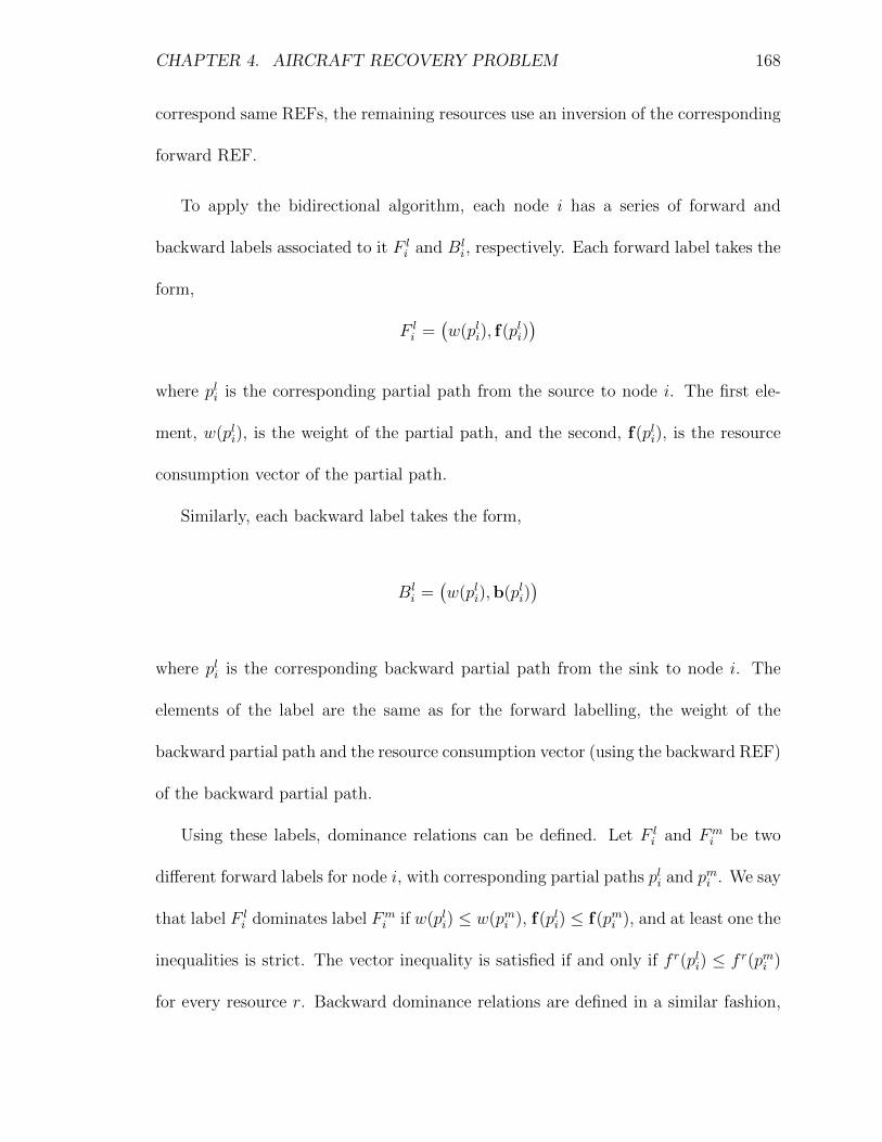
CHAPTER 4. AIRCRAFT RECOVERY PROBLEM 168
correspond same REFs, the remaining resources use an inversion of the corresponding
forward REF.
To apply the bidirectional algorithm, each node i has a series of forward and
backward labels associated to it F li and Bl
i, respectively. Each forward label takes the
form,
F li =
(w(pli), f(pli)
)where pli is the corresponding partial path from the source to node i. The first ele-
ment, w(pli), is the weight of the partial path, and the second, f(pli), is the resource
consumption vector of the partial path.
Similarly, each backward label takes the form,
Bli =
(w(pli),b(pli)
)
where pli is the corresponding backward partial path from the sink to node i. The
elements of the label are the same as for the forward labelling, the weight of the
backward partial path and the resource consumption vector (using the backward REF)
of the backward partial path.
Using these labels, dominance relations can be defined. Let F li and Fm
i be two
different forward labels for node i, with corresponding partial paths pli and pmi . We say
that label F li dominates label Fm
i if w(pli) ≤ w(pmi ), f(pli) ≤ f(pmi ), and at least one the
inequalities is strict. The vector inequality is satisfied if and only if f r(pli) ≤ f r(pmi )
for every resource r. Backward dominance relations are defined in a similar fashion,

CHAPTER 4. AIRCRAFT RECOVERY PROBLEM 169
but using backward labels and REFs.
The pseudo-code for the bidirectional labelling algorithm with dynamic halfway
point (Tilk et al., 2017) is shown in Algorithm 3. The inputs required are, a graph
(G), and lower and upper bounds for resources (L, L). The forward and backward
halfway points (HF, HB) are set to Lmono = HB < HF = Lmono
, line 2, as required for
the search to have a dynamic halfway point. Further initialisations are, two sets of
forward and backward unprocessed paths (F, B) and a set of processed paths P. Once
the direction is settled, in line 5, we proceed either a forward or backward search in
a very similar manner as the monodirectional labelling algorithm. After choosing a
path from the unprocessed set of paths, lines 7 (forward) or 17 (backward), we check
if the halfway point has been reached, lines 8 or 18, if not, then we proceed to extend
the selected path in the traditional way, lines 9-13 or 19-23. After this, we update the
value of the halfway point to reduce the size of the search in the opposite direction.
That is, in the forward search, in line 14, we update HB to a higher value if we have
searched past it. Conversely, in the backward search, in line 24, we update HF to a
lower value if we have searched past it. The algorithm carries on like this, updating
the direction of search in every iteration, and terminating when no more paths remain
to be processed in any direction. Moreover, in line 30, at the end of every iteration,
we can apply some dominance rules to remove unnecessary paths. To do so, labels
are generated for each forward or backward partial path.
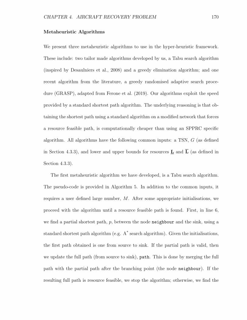
CHAPTER 4. AIRCRAFT RECOVERY PROBLEM 170
Metaheuristic Algorithms
We present three metaheuristic algorithms to use in the hyper-heuristic framework.
These include: two tailor made algorithms developed by us, a Tabu search algorithm
(inspired by Desaulniers et al., 2008) and a greedy elimination algorithm; and one
recent algorithm from the literature, a greedy randomised adaptive search proce-
dure (GRASP), adapted from Ferone et al. (2019). Our algorithms exploit the speed
provided by a standard shortest path algorithm. The underlying reasoning is that ob-
taining the shortest path using a standard algorithm on a modified network that forces
a resource feasible path, is computationally cheaper than using an SPPRC specific
algorithm. All algorithms have the following common inputs: a TSN, G (as defined
in Section 4.3.3), and lower and upper bounds for resources L and L (as defined in
Section 4.3.3).
The first metaheuristic algorithm we have developed, is a Tabu search algorithm.
The pseudo-code is provided in Algorithm 5. In addition to the common inputs, it
requires a user defined large number, M . After some appropriate initialisations, we
proceed with the algorithm until a resource feasible path is found. First, in line 6,
we find a partial shortest path, p, between the node neighbour and the sink, using a
standard shortest path algorithm (e.g. A* search algorithm). Given the initialisations,
the first path obtained is one from source to sink. If the partial path is valid, then
we update the full path (from source to sink), path. This is done by merging the full
path with the partial path after the branching point (the node neighbour). If the
resulting full path is resource feasible, we stop the algorithm; otherwise, we find the

CHAPTER 4. AIRCRAFT RECOVERY PROBLEM 171
edge that makes the full path resource infeasible, line 12, and place a tabu there, line
13. This is done by setting the weight of the edge to be M , hence, is avoided by the
shortest path algorithm. Using the new tabu edge, we update the neighbour node as
the head of the tabu edge, line 18. The function in line 13, GetNeighbour, ensures
that the tabu is not placed on the same edge twice. Instead, it backtracks from the
current tabu edge, returning the backward neighbouring edge (one incident to the
tabu edge) with the largest weight. Please see Appendix B.1.2 for more details on the
functions used. If the operations performed results in a non-valid partial path, then,
in line 16, we place the tabu edge on a backward neighbouring edge of the current
tabu edge.
Algorithm 5 Tabu Search for the SPPRC.
1: INPUTS: G = (V,A), L, L, M .2: Initialisations:3: stop = False, edgesToCheck = A, neighbour = Source, tabu = None, path =
[ ], neighbourhood = [ ].4: . See Appendix B.1.2 for functions employed5: while stop is False do6: p = ShortestPath(neighbour, Sink, G)7: if p is valid then8: path =UpdatePath(neighbour, neighbourhood, p)9: if path is resource feasible then
10: stop =True . Terminate the algorithm11: else12: Find edge g that makes the path resource infeasible13: tabu, edgesToCheck, neighbourhood =GetNeighbour(edgesToCheck,
neighbourhood, g) . Update tabu edge, array of edges to check andneighbourhood
14: end if15: else16: tabu, edgesToCheck, neighbourhood = GetNeighbour(edgesToCheck,
tabu) . Update tabu edge, array of edges to check and neighbourhood17: end if18: neighbour = h(tabu) . Update neighbour as head node of current tabu edge19: end while

CHAPTER 4. AIRCRAFT RECOVERY PROBLEM 172
The second metaheuristic algorithm we have developed, the Greedy Elimination
algorithm, is shown in Algorithm 6. Using the common inputs, and after the appro-
priate initialisations, in line 5, a standard algorithm is applied to obtain a full path,
p, from source to sink. Please see Appendix B.1.2 for more details on this function.
If the full path is valid, then we check if it is resource feasible. If this is true, then
we terminate the algorithm, line 8; otherwise, we remove the problematic edge (the
edge that makes the path resource infeasible) and resolve the shortest path problem.
If the resulting path turns out to be non-valid, we add back the edge we previously
removed, and instead, remove a backward neighbouring edge of the edge we previously
removed. We continue in this fashion until a resource feasible path is obtained.
Algorithm 6 Greedy Elimination Algorithm for the SPPRC.
1: INPUTS: G = (V,A), L, L.2: Initialisations: stop = False, neighbourhood = [ ].3: . See Appendix B.1.2 for functions employed4: while stop is False do5: p = ShortestPath(Source, Sink, G);6: if p is valid then . If a path exists7: if path is resource feasible then8: stop =True . Terminate the algorithm9: else
10: Find edge g that makes the path resource infeasible11: Remove g from G12: end if13: else . If no path exists14: Add g back to G15: . Get new neighbouring edge to remove and update neighbourhood array16: edge, neighbourhood = GetNextNeigh-
bouringEdge(neighbourhood, g)17: Remove edge from G18: end if19: end while
We implemented an adapted version of the GRASP presented by Ferone et al.

CHAPTER 4. AIRCRAFT RECOVERY PROBLEM 173
(2019). The inputs required, apart from the common inputs, include: maxiter, the
maximum number of iterations to terminate the algorithm; maxiterLocal, the max-
imum number of iterations to terminate the local search algorithm; α, the greediness
factor (a value close to 1 represents a greedy selection, and a value close to 0 rep-
resents to a random selection); c, a cost function to evaluate solutions given by the
algorithm; and M a large number to use as a penalty. Solutions are defined as ordered
sets of nodes in the network, connected or not. The cost associated with each solution
reflects on the connectivity and total weight of the path provided by the sequence of
nodes. That is, for a potential path (any set of two or more nodes in the graph) in a
given solution, the associated cost is equal to the sum of the weights of the edges in
the potential path. However, if the potential path is not valid, then the cost function
returns the penalty value, M .
After the appropriate initialisation, until the number of iterations exceeds maxiter,
the algorithm generates a solution, line 5, improves it using local search, line 6, eval-
uates and updates the best solution according to whether there is an improvement,
lines 7 and 8. The functions in lines 5 and 6, defined in Appendix B.1.3, perform
various operations.
The ConstructSolution function, line 5, after sampling a random starting
node, constructs a new solution by iteratively appending nodes based on their cost.
To select a node to append to the solution, we compute a restricted candidates list,
with all the nodes such that their cost, with respect to the last node in the solution,
satisfies a simple equation involving the greediness factor α. By the definition of the
cost function, if no edge exists between a candidate node and the last node in the
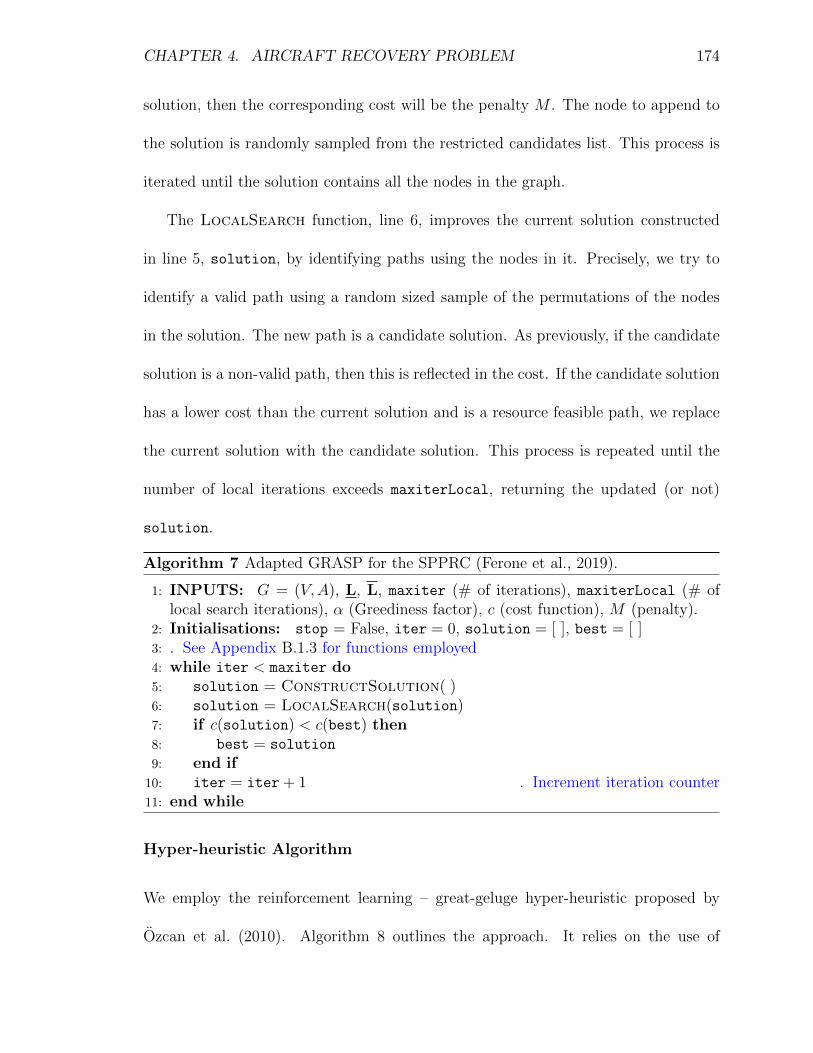
CHAPTER 4. AIRCRAFT RECOVERY PROBLEM 174
solution, then the corresponding cost will be the penalty M . The node to append to
the solution is randomly sampled from the restricted candidates list. This process is
iterated until the solution contains all the nodes in the graph.
The LocalSearch function, line 6, improves the current solution constructed
in line 5, solution, by identifying paths using the nodes in it. Precisely, we try to
identify a valid path using a random sized sample of the permutations of the nodes
in the solution. The new path is a candidate solution. As previously, if the candidate
solution is a non-valid path, then this is reflected in the cost. If the candidate solution
has a lower cost than the current solution and is a resource feasible path, we replace
the current solution with the candidate solution. This process is repeated until the
number of local iterations exceeds maxiterLocal, returning the updated (or not)
solution.
Algorithm 7 Adapted GRASP for the SPPRC (Ferone et al., 2019).
1: INPUTS: G = (V,A), L, L, maxiter (# of iterations), maxiterLocal (# oflocal search iterations), α (Greediness factor), c (cost function), M (penalty).
2: Initialisations: stop = False, iter = 0, solution = [ ], best = [ ]3: . See Appendix B.1.3 for functions employed4: while iter < maxiter do5: solution = ConstructSolution(.)6: solution = LocalSearch(solution)7: if c(solution) < c(best) then8: best = solution
9: end if10: iter = iter + 1 . Increment iteration counter11: end while
Hyper-heuristic Algorithm
We employ the reinforcement learning – great-geluge hyper-heuristic proposed by
Ozcan et al. (2010). Algorithm 8 outlines the approach. It relies on the use of

CHAPTER 4. AIRCRAFT RECOVERY PROBLEM 175
utilities to select heuristics from a set of heuristics H. In every iteration, we select the
heuristic with highest utility, apply it, and evaluate it using a function f(·), which we
are trying to minimise. Hence, the solution is compared to the previous one, fp, to
identify an improvement. If the heuristic has led to an improvement, i.e. a lower value
with respect to the previous solution, we improve the utility for that heuristic, if not,
then we worsen it. The authors define three different functions that can be employed
to update the utilities: addition, division or square root. That is, for a heuristic
Hi ∈ H the corresponding utility, ui, is worsened by either ui = ui−1 (U1), ui = ui/2
(U2), or ui =√ui (U3), and improved only for the additive case, by ui = ui + 1. The
improvement rate of U1 causes it to be provide less exploration of the heuristics than
the other utilities, favouring better performing heuristics Ozcan et al. (2010).
Algorithm 8 Reinforcement Learning – Great-Deluge Hyper-heuristic (Ozcan et al.,2010)
1: INPUTS: H (set of heuristics), utilities (array with initial utilities),f(·) (function to evaluate heuristic).
2: Initialisations: Apply a random heuristic H and set fp = f(H)3: while Stopping criteria not satisfied do4: Choose heuristic H ∈ H with maximum utility5: Apply heuristic H6: if f(H) < fp then7: Update utilities by improving the utility of heuristic H8: else9: Update utilities by worsening the utility of heuristic H
10: end if11: fp = f(H)12: end while
To adapt the great-deluge hyper-heuristic for our hybrid solution procedure, we
consider some column generation specific criteria. One hyper-heuristic is created per
subproblem which selects a heuristic and uses it to solve the subproblem, hence,

CHAPTER 4. AIRCRAFT RECOVERY PROBLEM 176
generating a column. The evaluation function f is defined to be the reduced cost
produced by the column. In order to update the utilities, we compare the reduced
cost with the previous reduced cost for the same subproblem. The utilities are then
updated as outlined above, being shared across all subproblems. Moreover, we can
update the set of heuristics and apply the exact algorithm in different ways. We outline
two hyper-heuristic algorithms that use this column generation specific criteria, HH1
and HH2.
In HH1, for a particular subproblem, we apply all heuristics, selecting them based
on their utility, until either, a column with negative reduced cost is generated, or all
heuristics fail to generate a column with negative reduced cost. If all heuristics fail,
we apply the exact algorithm to generate a column. If the column has a negative
reduced cost, we repeat the process until the exact algorithm generates columns with
non-negative reduced cost for all subproblems.
In HH2, for a particular subproblem, k, we define a subset of heuristics Hk ⊆ H.
A heuristic is selected from Hk, based on the utilities, and applied to the subproblem.
If the selected heuristic produces a column with non-negative reduced cost for a sub-
problem k, we remove it from Hk. Thus, it cannot be selected for future subproblems
k. Once all heuristics have been removed from Hk (i.e. all heuristics have gener-
ated columns with non-negative reduced cost) we use employ the exact algorithm to
generate columns for k thereafter.
CHAPTER 4. AIRCRAFT RECOVERY PROBLEM 177
4.5 Computational Experiments
To test the hybrid solution procedure which involves a hyper-heuristic algorithm for
column generation, as outlined in Section 4.4.2, we generated six different test in-
stances. For this purpose, we obtained flight schedules from Flightradar24 AB (2018)
using the package pyflighdata (Allamraju, 2014). After an extended data gathering
stage, we can easily filter data per airline. The six test instances were constructed
with flights in operation during varying time horizons in February 2017. Table 4.3
specifies the following information about the instances: the number of flights, the
number of aircraft, the number of aircraft types, the planning horizon, the dates of
the instance, and the size of the TSN generated (as outlined in 4.4.1). Table 4.4
summarises the algorithms used with their respective parameters, these are as sug-
gested by the authors (Ferone et al., 2019). We have released the implementation of
these algorithms (metaheuristic and exact) as a freely available Python package, cspy
(Torres Sanchez, Under review). Additionally, we include the implementation of the
hybrid particle swarm algorithm for the SPPRC by Marinakis et al. (2017); however,
this algorithm could not cope with our test instances. Please refer to Appendix B.2
for more information on the composition of the fleet and specific parameters employed
in the computational tests.
Table 4.5 shows the counts for the different metaheuristic algorithms as chosen by
each of the hyper-heuristics (HH1 and HH2) with the three different utility functions
U1 (additive), U2 (division), and U3 (square root). The average time per column,
i.e. per subproblem, is also included. The counts shown by HH1 are higher given

CHAPTER 4. AIRCRAFT RECOVERY PROBLEM 178
Table 4.3: Test instances.1 F = # of flights, A = # of aircraft, T = # of aircrafttypes, H = length of planning horizon in days, TSN= size of time-space network (#of nodes, # of arcs).
Name F A T H Dates TSN
I1 212 6 2 10 16/02/2017 - 26/02/2017 (220, 822)I2 273 6 1 10 17/02/2017 - 27/02/2017 (168,569)I3 230 8 1 2 17/02/2017 - 19/02/2017 (240, 910)I4 151 2 2 8 17/02/2017 - 25/02/2017 (168, 727)I5 314 5 1 4 17/02/2017 - 21/02/2017 (322, 1168)I6 187 8 3 7 14/02/2017 - 21/02/2017 (217, 743)
1 The data was obtained from real-world airline with theirrespective hub airport(s). For data protection, we have re-moved the real names.
Table 4.4: Algorithms used in solution procedure.
Abbrv. Algorithm Parameters
A1 Bidirectional labelling (Algorithm 3) n/aH1 Tabu Search (Algorithm 5) M = 1010
H2 Greedy Elimination (Algorithm 6) n/aH3 GRASP (Algorithm 7) maxiter = 100,
maxiterLocal =10, α = 0.2, M =1010
that it provides a fairer exploration of the metaheuristics, even more so using utilities
U2 and U3 (Ozcan et al., 2010). Algorithm H1 (Tabu Search) dominates in both of
the hyper-heuristics and the three utility functions. Even for the largest instance,
I2, the average computational time per iteration is under 1 second. Algorithm H2
(Greedy Elimination) also shows small computational times, regardless of the size
of the instance. Even though it takes significantly longer to process, H3 (GRASP)
is consistently worst and therefore last in the rankings for both hyper-heuristics.
Such rankings are consistent throughout the two hyper-heuristics and the three utility
functions.
Tables 4.6 and 4.7 show the computational results for all instances using hyper-
heuristics HH1 and HH2, respectively, with the three different utilities. Included

CHAPTER 4. AIRCRAFT RECOVERY PROBLEM 179
Table 4.5: Usage count of metaheuristics for the two hyperheuristics (HH1, HH2)using different utility functions.
HH1 HH2
Instance Heuristic Count per UtilityMean CPU
time percolumn (s)
U1 U2 U3 U1 U2 U3
I1 H1 44 49 42 36 100 58 0.09H2 15 19 20 9 10 11 0.01H3 14 19 19 8 10 8 102.55
I2 H1 19 17 28 21 17 20 0.05H2 14 11 20 15 13 12 0.01H3 10 11 16 14 10 12 193.96
I3 H1 40 38 36 30 44 41 0.11H2 16 18 15 11 11 12 0.01H3 13 18 15 9 10 12 127.10
I4 H1 5 5 10 10 5 10 0.06H2 3 3 4 3 3 3 0.01H3 2 2 4 3 2 2 51.58
I5 H1 17 15 16 19 14 19 0.15H2 8 7 8 7 8 8 0.01H3 7 7 7 6 7 7 200.01
I6 H1 29 29 22 28 31 29 0.04H2 15 21 17 11 14 13 0.01H3 12 16 15 11 12 12 102.16
in the tables are, the number of iterations, the number of columns generated with
negative reduced cost, the percentage of flights cancelled in the final solution, and
the total computational time. For every instance, the best utility is highlighted in
green. That is, the utility that provides the solution with smallest percentage of flight
cancellations or total operating costs if two solutions have the same percentage of
flight cancellations. Using HH1, all utilities U1, U2, and U3 are selected for 2 (out
of 6) instances. Using HH2, U2 is selected for 3 (out of 6) instances, while U1 and
U3 are selected for 2 and 1 instances, respectively. Moreover, HH1 shows significantly
higher computational times; for example, for the largest instance (I2), HH1 provides

CHAPTER 4. AIRCRAFT RECOVERY PROBLEM 180
a solution in 67 minutes versus 40 minutes using HH2. Also, it appears that HH1
does not provide significant improvements in the solutions with respect to HH2.
Table 4.6: Computational results of the hybrid solution procedure using hyperheuris-tic HH1.
Instance Utility Iterations Columns% Cancelled
Flights
CPUTime(min)
I1 U1 11 43 8.49 25.10U2 14 51 5.19 33.86U3 15 43 11.79 33.75
I2 U1 7 23 3.30 45.97U2 6 21 3.30 36.75U3 10 33 3.30 66.72
I3 U1 9 42 9.57 35.66U2 11 36 8.70 38.48U3 8 32 7.83 33.48
I4 U1 4 4 35.76 1.89U2 4 4 35.76 1.93U3 7 9 35.76 3.60
I5 U1 6 16 2.55 26.48U2 5 14 2.55 22.35U3 6 16 2.55 26.25
I6 U1 6 27 27.81 26.20U2 8 32 31.02 36.92U3 7 24 33.16 30.02

CHAPTER 4. AIRCRAFT RECOVERY PROBLEM 181
Table 4.7: Computational results of the hybrid solution procedure using hyperheuris-tic HH2.
Instance Utility Iterations Columns% Cancelled
Flights
CPUTime(min)
I1 U1 9 35 10.85 16.43U2 33 102 5.19 18.89U3 23 59 5.66 20.28
I2 U1 10 33 3.30 46.84U2 8 23 3.30 43.33U3 7 26 3.30 40.38
I3 U1 6 26 6.96 24.73U2 10 41 8.70 22.62U3 10 41 6.96 27.18
I4 U1 8 10 37.75 2.75U2 4 4 35.76 1.91U3 7 9 35.76 1.93
I5 U1 6 17 2.55 28.16U2 6 15 2.55 22.92U3 8 19 2.55 26.25
I6 U1 6 26 24.06 19.60U2 7 33 32.09 24.78U3 8 30 25.13 22.82

CHAPTER 4. AIRCRAFT RECOVERY PROBLEM 182
Figure 4.4 shows a detailed comparison between the best performing utility func-
tion for HH1 (results in red) and HH2 (results in blue) for each instance. The x-axis
shows the instances in increasing order proportional to their TSN size (I4, I1, I6, I3,
I5, and I2). As previously mentioned, HH2 dominates in computational time (blue
dashed line on the right-hand y-axis) when compared to HH1 (red dashed line), being
on average 22% faster than HH1. The bar chart, plotted against the left-hand y-axis,
shows the comparison in the percentage of cancelled flights for both hyper-heuristics.
It can be seen that HH2 (blue bars) has equal or lower cancellations than HH1 (red
bars) across all instances.
I4 I1 I6 I3 I5 I2Instance (ordered in increasing TSN size)
0
5
10
15
20
25
30
35
% Can
cella
tions
0
10
20
30
40
50
60
CPU tim
e (m
in)
% Cancellations (HH1)% Cancellations (HH2)
CPU time (HH1)CPU time (HH2)
Figure 4.4: Comparison between hyper-heuristics HH1 and HH2.
Given the clear dominance by hyper-heuristic HH2, we perform a more detailed
study and some further experiments. Figure 4.5 displays the relationship between the
TSN size, for each test instance, with the percentage of flights cancelled in the best
solution obtained using HH2 (green rows in Table 4.7). As in Figure 4.4, the x-axis
shows the instances in increasing order proportional to their TSN size (I4, I1, I6, I3,

CHAPTER 4. AIRCRAFT RECOVERY PROBLEM 183
I5, and I2). As indicated by the fitted least squares polynomial of degree two (in
blue), the percentage of cancelled flights decreases with the increase in the size of the
TSN. The trend supports the claim that the quality of the solution increases with the
size of the network. Unsurprisingly, a larger network, with higher number of nodes
and connections, allows for more flexibility when generating schedules and therefore,
leads to better solutions. Hence, our hybrid solution procedure performs increasingly
better with larger networks and seems to be computationally scalable.
Figure 4.6 shows the comparison between using three methods, the exact algo-
rithm (A1) to generate columns in every iteration, a random non-learning-based
hyper-heuristic, and the hybrid solution procedure. For the random non-learning-
based hyper-heuristic, we simply use HH1 with a random utility and a reduced set of
heuristics for performance, H ={H1, H2}; we refer to this method as RAND. Simi-
larly, for the hybrid solution procedure, HH2 is used with utility U2 and a reduced
set of heuristics for performance, Hk ={H1, H2} for all k subproblems; we refer to
this method as mHH2. The bar chart, plotted against the left-hand y-axis, shows the
percentage of flights cancelled in the optimal solution for the three methods. Red
bars show A1, blue bars show RAND, and purple bars show mHH2. Both RAND and
mHH2 dominate A1 in solution quality. The increase in the quality of the solution
is due to the use of different metaheuristics; this allows for a wider search of the
solution space. Against the right-hand y-axis, we have three points for each instance,
representing the computational times (in minutes) for A1 (crosses), RAND (circles)
and mHH2 (black diamonds). Please note that the computational time for method
A1 instance I5 is not included in the plot as its value (30 minutes) significantly skews

CHAPTER 4. AIRCRAFT RECOVERY PROBLEM 184
the plot. Our hybrid solution procedure (mHH2) provides consistently faster (all in-
stances were solved in under 50 seconds) and better solutions. Therefore, if one aims
for computational efficiency we recommend mHH2.
Using mHH2 to test the scalability claim further, we performed an experiment
with a significantly larger TSN. Using an instance of 658 flights and 28 aircraft (which
produces a TSN, 93% larger than I2, with 1302 nodes and 4882 arcs) we produced
a solution with only 4.3% of cancelled flights in 69 minutes (after 21 iterations and
277 columns with negative reduced cost). This result, fits with the trend exhibited in
Figure 4.5, thus, further supporting the scalability claim.
I4 I1 I6 I3 I5 I2Instance (ordered in increasing TSN size)
0
5
10
15
20
25
30
35
% Can
cella
tions
Trend in % CancellationsResiduals
Figure 4.5: Trend between network size(per instance) and percentage of flightscancelled (using HH2).
I4 I1 I6 I3 I5 I2Instance (ordered in increasing TSN size)
0
20
40
60
80
% Cancellatio
ns
0.2
0.4
0.6
0.8
1.0
1.2
1.4
CPU tim
e (m
in)
% Cancellations (A1)% Cancellations (RAND)% Cancellations (mHH2)
CPU time (A1)CPU time (RAND)CPU time (mHH2)
Figure 4.6: Performance comparisonfor each instance using the exact algo-rithm (A1), a random non-learning basedmethod (rHH1), and the hybrid solutionprocedure (mHH2).

CHAPTER 4. AIRCRAFT RECOVERY PROBLEM 185
4.6 Conclusions
We have solved the aircraft recovery problem considering operational restrictions.
Previous studies that tackle a similar problem pose restrictive assumptions on the op-
erational constraints. By using our hybrid solution procedure we are able to account
for generic and multiple operational restrictions. Such framework uses column gener-
ation with subproblems modelled as shortest path problems with resource constraints
(SPPRC). Furthermore, to improve computational efficiency and the quality of the
solutions, we implement different hyperheuristic algorithms. Such algorithms learn
and select varying metaheuristic or exact algorithms, depending on their past perfor-
mance, to employ for the generation of columns with negative reduced cost. Using
the exact bidirectional labelling algorithm with dynamic halfway point, we produce
optimal solutions for the LP relaxation of the aircraft recovery problem. Therefore,
this paper bridges between several disjoint areas in the literature and closes several
gaps in the aircraft recovery literature. The software that collects the implementa-
tions included in this paper is freely available as a Python package (Torres Sanchez,
Under review).
The hybrid solution procedure was tested using six real-world instances of different
sizes. Results show that our approach is not only efficient, solving all instances in
reasonable computational time, but it also produces better solutions than the exact
algorithm alone and than a random metaheuristic selection process. For the instances
studied, our Tabu search metaheuristic performed consistently better (i.e. providing
more negative reduced cost columns) than our Greedy Elimination metaheuristic and

CHAPTER 4. AIRCRAFT RECOVERY PROBLEM 186
an adapted GRASP metaheuristic. Also, the quality of the recovery solution seems
to increase with the size of the network. The use of a fairer hyper-heuristic, one that
brings a fairer exploration of the metaheuristics, does not lead to a higher quality
of recovery solutions. Furthermore, we suggest a computational setup for the hybrid
solution procedure that produces faster solutions. Using this set up, we were able
to solve a large instance, 658 flights 28 aircraft, in under 70 minutes. The resulting
solution suggests that the framework is scalable and adds to the claim that the quality
of recovery solutions increases with the size of the network. Hence, this framework
equips decision makers with an efficient learning-based tool that can handle various
network sizes and present adaptable and good quality solutions to the aircraft recovery
problem.
Some limitations are worth noting. There seems to be potential for scaling this
framework for larger network sizes. Some tests have been performed, however, a more
thorough study is required. We have used a reinforcement learning selection hyper-
heuristic in this work, nevertheless, the implementation of some of the more advanced
forms of hyper-heuristics would be an interesting extension. Additionally, includ-
ing more SPPRC algorithms would also enrich the hyper-heuristic selection. Even
though not typically considered in the literature, the inclusion of ferrying (operating
empty flights) brings more flexibility when generating schedules and would, therefore,
be a valuable development. With the graph representation employed in this paper
time-space network (TSN), ferrying (flying empty aircraft) could be accounted for by
either considering each TSN as a multigraph with a new edge alongside every flight

CHAPTER 4. AIRCRAFT RECOVERY PROBLEM 187
delay copy or in a similar fashion as Thengvall et al. (2001). Provided with ferrying
costs, one may use these to set an appropriate edge weight. Nonetheless, the multi-
graph modelling requires updating the solution algorithms to perform on these types
of graphs. Lastly, we did not implement a branch-and-price framework to preserve
computational performance, however, it is required if one aims to produce optimal
integer solutions for aircraft recovery problem.

Chapter 5
Thesis Conclusions, Limitationsand Further Work
This thesis has studied the recent developments in airline fleet maintenance scheduling
and other areas, such as aircraft recovery, and presented several contributions. Partic-
ularly, we have developed new models and efficient solution methods, and implemented
cutting-edge algorithms; providing practical solutions with their companion software.
The first contribution of this thesis focuses on the modelling of, among other
factors, the prognostic states of the aircraft and the resource allocation at different
workshops, while considering tail reassignments. This was the subject of Chapter
3. The second contribution solves the aircraft recovery problem, generating sched-
ules while taking airline operational restrictions into consideration and minimising
disruptions and operational costs. The operational restrictions include aircraft, main-
tenance, crew duty, and passenger delay. This work formed Chapter 4.
In Chapter 3, we resolve the pre-operational conflicts between a proposed flight
schedule and maintenance decisions. Although optimisation models that study air-
craft maintenance have been developed, certain aspects have not been fully addressed.
Such models mainly produce cyclic maintenance schedules for short-term mainte-
188

CHAPTER 5. CONCLUSIONS 189
nance; and albeit considering a single airline, no individual workshop restrictions
or legal remaining flying hours; they tend to be inefficient even for small-medium
data sets. In this paper we present a framework that addresses these gaps. The
proposed framework deals with the requirements introduced by a 30-day planning
horizon, multiple airlines and workshops, individual legal remaining flying hours, and
tight resource availabilities. Producing adaptive maintenance schedules for large data
sets while remaining computationally efficient. Such framework involves a series of
preprocessing steps, two multi-objective mixed integer linear programming (MMILP)
formulations, and an iterative algorithm. First, the preprocessing steps allow us to
extract maintenance opportunities (MOPs), long turnaround times at maintenance
workshops from flight schedules. These MOPs enable us to model the problem using
time intervals, as opposed to a traditional time discretisation, which significantly aids
the efficiency of our framework. Then the MMILP formulations model the airline fleet
maintenance scheduling problem with tail assignment considerations. We minimise
six lexicographically ordered objectives which include the number of regulations viola-
tions, maximum resource level, number of tail reassignments, number of maintenance
interventions, overall resource usage, and the amount of maintenance required by
each aircraft at the end of the planning horizon (maximise aircraft “health”). Lastly,
the iterative algorithm, ensures a balance between computational efficiency and good
quality solutions. Computational tests reveal that our solutions are near-optimal.
More importantly, tests highlight the importance of collaborations among airlines
and maintenance providers in order to attain a balance between the joint commercial
interests and regulations imposed by aviation authorities.
CHAPTER 5. CONCLUSIONS 190
Some limitations of this chapter are worth mentioning. The termination criteria
for the algorithm does not guarantee an optimal solution. When compared with a
traditional discretisation with a small time step, we see that our solution is better and
considerably faster. Thus, suggesting that our solution is near-optimal; however, the
proof is likely to be a non-trivial task. Additionally, the chapter does not consider the
complications that may arise from some of the long-term maintenance types. For in-
stance, the inclusion of inventory control. Further work includes the implementation
of a rolling horizon to lengthen the planning horizon and the exploration of clus-
tering methods to model larger instances with a higher frequency of multi-workshop
interaction.
In Chapter 4, we solve the aircraft recovery problem using a new hybrid solution
procedure. This approach combines the use of column generation with reinforcement
learning selection hyper-heuristics to solve the aircraft recovery problem with multiple
operational considerations. Specifically, we consider operational restrictions for air-
craft, maintenance, crew duty, and passenger delay. Moreover, our generic framework
can be easily extended for further considerations. This is due to the modelling of the
column generation subproblems as shortest path problems with resource constraints
(SPPRC). Hence, allowing each restriction to be modelled as a separate resource with
no restriction on the number of resources. Given that this can heavily condition the
solution times for the subproblems, we propose two new, and implement two recent
metaheuristic algorithms to solve the SPPRC. Additionally, we implement a bidirec-
tional labelling algorithm with a dynamic halfway point to solve the subproblems
CHAPTER 5. CONCLUSIONS 191
exactly. The implementation of these algorithms was released as a Python package
(Torres Sanchez, 2019a). Computational tests reveal that this approach is compu-
tationally efficient for reasonable real-world test instances, and has potential to be
scalable.
There are a number of limitations of this work. The hybrid solution procedure
finds optimal solutions for the LP relaxation of the aircraft recovery problem. How-
ever, the initial problem is an IP, therefore, to obtain optimal integer solutions the
implementation of a branch-and-price scheme is required. Some authors have man-
aged to implement a branch-and-price scheme with SPPRC subproblems, Feillet et al.
(2007), for example. As part of the solution procedure a reinforcement learning selec-
tion hyper-heuristic is employed, nonetheless, the exploration of other hyper-heuristics
would be an attractive research direction.
Final Remarks The two main chapters of this thesis have four common features.
The modelling of the problems was done using efficient mathematical formulations.
In Chapter 3, we introduced an interval-based formulation; while in Chapter 4, we
employed a traditional set covering formulation.
Varied solution algorithms were developed and implemented. In Chapter 3, we
developed a new problem-specific iterative algorithm that exploits the efficiency pro-
vided by the interval-based formulations; in Chapter 4, we developed a hybrid solution
procedure that consists on a combination of column generation with hyper-heuristics.
Real-world test instances were solved in reasonable computational time. In Chap-
ter 3, we solved multi-workshop multi-airline instances, the largest of which contained

CHAPTER 5. CONCLUSIONS 192
8 workshops, 16000 flights and 429 aircraft and was solved in under 2 hours. In Chap-
ter 4, we solved multiple test instances the largest of which contained 658 flights and
28 aircraft and was solved in under 70 minutes.
Solution algorithms produced near-optimal solutions. In Chapter 3, test results,
with a comparison against a solution obtained using a small traditional time discreti-
sation, suggest that our solution is close to the optimal. In Chapter 4, the imple-
mentation of an exact algorithm in the column generation framework ensure that the
optimal solution to the LP relaxation is found.

Appendix A
Appendix for Chapter 3
A.1 Extension: Airline Maintenance Scheduling with
Flight Re-Scheduling
An alternative for the resolution of violations not included in the paper, is one which,
instead of tail reassignments, allows flight delays. Recall that Model 3.3.1 identifies
maintenance regulation violations. To deal with these, we can allow for some flights
to be delayed. From the airlines’ perspective, if planning is far enough ahead (which
pre-operational planning is), they can notify their staff and customers at no extra
cost. This opens the possibility to extend a MOP by the precise amount of time that
allows a maintenance intervention to be performed. Our aim is, therefore, to delay
the smallest number of flights by the least amount of time so as to avoid knock-on
delays.
For Model 3.3.1 to allow flight delays, we simply require an extra variable and the
modification of constraints 3.3.10. Let pfk be a continuous variable that represents the
duration of a delay for flight f and aircraft k. We can limit the maximum single flight
delay to be ∆p. We assume that the delays introduced, if kept short, can be absorbed
by the (large enough) turnaround time (TAT) between two MOPs.
193

APPENDIX A. APPENDIX FOR CHAPTER 3 194
The additional constraints to extend Model 3.3.1, are as follows,
Minimum Time∑i′∈MOP j
k
(eti′ − sti′)mi′
kc + pfk ≥ ∆t(k),cmikc ∀k, c, j, i ∈MOP j
k , f ∈ Fidep; (A.1.1)
Variables
0 ≤ pfk ≤ ∆p ∀f, k ∈ Kf ; (A.1.2)
Constraints A.1.1 account for the additional time that can be allocated to mainte-
nance if the flight in question is delayed. Constraints A.1.2 bound the delay variable.
Additionally, to minimise delay in Model 3.3.1, we simply add a third objective, with
the total delay introduced.
A.2 Supplementary Proofs
Proposition A.2.1. For a given interval i and aircraft k, the following inequality
holds,
sup{MOP j−1k } < i ≤ sup{MOP j
k} ,
for some MOP jk provided that j 6= 1, i > sup{MOP 1
k } and i ≤ sup{MOP Jk } (J =
|MOPk|). In other words, provided that the interval under consideration starts after
the end of the first MOP and before the end of the last MOP.
Proof. For a given i and aircraft k, either i ∈ Ik or i /∈ Ik.
In the first case, by definition i ∈MOP jk for some j, hence, clearly, i ≤ sup{MOP j
k}.
Also, by definition, intervals in MOPs are disjoint i /∈MOP j−1k , thus i > sup{MOP j−1
k }.
Therefore, the inequality holds.
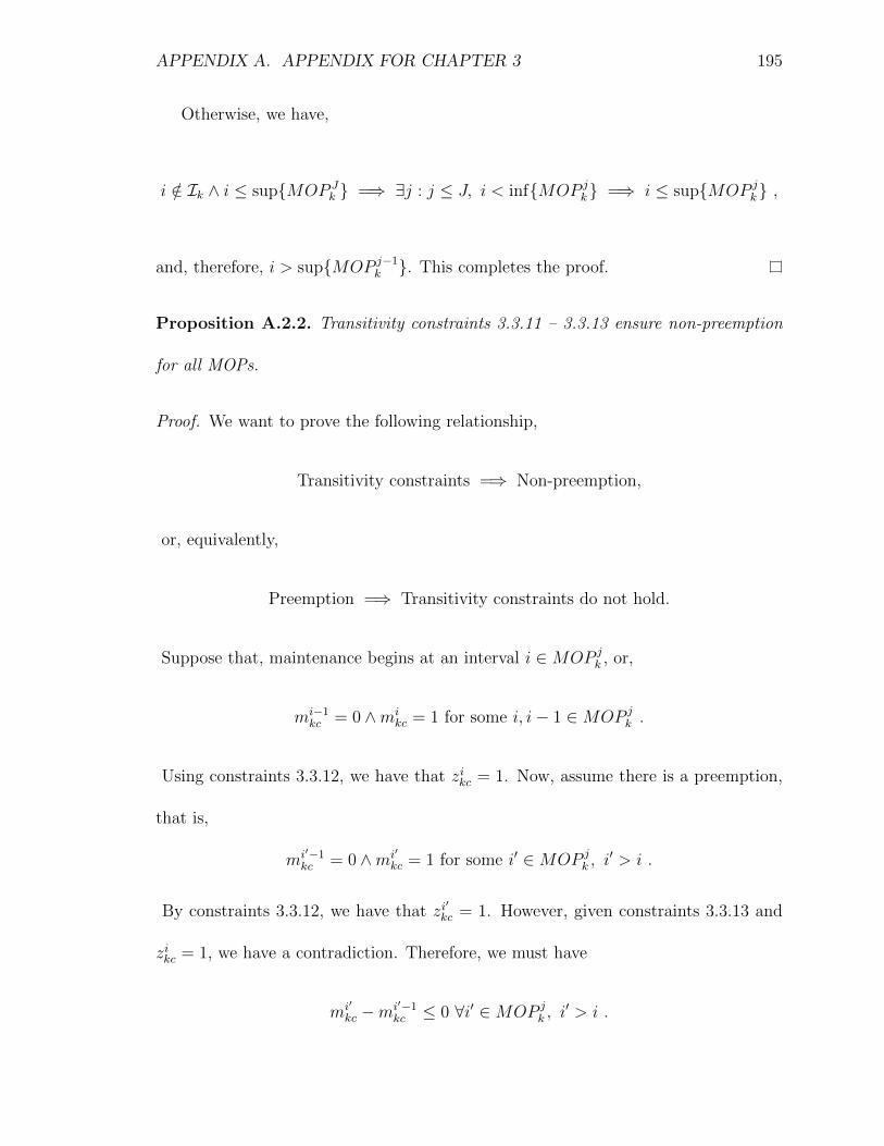
APPENDIX A. APPENDIX FOR CHAPTER 3 195
Otherwise, we have,
i /∈ Ik ∧ i ≤ sup{MOP Jk } =⇒ ∃j : j ≤ J, i < inf{MOP j
k} =⇒ i ≤ sup{MOP jk} ,
and, therefore, i > sup{MOP j−1k }. This completes the proof.
Proposition A.2.2. Transitivity constraints 3.3.11 – 3.3.13 ensure non-preemption
for all MOPs.
Proof. We want to prove the following relationship,
Transitivity constraints =⇒ Non-preemption,
or, equivalently,
Preemption =⇒ Transitivity constraints do not hold.
Suppose that, maintenance begins at an interval i ∈MOP jk , or,
mi−1kc = 0 ∧mi
kc = 1 for some i, i− 1 ∈MOP jk .
Using constraints 3.3.12, we have that zikc = 1. Now, assume there is a preemption,
that is,
mi′−1kc = 0 ∧mi′
kc = 1 for some i′ ∈MOP jk , i
′ > i .
By constraints 3.3.12, we have that zi′
kc = 1. However, given constraints 3.3.13 and
zikc = 1, we have a contradiction. Therefore, we must have
mi′
kc −mi′−1kc ≤ 0 ∀i′ ∈MOP j
k , i′ > i .
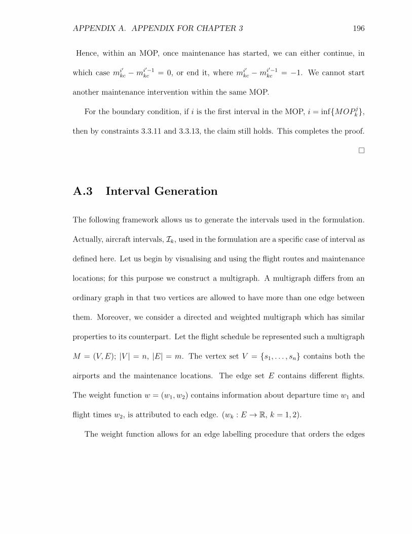
APPENDIX A. APPENDIX FOR CHAPTER 3 196
Hence, within an MOP, once maintenance has started, we can either continue, in
which case mi′
kc − mi′−1kc = 0, or end it, where mi′
kc − mi′−1kc = −1. We cannot start
another maintenance intervention within the same MOP.
For the boundary condition, if i is the first interval in the MOP, i = inf{MOP jk},
then by constraints 3.3.11 and 3.3.13, the claim still holds. This completes the proof.
A.3 Interval Generation
The following framework allows us to generate the intervals used in the formulation.
Actually, aircraft intervals, Ik, used in the formulation are a specific case of interval as
defined here. Let us begin by visualising and using the flight routes and maintenance
locations; for this purpose we construct a multigraph. A multigraph differs from an
ordinary graph in that two vertices are allowed to have more than one edge between
them. Moreover, we consider a directed and weighted multigraph which has similar
properties to its counterpart. Let the flight schedule be represented such a multigraph
M = (V,E); |V | = n, |E| = m. The vertex set V = {s1, . . . , sn} contains both the
airports and the maintenance locations. The edge set E contains different flights.
The weight function w = (w1, w2) contains information about departure time w1 and
flight times w2, is attributed to each edge. (wk : E → R, k = 1, 2).
The weight function allows for an edge labelling procedure that orders the edges

APPENDIX A. APPENDIX FOR CHAPTER 3 197
...sp sq
e1
en
e2
Figure A.1: Example of edge labelling for flights between airports sp and sq.
by departure time,
w1(e1) ≤ w1(e2) ≤ · · · ≤ w1(eN) ≤ · · · ≤ w1(eM).
Clearly, this edge labelling, which we denote as LE, is unique.
ejei
t(ei) = s(ej) t(ej)s(ei)
u v y
Figure A.2: Incident edges with source and sink functions.
Since we do not need to now exactly where each aircraft is at every period of
time, but rather, how it’s engines are being used and when it’s next maintenance
opportunity might be. We can narrow down the network to remove all the unnecessary
airports and group the into a supersource and a supersink. Let S ⊆ V be a set of
locations which can perform at least one type of maintenance check, with
ES = {e : e ∈ E, t(e) = s ∨ s(e) = s for some s ∈ S},

APPENDIX A. APPENDIX FOR CHAPTER 3 198
let |ES| = Q and LES⊆ LE be the corresponding labelling alphabet. Where s(·) and
t(·) are the ordinary source and sink functions. For notation purposes, we map the
labelling alphabet LESto a set of integers LQ = {1, . . . , Q} with ei ∈ LES
→ i ∈ LQ.
We can construct a refined incidence matrix “edge-adjacency” (Zoethout, 2015),
Q, as follows
q(i,j) =
1, If i < j ∧ t(ei) = s(ej) ∧ w1(ei) + w2(ei) + TAT < w1(ej)
0, Otherwise
Therefore, Q is a Q×Q strictly upper triangular matrix containing nonzero elements
only if the turn-around-time (TAT) (time from arrival to the next departure) is large
enough. That is, if flight j’s departure is at a later time than i’s (i < j) and the
arrival of flight i plus some TAT is less than the departure time of flight j; then we
may consider employing this time window for maintenance. Hence, we have identified
a maintenance opportunity. The values of the TAT can make Q represent either
a more relaxed feasible flight connections or a more restrictive (and perhaps more
robust) feasible intervals for maintenance checks.
We now show that N is linear in Q, the number of flights strictly between main-
tenance sites. Since N determines the number of variables, as they are indexed by
intervals, this proposition shows that the model is tractable for a reasonable Q.
Proposition A.3.1. An upper bound for N , the number of intervals, is
0 < N ≤ min{∆+,∆−}Q�⌊Q2 −Q
2
⌋

APPENDIX A. APPENDIX FOR CHAPTER 3 199
where ∆ denotes the maximum indegree (+) and outdegree (−) of the vertices in S.
Proof. For every edge in ei ∈ ES we can easily identify the outdegree of its sink vertex,
that is degout(t(ei)). Each row i of matrix Q represents the possible connections for
flight ei. For each of these, the maximum number of possible connections is the
outdegree of the sink vertex. For clarity, we drop the tilde notation. By the edge
labelling, a connection between ei and ej is not possible if j ≤ i. Thus, we can reduce
the initial number of connections for each flight ei to
Q∑j=i+1
q(i,j) ≤ degout(t(ei))− |Et(ei)|. (A.3.1)
Where Et(ei) = {ej : ej ∈ ES, j > i, t(ei) = s(ej)}. For completeness, we also need
to count the outdegree of the edges ingoing and outgoing to vertices in the set of
maintenance locations S we can define a super source S and a super sink T . For
every e ∈ ES if s(e) 6∈ S then s(e) = S, if t(e) 6∈ S then t(e) = T ; let S ′ = S ∪{S, T}.
The upper bound comes from considering the sum of all the nonzero elements in
the part of the upper triangular matrix Q, if every single element was 1, then the
total number of elements would be⌊Q2−Q
2
⌋. However, this is not the case and we can
sum equation A.3.1 to represent the total number of all the nonzero elements in the
matrix Q i.e. the size of P . Thus,
Q∑i=1
Q∑j=i+1
q(i,j) = N ≤Q∑i=1
[degout(t(ei))− |Et(ei)|
]=
Q∑i=1
degout(t(ei))−Q∑i=1
|Et(ei)|
(A.3.2)
Now, we can expand the first sum in equation A.3.2 of the RHS directly in terms of

APPENDIX A. APPENDIX FOR CHAPTER 3 200
the vertices as opposed to the sink of the edges. That is,
Q∑i=1
degout(t(ei)) =∑s∈S′
degout(s)degin(s)
now, by the first theorem of multigraph theory. equivalent to hand-shaking lemma
(Van Steen, 2010), and by Abel’s inequality (Dragomir et al., 1998), we get,
∑s∈S′
degout(s)degin(s) ≤ min{∆+,∆−}Q
by commutativity in the product of the non-negative degree functions.
For the second term in equation A.3.2, we have max{|Et(ei)|
}= degout(t(ei)) ≤ ∆+
and min{|Et(ei)|
}= 0. The result follows.

Appendix B
Appendix for Chapter 4
B.1 Functions Employed in Metaheuristic Algo-
rithms
B.1.1 Algorithm 3
The function employed in Algorithms 3 is defined as,
function getDirection(F, B)if F 6= ∅ and B = ∅ then
direction = forwardelse if F = ∅ and B 6= ∅ then
direction = backwardelse if F 6= ∅ and B 6= ∅ then
Randomly set direction to be either forward or backward.else
direction = Noneend if
end function
201

APPENDIX B. APPENDIX FOR CHAPTER 4 202
B.1.2 Algorithms 5 and 6
The shortest path function employed in Algorithms 5 and 6 is defined as,
function ShortestPath(i, j, G)Apply A* search algorithm to find the shortest path between nodes i and j, in
G.end function
The functions employed in Algorithm 5 are as follows,
function UpdatePath(neighbour, p)if iter= 0 then
path= pif neighbour in path then
Concatenate elements in path, up until neighbour, with pelse
Concatenate elements in path, up until an element node such that anedge (node, neighbour) exists in G, with p
end ifend if
end function
function GetNeighbour(edgesToCheck, neighbourhood, g)if edgesToCheck is not empty then . There still remains edges to try
if g in edgesToCheck then . If edge has not already been checkedcurrentEdge = g
else if h(g) = Source then . If the source has been reachedstop = True . Terminate the algorithmreturn
else . Otherwise try an edge from the predecessor array of edgescurrentEdge, neighbourhood = GetNextNeighbouringEdge(neighbourhood,
tabu)end if
elsestop= True . Stop if all edges have been removedreturn
end ifRemove currentEdge from edgesToCheck and set its weight to M (input large
number)return currentEdge, edgesToCheck, neighbourhood
end function
function GetNextNeighbouringEdge(neighbourhood, l)if neighbourhood is empty then

APPENDIX B. APPENDIX FOR CHAPTER 4 203
Update neighbourhood with all edges e′ in A if t(e′) = h(l)Sort neighbourhood in increasing order by edge cost
end ifLet edge be the last element in neighbourhood and remove it from neighbourhood
return edge, neighbourhoodend function
B.1.3 Algorithm 7
The functions employed in Algorithm 7 are as follows,
function ConstructSolution(.)candidates, RCL = [ ] . Initialise local arrayssolution = Sample(V ) . Initialise solution array by sampling a random nodewhile |solution| < |V | do . While solution does not contain all nodes
Populate candidates array using all nodes not in solution
candidate = GetRCL(candidates, solution)solution = solution ∪ candidate
end whilereturn solution
end function
function GetRCL(candidates, solution). Constructs a restricted candidate list (RCL) and returns one candidatecosts = [ ] . Initialise local arraysPopulate costs with the cost between each node in candidates and the last
node in solution
for node n in candidates doif costs[n] ≤ min(costs) + α(max(costs)−min(costs)) then
Add node n to RCL
end ifend forreturn random node in RCL
end function
function LocalSearch(solution). Conducts local search to return a valid pathlocaliter= 0 . Initialise local iteration counterwhile localiter < maxiterLocal do
Find a path in G using random sized samples of permutations of the nodesin solution.
Save the path as candidate
if c(candidate) < c(solution) and candidate is resource feasible then

APPENDIX B. APPENDIX FOR CHAPTER 4 204
solution = candidate
end iflocaliter = localiter + 1 . Increment local iteration counter
end whilereturn solution
end function
B.2 Parameters in the Computational Tests
Table B.1 reveals the precise aircraft makes and types for each test instance, their
respective range, standard total operational costs (as given by FAA, 2013) and oper-
ational costs under delay (as given by Cook and Tanner, 2015). For illustration and
recalling the notation from Section 4.3.3, for a given subproblem k, with the make of
aircraft k being DH8D, then, the standard total operating cost for a scheduled flight
is cstk = $922 (around e823 at the current exchange rate), the cost for non-scheduled
ground connections is cgwk = e540, and, the operating cost under delay for flight delay
copies is codk = e1630.
Table B.2 summarises the parameters employed in the computational tests. First,
the cancellation cost, captured in the costs of the initial schedules in the column
generation algorithm (in the notation of Section 4.3.3, cs where s ∈ S0), were given
by Palpant et al. (2009). The minimum duration of a crew duty break, breakMin,
is given by Federal Aviation Administration (2009). The minimum duration for a
maintenance intervention, maintMin, is given by Torres Sanchez et al. (n.d.). The
remaining parameters concern to the resource limits introduced in Section 4.3.3. These
ensure that the appropriate regulations are met. Please note that the values for
maintenance (FH) and crew duty rules (CD1, CD2) were given by Cook and Tanner

APPENDIX B. APPENDIX FOR CHAPTER 4 205
(2008) and Maher (2015), respectively.
Table B.1: Different aircraft types in test instances with their respective operatingcosts.
Operating Costs (per hour)
Aircraft Make Aircraft Type (Range) Inst.Standard
(cstk )Ground
(cgwk )
DelayedFlight(codk )
DH8D Turboprop (Short-haul) I1 $922 e540 e1630JS32 Turboprop (Short-haul) I2 $2887 e540 e1630A319 Narrow-body (Short/medium-haul) I1, I4 $9734 e810 e3420A320 Narrow-body (Short/medium-haul) I5 $9734 e900 e3490B738 Narrow-body (Short/medium-haul) I6 $10430 e1010 e3650B752 Narrow-body (Short/medium-haul) I6 $10430 e720 e4210A359 Wide-body (Long-haul) I3, I4 $13912 e1050 e4130B77L Wide-body (Long-haul) I6 $13912 e1310 e6230
Table B.2: Parameters for computational tests.
Parameter Representation Value
cs (s ∈ S0) Flight cancellation cost (per hour) e20000breakMin Minimum crew duty break 3 hoursmaintMin Minimum maintenance time 5 hours
FH Maximum flying hours betweenmaintenance (A check)
600 flyinghours
CD1 Maximum crew shift duration(Duty rule 1)
13 hours
CD2 Maximum crew flying hours with-out rest (Duty rule 2)
8 hours
APPENDIX B. APPENDIX FOR CHAPTER 4 206
B.3 cspy: A Python package with a collection of
algorithms for the (Resource) Constrained Short-
est Path problem
B.3.1 Introduction
When solving the shortest path problem and considering multiple operational restric-
tions, one may resort to the (resource) constrained shortest path (CSP) problem. It
consists, as its name suggests, in finding, among all paths, the shortest path from
source to sink nodes that satisfies a set of constraints for a defined set of resources.
Such set of resources and the way they evolve throughout the path are user defined
and controlled. This allows the modelling of a wide variety of problems including: the
vehicle routing problem with time windows, the technician routing and scheduling
problem, the capacitated arc-routing problem, on-demand transportation systems,
and, airport ground movement (Desrochers and Soumis, 1988; Feillet et al., 2004;
Irnich and Villeneuve, 2006; Righini and Salani, 2008; Bode and Irnich, 2014; Chen
et al., 2016; Garaix et al., 2010; Tilk et al., 2017; Zamorano and Stolletz, 2017).
cspy is a Python package that allows you to solve instances of the CSP problem
using up to eight different algorithms.
cspy is of interest to the operational research community and others that wish to
solve an instance of the CSP problem.

APPENDIX B. APPENDIX FOR CHAPTER 4 207
B.3.2 Algorithms
Even though the CSP problem is NP-hard (Garey and Johnson, 1990), several algo-
rithms have been developed to solve it. The most common algorithms are dynamic
programming labelling algorithms. Irnich and Desaulniers (2005) presented an exact
algorithm based on DP, the monodirectional forward labelling algorithm, based on
the pioneering work by Desrochers and Soumis (1988).
Advanced and efficient algorithms have been developed since. Boland et al. (2006)
published a state augmenting algorithm that uses a monodirectional labelling algo-
rithm to find an elementary path (one without repeating nodes). Such algorithm has
been implemented by Weyens (2018).
Righini and Salani (2006) introduced a bidirectional labelling algorithm for the
SPPRC. The bidirectional algorithm is an extension of the monodirectional algorithm
that supports search from both ends of the graph, hence, reducing the computational
efforts. More recently, Tilk et al. (2017) developed a bidirectional labelling algorithm
with dynamic halfway point. The bidirectional search is bounded for both directions
and these bounds are dynamically updated as the search in either direction advances.
The algorithm has shown to be significantly more efficient that monodirectional ones
(Gschwind et al., 2018).
Even with some of the most recent algorithms, solving an instance of the SPPRC
can be slow, thus, heuristic algorithms have been developed. Local search or meta-
heuristics start with a given path and perform a series of moves (edge/node deletion,
insertion, or exchange) to obtain another feasible path with lower cost. Some meta-
APPENDIX B. APPENDIX FOR CHAPTER 4 208
heuristics developed include, Tabu search (Desaulniers et al., 2008), hybrid particle
swarm algorithm (Marinakis et al., 2017), and, greedy randomised adaptive search
procedure (GRASP) (Ferone et al., 2019).
cspy implements several of these recent exact and metaheuristic algorithms in-
cluding:
• Bidirectional labeling algorithm with dynamic halfway point (Tilk et al., 2017);
which includes the bidirectional labeling algorithm with static halfway point,
and the monodirectional forward and backward labeling algorithms;
• Tabu search. Adapted from Desaulniers et al. (2008);
• Greedy elimination procedure;
• Greedy Randomised Adaptive Search Procedure (GRASP). Adapted from Fer-
one et al. (2019);
• Particle Swarm Optimization with combined Local and Global Expanding Neigh-
borhood Topology (PSOLGENT) (Marinakis et al., 2017).
B.4 Features
A key component of a CSP problem is to define a set of resources and a function to
apply for these to evolve through the graph. Such functions are typically referred to
as resource extension functions (REFs). The simplest REF is an additive one, where
every time an edge is traversed a constant unit of a certain resource is consumed.
However, custom and more generic REFs can be used.

APPENDIX B. APPENDIX FOR CHAPTER 4 209
cspy allows for custom and generic REFs to be used. Hence, allowing for a custom
consumption of the resources through the graph.
B.5 Example
Consider the following problem.
Example. Jane is part-time postwoman working in Delft, Netherlands. However,
she is assigned a small area (the Indische Buurt neighbourhood) so when planning
her daily route she wants to make it as long and exciting as possible. That is, when
planning her routes she has to consider the total shift time, sights visited, travel time,
and delivery time. Her shift has to be at most 5 hours.
This problem can easily be modelled as a CSP problem. With the description
above, the set of resources can be defined as,
1 R = [’sights ’, ’shift’, ’travel -time’, ’delivery -time’]
2 # len(R) = 4
Let G denote a directed graph with edges to/from all streets of the Indische Buurt
neighbourhood. Each edge has an attribute weight proportional to the distance (in
km) between the two nodes and an attribute res cost which is an array (specifically, a
numpy.array) with length len(R). To maximise the distance of the path, as required
by Jane, we simple negate the distance, hence, solving a shortest path problem with
negative distance will be the equivalent to solving a longest path problem. The
entries of res cost have the same order as the entries in R. The first entry of this
array, corresponds to the ’sights’ resource, i.e. how many sights there are along
a specific edge. The last entry of this array, corresponds to the ’delivery-time’
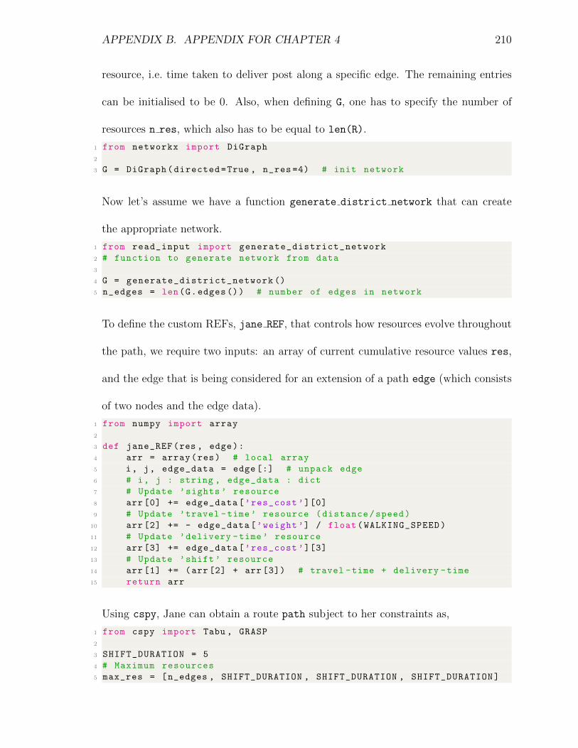
APPENDIX B. APPENDIX FOR CHAPTER 4 210
resource, i.e. time taken to deliver post along a specific edge. The remaining entries
can be initialised to be 0. Also, when defining G, one has to specify the number of
resources n res, which also has to be equal to len(R).
1 from networkx import DiGraph
2
3 G = DiGraph(directed=True , n_res =4) # init network
Now let’s assume we have a function generate district network that can create
the appropriate network.
1 from read_input import generate_district_network
2 # function to generate network from data
3
4 G = generate_district_network ()
5 n_edges = len(G.edges()) # number of edges in network
To define the custom REFs, jane REF, that controls how resources evolve throughout
the path, we require two inputs: an array of current cumulative resource values res,
and the edge that is being considered for an extension of a path edge (which consists
of two nodes and the edge data).
1 from numpy import array
2
3 def jane_REF(res , edge):
4 arr = array(res) # local array
5 i, j, edge_data = edge [:] # unpack edge
6 # i, j : string , edge_data : dict
7 # Update ’sights ’ resource
8 arr [0] += edge_data[’res_cost ’][0]
9 # Update ’travel -time’ resource (distance/speed)
10 arr [2] += - edge_data[’weight ’] / float(WALKING_SPEED)
11 # Update ’delivery -time’ resource
12 arr [3] += edge_data[’res_cost ’][3]
13 # Update ’shift ’ resource
14 arr [1] += (arr[2] + arr [3]) # travel -time + delivery -time
15 return arr
Using cspy, Jane can obtain a route path subject to her constraints as,
1 from cspy import Tabu , GRASP
2
3 SHIFT_DURATION = 5
4 # Maximum resources
5 max_res = [n_edges , SHIFT_DURATION , SHIFT_DURATION , SHIFT_DURATION]

APPENDIX B. APPENDIX FOR CHAPTER 4 211
6 # Minimum resources
7 min_res = [0, 0, 0, 0]
8 # Use Tabu Algorithm
9 path = Tabu(G, max_res , min_res , REF=jane_REF).run()
10 # Use GRASP algorithm
11 path = GRASP(G, max_res , min_res , REF=jane_REF).run()
Hence, each resource is restricted and updated as follows:
’sights’ : the cumulative number of sights visited has a dummy upper bound equal
to the number of edges in the graph as there is no restriction to as how many
sights Jane visits. Additionally, the value of this resource in the final path, will
provide us with the accumulated number of sights in the path;
’shift’ : the cumulative shift time is updated as the travel time along the edge
plus the delivery time, the upper bound of SHIFT DURATION ensures that Jane
doesn’t exceed her part-time hours;
’travel-time’ : the cumulative travel time is updated using the positive distance
travelled (-edge data[’weight’]) over an average walking speed. Given the re-
lationship between this resource and ’shift’, a maximum of the shift duration
provides no restriction.
’delivery-time’ : the cumulative delivery time is simply updated using edge data.
Similarly as for the previous resource, a maximum of the shift duration provides
no restriction.
If we wish to implement the bidirectional labelling algorithm, we have to invert
jane REF. In this case, it can be easily done,
1 def jane_REF_backward(res , edge):
2 arr = array(res) # local array

APPENDIX B. APPENDIX FOR CHAPTER 4 212
3 i, j, edge_data = edge [:] # unpack edge
4 # i, j : string , edge_data : dict
5 # Update ’sights ’ resource
6 arr [0] -= edge_data[’res_cost ’][0]
7 # Update ’travel -time’ resource (distance/speed)
8 arr [2] -= - edge_data[’weight ’] / float(WALKING_SPEED)
9 # Update ’delivery -time’ resource
10 arr [3] -= edge_data[’res_cost ’][3]
11 # Update ’shift ’ resource
12 arr [1] -= (arr[2] + arr [3]) # travel -time + delivery -time
13 return arr
Now we can run the bidirectional labelling algorithm for an exact solution
1 from cspy import BiDirectional
2
3 # Use BiDirectional algorithm
4 path = BiDirectional(G, max_res , min_res , REF_forward=jane_REF ,
5 REF_backward=jane_REF_backward).run()
To see a real implementation of this example, please see Torres Sanchez (2019b).

Bibliography
Abdelghany, K. F., Abdelghany, A. F. and Ekollu, G. (2008), ‘An integrated decision
support tool for airlines schedule recovery during irregular operations’, European
Journal of Operational Research 185(2), 825 – 848.
Ackert, S. (2011), The Relationship between an Aircraft’s Value and its Maintenance
Status, Technical report, Aircraft Monitor.
Afshar-Nadjafi, B. (2014), ‘Resource Constrained Project Scheduling Subject to Due
Dates: Preemption Permitted with Penalty’, Advances in Operations Research .
Afshar-Nadjafi, B. and Arani, M. (2014), ‘Multimode preemptive resource investment
problem subject to due dates for activities: Formulation and solution procedure’,
Advances in Operations Research .
Aircraft Analysis & Fleet Planning (2005), Can the 787 & A350 transform the eco-
nomics of long-haul services?, Technical report, Aircraft commerce.
Allamraju, H. (2014), ‘Flighradar24 Unofficial API: pyflightdata’. Accessed:
14/08/2019.
URL: http: // pyflightdata. readthedocs. io/ en/ latest/ about. html
Allen, S., Burke, E. K., Hyde, M. and Kendall, G. (2009), Evolving reusable 3d
213

BIBLIOGRAPHY 214
packing heuristics with genetic programming, in ‘Proceedings of the 11th Annual
conference on Genetic and evolutionary computation’, ACM, pp. 931–938.
Arguello, M. F. (1997), Framework for exact solutions and heuristics for approximate
solutions to airlines’ irregular operations control aircraft routing problem., PhD
thesis, The University of Texas at Austin.
Arguello, M. F., Bard, J. F. and Yu, G. (1997), ‘A GRASP for aircraft routing in re-
sponse to groundings and delays’, Journal of Combinatorial Optimization 1(3), 211–
228.
Arıkan, U., Gurel, S. and Akturk, M. S. (2016), ‘Integrated aircraft and passenger re-
covery with cruise time controllability’, Annals of Operations Research 236(2), 295–
317.
Arıkan, U., Gurel, S. and Akturk, M. S. (2017), ‘Flight network-based approach
for integrated airline recovery with cruise speed control’, Transportation Science
51(4), 1259–1287.
Bae, K. H. (2010), Integrated airline operations: schedule design, fleet assignment, air-
craft routing, and crew scheduling, PhD thesis, Faculty of the Virginia Polytechnic
Institute and State University.
Bard, J. F., Yu, G. and Arguello, M. F. (2001), ‘Optimizing aircraft routings in
response to groundings and delays’, IIE Transactions 33(10), 931–947.
Barnhart, C., Boland, N. L., Clarke, L. W., Johnson, E. L., Nemhauser, G. L. and

BIBLIOGRAPHY 215
Shenoi, R. G. (1998), ‘Flight String Models for Aircraft Fleeting and Routing’,
Transportation Science 32(3), 208–220.
Barnhart, C., Cohn, A. M., Johnson, E. L., Klabjan, D., Nemhauser, G. L. and Vance,
P. H. (2003), Airline crew scheduling, in ‘Handbook of transportation science’,
Springer, pp. 517–560.
Bisaillon, S., Cordeau, J.-F., Laporte, G. and Pasin, F. (2011), ‘A large neighbourhood
search heuristic for the aircraft and passenger recovery problem’, 4OR 9(2), 139–
157.
Bode, C. and Irnich, S. (2014), ‘The shortest-path problem with resource constraints
with (k, 2)-loop elimination and its application to the capacitated arc-routing prob-
lem’, European Journal of Operational Research 238(2), 415–426.
Boland, N., Dethridge, J. and Dumitrescu, I. (2006), ‘Accelerated label setting algo-
rithms for the elementary resource constrained shortest path problem’, Operations
Research Letters 34(1), 58–68.
Bratu, S. and Barnhart, C. (2006), ‘Flight operations recovery: New approaches
considering passenger recovery’, Journal of Scheduling 9(3), 279–298.
Brucker, P., Drexl, A., Mohring, R., Neumann, K. and Pesch, E. (1999), ‘Resource-
constrained project scheduling: Notation, classification, models, and methods’, Eu-
ropean Journal of Operational Research 112(1), 3–41.
Brucker, P. and Knust, S. (2012), Complex Scheduling, 2nd edn, Heidelberg: Springer
Berlin Heidelberg, Berlin.

BIBLIOGRAPHY 216
Burke, E. K., De Causmaecker, P., De Maere, G., Mulder, J., Paelinck, M. and Van-
den Berghe, G. (2010), ‘A multi-objective approach for robust airline scheduling’,
Comput. Oper. Res. 37(5), 822–832.
Burke, E. K., Gendreau, M., Hyde, M., Kendall, G., Ochoa, G., Ozcan, E. and
Qu, R. (2013), ‘Hyper-heuristics: A survey of the state of the art’, Journal of the
Operational Research Society 64(12), 1695–1724.
Burke, E. K., Hyde, M. R., Kendall, G., Ochoa, G., Ozcan, E. and Woodward, J. R.
(2019), A classification of hyper-heuristic approaches: Revisited, in ‘Handbook of
Metaheuristics’, Springer, pp. 453–477.
Burke, E. K., Kendall, G. and Soubeiga, E. (2003), ‘A tabu-search hyperheuristic for
timetabling and rostering’, Journal of heuristics 9(6), 451–470.
Burke, E. K., McCollum, B., Meisels, A., Petrovic, S. and Qu, R. (2007), ‘A graph-
based hyper-heuristic for educational timetabling problems’, European Journal of
Operational Research 176(1), 177–192.
Cacchiani, V. and Salazar-Gonzalez, J.-J. (2016), ‘Optimal solutions to a real-world
integrated airline scheduling problem’, Transp. Sci. 51(1), 250–268.
Cadarso, L., Vaze, V., Barnhart, C. and Marın, A. (2016), ‘Integrated airline schedul-
ing: considering competition effects and the entry of the high speed rail’, Transp.
Sci. 51(1), 132–154.
Cardillo, A., Zanin, M., Gomez-Gardenes, J., Romance, M., Garcıa del Amo, A. J.
and Boccaletti, S. (2013), ‘Modeling the multi-layer nature of the European Air

BIBLIOGRAPHY 217
Transport Network: Resilience and passengers re-scheduling under random failures’,
Eur. Phys. J. Spec. Top. 215(1), 23–33.
Chen, J., Weiszer, M., Stewart, P. and Shabani, M. (2016), ‘Toward a More Realistic,
Cost-Effective, and Greener Ground Movement Through Active RoutingPart I: Op-
timal Speed Profile Generation’, IEEE Transactions on Intelligent Transportation
Systems 17(5), 1196–1209.
Christer, A. H., Wang, W., Sharp, J. and Baker, R. (1998), ‘A case study of modelling
preventive maintenance of a production plant using subjective data’, J. Oper. Res.
Soc. 49(3), 210–219.
Chryssolouris, G., Pierce, J. E. and Dicke, K. (1992), ‘A decision-making approach to
the operation of flexible manufacturing systems’, Int. J. Flex. Manuf. Syst. 4, 309–
330.
Clarke, L., Johnson, E., Nemhauser, G. and Zhu, Z. (1997), ‘The aircraft rotation
problem’, Annals of Operations Research 69(0), 33–46.
Clausen, J., Larsen, A., Larsen, J. and Rezanova, N. J. (2010), ‘Disruption man-
agement in the airline industry– Concepts, models and methods’, Computers &
Operations Research 37(5), 809–821.
Coffman, E. G., Ng, C. T. and Timkovsky, V. G. (2015), ‘How small are shifts required
in optimal preemptive schedules?’, Journal of Scheduling 18(2), 155–163.
Cohn, A. M. and Barnhart, C. (2003), ‘Improving Crew Scheduling by Incorporating
Key Maintenance Routing Decisions’, Operations Research 51(3), 387–396.

BIBLIOGRAPHY 218
Cook, A. and Tanner, G. (2008), Innovative Cooperative Actions of R&D in EURO-
CONTROL Programme CARE INO III: Dynamic Cost Indexing: Aircraft mainte-
nance – marginal delay costs, Technical report, Transport Studies Group, University
of Westminster.
Cook, A. and Tanner, G. (2015), European airline delay cost reference values: Up-
dated and extended values, Technical report, University of Westminster.
Cordeau, J.-F., Stojkovic, G., Soumis, F. and Desrosiers, J. (2001), ‘Benders Decom-
position for Simultaneous Aircraft Routing and Crew Scheduling’, Transportation
Science 35(4), 375–388.
Creemers, S. (2019), ‘The preemptive stochastic resource-constrained project schedul-
ing problem’, European Journal of Operational Research 277(1), 238–247.
Dantzig, G. B. and Wolfe, P. (1960), ‘Decomposition principle for linear programs’,
Operations Research 8(1), 101–111.
Demassey, S., Artigues, C. and Michelon, P. (2005), ‘Constraint-Propagation-Based
Cutting Planes: An Application to the Resource-Constrained Project Scheduling
Problem’, INFORMS Journal on Computing 17(1), 52–65.
Department for BIS (2016), ‘UK Aerospace Maintenance, Repair, Overhaul & Logis-
tics Industry Analysis’, BIS Rearch Paper Number 275 .
DePold, H. R. and Gass, F. D. (1998), The application of expert systems and neural
networks to gas turbine prognostics and diagnostics, in ‘International Gas Turbine
& Aeroengine Congress & Exhibition Stockholm, Sweden’.

BIBLIOGRAPHY 219
Desaulniers, G., Desrosiers, J., Dumas, Y., Solomon, M. M. and Soumis, F. (1997),
‘Daily aircraft routing and scheduling’, Management Science 43(6), 841–855.
Desaulniers, G., Lessard, F. and Hadjar, A. (2008), ‘Tabu search, partial elementar-
ity, and generalized k-path inequalities for the vehicle routing problem with time
windows’, Transportation Science 42(3), 387–404.
Desrochers, M. (1986), La Fabrication d’Horaires de Travail pour les Conducteurs
d’Autobus par une Methode de Generation de Colonnes, PhD thesis, Centre de
recherche sur les Transports, Universite de Montreal, Montreal, Canada.
Desrochers, M. and Soumis, F. (1988), ‘A Generalized Permanent Labelling Algo-
rithm For The Shortest Path Problem With Time Windows’, INFOR: Information
Systems and Operational Research 26, 191–212.
Doerr, B., Lissovoi, A., Oliveto, P. S. and Warwicker, J. A. (2018), On the runtime
analysis of selection hyper-heuristics with adaptive learning periods, in ‘Proceedings
of the Genetic and Evolutionary Computation Conference’, ACM, pp. 1015–1022.
Dragomir, S. S., Pearce, C. E. M. and Sunde, J. (1998), ‘Abel–type inequalities,
complex numbers and Gauss–Polya type integral inequalities’, Mathematical Com-
munications 3, 95–101.
Eggenberg, N., Salani, M. and Bierlaire, M. (2010), ‘Constraint-specific recovery
network for solving airline recovery problems’, Computers & Operations Research
37(6), 1014 – 1026.
BIBLIOGRAPHY 220
Eurocontrol (2011), Study into the impact of the global economic crisis on airframe
utilisation., Technical report, Central Office for Delay Analysis, EUROCONTROL.
Accessed: 14/08/2019.
URL: https: // tinyurl. com/ yy57elfa
European Parliament and Council of the European Union (2004), ‘Regulation (EC)
No 261/2004 of the European Parliament and Council of the European Union’,
Official Journal of the European Union 46(1), 1–7.
FAA (2013), Benefit-Cost Analysis. Section 4: Aircraft operating costs., Technical
report, Federal Aviation Administration.
Federal Aviation Administration (2009), ‘Flightcrew Member Duty and Rest Require-
ments’, Federal Aviation Administration (FAA), DOT. .
Feillet, D., Dejax, P., Gendreau, M. and Gueguen, C. (2004), ‘An exact algorithm
for the elementary shortest path problem with resource constraints: Application to
some vehicle routing problems’, Networks 44(3), 216–229.
Feillet, D., Gendreau, M. and Rousseau, L.-M. (2007), ‘New Refinements for the
Solution of Vehicle Routing Problems with Branch and Price’, INFOR: Information
Systems and Operational Research 45(4), 239–256.
Feo, T. A. and Bard, J. F. (1989), ‘Flight scheduling and maintenance base planning’,
Management Science 35(12), 1415–1432.
Ferone, D., Festa, P. and Guerriero, F. (2019), ‘An efficient exact approach for the con-
https://www.faa.gov/regulations_policies/rulemaking/recently_published/media/2120-AJ58-FinalRule.pdf

BIBLIOGRAPHY 221
strained shortest path tour problem’, Optimization Methods and Software 0(0), 1–
20.
Flightradar24 AB (2018), ‘Flightradar24’. Accessed: 14/08/2019.
URL: https: // www. flightradar24. com/
Floudas, C. A. and Lin, X. (2004), ‘Continuous-time versus discrete-time approaches
for scheduling of chemical processes: A review’, Computers and Chemical Engineer-
ing 28(11), 2109–2129.
Floudas, C. A. and Lin, X. (2005), ‘Mixed integer linear programming in process
scheduling: Modeling, algorithms, and applications’, Annals of Operations Research
139(1), 131–162.
Garaix, T., Artigues, C., Feillet, D. and Josselin, D. (2010), ‘Vehicle routing problems
with alternative paths: An application to on-demand transportation’, European
Journal of Operational Research 204(1), 62 – 75.
Garey, M. R. and Johnson, D. S. (1990), Computers and Intractability; A Guide to
the Theory of NP-Completeness, W. H. Freeman & Co., New York, NY, USA.
Gopalan, R. and Talluri, K. T. (1998), ‘The Aircraft Maintenance Routing Problem’,
Operations Research 46(2), 260–271.
Grall, A., Berenguer, C. and Dieulle, L. (2002), ‘A condition-based maintenance policy
for stochastically deteriorating systems’, Reliab. Eng. Syst. Saf. 76(2), 167–180.
Grall, A., Dieulle, L., Berenguer, C. and Roussignol, M. (2002), ‘Continuous-time

BIBLIOGRAPHY 222
predictive-maintenance scheduling for a deteriorating system’, IEEE Trans. Reliab.
51(2), 141–150.
Gronkvist, M. (2005), The tail assignment problem, PhD thesis, Goteburg University.
Gschwind, T., Irnich, S., Rothenbacher, A.-K. and Tilk, C. (2018), ‘Bidirectional
labeling in column-generation algorithms for pickup-and-delivery problems’, Euro-
pean Journal of Operational Research 266(2), 521–530.
Gurkan, H., Gurel, S. and Akturk, M. S. (2016), ‘An integrated approach for airline
scheduling, aircraft fleeting and routing with cruise speed control’, Transp. Res.
Part C Emerg. Technol. 68, 38–57.
Gurobi Optimization version 8.1, I. (2019), ‘Gurobi Optimizer Reference Manual’.
Accessed: 14/08/2019.
URL: http: // www. gurobi. com
Habibi, F., Barzinpour, F. and Sadjadi, S. (2018), ‘Resource-Constrained Project
Scheduling Problem: Review of Past and Recent Developments’, Journal of Project
Management 3(2), 55–88.
Hane, C. A., Barnhart, C., Johnson, E. L., Marsten, R. E., Nemhauser, G. L. and
Sigismondi, G. (1993), ‘The fleet assignment problem: solving a large-scale integer
program’, Mathematical Programming 70(1-3), 211–232.
Haouari, M., Shao, S. and Sherali, H. D. (2013), ‘A Lifted Compact Formula-
tion for the Daily Aircraft Maintenance Routing Problem’, Transportation Science
47(4), 508–525.

BIBLIOGRAPHY 223
Heng, A., Zhang, S., Tan, A. C. and Mathew, J. (2009), ‘Rotating machinery prog-
nostics: State of the art, challenges and opportunities’, Mech. Syst. Signal Process.
23(3), 724–739.
Hicks, R., Madrid, R., Milligan, C., Pruneau, R., Kanaley, M., Dumas, Y., Lacroix,
B., Desrosiers, J. and Soumis, F. (2005), ‘Bombardier Flexjet Significantly Improves
Its Fractional Aircraft Ownership Operations’, Interfaces 35(1), 49–60.
IATA (2019), AVIATION DATA WHITE PAPER SERIES, Technical report, INTER-
NATIONAL AIR TRANSPORT ASSOCIATION (IATA).
Irnich, S. (2008), ‘Resource extension functions: Properties, inversion, and general-
ization to segments’, OR Spectrum 30(1), 113–148.
Irnich, S. and Desaulniers, G. (2005), Column Generation, Springer US, chapter Short-
est Path Problems with Resource Constraints, pp. 33–65.
Irnich, S. and Villeneuve, D. (2006), ‘The Shortest-Path Problem with Resource Con-
straints and k-Cycle Elimination for k ≥ 3’, INFORMS Journal on Computing
18(3), 391–406.
Jardine, A. K. S., Lin, D. and Banjevic, D. (2006), ‘A review on machinery diagnostics
and prognostics implementing condition-based maintenance’.
Jarrah, A. I., Yu, G., Krishnamurthy, N. and Rakshit, A. (1993), ‘A decision sup-
port framework for airline flight cancellations and delays’, Transportation Science
27(3), 266–280.

BIBLIOGRAPHY 224
Jayabalan, V. and Chaudhuri, D. (1992), ‘Cost optimisation of maintenance schedul-
ing for a system with assured reliability’, IEEE Trans. Reliab. 41(1), 21–25.
Jhwei, R., Aranki, N., Feldkamp, L. and Marko, K. (2008), ‘Ultra-compact neuropro-
cessor for automotive diagnostics and control’.
Keller, R. E. and Poli, R. (2007), Cost-benefit investigation of a genetic-programming
hyperheuristic, in ‘International Conference on Artificial Evolution (Evolution Ar-
tificielle)’, Springer, pp. 13–24.
Kenan, N., Jebali, A. and Diabat, A. (2018), ‘The integrated aircraft routing problem
with optional flights and delay considerations’, Transportation Research Part E:
Logistics and Transportation Review 118, 355–375.
Khaled, O., Minoux, M., Mousseau, V., Michel, S. and Ceugniet, X. (2018), ‘A Com-
pact Otimization Model for the Tail Assignment Problem’, European Journal of
Operational Research 264(2), 548–557.
Kolisch, R. and Sprecher, A. (1997), ‘PSPLIB - A project scheduling problem li-
brary: OR Software - ORSEP Operations Research Software Exchange Program’,
European Journal of Operational Research 96(1), 205 – 216.
Kone, O., Artigues, C., Lopez, P. and Mongeau, M. (2011), ‘Event-based MILP mod-
els for resource-constrained project scheduling problems’, Computers & Operations
Research 38, 3–13.
Kone, O., Artigues, C., Lopez, P. and Mongeau, M. (2013), ‘Comparison of mixed
integer linear programming models for the resource-constrained project schedul-

BIBLIOGRAPHY 225
ing problem with consumption and production of resources’, Flexible Services and
Manufacturing Journal 25(1-2), 25–47.
Kopanos, G. M., Kyriakidis, T. S. and Georgiadis, M. C. (2014), ‘New continuous-
time and discrete-time mathematical formulations for resource-constrained project
scheduling problems’, Computers & Chemical Engineering 68, 96 – 106.
Kumar, R., Joshi, A. H., Banka, K. K. and Rockett, P. I. (2008), Evolution of hy-
perheuristics for the biobjective 0/1 knapsack problem by multiobjective genetic
programming, in ‘Proceedings of the 10th annual conference on Genetic and evolu-
tionary computation’, ACM, pp. 1227–1234.
Lagerholm, M., Peterson, C. and Sderberg, B. (2000), ‘Airline crew scheduling using
Potts mean field techniques’, European Journal of Operational Research 120(1), 81–
96.
Lee, L. H., Lee, C. U. and Tan, Y. P. (2006), ‘A multi-objective genetic algorithm
for robust flight scheduling using simulation’, European Journal of Operational Re-
search 177(3), 1948–1968.
Lettovsky, L. (1997), Airline operations recovery: An optimization approach., PhD
thesis, School of Industrial and Systems Engineering, Georgia Institute of Technol-
ogy, Atlanta, GA.
Lettovsky, L., Johnson, E. L. and Nemhauser, G. L. (2000), ‘Airline Crew Recovery’,
Transportation Science 34(4), 337–348.

BIBLIOGRAPHY 226
Levin, A. (1971), ‘Scheduling and Fleet Routing Models for Transportation Systems’,
Transportation Science 5(3), 232–255.
Li, H., Wang, Y., Li, S. and Li, S. (2015), ‘A column generation based hyper-heuristic
to the bus driver scheduling problem’, Discrete Dynamics in Nature and Society
2015.
Li, Z., Guo, J. and Zhou, R. (2016), Maintenance scheduling optimization based on
reliability and prognostics information, in ‘Annual Reliability and Maintainability
Symposium (RAMS)’, pp. 1–5.
Liang, Z. and Chaovalitwongse, W. (2013), ‘A Network-Based Model for the In-
tegrated Weekly Aircraft Maintenance Routing and Fleet Assignment Problem’,
Transportation Science 47, 493–507.
Liang, Z., Xiao, F., Qian, X., Zhou, L., Jin, X., Lu, X. and Karichery, S. (2018),
‘A column generation-based heuristic for aircraft recovery problem with airport
capacity constraints and maintenance flexibility’, Transportation Research Part B:
Methodological 113, 70–90.
Liu, T.-K., Jeng, C.-R. and Chang, Y.-H. (2008), ‘Disruption management of an
inequality-based multi-fleet airline schedule by a multi-objective genetic algorithm’,
Transportation Planning and Technology 31(6), 613–639.
Løve, M., Sørensen, K., Larsen, J. and Clausen, J. (2001), ‘Using heuristics to solve
the dedicated aircraft recovery problem’, Optimization Online .

BIBLIOGRAPHY 227
Lozano, L., Duque, D. and Medaglia, A. L. (2015), ‘An Exact Algorithm for the Ele-
mentary Shortest Path Problem with Resource Constraints’, Transportation Science
50(1), 348–357.
Maher, S. J. (2015), ‘A novel passenger recovery approach for the integrated airline
recovery problem’, Computers & Operations Research 57, 123–137.
Maher, S. J. (2016), ‘Solving the Integrated Airline Recovery Problem Using Column-
and-Row Generation’, Transportation Science 50(1), 216–239.
Maher, S. J., Desaulniers, G. and Soumis, F. (2014), ‘Recoverable robust single day
aircraft maintenance routing problem’, Computers & Operations Research 51, 130–
145.
Maher, S. J., Desaulniers, G. and Soumis, F. (2018), ‘The daily tail assignment prob-
lem under operational uncertainty using look-ahead maintenance constraints’, Eu-
ropean Journal of Operational Research 264(2), 534–547.
Marinakis, Y., Migdalas, A. and Sifaleras, A. (2017), ‘A hybrid particle swarm
optimization–variable neighborhood search algorithm for constrained shortest path
problems’, European Journal of Operational Research 261(3), 819–834.
Marla, L., Vaaben, B. and Barnhart, C. (2016), ‘Integrated disruption management
and flight planning to trade off delays and fuel burn’, Transportation Science
51(1), 88–111.
Marseguerra, M., Zio, E. and Podofillini, L. (2002), ‘Condition-based maintenance
BIBLIOGRAPHY 228
optimization by means of genetic algorithms and Monte Carlo simulation’, Reliab.
Eng. Syst. Saf. 77(2), 151–166.
Martins, P. M. S. (2016), Systematization and optimization of Fokker 100 s Mainte-
nance Plan, Technical report, Instituto Superior Tecnico, Lisboa, Portugal.
Mercier, A., Cordeau, J. F. and Soumis, F. (2005), ‘A computational study of Benders
decomposition for the integrated aircraft routing and crew scheduling problem’,
Computers and Operations Research 32(6), 1451–1476.
Mercier, A. and Soumis, F. (2005), ‘An integrated aircraft routing, crew scheduling
and flight retiming model’, Computers and Operations Research 34(8), 2251–2265.
Minkowski, H. (1953), ‘Geometrie der Zahlen, Teubner, Leipzig, (1896)’, Reprint: H.
Minkowski, Geometrie der Zahlen, Chelsea .
Mueller, E. and Chatterji, G. B. (2002), Analysis of aircraft arrival and departure
delay characteristics, in ‘AIAA’s Aircraft Technology, Integration, and Operations
(ATIO)’, pp. 1–14.
Muter, I., Birbil, S. I. and Bulbul, K. (2013), ‘Simultaneous column-and-row gener-
ation for large-scale linear programs with column-dependent-rows’, Mathematical
Programming 142(1-2), 47–82.
Naber, A. (2017), ‘Resource-Constrained Project Scheduling with Flexible Resource
Profiles in Continuous Time’, Computers & Operations Research 84, 33–45.

BIBLIOGRAPHY 229
Nocedal, J. and Wright, S. (2006), Numerical Optimization: Springer Series in Op-
erations Research and Financial Engineering, Springer.
Ochoa, G., Walker, J., Hyde, M. and Curtois, T. (2012), Adaptive evolutionary al-
gorithms and extensions to the hyflex hyper-heuristic framework, in ‘International
Conference on Parallel Problem Solving from Nature’, Springer, pp. 418–427.
Orhan, I., Kapanoglu, M. and Karakoc, T. H. (2012), ‘Concurrent Aircraft Routing
and Maintenance Scheduling Using Goal Programming’, Journal of the Faculty of
Engineering and Architecture of Gazi University 27(1), 11–26.
Ozcan, E., Misir, M., Ochoa, G. and Burke, E. K. (2010), ‘A Reinforcement Learning -
Great-Deluge Hyper-Heuristic for Examination Timetabling’, International Journal
of Applied Metaheuristic Computing (IJAMC) 1(1), 39–59.
Palpant, M., Boudia, M., Robelin, C., Gabteni, S. and Laburthe, F. (2009), ‘ROADEF
2009 challenge: Disruption management for commercial aviation’, Sophia Antipolis,
France: Operations Research Division .
Papadakos, N. (2009), ‘Integrated airline scheduling’, Computers and Operations Re-
search 36(1), 176–195.
Papakostas, N., Papachatzakis, P., Xanthakis, V., Mourtzis, D. and Chryssolouris, G.
(2010), ‘An approach to operational aircraft maintenance planning’, Decis. Support
Syst. 48(4), 604–612.
Pecin, D., Pessoa, A., Poggi, M. and Uchoa, E. (2017), ‘Improved branch-cut-and-

BIBLIOGRAPHY 230
price for capacitated vehicle routing’, Mathematical Programming Computation
9(1), 61–100.
Peng, Z. and Chu, F. (2004), ‘Application of the wavelet transform in machine con-
dition monitoring and fault diagnostics: a review with bibliography’, Mechanical
Systems and Signal Processing 18(2), 199–221.
Petersen, J. D., Slveling, G., Clarke, J.-P., Johnson, E. L. and Shebalov, S. (2012),
‘An Optimization Approach to Airline Integrated Recovery’, Transportation Science
46(4), 482–500.
Qantas (2016), ‘Qantas News Room: The A, C and D of Aircraft Maintenance.’.
Accessed: 14/08/2019.
URL: http: // www. qantasnewsroom. com. au/ roo-tales/
the-a-c-and-d-of-aircraft-maintenance/
Righini, G. and Salani, M. (2006), ‘Symmetry helps: Bounded bi-directional dynamic
programming for the elementary shortest path problem with resource constraints’,
Discrete Optimization 3(3), 255–273.
Righini, G. and Salani, M. (2008), ‘New dynamic programming algorithms for the
resource constrained elementary shortest path problem’, Networks 51(3), 155–170.
Rolls-Royce Holdings plc (2015), ‘Annual Report’. Accessed: 14/08/2019.
URL: http: // ar. rolls-royce. com/ 2015/
Rolls-Royce Holdings plc (2016), ‘Civil Aerospace: Service Solutions’. Accessed:
14/08/2019.

BIBLIOGRAPHY 231
URL: https: // www. rolls-royce. com/ products-and-services/
civil-aerospace/ aftermarket-services. aspx
Rolls-Royce Holdings plc (2017), ‘Rolls-Royce Data Storytelling Challenge’. Accessed:
22/08/2019.
URL: https: // cfms. org. uk/ media/ 240635/ 72777_ rr_ digital_ story_
telling_ challenge_ v4. pdf
Runka, A. (2009), Evolving an edge selection formula for ant colony optimization, in
‘Proceedings of the 11th Annual conference on Genetic and evolutionary computa-
tion’, ACM, pp. 1075–1082.
Safaei, N. and Jardine, A. K. (2018), ‘Aircraft routing with generalized maintenance
constraints’, Omega 80, 111 – 122.
Salazar-Gonzalez, J. J. (2014), ‘Approaches to solve the fleet-assignment, aircraft-
routing, crew-pairing and crew-rostering problems of a regional carrier’, Omega
(United Kingdom) 43, 71–82.
Sarac, A., Batta, R. and Rump, C. M. (2006), ‘A branch-and-price approach for op-
erational aircraft maintenance routing’, European Journal of Operational Research
175(3), 1850–1869.
Sousa, J. P. and Wolsey, L. A. (1992), ‘A time indexed formulation of non-preemptive
single machine scheduling problems’, Mathematical Programming 54(1-3), 353–367.
Sriram, C. and Haghani, A. (2003), ‘An optimization model for aircraft maintenance
scheduling and re-assignment’, Transp. Res. Part A Policy Pract. 37(1), 29–48.
BIBLIOGRAPHY 232
Thengvall, B. G., Bard, J. F. and Yu, G. (2000), ‘Balancing user preferences for
aircraft schedule recovery during irregular operations’, Iie Transactions 32(3), 181–
193.
Thengvall, B. G., Yu, G. and Bard, J. F. (2001), ‘Multiple fleet aircraft schedule re-
covery following hub closures’, Transportation Research Part A: Policy and Practice
35(4), 289–308.
Tilk, C., Rothenbacher, A. K., Gschwind, T. and Irnich, S. (2017), ‘Asymmetry mat-
ters: Dynamic half-way points in bidirectional labeling for solving shortest path
problems with resource constraints faster’, European Journal of Operational Re-
search 261(2), 530–539.
Torres Sanchez, D. (2019a), ‘cspy: A Python package with a collection of algorithms
for the (Resource) Constrained Shortest Path problem’.
URL: https: // github. com/ torressa/ cspy
Torres Sanchez, D. (2019b), ‘jpath: cspy example with Jane the postwoman’.
URL: https: // github. com/ torressa/ jpath
Torres Sanchez, D. (Under review), ‘cspy: A Python package with a collection of
algorithms for the (Resource) Constrained Shortest Path problem’, Journal of
Open Source Software .
URL: https: // joss. theoj. org/ papers/ 25eda55801a528b982d03a6a61f7730d
Torres Sanchez, D., Boyacı, B. and Zografos, K. G. (n.d.), ‘An Optimisation Frame-

BIBLIOGRAPHY 233
work for Airline Fleet Maintenance Scheduling with Tail Assignment Considera-
tions’, Transportation Research Part B: Methodological .
Urgaonkar, R., Kozat, U. C., Igarashi, K. and Neely, M. J. (2010), Dynamic resource
allocation and power management in virtualized data centers, in ‘Network Opera-
tions and Management Symposium, IEEE’, pp. 479–486.
Van Steen, M. (2010), ‘An introduction to graph theory and complex networks’, 144.
Weyens, T. (2018), ‘pylgrim – Elementary Shortest Path Problem with or without
Resource Constraint’. Accessed: 14/08/2019.
URL: https: // github. com/ ToonWeyens/ pylgrim
Yan, S. and Tseng, C.-H. (2002), ‘A passenger demand model for airline flight schedul-
ing and fleet routing’, Computers and Operations Research 29(11), 1559–1581.
Yan, S., Yang, T. H. and Chen, H. H. (2004), ‘Airline short-term maintenance man-
power supply planning’, Transp. Res. Part A Policy Pract. 38(9-10), 615–642.
Zamorano, E. and Stolletz, R. (2017), ‘Branch-and-price approaches for the Multi-
period Technician Routing and Scheduling Problem’, European Journal of Opera-
tional Research 257(1), 55–68.
Zapata, J. C., Hodge, B. M. and Reklaitis, G. V. (2008), ‘The multimode resource
constrained multiproject scheduling problem: Alternative formulations’, AIChE
Journal 54(8), 2101–2119.

BIBLIOGRAPHY 234
Zoethout, J. (2015), The edge adjacency matrix of a graph, Bachelor thesis, Univer-
siteit Utrecht.