A data mining approach to guide students through the enrollment process based on academic...

User Model User-Adap Inter (2011) 21:217–248DOI 10.1007/s11257-011-9098-4

ORIGINAL PAPER

A data mining approach to guide students throughthe enrollment process based on academic performance

César Vialardi · Jorge Chue · Juan Pablo Peche ·Gustavo Alvarado · Bruno Vinatea ·Jhonny Estrella · Álvaro Ortigosa

Received: 16 April 2010 / Accepted in revised form: 8 February 2011 /Published online: 6 March 2011© Springer Science+Business Media B.V. 2011

Abstract Student academic performance at universities is crucial for educationmanagement systems. Many actions and decisions are made based on it, specificallythe enrollment process. During enrollment, students have to decide which courses tosign up for. This research presents the rationale behind the design of a recommendersystem to support the enrollment process using the students’ academic performancerecord. To build this system, the CRISP-DM methodology was applied to data fromstudents of the Computer Science Department at University of Lima, Perú. One ofthe main contributions of this work is the use of two synthetic attributes to improvethe relevance of the recommendations made. The first attribute estimates the inherentdifficulty of a given course. The second attribute, named potential, is a measure of thecompetence of a student for a given course based on the grades obtained in related

C. Vialardi (B) · J. Chue · J. P. Peche · G. Alvarado · B. Vinatea · J. EstrellaFacultad de Ingeniería de Sistemas, Universidad de Lima, Lima, Perúe-mail: [email protected]

J. Chuee-mail: [email protected]

J. P. Pechee-mail: [email protected]

G. Alvaradoe-mail: [email protected]

B. Vinateae-mail: [email protected]

J. Estrellae-mail: [email protected]

Á. OrtigosaEscuela Politécnica Superior, Universidad Autónoma de Madrid, Madrid, Spaine-mail: [email protected]

123

218 C. Vialardi et al.

courses. Data was mined using C4.5, KNN (K-nearest neighbor), Naïve Bayes, Bag-ging and Boosting, and a set of experiments was developed in order to determine thebest algorithm for this application domain. Results indicate that Bagging is the bestmethod regarding predictive accuracy. Based on these results, the “Student Perfor-mance Recommender System” (SPRS) was developed, including a learning engine.SPRS was tested with a sample group of 39 students during the enrollment process.Results showed that the system had a very good performance under real-life conditions.

Keywords Data mining · Enrollment process · Supervised classification ·Machine learning · Recommender systems · Predictive accuracy

1 Introduction

In the context of higher education, the decisions taken during the enrollment processat the beginning of each academic term are a key issue in the successful completionof university degrees. However, even though many universities offer the opportunityto receive advice from an experienced teacher, most of the times the students makedecisions on their own; therefore, the process generally depends on their experience aswell as on the available information. Unfortunately, the students’ experience is ofteninsufficient to make these decisions, as they do not take into consideration the time,effort and academic skills required by a course.

Generally, the students try to take as many courses as possible, with the goal ofcompleting their studies as soon as possible. This direct approach leads to unbal-anced amounts of workload and many times increases the risk of failing some of thecourses. The university provides information about available courses, sections, sched-ules, classrooms and professors. However, implicit information about other students’previous experiences from past enrollments, as well as their outcomes, is usuallyignored.

The core of this research is the acquisition of knowledge from students’ academicperformance records. While this knowledge could be used in different ways, thiswork proposes a methodology to develop recommender systems able to guide stu-dents through the enrollment process starting from this knowledge. These systemsare similar to collaborative recommender systems (CRSs) and use recommendationengines based on data mining techniques. CRSs are agents that suggest options amongwhich users can choose. They are based on the idea that individuals with the sameprofile generally have similar preferences and often make the same choices. In mostcases, they are well accepted by the users and offer good results in a large variety ofapplications.

In the field of education, a recommender system is an agent that suggests, in anintelligent manner, actions to students based on previous decisions of others with sim-ilar academic, demographic or personal characteristics (Zaïane 2002). In this context,data mining can be applied to data from two main types of educational environments:traditional classrooms and distance education systems, each having different datasources and objectives. In traditional classroom environments, educators attempt toenhance instruction by monitoring students’ learning processes and analyzing their

123

A data mining approach to guide students 219

performance through the study of academic records and observations. Distance edu-cation involves techniques and methods to provide access to educational programsresources for students separated by time and space from lecturers. Currently, the mostcommon paradigm in this context is web-based education, which provides students aconvenient way to learn through the Internet. Web-based educational systems gener-ally record the students’ actions in a web log that provides a raw trace of the learners’navigation on the site. In this way, data mining can work with these data to discoverpatterns and rules (Romero and Ventura 2010).

Unlike others CRSs in educational data mining, this work proposes using classi-fication techniques to provide students with the information needed to make betterenrollment-related decisions.

The focus of this research is on experiments with real-life data, mainly from theacademic database of the Computer Science Department at the University of Lima.The records span a period from its creation in 1991 to the first term of 2009. The data-base comprises, for each student: demographic data, enrollment on courses, gradesobtained, number of courses per academic term, average grade and the cumulativeaverage grade per academic term. It also includes two synthetic attributes: the diffi-culty of each course, and the potential of each student for every course.

Besides proposing to take into consideration specific attributes for the applicationdomain, the research includes four experimental phases. The final goal is to deter-mine the best configuration to develop a recommendation engine based on studentperformance data.

The goal of the first phase is to determine which of the classification algorithmstested (C4.5, KNN (K-nearest neighbor) and Naïve Bayes) has the highest accuracy.This phase also provides support to select the best set of attributes and the best wayto calculate the potential of the student in a specific course. In the second phase, ourresearch focuses on studying the effect of old data in the application domain. Theobjective of the third phase is to determine the best method to avoid the over fitting ofthe model with pruning methods. Finally, in the fourth phase, based on the previousresults, ensemble classification techniques like Bagging and Boosting are used. Thesetechniques showed to produce lower error rates.

The rest of this document is organized as follows: Sect. 2 presents related worksin which data mining has been applied to different aspects in the educational domain;Sect. 3 describes the recommendation mechanism proposed, with a CRISP-DM orien-tation; Sect. 4 explains the six phases of CRISP-DM (data mining is included as partof the process); Sect. 5 describes the experiments developed to evaluate the proposal;Sect. 6 describes the deployment of the recommender system; and finally, Sect. 7outlines the conclusions of this research.

2 Related works

Data mining techniques have been successfully applied in different areas of humanknowledge. Its results are especially useful in contexts in which it is required toanalyze large amounts of data, as it enables the extraction of patterns to be used inthe construction of predictive models. Finance and information management, banks

123


(Han and Kamber 2006), telecommunications (Han and Kamber 2006; Luan 2002b),medicine (Han and Kamber 2006; Han 2002; Feldman 2003), retail industry (Hanand Kamber 2006; Edelstein 2000), exploitation of information in the web (Mobasheret al. 1996) and education (Luan 2001, 2002a,b; Waiyamai 2003; Al-Radaideh et al.2006; Cortez and Silva 2008; Castellano and Martínez 2008) are some of the scenariosand situations in which it is currently being used.

Nowadays, there is an increasing interest in data mining techniques, as well as itsapplications, in the educational area. Following is a brief description of some of themost relevant studies found in related literature.

Luan (2002a,b) used data mining techniques in four studies. The first one groupedstudents according to their academic requirements, to tailor the availability of courses,curricula and teaching time. The second study aimed to predict the probability oftransferring a student, to facilitate an early intervention with students at greater riskof leaving the institution. In this case, artificial neural networks were used, achievingan accuracy of 72%, as well as C5.0 rule induction, showing an accuracy of 80%.

In the third case, Luan used data mining to help universities to identify those stu-dents with better chances of making an economic contribution after graduation.

Finally, the fourth study aimed to predict the probability of students dropping-outas well as to group those with greater risk. Institutions can then apply strategies toimprove persistence and reduce the drop-out rate. For this purpose, Luan took datafrom a university in Silicon Valley and used two classification techniques: artificialneural networks and decision trees.

Al-Radaideh et al. (2006) used the classification to evaluate performance of stu-dents enrolled in a C++ course at Yarmouk University. Twelve attributes and one classwere considered. In order to build a reliable classification model, the CRISP-DMmethodology was applied. Firstly, relevant characteristics were collected through aquestionnaire. Secondly, a classification model was built. In this step Naïve Bayes anddecision trees, specifically ID3 and C4.5, were used. The model contributed to theprediction of future performance of students from historical data. In order to measurethe performance of the classifier, holdout and ten times cross-validation were usedfor the three techniques applied in the study. However, accuracy of the classificationwas not very good. Therefore, the conclusion was that the examples collected wereinsufficient to create a high quality classification model.

Castellano and Martínez (2008) proposed the application of collaborative filter-ing for the recommendation of courses; grades to be obtained by the students wereestimated based on the performance of students with a similar academic profile. Theaim was to study the validity of using collaborative filtering as a tool to guide studentswhen making decisions related to course selection, and to detect courses with potentialproblems and requiring extra effort from the students.

The dataset comprised a total of 744 students from 9 classes in different Spanisheducative centers. The data contained close to 100 courses and a total of 15,752 grades.This dataset was used in Orieb, a system aimed at helping students who are willingto get into High School. The system gives three different types of recommendation:the most appropriate type of High School for the student out of four options, the mostrecommended type of courses and courses that will require extra learning effort by thestudent.

123


Cortez and Silva (2008) used data mining to build a model of the students’ perfor-mance in secondary schools. The research was based on data extracted from schoolrecords, as well as data provided by the students through questionnaires. Four super-vised techniques were used: decision trees, random trees, neural networks and supportvector machines. Each of these techniques were applied to three data setups, withdifferent combination of attributes, trying to find out those with more effect on theprediction. Instances were labeled considering three different classifications: binaryclasses (“approved” and “suspended”), discrete classes (five levels from “insufficient”to “very good”) and numeric grades, where regression was considered.

After the tests, it was concluded that the students’ achievement is highly correlatedwith their performance in the past years, and with other academic, social and culturalcharacteristic of the students and their contexts.

Dekker in (Dekker et al. 2009) designed a study to predict whether students woulddrop out in their first year of studies in the Electrical Engineering department of Eind-hoven University of Technology. The main reason for the study is the existence of asubgroup of students considered to be at risk by the department. That is, students whocould be successful but who need extra personalized temporal attention. Detecting thisrisk group is essential to prevent these students from deciding to drop out.

For this study the CRISP-DM methodology (Larose 2005) was used. In the datapreparation phase, the initial dataset was transformed to an appropriate format formining, splitting up the data from 648 students into two subsets: the first one con-tained attributes from the academic past of the students, and the other contained theuniversity grades and other related data.

When they mined the data from the university phase, they obtained a predictiveaccuracy of 78%. It was concluded that decision trees were the best classificationtechnique for that dataset.

Ramaswami and Bhaskaran (2010) used data mining in order to identify a set ofpredictive variables and to assess the impact of these variables on the academic per-formance of higher education students. First, they conducted a pilot experiment with224 students from two different colleges, and they collected 35 attributes. The modelwas built using simple regression and it was able to predict the students’ performancewith 39.23% of accuracy. This pilot study showed that there was a strong correlationbetween attributes such as location, school type, parents’ education, secondary schoolgrades and the students’ performance at the university.

Based on these results, they developed a new experiment. The data, gathered fromfive different schools in three different districts, was preprocessed through transfor-mations and filtering, in order to simplify and strengthen the model. As a result, 772instances were obtained, and they were processed through the Chi-squared AutomaticInteraction Detector (CHAID) tool to build decision trees. The accuracy of the modelbuilt through this procedure was 44.69%.

This research, unlike the other reviewed works, presents a recommender systemsupported by a model based on the historical data of students without consideringdemographic attributes. The recommendations provided by the system are only basedon the academic performance of the students.

Among all the studies we have reviewed, only Castellano and Martínez (2008)propose a recommender system. In their work, they recommend courses estimating

123


the student’s grades, based on the grades obtained in the past by students with similaracademic profile. While our research pursues similar goals, it uses other attributes:the enrolled credits, the number of times the student was enrolled without success,his/her cumulative average and two synthetic attributes representing the difficulty ofthe course and the level of knowledge of the student before taking the course.

3 Recommendation based on Crisp-DM

The importance of recommender systems has grown with the introduction of theInternet. Currently, there are recommender systems that automatically support usersin making the most accurate decisions among their preferences. These systems con-nect users with items (Schafer 2005) by associating the content of the recommendeditem or the opinion of other individuals with actions of previous users of the system.

Developing a recommender system is a complex process, especially when highaccuracy is required. This development involves several steps, like data cleaning anddata filtering and, in most cases, an evaluation phase where results obtained by theusers are analyzed.

In order to simplify this process, the CRISP-DM methodology focuses on the devel-opment of methods and techniques to give sense to the data. In this context, CRISP-DMcomprises the entire process: domain and data understanding phase, data preparation,modeling—where algorithms are applied to big sets of data—and, finally, evaluationand deployment.

The most important step in CRISP-DM is the modeling phase. In this step, data isanalyzed and proper algorithms area applied in order to produce new patterns fromthe original data. The challenge is, precisely, to work with large datasets, which canpresent their own problems: noise, missing data, volatility, etc.

A classification technique or a classifier is a systematic approximation to buildmodels from a dataset. Some examples are decision trees, rule-based classifiers, neuralnetworks, support vector machines, Naïve Bayes classifiers, etc. Each technique usesa learning algorithm to identify the model that best suits the training data. Afterwards,these models are validated using cross-validation, holdout resampling or simple evalu-ation on a testing set. Using this model, predictions can be obtained for new instances:the key goal of the learning algorithm is to build models with good generalizationcapacity.

From the classification techniques researched in this work, five were found to pro-duce good results with the working data: decision trees, Naïve Bayes, KNN, baggingand boosting.

Decision trees are diagrams constructed from a set of observations with attributesdescribing each item. According to Mitchell (1997), decision trees represent a “dis-junction of conjunctions of restrictions” of the values of the attributes of the instances.Each path corresponds to the conjunction of values to which the attribute has beensubordinated. Therefore, the tree itself is the disjunction of these conjunctions.

The algorithm used to generate decision trees in this work was C4.5, developed byQuinlan (1993). The input for the algorithm is known as the training set (of instances).C4.5 constructs the decision tree by determining, recursively at each step, which

123


attribute must be used as root of the new sub-tree. In order to answer this question,each instance is evaluated to determine the quality of classification. C4.5 builds upthe decision tree until it correctly classifies the training examples or all the attributeshave been used.

The Naïve Bayes algorithm applies to learning tasks where each instances of train-ing is described by a conjunction of attribute values. The algorithm estimates the classconditional probability by assuming that the attributes are conditionally independent,given a determined class label (Mitchell 1997).

The KNN algorithm is generally used when all the attributes are continuous, eventhough it can be used with discrete attributes. The idea of this algorithm is to esti-mate the classification of an unseen instance using the most common class of theneighboring instances.

Bagging and boosting, denominated ensemble techniques, introduce perturbationsin the training data to generate models from a single classifier. While Bagging (Breiman1996) generates multiple classifiers, that are later managed through a voting process,boosting builds classifiers in a serial way by assigning weights to the original instances.In each iteration, a classifier tries to compensate the errors committed previously bythe last classifier built (Freund and Schapire 1996). In this research, the C4.5 algorithmis used as the base learning technique for the application of bagging and boosting.

4 Applying the methodology

In order to build a model able to support decision making during the enrollment pro-cess, the CRISP-DM methodology was applied. Firstly, this section will provide abrief description of our application domain to help to understand the context and dataused to develop the experiments. Secondly, the data preparation phase is described,emphasizing the generation of two synthetic attributes—the difficulty of a course andthe level of knowledge of a student for that course—showing how they are calculatedthrough formulas and examples. Finally, modeling, evaluation and deployment phasesare introduced. Details about the development of these last three phases are describedin Sects. 5 and 6.

4.1 Domain and data understanding phases

This research was developed in the context of the University of Lima enrollment pro-cess. Therefore, a brief explanation of this context and the academic regulations ispresented here.

Studies at University of Lima are organized in two academic terms by year, eachone spanning four months. Additionally, there is a two month summer term, whichdue to its shortness implies greater effort from the students.

The qualification system uses a scale of from 0 to 20; in order to pass each course, thestudent has to obtain at least eleven points; otherwise he will be required to attend thecourse again in the following term. This rule applies even if there is a change inthe curricula. The maximum number of attempts to pass a course is three; otherwise,the student will not be able to continue his/her studies.

123


Fig. 1 Curricula comparison

In this context, students use the online enrollment system to decide how many andwhich courses to take each term. Students eligible for enrollment in a course are thosethat have passed the prerequisites for the said course.

The historical records contain data from eight different curricula, each of them withits own validity period. As our research uses historical data and each modification inthe curriculum implies change, it is necessary to consider the creation, replacement,elimination and modification of the prerequisites for each course in each curricularchange.

Figure 1 shows an example of a modification in the curriculum: the creation of thecourse Álgebra Lineal; the substitution of Matemática Básica II by Álgebra Lineal;and the modification of the prerequisites for Cálculo II.

A concept used throughout the following sections is the distance between a courseand its prerequisites. Figure 2 shows the section of the curriculum and the level corre-sponding to the course Gráficos por Computadora with its corresponding prerequisites.The figure also shows that they belong to two different academic areas (Basic Scienceand Software Engineering).

The distance is defined as the difference of levels in the dependency graph betweenone course and each of its prerequisites. In Fig. 2 it is shown that the distance betweenthe course Gráficos por Computadora and its direct prerequisite, Programación andCálculo III, is 1; while the distance with Matemática Básica is 4. When there is morethan one path from a prerequisite to a target course, the distance value will be that ofthe shortest path.

The set of prerequisite courses (SPC) is defined as the relation which returns a setof prerequisites for a determined course given a distance. The relation can be definedin the following way:

SPC(course,distance) = Set o f Prerequisi te Courses

For example, the SPC corresponding to Gráficos por Computadora, with distance 1is represented as:

SPC(Gra f icos por Computadora, 1

) = {Programaci on, Calculo I I I }.

123


Fig. 2 Dependency graph

Table 1 Description of the non-normalized tables

Table name Description Instances

Grade Grades from all the students from term 19912 to 20091 250843

Curriculum Courses per curriculum 667

Equivalence Courses and their immediate equivalences 311

Prerequisite Courses and their prerequisites in each curriculum 579

In the same way the SPC corresponding to Cálculo II with distance 2 is representedas:

SPC(Calculo I I, 2

) = {Calculo I, Algebra Lineal, Matematica Basica}

The data extracted from the Online Transaction Processing (OLTP) Database wasloaded into four tables (see Table 1). Each term is described by the corresponding cal-endar year and the academic term; for example, 19912 makes reference to the secondterm of year 1991.

The main goal of the current research is to discover patterns that can be used to givepositive or negative recommendations for a student to register on a given course, takingthe grades from other students with similar academic achievements as the basis. Afteranalyzing the role of each attribute and the relations among them, it was decided thatautomatic learning would be performed considering the attributes presented in Table 2.

4.2 Data preparation phase

The data described in the previous section was processed in order to generate a datasetable to be fed with the learning algorithms. This process was divided in four sub-pro-cesses.

123


Table 2 Relevant attributes

Attributes Rationale for selection

Course name Identifier for each course the student is enrolled on

Attempt number Whether the student has been enrolled on the same course before

Cumulative average Overview of the student’s performance over time

Course credits Practical and theoretical workload for each course

Number of credits Workload of the student by term

Final grade (class) Result obtained at the end of the term in each course

4.2.1 Data normalization

In this sub-process, the data was normalized so that it could be manipulated easily.The table Curriculum (667 instances) was separated into:

– courses (244 instances)– curriculum (8 instances)– curriculum contains courses (667 instances): this relational table represents the

inclusion of a course in certain curriculum.

4.2.2 Data aggregation

In this sub process, three additional tables were built to accelerate the manipulationof data (see Table 3).

The linear dependency table was created to support the calculation of the SPCrelation. This relation can be described as:

LD (Course, Curriculum) = Prerequisites of a course in a given Curriculum

Because of the several changes made to the Computer Science curriculum since itscreation, it is necessary to consider the equivalences of the courses. For this reason,Backward and Forward Equivalence tables were created and their relations can bedescribed as:

Backward Equivalence (course) = Set o f f ormer courses

Forward Equivalence (course) = Current Course

Table 3 Additional tables

Table Description Instances

Linear dependency Direct and indirect prerequisites of a course 2652Forward equivalence The most recent equivalence of a course 244Backward equivalence Equivalences of each course in previous curricula 404

123


4.2.3 Attribute generation

Preliminary experiments with the dataset showed that the accuracy of the modelsgenerated by the classification algorithms could be improved by using two syntheticattributes: the course difficulty and the student’s potential for a course (Vialardi et al.2010).

Difficulty The course difficulty is the weighted average of the grades of every studentthat has taken that course or its backward equivalences. It is represented by:

Di f f icultyc =∑

t∈B Ec

∑mtj=1 G j,t ∗ Wt

∑t∈B Ec

Wt ∗ mt

where c, current course; t , course equivalent to the current one; B Ec, Set of equiva-lence courses for course c; mt , Total number of students in course t; G j,t Grade of thej th student in course t ; Wt Number of credits of course t .

The following example shows how difficulty is computed for the Álgebra Linealcourse. This course in previous curricula had an equivalent course called MatemáticaBásica II with a different number of credits. The difficulty of this course in the 20062term is computed as follows based on Table 4:

Di f f icultyAlg Lineal = 12 × 4 + 10 × 4 + 14 × 4 + 13 × 2 + 14 × 2 + 10 × 2

4 × 3 + 2 × 3= 12.11

As the example shows, grades from students enrolled in the same course in previousterms are used in the calculation, even if they were enrolled more than once (Student2 in Table 4).

In order to consider the grades of new students, this attribute must be recalculatedbefore each enrollment period. As the value of the attribute is proportional to the aver-age grade of students enrolled on the course, a lower value represents a more difficultcourse.

Potential The potential represents the competence of a student for a given coursebased on the grades he has obtained in the prerequisites. Potential is calculatedas a weighted average of those grades divided by their corresponding difficulties.

Table 4 Grades for difficultycalculation

Term Course name Student name Grade Credits(depends oncurriculum)

Student 1 12 4

20052 Matemática Básica II Student 2 10 4

Student 3 14 4

20061 Álgebra Lineal Student 2 13 2

Student 4 14 2

Student 5 10 2

123


During the experimentation, four different values of potential are calculated, as canbe observed in Table 5.

The potential is represented by:

Potentials,c,d =∑

t∈SPCc,d

(∑Htv=1 Gs,t,v∗Wt

Dt

)

∑t∈SPCc,d

Wt ∗ Ht

where s, student; c, current target course; d, distance for the potential calculation; t ,prerequisite course; SPCc,d , set of prerequisites of course c at distance d; Ht , numberof times student s was enrolled in course c; Gs,t,v , grade from student s in the courset at attempt v; Wt number of credits from course t ; Dt difficulty from the course t .

The next example corresponds to the calculation of Cálculo III potential for Stu-dent 2 (previous example), using the dependency graph from Fig. 2 to determine thecourses to be included in the computation.

Table 6 shows the grades of Student 2, needed for calculating the potential of Cálcu-lo III, both in the current courses as well as in the ones replaced (Matemática Básica IIsubstituted by Álgebra Lineal). It is important to mention that the difficulty of ÁlgebraLineal is the same as that for Matemática Básica II because they are equivalent. Wecan observe that Lenguaje I does not have a distance associated because it is not aprerequisite of Cálculo III.

Pot.N1 =12×410.88

4 × 1= 1.1

Pot.N2 =12×410.88 + 15×4

10.83 + 13×210.08 + 9×2

10.08 + 10×410.08

4 × 1 + 4 × 1 + 2 × 2 + 4 × 1= 1.14

Pot.N T =12×410.88 + 15×4

10.83 + 13×210.08 + 9×2

10.08 + 10×410.08 + 16×4

10.87

4 × 1 + 4 × 1 + 2 × 2 + 4 × 1 + 4 × 1= 1.21

Pot.P P A =12×410.88 + 15×4

10.83 + 13×210.08 + 9×2

10.08 + 10×410.08 + 16×4

10.87 + 11×411.53

4 × 1 + 4 × 1 + 2 × 2 + 4 × 1 + 4 × 2 + 4 × 1= 1.17

In this case, the SPC relation is used to determine the different sets of prereq-uisite courses for the calculation of the potential. That relation returns the set of

Table 5 Treatments for potential calculation

Treatment Description

Potential N1 Potential is calculated on the basis that the linear dependencies of a courseconsist of their immediate prerequisites

Potential N2 Potential is calculated on the basis that the linear dependencies of a coursehave two levels of prerequisites

Potential NT The estimation of the potential is calculated using all the courses that areprerequisites for the target

Potential PPA It is a particular case, which takes all the courses (prerequisites or not) thatthe student has taken up to the moment, being the distance irrelevant forthis treatment

123


Table 6 Student 2 attributes for potential calculation

Course Distance Credits Difficulty Grade Attempt

Cálculo II 1 4 10.88 12 1

Cálculo I 2 4 10.83 15 1

Álgebra Lineal 2 2 10.08 13 3

Álgebra Lineal 2 2 10.08 09 2

Matemática Básica II 2 4 10.08 10 1

Matemática Básica 3 4 10.87 16 1

Lenguaje I – 4 11.53 11 1

prerequisites of a determined course that has been taken by the student, taking intoaccount the equivalence between courses and the different curricular changes.

Then the potential can be computed using the formula shown above. According tothis expression, the higher the value of the attribute, the better the chance the studentwill achieve good performance on the course.

In the case in which a course does not have prerequisites, the potential PPA (calcu-lated with all the grades obtained by the student until the moment of the query) is used.

4.2.4 Data cleaning and filtering

It is crucial to eliminate irrelevant information that could change results, disrupt theanalysis and therefore alter the accuracy of the prediction. Pattern discovery is use-ful only if data contained in the training set is an accurate representation of the realacademic performance of students and their past decisions.

The initial data contained 250,843 records corresponding to 5,938 different studentswho had been attending the Computer Science Academic Program. A brief descriptionof each filter is presented in Table 7 (Vialardi et al. 2009).

Table 7 Elimination filters

Description Rationale Deleted records Remaining records

Instances from otheracademic programs

The focus of this study is theSystems EngineeringAcademic Program

480 250363

Instances for which potentialcannot be calculated

There was no previous dataavailable for these studentsso an accurate pattern couldnot be identified

37575 212788

Instances that did not fit intothe current curriculum

In order to include instancesfrom previous curricula, anupdate was needed; if thiswas not feasible theinstances were eliminated

32647 180141

Summer term instances Their particular conditionsare harder and cannot becompared to those ofregular terms

18894 161247

123


Instances used as input for the machine-learning algorithm were composed by theattributes shown in Table 8 (CV means coefficient of variation).

Table 8 shows the attributes used and a short statistical summary for each of them.The table also shows that data types for number of credits and course credits are contin-uous. This is an implementation decision. If they were considered discrete attributes,a decision tree would have as many ramifications as attribute values, making the treeextremely complex and difficult to analyze.

Table 8 Selected attributes

Attributes Data type Possible values Statistical summary

Course name String Álgebra Lin-eal, CálculoI, Cálculo II,etc.

82 courses

Attempt number Discrete 1,2,3 Value Percentage

1 80.94

2 15.84

3 3.22

Cumulativeaverage

Continuous 〈0.00–20.00〉 Range = 19.55

Mean = 12.336

St. Dev. = 1.96

CoefVar = 15.89

Difficulty Continuous 〈0.00–20.00〉 Range = 6.172

Mean = 12.136

St. Dev. = 1.052

CoefVar = 8.67

Potential Continuous 〈0.0000–2.00〉 Range = 1.9845

Mean = 1.0234

St. Dev. = 0.2408

CoefVar = 23.53

Course credits Continuous 2,3,4,5 Value Percentage

2 16.27

3 49.28

4 24.55

5 9.9

Number of credits Continuous 1,2,3,…,27 Range = 25.00

Mean = 17.39

St. Dev. = 3.601

CoefVar = 20.71

Final grade (class) String FAIL, PASS Final grade Percentage

Fail 21.64

Pass 78.36

123


4.3 Modeling and evaluation phase

The overall problem is centered on finding groups of students with similar aca-demic performance. In the modeling phase, three basic algorithms and two ensembletechniques were considered. The three basic algorithms were decision trees, nearestneighbors and Naïve Bayes. The two first were used due to the need to find predic-tions with algorithms that have proven to be the most efficient for the classification ofsimilar problems (Wu et al. 2008). Naïve Bayes, on the other hand, is used because ithas a performance benchmark using a simple learning algorithm.

The evaluation phase is explained in detail in Sect. 5, together with the best condi-tions for automatic learning, the effectiveness of the classification algorithm, data sets,treatments for the potential calculation, time independence of the data, and analysisof ensemble classification techniques.

4.4 Deployment phase

The deployment phase is explained in Sect. 6, where a pilot experiment with a groupof students, carried out to test the effectiveness of the system, is presented.

5 Experimentation and evaluation

This section presents the descriptions and results of the four phases consider for theconstruction of the recommender system. The first phase was composed of three exper-iments related to the learning process; the second phase analyzed the independence ofthe data over time; the third focused on pruning methods; and in the last the ensembleclassification techniques of boosting and bagging were analyzed. In all the experi-ments, standard inferential statistics techniques were applied to test the hypothesisunder study.

5.1 Phase 1: determination of the best conditions for automatic learning

ObjectiveThe method used in this phase was sequential, in the sense that results from oneexperiment were used to design subsequent experiments. The goal was the empiricalverification of the following three factors:

1.1. The most effective classification algorithm.2.2. The best data set.3.3. The best treatment for potential calculation.

ProcedureTwo sets of the same size (number of instances) were considered. Both of them had161,247 instances. Each instance corresponded to one student enrolled on one course.The records represented all the data stored from the beginning of the academic term19912.

123


Table 9 Original data set errorpercentages

Split C4.5 KNN Naïve Bayes

1 18.8238 19.0326 22.1085

2 18.9664 19.0760 22.3959

3 18.9354 19.1049 22.2842

4 18.7225 18.8486 22.0899

5 18.9106 18.9871 22.3318

6 18.8258 19.0264 22.1251

7 19.1070 19.0760 22.1933

8 18.9664 19.0739 22.2057

9 18.7762 19.1276 22.1003

10 19.1339 19.1711 22.5488

18.92±0.13 19.05±0.09 22.24±0.15

The first dataset, with five attributes and one class, contained data from the originalset. The second dataset had, additionally, two synthetic attributes, resulting from apply-ing the methodology to the original database. In other words, both datasets had thesame instances the number of attributes being the only difference.

The first synthetic attribute was the potential. This attribute can have four differentvalues, as can be seen in the section related to the proposed methodology (Sect. 4.2.3),corresponding to the four ways of calculation.

The experimental design was based on holdout resampling, that is, randomly split-ting the dataset into two sets (training and testing) with 70% and 30% of the instancesof the original, respectively. This process was repeated ten times. Finally, predictionerrors were averaged through all the tests to calculate the mean prediction error andits corresponding variance.

With this configuration, decision trees, nearest neighbors and Naïve Bayes weretested. Each algorithm was executed with all the ten training sets, using differentconfigurations. For decision trees a confidence factor (F.C.=0.4) was used togetherwith a minimum of forty (M=40) for the number of instances in each leaf. Theseconfiguration values were found to yield the best results after several tests.

In the nearest neighbor algorithm case, it requires a parameter K, representing thenumber of neighbors that are taken into considerations in the learning process. The

value K=91 was used as it is known that the relation k = n38 obtains the best results

(Enas and Choi 1986), where n is the number of training instances and k is the numberof nearest neighbors.

Once the models were constructed, they were validated with their respective testingsets, obtaining the error rates.

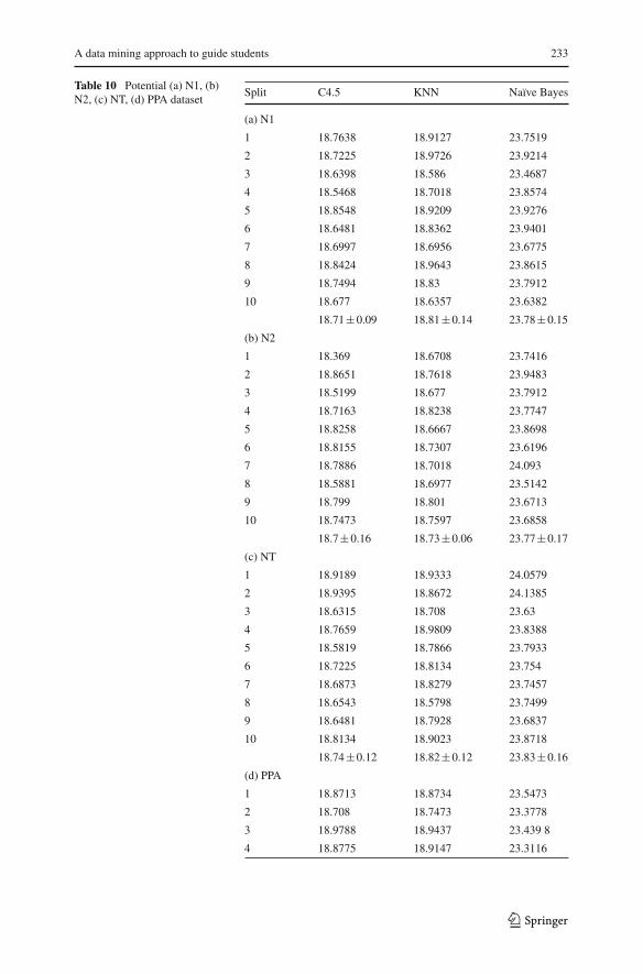
Table 9 shows error percentages resulting after the use of the three learning algo-rithms in the database with five attributes (original dataset). Likewise, Table 10a–dshow the error percentages obtained when considering the attribute potential, in eachof the four different methods of calculation: N1, N2, NT and PPA.

For statistical testing the paired t test was used. Generally, it is used when data fromthe same individual is recorded before and after the application of a treatment that

123


Table 10 Potential (a) N1, (b)N2, (c) NT, (d) PPA dataset

Split C4.5 KNN Naïve Bayes

(a) N1

1 18.7638 18.9127 23.7519

2 18.7225 18.9726 23.9214

3 18.6398 18.586 23.4687

4 18.5468 18.7018 23.8574

5 18.8548 18.9209 23.9276

6 18.6481 18.8362 23.9401

7 18.6997 18.6956 23.6775

8 18.8424 18.9643 23.8615

9 18.7494 18.83 23.7912

10 18.677 18.6357 23.6382

18.71±0.09 18.81±0.14 23.78±0.15

(b) N2

1 18.369 18.6708 23.7416

2 18.8651 18.7618 23.9483

3 18.5199 18.677 23.7912

4 18.7163 18.8238 23.7747

5 18.8258 18.6667 23.8698

6 18.8155 18.7307 23.6196

7 18.7886 18.7018 24.093

8 18.5881 18.6977 23.5142

9 18.799 18.801 23.6713

10 18.7473 18.7597 23.6858

18.7±0.16 18.73±0.06 23.77±0.17

(c) NT

1 18.9189 18.9333 24.0579

2 18.9395 18.8672 24.1385

3 18.6315 18.708 23.63

4 18.7659 18.9809 23.8388

5 18.5819 18.7866 23.7933

6 18.7225 18.8134 23.754

7 18.6873 18.8279 23.7457

8 18.6543 18.5798 23.7499

9 18.6481 18.7928 23.6837

10 18.8134 18.9023 23.8718

18.74±0.12 18.82±0.12 23.83±0.16

(d) PPA

1 18.8713 18.8734 23.5473

2 18.708 18.7473 23.3778

3 18.9788 18.9437 23.439 8

4 18.8775 18.9147 23.3116

123


Table 10 continuedSplit C4.5 KNN Naïve Bayes

5 18.8713 19.0098 23.6941

6 18.7783 19.1276 23.3902

7 18.7349 19.0636 23.4481

8 18.7969 19.0904 23.5618

9 18.6956 18.7514 23.4398

10 18.6253 18.9003 23.0842

18.79±0.11 18.94±0.13 23.43±0.16

Table 11 Hypothesis testing todetermine best algorithm

Hypothesis testing to analyze the effect of the classification algorithm

C4.5 vs. KNN On Tables 9 and 10a–dC4.5 vs. Naive

BayesOn Tables 9 and 10a–d

is going to be analyzed. The paired t test was used as follows: the treatments to bestudied were the classification algorithms, the datasets and the four ways for potentialcalculation, respectively; and the individuals were the different datasets obtained afterdoing the holdout resampling. The observations registered were error rates generatedwhen applying the different techniques to each of the generated sets.

A sign corresponding to the statistical test and its P-value are presented in the allhypothesis tests. These allow the analysis of the significance of the differences amongdifferent results. A sign +(−) in front of the P-value indicates that some of the condi-tions produced worse (better) learning. When the P-value is not preceded by a sign,but by a 0, it indicates that there are no meaningful differences between treatments.Values between parentheses represent P-values of the paired t test. A P-value is theprobability of obtaining a value (smaller or larger) more extreme than the observedstatistical test value. In our case, if a P-value is less than the significance level (0.05),we will reject the null hypothesis; so, we concluded that prediction error rates havedifferent means.

5.1.1 Experiment related to the effectiveness of the classification algorithm

The first experiment tried to answer the question as to which of the algorithms usedin this research would produce a lower prediction error.

In order to answer this question, the error percentages obtained previously wereconsidered. Statistical analysis was performed on each of the tables; it applied thepaired t test to the results of Tables 9 and 10a–d.

Table 11 shows a description of all the ten tests performed and Table 12 shows theobtained results.

Interpretation

• The error average rate of algorithm C4.5 is lower than the error average rate ofthe Naive Bayes algorithm, both in the original dataset and in the four treatmentsof the potential calculation.

123


• The error average rate of algorithm C4.5 is lower than the error average rate ofthe KNN algorithm when the original dataset and estimations N1, NT and PPAfor the potential were used. In the case of potential N2 the error was the same.

ConclusionIt can be concluded that C4.5 is the most effective algorithm predicting new instancesin our application domain. Besides, it is the most appropriate due to its representationcapability, ease of interpretation and lower computational cost (Rokach and Maimon2008).

5.1.2 Experimenting with the effectiveness of the dataset

The second experiment aimed at answering which of the datasets would produce lowerprediction error rates. Results from the previous experiment were used in this analysis.In that way, only decision trees were used to compare results using different datasets.

In order to answer the question the error percentages were used again. Statisticalanalysis between the different tables was undertaken, by applying the paired t test tothe results of Tables 9 and 10a–d.

Table 13 shows a description of all the tests performed and the obtained results canbe seen in Table 14.

Interpretation

• Classifiers built using potential N1, N2 and NT values had a lower average of errorrates than those built with the original dataset.

• It can be observed that in the case of the treatment for potential PPA there wasno meaningful difference in the error rate between this treatment and the originaldataset.

ConclusionWe conclude that the dataset with synthetic attributes produces better average errorrates. In other words, it enables the construction of a model better representing the

Table 12 P values and signs of paired t test of Table 11

Test First data set Potential N1 Potential N2 Potential NT Potential PPA

C4.5 vs. KNN − (0.0028) − (0.0188) 0 (0.5842) − (0.0299) − (0.0115)C4.5 vs. NB − (0) − (0) − (0) − (0) − (0)

Table 13 Hypothesis testing to determine the best set of attributes

Hypothesis testing to analyze effect of new attributes (potential and difficulty)

C4.5 applied to Table 9 vs. C4.5 applied to Table 10a

C4.5 applied to Table 9 vs. C4.5 applied to Table 10b

C4.5 applied to Table 9 vs. C4.5 applied to Table 10c

C4.5 applied to Table 9 vs. C4.5 applied to Table 10d

123


Table 14 P values and signs of paired t test of Table 13

Potential N1 Potential N2 Potential NT Potential PPA(C4.5) (C4.5) (C4.5) (C4.5)

Original data set(C4.5)

+ (0.0018) + (0.0069) + (0.0104) 0 (0.0877)

reality under study. However, using the PPA potential value does not produce a mean-ingful difference with the results obtained from the original dataset, and for this reasonit was excluded from subsequent experiments.

5.1.3 Experiment related to the effectiveness of the treatments for the potentialcalculation

The third experiment was to determine which of the treatments for the potential cal-culation produces the lowest prediction error rate. Again, results from the previousexperiment were used to design this experiment. For this reason only decision treesand databases with seven attributes were used.

In order to answer the question, statistical analysis among the different tables wascarried out, applying the paired t test to the results of Table 10a–c. Table 15 shows adescription of all the tests performed.

The obtained results can be seen in Table 16.

InterpretationThere are not meaningful differences between the averages of error rates of the threetreatments for potential N1, N2 and NT.

ConclusionThe treatments for potential N1, N2 and NT have statistically equal averages of errorrates.

Table 15 Hypothesis testing to determine the best potential

Hypothesis testing to analyze effect of methodology in calculation of potential

C4.5 applied to Table 10a N1 vs. C4.5 applied to Table 10b N2

C4.5 applied to Table 10a N1 vs. C4.5 applied to Table 10c NT

C4.5 applied to Table 10b N2 vs. C4.5 applied to Table 10c NT

Table 16 P values and Signs ofpaired t test of Table 15

Test Sign (P value)

Potential N1 vs. Potential N2 0 (0.8596)Potential N1 vs. Potential NT 0 (0.6925)Potential N2 vs. Potential NT 0 (0.6426)

123


5.2 Phase 2: experiment related to the independence of data from time

ObjectiveThe objective of this experiment was to verify the effect caused in the training setswhen older data is not considered.

ConsiderationsThe university environment, and especially our application domain, has some char-acteristics that allow data analysis under certain conditions from different points ofview. When considering student performance, courses are not the same term after term.Although normally there are no meaningful performance changes from one term toanother, it is possible that after some terms a generational change could mean a changein trends. This new trend should be reflected in training sets, so it can be captured inthe classifier model.

From the course point of view, normally a large group of them change every time.Every time a curriculum is modified, the university creates rules so that modificationswould not affect students. One of the most important rules is related to the equivalencesbetween courses. Without these equivalences it would be impossible to consider an oldcourse that has undergone more than one modification. In other words, the records ofthat course should be deleted during the cleaning phase, losing the related information.

In this sense, one hypothesis suggests that when old records are taken into account,they will impact negatively in predictions generated by the model used to give recom-mendations to future students.

In order to test this hypothesis, it is necessary to determine whether datasets withonly newer records lead to better classifiers. Otherwise, the most appropriate proce-dure will be to consider the whole dataset (dataset corresponding to term 19912 up toterm 20091). The reason is that datasets with more data will generally lead to betterestimations due to the concept of consistency (Lehmann and Casella 1998).

ProcedureThirty-one different training subsets were created as is shown in Fig. 3. Each subsetwas obtained by removing from the previous dataset the records corresponding to theoldest term. That is, the first subset comprises records from all the available terms.The second one includes all the records excepting the ones corresponding to the firstterm, 19912 in this case. The last subset includes only the records of the most recentterms. Afterwards, these subsets were studied using the algorithm C4.5.

As holdout resampling was used for evaluation, analyzing the variance of the errorsof each of the tests allows the estimation of the variability of the learning method inrelation to the training data.

ExperimentThe goal of the experiment was to find out if the oldest data increase the estimatederror of predictions. Again, results from the previous phases were used to design thisexperiment. It means that only the C4.5 algorithm was used on datasets containing thethree calculated values for the potential attribute (N1, N2 and NT)

The average error rates obtained in each of the tests was calculated. Afterwards,a hypothesis test of equality of proportions was applied. In this test, the chi-square

123


Fig. 3 Data subsets from academic terms

Table 17 Chi-squared and Pvalues obtained for test ofequality of proportions

N1 N2 NT

Chi-squared 7.5529 8.5929 7.7875

P value 0.9999 0.9999 0.9999

distribution is the statistic of the test. The objective was to determine if there weremeaningful differences between the average error rates found in the 31 subsets.

InterpretationTable 17 shows that P-values are greater than the significance level (0.05). Therefore,there is no statistical evidence to sustain the view that error average rates are differentin the 31 subsets for each one of the treatments for potential N1, N2 and NT.

ConclusionWith the test of proportions, we conclude that there are no meaningful differencesbetween error percentages obtained with the oldest data and data from more recentperiods for each one of the treatments. With these results it is convenient to use the dataset corresponding to the first subset. That is to say, records spanning 19912 to 20091.

5.3 Analysis of pruning methods

ObjectiveThis experiment aimed at determining which of the pruning methods produced lowererror rate in our domain of application.

ConsiderationsThe following pruning methods were used in this research: Reduced Error Prun-ing (REP) (Quinlan 1987), Pessimistic Error pruning (PEP) (Quinlan 1987), Mini-mum Error Pruning (MEP) (Cestnik and Bratko 1991), Critical Value Pruning (CVP)(Mingers 1987) and Error Based Pruning (EBP) (Quinlan 1993).

123


ProcedureBasically, all pruning methods follow the same procedure. First, a metric is calcu-lated for the two possible options: pruning and not pruning. Then both metrics arecompared, in order to determine which option should be selected. This is a recursiveprocedure and occurs at each sub-tree.

This section presents the results of an empirical comparison of the pruning meth-ods presented above. Nine datasets corresponding to the 19952, 20001, 20041 termswere chosen after having applied the machine-learning algorithm 279 times. The firstset corresponds to the term with the best error rate (that is, classifiers built with thisdataset produced the best accuracy). The second term generated the worst error rate,while the third one was chosen to coincide with curricular changes.

The base error would be obtained if the most frequent class were used to classifyeach instance. With the use of classification algorithms we expected lower error rates.

Each set was randomly divided into two subsets: training (70%) and testing (30%).The training set itself was subdivided into: growing (70%) and pruning (30%). Theerror rate is always evaluated on the testing set. This experimental design has beenused in similar empirical studies such as (Mingers 1989). The error rates are averagedand the standard error is calculated as well.

ExperimentsThis section discusses the results of the 45 experiments resulting from the combinationof the nine data sets and the five pruning methods.

The experiments show that EBP has the lowest error rates. On the other hand, PEPhas the highest error for the seventh and eighth dataset, while CVP has the highest forthe rest of them.

Table 18 reports the results of a paired t test using a 0.10 confidence level (Espositoet al. 1997). “+” (−) indicates better (worse) performance than the unpruned trees.0 indicates no change at all. The number of datasets that report + (−) may indicatewhich method is appropriate for each data set.

Due to the difficulty of presenting every comparison and the fact that the EBPappears to be the most stable, each method is compared with the EBP as shown inTable 19.

Table 18 Significance table

Term Distance REP MEP CVP PEP EBP Total

19952 1 + + − + + 4/1

2 + + − + + 4/1

NT + + − + + 4/1

20001 1 + + 0 + + 4/0

2 + + − + + 4/1

NT + + − + + 4/1

20041 1 + + − 0 + 3/1

2 + + − 0 + 3/1

NT + + − 0 + 3/1

123


Table 19 Significance of pruning method with EBP

Term Distance REP MEP CVP PEP

19952 1 0 (0.3434) − (0) − (0) − (0.0013)

2 − (0.0107) − (0) − (0) − (0.0002)

NT − (0.0019) − (0) − (0) − (0.0128)

20001 1 − (0.0084) − (0.0001) − (0) − (0.0095)

2 − (0.0957) − (0.0001) − (0) 0 (0.1773)

NT − (0.0842) − (0.0001) − (0) 0 (0.5554)

20041 1 0 (0.1188) − (0.0001) − (0) − (0.0031)

2 − (0.0024) − (0) − (0) − 0.0114)

NT − (0.0607) − (0.0001) − (0) − (0.0263)

InterpretationAccording to the results, the EBP method produces the lowest error rates for ourparticular domain while the CVP method shows the worst results.

The behavior of the PEP method is stable across datasets. REP and MEP may beconsidered interchangeable since they work similarly. One may go so far as to claimthat they produce equal trees.

ConclusionsIn conclusion, EBP can be considered to be the best pruning method because it is theone that has the best predictive accuracy. Therefore, it will be the one used during thedevelopment of the following experiments.

5.4 Analysis of ensemble classification techniques: bagging and boosting

ObjectiveThis experiment aimed to determine which ensemble classification techniques (suchas bagging and boosting) would perform better than base techniques in each variantof the potential calculation.

Accordingly to the results from the previous phases, the C4.5 base algorithm andthe variants for potential N1, N2 and NT were used. In the same way, data from theterm 19912 and the EBP pruning technique were chosen.

ProcedureHoldout resampling was applied to subset 19912 in order to generate a set composedof 70% training data and 30% testing data. Models for both the C4.5 base algorithmas the ensemble technique were generated.

Afterwards, 25 iterations (models) for the bagging algorithm and 10 iterations forboosting were defined. The whole process was performed ten times (Opitz and Maclin1999).

ExperimentThe goal was to find out whether a model obtained through an ensemble classifieris better than on obtained through a base method. With this intention, error rates

123


Table 20 Error rates of C4.5Split N1 N2 NT

1 18.7638 18.369 18.9189

2 18.7225 18.8651 18.9395

3 18.6398 18.5199 18.6315

4 18.5468 18.7163 18.7659

5 18.8548 18.8258 18.5819

6 18.6481 18.8155 18.7225

7 18.6997 18.7886 18.6873

8 18.8424 18.5881 18.6543

9 18.7494 18.799 18.6481

10 18.677 18.7473 18.8134

18.71±0.09 18.7±0.16 18.74±0.12

obtained when applying bagging, boosting and algorithm base C4.5 to the entire datawere analyzed. Then the algorithm with the lowest average error rate was determined.

In order to do this, a paired t test was performed on the results from Tables 20 and21a, b. Table 22 shows a description of the nine tests performed.

InterpretationThe results indicate that the average error rate decreases when using the bagging clas-sifier, compared against the C4.5 algorithm base as well as boosting. Besides, it canbe observed that the average error rate for C4.5 is lower than the one obtained withthe boosting classifier.

ConclusionDerived from these results, it can be concluded that applying bagging ensemble tech-nique can significantly reduce the error rate in each of the variants, compared with theuse of other algorithms.

To conclude this section, the best conditions for implementing the recommendersystem resulting from all the experiments showed above are in summary: bagging usingC4.5 with the pruning method EBP as a base classifier. Besides, it was demonstratedthat it is more effective to use all the historical data, because greater amounts of datawill give better estimations, and also the dataset including the two synthetic attributeswould produces lower error rates. With regard to the different potential approaches,we will use the variant for potential N1. The reason behind this decision is that, inour domain, the enrollment advisor mainly takes into consideration, mainly, the directprerequisites.

6 Recommender system deployment

The last step in the CRISP-DM methodology implies diffusion and use of the modelbuilt through data mining. Taking into consideration lessons learnt through the exper-iments, a model was built and included in a recommender module. In this section theintegration of the module with the enrollment system, the system interfaces and the

123


Table 21 Error rates of (a)bagging and (b) boosting

Split N1 N2 NT

(a) Bagging

1 18.3504 18.2305 18.7204

2 18.6109 18.5013 18.6233

3 18.2057 18.1705 18.3483

4 18.4269 18.5034 18.6481

5 18.5984 18.5178 18.3731

6 18.4889 18.4351 18.5592

7 18.2925 18.4661 18.4124

8 18.7618 18.3669 18.3711

9 18.4786 18.5984 18.3876

10 18.5116 18.524 18.584

18.47±0.16 18.43±0.14 18.5±0.14

(b) Boosting

1 19.6176 19.3488 19.6693

2 19.5452 19.7292 19.9711

3 19.5059 19.4398 19.5928

4 19.4894 19.6093 19.7623

5 19.6837 19.816 19.3282

6 19.3116 19.7251 19.6072

7 19.601 19.5245 19.6693

8 19.6858 19.2951 19.3344

9 19.5969 19.7168 19.6734

10 19.5225 19.5659 19.7891

19.56±0.11 19.58±0.18 19.62±0.2

Table 22 P values and signs ofpaired t test for C4.5, baggingand boosting

N1 N2 NT

C4.5 vs. Bagging + (0.0003) + (0) + (0)

C4.5 vs. Boosting − (0) − (0) − (0)

Bagging vs. Boosting − (0) − (0) − (0)

results of a pilot test are described. This pilot test was taken in the academic period20101 (from April to August, 2010).

6.1 Consult process sequence

Figure 4 presents the recommender system, implemented as a web service and inte-grated into the enrollment application of University of Lima. In order to answer queriesfrom the application, the web service interacts with a processed database and with therecommendation engine, implemented through an independent executable file namedConsult.exe.

123


Fig. 4 Consult process sequence

The following is the description of the control and data flow.The student logs into the enrolling application using his/her username and password

(1). At this point, his/her cumulative average, the list of courses that he is able to signinto and the attempt number are shown.

When the student selects a course, the enrolling application automatically invokesthe web service (2) sending it the code of the student, the course, the total amount ofcredits that he wishes to take, the attempt number and the cumulative average.

The web service obtains the difficulty of the course and the student potential througha query to the database (3)–(4).

With this information, the web service builds a new group of instances (5) to callthe recommender engine. The consult executable file reads the model (6), looking forthe predicted class of each instance (pass or fail) and its confidence factor (7), (8).Finally, these results are returned to the enrollment system (9) and presented to theuser (10).

6.2 SPRS user interface

In Fig. 5, the interface of the SPRS system is shown. The candidate courses, in whichthe student can enroll, are shown on the left. Once the student has selected a group ofthem, the system queries the recommender system, as shown in Fig. 4. The feedbackof the system, with its respective confidence factors, can be seen on the right of theinterface.

6.3 Preliminary results of the recommender system under enrollment conditions

In this section a pilot experiment and the preliminary results of the recommender sys-tem are presented. This system was implemented using data including the academicterm 20092 and taking into account the results from Sect. 5. Then it was tested on theacademic term 20101 enrollment.

During that period, 804 students were able to enroll on different courses; fromthis group, 50 students were chosen for the pilot experiment applying a systematicsampling technique. The features of the SPRS were explained to them and they wereinformed that, if they considered it convenient, they could use it. From these 50

123


Fig. 5 Enrollment system user interface

students, only 39 used the recommender system. These students generated 198 in-stances to test our system. As the enrollment procedure is carried out via the Internetand the experiment should simulate real conditions, students enrolled without super-vision using only the recommender system.

By comparing the predictions of the system with real results, we obtained 85.35%of accuracy. The interpretation of this accuracy has to take into consideration thefollowing issues:

• The proportion of students obtaining a positive recommendation by the systemand that, at the end of the term, really passed the courses was 82.32% of the total.

• The proportion of students obtaining a negative recommendation and that, at theend of the term, really failed was 3.03% of the total.

For this analysis, the prediction confidence factor was taken into consideration. Thisfactor represents the proportion of instances from the training dataset whose classifi-cation match the predicted outcome.

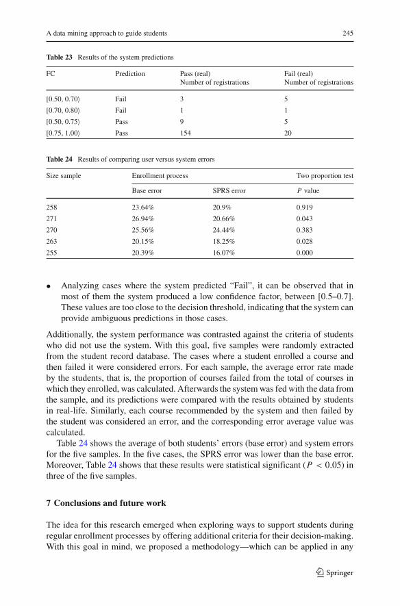
When testing the recommender system, students had the opportunity of seeing theconfidence factor of each recommendation and using it to decide whether to enroll ornot on a given course. Thus, results from Table 23 can be interpreted in the followingway:

• Analyzing cases where the system predicted “Pass” with a confidence factor be-tween [0.75–1], the prediction was correct 154 times, while in 20 cases it waswrong. As expected, the system is more efficient when it has a greater confidencefactor. It is worth mentioning that most of the cases of wrong prediction were dueto the unusual behavior of the students or because they just left the course.

123


Table 23 Results of the system predictions

FC Prediction Pass (real) Fail (real)Number of registrations Number of registrations

[0.50, 0.70〉 Fail 3 5

[0.70, 0.80〉 Fail 1 1

[0.50, 0.75〉 Pass 9 5

[0.75, 1.00〉 Pass 154 20

Table 24 Results of comparing user versus system errors

Size sample Enrollment process Two proportion test

Base error SPRS error P value

258 23.64% 20.9% 0.919

271 26.94% 20.66% 0.043

270 25.56% 24.44% 0.383

263 20.15% 18.25% 0.028

255 20.39% 16.07% 0.000

• Analyzing cases where the system predicted “Fail”, it can be observed that inmost of them the system produced a low confidence factor, between [0.5–0.7].These values are too close to the decision threshold, indicating that the system canprovide ambiguous predictions in those cases.

Additionally, the system performance was contrasted against the criteria of studentswho did not use the system. With this goal, five samples were randomly extractedfrom the student record database. The cases where a student enrolled a course andthen failed it were considered errors. For each sample, the average error rate madeby the students, that is, the proportion of courses failed from the total of courses inwhich they enrolled, was calculated. Afterwards the system was fed with the data fromthe sample, and its predictions were compared with the results obtained by studentsin real-life. Similarly, each course recommended by the system and then failed bythe student was considered an error, and the corresponding error average value wascalculated.

Table 24 shows the average of both students’ errors (base error) and system errorsfor the five samples. In the five cases, the SPRS error was lower than the base error.Moreover, Table 24 shows that these results were statistical significant (P < 0.05) inthree of the five samples.

7 Conclusions and future work

The idea for this research emerged when exploring ways to support students duringregular enrollment processes by offering additional criteria for their decision-making.With this goal in mind, we proposed a methodology—which can be applied in any

123


higher education institution—whose objective is to prepare student academic data tobe organized in such a way that it can be treated through the Crisp-DM methodologyto make predictions related to academic performance.

We observed that predictive accuracy depends, in most cases, on data quality. Fol-lowing this lead, the main contribution of this research was to include two syntheticattributes in the data preparation process. The first synthetic attribute, the difficultyof a course, is the cumulative average of previously registered grades; it measuresthe course difficulty or ease. The second synthetic attribute is the student’s potential,defined as the numeric value that measures his/her capacities and skills, particularlyfor a certain course.

In the section corresponding to the evaluation of the proposed methodology, weexplain the four different phases of experiments carried out.

In the first phase, we determined the best conditions for automatic learning. We con-cluded that the C4.5 algorithm was the most efficient for this particular domain, andthat the set that best represented the reality under study was that including syntheticattributes with treatments for potential N1, N2 and NT.

In the second phase, after applying the statistical test of equality of proportions, weconcluded that there were no meaningful differences in error rate among the terms.With this result, we decided to use—for the rest of the research—database informationavailable since the very creation of the Department.

Results from the third phase showed that pruning methods—especially EBP—pro-duced improvements in predictive accuracy as well as in the understanding of thetrees.

Finally, in the fourth phase we concluded that the bagging ensemble techniqueobtained better predictive accuracy than the base algorithm C4.5 and the boostingensemble technique.

Once we had determined the best conditions for the implementation of the system,we performed a pilot experiment with real enrollments of 50 students. In this context,the system was able to predict with 85.36% of accuracy.

We also compared the results of the system with the predictions made by studentswith no support from it. In this case, the system consistently produced better resultsthan the students did, as it can be observed in Table 24.

The prediction of academic performance opens many possibilities, as there arenumerous applications that can be obtained from grade prediction in the academiccontext. However, further analysis need to be done yet. For example, regarding theapplication domain, it is necessary to involve more variables in the study. These vari-ables could depend either on the environment (i.e., more detailed information on thedifficulty of the courses, student’s assistance and interest, or secondary school grades,among others) or on the student (time dedicated to study, his/her capacity for certaincourses, his/her disposition to face them, etc.). Future proposals of new techniquesthat assure a better classification for this domain of application would also be veryinteresting.

Acknowledgments This work has been funded by the Spanish Ministry of Science and Education throughthe projects HADA (TIN2007-64718) y ASIES (TIN2010-17344), the Comunidad Autónoma de Madrid(S2009/TIC-1650) and the University of Lima through the IDIC (Instituto de Investigación Científica).

123


References

Al-Radaideh, Q., AI-Shawakfa, M., Al-Najjar, M.: Mining student data using decision trees. In: The 2006International Arab Conference on Information Technology, Yarmouk University, Jordan (2006)

Breiman, L.: Bagging predictors. Mach. Learn. 24(2), 123–140 (1996)Castellano, E., Martínez, L.: ORIEB, A CRS for academic orientation using qualitative assessments. In:

Proceedings of the IADIS International Conference E-Learning, pp. 38–42 (2008)Cestnik, B., Bratko, I.: On estimating probabilities in tree pruning. In: Machine Learning (EWSL’91) Lecture

Notes in Computer Science, vol. 482, no. 3, pp. 138–150. Springer-Verlag, Berlin (1991)Cortez, P., Silva, A.: Using data mining to predict secondary school student performance. In: Proceedings

of 5th Future Business Technology Conference, Oporto, Portugal, pp. 5–12 (2008)Dekker, G., Pechenizkiy, M., Vleeshouwers, J.: Predicting students drop out: a case study. In: Proceedings

of the 2nd International Conference on Educational Data Mining (EDM’09), Cordoba, Spain, pp.41–50 (2009)

Edelstein, H.: Building profitable customer relationships with data mining. In: SPSS White Paper-ExecutiveBriefing, pp. 1–13. Two Crows Corporation (2000)

Enas, G., Choi, S.: Choice of the smoothing parameter and efficiency of K-nearest neighbor classifica-tion. Comput. Math. Appl. 12, 235–244 (1986)

Esposito, F., Malerba, D., Semeraro, G.: A comparative analysis of methods for pruning decisión trees. IEEETrans. Pattern Anal. Mach. Intell. 19(5), 476–491 (1997)

Feldman, R.: Mining the biomedical literature using semantic analysis. Biosilico 1(2), 69–80 (2003)Freund, Y., Schapire, R.: Experiments with a new boosting algorithm. In: Machine Learning, Proceedings

of the Thirteenth International Conference (ICML’96), pp. 148–156 (1996)Han, J.: How can data mining help bio-data analysis? In: Proceedings of the 2nd ACM SIGKDD Workshop

on Data Mining in Bioinformatics (BIOKDD’2002), Edmonton, Canada, pp. 1–2 (2002)Han, J., Kamber, M.: Data Mining: Concepts and Techniques. 2nd edn. Morgan Kaufmann, San Francisco

(2006)Larose, D.: Discovering Knowledge in Data. 1st edn. Willey, New Jersey (2005)Lehmann, E., Casella, G.: Theory of Point Estimation. 2nd edn. Springer-Verlag, New York (1998)Luan, J.: Data mining and knowledge management: a system analysis for establishing a Tiered Knowledge

Management Model (TKMM). In: Proceedings of AIR Forum, Toronto, Canada (2001)Luan, J.: Data mining and knowledge management in higher education-potential applications. In: Proceed-

ings of AIR Forum, Toronto, Canada, pp. 1–18 (2002a)Luan, J.: Data Mining Application in Higher Education. SPSS Executive Report, pp. 1–8 (2002b)Mingers, J.: Expert Systems-Rule Induction with Statistical Data. J. Oper. Res. Soc. 38, 39–47 (1987)Mingers, J.: An empirical comparison of pruning methods for decision tree induction. Mach. Learn.

4(2), 227–243 (1989)Mitchell, T.: Machine Learning. 1st edn. McGraw-Hill, Boston (1997)Mobasher, B., Jain, N., Han, E., Srivastava, J.: Web Mining: Pattern Discovery from World Wide Web

Transactions. Technical Report TR96-OS0. Department of Computer Science, University of Minne-sota (1996)

Opitz, D., Maclin, R.: Popular ensemble methods: an empirical study. J. Artif. Intell. Res. 11, 169–198 (1999)Quinlan, R.: Simplifying decision trees. Int. J. Man–Mach. Stud. 27, 221–234 (1987)Quinlan, R.: C4.5: Programs for Machine Learning. Morgan Kaufmann, San Mateo (1993)Ramaswami, M., Bhaskaran, R.: A CHAID based performance prediction model in educational data min-

ing. Int. J. Comput. Sci. Issues (IJCSI) 7(1), 10–18 (2010)Rokach, L., Maimon, O.: Data Mining with Decision Trees: Theory and Applications. World Scientific

Publishing, Danvers (2008)Romero, C., Ventura, S.: Educational data mining: a review of the state-of-the-art. IEEE Trans. Syst. Man

Cybern. C Appl. Rev. 40(6), 601–618 (2010)Schafer, J.B.: The application of data-mining to recommender systems. In: Encyclopedia of Data Ware-

housing and Mining, vol. 1, pp. 44–48. Idea Group Reference, Hershey, PA (2005)Vialardi, C., Bravo, J., Shafti, L. Ortigosa, A.: Recommendation in higher education using data min-

ing techniques. In: Proceedings of Second Educational Data Mining Conference, Córdoba, Spain,pp. 190–199 (2009)

123


Vialardi, C., Chue, J., Barrientos, A., Victoria, D., Estrella, J., Ortigosa, A., Peche, J.: A case study: datamining applied to student enrollment. In: Proceedings of Third Educational Data Mining Conference,Pennsylvania, USA, pp. 333–335 (2010)

Waiyamai, K.: Improving Quality of Graduate Students by Data Mining. Department of ComputerEngineering, Faculty of Engineering, Kasetsart University, Bangkok (2003)

Wu, X. et al.: Top ten algorithms in data mining. Knowl. Inform. Syst. 14(1), 1–37 (2008)Zaïane, O.: Building a recommender agent for E-learning systems. In: International Conference on

Computers in Education, New Zealand, pp. 55–59 (2002)

Author Biographies

César Vialardi is Professor of Systems Engineering Department of Universidad de Lima. He received hisPh.D. degree in Computer Science from the Universidad Autónoma de Madrid. He has worked in adaptivesystems, collaborative systems, user modeling, and authoring and evaluation of adaptive systems.

Jorge Chue is Professor in the Faculty of Systems Engineering of Lima University, Perú. He received hismaster degree in statistics from Universidad Nacional Mayor de San Marcos. His research interests lie ingeneralized linear modeling and data mining.

Juan Pablo Peche from the Scientific Initiation Program of Lima University; has interests in adaptivesystems, collaborative systems, user modeling, and data mining techniques to support prediction.

Gustavo Alvarado from the Scientific Initiation Program of Lima University; has interests in adaptivesystems, collaborative systems, user modeling, and data mining techniques to support prediction.

Bruno Vinatea from the Scientific Initiation Program of Lima University; has interests in adaptive systems,collaborative systems, user modeling, and data mining techniques to support prediction.

Jhonny Estrella from the Scientific Initiation Program of Lima University; has interests in adaptive sys-tems, collaborative systems, user modeling, and data mining techniques to support prediction.

Álvaro Ortigosa is Professor of Computer Science at Universidad Autónoma de Madrid and a member ofthe Forensics and Security Research Institute (ICFS). He received his Ph.D. degree in Computer Sciencefrom the Universidad Autónoma de Madrid. He has worked in software engineering support environments,software reuse, adaptive systems, collaborative systems, user modeling, mobile environments, and theauthoring and evaluation of adaptive systems.

123

A data mining approach to guide students through the enrollment process based on academic...

Documents

Transcript of A data mining approach to guide students through the enrollment process based on academic...