Faculty of Business Course Outline Course Title: Strategic Management Course Code: MGT703
Upload
khangminh22Category
view
1download
0
Cambridge University Press978-1-316-51893-9 — A Course of Modern AnalysisE. T. Whittaker , G. N. Watson , Edited by Victor H. Moll FrontmatterMore Information
www.cambridge.org© in this web service Cambridge University Press
A COURSE OF MODERN ANALYSIS
This classic work has been a unique resource for thousands of mathematicians, scientists
and engineers since its first appearance in 1902. Never out of print, its continuing value
lies in its thorough and exhaustive treatment of special functions of mathematical physics
and the analysis of differential equations from which they emerge. The book also is of
historical value as it was the first book in English to introduce the then modern methods
of complex analysis.
This fifth edition preserves the style and content of the original, but it has been
supplemented with more recent results and references where appropriate. All the
formulas have been checked and many corrections made. A complete bibliographical
search has been conducted to present the references in modern form for ease of
use. A new foreword by Professor S. J. Patterson sketches the circumstances of the
book’s genesis and explains the reasons for its longevity. A welcome addition to any
mathematician’s bookshelf, this will allow a whole new generation to experience the
beauty contained in this text.
e .t. whi ttaker was Professor of Mathematics at the University of Edinburgh. He
was awarded the Copley Medal in 1954, ‘for his distinguished contributions to both pure
and applied mathematics and to theoretical physics’.
g .n. watson was Professor of Pure Mathematics at the University of Birmingham.
He is known, amongst other things, for the 1918 result now known as Watson’s lemma
and was awarded the De Morgan Medal in 1947.
victor h . moll is Professor in the Department of Mathematics at Tulane University.
He co-authored Elliptic Curves (Cambridge, 1997) and was awarded the Weiss Presiden-
tial Award in 2017 for his Graduate Teaching. He first received a copy of Whittaker and
Watson during his own undergraduate studies at the Universidad Santa Maria in Chile.

Cambridge University Press978-1-316-51893-9 — A Course of Modern AnalysisE. T. Whittaker , G. N. Watson , Edited by Victor H. Moll FrontmatterMore Information
www.cambridge.org© in this web service Cambridge University Press
(Left): Edmund Taylor Whittaker (1873–1956); (Right): George Neville Watson
(1886–1965): Universal History Archive/Contributor/Getty Images.

Cambridge University Press978-1-316-51893-9 — A Course of Modern AnalysisE. T. Whittaker , G. N. Watson , Edited by Victor H. Moll FrontmatterMore Information
www.cambridge.org© in this web service Cambridge University Press
A COURSE OF MODERN ANALYSIS
Fif th Edit ion
An introduction to the general theory of infinite
processes and of analytic functions with an account
of the principal transcendental functions
E.T. WHITTAKER AND G.N. WATSON
Fifth edition edited and prepared for publication by
Victor H. MollTulane University, Louisiana

Cambridge University Press978-1-316-51893-9 — A Course of Modern AnalysisE. T. Whittaker , G. N. Watson , Edited by Victor H. Moll FrontmatterMore Information
www.cambridge.org© in this web service Cambridge University Press
University Printing House, Cambridge CB2 8BS, United Kingdom
One Liberty Plaza, 20th Floor, New York, NY 10006, USA
477 Williamstown Road, Port Melbourne, VIC 3207, Australia
314–321, 3rd Floor, Plot 3, Splendor Forum, Jasola District Centre, New Delhi – 110025, India
103 Penang Road, #05–06/07, Visioncrest Commercial, Singapore 238467
Cambridge University Press is part of the University of Cambridge.
It furthers the University’s mission by disseminating knowledge in the pursuit of
education, learning, and research at the highest international levels of excellence.
www.cambridge.org
Information on this title: www.cambridge.org/9781316518939
DOI: 10.1017/9781009004091
© Cambridge University Press 1902, 1915, 1920, 1927, 2021
This publication is in copyright. Subject to statutory exception
and to the provisions of relevant collective licensing agreements,
no reproduction of any part may take place without the written
permission of Cambridge University Press.
First edition 1902
Second edition 1915
Third edition 1920
Fourth edition 1927
Reprinted 1935, 1940, 1946, 1950, 1952, 1958, 1962, 1963
Reissued in the Cambridge Mathematical Library Series 1996
Sixth printing 2006
Fifth edition 2021
Printed in the United Kingdom by TJ Books Limited, Padstow Cornwall
A catalogue record for this publication is available from the British Library.
ISBN 978-1-316-51893-9 Hardback
Cambridge University Press has no responsibility for the persistence or accuracy of
URLs for external or third-party internet websites referred to in this publication
and does not guarantee that any content on such websites is, or will remain,
accurate or appropriate.

Cambridge University Press978-1-316-51893-9 — A Course of Modern AnalysisE. T. Whittaker , G. N. Watson , Edited by Victor H. Moll FrontmatterMore Information
www.cambridge.org© in this web service Cambridge University Press
Contents
Foreword by S.J. Patterson xvii
Preface to the Fifth Edition xxi
Preface to the Fourth Edition xxiii
Preface to the Third Edition xxiv
Preface to the Second Edition xxv
Preface to the First Edition xxvi
Introduction xxvii
Part I The Process of Analysis 1
1 Complex Numbers 3
1.1 Rational numbers 3
1.2 Dedekind’s theory of irrational numbers 4
1.3 Complex numbers 6
1.4 The modulus of a complex number 7
1.5 The Argand diagram 8
1.6 Miscellaneous examples 9
2 The Theory of Convergence 10
2.1 The definition of the limit of a sequence 10
2.11 Definition of the phrase ‘of the order of’ 10
2.2 The limit of an increasing sequence 10
2.21 Limit-points and the Bolzano–Weierstrass theorem 11
2.22 Cauchy’s theorem on the necessary and sufficient condition for the existence of a
limit 12
2.3 Convergence of an infinite series 13
2.31 Dirichlet’s test for convergence 16
2.32 Absolute and conditional convergence 17
2.33 The geometric series, and the series∑∞
n=11ns 17
2.34 The comparison theorem 18
v

Cambridge University Press978-1-316-51893-9 — A Course of Modern AnalysisE. T. Whittaker , G. N. Watson , Edited by Victor H. Moll FrontmatterMore Information
www.cambridge.org© in this web service Cambridge University Press
vi Contents
2.35 Cauchy’s test for absolute convergence 20
2.36 D’Alembert’s ratio test for absolute convergence 20
2.37 A general theorem on series for which limn→∞
|un+1/un | = 1 21
2.38 Convergence of the hypergeometric series 22
2.4 Effect of changing the order of the terms in a series 23
2.41 The fundamental property of absolutely convergent series 24
2.5 Double series 24
2.51 Methods of summing a double series 25
2.52 Absolutely convergent double series 26
2.53 Cauchy’s theorem on the multiplication of absolutely convergent series 27
2.6 Power series 28
2.61 Convergence of series derived from a power series 29
2.7 Infinite products 30
2.71 Some examples of infinite products 31
2.8 Infinite determinants 34
2.81 Convergence of an infinite determinant 34
2.82 The rearrangement theorem for convergent infinite determinants 35
2.9 Miscellaneous examples 36
3 Continuous Functions and Uniform Convergence 40
3.1 The dependence of one complex number on another 40
3.2 Continuity of functions of real variables 40
3.21 Simple curves. Continua 41
3.22 Continuous functions of complex variables 42
3.3 Series of variable terms. Uniformity of convergence 43
3.31 On the condition for uniformity of convergence 44
3.32 Connexion of discontinuity with non-uniform convergence 45
3.33 The distinction between absolute and uniform convergence 46
3.34 A condition, due to Weierstrass, for uniform convergence 47
3.35 Hardy’s tests for uniform convergence 48
3.4 Discussion of a particular double series 49
3.5 The concept of uniformity 51
3.6 The modified Heine–Borel theorem 51
3.61 Uniformity of continuity 52
3.62 A real function, of a real variable, continuous in a closed interval, attains its upper
bound 53
3.63 A real function, of a real variable, continuous in a closed interval, attains all values
between its upper and lower bounds 54
3.64 The fluctuation of a function of a real variable 54
3.7 Uniformity of convergence of power series 55
3.71 Abel’s theorem 55
3.72 Abel’s theorem on multiplication of convergent series 55
3.73 Power series which vanish identically 56
3.8 Miscellaneous examples 56
4 The Theory of Riemann Integration 58
4.1 The concept of integration 58
4.11 Upper and lower integrals 58
4.12 Riemann’s condition of integrability 59

Cambridge University Press978-1-316-51893-9 — A Course of Modern AnalysisE. T. Whittaker , G. N. Watson , Edited by Victor H. Moll FrontmatterMore Information
www.cambridge.org© in this web service Cambridge University Press
Contents vii
4.13 A general theorem on integration 60
4.14 Mean-value theorems 62
4.2 Differentiation of integrals containing a parameter 64
4.3 Double integrals and repeated integrals 65
4.4 Infinite integrals 67
4.41 Infinite integrals of continuous functions. Conditions for convergence 67
4.42 Uniformity of convergence of an infinite integral 68
4.43 Tests for the convergence of an infinite integral 68
4.44 Theorems concerning uniformly convergent infinite integrals 71
4.5 Improper integrals. Principal values 72
4.51 The inversion of the order of integration of a certain repeated integral 73
4.6 Complex integration 75
4.61 The fundamental theorem of complex integration 76
4.62 An upper limit to the value of a complex integral 76
4.7 Integration of infinite series 77
4.8 Miscellaneous examples 79
5 The Fundamental Properties of Analytic Functions; Taylor’s, Laurent’s and
Liouville’s Theorems 81
5.1 Property of the elementary functions 81
5.11 Occasional failure of the property 82
5.12 Cauchy’s definition of an analytic function of a complex variable 82
5.13 An application of the modified Heine–Borel theorem 83
5.2 Cauchy’s theorem on the integral of a function round a contour 83
5.21 The value of an analytic function at a point, expressed as an integral taken round a
contour enclosing the point 86
5.22 The derivatives of an analytic function f (z) 88
5.23 Cauchy’s inequality for f (n)(a) 89
5.3 Analytic functions represented by uniformly convergent series 89
5.31 Analytic functions represented by integrals 90
5.32 Analytic functions represented by infinite integrals 91
5.4 Taylor’s theorem 91
5.41 Forms of the remainder in Taylor’s series 94
5.5 The process of continuation 95
5.51 The identity of two functions 97
5.6 Laurent’s theorem 98
5.61 The nature of the singularities of one-valued functions 100
5.62 The ‘point at infinity’ 101
5.63 Liouvillle’s theorem 103
5.64 Functions with no essential singularities 104
5.7 Many-valued functions 105
5.8 Miscellaneous examples 106
6 The Theory of Residues; Application to the Evaluation of Definite Integrals 110
6.1 Residues 110
6.2 The evaluation of definite integrals 111
6.21 The evaluation of the integrals of certain periodic functions taken between the
limits 0 and 2π 111
6.22 The evaluation of certain types of integrals taken between the limits −∞ and +∞ 112

Cambridge University Press978-1-316-51893-9 — A Course of Modern AnalysisE. T. Whittaker , G. N. Watson , Edited by Victor H. Moll FrontmatterMore Information
www.cambridge.org© in this web service Cambridge University Press
viii Contents
6.23 Principal values of integrals 116
6.24 Evaluation of integrals of the form∫ ∞0
xa−1Q (x) dx 117
6.3 Cauchy’s integral 118
6.31 The number of roots of an equation contained within a contour 119
6.4 Connexion between the zeros of a function and the zeros of its derivative 120
6.5 Miscellaneous examples 121
7 The Expansion of Functions in Infinite Series 125
7.1 A formula due to Darboux 125
7.2 The Bernoullian numbers and the Bernoullian polynomials 125
7.21 The Euler–Maclaurin expansion 127
7.3 Bürmann’s theorem 129
7.31 Teixeira’s extended form of Bürmann’s theorem 131
7.32 Lagrange’s theorem 133
7.4 The expansion of a class of functions in rational fractions 134
7.5 The expansion of a class of functions as infinite products 137
7.6 The factor theorem of Weierstrass 138
7.7 Expansion in a series of cotangents 140
7.8 Borel’s theorem 141
7.81 Borel’s integral and analytic continuation 142
7.82 Expansions in series of inverse factorials 143
7.9 Miscellaneous examples 145
8 Asymptotic Expansions and Summable Series 153
8.1 Simple example of an asymptotic expansion 153
8.2 Definition of an asymptotic expansion 154
8.21 Another example of an asymptotic expansion 154
8.3 Multiplication of asymptotic expansions 156
8.31 Integration of asymptotic expansions 156
8.32 Uniqueness of an asymptotic expansion 157
8.4 Methods of summing series 157
8.41 Borel’s method of summation 158
8.42 Euler’s method of summation 158
8.43 Cesàro’s method of summation 158
8.44 The method of summation of Riesz 159
8.5 Hardy’s convergence theorem 159
8.6 Miscellaneous examples 161
9 Fourier Series and Trigonometric Series 163
9.1 Definition of Fourier series 163
9.11 Nature of the region within which a trigonometrical series converges 164
9.12 Values of the coefficients in terms of the sum of a trigonometrical series 167
9.2 On Dirichlet’s conditions and Fourier’s theorem 167
9.21 The representation of a function by Fourier series for ranges other than (−π, π) 168
9.22 The cosine series and the sine series 169
9.3 The nature of the coefficients in a Fourier series 171
9.31 Differentiation of Fourier series 172
9.32 Determination of points of discontinuity 173
9.4 Fejér’s theorem 174
Cambridge University Press978-1-316-51893-9 — A Course of Modern AnalysisE. T. Whittaker , G. N. Watson , Edited by Victor H. Moll FrontmatterMore Information
www.cambridge.org© in this web service Cambridge University Press
Contents ix
9.41 The Riemann–Lebesgue lemmas 177
9.42 The proof of Fourier’s theorem 179
9.43 The Dirichlet–Bonnet proof of Fourier’s theorem 181
9.44 The uniformity of the convergence of Fourier series 183
9.5 The Hurwitz–Liapounoff theorem concerning Fourier constants 185
9.6 Riemann’s theory of trigonometrical series 187
9.61 Riemann’s associated function 188
9.62 Properties of Riemann’s associated function; Riemann’s first lemma 189
9.63 Riemann’s theorem on trigonometrical series 191
9.7 Fourier’s representation of a function by an integral 193
9.8 Miscellaneous examples 195
10 Linear Differential Equations 201
10.1 Linear differential equations 201
10.2 Solutions in the vicinity of an ordinary point 201
10.21 Uniqueness of the solution 203
10.3 Points which are regular for a differential equation 204
10.31 Convergence of the expansion of §10.3 206
10.32 Derivation of a second solution in the case when the difference of the exponents is
an integer or zero 207
10.4 Solutions valid for large values of |z | 209
10.5 Irregular singularities and confluence 210
10.6 The differential equations of mathematical physics 210
10.7 Linear differential equations with three singularities 214
10.71 Transformations of Riemann’s P-equation 215
10.72 The connexion of Riemann’s P-equation with the hypergeometric equation 215
10.8 Linear differential equations with two singularities 216
10.9 Miscellaneous examples 216
11 Integral Equations 219
11.1 Definition of an integral equation 219
11.11 An algebraical lemma 220
11.2 Fredholm’s equation and its tentative solution 221
11.21 Investigation of Fredholm’s solution 223
11.22 Volterra’s reciprocal functions 226
11.23 Homogeneous integral equations 228
11.3 Integral equations of the first and second kinds 229
11.31 Volterra’s equation 229
11.4 The Liouville–Neumann method of successive substitutions 230
11.5 Symmetric nuclei 231
11.51 Schmidt’s theorem that, if the nucleus is symmetric, the equation D(λ) = 0 has at
least one root 232
11.6 Orthogonal functions 233
11.61 The connexion of orthogonal functions with homogeneous integral equations 234
11.7 The development of a symmetric nucleus 236
11.71 The solution of Fredholm’s equation by a series 237
11.8 Solution of Abel’s integral equation 238
11.81 Schlömilch’s integral equation 238
11.9 Miscellaneous examples 239

Cambridge University Press978-1-316-51893-9 — A Course of Modern AnalysisE. T. Whittaker , G. N. Watson , Edited by Victor H. Moll FrontmatterMore Information
www.cambridge.org© in this web service Cambridge University Press
x Contents
Part II The Transcendental Functions 241
12 The Gamma-Function 243
12.1 Definitions of the Gamma-function 243
12.11 Euler’s formula for the Gamma-function 245
12.12 The difference equation satisfied by the Gamma-function 245
12.13 The evaluation of a general class of infinite products 246
12.14 Connexion between the Gamma-function and the circular functions 248
12.15 The multiplication-theorem of Gauss and Legendre 248
12.16 Expansion for the logarithmic derivates of the Gamma-function 249
12.2 Euler’s expression of Γ(z) as an infinite integral 250
12.21 Extension of the infinite integral to the case in which the argument of the
Gamma-function is negative 252
12.22 Hankel’s expression of Γ(z) as a contour integral 253
12.3 Gauss’ infinite integral for Γ′(z)/Γ(z) 255
12.31 Binet’s first expression for log Γ(z) in terms of an infinite integral 257
12.32 Binet’s second expression for log Γ(z) in terms of an infinite integral 259
12.33 The asymptotic expansion of the logarithms of the Gamma-function 261
12.4 The Eulerian integral of the first kind 263
12.41 Expression of the Eulerian integral of the first kind in terms of the Gamma-function 264
12.42 Evaluation of trigonometrical integrals in terms of the Gamma-function 265
12.43 Pochhammer’s extension of the Eulerian integral of the first kind 266
12.5 Dirichlet’s integral 267
12.6 Miscellaneous examples 268
13 The Zeta-Function of Riemann 276
13.1 Definition of the zeta-function 276
13.11 The generalised zeta-function 276
13.12 The expression of ζ(s,a) as an infinite integral 276
13.13 The expression of ζ(s,a) as a contour integral 277
13.14 Values of ζ(s,a) for special values of s 278
13.15 The formula of Hurwitz for ζ(s,a) when σ < 0 279
13.2 Hermite’s formula for ζ(s,a) 280
13.21 Deductions from Hermite’s formula 282
13.3 Euler’s product for ζ(s) 282
13.31 Riemann’s hypothesis concerning the zeros of ζ(s) 283
13.4 Riemann’s integral for ζ(s) 283
13.5 Inequalities satisfied by ζ(s,a) when σ > 0 285
13.51 Inequalities satisfied by ζ(s,a) when σ ≤ 0 286
13.6 The asymptotic expansion of log Γ(z + a) 288
13.7 Miscellaneous examples 290
14 The Hypergeometric Function 293
14.1 The hypergeometric series 293
14.11 The value of F(a, b; c; 1) when Re(c − a − b) > 0 293
14.2 The differential equation satisfied by F(a, b; c; z) 295
14.3 Solutions of Riemann’s P-equation 295
14.4 Relations between particular solutions 298
14.5 Barnes’ contour integrals 299

Cambridge University Press978-1-316-51893-9 — A Course of Modern AnalysisE. T. Whittaker , G. N. Watson , Edited by Victor H. Moll FrontmatterMore Information
www.cambridge.org© in this web service Cambridge University Press
Contents xi
14.51 The continuation of the hypergeometric series 300
14.52 Barnes’ lemma 301
14.53 The connexion between hypergeometric functions of z and of 1 − z 303
14.6 Solution of Riemann’s equation by a contour integral 303
14.61 Determination of an integral which represents P(α) 306
14.7 Relations between contiguous hypergeometric functions 307
14.8 Miscellaneous examples 309
15 Legendre Functions 316
15.1 Definition of Legendre polynomials 316
15.11 Rodrigues’ formula for the Legendre polynomials 317
15.12 Schläfli’s integral for Pn(z) 317
15.13 Legendre’s differential equation 318
15.14 The integral properties of the Legendre polynomials 319
15.2 Legendre functions 320
15.21 The recurrence formulae 322
15.22 Murphy’s expression of Pn(z) as a hypergeometric function 326
15.23 Laplace’s integrals for Pn(z) 327
15.3 Legendre functions of the second kind 331
15.31 Expansion of Qn(z) as a power series 331
15.32 The recurrence formulae for Qn(z) 333
15.33 The Laplacian integral for Legendre functions of the second kind 334
15.34 Neumann’s formula for Qn(z), when n is an integer 335
15.4 Heine’s development of (t − z)−1 337
15.41 Neumann’s expansion of an arbitrary function in a series of Legendre polynomials 338
15.5 Ferrers’ associated Legendre functions Pmn (z) and Qm
n (z) 339
15.51 The integral properties of the associated Legendre functions 340
15.6 Hobson’s definition of the associated Legendre functions 341
15.61 Expression of Pmn (z) as an integral of Laplace’s type 342
15.7 The addition-theorem for the Legendre polynomials 342
15.71 The addition theorem for the Legendre functions 344
15.8 The function Cνn(z) 346
15.9 Miscellaneous examples 347
16 The Confluent Hypergeometric Function 355
16.1 The confluence of two singularities of Riemann’s equation 355
16.11 Kummer’s formulae 356
16.12 Definition of the function Wk ,m(z) 357
16.2 Expression of various functions by functions of the type Wk ,m(z) 358
16.3 The asymptotic expansion of Wk ,m(z), when |z | is large 360
16.31 The second solution of the equation for Wk ,m(z) 361
16.4 Contour integrals of the Mellin–Barnes type for Wk ,m(z) 361
16.41 Relations between Wk ,m(z) and Mk ,±m(z) 363
16.5 The parabolic cylinder functions. Weber’s equation 364
16.51 The second solution of Weber’s equation 365
16.52 The general asymptotic expansion of Dn(z) 366
16.6 A contour integral for Dn(z) 366
16.61 Recurrence formulae for Dn(z) 367
16.7 Properties of Dn(z) when n is an integer 367

Cambridge University Press978-1-316-51893-9 — A Course of Modern AnalysisE. T. Whittaker , G. N. Watson , Edited by Victor H. Moll FrontmatterMore Information
www.cambridge.org© in this web service Cambridge University Press
xii Contents
16.8 Miscellaneous examples 369
17 Bessel Functions 373
17.1 The Bessel coefficients 373
17.11 Bessel’s differential equation 375
17.2 Bessel’s equation when n is not necessarily an integer 376
17.21 The recurrence formulae for the Bessel functions 377
17.22 The zeros of Bessel functions whose order n is real 379
17.23 Bessel’s integral for the Bessel coefficients 380
17.24 Bessel functions whose order is half an odd integer 382
17.3 Hankel’s contour integral for Jn(z) 383
17.4 Connexion between Bessel coefficients and Legendre functions 385
17.5 Asymptotic series for Jn(z) when |z | is large 386
17.6 The second solution of Bessel’s equation 388
17.61 The ascending series for Yn(z) 390
17.7 Bessel functions with purely imaginary argument 391
17.71 Modified Bessel functions of the second kind 392
17.8 Neumann’s expansions 393
17.81 Proof of Neumann’s expansion 394
17.82 Schlömilch’s expansion of an arbitrary function in a series of Bessel coefficients
of order zero 396
17.9 Tabulation of Bessel functions 397
17.10 Miscellaneous examples 397
18 The Equations of Mathematical Physics 407
18.1 The differential equations of mathematical physics 407
18.2 Boundary conditions 408
18.3 A general solution of Laplace’s equation 409
18.31 Solutions of Laplace’s equation involving Legendre functions 412
18.4 The solution of Laplace’s equation 414
18.5 Laplace’s equation and Bessel coefficients 417
18.51 The periods of vibration of a uniform membrane 417
18.6 A general solution of the equation of wave motions 418
18.61 Solutions of the equation of wave motions which involve Bessel functions 418
18.7 Miscellaneous examples 420
19 Mathieu Functions 426
19.1 The differential equation of Mathieu 426
19.11 The form of the solution of Mathieu’s equation 428
19.12 Hill’s equation 428
19.2 Periodic solutions of Mathieu’s equation 428
19.21 An integral equation satisfied by even Mathieu functions 429
19.22 Proof that the even Mathieu functions satisfy the integral equation 430
19.3 The construction of Mathieu functions 431
19.31 The integral formulae for the Mathieu functions 433
19.4 Floquet’s theory 434
19.41 Hill’s method of solution 435
19.42 The evaluation of Hill’s determinant 437
19.5 The Lindemann–Stieltjes theory of Mathieu’s general equation 438

Cambridge University Press978-1-316-51893-9 — A Course of Modern AnalysisE. T. Whittaker , G. N. Watson , Edited by Victor H. Moll FrontmatterMore Information
www.cambridge.org© in this web service Cambridge University Press
Contents xiii
19.51 Lindemann’s form of Floquet’s theorem 439
19.52 The determination of the integral function associated with Mathieu’s equation 439
19.53 The solution of Mathieu’s equation in terms of F(ζ) 441
19.6 A second method of constructing the Mathieu function 442
19.61 The convergence of the series defining Mathieu functions 444
19.7 The method of change of parameter 446
19.8 The asymptotic solution of Mathieu’s equation 447
19.9 Miscellaneous examples 448
20 Elliptic Functions. General Theorems and the Weierstrassian Functions 451
20.1 Doubly-periodic functions 451
20.11 Period-parallelograms 452
20.12 Simple properties of elliptic functions 452
20.13 The order of an elliptic function 453
20.14 Relation between the zeros and poles of an elliptic function 454
20.2 The construction of an elliptic function. Definition of ℘(z) 455
20.21 Periodicity and other properties of ℘(z) 456
20.22 The differential equation satisfied by ℘(z) 458
20.3 The addition-theorem for the function ℘(z) 462
20.31 Another form of the addition-theorem 462
20.32 The constants e1, e2, e3 465
20.33 The addition of a half-period to the argument of ℘(z) 466
20.4 Quasi-periodic functions. The function ζ(z) 467
20.41 The quasi-periodicity of the function ζ(z) 468
20.42 The function σ(z) 469
20.5 Formulae in terms of Weierstrassian functions 471
20.51 The expression of any elliptic function in terms of ℘(z) and ℘′(z) 471
20.52 The expression of any elliptic function as a linear combination of zeta-functions
and their derivatives 472
20.53 The expression of any elliptic function as a quotient of sigma-functions 473
20.54 The connexion between any two elliptic functions with the same periods 474
20.6 On the integration of(
a0x4+ 4a1x3
+ 6a2x2+ 4a3x + a4
)−1/2475
20.7 The uniformisation of curves of genus unity 477
20.8 Miscellaneous examples 478
21 The Theta-Functions 486
21.1 The definition of a theta-function 486
21.11 The four types of theta-functions 487
21.12 The zeros of the theta-functions 489
21.2 The relations between the squares of the theta-functions 490
21.21 The addition-formulae for the theta-functions 491
21.22 Jacobi’s fundamental formulae 491
21.3 Theta-functions as infinite products 493
21.4 The differential equation satisfied by the theta-functions 494
21.41 A relation between theta-functions of zero argument 495
21.42 The value of the constant G 496
21.43 Connexion of the sigma-function with the theta-functions 498
21.5 Elliptic functions in terms of theta-functions 498
21.51 Jacobi’s imaginary transformation 499

Cambridge University Press978-1-316-51893-9 — A Course of Modern AnalysisE. T. Whittaker , G. N. Watson , Edited by Victor H. Moll FrontmatterMore Information
www.cambridge.org© in this web service Cambridge University Press
xiv Contents
21.52 Landen’s type of transformation 501
21.6 Differential equations of theta quotients 502
21.61 The genesis of the Jacobian elliptic function sn u 503
21.62 Jacobi’s earlier notation. The theta-function Θ(u) and the eta-function H(u) 504
21.7 The problem of inversion 505
21.71 The problem of inversion for complex values of c. The modular functions f (τ),g(τ), h(τ) 506
21.72 The periods, regarded as functions of the modulus 510
21.73 The inversion-problem associated with Weierstrassian elliptic functions 510
21.8 The numerical computation of elliptic functions 511
21.9 The notations employed for the theta-functions 512
21.10 Miscellaneous examples 513
22 The Jacobian Elliptic Functions 517
22.1 Elliptic functions with two simple poles 517
22.11 The Jacobian elliptic functions, sn u, cn u, dn u 517
22.12 Simple properties of sn u, cn u, dn u 519
22.2 The addition-theorem for the function sn u 521
22.21 The addition-theorems for cn u and dn u 523
22.3 The constant K 525
22.31 The periodic properties (associated with K) of the Jacobian elliptic functions 526
22.32 The constant K ′ 527
22.33 The periodic properties (associated with K + iK ′) of the Jacobian elliptic functions 529
22.34 The periodic properties (associated with iK ′) of the Jacobian elliptic functions 530
22.35 General description of the functions sn u, cn u, dn u 531
22.4 Jacobi’s imaginary transformation 532
22.41 Proof of Jacobi’s imaginary transformation by the aid of theta-functions 533
22.42 Landen’s transformation 534
22.5 Infinite products for the Jacobian elliptic functions 535
22.6 Fourier series for the Jacobian elliptic functions 537
22.61 Fourier series for reciprocals of Jacobian elliptic functions 539
22.7 Elliptic integrals 540
22.71 The expression of a quartic as the product of sums of squares 541
22.72 The three kinds of elliptic integrals 542
22.73 The elliptic integral of the second kind. The function E(u) 545
22.74 The elliptic integral of the third kind 551
22.8 The lemniscate functions 552
22.81 The values of K and K ′ for special values of k 554
22.82 A geometrical illustration of the functions sn u, cn u, dn u 556
22.9 Miscellaneous examples 557
23 Ellipsoidal Harmonics and Lamé’s Equation 567
23.1 The definition of ellipsoidal harmonics 567
23.2 The four species of ellipsoidal harmonics 568
23.21 The construction of ellipsoidal harmonics of the first species 568
23.22 Ellipsoidal harmonics of the second species 571
23.23 Ellipsoidal harmonics of the third species 572
23.24 Ellipsoidal harmonics of the fourth species 573
23.25 Niven’s expressions for ellipsoidal harmonics in terms of homogeneous harmonics 574

Cambridge University Press978-1-316-51893-9 — A Course of Modern AnalysisE. T. Whittaker , G. N. Watson , Edited by Victor H. Moll FrontmatterMore Information
www.cambridge.org© in this web service Cambridge University Press
Contents xv
23.26 Ellipsoidal harmonics of degree n 577
23.3 Confocal coordinates 578
23.31 Uniformising variables associated with confocal coordinates 580
23.32 Laplace’s equation referred to confocal coordinates 582
23.33 Ellipsoidal harmonics referred to confocal coordinates 584
23.4 Various forms of Lamé’s differential equation 585
23.41 Solutions in series of Lamé’s equation 587
23.42 The definition of Lamé functions 589
23.43 The non-repetition of factors in Lamé functions 590
23.44 The linear independence of Lamé functions 590
23.45 The linear independence of ellipsoidal harmonics 591
23.46 Stieltjes’ theorem on the zeros of Lamé functions 591
23.47 Lamé functions of the second kind 593
23.5 Lamé’s equation in association with Jacobian elliptic functions 594
23.6 The integral equation for Lamé functions 595
23.61 The integral equation satisfied by Lamé functions of the third and fourth species 597
23.62 Integral formulae for ellipsoidal harmonics 598
23.63 Integral formulae for ellipsoidal harmonics of the third and fourth species 600
23.7 Generalisations of Lamé’s equation 601
23.71 The Jacobian form of the generalised Lamé equation 604
23.8 Miscellaneous examples 607
Appendix. The Elementary Transcendental Functions 611
A.1 On certain results assumed in Chapters 1 to 4 611
A.11 Summary of the Appendix 612
A.12 A logical order of development of the elements of analysis 612
A.2 The exponential function exp z 613
A.21 The addition-theorem for the exponential function, and its consequences 613
A.22 Various properties of the exponential function 614
A.3 Logarithms of positive numbers 615
A.31 The continuity of the Logarithm 616
A.32 Differentiation of the Logarithm 616
A.33 The expansion of Log(1 + a) in powers of a 616
A.4 The definition of the sine and cosine 617
A.41 The fundamental properties of sin z and cos z 618
A.42 The addition-theorems for sin z and cos z 618
A.5 The periodicity of the exponential function 619
A.51 The solution of the equation exp γ = 1 619
A.52 The solution of a pair of trigonometrical equations 621
A.6 Logarithms of complex numbers 623
A.7 The analytical definition of an angle 623
References 625
Author index 648
Subject index 652

Cambridge University Press978-1-316-51893-9 — A Course of Modern AnalysisE. T. Whittaker , G. N. Watson , Edited by Victor H. Moll FrontmatterMore Information
www.cambridge.org© in this web service Cambridge University Press

Cambridge University Press978-1-316-51893-9 — A Course of Modern AnalysisE. T. Whittaker , G. N. Watson , Edited by Victor H. Moll FrontmatterMore Information
www.cambridge.org© in this web service Cambridge University Press
Foreword
S.J. Patterson
There are few books which remain in print and in constant use for over a century; “Whittaker
and Watson” belongs to this select group. In fact there were two books with the title “A
Course in Modern Analysis”, the first in 1902 by Edmund Whittaker alone, a textbook with
a very specific agenda, and then the joint work, first published in 1915 as a second edition.
It is an extension of the first edition but in such a fashion that it becomes a handbook for
those working in analysis. As late as 1966 J.T. Whittaker, the son of E.T. Whittaker, wrote in
his Biographical Memoir of Fellows of the Royal Society (i.e. obituary) of G.N. Watson that
there were still those who preferred the first edition but added that for most readers the later
edition was to be preferred. Indeed the joint work is superior in many different ways.
The first edition was written at a time when there was a movement for reform in mathe-
matics at Cambridge. Edmund Whittaker’s mentor Andrew Forsyth was one of the driving
forces in this movement and had himself written a Theory of Functions (1893) which was,
in its time, very influential but is now scarcely remembered. In the course of the nineteenth
century the mathematics education had become centered around the Mathematical Tripos, an
intensely competitive examination. Competitions and sports were salient features of Victo-
rian Britain, a move away from the older system of patronage and towards a meritocracy. The
reader familiar with Gilbert and Sullivan operettas will think of the Modern Major-General
in The Pirates of Penzance. The Tripos had become not only a sport but a spectator sport,
followed extensively in middle-class England1 . The result of this system was that the colleges
were in competition with one another and employed coaches to prepare the talented students
for the Tripos. They developed the skills needed to answer difficult questions quickly and
accurately – many Tripos questions can be found in the exercises in Whittaker and Watson.
The Tripos system did not encourage the students to become mathematicians and separated
them from the professors who were generally very well informed about the developments
on the Continent. It was a very inward-looking, self-reproducing system. The system on the
Continent, especially in the German universities, was quite different. The professors there
sought contact with the students, either as note-takers for lectures or in seminar talks, and
actively supported those by whom they were most impressed. The students vied with one an-
other for the attention of the professor, a different and more fruitful form of competition. This
1 Some idea of this may be gleaned from G.B. Shaw’s play Mrs Warren’s Profession, written in 1893 but held
back by censorship until 1902. In this play Mrs Warren’s daughter Vivie has distinguished herself in
Cambridge – she tied with the third Wrangler, described as a “magnificent achievement” by a character who
has no mathematical background. She herself could not be ranked as a Wrangler as she was female. She would
have been a contemporary of Grace Chisholm, later Grace Chisholm Young, whose family background was by
no means as colourful as that of the fictional Vivie Warren.
xvii

Cambridge University Press978-1-316-51893-9 — A Course of Modern AnalysisE. T. Whittaker , G. N. Watson , Edited by Victor H. Moll FrontmatterMore Information
www.cambridge.org© in this web service Cambridge University Press
xviii Foreword
system allowed the likes of Weierstrass and Klein to build up groups of talented and highly
motivated students. It had become evident to Andrew Forsyth and others that Cambridge was
missing out on the developments abroad because of the concentration on the Tripos system2 .
It is interesting to read what Whittaker himself wrote about the situation at the end of
the nineteenth century in Cambridge and so of the conditions under which Whittaker and
Watson was written. We quote from his Royal Society Obituary Notice (1942) of Andrew
Russell Forsyth:
He had for some time past realized, as no one else did, the most serious
deficiency of the Cambridge school, namely its ignorance of what had
been and was being done on the continent of Europe. The college lecturers
could not read German, and did not read French....
The schools of Göttingen and Berlin to a great extent ignored each other
(Berlin said that Göttingen proved nothing, and Göttingen retorted that
Berlin had no ideas) and both of them ignored French work.
But Cambridge had hitherto ignored them all: and the time was ripe
for Forsyth’s book. The younger men, even undergraduates, had heard in
his lectures of the extraordinary riches and beauty of the domain beyond
Tripos mathematics, and were eager to enter into it. From the day of its
publication in 1893, the face of Cambridge was changed: the majority of
the pure mathematicians who took their degrees in the next twenty years
became function-theorists.
and further
As head of the Cambridge school of mathematics he was conspicuously
successful. British mathematicians were already indebted to him for the
first introduction of the symbolic invariant-theory, the Weierstrassian ellip-
tic functions, the Cauchy–Hermite applications of contour-integration, the
Riemannian treatment of algebraic functions, the theory of entire func-
tions, and the theory of automorphic functions: and the importation of
novelties continued to occupy his attention. A great traveller and a good
linguist, he loved to meet eminent foreigners and invite them to enjoy
Trinity hospitality: and in this way his post-graduate students had oppor-
tunities of becoming known personally to such men as Felix Klein (who
came frequently), Mittag-Leffler, Darboux and Poincaré. To the students
themselves, he was devoted: young men fresh from the narrow examina-
tion routine of the Tripos were invited to his rooms and told of the latest
research papers: and under his fostering care, many of the wranglers of the
period 1894–1910 became original workers of distinction.
The two authors were very different people. Edmund Whittaker (1874–1956) went on
from Cambridge in 1906 to become the Royal Astronomer in Ireland (then still a part of the
2 For his arguments see A. Forsyth: Old Tripos Days at Cambridge, Math. Gazette 19 162–179 (1935). For a
dissenting opinion see K. Pearson: Old Tripos Days at Cambridge, as seen from another viewpoint, Math.
Gazette 20 27–36 (1936).

Cambridge University Press978-1-316-51893-9 — A Course of Modern AnalysisE. T. Whittaker , G. N. Watson , Edited by Victor H. Moll FrontmatterMore Information
www.cambridge.org© in this web service Cambridge University Press
Foreword xix
United Kingdom) and Director of Dunsink Observatory, thereby following in the footsteps
of William Rowan Hamilton. In 1985, on the occasion of the bicentenary of Dunsink, the
then Director, Patrick A. Wayman, singled out Whittaker as the greatest director aside from
Hamilton and one who, despite his relatively short tenure of office, 1906–1912, had achieved
most for the Observatory3 . This appointment brought out his skills as an administrator.
Following this he moved to Edinburgh where he exerted his influence to guide mathematics
there into the new century. Some indication of the success is given by the fact that it was
W.V.D. Hodge, a student of his, who, at the International Congress of Mathematicians in
1954, invited the International Mathematical Union to hold the next Congress in Edinburgh.
Whittaker himself did not live to experience the event which reflected the status in which
Edinburgh was held at the end of his life.
George Neville Watson (1886–1965) on the other hand was a retiring scholar who, after
leaving Cambridge, at least in the flesh, spent four years (1914–1918) in London, and then
became professor in Birmingham where he remained for the rest of his life4 , living a relatively
withdrawn life devoted to his mathematical work and with stamp-collecting and the study
of the history of railways as hobbies. His early work was very much in the direction of
E.W. Barnes and A.G. Greenhill. After Ramanujan’s death he took over from Hardy the
analysis of many of Ramanujan’s unpublished papers, especially those connected with the
theory of modular forms and functions, and of complex multiplication. It is worth remarking
that Greenhill, a student and ardent admirer of James Clerk Maxwell and primarily an
applied mathematician, concerned himself with the computation of singular moduli, and it
was probably he who aroused Ramanujan’s interest in this topic. Watson’s work in this area
is, besides his books, that for which he is best remembered today.
Both authors wrote other books that are still used today. In Whittaker’s case these are his
A Treatise on the Analytical Dynamics of Particles & Rigid Bodies, reprinted in 1999, with
a foreword by Sir William McCrea in the CUP series “Cambridge Mathematical Library”, a
source of much mathematics which is difficult to find elsewhere, and his History of Theories
of the Aether and Electricity which, despite some unconventional views, is an invaluable
source on the history of these parts of physics and the associated mathematics.
Watson, on the other hand, wrote his A Treatise on the Theory of Bessel Functions,
published in 1922, which like Whittaker and Watson has not been out of print since its
appearance. On coming across it for the first time as a student I was taken aback by such
a thick book being devoted to what seemed to be a very circumscribed subject. One of the
Fellows of my college, a physicist, replying to a fellow student who had made a similar
observation, declared that it was a work of genius and he would have been proud to have
written something like it. In the course of the years I have had recourse to it over and over
again and would now concur with this opinion.
Watson’s Bessel Functions, like Whittaker and Watson, despite being somewhat old-
fashioned, has retained a freshness and relevance that has made both of them classics. Unlike
many other books of this period the terminology, although not the style, is that of today. It
is less a Cours d’Analyse and more of a Handbuch der Funktionentheorie. Perhaps my own
experiences can illuminate this. My copy was given to me in 1967 by my mathematics teacher,
3 Irish Astronomical Journal 17 177–178 (1986).4 It is worth noting that from 1924 on E.W. Barnes was a disputative Bishop of Birmingham.

Cambridge University Press978-1-316-51893-9 — A Course of Modern AnalysisE. T. Whittaker , G. N. Watson , Edited by Victor H. Moll FrontmatterMore Information
www.cambridge.org© in this web service Cambridge University Press
xx Foreword
Mr Cecil Hawe, after I had been awarded a place to study mathematics in Cambridge. He had
bought it 20 years earlier as a student. During my student years the textbook on second year
analysis was J. Dieudonné’s Foundations of Modern Analysis. People then were prone to be
a bit supercilious at least about the “modern” in the title of Whittaker and Watson.5 At that
time it lay on my bookshelf unused. Five years later I was coming to terms with the theory
of non-analytic automorphic forms, especially with Selberg’s theory of Eisenstein series. At
this point I discovered how useful a book it was, both for the treatment of Bessel functions
and for that of the hypergeometric function. It also has a very useful chapter on Fredholm’s
theory of integral equations which Selberg had used. In the years since then several other
chapters have proved useful, and ones I thought I knew became useful in novel ways. It
became a constant companion. This was mainly in connection with doing mathematics but
it also proved its worth in teaching – for example the chapter on Fourier series gives very
useful results which can be obtained by relatively elementary methods and are suitable for
undergraduate lectures. Dieudonné’s book is tremendous for the university teacher; it gives
the fundamentals of analysis in a concentrated form, something very useful when one has an
overloaded syllabus and a limited number of hours to teach it in. On the other hand it is much
less useful as a “Handbuch” for the working analyst, at least in my experience. Nor was it
written for this purpose. Whittaker and Watson started, in the first edition, as such a book for
teaching but in the second and later editions became that book which has remained on the
bookshelves of generations of working mathematicians, be they formally mathematicians,
natural scientists or engineers.
One aspect that probably contributed to the long popularity of Whittaker and Watson is
the fact that it is not overloaded with many of the topics that are within range of the text.
Thus, for example, the authors do not go into the arithmetic theory of the Riemann zeta-
function beyond the Euler product over primes. Whereas they discuss the 24 solutions to
the hypergeometric equation in terms of the hypergeometric series from Riemann’s point of
view they do not go into H.A. Schwarz’ beautiful solution of Gauss’ problem as to which
of these functions is algebraic. Schwarz’ theory is covered in Forsyth’s Function Theory.
The decision to leave this out must have been difficult for Whittaker for it is a topic close to
his early research. Finally they touch on the theory of Hilbert spaces only very lightly, just
enough for their purposes. On the other hand Fredholm’s theory, well treated here, has often
been pushed aside by the theory of Hilbert spaces in other texts and it is a topic about which
an analyst should be aware.
So, gentle reader, you have in your hands a book which has been useful and instructive to
those working in mathematics for well over a hundred years. The language is perhaps a little
quaint but it is a pleasure to peruse. May you too profit from this new edition.
5 B.L. v.d. Waerden’s Moderne Algebra became simply Algebra from the 1955 edition on; with either name it
remains a great text on algebra.

Cambridge University Press978-1-316-51893-9 — A Course of Modern AnalysisE. T. Whittaker , G. N. Watson , Edited by Victor H. Moll FrontmatterMore Information
www.cambridge.org© in this web service Cambridge University Press
Preface to the Fifth Edition
In 1896 Edmund Whittaker was elected to a Fellowship at Trinity College, Cambridge.
Amongst other duties, he was employed to teach students, many of whom would later
become distinguished figures in science and mathematics. These included G.H. Hardy,
Arthur Eddington, James Jeans, J.E. Littlewood and a certain G. Neville Watson. His course
on mathematical analysis changed the way the subject was taught, and he decided to write
a book. So was born A Course of Modern Analysis, which was first published in 1902. It
introduced students to functions of a complex variable, to the ‘methods and processes of
higher mathematical analysis’, much of which was then fairly modern, and above all to special
functions associated with equations that were used to describe physical phenomena. It was
one of the first books in English to describe material developed on the continent, mostly in
France and Germany. Its breadth and depth of coverage were unparalleled at the time and it
became an instant classic. A second edition was called for, but in 1906 Whittaker had left
Cambridge, moving first to Dublin, and then in 1912 to Edinburgh. His various duties, and
no doubt, the moves themselves, impeded work on the new edition, and Whittaker gratefully
accepted the offer from Watson to help him. A greatly expanded second edition duly appeared
in 1915. The third edition, published five years later, was also enlarged by the addition of
chapters, but the fourth edition was not much more than a corrected reprint with added
references. I do not know if a fifth edition was ever planned. Both authors remained active
for many years (Watson wrote, amongst other publications, the definitive Treatise on Bessel
Functions), but perhaps they had nothing more to say to warrant a new edition. Nevertheless,
the book remained a classic, being continually in print and reissued in paperback, first in
1963, and again, in 1996, as a volume of the Cambridge Mathematical Library. It never lost
its appeal and occupied a unique place in the heart and work of many mathematicians (in
particular, me) as an indispensable reference.
The original editions were typeset using ‘hot metal’, and over the years successive reprint-
ings led to the degrading of the original plates. Photographic printing methods slowed this
decline, but David Tranah at Cambridge University Press had the idea to halt, indeed reverse,
the degradation, by rekeying the book and at the same time updating it with new references
and commentary. He spoke to me about this, and we agreed that if he arranged for the rekey-
ing into LaTeX, I would do the updating. I did not need much persuading: it has been a labor
of love. So much so that I have preserved the archaic spelling of the original, along with
the Peano decimal system of numbering paragraphs, as described by Watson in the Preface
to the fourth edition! This will make it straightforward for users of this fifth edition to refer
to the previous one. I have however decided to create a complete reference list and to refer
readers to that rather than to items in footnotes, items that were often hard to identify. Many
xxi

Cambridge University Press978-1-316-51893-9 — A Course of Modern AnalysisE. T. Whittaker , G. N. Watson , Edited by Victor H. Moll FrontmatterMore Information
www.cambridge.org© in this web service Cambridge University Press
xxii Preface to the Fifth Edition
of these items are now available in digital libraries and so for many people will be easier to
access than they were in the authors’ time.
I have made no substantial changes to the text: in particular, the original idea of adding
commentaries on the text was abandoned. I have checked and rechecked the mathematics, and
I have added some additional references. I have also written an introduction that describes
what’s in the book and how it may be used in contemporary teaching of analysis. I have also
provided summaries of each chapter, and, within them, make mention of more recent work
where appropriate.
As I said, preparing this edition has been a labor of love. I have also learned a lot of
mathematics, evidence of the enduring quality and value of the original work. It has been
a rewarding experience to edit A Course of Modern Analysis: I hope that it will be equally
rewarding for readers.
Victor H. Moll
2020, New Orleans

Cambridge University Press978-1-316-51893-9 — A Course of Modern AnalysisE. T. Whittaker , G. N. Watson , Edited by Victor H. Moll FrontmatterMore Information
www.cambridge.org© in this web service Cambridge University Press
Preface to the Fourth Edition
Advantage has been taken of the preparation of the fourth edition of this work to add a few
additional references and to make a number of corrections of minor errors.
Our thanks are due to a number of our readers for pointing out errors and misprints, and
in particular we are grateful to Mr E. T. Copson, Lecturer in Mathematics in the University
of Edinburgh, for the trouble which he has taken in supplying us with a somewhat lengthy
list.
E. T. W.
G. N. W.
June 18, 1927
The decimal system of paragraphing, introduced by Peano, is adopted in this work. The
integral part of the decimal represents the number of the chapter and the fractional parts are
arranged in each chapter in order of magnitude. Thus, e.g., on pp. 187, 1886 , §9.632 precedes
§9.7 [because 9.632 < 9.7.]
G.N.W.
July 1920
6 in the fourth edition
xxiii
Cambridge University Press978-1-316-51893-9 — A Course of Modern AnalysisE. T. Whittaker , G. N. Watson , Edited by Victor H. Moll FrontmatterMore Information
www.cambridge.org© in this web service Cambridge University Press
Preface to the Third Edition
Advantage has been taken of the preparation of the third edition of this work to add a chapter
on Ellipsoidal Harmonics and Lamé’s Equation and to rearrange the chapter on Trigonometric
Series so that the parts which are used in Applied Mathematics come at the beginning of the
chapter. A number of minor errors have been corrected and we have endeavoured to make
the references more complete.
Our thanks are due to Miss Wrinch for reading the greater part of the proofs and to the
staff of the University Press for much courtesy and consideration during the progress of the
printing.
E. T. W.
G. N. W.
July, 1920
xxiv

Cambridge University Press978-1-316-51893-9 — A Course of Modern AnalysisE. T. Whittaker , G. N. Watson , Edited by Victor H. Moll FrontmatterMore Information
www.cambridge.org© in this web service Cambridge University Press
Preface to the Second Edition
When the first edition of my Course of Modern Analysis became exhausted, and the Syndics
of the Press invited me to prepare a second edition, I determined to introduce many new
features into the work. The pressure of other duties prevented me for some time from carrying
out this plan, and it seemed as if the appearance of the new edition might be indefinitely
postponed. At this juncture, my friend and former pupil, Mr G. N. Watson, offered to share
the work of preparation; and, with his cooperation, it has now been completed.
The appearance of several treatises on the Theory of Convergence, such as Mr Hardy’s
Course of Pure Mathematics and, more particularly, Dr Bromwich’s Theory of Infinite Series,
led us to consider the desirability of omitting the first four chapters of this work; but we finally
decided to retain all that was necessary for subsequent developments in order to make the
book complete in itself. The concise account which will be found in these chapters is by no
means exhaustive, although we believe it to be fairly complete. For the discussion of Infinite
Series on their own merits, we may refer to the work of Dr Bromwich.
The new chapters of Riemann Integration, on Integral Equations, and on the Riemann
Zeta-Function, are entirely due to Mr Watson: he has revised and improved the new chapters
which I had myself drafted and he has enlarged or partly rewritten much of the matter which
appeared in the original work. It is therefore fitting that our names should stand together on
the title-page.
Grateful acknowledgement must be made to Mr W. H. A. Lawrence, B.A., and Mr C. E.
Winn, B.A., Scholars of Trinity College, who with great kindness and care have read the
proof-sheets, to Miss Wrinch, Scholar of Girton College, who assisted in preparing the index,
and to Mr Littlewood, who read the early chapters in manuscript and made helpful criticisms.
Thanks are due also to many readers of the first edition who supplied corrections to it; and
to the staff of the University Press for much courtesy and consideration during the progress
of the printing.
E.T. Whittaker
July 1915
xxv

Cambridge University Press978-1-316-51893-9 — A Course of Modern AnalysisE. T. Whittaker , G. N. Watson , Edited by Victor H. Moll FrontmatterMore Information
www.cambridge.org© in this web service Cambridge University Press
Preface to the First Edition
The first half of this book contains an account of those methods and processes of higher
mathematical analysis, which seem to be of greatest importance at the present time; as will
be seen by a glance at the table of contents, it is chiefly concerned with the properties
of infinite series and complex integrals and their applications to the analytical expression
of functions. A discussion of infinite determinants and of asymptotic expansions has been
included, as it seemed to be called for by the value of these theories in connexion with linear
differential equations and astronomy.
In the second half of the book, the methods of the earlier part are applied in order to
furnish the theory of the principal functions of analysis – the Gamma, Legendre, Bessel,
Hypergeometric, and Elliptic Functions. An account has also been given of those solutions
of the partial differential equations of mathematical physics which can be constructed by the
help of these functions.
My grateful thanks are due to two members of Trinity College, Rev. E. M. Radford, M.A.
(now of St John’s School, Leatherhead), and Mr J. E. Wright, B.A., who with great kindness
and care have read the proof-sheets; and to Professor Forsyth, for many helpful consultations
during the progress of the work. My great indebtedness to Dr Hobson’s memoirs on Legendre
functions must be specially mentioned here; and I must thank the staff of the University Press
for their excellent cooperation in the production of the volume.
E. T. WHITTAKER
Cambridge
1902 August 5
xxvi

Cambridge University Press978-1-316-51893-9 — A Course of Modern AnalysisE. T. Whittaker , G. N. Watson , Edited by Victor H. Moll FrontmatterMore Information
www.cambridge.org© in this web service Cambridge University Press
Introduction
The book is divided into two distinct parts. Part I. The Processes of Analysis discusses
topics that have become standard in beginning courses. Of course the emphasis is in concrete
examples and regrettably, this is different nowadays. Moreover the quality and level of the
problems presented in this part is higher than what appears in more modern texts. During the
second part of the last century, the tendency in introductory Analysis texts was to emphasize
the topological aspects of the material. For obvious reasons, this is absent in the present text.
There are 11 chapters in Part I.
For a student in an American university, the material presented here is roughly distributed
along the following lines:
• Chapter 1 (Complex Numbers)
• Chapter 2 (The Theory of Convergence)
• Chapter 3 (Continuous Functions and Uniform Convergence)
• Chapter 4 (The Theory of Riemann Integration)
are covered in Real Analysis courses.
• Chapter 5 (The Fundamental Properties of Analytic Functions; Taylor’s, Laurent’s and
Liouville’s Theorems)
• Chapter 6 (The Theory of Residues, Applications to the Evaluations of Definite Integrals)
• Chapter 7 (The Expansion of Functions in Infinite Series)
are covered in Complex Analysis. These courses usually cover the more elementary aspects
of
• Chapter 12 (The Gamma-Function)
appearing in Part II.
Most undergraduate programs also include basic parts of
• Chapter 9 (Fourier Series and Trigonometric Series)
• Chapter 10 (Linear Differential Equations)
and some of them will expose the student to the elementary parts of
• Chapter 8 ( Asymptotic Expansions and Summable Series)
• Chapter 11 (Integral Equations)
The material covered in Part II is mostly absent from a generic graduate program. Students
interested in Number Theory will be exposed to some parts of the contents in
xxvii

Cambridge University Press978-1-316-51893-9 — A Course of Modern AnalysisE. T. Whittaker , G. N. Watson , Edited by Victor H. Moll FrontmatterMore Information
www.cambridge.org© in this web service Cambridge University Press
xxviii Introduction
• Chapter 12 (The Gamma-Function)
• Chapter 13 (The Zeta-Function of Riemann)
• Chapter 14 (The Hypergeometric Function)
and a glimpse of
• Chapter 17 (Bessel Functions)
• Chapter 20 (Elliptic Functions. General Theorems and the Weierstrassian Functions)
• Chapter 21 (The Theta-Functions)
• Chapter 22 (The Jacobian Elliptic Functions).
Students interested in Applied Mathematics will be exposed to
• Chapter 15 (Legendre Functions)
• Chapter 16 (The Confluent Hypergeometric Function)
• Chapter 18 (The Equations of Mathematical Physics)
and some parts of
• Chapter 19 (Mathieu Functions)
• Chapter 23 (Ellipsoidal Harmonics and Lamé’s Equation)
It is perfectly possible to complete a graduate education without touching upon the topics
in Part II. For instance, in the most commonly used textbooks for Analysis, such as Royden
[565] and Wheeden and Zygmund [666] there is no mention of special functions. On the
complex variables side, in Ahlfors [13] and Greene–Krantz [260] one finds some discussion
on the Gamma function, but not much more.
This is not a new phenomenon. Fleix Klein [377] in 1928 (quoted in [91, p. 209]) writes
‘When I was a student, Abelian functions were, as an effect of the Jacobian tradition,
considered the uncontested summit of mathematics, and each of us was ambitious to make
progress in this field. And now? The younger generation hardly knows Abelian functions.
During the last two decades, the trend towards the abstraction is being complemented by
a group of researchers who emphasize concrete examples as developed by Whittaker and
Watson. Among the factors influencing this return to the classics one should include7 the
appearance of symbolic languages and algorithms producing automatic proofs of identities.
The work initiated by Wilf and Zeilberger, described in [518], shows that many identities
have automatic proofs. A second influential factor is the monumental work by B. Berndt,
G. Andrews and collaborators to provide context and proofs of all results appearing in
S. Ramanujan’s work. This has produced a collection of books, starting with [60] and
currently at [25]. The third example in this list is the work developed by J. M. Borwein and
his collaborators in the propagation of Experimental Mathematics. In the volumes [88, 89]
the authors present their ideas on how to transform mathematics into a subject, similar in
flavor to other experimental sciences. The point of view expressed in the three examples
mentioned above has attracted a new generation of researchers to get involved in this point
of view type of mathematics. This is just one direction in which Whittaker and Watson has
been a profound influence in modern authors.
7 This list is clearly a subjective one.

Cambridge University Press978-1-316-51893-9 — A Course of Modern AnalysisE. T. Whittaker , G. N. Watson , Edited by Victor H. Moll FrontmatterMore Information
www.cambridge.org© in this web service Cambridge University Press
Introduction xxix
The remainder of this chapter outlines the content of the book and a comparison with
modern practices.
The first part is named The Processes of Analysis. It consists of 11 chapters. A brief
description of each chapter is provided next.
Chapter 1: Complex Numbers. The authors begin with an informal description of positive
integers and move on to rational numbers. Stating that from the logical standpoint it is
improper to introduce geometrical intuition to supply deficiencies in arithmetical arguments,
they adopt Dedekind’s point of view on the construction of real numbers as classes of rational
numbers, later called Dedekind’s cuts. An example is given to show that there is no rational
number whose square is 2. The arithmetic of real numbers is defined in terms of these
cuts. Complex numbers are then introduced with a short description of Argand diagrams.
The current treatment offers two alternatives: some authors present the real number from a
collection of axioms (as an ordered infinite field) and other approach them from Cauchy’s
theory of sequences: a real number is an equivalence class of Cauchy sequences of rational
numbers. The reader will find the first point of view in [304] and the second one is presented
in [599].
Chapter 2. The Theory of Convergence. This chapter introduces the notion of convergence
of sequences of real or complex numbers starting with the definition of limn→∞
xn = L currently
given in introductory texts. The authors then consider monotone sequences of real numbers
and show that, for bounded sequences, there is a natural Dedekind cut (that is, a real number)
associated to them. A presentation of Bolzano’s theorem a bounded sequence of real numbers
contains a limit point and Cauchy’s formulation of the completeness of real numbers; that
is, the existence of the limit of a sequence in terms of elements being arbitrarily close,
is discussed. These ideas are then illustrated in the analysis of convergence of series. The
discussion begins with Dirichlet’s test for convergence: Assume an is a sequence of complex
numbers and fn is a sequence of positive real numbers. If the partial sumsp∑
n=1
an are uniformly
bounded and fn is decreasing and converges to 0, then∞∑
n=1
an fn converges. This is used to give
examples of convergence of Fourier series (discussed in detail in Chapter 9). The convergence
of the geometric series∞∑
n=1
xn and the series∞∑
n=1
1ns , for real s, are presented in detail. This
last series defines the Riemann zeta function ζ(s), discussed in Chapter 13. The elementary
ratio test states that∞∑
n=1
an converges if limn→∞
|an+1/an | < 1 and diverges if the limit is strictly
above 1. A discussion of the case when the limit is 1 is presented and illustrated with the
convergence analysis of the hypergeometric series (presented in detail in Chapter 14). The
chapter contains some standard material on the convergence of power series as well as some
topics not usually found in modern textbooks: discussion on double series, convergence of
infinite products and infinite determinants. The final exercise8 in this chapter presents the
evaluation of an infinite determinant considered by Hill in his analysis of the Schrödinger
8 In this book, Examples are often what are normally known as Exercises and are numbered by section, i.e.,
‘Example a.b.c’. At the end of most chapters are Miscellaneous Examples, all of which are Exercises, and
which are numbered by chapter: thus ‘Example a.b’. This is how to distinguish them.
Cambridge University Press978-1-316-51893-9 — A Course of Modern AnalysisE. T. Whittaker , G. N. Watson , Edited by Victor H. Moll FrontmatterMore Information
www.cambridge.org© in this web service Cambridge University Press
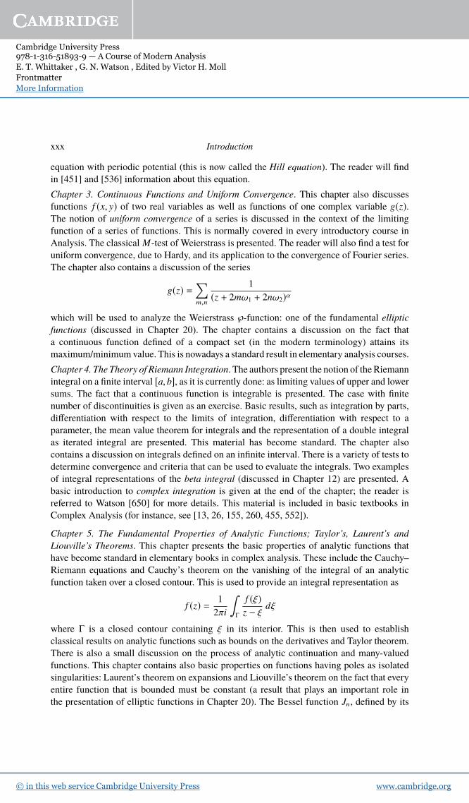
xxx Introduction
equation with periodic potential (this is now called the Hill equation). The reader will find
in [451] and [536] information about this equation.
Chapter 3. Continuous Functions and Uniform Convergence. This chapter also discusses
functions f (x, y) of two real variables as well as functions of one complex variable g(z).The notion of uniform convergence of a series is discussed in the context of the limiting
function of a series of functions. This is normally covered in every introductory course in
Analysis. The classical M-test of Weierstrass is presented. The reader will also find a test for
uniform convergence, due to Hardy, and its application to the convergence of Fourier series.
The chapter also contains a discussion of the series
g(z) =∑
m,n
1
(z + 2mω1 + 2nω2)α
which will be used to analyze the Weierstrass ℘-function: one of the fundamental elliptic
functions (discussed in Chapter 20). The chapter contains a discussion on the fact that
a continuous function defined of a compact set (in the modern terminology) attains its
maximum/minimum value. This is nowadays a standard result in elementary analysis courses.
Chapter 4. The Theory of Riemann Integration. The authors present the notion of the Riemann
integral on a finite interval [a, b], as it is currently done: as limiting values of upper and lower
sums. The fact that a continuous function is integrable is presented. The case with finite
number of discontinuities is given as an exercise. Basic results, such as integration by parts,
differentiation with respect to the limits of integration, differentiation with respect to a
parameter, the mean value theorem for integrals and the representation of a double integral
as iterated integral are presented. This material has become standard. The chapter also
contains a discussion on integrals defined on an infinite interval. There is a variety of tests to
determine convergence and criteria that can be used to evaluate the integrals. Two examples
of integral representations of the beta integral (discussed in Chapter 12) are presented. A
basic introduction to complex integration is given at the end of the chapter; the reader is
referred to Watson [650] for more details. This material is included in basic textbooks in
Complex Analysis (for instance, see [13, 26, 155, 260, 455, 552]).
Chapter 5. The Fundamental Properties of Analytic Functions; Taylor’s, Laurent’s and
Liouville’s Theorems. This chapter presents the basic properties of analytic functions that
have become standard in elementary books in complex analysis. These include the Cauchy–
Riemann equations and Cauchy’s theorem on the vanishing of the integral of an analytic
function taken over a closed contour. This is used to provide an integral representation as
f (z) = 1
2πi
∫
Γ
f (ξ)z − ξ dξ
where Γ is a closed contour containing ξ in its interior. This is then used to establish
classical results on analytic functions such as bounds on the derivatives and Taylor theorem.
There is also a small discussion on the process of analytic continuation and many-valued
functions. This chapter contains also basic properties on functions having poles as isolated
singularities: Laurent’s theorem on expansions and Liouville’s theorem on the fact that every
entire function that is bounded must be constant (a result that plays an important role in
the presentation of elliptic functions in Chapter 20). The Bessel function Jn, defined by its

Cambridge University Press978-1-316-51893-9 — A Course of Modern AnalysisE. T. Whittaker , G. N. Watson , Edited by Victor H. Moll FrontmatterMore Information
www.cambridge.org© in this web service Cambridge University Press
Introduction xxxi
integral representation
Jn(x) =1
2π
∫ 2π
0
cos(nθ − x sin θ) dθ
makes its appearance in an exercise. This function is discussed in detail in Chapter 17. The
chapter also contains a proof of the following fact: any function that is analytic, including
at ∞, except for a number of non-essential singularities, must be a rational function. This
has become a standard result. It represents the most elementary example of characterizing
functions of rational character on a Riemann surface. This is the case of P1, the Riemann
sphere. The next example corresponds to the torus C/L, where L is a lattice. This is the
class of elliptic functions described in Chapters 20, 21 and 22. The reader is referred to
[461, 553, 600, 665] for more details.
Chapter 6. The Theory of Residues: Application to the Evaluation of Definite Integrals. This
chapter presents application of Cauchy’s integral representation of functions analytic except
for a certain number of poles. Most of the material discussed here has become standard.
One of the central concepts is that of the residue of a function at a pole z = zk , defined
as the coefficient of (z − zk)−1 in the expansion of f near z = zk . As a first sign of the
importance of these residues is the statement that the integral of f (z) over the boundary of a
domainΩ is given by the sum of the residues of f insideΩ, the so-called argument principle
which gives the difference between zeros and poles of a function as a contour integral. This
chapter also presents methods based on residues to evaluate a variety of definite integrals
including rational functions of cos θ, sin θ over [0,2π], integrals over the whole real line
via deformation of a semicircle, integrals involving some of the kernels such as 1/(e2πz − 1)(coming from the Fermi–Dirac distribution in Statistical Mechanics) and 1/(1−2a cos x+a2)related to Legendre polynomials (discussed in Chapter 15). An important function makes its
appearance as Exercise 17:
ψ(t) =∞∑
n=−∞e−n
2πt,
introduced by Poisson in 1823. The exercise outlines a proof of the transformation rule
ψ(t) = t−1/2ψ(1/t)
known as Poisson summation formula. It plays a fundamental role in many problems in
Number Theory, including the proof of the prime number theorem. This states that, for x > 0,
the number of primes up to x, denoted by π(x), has the asymptotic behavior π(x) ∼ x/log x
as x → ∞. The reader will find in [492] how to use contour integration and the function ψ(t)to provide a proof of the asymptotic behavior of ψ(t). This function reappears in Chapter 21
in the study of theta functions.
Chapter 7. The Expansion of Functions in Infinite Series. This chapter begins with a result
of Darboux on the expansion of an analytic function defined on a region Ω. For points a, x,

Cambridge University Press978-1-316-51893-9 — A Course of Modern AnalysisE. T. Whittaker , G. N. Watson , Edited by Victor H. Moll FrontmatterMore Information
www.cambridge.org© in this web service Cambridge University Press
xxxii Introduction
with the segment from a to x contained in Ω, one has the expansion
φ(n)(0)[ f (z) − f (0)] =n
∑
k=1
(−1)k−1(z − a)k[
φ(n−k)(1) f (m)(z) − φn−k(0) f (k)(a)]
+ (−1)n(z − a)n+1
∫ 1
0
φ(t) f (n+1)(a + t(z − a)) dt,
for any polynomial φ. The formula is then applied to the Bernoulli polynomials currently
defined by the generating function
tezt
et − 1=
∞∑
n=0
Bn(z)n!
tn.
(The text employs the notation φn(t) without giving the value for n = 0.) Darboux’s theorem
then becomes the classical Euler–MacLaurin summation formula
n∑
j=0
f ( j) =∫ n
0
f (x) dx +f (n) + f (0)
2+
⌊p/2⌋∑
k=1
B2k
(2k)![
f (2k−1)(n) − f (2k−1)(0)]
+ (−1)p−1
∫ n
0
f (p)(x)Bp(x − ⌊x⌋)
p!dx.
The quantity x − ⌊x⌋ is the fractional part of x, denoted by x. This formula is used to
estimate partial sums of series of values of an analytic function in terms of the corresponding
integrals. The important example of the Riemann zeta function ζ(s) is presented in Chapter 13.
The chapter contains a couple of examples of expansions of one function in terms of
another one. The first one, due to Bürmann, starts with an analytic function φ(z) defined on
a region and φ(a) = b with φ′(a) , 0. Define ψ(z) = (z − a)/(φ(z) − a), then one obtains the
expansion
f (z) = f (a) +n−1∑
k=1
[φ(z) − b]kk!
(
d
da
)k−1[
f ′(a)ψk(a)]
+ Rn
where the error term has the integral representation
Rn =1
2πi
∫ z
a
∫
γ
[
φ(z) − b
φ(t) − b
]n−1f ′(t)φ′(z)φ(t) − φ(z) dt dz,
where γ is a contour in the t-plane, enclosing a and t and such that, for any µ interior to γ,
the equation φ(t) = φ(µ) has a unique solution t = µ. The discussion also contains results of
Teixeira on conditions for the convergence of the series for f (z) obtained by letting n → ∞.
This type of result also contains an expansion of Lagrange for solutions of the equation
µ = a + tφ(µ), for analytic function φ satisfying |tφ(z)| < |z − a|. The theorem states that
any analytic function f of the solution µ can be expanded as
f (µ) = f (a) +∞∑
n=1
tn
n!
(
d
da
)n−1
[ f ′(a)φn(a)] .
This expansion has interesting applications in Combinatorics; see [681] for details. The

Cambridge University Press978-1-316-51893-9 — A Course of Modern AnalysisE. T. Whittaker , G. N. Watson , Edited by Victor H. Moll FrontmatterMore Information
www.cambridge.org© in this web service Cambridge University Press
Introduction xxxiii
last type of series expansion described here corresponds to the classical partial fraction
expansions of a rational function and its extensions to trigonometric functions.
The results of this chapter are then used to prove representations of an entire function f
in the form
f (z) = f (0)eG(z)∞
∏
n=1
(
1 − z
an
)
egn (z)mn
where an is a zero of f of multiplicity mn and G(z) is an entire function. The function gn(z) is
a polynomial, introduced by Weierstrass, which makes the product converge. An application
to 1/Γ(z) is discussed in Chapter 12.
Chapter 8. Asymptotic Expansions and Summable Series. This chapter presents an intro-
duction to the basic concepts behind asymptotic expansion. The initial example considers
f (x) =∫ ∞
x
t−1ex−t dt. A direct integration by parts shows that the sum Sn(x) =∞∑
k=0
(−1)k k!
xk+1
satisfies, for fixed x, the inequality | f (x) − Sn(x)| ≤ n!/xn+1. Therefore, for x ≥ 2n, one
obtains | f (x) − Sn(x)| < 1/n22n+1. It follows that the integral f can be evaluated with great
accuracy for large values of x by computing the partial sum of the divergent series Sn(x).This type of behavior is written as f (x) ∼
∞∑
n=0
Anx−n and the series is called the asymptotic
expansion of f .
The chapter covers the basic properties of asymptotic series: such expansions can be
multiplied and integrated but not differentiated. Examples of asymptotic expansions of
special functions appear in later chapters: for the Gamma function in Chapter 12 and for the
Bessel function in Chapter 17.
The final part of the chapter deals with summation methods, concentrating on methods
assigning a value to a function given by a power series outside its circle of convergence D.
The first example, due to Borel, starts with the identity
∞∑
n=0
anzn =
∫ ∞
0
e−tφ(tz) dt where φ(u) =∞∑
n=0
an
n!un valid for z ∈ D.
The series∞∑
n=0
anzn is said to be Borel summable if the integral on the right converges for z
outside D. For such z, the Borel sum of the series is assigned to be the value of the integral.
The discussion continues with Cesàro summability, a notion to be discussed in the context
of Fourier series in Chapter 9. Extensions by Riesz and Hardy are mentioned. More details
on asymptotic expansions can be found in [468, 508].
Chapter 9. Fourier Series and Trigonometric Series. The authors discuss trigonometrical
series defined as series of the form
1
2a0 +
∞∑
n=1
(an cos nx + bn sin nx)
for two sequences of real numbers an and bn. Such series are named Fourier series if
there is a function f , with finite integral over (−π, π), such that the coefficients are given by
an =1
π
∫ π
−πf (t) cos nt dt and bn =
1
π
∫ π
−πf (t) sin nt dt .

Cambridge University Press978-1-316-51893-9 — A Course of Modern AnalysisE. T. Whittaker , G. N. Watson , Edited by Victor H. Moll FrontmatterMore Information
www.cambridge.org© in this web service Cambridge University Press
xxxiv Introduction
The chapter contains a variety of results dealing with conditions under which the Fourier
series associated to a function f converges to f . These include Dirichlet’s theorem stating
that, under some technical conditions, the Fourier series converges to 12[ f (x + 0) + f (x − 0)].
This is followed by Fejer’s theorem that the Fourier series is Césaro summable at all points
where the limits f (x±0) exist. The proofs are based on the analysis of the so-called Dirichlet–
Féjer kernel. Examples are provided where there is not a single analytic expression for the
Fourier series. The notion of orthogonality of the sequence of trigonometric functions makes
an implicit appearance in all the proofs. The so-called Riemann–Lebesgue theorem, on the
behavior of Fourier coefficients, is established. This result states that if ψ(θ) is integrable
on the interval (a, b), then limn→∞
∫ b
a
ψ(θ) sin(λθ) dθ = 0. The chapter contains results on the
function f which imply pointwise convergence of the Fourier series. The results of Dini and
Jordan, with conditions on the expressions f (x ± 2θ) − f (x ± 0) near θ = 0, are presented.
The reader will find more information about convergence of Fourier series in [368] and in
the treatise [690]. The results of Kolmogorov [381, 382] on an integrable function with a
Fourier series diverging everywhere, as well as the theorem of Carleson [118] on the almost-
everywhere convergence of the Fourier series of a continuous function, are some of the high
points of this difficult subject.
The chapter also includes a discussion on the uniqueness of the representation of a Fourier
series for a function f and also of the Gibbs phenomenon on the behavior of a Fourier series
in a neighborhood of a point of discontinuity of f .
Chapter 10. Linear Differential Equations. This chapter discusses properties of solutions of
second order linear differential equations
d2u
dz2+ p(z)du
dz+ q(z)u = 0,
where p, q are analytic functions of z except for a finite number of points. The discussion
is local; that is, in a neighborhood of a point c ∈ C. The points c are classified as ordinary,
where the functions p, q are assumed to be analytic at c and otherwise singular.
The question of existence and uniqueness of solutions of the equation is discussed. The
equation is transformed first into the formd2v
dz2+ J(z)v = 0, by an elementary change of
variables. Existence of solutions is obtained from an integral equation equivalent to the
original problem. An iteration process is used to produce a sequence of analytic functions
vn. Then it is shown that, in a neighborhood of an ordinary point, this sequence converges
uniformly to a solution of the equation. Uniqueness of the solution comes also from this
process.
The solutions near an ordinary point are presented in the case of an ordinary singular
point. These are points c ∈ C where p or q have a pole, but (z − c)p(z) and (z − c)2q(z) are
analytic functions in a deleted neighborhood of z = c. The so-called method of Frobenius is
then used to seek formal series solutions in the form
u(z) = (z − c)α[
1 +
∞∑
n=1
an(z − c)n]
.
The so-called indicial equation α2+ (p0 − 1)α + q0 = 0 and its roots α1, α2, control the

Cambridge University Press978-1-316-51893-9 — A Course of Modern AnalysisE. T. Whittaker , G. N. Watson , Edited by Victor H. Moll FrontmatterMore Information
www.cambridge.org© in this web service Cambridge University Press
Introduction xxxv
properties of these formal power series. The numbers p0, q0 are the leading terms of (z−c)p(z)and (z − c)2q(z), respectively. It is shown that if α1, α2 do not differ by an integer, there are
two formal solutions and these series actually converge and thus represent actual solutions.
Otherwise one of the formal series is an actual solution and there is a procedure to obtain a
second solution containing a logarithmic term. The reader will find in [151] all the details.
It is a remarkable fact that the behavior of the singularities determines the equation itself.
For example, the most general differential equation of second order which has every point
except a1, a2, a3, a4 and ∞ as ordinary points and these five points as regular points, must be
of the form
d2u
dz2+
4∑
r=1
1 − αr − βr
z − ar
du
dz
+
4∑
r=1
αr βr
(z − ar )2+
Az2+ Bz + C
(z − a1)(z − a2)(z − a3)(z − a4)
u = 0,
for some constants αr , βr , A, B, C. F. Klein [376] describes how all the classical equations
of Mathematical Physics appear in this class. Six classes, carrying the names of their discov-
erers (Lamé, Mathieu, Legendre, Bessel, Weber–Hermite and Stokes) are discussed in later
chapters.
The chapter finally discusses the so-called Riemann P-function. This is a mechanism used
to write a solution of an equation with three singular points and the corresponding roots
of the indicial equation. Some examples of formal rules on P, which allow to transform a
solution with expansion at one singularity to another are presented. The chapter concludes
showing that a second order equation with three regular singular points may be converted to
the hypergeometric equation. This is the subject of Chapter 14.
The modern theory of this program, to classify differential equations by their singularities,
is its extension to nonlinear equations. A singularity of an ordinary differential equation
is called movable if its location depends on the initial condition. An equation is called a
Painlevé equation if its only movable singularities are poles. Poincaré and Fuchs proved
that any first-order equation with this property may be transformed into the Ricatti equation
or it may be solved in terms of the Weierstrass elliptic function. Painlevé considered the
case of second order, transformed them into the form u′′= R(u,u′, z), where R is a rational
function. Then he put them into 50 canonical forms and showed that all but six may be
solved in terms of previously known functions. The six remaining cases gave rise to the six
Painlevé functions PI, . . . ,PVI. See [261, 310, 336] for details. It is a remarkable fact that
these functions, created for an analytic study, have recently appeared in a large variety of
problems. See [37] and [562] for their appearance in combinatorial questions, [76, 636] for
their relations to classical functions, [640] for connections to orthogonal polynomials, [632]
for their appearance in Statistical Physics. The reader will find in [212] detailed information
about their asymptotic behavior.
Chapter 11. Integral Equations. Given a function f , continuous on an interval [a, b] and
a kernel K(x, y), say continuous on both variables or in the region a ≤ y ≤ x ≤ b and
Cambridge University Press978-1-316-51893-9 — A Course of Modern AnalysisE. T. Whittaker , G. N. Watson , Edited by Victor H. Moll FrontmatterMore Information
www.cambridge.org© in this web service Cambridge University Press
xxxvi Introduction
vanishing for y > x, the equation
φ(x) = f (x) + λ∫ b
a
K(x, y)φ(y) dy
for the unknown function φ, is called the Fredholm integral equation of the second kind. The
solution presented in this chapter is based on the construction of functions D(x, y, λ) and
D(λ), both entire in λ, as a series in which the nth-term consists of determinants of order
n × n based on the function K(x, y). The solution is then expressed as
φ(x) = f (x) + 1
D(λ)
∫ b
a
D(x, ξ, λ) f (ξ) dξ.
In particular, in the homogeneous case f ≡ 0, there is a unique solution φ ≡ 0 for those
values of λ with D(λ) , 0. A process to obtain a solution for those values of λ with D(λ) = 0
is also described.
Volterra introduced the concept of reciprocal functions for a pair of functions K(x, y) and
k(x, y; λ) satisfying the relation
K(x, y) + k(x, y; λ) = λ∫ b
a
k(x, ξ; λ)K(ξ, y)dξ.
Then the solution to the Fredholm equation is given by
f (x) = φ(x) + λ∫ b
a
k(x, ξ; λ)φ(ξ)dξ.
The last part of the chapter discusses the equation
Φ(x) = f (x) + λ∫ b
a
K(x, ξ)Φ(ξ) dξ
and the solution is expressed as a series in terms of a sequence of orthonormal functions and
the sequence λn of eigenvalues of the kernel K(x, y). In detail, if f (x) = ∑
bnφn(x), then
the solution Φ is given by Φ(x) = ∑ bnλn
λ−λn
φn(x).The Fredholm equation is written formally asΦ = f +KΦ and this givesΦ = f +K f +K2
Φ.
Iteration of this process gives the so-called Neumann series Φ =∞∑
n=0
Kn f , expressing the
unknown Φ in terms of iterations of the functional defined by the kernel K .
The study of Fredholm integral equations is one of the beginnings of modern Functional
Analysis. The reader will find more details in P. Lax [415]. The ideas of Fredholm have
many applications: the reader will find in H. P. McKean [460] a down-to-earth explanation
of Fredholm’s work and applications to integrable systems (such as the Korteweg–de Vries
equation ut = uxxx + 6uux and some special solutions called solitons), to the calculations of
some integrals involving Brownian paths (such as P. Lévy’s formula for the area generated by
a two-dimensional Brownian path) and finally to explain the appearance of the so-called sine
kernel in the limiting distribution of eigenvalues of random unitary matrices. This subject has
some mysterious connections to the Riemann hypothesis as described by B. Conrey [154].
The second part of the book is called The Transcendental Functions and it consists of
12 chapters. A brief description of them is provided next.
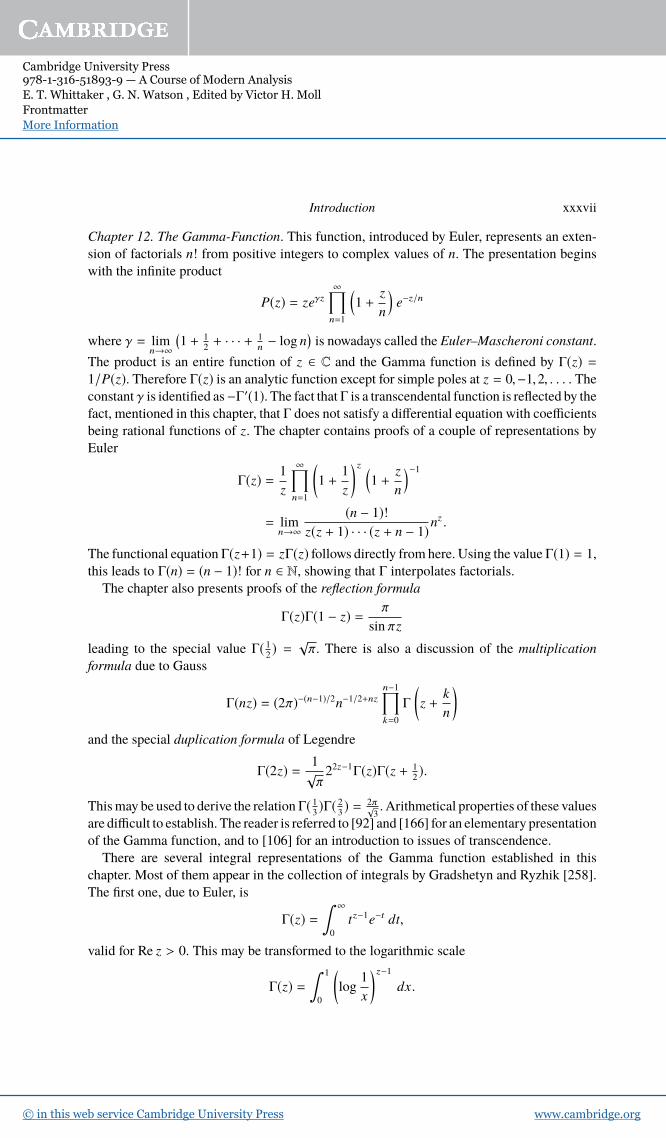
Cambridge University Press978-1-316-51893-9 — A Course of Modern AnalysisE. T. Whittaker , G. N. Watson , Edited by Victor H. Moll FrontmatterMore Information
www.cambridge.org© in this web service Cambridge University Press
Introduction xxxvii
Chapter 12. The Gamma-Function. This function, introduced by Euler, represents an exten-
sion of factorials n! from positive integers to complex values of n. The presentation begins
with the infinite product
P(z) = zeγz∞
∏
n=1
(
1 +z
n
)
e−z/n
where γ = limn→∞
(
1 + 12+ · · · + 1
n− log n
)
is nowadays called the Euler–Mascheroni constant.
The product is an entire function of z ∈ C and the Gamma function is defined by Γ(z) =1/P(z). Therefore Γ(z) is an analytic function except for simple poles at z = 0,−1,2, . . . . The
constant γ is identified as−Γ′(1). The fact that Γ is a transcendental function is reflected by the
fact, mentioned in this chapter, that Γ does not satisfy a differential equation with coefficients
being rational functions of z. The chapter contains proofs of a couple of representations by
Euler
Γ(z) = 1
z
∞∏
n=1
(
1 +1
z
)z(
1 +z
n
)−1
= limn→∞
(n − 1)!z(z + 1) · · · (z + n − 1)nz .
The functional equation Γ(z+1) = zΓ(z) follows directly from here. Using the value Γ(1) = 1,
this leads to Γ(n) = (n − 1)! for n ∈ N, showing that Γ interpolates factorials.
The chapter also presents proofs of the reflection formula
Γ(z)Γ(1 − z) = π
sin πz
leading to the special value Γ( 12) =
√π. There is also a discussion of the multiplication
formula due to Gauss
Γ(nz) = (2π)−(n−1)/2n−1/2+nzn−1∏
k=0
Γ
(
z +k
n
)
and the special duplication formula of Legendre
Γ(2z) = 1√π
22z−1Γ(z)Γ(z + 1
2).
This may be used to derive the relation Γ( 13)Γ( 2
3) = 2π√
3. Arithmetical properties of these values
are difficult to establish. The reader is referred to [92] and [166] for an elementary presentation
of the Gamma function, and to [106] for an introduction to issues of transcendence.
There are several integral representations of the Gamma function established in this
chapter. Most of them appear in the collection of integrals by Gradshetyn and Ryzhik [258].
The first one, due to Euler, is
Γ(z) =∫ ∞
0
tz−1e−t dt,
valid for Re z > 0. This may be transformed to the logarithmic scale
Γ(z) =∫ 1
0
(
log1
x
)z−1
dx.

Cambridge University Press978-1-316-51893-9 — A Course of Modern AnalysisE. T. Whittaker , G. N. Watson , Edited by Victor H. Moll FrontmatterMore Information
www.cambridge.org© in this web service Cambridge University Press
xxxviii Introduction
There is also a presentation of Hankel’s contour integral
Γ(z) = − 1
2i sin πz
∫
C
(−t)z−1e−t dt, z < Z
where C is a thin contour enclosing the positive real axis.
The chapter also contains a discussion of two functions related to Γ: its logarithm log Γ(z)and the digamma function, ψ(z) = Γ′(z)/Γ(z) = (log Γ(z))′. Integral representations for ψ(z)include
ψ(z) =∫ ∞
0
(
e−t
t− e−zt
1 − e−t
)
dt
=
∫ ∞
0
(
e−x − 1
(1 + x)z
)
dx
x;
the first one is due to Gauss and the second one to Dirichlet. The chapter also contains a
multi-dimensional integral due to Dirichlet that can be reduced to a single variable problem:∫
Rn+
f (t1 + · · · + tn)ta1−1
1· · · tan−1
n dt1 · · · dtn
=
Γ(a1) · · · Γ(an)Γ(a1 + · · · + an)
∫ 1
0
f (τ)τa1+· · ·+an−1 dτ.
Other multi-dimensional integrals appear in the modern literature. For a description of a
remarkable example due to Selberg, the reader is referred to [214].
The properties of log Γ(z) presented in this chapter include a proof of the identity
d2
dz2log Γ(z + 1) =
∞∑
k=1
1
(z + k)2 ,
showing that Γ(z+1) is log-convex. This property, the functional equation and the value Γ(1) =1 characterize the Gamma function. The reader will also find two integral representations
due to Binet
log Γ(z) =(
z − 1
2
)
log z − z +1
2log 2π +
∫ ∞
0
(
1
2− 1
t+
1
et − 1
)
e−tz
tdt
and
log Γ(z) =(
z − 1
2
)
log z − z +1
2log 2π + 2
∫ ∞
0
tan−1( tz)
e2πt − 1dt .
Integrals involving log Γ(z) present interesting challenges. The value
∫ 1
0
log Γ(z) dz = log√
2π
due to Euler, may be obtained from the reflection formula for Γ(z). The generalization of the
previous evaluation to
Ln =
∫ 1
0
(log Γ(z))n dz
is discussed next. The value of L2 is presented in [196] as an expression involving the

Cambridge University Press978-1-316-51893-9 — A Course of Modern AnalysisE. T. Whittaker , G. N. Watson , Edited by Victor H. Moll FrontmatterMore Information
www.cambridge.org© in this web service Cambridge University Press
Introduction xxxix
Riemann zeta function and its derivatives. The values of L3 and L4 were obtained in [38] and
they involve more advanced objects: multiple zeta values. At the present time an evaluation
of Ln, for n ≥ 5, is an open question.
The chapter also contains a discussion of the asymptotic behavior of log Γ(z), as a gener-
alization of Stirling’s formula for factorials and also a proof of the expression for the Fourier
series of log Γ(z) due to Kummer. The Barnes G-function, an important generalization of
Γ(z), appears in the exercises at the end of this chapter. A detailed presentation of these and
other topics may be found in [20].
Chapter 13. The Zeta-Function of Riemann. For s = σ + it ∈ C, the function
ζ(s) =∞∑
n=1
1
ns
is the Riemann zeta function. This had been considered by Euler for s ∈ R. For δ > 0, the
series defines an analytic function of s on the half-plane σ = Re s ≥ 1 + δ. The function
admits the integral representation
ζ(s) = 1
Γ(s)
∫ ∞
0
xs−1e−x
1 − e−xdx.
Euler produced the infinite product
ζ(s) =∏
p
(1 − p−s)−1
where the product extends over all prime numbers. This formula shows that ζ(s) has no zeros
in the open half-plane Re s > 1. The auxiliary function
ξ(s) = 1
2π−s/2s(s − 1)Γ
( s
2
)
ζ(s)
is analytic and satisfies the identity ξ(s) = ξ(1 − s). This function now shows that ζ(s) has
no zeros for Re s < 0, aside for the so-called trivial zeros at s = −2, −4, −6, . . . coming from
the poles of Γ(s/2). Thus all the non-trivial zeros lie on the strip 0 ≤ Re s ≤ 1. The Riemann
hypothesis states that all the roots of ζ(s) = 0 are on the critical line Re s = 12. At the end of
§13.3 the authors state that:
It was conjectured by Riemann, but it has not yet been proved, that all the zeros of ζ(s) in this
strip lie on the line σ = 12; while it has quite recently been proved by Hardy [279] that an
infinity of zeros of ζ(s) actually lie on σ = 12. It is highly probable that Riemann’s conjecture
is correct, and the proof of it would have far-reaching consequences in the theory of Prime
Numbers.
The reader will find in [93, 153, 458] more information about the Riemann hypothesis. In
a remarkable new connection, it seems that the distribution of the zeros of ζ(s) is related to
the eigenvalues of random matrices [367, 369].
This chapter establishes the identity
ζ(2n) = (−1)n−1B2n(2π)2n2 (2n)!
where n ∈ N and B2n is the Bernoulli number. This is a generalization of the so-called Basel

Cambridge University Press978-1-316-51893-9 — A Course of Modern AnalysisE. T. Whittaker , G. N. Watson , Edited by Victor H. Moll FrontmatterMore Information
www.cambridge.org© in this web service Cambridge University Press
xl Introduction
problem ζ(2) = π2/6. The solution of this problem won the young Euler instant fame. It
follows that ζ(2n) is a rational multiple of π2n, therefore this is a transcendental number.
The arithmetic properties of the odd zeta values are more difficult to obtain. Apéry proved
in 1979 that ζ(3) is not a rational number; see [27, 72, 689]. It is still unknown whether
ζ(5) is irrational, but Zudilin [688] proved that one of the numbers ζ(5), ζ(7), ζ(9), ζ(11) is
irrational. It is conjectured that all odd zeta values are irrational.
The literature contains a large variety of extensions of the Riemann zeta function. The
chapter contains information about some of them: the Hurwitz zeta function
ζ(s,a) =∞∑
n=0
1
(n + a)s , with 0 < a ≤ 1
with integral representation
ζ(s,a) = 1
Γ(s)
∫ ∞
0
xs−1 e−ax
1 − e−xdx.
The chapter establishes the values of ζ(−m,a) in terms of derivatives of the Bernoulli
polynomials and presents a proof of Lerch’s theorem
d
dsζ(s,a)
s=0= log
(
Γ(a)√
2π
)
.
The chapter mentions two further generalizations: one introduced by Lerch (see [414] for
details)
φ(x,a; s) =∞∑
n=0
e2πinx
(n + a)s ,
and another one by Barnes [43, 44, 45, 46]
ζN (s,w | a1, . . . ,aN ) =∑
n1 ,...,nN
1
(w + n1a1 + · · · + nNaN )s.
The reader will find in [566] more recent information on this function.
Chapter 14. The Hypergeometric Function. This function is defined by the series
F(a, b; c, z) =∞∑
n=0
(a)n(b)n(c)nn!
zn,
provided c is not a negative integer. Here (u)n = Γ(u + n)/Γ(u) is the Pochhammer symbol.
The series converges for |z | < 1 and on the unit circle |z | = 1 if Re (c − a − b) > 0. Many
elementary functions can be expressed in hypergeometric form, for instance
F(1,1; 1; z) = 1
1 − zand ez = lim
b→∞F
(
1, b; 1;z
b
)
.
The chapter begins with Gauss’ evaluation F(a, b; c; 1) in the form
F(a, b; c; 1) = Γ(c)Γ(c − a − b)Γ(c − a)Γ(c − b) .
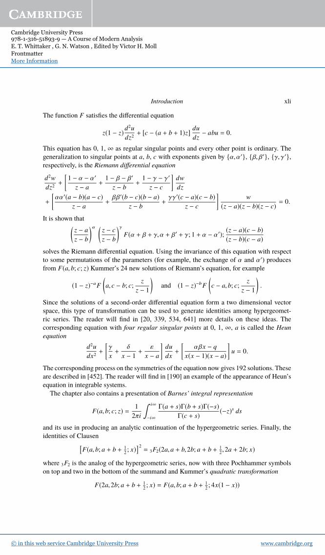
Cambridge University Press978-1-316-51893-9 — A Course of Modern AnalysisE. T. Whittaker , G. N. Watson , Edited by Victor H. Moll FrontmatterMore Information
www.cambridge.org© in this web service Cambridge University Press
Introduction xli
The function F satisfies the differential equation
z(1 − z)d2u
dz2+ [c − (a + b + 1)z] du
dz− abu = 0.
This equation has 0, 1, ∞ as regular singular points and every other point is ordinary. The
generalization to singular points at a, b, c with exponents given by α,α′, β, β′, γ, γ ′,respectively, is the Riemann differential equation
d2w
dz2+
[
1 − α − α′
z − a+
1 − β − β′
z − b+
1 − γ − γ ′
z − c
]
dw
dz
+
[
αα′(a − b)(a − c)z − a
+
ββ′(b − c)(b − a)z − b
+
γγ ′(c − a)(c − b)z − c
]
w
(z − a)(z − b)(z − c) = 0.
It is shown that(
z − a
z − b
)α (
z − c
z − b
)γ
F(α + β + γ,α + β′ + γ; 1 + α − α′); (z − a)(c − b)(z − b)(c − a)
solves the Riemann differential equation. Using the invariance of this equation with respect
to some permutations of the parameters (for example, the exchange of α and α′) produces
from F(a, b; c; z) Kummer’s 24 new solutions of Riemann’s equation, for example
(1 − z)−aF
(
a, c − b; c;z
z − 1
)
and (1 − z)−bF
(
c − a, b; c;z
z − 1
)
.
Since the solutions of a second-order differential equation form a two dimensional vector
space, this type of transformation can be used to generate identities among hypergeomet-
ric series. The reader will find in [20, 339, 534, 641] more details on these ideas. The
corresponding equation with four regular singular points at 0, 1, ∞, a is called the Heun
equation
d2u
dx2+
[
γ
x+
δ
x − 1+
ε
x − a
]
du
dx+
[
αβx − q
x(x − 1)(x − a)
]
u = 0.
The corresponding process on the symmetries of the equation now gives 192 solutions. These
are described in [452]. The reader will find in [190] an example of the appearance of Heun’s
equation in integrable systems.
The chapter also contains a presentation of Barnes’ integral representation
F(a, b; c; z) = 1
2πi
∫ i∞
−i∞
Γ(a + s)Γ(b + s)Γ(−s)Γ(c + s) (−z)s ds
and its use in producing an analytic continuation of the hypergeometric series. Finally, the
identities of Clausen
[
F(a, b; a + b + 12; x)
]2= 3F2(2a,a + b,2b; a + b + 1
2,2a + 2b; x)
where 3F2 is the analog of the hypergeometric series, now with three Pochhammer symbols
on top and two in the bottom of the summand and Kummer’s quadratic transformation
F(2a,2b; a + b + 12; x) = F(a, b; a + b + 1
2; 4x(1 − x))

Cambridge University Press978-1-316-51893-9 — A Course of Modern AnalysisE. T. Whittaker , G. N. Watson , Edited by Victor H. Moll FrontmatterMore Information
www.cambridge.org© in this web service Cambridge University Press
xlii Introduction
appear as exercises in this chapter. The reader will find in [20] a detailed analysis of these
topics.
Chapter 15. Legendre Functions. This chapter discusses Legendre polynomials Pn(z) and
some of their extensions. These days, the usual starting point for these functions is defining
them as orthogonal polynomials on the interval (−1,1); that is,
∫ 1
−1
Pn(z)Pm(z) dz = 0 if n , m,
plus some normalization in the case n = m. The starting point in this chapter is the generating
function
(1 − 2zh + h2)−1/2=
∞∑
n=0
Pn(z)hn.
It is established from here that
Pn(z) =
⌊
n2
⌋
∑
r=0
(−1)r (2n − 2r)!2nr!(n − r)!(n − 2r)! zn−2r
showing that Pn(z) is a polynomial of degree n with leading coefficient 2−n (2nn
)
.
The properties of these polynomials established in this chapter include
Rodriguez formula
Pn(z) =1
2n n!
(
d
dz
)n
(z2 − 1)n.
Legendre’s differential equation The polynomials Pn(z) are solutions of the differential
equation
(1 − z2)d2u
dz2− 2z
du
dz+ n(n + 1)u = 0.
In the new scale x = z2, this equation takes its hypergeometric form
x(1 − x)d2y
dx2+
1
2(1 − 3x)du
dx+
1
4n(n + 1)u = 0.
The (more convenient) hypergeometric form Pn(z) = 2F1(n + 1,−n; 1; 12(1 − z) is
also established.
Recurrences The chapter presents proofs of the recurrences
(n + 1)Pn+1(z) − (2n + 1)zPn(z)zPn(z) − nzPn(z) = 0
and
P′n+1(z) − zP′
n(z) − (n + 1)Pn(z) = 0.
Integral representations A variety of integral representations for the Legendre polynomials
are presented:
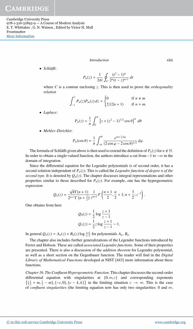
Cambridge University Press978-1-316-51893-9 — A Course of Modern AnalysisE. T. Whittaker , G. N. Watson , Edited by Victor H. Moll FrontmatterMore Information
www.cambridge.org© in this web service Cambridge University Press
Introduction xliii
• Schläfli:
Pn(z) =1
2πi
∮
C
(t2 − 1)n2n(t − z)n+1
dt
where C is a contour enclosing z. This is then used to prove the orthogonality
relation∫ 1
−1
Pn(z)Pm(z) dz =
0 if n , m
2/(2n + 1) if n = m.
• Laplace:
Pn(z) =1
π
∫ π
0
[
z + (z2 − 1)1/2 cos θ]n
dθ
• Mehler–Dirichlet:
Pn(cos θ) = 1
π
∫ θ
−θ
e(n+12)iϕ
(2 cos ϕ − 2 cos θ)1/2 dϕ.
The formula of Schläfli given above is then used to extend the definition of Pn(z) for n < N.
In order to obtain a single-valued function, the authors introduce a cut from −1 to −∞ in the
domain of integration.
Since the differential equation for the Legendre polynomials is of second order, it has a
second solution independent of Pn(z). This is called the Legendre function of degree n of the
second type. It is denoted by Qn(z). The chapter discusses integral representations and other
properties similar to those described for Pn(z). For example, one has the hypergeometric
expression
Qn(z) =√πΓ(n + 1)
2n+1Γ(
n + 32
)
1
zn+1F
(
n + 1
2,n
2+ 1; n +
3
2; z−2
)
.
One obtains from here
Q0(z) =1
2log
z + 1
z − 1
Q1(z) =1
2z log
z + 1
z − 1− 1.
In general Qn(z) = An(z) + Bn(z) log z+1z−1
for polynomials An, Bn.
The chapter also includes further generalizations of the Legendre functions introduced by
Ferrer and Hobson. These are called associated Legendre functions. Some of their properties
are presented. There is also a discussion of the addition theorem for Legendre polynomial,
as well as a short section on the Gegenbauer function. The reader will find in the Digital
Library of Mathematical Functions developed at NIST [443] more information about these
functions.
Chapter 16. The Confluent Hypergeometric Function. This chapter discusses the second-order
differential equation with singularities at 0,∞, c and corresponding exponents
12+ m, 1
2− m, −c,0, c − k, k
in the limiting situation c → ∞. This is the case
of confluent singularities (the limiting equation now has only two singularities: 0 and ∞,

Cambridge University Press978-1-316-51893-9 — A Course of Modern AnalysisE. T. Whittaker , G. N. Watson , Edited by Victor H. Moll FrontmatterMore Information
www.cambridge.org© in this web service Cambridge University Press
xliv Introduction
with 0 remaining regular and∞ becomes an irregular singularity). After a change of variables
to eliminate the first derivative term, the limiting equation becomes
d2W
dz2+
(
−1
4+
k
z+
14− m2
z2
)
W = 0.
This is called Whittaker equation.
The authors introduce the functions
Mk ,m(z) = z1/2+me−z/2
(
1 +
12+ m − k
1! (2m + 1) z +( 1
2+ m − k)( 3
2+ m − k)
2! (2m + 1)(2m + 2) z2+ · · ·
)
and show that, when 2m < N, the functions Mk ,m(z) and Mk ,−m(z) form a fundamental set of
solutions.
It turns out that it is more convenient to work with the functions Wk ,m(z) defined by the
integral representation
Wk ,m(z) =zke−k/2
Γ( 12− k + m)
∫ ∞
0
t−k−1/2+m(
1 +t
z
)k−1/2+m
e−t dt .
The reader is referred to [59, Chapter 6] for a readable description of the basic properties of
these functions, called Whittaker functions in the literature.
The chapter also presents a selection of special functions that can be expressed in terms
of Wk ,m(z). This includes the incomplete gamma function
γ(a, x) =∫ x
0
ta−1e−t dt
that can be expressed as
γ(a, x) = Γ(a) − x(a−1)/2e−x/2W 12(a−1), 1
2a(x),
as well as the logarithmic integral function, defined by
li(z) =∫ x
0
dt
log t= −(− log z)−1/2z1/2W
− 12,0(− log z).
This function appears in the description of the asymptotic behavior of the function
π(x) = number of primes p ≤ x.
The prime number theorem may be written as π(x) ∼ li(x) as x → ∞. See [191] for details.
The final example is the function
Dn(z) = 2n/2+1/4z−1/2W n2+
14,− 1
4
(
z2
2
)
,
related in a simple manner to the Hermite polynomials, defined by
Hn(z) = (−1)nez2/2
(
d
dz
)n
e−z2/2.
See [20] for information on this class of orthogonal polynomials.

Cambridge University Press978-1-316-51893-9 — A Course of Modern AnalysisE. T. Whittaker , G. N. Watson , Edited by Victor H. Moll FrontmatterMore Information
www.cambridge.org© in this web service Cambridge University Press
Introduction xlv
Chapter 17. Bessel Functions. This chapter discusses the Bessel functions defined, for n ∈ Z,
by the expansion
exp
(
z
2
(
t − 1
t
))
=
∞∑
n=−∞Jn(z)tn.
Some elementary properties of Jn(z) are derived directly from this definition, such as J−n(z) =(−1)nJn(z), the series
Jn(z) =∞∑
r=0
(−1)rr! (n + r)!
( z
2
)n+2r
,
and the addition theorem
Jn(y + z) =∞∑
m=−∞Jm(y)Jn−m(z).
The Cauchy integral formula is then used to produce the representation
Jn(z) =1
2πi
( z
2
)n∮
C
t−n−1et−z2/4t dt,
where C is a closed contour enclosing the origin. From here it is possible to extend the
definition of Jn(z) to values n < Z and produce the series representation
Jn(z) =∞∑
r=0
(−1)r zn+2r
2n+2rr!Γ(n + r + 1) .
This function is called the Bessel function of the first kind of order n. The integral repre-
sentation of Jn(z) is then used to show that y(z) = Jn(z) is a solution of the differential
equation
d2y
dz2+
1
z
dy
dz+
(
1 − n2
z2
)
y = 0,
called the Bessel equation. In the case n < Z, the functions Jn(z) and J−n(z) form a basis for
the space of solutions. In the case n ∈ Z a second solution, independent of Jn(z), is given by
Yn(z) = limε→0
2πeπi(n+ε)(
Jn+ε(z) cos(π(n + ε)) − J−(n+ε)(z)sin(2π(n + ε))
)
.
The functions Yn(z) are called the Bessel functions of the second kind.
This chapter also contains some information on some variations of the Bessel function
such as
In(z) = i−nJn(iz) and Kn(z) =π
2[I−n(z) − In(z)] cot(πn).
Among the results presented here one finds
Recurrences such as
Jn−1(z) + Jn+1(z) =2n
zJn(z),
J ′n(z) =
n
zJn(z) − Jn+1(z)

Cambridge University Press978-1-316-51893-9 — A Course of Modern AnalysisE. T. Whittaker , G. N. Watson , Edited by Victor H. Moll FrontmatterMore Information
www.cambridge.org© in this web service Cambridge University Press
xlvi Introduction
and
z−n−1Jn+1(z) = −1
z
d
dz[z−nJn(z)]
which produces relations of Bessel functions of consecutive indices.
Zeros of Bessel functions it is shown that between any two non-zero consecutive roots of
Jn(z) = 0 there is a unique root of Jn+1(z) = 0.
Integral representations such as
Jn(z) =1
π
∫ π
0
cos(nθ − z sin θ) dθ − sin πn
π
∫ ∞
0
e−nθ−z sinh θ dθ,
where, for n ∈ Z, the second term vanishes.
Hankel representation in the form
Jn(z) =Γ( 1
2− n)
2πi√π
( z
2
)n∫
C
(t2 − 1)n−1/2 cos(zt) dt
where C is a semi-infinite contour on the real line.
Evaluation of definite integrals such as one due to Mahler
K0(x) =∫ ∞
0
t
1 + t2J0(t x) dt
and an example due to Sonine giving an expression for
∫ ∞
0
x1−mJm(ax)Jm(bx)Jm(cx) dx.
A large selection of integrals involving Bessel functions may be found in [105],
[258] and [544].
Series expansion The chapter also contains information about expansions of a function f (z)in a series of the form
f (z) =∞∑
n=0
anJn(z) or f (z) =∞∑
n=0
anJ0(nz).
The reader will find in [20] and [59] more information on these functions at the level
discussed in this chapter. Much more appears in the volume [653].
There are many problems whose solutions involve the Bessel functions. As a current
problem of interest, consider the symmetric group SN of permutations π of N symbols.
An increasing sequence of length k is a collection of indices 1 ≤ i1 < · · · < ik ≤ N such
that π(i1) < π(i2) < · · · < π(ik). Define on SN a uniform probability distribution; that is,
P(π) = 1/N! for each permutation π. Then the maximal length of an increasing subsequence
of π is a random variable, denoted by ℓN (π), and its distribution is of interest. This is the
Ulam problem. Introduce the centered and scaled function
χN (π) =ℓN (π) − 2
√N
N1/6 .

Cambridge University Press978-1-316-51893-9 — A Course of Modern AnalysisE. T. Whittaker , G. N. Watson , Edited by Victor H. Moll FrontmatterMore Information
www.cambridge.org© in this web service Cambridge University Press
Introduction xlvii
Baik–Deift–Johannson [36] proved that limN→∞P(χN (π) ≤ x) = F(x),where F(x), the so-called
Tracy–Widom distribution, is given by
F(x) = exp
(
−∫ ∞
x
(y − x)u2(y) dy
)
.
Here u(x) is the solution of the Painlevé PII equation u′′(x) = 2u3(x) + xu(x), with
asymptotic behavior u(x) ∼ Ai(x) as x → ∞. The Airy function Ai(x) is defined by
Ai(x) =√
xK1/3
(
23
x3/2)
/π√
3. The reader will find in [37] an introduction to this fasci-
nating problem.
Chapter 18. The Equations of Mathematical Physics. This chapter contains a brief description
of methods of solutions for the basic equations encountered in Mathematical Physics. The
results are given for Laplace’s equation
∆V =∂2V
∂x2+
∂2V
∂y2+
∂2V
∂z2
on a domain Ω ⊂ R3. The chapter has a presentation on the physical problems modeled by
this equation.
The results include the integral representation of the solution
V(x, y, z) =∫ π
−πf (z + ix cos u + iy sin u,u) du
as the 3-dimensional analog of the form V(x, y) = f (x + iy) + g(x − iy) valid in the 2-
dimensional case as well as an expression for V(x, y, z) as a series with terms of the form
∫ π
−π(z + ix cos u + iy sin u)n
(
cos mu
sin mu
)
du.
This series is then converted into one of the form
V =
∞∑
n=0
rn
AnPn(cos θ) +∞∑
m=1
(
A(m)n cos mφ + B(m)
n sin mφ)
Pmn (cos θ)
where Pmn is Ferrer’s version of the associated Legendre function.
The chapter also contains similar results for Laplace’s equation on a sphere. For this type
of domain, the authors obtain the formula
V(r, θ, φ) = a(a2 − r2)4π
∫ π
−π
∫ π
0
f (θ ′, φ′) sin θ ′ dθ ′ dφ′
[r2 − 2arcos θ cos θ ′ + sin θ sin θ ′ cos(φ − φ′) + a2]3/2 ,
and refer to Thompson and Tait [628] for further discussions on the theory of Green’s
functions. A similar analysis for an equation on a cylinder also appears in this chapter. In
that case the Legendre functions are replaced by Bessel functions. Some of the material
discussed in this chapter has become standard in basic textbooks in Mathematical Physics;
see for instance [476].
Chapter 19. Mathieu Functions. This chapter discusses the wave equation Vtt = c2∆V and
assuming a special form V(x, y, t) = u(x, y) cos(pt + ε) of the unknown V in a special system
Cambridge University Press978-1-316-51893-9 — A Course of Modern AnalysisE. T. Whittaker , G. N. Watson , Edited by Victor H. Moll FrontmatterMore Information
www.cambridge.org© in this web service Cambridge University Press
xlviii Introduction
of coordinates (ξ, η) (introduced by Lamé) yields an equation for u(x, y). Using the classical
method of separation of variables (u ∗ x, y) = F(ξ)G(η) produces the equation
d2y
dz2+ (a + 16q cos(2z)) y = 0.
This is called Mathieu’s equation. The value of a is determined by the periodicity condition
G(η+2π) = G(η) and q is determined by a vanishing condition at the boundary. This type of
equation is now called Hill’s equation, considered by Hill [306] in a study on lunar motion.
Details about this equation appear in [451] and connections to integrable systems appear in
[459, 462, 463].
The authors show that G(η) satisfies the integral equation
G(η) = λ∫ π
−πek cosη cos θG(θ) dθ
and this λ must be a characteristic value as described in Chapter 11.
A sequence of functions, named Mathieu functions, are introduced from the study of
Mathieu’s equation. In the case q = 0, the solutions are 1,cos nz, sin nzn∈N, and via Fourier
series the authors introduce functions ce0(z,q), cen(z,q), sen(z,q)n∈N, reducing to the pre-
vious set as q → 0. Some expressions for the first coefficients in the Fourier series of these
functions are produced (it looks complicated to obtain exact expressions for them).
The authors present basic aspects of Floquet theory (more details appear in [451]). One
looks for solution of Mathieu’s equation in the form y(z) = eµzφ(z), with φ periodic. The
values of µ producing such solutions are obtained in terms of a determinant (called the Hill
determinant). The modern theory yields these values in terms of a discriminant attached
to the equation. The chapter also discusses results of Lindemann, transforming Mathieu’s
equation into the form
4ξ(1 − ξ)u′′+ 2(1 − 2ξ)u′
+ (a − 16q + 32qξ)u = 0.
This equation is not of hypergeometric type: the points 0, 1 are regular, but ∞ is an irregular
singular point. Finally, the chapter includes some description of the asymptotic behavior of
Mathieu functions. More details appear in [34] and [509].
Chapter 20. Elliptic Functions. General Theorems and the Weierstrassian Functions. Con-
sider two complex numbers ω1, ω2 with non-real ratio. An elliptic function is a doubly-
periodic functions: f (z+2ω1) = f (z+2ω2) = f (z) where its singularities are at worst poles.
The chapter discusses basic properties of the class E of elliptic functions. It is simple to
verify that E is closed under differentiation and that the values of f ∈ E are determined by
its values on the parallelogram with vertices 0, 2ω1, 2ω1 + 2ω2, 2ω2. (Observe the factor
of 2 in the periods.) This is called a fundamental cell and is denoted by L. One may always
assume that there are no poles of the function on the boundary of the cell. The first type of
results deal with basic properties of an elliptic function:
(1) the number of poles is always finite; the same is true for the number of solutions of
f (z) = c. This is independent of c ∈ C and is called the degree of the function f .
(2) any elliptic function without poles must be constant.
Cambridge University Press978-1-316-51893-9 — A Course of Modern AnalysisE. T. Whittaker , G. N. Watson , Edited by Victor H. Moll FrontmatterMore Information
www.cambridge.org© in this web service Cambridge University Press
Introduction xlix
This result is used throughout the chapter to establish a large number of identities. The
fundamental example
℘(z) = 1
z2+
∑
(
1
(z − ω)2 − 1
ω2
)
where the sum runs over all non-zero ω = 2nω1 + 2mω2, was introduced by Weierstrass. It
is an elliptic function of order 2. It has a double pole at z = 0. It is an even function, so its
zeros in the fundamental cell are of the form ±z0 mod L. A remarkably recent formula for z0
is given by Eichler and Zagier [192]. The ℘ function satisfies a differential equation
(
d℘(z)dz
)2
= 4℘(z)3 − g2℘(z) − g3,
where g2, g3 are the so-called invariants of the lattice L. This function is then used to
parametrize the algebraic curve y2= 4x3
+ ax + b, for a, b ∈ C with a3+ 27b2
, 0. The
subject is also connected to differential equation by showing that if y = ℘(z), then the inverse
z = ℘−1(y) (given by an elliptic integral) can be written as the quotient of two solutions of
d2v
dy2+
(
3
16
3∑
r=1
(y − er )−2 − 3
8y
3∏
r=1
(y − er )−1
)
v = 0.
Here er are the roots of the cubic polynomial appearing in the differential equation for ℘(z).The addition theorem
℘(z + y) = 1
4
[
℘′(z) − ℘′(y)℘(z) − ℘(y)
]2
− ℘(z) − ℘(y)
is established by a variety of methods. One presented by Abel deals with the intersection
of the cubic curve y2= 4x3
+ ax + b and a line and it is the basis for an addition on
the elliptic curve, as the modern language states. Take two points a, b on the curve and
compute the line joining them. This line intersects the cubic at three points: the third is
declared −a ⊕ b. The points on the curve now form an abelian group: this is expected since
the cubic may be identified with a torus C/L. The remarkable fact is that the addition of
points preserves points with rational coordinates, so this set is also an abelian group. A
theorem of Mordell and Weil states that this group is finitely generated. More information
about the arithmetic of elliptic curves may be found in [331, 461, 592, 593]. The chapter
also contains some information about two additional functions: the Weierstrass ζ-function,
defined by ζ ′(z) = −℘(z) with limz→0
ζ(z) − 1/z = 0 and the Weierstrass σ-function, defined
by (logσ(z))′ = ζ(z) with limz→0
σ(z)/z = 1. These are the elliptic analogs of the cotangent
and sine functions. The chapter contains some identities for them, for instance one due to
Stickelberger: if x + y + z = 0, then
[ζ(x) + ζ(y) + ζ(z)]2 + ζ ′(x) + ζ ′(y) + ζ ′(z) = 0,
as well as the identity
℘(z) − ℘(y) = −σ(z + y)σ(z − y)σ2(z)σ2(y) ,

Cambridge University Press978-1-316-51893-9 — A Course of Modern AnalysisE. T. Whittaker , G. N. Watson , Edited by Victor H. Moll FrontmatterMore Information
www.cambridge.org© in this web service Cambridge University Press
l Introduction
just to cite two of many. Among the many important results established in this chapter, we
select three:
(1) any elliptic function f can be written in the form R1(℘)+R2(℘)℘′(z), with R1, R2 rational
functions;
(2) every elliptic function f satisfies an algebraic differential equation;
(3) any curve of genus 1 can be parametrized by elliptic functions.
The chapter contains a brief discussion on the uniformization of curves of higher genus. This
problem is discussed in detail in [7, 12, 477].
Chapter 21. The Theta-Functions. The study of the function
ϑ(z,q) =∞∑
n=−∞(−1)nqn2
e2niz
with q = exp(πiτ) and Im τ > 0 was initiated by Euler and perfected by Jacobi in [349]. This
is an example of a theta function. It is a non-constant analytic function of z ∈ C, so it cannot
be elliptic, but it has a simple transformation rule under z 7→ z+ τ. This chapter considers ϑ,
relabelled as ϑ1 as well as three other companion functions ϑ2, ϑ3 and ϑ4. These functions
have a single zero in the fundamental cell L and since they transform in a predictable manner
under the elements of L, it is easy to produce elliptic functions from them. This leads to a
remarkable series of identities such as
ϑ3(z,q) = ϑ3(2z,q4) + ϑ2(2z,q4)
and
ϑ42(0,q) + ϑ4
4(0,q) = ϑ43(0,q)
that represents a parametrization of the Fermat projective curve x4+ y
4= z4. The chapter
also discusses the addition theorem
ϑ3(z + y)ϑ3(z − y)ϑ23(0) = ϑ2
3(y)ϑ23(z) + ϑ2
1(y)ϑ21(z)
(where the second variable q has been omitted) as well as an identity of Jacobi
ϑ′1(0) = ϑ2(0)ϑ3(0)ϑ4(0).
This corresponds to the triple product identity, written as
∞∏
n=1
(1 − q2n)(1 + q2n−1p2)(1 + q2m−1p−2) =∞∑
n=−∞qn2
p2n,
using the representation of theta functions as infinite products. The literature contains a
variety of proofs of this fundamental identity; see Andrews [19] for a relatively simple one,
Lewis [433] and Wright [683] for enumerative proofs and [311] for more general information
on the so-called q-series. The chapter also shows that a quotient of theta functions ξ satisfies
the differential equation
(
dξ
dτ
)2
=
(
ϑ22(0) − ξ2ϑ2
3(0)) (
ϑ23(0) − ξ2ϑ2
2(0))
.

Cambridge University Press978-1-316-51893-9 — A Course of Modern AnalysisE. T. Whittaker , G. N. Watson , Edited by Victor H. Moll FrontmatterMore Information
www.cambridge.org© in this web service Cambridge University Press
Introduction li
This is Jacobi’s version of the differential equation satisfied by the Weierstrass ℘-function.
The properties of solutions of this equation form the subject of the next chapter.
The reader will find in Baker [39, 40] a large amount of information on these functions
from the point of view of the 19th century, Mumford [478, 479, 480] for a more modern point
of view and [208, 209] for their connections to Riemann surfaces. Theta functions appeared
scattered in the magnificent collection by Berndt [60, 61, 62, 63, 64] and Andrews–Berndt
[21, 22, 23, 24, 25] on the formulas stated by Ramanujan.
Chapter 22. The Jacobian Elliptic Functions. Each elliptic function f has a degree attached
to it. This is defined as the number of solutions to f (z) = c in a fundamental cell. Constants
have degree 0 and there are no functions of degree 1. A function of degree 2 either has
a double pole (say at the origin) or two simple poles. The first case corresponds to the
Weierstrass ℘ function described in Chapter 20. The second case is discussed in this chapter.
The starting point is to show that any such function y = y(u) may be written as a quotient of
theta functions. From here the authors show that y must satisfy the equation
(
dy
du
)2
=
(
1 − y2) (
1 − k2y
2)
where k ∈ C is the modulus. An expression for k as a ratio of null-values of theta functions
is provided. Then y = y(u) is seen to come from the inversion of the relation
u =
∫ y
0
(
1 − t2)−1/2 (
1 − k2t2)−1/2
dt
and, following Jacobi, the function y is called the sinus amplitudinus and is denoted by
y = sn(u, k). This function becomes the trigonometrical y = sin u when k → 0. Two
companion functions cn(u, k) and dn(u, k) are also introduced. These functions satisfy a
system of nonlinear differential equations
ÛX = Y Z, ÛY = −Z X, ÛZ = −k2XY,
and they are shown to parametrize the curve ξ2= (1 − η2)(1 − k2η2).
The chapter also contains an addition theorem for these functions, such as
sn(u + v) = sn u cn v dn v + sn v cn u dnu
1 − k2 sn2 u sn2v
and other similar expressions.
The complete elliptic integral of the first kind K(k) (and the complementary one K ′(k))appears here from sn(K(k), k) = 1. The authors establish an expression for K(k) in terms of
theta values, prove Legendre’s identity
d
dk
(
k(k ′)2 dK
dk
)
= kK,
and present a discussion of the periods of the (Jacobian elliptic) functions sn, cn, dn in terms
of elliptic integrals. The reader will find details of these properties in [90, 461]. Other results
appearing here include product representations of Jacobi functions, the Landen transforma-
tion and several definite integrals involving these functions. There is also a discussion on
the so-called singular values: these are special values of the modulus k such that the ratio
Cambridge University Press978-1-316-51893-9 — A Course of Modern AnalysisE. T. Whittaker , G. N. Watson , Edited by Victor H. Moll FrontmatterMore Information
www.cambridge.org© in this web service Cambridge University Press
lii Introduction
K ′(k)/K(k) has the form (a + b√
n)/(c + d√
n) with a, b, c, d and n ∈ Z. These values of
k satisfy polynomial equations with integer coefficients. The authors state that the study of
these equation lies beyond the scope of this book. The reader will find information about
these equations in [90].
Chapter 23. Ellipsoidal Harmonics and Lamé’s Equation. This chapter presents the basic
theory of ellipsoidal harmonics. It begins with the expression
Θp =x2
a2+ θp
+
y2
b2+ θp
+
z2
c2+ θp
− 1
where a > b > c are the semi-axis of the ellipsoid Θp = 0. A function of the form
Πm(Θ) = Θ1 · · ·Θm is called an ellipsoidal harmonic of the first species. The chapter de-
scribes harmonic functions (that is, one satisfying ∆u = 0) of this form. It turns out that
every such function (with n even) has the form
n/2∏
p=1
(
x2
a2+ θp
+
y2
b2+ θp
+
z2
c2+ θp
− 1
)
where θ1, . . . , θn/2 are zeros of a polynomial Λ(θ) of degree n/2. This polynomial solves the
Lamé equation
4√
(a2+ θ)(b2
+ θ)(c2+ θ) d
dθ
[
√
(a2+ θ)(b2
+ θ)(c2+ θ)dΛ
dθ
]
= [n(n + 1)θ + C]Λ(θ).
The value C is constant and it is shown that there are 12n+1 possible choices. There are three
other types of ellipsoidal harmonics with a similar theory behind them.
The chapter contains many versions of Lamé’s equation: the algebraic form
d2Λ
dλ2+
1
2
(
1
a2+ λ+
1
b2+ λ+
1
c2+ λ
)
dΛ
dλ=
[n(n + 1)λ + C]Λ4(a2+ λ)(b2
+ λ)(c2+ λ)
as well as the Weierstrass elliptic form
d2Λ
du2= [n(n + 1)℘(u) + B]Λ
and finally the Jacobi elliptic form
d2Λ
dα2=
[
n(n + 1)k2sn2α + A]
Λ.
These equations are used to introduce Lamé functions. These are used to show that there are
2n + 1 ellipsoidal harmonics that form a fundamental system of the harmonic functions of
degree n.
The chapter contains a brief comment on work by Heun [300, 301] mentioning the study
of an equation with four singular points. The reader will find in Ronveaux [563] more
information about this equation.
Copyright © 2022 FDOKUMEN