PIVOT TABLE CREATION:

Set up your data in Excel so it is in a

format that you can use for a pivot

table.

Create a pivot table with that data

Change the pivot table report to reflect

different views on the same data.

The data we'll work with in this example is

an Excel table that has two months of daily

sales data for a team of four sales people,

broken down by product. The first few rows

are shown below:

In fact, this spreadsheet extends down for

688 rows of sales data, for all of January

and February. So while you might look at

the data in the table above and think "I

could summarise that quickly by hand or

with a few clever formulas", the likelihood

is that it would all get too much - and

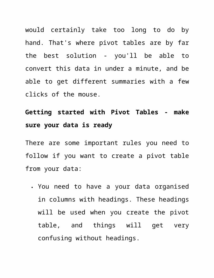
would certainly take too long to do by

hand. That's where pivot tables are by far

the best solution - you'll be able to

convert this data in under a minute, and be

able to get different summaries with a few

clicks of the mouse.

Getting started with Pivot Tables - make

sure your data is ready

There are some important rules you need to

follow if you want to create a pivot table

from your data:

You need to have a your data organised

in columns with headings. These headings

will be used when you create the pivot

table, and things will get very

confusing without headings.

Make sure there are no empty columns or

rows in your data. Excel is good at

sensing the start and end of a data

table by looking for empty rows and

columns at which point it stops.

o A quick tip to check if your data is

formatted in one contiguous range (a

fancy term way of saying "one block

of data") is to click a single cell

in the table then press SHIFT+* (or

CTRL+SHIFT+8). This automatically

selects the whole table. You'll then

see if you have any problems with

the layout of your table.

o Note that empty cells are OK. What

isn't OK is a whole row or a whole

column of empty cells.

Consistent data in all cells.

o If you have a date column, make sure

all the values in that column are

dates (or blank).

o If you have a quantity column, make

sure all the values are numbers (or

blank) and not words.

At this point, if everything is looking OK,

you're ready to move on to the next step.

Create a blank Pivot Table

To start your pivot table, follow these

steps:

Click on a cell in the data table. Any

cell will do, provided your data meets

the rules outlined above. In fact, at

this point it's all or nothing - select

the whole table or just one cell in the

table. Don't select a few cells, because

Excel may think you are trying to create

a pivot table from just those cells.

Click on the Insert menu and click the

PivotTable button:

The following dialog box will appear:

Note that the Table/Range value will

automatically reflect the data in your

table (you can click in the field to

change the Table/Range value if Excel

guessed wrong). Alternatively, you can

choose an external data source such as a

database (we'll cover that another day!)

Also notice that you can choose where

the new PivotTable should go. By

default, Excel will suggest a New

Worksheet, which I think is the best

choice unless you already know you want

it on an existing worksheet.

o Be warned that if your data changes

a lot, or you find yourself changing

the Pivot Table layout a lot, then

refreshing the data in your Pivot

Table can result in the Pivot Table

changing shape and covering a larger

area. If you have data or formulas

in that area, they'll disappear.

Therefore, putting a Pivot Table on

the same page as data or other

information can cause you real

headaches later on, and thats' why

New Worksheet is the recommended

option.

Once you've completed your selections,

click OK. Assuming you chose the New

Worksheet option, Excel will create a new

worksheet in the current workbook, and

place the blank PivotTable in the worksheet

for you. You are now ready to design your

Pivot Table.

Designing your PivotTable layout.

When you switch to the worksheet with

your new Pivot Table, you'll notice

three separate elements of the Pivot

Table on the screen, starting with the

PivotTable report itself:

Then you'll see the Pivot Table Field

List and under that the field layout

area. Note that it should show the

column headings from your data table.

  

To create the layout, you need to first

select the fields you want in your

table, and then place them in the

correct location.

o You can check the boxes for the

fields you want to include, and

Excel will guess which area each

field should be placed in. However,

the Pivot Table is recalculated each

time you check one of the boxes

which can slow you down, especially

if Excel places a field in the wrong

place.

o Therefore, I recommend you drag and

drop each field to the area you want

it to be.

As an example, here are the Field List

and the Field Layout area above with the

fields in place to show a report with:

o Each day down the left, with each

sales person listed separately for

each day

o Items shown across the top.

o The total quantity of items sold for

each cell in the Pivot Table.

Here is how to layout this report:

   

The report that this generates looks

like this:

Notice how the Pivot Table has

automatically created a list of the

sales people for each day covered in the

source data.

VLOOK UP

VLOOKUP Example

Note: Refer to the image above for more information on this example. The syntax of the VLOOKUP function is covered in detail on page two.

=VLOOKUP("Widget",D4:E9,2,False)

"Widget" - this VLOOKUP function is looking for theprice of Widgets.

D4 : E9 - it is looking for this information in thedata table located in cells D4 to E9.

2- VLOOKUP is looking for the price in the second column of the table.

False - indicates that only an exact match to the lookup _value "Widget" will be accepted.

The VLOOKUP function returns the results of its search - $14.76 - in cell D1.

http://0.tqn.com/d/spreadsheets/1/0/P/1/-/-/vlookup_error.gif

Run Code from a Module As a beginner to Excel VBA, you might find it difficult to decide where to put your VBA code. The Create a Macro chapter illustrates howto run code by clicking on a command button. This example teaches you how to run code from a module.

1. Open the Visual Basic Editor.

2. Click Insert, Module.

3. Create a procedure (macro) called Cyan.

Sub Cyan()

End Sub

4. The sub changes the background color of your worksheet to cyan. To achieve this, add the following code line.

Cells.Interior.ColorIndex = 28

Note: instead of ColorIndex number 28 (cyan), you can use any ColorIndex number.

To run the procedure, execute the following steps.

5. Click Macros.

6. Select Cyan and click Run.

Result:

Note: code placed into a module is available to the whole workbook. That means, you can select Sheet2 or Sheet3 and change the background color of these sheets as well. The Add a Macro to the Toolbar program illustrates how to make a macro available to all your workbooks (Excel files). Remember, code placed on a sheet (assigned to a command button) is only available for that particular sheet.

Create a MacroDeveloper Tab

To turn on the Developter tab, execute the following steps.

1. Right click anywhere on the ribbon, and then click Customize the Ribbon.

2. Under Customize the Ribbon, on the right side of the dialog box, select Main tabs (if necessary).

3. Check the Developer check box.

4. Click OK.

5. You can find the Developer tab next to the View tab.

Command Button

To place a command button on your worksheet, execute the following steps.

1. On the Developer tab, click Insert.

2. In the ActiveX Controls group, click Command Button.

3. Drag a command button on your worksheet.

Assign a Macro

To assign a macro (one or more code lines) to the command button,execute the following steps.

1. Right click CommandButton1 (make sure Design Mode is selected).

2. Click View Code.

The Visual Basic Editor appears.

3. Place your cursor between Private Sub CommandButton1_Click() and End Sub.

4. Add the code line shown below.

Note: the window on the left with the names Sheet1, Sheet2 and Sheet3 is called the Project Explorer. If the Project Explorer isnot visible, click View, Project Explorer. To add the Code windowfor the first sheet, click Sheet1 (Sheet1).

5. Close the Visual Basic Editor.

6. Click the command button on the sheet (make sure Design Mode is deselected).

Result:

Congratulations. You've just created a macro in Excel!

Visual Basic Editor

To open the Visual Basic Editor, on the Developer tab, click Visual Basic.

The Visual Basic Editor appears.

Macro RecorderThe Macro Recorder, a very useful tool included in Excel VBA, records every task you perform with Excel. All you have to do is record a specific task once. Next, you can execute the task over and over with the click of a button. The Macro Recorder is also agreat help when you don't know how to program a specific task in Excel VBA. Simply open the Visual Basic Editor after recording the task to see how it can be programmed.

Unfortunately, there are a lot of things you cannot do with the Macro Recorder. For example, you cannot loop through a range of data with the Macro Recorder. Moreover, the Macro Recorder uses alot more code than is required, which can slow your process down.

Record a Macro

1. On the Developer tab, click Record Macro.

2. Enter a name.

3. Select This Workbook from the drop-down list. As a result, themacro will only be available in the current workbook.

Note: if you store your macro in Personal Macro Workbook, the macro will be available to all your workbooks (Excel files). Thisis possible because Excel stores your macro in a hidden workbook that opens automatically when Excel starts. If you store your macro in New Workbook, the macro will only be available in an automatically new opened workbook.

4. Click OK.

5. Right mouse click on the active cell (selected cell). Be sure not to select any other cell! Next, click Format Cells.

6. Select Percentage.

7. Click OK.

8. Finally, click Stop Recording.

Congratulations. You've just recorded a macro with the Macro Recorder!

Run a Recorded Macro

Now we'll test the macro to see if it can change the number format to Percentage.

1. Enter some numbers between 0 and 1.

2. Select the numbers.

3. On the Developer tab, click Macros.

4. Click Run.

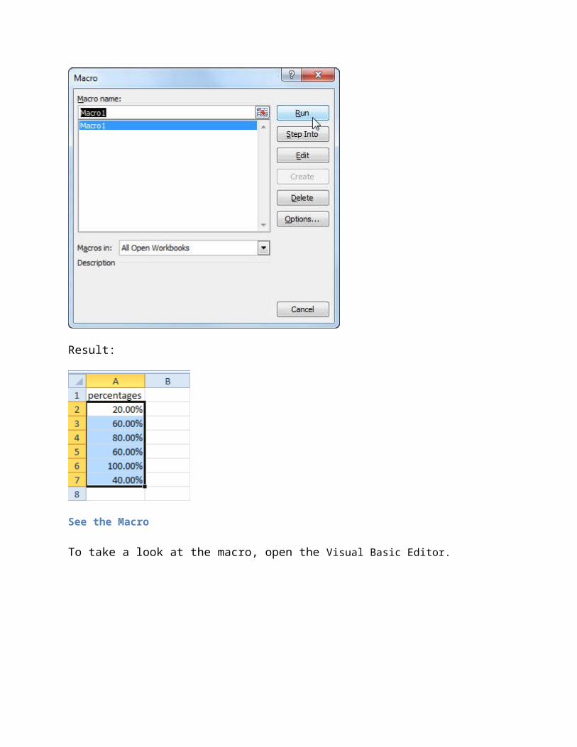
Result:

See the Macro

To take a look at the macro, open the Visual Basic Editor.

Note: the macro has been placed into a module called Module1. Code placed into a module is available to the whole workbook. That means, you can select Sheet2 or Sheet3 and change the numberformat of cells on these sheets as well. Remember, code placed ona sheet (assigned to a command button) is only available for thatparticular sheet.

Swap Values This example teaches you how to swap two values in Excel VBA. You will often need this structure in more complicated programs as we willsee later.

Situation:

Two values on your worksheet.

Place a command button on your worksheet and add the following code lines:

1. First, we declare a variable called temp of type Double.

Dim temp As Double

2. We initialize the variable temp with the value of cell A1.

temp = Range("A1").Value

3. Now we can safely write the value of cell B1 to cell A1 (we have stored the value of cell A1 to temp so we will not lose it).

Range("A1").Value = Range("B1").Value

4. Finally, we write the value of cell A1 (written to temp) to cell B1.

Range("B1").Value = temp

5. Click the command button two times.

Result: