This article was downloaded by: [b-on: Biblioteca do conhecimento online UL]On: 11 January 2012, At: 04:28Publisher: Taylor & FrancisInforma Ltd Registered in England and Wales Registered Number: 1072954 Registeredoffice: Mortimer House, 37-41 Mortimer Street, London W1T 3JH, UK

Journal of Statistical Computation andSimulationPublication details, including instructions for authors andsubscription information:http://www.tandfonline.com/loi/gscs20

A computational study of a quasi-PORTmethodology for VaR based on second-order reduced-bias estimationFernanda Figueiredo a , M. Ivette Gomes b , Lígia Henriques-Rodrigues c & M. Cristina Miranda da Faculdade de Economia, Universidade do Porto, Porto, andCEAUL, Lisboa, Portugalb FCUL, DEIO and CEAUL, Universidade de Lisboa, Lisboa, Portugalc Instituto Politécnico de Tomar, Tomar, and CEAUL, Lisboa,Portugald ISCA, Universidade de Aveiro, Aveiro, and CEAUL, Lisboa,Portugal

Available online: 13 Jun 2011

To cite this article: Fernanda Figueiredo, M. Ivette Gomes, Lígia Henriques-Rodrigues & M.Cristina Miranda (2011): A computational study of a quasi-PORT methodology for VaR basedon second-order reduced-bias estimation, Journal of Statistical Computation and Simulation,DOI:10.1080/00949655.2010.547196

To link to this article: http://dx.doi.org/10.1080/00949655.2010.547196

PLEASE SCROLL DOWN FOR ARTICLE

Full terms and conditions of use: http://www.tandfonline.com/page/terms-and-conditions

This article may be used for research, teaching, and private study purposes. Anysubstantial or systematic reproduction, redistribution, reselling, loan, sub-licensing,systematic supply, or distribution in any form to anyone is expressly forbidden.

The publisher does not give any warranty express or implied or make any representationthat the contents will be complete or accurate or up to date. The accuracy of any

instructions, formulae, and drug doses should be independently verified with primarysources. The publisher shall not be liable for any loss, actions, claims, proceedings,demand, or costs or damages whatsoever or howsoever caused arising directly orindirectly in connection with or arising out of the use of this material.

Dow

nloa

ded

by [

b-on

: Bib

liote

ca d

o co

nhec

imen

to o

nlin

e U

L]

at 0

4:28

11

Janu

ary

2012

Journal of Statistical Computation and SimulationiFirst, 2011, 1–16

A computational study of a quasi-PORT methodology for VaRbased on second-order reduced-bias estimation

Fernanda Figueiredoa, M. Ivette Gomesb*, Lígia Henriques-Rodriguesc andM. Cristina Mirandad

aFaculdade de Economia, Universidade do Porto, Porto, and CEAUL, Lisboa, Portugal; bFCUL, DEIOand CEAUL, Universidade de Lisboa, Lisboa, Portugal; cInstituto Politécnico de Tomar, Tomar, and

CEAUL, Lisboa, Portugal; d ISCA, Universidade de Aveiro, Aveiro, and CEAUL, Lisboa, Portugal

(Received 20 May 2010; final version received 8 December 2010 )

In this paper, we deal with the estimation, under a semi-parametric framework, of the Value-at-Risk (VaR)at a level p, the size of the loss occurred with a small probability p. Under such a context, the classical VaRestimators are the Weissman–Hill estimators, based on any intermediate number k of top-order statistics.But these VaR estimators do not enjoy the adequate linear property of quantiles, contrarily to the PORTVaR estimators, which depend on an extra tuning parameter q, with 0 ≤ q < 1. We shall here consider‘quasi-PORT’ reduced-bias VaR estimators, for which such a linear property is obtained approximately.They are based on a partially shifted version of a minimum-variance reduced-bias (MVRB) estimator ofthe extreme value index (EVI), the primary parameter in Statistics of Extremes. Due to the stability on k

of the MVRB EVI and associated VaR estimates, we propose the use of a heuristic stability criterion forthe choice of k and q, providing applications of the methodology to simulated data and to log-returns offinancial stocks.

Keywords: statistics of extremes; value-at-risk; semi-parametric estimation; heuristics

2000 AMS Subject Classifications: 62G32; 65C05

1. Introduction, preliminaries and scope of the paper

We shall place ourselves under a semi-parametric framework, to refer the estimation of a positiveextreme value index (EVI), denoted γ , the primary parameter in Statistics of Extremes and thebasis for the estimation of the Value-at-Risk (VaR) at a level p, denoted VaRp, the size of the lossoccurred with a small probability p. In other words, we are interested in the estimation of a (high)quantile, χ1−p := F←(1 − p), of a probability distribution function (d.f.) F , with F←(y) :=inf{x : F(x) ≥ y}, the generalized inverse function of F . Let us denote U(t) := F←(1 − 1/t),t ≥ 1, a reciprocal quantile function such that χ1−p ≡ VaRp = U(1/p). We shall thus considerheavy-tailed parents, quite common in the most diversified areas of application, like insurance

*Corresponding author. Email: ivette.gomes@fc.ul.pt

ISSN 0094-9655 print/ISSN 1563-5163 online© 2011 Taylor & FrancisDOI: 10.1080/00949655.2010.547196http://www.informaworld.com

Dow

nloa

ded

by [

b-on

: Bib

liote

ca d

o co

nhec

imen

to o

nlin

e U

L]

at 0

4:28

11

Janu

ary

2012

2 F. Figueiredo et al.

and finance, i.e. parents such that, as t → ∞,

U ∈ RVγ ⇐⇒ 1 − F ∈ RV−1/γ ,

where, as usual, the notation RVα stands for regularly varying functions with an index of regularvariation equal to α, i.e. positive measurable functions g(·) such that for any x ≥ 0, g(tx)/g(t) →xα , as t → ∞. We are then working in DM(EVγ>0), the domain of attraction for maxima of EVγ ,γ > 0, with EVγ denoting the general extreme value distribution (EVD), given by

EVγ (x) ={

exp(−(1 + γ x)−1/γ ), 1 + γ x > 0 if γ �= 0

exp(− exp(−x)), x ∈ R if γ = 0,(1)

with γ the EVI.The EVD, in Equation (1), is one of the crucial models in the field of extreme value theory

(EVT). Indeed, all possible non-degenerate weak limit distributions of the normalized partialmaxima Xn:n, of i.i.d. random variables X1, . . . , Xn, from an underlying parent F , are EVDs, i.e.if there are normalizing constants an > 0, bn ∈ R and some non-degenerate d.f. G such that, forall x,

limn→∞ P

{Xn:n − bn

an

≤ x

}= G(x),

we can redefine the constants in such a way that G(x) = EVγ (x), in Equation (1), for someγ ∈ R [1]. We then write F ∈ DM(EVγ ).

Another seminal result in the field of EVT is the one due to Balkema and de Haan [2] andPickands [3]. Independently, they proved that, under adequate conditions, the generalized Paretodistribution (GPD),

GPγ (x) ={

1 − (1 + γ x)−1/γ , 1 + γ x > 0, x ≥ 0 if γ �= 0

1 − exp(−x), x ≥ 0 if γ = 0,(2)

is the limit distribution of scaled excesses over high thresholds. More precisely, consider theexcess function, Fu(x) := P [X − u ≤ x|X > u]. Denoting xF := U(∞), the right endpoint ofF , F ∈ DM(Gγ ) if and only if there exists a positive real function σ(u) such that

limu→xF

|Fu(σ (u)x) − GPγ (x)| = 0

(see, for instance, Embrechts et al. [4, Section 3.4], and Reiss and Thomas [5, Section 1.4], formore details). Such a limiting result enabled the development of the so-called maximum likelihood(ML) EVI estimators. We here refer the peaks over threshold methodology of estimation [6] aswell as the methodology used by Drees et al. [7], named PORT (peaks over random threshold)in Araújo Santos et al. [8].

For heavy-tailed parents and given a sample Xn = (X1, . . . , Xn), the classical EVI estimatoris the Hill estimator [9], denoted H ≡ Hn(k) and given by

Hn(k) ≡ Hn(k; Xn) := 1

k

k∑i=1

{ln Xn−i+1:n − ln Xn−k:n}, 1 ≤ k < n, (3)

the average of the k log-excesses over a high random threshold Xn−k:n. Consistency of the estimatorin Equation (3) is achieved if Xn−k:n is an intermediate order statistic (o.s.), i.e. if

k = kn → ∞ andk

n→ 0, as n → ∞. (4)

The Hill estimator in Equation (3) is scale-invariant but not location invariant, as often desired,and this contrarily to the PORT-Hill estimators, recently introduced in Araújo Santos et al. [8] and

Dow

nloa

ded

by [

b-on

: Bib

liote

ca d

o co

nhec

imen

to o

nlin

e U

L]

at 0

4:28

11

Janu

ary

2012

Journal of Statistical Computation and Simulation 3

further studied in Gomes et al. [10]. The class of PORT-Hill estimators is based on a sample ofexcesses over a random threshold Xnq :n, nq := [nq] + 1, with [x] denoting, as usual, the integerpart of x, i.e. it is based on

X(q)n := (Xn:n − Xnq :n, Xn−1:n − Xnq :n, . . . , Xnq+1:n − Xnq :n), nq = [nq] + 1. (5)

We need to have 0 < q < 1, for d.f.’s with an infinite left endpoint xF := inf{x : F(x) > 0} (therandom threshold is an empirical quantile). We can also have q = 0, provided that the underlyingmodel has a finite left endpoint xF (the random threshold is then the minimum). These new classesof EVI estimators are the so-called PORT-Hill estimators, denoted by H

(q)n , and, for 0 ≤ q < 1

and k < n − nq , they are given by

H(q)n (k) := Hn(k; X(q)

n ) = 1

k

k∑i=1

lnXn−i+1:n − Xnq :nXn−k:n − Xnq :n

, (6)

i.e. they have the same functional form of the Hill estimator in Equation (3), but with the originalsample Xn = (X1, . . . , Xn) replaced by the sample of excesses X(q)

n in Equation (5). These estima-tors are now invariant for both changes of scale and location in the data, and depend on the tuningparameter q, which provides a highly flexible class of EVI estimators. Provided that we ade-quately choose the tuning parameter q, the PORT-Hill estimators may even compare favourablywith the second-order minimum-variance reduced-bias (MVRB) EVI estimators, recently intro-duced in the literature and briefly discussed in the following. Indeed, due to the high bias of theHill estimator, in Equation (3), for moderate up to large k, several authors have dealt with biasreduction in the field of extremes, working then in a slightly more strict class than DM(EVγ>0),the class of models U(·) such that

U(t) = C tγ(

1 + A(t)

ρ+ o(tρ)

), A(t) = γβtρ, (7)

as t → ∞, where ρ < 0 and β �= 0. This means that the slowly varying function L(t) in U(t) =tγ L(t) is assumed to behave asymptotically as a constant C. Note that to assume Equation (7) isequivalent to saying that we can choose A(t) = γβtρ , ρ < 0, in the more general second-ordercondition

limt→∞

ln U(tx) − ln U(t) − γ ln x

A(t)= xρ − 1

ρ. (8)

The Hill estimator, in Equation (3), reveals usually a high asymptotic bias, i.e. as n → ∞,√k(Hn(k) − γ ) is asymptotically normal with variance γ 2 and a non-null mean value, equal

to λA/(1 − ρ), whenever

√k A(n/k) → λ

A�= 0, finite, with A(·) the function in Equation (8).

This non-null asymptotic bias, together with a rate of convergence of the order of 1/√

k, leadsto sample paths with a high variance for small k, a high bias for large k, and a very sharp mean-squared error (MSE) pattern, as a function of k. A simple class of second-order MVRB EVIestimators is the one in Caeiro et al. [11], used for a semi-parametric estimation of ln VaRp inGomes and Pestana [12]. This class, here defined b H̄ ≡ H̄n(k), depends upon the estimation ofthe second-order parameters (β, ρ) in Equation (7). Its functional form is

H̄n(k) ≡ H̄n(k; Xn) ≡ H̄β̂,ρ̂ (k) := Hn(k)

(1 − β̂(n/k)ρ̂

1 − ρ̂

), (9)

with Hn(k) the Hill estimator in Equation (3), and where (β̂, ρ̂) needs to be an adequate consistentestimator of (β, ρ). Algorithms for the estimation of (β, ρ) are provided in Gomes and Pestana[12,13], among others.

Dow

nloa

ded

by [

b-on

: Bib

liote

ca d

o co

nhec

imen

to o

nlin

e U

L]

at 0

4:28

11

Janu

ary

2012

4 F. Figueiredo et al.

Let us now think about semi-parametric high quantile estimation. With Q standing for quantilefunction, the classical Weissman–Hill Varp estimator,

Qp|H (k) := Xn−k+1:n cHn(k)k , ck ≡ ck,n,p = k

np, (10)

has been introduced in Weissman [14]. The MVRB VaR-estimator Qp|H̄ , with Qp|H given inEquation (10), was studied in Gomes and Pestana [12]. However, for any positive real δ, and withQp|• denoting either Qp|H or Qp|H̄ , Qp|•(k; δ Xn) = δ Qp|•(k; Xn), as desirable, but contrarilyto the linear property for quantiles, χp(δX + s) = δχp(X) + s for any real s and positive real δ,we no longer have Qp|•(k; s1n + δXn) = s + δ Qp|•(k; Xn), with 1n denoting, as usual, a vectorwith n unit elements. Araújo Santos et al. [8] have developed a class of high quantile estimatorsbased on the sample of excesses over a random threshold Xnq :n, provided in Equation (5), and,among others, they propose the so-called PORT-Weisman–Hill VaRp-estimators,

Q(q)

p|H (k) := (Xn−k:n − Xnq :n) cH

(q)n (k)

k + Xnq :n, (11)

where H(q)n (k) is the Hill estimator of γ , made location/scale invariant by using the transformed

sample X(q)n , i.e. H

(q)n (k) is the estimator in Equation (6). They consequently obtain exactly the

above-mentioned linear property for the quantile estimators, but they still get a high bias formoderate values of k, induced by PORT-Hill EVI estimation.

We get to know that the second-order MVRB EVI estimators in Equation (9) are not loca-tion invariant, but they are ‘approximately’ location invariant. However, if we merely replace, inEquation (11), H

(q)n (k) by H̄n(k) in Equation (9), we have practically no improvement compara-

tively with the MVRB-estimator Qp|H̄ , introduced and studied in Gomes and Pestana [12]. With

H(q)n (k) defined in Equation (6), we shall consider here the ‘quasi-PORT’ EVI estimator,

H̄ (q)n (k) ≡ H̄ (q)

n (k; β̂, ρ̂) := H(q)n (k)

(1 − β̂(n/k)ρ̂

1 − ρ̂

)(12)

and the associated ‘quasi-PORT’ Varp-estimator, with the functional form

Q(q)

p|H̄ (k) := (Xn−k:n − Xnq :n)cH̄(q)n (k)

k + Xnq :n. (13)

In Section 2 of this paper, after a brief discussion on the estimation of the second-order param-eters β and ρ, we describe the results associated with a Monte-Carlo simulation study of the newVaR-estimators, in Equation (13), making also a short remark on the use of the GPD approxi-mation for high quantile estimation. Finally, in Section 3, due to the stability on k of the MVRBestimates H̄ , in Equation (9), and Qp|H̄ , with Qp|H provided in Equation (10), as well as the newVaR-estimates in Equation (13), we propose the use of a heuristic stability criterion for the choiceof k and q, providing applications of the methodology to simulated data and to log-returns offinancial stocks.

2. Finite sample behaviour: a Monte-Carlo simulation

In this section, for p = 1/n and q = 0, 0.1 and 0.25, we are interested in the finite-samplebehaviour of the new VaR-estimators, Q(q)

p|H̄ (k), in Equation (13), comparatively with the classicalWeissman–Hill VaR-estimator, Qp|H (k), in Equation (10), the associated PORT-Weissman–Hill

Dow

nloa

ded

by [

b-on

: Bib

liote

ca d

o co

nhec

imen

to o

nlin

e U

L]

at 0

4:28

11

Janu

ary

2012

Journal of Statistical Computation and Simulation 5

VaR-estimators, Q(q)

p|H (k), in Equation (11), and the MVRBVaR-estimator Qp|H̄ (k), with Qp|H (k)

given in Equation (10). The overall simulation is based on a multi-sample simulation with size5000 × 20, i.e. 20 replicates with 5000 runs each. For details on multi-sample simulation, referto Gomes and Oliveira [15]. The patterns of mean value (E) and root mean squared error (RMSE)are based on the first replicate only. We have considered the following underlying parents:

(A) the Burr model, with d.f. Bγ,ρ(x) = 1 − (1 + x−ρ/γ )1/ρ , x ≥ 0, for γ = 0.25 and ρ = −0.5;(B) Student’s tν-model, with a probability density function

ftν (t) = �((ν + 1)/2)[1 + t2/ν]−(ν+1)/2

√πν�(ν/2)

, t ∈ R (ν > 0),

for ν = 4 degrees of freedom. We then have γ = 1/ν = 0.25 and ρ = −2/ν = −0.5;(C) the general EV model, with d.f. EVγ (x) in Equation (1), for γ = 0.5 (ρ = −0.5).

All reduced-bias EVI estimators, like the ones in Equation (9) and in Equation (12), as wellas associated VaR-estimators, require the estimation of scale and shape second-order parameters,(β, ρ), in Equation (7). Such an estimation will be briefly discussed in Section 2.1. Bias-reductionis neatly needed for models with |ρ| ≤ 1, the most common in practical situations, and the type ofmodels also considered in this simulation study. On the basis of the algorithms proposed before inpapers like Gomes and Pestana [12] and Gomes et al. [16], we shall use now the tuning parameterτ = 0, in the ρ-estimators discussed in Fraga Alves et al. [17], and the associated β-estimatorsin Gomes and Martins [18].

2.1. Estimation of second-order parameters

As mentioned above, we shall here consider the estimator

ρ̂0(k) := min

(0,

3(Tn(k) − 1)

Tn(k) − 3

), k < n, (14)

with

Tn(k) := ln M(1)n (k) − ln(M(2)

n (k)/2)/2

ln(M(2)n (k)/2)/2 − ln(M

(3)n (k)/6)/3

, M(j)n (k) := 1

k

k∑i=1

{ln

Xn−i+1:nXn−k:n

}j

,

for j = 1, 2, 3, a particular member of the class of estimators in Fraga Alves et al. [17]. Otherinteresting alternative classes of ρ-estimators have recently been introduced in Goegebeur et al.[19], Ciuperca and Mercadier [20] and Goegebeur et al. [21]. Distributional properties of theestimators in Equation (14) can be found in Fraga Alves et al. [17]. Consistency is achieved inthe class of models in Equation (7), for intermediate k-values, denoted by k1, such that apartfrom condition (4), with k replaced by k1, we have

√k1A(n/k1) → ∞, as n → ∞. We have here

decided for the choice

k1 = [n1−ε], ε = 0.001, (15)

both in simulations and in case studies.

Remark 2.1 With the choice of k1 in Equation (15), and whenever√

k1 A(n/k1) → ∞, weget ρ̂ − ρ := ρ̂0(k1) − ρ = op(1/ ln n), a condition needed, in order not to have any increase inthe asymptotic variance of the new bias-corrected Hill estimator in Equation (9), comparativelywith the Hill estimator in Equation (3). Note that with the choice of k1 in Equation (15), we get

Dow

nloa

ded

by [

b-on

: Bib

liote

ca d

o co

nhec

imen

to o

nlin

e U

L]

at 0

4:28

11

Janu

ary

2012

6 F. Figueiredo et al.

√k1A(n/k1) → ∞ if and only if ρ > 1/2 − 1/(2ε) = −499.5, an irrelevant restriction, from a

practical point of view.

For the estimation of the scale second-order parameter β, in Equation (7), we shall consider

β̂ρ̂ (k) :=(

k

n

)ρ̂dρ̂(k) D0(k) − Dρ̂(k)

dρ̂(k) Dρ̂(k) − D2ρ̂ (k), k < n, (16)

dependent on the estimator ρ̂ = ρ̂0(k1), with ρ̂0(k) and k1 given in Equations (14) and (15),respectively, and where, for any α ≤ 0,

dα(k) := 1

k

k∑i=1

(i

k

)−α

and Dα(k) := 1

k

k∑i=1

(i

k

)−α

Ui,

with Ui := i(ln Xn−i+1:n − ln Xn−i:n), 1 ≤ i ≤ k, the scaled log-spacings. Moreover, we shallcompute β̂ρ̂ (k), in Equation (16), at the value k1, in Equation (15), and work with β̂ = β̂ρ̂ (k1).

Details on the distributional behaviour of the estimator in Equation (16) can be found in Gomesand Martins [18] and more recently in Gomes et al. [16] and Caeiro et al. [22]. Consistency isachieved for models in Equation (7), k values such that Equation (4) holds and

√kA(n/k) → ∞,

as n → ∞, and estimators ρ̂ of ρ such that ρ̂ − ρ = op(1/ ln n). Alternative estimators of β canbe found in Caeiro and Gomes [23] and Gomes et al. [24].

2.2. Mean value and RMSE patterns

We shall consider the following normalized V aRp-estimators, Qp|H (k)/VaRp, Qp|H̄ (k)/VaRp,

Q(q)

p|H (k)/VaRp and Q(q)

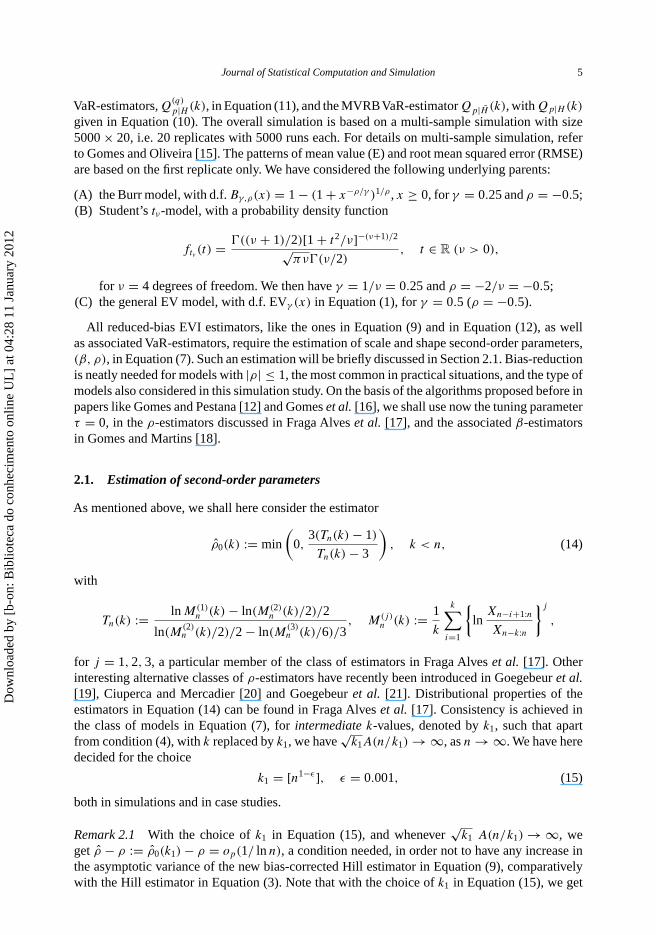
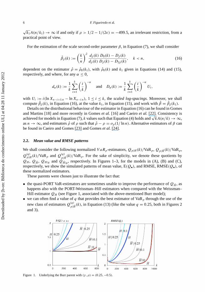
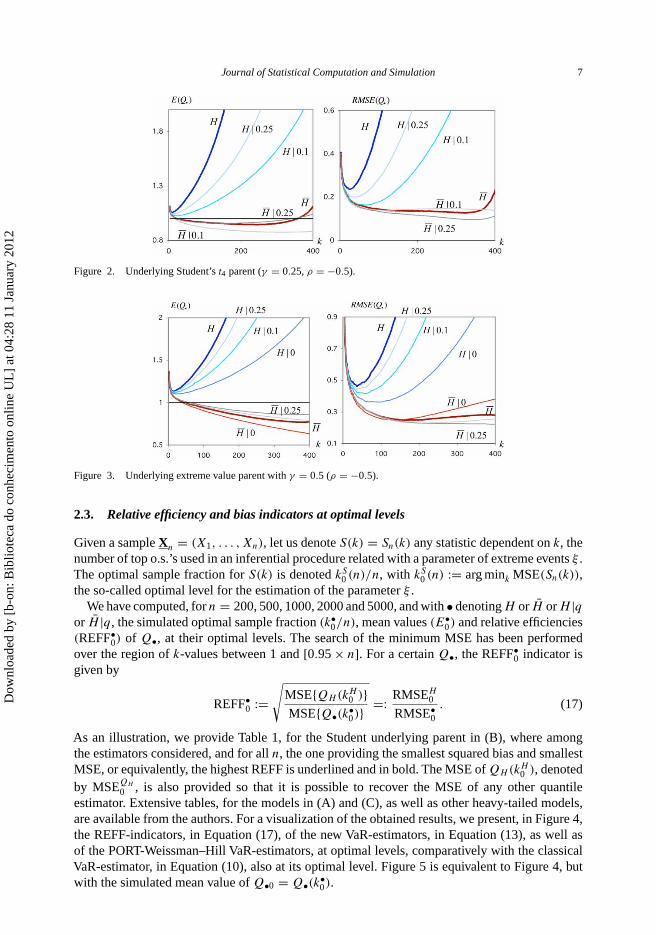
p|H̄ (k)/VaRp. For the sake of simplicity, we denote these quotients byQH , QH̄ , QH |q and QH̄ |q , respectively. In Figures 1–3, for the models in (A), (B) and (C),respectively, we show the simulated patterns of mean value, E(Q•), and RMSE, RMSE(Q•), ofthese normalized estimators.

These parents were chosen just to illustrate the fact that:

• the quasi-PORT VaR-estimators are sometimes unable to improve the performance of QH̄ , ashappens also with the PORT-Weissman–Hill estimators when compared with the Weissman–Hill estimator QH (see Figure 1, associated with the above-mentioned Burr model);

• we can often find a value of q that provides the best estimator of VaRp through the use of thenew class of estimators Q

(q)

p|H̄ (k), in Equation (13) (like the value q = 0.25, both in Figures 2and 3).

Figure 1. Underlying the Burr parent with (γ, ρ) = (0.25, −0.5).

Dow

nloa

ded

by [

b-on

: Bib

liote

ca d

o co

nhec

imen

to o

nlin

e U

L]

at 0

4:28

11

Janu

ary

2012

Journal of Statistical Computation and Simulation 7

Figure 2. Underlying Student’s t4 parent (γ = 0.25, ρ = −0.5).

Figure 3. Underlying extreme value parent with γ = 0.5 (ρ = −0.5).

2.3. Relative efficiency and bias indicators at optimal levels

Given a sample Xn = (X1, . . . , Xn), let us denote S(k) = Sn(k) any statistic dependent on k, thenumber of top o.s.’s used in an inferential procedure related with a parameter of extreme events ξ .The optimal sample fraction for S(k) is denoted kS

0 (n)/n, with kS0 (n) := arg mink MSE(Sn(k)),

the so-called optimal level for the estimation of the parameter ξ .We have computed, for n = 200, 500, 1000, 2000 and 5000, and with • denoting H or H̄ or H |q

or H̄ |q, the simulated optimal sample fraction (k•0/n), mean values (E•

0) and relative efficiencies(REFF•

0) of Q•, at their optimal levels. The search of the minimum MSE has been performedover the region of k-values between 1 and [0.95 × n]. For a certain Q•, the REFF•

0 indicator isgiven by

REFF•0 :=

√MSE{QH(kH

0 )}MSE{Q•(k•

0)}=: RMSEH

0

RMSE•0

. (17)

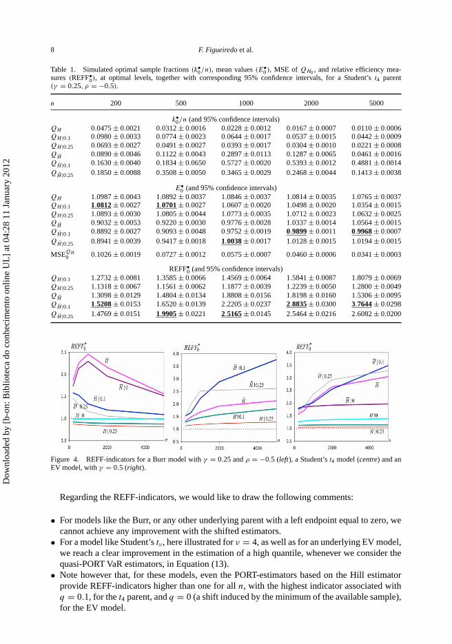
As an illustration, we provide Table 1, for the Student underlying parent in (B), where amongthe estimators considered, and for all n, the one providing the smallest squared bias and smallestMSE, or equivalently, the highest REFF is underlined and in bold. The MSE of QH(kH

0 ), denotedby MSEQH

0 , is also provided so that it is possible to recover the MSE of any other quantileestimator. Extensive tables, for the models in (A) and (C), as well as other heavy-tailed models,are available from the authors. For a visualization of the obtained results, we present, in Figure 4,the REFF-indicators, in Equation (17), of the new VaR-estimators, in Equation (13), as well asof the PORT-Weissman–Hill VaR-estimators, at optimal levels, comparatively with the classicalVaR-estimator, in Equation (10), also at its optimal level. Figure 5 is equivalent to Figure 4, butwith the simulated mean value of Q•0 = Q•(k•

0).

Dow

nloa

ded

by [

b-on

: Bib

liote

ca d

o co

nhec

imen

to o

nlin

e U

L]

at 0

4:28

11

Janu

ary

2012

8 F. Figueiredo et al.

Table 1. Simulated optimal sample fractions (k•0/n), mean values (E•

0 ), MSE of QH0 , and relative efficiency mea-sures (REFF•

0), at optimal levels, together with corresponding 95% confidence intervals, for a Student’s t4 parent(γ = 0.25, ρ = −0.5).

n 200 500 1000 2000 5000

k•0/n (and 95% confidence intervals)

QH 0.0475 ± 0.0021 0.0312 ± 0.0016 0.0228 ± 0.0012 0.0167 ± 0.0007 0.0110 ± 0.0006QH |0.1 0.0980 ± 0.0033 0.0774 ± 0.0023 0.0644 ± 0.0017 0.0537 ± 0.0015 0.0442 ± 0.0009QH |0.25 0.0693 ± 0.0027 0.0491 ± 0.0027 0.0393 ± 0.0017 0.0304 ± 0.0010 0.0221 ± 0.0008QH̄ 0.0890 ± 0.0046 0.1122 ± 0.0043 0.2897 ± 0.0113 0.1287 ± 0.0065 0.0461 ± 0.0016QH̄ |0.1 0.1630 ± 0.0040 0.1834 ± 0.0650 0.5727 ± 0.0020 0.5393 ± 0.0012 0.4881 ± 0.0014QH̄ |0.25 0.1850 ± 0.0088 0.3508 ± 0.0050 0.3465 ± 0.0029 0.2468 ± 0.0044 0.1413 ± 0.0038

E•0 (and 95% confidence intervals)

QH 1.0987 ± 0.0043 1.0892 ± 0.0037 1.0846 ± 0.0037 1.0814 ± 0.0035 1.0765 ± 0.0037QH |0.1 1.0812 ± 0.0027 1.0701 ± 0.0027 1.0607 ± 0.0020 1.0498 ± 0.0020 1.0354 ± 0.0015QH |0.25 1.0893 ± 0.0030 1.0805 ± 0.0044 1.0773 ± 0.0035 1.0712 ± 0.0023 1.0632 ± 0.0025QH̄ 0.9032 ± 0.0053 0.9220 ± 0.0030 0.9776 ± 0.0028 1.0337 ± 0.0014 1.0564 ± 0.0015QH̄ |0.1 0.8892 ± 0.0027 0.9093 ± 0.0048 0.9752 ± 0.0019 0.9899 ± 0.0011 0.9968 ± 0.0007QH̄ |0.25 0.8941 ± 0.0039 0.9417 ± 0.0018 1.0038 ± 0.0017 1.0128 ± 0.0015 1.0194 ± 0.0015

MSEQH0 0.1026 ± 0.0019 0.0727 ± 0.0012 0.0575 ± 0.0007 0.0460 ± 0.0006 0.0341 ± 0.0003

REFF•0 (and 95% confidence intervals)

QH |0.1 1.2732 ± 0.0081 1.3585 ± 0.0066 1.4569 ± 0.0064 1.5841 ± 0.0087 1.8079 ± 0.0069QH |0.25 1.1318 ± 0.0067 1.1561 ± 0.0062 1.1877 ± 0.0039 1.2239 ± 0.0050 1.2800 ± 0.0049QH̄ 1.3098 ± 0.0129 1.4804 ± 0.0134 1.8808 ± 0.0156 1.8198 ± 0.0160 1.5306 ± 0.0095QH̄ |0.1 1.5208 ± 0.0153 1.6520 ± 0.0139 2.2205 ± 0.0237 2.8835 ± 0.0300 3.7644 ± 0.0298QH̄ |0.25 1.4769 ± 0.0151 1.9905 ± 0.0221 2.5165 ± 0.0145 2.5464 ± 0.0216 2.6082 ± 0.0200

Figure 4. REFF-indicators for a Burr model with γ = 0.25 and ρ = −0.5 (left), a Student’s t4 model (centre) and anEV model, with γ = 0.5 (right).

Regarding the REFF-indicators, we would like to draw the following comments:

• For models like the Burr, or any other underlying parent with a left endpoint equal to zero, wecannot achieve any improvement with the shifted estimators.

• For a model like Student’s tν , here illustrated for ν = 4, as well as for an underlying EV model,we reach a clear improvement in the estimation of a high quantile, whenever we consider thequasi-PORT VaR estimators, in Equation (13).

• Note however that, for these models, even the PORT-estimators based on the Hill estimatorprovide REFF-indicators higher than one for all n, with the highest indicator associated withq = 0.1, for the t4 parent, and q = 0 (a shift induced by the minimum of the available sample),for the EV model.

Dow

nloa

ded

by [

b-on

: Bib

liote

ca d

o co

nhec

imen

to o

nlin

e U

L]

at 0

4:28

11

Janu

ary

2012

Journal of Statistical Computation and Simulation 9

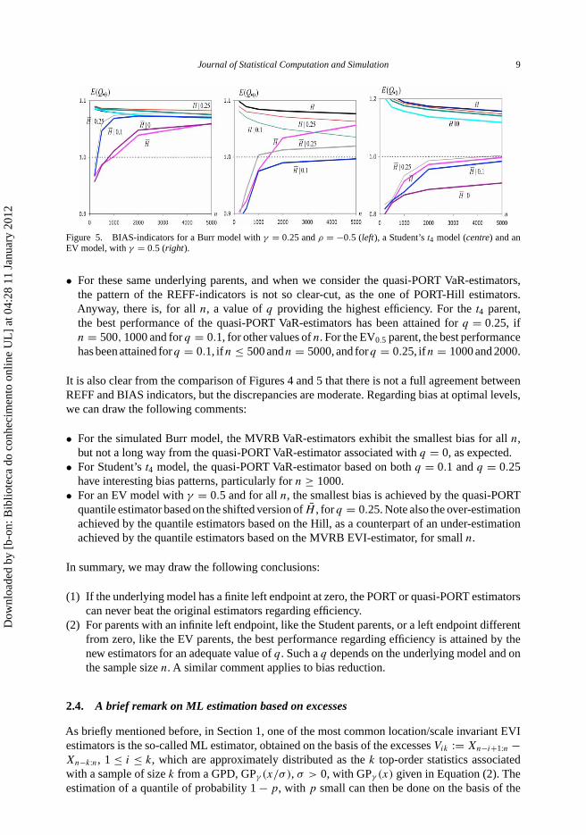
Figure 5. BIAS-indicators for a Burr model with γ = 0.25 and ρ = −0.5 (left), a Student’s t4 model (centre) and anEV model, with γ = 0.5 (right).

• For these same underlying parents, and when we consider the quasi-PORT VaR-estimators,the pattern of the REFF-indicators is not so clear-cut, as the one of PORT-Hill estimators.Anyway, there is, for all n, a value of q providing the highest efficiency. For the t4 parent,the best performance of the quasi-PORT VaR-estimators has been attained for q = 0.25, ifn = 500, 1000 and for q = 0.1, for other values of n. For the EV0.5 parent, the best performancehas been attained forq = 0.1, ifn ≤ 500 andn = 5000, and forq = 0.25, ifn = 1000 and 2000.

It is also clear from the comparison of Figures 4 and 5 that there is not a full agreement betweenREFF and BIAS indicators, but the discrepancies are moderate. Regarding bias at optimal levels,we can draw the following comments:

• For the simulated Burr model, the MVRB VaR-estimators exhibit the smallest bias for all n,but not a long way from the quasi-PORT VaR-estimator associated with q = 0, as expected.

• For Student’s t4 model, the quasi-PORT VaR-estimator based on both q = 0.1 and q = 0.25have interesting bias patterns, particularly for n ≥ 1000.

• For an EV model with γ = 0.5 and for all n, the smallest bias is achieved by the quasi-PORTquantile estimator based on the shifted version of H̄ , for q = 0.25. Note also the over-estimationachieved by the quantile estimators based on the Hill, as a counterpart of an under-estimationachieved by the quantile estimators based on the MVRB EVI-estimator, for small n.

In summary, we may draw the following conclusions:

(1) If the underlying model has a finite left endpoint at zero, the PORT or quasi-PORT estimatorscan never beat the original estimators regarding efficiency.

(2) For parents with an infinite left endpoint, like the Student parents, or a left endpoint differentfrom zero, like the EV parents, the best performance regarding efficiency is attained by thenew estimators for an adequate value of q. Such a q depends on the underlying model and onthe sample size n. A similar comment applies to bias reduction.

2.4. A brief remark on ML estimation based on excesses

As briefly mentioned before, in Section 1, one of the most common location/scale invariant EVIestimators is the so-called ML estimator, obtained on the basis of the excesses Vik := Xn−i+1:n −Xn−k:n, 1 ≤ i ≤ k, which are approximately distributed as the k top-order statistics associatedwith a sample of size k from a GPD, GPγ (x/σ ), σ > 0, with GPγ (x) given in Equation (2). Theestimation of a quantile of probability 1 − p, with p small can then be done on the basis of the

Dow

nloa

ded

by [

b-on

: Bib

liote

ca d

o co

nhec

imen

to o

nlin

e U

L]

at 0

4:28

11

Janu

ary

2012

10 F. Figueiredo et al.

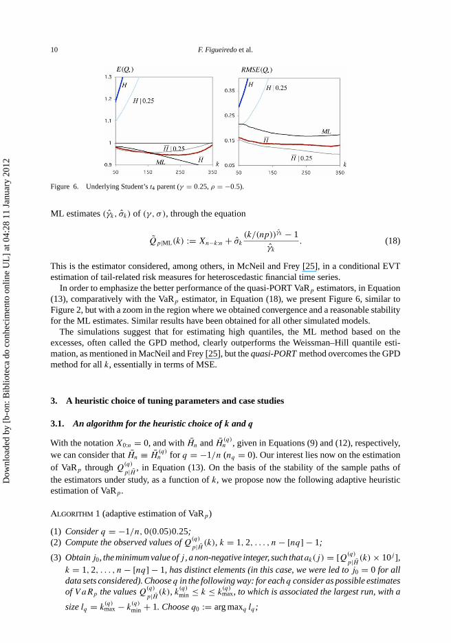
Figure 6. Underlying Student’s t4 parent (γ = 0.25, ρ = −0.5).

ML estimates (γ̂k, σ̂k) of (γ, σ ), through the equation

Q̃p|ML(k) := Xn−k:n + σ̂k

(k/(np))γ̂k − 1

γ̂k

. (18)

This is the estimator considered, among others, in McNeil and Frey [25], in a conditional EVTestimation of tail-related risk measures for heteroscedastic financial time series.

In order to emphasize the better performance of the quasi-PORT VaRp estimators, in Equation(13), comparatively with the VaRp estimator, in Equation (18), we present Figure 6, similar toFigure 2, but with a zoom in the region where we obtained convergence and a reasonable stabilityfor the ML estimates. Similar results have been obtained for all other simulated models.

The simulations suggest that for estimating high quantiles, the ML method based on theexcesses, often called the GPD method, clearly outperforms the Weissman–Hill quantile esti-mation, as mentioned in MacNeil and Frey [25], but the quasi-PORT method overcomes the GPDmethod for all k, essentially in terms of MSE.

3. A heuristic choice of tuning parameters and case studies

3.1. An algorithm for the heuristic choice of k and q

With the notation X0:n = 0, and with H̄n and H̄(q)n , given in Equations (9) and (12), respectively,

we can consider that H̄n ≡ H̄(q)n for q = −1/n (nq = 0). Our interest lies now on the estimation

of VaRp through Q(q)

p|H̄ , in Equation (13). On the basis of the stability of the sample paths ofthe estimators under study, as a function of k, we propose now the following adaptive heuristicestimation of VaRp.

Algorithm 1 (adaptive estimation of VaRp)

(1) Consider q = −1/n, 0(0.05)0.25;(2) Compute the observed values of Q

(q)

p|H̄ (k), k = 1, 2, . . . , n − [nq] − 1;

(3) Obtain j0, the minimum value of j , a non-negative integer, such thatak(j) = [Q(q)

p|H̄ (k) × 10j ],k = 1, 2, . . . , n − [nq] − 1, has distinct elements (in this case, we were led to j0 = 0 for alldata sets considered). Choose q in the following way: for each q consider as possible estimatesof V aRp the values Q

(q)

p|H̄ (k), k(q)

min ≤ k ≤ k(q)max, to which is associated the largest run, with a

size lq = k(q)max − k

(q)

min + 1. Choose q0 := arg maxq lq;

Dow

nloa

ded

by [

b-on

: Bib

liote

ca d

o co

nhec

imen

to o

nlin

e U

L]

at 0

4:28

11

Janu

ary

2012

Journal of Statistical Computation and Simulation 11

(4) Consider all those estimates, Q(q0)

p|H̄ (k), k(q0)

min ≤ k ≤ k(q0)max, now with an extra decimal place,

i.e. Q(q0)

p|H̄ (k) = ak(j0 + 1)/10j0+1. Count the frequencies associated to these estimates andobtain the mode of these values, considering them with an extra decimal figure. Let us denoteK∗ the set of k-values corresponding to those estimates. Take k0 as the maximum of K∗ (inorder to minimize the variance).

3.2. Applications to a simulated data set

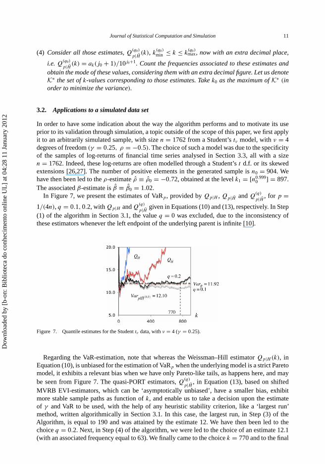
In order to have some indication about the way the algorithm performs and to motivate its useprior to its validation through simulation, a topic outside of the scope of this paper, we first applyit to an arbitrarily simulated sample, with size n = 1762 from a Student’s tν model, with ν = 4degrees of freedom (γ = 0.25, ρ = −0.5). The choice of such a model was due to the specificityof the samples of log-returns of financial time series analysed in Section 3.3, all with a sizen = 1762. Indeed, these log-returns are often modelled through a Student’s t d.f. or its skewedextensions [26,27]. The number of positive elements in the generated sample is n0 = 904. Wehave then been led to the ρ-estimate ρ̂ ≡ ρ̂0 = −0.72, obtained at the level k1 = [n0.999

0 ] = 897.The associated β-estimate is β̂ ≡ β̂0 = 1.02.

In Figure 7, we present the estimates of VaRp, provided by Qp|H , Qp|H̄ and Q(q)

p|H̄ , for p =1/(4n), q = 0.1, 0.2, with Qp|H and Q

(q)

p|H̄ given in Equations (10) and (13), respectively. In Step(1) of the algorithm in Section 3.1, the value q = 0 was excluded, due to the inconsistency ofthese estimators whenever the left endpoint of the underlying parent is infinite [10].

Figure 7. Quantile estimates for the Student tν data, with ν = 4 (γ = 0.25).

Regarding the VaR-estimation, note that whereas the Weissman–Hill estimator Qp|H (k), inEquation (10), is unbiased for the estimation of VaRp when the underlying model is a strict Paretomodel, it exhibits a relevant bias when we have only Pareto-like tails, as happens here, and maybe seen from Figure 7. The quasi-PORT estimators, Q

(q)

p|H̄ , in Equation (13), based on shiftedMVRB EVI-estimators, which can be ‘asymptotically unbiased’, have a smaller bias, exhibitmore stable sample paths as function of k, and enable us to take a decision upon the estimateof γ and VaR to be used, with the help of any heuristic stability criterion, like a ‘largest run’method, written algorithmically in Section 3.1. In this case, the largest run, in Step (3) of theAlgorithm, is equal to 190 and was attained by the estimate 12. We have then been led to thechoice q = 0.2. Next, in Step (4) of the algorithm, we were led to the choice of an estimate 12.1(with an associated frequency equal to 63). We finally came to the choice k = 770 and to the final

Dow

nloa

ded

by [

b-on

: Bib

liote

ca d

o co

nhec

imen

to o

nlin

e U

L]

at 0

4:28

11

Janu

ary

2012

12 F. Figueiredo et al.

estimate VaRp|H̄ (0.2) := Q(0.2)

p|H̄ (770) = 12.10, quite close to the real value of VaRp, equal to 11.92.Similar results were obtained for other simulated samples.

3.3. Applications to data in the field of finance

We have next considered the performance of the non-adaptive and adaptive VaR-estimators stud-ied in this paper, when applied to the analysis of the log-returns associated with two of the foursets of finance data considered in Gomes and Pestana [12]. Those sets of data, collected over thesame period, i.e. from 4 January 1999 through 17 November 2005, were the daily closing valuesof the Dow Jones Industrial Average In (DJI) and Microsoft Corp. (MSFT). Additionally, we haveconsidered over the same period the Euro-GB Pound (EGBP) daily exchange rates. All thesesamples have a size n = 1762. The VaR, defined as a large quantile of negative log-returns, i.e. ofLi = − ln(Si+1/Si), 1 ≤ i ≤ n − 1, with Si , 1 ≤ i ≤ n, a sample of consecutive close prices, is acommon risk measure for large losses. For details about VaR see, for instance, Holton [28], amongothers. Here, since we are interested in the analysis of the risk of holding short positions, we havedealt with the positive log-returns, i.e. with Pi = ln(Si+1/Si) = −Li , 1 ≤ i ≤ n − 1. Althoughthere is some increasing trend in the volatility, stationarity and weak dependence are assumed,under the same considerations as in Drees [29]. All the above-mentioned semi-parametric esti-mators are then still consistent and asymptotically normal for adequate k, although with differentasymptotic variances and slightly different dominant components of asymptotic bias.

Indeed, whenever confronted with weakly dependent processes with an extremal index θ < 1,we heuristically expect a shrinkage of maximum values and a mean size approximately equal to1/θ for the size of the clusters of exceedances of high levels. Asymptotically, we thus expect anincrease in the variance of a factor proportional to 1/θ , a high increase in the MSE of the estimators,but small changes in the bias. The presence of clustered volatility, or equivalently conditionalheteroscedasticity, seems not to be highly crucial in the performance of semi-parametric reduced-bias estimators. See Gomes et al. [30] and Gomes and Miranda [31], among others. Note, however,that the possible presence of clustered volatility is a question of particular relevance to appliedfinancial research, as extensively discussed in McNeil and Frey [25], where VaR is estimatedfor heteroscedastic return series, through an approach combining quasi-likelihood fitting of aGARCH model to estimate the current volatility and EVT for estimating the tail of the innovations’distribution of the GARCH model. We now advance with the possible use of an approach similarto the one in McNeil and Frey [25], but with the combination of the quasi-likelihood fitting of aGARCH model to estimate the current volatility, together with the methodology in this paper forthe estimation of the tail of the innovations’ distribution of such a GARCH model. A comparisonof such a technique with the one carried out in this paper, as well as with the methodology inMcNeil and Frey [25], deserves further research, both from a theoretical as well as from an appliedpoint of view, to be dealt with in the near future.

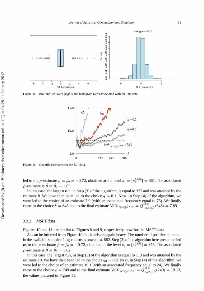
For all data sets, we present essentially two figures. In the first one, we picture a box-and-whiskers’ plot (left) and a histogram (right) of the available data. It is clear from all the graphsthat all sets of data have heavy left and right tails, and we have thus eliminated the estimatorsassociated with q = 0, due to their inconsistency. In the second figure, we present, for p = 1/(2n),the estimates of VaRp, provided by the Qp|H , Qp|H̄ and Q

(q)

p|H̄ , q = 0.1, 0.2, with Qp|H and Q(q)

p|H̄given in Equations (10) and (13), respectively.

3.3.1. DJI data

From Figure 8, we immediately see that the underlying model has heavy left and right tails. Thenumber of positive elements in the available sample of log-returns is n0 = 867. We have been

Dow

nloa

ded

by [

b-on

: Bib

liote

ca d

o co

nhec

imen

to o

nlin

e U

L]

at 0

4:28

11

Janu

ary

2012

Journal of Statistical Computation and Simulation 13

-6 -4 -2 0 2 4 6

DJI Log-returns

Histogram of DJI

DJI Log-returns

Den

sity

-5 0 5

0.00

0.05

0.10

0.15

0.20

0.25

0.30

0.35

Figure 8. Box-and-whiskers (right) and histogram (left) associated with the DJI data.

Figure 9. Quantile estimates for the DJI data.

led to the ρ-estimate ρ̂ ≡ ρ̂0 = −0.72, obtained at the level k1 = [n0.9990 ] = 861. The associated

β-estimate is β̂ ≡ β̂0 = 1.03.In this case, the largest run, in Step (3) of the algorithm, is equal to 327 and was attained by the

estimate 8. We have then been led to the choice q = 0.1. Next, in Step (4) of the algorithm, wewere led to the choice of an estimate 7.9 (with an associated frequency equal to 75). We finallycame to the choice k = 645 and to the final estimate VaR1/(2n)|H̄ (0.1) := Q

(0.1)

1/(2n)|H̄ (645) = 7.89.

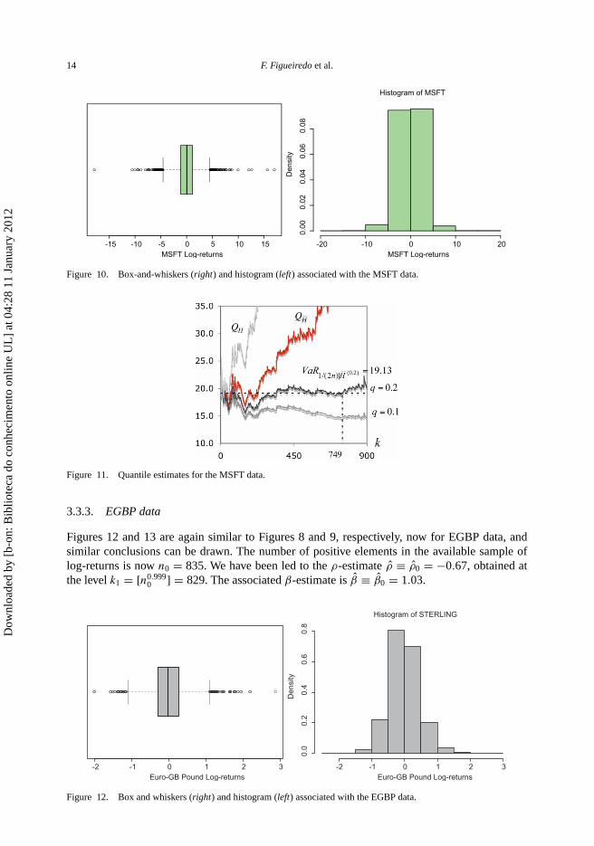
3.3.2. MSFT data

Figures 10 and 11 are similar to Figures 8 and 9, respectively, now for the MSFT data.As can be inferred from Figure 10, both tails are again heavy. The number of positive elements

in the available sample of log-returns is now n0 = 882. Step (3) of the algorithm here presented ledus to the ρ-estimate ρ̂ ≡ ρ̂0 = −0.72, obtained at the level k1 = [n0.999

0 ] = 876. The associatedβ-estimate is β̂ ≡ β̂0 = 1.02.

In this case, the largest run, in Step (3) of the algorithm is equal to 113 and was attained by theestimate 19. We have then been led to the choice q0 = 0.2. Next, in Step (4) of the algorithm, wewere led to the choice of an estimate 19.1 (with an associated frequency equal to 24). We finallycame to the choice k = 749 and to the final estimate VaR1/(2n)|H̄ (0.2) := Q

(0.2)

1/(2n)|H̄ (749) = 19.13,the values pictured in Figure 11.

Dow

nloa

ded

by [

b-on

: Bib

liote

ca d

o co

nhec

imen

to o

nlin

e U

L]

at 0

4:28

11

Janu

ary

2012

14 F. Figueiredo et al.

-15 -10 -5 0 5 10 15MSFT Log-returns

Histogram of MSFT

MSFT Log-returns

Den

sity

-20 -10 0 10 20

0.00

0.02

0.04

0.06

0.08

Figure 10. Box-and-whiskers (right) and histogram (left) associated with the MSFT data.

Figure 11. Quantile estimates for the MSFT data.

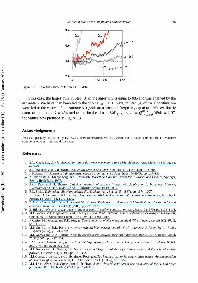
3.3.3. EGBP data

Figures 12 and 13 are again similar to Figures 8 and 9, respectively, now for EGBP data, andsimilar conclusions can be drawn. The number of positive elements in the available sample oflog-returns is now n0 = 835. We have been led to the ρ-estimate ρ̂ ≡ ρ̂0 = −0.67, obtained atthe level k1 = [n0.999

0 ] = 829. The associated β-estimate is β̂ ≡ β̂0 = 1.03.

-2 -1 0 1 2 3Euro-GB Pound Log-returns

Histogram of STERLING

Euro-GB Pound Log-returns

Den

sity

-2 -1 0 1 2 3

0.0

0.2

0.4

0.6

0.8

Figure 12. Box and whiskers (right) and histogram (left) associated with the EGBP data.

Dow

nloa

ded

by [

b-on

: Bib

liote

ca d

o co

nhec

imen

to o

nlin

e U

L]

at 0

4:28

11

Janu

ary

2012

Journal of Statistical Computation and Simulation 15

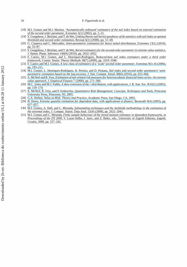
Figure 13. Quantile estimates for the EGBP data.

In this case, the largest run, in Step (3) of the algorithm is equal to 886 and was attained by theestimate 3. We have then been led to the choice q0 = 0.1. Next, in Step (4) of the algorithm, wewere led to the choice of an estimate 3.0 (with an associated frequency equal to 226). We finallycame to the choice k = 494 and to the final estimate VaR1/(2n)|H̄ (0.1) := Q

(0.1)

1/(2n)|H̄ (494) = 2.97,the values now pictured in Figure 13.

Acknowledgements

Research partially supported by FCT/OE and PTDC/FEDER. We also would like to thank a referee for the valuablecomments on a first version of this paper.

References

[1] B.V. Gnedenko, Sur la distribution limite du terme maximum d’une série aléatoire, Ann. Math. 44 (1943), pp.423–453.

[2] A.A. Balkema and L. de Haan, Residual life time at great age, Ann. Probab. 2 (1974), pp. 792–804.[3] J. Pickands III, Statistical inference using extreme order statistics, Ann. Statist. 3 (1975), pp. 119–131.[4] P. Embrechts, C. Klüppelberg, and T. Mikosch, Modelling Extremal Events for Insurance and Finance, Springer,

Berlin, Heidelberg, 1997.[5] R.-D. Reiss and M. Thomas, Statistical Analysis of Extreme Values, with Application to Insurance, Finance,

Hydrology and Other Fields, 3rd ed., Birkhäuser Verlag, Basel, 2007.[6] R.L. Smith, Estimating tails of probability distributions, Ann. Statist. 15 (1987), pp. 1174–1207.[7] H. Drees, A. Ferreira, and L. de Haan, On maximum likelihood estimation of the extreme value index, Ann. Appl.

Probab. 14 (2004), pp. 1179–1201.[8] P. Araújo Santos, M.I. Fraga Alves, and M.I. Gomes, Peaks over random threshold methodology for tail index and

quantile estimation, Revstat 4(3) (2006), pp. 227–247.[9] B. Hill, A simple general approach to inference about the tail of a distribution, Ann. Statist. 3 (1975), pp. 1163–1174.

[10] M.I. Gomes, M.I. Fraga Alves, and P. Araújo Santos, PORT Hill and moment estimators for heavy-tailed models,Comm. Statist. Simulation Comput. 37 (2008), pp. 1281–1306.

[11] F. Caeiro, M.I. Gomes, and D.D. Pestana, Direct reduction of bias of the classical Hill estimator, Revstat 3(2) (2005),pp. 111–136.

[12] M.I. Gomes and D.D. Pestana, A sturdy reduced-bias extreme quantile (VaR) estimator, J. Amer. Statist. Assoc.102(477) (2007), pp. 280–292.

[13] M.I. Gomes and D.D. Pestana, A simple second order reduced-bias’ tail index estimator, J. Stat. Comput. Simul.77(6) (2007), pp. 487–504.

[14] I. Weissman, Estimation of parameters and large quantiles based on the k largest observations, J. Amer. Statist.Assoc. 73 (1978), pp. 812–815.

[15] M.I. Gomes and O. Oliveira, The bootstrap methodology in statistics of extremes: Choice of the optimal samplefraction, Extremes 4(4) (2001), pp. 331–358.

[16] M.I. Gomes, L. de Haan, and L. Henriques-Rodrigues, Tail index estimation for heavy-tailed models: Accommodationof bias in weighted log-excesses, J. R. Stat. Soc. B 70(1) (2008b), pp. 31–52.

[17] M.I. Fraga Alves, M.I. Gomes, and L. de Haan, A new class of semi-parametric estimators of the second orderparameter, Port. Math. 60(2) (2003), pp. 194–213.

Dow

nloa

ded

by [

b-on

: Bib

liote

ca d

o co

nhec

imen

to o

nlin

e U

L]

at 0

4:28

11

Janu

ary

2012

16 F. Figueiredo et al.

[18] M.I. Gomes and M.J. Martins, ‘Asymptotically unbiased’ estimators of the tail index based on external estimationof the second order parameter, Extremes 5(1) (2002), pp. 5–31.

[19] Y. Goegebeur, J. Beirlant, and T. de Wet, Linking Pareto-tail kernel goodness-of-fit statistics with tail index at optimalthreshold and second order estimation, Revstat 6(1) (2008), pp. 51–69.

[20] G. Ciuperca and C. Mercadier, Semi-parametric estimation for heavy tailed distributions, Extremes 13(1) (2010),pp. 55–87.

[21] Y. Goegebeur, J. Beirlant, and T. de Wet, Kernel estimators for the second order parameter in extreme value statistics,J. Statist. Plann. Inference 140(9) (2010), pp. 2632–2652.

[22] F. Caeiro, M.I. Gomes, and L. Henriques-Rodrigues, Reduced-bias tail index estimators under a third orderframework, Comm. Statist. Theory Methods 38(7) (2009), pp. 1019–1040.

[23] F. Caeiro and M.I. Gomes, A new class of estimators of a ‘scale’ second order parameter, Extremes 9(3–4) (2006),pp. 193–211.

[24] M.I. Gomes, L. Henriques-Rodrigues, H. Pereira, and D. Pestana, Tail index and second order parameters’ semi-parametric estimation based on the log-excesses, J. Stat. Comput. Simul. 80(6) (2010), pp. 653–666.

[25] A. McNeil and R. Frey, Estimation of tail-related risk measures for heteroscedastic financial times series: An extremevalue approach, J. Empirical Finance 7 (2000), pp. 271–300.

[26] M.C. Jones and M.J. Faddy, A skew extension of the t-distribution, with applications, J. R. Stat. Soc. B 65(1) (2003),pp. 159–174.

[27] A. McNeil, R. Frey, and P. Embrechts, Quantitative Risk Management: Concepts, Techniques and Tools, PrincetonUniversity Press, Princeton, NJ, 2005.

[28] G.A. Holton, Value-at-Risk: Theory and Practice, Academic Press, San Diego, CA, 2003.[29] H. Drees, Extreme quantile estimation for dependent data, with applications to finance, Bernoulli 9(4) (2003), pp.

617–657.[30] M.I. Gomes, A. Hall, and C. Miranda, Subsampling techniques and the Jackknife methodology in the estimation of

the extremal index, J. Comput. Statist. Data Anal. 52(4) (2008), pp. 2022–2041.[31] M.I. Gomes and C. Miranda, Finite sample behaviour of the mixed moment estimator in dependent frameworks, in

Proceedings of the ITI 2009, V. Luzar-Stifler, I. Jarec, and Z. Bekic, eds., University of Zagreb Editions, Zagreb,Croatia, 2009, pp. 237–242.

Dow

nloa

ded

by [

b-on

: Bib

liote

ca d

o co

nhec

imen

to o

nlin

e U

L]

at 0

4:28

11

Janu

ary

2012