A Computational Approach to Essential and Nonessential Objective Functions in Linear Multicriteria...

arX

iv:0

706.

1192

v1 [

mat

h.O

C]

8 J

un 2

007

A Computational Approach to Essential

and Nonessential Objective Functions

in Linear Multicriteria Optimization1

A. B. Malinowska2 and D. F. M. Torres3

Abstract. The question of obtaining well-defined criteria for multiple cri-teria decision making problems is well-known. One of the approaches dealingwith this question is the concept of nonessential objective function. A cer-tain objective function is called nonessential if the set of efficient solutionsis the same both with or without that objective function. In this paper weput together two methods for determining nonessential objective functions.A computational implementation is done using a computer algebra system.

Key Words. Multiobjective optimization problems. Efficient (Pareto op-timal) solutions. Essential/nonessential objective functions.

1 Introduction

Multiple criteria decision making (MCDM) arise in connection with the so-lution of problems in the areas of economy, environment, business and engi-neering (see e.g. Refs. 1-4). Multiobjective programming is concerned with

1To be partially presented at the 23rd IFIP TC 7 International Conference on SystemModelling and Optimization, Cracow, Poland, July 23-27, 2007. Work supported by KBNunder Bialystok Technical University grant W/WI/17/07; and the R&D unit CEOC ofthe University of Aveiro through FCT and FEDER/POCI 2010.

2Assistant Professor, Faculty of Computer Science, Technical University of Bia lystok,Bia lystok, Poland

3Associate Professor, Department of Mathematics, University of Aveiro, Aveiro, Por-tugal.

1

http://arxiv.org/abs/0706.1192v1

the generation of solution sets for multiobjective problems that usually in-clude a large or an infinite number of points, known as efficient solutions.Those efficient points are then the candidates for an optimal solution of theMCDM problem.

The question of obtaining well-defined criteria for MCDM problems iswell-known. Often mathematical models done by inexperienced practitionerslead to redundant formulations, which are not only deceptive but also compu-tationally cumbersome (see Refs. 5-7 and therein). Sometimes the decision-maker end up without any decision support, while a simple reformulation ofthe problem would achieve the desired result. One of the approaches dealingwith the question of obtaining well-defined criteria for MCDM is based onthe concept of nonessential objective function. A certain objective functionis called nonessential if the set of efficient solutions is the same both with orwithout that objective function. Information about nonessential objectiveshelps a decision maker to get insights and better understand a problem, andthis might be a good starting point for further investigations or revision ofthe model. Dropping out nonessential functions leads to a problem with asmaller number of objectives, which can be solved more easily. For this rea-son, the identification of nonessential objectives is an important feature inthe analysis of multiple criteria programs.

The seminal papers by Gal and Leberling (Refs. 8, 9) define and investi-gate nonessential objectives in linear multiobjective optimization problems;Gal and Hanne (Refs. 6, 7) study the consequences of dropping nonessen-tial objectives functions in the application of MCDM methods. Recently,the concept of nonessential objective has been generalized by Malinowska toconvex multiobjective optimization problems, and new definitions of weaklynonessential and properly nonessential objective functions were introducedand investigated (Refs. 10, 11); a new method to determine if a given objec-tive function of a certain linear problem is essential or not has been proved(Ref. 12).

Here we put together, in a constructive and algorithmic way, the twoavailable methods (Refs. 8, 12) for determining nonessential objective func-tions. A computational implementation is done using the computer algebrasystem Maple. The plan of the paper is as follows. Section 2 gives the nec-essary preliminaries and provides the notation used in the text. In Section 3we develop the theory of nonessential objectives. Main result of the paperappears in Section 4: the algorithm to determine if a given objective functionof a linear multiobjective problem is essential or not. Finally, in Section 5 we

2

provide some examples that show the applicability of our methodology andthe convenience of the developed computer software. The paper ends withsome conclusions, the references, and an appendix with all the Maple codethat implements the proposed algorithm.

2 Preliminaries and Notation

In this section we present some general concepts and notations. We usesuperscripts for vectors (for example x1, or simply x when no confusion canarise), and subscripts for components of vectors (for example x1). All thevectors are assumed to be column vectors. The symbol 1 stands for the vector[1, . . . , 1]T . For two vectors x, x′ ∈ R

k we define the relations (Ref. 13):

x ≧ x′ ⇔ ∀i ∈ {1, . . . , k} : xi ≥ x′

i ,

x ≥ x′ ⇔ ∀i ∈ {1, . . . , k} : xi ≥ x′

i ∧ ∃i ∈ {1, . . . , k} : xi > x′

i ,

x > x′ ⇔ ∀i ∈ {1, . . . , k} : xi > x′

i .

Throughout this paper we study the following linear multiobjective opti-mization problem:

max{F n+1(x) : x ∈ X}, (1)

whereX = {x ∈ R

k : Ax ≦ b , x ≧ 0} , A ∈ Rm×k , b ∈ R

m

is the feasible set, and

F n+1(x) = Cx = [(c1)T x, . . . , (cn+1)T x]T , ci ∈ Rk(i = 1, . . . , n+1) , n ≥ 1

is the vector of objective functions: fi : Rk → R (i = 1, . . . , n + 1). We are

using “max” to mean that we want to maximize all the objective functionssimultaneously. This involves no loss of generality. In general it does notexist a solution that is optimal with respect to every objective function, andone is lead to the concept of Pareto optimality.

Definition 2.1 A vector x0 ∈ X is said to be an efficient (Pareto opti-mal) solution of problem (1) if there exists no x ∈ X such that F n+1(x) ≥F n+1(x0). The set of efficient solutions of problem (1) is denoted by Xn+1

E .

3

3 Nonessential Objectives

Let XnE denote the set of efficient solutions of problem (1) without one ob-

jective function fk, k ∈ {1, . . . , n + 1}. Without loss of generality we assumek = n + 1.

Definition 3.1 The objective function fn+1 is said to be nonessential inproblem (1) if Xn

E = Xn+1

E . An objective function which is not nonessen-tial is called essential.

We now recall two theorems that characterize a nonessential objective func-tion, and which will be used in the proposed algorithm to determine if agiven objective function is essential or not.

Theorem 3.1 (Ref. 8) The objective function fn+1 is nonessential in (1) ifthe following holds:

cn+1 =n

∑

i=1

αici , αi ≥ 0 (i = 1, . . . , n) . (2)

Theorem 3.1 is very useful because condition (2) is easy to check. Unfortu-nately, it is only a sufficient condition. Theorem 3.2 below gives a necessaryand sufficient condition for an objective function to be nonessential.

Let Xn+1 denote the set of solutions of the single objective optimizationproblem

max{fn+1(x) : x ∈ X} . (3)

In other words,

Xn+1 = {x0 ∈ X : ∀x ∈ X fn+1(x0) ≥ fn+1(x)}. (4)

Theorem 3.2 (Refs. 10, 11) If the set X is nonempty and bounded (inother words, if X is a convex polyhedron), then the objective function fn+1 isnonessential in (1) if and only if the following three conditions hold:

(i) ∀x ∈ X\XnE ∃x′ ∈ R

k : F n+1(x′) ≥ F n+1(x);

(ii) XnE ∩ Xn+1 6= ∅;

(iii) XnE ⊂ Xn+1

E .

4

4 Main Results

The theory described in the previous section enable us to work out on acomputational algorithm to test if an objective function fn+1 in problem(1) is essential or not. The proposed algorithm consists of eight steps andeach one has been implemented in the computer algebra system Maple (seeAppendix on page 19).

Step 0. Does cn+1 =∑n

i=1αic

i, αi ≥ 0 (i = 1, . . . , n)?If the answer is ”TRUE”, then the objective function fn+1 is nonessential byTheorem 3.1. Otherwise, we go to Step 1.

We implement Step 0 as a Maple command glm (Gal-Leberling method),which receives in its first argument a list with the objective functions, andin its second argument the number of variables of the problem.

Example 4.1 Consider the multiobjective optimization problem

max{F 4(x) : x ∈ X},

where

f1(x) = x1 + 3x2,

f2(x) = 3x1,

f3(x) = 2x1 + x2,

f4(x) = −3x1 − x2,

and X ⊂ R2. With our Maple package we do:

> glm([x1+3*x2,3*x1,2*x1+x2,-3*x1-x2],2);

false

We conclude that the answer to Step 0 is ”FALSE”, so we go to Step 1.Now, let us change the order of objective functions as follows:

f1(x) = x1 + 3x2,

f2(x) = 3x1,

f3(x) = −3x1 − x2,

f4(x) = 2x1 + x2.

This time our glm procedure gives

5

> glm([x1+3*x2,3*x1,-3*x1-x2,2*x1+x2],2);

true

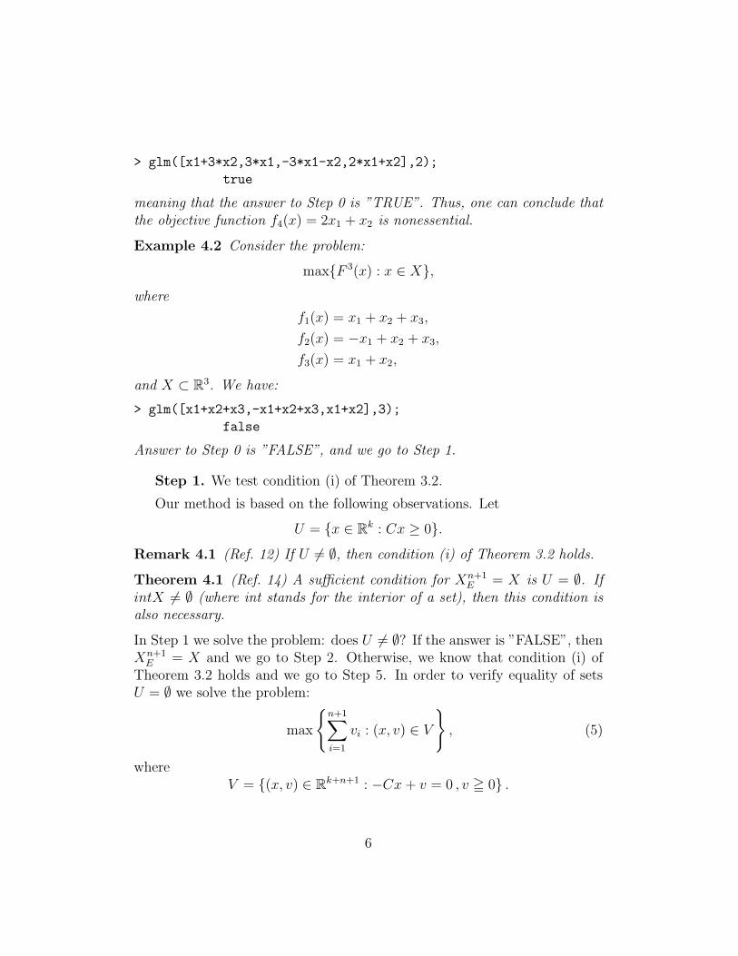
meaning that the answer to Step 0 is ”TRUE”. Thus, one can conclude thatthe objective function f4(x) = 2x1 + x2 is nonessential.

Example 4.2 Consider the problem:

max{F 3(x) : x ∈ X},

where

f1(x) = x1 + x2 + x3,

f2(x) = −x1 + x2 + x3,

f3(x) = x1 + x2,

and X ⊂ R3. We have:

> glm([x1+x2+x3,-x1+x2+x3,x1+x2],3);

false

Answer to Step 0 is ”FALSE”, and we go to Step 1.

Step 1. We test condition (i) of Theorem 3.2.

Our method is based on the following observations. Let

U = {x ∈ Rk : Cx ≥ 0}.

Remark 4.1 (Ref. 12) If U 6= ∅, then condition (i) of Theorem 3.2 holds.

Theorem 4.1 (Ref. 14) A sufficient condition for Xn+1

E = X is U = ∅. IfintX 6= ∅ (where int stands for the interior of a set), then this condition isalso necessary.

In Step 1 we solve the problem: does U 6= ∅? If the answer is ”FALSE”, thenXn+1

E = X and we go to Step 2. Otherwise, we know that condition (i) ofTheorem 3.2 holds and we go to Step 5. In order to verify equality of setsU = ∅ we solve the problem:

max

{

n+1∑

i=1

vi : (x, v) ∈ V

}

, (5)

whereV = {(x, v) ∈ R

k+n+1 : −Cx + v = 0 , v ≧ 0} .

6

Remark 4.2 (Ref. 14) One has U = ∅ if and only if problem (5) has zeroas the optimal objective function value.

Example 4.3 Consider the problem from Example 4.1:

max{F 4(x) : x ∈ X},

where

f1(x) = x1 + 3x2,

f2(x) = 3x1,

f3(x) = 2x1 + x2,

f4(x) = −3x1 − x2,

and X ⊂ R2. Using our Maple command step1 we obtain:

> step1(2,[x1+3*x2, 3*x1, 2*x1+x2, -3*x1-x2]);

false

We conclude that Step 1 has answer ”FALSE”. Thus, X4E = X and we go

to Step 2.

Example 4.4 Consider again the problem from Example 4.2:

max{F 3(x) : x ∈ X},

where

f1(x) = x1 + x2 + x3,

f2(x) = −x1 + x2 + x3,

f3(x) = x1 + x2,

and X ⊂ R3. We obtain

> step1(3,[x1+x2+x3, -x1+x2+x3, x1+x2]);

true

so the answer to Step 1 is ”TRUE”. Thus, condition (i) of Theorem 3.2holds and we go to Step 5.

7

Step 2. Let U = {x ∈ Rk : Cx ≥ 0}, where C = [(c1)T , . . . , (cn)T ]T . In

Step 2 we address the following question: does U 6= ∅?

The method we use is the same as the one described in Step 1. If theanswer is ”FALSE”, then Theorem 4.1 implies Xn

E = X and the objectivefunction fn+1 is nonessential. Otherwise, we go to Step 3.

Example 4.5 Let us consider again the problem from Example 4.3. Usingour Maple command step2 one has:

> step2(2,[x1+3*x2, 3*x1, 2*x1+x2, -3*x1-x2]);

true

Since the answer to Step 2 is ”TRUE” we go to Step 3.

Step 3. In this step we solve the problem: does intX 6= ∅?

Our method is based on the following remark.

Remark 4.3 If intX 6= ∅, then problem max{a : (x, v, a) ∈ V }, where

V ={

(x, v, a) ∈ Rk+m+1 : Ax + v + a1 = b , v ≧ 0, x ≧ ε1 , a ≥ 0

}

with ε > 0 sufficiently small, has an optimal objective function value greaterthan zero.

If in Step 3 the answer is ”TRUE”, then Theorem 4.1 implies XnE 6= X, and

the objective function fn+1 is essential. Otherwise, we go to Step 4.In order to use the simplex package already available from the Maple

system, we put ε = 0, 001. We note that by default we are assuming that allx variables are greater or equal than zero (the user does not need to mentionthis explicitly in the definition of the set X while using our Maple package).

Example 4.6 Let us continue the problem from Examples 4.3 and 4.5 with

X = {x ∈ R2 : x1 ≤ 1, x2 ≤ 1, x ≧ 0}.

Using our Maple command step3 we obtain

> step3(3,{x1 <= 1, x2 <= 1});

true

8

Since the answer to Step 3 is ”TRUE”, the objective function f4(x) = −3x1−x2 is essential.Now, let us consider a different problem by changing the set X as follows:

X = {x ∈ R2 : x1 + x2 ≤ 1,−x1 − x2 ≤ −1, x ≧ 0}.

Now we obtain

> step3(2,{x1+x2<=1,-x1-x2<=-1});

false

Since Step 3 has the answer ”FALSE”, we go to Step 4.

Step 4. In this step we solve the problem: does XnE = X?

Our method is the following: we compute a vertex x0 of X and test if x0

is an element of XnE.

Theorem 4.2 (Ref. 15) Let x0 ∈ X be given. Solve the problem

max

{

n∑

i=1

ǫi : (x, ǫ) ∈ S

}

(6)

with

S = {(x, ǫ) ∈ Rk+n : x ∈ X, fi(x) − ǫi = fi(x

0), ǫi ≥ 0, i = 1, . . . , n} .

The vector x0 is efficient if and only if problem (6) has zero as the optimalobjective function value.

If x0 is not efficient, then the answer from Step 4 is ”FALSE” and theobjective function fn+1 is essential. Otherwise, we compute the next vertexof X and check if it is efficient or not. Our procedure stops as soon as anon-efficient vertex is found.

Example 4.7 Consider the problem:

max{F 3(x) : x ∈ X},

9

where

f1(x) = x1 + x2,

f2(x) = x1,

f3(x) = −3x1 − x2,

andX = {x ∈ R

2 : x1 + x2 ≤ 1,−x1 − x2 ≤ −1, x ≧ 0}.

Answers from Steps 1 to 4 are easily obtained from the respective commandsof our Maple package:

> step1(2, [x1 + x2, x1, -3 x1 - x2]);

false

> step2(2, [x1 + x2, x1, -3 x1 - x2]);

true

> step3(2,{x1+x2<=1,-x1-x2<=-1});

false

> step4([x1+x2,x1,-3*x1-x2],{x1+x2<=1,-x1-x2<=-1},2);

false

We conclude that f3(x) = −3x1 − x2 is essential and that X2E ⊂ X3

E.

In the case all vertices are efficient, two situations may appear: objectivefunction fn+1 may be essential (answer ”FALSE”) or not (answer ”TRUE”).To distinguish between these two cases we apply the following remark.

Remark 4.4 Let x1, x2, . . . , xp be all vertexes of X and intX = ∅. Then,Xn

E = X if and only if there exists a vector w > 0 with∑n

i=1wi = 1 such

that wTF n(x1) = wT F n(x2) = · · · = wTF n(xp).

Proof. As far as intX = ∅, we have X ⊂ H , where H is a hyperplane.Therefore, Xn

E = X if and only if there exists w > 0 (∑n

i=1wi = 1) such that

for all x in X, x is a solution of the problem max{wT F n(x) : x ∈ X} (see forinstance Ref. 16, p. 54). This completes the proof.

In order to use the simplex method as provided by Maple, we changecondition from Remark 4.4 into the form

∃w ∈ Rn : wTF n(x1) = wTF n(x2) = · · · = wT F n(xp),

n∑

i=1

wi = 1, wT1 ≥ ε1,

where ε > 0 is sufficiently small. In our procedure we set ε = 0, 00001.

10

Example 4.8 Let us continue the problem from Examples 4.3, 4.5 and 4.6with

X = {x ∈ R2 : x1 + x2 ≤ 1,−x1 − x2 ≤ −1, x ≧ 0}.

Our Maple command step4 give us

> step4([x1+3*x2,2*x1+x2,3*x1,-3*x1-x2],{x1+x2<=1,-x1-x2<=-1},2);

true

Thus, X2E = X and it follows that f4(x) = −3x1 − x2 is nonessential.

Now we show an example where all vertices are efficient but XnE 6= X.

Example 4.9 Let us consider the problem

max{F 3(x) : x ∈ X},

where

f1(x1, x2, x3) = −x1 − 2x2 + 2x3,

f2(x1, x2, x3) = 2x1 + 3x2,

f3(x1, x2, x3) = −x1 − x2 − 2x3,

and

X ={

x ∈ R3 : x2 + x3 ≤ 2,−x2 − x3 ≤ −2, x1 + x2 + x3 ≤ 3,

− x1 − x2 − x3 ≤ −2, x1 + x2 ≤ 2 , x ≧ 0}

.

Using our Maple commands we obtain:

> step1([-x1-2*x2+2*x3, 2*x1+3*x2,-x1-x2-2*x3]);

false

> step2([-x1-2*x2+2*x3, 2*x1+3*x2,-x1-x2-2*x3]);

true

> step3(3,{x2+x3<=2,-x2-x3<=-2,x1+x2+x3<=3,-x1-x2-x3<=-2,x1+x2<=2});

false

> step4([-x1-2*x2+2*x3,2*x1+3*x2,-x1-x2-2*x3],

{x2+x3<=2,-x2-x3<=-2,x1+x2+x3<=3,-x1-x2-x3<=-2,x1+x2<=2},3);

false

11

We conclude that the objective function f3 is essential and that X2E ⊂ X3

E.

Step 5. In this step we calculate all vertexes of Xn+1 (see (4)).

Let XWn+1 = {x1, x2, . . . , xq} be the set of all vertexes of Xn+1. We have:

Xn+1 =

{

x ∈ Rk : x =

q∑

j=1

αjxj ,

q∑

j=1

αj = 1 , αj ≥ 0, j = 1, . . . , q

}

.

Example 4.10 Consider again the problem from Example 4.4 with

X = {x ∈ R3 : x1 ≤ 1, x2 ≤ 1, x3 ≤ 1, x ≧ 0}.

Our procedure step5 give us

> step5([x1+x2+x3,-x1+x2+x3,x1+x2],{x1<=1,x2<=1,x3<=1});

{{x1 = 1, x2 = 1, x3 = 1} , {x1 = 1, x2 = 1, x3 = 0}}

Hence, XW3 = {[1, 1, 0]T , [1, 1, 1]T} and

X3 = {x : x = α[1, 1, 0]T + (1 − α)[1, 1, 1]T , 0 ≤ α ≤ 1}.

Step 6. In this step we solve the following problem (condition (ii) ofTheorem 3.2): does Xn+1 ∩ Xn

E 6= ∅?

The basic idea of our method is to use Theorem 4.3.

Theorem 4.3 (Ref. 17) Let Z = {x1, x2, . . . , xq} ⊂ X. If Z ⊂ X \XnE, then

{

x ∈ Rk : x =

q∑

j=1

αjxj ,

q∑

j=1

αj = 1, αj ≥ 0, j = 1, . . . , q

}

⊂ X \ XnE .

Having in mind Theorem 4.3, it is sufficient to consider only vertexes of Xn+1.Applying Theorem 4.2 we check if there exists a vertex of Xn+1 which belongsto Xn

E . If the answer is ”TRUE”, then the condition (ii) of Theorem 3.2 holdsand we go to Step 7. Otherwise, we conclude that the objective function fn+1

is essential.

Example 4.11 Let us continue the problem from Examples 4.4 and 4.10.Our procedure step6 give the answer ”TRUE”

12

> step6([x1+x2+x3,-x1+x2+x3,x1+x2],{x1<=1,x2<=1,x3<=1});

true

and we proceed to Step 7.

Example 4.12 Now we consider a problem borrowed from Ref. 4:

max{F 3(x) : x ∈ X},

where

f1(x) = x1 + 2x2 − x3 + 3x4 + 2x5 + x7,

f2(x) = x2 + x3 + 2x4 + 3x5 + x6,

f3(x) = x1 + x3 − x4 − x6 − x7,

and

X = {x ∈ R7 : x1 + 2x2 + x3 + x4 + 2x5 + x6 + 2x7 ≤ 16,

− 2x1 − x2 + x4 + 2x5 + x7 ≤ 16,

− x1 + x3 + 2x5 − 2x7 ≤ 16, x2 + 2x3 − x4 + x5 − 2x6 − x7 ≤ 1, x ≧ 0}.

With our Maple command step6 we obtain

> step6([x1+2*x2-x3+3*x4+2*x5+x7,x2+x3+2*x4+3*x5+x6,x1+x3-x4-x6-x7],

{x1+2*x2+x3+x4+2*x5+x6+2*x7<=16,-2*x1-x2+x4+2*x5+x7<=16,

-x1+x3+2*x5-2*x7<=16,x2+2*x3-x4+x5-2*x6-x7<=1});

false

and since the answer is ”FALSE”, we conclude that the objective functionf3(x) = x1 + x3 − x4 − x6 − x7 is essential.

Step 7. In this step we solve the following problem (condition (iii) ofTheorem 3.2): does Xn

E ⊂ Xn+1

E ?

Our method is based on the following observations.

Proposition 4.1 (Refs. 10, 18) If the vector-valued function F n is one-to-one on the set Xn

E, then condition (iii) of Theorem 3.2 holds.

Let〈Xn

E〉 = {xi − xj : xi, xj ∈ XnE}.

13

Lemma 4.1 (Ref. 19) The vector-valued function F n is one-to-one on theset Xn

E if and only if KerF n ∩ 〈XnE〉 = ∅ (Ker stands for the kernel of a

map).

In practice it is usually impossible to determine the set 〈XnE〉. For this reason,

in our Maple procedure we use the following set:

〈XnWE〉 = {xi − x0 : xi, x0 ∈ Xn

E},

where xi, x0 are vertexes of XnE and x0 is free but fixed. Obviously, 〈Xn

E〉 ⊂Lin{〈Xn

WE〉}.

Remark 4.5 If KerF n ∩ Lin{〈XnWE〉} = ∅, then condition (iii) of Theo-

rem 3.2 holds (that is, XnE ⊂ Xn+1

E ).

If the answer from Step 7 is ”TRUE”, then the objective function fn+1 isnonessential. Otherwise, we know that Xn+1

E ⊂ XnE .

Example 4.13 Let us continue the problem from Examples 4.4, 4.10 and4.11. We obtain:

> step7([x1+x2+x3,-x1+x2+x3,x1+x2],{x1<=1,x2<=1,x3<=1},3);

true

The answer from Step 7 is ”TRUE”, hence the objective function f3(x) =x1 + x2 is nonessential.

5 Illustrative Examples

We have implemented all the steps described in Section 4 together in a singleMaple command called nonessential (see Figure 1). This main procedurereceives a list with the definition of the objective functions, and the setX of constraints in the second argument. Below we give some examplesof computer sessions with our Maple package. The interested reader maydownload it from [http://www.mat.ua.pt/delfim/essential.html] andfind there more examples than the ones we are able to provide here. We inviteand welcome the reader to experiment our Maple package with her/his ownproblems.

14

http://www.mat.ua.pt/delfim/essential.html

Step 0

Tllllll

vvlll F

RRRRRR

((RRRRRR

fn+1 isnonessential

Step 1

Fllllll

vvllllll TQQ

QQQQ

((QQQQQ

Q

Step 2

Fllllll

vvlll T

��

Step 5

��fn+1 is

nonessentialStep 3

Tnn

nnnnn

wwnnnn

F

��

Step 6

Foooooo

wwoooo

T

��fn+1 is

essentialStep 4

Fqqqqqqq

xxqq T

��

fn+1 isessential

Step 7

Trrrrrrr

yyrrrr

r

��fn+1 isessential andXn

E ⊆ Xn+1

E

fn+1 isnonessential

fn+1 isnonessential

Xn+1

E ⊆ XnE

Figure 1: Scheme of the method implemented in Maple.

We begin with a simple example with three objective functions and threevariables.

> nonessential([x1+x2,x1+x2+x3,-3*x1-3*x2-x3],{x1+x2+x3 <= 1});

Objective function -3*x1-3*x2-x3 is essential from Step 3

Next we consider a problem with four objective functions and five vari-ables. It turns out that the problem may be reduced to a simpler one withthe same set of efficient solutions.

> st:= time():

nonessential([x1+x2+x3+x4+x5,-x1+x2+x3+x4+x5,-x1-x2+x3+x4+x5,x1+x2],

{x1<=1,x2<=1,x3<=1,x4<=1,x5<=1});

printf("%a seconds\n",time() - st);

Objective function x1+x2 is nonessential from step 7

2.072 seconds

15

The only situation where our Maple procedure nonessential can notconclude that a given function is essential or not, is when one reaches Step 7and the answer is not true.

> st:= time():

nonessential([-x3-x4,-x5-x6,-x4-x6],

{x1+3*x2<=24,3*x1+x2<=24,x1+4*x2+x3-x4<=40,

-x1+4*x2-x3+x4<=-40,4*x1+x2+x5-x6<=40,-4*x1-x2-x5+x6<=-40});

printf("%a seconds\n",time() - st);

X_E^3 C X_E^2 from step 7

7.251 seconds

Our Maple package is useful to identify redundant objective functions.We finish with an example where the mathematical model can be simplifiedby elimination of two of the objective functions.

> nonessential([x1+3*x2,2*x1+x2,3*x1,-3*x1-x2],

{x1+x2<=1,-x1-x2<=-1});

Objective function -3*x1-x2 is nonessential from step 4

> nonessential([x1+3*x2,2*x1+x2,3*x1],{x1+x2<=1,-x1-x2<=-1});

Objective function 3*x1 is nonessential from step 7

> nonessential([x1+3*x2,2*x1+x2],{x1+x2<=1,-x1-x2<=-1});

Objective function 2*x1+x2 is essential from step 6

> nonessential([2*x1+x2,x1+3*x2],{x1+x2<=1,-x1-x2<=-1});

Objective function x1+3*x2 is essential from step 6

6 Conclusion

There are theoretical and practical reasons for developing a method to findnonessential objective functions. In this paper we present such a methodand its implementation in Maple. Our algorithm is based on necessary andsufficient conditions for an objective function to be nonessential, and needonly to solve a finite number of single objective linear optimization prob-lems. Examples showing the usefulness of our Maple package are provided:identification of nonessential objective functions permits to simplify the cor-respondent mathematical model.

16

References

1. COHON, J. L., Multiobjective programming and planning, AcademicPress, New York, 1978.

2. LEITMANN, G., Cooperative and non-cooperative differential games, inThe theory and application of differential games (Proc. NATO AdvancedStudy Inst., Univ. Warwick, Coventry, 1974), 85–96. NATO Adv. StudyInst. Ser., Ser. C: Math. and Phys. Sci., 13, Reidel, Dordrecht, 1975.

3. LEITMANN, G., and MARZOLLO, A., Multicriteria decision making.CISM. International Centre for Mechanical Sciences. Courses and Lec-tures. No. 211. Wien - New York: Springer-Verlag, 1975.

4. ZELENY, M., Multiple criteria decision making. McGraw-Hill Series inQuantitative Methods for Management. New York, McGraw-Hill BookCompany (1982).

5. GAL, T., Postoptimal analyses, parametric programming, and relatedtopics: degeneracy, multicriteria decision making, redundancy, WalterDe Gruyter Inc, Berlin (1995).

6. GAL, T., and HANNE, T., Consequences of dropping nonessential ob-jectives for the application of MCDM methods. European Journal ofOperational Research, 119, 373-378, (1999)

7. GAL, T., and HANNE, T., Nonessential objectives within network ap-proaches for MCDM, European J. Oper. Res. 168 (2006), no. 2, 584–592.

8. GAL, T., and LEBERLING, H., Redundant objective functions in linearvector maximum problems and their determination, European J. Oper.Res. 1 (1977), no. 3, 176–184.

9. GAL, T., A note on size reduction of the objective functions matrix invector maximum problems, in Multiple criteria decision making theoryand application (Proc. Third Conf., Hagen/Konigswinter, 1979), 74–84,Lecture Notes in Econom. and Math. Systems, 177, Springer, Berlin-NewYork, 1980.

10. MALINOWSKA, A. B., Istotnosc skalarnych funkcji ocen w zadaniachwektorowej optymalizacji (in Polish), Ph.D. thesis, SRI, Polish Academyof Sciences, Warsaw, 2002.

17

11. MALINOWSKA, A. B., Changes of the set of efficient solutions by ex-tending the number of objectives and its evaluation. Control and Cyber-netics, 31, 4, 964–974, (2002).

12. MALINOWSKA, A. B., Nonessential objective functions in linear multi-objective optimization problems, Control and Cybernetics, 35, 4, 873–880(2006).

13. YU, P. L., Cone convexity, cone extreme points, and nondominated solu-tions in decision problems with multiobjectives, J. Optimization TheoryAppl. 14 (1974), 319–377.

14. GALAS, Z., NYKOWSKI, I., and ZO LKIEWSKI, Z., Programowaniewielokryterialne (in Polish) PWE, Warszawa, 1987.

15. BENSON, H. P., Existence of efficient solutions for vector maximizationproblems, J. Optim. Theory Appl. 26 (1978), no. 4, 569–580.

16. CHANKONG, V., HAIMES, Y. Y., THADATHIL, J., and ZIONTS, S.,Multiple criteria optimization: a state of the art review, in Decisionmaking with multiple objectives (Cleveland, Ohio, 1984), 36–90, LectureNotes in Econom. and Math. Systems, 242, Springer, Berlin, 1985.

17. YU, P. L., and ZELENY, M., The set of all nondominated solutions inlinear cases and a multicriteria simplex method, J. Math. Anal. Appl.49 (1975), 430–468.

18. GUTENBAUM, J., and INKIELMAN, M., Multicriterial decision-making by comparison of the Pareto-optimal sets for a reduced numberof objectives. In: Proceedings of the 25th Conference on Macromodelsand Modelling Economies in Transition, Jurata 3-4 December, vol. 2,15–25,(1998).

19. MALINOWSKA, A. B., Wyznaczanie kryteriow nieistotnych w zada-niach liniowych (in Polish), In: Kacprzyk, J. and Budzinski, R. (eds.),Badania operacyjne i systemowe’2006. Metody i techniki, Warsaw, 75–82(2006).

18

Appendix – Maple Definitions

Our Maple definitions follow below. The reader can download the code from[http://www.mat.ua.pt/delfim/essential.html] together with many moreexamples than the ones we are able to provide in the paper.

We begin by implementing the Gal-Leberling method (see Examples 4.1and 4.2), which is based on the results of Ref. 8.

> ##################################################################

> # GL method; returns true if F[-1] is nonessential;

> # returns false if one can not conclude nothing from GL method

> ##################################################################

> glm := proc(F,NumVar)

> local c, f, v, LV, lc, SolSet, SS, i;

> c := proc(var,exp)

> local v;

> v:= select(has,exp+abm,var);

> if v = NULL then

> return(0);

> else

> return(v/var):

> fi:

> end proc;

> f := o -> if type(o,numeric) then o else 0 fi:

> v := (exp,n) -> Vector([seq(f(c(x||i,exp)),i=1..n)]):

> LV := [seq(LinearAlgebra[VectorScalarMultiply](v(F[i],NumVar),

alpha||i),i=1..nops(F)-1)];

> lc := Vector(NumVar);

> for i in LV do

> lc := LinearAlgebra[VectorAdd](lc,i):

> od;

> SolSet := solve({seq(lc[i]=c(x||i,F[-1]),i=1..NumVar)});

> if SolSet = NULL then

> return(false);

> else

> SS := {seq(simplex[maximize](alpha||i,SolSet,

NONNEGATIVE),i=1..nops(F)-1)};

> if SS = {{}} then

> return(false);

> else

> return(true);

> fi:

> fi:

> end proc:

19

For illustrative examples on how to use the procedures step1 and step2

see Examples 4.3, 4.4 and 4.5.

> ###################

> # step 1

> ###################

> step1 := proc(F)

> local of, const, S;

> of := add(v||i,i=1..nops(F));

> const := seq(-F[i]+v||i=0,i=1..nops(F));

> const := [const,seq(v||i>=0,i=1..nops(F))];

> S := simplex[maximize](of,const);

> return(not(evalb(subs(S,of)=0))):

> end proc:

> ###################

> # step 2

> ###################

> step2 := F -> step1(F[1..-2]):

Follows our implementation in Maple for Step 3 (see Example 4.6).

> step3 := proc(NumVar,X)

> local LHS, RHS, SC1, SC2, SC3, SC, SS3, i, a, epsilon, mylhs, myrhs;

> epsilon := 0.001;

> mylhs := E -> if type(lhs(E),numeric) then rhs(E) else lhs(E) fi:

> myrhs := E -> if type(rhs(E),numeric) then rhs(E) else lhs(E) fi:

> LHS := [seq(mylhs(i),i=X)];

> RHS := [seq(myrhs(i),i=X)];

> SC1 := {seq(LHS[i]+a+v||i = RHS[i],i=1..nops(LHS))};

> SC2 := {seq(v||i >= 0,i=1..nops(LHS)), a>=0};

> SC3 := {seq(x||i>=0.001,i=1..NumVar)};

> SC := SC1 union SC2 union SC3;

> SS3 := simplex[maximize](a,SC);

> assign(select(has,SS3,a));

> if a = 0 then return(false) else return(true) fi;

> end proc:

In Step 4 we use a rank method, computing the rank of a matrix A bythe Rank command from the standard LinearAlgebra package of Maplesystem. We notice that the procedure step4 does not use the last objectivefunction (the last objective is given in Maple by F[-1], and we exclude itfrom consideration by writing F[1..-2]). The auxiliary procedure matrixAis used both by Steps 4 and 7. The procedure Proposition4dot12 is ourMaple definition for Remark 4.4.

20

> matrixA := proc(X,NumVar)

> local c, LHS, row, mylhs;


> c := (var,exp) -> if evalb({select(has,exp,var)} = {}) then

0

else

select(has,exp,var)/var

fi:

> LHS := [seq(mylhs(i)+abm,i=X)];

> row := (exp,NumVar) -> map(c,[seq(x||i,i=1..NumVar)],exp):

> return(Matrix(map(row,LHS,NumVar)));

> end proc:

>

> Proposition4dot12 := proc(F,X,LE)

> local SE, v, ETS, solW, SS, SV;

> SE := NULL;

> for v in LE do

> SV := subs(v,F);

> SE := SE, add(SV[i]*w||i,i=1..nops(SV));

> od;

> ETS := seq(SE[1]=i,i=SE[2..-1]), add(w||i,i=1..nops(SV))=1;

> solW := solve({ETS, add(w||i,i=1..nops(SV))=1})

union {seq(w||i>=0.00001,i=1..nops(SV))};

> SS := {seq(simplex[maximize](w||i,solW),i=1..nops(SV))};

> return(not(remove(i->i={},SS) = {}));

> end proc:

> step4 := proc(F,X,NumVar)

> local NX,NNumVar,b,A,rnk,dif,LP,zero,efficient,v,admissible,

> vs,AM,sol,of,cstEps,cst,SC,p,myrhs,mylhs,LE, tv, val;



> tv := (x,s) -> myrhs(op(select(has,s,x))):

> b := X -> Vector([seq(myrhs(i),i=X)]):

> NX := {seq(mylhs(X[i])+x||(NumVar+i)=myrhs(X[i]),i=1..nops(X))};

> NNumVar := NumVar+nops(X);

> A := matrixA(NX,NNumVar);

> rnk := LinearAlgebra[Rank](A);

> dif := NNumVar - rnk;

> LP := combinat[choose]([seq(x||i,i=1..NNumVar)],dif);

> zero := L -> {seq(i=0,i=L)}:

> efficient := true;

> v := Vector([seq(x||i,i=1..NNumVar)]);

> admissible := sc -> not(member(false,{seq(evalb(myrhs(i)>=0),i=sc)})):

> LE := NULL;

> for p in LP while efficient do

21

> vs := subs({seq(i=0,i=p)},v);

> AM := LinearAlgebra[MatrixVectorMultiply](A,vs);

> sol := solve({seq(AM[i]=b(NX)[i],i=1..nops(NX))});

> if not(sol = NULL) and admissible(sol) then

> sol := sol union zero(p):

> of := add(epsilon||i,i=1..nops(F)-1);

> cstEps := seq(epsilon||i>=0,i=1..nops(F)-1);

> cst := seq(F[i]-epsilon||i=subs(sol,F[i]),i=1..nops(F)-1);

> SC := {cst} union {cstEps} union NX;

> efficient := evalb(subs(simplex[maximize](of,SC,NONNEGATIVE),of)=0);

> if efficient then

> val := [seq(tv(x||i, sol),i=1..NumVar)];

> if not(member(false,map(i->type(i,numeric),val))) then

> LE := LE, {seq(x||i=val[i],i=1..NumVar)};

> fi;

> fi;

> fi:

> od;

> if not(efficient) then

> return(efficient);

> else

> Proposition4dot12(F[1..-2],X,{LE});

> fi:

> end proc:

The procedure step5 makes use of an auxiliar procedure vert that receivesthree arguments: one solution given by the simplex method (denoted bySol); an objective function of; and a set of constraints X. We remark thatin Step 5 only the last objective function is used (that is given in Maple byF[-1], where F is the list of all the objectives under consideration).

> vert := proc(Sol,of,X)

> local v,S,LFV,LS,i,tv,Min,Max,LL,LV,gaa,ga,VFV,freeVar,Sub,LSub,

s,delFreeVar,varSol,varOF1,varOF,VerifySol,aux,NX, mylhs, myrhs;



> v := subs(Sol,of);

> varOF1 := t -> op(select(i->not(type(i,numeric)),[op(t)])):

> varOF := of -> map(varOF1,{op(of)}):

> S := solve(of = v,varOF(of));

> freeVar := SS -> {seq(mylhs(i),i=select(i->mylhs(i)=myrhs(i),SS))}:

> varSol := E -> {seq(mylhs(i),i=E)}:

> LFV := freeVar(S) union (varSol(Sol) minus varOF(of));

> tv := (x,s) -> myrhs(op(select(has,s,x))):

> Min := (x,X) -> simplex[minimize](x,X union S,NONNEGATIVE):

> Max := (x,X) -> simplex[maximize](x,X union S,NONNEGATIVE):

22

> LL := [seq([tv(x,Min(x,X)),tv(x,Max(x,X))],x=LFV)];

> LV := n -> [seq(i[j],j=1..n)]:

> gaa := (n,m,L) -> if m=n then

seq(LV(m),i[m]=L[m])

else

seq(gaa(n,m+1,L),i[m]=L[m])

fi:

> ga := L -> gaa(nops(L),1,L):

> VFV := {ga(LL)};

> Sub := (C1,C2) -> seq({seq(C2[j]=i[j],j=1..nops(i))},i=C1):

> LSub := Sub(VFV,LFV);

> delFreeVar := SS -> SS minus {seq(i,i=select(i->mylhs(i)=myrhs(i),SS))}:

> NX := X union {seq(i>=0,i=varSol(Sol))}:

> VerifySol := PS -> not(member(false,{seq(evalb(subs(PS,i)),i=NX)})):

> aux := {seq(subs(s,delFreeVar(S)) union s,s={LSub})}:

> return(select(VerifySol,aux));

> end proc:

>

> step5 := proc(F,X)

> local SolSM;

> SolSM := simplex[maximize](F[-1],X,NONNEGATIVE);

> return(vert(SolSM,F[-1],X));

> end proc:

Examples 4.11 and 4.12 illustrate the use of our Maple command step6.

> step6 := proc(F,X)

> local STEP5, of, cstEps, notEfficient, sol, cst, SC;

> STEP5 := step5(F,X);



> notEfficient := true;

> for sol in STEP5 while notEfficient do

> cst := seq(F[i]-epsilon||i=subs(sol,F[i]),i=1..nops(F)-1):

> SC := {cst} union {cstEps} union X:

> subs(simplex[maximize](of,SC,NONNEGATIVE),of);

> notEfficient := evalb(subs(simplex[maximize](of,SC,NONNEGATIVE),of)<>0);

> end do;

> return(not(notEfficient));

> end proc:

Follows our Maple definition for Step 7 (see Example 4.13).

> step7a := proc(F,X,NumVar)

> local b,A,rnk,dif,LP,zero,efficient,v,admissible,

vs,AM,sol,of,cstEps,cst,SC,p,LE,myrhs;

23


> b := X -> Vector([seq(myrhs(i),i=X)]):

> A := matrixA(X,NumVar);

> rnk := LinearAlgebra[Rank](A);

> dif := NumVar - rnk;

> LP := combinat[choose]([seq(x||i,i=1..NumVar)],dif);

> zero := L -> {seq(i=0,i=L)}:

> LE := NULL;

> v := Vector([seq(x||i,i=1..NumVar)]);

> admissible := sc -> not(member(false,{seq(evalb(myrhs(i)>=0),i=sc)})):

> for p in LP do

> vs := subs({seq(i=0,i=p)},v);

> AM := LinearAlgebra[MatrixVectorMultiply](A,vs);

> sol := solve({seq(AM[i]=b(X)[i],i=1..nops(X))});

> if not(sol = NULL) and admissible(sol) then

> sol := sol union zero(p):



> cst := seq(F[i]-epsilon||i=subs(sol,F[i]),i=1..nops(F)-1);

> SC := {cst} union {cstEps} union X;

> efficient := evalb(subs(simplex[maximize](of,SC,NONNEGATIVE),of)=0);

> if efficient then LE := LE, sol; fi:

> fi:

> od;

> return([LE]);

> end proc:

> ##############################################################

> # In step7b we change X

> # Note: All inequalities must be given in the form Ax <= b

> ##############################################################

> step7b := proc(F,X,NumVar)

> local TX, SEV, good, sel, mylhs, myrhs;



> TX := {seq(mylhs(X[i])+x||(NumVar+i)=myrhs(X[i]),i=1..nops(X))};

> SEV := step7a(F,TX,NumVar+nops(X));

> good := (v,nv) -> member(v,{seq(x||i,i=1..nv)}):

> sel := (es,NumVar) -> select(e->good(mylhs(e),NumVar),es):

> return(map(sel,SEV,NumVar));

> end proc:

>

> step7 := proc(F,X,NumVar)

> local C, kernel, S7, tv, five, SD, basis, IBK, myrhs;


> C := matrixA([seq(i=0,i=F[1..-2])],NumVar);

24

> kernel := LinearAlgebra[NullSpace](C);

> if kernel = {} then

> printf("Objective function %a is nonessential from step 7\n",F[-1]);

> else

> S7 := step7b(F,X,NumVar);

> tv := (x,S) -> myrhs(op(select(has,S,x))):

> five := (S1,S2,NumVar) -> Vector([seq(tv(x||i,S2)-tv(x||i,S1),i=1..NumVar)]):

> SD := [seq(five(S7[1],S7[i],NumVar),i=2..nops(S7))];

> basis := LinearAlgebra[Basis](SD);

> IBK := LinearAlgebra[IntersectionBasis]([basis,kernel]);

> if IBK = {} then


> else

> printf("X_E^%a C X_E^%a from step 7\n",nops(F),nops(F)-1);

> fi:

> fi:

> end proc:

Our Maple procedure mm is based on the theory introduced in Ref. 12 (mmstands for “Malinowska Method”).

> mm := proc(F,X,NumVar)

> if step1(F) then

> if step6(F,X) then

> step7(F,X,NumVar);

> else

> printf("Objective function %a is essential from step 6\n",F[-1]);

> fi;

> else

> if not(step2(F)) then


> else

> if step3(NumVar,X) then

> printf("Objective function %a is essential from step 3\n",F[-1]);

> else

> if step4(F,X,NumVar) then


> else

> printf("Objective function %a is essential from step 4

> and X_E^%a C X_E^%a\n",F[-1],nops(F)-1,nops(F));

> fi:

> fi:

> fi:

> fi:

> end proc:

Follows the main procedure of our Maple package (see Section 5).

25

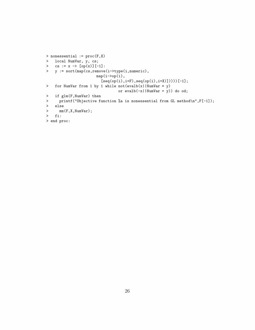
> nonessential := proc(F,X)

> local NumVar, y, cs;

> cs := x -> [op(x)][-1]:

> y := sort(map(cs,remove(i->type(i,numeric),

map(i->op(i),

[seq(op(i),i=F),seq(op(i),i=X)]))))[-1];

> for NumVar from 1 by 1 while not(evalb(x||NumVar = y)

or evalb(-x||NumVar = y)) do od;

> if glm(F,NumVar) then

> printf("Objective function %a is nonessential from GL method\n",F[-1]);

> else

> mm(F,X,NumVar);

> fi:

> end proc:

26

A Computational Approach to Essential and Nonessential Objective Functions in Linear Multicriteria...

Documents

Transcript of A Computational Approach to Essential and Nonessential Objective Functions in Linear Multicriteria...