A comparison of tests for restricted orderings in the three-class case

STATISTICS IN MEDICINEStatist. Med. 2009; 28:1144–1158Published online 20 January 2009 in Wiley InterScience(www.interscience.wiley.com) DOI: 10.1002/sim.3536

A comparison of tests for restricted orderings in thethree-class case

Todd A. Alonzo1,∗,†, Christos T. Nakas2, Constantin T. Yiannoutsos3

and Sherri Bucher4

1Division of Biostatistics, University of Southern California, Keck School of Medicine 440 E. Huntington Dr,Suite 400, Arcadia, CA 91006, U.S.A.

2Laboratory of Biometry, School of Agricultural Sciences, University of Thessaly, Magnesia, Greece3Division of Biostatistics, Indiana University School of Medicine, Indianapolis, IN, U.S.A.

4Department of Pediatrics, Neonatal and Perinatal Medicine Section and IU-Kenya Program, Indiana UniversitySchool of Medicine, Indianapolis, IN, U.S.A.

SUMMARY

A variety of methods for comparing three distributions have been proposed in the literature. These methodsassess the same null hypothesis of equal distributions but differ in the alternative hypothesis they consider.The alternative hypothesis can be that measurements from the three classes are distributed according tounequal distributions or that measurements between the three classes follow a specific monotone ordering,an inverse-U-shaped (umbrella) ordering, or a U-shaped (tree) ordering. This paper compares these testswith respect to power and test size under different simulation scenarios. In addition, the methods areillustrated in two applications generated by different research questions with data from three classessuggesting monotone and umbrella orders. Additionally, proposals for the appropriate application of thesetests are provided. Copyright q 2009 John Wiley & Sons, Ltd.

KEY WORDS: ANOVA; non-parametric tests; ordered alternatives; umbrella alternatives; umbrella ROCvolume; volume under the ROC surface; area under ROC curve; Wilcoxon–Mann–Whitneytest; Kruskal–Walis test

1. INTRODUCTION

A variety of methods have been proposed for comparing treatment effects or, more generally,comparing relative locations (medians) of different populations. This paper focuses on the settingwith three populations because this research was motivated by projects with three populations.However, the methods discussed in this paper are also applicable to settings with more than three

∗Correspondence to: Todd A. Alonzo, Division of Biostatistics, University of Southern California, Keck School ofMedicine 440 E. Huntington Dr, Suite 400, Arcadia, CA 91006, U.S.A.

†E-mail: [email protected]

Received 9 June 2008Copyright q 2009 John Wiley & Sons, Ltd. Accepted 17 December 2008

COMPARISON OF TESTS FOR RESTRICTED ORDERINGS 1145

populations of interest. The methods considered assess the same null hypothesis of no differenceamong the treatment effects but differ in the alternative hypotheses considered. These can be ageneral alternative hypotheses that at least two treatment effects are not equal. Otherwise, thealternative hypothesis might involve specific orderings of the classes such that measurementsamong the three classes follow a monotone ordering (e.g. class 1 < class 2 < class 3). An inverse-U-shaped (umbrella) ordering can also be considered where the hypothesis is that two classeshave smaller measurements, compared with a third class without imposing an ordering betweenthese two classes (e.g. class 1 < class 2 > class 3) or even a U-shaped (tree) ordering wheretwo classes have larger measurements compared with a third class, without imposing an orderingbetween these two classes, (e.g. class 1 > class 2 < class 3). The research question under studydictates the alternative hypothesis to be tested. Monotone orderings are often observed in toxicitystudies where the risk of the occurrence of adverse events is expected to rise with increasing doselevels. On the other hand, umbrella orderings are commonly encountered in efficacy studies, inwhich treatment efficacy is expected to increase with dose only until a maximum efficacy level isreached [1].

Recently, there has been increased focus directed toward evaluation of the accuracy of newbiomarkers being developed for a variety of medical conditions. Receiver operating characteristic(ROC) curves and the summary measure area under the ROC curve (AUC) are the standardapproaches for assessing the ability of biomarkers measured on a continuous scale to accuratelydistinguish between two disease states or classes (e.g. presence vs absence of cancer) [2]. ROCanalysis has been extended to accommodate three disease states. Specifically, ROC surfaces andthe corresponding summary measure volume under the ROC surface (VUS) have been proposedwhen a monotone ordering is of interest (see, e.g. [3]). The umbrella ROC graph and summarymeasure umbrella volume (UV) have been recently proposed when umbrella orderings are ofinterest [4]. Comparisons of UV and VUS have been made [4], but comparisons have not beenmade with parametric and non-parametric approaches developed to compare treatment effectsor population location rather than diagnostic accuracy where particular order restrictions are ofinterest. Therefore, a novel contribution of this paper is to provide a comparison of UV and VUS,methods which assess the ability of continuous biomarkers to accurately distinguish between threedisease states, versus parametric and non-parametric methods that test particular orderings of thelocations of three populations.

Brief descriptions of the different tests are provided in Section 2. Simulation studies to evaluatethe power and size of the tests are summarized in Section 3. In Section 4 the methods are appliedto determine the ability of a biomarker to accurately distinguish between HIV-negative personsand HIV-positive patients with and without HIV-related neurological sequelae. A second exampleconcerns the assessment of the effects of different doses of haloperidol on the motor activityof juvenile rats. We end with a discussion of the findings and include recommendations on theappropriate use of each method.

2. DESCRIPTION OF METHODS

Consider the setting when there are three classes of interest, denoted 1, 2, and 3. Let Yi j , i={1,2,3}, j =1, . . . ,ni be the observed measurements for the three classes 1, 2, and 3, respectively.There are a total of N =n1+n2+n3 measurements. For ease of presentation, it is assumed that

Copyright q 2009 John Wiley & Sons, Ltd. Statist. Med. 2009; 28:1144–1158DOI: 10.1002/sim

1146 T. A. ALONZO ET AL.

there are N unique measurements. Methods to correct for ties in the data are available but are notdiscussed here.

2.1. General alternative hypothesis

The Kruskal–Wallis (KW) test is a distribution-free test that addresses the null hypothesis thatthere is no treatment effect or equivalently no difference in population locations against the generalalternative hypothesis that at least two treatment effects or disease classes are not equal [5]. TheKW test statistic is calculated by first ordering all N observations from smallest to largest. Let ri jdenote the rank of Yi j in the combined data. Let Ri be the sum of the ranks for group i and letRi. be the average rank for group i . Then the KW test statistic is given by

KW= 12

N (N+1)

3∑i=1

(Ri.− N+1

2

)2

(1)

The null hypothesis is rejected if the test statistic (1) is larger than a value chosen to make the type Ierror probability equal to �. Post-hoc procedures would be required to determine which classmeasurements differ.

A parametric approach to test the general alternative hypothesis is the one-way analysis ofvariance (ANOVA). ANOVA compares the means of the groups by calculating the ratio of the withinsum of squares and the between sum of squares. More specifically, the F-statistic is calculated as

F=∑3

i=1 ni Y2i −Y 2

.. /N∑3i=1(ni −1)s2i

where Y.. is the sum of the measurements across all groups, Yi is the average of the measurementsfor group i , and s2i is the sample variance for group i . The p-value is obtained by comparing theF-statistic with an F distribution with 2 and n−2 degrees of freedom.

2.2. Monotone ordering

The Jonckheere–Terpstra (JT) test is a distribution-free test for ordered alternative hypothesis thatthe treatment effects are in a specified monotone ordering, e.g. Y1<Y2<Y3 [6, 7]. To calculatethe JT test statistic, one calculates the three Mann–Whitney counts U12, U13, and U23, whereUi j is the number of measurements with disease class i that are smaller than measurements fordisease class j . The null hypothesis is rejected if the test statistic is larger than a value chosen tomake the type I error probability equal to �. A corresponding summary measure, S1, has recentlybeen proposed for the JT test to measure the accuracy of classifying into the correct classes [8].S1 ranges from 1 for perfect classification in the monotone ordering, say Y1<Y2<Y3, to −1 wherethe classification is in the opposite ordering Y1>Y2>Y3.

Terpstra and Magel proposed a non-parametric test for the same monotone ordered alternativehypothesis as the JT test, but the Terpstra and Magel (TM) test is based on comparing measurementsfrom all three classes at the same time, rather than performing pairwise comparisons as the JT testdoes. More specifically, the TM test is based on the test statistic

T =n1∑i=1

n2∑j=1

n3∑k=1

I (Y1i ,Y2 j ,Y3k) (2)



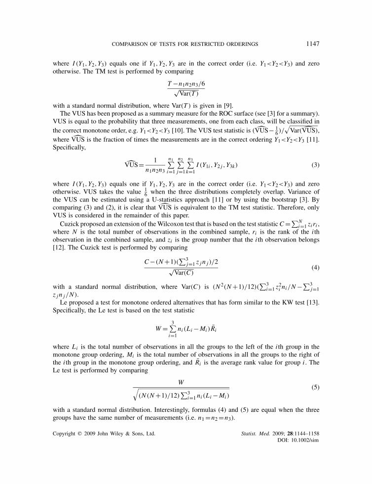
where I (Y1,Y2,Y3) equals one if Y1,Y2,Y3 are in the correct order (i.e. Y1<Y2<Y3) and zerootherwise. The TM test is performed by comparing

T −n1n2n3/6√Var(T )

with a standard normal distribution, where Var(T ) is given in [9].The VUS has been proposed as a summary measure for the ROC surface (see [3] for a summary).

VUS is equal to the probability that three measurements, one from each class, will be classified inthe correct monotone order, e.g. Y1<Y2<Y3 [10]. The VUS test statistic is (VUS− 1

6 )/√Var(VUS),

where VUS is the fraction of times the measurements are in the correct ordering Y1<Y2<Y3 [11].Specifically,

VUS= 1

n1n2n3

n1∑i=1

n2∑j=1

n3∑k=1

I (Y1i ,Y2 j ,Y3k) (3)

where I (Y1,Y2,Y3) equals one if Y1,Y2,Y3 are in the correct order (i.e. Y1<Y2<Y3) and zerootherwise. VUS takes the value 1

6 when the three distributions completely overlap. Variance ofthe VUS can be estimated using a U-statistics approach [11] or by using the bootstrap [3]. Bycomparing (3) and (2), it is clear that VUS is equivalent to the TM test statistic. Therefore, onlyVUS is considered in the remainder of this paper.

Cuzick proposed an extension of theWilcoxon test that is based on the test statisticC=∑Ni=1 ziri ,

where N is the total number of observations in the combined sample, ri is the rank of the i thobservation in the combined sample, and zi is the group number that the i th observation belongs[12]. The Cuzick test is performed by comparing

C−(N+1)(∑3

j=1 z j n j )/2√Var(C)

(4)

with a standard normal distribution, where Var(C) is (N 2(N+1)/12)(∑3

i=1 z2i ni/N−∑3

j=1z j n j/N ).

Le proposed a test for monotone ordered alternatives that has form similar to the KW test [13].Specifically, the Le test is based on the test statistic

W =3∑

i=1ni (Li −Mi )Ri

where Li is the total number of observations in all the groups to the left of the i th group in themonotone group ordering, Mi is the total number of observations in all the groups to the right ofthe i th group in the monotone group ordering, and Ri is the average rank value for group i . TheLe test is performed by comparing

W√(N (N+1)/12)

∑3i=1 ni (Li −Mi )

(5)

with a standard normal distribution. Interestingly, formulas (4) and (5) are equal when the threegroups have the same number of measurements (i.e. n1=n2=n3).



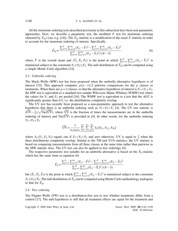
All the monotone ordering tests described previously in this subsection have been non-parametricapproaches. Next, we describe a parametric test, the modified F test for monotone ordering(denoted by Fm) (see, e.g. [14]). The Fm-statistic is a modification of the usual F-statistic in orderto account for the monotone ordering of interest. Specifically

Fm=∑3

i=1∑ni

j=1(Yi j − Y )2−∑3i=1

∑nij=1(Yi j − Yi )2∑3

i=1∑ni

j=1(Yi j − Yi )2/(N−3)(6)

where Y is the overall mean and (Y1, Y2, Y3) is the point at which∑3

i=1∑ni

j=1(Yi j − Yi )2 is

minimized subject to the constraint Y1�Y2�Y3. The null distribution of Fm can be computed usinga simple Monte Carlo algorithm [14].2.3. Umbrella ordering

The Mack–Wolfe (MW) test has been proposed when the umbrella alternative hypothesis is ofinterest [15]. This approach computes p(p−1)/2 pairwise comparisons for the p classes ortreatments. When there are p=3 classes, so that the alternative hypothesis of interest is Y1<Y2>Y3,the MW test is equivalent to a standard two-sample Wilcoxon–Mann–Whitney (WMW) test wherethe values for Y1 and Y3 are pooled [16]. The WMW test is equivalent to a test that the AUC issignificantly greater than 0.5, i.e. the distributions completely overlap.

The UV test has recently been proposed as a non-parametric approach to test the alternativehypothesis that there is an umbrella ordering such as Y1<Y2>Y3 [4]. The UV test statistic is(UV− 1

3 )/√Var(UV), where UV is the fraction of times the measurements are in the umbrella

ordering of interest and Var(UV) is provided in [4]. In other words, for the umbrella orderingY1<Y2>Y3

UV= 1

n1n2n3

n1∑i=1

n2∑j=1

n3∑k=1

IU [Y1i ,Y2 j ,Y3k]

where IU (Y1,Y2,Y3) equals one if Y1<Y2>Y3 and zero otherwise. UV is equal to 13 when the

three distributions completely overlap. Similar to the TM and VUS statistics, the UV statistic isbased on comparing measurements from all three classes at the same time rather than pairwise asthe MW statistic does. The UV test can also be applied to tree orderings [4].

The respective parametric test suitable for an umbrella alternative is based on the Fu-statisticwhich has the same form as equation (6)

Fu=∑3

i=1∑ni

j=1(Yi j − Y )2−∑3i=1

∑nij=1(Yi j − Yi )2∑3

i=1∑ni

j=1(Yi j − Yi )2/(N−3)

but (Y1, Y2, Y3) is the point at which∑3

i=1∑ni

j=1(Yi j − Yi )2 is minimized subject to the constraint

Y1�Y2�Y3. The null distribution of Fu can be computed using Monte Carlo methodology analogousto that for Fm.

2.4. Tree ordering

The Fligner–Wolfe (FW) test is a distribution-free test to test whether treatments differ from acontrol [17]. The null hypothesis is still that all treatment effects are equal for the treatment and



Table I. List of methods for assessing the ability of continuous measurements to correctly classify threeclasses in a particular order. All approaches consider the null hypothesis that measurements from the three

classes follow the same distribution but different alternative hypotheses.

Test Approach Alternative Notes

Kruskal–Wallis (KW) Non-para GeneralANOVA Para GeneralJonckheere–Terpstra (JT) Non-para MonotoneTerpstra–Magel (TM) Non-para Monotone Essentially equivalent to VUSVUS Non-para Monotone Essentially equivalent to TMCuzick Non-para Monotone Equivalent to Le for equal class sizesLe Non-para Monotone Equivalent to Cuzick for equal class sizesFm Para MonotoneMack–Wolfe (MW) Non-para Umbrella Equivalent to WMW for 3 classesUmbrella volume (UV) Non-para UmbrellaFu Para UmbrellaFligner–Wolfe (FW) Non-para Tree

control groups while the alternative hypothesis is that the effect for at least one treatment groupis different from the control group. The FW test statistic is calculated by first ordering all Nobservations from smallest to largest. Then the FW test statistic is the sum of the joint ranks forthe non-control treatments. This test statistic is equivalent to the two-sample WMW test statisticcomputed for the control observations and the combined treatment observations.

2.5. Summary of methods

All methods considered in this section assess the null hypothesis that measurements from thethree classes follow the same distribution, i.e. Y1=Y2=Y3. However, there are differences in thealternative hypotheses considered and the test statistics used (Table I). Some of the approaches arenon-parametric while others make parametric assumptions. The KW and ANOVA tests considerthe general alternative hypothesis that Yi �=Y j for some (i, j)∈{1,2,3} and i �= j . Conversely,MW, UV, and Fu test the alternative hypothesis that the classes follow an umbrella ordering, e.g.Y1<Y2>Y3. In this case, the MW test is equivalent to the WMW test where Y1 and Y3 are pooled.The VUS, TM, Cuzick, Le, Fm, and JT tests consider the alternative hypothesis that the classesfollow a monotone ordering, e.g. Y1<Y2<Y3. The Cuzick and Le tests are equivalent when thethree classes have the same number of measurements. Finally, the FW test considers the alternativehypothesis of a tree ordering.

3. SIMULATION STUDIES

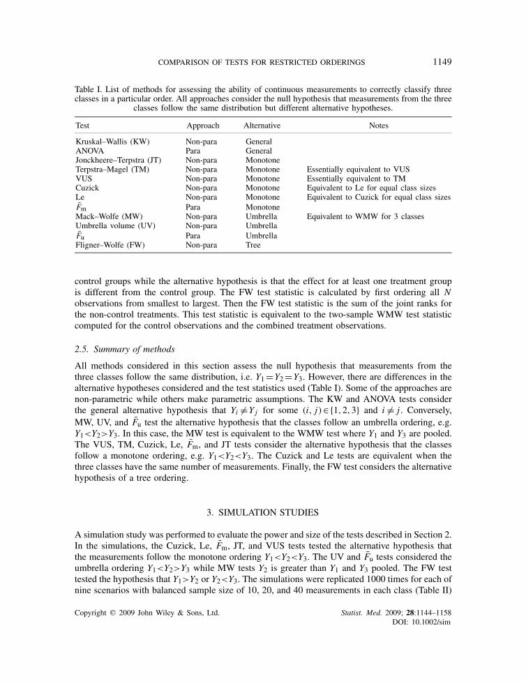
A simulation study was performed to evaluate the power and size of the tests described in Section 2.In the simulations, the Cuzick, Le, Fm, JT, and VUS tests tested the alternative hypothesis thatthe measurements follow the monotone ordering Y1<Y2<Y3. The UV and Fu tests considered theumbrella ordering Y1<Y2>Y3 while MW tests Y2 is greater than Y1 and Y3 pooled. The FW testtested the hypothesis that Y1>Y2 or Y2<Y3. The simulations were replicated 1000 times for each ofnine scenarios with balanced sample size of 10, 20, and 40 measurements in each class (Table II)



TableII.Results

ofsimulations

tostudysize

(Scenario1)

andpower

(Scenarios

2–9)

forn i

numberof

measurements

ineach

class.Scenariosarepresentedforthenullhypothesis(Scenario1)

aswellas

formonotoneorderings(Scenarios

2–3),

umbrella

orderings(Scenarios

4–7),andtree

orderings(Scenarios

8–9).

Scenario—

Y1,Y

2,Y

3n i

KW

ANOVA

JTVUS

Cuzick

Le

Fm

MW

UV

Fu

FW

1−N

(0,1

),N

(0,1

),N

(0,1

)10

0.05

30.05

80.06

70.04

80.06

60.06

60.05

80.07

30.05

20.05

40.05

1(Y

1=Y

2=Y

3)

200.04

20.04

20.03

70.02

50.03

60.03

60.03

70.07

70.05

10.05

10.04

640

0.07

00.05

80.06

50.05

00.06

30.06

30.05

50.05

00.04

80.04

90.06

22−N

(0,1

),N

(0.5

,1),N

(1,1

)10

0.40

90.44

70.66

00.53

00.67

20.67

20.63

10.06

20.03

40.37

70.04

3(Y

1<Y2<Y3)

200.75

10.77

10.89

40.80

60.89

60.89

60.88

50.04

50.01

90.68

50.05

140

0.98

30.98

30.99

90.98

60.99

90.99

90.99

70.04

60.01

20.94

70.03

93−t

3,t3+0

.5,t3+1

100.28

00.23

70.52

40.43

90.52

90.52

90.40

30.07

00.02

70.21

90.04

4(Y

1<Y2<Y3)

200.58

10.45

30.79

30.69

20.79

00.79

00.63

50.05

20.02

90.38

60.04

640

0.88

50.67

40.96

90.91

70.96

90.96

90.80

20.07

10.02

40.60

40.05

54−N

(0,1

),N

(1,1

),N

(0,1

)10

0.53

40.57

20.02

50.01

00.03

40.03

40.23

30.83

40.76

30.69

80.00

0(Y

1<Y2>Y3)

200.89

00.90

20.03

40.01

00.04

80.04

80.45

80.97

70.96

40.94

90.00

040

0.99

60.99

60.03

30.00

00.03

40.03

40.72

51.00

01.00

00.99

80.00

05−t

3,t3+1

,t3

100.35

60.27

70.03

80.01

70.04

10.04

10.14

00.68

30.62

00.39

60.00

0(Y

1<Y2>Y3)

200.67

10.48

00.04

40.01

10.04

40.04

40.19

60.87

00.84

80.61

20.00

040

0.94

10.77

30.00

30.00

30.03

20.03

20.37

90.98

90.98

60.85

40.00

06−N

(0,0

.25)

,N(1

,9),N

(0,4

)10

0.15

20.17

90.03

60.00

30.04

40.04

40.05

00.28

60.40

30.25

00.01

2(Y

1<Y2>Y3)

200.27

10.30

80.03

40.00

20.04

50.04

50.06

20.41

70.65

70.39

40.00

240

0.49

60.57

80.05

70.00

00.06

30.06

30.15

40.62

10.89

40.67

20.00

07−U

[0.2,1.2],

N(1

.3,1

),�2 1

100.30

00.24

80.02

20.01

90.02

30.02

30.13

60.55

50.56

70.33

10.00

0(Y

1<Y2>Y3)

200.53

80.35

00.03

60.01

80.03

00.03

00.31

60.73

00.76

80.45

00.00

040

0.88

20.71

00.04

00.03

40.02

30.02

30.67

90.95

40.96

60.83

10.00

08−N

(1,1

),N

(0,1

),N

(1,1

)10

0.53

10.57

50.02

30.00

70.02

80.02

80.22

50.00

00.00

00.00

00.77

5(Y

1>Y2<Y3)

200.89

10.91

00.02

40.00

40.02

80.02

80.42

70.00

00.00

00.00

00.97

540

0.99

50.99

80.03

30.00

00.03

80.03

80.73

30.00

00.00

00.00

00.99

89−t

3+1

,t3,t3+1

100.35

90.30

80.04

50.02

80.04

90.04

90.14

50.00

00.00

01.00

00.60

1(Y

1>Y2<Y3)

200.71

00.53

60.02

50.00

50.02

60.02

60.19

20.00

00.00

00.00

20.88

740

0.94

30.77

90.04

70.00

50.04

80.04

80.36

60.00

00.00

00.00

00.99

3



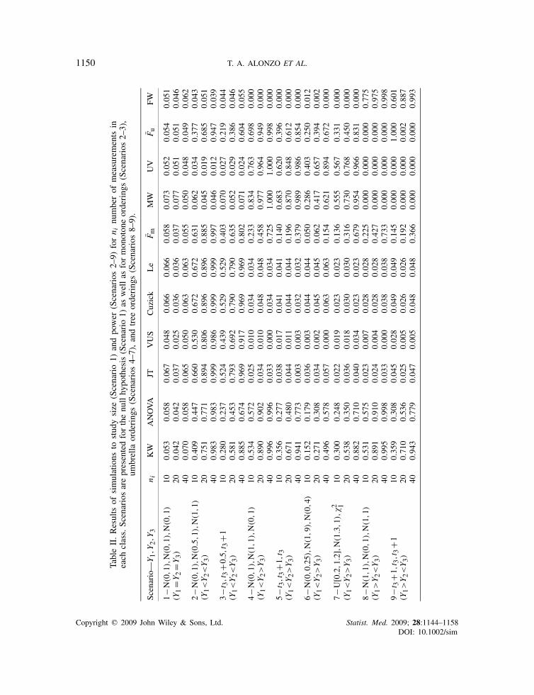
and unbalanced sample sizes (n1,n2,n3) of (10,10,20), (10,10,40), and (10,20,40) (Table III). Alltests were one-sided with 0.05 type I error.

In Scenario 1 sampling was performed under the null hypothesis where Y1,Y2, and Y3 weresimulated from a standard normal distribution. The simulated size for some of the tests deviatedsubstantially from the nominal level for small sample sizes. However, the simulated size is generallycloser to the nominal level for n1=n2=n3=40 and are much closer to the nominal level forn1=n2=n3=80 (results not provided). The Le test has unacceptably large size for unbalanced datascenarios and thus, the Le test is not recommended when there is unequal number of measurementsin the classes. Since the Le test clearly is not appropriate for unbalanced data settings and it isequivalent to the Cuzick test for balanced data in the three-class case, the performance of the Letest is not discussed for the other simulated scenarios.

In Scenario 2 a monotone ordering was considered for the class measurements with Y1∼N(0,1),Y2∼N(0.5,1), and Y3∼N(1,1). The Cuzick test was the most powerful for all the samplesizes considered, but power for the JT test was only slightly smaller. The next powerful tests werethe Fm test and the VUS test. As expected, all the tests that test a monotone ordering had largerpower than the general alternative tests (KW and ANOVA). As desired, the MW and UV tests,which test umbrella orderings, had low power to detect the monotone ordering. Conversely, it isundesired that the Fu test, which tests umbrella orderings, had relatively high power to detect themonotone ordering. Similar results are observed for Scenario 3 where Y1∼ t3,Y2∼ t3+0.5, andY3∼ t3+1. It is not surprising that the power is larger for the non-parametric KW test than theparametric ANOVA test in Scenario 3 and the reverse is observed in Scenario 2 where the dataare simulated from Normal distributions.

Scenario 4 simulates an umbrella alternative where Y1∼N(0,1),Y2∼N(1,1), and Y3∼N(0,1)while in Scenario 5 Y1∼ t3,Y2∼ t3+1, and Y3∼ t3. In both of these scenarios the MW test appearsto be the most powerful followed by UV and Fu, which are all more powerful than the generalalternative approaches. The large power for MW likely results from the large effective sample sizedue to pooling of measurements for Y1 and Y3 which follow identical distributions. The monotoneordering approaches are not sensitive to the umbrella alternative in this scenario, except for Fm.

In Scenario 6, simulated distributions have the same locations as in Scenario 4 but they havedifferent scale parameters with Y1∼N(0,0.25), Y2∼N(1,9), and Y3∼N(0,4). Here the UV testis the most powerful for all sample sizes considered. This finding is repeated in Scenario 7 wheremeasurements come from distributions with different shapes, i.e. Y1∼Unif[0.2,1.2], Y2∼N(1.3,1),and Y3∼�21. Again the UV test is the most powerful with MW having close, but smaller, powerfor balanced sample sizes. The difference in power is greater for unbalanced data.

Scenario 8 considers Y1∼N(1,1),Y2∼N(0,1), and Y3∼N(1,1) so that the data follow thereverse umbrella ordering or tree ordering Y1>Y2<Y3. In this scenario the FW test had the highestpower but the KW and ANOVA tests had reasonable power for the larger sample sizes considered.The difference in power between the FW and the ANOVA test was larger in Scenario 9 wherethe measurements were not generated using a Normal distribution (Y1∼ t3+1,Y2∼ t3,Y3∼ t3+1).The JT, Cuzick, Le, and F tests appear to be very sensitive even for scenarios where the alternativeis not a monotone ordering. However, this is not true for the VUS test, which is only sensitive indetecting monotone orderings.

In summary, when the measurements follow a particular ordering, tests that test that particularordering have higher power than the general alternative approaches (KW and ANOVA tests). JTand Cuzick, which is equivalent to the Le test for balanced data, have the greatest power formonotone orderings. When Y1 and Y3 come from the same distribution, the MW test has the



TableIII.Results

ofsimulations

tostudysize

(Scenario1)

andpower

(Scenarios

2–9)

forn�

numberof

measurements

inthe

classes,

where

n�equalto

1,2,

and3correspondsto

(n1,n

2,n

3)equalto

(10,10,20),(10,10,40),and(10,20,40),respectiv

ely.

Scenariosarepresentedforthenull

hypothesis

(Scenario1)

aswellas

formonotoneorderings(Scenarios

2–3),um

brella

orderings(Scenarios

4–7),andtree

orderings(Scenarios

8–9).

Scenario—

Y1,Y

2,Y

3n�

KW

ANOVA

JTVUS

Cuzick

Le

Fm

MW

UV

Fu

FW

1–N

(0,1

),N

(0,1

),N

(0,1

)1

0.04

40.04

20.04

50.03

80.04

70.35

50.04

10.06

70.05

40.04

50.04

5(Y

1=Y

2=Y

3)

20.05

20.05

10.05

60.04

40.06

30.83

10.05

20.06

30.06

30.05

40.05

73

0.04

50.04

50.04

30.03

90.04

70.56

20.04

30.07

50.06

20.04

20.04

32–

N(0

,1),N

(0.5

,1),N

(1,1

)1

0.59

10.62

60.79

80.63

70.81

30.98

10.78

90.03

00.03

30.51

60.10

3(Y

1<Y2<Y3)

20.68

30.70

70.86

30.69

50.88

41.00

00.86

60.00

80.03

20.63

10.18

53

0.71

60.75

90.88

40.74

60.89

60.99

60.87

90.00

80.02

00.58

00.27

13–

t 3,t3+0

.5,t3+1

10.42

70.32

30.65

50.52

80.65

70.95

30.50

60.03

20.03

80.27

70.09

2(Y

1<Y2<Y3)

20.48

00.35

70.70

70.54

00.72

80.99

90.54

10.02

00.03

10.30

90.14

03

0.54

30.37

70.74

30.60

10.75

50.98

80.55

90.00

30.01

60.27

00.23

74–

N(0

,1),N

(1,1

),N

(0,1

)1

0.60

80.65

60.00

50.00

40.01

20.06

70.16

00.87

40.85

40.75

20.00

0(Y

1<Y2>Y3)

20.64

70.70

40.00

50.00

80.00

80.16

00.10

30.88

30.88

60.78

90.00

03

0.90

90.92

30.00

00.00

50.00

10.00

60.15

20.99

00.96

30.96

70.00

05–

t 3,t3+1

,t3

10.42

60.36

10.01

30.01

50.01

40.10

70.10

40.73

20.72

50.45

20.00

0(Y

1<Y2>Y3)

20.44

80.34

20.00

00.00

90.00

30.26

60.04

10.70

00.73

40.43

00.00

03

0.72

40.55

60.00

00.01

20.00

20.02

00.11

30.88

50.82

70.65

40.00

06–

N(0

,0.25)

,N(1

,9),N

(0,4

)1

0.14

50.19

40.01

60.00

10.02

30.19

60.01

70.31

10.55

30.27

10.01

4(Y

1<Y2>Y3)

20.14

40.22

10.00

40.00

10.00

70.56

50.00

20.29

50.61

70.28

10.00

83

0.21

80.26

90.00

40.00

00.00

30.16

90.00

20.40

50.76

10.36

30.00

27–

U[0.

2,1.2],

N(1

.3,1

),�2 1

10.28

20.15

00.00

20.02

30.00

20.06

60.03

00.51

70.69

10.20

30.00

1(Y

1<Y2>Y3)

20.29

90.09

90.00

00.02

20.00

10.25

00.00

70.54

90.80

50.14

60.00

13

0.43

20.14

90.00

00.02

50.00

00.03

60.01

00.73

70.91

10.21

50.00

08–

N(1

,1),N

(0,1

),N

(1,1

)1

0.59

60.63

00.11

90.00

40.08

50.72

30.32

40.00

00.00

00.00

00.83

7(Y

1>Y2<Y3)

20.68

40.71

40.33

40.01

40.20

00.99

80.45

80.00

00.00

00.00

50.86

53

0.91

00.92

30.56

70.00

60.33

50.99

80.77

10.00

00.00

00.00

30.97

39–

t 3+1

,t3,t3+1

10.43

30.32

90.12

50.01

60.09

80.62

80.17

80.00

00.00

10.00

20.67

9(Y

1>Y2<Y3)

20.47

90.35

80.23

20.01

40.12

60.99

50.22

20.00

00.00

00.00

70.73

43

0.71

90.56

40.44

60.01

30.27

80.98

60.43

90.00

00.00

00.00

40.88

7



greatest power for the umbrella ordering; otherwise, the UV test has the greatest power. The FWtest had the greatest power for tree orderings. Recommendations on the appropriate use of eachmethod are provided in Section 5.

4. DATA ANALYSIS

In this section, the approaches are applied to a study of a metabolite to accurately distinguishbetween HIV-negative persons and HIV-positive patients with and without HIV-related neurologicalsequelae and to a study to assess the effects of different doses of haloperidol on the play behaviorof juvenile rats.

4.1. Analysis of AIDS neurological sequelae

The Human immunodeficiency virus (HIV) invades the central nervous system causing structuraland metabolic changes in the brain. Patients with AIDS often show varying degrees of cognitive,motor and behavioral impairment, including dementia (AIDS dementia complex—ADC [18]).A number of studies have shown that an imaging technique called proton magnetic resonancespectroscopy (1H-MRS) provides a reliable in vivo, non-invasive method for the assessment ofHIV-associated brain injury (for example, see [19]). The area under each spectral peak is associatedwith the concentration of a metabolite that reflects activity in a specific cell type in response tosignals in its microenvironment. A frequently measured metabolite is the ratio of myoinositol (MI)over creatine (Cr). MI is a marker of glial cells that are involved in providing nutrition, structuralsupport of neuronal cells, and removing pathogens and damaged neurons from the brain. As amarker of glial cell proliferation, MI is an index of ongoing inflammation and injury to the brain.Creatine, on the other hand, is a marker of cellular metabolism that is assumed to be constant inmost cases, including during many pathological conditions. Thus, dividing by Cr in the ratio is usedas an internal standard to reduce the variability of the MI signal by accounting for difference amongimaging machine technologies, brain structure localization and other considerations particular toeach specific imaging procedure.

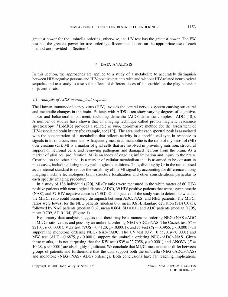
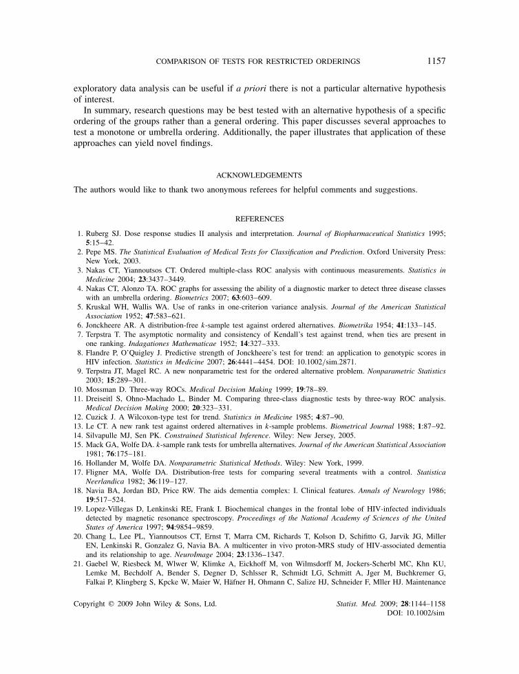
In a study of 136 individuals [20], MI/Cr ratios were measured in the white matter of 60 HIV-positive patients with neurological disease (ADC), 39 HIV-positive patients that were asymptomatic(NAS), and 37 HIV-negative controls (NEG). One objective of the study was to determine whetherthe MI/Cr ratio could accurately distinguish between ADC, NAS, and NEG patients. The MI/Crratios were lowest for the NEG patients (median 0.6, mean 0.614, standard deviation (SD) 0.073),followed by NAS patients (median 0.67, mean 0.664, SD 0.03), and ADC patients (median 0.705,mean 0.709, SD 0.134) (Figure 1).

Exploratory data analysis suggests that there may be a monotone ordering NEG<NAS<ADCin MI/Cr ratio values and possibly an umbrella ordering NEG<ADC>NAS. The Cuzick test (C=22103, p<0.0001), VUS test (VUS=0.4120, p<0.0001), and JT test (S1=0.3955, p<0.0001) allsupport the monotone ordering NEG<NAS<ADC. The UV test (UV=0.5580, p<0.0001) andMW test (AUC=0.6875, p<0.0001) support the umbrella ordering NEG<ADC>NAS. Giventhese results, it is not surprising that the KW test (KW=22.7058, p<0.0001) and ANOVA (F=10.28, p<0.0001) are also highly significant. We conclude that MI/Cr measurements differ betweengroups of patients and furthermore that the data support both the umbrella (NEG<ADC>NAS)and monotone (NEG<NAS<ADC) orderings. Both conclusions have far reaching implications



0.2

0.4

0.6

0.8

1

1.2

MI/C

r ra

tio

NEG NAS ADC

Figure 1. Box plots of MI/Cr ratios in the white matter of HIV-negative controls (NEG), HIV-positivepatients that are asymptomatic (NAS), and HIV-positive patients with neurological disease (ADC).

for our understanding of HIV-related neurological disease progression. The monotone orderingimplies that, despite not having overt clinical symptoms, NAS subjects do exhibit perturbationsthat are measurable through proton MRS. The combination of the results of both the monotonetrend and umbrella ordering strengthens the impression that brain inflammation, which has beenwidely reported as being the hallmark of HIV infection and is thus inflammation is ubiquitous in allstages of neurological progression (e.g. [19]), persists and increases further among neurologicallyadvanced (ADC) patients.

4.2. Analysis of rat play behavior

Haloperidol, a non-selective neuroleptic medication widely used in the past to treat schizophrenia[21], binds to a wide variety of neurotransmitter receptors, but is thought to exert its primaryneurochemical and behavioral effects via antagonism of dopaminergic systems in the brain. Thedose-dependent effects of haloperidol have been extensively studied; at higher doses, haloperidolhas sedative properties, whereas at lower doses, haloperidol has sometimes been associated withstimulatory effects [22–24]. The rodent model has been frequently used to investigate the neuro-chemical impact of haloperidol on the central nervous system, as well as the drug’s effect onappetitive and movement behaviors thought to be significantly underpinned by central dopamin-ergic systems (e.g. the basal ganglia) [25, 26]. Juvenile rats engage in rough-and-tumble play (RTP)behavior during a specific period of normal development, from around days 20–40 [27]. BecauseRTP behavior involves vigorous motoric behaviors including chasing, wrestling, and pinning [28],it is reasonable to assume that brain areas associated with movement (e.g. cerebellum and basalganglia), and the neurochemical systems that innervate these structures, might underlie rat playactivities. Further, perturbation of these systems via either surgical or neurochemical means, andobservation of the resulting effects, can provide information regarding the relative importance ofthese central nervous systems on behavior [29–35]. In order to investigate the manner by whichdopaminergic systems might impact juvenile RTP play behavior, various doses of haloperidol were



0

50

100

150

200

250

# of

RT

P b

ehav

iors

Vehicle Low dose High dose

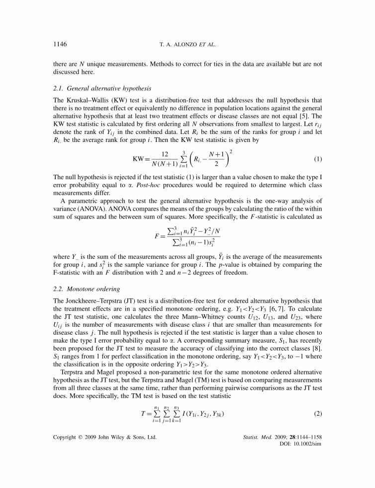
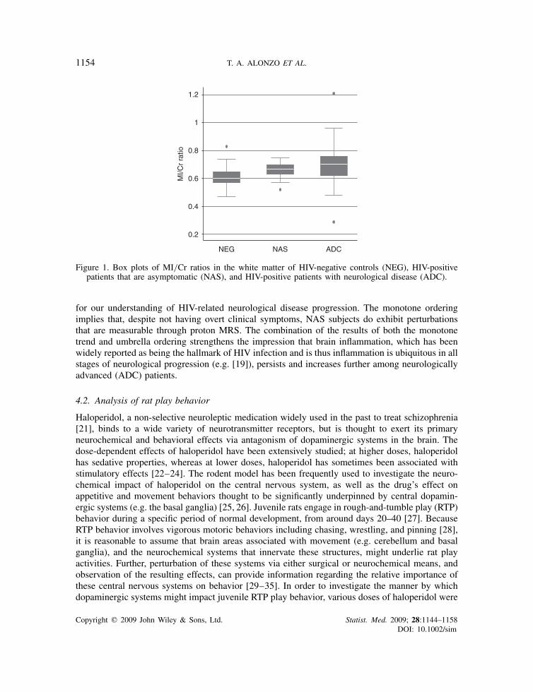
Figure 2. Box plots of number of RTP behaviors observed in pairs of rats that received vehicle, low dosehaloperidol, and high dose haloperidol.

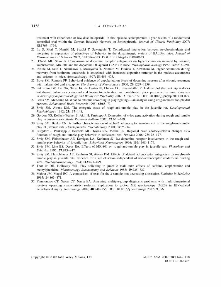
administered to juvenile rats. This analysis compares the results of tartaric acid vehicle, low dosehaloperidol (0.025mg/kg and 0.05mg/kg), and high dose haloperidol (0.1mg/kg and 0.2mg/kg).Pairs of juvenile rats were videotaped, and their play interactions later analyzed by one of theauthors (S.B).

Figure 2 summarizes the aggregate number of RTP behaviors (e.g. wrestle, chase, pin) for the19 rats administered vehicle (median 105, mean 118.05, SD 48.5), 39 rats injected with low dosehaloperidol (median 119, mean 117.9, SD 38.9), and 39 rats injected with high dose haloperidol(median 76, mean 83.2, SD 44.4). The UV test yields a significant umbrella ordering Vehicle <

Low dose > High dose (UV=0.4481, p=0.0421), as does the Fu test (Fu=15.14, p<0.0001).The MW test also suggests that rats that received low dose haloperidol exhibited more RTPbehaviors than rats that received vehicle or high dose haloperidol (AUC=0.6647, p=0.0009).Therefore, these data support the hypothesis that at higher doses, haloperidol exerts sedativeproperties on juvenile rat RTP behavior, whereas at lower doses, haloperidol exerts stimulatoryeffects. Interestingly, the Cuzick test (C=10387, p=0.0002), JT test (S1=0.3477, p=0.0002)and VUS test (VUS=0.315, p=0.0024) also suggest a significant monotone ordering High dose <

Vehicle < Low dose, illustrating the sedative effect of high doses of haloperidol on this particulartype of vigorous motoric activity.

5. DISCUSSION

In this paper we compare and contrast approaches for testing hypotheses regarding treatmenteffects distributions, or equivalently, the accuracy of biomarkers. The specific focus is on settingsand research questions where there are three classes or populations and the measurements ofinterest are made on a continuous scale. We agree with Terpstra and Magel [9] that a monotoneor umbrella ordered test should have the following properties: (1) the size of the test should beapproximately equal to the nominal size, (2) the test should have higher power than a general



alternative test when the alternative hypothesis being tested is true, (3) the test should have lowpower for any alternative hypothesis that is not consistent with the true alternative. Simulationssuggest that the Cuzick and JT tests, both designed to detect monotone orderings, have high powerto detect a monotone ordering but the VUS is less sensitive to situations that are not consistent witha monotone ordering, especially with unbalanced data. These results are consistent with previousfindings [9, 36]. Thus, the VUS test may be the preferred method of analysis in actual researchpractice.

Our simulation results also suggest that the UV test has higher power than the MW testfor umbrella orderings except when measurements for two of the classes come from the samedistribution, which is not common in real-world applications. The UV test also has the appealingproperty that it has lower power than MW for alternative hypotheses not consistent with anumbrella ordering. The ANOVA and KW tests yielded lower power than tests of restricted ordersin all of the research scenarios considered, and hence should not serve as the initial test, unlessrestricted orderings are not of interest. This finding for KW is consistent with previously publishedresults [16].

There are interesting relationships between monotone, umbrella, and tree orderings. First, a treealternative hypothesis can be converted to an umbrella alternative hypothesis by changing the signsof the measurement values. For example, the tree ordering Y1>Y2<Y3 is equivalent to the umbrellaordering −Y1<−Y2>−Y3. Second, an alternative hypothesis regarding a monotone ordering canbe converted to a less stringent hypothesis of a tree or umbrella ordering by changing the order ofthe groups. For example, an alternative hypothesis of the monotone ordering Y1<Y2<Y3 can beconverted to a less stringent hypothesis of the tree ordering Y2>Y1<Y3 and the umbrella orderingY1<Y3>Y2. In real research data, however, there often is inherent ordering of the groups so that itis not possible to change the order of the groups, as is the case in the data analyzed in Section 4.Furthermore, it is in settings with an inherent ordering that the contrast between umbrella andmonotone orderings is especially interesting because the orderings yield different explanations.This paper compares methods that can detect and distinguish between the two orderings.

Ideally, the research question will drive the alternative hypothesis to be tested. This will dictatethe statistical test to be performed and, thus, will limit the need to worry about inflated type I errordue to multiple testing. In Section 4.2, there was particular interest in testing whether juvenilerats that received low dose haloperidol exhibited greater RTP activity as compared with rats thatreceived vehicle or high dose haloperidol. In other words, an umbrella ordering was of interest. Inthe neurological impact of HIV example (Section 4.1), both a monotone and an umbrella orderingwere of interest. The monotone ordering is plausible, since neurological disease progression should,theoretically, be associated with higher brain inflammation. Thus, higher MI/Cr levels wouldbe expected among more severely affected HIV-infected patients [20, 37]. On the other hand,an umbrella ordering is also plausible. NAS subjects would be expected to have higher MI/Crlevels than HIV-negative controls as brain inflammation has been reported in all stages of HIVinfection regardless of whether or not patients are symptomatic for neurological deterioration[19, 37]. Results of these analyses have far reaching implications for our understanding of HIV-related neurological disease progression. The result that inflammation continues in the ADC stageis interesting (umbrella ordering) because lack of that would imply a burn-out disease situation.The result that inflammation is present among subjects without overt clinical symptoms (monotoneordering) implies two things: first, interventions in the brain are needed for those who do notexhibit clinical symptoms; second, MRS is a non-invasive early warning system that can identifythose otherwise clinically asymptomatic patients most in need of this intervention. In all cases,



exploratory data analysis can be useful if a priori there is not a particular alternative hypothesisof interest.

In summary, research questions may be best tested with an alternative hypothesis of a specificordering of the groups rather than a general ordering. This paper discusses several approaches totest a monotone or umbrella ordering. Additionally, the paper illustrates that application of theseapproaches can yield novel findings.

ACKNOWLEDGEMENTS

The authors would like to thank two anonymous referees for helpful comments and suggestions.

REFERENCES

1. Ruberg SJ. Dose response studies II analysis and interpretation. Journal of Biopharmaceutical Statistics 1995;5:15–42.

2. Pepe MS. The Statistical Evaluation of Medical Tests for Classification and Prediction. Oxford University Press:New York, 2003.

3. Nakas CT, Yiannoutsos CT. Ordered multiple-class ROC analysis with continuous measurements. Statistics inMedicine 2004; 23:3437–3449.

4. Nakas CT, Alonzo TA. ROC graphs for assessing the ability of a diagnostic marker to detect three disease classeswith an umbrella ordering. Biometrics 2007; 63:603–609.

5. Kruskal WH, Wallis WA. Use of ranks in one-criterion variance analysis. Journal of the American StatisticalAssociation 1952; 47:583–621.

6. Jonckheere AR. A distribution-free k-sample test against ordered alternatives. Biometrika 1954; 41:133–145.7. Terpstra T. The asymptotic normality and consistency of Kendall’s test against trend, when ties are present in

one ranking. Indagationes Mathematicae 1952; 14:327–333.8. Flandre P, O’Quigley J. Predictive strength of Jonckheere’s test for trend: an application to genotypic scores in

HIV infection. Statistics in Medicine 2007; 26:4441–4454. DOI: 10.1002/sim.2871.9. Terpstra JT, Magel RC. A new nonparametric test for the ordered alternative problem. Nonparametric Statistics

2003; 15:289–301.10. Mossman D. Three-way ROCs. Medical Decision Making 1999; 19:78–89.11. Dreiseitl S, Ohno-Machado L, Binder M. Comparing three-class diagnostic tests by three-way ROC analysis.

Medical Decision Making 2000; 20:323–331.12. Cuzick J. A Wilcoxon-type test for trend. Statistics in Medicine 1985; 4:87–90.13. Le CT. A new rank test against ordered alternatives in k-sample problems. Biometrical Journal 1988; 1:87–92.14. Silvapulle MJ, Sen PK. Constrained Statistical Inference. Wiley: New Jersey, 2005.15. Mack GA, Wolfe DA. k-sample rank tests for umbrella alternatives. Journal of the American Statistical Association

1981; 76:175–181.16. Hollander M, Wolfe DA. Nonparametric Statistical Methods. Wiley: New York, 1999.17. Fligner MA, Wolfe DA. Distribution-free tests for comparing several treatments with a control. Statistica

Neerlandica 1982; 36:119–127.18. Navia BA, Jordan BD, Price RW. The aids dementia complex: I. Clinical features. Annals of Neurology 1986;

19:517–524.19. Lopez-Villegas D, Lenkinski RE, Frank I. Biochemical changes in the frontal lobe of HIV-infected individuals

detected by magnetic resonance spectroscopy. Proceedings of the National Academy of Sciences of the UnitedStates of America 1997; 94:9854–9859.

20. Chang L, Lee PL, Yiannoutsos CT, Ernst T, Marra CM, Richards T, Kolson D, Schifitto G, Jarvik JG, MillerEN, Lenkinski R, Gonzalez G, Navia BA. A multicenter in vivo proton-MRS study of HIV-associated dementiaand its relationship to age. NeuroImage 2004; 23:1336–1347.

21. Gaebel W, Riesbeck M, Wlwer W, Klimke A, Eickhoff M, von Wilmsdorff M, Jockers-Scherbl MC, Khn KU,Lemke M, Bechdolf A, Bender S, Degner D, Schlsser R, Schmidt LG, Schmitt A, Jger M, Buchkremer G,Falkai P, Klingberg S, Kpcke W, Maier W, Hafner H, Ohmann C, Salize HJ, Schneider F, Mller HJ. Maintenance



treatment with risperidone or low-dose haloperidol in first-episode schizophrenia: 1-year results of a randomizedcontrolled trial within the German Research Network on Schizophrenia. Journal of Clinical Psychiatry 2007;68:1763–1774.

22. Ito S, Mori T, Namiki M, Suzuki T, Sawaguchi T. Complicated interaction between psychostimulants andmorphine in expression of phenotype of behavior in the dopaminergic system of BALB/c mice. Journal ofPharmacological Sciences 2007; 105:326–333. DOI: 10.1254/jphs.FP0070653.

23. O’Neill MF, Shaw G. Comparison of dopamine receptor antagonists on hyperlocomotion induced by cocaine,amphetamine, MK-801 and the dopamine D1 agonist C-APB in mice. Psyhcopharamacology 1999; 145:237–250.

24. Irifune M, Sato T, Nishikawa T, Masuyama T, Nomoto M, Fukuda T, Kawahara M. Hyperlocomotion duringrecovery from isoflurane anesthesia is associated with increased dopamine turnover in the nucleus accumbensand striatum in mice. Anesthesiology 1997; 86:464–475.

25. Boye SM, Rompre PP. Behavioral evidence of depolarization block of dopamine neurons after chronic treatmentwith haloperidol and clozapine. The Journal of Neuroscience 2000; 20:1229–1239.

26. Fukushiro DF, Jdo NA, Tatsu JA, de Castro JP, Chinen CC, Frussa-Filho R. Haloperidol (but not ziprasidone)withdrawal enhances cocaine-induced locomotor activation and conditioned place preference in mice. Progressin Neuro-psychopharmacology and Biological Psychiatry 2007; 31:867–872. DOI: 10.1016/j.pnpbp.2007.01.025.

27. Pellis SM, McKenna M. What do rats find rewarding in play fighting?—an analysis using drug-induced non-playfulpartners. Behavioural Brain Research 1995; 68:65–73.

28. Siviy SM, Atrens DM. The energetic costs of rough-and-tumble play in the juvenile rat. DevelopmentalPsychobiology 1992; 25:137–148.

29. Gordon NS, Kollack-Walker S, Akil H, Panksepp J. Expression of c-fos gene activation during rough and tumbleplay in juvenile rats. Brain Research Bulletin 2002; 57:651–659.

30. Siviy SM, Baliko CN. A further characterization of alpha-2 adrenoceptor involvement in the rough-and-tumbleplay of juvenile rats. Developmental Psychobiology 2000; 37:25–34.

31. Burgdorf J, Panksepp J, Beinfeld MC, Kroes RA, Moskal JR. Regional brain cholecystokinin changes as afunction of rough-and-tumble play behavior in adolescent rats. Peptides 2006; 27:172–177.

32. Siviy SM, Fleischhauer AE, Kerrigan LA, Kuhlman SJ. D2 dopamine receptor involvement in the rough-and-tumble play behavior of juvenile rats. Behavioral Neuroscience 1996; 110:1168–1176.

33. Siviy SM, Line BS, Darcy EA. Effects of MK-801 on rough-and-tumble play in juvenile rats. Physiology andBehavior 1995; 57:843–847.

34. Siviy SM, Fleischhauer AE, Kuhlman SJ, Atrens DM. Effects of alpha-2 adrenoceptor antagonists on rough-and-tumble play in juvenile rats: evidence for a site of action independent of non-adrenoceptor imidazoline bindingsites. Psychopharmacology 1994; 113:493–499.

35. Thor Jr DH, Holloway WR. Play soliciting in juvenile male rats: effects of caffeine, amphetamine andmethylphenidate. Pharmacology Biochemistry and Behavior 1983; 19:725–727.

36. Mahrer JM, Magel RC. A comparison of tests for the k-sample non-decreasing alternative. Statistics in Medicine1995; 14:863–871.

37. Yiannoutsos CT, Nakas CT, Navia BA. Assessing multiple-group diagnostic problems with multi-dimensionalreceiver operating characteristic surfaces: application to proton MR spectroscopy (MRS) in HIV-relatedneurological injury. NeuroImage 2008; 40:248–255. DOI: 10.1016/j.neuroimage.2007.09.056.


A comparison of tests for restricted orderings in the three-class case

Documents

Transcript of A comparison of tests for restricted orderings in the three-class case