A comparison of eigensolvers for large-scale 3D modal analysis using AMG-preconditioned iterative...

INTERNATIONAL JOURNAL FOR NUMERICAL METHODS IN ENGINEERINGInt. J. Numer. Meth. Engng 2005; 64:204–236Published online 14 June 2005 in Wiley InterScience (www.interscience.wiley.com). DOI: 10.1002/nme.1365

A comparison of eigensolvers for large-scale 3D modal analysisusing AMG-preconditioned iterative methods

Peter Arbenz1,‡, Ulrich L. Hetmaniuk2,�,Richard B. Lehoucq2,∗,† and Raymond S. Tuminaro3,¶

1Swiss Federal Institute of Technology (ETH), Institute of Scientific Computing, CH-8092 Zurich, Switzerland2Sandia National Laboratories, Computational Mathematics and Algorithms, MS 1110, P.O. Box 5800,

Albuquerque, NM 87185-1110, U.S.A.3Sandia National Laboratories, Computational Mathematics and Algorithms, MS 9159, P.O. Box 969,

Livermore, CA 94551, U.S.A.

SUMMARY

The goal of our paper is to compare a number of algorithms for computing a large number ofeigenvectors of the generalized symmetric eigenvalue problem arising from a modal analysis of elasticstructures. The shift-invert Lanczos algorithm has emerged as the workhorse for the solution of thisgeneralized eigenvalue problem; however, a sparse direct factorization is required for the resultingset of linear equations. Instead, our paper considers the use of preconditioned iterative methods. Wepresent a brief review of available preconditioned eigensolvers followed by a numerical comparisonon three problems using a scalable algebraic multigrid (AMG) preconditioner. Copyright � 2005 JohnWiley & Sons, Ltd.

KEY WORDS: eigenvalues; large sparse symmetric eigenvalue problems; modal analysis; algebraicmultigrid; preconditioned eigensolvers; shift-invert Lanczos

1. INTRODUCTION

The goal of our paper is to compare a number of algorithms for computing a large number ofeigenvectors of the generalized eigenvalue problem

Kx = �Mx, K, M ∈ Rn×n (1)

∗Correspondence to: Richard B. Lehoucq, Sandia National Laboratories, Computational Mathematics andAlgorithms, MS 1110, P.O. Box 5800, Albuquerque, NM 87185-1110, U.S.A.

†E-mail: [email protected]‡E-mail: [email protected]�E-mail: [email protected]¶E-mail: [email protected]

Contract/grant sponsor: Sandia National Laboratories; contract/grant number: DE-AC04-94AL85000

Received 12 March 2003Revised 24 January 2005

Copyright � 2005 John Wiley & Sons, Ltd. Accepted 12 March 2005

COMPARISON OF EIGENSOLVERS FOR 3D MODAL ANALYSIS 205

using preconditioned iterative methods. The matrices K and M are large, sparse, and symmetricpositive definite and they arise in a modal analysis of elastic structures.

The current state-of-the-art is to use a block Lanczos [1] code with a shift-inverttransformation (K − �M)−1M. The resulting set of linear equations is solved by forwardand backward substitution with the factors computed by a sparse direct factorization. Thisalgorithm is commercially available and is incorporated in the MSC.Nastran finite elementlibrary.

The three major costs associated with a shift-invert block Lanczos code are

• factoring K − �M;• solving linear systems with the above factor;• the cost (and storage) of maintaining the orthogonality of Lanczos vectors.

The block shift-invert Lanczos approach allows for an efficient solution of (1) as long as anyof the above three costs (or a combination of them) are not prohibitive. We refer to Reference[1] for further details and information on a state-of-the-art block Lanczos implementationfor problems in structural dynamics. However, we note that the factorization costs increasequadratically with the dimension n. Secondly, this Lanczos algorithm contains a scheme forquickly producing a series of shifts � = �1, . . . , �p that extends over the frequency range ofinterest and that requires further factorizations.

What if performing a series of sparse direct factorizations becomes prohibitively expen-sive because the dimension n is large, the frequency range of interest is wide, or bothcases apply? The goal of our paper will be to investigate how preconditioned iterative meth-ods perform when the dimension n is large (of order 105–106) and when a large num-ber, say a few hundred eigenvalues and eigenvectors, are to be computed. With the useof an algebraic multigrid (AMG) preconditioner, the approaches we consider are thefollowing:

• replace the sparse direct method with an AMG-preconditioned conjugate gradient iterationwithin the shift-invert Lanczos algorithm;

• replace the shift-invert Lanczos algorithm with an AMG-preconditioned eigenvaluealgorithm.

The former approach is not new and neither are algorithms for the latter alternative (seeReference [2]). What we propose is a comparison of several algorithms on some representa-tive problems in vibrational analysis. Several recent studies have demonstrated the viability ofAMG preconditioners for problems in computational mechanics [3, 4] but to the best of ourknowledge, there are no comparable studies for vibration analysis.

The paper is organized as follows. We present a general derivation of the algorithms inSection 2 followed by details in Sections 3 and 4 associated with

• our implementation of LOBPCG [5];• our block extensions of DACG [6], the Davidson [7] algorithm, and the Jacobi–Davidson

variant JDCG [8];• and our minor modification of the implicitly restarted Lanczos method [9] in

ARPACK [10].We also provide pseudocode for the implementations that we tested. We hope these descriptionsprove useful to other researchers (and the authors of the algorithms). Finally, Section 5 presents

Copyright � 2005 John Wiley & Sons, Ltd. Int. J. Numer. Meth. Engng 2005; 64:204–236

206 P. ARBENZ ET AL.

numerical experiments that we performed by means of realistic eigenvalue problems stemmingfrom finite element discretizations of elastodynamic problems in structural dynamics. Althoughour problems are of most interest for structural analysts, we believe that our results are ap-plicable to problems in other domains such as computational chemistry or electromagnetismprovided that they are real-symmetric or Hermitian and a multilevel preconditioner is available.

2. OVERVIEW OF ALGORITHMS

This section presents the basic ingredients of the algorithms compared in our paper. We firstdiscuss a generic algorithm that embodies the salient issues of all our algorithms. We thenhighlight some of the key aspects of the algorithms we compare. The final subsection reviewssome useful notation for the pseudocodes provided.

2.1. A generic algorithm

Let the eigenvalues of problem (1) be arranged in ascending order,

�1 � �2 � · · · � �n (2)

and let Kuj = �j Muj where the eigenvectors uj are assumed to be M-orthonormalized,

uTi Muj = �ij

where �ij = 1 when i = j and is zero otherwise. The algorithms we compare are designedto exploit the characterization of the eigenvalues of (1) as successive minima of the Rayleighquotient

�(x) = xTKxxTMx

∀x ∈ Rn, x �= 0 (3)

Algorithm 1 lists the key steps of all the algorithms. Ultimately, the success of an algorithmdepends crucially upon the subspace S constructed. Our generic algorithm is also colloquiallyreferred to as the outer loop or iteration because Algorithm 1 is typically one step of aniteration where step (1) can invoke a further inner iteration.

ALGORITHM 1: Generic Eigenvalue Algorithm (outer loop)

(1) Update a basis S ∈ Rn×m for the subspace S of dimension m < n.(2) Perform a Rayleigh–Ritz analysis:

Solve the projected eigenvalue problem STKSy = STMSy�.

(3) Form the residual: r = Kx − Mx�, where x = Sy is called a Ritz vectorand � = �(x) a Ritz value.

(4) Flag a Ritz pair (x, �(x)) if the corresponding residual satisfies the specifiedconvergence criterion.



2.2. The subspace S

A distinguishing characteristic of all the algorithms is the size, or number of basis vectors,m of the subspace S when a Rayleigh–Ritz analysis is performed. The size of the basis Sis either constant or increases. Examples of the former are the gradient-based methods DACG[11–13] and LOBPCG [5] while examples of the latter are the Davidson algorithm [7], theJacobi–Davidson algorithm [14], and the shift-invert Lanczos algorithm [15].

After step (4) of Algorithm 1, the subspace S is updated. Different choices arepossible.

• Exploiting the property that a stationary point of the Rayleigh quotient is a zero of thegradient

g(x) = grad �(x) = 2

xTMx(Kx − Mx�(x)) = 2

xTMxr(x)

where r(x) is defined to be the residual vector, a Newton step gives the correction vector

t = −(

�g�x

(x)

)−1

g(x) (4)

If we require that xTMt = 0, then Equation (4) is mathematically equivalent to

[K − �(x)M Mx

xTM 0

] (t�

)= − 2

xTMx

(r(x)

0

)(5)

where � is a Lagrange multiplier enforcing the M-orthogonality of t against x. TheRayleigh quotient iteration uses the exact solution t, while the Davidson and Jacobi–Davidson algorithms approximate this correction vector. We refer the reader to References[14, 16–18] and the references therein for further details.

• The update is the search direction of a gradient method applied to the minimization ofthe Rayleigh quotient (3). Hestenes and Karush [19] proposed an algorithm à la steepestdescent, where the update direction p is proportional to the gradient g(x). Bradbury andFletcher [20] introduced a conjugate gradient-type algorithm where consecutive updatedirections p are K-orthogonal. Knyazev [5] employs a three-term recurrence. We refer thereader to References [21–26] for variants including the incorporation of preconditioning,convergence analysis, and deflation schemes.

• The update z is the solution of the linear set of equations

(K − �M)z = Mqk (6)

where the subspace {q0, . . . , qk, z} defines a Krylov subspace for (K−�M)−1M generatedby the starting vector q0. The reader is referred to References [1, 15, 27] for furtherinformation.



Preconditioning can be incorporated in all the updates. The gradient-based methods are ac-celerated by applying the preconditioner N to the gradient g (or the residual r) while theNewton-based schemes and the shift-invert Lanczos method employ preconditioned iterativemethods for the solution of the associated sets of linear equations.

Finally, except for the ARPACK implementation of the Lanczos algorithm, our algorithmsincorporate an explicit deflation (or locking) step when a Ritz vector satisfies the convergencecriterion. In our implementations, the columns of S satisfy the orthogonality condition

QTMS = 0

where Q contains the converged Ritz vectors.

2.3. Some notations

In the remainder of the paper, we provide pseudocode for the algorithms we employed inour comparison. The notation � := � denotes that � is overwritten with the results of �. Thefollowing functions will be used repeatedly within the pseudocodes provided.

1. (Y, �) := RR(S, b) performs a Rayleigh–Ritz analysis where eigenvectors Y and eigen-values � are computed for the pencil (STKS, STMS). The first b pairs with smallest Ritzvalues are returned in Y and � in a non-decreasing order.

2. Y := ORTHO(X, Q) denotes that Y = (I − QQTM)X where QTMQ = I.3. Y := QR(X) denotes that the output matrix Y satisfies YTMY = I and Range(Y) =

Range(X).4. size(X, 1) and size(X, 2) denote the number of rows and columns of X, respectively.5. The matrix Q always denotes the Ritz vectors that satisfy the convergence criterion; K, M,

and N denote the stiffness, mass, and preconditioning matrices. Application of N to avector b implies computing the vector N−1b.

The generic function RR(·, ·) invokes the appropriate LAPACK [28] subroutine. The genericfunctions ORTHO(·) and QR(·) implement a classical block Gram–Schmidt algorithm[29, p. 186] with iterative refinement [30, 31].

3. SCHEMES WITH CONSTANT-SIZE SUBSPACES

This section describes two schemes for minimizing the Rayleigh quotient on a subspace witha fixed size. The first scheme is based on the Bradbury and Fletcher [20] conjugate gradientalgorithm. The second scheme uses a three-term recurrence.

3.1. The block deflation-accelerated conjugate gradient (BDACG) algorithm

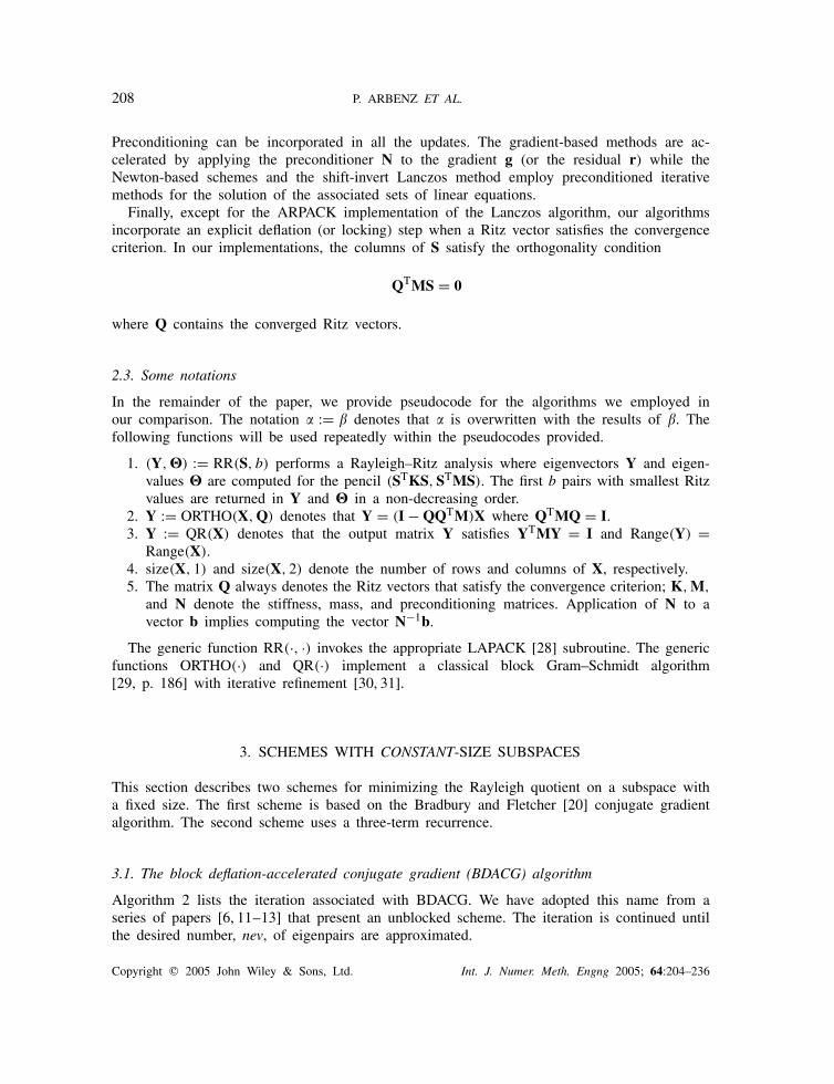
Algorithm 2 lists the iteration associated with BDACG. We have adopted this name from aseries of papers [6, 11–13] that present an unblocked scheme. The iteration is continued untilthe desired number, nev, of eigenpairs are approximated.



ALGORITHM 2: (BDACG) Block deflation-accelerated conjugate gradientalgorithm

(1) Select a random X0 ∈ Rn×b where 1 � b < n is the blocksize; X0 := X0Y0

where (Y0, �0) := RR(X0, b) and let R0 := KX0 − MX0�0.(2) Set k := 0 and Q := [].(3) Until size(Q, 2) � nev do(4) Solve the preconditioned linear system NHk = Rk.

(5) If k = 0 thenPk := −Hk and Bk := diag(HT

k Rk).

elsePk := −Hk + Pk−1Bk and Bk := diag(HT

k Rk)B−1k−1.

end if.(6) Pk := ORTHO(Pk, Q).

(7) Let Sk := [Xk, Pk] and compute (Yk, �k+1) := RR(Sk, b).

(8) Xk+1 := SkYk.

(9) Rk+1 := KXk+1 − MXk+1�k+1.

(10) k := k + 1.(11) If some columns of Rk satisfy the convergence criterion then

Augment Q with the corresponding Ritz vectors from Xk;set k := 0 and define new X0 and R0.

end if.(12) end Until.

The space for the minimization of the Rayleigh quotient is the span of [Xk, Pk]. The blockof vectors Pk is our block extension for the search direction introduced by the gradient schemeof Bradbury–Fletcher [20]. BDACG-(5), i.e. step (5) in the BDACG Algorithm 2, computesthe search directions with the preconditioned residuals instead of the preconditioned gradientsbecause the columns of Xk are M-orthonormal. We remark that the condition PT

k KPk−1 = 0lead to a more expensive iteration with no reduction in the number of (outer) iterations. Asimilar scheme was introduced in Reference [32], however, the block size is required to be atleast as large as the number of eigenvalues requested.

BDACG-(6) M-orthogonalizes the current search directions Pk against the column spanof Q that contains Ritz vectors that have been deflated. Our experiments revealed that thisorthogonalization prevented copies of Ritz values from emerging during the course of theiteration. In our experiments, we determined that the eigenvectors computed in BDACG-(7) needed to be scaled so that the diagonal elements of Yk are non-negative. This isa generalization of quadratic line search that retains the positive root in the unblockedalgorithm.

BDACG-(11) deflates Ritz vectors from Xk when they satisfy the convergence criterion. Thenew columns of X0 are defined by the vectors not-deflated and the vectors associated with thenext largest Ritz values. In practice, the generic function RR(·, ·) calls the LAPACK routineDSYGV that computes the 2 · b eigenpairs of the projected eigenproblem.



The matrices K, M, and N are accessed only once per iteration (except where M is usedfor deflation). Therefore, we store the block vectors Xk , KXk , MXk , Pk , KPk , MPk , Rk , andHk . When the first nev eigenpairs are requested, the overall storage requirements for BDACGare:

• a vector of length nev elements (for the converged Ritz values),• nev vectors of length n (for the converged Ritz vectors),• 8 · b vectors of length n,• O(b2) elements (for the Rayleigh–Ritz analysis).

In our experiments, the matrix Bk remained non-singular throughout the computation and theRayleigh–Ritz analysis never failed. However, for the sake of robustness, we have equippedBDACG with a restart when one of these failures occurs.

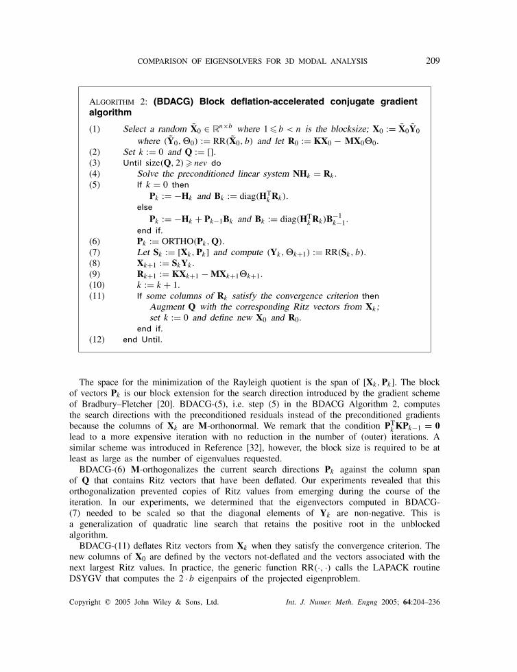
3.2. The locally—optimal block preconditioned conjugate gradient (LOBPCG) algorithm

ALGORITHM 3: (LOBPCG) Locally—optimal block preconditioned conjugategradient method


where (Y0, �0) := RR(X0, b) and let R0 := KX0 − MX0�0.(2) Set k := 0, Q := [], and P0 := [].(3) Until size(Q, 2) � nev do(4) Solve the preconditioned linear system NHk = Rk .(5) Hk := ORTHO(Hk, Q).(6) Let Sk := [Xk, Hk, Pk] and compute (Yk, �k+1) := RR(Sk, b).(7) Xk+1 := [Xk, Hk, Pk]Yk .(8) Pk+1 := [0, Hk, Pk]Yk .(9) Rk+1 := KXk+1 − MXk+1�k+1.(10) k := k + 1.(11) If some columns of Rk satisfy the convergence criterion then

Augment Q with the corresponding Ritz vectors from Xk;set k := 0 and define new X0 and R0.


In contrast to BDACG, Knyazev [5] suggests that the space for the minimization be augmentedby the span of Xk−1. The resulting algorithm is deemed locally optimal because the Rayleighquotient � is minimized with respect to all available vectors. Mathematically, the span of[Xk, Hk, Pk] is equal to the span of [Xk, Hk, Xk−1]. The columns of the former matrix arebetter conditioned than the columns of the latter matrix.

Algorithm 3 lists the iteration associated with LOBPCG. Our implementation of LOBPCGdiffers from the one presented in Reference [5]. For instance, we employ explicit deflation andallow the block size b to be independent of the number of Ritz pairs desired. The iteration iscontinued until the desired number of eigenpairs are approximated.



LOBPCG-(5) M-orthogonalizes the current preconditioned residuals Hk against column spanof Q that contains Ritz vectors that have been deflated. Our experiments revealed that thisorthogonalization prevented copies of Ritz values from emerging during the course of theiteration.

LOBPCG-(11), as in BDACG, deflates Ritz vectors from Xk when they satisfy the conver-gence criterion. The new columns of X0 are defined by the vectors not-deflated and the vectorsassociated with the next largest Ritz values. In practice, the generic function RR(·, ·) calls theLAPACK routine DSYGV.

The matrices K, M, and N are accessed only once per iteration (except where M is used fordeflation). Therefore, we store the block vectors Xk , KXk , MXk , Hk , KHk , MHk , Pk , KPk ,MPk , and Rk . When the first nev eigenpairs are requested, the overall storage requirements forthe algorithm LOBPCG are:

• a vector of length nev elements (for the converged Ritz values),• nev vectors of length n (for the converged Ritz vectors),• 10 · b vectors of length n,• O(b2) elements (for the Rayleigh–Ritz analysis).

In our experiments, the Rayleigh–Ritz analysis never failed. But, for the sake of robustness,we have equipped our code with a restart when the routine DSYGV fails.

4. SCHEMES WITH SUBSPACES THAT INCREASE IN SIZE

In this section, we present three schemes for minimizing the Rayleigh quotient on a subspacewith a varying size. The first two are Newton-based schemes and the third is a shift-invertLanczos method.

4.1. The block Davidson algorithm

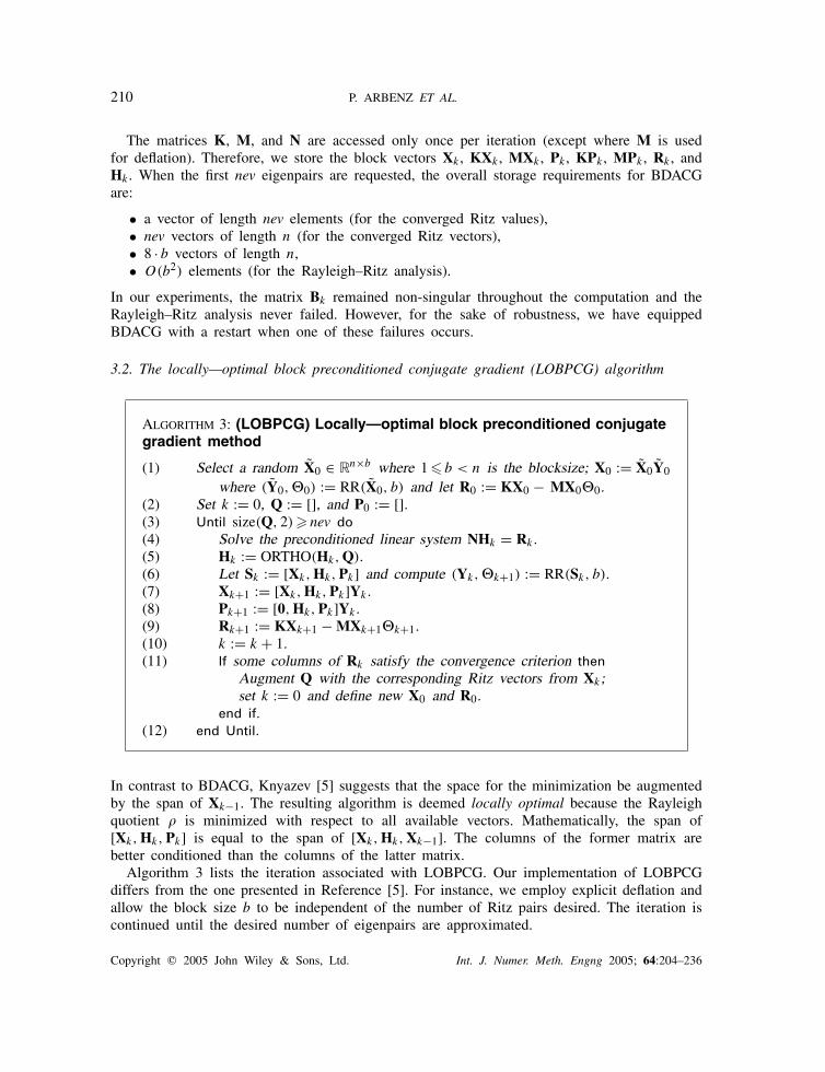
Algorithm 4 lists the iteration associated with our block extension of the Davidson algorithm(see References [33, 34] for alternate block variants and references). The iteration is continueduntil the desired number of eigenpairs are approximated.

At the kth iteration, the subspace Sk for the minimization of the Rayleigh quotient isspanned by the M-orthonormal basis Sk . To enrich the subspace at each iteration, we use thepreconditioned residuals N−1Rk as an approximation to the correction vectors for the Newtonstep of Equation (4). This approximation differs from the Davidson algorithm [7] in that weemploy a fixed preconditioner N at every step.

The step Davidson-(5) M-orthogonalizes the columns of Hk against the deflated Ritz vectorsstored in Q and the basis Sk . Then Davidson-(6) M-orthonormalizes the resulting vectors.

The generic function RR(·, ·) in Davidson-(7) calls the LAPACK routine DSYEV that com-putes all the eigenpairs of the projected eigenproblem.

Davidson-(11) deflates Ritz vectors from Xk when they satisfy the convergence criterion.The columns of the residual matrix Rk associated with deflated Ritz vectors are replaced withthe Ritz vectors corresponding to the next largest Ritz values.

Davidson-(12) limits the dimension of the subspace basis Sk . When nev eigenpairs arerequested, the number of vectors allocated for the storage of [Q, Sk] is 2 · nev + b and this



ALGORITHM 4: Block Davidson algorithm


where (Y0, �0) := RR(X0, b) and let R0 := KX0 − MX0�0.(2) Set k := 0, Q := [], and S0 := [X0].(3) Until size(Q, 2) � nev do(4) Solve the preconditioned linear system NHk = Rk .(5) Hk := ORTHO(Hk, [Q, Sk]).(6) Hk := QR(Hk).(7) Let Sk+1 := [Sk, Hk] and compute (Yk+1, �k+1) := RR(Sk+1, b).(8) Xk+1 := Sk+1Yk+1.(9) Rk+1 := KXk+1 − MXk+1�k+1.(10) k := k + 1.(11) If any columns of Rk satisfy the convergence criterion then

Augment Q with the corresponding Ritz vectors from Xk andrestart to obtain an updated Sk .

end if.(12) If the dimensions of Sk reach the limit of storage allocated then

Restart to obtain an updated Sk .end if.

(13) end Until.

combined storage represents the working subspace. As the iteration progresses and Ritz pairsconverge, the number of vectors in the active subspace Sk is bounded by

2 · nev −⌊

size(Q, 2)

b

⌋· b (7)

where �·� is the floor function.Both Davidson-(11) and Davidson-(12) effect a restart. Suppose that the number of columns

of Sk is p · b. Then we restart by multiplying Sk with Yk (where (Yk, �k) = RR(Sk, �p/2� · b)

with the columns of Yk associated with the smallest Ritz values not-deflated). The choiceof �p/2� · b columns for the restart of Sk is a balance between a number large enough sothat the loss of information is minimized and small enough so that a useful subspace Sk isconstructed before the limit (7) on the number of columns is attained. Restarting with Ritzvectors associated with the smallest Ritz values worked better in practice than using randomvectors. Reference [35] discusses related restart strategies.

The preconditioner N is applied only once per iteration, while the matrices K and M areaccessed twice per iteration (except where M is used for deflation and orthonormalization).When the first nev eigenpairs are requested and with the upper limit (7), the overall storagerequirements for our implementation of Davidson are:

• a vector of length nev words (for the converged Ritz values),• 2 · nev vectors of length n (the converged Ritz vectors are stored in the initial nev vectors),• 4 · b vectors of length n,



• O(nev2) elements (for the Rayleigh–Ritz analysis),• O(b2) elements.

Our implementation proved stable during all our experiments.

4.2. The block Jacobi–Davidson conjugate gradient algorithm (BJDCG)

Our second scheme for minimizing the Rayleigh quotient by expanding the subspace is a blockextension of a Jacobi–Davidson algorithm [14]. We implement a block version of the Jacobi–Davidson variant due to Notay [8] tailored for symmetric matrices. We do not list an algorithmfor BJDCG because the differences with Algorithm 4 are slight. The algorithms differ mainlyin the enrichment of the subspace. Step (4) of Algorithm 4 is replaced by

Hk = CORRECTION(Rk, N, Q, , ) where Q := [Q, Xk]that solves the correction equation

(I − MQQT)(K − M)(I − QQTM)T = −Rk with QTMT = 0 (8)

with a block preconditioned conjugate gradient (BPCG) algorithm. The correction equation (8)is equivalent to the block extension of Equation (5) with right-hand side

−(

Rk

0

)

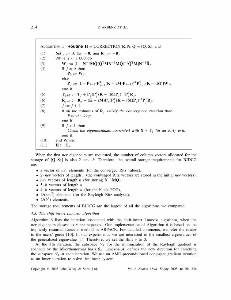
Algorithm 5 lists the BPCG iteration we used to solve the correction equation (8). Step (3)applies the preconditioner N to the correction equation (8) (see Reference [36] for details). Step(4) computes the block of search directions, and steps (5)–(6) compute the j th approximation tothe correction equation and corresponding residual, respectively. Step (8) terminates the BPCGiteration when the Euclidean norms of the columns of Rj have been reduced by a factor of relative to the columns of R0. The tolerance used in Algorithm 5 is set equal to 2−� where� is a counter on the number of (outer) BJDCG iterations needed to compute a Ritz value (seeReference [17, p. 130] for a discussion).

The coefficient is set to 0 when the norm of residuals in Rk are larger than a giventolerance. Otherwise, is set to the smallest Ritz value in �k . The reader is referred toReference [37] for further details.

In contrast to step (8) that checks for termination of the BPCG algorithm, step (9) checksthe Ritz pair residuals. Because Tj is the approximation to the correction equation, we define

V = (X + Tj )Y where (Y, �) = RR(X + Tj , b)

and check the columns norms of KV − MV�. If any column norm stagnates, increases innorm, or satisfies the convergence criterion, then we exit the BPCG iteration with the currentapproximation Tj (see Reference [8] for further details and discussion).

A generalization of the proof given by Notay [8] to the generalized symmetric positivedefinite eigenvalue problem shows that PT

j (K − M)Pj is symmetric positive definite (on the

space orthogonal to the range of Q). For robustness, if this matrix becomes indefinite, we exitthe BPCG loop and perform a restart of the search space Sk in BJDCG. In our numericalexperiments, the maximum number of BPCG iterations was never reached.



ALGORITHM 5: Routine H = CORRECTION(R, N, Q = [Q, X], , )(1) Set j := 0, T0 := 0, and R0 := −R.(2) While j < 1, 000 do

(3) Wj := [I − N−1MQ(QTMN−1MQ)−1QTM]N−1Rj .(4) If j = 0 then

P0 := W0.else

Pj := [I − Pj−1(PTj−1(K − M)Pj−1)

−1PTj−1(K − M)]Wj .

end if.(5) Tj+1 := Tj + Pj (PT

j (K − M)Pj )−1PT

j Rj .

(6) Rj+1 := Rj − (K − M)Pj (PTj (K − M)Pj )

−1PTj Rj .

(7) j := j + 1.(8) If all the columns of Rj satisfy the convergence criterion then

Exit the loop.end if

(9) If j > 1 thenCheck the eigenresiduals associated with X + Tj for an early exit.

end if.(10) end While.(11) H := Tj .

When the first nev eigenpairs are requested, the number of column vectors allocated for thestorage of [Q, Sk] is also 2 · nev+b. Therefore, the overall storage requirements for BJDCGare:

• a vector of nev elements (for the converged Ritz values),• 2 · nev vectors of length n (the converged Ritz vectors are stored in the initial nev vectors),• nev vectors of length n (for storing N−1MQ),• 5 · b vectors of length n,• 4 · b vectors of length n (for the block PCG),• O(nev2) elements (for the Rayleigh–Ritz analysis),• O(b2) elements.

The storage requirements of BJDCG are the largest of all the algorithms we compared.

4.3. The shift-invert Lanczos algorithm

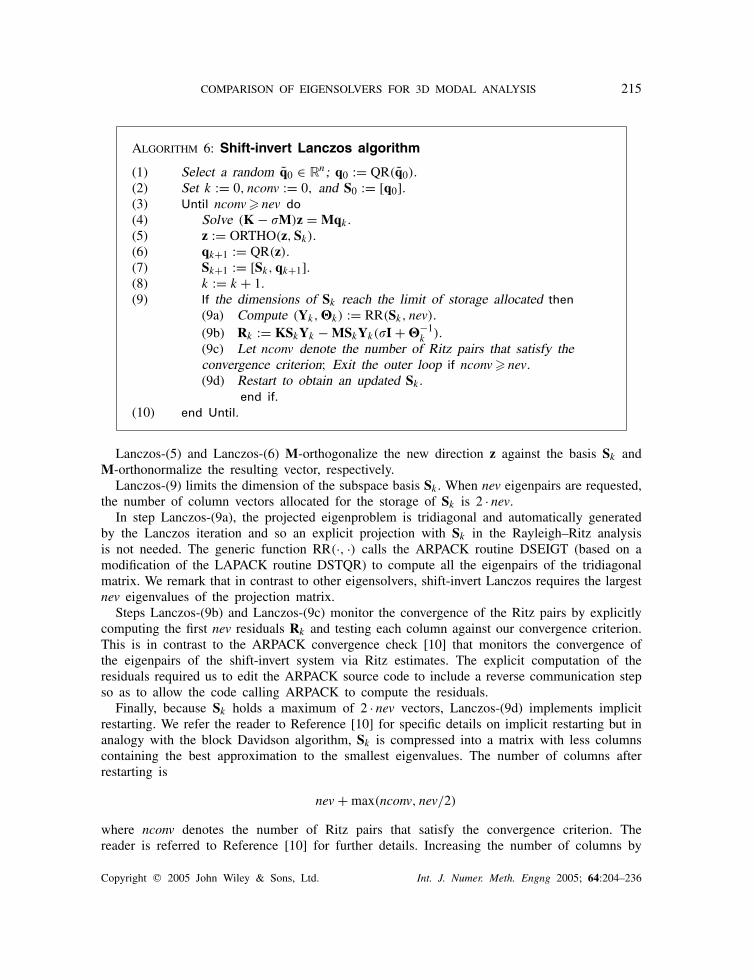
Algorithm 6 lists the iteration associated with the shift-invert Lanczos algorithm, when thenev eigenpairs closest to � are requested. Our implementation of Algorithm 6 is based on theimplicitly restarted Lanczos method in ARPACK. For detailed comments, we refer the readerto the users’ guide [10]. In our experiments, we are interested in the smallest eigenvalues ofthe generalized eigenvalue (1). Therefore, we set the shift � to 0.

At the kth iteration, the subspace Sk for the minimization of the Rayleigh quotient isspanned by the M-orthonormal basis Sk . Lanczos-(4) defines the new direction for enrichingthe subspace Sk at each iteration. We use an AMG-preconditioned conjugate gradient iterationas an inner iteration to solve the linear system.



ALGORITHM 6: Shift-invert Lanczos algorithm

(1) Select a random q0 ∈ Rn; q0 := QR(q0).(2) Set k := 0, nconv := 0, and S0 := [q0].(3) Until nconv � nev do(4) Solve (K − �M)z = Mqk .(5) z := ORTHO(z, Sk).(6) qk+1 := QR(z).(7) Sk+1 := [Sk, qk+1].(8) k := k + 1.(9) If the dimensions of Sk reach the limit of storage allocated then

(9a) Compute (Yk, �k) := RR(Sk, nev).(9b) Rk := KSkYk − MSkYk(�I + �−1

k ).(9c) Let nconv denote the number of Ritz pairs that satisfy theconvergence criterion; Exit the outer loop if nconv � nev.(9d) Restart to obtain an updated Sk .


Lanczos-(5) and Lanczos-(6) M-orthogonalize the new direction z against the basis Sk andM-orthonormalize the resulting vector, respectively.

Lanczos-(9) limits the dimension of the subspace basis Sk . When nev eigenpairs are requested,the number of column vectors allocated for the storage of Sk is 2 · nev.

In step Lanczos-(9a), the projected eigenproblem is tridiagonal and automatically generatedby the Lanczos iteration and so an explicit projection with Sk in the Rayleigh–Ritz analysisis not needed. The generic function RR(·, ·) calls the ARPACK routine DSEIGT (based on amodification of the LAPACK routine DSTQR) to compute all the eigenpairs of the tridiagonalmatrix. We remark that in contrast to other eigensolvers, shift-invert Lanczos requires the largestnev eigenvalues of the projection matrix.

Steps Lanczos-(9b) and Lanczos-(9c) monitor the convergence of the Ritz pairs by explicitlycomputing the first nev residuals Rk and testing each column against our convergence criterion.This is in contrast to the ARPACK convergence check [10] that monitors the convergence ofthe eigenpairs of the shift-invert system via Ritz estimates. The explicit computation of theresiduals required us to edit the ARPACK source code to include a reverse communication stepso as to allow the code calling ARPACK to compute the residuals.

Finally, because Sk holds a maximum of 2 · nev vectors, Lanczos-(9d) implements implicitrestarting. We refer the reader to Reference [10] for specific details on implicit restarting but inanalogy with the block Davidson algorithm, Sk is compressed into a matrix with less columnscontaining the best approximation to the smallest eigenvalues. The number of columns afterrestarting is

nev + max(nconv, nev/2)

where nconv denotes the number of Ritz pairs that satisfy the convergence criterion. Thereader is referred to Reference [10] for further details. Increasing the number of columns by



the number of converged Ritz pairs effects an implicit deflation or equivalently soft-locking [5]mechanism.

In our experiments, when the smallest nev eigenpairs are requested, the overall storagerequirements for shift-invert Lanczos are:

• a vector of length nev elements (for the converged Ritz values),• 2 · nev vectors of length n (for storing Sk and the converged Ritz vectors),• 5 vectors of length n,• O(nev2) elements,• 3 vectors of length n (for conjugate gradient algorithm),• 6 min(nev, 5) vectors of length n (for computing the residuals).

We remark, that unlike the previous algorithms, ARPACK does not check for convergence ateach outer iteration. Instead, convergence of Ritz pairs is determined at restart. Moreover, thereis no explicit deflation step only a postprocessing step to overwrite the Lanczos vectors withRitz vectors upon convergence of nev (or more) Ritz pairs.

5. NUMERICAL EXPERIMENTS

In this section, we discuss the numerical experiments used for the comparisons. The codes areimplemented in C++, using the Trilinos [38] project. This project provides, through a collectionof classes, the algebraic operations, the smoothed aggregation AMG preconditioner, and thepreconditioned conjugate gradient algorithm. For the shift-invert Lanczos algorithm, our C++code invokes the Fortran 77 package ARPACK [10].

Inside Trilinos, the linear algebra class, namely Epetra, manipulates the vectors, the blocksof vectors (or multivectors), and the sparse matrices. All these objects are distributed acrossthe processors. Whenever possible, Epetra implements the algebraic operations blockwise. Forinstance, the matrices K and M can be applied efficiently to a block of vectors.

Because ARPACK is a publicly available high-quality Lanczos implementation that includesa distributed memory implementation, we present the normalized timings

time for an eigensolver

time for ARPACK(9)

where the eigensolver is in turn BDACG, LOBPCG, block Davidson, and BJDCG. The initialvectors used by all the algorithms are generated using a random number generator. In additionto reporting the size of residuals, all the algorithms checked the orthonormality of the Ritzvectors computed via the check

maxi,j=1,...,nev

|eTi (XTMX − I)ej | (10)

We first describe some details associated with the AMG preconditioner in Section 5.1 fol-lowed by the results of our experiments on three problems.

5.1. AMG preconditioner

The package ML provides the smoothed aggregation AMG preconditioner [39]. Several recentstudies have demonstrated the viability of AMG preconditioners for problems in computational



mechanics [3, 4]. In addition to the public domain package ML, the commercial finite elementanalysis program ANSYS now provides an AMG-based solver [40].

The smoothed aggregation AMG algorithm requires no geometric information and therefore isattractive for complex domains with unstructured meshes. The basic idea of all AMG algorithmsis to capture errors by utilizing multiple resolutions. High-energy (or oscillatory) componentsare effectively reduced through a simple smoothing procedure, while low energy (or smooth)components are tackled using an auxiliary lower resolution version of the problem. The ideais applied recursively on the next coarser level. A sample multilevel iteration is illustrated inAlgorithm 7 to solve A1v1 = b1.

ALGORITHM 7: Multigrid V cycle with G grids to solve A1v1 = b1.

(1) Procedure Multilevel(Ak, bk, vk, k)

(2) Smooth vk .(3) If (k �= G)

(4) rk = bk − Akvk .(5) Project Ak and rk to generate Ak+1 and rk .(6) Multilevel(Ak+1, rk, vk+1, k + 1).(7) Interpolate vk+1 to generate vk+1.(8) Smooth vk + vk+1.(9) end if

The Ak’s (k > 1) are coarse grid discretization matrices computed by a Galerkinprojection.|| Smoothing damps high-energy errors and corresponds to iterations of a Chebyshevsemi-iterative method tuned to damp errors over the interval [�(Ak)/30, �(Ak)] where �(Ak)

is the spectral radius estimated with 10 Lanczos iterations. This is divided by the approxi-mate multigrid coarsening rate to obtain the lower endpoint of the interval. Interpolation (orprolongation) operators transfer solutions from coarse grids to fine grids.

In smoothed aggregation, nodes are aggregated together to effectively produce a coarsemesh and a tentative prolongator is generated to transfer solutions between these meshes. ForPoisson problems, this prolongator is essentially a matrix of zeros and ones correspondingto piecewise-constant interpolation. The tentative prolongator for elasticity exactly interpolateslow energy modes. In each matrix column (or coarse grid basis function), only rows cor-responding to nodes within one aggregate are non-zero. The tentative prolongator is thensmoothed to improve the grid transfer operator. The general idea is to reduce the energyof the coarse grid basis functions while maintaining accurate rigid body mode interpola-tion. This smoothing step is critical to obtaining mesh-independent multigrid convergence[41, 42].

||The Ak’s are determined in a preprocessing step and not computed within the iteration as shown here.



5.2. The Laplace eigenvalue problem

We consider the continuous problem

−�u(x) = �u(x) in � = (0, 1) × (0,√

2) × (0,√

3)

u(x) = 0 on ��(11)

We use an orthogonal mesh composed of 8-noded brick elements. On each co-ordinate axis,we define 100 interior nodes. The resulting finite element discretization generates matrices Kand M of order n = 1 000 000.

Analytical expressions of the eigenmodes and frequencies for (K, M) are available. Whenn = 1 000 000, we have

�1 ≈ 18.1, �n ≈ 21 938, �n − �1 ≈ 2 · 105

and the relative gap

�i − �i−1

�n − �1(12)

for the 200 smallest eigenvalues varies between 10−8 and 10−4 with eigenvalues 20–23 nearlyidentical. We remark that all the eigenvalues are simple. This model problem is extremelyuseful because it allows us to verify our implementations of the various algorithms. We verifythe results against expected rates of convergence given by the finite element method and byusing the analytic expressions to determine the reliability of our implementations—were anyeigenvalues missed?

The AMG preconditioner generated four levels with 41616, 2016, 180, and 32 vertices. Thestorage needed to represent the operators on these levels represented 7% of the storage forK. As an indication of the quality of the preconditioner, the preconditioned conjugate gradientreduces the residual norm by a factor 105 in 10 iterations.

The computations were performed on a cluster of DEC Alpha processors, where each proces-sor has access to 512 MB of memory. We used 16 processors to determine the 10, 20, 50, 100,and 200 smallest eigenpairs. A pair (x, �) is considered converged when the criterion

1√�1

‖Kx − Mx�‖2

‖x‖M�� · 10−4 (13)

is satisfied. The scalar �1 is the smallest eigenvalue of the mass matrix M; when n = 1 000 000,�1 ≈ 8 · 10−8. We remark that the tolerance of 10−4 represents the discretization error.

For the shift-invert Lanczos algorithm, we solve the linear system to an accuracy of 10−5

relative to the norm of the initial residual.For the Jacobi–Davidson algorithm, the coefficient is set to the smallest Ritz value as soon

as the criterion

1√�1

‖Kx − Mx�‖2

‖x‖M�� ·

√10−4 (14)

is satisfied.



5.2.1. Reliability. After the computation, we performed the following tests to verify the qualityof the computation.

• All the algorithms returned Ritz vectors M-orthonormal to machine precision.• The largest angle between the span of the computed eigenvectors and the span of the

exact discrete eigenvectors was smaller than 10−5 radians.• No algorithm missed an eigenvalue, when the block size was 1. For larger block sizes,

the computations for 20 eigenvalues often missed the 20th eigenvalue. At the continuouslevel, this eigenvalue has a multiplicity of 4, while, at the discrete level, the spectrumhas a cluster of 4 eigenvalues in the interval [97.1, 97.22]. BDACG had the most misses,while BJDCG had the least. The LOBPCG and Davidson algorithms behaved in a similarfashion.

We remark that for nearly all eigenvalue problems the answers are not known beforehandso reliability cannot be ascertained. A defect of using preconditioned iterative methods is theinability to determine whether all eigenvalues in the frequency range of interest were computed.This lack of reliability is a factor for high-consequence modal analysis.

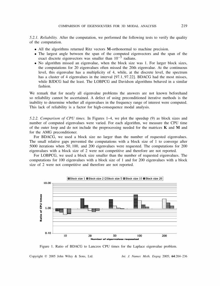
5.2.2. Comparison of CPU times. In Figures 1–4, we plot the speedup (9) as block sizes andnumber of computed eigenvalues were varied. For each algorithm, we measure the CPU timeof the outer loop and do not include the preprocessing needed for the matrices K and M andfor the AMG preconditioner.

For BDACG, we used a block size no larger than the number of requested eigenvalues.The small relative gaps prevented the computations with a block size of 1 to converge after5000 iterations when 50, 100, and 200 eigenvalues were requested. The computations for 200eigenvalues with a block size of 2 were not competitive and therefore are not reported.

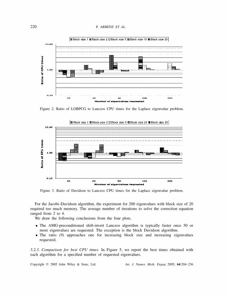
For LOBPCG, we used a block size smaller than the number of requested eigenvalues. Thecomputations for 100 eigenvalues with a block size of 1 and for 200 eigenvalues with a blocksize of 2 were not competitive and therefore are not reported.

Figure 1. Ratio of BDACG to Lanczos CPU times for the Laplace eigenvalue problem.



Figure 2. Ratio of LOBPCG to Lanczos CPU times for the Laplace eigenvalue problem.

Figure 3. Ratio of Davidson to Lanczos CPU times for the Laplace eigenvalue problem.

For the Jacobi–Davidson algorithm, the experiment for 200 eigenvalues with block size of 20required too much memory. The average number of iterations to solve the correction equationranged from 2 to 4.

We draw the following conclusions from the four plots.

• The AMG-preconditioned shift-invert Lanczos algorithm is typically faster once 50 ormore eigenvalues are requested. The exception is the block Davidson algorithm.

• The ratio (9) approaches one for increasing block size and increasing eigenvaluesrequested.

5.2.3. Comparison for best CPU times. In Figure 5, we report the best times obtained witheach algorithm for a specified number of requested eigenvalues.



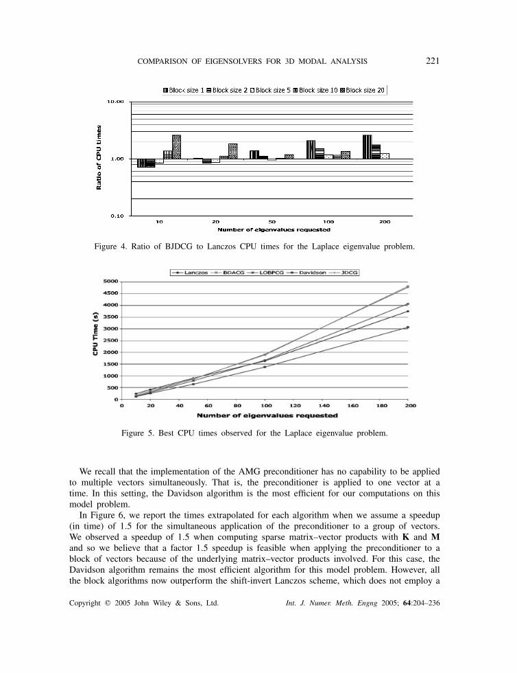
Figure 4. Ratio of BJDCG to Lanczos CPU times for the Laplace eigenvalue problem.

Figure 5. Best CPU times observed for the Laplace eigenvalue problem.

We recall that the implementation of the AMG preconditioner has no capability to be appliedto multiple vectors simultaneously. That is, the preconditioner is applied to one vector at atime. In this setting, the Davidson algorithm is the most efficient for our computations on thismodel problem.

In Figure 6, we report the times extrapolated for each algorithm when we assume a speedup(in time) of 1.5 for the simultaneous application of the preconditioner to a group of vectors.We observed a speedup of 1.5 when computing sparse matrix–vector products with K and Mand so we believe that a factor 1.5 speedup is feasible when applying the preconditioner to ablock of vectors because of the underlying matrix–vector products involved. For this case, theDavidson algorithm remains the most efficient algorithm for this model problem. However, allthe block algorithms now outperform the shift-invert Lanczos scheme, which does not employ a



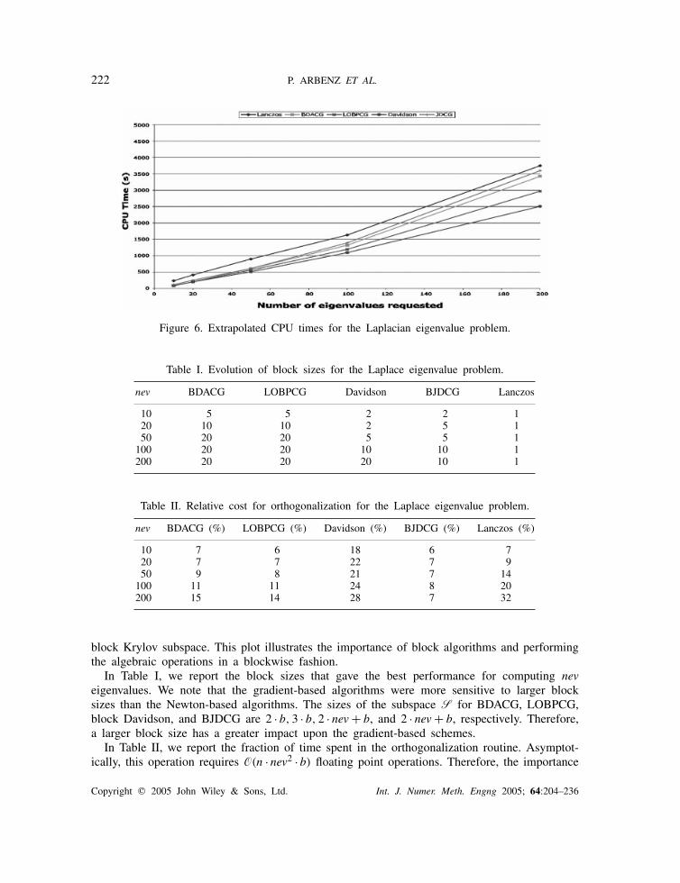
Figure 6. Extrapolated CPU times for the Laplacian eigenvalue problem.

Table I. Evolution of block sizes for the Laplace eigenvalue problem.

nev BDACG LOBPCG Davidson BJDCG Lanczos

10 5 5 2 2 120 10 10 2 5 150 20 20 5 5 1

100 20 20 10 10 1200 20 20 20 10 1

Table II. Relative cost for orthogonalization for the Laplace eigenvalue problem.

nev BDACG (%) LOBPCG (%) Davidson (%) BJDCG (%) Lanczos (%)

10 7 6 18 6 720 7 7 22 7 950 9 8 21 7 14

100 11 11 24 8 20200 15 14 28 7 32

block Krylov subspace. This plot illustrates the importance of block algorithms and performingthe algebraic operations in a blockwise fashion.

In Table I, we report the block sizes that gave the best performance for computing neveigenvalues. We note that the gradient-based algorithms were more sensitive to larger blocksizes than the Newton-based algorithms. The sizes of the subspace S for BDACG, LOBPCG,block Davidson, and BJDCG are 2 · b, 3 · b, 2 · nev + b, and 2 · nev + b, respectively. Therefore,a larger block size has a greater impact upon the gradient-based schemes.

In Table II, we report the fraction of time spent in the orthogonalization routine. Asymptot-ically, this operation requires O(n · nev2 · b) floating point operations. Therefore, the importance



Table III. Number of preconditioned operations for the Laplace eigenvalue problem.


10 273 (68%) 230 (64%) 156 (45%) 90 (60%) 49 (89%)20 596 (66%) 530 (61%) 320 (42%) 232 (52%) 85 (88%)50 1620 (61%) 1380 (58%) 810 (42%) 510 (54%) 176 (83%)

100 3420 (60%) 2820 (56%) 1663 (40%) 1163 (50%) 301 (77%)200 8386 (58%) 6620 (54%) 3393 (37%) 2486 (53%) 601 (65%)

of orthogonalization increases with the number of eigenvalues requested. The Davidson andthe shift-invert Lanczos algorithms both build an M-orthonormal search space, which explainsthe higher relative cost. The Jacobi–Davidson seems to have a smaller growth for this cost.However, the growth is offset by the cost of solving the correction equation.

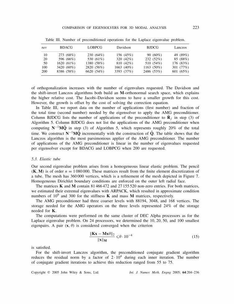
In Table III, we report data on the number of applications (first number) and fraction ofthe total time (second number) needed by the eigensolver to apply the AMG preconditioner.Column BJDCG lists the number of applications of the preconditioner to Rj in step (3) ofAlgorithm 5. Column BJDCG does not list the applications of the AMG preconditioner whencomputing N−1MQ in step (3) of Algorithm 5, which represents roughly 20% of the totaltime. We construct N−1MQ incrementally with the construction of Q. The table shows that theLanczos algorithm is the most parsimonious applier of the AMG preconditioner. The numberof applications of the AMG preconditioner is linear in the number of eigenvalues requestedper eigensolver except for BDACG and LOBPCG when 200 are requested.

5.3. Elastic tube

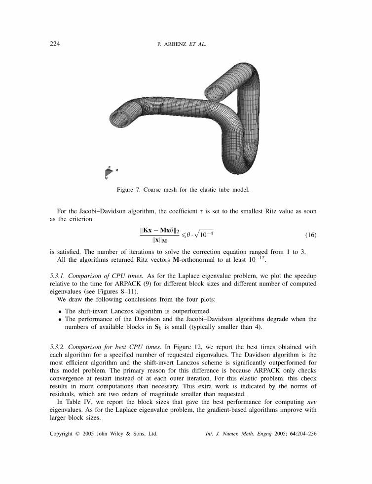
Our second eigenvalue problem arises from a homogeneous linear elastic problem. The pencil(K, M) is of order n = 1 080 000. These matrices result from the finite element discretization ofa tube. The mesh has 360 000 vertices, which is a refinement of the mesh depicted in Figure 7.Homogeneous Dirichlet boundary conditions are enforced on the outer left radial face.

The matrices K and M contain 81 466 472 and 27 155 520 non-zero entries. For both matrices,we estimated their extremal eigenvalues with ARPACK, which resulted in approximate conditionnumbers of 109 and 300 for the stiffness K and mass M matrices, respectively.

The AMG preconditioner had three coarser levels with 88194, 3048, and 168 vertices. Thestorage needed for the AMG operators on the three levels represented 24% of the storageneeded for K.

The computations were performed on the same cluster of DEC Alpha processors as for theLaplace eigenvalue problem. On 24 processors, we determined the 10, 20, 50, and 100 smallesteigenpairs. A pair (x, �) is considered converged when the criterion

‖Kx − Mx�‖2

‖x‖M�� · 10−4 (15)

is satisfied.For the shift-invert Lanczos algorithm, the preconditioned conjugate gradient algorithm

reduces the residual norm by a factor of 2 · 104 during each inner iteration. The numberof conjugate gradient iterations to achieve this reduction ranged from 55 to 75.



Figure 7. Coarse mesh for the elastic tube model.

For the Jacobi–Davidson algorithm, the coefficient is set to the smallest Ritz value as soonas the criterion

‖Kx − Mx�‖2

‖x‖M�� ·

√10−4 (16)

is satisfied. The number of iterations to solve the correction equation ranged from 1 to 3.All the algorithms returned Ritz vectors M-orthonormal to at least 10−12.

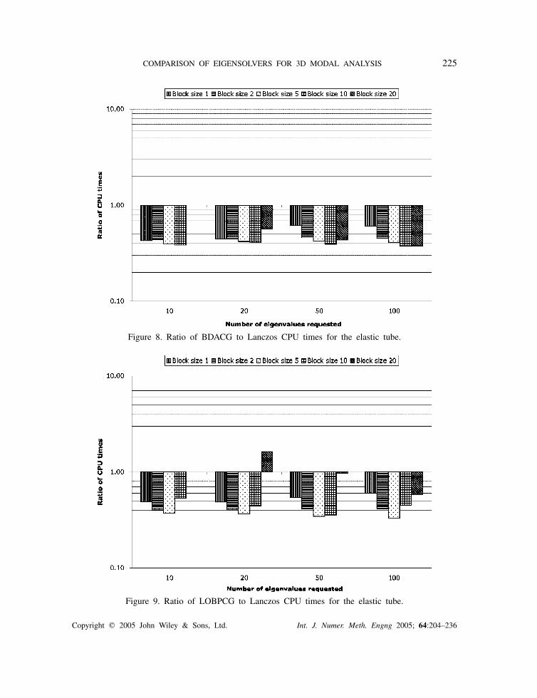
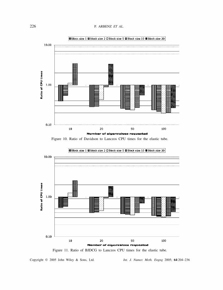
5.3.1. Comparison of CPU times. As for the Laplace eigenvalue problem, we plot the speeduprelative to the time for ARPACK (9) for different block sizes and different number of computedeigenvalues (see Figures 8–11).

We draw the following conclusions from the four plots:

• The shift-invert Lanczos algorithm is outperformed.• The performance of the Davidson and the Jacobi–Davidson algorithms degrade when the

numbers of available blocks in Sk is small (typically smaller than 4).

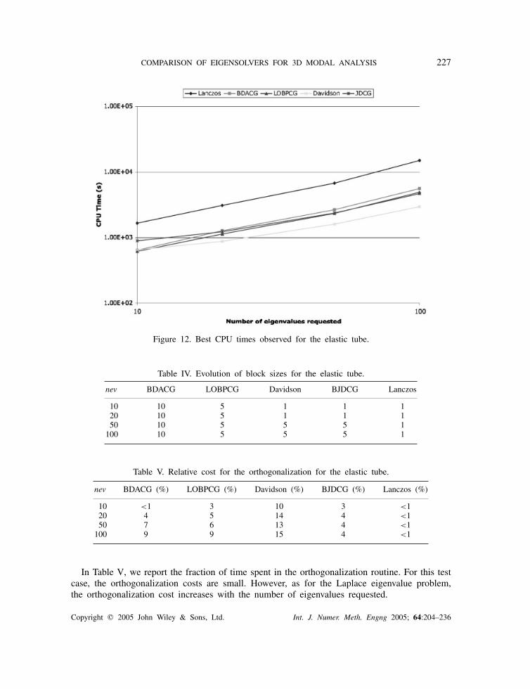
5.3.2. Comparison for best CPU times. In Figure 12, we report the best times obtained witheach algorithm for a specified number of requested eigenvalues. The Davidson algorithm is themost efficient algorithm and the shift-invert Lanczos scheme is significantly outperformed forthis model problem. The primary reason for this difference is because ARPACK only checksconvergence at restart instead of at each outer iteration. For this elastic problem, this checkresults in more computations than necessary. This extra work is indicated by the norms ofresiduals, which are two orders of magnitude smaller than requested.

In Table IV, we report the block sizes that gave the best performance for computing neveigenvalues. As for the Laplace eigenvalue problem, the gradient-based algorithms improve withlarger block sizes.



Figure 8. Ratio of BDACG to Lanczos CPU times for the elastic tube.

Figure 9. Ratio of LOBPCG to Lanczos CPU times for the elastic tube.



Figure 10. Ratio of Davidson to Lanczos CPU times for the elastic tube.

Figure 11. Ratio of BJDCG to Lanczos CPU times for the elastic tube.



Figure 12. Best CPU times observed for the elastic tube.

Table IV. Evolution of block sizes for the elastic tube.


10 10 5 1 1 120 10 5 1 1 150 10 5 5 5 1

100 10 5 5 5 1

Table V. Relative cost for the orthogonalization for the elastic tube.

nev BDACG (%) LOBPCG (%) Davidson (%) BJDCG (%) Lanczos (%)

10 <1 3 10 3 <120 4 5 14 4 <150 7 6 13 4 <1

100 9 9 15 4 <1

In Table V, we report the fraction of time spent in the orthogonalization routine. For this testcase, the orthogonalization costs are small. However, as for the Laplace eigenvalue problem,the orthogonalization cost increases with the number of eigenvalues requested.



Table VI. Preconditioned operations for the elastic tube.


10 570 (85%) 535 (83%) 446 (65%) 457 (49%) 1565 (99%)20 1100 (83%) 965 (82%) 559 (61%) 620 (48%) 2921 (99%)50 2250 (81%) 1970 (81%) 1100 (66%) 1195 (48%) 6381 (99%)

100 4580 (78%) 4020 (79%) 1920 (62%) 2345 (46%) 13986 (99%)

Table VII. Statistics for LOBPCG with a tolerance of 10−7 on the elastictube. The column headings list the number of eigenvalues computed.

10 20 50 100

Ratio of CPU times 0.62 0.66 0.63 0.68Applications of N 870 1745 3610 8370

In Table VI, we report, for each eigensolver, the number of applications of the AMGpreconditioner (first number) and the corresponding fraction of total time (second number). Asin Table III, BJDCG does not list the applications of the AMG preconditioner when computingN−1MQ in step (3) of Algorithm 5, which represents roughly 22% of the total time. The blockDavidson algorithm uses the least number of preconditioner applications. Table VI emphasizesthe point made previously that the Lanczos algorithm over-solves the eigenvalue problem.Because ARPACK returned residuals that were at least two orders of magnitude smaller thanthe requested tolerance, we benchmarked LOBPCG with a tolerance of 10−7. Table VII liststhe ratio of CPU times between LOBPCG (with the tolerance of 10−7) and ARPACK (usedin Figures 8–11) and the number of preconditioner application for this benchmark. LOBPCGis still faster but the number of preconditioner applications increased and so the gap withARPACK has narrowed.

5.4. The aircraft carrier

Our third and final problem arises from a finite element discretization of an aircraft carrier. Themodel is made up of elastic shells, beams, and concentrated masses. The mesh has 315 444vertices. A mode of the carrier is depicted in Figure 13. The pencil (K, M) is of ordern = 1 892 644. This was our most challenging problem.

The stiffness matrix K has 63 306 430 non-zero entries. Because no boundary conditionsare imposed, K has six rigid-body modes. Therefore, we performed our computations in theM-orthogonal complement of the null space of K. The mass matrix M has 18 163 994 non-zeroentries. Using ARPACK to compute the extremal eigenvalues of M, we determined that themass matrix is numerically singular.

The AMG preconditioner generated three levels with 32 056, 1336, and 26 vertices. Thestorage requirement used by AMG on these levels represents 30% of the storage for K. Asan indication of the quality of the preconditioner, for the shift-invert Lanczos algorithm, thepreconditioned conjugate gradient algorithm reduces the residual norm by a factor of 2 · 105 inan average of 200 iterations.



Figure 13. Mode for the aircraft carrier model.

The computations were performed on Cplant [43], which is a cluster of 256 compute nodescomposed of 160 Compaq XP1000 Alpha 500 MHz processors and 96 Compaq DS10Ls Alpha466 MHz processors. All nodes have access to 1 GB of memory.

On 48 processors, we determined the 10, 20, 50, and 100 smallest non-zero eigenpairs. Apair (x, �) is considered converged when the criterion

‖Kx − Mx�‖2

‖x‖M�� · 10−5 (17)

is satisfied.For the Jacobi–Davidson algorithm, the coefficient is set to the smallest Ritz value as soon

as the criterion

‖Kx − Mx�‖2

‖x‖M�� ·

√10−5 (18)

is satisfied. The average number of iterations to solve the correction equation ranged from 2to 6.

All the algorithms returned Ritz vectors that were M-orthonormal to at least 10−12.

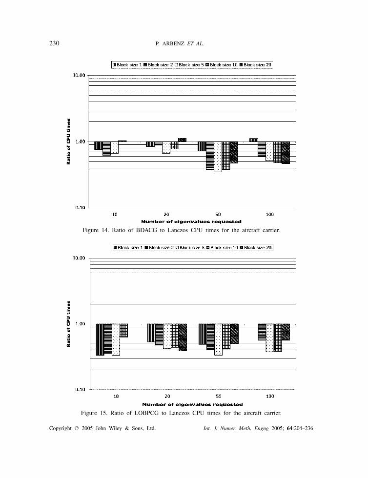
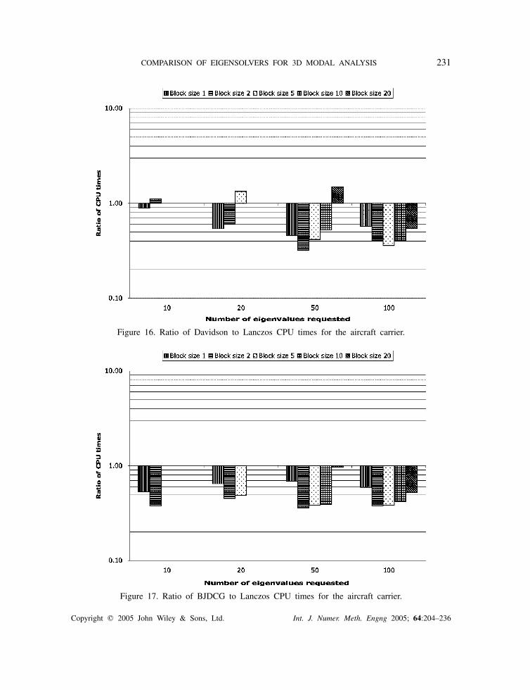
5.4.1. Comparison of CPU times. As for the Laplace eigenvalue problem, we plot the speeduprelative to the time for ARPACK (9) for different block sizes and different number of computedeigenvalues (see Figures 14–17).

We draw the following conclusions.

• The shift-invert Lanczos algorithm is not competitive with the other algorithms. Theexplanation is the large number of preconditioned conjugate gradient iterations requiredper outer iteration.

• The performance of the Davidson and the Jacobi–Davidson algorithms deteriorate whenthe numbers of available blocks in Sk is small (typically four or less).



Figure 14. Ratio of BDACG to Lanczos CPU times for the aircraft carrier.

Figure 15. Ratio of LOBPCG to Lanczos CPU times for the aircraft carrier.



Figure 16. Ratio of Davidson to Lanczos CPU times for the aircraft carrier.

Figure 17. Ratio of BJDCG to Lanczos CPU times for the aircraft carrier.



After step (3) of Algorithm 5 associated with BJDCG, the ill-conditioning of M and Ncan destroy the orthogonality property QTMWj = 0 necessary to ensure that copies of Ritzvalues do not emerge. When a loss of orthogonality occurs, we reorthogonalize by projectingWj in the space M-orthogonal to Q. This extra step of orthogonalization is accomplished byaugmenting step (3) of Algorithm 5 with

Wj := (I − N−1MQ(QTMN−1MQ)−1QTM)Wj

This ensures not only that QTMWj = 0 but also that the preconditioner of step (3) ofAlgorithm 5 is applied accurately.

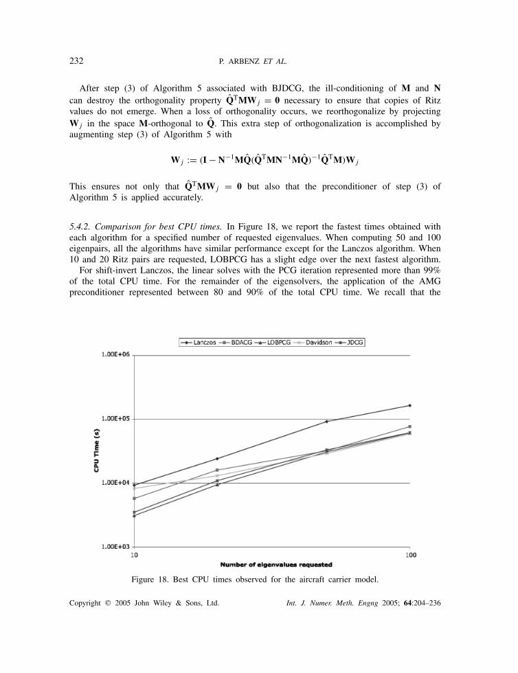
5.4.2. Comparison for best CPU times. In Figure 18, we report the fastest times obtained witheach algorithm for a specified number of requested eigenvalues. When computing 50 and 100eigenpairs, all the algorithms have similar performance except for the Lanczos algorithm. When10 and 20 Ritz pairs are requested, LOBPCG has a slight edge over the next fastest algorithm.

For shift-invert Lanczos, the linear solves with the PCG iteration represented more than 99%of the total CPU time. For the remainder of the eigensolvers, the application of the AMGpreconditioner represented between 80 and 90% of the total CPU time. We recall that the

Figure 18. Best CPU times observed for the aircraft carrier model.



AMG preconditioner is applied one vector at a time. Once again, the importance of applyingthe preconditioner to a block of vectors is crucial.

In contrast to the Laplace and elastic tube eigenvalue problems, we do not present tableslisting the time spent in orthogonalization and application of the preconditioner. Since Cplantimplements a batch queue, the times varied substantially because of other jobs run currentlyalong with our benchmarks.

6. CONCLUSIONS

The goal of our report was to compare a number of algorithms for computing a large numberof eigenpairs of the generalized eigenvalue problem arising from a modal analysis of elasticstructures using preconditioned iterative methods. After a review of various iteration schemes,a substantial amount of experiments were run on three problems. Based on the results of thethree problems, our overall conclusions are the following.

1. The single vector iterations were not competitive with block iterations. This statementholds under the condition that matrix–vector multiplications, orthogonalizations and, mostsignificantly, the application of the preconditioner are applied in a block fashion andthe block size is selected appropriately. The exception occurs when the preconditionedconjugate iteration needed by the Lanczos algorithm is efficiently computed (as in theLaplace eigenvalue problem) because of the availability of a high-qualitypreconditioner.

2. Maintaining numerical orthogonality of the basis vectors is the dominant cost of themodal analysis as the number of eigenpairs requested increases. The point at whichthis occurs will of course depend upon the computing resources and the eigenvalueproblem to be solved. Therefore, an efficient and stable orthogonalization procedure iscrucial.

3. Checking convergence of Ritz pairs at every outer iteration prevents over-solving the prob-lem. This was clearly an issue with our second problem and demonstrated the inefficiencyof ARPACK. Along these lines, our results demonstrated that the tolerances used for theeigensolvers can be set at the level of discretization error.

4. For an increasing number of eigenpairs requested, the gradient-based algorithms are themost conservative in memory use while BJDCG uses the most memory. We remarkthat all the algorithms can be implemented to use less storage at the cost of morematrix–vector applications and/or outer iterations. For example, the Davidson, BJDCG,and Lanczos algorithms can be made to restart when the subspace size is less than2 · nev at the cost of more outer iterations; LOBPCG can be implemented to use only4 · b instead of 10 · b vectors of length n at the cost of more applications of Kand M.

5. Until the cost of maintaining numerical orthogonality becomes dominant, the efficiencyand cost of the preconditioner is a fundamental problem.

6. Except for BJDCG and the Lanczos algorithm, the eigensolvers required only a singleapplication of the preconditioner per outer iteration. Although a preconditioned conjugateiteration to a specified accuracy can be carried out per outer iteration, experiments on theLaplace eigenvalue problem revealed longer overall computation times even though lessouter iterations were needed.



As can be expected, our paper raises several questions for further study. One importantquestion is how well the shift-invert block Lanczos method of [1] would perform if the sparsedirect linear solver is replaced with an AMG-preconditioned conjugate gradient algorithm.

We caution the reader not to take the results of the numerical experiments out of context. Ourintent is less in deciding the best algorithm (and implementation) but instead determining whatare the best features and limitations among a class of algorithms on realistic problems whenusing preconditioned iterative methods. Finally, we remark that an important criterion is thesimplicity of the algorithm and resulting implementation that leads to maintainable productionlevel software. Our implementations will be released in the public domain within the Anasazipackage of the Trilinos project.

ACKNOWLEDGEMENTS

We thank Roman Geus, ETH Zurich, and Yvan Notay, Free University of Brussels, for providing uswith MATLAB codes of their Jacobi–Davidson implementation, Andrew Knyazev of the University ofColorado at Denver, David Day and Kendall Pierson of Sandia National Labs, and Eugene Ovtchinnikovof the University of Westminster for helpful discussions; Michael Gee and Garth Reese, of SandiaNational Labs, for the second and third problems of Section 5; Bill Cochran of UIUC for someearly work on benchmarking the sparse matrix–vectors products; and Luca Bergamaschi for pointingout Reference [32]. The work of Dr Arbenz was in part supported by the CSRI, Sandia NationalLaboratories. Sandia is a multiprogram laboratory operated by Sandia Corporation, a Lockheed MartinCompany, for the United States Department of Energy; contract/grant number: DE-AC04-94AL85000.

REFERENCES

1. Grimes R, Lewis JR, Simon H. A shifted block Lanczos algorithm for solving sparse symmetric generalizedeigenproblems. SIAM Journal on Matrix Analysis and Applications 1994; 15:228–272.

2. Knyazev AV, Neymeyr K. Efficient solution of symmetric eigenvalue problems using multigrid preconditionersin the locally optimal block conjugate gradient method. Electronic Transactions on Numerical Analysis 2003;7:38–55.

3. Adams M. Evaluation of three unstructured multigrid methods on 3d finite element problems in solidmechanics. International Journal for Numerical Methods in Engineering 2002; 55:519–534.

4. Stüben K. A review of algebraic multigrid. Journal of Computational and Applied Mathematics 2001;128(1–2):281–309.

5. Knyazev AV. Toward the optimal preconditioned eigensolver: locally optimal block preconditioned conjugategradient method. SIAM Journal on Scientific Computing 2001; 23(2):517–541.

6. Bergamaschi L, Putti M. Numerical comparison of iterative eigensolvers for large sparse symmetric positivedefinite matrices. Computer Methods in Applied Mechanics and Engineering 2002; 191:5233–5247.

7. Davidson ER. The iterative calculation of a few of the lowest eigenvalues and corresponding eigenvectorsof large real-symmetric matrices. Journal of Computational Physics 1975; 17:87–94.

8. Notay Y. Combination of Jacobi–Davidson and conjugate gradients for the partial symmetric eigenproblem.Numerical Linear Algebra with Applications 2002; 9:21–44.

9. Sorensen DC. Implicit application of polynomial filters in a k-step Arnoldi method. SIAM Journal on MatrixAnalysis and Applications 1992; 13:357–385.

10. Lehoucq RB, Sorensen DC, Yang C. ARPACK Users’ Guide: Solution of Large-Scale Eigenvalue ProblemsBy Implicitely Restarted Arnoldi Methods. SIAM: Philadelphia, PA, 1998 (The software and this manual areavailable at URL http://www.caam.rice.edu/software/ARPACK/).

11. Gambolati G, Sartoretto F, Florian P. An orthogonal accelerated deflation technique for large symmetriceigenvalue problem. Computer Methods in Applied Mechanics and Engineering 1992; 94:13–23.

12. Bergamaschi L, Pini G, Sartoretto F. Approximate inverse preconditioning in the parallel solution of sparseeigenproblems. Numerical Linear Algebra with Applications 2000; 7(3):99–116.



13. Bergamaschi L, Pini G, Sartoretto F. Parallel preconditioning of a sparse eigensolver. Parallel Computing2001; 27:963–976.

14. Sleijpen GLG, van der Vorst HA. A Jacobi–Davidson iteration method for linear eigenvalue problems. SIAMJournal on Matrix Analysis and Applications 1996; 17(2):401–425.

15. Ericsson T, Ruhe A. The spectral transformation method for the numerical solution of large sparse generalizedsymmetric eigenvalue problems. Mathematics of Computation 1980; 35:1251–1268.

16. Feng Y. An integrated multigrid and Davidson approach for very large scale symmetric eigenvalue problems.Computer Methods in Applied Mechanics and Engineering 2001; 160:3543–3563.

17. van der Vorst HA. Computational methods for large eigenvalue problems. In Handbook of Numerical Analysis,Ciarlet P, Lions J (eds), vol. VIII. Elsevier, North-Holland: Amsterdam, 2002; 3–179.

18. Wu K, Saad Y, Stathopoulos A. Inexact Newton preconditioning techniques for large symmetric eigenvalueproblems. Electronic Transactions on Numerical Analysis 1998; 7:202–214.

19. Hestenes MR, Karush W. A method of gradients for the calculation of the characteristic roots and vectorsof a real symmetric matrix. Journal of Research of the National Bureau of Standards 1951; 47:45–61.

20. Bradbury WW, Fletcher R. New iterative methods for solution of the eigenproblem. Numerische Mathematik1966; 9:259–267.

21. Feng YT, Owen DRJ. Conjugate gradient methods for solving the smallest eigenpair of large symmetriceigenvalue problems. International Journal for Numerical Methods in Engineering 1996; 39(13):2209–2229.

22. Perdon A, Gambolati G. Extreme eigenvalues of large sparse matrices by Rayleigh quotient and modifiedconjugate gradients. Computer Methods in Applied Mechanics and Engineering 1986; 56:125–156.

23. Gambolati G, Pini G, Sartoretto F. An improved iterative optimization technique for the leftmost eigenpairsof large sparse matrices. Journal of Computational Physics 1988; 74:41–60.

24. Bergamaschi L, Gambolati G, Pini G. Asymptotic convergence of conjugate gradient methods for the partialsymmetric eigenproblem. Numerical Linear Algebra with Applications 1997; 4(2):69–84.

25. Schwarz HR. Eigenvalue problems and preconditioning. In Numerical Treatment of Eigenvalue Problems,Albrecht J, Collatz L, Hagedorn P, Velte W (eds), vol. 5. International Series of Numerical Mathematics(ISNM) 96. Birkhäuser: Basel, 1991; 191–208.

26. Knyazev AV. Preconditioned eigensolvers—an oxymoron. Electronic Transactions on Numerical Analysis 1998;7:104–123.

27. Sorensen D. Numerical Methods for Large Eigenvalue Problems, Acta Numerica. Cambridge University Press:Cambridge, 2002; 519–584.

28. Anderson E, Bai Z, Bischof C, Demmel J, Dongarra J, Croz JD, Greenbaum A, Hammarling S, McKenneyA, Ostrouchov S, Sorensen D. LAPACK Users’ Guide—Release 2.0. SIAM: Philadelphia, PA, 1994 (Softwareand guide are available from Netlib at URL http://www.netlib.org/lapack/).

29. Bai Z, Demmel J, Dongarra J, Ruhe A, van der Vorst H. Templates for the Solution of Algebraic EigenvalueProblems: A Practical Guide. SIAM: Philadelphia, PA, 2000.

30. Hoffmann W. Iterative algorithms for Gram–Schmidt orthogonalization. Computing 1989; 41:335–348.31. Björck Å. Numerics of Gram–Schmidt orthogonalization. Linear Algebra with Applications 1994; 197/198:

297–316.32. Sartoretto F, Pini G, Gambolati G. Accelerated simultaneous iterations for large finite element eigenproblems.

Journal of Computational Physics 1989; 81:53–69.33. Sadkane M, Sidje RB. Implementation of a variable block Davidson method with deflation for solving large

sparse eigenproblems. Numerical Algorithms 1999; 20:217–240.34. Stathopoulos A, Fischer CF. A Davidson program for finding a few selected extreme eigenpairs of a large,

sparse, real, symmetric matrix. Computational Physics Communications 1994; 79:268–290.35. Stathopoulos A, Saad Y, Wu K. Dynamic thick restarting of the Davidson, and the implicitly restarted

Arnoldi methods. SIAM Journal on Scientific Computing 1998; 19:227–245.36. Geus R. The Jacobi–Davidson algorithm for solving large sparse symmetric eigenvalue problems. Ph.D.

Thesis No. 14734, ETH Zurich, 2002.37. Fokkema DR, Sleijpen GLG, van der Vorst HA. Jacobi–Davidson style QR and QZ algorithms for the

reduction of matrix pencils. SIAM Journal on Scientific Computing 1998; 20(1):94–125.38. Heroux MA, Bartlett RA, Howle VE, Hoekstra RJ, Hu JJ, Kolda TG, Lehoucq RB, Long KR, Pawlowski

RP, Phipps ET, Salinger AG, Thornquist HK, Tuminaro RS, Willenbring JM, Williams A, Stanley KS.An overview of the trilinos project. ACM Transactions on Mathematical Software. Software is available athttp://software.sandia.gov/trilinos/index.html.



39. Vanek P, Mandel J, Brezina M. Algebraic multigrid based on smoothed aggregation for second and fourthorder problems. Computing 1996; 56(3):179–196.

40. Poole G, Liu Y-C, Mandel J. Advancing analysis capabilities in ANSYS through solver technology. ElectronicTransactions on Numerical Analysis 2002; 15:106–121.

41. Bramble J, Pasciak J, Wang J, Xu J. Convergence estimates for multigrid algorithms without regularityassumptions. Mathematics of Computation 1991; 57:23–45.

42. Vanek P, Brezina M, Mandel J. Convergence of algebraic multigrid based on smoothed aggregation.Numerische Mathematik 2001; 88:559–579.

43. Brightwell R, Fisk LA, Greenberg DS, Hudson TB, Levenhagen MJ, Maccabe AB, Riesen RE. Massivelyparallel computing using commodity components. Parallel Computing 2000; 26(2–3):243–266.


A comparison of eigensolvers for large-scale 3D modal analysis using AMG-preconditioned iterative...

Documents

Transcript of A comparison of eigensolvers for large-scale 3D modal analysis using AMG-preconditioned iterative...