A comparative study of soft-computing methodologies in identification of robotic manipulators

1

A Comparative Study of Soft Computing Methodologies in

Identification of Robotic Manipulators

M. Onder Efe

Electrical and Electronic Eng. Department

Mechatronics Research and Application Center

Bogaziçi University, Bebek, 80815 Istanbul, Turkey

e-mail: [email protected]

Prof. Okyay Kaynak

Chairman of Electrical and Electronic Eng. Department


Bogaziçi University, Bebek, 80815 Istanbul, Turkey

(Corresponding Author)

Tel: +90-212-287 24 75

Fax: +90-212-287 24 65

e-mail: [email protected]

2



M. Onder Efe and Okyay Kaynak



Bogaziçi University, Bebek, Istanbul, Turkey

Abstract

This paper investigates the identification of nonlinear systems by

utilizing soft-computing approaches. As the identification methods,

Feedforward Neural Network architecture (FNN), Radial Basis

Function Neural Networks (RBFNN), Runge-Kutta Neural Networks

(RKNN) and Adaptive Neuro-Fuzzy Inference Systems (ANFIS)

based identification mechanisms are studied and their performances

are comparatively evaluated on a two degrees of freedom direct drive

robotic manipulator.

Keywords: Neural Networks, Fuzzy Systems, Identification, Robotics, Comparison

3



M. Onder Efe and Okyay Kaynak



Bogaziçi University, Bebek, Istanbul, Turkey

Abstract

This paper investigates the identification of nonlinear systems by utilizing soft-

computing approaches. As the identification methods, Feedforward Neural Network

architecture (FNN), Radial Basis Function Neural Networks (RBFNN), Runge-Kutta

Neural Networks (RKNN) and Adaptive Neuro-Fuzzy Inference Systems (ANFIS)

based identification mechanisms are studied and their performances are comparatively

evaluated on a two degrees of freedom direct drive robotic manipulator.

1. Introduction

Identification of systems has drawn a great interest because of the increasing needs in

estimating the behavior of a system with partially known dynamics. Especially in the

areas of control, pattern recognition and even in the realm of stock markets the system

of interest needs to be known to some extent. A common property of real life systems is

the fact that they have multiple variables, some of which are subjected to stochastic

disturbances. Since a system may have a complicated dynamic behavior, the varying

environmental changes make the identification process much more difficult than the

cases in which those changes are modeled deterministically. In the latter, the

identification is performed at the cost of losing the reliability and preciseness.

Therefore, deciding on what the future behavior of a system will be and performing an

adaptive estimation is a formidable problem for real life systems.

4

Soft-computing is a practical alternative for solving computationally complex and

mathematically intractable problems. The reason that lies behind this understanding is

the fact that through the use of soft-computing methodologies, one can easily combine

the natural system dynamics and an intelligent machine. In this respect, the intelligence

stems from the combination of an expert’s knowledge and massively parallel and,

adaptive data processing architecture of the computationally intelligent approach

adopted. The most popular members of the soft-computing methodologies are the neural

networks and fuzzy inference systems. Neural networks provide the mathematical

power of the brain whereas the fuzzy logic based mechanisms employ the verbal power.

The latter allows the linguistic manipulation of input-state-output data. The most

interesting applications offer an appropriate combination of these two approaches

resulting in a hybrid system that both operates on linguistic descriptions of the variables

and the numeric values through a parallel and fault tolerant architecture.

The mapping properties of artificial neural networks have been analyzed by many

researchers. Hornik [6], and Funahashi [5] have shown that as long as the hidden layer

comprises sufficient number of nonlinear neurons, a function can be realized with a

desired degree of accuracy. This proof is followed by the study of Narendra and

Parthasarathy [7]. In their pioneering work, they have debated how useful artificial

neural networks can be for identification and control purposes. Their paper dwells on

the realization of an unknown nonlinearity by artificial neural networks. The training is

performed by the error backpropagation algorithm [8]. On the other hand, a novel

approach has been presented in [9] where the neural network realizes the behavior of a

set of ordinary differential equations utilizing the Runge-Kutta algorithm. The method is

proved to be successful in predicting the future behavior accurately. In [2], Radial Basis

Function Neural Networks are explained with their functional equivalence to Fuzzy

Inference Systems (FIS). In the same reference the details of Adaptive Neuro Fuzzy

Inference Systems (ANFIS) structure can be found, proposed as a core neuro-fuzzy

model that can incorporate human expertise as well as adapt itself through repeated

learning. This architecture has revealed a high performance in many applications. This

paper considers the ANFIS structure for the identification of a two degrees of freedom

direct drive robotic manipulator.

5

In [11], several neural network based identification strategies are discussed on a three

degrees of freedom anthropoid robot. Erbatur et al [10] cosider the standard fuzzy

system model proposed by Wang [3-4] for the approximation of the inverse dynamics of

the manipulator studied in this paper.

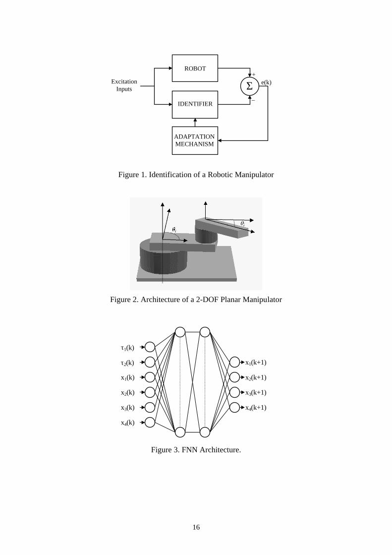
The identification procedure followed in all of the methods considered is as depicted in

Fig. 1. During the training, the excitation input is applied to both the robot system and

the identifier. The output error is then used to update the parameters of the identifier.

The excitation input cannot be selected randomly for any real system. Therefore, in the

simulations the manipulator is kept under an external control loop while the identifier

performance is being tested.

In the next section the system under observation is introduced, the following section

dwells on FNN based identification schemes. Next, RBFNN approach is derived. The

fifth section describes the application of Runge-Kutta neural network methodology for

the identification of robotic manipulators. In the sixth section ANFIS structure is

elaborated. In the seventh section, a comparison of the four approaches is presented.

Conclusions constitute the last part of the paper.

2. Two DOF Direct Drive Robotic Manipulator Dynamics

A robotic manipulator is a proper candidate for the evaluation of the performance of

identification mechanisms stated in the previous section. The main reason for this is the

fact that the dynamics are highly involved, being comprised of coupled nonlinear

differential equations. The general form of the manipulator dynamics is given by (1) and

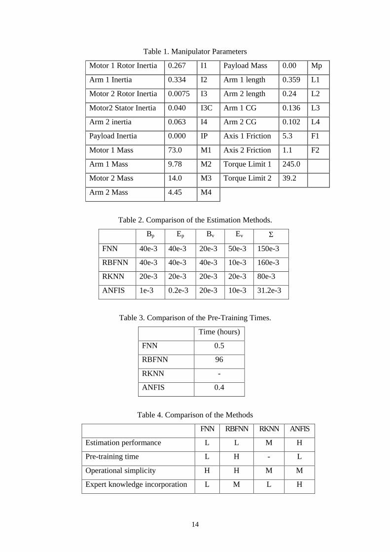
the nominal values of the parameters are summarized in Table 1 in standard units. The

architecture of the manipulator is illustrated in Fig. 2.

ftVM −=+ )(),()( τθθθθ &&& (1)

By assuming the angular positions and angular velocities as state variables of the

system, total of four 1st-order differential equations are obtained. The state varying

inertia matrix and coriolis terms are given in (2) and (3) respectively.

6

+

++=

2232

232231

)cos(

)cos()cos(2)(

ppp

ppppM

θθθ

θ (2)

+−=

)sin(

)sin()2(),(

2321

23212

θθθθθθ

θθp

pV

&

&&&& (3)

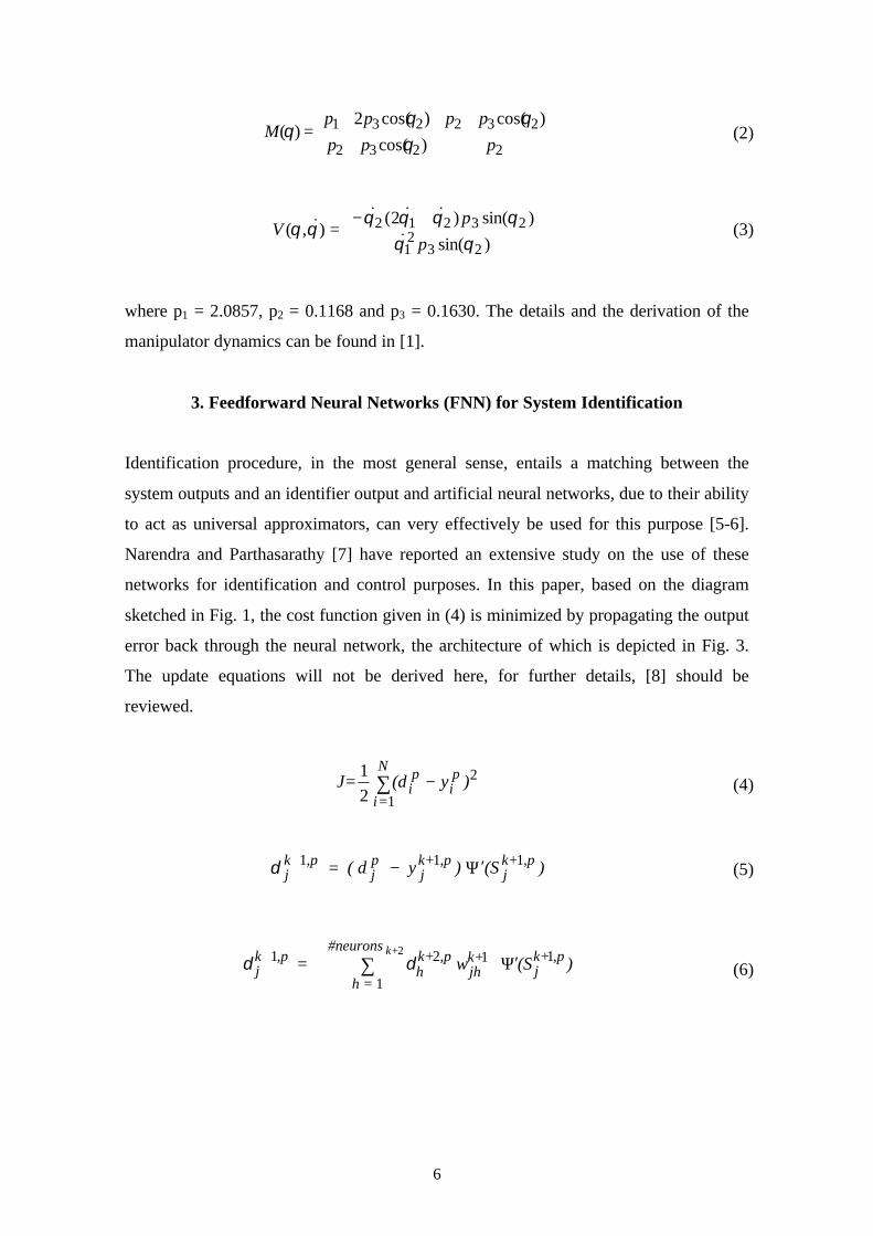
where p1 = 2.0857, p2 = 0.1168 and p3 = 0.1630. The details and the derivation of the

manipulator dynamics can be found in [1].

3. Feedforward Neural Networks (FNN) for System Identification

Identification procedure, in the most general sense, entails a matching between the

system outputs and an identifier output and artificial neural networks, due to their ability

to act as universal approximators, can very effectively be used for this purpose [5-6].

Narendra and Parthasarathy [7] have reported an extensive study on the use of these

networks for identification and control purposes. In this paper, based on the diagram

sketched in Fig. 1, the cost function given in (4) is minimized by propagating the output

error back through the neural network, the architecture of which is depicted in Fig. 3.

The update equations will not be derived here, for further details, [8] should be

reviewed.

∑=

−N

i

pi

pi )y(dJ=

1

2 2

1(4)

)(S) y ( d ,pk+j

,pk+j

pj

,pkj

111 Ψ′−=+δ (5)

)(S w ,pk+j

#neurons

h

k+jh

,pk+h

,pkj

k+ 1

1

121 2Ψ′

= ∑

=

+ δδ (6)

7

In (4), piy denotes the ith entry of pth pattern in neural network response, p

id denotes the

ith entry of pth target vector. Equations (5) and (6) give the delta values for the output

layer and hidden layer neurons respectively.

In (5) and (6), Sjk+1 denotes the net summation of the jth neuron in the (k+1)th layer, ψ

denotes the nonlinear activation function attached to each neuron in the hidden layer.

After the evaluation of the delta values during the backward pass, the weight update rule

given in (7) is applied for each training pair.

k,pi

,pkj

kij o w 1+=∆ δη (7)

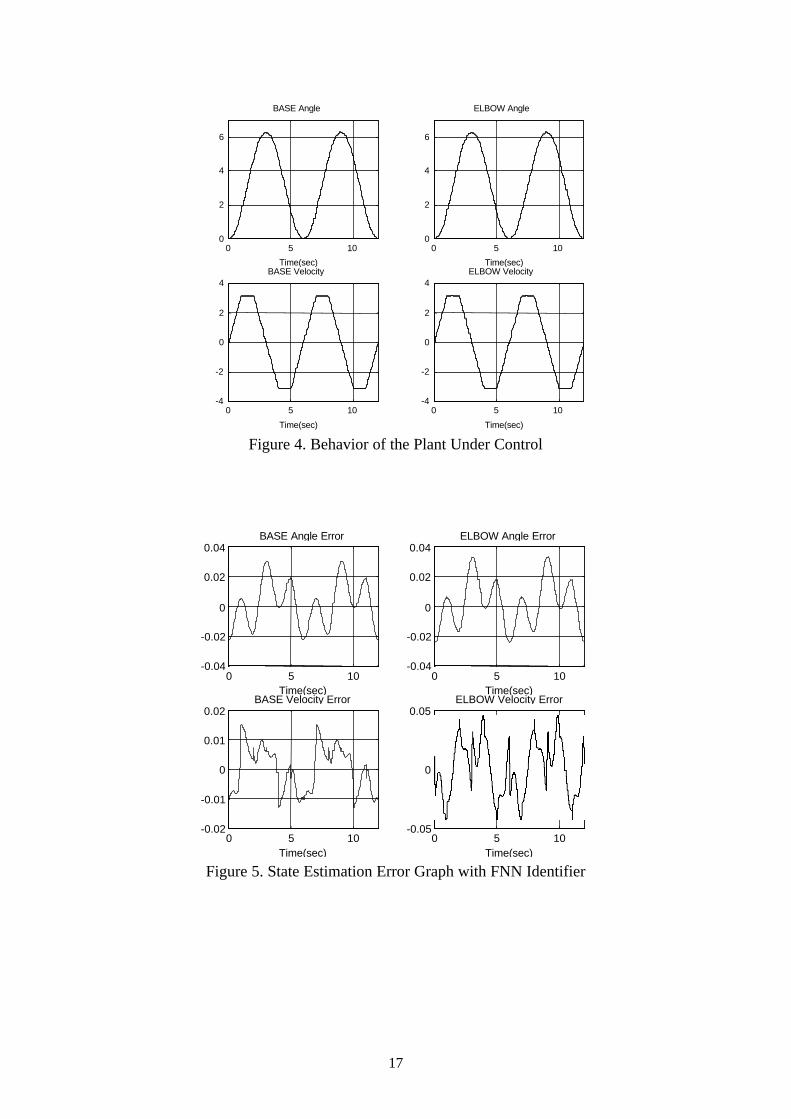
In the simulations, the plant is kept under an external control loop, which enforces the

manipulator to follow a trapezoidal velocity profile for both links as illustrated in Fig. 4.

All four approaches discussed throughout the paper aim to estimate the behavior in Fig.

4. The state estimation error graphs for FNN based identification scheme are presented

in Fig. 5.

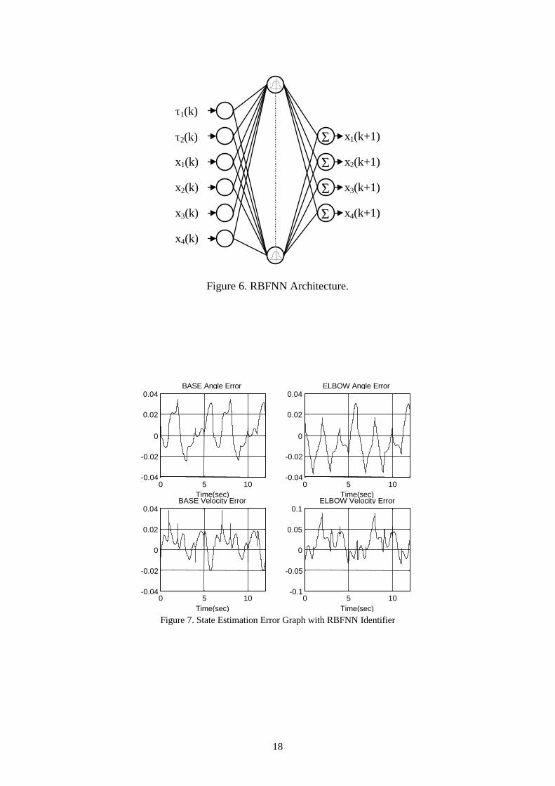
4. Radial Basis Function Neural Networks (RBFNN) for System Identification

In most of the literature, RBFNN are considered as a smooth transition between fuzzy

logic and neural networks. Structurally, RBFNN are composed of receptive units

(neurons) which act as the operators providing the information about the class to which

the input signal belongs. If the aggregation method, number of receptive units in the

hidden layer and the constant terms are equal to those of a Fuzzy Inference System

(FIS), then there exists a functional equivalence between RBFNN and FIS [2]. In Fig. 6,

a RBFNN structure is illustrated. Each neuron in the hidden layer provides a degree of

membership value for the input pattern with respect to the basis vector of the receptive

unit itself. The output layer is comprised of linear combiners. Neural network

interpretation makes RBFNN useful in incorporating the mathematical tractability,

especially in the sense of propagating the error back through the network, while the

fuzzy system interpretation enables the incorporation of the expert knowledge into the

identification procedure. The latter may be crucial in assigning the initial value of the

RBFNN parameter vector to a vector that is close to the optimal one. This results in

8

faster convergence in parameter space if the system dynamics is known. In this paper,

the parameter vector is randomly initialized.

In this approach, 12 hidden neurons are used. As is given by (8), each neuron output is

evaluated from the multiplication of the outputs of individual Gaussians corresponding

to each input. The overall response is evaluated through the multiplication of hidden

layer output vector by a matrix of appropriate dimensions. In fuzzy terms, this is

equivalent to say that, product inference rule is used with weighted sum defuzzifier. If

the network output and hidden layer output vectors are denoted by y and o respectively,

the activation level of ith receptive unit (or firing strength of ith rule) and the overall

realization performed by the network can be given by (8) and (9) respectively.

∏=

−=

inputs

j ij

ijji

w

cxo

#

12

2)( exp (8)

oWy neuronshiddenxoutputs # #= (9)

According to the error backpropagation rule, the parameter update law can be

summarized as follows:

ydoutput −=δ (10)

outputT

hidden W δδ = (11)

joutputijij okWkW i )()1( ηδ+=+ (12)

2

i )(

)(2)()1(

−+=+

kw

kcxokckc

ij

ijjjhiddenijij ηδ (13)

9

( )3

2

i )(

)(2)()1(

kw

kcxokwkw

ij

ijjjhiddenijij

−+=+ ηδ (14)

The state estimation error graphs for RBFNN based identification scheme are presented

in Fig. 7.

5. Runge-Kutta Neural Networks (RKNN) for System Identification

Runge-Kutta method is a powerful way of solving the behavior of a dynamic system if

the system is characterized by ordinary differential equations. In [9], the proposed

method is applied to several problems. Mainly, the method is observed to be successful

in estimating the system states given long enough time. It should be emphasized that the

neural network architecture realizes the changing rates of the system states instead of

the [x(k),ττ(k)]⇒ [x(k+1)] mapping. Therefore, the RKNN approach alleviates the

difficulties introduced by the discretization methods. As known, the first order

discretization brings large approximation errors. Wang and Lin has simulated the

approach with RBFNN architecture and trained the neural network for priorily observed

data [9]. This paper considers the approach with FNN, with on-line tuning of the

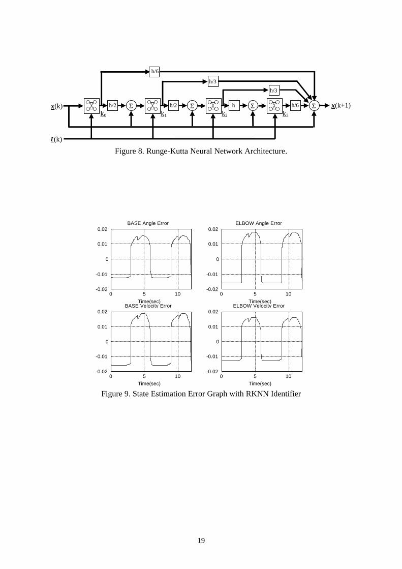
parameters. The RKNN architecture is illustrated in Fig. 8. In this figure, h denotes the

Runge-Kutta integration stepsize.

Robot dynamics can be stated more compactly as given by (15). All of the neural

networks appearing in Fig. 8, realize the vector function f. Therefore, for fourth order

Runge-Kutta approximation, the overall scheme is comprised of four times repeatedly

connected neural network blocks and corresponding stage gains. The update mechanism

is based on the error backpropagation. The derivation for FNN based identification

scheme is given in (16) through (25).

),( τxfx =& (15)

( )3210 226

)()1( kkkkh

ixix ++++=+ (16)

10

);( );( 00 φφ xNxNk == (17)

);();2

1( 101 φφ xNkhxNk =+= (18)

);();2

1( 212 φφ xNkhxNk =+= (19)

);( );( 323 φφ xNkhxNk =+= (20)

where, φ is a generic parameter of neural network. Figure 8 clarifies how the error

backpropagation rule is applied. There are two paths to be considered in this

propagation. The first is the direct connection to the output summation; the other is

through the FNN stages of the architecture. Therefore, each partial derivative, except

the first one, will concern two terms. The rule is summarized below for the fourth order

Runge-Kutta approximation.

∂φφ∂

∂φ∂ );( 00 xNk

= (21)

∂φ∂

∂φ∂

∂∂

∂∂

∂φ∂ 10

0

1

1

11 kk

k

x

x

kk+= (22)

∂φ∂

∂φ∂

∂∂

∂∂

∂φ∂ 21

1

2

2

22 kk

k

x

x

kk+= (23)

∂φ∂

∂φ∂

∂∂

∂∂

∂φ∂ 32

2

3

3

33 kk

k

x

x

kk+= (24)

( )

+++−=∆

∂φ∂

∂φ∂

∂φ∂

∂φ∂ηφ 3210 22)()(

6)(

kkkkixid

hi TT (25)

11

In (25), η represents the learning rate and d(i) represents the measured state vector of

the plant at time index i. Simulation results for RKNN methodology are presented in

Fig. 9.

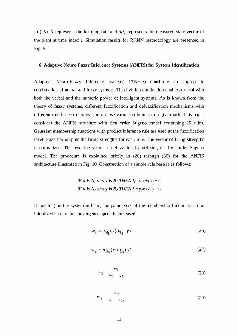
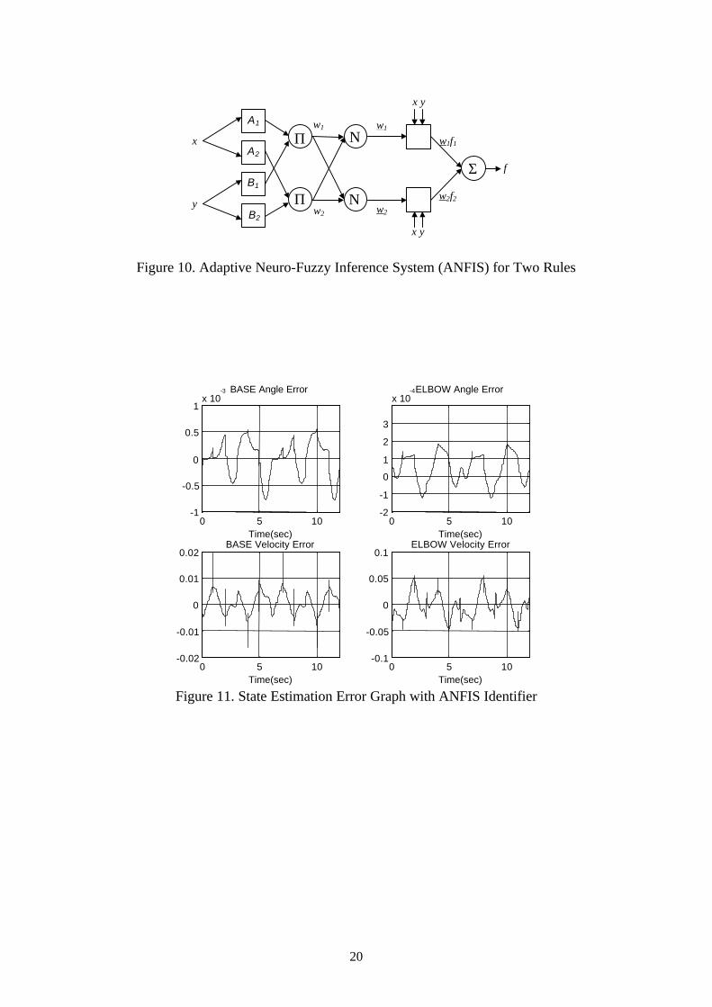
6. Adaptive Neuro Fuzzy Inference Systems (ANFIS) for System Identification

Adaptive Neuro-Fuzzy Inference Systems (ANFIS) constitute an appropriate

combination of neural and fuzzy systems. This hybrid combination enables to deal with

both the verbal and the numeric power of intelligent systems. As is known from the

theory of fuzzy systems, different fuzzification and defuzzification mechanisms with

different rule base structures can propose various solutions to a given task. This paper

considers the ANFIS structure with first order Sugeno model containing 25 rules.

Gaussian membership functions with product inference rule are used at the fuzzification

level. Fuzzifier outputs the firing strengths for each rule. The vector of firing strengths

is normalized. The resulting vector is defuzzified by utilizing the first order Sugeno

model. The procedure is explained briefly in (26) through (30) for the ANFIS

architecture illustrated in Fig. 10. Construction of a simple rule base is as follows:

IF x is A1 and y is B1 THEN f1=p1x+q1y+r1

IF x is A2 and y is B2 THEN f2=p2x+q2y+r2

Depending on the system in hand, the parameters of the membership functions can be

initialized so that the convergence speed is increased.

)()(111 yxw BA µµ= (26)

)()(222 yxw BA µµ= (27)

21

11 ww

ww

+= (28)

21

22 ww

ww

+= (29)

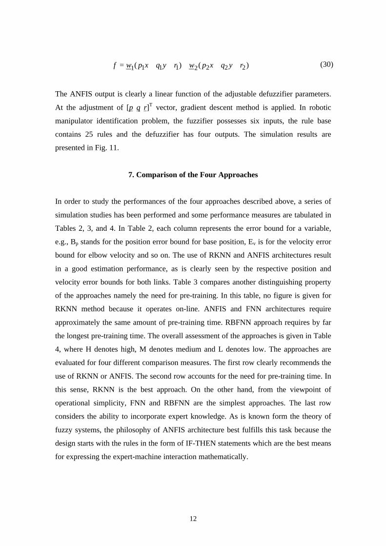
12

)()( 22221111 ryqxpwryqxpwf +++++= (30)

The ANFIS output is clearly a linear function of the adjustable defuzzifier parameters.

At the adjustment of [p q r]T vector, gradient descent method is applied. In robotic

manipulator identification problem, the fuzzifier possesses six inputs, the rule base

contains 25 rules and the defuzzifier has four outputs. The simulation results are

presented in Fig. 11.

7. Comparison of the Four Approaches

In order to study the performances of the four approaches described above, a series of

simulation studies has been performed and some performance measures are tabulated in

Tables 2, 3, and 4. In Table 2, each column represents the error bound for a variable,

e.g., Bp stands for the position error bound for base position, Ev is for the velocity error

bound for elbow velocity and so on. The use of RKNN and ANFIS architectures result

in a good estimation performance, as is clearly seen by the respective position and

velocity error bounds for both links. Table 3 compares another distinguishing property

of the approaches namely the need for pre-training. In this table, no figure is given for

RKNN method because it operates on-line. ANFIS and FNN architectures require

approximately the same amount of pre-training time. RBFNN approach requires by far

the longest pre-training time. The overall assessment of the approaches is given in Table

4, where H denotes high, M denotes medium and L denotes low. The approaches are

evaluated for four different comparison measures. The first row clearly recommends the

use of RKNN or ANFIS. The second row accounts for the need for pre-training time. In

this sense, RKNN is the best approach. On the other hand, from the viewpoint of

operational simplicity, FNN and RBFNN are the simplest approaches. The last row

considers the ability to incorporate expert knowledge. As is known form the theory of

fuzzy systems, the philosophy of ANFIS architecture best fulfills this task because the

design starts with the rules in the form of IF-THEN statements which are the best means

for expressing the expert-machine interaction mathematically.

13

8. Conclusions

This study analyzes the performance of soft-computing methodologies from the point of

system identification. In the assessment level, the estimation performance, together with

the training times are considered as the primary comparison measures. Numerous

simulations are performed on a two degrees of freedom direct drive robotic manipulator

model.

All four of the approaches are tested for the same command signal. For the tracking

error performance, ANFIS showed the best performance. On the other hand, RBFNN

and FNN are the simplest approaches in the sense of computational complexity.

Another important criterion is the requirement to a priori knowledge. Except the RKNN

approach, all methods need a pre-training phase.

The contribution of this paper is to show the identification performance of ANFIS

structure and to demonstrate the distinguished performance of the RKNN approach with

on-line operation and with ordinary feedforward neural network stages.

9. Acknowledgments

This work supported in part by Foundation for Promotion of Advanced Automation

Technology, FANUC grant and Bogazici University Research Fund (Project No:

97A0202).

14

Table 1. Manipulator Parameters

Motor 1 Rotor Inertia 0.267 I1 Payload Mass 0.00 Mp

Arm 1 Inertia 0.334 I2 Arm 1 length 0.359 L1

Motor 2 Rotor Inertia 0.0075 I3 Arm 2 length 0.24 L2

Motor2 Stator Inertia 0.040 I3C Arm 1 CG 0.136 L3

Arm 2 inertia 0.063 I4 Arm 2 CG 0.102 L4

Payload Inertia 0.000 IP Axis 1 Friction 5.3 F1

Motor 1 Mass 73.0 M1 Axis 2 Friction 1.1 F2

Arm 1 Mass 9.78 M2 Torque Limit 1 245.0

Motor 2 Mass 14.0 M3 Torque Limit 2 39.2

Arm 2 Mass 4.45 M4

Table 2. Comparison of the Estimation Methods.

Bp Ep Bv Ev Σ

FNN 40e-3 40e-3 20e-3 50e-3 150e-3

RBFNN 40e-3 40e-3 40e-3 10e-3 160e-3

RKNN 20e-3 20e-3 20e-3 20e-3 80e-3

ANFIS 1e-3 0.2e-3 20e-3 10e-3 31.2e-3

Table 3. Comparison of the Pre-Training Times.

Time (hours)

FNN 0.5

RBFNN 96

RKNN -

ANFIS 0.4

Table 4. Comparison of the Methods

FNN RBFNN RKNN ANFIS

Estimation performance L L M H

Pre-training time L H - L

Operational simplicity H H M M

Expert knowledge incorporation L M L H

15

References

[1] Direct Drive Manipulator R&D Package User Guide, Integrated Motions

Incorporated, 704 Gillman Street, Berkeley, California 94710.

[2] J.-S. R. Jang, C.-T. Sun and E. Mizutani, Neuro-Fuzzy and Soft Computing

(PTR Prentice Hall, Upper Saddle River, 1997) 335-368.

[3] L. X. Wang, A Course in Fuzzy Systems and Control (PTR Prentice Hall, Upper

Saddle River, 1997) 168-179.

[4] L. X. Wang, Adaptive Fuzzy Systems and Control, Design and Stability

Analysis (PTR Prentice Hall, New Jersey, 1994) 29-48.

[5] K. Funahashi, “On the Approximate Realization of Continuous Mappings by

Neural Networks,” Neural Networks, 2, (1989) 183-192.

[6] K. Hornik, “Multilayer Feedforward Networks are Universal Approximators,”

Neural Networks, 2, (1989) 359-366.

[7] K. S. Narendra, and K. Parthasarathy, “Identification and Control of Dynamical

Systems Using Neural Networks,” IEEE Transactions on Neural Networks, 1,

no.1 (1990) 4-27.

[8] D. E. Rumelhart, G. E. Hinton and R. J. Williams, “Learning Internal

Representations by Error Propagation,” in D. E. Rumelhart and J. L.

McClelland, eds., Parallel Distributed Processing, 1, (MIT Press, Cambridge,

1986) 318-362.

[9] Y.-J. Wang and C.-T. Lin “Runge-Kutta Neural Network for Identification of

Dynamical Systems in High Accuracy,” IEEE Transactions on Neural

Networks, 9, no.2 (1998) 294-307.

[10] K. Erbatur, O. Kaynak and I. J. Rudas, “An Inverse Dynamics Based Robot

Control Method Using Fuzzy Identifiers,” IEEE/ASME International

Conference on Advanced Intelligent Mechatronics, (Tokyo, 1997).

[11] M. O. Efe and O. Kaynak, “A Comparative Study of Neural Network Structures

in Identification of Nonlinear Systems,” Mechatronics, 9, no.3 (1999), 287-300.

16

Figure 1. Identification of a Robotic Manipulator

Figure 2. Architecture of a 2-DOF Planar Manipulator

Figure 3. FNN Architecture.

Σ

ROBOT

IDENTIFIER

ADAPTATIONMECHANISM

+

_

ExcitationInputs

e(k)

τ1(k)

x1(k+1)τ2(k)

x2(k+1)x1(k)

x3(k+1)x2(k)

x4(k+1)x3(k)

x4(k)

17

0 5 100

2

4

6

BASE Angle

Time(sec)

0 5 100

2

4

6

ELBOW Angle

Time(sec)

0 5 10-4

-2

0

2

4BASE Velocity

Time(sec)

0 5 10-4

-2

0

2

4ELBOW Velocity

Time(sec)

Figure 4. Behavior of the Plant Under Control

0 5 10-0.04

-0.02

0

0.02

0.04BASE Angle Error

Time(sec)0 5 10

-0.04

-0.02

0

0.02

0.04ELBOW Angle Error

Time(sec)

0 5 10-0.02

-0.01

0

0.01

0.02BASE Velocity Error

Time(sec)0 5 10

-0.05

0

0.05ELBOW Velocity Error

Time(sec)

Figure 5. State Estimation Error Graph with FNN Identifier

18

Figure 6. RBFNN Architecture.

0 5 10-0.04

-0.02

0

0.02


Time(sec)0 5 10

-0.04

-0.02

0

0.02


Time(sec)

0 5 10-0.04

-0.02

0

0.02


Time(sec)0 5 10

-0.1

-0.05

0

0.05


Time(sec)

Figure 7. State Estimation Error Graph with RBFNN Identifier

τ1(k)

x1(k+1)τ2(k)

x2(k+1)x1(k)

x3(k+1)x2(k)

x4(k+1)x3(k)

x4(k)

Σ

Σ

Σ

Σ

19

Figure 8. Runge-Kutta Neural Network Architecture.

0 5 10-0.02

-0.01

0

0.01


Time(sec)

0 5 10-0.02

-0.01

0

0.01


Time(sec)

0 5 10-0.02

-0.01

0

0.01


Time(sec)

0 5 10-0.02

-0.01

0

0.01


Time(sec)

Figure 9. State Estimation Error Graph with RKNN Identifier

Σ Σ Σ Σ

h/6

h/3

h/3

h/6hh/2h/2 x(k+1)x(k)

ττ(k)

k3k2k1k0

20

Figure 10. Adaptive Neuro-Fuzzy Inference System (ANFIS) for Two Rules

0 5 10-1

-0.5

0

0.5

1x 10

-3 BASE Angle Error

Time(sec)0 5 10

-2

-1

0

1

2

3

x 10-4ELBOW Angle Error

Time(sec)

0 5 10-0.02

-0.01

0

0.01


Time(sec)0 5 10

-0.1

-0.05

0

0.05


Time(sec)

Figure 11. State Estimation Error Graph with ANFIS Identifier

w1 w1

ΝΑ1

ΠΑ2

Β1

Β2w2

Σ

ΝΠw2

x y

w1f1x

f

w2f2y

x y

21

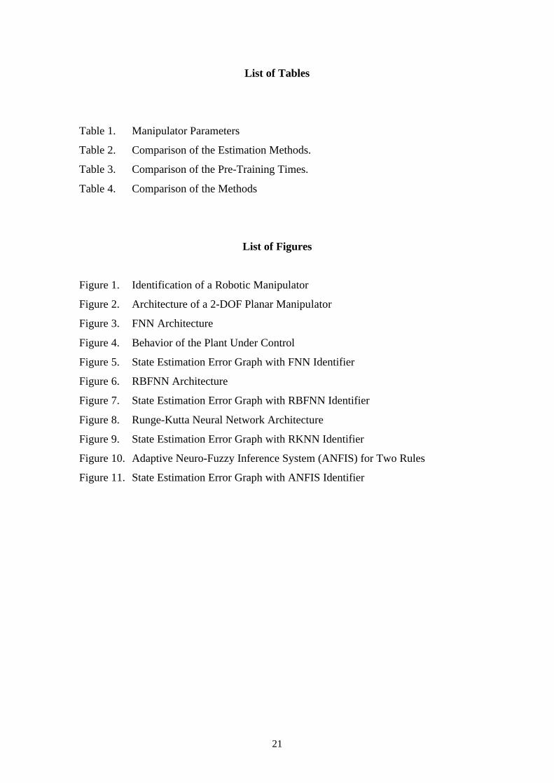
List of Tables

Table 1. Manipulator Parameters

Table 2. Comparison of the Estimation Methods.

Table 3. Comparison of the Pre-Training Times.

Table 4. Comparison of the Methods

List of Figures

Figure 1. Identification of a Robotic Manipulator

Figure 2. Architecture of a 2-DOF Planar Manipulator

Figure 3. FNN Architecture

Figure 4. Behavior of the Plant Under Control

Figure 5. State Estimation Error Graph with FNN Identifier

Figure 6. RBFNN Architecture

Figure 7. State Estimation Error Graph with RBFNN Identifier

Figure 8. Runge-Kutta Neural Network Architecture

Figure 9. State Estimation Error Graph with RKNN Identifier

Figure 10. Adaptive Neuro-Fuzzy Inference System (ANFIS) for Two Rules

Figure 11. State Estimation Error Graph with ANFIS Identifier

A comparative study of soft-computing methodologies in identification of robotic manipulators

Documents

Transcript of A comparative study of soft-computing methodologies in identification of robotic manipulators