1

A Comparative Study of Cost Estimation Models for Web Hypermedia Applications

Emilia Mendes1, Ian

Watson1, Chris Triggs2 1Computer Science Department

2Statistics Department The University of Auckland

Auckland, New Zealand 1{emilia,ian}@cs.auckland.ac.nz

2triggs@stat.auckland.ac.nz

Nile Mosley MxM Technology

Auckland, New Zealand nile_mosley@yahoo.com

Steve Counsell Computer Science Department

Birkbeck College, University of London

London, UK steve@dcs.bbk.ac.uk

Abstract Software cost models and effort estimates help project managers allocate resources, control costs and schedule and

improve current practices, leading to projects finished on time and within budget. In the context of Web development,

these issues are also crucial, and very challenging given that Web projects have short schedules and very fluidic scope. In

the context of Web engineering, few studies have compared the accuracy of different types of cost estimation techniques

with emphasis placed on linear and stepwise regressions, and Case-based Reasoning (CBR). To date only one type of

CBR technique has been employed in Web engineering. We believe results obtained from that study may have been

biased, given that other CBR techniques can also be used for effort prediction.

Consequently, the first objective of this study is to compare the prediction accuracy of three CBR techniques to estimate

the effort to develop Web hypermedia applications and to choose the one with the best estimates.

The second objective is to compare the prediction accuracy of the best CBR technique against two commonly used

prediction models, namely stepwise regression and regression trees.

One dataset was used in the estimation process and the results showed that the best predictions were obtained for stepwise

regression.

1. Introduction Software practitioners recognise the importance of realistic estimates of effort to the successful management of software

projects, the Web being no exception. Having realistic estimates at an early stage in a project's life cycle allow project

managers and development organisations to manage resources effectively.

In the context of Web development, cost estimation is also crucial, and very challenging given that:

• Web projects have short schedules and a fluidic scope (Pressman, 2000).

• There is no standard to sizing Web applications since they can be created using diverse technologies such as several

varieties of Java (Java, servlets, Enterprise java Beans, applets, and Java Server Pages), HTML, JavaScript, XML,

XSL, and so on.

• Web development differs substantially from traditional approaches (Reifer, 2002)

2

• Web project’s primary goal is to bring quality applications to market as quickly as possible, varying from a few

weeks (Pressman, 2000 ) to 6 months (Reifer, 2002).

• People involved in Web development are represented by less experienced programmers, users as developers, graphic

designers and new hires straight from university (Reifer, 2002).

• Typical project size is small, using 3 to 7 team members (Reifer, 2002).

• Processes employed are in general ad hoc, although some organisations are starting to look into the use of agile

methods (Ambler, 2002).

Several techniques for cost and effort estimation have been proposed over the last 30 years in software engineering,

falling into three general categories (Shepperd et al., 1996):

1) Expert judgement (EJ) – EJ has been widely used. However, the means of deriving an estimate are not explicit and

therefore not repeatable. Expert opinion, although always difficult to quantify, can be an effective estimating tool on its

own or as an adjusting factor for algorithmic models (Gray et al., 1999).

2) Algorithmic models (AM) – AM, to date the most popular in the literature, attempt to represent the relationship

between effort and one or more project characteristics. The main “cost driver” used in such a model is usually taken to be

some notion of software size (e.g. the number of lines of source code, number of pages, number of links). Algorithmic

models need calibration or adjustement to local circumstances. Examples of algorithmic models are the COCOMO model

(Boehm, 1981), the SLIM model (Putnam, 1978).

3) Machine learning (ML) - Machine learning techniques have in the last decade been used as a complement or

alternative to the previous two categories. Examples include fuzzy logic models (Kumar et al., 1994), regression trees

(Selby and Porter, 1998), neural networks (Srinivasan and Fisher, 1995), and case-based reasoning (Shepperd et al.,

1996). A useful summary of these techniques is presented in (Gray and MacDonell, 1997b).

An advantage of AM over ML and EJ is to allow users to see how a model derives its conclusions, an important factor for

verification as well as theory building and understanding of the process being modelled (Gray and MacDonell, 1997b).

Algorithmic models need to be calibrated relative to the local environment in which they are used, considered by some to

be an advantage (Kok et al., 1990; DeMarco, 1982).

Over the past 15 years numerous comparisons have been made in software engineering between the three categories of

prediction techniques aforementioned, based on their prediction power (Gray and MacDonell, 1997a; Gray and

MacDonell,1997b; Briand et al., 1999; Briand et al. 2000; Jeffery et al., 2000; Jeffery et al., 2001; Myrtveit and Stensrud,

1999; Shepperd et al., 1996; Shepperd and Schofield, 1997; Kadoda et al., 2001; Shepperd and Kadoda, 2001; Kemerer,

1987; Angelis and Stamelos, 2000; Finnie et al., 1997; Schofield, 1998; Hughes, 1997). However, as the datasets

employed had differing characteristics (outliers, collinearity, number of features, number of cases etc) and they engaged

different comparative designs, it is of little surprise that no convergence has been obtained to date.

In addition, Shepperd and Kadoda (2001) suggest that there is a strong relationship between the success of a particular

technique and training set size, nature of the “cost” function and characteristics of the dataset (outliers, collinearity,

3

number of features, number of cases etc), concluding that the “best” prediction technique might not be the right idea to

follow.

Most cost estimation comparisons in the software engineering literature use size attributes (e.g. lines of code, function

points) of conventional software as effort predictors. This paper looks at cost estimation modelling techniques based on

size attributes of Web hypermedia applications instead.

The World Wide Web (Web) has become the best known example of a hypermedia system. To date, numerous

organisations world-wide have developed thousands of commercial and/or educational Web applications. The Web has

been used as the delivery platform for two types of applications: Web hypermedia applications and Web software

applications (Christodoulou et al., 2000). A Web hypermedia application is a non-conventional application characterised

by the authoring of information using nodes (chunks of information), links (relations between nodes), anchors, access

structures (for navigation) and its delivery over the Web. Technologies commonly used for developing such applications

are HTML, JavaScript and multimedia. In addition, typical developers are writers, artists and organisations who wish to

publish information on the Web and/or CD-ROM without the need to know programming languages such as Java. These

applications have great potential in areas such as software engineering (Fielding and Taylor, 2000), literature (Tosca,

1999), education (Michau et al., 2001), and training (Ranwez at al., 2000).

A Web software application, on the other hand, represents any conventional software application that depends on the Web

or uses the Web's infrastructure for execution. Typical applications include legacy information systems such as databases,

booking systems, knowledge bases etc. Many e-commerce applications fall into this category. The technology employed

here are COTS components, components such as DCOM, OLE, ActiveX, XML, PHP, dynamic HTML, databases, and

development solutions such as J2EE. Typical developers are young programmers fresh from a Computer Science or

Software Engineering degree, managed by a few more senior staff.

Over the last three years our research has focused on proposing and comparing (Mendes et al., 2000; Mendes et al., 2001a;

Mendes et al., 2001b; Mendes et al., 2002a; Mendes et al., 2002b) cost estimation techniques for Web hypermedia

applications. The techniques used are Case-based Reasoning (CBR), linear and stepwise regressions. The only previous

study that compared all three techniques, using only one type of CBR, showed better prediction accuracy for CBR.

However, as design decisions (e.g. similarity measure, analogy adaptation), when building CBR prediction systems, are

influential upon the results (Kadoda et al., 2000), we believe results obtained previously may have been biased, given that

there are others CBR techniques that could also be used for effort prediction.

Consequently, this paper has two objectives: the first is to compare the prediction accuracy of three CBR techniques to

estimate the effort to develop Web hypermedia applications and to choose the one that gives the best estimates, according

to several measures of accuracy. The second objective is to compare the best CBR technique, according to our findings,

against two commonly used cost modelling techniques, namely stepwise regression and regression trees.

Our research objectives are reflected in the following questions:

1) Will different combinations of parameter categories (e.g. similarity measure, analogy adaptation) for the CBR

technique generate statistically significantly different prediction accuracy?

4

2) Which of the techniques employed in this study gives the most accurate predictions for the dataset?

These issues are investigated using a dataset containing 37 Web hypermedia projects developed by postgraduate and MSc

students attending a Hypermedia and Multimedia Systems course at the University of Auckland. Several confounding

factors, such as Web authoring experience, tools used, structure of the application developed, were controlled, so

increasing the validity of the obtained data.

The remainder of the paper is organised as follows: Section 2 provides a literature review and places this paper in the

context of existing research. Section 3 describes the cost modelling techniques we employ in this study. Section 4 gives

details on the dataset used. Results of our comparisons are presented in Section 5 and Section 6 presents our conclusions

and comments on future work.

2. Related Work To our knowledge, there are relatively few examples in the literature of studies that compare cost estimation techniques

for Web hypermedia applications (Mendes et al., 2000; Mendes et al., 2001b; Mendes et al., 2002a; Mendes et al., 2002b).

Most research in Web/hypermedia engineering has concentrated on the proposal of methods, methodologies and tools as a

basis for process improvement and higher product quality (Garzotto et al., 1993; Schwabe and Rossi, 1994;

Balasubramanian et al., 1995; Coda et al., 1998).

Mendes et al. (2000) (1st study) describes a case study involving the development of 76 Web hypermedia applications

structured according to the Cognitive Flexibility Theory (CFT) (Spiro et al., 1995) principles in which length size and

complexity size measures were collected. The measures obtained were page count, connectivity, compactness (Botafogo

et al., 1992), stratum (Botafogo et al., 1992) and reused page count. The original dataset was split into four homogeneous

datasets of sizes 22, 19, 15 and 14 respectively. Several prediction models were generated for each dataset using three

cost modelling techniques, namely multiple linear regression, stepwise regression, and case-based reasoning. Their

predictive power was compared using the Mean Magnitude of Relative Error (MMRE) and the Median Magnitude of

Relative Error (MdMRE) measures. Results showed that the best predictions were obtained using Case-based Reasoning

for all four datasets. Limitations of this study are: i) some measures used were highly subjective, which may have

influenced the validity of their results; ii) they applied only one CBR technique, measuring similarity between cases using

the unweight Euclidean distance and calculating the estimated effort using 1 analogy and the mean for 2 and 3 analogies;

iii) they compared predictions using only MMRE and MdMRE. As MMRE in fact measures the spread of z

(z=estimate/actual) rather than the accuracy (Kitchenham et al., 2001), other measures, such as boxplots of residuals and

boxplots of z, should be used as alternatives or complement to summary statistics.

Mendes et al. (2001b) (2nd study) describes a case study in which 37 Web hypermedia applications were used. These were

also structured according to the CFT principles and the Web hypermedia measures collected were organised into five

categories: length size, complexity size, reusability, effort and confounding factors. Size and reusability measures were

used to generate top down and bottom up prediction models using linear and stepwise regression techniques. They

compared the predictive power of the regression models using the MMRE measure. Both techniques presented similar

5

results. Limitations of this study are: i) they applied two very similar techniques, omitting techniques such as CBR and

regression trees. ii) they compared predictions using only MMRE.

The work we present in this paper is an extension of the 2nd study. We use the same dataset to investigate CBR techniques

and regression trees, and compare results using MMRE, MdMRE, Pred(25), boxplots of residuals and boxplots of z. We

compare different cost modelling techniques based on training and validation sets, randomly generated from the original

dataset. All models generated are top-down.

Mendes et al. (2002a) (3rd study) presents a case study where size measures of 37 Web hypermedia applications were

collected. Those measures correspond to three size categories, namely Length, Complexity and Functionality. This work

also used the same dataset employed on the 2nd study, however this time we investigated if different size measures would

lead to statistically significant different predictions. The aim was not to look for the “best” technique, but to compare size

measures, organised in three categories. Length and Complexity size measures had been collected when the data was

initially gathered. Functional size was manually measured for each Web application developed, which had been saved on

a CD-ROM. The COSMIC-FFP (1999) approach was used to measure functional size. For each size category we

generated prediction models using linear and stepwise regressions and assessed the prediction accuracy using boxplots of

the residuals (Kitchenham et al., 2001). Results suggested that all the models offered similar prediction accuracy,

indicating that relative to this dataset, it would not matter which size category is used. The work presented in this paper

uses size measures that reflect two categories (length and complexity). We have limited our analysis to size measures

which reflect current industrial practices for developing multimedia and Web hypermedia applications (Cowderoy, 2000;

Cowderoy et al., 1998). We also believe that functional size measures are more suited to Web software applications, as

they reflect applications exhibiting high degree of functionality manipulating structured data, in contrast to Web

hypermedia applications, which exhibit unstructured data and high navigability with low functionality.

Mendes et al. (2002b) (4th study) applies on another Web hypermedia dataset (25 cases) (DS2) the same three CBR

techniques we are employing in this paper. Regarding DS2, each application was developed by subject pairs. The size

measures collected were the same we use here, except for RMC and RPC. Despite DS2 presenting very different

characteristics to the one we employed in this paper, e.g., there is no linear relationship between size and effort,

collinearity is 2/5, several outliers. The best results were also obtained using the weighted Euclidean distance, where

higher weights were given to Page count (total number of HTML files) and Media count (total number of media files).

They measured prediction accuracy using MMRE, MdMRE and Pred(25). The limitation of this study is that it did not use

boxplots of residuals or boxplots of z. Both results converged suggesting that measures such as Page count and Media

count may indeed be strong candidates as effort predictors for the type of Web application we focus. In practice, we have

come across several Web consulting organisations who use those two size measures when costing Web hypermedia

development projects. Therefore, our results are an indication that we are at least heading in the right direction.

3. Cost Modelling Techniques 3.1 Choice of Techniques

6

Several cost modelling techniques have been compared in the Software engineering literature. Three of which, multiple

linear regression, stepwise regression and case-based reasoning, have also been compared in the Web engineering

literature.

For the scope of this paper we selected a subset of techniques based on the following criteria:

• Can the technique be automated? (Briand et al., 1999)

Similar to (Briand et al., 1999; Briand et al., 2000), we use a computationally intensive cross-validation approach to

calculate the accuracy values, opting for automated techniques.

• Has the technique been used previously in Software or Web engineering? (Briand et al., 1999)

By choosing techniques that had been used in Software and/or Web engineering would give the opportunity to compare

results, where applicable, looking for convergence with other techniques previously used.

• Are the results easy to understand from a practitioner's point of view? (Briand et al., 1999)

If cost modelling techniques are to be used by practitioners they should be easily understood to aid facilitation.

• Do the techniques chosen assume a highly contrasting approach to generate a prediction?

We wanted to compare techniques that generated predictions with a high degree of difference, similarly to (Shepperd and

Kadoda, 2001).

• Does the technique represent an area of significant research activity by the software metrics community?

We wanted to use techniques that represent areas of research activity in the community, also similarly to (Shepperd and

Kadoda, 2001).

Based on the criteria aforementioned we chose the following techniques:

• Case Based Reasoning (CBR)

• Stepwise Regression (SWR)

• Regression Trees (CART)

3.2 Case-based Reasoning

The rationale for CBR is the use of historical information from completed projects with known effort. It involves (Angelis

and Stamelos, 2000):

� Characterising a new active project p, for which an estimate is required, with attributes (features) common to those

completed project stored in the case base. In our context most features represent size measures which have a bearing

on effort. Feature values are normally standardized (between 0 and 1) such that they have the same degree of

influence on the results.

� Use of this characterisation as a basis for finding similar (analogous) completed projects, for which effort is known.

This process can be achieved by measuring the “distance” between two projects, based on the values for the k features

for these projects. Although numerous techniques can be used to measure similarity, nearest neighbour algorithms

7

(Okamoto and Satoh, 1995) using unweighted Euclidean distance measure have been the most widely used in

Software and Web engineering.

� Generation of a predicted value of effort for project p based on the effort for those completed projects that are similar

to p. The number of similar projects normally depends on the size of the dataset. For small datasets typical values are

1, 2 and 3 closest neighbours (analogies). The calculation of estimated effort is often obtained by using the same

effort value of the closest neighbour, or the mean of effort values (2 or more analogies). In Software engineering and

Web engineering a common choice is the nearest neighbour or the mean for 2 and 3 analogies.

When using CBR there are a number of parameters to decide upon (Shepperd and Kadoda, 2001):

• Feature Subset Selection

• Similarity Measure

• Scaling

• Number of analogies

• Analogy Adaptation

Each parameter in turn can be split into more detail, and maybe incorporated for a given CBR tool, allowing several CBR

configurations.

Each parameter is described below. We also indicate our choice and the motivation for each within this study.

All the results for CBR were obtained using CBR-Works (Schulz, 1995), a commercially available CBR tool.

3.2.1 Feature Subset Selection

Feature subset selection involves determining the optimum subset of features that give the most accurate estimation. Some

existing CBR tools, e.g. ANGEL (Shepperd and Schofield, 1997) optionally offer this functionality by applying a brute

force algorithm, searching for all possible feature subsets. CBR-Works does not offer such functionality, therefore every

time we had to obtain an estimated effort, we used all features in order to retrieve the most similar cases.

3.2.2 Similarity Measure

Similarity Measure measures the level of similarity between cases. Several similarity measures have been proposed in the

literature, however the ones we will describe here and use in this study are the unweighed Euclidean distance, the

weighted Euclidean distance and the Maximum distance. Readers are referred to (Angelis and Stamelos, 2000) for details

on other similarity measures. The motivation for using unweighted Euclidean (UE) and Maximum (MX) distances is that

they have been previously used with good results in cost estimation studies (UE: Shepperd and Schofield, 1997; Mendes

et al., 2000; MX: Angelis and Stamelos, 2000) and are applicable to quantitative variables, as in our case. The weighted

Euclidean was also chosen as it seemed reasonable to give different weights to our size measures (features) in order to

reflect the importance of each, rather to expect all size measures to have the same influence on effort. Our dataset has

seven size measures (section 4.2), representing different facets of size. Each similarity measure we used is described

below:

8

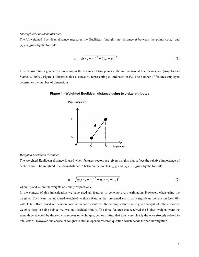
Unweighted Euclidean distance:

The Unweighted Euclidean distance measures the Euclidean (straight-line) distance d between the points (x0,y0) and

(x1,y1), given by the formula:

210

210 )()( yyxxd −+−= (1)

This measure has a geometrical meaning as the distance of two points in the n-dimensional Euclidean space (Angelis and

Stamelos, 2000). Figure 1 illustrates this distance by representing co-ordinates in E2. The number of features employed

determines the number of dimensions.

Figure 1 - Weighted Euclidean distance using two size attributes

Weighted Euclidean distance:

The weighted Euclidean distance is used when features vectors are given weights that reflect the relative importance of

each feature. The weighted Euclidean distance d between the points (x0,y0) and (x1,y1) is given by the formula:

210

210 )()( yywxxwd yx −+−= (2)

where wx and wy are the weights of x and y respectively.

In the context of this investigation we have used all features to generate every estimation. However, when using the

weighted Euclidean, we attributed weight=2 to those features that presented statistically significant correlation (α=0.01)

with Total effort, based on Pearson correlation coefficient test. Remaining features were given weight =1. The choice of

weights, despite being subjective, was not decided blindly. The three features that received the highest weights were the

same three selected by the stepwise regression technique, demonstrating that they were clearly the ones strongly related to

total effort. However, the choice of weights is still an opened research question which needs further investigation.

Page-count x0 x1

Page-complexity

Y1

Y0

d

0

9

Maximum measure:

The maximum measure computes the highest feature similarity, which is the one to define the closest analogy. For two

points (x0,y0) and (x1,y1), the maximum measure d is equivalent to the formula:

))(,)max(( 210

210 yyxxd −−= (3)

This effectively reduces the similarity measure down to a single feature, although the maximum feature may differ for

each retrieval episode. In other words, although we used 7 size features, for a given “new” project p, the closest project in

the case base will be the one that has at least one size feature that has the most similar value to the same feature for that

project p.

3.2.3 Scaling

Scaling or Standardisation represents the transformation of attribute values according to a defined rule such that all

attributes have the same degree of influence and the method is immune to the choice of units (Angelis and Stamelos,

2000). One possible solution is to assign zero to the minimum observed value and one to the maximum observed value

(Kadoda et al., 2000). This is the strategy used by ANGEL. We have scaled all features used in this study by dividing each

feature value by that features range, similarly to ANGEL.

3.2.4 Number of Analogies

The number of analogies refers to the number of most similar cases that will be used to generate the estimation. According

to Angelis and Stamelos (2000) when small sets of data are used it is reasonable to consider only a small number of

analogies. Several studies in software engineering have restricted their analysis to the closest analogy (k=1) (Briand et al.,

1999; Briand et al., 2000; Myrveit and Stensrud, 1999). However, we decided to use 1, 2 and 3 analogies, similarly to (;

Jeffery et al., 2001; Angelis and Stamelos, Schofield, 1998; Mendes et al., 2000; Mendes et al., 2001a; Jeffery et al.,

2000).

3.2.5 Analogy Adaptation

Once the most similar case(s) has/have been selected the next step is to decide how to generate the estimation for the

“new” project p. Choices of analogy adaptation techniques presented in the Software engineering literature vary from the

nearest neighbour (Briand et al., 1999; Jeffery et al., 2001), the mean of the closest analogies (Shepperd and Schofield,

1997), the median (Angelis and Stamelos, 2000), inverse distance weighted mean and inverse rank weighted mean

(Kadoda et al., 2000), to illustrate just a few. In the Web engineering literature, the adaptations used to date are the nearest

neighbour and mean of the closest analogies (Mendes et al., 2000; Mendes et al., 2001a), and the inverse rank weighted

mean (Mendes et al., 2002b).

We opted for the mean, median and the inverse rank weighted mean. Each adaptation and the motivation for using it are

explained as follows:

10

• Mean: Represents the average of k analogies, when k>1. Typical measure of central tendency, that has been used

often in the Software eng Web engineering literature. Treats all analogies as being equally influential on the outcome.

• Median: Represents the median of k analogies, when k>2. Another measure of central tendency, a more robust

statistics when the number of closest projects increases (Angelis and Stamelos, 2000). Although this measure when

used by Angelis and Stamelos (2000) did not present good results, measured using MMRE and Pred(25), we wanted

to observe how it would behave for our dataset.

• Inverse rank weighted mean: Allows higher ranked analogies to have more influence than lower ones. If we use 3

analogies, for example, the closest analogy (CA) would have weight = 3, the second closest (SC) weight = 2 and the

last one (LA) weight =1. The estimation would then be calculated as (3*CA + 2*SC + LA)/6). It seemed reasonable

to us to allow higher ranked analogies to have more influence than lower ranked ones, so we decided to use this

adaptation as well.

3.3 Stepwise Regression

Stepwise regression (Schroeder et al., 1986) builds a prediction model by adding to the model, at each stage, the variable

with the highest partial correlation to the response variable, taking into account all variables currently in the model. Its

aim is to find the set of predictors that maximise F. F assesses whether the regressors, taken together, are significantly

associated with the response variable. The criteria used to add a variable is whether it increases the F value for the

regression by some specified amount k. When a variable reduces F, also by some specified amount w, it is removed from

the model.

Stepwise regression has been frequently used as a benchmark (Shepperd et al., 1996; Kadoda et al., 2001; Shepperd and

Kadoda, 2001; Mendes et al., 2001b) and is regarded by some as a good prediction technique (Kok et al., 1990).

All statistical analyses presented in the paper, except for CBR and CART models, were conducted using the statistical

software SPSS v.10.01 (Kinnear and Gray, 1999).

3.4 Regression Trees (CART)

The objective of CART (Brieman et al., 1984) models is to develop a simple tree-structured decision process for

classifying an observation obs. The partitioning criteria are simple tests on single features: for numerical variables

numerical thresholds are used (e.g., Q: is MeC > 1.5); for categorical variables feature values are used (e.g., Q: is

authoring experience high?).

Trees used for problems with numerical features are often called regression trees and trees used for problems with

categorical features are often called classification trees. As all our features are numerical, we are using in this study a

regression tree.

CART models build a binary tree by recursively partitioning the predictor space into subsets where the distribution of the

response variable is successively more homogeneous. The partition is determined by splitting rules associated with each

11

of the internal nodes. Each observation is assigned to a unique leaf node, where the conditional distribution of the

response variable is determined.

The best splitting for each node is searched based on a "purity" function calculated from the data. The data is considered

to be pure when it contains data samples from only one class. The least squared deviation (LSD) measure of impurity was

applied to our dataset. This index is computed as the within-node variance, adjusted for frequency or case weights (if any).

For most cases we set the maximum tree depth to 5, the minimum number of cases in a parent node to 2 and the minimum

number of cases in child nodes to 1. We looked to trees that gave the small risk estimates (SRE), which were set at a

minimum of 95%, and calculated as:

SRE =

−−−

iancelainederrornodevarexp

1*100 (4)

where node-error is calculated as the within-node variance about the mean of the node. Explained-variance is calculated

as the within-node (error) variance plus the between-node (explained) variance.

By setting the SRE to a minimum of 95% we believe that we have captured the most important variables.

Our regression trees were generated using SPSS Answer Tree version 2.1.1.

4. Data Collection 4.1 Description

All analysis presented in this paper was based on a dataset containing information for 37 Web hypermedia applications

developed by postgraduate students.

Two questionnaires were used to collect the data. The first1 asked subjects to rate their Web authoring experience using

five scales, from no experience (one) to very good experience (five). The second questionnaire2 was used to measure

characteristics of the Web applications developed (suggested metrics) and the effort involved in designing and authoring

those applications. On both questionnaires, we describe in depth each scale type, to avoid any misunderstanding. Members

of the research group checked both questionnaires for ambiguous questions, unusual tasks, number of questions and

definitions in the Appendix.

To reduce learning effects, subjects were given a coursework prior to designing and authoring the Web applications,

which consisted of:

� Creating a simple personal homepage.

� Designing a multi-page Web application.

� Creating a Web site the Matakohe Kauri Museum3, improving on their existing site.

� Loading the Web pages onto a Web server.

1 The questionnaire is available at http://www.cs.auckland.ac.nz/~emilia/Assignments/exp-questionnaire.html. 2 The questionnaire is available at http://www.cs.auckland.ac.nz/~emilia/Assignments/questionnaire.html.

12

Finally, all subjects received training on the Cognitive Flexibility Theory authoring principles for approximately 150

minutes.

4.2 Measures

Each Web hypermedia application provided 46 variables (Mendes et al., 2001b), from which we identified 8 (Table 1), to

characterise a Web hypermedia application and its development process. These variables form a basis for our data

analysis. Total effort is our dependent/response variable and the other 7 variables are our independent/predictor variables.

All variables were measured on a ratio scale.

Table 2 outlines the properties of the dataset used. The original dataset of 37 observations had three outliers where total

effort was unrealistic compared to duration. Those outliers were removed from the dataset, leaving 34 observations.

Collinearity represents the number of statistically significant correlations with other independent variables out of the total

number of independent variables (Kadoda et al., 2001).

Summary statistics for all the variables are presented on table 3.

Table 1 - Size and Complexity Metrics Measure Description Page Count (PaC) Number of html or shtml files used in the application. Media Count (MeC) Number of media files used in the application. Program Count (PRC) Number of JavaScript files and Java applets used in the application. Reused Media Count (RMC) Number of reused/modified media files. Reused Program Count (RPC) Number of reused/modified programs. Connectivity Density (COD) Total number of internal links divided by Page Count. Total Page Complexity (TPC) Average number of different types of media per page. Total Effort (TE) Effort in person hours to design and author the application

Table 2 - Properties of the dataset

Number of Cases Features Categorical features Outliers Collinearity 34 8 0 0 2/7

Table 3 - Summary statistics for all variables Variable Mean Median Minimum Maximum Std. deviation Skewness

PaC 55.21 53 33 100 11.26 1.85 MeC 24.82 53 0 126 29.28 1.7 PRC 0.41 0 0 5 1.04 3.27 RMC 42.06 42.50 0 112 31.60 0.35 RPC 0.24 0 0 8 1.37 5.83 COD 10.44 9.01 1.69 23.30 6.14 0.35 TPC 1.16 1 0 2.51 0.57 0.33 TE 111.89 114.65 58.36 153.78 26.43 -0.36

3 http://www.hmu.auckland.ac.nz:8001/gilchrist/matakohe/.

13

All the measures collected, apart from total effort, were checked against the original Web hypermedia applications to

ensure that variables were precisely measured. Total effort was calculated as:

Total-effort = ∑ ∑∑=

=

=

=

=

=

++mj

j

ok

k

ni

i

PREMAEPAE0 01

(5)

where PAE is the page authoring effort, MAE the media authoring effort and PRE the program authoring effort (Mendes

et al., 2001b). When the dataset was collected, two levels of granularity were used to measure the total effort to develop a

Web hypermedia application: the first level (L1) collected effort with respect to coarser sub-tasks related to the

application's development process (e.g., effort to plan the interface, effort to test all links in the whole application); the

second level (L2) collected effort with respect to finer levels of granularity related to sub-tasks at the page, media and

program levels (e.g. effort to create links for each page, effort to digitise each media etc). To record the finer levels of

granularity subjects were given forms created using a spreadsheet, similar to those used in the PSP method (Humphrey,

1995). Although forms do not prevent the introduction of error in the data collection activity (Johnson and Disney, 1999),

we chose to use total-effort based on the finer granularity measures. We used a Wilcoxon Rank Sum Test (α = 0.01) to

check if L1 and L2 came from the same population. No statistically significant results were obtained. Although these

results do not mean that the two samples come from the same population, we cannot prove that they do not come from the

same population.

4.3 Threats to Validity

In this section we give our comments on the validity of the case study based on three types of threats to validity of an

empirical study (Kitchenham et al., 1995):

• Construct validity, that represents to what extent the predictor and response variables precisely measure the concepts

they claim to measure.

• Internal validity, that represents to what extent conclusions can be drawn about the causal effect of the predictor

variables on the response variables.

• External validity, that represents the domain to which a study’s findings can be generalised.

4.3.1 Construct validity

The criteria used to select our size measures was (Cowderoy, 2000): i) practical relevance for Web hypermedia

developers; ii) measures which are easy to learn and cheap to collect; iii) measures which can be estimated early in the

development. This applies in particular to PaC, MeC and RMC. iv) counting rules which were simple and consistent.

All size measures were re-measured to ensure that the information given by subjects was correct.

Some of our size measures (PaC and MeC) are currently used by Web consulting organisations to give preliminary costs

to develop an application.

14

Effort, as mentioned earlier, was collected using two levels of granularity, L1 and L2, where L1 used a questionnaire to

gather effort data on coarser sub-tasks related to the application's development process (e.g., effort to plan the interface,

effort to test all links in the whole application); L2 gathered effort with respect to finer levels of granularity related to sub-

tasks at the page, media and program levels (e.g. effort to create links for each page, effort to digitise each media etc).

Subjects had to fill in three different spreadsheets, related to page, media and program effort respectively, leading to a

time consuming activity. Further investigation of the data revealed that most values for effort, for a specific item (create a

link, create an image, scan an image etc), were either very similar or quite often the same, suggesting that subjects used

values they previously agreed upon, rather than measuring their own separately. It seemed as if they all had spent the same

amount of time to create an image, write a link and so on. As all students had very similar Web authoring experiences and

one could argue that the same effort is a consequence of having the same experience, although not possible to justify for

all 34 subjects.

Effort is notoriously difficult to measure accurately, even within the same organisation (Maxwell, 2001). A recent study

(Shepperd and Cartwright, 2001) described a case in which the total effort gathered for the same project, by three different

sources in the same organisation differed in over 30%.

We do not wish to claim that our effort data has not been biased, however, when one of the authors inquired some Web

development organisations whether the total effort values given would be realistic in practice for the types of Web

hypermedia applications developed, the answers obtained indicated that they were.

We are aware that unless effort and duration are collected automatically, there will always be a very high probability to

have obtained biased data. In light of that we have developed a measurement tool, to be used in an experiment in the

second semester/2002, that measures automatically effort and duration. This tool will be available free of charge for the

metrics community, hoping that it will help academics and organisations alike to gather reliable effort and duration data.

4.3.2 Internal validity

There were four confounding factors in the case study evaluation:

• Subjects' Web development experience.

• Maturation effects, i.e. learning effects caused by subjects learning as an experiment proceeds.

• Structure of the application.

• Tools used to help develop the Web hypermedia application.

The data collected revealed that:

Subjects' development experiences were mostly scaled little (experience=2) or average (experience=3), with a low skill

differential4. A scatterplot between experience and effort was used to investigate their relationship. Most datapoints fell

within the same clusters, either for experience 2 or 3. Consequently the original dataset was left intact.

Prior to developing the Web hypermedia applications, subjects had to develop a small Web hypermedia application as part

of a previous coursework. In addition, they all received training in the CFT principles, reducing maturation effects.

15

Notepad (or similar text editor) and FirstPage were the two tools most frequently used. Notepad is a simple text editor

while FirstPage is freeware offering button-embedded HTML tags. Although they differ with respect to the functionality

offered, a scatterplot between total-effort and tool revealed that for both tools most datapoints fell within the same

clusters. Consequently, confounding effects from the tools were reduced.

The instrumentation effects in general did not occur in this evaluation; the questionnaires used were the same.

4.3.3 External validity

The results may be domain dependent as all subjects answered the questionnaires based on their experience in developing

Web hypermedia applications for education. This evaluation should therefore be repeated in domains other than education

if the results are to be generalised to other domains.

The web hypermedia applications developed were all static, having a mean of 55 pages, 24 original media files and 42

reused media files per application. Recently one of the authors had to search on the Web for several examples of static

Web hypermedia applications and, out of a total of 30 applications, more than half had on average 25-30 pages, well

below our average of 55. Therefore, we are convinced that our applications can be representative of small to medium size

(Lowe and Hall, 1998) static Web hypermedia applications.

Our dataset contains 34 projects. This is not a large dataset. However, if compared to the size of software datasets publicly

available5, 34 is above their median of 26 projects.

In addition, it is worth mentioning that subjects had only two weeks to develop their applications, which would roughly

correspond to an average effort of 0.9 person/month. Despite Web projects normally lasting for a short period of time

(often less than one of two months) (Pressman, 2000), or up to six months (Reifer, 2002), two weeks would only be

representative of projects that are very short. Consequently, further investigation based on Web hypermedia projects with

longer duration are necessary in order to make results applicable to a wider range of projects.

In terms of financial risks for stakeholders, and assuming our dataset to be representative of Web hypermedia projects, our

comments are as follows:

If we estimate a project to use 111 person/hours (effort mean), and it uses another 24 person/hours (roughly 3 working

days), that would represent an increase of 21.6% on schedule and costs. Suppose that the organisation developing the

application charges 100 dollars per person/hour. The total cost of 11,100 dollars would have an increase of 2,160 dollars.

If our reality represents small organisations and small clients, that increase in costs would be significant.

Subjects had very similar Web authoring experience and were either final year undergraduate students or MSc students. It

is likely that they present skill sets similar to Web professionals at the start of their careers (Reifer, 2002).

Each Web hypermedia application was developed by one subject. This might not be representative of typical Web projects

involving 3 to 7 team members. However, if our focus is on small Web development organisations where sometimes the

total number of employees is not greater than a handful, having a single person developing a Web hypermedia application

4 low difference between skill levels 5 Albrecht with 24; Atkinson with 21; Desharnais with 81; Finnish with 38; Kemerer with 15; Mermaid with 28. Information obtained from (Shepperd

16

is more likely to occur. The organisation might employ, for example, one graphics designer who does all the graphics and

interface design, and a few programmers who develop applications on HTML + Javascript. If that is the case, our

prediction models do not need to assume large project teams such that individual performance be cancelled out. In

addition, for small organisations, it is more likely that they will employ individuals who already have a reasonable

expertise in what they do, in order to reduce risks.

Finally, the use of students as subjects was the only viable option for this case study.

5. Results 5.1 Summary statistics and Measures of Prediction Accuracy

The most common approaches to date to assess the predictive power of effort prediction models have been:

• The Magniture of Relative Error (MRE) (Kemerer, 1987)

• The Mean Magnitude of Relative Error (MMRE) (Shepperd et al., 1996)

• The Median Magnitude of Relative Error (MdMRE) (Myrtveit and Stensrud, 1999)

• The Prediction at level n (Pred(n)) (Shepperd and Schofield, 1997)

MRE if the basis for calculating MMRE and MdMRE, and defined as:

MRE = e

ee − (6)

where e represents actual effort and ê estimated effort.

The mean of all MREs is the MMRE, which is calculated as:

MMRE = ∑=

=

−ni

i i

ii

eee

n 1

ˆ1 (7)

The mean takes into account the numerical value of every observation in the data distribution, and is sensitive to

individual predictions with large MREs.

An option to the mean is the median, which also represents a measure of central tendency, however it is less sensitive to

extreme values. The median of MRE values for the number i of observations is called the MdMRE.

Another indicator which is commonly used is the Prediction at level l, also known as Pred(l). It measures the percentage

of estimates that are within l% of the actual values. Suggestions have been made (Conte et al., 1986) that l should be set at

25% and that a good prediction system should offer this accuracy level 75% of the time.

Although MMRE, MdMRE and Pred(l) have emerged as the de facto standard evaluation criteria to assess the accuracy of

cost estimation models (Stensrud et al., 2002), recent work by Kitchenham et al. (2001) shows that MMRE and Pred(l) are

respectively measures of the spread and kurtosis of z, where (z = ee ). They suggest boxplots of z and boxplots of the

and Kadoda, 2001).

17

residuals ( ee ˆ− ) (Pickard et al., 1999) as useful alternatives to simple summary measures since they can give a good

indication of the distribution of residuals and z and can help explain summary statistics such as MMRE and Pred(25)

(Kitchenham et al., 2001).

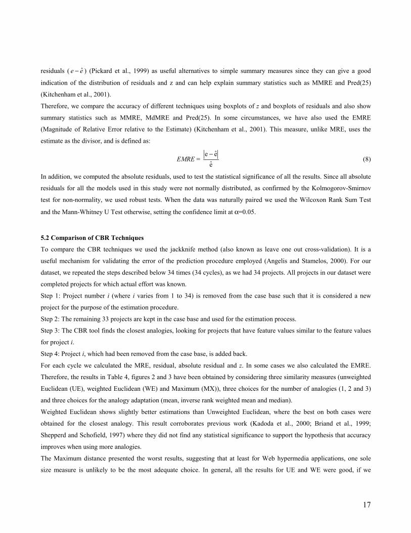
Therefore, we compare the accuracy of different techniques using boxplots of z and boxplots of residuals and also show

summary statistics such as MMRE, MdMRE and Pred(25). In some circumstances, we have also used the EMRE

(Magnitude of Relative Error relative to the Estimate) (Kitchenham et al., 2001). This measure, unlike MRE, uses the

estimate as the divisor, and is defined as:

EMRE = e

ee − (8)

In addition, we computed the absolute residuals, used to test the statistical significance of all the results. Since all absolute

residuals for all the models used in this study were not normally distributed, as confirmed by the Kolmogorov-Smirnov

test for non-normality, we used robust tests. When the data was naturally paired we used the Wilcoxon Rank Sum Test

and the Mann-Whitney U Test otherwise, setting the confidence limit at α=0.05.

5.2 Comparison of CBR Techniques

To compare the CBR techniques we used the jackknife method (also known as leave one out cross-validation). It is a

useful mechanism for validating the error of the prediction procedure employed (Angelis and Stamelos, 2000). For our

dataset, we repeated the steps described below 34 times (34 cycles), as we had 34 projects. All projects in our dataset were

completed projects for which actual effort was known.

Step 1: Project number i (where i varies from 1 to 34) is removed from the case base such that it is considered a new

project for the purpose of the estimation procedure.

Step 2: The remaining 33 projects are kept in the case base and used for the estimation process.

Step 3: The CBR tool finds the closest analogies, looking for projects that have feature values similar to the feature values

for project i.

Step 4: Project i, which had been removed from the case base, is added back.

For each cycle we calculated the MRE, residual, absolute residual and z. In some cases we also calculated the EMRE.

Therefore, the results in Table 4, figures 2 and 3 have been obtained by considering three similarity measures (unweighted

Euclidean (UE), weighted Euclidean (WE) and Maximum (MX)), three choices for the number of analogies (1, 2 and 3)

and three choices for the analogy adaptation (mean, inverse rank weighted mean and median).

Weighted Euclidean shows slightly better estimations than Unweighted Euclidean, where the best on both cases were

obtained for the closest analogy. This result corroborates previous work (Kadoda et al., 2000; Briand et al., 1999;

Shepperd and Schofield, 1997) where they did not find any statistical significance to support the hypothesis that accuracy

improves when using more analogies.

The Maximum distance presented the worst results, suggesting that at least for Web hypermedia applications, one sole

size measure is unlikely to be the most adequate choice. In general, all the results for UE and WE were good, if we

18

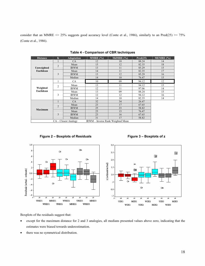
consider that an MMRE <= 25% suggests good accuracy level (Conte et al., 1986), similarly to an Pred(25) >= 75%

(Conte et al., 1986).

Table 4 - Comparison of CBR techniques

Distance K Adaptation MMRE (%) MdMRE (%) Pred(25) MEMRE (%) 1 CA 12 10 88.24 14

Mean 15 12 82.35 18 2 IRWM 13 11 85.29 15 Mean 14 11 82.35 17

IRWM 13 12 85.29 16

Unweighted Euclidean

3 Median 14 10 76.47 15

1 CA 10 09 94.12 12 Mean 13 11 94.12 15 2

IRWM 12 11 97.06 14 Mean 13 09 88.24 15

IRWM 12 12 94.12 16

Weighted Euclidean

3 Median 14 10 82.35 14

1 CA 32 34 26.47 Mean 23 17 67.65 2 IRWM 25 23 58.82 Mean 25 15 76.47

IRWM 23 16 67.65

Maximum

3 Median 31 17 58.82

CA – Closest Analogy IRWM – Inverse Rank Weighted Mean

Figure 2 – Boxplots of Residuals Figure 3 – Boxplots of z

Boxplots of the residuals suggest that:

• except for the maximum distance for 2 and 3 analogies, all medians presented values above zero, indicating that the

estimates were biased towards underestimation.

• there was no symmetrical distribution.

19

• both UE and WE for one analogy, the ones that presented the best predictions according to the summary statistics,

showed positively skewed distributions, where WE has a tighter spread and is more peaked than UE.

Both boxplots of residuals and boxplots of z suggest that WE for 1 analogy gives better predictions than other models: the

box length and tails are smaller than the box length and the tails for other models. In addition, the outlier for the WE

model for 1 analogy is less extreme than outliers from other models.

Most CBR models used in this study tend to underestimate, observed by the number of medians above zero, for boxplots

of the residuals, and below one, for boxplots of z. These are not promising results for CBR, based on our dataset, as in

most cases overestimates are less serious than underestimates (Kitchenham et al., 2001).

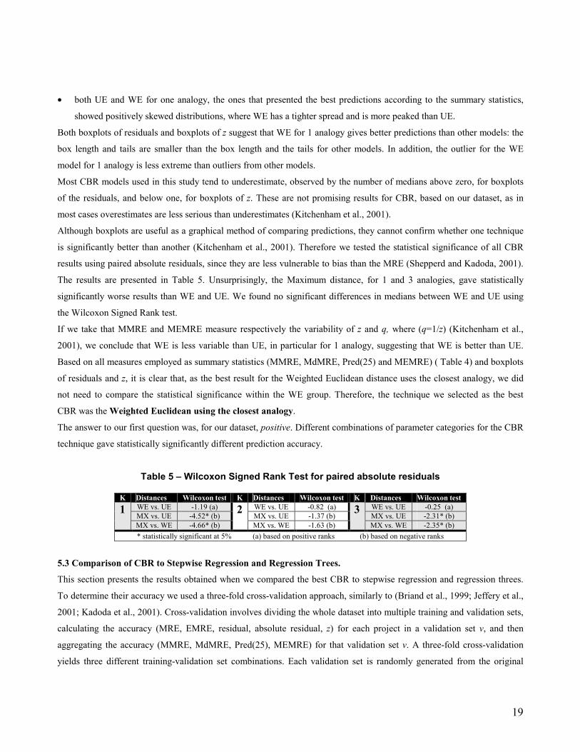
Although boxplots are useful as a graphical method of comparing predictions, they cannot confirm whether one technique

is significantly better than another (Kitchenham et al., 2001). Therefore we tested the statistical significance of all CBR

results using paired absolute residuals, since they are less vulnerable to bias than the MRE (Shepperd and Kadoda, 2001).

The results are presented in Table 5. Unsurprisingly, the Maximum distance, for 1 and 3 analogies, gave statistically

significantly worse results than WE and UE. We found no significant differences in medians between WE and UE using

the Wilcoxon Signed Rank test.

If we take that MMRE and MEMRE measure respectively the variability of z and q, where (q=1/z) (Kitchenham et al.,

2001), we conclude that WE is less variable than UE, in particular for 1 analogy, suggesting that WE is better than UE.

Based on all measures employed as summary statistics (MMRE, MdMRE, Pred(25) and MEMRE) ( Table 4) and boxplots

of residuals and z, it is clear that, as the best result for the Weighted Euclidean distance uses the closest analogy, we did

not need to compare the statistical significance within the WE group. Therefore, the technique we selected as the best

CBR was the Weighted Euclidean using the closest analogy.

The answer to our first question was, for our dataset, positive. Different combinations of parameter categories for the CBR

technique gave statistically significantly different prediction accuracy.

Table 5 – Wilcoxon Signed Rank Test for paired absolute residuals

K Distances Wilcoxon test K Distances Wilcoxon test K Distances Wilcoxon test WE vs. UE -1.19 (a) WE vs. UE -0.82 (a) WE vs. UE -0.25 (a) MX vs. UE -4.52* (b) MX vs. UE -1.37 (b) MX vs. UE -2.31* (b)

1 MX vs. WE -4.66* (b)

2MX vs. WE -1.63 (b)

3MX vs. WE -2.35* (b)

* statistically significant at 5% (a) based on positive ranks (b) based on negative ranks

5.3 Comparison of CBR to Stepwise Regression and Regression Trees.

This section presents the results obtained when we compared the best CBR to stepwise regression and regression threes.

To determine their accuracy we used a three-fold cross-validation approach, similarly to (Briand et al., 1999; Jeffery et al.,

2001; Kadoda et al., 2001). Cross-validation involves dividing the whole dataset into multiple training and validation sets,

calculating the accuracy (MRE, EMRE, residual, absolute residual, z) for each project in a validation set v, and then

aggregating the accuracy (MMRE, MdMRE, Pred(25), MEMRE) for that validation set v. A three-fold cross-validation

yields three different training-validation set combinations. Each validation set is randomly generated from the original

20

dataset, and we use the remaining projects as the training set. There is no standard to what is the best size for training sets.

However, as it seems that larger training sets reduce prediction errors (measured as absolute residuals) (Shepperd and

Kadoda, 2001) we decided to use two different types of split where there were always more projects in the training set

than in the validation set, similarly to (Briand et al., 2000). The first (SP1) was a 66% split (23 observations in the training

set and 11 in validation set) and the second (SP2) was a 86% split (29 observations in the training set and 5 in the

validation set). We therefore had in total six different combinations for each technique employed. Having training sets of

different sizes would also give an opportunity to compare their prediction accuracy using absolute residuals.

In addition to estimating effort based on training sets, we also used as estimated effort the mean effort, to assess if any

cost estimation techniques would give significantly better results than the simple mean effort.

For the stepwise regression model we addressed several issues (Myrtveit and Stensrud, 1999):

• Does the model use the right and most important attributes?

• Is the formal model correctly specified?

To investigate the first issue we performed a Pearson's correlation looking for those attributes significantly correlated to

total effort (α=0.01). Three attributes, namely Page Count (PaC), Media Count (MeC) and Reused Media Count (RMC),

were commonly selected. This result supports information obtained from several practitioners regarding those attributes

taken into consideration when bidding for Web hypermedia development projects.

To investigate the second issue we verified the distribution of the residuals looking for any unusual patterns. The analysis

of the residuals did not indicate any non-linearity.

The final linear models for stepwise regression presented very high R2 (adj.) (Table 6), making it difficult not to choose

stepwise regression as the best cost estimation technique for our dataset.

Table 6 - Formulas for the Stepwise Regression Models

Split Version Formula R2 adj. v1 5.107 + 1.276 PaC+ 0.644 MeC + 0.490 RMC 0.957 v2 10.068 +1.226 PaC + 0.626 MeC + 0.470 RMC 0.945 SP1 v3 5.712 +1.256 PaC + 0.653 MeC + 0.495 RMC 0.967 v1 5.295 +1.284 PaC + 0.619 MeC + 0.490 RMC 0.97 v2 4.710 +1.298 PaC + 0.6 MeC + 0.484 RMC 0.986 SP2 v3 5.325 +1.292 PaC + 0.589 MeC + 0.476 RMC 0.985

Summary statistics for z, organised by split and versions, are presented in Table7.

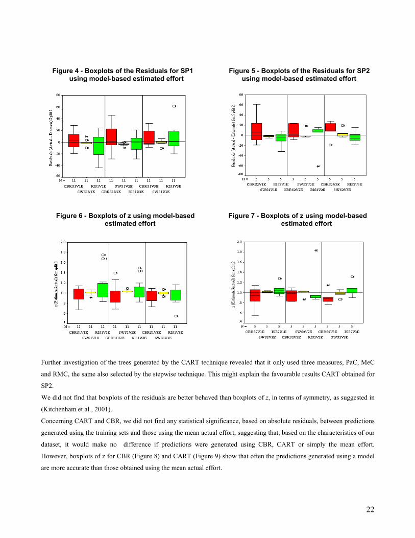
Boxplots of residuals6 (Figures 4 and 5) suggest that stepwise regression gives the best prediction accuracy for SP1 and

SP2, confirmed by the tests of significance using absolute residuals (Table 8). Boxplots of z (Figures 6 and 7) show very

similar pattern for SP1 as presented by boxplots of residuals, however for SP2, some boxplots for CART (versions 2 and

3), although with distributions of higher spread than those for SW, did not show any statistical significance based on

absolute residuals. All tests of significance were the same when we used paired MREs. These results were confirmed by

the Wilcoxon Signed rank test based on absolute residuals (Table 8).

6 CART variables are identified as RI, which stands for rule induction.

21

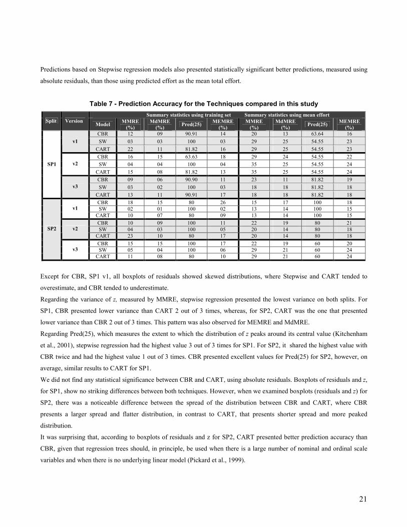
Predictions based on Stepwise regression models also presented statistically significant better predictions, measured using

absolute residuals, than those using predicted effort as the mean total effort.

Table 7 - Prediction Accuracy for the Techniques compared in this study Summary statistics using training set Summary statistics using mean effort

Split Version Model MMRE (%)

MdMRE (%) Pred(25) MEMRE

(%) MMRE

(%) MdMRE

(%) Pred(25) MEMRE (%)

CBR 12 09 90.91 14 20 13 63.64 16 SW 03 03 100 03 29 25 54.55 23 v1

CART 22 11 81.82 16 29 25 54.55 23 CBR 16 15 63.63 18 29 24 54.55 22 SW 04 04 100 04 35 25 54.55 24 v2

CART 15 08 81.82 13 35 25 54.55 24 CBR 09 06 90.90 11 23 11 81.82 19 SW 03 02 100 03 18 18 81.82 18

SP1

v3 CART 13 11 90.91 17 18 18 81.82 18 CBR 18 15 80 26 15 17 100 18 SW 02 01 100 02 13 14 100 15 v1

CART 10 07 80 09 13 14 100 15 CBR 10 09 100 11 22 19 80 21 SW 04 03 100 05 20 14 80 18 v2

CART 23 10 80 17 20 14 80 18 CBR 15 15 100 17 22 19 60 20 SW 05 04 100 06 29 21 60 24

SP2

v3 CART 11 08 80 10 29 21 60 24

Except for CBR, SP1 v1, all boxplots of residuals showed skewed distributions, where Stepwise and CART tended to

overestimate, and CBR tended to underestimate.

Regarding the variance of z, measured by MMRE, stepwise regression presented the lowest variance on both splits. For

SP1, CBR presented lower variance than CART 2 out of 3 times, whereas, for SP2, CART was the one that presented

lower variance than CBR 2 out of 3 times. This pattern was also observed for MEMRE and MdMRE.

Regarding Pred(25), which measures the extent to which the distribution of z peaks around its central value (Kitchenham

et al., 2001), stepwise regression had the highest value 3 out of 3 times for SP1. For SP2, it shared the highest value with

CBR twice and had the highest value 1 out of 3 times. CBR presented excellent values for Pred(25) for SP2, however, on

average, similar results to CART for SP1.

We did not find any statistical significance between CBR and CART, using absolute residuals. Boxplots of residuals and z,

for SP1, show no striking differences between both techniques. However, when we examined boxplots (residuals and z) for

SP2, there was a noticeable difference between the spread of the distribution between CBR and CART, where CBR

presents a larger spread and flatter distribution, in contrast to CART, that presents shorter spread and more peaked

distribution.

It was surprising that, according to boxplots of residuals and z for SP2, CART presented better prediction accuracy than

CBR, given that regression trees should, in principle, be used when there is a large number of nominal and ordinal scale

variables and when there is no underlying linear model (Pickard et al., 1999).

22

Figure 4 - Boxplots of the Residuals for SP1 Figure 5 - Boxplots of the Residuals for SP2 using model-based estimated effort using model-based estimated effort

Figure 6 - Boxplots of z using model-based Figure 7 - Boxplots of z using model-based estimated effort estimated effort

Further investigation of the trees generated by the CART technique revealed that it only used three measures, PaC, MeC

and RMC, the same also selected by the stepwise technique. This might explain the favourable results CART obtained for

SP2.

We did not find that boxplots of the residuals are better behaved than boxplots of z, in terms of symmetry, as suggested in

(Kitchenham et al., 2001).

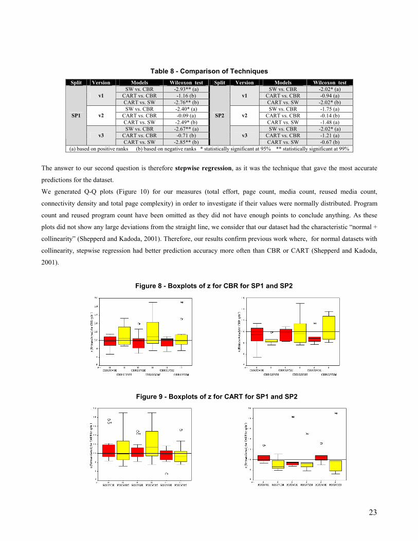
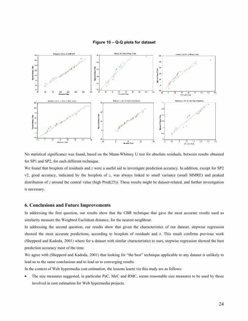
Concerning CART and CBR, we did not find any statistical significance, based on absolute residuals, between predictions

generated using the training sets and those using the mean actual effort, suggesting that, based on the characteristics of our

dataset, it would make no difference if predictions were generated using CBR, CART or simply the mean effort.

However, boxplots of z for CBR (Figure 8) and CART (Figure 9) show that often the predictions generated using a model

are more accurate than those obtained using the mean actual effort.

23

Table 8 - Comparison of Techniques Split Version Models Wilcoxon test Split Version Models Wilcoxon test

SW vs. CBR -2.93** (a) SW vs. CBR -2.02* (a) CART vs. CBR -1.16 (b) CART vs. CBR -0.94 (a) v1 CART vs. SW -2.76** (b)

v1 CART vs. SW -2.02* (b)

SW vs. CBR -2.40* (a) SW vs. CBR -1.75 (a) CART vs. CBR -0.09 (a) CART vs. CBR -0.14 (b) v2 CART vs. SW -2.49* (b)

v2 CART vs. SW -1.48 (a)

SW vs. CBR -2.67** (a) SW vs. CBR -2.02* (a) CART vs. CBR -0.71 (b) CART vs. CBR -1.21 (a)

SP1

v3 CART vs. SW -2.85** (b)

SP2

v3 CART vs. SW -0.67 (b)

(a) based on positive ranks (b) based on negative ranks * statistically significant at 95% ** statistically significant at 99%

The answer to our second question is therefore stepwise regression, as it was the technique that gave the most accurate

predictions for the dataset.

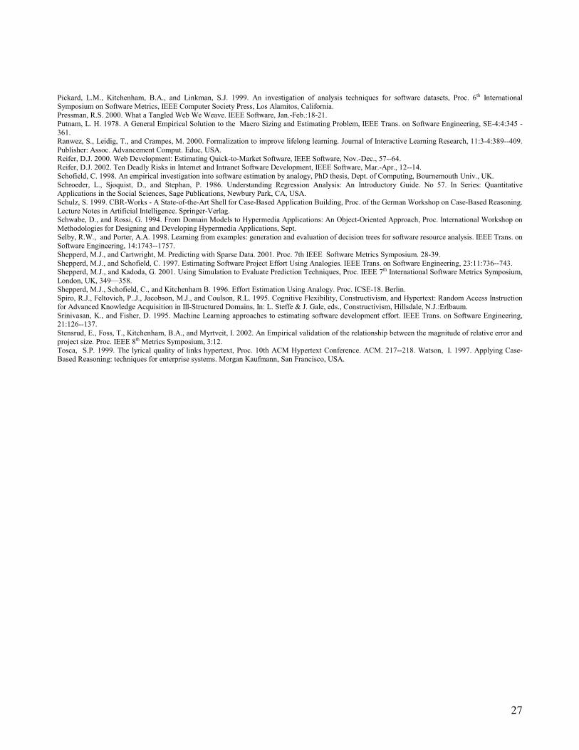
We generated Q-Q plots (Figure 10) for our measures (total effort, page count, media count, reused media count,

connectivity density and total page complexity) in order to investigate if their values were normally distributed. Program

count and reused program count have been omitted as they did not have enough points to conclude anything. As these

plots did not show any large deviations from the straight line, we consider that our dataset had the characteristic “normal +

collinearity” (Shepperd and Kadoda, 2001). Therefore, our results confirm previous work where, for normal datasets with

collinearity, stepwise regression had better prediction accuracy more often than CBR or CART (Shepperd and Kadoda,

2001).

Figure 8 - Boxplots of z for CBR for SP1 and SP2

Figure 9 - Boxplots of z for CART for SP1 and SP2

24

Figure 10 – Q-Q plots for dataset

No statistical significance was found, based on the Mann-Whitney U test for absolute residuals, between results obtained

for SP1 and SP2, for each different technique.

We found that boxplots of residuals and z were a useful aid to investigate prediction accuracy. In addition, except for SP2

v2, good accuracy, indicated by the boxplots of z, was always linked to small variance (small MMRE) and peaked

distribution of z around the central value (high Pred(25)). These results might be dataset-related, and further investigation

is necessary.

6. Conclusions and Future Improvements In addressing the first question, our results show that the CBR technique that gave the most accurate results used as

similarity measure the Weighted Euclidean distance, for the nearest neighbour.

In addressing the second question, our results show that given the characteristics of our dataset, stepwise regression

showed the most accurate predictions, according to boxplots of residuals and z. This result confirms previous work

(Shepperd and Kadoda, 2001) where for a dataset with similar characteristics to ours, stepwise regression showed the best

prediction accuracy most of the time.

We agree with (Shepperd and Kadoda, 2001) that looking for “the best” technique applicable to any dataset is unlikely to

lead us to the same conclusions and to lead us to converging results.

In the context of Web hypermedia cost estimation, the lessons learnt via this study are as follows:

• The size measures suggested, in particular PaC, MeC and RMC, seems reasonable size measures to be used by those

involved in cost estimation for Web hypermedia projects.

25

• Our dataset represented Web hypermedia applications, so results should not be generalised to other contexts such as

Web software development.

• The data presented a strong linear relationship between size and effort, leading to a high adjusted R squared.

Although there is a strong indication that size and effort do indeed have a linear relationship (Dolado, 2001) for

conventional software, further investigation into Web development is necessary in order to confirm the same trend for

Web hypermedia/software applications.

Other more general conclusions are as follows:

Will datasets with strong linear relationship, but higher variance in the data values, give similar results to those obtained

in this study?

Although CBR did not present good prediction accuracy, based on boxplots of residuals and z, compared to stepwise

regression and even CART, there is still more to be investigated regarding this technique. For example, questions we wish

to address as part of our future work are:

• What weights would give the best results for CBR?

• Would adaptation rules increase the prediction accuracy? What sort of adaptation rules?

• What other CBR techniques might give better results, given a dataset with similar characteristics to the one used in

this study?

• To what extent feature subset selection helps obtaining more accurate predictions?

We are on the process of replicating this study using another dataset of Web hypermedia projects, addressing not only the

questions asked in this paper, but also questions such as:

- What are the typical dataset characteristics that may be found in a Web hypermedia project dataset?

- To what extent do those datasets show similar characteristics to Web software project datasets and conventional

software project datasets?

- Will our results on other datasets also converge with those found in (Shepperd and Kadoda, 2001)?

- What are the best size measures for each type of Web application? To what extent is it dependent on a technological

solution?

Acknowledgements We would like to thank Lionel Briand for his fairness and all the reviewers for their valuable comments.

7. References Ambler, S.W. 2002. Lessons in Agility from Internet-Based Development, IEEE Software, Mar.-Apr. : 66-73. Angelis, L., and Stamelos, I. 2000. A Simulation Tool for Efficient Analogy Based Cost Estimation, Empirical Software Engineering, 5:35--68. Balasubramanian, V., Isakowitz, T. and Stohr, E.A. 1995. RMM: A Methodology for Structured Hypermedia Design, CACM, 38:8, Aug. Boehm, B. 1981. Software Engineering Economics. Prentice-Hall: Englewood Cliffs, N.J. Botafogo, R., Rivlin, A.E. and Shneiderman, B. 1992. Structural Analysis of Hypertexts: Identifying Hierarchies and Useful Metrics, ACM TOIS,10:2:143--179.

26

Briand, L.C., El-Emam, K., Surmann, D., Wieczorek, I., and Maxwell, K.D. 1999. An Assessment and Comparison of Common Cost Estimation Modeling Techniques, Proc. ICSE 1999, Los Angeles, USA, 313—322. Briand, L.C., Langley, T., and Wieczorek, I. 2000. A Replicated Assessment and Comparison of Common Software Cost Modeling Techniques, Proc. ICSE 2000, Limerick, Ireland, 377—386. Brieman, L., Friedman, J., Olshen, R., and Stone, C. 1984. Classification and Regression Trees. Wadsworth Inc., Belmont. Christodoulou, S. P., Zafiris, P. A., Papatheodorou, T. S. 2000. Proc. 2nd ICSE Workshop Web Eng. 75--92. Coda, F., Ghezzi, C., Vigna, G., and Garzotto, F. 1998. Towards a Software Engineering Approach to Web Site Development, Proc. 9th International Workshop on Software Specification and Design, 8--17. Conte, S., Dunsmore, H., and Shen, V. 1986. Software Engineering Metrics and Models. Benjamin/Cummings, Menlo Park, California. COSMIC, 1999. “COSMIC-FFP Measurement manual”, version 2.0, http://www.cosmicon.com. Cowderoy, A.J.C., Donaldson, A.J.M., Jenkins, J.O. 1998. A Metrics framework for multimedia creation, Proc. 5th IEEE International Software Metrics Symposium, Maryland, USA. Cowderoy, A.J.C., 2000. Measures of size and complexity for web-site content, Proc. Combined 11th ESCOM Conference and the 3rd SCOPE conference on Software Product Quality, Munich, Germany, 423—431. DeMarco, T., 1982. Controlling Software Projects: Management, Measurement and Estimation, Yourdon: New York. Dolado, J.J. 2001. On the Problem of the software cost function. IST. 43:61-72. Fielding, R.T., and Taylor, R.N. 2000. Principled design of the modern Web architecture. Proc. ICSE. ACM. New York, NY, USA, 407--416. Finnie, G.R., Wittig, G.E., and Desharnais, J-M. 1997. A Comparison of Software Effort Estimation Techniques: Using Function Points with Neural Networks, Case-Based Reasoning and Regression Models, Journal of Systems and Software, 39:281--289. Garzotto, F., Paolini, P., and Schwabe, D. 1993. HMD – A Model-Based Approach to Hypertext Application Design, ACM TOIS, 11:1, January. Gray, A., and MacDonell, S. 1997a. Applications of Fuzzy Logic to Software Metric Models for Development Effort Estimation, Proc. Annual Meeting of the North American Fuzzy Information Processing Society - NAFIPS, Syracuse NY, USA, IEEE, 394—399. Gray, A.R., and MacDonell, S.G. 1997b. A comparison of model building techniques to develop predictive equations for software metrics. Information and Software Technology, 39: 425--437. Gray, R., MacDonell, S. G., and Shepperd, M. J. 1999. Factors Systematically associated with errors in subjective estimates of software development effort: the stability of expert judgement, Proc. IEEE 6th Metrics Symposium. Hughes, R.T., 1997. An Empirical investigation into the estimation of software development effort, PhD thesis, Dept. of Computing, the University of Brighton, UK. Humphrey, W.S., 1995. A Discipline for Software Engineering, SEI Series in Software Engineering, Addison-Wesley. Jeffery, R., Ruhe, M., and Wieczorek, I. 2000. A Comparative study of two software development cost modelling techniques using multi-organizational and company-specific data, Information and Software Technology, 42:1009--1016. Jeffery, R., Ruhe, M., and Wieczorek, I. 2001. Using Public Domain Metrics to Estimate Software Development Effort, Proc. IEEE 7th Metrics Symposium, London, UK, 16—27. Johnson, P.M., and Disney, A.M. 1999. A critical analysis of PSP data quality: Results from a case study. Journal of Empirical Software Engineering, Dec. Kadoda, G., Cartwright, M., and Shepperd, M.J. 2001. Issues on the effective use of CBR technology for software project prediction, Proc. 4th International Conference on Case-Based Reasoning, Vancouver, Canada, July/August, 276--290. Kadoda, G., Cartwright, M., Chen, L., and Shepperd, M.J. 2000. Experiences Using Case-Based Reasoning to Predict Software Project Effort, Proc. EASE 2000 Conference, Keele, UK. Kemerer, C.F. 1987. An Empirical Validation of Software Cost Estimation Models, CACM, 30:5:416--429. Kinnear, P.R., and Gray, C.D. 1999. SPSS for Windows Made Simple, 3rd edition, Psychology Press Ltd. Kirsopp, C. and Shepperd, M. 2001. Making Inferences with Small Numbers of Training Sets, January, TR02-01., Bournemouth University. Kitchenham, B.A., Pickard, L.M., MacDonell, S.G., and Shepperd, M.J. 2001. What accuracy statistics really measure, IEE Proc. - Software Engineering, 148:3, June. Kitchenham, B.A., Pickard, L., and Pfleeger, S.L. 1995. Case Studies for Method and Tool Evaluation. IEEE Software, Jul.:52-62. Kok, P., Kitchenham, B. A., and Kirakowski, J. 1990. The MERMAID Approach to software cost estimation, ESPRIT Annual Conference, Brussels, 296--314. Kumar, S., Krishna, B.A., and Satsangi, P.S. 1994. Fuzzy systems and neural networks in software engineering project management. Journal of Applied Intelligence, 4:31--52. Maxwell, K.D. 2001. Collecting Data for Comparability: Benchmarking Software Development Productivity. IEEE Software, Sep.-Oct.:22-25. Mendes, E., Counsell, S., and Mosley, N. 2000. Measurement and Effort Prediction of Web Applications, Proc. 2nd ICSE Workshop on Web Engineering, June, Limerick, Ireland. Mendes, E., Counsell, S., and Mosley, N. 2001a. Towards the Prediction of Development Effort for Hypermedia Applications, Proc. ACM Hypertext'01 Conference, Aahrus, Denmark, ACM. Mendes, E., Mosley, N., and Counsell, S. 2001b. Web Metrics – Estimating Design and Authoring Effort. IEEE Multimedia, Special Issue on Web Engineering, Jan.-Mar., 50--57. Mendes, E., Mosley, N., and Counsell, S. 2002a. A Comparison of Size Measures for Predicting Web Design and Authoring Effort, IEE Proc. – Software Engineering, (accepted for publication). Mendes, E., Mosley, N., and Watson, I. 2002b. A Comparison of Case-based Reasoning Approaches to Web Hypermedia Project Cost Estimation. Proc. 11th International World-Wide Web Conference, Hawaii. Michau, F., Gentil, S., and Barrault, M. 2001. Expected benefits of web-based learning for engineering education: examples in control engineering. European Journal of Engineering Education, 26:2:151—168, June. Myrtveit, I. and . Stensrud, E. 1999. A Controlled Experiment to Assess the Benefits of Estimating with Analogy and Regression Models, IEEE Trans. on Software Engineering, 25:4:510--525, Jul.-Aug. Okamoto, S., and Satoh, K. 1995. An average-case analysis of k-nearest neighbour classifier. In, CBR Research and Development, Veloso, M., & Aamodt, A. (Eds.) Lecture Notes in Artificial Intelligence 1010 Springer-Verlag.

27

Pickard, L.M., Kitchenham, B.A., and Linkman, S.J. 1999. An investigation of analysis techniques for software datasets, Proc. 6th International Symposium on Software Metrics, IEEE Computer Society Press, Los Alamitos, California. Pressman, R.S. 2000. What a Tangled Web We Weave. IEEE Software, Jan.-Feb.:18-21. Putnam, L. H. 1978. A General Empirical Solution to the Macro Sizing and Estimating Problem, IEEE Trans. on Software Engineering, SE-4:4:345 - 361. Ranwez, S., Leidig, T., and Crampes, M. 2000. Formalization to improve lifelong learning. Journal of Interactive Learning Research, 11:3-4:389--409. Publisher: Assoc. Advancement Comput. Educ, USA. Reifer, D.J. 2000. Web Development: Estimating Quick-to-Market Software, IEEE Software, Nov.-Dec., 57--64. Reifer, D.J. 2002. Ten Deadly Risks in Internet and Intranet Software Development, IEEE Software, Mar.-Apr., 12--14. Schofield, C. 1998. An empirical investigation into software estimation by analogy, PhD thesis, Dept. of Computing, Bournemouth Univ., UK. Schroeder, L., Sjoquist, D., and Stephan, P. 1986. Understanding Regression Analysis: An Introductory Guide. No 57. In Series: Quantitative Applications in the Social Sciences, Sage Publications, Newbury Park, CA, USA. Schulz, S. 1999. CBR-Works - A State-of-the-Art Shell for Case-Based Application Building, Proc. of the German Workshop on Case-Based Reasoning. Lecture Notes in Artificial Intelligence. Springer-Verlag. Schwabe, D., and Rossi, G. 1994. From Domain Models to Hypermedia Applications: An Object-Oriented Approach, Proc. International Workshop on Methodologies for Designing and Developing Hypermedia Applications, Sept. Selby, R.W., and Porter, A.A. 1998. Learning from examples: generation and evaluation of decision trees for software resource analysis. IEEE Trans. on Software Engineering, 14:1743--1757. Shepperd, M.J., and Cartwright, M. Predicting with Sparse Data. 2001. Proc. 7th IEEE Software Metrics Symposium. 28-39. Shepperd, M.J., and Schofield, C. 1997. Estimating Software Project Effort Using Analogies. IEEE Trans. on Software Engineering, 23:11:736--743. Shepperd, M.J., and Kadoda, G. 2001. Using Simulation to Evaluate Prediction Techniques, Proc. IEEE 7th International Software Metrics Symposium, London, UK, 349—358. Shepperd, M.J., Schofield, C., and Kitchenham B. 1996. Effort Estimation Using Analogy. Proc. ICSE-18. Berlin. Spiro, R.J., Feltovich, P..J., Jacobson, M.J., and Coulson, R.L. 1995. Cognitive Flexibility, Constructivism, and Hypertext: Random Access Instruction for Advanced Knowledge Acquisition in Ill-Structured Domains, In: L. Steffe & J. Gale, eds., Constructivism, Hillsdale, N.J.:Erlbaum. Srinivasan, K., and Fisher, D. 1995. Machine Learning approaches to estimating software development effort. IEEE Trans. on Software Engineering, 21:126--137. Stensrud, E., Foss, T., Kitchenham, B.A., and Myrtveit, I. 2002. An Empirical validation of the relationship between the magnitude of relative error and project size. Proc. IEEE 8th Metrics Symposium, 3:12. Tosca, S.P. 1999. The lyrical quality of links hypertext, Proc. 10th ACM Hypertext Conference. ACM. 217--218. Watson, I. 1997. Applying Case-Based Reasoning: techniques for enterprise systems. Morgan Kaufmann, San Francisco, USA.

28

Keywords: Web hypermedia applications, effort prediction models, prediction accuracy, Case-based reasoning

techniques, multiple regression models.

Footnotes:

1 The questionnaire is available at http://www.cs.auckland.ac.nz/~emilia/Assignments/exp-questionnaire.html. 2 The questionnaire is available at http://www.cs.auckland.ac.nz/~emilia/Assignments/questionnaire.html. 3 low difference between skill levels 4 Albrecht with 24; Atkinson with 21; Desharnais with 81; Finnish with 38; Kemerer with 15; Mermaid with 28.

Information obtained from (Shepperd and Kadoda, 2001).

5 CART variables are identified as RI, which stands for rule induction.