A comparative study of a multilayer and a productivity (light-use) efficiency land-surface model...

A comparative study of a multilayer and a productivity (light-use) efficiencyland-surface model over different temporal scales

Paul Alton *, Per Bodin

Geography Dept., University of Swansea, Swansea, Wales SA2 8PP, UK

Agricultural and Forest Meteorology 150 (2010) 182–195

A R T I C L E I N F O

Article history:

Received 16 February 2009

Received in revised form 5 October 2009

Accepted 9 October 2009

Keywords:

Radiative transfer

Light-use efficiency

Eddy-covariance

Global carbon cycle

Model comparison

Model inversion

A B S T R A C T

Several recent studies suggest that a simple productivity efficiency model (PEM), based on daily or

weekly light-use efficiency, is sufficient to represent the exchange of carbon, water and energy at the

land-surface. At the same time, many global land-surface models are becoming more process-based,

simulating at high temporal resolution the interception of direct and diffuse sunlight at different depths

within the canopy. Quantifying the accuracy and limitations of both types of model has become of great

importance. The current study compares a PEM with a more complex (and computationally expensive)

multilayer model operating at timesteps as short as 30 min (JULES-SF). Each model is optimised against

observed fluxes (net carbon exchange, latent heat, sensible heat and net radiation) within the FLUXNET

archive for an unprecedented number of sites (30) and site-years (71). Our main finding is that, after

optimisation, the process-based multilayer model performs significantly better than the PEM on all

timescales (daily and seasonal). However, the difference in model performance appears to diminish with

an increase in measurement timescale. Thus, on average, the modelling efficiency increases from 0.32

(daily) to 0.46 (seasonal) using the PEM approach (r2 ¼ 0:53!0.71), whilst it remains close to 0.6 for

JULES-SF on both timescales (r2 ¼ 0:69!0.75). We find that the maximum number of biophysical

parameters that can be tuned against site fluxes (4 observables) is quite limited (typically 3–4). This

inference applies to both models despite their considerable difference in complexity.

� 2009 Elsevier B.V. All rights reserved.

Contents lists available at ScienceDirect

Agricultural and Forest Meteorology

journal homepage: www.e lsev ier .com/ locate /agr formet

1. Introduction

Global land-surface models (LSMs) traditionally adopt simplealgorithms for reasons of computational expediency (Raupach andFinnigan, 1988; Sellers et al., 1996a, 1997). Recently, however,some global LSMs have increased in complexity, especially withrespect to canopy light-interception (Dai et al., 2004; Alton et al.,2007b; Mercado et al., 2009). This change is in recognition of theimportant role played by cloud and diffuse sunlight in the accuratepredictions of carbon, water and energy exchange (Gu et al., 1999;Roderick et al., 2001; Gu et al., 2002; Lyons, 2002; Niyogi et al.,2004). At the same time, some authors find simple empirical LSMs,once calibrated against observations, provide sufficient accuracyfor most purposes. For example, the productivity efficiency model(light-use efficiency or epsilon model), which is forced by daily,weekly or monthly climate, and takes no explicit account ofvertical canopy structure, is shown to reproduce Gross PrimaryProductivity (GPP) fairly well at several carbon-monitoring eddy-covariance sites at least on longer (weekly and monthly)

* Corresponding author.

E-mail address: [email protected] (P. Alton).

0168-1923/$ – see front matter � 2009 Elsevier B.V. All rights reserved.

doi:10.1016/j.agrformet.2009.10.001

timescales (Medlyn et al., 2003; Sims et al., 2005; Yuan et al.,2007). Such models are well suited to available satellite data.Indeed, a PEM algorithm allows global GPP to be derived on a dailybasis using MODIS estimates of absorbed photosynthetically activeradiation (PAR; Running et al., 2004; Zhao et al., 2005; Heinschet al., 2006. A coarse timestep is also better suited to currentlyavailable meteorological forcing data although reconstructeddatasets on shorter (3-hourly) timesteps are starting to becomeavailable (Dirmeyer et al., 1999; Sheffield et al., 2006).

All global LSMs, especially the more process-based, require alarge number of input biophysical parameters to represent carbon,water and energy exchange at the vegetated land-surface. Forexample, the Met.Office Surface Exchange Scheme (MOSES; Coxet al., 1999) and the Lund-Potsdam-Jena model (LPJ; Zaehle et al.,2005) contain, about 50 and 40 parameters, respectively. Within themodel, many of these parameters assume different values accordingto biome or Plant Functional Type (PFT). Although field measure-ments are available for parameterization of global LSMs, manybiophysical properties are not well known across all PFTs (Sellerset al., 1995). A considerable advantage of the PEM-approach is that itreduces significantly the number of prescribed parameters.

One way to use a LSM is to optimise against site fluxes and thenscale globally. Indeed, Falge et al. (2002) emphasize the urgent

mailto:[email protected]

http://www.sciencedirect.com/science/journal/01681923

http://dx.doi.org/10.1016/j.agrformet.2009.10.001

P. Alton, P. Bodin / Agricultural and Forest Meteorology 150 (2010) 182–195 183

need to calibrate global LSMs more rigorously in this way. Therecent expansion of the FLUXNET archives (Baldocchi et al., 2001;Falge et al., 2002) provides a long-awaited opportunity to calibrateglobal LSMs against carbon, water and energy fluxes recorded at alarge number of sites and for several PFTs.

In this study, we calibrate two global land-surface models bycomparing model output against observed carbon, water andenergy fluxes from 30 sites (71 site-years) contained in theMarconi FLUXNET archive. The two models span a large range incomplexity. The simpler model is forced with daily climate andyields GPP according to light-use efficiency. The more complexmodel is a process-based approach forced by half-hourly climatewhich takes account of changes in leaf nitrogen, microclimate andlight interception with depth through the canopy. It has recentlybeen enhanced to take explicit account of leaf orientation, diffusesky radiance and sunfleck penetration, and is therefore one of themost complex LSMs that operate globally, at least in terms ofcanopy light-interception (Alton et al., 2005, 2007a,b). For bothmodels, the most influential parameters are determined bysensitivity analysis and then optimised to produce closestagreement with observed carbon, water and energy fluxesrecorded at site-level. The main scientific research question canbe summarised as follows: once optimised, how accurately caneach of the LSMs reproduce site-level carbon, water and energyfluxes measured over different timescales (half-hourly, daily andseasonally) and by how much does the process-based, multilayermodel perform better than the simple PEM?

2. Methods and materials

The methodology consists of two main parts: (1) a sensitivityanalysis to determine the most influential parameters within themodel; and (2) the use of FLUXNET archival data to optimise (tune)the model and to assess its performance at site-level. The two partsare carried out for a relatively simple productivity efficiency model(JULES-PEM) and a more complex, multilayer, process-basedmodel (JULES-SF). The following sections describe the models(Section 2.1), the datasets (Section 2.2) and the two parts of themethodology (Section 2.3).

2.1. Land-surface modelling

The more complex model (JULES-SF) is based on the Met.OfficeSurface Exchange Scheme (MOSES; Cox et al., 1999), after a seriesof enhancements (Alton et al., 2007a; Mercado et al., 2007; Alton,2008). Detail for the land-surface model, including importantequations, are contained in Appendix A. Here we focus on the maindifferences between JULES-SF and JULES-PEM which concernprimarily the representation of the canopy.

The energy calculation central to JULES (Joint UK LandEnvironmental Simulator) is the Penman–Monteith approach(Monteith, 1965), ensuring the balance of ingoing and outgoingfluxes at the land-surface. Within JULES-SF, stomatal conductance,transpiration and photosynthesis are calculated in each of five leaflayers, before summing to produce total values for the entirecanopy (Alton et al., 2007a; Mercado et al., 2007). Enhancementsfor sunfleck penetration, explicit leaf orientation and diffusesunlight permit a more realistic canopy response under both directsunlight and cloud (Alton et al., 2005, 2007a). Leaf photosynthesisfor the C3 and C4 pathways are derived using the co-limitationmodel of Collatz et al. (1991, 1992) which is conceptually similar tothe biochemical model of Farquhar et al. (1980). Input to the modelconsists of meteorological (forcing) driving data, LAI phenologyand biophysical parameters. We use the AVHRR (satellite-derived)LAI which possesses a 10-day temporal resolution and a spatialresolution of 0.25 � or �20 km (Los et al., 2000). The satellite

timeseries is normalised so that the peak, growing season LAI isequal to LAImax . LAImax is a PFT-specific parameter and is includedin the parameter sensitivity analysis discussed below.

To create the productivity efficiency model (JULES-PEM) we usethe same soil hydrology and soil respiration as JULES-SF. However,we make the following simplifications with respect to canopy,surface reflectance and climatic forcing:

1. C
anopy GPP is estimated according to total solar irradiance andlight-use efficiency (LUE; Monteith, 1977; Gower et al., 1999;Medlyn et al., 2003; Yuan et al., 2007):
GPP ¼ e� fPAR� IPAR � FSMC � FT (1)

where e is the potential light-use efficiency (g m�2 MW�1), IPAR

is the PAR incident at the top of the canopy (MW�1) and fPAR is

the fraction of absorbed PAR. Eq. (1) replaces an estimation of

gross productivity within each leaf layer before summing all

layers to produce GPP for the entire canopy. The stresses on leaf

productivity owing to temperature and soil moisture content, FT

and FSMC in Eq. (1), remain as before (Appendix A).
2. T o simplify the calculation of autotrophic respiration, the carbon
use efficiency (CUE) is prescribed:

CUE ¼ NPP

GPP(2)

where NPP is the net primary productivity (Running and

Coughlan, 1988; Waring et al., 1998; de Lucia et al., 2007). This

replaces the calculation of leaf respiration within each canopy

layer, based on foliar temperature and nitrogen content, which

is then scaled in JULES-SF according to the ratios of plant-to-leaf

nitrogen and growth-to-maintenance respiration to yield total

autotrophic respiration (Eqs. (11) and (13) in Appendix A).

Within the literature, PEMs are adopted for both GPP

(Choudhury, 2001; Medlyn et al., 2003; Heinsch et al., 2006;

Yuan et al., 2007) and NPP (Potter et al., 1993; Goetz and Prince,

1996; Gower et al., 1999; Ruimy et al., 1999; Barrett, 2002;

Running et al., 2004). The implementation within JULES-PEM of

both CUE and e permits comparison with both types of model.
3. T he vertical gradients in leaf nitrogen, photosynthetic capacity
and boundary-layer resistance are not modelled within JULES-PEM. Total stomatal conductance of the canopy (gc;mol m�2 s�1) is estimated via the diffusion equation:

gc ¼Ac

ca � ci(3)

where Ac and ca are, respectively, the canopy net productivity

(mol m�2 s�1) and the ambient CO2 concentration (mol mol�1;

e.g. Cox et al., 1998). The quantity ci (mol mol�1) is the leaf CO2

concentration which is often observed to be constant over a

wide range of conditions (Wong et al., 1979; Long and Hutchin,

1991; Campbell and Norman, 1998, although see Houborg et al.,

in press). It is now prescribed as an input parameter, rather than

calculated as an internal variable using the Ball–Berry relation

(Eq. (14) in Appendix A). Ac follows from GPP- RL where the total

leaf respiration within the canopy, RL, is given by:

RL ¼RPM

PL¼ GPP

PL� 1� CUE� Rgrow

1� Rgrow(4)

where RPM , PL and Rgrow are, respectively, the plant maintenance

respiration, the plant-to-leaf nitrogen ratio and the growth-to-

maintenance ratio (Appendix A). Note that we constrain RL� 0

in Eq. (4) (otherwise RL is negative when CUE is very high) and

gc=0 when RL�GPP (stomatal closure).

P. Alton, P. Bodin / Agricultural and Forest Meteorology 150 (2010) 182–195184

4. N

TaDe

fol

fro

Law

(20

Sch

Fie

(19

Lew

(19

act

N

1

1

1

1

1

1

1

1

1

1

2

2

2

2

2

2

2

2

2

2

3

3

3

3

3

3

3

3

3

3

4

4

4

4

o account is taken of the directionality of solar radiance(diffuse/direct). Albedo pertaining to the whole surface (soil +vegetation) is prescribed for the visible and near-infraredwavebands via the parameters albpar and albnir, respectively.This replaces the two-stream calculation based on soil albedo,LAI and leaf optical properties (Sellers et al., 1996a).

5. A
daily climatology is employed by averaging the half-hourlyclimatology used in the complex model.
In summary, 5 parameters introduced into JULES-PEM replace15 parameters required for JULES-SF. Parameters are assigned

ble 1fault (literature) values for the input biophysical parameters. Where there are suffic

lowing order: broadleaf forest (BL), needleleaf forest (NL), C3 grassland (C3), C4 grassla

m the following sources and references therein: Baldocchi and Harley (1995) for param

et al. (2002) and Asner et al. (2003) for 5; Cosby et al. (1984) and Dirmeyer et al. (19

00) for 14; Jackson et al. (1996) for 16; Collatz et al. (1991) and Sellers et al. (1996a,

lesinger (1992) for 21; Singsaas et al. (2001) for 22; Williams (1991) for 23 and 24; Far

ld and Mooney (1986); Schulze et al. (1994); Meir et al. (2002) for 26 and 27; Bolstad

91) for 29 and 30; Ryan (1991b) for 31; Campbell and ?Schrader et al. (2004); Hendric

is et al. (2000); Meir et al. (2002); Dang et al. (1998) for 34; Udo and Aro (1999) for 3

98) for 38, Yuan et al. (2007) for 39, Wong et al. (1979) for 40, de Lucia et al. for 41, B

ive radiation, near-infrared radiation and Leaf Area Index.

umber Model(s) Name Value Uncertainty

1 SF/PEM z1u 10 5

2 SF/PEM z1t 10 5

3 SF/PEM SMCi 0.62 0.11

4 SF/PEM h 25 20 1 1 2 5 5 0.5 0.5 1.0

5 SF/PEM LAImax 4.3 4.4 3.1 3.1 1.5 1.4 2.3 1.4 1.4

6 SF/PEM b 7 4

7 SF/PEM sathh 0.035 0.015

8 SF/PEM satcon 0.0073 0.0037

9 SF/PEM SMCV 0.42 0.04

0 SF/PEM hcap 1.26e6 0.07e6

1 SF/PEM hcon 0.27 0.05

2 SF ag 0.18 0.08

3 SF/PEM cc �200 100

4 SF/PEM dcatch0 0.2 0.1

5 SF infil 4 4 2 2 2 1

6 SF/PEM Dr 0.33 0.33 0.2 0.2 0.11 0.05

7 SF b1 0.89 0.09

8 SF b2 0.89 0.09

9 SF/PEM Q10(leaf) 2.3 0.5

0 SF/PEM k 1.8e �8 1.3e �8

1 SF/PEM Q10(soil) 2.3 0.7

2 SF QE 0.07 0.02

3 SF RNIR 0.50 0.05

4 SF RPAR 0.10 0.05

5 SF Fd 0.020 0.015

6 SF Ne f f 28 16

7 SF Na 3.0 3.0 1.5 1.5 3.0 1.0 1.0 0.5 0.5

8 SF/PEM PL 8 4 4 4 4 3 1.6 1.6 1.6 1

9 SF TPAR 0.05 0.05

0 SF TNIR 0.30 0.15

1 SF/PEM Rgrow 0.25 0.10

2 SF/PEM Tl 5 10

3 SF/PEM Th 40 10

4 SF krub 0.15 0.10

5 SF/PEM PS 0.50 0.05

6 SF gmin 0.03 0.02

7 SF m 8 4

8 SF/PEM dzm 0.05 0.05 0.1 0.1 0.1 0.025 0.025 0.

0.05 0.05

9 PEM e 2 1

0 PEM ci 20 8

1 PEM CUE 0.5 0.3

2 PEM albpar 0.20 0.15

3 PEM albnir 0.40 0.30

default values from the literature in Table 1 whilst the salientdifferences between JULES-SF and JULES-PEM are summarised inTable 2. Whilst it might have been possible to employ a pre-existing PEM to compare with JULES-SF, our chosen methodensures that any differences between the models, in terms ofperformance and behaviour, can be attributed to the simplifica-tions we have made rather than the diverse origin and constructionof each model. Such a modular approach is advocated by Knorrand Heimann (2001). We recognise that our chosen PEM issimple and that, within at least one recent version of the PEM, amore elaborate calculation of canopy stomatal conductance

ient data to indicate significant differences amongst PFTs, values are given in the

nd (C4) and tundra shrubland (SH). Default values and their uncertainties are taken

eters 1 and 2; main text for 3 (Section 2.2); Cox (2001) and Alton et al. (2007a) for 4;

99) for 6–11; Barnsley (2007) for 12; Newman (1969) for 13; Ramirez and Senarath

b) for 17 and 18; Tjoelker et al. (2001) for 19; Schlesinger (1997) for 20; Raich and

quhar et al. (1980); Lloyd et al. (2002); Law et al. (1999); Bolstad et al. (2004) for 25;

et al. (2004); Law et al. (1999); Lloyd et al. (2002); Ryan (1991a) for 28; Williams

kson et al. (2004); Al-Khatib and Paulsen (1999) for 32 and 33; Carswell et al. (2000);

5; Misson et al. (2004); Sellers et al. (1996a,b) for 36 and 37, Campbell and Norman

arnsley (2007) for 42 and 43. PAR, NIR and LAI are, respectively, photosynthetically

Units Description

m Height above canopy for measurement of

wind speed

m Height above canopy for measurement of

temperature & humidity

– Initial soil moisture as fraction of saturation

m Height to top of canopy

0.5 m Peak LAI of growing season

– Clapp–Hornberger exponent

m Absolute soil matric suction at saturation

mm s�1 Hydraulic conductivity at saturation

m3 m�3 Volumetric soil moisture at saturation

Jm�3 K�1 Dry heat capacity of soil

Wm�1 K�1 Dry thermal conductivity of soil

– Soil albedo for solar radiation

m Critical potential for soil moisture stress

kg m�2 Change in water-holding capacity w.r.t. LAI

– Enhancement factor for infiltration of top soil

m Root exponential scale-depth

– Light-Rubisco photosynthetic co-limitation factor

– Sucrose photosynthetic co-limitation factor

– Fractional change in leaf respiration per 10 K

change in temperature

kg m�2 s�1 Decompositional rate of soil carbon

– Fractional change in soil decomposition per 10 K

change in temperature

mol mol�1 Top-of-canopy quantum efficiency to absorbed PAR

– Leaf reflectance in NIR waveband

– Leaf reflectance in PAR waveband

– Leaf dark respiration as fraction of leaf

photosynthetic capacity (Vcmax)

m mol g�1 s�1 Ratio Vcmax (m mol m�2 s�1) to leaf nitrogen (g m�2)

1.0 g m�2 Leaf nitrogen content

.6 – Ratio of plant-to-leaf nitrogen

– Leaf transmittance in the PAR waveband

– Leaf transmittance in the NIR waveband

– Ratio growth to maintenance respiration�C Lower inhibition temperature for photosynthesis�C Upper inhibition temperature for photosynthesis

– Nitrogen allocation exponential coefficient

– Fraction of sky irradiance which is PAR

mol m�2 s�1 Intercept of the Ball-Berry stomatal model

– Slope of the Ball–Berry stomatal model

05 m m�1 Change in roughness length with canopy height

g m�2 MW�1 Potential light-use efficiency

Pa Leaf internal CO2 concentration

– Carbon-use efficiency (net to primary

productivity ratio)

– Surface albedo in PAR waveband

– Surface albedo in NIR waveband

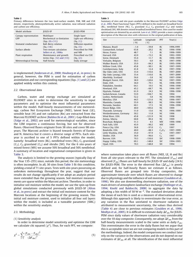
Table 2Primary differences between the two land-surface models. PAR, NIR and CUE

denote, respectively, photosynthetically active radiation, near-infrared radiation

and carbon-use efficiency.

Model attribute JULES-SF JULES-PEM

Canopy representation Multilayer Single layer

GPP Biochemical co-limitation

(Eqs. (8)–(11))

Light-use efficiency

(Eq. (1))

Stomatal conductance Ball–Berry relation

(Eq. (14))

Diffusion equation

(Eq. (3))

Surface albedo Two-stream calculation

Sellers et al., 1996a

Prescribed for PAR

and NIR

Plant respiration Maintenance and growth

terms (Eqs. (12) and (13))

Prescribed via CUE

(Eq. (2))

Meteorological forcing Half-hourly Daily average

Table 3Summary of sites and site-years available in the Marconi FLUXNET archive Falge

et al., 2002. Plant Functional Types (PFTs) defined in the model are broadleaf forest

(BL), needleleaf forest (NL), C3 grassland (C3), C4 grassland (C4) and tundra

shrubland (SH). MX denotes mixed broadleaf/needleleaf forest. Sites used for model

optimisation are denoted by an asterisk. Law et al. (2002) provide a more complete

description of the Marconi sites with references to the original publication of data.

Site Latitude

(�N)

Longitude

(�E)

PFT Year(s)

Manaus, Brazil �1.4 �59.8 BL�

1996,1999

Gunnarsholt, Iceland 63.8 �20.2 BL�

1996–1998

Hesse, France 48.7 7.1 BL�

1996–1999

Harvard, USA 42.0 �72.2 BL�

1992–1999

Soroe, Denmark 55.4 11.7 BL�

1996–1999

Vielsalm, Belgium 50.3 6.0 BL�

1997–1998

Walker Branch, USA 35.9 �84.3 BL�

1995–1998

Willow Creek, USA 45.8 �90.1 BL�

1997–1999

Castelporziano, Italy 41.8 12.4 BL�

1997–1998

Sky Oaks (old), USA 33.4 �116.6 BL 1997–2000

Sky Oaks (young), USA 33.4 �116.6 BL 1997–2000

Aberfeldy, Scotland 56.6 �3.8 NL�

1997–1998

Blodgett Forest, USA 38.9 �120.6 NL�

1997–1999

Duke, USA 36.0 �79.1 NL 1998–1999

Flakaliden, Sweden 64.1 19.5 NL�

1996–1998

Howland, USA 45.2 �68.7 NL 1996–1997

Hyytiala, Finland 61.9 24.3 NL�

1996–1998

Saskatchewan, Canada 53.9 �104.7 NL 1994

Loobos, Netherlands 52.2 5.8 NL�

1996–1998

Metolius, USA 44.5 �121.6 NL�

1996–1997

Manitoba, Canada 55.9 �98.5 NL�

1994–1998

Norunda, Sweden 60.1 17.5 NL�

1996–1998

Niwot Ridge, USA 40.0 �105.6 NL�

1999

Tharandt, Germany 51.0 13.6 NL�

1996–1999

Weidenbrunnen, Germany 50.2 11.8 NL�

1996

Wind River, USA 45.8 �121.9 NL�

1998

Zotino, Siberia 60.8 89.4 NL�

1999

Braschaat, Belgium 51.3 4.5 MX�

1996–1998

Park Falls, USA 45.9 �90.2 MX�

1999

Ponca City, USA 36.8 �97.0 C3�

1997

Bondville, USA 40.0 �88.3 C3/C4�

1997–1999

Little Washita, USA 35.0 �97.9 C4�

1997–1997

Shidler, USA 36.9 �96.6 C4�

1997

Barrow, USA 70.3 �156.6 SH�

1998–1999

Happy Valley, USA 69.1 �148.8 SH�

1994–1995

Upad, USA 70.3 �148.8 SH 1994


is implemented (Anderson et al., 2000; Houborg et al., in press). Ingeneral, however, the PEM is used for estimation of carbonassimilation and our corresponding equations (Eqs. (1) and (2)) areapplied widely within this context.

2.2. Observational data

Carbon, water and energy exchange are simulated atFLUXNET sites in order to determine the sensitivity to inputparameters and to optimise the most influential parameterswithin the model. Half-hourly measurements of site meteorol-ogy, carbon Net Ecosystem Exchange (NEE), latent heat (LE),sensible heat (H) and net radiation (Rn) are extracted from theMarconi FLUXNET archive (Baldocchi et al., 2001). Gap-filled data(Falge et al., 2002) are used for meteorological variables, sincethe LSM requires a continuous forcing, but not for observedfluxes. Observed fluxes originate from 38 sites and cover 98 site-years. The Marconi archive is biased towards forests of Europeand N. America but it covers a diverse range of PFTs. Each site-year is ascribed to one of 5 PFTs defined within the model,namely: broadleaf trees (BL), needleleaf trees (NL), C3 grassland(C3), C4 grassland (C4) and shrubs (SH). For the 6 site-years ofmixed forest (MX) we assume 50% broadleaf and 50% needleleaf.A summary of location and vegetational composition is given inTable 3.

The analysis is limited to the growing season (typically Day ofthe Year 135–255) since, outside this period, the site meteorologyis often incomplete. In all, 30 sites from Table 3 fit this condition,yielding a total of 71 site-years. Tests with site-years possessing anunbroken meteorology throughout the year, suggest that ourresults do not change significantly if we adopt an analysis periodmore extended than the growing season. Soil moisture measure-ments are sparse within the Marconi archive. Therefore, in order toinitialise soil moisture within the model, we use the spin-up fromglobal simulations conducted previously with JULES-SF (Altonet al., in press) and extract the initial soil moisture content for theMarconi locations at the beginning of the growing season. Thisinitial soil moisture content, used to initialise all four soil layerswithin the model, is included as a tuneable parameter (SMCi)within the sensitivity analysis.

2.3. Methodology

(1) Sensitivity analysis

In order to determine model sensitivity and optimise the LSMwe calculate chi squared (x2). Thus, for each PFT, we compute:

x2 ¼Xn

i¼1

ðFsim � FobsÞ2

ðDFobsÞ2

(5)

where summation takes place over all fluxes (NEE, LE, H and Rn)from all site-years relevant to the PFT. The simulated (Fsim) andobserved (Fobs) fluxes are half-hourly for JULES-SF and daily (24 h)for JULES-PEM. The error in the observed flux (DFobs) is poorlydefined and, for half-hourly fluxes we estimate it as follows.Observed fluxes are grouped into 10-day composites, theapproximate timescale over which fluxes are observed to changedue to physiology and the influence of soil moisture (Goulden et al.,1996). We also use downwelling shortwave radiation, one of themain drivers of atmosphere-landsurface exchange (Hollinger et al.,1994; Knohl and Baldocchi, 2008) to aggregate the data byadopting a bin width of 50 W m�2. The standard deviation aboutthe mean of each bin is used as a measure of observational error.Although this approach is likely to overestimate the true error, asany variation in the flux unrelated to shortwave radiation isattributed to measurement uncertainty, the values thus derived(Table 4) are close to previous estimates (Goulden et al., 1996;Medlyn et al., 2005). It is difficult to estimate daily DFobs for JULES-PEM since daily values of shortwave radiation vary considerablyover the 10-day composite. Consequently, we adopt DFobs from thehalf-hourly measurements scaled to the same units as daily Fobs.This overestimates the error in the daily fluxes but we argue thatthis is acceptable since we are not comparing models in this part ofthe methodology. Indeed, the model comparisons we conduct laterrely on the variance in the observations and do not depend on ourestimates of DFobs at all. The identification of the most influential

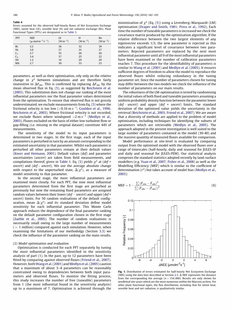
Table 4Errors assumed for the observed half-hourly fluxes of Net Ecosystem Exchange

(NEE), latent heat (LE), sensible heat (H) and net radiative exchange (Rn). Plant

Functional Types (PFTs) are designated as in Table 3.

PFT NEE

(m mol m�2 s�1)

LE

(W m�2)

H

(W m�2)

Rn

(W m�2)

BL 3.2 36 32 39

NL 3.0 27 35 37

C3 2.7 35 26 26

C4 3.4 37 25 22

SH 1.2 16 20 20

MX 2.7 39 33 23

Fig. 1. Distribution of errors estimated for half-hourly Net Ecosystem Exchange

(NEE) using the data bins described in Section 2.3. D NEE represents the distance

from the corresponding bin average (n ¼ 154;000). Results are only shown for

needleleaf site-years which are the most numerous within the Marconi archive. For

other plant functional types, the flux distribution, including that for latent heat,

sensible heat and net radiation, is qualitatively similar.


parameters, as well as their optimisation, rely only on the relative

change in x2 between simulations and are therefore fairlyinsensitive to DFobs. This is confirmed by replacing DFobs by themean observed flux in Eq. (5), as suggested by Reichstein et al.(2003). This substitution does not change our ranking of the mostinfluential parameters nor the final parameter values determinedfrom the optimisation. To ensure that observed flux is not grosslyunderestimated, we exclude measurements from Eq. (5) where thefrictional velocity is too low (<0.16 m s�1; Goulden et al., 1996;Reichstein et al., 2003). Where frictional velocity is not recorded,we exclude fluxes where windspeed <2 m s�1 (Medlyn et al.,2003). Fluxes excluded on the basis of either low turbulent flow orgap-filling (i.e. missing in the original dataset) constitute 44% ofmeasurements.

The sensitivity of the model to its input parameters isdetermined in two stages. In the first stage, each of the inputparameters is perturbed in turn by an amount corresponding to theestimated uncertainty in that parameter. Whilst each parameter isperturbed all other parameters remain at their default values(Knorr and Heimann, 2001). Default values (def) and parameteruncertainties (uncert) are taken from field measurements, andcompilations thereof, given in Table 1. Eq. (5) yields x2 at (def +uncert) and (def � uncert). We use the average absolute changewith respect to the unperturbed state, Dðx2Þ, as a measure ofmodel sensitivity to that parameter.

In the second stage, the most influential parameters areexamined more closely. For each PFT, the nine most influentialparameters determined from the first stage are perturbed aspreviously but now the remaining fixed parameters are assignedrandom values between their lower (def � uncert) and upper (def +uncert) limits. For 50 random realisations of the default config-uration, mean Dðx2Þ and its standard deviation define modelsensitivity for each influential parameter. This Monte Carloapproach reduces the dependence of the final parameter rankingon the default parameter configuration chosen in the first stage(Zaehle et al., 2005). The number of random realisations isnecessarily small owing to the large number of measurements(’ 1 million) compared against each simulation. However, whenexamining the limitations of our methodolgy (Section 3.3) wecheck the influence of the parameter ranking on the main results.

(2) Model optimisation and evaluation

Optimisation is conducted for each PFT separately by tuningthe most influential parameters identified in the sensitivityanalysis of part (1). In the past, up to 12 parameters have beenfitted by comparing against observed fluxes (Friend et al., 2007).However, both Wang et al. (2001) and Medlyn et al. (2005) cautionthat a maximum of about 3–4 parameters can be reasonablyconstrained owing to dependencies between both input para-meters and observed fluxes. To monitor the fitting process,this study increases the number of free (tuneable) parametersfrom 1 (the most influential found in the sensitivity analysis)up to a maximum of 7. Optimisation is achieved through the

minimisation of x2 (Eq. (5)) using a Levenberg–Marquardt (LM)optimisation (Draper and Smith, 1981; Press et al., 1992). Eachtime the number of tuneable parameters is increased we check thecovariance matrix produced by the optimisation algorithm. If therelative difference between the two largest elements of anyeigenvector exceeds 1/3, the new parameter is rejected as thisindicates a significant level of covariance between two para-meters. Rejected parameters are replaced by the next mostinfluential parameter until all 9 of the most influential parametershave been examined or the number of calibration parametersreaches 7. This procedure for the identifiability of parameters issimilar to Wang et al. (2001) and Medlyn et al. (2005). It ensuressufficient degrees of freedom to allow the model to reproduce theobserved fluxes whilst reducing redundancy in the tuningparameter set. Since the number of parameters chosen for tuningmay differ between the two models we check the influence of thenumber of parameters on our main results.

The robustness of the LM-optimisation is tested by randomisingthe initial values of both fixed and tuneable parameters assuming auniform probability density function between the parameter lower(def � uncert) and upper (def + uncert) limits. The standarddeviation of the optimised value yields the uncertainty in theretrieval (Reichstein et al., 2003; Friend et al., 2007). We are awarethat a diversity of methods are applied to the problem of modeloptimisation, including techniques for identifying the subsets ofparameters which are retrievable (Medlyn et al., 2005). Theapproach adopted in the present investigation is well suited to thelarge number of parameters contained in the model (30-40) andthe massive quantity of measured fluxes available for comparison.

Model performance at site-level is evaluated by comparingoutput from the optimised model with the observed fluxes over arange of timescales (half-hourly, daily and seasonal for JULES-SFand daily and seasonal for JULES-PEM). Our statistical analysiscomprises the standard statistics adopted recently by land-surfacemodellers (e.g. Yuan et al., 2007; Fisher et al., 2008) as well as theModelling Efficiency (MEF) which is similar to the coefficient ofdetermination (r2) but takes account of model bias (Medlyn et al.,2003):

MEF ¼ 1�PðFsim � FobsÞ2PðFobs � hFobsiÞ2

(6)

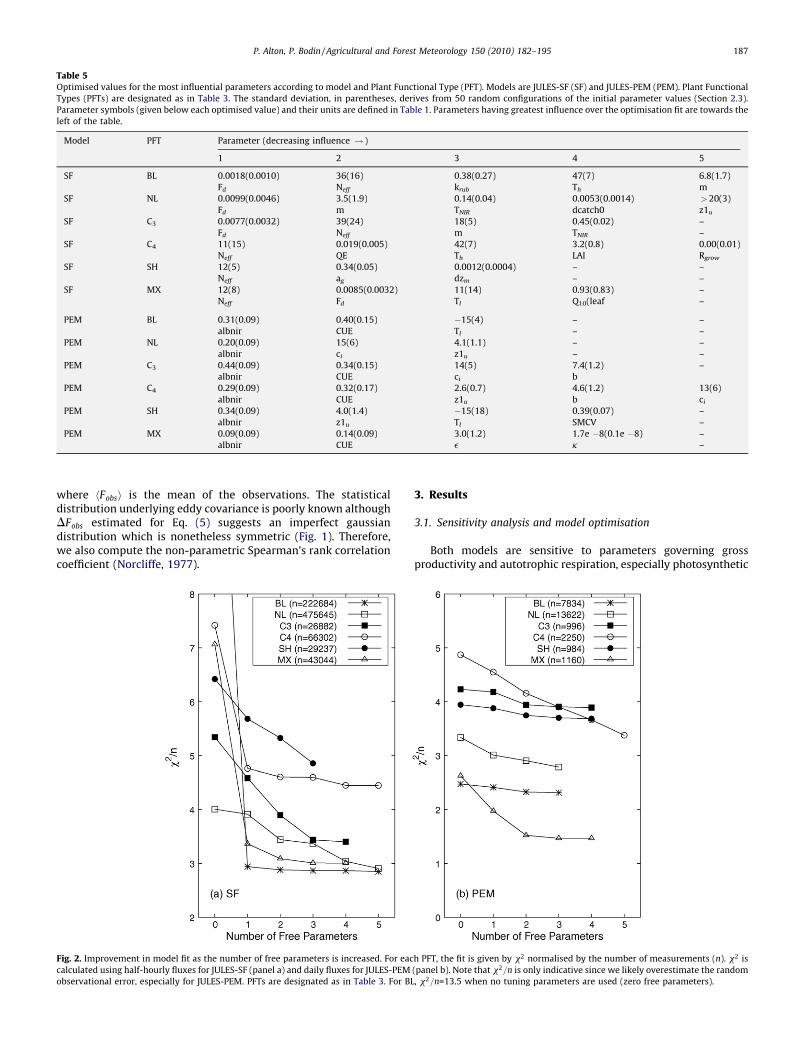
Table 5Optimised values for the most influential parameters according to model and Plant Functional Type (PFT). Models are JULES-SF (SF) and JULES-PEM (PEM). Plant Functional

Types (PFTs) are designated as in Table 3. The standard deviation, in parentheses, derives from 50 random configurations of the initial parameter values (Section 2.3).

Parameter symbols (given below each optimised value) and their units are defined in Table 1. Parameters having greatest influence over the optimisation fit are towards the

left of the table.

Model PFT Parameter (decreasing influence ! )

1 2 3 4 5

SF BL 0.0018(0.0010) 36(16) 0.38(0.27) 47(7) 6.8(1.7)

Fd Neff krub Th m

SF NL 0.0099(0.0046) 3.5(1.9) 0.14(0.04) 0.0053(0.0014) >20(3)

Fd m TNIR dcatch0 z1u

SF C3 0.0077(0.0032) 39(24) 18(5) 0.45(0.02) –

Fd Neff m TNIR –

SF C4 11(15) 0.019(0.005) 42(7) 3.2(0.8) 0.00(0.01)

Neff QE Th LAI Rgrow

SF SH 12(5) 0.34(0.05) 0.0012(0.0004) – –

Neff ag dzm – –

SF MX 12(8) 0.0085(0.0032) 11(14) 0.93(0.83) –

Neff Fd Tl Q10(leaf –

PEM BL 0.31(0.09) 0.40(0.15) �15(4) – –

albnir CUE Tl – –

PEM NL 0.20(0.09) 15(6) 4.1(1.1) – –

albnir ci z1u – –

PEM C3 0.44(0.09) 0.34(0.15) 14(5) 7.4(1.2) –

albnir CUE ci b

PEM C4 0.29(0.09) 0.32(0.17) 2.6(0.7) 4.6(1.2) 13(6)

albnir CUE z1u b ci

PEM SH 0.34(0.09) 4.0(1.4) �15(18) 0.39(0.07) –

albnir z1u Tl SMCV –

PEM MX 0.09(0.09) 0.14(0.09) 3.0(1.2) 1.7e �8(0.1e �8) –

albnir CUE e k –


where hFobsi is the mean of the observations. The statisticaldistribution underlying eddy covariance is poorly known althoughDFobs estimated for Eq. (5) suggests an imperfect gaussiandistribution which is nonetheless symmetric (Fig. 1). Therefore,we also compute the non-parametric Spearman’s rank correlationcoefficient (Norcliffe, 1977).

Fig. 2. Improvement in model fit as the number of free parameters is increased. For eac

calculated using half-hourly fluxes for JULES-SF (panel a) and daily fluxes for JULES-PEM

observational error, especially for JULES-PEM. PFTs are designated as in Table 3. For BL

3. Results

3.1. Sensitivity analysis and model optimisation

Both models are sensitive to parameters governing grossproductivity and autotrophic respiration, especially photosynthetic

h PFT, the fit is given by x2 normalised by the number of measurements (n). x2 is

(panel b). Note that x2=n is only indicative since we likely overestimate the random

, x2=n=13.5 when no tuning parameters are used (zero free parameters).


capacity (Ne f f ) and leaf dark respiration (Fd) within JULES-SF, andCUE and e within JULES-PEM (Table 5). The important role ofphotosynthetic capacity is already noted for several LSMs (Danget al., 1998; Reichstein et al., 2003; Wang et al., 2001). In agreementwith previous authors (Reichstein et al., 2003; Misson et al., 2004;Knorr and Kattge, 2005), parameters governing stomatal conduc-tance are also found to be influential, i.e. m within JULES-SF and ci

within JULES-PEM. A third group of influential parameters emergewhich govern shortwave energy balance and surface temperature(TNIR and ag in JULES-SF and albnir in JULES-PEM). It is particularlyimportant to constrain properties in the near-infrared waveband(via TNIR and albnir) which are known to diverge dramatically forphotosynthetic and non-photosynthetic elements within thevegetation canopy. Leaves are fairly poorly absorbers of near-infrared radiation whilst trunks and branches are not (Williams,1991).

In general, the three most influential parameters for each PFTand model lie within ’1s of the literature values given in Table 1.

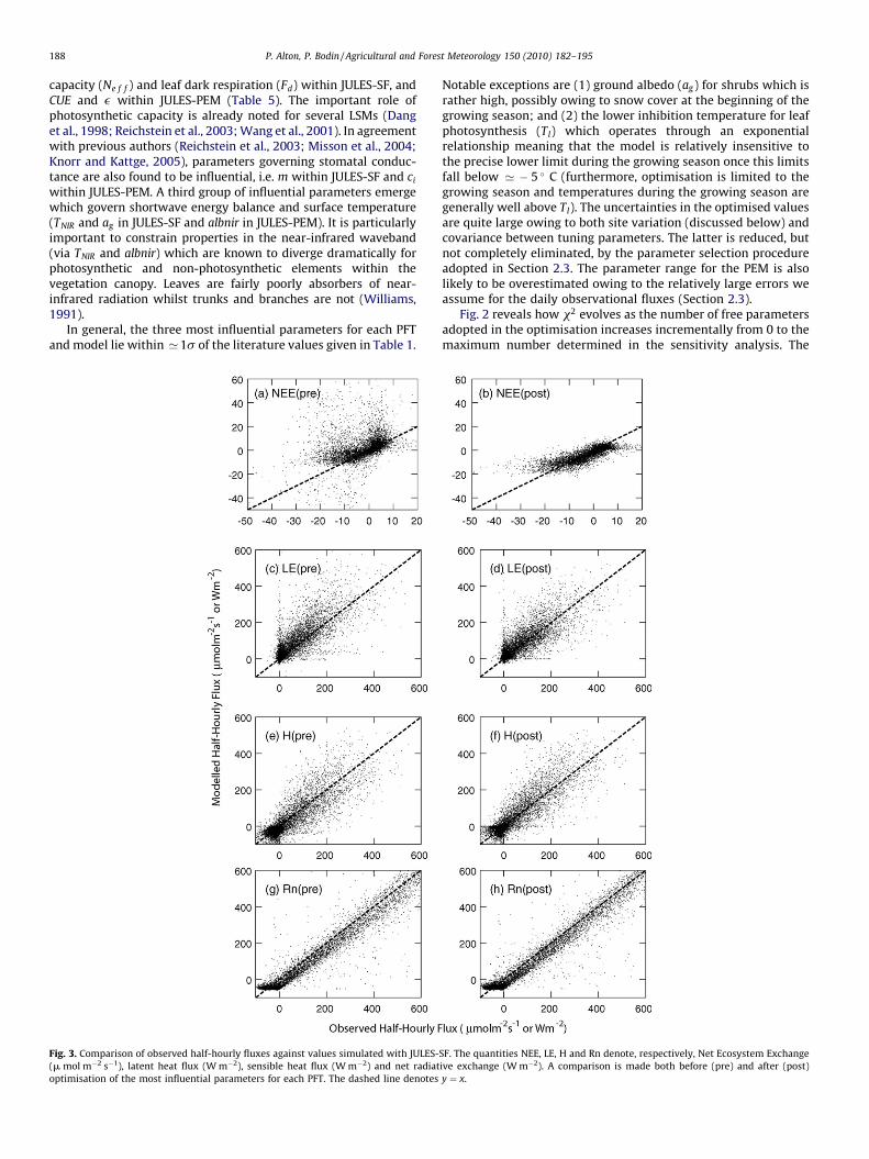
Fig. 3. Comparison of observed half-hourly fluxes against values simulated with JULES-

(m mol m�2 s�1), latent heat flux (W m�2), sensible heat flux (W m�2) and net radiat

optimisation of the most influential parameters for each PFT. The dashed line denotes

Notable exceptions are (1) ground albedo (ag) for shrubs which israther high, possibly owing to snow cover at the beginning of thegrowing season; and (2) the lower inhibition temperature for leafphotosynthesis (Tl) which operates through an exponentialrelationship meaning that the model is relatively insensitive tothe precise lower limit during the growing season once this limitsfall below ’ � 5 � C (furthermore, optimisation is limited to thegrowing season and temperatures during the growing season aregenerally well above Tl). The uncertainties in the optimised valuesare quite large owing to both site variation (discussed below) andcovariance between tuning parameters. The latter is reduced, butnot completely eliminated, by the parameter selection procedureadopted in Section 2.3. The parameter range for the PEM is alsolikely to be overestimated owing to the relatively large errors weassume for the daily observational fluxes (Section 2.3).

Fig. 2 reveals how x2 evolves as the number of free parametersadopted in the optimisation increases incrementally from 0 to themaximum number determined in the sensitivity analysis. The

SF. The quantities NEE, LE, H and Rn denote, respectively, Net Ecosystem Exchange

ive exchange (W m�2). A comparison is made both before (pre) and after (post)

y ¼ x.

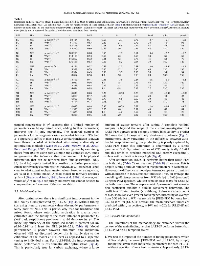
Table 6Regression and error analysis of half-hourly fluxes predicted by JULES-SF after model optimisation. Information is shown per Plant Functional Type (PFT) for Net Ecosystem

Exchange (NEE), latent heat (LE), sensible heat (H) and net radiation (Rn). PFTs are designated as in Table 3. The following indices Janssen and Heuberger, 1995 are given: the

number of fitted data (n); the modelling efficiency (MEF); gradient (a) and intercept (b) of a least-squares linear fit; the coefficient of determination (r2); the mean absolute

error (MAE); mean observed flux (hobsi); and the mean simulated flux (hmodi).

PFT Flux Units n MEF a b r2 MAE hobsi hmodi

BL NEE m mol m�2 s�1 59,184 0.71 0.65 �2.7 0.73 3.7 �5.1 �6.0

BL LE W m�2 61,797 0.63 0.89 31 0.72 38 76 98

BL H W m�2 53,113 0.63 0.98 6.5 0.72 41 47 53

BL Rn W m�2 48,590 0.90 0.93 �16 0.91 42 180 150

NL NEE m mol m�2 s�1 109,250 0.60 0.55 �1.7 0.61 3.4 �2.7 �3.2

NL LE W m�2 113,118 0.53 0.66 22 0.55 33 65 65

NL H W m�2 116,862 0.72 0.91 12 0.75 41 63 70

NL Rn W m�2 136,415 0.93 0.93 �8.2 0.94 39 160 140

C3 NEE mmol m�2 s�1 6,174 0.57 0.53 �2.3 0.58 3.9 �3.6 �4.2

C3 LE W m�2 5,557 0.78 0.93 12 0.80 40 130 130

C3 H W m�2 6,534 0.43 0.89 3.5 0.59 36 34 34

C3 Rn W m�2 8,617 0.96 1.0 �10 0.96 28 160 150

C4 NEE m mol m�2 s�1 13,793 0.41 0.36 �3.0 0.44 6.5 �6.6 �5.4

C4 LE W m�2 12,987 0.56 1.1 15 0.76 48 120 140

C4 H W m�2 13,388 0.68 0.95 13 0.75 32 59 70

C4 Rn W m�2 14,684 0.98 1.1 -18 0.99 27 230 230

SH NEE m mol m�2 s�1 6,838 0.26 0.28 �0.70 0.26 1.2 �0.82 �0.93

SH LE W m�2 6,818 0.47 0.86 �4.1 0.62 23 44 34

SH H W m�2 6,867 0.35 0.77 6.0 0.50 29 46 42

SH Rn W m�2 8,714 0.77 0.98 -35 0.88 49 110 71

MX NEE m mol m�2 s�1 10,633 0.68 0.80 �0.58 0.69 2.8 �1.4 �1.7

MX LE W m�2 11,580 0.52 0.65 40 0.57 43 63 81

MX H W m�2 11,625 0.18 1.1 �4.2 0.62 43 26 26

MX Rn W m�2 9,206 0.95 0.95 �20 0.97 36 160 130


general convergence in x2 suggests that a limited number ofparameters can be optimised since, adding further parameters,improves the fit only marginally. The required number ofparameters for convergence varies somewhat between PFTs but3–4 appears to suffice in most cases. A similar conclusion is drawnfrom fluxes recorded at individual sites using a diversity ofoptimisation methods (Wang et al., 2001; Medlyn et al., 2003;Knorr and Kattge, 2005). The present investigation, by examiningfluxes from 30 sites using both a simple and a complex LSM, tendsto generalise the inference that the amount of biophysicalinformation that can be retrieved from four observables (NEE,LE, H and Rn) is quite limited. It is possible that further parameterscan be retrieved by examining sites individually. However, it is notclear to what extent such parameter values, based on a single site,are valid in a global model. A good model fit formally requiresx2=n’1 (Draper and Smith, 1981; Press et al., 1992). However, ourvalues of x2=n in Fig. 2 are purely indicative and cannot be used tocompare the performance of the two models.

3.2. Model evaluation

After optimisation, there is a significant improvement in thehalf-hourly fluxes predicted by JULES-SF (Fig. 3). Without tuning(i.e. using literature parameter values) the model performance isfairly poor for NEE. This is particularly true for broadleaf andmixed forest where autotrophic respiration is greatly over-estimated and the tuning of the most influential parameter Fd

(leaf dark respiration) produces a rapid decrease in x2. Themodelling efficiency of the optimised model is greatest for Rn(0.90–0.98) and least for NEE (0.26–0.71; Table 6). Modelperformance is poorer towards minimum and maximumobserved NEE. As discussed below, this is mainly due to thecalibration of the model at PFT-level as opposed to a separatetuning to individual sites. For JULES-PEM, the improvement inmodel performance is less dramatic after optimisation (Fig. 4).This is particularly true for carbon exchange, where a large

amount of scatter remains after tuning. A complete residualanalysis is beyond the scope of the current investigation butJULES-PEM appears to be severely limited in its ability to predictNEE over the full range of daily shortwave irradiance (Fig. 5).Furthermore, daily variability in the difference between auto-trophic respiration and gross productivity is poorly captured byJULES-PEM since this difference is determined by a singleparameter CUE. Optimised values of CUE are typically 0.3–0.4and this tends to preclude modelled NEE greatly exceeding 0unless soil respiration is very high (Fig. 4).

After optimisation, JULES-SF performs better than JULES-PEMon both daily (Table 7) and seasonal (Table 8) timescales. This isdespite tuning a similar number of free parameters in each model.However, the difference in model performance appears to diminishwith an increase in measurement timescale. Thus, on average, themodelling efficiency increases from 0.32 (daily) to 0.46 (seasonal)using the PEM approach, whilst it remains close to 0.6 for JULES-SFon both timescales. The non-parametric Spearman’s rank correla-tion coefficient exhibits a similar convergent behaviour. Thecoefficient of determination (r2), although it does not take accountof bias, shows an even greater convergence, increasing on averagefrom 0.53 (daily) to 0.71 (seasonal) for JULES-PEM but only from0.69 to 0.75 for JULES-SF. Overall, the mean observed fluxes arepredicted within, respectively, ’10% and ’20% for JULES-SF andJULES-PEM.

3.3. Caveats and limitations

The limitations of the methodology are examined within thecontext of the main finding, i.e. that JULES-SF performs better thanJULES-PEM on all temporal scales:

1. W
e test the impact of the number of tuning parameters, whichdiffers slightly between JULES-PEM and JULES-SF, by simplytuning the seven most influential parameters for each PFT, i.e.without rejection of covariant parameters. As previously, JULES-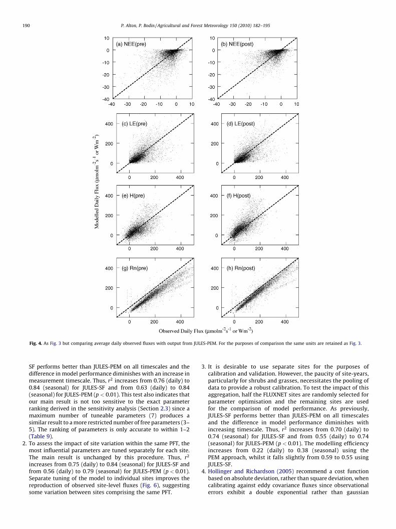

Fig. 4. As Fig. 3 but comparing average daily observed fluxes with output from JULES-PEM. For the purposes of comparison the same units are retained as Fig. 3.


SF performs better than JULES-PEM on all timescales and thedifference in model performance diminishes with an increase inmeasurement timescale. Thus, r2 increases from 0.76 (daily) to0.84 (seasonal) for JULES-SF and from 0.63 (daily) to 0.84(seasonal) for JULES-PEM (p < 0.01). This test also indicates thatour main result is not too sensitive to the exact parameterranking derived in the sensitivity analysis (Section 2.3) since amaximum number of tuneable parameters (7) produces asimilar result to a more restricted number of free parameters (3–5). The ranking of parameters is only accurate to within 1–2(Table 9).

2. T
o assess the impact of site variation within the same PFT, themost influential parameters are tuned separately for each site.The main result is unchanged by this procedure. Thus, r2
increases from 0.75 (daily) to 0.84 (seasonal) for JULES-SF andfrom 0.56 (daily) to 0.79 (seasonal) for JULES-PEM (p < 0.01).Separate tuning of the model to individual sites improves thereproduction of observed site-level fluxes (Fig. 6), suggestingsome variation between sites comprising the same PFT.

3. I
t is desirable to use separate sites for the purposes ofcalibration and validation. However, the paucity of site-years,particularly for shrubs and grasses, necessitates the pooling ofdata to provide a robust calibration. To test the impact of thisaggregation, half the FLUXNET sites are randomly selected forparameter optimisation and the remaining sites are usedfor the comparison of model performance. As previously,JULES-SF performs better than JULES-PEM on all timescalesand the difference in model performance diminishes withincreasing timescale. Thus, r2 increases from 0.70 (daily) to0.74 (seasonal) for JULES-SF and from 0.55 (daily) to 0.74(seasonal) for JULES-PEM (p < 0.01). The modelling efficiencyincreases from 0.22 (daily) to 0.38 (seasonal) using thePEM approach, whilst it falls slightly from 0.59 to 0.55 usingJULES-SF.
4. H
ollinger and Richardson (2005) recommend a cost functionbased on absolute deviation, rather than square deviation, whencalibrating against eddy covariance fluxes since observationalerrors exhibit a double exponential rather than gaussian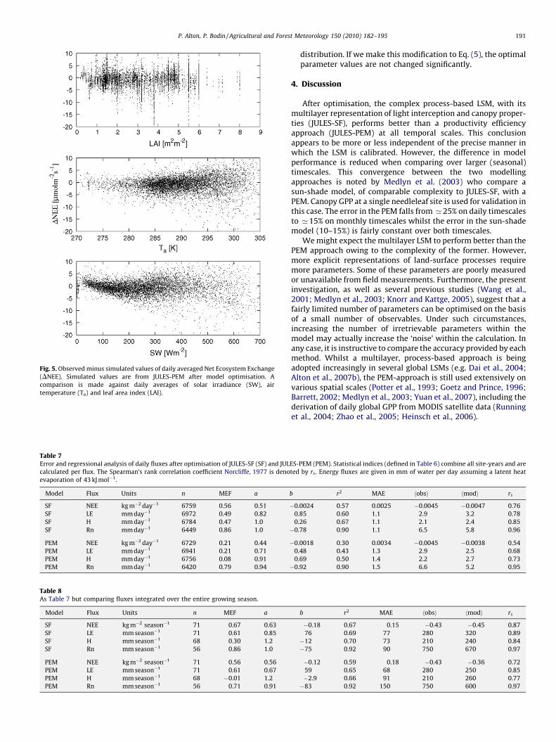

Fig. 5. Observed minus simulated values of daily averaged Net Ecosystem Exchange

(DNEE). Simulated values are from JULES-PEM after model optimisation. A

comparison is made against daily averages of solar irradiance (SW), air

temperature (Ta) and leaf area index (LAI).

Table 7Error and regressional analysis of daily fluxes after optimisation of JULES-SF (SF) and JUL

calculated per flux. The Spearman’s rank correlation coefficient Norcliffe, 1977 is deno

evaporation of 43 kJ mol�1.

Model Flux Units n MEF a

SF NEE kg m�2 day�1 6759 0.56 0.51

SF LE mm day�1 6972 0.49 0.82

SF H mm day�1 6784 0.47 1.0

SF Rn mm day�1 6449 0.86 1.0

PEM NEE kg m�2 day�1 6729 0.21 0.44

PEM LE mm day�1 6941 0.21 0.71

PEM H mm day�1 6756 0.08 0.91

PEM Rn mm day�1 6420 0.79 0.94

Table 8As Table 7 but comparing fluxes integrated over the entire growing season.

Model Flux Units n MEF a

SF NEE kg m�2 season�1 71 0.67 0.63

SF LE mm season�1 71 0.61 0.85

SF H mm season�1 68 0.30 1.2

SF Rn mm season�1 56 0.86 1.0

PEM NEE kg m�2 season�1 71 0.56 0.56

PEM LE mm season�1 71 0.61 0.67

PEM H mm season�1 68 �0.01 1.2

PEM Rn mm season�1 56 0.71 0.91


distribution. If we make this modification to Eq. (5), the optimalparameter values are not changed significantly.

4. Discussion

After optimisation, the complex process-based LSM, with itsmultilayer representation of light interception and canopy proper-ties (JULES-SF), performs better than a productivity efficiencyapproach (JULES-PEM) at all temporal scales. This conclusionappears to be more or less independent of the precise manner inwhich the LSM is calibrated. However, the difference in modelperformance is reduced when comparing over larger (seasonal)timescales. This convergence between the two modellingapproaches is noted by Medlyn et al. (2003) who compare asun-shade model, of comparable complexity to JULES-SF, with aPEM. Canopy GPP at a single needleleaf site is used for validation inthis case. The error in the PEM falls from ’25% on daily timescalesto ’15% on monthly timescales whilst the error in the sun-shademodel (10–15%) is fairly constant over both timescales.

We might expect the multilayer LSM to perform better than thePEM approach owing to the complexity of the former. However,more explicit representations of land-surface processes requiremore parameters. Some of these parameters are poorly measuredor unavailable from field measurements. Furthermore, the presentinvestigation, as well as several previous studies (Wang et al.,2001; Medlyn et al., 2003; Knorr and Kattge, 2005), suggest that afairly limited number of parameters can be optimised on the basisof a small number of observables. Under such circumstances,increasing the number of irretrievable parameters within themodel may actually increase the ‘noise’ within the calculation. Inany case, it is instructive to compare the accuracy provided by eachmethod. Whilst a multilayer, process-based approach is beingadopted increasingly in several global LSMs (e.g. Dai et al., 2004;Alton et al., 2007b), the PEM-approach is still used extensively onvarious spatial scales (Potter et al., 1993; Goetz and Prince, 1996;Barrett, 2002; Medlyn et al., 2003; Yuan et al., 2007), including thederivation of daily global GPP from MODIS satellite data (Runninget al., 2004; Zhao et al., 2005; Heinsch et al., 2006).

ES-PEM (PEM). Statistical indices (defined in Table 6) combine all site-years and are

ted by rs . Energy fluxes are given in mm of water per day assuming a latent heat

b r2 MAE hobsi hmodi rs

�0.0024 0.57 0.0025 �0.0045 �0.0047 0.76

0.85 0.60 1.1 2.9 3.2 0.78

0.26 0.67 1.1 2.1 2.4 0.85

�0.78 0.90 1.1 6.5 5.8 0.96

�0.0018 0.30 0.0034 �0.0045 �0.0038 0.54

0.48 0.43 1.3 2.9 2.5 0.68

0.69 0.50 1.4 2.2 2.7 0.73

�0.92 0.90 1.5 6.6 5.2 0.95

b r2 MAE hobsi hmodi rs

�0.18 0.67 0.15 �0.43 �0.45 0.87

76 0.69 77 280 320 0.89

�12 0.70 73 210 240 0.84

�75 0.92 90 750 670 0.97

�0.12 0.59 0.18 �0.43 �0.36 0.72

59 0.65 68 280 250 0.85

�2.9 0.66 91 210 260 0.77

�83 0.92 150 750 600 0.97

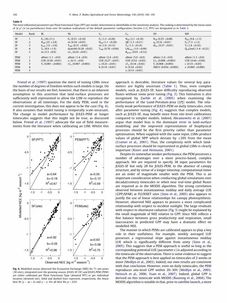
Table 9The most influential parameters per Plant Functional Type (PFT) per model, determined as identifiable in the sensitivity analysis. The ranking is determined by the mean value

of Dðx2Þ/n (in parentheses) from over 50 random realisations of the default parameter configuration (Section 2.3). PFTs are designated as in Table 3.

Model Rank BL NL C3 C4 SH MX

SF 1 Fd (26�5.1) Fd (0.51 �0.10) Fd (1.2 �0.28) Neff (2.1 �0.18) Neff (0.55 �0.08) Neff (9.8 �1.3)

SF 2 Neff (25 �3.8) m (0.34 �0.03) Neff (1.1 �0.28) QE (1.3 �0.21) ag (0.32 �0.01) Fd (7.3 �1.2)

SF 3 krub (12 �3.0) TNIR (0.31 �0.02) m (1.0 �0.13) Th (1.3 �0.14) dzm (0.27 �0.01) Tl (1.8 �0.32)

SF 4 Th (8.9 �1.9) dcatch0 (0.28 �0.02) TNIR (0.70 �0.04) LAImax (1.0 �0.09) Q10(leaf) (1.4 �0.22)

SF 5 m (5.3 �0.9) z1u (0.24 �0.01) Rgrow (0.91 �0.12)

PEM 1 albnir (1.1 �0.0) albnir (1.4 �0.0) albnir (2.4 �0.0) albnir (5.0 �0.0) albnir (1.6 �0.0) albnir (1.3 �0.0)

PEM 2 CUE (0.30 �0.01) ci (0.11 �0.0) CUE (0.27 �0.01) CUE (0.52 �0.03) z1u (0.098 �0.003) CUE (0.44 �0.04)

PEM 3 Tl (0.081 �0.003) z1u (0.067 �0.003) ci (0.23 �0.01) z1u (0.34 �0.02) Tl (0.068 �0.003) e (0.33 �0.03)

PEM 4 b (0.19 �0.01) b (0.34 �0.02) SMCV (0.034 �0.002) k (0.069 �0.006)

PEM 5 ci (0.15 �0.01)


Friend et al. (1997) question the merit of tuning LSMs sincethe number of degrees of freedom within such models is large. Onthe basis of our results we feel, however, that there is an inherentassumption in this assertion that land-surface processes aresufficiently well represented to allow the LSM to reproduce theobservations at all timesteps. For the daily PEM, used in thecurrent investigation, this does not appear to be the case (Fig. 4).It also assumes that model tuning is temporally scale-invariant.The change in model performance by JULES-PEM at longertimescales suggests that this might not be true, as discussedbelow. Friend et al. (1997) advocate the use of field measure-ments from the literature when calibrating an LSM. Whilst this

Fig. 6. Modelled versus observed Net Ecosystem Exchange (NEE) for 71 site-years

(30 sites), integrated over the growing season. JULES-SF (SF) and JULES-PEM (PEM)

are either calibrated per Plant Functional Type (denoted PFT) or per individual

location (denoted site). Solid and dashed lines represent, respectively, the linear

best fit (y ¼ axþ b) and y ¼ x. For all best fits p < 0.01.

approach is desirable, literature values for several key para-meters are highly uncertain (Table 1). Thus, even complexmodels, such as JULES-SF, have difficulty reproducing observedfluxes without some prior tuning (Fig. 3). This limitation is alsorecognised by Zaehle et al. (2005) when examining theperformance of the Lund-Potsdam-Jena (LPJ) model. The rela-tively weak performance of JULES-PEM on daily timescales, evenafter parameter tuning (Fig. 4), suggests that complex models,such as JULES-SF, may benefit more from site-level calibrationscompared to simpler models. Indeed, Abramowitz et al. (2007)argue that model bias is the dominant error in land-surfacemodelling and the improved representation of biophysicalprocesses should be the first priority rather than parameteroptimisation. When supplied with the same input, LSMs producevalues of global NPP which deviate by �20% from the mean(Cramer et al., 2001). Thus, the complexity with which land-surface processes should be represented in global LSMs is clearlyimportant (Knorr and Heimann, 2001).

Despite its somewhat weaker performance, the PEM possesses anumber of advantages over a more process-based, complexapproach. We are required to specify 38 input parameters forJULES-SF but only 28 for JULES-PEM. In the absence of canopystructure, and by virtue of a longer timestep, computational timesare an order of magnitude smaller with the PEM. This is animportant consideration when conducting global simulations overdecadal/century timescales or when near real-time global fluxesare required as in the MODIS algorithm. The strong correlationobserved between instantaneous midday and daily average LUE(GPP/APAR) at FLUXNET sites (Sims et al., 2005) also appears tojustify the use of linear relationships for canopy photosynthesis.However, observed NEE appears to possess a more complicatedrelationship with respect to incident sunlight. The large residualswith respect to shortwave radiation (Fig. 5) might be explained bythe small magnitude of NEE relative to GPP. Since NEE reflects afine balance between gross productivity and respiration, smallinaccuracies in predicted GPP may have a dramatic effect onmodelled NEE.

The manner in which PEMs are calibrated appears to play a keyrole in their usefulness. For example, weekly averaged LUEpossesses a regressional slope against instantaneous middayLUE which is significantly different from unity (Sims et al.,2005). This suggests that a PEM approach is useful so long as thecorresponding potential LUE (parameter e) is adjusted according tothe timescale of the observation. There is some evidence to suggestthat the PEM-approach is best applied on timescales of 2 weeks ormore (Medlyn et al., 2003). Indeed, our own results are consistentwith that conclusion. However, even on daily timescales, the PEMreproduces site-level GPP within 20–30% (Medlyn et al., 2003;Heinsch et al., 2006; Yuan et al., 2007). Indeed, global GPP isderived on this timescale with MODIS (Running et al., 2004). TheMODIS algorithm is notable in that, prior to satellite launch, a more


complex, process-based LSM (BIOME-BGC) was used to calibratethe PEM algorithm for each PFT (Zhao et al., 2005).

5. Conclusions

We compare the performance of a productivity efficiency model(JULES-PEM) with a more complex, multilayer model that hasrecently been enhanced to take account of sunfleck penetrationand diffuse sunlight (JULES-SF). JULES-PEM contains no canopystructure and is based on daily LUE. JULES-SF is driven by half-hourly climate at site-level and takes account of changes in leafnitrogen, microclimate and light interception with depth throughthe canopy. Optimisation of both models is conducted againstobserved fluxes (NEE, LE, H and Rn) from 30 FLUXNET sitesspanning a wide range of PFTs (71 site-years in all). Our mainconclusions are as follows:

1. T
he process-based, multilayer model performs better than aproductivity efficiency approach. However, the difference inmodel performance appears to diminish with an increase inmeasurement timescale. Thus, on average, the modellingefficiency increases from 0.32 (daily) to 0.46 (seasonal) usingthe PEM approach, whilst it remains close to 0.6 for JULES-SF onboth timescales. Both the coefficient of determination (r2) andthe non-parametric Spearman’s rank correlation coefficientdemonstrate a similar convergence in model performance.Overall, the mean observed fluxes are predicted within,respectively, ’10% and ’20% using JULES-SF and JULES-PEM.
2. F
or any given PFT, the maximum number of biophysicalparameters that can be tuned against four observables (NEE,LE, H and Rn) is quite limited (3–4). This is true for both modelsdespite their considerable difference in complexity.
Acknowledgements

We are grateful to the PIs and Co-Is of FLUXNET who make theirdata freely available to the ecological modelling communitythrough the Marconi archive, namely: E. Falge, M. Aubinet, P.Bakwin, P. Berbigier, C. Bernhofer, A. Black, R. Ceulemans, A.Dolman, A. Goldstein, M. Goulden, A. Granier, D. Hollinger, P. Jarvis,N. Jensen, K. Pilegaard, G. Katul, P. Kyaw Tha Paw, B. Law, A.Lindroth, D. Loustau, Y. Mahli, R. Manson, P.Moncrieff, E. Moors, W.Munger, T. Meyers, W. Oechel, E. Schulze, H. Thorgeirsson, J.Tenhunen, R. Valentini, S. Verma, T. Vesala, and S. Wofsy. 2005.FLUXNET Marconi Conference Gap-Filled Flux and MeteorologyData (1992–2000) are available online from Oak Ridge NationalLaboratory Distributed Active Archive Center http://www.daa-c.ornl.gov. This work is supported by the Natural EnvironmentResearch Council (NERC) under grant NE/F00205X/1.

Appendix A. Description of JULES-SF

The Joint UK Land Environmental Simulator (JULES) is forced bythe following meteorological variables: downwelling shortwaveradiation, downwelling longwave radiation, precipitation, airtemperature, windspeed, air humidity and pressure. The energycalculation central to the model is based on a Penman–Monteithapproach (Monteith, 1965), ensuring that the downwellingshortwave and longwave fluxes are balanced by the outgoingfluxes of sensible heat, latent heat, reflected shortwave radiation,radiant thermal energy and conduction into the ground. Surfacealbedo and the penetration of light into the canopy are estimatedaccording to the two-stream formulation (Sellers et al., 1996a).Stomatal conductance, leaf boundary-layer resistance, transpira-tion and photosynthesis are calculated in each canopy layer, before

summing to produce total values for the entire canopy (Alton et al.,2007a; Mercado et al., 2007). In general, five layers providesufficient numerical precision and we adopt this number for thecurrent study.

Alton et al. (2007a) enhance the standard JULES version to takeaccount of sunfleck penetration, explicit leaf orientation anddiffuse sunlight. This modification (JULES-SF) produces a morerealistic canopy response under both direct sunlight and cloud(Alton et al., 2005, 2007a). A sunfleck reaches a given canopy layerif a randomly generated number, between 0 and 1, is less than orequal to P, where:

P ¼ exp�LAIc � kext

cos ðusÞ

� �(7)

and LAIc is the cumulative LAI lying above the leaf layer, us is thesolar zenith angle and kext is the light extinction coefficient(Norman, 1981; Jones, 1992). Assuming a spherical Leaf AngleDistribution (Campbell and Norman, 1998), kext = 0.5. Diffuse lightin the canopy follows from the two-stream formulation, theequations for which are given by (Sellers et al., 1996a). At any giventimestep, the fraction of diffuse sunlight incident at the top of thecanopy is derived using the ratio of observed surface irradiance andtop-of-atmosphere irradiance, as given by (Roderick et al., 2001).

Leaf photosynthesis for the C3 and C4 pathways are derived usingthe co-limitation model of (Collatz et al., 1991, 1992) which isconceptually similar to the biochemical model of Farquhar et al.(1980). The leaf photosynthetic rate Al (m mol m�2 s�1) is thesmoothed minimum of three limits: the photosynthetic rate due toincident light JPAR; photosynthetic capacity due to the concentrationand chemical activity of ribulose-1,5-bisphosphate carboxylase/oxygenase (i.e. Rubisco) Jr; and the photosynthetic rate based on theability of the leaf to export the products of photosynthesis Je. Four ofthe five Plant Functional Types defined in JULES concern the C3

pathway and we elaborate the corresponding equations below.Note, however, that these leaf photosynthetic limits (Eqs. (8), (9) and(11)) change somewhat for the C4 pathway as detailed in Collatzet al. (1992) and Sellers et al. (1996b).

The light-limited rate is given thus:

JPAR ¼ QE� IL �ci � c0

ci þ 2� c0(8)

where QE is the quantum efficiency and IL (m mol m�2 s�1) is theleaf PAR irradiance. ci (mol mol�1) and c0 (mol mol�1) are,respectively, the CO2 concentration internal to the leaf and thephotorespiratory compensatory point.

The Rubisco-limited rate of leaf photosynthesis is given by:

Jr ¼Vm � ðci � c0Þ

ci þ Kcð1þ Oa=KoÞ(9)

where Kc (mol mol�1) and Ko (mol mol�1) are the Michaelisconstants determining the competing rates of carboxylation andoxgenation and Oa is the oxygen concentration (mol mol�1). Vm

(m mol m�2 s�1) describes the chemical activity of Rubisco at leaftemperature TL (�C):

Vm ¼Vcmax � Q0:1ðTL�25Þ

10

ð1þ e0:3ðTL�ThÞÞ � ð1þ e0:3ðTl�TLÞÞ (10)

where Q10 is a dimensionless coefficient for leaf respiration. Tl andTh are the inhibition temperatures (�C) for photosynthesis. Thus,the ratio Vm/ Vcmax (= FT) can be considered as the stress onphotosynthesis owing to temperature. Vcmax is the leaf photo-synthetic capacity at the top of the canopy. Both Vcmax and QEdecline exponentially according to the nitrogen allocationcoefficient krub and cumulative LAI (Hirose and Werger, 1987).

http://www.daac.ornl.gov

http://www.daac.ornl.gov


Finally, the export-limited rate of leaf photosynthesis isdetermined by:

Je ¼Vm

2(11)

Leaf respiration RL is set to 0.015�Vm (Collatz et al., 1991). Totalplant respiration (RP) consists of respiration for maintenance (RPM)and for growth (RPG). The former scales as the plant-to-leafnitrogen ratio (PL):

RPM ¼ PL� RL (12)

Growth respiration is a prescribed fraction (Rgrow) of thedifference between gross productivity and maintenance respira-tion (Ryan, 1991b):

RPG ¼ Rgrow � ðGPP � RPMÞ (13)

Leaf stomatal conductance (gl; mol m�2 s�1) within each leaflayer is calculated according to the Ball–Berry relation:

gl ¼ m� AlH

ciþ gmin (14)

where Al is the leaf photosynthetic rate (mol m�2 s�1), H is therelative humidity of the canopy airspace, m the stomatal slopefactor, and gmin (mol m�2 s�1) is the minimum stomatal con-ductance (Ball et al., 1987; Collatz et al., 1991, 1992; Sellers et al.,1996b). The stomatal parameters (m and gmin) assume differentvalues for the C3 and C4 pathways (Collatz et al., 1991, 1992).

Rubisco-limited photosynthetic capacity, leaf respirationand gmin are all linearly dependent on the soil moisture factor(FSMC). FSMC depends exponentially on soil water potential, cs

(MPa):

FSMC ¼ 1

1þ expð2ðcc �csÞÞ(15)

where cc is the critical soil water potential (Sellers et al., 1996b).Eq. (15) is consistent with the steep rise in rhizospheric hydraulicresistance observed at low soil moisture content (Newman, 1969)and differs from the JULES standard release which utilises a linearramp function for FSMC.

For further explanation concerning the role of the original JULESparameters we refer to Cox et al. (1999) and Cox (2001).

References

Abramowitz, G., Pitman, A., Gupta, H., Kowalczyk, E., Wang, Y.-P., 2007. Systematicbias in land surface models. Journal of Hydrometeorology 8, 989–1001.

Al-Khatib, K., Paulsen, G., 1999. High-temperature effects on photosynthetic pro-cesses in temperate and tropical cereals. Crop Science 39, 119–125.

Alton, P., North, P., Kaduk, J., Los, S., 2005. Radiative transfer modelling of direct anddiffuse sunlight in a siberian pine forest. JGR Atmospheres 110, 23209.

Alton, P., North, P., Los, S., 2007a. The impact of diffuse sunlight on canopy light-useefficiency, gross photosynthetic product and net ecosystem exchange in threeforest biomes. Global Change Biology 13, 776–787.

Alton, P., Ellis, R., Los, S., North, P., 2007b. Improved global simulations of GrossPrimary Product based on a separate and explicit treatment of diffuse and directsunlight. JGR 112, 07203.

Alton, P., 2008. Reduced carbon sequestration in terrestrial ecosystems underovercast skies compared to clear skies. Forest and Agricultural Meteorology148, 1641–1653.

Alton, P., Fisher, R., Los, S., Williams, M., in press. Simulations of global evapo-transpiration using semi-empirical and mechanistic schemes of plant hydrol-ogy, Global Biogeochemical Cycles.

Anderson, M., Norman, J., Meyers, T., Diak, G., 2000. An analytical model forestimating canopy transpiration and carbon assimilation fluxes based oncanopy light use efficiency. Agricultural and Forest Meteorology 101, 265–289.

Asner, G., Scurlock, J., Hicke, J., 2003. Global synthesis of leaf area index observa-tions: implications for ecological and remote sensing studies. Global Ecology &Biogeography 12, 191–205.

Baldocchi, D., Harley, P., 1995. Scaling carbon dioxide and water vapour exchangefrom leaf to canopy in deciduous forest. II. Model testing and application Plant.Cell and Environment 18, 1157–1173.

Baldocchi, D., Falge, E., Gu, L., 2001. FLUXNET: a new tool to study the temporatl andspatial variability of ecosystem-scale carbon dioxide, water vapour and energyflux densities. Bulletin of the American Meteorological Society 82, 2415–2434.

Ball, J., Woodrow, E., Berry, J., 1987. A model predicting stomatal conductance andits contribution to the control of photosynthesis under different environmentalconditions, in: Biggins, J., Nijhoff, M. (Eds.), Progress in Photosynthesis Research.Dordrecht, Netherlands, pp. 221–224.

Barnsley, M., 2007. Environmental Modelling: A Practical Introduction. CRC Press,New York.

Barrett, D., 2002. Steady state turnover of carbon in the Australian terrestrialbiosphere. Global Biogeochemical Cycles 16, 1108.

Bolstad, P., Davis, K., Martin, J., Cook, B., Wang, W., 2004. Component and whole-system respiration fluxes in northern deciduous forests. Tree Physiology 24,493–504.

Campbell, B., Norman, J., 1998. Environmental Biophysics. Springer-Verlag, NewYork.

Carswell, F., Meir, P., Wandelli, E., 2000. Photosynthetic capacity in a central.Amazonian Rain Forest Tree Physiology 20, 179–186.

Choudhury, B., 2001. Estimating gross photosynthesis using satellite and ancillarydata: approach and preliminary results. Remote Sensing of Environment 75, 1–21.

Collatz, G., Ball, J., Grivet, C., Berry, J., 1991. Physiological and environmentalregulation of stomatal conductance, photosynthesis and transpiration: a modelthat includes laminar boundary layer. Agricultural and Forest Meteorology 54,107–136.

Collatz, G., Ribas-Carbo, J., Berry, J., 1992. Coupled photosynthesis-stomatal con-ductance model for leaves of C4 plants. Australian Journal of Plant Physiology19, 519–538.

Cosby, B.J., Hornberger, G.M., Clapp, R.B., Ginn, T.R., 1984. A statistical exploration ofthe relationship of moisture characteristics to the physical properties of soils.Water Resource Research 20, 682–690.

Cox, P., Huntingford, C., Harding, R., 1998. A canopy conductance and photosynth-esis model for use in a GCM land surface scheme. Journal of Hydrology 212–213,79–94.

Cox, P., Betts, R., Bunton, C., Essery, R., Rowntree, P., Smith, J., 1999. The impact ofnew land surface physics on the GCM simulation of climate and climatesensitivity. Journal of Climate Dynamics 15, 183–203.

Cox, P., 2001. Description of the TRIFFID dynamic global vegetation modelHadley Centre Technical Note 24, (Ed. Met. Office, Bracknell, UK) availableon-line http://www.metoffice.gov.uk/research/hadleycentre/pubs/HCTN/HCTN_24.pdf.

Cramer, W., Bondeau, A., Woodward, F., 2001. Global response of terrestrial eco-system structure and function to CO2 and climate change: results from sixdynamic global vegetation models. Global Change Biology 7, 357–373.

Dai, Y., Dickinson, R., Wang, Y., 2004. A two-big-leaf model for canopy temperature,photosynthesis, and stomatal conductance. Journal of Climate 17, 2281–2299.

Dang, Q., Margolis, H., Collatz, G., 1998. Parameterization and testing of a coupledphotosynthesis-stomatal conductance model for boreal trees. Tree Physiology18, 141–153.

Dirmeyer, P., Dolman, A., Sato, N., 1999. The global soil wetness project; a pilotproject for global land surface modelling and validation. Bulletin of AmericanMeteorological Society 80, 851–878. http://www.iges.org/gswp/.

Draper, N., Smith, H., 1981. Applied Regression Analysis. John Wiley and Sons, NewYork.

Falge, E., Tenhunen, J., Baldocchi, D., 2002. Phase and amplitude of ecosystemcarbon release and uptake potential as derived from FLUXNET measurements.Agricultural and Forest Meteorology 113, 75–95.

Farquhar, G., von Caemmerer, S., Berry, J., 1980. A biochemical model of photo-synthetic CO2 assimilation in leaves of C3 species. Planta 149, 78–90.

Field, C., Mooney, H., 1986. The photosynthesis-nitrogen relationship in wild plants.In: Givnish, T. (Ed.), On the economy of plant form and function. CambridgeUniversity Press, Cambridge, pp. 25–55.

Fisher, J., Tu, K., Baldocchi, D., 2008. Global estimates of the land-atmosphere waterflux based on monthly AVHRR and ISLSCP-II data, validated at 16 FLUXNET sites.Remote Sensing of Environment 112, 901–919.

Friend, A., Stevens, A., Knox, R., Cannell, M., 1997. A process-based, terrestrialbiosphere model of ecosystem dynamics (Hybrid v3.0). Ecological Modelling95, 249–287.

Friend, A., Arneth, A., Kiang, N., 2007. FLUXNET and modelling the global carboncycle. Global Change Biology 13, 610–633.

Goetz, S., Prince, S., 1996. Remote sensing of net primary production in boreal foreststands. Agricultural and Forest Meteorology 78, 149–179.

Goulden, M., Munger, J., Fan, S., Daube, B., Wofsy, S., 1996. Measurements of carbonsequestration by long-term eddy covariance: methods and a critical evaluationof accuracy. Global Change Biology 2, 169–182.

Gower, S., Kucharik, C., Norman, J., 1999. Direct and indirect estimation of leaf areaindex, fAPAR and net primary production of terrestrial ecosystems. RemoteSensing of Environment 70, 29–51.

Gu, L., Fuentes, J.D., Shugart, H.H., Staebler, R.M., Black, T.A.T.A., 1999. Responses ofnet ecosystem exchanges of carbon dioxide to changes in cloudiness: resultsfrom two North American deciduous forests. Journal of Geophysical Research104, 31421–31434.

Gu, L., Baldocchi, D., Verma, S., 2002. Advantages of diffuse radiation for terrestrialecosystem productivity. Journal of Geophysical Research 107, 101029.

http://www.metoffice.gov.uk/research/hadleycentre/pubs/HCTN/HCTN_24.pdf

http://www.metoffice.gov.uk/research/hadleycentre/pubs/HCTN/HCTN_24.pdf

http://www.iges.org/gswp/


Heinsch, F., Zhao, M., Running, S., 1908–1925. Evaluation of remote sensing basedterrestrial productivity from MODIS using regional tower eddy flux networkobservations. IEEE Transactions on Geoscience and Remote Sensing 44 .

Hendrickson, L., Ball, M., Wood, J., Chow, W., Furbank, R., 2004. Low temperatureeffects on photosynthesis and growth of grapevine. Plant Cell and Environment27, 795–809.

Hirose, T., Werger, M., 1987. Maximising daily canopy photosynthesis with respectto leaf N allocation pattern in the canopy. Oecologia 72, 520–526.

Hollinger, D., Kelliher, F., Byers, J., Hunt, J., McSeveny, T., Wier, P., 1994. Carbondioxide exchange between an undisturbed old-growth temperate forest and theatmosphere. Ecology 75, 134–150.

Hollinger, D., Richardson, A., 2005. Uncertainty in eddy covariance measurementsand its application to physiological models. Tree Physiology 25, 873–885.

Houborg, R., Anderson, M., Norman, J., Wilson, T., Meyers, T., in press. Intercompar-ison of a bottom-up and top-down modeling paradigm for estimating carbonand energy fluxes over a variety of vegetative regimes across the U.S. Agricul-tural and Forest Meteorology. doi:10.1016/j.agrformet.2009.06.014.

Jackson, R., Canadell, J., Ehleringer, J., Mooney, H., Sala, O., Schulze, E., 1996. A globalanalysis of root distributions for terrestrial biomes. Oecologia 108, 389–411.

Janssen, P., Heuberger, P., 1995. Calibration of process oriented models. EcololgicalModelling 83, 55–66.

Jones, H., 1992. Plant and Microclimate. Cambridge University Press, Cambridge.Knohl, A., Baldocchi, D., 2008. Effects of diffuse radiation on canopy gas exchange

processes in a forest ecosystem. Journal of Geophysical Research 113, 02023.Knorr, W., Heimann, M., 2001. Uncertainties in global terrestrial biosphere model-

ing. Part I. A comprehensive sensitivity analysis with a new photosynthesis andenergy balance scheme. Global Biogeochemical Cycles 15, 207–225.

Knorr, W., Kattge, J., 2005. Inversion of terrestrial ecosystem model parametervalues against eddy covariance measurements by Monte Carlo sampling. GlobalChange Biology 11, 1333–1351.

Law, B., Ryan, M., Anthoni, P., 1999. Seasonal and annual respiration of a ponderosapine ecosystem. Global Change Biology 5, 169–182.

Law, B., Falge, E., Gu, L., Baldocchi, D., Bakwin, P., Berbigier, P., Davis, K., Dolman, A.,Falk, M., Fuentes, J., Goldstein, A., Granier, A., Grelle, A., Hollinger, D., Janssens, I.,Jarvis, P., Jensen, N., Katul, G., Mahli, Y., Matteuccir, G., Meyers, T., Monson, R.,Munger, W., Oechel, W., Olson, R., Pilegaard, K., Paw, K., Thorgeirsson, H.,Valentini, R., Verma, S., Vesala, T., Wilson, K., Wofsy, S., 2002. Environmentalcontrols over carbon dioxide and water vapour exchange of terrestrial vegeta-tion. Agricultural and Forest Meteorology 113, 97–120.

Lewis, J., McKane, R., Tingey, D., Beedlow, P., 2000. Vertical gradients in photo-synthetic light response within an old-growth douglas-fir and western hemlockcanopy. Tree Physiology 20, 447.

Lloyd, J., Shibistova, O., Zolotoukhine, D., 2002. Seasonal and annual variations in thephotosynthetic productivity and carbon balance of a central Siberian pineforest. Tellus 54B, 590–610.

Long, S., Hutchin, P., 1991. Primary productivity in grasslands and coniferous forestswith climate change: an overview. Ecological Applications 12, 139–156.

Los, S., Pollack, N., Parris, M., 2000. A global 9-yr biophysical land surface datasetfrom NOAA AVHRR data. Journal of Hydrometeorology 1, 183–199.

de Lucia, E., Drake, J., Thomas, R., Gonzalez-Melers, M., 2007. Forest carbon useefficiency: is respiration a constant fraction of gross primary production?Global Change Biology 13, 1157–1167.

Lyons, T., 2002. Clouds prefer native vegetation. Meteorology Atmospheric Physics80, 131–140.

Medlyn, B., Barrett, D., Landsberg, J., Sands, P., Clement, R., 2003. Conversion ofcanopy-intercepted radiation to photosynthate: review of modellingapproaches for regional scales. Functional Plant Biology 30, 153–169.

Medlyn, B., Robinson, A., Clement, R., McMurtie, E., 2005. On the validation ofmodels of forest CO2 exchange using eddy covariance data: some perils andpitfalls. Tree Physiology 25, 839–857.

Meir, P., Kruijt, B., Broadmeadow, M., 2002. Acclimation of photosynthetic capacityto irradiance in tree canopies in relation to leaf N concentration and leaf massper unit area. Plant Cell and Environment 25, 343–357.

Mercado, L., Huntingford, C., Gash, J., Cox, P., Jogireddy, V., 2007. Improving therepresentation of radiation interception and photosynthesis for climate modelapplication. Tellus B 59, 553–569.

Mercado, L., Bellouin, N., Sitch, S., Boucher, O., Huntingford, C., Wild, M., Cox, P.,2009. Impact of changes in diffuse radiation of the global land carbon sink.Nature 458, 1014–1018.

Misson, L., Panek, J., Goldstein, A., 2004. A comparison of three approaches tomodelling leaf gas exchange in annually drought-stressed ponderosa pineforests. Tree Physiology 24, 529–541.

Monteith, J.L., 1965. Evaporation and environment. Symposia of the Society forExperimental Biology 19, 205–234.

Monteith, J.L., 1977. Climate and the efficiency of crop production in Britain.Transactions of the Royal Society of London Series B 281, 277–294.

Newman, E., 1969. Resistance to water flow in soil and plant. I. Soil resistance inrelation to amounts of root: theoretical estimates. Journal of Applied Ecology 6,1–12.

Niyogi, D., 2004. Direct observations of the effects of aerosol loading on netecosystem CO2 exchanges over different landscapes Geophy. Research Letters31, 3120506.

Norcliffe, G., 1977. Inferential Statistics for Geographers. Hutchinson and Co, London.Norman, J., 1981. Interfacing Leaf and canopy light interception models, in: Hesketh,

J., Jones, J. (Eds.). Predicting Photosynthesis for Ecosystem Models 49–67, CRCPress, Boca Raton, FL.

Potter, C., Randerson, J., Field, C., Matson, P., Vitousek, P., Mooney, H., Klooster, S.,1993. Terrestrial ecosystem production: a process model based on globalsatellite and surface data. Global Biogeochemical Cycles 7, 811–841.

Press, W., Teukolsky, S., Vetterling, W., Flannery, B., 1992. Numerical Recipes: TheArt of Scientific Computing. Cambridge University Press, Cambridge.

Raich, P., 1992. The global carbon dioxide flux in soil respiration and its relationshipto vegetation and climate. Tellus 44B, 81–99.

Ramirez, J., Senarath, S., 2000. A statistical-dynamical parameterization of canopyinterception and land surface-atmosphere interactions. Journal of Climate 13,4050–4063.

Raupach, M., Finnigan, J., 1988. Single layer models of evaporation from plantcanopies are incorrect but useful, whereas multilayer models are correct butuseless. Australian journal of plant physiology 15, 705–716.

Reichstein, M., Tenhunen, J., Roupsard, O., 2003. Inverse Modelling of seasonaldrought effects on canopy CO2/H2O exchange in three Mediterranean ecosys-tems. JGR 108 (D23), 4726.

Roderick, M., Farquhar, G., Berry, S., Noble, I., 2001. On the direct effect of clouds andatmospheric particles on the productivity and structure of vegetation. Oeco-logia 129, 21–30.

Ruimy, A., Kergoat, L., Bondeau, A., 1999. Comparing global models of terrestrial netprimary production (NPP): analysis of differences in light absorption and light-use efficiency. Global Change Biology 5, 56–64.

Running, S., Coughlan, J., 1988. A general-model of forest ecosystem processes forregional applications: 1. Hydrologic balance, canopy gas-exchange and primaryproduction processes. Ecological Modelling 42, 125–154.

Running, S., Nemani, R., Heinsch, F., Zhao, M., Reeves, M., Hashimoto, H., 2004. Acontinuous satellite-derived measure of global terrestrial primary production.Bio Science 54, 547–560.

Ryan, M., 1991a. A simple method for estimating gross carbon budgets for vegeta-tion in forest ecosystems. Tree Physiology 9, 255–266.

Ryan, M., 1991b. The effects of climate change on plant respiration. EcologicalApplications 1, 157–167.

Schlesinger, W., 1997. Biogeochemistry: An Analysis of Global Change. AcademicPress, San Diego.

Schrader, S.M., Wise, R.R., Wacholtz, W.F., Ort, D.R., Sharkey, T.D., 2004. Thylakoidmembrane responses to moderately high leaf temperature in Pima cotton.Plant, Cell and Environment 27, 725–736.

Schulze, E-D., Kelliher, F., Korner, C., Lloyd, J., Leuning, R., 1994. Relationshipsamoung maximum stomatal conductance, ecosystem surface conductance,carbon assimilation rate and plant nitrogen nutrition: a global ecology scalingexercise. Annual Review of Ecology and Systematics 25, 629–660.

Sellers, P., Meeson, B., Hall, F., 1995. Remote sensing of the land surface for studies ofglobal change: model-algorithms-experiments. Remote Sensing of Environ-ment 51, 3–26.

Sellers, P.,Randall, D., Collatz, G.,1996a. A revised land surfaceparameterization(SiB2)for atmospheric GCMs. Part I. Model formulation. Journal of Climate 9, 676–705.

Sellers, P., Los, S., Tucker, C., Justice, C., Dazlich, D., Collatz, G., Randall, D., 1996b. Arevised land surface parameterization (SiB2) for atmospheric GCMs. Part II. Thegeneration of global fields of terrestrial biophysical parameters from satellitedata. Journal of Climate 9, 706–737.

Sellers, P., Dickinson, R., Randall, D., 1997. Modeling the exchanges of energy, waterand carbon between continents and the atmosphere. Science 275, 502–509.

Sheffield, J., Goteti, G., Wood, E., 2006. Development of a 50-year high-resolutionglobal dataset of meteorological forcings for land surface modelling. Journal ofClimate 19, 3088–3111.

Sims, D., Rahman, A., Cordova, V., Baldocchi, D., Flanagan, L., Goldstein, A.,Hollinger, D.,Misson, L., Monson, R., Schmid, H., Wofsy, S., Xu, L., 2005. Midday values of grossCO2 flux and light-use efficiency during satellite overpasses can be used to directlyestimate eight-day mean flux. Agricultural and Forest Meteorology 131, 1–12.

Singsaas, E., Ort, D., DeLucia, E., 2001. Variation in measured values of photosyn-thetic quantum yield in ecophysiological studies. Oecologia 128, 15–23.

Tjoelker, M.G., Oleksyn, J., Lee, T.D., Reich, P.B., 2001. Direct inhibition of leaf darkrespiration by elevated CO2 is minor in 12 grassland species. New Phytology150, 419–424.

Udo, S., Aro, T., 1999. Global PAR related to global solar radiation for central Nigeria.Agricultural and Forest Meteorology 97, 21–31.

Wang, Y., Leuning, R., Cleugh, H., Coppin, P., 2001. Parameter estimation in surfaceexchange models using nonlinear inversion; how many parameters can weestimate and which measurements are most useful? Global Change Biology 7,495–510.

Waring, R.H., Landseberg, J.J., Williams, M., 1998. Net primary production of forests:a constant fraction of gross primary production? Tree Physiology 18, 129–134.

Williams, D., 1991. A comparison of spectral reflectance properties at the needle,branch and canopy level for selected conifer species Remote Sens. Environ. 35,79–93.

Wong, S., Cowan, I., Farquhar, G., 1979. Stomatal conductance correlates withphotosynthetic capacity. Nature 282, 424–426.

Yuan, W., Liu, S., Zhou, G., 2007. Deriving a light-use efficiency model from eddycovariance flux data for predicting daily gross primary production acrossbiomes. Agricultural and Forest Meteorology 143, 189–207.

Zaehle, S., Sitch, S., Smith, B., Hatterman, F., 2005. Effects of parameter uncertaintieson the modeling of terrestrial biosphere dynamics. Global BiogeochemicalCycles 19, G3020.

Zhao, M., Heinscha, F., Ramakrishna, R., Nemani, B., Running, S., 2005. Improve-ments of the MODIS terrestrial gross and net primary production global dataset. Remote Sensing of Environment 95, 164–176.

http://dx.doi.org/10.1016/j.agrformet.2009.06.014

A comparative study of a multilayer and a productivity (light-use) efficiency land-surface model...

Documents

Transcript of A comparative study of a multilayer and a productivity (light-use) efficiency land-surface model...