Aom

LS

a

ARRAA

KTPWCSRP

1

tliemgc[OtHt

altd

eG

0d

Analytica Chimica Acta 642 (2009) 257–265

Contents lists available at ScienceDirect

Analytica Chimica Acta

journa l homepage: www.e lsev ier .com/ locate /aca

chemometric study of chromatograms of tea extracts by correlationptimization warping in conjunction with PCA, support vectorachines and random forest data modeling

. Zheng, D.G. Watson ∗, B.F. Johnston, R.L. Clark, R. Edrada-Ebel, W. Elseheritrathclyde Institute of Pharmacy and Biomedical Sciences, 27 Taylor Street, Glasgow G4 0NR, UK

r t i c l e i n f o

rticle history:eceived 11 August 2008eceived in revised form 7 December 2008ccepted 8 December 2008vailable online 13 December 2008

a b s t r a c t

A reverse phase high performance liquid chromatography (HPLC) separation was established for profilingwater soluble compounds in extracts from tea. Whole chromatograms were pre-processed by techniquesincluding baseline correction, binning and normalisation. In addition, peak alignment by correction ofretention time shifts was performed using correlation optimization warping (COW) producing a correla-tion score of 0.96. To extract the chemically relevant information from the data, a variety of chemometric

eywords:earinciple component analysisarping

orrelation optimization warpingupport vector machines

approaches were employed. Principle component analysis (PCA) was used to group the tea samplesaccording to their chromatographic differences. Three principal components (PCs) described 78% of thetotal variance after peak alignment (64% before) and analysis of the score and loading plots providedinsight into the main chemical differences between the samples. Finally, PCA, support vector machines(SVMs) and random forest (RF) machine learning methods were evaluated comparatively on their abilityto predict unknown tea samples using models constructed from a predetermined training set. The best

re ob

andom forestrediction

predictions of identity we

. Introduction

Tea is an infusion of the leaves of Camellia sinensis; differentypes of tea are produced according to their treatment after theeaves have been picked. Tea contains a variety of constituentsncluding gallic acid, epigallocatechin gallate, epigallocatechin, cat-chin, rutin, caffeine, theobromine and phenylalanine. A number ofethods have been used to profile the components of tea including:

as chromatographic analysis of volatile fractions of green tea [1];apillary electrophoresis to characterise amino acids in tea leaves2]; near infra-red spectrophotometry to identify green, black andolong tea [3]; nuclear magnetic resonance (NMR) to profile black

ea which was then correlated to organoleptic properties [4]; andPLC which has been used by a number of research groups to profile

he different chemical components of tea [5–9].Comparison of chromatographic fingerprints by chemometric

pproaches is regarded as a powerful tool since it helps to high-ight chemically relevant information and patterns present withinhe data [10]. Prior to chemometric processing of chromatograms,ata pre-processing must be considered since it not only eliminates

∗ Corresponding author at: University of Strathclyde, Dept. of Pharmaceutical Sci-nces, Strathclyde Institute of Pharmacy and Biomedical Sciences, 27 Taylor Street,lasgow G4 0NR, UK. Tel.: +44 1415482607; fax: +44 1415526399.

E-mail address: d.g.watson@strath.ac.uk (D.G. Watson).

003-2670/$ – see front matter © 2009 Elsevier B.V. All rights reserved.oi:10.1016/j.aca.2008.12.015

tained by using RF.© 2009 Elsevier B.V. All rights reserved.

signal noise, which would otherwise impede analysis, but can alsobe used to align peaks to eliminate retention time drift from runto run. Peak shifting is a common occurrence in LC due to minorchanges in mobile phase composition, temperature and flow varia-tion. Nielsen et al. [11] developed correlation optimization warping(COW) for use in their chromatographic analysis of fungal extractswhich proved to be an effective method in the current study whendealing with retention time shifts. Robust alignment is requiredto improve the quality of chromatography data but also in orderto determine which type of data analysis should be considered[12]. The study of alignment algorithms has increasingly becomea separate subject in this field [13–15].

Principle component analysis (PCA) is used to discriminatebetween sample categories by reducing the dimensions of the vari-ables in order to simplify subsequent analysis. Loading plots showwhich areas of the chromatograms are significant and contribute tothe largest variance in the data and are thus useful for sample clas-sification. Support vector machines (SVMs) and random forest (RF)classification are relatively new pattern recognition and regressionmethods. They are not comparable to traditional chemometrics,which has a full theoretical foundation in statistics [16]. However,

their advantages include good predictive capability [17–22] andbalancing all variables in case of overfitting [23]. Unlike other clas-sical chemometrics methods, SVMs and RF fix the classificationdecision on structure risk minimization (SRM) rather than empiri-cal risk minimization (ERM). SVMs solve classification problems by

2 himica Acta 642 (2009) 257–265

fitituWSdticaGtpolfSq

1

ic

imsetepttuptsssailFcctI([

1

aptdVtetie

Fig. 1. SVMs classification. The solid line and dashed line denotes the hyperplane and

58 L. Zheng et al. / Analytica C

nding a hyperplane with a maximal margin and uses support vec-ors to represent it. When a dataset is noisy and has cross-linkednteractions, SVMs project the dataset to a higher dimension andransforms it so that it is linearly separable. Recently, SVMs has beensed in phytochemical, protein and cancer classification [19–21].u et al. studied image textures for sorting of tea categories with

VMs [22]. RF achieves a classification by constructing a series ofecision trees [23] and takes input variables down all trees in ordero optimise classification. RF places no limit on the dimensional-ty of the data. The so-called ‘out-of-bag’ error estimate can enablelassification to be cross-validated internally and thus increase theccuracy of prediction and resistance to noise [24–32]. In 2008,rimm et al. applied RF to the mapping of organic carbon concentra-

ion in soil [33]. Perdiguero-Alonso et al. used RF to differentiate fishopulations using parasites as biological tags [41]. These method-logies have not yet been explored in the field of tea profiling byiquid chromatography, and the analysis of teas represent a use-ul challenge since their chromatographic profiles are very similar.uch methods could for example have wider applications in theuality control of herbal medicines.

.1. Alignment

COW aligns chromatograms by means of sectional linear stretch-ng and compression, which shifts the peaks of one profile to betterorrelate with that of a reference profile.

The profile to align, P, and the reference profile, T, are first dividednto a number of subsections, N. Each section, i, in P is warped to

eet the ith section in the reference profile (T) sequentially: the ithection is stretched or compressed by shifting the position of thend point by a limited number of lengths, s, called slack parame-ers. Each section end point can be shifted by −s to +s points. Forxample, if s equals 1, three possible shifts are possible: −1 (com-ressed by 1), 0, or +1 (stretched by 1). If stretched, the length ofhe section is linearly interpolated to the gap in P. Once one sec-ion has been aligned, the next section in P and T will be treatedsing the same approach described above. The end point of therevious section becomes the new start point of the second sec-ion in P. Thus the end point of the second section in P is againhifted from −s to s, and interpolated to meet the length in T. Theelection of the s parameter is usually guided by observed peakhifts and by the section length. The slack parameter, s, should belarge enough value to ensure satisfactory flexibility when warp-

ng and the number of data points in a section minus s should bearger than 1. To measure the warping effect, an objective function,, is constructed as a cumulative sum of the correlation coeffi-ients of all sections. Only the highest value of the correlationoefficient is stored for each section. A more detailed explana-ion of COW can be found in a number of references [11,35,36].n the current study, COW was implemented with MATLAB 7.0Mathworks, Natick, MA, USA) using core code supplied by Tomasi37].

.2. SVMs

SVMs are a set of supervised learning method used for regressionnd prediction; it is a linear classifier. The original algorithm wasroposed by Vapnik and Chervonenkis in the Vapnik–Chervonenkisheory published in 1963 [18,19]. Noisy and highly dimensionalatasets present a challenge to SVMs. In 1992, Boser, Guyon andapnik suggested a way to create non-linear classifiers by applying

he kernel to maximum-margin hyperplanes [38]. In this theory,very dot product is replaced by a non-linear kernel function inhe transformed feature space. Here, a basic description of SVMss presented, and the technique has been described in more detaillsewhere [39,40].

margins. Squares and circles denote the negative and the positive training samples.The green arrows in margin denote the support vectors. (For interpretation of thereferences to colour in this figure legend, the reader is referred to the web versionof the article.)

The classic SVMs deals with two-class problems, in which thedata are separated with a hyperplane defined by a number of sup-port vectors. There are many hyperplanes that can classify thedata, and the best effort is finding the maximum separation (mar-gin) between the two classes. Take a two-dimensional situation forexample: the action of SVMs is shown in Fig. 1. The classes of dataare given symbols – circles (class A) and squares (class B). First,the SVMs sets up an appropriate hyperplane so that the distancebetween the space margin boundary and the data point is maximal.Then the boundary is placed in the middle of the margin, the near-est data points which are laid on the margin are used to define theclassifier, called support vectors (SVs). Once the SVs are determined,SV will represent all the necessary information of that classifier.

In more detail, suppose a class problem with l training sam-ples, {(�i, yi)|i = 1, 2, 3, . . ., l}, where � ∈ Rn, a n-dimensional vector,y ∈ {−1, +1}, is a class ID. Thus, the boundary is expressed as

{(�i, yi)|y = ω · � + ˇ, ω ∈ Rn, ˇ ∈ R} (1)

Considering the classification, the equation for A and B can be as:

ω · � + ˇ ≤ −1, class B (square) (2)

ω · � + ˇ ≥ +1, class A (circle) (3)

Clearly, SVs correspond to the extremism of the data for the class.In that the equation is equal to +1 or −1. The function of sign can rep-resent all data which lies between −1 and +1; the decision functionis used to classify any point in either class A and B

F(x) = sign((w · �) + ˇ) (4)

Considering Eqs. (2) and (3), the margin width is calculated as2/|ω|. The broader margin will give out a smaller |ω|. SVMs is tryingto find an optimal hyperplane to achieve the maximal margin, sothe minimum |ω| will be represented as

�(ω) = min{ 12 ωT ω} or �(ω) = min{ 1

2 ||ω||2}subject to y (ω · � + ˇ) ≥ 1 (y = −1 or + 1)

(5)

i i

Eq. (5) is a common calculation for simple linear dataset. As thesquare (or circle) point gradually merged to the opposite side ofclass, as seen in Fig. 2, the previous calculation results in misclassi-fication and fault prediction. In 1995, Cortes and Vapnik proposed

L. Zheng et al. / Analytica Chimica

Fbit

awf

�

y

wtc

ω

wd

f

⎛∑ ⎞

Fd

ig. 2. Application of the slack parameter. The separated points start to merge. Somelue squares go to red and red circles go to blue. �i is the slack parameter. (For

nterpretation of the references to colour in this figure legend, the reader is referredo the web version of the article.)

soft margin idea by introducing a slack variable, �i, i = 1, 2, . . ., lhich measure the degree of misclassification of data [34]. The new

ormula incorporating slack variables will be

(ω) = minωˇ�

[12

||ω||2 + C

l∑i=1

�i

](6)

i(ω · � + ˇ) ≥ 1 − �i and �i ≥ 0 for all i

here C is called the penalty coefficient, which is used to con-rol the tradeoff between minimizing the training error and modelomplexity. The constraint, new ω can be optimised as

=∑

yi˛ixi (7)

here ˛i is called the Lagrange multiplier. Apply Eq. (7) to (4); the

ecision function will be as

(x) = sign

⎛⎝∑

i,j

˛ixiyi˛jxjyj + ˇ

⎞⎠ (8)

ig. 3. The transformation of input to a higher dimension by SVMs: (a) non-linearly seimensions; (c) projection to feature space and classification.

Acta 642 (2009) 257–265 259

where j = 1, 2, . . ., l. As the dataset complexity continue the linearboundary in input spaces might not be enough to separate themproperly, shown in Fig. 3a and b. It is thought whether to create ahyperplane that allows linear separation in the higher dimension(had to use curved surface in lower-dimensional input space). InSVMs, it is solved by a transformation function ˚(x) that convertsthe data from an input space to feature space:

p = ˚(x) (9)

Fig. 3c shows the transformation from the input space to thefeature space. The non-linear boundary has been transformed intoa linear boundary in feature space. New classification appears.

1.2.1. Kernel trickA kernel function is used to perform this transformation. Two

advantages of a kernel include reducing the computation load andretaining the effect of higher-dimensional transformation. The ker-nel function K(xi, xj) is defined as follows:

K(xi, yi) = ˚(xi) · ˚(xj) (10)

where ˚ is a function to project the data into feature spaces. Themore popular kernel functions now are the radial basic function(RBF), polynomial, sigmoid kernel function, etc., as follows:

• RBF:

K(xi, xj) = exp

(−||xi − xj||2

2�2

)(11)

• Polynomial:

K(xi, xj) = (1 + xixj)� (12)

• Sigmoid:

K(xi, xj) = tanh(�xixj + �)� (13)

where parameter � of the kernel defines implicitly the non-linearmapping from input space to feature space. Finally, consider the useof a kernel to substitute for input space functions. The SVMs will bechanged as Eq. (14). Then apply Eqs. (11), (12) or (13) to (8).

f (x) = sign⎝i,j

˛i˛jyiyjK(xi, yj) + ˇ⎠ (14)

where K(xi, yj) can be RBF, polynomial or sigmoid kernels. SVMs inthis study are implemented in STATISTICA 7.0.

parable variables in one dimension; (b) non-linearly separable variables in two-

2 himica

1

scdil

1

dsobat

1

soet

1

paicwpa

1

gvOnOtisd

olcreo

F(

60 L. Zheng et al. / Analytica C

.3. Random forest

RF is another advanced method of machine learning. The clas-ification is achieved by constructing an ensemble of randomisedlassification and regression tress (CART) [29]. For a given trainingataset, A = {(�1, y1), (�2, y2), . . ., (�n, yn)}, where �i = 1, 2, . . ., n,

s a variable or vector and yi is its corresponding property or classabel; the basic RF algorithm is presented as follows:

.3.1. Bootstrap sampleEach training set is drawn with replacement from the original

ataset A. Bootstrapping allows replacement, so that some of theamples will be repeated in the sample, while others will be “leftut” of the sample. The “left out” samples constitute the “Out-of-ag (OOB)” which has, for example, one-third, of samples in A whichre used later to get a running unbiased estimate of the classifica-ion error as trees are added to the forest and variable importance.

.3.2. Growing treesFor each bootstrap sample, a tree is grown. m variables (mtry) are

elected at random from all n variables (mtry ≤ n) and the best splitf all mtry is used at each node. Each tree is grown to the largestxtent (until no further splitting is possible) and no pruning of therees occurs.

.3.3. OOB error estimateEach tree is constructed on the bootstrap sample. The OOB sam-

les are not used and therefore regarded as a test set to providen unbiased estimate of the prediction accuracy. Each OOB samples put down the constructed trees to get a classification. A test setlassification is formed. At the end of the run, take k to be the classhich got most of the “votes” every time sample n was OOB. Theroportion of times that k is not the true class of n averaged overll samples is the OOB error estimate.

.3.4. Variable importanceRF has the ability to rank the variable importance. For each tree

rown in the forest, put down the OOB and count the number ofotes cast for the correct class. Permute the value of variable m inOB randomly and put these samples down the tree. Count theumber of votes for the correct class in the variable-m-permutedOB data. Again count the number of votes for the correct class in

he untouched OOB data. Subtracting the two counts and averag-ng this number over all trees in the forest is the raw importancecore for variable m. Finally importance score will be computedepending on the correlations between trees.

RF has several advantages over other statistical modeling meth-ds [29]. Its variables can be both continuous and categorical. As a

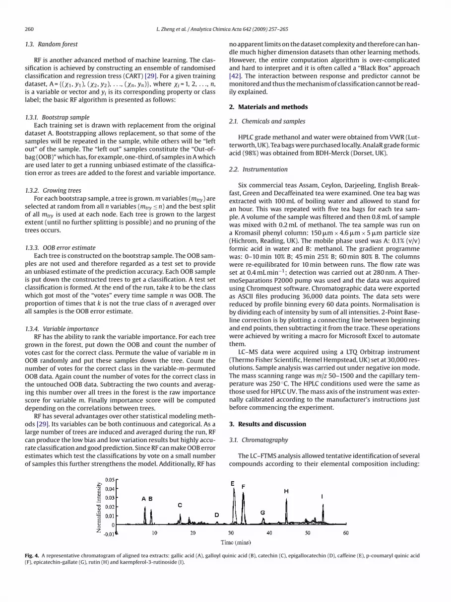
arge number of trees are induced and averaged during the run, RFan produce the low bias and low variation results but highly accu-ate classification and good prediction. Since RF can make OOB errorstimates which test the classifications by vote on a small numberf samples this further strengthens the model. Additionally, RF has

ig. 4. A representative chromatogram of aligned tea extracts: gallic acid (A), galloyl quiF), epicatechin-gallate (G), rutin (H) and kaempferol-3-rutinoside (I).

Acta 642 (2009) 257–265

no apparent limits on the dataset complexity and therefore can han-dle much higher dimension datasets than other learning methods.However, the entire computation algorithm is over-complicatedand hard to interpret and it is often called a “Black Box” approach[42]. The interaction between response and predictor cannot bemonitored and thus the mechanism of classification cannot be read-ily explained.

2. Materials and methods

2.1. Chemicals and samples

HPLC grade methanol and water were obtained from VWR (Lut-terworth, UK). Tea bags were purchased locally. AnalaR grade formicacid (98%) was obtained from BDH-Merck (Dorset, UK).

2.2. Instrumentation

Six commercial teas Assam, Ceylon, Darjeeling, English Break-fast, Green and Decaffeinated tea were examined. One tea bag wasextracted with 100 mL of boiling water and allowed to stand foran hour. This was repeated with five tea bags for each tea sam-ple. A volume of the sample was filtered and then 0.8 mL of samplewas mixed with 0.2 mL of methanol. The tea sample was run ona Kromasil phenyl column: 150 �m × 4.6 �m × 5 �m particle size(Hichrom, Reading, UK). The mobile phase used was A: 0.1% (v/v)formic acid in water and B: methanol. The gradient programmewas: 0–10 min 10% B; 45 min 25% B; 60 min 80% B. The columnswere re-equilibrated for 10 min between runs. The flow rate wasset at 0.4 mL min−1; detection was carried out at 280 nm. A Ther-moSeparations P2000 pump was used and the data was acquiredusing Chromquest software. Chromatographic data were exportedas ASCII files producing 36,000 data points. The data sets werereduced by profile binning every 60 data points. Normalisation isby dividing each of intensity by sum of all intensities. 2-Point Base-line correction is by plotting a connecting line between beginningand end points, then subtracting it from the trace. These operationswere achieved by writing a macro for Microsoft Excel to automatethem.

LC–MS data were acquired using a LTQ Orbitrap instrument(Thermo Fisher Scientific, Hemel Hempstead, UK) set at 30,000 res-olutions. Sample analysis was carried out under negative ion mode.The mass scanning range was m/z 50–1500 and the capillary tem-perature was 250 ◦C. The HPLC conditions used were the same asthose used for HPLC UV. The mass axis of the instrument was exter-nally calibrated according to the manufacturer’s instructions justbefore commencing the experiment.

3. Results and discussion

3.1. Chromatography

The LC–FTMS analysis allowed tentative identification of severalcompounds according to their elemental composition including:

nic acid (B), catechin (C), epigallocatechin (D), caffeine (E), p-coumaryl quinic acid

L. Zheng et al. / Analytica Chimica Acta 642 (2009) 257–265 261

lignm

gc(wrmc

t(Fac3t

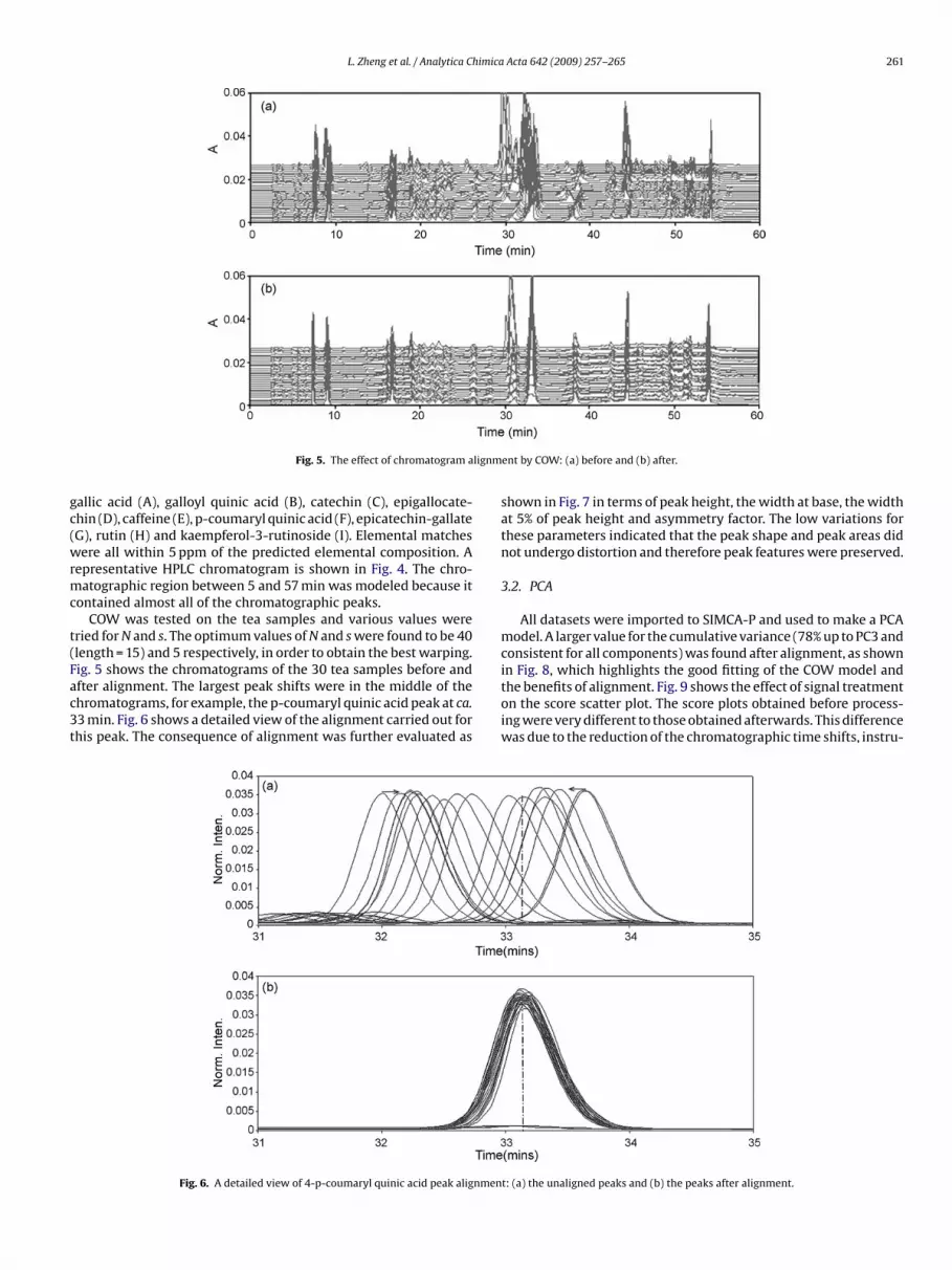
Fig. 5. The effect of chromatogram a

allic acid (A), galloyl quinic acid (B), catechin (C), epigallocate-hin (D), caffeine (E), p-coumaryl quinic acid (F), epicatechin-gallateG), rutin (H) and kaempferol-3-rutinoside (I). Elemental matchesere all within 5 ppm of the predicted elemental composition. A

epresentative HPLC chromatogram is shown in Fig. 4. The chro-atographic region between 5 and 57 min was modeled because it

ontained almost all of the chromatographic peaks.COW was tested on the tea samples and various values were

ried for N and s. The optimum values of N and s were found to be 40length = 15) and 5 respectively, in order to obtain the best warping.

ig. 5 shows the chromatograms of the 30 tea samples before andfter alignment. The largest peak shifts were in the middle of thehromatograms, for example, the p-coumaryl quinic acid peak at ca.3 min. Fig. 6 shows a detailed view of the alignment carried out forhis peak. The consequence of alignment was further evaluated as

Fig. 6. A detailed view of 4-p-coumaryl quinic acid peak alignmen

ent by COW: (a) before and (b) after.

shown in Fig. 7 in terms of peak height, the width at base, the widthat 5% of peak height and asymmetry factor. The low variations forthese parameters indicated that the peak shape and peak areas didnot undergo distortion and therefore peak features were preserved.

3.2. PCA

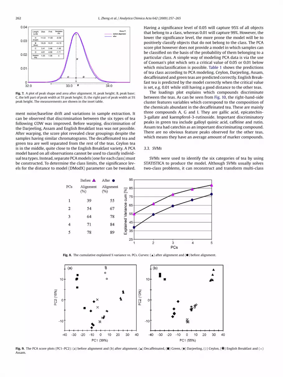
All datasets were imported to SIMCA-P and used to make a PCAmodel. A larger value for the cumulative variance (78% up to PC3 andconsistent for all components) was found after alignment, as shown

in Fig. 8, which highlights the good fitting of the COW model andthe benefits of alignment. Fig. 9 shows the effect of signal treatmenton the score scatter plot. The score plots obtained before process-ing were very different to those obtained afterwards. This differencewas due to the reduction of the chromatographic time shifts, instru-

t: (a) the unaligned peaks and (b) the peaks after alignment.

262 L. Zheng et al. / Analytica Chimica

FCp

mcftAsgimube

FA

ig. 7. A plot of peak shape and area after alignment. H, peak height; B, peak base;, the left part of peak width at 5% peak height; D, the right part of peak width at 5%eak height. The measurements are shown in the inset table.

ent noise/baseline drift and variations in sample extraction. Itan be observed that discrimination between the six types of teaollowing COW was improved. Before warping, discrimination ofhe Darjeeling, Assam and English Breakfast teas was not possible.fter warping, the score plot revealed clear groupings despite theamples having similar chromatograms. The decaffeinated tea andreen tea are well separated from the rest of the teas. Ceylon tea

s in the middle, quite close to the English Breakfast variety. A PCA

odel based on all observations cannot be used to classify individ-al tea types. Instead, separate PCA models (one for each class) muste constructed. To determine the class limits, the significance lev-ls for the distance to model (DModX) parameter can be tweaked.

Fig. 8. The cumulative explained % variance vs. PCs. Curv

ig. 9. The PCA score plots (PC1–PC2): (a) before alignment and (b) after alignment. (�)ssam.

Acta 642 (2009) 257–265

Having a significance level of 0.05 will capture 95% of all objectsthat belong to a class, whereas 0.01 will capture 99%. However, thelower the significance level, the more prone the model will be topositively classify objects that do not belong to the class. The PCAscore plot however does not provide a model in which samples canbe classified on the basis of the probability of them belonging to aparticular class. A simple way of modeling PCA data is via the useof Cooman’s plot which sets a critical value of 0.05 or 0.01 belowwhich misclassification is possible. Table 1 shows the predictionsof tea class according to PCA modeling. Ceylon, Darjeeling, Assam,decaffeinated and green teas are predicted correctly. English Break-fast tea is predicted by the model correctly when the critical valueis set, e.g. 0.01 while still having a good distance to the other teas.

The loadings plot explains which compounds discriminatebetween the teas. As can be seen from Fig. 10, the right-hand-sidecluster features variables which correspond to the composition ofthe chemicals abundant in the decaffeinated tea. These are mainlythree compounds A, G and I. They are gallic acid, epicatechin-3-gallate and kaempferol-3-rutinoside. Important discriminatorypeaks in green tea include galloyl quinic acid, caffeine and rutin.Assam tea had catechin as an important discriminating compound.There are no obvious feature peaks observed for the other teas,which means they have an average amount of marker compounds.

3.3. SVMs

SVMs were used to identify the six categories of tea by usingSTATISTICA to produce the model. Although SVMs usually solvestwo-class problems, it can reconstruct and transform multi-class

es: (�) after alignment and (�) before alignment.

Decaffeinated, (�) Green, (�) Darjeeling, (♦) Ceylon, ( ) English Breakfast and (×)

L. Zheng et al. / Analytica Chimica Acta 642 (2009) 257–265 263

Table 1Classification of teas according to Cooman’s plot (D-Crit 0.05).

Test M1.PModXPS, +[2] M2.PModXPS, +[2] M3.PModXPS, +[2] M4.PModXPS, +[2] M5.PModXPS, +[2] M6.PModXPS, +[2]Assam English Breakfast Tea Ceylon Darjeeling Decaffeinated Green

Green T 0 0 0 0.002 0 0.112English Br. T 0.002 0.043 0.001 0.002 0 0Ceylon T 0.001 0.001 0.084 0.002 0 0Darjeeling T 0 0.001 0.001 0.100 0 0Decaff. T 0 0 0 0.001 0.091 0Assam T 0.176 0.002 0.001 0.001 0 0

Table 2Overall classification for the tea samples according to SVMs with three different kernel functions using full variables or six PCs.

No. of SVs Cross-validation accuracy (%) Class-accuracy (training) Class-accuracy (test)

(a) Full variablesPolynomial 24 16.67 88.12 83.33RBF 23 100 100 100Sigmoid 24 83.33 95.13 83.33

(b) Six PCsPolynomial 7 33.33RBF 7 100Sigmoid 7 66.67

Fn

dsucatTpw

correctly. After extraction of the PCs, Assam got the lowest value

TT

(

(

ig. 10. PCA loadings plot (PC1:PC2) with location of the compounds A–H; for theirames refer to Fig. 4 legend.

atasets to a two-class model [43]. In this study of tea, 24 out of 30amples were randomly selected as the training set, the rest weresed as the test set. As mentioned earlier, various kernel functionsan be used in the SVMs equations. In order to obtain the best modelccuracy, three kernels were used with STATISTICA. Their parame-

ers including cross-validation were used to improve performance.able 2 shows the descriptive statistics for the three kernels. Theolynomial kernel possessed a cross validation accuracy of 16.67%,hile the RBF had an accuracy of 100%. The RBF used 23 support

able 3he probability of classification of tea samples using three different kernels with full varia

Assam (%) Darjeeling (%) Decaffeinated

a) Full variablesPolynomial 33 33 33RBF 60 60 60Sigmoid 42 42 42

b) Six PCsPolynomial 27 19 31RBF 66 66 66Sigmoid 38 38 33

88.12 66.67100 100

88.12 83.33

vectors to model the six tea classes while the polynomial, and sig-moid kernels used 24. For the classification and prediction accuracy,the RBF got 100% correct. Thus RBF was not only the best classifierbut also the most effective one, which used least number of supportvectors and achieved the best results. Similar trends also could befound in the individual prediction results. Table 3 shows the pre-diction results on the test samples. For example in the classificationof Assam, polynomial gave the lowest value of 33% and RBF got thehighest of 60%, the sigmoid kernel yielded a probability of 42%. RBFthus exhibited the best predictive ability. However, it was observedthat when the polynomial and sigmoid kernels were used to pre-dict English Breakfast and Ceylon tea, the probability had decreasedto 19% and 25% respectively. This might be explained in two ways.Ceylon and English Breakfast tea are very close according to thePCA score plots and therefore their chromatograms are very similar.In addition, the polynomial and sigmoid kernels are less useful forclassifying the groups if the number of variables is large. There were24 samples in the training set, and 23–24 SVs were used in themodel. This model is not persuasive and indicated that SVMs couldnot reduce the number of variables if the dimensions were too high.Thus, PCA was considered as a method for reducing the variables.Six PCs were extracted containing 98.8% of the variation. This newdataset was used in SVMs to do the analysis again. Table 3b showsthat seven SVs were created in the new model and RBF still classified

of 27% by polynomial and the highest of 66% by RBF. Ceylon andEnglish Breakfast tea got 19% and 13% by polynomial, 52% and 50%by RBF. The decreased prediction might be explained by the factthat Ceylon and English Breakfast tea are close together in the PCA

bles or with six PCs.

(%) English Breakfast (%) Ceylon (%) Green (%)

19 19 3360 60 6025 31 42

13 13 2150 52 6613 19 27

264 L. Zheng et al. / Analytica Chimica Acta 642 (2009) 257–265

Table 4Probability of classification of different tea samples according to RF modeling using full variables or six PCs.

Training set Test set

Assam (%) Darjeeling (%) Decaffeinated (%) English Breakfast (%) Ceylon (%) Green (%)

(a) Full variablesAssam 75 5 0 10 10 0Darjeeling 5 92.5 0 0 2 0.5Decaffeinated 0 0 95 0 5 0English Breakfast 5 0 2.5 90 0 2.5Ceylon 10 0 0 5 85 0Green 0 0 0 0 5 95

(b) Six PCsAssam 0.020 0.111 0.050 0.191 0.000 0.628Darjeeling 0.172 0.290 0.250 0.098 0.090 0.100Decaffeinated 0.160 0.230 0.313 0.110 0.090 0.097

0 0.580 0.090 0.0503 0.031 0.414 0.0902 0.067 0.000 0.000

m2

3

vpptTaidspnaiagGdDa9oreaeRtihcinaTnftwpgd

Table 5Important chromatographic regions for classification of the tea samples accordingto RF modeling (uk = unknown).

Variable Variable rank Importance Identity

472 100 1.00 uka

537 82 0.82 uk305 74 0.74 Caffeine311 69 0.69 Caffeine318 68 0.68 Caffeine112 68 0.68 uk347 67 0.67 uk284 64 0.64 uk442 63 0.63 Rutin367 63 0.63 uk447 62 0.62 Rutin140 62 0.62 uk

2 61 0.61 Tea identity424 59 0.59 uk

92 55 0.55 Galloyl quinic acid181 54 0.54 uk392 54 0.54 uk

73 54 0.54 Gallic acid

English Breakfast 0.130 0.090 0.06Ceylon 0.110 0.222 0.13Green 0.480 0.280 0.17

odel. By using six PCs, the number of SVs was decreased to 7 from3, while the results did not undergo too much change.

.4. RF

The teas datasets were analysed by using RF. STATISTICA pro-ides several parameters to optimise classification and predictionerformance. All retention time bins were defined as continuousredictors and the tea identities were defined as categorical predic-ors. Misclassification costs were set to be equal for all categories.he bootstrap splitting ratio was defined as 0.2 in order to makeconstant proportion with SVMs. The number of predictors was

mportant and was optimised by STATISTICA; this is helpful for largeatasets. STATISTICA uses Breiman’s method and 10 predictors areet [31]. The maximum number of trees was set to be 150. The stop-ing condition parameters were defined as five for the minimumumber of child nodes, 100 for the maximum number of nodes andminimum 5% for the decrease in training estimate error after one

teration. The stopping conditions were used to terminate the iter-tion of the RF model at the point where no more useful trees wereenerated. Table 4 shows the results of the RF model performance.reen and decaffeinated tea gave 95% probability for correct pre-iction. This was much better prediction than that given by SVMs.arjeeling was correctly classified with 92.5% probability. Ceylonnd English Breakfast tea were predicted correctly with 85% and0% accuracy since there was some probability of misclassificationf English Breakfast as Ceylon or Assam and Ceylon as Assam. Theesults indicated that RF gave correct answer for each class, how-ver, the high number of variables and the small size of the sampleslso pose a question to RF whether or not the model is correct. How-ver, according to Breiman [41] the number of variables used in theF approach is not critical. The PCA extraction data was used againo study the effect of reducing the number of variables. The resultsn Table 4 show that green tea gets a probability of 62.8% as theighest and Ceylon gets 31.3% as the lowest. The predictions areorrect for each class when using six PCs even though the probabil-ties are lower. There is nothing in the literature to suggest that theumber of variables should be restricted in RF models. RF uses vari-ble importance to describe the weight of the different predictors.able 5 shows the top 20 dominating variables; some of these wereot identified. Of the identified variables the regions of the peaks

or caffeine, rutin, galloyl quinic acid and gallic acid were impor-

ant. Even the categorical predictor, class name, was regarded as aeighted predictor. However, not all of them were helpful in inter-reting the RF model. Overall it was confirmed that caffeine, rutin,alloyl quinic acid and gallic acid were very relevant descriptors forifferentiating green, Darjeeling and decaffeinated teas.

225 53 0.53 uk83 52 0.52 uk

a No. of peaks observed in this region.

4. Conclusion

In this paper, chromatography based chemometrics was per-formed in order to distinguish between different teas. Thisrepresented a significant challenge since the differences in thetea chromatograms were small. Signal treatment which includedCOW, binning and normalisation proved to be effective for remov-ing effects that did not contribute to the classification. This thenallowed better classification by PCA. Although PCA gives a classifi-cation of the teas it does not give a model where the classificationcan be assigned a probability. PCA, SVMs and RF were comparativelyevaluated as methods for processing the tea chromatograms forclassification and prediction of the different tea samples. Cooman’splots derived from the PCA model all teas correctly when a signif-icance threshold of 0.01 was used. In the case of SVMs, RBF usingseven support vectors produced the best accuracy, thus RBF provedto be the best kernel. RF exhibits the better predictive power thanSVMs in classifying the tea extracts in the test set. Several com-ponents which were identified by MS were found to be important

in classifying the teas. These compounds agreed with the loadingsobserved in the PCA model. In this study, SIMCA-P and STATISTICAwere used. SIMCA was very suitable for multivariate regression withgood visual output; while STATISTICA had much more comprehen-sive statistical power.

himica

A

C

R

[

[[[[

[

[[[

[

[

[[[

[

[[[

[[[[

[

[

[

[[[ .

L. Zheng et al. / Analytica C

cknowledgement

We want to thank University of Copenhagen who provided coreOW programmes on their website.

eferences

[1] P. Wipawee, F. Eiichiro, B. Takeshi, Y. Tsutomu, J. Agric. Food Chem. 55 (2007)231.

[2] M.M. Hsieh, S.M. Chen, Talanta 73 (2007) 326.[3] J. Zhao, Q.S. Chen, X.Y. Huang, J. Pharm. Biomed. Anal. 41 (2006) 1198.[4] M.P. Lillo, P.N. Sanderson, E.L. Wantling, D.A. Pudney, Dev. Food Sci. 43 (2006)

537.[5] D.M. Wang, J.L. Lu, A.Q. Miao, Z.Y. Xie, D.P. Yang, J. Food Comp. Anal. 21 (2008)

361.[6] Y. Lv, X.B. Yang, Y. Zhao, Y. Ruan, Y. Yang, Food Chem. (2008).[7] L. Xiang, D.M. Xing, F. Lei, W. Wang, L.Z. Xu, L. Nie, L.J. Du, Tsinghua Sci. Technol.

13 (2008) 460.[8] M. Daszykowski, Y.V. Heyden, B. Walczak, J. Chromatogr. A 1176 (2007) 12.[9] S.D. Kumar, G. Narayan, S. Hassarajani, Food Chem. 111 (2008) 784–788.10] M. Daszykowski, W. Wu, A.W. Nicholls, T. Czekaj, B. Walczak, J. Chemometr. 21

(2007) 292.11] N.V. Nielsen, J.M. Carstensen, J. Smedsgaard, J. Chromatogr. A 805 (1998) 17.12] M. Katajamaa, M. Oresic, J. Chromatogr. A 1158 (2007) 318.13] M. Chae, R.J.S. Reis, J.J. Thaden, BMC Bioinform. 9 (2008) (available online).14] K.J. Johnson, B.W. Wright, K.H. Jarman, R.E. Synovec, J. Chromtatogr. A 996

(2003) 141.15] C.A. Smith, E.J. Want, G.O. Maille, R. Abagyan, G. Siuzdak, Anal. Chem. 78 (2006)

779.16] Machine learning, http://hunch.net/.17] H.C. Kim, S. Pang, H.M. Je, D. Kim, S.Y. Bang, Pattern Recogn. 36 (2003) 2757.18] V.N. Vapnik, A.Y. Chervonenkis, Theory Prob. Appl. 17 (1971) 26.

[[[[[[

Acta 642 (2009) 257–265 265

19] V.N. Vapnik, The Nature of Statistical Learning Theory, Springer–Verlag,2000.

20] H.T. Kam, Proceedings of the 3rd International Conference on Document Anal-ysis and Recognition, 1995, p. 278.

21] H.T. Kim, IEEE Trans. Pattern Anal. Mach. Intell. 20 (2005) 832.22] A. Yali, G. Donald, Neural Comput. 9 (1997) 1545.23] H.T. Kim, S.S. Kim, S.J. Kim, Proceedings of the 2005 IEEE Engineering in

Medicine and Biology, 27th Annual Conference, 2005.24] I. Yélamos, G. Escudero, M. Graells, L. Puigjaner, Comp. Aided Chem. Eng. 24

(2007) 1253.25] H.T. Kim, H. Park, Protein Eng. 16 (2003) 553.26] I. Guyon, J. Weston, S. Barnhill, V. Vapnik, Mach. Learn. 46 (2002) 389.27] D. Wu, X.J. Chen, Y. He, International Conference on Computational Intelligence

and Security Workshops, 2007.28] L. Breiman, Mach. Learn. 24 (1996) 123.29] L. Breiman, Mach. Learn. 45 (2001) 5.30] S. Brown, A.E. Lugo, Plant Soil 124 (1990) 53.31] L. Breiman, A. Cutler, Random Forest—Manual, http://www.stat.berkeley.

edu/∼breiman/RandomForests/cc manual.htm, 2004.32] L. Breiman, J. Friedman, R. Olshen, C. Stone, Classification and Regression Trees,

Wadsworth International, Belmont, California, 1984.33] R. Grimm, T. Behrens, M. Märker, H. Elsenbeer, Geoderma 146 (2008)

102–113.34] D. Perdiguero-Alonso, F.E. Montero, A. Kostadionva, J.A. Raga, J. Barrett, Int. J.

Parasitol. (2008) (available online).35] V. Pravdova, B. Walczak, D.L. Massart, Anal. Chim. Acta 456 (2002) 77.36] G. Tomasi, F. van den Berg, C. Anderson, J. Chemometr. 18 (2004) 231.37] G. Tomasi, COW codes, http://www.models.kvl.dk/source/DTW COW/index.asp

38] M. Aizerman, E. Braverman, L. Rozonoer, Automat. Rem. Control 25 (1964) 821.39] C.J.C. Burges, Data Mining Knowl. Disc. 2 (1998) 121.40] D. Meyer, F. Leisch, K. Hornik, Neurocomputing 55 (2003) 169.41] C. Cortes, V. Vapnik, Mach. Learn. 20 (1995) 273–297.42] L. Breiman, Looking inside the black box, in: Wald Lecture II, 2002.43] C. Angulo, X. Parra, A. Català, Neurocomputing 55 (2003) 57.