1

METHOD FOR INVESTIGATING INTRADRIVER HETEROGENEITY USING VEHICLE

TRAJECTORY DATA: A DYNAMIC TIME WARPING APPROACH

Jeffrey Taylor

Department of Civil and Environmental Engineering

University of Utah, Salt Lake City, UT 84112-0561

Email: jeff.d.taylor@utah.edu

Xuesong Zhou*, Ph.D.

School of Sustainable Engineering and the Built Environment

Arizona State University

Tempe, AZ 85287, USA

Tel.: (1)-480-9655827

Email: xzhou74@asu.edu

Nagui M. Rouphail, Ph.D.

Institute for Transportation Research and Education (ITRE)

Civil Engineering

North Carolina State University

Centennial Campus, Box 8601

Raleigh, NC 27695-8601

Email: rouphail@eos.ncsu.edu

Richard J. Porter, Ph.D.

Department of Civil and Environmental Engineering

University of Utah, Salt Lake City, UT 84112-0561

Email: richard.jon.porter@utah.edu

*Corresponding Author

Submitted for publication in Transportation Research Part B

First submission: May 28, 2014

Revised submission: December 26, 2014

2

ABSTRACT

After first extending Newell’s car-following model to incorporate time-dependent parameters, this paper

describes the Dynamic Time Warping (DTW) algorithm and its application for calibrating this microscopic

simulation model by synthesizing driver trajectory data. Using the unique capabilities of the DTW

algorithm, this paper attempts to examine driver heterogeneity in car-following behavior, as well as the

driver’s heterogeneous situation-dependent behavior within a trip, based on the calibrated time-varying

response times and critical jam spacing. The standard DTW algorithm is enhanced to address a number of

estimation challenges in this specific application, and a numerical experiment is presented with vehicle

trajectory data extracted from the Next Generation Simulation (NGSIM) project for demonstration

purposes. The DTW algorithm is shown to be a reasonable method for processing large vehicle trajectory

datasets, but requires significant data reduction to produce reasonable results when working with high

resolution vehicle trajectory data. Additionally, singularities present an interesting match solution set to

potentially help identify changing driver behavior; however, they must be avoided to reduce analysis

complexity.

Keywords: Dynamic Time Warping, Car-following model, Driver behavior heterogeneity, Vehicle

trajectory data

3

1. Introduction

It has been evident over the past decade that continuing advances in traffic simulation systems intrinsically

depend on advances in driving behavior modeling. Traffic incidents, driver inattention, and recurring

bottlenecks are widely recognized as the most significant factors affecting congestion (in conjunction with

bad weather, work zones and poor signal timing). Thus, for most planning and operational applications,

transportation analysts must strive to achieve realistic representations of driving behaviors during unusual

and complex traffic situations.

Individual driver characteristics, such as response time and spacing in jam conditions, are expected to be

altered during complex driving conditions, and thus are expected to contribute toward the occurrence of

stop-and-go traffic patterns which eventually translate into changes in travel time reliability, roadway

capacity, and vehicle emissions. This paper aims to address the following theoretically challenging and

practically important question: How can we enhance existing traffic simulation models and the

corresponding calibration algorithms so that they can more accurately and sensitively capture the impacts

of time-dependent and situation-dependent driver behavior? We first start with a comprehensive review on

various topics related to the above question.

1.1 Driving Behavior and Microscopic Simulation Models

Driving behavior is a difficult human decision-making processes to model. A wide range of car-following

models, psycho-physical models and multi-phase traffic flow theories have been proposed in an attempt to

capture the driving behavior at a microscopic level. In many existing simulations of driving models, the

behavior of a driver is mainly determined by the relative headway, gap, speed and acceleration of the lead

and surrounding vehicles. Although a number of traffic simulation models have considered multiple driver

classes to accurately describe heterogeneous perception and preferences, most widely used models still

assume the same behavioral characteristics under both congested and uncongested driving situations.

Within our experimental and conceptual understanding, several studies (e.g., Ossen and Hoogendoorn,

2005; Ossen and Hoogendoorn, 2007; Duret et al., 2008; Chiabaut et al., 2010) have confirmed that

calibrated car-following model parameters can be different for different drivers. In particular Chiabaut et

al. (2010) developed an effective estimation method to examine and calibrate interdriver heterogeneity in

Newell's car-following model. Generically, interdriver heterogeneity describes the idea that different

drivers may have different reactions to the same stimulus. Extending this concept, other studies (e.g., Ossen

et al., 2006) have found that the actions of different drivers in a group of vehicles may be better explained

using multiple car-following models rather than a single model.

4

Several recent studies have examined driver behavior heterogeneity and its impact on microscopic

simulation models. Ossen and Hoogendoorn (2005) used high resolution trajectory data from a helicopter

to find optimal sensitivity and reaction time parameters for individual drivers and for multiple car-following

models. A later study in Ossen and Hoogendoorn (2007) showed that driver heterogeneity could not be

explained only with model parameters, but must also include model specifications. Most recently, Ossen

and Hoogendoorn (2011) studied vehicle trajectories for passenger vehicles and trucks in different leader-

follower scenarios. Their results showed large variations between how passenger car drivers react to

different stimuli and which stimuli influence their behavior, while truck drivers maintained more consistent

speeds over time. They also showed that driver behavior can change depending on the leader’s vehicle type.

Kim and Mahmassani (2011) calibrated multiple car-following models using NGSIM trajectory data to

examine the effects of considering correlation between model parameters. Their results indicate a

statistically-significant difference between correlated and uncorrelated parameter sets for the models tested,

but the effects varied widely between those models. Recent studies by Chen et al. (2010) and Li et al. (2010)

also proposed enhanced car-following models by considering stochastic headway and spacing distributions.

Laval and Leclercq (2010) presented a theory for modeling aggressive and timid driver behavior which

describes traffic oscillations and their transformation into stop-and-go waves. They specifically identified

traffic oscillations as a consequence of drivers’ heterogeneous reactions to deceleration waves, but noted

that aggressive and timid driving behavior alone could not produce the observed traffic oscillations. Based

on Laval and Leclerc’s (2010) study for capturing intra-driver variance, a recent paper by Chen et al. (2012)

aims to further capture intra-driver variance by considering situation-dependent time and space lag

parameters when drivers experience driving disturbances. By assuming constant wave speed, their observed

different reaction patterns across different drivers, e.g., caused by stop-and-go conditions.

In this paper, we are interested in extending Newell’s simplified linear car-following model (LCF) (1962,

2002), which considers the following two driving modes: (i) Under uncongested conditions, vehicles are

driving at free-flow speed, and (ii) Under congested conditions, a following vehicle changes speeds to

maintain a minimum jam spacing and a response time lag with respect to the leading vehicle’s trajectory.

Brockfeld et al. (2004) calibrated and validated a number of well-known car following models, and

Newell’s simplified LCF model showed reasonable performance with limited calibration efforts.

1.2 Intra-driver Heterogeneity

In general, intradriver heterogeneity implies that the same driver may react differently to the same stimulus

at different times or under different conditions. More recent studies have also (e.g., Wang et al., 2010; Kim

et al., 2013) found evidence which suggests that a single driver’s actions can be better described by using

5

different car-following parameters and/or different car-following models to describe a single vehicle

trajectory. Focusing on Newell’s car following model, Ahn et al. (2013) systematically discussed how

speed-spacing relationships can evolve during different phases of acceleration/deceleration. In their study,

they have considered varying wave speed within driver due to stochasticity, and presented methods to

identify wave paths by matching points with similar speed. Zheng et al. (2011; 2013) further examined the

changes in the speed-spacing parameters under major disturbances such as lane changes and traffic flow

oscillations.

Several studies have examined driver heterogeneity using trajectory data in terms of driver-specific (inter-

driver) and/or time-varying (intra-driver) car-following model parameters. Hamdar et al. (2009) noted that

“heterogeneity observed in traffic dynamics may be attributed to intra-driver heterogeneity rather than inter-

driver heterogeneity.” This matches Kesting and Treiber’s (2009) observation that “intra-driver variability

accounts for a large part of the deviations between simulations and empirical observations.” Wagner (2012)

also reported similar results, indicating that most fluctuations in time headways can be attributed to

individual drivers adopting new preferred headways. Ahn et al. (2004) confirmed driver-specific model

parameters in Newell’s Car-Following model, aligning with Newell’s model definition, but did not confirm

the presence of time-varying parameters. Ossen et al. (2006) used individual vehicle trajectory data to

compare optimal car-following model parameters and different models for only individual drivers. Wang

et al. (2010) used data from Dutch motorways to identify longer response times for drivers while

accelerating compared to decelerating. They found that 65% of drivers demonstrated different “driving

styles” between the two states, where the calibrated model in the acceleration state could not accurately

describe the trajectory in the deceleration state. They suggested a multiphase car-following model to capture

this heterogeneity for more reliable traffic simulation.

While several studies point to intra-driver variability in model parameters as a significant source of error in

traffic simulation, few studies have thoroughly described intra-driver heterogeneity. For example, Wang et

al. (2010) directly addresses the intra-driver heterogeneity issue, but only provides a comparison based on

“car-following phases” (acceleration and deceleration phases). Overall, most studies on this subject have

focused on how model parameters change between acceleration and deceleration phases in car-following,

or on which car-following models are most appropriate for these phases. However, the calibration

techniques applied in these efforts tend to limit the temporal resolution at which model parameters may be

estimated. For example, an acceleration or deceleration phase may last several seconds, and the calibration

technique may offer model parameter estimates which are applicable over several seconds. Thus far,

however, few researchers have attempted to estimate how car-following model parameters might change

second-by-second, or at sub-second temporal resolutions.

6

1.3 Car-Following Model Calibration

Microscopic vehicle trajectory data has been used for calibrating car-following models by numerous

authors, and several methods have been used for calibrating those models. For instance, Ma and Andreasson

(2006) describe calibration as a nonlinear optimization problem, where the solution approaches can be

divided into gradient-based methods or derivative-free methods, which include grid-search algorithms and

the genetic algorithm. Their study calibrated a GM-type model with data collected using an instrumented

Volvo vehicle. Ciuffo et al. (2011) provides a review of several methodologies used for microsimulation

calibration, including Simultaneous Perturbation Stochastic Approximation, Simulated Annealing, Genetic

Algorithms, and the OptQuest/Multistart heuristic algorithm. Genetic algorithms were noted as the most

common in their study. Hamdar et al. (2009) used a Genetic Algorithm to calibrate a stochastic car-

following model using NGSIM data. Kesting and Trieber (2008) used a method similar to a Genetic

Algorithm to calibrate the Intelligent Driver Model (IDM) and the Velocity Difference model from vehicle-

mounted radar sensors. Ciuffo et al. (2011) also described a Kriging Meta-model approach to

microsimulation calibration, where the model attempts to match the global and local optimum features of

the solution quality parameters with the same features for the simulation model.

Ossen and Hoogendoorn (2008a) took a critical look at calibrating car-following models with real-world

vehicle trajectories. They began with speed data from real-world trajectories, and developed 25 leader

vehicle trajectories using a model with known calibration parameters. These synthetic datasets were then

injected with artificial errors, representing different types of measurement errors, and a new calibration was

performed. The new parameters were then compared with the known parameters to evaluate the effects of

those errors in calibration. Their study found that measurement errors can introduce bias when estimating

model parameters, the objective function used in their calibration process became less sensitive with

measurement errors, and their optimization results did not produce the optimal model parameters used to

create the synthetic calibration data. Additionally, they showed that the calibration results improved when

using a simple moving average for smoothing to account for some measurement errors. Hoogendoorn et al.

(2011) describes a piecewise linear approximation filtering technique, showing that speed profiles in

NGSIM data can be represented well using periods of constant acceleration. A later study by Ossen and

Hoogendoorn (2009) examined the degree of information contained in vehicle trajectories and the effects

of measurement errors on the calibration objective function’s sensitivity. They provide a more in-depth

review of vehicle trajectory data collection techniques, calibration and verification methods, and assess the

influence of measurement errors in a guide available online (Ossen and Hoogendoorn, 2008b).

7

1.4 Proposed Modeling Approach Using Dynamic Time Warping Algorithm

The Dynamic Time Warping (DTW) algorithm is used to measure the similarities between two time-series

datasets, which can be viewed as an optimization problem minimizes the effects of shifting and distortion

in time through a flexible transformation/mapping of time series (Senin, 2008). This approach can also be

used to identify the optimal alignment between two time-dependent data series, and the algorithm finds the

alignment with the least cumulative cost, called the warp path (Keogh and Pazzani, 2001), using a shortest

path algorithm which starts at the last pair and works back to the first pair. The commonly used cost is a

quantitative measure of the similarity or difference between two points.

The goal of this research is to enable investigations into intra-driver heterogeneity by estimating time-

varying, car-following model parameters based on high-resolution vehicle trajectory datasets. This is

accomplished by providing model parameter estimates at each discrete point in time along the vehicle

trajectory, rather than providing one set of model parameter estimates for an entire trajectory or a “car-

following phase.” In this research, we use the DTW algorithm to find the optimal alignment between two

time-series data sets. When applied to vehicle trajectory data, the alignment is considered an estimate of

the stimulus-response relationship for a driver following a leading vehicle, and it is used to infer the time-

varying, car-following model parameters for a driver during the observation time period. The underlying

assumption is that the stimulus-response driver behavior model can be represented in terms of time-series

similarity and further estimated using the DTW algorithm. That is, time-series similarity techniques may

help to identify the stimulus-response interactions observed in empirical data.

Our advantage here is the combination of Newell’s model and DTW. Newell’s simplified model parameters

reduce calibration process complexity, and the DTW algorithm’s pattern-matching capabilities should

significantly improve our calibration solution for small datasets. With higher-resolution data, we can

attempt to quantify the stochasticity present in the different model parameters and describe parameter

sensitivity, providing information for incorporating time-varying parameters in car-following models which

is not likely to be found in the literature. We can also analyze the data for patterns based on different “car-

following phases”, such as acceleration and deceleration states, which can be used to improve multiphase

models.

The organization of this paper can be described as follows. Section 2 attempts to extend Newell’s classical

simplified linear car-following model (2002) to incorporate time-dependent response time and spacing

parameters. In Section 3, this enhanced microscopic simulation model will be calibrated through a novel

use of the Dynamic Time Warping (DTW) algorithm using recently available continuous or semi-

continuous vehicle location, speed and acceleration data across different time periods. Finally, a numerical

8

experiment and a discussion on the limitation and challenges are presented in Sections 4 and 5 to explore

the capabilities of the DTW algorithm for estimating time-dependent driver behavior under different

conditions.

2. Car Following Model Formulation

2.1 Newell’s car-following model

Newell’s car-following model (Newell, 2002) is based upon one basic assumption: A vehicle following

another vehicle (the leader vehicle) in a homogenous space replicates the trajectory of the leader vehicle,

but their trajectories are separated by a time and distance offset. This relationship between vehicle

trajectories is described mathematically in the following equation:

𝑥𝑛(𝑡 + 𝜏𝑛) = 𝑥𝑛−1(𝑡) − 𝑑𝑛 (1)

where

𝑡 = time index,

𝑛 = vehicle number index,

𝑥𝑛 = position of vehicle 𝑛,

𝑑𝑛 = critical jam spacing, or distance offset, for vehicle 𝑛, and

𝜏𝑛 = time lag, or response time, for vehicle 𝑛.

The left hand side of Eq. (1) describes the position of the following vehicle at time (𝑡 + 𝜏𝑛), where 𝑛

refers to the following vehicle. The right side of Eq. (1) refers to the position of the leader vehicle at time

𝑡 and the distance offset between the two trajectories, where 𝑛 − 1 refers to the vehicle preceding the

following vehicle. In this generalized formulation, the model parameters 𝑑𝑛 and 𝜏𝑛, are associated with

each vehicle, and may be assumed to be constant over time. This car-following model is also consistent

with Newell’s simplified kinematic wave model (Newell, 1993), where the Fundamental Diagram of

Traffic Flow takes a triangular shape, as shown in Fig. 1. Under this model, the critical jam spacing is the

inverse of the jam density (𝑑𝑛 = 1/𝑘𝑗𝑎𝑚), and the backward shockwave speed 𝑤 is related to both car-

following parameters (𝑤𝑛 = 𝑑𝑛/𝜏𝑛).

9

Figure 1. Flow-Density and Speed-Density diagrams associated with Newell’s car-following model.

Typical values: 𝑤 = 19 km/h and 𝑘𝑗𝑎𝑚 = 112 vehicles/km/lane, which leads to 𝑑𝑛̅̅̅̅ = 9 meters, 𝜏𝑛̅̅ ̅ = 1.7

seconds.

Since vehicle trajectories are replicated in Newell’s simplified car-following model, the speeds of both

vehicles are also replicated with a certain time lag. The first derivative of Eq. (1) indicates that the speed

of the leader vehicle is replicated by the speed of the following vehicle after the time offset 𝜏𝑛, as derived

in Eq. (2) and shown in Eq. (3). This is important because it identifies velocity time-series data as a good

candidate for pattern matching, where matching the speed profile of two vehicles can help estimate the

time offset.

𝑑

𝑑𝑡(𝑥𝑛(𝑡 + 𝜏𝑛)) =

𝑑

𝑑𝑡(𝑥𝑛−1(𝑡) − 𝑑𝑛) (2)

�̇�𝑛(𝑡 + 𝜏𝑛) = �̇�𝑛−1(𝑡) (3)

Newell makes an additional simplifying assumption by using a piecewise linear approximation to

describe vehicle trajectories. The visual representation in Fig. 2 shows the position of the leader vehicle in

a time-space diagram with both a solid line and a dashed line, where the solid line is the linear

approximation to the observed dashed line. This implicitly assumes that all acceleration is instantaneous.

If the velocity of the (𝑛 − 1)𝑡ℎ car and the 𝑛𝑡ℎ car are the same, the piecewise linear approximation is

reasonable, but this may not be the case where drivers’ reactions to the change in speed are not

homogeneous.

0

500

1000

1500

2000

0 50 100 150

Flo

w (

Veh

icle

s/H

ou

r)

Density (Vehicles/Kilometer/Lane)

0

20

40

60

80

100

120

0 50 100 150

Sp

eed

(K

PH

)

Density (Vehicles/Kilometer/Lane)

10

Sn

Sn'

τn

dn

Xn(t)

Xn-1(t)

Time, t

Dis

tance

, X

Figure 2. Visual representation of Newell's Car-Following Model with piecewise linear approximation

(replicated from Newell, 2002).

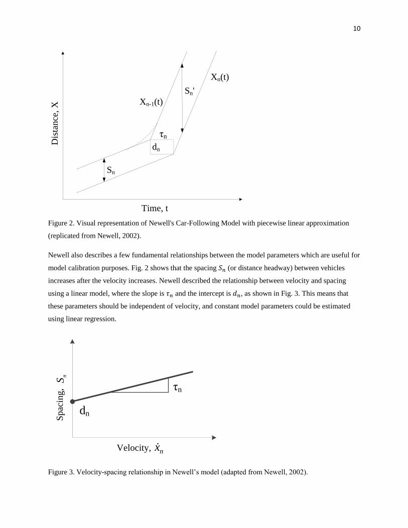
Newell also describes a few fundamental relationships between the model parameters which are useful for

model calibration purposes. Fig. 2 shows that the spacing 𝑆𝑛 (or distance headway) between vehicles

increases after the velocity increases. Newell described the relationship between velocity and spacing

using a linear model, where the slope is 𝜏𝑛 and the intercept is 𝑑𝑛, as shown in Fig. 3. This means that

these parameters should be independent of velocity, and constant model parameters could be estimated

using linear regression.

dn

Velocity,

Spac

ing,

nx

nS

τn

Figure 3. Velocity-spacing relationship in Newell’s model (adapted from Newell, 2002).

11

2.2 Formulation with Time-Varying Parameters

As stated before, the goal of this research is to investigate intra-driver heterogeneity by estimating time-

varying, car-following model parameters. That is, it is assumed that the manner by which those model

parameters vary with time can be used to describe intra-driver heterogeneity. More systematically, we can

also assume that the underlying process indeed show a “disturbance” for tau and d because even if these

are allowed to vary with time, there will be additional variation from factors known (but unmeasured) and

unknown.

Thus, this research begins with the hypothesis that car-following model parameters are not constant for

each driver, but actually change over time. In order to test this hypothesis with Newell’s car-following

model using the proposed methodology, Newell’s model needs to be re-formulated using time-varying

parameters. As a result, Eq. (1) becomes Eq. (4):

𝑥𝑛(𝑡 + 𝜏𝑛,𝑡) = 𝑥𝑛−1(𝑡) − 𝑑𝑛,𝑡 (4)

where

𝜏𝑛,𝑡 = time lag, or time offset, for vehicle 𝑛 at time 𝑡,

𝑑𝑛,𝑡 = critical jam spacing, or distance offset, for vehicle 𝑛 at time 𝑡.

Redefining Newell’s car-following model in order to use time-varying parameters introduces several

potential issues. The most significant issues are related to the Newell’s modeling assumptions. For

example, if 𝑑 and 𝜏 vary with time, the linear relationship between velocity and spacing described in Fig.

3 is no longer valid.

3. Dynamic Time Warping Algorithm

In order to better explain the inner workings of the algorithm and its components, this section first

identifies the notation used to describe the algorithm. Next, the algorithm is explained step-by-step with

illustrative elements which help to explain each component in the algorithm. Details are also provided for

an alternative formulation where the algorithm is translated into an optimization problem which can be

solved using linear programming. This section ends with an illustrative example aligning two sets of

vehicle speed data time series.

3.1 Notation

𝑋 = {𝑥1, 𝑥2, … , 𝑥𝑖, … , 𝑥𝑁}, which is the 1st time series data set

𝑃 = {𝑝1, 𝑝2, … , 𝑝𝑖 , … , 𝑝𝑁}, which is the position data associated with the 1st time series data set

12

𝑇1 = {𝑡1,1, 𝑡1,2, … , 𝑡1,𝑖, … , 𝑡1,𝑁}, which is the time stamp data associated with the 1st time series data set

𝑌 = {𝑦1, 𝑦2, … , 𝑦𝑗 , … , 𝑦𝑀}, which is the 2nd time series data set

𝑄 = {𝑞1, 𝑞2, … , 𝑞𝑗, … , 𝑞𝑀}, which is the position data associated with the 2nd time series data set

𝑇2 = {𝑡2,1, 𝑡2,2, … , 𝑡2,𝑗, … , 𝑡2,𝑀}, which is the time stamp data associated with the 2nd time series data set

𝑖 = index for time series 𝑋 made up of measurements 𝑃 and 𝑇1, (𝑖 = 1, 2, … , 𝑁)

𝑗 = index for time series 𝑌 made up of measurements 𝑄 and 𝑇2, (𝑗 = 1, 2, … , 𝑀)

𝐶(𝑖, 𝑗) = the cost (in terms of similarity) of mapping/aligning point 𝑋𝑖 to point 𝑌𝑗

𝐷(𝑖, 𝑗) = the cumulative least cost (in terms of similarity) of mapping/aligning point 𝑋𝑖 to point 𝑌𝑗,

considering the cost of mapping/aligning point 𝑋𝑖 to point 𝑌𝑗 as well as the costs of previous mapped

points between (𝑋1, 𝑌1) and (𝑋𝑖, 𝑌𝑗)

𝑘 = index for time series 𝑊

𝐿 = number of coordinates in 𝑊

𝑊 = {𝑤1, 𝑤2, … , 𝑤𝑘 , … , 𝑤𝐿}, which is the warp path – a list of coordinates which constitutes the shortest

path (or more precisely least matching cost path) through matrix D, such that 𝑤𝑘 = (𝑖, 𝑗).

3.2 DTW Algorithm

In its basic form, the DTW algorithm first assesses the cost for aligning each data point in one time series

to all other points in the second time series, creating a cost matrix. It then begins at the first data series

pair in the cost matrix, calculating the cumulative least cost for continuously moving from the first pair to

the last pair in the matrix, creating a cumulative cost matrix. Lastly, the algorithm finds the alignment

with the least cumulative cost, using a shortest path algorithm which starts at the last pair in the

cumulative cost matrix and works back to the first pair. While the cost is a quantitative measure of the

similarity or difference between two points in each time-series dataset (distance is commonly used), it can

also be a flexible term which may be modified to suit the application. The algorithm is explained in

further detail below with visual elements to help understand the different components.

3.2.1 Input Data

The DTW algorithm is based on the idea of measuring the similarity or distance between two or more

elements or sets of data. This measurement is usually performed using a metric, such as the generalized

13

norm, or Lp distance (the L2 norm, or Euclidean distance, is commonly chosen). The cost 𝐶(𝑖, 𝑗) of

mapping two points (𝑋𝑖, 𝑌𝑗) together is based on this measured similarity or distance calculated from the

input time series data sets 𝑋 and 𝑌. In this study, the metric is based upon the input data taken from the

underlying car-following model. For Newell’s car-following model, the similarity metric should be based

on vehicle velocity because Eq. (3) showed that the velocities of the lead and following vehicles should

be the same at a time offset from each other.

Since Newell’s model assumes that the velocities are the same, the acceleration should also be the same

and could be a potential candidate as input data for the DTW algorithm. However, high resolution

observation data typically shows that acceleration data is more volatile and subject to greater uncertainty,

often due to measurement error. DTW can be sensitive to noisy input data, so velocity data was selected

as the input data for the DTW algorithm. An example of velocity input time series data is shown in Fig. 4.

Time

Po

siti

on

1 2 3 4 5 6 7 8

(a) Raw Vehicle Trajectories

X: Leader

Y: Follower

Time

Velo

cit

y

X: LeaderY: Follower

1 2 3 4 5 6 7 8

(b) Vehicle Velocity Time Series

Figure 4. (a) Raw vehicle trajectories, and (b) their corresponding velocity time series datasets.

3.2.2 Cost Matrix

The first step in the DTW algorithm, after assembling the input data, is to construct the cost matrix. The

cost matrix 𝐶(𝑖, 𝑗) is an 𝑁 × 𝑀 matrix which stores all pair-wise distances between X and Y. The cost in

each cell of the cost matrix is calculated using Eq. 5.

𝐶(𝑖, 𝑗) = √(𝑥𝑖 − 𝑦𝑗)2

= |𝑥𝑖 − 𝑦𝑗| (5)

14

The cost matrix is created using Algorithm 1. An example of a cost matrix is shown in Fig. 5.

Algorithm 1:

For i = 1 to N

For j = 1 to M

𝐶(𝑖, 𝑗) = |𝑥𝑖 − 𝑦𝑗|

EndFor

EndFor

Time

Velocity Y: Follower

Tim

e

Velocity

X: L

eader

1 2 3 4 5 6 7 8

1 0 0 0 0 18 18 18 5

2 0 0 0 0 18 18 18 5

3 0 0 0 0 18 18 18 5

4 20 20 20 20 2 2 2 25

5 20 20 20 20 2 2 2 25

6 5 5 5 5 23 23 23 0

7 5 5 5 5 23 23 23 0

8 5 5 5 5 23 23 23 0

Figure 5. Visual representation of the cost matrix

3.2.3 Cumulative Cost Matrix

The next step is to calculate the cumulative cost matrix 𝐷(𝑖, 𝑗), which is an 𝑁 × 𝑀 matrix which stores

the cumulative least cost required to arrive at any location in the matrix by following a specified search

pattern from (1,1) to (𝑁, 𝑀). The most common search pattern allows the algorithm to check costs in the

next cell vertically, horizontally, or diagonally away from the current cell in the matrix. The cumulative

least cost in each cell of the matrix is calculated using Eq. (6), which also identifies the search direction.

𝐷(𝑖, 𝑗) = 𝐶(𝑖, 𝑗) + min(𝐷(𝑖 − 1, 𝑗 − 1), 𝐷(𝑖 − 1, 𝑗), 𝐷(𝑖, 𝑗 − 1)) 𝑖 ∈ 𝑁, 𝑗 ∈ 𝑀 (6)

15

The cumulative cost matrix is created using Algorithm 2. An example of a cumulative cost matrix is

shown in Fig. 6.

Algorithm 2:

For i = 1 to N

For j = 1 to M

If i = 1 and j = 1

𝐷(𝑖, 𝑗) = 𝐶(𝑖, 𝑗)

ElseIf i = 1

𝐷(𝑖, 𝑗) = 𝐷(𝑖, 𝑗 − 1) + 𝐶(𝑖, 𝑗)

ElseIf j = 1

𝐷(𝑖, 𝑗) = 𝐷(𝑖 − 1, 𝑗) + 𝐶(𝑖, 𝑗)

Else

𝐷(𝑖, 𝑗) = min(𝐷(𝑖 − 1, 𝑗 − 1), 𝐷(𝑖 − 1, 𝑗), 𝐷(𝑖, 𝑗 − 1)) + 𝐶(𝑖, 𝑗)

EndIf

EndFor

EndFor

Follower

1 2 3 4 5 6 7 8

1 0 0 0 0 18 36 54 59

2 0 0 0 0 18 36 54 59

3 0 0 0 0 18 36 54 59

4 20 20 20 20 2 4 6 31

5 40 40 40 40 4 4 6 31

6 45 45 45 45 27 27 27 6

7 50 50 50 50 50 50 50 6

8 55 55 55 55 73 73 73 6

Lea

der

Figure 6. Visual representation of the cumulative cost matrix

16

3.2.4 Warp Path and Constraints

The last step in the algorithm is to find the optimal alignment by calculating the warp path 𝑊 through the

cumulative cost matrix. The warp path is the shortest path from (𝑁, 𝑀) to (1,1) through the cumulative

cost matrix, following a specific search pattern. Similar to the process for constructing the cumulative

cost matrix, the warp path search pattern typically allows searching the next cell vertically, horizontally,

and diagonally away from the current cell in the warp path.

Additionally, the warp path must satisfy the following three constraints:

Boundaries: The start and end points of the datasets must be the start and end points of the warp

path. 𝑤1 = (1, 1) 𝑤𝐿 = (𝑁, 𝑀)

Continuity: The warp path cannot step forward more than one time index in any direction at one

time. 𝑤𝑘 = (𝑖, 𝑗) 𝑤𝑘−1 = (𝑖′, 𝑗′) 𝑖 − 𝑖′ ≤ 1 𝑗 − 𝑗′ ≤ 1

Monotonicity: The warp path must continuously step forward from beginning to end; the algorithm

cannot step backward. 𝑤𝑘 = (𝑖, 𝑗) 𝑤𝑘−1 = (𝑖′, 𝑗′) 𝑖 − 𝑖′ ≥ 0 𝑗 − 𝑗′ ≥ 0

The warp path is created using Algorithm 3. An example of the warp path, and its relation to the

cumulative cost matrix, is shown in Fig. 7.

Follower

1 2 3 4 5 6 7 8

1 0 0 0 0 18 36 54 59

2 0 0 0 0 18 36 54 59

3 0 0 0 0 18 36 54 59

4 20 20 20 20 2 4 6 31

5 40 40 40 40 4 4 6 31

6 45 45 45 45 27 27 27 6

7 50 50 50 50 50 50 50 6

8 55 55 55 55 73 73 73 6

Lea

der

τ = tj – ti

d = pi - qj

Figure 7. Visual representation of the warp path (highlighted in grey) in the cumulative cost matrix

17

Algorithm 3:

Initialize i = N; j = M; k = 1

While i ≥ 1 and j ≥ 1

𝑘 = 𝑘 + 1

If i = 1 and j = 1

Break

ElseIf i = 1

𝑗 = 𝑗 − 1

ElseIf j = 1

𝑖 = 𝑖 − 1

Else

If 𝐷(𝑖 − 1, 𝑗) = min(𝐷(𝑖 − 1, 𝑗 − 1), 𝐷(𝑖 − 1, 𝑗), 𝐷(𝑖, 𝑗 − 1))

𝑖 = 𝑖 − 1

ElseIf 𝐷(𝑖, 𝑗 − 1) = min(𝐷(𝑖 − 1, 𝑗 − 1), 𝐷(𝑖 − 1, 𝑗), 𝐷(𝑖, 𝑗 − 1))

𝑗 = 𝑗 − 1

Else

𝑖 = 𝑖 − 1; 𝑗 = 𝑗 − 1

EndIf

𝑊𝑘 = (𝑖, 𝑗)

EndIf

EndWhile

Once the warp path is assembled, the car-following model parameters are calculated based upon the

matching coordinates for each time step in the warp path using Eqs. (7-8).

𝜏𝑛(𝑘) = 𝑡2,𝑗 − 𝑡1,𝑖 (7)

𝑑𝑛(𝑘) = 𝑝𝑖 − 𝑞𝑗 (8)

The DTW algorithm allows one-to-many matching in each time series, so there may be more than one

parameter estimate for each time index in the follower driver time series data set. As a result, some

additional filtering is necessary to remove duplicate estimates.

18

3.3 DTW Algorithm Modifications

While the DTW algorithm was designed to match time series data, the matching results for vehicle

trajectory data may not always be consistent with our understanding of car-following behavior. For

example, without modifications, the DTW algorithm could return negative time offsets, which might

indicate that the driver reacted to a change in the leading vehicle’s trajectory before it occurred. Also,

similar to other calibration methods, the DTW algorithm may have difficulty in attempting to match

trajectory data sets containing time periods with little variation (e.g., trajectories with constant speed).

This section describes several algorithm modifications/adjustments to help address these issues, primarily

related to changing the cost function and adding constraints.

3.4 Constraints and Costs

As mentioned above, the DTW algorithm (without modifications) can return matching results which

produce negative car-following model parameters. Alternatively, the algorithm may also return extreme

estimates with very large values for 𝜏𝑛,𝑡 and/or 𝑑𝑛,𝑡. The logical solution to these issues would be to add

constraints to the algorithm to prevent unreasonable matching results – essentially adding an upper and

lower bound on 𝜏𝑛,𝑡 and 𝑑𝑛,𝑡. Setting boundary conditions for these parameters is similar to the

“windowing” methods described in the literature (e.g., Sakoe-Chiba bands by Sakoe and Chiba, 1978).

However, an upper bound condition may artificially prevent the algorithm from identifying correct

matches, dependent upon the leader-follower relationship. For example, an upper bound placed on an

actual, abnormally long following distance may exclude several matches for a leader-follower pair. In the

proposed methodology, a more conservative approach is implemented by only considering the lower

bound constraint, and implementing the lower bound constraint as a soft constraint by modifying the cost

function. In this way, the new cost function penalizes unacceptable matching pairs (𝜏𝑛,𝑡 ≤ 0, 𝑑𝑛,𝑡 ≪ 0)

between the trajectory time series data sets, as shown in Eq. 9.

𝐶(𝑖, 𝑗) = {𝑃𝑒𝑛𝑎𝑙𝑡𝑦 × |𝑥𝑖 − 𝑦𝑗| 𝜏𝑛,𝑡 ≤ 0, 𝑑𝑛,𝑡 ≤ 0

|𝑥𝑖 − 𝑦𝑗| 𝑂𝑡ℎ𝑒𝑟𝑤𝑖𝑠𝑒 (9)

This soft constraint encourages the algorithm to make theoretically-acceptable matches, but allows

unacceptable matches when necessary to guarantee a continuous path for both trajectories. Additionally,

the penalty is applied as a scaling factor to the calculated cost so that the similarity information at these

locations is not lost. This is important because there may be situations in which the penalty is applied to a

block of cells in the cost matrix. In that situation, if the penalty simply replaced the cost in the cell, there

would be no obvious best choice for the warp path through the matrix. This formulation for the cost

function could be further adjusted to implement an upper bound limit, and the penalty could be adjusted

19

as necessary (a reasonable Penalty value might ten times greater than the maximum speed difference in

the data sets).

When building the warp path, another potential issue arises in which the cumulative cost in the adjacent

cells may be equal. When this occurs, the algorithm may not have an obvious best choice for the next step

in the warp path. With a well-defined cost function and relatively precise measurements, there should be

very few pairs of time-series data which produce equal costs in close proximity in a matrix. In this

application, however, this “equal-cost” situation may arise when the speeds are nearly constant for both

vehicles over a short period of time. To resolve this issue, a pre-specified warp path step direction

(diagonal step is preferred) is specified to help guide the algorithm through the cumulative cost matrix.

While this may be the simplest option, it may create additional issues when the same situation arises

consecutively because the shortest path is unknown beyond the current location in the cumulative cost

matrix. In this way, using alternative (robust) optimization model formulations may produce more reliable

warp paths.

4. Numerical Experiment with NGSIM Data

Starting with data from the NGSIM project for I-80 in California (USDOT, 2006), we use the DTW

algorithm to extract the optimal match points and analyze individual drivers’ car-following parameters as

they change over time. For this numerical experiment, we’ve extracted a series of vehicles from Lane 4,

including both trucks and passenger cars. Data for these vehicles are available at 0.1 second resolution,

and the dataset was trimmed to approximately 60 seconds so that data was available for all vehicles for each

time index. The DTW algorithm was applied using the calculated acceleration to develop the cost matrix,

with a lower bound constraint applied when calculating the cost matrix (i.e. artificial cost = 100). The

methodology was applied with and without reduced input data. All DTW calculations and visualizations

were performed with MATLAB.

4.1 Analysis Results with Data Reduction

First, we apply the DTW algorithm to a time series which has undergone data reduction. This was performed

manually, where best judgment was used to form a piecewise linear approximation for each vehicle

trajectory. The algorithm produced nine match points for the first following vehicle (the truck, highlighted

in the middle red line in Fig. 8), and ten match points for the second following vehicle (the vehicle following

the truck). The figure only shows six and seven plotted matches for the first and second following vehicles,

respectively, because only acceptable solutions are plotted (i.e. τ > 0, d > 0). Complete results for the

matches are shown in the time series in Fig. 9.

20

Figure 8. DTW trajectory match for reduced data

The matching solution results, especially in the congested region between t = 5150 and t = 5400, appears

to show consistent backward wave speeds in multiple locations along the trajectory. Additionally, the wave

speed also appears to change in the deceleration and acceleration regions, showing a slight trend toward

decreasing before congestion and increasing after congestion. This presents the possibility that situation-

dependent car-following parameters may exist, but does not conclusively prove or disprove their existence.

Further study on a larger scale is required to investigate these characteristics. Further enhancements to the

DTW algorithm which could also improve solution quality (which are not applied here) are discussed in

the next section.

5100 5200 5300 5400 5500 5600 5700 58000

200

400

600

800

1000

1200

1400

1600

1800

Time (1/10 sec)

Positio

n (

ft)

DTW Trajectory Match (Reduced Data)

21

Following Driver #1 Following Driver #2

-1

0

1

2

3

4

5

0

30

60

90

120

150

180

5000 5200 5400 5600 5800

Re

acti

on

Tim

e τ

(1/1

0 s

ec)

Cri

tica

l Jam

Sp

acin

g d

(ft

)

Time (1/10 sec) Dist., d Time, tao

-3

-2

-1

0

1

2

3

4

5

6

7

0

20

40

60

80

100

120

140

160

5000 5200 5400 5600 5800

Re

acti

on

Tim

e τ

(1/1

0 s

ec)

Cri

tica

l Jam

Sp

acin

g d

(ft

)

Time (1/10 sec) Dist., d Time, tao

-250

-200

-150

-100

-50

0

50

100

150

200

250

5000 5200 5400 5600 5800

Wav

e S

pe

ed

(km

/hr)

Time (1/10 sec) Wave Speed, w

-100

-50

0

50

100

150

200

250

5000 5200 5400 5600 5800

Wav

e S

pe

ed

(km

/hr)

Time (1/10 sec) Wave Speed, w

0

200

400

600

800

1000

1200

1400

1600

1800

5000 5200 5400 5600 5800

Leader

Follower #10

200

400

600

800

1000

1200

1400

1600

5000 5200 5400 5600 5800

Follower #1

Follower #2

Re

spo

nse

Tim

e τ

(1

/10

se

c)

Re

spo

nse

Tim

e τ

(1

/10

se

c)

Cri

tica

l Jam

Sp

acin

g d

(ft

)

Cri

tica

l Jam

Sp

acin

g d

(ft

)

Wav

e S

pe

ed

(km

/hr)

Wav

e S

pe

ed

(km

/hr)

Figure 9. Time-series plots for car-following parameters d, τ, and w

Examining the complete solution set in Fig. 9, we observe multiple solutions which are not within the

boundary constraints (τ > 0, d > 0) for the car-following model. The wave speeds at the end points (w =

infinity) are ignored because the matching points create vertical lines with τ = 0. We also observe that

singularities are located near points of extreme results in the time-series plots, but their influence at these

locations is not clear from the simple analysis provided in this numerical experiment.

22

Figure 10. DTW trajectory match for unreduced data

4.2 Results without Data Reduction

The datasets are approximately 60 times larger without using the data reduction algorithm (approximately

600 data points for each trajectory). This produces a very different matching pattern compared to the

reduced data matching solution. The match solution in Fig. 10 is focused upon an area within the plot shown

in Fig. 8 so that the reader may inspect the solution quality. The changing slope is observed again here,

indicating a changing wave speed. This plot shows a much stronger case for situation dependent parameters,

where the response time increases greatly for the second following vehicle after congestion begins and

increases after congestion ends. It appears that the matching solutions for both drivers align well with each

other in some regions of the plot. However, singularities once again introduce an element of uncertainty in

the matching solution. This uncertainty limits our ability to draw conclusions at this state in our research.

4.3 Example of Time Series Results for Car-Following Parameters

Translating the DTW matching results, following the procedures described in section 3, produces car-

following parameter estimates which can be represented as a time-series. An example is shown below in

Fig. 11 using a vehicle from the I-80 NGSIM dataset. Fig. 11 shows the estimated time lag, critical spacing,

and backward wave speed (shown in blue, red, and green, respectively) at each time interval over the

5160 5180 5200 5220 5240 5260 5280 5300 5320 5340 5360

300

350

400

450

500

550

600

650

700

750

DTW Trajectory Match (Not Reduced)

Time (1/10 sec)

Positio

n (

ft)

23

duration of the observed vehicle trajectory. Overlaid on top of this time-series data, the purple and gold

lines show the space-time trajectory of the leader and follower, respectively. The DTW matching results in

this case used prior estimates for the parameters to help reduce the effect of singularities in the experiment

results.

0

0.5

1

1.5

2

2.5

3

3.5

0

5

10

15

20

25

0 100 200 300 400 500 600

Re

spo

nse

Tim

e (

seco

nd

s)

Spac

ing

(m)

& W

ave

Sp

ee

d (

km/h

r)

Time (1/10 sec)

Critical Jam Spacing Backward Wave Speed Response Time Follower Position Leader Position

Response

Time (sec)

Critical

Spacing (m)

Backward Wave

Speed (km/hr)

Avg. 2.62 13.39 18.46

St. Dev. 0.41 2.08 1.05

Figure 11. Model Parameter Estimates for a Single Following Vehicle, Displayed as a Time Series

(produced using prior information method)

The experimental results show a decrease in the time lag and critical spacing during a deceleration period

at the beginning of the time series. After a few seconds, these parameters appear to recover back to some

near-steady-state condition for each parameter (which is similar to the prior estimate values). In this case,

the backward wave speed doesn’t vary much over the duration of the time series, potentially indicating that

the weight on this parameter is biasing the matching results to minimize its variation.

Another vehicle from the NGSIM data set is analyzed in further detail in Figs. 12 and 13. Fig. 12 shows

how the parameter estimates and the vehicle spacing (i.e., distance between leader and follower) vary over

the duration of the vehicle trajectory. In this case, there is less variation in velocities than in Fig. 11, and

24

relationships between variables are not as clear. It appears that the response time is more sensitive to vehicle

spacing than velocity, and the critical spacing is less sensitive to the vehicle spacing. The wave speed shows

more variation in Fig. 12 than in Fig. 11, partially due to a lighter weight on the wave speed.

Figure 12. Model Parameter Estimates for a Second Following Vehicle, Displayed as a Time Series

(produced using prior information method)

25

Figure 13. Speed-Spacing Relationships for Multiple Time Periods over the Vehicle Trajectory

Fig. 13 shows the observed speed-spacing relationship for the vehicle data shown in Fig. 12, similar to the

diagram shown in Fig. 3. The top-left plot shows the observed speed-spacing relationship for all data points

in this vehicle trajectory time series. The remaining plots show time periods within this trajectory where

driver’s behavior shows different speed-spacing relationships. The linear regression line identifies an

estimated critical spacing (intercept) and response time (slope multiplied by 3.6) for the separate time

segments. The observed data appears to be similar to the linear speed-spacing relationship assumed in

Newell’s model, but it is clearly not completely linear, and the relationship can change under different

conditions. Importantly, the estimated parameters in Fig. 12 are relatively close to the parameters estimated

using the simple linear regression technique.

When applied to the entire I-80 dataset, these high-resolution car-following parameter estimates can be

aggregated to estimate distributions for these parameters. Experimental results are shown in Fig. 14 for the

time lag, critical spacing, and backward wave speed. It takes approximately one hour of single-thread CPU

time to process 15 min of NGSIM data with 2052 trajectories with an implementation in MATLAB.

26

Figure 14. Estimated Distributions for Car-Following Parameters for the I-80 Dataset

27

The time lag and critical spacing appear to have broad distributions with long tails at one end of the

distribution. The frequency of parameter estimates in the tail could be attributed to unrealistic or

inappropriate matching results (e.g., matching vehicles when they are too far apart), but they could also be

related to different vehicle types in the dataset (e.g., trucks with long following distances). Further analysis

by vehicle type would help to identify the source of these outlier parameter estimates. Additionally, the

backward wave speed distribution appears to show a very tight distribution. This most likely can be

attributed to an overestimated weight applied to the backward wave speed in the prior information

formulation. That is, the higher weight on the backward wave term biases the matching results to minimize

the deviation from the prior estimate for this parameter, thus providing an estimated distribution with a

much narrower distribution.

5. Limitations and Challenges

5.1 DTW Input Data

Applying the DTW algorithm when working with vehicle trajectories requires some considerations for

selecting input data, including the type of data, its time resolution, and the size of the datasets. The time-

series input data for the DTW algorithm is two time-series datasets – one for the lead vehicle, and one for

the following vehicle. Since the goal is to determine the driver’s car-following parameters, the input data

should come from the variable which forms the basis for the car-following model – velocity or acceleration.

However, the algorithm is often applied with a distance measure used as the cost of aligning the datasets,

where the distance is related to the difference in the two variables. This means that using velocity as the

input will match the leader’s velocity to the follower’s velocity as it changes with time. If acceleration is

chosen as the input, the match is performed based on the response to the change in velocity. According to

our numerical experiments using the existing NGSIM data, it is difficult to find patterns from acceleration

data. From a purely data analysis standpoint, caution must be taken because smoothing the time series data

can create artificial patterns, potentially producing unrealistic results. In our future study, we plan to explore

using Kalman filtering or the other data averaging methods to smooth out the noises and provide more

stable acceleration data for advanced pattern identification.

Data resolution is another issue of concern when working with DTW for vehicle trajectory matching. High

resolution (0.1 seconds) vehicle trajectory data is widely available, but significantly increases the

computational resources required by the DTW algorithm, especially for large datasets. It may be desirable

to reduce the datasets to only the most important data points for each time series. However, more dispersed

data points may result in unrealistic or undesirable matches, and data reduction further reduces the number

of points available for analysis. A multi-resolution approach may be necessary, where the matches are made

28

between the reduced data points, followed by a second run through the algorithm for matching the

trajectories between the reduced data points.

In many cases, the datasets may have different sizes, especially after any kind of data reduction algorithm

is applied to the raw input data. The DTW algorithm can analyze datasets with different sizes, but this

increases the number of singularities in the output data. While singularities may be undesirable in some

cases, they may also be useful for different analyses, which will be discussed in the following section.

5.2 Singularities

Several variations of the DTW algorithm exist, each with their own unique features and components.

Examples include Derivative DTW (Keogh and Pazzani, 2001), Fast DTW (Salvador and Chan, 2004),

Multi-scale DTW (Zinke and Mayer, 2006), and DTW with Piecewise Aggregate Approximation or PDTW

(Chu et al., 2002), among many others. Similarly, many modifications have been made to this algorithm to

reduce the incidence of “singularities” – a case where a large section of one time series is matched with a

single point in the other time series, sometimes in undesirable or unexpected combinations. For vehicle

trajectory analysis, a singularity exists when the follower’s reaction is mapped to multiple actions by the

leader, or multiple actions by the follower are mapped to a single action by the leader. This also tends to

occur in regions with constant velocity, and when a car-following parameter changes compared to that

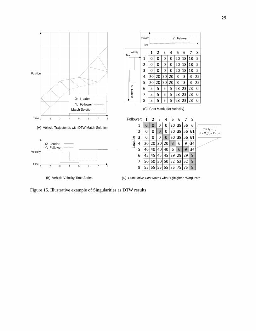
estimated in a previous time period. Viewed as part of a warp path in a matrix, as in Fig. 15 (D), singularities

occur when the path moves vertically or horizontally, rather than diagonally. Horizontal and vertical steps

in the warp path indicate changes in the response time τ (horizontal = increases, vertical = decreases,

diagonal = same).

29

Time

Position

Time

Velocity

X: LeaderY: Follower

1 2 3 4 5 6 7 8

1 2 3 4 5 6 7 8

1 2 3 4 5 6 7 8

1 0 0 0 0 20 18 18 5

2 0 0 0 0 20 18 18 5

3 0 0 0 0 20 18 18 5

4 20 20 20 20 3 3 3 25

5 20 20 20 20 3 3 3 25

6 5 5 5 5 23 23 23 0

7 5 5 5 5 23 23 23 0

8 5 5 5 5 23 23 23 0

Time

Velocity Y: Follower

Time

Velocity

X: L

ea

de

r

1 2 3 4 5 6 7 8

1 0 0 0 0 20 38 56 6

2 0 0 0 0 20 38 56 61

3 0 0 0 0 20 38 56 61

4 20 20 20 20 3 6 9 34

5 40 40 40 40 6 6 9 34

6 45 45 45 45 29 29 29 9

7 50 50 50 50 52 52 52 9

8 55 55 55 55 75 75 75 9

(C) Cost Matrix (for Velocity)

(D) Cumulative Cost Matrix with Highlighted Warp Path

τ = TF – TL

d = XL(tL) - XF(tF)

(A) Vehicle Trajectories with DTW Match Solution

(B) Vehicle Velocity Time Series

X: Leader

Y: Follower

Match Solution

Follower:

Le

ad

er

Figure 15. Illustrative example of Singularities as DTW results

30

Figure 16. Example output for DTW Vehicle Trajectory Match with highlighted singularity

From a theoretical standpoint, singularities offer an interesting new perspective for analysis while

simultaneously complicating that analysis. The match results for singularities imply a more complicated

following behavior than the underlying model, where one stimulus could result in multiple responses, and

vice versa. Additionally, singularities could also be used to classify drivers, where multiple responses to a

single stimulus could indicate more aggressive behavior. However, to what degree singularities truly

represent the leader-follower relationship, as opposed to artifacts of the algorithm, needs further study and

analysis. Singularities have been considered undesirable in most studies using DTW, and a singularity must

exist when datasets are not of equal size so that all points are matched. Additionally, a singularity may

present multiple solutions at one point for the time-dependent model parameters, which raises the issue of

which value to use for calibration.

As a result of these issues, we cannot conclude that a singularity accurately reflects the leader-follower

response. At the same time, we can only assume that a more complicated driver behavior is not present. We

can implement some algorithm enhancements to reduce the presence of singularities, but care must also be

taken to ensure that the methods used to reduce singularities also do not produce undesirable singularities

5160 5180 5200 5220 5240 5260 5280 5300 5320300

350

400

450

500

550

600

650

Time (1/10 sec)

Positio

n (

ft)

DTW Trajectory Match (Based on Acceleration Data)

5160 5180 5200 5220 5240 5260 5280 5300 5320300

350

400

450

500

550

600

650

Time (1/10 sec)

Positio

n (

ft)

DTW Trajectory Match (Based on Acceleration Data)

Singularity

31

which may also affect solution quality. For example, Fig. 16 highlights a singularity which helps the

algorithm transition from an impossibly-high w (nearly vertical slope) to more reasonable results.

5.3 Additional Enhancements for Singularity Reduction

Essentially, the multiple matching solutions at an instance in time (a singularity) is a characteristic of DTW,

but it occurs where the response time changes. In this way, it is a necessary component, but one which can

be handled with post-processing techniques to find a single estimated response time for each time instance

in the vehicle trajectory.

Additionally, when creating the warp path, there can be several possible next steps in the warp path where

the cost is the same. This occurs when the velocities for the leader and follower are the same for a period

of time. As explained in section 5.2, moving horizontally or vertically through the matrix means that the

response time increases and decreases. The diagonal step means that the response time doesn’t change at

that time step. The preference for the diagonal step in the warp path in this situation means that, without

additional information about the driver’s response (no change in speed), the estimated response time doesn’t

change.

Methods used to reduce the occurrence of singularities include, but are not limited to, windowing, slope

weighting, and using different step patterns. Windowing is a process which limits the available number of

matches to a single point based on a selected window width, which limits the size of a singularity. For

vehicle trajectories, this method simply limits the calculated τ value for any given match to a range of

reasonable values. This can also be used in conjunction with calculated d and w values for those match

points to force the algorithm to always provide theoretically-acceptable matches.

Slope weighting adds coefficients to the cumulative cost terms in Eq. 6. Its implementation is a modified

form of Eq. 6, which is shown in Eq. 10. The weight coefficients tend to encourage a more diagonal warp

path through the cumulative cost matrix.

𝐷(𝑖, 𝑗) = 𝐶(𝑖, 𝑗) + min(𝐷(𝑖 − 1, 𝑗 − 1), 𝛽 ∗ 𝐷(𝑖 − 1, 𝑗), 𝛽 ∗ 𝐷(𝑖, 𝑗 − 1)) (10)

As the coefficients increase, the warp path should become more diagonal in nature. A more diagonal warp

path limits the presence of singularities, but may also have implications for the resulting model parameters

from that warp path. Since the algorithm must produce matches near the beginning and end of the dataset,

it may require some “warm-up time” before it produces reasonable results. This transition usually requires

singularities so that the response time changes from zero to a reasonable solution. Thus, an attempt to limit

the formation of singularities may extend that “warm-up time.” Additionally, if the driver’s behavior

32

changes such that the model parameters are different at that location in the trajectory, a singularity should

be expected, but large slope weights may disguise that change.

Different step patterns can also be implemented in the cumulative cost calculation. This requires changing

Eq. 6 so that the algorithm works with cells in the cumulative cost matrix that are more than one step away

in each direction. An example of this approach is given in Eq. 11 below.

𝐷(𝑖, 𝑗) = 𝐶(𝑖, 𝑗) + min(𝐷(𝑖 − 1, 𝑗 − 1), 𝐷(𝑖 − 2, 𝑗 − 1), 𝐷(𝑖 − 1, 𝑗 − 2)) (11)

Again, this method increases the likelihood for a more diagonal warp path by forcing the path to move

diagonally in addition to when it moves vertically or horizontally.

6. Conclusions and Future Study

This paper describes a method for using the Dynamic Time Warping algorithm to calibrate an extension of

Newell’s car-following model incorporating time-dependent car-following parameters. The unique

capabilities of the DTW algorithm may provide an efficient method for observing driver heterogeneity in

car-following behavior, as well as the driver’s heterogeneous situation-dependent behavior within a trip.

Although the algorithm was made to analyze time-series data, several modification techniques are described

to address specific challenges in this application and the algorithm solution quality for analyzing vehicle

trajectories. A brief numerical experiment is presented with vehicle trajectory data extracted from the Next

Generation Simulation (NGSIM) project, demonstrating the algorithm’s ability to process large vehicle

trajectory datasets, but significant data reduction and more algorithm modification may be necessary to

produce more reasonable results. Additionally, singularities present an interesting match solution set to

potentially help identify changing driver behavior, but they must be avoided to reduce analysis complexity

and solution uncertainty. Further research will focus on algorithm enhancements with different traffic data

sources (e.g. an extended version of Newell’s three detector model by Den et al. 2013), parameter validation

methods, comparisons with alternative calibration methods, evaluating potential applications with other

car-following models, and large-scale vehicle trajectory analysis to potentially explore situation-dependent

driver behavior. For a more complicated car following model, the proposed DTW algorithm can be applied

to match the stimulus and response factors with varying time lags. On the other hand, one needs to carefully

restrict the possible ranges of parameter changes in order to derive meaningful results from trajectory data.

Acknowledgements

Although the research described here has been funded wholly or in part by the U.S. Environmental

Protection Agency’s STAR program through EPA Assistance ID No. RD-83455001, it has not been

33

subjected to any EPA review and therefore does not necessarily reflect the views of the Agency, and no

official endorsement should be inferred.

Appendix A: Illustrative Example for Vehicle Trajectory Data

To assist the reader in understanding how the algorithm works and how it is applied to vehicle trajectory

data, this section describes an illustrative example in detail. The input data used in the algorithm,

summarized in Table A1, consists of velocity data for two vehicles. Their trajectories are represented

visually in a time-space diagram in Fig. A1-a, and the velocities are plotted in Fig. A1-b.

Table A1: Velocity time-series data for illustrative example.

Time 1 2 3 4 5 6 7 8

X (Leader Velocity) 25 25 25 5 5 30 30 30

Y (Follower Velocity) 25 25 25 25 7 7 7 30

Time

Po

siti

on

1 2 3 4 5 6 7 8

(a) Vehicle Trajectories in Time-Space Diagram

X: Leader

Y: Follower

Time

Velo

cit

y

X: LeaderY: Follower

1 2 3 4 5 6 7 8

(b) Vehicle Velocity Time Series

Figure A1. Vehicle trajectory data for illustrative example, corresponding to the velocity data in Table A1

Following Algorithm 1, the cost matrix is first calculated based upon the input data. In this case, 𝑋 =

{25, 25, 25, 5, 5, 30, 30, 30} and 𝑌 = {25, 25, 25, 25, 7, 7, 7, 30}, and each cell in the cost matrix is

calculated as the difference between each pair of data points between the two time-series data sets. Since

the cost 𝐶(𝑖, 𝑗) = |𝑥𝑖 − 𝑦𝑗|, the cost in the first cell is 𝐶(1, 1) = |𝑥1 − 𝑦1| = |25 − 25| = 0, and the cost

34

at (4, 5) is 𝐶(4, 5) = |𝑥4 − 𝑦5| = |5 − 7| = 2. The complete cost matrix for this illustrative example is

shown in Fig. A2.

Figure A2. Cost matrix for the illustrative example, with visual orientation of the leader and follower

velocity data along the dimensions of the matrix

The second step is to follow Algorithm 2 and calculate the cumulative cost matrix using the cost matrix

calculated in the previous step. The cumulative cost matrix could be thought of as a network, where the

objective is to travel from (1, 1) to (8, 8) by passing through the cells in the matrix. Each step along this

path has a cost, and the search pattern restricts the “traveler’s” movement to only the next adjacent cell in

the matrix horizontally, vertically, or diagonally. The least cost required to arrive at a cell in the matrix is

the accumulation of the costs in the previously-used cells. In this example, the cost 𝐷(1, 1) at the start of

the matrix is 0 because 𝐶(1, 1) = 0. At location (1, 5) in the cumulative cost matrix, the cost 𝐶(1, 5) =

18 and the search pattern only allows horizontal movement at this boundary since no backward

movement is allowed, so the cumulative least cost to reach this point is 𝐷(1, 5) = 𝐷(1, 4) + 𝐶(1, 5) =

18. At location (4, 5), the search pattern allows searching in all three directions (horizontally, vertically,

or diagonally). As a result, the cumulative least cost to arrive at location (4, 5) is 𝐷(4, 5) =

min(𝐷(4, 4), 𝐷(3, 4), 𝐷(3, 5)) + 𝐶(4, 5). The minimum cost in the adjacent cells is at location (3, 4), so

Time

Velocity Y: Follower

Tim

e

Velocity

X: L

eader

1 2 3 4 5 6 7 8

1 0 0 0 0 18 18 18 5

2 0 0 0 0 18 18 18 5

3 0 0 0 0 18 18 18 5

4 20 20 20 20 2 2 2 25

5 20 20 20 20 2 2 2 25

6 5 5 5 5 23 23 23 0

7 5 5 5 5 23 23 23 0

8 5 5 5 5 23 23 23 0

35

the cumulative least cost at location (4, 5) is 𝐷(4, 5) = [𝐷(3, 4) + 𝐶(4, 5)] = [0 + 2] = 2. The complete

cumulative cost matrix for this illustrative example is shown in Fig.A3.

Follower

1 2 3 4 5 6 7 8

1 0 0 0 0 18 36 54 59

2 0 0 0 0 18 36 54 59

3 0 0 0 0 18 36 54 59

4 20 20 20 20 2 4 6 31

5 40 40 40 40 4 4 6 31

6 45 45 45 45 27 27 27 6

7 50 50 50 50 50 50 50 6

8 55 55 55 55 73 73 73 6

Lea

der

Figure A3. Cumulative cost matrix for illustrative example

The last step in the DTW algorithm is to follow Algorithm 3 and find the warp path through the

cumulative cost matrix. Similar to calculating the cumulative least cost matrix, it is convenient to think of

the warp path as the shortest path through the matrix, where the matrix is actually a network composed of

cells. Again, a search pattern restricts the “traveler’s” movement to only the next adjacent cell in the

matrix horizontally, vertically, or diagonally. However, rather than moving from the beginning to the end

of the matrix, the warp path finds the shortest path from (8, 8) to (1, 1) by following the cumulative least

cost. The next step through the matrix is selected based on the least cost at arriving at the potential next

step.

Consider the warp path shown in Fig. A4. Starting at location (8, 8), the algorithm checks the cumulative

costs at the potential next steps (8, 7), (7, 7), and (7, 8). The least cumulative cost amongst the available

cells is at location (7, 8) because 𝐷(7, 8) = 6, so the algorithm adds location (7, 8) to the warp path and

moves to this new location. This procedure continues until the algorithm reaches location (1,1) at the

beginning of the cumulative cost matrix.

36

Follower

1 2 3 4 5 6 7 8

1 0 0 0 0 18 36 54 59

2 0 0 0 0 18 36 54 59

3 0 0 0 0 18 36 54 59

4 20 20 20 20 2 4 6 31

5 40 40 40 40 4 4 6 31

6 45 45 45 45 27 27 27 6

7 50 50 50 50 50 50 50 6

8 55 55 55 55 73 73 73 6

Lea

der

Figure A4. Warp path (highlighted in grey) through the cumulative cost matrix for the illustrative

example

The warp path indicates the optimal alignment between points over time. For example, it matches point

𝑥5 in the leader trajectory with points 𝑦6 and 𝑦7 in the follower trajectory. Using this information, the

velocity data points are matched in Fig. A5. Additionally, this matching can be translated into the time-

space domain in Fig. A6. This alignment information is then used to estimate the time offset 𝜏𝑛,𝑡 and

distance offset 𝑑𝑛,𝑡 following the Eqs. (7-8). For example, at time 𝑡 = 4 in the follower’s time-series

(vehicle 𝑛 = 1), 𝜏1,4 = (4 − 3) = 1 time unit, and 𝑑1,4 = 𝑝4 − 𝑞3.

Time1 2 3 4 5 6 7 8

X: LeaderY: Follower

Match

37

Figure A5. Matching/alignment between vehicle velocity data for illustrative example

Time

Posi

tion

1 2 3 4 5 6 7 8

X: Leader

Y: Follower

Match

Figure A6. Matching/alignment between vehicle trajectory data for illustrative example

References

Ahn, S., Cassidy, M. J., Laval, J., 2004. Verification of a simplified car-following theory. Transportation

Research Part B: Methodological, 38, 431-440.

Ahn, S., Vadlamani, S., Laval, J., 2013. A method to account for non-steady state conditions in measuring

traffic hysteresis. Transportation Research Part C 34, 138-147.

Brockfeld, E., Kühne, R., Wagner, P., 2004. Calibration and Validation of Microscopic Traffic Flow

Models. Transportation Research Record: Journal of the Transportation Research Board, 1876, 62–

70.

Chen, D., Laval, J., Zheng, Z., Ahn, S., 2012. A behavioral car-following model that captures traffic

oscillations. Transportation Research Part B 46 (6), 744-761. Chen, X., Li, L., Zhang, Y. 2010. A Markov model for headway/spacing distribution of road traffic. Intelligent

Transportation Systems, IEEE Transactions on Intelligent Transportation Systems, 11(4), 773-785. Chiabaut, N., Leclercq, L., Buisson, C., 2010. From heterogeneous drivers to macroscopic patterns in

congestion. Transportation Research Part B 44 (2), 299-308.

Chu, S., Keogh, E., Hart, D., Pazzani, M., 2002. Iterative Deepening Dynamic Time Warping for Time

Series. In Proc. of the Second SIAM Intl. Conf. on Data Mining. Arlington, Virginia.

Ciuffo, B., Punzo, V., Quaglietta, E., 2011. Kriging meta-modelling to verify traffic micro-simulation

calibration methods. 90th Annual Meeting of the Transportation Research Board. Washington,

D.C.

Den, W., Lei H., Zhou, X., 2013. Freeway Traffic State Estimation and Uncertainty Quantification based

on Heterogeneous Data Sources: Stochastic Three Detector Transportation Research Part B:

Methodological, 57, 132-157

38

Duret, A., Buisson, C., Chiabaut, N., 2008. Estimating Individual Speed-Spacing Relationship and

Assessing Ability of Newell's Car-Following Model to Reproduce Trajectories. Transportation

Research Record: Journal of the Transportation Research Board, 2088, 188-197.

Hamdar, S. H., Treiber, M., Mahmassani, H. S., 2009. Genetic Algorithm Calibration for a Stochastic

Car-Following Model Using Trajectory Data: Exploration and Model Properties 88th Annual

Meeting of the Transportation Research Board. Washington, D.C.

Hoogendoorn , S. P., Hoogendoorn, R. G., Daamen, W., 2011. Wiedemann revisited: A New Trajectory

Filtering Technique and its Implications for Car-Following Modeling 90th Annual Meeting of

the Transportation Research Board. Washington, D.C.

Keogh, E., Pazzani, M., 2001. Derivative Dynamic Time Warping. First SIAM International Conference

on Data Mining (SDM’2001), Chicago, Illinois.

Kesting, A., Treiber, M., 2008. Calibrating Car-Following Models by Using Trajectory Data:

Methodological Study. Transportation Research Record: Journal of the Transportation Research

Board, 2088, 148-156.

Kesting, A., Treiber, M. Calibration of Car-Following Models Using Floating Car Data. In: Appert-

Rolland, C., Chevoir, F., Gondret, P., Lassarre, S., Lebacque, J.-P. and Schreckenberg, M., eds.

Traffic and Granular Flow ’07, 2009. Springer Berlin Heidelberg, 117-127.

Kim, I., Kim, T., Sohn, K., 2013. Identifying driver heterogeneity in car-following based on a random

coefficient model. Transportation Research Part C: Emerging Technologies, 36, 35-44.

Kim, J., Mahmassani, H. S., 2011. Correlated Parameters in Driving Behavior Models: Car-Following

Example and Implications for Traffic Microsimulation, Transportation Research Board 90th

Annual Meeting, Washington, DC, January 23-27, 2011.

Laval, J. A., Leclercq, L., 2010. A mechanism to describe the formation and propagation of stop-and-go

waves in congested freeway traffic. Philosophical Transactions of the Royal Society A:

Mathematical, Physical and Engineering Sciences, 368, 4519-4541. Li, L., Wang, F., Jiang, R., Hu, J, H., Ji Y. 2010. A new car-following model yielding log-normal type

headways distributions. Chinese Physics B,19(2), 020513. Ossen, S., Hoogendoorn, S. P., 2005. Car-Following Behavior Analysis from Microscopic Trajectory Data.

In Transportation Research Record: Journal of the Transportation Research Board, No. 1934,

Transportation Research Board of the National Academies, Washington, D.C., 13-21.

Ossen, S., Hoogendoorn, S. P., 2007. Driver Heterogeneity in Car Following and Its Impact on Modeling

Traffic Dynamics. In Transportation Research Record: Journal of the Transportation Research

Board, No. 1999, Transportation Research Board of the National Academies, Washington, D.C.,

95-103.

Ossen, S., Hoogendoorn, S. P., 2008a. Validity of Trajectory-Based Calibration Approach of Car-

Following Models in Presence of Measurement Errors. Transportation Research Record: Journal

of the Transportation Research Board, 2088, 117-125.

Ossen, S., Hoogendoorn, S. P., 2008b. Calibrating car-following models using microscopic trajectory

data: A critical analysis of both microscopic trajectory data collection methods and calibration

studies based on these data. Version 1.1 ed. Delft, Netherlands: Delft University of Technology.

Ossen, S., Hoogendoorn, S. P., 2009. Reliability of Parameter Values Estimated Using Trajectory

Observations. Transportation Research Record: Journal of the Transportation Research Board,

2124, 36-44.

Ossen, S., Hoogendoorn, S. P., 2011. Heterogeneity in car-following behavior: Theory and empirics.

Transportation Research Part C: Emerging Technologies, 19(2), 182-195.

Ossen, S., Hoogendoorn, S. P., Gorte, B., 2006. Interdriver Differences in Car-Following: A Vehicle

Trajectory-Based Study. Transportation Research Record: Journal of the Transportation

Research Board, 1965, 121-129.

Ma, X., Andréasson, I., 2006. Estimation of Driver Reaction Time from Car-Following Data: Application

in Evaluation of General Motor-Type Model. Transportation Research Record: Journal of the

Transportation Research Board, 1965, 130-141.

39

Newell, G. F., 1962. Theories of instabilities in dense highway traffic, Journal of the Operations Research

Society of Japan, 5, 9-54.

Newell, G. F., 1993. A simplified theory of kinematic waves in highway traffic, part I: general theory.

Transportation Research Part B: Methodological, 27, 281-287.

Newell, G. F., 2002. A simplified car-following theory: a lower order model. Transportation Research

Part B: Methodological, 36, 195-205.

Sakoe H., Chiba S., 1978. Dynamic programming algorithm optimization for spoken word recognition.

IEEE Trans Acoustics Speech Signal Process ASSP 26, 43–49.

Salvador, S., Chan, P., 2004. FastDTW: Toward Accurate Dynamic Time Warping in Linear Time and

Space. In: KDD Workshop on Mining Temporal and Sequential Data. Seattle, WA, USA, pp. 70–

80.

Senin, P., 2008. Dynamic Time Warping Algorithm Review. Honolulu, HI: University of Hawaii at

Manoa.

US Department of Transportation (USDOT). 2006. NGSIM - Next Generation Simulation. Available

from <http://ngsim-community.org>, Accessed June 20, 2011.

Wagner, P., 2012. Analyzing fluctuations in car-following. Transportation Research Part B:

Methodological, 46, 1384-1392.

Wang, H., Wang, W., Chen, J., Jing, M., 2010. Using Trajectory Data to Analyze Intradriver

Heterogeneity in Car-Following. Transportation Research Record: Journal of the Transportation

Research Board, 2188, 85-95.

Zheng, Z., Ahn, S., Chen, D., Laval, J., 2011. Freeway traffic oscillations: microscopic analysis of

formations and propagations using wavelet transform. Transportation Research Part B 45 (9),

1378-1388

Zheng, Z., Ahn, S., Chen, D., Laval, J., 2013. The impact of lane-changing on the immediate follower:

anticipation, relaxation, and behavioral change. Transportation Research Part C 26 (1), 367-379.

Zinke, A., Mayer, D., 2006. Iterative Multi Scale Dynamic Time Warping. Technical Report CG-2006-1,

Universität Bonn.