A Frequency Warping Approach to Speaker Normalization

by

Li Lee

Submitted to the Department of Electrical Engineering and Computer Sciencein partial fulfillment of the requirements for the degrees of

Bachelor of Science

and

Master of Engineering

at the

MASSACHUSETTS INSTITUTE OF TECHNOLOGY

February 1996

@ Li Lee, MCMXCVI. All rights reserved.

The author hereby grants to MIT permission to reproduce and distribute publiclypaper and electronic copies of this thesis document in whole or in part, and to grant

others the right to do so.

A uthor .................................... . . .......... . .. ....................Department of Electrical Engineering and Computer Science

January 30, 1996

C ertified by ....................... .. . ...........

Distinguis'ed Professor

Certified by ....

Memv r o Technical Staff,A i I i

.. .. .. .... .. .. .. .... ... .

Alan V. Oppenheimof Electrical Engineering

T4Wft Supervisor

. . . . . . . . . . . . . . . . . . . . . . . .

Richard C. RoseAT&T Bell Laboratories

Thesis Supervisor

A ccepted by ................................. . .. ........ ....................."t Frederic R. Morgenthaler

Chairman, Depart ent Committee on Graduate ThesesMAACU:. rFTS 4INST J I'L:

OF TECHNOLOGY

JUN 111996 jEng.LIBRARIES

A Frequency Warping Approach to Speaker Normalization

by

Li Lee

Submitted to the Department of Electrical Engineering and Computer Scienceon January 30, 1996, in partial fulfillment of the

requirements for the degrees ofBachelor of Science

andMaster of Engineering

Abstract

In an effort to reduce the degradation in speech recognition performance caused byvariations in vocal tract shape among speakers, this thesis studies a set of low-complexity, maximum likelihood based speaker normalization procedures. By ap-proximately modeling the vocal tract as a simple acoustic tube, these procedurescompensate for the effects of the variations in vocal tract length by linearly warpingthe frequency axis of speech signals. In this thesis, we evaluate the effectiveness of theprocedures using a telephone based connected digit recognition task with very shortutterances. Experiments are performed to evaluate the convergence properties of theproposed procedures, as well as their ability to reduce measures of inter-speaker vari-ability. In addition, methods for improving the efficiency of performing model-basedspeaker normalization and implementing frequency warping are proposed and evalu-ated. Finally, comparisons of speaker normalization with other techniques to reduceinter-speaker variations are made in order to gain insight into how to most efficientlyimprove the robustness of speech recognizers to varying speaker characteristics. Theresults of the study show the frequency warping approach to speaker normalizationto be a promising way to improve speech recognition performance.

Thesis Supervisor: Alan V. OppenheimTitle: Distinguished Professor of Electrical Engineering

Thesis Supervisor: Richard C. RoseTitle: Member of Technical Staff, AT&T Bell Laboratories

Acknowledgments

I wish to express my deepest gratitude to my thesis advisor Dr. Richard Rose for his

guidance and friendship over the past few years. Rick sparked my first interests in

the speech recognition field, and his exceptional standards and humor made my thesis

experience both challenging and fun. I also want to thank Prof. Alan Oppenheim for

his support and helpful advice on the thesis.

I have benefited greatly from opportunities to work with and learn from many

wonderful people at MIT and at Bell Labs during my undergraduate years. I am es-

pecially indebted to Dr. Alan Berenbaum at Bell Labs for his cheerful encouragement

and wonderful books, Dr. Victor Zue at MIT for his honest advice in times of inde-

cision, and Prof. James Chung at MIT for his insistence that I have fun regardless

of my academic pursuits. I want to thank them for always taking time out of their

busy schedules to offer me advice when I needed it.

Finally, I thank my family for their love, encouragement, and humor. This thesis,

like all of my other accomplishments, would not have been possible without their

support.

Contents

1 Introduction

1.1 Problem Description ...........................

1.2 Proposed Solution .............................

1.3 Thesis Outline ...............................

2 Background

2.1 Hidden Markov Models ..........................

2.2 Speaker Adaptation ............................

2.3 Speaker-Robust Features and Models . .................

2.4 Telephone-based speech recognition . ..................

2.5 Summary .................................

3 A Frequency Warping Approach to Speaker

3.1 Warping Factor Estimation .........

3.2 Training Procedure ..............

3.3 Recognition Procedure ............

3.4 Baseline Front-End Signal Processing . . . .

3.4.1 Filter Bank Front-end ........

3.4.2 Linear Predictive Analysis ......

3.5 Frequency Warping ..............

3.5.1

3.5.2

3.5.3

Normalization 20

. . . . . . . . . . 2 1

.. ... ... ... ... 2 2

.. ... .... .. ... 24

. . . . . . . . . . . . . . 24

.. ... .... ... .. 2 5

. . . . . . . . . . . . . . 2 7

. . ... . .. ... .. 27

Filter Bank Analysis with Frequency Warping

LPC Analysis with Frequency Warping . . . .

Discussion on Bandwidth Differences . . . . .

. . . . . . . . . 28

. . . . . . . . . 28

. . . . . . . . 29

3.6 Sum m ary . . . . . . . . . . . . . . . . . . . . . . . . . . . . . . . . .

4 Baseline Experiments

4.1 Task and Databases ........ .........

4.2 Baseline Speech Recognizer . . . . . . . . . . . . .

4.3 Speech Recognition Performance . . . . . . . . . . .

4.4 Distribution of Chosen Warping Factors . . . . . .

4.5 Speaker Variability and HMM Distances . . . . . .

4.5.1 Definition of HMM Distance Measure . . . .

4.5.2 Experimental Setup ..............

4.5.3 Results . . . . . . . . . . . . . . . ....

4.6 Warping Factor Estimation With Short Utterances

4.7 Convergence of Model Training Procedure . . . . .

4.8 Summary ........... ...........

5 Efficient Approaches to Speaker Robust Systems

5.1 Efficient Warping Factor Estimation . . . . . . . . .

5.1.1 Mixture-based Warping Factor Estimation .

5.1.2 Experimental Results . . . . . . . . . . . . .

5.2 Comparison with Other Approaches . . . . . . . . .

5.2.1 Gender-Dependent Models . . . . . . . . . .

5.2.2 Cepstral Mean Normalization . . . . . . . .

5.2.3 Experimental Results . . . . . . . . .....

5.3

5.4

5.2.4 Speaker Normalization vs. Class-Dependent Models

HMM Parametrization ....................

Sum m ary . . . . . . . . . . . . . . . . . . . . . .....

6 Conclusions

6.1 Summary

6.2 Future Work . .

34

... ... ... . 35

. . . . . . . . . . 36

. . . . . . . . . . 36

. . . . . . . . . . 37

. . . . . . . . . . 39

. . . . . . . . . . 40

... ... .... 40

... ... ... . 4 1

. . . . . . . . . . 42

. . . . . . . . . . 45

.. ... ... . 46

48

49

50

51

52

53

53

54

55

56

57

Chapter 1

Introduction

While speech is clearly a natural mode of communication between human beings, it

is only recently that human-machine interactions using speech has become practical.

However, even today's most advanced systems suffer from performance degradations

due to variations in the acoustic environment, communications channel, and speaker

characteristics. The goal of this thesis is to develop techniques which reduce the effect

of speaker-dependent variability on speech recognition performance. This chapter

motivates this work and describes the organization of the thesis. First the problem

of speaker variability in automatic speech recognition(ASR) is described. Then, the

general approach taken to solve this problem is introduced. Finally, an outline of the

thesis is provided.

1.1 Problem Description

Physiological and dialectal differences that exist among speakers lead to variations

in the characteristics of the speech signal. Whereas variations in vocal tract shape

change speech features such as formant positions in vowels, dialectal differences affect

both the acoustic and the phonological properties of utterances. In this thesis, we are

interested in methods which enable ASR systems to handle these variations grace-

fully, with minimal degradation in performance. We refer to the ability of an ASR

system to be relatively insensitive to unexpected changes in speaker characteristics as

robustness to speaker-dependent variabilities. Because the thesis is mostly concerned

with physiological differences, this section discusses vocal tract variations and their

effect on speech modeling.

Human speech production apparatus differ in many ways, leading to differences in

the pitch and formant frequencies among utterances of the same sound. While some

types of variation, such the vocal tract shape, carry crucial phonetic information,

others, such as the vocal tract length, are irrelevant for speech recognition and should

be treated as "noise". For example, vocal tract length in the human population ranges

from about 13cm for a female to over 18cm for a male. Since the positions of formant

peaks are inversely proportional to the length of the vocal tract, formant center

frequencies can vary by as much as 25% across speakers for utterances of the same

sound.

Speech recognition features for the English language are chosen to represent the

spectral envelope of short-time segments of speech. The large variations in formant

positions lead to a large discrepancy between error rates found for speaker indepen-

dent (SI) recognizers and those found for speaker dependent (SD) recognizers. While

SI systems are trained using tokens from a large number of speakers, SD recognizers

are trained on tokens from only one speaker. Error rates of SI systems are often two to

three times that of SD systems for similar recognition tasks. Two practical problems

account for this degradation. First, statistical models trained on data from a large

number of speakers tend to show higher variances within each phonetic class, causing

overlap between distributions of neighboring classes. Highly-overlapping statistical

distributions in turn lead to highly-confusable speech units, reducing the recognition

accuracy of the system. Secondly, high variability in formant positions gives rise to

the existence of statistical outliers. Even when the training speaker population con-

sists of a large number of speakers, the characteristics of certain test speakers may

not be closely matched to that of the speakers in the training set. Statistical outliers

are often the dominant source of errors in SI recognition systems.

Examples of the performance discrepancy that exists between SI and SD recogni-

tion have been published by many research laboratories using the DARPA Resource

Management task. This task consists of continuously spoken utterances taken from

a 1000 word vocabulary designed to simulate queries to a naval battle management

database. After training a SI system with 104 speakers, Huang and Lee reported a

word error rate of 4.3% [11]. However, the average word error rate for 12 speakers

using SD models was only 1.4%. The result is typical of many speech recognition

tasks and serves to illustrate the need for techniques to make ASR systems more

robust with respect to inter-speaker variabilities.

This thesis attempts to develop techniques which achieves speaker-robustness by

compensating for sources of speaker variability. The problem is studied in the con-

text of telephone-based speech recognition with very short utterances. The context

of the problem places two major constraints on the types of approaches that can be

examined. First, we assume that no prior knowledge of the speaker characteristics

is available, so that any adjustment to the acoustic signal or the models must be

determined based only on a single utterance. Secondly, it is assumed that the ut-

terances can be as short as one or two words in duration. This places a limitation

on the complexity of the approaches that can be applied. For example, with such

a small amount of data available for estimating the properties of each speaker, the

effectiveness of methods which require the estimation of a large number of parameters

is limited.

1.2 Proposed Solution

The technique studied in this thesis is motivated by the fact that robustness to speaker

variations can be improved if the physical sources of the variations are explicitly

modeled and compensated for. We consider a method of speaker normalization over

different vocal tract lengths by using a simple linear warping of the frequency axis.

Vocal tract length is clearly a physiological variation which changes the acoustic

properties of each speaker's speech without bearing phonetic or linguistic information.

Given a certain vocal tract configuration, changing only the vocal tract length does

not change phonetic content of the sound, and the effect can be approximated by a

linear scaling of the resonant frequencies of the tract. In this thesis, we propose that

if all vocal tract shapes from all speakers are normalized to have the same length, the

acoustic space distributions for each phone would be better clustered, with reduced

within-class variance.

Conceptually, normalizing for vocal tract length requires two steps. First, a mea-

sure of the ratio of the vocal tract length of the speaker to a reference "normal" length

is estimated. Then, this ratio is used as a scaling factor with which the frequency axis

of the acoustic signal is warped. The resulting signal should be one which would have

been produced from a vocal tract of the same shape, but of the reference length. For

example, since the formant frequencies produced by someone with a short vocal tract

length tend to be higher than average, their speech could be normalized by uniformly

compressing the frequency axis of the utterances. Since the vocal tract tends to be

shorter in females and longer in males, the normalization process tends to perform

frequency compression for females, and frequency expansion for males.

In practice, the estimation of the vocal tract length of the speaker based on the

acoustic data is a difficult problem. Techniques based on tracking formants are often

not very reliable. In this thesis, a model-based approach for estimating the warping

factor is used. In other words, the warping factor is chosen to maximize the likeli-

hood of the frequency-warped features with respect to a given model. The reference

"normal" length is thus defined implicitly in terms of the parameters of the statistical

models.

When the acoustic feature space of the training speech has been normalized using

the warping process, models can be built using the normalized features. The result

of such a training process is a set of models which is more efficient and effective at

describing the vocal tract variations which carry phonetic information. This normal-

ized set of models can then be used during recognition to first estimate the frequency

warping factor for the test utterances, and then to decode the utterances.

This thesis is an experimental study of the speaker normalization process outlined

above. We study the effectiveness and efficiency of a maximum-likelihood speaker nor-

malization technique from a variety of different perspectives. In addition to speech

recognition performance, several measures are used to evaluate the convergence prop-

erties of the proposed procedures, as well as their ability to reduce measures of inter-

speaker variability. Methods for improving the efficiency of performing model-based

speaker normalization and implementing frequency warping are proposed and evalu-

ated. Finally, comparisons of speaker normalization with other techniques to reduce

inter-speaker variations are made in order to gain insight into how to most efficiently

improve the speaker robustness of ASR systems. The goal of such a study is to better

understand the basic properties of speaker normalization so that the technique can

become practical for use in existing applications.

1.3 Thesis Outline

The body of this thesis is divided into five chapters:

Chapter 2 covers the background information useful for the discussion of speaker

normalization procedures presented later in the thesis. Statistical modeling of speech

using Hidden Markov Models (HMMs) is described. Current work in the areas of

speaker adaptation and speaker normalization is examined. Finally, a brief discussion

of the acoustic properties of telephone handsets and channels is presented. This

discussion is relevant because the experimental study to be described in the thesis

was performed using speech utterances collected over the telephone network.

Chapter 3 presents a detailed description of procedures for implementing HMM-

based speaker normalization using frequency warping. Procedures to perform warping

factor estimation, model training, and recognition are described. Efficient methods

used to implement frequency warping for two different feature analysis front-ends are

presented and discussed.

Chapter 4 presents an experimental study of the effectiveness of the speaker nor-

malization procedures. The database, task, and baseline system are described. The

effectiveness of speaker normalization is examined from a few perspectives. First,

speech recognition performance before and after using speaker normalization is com-

pared. In addition, experiments were performed to understand the ability of the

speaker normalization procedures to decrease inter-speaker variability, and to pro-

duce normalized HMMs which describe the data more efficiently. We show statistics

reflecting the ability of the warping factor estimation procedures to estimate the

warping factor reliably with small amounts of data. Convergence issues related to the

training procedure will also be discussed.

Chapter 5 further studies the speaker normalization procedures by proposing tech-

niques to make them more efficient, by comparing them with other types of proce-

dures also designed to reduce the effects of speaker variability, and by evaluating

their effectiveness over different degrees of modeling complexity. A mixture-based

method for estimating the warping factor is presented and compared against the

less efficient HMM-based method. Speaker normalization is compared with gender-

dependent models and cepstral mean normalization to gain insight into the possible

advantages of using a physiologically-motivated procedure like frequency warping over

other statistically-based compensation and modeling procedures.

Chapter 6 concludes the thesis with a summary and directions for future work.

The techniques and experiments that were presented in the thesis have left many

open issues. It is hoped that this work will stimulate further investigations which

may address these issues.

Chapter 2

Background

This chapter provides the background for further discussion on the model-based

speaker normalization procedures which are investigated later in this thesis. It in-

cludes discussion of the statistical modeling techniques used, of the previous work in

the areas of speaker adaptation and speaker normalization, of the acoustic character-

ization of the telephone-based speech. The first section briefly reviews the structure

and properties of Hidden Markov Models(HMMs). The second section provides an

overview of previous work in speaker adaptation. The third section discusses previ-

ous work on robust modeling for inter-speaker variations and speaker normalization

techniques. Finally, the last section describes the acoustic properties of telephone

handsets and channels in an attempt to characterize the telephone-based databases

which are used in the experimental study of this thesis.

2.1 Hidden Markov Models

Hidden Markov Models are perhaps the most widely used statistical modeling tool

used in speech recognition today [22]. There are two stochastic components in a

HMM. The first is a discrete state Markov chain. The second is a set of observation

distribution functions associated with each state of the Markov chain. This doubly

stochastic structure allows the HMM to simultaneously capture the local character-

istics of a speech signal, and the dependencies between neighboring sounds. In the

context of speech recognition, it is assumed that at each instant of time, the HMM

generates a "hidden" state index according to the underlying Markov chain and then

generates a speech observation vector according to the observation density associated

with that state. Thus, given a particular observation sequence and an HMM, it is

possible to compute the probability that the sequence has been generated by the

HMM [21].

In a speech recognizer, HMMs are trained for each lexical item in the vocabulary of

the recognizer using the Baum-Welch algorithm or the segmental k-means algorithm

[7]. These iterative algorithms estimate parameters of the HMMs to maximize the

likelihood of the training data with respect to the trained models. During recognition,

the Viterbi algorithm is used to find the sequence of HMMs which maximizes the

likelihood of the observed speech.

A variety of different HMM structures are possible for speech modeling. In this

thesis, we use a simple left-to-right Markov structure, which means that all of the

allowable state transitions are from a state of lower state index to a state of higher

index. In addition, within each state, mixtures of multivariate Gaussian distributions

are used as the observation densities for each state. The Gaussian distributions are

assumed to have diagonal covariance matrices, and are defined over cepstral feature

vectors. Signal processing implementations to derive the feature vectors from the

speech time waveforms will be described in Chapter 3.

2.2 Speaker Adaptation

As already mentioned in Chapter 1, for any particular speaker, sources of inter-speaker

variability make SI HMMs less accurate than SD HMMs trained for that speaker.

Research efforts at making ASR systems more robust to speaker differences has taken

two major approaches. First, a large number of speaker adaptation procedures have

been developed to improve the recognition performance of SI systems to the level of

SD systems as more and more data from a particular speaker becomes available. A

second approach is to develop more speaker-robust acoustic features and models which

are invariant to acoustic characteristics that are not relevant for speech recognition.

This section describes work in the speaker adapation area. The next section describes

work in speaker-robust features and models.

Speaker adaptation (SA) is the process of modifying either an existing HMM

model or the input signal to reduce the differences between the new speaker's char-

acteristics and those represented by the model. It has been applied successfully in

many commercial systems which are used extensively by only one user. SA procedures

"learn" from the user's utterances, and modify the system so that the model statistics

become well-matched to the actual acoustic observations from that speaker. As more

adaptation utterances become available, the performance of speaker independent ASR

systems can be made to approach that of SD systems using SA techniques.

The adaptation of model or data transformation parameters requires speech data

from each new speaker. Adaptation utterances can be obtained in several ways under

different levels of supervision. First, in the simplest case, the SA data can be col-

lected during an enrollment or adaptation phase in which the new user speaks a set

of pre-specified sentences whose transcriptions are assumed to be known. Since this

enrollment process is not always convenient, SA data can also be gathered during the

normal recognition process itself. For recognition-time adaptation, the system de-

codes each incoming utterance with the existing model, and then updates the models

based on the recognition result. Some systems operate in a supervised mode by elicit-

ing feedback from the user concerning the accuracy of the recognized string. However,

the feedback process can work without the help of the user in systems whose initial

accuracy (without adaptation) is already high enough [19].

Using the additional adaptation data, one approach to SA consists of modifying

the model parameters to maximize some design criterion. For example, Gauvain and

Lee applied Bayesian MAP estimation to adapt SI models to individual speakers and

reported a error rate reduction of approximately 40% with 2 minutes of adaptation

data on the Resource Management task which was briefly described in the last chapter

[10]. As the amount of adaptation data increased to 30 minutes, the error rate dropped

to the level of SD models. ML model reestimation and other types of probabilistic

mappings have also been used to adapt the model parameters to fit the speaker [14]

[24].A second approach to SA consists of mapping the incoming speech features to a

new space using transformations designed to minimize the distance between the new

speech vectors and a set of "reference" speech vectors. The forms of the transfor-

mation can be linear, piecewise linear, or even non-linear (as modeled by a neural

network) [4] [2]. For example, Huang described a method of using neural networks to

map between the acoustic spaces of different speakers' speech [12]. The extension of

such a technique is to map the acoustic space of all speakers to one chosen reference

speaker, and then use the SD model built with the reference speaker's speech for

recognition purposes.

2.3 Speaker-Robust Features and Models

While speaker adaptation techniques have been successful, they cannot be used in

systems where the only available speech from a given speaker is a single, possibly

very short, utterance. In such cases, the ability to extract speaker-robust features,

and to build models from these features is needed. In the area of robust modeling,

techniques have been developed to train separate models for different speaker groups

according to gender, dialect, or by automatic clustering of speakers [22] [16]. While

the resulting models are more refined and accurate, separating the speakers into a

large number of classes can sometimes lead to under-trained models due to the lack

of data.

Techniques which attempted to "normalize" speech parameters in order to elimi-

nate inter-speaker differences were first developed in the context of vowel identifica-

tion. Linear and non-linear frequency warping functions were developed to compen-

sate for variations in formant positions of vowels spoken by different speakers [9] [26].

These normalization methods relied on estimates of formant positions as indications

of the vocal tract shape and length of each speaker, and then compensated for these

differences.

These vowel space normalization techniques were not extended to continuous

speech recognition until recently. Andreou, et al., proposed a set of maximum-

likelihood speaker normalization procedures to extract and use acoustic features which

are robust to variations in vocal tract length[l]. The procedures reduced speaker-

dependent variations between formant frequencies through a simple linear warping

of the frequency axis, which was implemented by resampling the speech waveform in

the time domain. However, despite the simple form of the transformation being con-

sidered, over five minutes of speech was used to estimate the warping factor for each

speaker in their study. While this and other studies of frequency warping procedures

have shown improved speaker-independent ASR performance, the performance im-

provements were achieved at the cost of highly computationally intensive procedures

[23].

As a simplification, Eide and Gish proposed using the average position of the third

formant over the utterance as the estimate the length of the vocal tract. Different

vocal tract lengths can then be normalized by using a linear or exponential frequency

warping function [8]. However, besides the difficulty of reliably estimating formants,

the position of the third formant changes according to the sound being produced,

and therefore does not directly reflect the vocal tract length of the speaker [26]. This

thesis extends the approach of Andreou, et al., by applying the procedures to very

short utterances, by using an experimental study to further understand the properties

of the procedures, and by proposing methods to make them more efficient.

2.4 Telephone-based speech recognition

The experimental study to be described in the thesis was performed using speech ut-

terances collected over the telephone network. Since the telephone channel introduces

many sources of variability in addition to those due to differences between speakers,

this section describes characteristics of the telephone channels. In addition, the char-

acteristics of carbon and electret telephone transducers are discussed in relation to

their effect on ASR performance.

The combined channel composed of the handset transducer and telephone network

introduces several different types of distortion on the speech signal. It is well known

that the transmission channel filters the signal between 200 and 3400 Hz, with differ-

ent degrees of attenuation within the passband. Besides this convolutional effect, the

local loop, long distance transmission lines, and switching equipment in the telephone

network are also sources of additive noise. The severity of these and other nonlinear

effects often vary from call to call, leaving the exact types or degree of distortion

almost impossible to predict from one call to the next.

The telephone handset is an additional source of variable distortion. The electret

transducers used in the newer telephones have linear filtering characteristics. On

the other hand, carbon button transducers, which are still widely used throughout

the telephone network, are known to have highly nonlinear characteristics which vary

over time and from one transducer to the next[17]. In addition to these nonlinearities,

adverse environmental conditions, variation in the electrical conditions, and simple

aging can result in further variation in the characteristics of the carbon transducer.

For example, excessive humidity can cause "packing" of the carbon granules and result

in a reduction in sensitivity of 10-20 dB [17]. This severe variability resulting from a

carbon transducer that is not in proper working order can also result in degradations

in ASR performance.

In comparing ASR performance when using electret and carbon handsets which

were known to be in good working condition, however, Potamianos, et al., found

that ASR performance obtained using carbon transducers was actually better than

that obtained for electret transducers [20]. This suggests that the carbon transducers

perform some transformation which is beneficial to ASR performance. One possible

cause of the discrepancy in performance may be that the carbon transducer suppresses

speech energy in portions of the signal where variability is high, and modeling accu-

racy is low. Such areas may include fricative sounds, and formant valleys in voiced

sounds.

In the same study, Potamianos, et al., also found empirical evidence that the car-

bon transducer is relatively less affected by the direct airflow energy that accompanies

the production of plosive and fricative sounds [20]. An example of this observation is

displayed in figure 2-1, where the short-time energy contours for stereo carbon(solid)

and electret (dashed) utterances are plotted for the string "three-six-six." It is clear

that the areas of the greatest energy differences are in the plosive production of /ks/

and the fricative productions of /s/ and /th/. The plot shows that the electret trans-

ducers are more affected by the direct airflow that accompanies plosive and fricative

production. The amount of this 'pop' noise is highly dependent on the design of the

handset as well as the position of the handset relative to the speaker's mouth. It

is believed that because of the electret transducer's higher sensitivity to this type

of noise, there is a increased variability associated with speech passed through the

electret transducer, and hence the ASR error rates obtained using electret handsets

are higher.

TIME (sec)

Figure 2-1: Short-time energy contours for stereo carbon (solid) and electret (dashed)utterances for the string "three-six-six". From [17]

2.5 Summary

This chapter attempted to cover the background information necessary for a better

perspective of the speaker normalization procedures and experimental study which

will be described later. The structure and properties of hidden Markov models was

first described. Then, model adaptation and feature space mapping techniques for

dealing with speaker differences were discussed. While these techniques are effective,

they require adaptation data from each speaker, which is not possible in scenarios

where only one single utterance is available from each speaker. For that type of ap-

plication, speaker-robust models and features are needed. Work in frequency warping

approaches to speaker normalization was described in Section 2.3. The advantage

of these techniques is that the use of simple models of physiological variations lim-

ited the number of parameters which must be estimated in real time. As a result, it

is plausible that these procedures can be effective even when applied to very short

utterances.

Chapter 3

A Frequency Warping Approach to

Speaker Normalization

The goal of the speaker normalization procedures described in this chapter is to re-

duce the inter-speaker variation of speech sounds by compensating for physiological

differences among speakers. In chapter 1, these normalization procedures were mo-

tivated as a means to compensate for "distortions" due to differences in vocal tract

length. This distortion is modeled as a simple linear warping in the frequency domain

of the signal. As a result, the normalization procedure compensates for the distortion

by linearly warping the frequency axis by an appropriately estimated warping factor.

This chapter presents detailed descriptions of the procedures used to implement

a frequency warping approach to speaker normalization. It is divided into four parts.

First, the warping factor estimation process is presented. The second section describes

the iterative procedure used to train HMMs using normalized feature vectors from

the training data. The third section describes how warping factor estimation and

frequency warping is incorporated into the HMM recognition procedures. Finally,

methods for implementing frequency warping as part of both filter bank and linear

prediction based feature analysis procedures will be described.

3.1 Warping Factor Estimation

Conceptually, the warping factor represents the ratio between a speaker's vocal tract

length and some notion of a reference vocal tract length. However, reliably estimating

vocal tract length of speakers based on the acoustic data is a difficult problem. In the

work described here, the warping factor is chosen to maximize the likelihood of the

normalized feature set with respect to a given statistical model, so that the "reference"

is taken implicitly from the model parameters. Even though lip movements and other

variations change the length of the vocal tract of the speaker according to the sound

being produced, it is assumed that these types of variations are similar across speakers,

and do not significantly affect the estimated warping factor. Therefore, one warping

factor is estimated for each person using all of the available utterances. Evidence

supporting the validity of this assumption will be presented in Chapter 4.

The warping factor estimation process is described mathematically as follows. The

basic notation is defined here. In the short-time analysis of utterance j from speaker

i, the samples in the t-th speech frame, obtained by applying an M-point tapered

Hamming window to the sampled speech wavefrom, are denoted with si,j,t[m], m =

1...M. The discrete-time Fourier transform of si,j,t[m] is denoted as Si,j,t(w), and the

cepstral feature vectors obtained from this spectrum is denoted as £i,3,t. The entire

utterance is represented as a sequence of feature vectors Xilj = {i,j,,1, i,j,2, ... , i,j,T}.

In the context of frequency warping, Saj,t(w) is defined to be Si,jt(aw). The

cepstrum feature vectors which are computed from the warped spectrum is denoted

as ,j,t, and the warped representation of the utterance is represented as a sequence

of the warped feature vectors Xi, = {j,1, 4,j,2, ... , j,T}.

Additionally, Wi,3 refers to the word level transcription of utterance j from speaker

i. This transcription can be either known in advance or obtained from the speech

recognizer.

Finally, we let

SX = {X,, X 2, ... , XN } denote the set of feature space representations of all

of the available utterances from speaker i, warped by a;

* Wi = {Wi, 1, Wi,2 , ... , Wi,Ni} denote the set of transcriptions of all of the utter-

ances;

* &i denote the optimal warping factor for speaker i; and

* A denote a given set of HMMs.

Then, the optimal warping factor for speaker i, &i, is obtained by maximizing the

likelihood of the warped utterances with respect to the model and the transcriptions:

&i = argmaxPr(X |A, Wi). (3.1)

However, a closed form solution for & from equation 3.1 is difficult to obtain. This

is primarily because frequency warping corresponds to a highly non-linear transfor-

mation of the speech recognition features. Therefore, the optimum warping factor is

obtained by search over a grid of 13 factors spaced evenly between 0.88 < a < 1.12.

This range of a is chosen to roughly reflect the 25% range in vocal tract lengths found

in humans.

3.2 Training Procedure

The goal of the training procedure is to appropriately warp the frequency scale of

the utterances for each speaker in the training set consistently, so that the resulting

speaker-independent HMM will be defined over a frequency normalized feature set.

It is clear from equation 3.1 that the warping factor estimation process requires a

preexisting speech model. Therefore, an iterative procedure is used to alternately

choose the best warping factor for each speaker, and then build a model using the

warped training utterances. A diagram of the procedure is shown in Figure 3-1.

First, the speakers in the training data are divided into two sets, training(T) and

aligning(A). An HMM, AT, is then built using the utterances in set T. Then, the opti-

mal warping factor for each speaker i in set A is chosen to maximize Pr(Xc AT, Wi).

Since we assume the vocal tract length to be a property of the speaker, all of the

3. SwaA sets.

Aligning

1. Train an HMM h, with 2. Choose &i in set Awarped utterances in set T. to maximize Pr(XI j r, Wi

Figure 3-1: HMM training with speaker normalization

utterances from the same speaker are used to estimate & for that speaker. Sets A

and T are then swapped, and we iterate this process of training an HMM with half

of the data, and then finding the best warping factor for the second half. A final

frequency normalized model, AN, is built with all of the frequency warped utterances

when there is no significant change in the estimated &'s between iterations.

With a large amount of training data from a large number of speakers, it may

not be necessary to divide the data set into half. If the data were not divided into

two separate sets, it can be easily shown that the iterative procedure of estimating

warping factors and then updating the model always increases the likelihood of the

trained model with respect to the warped data. Suppose we use Xj-1 to denote the

set of all warped training vectors from all speakers in iteration j - 1, and A3-1 to

denote the model trained with this data. Then, in reestimating the warping factors

during the jth iteration, the warping factors are chosen to increase the likelihood of

the data set, Xj, with respect to Aj-l:

Pr(XjAjI, W) > Pr(XjIiAj-1, W). (3.2)

In addition, the use of the Baum-Welch algorithm to train Aj using X3 guarantees

the following:

Pr(XjlAj, W) Pr(XjIA,-1, W). (3.3)

By combining Equations 3.2 and 3.3, it is seen that the likelihood of the data with

respect to the model is increased with each iteration of training:

Pr(XjlAj, W) _> Pr(Xj_|Ajl, 1,W). (3.4)

While this informal proof of convergence does not hold when the data is divided in

half, empirical evidence is presented in Chapter 4 to show that the model likelihood

converges even in that case.

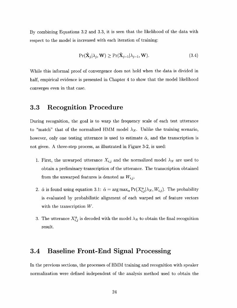
3.3 Recognition Procedure

During recognition, the goal is to warp the frequency scale of each test utterance

to "match" that of the normalized HMM model AN. Unlike the training scenario,

however, only one testing utterance is used to estimate 6, and the transcription is

not given. A three-step process, as illustrated in Figure 3-2, is used:

1. First, the unwarped utterance Xij and the normalized model AN are used to

obtain a preliminary transcription of the utterance. The transcription obtained

from the unwarped features is denoted as Wij.

2. & is found using equation 3.1: & = arg max Pr(X 3 AN, Wi,). The probability

is evaluated by probabilistic alignment of each warped set of feature vectors

with the transcription W.

3. The utterance Xj is decoded with the model AN to obtain the final recognition

result.

3.4 Baseline Front-End Signal Processing

In the previous sections, the processes of HMM training and recognition with speaker

normalization were defined independent of the analysis method used to obtain the

1 ------

Figure 3-2: HMM Recognition with Speaker Normalization

cepstrum. The most commonly used speech recognition feature sets are cepstra de-

rived either from linear predictive analysis, or from a filter bank. Both of these

front-ends are described in this section. The next section describes the steps taken to

implement frequency warping within these front-ends. While the notation from the

previous sections is kept consistent, the subscripts denoting the speaker, utterance,

and frame numbers are dropped hereafter.

3.4.1 Filter Bank Front-end

A block diagram of the mel-scale filter bank front-end proposed by Davis and Mermel-

stein is shown in Figure 3-3 [6]. After the sampled speech waveform has been passed

through a Hamming window, the short-time magnitude spectrum, S[k], is computed

on the speech segment. The resulting spectrum is then passed through a bank of

overlapped, triangular filters, and an inverse cosine transform is used to convert the

sequence of the output filter energies to cepstrum. The process is then repeated by

[1 S[k] Y[I] x[m]FinT 1'rv2 L1ZJmel-scale filterbank

Figure 3-3: Mel Filter Bank Analysis

shifting the position of the Hamming window.

In a mel-scale filter bank, the spacing and width of the filters are designed to

model the variations in the human ear's ability to discriminate frequency differences

as a function of the frequency of the sound. Physiological and perceptual data show

that the human ear is more sensitive at lower frequencies than at higher frequencies

[3]. Therefore, the filters are spaced linearly between 0 and 1000 Hz, and logarithmi-

cally above 1000 Hz. The lower and upper band-edges of each filter, corresponding

to the DFT indices L1 and U1, coincide with the center frequencies of its adjacent

filters, resulting in 50% overlap between adjacent filters. The bandwidth of the filters

increases for the higher frequency bands. The magnitudes of the filters are normalized

so that the area of each filter is constant, i.e., Ek=UL, F, [k] = 1.

The filters cover the entire signal bandwidth, and the mel-filter bank representa-

tion of the signal consists of the log energy output of the filters when S [k] is passed

through them:

Y[l] = log ( Fc [k] S [k] . (3.5)\k=Ll

The last step of the front-end computes the cepstral coefficients of the filter bank

vector using an inverse cosine transform:

1 NFx[m] = E Y[1] cos(m( - •) - ) m = 1, ..., NF - 1. (3.6)

NF 2 NF1l=1

Only the first 10 to 15 cepstral coefficients are used as speech features. Cepstral

coefficients are used in place of filter bank energies mainly because they tend to be

less correlated with one another. The high degree of overlap between neighboring

filters results in a high degree of correlation between filter bank coefficients. The less

correlated cepstrum features allow the independence assumption implied by the use of

diagonal covariance Gaussian distributions in the recognizer to be a more reasonable

approximation.

3.4.2 Linear Predictive Analysis

The theory of linear predictive coding(LPC) in speech has been well-understood for

many years [22]. This section provides a brief overview of the autocorrelation method

of calculating LPC cepstra. The reader is referred to [22] for a detailed mathematical

derivation.

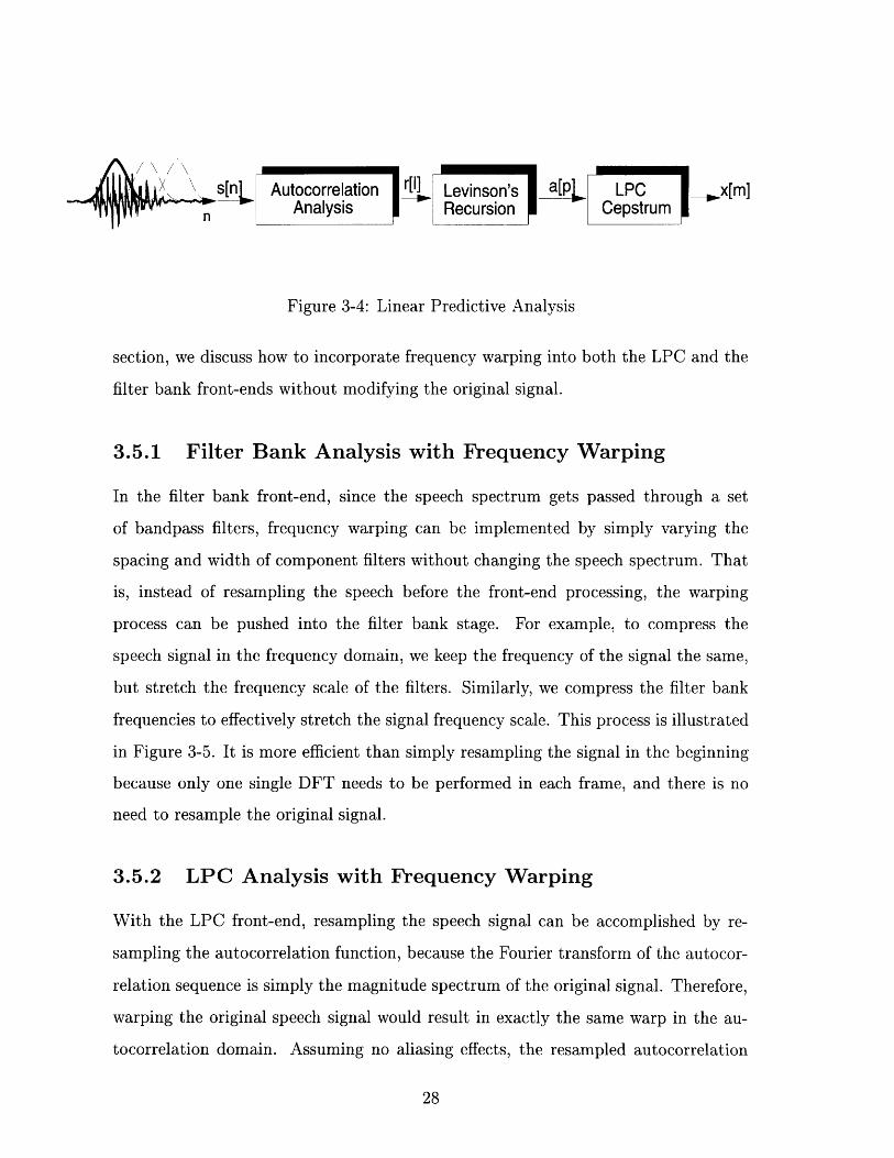
A block diagram of the autocorrelation method is shown in Figure 3-4. The first

step is similar to that of the filter bank front-end in that the incoming speech is win-

dowed using a Hamming window. Each frame of speech, s[k], is then autocorrelated

to calculate a set of L + 1 correlation coefficients r[l]:

K-1

r[l] = Zs[k]s[k + 1], 1 = O, 1, ...L (3.7)k=O

The set of autocorrelations is then converted into the LPC coefficients a[p] using

Levinson's recursion. The all-pole filter 1/(1 - , a[p]z -P ) represents the vocal tract

transfer function under the LPC model. Finally, the LPC cepstral coefficients, x[m],

can be derived from the LPC coefficients a[m] through a recursive relationship [22].

These coefficients represent the Fourier transform of the log magnitude spectrum of

the LPC filter, and they have been found to be more statistically well-behaved as

speech recognition features than the LPC coefficients.

3.5 Frequency Warping

Linearly compressing and expanding the frequency axis of a signal is perhaps most

intuitively done by resampling the signal in the time domain [1]. However, resampling

in the time domain is inefficient, especially in the range of allowable a's. In this

S Levinson's a[ LPC xm]Recursion Cepstrum

Figure 3-4: Linear Predictive Analysis

section, we discuss how to incorporate frequency warping into both the LPC and the

filter bank front-ends without modifying the original signal.

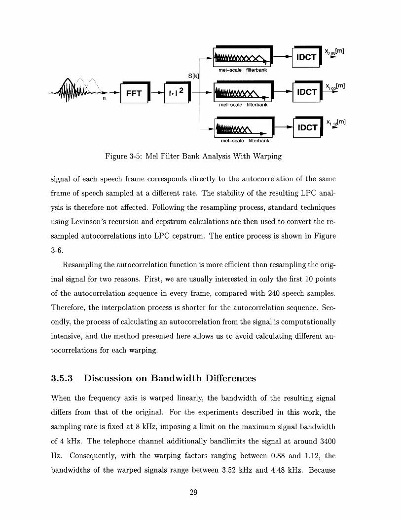
3.5.1 Filter Bank Analysis with Frequency Warping

In the filter bank front-end, since the speech spectrum gets passed through a set

of bandpass filters, frequency warping can be implemented by simply varying the

spacing and width of component filters without changing the speech spectrum. That

is, instead of resampling the speech before the front-end processing, the warping

process can be pushed into the filter bank stage. For example, to compress the

speech signal in the frequency domain, we keep the frequency of the signal the same,

but stretch the frequency scale of the filters. Similarly, we compress the filter bank

frequencies to effectively stretch the signal frequency scale. This process is illustrated

in Figure 3-5. It is more efficient than simply resampling the signal in the beginning

because only one single DFT needs to be performed in each frame, and there is no

need to resample the original signal.

3.5.2 LPC Analysis with Frequency Warping

With the LPC front-end, resampling the speech signal can be accomplished by re-

sampling the autocorrelation function, because the Fourier transform of the autocor-

relation sequence is simply the magnitude spectrum of the original signal. Therefore,

warping the original speech signal would result in exactly the same warp in the au-

tocorrelation domain. Assuming no aliasing effects, the resampled autocorrelation

mel-scale filterbankS[k]

[m]

mel-scale filterbank

xI ,[m]

mel-scale filterbank

Figure 3-5: Mel Filter Bank Analysis With Warping

signal of each speech frame corresponds directly to the autocorrelation of the same

frame of speech sampled at a different rate. The stability of the resulting LPC anal-

ysis is therefore not affected. Following the resampling process, standard techniques

using Levinson's recursion and cepstrum calculations are then used to convert the re-

sampled autocorrelations into LPC cepstrum. The entire process is shown in Figure

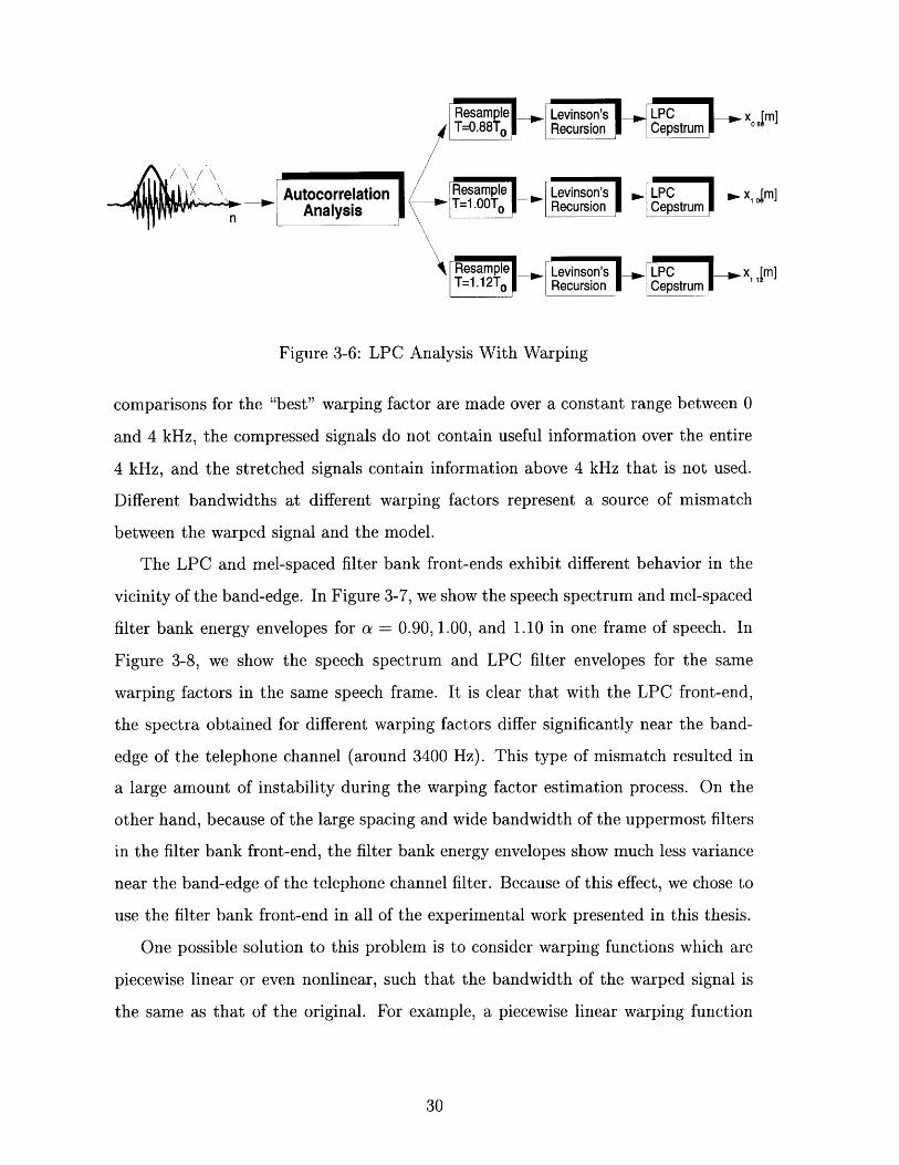
3-6.

Resampling the autocorrelation function is more efficient than resampling the orig-

inal signal for two reasons. First, we are usually interested in only the first 10 points

of the autocorrelation sequence in every frame, compared with 240 speech samples.

Therefore, the interpolation process is shorter for the autocorrelation sequence. Sec-

ondly, the process of calculating an autocorrelation from the signal is computationally

intensive, and the method presented here allows us to avoid calculating different au-

tocorrelations for each warping.

3.5.3 Discussion on Bandwidth Differences

When the frequency axis is warped linearly, the bandwidth of the resulting signal

differs from that of the original. For the experiments described in this work, the

sampling rate is fixed at 8 kHz, imposing a limit on the maximum signal bandwidth

of 4 kHz. The telephone channel additionally bandlimits the signal at around 3400

Hz. Consequently, with the warping factors ranging between 0.88 and 1.12, the

bandwidths of the warped signals range between 3.52 kHz and 4.48 kHz. Because

Rscomparisons forample the "best" Levinsons tant range between 04 kHz, and the stretched sigT=.88Tion Recursionv e 4 kHz that is not used.

Different bandwidths at diffocorrent warping factors represent a son'surce of mismatchbetween the warped Recursin Cepstruand the model.

filter bank energy envelopResamplees for = 0.90, Levinson's frame of sLPCeech. InT=1. 12To Recursion Cepstrum,

Figure 3-6: LPC Analysis With Warping

comparisons for the "best" warping factor are made over a constant range between 0

and 4 kHz, the compressed signals do not contain useful information over the entire

4 kHz, and the stretched signals contain information above 4 kHz that is not used.

Different bandwidths at different warping factors represent a source of mismatch

between the warped signal and the model.

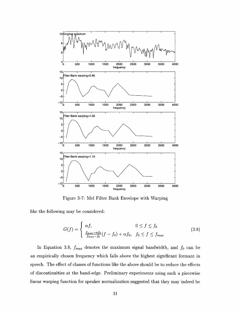
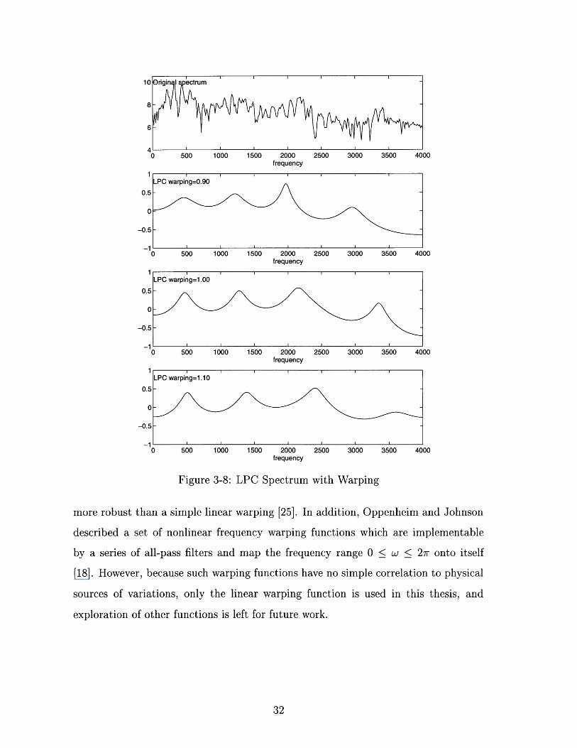
The LPC and mel-spaced filter bank front-ends exhibit different behavior in the

vicinity of the band-edge. In Figurthe telephone channel filter. B speech spectrum and mel-spaced

filter bank energy envelopes for al = 0.90, 1.00, and 1.10 in one frame of speech. In

Figure 3-8, we show the speech spectrum and LPC filter envelopes for the same

warping factors in the same speech frame. It is clear that with the LPC front-end,

the spectra obtained for different warping factors differ significantly near the band-

edge of the telephone channel (around 3400 Hz). This type of mismatch resulted in

a large amount of instability during the warping factor estimation process. On the

other hand, because of the large spacing and wide bandwidth of the uppermost filters

in the filter bank front-end, the filter bank energy envelopes show much less variance

near the band-edge of the telephone channel filter. Because of this effect, we chose to

use the filter bank front-end in all of the experimental work presented in this thesis.

One possible solution to this problem is to consider warping functions which are

piecewise linear or even nonlinear, such that the bandwidth of the warped signal is

the same as that of the original. For example, a piecewise linear warping function

00frequency

500 1000 1500 2000frequency

10

5

0

-5

-100

15

10

5

0

-5

-100

2500 3000 3500

2500 3000 3500

4000

40

5 I I I I I I I500 1000 1500 2000 2500 3000 3500

frequency

e 3-7: Mel Filter Bank Envelope with Warping

40

00

00

like the following may be considered:

(3.8)G(f) = f, O< f < fo{f)= -afo ( fo) + afo, fo < f < fmaxfmax -fo

In Equation 3.8, fmax denotes the maximum signal bandwidth, and fo can be

an empirically chosen frequency which falls above the highest significant formant in

speech. The effect of classes of functions like the above should be to reduce the effects

of discontinuities at the band-edge. Preliminary experiments using such a piecewise

linear warping function for speaker normalization suggested that they may indeed be

Filter Bank warping=0.90

-

500 1000 1500 2000frequency

Filter Bank warping=1.00

1

1

-1

Filter Bank warping=1. 10

5-0

5

0

Figur

·I i I I I

-

-

4 f

-

-

-

00frequency

500 1000 1500 2000frequency

500 1000 1500 2000frequency

50 100 150 2000I500 1000 1500 2000

frequency

Figure 3-8: LPC Spectrum

2500 3000 3500 4000

2500 3000 3500 4000

2500 3000 3500 4000

with Warping

more robust than a simple linear warping [25]. In addition, Oppenheim and Johnson

described a set of nonlinear frequency warping functions which are implementable

by a series of all-pass filters and map the frequency range 0 < w < 27w onto itself

[18]. However, because such warping functions have no simple correlation to physical

sources of variations, only the linear warping function is used in this thesis, and

exploration of other functions is left for future work.

-PC warping=0.90--

-

LPC warping=1.00

0.5

0

-0.5

1

0

1

0.5

0

-0.5

-10

1

0.5

0

-0.5

-10

LPC warping=1.10

· 1 1 1 · I

-

-

-

-

1

3.6 Summary

This chapter presented a set of procedures used to perform speaker vocal tract

length normalization. The criterion for warping factor estimation was presented in a

maximum-likelihood framework. The procedures used to perform speaker normaliza-

tion during HMM training and recognition were also described. In addition, methods

for performing frequency warping within the filter bank and the LPC feature ex-

traction front-ends were presented. Finally, the issue of different signal bandwidths

resulting from warping the original signal in varying degrees was discussed. Because

the uppermost filters are very wide in the filter bank front-end, this effect is less ap-

parent in the filter bank front-end, and we chose to use the filter bank instead of the

LPC front-end in this work.

Chapter 4

Baseline Experiments

This chapter presents an experimental study of the effectiveness of the speaker nor-

malization procedures described in Chapter 3. The principle measure of effectiveness

is speech recognition performance obtained on a connected digit speech recognition

task over the telephone network. Besides speech recognition performance, a number of

issues are investigated and discussed. Experiments were performed to understand the

ability of the speaker normalization procedures to decrease inter-speaker variability,

and to produce normalized HMMs which describe the data more efficiently.

The chapter is divided into six sections. After the task, database, and speech

recognizer are described in Sections 4.1 and 4.2, ASR performance before and after

speaker normalization is presented in Section 4.3. Section 4.4 presents a analysis of

the distribution of the chosen warping factors among the speakers in the training

set to verify the effectiveness of ML warping factor estimation procedure. Section

4.5 describes the application of a HMM distance measure to speaker dependent (SD)

HMMs in an attempt to quantitatively measure the amount of inter-speaker variability

among a set of speakers before and after frequency warping. Section 4.6 presents

statistics on the ability of the warping factor estimation procedure to generate reliable

estimates on utterances of only 1 or 2 digits in length. Finally, Section 4.7 describes

speech recognition performance over successive iterations of the training procedure

described in Chapter 3 as empirical evidence of the convergence properties of the

iterative training procedure.

Training Set Testing set

# digits 26717 13185# utterances 8802 4304# carbon utts. 4426 2158# electret utts. 4376 2146# male spkers 372 289# female spkers 341 307

Table 4.1: Database DB1 Description

4.1 Task and Databases

Two telephone-based connected digit databases were used in this study. The first,

DB1, was used in all of the speech recognition experiments. It was recorded in

shopping malls across 15 dialectally distinct regions in the US, using two carbon and

two electret handsets which were tested to be in good working condition. The size

of the vocabulary was eleven words: "one" to "nine", as well as "zero" and "oh".

The speakers read digit strings between 1 and 7 digits in a continuous manner over

a telephone, so that the length of each utterance ranged from about .5 seconds to

4 seconds. The training utterances were endpointed, whereas the testing utterances

were not. All of the data was sampled at 8 kHz. Table 4.1 lists the specifics about

the training and testing sets.

A second connected digit database, DB2, was used to evaluate properties of the

speaker normalization procedures which required more data per speaker than available

in DB1. DB2 was taken from one of the dialectal regions used for DB1, but contains

a larger number of utterances per speaker. In DB2, approximately 100 digit strings

were recorded for each speaker. A total of 2239 utterances, or 6793 digits, were

available from 22 speakers(10 males, 12 females.)

Throughout this thesis, word error rate is used to evaluate the performance of

various techniques. The error rate is computed as follows:

Sub + Del + Ins% Error = 100 TotaNumberofWords (4.1)TotalNumberof Words'

where Sub is the number of substitutions, Del is the number of deletions, and Ins

is the number insertions. These quantities are found using a dynamic programming

algorithm to obtain the highest scoring alignment between the recognized word string

and the correct word string.

4.2 Baseline Speech Recognizer

The experiments in this thesis have been conducted using an HMM speech recognition

system built in AT&T Bell Laboratories. Each digit was modeled by 8 to 10 state

continuous-density left-to-right HMMs. In addition, silence was explicitly modeled

by a single-state HMM. The observation densities were mixtures of 8 multi-variate

Gaussian distributions with diagonal covariance matrices. 39-dimensional feature

vectors were used: normalized energy, c[1]-c[12] derived from a mel-spaced filter bank

of 22 filters, and their first and second derivatives. The performance metric used was

word error rate. This configuration is used for all of the experiments described in this

chapter unless otherwise noted.

4.3 Speech Recognition Performance

Table 4.2 shows the recognition word error rate on DB1 using only the baseline rec-

ognizer, and using the baseline recognizer with the speaker normalization procedures.

The first row reports the word error rate observed when testing unwarped feature

vectors using models trained on unwarped feature vectors. The second row reports

the error rate observed using the speaker normalization training and recognition pro-

cedures described in Chapter 3. The models were trained using frequency-normalized

feature vectors obtained after the first iteration of the iterative HMM training pro-

cedure. The error rates for utterances through the carbon and electret handsets are

shown separately in the second and third columns, and averaged in the last column.

There are several observations that can be made from Table 4.2. First, it is clear

from the table that the overall word error rate is reduced by approximately 20%

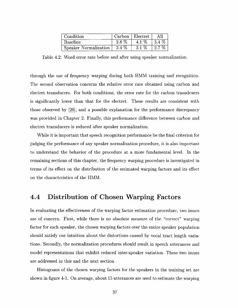
Condition Carbon Electret AllBaseline 2.8 % 4.1 % 3.4 %Speaker Normalization 2.4 % 3.1 % 2.7 %

Table 4.2: Word error rate before and after using speaker normalization.

through the use of frequency warping during both HMM training and recognition.

The second observation concerns the relative error rate obtained using carbon and

electret transducers. For both conditions, the error rate for the carbon transdcuers

is significantly lower than that for the electret. These results are consistent with

those observed by [20], and a possible explanation for the performance discrepancy

was provided in Chapter 2. Finally, this performance difference between carbon and

electret transducers is reduced after speaker normalization.

While it is important that speech recognition performance be the final criterion for

judging the performance of any speaker normalization procedure, it is also important

to understand the behavior of the procedure at a more fundamental level. In the

remaining sections of this chapter, the frequency warping procedure is investigated in

terms of its effect on the distribution of the estimated warping factors and its effect

on the characteristics of the HMM.

4.4 Distribution of Chosen Warping Factors

In evaluating the effectiveness of the warping factor estimation procedure, two issues

are of concern. First, while there is no absolute measure of the "correct" warping

factor for each speaker, the chosen warping factors over the entire speaker population

should satisfy our intuition about the distortions caused by vocal tract length varia-

tions. Secondly, the normalization procedures should result in speech utterances and

model representations that exhibit reduced inter-speaker variation. These two issues

are addressed in this and the next section.

Histograms of the chosen warping factors for the speakers in the training set are

shown in figure 4-1. On average, about 15 utterances are used to estimate the warping

factor for each speaker. The warping factors chosen for the males are shown on top,

and those for the females shown on the bottom. The value of the estimated warping

factor is displayed along the horizontal axis, and the number of speakers who were

assigned to each given warping factor is plotted on the vertical axis. Warping factors

below 1.00 correspond to frequency compression, and those above 1.00 correspond to

frequency expansion. The mean of warping factors is 1.00 for males, 0.94 for females,

and 0.975 for all of the speakers.

MALESOU

40

0E 20z

A0.85 0.9 0.95 1 1.05 1.1

warping factor chosenFEMALES

Iuu I I I I1

801-6u

a)d"I ~LU,

, 40.ME:: 20-Z

0.85 0.9 0.95 1 1.05 1.1warping factor chosen

Figure 4-1: Histogram of warping factors chosen for speakers in the training set

Clearly, the average warping factor among males is higher than that among fe-

males. This satisfies our intuition because females tend to have shorter vocal tract

lengths, and higher formant frequencies. As a result, it is reasonable that the nor-

malization procedure chooses to compress the frequency axis more often for female

speech than for male speech.

At the same time, however, the fact that the mean of the estimated warping fac-

tors over all speakers is not 1.00 is somewhat surprising, because the iterative training

I

Hrn~-~ I-I

I I I I I

I I I

1 1

I~s

I

I

I

I

process was initiated with a model built with unwarped utterances. One explanation

for this result lies in the difference in the effective bandwidth between utterances

whose frequency axes have been compressed or expanded to different degrees. One

side-effect of frequency compression is the inclusion of portions of the frequency spec-

trum which may have originally been out-of-band. If parts of the discarded spectra

carry information useful for recognition, the ML warping factor estimation is likely to

be biased toward frequency compression. This is perhaps best-illustrated in Figure

3-7.

The mean of estimated warping factors is not required to be 1.0 under model-based

warping factor estimation because any notion of a "reference" vocal tract length must

be considered in reference to the model parameters. It is the relative differences in

warping factors chosen for different speakers which is most significant to the ability of

the procedure to generate a consistently frequency-normalized feature set. The next

section describes an experiment to measure the HMM model based similarity among

speakers before and after warping factor estimation and frequency warping.

4.5 Speaker Variability and HMM Distances

One way to gauge the effectiveness of the warping factor estimation process is to use

a quantitative measure of the degree of similarity between the acoustic spaces of the

speech from two speakers. Such a measure can indicate whether or not the speaker

normalization process reduces the inter-speaker variability in the feature space. This

section describes an experiment in which the HMM distance measure proposed by

Juang and Rabiner in [13] was applied to two sets of speaker-dependent HMMs. The

first set was trained using unwarped feature vectors, and the second was trained using

frequency-normalized feature vectors where the warping factor was found using the

standard ML method. The distances between the SD HMMs within the first and

second sets were then compared as a measure of the inter-speaker variability before

and after speaker normalization. We first describe the HMM distance measure, then

the experimental setup, and finally the results.

4.5.1 Definition of HMM Distance Measure

The HMM distance measure was proposed and derived following the concepts of

divergence and discrimination information in [13]. Given two HMMs A1 and A2, the

resulting metric quantitatively describes the difficulty of discriminating between the

two models. The distance measure is mathematically stated as follows.

Consider two HMMs A1 and A2 . Suppose that X 1 is a sequence of T1 observations

generated by A1, and X2 is a sequence of T2 observations generated by A2. The

distance between A1 and A2 , D(A1 , A2), is then defined as follows:

D(A1, A2) = 1 (logPr(XIAi1) - log Pr(Xi A2))T1

1 (log Pr(X21 2) - log Pr(X2 J1))T2

The distance measure shown in equation 4.2 is symmetric with respect to A1 and A2.

It represents a measure of the difficulty of discriminating between two HMMs. Since

a SD HMM represents the feature space distribution of the speech of a particular

speaker, the distance between SD HMMs corresponding to two different speakers can

be taken as a measure of the similarity between the speakers in feature space.

The formulation of the HMM distance measure in [13] assumed that the HMMs

are ergodic. However, it was found in [13] that for left-to-right HMM models, using a

series of restarted sequences as the generated observation sequence for the likelihood

calculations yields reliable distance measurements. In the work presented here, this

is implemented by using a large ensemble of utterances from each speaker to evaluate

the average likelihood used in the distance measure.

4.5.2 Experimental Setup

This experiment was performed using DB2. As mentioned earlier, two sets of SD

HMMs were trained for each speaker: one using unwarped data, and the other using

frequency-warped data. In the second case, the warping factor was determined with

the frequency-normalized SI HMMs used in the baseline recognition experiments re-

(4.2)

ported in Section 4.3. Additionally, the estimation of the warping factor operated

under the HMM training scenario. That is, the known text transcriptions of the ut-

terances were used, and all of the utterances from each speaker were pooled together

to estimate one single warping factor.

For each speaker i, we use the following notation:

* X'j denotes the unwarped feature vectors of the jth utterance of speaker i;

* Xiw denotes the warped feature vectors of the same utterance;

* X' denotes the set of all unwarped feature vectors of speaker i:

Xi = {XU,X 2,... , I

* XT denotes the set of all warped feature vectors of speaker i:

Xi = {Xi, i,2,., i,N ,}

In this experiment, SD HMMs AY were trained using Xj, and Al were trained using

Xw for all of the speakers. The HMMs consisted of 8-10 states per digit and mixtures

of 2 to 4 Gaussians per state-dependent observation density. The log-likelihoods

log Pr(XilAj) were evaluated using probabilistic alignment. Inter-speaker distance

measures D(AY, A) and D(A', Aý') were computed for all pairs (i,j), i • j. Since

DB2 was used, about 100 utterances were available from each speaker for HMM

training and likelihood evaluations.

4.5.3 Results

Table 4.3 shows averages in the HMM distances before and after speaker normalization

is used. The second column shows the average HMM distances between two male SD

HMMs or two female SD HMMs. The third column shows the average HMM distances

between a male SD HMM and a female SD HMM. The fourth column shows the overall

average for all speaker pairs in the database.

A few interesting observations can be made from the table. First, it is clear that

the average HMM distance between speakers has decreased after speaker normaliza-

tion. It is also clear that inter-speaker differences within the same gender is much

Condition Within-Gender Across-Gender AllBaseline 22.8 27.0 24.3Speaker Normalization 22.7 25.6 23.7

Table 4.3: Average HMM distances before and after using speaker normalization.

smaller than that across genders. The speaker normalization procedure seemed to

have significantly reduced the across-gender differences, although there still remains

a large gap between the first and second columns of the second row. These results

agree with our hypothesis that speaker normalization can produce feature sets which

show less inter-speaker variability. At the same time, however, a large portion of the

variations still remains, perhaps due to the fact that a linear frequency warping is a

very coarse model of the vocal tract length variations, and that many other sources

of variation have been ignored in our method.

4.6 Warping Factor Estimation With Short Utter-

ances

A major assumption made in the thesis is that the vocal tract length of the speaker

is a long-term speaker characteristic. Therefore, it is assumed that the variations in

effective vocal tract length due to the production of different sounds do not signif-

icantly affect the warping factor estimation process. Under this assumption, with

"sufficient" amounts of data for each utterance, the warping factor estimates should

not vary significantly among different utterances by the same speaker. This section

presents an experiment which attempted to test and better understand this assump-

tion by gathering and examining statistics reflecting how the warping factor estimates

change across utterances of different durations for the same speaker. These statistics

also reflect the ability of the ML-based warping factor estimation method to generate

reliable estimates even when the utterances are very short.

In this experiment, the 3-step speaker normalization recognition procedure de-

picted in Figure 3-2 was used on the data in DB2, where approximately 100 utter-

ances are available for each of 22 speakers. The set of all utterances Xi from speaker

i is divided roughly evenly into two sets based on the number of digits in each utter-

ance. The set of utterances containing 1 or 2 digits is denoted by Si, and the set of

utterances containing 3 to 7 digits is denoted by Li. For each speaker i, the means

and standard deviations of the warping factor estimates for utterances within each of

Si and Li are computed. The differences between the means computed for Si and Li

are examined to observe any significant differences in the warping factor estimates as

the amount of available data increases. The standard deviations are also compared

to see if the variance of warping factor estimates over different utterances decreases

with longer utterances.

Figure 4-2 shows two plots in which the mean and standard deviation of warping

factor estimates for utterances in Si are plotted against those statistics computed

over Li, for all of the speakers in DB2. In the top plot, the x-axis denotes the mean

of the warping factor estimates among utterances in set Si, and the y-axis denotes

the mean of the warping factor estimates among utterances in set Li. Points marked

by "*"'s correspond to the female speakers, and those marked by "+"'s correspond

to the male speakers. In the bottom plot, the x-axis denotes the standard deviation

of the warping factor estimates among utterances in set Si, and the y-axis denotes

the standard deviation of the warping factor estimates among utterances in set Li.

"X"'s are used to marked the data points. In both plots, the line y = x is drawn as

a reference to aid in discussing the trends in the plotted points.

Two important observations can be made based on the top plot of Figure 4-2.

First, the means of the warping factor estimates of the male speakers are always higher

than those of the female speakers regardless of the length of the utterance. Second, the

mean of the warping factor estimates over the longer utterances is significantly higher

than the mean over the shorter utterances among the male speakers. This difference

ranged from only 1% to almost 7.5%. While the cause of this trend is not clear, one

possible explanation may be that for the shorter utterances, a larger portion of the

available data consists of silences and other non-voiced sounds for which the frequency

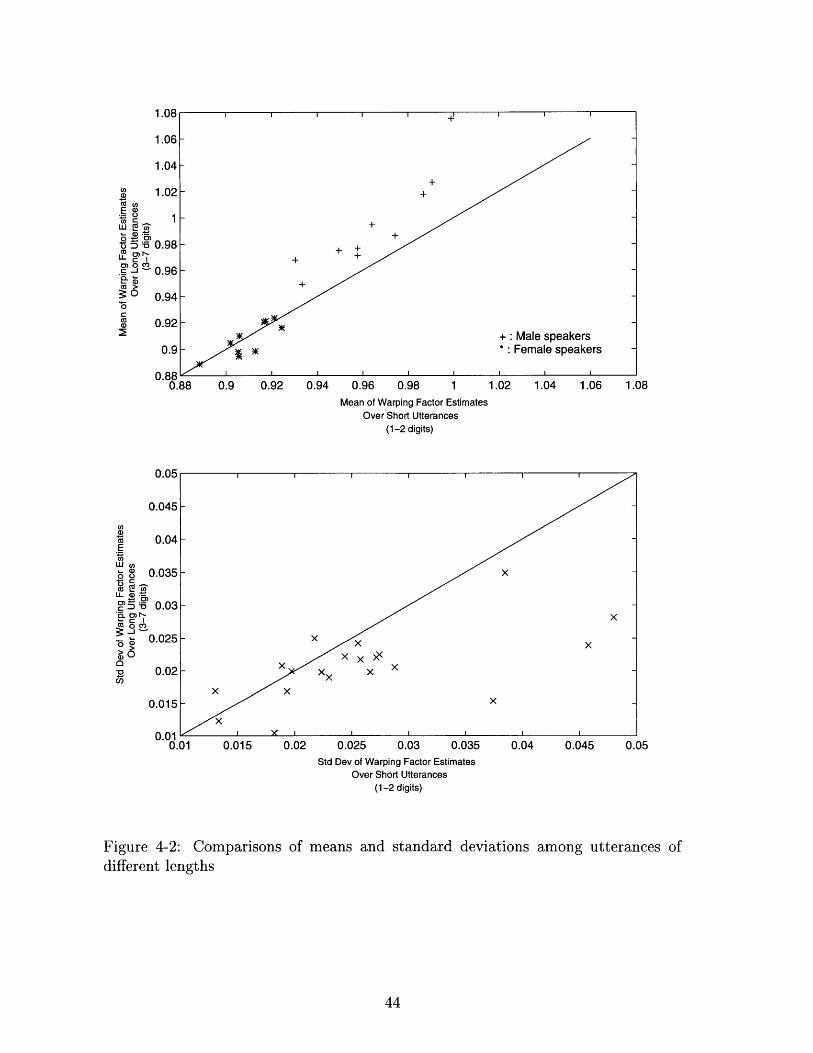
0.9 0.92 0.94 0.96 0.98 1 1.02 1.04 1.06 1.08Mean of Warping Factor Estimates

Over Short Utterances(1-2 digits)

0.01 0.015 0.02 0.025 0.03 0.035 0.04 0.045 0.05Std Dev of Warping Factor Estimates

Over Short Utterances(1-2 digits)

Figure 4-2: Comparisons of means and standard deviations among utterances ofdifferent lengths

1.08

1.06

1.04

0 1.02(Uc,

C:•o ol)EUO 1w-

55-o 0.98U)0 M-i -5 0.98CL

c(a>0 0.94

C(U 0.92

0.9

0 000.880.88

(nU)

E

-U)00

(ULLU)

0)

'aC

Uo

>U)

warping compensation model is not appropriate. Since the test utterances are not

endpointed, a large portion of the single-digit utterances is not speech. The computed

likelihood over non-speech frames may be higher for feature vectors corresponding

to frequency compression because frequency compression results in the inclusion of

portions of the frequency spectrum which would have been discarded otherwise.

Two observations can be made from the second plot of Figure 4-2. First, it is clear

that the standard deviation of the warping factor estimates generally decreases for

the set of longer utterances. This implies that the warping factor estimation process

does become more "stable" as the amount of available data increases. Second, the

standard deviation of the warping factor estimates over the shorter utterances is less

than 0.04 for a majority of the speakers. Taking into account that the possible warping

factors are spaced 0.02 apart in the grid search process, we see that the warping factor

estimation process produces estimates which do not vary greatly from utterance to

utterance, depending on the particular phonetic content of the utterance. Hence,

these observations are consistent with our assumption that the vocal tract length of

the speaker does not change significantly with the sound being produced.

4.7 Convergence of Model Training Procedure

This section presents an experiment performed to understand the convergence prop-

erties of the iterative training procedure. In the standard Baum-Welch HMM training

algorithm, the likelihood of the training data with respect to the models is mathe-

matically guaranteed to increase at the end of each iteration. While the iterative

normalized-HMM training procedure is not guaranteed to converge mathematically,

we study changes in recognition error rate on the training and testing data as the

number of training iterations is increased. This experiment also serves to further test

whether the frequency warping procedures are indeed reducing the speaker variabil-

ity (at least in the training set), and that the normalized HMMs are becoming more

efficient over the iterations.

Table 4.4 shows how the model likelihood and recognition word error rate on the

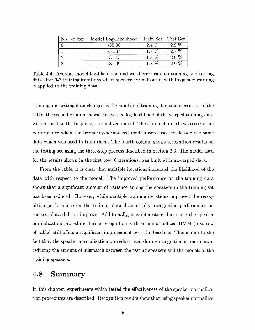
No. of Iter. Model Log-Likelihood Train Set Test Set0 -32.08 2.4 % 2.9 %1 -31.35 1.7 % 2.7 %2 -31.13 1.3 % 2.9 %3 -31.09 1.3 % 2.9 %

Table 4.4: Average model log-likelihood and word error rate on training and testingdata after 0-3 training iterations where speaker normalization with frequency warpingis applied to the training data.

training and testing data changes as the number of training iteration increases. In the

table, the second column shows the average log-likelihood of the warped training data

with respect to the frequency-normalized model. The third column shows recognition

performance when the frequency-normalized models were used to decode the same

data which was used to train them. The fourth column shows recognition results on

the testing set using the three-step process described in Section 3.3. The model used

for the results shown in the first row, 0 iterations, was built with unwarped data.

From the table, it is clear that multiple iterations increased the likelihood of the

data with respect to the model. The improved performance on the training data

shows that a significant amount of variance among the speakers in the training set

has been reduced. However, while multiple training iterations improved the recog-

nition performance on the training data dramatically, recognition performance on

the test data did not improve. Additionally, it is interesting that using the speaker

normalization procedure during recognition with an unnormalized HMM (first row

of table) still offers a significant improvement over the baseline. This is due to the

fact that the speaker normalization procedure used during recognition is, on its own,

reducing the amount of mismatch between the testing speakers and the models of the

training speakers.

4.8 Summary

In this chapter, experiments which tested the effectiveness of the speaker normaliza-

tion procedures are described. Recognition results show that using speaker normaliza-

tion reduces the word error rate by about 20% on a telephone-based digit recognition

task. The distribution of estimated warping factors across speakers showed that the

ML warping factor estimation criterion does yield results which are consistent with

our simple model of the acoustic effects of vocal tract variations. However, a bias

toward warping factors corresponding to frequency compression is observed, perhaps

due to the fact that a larger portion of the speech spectra is included when signals are

compressed. By using HMM distances as a measure of inter-speaker differences, we

conclude that frequency warping is reducing a portion of the inter-speaker variability.

We also showed that the warping factor estimation process used during recognition

produces estimates which do not vary greatly across different utterances from the

speaker. Finally, observations of changes in recognition performance on the training

and testing data show that while multiple training iterations does incrementally pro-

duce models which better represent the training data, it does not help recognition

performance on the test data.

Chapter 5

Efficient Approaches to Speaker

Robust Systems

In Chapter 3, a set of procedures for implementing ML-based speaker normalization

with frequency warping was described, and in Chapter 4, recognition results showed

that these procedures can reduce the error rate by 20% on a telephone-based speech

recognition task. Due to the additional computational requirements of these proce-

dures, however, it is important to consider less computationally intensive alternatives

which may also be effective in improving the robustness of the system with respect to

speaker variabilities. This chapter proposes new, less complex methods for warping

factor estimation. It also considers existing methods which were originally designed to

reduce the effects of speaker variability on speech recognition performance. In com-

paring the frequency warping approach to speaker normalization with these other

techniques, we gain additional insight into the advantages and disadvantages of using

this physiologically-motivated procedure over other statistically-based compensation

and modeling procedures.

The chapter is divided into three sections. In Section 5.1, the high computational

cost and long time latencies that result from the 3-step procedure shown in Figure

3-2 are addressed. A more efficient procedure for estimating the warping factor is

presented, and compared against variations of the existing method described earlier.

A second section studies how speaker normalization procedures compare with

other compensation procedures. In many speech recognition applications, better

speaker-independent recognition performance has been obtained by training separate

sets of HMMs for different classes of speakers. Also, simply normalizing the speech

feature vectors with respect to long-term spectral averages has been shown to com-

pensate for both speaker-dependent and channel-dependent variabilities. In Section

5.2, the recognition performance of the frequency warping approach to speaker nor-

malization is compared to examples of these two other approaches. Gender-dependent

modeling is investigated as an example of class-dependent models, and cepstral mean

normalization is investigated as an example of compensation using long-term spectral

averaging.

Third, we study whether the effects of speaker normalization can be achieved sim-

ply by using more parameters in the HMM. A closely-associated question is whether

the complexity of the HMMs affects the amount of performance gain achieved by

speaker normalization. Experimental results answering these questions are presented

in Section 5.3

5.1 Efficient Warping Factor Estimation

In the three-step recognition procedure shown in Figure 3-2, the inefficiency of per-

forming an exhaustive grid search to estimate the warping factor is compounded by

the need to use probabilistic alignment at each possible warping factor. Having to

use two recognition passes at each utterance is an additional computation complex-

ity which causes the entire recognition process to be much slower than using simple

HMM decoding. In this section, two methods to improve the efficiency of warping

factor estimation are proposed and tested. The first method is to use more coarsely

sampled search grids for estimating the warping factor a during recognition. That

is, whereas successive samples of a were originally separated by 2%, we propose to

increase this separation to reduce the total number of sample points. Even though

the a estimates may be less accurate as a result, the recognition performance may be

only marginally degraded.

A second method involves leaving the HMM-based warping factor estimation

paradigm altogether, and estimating warping factors using likelihoods computed from

Gaussian mixtures rather than HMMs. This method is described below.

5.1.1 Mixture-based Warping Factor Estimation

In the earlier chapters, the warping factor is conceptualized simply as a representa-

tion of the ratio between a speaker's vocal tract length and some notion of a reference

vocal tract length. However, warping factor estimation can also be considered as a

classification problem. During speaker normalization, each speaker is first classified

according to an estimate of his/her vocal tract length, and class-dependent trans-

formations are then applied to the speech to yield a final feature set which is used

in recognition. From this point of view, speakers are placed into different classes

based on the warping factor estimated using their utterances, and the warping factor

can be better stated as a class identifier. Intuitively, the feature space distributions

of untransformed speech from the different classes of speakers would vary due to the

acoustic differences of speech produced by vocal tracts of different lengths. Therefore,

if statistical models of the feature space distribution of each class are available, it may

be possible to determine the warping factor by finding out which class distribution is

most likely to have generated the given sequence of feature vectors.

The mixture-based warping factor estimation technique described here is moti-

vated by this classification perspective of speaker normalization. In training, after

warping factors have been determined for all of the speakers using the process shown

in Figure 3-1, mixtures of multivariate Gaussians are trained to represent the feature

space distributions of each of the possible classes. That is, for each warping fac-

tor, mixtures are trained using the unwarped feature vectors from utterances which

were assigned to that warping factor. Then, during recognition, the probability of the

incoming utterance before frequency warping is evaluated against each of these distri-

butions, and the warping factor is chosen for the distribution which yields the highest

likelihood over the entire utterance. The speech is warped using this estimated warp-

ing factor, and the resulting feature vectors are then used for HMM decoding. This

process is diagrammed in Figure 5-1.

This mixture-based method results in faster recognition time, because it eliminates

the need to obtain a preliminary transcription using the unwarped utterance which is

used for performing probabilistic alignment at all of the grid points. However, unlike

the method described in Section 3.3, it does not take advantage of the temporal

information in the signal during warping factor estimation, so that the estimated

warping factor may be less accurate.

TRAINING

MMI . I ^ GaussianMixture

Parameter MaEstimation a=0.88,0.90,...,1.12

MA

I i- I INIlU

Unwarped Si

Figure 5-1: Mixture-based optimal factor estimation

5.1.2 Experimental Results

The results of applying the above procedures for improving the efficiency of the recog-

nition procedure are shown in Table 5.1. The first row of the table gives the error rate

for the baseline speech recognizer described in Section 4.2 without frequency warping.

HMM-based search method refers to using probabilistic alignment at each possible

warping factor during recognition. The second through the fifth rows therefore show

the recognition performance when the number of possible warping factor values is

decreased from 13 down to 3 points. The last row of the table shows the recognition

Unwarped S i

ICAIILIA

MAX-- a

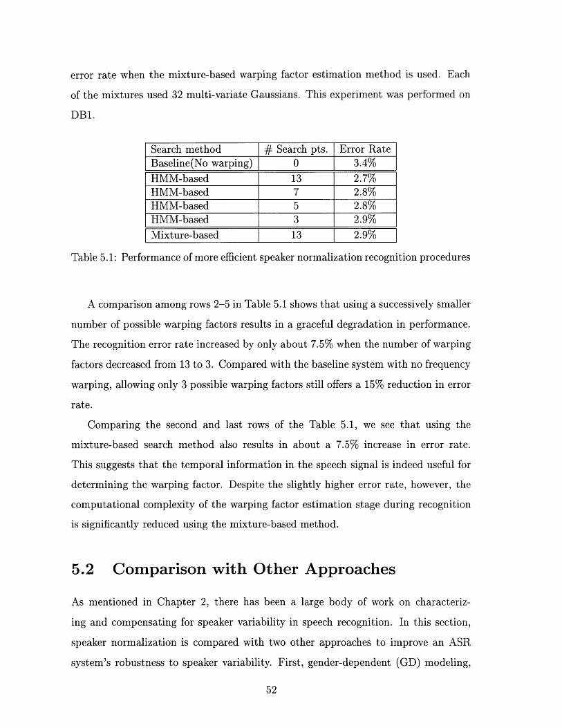
error rate when the mixture-based warping factor estimation method is used. Each

of the mixtures used 32 multi-variate Gaussians. This experiment was performed on

DB1.

Search method # Search pts. Error RateBaseline(No warping) 0 3.4%

HMM-based 13 2.7%HMM-based 7 2.8%HMM-based 5 2.8%HMM-based 3 2.9%

Mixture-based 13 2.9%

Table 5.1: Performance of more efficient speaker normalization recognition procedures

A comparison among rows 2-5 in Table 5.1 shows that using a successively smaller

number of possible warping factors results in a graceful degradation in performance.

The recognition error rate increased by only about 7.5% when the number of warping

factors decreased from 13 to 3. Compared with the baseline system with no frequency

warping, allowing only 3 possible warping factors still offers a 15% reduction in error

rate.

Comparing the second and last rows of the Table 5.1, we see that using the

mixture-based search method also results in about a 7.5% increase in error rate.

This suggests that the temporal information in the speech signal is indeed useful for

determining the warping factor. Despite the slightly higher error rate, however, the

computational complexity of the warping factor estimation stage during recognition

is significantly reduced using the mixture-based method.

5.2 Comparison with Other Approaches

As mentioned in Chapter 2, there has been a large body of work on characteriz-

ing and compensating for speaker variability in speech recognition. In this section,

speaker normalization is compared with two other approaches to improve an ASR

system's robustness to speaker variability. First, gender-dependent (GD) modeling,

an example of an approach to speaker class-dependent modeling, is implemented and

tested. Second, we investigate cepstral mean normalization (CMN), an example of

a technique which use long-term spectral averages to characterize fixed speaker and

channel characteristics. These techniques are described, and the recognition results

are presented below.

5.2.1 Gender-Dependent Models

Gender-dependent models exemplify the speaker class-dependent modeling techniques

which were briefly described in Chapter 2. This class of procedures can improve

recognition performance because models trained to represent a specific speaker class

are expected to represent less inter-speaker variability, and therefore may provide

"sharper" distributions. In GD modeling, two sets of HMMs are trained: one using

speech from males, and another using speech from females. During the Viterbi search

for the most likely state sequence in recognition, these HMMs are used to create two

separate gender specific networks. Again, the maximum-likelihood criterion is used

to find the best state sequence. Because the average vocal tract length differs sig-

nificantly between males and females and GD modeling can capture such differences,

GD models can be considered to "approximate" the speaker normalization process.

For this reason, it is important to understand whether the extra computational re-

quirements of speaker normalization results in higher performance.

5.2.2 Cepstral Mean Normalization

Long-term spectral averages have been used to characterize both speaker and chan-

nel characteristics [15]. CMN is an example of one of these techniques that has been

successfully used in ASR to compensate for both types of distortions. In our imple-

mentation of CMN, the mean of the cepstral vectors in the non-silence portions of

each utterance is assumed to characterize long-term characteristics of the speaker and

channel. Therefore, the cepstral mean is computed and subtracted from the entire

utterance. Two processing steps are taken. First, an energy-based speech activity

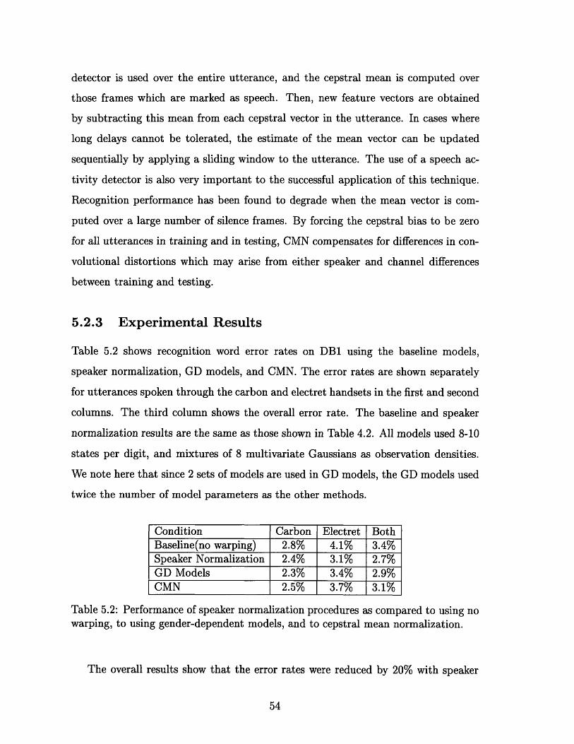
detector is used over the entire utterance, and the cepstral mean is computed over

those frames which are marked as speech. Then, new feature vectors are obtained

by subtracting this mean from each cepstral vector in the utterance. In cases where

long delays cannot be tolerated, the estimate of the mean vector can be updated

sequentially by applying a sliding window to the utterance. The use of a speech ac-

tivity detector is also very important to the successful application of this technique.

Recognition performance has been found to degrade when the mean vector is com-

puted over a large number of silence frames. By forcing the cepstral bias to be zero

for all utterances in training and in testing, CMN compensates for differences in con-

volutional distortions which may arise from either speaker and channel differences

between training and testing.

5.2.3 Experimental Results

Table 5.2 shows recognition word error rates on DB1 using the baseline models,

speaker normalization, GD models, and CMN. The error rates are shown separately

for utterances spoken through the carbon and electret handsets in the first and second

columns. The third column shows the overall error rate. The baseline and speaker

normalization results are the same as those shown in Table 4.2. All models used 8-10

states per digit, and mixtures of 8 multivariate Gaussians as observation densities.

We note here that since 2 sets of models are used in GD models, the GD models used

twice the number of model parameters as the other methods.

Condition Carbon Electret BothBaseline(no warping) 2.8% 4.1% 3.4%Speaker Normalization 2.4% 3.1% 2.7%GD Models 2.3% 3.4% 2.9%CMN 2.5% 3.7% 3.1%

Table 5.2: Performance of speaker normalization procedures as compared to using nowarping, to using gender-dependent models, and to cepstral mean normalization.

The overall results show that the error rates were reduced by 20% with speaker

normalization, by 15% with GD models, and by 10% with CMN. For all of the condi-

tions in the experiment, recognition performance on the test data spoken through the

carbon transducers is better than that for the electret transducers, even though the

model was trained from data spoken through both carbon and electret tranducers.

This result is consistent with those presented in [20], and some possible explanations

are presented there.

5.2.4 Speaker Normalization vs. Class-Dependent Models

As described in Chapter 2, class-dependent models can be trained for different speaker

groups according to gender, dialect, or by automatic clustering of speakers [22] [16].

Using this set of procedures, the separate HMMs are used in parallel during recog-

nition to simultaneously determine the class that the speaker belongs to, as well as

the string transcription of the utterance. It is important to realize that, with enough

data, a similar approach could be taken for the speaker normalization procedures. One

could train different sets of HMMs using training speakers assigned to each warping

factor, and decode using all of the HMMs. However, one common problem in training

class-dependent models is that as the number of classes increases, the models may

become under-trained.

In class-dependent modeling techniques like GD models, no attempt is made to

explicit characterize and compensate for the defining aspects of different classes in

feature space so that the spaces modeled by the class-dependent HMMs can become

more similar. As a result, there is a need to build complete models carrying both

phonetic and classification information for each class. The amount of available train-

ing data therefore limits the number of speaker classes. In the speaker normalization

approach, however, the inter-class differences are modeled using a relatively simple

parametrization and transformation. It is possible to transform the data from dif-

ferent classes into the same class, and build a model using all of the data, without

the occurrence of under-trained models even with a large number of classes. The

additional "resolution" in speaker class divisions allows for better recognition perfor-

mance with speaker normalization. This is clear from rows 2 and 3 in Table 5.2, where

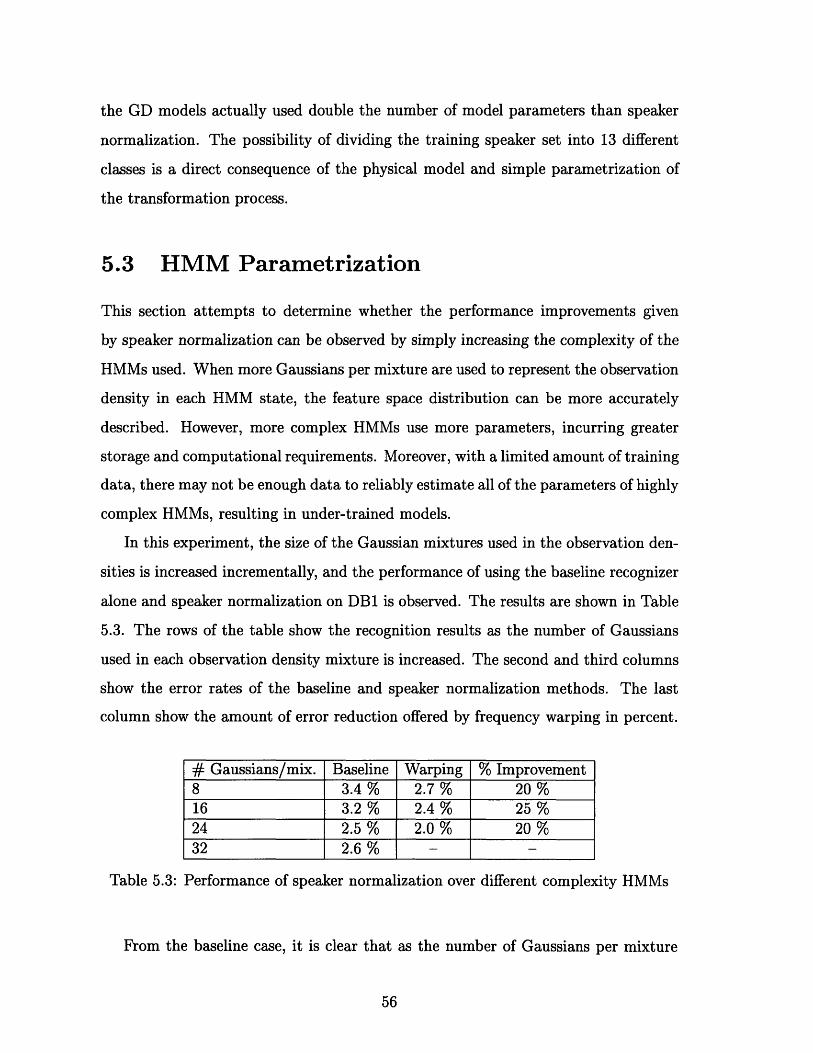
the GD models actually used double the number of model parameters than speaker

normalization. The possibility of dividing the training speaker set into 13 different

classes is a direct consequence of the physical model and simple parametrization of

the transformation process.

5.3 HMM Parametrization

This section attempts to determine whether the performance improvements given

by speaker normalization can be observed by simply increasing the complexity of the

HMMs used. When more Gaussians per mixture are used to represent the observation

density in each HMM state, the feature space distribution can be more accurately

described. However, more complex HMMs use more parameters, incurring greater

storage and computational requirements. Moreover, with a limited amount of training

data, there may not be enough data to reliably estimate all of the parameters of highly

complex HMMs, resulting in under-trained models.

In this experiment, the size of the Gaussian mixtures used in the observation den-

sities is increased incrementally, and the performance of using the baseline recognizer

alone and speaker normalization on DB1 is observed. The results are shown in Table

5.3. The rows of the table show the recognition results as the number of Gaussians

used in each observation density mixture is increased. The second and third columns

show the error rates of the baseline and speaker normalization methods. The last

column show the amount of error reduction offered by frequency warping in percent.

# Gaussians/mix. Baseline Warping % Improvement8 3.4 % 2.7 % 20 %16 3.2 % 2.4 % 25 %24 2.5 % 2.0 % 20 %32 2.6 % - -

Table 5.3: Performance of speaker normalization over different complexity HMMs

From the baseline case, it is clear that as the number of Gaussians per mixture

increases to 32, the models become under-trained, and no further performance im-

provements can be observed. It is especially notable from Table 5.3 that in every case,

using frequency warping with a simpler HMM performs better than using no warping

with more complex HMMs. While speaker normalization requires more computation,

it enables higher performance to be achieved with less complex HMMs. In conclusion,

the performance achieved by using frequency warping cannot be achieved by simply

increasing the complexity of the HMMs.

5.4 Summary

This chapter attempted to present a comparative study of different approaches for

reducing the effect of speaker variabilities on ASR performance in order to determine

how to most efficiently improve the speaker robustness of ASR systems. A mixture-

based warping factor estimation procedure was described, and the results show that

a significant amount of computational complexity can be reduced with only a slight

degradation in performance. All of the techniques studied work under the important

constraint that no information outside of the given, possibly short duration, test

utterance is available for the estimation of transformation or classification parameters.

Based on the performance comparisons made here, one sees the advantage that the

frequency warping approach to speaker normalization has over the other techniques.

Due to the simple way that a physical source of variation is explicitly modeled in

speaker normalization, only one single parameter needs to be estimated, and the

form of the transformation is physiologically meaningful. The approaches of GD

modeling and CMN both attempt to improve the statistical properties of the feature

space without explicitly taking advantage of knowledge about the sources of variation.

Simply using more complex HMMs to model the variations without reducing them

also cannot perform better than speaker normalization. The recognition results from

this set of experiments underscore the importance of explicitly exploiting knowledge

about the physical processes of speech production in the design of procedures to

reduce inter-speaker variabilities.

Chapter 6

Conclusions

6.1 Summary

In this thesis, we developed and evaluated a set of speaker normalization procedures

which explicitly model and compensate for the effects of variations in vocal tract

length by linearly warping the frequency axis of speech signals. The degree of warping

applied to each speaker's speech was estimated using the speaker's utterance(s) within

a model-based maximum-likelihood framework. An iterative procedure was used as

a part of the segmental k-means HMM training procedure to alternately choose the

optimal warping factor for each speaker, and then build a model using the warped

training utterances. The recognition process consisted of first estimating the warping

factor based on the unwarped test utterance, and then decoding the utterance using

the warped feature vectors. Frequency warping was implemented in the filter bank

front-end by appropriately warping the frequency axis of the component filters in the

filter bank. Because the filter bank features are less susceptible to varying bandwidths

which result from using a linear warping function, the filter bank front-end was used

instead of the LPC front-end.

The effectiveness of this set of speaker normalization procedures was examined in

an experimental study presented in Chapter 4. The experiments were performed using

a telephone-based digit recognition database in which the utterances are between 1

and 7 digits in length. Recognition results showed that using speaker normalization

reduces the word error rate by about 20% on this task. The best performance obtained

was a word error rate of 2.0%. However, applying frequency warping during HMM

training had less of an effect on performance. While successive training iterations

produced models which both increased the training data likelihood and improved the

recognition rate on the training data, no improvements were observed on the testing

data.

In order to demonstrate that the frequency warping based speaker normalization

procedure does indeed reduce inter-speaker variability, several experiments were per-

formed after the first training iteration. Three observations concerning the optimal

warping factor estimation process were made which showed that the procedures pro-

duced results consistent with our simple model of the effects of vocal tract length

variations. First, the procedure generally chose to expand the frequency axis of male

speech and compress the frequency scale of female speech. Second, HMM distance

measures on a set of SD HMMs were reduced after frequency warping. Third, the

warping factor estimates did not vary greatly across different utterances from the same

speaker. These results demonstrated that the frequency warping approach to speaker

normalization is an effective method to improve SI speech recognition performance

by reducing inter-speaker differences.

Two further developments were presented in Chapter 5. First, a new, more ef-

ficient, mixture-based method for warping factor estimation was described. Under

this method, each warping factor was represented by a Gaussian mixture trained on

utterances which were assigned to that warping factor. During recognition, the warp-

ing factor was chosen for the distribution which yields the highest likelihood over

the input utterance. Recognition results show that this method offers a significant

reduction in computational complexity with only a slight degradation in performance.

The second portion of Chapter 5 compared speaker normalization using frequency

warping to cepstral mean normalization, gender-dependent modeling, and higher com-

plexity HMM parameterizations. CMN performs normalization to correct for varia-

tions in average spectral bias, and comparison of the recognition results show that

the vocal tract length normalization procedure is more effective at reducing errors.

GD models and higher complexity HMM parameterizations are statistically- moti-

vated methods which improve recognition performance by using more parameters to

describe the features space. Results show that the physiologically based speaker nor-

malization procedures investigated in this thesis performs significantly better than

these statistically-motivated methods which do not explicitly model the effects of

known physical sources of variation.

6.2 Future Work

The experimental study and analysis presented in this thesis have shown the frequency

warping approach to speaker normalization to be a promising way to improve SI

ASR performance. However, a number of issues were not addressed, and further

investigations into these issues may yield interesting results and insights into improved

speaker normalization techniques. In this section, we give a few ideas into possible

directions of future work.

First, this study applied speaker normalization to a simple baseline HMM system.

It would be interesting to conduct studies applying speaker normalization along with

other procedures which improve the performance of HMM systems. Examples of these

procedures include channel compensation procedures or discriminative training pro-

cedures. We did some preliminary work in this direction in combining cepstral mean

normalization with speaker normalization, but observed little change in recognition

performance. More work is needed to understand how to best combine techniques for

which parameters are optimized based on different criteria. Observations on whether

speaker normalization can provide additional performance improvements when used

in conjunction with the other techniques can give additional insights as to the effects

and properties of the frequency warping.

Secondly, one of the weaknesses of the iterative training procedure presented is

that there is no guarantee that successive iterations will produce more accurate mod-

els. In fact, perhaps one of the more surprising observations made in the thesis is

that the iterative training procedure improves the recognition rate on the training

set, but not on the test set. Since warping factor estimates for speakers in the train-

ing set are not constrained in any manner, it was observed that successive iterations

produced warping factor distributions which incrementally "drifted" lower. Addi-

tional constraints on the optimization process may need to be placed on the iterative

training procedure to improve recognition performance on the test set over successive

iterations.

Third, techniques which better discriminate between the effect of vocal tract

length variations on different phonemes should be investigated. It is clear that un-

voiced portions of speech are less affected by vocal tract length variations than voiced

speech. Better warping factor estimates may be possible if some phonetic units are

weighed less heavily than others in the determination of the optimal warping fac-

tor. Further, it is assumed throughout this thesis that the warping factor is a global

characteristic of the speaker, and that it should be estimated based on data from the

entire utterance. However, more accurate recognition results may be possible if the

warping factor is estimated on a shorter time scale. For example, perhaps different

warping factors can be estimated for different phonetic units. One important trade-

off in considering such a technique is that the amount of data available to estimate

each phonetic unit may not be sufficient to produce reliable estimates. To alleviate

this problem, warping factor estimates over different speech segments from the same

speaker probably should not be considered entirely independently from one another.

Fourth, nonlinear frequency warping functions may be more effective than the

linear frequency warping function. One problem with the linear warping function is

that the warped signals have different bandwidths. It may be beneficial to consider

frequency warpings in which the frequency range of the signal is not changed. Besides

the piecewise linear frequency warping function which was briefly described in Chapter

3, a set of frequency warping functions for digital signals were described by Oppenheim

and Johnson [18]. These monitonically increasing frequency warping functions map

the frequency range 0 < w < 7r onto itself, and the resulting time sequence of the

warped signals can be obtained by passing the original signal through a network of

all-pass filters. Functions such as these may prove to be more appropriate than the

linear warping function for normalization purposes.

Finally, the work in this thesis was done based on an existing feature set, and it

would be interesting to re-design the features such that speaker normalization can

be implemented more effectively and efficiently. First, traditional feature extraction

techniques like the filter-bank front-end use smoothing in the spectral domain to re-

duce sensitivity to speaker-dependent characteristics. With the inclusion of frequency

warping techniques, it may be beneficial to re-evaluate the amount of frequency reso-

lution which may be better suited for the normalization process. Second, the speaker

normalization procedures considered in this thesis are fairly complex because while the

normalization process requires modifications to the signal in the frequency domain,

the feature vectors are in the cepstral domain. Therefore, normalization procedures or

functions which can be implemented as direct operations on the cepstrum should be

investigated. Such functions would significantly reduce the computational complexity

of the speaker normalization procedure. Conversely, it may be the case that the cep-

strum is not the best domain in which to consider speaker normalization procedures.

The development of a new feature space which retains the desirable characteristics

of cepstrum while allowing speaker normalization to take place with simple transfor-

mations would be a big step toward finding features sets which are more robust to

inter-speaker variabilities.

Bibliography

[1] A. Andreou, T. Kamm, and J. Cohen, "Experiments in Vocal Tract Normaliza-

tion," Proc. the CAIP Workshop: Frontiers in Speech Recognition II, 1994.

[2] J. R. Bellegarda, P. V. de Souza, A. J. Nadas, D. Nahamoo, M.A. Picheny,

and L. R. Bahl, "Robust Speaker Adaptation Using a Piecewise Linear Acoustic

Mapping," Proc. ICASSP 92, Vol. 1, pp. 445-448.

[3] L. L. Beranek, Acoustics, Acoustical Society of America, 1993.

[4] F. Class, A. Kaltenmeier, P. Regel, K. Trottler. "Fast Speaker Adaptation for

Speech Recognition Systems," Proc. ICASSP 90, pp. 133-136.

[5] R. Cole, L. Hirschman, L. Atlas, M. Beckman, A. Biermann, M. Bush, M.

Clements, J. Cohen, O. Garcia, B. Hanson, H. Hermansky, S. Levinson, K. McK-

eown, N. Morgan, D. G. Novick, M. Ostendorf, S. Oviatt, P.Price, H. Silverman,

J. Spitz, A. Waibel, C. Weinstein, S. Zahorian, and V. Zue, "the Challenge of

spoken Language systems: Research Directions for the Nineties," IEEE Trans.

on Speech and Audio Processing, Vol. 3, No. 1, Jan. 1995, pp. 1-21.

[6] S. B. Davis and P. Mermelstein, "Comparison of Parametric Representations

for Monosyllabic Word Recognition in Continuously Spoken Sentences," IEEE

Transactions on Acoustics, Speech and Signal Processing, Vol.28, No.4, Aug.

1980, pp. 357-366.

[7] A.P. Dempster, N. M. Laird, and D. B. Rubin, "Maximum Likelihood from

Incomplete Data via the EM Algorithm," Jour. Roy. Stat. Soc., vol. 39, no. 1,

1997, pp. 1-38.

[8] E. Eide and H. Gish, "A Parametric Approach to Vocal-Tract-Length Normal-

ization," Proc. of the 15th Annual Speech Research Symposium, 1995.

[9] G. Fant, "Non-Uniform Vowel Normalization," Speech Transmission Lab. Quar-

ter Progr. Status Rep., Royal Inst. Tech., Stockholm, Sweden, pp. 1-19, 2-3,

1975.

[10] J.-L. Gauvain and C.-H. Lee, "Maximum a Posteriori Estimation for Multivari-

ate Gaussian Mixture Observations of Markov Chains," IEEE Trans. on Speech

and Audio Processing, Vol. 2, No.2, Apr. 1994, pp. 291-298,

[11] X. D. Huang and K. F. Lee, "On Speaker-Independent, Speaker-Dependent, and

Speaker-Adaptive Speech Recognition," Proc. ICASSP 91, Vol. 2, pp. 877-880.

[12] X. D. Huang, "Speaker Normalization for Speech Recognition," Proc. ICASSP

92, Vol. 1, pp. 465-468.

[13] B.-H. Juang and L. R. Rabiner, "A Probabilistic Distance Measure for Hidden

Markov Models," AT& T Technical Journal, Vol.64, No.2, Feb. 1985, pp. 391-408.

[14] C.-H. Lee, C.-H. Lin, and B.-H. Juang, "A Study on Speaker Adaptation of the

Parameters of Continuous Density Hidden Markov Models," IEEE Trans. on

Signal Processing, Vol. 39, No. 4, Apr. 1991, pp. 806-814.

[15] J. D. Markel, B. T. Oshika, and A. H. Gray, Jr., "Long-term Feature Aver-

aging for Speaker Recognition," IEEE Trans. on Acoustics, Speech, and Signal

Processing, Vol. 25, No. 4, August 1977, pp. 330-337.

[16] L. Mathan and L. Miclet, "Speaker Hierarchical Clustering for Improving

Speaker-Independent HMM Word Recognition," Proc. ICASSP 90, pp. 149-152.

[17] L. S. Moye, "Study of the Effects on Speech Analysis of the Types of Degradation

Occurring in Telephony," Tech. Report, Standard Telecommunication Laborato-

ries Limited, 1979.

[18] A. V. Oppenheim and D. H. Johnson, "Discrete Representation of Signals," Proc.

of the IEEE, Vol. 60, No. 6, pp.6 8 1-6 9 1 .

[19] D. B. Paul and B. f. Necioglu, "The Lincoln Large-Vocabulary Stack-Decoder

HMM CSR," Proc. ICASSP 92, Vol. 2, pp.6 6 0-6 64 .

[20] A. Potamianos, L. Lee, and R. C. Rose, "A Feature-Space Transformation for

Telephone Based Speech Recognition," Eurospeech 95.

[21] L. R. Rabiner, "A Tutorial on Hidden Markov Models and Selected Applications

in Speech Recognition," Proceedings of the IEEE, Vol. 77, No. 2, Feb. 1989, pp.

257-286.

[22] L. R. Rabiner and B.-H. Juang, Fundamentals of Speech Recognition, PTR

Prentice-Hall, Englewood Cliffs, NJ, 1993.

[23] R. Roth, et. al., "Dragon Systems' 1994 Large Vocabulary Continuous Speech

Recognizer" Proc. of the Spoken Language Systems Technology Workshop, 1995.

[24] R. Schwartz, Y.-L. Chow, and F. Kubala, "Rapid Speaker Adaptation Using a

Probabilistic Mapping," Proc. ICASSP 87, Vol. 2, pp. 633-636.

[25] W. Torres. Personal Communications.

[26] H. Wakita, "Normalization of Vowels by Vocal-Tract Length and Its Application

to Vowel Identification," IEEE Trans. on Acoustics, Speech, and Signal Process-

ing, Vol. 25, No.2, Apr 1977, pp. 183-192.