Au

Da

b

Dc

a

ARRA

KCUGMML

1

fti(stact2lnsa

RU

(

0d

Landscape and Urban Planning 99 (2011) 141–153

Contents lists available at ScienceDirect

Landscape and Urban Planning

journa l homepage: www.e lsev ier .com/ locate / landurbplan

cellular automata model of land cover change to integraterban growth with open space conservation

iana Mitsovaa,∗, William Shusterb, Xinhao Wangc

Florida Atlantic University, School of Urban and Regional Planning, Fort Lauderdale, FL 33301, United StatesU.S. Environmental Protection Agency, National Risk Management Research Laboratory, Sustainable Technologyivision/Sustainable Environments Branch, Cincinnati, OH 45268, United StatesUniversity of Cincinnati, School of Planning, 6210 DAAP, Cincinnati, OH 45221, United States

r t i c l e i n f o

rticle history:eceived 13 May 2010eceived in revised form 1 October 2010ccepted 18 October 2010

eywords:ellular automata

a b s t r a c t

The preservation of riparian zones and other environmentally sensitive areas has long been recognized asone of the most cost-effective methods of managing stormwater and providing a broad range of ecosys-tem services. In this research, a cellular automata (CA)—Markov chain model of land cover change wasdeveloped to integrate protection of environmentally sensitive areas into urban growth projections ata regional scale. The baseline scenario is a continuation of the current trends and involves only limitedconstraints on development. The green infrastructure (GI) conservation scenario incorporates an openspace conservation network based on the functional boundaries of environmentally sensitive areas. It

rban growthreen infrastructurearkov transition probabilitiesulti-criteria evaluation

andscape metrics

includes variable buffer widths for impaired streams (as identified on the USEPA 303d list for streamimpairment), 100-year floodplain, wetlands, urban open space and steep slopes. Comparative analysisof each scenario with landscape metrics indicated that under the GI conservation scenario, the numberof urban patches decreased while the extent of interspersion of urban land with green infrastructurepatches increased leading to improved connectivity among open space features. The analysis provides

of hn infr

a quantitative illustrationwhile incorporating gree

. Introduction

Landscape alterations due to urban development have a pro-ound effect on ecosystem functions, and can regulate or modulatehe benefits that humans derive from physical, biological or chem-cal properties and/ or processes occurring in natural systemsCostanza et al., 1997). These benefits, often termed ecosystemervices, include infiltration and evapotranspiration of stormwa-er runoff, groundwater recharge, protection of water resourcesgainst sedimentation, reduced risk of nutrient enrichment andontamination, and preservation of landscapes that provide aes-hetic and recreational value (Osborne and Kovacic, 1993; Dosskey,001; Randolph, 2004). A wider vegetated riparian buffer zone can

ead to a longer travel time and distance for runoff, increasing theumber of infiltration opportunities, and thereby promoting depo-ition of eroded soil material, facilitating nutrient removal whilelso cooling stormwater before it reaches the streambed (Osborne

∗ Corresponding author at: Florida Atlantic University, School of Urban andegional Planning, 111 East Las Olas Blvd. HEC 1009J, Fort Lauderdale, FL 33301,nited States. Tel.: +1 954 762 5674; fax: +1 954 762 5673.

E-mail addresses: dmitsova@fau.edu (D. Mitsova), shuster.william@epa.govW. Shuster), xinhao.wang@uc.edu (X. Wang).

169-2046/$ – see front matter © 2010 Elsevier B.V. All rights reserved.oi:10.1016/j.landurbplan.2010.10.001

ow our process contributes towards achieving urban planning objectivesastructure.

© 2010 Elsevier B.V. All rights reserved.

and Kovacic, 1993; Dosskey, 2001). Moreover, terrain characteris-tics such as slope, vegetative cover, infiltration rates, soil moisturestorage capacity, and slope can impact the effectiveness of a ripar-ian buffer zone for water quantity and quality objectives (Polyakovet al., 2005). However, the importance of preserving and enhancingnatural areas in an urbanizing landscape has often been understoodafter development has removed or altered vegetated areas.

A key principle of smart growth which attempts to minimizethe negative side effects of urbanization through a set of planningand policy options, is preservation of open space, prime agriculturalland and environmentally sensitive areas (Smart Growth Network,1996). The Smart Growth Manual specifically emphasizes the roleof regional planning in prioritizing areas for development begin-ning with the creation of a green footprint, i.e., mapping a region’s“rural reserve” and other environmentally important areas (Duanyet al., 2009). The concept of green infrastructure describes the inter-dependence of land conservation and land development (Benedictand McMahon, 2006) and refers to a contiguous, interconnectedgreen network consisting of riparian areas, floodplains, aquifer

recharge zones, wetlands, and forested areas. To incorporate greeninfrastructure into land management states of Florida, Georgia andMaryland have adopted programs aimed at enhancing connectivityof protected natural areas as part of a state-scale initiative to estab-lish and maintain green infrastructure networks (Randolph, 2004;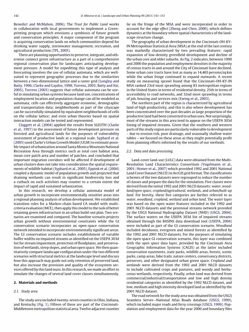

1 d Urba

Bipaida

ermfsbB2feaacoi

efa(bRmiumcdai

uatcrnucnTblttshbvs

2

2

aM

42 D. Mitsova et al. / Landscape an

enedict and McMahon, 2006). The Trust for Public Land worksn collaboration with local governments to implement a Green-rinting program which envisions a symbiosis of future growthnd conservation principles. A major component of the programs acquiring conservation lands on which communities depend forrinking water supply, stormwater management, recreation, andgricultural production (TPL, 2005).

There are planning opportunities to preserve, integrate, and oth-rwise connect green infrastructure as a part of a comprehensiveegional conservation plan for landscapes anticipating develop-ent pressure. A model for expediting this type of analysis and

orecasting involves the use of cellular automata, which are well-uited to represent geographic processes due to the similaritiesetween a two-dimensional lattice and a raster grid (Longley andatty, 1996; Clarke and Gaydos, 1998; Torrens, 2003; Batty and Xie,005). Torrens (2003) suggests that cellular automata can be use-ul in simulating urban systems because land use, concentrations ofmployment location and population change can all be modeled asutomata; cells can effectively aggregate economic, demographicnd transportation data; neighborhoods as part of the cityscapean be successfully simulated by equivalent neighborhoods of cellsn the cellular lattice; and even urban theories based on spatialnteraction models can be tested and represented.

Claggett et al. (2004) applied the results from SLEUTH (Clarket al., 1997) to the assessment of future development pressure onorested and agricultural lands for the purposes of vulnerabilityssessment of productive lands at a regional scale. Syphard et al.2005) used Clarke’s Urban Growth Model (UGM) to estimate possi-le impact of urbanization around Santa Monica Mountain Nationalecreation Area through metrics such as total core habitat area,ean core patch area and number of patches, and concluded that

mportant migration corridors will be affected if development ofrban clusters does not take into consideration the spatial require-ents of wildlife habitat (Syphard et al., 2005). Eppink et al. (2004)

oupled a dynamic model of population growth and projected thatraining wetlands can result in significant biodiversity loss andcutback on such activities may counter to a certain extent the

mpact of rapid and sustained urbanization.In this research, we develop a cellular automata model of

rban growth to incorporate environmentally sensitive areas intoregional planning analysis of urban development. We established

ransition rules for a Markov-chain based CA model with multi-riteria evaluation (MCE), then apply this model to the task of betteretaining green infrastructure in an urban build-out plan. Two sce-arios are examined and compared. The baseline scenario projectsrban growth without environmental constraints while the GIonservation scenario incorporates an open-space conservationetwork intended to incorporate environmentally significant areas.he GI conservation scenario includes establishment of variableuffer widths on impaired streams as identified on the USEPA 303d

ist for stream impairment, protection of floodplains, and preserva-ion of wetlands, steep slopes, and urban open space. We then quan-itatively compare landscape configuration under the two differentcenarios with structural metrics at the landscape level and discussow this approach may guide not only retention of preserved land,ut also increase the provision and quality of the ecosystem ser-ices offered by this land mass. In this research, we made an effort toimulate the changes of several land cover classes simultaneously.

. Materials and methods

.1. Study area

The study area included twenty-seven counties in Ohio, Indiana,nd Kentucky (Fig. 1). Fifteen of these are part of the Cincinnati-iddletown metropolitan statistical area. Twelve adjacent counties

n Planning 99 (2011) 141–153

lie on the fringe of the MSA and were incorporated in order toaccount for the edge effect (Zheng and Chen, 2000), which definesdynamics at the boundary where spatial characteristics of the land-scape structure change.

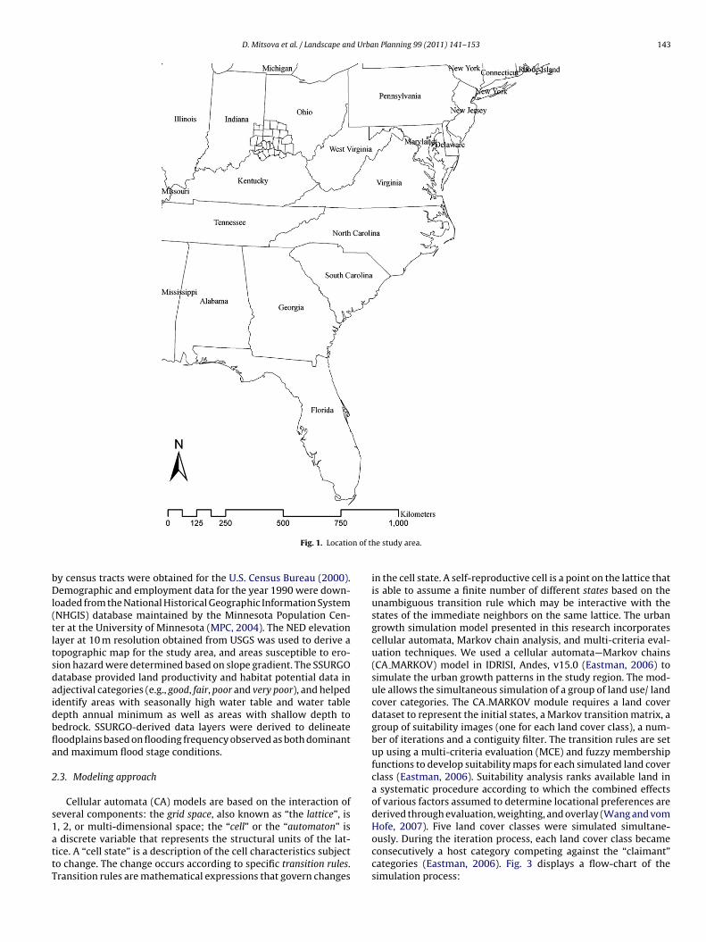
The geography of urban development in the Cincinnati-OH-KY-IN Metropolitan Statistical Area (MSA) at the end of the last centurywas markedly characterized by two prevailing features: rapidexpansion of low-density greenfield development and decline ofthe urban core and older suburbs. As Fig. 2 indicates, between 1990and 2000 the population and employment densities in the majorityof census tracts in and around the City of Cincinnati have declined.Some urban core tracts have lost as many as 14,465 persons/sq kmwhile the urban fringe continued to expand outwards. A recentstudy on measuring sprawl found that the Cincinnati-OH-KY-INMSA ranked 23rd most sprawling among 83 metropolitan regionsin the United States in terms of residential density, 25th in terms ofaccessibility to road networks, and 32nd most sprawling in termsof job, housing and services mix (Ewing et al., 2003).

The northern part of the region is characterized by agriculturalland of high productivity, and this is also where development hasbeen concentrated over the past decades as large proportion of theproductive land had been converted to urban uses. Not surprisingly,most of the streams in this area tend to appear on the USEPA 303dlisting of impaired streams. Given that the southern and westernparts of the study region are particularly vulnerable to development– due to erosion risk, poor drainage, and seasonally shallow watertables – we focused on these areas as they might potentially profitfrom planning efforts informed by the results of our methods.

2.2. Data and data processing

Land-cover land-use (LULC) data were obtained from the Multi-Resolution Land Characteristics Consortium (Vogelmann et al.,2001; Homer et al., 2007) which provided 1992 and 2001 NationalLand Cover Dataset (NLCD) in ArcGIS grid format. The classificationsschemes of the two datasets were regrouped to reduce the numberof classes and prepare the data for the simulation. Five classes werederived from the initial 1992 and 2001 NLCD datasets: water, wood-land/open space, cropland/agricultural, wetlands, and urban/built-upland. For brevity, these five categories are further referred to aswater, woodland, cropland, wetland and urban land. The water layerwas based on the open water features included in the 1992 and2001 NLCD datasets and the perennial streams network providedby the USGS National Hydrography Dataset (NHD) (USGS, 2004).The surface waters on the USEPA 303d list of impaired streamsobtained through the BASINS data download tool (USEPA, 2004)were included as part of the GI conservation scenario. Woodlandincluded deciduous, evergreen and mixed forests as identified bythe 1992 and 2001 NLCD datasets. For the purposes of simulatingthe open space GI conservation scenario, this layer was combinedwith the open space data layer, provided by the Cincinnati AreaGeographic Information Systems (CAGIS) as the latter includedconservation easements, state parks, wildlife areas, forests, scenicparks, camp areas, bike trails, nature centers, conservancy districts,preserves, and other designated urban green space. Cropland andwetlands were derived from the 1992 and 2001 NLCD datasetsto include cultivated crops and pastures, and woody and herba-ceous wetlands, respectively. Finally, urban land was derived fromcommercial/industrial/transportation and low and high densityresidential categories as identified by the 1992 NLCD dataset, andlow, medium and high intensity developed land as identified by the

2001 NLCD dataset.

The road network for the study area was obtained from the USGSSeamless Server—National Atlas Roads database (USGS, 1999),which included major roads and ferry crossings (USGS, 1999). Pop-ulation and employment data for the year 2000 and boundary files

D. Mitsova et al. / Landscape and Urban Planning 99 (2011) 141–153 143

n of th

bDl(tltsdaidbfla

2

s1attT

Fig. 1. Locatio

y census tracts were obtained for the U.S. Census Bureau (2000).emographic and employment data for the year 1990 were down-

oaded from the National Historical Geographic Information SystemNHGIS) database maintained by the Minnesota Population Cen-er at the University of Minnesota (MPC, 2004). The NED elevationayer at 10 m resolution obtained from USGS was used to derive aopographic map for the study area, and areas susceptible to ero-ion hazard were determined based on slope gradient. The SSURGOatabase provided land productivity and habitat potential data indjectival categories (e.g., good, fair, poor and very poor), and helpeddentify areas with seasonally high water table and water tableepth annual minimum as well as areas with shallow depth toedrock. SSURGO-derived data layers were derived to delineateoodplains based on flooding frequency observed as both dominantnd maximum flood stage conditions.

.3. Modeling approach

Cellular automata (CA) models are based on the interaction ofeveral components: the grid space, also known as “the lattice”, is

, 2, or multi-dimensional space; the “cell” or the “automaton” isdiscrete variable that represents the structural units of the lat-

ice. A “cell state” is a description of the cell characteristics subjecto change. The change occurs according to specific transition rules.ransition rules are mathematical expressions that govern changes

e study area.

in the cell state. A self-reproductive cell is a point on the lattice thatis able to assume a finite number of different states based on theunambiguous transition rule which may be interactive with thestates of the immediate neighbors on the same lattice. The urbangrowth simulation model presented in this research incorporatescellular automata, Markov chain analysis, and multi-criteria eval-uation techniques. We used a cellular automata—Markov chains(CA MARKOV) model in IDRISI, Andes, v15.0 (Eastman, 2006) tosimulate the urban growth patterns in the study region. The mod-ule allows the simultaneous simulation of a group of land use/ landcover categories. The CA MARKOV module requires a land coverdataset to represent the initial states, a Markov transition matrix, agroup of suitability images (one for each land cover class), a num-ber of iterations and a contiguity filter. The transition rules are setup using a multi-criteria evaluation (MCE) and fuzzy membershipfunctions to develop suitability maps for each simulated land coverclass (Eastman, 2006). Suitability analysis ranks available land ina systematic procedure according to which the combined effectsof various factors assumed to determine locational preferences arederived through evaluation, weighting, and overlay (Wang and vom

Hofe, 2007). Five land cover classes were simulated simultane-ously. During the iteration process, each land cover class becameconsecutively a host category competing against the “claimant”categories (Eastman, 2006). Fig. 3 displays a flow-chart of thesimulation process: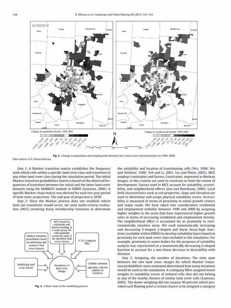

144 D. Mitsova et al. / Landscape and Urban Planning 99 (2011) 141–153

nsitieD

waMqdso

lt

Fig. 2. Change in population and employment deata source: U.S. Census Bureau.

Step 1: A Markov transition matrix establishes the frequencyith which cells within a specific land cover class will transition to

ny other land cover class during the simulation period. The initialarkov transition probabilities matrix is based on the observed fre-

uencies of transition between the initial and the latter land coveratasets using the MARKOV module in IDRISI (Eastman, 2006). Apecific Markov chain matrix was derived for each ten-year period

f land cover projections. The end year of projection is 2030.

Step 2: Since the Markov process does not establish whereand use transitions would occur, we used multi-criteria evalua-ion (MCE) involving fuzzy membership functions to determine

Fig. 3. A flow-chart of the modeling process.

s per census tract (persons/sq km) in 1990–2000

the suitability and location of transitioning cells (Wu, 1998; Wuand Webster, 1998; Yeh and Li, 2001; Liu and Phinn, 2003). MCEemploys constraints and factors. Constraints, expressed as Booleanimages, in this context are used to constrain or limit the extent ofdevelopment. Factors used in MCE account for suitability, accessi-bility, and neighborhood effects (Jiao and Boerboom, 2006). Localfield characteristics such as soil properties, slope and elevation areused to determine and assign physical suitability scores. Accessi-bility is measured in terms of proximity to urban growth centersand major roads. We have taken into consideration residentialand employment mobility between 1990 and 2000 by assigninghigher weights to the areas that have experienced higher growthrates in terms of increasing residential and employment density.The neighborhood effect is accounted for as proximity to envi-ronmentally sensitive areas. We used monotonically increasingand decreasing S-shaped, J-shaped and linear fuzzy-logic func-tions (available within IDRISI) to develop suitability layers based onproximity for each land cover class included in the simulation. Forexample, proximity to water bodies for the purposes of suitabilityanalysis was represented as a monotonically decreasing S-shapedfunction to account for a non-linear decrease in desirability withdistance.

Step 3: Assigning the number of iterations. The time spanbetween the two land cover images for which Markov transi-tion probabilities were estimated determined how many iterations

would be used in the simulation. A contiguity filter assigned lowerweights to suitability scores of isolated cells that did not belongto any of the nearby clusters of similar land cover cells (Eastman,2006). The down-weighing did not surpass 90 percent which pro-vided each floating pixel a certain chance to be assigned a category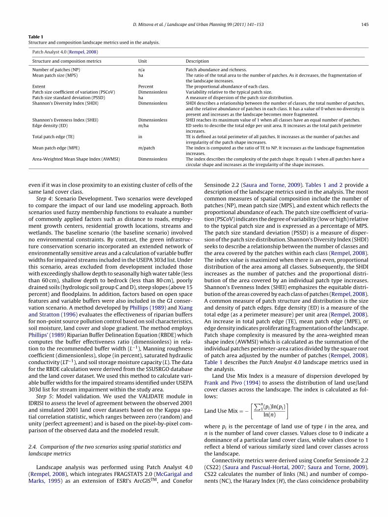

D. Mitsova et al. / Landscape and Urban Planning 99 (2011) 141–153 145

Table 1Structure and composition landscape metrics used in the analysis.

Patch Analyst 4.0 (Rempel, 2008)

Structure and composition metrics Unit Description

Number of patches (NP) n/a Patch abundance and richness.Mean patch size (MPS) ha The ratio of the total area to the number of patches. As it decreases, the fragmentation of

the landscape increases.Extent Percent The proportional abundance of each class.Patch size coefficient of variation (PSCoV) Dimensionless Variability relative to the typical patch size.Patch size standard deviation (PSSD) ha A measure of dispersion of the patch size distribution.Shannon’s Diversity Index (SHDI) Dimensionless SHDI describes a relationship between the number of classes, the total number of patches,

and the relative abundance of patches in each class. It has a value of 0 when no diversity ispresent and increases as the landscape becomes more fragmented.

Shannon’s Evenness Index (SHEI) Dimensionless SHEI reaches its maximum value of 1 when all classes have an equal number of patches.Edge density (ED) m/ha ED seeks to describe the total edge per unit area. It increases as the total patch perimeter

increases.Total patch edge (TE) in TE is defined as total perimeter of all patches. It increases as the number of patches and

irregularity of the patch shape increases.Mean patch edge (MPE) m/patch The index is computed as the ratio of TE to NP. It increases as the landscape fragmentation

easesindexular sh

es

tsomwntewtwtdpfvafsPctccfaa3

Iatup

2l

(M

incrArea-Weighted Mean Shape Index (AWMSI) Dimensionless The

circ

ven if it was in close proximity to an existing cluster of cells of theame land cover class.

Step 4: Scenario Development. Two scenarios were developedo compare the impact of our land use modeling approach. Bothcenarios used fuzzy membership functions to evaluate a numberf commonly applied factors such as distance to roads, employ-ent growth centers, residential growth locations, streams andetlands. The baseline scenario (the baseline scenario) involvedo environmental constraints. By contrast, the green infrastruc-ure conservation scenario incorporated an extended network ofnvironmentally sensitive areas and a calculation of variable bufferidths for impaired streams included in the USEPA 303d list. Under

his scenario, areas excluded from development included thoseith exceedingly shallow depth to seasonally high water table (less

han 60 cm), shallow depth to bedrock (less than 80 cm), poorlyrained soils (hydrologic soil group C and D), steep slopes (above 15ercent) and floodplains. In addition, factors based on open spaceeatures and variable buffers were also included in the GI conser-ation scenario. A method developed by Phillips (1989) and Xiangnd Stratton (1996) evaluates the effectiveness of riparian buffersor non-point source pollution control based on soil characteristics,oil moisture, land cover and slope gradient. The method employshillips’ (1989) Riparian Buffer Delineation Equation (RBDE) whichomputes the buffer effectiveness ratio (dimensionless) in rela-ion to the recommended buffer width (L−1), Manning roughnessoefficient (dimensionless), slope (in percent), saturated hydrauliconductivity (LT−1), and soil storage moisture capacity (L). The dataor the RBDE calculation were derived from the SSUSRGO databasend the land cover dataset. We used this method to calculate vari-ble buffer widths for the impaired streams identified under USEPA03d list for stream impairment within the study area.

Step 5: Model validation. We used the VALIDATE module inDRISI to assess the level of agreement between the observed 2001nd simulated 2001 land cover datasets based on the Kappa spa-ial correlation statistic, which ranges between zero (random) andnity (perfect agreement) and is based on the pixel-by-pixel com-arison of the observed data and the modeled result.

.4. Comparison of the two scenarios using spatial statistics and

andscape metrics

Landscape analysis was performed using Patch Analyst 4.0Rempel, 2008), which integrates FRAGSTATS 2.0 (McGarigal and

arks, 1995) as an extension of ESRI’s ArcGISTM, and Conefor

.describes the complexity of the patch shape. It equals 1 when all patches have aape and increases as the irregularity of the shape increases.

Sensinode 2.2 (Saura and Torne, 2009). Tables 1 and 2 provide adescription of the landscape metrics used in the analysis. The mostcommon measures of spatial composition include the number ofpatches (NP), mean patch size (MPS), and extent which reflects theproportional abundance of each. The patch size coefficient of varia-tion (PSCoV) indicates the degree of variability (low or high) relativeto the typical patch size and is expressed as a percentage of MPS.The patch size standard deviation (PSSD) is a measure of disper-sion of the patch size distribution. Shannon’s Diversity Index (SHDI)seeks to describe a relationship between the number of classes andthe area covered by the patches within each class (Rempel, 2008).The index value is maximized when there is an even, proportionaldistribution of the area among all classes. Subsequently, the SHDIincreases as the number of patches and the proportional distri-bution of the area covered by an individual patch type increases.Shannon’s Evenness Index (SHEI) emphasizes the equitable distri-bution of the areas covered by each class of patches (Rempel, 2008).A common measure of patch structure and distribution is the sizeand density of patch edges. Edge density (ED) is a measure of thetotal edge (as a perimeter measure) per unit area (Rempel, 2008).An increase in total patch edge (TE), mean patch edge (MPE), oredge density indicates proliferating fragmentation of the landscape.Patch shape complexity is measured by the area-weighted meanshape index (AWMSI) which is calculated as the summation of theindividual patches perimeter-area ratios divided by the square rootof patch area adjusted by the number of patches (Rempel, 2008).Table 1 describes the Patch Analyst 4.0 landscape metrics used inthe analysis.

Land Use Mix Index is a measure of dispersion developed byFrank and Pivo (1994) to assess the distribution of land use/landcover classes across the landscape. The index is calculated as fol-lows:

Land Use Mix = −[∑n

1(pi)ln(pi)

ln(n)

]

where pi is the percentage of land use of type i in the area, andn is the number of land cover classes. Values close to 0 indicate adominance of a particular land cover class, while values close to 1reflect a blend of various similarly sized land cover classes across

the landscape.

Connectivity metrics were derived using Conefor Sensinode 2.2(CS22) (Saura and Pascual-Hortal, 2007; Saura and Torne, 2009).CS22 calculates the number of links (NL) and number of compo-nents (NC), the Harary Index (H), the class coincidence probability

146 D. Mitsova et al. / Landscape and Urban Planning 99 (2011) 141–153

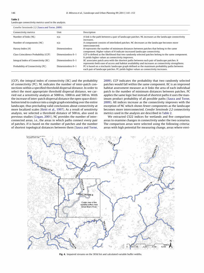
Table 2Landscape connectivity metrics used in the analysis.

Conefor Sensinode 2.2 (Saura and Torne, 2009)

Connectivity metrics Unit Description

Number of links (NL) n/a A link is the path between a pair of landscape patches. NL increases as the landscape connectivityincreases.

Number of components (NC) n/a A component consists of interlinked patches. NC decreases as the landscape becomes moreinterconnected.

Harary Index (H) Dimensionless H represents the number of minimum distances between patches that belong to the samecomponent. Higher values of H indicate increased landscape connectivity.

Class Coincidence Probability (CCP) Dimensionless 0–1 CCP is defined as the likelihood that two randomly selected patches belong to the same component.It yields higher values as connectivity improves.

Integral Index of Connectivity (IIC) Dimensionless 0–1 IIC associates patch area with the shortest paths between each pair of landscape patches. Itth easa sto

ndsca

(onsrtblmapcoo

represents boProbability of Connectivity (PC) Dimensionless 0–1 PC is based on

each pair of la

CCP), the integral index of connectivity (IIC) and the probabilityf connectivity (PC). NL indicates the number of inter-patch con-ections within a specified threshold dispersal distance. In order toelect the most appropriate threshold dispersal distance, we car-ied out a sensitivity analysis at 5000 m, 1000 m and 500 m. Withhe increase of inter-patch dispersal distance the open space distri-ution tend to coalesce into a single graph extending over the entire

andscape, thus precluding valid conclusions about connectivity atore localized scales (Keitt et al., 1997). As a result of sensitivity

nalysis, we selected a threshold distance of 500 m, also used inrevious studies (Cogan, 2001). NC provides the number of inter-onnected areas, i.e., the areas in which paths connect every pairf patches. H is based on the number of patches and the numberf shortest topological distances between them (Saura and Torne,

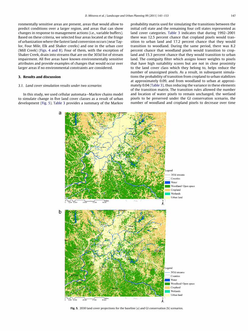
Fig. 4. Impaired streams on the 303d list a

e of access and habitat availability and increases as connectivity strengthens.chastic landscape graph defined as the maximum probability paths betweenpe patches. PC yields higher values as connectivity increases.

2009). CCP indicates the probability that two randomly selectedpatches would fall within the same component. IIC is an improvedhabitat assessment measure as it links the area of each individualpatch to the number of minimum distances between patches. PCapplies the same logic but instead of shortest paths it uses the max-imum product probability of all possible paths (Saura and Torne,2009). All indices increase as the connectivity improves with theexception of NC which shows fewer components as the landscapebecomes more interconnected. Conefor Sensinode 2.2 connectivity

metrics used in the analysis are described in Table 2.

We extracted CS22 indices for wetlands and five comparisonareas to examine changes in connectivity under the two scenarios.The comparison areas were selected using the following criteria:areas with high potential for measuring change, areas where envi-

nd calculated variable buffer widths.

d Urba

rpcBol(Sial

3

3

td

D. Mitsova et al. / Landscape an

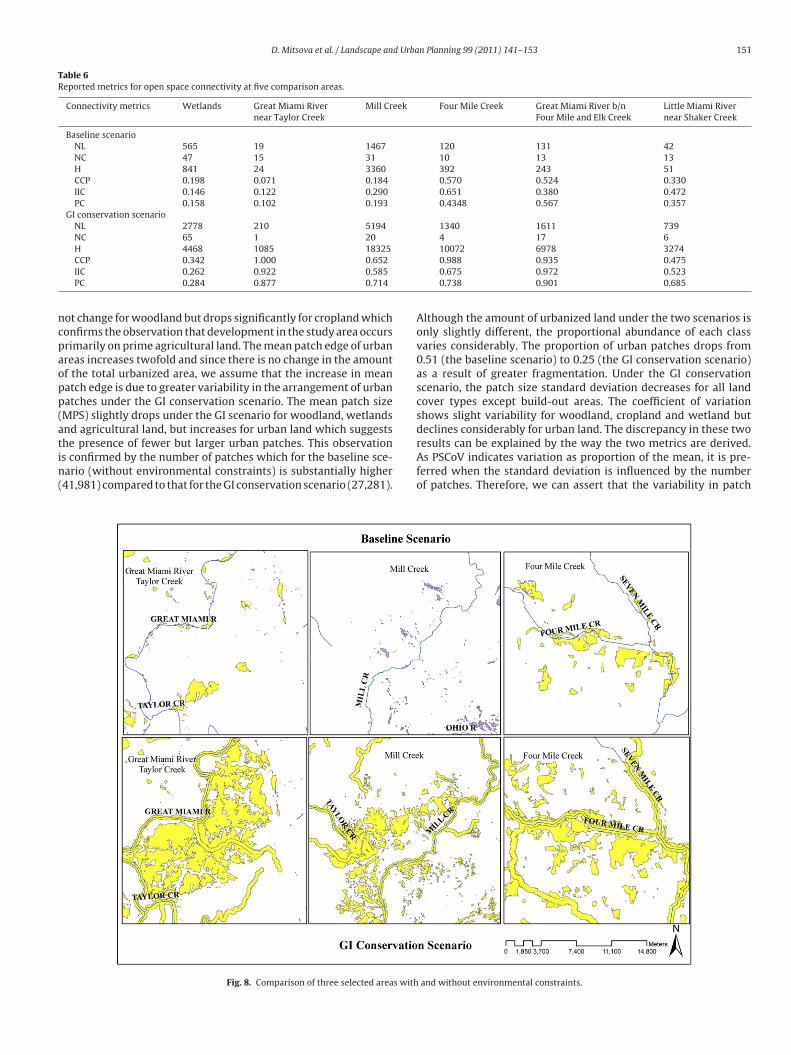
onmentally sensitive areas are present, areas that would allow toredict conditions over a larger region, and areas that can showhanges in response to management actions (i.e., variable buffers).ased on these criteria, we selected four areas located at the fringef urbanization where the fastest land conversion occurs (near Tay-or, Four Mile, Elk and Shaker creeks) and one in the urban coreMill Creek) (Figs. 4 and 8). Four of them, with the exception ofhaker Creek, drain into streams that are on the 303d list of streammpairment. All five areas have known environmentally sensitivettributes and provide examples of changes that would occur overarger areas if no environmental constraints are considered.

. Results and discussion

.1. Land cover simulation results under two scenarios

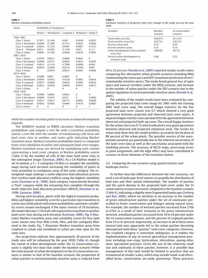
In this study, we used cellular automata—Markov chains modelo simulate change in five land cover classes as a result of urbanevelopment (Fig. 5). Table 3 provides a summary of the Markov

Fig. 5. 2030 land cover projections for the base

n Planning 99 (2011) 141–153 147

probability matrix used for simulating the transitions between theinitial cell state and the remaining four cell states represented asland cover categories. Table 3 indicates that during 1992–2001there was 12.5 percent chance that cropland pixels would tran-sition to urban land and 17.2 percent chance that they wouldtransition to woodland. During the same period, there was 8.2percent chance that woodland pixels would transition to crop-land and 15.3 percent chance that they would transition to urbanland. The contiguity filter which assigns lower weights to pixelsthat have high suitability scores but are not in close proximityto the land cover class which they belong to, helps reduce thenumber of unassigned pixels. As a result, in subsequent simula-tions the probability of transition from cropland to urban stabilizesat approximately 0.09, and from woodland to urban at approxi-

mately 0.04 (Table 3), thus reducing the variance in these elementsof the transition matrix. The transition rules allowed the numberand location of water pixels to remain unchanged, the wetlandpixels to be preserved under the GI conservation scenario, thenumber of woodland and cropland pixels to decrease over time

line (a) and GI conservation (b) scenarios.

148 D. Mitsova et al. / Landscape and Urban Planning 99 (2011) 141–153

Table 3Markov transition probability matrix.

Given Probability of changing to

Water 1 Woodland 2 Cropland 3 Wetland 4 Urban 5

1992–2001Class 1 Water 0.7871 0.1166 0.047 0.0106 0.0387Class 2 Woodland 0.0046 0.7586 0.1515 0.0027 0.0826Class 3 Cropland 0.0033 0.1722 0.6987 0.0007 0.1251Class 4 Wetland 0.053 0.6393 0.1758 0.021 0.111Class 5 Urban 0.0045 0.1182 0.0858 0.0018 0.7897

2001–2010Class 1 Water 0.9979 0.0011 0.0009 0.0001 0Class 2 Woodland 0.0004 0.8751 0.0805 0.0013 0.0425Class 3 Cropland 0.0013 0.1134 0.7909 0.0004 0.094Class 4 Wetland 0.0034 0.3038 0.0514 0.6344 0.007Class 5 Urban 0 0.0019 0.0013 0.0001 0.9966

2010–2020Class 1 Water 0.9989 0.001 0.0001 0 0Class 2 Woodland 0.0005 0.9452 0.0128 0.0001 0.0414Class 3 Cropland 0.0013 0.0428 0.8624 0.0002 0.0934Class 4 Wetland 0.0033 0.0429 0.0056 0.9411 0.0071Class 5 Urban 0 0 0 0 1

2020–2030Class 1 Water 0.9998 0.0001 0.0001 0 0Class 2 Woodland 0.0006 0.9472 0.012 0 0.0402Class 3 Cropland 0.0012 0.0417 0.8712 0.0001 0.0858

we

pmltfMr(tsmcwtsam1

baitltcucs

stntnu

Table 4Summary statistics of projected land cover change in the study area by the year2030.

Variables Baselinescenario

GI conservationscenario

Total urban area (ha) 438,874 421,319Total sensitive areas (ha) 226,723 226,723Percent urban land 0.33 0.29Percent sensitive areas 0.16 0.16Urban development in the sensitive 108,989 48,715

Class 4 Wetland 0.0032 0.0385 0.0044 0.9474 0.0065Class 5 Urban 0 0 0 0 1

hile the number of urban pixels to increase as urban developmentxpands.

The MARKOV module in IDRISI calculates Markov transitionrobabilities and outputs a text file with a transition probabilityatrix, a text file with the number of transitioning cells from one

and cover class to another, and raster grids indicating Markovransition areas. Markov transition probability matrix is computedrom cross-tabulation of earlier and subsequent land cover images.

arkov transition areas are derived by multiplying each columnepresenting a land cover category in Markov probability matrixTable 3) by the number of cells of the same land cover class inhe subsequent image (Eastman, 2006). As a CA-Markov model iset in motion, a 5 × 5 contiguity CA filter re-weights the suitabilityaps during each iteration increasing the suitability of pixels in

lose proximity to contiguous areas of the same category. The re-eighted maps undergo a multi-objective land allocation process

hat resolves land allocation conflicts using the highest suitabilitycore (Eastman et al., 1998). Each category consecutively becomes“host” category while the remaining four complete through theulti-objective land allocation procedure (MOLA) (Eastman et al.,

998; Eastman, 2006).During each iteration, pixels with the highest transition proba-

ility and highest suitability score for a particular class transition tonew class while pixels with lower probabilities and lower suitabil-

ty scores remain unchanged. If the input consists of 10 iterations,he model allocates 1/10 of all cells expected to transition to anotherand cover class during each iteration (Eastman, 2006). Fig. 6 illus-rates Markov transition areas and suitability scores for four landover classes near Four Mile Creek, Ohio, and the contiguity filtersed in the study. Fig. 7 illustrates Markov transition areas fromropland to urban and woodland to urban per time span for theame area.

Our projections indicate that approximately 30 percent of thetudy area will be urbanized by the year 2030 (Table 4), thoughhe extent of urban development under the GI conservation sce-

ario is slightly less than that under the baseline scenario Whilehe total amount of urban development in the GI conservation sce-ario is similar to that of the baseline scenario, the proportion ofrban patches in environmentally sensitive areas is reduced from

areas (ha)Percent urban development in

sensitive areas0.48 0.22

48 to 22 percent. Herold et al. (2005) reported similar results whencomparing five alternative urban growth scenarios including MSQ(maintaining the status quo) and EEP (maximum protection of envi-ronmentally sensitive areas). The study found general loss of openspace and natural corridors under the MSQ scenario, and increasein the number of urban patches under the EEP scenario due to thespatial regulation of environmentally sensitive areas (Herold et al.,2005).

The validity of the model results have been evaluated by com-paring the projected land cover image for 2001 with the existing2001 land cover map. The overall Kappa statistics for the fiveprojected land cover classes was 0.7 which showed a very goodagreement between projected and observed land cover layers. Aseparate Kappa statistics was calculated for the agreement betweenobserved and projected built-up areas. The overall Kappa statisticsfor the urban class was 0.75 which indicated a very good agreementbetween observed and projected urbanized areas. The results forurban land show that the model predicts accurately the location of88 percent of the urban pixels. The possible sources of the unex-plained variation are potentially due to the inherent uncertainty ofthe land cover data as well as the uncertainty associated with themodeling process. The accuracy of NLCD maps, processing errorsas pixel assignment, and the edge effect may have contributed tovariance in these elements of the transition matrix.

3.2. Comparing the two scenarios using spatial statistics andlandscape metrics

To further describe differences between the two scenarios, weused a set of landscape-level metrics to quantify the distribution ofland uses and their spatial relationships. The number of patchesand the patch density in the projected land cover under the GIconservation scenario increased, compared to the baseline scenario(Table 6), indicating a slightly more fragmented landscape (Furbergand Ban, 2008), which we attribute to an increase in the numberof green infrastructure patches under the set of constraints pre-scribed to foster conservation and linkages among natural areas.For example, the number of wetland patches increased from 2769to 6763 as a result of their inclusion in the green infrastructurenetwork, woodland patches increased from 18 to 24 percent underthe GI conservation scenario, and the percent of cropland patchesfrom 22 to 41 percent. Importantly, an increase in all of these morenatural land uses apparently led to the urban patches becominginterspersed with these “greener” land cover categories. However,the cropland category is somewhat ambiguous, as it implies theimplementation of any of several agricultural management prac-tices including row-crops, horticulture, silviculture, among othermore specialized practices. Given the size of the relatively small

size and continuity of these patches, however, it is possible thatmanagement of this land would be limited to practices that areeconomical at smaller scales, which may include small-scale diver-sified farms, conservation set-aside, greenways. These practices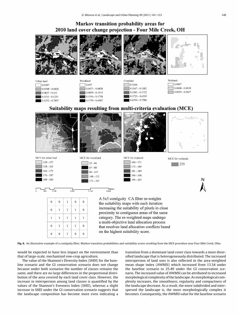

D. Mitsova et al. / Landscape and Urban Planning 99 (2011) 141–153 149

F and s

wt

lbsbivit

ig. 6. An illustrative example of a contiguity filter, Markov transition probabilities

ould be expected to have less impact on the environment thanhat of large-scale, mechanized row-crop agriculture.

The value of the Shannon’s Diversity Index (SHDI) for the base-ine scenario and the GI conservation scenario does not changeecause under both scenarios the number of classes remains theame, and there are no large differences in the proportional distri-

ution of the area covered by each land cover class. However, the

ncrease in interspersion among land classes is quantified by thealues of the Shannon’s Evenness Index (SHEI), whereas a slightncrease in SHEI under the GI conservation scenario suggests thathe landscape composition has become more even indicating a

uitability scores resulting from the MCE procedure near Four Mile Creek, Ohio.

transition from a dominant land cover class towards a more diver-sified landscape that is heterogeneously distributed. The increasedinterspersion of land uses is also reflected in the area-weightedmean shape index (AWMSI) which increased from 13.34 underthe baseline scenario to 25.49 under the GI conservation sce-nario. The increased value of AWMSI can be attributed to increased

morphological complexity of the landscape. As morphological com-plexity increases, the smoothness, regularity and compactness ofthe landscape decrease. As a result, the more subdivided and inter-spersed the landscape is, the more morphologically complex itbecomes. Consequently, the AWMSI value for the baseline scenario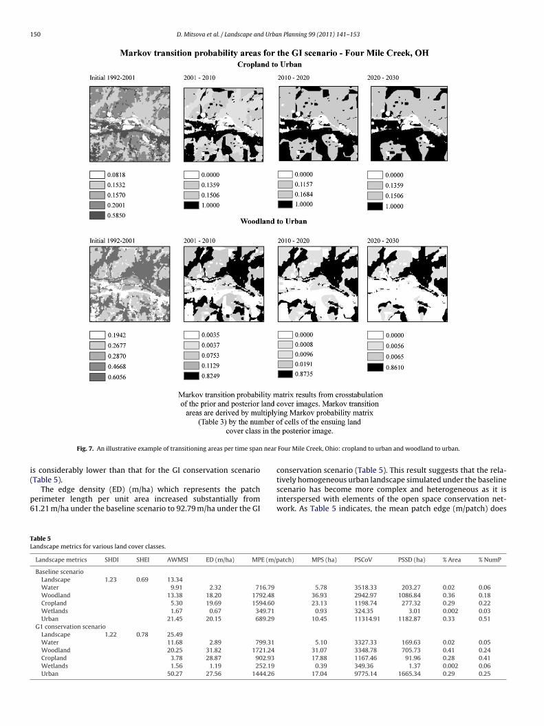

150 D. Mitsova et al. / Landscape and Urban Planning 99 (2011) 141–153

near

i(

p6

TL

Fig. 7. An illustrative example of transitioning areas per time span

s considerably lower than that for the GI conservation scenario

Table 5).

The edge density (ED) (m/ha) which represents the patcherimeter length per unit area increased substantially from1.21 m/ha under the baseline scenario to 92.79 m/ha under the GI

able 5andscape metrics for various land cover classes.

Landscape metrics SHDI SHEI AWMSI ED (m/ha) MPE (m/p

Baseline scenarioLandscape 1.23 0.69 13.34Water 9.91 2.32 716.79Woodland 13.38 18.20 1792.48Cropland 5.30 19.69 1594.60Wetlands 1.67 0.67 349.71Urban 21.45 20.15 689.29

G1 conservation scenarioLandscape 1.22 0.78 25.49Water 11.68 2.89 799.31Woodland 20.25 31.82 1721.24Cropland 3.78 28.87 902.93Wetlands 1.56 1.19 252.19Urban 50.27 27.56 1444.26

Four Mile Creek, Ohio: cropland to urban and woodland to urban.

conservation scenario (Table 5). This result suggests that the rela-

tively homogeneous urban landscape simulated under the baselinescenario has become more complex and heterogeneous as it isinterspersed with elements of the open space conservation net-work. As Table 5 indicates, the mean patch edge (m/patch) does

atch) MPS (ha) PSCoV PSSD (ha) % Area % NumP

5.78 3518.33 203.27 0.02 0.0636.93 2942.97 1086.84 0.36 0.1823.13 1198.74 277.32 0.29 0.22

0.93 324.35 3.01 0.002 0.0310.45 11314.91 1182.87 0.33 0.51

5.10 3327.33 169.63 0.02 0.0531.07 3348.78 705.73 0.41 0.2417.88 1167.46 91.96 0.28 0.41

0.39 349.36 1.37 0.002 0.0617.04 9775.14 1665.34 0.29 0.25

D. Mitsova et al. / Landscape and Urban Planning 99 (2011) 141–153 151

Table 6Reported metrics for open space connectivity at five comparison areas.

Connectivity metrics Wetlands Great Miami Rivernear Taylor Creek

Mill Creek Four Mile Creek Great Miami River b/nFour Mile and Elk Creek

Little Miami Rivernear Shaker Creek

Baseline scenarioNL 565 19 1467 120 131 42NC 47 15 31 10 13 13H 841 24 3360 392 243 51CCP 0.198 0.071 0.184 0.570 0.524 0.330IIC 0.146 0.122 0.290 0.651 0.380 0.472PC 0.158 0.102 0.193 0.4348 0.567 0.357

GI conservation scenarioNL 2778 210 5194 1340 1611 739NC 65 1 20 4 17 6

ncpaopp(atin(

H 4468 1085 18325CCP 0.342 1.000 0.652IIC 0.262 0.922 0.585PC 0.284 0.877 0.714

ot change for woodland but drops significantly for cropland whichonfirms the observation that development in the study area occursrimarily on prime agricultural land. The mean patch edge of urbanreas increases twofold and since there is no change in the amountf the total urbanized area, we assume that the increase in meanatch edge is due to greater variability in the arrangement of urbanatches under the GI conservation scenario. The mean patch sizeMPS) slightly drops under the GI scenario for woodland, wetlandsnd agricultural land, but increases for urban land which suggests

he presence of fewer but larger urban patches. This observations confirmed by the number of patches which for the baseline sce-ario (without environmental constraints) is substantially higher41,981) compared to that for the GI conservation scenario (27,281).

Fig. 8. Comparison of three selected areas with

10072 6978 32740.988 0.935 0.4750.675 0.972 0.5230.738 0.901 0.685

Although the amount of urbanized land under the two scenarios isonly slightly different, the proportional abundance of each classvaries considerably. The proportion of urban patches drops from0.51 (the baseline scenario) to 0.25 (the GI conservation scenario)as a result of greater fragmentation. Under the GI conservationscenario, the patch size standard deviation decreases for all landcover types except build-out areas. The coefficient of variationshows slight variability for woodland, cropland and wetland butdeclines considerably for urban land. The discrepancy in these two

results can be explained by the way the two metrics are derived.As PSCoV indicates variation as proportion of the mean, it is pre-ferred when the standard deviation is influenced by the numberof patches. Therefore, we can assert that the variability in patch

and without environmental constraints.

1 d Urba

stuiosisb

wcaicmFGaituil

wc2cpmTpctccanSoisPiali

4

ssgcpoff

Muptr

52 D. Mitsova et al. / Landscape an

ize distribution of urban patches decreases for the GI conserva-ion scenario. The patterns revealed by these metrics suggest thatnder the baseline scenario there is a consolidated urbanized area

n which the existing intra-urban open space is gradually build-ut, thus creating a smaller number of larger urban patches andignificant variability in patch size. The number of urban patchesncreases for the GI conservation scenario as the build-out area isubdivided by open space, natural corridors and variable riparianuffer zones.

Both scenarios reveal that development occurs primarily out-ard of the existing urban core following an approximately

oncentric pattern. Smaller or satellite urban cores also formedround existing urban centers as the expansion of the urban lands projected into the future. Urban cores under both scenarios areharacterized by larger urban patches at the center and a mosaic ofore fragmented land cover classes at the rural/urban periphery.

ig. 5 indicates that the fragmentation of the urban core under theI conservation scenario reflects the presence of more natural areasnd connected vegetated corridors along the major watercoursesn the region. The land cover mix index increased from 0.68 underhe baseline scenario to 0.73 under the GI scenario, indicating thatnder the GI scenario, the built environment has retained more of

ts green features thus creating a more diverse and balanced mix ofandscape features.

Table 6 provides a summary of the connectivity metrics foretlands and open space under the two scenarios. The results indi-

ate that the number of links in wetland areas grow from 565 to778 and the Harary Index increases from 841 to 4468. The classoincidence probability, the integral index of connectivity, and therobability of connectivity also improve, reflecting an improve-ent in interconnectedness under the GI conservation scenario.

he number of links between the green patches in all five com-arison areas increases in order of magnitude. The number ofomponents drops for four of the five areas, thus indicating thathe paths between patches have increased creating larger inter-onnected regions under the GI conservation scenario. Under the GIonservation scenario, the Harary Index increases exponentially forll selected comparison areas. The most significant change occursear Four Mile Creek, between Four Mile and Elk Creek, and nearhaker Creek (Fig. 8). These areas are located in the northern partf the study region where the rate of land conversion to urban usess among the highest. CCP indicates a substantial increase in theame portion of the study region as well as at Taylor Creek. IIC andC have higher value for all five comparison areas, thus reflect-ng a stable trend towards improved connectivity in the study areafter the inclusion of a green infrastructure network in the simu-ation model. The importance of the variable buffer widths for themproved connectivity is difficult to assess directly.

. Conclusion

A focal objective of urban growth modeling is evaluating pos-ible future paths of development (Herold et al., 2005). In thistudy, we have examined the spatial structure of continued urbanrowth under two scenarios: with and without green infrastructureonservation. The approach based on cellular automata, Markovrobabilities and multi-criteria evaluation allowed the simulationf five land cover classes simultaneously and thus provided a basisor meaningful examination of the landscape dynamics under dif-erent scenarios.

Setting transition rules in the form of suitability maps based on

CE allows for consideration of various factors that are commonly

sed in land use planning and decision-making such as changes inopulation and employment density, proximity to roads, proximityo waterbodies as well as protection of open space, water resources,iparian corridors, and other environmentally sensitive areas. This

n Planning 99 (2011) 141–153

type of systematic evaluation in a GIS environment combined withforesight scenarios and projections equips environmental and landuse planners with a useful tool that can integrate activities consis-tent with the smart growth implementation options and strategies.Two limitations of the proposed approach require further inves-tigation. First, the model is scale-dependent. Its results hinge onthe scale at which grids are aggregated assuming that all the pro-cesses in the landscape are occurring at that scale. However, bothurban development and ecological effects are multi-scalar pro-cesses that involve dynamic responses at various levels. In orderto account for these responses, in this research, we integratedthree levels of spatial resolution: a pixel, comparison area, andregion. Other approaches are worth further investigating. Albertiand Waddell (2000), for example, suggested treating land use at aparcel level, and land cover—at a patch level in order to respondto the underlying dynamics. Second, preserving open space andcritical environmental areas depends largely on local governmentregulation and local-level land use planning. Each regulation mustincorporate acceptable methodology for critical area identificationbased on current scientific research. Therefore, the results of thisresearch are descriptive rather than prescriptive.

The results show that under the GI conservation scenario theoverall extent of urban development decreased, the mean patchsize for urban land increased, and the percent of urban patchesdecreased as they become interspersed with a variety of otherpatches. The strength of the GI conservation scenario is also relatedto its ability to incorporate variable buffer widths for the impairedstreams on the USEPA 303d list. As the impaired streams oftentimescross jurisdictional boundaries, their incorporation in an urbangrowth simulation suggests a more holistic approach towards themanagement of such impaired waters in the projected future. Formunicipalities that require comprehensive planning account forpresent and future environmental regulations, this type of mod-eling and prediction will play a significant role in illustrating theprobable outcomes of different land use choices upon expandingthe extent of green infrastructure and the numerous ecosystem-level services that are provided by such area.

Local governments have at their disposal several planning toolsthat can help construct, operate and maintain the green infrastruc-ture network. Acquisition through easements, special area zoning,transferable development rights, specific water quality standardsfor designated areas, wetland restoration, wide-ranging watershedplanning, and outreach programs can become part of directingregional (USEPA, 2005). In addition, Arendt (2004) recognized thatpreserving open space at a site scale does not prevent the cumula-tive development impacts on natural systems and suggested that acommunity-wide approach be used for preserving the connectivityof green networks, and that local land-use regulations that wouldidentify and protect potential conservation areas would play a rolein this process.

Combined with the capabilities of urban growth models, includ-ing cellular automata these planning instruments can be used togenerate and assess different scenarios of urban growth. A publicdiscussion of these scenarios involving stakeholder participationcan bring awareness of the expected change and valuable inputsto the planning process. Given transparency of the process andability to visually and quantitatively compare development sce-narios accounting for the non-linearities that are not considered inlinear GIS map algebra, this may offer an improvement over themore qualitative and subjective suitability overlays. Urban growthprojections under various conservation scenarios can be used to

resolve conflicts of interests in land development and build consen-sus among stakeholders about the future patterns and directions ofurban development, if visions differ. As part of future research, themodel developed in this study can incorporate various growth man-agement strategies, zoning ordinances or other regulatory tools

d Urba

td

R

A

A

B

B

C

C

C

C

C

D

D

E

EE

E

F

F

H

H

J

K

L

L

D. Mitsova et al. / Landscape an

hat may influence and redirect the patterns and pace of urbanevelopment.

eferences

lberti, M., Waddell, P., 2000. An integrated urban development and ecologicalsimulation model. Integr. Assess. 1, 215–227.

rendt, R., 2004. Linked landscapes: creating greenway corridors through conserva-tion subdivision design strategies in the northeastern and central United States.Landscape Urban Plan. 68, 241–269.

atty, M., Xie, Y., 2005. Urban growth using cellular automata models. In: Mcguire,D., Batty, M., Goodchild, M.F. (Eds.), GIS, Spatial Analysis and Modeling. ESRIPress, Redlands, CA, pp. 151–172.

enedict, M., McMahon, E.T., 2006. Green Infrastructure: Linking Landscape andCommunities. Island Press, Washington, DC.

laggett, P., Jantz, C.A., Goetz, S.J., Bisland, C., 2004. Assessing development pressurein the Chesapeake Bay watershed: an evaluation of two land-use change models.Environ. Monitor. Assess. 94, 129–146.

larke, K.C., Hoppen, S., Gaydos, L., 1997. A self-modifying cellular automaton modelof historical urbanization in the San Francisco Bay area. Environ. Plann. B 24,247–261.

larke, K.C., Gaydos, L., 1998. Loose-coupling a cellular automaton model andGIS: long-term urban growth prediction for San Francisco and Washington-Baltimore. Int. J. Geogr. Inf. Sci. 12, 699–714.

ogan, C., 2001. Biodiversity predictions: integrating urban growth models withland cover data and species habitat information. USGS GAP Anal. Bull. 10 (4),33–36.

ostanza, R., d’Arge, R., de Groot, R., Farber, S., Grasso, M., Hannon, B., Limburg, K.,Naeem, S., O’Neill, R.V., Paruelo, J., Raskin, R.G., Sutton, P., van den Belt, M., 1997.The value of the world’s ecosystem services and natural capital. Nature 387,253–260.

osskey, M., 2001. Toward quantifying water pollution abatement in response toinstalling buffers on crop land. J. Environ. Manage. 28 (5), 577–598.

uany, A., Speck, J., Lydon, M., 2009. The Smart Growth Manual. McGraw-Hill, NewYork, NY.

astman, J.R., Jiang, H., Toledano, J., 1998. Multi-criteria and multi-objective deci-sion making for land allocation using GIS. In: Beinat, E., Nijkamp, P. (Eds.),Multi-criteria Analysis for Land-Use Management. Kluwer Academic Publishers,Dordrecht, pp. 227–251.

astman, J.R., 2006. IDRISI Andes. Clark University, Worcester, MA.ppink, F., van den Bergh, J., Rietveld, P., 2004. Modeling biodiversity and land use:

urban growth, agriculture and nature in a wetland area. Ecol. Econ. 51, 201–216.wing, R., Pendall, R., Chen, D., 2003. Measuring Sprawl and Its Impacts. Smart

Growth America, Washington, DC, Available at www.smartgrowthamerica.org(accessed August 14, 2010).

rank, L.D., Pivo, G., 1994. Impacts of mixed use and density on utilization of threemodes of travel: single-occupant vehicle, transit, and walking. Transport. Res.Rec. 1466, 44–52.

urberg, D., Ban, Y., 2008. Satellite monitoring of urban sprawl and assessing theimpact of land cover changes in the Greater Toronto Area. Int. Arch. Photogram.Rem. S., Spatial Inf. Sci. 37 (Part B8), 131–137.

erold, M., Couclelis, H., Clarke, K.C., 2005. The role of spatial metrics in the analysisand modeling of urban land use change. Comput. Environ. Urban 29, 369–399.

omer, C., Dewitz, J., Fry, J., Coan, M., Hossain, N., Larson, C., Herold, N., McKerrow,A., Van Driel, J.N., Wickham, J.D., 2007. Completion of the 2001 National LandCover Database for the conterminous United States. Photogramm. Eng. Rem. S.73, 337–341.

iao, J., Boerboom, L., 2006. Transition rules elicitation methods for urban cellularautomata models. In: Van Leeuwen, J.P., Timmermans, H.J.P. (Eds.), Innova-tions in Design & Decision Support Systems in Architecture and Urban Planning.Springer, Dordrecht, pp. 53–68.

eitt, T.H., Urban, D.L., Milne, B.T., 1997. Detecting critical scales in fragmented

landscapes. Conserv. Ecol. 1 (1), 4.

iu, Y., Phinn, S.R., 2003. Modeling urban development with cellular automata incor-porating fuzzy-set approaches. Comput. Environ. Urban 27 (6), 637–658.

ongley, P., Batty, M., 1996. Analysis, modeling, forecasting, and GIS technology. In:Longley, P., Batty, M. (Eds.), Spatial Analysis: Modeling in a GIS Environment.Geo-Information International, Cambridge, UK, pp. 1–15.

n Planning 99 (2011) 141–153 153

McGarigal, K., Marks, B.J., 1995. FRAGSTATS: spatial pattern analysis pro-gram for quantifying landscape structure. USDA For. Serv. Gen. Tech. Rep.PNW-351.

Minnesota Population Center (MPC), 2004. National Historical Geographic Informa-tion System: Pre-release Version 0.1. University of Minnesota, Minneapolis, MN,http://www.nhgis.org.

Osborne, L., Kovacic, D.A., 1993. Riparian vegetated buffer strips in water qualityrestoration and stream management. Freshwater Biol. 29, 243–258.

Phillips, J.D., 1989. An evaluation of the factors determining the effectiveness ofwater quality buffer zones. J. Hydrol. 107, 133–145.

Polyakov, V., Fares, A., Ryder, M.H., 2005. Precision riparian buffers for the controlof nonpoint source pollutant loading into surface water: a review. Environ. Res.13, 129–144.

Randolph, J., 2004. Environmental Land Use Planning and Management. Island Press,Washington, DC.

Rempel, R., 2008. Patch Analyst v4.0, Available athttp://flash.lakeheadu.ca/∼rrempel/patch/.

Saura, S., Pascual-Hortal, L., 2007. A new habitat availability to integrate con-nectivity in landscape conservation planning: comparison with existingindices and application to a case study. Landscape Urban Plan. 83 (2–3),91–103.

Saura, S., Torne, J., 2009. Conefor Sensinode 2.2: a software package for quantifyingthe importance of habitat patches for landscape connectivity. Environ. Model.Software 24, 135–139.

Smart Growth Network, 1996. Principles of Smart Growth, Available athttp://www.smartgrowth.org/about/principles/ (accessed August 26, 2010).

Syphard, A., Clarke, K.C., Franklin, J., 2005. Using a cellular automaton model toforecast the effects of urban growth on habitat pattern in southern California.Ecol. Compl. 2, 185–203.

Torrens, P., 2003. Automata-based models of urban systems. In: Longley, P.A., Batty,M. (Eds.), Advanced Spatial Analysis: the CASA Book of GIS. ESRI Press, Redlands,CA, pp. 61–81.

Trust for Public Land (TPL), 2005. GreenPrint for King County, WA. WLRDVisual Communications and GIS Unit Archives, Seattle, WA, Available athttp://your.kingcounty.gov/dnrp/library/2005/KCR1856/0505 Greenprint.pdf(accessed August 15, 2010).

U.S. Census Bureau, 2000. American FactFinder for Selected Ohio Counties.U.S. Environmental Protection Agency (USEPA), 2004. Better Assessment Science

Integrating Point and Nonpoint Sources (BASINS), Version 4.0. Office of Water,Washington, DC.

U.S. Environmental Protection Agency (USEPA), 2005. Riparian Buffer Width, Vegeta-tive Cover, and Nitrogen Removal Effectiveness: A Review of Current Science andRegulations. EPA/600/R-05/118. Office of Research and Development, NationalRisk Management Research Laboratory, Ada, OK.

U.S. Geological Survey (USGS), 1999. Major Roads of the United States. U.S. GeologicalSurvey, Reston, VA, Available at http://nationalatlas.gov/atlasftp.html (accessedJune 2008).

U.S. Geological Survey (USGS), 2004. National Hydrography Dataset (NHD). USGS,Lakewood, CO, Available at http://nhdgeo.usgs.gov/viewer.htm (accessed June2008).

Vogelmann, J.E., Howard, S.M., Yang, L., Larson, C.R., Wylie, B.K., Van Driel, N., 2001.Completion of the 1990s National Land Cover Data Set for the ConterminousUnited States from Landsat Thematic Mapper data and ancillary data sources.Photogramm. Eng. Rem. S. 67, 650–662.

Wang, X., vom Hofe, R., 2007. Research Methods in Urban and Regional Planning.Springer and Tsinghua University Press, Beijing.

Wu, F., 1998. Simulating urban encroachment on rural land with fuzzy-logic-controlled cellular automata in a geographical information system. J. Environ.Manage. 53 (4), 293–308.

Wu, F., Webster, C.J., 1998. Simulation of land development through the integra-tion of cellular automata and multi-criteria evaluation. Environ. Plann. B 25,103–126.

Xiang, W., Stratton, W., 1996. The b-function and variable stream buffer mapping: a

note on A GIS method for riparian water quality buffer generation. Int. J. Geogr.Inf. S. 10 (4), 499–510.

Yeh, A.G, Li, X., 2001. A constrained CA model for simulation and planning of sus-tainable urban forms by using GIS. Environ. Plann. B 28, 733–753.

Zheng, D., Chen, J., 2000. Edge effects in fragmented landscapes: a generic model fordelineating area of edge influences (D-AEI). Ecol. Model. 132, 175–190.