This page intentionally left blank

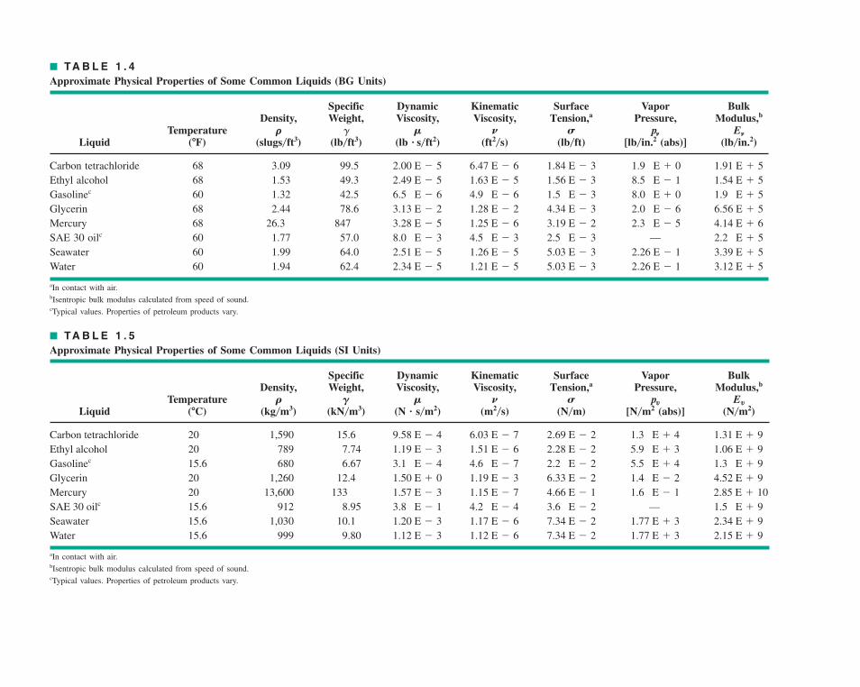
■ TA B L E 1 . 4

Approximate Physical Properties of Some Common Liquids (BG Units)

Specific Dynamic Kinematic Surface Vapor BulkDensity, Weight, Viscosity, Viscosity, Pressure,

Temperature pvv EvvLiquid ( ) ( ) ( ) ( 2) ( ) ( ) [ .2 (abs)] ( )

Carbon tetrachloride 68 3.09 99.5Ethyl alcohol 68 1.53 49.3

60 1.32 42.5Glycerin 68 2.44 78.6Mercury 68 26.3 847SAE 30 60 1.77 57.0 —Seawater 60 1.99 64.0Water 60 1.94 62.4

aIn contact with air.bIsentropic bulk modulus calculated from speed of sound.cTypical values. Properties of petroleum products vary.

3.12 E � 52.26 E � 15.03 E � 31.21 E � 52.34 E � 53.39 E � 52.26 E � 15.03 E � 31.26 E � 52.51 E � 52.2 E � 52.5 E � 34.5 E � 38.0 E � 3oilc

4.14 E � 62.3 E � 53.19 E � 21.25 E � 63.28 E � 56.56 E � 52.0 E � 64.34 E � 31.28 E � 23.13 E � 21.9 E � 58.0 E � 01.5 E � 34.9 E � 66.5 E � 6Gasolinec

1.54 E � 58.5 E � 11.56 E � 31.63 E � 52.49 E � 51.91 E � 51.9 E � 01.84 E � 36.47 E � 62.00 E � 5

lb�in.2lb�inlb�ftft2�slb � s�ftlb�ft3slugs�ft3�FSNM��

Modulus,bTension,a

■ TA B L E 1 . 5

Approximate Physical Properties of Some Common Liquids (SI Units)

Specific Dynamic Kinematic Surface Vapor BulkDensity, Weight, Viscosity, Viscosity, Pressure,

Temperature pvv Evv

Liquid ( ) ( ) ( ) ( ) ( ) ( ) [ (abs)] ( )

Carbon tetrachloride 20 1,590 15.6Ethyl alcohol 20 789 7.74

15.6 680 6.67Glycerin 20 1,260 12.4Mercury 20 13,600 133SAE 30 15.6 912 8.95 —Seawater 15.6 1,030 10.1Water 15.6 999 9.80

aIn contact with air.bIsentropic bulk modulus calculated from speed of sound.cTypical values. Properties of petroleum products vary.

2.15 E � 91.77 E � 37.34 E � 21.12 E � 61.12 E � 32.34 E � 91.77 E � 37.34 E � 21.17 E � 61.20 E � 31.5 E � 93.6 E � 24.2 E � 43.8 E � 1oilc

2.85 E � 101.6 E � 14.66 E � 11.15 E � 71.57 E � 34.52 E � 91.4 E � 26.33 E � 21.19 E � 31.50 E � 01.3 E � 95.5 E � 42.2 E � 24.6 E � 73.1 E � 4Gasolinec

1.06 E � 95.9 E � 32.28 E � 21.51 E � 61.19 E � 31.31 E � 91.3 E � 42.69 E � 26.03 E � 79.58 E � 4

N�m2N�m2N�mm2�sN � s�m2kN�m3kg�m3�CSNMGR

Modulus,bTension,a

ifc.qxd 8/31/10 7:15 PM Page 2

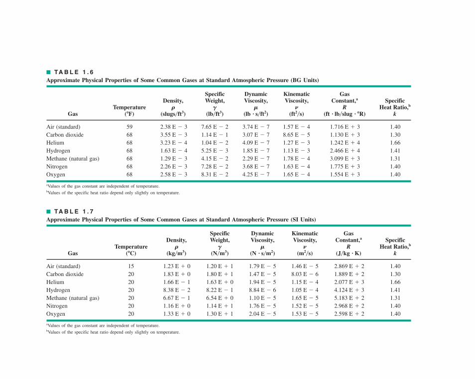
■ TA B L E 1 . 6

Approximate Physical Properties of Some Common Gases at Standard Atmospheric Pressure (BG Units)

Specific Dynamic Kinematic GasDensity, Weight, Viscosity, Viscosity, Specific

Temperature RGas ( ) ( ) ( ) ( ) ( ) ( ) k

Air (standard) 59 1.40Carbon dioxide 68 1.30Helium 68 1.66Hydrogen 68 1.41Methane (natural gas) 68 1.31Nitrogen 68 1.40Oxygen 68 1.40

aValues of the gas constant are independent of temperature.bValues of the specific heat ratio depend only slightly on temperature.

1.554 E � 31.65 E � 44.25 E � 78.31 E � 22.58 E � 31.775 E � 31.63 E � 43.68 E � 77.28 E � 22.26 E � 33.099 E � 31.78 E � 42.29 E � 74.15 E � 21.29 E � 32.466 E � 41.13 E � 31.85 E � 75.25 E � 31.63 E � 41.242 E � 41.27 E � 34.09 E � 71.04 E � 23.23 E � 4 1.130 E � 38.65 E � 53.07 E � 71.14 E � 13.55 E � 31.716 E � 31.57 E � 43.74 E � 77.65 E � 22.38 E � 3

ft � lb�slug � �Rft2�slb � s�ft2lb�ft3slugs�ft3�FHeat Ratio,bNMGR

Constant,a

■ TA B L E 1 . 7

Approximate Physical Properties of Some Common Gases at Standard Atmospheric Pressure (SI Units)

Specific Dynamic Kinematic GasDensity, Weight, Viscosity, Viscosity, Specific

Temperature RGas ( ) ( ) ( ) ( ) ( ) ( ) k

Air (standard) 15 1.40Carbon dioxide 20 1.30Helium 20 1.66Hydrogen 20 1.41Methane (natural gas) 20 1.31Nitrogen 20 1.40Oxygen 20 1.40

aValues of the gas constant are independent of temperature.bValues of the specific heat ratio depend only slightly on temperature.

2.598 E � 21.53 E � 52.04 E � 51.30 E � 11.33 E � 02.968 E � 21.52 E � 51.76 E � 51.14 E � 11.16 E � 05.183 E � 21.65 E � 51.10 E � 56.54 E � 06.67 E � 14.124 E � 31.05 E � 48.84 E � 68.22 E � 18.38 E � 22.077 E � 31.15 E � 41.94 E � 51.63 E � 01.66 E � 11.889 E � 28.03 E � 61.47 E � 51.80 E � 11.83 E � 02.869 E � 21.46 E � 51.79 E � 51.20 E � 11.23 E � 0

J�kg � Km2�sN � s�m2N�m3kg�m3�CHeat Ratio,bNMGR

Constant,a

ifc.qxd 8/31/10 7:15 PM Page 3

accessible, affordable,active learning

FMTOC.qxd 9/28/10 9:10 AM Page i

FMTOC.qxd 9/28/10 9:10 AM Page ii

Fifth Edition

A Brief Introductionto Fluid Mechanics

John Wiley & Sons, Inc.

DONALD F. YOUNGBRUCE R. MUNSONDepartment of Aerospace Engineering and Engineering Mechanics

THEODORE H. OKIISHIDepartment of Mechanical EngineeringIowa State UniversityAmes, Iowa, USA

WADE W. HUEBSCHDepartment of Mechanical and Aerospace EngineeringWest Virginia UniversityMorgantown, West Virginia, USA

FMTOC.qxd 9/29/10 10:42 AM Page iii

Publisher Don FowleyEditor Jennifer WelterEditorial Assistant Renata MarchioneMarketing Manager Christopher RuelContent Manager Dorothy SinclairProduction Editor Sandra DumasArt Director Jeofrey VitaExecutive Media Editor Thomas KulesaPhoto Department Manager Hilary NewmanPhoto Editor Sheena GoldsteinProduction Management Services Aptara

Cover Photo: A group of pelicans in flight near the water surface. Note the unique wing shapes employed from theroot to the tip to achieve this biological flight. See Chapter 9 for an introduction to external fluid flow past a wing.

This book was typeset in 10/12 Times Ten Roman at Aptara and printed and bound by R. R. Donnelley(Jefferson City). The cover was printed by R. R. Donnelley (Jefferson City).

Founded in 1807, John Wiley & Sons, Inc. has been a valued source of knowledge and understanding for morethan 200 years, helping people around the world meet their needs and fulfill their aspirations. Our company is builton a foundation of principles that include responsibility to the communities we serve and where we live and work.In 2008, we launched a Corporate Citizenship Initiative, a global effort to address the environmental, social,economic, and ethical challenges we face in our business. Among the issues we are addressing are carbon impact,paper specifications and procurement, ethical conduct within our business and among our vendors, and communityand charitable support. For more information, please visit our website: www.wiley.com/go/citizenship.

The paper in this book was manufactured by a mill whose forest management programs include sustainedyield-harvesting of its timberlands. Sustained yield harvesting principles ensure that the number of trees cuteach year does not exceed the amount of new growth.

This book is printed on acid-free paper. �

Copyright © 2011, 2007, 2004, 2000, 1996, 1993, 1988 by John Wiley & Sons, Inc. All rights reserved.

No part of this publication may be reproduced, stored in a retrieval system or transmitted in any form or by anymeans, electronic, mechanical, photocopying recording, scanning or otherwise, except as permitted underSections 107 or 108 of the 1976 United States Copyright Act, without either the prior written permission of thePublisher or authorization through payment of the appropriate per-copy fee to the Copyright Clearance Center,222 Rosewood Drive, Danvers, MA 01923, (978) 750-8400, fax (978) 646-8600. Requests to the Publisher forpermission should be addressed to the Permissions Department, John Wiley & Sons, Inc., 111 River Street,Hoboken, NJ 07030-5774, (201) 748-6011, fax (201) 748-6008.

Evaluation copies are provided to qualified academics and professionals for review purposes only, for use in theircourses during the next academic year. These copies are licensed and may not be sold or transferred to a thirdparty. Upon completion of the review period, please return the evaluation copy to Wiley. Return instructions anda free of charge return shipping label are available at www.wiley.com/go/returnlabel. Outside of the United States,please contact your local representative.

ISBN 13 978-0470-59679-1

Printed in the United States of America.

10 9 8 7 6 5 4 3 2 1

FMTOC.qxd 9/30/10 9:43 AM Page iv

About the Authors

Donald F. Young, Anson Marston Distinguished Professor Emeritus in Engineering, is a fac-ulty member in the Department of Aerospace Engineering and Engineering Mechanics at IowaState University. Dr. Young received his B.S. degree in mechanical engineering, his M.S. andPh.D. degrees in theoretical and applied mechanics from Iowa State, and has taught both un-dergraduate and graduate courses in fluid mechanics for many years. In addition to beingnamed a Distinguished Professor in the College of Engineering, Dr. Young has also receivedthe Standard Oil Foundation Outstanding Teacher Award and the Iowa State UniversityAlumni Association Faculty Citation. He has been engaged in fluid mechanics research formore than 45 years, with special interests in similitude and modeling and the interdisciplinaryfield of biomedical fluid mechanics. Dr. Young has contributed to many technical publicationsand is the author or coauthor of two textbooks on applied mechanics. He is a Fellow of theAmerican Society of Mechanical Engineers.

Bruce R. Munson, Professor Emeritus of Engineering Mechanics, has been a faculty memberat Iowa State University since 1974. He received his B.S. and M.S. degrees from Purdue Uni-versity and his Ph.D. degree from the Aerospace Engineering and Mechanics Department ofthe University of Minnesota in 1970.

From 1970 to 1974, Dr. Munson was on the mechanical engineering faculty of DukeUniversity. From 1964 to 1966, he worked as an engineer in the jet engine fuel control depart-ment of Bendix Aerospace Corporation, South Bend, Indiana.

Dr. Munson’s main professional activity has been in the area of fluid mechanics educa-tion and research. He has been responsible for the development of many fluid mechanicscourses for studies in civil engineering, mechanical engineering, engineering science, andagricultural engineering and is the recipient of an Iowa State University Superior EngineeringTeacher Award and the Iowa State University Alumni Association Faculty Citation.

He has authored and coauthored many theoretical and experimental technical papers onhydrodynamic stability, low Reynolds number flow, secondary flow, and the applications ofviscous incompressible flow. He is a member of the American Society of Mechanical Engineers(ASME), the American Physical Society, and the American Society for Engineering Education.

Theodore H. Okiishi, Associate Dean of Engineering and past Chair of Mechanical Engi-neering at Iowa State University, has taught fluid mechanics courses there since 1967. He re-ceived his undergraduate and graduate degrees at Iowa State.

From 1965 to 1967, Dr. Okiishi served as a U.S. Army officer with duty assignments atthe National Aeronautics and Space Administration Lewis Research Center, Cleveland, Ohio,where he participated in rocket nozzle heat transfer research, and at the Combined IntelligenceCenter, Saigon, Republic of South Vietnam, where he studied seasonal river flooding problems.

Professor Okiishi is active in research on turbomachinery fluid dynamics. He and hisgraduate students and other colleagues have written a number of journal articles based ontheir studies. Some of these projects have involved significant collaboration with govern-ment and industrial laboratory researchers with one technical paper winning the ASMEMelville Medal.

v

FMTOC.qxd 9/28/10 9:10 AM Page v

Dr. Okiishi has received several awards for teaching. He has developed undergraduate andgraduate courses in classical fluid dynamics as well as the fluid dynamics of turbomachines.

He is a licensed professional engineer. His technical society activities include havingbeen chair of the board of directors of the ASME International Gas Turbine Institute. He is afellow member of the ASME and the technical editor of the Journal of Turbomachinery.

Wade W. Huebsch has been a faculty member in the Department of Mechanical and Aero-space Engineering at West Virginia University (WVU) since 2001. He received his B.S. degreein aerospace engineering from San Jose State University where he played college baseball. Hereceived his M.S. degree in mechanical engineering and his Ph.D. in aerospace engineeringfrom Iowa State University in 2000.

Dr. Huebsch specializes in computational fluid dynamics research and has authoredmultiple journal articles in the areas of aircraft icing, roughness-induced flow phenomena, andboundary layer flow control. He has taught both undergraduate and graduate courses in fluidmechanics and has developed a new undergraduate course in computational fluid dynamics.He has received multiple teaching awards such as Outstanding Teacher and Teacher of theYear from the College of Engineering and Mineral Resources at WVU as well as the Ralph R.Teetor Educational Award from Society of Automotive Engineers. He was also named as theYoung Researcher of the Year from WVU. He is a member of the American Institute ofAeronautics and Astronautics, the Sigma Xi research society, the SAE, and the AmericanSociety of Engineering Education.

vi About the Authors

FMTOC.qxd 9/28/10 9:10 AM Page vi

Also by these authors

Fundamentals of Fluid Mechanics, 6e978-0470-26284-9

Complete in-depth coverage of basic fluid mechanics principles, including compressible flow, for use in

either a one- or two-semester course.

FMTOC.qxd 9/28/10 9:10 AM Page vii

This page intentionally left blank

Preface

A Brief Introduction to Fluid Mechanics, fifth edition, is an abridged version of a more com-prehensive treatment found in Fundamentals of Fluid Mechanics by Munson, Young, Okiishi,and Huebsch. Although this latter work continues to be successfully received by students andcolleagues, it is a large volume containing much more material than can be covered in a typi-cal one-semester undergraduate fluid mechanics course. A consideration of the numerousfluid mechanics texts that have been written during the past several decades reveals that thereis a definite trend toward larger and larger books. This trend is understandable because theknowledge base in fluid mechanics has increased, along with the desire to include a broaderscope of topics in an undergraduate course. Unfortunately, one of the dangers in this trend isthat these large books can become intimidating to students who may have difficulty, in a be-ginning course, focusing on basic principles without getting lost in peripheral material. It iswith this background in mind that the authors felt that a shorter but comprehensive text, cov-ering the basic concepts and principles of fluid mechanics in a modern style, was needed. Inthis abridged version there is still more than ample material for a one-semester undergraduatefluid mechanics course. We have made every effort to retain the principal features of the orig-inal book while presenting the essential material in a more concise and focused manner thatwill be helpful to the beginning student.

This fifth edition has been prepared by the authors after several years of using the pre-vious editions for an introductory course in fluid mechanics. Based on this experience, alongwith suggestions from reviewers, colleagues, and students, we have made a number ofchanges and additions in this new edition.

New to This Edition

In addition to the continual effort of updating the scope of the material presented and improv-ing the presentation of all of the material, the following items are new to this edition.

With the widespread use of new technologies involving the web, DVDs, digital cameras,and the like, there are increasing use and appreciation of the variety of visual tools availablefor learning. After all, fluid mechanics can be a very visual topic. This fact has been addressedin the new edition by the inclusion of numerous new illustrations, graphs, photographs, andvideos.Illustrations: The book contains 148 new illustrations and graphs, bringing the total numberto 890. These illustrations range from simple ones that help illustrate a basic concept orequation to more complex ones that illustrate practical applications of fluid mechanics in oureveryday lives.Photographs: The book contains 224 new photographs, bringing the total number to 240.Some photos involve situations that are so common to us that we probably never stop to realizehow fluids are involved in them. Others involve new and novel situations that are still bafflingto us. The photos are also used to help the reader better understand the basic concepts andexamples discussed.

ix

FMTOC.qxd 9/28/10 9:10 AM Page ix

Videos: The video library for the book has been significantly enhanced by the addition of76 new videos directly related to the text material, bringing the total number to 152. Theyillustrate many of the interesting and practical applications of real-world fluid phenomena.In addition to being located at the appropriate places within the text, they are all listed, eachwith an appropriate thumbnail photo, in a new video index. In the electronic version of thebook, the videos can be selected directly from this index.Examples: The book contains several new example problems that involve various fluidflow fundamentals. These examples also incorporate PtD (Prevention through Design) dis-cussion material. The PtD project, under the direction of the National Institute for Occupa-tional Safety and Health, involves, in part, the use of textbooks to encourage the proper designand use of workday equipment and material so as to reduce accidents and injuries in theworkplace.List of equations: Each chapter ends with a new summary of the most important equations inthe chapter.Problems: The book contains approximately 273 new homework problems, bringing the totalnumber to 919. The print version of the book contains all the even-numbered problems; all theproblems (even and odd numbered) are contained on the book’s web site, www.wiley.com/college/young, or WileyPLUS. There are several new problems in which the student is askedto find a photograph or image of a particular flow situation and write a paragraph describingit. In addition, each chapter contains new Lifelong Learning Problems (i.e., one aspect of thelifelong learning as interpreted by the authors) that ask the student to obtain information abouta given new flow concept and to write about it.

Key Features

Illustrations, Photographs, and Videos

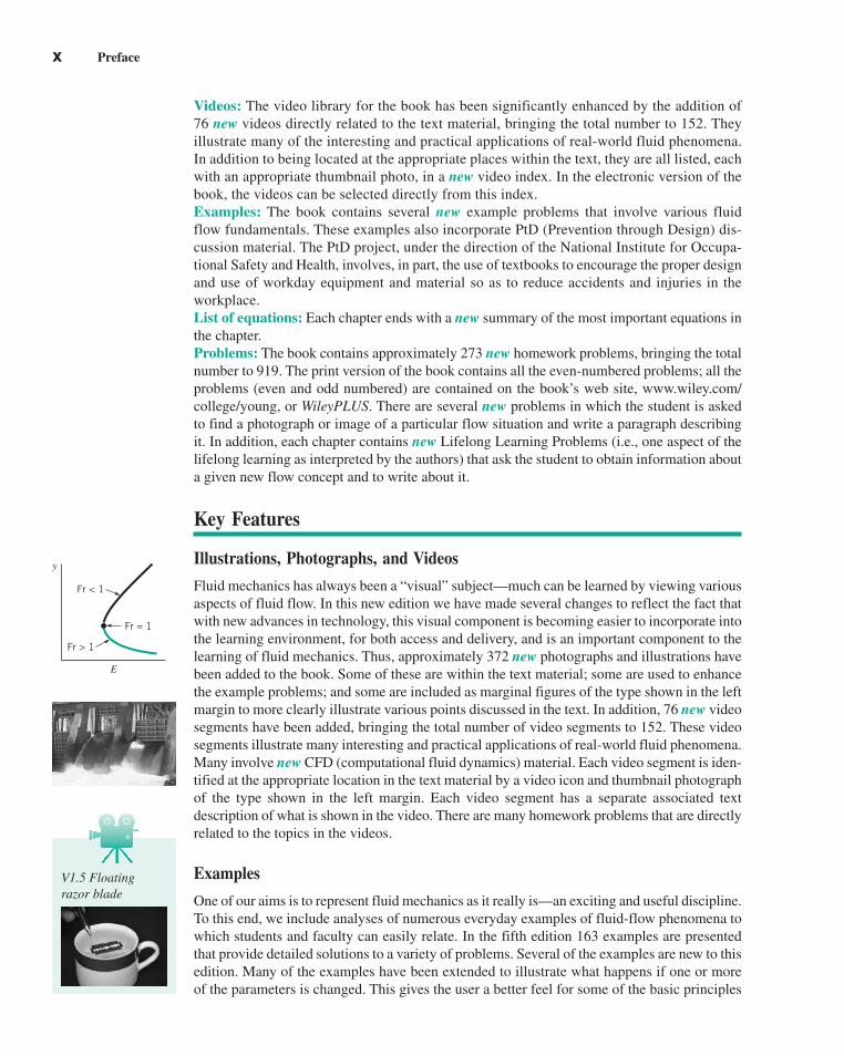
Fluid mechanics has always been a “visual” subject—much can be learned by viewing variousaspects of fluid flow. In this new edition we have made several changes to reflect the fact thatwith new advances in technology, this visual component is becoming easier to incorporate intothe learning environment, for both access and delivery, and is an important component to thelearning of fluid mechanics. Thus, approximately 372 new photographs and illustrations havebeen added to the book. Some of these are within the text material; some are used to enhancethe example problems; and some are included as marginal figures of the type shown in the leftmargin to more clearly illustrate various points discussed in the text. In addition, 76 new videosegments have been added, bringing the total number of video segments to 152. These videosegments illustrate many interesting and practical applications of real-world fluid phenomena.Many involve new CFD (computational fluid dynamics) material. Each video segment is iden-tified at the appropriate location in the text material by a video icon and thumbnail photographof the type shown in the left margin. Each video segment has a separate associated text description of what is shown in the video. There are many homework problems that are directlyrelated to the topics in the videos.

Examples

One of our aims is to represent fluid mechanics as it really is—an exciting and useful discipline.To this end, we include analyses of numerous everyday examples of fluid-flow phenomena towhich students and faculty can easily relate. In the fifth edition 163 examples are presentedthat provide detailed solutions to a variety of problems. Several of the examples are new to thisedition. Many of the examples have been extended to illustrate what happens if one or moreof the parameters is changed. This gives the user a better feel for some of the basic principles

x Preface

V1.5 Floating razor blade

E

Fr = 1

Fr < 1

Fr > 1

y

FMTOC.qxd 9/29/10 10:47 AM Page x

Preface xi

involved. In addition, many of the examples contain new photographs of the actual deviceor item involved in the example. Also, all the examples are outlined and carried out withthe problem-solving methodology of “Given, Find, Solution, and Comment” as discussedin the “Note to User” before Example 1.1. This edition contains several new example problemsthat incorporate PtD (Prevention through Design) discussion material as indicated on theprevious page.

Fluids in the News

A set of 63 short “Fluids in the News” stories that reflect some of the latest important andnovel ways that fluid mechanics affects our lives is provided. Many of these problems havehomework problems associated with them.

Homework Problems

A set of 919 homework problems is provided. This represents an increase of approximately42% more problems than in the previous edition. The even-numbered problems are in theprint version of the book; all of the problems (even and odd) are at the book’s web site,www.wiley.com/college/young, or WileyPLUS. These problems stress the practical applica-tion of principles. The problems are grouped and identified according to topic. An effort hasbeen made to include several easier problems at the start of each group. The following typesof problems are included:1) “standard” problems2) computer problems3) discussion problems4) supply-your-own-data problems5) review problems with solutions6) problems based on the “Fluids in theNews” topics7) problems based on the fluid videos8) Excel-based lab problems

9) new “Lifelong Learning” problems10) problems that require the user to obtain aphotograph or image of a given flow situationand write a brief paragraph to describe it11) simple CFD problems to be solved usingFlowLab12) Fundamental of Engineering (FE) examquestions available on book web site

Lab Problems—There are 30 extended, laboratory-type problems that involve actual experi-mental data for simple experiments of the type that are often found in the laboratory portionof many introductory fluid mechanics courses. The data for these problems are provided inExcel format.Lifelong Learning Problems—There are 33 new lifelong learning problems that involveobtaining additional information about various new state-of-the-art fluid mechanics topicsand writing a brief report about this material.Review Problems—There is a set of 186 review problems covering most of the main topics inthe book. Complete, detailed solutions to these problems can be found in the Student SolutionManual and Study Guide for A Brief Introduction to Fluid Mechanics, by Young et al. (© 2011John Wiley and Sons, Inc.).

Well-Paced Concept and Problem-Solving Development

Since this is an introductory text, we have designed the presentation of material to allow forthe gradual development of student confidence in fluid problem solving. Each important con-cept or notion is considered in terms of simple and easy-to-understand circumstances beforemore complicated features are introduced.

FMTOC.qxd 9/30/10 7:04 PM Page xi

Several brief components have been added to each chapter to help the user obtain the“big picture” idea of what key knowledge is to be gained from the chapter. A brief LearningObjectives section is provided at the beginning of each chapter. It is helpful to read throughthis list prior to reading the chapter to gain a preview of the main concepts presented. Uponcompletion of the chapter, it is beneficial to look back at the original learning objectives to en-sure that a satisfactory level of understanding has been acquired for each item. Additional re-inforcement of these learning objectives is provided in the form of a Chapter Summary andStudy Guide at the end of each chapter. In this section a brief summary of the key concepts andprinciples introduced in the chapter is included along with a listing of important terms withwhich the student should be familiar. These terms are highlighted in the text. A new list of themain equations in the chapter is included in the chapter summary.

System of Units

Two systems of units continue to be used throughout most of the text: the International Sys-tem of Units (newtons, kilograms, meters, and seconds) and the British Gravitational System(pounds, slugs, feet, and seconds). About one-half of the examples and homework problemsare in each set of units.

Topical Organization

In the first four chapters the student is made aware of some fundamental aspects of fluid mo-tion, including important fluid properties, regimes of flow, pressure variations in fluids at restand in motion, fluid kinematics, and methods of flow description and analysis. The Bernoulliequation is introduced in Chapter 3 to draw attention, early on, to some of the interesting ef-fects of fluid motion on the distribution of pressure in a flow field. We believe that this timelyconsideration of elementary fluid dynamics increases student enthusiasm for the more com-plicated material that follows. In Chapter 4 we convey the essential elements of kinematics, in-cluding Eulerian and Lagrangian mathematical descriptions of flow phenomena, and indicatethe vital relationship between the two views. For teachers who wish to consider kinematics indetail before the material on elementary fluid dynamics, Chapters 3 and 4 can be interchangedwithout loss of continuity.

Chapters 5, 6, and 7 expand on the basic analysis methods generally used to solve or tobegin solving fluid mechanics problems. Emphasis is placed on understanding how flow phe-nomena are described mathematically and on when and how to use infinitesimal and finitecontrol volumes. The effects of fluid friction on pressure and velocity distributions are alsoconsidered in some detail. A formal course in thermodynamics is not required to understandthe various portions of the text that consider some elementary aspects of the thermodynamicsof fluid flow. Chapter 7 features the advantages of using dimensional analysis and similitudefor organizing test data and for planning experiments and the basic techniques involved.

Owing to the growing importance of computational fluid dynamics (CFD) in engineer-ing design and analysis, material on this subject is included in Appendix A. This material maybe omitted without any loss of continuity to the rest of the text. This introductory CFDoverview includes examples and problems of various interesting flow situations that are to besolved using FlowLab software.

Chapters 8 through 11 offer students opportunities for the further application of the prin-ciples learned early in the text. Also, where appropriate, additional important notions such asboundary layers, transition from laminar to turbulent flow, turbulence modeling, and flow sep-aration are introduced. Practical concerns such as pipe flow, open-channel flow, flow mea-surement, drag and lift, and the fluid mechanics fundamentals associated with turbomachinesare included.

xii Preface

FMTOC.qxd 9/28/10 9:10 AM Page xii

Students who study this text and who solve a representative set of the exercisesprovided should acquire a useful knowledge of the fundamentals of fluid mechanics.Faculty who use this text are provided with numerous topics to select from in order tomeet the objectives of their own courses. More material is included than can be reason-ably covered in one term. All are reminded of the fine collection of supplementary mate-rial. We have cited throughout the text various articles and books that are available forenrichment.

Student and Instructor Resources

Student Solution Manual and Study Guide, by Young et al. (© 2011 John Wiley and Sons,Inc.)—This short paperback book is available as a supplement for the text. It provides detailedsolutions to the Review Problems and a concise overview of the essential points of most of themain sections of the text, along with appropriate equations, illustrations, and worked exam-ples. This supplement is available through your local bookstore, or you may purchase it on theWiley web site at www.wiley.com/college/young.

Student Companion Site—The student section of the book web site at www.wiley.com/college/young contains the assets that follow. Access is free of charge with the registration code in-cluded in the front of every new book.Video Library CFD-Driven Cavity ExampleReview Problems with Answers FlowLab Tutorial and User’s GuideLab Problems FlowLab ProblemsComprehensive Table of Conversion Factors

Instructor Companion Site—The instructor section of the book web site at www.wiley.com/college/young contains the assets in the Student Companion Site, as well as the following,which are available only to professors who adopt this book for classroom use:

Instructor Solutions Manual, containing complete, detailed solutions to all of the prob-lems in the text.

Figures from the text, appropriate for use in lecture slides.

These instructor materials are password-protected. Visit the Instructor Companion Site to reg-ister for a password.

FlowLab®—In cooperation with Wiley, Ansys Inc. is offering to instructors who adopt thistext the option to have FlowLab software installed in their department lab free of charge.(This offer is available in the Americas only; fees vary by geographic region outside theAmericas.) FlowLab is a CFD package that allows students to solve fluid dynamics problemswithout requiring a long training period. This software introduces CFD technology to under-graduates and uses CFD to excite students about fluid dynamics and learning more abouttransport phenomena of all kinds. To learn more about FlowLab and request installation inyour department, visit the Instructor Companion Site at www.wiley.com/college/young, orWileyPLUS.

WileyPLUS—WileyPLUS combines the complete, dynamic online text with all of the teach-ing and learning resources you need in one easy-to-use system. The instructor assigns WileyPLUS, but students decide how to buy it: They can buy the new, printed text packagedwith a WileyPLUS registration code at no additional cost or choose digital delivery of Wiley-PLUS, use the online text and integrated read, study, and practice tools, and save off the costof the new book.

Preface xiii

FMTOC.qxd 9/28/10 9:10 AM Page xiii

Acknowledgments

We wish to express our gratitude to the many persons who provided suggestions for this andprevious editions through reviews and surveys. In addition, we wish to express our apprecia-tion to the many persons who supplied the photographs and videos used throughout the text.A special thanks to Chris Griffin and Richard Rinehart for helping us incorporate the new PtD(Prevention through Design) material in this edition. Finally, we thank our families for theircontinued encouragement during the writing of this fifth edition.

Working with students over the years has taught us much about fluid mechanics educa-tion. We have tried in earnest to draw from this experience for the benefit of users of thisbook. Obviously we are still learning, and we welcome any suggestions and commentsfrom you.

BRUCE R. MUNSON

DONALD F. YOUNG

THEODORE H. OKIISHI

WADE W. HUEBSCH

xiv Preface

FMTOC.qxd 9/28/10 9:10 AM Page xiv

Featured in This Book

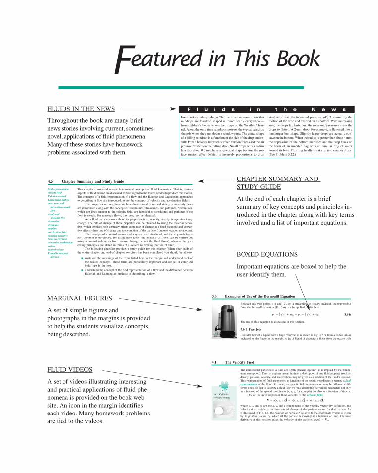
FLUIDS IN THE NEWS

Throughout the book are many briefnews stories involving current, sometimesnovel, applications of fluid phenomena.Many of these stories have homeworkproblems associated with them.

F l u i d s i n t h e N e w s

Incorrect raindrop shape The incorrect representation that

raindrops are teardrop shaped is found nearly everywhere—

from children’s books to weather maps on the Weather Chan-

nel. About the only time raindrops possess the typical teardrop

shape is when they run down a windowpane. The actual shape

of a falling raindrop is a function of the size of the drop and re-

sults from a balance between surface tension forces and the air

pressure exerted on the falling drop. Small drops with a radius

less than about 0.5 mm have a spherical shape because the sur-

face tension effect (which is inversely proportional to drop

size) wins over the increased pressure, caused by the

motion of the drop and exerted on its bottom. With increasing

size, the drops fall faster and the increased pressure causes the

drops to flatten. A 2-mm drop, for example, is flattened into a

hamburger bun shape. Slightly larger drops are actually con-

cave on the bottom. When the radius is greater than about 4 mm,

the depression of the bottom increases and the drop takes on

the form of an inverted bag with an annular ring of water

around its base. This ring finally breaks up into smaller drops.

(See Problem 3.22.)

�V 20/2,

CHAPTER SUMMARY AND STUDY GUIDE

At the end of each chapter is a briefsummary of key concepts and principles in-troduced in the chapter along with key termsinvolved and a list of important equations.

field representationvelocity fieldEulerian methodLagrangian methodone-, two-, and

three-dimensional flow

steady and unsteady flow

streamlinestreaklinepathlineacceleration fieldmaterial derivativelocal accelerationconvective accelerationsystemcontrol volumeReynolds transport

theorem

4.5 Chapter Summary and Study Guide

This chapter considered several fundamental concepts of fluid kinematics. That is, various

aspects of fluid motion are discussed without regard to the forces needed to produce this motion.

The concepts of a field representation of a flow and the Eulerian and Lagrangian approaches

to describing a flow are introduced, as are the concepts of velocity and acceleration fields.

The properties of one-, two-, or three-dimensional flows and steady or unsteady flows

are introduced along with the concepts of streamlines, streaklines, and pathlines. Streamlines,

which are lines tangent to the velocity field, are identical to streaklines and pathlines if the

flow is steady. For unsteady flows, they need not be identical.

As a fluid particle moves about, its properties (i.e., velocity, density, temperature) may

change. The rate of change of these properties can be obtained by using the material deriva-

tive, which involves both unsteady effects (time rate of change at a fixed location) and convec-

tive effects (time rate of change due to the motion of the particle from one location to another).

The concepts of a control volume and a system are introduced, and the Reynolds trans-

port theorem is developed. By using these ideas, the analysis of flows can be carried out

using a control volume (a fixed volume through which the fluid flows), whereas the gov-

erning principles are stated in terms of a system (a flowing portion of fluid).

The following checklist provides a study guide for this chapter. When your study of

the entire chapter and end-of-chapter exercises has been completed you should be able to

write out the meanings of the terms listed here in the margin and understand each of

the related concepts. These terms are particularly important and are set in color and

bold type in the text.

understand the concept of the field representation of a flow and the difference between

Eulerian and Lagrangian methods of describing a flow.

3.6 Examples of Use of the Bernoulli Equation

Between any two points, (1) and (2), on a streamline in steady, inviscid, incompressibleflow the Bernoulli equation (Eq. 3.6) can be applied in the form

(3.14)

The use of this equation is discussed in this section.

3.6.1 Free Jets

Consider flow of a liquid from a large reservoir as is shown in Fig. 3.7 or from a coffee urn asindicated by the figure in the margin. A jet of liquid of diameter d flows from the nozzle with

p1 � 12 �V2

1 � �z1 � p2 � 12 �V2

2 � �z2

V

BOXED EQUATIONS

Important equations are boxed to help theuser identify them.

MARGINAL FIGURES

A set of simple figures andphotographs in the margins is providedto help the students visualize conceptsbeing described.

FLUID VIDEOS

A set of videos illustrating interestingand practical applications of fluid phe-nomena is provided on the book website. An icon in the margin identifieseach video. Many homework problemsare tied to the videos.

4.1 The Velocity Field

The infinitesimal particles of a fluid are tightly packed together (as is implied by the contin-uum assumption). Thus, at a given instant in time, a description of any fluid property (such asdensity, pressure, velocity, and acceleration) may be given as a function of the fluid’s location.This representation of fluid parameters as functions of the spatial coordinates is termed a fieldrepresentation of the flow. Of course, the specific field representation may be different at dif-ferent times, so that to describe a fluid flow we must determine the various parameters not onlyas a function of the spatial coordinates (x, y, z, for example) but also as a function of time, t.

One of the most important fluid variables is the velocity field,

where u, y, and w are the x, y, and z components of the velocity vector. By definition, thevelocity of a particle is the time rate of change of the position vector for that particle. Asis illustrated in Fig. 4.1, the position of particle A relative to the coordinate system is givenby its position vector, rA, which (if the particle is moving) is a function of time. The timederivative of this position gives the velocity of the particle, drA/dt � VA.

V � u1x, y, z, t2 i � y1x, y, z, t2 j � w1x, y, z, t2k

V4.3 Cylinder-velocity vectors

FMTOC.qxd 9/28/10 9:10 AM Page xv

EXAMPLE PROBLEMS

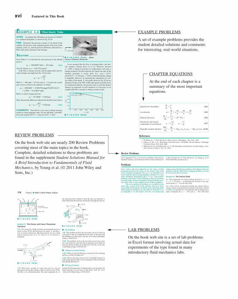
A set of example problems provides thestudent detailed solutions and commentsfor interesting, real-world situations.

xvi Featured in This Book

GIVEN An airplane flies 200 mph at an elevation of 10,000 ft

in a standard atmosphere as shown in Fig. E3.6a.

FIND Determine the pressure at point (1) far ahead of the

airplane, the pressure at the stagnation point on the nose of the

airplane, point (2), and the pressure difference indicated by a

Pitot-static probe attached to the fuselage.

SOLUTION

Pitot-Static Tube

It was assumed that the flow is incompressible—the den-

sity remains constant from (1) to (2). However, because

� � p/RT, a change in pressure (or temperature) will cause a

change in density. For this relatively low speed, the ratio of the

absolute pressures is nearly unity [i.e., p1/p2 � (10.11

psia)/(10.11 � 0.524 psia) � 0.951] so that the density change

is negligible. However, by repeating the calculations for vari-

ous values of the speed, , the results shown in Fig. E3.6b are

obtained. Clearly at the 500- to 600-mph speeds normally flown

by commercial airliners, the pressure ratio is such that density

changes are important. In such situations it is necessary to use

compressible flow concepts to obtain accurate results.

V1

EXAMPLE 3.6

From Table C.1 we find that the static pressure at the altitude

given is

(Ans)

Also the density is � � 0.001756 slug/ft3.

If the flow is steady, inviscid, and incompressible and ele-

vation changes are neglected, Eq. 3.6 becomes

With V1 � 200 mph � 293 ft/s and V2 � 0 (since the coordi-

nate system is fixed to the airplane) we obtain

Hence, in terms of gage pressure

(Ans)

Thus, the pressure difference indicated by the Pitot-static tube is

(Ans)

COMMENTS Note that it is very easy to obtain incorrect

results by using improper units. Do not add lb/in.2 and lb/ft2.

Note that (slug/ft3)(ft2/s2) � (slug�ft/s2)/(ft2) � lb/ft2.

p2 � p1 ��V 2

1

2� 0.524 psi

p2 � 75.4 lb/ft2 � 0.524 psi

� 11456 � 75.42 lb/ft2 1abs2

p2 � 1456 lb/ft2 � 10.001756 slugs/ft32 1293 ft/s22/2

p2 � p1 ��V 2

1

2

p1 � 1456 lb/ft2 1abs2 � 10.11psia

F I G U R E E3.6a (Photocourtesy of Hawker Beechcraft.)

(2)

(1)

Pitot-static tubeV1 = 200 mph

F I G U R E E3.6b

(200 mph, 0.951)1

0.8

0.6

0.4

0.2

00 100 200 300

V1, mph

p 1/p

2

400 500 600

REVIEW PROBLEMS

On the book web site are nearly 200 Review Problemscovering most of the main topics in the book.Complete, detailed solutions to these problems arefound in the supplement Student Solutions Manual forA Brief Introduction to Fundamentals of FluidMechanics, by Young et al. (© 2011 John Wiley andSons, Inc.)

LAB PROBLEMS

On the book web site is a set of lab problemsin Excel format involving actual data for experiments of the type found in many introductory fluid mechanics labs.

CHAPTER EQUATIONS

At the end of each chapter is asummary of the most importantequations.

Section 5.3 The Energy and Linear MomentumEquations

5.94 Two water jets collide and form one homogeneous jet asshown in Fig. P5.94. (a) Determine the speed, V, and direc-tion, of the combined jet. (b) Determine the loss for a fluidparticle flowing from (1) to (3), from (2) to (3). Gravity isnegligible.

�,

5.96 Water flows steadily in a pipe and exits as a free jetthrough an end cap that contains a filter as shown in Fig. P5.96.The flow is in a horizontal plane. The axial component, , ofRy

� Lab Problems

5.98 This problem involves the force that a jet of air exerts ona flat plate as the air is deflected by the plate. To proceed withthis problem, go to the book’s web site, www.wiley.com/college/young, or WileyPLUS.

5.100 This problem involves the force that a jet of water exertson a vane when the vane turns the jet through a given angle. Toproceed with this problem, go to the book’s web site, www.wiley.com/college/young, or WileyPLUS.

� Lifelong Learning Problems

5.102 What are typical efficiencies associated with swimmingand how can they be improved?

5.104 Discuss the main causes of loss of available energy in aturbo-pump and how they can be minimized. What are typicalturbo-pump efficiencies?

� FE Exam Problems

Sample FE (Fundamentals of Engineering) exam questions forfluid mechanics are provided on the book’s web site, www.wiley.com/college/young, or WileyPLUS.

174 Chapter 5 � Finite Control Volume Analysis

F I G U R E P5.92

Fan

10 ft

Air curtain (0.5-ft thickness)

Open door

V = 30 ft/s

F I G U R E P5.94

V2 = 6 m/s

V

V1 = 4 m/s

θ

0.12 m

0.10 m(1)

(2)

(3)

90°

F I G U R E P5.96

Area = 0.10 ft2

Area = 0.12 ft2

Ry = 60 lb

V = 10 ft/s

Rx

Pipe

Filter30°

the anchoring force needed to keep the end cap stationary is 60 lb. Determine the head loss for the flow through the end cap.

Equation for streamlines (4.1)

Acceleration (4.3)

Material derivative (4.6)

Streamwise and normal components of acceleration (4.7)

Reynolds transport theorem (4.14)

References

1. Goldstein, R. J., Fluid Mechanics Measurements, Hemisphere, New York, 1983.2. Homsy, G. M., et al., Multimedia Fluid Mechanics, CD-ROM, Second Edition, Cambridge

University Press, New York, 2008.3. Magarvey, R. H., and MacLatchy, C. S., The Formation and Structure of Vortex Rings, Cana-

dian Journal of Physics, Vol. 42, 1964.

DBsys

Dt�0Bcv

0t� g�out AoutVout bout � g�in AinVinbin

as � V0V0s

, an �V 2

r

D1 2

Dt�0 1 20t

� 1V # § 2 1 2

a �0V0t

� u0V0x

� y0V0y

� w0V0z

dy

dx�y

u

Review Problems

Go to Appendix F for a set of review problems with answers.Detailed solutions can be found in Student Solution Manual for

a Brief Introduction to Fluid Mechanics, by Young et al. (©2010 John Wiley and Sons, Inc.).

Problems

Note: Unless otherwise indicated use the values of fluidproperties found in the tables on the inside of the frontcover. Problems designated with an (*) are intended to besolved with the aid of a programmable calculator or a com-puter. Problems designated with a (†) are “open-ended”problems and require critical thinking in that to work themone must make various assumptions and provide the neces-sary data. There is not a unique answer to these problems.

The even-numbered problems are included in thehard copy version of the book, and the answers to theseeven-numbered problems are listed at the end of the book.Odd-numbered problems are provided in WileyPLUS, orin Appendix L on the book’s web site, www.wiley.com/

college/young. The lab-type problems, FE problems, FlowLabproblems, and the videos that accompany problems can alsobe accessed on these web sites.

Section 4.1 The Velocity Field

4.2 The components of a velocity field are given by and . Determine the location of any stag-

nation points in the flow field.

4.4 A flow can be visualized by plotting the velocity field asvelocity vectors at representative locations in the flow as shownin Video V4.2 and Fig. E4.1. Consider the velocity field given inpolar coordinates by yr � �10/r and y� � 10/r. This flow

1V � 02w � 0y � xy3 � 16,

u � x � y,

FMTOC.qxd 9/29/10 11:38 AM Page xvi

Featured in This Book xvii

STUDENT SOLUTIONS MANUAL

A brief paperback book titled Student SolutionsManual for A Brief Introduction to Fluid Mechanics,by Young et al. (© 2011 John Wiley and Sons,Inc.), is available. It contains detailed solutions tothe Review Problems.

PROBLEMS

A generous set of homework problemsat the end of each chapter stresses thepractical applications of fluid mechan-ics principles. This set contains 919homework problems.

Axial Velocity (m/s) Legend

Axial Velocity

Full

Done Legend Freeze

XLog YLog Lines X Grid Y Grid Legend ManagerSymbols

Auto Raise Export DataPrint

0.0442

0.0395

0.0347

0.03

0.0253

0.0205

0.0158

0.0111

0.00631

0.001570Position (n)

0.1

inlet

outlet

x = 0.5d

x = 5dx = 1d

x = 10dx = 25d

CFD AND FlowLab

For those who wish to become familiar with thebasic concepts of computational fluid dynamics,an overview to CFD is provided in Appendices A and I. In addition, the use of FlowLab softwareto solve interesting flow problems is described inAppendices J and K.

hose, what pressure must be maintained just upstream of thenozzle to deliver this flowrate?

3.37 Air is drawn into a wind tunnel used for testing automo-biles as shown in Fig. P3.37. (a) Determine the manometerreading, h, when the velocity in the test section is 60 mph. Notethat there is a 1-in. column of oil on the water in the manometer.(b) Determine the difference between the stagnation pressure onthe front of the automobile and the pressure in the test section.

3.39 Water (assumed inviscid and incompressible) flowssteadily in the vertical variable-area pipe shown in Fig. P3.39.Determine the flowrate if the pressure in each of the gages reads50 kPa.

3.41 Water flows through the pipe contraction shown in Fig.P3.41. For the given 0.2-m difference in the manometer level,determine the flowrate as a function of the diameter of the smallpipe, D.

3.43 Water flows steadily with negligible viscous effectsthrough the pipe shown in Fig. P3.43. Determine the diame-ter, D, of the pipe at the outlet (a free jet) if the velocity there is20 ft/s.

3.45 Water is siphoned from the tank shown in Fig. P3.45. Thewater barometer indicates a reading of 30.2 ft. Determine themaximum value of h allowed without cavitation occurring. Notethat the pressure of the vapor in the closed end of the barometerequals the vapor pressure.

3.47 An inviscid fluid flows steadily through the contractionshown in Fig. P3.47. Derive an expression for the fluid velocityat (2) in terms of D1, D2, �, �m, and h if the flow is assumed incompressible.

3.49 Carbon dioxide flows at a rate of 1.5 ft3/s from a 3-in. pipein which the pressure and temperature are 20 psi (gage) and 120 �F,respectively, into a 1.5-in. pipe. If viscous effects are neglectedand incompressible conditions are assumed, determine the pres-sure in the smaller pipe.

Wind tunnel

Fan

60 mph

h

Water

Open

1 in.

Oil (SG = 0.9)

F I G U R E P3.37

Q

10 m

1 m

2 m

p = 50 kPa

F I G U R E P3.39

0.2 m

Q0.1 m D

F I G U R E P3.41

V = 20 ft/s

D

10 ft15 ft

Open

1.5-in. diameter

F I G U R E P3.43

30.2 ft

6 ft

3 in.diameter

h

Closed end

5-in. diameter

F I G U R E P3.45

h

D2D1

ρQ

Density mρ

F I G U R E P3.47

This page intentionally left blank

1INTRODUCTION 1

1.1 Some Characteristics of Fluids 31.2 Dimensions, Dimensional Homogeneity,

and Units 31.2.1 Systems of Units 6

1.3 Analysis of Fluid Behavior 91.4 Measures of Fluid Mass and Weight 9

1.4.1 Density 91.4.2 Specific Weight 101.4.3 Specific Gravity 10

1.5 Ideal Gas Law 111.6 Viscosity 121.7 Compressibility of Fluids 17

1.7.1 Bulk Modulus 171.7.2 Compression and Expansion

of Gases 181.7.3 Speed of Sound 19

1.8 Vapor Pressure 211.9 Surface Tension 211.10 A Brief Look Back in History 241.11 Chapter Summary and Study Guide 27

Review Problems 28Problems 28

2FLUID STATICS 32

2.1 Pressure at a Point 332.2 Basic Equation for Pressure Field 342.3 Pressure Variation in a Fluid at Rest 36

2.3.1 Incompressible Fluid 362.3.2 Compressible Fluid 38

2.4 Standard Atmosphere 392.5 Measurement of Pressure 392.6 Manometry 42

2.6.1 Piezometer Tube 422.6.2 U-Tube Manometer 432.6.3 Inclined-Tube Manometer 46

2.7 Mechanical and Electronic Pressure-Measuring Devices 47

2.8 Hydrostatic Force on a Plane Surface 47

2.9 Pressure Prism 522.10 Hydrostatic Force on a Curved

Surface 542.11 Buoyancy, Flotation, and Stability 57

2.11.1 Archimedes’ Principle 572.11.2 Stability 59

2.12 Pressure Variation in a Fluid with Rigid-Body Motion 60

2.13 Chapter Summary and Study Guide 60References 61Review Problems 62Problems 62

3ELEMENTARY FLUID DYNAMICS—THE BERNOULLIEQUATION 68

3.1 Newton’s Second Law 693.2 F � ma Along a Streamline 703.3 F � ma Normal to a Streamline 743.4 Physical Interpretation 753.5 Static, Stagnation, Dynamic, and Total

Pressure 783.6 Examples of Use of the Bernoulli

Equation 813.6.1 Free Jets 813.6.2 Confined Flows 823.6.3 Flowrate Measurement 89

3.7 The Energy Line and the Hydraulic Grade Line 92

3.8 Restrictions on the Use of the Bernoulli Equation 94

3.9 Chapter Summary and Study Guide 95Review Problems 96Problems 97

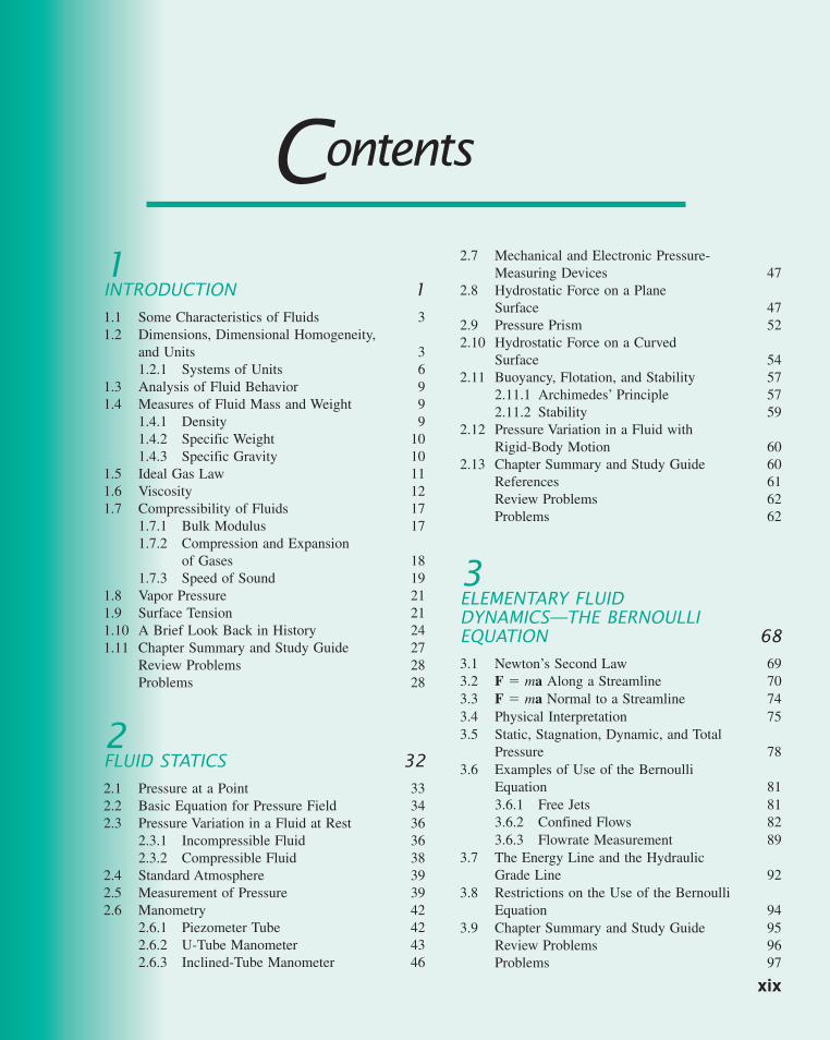
Contents

xix

FMTOC.qxd 9/28/10 9:10 AM Page xix

4FLUID KINEMATICS 102

4.1 The Velocity Field 1034.1.1 Eulerian and Lagrangian Flow

Descriptions 1054.1.2 One-, Two-, and Three-

Dimensional Flows 1054.1.3 Steady and Unsteady Flows 1064.1.4 Streamlines, Streaklines, and

Pathlines 1074.2 The Acceleration Field 110

4.2.1 The Material Derivative 1104.2.2 Unsteady Effects 1124.2.3 Convective Effects 1134.2.4 Streamline Coordinates 114

4.3 Control Volume and System Representations 1154.4 The Reynolds Transport Theorem 116

4.4.1 Derivation of the Reynolds Transport Theorem 116

4.4.2 Selection of a Control Volume 1204.5 Chapter Summary and Study Guide 120

References 121Review Problems 121Problems 121

5FINITE CONTROL VOLUME ANALYSIS 125

5.1 Conservation of Mass—The ContinuityEquation 1265.1.1 Derivation of the Continuity

Equation 1265.1.2 Fixed, Nondeforming Control

Volume 1275.1.3 Moving, Nondeforming Control

Volume 1315.2 Newton’s Second Law—The Linear

Momentum and Moment-of-MomentumEquations 1335.2.1 Derivation of the Linear

Momentum Equation 1335.2.2 Application of the Linear

Momentum Equation 1345.2.3 Derivation of the Moment-of-

Momentum Equation 1445.2.4 Application of the Moment-of-

Momentum Equation 145

xx Contents

5.3 First Law of Thermodynamics—The Energy Equation 1525.3.1 Derivation of the Energy

Equation 1525.3.2 Application of the Energy

Equation 1545.3.3 Comparison of the Energy

Equation with the Bernoulli Equation 157

5.3.4 Application of the Energy Equation to Nonuniform Flows 162

5.4 Chapter Summary and Study Guide 164Review Problems 166Problems 166

6DIFFERENTIAL ANALYSIS OF FLUID FLOW 175

6.1 Fluid Element Kinematics 1766.1.1 Velocity and Acceleration

Fields Revisited 1766.1.2 Linear Motion and Deformation 1776.1.3 Angular Motion and Deformation 179

6.2 Conservation of Mass 1826.2.1 Differential Form of

Continuity Equation 1826.2.2 Cylindrical Polar Coordinates 1846.2.3 The Stream Function 185

6.3 Conservation of Linear Momentum 1886.3.1 Description of Forces Acting on

Differential Element 1896.3.2 Equations of Motion 191

6.4 Inviscid Flow 1926.4.1 Euler’s Equations of Motion 1926.4.2 The Bernoulli Equation 1936.4.3 Irrotational Flow 1956.4.4 The Bernoulli Equation for

Irrotational Flow 1966.4.5 The Velocity Potential 196

6.5 Some Basic, Plane Potential Flows 1996.5.1 Uniform Flow 2016.5.2 Source and Sink 2016.5.3 Vortex 2036.5.4 Doublet 207

6.6 Superposition of Basic, Plane Potential Flows 2096.6.1 Source in a Uniform

Stream—Half-Body 2096.6.2 Flow around a Circular Cylinder 212

FMTOC.qxd 9/28/10 9:10 AM Page xx

Contents xxi

6.7 Other Aspects of Potential Flow Analysis 2196.8 Viscous Flow 219

6.8.1 Stress–Deformation Relationships 2196.8.2 The Navier–Stokes Equations 220

6.9 Some Simple Solutions for Laminar,Viscous, Incompressible Fluids 2216.9.1 Steady, Laminar Flow between

Fixed Parallel Plates 2226.9.2 Couette Flow 2246.9.3 Steady, Laminar Flow in Circular

Tubes 2276.10 Other Aspects of Differential Analysis 2296.11 Chapter Summary and Study Guide 230

References 232Review Problems 232Problems 232

7SIMILITUDE, DIMENSIONAL ANALYSIS, AND MODELING 238

7.1 Dimensional Analysis 2397.2 Buckingham Pi Theorem 2407.3 Determination of Pi Terms 2417.4 Some Additional Comments about

Dimensional Analysis 2467.4.1 Selection of Variables 2477.4.2 Determination of Reference

Dimensions 2477.4.3 Uniqueness of Pi Terms 247

7.5 Determination of Pi Terms by Inspection 248

7.6 Common Dimensionless Groups in Fluid Mechanics 249

7.7 Correlation of Experimental Data 2507.7.1 Problems with One Pi Term 2517.7.2 Problems with Two or More

Pi Terms 2527.8 Modeling and Similitude 254

7.8.1 Theory of Models 2547.8.2 Model Scales 2587.8.3 Distorted Models 259

7.9 Some Typical Model Studies 2607.9.1 Flow through Closed Conduits 2607.9.2 Flow around Immersed Bodies 2627.9.3 Flow with a Free Surface 264

7.10 Chapter Summary and Study Guide 267References 268Review Problems 269Problems 269

8VISCOUS FLOW IN PIPES 274

8.1 General Characteristics of Pipe Flow 2758.1.1 Laminar or Turbulent Flow 2758.1.2 Entrance Region and Fully

Developed Flow 2778.2 Fully Developed Laminar Flow 278

8.2.1 From F � ma Applied Directlyto a Fluid Element 278

8.2.2 From the Navier–Stokes Equations 282

8.3 Fully Developed Turbulent Flow 2828.3.1 Transition from Laminar to

Turbulent Flow 2838.3.2 Turbulent Shear Stress 2848.3.3 Turbulent Velocity Profile 285

8.4 Dimensional Analysis of Pipe Flow 2858.4.1 Major Losses 2868.4.2 Minor Losses 2908.4.3 Noncircular Conduits 298

8.5 Pipe Flow Examples 2998.5.1 Single Pipes 3008.5.2 Multiple Pipe Systems 307

8.6 Pipe Flowrate Measurement 3098.7 Chapter Summary and Study Guide 313

References 314Review Problems 315Problems 315

9FLOW OVER IMMERSED BODIES 321

9.1 General External Flow Characteristics 3229.1.1 Lift and Drag Concepts 3229.1.2 Characteristics of Flow Past

an Object 3259.2 Boundary Layer Characteristics 328

9.2.1 Boundary Layer Structure and Thickness on a Flat Plate 328

9.2.2 Prandtl/Blasius Boundary Layer Solution 330

9.2.3 Momentum Integral Boundary Layer Equation for a Flat Plate 332

9.2.4 Transition from Laminar to Turbulent Flow 334

9.2.5 Turbulent Boundary Layer Flow 3369.2.6 Effects of Pressure Gradient 338

FMTOC.qxd 9/28/10 9:10 AM Page xxi

9.3 Drag 3419.3.1 Friction Drag 3429.3.2 Pressure Drag 3429.3.3 Drag Coefficient Data and Examples 343

9.4 Lift 3579.4.1 Surface Pressure Distribution 3579.4.2 Circulation 361

9.5 Chapter Summary and Study Guide 363References 364Review Problems 364Problems 364

10OPEN-CHANNEL FLOW 370

10.1 General Characteristics of Open-Channel Flow 370

10.2 Surface Waves 37110.2.1 Wave Speed 37210.2.2 Froude Number Effects 374

10.3 Energy Considerations 37410.3.1 Specific Energy 375

10.4 Uniform Depth Channel Flow 37810.4.1 Uniform Flow Approximations 37810.4.2 The Chezy and Manning

Equations 37810.4.3 Uniform Depth Examples 381

10.5 Gradually Varied Flow 38510.6 Rapidly Varied Flow 386

10.6.1 The Hydraulic Jump 38610.6.2 Sharp-Crested Weirs 39010.6.3 Broad-Crested Weirs 39310.6.4 Underflow Gates 395

10.7 Chapter Summary and Study Guide 397References 398Review Problems 398Problems 398

11TURBOMACHINES 403

11.1 Introduction 40411.2 Basic Energy Considerations 40411.3 Basic Angular Momentum Considerations 40811.4 The Centrifugal Pump 410

11.4.1 Theoretical Considerations 41011.4.2 Pump Performance Characteristics 41411.4.3 System Characteristics and Pump

Selection 416

xxii Contents

11.5 Dimensionless Parameters and Similarity Laws 41911.5.1 Specific Speed 422

11.6 Axial-Flow and Mixed-Flow Pumps 42311.7 Turbines 426

11.7.1 Impulse Turbines 42711.7.2 Reaction Turbines 433

11.8 Compressible Flow Turbomachines 43611.9 Chapter Summary and Study Guide 437

References 438Review Problems 439Problems 439

ACOMPUTATIONAL FLUID DYNAMICS AND FLOWLAB 443

BPHYSICAL PROPERTIES OF FLUIDS 458

CPROPERTIES OF THE U.S. STANDARD ATMOSPHERE 463

DREYNOLDS TRANSPORT THEOREM 465

ECOMPREHENSIVE TABLE OF CONVERSION FACTORS 470

ONLINE APPENDIX LIST 474

FVIDEO LIBRARYSee book web site, www.wiley.com/college/young, or WileyPLUS, for this material.

FMTOC.qxd 9/28/10 9:10 AM Page xxii

Contents xxiii

GREVIEW PROBLEMSSee book web site, www.wiley.com/college/young, or WileyPLUS, for this material.

HLABORATORY PROBLEMSSee book web site, www.wiley.com/college/young, or WileyPLUS, for this material.

ICFD-DRIVEN CAVITY EXAMPLESee book web site, www.wiley.com/college/young, or WileyPLUS, for this material.

JFLOWLAB TUTORIAL AND USER’S GUIDESee book web site, www.wiley.com/college/young, or WileyPLUS, for this material.

KFLOWLAB PROBLEMSSee book web site, www.wiley.com/college/young, or WileyPLUS, for this material.

LODD-NUMBERED HOMEWORKPROBLEMSSee book web site, www.wiley.com/college/young, or WileyPLUS, for this material.

ANSWERS ANS-1

INDEX I-1

INDEX OF FLUIDS PHENOMENA VIDEOS VI-1

FMTOC.qxd 9/28/10 9:10 AM Page xxiii

This page intentionally left blank

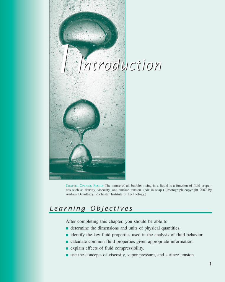
CHAPTER OPENING PHOTO: The nature of air bubbles rising in a liquid is a function of fluid proper-ties such as density, viscosity, and surface tension. (Air in soap.) (Photograph copyright 2007 byAndrew Davidhazy, Rochester Institute of Technology.)

11IntroductionIntroduction

Learn ing Ob j ec t i v e s

After completing this chapter, you should be able to:

■ determine the dimensions and units of physical quantities.

■ identify the key fluid properties used in the analysis of fluid behavior.

■ calculate common fluid properties given appropriate information.

■ explain effects of fluid compressibility.

■ use the concepts of viscosity, vapor pressure, and surface tension.

1

c01Introduction.qxd 9/24/10 11:11 AM Page 1

Fluid mechanics is the discipline within the broad field of applied mechanics that is con-cerned with the behavior of liquids and gases at rest or in motion. It covers a vast array ofphenomena that occur in nature (with or without human intervention), in biology, and innumerous engineered, invented, or manufactured situations. There are few aspects of ourlives that do not involve fluids, either directly or indirectly.

The immense range of different flow conditions is mind-boggling and strongly depen-dent on the value of the numerous parameters that describe fluid flow. Among the long listof parameters involved are (1) the physical size of the flow, ; (2) the speed of the flow,V; and (3) the pressure, p, as indicated in the figure in the margin for a light aircraft para-chute recovery system. These are just three of the important parameters that, along withmany others, are discussed in detail in various sections of this book. To get an inkling ofthe range of some of the parameter values involved and the flow situations generated, con-sider the following.

Size,Every flow has a characteristic (or typical) length associated with it. For example,for flow of fluid within pipes, the pipe diameter is a characteristic length. Pipe flowsinclude the flow of water in the pipes in our homes, the blood flow in our arteriesand veins, and the airflow in our bronchial tree. They also involve pipe sizes that arenot within our everyday experiences. Such examples include the flow of oil acrossAlaska through a 4-foot-diameter, 799-mile-long pipe and, at the other end of the sizescale, the new area of interest involving flow in nanoscale pipes whose diameters are

/

/

2 Chapter 1 ■ Introduction

V1.1 Mt. St. Helenseruption

�

p

V

(Photograph courtesyof CIRRUS DesignCorporation.)

104

106

108

Jupiter red spot diameter

Ocean current diameter

Diameter of hurricane

Mt. St. Helens plume

Average width of middleMississippi River

Boeing 787NACA Ames wind tunnel

Diameter of Space Shuttlemain engine exhaust jet

Outboard motor prop

Water pipe diameter

Raindrop

Water jet cutter widthAmoebaThickness of lubricating oillayer in journal bearingDiameter of smallest bloodvessel

Artificial kidney filterpore size

Nanoscale devices

102

100

10-4

10-2

10-6

10-8

�, m

104

106

Meteor entering atmosphere

Space Shuttle reentry

Rocket nozzle exhaustSpeed of sound in airTornado

Water from fire hose nozzleFlow past bike rider

Mississippi River

Syrup on pancake

Microscopic swimminganimal

Glacier flow

Continental drift

102

100

10-4

10-2

10-6

10-8

V, m

/s

104

106

Fire hydrant

Hydraulic ram

Car engine combustionScuba tank

Water jet cuttingMariana Trench in PacificOcean

Auto tire

Pressure at 40-mile altitude

Vacuum pump

Sound pressure at normaltalking

102

100

10-4

10-2

10-6

p, lb

/ft2

Pressure change causingears to “pop” in elevator

Atmospheric pressure onMars

“Excess pressure” on handheld out of car traveling 60mph

Standard atmosphere

(a) (b) (c)

F I G U R E 1.1 Characteristic values of some fluid flow parameters for a variety of flows: (a) object size, (b) fluid speed, (c) fluid pressure.

V1.2 E. coliswimming

c01Introduction.qxd 9/24/10 11:11 AM Page 2

1.2 Dimensions, Dimensional Homogeneity, and Units 3

on the order of 10�8 m. Each of these pipe flows has important characteristics that arenot found in the others.

Characteristic lengths of some other flows are shown in Fig. 1.1a.

Speed, VAs we note from The Weather Channel, on a given day the wind speed may cover whatwe think of as a wide range, from a gentle 5-mph breeze to a 100-mph hurricane ora 250-mph tornado. However, this speed range is small compared to that of the almostimperceptible flow of the fluid-like magma below the Earth’s surface that drives thecontinental drift motion of the tectonic plates at a speed of about 2 � 10�8 m/s or the hyper-sonic airflow past a meteor as it streaks through the atmosphere at 3 � 104 m/s.

Characteristic speeds of some other flows are shown in Fig. 1.1b.

Pressure, PCharacteristic pressures of some flows are shown in Fig. 1.1c.

1.1 Some Characteristics of Fluids

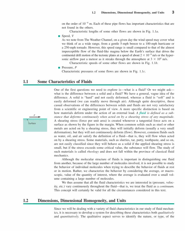
One of the first questions we need to explore is—what is a fluid? Or we might ask—what is the difference between a solid and a fluid? We have a general, vague idea of thedifference. A solid is “hard” and not easily deformed, whereas a fluid is “soft” and iseasily deformed (we can readily move through air). Although quite descriptive, thesecasual observations of the differences between solids and fluids are not very satisfactoryfrom a scientific or engineering point of view. A more specific distinction is based onhow materials deform under the action of an external load. A fluid is defined as a sub-stance that deforms continuously when acted on by a shearing stress of any magnitude.A shearing stress (force per unit area) is created whenever a tangential force acts on asurface as shown by the figure in the margin. When common solids such as steel or othermetals are acted on by a shearing stress, they will initially deform (usually a very smalldeformation), but they will not continuously deform (flow). However, common fluids suchas water, oil, and air satisfy the definition of a fluid—that is, they will flow when actedon by a shearing stress. Some materials, such as slurries, tar, putty, toothpaste, and so on,are not easily classified since they will behave as a solid if the applied shearing stress issmall, but if the stress exceeds some critical value, the substance will flow. The study ofsuch materials is called rheology and does not fall within the province of classical fluidmechanics.

Although the molecular structure of fluids is important in distinguishing one fluidfrom another, because of the large number of molecules involved, it is not possible to studythe behavior of individual molecules when trying to describe the behavior of fluids at restor in motion. Rather, we characterize the behavior by considering the average, or macro-scopic, value of the quantity of interest, where the average is evaluated over a small vol-ume containing a large number of molecules.

We thus assume that all the fluid characteristics we are interested in (pressure, veloc-ity, etc.) vary continuously throughout the fluid—that is, we treat the fluid as a continuum.This concept will certainly be valid for all the circumstances considered in this text.

1.2 Dimensions, Dimensional Homogeneity, and Units

Since we will be dealing with a variety of fluid characteristics in our study of fluid mechan-ics, it is necessary to develop a system for describing these characteristics both qualitativelyand quantitatively. The qualitative aspect serves to identify the nature, or type, of the

F

Surface

c01Introduction.qxd 9/24/10 11:11 AM Page 3

characteristics (such as length, time, stress, and velocity), whereas the quantitative aspectprovides a numerical measure of the characteristics. The quantitative description requiresboth a number and a standard by which various quantities can be compared. A standard forlength might be a meter or foot, for time an hour or second, and for mass a slug or kilo-gram. Such standards are called units, and several systems of units are in common use asdescribed in the following section. The qualitative description is conveniently given in termsof certain primary quantities, such as length, L, time, T, mass, M, and temperature, . Theseprimary quantities can then be used to provide a qualitative description of any other sec-ondary quantity, for example, area � L2, velocity � LT�1, density � ML�3, and so on, wherethe symbol � is used to indicate the dimensions of the secondary quantity in terms of theprimary quantities. Thus, to describe qualitatively a velocity, V, we would write

and say that “the dimensions of a velocity equal length divided by time.” The primary quan-tities are also referred to as basic dimensions.

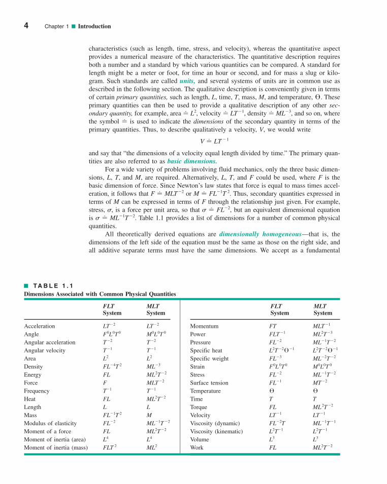
For a wide variety of problems involving fluid mechanics, only the three basic dimen-sions, L, T, and M, are required. Alternatively, L, T, and F could be used, where F is thebasic dimension of force. Since Newton’s law states that force is equal to mass times accel-eration, it follows that F � MLT�2 or M � FL�1T 2. Thus, secondary quantities expressed interms of M can be expressed in terms of F through the relationship just given. For example,stress, �, is a force per unit area, so that � � FL�2, but an equivalent dimensional equationis � � ML�1T�2. Table 1.1 provides a list of dimensions for a number of common physicalquantities.

All theoretically derived equations are dimensionally homogeneous—that is, thedimensions of the left side of the equation must be the same as those on the right side, andall additive separate terms must have the same dimensions. We accept as a fundamental

V � LT �1

™

4 Chapter 1 ■ Introduction

TA B L E 1 . 1

Dimensions Associated with Common Physical Quantities

FLT MLTSystem System

Acceleration LT�2 LT�2

Angle F0L0T 0 M0L0T 0

Angular acceleration T�2 T�2

Angular velocity T�1 T�1

Area L2 L2

Density FL�4T 2 ML�3

Energy FL ML2T�2

Force F MLT�2

Frequency T�1 T�1

Heat FL ML2T�2

Length L LMass FL�1T 2 MModulus of elasticity FL�2 ML�1T �2

Moment of a force FL ML2T�2

Moment of inertia (area) L4 L4

Moment of inertia (mass) FLT 2 ML2

Momentum FT MLT�1

Power FLT�1 ML2T�3

Pressure FL�2 ML�1T�2

Specific heat L2T�2 �1 L2T�2 �1

Specific weight FL�3 ML�2T�2

Strain F0L 0T 0 M0L0T 0

Stress FL�2 ML�1T�2

Surface tension FL�1 MT�2

TemperatureTime T TTorque FL ML 2T�2

Velocity LT�1 LT�1

Viscosity (dynamic) FL�2T ML�1T�1

Viscosity (kinematic) L2T�1 L2T�1

Volume L3 L3

Work FL ML2T�2

™™

™™

FLT MLTSystem System

c01Introduction.qxd 9/24/10 11:11 AM Page 4

1.2 Dimensions, Dimensional Homogeneity, and Units 5

premise that all equations describing physical phenomena must be dimensionally homoge-neous. For example, the equation for the velocity, V, of a uniformly accelerated body is

(1.1)

where V0 is the initial velocity, a the acceleration, and t the time interval. In terms of dimen-sions the equation is

and thus Eq. 1.1 is dimensionally homogeneous.Some equations that are known to be valid contain constants having dimensions. The

equation for the distance, d, traveled by a freely falling body can be written as

(1.2)

and a check of the dimensions reveals that the constant must have the dimensions of LT�2

if the equation is to be dimensionally homogeneous. Actually, Eq. 1.2 is a special form ofthe well-known equation from physics for freely falling bodies,

(1.3)

in which g is the acceleration of gravity. Equation 1.3 is dimensionally homogeneous andvalid in any system of units. For g � 32.2 ft/s2 the equation reduces to Eq. 1.2, and thusEq. 1.2 is valid only for the system of units using feet and seconds. Equations that arerestricted to a particular system of units can be denoted as restricted homogeneous equa-tions, as opposed to equations valid in any system of units, which are general homogeneousequations. The concept of dimensions also forms the basis for the powerful tool of dimen-sional analysis, which is considered in detail in Chapter 7.

Note to the users of this text. All of the examples in the text use a consistent problem-solving methodology, which is similar to that in other engineering courses such as statics.Each example highlights the key elements of analysis: Given, Find, Solution, and Comment.

The Given and Find are steps that ensure the user understands what is being askedin the problem and explicitly list the items provided to help solve the problem.

The Solution step is where the equations needed to solve the problem are formulatedand the problem is actually solved. In this step, there are typically several other tasks thathelp to set up the solution and are required to solve the problem. The first is a drawing ofthe problem; where appropriate, it is always helpful to draw a sketch of the problem. Herethe relevant geometry and coordinate system to be used as well as features such as controlvolumes, forces and pressures, velocities, and mass flow rates are included. This helps ingaining a visual understanding of the problem. Making appropriate assumptions to solvethe problem is the second task. In a realistic engineering problem-solving environment, thenecessary assumptions are developed as an integral part of the solution process. Assump-tions can provide appropriate simplifications or offer useful constraints, both of which canhelp in solving the problem. Throughout the examples in this text, the necessary assump-tions are embedded within the Solution step, as they are in solving a real-world problem.This provides a realistic problem-solving experience.

The final element in the methodology is the Comment. For the examples in the text,this section is used to provide further insight into the problem or the solution. It can alsobe a point in the analysis at which certain questions are posed. For example: Is the answerreasonable, and does it make physical sense? Are the final units correct? If a certain pa-rameter were changed, how would the answer change? Adopting this type of methodologywill aid in the development of problem-solving skills for fluid mechanics, as well as otherengineering disciplines.

d �gt2

2

d � 16.1t 2

LT �1 � LT

�1 � LT �1

V � V0 � at

c01Introduction.qxd 9/24/10 11:11 AM Page 5

6 Chapter 1 ■ Introduction

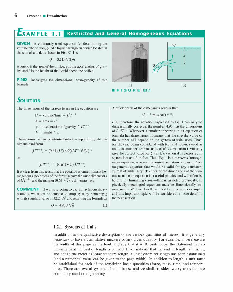
GIVEN A commonly used equation for determining thevolume rate of flow, Q, of a liquid through an orifice located inthe side of a tank as shown in Fig. E1.1 is

where A is the area of the orifice, g is the acceleration of grav-ity, and h is the height of the liquid above the orifice.

FIND Investigate the dimensional homogeneity of thisformula.

Q � 0.61A12gh

SOLUTION

Restricted and General Homogeneous Equations

A quick check of the dimensions reveals that

and, therefore, the equation expressed as Eq. 1 can only bedimensionally correct if the number, 4.90, has the dimensionsof L1/ 2T�1. Whenever a number appearing in an equation orformula has dimensions, it means that the specific value ofthe number will depend on the system of units used. Thus,for the case being considered with feet and seconds used asunits, the number 4.90 has units of ft1/ 2/s. Equation 1 will onlygive the correct value for Q (in ft3/s) when A is expressed insquare feet and h in feet. Thus, Eq. 1 is a restricted homoge-neous equation, whereas the original equation is a general ho-mogeneous equation that would be valid for any consistentsystem of units. A quick check of the dimensions of the vari-ous terms in an equation is a useful practice and will often behelpful in eliminating errors—that is, as noted previously, allphysically meaningful equations must be dimensionally ho-mogeneous. We have briefly alluded to units in this example,and this important topic will be considered in more detail inthe next section.

L3T �1 � 14.902 1L5/2 2

EXAMPLE 1.1

The dimensions of the various terms in the equation are

These terms, when substituted into the equation, yield thedimensional form

or

It is clear from this result that the equation is dimensionally ho-mogeneous (both sides of the formula have the same dimensionsof L3T�1), and the number (0.61 ) is dimensionless.

COMMENT If we were going to use this relationship re-peatedly, we might be tempted to simplify it by replacing gwith its standard value of 32.2 ft/s2 and rewriting the formula as

(1)Q � 4.90 A1h

12

1L3T �12 � 3 10.61212 4 1L3 T

�12

1L3T �12 � 10.612 1L22 1122 1LT

�221/21L21/2

h � height � L

g � acceleration of gravity � LT �2

A � area � L2

Q � volume/time � L3T �1

(a)

h

AQ

(b)

F I G U R E E1.1

1.2.1 Systems of Units

In addition to the qualitative description of the various quantities of interest, it is generallynecessary to have a quantitative measure of any given quantity. For example, if we measurethe width of this page in the book and say that it is 10 units wide, the statement has nomeaning until the unit of length is defined. If we indicate that the unit of length is a meter,and define the meter as some standard length, a unit system for length has been established(and a numerical value can be given to the page width). In addition to length, a unit mustbe established for each of the remaining basic quantities (force, mass, time, and tempera-ture). There are several systems of units in use and we shall consider two systems that arecommonly used in engineering.

c01Introduction.qxd 9/24/10 11:11 AM Page 6

1.2 Dimensions, Dimensional Homogeneity, and Units 7

F l u i d s i n t h e N e w s

How long is a foot? Today, in the United States, the commonlength unit is the foot, but throughout antiquity the unit used tomeasure length has quite a history. The first length units werebased on the lengths of various body parts. One of the earliestunits was the Egyptian cubit, first used around 3000 B.C. anddefined as the length of the arm from elbow to extended fin-gertips. Other measures followed with the foot simply takenas the length of a man’s foot. Since this length obviouslyvaries from person to person it was often “standardized” byusing the length of the current reigning royalty’s foot. In 1791

a special French commission proposed that a new universallength unit called a meter (metre) be defined as the distanceof one-quarter of the earth’s meridian (north pole to the equa-tor) divided by 10 million. Although controversial, the meterwas accepted in 1799 as the standard. With the developmentof advanced technology, the length of a meter was redefinedin 1983 as the distance traveled by light in a vacuum duringthe time interval of 1/299,792,458 s. The foot is now definedas 0.3048 meter. Our simple rulers and yardsticks indeedhave an intriguing history.

International System (SI). In 1960, the Eleventh General Conference on Weightsand Measures, the international organization responsible for maintaining precise uniform stan-dards of measurements, formally adopted the International System of Units as the interna-tional standard. This system, commonly termed SI, has been adopted worldwide and is widelyused (although certainly not exclusively) in the United States. It is expected that the long-termtrend will be for all countries to accept SI as the accepted standard, and it is imperative thatengineering students become familiar with this system. In SI the unit of length is the meter(m), the time unit is the second (s), the mass unit is the kilogram (kg), and the temperatureunit is the kelvin (K). Note that there is no degree symbol used when expressing a tempera-ture in kelvin units. The Kelvin temperature scale is an absolute scale and is related to theCelsius (centigrade) scale (�C) through the relationship

Although the Celsius scale is not in itself part of SI, it is common practice to specify tem-peratures in degrees Celsius when using SI units.

K � °C � 273.15

British Gravitational (BG) System. In the BG system the unit of length is thefoot (ft), the time unit is the second (s), the force unit is the pound (lb), and the temperatureunit is the degree Fahrenheit (�F), or the absolute temperature unit is the degree Rankine (�R),where

The mass unit, called the slug, is defined from Newton’s second law (force � mass �acceleration) as

This relationship indicates that a 1-lb force acting on a mass of 1 slug will give the massan acceleration of 1 ft/s2.

The weight, w (which is the force due to gravity, g), of a mass, m, is given by theequation

w � mg

and in BG units

w

Since Earth’s standard gravity is taken as g � 32.174 ft/s2 (commonly approximated as32.2 ft/s2), it follows that a mass of 1 slug weighs 32.2 lb under standard gravity.

1lb2 � m 1slugs2 g 1ft/s22

1 lb � 11 slug2 11 ft/s22

°R � °F � 459.67

c01Introduction.qxd 9/24/10 11:11 AM Page 7

The force unit, called the newton (N), is defined from Newton’s second law as

Thus, a 1-N force acting on a 1-kg mass will give the mass an acceleration of 1 m/s2. Stan-dard gravity in SI is 9.807 m/s2 (commonly approximated as 9.81 m/s2) so that a 1-kg massweighs 9.81 N under standard gravity. Note that weight and mass are different, both qual-itatively and quantitatively! The unit of work in SI is the joule (J), which is the work donewhen the point of application of a 1-N force is displaced through a 1-m distance in thedirection of the force. Thus,

The unit of power is the watt (W) defined as a joule per second. Thus,

Prefixes for forming multiples and fractions of SI units are commonly used. For exam-ple, the notation kN would be read as “kilonewtons” and stands for 103 N. Similarly, mmwould be read as “millimeters” and stands for 10�3 m. The centimeter is not an acceptedunit of length in the SI system, and for most problems in fluid mechanics in which SI unitsare used, lengths will be expressed in millimeters or meters.

In this text we will use the BG system and SI for units. Approximately one-half theproblems and examples are given in BG units and one-half in SI units. Tables 1.2 and 1.3provide conversion factors for some quantities that are commonly encountered in fluidmechanics, and these tables are located on the inside of the back cover. Note that in thesetables (and others) the numbers are expressed by using computer exponential notation. Forexample, the number 5.154 E � 2 is equivalent to 5.154 � 102 in scientific notation, andthe number 2.832 E � 2 is equivalent to 2.832 � 10�2. More extensive tables of conver-sion factors for a large variety of unit systems can be found in Appendix E.

1 W � 1 J/s � 1 N.m/s

1 J � 1 N.m

1 N � 11 kg2 11 m/s22

8 Chapter 1 ■ Introduction

TA B L E 1 . 2

Conversion Factors from BG Units to SI Units

(See inside of back cover.)

TA B L E 1 . 3

Conversion Factors from SI Units to BG Units

(See inside of back cover.)

F l u i d s i n t h e N e w s

Units and space travel A NASA spacecraft, the Mars ClimateOrbiter, was launched in December 1998 to study the Martiangeography and weather patterns. The spacecraft was slated tobegin orbiting Mars on September 23, 1999. However, NASAofficials lost communication with the spacecraft early thatday, and it is believed that the spacecraft broke apart or over-heated because it came too close to the surface of Mars. Errors

in the maneuvering commands sent from Earth caused theOrbiter to sweep within 37 miles of the surface rather than theintended 93 miles. The subsequent investigation revealed thatthe errors were due to a simple mix-up in units. One team con-trolling the Orbiter used SI units whereas another team usedBG units. This costly experience illustrates the importance ofusing a consistent system of units.

c01Introduction.qxd 9/24/10 11:11 AM Page 8

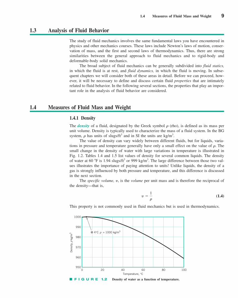
1.4 Measures of Fluid Mass and Weight 9

1.3 Analysis of Fluid Behavior

The study of fluid mechanics involves the same fundamental laws you have encountered inphysics and other mechanics courses. These laws include Newton’s laws of motion, conser-vation of mass, and the first and second laws of thermodynamics. Thus, there are strongsimilarities between the general approach to fluid mechanics and to rigid-body anddeformable-body solid mechanics.

The broad subject of fluid mechanics can be generally subdivided into fluid statics,in which the fluid is at rest, and fluid dynamics, in which the fluid is moving. In subse-quent chapters we will consider both of these areas in detail. Before we can proceed, how-ever, it will be necessary to define and discuss certain fluid properties that are intimatelyrelated to fluid behavior. In the following several sections, the properties that play an impor-tant role in the analysis of fluid behavior are considered.

1.4 Measures of Fluid Mass and Weight

1.4.1 Density

The density of a fluid, designated by the Greek symbol � (rho), is defined as its mass perunit volume. Density is typically used to characterize the mass of a fluid system. In the BGsystem, � has units of slugs/ft3 and in SI the units are kg/m3.

The value of density can vary widely between different fluids, but for liquids, varia-tions in pressure and temperature generally have only a small effect on the value of �. Thesmall change in the density of water with large variations in temperature is illustrated inFig. 1.2. Tables 1.4 and 1.5 list values of density for several common liquids. The densityof water at 60 �F is 1.94 slugs/ft3 or 999 kg/m3. The large difference between those two val-ues illustrates the importance of paying attention to units! Unlike liquids, the density of agas is strongly influenced by both pressure and temperature, and this difference is discussedin the next section.

The specific volume, y, is the volume per unit mass and is therefore the reciprocal ofthe density—that is,

(1.4)

This property is not commonly used in fluid mechanics but is used in thermodynamics.

y �1�

F I G U R E 1.2 Density of water as a function of temperature.

@ 4°C = 1000 kg/m3

1000

990

980

970

960

9500

Den

sity

,

kg/m

3ρ

20 40 60 80 100Temperature, °C

ρ

c01Introduction.qxd 9/24/10 11:11 AM Page 9

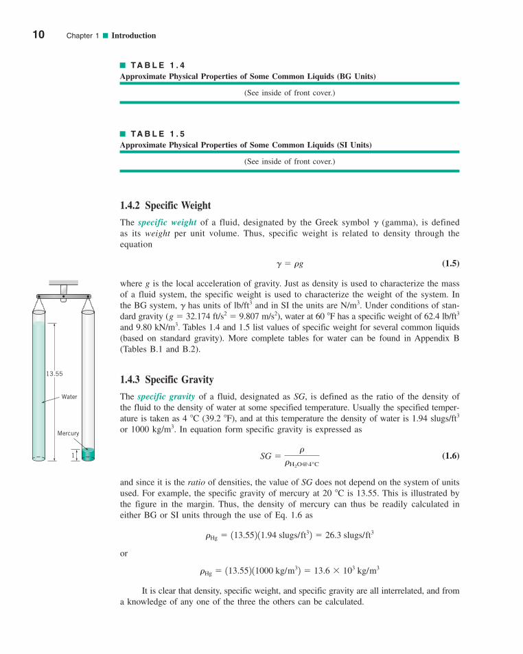
1.4.2 Specific Weight

The specific weight of a fluid, designated by the Greek symbol � (gamma), is definedas its weight per unit volume. Thus, specific weight is related to density through theequation

(1.5)

where g is the local acceleration of gravity. Just as density is used to characterize the massof a fluid system, the specific weight is used to characterize the weight of the system. Inthe BG system, � has units of lb/ft3 and in SI the units are N/m3. Under conditions of stan-dard gravity (g � 32.174 ft/s2 � 9.807 m/s2), water at 60 �F has a specific weight of 62.4 lb/ft3

and 9.80 kN/m3. Tables 1.4 and 1.5 list values of specific weight for several common liquids(based on standard gravity). More complete tables for water can be found in Appendix B(Tables B.1 and B.2).

1.4.3 Specific Gravity

The specific gravity of a fluid, designated as SG, is defined as the ratio of the density ofthe fluid to the density of water at some specified temperature. Usually the specified temper-ature is taken as 4 �C (39.2 �F), and at this temperature the density of water is 1.94 slugs/ft3

or 1000 kg/m3. In equation form specific gravity is expressed as

(1.6)

and since it is the ratio of densities, the value of SG does not depend on the system of unitsused. For example, the specific gravity of mercury at 20 �C is 13.55. This is illustrated bythe figure in the margin. Thus, the density of mercury can thus be readily calculated ineither BG or SI units through the use of Eq. 1.6 as

or

It is clear that density, specific weight, and specific gravity are all interrelated, and froma knowledge of any one of the three the others can be calculated.

�Hg � 113.552 11000 kg/m32 � 13.6 � 103 kg/m3

�Hg � 113.552 11.94 slugs/ft32 � 26.3 slugs/ft3

SG ��

�H2O@4°C

� � �g

10 Chapter 1 ■ Introduction

TA B L E 1 . 4

Approximate Physical Properties of Some Common Liquids (BG Units)

(See inside of front cover.)

TA B L E 1 . 5

Approximate Physical Properties of Some Common Liquids (SI Units)

(See inside of front cover.)

13.55

1

Water

Mercury

c01Introduction.qxd 9/24/10 11:11 AM Page 10

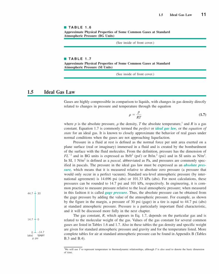
1.5 Ideal Gas Law 11

1.5 Ideal Gas Law

Gases are highly compressible in comparison to liquids, with changes in gas density directlyrelated to changes in pressure and temperature through the equation

(1.7)

where p is the absolute pressure, � the density, T the absolute temperature,1 and R is a gasconstant. Equation 1.7 is commonly termed the perfect or ideal gas law, or the equation ofstate for an ideal gas. It is known to closely approximate the behavior of real gases undernormal conditions when the gases are not approaching liquefaction.

Pressure in a fluid at rest is defined as the normal force per unit area exerted on aplane surface (real or imaginary) immersed in a fluid and is created by the bombardmentof the surface with the fluid molecules. From the definition, pressure has the dimension ofFL�2 and in BG units is expressed as lb/ft2 (psf) or lb/in.2 (psi) and in SI units as N/m2.In SI, 1 N/m2 is defined as a pascal, abbreviated as Pa, and pressures are commonly spec-ified in pascals. The pressure in the ideal gas law must be expressed as an absolute pres-sure, which means that it is measured relative to absolute zero pressure (a pressure thatwould only occur in a perfect vacuum). Standard sea-level atmospheric pressure (by inter-national agreement) is 14.696 psi (abs) or 101.33 kPa (abs). For most calculations, thesepressures can be rounded to 14.7 psi and 101 kPa, respectively. In engineering, it is com-mon practice to measure pressure relative to the local atmospheric pressure; when measuredin this fashion it is called gage pressure. Thus, the absolute pressure can be obtained fromthe gage pressure by adding the value of the atmospheric pressure. For example, as shownby the figure in the margin, a pressure of 30 psi (gage) in a tire is equal to 44.7 psi (abs)at standard atmospheric pressure. Pressure is a particularly important fluid characteristic,and it will be discussed more fully in the next chapter.

The gas constant, R, which appears in Eq. 1.7, depends on the particular gas and isrelated to the molecular weight of the gas. Values of the gas constant for several commongases are listed in Tables 1.6 and 1.7. Also in these tables the gas density and specific weightare given for standard atmospheric pressure and gravity and for the temperature listed. Morecomplete tables for air at standard atmospheric pressure can be found in Appendix B (TablesB.3 and B.4).

� �p

RT

1We will use T to represent temperature in thermodynamic relationships, although T is also used to denote the basic dimensionof time.

TA B L E 1 . 6

Approximate Physical Properties of Some Common Gases at Standard Atmospheric Pressure (BG Units)

(See inside of front cover.)

TA B L E 1 . 7

Approximate Physical Properties of Some Common Gases at Standard Atmospheric Pressure (SI Units)

(See inside of front cover.)

44.7

14.7 0

0 –14.7

30

(abs) (gage)p, psi

c01Introduction.qxd 9/24/10 11:11 AM Page 11

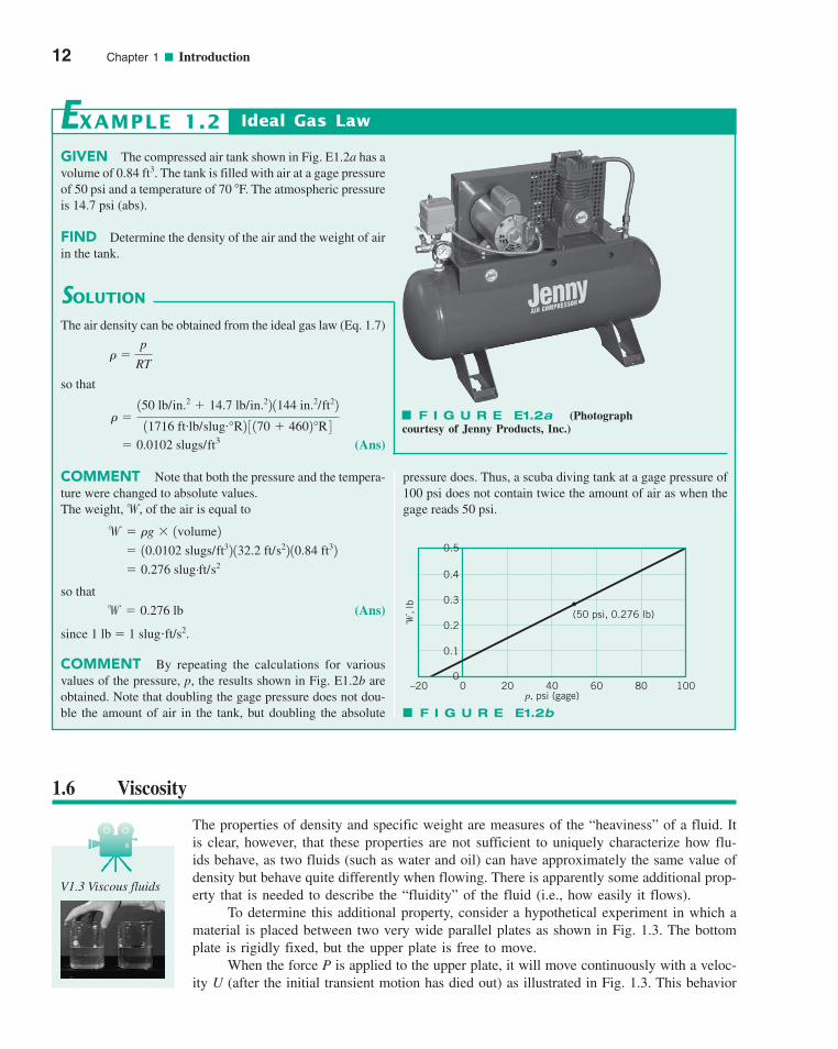
12 Chapter 1 ■ Introduction

GIVEN The compressed air tank shown in Fig. E1.2a has avolume of 0.84 ft3. The tank is filled with air at a gage pressureof 50 psi and a temperature of 70 �F. The atmospheric pressureis 14.7 psi (abs).

FIND Determine the density of the air and the weight of airin the tank.

SOLUTION

Ideal Gas Law

pressure does. Thus, a scuba diving tank at a gage pressure of100 psi does not contain twice the amount of air as when thegage reads 50 psi.

EXAMPLE 1.2

The air density can be obtained from the ideal gas law (Eq. 1.7)

so that

(Ans)

COMMENT Note that both the pressure and the tempera-ture were changed to absolute values.The weight,w, of the air is equal to

so that

(Ans)

since 1 lb � 1 slug�ft/s2.

COMMENT By repeating the calculations for variousvalues of the pressure, p, the results shown in Fig. E1.2b areobtained. Note that doubling the gage pressure does not dou-ble the amount of air in the tank, but doubling the absolute

w � 0.276 lb

� 0.276 slug..ft/s2

� 10.0102 slugs/ft32 132.2 ft/s22 10.84 ft32

w � �g � 1volume2

� 0.0102 slugs/ft3

� �150 lb/in.2 � 14.7 lb/in.22 1144 in.2/ft22

11716 ft.lb/slug.°R2 3 170 � 4602°R 4

� �p

RT

F I G U R E E1.2a (Photograph courtesy of Jenny Products, Inc.)

10080604020–20 0p, psi (gage)

w, l

b

(50 psi, 0.276 lb)

0.4

0.3

0.2

0.1

0

0.5

F I G U R E E1.2b

V1.3 Viscous fluids

1.6 Viscosity

The properties of density and specific weight are measures of the “heaviness” of a fluid. Itis clear, however, that these properties are not sufficient to uniquely characterize how flu-ids behave, as two fluids (such as water and oil) can have approximately the same value ofdensity but behave quite differently when flowing. There is apparently some additional prop-erty that is needed to describe the “fluidity” of the fluid (i.e., how easily it flows).

To determine this additional property, consider a hypothetical experiment in which amaterial is placed between two very wide parallel plates as shown in Fig. 1.3. The bottomplate is rigidly fixed, but the upper plate is free to move.

When the force P is applied to the upper plate, it will move continuously with a veloc-ity U (after the initial transient motion has died out) as illustrated in Fig. 1.3. This behavior

c01Introduction.qxd 9/24/10 11:11 AM Page 12

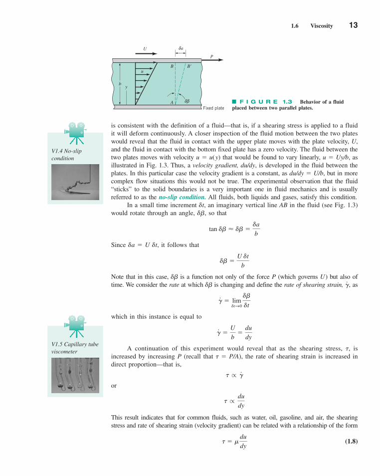
1.6 Viscosity 13

is consistent with the definition of a fluid—that is, if a shearing stress is applied to a fluidit will deform continuously. A closer inspection of the fluid motion between the two plateswould reveal that the fluid in contact with the upper plate moves with the plate velocity, U,and the fluid in contact with the bottom fixed plate has a zero velocity. The fluid between thetwo plates moves with velocity u � u(y) that would be found to vary linearly, u � Uy/b, asillustrated in Fig. 1.3. Thus, a velocity gradient, du/dy, is developed in the fluid between theplates. In this particular case the velocity gradient is a constant, as du/dy � U/b, but in morecomplex flow situations this would not be true. The experimental observation that the fluid“sticks” to the solid boundaries is a very important one in fluid mechanics and is usuallyreferred to as the no-slip condition. All fluids, both liquids and gases, satisfy this condition.

In a small time increment �t, an imaginary vertical line AB in the fluid (see Fig. 1.3)would rotate through an angle, ��, so that

Since �a � U �t, it follows that

Note that in this case, �� is a function not only of the force P (which governs U) but also oftime. We consider the rate at which �� is changing and define the rate of shearing strain, as

which in this instance is equal to

A continuation of this experiment would reveal that as the shearing stress, �, isincreased by increasing P (recall that � � P/A), the rate of shearing strain is increased indirect proportion—that is,

or

This result indicates that for common fluids, such as water, oil, gasoline, and air, the shearingstress and rate of shearing strain (velocity gradient) can be related with a relationship of the form

(1.8)� � �

du

dy

� rdu

dy

� r �#

�#

�U

b�

du

dy

�#

� lim�tS0

��

�t

�#,

�� �U �t

b

tan �� � �� ��a

b

V1.4 No-slip condition

V1.5 Capillary tubeviscometer

F I G U R E 1.3 Behavior of a fluid placed between two parallel plates.

b

U

δβ

B'B

P

u

Fixed plate

y

δ

A

a

c01Introduction.qxd 9/24/10 11:11 AM Page 13

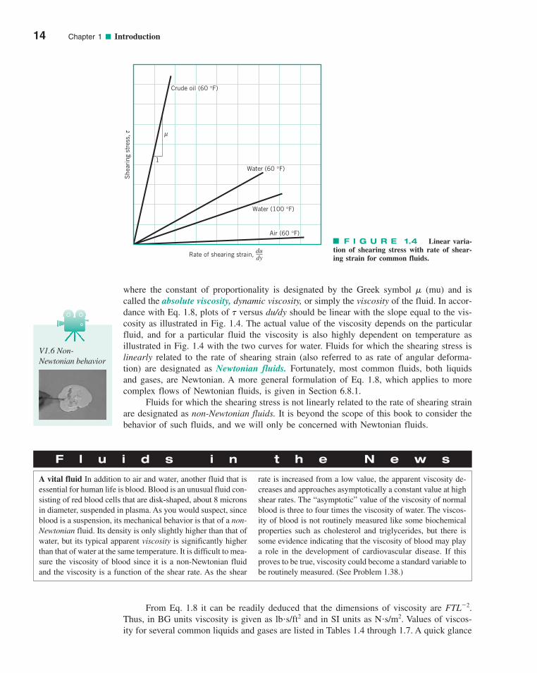
where the constant of proportionality is designated by the Greek symbol � (mu) and iscalled the absolute viscosity, dynamic viscosity, or simply the viscosity of the fluid. In accor-dance with Eq. 1.8, plots of � versus du/dy should be linear with the slope equal to the vis-cosity as illustrated in Fig. 1.4. The actual value of the viscosity depends on the particularfluid, and for a particular fluid the viscosity is also highly dependent on temperature asillustrated in Fig. 1.4 with the two curves for water. Fluids for which the shearing stress islinearly related to the rate of shearing strain (also referred to as rate of angular deforma-tion) are designated as Newtonian fluids. Fortunately, most common fluids, both liquidsand gases, are Newtonian. A more general formulation of Eq. 1.8, which applies to morecomplex flows of Newtonian fluids, is given in Section 6.8.1.

Fluids for which the shearing stress is not linearly related to the rate of shearing strainare designated as non-Newtonian fluids. It is beyond the scope of this book to consider thebehavior of such fluids, and we will only be concerned with Newtonian fluids.

14 Chapter 1 ■ Introduction

V1.6 Non-Newtonian behavior

F I G U R E 1.4 Linear varia-tion of shearing stress with rate of shear-ing strain for common fluids.

She

arin

g st

ress

,

Crude oil (60 °F)

μ

1Water (60 °F)

Water (100 °F)

Air (60 °F)

Rate of shearing strain, du__dy

τ

F l u i d s i n t h e N e w s

A vital fluid In addition to air and water, another fluid that isessential for human life is blood. Blood is an unusual fluid con-sisting of red blood cells that are disk-shaped, about 8 micronsin diameter, suspended in plasma. As you would suspect, sinceblood is a suspension, its mechanical behavior is that of a non-Newtonian fluid. Its density is only slightly higher than that ofwater, but its typical apparent viscosity is significantly higherthan that of water at the same temperature. It is difficult to mea-sure the viscosity of blood since it is a non-Newtonian fluidand the viscosity is a function of the shear rate. As the shear

rate is increased from a low value, the apparent viscosity de-creases and approaches asymptotically a constant value at highshear rates. The “asymptotic” value of the viscosity of normalblood is three to four times the viscosity of water. The viscos-ity of blood is not routinely measured like some biochemicalproperties such as cholesterol and triglycerides, but there issome evidence indicating that the viscosity of blood may playa role in the development of cardiovascular disease. If thisproves to be true, viscosity could become a standard variable tobe routinely measured. (See Problem 1.38.)

From Eq. 1.8 it can be readily deduced that the dimensions of viscosity are FTL�2.Thus, in BG units viscosity is given as lb�s/ft2 and in SI units as N�s/m2. Values of viscos-ity for several common liquids and gases are listed in Tables 1.4 through 1.7. A quick glance

c01Introduction.qxd 9/24/10 11:11 AM Page 14

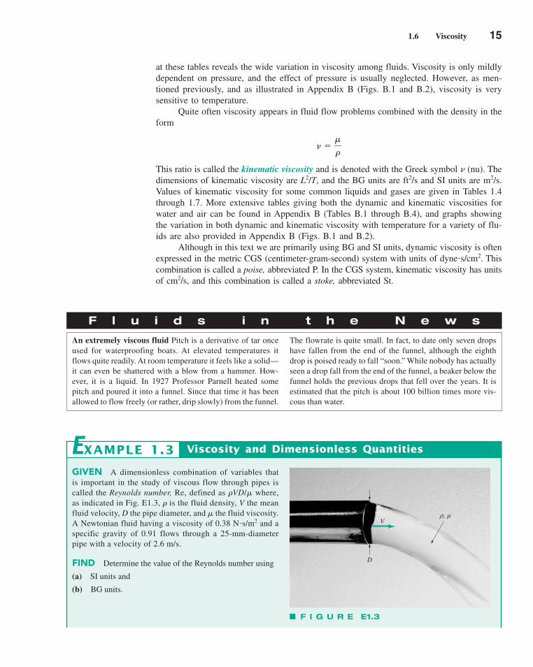
1.6 Viscosity 15

at these tables reveals the wide variation in viscosity among fluids. Viscosity is only mildlydependent on pressure, and the effect of pressure is usually neglected. However, as men-tioned previously, and as illustrated in Appendix B (Figs. B.1 and B.2), viscosity is verysensitive to temperature.

Quite often viscosity appears in fluid flow problems combined with the density in theform

This ratio is called the kinematic viscosity and is denoted with the Greek symbol (nu). Thedimensions of kinematic viscosity are L2/T, and the BG units are ft2/s and SI units are m2/s.Values of kinematic viscosity for some common liquids and gases are given in Tables 1.4through 1.7. More extensive tables giving both the dynamic and kinematic viscosities forwater and air can be found in Appendix B (Tables B.1 through B.4), and graphs showingthe variation in both dynamic and kinematic viscosity with temperature for a variety of flu-ids are also provided in Appendix B (Figs. B.1 and B.2).

Although in this text we are primarily using BG and SI units, dynamic viscosity is oftenexpressed in the metric CGS (centimeter-gram-second) system with units of dyne�s/cm2. Thiscombination is called a poise, abbreviated P. In the CGS system, kinematic viscosity has unitsof cm2/s, and this combination is called a stoke, abbreviated St.

� ��

�

F l u i d s i n t h e N e w s

An extremely viscous fluid Pitch is a derivative of tar onceused for waterproofing boats. At elevated temperatures itflows quite readily. At room temperature it feels like a solid—it can even be shattered with a blow from a hammer. How-ever, it is a liquid. In 1927 Professor Parnell heated somepitch and poured it into a funnel. Since that time it has beenallowed to flow freely (or rather, drip slowly) from the funnel.

The flowrate is quite small. In fact, to date only seven dropshave fallen from the end of the funnel, although the eighthdrop is poised ready to fall “soon.” While nobody has actuallyseen a drop fall from the end of the funnel, a beaker below thefunnel holds the previous drops that fell over the years. It isestimated that the pitch is about 100 billion times more vis-cous than water.

GIVEN A dimensionless combination of variables thatis important in the study of viscous flow through pipes iscalled the Reynolds number, Re, defined as �VD/� where,as indicated in Fig. E1.3, � is the fluid density, V the meanfluid velocity, D the pipe diameter, and � the fluid viscosity.A Newtonian fluid having a viscosity of 0.38 N�s/m2 and aspecific gravity of 0.91 flows through a 25-mm-diameterpipe with a velocity of 2.6 m/s.

FIND Determine the value of the Reynolds number using

(a) SI units and

(b) BG units.

Viscosity and Dimensionless QuantitiesEXAMPLE 1.3

F I G U R E E1.3

V

D

r, m

c01Introduction.qxd 9/24/10 11:11 AM Page 15

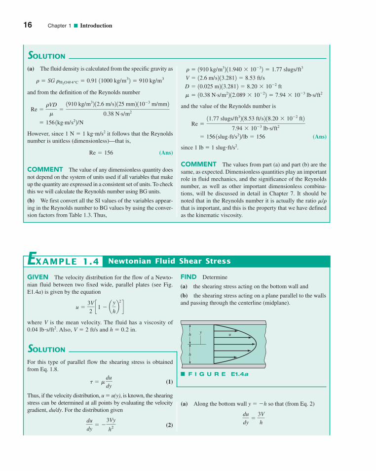
16 Chapter 1 ■ Introduction

SOLUTION

and the value of the Reynolds number is

(Ans)

since 1 lb � 1 slug�ft/s2.

COMMENT The values from part (a) and part (b) are thesame, as expected. Dimensionless quantities play an importantrole in fluid mechanics, and the significance of the Reynoldsnumber, as well as other important dimensionless combina-tions, will be discussed in detail in Chapter 7. It should benoted that in the Reynolds number it is actually the ratio �/�that is important, and this is the property that we have definedas the kinematic viscosity.

� 156 1slug.ft/s22/lb � 156

Re �11.77 slugs/ft32 18.53 ft/s2 18.20 � 10�2 ft2

7.94 � 10�3 lb.s/ft2

� � 10.38 N.s/m22 12.089 � 10�22 � 7.94 � 10�3 lb.s/ft2

D � 10.025 m2 13.2812 � 8.20 � 10�2 ft

V � 12.6 m/s2 13.2812 � 8.53 ft/s

� � 1910 kg/m32 11.940 � 10�32 � 1.77 slugs/ft3(a) The fluid density is calculated from the specific gravity as

and from the definition of the Reynolds number

However, since 1 N � 1 kg�m/s2 it follows that the Reynoldsnumber is unitless (dimensionless)—that is,

(Ans)

COMMENT The value of any dimensionless quantity doesnot depend on the system of units used if all variables that makeup the quantity are expressed in a consistent set of units. To checkthis we will calculate the Reynolds number using BG units.

(b) We first convert all the SI values of the variables appear-ing in the Reynolds number to BG values by using the conver-sion factors from Table 1.3. Thus,

Re � 156

� 156 1kg.m/s22/N

Re ��VD

��1910 kg/m32 12.6 m/s2 125 mm2 110�3 m/mm 2

0.38 N.s/m2

� � SG �H2O@4°C � 0.91 11000 kg/m32 � 910 kg/m3

GIVEN The velocity distribution for the flow of a Newto-nian fluid between two fixed wide, parallel plates (see Fig.E1.4a) is given by the equation

where V is the mean velocity. The fluid has a viscosity of0.04 lb�s/ft2. Also, V � 2 ft/s and h � 0.2 in.

u �3V

2c1 � a

y

hb

2

d

SOLUTION

Newtonian Fluid Shear Stress

(a) Along the bottom wall y � �h so that (from Eq. 2)

du

dy�

3V

h

FIND Determine

(a) the shearing stress acting on the bottom wall and

(b) the shearing stress acting on a plane parallel to the wallsand passing through the centerline (midplane).

EXAMPLE 1.4

For this type of parallel flow the shearing stress is obtainedfrom Eq. 1.8.

(1)

Thus, if the velocity distribution, u � u(y), is known, the shearingstress can be determined at all points by evaluating the velocitygradient, du/dy. For the distribution given

(2)du

dy� �

3Vy

h2

� � �

du

dy

F I G U R E E1.4a

h

h

y u

c01Introduction.qxd 9/24/10 11:12 AM Page 16

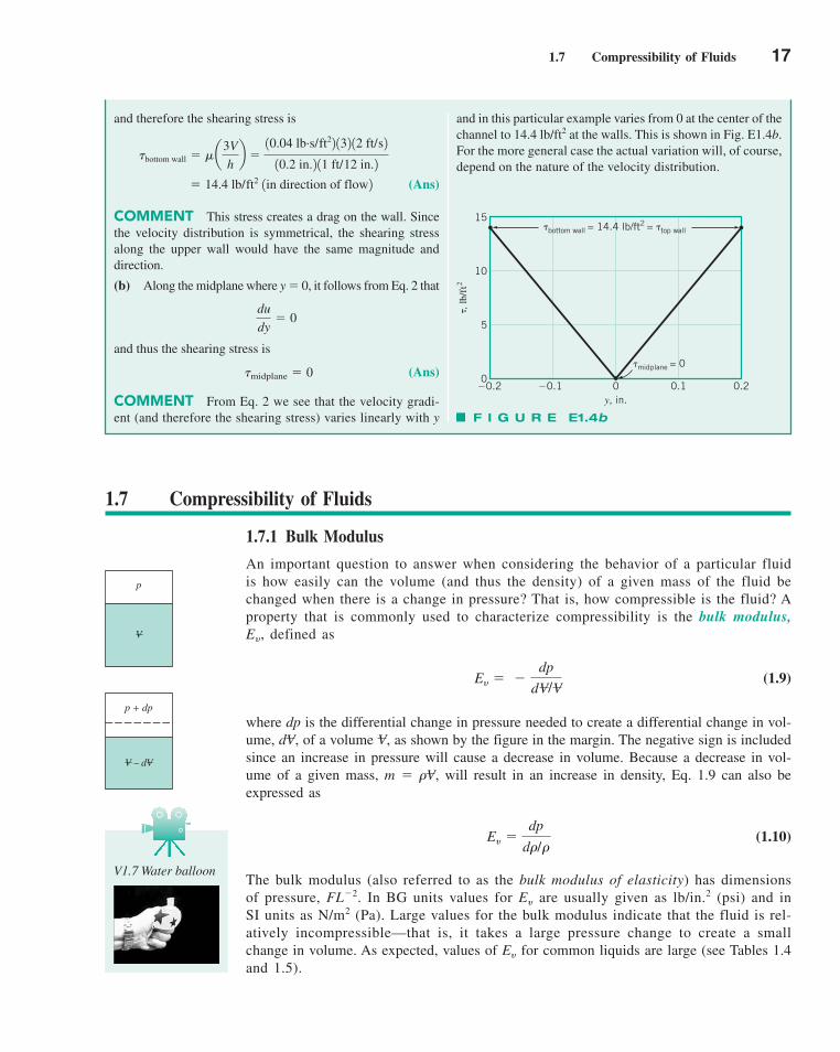
�0.2 �0.1 0 0.1 0.2

15

10

5

0

, lb

/ft2

y, in.

midplane = 0

bottom wall = 14.4 lb/ft2 = top wall

1.7 Compressibility of Fluids 17

and therefore the shearing stress is

(Ans)

COMMENT This stress creates a drag on the wall. Sincethe velocity distribution is symmetrical, the shearing stressalong the upper wall would have the same magnitude and direction.

(b) Along the midplane where y � 0, it follows from Eq. 2 that

and thus the shearing stress is

(Ans)

COMMENT From Eq. 2 we see that the velocity gradi-ent (and therefore the shearing stress) varies linearly with y

�midplane � 0

du

dy� 0

� 14.4 lb/ft2 1in direction of flow2

�bottom wall � � a3V

hb �

10.04 lb.s/ft22 132 12 ft/s2

10.2 in.2 11 ft/12 in.2

and in this particular example varies from 0 at the center of thechannel to 14.4 lb/ft2 at the walls. This is shown in Fig. E1.4b.For the more general case the actual variation will, of course,depend on the nature of the velocity distribution.

F I G U R E E1.4b

1.7 Compressibility of Fluids

1.7.1 Bulk Modulus

An important question to answer when considering the behavior of a particular fluidis how easily can the volume (and thus the density) of a given mass of the fluid bechanged when there is a change in pressure? That is, how compressible is the fluid? Aproperty that is commonly used to characterize compressibility is the bulk modulus,Ey, defined as

(1.9)

where dp is the differential change in pressure needed to create a differential change in vol-ume, of a volume , as shown by the figure in the margin. The negative sign is includedsince an increase in pressure will cause a decrease in volume. Because a decrease in vol-ume of a given mass, m � will result in an increase in density, Eq. 1.9 can also beexpressed as

(1.10)

The bulk modulus (also referred to as the bulk modulus of elasticity) has dimensionsof pressure, FL�2. In BG units values for Ey are usually given as lb/in.2 (psi) and inSI units as N/m2 (Pa). Large values for the bulk modulus indicate that the fluid is rel-atively incompressible—that is, it takes a large pressure change to create a smallchange in volume. As expected, values of Ey for common liquids are large (see Tables 1.4and 1.5).

Ey �dp

d�/�

�V,

VdV,

Ey � �dp

dV/V

p

V

p + dp

V – dV

V1.7 Water balloon

c01Introduction.qxd 9/24/10 11:12 AM Page 17

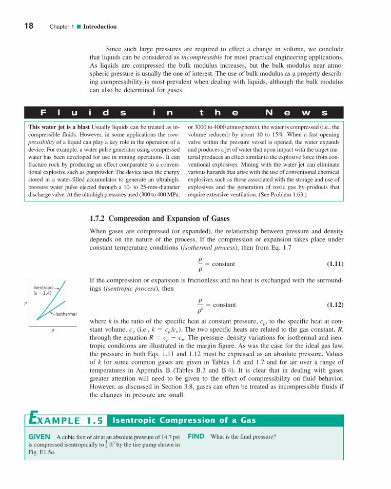
1.7.2 Compression and Expansion of Gases

When gases are compressed (or expanded), the relationship between pressure and densitydepends on the nature of the process. If the compression or expansion takes place underconstant temperature conditions (isothermal process), then from Eq. 1.7

(1.11)

If the compression or expansion is frictionless and no heat is exchanged with the surround-ings (isentropic process), then

(1.12)

where k is the ratio of the specific heat at constant pressure, cp, to the specific heat at con-stant volume, cy (i.e., k � cp /cy). The two specific heats are related to the gas constant, R,through the equation R � cp � cy. The pressure–density variations for isothermal and isen-tropic conditions are illustrated in the margin figure. As was the case for the ideal gas law,the pressure in both Eqs. 1.11 and 1.12 must be expressed as an absolute pressure. Valuesof k for some common gases are given in Tables 1.6 and 1.7 and for air over a range oftemperatures in Appendix B (Tables B.3 and B.4). It is clear that in dealing with gasesgreater attention will need to be given to the effect of compressibility on fluid behavior.However, as discussed in Section 3.8, gases can often be treated as incompressible fluids ifthe changes in pressure are small.

p

�k� constant

p

�� constant

Since such large pressures are required to effect a change in volume, we concludethat liquids can be considered as incompressible for most practical engineering applications.As liquids are compressed the bulk modulus increases, but the bulk modulus near atmo-spheric pressure is usually the one of interest. The use of bulk modulus as a property describ-ing compressibility is most prevalent when dealing with liquids, although the bulk moduluscan also be determined for gases.

18 Chapter 1 ■ Introduction

F l u i d s i n t h e N e w s

This water jet is a blast Usually liquids can be treated as in-compressible fluids. However, in some applications the com-pressibility of a liquid can play a key role in the operation of adevice. For example, a water pulse generator using compressedwater has been developed for use in mining operations. It canfracture rock by producing an effect comparable to a conven-tional explosive such as gunpowder. The device uses the energystored in a water-filled accumulator to generate an ultrahigh-pressure water pulse ejected through a 10- to 25-mm-diameterdischarge valve. At the ultrahigh pressures used (300 to 400 MPa,

or 3000 to 4000 atmospheres), the water is compressed (i.e., thevolume reduced) by about 10 to 15%. When a fast-openingvalve within the pressure vessel is opened, the water expandsand produces a jet of water that upon impact with the target ma-terial produces an effect similar to the explosive force from con-ventional explosives. Mining with the water jet can eliminatevarious hazards that arise with the use of conventional chemicalexplosives such as those associated with the storage and use ofexplosives and the generation of toxic gas by-products that require extensive ventilation. (See Problem 1.63.)

p

Isothermal

Isentropic (k = 1.4)

ρ

GIVEN A cubic foot of air at an absolute pressure of 14.7 psiis compressed isentropically to ft3 by the tire pump shown inFig. E1.5a.

12

FIND What is the final pressure?

Isentropic Compression of a GasEXAMPLE 1.5

c01Introduction.qxd 9/24/10 11:12 AM Page 18

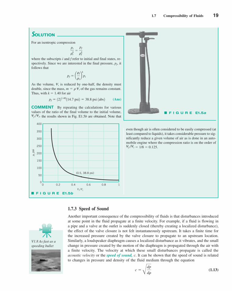
1.7 Compressibility of Fluids 19

1.7.3 Speed of Sound

Another important consequence of the compressibility of fluids is that disturbances introducedat some point in the fluid propagate at a finite velocity. For example, if a fluid is flowing ina pipe and a valve at the outlet is suddenly closed (thereby creating a localized disturbance),the effect of the valve closure is not felt instantaneously upstream. It takes a finite time forthe increased pressure created by the valve closure to propagate to an upstream location.Similarly, a loudspeaker diaphragm causes a localized disturbance as it vibrates, and the smallchange in pressure created by the motion of the diaphragm is propagated through the air witha finite velocity. The velocity at which these small disturbances propagate is called theacoustic velocity or the speed of sound, c. It can be shown that the speed of sound is relatedto changes in pressure and density of the fluid medium through the equation

(1.13)c �B

dp

d�

SOLUTION

even though air is often considered to be easily compressed (atleast compared to liquids), it takes considerable pressure to sig-nificantly reduce a given volume of air as is done in an auto-mobile engine where the compression ratio is on the order of

� 1/8 � 0.125.Vf Vi

For an isentropic compression

where the subscripts i and f refer to initial and final states, re-spectively. Since we are interested in the final pressure, pf, itfollows that

As the volume, is reduced by one-half, the density mustdouble, since the mass, of the gas remains constant.Thus, with k � 1.40 for air

(Ans)

COMMENT By repeating the calculations for variousvalues of the ratio of the final volume to the initial volume,

the results shown in Fig. E1.5b are obtained. Note thatVf Vi,

pf � 1221.40114.7 psi2 � 38.8 psi 1abs2

m � � V,V,

pf � a�f

�ib

k

pi

pi

�ki

�pf

�kf

F I G U R E E1.5a

F I G U R E E1.5b

400

350

300

250

200

150

100

50

00 0.2 0.4 0.6 0.8 1

(0.5, 38.8 psi)

p f, p

si

Vf /Vi

V1.8 As fast as aspeeding bullet

c01Introduction.qxd 9/24/10 11:12 AM Page 19

or in terms of the bulk modulus defined by Eq. 1.10

(1.14)

Because the disturbance is small, there is negligible heat transfer and the process is assumedto be isentropic. Thus, the pressure–density relationship used in Eq. 1.13 is that for an isen-tropic process.

For gases undergoing an isentropic process, Ey � kp, so that

and making use of the ideal gas law, it follows that

(1.15)

Thus, for ideal gases the speed of sound is proportional to the square root of the absolutetemperature. The speed of sound in air at various temperatures can be found in AppendixB (Tables B.3 and B.4). Equation 1.14 is also valid for liquids, and values of Ey can beused to determine the speed of sound in liquids. As shown by the figure in the margin, the speedof sound in water is much higher than in air. If a fluid were truly incompressible (Ey � q) thespeed of sound would be infinite. The speed of sound in water for various temperatures canbe found in Appendix B (Tables B.1 and B.2).

c � 2kRT

c �B

kp

�

c �B

Ey�

20 Chapter 1 ■ Introduction

GIVEN A jet aircraft flies at a speed of 550 mph at an alti-tude of 35,000 ft, where the temperature is �66 �F and thespecific heat ratio is k � 1.4.

FIND Determine the ratio of the speed of the aircraft, V, tothat of the speed of sound, c, at the specified altitude.

SOLUTION

Speed of Sound and Mach Number

By repeating the calculations for different temperatures,the results shown in Fig. E1.6 are obtained. Because the speedof sound increases with increasing temperature, for a constantairplane speed, the Mach number decreases as the temperatureincreases.

EXAMPLE 1.6

From Eq. 1.15 the speed of sound can be calculated as

Since the air speed is

the ratio is

(Ans)

COMMENT This ratio is called the Mach number, Ma. IfMa � 1.0 the aircraft is flying at subsonic speeds, whereas forMa � 1.0 it is flying at supersonic speeds. The Mach numberis an important dimensionless parameter used in the study ofthe flow of gases at high speeds and will be further discussedin Chapters 7 and 9.

V

c�

807 ft/s

973 ft/s� 0.829

V �1550 mi/hr2 15280 ft/mi2

13600 s/hr2� 807 ft/s

� 973 ft/s

� 211.402 11716 ft.lb/slug.°R2 1�66 � 4602 °R

c � 2kRT

F I G U R E E1.6

0.9

0.8

0.7

0.6

0.5–100 –50 0 50 100

Ma

= V

/c

(–66 �F, Ma)

T, �F

6000

water

air

4000

2000

0 100 2000

c, ft

/s

T, �F

c01Introduction.qxd 9/24/10 11:12 AM Page 20

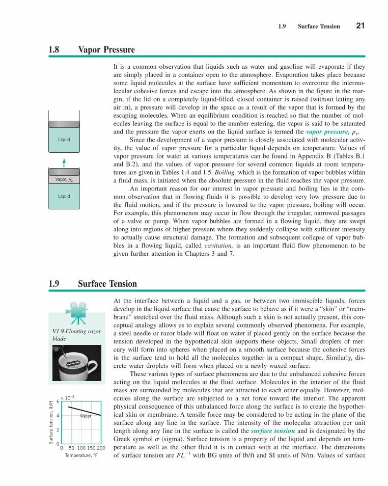
1.9 Surface Tension 21

1.8 Vapor Pressure

It is a common observation that liquids such as water and gasoline will evaporate if theyare simply placed in a container open to the atmosphere. Evaporation takes place becausesome liquid molecules at the surface have sufficient momentum to overcome the intermo-lecular cohesive forces and escape into the atmosphere. As shown in the figure in the mar-gin, if the lid on a completely liquid-filled, closed container is raised (without letting anyair in), a pressure will develop in the space as a result of the vapor that is formed by theescaping molecules. When an equilibrium condition is reached so that the number of mol-ecules leaving the surface is equal to the number entering, the vapor is said to be saturatedand the pressure the vapor exerts on the liquid surface is termed the vapor pressure, py.

Since the development of a vapor pressure is closely associated with molecular activ-ity, the value of vapor pressure for a particular liquid depends on temperature. Values ofvapor pressure for water at various temperatures can be found in Appendix B (Tables B.1and B.2), and the values of vapor pressure for several common liquids at room tempera-tures are given in Tables 1.4 and 1.5. Boiling, which is the formation of vapor bubbles withina fluid mass, is initiated when the absolute pressure in the fluid reaches the vapor pressure.

An important reason for our interest in vapor pressure and boiling lies in the com-mon observation that in flowing fluids it is possible to develop very low pressure due tothe fluid motion, and if the pressure is lowered to the vapor pressure, boiling will occur.For example, this phenomenon may occur in flow through the irregular, narrowed passagesof a valve or pump. When vapor bubbles are formed in a flowing liquid, they are sweptalong into regions of higher pressure where they suddenly collapse with sufficient intensityto actually cause structural damage. The formation and subsequent collapse of vapor bub-bles in a flowing liquid, called cavitation, is an important fluid flow phenomenon to begiven further attention in Chapters 3 and 7.

1.9 Surface Tension

At the interface between a liquid and a gas, or between two immiscible liquids, forcesdevelop in the liquid surface that cause the surface to behave as if it were a “skin” or “mem-brane” stretched over the fluid mass. Although such a skin is not actually present, this con-ceptual analogy allows us to explain several commonly observed phenomena. For example,a steel needle or razor blade will float on water if placed gently on the surface because thetension developed in the hypothetical skin supports these objects. Small droplets of mer-cury will form into spheres when placed on a smooth surface because the cohesive forcesin the surface tend to hold all the molecules together in a compact shape. Similarly, dis-crete water droplets will form when placed on a newly waxed surface.

These various types of surface phenomena are due to the unbalanced cohesive forcesacting on the liquid molecules at the fluid surface. Molecules in the interior of the fluidmass are surrounded by molecules that are attracted to each other equally. However, mol-ecules along the surface are subjected to a net force toward the interior. The apparentphysical consequence of this unbalanced force along the surface is to create the hypothet-ical skin or membrane. A tensile force may be considered to be acting in the plane of thesurface along any line in the surface. The intensity of the molecular attraction per unitlength along any line in the surface is called the surface tension and is designated by theGreek symbol � (sigma). Surface tension is a property of the liquid and depends on tem-perature as well as the other fluid it is in contact with at the interface. The dimensionsof surface tension are FL�1 with BG units of lb/ft and SI units of N/m. Values of surface

Liquid

Liquid

Vapor, py

V1.9 Floating razorblade

200150100500

Sur

face

ten

sion

, lb

/ft 6

× 10−3

4

2

0

Water

Temperature, �F

c01Introduction.qxd 9/24/10 11:12 AM Page 21

tension for some common liquids (in contact with air) are given in Tables 1.4 and 1.5and in Appendix B (Tables B.1 and B.2) for water at various temperatures. As indicatedby the figure in the margin of the previous page, the value of the surface tension decreasesas the temperature increases.

Among common phenomena associated with surface tension is the rise (or fall) of aliquid in a capillary tube. If a small open tube is inserted into water, the water level in thetube will rise above the water level outside the tube as is illustrated in Fig. 1.5a. In this sit-uation we have a liquid–gas–solid interface. For the case illustrated there is an attraction(adhesion) between the wall of the tube and liquid molecules, which is strong enough toovercome the mutual attraction (cohesion) of the molecules and pull them up to the wall.Hence, the liquid is said to wet the solid surface.

The height, h, is governed by the value of the surface tension, �, the tube radius, R,the specific weight of the liquid, �, and the angle of contact, between the fluid and tube.From the free-body diagram of Fig. 1.5b we see that the vertical force due to the surfacetension is equal to 2R� cos � and the weight is R2h and these two forces must balancefor equilibrium. Thus,

so that the height is given by the relationship

(1.16)h �2� cos �

�R

�R2h � 2R� cos �

�,

22 Chapter 1 ■ Introduction

F l u i d s i n t h e N e w s

Walking on water Water striders are insects commonly foundon ponds, rivers, and lakes that appear to “walk” on water. Atypical length of a water strider is about 0.4 in., and they cancover 100 body lengths in one second. It has long been recog-nized that it is surface tension that keeps the water strider fromsinking below the surface. What has been puzzling is how theypropel themselves at such a high speed. They can’t pierce thewater surface or they would sink. A team of mathematicians andengineers from the Massachusetts Institute of Technology(MIT) applied conventional flow visualization techniques and

high-speed video to examine in detail the movement of the wa-ter striders. They found that each stroke of the insect’s legs cre-ates dimples on the surface with underwater swirling vorticessufficient to propel it forward. It is the rearward motion of thevortices that propels the water strider forward. To further sub-stantiate their explanation the MIT team built a working modelof a water strider, called Robostrider, which creates surface rip-ples and underwater vortices as it moves across a water surface.Waterborne creatures, such as the water strider, provide an inter-esting world dominated by surface tension. (See Problem 1.71.)

V1.10 Capillaryrise

π

hR2h

2 R

θ

2R

θ

(a) (b) (c)

γπ

σ

h

F I G U R E 1.5 Effect of capillary action in small tubes. (a) Rise ofcolumn for a liquid that wets the tube. (b) Free-body diagram for calculatingcolumn height. (c) Depression of column for a nonwetting liquid.

c01Introduction.qxd 9/24/10 11:12 AM Page 22

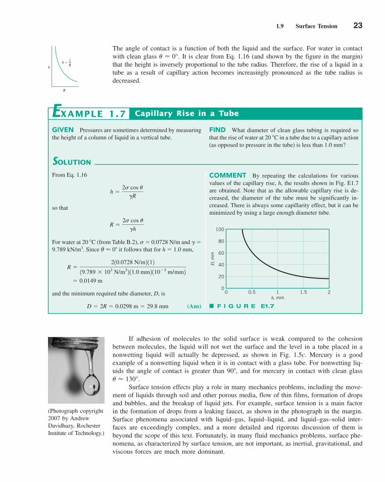
1.9 Surface Tension 23

The angle of contact is a function of both the liquid and the surface. For water in contactwith clean glass It is clear from Eq. 1.16 (and shown by the figure in the margin)that the height is inversely proportional to the tube radius. Therefore, the rise of a liquid in atube as a result of capillary action becomes increasingly pronounced as the tube radius isdecreased.

� � 0°.

If adhesion of molecules to the solid surface is weak compared to the cohesionbetween molecules, the liquid will not wet the surface and the level in a tube placed in anonwetting liquid will actually be depressed, as shown in Fig. 1.5c. Mercury is a goodexample of a nonwetting liquid when it is in contact with a glass tube. For nonwetting liq-uids the angle of contact is greater than 90�, and for mercury in contact with clean glass

Surface tension effects play a role in many mechanics problems, including the move-ment of liquids through soil and other porous media, flow of thin films, formation of dropsand bubbles, and the breakup of liquid jets. For example, surface tension is a main factorin the formation of drops from a leaking faucet, as shown in the photograph in the margin.Surface phenomena associated with liquid–gas, liquid–liquid, and liquid–gas–solid inter-faces are exceedingly complex, and a more detailed and rigorous discussion of them isbeyond the scope of this text. Fortunately, in many fluid mechanics problems, surface phe-nomena, as characterized by surface tension, are not important, as inertial, gravitational, andviscous forces are much more dominant.

� � 130°.

GIVEN Pressures are sometimes determined by measuringthe height of a column of liquid in a vertical tube.

FIND What diameter of clean glass tubing is required sothat the rise of water at 20 �C in a tube due to a capillary action(as opposed to pressure in the tube) is less than 1.0 mm?

SOLUTION

Capillary Rise in a Tube

COMMENT By repeating the calculations for variousvalues of the capillary rise, h, the results shown in Fig. E1.7are obtained. Note that as the allowable capillary rise is de-creased, the diameter of the tube must be significantly in-creased. There is always some capillarity effect, but it can beminimized by using a large enough diameter tube.

EXAMPLE 1.7

From Eq. 1.16

so that

For water at 20 �C (from Table B.2), � � 0.0728 N/m and � �9.789 kN/m3. Since � 0� it follows that for h � 1.0 mm,

and the minimum required tube diameter, D, is

(Ans)D � 2R � 0.0298 m � 29.8 mm

� 0.0149 m

R �210.0728 N/m2 112

19.789 � 103 N/m32 11.0 mm2 110�3 m/mm2

�

R �2� cos �

�h

h �2� cos �

�R

F I G U R E E1.7

21.510.50h, mm

D, m

m

100

80

60

40

20

0

(Photograph copyright2007 by Andrew Davidhazy, RochesterInstitute of Technology.)

h

R

R~ h 1__

c01Introduction.qxd 9/24/10 11:12 AM Page 23

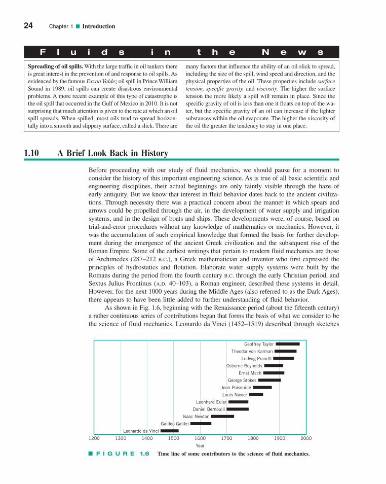
24 Chapter 1 ■ Introduction

F l u i d s i n t h e N e w s

Spreading of oil spills. With the large traffic in oil tankers thereis great interest in the prevention of and response to oil spills. Asevidenced by the famous Exxon Valdez oil spill in Prince WilliamSound in 1989, oil spills can create disastrous environmentalproblems. A more recent example of this type of catastrophe isthe oil spill that occurred in the Gulf of Mexico in 2010. It is notsurprising that much attention is given to the rate at which an oilspill spreads. When spilled, most oils tend to spread horizon-tally into a smooth and slippery surface, called a slick. There are

many factors that influence the ability of an oil slick to spread,including the size of the spill, wind speed and direction, and thephysical properties of the oil. These properties include surfacetension, specific gravity, and viscosity. The higher the surfacetension the more likely a spill will remain in place. Since thespecific gravity of oil is less than one it floats on top of the wa-ter, but the specific gravity of an oil can increase if the lightersubstances within the oil evaporate. The higher the viscosity ofthe oil the greater the tendency to stay in one place.

1.10 A Brief Look Back in History

Before proceeding with our study of fluid mechanics, we should pause for a moment toconsider the history of this important engineering science. As is true of all basic scientific andengineering disciplines, their actual beginnings are only faintly visible through the haze ofearly antiquity. But we know that interest in fluid behavior dates back to the ancient civiliza-tions. Through necessity there was a practical concern about the manner in which spears andarrows could be propelled through the air, in the development of water supply and irrigationsystems, and in the design of boats and ships. These developments were, of course, based ontrial-and-error procedures without any knowledge of mathematics or mechanics. However, itwas the accumulation of such empirical knowledge that formed the basis for further develop-ment during the emergence of the ancient Greek civilization and the subsequent rise of theRoman Empire. Some of the earliest writings that pertain to modern fluid mechanics are thoseof Archimedes (287–212 B.C.), a Greek mathematician and inventor who first expressed theprinciples of hydrostatics and flotation. Elaborate water supply systems were built by theRomans during the period from the fourth century B.C. through the early Christian period, andSextus Julius Frontinus (A.D. 40–103), a Roman engineer, described these systems in detail.However, for the next 1000 years during the Middle Ages (also referred to as the Dark Ages),there appears to have been little added to further understanding of fluid behavior.

As shown in Fig. 1.6, beginning with the Renaissance period (about the fifteenth century)a rather continuous series of contributions began that forms the basis of what we consider to bethe science of fluid mechanics. Leonardo da Vinci (1452–1519) described through sketches

Year

200019001800170016001500140013001200

Geoffrey Taylor

Theodor von Karman

Ludwig Prandtl

Osborne Reynolds

Ernst Mach

George Stokes

Leonardo da Vinci

Galileo Galilei

Isaac Newton

Daniel Bernoulli

Leonhard Euler

Louis Navier

Jean Poiseuille

F I G U R E 1.6 Time line of some contributors to the science of fluid mechanics.

c01Introduction.qxd 9/24/10 11:12 AM Page 24

1.10 A Brief Look Back in History 25

and writings many different types of flow phenomena. The work of Galileo Galilei(1564–1642) marked the beginning of experimental mechanics. Following the early Renais-sance period and during the seventeenth and eighteenth centuries, numerous significant con-tributions were made. These include theoretical and mathematical advances associated withthe famous names of Newton, Bernoulli, Euler, and d’Alembert. Experimental aspects offluid mechanics were also advanced during this period, but unfortunately the two differentapproaches, theoretical and experimental, developed along separate paths. Hydrodynamicswas the term associated with the theoretical or mathematical study of idealized, frictionlessfluid behavior, with the term hydraulics being used to describe the applied or experimentalaspects of real fluid behavior, particularly the behavior of water. Further contributions andrefinements were made to both theoretical hydrodynamics and experimental hydraulics dur-ing the nineteenth century, with the general differential equations describing fluid motionsthat are used in modern fluid mechanics being developed in this period. Experimentalhydraulics became more of a science, and many of the results of experiments performedduring the nineteenth century are still used today.

At the beginning of the twentieth century, both the fields of theoretical hydrodynam-ics and experimental hydraulics were highly developed, and attempts were being made tounify the two. In 1904 a classic paper was presented by a German professor, Ludwig Prandtl(1875–1953), who introduced the concept of a “fluid boundary layer,” which laid the foun-dation for the unification of the theoretical and experimental aspects of fluid mechanics.Prandtl’s idea was that for flow next to a solid boundary a thin fluid layer (boundary layer)develops in which friction is very important, but outside this layer the fluid behaves verymuch like a frictionless fluid. This relatively simple concept provided the necessary impe-tus for the resolution of the conflict between the hydrodynamicists and the hydraulicists.Prandtl is generally accepted as the founder of modern fluid mechanics.

Also, during the first decade of the twentieth century, powered flight was first success-fully demonstrated with the subsequent vastly increased interest in aerodynamics. Becausethe design of aircraft required a degree of understanding of fluid flow and an ability to makeaccurate predictions of the effect of airflow on bodies, the field of aerodynamics provided agreat stimulus for the many rapid developments in fluid mechanics that took place duringthe twentieth century.

As we proceed with our study of the fundamentals of fluid mechanics, we will con-tinue to note the contributions of many of the pioneers in the field. Table 1.8 provides achronological listing of some of these contributors and reveals the long journey that makes

ARCHIMEDES 1287–212 B.C.2Established elementary principles of buoyancyand flotation.

SEXTUS JULIUS FRONTINUS 1A.D. 40–1032Wrote treatise on Roman methods of waterdistribution.

LEONARDO da VINCI 11452–15192Expressed elementary principle of continuity;observed and sketched many basic flow phenomena;suggested designs for hydraulic machinery.

GALILEO GALILEI 11564–16422Indirectly stimulated experimental hydraulics;revised Aristotelian concept of vacuum.

EVANGELISTA TORRICELLI 11608–16472Related barometric height to weight of atmosphere,and form of liquid jet to trajectory of free fall.

BLAISE PASCAL 11623–16622Finally clarified principles of barometer,hydraulic press, and pressure transmissibility.

ISAAC NEWTON 11642–17272Explored various aspects of fluid resistance—inertial, viscous, and wave; discovered jetcontraction.

HENRI de PITOT 11695–17712Constructed double-tube device to indicate watervelocity through differential head.

TA B L E 1 . 8

Chronological Listing of Some Contributors to the Science of Fluid Mechanics Noted in the Texta

Leonardo da Vinci

Isaac Newton (continued )

c01Introduction.qxd 9/24/10 11:12 AM Page 25

26 Chapter 1 ■ Introduction

DANIEL BERNOULLI 11700–17822Experimented and wrote on many phases of fluidmotion, coining name “hydrodynamics”; devisedmanometry technique and adapted primitiveenergy principle to explain velocity-headindication; proposed jet propulsion.

LEONHARD EULER 11707–17832First explained role of pressure in fluid flow;formulated basic equations of motion and so-called Bernoulli theorem; introduced concept ofcavitation and principle of centrifugalmachinery.

JEAN le ROND d’ALEMBERT 11717–17832Originated notion of velocity and accelerationcomponents, differential expression of continuity,and paradox of zero resistance to steadynonuniform motion.

ANTOINE CHEZY 11718–17982Formulated similarity parameter for predictingflow characteristics of one channel frommeasurements on another.

GIOVANNI BATTISTA VENTURI 11746–18222Performed tests on various forms ofmouthpieces—in particular, conical contractionsand expansions.

LOUIS MARIE HENRI NAVIER 11785–18362Extended equations of motion to include“molecular” forces.

AUGUSTIN LOUIS de CAUCHY 11789–18572Contributed to the general field of theoreticalhydrodynamics and to the study of wave motion.

GOTTHILF HEINRICH LUDWIG HAGEN11797–18842Conducted original studies of resistance in andtransition between laminar and turbulent flow.

JEAN LOUIS POISEUILLE 11799–18692Performed meticulous tests on resistance of flowthrough capillary tubes.

HENRI PHILIBERT GASPARD DARCY 11803–18582Performed extensive tests on filtration and piperesistance; initiated open-channel studies carriedout by Bazin.

JULIUS WEISBACH 11806–18712Incorporated hydraulics in treatise on engineeringmechanics, based on original experiments;noteworthy for flow patterns, nondimensionalcoefficients, weir, and resistance equations.

WILLIAM FROUDE 11810–18792Developed many towing-tank techniques, inparticular the conversion of wave and boundarylayer resistance from model to prototype scale.

ROBERT MANNING 11816–18972Proposed several formulas for open-channelresistance.

GEORGE GABRIEL STOKES 11819–19032Derived analytically various flow relationshipsranging from wave mechanics to viscousresistance—particularly that for the settling ofspheres.

ERNST MACH 11838–19162One of the pioneers in the field of supersonicaerodynamics.

OSBORNE REYNOLDS 11842–19122Described original experiments in many fields—cavitation, river model similarity, piperesistance—and devised two parameters forviscous flow; adapted equations of motion of aviscous fluid to mean conditions of turbulentflow.

JOHN WILLIAM STRUTT, LORD RAYLEIGH11842–19192Investigated hydrodynamics of bubble collapse,wave motion, jet instability, laminar flowanalogies, and dynamic similarity.

VINCENZ STROUHAL 11850–19222Investigated the phenomenon of “singing wires.”

EDGAR BUCKINGHAM 11867–19402Stimulated interest in the United States in theuse of dimensional analysis.

MORITZ WEBER 11871–19512Emphasized the use of the principles ofsimilitude in fluid flow studies and formulated acapillarity similarity parameter.

LUDWIG PRANDTL 11875–19532Introduced concept of the boundary layer and isgenerally considered to be the father of present-day fluid mechanics.

LEWIS FERRY MOODY 11880–19532Provided many innovations in the field ofhydraulic machinery. Proposed a method ofcorrelating pipe resistance data that is widelyused.

THEODOR VON KÁRMÁN 11881–19632One of the recognized leaders of twentiethcentury fluid mechanics. Provided majorcontributions to our understanding of surfaceresistance, turbulence, and wake phenomena.

PAUL RICHARD HEINRICH BLASIUS11883–19702One of Prandtl’s students who provided ananalytical solution to the boundary layerequations. Also demonstrated that pipe resistancewas related to the Reynolds number.

TA B L E 1 . 8 (continued)

aAdapted from Rouse, H. and Ince, S., History of Hydraulics, Iowa Institute of Hydraulic Research, Iowa City, 1957, Dover, NewYork, 1963. Used by permission of the Iowa Institute of Hydraulic Research, University of Iowa.

Daniel Bernoulli

Ernst Mach

Osborne Reynolds

Ludwig Prandtl

c01Introduction.qxd 9/24/10 11:12 AM Page 26

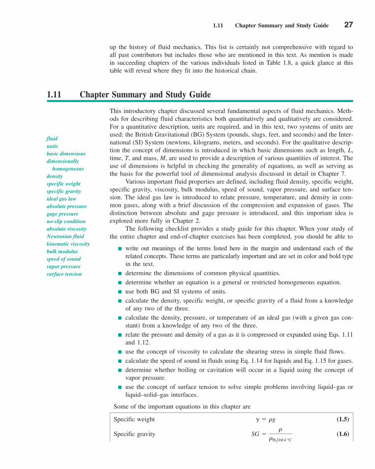
1.11 Chapter Summary and Study Guide 27

up the history of fluid mechanics. This list is certainly not comprehensive with regard toall past contributors but includes those who are mentioned in this text. As mention is madein succeeding chapters of the various individuals listed in Table 1.8, a quick glance at thistable will reveal where they fit into the historical chain.

fluidunitsbasic dimensionsdimensionally

homogeneousdensityspecific weightspecific gravityideal gas lawabsolute pressuregage pressureno-slip conditionabsolute viscosityNewtonian fluidkinematic viscositybulk modulusspeed of soundvapor pressuresurface tension

1.11 Chapter Summary and Study Guide

This introductory chapter discussed several fundamental aspects of fluid mechanics. Meth-ods for describing fluid characteristics both quantitatively and qualitatively are considered.For a quantitative description, units are required, and in this text, two systems of units areused: the British Gravitational (BG) System (pounds, slugs, feet, and seconds) and the Inter-national (SI) System (newtons, kilograms, meters, and seconds). For the qualitative descrip-tion the concept of dimensions is introduced in which basic dimensions such as length, L,time, T, and mass, M, are used to provide a description of various quantities of interest. Theuse of dimensions is helpful in checking the generality of equations, as well as serving asthe basis for the powerful tool of dimensional analysis discussed in detail in Chapter 7.

Various important fluid properties are defined, including fluid density, specific weight,specific gravity, viscosity, bulk modulus, speed of sound, vapor pressure, and surface ten-sion. The ideal gas law is introduced to relate pressure, temperature, and density in com-mon gases, along with a brief discussion of the compression and expansion of gases. Thedistinction between absolute and gage pressure is introduced, and this important idea isexplored more fully in Chapter 2.

The following checklist provides a study guide for this chapter. When your study ofthe entire chapter and end-of-chapter exercises has been completed, you should be able to

write out meanings of the terms listed here in the margin and understand each of therelated concepts. These terms are particularly important and are set in color and bold typein the text.

determine the dimensions of common physical quantities.

determine whether an equation is a general or restricted homogeneous equation.

use both BG and SI systems of units.

calculate the density, specific weight, or specific gravity of a fluid from a knowledgeof any two of the three.

calculate the density, pressure, or temperature of an ideal gas (with a given gas con-stant) from a knowledge of any two of the three.

relate the pressure and density of a gas as it is compressed or expanded using Eqs. 1.11and 1.12.

use the concept of viscosity to calculate the shearing stress in simple fluid flows.

calculate the speed of sound in fluids using Eq. 1.14 for liquids and Eq. 1.15 for gases.

determine whether boiling or cavitation will occur in a liquid using the concept ofvapor pressure.

use the concept of surface tension to solve simple problems involving liquid–gas orliquid–solid–gas interfaces.

Some of the important equations in this chapter are

Specific weight (1.5)

Specific gravity (1.6)SG �r

rH2O@4 °C

g � rg

c01Introduction.qxd 9/24/10 11:12 AM Page 27

Ideal gas law (1.7)

Newtonian fluid shear stress (1.8)

Bulk modulus (1.9)

Speed of sound in an ideal gas (1.15)

Capillary rise in a tube(1.16)

h �2s cos u

gR

c � 1kRT

Ev � �dp

dV��V�

� � � du

dy

r �p

RT

28 Chapter 1 ■ Introduction

Review Problems

Go to Appendix G for a set of review problems with answers.Detailed solutions can be found in Student Solution Manual for

a Brief Introduction to Fluid Mechanics, by Young et al. (© 2011John Wiley and Sons, Inc.).

Problems

Note: Unless specific values of required fluid properties aregiven in the statement of the problem, use the values foundin the tables on the inside of the front cover. Problems desig-nated with an (*) are intended to be solved with the aid of aprogrammable calculator or a computer. Problems desig-nated with a (†) are “open-ended” problems and requirecritical thinking in that to work them one must make vari-ous assumptions and provide the necessary data. There isnot a unique answer to these problems.

The even-numbered problems are included in thehard copy version of the book, and the answers to theseeven-numbered problems are listed at the end of the book.Odd-numbered problems are provided in WileyPLUS, orin Appendix L on the book’s web site, www.wiley.com/college/young. The lab-type problems, FE problems, FlowLabproblems, and the videos that accompany problems can alsobe accessed on these web sites.

Section 1.2 Dimensions, Dimensional Homogeneity,and Units

1.2 Determine the dimensions, in both the FLT system andMLT system, for (a) the product of force times volume, (b) theproduct of pressure times mass divided by area, and (c) momentof a force divided by velocity.

1.4 The force, F, of the wind blowing against a building is givenby where V is the wind speed, the density ofthe air, A the cross-sectional area of the building, and CD is a con-stant termed the drag coefficient. Determine the dimensions of thedrag coefficient.

1.6 Dimensionless combinations of quantities (commonlycalled dimensionless parameters) play an important role in fluidmechanics. Make up five possible dimensionless parameters byusing combinations of some of the quantities listed in Table 1.1.

rF � CDrV2 A�2,

1.8 The pressure difference, across a partial blockage in anartery 1called a stenosis2 is approximated by the equation

where V is the blood velocity, the blood viscosity the blood density the artery diameter, the area of

the unobstructed artery, and the area of the stenosis. Determinethe dimensions of the constants Kv and Would this equation bevalid in any system of units?

1.10 Assume that the speed of sound, c, in a fluid depends onan elastic modulus, , with dimensions and the fluiddensity, in the form If this is to be a dimen-sionally homogeneous equation, what are the values for a andb? Is your result consistent with the standard formula for thespeed of sound? 1See Eq. 1.14.2

†1.12 Cite an example of a restricted homogeneous equationcontained in a technical article found in an engineering journalin your field of interest. Define all terms in the equation, explainwhy it is a restricted equation, and provide a complete journalcitation (title, date, etc.).

1.14 Make use of Table 1.3 to express the following quantitiesin BG units: (a) 14.2 km, (b) 8.14 N/m3, (c) 1.61 kg/m3,(d) 0.0320 N�m/s, (e) 5.67 mm/hr.

1.16 An important dimensionless parameter in certain types offluid flow problems is the Froude number defined as where V is a velocity, g the acceleration of gravity, and alength. Determine the value of the Froude number for V � 10 ft/s,g � 32.2 ft/s2, and � 2 ft. Recalculate the Froude number us-ing SI units for V, g, and . Explain the significance of theresults of these calculations.

��

�V/1g�,

c � 1Ev2a1r2b.r,

FL�2,Ev

Ku.A1

A01ML�32, D�1FL�2T 2,�

¢p � Kv �V

D� Ku a

A0

A1� 1b

2

�V 2

¢p,

c01Introduction.qxd 10/18/10 7:56 AM Page 28

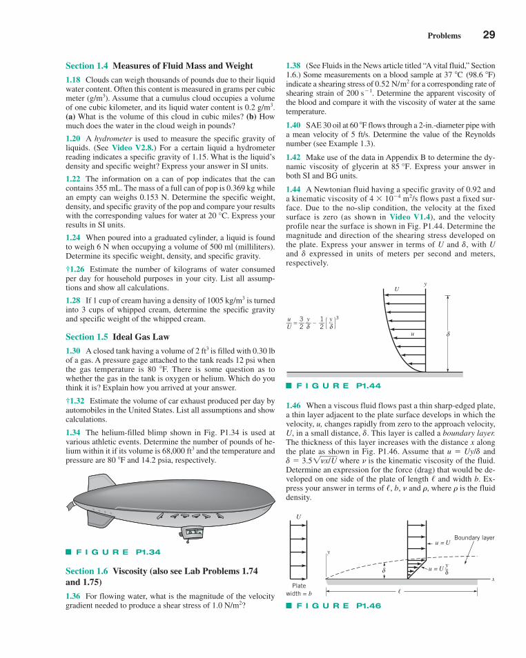
Section 1.6 Viscosity (also see Lab Problems 1.74and 1.75)

1.36 For flowing water, what is the magnitude of the velocitygradient needed to produce a shear stress of 1.0 N/m2?

1.38 (See Fluids in the News article titled “A vital fluid,” Section1.6.) Some measurements on a blood sample at 37 �C (98.6 �F)indicate a shearing stress of for a corresponding rate ofshearing strain of . Determine the apparent viscosity ofthe blood and compare it with the viscosity of water at the sametemperature.

1.40 SAE 30 oil at 60 �F flows through a 2-in.-diameter pipe witha mean velocity of 5 ft/s. Determine the value of the Reynoldsnumber (see Example 1.3).

1.42 Make use of the data in Appendix B to determine the dy-namic viscosity of glycerin at Express your answer inboth SI and BG units.

1.44 A Newtonian fluid having a specific gravity of 0.92 anda kinematic viscosity of 4 � 10�4 m2/s flows past a fixed sur-face. Due to the no-slip condition, the velocity at the fixedsurface is zero (as shown in Video V1.4), and the velocityprofile near the surface is shown in Fig. P1.44. Determine themagnitude and direction of the shearing stress developed onthe plate. Express your answer in terms of U and �, with Uand � expressed in units of meters per second and meters,respectively.

85 °F.

200 s�10.52 N/m2

1.46 When a viscous fluid flows past a thin sharp-edged plate,a thin layer adjacent to the plate surface develops in which thevelocity, u, changes rapidly from zero to the approach velocity,U, in a small distance, �. This layer is called a boundary layer.The thickness of this layer increases with the distance x alongthe plate as shown in Fig. P1.46. Assume that u � Uy/� and

where is the kinematic viscosity of the fluid.Determine an expression for the force (drag) that would be de-veloped on one side of the plate of length and width b. Ex-press your answer in terms of , b, and �, where � is the fluiddensity.

�//

� � 3.51�x/U

Problems 29

Section 1.4 Measures of Fluid Mass and Weight

1.18 Clouds can weigh thousands of pounds due to their liquidwater content. Often this content is measured in grams per cubicmeter (g/m3). Assume that a cumulus cloud occupies a volumeof one cubic kilometer, and its liquid water content is 0.2 g/m3.(a) What is the volume of this cloud in cubic miles? (b) Howmuch does the water in the cloud weigh in pounds?

1.20 A hydrometer is used to measure the specific gravity ofliquids. (See Video V2.8.) For a certain liquid a hydrometerreading indicates a specific gravity of 1.15. What is the liquid’sdensity and specific weight? Express your answer in SI units.

1.22 The information on a can of pop indicates that the cancontains 355 mL. The mass of a full can of pop is 0.369 kg whilean empty can weighs 0.153 N. Determine the specific weight,density, and specific gravity of the pop and compare your resultswith the corresponding values for water at Express yourresults in SI units.

1.24 When poured into a graduated cylinder, a liquid is foundto weigh 6 N when occupying a volume of 500 ml (milliliters).Determine its specific weight, density, and specific gravity.

†1.26 Estimate the number of kilograms of water consumedper day for household purposes in your city. List all assump-tions and show all calculations.

1.28 If 1 cup of cream having a density of 1005 kg/m3 is turnedinto 3 cups of whipped cream, determine the specific gravityand specific weight of the whipped cream.

Section 1.5 Ideal Gas Law

1.30 A closed tank having a volume of 2 ft3 is filled with 0.30 lbof a gas. A pressure gage attached to the tank reads 12 psi whenthe gas temperature is 80 �F. There is some question as towhether the gas in the tank is oxygen or helium. Which do youthink it is? Explain how you arrived at your answer.

†1.32 Estimate the volume of car exhaust produced per day byautomobiles in the United States. List all assumptions and showcalculations.

1.34 The helium-filled blimp shown in Fig. P1.34 is used atvarious athletic events. Determine the number of pounds of he-lium within it if its volume is 68,000 ft3 and the temperature andpressure are 80 �F and 14.2 psia, respectively.

20 °C.

F I G U R E P1.34

u__U

3__2

1__2

3y__

y

u

U

= – δδδ

( )y–

F I G U R E P1.44

�

y

xδ

Platewidth = b

U

u = U

u = U y_δ

Boundary layer

F I G U R E P1.46

c01Introduction.qxd 9/24/10 11:12 AM Page 29

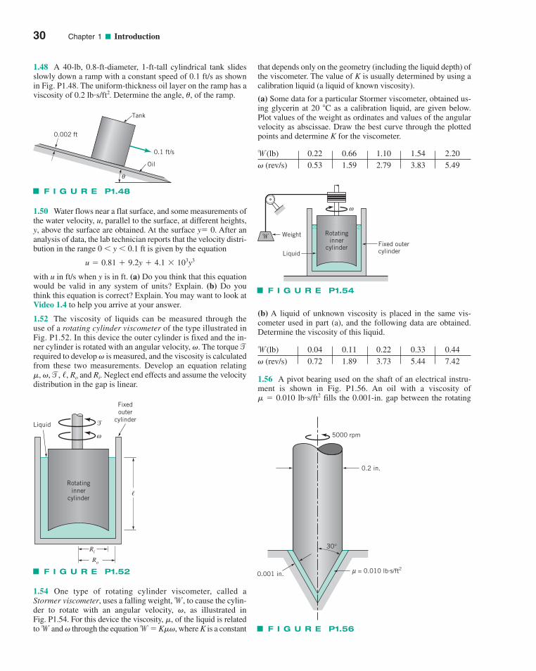
1.48 A 40-lb, 0.8-ft-diameter, 1-ft-tall cylindrical tank slidesslowly down a ramp with a constant speed of 0.1 ft/s as shownin Fig. P1.48. The uniform-thickness oil layer on the ramp has aviscosity of 0.2 lb�s/ft2. Determine the angle, , of the ramp.�

1.50 Water flows near a flat surface, and some measurements ofthe water velocity, u, parallel to the surface, at different heights,y, above the surface are obtained. At the surface y� 0. After ananalysis of data, the lab technician reports that the velocity distri-bution in the range 0 � y � 0.1 ft is given by the equation

with u in ft/s when y is in ft. (a) Do you think that this equationwould be valid in any system of units? Explain. (b) Do youthink this equation is correct? Explain. You may want to look atVideo 1.4 to help you arrive at your answer.

1.52 The viscosity of liquids can be measured through theuse of a rotating cylinder viscometer of the type illustrated inFig. P1.52. In this device the outer cylinder is fixed and the in-ner cylinder is rotated with an angular velocity, �. The torque trequired to develop � is measured, and the viscosity is calculatedfrom these two measurements. Develop an equation relating �, �,t, , Ro and Ri. Neglect end effects and assume the velocitydistribution in the gap is linear.

/

u � 0.81 � 9.2y � 4.1 � 103y3

that depends only on the geometry (including the liquid depth) ofthe viscometer. The value of K is usually determined by using acalibration liquid (a liquid of known viscosity).

(a) Some data for a particular Stormer viscometer, obtained us-ing glycerin at 20 �C as a calibration liquid, are given below.Plot values of the weight as ordinates and values of the angularvelocity as abscissae. Draw the best curve through the plottedpoints and determine K for the viscometer.

w(lb) 0.22 0.66 1.10 1.54 2.20� (rev/s) 0.53 1.59 2.79 3.83 5.49

(b) A liquid of unknown viscosity is placed in the same vis-cometer used in part (a), and the following data are obtained.Determine the viscosity of this liquid.

w(lb) 0.04 0.11 0.22 0.33 0.44� (rev/s) 0.72 1.89 3.73 5.44 7.42

1.56 A pivot bearing used on the shaft of an electrical instru-ment is shown in Fig. P1.56. An oil with a viscosity of � � 0.010 lb�s/ft2 fills the 0.001-in. gap between the rotating

30 Chapter 1 ■ Introduction

Tank

0.1 ft/s

Oil

0.002 ft

θ

F I G U R E P1.48

Liquid

Fixedouter

cylinder�

ω

�

Ri

Ro

Rotatinginner

cylinder

F I G U R E P1.52

1.54 One type of rotating cylinder viscometer, called aStormer viscometer, uses a falling weight,w, to cause the cylin-der to rotate with an angular velocity, �, as illustrated in Fig. P1.54. For this device the viscosity, �, of the liquid is relatedto w and � through the equation w� K��, where K is a constant

F I G U R E P1.54

Liquid

Fixed outercylinder

Weight

ω

Rotatinginner

cylinder

�

F I G U R E P1.56

0.2 in.

0.001 in.

5000 rpm

30°

= 0.010 lb s/ft2µ .

c01Introduction.qxd 9/24/10 11:12 AM Page 30

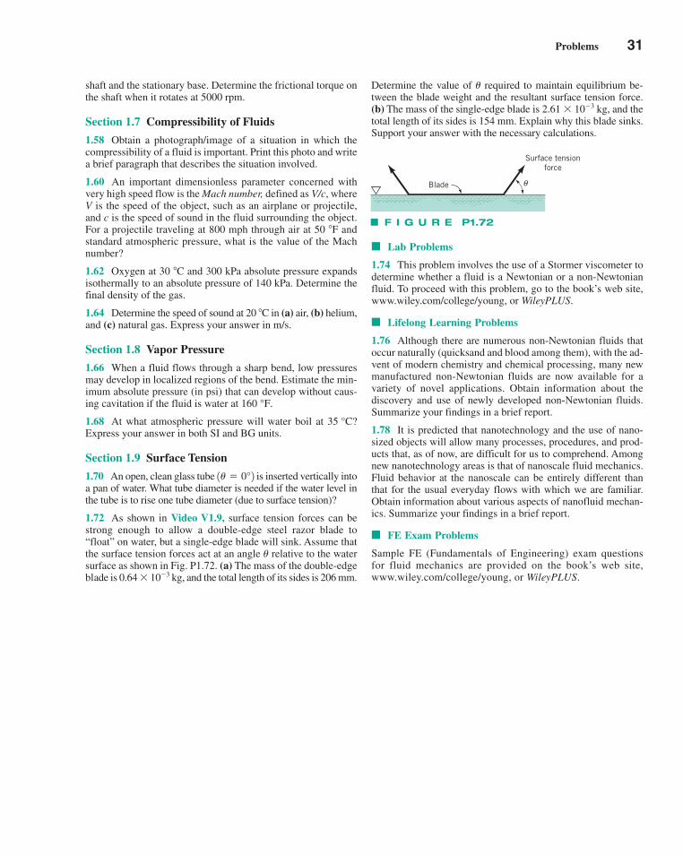
Problems 31

shaft and the stationary base. Determine the frictional torque onthe shaft when it rotates at 5000 rpm.

Section 1.7 Compressibility of Fluids

1.58 Obtain a photograph/image of a situation in which thecompressibility of a fluid is important. Print this photo and writea brief paragraph that describes the situation involved.

1.60 An important dimensionless parameter concerned withvery high speed flow is the Mach number, defined as V/c, whereV is the speed of the object, such as an airplane or projectile,and c is the speed of sound in the fluid surrounding the object.For a projectile traveling at 800 mph through air at 50 �F andstandard atmospheric pressure, what is the value of the Machnumber?

1.62 Oxygen at 30 �C and 300 kPa absolute pressure expandsisothermally to an absolute pressure of 140 kPa. Determine thefinal density of the gas.

1.64 Determine the speed of sound at 20 �C in (a) air, (b) helium,and (c) natural gas. Express your answer in m/s.

Section 1.8 Vapor Pressure

1.66 When a fluid flows through a sharp bend, low pressuresmay develop in localized regions of the bend. Estimate the min-imum absolute pressure (in psi) that can develop without caus-ing cavitation if the fluid is water at

1.68 At what atmospheric pressure will water boil at Express your answer in both SI and BG units.

Section 1.9 Surface Tension

1.70 An open, clean glass tube is inserted vertically intoa pan of water. What tube diameter is needed if the water level inthe tube is to rise one tube diameter (due to surface tension)?

1.72 As shown in Video V1.9, surface tension forces can bestrong enough to allow a double-edge steel razor blade to“float” on water, but a single-edge blade will sink. Assume thatthe surface tension forces act at an angle relative to the watersurface as shown in Fig. P1.72. (a) The mass of the double-edgeblade is 0.64 � 10�3 kg, and the total length of its sides is 206 mm.

�

1� � 0°2

35 °C?

160 °F.

Determine the value of required to maintain equilibrium be-tween the blade weight and the resultant surface tension force.(b) The mass of the single-edge blade is 2.61 � 10�3 kg, and thetotal length of its sides is 154 mm. Explain why this blade sinks.Support your answer with the necessary calculations.

�

■ Lab Problems

1.74 This problem involves the use of a Stormer viscometer todetermine whether a fluid is a Newtonian or a non-Newtonianfluid. To proceed with this problem, go to the book’s web site,www.wiley.com/college/young, or WileyPLUS.

■ Lifelong Learning Problems

1.76 Although there are numerous non-Newtonian fluids thatoccur naturally (quicksand and blood among them), with the ad-vent of modern chemistry and chemical processing, many newmanufactured non-Newtonian fluids are now available for avariety of novel applications. Obtain information about thediscovery and use of newly developed non-Newtonian fluids.Summarize your findings in a brief report.

1.78 It is predicted that nanotechnology and the use of nano-sized objects will allow many processes, procedures, and prod-ucts that, as of now, are difficult for us to comprehend. Amongnew nanotechnology areas is that of nanoscale fluid mechanics.Fluid behavior at the nanoscale can be entirely different thanthat for the usual everyday flows with which we are familiar.Obtain information about various aspects of nanofluid mechan-ics. Summarize your findings in a brief report.

■ FE Exam Problems

Sample FE (Fundamentals of Engineering) exam questionsfor fluid mechanics are provided on the book’s web site,www.wiley.com/college/young, or WileyPLUS.

Surface tensionforce

Blade θ

F I G U R E P1.72

c01Introduction.qxd 9/24/10 11:12 AM Page 31

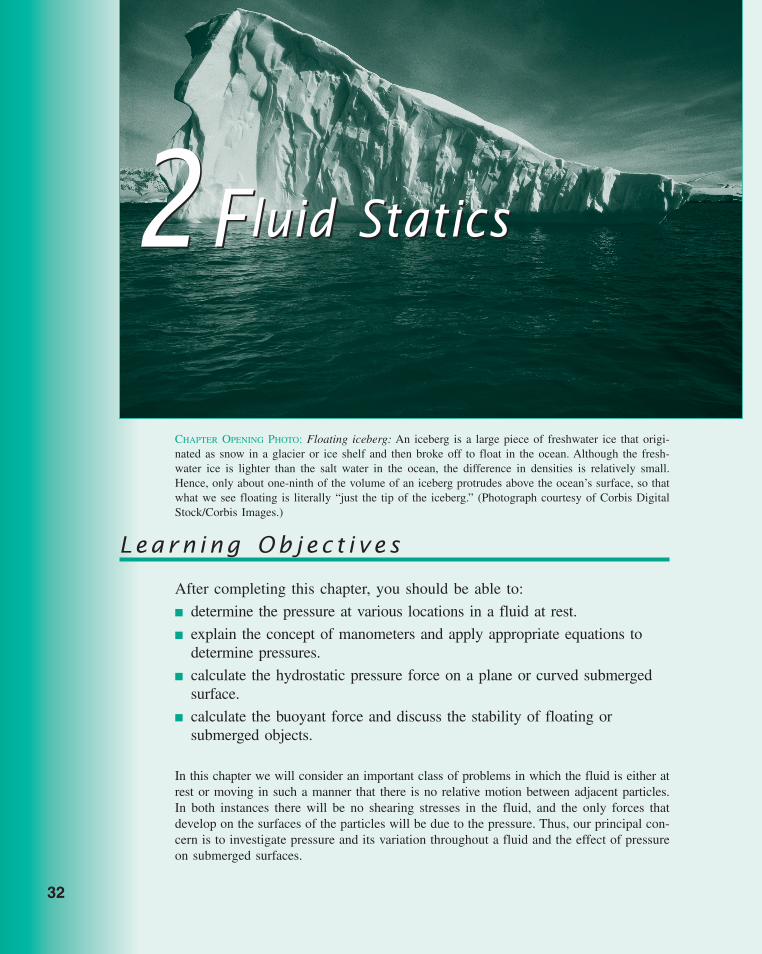
32

Learn ing Ob j ec t i v e s

After completing this chapter, you should be able to:

■ determine the pressure at various locations in a fluid at rest.

■ explain the concept of manometers and apply appropriate equations todetermine pressures.

■ calculate the hydrostatic pressure force on a plane or curved submergedsurface.

■ calculate the buoyant force and discuss the stability of floating orsubmerged objects.

In this chapter we will consider an important class of problems in which the fluid is either atrest or moving in such a manner that there is no relative motion between adjacent particles.In both instances there will be no shearing stresses in the fluid, and the only forces thatdevelop on the surfaces of the particles will be due to the pressure. Thus, our principal con-cern is to investigate pressure and its variation throughout a fluid and the effect of pressureon submerged surfaces.

22Fluid StaticsFluid Statics

CHAPTER OPENING PHOTO: Floating iceberg: An iceberg is a large piece of freshwater ice that origi-nated as snow in a glacier or ice shelf and then broke off to float in the ocean. Although the fresh-water ice is lighter than the salt water in the ocean, the difference in densities is relatively small.Hence, only about one-ninth of the volume of an iceberg protrudes above the ocean’s surface, so thatwhat we see floating is literally “just the tip of the iceberg.” (Photograph courtesy of Corbis DigitalStock/Corbis Images.)

c02FluidStatics.qxd 9/24/10 11:38 AM Page 32

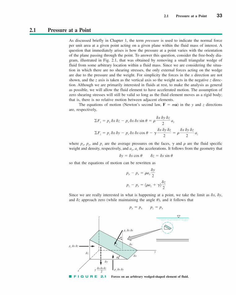
2.1 Pressure at a Point 33

δθ

θ

ps

y

z

________

2

δ y

δ x

δ s

δδ sx

pz δδ yx

py δδ zx

x

z

δx δyδzγ

2.1 Pressure at a Point

As discussed briefly in Chapter 1, the term pressure is used to indicate the normal forceper unit area at a given point acting on a given plane within the fluid mass of interest. Aquestion that immediately arises is how the pressure at a point varies with the orientationof the plane passing through the point. To answer this question, consider the free-body dia-gram, illustrated in Fig. 2.1, that was obtained by removing a small triangular wedge offluid from some arbitrary location within a fluid mass. Since we are considering the situa-tion in which there are no shearing stresses, the only external forces acting on the wedgeare due to the pressure and the weight. For simplicity the forces in the x direction are notshown, and the z axis is taken as the vertical axis so the weight acts in the negative z direc-tion. Although we are primarily interested in fluids at rest, to make the analysis as generalas possible, we will allow the fluid element to have accelerated motion. The assumption ofzero shearing stresses will still be valid so long as the fluid element moves as a rigid body;that is, there is no relative motion between adjacent elements.

The equations of motion (Newton’s second law, F � ma) in the y and z directionsare, respectively,

where px, py, and pz are the average pressures on the faces, � and � are the fluid specificweight and density, respectively, and ay, az the accelerations. It follows from the geometry that

so that the equations of motion can be rewritten as

Since we are really interested in what is happening at a point, we take the limit as �x, �y,and �z approach zero (while maintaining the angle �), and it follows that

py � ps pz � ps

pz � ps � 1�az � �2 �z

2

py � ps � �ay

�y

2

�y � �s cos � �z � �s sin �

©Fz � pz �x �y � ps �x �s cos � � �

�x �y �z

2� �

�x �y �z

2 az

©Fy � py �x �z � ps �x �s sin � � �

�x �y �z

2 ay

F I G U R E 2.1 Forces on an arbitrary wedged-shaped element of fluid.

c02FluidStatics.qxd 9/24/10 11:38 AM Page 33

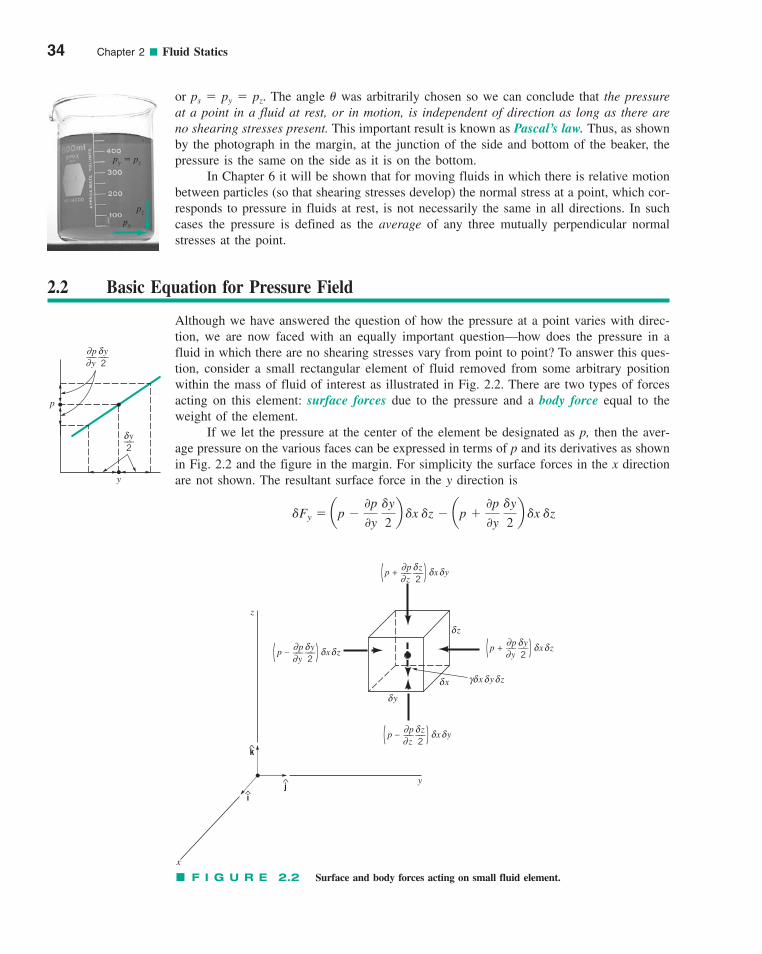
34 Chapter 2 ■ Fluid Statics

or ps � py � pz. The angle � was arbitrarily chosen so we can conclude that the pressureat a point in a fluid at rest, or in motion, is independent of direction as long as there areno shearing stresses present. This important result is known as Pascal’s law. Thus, as shownby the photograph in the margin, at the junction of the side and bottom of the beaker, thepressure is the same on the side as it is on the bottom.

In Chapter 6 it will be shown that for moving fluids in which there is relative motionbetween particles (so that shearing stresses develop) the normal stress at a point, which cor-responds to pressure in fluids at rest, is not necessarily the same in all directions. In suchcases the pressure is defined as the average of any three mutually perpendicular normalstresses at the point.

2.2 Basic Equation for Pressure Field

Although we have answered the question of how the pressure at a point varies with direc-tion, we are now faced with an equally important question—how does the pressure in afluid in which there are no shearing stresses vary from point to point? To answer this ques-tion, consider a small rectangular element of fluid removed from some arbitrary positionwithin the mass of fluid of interest as illustrated in Fig. 2.2. There are two types of forcesacting on this element: surface forces due to the pressure and a body force equal to theweight of the element.

If we let the pressure at the center of the element be designated as p, then the aver-age pressure on the various faces can be expressed in terms of p and its derivatives as shownin Fig. 2.2 and the figure in the margin. For simplicity the surface forces in the x directionare not shown. The resultant surface force in the y direction is

�Fy � ap �0p

0y �y

2b �x �z � ap �

0p

0y �y

2b �x �z

py � pz

pz

py

p

y

∂ δ∂y

p––– –––

2y

δ–––2y

k

ij

z

∂ δ δ δ

δ

xδ

yδ

∂

xγδ yδ zδ

^

^

^

x

y

z

( ) x yp +zp

––– –––2z

∂ δ δ δ∂( ) x zp +

yp

––– –––2y

∂ δ δ δ∂( ) x yp –

zp

––– –––2z

∂ δ δ δ∂( ) x zp –

yp

––– –––2y

F I G U R E 2.2 Surface and body forces acting on small fluid element.

c02FluidStatics.qxd 9/24/10 11:38 AM Page 34

or

Similarly, for the x and z directions the resultant surface forces are

The resultant surface force acting on the element can be expressed in vector form as

or

(2.1)

where and are the unit vectors along the coordinate axes shown in Fig. 2.2. The groupof terms in parentheses in Eq. 2.1 represents in vector form the pressure gradient and canbe written as

where

and the symbol is the gradient or “del” vector operator. Thus, the resultant surface forceper unit volume can be expressed as

Because the z axis is vertical, the weight of the element is

where the negative sign indicates that the force due to the weight is downward (in the neg-ative z direction). Newton’s second law, applied to the fluid element, can be expressed as

where � �F represents the resultant force acting on the element, a is the acceleration ofthe element, and �m is the element mass, which can be written as � �x �y �z. It followsthat

or

and, therefore,

(2.2)

Equation 2.2 is the general equation of motion for a fluid in which there are no shearingstresses. Although Eq. 2.2 applies to both fluids at rest and moving fluids, we will primar-ily restrict our attention to fluids at rest.

�§p � � k � �a

�§p �x �y �z � � �x �y �z k � � �x �y �z a

© �F � �Fs � �� k � �m a

© �F � �m a

��� k � � � �x �y �z k

�Fs

�x �y �z� �§p

§

§ 1 2 �0 1 20x

i �0 1 20y

j �0 1 20z

k

0p

0xi �

0p

0yj �

0p

0zk � §p

kj,i,

�Fs � � a0p

0x i �

0p

0yj �

0p

0zkb �x �y �z

�Fs � �Fx i � �Fy j � �Fz˛k

�Fx � �

0p

0x �x �y �z �Fz � �

0p

0z �x �y �z

�Fy � �

0p

0y �x �y �z

2.2 Basic Equation for Pressure Field 35

c02FluidStatics.qxd 9/24/10 11:38 AM Page 35

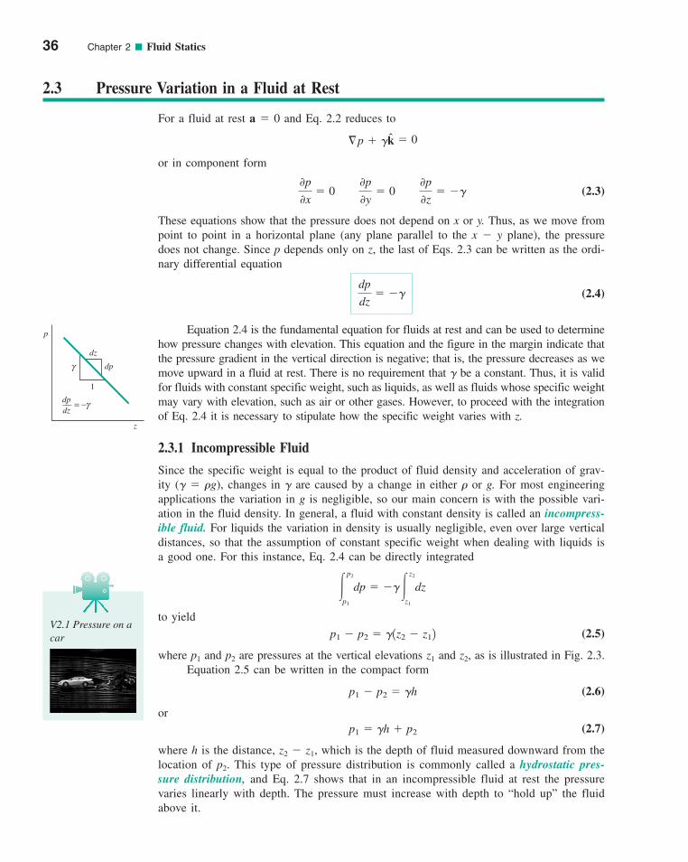
36 Chapter 2 ■ Fluid Statics

2.3 Pressure Variation in a Fluid at Rest

For a fluid at rest a � 0 and Eq. 2.2 reduces to

or in component form

(2.3)

These equations show that the pressure does not depend on x or y. Thus, as we move frompoint to point in a horizontal plane (any plane parallel to the x � y plane), the pressuredoes not change. Since p depends only on z, the last of Eqs. 2.3 can be written as the ordi-nary differential equation

(2.4)

Equation 2.4 is the fundamental equation for fluids at rest and can be used to determinehow pressure changes with elevation. This equation and the figure in the margin indicate thatthe pressure gradient in the vertical direction is negative; that is, the pressure decreases as wemove upward in a fluid at rest. There is no requirement that � be a constant. Thus, it is validfor fluids with constant specific weight, such as liquids, as well as fluids whose specific weightmay vary with elevation, such as air or other gases. However, to proceed with the integrationof Eq. 2.4 it is necessary to stipulate how the specific weight varies with z.

2.3.1 Incompressible Fluid

Since the specific weight is equal to the product of fluid density and acceleration of grav-ity (� � �g), changes in � are caused by a change in either � or g. For most engineeringapplications the variation in g is negligible, so our main concern is with the possible vari-ation in the fluid density. In general, a fluid with constant density is called an incompress-ible fluid. For liquids the variation in density is usually negligible, even over large verticaldistances, so that the assumption of constant specific weight when dealing with liquids isa good one. For this instance, Eq. 2.4 can be directly integrated

to yield

(2.5)

where p1 and p2 are pressures at the vertical elevations z1 and z2, as is illustrated in Fig. 2.3.Equation 2.5 can be written in the compact form

(2.6)

or(2.7)

where h is the distance, z2 � z1, which is the depth of fluid measured downward from thelocation of p2. This type of pressure distribution is commonly called a hydrostatic pres-sure distribution, and Eq. 2.7 shows that in an incompressible fluid at rest the pressurevaries linearly with depth. The pressure must increase with depth to “hold up” the fluidabove it.

p1 � �h � p2

p1 � p2 � �h

p1 � p2 � �1z2 � z12

�p2

p1

dp � ���z2

z1

dz

dp

dz� ��

0p

0x� 0

0p

0y� 0

0p

0z� ��

§p � �k � 0

p

z

g

dzdp––– = −g

dz

dp

1

V2.1 Pressure on acar

c02FluidStatics.qxd 9/24/10 11:38 AM Page 36

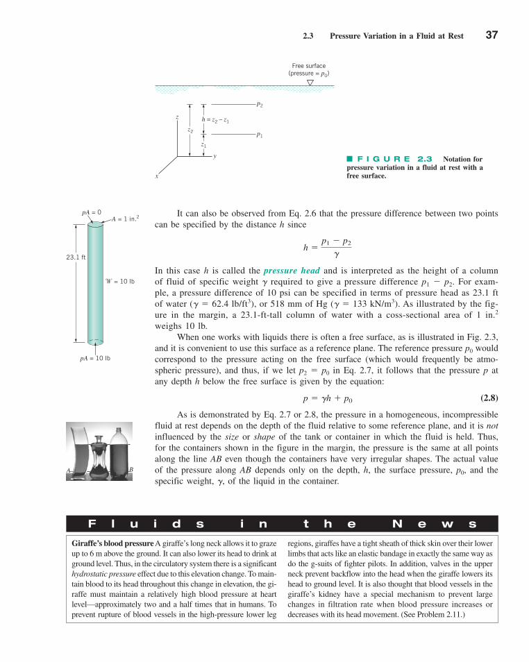
It can also be observed from Eq. 2.6 that the pressure difference between two pointscan be specified by the distance h since

In this case h is called the pressure head and is interpreted as the height of a columnof fluid of specific weight � required to give a pressure difference p1 � p2. For exam-ple, a pressure difference of 10 psi can be specified in terms of pressure head as 23.1 ftof water (� � 62.4 lb/ft3), or 518 mm of Hg (� � 133 kN/m3). As illustrated by the fig-ure in the margin, a 23.1-ft-tall column of water with a coss-sectional area of 1 in.2

weighs 10 lb.When one works with liquids there is often a free surface, as is illustrated in Fig. 2.3,

and it is convenient to use this surface as a reference plane. The reference pressure p0 wouldcorrespond to the pressure acting on the free surface (which would frequently be atmo-spheric pressure), and thus, if we let p2 � p0 in Eq. 2.7, it follows that the pressure p atany depth h below the free surface is given by the equation:

(2.8)

As is demonstrated by Eq. 2.7 or 2.8, the pressure in a homogeneous, incompressiblefluid at rest depends on the depth of the fluid relative to some reference plane, and it is notinfluenced by the size or shape of the tank or container in which the fluid is held. Thus,for the containers shown in the figure in the margin, the pressure is the same at all pointsalong the line AB even though the containers have very irregular shapes. The actual valueof the pressure along AB depends only on the depth, h, the surface pressure, and thespecific weight, of the liquid in the container.�,

p0,

p � �h � p0

h �p1 � p2

�

2.3 Pressure Variation in a Fluid at Rest 37

z

x

y

z1

z2 p1

p2

h = z2 – z1

Free surface(pressure = p0)

F I G U R E 2.3 Notation for pressure variation in a fluid at rest with a free surface.

pA = 0

pA = 10 lb

A = 1 in.2

� = 10 lb

23.1 ft

A B

F l u i d s i n t h e N e w s

Giraffe’s blood pressureA giraffe’s long neck allows it to grazeup to 6 m above the ground. It can also lower its head to drink atground level. Thus, in the circulatory system there is a significanthydrostatic pressure effect due to this elevation change. To main-tain blood to its head throughout this change in elevation, the gi-raffe must maintain a relatively high blood pressure at heartlevel—approximately two and a half times that in humans. Toprevent rupture of blood vessels in the high-pressure lower leg

regions, giraffes have a tight sheath of thick skin over their lowerlimbs that acts like an elastic bandage in exactly the same way asdo the g-suits of fighter pilots. In addition, valves in the upperneck prevent backflow into the head when the giraffe lowers itshead to ground level. It is also thought that blood vessels in thegiraffe’s kidney have a special mechanism to prevent largechanges in filtration rate when blood pressure increases or decreases with its head movement. (See Problem 2.11.)

c02FluidStatics.qxd 9/24/10 11:38 AM Page 37

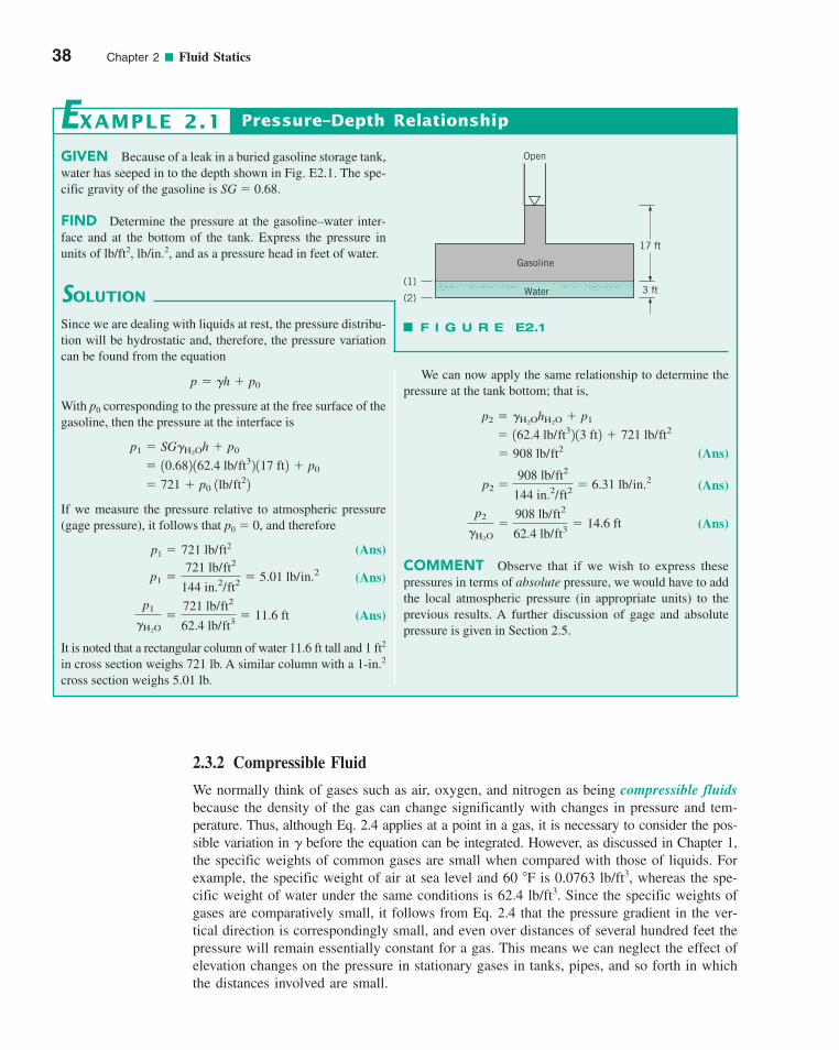
38 Chapter 2 ■ Fluid Statics

GIVEN Because of a leak in a buried gasoline storage tank,water has seeped in to the depth shown in Fig. E2.1. The spe-cific gravity of the gasoline is SG � 0.68.

FIND Determine the pressure at the gasoline–water inter-face and at the bottom of the tank. Express the pressure inunits of lb/ft2, lb/in.2, and as a pressure head in feet of water.

SOLUTION

Pressure–Depth Relationship

We can now apply the same relationship to determine thepressure at the tank bottom; that is,

(Ans) � 908 lb/ft2 � 162.4 lb/ft32 13 ft2 � 721 lb/ft2

p2 � �H2OhH2O � p1

(Ans) p2 �908 lb/ft2

144 in.2/ft2� 6.31 lb/in.2

(Ans)

COMMENT Observe that if we wish to express thesepressures in terms of absolute pressure, we would have to addthe local atmospheric pressure (in appropriate units) to theprevious results. A further discussion of gage and absolutepressure is given in Section 2.5.

p2

�H2O�

908 lb/ft2

62.4 lb/ft3� 14.6 ft

EXAMPLE 2.1

Since we are dealing with liquids at rest, the pressure distribu-tion will be hydrostatic and, therefore, the pressure variationcan be found from the equation

With p0 corresponding to the pressure at the free surface of thegasoline, then the pressure at the interface is

If we measure the pressure relative to atmospheric pressure(gage pressure), it follows that p0 � 0, and therefore

(Ans) p1 � 721 lb/ft2

� 721 � p0 1lb/ft22

� 10.682 162.4 lb/ft32 117 ft2 � p0

p1 � SG�H2Oh � p0

p � �h � p0

(1)

(2)Water

Gasoline

Open

17 ft

3 ft

F I G U R E E2.1

(Ans) p1 �721 lb/ft2

144 in.2/ft2� 5.01 lb/in.2

(Ans)

It is noted that a rectangular column of water 11.6 ft tall and 1 ft2

in cross section weighs 721 lb. A similar column with a 1-in.2

cross section weighs 5.01 lb.

p1

�H2O�

721 lb/ft2

62.4 lb/ft3� 11.6 ft

2.3.2 Compressible Fluid

We normally think of gases such as air, oxygen, and nitrogen as being compressible fluidsbecause the density of the gas can change significantly with changes in pressure and tem-perature. Thus, although Eq. 2.4 applies at a point in a gas, it is necessary to consider the pos-sible variation in � before the equation can be integrated. However, as discussed in Chapter 1,the specific weights of common gases are small when compared with those of liquids. Forexample, the specific weight of air at sea level and 60 �F is 0.0763 lb/ft3, whereas the spe-cific weight of water under the same conditions is 62.4 lb/ft3. Since the specific weights ofgases are comparatively small, it follows from Eq. 2.4 that the pressure gradient in the ver-tical direction is correspondingly small, and even over distances of several hundred feet thepressure will remain essentially constant for a gas. This means we can neglect the effect ofelevation changes on the pressure in stationary gases in tanks, pipes, and so forth in whichthe distances involved are small.

c02FluidStatics.qxd 9/24/10 11:38 AM Page 38

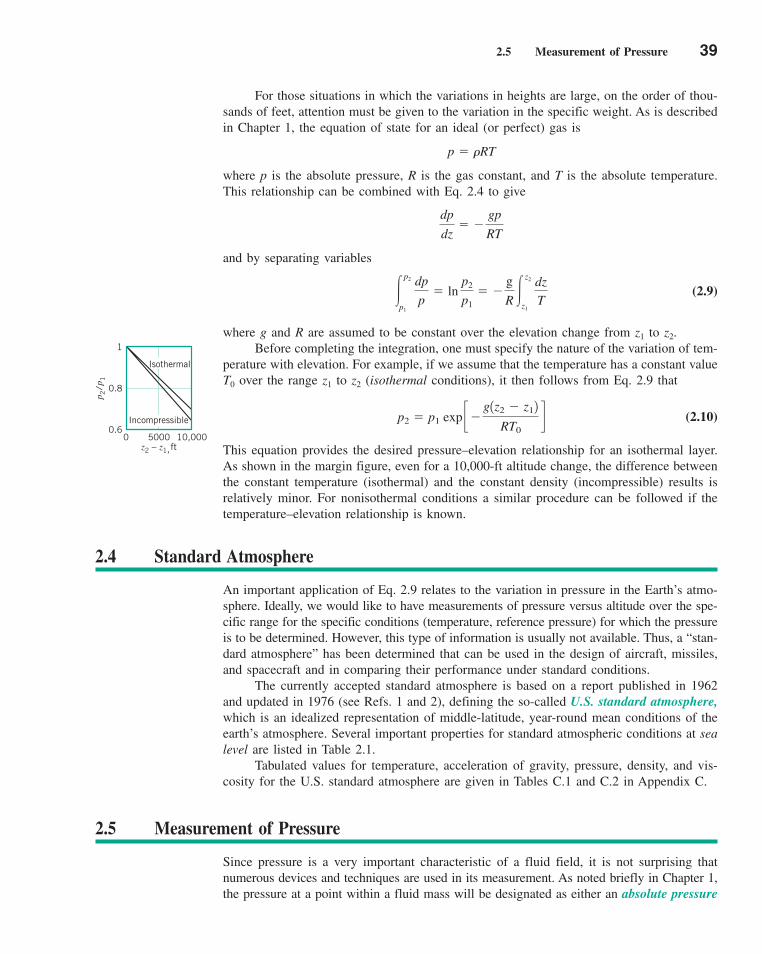
For those situations in which the variations in heights are large, on the order of thou-sands of feet, attention must be given to the variation in the specific weight. As is describedin Chapter 1, the equation of state for an ideal (or perfect) gas is

where p is the absolute pressure, R is the gas constant, and T is the absolute temperature.This relationship can be combined with Eq. 2.4 to give

and by separating variables

(2.9)

where g and R are assumed to be constant over the elevation change from z1 to z2.Before completing the integration, one must specify the nature of the variation of tem-

perature with elevation. For example, if we assume that the temperature has a constant valueT0 over the range z1 to z2 (isothermal conditions), it then follows from Eq. 2.9 that

(2.10)

This equation provides the desired pressure–elevation relationship for an isothermal layer.As shown in the margin figure, even for a 10,000-ft altitude change, the difference betweenthe constant temperature (isothermal) and the constant density (incompressible) results isrelatively minor. For nonisothermal conditions a similar procedure can be followed if thetemperature–elevation relationship is known.

p2 � p1 exp c�

g1z2 � z12

RT0d

�p2

p1

dp

p� ln

p2

p1� �

g

R �z2

z1

dz

T

dp

dz� �

gp

RT

p � �RT

2.5 Measurement of Pressure 39

1

0.8

0.60 5000 10,000

z2 – z1,ft

p 2/p

1

Isothermal

Incompressible

2.4 Standard Atmosphere

An important application of Eq. 2.9 relates to the variation in pressure in the Earth’s atmo-sphere. Ideally, we would like to have measurements of pressure versus altitude over the spe-cific range for the specific conditions (temperature, reference pressure) for which the pressureis to be determined. However, this type of information is usually not available. Thus, a “stan-dard atmosphere” has been determined that can be used in the design of aircraft, missiles,and spacecraft and in comparing their performance under standard conditions.

The currently accepted standard atmosphere is based on a report published in 1962and updated in 1976 (see Refs. 1 and 2), defining the so-called U.S. standard atmosphere,which is an idealized representation of middle-latitude, year-round mean conditions of theearth’s atmosphere. Several important properties for standard atmospheric conditions at sealevel are listed in Table 2.1.

Tabulated values for temperature, acceleration of gravity, pressure, density, and vis-cosity for the U.S. standard atmosphere are given in Tables C.1 and C.2 in Appendix C.

2.5 Measurement of Pressure

Since pressure is a very important characteristic of a fluid field, it is not surprising thatnumerous devices and techniques are used in its measurement. As noted briefly in Chapter 1,the pressure at a point within a fluid mass will be designated as either an absolute pressure

c02FluidStatics.qxd 9/24/10 11:38 AM Page 39

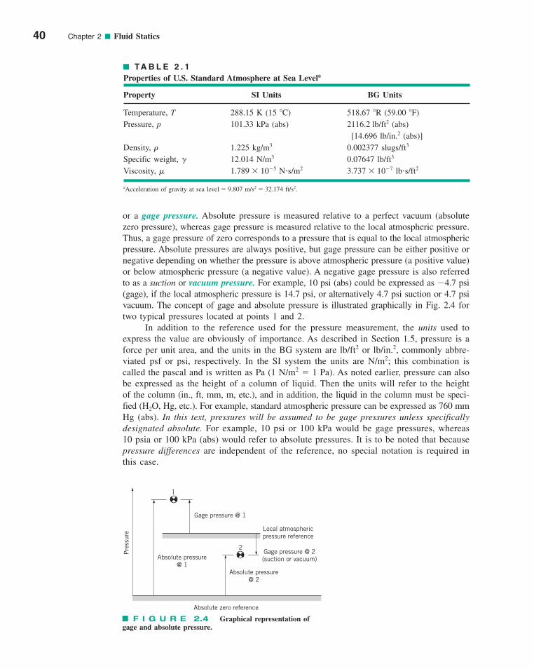
40 Chapter 2 ■ Fluid Statics

TA B L E 2 . 1

Properties of U.S. Standard Atmosphere at Sea Levela

Property SI Units BG Units

Temperature, T 288.15 K (15 �C) 518.67 �R (59.00 �F)Pressure, p 101.33 kPa (abs) 2116.2 lb/ft2 (abs)

[14.696 lb/in.2 (abs)]Density, � 1.225 kg/m3 0.002377 slugs/ft3

Specific weight, � 12.014 N/m3 0.07647 lb/ft3

Viscosity, � 1.789 � 10�5 N�s/m2 3.737 � 10�7 lb�s/ft2

aAcceleration of gravity at sea level � 9.807 m/s2 � 32.174 ft/s2.

F I G U R E 2.4 Graphical representation ofgage and absolute pressure.

1

2

Absolute pressure@ 2

Absolute pressure@ 1

Gage pressure @ 1

Pre

ssur

e

Absolute zero reference

Local atmosphericpressure reference

Gage pressure @ 2(suction or vacuum)

or a gage pressure. Absolute pressure is measured relative to a perfect vacuum (absolutezero pressure), whereas gage pressure is measured relative to the local atmospheric pressure.Thus, a gage pressure of zero corresponds to a pressure that is equal to the local atmosphericpressure. Absolute pressures are always positive, but gage pressure can be either positive ornegative depending on whether the pressure is above atmospheric pressure (a positive value)or below atmospheric pressure (a negative value). A negative gage pressure is also referredto as a suction or vacuum pressure. For example, 10 psi (abs) could be expressed as �4.7 psi(gage), if the local atmospheric pressure is 14.7 psi, or alternatively 4.7 psi suction or 4.7 psivacuum. The concept of gage and absolute pressure is illustrated graphically in Fig. 2.4 fortwo typical pressures located at points 1 and 2.

In addition to the reference used for the pressure measurement, the units used toexpress the value are obviously of importance. As described in Section 1.5, pressure is aforce per unit area, and the units in the BG system are lb/ft2 or lb/in.2, commonly abbre-viated psf or psi, respectively. In the SI system the units are N/m2; this combination iscalled the pascal and is written as Pa (1 N/m2 � 1 Pa). As noted earlier, pressure can alsobe expressed as the height of a column of liquid. Then the units will refer to the heightof the column (in., ft, mm, m, etc.), and in addition, the liquid in the column must be speci-fied (H2O, Hg, etc.). For example, standard atmospheric pressure can be expressed as 760 mmHg (abs). In this text, pressures will be assumed to be gage pressures unless specificallydesignated absolute. For example, 10 psi or 100 kPa would be gage pressures, whereas10 psia or 100 kPa (abs) would refer to absolute pressures. It is to be noted that becausepressure differences are independent of the reference, no special notation is required inthis case.

c02FluidStatics.qxd 9/24/10 11:38 AM Page 40

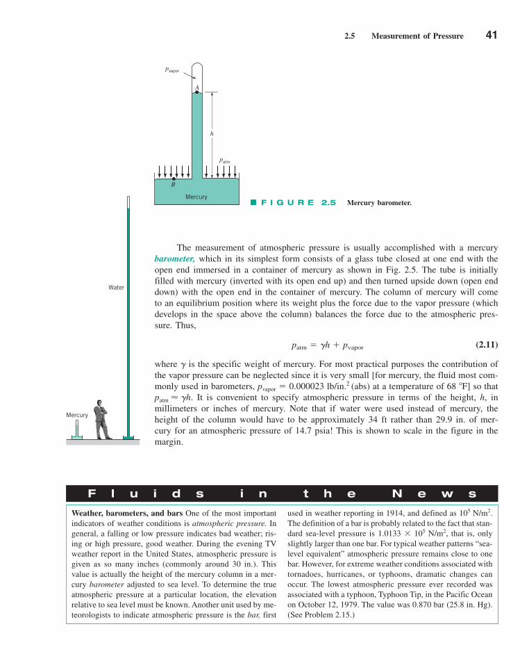
The measurement of atmospheric pressure is usually accomplished with a mercurybarometer, which in its simplest form consists of a glass tube closed at one end with theopen end immersed in a container of mercury as shown in Fig. 2.5. The tube is initiallyfilled with mercury (inverted with its open end up) and then turned upside down (open enddown) with the open end in the container of mercury. The column of mercury will cometo an equilibrium position where its weight plus the force due to the vapor pressure (whichdevelops in the space above the column) balances the force due to the atmospheric pres-sure. Thus,

(2.11)

where � is the specific weight of mercury. For most practical purposes the contribution ofthe vapor pressure can be neglected since it is very small [for mercury, the fluid most com-monly used in barometers, pvapor � 0.000023 lb/in.2 (abs) at a temperature of 68 �F] so thatpatm � �h. It is convenient to specify atmospheric pressure in terms of the height, h, inmillimeters or inches of mercury. Note that if water were used instead of mercury, theheight of the column would have to be approximately 34 ft rather than 29.9 in. of mer-cury for an atmospheric pressure of 14.7 psia! This is shown to scale in the figure in themargin.

patm � �h � pvapor

2.5 Measurement of Pressure 41

pvapor

A

h

patm

B

MercuryF I G U R E 2.5 Mercury barometer.

Water

Mercury

F l u i d s i n t h e N e w s

Weather, barometers, and bars One of the most importantindicators of weather conditions is atmospheric pressure. Ingeneral, a falling or low pressure indicates bad weather; ris-ing or high pressure, good weather. During the evening TVweather report in the United States, atmospheric pressure isgiven as so many inches (commonly around 30 in.). Thisvalue is actually the height of the mercury column in a mer-cury barometer adjusted to sea level. To determine the true atmospheric pressure at a particular location, the elevationrelative to sea level must be known. Another unit used by me-teorologists to indicate atmospheric pressure is the bar, first

used in weather reporting in 1914, and defined as 105 N/m2.The definition of a bar is probably related to the fact that stan-dard sea-level pressure is 1.0133 � 105 N/m2, that is, onlyslightly larger than one bar. For typical weather patterns “sea-level equivalent” atmospheric pressure remains close to onebar. However, for extreme weather conditions associated withtornadoes, hurricanes, or typhoons, dramatic changes canoccur. The lowest atmospheric pressure ever recorded wasassociated with a typhoon, Typhoon Tip, in the Pacific Oceanon October 12, 1979. The value was 0.870 bar (25.8 in. Hg).(See Problem 2.15.)

c02FluidStatics.qxd 9/24/10 11:39 AM Page 41

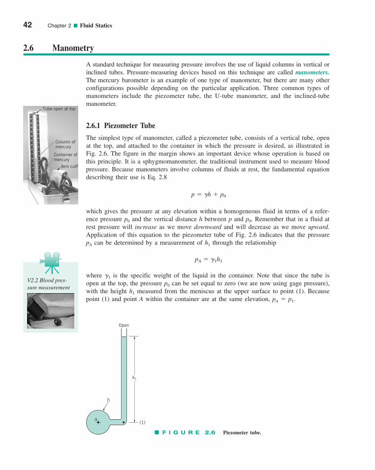
42 Chapter 2 ■ Fluid Statics

2.6 Manometry

A standard technique for measuring pressure involves the use of liquid columns in vertical orinclined tubes. Pressure-measuring devices based on this technique are called manometers.The mercury barometer is an example of one type of manometer, but there are many otherconfigurations possible depending on the particular application. Three common types ofmanometers include the piezometer tube, the U-tube manometer, and the inclined-tubemanometer.

2.6.1 Piezometer Tube

The simplest type of manometer, called a piezometer tube, consists of a vertical tube, openat the top, and attached to the container in which the pressure is desired, as illustrated inFig. 2.6. The figure in the margin shows an important device whose operation is based onthis principle. It is a sphygmomanometer, the traditional instrument used to measure bloodpressure. Because manometers involve columns of fluids at rest, the fundamental equationdescribing their use is Eq. 2.8

which gives the pressure at any elevation within a homogeneous fluid in terms of a refer-ence pressure p0 and the vertical distance h between p and p0. Remember that in a fluid atrest pressure will increase as we move downward and will decrease as we move upward.Application of this equation to the piezometer tube of Fig. 2.6 indicates that the pressurepA can be determined by a measurement of h1 through the relationship

where �1 is the specific weight of the liquid in the container. Note that since the tube isopen at the top, the pressure p0 can be set equal to zero (we are now using gage pressure),with the height h1 measured from the meniscus at the upper surface to point (1). Becausepoint (1) and point A within the container are at the same elevation, pA � p1.

pA � �1h1

p � �h � p0

Column ofmercury

Tube open at top

Container ofmercury

Arm cuff

Open

h1

1

(1)

γ

A

F I G U R E 2.6 Piezometer tube.

V2.2 Blood pres-sure measurement

c02FluidStatics.qxd 9/24/10 11:39 AM Page 42

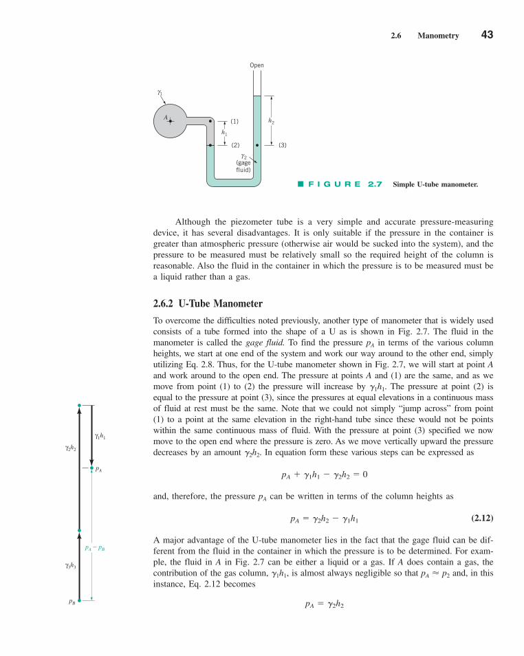
Although the piezometer tube is a very simple and accurate pressure-measuringdevice, it has several disadvantages. It is only suitable if the pressure in the container isgreater than atmospheric pressure (otherwise air would be sucked into the system), and thepressure to be measured must be relatively small so the required height of the column isreasonable. Also the fluid in the container in which the pressure is to be measured must bea liquid rather than a gas.

2.6.2 U-Tube Manometer

To overcome the difficulties noted previously, another type of manometer that is widely usedconsists of a tube formed into the shape of a U as is shown in Fig. 2.7. The fluid in themanometer is called the gage fluid. To find the pressure pA in terms of the various columnheights, we start at one end of the system and work our way around to the other end, simplyutilizing Eq. 2.8. Thus, for the U-tube manometer shown in Fig. 2.7, we will start at point Aand work around to the open end. The pressure at points A and (1) are the same, and as wemove from point (1) to (2) the pressure will increase by �1h1. The pressure at point (2) isequal to the pressure at point (3), since the pressures at equal elevations in a continuous massof fluid at rest must be the same. Note that we could not simply “jump across” from point(1) to a point at the same elevation in the right-hand tube since these would not be pointswithin the same continuous mass of fluid. With the pressure at point (3) specified we nowmove to the open end where the pressure is zero. As we move vertically upward the pressuredecreases by an amount �2h2. In equation form these various steps can be expressed as

and, therefore, the pressure pA can be written in terms of the column heights as

(2.12)

A major advantage of the U-tube manometer lies in the fact that the gage fluid can be dif-ferent from the fluid in the container in which the pressure is to be determined. For exam-ple, the fluid in A in Fig. 2.7 can be either a liquid or a gas. If A does contain a gas, thecontribution of the gas column, �1h1, is almost always negligible so that pA p2 and, in thisinstance, Eq. 2.12 becomes

pA � �2h2

�

pA � �2h2 � �1h1

pA � �1h1 � �2h2 � 0

2.6 Manometry 43

h1

h2

Open

(1)

(3)(2)

A

(gagefluid)

1γ

2γ

F I G U R E 2.7 Simple U-tube manometer.

pA

γ2h2

γ1h1

γ3h3

pA − pB

pB

c02FluidStatics.qxd 9/24/10 11:39 AM Page 43

44 Chapter 2 ■ Fluid Statics

GIVEN A closed tank contains compressed air and oil(SGoil � 0.90) as is shown in Fig. E2.2. A U-tube manometerusing mercury (SGHg � 13.6) is connected to the tank as shown.The column heights are h1 � 36 in., h2 � 6 in., and h3 � 9 in.

FIND Determine the pressure reading (in psi) of the gage.

SOLUTION

Simple U-Tube Manometer

Because the specific weight of the air above the oil is muchsmaller than the specific weight of the oil, the gage shouldread the pressure we have calculated; that is,

(Ans)

COMMENT Assume that the gage pressure remains at3.06 psi, but the manometer is altered so that it contains onlyoil. That is, the mercury is replaced by oil. A simple calcula-tion shows that in this case the vertical oil-filled tube wouldneed to be h3 � 11.3 ft tall, rather than the original h3 � 9 in.There is an obvious advantage of using a heavy fluid such asmercury in manometers.

pgage �440 lb/ft2

144 in.2/ft2� 3.06 psi

EXAMPLE 2.2

Following the general procedure of starting at one end of themanometer system and working around to the other, we willstart at the air–oil interface in the tank and proceed to the openend where the pressure is zero. The pressure at level (1) is

This pressure is equal to the pressure at level (2), as these twopoints are at the same elevation in a homogeneous fluid at rest.As we move from level (2) to the open end, the pressure mustdecrease by �Hgh3, and at the open end the pressure is zero.Thus, the manometer equation can be expressed as

or

For the values given

pair � �10.92 162.4 lb/ft32 a36 � 6

12 ftb

pair � 1SGoil2 1�H2O2 1h1 � h22 � 1SGHg2 1�H2O2h3 � 0

pair � �oil1h1 � h22 � �Hgh3 � 0

p1 � pair � �oil1h1 � h22F I G U R E E2.2

� 113.62 162.4 lb/ft32 a9

12 ftb

so that

pair � 440 lb/ft2

Pressuregage

Air

Oil

Open

Hg

(1) (2)

h1

h2

h3

The U-tube manometer is also widely used to measure the difference in pressure betweentwo containers or two points in a given system. Consider a manometer connected betweencontainers A and B as is shown in Fig. 2.8. The difference in pressure between A and B canbe found by again starting at one end of the system and working around to the other end. Forexample, at A the pressure is pA, which is equal to p1, and as we move to point (2) the pres-sure increases by �1h1. The pressure at p2 is equal to p3, and as we move upward to point (4)the pressure decreases by �2h2. Similarly, as we continue to move upward from point (4) to(5) the pressure decreases by �3h3. Finally, p5 � pB, as they are at equal elevations. Thus,

Or, as indicated in the figure in the margin on the previous page, we could start at B and workour way around to A to obtain the same result. In either case, the pressure difference is

pA � pB � �2h2 � �3h3 � �1h1

pA � �1h1 � �2h2 � �3h3 � pB

c02FluidStatics.qxd 9/24/10 11:39 AM Page 44

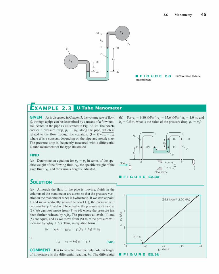
2.6 Manometry 45

(1)

(2) (3)

(4)

(5)

A

B

h1

h2

h3

2γ

3γ

1γ

F I G U R E 2.8 Differential U-tubemanometer.

GIVEN As is discussed in Chapter 3, the volume rate of flow,Q, through a pipe can be determined by a means of a flow noz-zle located in the pipe as illustrated in Fig. E2.3a. The nozzlecreates a pressure drop, pA � pB, along the pipe, which is related to the flow through the equation, ,where K is a constant depending on the pipe and nozzle size.The pressure drop is frequently measured with a differentialU-tube manometer of the type illustrated.

FIND(a) Determine an equation for pA � pB in terms of the spe-cific weight of the flowing fluid, �1, the specific weight of thegage fluid, �2, and the various heights indicated.

Q � K1pA � pB

U-Tube Manometer

(b) For �1 � 9.80 kN/m3, �2 � 15.6 kN/m3, h1 � 1.0 m, andh2 � 0.5 m, what is the value of the pressure drop, pA � pB?

EXAMPLE 2.3

SOLUTION

F I G U R E E2.3a

A B

Flow nozzle

(1)

h1

(2) (3)

(4)h2

(5)

Flow

γ1

γ2

γ1

8

3

2

1

010 12 14 16

p A –

pB,

kPa

�2, kN/m3

�2 = �1

(15.6 kN/m3, 2.90 kPa)

(a) Although the fluid in the pipe is moving, fluids in thecolumns of the manometer are at rest so that the pressure vari-ation in the manometer tubes is hydrostatic. If we start at pointA and move vertically upward to level (1), the pressure willdecrease by �1h1 and will be equal to the pressure at (2) and at(3). We can now move from (3) to (4) where the pressure hasbeen further reduced by �2h2. The pressures at levels (4) and(5) are equal, and as we move from (5) to B the pressure willincrease by �1(h1 � h2). Thus, in equation form

or(Ans)

COMMENT It is to be noted that the only column heightof importance is the differential reading, h2. The differential

pA � pB � h21�2 � �12

pA � �1h1 � �2h2 � �11h1 � h22 � pB

F I G U R E E2.3b

c02FluidStatics.qxd 9/24/10 11:39 AM Page 45

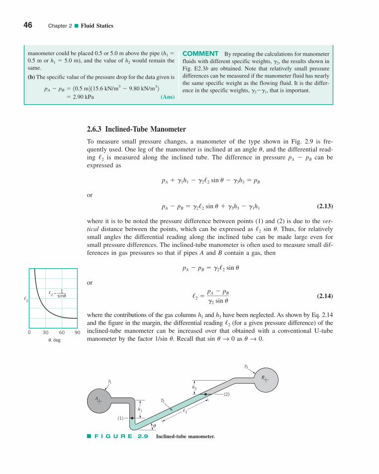
46 Chapter 2 ■ Fluid Statics

2.6.3 Inclined-Tube Manometer

To measure small pressure changes, a manometer of the type shown in Fig. 2.9 is fre-quently used. One leg of the manometer is inclined at an angle �, and the differential read-ing /2 is measured along the inclined tube. The difference in pressure pA � pB can beexpressed as

or

(2.13)

where it is to be noted the pressure difference between points (1) and (2) is due to the ver-tical distance between the points, which can be expressed as /2 sin �. Thus, for relativelysmall angles the differential reading along the inclined tube can be made large even forsmall pressure differences. The inclined-tube manometer is often used to measure small dif-ferences in gas pressures so that if pipes A and B contain a gas, then

or

(2.14)

where the contributions of the gas columns h1 and h3 have been neglected. As shown by Eq. 2.14and the figure in the margin, the differential reading /2 (for a given pressure difference) of theinclined-tube manometer can be increased over that obtained with a conventional U-tubemanometer by the factor 1/sin �. Recall that sin � → 0 as � → 0.

/2 �pA � pB

�2 sin �

pA � pB � �2/2 sin �

pA � pB � �2/2 sin � � �3h3 � �1h1

pA � �1h1 � �2/2 sin � � �3h3 � pB

COMMENT By repeating the calculations for manometerfluids with different specific weights, �2, the results shown inFig. E2.3b are obtained. Note that relatively small pressuredifferences can be measured if the manometer fluid has nearlythe same specific weight as the flowing fluid. It is the differ-ence in the specific weights, �2��1, that is important.

manometer could be placed 0.5 or 5.0 m above the pipe (h1 �0.5 m or h1 � 5.0 m), and the value of h2 would remain thesame.

(b) The specific value of the pressure drop for the data given is

(Ans) � 2.90 kPa

pA � pB � 10.5 m2 115.6 kN/m3 � 9.80 kN/m32

h1

h3

�2

(2)

γ3

γ2

γ1

A

B

θ(1)

�2

300 60 90

θ , deg

~�2 sin

1θ

F I G U R E 2.9 Inclined-tube manometer.

c02FluidStatics.qxd 9/24/10 11:39 AM Page 46

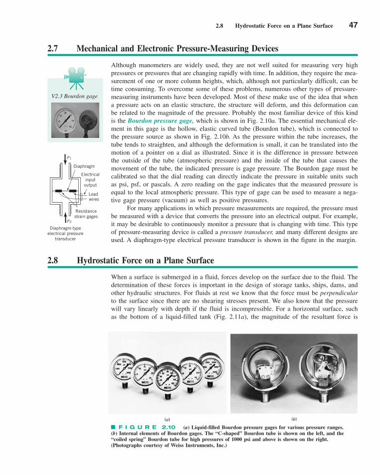
2.8 Hydrostatic Force on a Plane Surface 47

2.7 Mechanical and Electronic Pressure-Measuring Devices

Although manometers are widely used, they are not well suited for measuring very highpressures or pressures that are changing rapidly with time. In addition, they require the mea-surement of one or more column heights, which, although not particularly difficult, can betime consuming. To overcome some of these problems, numerous other types of pressure-measuring instruments have been developed. Most of these make use of the idea that whena pressure acts on an elastic structure, the structure will deform, and this deformation canbe related to the magnitude of the pressure. Probably the most familiar device of this kindis the Bourdon pressure gage, which is shown in Fig. 2.10a. The essential mechanical ele-ment in this gage is the hollow, elastic curved tube (Bourdon tube), which is connected tothe pressure source as shown in Fig. 2.10b. As the pressure within the tube increases, thetube tends to straighten, and although the deformation is small, it can be translated into themotion of a pointer on a dial as illustrated. Since it is the difference in pressure betweenthe outside of the tube (atmospheric pressure) and the inside of the tube that causes themovement of the tube, the indicated pressure is gage pressure. The Bourdon gage must becalibrated so that the dial reading can directly indicate the pressure in suitable units suchas psi, psf, or pascals. A zero reading on the gage indicates that the measured pressure isequal to the local atmospheric pressure. This type of gage can be used to measure a nega-tive gage pressure (vacuum) as well as positive pressures.

For many applications in which pressure measurements are required, the pressure mustbe measured with a device that converts the pressure into an electrical output. For example,it may be desirable to continuously monitor a pressure that is changing with time. This typeof pressure-measuring device is called a pressure transducer, and many different designs areused. A diaphragm-type electrical pressure transducer is shown in the figure in the margin.

V2.3 Bourdon gage

F I G U R E 2.10 (a) Liquid-filled Bourdon pressure gages for various pressure ranges.(b) Internal elements of Bourdon gages. The “C-shaped” Bourdon tube is shown on the left, and the“coiled spring” Bourdon tube for high pressures of 1000 psi and above is shown on the right.(Photographs courtesy of Weiss Instruments, Inc.)

Electrical input output

Lead

Diaphragm

Diaphragm-type electrical pressure

transducer

wires

Resistance strain gages

p2

p1

2.8 Hydrostatic Force on a Plane Surface

When a surface is submerged in a fluid, forces develop on the surface due to the fluid. Thedetermination of these forces is important in the design of storage tanks, ships, dams, andother hydraulic structures. For fluids at rest we know that the force must be perpendicularto the surface since there are no shearing stresses present. We also know that the pressurewill vary linearly with depth if the fluid is incompressible. For a horizontal surface, suchas the bottom of a liquid-filled tank (Fig. 2.11a), the magnitude of the resultant force is

c02FluidStatics.qxd 9/24/10 11:39 AM Page 47

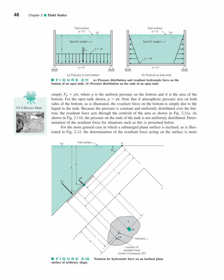
simply FR � pA, where p is the uniform pressure on the bottom and A is the area of thebottom. For the open tank shown, p � �h. Note that if atmospheric pressure acts on bothsides of the bottom, as is illustrated, the resultant force on the bottom is simply due to theliquid in the tank. Because the pressure is constant and uniformly distributed over the bot-tom, the resultant force acts through the centroid of the area as shown in Fig. 2.11a. Asshown in Fig. 2.11b, the pressure on the ends of the tank is not uniformly distributed. Deter-mination of the resultant force for situations such as this is presented below.

For the more general case in which a submerged plane surface is inclined, as is illus-trated in Fig. 2.12, the determination of the resultant force acting on the surface is more

48 Chapter 2 ■ Fluid Statics

V2.4 Hoover Dam

F I G U R E 2.11 (a) Pressure distribution and resultant hydrostatic force on the bottom of an open tank. (b) Pressure distribution on the ends of an open tank.

Free surfacep = 0

Specific weight = γ

FRh

p = 0

p = hγ

(a) Pressure on tank bottom

Free surfacep = 0

Specific weight = γ

p = 0

p = hγ

(b) Pressure on tank ends

y

ycyR

xR

xc

c

CP Centroid, c

Location ofresultant force

(center of pressure, CP)

dA

A

x

x

y

θ

0Free surface

hhc

FR

dF

F I G U R E 2.12 Notation for hydrostatic force on an inclined planesurface of arbitrary shape.

c02FluidStatics.qxd 9/24/10 11:39 AM Page 48

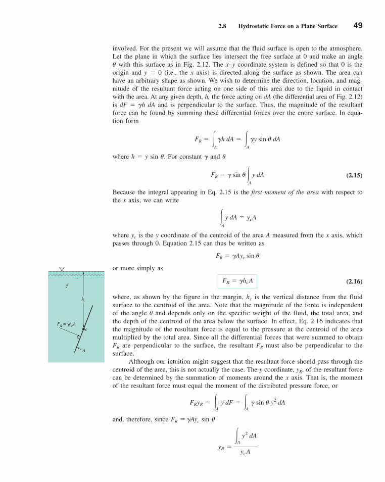
2.8 Hydrostatic Force on a Plane Surface 49

involved. For the present we will assume that the fluid surface is open to the atmosphere.Let the plane in which the surface lies intersect the free surface at 0 and make an angle� with this surface as in Fig. 2.12. The x–y coordinate system is defined so that 0 is theorigin and y � 0 (i.e., the x axis) is directed along the surface as shown. The area canhave an arbitrary shape as shown. We wish to determine the direction, location, and mag-nitude of the resultant force acting on one side of this area due to the liquid in contactwith the area. At any given depth, h, the force acting on dA (the differential area of Fig. 2.12)is dF � �h dA and is perpendicular to the surface. Thus, the magnitude of the resultantforce can be found by summing these differential forces over the entire surface. In equa-tion form

where h � y sin �. For constant � and �

(2.15)

Because the integral appearing in Eq. 2.15 is the first moment of the area with respect tothe x axis, we can write

where yc is the y coordinate of the centroid of the area A measured from the x axis, whichpasses through 0. Equation 2.15 can thus be written as

or more simply as

(2.16)

where, as shown by the figure in the margin, hc is the vertical distance from the fluidsurface to the centroid of the area. Note that the magnitude of the force is independentof the angle � and depends only on the specific weight of the fluid, the total area, andthe depth of the centroid of the area below the surface. In effect, Eq. 2.16 indicates thatthe magnitude of the resultant force is equal to the pressure at the centroid of the areamultiplied by the total area. Since all the differential forces that were summed to obtainFR are perpendicular to the surface, the resultant FR must also be perpendicular to thesurface.

Although our intuition might suggest that the resultant force should pass through thecentroid of the area, this is not actually the case. The y coordinate, yR, of the resultant forcecan be determined by the summation of moments around the x axis. That is, the momentof the resultant force must equal the moment of the distributed pressure force, or

and, therefore, since FR � �Ayc sin �

yR �

�

A y

2 dA

ycA

FRyR � �

A y dF � �

A � sin � y2 dA

FR � �hcA

FR � �Ayc sin �

�

A

y dA � ycA

FR � � sin ��

A

y dA

FR � �

A

�h dA � �

A

�y sin � dA

γ

A

hc

cFR = γhcA

c02FluidStatics.qxd 9/24/10 11:39 AM Page 49

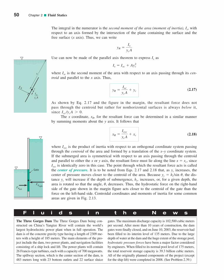
The integral in the numerator is the second moment of the area (moment of inertia), Ix, withrespect to an axis formed by the intersection of the plane containing the surface and thefree surface (x axis). Thus, we can write

Use can now be made of the parallel axis theorem to express Ix as

where Ixc is the second moment of the area with respect to an axis passing through its cen-troid and parallel to the x axis. Thus,

(2.17)

As shown by Eq. 2.17 and the figure in the margin, the resultant force does notpass through the centroid but rather for nonhorizontal surfaces is always below it,since Ixc /ycA 0.

The x coordinate, xR, for the resultant force can be determined in a similar mannerby summing moments about the y axis. It follows that

(2.18)

where Ixyc is the product of inertia with respect to an orthogonal coordinate system passingthrough the centroid of the area and formed by a translation of the x–y coordinate system.If the submerged area is symmetrical with respect to an axis passing through the centroidand parallel to either the x or y axis, the resultant force must lie along the line x � xc, sinceIxyc is identically zero in this case. The point through which the resultant force acts is calledthe center of pressure. It is to be noted from Eqs. 2.17 and 2.18 that, as yc increases, thecenter of pressure moves closer to the centroid of the area. Because yc � hc/sin �, the dis-tance yc will increase if the depth of submergence, hc, increases, or, for a given depth, thearea is rotated so that the angle, �, decreases. Thus, the hydrostatic force on the right-handside of the gate shown in the margin figure acts closer to the centroid of the gate than theforce on the left-hand side. Centroidal coordinates and moments of inertia for some commonareas are given in Fig. 2.13.

xR �Ixyc

ycA� xc

yR �Ixc

ycA� yc

Ix � Ixc � Ay2c

yR �Ix

ycA

50 Chapter 2 ■ Fluid Statics

F l u i d s i n t h e N e w s

The Three Gorges Dam The Three Gorges Dam being con-structed on China’s Yangtze River will contain the world’slargest hydroelectric power plant when in full operation. Thedam is of the concrete gravity type having a length of 2309 me-ters with a height of 185 meters. The main elements of the pro-ject include the dam, two power plants, and navigation facilitiesconsisting of a ship lock and lift. The power plants will contain26 Francis-type turbines, each with a capacity of 700 megawatts.The spillway section, which is the center section of the dam, is483 meters long with 23 bottom outlets and 22 surface sluice

gates. The maximum discharge capacity is 102,500 cubic metersper second. After more than 10 years of construction, the damgates were finally closed, and on June 10, 2003, the reservoir hadbeen filled to its interim level of 135 meters. Due to the largedepth of water at the dam and the huge extent of the storage pool,hydrostatic pressure forces have been a major factor consideredby engineers. When filled to its normal pool level of 175 meters,the total reservoir storage capacity is 39.3 billion cubic meters.All of the originally planned components of the project (exceptfor the ship lift) were completed in 2008. (See Problem 2.39.)

c

yc

Ixc

ycA

FR

FRleft

FRright

c

Gate

c02FluidStatics.qxd 9/24/10 11:39 AM Page 50

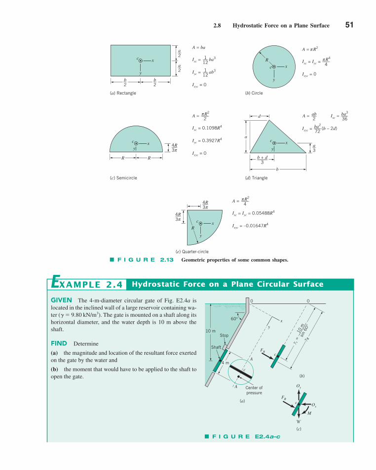
2.8 Hydrostatic Force on a Plane Surface 51

F I G U R E 2.13 Geometric properties of some common shapes.

c

y

x

4R–––3π

4R–––3π

A = R2–––––4

π

Ixc = Iyc = 0.05488R4

Ixyc = –0.01647R4

A = R2–––––2

π

Ixc = 0.1098R4

Iyc = 0.3927R4

Ixyc = 0

A = ab–––2

Ixc =

Ixyc = (b – 2d)

ba3–––-–36

ba2–––––72

A = R2

R4–––––4

πIxc = Iyc =

Ixyc = 0

πA = ba

1–––12

Ixc = ba3

Iyc = ab3

Ixyc = 0

1–––12

c

yx

R R

4R–––3π

c

yx

b + d–––––––3

b

a––3

d

a

R

c

y

xRc

y

x

b––2

b––2

a––2

a––2

(a) Rectangle (b) Circle

(c) Semicircle (d) Triangle

(e) Quarter-circle

GIVEN The 4-m-diameter circular gate of Fig. E2.4a islocated in the inclined wall of a large reservoir containing wa-ter (� � 9.80 kN/m3). The gate is mounted on a shaft along itshorizontal diameter, and the water depth is 10 m above theshaft.

FIND Determine

(a) the magnitude and location of the resultant force exertedon the gate by the water and

(b) the moment that would have to be applied to the shaft toopen the gate.

Hydrostatic Force on a Plane Circular SurfaceEXAMPLE 2.4

xy

c

A

A Center ofpressure

FR

�

M

Oy

Oxc(a)

(c)

(b)

4 m

Shaft

Stop10 m

60°

0 0

FRc

y R

y c =

10

m––

––––

–––

sin

60°

F I G U R E E2.4a–c

c02FluidStatics.qxd 9/24/10 11:39 AM Page 51

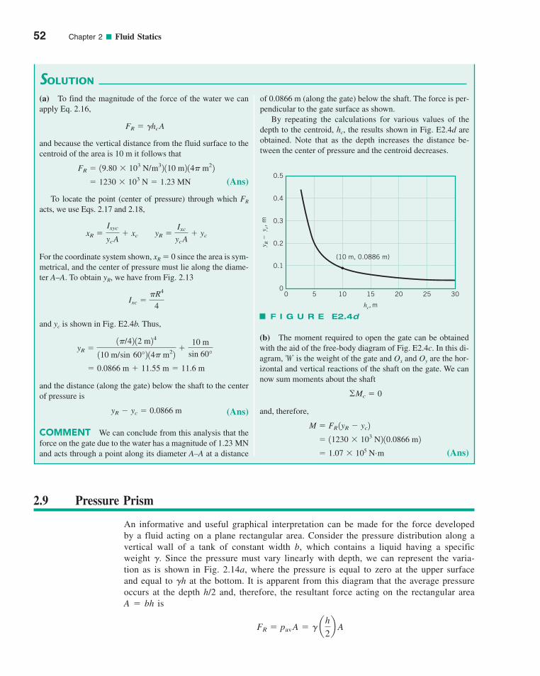
52 Chapter 2 ■ Fluid Statics

SOLUTION

of 0.0866 m (along the gate) below the shaft. The force is per-pendicular to the gate surface as shown.

By repeating the calculations for various values of thedepth to the centroid, hc, the results shown in Fig. E2.4d areobtained. Note that as the depth increases the distance be-tween the center of pressure and the centroid decreases.

(b) The moment required to open the gate can be obtainedwith the aid of the free-body diagram of Fig. E2.4c. In this di-agram,w is the weight of the gate and Ox and Oy are the hor-izontal and vertical reactions of the shaft on the gate. We cannow sum moments about the shaft

and, therefore,

(Ans) � 1.07 � 105 N.m

� 11230 � 103 N2 10.0866 m2

M � FR 1yR � yc2

©Mc � 0

(a) To find the magnitude of the force of the water we canapply Eq. 2.16,

and because the vertical distance from the fluid surface to thecentroid of the area is 10 m it follows that

(Ans)

To locate the point (center of pressure) through which FR

acts, we use Eqs. 2.17 and 2.18,

For the coordinate system shown, xR � 0 since the area is sym-metrical, and the center of pressure must lie along the diame-ter A–A. To obtain yR, we have from Fig. 2.13

and yc is shown in Fig. E2.4b. Thus,

and the distance (along the gate) below the shaft to the centerof pressure is

(Ans)

COMMENT We can conclude from this analysis that theforce on the gate due to the water has a magnitude of 1.23 MNand acts through a point along its diameter A–A at a distance

yR � yc � 0.0866 m

� 0.0866 m � 11.55 m � 11.6 m

yR �1�/42 12 m24

110 m/sin 60°2 14� m22�

10 m

sin 60°

Ixc ��R4

4

xR �Ixyc

ycA� xc yR �

Ixc

ycA� yc

� 1230 � 103 N � 1.23 MN

FR � 19.80 � 103 N/m32 110 m2 14� m22

FR � �hcA

25 30201510500

0.1

0.2

0.3

0.4

0.5

y R –

y c

, m

hc, m

(10 m, 0.0886 m)

F I G U R E E2.4d

2.9 Pressure Prism

An informative and useful graphical interpretation can be made for the force developedby a fluid acting on a plane rectangular area. Consider the pressure distribution along avertical wall of a tank of constant width b, which contains a liquid having a specificweight �. Since the pressure must vary linearly with depth, we can represent the varia-tion as is shown in Fig. 2.14a, where the pressure is equal to zero at the upper surfaceand equal to �h at the bottom. It is apparent from this diagram that the average pressureoccurs at the depth h/2 and, therefore, the resultant force acting on the rectangular areaA � bh is

FR � pavA � � ah

2b A

c02FluidStatics.qxd 9/24/10 11:39 AM Page 52

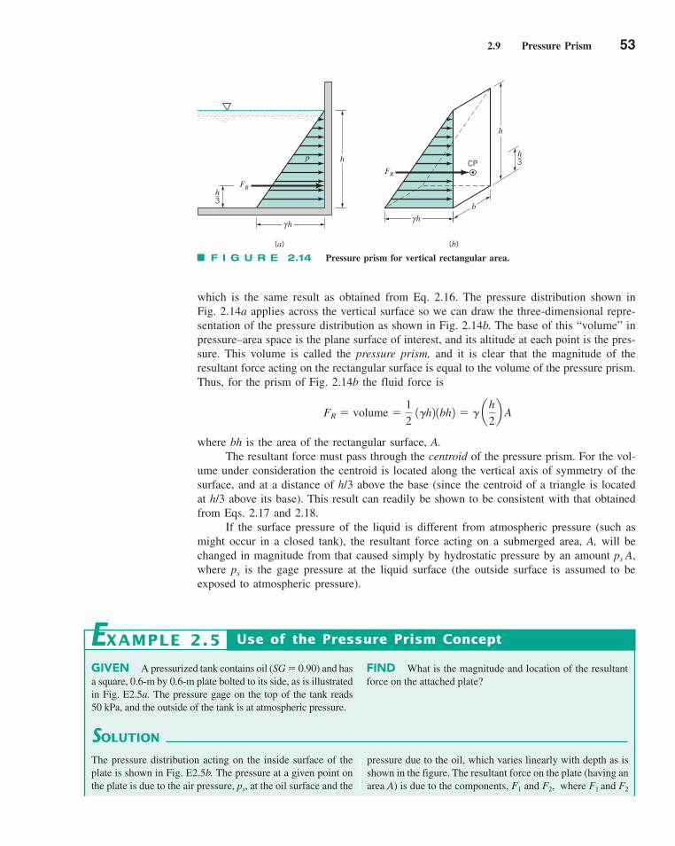
2.9 Pressure Prism 53

which is the same result as obtained from Eq. 2.16. The pressure distribution shown inFig. 2.14a applies across the vertical surface so we can draw the three-dimensional repre-sentation of the pressure distribution as shown in Fig. 2.14b. The base of this “volume” inpressure–area space is the plane surface of interest, and its altitude at each point is the pres-sure. This volume is called the pressure prism, and it is clear that the magnitude of theresultant force acting on the rectangular surface is equal to the volume of the pressure prism.Thus, for the prism of Fig. 2.14b the fluid force is

where bh is the area of the rectangular surface, A.The resultant force must pass through the centroid of the pressure prism. For the vol-

ume under consideration the centroid is located along the vertical axis of symmetry of thesurface, and at a distance of h/3 above the base (since the centroid of a triangle is locatedat h/3 above its base). This result can readily be shown to be consistent with that obtainedfrom Eqs. 2.17 and 2.18.

If the surface pressure of the liquid is different from atmospheric pressure (such asmight occur in a closed tank), the resultant force acting on a submerged area, A, will bechanged in magnitude from that caused simply by hydrostatic pressure by an amount ps A,where ps is the gage pressure at the liquid surface (the outside surface is assumed to beexposed to atmospheric pressure).

FR � volume �1

2 1�h2 1bh2 � � a

h

2b A

FR

γ h

h

h–3

(a) (b)

γ h

h

FR

h–3

b

CPp

F I G U R E 2.14 Pressure prism for vertical rectangular area.

GIVEN A pressurized tank contains oil (SG � 0.90) and hasa square, 0.6-m by 0.6-m plate bolted to its side, as is illustratedin Fig. E2.5a. The pressure gage on the top of the tank reads 50 kPa, and the outside of the tank is at atmospheric pressure.

SOLUTION

Use of the Pressure Prism Concept

FIND What is the magnitude and location of the resultantforce on the attached plate?

EXAMPLE 2.5

The pressure distribution acting on the inside surface of theplate is shown in Fig. E2.5b. The pressure at a given point onthe plate is due to the air pressure, ps, at the oil surface and the

pressure due to the oil, which varies linearly with depth as isshown in the figure. The resultant force on the plate (having anarea A) is due to the components, F1 and F2, where F1 and F2

c02FluidStatics.qxd 9/24/10 11:39 AM Page 53

54 Chapter 2 ■ Fluid Statics

does not affect the resultant force (magnitude or location), asit acts on both sides of the plate, thereby canceling its effect.

are due to the rectangular and triangular portions of the pres-sure distribution, respectively. Thus,

and

The magnitude of the resultant force, FR, is therefore

(Ans)

The vertical location of FR can be obtained by summingmoments around an axis through point O so that

or

(Ans)

Thus, the force acts at a distance of 0.296 m above the bottomof the plate along the vertical axis of symmetry.

COMMENT Note that the air pressure used in the calcu-lation of the force was gage pressure. Atmospheric pressure

� 0.296 m

yO �124.4 � 103 N2 10.3 m2 � 10.954 � 103 N2 10.2 m2

25.4 � 103 N

FRyO � F110.3 m2 � F210.2 m2

FR � F1 � F2 � 25.4 � 103 N � 25.4 kN

� 0.954 � 103 N

� 10.902 19.81 � 103 N/m32 a0.6 m

2b 10.36 m22

F2 � � ah2 � h1

2b A

� 24.4 � 103 N

� 10.902 19.81 � 103 N/m32 12 m2 4 10.36 m22 � 350 � 103 N/m2

F1 � 1ps � �h12A

p = 50 kPa

Air

2 m

0.6 m

(a)

F1

FR

PlateO

(h2 – h1)γ

0.2 m

F2

yO0.3 m

0.6 m

h2 = 2.6 mh1 = 2 m

h1γps Oil surface

(b)

Oil

F I G U R E E2.5

2.10 Hydrostatic Force on a Curved Surface

The equations developed in Section 2.8 for the magnitude and location of the resultantforce acting on a submerged surface only apply to plane surfaces. However, many sur-faces of interest (such as those associated with dams, pipes, and tanks or the bottom ofthe beverage bottle shown in the figure in the margin) are nonplanar. Although the resul-tant fluid force can be determined by integration, as was done for the plane surfaces,this is generally a rather tedious process and no simple, general formulas can be devel-oped. As an alternative approach we will consider the equilibrium of the fluid volumeenclosed by the curved surface of interest and the horizontal and vertical projections ofthis surface.

For example, consider the swimming pool shown in Fig. 2.15a. We wish to find theresultant fluid force acting on section BC shown in Fig. 2.15b. This section has a unit lengthperpendicular to the plane of the paper. We first isolate a volume of fluid that is boundedby the surface of interest, in this instance section BC, and the horizontal plane surfaceAB and the vertical plane surface AC. The free-body diagram for this volume is shown

c02FluidStatics.qxd 9/24/10 11:39 AM Page 54

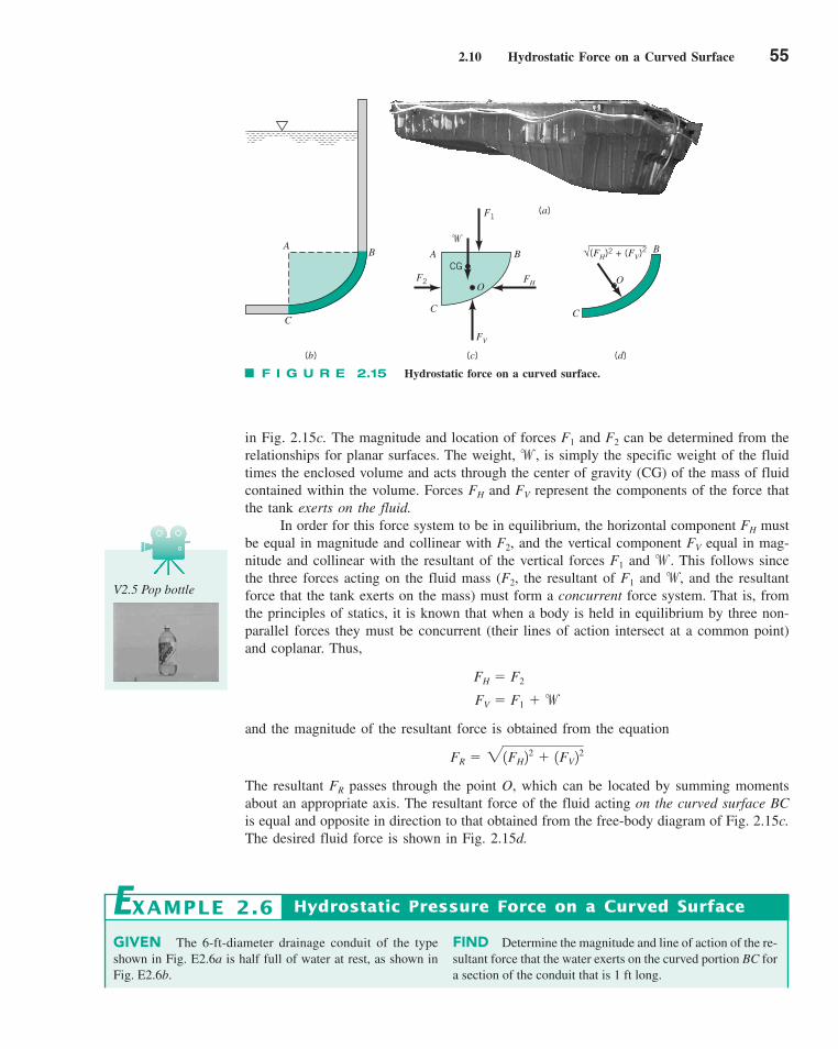
2.10 Hydrostatic Force on a Curved Surface 55

in Fig. 2.15c. The magnitude and location of forces F1 and F2 can be determined from therelationships for planar surfaces. The weight, w, is simply the specific weight of the fluidtimes the enclosed volume and acts through the center of gravity (CG) of the mass of fluidcontained within the volume. Forces FH and FV represent the components of the force thatthe tank exerts on the fluid.

In order for this force system to be in equilibrium, the horizontal component FH mustbe equal in magnitude and collinear with F2, and the vertical component FV equal in mag-nitude and collinear with the resultant of the vertical forces F1 and w. This follows sincethe three forces acting on the fluid mass (F2, the resultant of F1 and w, and the resultantforce that the tank exerts on the mass) must form a concurrent force system. That is, fromthe principles of statics, it is known that when a body is held in equilibrium by three non-parallel forces they must be concurrent (their lines of action intersect at a common point)and coplanar. Thus,

and the magnitude of the resultant force is obtained from the equation

The resultant FR passes through the point O, which can be located by summing momentsabout an appropriate axis. The resultant force of the fluid acting on the curved surface BCis equal and opposite in direction to that obtained from the free-body diagram of Fig. 2.15c.The desired fluid force is shown in Fig. 2.15d.

FR � 21FH22 � 1FV2

2

FV � F1 �w

FH � F2

F I G U R E 2.15 Hydrostatic force on a curved surface.

CG

O

C

A B

FH

FV

F2

F1

�A

C

B

(b) (c) (d)

O

B

C

√(FH)2 + (FV)2

(a)

Hydrostatic Pressure Force on a Curved SurfaceEXAMPLE 2.6

GIVEN The 6-ft-diameter drainage conduit of the typeshown in Fig. E2.6a is half full of water at rest, as shown inFig. E2.6b.

FIND Determine the magnitude and line of action of the re-sultant force that the water exerts on the curved portion BC fora section of the conduit that is 1 ft long.

V2.5 Pop bottle

c02FluidStatics.qxd 9/24/10 11:39 AM Page 55

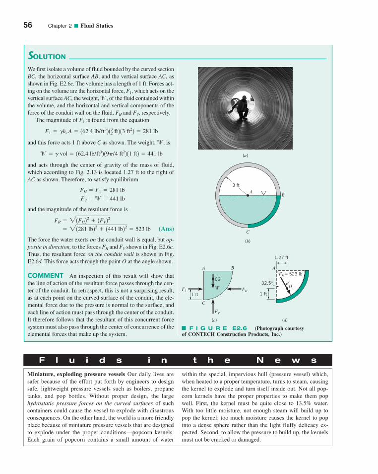
56 Chapter 2 ■ Fluid Statics

SOLUTION

We first isolate a volume of fluid bounded by the curved sectionBC, the horizontal surface AB, and the vertical surface AC, asshown in Fig. E2.6c. The volume has a length of 1 ft. Forces act-ing on the volume are the horizontal force, F1, which acts on thevertical surface AC, the weight,w, of the fluid contained withinthe volume, and the horizontal and vertical components of theforce of the conduit wall on the fluid, FH and FV, respectively.

The magnitude of F1 is found from the equation

and this force acts 1 ft above C as shown. The weight,w, is

and acts through the center of gravity of the mass of fluid,which according to Fig. 2.13 is located 1.27 ft to the right ofAC as shown. Therefore, to satisfy equilibrium

and the magnitude of the resultant force is

(Ans)

The force the water exerts on the conduit wall is equal, but op-posite in direction, to the forces FH and FV shown in Fig. E2.6c.Thus, the resultant force on the conduit wall is shown in Fig.E2.6d. This force acts through the point O at the angle shown.

COMMENT An inspection of this result will show thatthe line of action of the resultant force passes through the cen-ter of the conduit. In retrospect, this is not a surprising result,as at each point on the curved surface of the conduit, the ele-mental force due to the pressure is normal to the surface, andeach line of action must pass through the center of the conduit.It therefore follows that the resultant of this concurrent forcesystem must also pass through the center of concurrence of theelemental forces that make up the system.

� 21281 lb22 � 1441 lb22 � 523 lb

FR � 21FH22 � 1FV2

2

FV �w � 441 lb

FH � F1 � 281 lb

w � � vol � 162.4 lb/ft32 19�/4 ft22 11 ft2 � 441 lb

F1 � �hcA � 162.4 lb/ft32 132 ft2 13 ft22 � 281 lb

B

C

(b)

A B

C

FV

FHF11 ft

�

CG

(c)

1 ft

A

1.27 ft

O

FR = 523 lb

32.5°

(d)

3 ftA

(a)

F I G U R E E2.6 (Photograph courtesyof CONTECH Construction Products, Inc.)

F l u i d s i n t h e N e w s

Miniature, exploding pressure vessels Our daily lives aresafer because of the effort put forth by engineers to designsafe, lightweight pressure vessels such as boilers, propanetanks, and pop bottles. Without proper design, the large hydrostatic pressure forces on the curved surfaces of suchcontainers could cause the vessel to explode with disastrousconsequences. On the other hand, the world is a more friendlyplace because of miniature pressure vessels that are designedto explode under the proper conditions—popcorn kernels.Each grain of popcorn contains a small amount of water

within the special, impervious hull (pressure vessel) which,when heated to a proper temperature, turns to steam, causingthe kernel to explode and turn itself inside out. Not all pop-corn kernels have the proper properties to make them popwell. First, the kernel must be quite close to 13.5% water.With too little moisture, not enough steam will build up topop the kernel; too much moisture causes the kernel to popinto a dense sphere rather than the light fluffy delicacy ex-pected. Second, to allow the pressure to build up, the kernelsmust not be cracked or damaged.

c02FluidStatics.qxd 9/24/10 11:39 AM Page 56

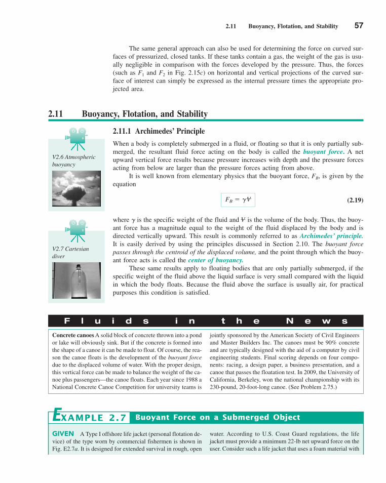
2.11 Buoyancy, Flotation, and Stability 57

The same general approach can also be used for determining the force on curved sur-faces of pressurized, closed tanks. If these tanks contain a gas, the weight of the gas is usu-ally negligible in comparison with the forces developed by the pressure. Thus, the forces(such as F1 and F2 in Fig. 2.15c) on horizontal and vertical projections of the curved sur-face of interest can simply be expressed as the internal pressure times the appropriate pro-jected area.

2.11 Buoyancy, Flotation, and Stability

2.11.1 Archimedes’ Principle

When a body is completely submerged in a fluid, or floating so that it is only partially sub-merged, the resultant fluid force acting on the body is called the buoyant force. A netupward vertical force results because pressure increases with depth and the pressure forcesacting from below are larger than the pressure forces acting from above.

It is well known from elementary physics that the buoyant force, FB, is given by theequation

(2.19)

where � is the specific weight of the fluid and is the volume of the body. Thus, the buoy-ant force has a magnitude equal to the weight of the fluid displaced by the body and isdirected vertically upward. This result is commonly referred to as Archimedes’ principle.It is easily derived by using the principles discussed in Section 2.10. The buoyant forcepasses through the centroid of the displaced volume, and the point through which the buoy-ant force acts is called the center of buoyancy.

These same results apply to floating bodies that are only partially submerged, if thespecific weight of the fluid above the liquid surface is very small compared with the liquidin which the body floats. Because the fluid above the surface is usually air, for practicalpurposes this condition is satisfied.

V

FB � �V

V2.6 Atmosphericbuoyancy

V2.7 Cartesiandiver

F l u i d s i n t h e N e w s

Concrete canoes A solid block of concrete thrown into a pondor lake will obviously sink. But if the concrete is formed intothe shape of a canoe it can be made to float. Of course, the rea-son the canoe floats is the development of the buoyant forcedue to the displaced volume of water. With the proper design,this vertical force can be made to balance the weight of the ca-noe plus passengers—the canoe floats. Each year since 1988 aNational Concrete Canoe Competition for university teams is

jointly sponsored by the American Society of Civil Engineersand Master Builders Inc. The canoes must be 90% concreteand are typically designed with the aid of a computer by civilengineering students. Final scoring depends on four compo-nents: racing, a design paper, a business presentation, and acanoe that passes the floatation test. In 2009, the University ofCalifornia, Berkeley, won the national championship with its230-pound, 20-foot-long canoe. (See Problem 2.75.)

Buoyant Force on a Submerged ObjectEXAMPLE 2.7

water. According to U.S. Coast Guard regulations, the lifejacket must provide a minimum 22-lb net upward force on theuser. Consider such a life jacket that uses a foam material with

GIVEN A Type I offshore life jacket (personal flotation de-vice) of the type worn by commercial fishermen is shown inFig. E2.7a. It is designed for extended survival in rough, open

c02FluidStatics.qxd 9/24/10 11:39 AM Page 57

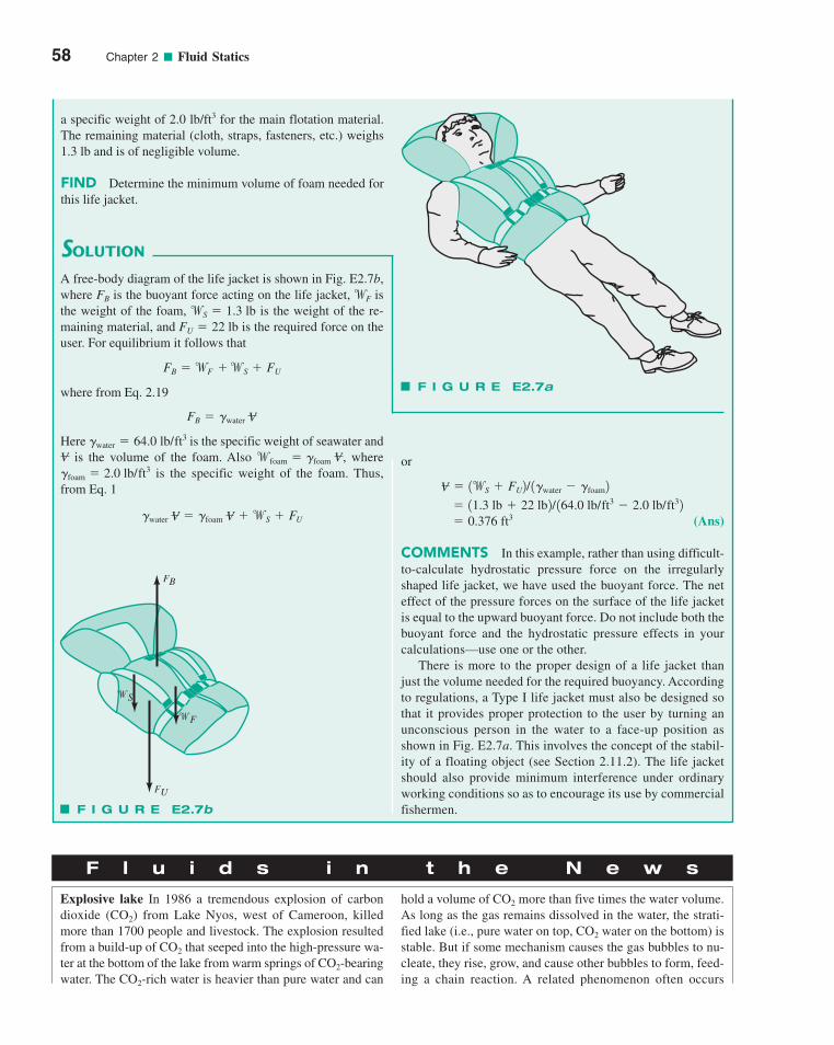
58 Chapter 2 ■ Fluid Statics

a specific weight of 2.0 lb/ft3 for the main flotation material.The remaining material (cloth, straps, fasteners, etc.) weighs1.3 lb and is of negligible volume.

FIND Determine the minimum volume of foam needed forthis life jacket.

SOLUTION

A free-body diagram of the life jacket is shown in Fig. E2.7b,where FB is the buoyant force acting on the life jacket,wF isthe weight of the foam, is the weight of the re-maining material, and is the required force on theuser. For equilibrium it follows that

where from Eq. 2.19

Here is the specific weight of seawater andis the volume of the foam. Also , where

is the specific weight of the foam. Thus,from Eq. 1

�water V � �foam V �wS � FU

�foam � 2.0 lb/ft3wfoam � �foam VV

�water � 64.0 lb/ft3

FB � �water V

FB �wF �wS � FU

FU � 22 lbwS � 1.3 lb

F I G U R E E2.7a

F I G U R E E2.7b

F l u i d s i n t h e N e w s

�F

�S

FU

FB

or

(Ans)

COMMENTS In this example, rather than using difficult-to-calculate hydrostatic pressure force on the irregularlyshaped life jacket, we have used the buoyant force. The neteffect of the pressure forces on the surface of the life jacketis equal to the upward buoyant force. Do not include both thebuoyant force and the hydrostatic pressure effects in yourcalculations—use one or the other.

There is more to the proper design of a life jacket thanjust the volume needed for the required buoyancy. Accordingto regulations, a Type I life jacket must also be designed sothat it provides proper protection to the user by turning anunconscious person in the water to a face-up position asshown in Fig. E2.7a. This involves the concept of the stabil-ity of a floating object (see Section 2.11.2). The life jacketshould also provide minimum interference under ordinaryworking conditions so as to encourage its use by commercialfishermen.

� 0.376 ft3 � 11.3 lb � 22 lb2/ 164.0 lb/ft3 � 2.0 lb/ft32

V � 1wS � FU2/ 1�water � �foam2

Explosive lake In 1986 a tremendous explosion of carbondioxide (CO2) from Lake Nyos, west of Cameroon, killedmore than 1700 people and livestock. The explosion resultedfrom a build-up of CO2 that seeped into the high-pressure wa-ter at the bottom of the lake from warm springs of CO2-bearingwater. The CO2-rich water is heavier than pure water and can

hold a volume of CO2 more than five times the water volume.As long as the gas remains dissolved in the water, the strati-fied lake (i.e., pure water on top, CO2 water on the bottom) isstable. But if some mechanism causes the gas bubbles to nu-cleate, they rise, grow, and cause other bubbles to form, feed-ing a chain reaction. A related phenomenon often occurs

c02FluidStatics.qxd 9/24/10 11:39 AM Page 58

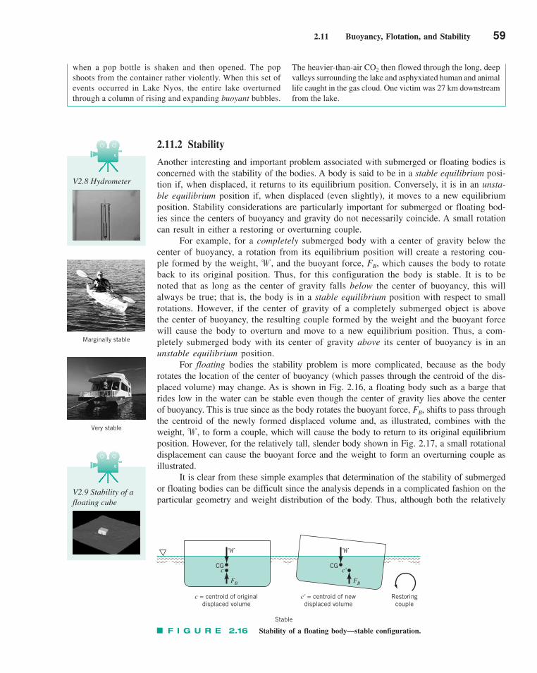
2.11 Buoyancy, Flotation, and Stability 59

2.11.2 Stability

Another interesting and important problem associated with submerged or floating bodies isconcerned with the stability of the bodies. A body is said to be in a stable equilibrium posi-tion if, when displaced, it returns to its equilibrium position. Conversely, it is in an unsta-ble equilibrium position if, when displaced (even slightly), it moves to a new equilibriumposition. Stability considerations are particularly important for submerged or floating bod-ies since the centers of buoyancy and gravity do not necessarily coincide. A small rotationcan result in either a restoring or overturning couple.

For example, for a completely submerged body with a center of gravity below thecenter of buoyancy, a rotation from its equilibrium position will create a restoring cou-ple formed by the weight, w, and the buoyant force, FB, which causes the body to rotateback to its original position. Thus, for this configuration the body is stable. It is to benoted that as long as the center of gravity falls below the center of buoyancy, this willalways be true; that is, the body is in a stable equilibrium position with respect to smallrotations. However, if the center of gravity of a completely submerged object is abovethe center of buoyancy, the resulting couple formed by the weight and the buoyant forcewill cause the body to overturn and move to a new equilibrium position. Thus, a com-pletely submerged body with its center of gravity above its center of buoyancy is in anunstable equilibrium position.

For floating bodies the stability problem is more complicated, because as the bodyrotates the location of the center of buoyancy (which passes through the centroid of the dis-placed volume) may change. As is shown in Fig. 2.16, a floating body such as a barge thatrides low in the water can be stable even though the center of gravity lies above the centerof buoyancy. This is true since as the body rotates the buoyant force, FB, shifts to pass throughthe centroid of the newly formed displaced volume and, as illustrated, combines with theweight, , to form a couple, which will cause the body to return to its original equilibriumposition. However, for the relatively tall, slender body shown in Fig. 2.17, a small rotationaldisplacement can cause the buoyant force and the weight to form an overturning couple asillustrated.

It is clear from these simple examples that determination of the stability of submergedor floating bodies can be difficult since the analysis depends in a complicated fashion on theparticular geometry and weight distribution of the body. Thus, although both the relatively

w

V2.8 Hydrometer

�

FB

cCG

Restoringcouple

c' = centroid of newdisplaced volume

c = centroid of originaldisplaced volume

Stable

�

FB

c'CG

F I G U R E 2.16 Stability of a floating body—stable configuration.

Marginally stable

Very stable

V2.9 Stability of afloating cube

when a pop bottle is shaken and then opened. The popshoots from the container rather violently. When this set ofevents occurred in Lake Nyos, the entire lake overturnedthrough a column of rising and expanding buoyant bubbles.

The heavier-than-air CO2 then flowed through the long, deepvalleys surrounding the lake and asphyxiated human and animallife caught in the gas cloud. One victim was 27 km downstreamfrom the lake.

c02FluidStatics.qxd 9/24/10 11:39 AM Page 59

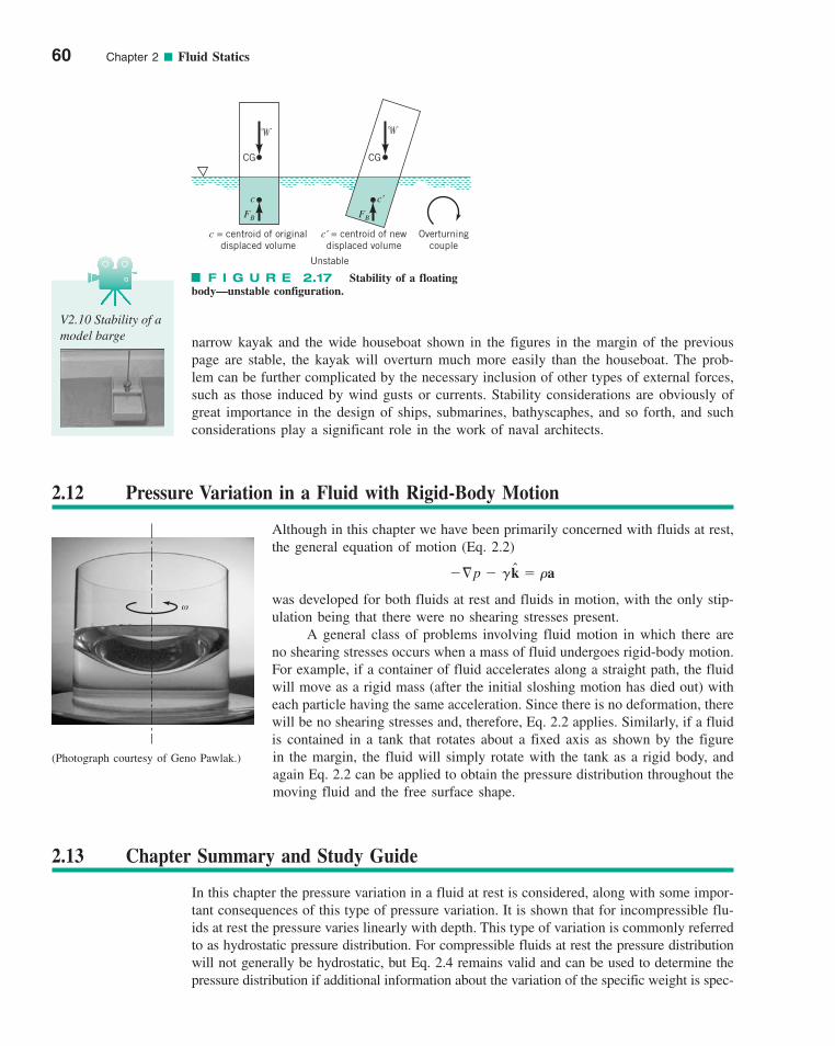
narrow kayak and the wide houseboat shown in the figures in the margin of the previouspage are stable, the kayak will overturn much more easily than the houseboat. The prob-lem can be further complicated by the necessary inclusion of other types of external forces,such as those induced by wind gusts or currents. Stability considerations are obviously ofgreat importance in the design of ships, submarines, bathyscaphes, and so forth, and suchconsiderations play a significant role in the work of naval architects.

60 Chapter 2 ■ Fluid Statics

V2.10 Stability of amodel barge

2.12 Pressure Variation in a Fluid with Rigid-Body Motion

Although in this chapter we have been primarily concerned with fluids at rest,the general equation of motion (Eq. 2.2)

was developed for both fluids at rest and fluids in motion, with the only stip-ulation being that there were no shearing stresses present.

A general class of problems involving fluid motion in which there areno shearing stresses occurs when a mass of fluid undergoes rigid-body motion.For example, if a container of fluid accelerates along a straight path, the fluidwill move as a rigid mass (after the initial sloshing motion has died out) witheach particle having the same acceleration. Since there is no deformation, therewill be no shearing stresses and, therefore, Eq. 2.2 applies. Similarly, if a fluidis contained in a tank that rotates about a fixed axis as shown by the figurein the margin, the fluid will simply rotate with the tank as a rigid body, andagain Eq. 2.2 can be applied to obtain the pressure distribution throughout themoving fluid and the free surface shape.

�§p � � k � �a

2.13 Chapter Summary and Study Guide

In this chapter the pressure variation in a fluid at rest is considered, along with some impor-tant consequences of this type of pressure variation. It is shown that for incompressible flu-ids at rest the pressure varies linearly with depth. This type of variation is commonly referredto as hydrostatic pressure distribution. For compressible fluids at rest the pressure distributionwill not generally be hydrostatic, but Eq. 2.4 remains valid and can be used to determine thepressure distribution if additional information about the variation of the specific weight is spec-

ω

(Photograph courtesy of Geno Pawlak.)

� �

CGCG

c c'

FB FB

Overturningcouple

c' = centroid of newdisplaced volume

c = centroid of originaldisplaced volume

Unstable

F I G U R E 2.17 Stability of a floatingbody—unstable configuration.

c02FluidStatics.qxd 9/24/10 11:39 AM Page 60

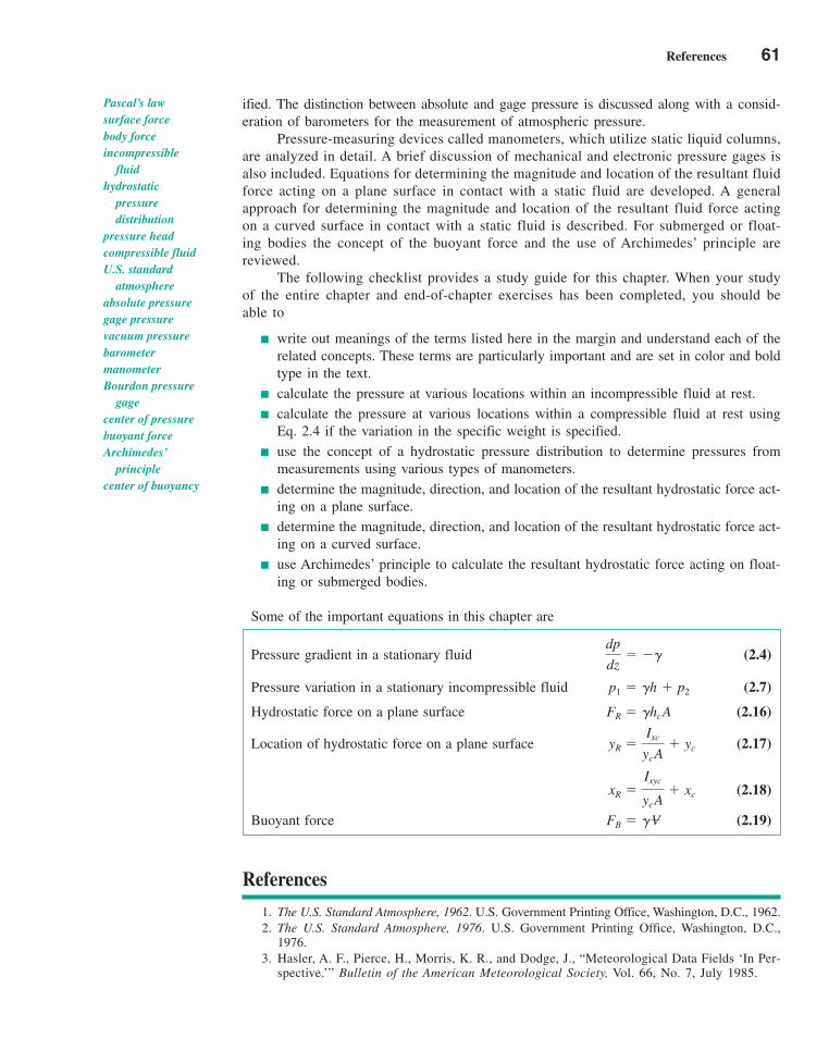
References 61

ified. The distinction between absolute and gage pressure is discussed along with a consid-eration of barometers for the measurement of atmospheric pressure.

Pressure-measuring devices called manometers, which utilize static liquid columns,are analyzed in detail. A brief discussion of mechanical and electronic pressure gages isalso included. Equations for determining the magnitude and location of the resultant fluidforce acting on a plane surface in contact with a static fluid are developed. A generalapproach for determining the magnitude and location of the resultant fluid force actingon a curved surface in contact with a static fluid is described. For submerged or float-ing bodies the concept of the buoyant force and the use of Archimedes’ principle arereviewed.

The following checklist provides a study guide for this chapter. When your studyof the entire chapter and end-of-chapter exercises has been completed, you should beable to

write out meanings of the terms listed here in the margin and understand each of therelated concepts. These terms are particularly important and are set in color and boldtype in the text.

calculate the pressure at various locations within an incompressible fluid at rest.

calculate the pressure at various locations within a compressible fluid at rest usingEq. 2.4 if the variation in the specific weight is specified.

use the concept of a hydrostatic pressure distribution to determine pressures frommeasurements using various types of manometers.

determine the magnitude, direction, and location of the resultant hydrostatic force act-ing on a plane surface.

determine the magnitude, direction, and location of the resultant hydrostatic force act-ing on a curved surface.

use Archimedes’ principle to calculate the resultant hydrostatic force acting on float-ing or submerged bodies.

Some of the important equations in this chapter are

Pressure gradient in a stationary fluid (2.4)

Pressure variation in a stationary incompressible fluid (2.7)

Hydrostatic force on a plane surface (2.16)

Location of hydrostatic force on a plane surface (2.17)

(2.18)

Buoyant force (2.19)FB � �V

xR �Ixyc

ycA� xc

yR �Ixc

ycA� yc

FR � �hcA

p1 � �h � p2

dp

dz� ��

Pascal’s lawsurface forcebody forceincompressible

fluidhydrostatic

pressure distribution

pressure headcompressible fluidU.S. standard

atmosphereabsolute pressuregage pressurevacuum pressurebarometermanometerBourdon pressure

gagecenter of pressurebuoyant forceArchimedes’

principlecenter of buoyancy

References

1. The U.S. Standard Atmosphere, 1962. U.S. Government Printing Office, Washington, D.C., 1962.2. The U.S. Standard Atmosphere, 1976. U.S. Government Printing Office, Washington, D.C.,

1976.3. Hasler, A. F., Pierce, H., Morris, K. R., and Dodge, J., “Meteorological Data Fields ‘In Per-

spective.’” Bulletin of the American Meteorological Society, Vol. 66, No. 7, July 1985.

c02FluidStatics.qxd 9/24/10 11:39 AM Page 61

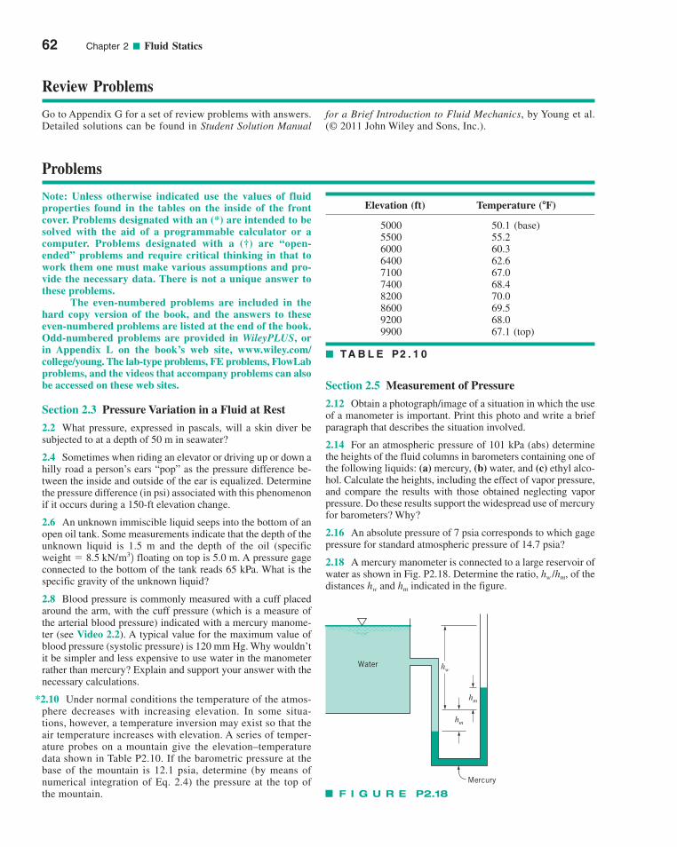
62 Chapter 2 ■ Fluid Statics

Note: Unless otherwise indicated use the values of fluidproperties found in the tables on the inside of the frontcover. Problems designated with an (*) are intended to besolved with the aid of a programmable calculator or acomputer. Problems designated with a (†) are “open-ended” problems and require critical thinking in that towork them one must make various assumptions and pro-vide the necessary data. There is not a unique answer tothese problems.

The even-numbered problems are included in thehard copy version of the book, and the answers to theseeven-numbered problems are listed at the end of the book.Odd-numbered problems are provided in WileyPLUS, orin Appendix L on the book’s web site, www.wiley.com/college/young. The lab-type problems, FE problems, FlowLabproblems, and the videos that accompany problems can alsobe accessed on these web sites.

Section 2.3 Pressure Variation in a Fluid at Rest

2.2 What pressure, expressed in pascals, will a skin diver besubjected to at a depth of 50 m in seawater?

2.4 Sometimes when riding an elevator or driving up or down ahilly road a person’s ears “pop” as the pressure difference be-tween the inside and outside of the ear is equalized. Determinethe pressure difference (in psi) associated with this phenomenonif it occurs during a 150-ft elevation change.

2.6 An unknown immiscible liquid seeps into the bottom of anopen oil tank. Some measurements indicate that the depth of theunknown liquid is 1.5 m and the depth of the oil (specificweight floating on top is 5.0 m. A pressure gageconnected to the bottom of the tank reads 65 kPa. What is thespecific gravity of the unknown liquid?

2.8 Blood pressure is commonly measured with a cuff placedaround the arm, with the cuff pressure (which is a measure ofthe arterial blood pressure) indicated with a mercury manome-ter (see Video 2.2). A typical value for the maximum value ofblood pressure (systolic pressure) is 120 mm Hg. Why wouldn’tit be simpler and less expensive to use water in the manometerrather than mercury? Explain and support your answer with thenecessary calculations.

*2.10 Under normal conditions the temperature of the atmos-phere decreases with increasing elevation. In some situa-tions, however, a temperature inversion may exist so that theair temperature increases with elevation. A series of temper-ature probes on a mountain give the elevation–temperaturedata shown in Table P2.10. If the barometric pressure at thebase of the mountain is 12.1 psia, determine (by means ofnumerical integration of Eq. 2.4) the pressure at the top ofthe mountain.

� 8.5 kN/m32

Section 2.5 Measurement of Pressure

2.12 Obtain a photograph/image of a situation in which the useof a manometer is important. Print this photo and write a briefparagraph that describes the situation involved.

2.14 For an atmospheric pressure of 101 kPa (abs) determinethe heights of the fluid columns in barometers containing one ofthe following liquids: (a) mercury, (b) water, and (c) ethyl alco-hol. Calculate the heights, including the effect of vapor pressure,and compare the results with those obtained neglecting vaporpressure. Do these results support the widespread use of mercuryfor barometers? Why?

2.16 An absolute pressure of 7 psia corresponds to which gagepressure for standard atmospheric pressure of 14.7 psia?

2.18 A mercury manometer is connected to a large reservoir ofwater as shown in Fig. P2.18. Determine the ratio, hw /hm, of thedistances hw and hm indicated in the figure.

Elevation (ft) Temperature ( )

5000 50.1 (base)5500 55.26000 60.36400 62.67100 67.07400 68.48200 70.08600 69.59200 68.09900 67.1 (top)

�F

TA B L E P2 . 1 0

F I G U R E P2.18

Mercury

Water hw

hm

hm

Problems

Review Problems

Go to Appendix G for a set of review problems with answers.Detailed solutions can be found in Student Solution Manual

for a Brief Introduction to Fluid Mechanics, by Young et al.(© 2011 John Wiley and Sons, Inc.).

c02FluidStatics.qxd 10/18/10 7:55 AM Page 62

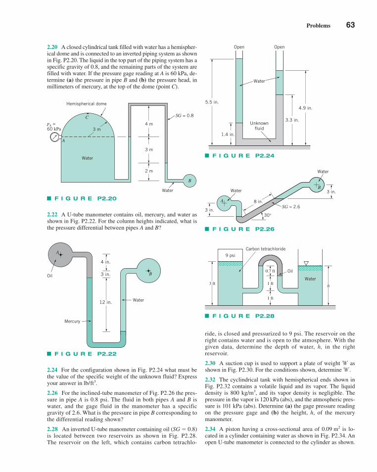
Problems 63

2.24 For the configuration shown in Fig. P2.24 what must bethe value of the specific weight of the unknown fluid? Expressyour answer in .

2.26 For the inclined-tube manometer of Fig. P2.26 the pres-sure in pipe A is 0.8 psi. The fluid in both pipes A and B iswater, and the gage fluid in the manometer has a specificgravity of 2.6. What is the pressure in pipe B corresponding tothe differential reading shown?

2.28 An inverted U-tube manometer containing oil (SG � 0.8)is located between two reservoirs as shown in Fig. P2.28.The reservoir on the left, which contains carbon tetrachlo-

lb/ft3

F I G U R E P2.20

pA =60 kPa

Water

B

2 m

4 m

3 m

3 m

SG = 0.8

Water

Hemispherical dome

C

A

F I G U R E P2.22

Oil

Mercury

Water

B

4 in.

3 in.

12 in.

A

F I G U R E P2.24

5.5 in.4.9 in.

1.4 in.

Open

Water

Unknownfluid

Open

3.3 in.

F I G U R E P2.28

Carbon tetrachloride

Oil

9 psi

3 ft h1 ft

0.7 ft

1 ft

Water

F I G U R E P2.26

Water

Water

8 in.

30°3 in.

3 in.

A

B

SG = 2.6

ride, is closed and pressurized to 9 psi. The reservoir on theright contains water and is open to the atmosphere. With thegiven data, determine the depth of water, h, in the rightreservoir.

2.30 A suction cup is used to support a plate of weight w asshown in Fig. P2.30. For the conditions shown, determine w.

2.32 The cyclindrical tank with hemispherical ends shown inFig. P2.32 contains a volatile liquid and its vapor. The liquiddensity is 800 kg/m3, and its vapor density is negligible. Thepressure in the vapor is 120 kPa (abs), and the atmospheric pres-sure is 101 kPa (abs). Determine (a) the gage pressure readingon the pressure gage and (b) the height, h, of the mercurymanometer.

2.34 A piston having a cross-sectional area of is lo-cated in a cylinder containing water as shown in Fig. P2.34. Anopen U-tube manometer is connected to the cylinder as shown.

0.09 m2

2.20 A closed cylindrical tank filled with water has a hemispher-ical dome and is connected to an inverted piping system as shownin Fig. P2.20. The liquid in the top part of the piping system has aspecific gravity of 0.8, and the remaining parts of the system arefilled with water. If the pressure gage reading at A is 60 kPa, de-termine (a) the pressure in pipe B and (b) the pressure head, inmillimeters of mercury, at the top of the dome (point C).

2.22 A U-tube manometer contains oil, mercury, and water asshown in Fig. P2.22. For the column heights indicated, what isthe pressure differential between pipes A and B?

c02FluidStatics.qxd 9/24/10 11:39 AM Page 63

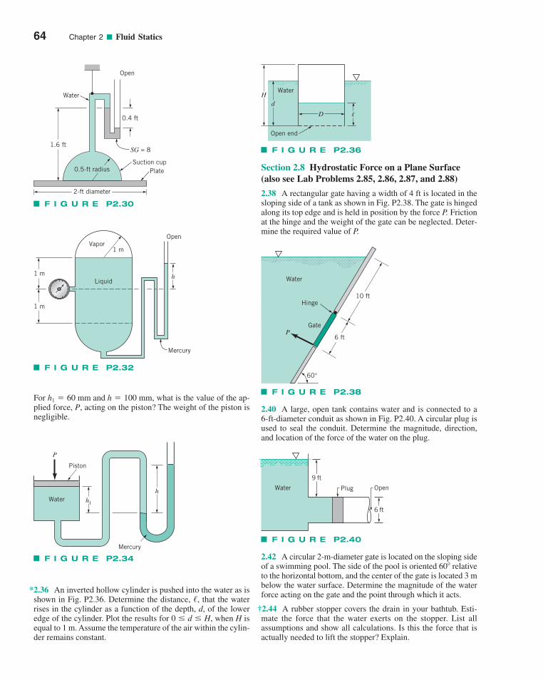
64 Chapter 2 ■ Fluid Statics

For what is the value of the ap-plied force, P, acting on the piston? The weight of the piston isnegligible.

h1 � 60 mm and h � 100 mm,

Section 2.8 Hydrostatic Force on a Plane Surface(also see Lab Problems 2.85, 2.86, 2.87, and 2.88)

2.38 A rectangular gate having a width of 4 ft is located in thesloping side of a tank as shown in Fig. P2.38. The gate is hingedalong its top edge and is held in position by the force P. Frictionat the hinge and the weight of the gate can be neglected. Deter-mine the required value of P.

*2.36 An inverted hollow cylinder is pushed into the water as isshown in Fig. P2.36. Determine the distance, that the waterrises in the cylinder as a function of the depth, d, of the loweredge of the cylinder. Plot the results for when H isequal to 1 m. Assume the temperature of the air within the cylin-der remains constant.

0 d H,

/,

F I G U R E P2.32

Liquid

Vapor1 m

Open

Mercury

1 m

1 m

h

F I G U R E P2.34

Piston

Mercury

Waterh

h1

P

F I G U R E P2.36

Water

Open end

D �

dH

F I G U R E P2.38

60°

10 ft

6 ft

Hinge

GateP

Water

F I G U R E P2.40

Plug OpenWater

9 ft

6 ft

2.40 A large, open tank contains water and is connected to a 6-ft-diameter conduit as shown in Fig. P2.40. A circular plug isused to seal the conduit. Determine the magnitude, direction,and location of the force of the water on the plug.

F I G U R E P2.30

Water

Open

0.5-ft radius

2-ft diameter

0.4 ft

Suction cupPlate

1.6 ftSG = 8

2.42 A circular 2-m-diameter gate is located on the sloping sideof a swimming pool. The side of the pool is oriented 60� relativeto the horizontal bottom, and the center of the gate is located 3 mbelow the water surface. Determine the magnitude of the waterforce acting on the gate and the point through which it acts.

†2.44 A rubber stopper covers the drain in your bathtub. Esti-mate the force that the water exerts on the stopper. List allassumptions and show all calculations. Is this the force that isactually needed to lift the stopper? Explain.

c02FluidStatics.qxd 9/24/10 11:39 AM Page 64

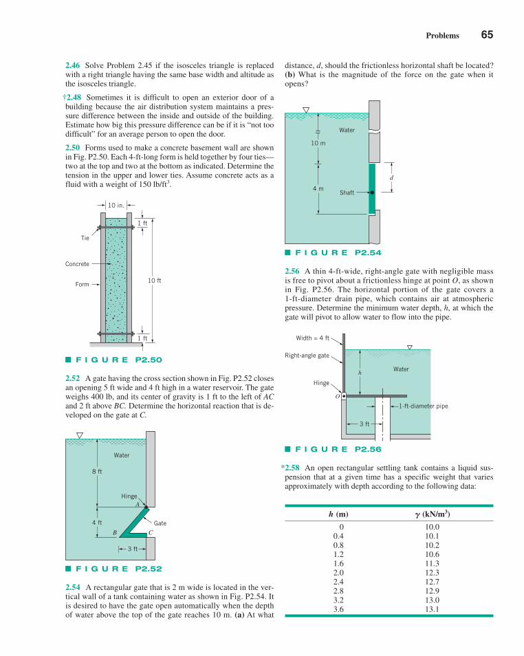
Problems 65

2.46 Solve Problem 2.45 if the isosceles triangle is replacedwith a right triangle having the same base width and altitude asthe isosceles triangle.

†2.48 Sometimes it is difficult to open an exterior door of abuilding because the air distribution system maintains a pres-sure difference between the inside and outside of the building.Estimate how big this pressure difference can be if it is “not toodifficult” for an average person to open the door.

2.50 Forms used to make a concrete basement wall are shownin Fig. P2.50. Each 4-ft-long form is held together by four ties—two at the top and two at the bottom as indicated. Determine thetension in the upper and lower ties. Assume concrete acts as afluid with a weight of 150 lb/ft3.

2.52 A gate having the cross section shown in Fig. P2.52 closesan opening 5 ft wide and 4 ft high in a water reservoir. The gateweighs 400 lb, and its center of gravity is 1 ft to the left of ACand 2 ft above BC. Determine the horizontal reaction that is de-veloped on the gate at C.

distance, d, should the frictionless horizontal shaft be located?(b) What is the magnitude of the force on the gate when itopens?

F I G U R E P2.50

Tie

Concrete

Form10 ft

1 ft

1 ft

10 in.

F I G U R E P2.52

8 ft

4 ft

Water

Hinge

GateCB

A

3 ft

F I G U R E P2.54

d

4 m

10 m

~~ Water

Shaft

F I G U R E P2.56

Water

Hinge

Right-angle gate

Width = 4 ft

1-ft-diameter pipe

O

h

3 ft

2.56 A thin 4-ft-wide, right-angle gate with negligible massis free to pivot about a frictionless hinge at point O, as shownin Fig. P2.56. The horizontal portion of the gate covers a 1-ft-diameter drain pipe, which contains air at atmosphericpressure. Determine the minimum water depth, h, at which thegate will pivot to allow water to flow into the pipe.

h (m) � (kN/m3)

0 10.00.4 10.10.8 10.21.2 10.61.6 11.32.0 12.32.4 12.72.8 12.93.2 13.03.6 13.1

*2.58 An open rectangular settling tank contains a liquid sus-pension that at a given time has a specific weight that variesapproximately with depth according to the following data:

2.54 A rectangular gate that is 2 m wide is located in the ver-tical wall of a tank containing water as shown in Fig. P2.54. Itis desired to have the gate open automatically when the depthof water above the top of the gate reaches 10 m. (a) At what

c02FluidStatics.qxd 9/24/10 11:39 AM Page 65

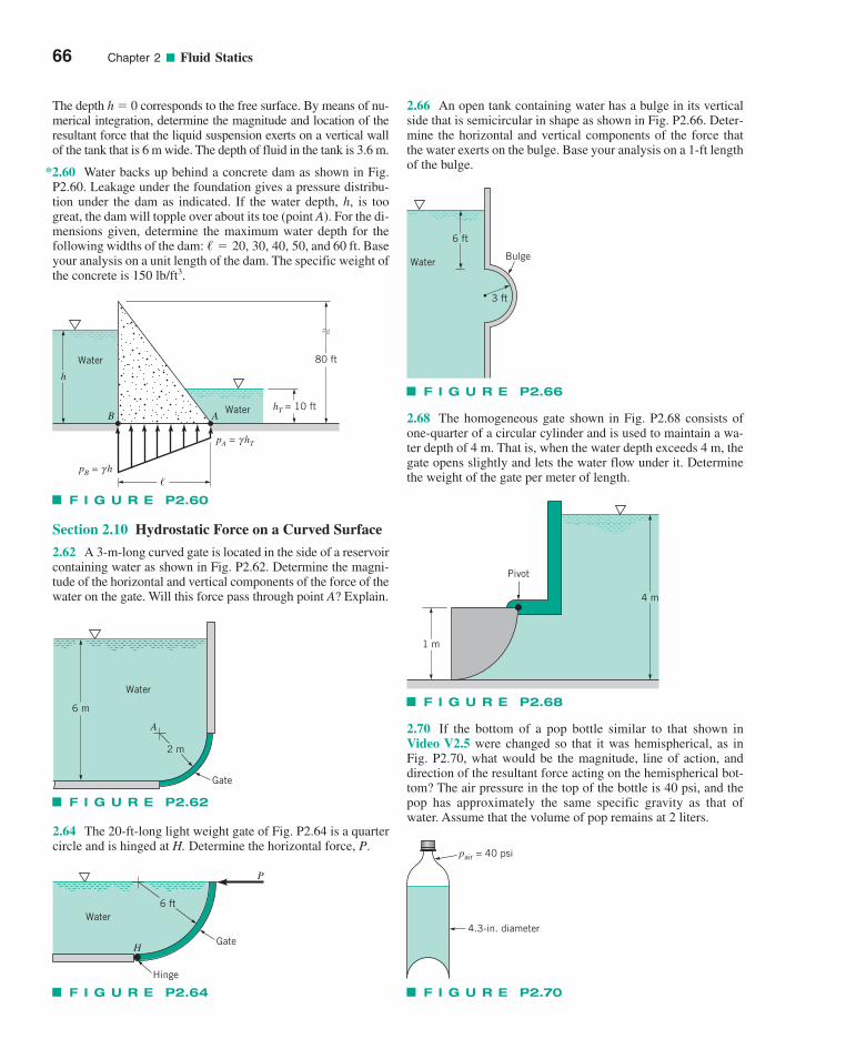
The depth h � 0 corresponds to the free surface. By means of nu-merical integration, determine the magnitude and location of theresultant force that the liquid suspension exerts on a vertical wallof the tank that is 6 m wide. The depth of fluid in the tank is 3.6 m.

*2.60 Water backs up behind a concrete dam as shown in Fig.P2.60. Leakage under the foundation gives a pressure distribu-tion under the dam as indicated. If the water depth, h, is toogreat, the dam will topple over about its toe (point A). For the di-mensions given, determine the maximum water depth for thefollowing widths of the dam: , and 60 ft. Baseyour analysis on a unit length of the dam. The specific weight ofthe concrete is 150 lb/ft3.

/ � 20, 30, 40, 50

66 Chapter 2 ■ Fluid Statics

2.66 An open tank containing water has a bulge in its verticalside that is semicircular in shape as shown in Fig. P2.66. Deter-mine the horizontal and vertical components of the force thatthe water exerts on the bulge. Base your analysis on a 1-ft lengthof the bulge.

Section 2.10 Hydrostatic Force on a Curved Surface

2.62 A 3-m-long curved gate is located in the side of a reservoircontaining water as shown in Fig. P2.62. Determine the magni-tude of the horizontal and vertical components of the force of thewater on the gate. Will this force pass through point A? Explain.

2.70 If the bottom of a pop bottle similar to that shown inVideo V2.5 were changed so that it was hemispherical, as inFig. P2.70, what would be the magnitude, line of action, anddirection of the resultant force acting on the hemispherical bot-tom? The air pressure in the top of the bottle is 40 psi, and thepop has approximately the same specific gravity as that ofwater. Assume that the volume of pop remains at 2 liters.

F I G U R E P2.60

pB = hγ

pA = hTγ

ABWater

Water

h

hT = 10 ft

80 ft

�

F I G U R E P2.62

2 m

Water

6 m

A

Gate

F I G U R E P2.64

P

6 ft

Gate

Hinge

H

Water

F I G U R E P2.66

6 ft

3 ft

Water Bulge

F I G U R E P2.68

4 m

1 m

Pivot

F I G U R E P2.70

4.3-in. diameter

pair = 40 psi

2.64 The 20-ft-long light weight gate of Fig. P2.64 is a quartercircle and is hinged at H. Determine the horizontal force, P.

2.68 The homogeneous gate shown in Fig. P2.68 consists ofone-quarter of a circular cylinder and is used to maintain a wa-ter depth of 4 m. That is, when the water depth exceeds 4 m, thegate opens slightly and lets the water flow under it. Determinethe weight of the gate per meter of length.

c02FluidStatics.qxd 9/24/10 11:39 AM Page 66

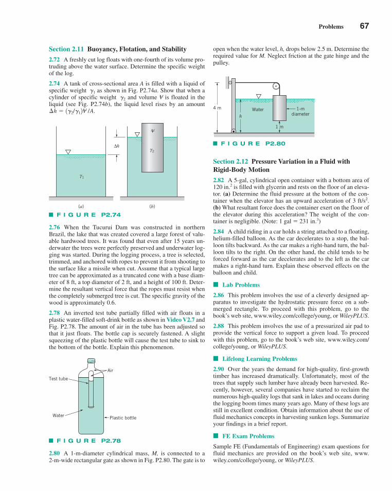
Problems 67

Section 2.11 Buoyancy, Flotation, and Stability

2.72 A freshly cut log floats with one-fourth of its volume pro-truding above the water surface. Determine the specific weightof the log.

2.74 A tank of cross-sectional area A is filled with a liquid ofspecific weight as shown in Fig. P2.74a. Show that when acylinder of specific weight and volume is floated in theliquid (see Fig. P2.74b), the liquid level rises by an amount¢h � 1�2/�12V�/A.

V� �2

�1

open when the water level, h, drops below 2.5 m. Determine therequired value for M. Neglect friction at the gate hinge and thepulley.

2.76 When the Tucurui Dam was constructed in northernBrazil, the lake that was created covered a large forest of valu-able hardwood trees. It was found that even after 15 years un-derwater the trees were perfectly preserved and underwater log-ging was started. During the logging process, a tree is selected,trimmed, and anchored with ropes to prevent it from shooting tothe surface like a missile when cut. Assume that a typical largetree can be approximated as a truncated cone with a base diam-eter of 8 ft, a top diameter of 2 ft, and a height of 100 ft. Deter-mine the resultant vertical force that the ropes must resist whenthe completely submerged tree is cut. The specific gravity of thewood is approximately 0.6.

2.78 An inverted test tube partially filled with air floats in aplastic water-filled soft-drink bottle as shown in Video V2.7 andFig. P2.78. The amount of air in the tube has been adjusted sothat it just floats. The bottle cap is securely fastened. A slightsqueezing of the plastic bottle will cause the test tube to sink tothe bottom of the bottle. Explain this phenomenon.

Section 2.12 Pressure Variation in a Fluid withRigid-Body Motion

2.82 A 5-gal, cylindrical open container with a bottom area of120 in.2 is filled with glycerin and rests on the floor of an eleva-tor. (a) Determine the fluid pressure at the bottom of the con-tainer when the elevator has an upward acceleration of 3 ft/s2.(b) What resultant force does the container exert on the floor ofthe elevator during this acceleration? The weight of the con-tainer is negligible. (Note: 1 gal � 231 in.3)

2.84 A child riding in a car holds a string attached to a floating,helium-filled balloon. As the car decelerates to a stop, the bal-loon tilts backward. As the car makes a right-hand turn, the bal-loon tilts to the right. On the other hand, the child tends to beforced forward as the car decelerates and to the left as the carmakes a right-hand turn. Explain these observed effects on theballoon and child.

■ Lab Problems

2.86 This problem involves the use of a cleverly designed ap-paratus to investigate the hydrostatic pressure force on a sub-merged rectangle. To proceed with this problem, go to thebook’s web site, www.wiley.com/college/young, or WileyPLUS.

2.88 This problem involves the use of a pressurized air pad toprovide the vertical force to support a given load. To proceedwith this problem, go to the book’s web site, www.wiley.com/college/young, or WileyPLUS.

■ Lifelong Learning Problems

2.90 Over the years the demand for high-quality, first-growthtimber has increased dramatically. Unfortunately, most of thetrees that supply such lumber have already been harvested. Re-cently, however, several companies have started to reclaim thenumerous high-quality logs that sank in lakes and oceans duringthe logging boom times many years ago. Many of these logs arestill in excellent condition. Obtain information about the use offluid mechanics concepts in harvesting sunken logs. Summarizeyour findings in a brief report.

■ FE Exam Problems

Sample FE (Fundamentals of Engineering) exam questions forfluid mechanics are provided on the book’s web site, www.wiley.com/college/young, or WileyPLUS.

F I G U R E P2.74

2γ

1γ

V

Δh

(a) (b)

F I G U R E P2.80

4 m

1 m

1-m diameter

Waterh

F I G U R E P2.78

Air

Plastic bottleWater

Test tube

2.80 A 1-m-diameter cylindrical mass, M, is connected to a 2-m-wide rectangular gate as shown in Fig. P2.80. The gate is to

c02FluidStatics.qxd 9/24/10 11:39 AM Page 67

68

33Elementary FluidDynamics—TheBernoulli Equation

Elementary FluidDynamics—TheBernoulli Equation

CHAPTER OPENING PHOTO: Flow past a blunt body: On any object placed in a moving fluid there is astagnation point on the front of the object where the velocity is zero. This location has a relativelylarge pressure and divides the flow field into two portions—one flowing to the left of the body andone flowing to the right of the body. (Dye in water) (Photograph by B. R. Munson.)

Learn ing Ob j ec t i v e s

After completing this chapter, you should be able to:

■ discuss the application of Newton’s second law to fluid flows.

■ explain the development, uses, and limitations of the Bernoulli equation.

■ use the Bernoulli equation (stand-alone or in combination with the continuity equation) to solve simple flow problems.

■ apply the concepts of static, stagnation, dynamic, and total pressures.

■ calculate various flow properties using the energy and hydraulic grade lines.

In this chapter we investigate some typical fluid motions (fluid dynamics) in an elementaryway. We will discuss in some detail the use of Newton’s second law (F � ma) as it isapplied to fluid particle motion that is “ideal” in some sense. We will obtain the celebratedBernoulli equation and apply it to various flows. Although this equation is one of the oldestin fluid mechanics and the assumptions involved in its derivation are numerous, it can beused effectively to predict and analyze a variety of flow situations.

c03ElementaryFluidDynamicsTheBernoulliEquation.qxd 9/24/10 12:21 PM Page 68

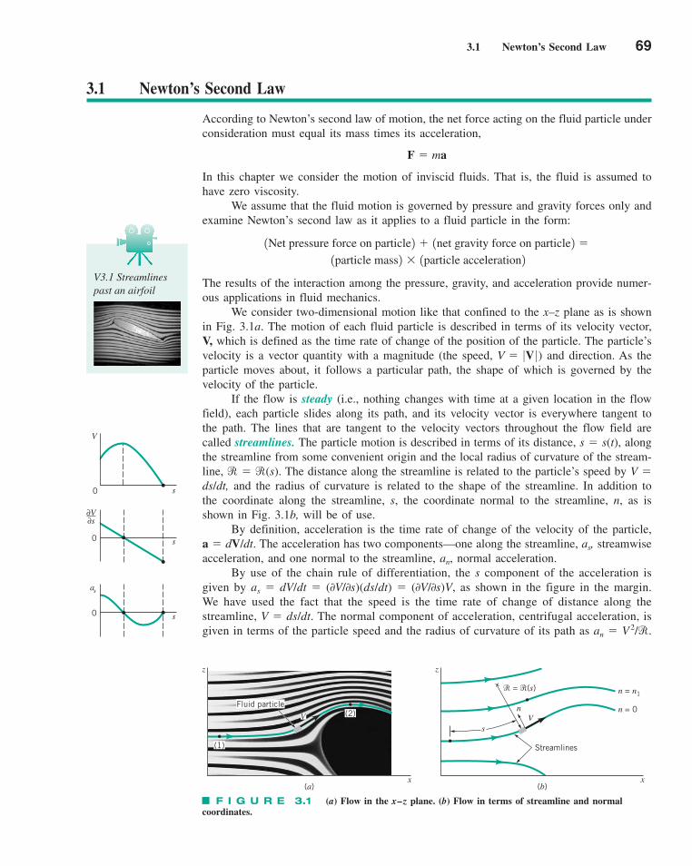
3.1 Newton’s Second Law 69

3.1 Newton’s Second Law

According to Newton’s second law of motion, the net force acting on the fluid particle underconsideration must equal its mass times its acceleration,

In this chapter we consider the motion of inviscid fluids. That is, the fluid is assumed tohave zero viscosity.

We assume that the fluid motion is governed by pressure and gravity forces only andexamine Newton’s second law as it applies to a fluid particle in the form:

The results of the interaction among the pressure, gravity, and acceleration provide numer-ous applications in fluid mechanics.

We consider two-dimensional motion like that confined to the x–z plane as is shownin Fig. 3.1a. The motion of each fluid particle is described in terms of its velocity vector,V, which is defined as the time rate of change of the position of the particle. The particle’svelocity is a vector quantity with a magnitude (the speed, ) and direction. As theparticle moves about, it follows a particular path, the shape of which is governed by thevelocity of the particle.

If the flow is steady (i.e., nothing changes with time at a given location in the flowfield), each particle slides along its path, and its velocity vector is everywhere tangent tothe path. The lines that are tangent to the velocity vectors throughout the flow field arecalled streamlines. The particle motion is described in terms of its distance, s � s(t), alongthe streamline from some convenient origin and the local radius of curvature of the stream-line, r � r(s). The distance along the streamline is related to the particle’s speed by V �ds/dt, and the radius of curvature is related to the shape of the streamline. In addition tothe coordinate along the streamline, s, the coordinate normal to the streamline, n, as isshown in Fig. 3.1b, will be of use.

By definition, acceleration is the time rate of change of the velocity of the particle,a � dV/dt. The acceleration has two components—one along the streamline, as, streamwiseacceleration, and one normal to the streamline, an, normal acceleration.

By use of the chain rule of differentiation, the s component of the acceleration isgiven by as � dV/dt � (0V/0s)(ds/dt) � (0V/0s)V, as shown in the figure in the margin.We have used the fact that the speed is the time rate of change of distance along thestreamline, V � ds/dt. The normal component of acceleration, centrifugal acceleration, isgiven in terms of the particle speed and the radius of curvature of its path as an � V 2/r.

V � 0V 0

1particle mass2 � 1particle acceleration2

1Net pressure force on particle2 � 1net gravity force on particle2 �

F � ma

V

s0

s0

as

s0

∂V∂s

z

x(a)

(1)

(2)Fluid particle

V

z

x(b)

Vs

� = �(s)

n = 0

n = n1

n

Streamlines

F I G U R E 3.1 (a) Flow in the x–z plane. (b) Flow in terms of streamline and normalcoordinates.

V3.1 Streamlinespast an airfoil

c03ElementaryFluidDynamicsTheBernoulliEquation.qxd 9/24/10 12:21 PM Page 69

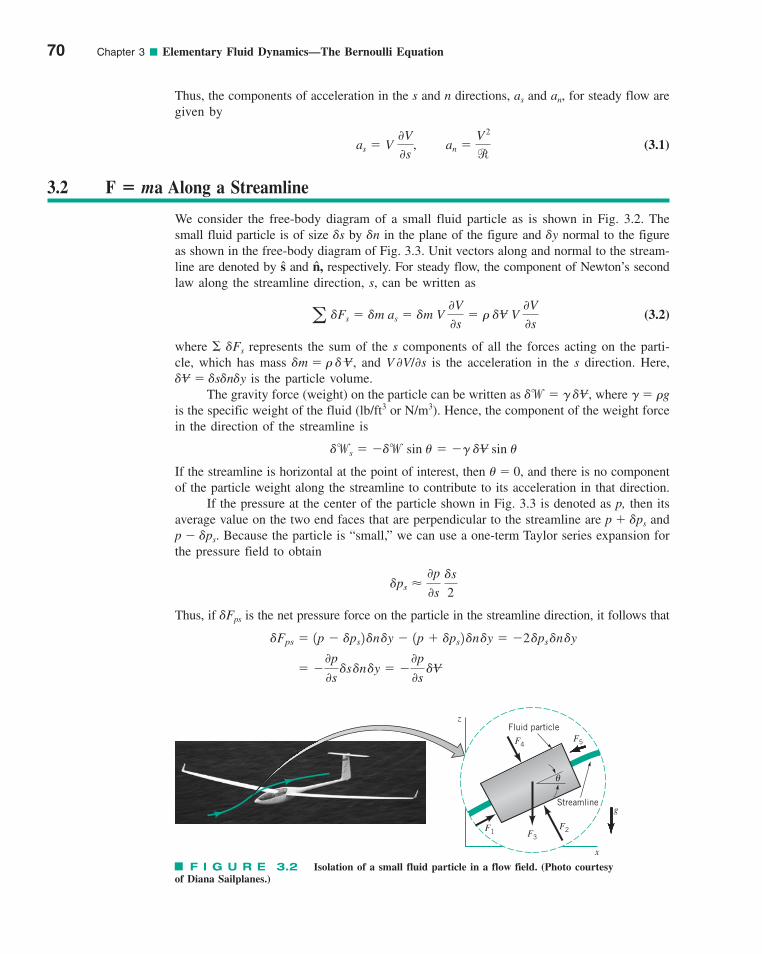
70 Chapter 3 ■ Elementary Fluid Dynamics—The Bernoulli Equation

Thus, the components of acceleration in the s and n directions, as and an, for steady flow aregiven by

(3.1)an �V 2

ras � V

0V

0s,

3.2 F � ma Along a Streamline

We consider the free-body diagram of a small fluid particle as is shown in Fig. 3.2. Thesmall fluid particle is of size �s by �n in the plane of the figure and �y normal to the figureas shown in the free-body diagram of Fig. 3.3. Unit vectors along and normal to the stream-line are denoted by and , respectively. For steady flow, the component of Newton’s secondlaw along the streamline direction, s, can be written as

(3.2)

where � �Fs represents the sum of the s components of all the forces acting on the parti-cle, which has mass �m � � � , and V ∂V/∂s is the acceleration in the s direction. Here,� � �s�n�y is the particle volume.

The gravity force (weight) on the particle can be written as �w� � � , where � � �gis the specific weight of the fluid (lb/ft3 or N/m3). Hence, the component of the weight forcein the direction of the streamline is

If the streamline is horizontal at the point of interest, then � � 0, and there is no componentof the particle weight along the streamline to contribute to its acceleration in that direction.

If the pressure at the center of the particle shown in Fig. 3.3 is denoted as p, then itsaverage value on the two end faces that are perpendicular to the streamline are p � �ps andp � �ps. Because the particle is “small,” we can use a one-term Taylor series expansion forthe pressure field to obtain

Thus, if �Fps is the net pressure force on the particle in the streamline direction, it follows that

� �0p

0s �s �n �y � �

0p

0s @V

�Fps � 1p � �ps2 �n �y � 1p � �ps2 �n �y � �2 �ps �n �y

�ps �0p

0s �s

2

�ws � ��w sin � � �� �V sin �

VV

V

a �Fs � �m as � �m V 0V

0s� � �V V

0V

0s

ns

F1F2F3

F5

θ

Streamline

Fluid particle

g

x

z

F4

F I G U R E 3.2 Isolation of a small fluid particle in a flow field. (Photo courtesyof Diana Sailplanes.)

c03ElementaryFluidDynamicsTheBernoulliEquation.qxd 9/24/10 12:21 PM Page 70

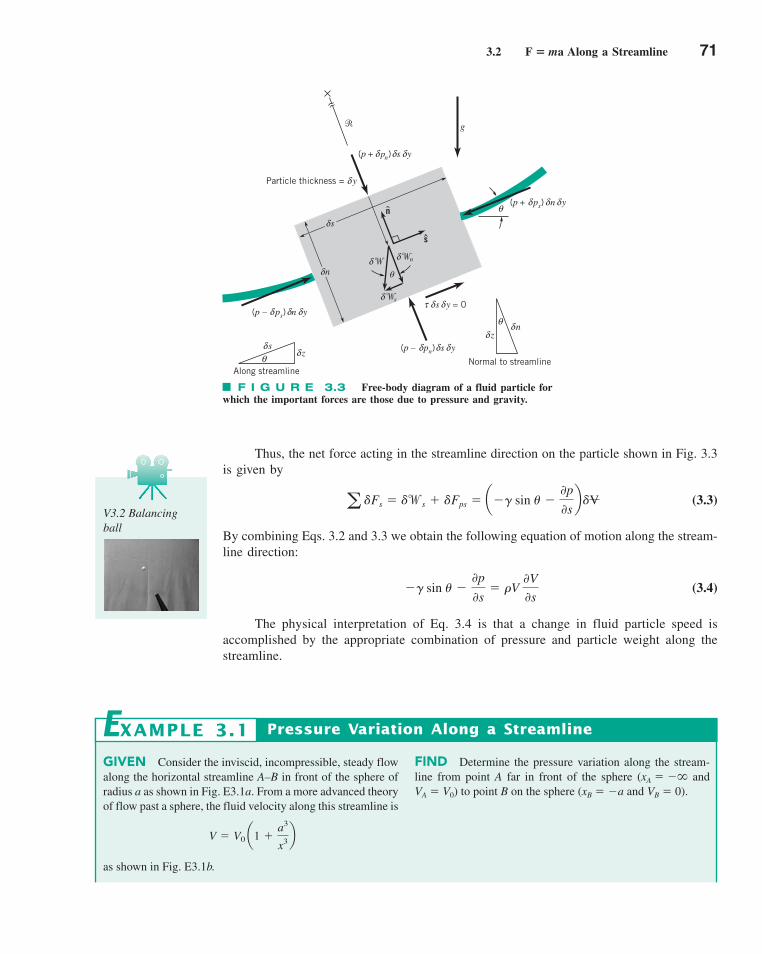
3.2 F � ma Along a Streamline 71

Thus, the net force acting in the streamline direction on the particle shown in Fig. 3.3is given by

(3.3)

By combining Eqs. 3.2 and 3.3 we obtain the following equation of motion along the stream-line direction:

(3.4)

The physical interpretation of Eq. 3.4 is that a change in fluid particle speed isaccomplished by the appropriate combination of pressure and particle weight along thestreamline.

�� sin � �0p

0s� �V

0V

0s

a �Fs � �ws � �Fps � a�� sin � �0p

0sb @V

GIVEN Consider the inviscid, incompressible, steady flowalong the horizontal streamline A–B in front of the sphere ofradius a as shown in Fig. E3.1a. From a more advanced theoryof flow past a sphere, the fluid velocity along this streamline is

as shown in Fig. E3.1b.

V � V0 a1 �a3

x3b

FIND Determine the pressure variation along the stream-line from point A far in front of the sphere (xA � �� andVA � V0) to point B on the sphere (xB � �a and VB � 0).

Pressure Variation Along a StreamlineEXAMPLE 3.1

Particle thickness = y

Along streamlineNormal to streamline

g�

(p + pn) s yδ δ δ

δ

(p + ps) n yδ δ δ

(p – ps) n yδ δ δ

(p – pn) s yδ δ δ

s yδ δτ = 0

sδ zδθ

zδθ

nδ

sδ

nδ

s

nδδ

sδ

θ

θn

��

�

F I G U R E 3.3 Free-body diagram of a fluid particle forwhich the important forces are those due to pressure and gravity.

V3.2 Balancingball

c03ElementaryFluidDynamicsTheBernoulliEquation.qxd 9/24/10 12:21 PM Page 71

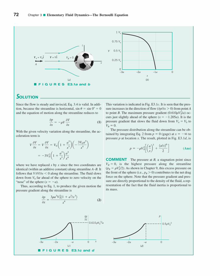
72 Chapter 3 ■ Elementary Fluid Dynamics—The Bernoulli Equation

VA = VO i

A

V = V i VB = 0

Ba

z

(a) (b)

x

x

V

–3a

0–2a –1a 0

1 Vo

0.75 Vo

0.5 Vo

0.25 Vo

ˆˆ

SOLUTION

This variation is indicated in Fig. E3.1c. It is seen that the pres-sure increases in the direction of flow (∂p/∂x � 0) from point Ato point B. The maximum pressure gradient (0.610�V2

0/a) oc-curs just slightly ahead of the sphere (x � �1.205a). It is thepressure gradient that slows the fluid down from VA � V0 toVB � 0.

The pressure distribution along the streamline can be ob-tained by integrating Eq. 2 from p � 0 (gage) at x � �� topressure p at location x. The result, plotted in Fig. E3.1d, is

(Ans)

COMMENT The pressure at B, a stagnation point sinceVB � 0, is the highest pressure along the streamline(pB � �V2

0 /2). As shown in Chapter 9, this excess pressure onthe front of the sphere (i.e., pB � 0) contributes to the net dragforce on the sphere. Note that the pressure gradient and pres-sure are directly proportional to the density of the fluid, a rep-resentation of the fact that the fluid inertia is proportional toits mass.

p � ��V20 c a

a

xb

3

�1a/x26

2d

Since the flow is steady and inviscid, Eq. 3.4 is valid. In addi-tion, because the streamline is horizontal, sin � � sin 0 � 0and the equation of motion along the streamline reduces to

(1)

With the given velocity variation along the streamline, the ac-celeration term is

where we have replaced s by x since the two coordinates areidentical (within an additive constant) along streamline A–B. Itfollows that V∂V/∂s 0 along the streamline. The fluid slowsdown from V0 far ahead of the sphere to zero velocity on the“nose” of the sphere (x � �a).

Thus, according to Eq. 1, to produce the given motion thepressure gradient along the streamline is

(2)0p

0x�

3�a3V2011 � a3/x32

x4

� �3V20 a1 �

a3

x3b a3

x4

V 0V

0s� V

0V

0x� V0 a1 �

a3

x3b a�

3V0 a3

x4 b

0p

0s� ��V

0V

0s

F I G U R E S E3.1a and b

–3a –2a –a 0 x

∂p__∂x

0.610 V02/aρ

(c)–3a –2a –a 0 x

(d)

p

0.5 V02

ρ

F I G U R E S E3.1c and d

c03ElementaryFluidDynamicsTheBernoulliEquation.qxd 9/24/10 12:21 PM Page 72

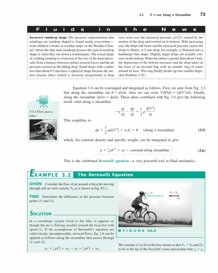
3.2 F � ma Along a Streamline 73

Equation 3.4 can be rearranged and integrated as follows. First, we note from Fig. 3.3that along the streamline sin � � dz/ds. Also we can write VdV/ds � 1

—

2d(V2)/ds. Finally,along the streamline ∂p/∂s � dp/ds. These ideas combined with Eq. 3.4 give the followingresult valid along a streamline

This simplifies to

(along a streamline) (3.5)

which, for constant density and specific weight, can be integrated to give

(3.6)

This is the celebrated Bernoulli equation—a very powerful tool in fluid mechanics.

p � 12 �V2 � �z � constant along streamline

dp �1

2 �d 1V22 � � dz � 0

�� dz

ds�

dp

ds�

1

2 �

d1V22

ds

F l u i d s i n t h e N e w s

Incorrect raindrop shape The incorrect representation thatraindrops are teardrop shaped is found nearly everywhere—from children’s books to weather maps on the Weather Chan-nel. About the only time raindrops possess the typical teardropshape is when they run down a windowpane. The actual shapeof a falling raindrop is a function of the size of the drop and re-sults from a balance between surface tension forces and the airpressure exerted on the falling drop. Small drops with a radiusless than about 0.5 mm have a spherical shape because the sur-face tension effect (which is inversely proportional to drop

size) wins over the increased pressure, caused by themotion of the drop and exerted on its bottom. With increasingsize, the drops fall faster and the increased pressure causes thedrops to flatten. A 2-mm drop, for example, is flattened into ahamburger bun shape. Slightly larger drops are actually con-cave on the bottom. When the radius is greater than about 4 mm,the depression of the bottom increases and the drop takes onthe form of an inverted bag with an annular ring of wateraround its base. This ring finally breaks up into smaller drops.(See Problem 3.22.)

�V 20/2,

V3.3 Flow past abiker

GIVEN Consider the flow of air around a bicyclist movingthrough still air with velocity V0 as is shown in Fig. E3.2.

FIND Determine the difference in the pressure betweenpoints (1) and (2).

SOLUTION

The Bernoulli Equation

We consider (1) to be in the free stream so that V1 � V0 and (2)to be at the tip of the bicyclist’s nose and assume that z1 � z2

EXAMPLE 3.2

In a coordinate system fixed to the bike, it appears asthough the air is flowing steadily toward the bicyclist withspeed V0. If the assumptions of Bernoulli’s equation arevalid (steady, incompressible, inviscid flow), Eq. 3.6 can beapplied as follows along the streamline that passes through(1) and (2).

p1 � 12 �V2

1 � �z1 � p2 � 12 �V2

2 � �z2

V2 = 0 V1 = V0

(1)(2)

F I G U R E E3.2

c03ElementaryFluidDynamicsTheBernoulliEquation.qxd 9/24/10 12:21 PM Page 73

74 Chapter 3 ■ Elementary Fluid Dynamics—The Bernoulli Equation

velocity distribution is not needed—only the “boundary con-ditions” at (1) and (2) are required. Of course, knowledge ofthe value of V along the streamline is needed to determinethe pressure at points between (1) and (2). Note that if wemeasure p2 � p1 we can determine the speed, V0. As dis-cussed in Section 3.5, this is the principle upon which manyvelocity-measuring devices are based.

If the bicyclist were accelerating or decelerating, the flowwould be unsteady (i.e., V0 � constant) and the aforemen-tioned analysis would be incorrect, as Eq. 3.6 is restricted tosteady flow.

and V2 � 0 (both of which, as is discussed in Section 3.5, arereasonable assumptions). It follows that the pressure of (2) isgreater than that at (1) by an amount

(Ans)

COMMENTS A similar result was obtained in Example3.1 by integrating the pressure gradient, which was knownbecause the velocity distribution along the streamline, V(s),was known. The Bernoulli equation is a general integrationof F � ma. To determine p2 � p1, knowledge of the detailed

p2 � p1 � 12 �V2

1 � 12 �V2

0

3.3 F � ma Normal to a Streamline

We again consider the force balance on the fluid particle shown in Fig. 3.3. This time, how-ever, we consider components in the normal direction, , and write Newton’s second lawin this direction as

(3.7)

where � �Fn represents the sum of the normal components of all the forces acting on theparticle. We assume the flow is steady with a normal acceleration an � V2/r, where r isthe local radius of curvature of the streamlines.

We again assume that the only forces of importance are pressure and gravity. Usingthe method of Section 3.2 for determining forces along the streamline, the net force actingin the normal direction on the particle shown in Fig. 3.3 is determined to be

(3.8)

where ∂p/∂n is the pressure gradient normal to the streamline. By combining Eqs. 3.7 and3.8 and using the fact that along a line normal to the streamline cos � � dz/dn (see Fig. 3.3),we obtain the following equation of motion along the normal direction:

(3.9)

The physical interpretation of Eq. 3.9 is that a change in the direction of flow of afluid particle (i.e., a curved path, r �) is accomplished by the appropriate combinationof pressure gradient and particle weight normal to the streamline. By integration of Eq. 3.9,the final form of Newton’s second law applied across the streamlines for steady, inviscid,incompressible flow is obtained as

(3.10)p � ��V 2

r dn � �z � constant across the streamline

�� dz

dn�

0p

0n�

�V 2

r

a �Fn � �wn � �Fpn � a�� cos � �0p

0nb �V

a �Fn ��m V 2

r�

� �V V 2

r

n

V3.5 Aircraft wingtip vortex

V3.4 Hydrocycloneseparator

V3.6 Free vortex

c03ElementaryFluidDynamicsTheBernoulliEquation.qxd 9/24/10 12:21 PM Page 74

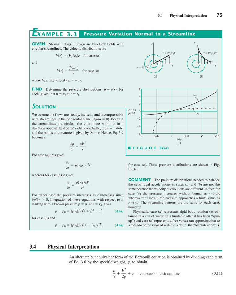
3.4 Physical Interpretation 75

GIVEN Shown in Figs. E3.3a,b are two flow fields withcircular streamlines. The velocity distributions are

for case (a)

and

for case (b)

where V0 is the velocity at

FIND Determine the pressure distributions, p � p(r), foreach, given that p � p0 at r � r0.

r � r0.

V1r2 �1V0 r02

r

V1r2 � 1V0 /r02r

SOLUTION

Pressure Variation Normal to a Streamline

for case (b). These pressure distributions are shown in Fig.E3.3c.

COMMENT The pressure distributions needed to balancethe centrifugal accelerations in cases (a) and (b) are not thesame because the velocity distributions are different. In fact, forcase (a) the pressure increases without bound as r → �,whereas for case (b) the pressure approaches a finite value asr → �. The streamline patterns are the same for each case,however.

Physically, case (a) represents rigid-body rotation (as ob-tained in a can of water on a turntable after it has been “spunup”) and case (b) represents a free vortex (an approximation toa tornado or the swirl of water in a drain, the “bathtub vortex”).

EXAMPLE 3.3

We assume the flows are steady, inviscid, and incompressiblewith streamlines in the horizontal plane (dz/dn � 0). Becausethe streamlines are circles, the coordinate n points in adirection opposite that of the radial coordinate, ∂/∂n � �∂/∂r,and the radius of curvature is given by r � r. Hence, Eq. 3.9becomes

For case (a) this gives

whereas for case (b) it gives

For either case the pressure increases as r increases since∂p/∂r � 0. Integration of these equations with respect to r,starting with a known pressure p � p0 at r � r0, gives

(Ans)

for case (a) and

(Ans)p � p0 � 1�V20 �22 31 � 1r0/r22 4

p � p0 � 1�V20 �22 3 1r/r02

2 � 1 4

0p

0r�

�1V0 r022

r3

0p

0r� �1V0 /r02

2r

0p

0r�

�V2

r

y

r = � n

(a)

V = (V0/r0)r V = (V0r0)/r

y

(b)

xx

(a)

(b)

4

6

2

0

�2

�4

�60 0.5 1 1.5 2 2.5

r/r0

p – p0

V 02/2

(c)

ρ

F I G U R E E3.3

3.4 Physical Interpretation

An alternate but equivalent form of the Bernoulli equation is obtained by dividing each termof Eq. 3.6 by the specific weight, �, to obtain

(3.11)p

��

V2

2g� z � constant on a streamline

c03ElementaryFluidDynamicsTheBernoulliEquation.qxd 9/24/10 12:21 PM Page 75

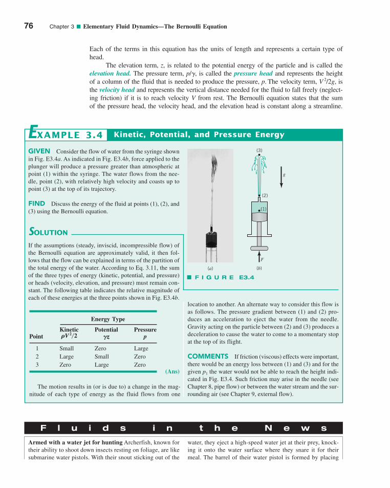
76 Chapter 3 ■ Elementary Fluid Dynamics—The Bernoulli Equation

Each of the terms in this equation has the units of length and represents a certain type ofhead.

The elevation term, z, is related to the potential energy of the particle and is called theelevation head. The pressure term, p/�, is called the pressure head and represents the heightof a column of the fluid that is needed to produce the pressure, p. The velocity term, V 2/2g, isthe velocity head and represents the vertical distance needed for the fluid to fall freely (neglect-ing friction) if it is to reach velocity V from rest. The Bernoulli equation states that the sumof the pressure head, the velocity head, and the elevation head is constant along a streamline.

GIVEN Consider the flow of water from the syringe shownin Fig. E3.4a. As indicated in Fig. E3.4b, force applied to theplunger will produce a pressure greater than atmospheric atpoint (1) within the syringe. The water flows from the nee-dle, point (2), with relatively high velocity and coasts up topoint (3) at the top of its trajectory.

FIND Discuss the energy of the fluid at points (1), (2), and(3) using the Bernoulli equation.

SOLUTION

Kinetic, Potential, and Pressure Energy

location to another. An alternate way to consider this flow isas follows. The pressure gradient between (1) and (2) pro-duces an acceleration to eject the water from the needle.Gravity acting on the particle between (2) and (3) produces adeceleration to cause the water to come to a momentary stopat the top of its flight.

COMMENTS If friction (viscous) effects were important,there would be an energy loss between (1) and (3) and for thegiven p1 the water would not be able to reach the height indi-cated in Fig. E3.4. Such friction may arise in the needle (seeChapter 8, pipe flow) or between the water stream and the sur-rounding air (see Chapter 9, external flow).

EXAMPLE 3.4

If the assumptions (steady, inviscid, incompressible flow) ofthe Bernoulli equation are approximately valid, it then fol-lows that the flow can be explained in terms of the partition ofthe total energy of the water. According to Eq. 3.11, the sumof the three types of energy (kinetic, potential, and pressure)or heads (velocity, elevation, and pressure) must remain con-stant. The following table indicates the relative magnitude ofeach of these energies at the three points shown in Fig. E3.4b.

The motion results in (or is due to) a change in the mag-nitude of each type of energy as the fluid flows from one

Energy Type

Kinetic Potential PressurePoint p

1 Small Zero Large2 Large Small Zero3 Zero Large Zero

GzzRV 2�2

g

F

(1)

(2)

(3)

(b)

F I G U R E E3.4

(a)

F l u i d s i n t h e N e w s

Armed with a water jet for hunting Archerfish, known fortheir ability to shoot down insects resting on foliage, are likesubmarine water pistols. With their snout sticking out of the

water, they eject a high-speed water jet at their prey, knock-ing it onto the water surface where they snare it for theirmeal. The barrel of their water pistol is formed by placing

(Ans)

c03ElementaryFluidDynamicsTheBernoulliEquation.qxd 9/24/10 12:21 PM Page 76

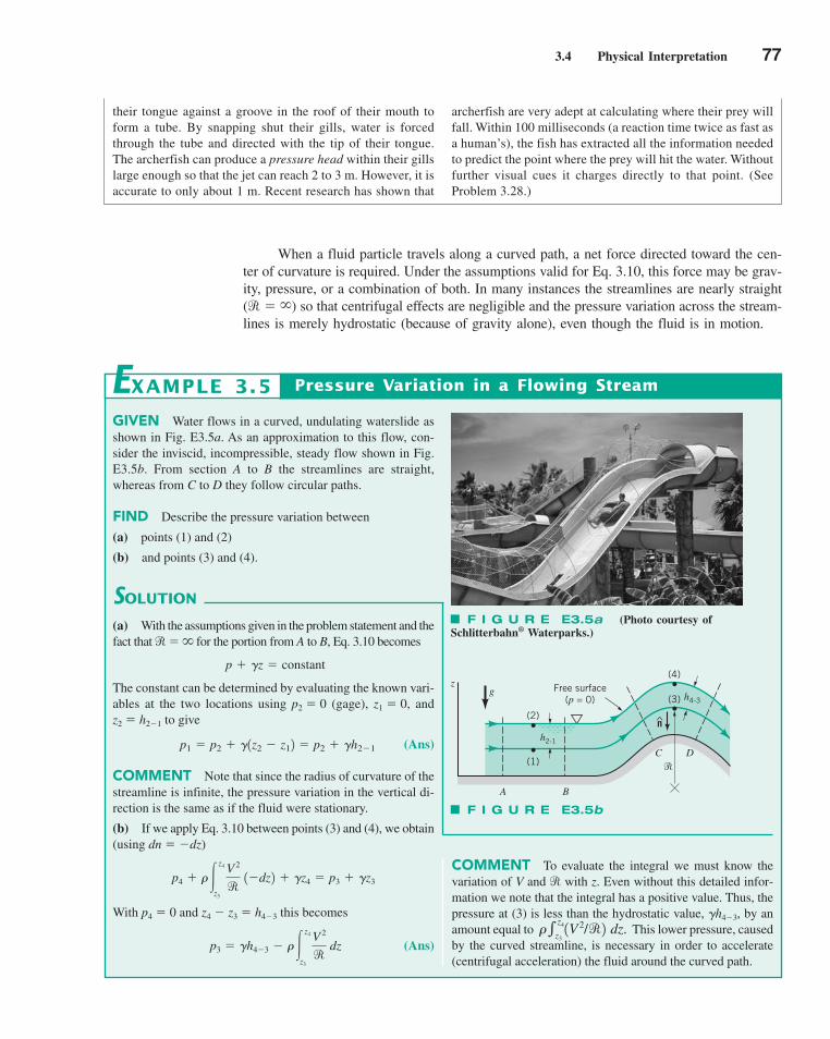
3.4 Physical Interpretation 77

When a fluid particle travels along a curved path, a net force directed toward the cen-ter of curvature is required. Under the assumptions valid for Eq. 3.10, this force may be grav-ity, pressure, or a combination of both. In many instances the streamlines are nearly straight(r � �) so that centrifugal effects are negligible and the pressure variation across the stream-lines is merely hydrostatic (because of gravity alone), even though the fluid is in motion.

their tongue against a groove in the roof of their mouth toform a tube. By snapping shut their gills, water is forcedthrough the tube and directed with the tip of their tongue.The archerfish can produce a pressure head within their gillslarge enough so that the jet can reach 2 to 3 m. However, it isaccurate to only about 1 m. Recent research has shown that

archerfish are very adept at calculating where their prey willfall. Within 100 milliseconds (a reaction time twice as fast asa human’s), the fish has extracted all the information neededto predict the point where the prey will hit the water. Withoutfurther visual cues it charges directly to that point. (SeeProblem 3.28.)

GIVEN Water flows in a curved, undulating waterslide asshown in Fig. E3.5a. As an approximation to this flow, con-sider the inviscid, incompressible, steady flow shown in Fig.E3.5b. From section A to B the streamlines are straight,whereas from C to D they follow circular paths.

FIND Describe the pressure variation between

(a) points (1) and (2)

(b) and points (3) and (4).

SOLUTION

Pressure Variation in a Flowing Stream

COMMENT To evaluate the integral we must know thevariation of V and r with z. Even without this detailed infor-mation we note that the integral has a positive value. Thus, thepressure at (3) is less than the hydrostatic value, �h4�3, by anamount equal to This lower pressure, causedby the curved streamline, is necessary in order to accelerate(centrifugal acceleration) the fluid around the curved path.

�� z4

z31V 2/r2 dz.

EXAMPLE 3.5

(a) With the assumptions given in the problem statement and thefact that r� � for the portion from A to B, Eq. 3.10 becomes

The constant can be determined by evaluating the known vari-ables at the two locations using p2 � 0 (gage), z1 � 0, andz2 � h2�1 to give

(Ans)

COMMENT Note that since the radius of curvature of thestreamline is infinite, the pressure variation in the vertical di-rection is the same as if the fluid were stationary.

(b) If we apply Eq. 3.10 between points (3) and (4), we obtain(using dn � �dz)

With p4 � 0 and z4 � z3 � h4�3 this becomes

(Ans)p3 � �h4�3 � ��z4

z3

V 2

r dz

p4 � ��z4

z3

V 2

r 1�dz2 � �z4 � p3 � �z3

p1 � p2 � �1z2 � z12 � p2 � �h2�1

p � �z � constantz

g

(2)

(1)

h2-1

A B

C D�

Free surface(p = 0)

n

h4-3

(4)

(3)

^

F I G U R E E3.5b

F I G U R E E3.5a (Photo courtesy ofSchlitterbahn® Waterparks.)

c03ElementaryFluidDynamicsTheBernoulliEquation.qxd 9/24/10 12:21 PM Page 77

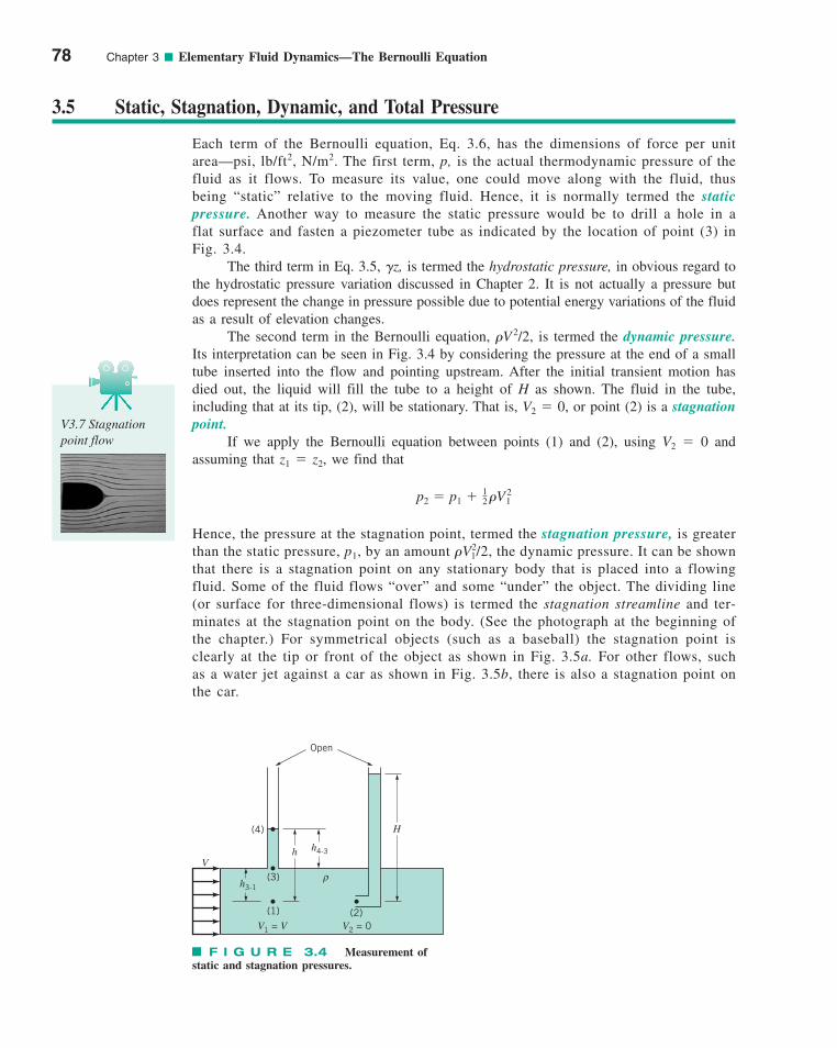
78 Chapter 3 ■ Elementary Fluid Dynamics—The Bernoulli Equation

3.5 Static, Stagnation, Dynamic, and Total Pressure

Each term of the Bernoulli equation, Eq. 3.6, has the dimensions of force per unitarea—psi, lb/ft2, N/m2. The first term, p, is the actual thermodynamic pressure of thefluid as it flows. To measure its value, one could move along with the fluid, thusbeing “static” relative to the moving fluid. Hence, it is normally termed the staticpressure. Another way to measure the static pressure would be to drill a hole in aflat surface and fasten a piezometer tube as indicated by the location of point (3) inFig. 3.4.

The third term in Eq. 3.5, �z, is termed the hydrostatic pressure, in obvious regard tothe hydrostatic pressure variation discussed in Chapter 2. It is not actually a pressure butdoes represent the change in pressure possible due to potential energy variations of the fluidas a result of elevation changes.

The second term in the Bernoulli equation, �V 2/2, is termed the dynamic pressure.Its interpretation can be seen in Fig. 3.4 by considering the pressure at the end of a smalltube inserted into the flow and pointing upstream. After the initial transient motion hasdied out, the liquid will fill the tube to a height of H as shown. The fluid in the tube,including that at its tip, (2), will be stationary. That is, V2 � 0, or point (2) is a stagnationpoint.

If we apply the Bernoulli equation between points (1) and (2), using V2 � 0 andassuming that z1 � z2, we find that

Hence, the pressure at the stagnation point, termed the stagnation pressure, is greaterthan the static pressure, p1, by an amount �V2

1/2, the dynamic pressure. It can be shownthat there is a stagnation point on any stationary body that is placed into a flowingfluid. Some of the fluid flows “over” and some “under” the object. The dividing line(or surface for three-dimensional flows) is termed the stagnation streamline and ter-minates at the stagnation point on the body. (See the photograph at the beginning ofthe chapter.) For symmetrical objects (such as a baseball) the stagnation point isclearly at the tip or front of the object as shown in Fig. 3.5a. For other flows, suchas a water jet against a car as shown in Fig. 3.5b, there is also a stagnation point onthe car.

p2 � p1 � 12 �V 2

1

V3.7 Stagnationpoint flow

F I G U R E 3.4 Measurement ofstatic and stagnation pressures.

(1) (2)

(3)

(4)

h3-1

h h4-3

ρ

Open

H

V

V1 = V V2 = 0

c03ElementaryFluidDynamicsTheBernoulliEquation.qxd 9/24/10 12:21 PM Page 78

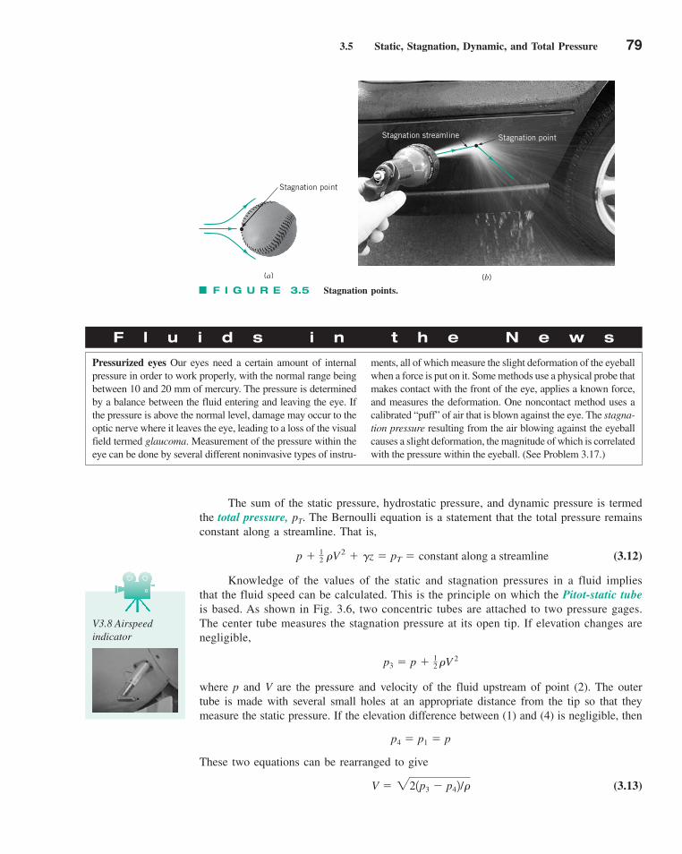
3.5 Static, Stagnation, Dynamic, and Total Pressure 79

The sum of the static pressure, hydrostatic pressure, and dynamic pressure is termedthe total pressure, pT. The Bernoulli equation is a statement that the total pressure remainsconstant along a streamline. That is,

(3.12)

Knowledge of the values of the static and stagnation pressures in a fluid impliesthat the fluid speed can be calculated. This is the principle on which the Pitot-static tubeis based. As shown in Fig. 3.6, two concentric tubes are attached to two pressure gages.The center tube measures the stagnation pressure at its open tip. If elevation changes arenegligible,

where p and V are the pressure and velocity of the fluid upstream of point (2). The outertube is made with several small holes at an appropriate distance from the tip so that theymeasure the static pressure. If the elevation difference between (1) and (4) is negligible, then

These two equations can be rearranged to give

(3.13)V � 221p3 � p42/�

p4 � p1 � p

p3 � p � 12 �V 2

p � 12 �V2 � �z � pT � constant along a streamline

Stagnation point

(a)

Stagnation streamline

(b)

Stagnation point

F I G U R E 3.5 Stagnation points.

F l u i d s i n t h e N e w s

Pressurized eyes Our eyes need a certain amount of internalpressure in order to work properly, with the normal range beingbetween 10 and 20 mm of mercury. The pressure is determinedby a balance between the fluid entering and leaving the eye. Ifthe pressure is above the normal level, damage may occur to theoptic nerve where it leaves the eye, leading to a loss of the visualfield termed glaucoma. Measurement of the pressure within theeye can be done by several different noninvasive types of instru-

ments, all of which measure the slight deformation of the eyeballwhen a force is put on it. Some methods use a physical probe thatmakes contact with the front of the eye, applies a known force,and measures the deformation. One noncontact method uses acalibrated “puff” of air that is blown against the eye. The stagna-tion pressure resulting from the air blowing against the eyeballcauses a slight deformation, the magnitude of which is correlatedwith the pressure within the eyeball. (See Problem 3.17.)

V3.8 Airspeedindicator

c03ElementaryFluidDynamicsTheBernoulliEquation.qxd 9/24/10 12:21 PM Page 79

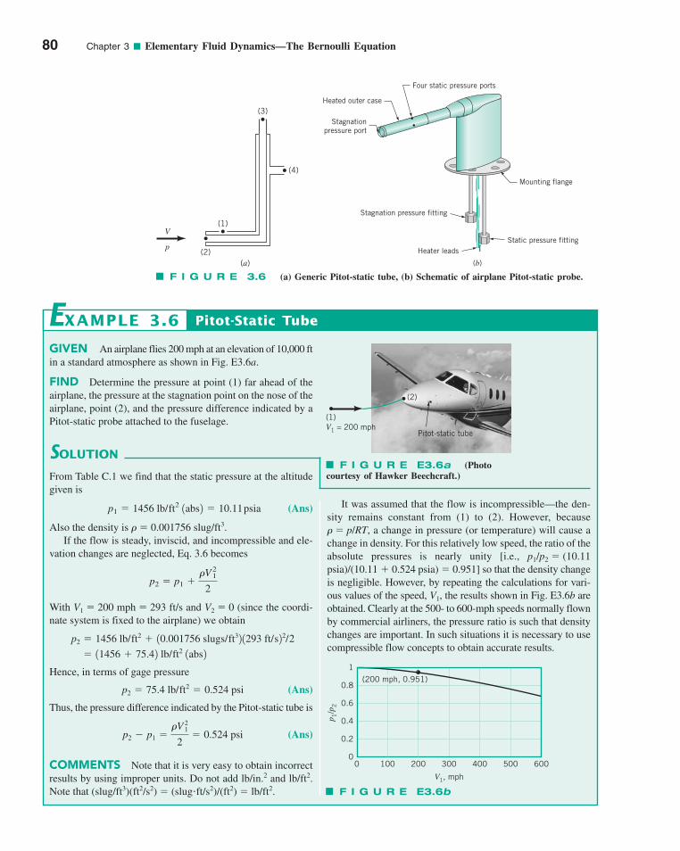
80 Chapter 3 ■ Elementary Fluid Dynamics—The Bernoulli Equation

Four static pressure ports

Heated outer case

Stagnationpressure port

Stagnation pressure fitting

Heater leads

Mounting flange

Static pressure fitting

(b)

V

p

(1)

(2)

(4)

(3)

(a)

F I G U R E 3.6 (a) Generic Pitot-static tube, (b) Schematic of airplane Pitot-static probe.

GIVEN An airplane flies 200 mph at an elevation of 10,000 ftin a standard atmosphere as shown in Fig. E3.6a.

FIND Determine the pressure at point (1) far ahead of theairplane, the pressure at the stagnation point on the nose of theairplane, point (2), and the pressure difference indicated by aPitot-static probe attached to the fuselage.

SOLUTION

Pitot-Static Tube

It was assumed that the flow is incompressible—the den-sity remains constant from (1) to (2). However, because� � p/RT, a change in pressure (or temperature) will cause achange in density. For this relatively low speed, the ratio of theabsolute pressures is nearly unity [i.e., p1/p2 � (10.11psia)/(10.11 � 0.524 psia) � 0.951] so that the density changeis negligible. However, by repeating the calculations for vari-ous values of the speed, , the results shown in Fig. E3.6b areobtained. Clearly at the 500- to 600-mph speeds normally flownby commercial airliners, the pressure ratio is such that densitychanges are important. In such situations it is necessary to usecompressible flow concepts to obtain accurate results.

V1

EXAMPLE 3.6

From Table C.1 we find that the static pressure at the altitudegiven is

(Ans)

Also the density is � � 0.001756 slug/ft3.If the flow is steady, inviscid, and incompressible and ele-

vation changes are neglected, Eq. 3.6 becomes

With V1 � 200 mph � 293 ft/s and V2 � 0 (since the coordi-nate system is fixed to the airplane) we obtain

Hence, in terms of gage pressure

(Ans)

Thus, the pressure difference indicated by the Pitot-static tube is

(Ans)

COMMENTS Note that it is very easy to obtain incorrectresults by using improper units. Do not add lb/in.2 and lb/ft2.Note that (slug/ft3)(ft2/s2) � (slug�ft/s2)/(ft2) � lb/ft2.

p2 � p1 ��V 2

1

2� 0.524 psi

p2 � 75.4 lb/ft2 � 0.524 psi

� 11456 � 75.42 lb/ft2 1abs2

p2 � 1456 lb/ft2 � 10.001756 slugs/ft32 1293 ft/s22/2

p2 � p1 ��V 2

1

2

p1 � 1456 lb/ft2 1abs2 � 10.11 psia

F I G U R E E3.6a (Photocourtesy of Hawker Beechcraft.)

(2)

(1)

Pitot-static tubeV1 = 200 mph

F I G U R E E3.6b

(200 mph, 0.951)1

0.8

0.6

0.4

0.2

00 100 200 300

V1, mph

p 1/p

2

400 500 600

c03ElementaryFluidDynamicsTheBernoulliEquation.qxd 9/24/10 12:21 PM Page 80

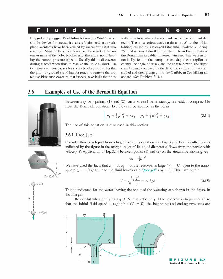
3.6 Examples of Use of the Bernoulli Equation 81

F l u i d s i n t h e N e w s

Bugged and plugged Pitot tubes Although a Pitot tube is asimple device for measuring aircraft airspeed, many air-plane accidents have been caused by inaccurate Pitot tubereadings. Most of these accidents are the result of havingone or more of the holes blocked and, therefore, not indicat-ing the correct pressure (speed). Usually this is discoveredduring takeoff when time to resolve the issue is short. Thetwo most common causes for such a blockage are either thatthe pilot (or ground crew) has forgotten to remove the pro-tective Pitot tube cover or that insects have built their nest

within the tube where the standard visual check cannot de-tect it. The most serious accident (in terms of number of fa-talities) caused by a blocked Pitot tube involved a Boeing757 and occurred shortly after takeoff from Puerto Plata inthe Dominican Republic. Incorrect airspeed data were auto-matically fed to the computer causing the autopilot tochange the angle of attack and the engine power. The flightcrew became confused by the false indications: the aircraftstalled and then plunged into the Caribbean Sea killing allaboard. (See Problem 3.18.)

3.6 Examples of Use of the Bernoulli Equation

Between any two points, (1) and (2), on a streamline in steady, inviscid, incompressibleflow the Bernoulli equation (Eq. 3.6) can be applied in the form

(3.14)

The use of this equation is discussed in this section.

3.6.1 Free Jets

Consider flow of a liquid from a large reservoir as is shown in Fig. 3.7 or from a coffee urn asindicated by the figure in the margin. A jet of liquid of diameter d flows from the nozzle withvelocity V. Application of Eq. 3.14 between points (1) and (2) on the streamline shown gives

We have used the facts that z1 � h, z2 � 0, the reservoir is large (V1 � 0), open to the atmo-sphere ( p1 � 0 gage), and the fluid leaves as a “free jet” (p2 � 0). Thus, we obtain

(3.15)

This is indicated for the water leaving the spout of the watering can shown in the figure inthe margin.

Be careful when applying Eq. 3.15. It is valid only if the reservoir is large enough sothat the initial fluid speed is negligible (V1 � 0), the beginning and ending pressures are

V �B

2 �h

�� 12gh

�h � 12�V 2

p1 � 12 �V2

1 � �z1 � p2 � 12 �V2

2 � �z2

F I G U R E 3.7Vertical flow from a tank.

(2) (4)

(1)

(3)

V

d

(5)

H

�

h z

(2)

V

V = 0

V = 2gh

h

h

(1)

(2)V = √2gh

c03ElementaryFluidDynamicsTheBernoulliEquation.qxd 9/24/10 12:21 PM Page 81

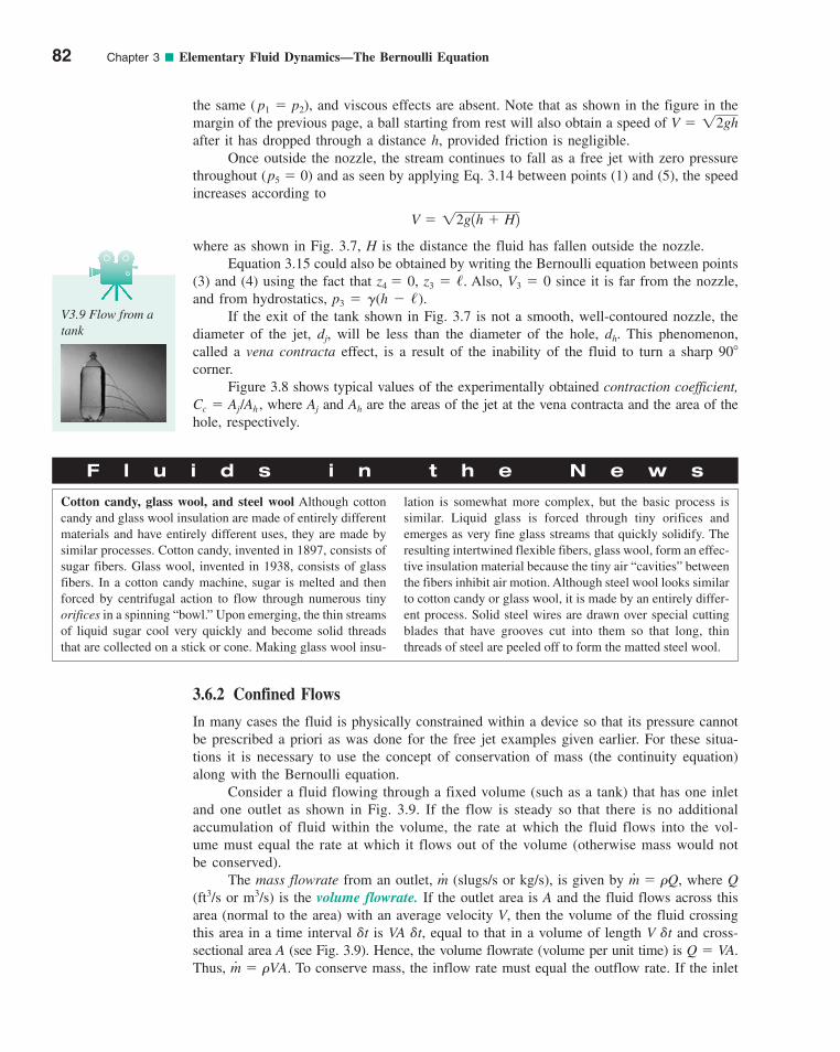
3.6.2 Confined Flows

In many cases the fluid is physically constrained within a device so that its pressure cannotbe prescribed a priori as was done for the free jet examples given earlier. For these situa-tions it is necessary to use the concept of conservation of mass (the continuity equation)along with the Bernoulli equation.

Consider a fluid flowing through a fixed volume (such as a tank) that has one inletand one outlet as shown in Fig. 3.9. If the flow is steady so that there is no additionalaccumulation of fluid within the volume, the rate at which the fluid flows into the vol-ume must equal the rate at which it flows out of the volume (otherwise mass would notbe conserved).

The mass flowrate from an outlet, (slugs/s or kg/s), is given by where Q(ft3/s or m3/s) is the volume flowrate. If the outlet area is A and the fluid flows across thisarea (normal to the area) with an average velocity V, then the volume of the fluid crossingthis area in a time interval �t is VA �t, equal to that in a volume of length V �t and cross-sectional area A (see Fig. 3.9). Hence, the volume flowrate (volume per unit time) is Q � VA.Thus, To conserve mass, the inflow rate must equal the outflow rate. If the inletm

#� �VA.

m#

� �Q,m#

82 Chapter 3 ■ Elementary Fluid Dynamics—The Bernoulli Equation

the same ( p1 � p2), and viscous effects are absent. Note that as shown in the figure in themargin of the previous page, a ball starting from rest will also obtain a speed of after it has dropped through a distance h, provided friction is negligible.

Once outside the nozzle, the stream continues to fall as a free jet with zero pressurethroughout (p5 � 0) and as seen by applying Eq. 3.14 between points (1) and (5), the speedincreases according to

where as shown in Fig. 3.7, H is the distance the fluid has fallen outside the nozzle.Equation 3.15 could also be obtained by writing the Bernoulli equation between points

(3) and (4) using the fact that z4 � 0, z3 � /. Also, V3 � 0 since it is far from the nozzle,and from hydrostatics, p3 � �(h � /).

If the exit of the tank shown in Fig. 3.7 is not a smooth, well-contoured nozzle, thediameter of the jet, dj, will be less than the diameter of the hole, dh. This phenomenon,called a vena contracta effect, is a result of the inability of the fluid to turn a sharp 90corner.

Figure 3.8 shows typical values of the experimentally obtained contraction coefficient,Cc � Aj/Ah , where Aj and Ah are the areas of the jet at the vena contracta and the area of thehole, respectively.

V � 12g1h � H2

V � 12gh

V3.9 Flow from atank

F l u i d s i n t h e N e w s

Cotton candy, glass wool, and steel wool Although cottoncandy and glass wool insulation are made of entirely differentmaterials and have entirely different uses, they are made bysimilar processes. Cotton candy, invented in 1897, consists ofsugar fibers. Glass wool, invented in 1938, consists of glassfibers. In a cotton candy machine, sugar is melted and thenforced by centrifugal action to flow through numerous tinyorifices in a spinning “bowl.” Upon emerging, the thin streamsof liquid sugar cool very quickly and become solid threadsthat are collected on a stick or cone. Making glass wool insu-

lation is somewhat more complex, but the basic process issimilar. Liquid glass is forced through tiny orifices andemerges as very fine glass streams that quickly solidify. Theresulting intertwined flexible fibers, glass wool, form an effec-tive insulation material because the tiny air “cavities” betweenthe fibers inhibit air motion. Although steel wool looks similarto cotton candy or glass wool, it is made by an entirely differ-ent process. Solid steel wires are drawn over special cuttingblades that have grooves cut into them so that long, thinthreads of steel are peeled off to form the matted steel wool.

c03ElementaryFluidDynamicsTheBernoulliEquation.qxd 9/24/10 12:21 PM Page 82

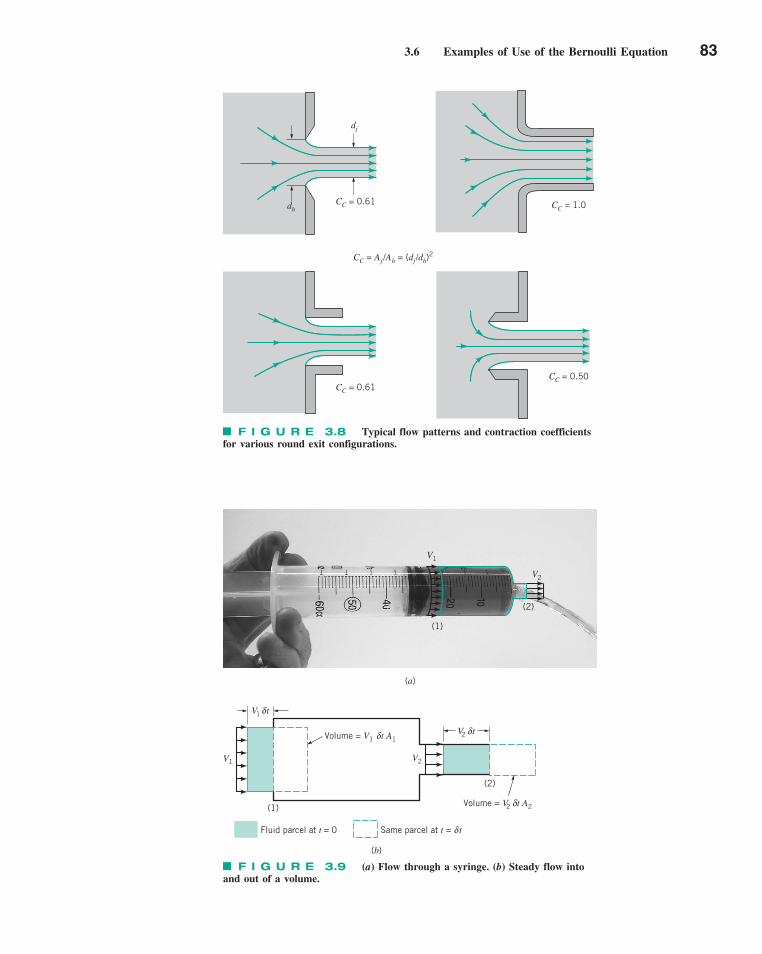
3.6 Examples of Use of the Bernoulli Equation 83

dh

dj

CC = 0.61

CC = 0.61CC = 0.50

CC = 1.0

CC = Aj /Ah = (dj /dh)2

F I G U R E 3.8 Typical flow patterns and contraction coefficientsfor various round exit configurations.

V1

(1)

Volume = V1 t A1

V2

(2)

Volume = V2 t A2

Same parcel at t = tFluid parcel at t = 0

V1 tδ

δ δV2 t

δ

δ

(b)

V1

V2

(2)

(1)

(a)

F I G U R E 3.9 (a) Flow through a syringe. (b) Steady flow intoand out of a volume.

c03ElementaryFluidDynamicsTheBernoulliEquation.qxd 9/24/10 12:22 PM Page 83

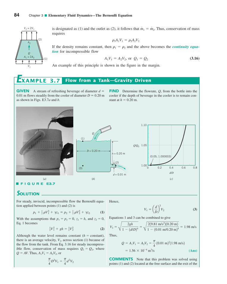
84 Chapter 3 ■ Elementary Fluid Dynamics—The Bernoulli Equation

is designated as (1) and the outlet as (2), it follows that Thus, conservation of massrequires

If the density remains constant, then �1 � �2 and the above becomes the continuity equa-tion for incompressible flow

or (3.16)

An example of this principle is shown in the figure in the margin.

Q1 � Q2A1V1 � A2V2,

�1A1V1 � �2A2V2

m#

1 � m#

2.

GIVEN A stream of refreshing beverage of diameter d �0.01 m flows steadily from the cooler of diameter D � 0.20 mas shown in Figs. E3.7a and b.

FIND Determine the flowrate, Q, from the bottle into thecooler if the depth of beverage in the cooler is to remain con-stant at h � 0.20 m.

Flow from a Tank—Gravity DrivenEXAMPLE 3.7

(a) (b)

d = 0.01 m

h = 0.20 mD = 0.20 m

(1)

(2)

(3)

Q

1.10

1.05

1.000 0.2 0.4 0.6 0.8

d/D

Q/Q0

(c)

(0.05, 1.000003)

F I G U R E E3.7

SOLUTION

Hence,

(3)

Equations 1 and 3 can be combined to give

Thus,

(Ans)

COMMENTS Note that this problem was solved usingpoints (1) and (2) located at the free surface and the exit of the

� 1.56 � 10�4 m3/s

Q � A1V1 � A2V2 ��

410.01 m2211.98 m/s2

V2 �B

2gh

1 � 1d/D24�B

219.81 m/s22 10.20 m2

1 � 10.01 m/0.20 m24� 1.98 m/s

V1 � ad

Db

2

V2

For steady, inviscid, incompressible flow the Bernoulli equa-tion applied between points (1) and (2) is

(1)

With the assumptions that p1 � p2 � 0, z1 � h, and z2 � 0,Eq. 1 becomes

(2)

Although the water level remains constant (h � constant),there is an average velocity, V1, across section (1) because ofthe flow from the tank. From Eq. 3.16 for steady incompress-ible flow, conservation of mass requires Q1 � Q2, whereQ � AV. Thus, A1V1 � A2V2, or

�

4 D2V1 �

�

4 d2V2

12V

21 � gh � 1

2V22

p1 � 12 �V2

1 � �z1 � p2 � 12 �V2

2 � �z2

A2

Q

V2 = 2V1

V1

A1 = 2A2 (1)

(2)

c03ElementaryFluidDynamicsTheBernoulliEquation.qxd 9/24/10 12:22 PM Page 84

3.6 Examples of Use of the Bernoulli Equation 85

The fact that a kinetic energy change is often accompanied by a change in pressureis shown by Example 3.8.

and the assumption that would be reason-able. The error associated with this assumption can be seenby calculating the ratio of the flowrate assuming de-noted Q, to that assuming denoted This ratio,written as

is plotted in Fig. E3.7c. With it follows thatand the error in assuming is less

than 1%. For this example with d/D � 0.01 m/0.20 m � 0.05,it follows that Q/Q0 � 1.000003. Thus, it is often reasonableto assume V1 � 0.

V1 � 01 6 Q/Q0 1.01,0 6 d/D 6 0.4

Q

Q0�

V2

V2 0 D��

�22gh� 31 � 1d�D24 4

22gh�

1

21 � 1d�D24

Q0.V1 � 0,V1 � 0,

V1 � 0V1 � V2pipe, respectively. Although this was convenient (becausemost of the variables are known at those points), other pointscould be selected and the same result would be obtained. Forexample, consider points (1) and (3) as indicated in Fig.E3.7b. At (3), located sufficiently far from the tank exit, V3 �0 and z3 � z2 � 0. Also, p3 � �h since the pressure is hydro-static sufficiently far from the exit. Use of this information inthe Bernoulli equation applied between (1) and (3) gives theexact same result as obtained using it between (1) and (2). Theonly difference is that the elevation head, z1 � h, has been in-terchanged with the pressure head at (3), p3/� � h.

In this example we have not neglected the kinetic energyof the water in the tank If the tank diameter is largecompared to the jet diameter Eq. 3 indicates that1D � d2,

1V1 � 02.

GIVEN Air flows steadily from a tank, through a hose ofdiameter D � 0.03 m, and exits to the atmosphere from a nozzleof diameter d � 0.01 m as shown in Fig. E3.8a. The pressure inthe tank remains constant at 3.0 kPa (gage), and the atmos-pheric conditions are standard temperature and pressure.

FIND Determine

(a) the flowrate and

(b) the pressure in the hose.

SOLUTION

Flow from a Tank—Pressure DrivenEXAMPLE 3.8

p1 = 3.0 kPaD = 0.03 m d = 0.01 m

Q

(1)(2)

(3)Air

F I G U R E E3.8a

Thus, we find that

or

(Ans)

COMMENT Note that the value of V3 is determinedstrictly by the value of p1 (and the assumptions involved inthe Bernoulli equation), independent of the “shape” of thenozzle. The pressure head within the tank, p1/� � (3.0 kPa)/(9.81 m/s2)(1.26 kg/m3) � 243 m, is converted to the veloc-ity head at the exit,V 2

2/2g � (69.0 m/s)2/(2 � 9.81 m/s2) � 243 m.Although we used gage pressure in the Bernoulli equation(p3 � 0), we had to use absolute pressure in the perfect gaslaw when calculating the density.

� 0.00542 m3/s

Q � A3V3 ��

4 d 2V3 �

�

4 10.01 m22169.0 m/s2

V3 �B

213.0 � 103 N/m22

1.26 kg/m3 � 69.0 m/s

(a) If the flow is assumed steady, inviscid, and incompress-ible, we can apply the Bernoulli equation along the streamlinefrom (1) to (2) to (3) as

With the assumption that z1 � z2 � z3 (horizontal hose),V1 � 0 (large tank), and p3 � 0 (free jet) this becomes

and

(1)

The density of the air in the tank is obtained from the perfectgas law, using standard absolute pressure and temperature, as

� 1.26 kg/m3

�103 N/kN

1286.9 N � m/kg � K2 115 � 2732K

� 3 13.0 � 1012 kN/m2 4

� �p1

RT1

p2 � p1 � 12 �V 2

2

V3 �B

2p1

�

� p3 � 12 �V2

3 � �z3

p1 � 12 �V2

1 � �z1 � p2 � 12 �V2

2 � �z2

c03ElementaryFluidDynamicsTheBernoulliEquation.qxd 9/24/10 12:22 PM Page 85

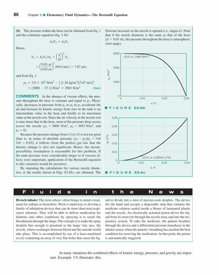
In many situations the combined effects of kinetic energy, pressure, and gravity are impor-tant. Example 3.9 illustrates this.

86 Chapter 3 ■ Elementary Fluid Dynamics—The Bernoulli Equation

flowrate increases as the nozzle is opened (i.e., larger d ). Notethat if the nozzle diameter is the same as that of the hose

the pressure throughout the hose is atmospheric(zero gage).1d � 0.03 m2,

(b) The pressure within the hose can be obtained from Eq. 1and the continuity equation (Eq. 3.16)

Hence,

and from Eq. 1

(Ans)

COMMENTS In the absence of viscous effects, the pres-sure throughout the hose is constant and equal to p2. Physi-cally, decreases in pressure from p1 to p2 to p3 accelerate theair and increase its kinetic energy from zero in the tank to anintermediate value in the hose and finally to its maximumvalue at the nozzle exit. Since the air velocity in the nozzle exitis nine times that in the hose, most of the pressure drop occursacross the nozzle (p1 � 3000 N/m2, p2 � 2963 N/m2, andp3 � 0).

Because the pressure change from (1) to (3) is not too great[that is, in terms of absolute pressure (p1 � p3)/p1 � 3.0/101 � 0.03], it follows from the perfect gas law that thedensity change is also not significant. Hence, the incom-pressibility assumption is reasonable for this problem. Ifthe tank pressure were considerably larger or if viscous ef-fects were important, application of the Bernoulli equationto this situation would be incorrect.

By repeating the calculations for various nozzle diame-ters, d, the results shown in Figs. E3.8b,c are obtained. The

� 13000 � 37.12 N/m2 � 2963 N/m2

p2 � 3.0 � 103 N/m2 � 12 11.26 kg/m32 17.67 m/s22

� a0.01 m

0.03 mb

2

169.0 m/s2 � 7.67 m/s

V2 � A3V3 /A2 � ad

Db

2

V3

A2V2 � A3V3

0

1000

2000

3000

0

d, m

p 2,

N/m

2

0.01 0.02 0.03

(0.01 m, 2963 N/m2)

0

0.01

0.03

0.02

0.04

0.05

0

d, m

Q,

m3/s

(0.01 m, 0.00542 m3/s)

0.01 0.02 0.03

F I G U R E E3.8b

F I G U R E E3.8c

F l u i d s i n t h e N e w s

Hi-tech inhaler The term inhaler often brings to mind a treat-ment for asthma or bronchitis. Work is underway to develop afamily of inhalation devices that can do more than treat respi-ratory ailments. They will be able to deliver medication fordiabetes and other conditions by spraying it to reach thebloodstream through the lungs. The concept is to make the spraydroplets fine enough to penetrate to the lungs’ tiny sacs, thealveoli, where exchanges between blood and the outside worldtake place. This is accomplished by use of a laser-machinednozzle containing an array of very fine holes that cause the liq-

uid to divide into a mist of micron-scale droplets. The devicefits the hand and accepts a disposable strip that contains themedicine solution sealed inside a blister of laminated plasticand the nozzle. An electrically actuated piston drives the liq-uid from its reservoir through the nozzle array and into the res-piratory system. To take the medicine, the patient breathesthrough the device and a differential pressure transducer in theinhaler senses when the patient’s breathing has reached the bestcondition for receiving the medication. At that point, the pistonis automatically triggered.

c03ElementaryFluidDynamicsTheBernoulliEquation.qxd 9/24/10 12:22 PM Page 86

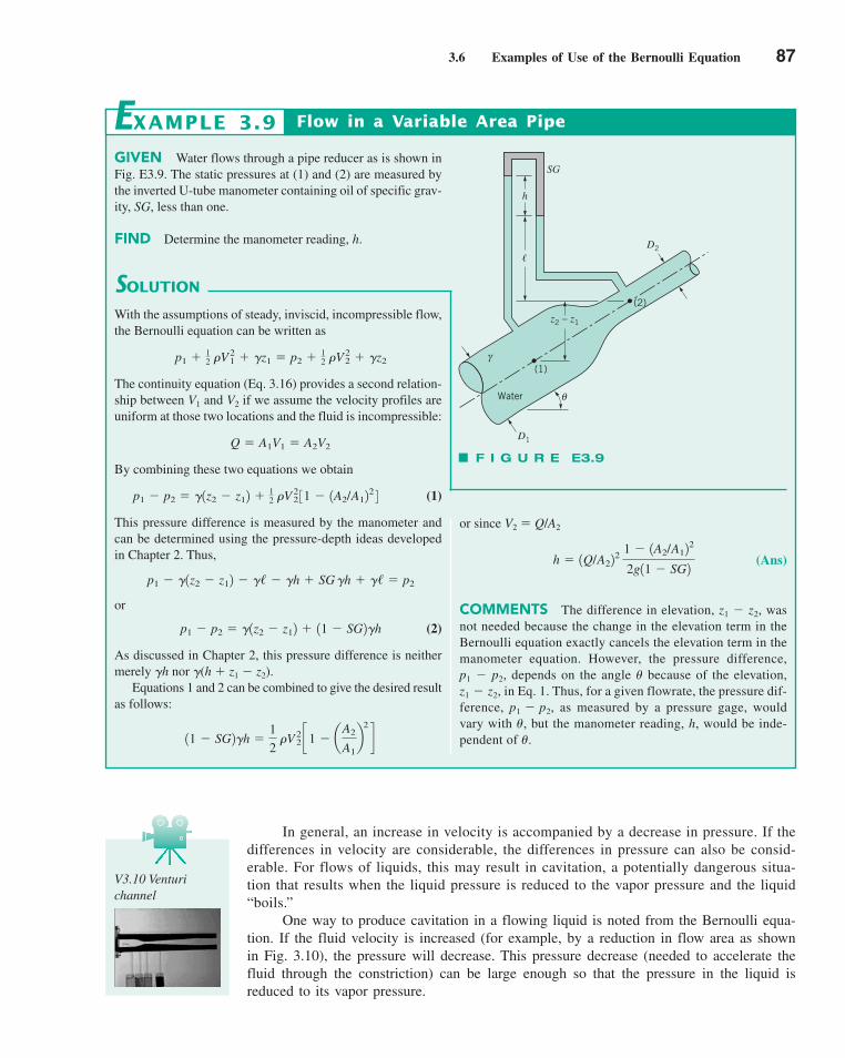
3.6 Examples of Use of the Bernoulli Equation 87

In general, an increase in velocity is accompanied by a decrease in pressure. If thedifferences in velocity are considerable, the differences in pressure can also be consid-erable. For flows of liquids, this may result in cavitation, a potentially dangerous situa-tion that results when the liquid pressure is reduced to the vapor pressure and the liquid“boils.”

One way to produce cavitation in a flowing liquid is noted from the Bernoulli equa-tion. If the fluid velocity is increased (for example, by a reduction in flow area as shownin Fig. 3.10), the pressure will decrease. This pressure decrease (needed to accelerate thefluid through the constriction) can be large enough so that the pressure in the liquid isreduced to its vapor pressure.

GIVEN Water flows through a pipe reducer as is shown inFig. E3.9. The static pressures at (1) and (2) are measured bythe inverted U-tube manometer containing oil of specific grav-ity, SG, less than one.

FIND Determine the manometer reading, h.

SOLUTION

Flow in a Variable Area Pipe

or since V2 � Q/A2

(Ans)

COMMENTS The difference in elevation, z1 � z2, wasnot needed because the change in the elevation term in theBernoulli equation exactly cancels the elevation term in themanometer equation. However, the pressure difference,p1 � p2, depends on the angle � because of the elevation,z1 � z2, in Eq. 1. Thus, for a given flowrate, the pressure dif-ference, p1 � p2, as measured by a pressure gage, wouldvary with �, but the manometer reading, h, would be inde-pendent of �.

h � 1Q/A222

1 � 1A2/A122

2g11 � SG2

EXAMPLE 3.9

With the assumptions of steady, inviscid, incompressible flow,the Bernoulli equation can be written as

The continuity equation (Eq. 3.16) provides a second relation-ship between V1 and V2 if we assume the velocity profiles areuniform at those two locations and the fluid is incompressible:

By combining these two equations we obtain

(1)

This pressure difference is measured by the manometer andcan be determined using the pressure-depth ideas developedin Chapter 2. Thus,

or

(2)

As discussed in Chapter 2, this pressure difference is neithermerely �h nor �(h � z1 � z2).

Equations 1 and 2 can be combined to give the desired resultas follows:

11 � SG2�h �1

2 �V 2

2 c1 � aA2

A1b

2

d

p1 � p2 � �1z2 � z12 � 11 � SG2�h

p1 � �1z2 � z12 � �/ � �h � SG �h � �/ � p2

p1 � p2 � �1z2 � z12 � 12 �V 2

2 31 � 1A2/A122 4

Q � A1V1 � A2V2

p1 � 12 �V2

1 � �z1 � p2 � 12 �V2

2 � �z2

F I G U R E E3.9

�

γ(1)

z2 – z1

(2)

Water θ

D1

D2

h

SG

V3.10 Venturichannel

c03ElementaryFluidDynamicsTheBernoulliEquation.qxd 9/27/10 8:34 AM Page 87

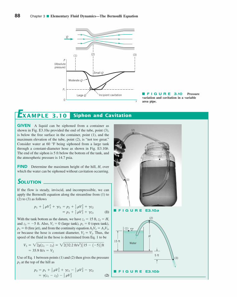
88 Chapter 3 ■ Elementary Fluid Dynamics—The Bernoulli Equation

F I G U R E 3.10 Pressurevariation and cavitation in a variablearea pipe.

Q

p

(Absolutepressure)

(1) (2) (3)

Small Q

Moderate Q

Large Q Incipient cavitation

pv

0 x

GIVEN A liquid can be siphoned from a container asshown in Fig. E3.10a provided the end of the tube, point (3),is below the free surface in the container, point (1), and themaximum elevation of the tube, point (2), is “not too great.”Consider water at 60 °F being siphoned from a large tankthrough a constant-diameter hose as shown in Fig. E3.10b.The end of the siphon is 5 ft below the bottom of the tank, andthe atmospheric pressure is 14.7 psia.

FIND Determine the maximum height of the hill, H, overwhich the water can be siphoned without cavitation occurring.

SOLUTION

Siphon and CavitationEXAMPLE 3.10

(2)

(3)

(1)

Water

(1)

(2)

(3)5 ft

H

15 ft

F I G U R E E3.10b

F I G U R E E3.10a

If the flow is steady, inviscid, and incompressible, we canapply the Bernoulli equation along the streamline from (1) to(2) to (3) as follows

(1)

With the tank bottom as the datum, we have z1 � 15 ft, z2 � H,and z3 � �5 ft. Also, V1 � 0 (large tank), p1 � 0 (open tank),p3 � 0 (free jet), and from the continuity equation A2V2 � A3V3,or because the hose is constant diameter, V2 � V3. Thus, thespeed of the fluid in the hose is determined from Eq. 1 to be

Use of Eq. 1 between points (1) and (2) then gives the pressurep2 at the top of the hill as

(2)� �1z1 � z22 � 12 �V2

2

p2 � p1 � 12 �V2

1 � �z1 � 12 �V2

2 � �z2

� 35.9 ft/s � V2

V3 � 22g1z1 � z32 � 22132.2 ft/s22 315 � 1�52 4 ft

� p3 � 12 �V2

3 � �z3

p1 � 12 �V2

1 � �z1 � p2 � 12 �V2

2 � �z2

c03ElementaryFluidDynamicsTheBernoulliEquation.qxd 9/24/10 12:22 PM Page 88

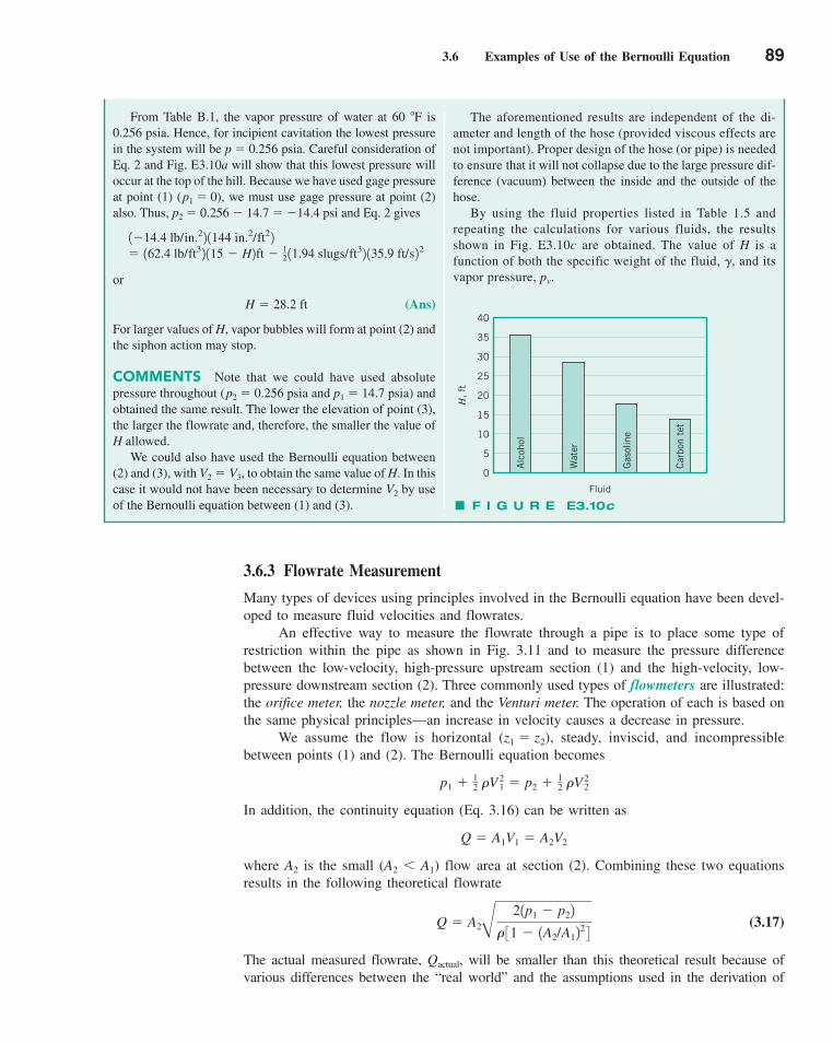
3.6 Examples of Use of the Bernoulli Equation 89

3.6.3 Flowrate Measurement

Many types of devices using principles involved in the Bernoulli equation have been devel-oped to measure fluid velocities and flowrates.

An effective way to measure the flowrate through a pipe is to place some type ofrestriction within the pipe as shown in Fig. 3.11 and to measure the pressure differencebetween the low-velocity, high-pressure upstream section (1) and the high-velocity, low-pressure downstream section (2). Three commonly used types of flowmeters are illustrated:the orifice meter, the nozzle meter, and the Venturi meter. The operation of each is based onthe same physical principles—an increase in velocity causes a decrease in pressure.

We assume the flow is horizontal (z1 � z2), steady, inviscid, and incompressiblebetween points (1) and (2). The Bernoulli equation becomes

In addition, the continuity equation (Eq. 3.16) can be written as

where A2 is the small (A2 A1) flow area at section (2). Combining these two equationsresults in the following theoretical flowrate

(3.17)

The actual measured flowrate, Qactual, will be smaller than this theoretical result because ofvarious differences between the “real world” and the assumptions used in the derivation of

Q � A2B

21p1 � p22

� 31 � 1A2/A122 4

Q � A1V1 � A2V2

p1 � 12 �V 2

1 � p2 � 12 �V 2

2

The aforementioned results are independent of the di-ameter and length of the hose (provided viscous effects arenot important). Proper design of the hose (or pipe) is neededto ensure that it will not collapse due to the large pressure dif-ference (vacuum) between the inside and the outside of thehose.

By using the fluid properties listed in Table 1.5 and repeating the calculations for various fluids, the resultsshown in Fig. E3.10c are obtained. The value of H is afunction of both the specific weight of the fluid, �, and itsvapor pressure, pv.

From Table B.1, the vapor pressure of water at 60 F is0.256 psia. Hence, for incipient cavitation the lowest pressurein the system will be p � 0.256 psia. Careful consideration ofEq. 2 and Fig. E3.10a will show that this lowest pressure willoccur at the top of the hill. Because we have used gage pressureat point (1) (p1 � 0), we must use gage pressure at point (2)also. Thus, p2 � 0.256 � 14.7 � �14.4 psi and Eq. 2 gives

or

(Ans)

For larger values of H, vapor bubbles will form at point (2) andthe siphon action may stop.

COMMENTS Note that we could have used absolutepressure throughout (p2 � 0.256 psia and p1 � 14.7 psia) andobtained the same result. The lower the elevation of point (3),the larger the flowrate and, therefore, the smaller the value ofH allowed.

We could also have used the Bernoulli equation between(2) and (3), with V2 � V3, to obtain the same value of H. In thiscase it would not have been necessary to determine V2 by useof the Bernoulli equation between (1) and (3).

H � 28.2 ft

� 162.4 lb/ft32 115 � H2ft � 12 11.94 slugs/ft32 135.9 ft/s22

1�14.4 lb/in.22 1144 in.2/ft22

F I G U R E E3.10c

0

5

10

15

20

25

30

35

40

H,

ft

Fluid

Alc

ohol

Wat

er

Gas

olin

e

Car

bon

tet

c03ElementaryFluidDynamicsTheBernoulliEquation.qxd 9/24/10 12:22 PM Page 89

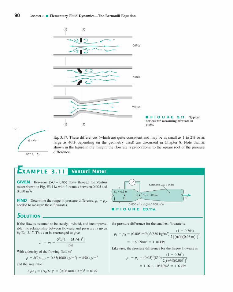
90 Chapter 3 ■ Elementary Fluid Dynamics—The Bernoulli Equation

Eq. 3.17. These differences (which are quite consistent and may be as small as 1 to 2% or aslarge as 40% depending on the geometry used) are discussed in Chapter 8. Note that asshown in the figure in the margin, the flowrate is proportional to the square root of the pressuredifference.

F I G U R E 3.11 Typicaldevices for measuring flowrate inpipes.

(1) (2)

(1) (2)

Venturi

Nozzle

Orifice

GIVEN Kerosene (SG � 0.85) flows through the Venturimeter shown in Fig. E3.11a with flowrates between 0.005 and0.050 m3/s.

FIND Determine the range in pressure difference, p1 � p2,needed to measure these flowrates.

SOLUTION

Venturi MeterEXAMPLE 3.11

D1 = 0.1 m

(1)(2)

0.005 m3/s < Q < 0.050 m3/s

D2 = 0.06 m

Kerosene, SG = 0.85

Q

F I G U R E E3.11a

If the flow is assumed to be steady, inviscid, and incompress-ible, the relationship between flowrate and pressure is givenby Eq. 3.17. This can be rearranged to give

With a density of the flowing fluid of

and the area ratio

A2/A1 � 1D2/D122 � 10.06 m/0.10 m22 � 0.36

� � SG �H2O � 0.8511000 kg/m32 � 850 kg/m3

p1 � p2 �Q2� 31 � 1A2/A12

2 4

2A22

the pressure difference for the smallest flowrate is

Likewise, the pressure difference for the largest flowrate is

� 1.16 � 102 N/m2 � 116 kPa

p1 � p2 � 10.052218502 11 � 0.3622

2 3 1�/42 10.0622 42

� 1160 N/m2 � 1.16 kPa

p1 � p2 � 10.005 m3/s22 1850 kg/m32 11 � 0.3622

2 3 1�/42 10.06 m22 42

Q

Δp = p1 – p2

Q ~ Δp

c03ElementaryFluidDynamicsTheBernoulliEquation.qxd 9/24/10 4:51 PM Page 90

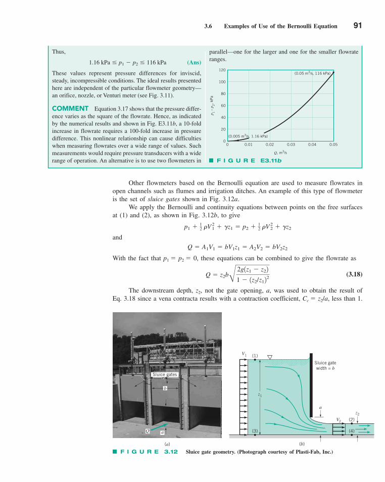
3.6 Examples of Use of the Bernoulli Equation 91

Other flowmeters based on the Bernoulli equation are used to measure flowrates inopen channels such as flumes and irrigation ditches. An example of this type of flowmeteris the set of sluice gates shown in Fig. 3.12a.

We apply the Bernoulli and continuity equations between points on the free surfacesat (1) and (2), as shown in Fig. 3.12b, to give

and

With the fact that p1 � p2 � 0, these equations can be combined to give the flowrate as

(3.18)

The downstream depth, z2, not the gate opening, a, was used to obtain the result ofEq. 3.18 since a vena contracta results with a contraction coefficient, Cc � z2/a, less than 1.

Q � z2b

B

2g1z1 � z22

1 � 1z2/z122

Q � A1V1 � bV1z1 � A2V2 � bV2z2

p1 � 12 �V2

1 � �z1 � p2 � 12 �V2

2 � �z2

parallel—one for the larger and one for the smaller flowrateranges.

Thus,

(Ans)

These values represent pressure differences for inviscid,steady, incompressible conditions. The ideal results presentedhere are independent of the particular flowmeter geometry—an orifice, nozzle, or Venturi meter (see Fig. 3.11).

COMMENT Equation 3.17 shows that the pressure differ-ence varies as the square of the flowrate. Hence, as indicatedby the numerical results and shown in Fig. E3.11b, a 10-foldincrease in flowrate requires a 100-fold increase in pressuredifference. This nonlinear relationship can cause difficultieswhen measuring flowrates over a wide range of values. Suchmeasurements would require pressure transducers with a widerange of operation. An alternative is to use two flowmeters in

1.16 kPa � p1 � p2 � 116 kPa

F I G U R E E3.11b

0

20

40

60

80

100

120

p 1 –

p 2, kP

a

Q, m3/s

0 0.01 0.02 0.03 0.04 0.05

(0.005 m3/s, 1.16 kPa)

(0.05 m3/s, 116 kPa)

Sluice gatewidth = b

(1)

(2)

(4)(3)

V1

z1

a

V2

z2

(b)(a)

Sluice gates

b

aQ

F I G U R E 3.12 Sluice gate geometry. (Photograph courtesy of Plasti-Fab, Inc.)

c03ElementaryFluidDynamicsTheBernoulliEquation.qxd 9/24/10 12:23 PM Page 91

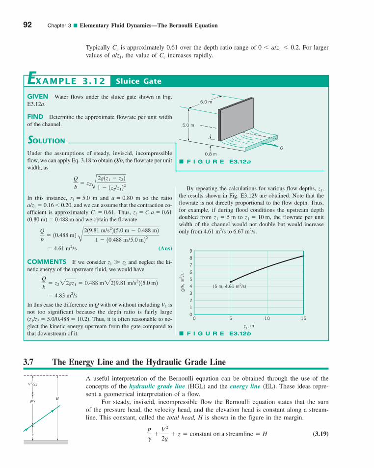
Typically Cc is approximately 0.61 over the depth ratio range of 0 a/z1 0.2. For largervalues of a/z1, the value of Cc increases rapidly.

92 Chapter 3 ■ Elementary Fluid Dynamics—The Bernoulli Equation

GIVEN Water flows under the sluice gate shown in Fig.E3.12a.

FIND Determine the approximate flowrate per unit widthof the channel.

SOLUTION

Sluice GateEXAMPLE 3.12

Under the assumptions of steady, inviscid, incompressibleflow, we can apply Eq. 3.18 to obtain Q/b, the flowrate per unitwidth, as

In this instance, z1 � 5.0 m and a � 0.80 m so the ratioa/z1 � 0.16 0.20, and we can assume that the contraction co-efficient is approximately Cc � 0.61. Thus, z2 � Cca � 0.61(0.80 m) � 0.488 m and we obtain the flowrate

(Ans)

COMMENTS If we consider z1 �� z2 and neglect the ki-netic energy of the upstream fluid, we would have

In this case the difference in Q with or without including V1 isnot too significant because the depth ratio is fairly large(z1/z2 � 5.0/0.488 � 10.2). Thus, it is often reasonable to ne-glect the kinetic energy upstream from the gate compared tothat downstream of it.

� 4.83 m2/s

Q

b� z222gz1 � 0.488 m2219.81 m/s22 15.0 m2

� 4.61 m2/s

Q

b� 10.488 m2

B

219.81 m/s22 15.0 m � 0.488 m2

1 � 10.488 m/5.0 m22

Q

b� z2B

2g1z1 � z22

1 � 1z2/z122

By repeating the calculations for various flow depths, z1,the results shown in Fig. E3.12b are obtained. Note that theflowrate is not directly proportional to the flow depth. Thus,for example, if during flood conditions the upstream depthdoubled from to the flowrate per unitwidth of the channel would not double but would increaseonly from 4.61 m2/s to 6.67 m2/s.

z1 � 10 m,z1 � 5 m

Q

5.0 m

6.0 m

0.8 m

F I G U R E E3.12a

F I G U R E E3.12b

0

1

2

3

4

5

6

7

8

9

z1, m

Q/b

, m

2/s

0 5 10 15

(5 m, 4.61 m2/s)

3.7 The Energy Line and the Hydraulic Grade Line

A useful interpretation of the Bernoulli equation can be obtained through the use of theconcepts of the hydraulic grade line (HGL) and the energy line (EL). These ideas repre-sent a geometrical interpretation of a flow.

For steady, inviscid, incompressible flow the Bernoulli equation states that the sumof the pressure head, the velocity head, and the elevation head is constant along a stream-line. This constant, called the total head, H is shown in the figure in the margin.

(3.19)p

��

V 2

2g� z � constant on a streamline � H

H

V2/2g

p/�

z

c03ElementaryFluidDynamicsTheBernoulliEquation.qxd 9/24/10 12:23 PM Page 92

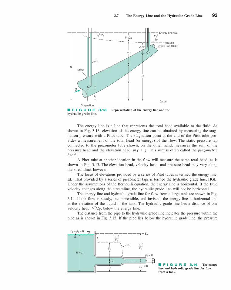
3.7 The Energy Line and the Hydraulic Grade Line 93

The energy line is a line that represents the total head available to the fluid. Asshown in Fig. 3.13, elevation of the energy line can be obtained by measuring the stag-nation pressure with a Pitot tube. The stagnation point at the end of the Pitot tube pro-vides a measurement of the total head (or energy) of the flow. The static pressure tapconnected to the piezometer tube shown, on the other hand, measures the sum of thepressure head and the elevation head, p/� � z. This sum is often called the piezometrichead.

A Pitot tube at another location in the flow will measure the same total head, as isshown in Fig. 3.13. The elevation head, velocity head, and pressure head may vary alongthe streamline, however.

The locus of elevations provided by a series of Pitot tubes is termed the energy line,EL. That provided by a series of piezometer taps is termed the hydraulic grade line, HGL.Under the assumptions of the Bernoulli equation, the energy line is horizontal. If the fluidvelocity changes along the streamline, the hydraulic grade line will not be horizontal.

The energy line and hydraulic grade line for flow from a large tank are shown in Fig.3.14. If the flow is steady, incompressible, and inviscid, the energy line is horizontal andat the elevation of the liquid in the tank. The hydraulic grade line lies a distance of onevelocity head, V2/2g, below the energy line.

The distance from the pipe to the hydraulic grade line indicates the pressure within thepipe as is shown in Fig. 3.15. If the pipe lies below the hydraulic grade line, the pressure

F I G U R E 3.13 Representation of the energy line and thehydraulic grade line.

Q

HStatic

Stagnation

z1

p1/

V12/2g

V 2/2g

z

z2

p2/

V22

___2g

Hydraulicgrade line (HGL)

Energy line (EL)

Datum

p/ γ

γ

γ

F I G U R E 3.14 The energyline and hydraulic grade line for flowfrom a tank.

HGL

EL

(3)

(2)

(1)

V1 = p1 = 0

H = z1

p2__

V22

___2g

z2z3

V32

___2g

p3 = 0

γ

c03ElementaryFluidDynamicsTheBernoulliEquation.qxd 9/24/10 12:23 PM Page 93

94 Chapter 3 ■ Elementary Fluid Dynamics—The Bernoulli Equation

within the pipe is positive (above atmospheric). If the pipe lies above the hydraulic grade line,the pressure is negative (below atmospheric).

F I G U R E 3.15Use of the energy line and thehydraulic grade line.

Q

p > 0

p < 0

p/

zz

V2__2g

EL

HGLγp/γ

GIVEN Water is siphoned from the tank shown in Fig.E3.13 through a hose of constant diameter. A small hole isfound in the hose at location (1) as indicated.

FIND When the siphon is used, will water leak out of thehose or will air leak into the hose, thereby possibly causing thesiphon to malfunction?

SOLUTION

Energy Line and Hydraulic Grade LineEXAMPLE 3.13

Whether air will leak into or water will leak out of the hose depends on whether the pressure within the hose at (1) is lessthan or greater than atmospheric. Which happens can be deter-mined easily by using the energy line and hydraulic grade lineconcepts. With the assumption of steady, incompressible, in-viscid flow it follows that the total head is constant—thus, theenergy line is horizontal.

Because the hose diameter is constant, it follows from thecontinuity equation (AV � constant) that the water velocity inthe hose is constant throughout. Thus, the hydraulic grade lineis a constant distance, V2/2g, below the energy line as shownin Fig. E3.13. Because the pressure at the end of the hose is atmospheric, it follows that the hydraulic grade line is at thesame elevation as the end of the hose outlet. The fluid withinthe hose at any point above the hydraulic grade line will be atless than atmospheric pressure.

Thus, air will leak into the hose through the hole at point (1). (Ans)

COMMENT In practice, viscous effects may be quite im-portant, making this simple analysis (horizontal energy line)incorrect. However, if the hose is “not too small diameter,”“not too long,” the fluid “not too viscous,” and the flowrate“not too large,” the aforementioned result may be very accu-rate. If any of these assumptions are relaxed, a more detailedanalysis is required (see Chapter 8). If the end of the hosewere closed so the flowrate were zero, the hydraulic gradeline would coincide with the energy line (V2/2g � 0 through-out), the pressure at (1) would be greater than atmospheric,and water would leak through the hole at (1).

F I G U R E E3.13

ValveHGL with valve open

HGL with valve closed andEL with valve open or closed

(1)

V2__2g p_

γ

3.8 Restrictions on the Use of the Bernoulli Equation

One of the main assumptions in deriving the Bernoulli equation is that the fluid is incom-pressible. Although this is reasonable for most liquid flows, it can, in certain instances, intro-duce considerable errors for gases.

In the previous section we saw that the stagnation pressure is greater than the staticpressure by an amount �V 2/2, provided that the density remains constant. If this dynamic

c03ElementaryFluidDynamicsTheBernoulliEquation.qxd 9/24/10 12:23 PM Page 94

3.9 Chapter Summary and Study Guide 95

pressure is not too large compared with the static pressure, the density change between twopoints is not very large and the flow can be considered incompressible. However, becausethe dynamic pressure varies as V 2, the error associated with the assumption that a fluid isincompressible increases with the square of the velocity of the fluid.

A rule of thumb is that the flow of a perfect gas may be considered as incompressibleprovided the Mach number is less than about 0.3. The Mach number, Ma � V/c, is the ratioof the fluid speed, V, to the speed of sound in the fluid, c. In standard air (T1 � 59 F,

) this corresponds to a speed of V1 � c1Ma1 � 0.3 (1117 ft/s) � 335ft/s � 228 mi/hr. At higher speeds, compressibility may become important.

Another restriction of the Bernoulli equation (Eq. 3.6) is the assumption that theflow is steady. For such flows, on a given streamline the velocity is a function of onlys, the location along the streamline. That is, along a streamline V � V(s). For unsteadyflows the velocity is also a function of time, so that along a streamline V � V(s, t).Thus, when taking the time derivative of the velocity to obtain the streamwise acceler-ation, we obtain as � 0V/0t � V 0V/0s rather than just as � V 0V/0s as is true for steadyflow. The unsteady term, 0V/0t, does not allow the equation of motion to be integratedeasily (as was done to obtain the Bernoulli equation) unless additional assumptions aremade.

Another restriction on the Bernoulli equation is that the flow is inviscid. Recall thatthe Bernoulli equation is actually a first integral of Newton’s second law along a stream-line. This general integration was possible because, in the absence of viscous effects, thefluid system considered was a conservative system. The total energy of the system remainsconstant. If viscous effects are important, the system is nonconservative and energy lossesoccur. A more detailed analysis is needed for these cases. Such material is presented inChapter 8.

The final basic restriction on use of the Bernoulli equation is that there are no mechan-ical devices (pumps or turbines) in the system between the two points along the streamlinefor which the equation is applied. These devices represent sources or sinks of energy. Sincethe Bernoulli equation is actually one form of the energy equation, it must be altered to includepumps or turbines, if these are present. The inclusion of pumps and turbines is covered inChapters 5 and 11.

c1 � 1kRT1 � 1117 ft/s

3.9 Chapter Summary and Study Guide

In this chapter, several aspects of the steady flow of an inviscid, incompressible fluid arediscussed. Newton’s second law, F � ma, is applied to flows for which the only importantforces are those due to pressure and gravity (weight)—viscous effects are assumed negligi-ble. The result is the often-used Bernoulli equation, which provides a simple relationshipamong pressure, elevation, and velocity variations along a streamline. A similar but lessoften used equation is also obtained to describe the variations in these parameters normalto a streamline.

The concept of a stagnation point and the corresponding stagnation pressure is intro-duced, as are the concepts of static, dynamic, and total pressure and their related heads.

Several applications of the Bernoulli equation are discussed. In some flow situations,such as the use of a Pitot-static tube to measure fluid velocity or the flow of a liquid as afree jet from a tank, a Bernoulli equation alone is sufficient for the analysis. In otherinstances, such as confined flows in tubes and flowmeters, it is necessary to use both theBernoulli equation and the continuity equation, which is a statement of the fact that massis conserved as fluid flows.

c03ElementaryFluidDynamicsTheBernoulliEquation.qxd 9/24/10 12:23 PM Page 95

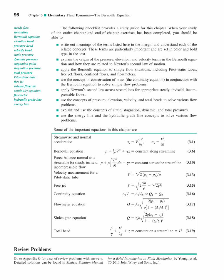
The following checklist provides a study guide for this chapter. When your studyof the entire chapter and end-of-chapter exercises has been completed, you should beable to

write out meanings of the terms listed here in the margin and understand each of therelated concepts. These terms are particularly important and are set in color and boldtype in the text.

explain the origin of the pressure, elevation, and velocity terms in the Bernoulli equa-tion and how they are related to Newton’s second law of motion.

apply the Bernoulli equation to simple flow situations, including Pitot-static tubes,free jet flows, confined flows, and flowmeters.

use the concept of conservation of mass (the continuity equation) in conjunction withthe Bernoulli equation to solve simple flow problems.

apply Newton’s second law across streamlines for appropriate steady, inviscid, incom-pressible flows.

use the concepts of pressure, elevation, velocity, and total heads to solve various flowproblems.

explain and use the concepts of static, stagnation, dynamic, and total pressures.

use the energy line and the hydraulic grade line concepts to solve various flowproblems.

Some of the important equations in this chapter are

Streamwise and normal acceleration (3.1)

Bernoulli equation (3.6)

Force balance normal to a streamline for steady, inviscid, (3.10)incompressible flow

Velocity measurement for a Pitot-static tube

(3.13)

Free jet (3.15)

Continuity equation (3.16)

Flowmeter equation (3.17)

Sluice gate equation (3.18)

Total head (3.19) p

��

V2

2g� z � constant on a streamline � H

Q � z2b

B

2g1z1 � z22

1 � 1z2/z122

Q � A2

B

21p1 � p22

� 31 � 1A2/A122 4

A1V1 � A2V2, or Q1 � Q2

V �B

2

�h

�� 12gh

V � 22 1p3 � p42/�

p � ��V 2

r dn � �z � constant across the streamline

p � 12�V 2 � �z � constant along streamline

as � V

0V

0s, an �

V2

r

96 Chapter 3 ■ Elementary Fluid Dynamics—The Bernoulli Equation

Review Problems

Go to Appendix G for a set of review problems with answers.Detailed solutions can be found in Student Solution Manual

for a Brief Introduction to Fluid Mechanics, by Young, et al.(© 2011 John Wiley and Sons, Inc.).

steady flowstreamlineBernoulli equationelevation headpressure headvelocity headstatic pressuredynamic pressurestagnation pointstagnation pressuretotal pressurePitot-static tubefree jetvolume flowratecontinuity equationflowmeterhydraulic grade lineenergy line

c03ElementaryFluidDynamicsTheBernoulliEquation.qxd 10/18/10 8:00 AM Page 96

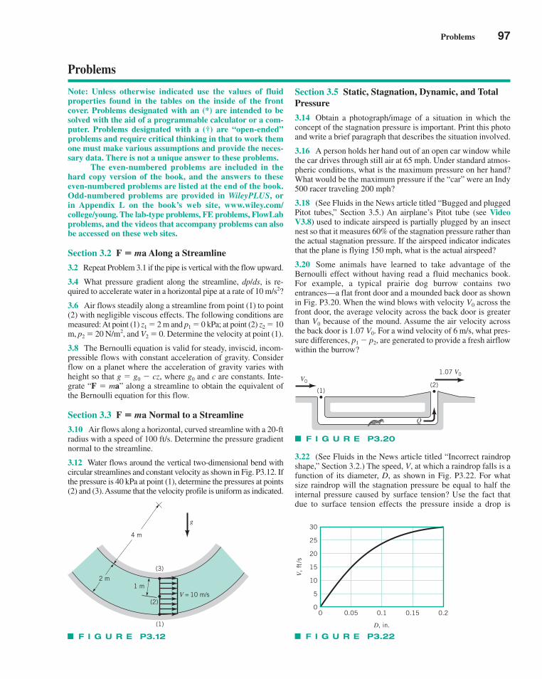
Problems 97

Problems

Note: Unless otherwise indicated use the values of fluidproperties found in the tables on the inside of the frontcover. Problems designated with an (*) are intended to besolved with the aid of a programmable calculator or a com-puter. Problems designated with a (†) are “open-ended”problems and require critical thinking in that to work themone must make various assumptions and provide the neces-sary data. There is not a unique answer to these problems.

The even-numbered problems are included in thehard copy version of the book, and the answers to theseeven-numbered problems are listed at the end of the book.Odd-numbered problems are provided in WileyPLUS, orin Appendix L on the book’s web site, www.wiley.com/college/young. The lab-type problems, FE problems, FlowLabproblems, and the videos that accompany problems can alsobe accessed on these web sites.

Section 3.2 F � ma Along a Streamline

3.2 Repeat Problem 3.1 if the pipe is vertical with the flow upward.

3.4 What pressure gradient along the streamline, dp/ds, is re-quired to accelerate water in a horizontal pipe at a rate of 10 m/s2?

3.6 Air flows steadily along a streamline from point (1) to point(2) with negligible viscous effects. The following conditions aremeasured:At point (1) z1 � 2 m and p1 � 0 kPa; at point (2) z2 � 10m, p2 � 20 N/m2, and V2 � 0. Determine the velocity at point (1).

3.8 The Bernoulli equation is valid for steady, inviscid, incom-pressible flows with constant acceleration of gravity. Considerflow on a planet where the acceleration of gravity varies withheight so that where g0 and c are constants. Inte-grate “F � ma” along a streamline to obtain the equivalent ofthe Bernoulli equation for this flow.

Section 3.3 F � ma Normal to a Streamline

3.10 Air flows along a horizontal, curved streamline with a 20-ftradius with a speed of 100 ft/s. Determine the pressure gradientnormal to the streamline.

3.12 Water flows around the vertical two-dimensional bend withcircular streamlines and constant velocity as shown in Fig. P3.12. Ifthe pressure is 40 kPa at point (1), determine the pressures at points(2) and (3). Assume that the velocity profile is uniform as indicated.

g � g0 � cz,

Section 3.5 Static, Stagnation, Dynamic, and TotalPressure

3.14 Obtain a photograph/image of a situation in which theconcept of the stagnation pressure is important. Print this photoand write a brief paragraph that describes the situation involved.

3.16 A person holds her hand out of an open car window whilethe car drives through still air at 65 mph. Under standard atmos-pheric conditions, what is the maximum pressure on her hand?What would be the maximum pressure if the “car” were an Indy500 racer traveling 200 mph?

3.18 (See Fluids in the News article titled “Bugged and pluggedPitot tubes,” Section 3.5.) An airplane’s Pitot tube (see VideoV3.8) used to indicate airspeed is partially plugged by an insectnest so that it measures 60% of the stagnation pressure rather thanthe actual stagnation pressure. If the airspeed indicator indicatesthat the plane is flying 150 mph, what is the actual airspeed?

3.20 Some animals have learned to take advantage of theBernoulli effect without having read a fluid mechanics book.For example, a typical prairie dog burrow contains two entrances—a flat front door and a mounded back door as shownin Fig. P3.20. When the wind blows with velocity V0 across thefront door, the average velocity across the back door is greaterthan V0 because of the mound. Assume the air velocity acrossthe back door is 1.07 V0. For a wind velocity of 6 m/s, what pres-sure differences, p1 � p2, are generated to provide a fresh airflowwithin the burrow?

3.22 (See Fluids in the News article titled “Incorrect raindropshape,” Section 3.2.) The speed, V, at which a raindrop falls is afunction of its diameter, D, as shown in Fig. P3.22. For whatsize raindrop will the stagnation pressure be equal to half the internal pressure caused by surface tension? Use the fact thatdue to surface tension effects the pressure inside a drop is

(1)

(2)

(3)

1 m2 m

4 m

g

V = 10 m/s

F I G U R E P3.12

1.07 V0

(1)(2)

V0

Q

F I G U R E P3.20

F I G U R E P3.22

0

5

10

15

20

25

30

D, in.

V,

ft/s

0 0.05 0.1 0.15 0.2

c03ElementaryFluidDynamicsTheBernoulliEquation.qxd 9/24/10 12:23 PM Page 97

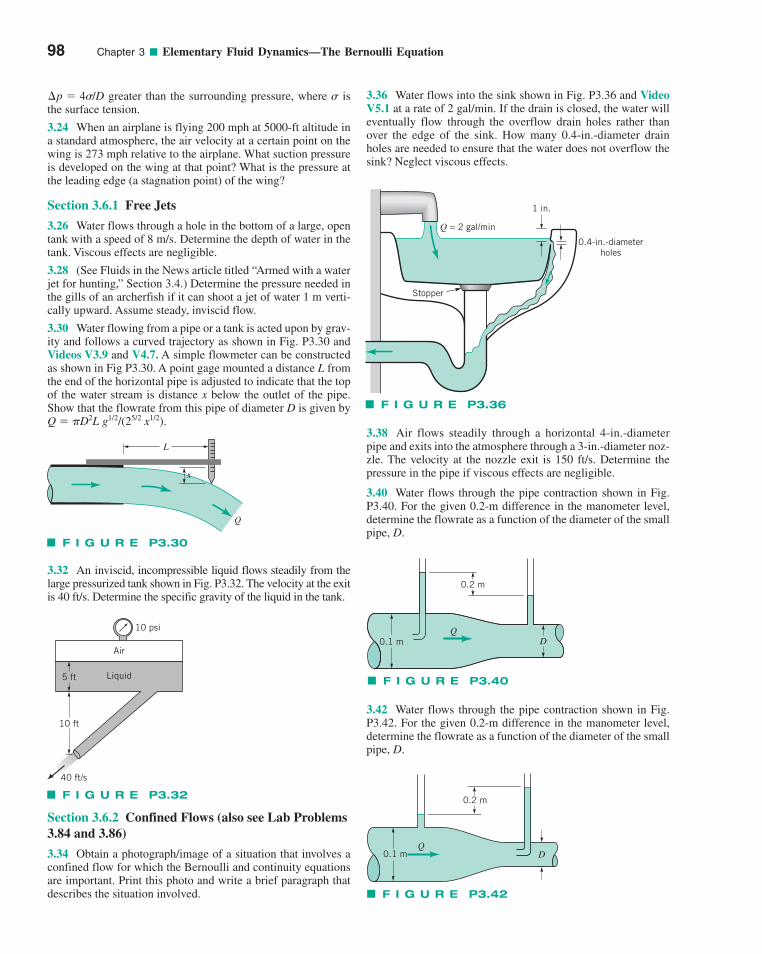
98 Chapter 3 ■ Elementary Fluid Dynamics—The Bernoulli Equation

3.36 Water flows into the sink shown in Fig. P3.36 and VideoV5.1 at a rate of 2 gal/min. If the drain is closed, the water willeventually flow through the overflow drain holes rather thanover the edge of the sink. How many 0.4-in.-diameter drainholes are needed to ensure that the water does not overflow thesink? Neglect viscous effects.

3.38 Air flows steadily through a horizontal 4-in.-diameterpipe and exits into the atmosphere through a 3-in.-diameter noz-zle. The velocity at the nozzle exit is 150 ft/s. Determine thepressure in the pipe if viscous effects are negligible.

3.40 Water flows through the pipe contraction shown in Fig.P3.40. For the given 0.2-m difference in the manometer level,determine the flowrate as a function of the diameter of the smallpipe, D.

3.42 Water flows through the pipe contraction shown in Fig.P3.42. For the given 0.2-m difference in the manometer level,determine the flowrate as a function of the diameter of the smallpipe, D.

greater than the surrounding pressure, where isthe surface tension.

3.24 When an airplane is flying 200 mph at 5000-ft altitude ina standard atmosphere, the air velocity at a certain point on thewing is 273 mph relative to the airplane. What suction pressureis developed on the wing at that point? What is the pressure atthe leading edge (a stagnation point) of the wing?

Section 3.6.1 Free Jets

3.26 Water flows through a hole in the bottom of a large, opentank with a speed of 8 m/s. Determine the depth of water in thetank. Viscous effects are negligible.

3.28 (See Fluids in the News article titled “Armed with a waterjet for hunting,” Section 3.4.) Determine the pressure needed inthe gills of an archerfish if it can shoot a jet of water 1 m verti-cally upward. Assume steady, inviscid flow.

3.30 Water flowing from a pipe or a tank is acted upon by grav-ity and follows a curved trajectory as shown in Fig. P3.30 andVideos V3.9 and V4.7. A simple flowmeter can be constructedas shown in Fig P3.30. A point gage mounted a distance L fromthe end of the horizontal pipe is adjusted to indicate that the topof the water stream is distance x below the outlet of the pipe.Show that the flowrate from this pipe of diameter D is given byQ � �D2L g1/2/(25/2 x1/2).

3.32 An inviscid, incompressible liquid flows steadily from thelarge pressurized tank shown in Fig. P3.32. The velocity at the exitis 40 ft/s. Determine the specific gravity of the liquid in the tank.

Section 3.6.2 Confined Flows (also see Lab Problems3.84 and 3.86)

3.34 Obtain a photograph/image of a situation that involves aconfined flow for which the Bernoulli and continuity equationsare important. Print this photo and write a brief paragraph thatdescribes the situation involved.

�¢p � 4�/D

F I G U R E P3.30

Q

L

x

40 ft/s

10 ft

5 ft

10 psi

Liquid

Air

F I G U R E P3.32

F I G U R E P3.36

Q = 2 gal/min

1 in.

0.4-in.-diameterholes

Stopper

0.2 m

Q0.1 m D

F I G U R E P3.40

Q0.1 m

0.2 m

D

F I G U R E P3.42

c03ElementaryFluidDynamicsTheBernoulliEquation.qxd 9/24/10 12:23 PM Page 98

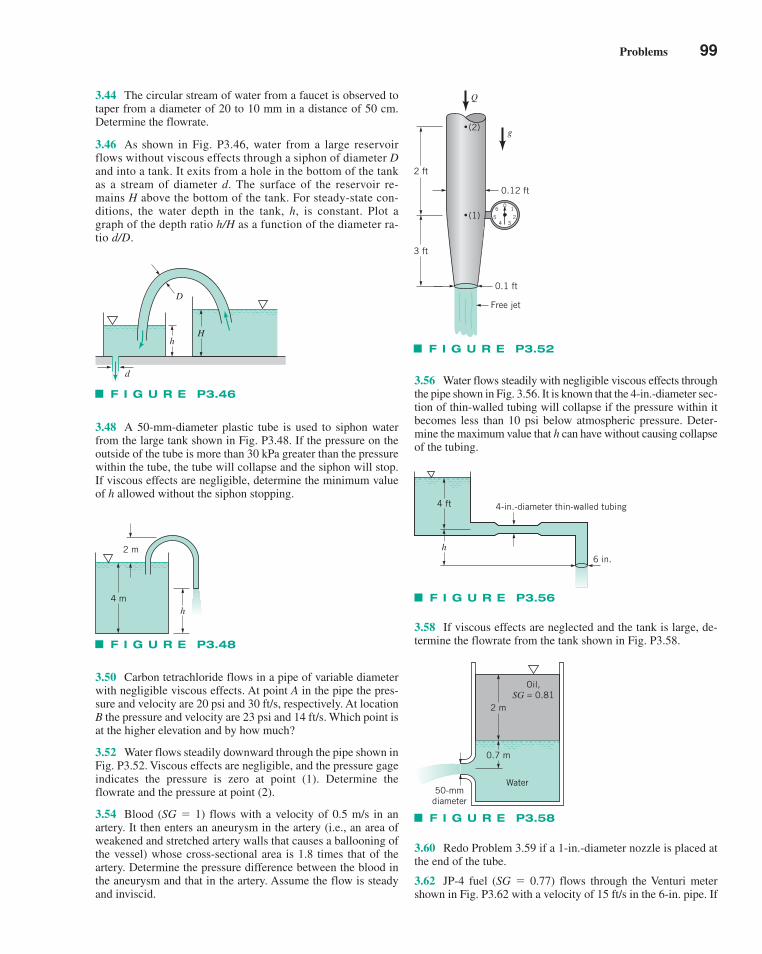
Problems 99

3.44 The circular stream of water from a faucet is observed totaper from a diameter of 20 to 10 mm in a distance of 50 cm.Determine the flowrate.

3.46 As shown in Fig. P3.46, water from a large reservoirflows without viscous effects through a siphon of diameter Dand into a tank. It exits from a hole in the bottom of the tankas a stream of diameter d. The surface of the reservoir re-mains H above the bottom of the tank. For steady-state con-ditions, the water depth in the tank, h, is constant. Plot agraph of the depth ratio h/H as a function of the diameter ra-tio d/D.

3.48 A 50-mm-diameter plastic tube is used to siphon waterfrom the large tank shown in Fig. P3.48. If the pressure on theoutside of the tube is more than 30 kPa greater than the pressurewithin the tube, the tube will collapse and the siphon will stop.If viscous effects are negligible, determine the minimum valueof h allowed without the siphon stopping.

3.50 Carbon tetrachloride flows in a pipe of variable diameterwith negligible viscous effects. At point A in the pipe the pres-sure and velocity are 20 psi and 30 ft/s, respectively. At locationB the pressure and velocity are 23 psi and 14 ft/s. Which point isat the higher elevation and by how much?

3.52 Water flows steadily downward through the pipe shown inFig. P3.52. Viscous effects are negligible, and the pressure gageindicates the pressure is zero at point (1). Determine theflowrate and the pressure at point (2).

3.54 Blood (SG � 1) flows with a velocity of 0.5 m/s in anartery. It then enters an aneurysm in the artery (i.e., an area ofweakened and stretched artery walls that causes a ballooning ofthe vessel) whose cross-sectional area is 1.8 times that of theartery. Determine the pressure difference between the blood inthe aneurysm and that in the artery. Assume the flow is steadyand inviscid.

3.56 Water flows steadily with negligible viscous effects throughthe pipe shown in Fig. 3.56. It is known that the 4-in.-diameter sec-tion of thin-walled tubing will collapse if the pressure within itbecomes less than 10 psi below atmospheric pressure. Deter-mine the maximum value that h can have without causing collapseof the tubing.

3.58 If viscous effects are neglected and the tank is large, de-termine the flowrate from the tank shown in Fig. P3.58.

3.60 Redo Problem 3.59 if a 1-in.-diameter nozzle is placed atthe end of the tube.

3.62 JP-4 fuel (SG � 0.77) flows through the Venturi metershown in Fig. P3.62 with a velocity of 15 ft/s in the 6-in. pipe. If

hH

d

D

F I G U R E P3.46

F I G U R E P3.48

2 m

4 mh

0.12 ft

0.1 ft

Free jet

2 ft

0.12 ft

3 ft

0

234

16

5

(2)

(1)

Q

g

F I G U R E P3.52

4-in.-diameter thin-walled tubing

6 in.h

4 ft

F I G U R E P3.56

F I G U R E P3.58

Water

Oil,SG = 0.81

2 m

0.7 m

50-mmdiameter

c03ElementaryFluidDynamicsTheBernoulliEquation.qxd 9/24/10 12:23 PM Page 99

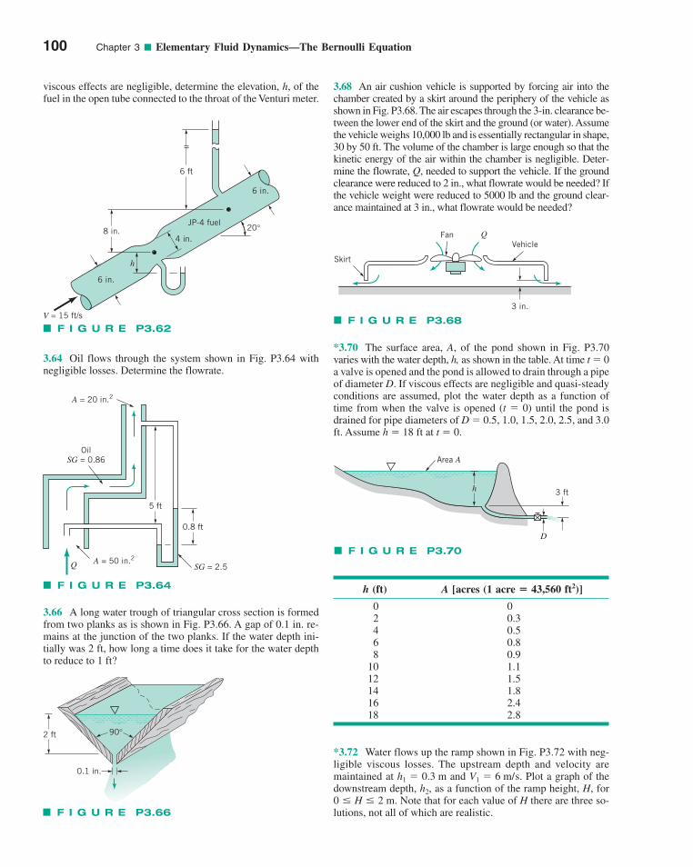
3.68 An air cushion vehicle is supported by forcing air into thechamber created by a skirt around the periphery of the vehicle asshown in Fig. P3.68. The air escapes through the 3-in. clearance be-tween the lower end of the skirt and the ground (or water). Assumethe vehicle weighs 10,000 lb and is essentially rectangular in shape,30 by 50 ft. The volume of the chamber is large enough so that thekinetic energy of the air within the chamber is negligible. Deter-mine the flowrate, Q, needed to support the vehicle. If the groundclearance were reduced to 2 in., what flowrate would be needed? Ifthe vehicle weight were reduced to 5000 lb and the ground clear-ance maintained at 3 in., what flowrate would be needed?

*3.70 The surface area, A, of the pond shown in Fig. P3.70varies with the water depth, h, as shown in the table. At time t � 0a valve is opened and the pond is allowed to drain through a pipeof diameter D. If viscous effects are negligible and quasi-steadyconditions are assumed, plot the water depth as a function oftime from when the valve is opened (t � 0) until the pond isdrained for pipe diameters of D � 0.5, 1.0, 1.5, 2.0, 2.5, and 3.0ft. Assume h � 18 ft at t � 0.

*3.72 Water flows up the ramp shown in Fig. P3.72 with neg-ligible viscous losses. The upstream depth and velocity aremaintained at and Plot a graph of thedownstream depth, as a function of the ramp height, H, for

Note that for each value of H there are three so-lutions, not all of which are realistic.0 � H � 2 m.

h2,V1 � 6 m/s.h1 � 0.3 m

100 Chapter 3 ■ Elementary Fluid Dynamics—The Bernoulli Equation

viscous effects are negligible, determine the elevation, h, of thefuel in the open tube connected to the throat of the Venturi meter.

3.64 Oil flows through the system shown in Fig. P3.64 withnegligible losses. Determine the flowrate.

3.66 A long water trough of triangular cross section is formedfrom two planks as is shown in Fig. P3.66. A gap of 0.1 in. re-mains at the junction of the two planks. If the water depth ini-tially was 2 ft, how long a time does it take for the water depthto reduce to 1 ft?

V = 15 ft/s

h

6 in.

8 in.4 in.

JP-4 fuel

6 ft

6 in.

20°

F I G U R E P3.62

F I G U R E P3.64

0.8 ft

5 ft

Q A = 50 in.2

A = 20 in.2

OilSG = 0.86

SG = 2.5

2 ft

0.1 in.

90°

F I G U R E P3.66

Skirt

FanVehicle

3 in.

Q

F I G U R E P3.68

h (ft) A [acres (1 acre � 43,560 ft2)]

0 02 0.34 0.56 0.88 0.9

10 1.112 1.514 1.816 2.418 2.8

Area A

h

D

3 ft

F I G U R E P3.70

c03ElementaryFluidDynamicsTheBernoulliEquation.qxd 9/24/10 12:23 PM Page 100

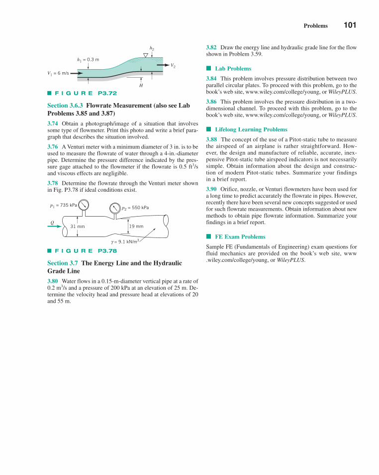
Problems 101

Section 3.6.3 Flowrate Measurement (also see LabProblems 3.85 and 3.87)

3.74 Obtain a photograph/image of a situation that involvessome type of flowmeter. Print this photo and write a brief para-graph that describes the situation involved.

3.76 A Venturi meter with a minimum diameter of 3 in. is to beused to measure the flowrate of water through a 4-in.-diameterpipe. Determine the pressure difference indicated by the pres-sure gage attached to the flowmeter if the flowrate is 0.5 ft3/sand viscous effects are negligible.

3.78 Determine the flowrate through the Venturi meter shownin Fig. P3.78 if ideal conditions exist.

Section 3.7 The Energy Line and the HydraulicGrade Line

3.80 Water flows in a 0.15-m-diameter vertical pipe at a rate of0.2 m3/s and a pressure of 200 kPa at an elevation of 25 m. De-termine the velocity head and pressure head at elevations of 20and 55 m.

3.82 Draw the energy line and hydraulic grade line for the flowshown in Problem 3.59.

■ Lab Problems

3.84 This problem involves pressure distribution between twoparallel circular plates. To proceed with this problem, go to thebook’s web site, www.wiley.com/college/young, or WileyPLUS.

3.86 This problem involves the pressure distribution in a two-dimensional channel. To proceed with this problem, go to thebook’s web site, www.wiley.com/college/young, or WileyPLUS.

■ Lifelong Learning Problems

3.88 The concept of the use of a Pitot-static tube to measurethe airspeed of an airplane is rather straightforward. How-ever, the design and manufacture of reliable, accurate, inex-pensive Pitot-static tube airspeed indicators is not necessarilysimple. Obtain information about the design and construc-tion of modern Pitot-static tubes. Summarize your findingsin a brief report.

3.90 Orifice, nozzle, or Venturi flowmeters have been used fora long time to predict accurately the flowrate in pipes. However,recently there have been several new concepts suggested or usedfor such flowrate measurements. Obtain information about newmethods to obtain pipe flowrate information. Summarize yourfindings in a brief report.

■ FE Exam Problems

Sample FE (Fundamentals of Engineering) exam questions forfluid mechanics are provided on the book’s web site, www.wiley.com/college/young, or WileyPLUS.

F I G U R E P3.72

V1 = 6 m/s

V2

H

h2

h1 = 0.3 m

F I G U R E P3.78

p1 = 735 kPa p2 = 550 kPa

Q19 mm31 mm

γ = 9.1 kN/m3

c03ElementaryFluidDynamicsTheBernoulliEquation.qxd 9/24/10 12:23 PM Page 101

102

V4.1 Streaklines

CHAPTER OPENING PHOTO: A vortex ring: The complex, three-dimensional structure of a smoke ring isindicated in this cross-sectional view. (Smoke in air.) (Photograph courtesy of R. H. Magarvey and C. S. MacLatchy, Ref. 3.)

Learn ing Ob j ec t i v e s

After completing this chapter, you should be able to:

■ discuss the differences between the Eulerian and Lagrangian descriptionsof fluid motion.

■ identify various flow characteristics based on the velocity field.

■ determine the streamline pattern and acceleration field given a velocityfield.

■ discuss the differences between a system and control volume.

■ apply the Reynolds transport theorem and the material derivative.

In this chapter we will discuss various aspects of fluid motion without being concerned withthe actual forces necessary to produce the motion. That is, we will consider the kinematicsof the motion—the velocity and acceleration of the fluid, and the description and visualiza-tion of its motion.

Fluid Kinematics4Fluid Kinematics4

c04Fluidkinematics.qxd 9/24/10 1:01 PM Page 102

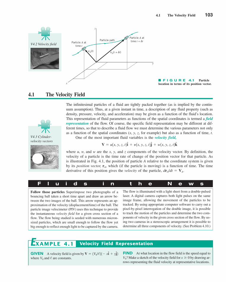
4.1 The Velocity Field

4.1 The Velocity Field 103

The infinitesimal particles of a fluid are tightly packed together (as is implied by the contin-uum assumption). Thus, at a given instant in time, a description of any fluid property (such asdensity, pressure, velocity, and acceleration) may be given as a function of the fluid’s location.This representation of fluid parameters as functions of the spatial coordinates is termed a fieldrepresentation of the flow. Of course, the specific field representation may be different at dif-ferent times, so that to describe a fluid flow we must determine the various parameters not onlyas a function of the spatial coordinates (x, y, z, for example) but also as a function of time, t.

One of the most important fluid variables is the velocity field,

where u, y, and w are the x, y, and z components of the velocity vector. By definition, thevelocity of a particle is the time rate of change of the position vector for that particle. Asis illustrated in Fig. 4.1, the position of particle A relative to the coordinate system is givenby its position vector, rA, which (if the particle is moving) is a function of time. The timederivative of this position gives the velocity of the particle, drA/dt � VA.

V � u1x, y, z, t2 i � y1x, y, z, t2 j � w1x, y, z, t2k

F I G U R E 4.1 Particlelocation in terms of its position vector.

F l u i d s i n t h e N e w s

Follow those particles Superimpose two photographs of abouncing ball taken a short time apart and draw an arrow be-tween the two images of the ball. This arrow represents an ap-proximation of the velocity (displacement/time) of the ball. Theparticle image velocimeter (PIV) uses this technique to providethe instantaneous velocity field for a given cross section of aflow. The flow being studied is seeded with numerous micron-sized particles, which are small enough to follow the flow yetbig enough to reflect enough light to be captured by the camera.

The flow is illuminated with a light sheet from a double-pulsedlaser. A digital camera captures both light pulses on the sameimage frame, allowing the movement of the particles to betracked. By using appropriate computer software to carry out apixel-by-pixel interrogation of the double image, it is possibleto track the motion of the particles and determine the two com-ponents of velocity in the given cross section of the flow. By us-ing two cameras in a stereoscopic arrangement it is possible todetermine all three components of velocity. (See Problem 4.10.)

z

y

x

Particle A attime t

rA(t) rA(t + t)δ

Particle pathParticle A attime t + tδ

V4.2 Velocity field

V4.3 Cylinder-velocity vectors

GIVEN A velocity field is given by where and are constants./V0

V � 1V0//2 1� xi � yj2

Velocity Field Representation

FIND At what location in the flow field is the speed equal toMake a sketch of the velocity field for by drawing ar-

rows representing the fluid velocity at representative locations.x � 0V0?

EXAMPLE 4.1

c04Fluidkinematics.qxd 9/24/10 1:01 PM Page 103

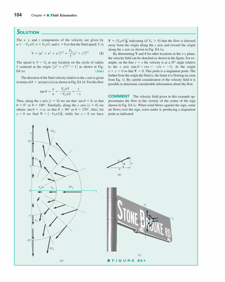
104 Chapter 4 ■ Fluid Kinematics

SOLUTION

The x, y, and z components of the velocity are given byand so that the fluid speed, V, is

(1)

The speed is at any location on the circle of radiuscentered at the origin as shown in Fig.

E4.1a. (Ans)

The direction of the fluid velocity relative to the x axis is givenin terms of as shown in Fig. E4.1b. For this flow

Thus, along the x axis we see that so thator Similarly, along the y axis we

obtain so that or Also, forwe find , while for we havex � 0V � 1�V0x//2 iy � 0

� � 270°.� � 90° tan � � �q1x � 02� � 180°.� � 0°

tan � � 0,1y � 02

tan � �y

u�

V0 y//�V0 x//

�y

�x

1y/u2� � arctan

3 1x2 � y221/2 � / 4/V � V0

V � 1u2 � y2 � w221/2 �V0

/1x2 � y221/2

w � 0u � �V0 x//, y� V0 y//,, indicating (if that the flow is directed

away from the origin along the y axis and toward the originalong the x axis as shown in Fig. E4.1a.

By determining V and for other locations in the x–y plane,the velocity field can be sketched as shown in the figure. For ex-ample, on the line the velocity is at a 45� angle relative to the x axis At the origin

so that This point is a stagnation point. Thefarther from the origin the fluid is, the faster it is flowing (as seenfrom Eq. 1). By careful consideration of the velocity field it ispossible to determine considerable information about the flow.

COMMENT The velocity field given in this example ap-proximates the flow in the vicinity of the center of the signshown in Fig. E4.1c. When wind blows against the sign, someair flows over the sign, some under it, producing a stagnationpoint as indicated.

V � 0.x � y � 01tan � � y/u � �y/x � �12.

y � x

�

V0 7 02V � 1V0y//2j

θV

u

(b)

v

(c)

y

V = 0x

F I G U R E E4.1

y

2�

2V0

2V0

2V0

V0

V0

V0

V0/2

�

−2�

−�

0 x

(a)

c04Fluidkinematics.qxd 9/24/10 1:01 PM Page 104

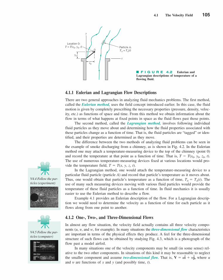
4.1.1 Eulerian and Lagrangian Flow Descriptions

There are two general approaches in analyzing fluid mechanics problems. The first method,called the Eulerian method, uses the field concept introduced earlier. In this case, the fluidmotion is given by completely prescribing the necessary properties (pressure, density, veloc-ity, etc.) as functions of space and time. From this method we obtain information about theflow in terms of what happens at fixed points in space as the fluid flows past those points.

The second method, called the Lagrangian method, involves following individualfluid particles as they move about and determining how the fluid properties associated withthese particles change as a function of time. That is, the fluid particles are “tagged” or iden-tified, and their properties are determined as they move.

The difference between the two methods of analyzing fluid problems can be seen inthe example of smoke discharging from a chimney, as is shown in Fig. 4.2. In the Eulerianmethod one may attach a temperature-measuring device to the top of the chimney (point 0)and record the temperature at that point as a function of time. That is, T � T(x0, y0, z0, t).The use of numerous temperature-measuring devices fixed at various locations would pro-vide the temperature field, T � T(x, y, z, t).

In the Lagrangian method, one would attach the temperature-measuring device to aparticular fluid particle (particle A) and record that particle’s temperature as it moves about.Thus, one would obtain that particle’s temperature as a function of time, TA � TA(t). Theuse of many such measuring devices moving with various fluid particles would provide thetemperature of these fluid particles as a function of time. In fluid mechanics it is usuallyeasier to use the Eulerian method to describe a flow.

Example 4.1 provides an Eulerian description of the flow. For a Lagrangian descrip-tion we would need to determine the velocity as a function of time for each particle as itflows along from one point to another.

4.1.2 One-, Two-, and Three-Dimensional Flows

In almost any flow situation, the velocity field actually contains all three velocity compo-nents (u, y, and w, for example). In many situations the three-dimensional flow characteristicsare important in terms of the physical effects they produce. A feel for the three-dimensionalstructure of such flows can be obtained by studying Fig. 4.3, which is a photograph of theflow past a model airfoil.

In many situations one of the velocity components may be small (in some sense) rel-ative to the two other components. In situations of this kind it may be reasonable to neglectthe smaller component and assume two-dimensional flow. That is, , where uand y are functions of x and y (and possibly time, t).

V � ui � yj

4.1 The Velocity Field 105

F I G U R E 4.2 Eulerian andLagrangian descriptions of temperature of aflowing fluid.

y0

x0

0

x

Location 0:T = T(x0, y0, t) Particle A:

TA = TA(t)

y

V4.4 Follow the par-ticles (experiment)

V4.5 Follow the par-ticles (computer)

c04Fluidkinematics.qxd 9/24/10 1:01 PM Page 105

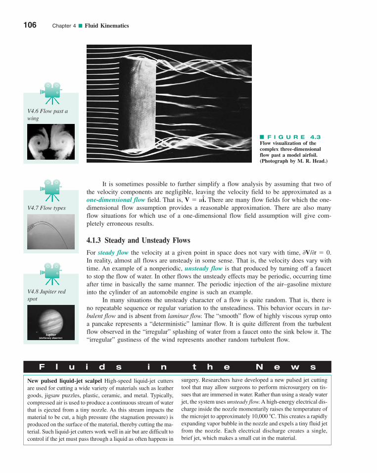
106 Chapter 4 ■ Fluid Kinematics

It is sometimes possible to further simplify a flow analysis by assuming that two ofthe velocity components are negligible, leaving the velocity field to be approximated as aone-dimensional flow field. That is, . There are many flow fields for which the one-dimensional flow assumption provides a reasonable approximation. There are also manyflow situations for which use of a one-dimensional flow field assumption will give com-pletely erroneous results.

4.1.3 Steady and Unsteady Flows

For steady flow the velocity at a given point in space does not vary with time, 0V/0t � 0.In reality, almost all flows are unsteady in some sense. That is, the velocity does vary withtime. An example of a nonperiodic, unsteady flow is that produced by turning off a faucetto stop the flow of water. In other flows the unsteady effects may be periodic, occurring timeafter time in basically the same manner. The periodic injection of the air–gasoline mixtureinto the cylinder of an automobile engine is such an example.

In many situations the unsteady character of a flow is quite random. That is, there isno repeatable sequence or regular variation to the unsteadiness. This behavior occurs in tur-bulent flow and is absent from laminar flow. The “smooth” flow of highly viscous syrup ontoa pancake represents a “deterministic” laminar flow. It is quite different from the turbulentflow observed in the “irregular” splashing of water from a faucet onto the sink below it. The“irregular” gustiness of the wind represents another random turbulent flow.

V � ui

F l u i d s i n t h e N e w s

New pulsed liquid-jet scalpel High-speed liquid-jet cuttersare used for cutting a wide variety of materials such as leathergoods, jigsaw puzzles, plastic, ceramic, and metal. Typically,compressed air is used to produce a continuous stream of waterthat is ejected from a tiny nozzle. As this stream impacts thematerial to be cut, a high pressure (the stagnation pressure) isproduced on the surface of the material, thereby cutting the ma-terial. Such liquid-jet cutters work well in air but are difficult tocontrol if the jet must pass through a liquid as often happens in

surgery. Researchers have developed a new pulsed jet cuttingtool that may allow surgeons to perform microsurgery on tis-sues that are immersed in water. Rather than using a steady waterjet, the system uses unsteady flow. A high-energy electrical dis-charge inside the nozzle momentarily raises the temperature ofthe microjet to approximately 10,000 �C. This creates a rapidlyexpanding vapor bubble in the nozzle and expels a tiny fluid jetfrom the nozzle. Each electrical discharge creates a single,brief jet, which makes a small cut in the material.

F I G U R E 4.3Flow visualization of thecomplex three-dimensionalflow past a model airfoil.(Photograph by M. R. Head.)

V4.6 Flow past awing

V4.7 Flow types

V4.8 Jupiter redspot

c04Fluidkinematics.qxd 9/24/10 1:01 PM Page 106

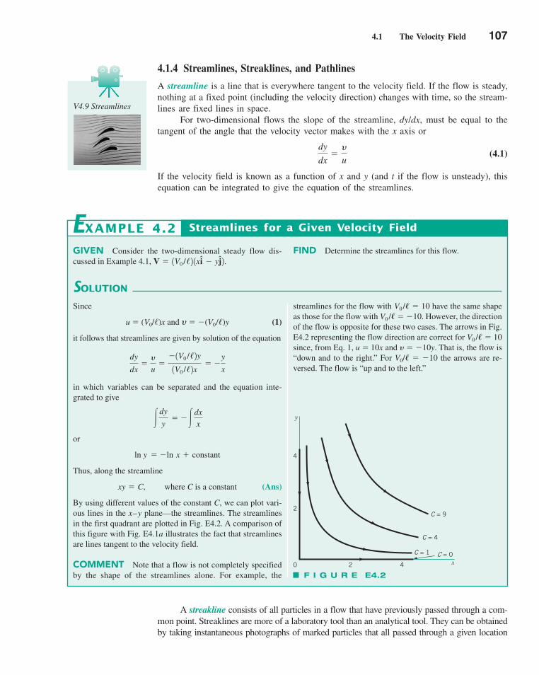
4.1 The Velocity Field 107

4.1.4 Streamlines, Streaklines, and Pathlines

A streamline is a line that is everywhere tangent to the velocity field. If the flow is steady,nothing at a fixed point (including the velocity direction) changes with time, so the stream-lines are fixed lines in space.

For two-dimensional flows the slope of the streamline, dy/dx, must be equal to thetangent of the angle that the velocity vector makes with the x axis or

(4.1)

If the velocity field is known as a function of x and y (and t if the flow is unsteady), thisequation can be integrated to give the equation of the streamlines.

dy

dx�y

u

GIVEN Consider the two-dimensional steady flow dis-cussed in Example 4.1, .V � 1V0 //2 1xi � yj2

SOLUTION

Streamlines for a Given Velocity Field

streamlines for the flow with V0 /� � 10 have the same shapeas those for the flow with V0 /� � �10. However, the directionof the flow is opposite for these two cases. The arrows in Fig.E4.2 representing the flow direction are correct for V0 /� � 10since, from Eq. 1, u � 10x and y � �10y. That is, the flow is“down and to the right.” For V0/� � �10 the arrows are re-versed. The flow is “up and to the left.”

EXAMPLE 4.2

Since

u � (V0//)x and y� �(V0//)y (1)

it follows that streamlines are given by solution of the equation

in which variables can be separated and the equation inte-grated to give

or

Thus, along the streamline

where C is a constant (Ans)

By using different values of the constant C, we can plot vari-ous lines in the x–y plane—the streamlines. The streamlinesin the first quadrant are plotted in Fig. E4.2. A comparison ofthis figure with Fig. E4.1a illustrates the fact that streamlinesare lines tangent to the velocity field.

COMMENT Note that a flow is not completely specifiedby the shape of the streamlines alone. For example, the

xy � C,

ln y � �ln x � constant

�dy

y� ��dx

x

dy

dx�y

u�

�1V0 //2y1V0 //2x

� �y

x

FIND Determine the streamlines for this flow.

A streakline consists of all particles in a flow that have previously passed through a com-mon point. Streaklines are more of a laboratory tool than an analytical tool. They can be obtainedby taking instantaneous photographs of marked particles that all passed through a given location

V4.9 Streamlines

y

4

2

0 2 4 x= 0CC = 1

C = 4

C = 9

F I G U R E E4.2

c04Fluidkinematics.qxd 9/24/10 1:01 PM Page 107

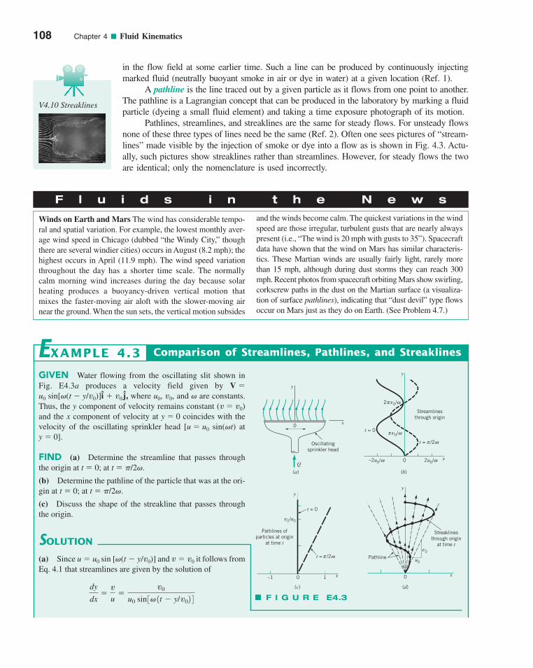
108 Chapter 4 ■ Fluid Kinematics

in the flow field at some earlier time. Such a line can be produced by continuously injectingmarked fluid (neutrally buoyant smoke in air or dye in water) at a given location (Ref. 1).

A pathline is the line traced out by a given particle as it flows from one point to another.The pathline is a Lagrangian concept that can be produced in the laboratory by marking a fluidparticle (dyeing a small fluid element) and taking a time exposure photograph of its motion.

Pathlines, streamlines, and streaklines are the same for steady flows. For unsteady flowsnone of these three types of lines need be the same (Ref. 2). Often one sees pictures of “stream-lines” made visible by the injection of smoke or dye into a flow as is shown in Fig. 4.3. Actu-ally, such pictures show streaklines rather than streamlines. However, for steady flows the twoare identical; only the nomenclature is used incorrectly.

F l u i d s i n t h e N e w s

Winds on Earth and Mars The wind has considerable tempo-ral and spatial variation. For example, the lowest monthly aver-age wind speed in Chicago (dubbed “the Windy City,” thoughthere are several windier cities) occurs in August (8.2 mph); thehighest occurs in April (11.9 mph). The wind speed variationthroughout the day has a shorter time scale. The normallycalm morning wind increases during the day because solarheating produces a buoyancy-driven vertical motion thatmixes the faster-moving air aloft with the slower-moving airnear the ground. When the sun sets, the vertical motion subsides

and the winds become calm. The quickest variations in the windspeed are those irregular, turbulent gusts that are nearly alwayspresent (i.e., “The wind is 20 mph with gusts to 35”). Spacecraftdata have shown that the wind on Mars has similar characteris-tics. These Martian winds are usually fairly light, rarely morethan 15 mph, although during dust storms they can reach 300mph. Recent photos from spacecraft orbiting Mars show swirling,corkscrew paths in the dust on the Martian surface (a visualiza-tion of surface pathlines), indicating that “dust devil” type flowsoccur on Mars just as they do on Earth. (See Problem 4.7.)

GIVEN Water flowing from the oscillating slit shown inFig. E4.3a produces a velocity field given by V �u0 sin[�(t � y/v0)]i � v0 j, where u0, v0, and � are constants.Thus, the y component of velocity remains constant (v � v0)and the x component of velocity at y � 0 coincides with thevelocity of the oscillating sprinkler head [u � u0 sin(�t) aty � 0].

FIND (a) Determine the streamline that passes throughthe origin at t � 0; at t � �/2�.

(b) Determine the pathline of the particle that was at the ori-gin at t � 0; at t � �/2�.

(c) Discuss the shape of the streakline that passes throughthe origin.

SOLUTION

(a) Since u � u0 sin [�(t � y/v0)] and v � v0 it follows fromEq. 4.1 that streamlines are given by the solution of

dy

dx�

vu

�v0

u0 sin 3� 1t � y/v02 4

Comparison of Streamlines, Pathlines, and StreaklinesEXAMPLE 4.3

V4.10 Streaklines

0

y

x

Oscillatingsprinkler head

Q

(a)

2 v0/π ω

v0/π ωt = 0

t = /2 ωπ

Streamlinesthrough origin

y

–2u0/ω 2u0/ω x0

(b)

xx

y

t = 0

Pathlines ofparticles at origin

at time t

v0/u0

–1 10

(c) (d)

0

t = /2π ω Pathline

v0

u0

Streaklinesthrough origin

at time t

y

F I G U R E E4.3

c04Fluidkinematics.qxd 9/25/10 4:44 PM Page 108

4.1 The Velocity Field 109

in which the variables can be separated and the equation inte-grated (for any given time t) to give

or

(1)

where C is a constant. For the streamline at t � 0 that passesthrough the origin (x � y � 0), the value of C is obtainedfrom Eq. 1 as C � u0v0 /�. Hence, the equation for thisstreamline is

(2) (Ans)

Similarly, for the streamline at t � �/2� that passes throughthe origin, Eq. 1 gives C � 0. Thus, the equation for thisstreamline is

or

(3) (Ans)

COMMENT These two streamlines, plotted in FigureE4.3b, are not the same because the flow is unsteady. Forexample, at the origin (x � y � 0) the velocity is V � v0 j att � 0 and V � u0i � v0 j at t � �/2�. Thus, the angle of thestreamline passing through the origin changes with time.Similarly, the shape of the entire streamline is a function oftime.

(b) The pathline of a particle (the location of the particle asa function of time) can be obtained from the velocity field andthe definition of the velocity. Since u � dx/dt and v � dy/dtwe obtain

and

The y equation can be integrated (since v0 � constant) to givethe y coordinate of the pathline as

(4)

where C1 is a constant. With this known y � y(t) dependence,the x equation for the pathline becomes

dx

dt� u0 sin c� at �

v0 t � C1

v0b d � �u0 sin a

C1�

v0b

y � v0 t � C1

dy

dt� v0

dx

dt� u0 sin c� at �

y

v0b d

x �u0

� sin a

�y

v0b

x �u0

� cos c� a

�

2��

y

v0b d �

u0

� cos a

�

2�

�y

v0b

x �u0

� c cos a

�y

v0b � 1 d

u01v0 /�2 cos c� at �y

v0b d � v0x � C

u0�sin c� at �y

v0b ddy � v0�dx,

This can be integrated to give the x component of the path-line as

(5)

where C2 is a constant. For the particle that was at the origin(x � y � 0) at time t � 0, Eqs. 4 and 5 give C1 � C2 � 0.Thus, the pathline is

(6) (Ans)

Similarly, for the particle that was at the origin at t � �/2�,Eqs. 4 and 5 give C1 � ��v0 /2� and C2 � ��v0 /2�. Thus,the pathline for this particle is

and (7)

The pathline can be drawn by plotting the locus of x(t), y(t)values for t � 0 or by eliminating the parameter t from Eq. 7to give

(8) (Ans)

COMMENT The pathlines given by Eqs. 6 and 8, shownin Fig. E4.3c, are straight lines from the origin (rays). Thepathlines and streamlines do not coincide because the flow isunsteady.

(c) The streakline through the origin at time t � 0 is the lo-cus of particles at t � 0 that previously (t � 0) passedthrough the origin. The general shape of the streaklines canbe seen as follows. Each particle that flows through the origintravels in a straight line (pathlines are rays from the origin),the slope of which lies between �v0 /u0 as shown in Fig.E4.3d. Particles passing through the origin at different timesare located on different rays from the origin and at differentdistances from the origin. The net result is that a stream ofdye continually injected at the origin (a streakline) wouldhave the shape shown in Fig. E4.3d. Because of the unsteadi-ness, the streakline will vary with time, although it will al-ways have the oscillating, sinuous character shown. Similarstreaklines are given by the stream of water from a gardenhose nozzle that oscillates back and forth in a direction nor-mal to the axis of the nozzle.

COMMENT In this example streamlines, pathlines, andstreaklines do not coincide. If the flow were steady, all of theselines would be the same.

y �v0

u0 x

y � v0 at ��

2�bx � u0 at �

�

2�b

x � 0 and y � v0 t

x � � cu0 sin aC1�

v0b d t � C2

c04Fluidkinematics.qxd 9/24/10 1:02 PM Page 109

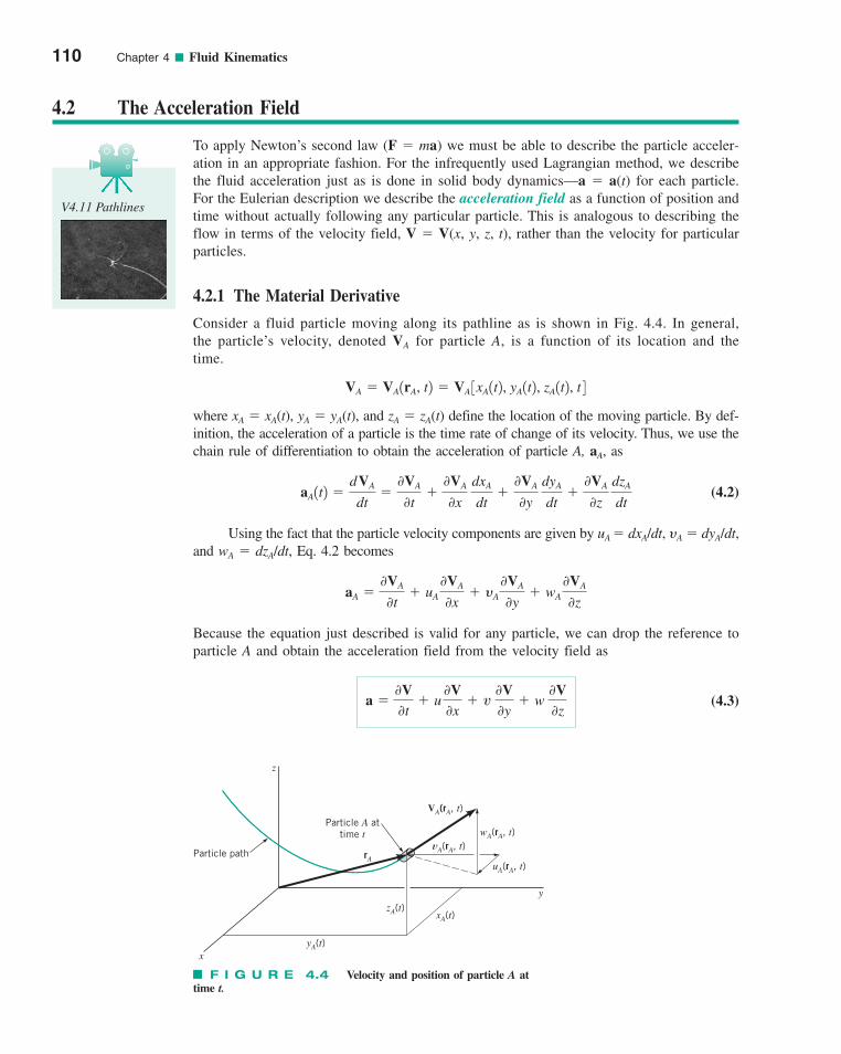
110 Chapter 4 ■ Fluid Kinematics

4.2 The Acceleration Field

To apply Newton’s second law (F � ma) we must be able to describe the particle acceler-ation in an appropriate fashion. For the infrequently used Lagrangian method, we describethe fluid acceleration just as is done in solid body dynamics—a � a(t) for each particle.For the Eulerian description we describe the acceleration field as a function of position andtime without actually following any particular particle. This is analogous to describing theflow in terms of the velocity field, V � V(x, y, z, t), rather than the velocity for particularparticles.

4.2.1 The Material Derivative

Consider a fluid particle moving along its pathline as is shown in Fig. 4.4. In general,the particle’s velocity, denoted VA for particle A, is a function of its location and thetime.

where xA � xA(t), yA � yA(t), and zA � zA(t) define the location of the moving particle. By def-inition, the acceleration of a particle is the time rate of change of its velocity. Thus, we use thechain rule of differentiation to obtain the acceleration of particle A, aA, as

(4.2)

Using the fact that the particle velocity components are given by uA � dxA/dt, yA � dyA/dt,and wA � dzA/dt, Eq. 4.2 becomes

Because the equation just described is valid for any particle, we can drop the reference toparticle A and obtain the acceleration field from the velocity field as

(4.3)a �0V0t

� u0V0x

� v 0V0y

� w 0V0z

aA �0VA

0t� uA

0VA

0x� yA

0VA

0y� wA

0VA

0z

aA1t2 �dVA

dt�

0VA

0t�

0VA

0x

dxA

dt�

0VA

0y

dyA

dt�

0VA

0z

dzA

dt

VA � VA1rA, t2 � VA 3xA1t2, yA1t2, zA1t2, t 4

F I G U R E 4.4 Velocity and position of particle A attime t.

V4.11 Pathlines

Particle A attime t

rA

VA(rA, t)

Particle path

z

x

y

wA(rA, t)

uA(rA, t)

vA(rA, t)

zA(t)xA(t)

yA(t)

c04Fluidkinematics.qxd 9/24/10 1:02 PM Page 110

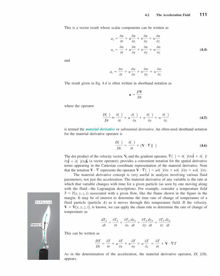
This is a vector result whose scalar components can be written as

(4.4)

and

The result given in Eq. 4.4 is often written in shorthand notation as

where the operator

(4.5)

is termed the material derivative or substantial derivative. An often-used shorthand notationfor the material derivative operator is

(4.6)

The dot product of the velocity vector, V, and the gradient operator,(a vector operator), provides a convenient notation for the spatial derivative

terms appearing in the Cartesian coordinate representation of the material derivative. Notethat the notation represents the operator

The material derivative concept is very useful in analysis involving various fluidparameters, not just the acceleration. The material derivative of any variable is the rate atwhich that variable changes with time for a given particle (as seen by one moving alongwith the fluid—the Lagrangian description). For example, consider a temperature field

associated with a given flow, like the flame shown in the figure in themargin. It may be of interest to determine the time rate of change of temperature of afluid particle (particle A) as it moves through this temperature field. If the velocity,

is known, we can apply the chain rule to determine the rate of change oftemperature as

This can be written as

As in the determination of the acceleration, the material derivative operator,appears.

D1 2/Dt,

DT

Dt�

0T

0t� u

0T

0x� y

0T

0y� w

0T

0z �

0T

0t� V . §T

dTA

dt�

0TA

0t�

0TA

0x

dxA

dt�

0TA

0y

dyA

dt�

0TA

0z

dzA

dt

V � V1x, y, z, t2,

T � T1x, y, z, t2

V . § 1 2 � u0 1 2/0x � y0 1 2/0y � w0 1 2/0z.V . §

0yj � 0 1 2/0zk§ 1 2 � 0 1 2/0xi � 0 1 2/

D1 2Dt

�0 1 20t

� 1V . § 2 1 2

D1 2Dt

�0 1 20t

� u 0 1 20x

� v 0 1 20y

� w 0 1 20z

a �DVDt

az �0w

0t� u

0w

0x� y

0w

0y� w

0w

0z

ay �0y0t

� u0y0x

� y0y0y

� w0y0z

ax �0u

0t� u

0u

0x� y

0u

0y� w

0u

0z

4.2 The Acceleration Field 111

V

T = T (x, y, z, t)

Particle A

yx

z

c04Fluidkinematics.qxd 9/24/10 1:02 PM Page 111

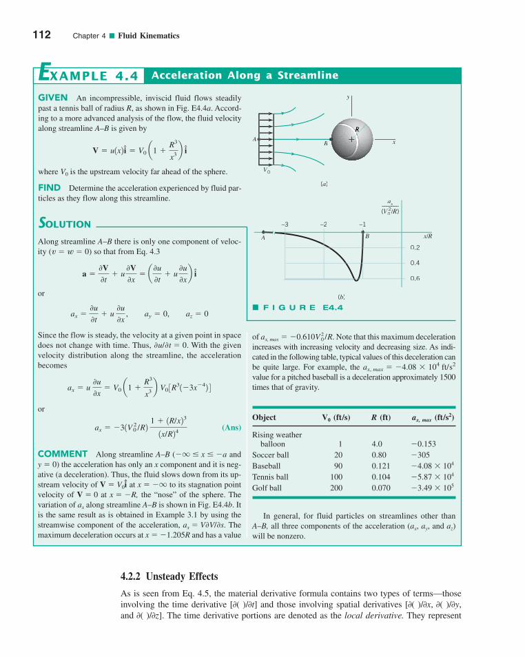
112 Chapter 4 ■ Fluid Kinematics

4.2.2 Unsteady Effects

As is seen from Eq. 4.5, the material derivative formula contains two types of terms—thoseinvolving the time derivative [0( )/0t] and those involving spatial derivatives [0( )/0x, 0( )/0y,and 0( )/0z]. The time derivative portions are denoted as the local derivative. They represent

GIVEN An incompressible, inviscid fluid flows steadilypast a tennis ball of radius R, as shown in Fig. E4.4a. Accord-ing to a more advanced analysis of the flow, the fluid velocityalong streamline A–B is given by

where V0 is the upstream velocity far ahead of the sphere.

FIND Determine the acceleration experienced by fluid par-ticles as they flow along this streamline.

V � u1x2 i � V0 a1 �R3

x3 b i

Acceleration Along a StreamlineEXAMPLE 4.4

SOLUTION

of ax, max � �0.610 . Note that this maximum decelerationincreases with increasing velocity and decreasing size. As indi-cated in the following table, typical values of this deceleration canbe quite large. For example, the value for a pitched baseball is a deceleration approximately 1500times that of gravity.

Object V0 (ft/s) R (ft) ax, max (ft/s2)

Rising weatherballoon 1 4.0 �0.153

Soccer ball 20 0.80 �305Baseball 90 0.121 �4.08 104

Tennis ball 100 0.104 �5.87 104

Golf ball 200 0.070 �3.49 105

In general, for fluid particles on streamlines other thanA–B, all three components of the acceleration (ax, ay, and az)will be nonzero.

ax, max � �4.08 104 ft/s2

V 20 /R

Along streamline A–B there is only one component of veloc-ity (v � w � 0) so that from Eq. 4.3

or

Since the flow is steady, the velocity at a given point in spacedoes not change with time. Thus, u/t � 0. With the givenvelocity distribution along the streamline, the accelerationbecomes

or

(Ans)

COMMENT Along streamline A–B (� � x � �a andy � 0) the acceleration has only an x component and it is neg-ative (a deceleration). Thus, the fluid slows down from its up-stream velocity of V � V0i at x � � to its stagnation pointvelocity of V � 0 at x � �R, the “nose” of the sphere. Thevariation of ax along streamline A–B is shown in Fig. E4.4b. Itis the same result as is obtained in Example 3.1 by using thestreamwise component of the acceleration, ax � VV/s. Themaximum deceleration occurs at x � �1.205R and has a value

q

q

ax � �31V 20 /R2

1 � 1R/x23

1x/R24

ax � u 0u

0x� V0 a1 �

R3

x3 b V0 3R31�3x�42 4

az � 0ay � 0,ax �0u

0t� u

0u

0x ,

a �0V0t

� u0V0x

� a0u

0t� u

0u

0xb i

A x

y

V0VV

(a)

B

A B

(b)

–0.2

–0.4

–0.6

x/xx R//

–1–2–3

ax_______(V0VV 2/R// )

F I G U R E E4.4

c04Fluidkinematics.qxd 9/24/10 1:02 PM Page 112

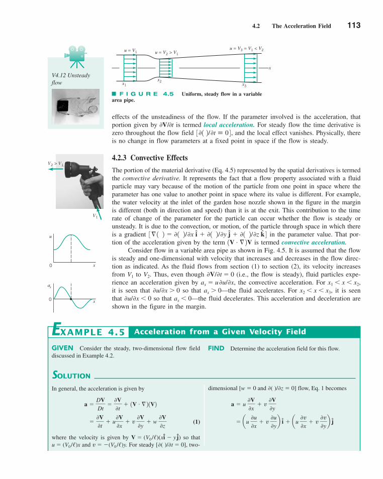
4.2 The Acceleration Field 113

effects of the unsteadiness of the flow. If the parameter involved is the acceleration, thatportion given by 0V/0t is termed local acceleration. For steady flow the time derivative iszero throughout the flow field and the local effect vanishes. Physically, thereis no change in flow parameters at a fixed point in space if the flow is steady.

4.2.3 Convective Effects

The portion of the material derivative (Eq. 4.5) represented by the spatial derivatives is termedthe convective derivative. It represents the fact that a flow property associated with a fluidparticle may vary because of the motion of the particle from one point in space where theparameter has one value to another point in space where its value is different. For example,the water velocity at the inlet of the garden hose nozzle shown in the figure in the marginis different (both in direction and speed) than it is at the exit. This contribution to the timerate of change of the parameter for the particle can occur whether the flow is steady orunsteady. It is due to the convection, or motion, of the particle through space in which thereis a gradient in the parameter value. That por-tion of the acceleration given by the term is termed convective acceleration.

Consider flow in a variable area pipe as shown in Fig. 4.5. It is assumed that the flowis steady and one-dimensional with velocity that increases and decreases in the flow direc-tion as indicated. As the fluid flows from section (1) to section (2), its velocity increasesfrom V1 to V2. Thus, even though V/t � 0 (i.e., the flow is steady), fluid particles expe-rience an acceleration given by ax � uu/x, the convective acceleration. For x1 � x � x2,it is seen that u/x � 0 so that ax � 0—the fluid accelerates. For x2 � x � x3, it is seenthat u/x � 0 so that ax � 0—the fluid decelerates. This acceleration and deceleration areshown in the figure in the margin.

1V . § 2V3§ 1 2 � 0 1 2/0x i � 0 1 2/0y j � 0 1 2/0z k 4

3 0 1 2/0t � 0 4 ,

V4.12 Unsteadyflow

V2 > V1

V1

F I G U R E 4.5 Uniform, steady flow in a variablearea pipe.

x

u = V3 = V1 < V2

x3

x2x1

u = V2 > V1u = V1

u

x0

ax

x0

GIVEN Consider the steady, two-dimensional flow fielddiscussed in Example 4.2.

FIND Determine the acceleration field for this flow.

SOLUTION

Acceleration from a Given Velocity Field

dimensional [w � 0 and ( )/z � 0] flow, Eq. 1 becomes

� au 0u

0x� v

0u

0yb i � au

0v

0x� v

0v

0yb j

a � u 0V0x

� v 0V0y

EXAMPLE 4.5

In general, the acceleration is given by

(1)

where the velocity is given by V � (V0 //)(xi � y j) so thatu � (V0 //)x and v � �(V0 //)y. For steady [( )/t � 0], two-

�0V0t

� u0V0x

� v 0V0y

� w 0V0z

a �DVDt

�0V0t

� 1V . § 2 1V2

c04Fluidkinematics.qxd 9/24/10 1:02 PM Page 113

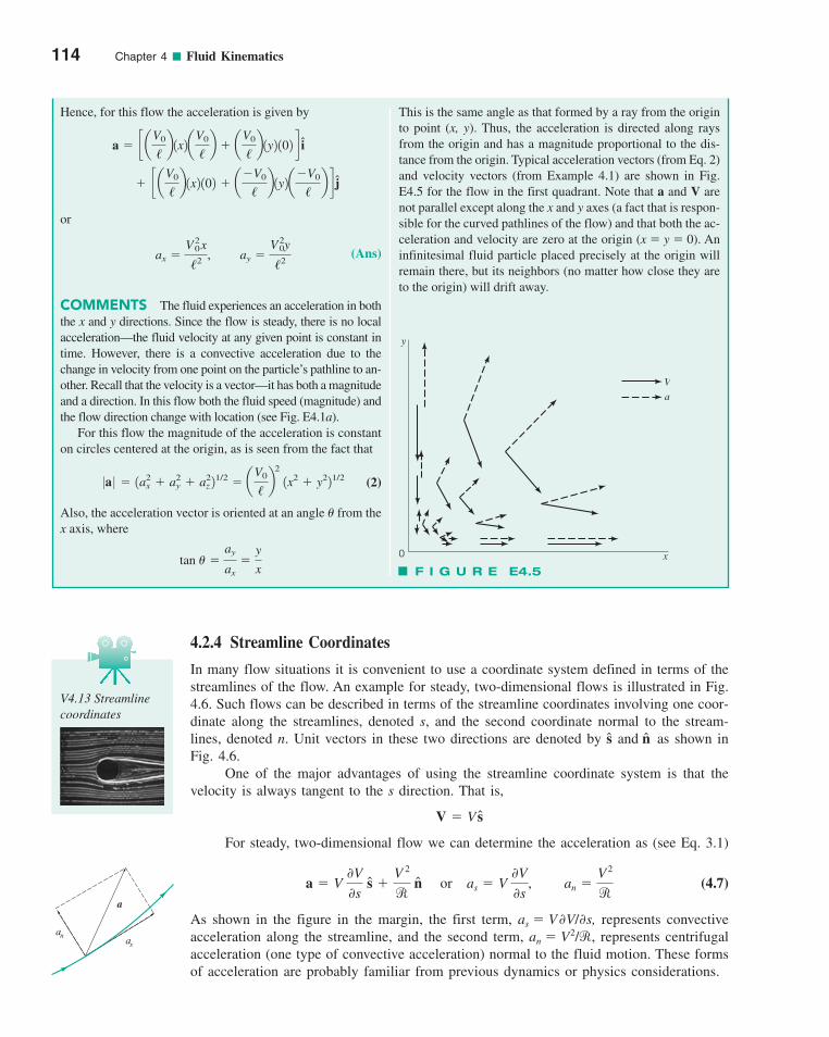
114 Chapter 4 ■ Fluid Kinematics

4.2.4 Streamline Coordinates

In many flow situations it is convenient to use a coordinate system defined in terms of thestreamlines of the flow. An example for steady, two-dimensional flows is illustrated in Fig.4.6. Such flows can be described in terms of the streamline coordinates involving one coor-dinate along the streamlines, denoted s, and the second coordinate normal to the stream-lines, denoted n. Unit vectors in these two directions are denoted by and as shown inFig. 4.6.

One of the major advantages of using the streamline coordinate system is that thevelocity is always tangent to the s direction. That is,

For steady, two-dimensional flow we can determine the acceleration as (see Eq. 3.1)

(4.7)

As shown in the figure in the margin, the first term, as � VV/s, represents convectiveacceleration along the streamline, and the second term, an � V2/r, represents centrifugalacceleration (one type of convective acceleration) normal to the fluid motion. These formsof acceleration are probably familiar from previous dynamics or physics considerations.

a � V 0V

0s s �

V 2

r n or as � V

0V

0s, an �

V 2

r

V � V s

ns

Hence, for this flow the acceleration is given by

or

(Ans)

COMMENTS The fluid experiences an acceleration in boththe x and y directions. Since the flow is steady, there is no local acceleration—the fluid velocity at any given point is constant intime. However, there is a convective acceleration due to thechange in velocity from one point on the particle’s pathline to an-other. Recall that the velocity is a vector—it has both a magnitudeand a direction. In this flow both the fluid speed (magnitude) andthe flow direction change with location (see Fig. E4.1a).

For this flow the magnitude of the acceleration is constanton circles centered at the origin, as is seen from the fact that

(2)

Also, the acceleration vector is oriented at an angle � from thex axis, where

tan � �ay

ax�

y

x

0a 0 � 1a2x � a2

y � a2z 2

1/2 � aV0

/b

2

1x2 � y221/2

ax �V2

0x

/2 , ay �V2

0y

/2

� c aV0

/b1x2 102 � a

�V0

/b1y2a

�V0

/b d j

a � c aV0

/b1x2a

V0

/b � a

V0

/b1y2 102 d i

This is the same angle as that formed by a ray from the originto point (x, y). Thus, the acceleration is directed along raysfrom the origin and has a magnitude proportional to the dis-tance from the origin. Typical acceleration vectors (from Eq. 2)and velocity vectors (from Example 4.1) are shown in Fig.E4.5 for the flow in the first quadrant. Note that a and V arenot parallel except along the x and y axes (a fact that is respon-sible for the curved pathlines of the flow) and that both the ac-celeration and velocity are zero at the origin (x � y � 0). Aninfinitesimal fluid particle placed precisely at the origin willremain there, but its neighbors (no matter how close they areto the origin) will drift away.

Va

y

x0

F I G U R E E4.5

V4.13 Streamlinecoordinates

an as

a

c04Fluidkinematics.qxd 9/24/10 1:03 PM Page 114

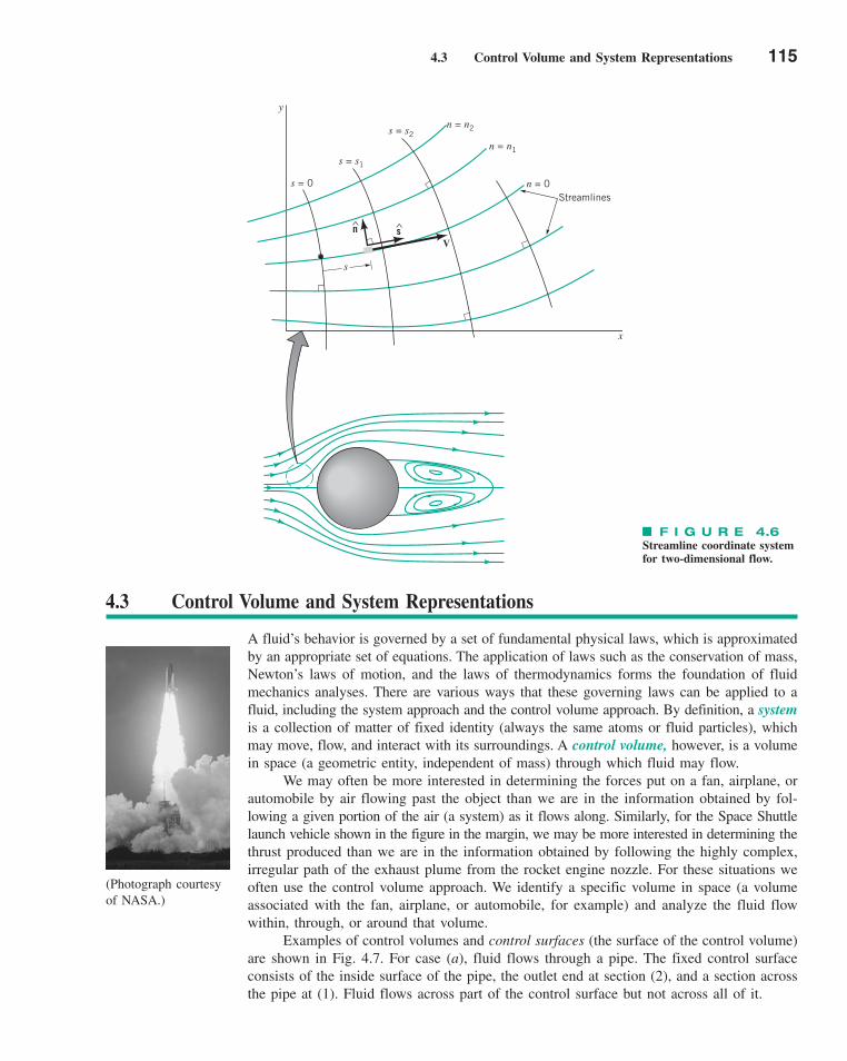
4.3 Control Volume and System Representations 115

F I G U R E 4.6Streamline coordinate systemfor two-dimensional flow.

s

n^ s^

V

s = 0

s = s1

s = s2n = n2

n = n1

n = 0Streamlines

y

x

4.3 Control Volume and System Representations

A fluid’s behavior is governed by a set of fundamental physical laws, which is approximatedby an appropriate set of equations. The application of laws such as the conservation of mass,Newton’s laws of motion, and the laws of thermodynamics forms the foundation of fluidmechanics analyses. There are various ways that these governing laws can be applied to afluid, including the system approach and the control volume approach. By definition, a systemis a collection of matter of fixed identity (always the same atoms or fluid particles), whichmay move, flow, and interact with its surroundings. A control volume, however, is a volumein space (a geometric entity, independent of mass) through which fluid may flow.

We may often be more interested in determining the forces put on a fan, airplane, orautomobile by air flowing past the object than we are in the information obtained by fol-lowing a given portion of the air (a system) as it flows along. Similarly, for the Space Shuttlelaunch vehicle shown in the figure in the margin, we may be more interested in determining thethrust produced than we are in the information obtained by following the highly complex,irregular path of the exhaust plume from the rocket engine nozzle. For these situations weoften use the control volume approach. We identify a specific volume in space (a volumeassociated with the fan, airplane, or automobile, for example) and analyze the fluid flowwithin, through, or around that volume.

Examples of control volumes and control surfaces (the surface of the control volume)are shown in Fig. 4.7. For case (a), fluid flows through a pipe. The fixed control surfaceconsists of the inside surface of the pipe, the outlet end at section (2), and a section acrossthe pipe at (1). Fluid flows across part of the control surface but not across all of it.

(Photograph courtesyof NASA.)

c04Fluidkinematics.qxd 9/24/10 1:03 PM Page 115

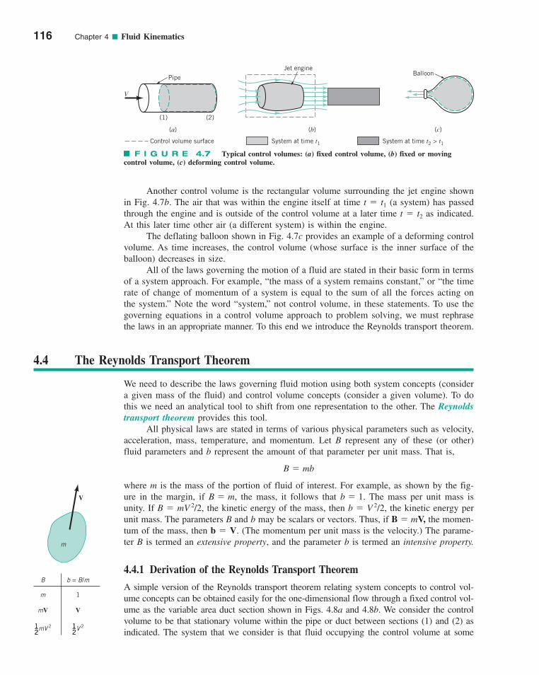
116 Chapter 4 ■ Fluid Kinematics

Another control volume is the rectangular volume surrounding the jet engine shownin Fig. 4.7b. The air that was within the engine itself at time t � t1 (a system) has passedthrough the engine and is outside of the control volume at a later time t � t2 as indicated.At this later time other air (a different system) is within the engine.

The deflating balloon shown in Fig. 4.7c provides an example of a deforming controlvolume. As time increases, the control volume (whose surface is the inner surface of theballoon) decreases in size.

All of the laws governing the motion of a fluid are stated in their basic form in termsof a system approach. For example, “the mass of a system remains constant,” or “the timerate of change of momentum of a system is equal to the sum of all the forces acting onthe system.” Note the word “system,” not control volume, in these statements. To use thegoverning equations in a control volume approach to problem solving, we must rephrasethe laws in an appropriate manner. To this end we introduce the Reynolds transport theorem.

F I G U R E 4.7 Typical control volumes: (a) fixed control volume, (b) fixed or movingcontrol volume, (c) deforming control volume.

V

Pipe

(1) (2)

(a) (b)

Jet engine

(c)

Balloon

Control volume surface System at time t1 System at time t2 > t1

4.4 The Reynolds Transport Theorem

We need to describe the laws governing fluid motion using both system concepts (considera given mass of the fluid) and control volume concepts (consider a given volume). To dothis we need an analytical tool to shift from one representation to the other. The Reynoldstransport theorem provides this tool.

All physical laws are stated in terms of various physical parameters such as velocity,acceleration, mass, temperature, and momentum. Let B represent any of these (or other)fluid parameters and b represent the amount of that parameter per unit mass. That is,

where m is the mass of the portion of fluid of interest. For example, as shown by the fig-ure in the margin, if the mass, it follows that The mass per unit mass isunity. If B � mV 2/2, the kinetic energy of the mass, then b � V 2/2, the kinetic energy perunit mass. The parameters B and b may be scalars or vectors. Thus, if B � mV, the momen-tum of the mass, then b � V. (The momentum per unit mass is the velocity.) The parame-ter B is termed an extensive property, and the parameter b is termed an intensive property.

4.4.1 Derivation of the Reynolds Transport Theorem

A simple version of the Reynolds transport theorem relating system concepts to control vol-ume concepts can be obtained easily for the one-dimensional flow through a fixed control vol-ume as the variable area duct section shown in Figs. 4.8a and 4.8b. We consider the controlvolume to be that stationary volume within the pipe or duct between sections (1) and (2) asindicated. The system that we consider is that fluid occupying the control volume at some

b � 1.B � m,

B � mb

V

m

V

B b = B/m

1m

mV

1_2mV 21_2

1_2V 21_2

c04Fluidkinematics.qxd 9/24/10 1:03 PM Page 116

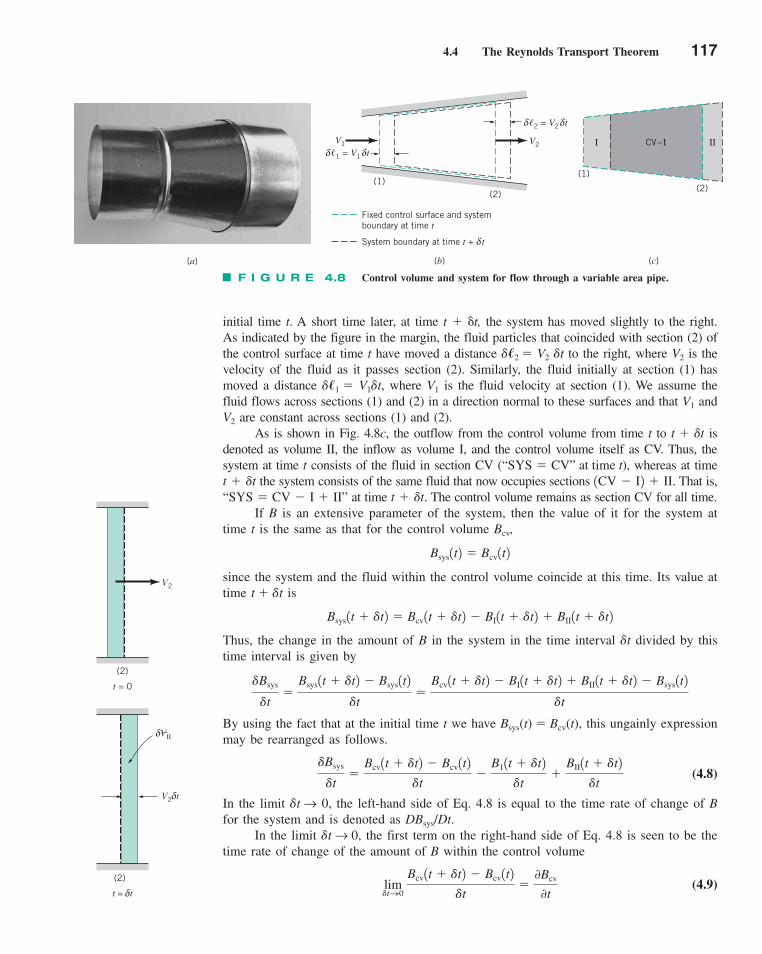
initial time t. A short time later, at time t � t, the system has moved slightly to the right.As indicated by the figure in the margin, the fluid particles that coincided with section (2) ofthe control surface at time t have moved a distance ��2 � V2 �t to the right, where V2 is thevelocity of the fluid as it passes section (2). Similarly, the fluid initially at section (1) hasmoved a distance ��1 � V1�t, where V1 is the fluid velocity at section (1). We assume thefluid flows across sections (1) and (2) in a direction normal to these surfaces and that V1 andV2 are constant across sections (1) and (2).

As is shown in Fig. 4.8c, the outflow from the control volume from time t to isdenoted as volume II, the inflow as volume I, and the control volume itself as CV. Thus, thesystem at time t consists of the fluid in section CV ( ), whereas at time

the system consists of the same fluid that now occupies sections That is,at time The control volume remains as section CV for all time.

If B is an extensive parameter of the system, then the value of it for the system attime t is the same as that for the control volume Bcv,

since the system and the fluid within the control volume coincide at this time. Its value attime t � �t is

Thus, the change in the amount of B in the system in the time interval �t divided by thistime interval is given by

By using the fact that at the initial time t we have Bsys(t) � Bcv(t), this ungainly expressionmay be rearranged as follows.

(4.8)

In the limit �t → 0, the left-hand side of Eq. 4.8 is equal to the time rate of change of Bfor the system and is denoted as DBsys/Dt.

In the limit �t → 0, the first term on the right-hand side of Eq. 4.8 is seen to be thetime rate of change of the amount of B within the control volume

(4.9)lim�tS0

Bcv1t � �t2 � Bcv1t2

�t�

0Bcv

0t

�Bsys

�t�

Bcv1t � �t2 � Bcv1t2

�t�

B11t � �t2

�t�

BII1t � �t2

�t

�Bsys

�t�

Bsys1t � �t2 � Bsys1t2

�t�

Bcv1t � �t2 � BI1t � �t2 � BII1t � �t2 � Bsys1t2

�t

Bsys1t � �t2 � Bcv1t � �t2 � BI1t � �t2 � BII1t � �t2

Bsys1t2 � Bcv1t2

t � dt.“SYS � CV � I � II”1CV � I2 � II.t � dt

“SYS � CV” at time t

t � dt

4.4 The Reynolds Transport Theorem 117

V1 V2�1 = V1 tδ δ

(1)(2)

�2 = V2 tδ δ

Fixed control surface and systemboundary at time t

System boundary at time t + tδ

(b) (c)

I IICV– I

(2)

(1)

F I G U R E 4.8 Control volume and system for flow through a variable area pipe.

(a)

V2

(2)

t = 0

V2 tδ

(2)

t = tδ

VIIδ

c04Fluidkinematics.qxd 9/24/10 1:03 PM Page 117

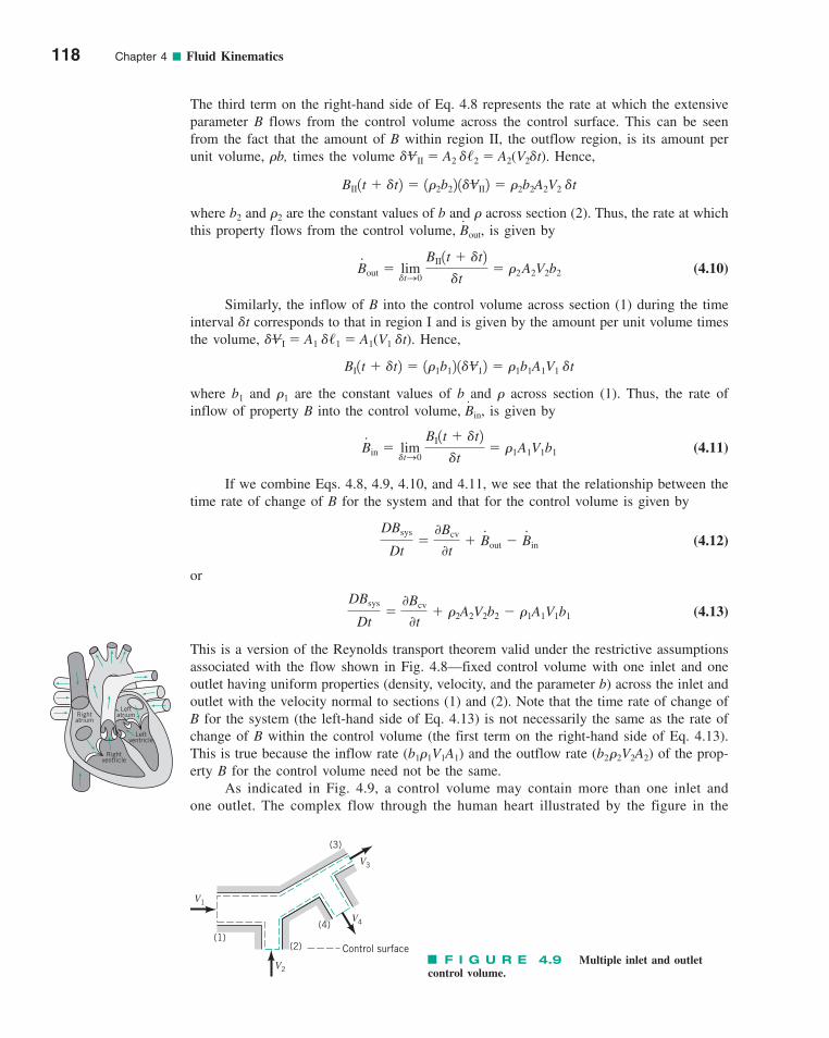
118 Chapter 4 ■ Fluid Kinematics

The third term on the right-hand side of Eq. 4.8 represents the rate at which the extensiveparameter B flows from the control volume across the control surface. This can be seenfrom the fact that the amount of B within region II, the outflow region, is its amount perunit volume, �b, times the volume � II � A2 �/2 � A2(V2�t). Hence,

where b2 and �2 are the constant values of b and � across section (2). Thus, the rate at whichthis property flows from the control volume, Bout, is given by

(4.10)

Similarly, the inflow of B into the control volume across section (1) during the timeinterval �t corresponds to that in region I and is given by the amount per unit volume timesthe volume, � I � A1 �/1 � A1(V1 �t). Hence,

where b1 and �1 are the constant values of b and � across section (1). Thus, the rate ofinflow of property B into the control volume, Bin, is given by

(4.11)

If we combine Eqs. 4.8, 4.9, 4.10, and 4.11, we see that the relationship between thetime rate of change of B for the system and that for the control volume is given by

(4.12)

or

(4.13)

This is a version of the Reynolds transport theorem valid under the restrictive assumptionsassociated with the flow shown in Fig. 4.8—fixed control volume with one inlet and oneoutlet having uniform properties (density, velocity, and the parameter b) across the inlet andoutlet with the velocity normal to sections (1) and (2). Note that the time rate of change ofB for the system (the left-hand side of Eq. 4.13) is not necessarily the same as the rate ofchange of B within the control volume (the first term on the right-hand side of Eq. 4.13).This is true because the inflow rate (b1�1V1A1) and the outflow rate (b2�2V2A2) of the prop-erty B for the control volume need not be the same.

As indicated in Fig. 4.9, a control volume may contain more than one inlet andone outlet. The complex flow through the human heart illustrated by the figure in the

DBsys

Dt�

0Bcv

0t� �2A2V2b2 � �1A1V1b1

DBsys

Dt�

0Bcv

0t� B

#out � B

#in

B#

in � lim�tS0

BI1t � �t2

�t� �1A1V1b1

BI1t � �t2 � 1�1b12 1�V12 � �1b1A1V1 �t

V

B#

out � lim�tS0

BII1t � �t2

�t� �2A2V2b2

BII1t � �t2 � 1�2b22 1�VII2 � �2b2A2V2 �t

V

LeftatriumRight

atrium

Rightventricle

Leftventricle

(1)(2)

(3)

(4)

V1

V2

V4

V3

Control surfaceF I G U R E 4.9 Multiple inlet and outlet

control volume.

c04Fluidkinematics.qxd 9/24/10 1:03 PM Page 118

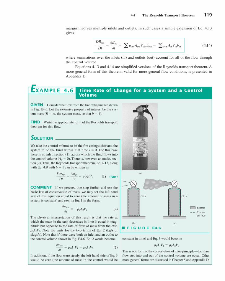
margin involves multiple inlets and outlets. In such cases a simple extension of Eq. 4.13gives.

(4.14)

where summations over the inlets (in) and outlets (out) account for all of the flow throughthe control volume.

Equations 4.13 and 4.14 are simplified versions of the Reynolds transport theorem. Amore general form of this theorem, valid for more general flow conditions, is presented inAppendix D.

DBsys

Dt�

0Bcv

0t� a �out AoutVoutbout � a �in AinVinbin

4.4 The Reynolds Transport Theorem 119

GIVEN Consider the flow from the fire extinguisher shownin Fig. E4.6. Let the extensive property of interest be the sys-tem mass (B � m, the system mass, so that b � 1).

FIND Write the appropriate form of the Reynolds transporttheorem for this flow.

SOLUTION

Time Rate of Change for a System and a ControlVolume

constant in time) and Eq. 3 would become

This is one form of the conservation of mass principle—the massflowrates into and out of the control volume are equal. Othermore general forms are discussed in Chapter 5 and Appendix D.

�1A1V1 � �2A2V2

EXAMPLE 4.6

We take the control volume to be the fire extinguisher and thesystem to be the fluid within it at time t � 0. For this casethere is no inlet, section (1), across which the fluid flows intothe control volume (A1 � 0). There is, however, an outlet, sec-tion (2). Thus, the Reynolds transport theorem, Eq. 4.13, alongwith Eq. 4.9 with b � 1 can be written as

(1) (Ans)

COMMENT If we proceed one step further and use thebasic law of conservation of mass, we may set the left-handside of this equation equal to zero (the amount of mass in asystem is constant) and rewrite Eq. 1 in the form:

(2)

The physical interpretation of this result is that the rate atwhich the mass in the tank decreases in time is equal in mag-nitude but opposite to the rate of flow of mass from the exit,�2A2V2. Note the units for the two terms of Eq. 2 (kg/s orslugs/s). Note that if there were both an inlet and an outlet tothe control volume shown in Fig. E4.6, Eq. 2 would become

(3)

In addition, if the flow were steady, the left-hand side of Eq. 3would be zero (the amount of mass in the control would be

0mcv

0t� �1A1V1 � �2A2V2

0mcv

0t� ��2A2V2

Dmsys

Dt�

0mcv

0t� �2A2V2

F I G U R E E4.6

(b) (c)

System

Controlsurface

t = 0 t > 0

(a)

c04Fluidkinematics.qxd 9/24/10 1:03 PM Page 119

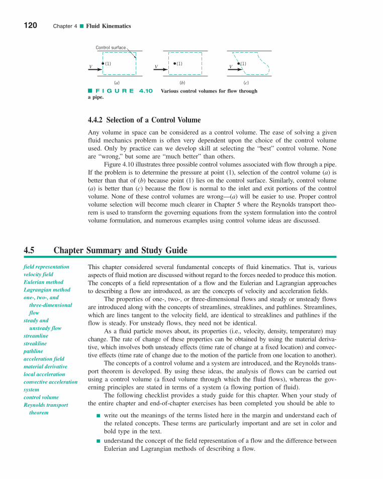
120 Chapter 4 ■ Fluid Kinematics

4.4.2 Selection of a Control Volume

Any volume in space can be considered as a control volume. The ease of solving a givenfluid mechanics problem is often very dependent upon the choice of the control volumeused. Only by practice can we develop skill at selecting the “best” control volume. Noneare “wrong,” but some are “much better” than others.

Figure 4.10 illustrates three possible control volumes associated with flow through a pipe.If the problem is to determine the pressure at point (1), selection of the control volume (a) isbetter than that of (b) because point (1) lies on the control surface. Similarly, control volume(a) is better than (c) because the flow is normal to the inlet and exit portions of the controlvolume. None of these control volumes are wrong—(a) will be easier to use. Proper controlvolume selection will become much clearer in Chapter 5 where the Reynolds transport theo-rem is used to transform the governing equations from the system formulation into the controlvolume formulation, and numerous examples using control volume ideas are discussed.

V

Control surface

(1)

(a)

V(1)

(b)

V(1)

(c)

F I G U R E 4.10 Various control volumes for flow througha pipe.

field representationvelocity fieldEulerian methodLagrangian methodone-, two-, and

three-dimensional flow

steady and unsteady flow

streamlinestreaklinepathlineacceleration fieldmaterial derivativelocal accelerationconvective accelerationsystemcontrol volumeReynolds transport

theorem

4.5 Chapter Summary and Study Guide

This chapter considered several fundamental concepts of fluid kinematics. That is, variousaspects of fluid motion are discussed without regard to the forces needed to produce this motion.The concepts of a field representation of a flow and the Eulerian and Lagrangian approachesto describing a flow are introduced, as are the concepts of velocity and acceleration fields.

The properties of one-, two-, or three-dimensional flows and steady or unsteady flowsare introduced along with the concepts of streamlines, streaklines, and pathlines. Streamlines,which are lines tangent to the velocity field, are identical to streaklines and pathlines if theflow is steady. For unsteady flows, they need not be identical.

As a fluid particle moves about, its properties (i.e., velocity, density, temperature) maychange. The rate of change of these properties can be obtained by using the material deriva-tive, which involves both unsteady effects (time rate of change at a fixed location) and convec-tive effects (time rate of change due to the motion of the particle from one location to another).

The concepts of a control volume and a system are introduced, and the Reynolds trans-port theorem is developed. By using these ideas, the analysis of flows can be carried outusing a control volume (a fixed volume through which the fluid flows), whereas the gov-erning principles are stated in terms of a system (a flowing portion of fluid).

The following checklist provides a study guide for this chapter. When your study ofthe entire chapter and end-of-chapter exercises has been completed you should be able to

write out the meanings of the terms listed here in the margin and understand each ofthe related concepts. These terms are particularly important and are set in color andbold type in the text.

understand the concept of the field representation of a flow and the difference betweenEulerian and Lagrangian methods of describing a flow.

c04Fluidkinematics.qxd 9/24/10 1:03 PM Page 120

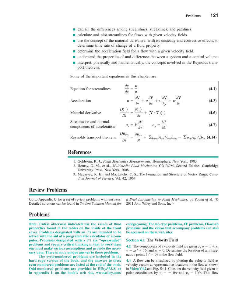
explain the differences among streamlines, streaklines, and pathlines.

calculate and plot streamlines for flows with given velocity fields.

use the concept of the material derivative, with its unsteady and convective effects, todetermine time rate of change of a fluid property.

determine the acceleration field for a flow with a given velocity field.

understand the properties of and differences between a system and a control volume.

interpret, physically and mathematically, the concepts involved in the Reynolds trans-port theorem.

Some of the important equations in this chapter are

Equation for streamlines (4.1)

Acceleration (4.3)

Material derivative (4.6)

Streamwise and normal components of acceleration (4.7)

Reynolds transport theorem (4.14)

References

1. Goldstein, R. J., Fluid Mechanics Measurements, Hemisphere, New York, 1983.2. Homsy, G. M., et al., Multimedia Fluid Mechanics, CD-ROM, Second Edition, Cambridge

University Press, New York, 2008.3. Magarvey, R. H., and MacLatchy, C. S., The Formation and Structure of Vortex Rings, Cana-

dian Journal of Physics, Vol. 42, 1964.

DBsys

Dt�

0Bcv

0t� g�out AoutVout bout � g�in AinVinbin

as � V

0V

0s, an �

V 2

r

D1 2

Dt�

0 1 2 0t

� 1V # § 2 1 2

a �0V0t

� u

0V0x

� y

0V0y

� w

0V0z

dy

dx�y

u

Problems 121

Review Problems

Go to Appendix G for a set of review problems with answers.Detailed solutions can be found in Student Solution Manual for

a Brief Introduction to Fluid Mechanics, by Young et al. (©2011 John Wiley and Sons, Inc.).

Problems

Note: Unless otherwise indicated use the values of fluidproperties found in the tables on the inside of the frontcover. Problems designated with an (*) are intended to besolved with the aid of a programmable calculator or a com-puter. Problems designated with a (†) are “open-ended”problems and require critical thinking in that to work themone must make various assumptions and provide the neces-sary data. There is not a unique answer to these problems.

The even-numbered problems are included in thehard copy version of the book, and the answers to theseeven-numbered problems are listed at the end of the book.Odd-numbered problems are provided in WileyPLUS, orin Appendix L on the book’s web site, www.wiley.com/

college/young. The lab-type problems, FE problems, FlowLabproblems, and the videos that accompany problems can alsobe accessed on these web sites.

Section 4.1 The Velocity Field

4.2 The components of a velocity field are given by and . Determine the location of any stag-

nation points in the flow field.

4.4 A flow can be visualized by plotting the velocity field asvelocity vectors at representative locations in the flow as shownin Video V4.2 and Fig. E4.1. Consider the velocity field given inpolar coordinates by yr � �10/r and y� � 10/r. This flow

1V � 02w � 0y � xy3 � 16,

u � x � y,

c04Fluidkinematics.qxd 10/18/10 7:58 AM Page 121

122 Chapter 4 ■ Fluid Kinematics

velocity, which is given by where a is thesphere radius and is the fluid speed far from the sphere.

Particle

1 0.500 0.4802 0.250 0.2323 0.140 0.1284 0.120 0.112 ��

��

��

��

x at t � 0.002 s 1ft2x at t � 0 s 1ft2

V0

V � V0 11 � a3/x32,

Section 4.2 The Acceleration Field

4.12 A velocity field is given by and where cis a constant. Determine the x and y components of the acceler-ation. At what point (points) in the flow field is the accelerationzero?

4.14 The velocity of the water in the pipe shown in Fig. P4.14is given by V1 � 0.50t m/s and V2 � 1.0t m/s, where t is in sec-onds. (a) Determine the local acceleration at points (1) and (2).(b) Is the average convective acceleration between these twopoints negative, zero, or positive? Explain.

y � cy2,u � cx2

4.16 A fluid flows along the x axis with a velocity given bywhere x is in feet and t in seconds. (a) Plot the speed

for and (b) Plot the speed for and (c) Determine the local and convective accel-eration. (d) Show that the acceleration of any fluid particle inthe flow is zero. (e) Explain physically how the velocity of aparticle in this unsteady flow remains constant throughout itsmotion.

4.18 A shock wave is a very thin layer in ahigh-speed (supersonic) gas flow across which the flow proper-ties (velocity, density, pressure, etc.) change from state (1) tostate (2) as shown in Fig. P4.18. If V1 � 1800 fps, V2 � 700 fps,and estimate the average deceleration of the gasas it flows across the shock wave. How many g’s decelerationdoes this represent?

/ � 10�4 in.,

1thickness � /2

2 � t � 4 s.x � 7 ftt � 3 s.0 � x � 10 ft

V � 1x/t2 i,

approximates a fluid swirling into a sink as shown in Fig. P4.4.Plot the velocity field at locations given by r � 1, 2, and 3 with� � 0, 30, 60, and 90�.

4.6 A velocity field is given by where u and y are in ft/s and x and y are in feet. Plot the stream-line that passes through x � 0 and y � 0. Compare this stream-line with the streakline through the origin.

4.8 In addition to the customary horizontal velocity compo-nents of the air in the atmosphere (the “wind”), there often arevertical air currents (thermals) caused by buoyant effects due touneven heating of the air as indicated in Fig. P4.8. Assume thatthe velocity field in a certain region is approximated by u � u0,y� y0 (1 � y/h) for 0 � y � h, and u � u0, y� 0 for y � h. De-termine the equation for the streamlines and plot the streamlinethat passes through the origin for values of u0/y0 � 0.5, 1, and 2.

V � x i � x 1x � 12 1y �12 j,

4.10 (See Fluids in the News article titled “Follow those parti-cles,” Section 4.1.) Two photographs of four particles in a flowpast a sphere are superposed as shown in Fig. P4.10. The time in-terval between the photos is s. The locations of theparticles, as determined from the photos, are shown in the table.(a) Determine the fluid velocity for these particles. (b) Plot agraph to compare the results of part (a) with the theoretical

¢t � 0.002

F I G U R E P4.4

vr

v

rθ

θ

u0

y

y = h

x0

F I G U R E P4.8

–0.4 –0.2a = 0.1 ft

t = 0t = 0.002 s

x, ft

y, ft

F I G U R E P4.10

V1 = 0.50t m/s

V2 = 1.0t m/s

(1)(2)

F I G U R E P4.14

c04Fluidkinematics.qxd 9/24/10 1:03 PM Page 122

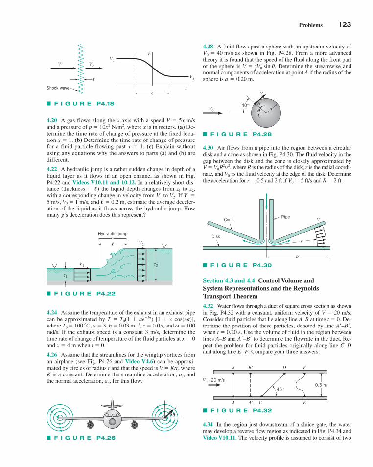
4.20 A gas flows along the x axis with a speed V � 5x m/sand a pressure of p � 10x2 N/m2, where x is in meters. (a) De-termine the time rate of change of pressure at the fixed loca-tion x � 1. (b) Determine the time rate of change of pressurefor a fluid particle flowing past x � 1. (c) Explain without using any equations why the answers to parts (a) and (b) aredifferent.

4.22 A hydraulic jump is a rather sudden change in depth of aliquid layer as it flows in an open channel as shown in Fig.P4.22 and Videos V10.11 and 10.12. In a relatively short dis-tance (thickness � �) the liquid depth changes from z1 to z2,with a corresponding change in velocity from V1 to V2. If V1 �5 m/s, V2 � 1 m/s, and � � 0.2 m, estimate the average deceler-ation of the liquid as it flows across the hydraulic jump. Howmany g’s deceleration does this represent?

4.24 Assume the temperature of the exhaust in an exhaust pipecan be approximated by T � T0(1 � ae�bx) [1 � c cos(�t)],where T0 � 100 �C, a � 3, b � 0.03 m�1, c � 0.05, and � � 100rad/s. If the exhaust speed is a constant 3 m/s, determine thetime rate of change of temperature of the fluid particles at x � 0and x � 4 m when t � 0.

4.26 Assume that the streamlines for the wingtip vortices froman airplane (see Fig. P4.26 and Video V4.6) can be approxi-mated by circles of radius r and that the speed is V � K/r, whereK is a constant. Determine the streamline acceleration, as, andthe normal acceleration, an, for this flow.

4.28 A fluid flows past a sphere with an upstream velocity ofas shown in Fig. P4.28. From a more advanced

theory it is found that the speed of the fluid along the front partof the sphere is Determine the streamwise andnormal components of acceleration at point A if the radius of thesphere is a � 0.20 m.

V � 32V0 sin �.

V0 � 40 m/s

4.30 Air flows from a pipe into the region between a circulardisk and a cone as shown in Fig. P4.30. The fluid velocity in thegap between the disk and the cone is closely approximated by V � V0R2/r2, where R is the radius of the disk, r is the radial coordi-nate, and V0 is the fluid velocity at the edge of the disk. Determinethe acceleration for r � 0.5 and 2 ft if V0 � 5 ft/s and R � 2 ft.

Section 4.3 and 4.4 Control Volume and System Representations and the Reynolds Transport Theorem

4.32 Water flows through a duct of square cross section as shownin Fig. P4.32 with a constant, uniform velocity of V � 20 m/s.Consider fluid particles that lie along line A–B at time t � 0. De-termine the position of these particles, denoted by line A�–B�,when t � 0.20 s. Use the volume of fluid in the region betweenlines A–B and A�–B� to determine the flowrate in the duct. Re-peat the problem for fluid particles originally along line C–Dand along line E–F. Compare your three answers.

Problems 123

Shock wave

V2V1

�V2

V1

V

�x

F I G U R E P4.18

�

Hydraulic jump

z1

V1

V2

z2

F I G U R E P4.22

F I G U R E P4.26

r

θ

V

Aaθ

40°V0

F I G U R E P4.28

PipeCone

Disk

R

V

r

F I G U R E P4.30

V = 20 m/s

B B' D F

A A' C E

45°0.5 m

F I G U R E P4.32

4.34 In the region just downstream of a sluice gate, the watermay develop a reverse flow region as indicated in Fig. P4.34 andVideo V10.11. The velocity profile is assumed to consist of two

c04Fluidkinematics.qxd 9/24/10 1:04 PM Page 123

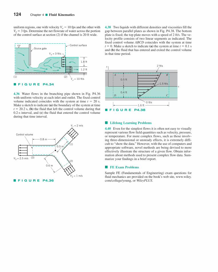
124 Chapter 4 ■ Fluid Kinematics

uniform regions, one with velocity Va � 10 fps and the other withVb � 3 fps. Determine the net flowrate of water across the portionof the control surface at section (2) if the channel is 20 ft wide.

4.36 Water flows in the branching pipe shown in Fig. P4.36with uniform velocity at each inlet and outlet. The fixed controlvolume indicated coincides with the system at time t � 20 s.Make a sketch to indicate (a) the boundary of the system at timet � 20.2 s, (b) the fluid that left the control volume during that0.2-s interval, and (c) the fluid that entered the control volumeduring that time interval.

4.38 Two liquids with different densities and viscosities fill thegap between parallel plates as shown in Fig. P4.38. The bottomplate is fixed; the top plate moves with a speed of 2 ft/s. The ve-locity profile consists of two linear segments as indicated. Thefixed control volume ABCD coincides with the system at time t � 0. Make a sketch to indicate (a) the system at time t � 0.1 sand (b) the fluid that has entered and exited the control volumein that time period.

■ Lifelong Learning Problems

4.40 Even for the simplest flows it is often not easy to visuallyrepresent various flow field quantities such as velocity, pressure,or temperature. For more complex flows, such as those involv-ing three-dimensional or unsteady effects, it is extremely diffi-cult to “show the data.” However, with the use of computers andappropriate software, novel methods are being devised to moreeffectively illustrate the structure of a given flow. Obtain infor-mation about methods used to present complex flow data. Sum-marize your findings in a brief report.

■ FE Exam Problems

Sample FE (Fundamentals of Engineering) exam questions forfluid mechanics are provided on the book’s web site, www.wiley.com/college/young, or WileyPLUS.

Sluice gateControl surface

Vb = 3 ft/s

Va = 10 ft/s

1.8 ft

1.2 ft

(1) (2)

F I G U R E P4.34

0.8 m

Control volume

0.6 m

0.5 m(1)

(2)(3)V3 = 2.5 m/s

V2 = 1 m/s

V1 = 2 m/s

F I G U R E P4.36

F I G U R E P4.38

1.6 ft

A

D

B

C

y

x

0.5 ft

1.5 ft/s

2 ft/s

0 ft/s

0.4 ft

c04Fluidkinematics.qxd 9/24/10 1:04 PM Page 124

125

CHAPTER OPENING PHOTO: Wind turbine farms (this is the Middelgrunden Offshore Wind Farm inDenmark) are becoming more common. Finite control volume analysis can be used to estimate theamount of energy transferred between the moving air and each turbine rotor. (Photograph courtesy ofSiemens Wind Power.)

Learn ing Ob j ec t i v e s

After completing this chapter, you should be able to:

■ identify an appropriate control volume and draw the correspondingdiagram.

■ calculate flowrates using the continuity equation.

■ calculate forces and torques using the linear momentum and moment-of-momentum equations.

■ use the energy equation to account for losses due to friction, as well aseffects of pumps and turbines.

■ apply the kinetic energy coefficient to nonuniform flows.

Many practical problems in fluid mechanics require analysis of the behavior of the contentsof a finite region in space (a control volume). For example, we may be asked to calculate theanchoring force required to hold a jet engine in place during a test. Important questions canbe answered readily with finite control volume analyses. The bases of this analysis methodare some fundamental principles of physics, namely, conservation of mass, Newton’s second

55Finite ControlVolume Analysis

Finite ControlVolume Analysis

c05FiniteControlVolumeAnalysis.qxd 9/25/10 4:02 PM Page 125

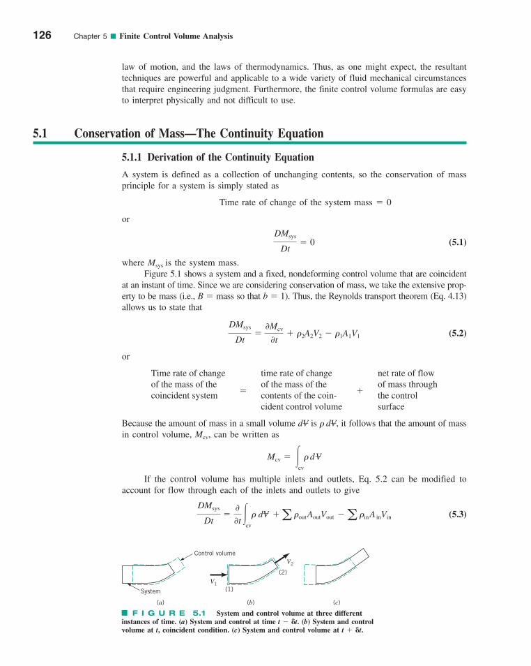
law of motion, and the laws of thermodynamics. Thus, as one might expect, the resultanttechniques are powerful and applicable to a wide variety of fluid mechanical circumstancesthat require engineering judgment. Furthermore, the finite control volume formulas are easyto interpret physically and not difficult to use.

126 Chapter 5 ■ Finite Control Volume Analysis

5.1 Conservation of Mass—The Continuity Equation

5.1.1 Derivation of the Continuity Equation

A system is defined as a collection of unchanging contents, so the conservation of massprinciple for a system is simply stated as

Time rate of change of the system mass � 0

or

(5.1)

where Msys is the system mass.Figure 5.1 shows a system and a fixed, nondeforming control volume that are coincident

at an instant of time. Since we are considering conservation of mass, we take the extensive prop-erty to be mass (i.e., B � mass so that b � 1). Thus, the Reynolds transport theorem (Eq. 4.13)allows us to state that

(5.2)

or

Because the amount of mass in a small volume is , it follows that the amount of massin control volume, Mcv, can be written as

If the control volume has multiple inlets and outlets, Eq. 5.2 can be modified toaccount for flow through each of the inlets and outlets to give

(5.3)DMsys

Dt�

00t �

cv

� dV �a �outAoutVout �a �inA inVin

Mcv � �cv

� d V

� dVdV

Time rate of change time rate of change net rate of flowof the mass of the

�of the mass of the

�of mass through

coincident system contents of the coin- the controlcident control volume surface

DMsys

Dt�

0Mcv

0t� �2A2V2 � �1A1V1

DMsys

Dt� 0

System

Control volume

(a) (b)

(1)

(2)

(c)

V1

V2

F I G U R E 5.1 System and control volume at three differentinstances of time. (a) System and control at time t � �t. (b) System and controlvolume at t, coincident condition. (c) System and control volume at t � �t.

c05FiniteControlVolumeAnalysis.qxd 9/24/10 1:21 PM Page 126

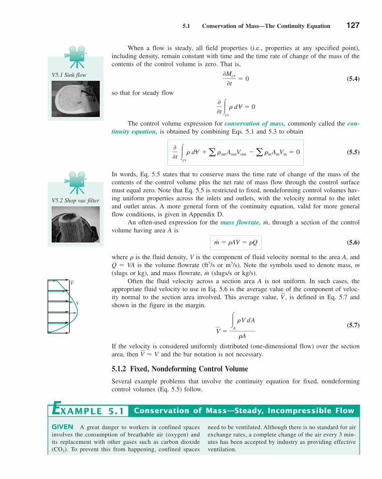
5.1 Conservation of Mass—The Continuity Equation 127

When a flow is steady, all field properties (i.e., properties at any specified point),including density, remain constant with time and the time rate of change of the mass of thecontents of the control volume is zero. That is,

(5.4)

so that for steady flow

The control volume expression for conservation of mass, commonly called the con-tinuity equation, is obtained by combining Eqs. 5.1 and 5.3 to obtain

(5.5)

In words, Eq. 5.5 states that to conserve mass the time rate of change of the mass of thecontents of the control volume plus the net rate of mass flow through the control surfacemust equal zero. Note that Eq. 5.5 is restricted to fixed, nondeforming control volumes hav-ing uniform properties across the inlets and outlets, with the velocity normal to the inletand outlet areas. A more general form of the continuity equation, valid for more generalflow conditions, is given in Appendix D.

An often-used expression for the mass flowrate, , through a section of the controlvolume having area A is

(5.6)

where � is the fluid density, V is the component of fluid velocity normal to the area A, andQ � VA is the volume flowrate (ft3/s or m3/s). Note the symbols used to denote mass, m(slugs or kg), and mass flowrate, (slugs/s or kg/s).

Often the fluid velocity across a section area A is not uniform. In such cases, theappropriate fluid velocity to use in Eq. 5.6 is the average value of the component of veloc-ity normal to the section area involved. This average value, , is defined in Eq. 5.7 andshown in the figure in the margin.

(5.7)

If the velocity is considered uniformly distributed (one-dimensional flow) over the sectionarea, then and the bar notation is not necessary.

5.1.2 Fixed, Nondeforming Control Volume

Several example problems that involve the continuity equation for fixed, nondeformingcontrol volumes (Eq. 5.5) follow.

V � V

V �

�A

� V d A

�A

V

m#

m# � �AV � �Q

m#

00t

�cv

� dV �a �outAoutVout �a �inAinVin � 0

00t �

cv

� d V � 0

0Mcv

0t� 0

V5.1 Sink flow

V5.2 Shop vac filter

V

V

GIVEN A great danger to workers in confined spacesinvolves the consumption of breathable air (oxygen) andits replacement with other gases such as carbon dioxide(CO2). To prevent this from happening, confined spaces

Conservation of Mass—Steady, Incompressible Flow

need to be ventilated. Although there is no standard for airexchange rates, a complete change of the air every 3 min-utes has been accepted by industry as providing effectiveventilation.

EXAMPLE 5.1

c05FiniteControlVolumeAnalysis.qxd 9/24/10 1:21 PM Page 127

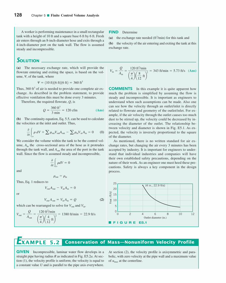
128 Chapter 5 ■ Finite Control Volume Analysis

A worker is performing maintenance in a small rectangulartank with a height of 10 ft and a square base 6 ft by 6 ft. Freshair enters through an 8-inch-diameter hose and exits through a4-inch-diameter port on the tank wall. The flow is assumedsteady and incompressible.

SOLUTION

FIND Determine

(a) the exchange rate needed (ft3/min) for this tank and

(b) the velocity of the air entering and exiting the tank at thisexchange rate.

(Ans)

COMMENTS In this example it is quite apparent howmuch the problem is simplified by assuming the flow issteady and incompressible. It is important as engineers tounderstand when such assumptions can be made. Also onecan see how the velocity through an outlet/inlet is directlyrelated to flowrate and geometry of the outlet/inlet. For ex-ample, if the air velocity through the outlet causes too muchdust to be stirred up, the velocity could be decreased by in-creasing the diameter of the outlet. The relationship be-tween velocity and diameter is shown in Fig. E5.1. As ex-pected, the velocity is inversely proportional to the squareof the diameter.

As mentioned, there is no written standard for air ex-change rates, but changing the air every 3 minutes has beenaccepted by industry. It is important for engineers to under-stand that individual industries and companies will havetheir own established safety precautions, depending on thenature of their work. As an engineer one must heed these pre-cautions. Safety is always a key component in the designprocess.

Vin �Q

Ain�

120 ft2/min

a�

4b a

8

12 ftb

2� 343 ft/min � 5.73 ft/s

(a) The necessary exchange rate, which will provide theflowrate entering and exiting the space, is based on the vol-ume, of the tank, where

Thus, 360 ft3 of air is needed to provide one complete air ex-change. As described in the problem statement, to provideeffective ventilation this must be done every 3 minutes.

Therefore, the required flowrate, Q, is

(Ans)

(b) The continuity equation, Eq. 5.5, can be used to calculatethe velocities at the inlet and outlet. Thus,

(1)

We consider the volume within the tank to be the control vol-ume, Ain the cross-sectional area of the hose as it protrudesthrough the tank wall, and Aout the area of the port in the tankwall. Since the flow is assumed steady and incompressible,

and

Thus, Eq. 1 reduces to

or

(2)

which can be rearranged to solve for and .

Vout �Q

Aout�

120 ft2/min

a�

4b a

4

12 ftb

2� 1380 ft/min � 22.9 ft/s

VinVout

Vout Aout � Vin Ain � Q

Vout Aout � Vin Ain � 0

�out � �in

00t �cv

�dV � 0

00t �

cv

� dV �a �outVoutAout �a �inV in Ain � 0

Q �360 ft3

3 min� 120 cfm

V � 110 ft2 16 ft2 16 ft2 � 360 ft3

V,

F I G U R E E5.1

Outlet diameter (in.)

Vou

t (f

t/s)

6 8 10 12420

25

0

5

10

15

20(4 in., 22.9 ft/s)

GIVEN Incompressible, laminar water flow develops in astraight pipe having radius R as indicated in Fig. E5.2a. At sec-tion (1), the velocity profile is uniform; the velocity is equal toa constant value U and is parallel to the pipe axis everywhere.

At section (2), the velocity profile is axisymmetric and para-bolic, with zero velocity at the pipe wall and a maximum valueof umax at the centerline.

Conservation of Mass—Nonuniform Velocity ProfileEXAMPLE 5.2

c05FiniteControlVolumeAnalysis.qxd 9/24/10 1:21 PM Page 128

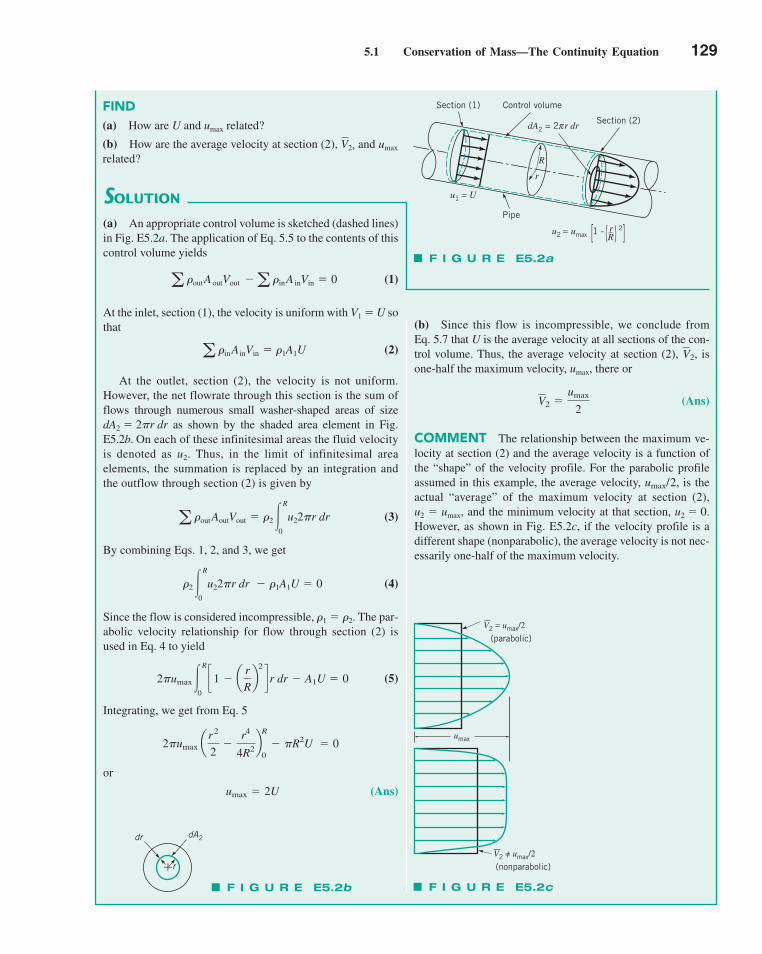
5.1 Conservation of Mass—The Continuity Equation 129

SOLUTION

(b) Since this flow is incompressible, we conclude fromEq. 5.7 that U is the average velocity at all sections of the con-trol volume. Thus, the average velocity at section (2), , isone-half the maximum velocity, umax, there or

(Ans)

COMMENT The relationship between the maximum ve-locity at section (2) and the average velocity is a function ofthe “shape” of the velocity profile. For the parabolic profileassumed in this example, the average velocity, is theactual “average” of the maximum velocity at section (2),

and the minimum velocity at that section, u2 � 0.However, as shown in Fig. E5.2c, if the velocity profile is adifferent shape (nonparabolic), the average velocity is not nec-essarily one-half of the maximum velocity.

u2 � umax,

umax/2,

V2 �umax

2

V2

(a) An appropriate control volume is sketched (dashed lines)in Fig. E5.2a. The application of Eq. 5.5 to the contents of thiscontrol volume yields

(1)

At the inlet, section (1), the velocity is uniform with V1 � U sothat

(2)

At the outlet, section (2), the velocity is not uniform.However, the net flowrate through this section is the sum offlows through numerous small washer-shaped areas of sizedA2 � 2�r dr as shown by the shaded area element in Fig.E5.2b. On each of these infinitesimal areas the fluid velocityis denoted as u2. Thus, in the limit of infinitesimal areaelements, the summation is replaced by an integration andthe outflow through section (2) is given by

(3)

By combining Eqs. 1, 2, and 3, we get

(4)

Since the flow is considered incompressible, �1 � �2. The par-abolic velocity relationship for flow through section (2) isused in Eq. 4 to yield

(5)

Integrating, we get from Eq. 5

or

(Ans)umax � 2U

2�umax ar2

2�

r4

4R2bR

0� �R2U � 0

2�umax�R

0

c1 � ar

Rb

2

d r dr � A1U � 0

�2�R

0

u22�r dr � �1A1U � 0

a �outAoutVout � �2�R

0

u22�r dr

a �inAinVin � �1A1U

a �outA outVout �a �inA inVin � 0

FIND(a) How are U and umax related?

(b) How are the average velocity at section (2), and umax

related?V2,

F I G U R E E5.2a

Section (1) Control volume

dA2 = 2 r drπ Section (2)

Pipe

R

r

u1 = U

u2 = umax 1 - r 2

_R( )[ ]

F I G U R E E5.2b

�

dA2dr

r

V2 = umax/2

(parabolic)

V2 = umax/2

(nonparabolic)

umax

F I G U R E E5.2c

c05FiniteControlVolumeAnalysis.qxd 9/24/10 4:47 PM Page 129

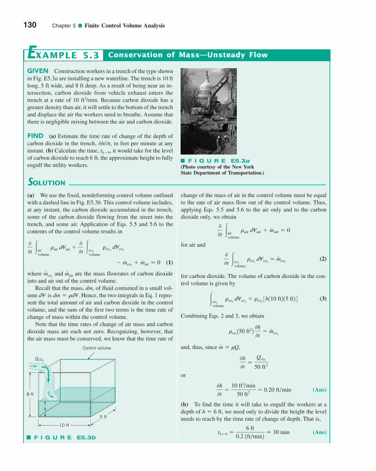
130 Chapter 5 ■ Finite Control Volume Analysis

GIVEN Construction workers in a trench of the type shownin Fig. E5.3a are installing a new waterline. The trench is 10 ftlong, 5 ft wide, and 8 ft deep. As a result of being near an in-tersection, carbon dioxide from vehicle exhaust enters thetrench at a rate of 10 ft3/min. Because carbon dioxide has agreater density than air, it will settle to the bottom of the trenchand displace the air the workers need to breathe. Assume thatthere is negligible mixing between the air and carbon dioxide.

FIND (a) Estimate the time rate of change of the depth ofcarbon dioxide in the trench, in feet per minute at anyinstant. (b) Calculate the time, it would take for the levelof carbon dioxide to reach 6 ft, the approximate height to fullyengulf the utility workers.

th�6,0h/0t,

SOLUTION

Conservation of Mass—Unsteady Flow

change of the mass of air in the control volume must be equalto the rate of air mass flow out of the control volume. Thus,applying Eqs. 5.5 and 5.6 to the air only and to the carbondioxide only, we obtain

for air and

(2)

for carbon dioxide. The volume of carbon dioxide in the con-trol volume is given by

(3)

Combining Eqs. 2 and 3, we obtain

and, thus, since

or

(Ans)

(b) To find the time it will take to engulf the workers at adepth of we need only to divide the height the levelneeds to reach by the time rate of change of depth. That is,

(Ans)th�6 �6 ft

0.2 1ft�min2� 30 min

h � 6 ft,

0h

0t�

10 ft3�min

50 ft2 � 0.20 ft�min

0h

0t�

Qco2

50 ft2

m#

� �Q,

�co2150 ft22

0h

0t� m

#co2

�co2volume

�co2 dVco2

� �co23h110 ft2 15 ft2 4

00t

�co2volume

�co2 dVco2

� m#

co2

00t

�airvolume

�air dVair � m#

air � 0

EXAMPLE 5.3

(a) We use the fixed, nondeforming control volume outlinedwith a dashed line in Fig. E5.3b. This control volume includes,at any instant, the carbon dioxide accumulated in the trench,some of the carbon dioxide flowing from the street into thetrench, and some air. Application of Eqs. 5.5 and 5.6 to thecontents of the control volume results in

(1)

where are the mass flowrates of carbon dioxideinto and air out of the control volume.

Recall that the mass, dm, of fluid contained in a small vol-ume Hence, the two integrals in Eq. 1 repre-sent the total amount of air and carbon dioxide in the controlvolume, and the sum of the first two terms is the time rate ofchange of mass within the control volume.

Note that the time rates of change of air mass and carbondioxide mass are each not zero. Recognizing, however, thatthe air mass must be conserved, we know that the time rate of

dV� is dm � �dV�.

m#

co2 and m

#air

� m#

co2� m

#air � 0

00t

�airvolume

�air dVair �00t

�co2volume

�co2 dVco2

F I G U R E E5.3a(Photo courtesy of the New YorkState Department of Transportation.)

h

5 ft

10 ft

8 ft

Control volume

QCO2

F I G U R E E5.3b

c05FiniteControlVolumeAnalysis.qxd 9/24/10 1:21 PM Page 130

5.1 Conservation of Mass—The Continuity Equation 131

The preceding example problems illustrate that when the flow is steady, the time rateof change of the mass of the contents of the control volume is zero and the net amount ofmass flowrate, , through the control surface is, therefore, also zero

(5.8)

If the steady flow is also incompressible, the net amount of volume flowrate, Q, throughthe control surface is also zero

(5.9)

When the flow is unsteady, the instantaneous time rate of change of the mass of the con-tents of the control volume is not necessarily zero.

For steady flow involving only one stream of a specific fluid flowing through the con-trol volume at sections (1) and (2),

(5.10)

and for incompressible flow,

(5.11)Q � A1V1 � A2V2

m#

� �1A1V1 � �2A2V2

a Qout �a Qin � 0

a m#

out �a m#

in � 0

m�

COMMENTS As shown in this example, it would nottake long for the air within the confined space of the trench tobe displaced enough to become a danger to the workers. Fur-thermore, by the time workers feel the effects of an oxygen-deficient atmosphere, they may be unable to remove them-selves from the dangerous space.

Note that the answer to part (b) can be easily obtained byrealizing that the accumulated volume, , of a flow is theV�

flowrate, Q, times the time it has been flowing, t. That is,� Qt. For this example, the volume of the carbon diox-

ide in the trench when it is 6 ft deep (neglecting the vol-ume of the workers and equipment within the trench) is

Thus, with a flowrate of Q � 10 ft3/min, th �6 � 300 ft3/10 ft3/min � 30 min in agree-ment with the foregoing answer.

V� � 5 ft � 10 ft � 6 ft � 300 ft3.

V�

F l u i d s i n t h e N e w s

New 1.6-gpf standards Toilets account for approximately 40%of all indoor household water use. To conserve water, the newstandard is 1.6 gallons of water per flush (gpf). Old toilets useup to 7 gpf; those manufactured after 1980 use 3.5 gpf. Neitheris considered a low-flush toilet. A typical 3.2-person householdin which each person flushes a 7-gpf toilet 4 times a day uses32,700 gallons of water each year; with a 3.5-gpf toilet theamount is reduced to 16,400 gallons. Clearly the new 1.6-gpftoilets will save even more water. However, designing a toilet

that flushes properly with such a small amount of water is notsimple. Today there are two basic types involved: those that aregravity powered and those that are pressure powered. Gravitytoilets (typical of most currently in use) have rather long cycletimes. The water starts flowing under the action of gravity andthe swirling vortex motion initiates the siphon action that buildsto a point of discharge. In the newer pressure-assisted models,the flowrate is large but the cycle time is short and the amountof water used is relatively small. (See Problem 5.18.)

V5.3 Flow througha contraction

5.1.3 Moving, Nondeforming Control Volume

When a moving control volume is used, the velocity relative to the moving control volume (rel-ative velocity) is an important flow field variable. The relative velocity, W, is the fluid velocityseen by an observer moving with the control volume. The control volume velocity, Vcv, is thevelocity of the control volume as seen from a fixed coordinate system. The absolute velocity,V, is the fluid velocity seen by a stationary observer in a fixed coordinate system. As indicatedby the figure in the margin, these velocities are related to each other by the vector equation

(5.12)V � W � Vcv

V VCV

W

c05FiniteControlVolumeAnalysis.qxd 9/24/10 1:21 PM Page 131

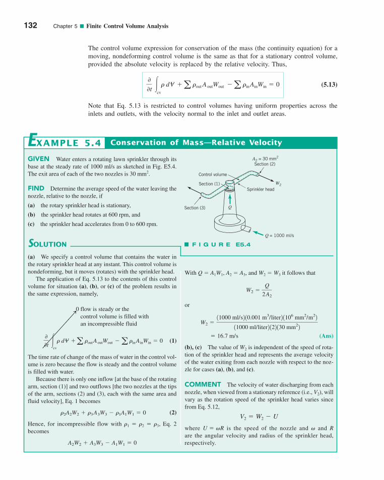
The control volume expression for conservation of the mass (the continuity equation) for amoving, nondeforming control volume is the same as that for a stationary control volume,provided the absolute velocity is replaced by the relative velocity. Thus,

(5.13)

Note that Eq. 5.13 is restricted to control volumes having uniform properties across theinlets and outlets, with the velocity normal to the inlet and outlet areas.

00t

�cv

� d V �a �out A outWout �a �inAinWin � 0

132 Chapter 5 ■ Finite Control Volume Analysis

GIVEN Water enters a rotating lawn sprinkler through itsbase at the steady rate of 1000 ml/s as sketched in Fig. E5.4.The exit area of each of the two nozzles is 30 mm2.

FIND Determine the average speed of the water leaving thenozzle, relative to the nozzle, if

(a) the rotary sprinkler head is stationary,

(b) the sprinkler head rotates at 600 rpm, and

(c) the sprinkler head accelerates from 0 to 600 rpm.

SOLUTION

Conservation of Mass—Relative Velocity

With Q � A1W1, A2 � A3, and W2 � W3 it follows that

or

(Ans)

(b), (c) The value of W2 is independent of the speed of rota-tion of the sprinkler head and represents the average velocityof the water exiting from each nozzle with respect to the noz-zle for cases (a), (b), and (c).

COMMENT The velocity of water discharging from eachnozzle, when viewed from a stationary reference (i.e., V2), willvary as the rotation speed of the sprinkler head varies sincefrom Eq. 5.12,

where U � �R is the speed of the nozzle and � and Rare the angular velocity and radius of the sprinkler head,respectively.

V2 � W2 � U

� 16.7 m/s

W2 �11000 ml/s2 10.001 m3/liter2 1106 mm2/m22

11000 ml/liter2 122 130 mm22

W2 �Q

2 A2

EXAMPLE 5.4

(a) We specify a control volume that contains the water inthe rotary sprinkler head at any instant. This control volume isnondeforming, but it moves (rotates) with the sprinkler head.

The application of Eq. 5.13 to the contents of this controlvolume for situation (a), (b), or (c) of the problem results inthe same expression, namely,

0 flow is steady or thecontrol volume is filled with an incompressible fluid

(1)

The time rate of change of the mass of water in the control vol-ume is zero because the flow is steady and the control volumeis filled with water.

Because there is only one inflow [at the base of the rotatingarm, section (1)] and two outflows [the two nozzles at the tipsof the arm, sections (2) and (3), each with the same area andfluid velocity], Eq. 1 becomes

(2)

Hence, for incompressible flow with �1 � �2 � �3, Eq. 2becomes

A2W2 � A3W3 � A1W1 � 0

�2A2W2 � �3A3W3 � �1A1W1 � 0

00t

�cv

� d V �a �outA outWout �a �inAinWin � 0

F I G U R E E5.4

Control volume

Section (3)

Sprinkler headW2

Q

Q = 1000 ml/s

Section (1)

A2 = 30 mm2

Section (2)

88888888888n

c05FiniteControlVolumeAnalysis.qxd 9/24/10 5:43 PM Page 132

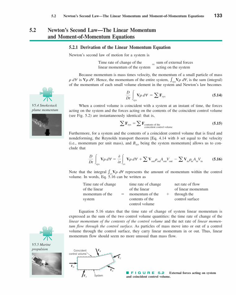
5.2 Newton’s Second Law—The Linear Momentum and Moment-of-Momentum Equations 133

5.2 Newton’s Second Law—The Linear Momentum and Moment-of-Momentum Equations

5.2.1 Derivation of the Linear Momentum Equation

Newton’s second law of motion for a system is

Because momentum is mass times velocity, the momentum of a small particle of mass

Time rate of change of thelinear momentum of the system

�sum of external forcesacting on the system

is V� d . Hence, the momentum of the entire system, , is the sum (integral)of the momentum of each small volume element in the system and Newton’s law becomes

(5.14)

When a control volume is coincident with a system at an instant of time, the forcesacting on the system and the forces acting on the contents of the coincident control volume(see Fig. 5.2) are instantaneously identical: that is,

(5.15)

Furthermore, for a system and the contents of a coincident control volume that is fixed andnondeforming, the Reynolds transport theorem [Eq. 4.14 with b set equal to the velocity(i.e., momentum per unit mass), and Bsys being the system momentum] allows us to con-clude that

(5.16)

Note that the integral represents the amount of momentum within the controlvolume. In words, Eq. 5.16 can be written as

Equation 5.16 states that the time rate of change of system linear momentum isexpressed as the sum of the two control volume quantities: the time rate of change of thelinear momentum of the contents of the control volume and the net rate of linear momen-tum flow through the control surface. As particles of mass move into or out of a controlvolume through the control surface, they carry linear momentum in or out. Thus, linearmomentum flow should seem no more unusual than mass flow.

Time rate of changeof the linearmomentum of thesystem

�

time rate of changeof the linearmomentum of thecontents of thecontrol volume

�

net rate of flowof linear momentumthrough thecontrol surface

�cvV� dV

D

Dt �

sys

V� d V �00t �

cv

V� d V �a Vout

�out

Aout

Vout

�a Vin

�in

Ain

Vin

a Fsys �a Fcontents of thecoincident control volume

D

Dt �

sys

V� d V �a Fsys

�sysV� dVV� d�V

V5.4 Smokestackplume momentum

V5.5 Marinepropulsion

FD

FA

FE

FC

FBCoincidentcontrol volume

SystemF I G U R E 5.2 External forces acting on system

and coincident control volume.

c05FiniteControlVolumeAnalysis.qxd 9/24/10 1:22 PM Page 133

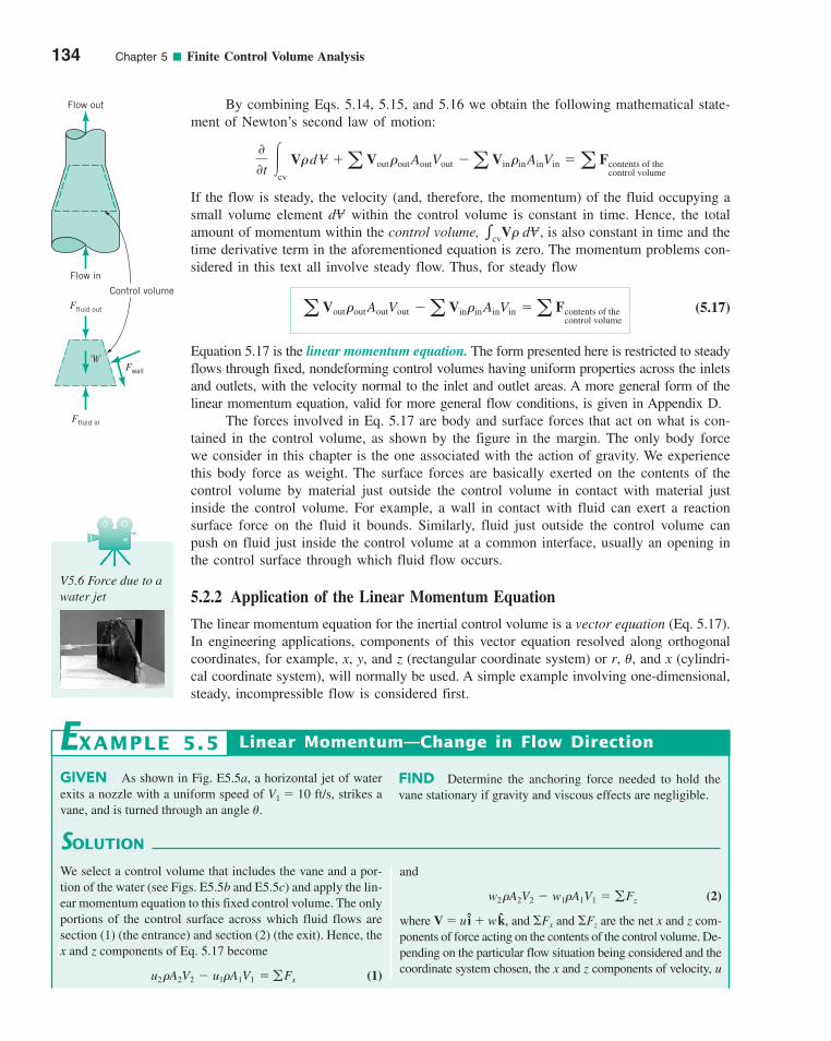
By combining Eqs. 5.14, 5.15, and 5.16 we obtain the following mathematical state-ment of Newton’s second law of motion:

If the flow is steady, the velocity (and, therefore, the momentum) of the fluid occupying asmall volume element within the control volume is constant in time. Hence, the totalamount of momentum within the control volume, , is also constant in time and thetime derivative term in the aforementioned equation is zero. The momentum problems con-sidered in this text all involve steady flow. Thus, for steady flow

(5.17)

Equation 5.17 is the linear momentum equation. The form presented here is restricted to steadyflows through fixed, nondeforming control volumes having uniform properties across the inletsand outlets, with the velocity normal to the inlet and outlet areas. A more general form of thelinear momentum equation, valid for more general flow conditions, is given in Appendix D.

The forces involved in Eq. 5.17 are body and surface forces that act on what is con-tained in the control volume, as shown by the figure in the margin. The only body forcewe consider in this chapter is the one associated with the action of gravity. We experiencethis body force as weight. The surface forces are basically exerted on the contents of thecontrol volume by material just outside the control volume in contact with material justinside the control volume. For example, a wall in contact with fluid can exert a reactionsurface force on the fluid it bounds. Similarly, fluid just outside the control volume canpush on fluid just inside the control volume at a common interface, usually an opening inthe control surface through which fluid flow occurs.

5.2.2 Application of the Linear Momentum Equation

The linear momentum equation for the inertial control volume is a vector equation (Eq. 5.17).In engineering applications, components of this vector equation resolved along orthogonalcoordinates, for example, x, y, and z (rectangular coordinate system) or r, �, and x (cylindri-cal coordinate system), will normally be used. A simple example involving one-dimensional,steady, incompressible flow is considered first.

a Vout�outAoutVout �a Vin�inAinVin �a Fcontents of thecontrol volume

�cvV� dVdV

00t

�cv

V� d V �a Vout�outAoutVout �a Vin�inAinVin �a Fcontents of thecontrol volume

134 Chapter 5 ■ Finite Control Volume Analysis

Flow out

Flow in

Control volume

Ffluid in

Ffluid out

Fwall

�

V5.6 Force due to awater jet

GIVEN As shown in Fig. E5.5a, a horizontal jet of waterexits a nozzle with a uniform speed of V1 � 10 ft/s, strikes avane, and is turned through an angle �.

FIND Determine the anchoring force needed to hold thevane stationary if gravity and viscous effects are negligible.

SOLUTION

Linear Momentum—Change in Flow Direction

and

(2)

where V � u i � w k, and �Fx and �Fz are the net x and z com-ponents of force acting on the contents of the control volume. De-pending on the particular flow situation being considered and thecoordinate system chosen, the x and z components of velocity, u

w2 �A2V2 � w1�A1V1 � gFz

EXAMPLE 5.5

We select a control volume that includes the vane and a por-tion of the water (see Figs. E5.5b and E5.5c) and apply the lin-ear momentum equation to this fixed control volume. The onlyportions of the control surface across which fluid flows aresection (1) (the entrance) and section (2) (the exit). Hence, thex and z components of Eq. 5.17 become

(1)u2 �A2V2 � u1�A1V1 �gFx

c05FiniteControlVolumeAnalysis.qxd 9/24/10 1:22 PM Page 134

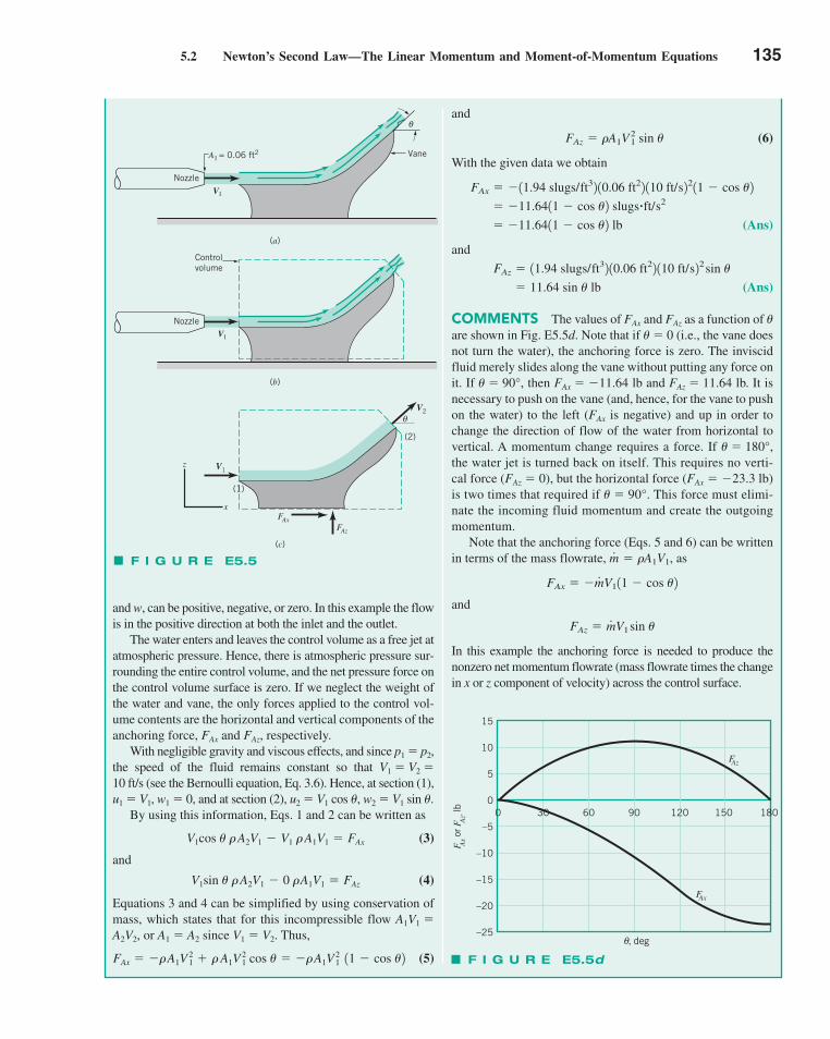
5.2 Newton’s Second Law—The Linear Momentum and Moment-of-Momentum Equations 135

and w, can be positive, negative, or zero. In this example the flowis in the positive direction at both the inlet and the outlet.

The water enters and leaves the control volume as a free jet atatmospheric pressure. Hence, there is atmospheric pressure sur-rounding the entire control volume, and the net pressure force onthe control volume surface is zero. If we neglect the weight ofthe water and vane, the only forces applied to the control vol-ume contents are the horizontal and vertical components of theanchoring force, FAx and FAz, respectively.

With negligible gravity and viscous effects, and since p1 � p2,the speed of the fluid remains constant so that V1 � V2 �10 ft/s (see the Bernoulli equation, Eq. 3.6). Hence, at section (1),u1 � V1, w1 � 0, and at section (2), u2 � V1 cos �, w2 � V1 sin �.

By using this information, Eqs. 1 and 2 can be written as

(3)

and

(4)

Equations 3 and 4 can be simplified by using conservation ofmass, which states that for this incompressible flow A1V1 �A2V2, or A1 � A2 since V1 � V2. Thus,

(5) FAx � ��A1V21 � � A1V

21 cos � � ��A1V

21 11 � cos �2

V1sin � � A2V1 � 0 � A1V1 � FAz

V1cos � � A2V1 � V1 � A1V1 � FAx

and

(6)

With the given data we obtain

(Ans)

and

(Ans)

COMMENTS The values of FAx and FAz as a function of �are shown in Fig. E5.5d. Note that if � � 0 (i.e., the vane doesnot turn the water), the anchoring force is zero. The inviscidfluid merely slides along the vane without putting any force onit. If � � 90°, then FAx � �11.64 lb and FAz � 11.64 lb. It isnecessary to push on the vane (and, hence, for the vane to pushon the water) to the left (FAx is negative) and up in order tochange the direction of flow of the water from horizontal tovertical. A momentum change requires a force. If � � 180°,the water jet is turned back on itself. This requires no verti-cal force (FAz � 0), but the horizontal force (FAx � �23.3 lb)is two times that required if � � 90°. This force must elimi-nate the incoming fluid momentum and create the outgoingmomentum.

Note that the anchoring force (Eqs. 5 and 6) can be writtenin terms of the mass flowrate, as

and

In this example the anchoring force is needed to produce thenonzero net momentum flowrate (mass flowrate times the changein x or z component of velocity) across the control surface.

FAz � m#V1 sin �

FAx � �m#V111 � cos �2

m#

� �A1V1,

� 11.64 sin � lb

FAz � 11.94 slugs/ft32 10.06 ft22 110 ft/s22 sin �

� �11.6411 � cos �2 lb

� �11.6411 � cos �2 slugs�ft/s2

FAx � �11.94 slugs/ft32 10.06 ft22 110 ft/s2211 � cos �2

FAz � �A1V21 sin �

Nozzle

A1 = 0.06 ft2 Vane

V1

(a)

θ

NozzleV1

(b)

Controlvolume

(c)

z

x

(2)

FAxFAz

V1

V2θ

(1)

F I G U R E E5.5d

–25

–20

–15

–10

–5

0

5

10

15

F Ax or

FA

z, lb 30 60 90 120 150 180

θ , deg

FAx

FAz

0

F I G U R E E5.5

c05FiniteControlVolumeAnalysis.qxd 9/24/10 1:22 PM Page 135

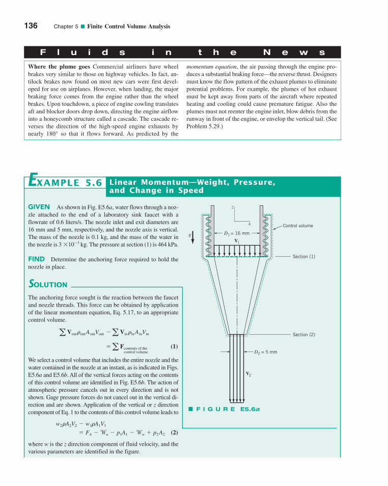
136 Chapter 5 ■ Finite Control Volume Analysis

F l u i d s i n t h e N e w s

Where the plume goes Commercial airliners have wheelbrakes very similar to those on highway vehicles. In fact, an-tilock brakes now found on most new cars were first devel-oped for use on airplanes. However, when landing, the majorbraking force comes from the engine rather than the wheelbrakes. Upon touchdown, a piece of engine cowling translatesaft and blocker doors drop down, directing the engine airflowinto a honeycomb structure called a cascade. The cascade re-verses the direction of the high-speed engine exhausts bynearly 180° so that it flows forward. As predicted by the

momentum equation, the air passing through the engine pro-duces a substantial braking force—the reverse thrust. Designersmust know the flow pattern of the exhaust plumes to eliminatepotential problems. For example, the plumes of hot exhaustmust be kept away from parts of the aircraft where repeatedheating and cooling could cause premature fatigue. Also theplumes must not reenter the engine inlet, blow debris from therunway in front of the engine, or envelop the vertical tail. (SeeProblem 5.29.)

GIVEN As shown in Fig. E5.6a, water flows through a noz-zle attached to the end of a laboratory sink faucet with aflowrate of 0.6 liters/s. The nozzle inlet and exit diameters are16 mm and 5 mm, respectively, and the nozzle axis is vertical.The mass of the nozzle is 0.1 kg, and the mass of the water inthe nozzle is 3 �10�3 kg. The pressure at section (1) is 464 kPa.

FIND Determine the anchoring force required to hold thenozzle in place.

SOLUTION

Linear Momentum—Weight, Pressure, and Change in Speed

EXAMPLE 5.6

The anchoring force sought is the reaction between the faucetand nozzle threads. This force can be obtained by applicationof the linear momentum equation, Eq. 5.17, to an appropriatecontrol volume.

(1)

We select a control volume that includes the entire nozzle and thewater contained in the nozzle at an instant, as is indicated in Figs.E5.6a and E5.6b. All of the vertical forces acting on the contentsof this control volume are identified in Fig. E5.6b. The action ofatmospheric pressure cancels out in every direction and is notshown. Gage pressure forces do not cancel out in the vertical di-rection and are shown. Application of the vertical or z directioncomponent of Eq. 1 to the contents of this control volume leads to

(2)

where w is the z direction component of fluid velocity, and thevarious parameters are identified in the figure.

� FA �wn � p1A1 �ww � p2 A2

w2 �A2V2 � w1�A1V1

�a Fcontents of thecontrol volume

a Vout �outAoutVout �a Vin �inAinVin

gV1

D1 = 16 mm

x

z

Control volume

Section (1)

Section (2)

D2 = 5 mm

V2

F I G U R E E5.6a

c05FiniteControlVolumeAnalysis.qxd 9/24/10 1:22 PM Page 136

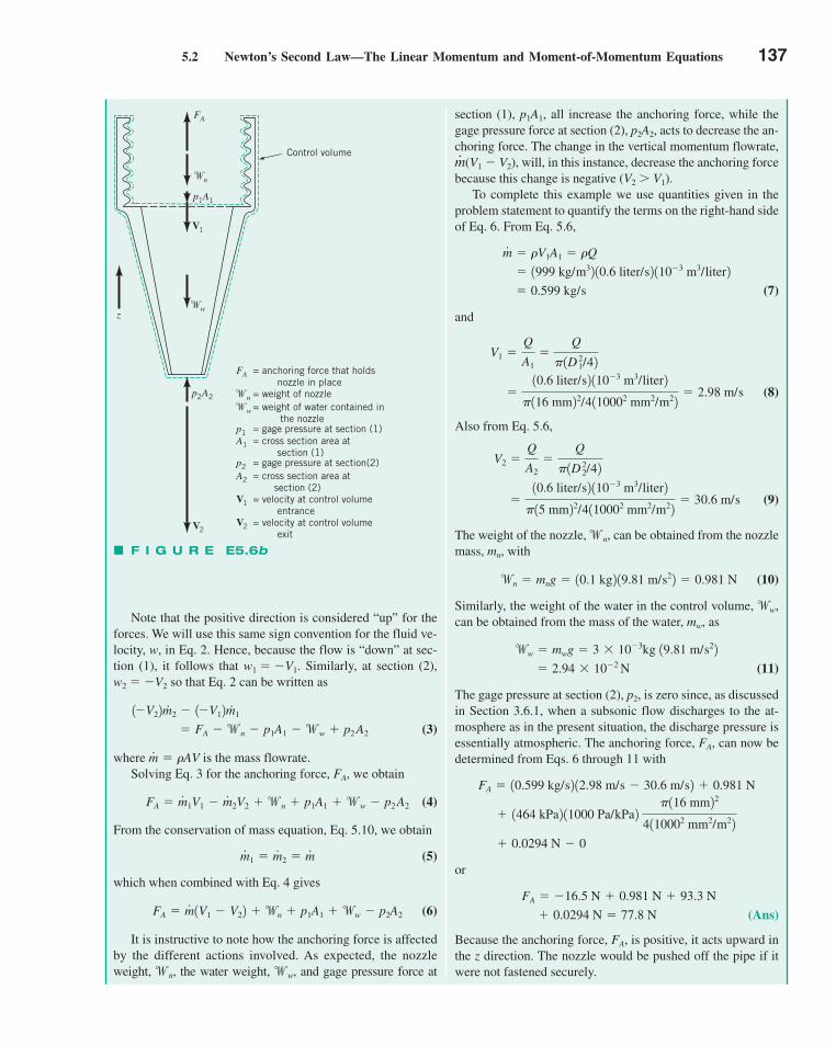
5.2 Newton’s Second Law—The Linear Momentum and Moment-of-Momentum Equations 137

Note that the positive direction is considered “up” for theforces. We will use this same sign convention for the fluid ve-locity, w, in Eq. 2. Hence, because the flow is “down” at sec-tion (1), it follows that w1 � �V1. Similarly, at section (2),w2 � �V2 so that Eq. 2 can be written as

(3)

where is the mass flowrate.Solving Eq. 3 for the anchoring force, FA, we obtain

(4)

From the conservation of mass equation, Eq. 5.10, we obtain

(5)

which when combined with Eq. 4 gives

(6)

It is instructive to note how the anchoring force is affectedby the different actions involved. As expected, the nozzleweight,wn, the water weight,ww, and gage pressure force at

FA � m#1V1 � V22 �wn � p1A1 �ww � p2A2

m#

1 � m#

2 � m#

FA � m#

1V1 � m#

2V2 �wn � p1A1 �ww � p2 A2

m#

� �AV

� FA �wn � p1A1 �ww � p2 A2

1�V22m#

2 � 1�V12m#

1

section (1), p1A1, all increase the anchoring force, while thegage pressure force at section (2), p2A2, acts to decrease the an-choring force. The change in the vertical momentum flowrate,

(V1 � V2), will, in this instance, decrease the anchoring forcebecause this change is negative (V2 � V1).

To complete this example we use quantities given in theproblem statement to quantify the terms on the right-hand sideof Eq. 6. From Eq. 5.6,

(7)

and

(8)

Also from Eq. 5.6,

(9)

The weight of the nozzle,wn, can be obtained from the nozzlemass, mn, with

(10)

Similarly, the weight of the water in the control volume,ww,can be obtained from the mass of the water, mw, as

(11)

The gage pressure at section (2), p2, is zero since, as discussedin Section 3.6.1, when a subsonic flow discharges to the at-mosphere as in the present situation, the discharge pressure isessentially atmospheric. The anchoring force, FA, can now bedetermined from Eqs. 6 through 11 with

or

(Ans)

Because the anchoring force, FA, is positive, it acts upward inthe z direction. The nozzle would be pushed off the pipe if itwere not fastened securely.

� 0.0294 N � 77.8 N

FA � �16.5 N � 0.981 N � 93.3 N

� 0.0294 N � 0

� 1464 kPa2 11000 Pa/kPa2 �116 mm22

4110002 mm2/m22

FA � 10.599 kg/s2 12.98 m/s � 30.6 m/s2 � 0.981 N

� 2.94 � 10�2 N

ww � mwg � 3 � 10�3kg 19.81 m/s22

wn � mng � 10.1 kg2 19.81 m/s22 � 0.981 N

�10.6 liter/s2 110�3 m3/liter2

�15 mm22/4110002 mm2/m22� 30.6 m/s

V2 �Q

A2�

Q

�1D 22/42

�10.6 liter/s2 110�3 m3/liter2

�116 mm22/4110002 mm2/m22� 2.98 m/s

V1 �Q

A1�

Q

�1D 21/42

� 0.599 kg/s

� 1999 kg/m32 10.6 liter/s2 110�3 m3/liter2

m#

� �V1A1 � �Q

m#

F I G U R E E5.6b

FA

�n

p1A1

V1

�w

p2A2

V2

z

Control volume

FA

�n

�w

p1A1

p2A2

V1

V2

= anchoring force that holds nozzle in place= weight of nozzle= weight of water contained in the nozzle= gage pressure at section (1)= cross section area at section (1)= gage pressure at section(2)= cross section area at section (2)= velocity at control volume entrance= velocity at control volume exit

c05FiniteControlVolumeAnalysis.qxd 9/24/10 1:22 PM Page 137

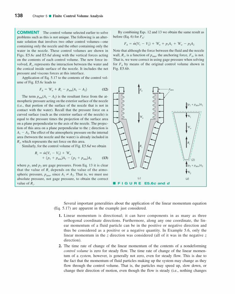
Several important generalities about the application of the linear momentum equation(Eq. 5.17) are apparent in the example just considered.

1. Linear momentum is directional; it can have components in as many as threeorthogonal coordinate directions. Furthermore, along any one coordinate, the lin-ear momentum of a fluid particle can be in the positive or negative direction andthus be considered as a positive or a negative quantity. In Example 5.6, only thelinear momentum in the z direction was considered (all of it was in the negative zdirection).

2. The time rate of change of the linear momentum of the contents of a nondeformingcontrol volume is zero for steady flow. The time rate of change of the linear momen-tum of a system, however, is generally not zero, even for steady flow. This is due tothe fact that the momentum of fluid particles making up the system may change as theyflow through the control volume. That is, the particles may speed up, slow down, orchange their direction of motion, even though the flow is steady (i.e., nothing changes

138 Chapter 5 ■ Finite Control Volume Analysis

COMMENT The control volume selected earlier to solveproblems such as this is not unique. The following is an alter-nate solution that involves two other control volumes—onecontaining only the nozzle and the other containing only thewater in the nozzle. These control volumes are shown inFigs. E5.6c and E5.6d along with the vertical forces actingon the contents of each control volume. The new force in-volved, Rz, represents the interaction between the water andthe conical inside surface of the nozzle. It includes the netpressure and viscous forces at this interface.

Application of Eq. 5.17 to the contents of the control vol-ume of Fig. E5.6c leads to

(12)

The term patm(A1 � A2) is the resultant force from the at-mospheric pressure acting on the exterior surface of the nozzle(i.e., that portion of the surface of the nozzle that is not incontact with the water). Recall that the pressure force on acurved surface (such as the exterior surface of the nozzle) isequal to the pressure times the projection of the surface areaon a plane perpendicular to the axis of the nozzle. The projec-tion of this area on a plane perpendicular to the z direction isA1 � A2. The effect of the atmospheric pressure on the internalarea (between the nozzle and the water) is already included inRz, which represents the net force on this area.

Similarly, for the control volume of Fig. E5.6d we obtain

(13)

where p1 and p2 are gage pressures. From Eq. 13 it is clearthat the value of Rz depends on the value of the atmo-spheric pressure, patm, since A1 � A2. That is, we must useabsolute pressure, not gage pressure, to obtain the correctvalue of Rz.

� 1p1 � patm2A1 � 1p2 � patm2A2

Rz � m#1V1 � V22 �ww

FA �wn � Rz � patm1A1 � A22

By combining Eqs. 12 and 13 we obtain the same result asbefore (Eq. 6) for FA:

Note that although the force between the fluid and the nozzlewall, Rz, is a function of patm, the anchoring force, FA, is not.That is, we were correct in using gage pressure when solvingfor FA by means of the original control volume shown inFig. E5.6b.

FA � m#1V1 � V22 �wn � p1A1 �ww � p2A2

FA

�n

Rz

patm

(c)

(p1 + patm)A1

�w

V1

V2

Rz

(p2 + patm)A2

(2)

(d)

F I G U R E E5.6c and d

c05FiniteControlVolumeAnalysis.qxd 9/24/10 1:22 PM Page 138

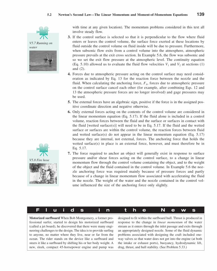
5.2 Newton’s Second Law—The Linear Momentum and Moment-of-Momentum Equations 139

with time at any given location). The momentum problems considered in this text allinvolve steady flow.

3. If the control surface is selected so that it is perpendicular to the flow where fluidenters or leaves the control volume, the surface force exerted at these locations byfluid outside the control volume on fluid inside will be due to pressure. Furthermore,when subsonic flow exits from a control volume into the atmosphere, atmosphericpressure prevails at the exit cross section. In Example 5.6, the flow was subsonic andso we set the exit flow pressure at the atmospheric level. The continuity equation(Eq. 5.10) allowed us to evaluate the fluid flow velocities V1 and V2 at sections (1)and (2).

4. Forces due to atmospheric pressure acting on the control surface may need consid-eration as indicated by Eq. 13 for the reaction force between the nozzle and thefluid. When calculating the anchoring force, FA, forces due to atmospheric pressureon the control surface cancel each other (for example, after combining Eqs. 12 and13 the atmospheric pressure forces are no longer involved) and gage pressures maybe used.

5. The external forces have an algebraic sign, positive if the force is in the assigned pos-itive coordinate direction and negative otherwise.

6. Only external forces acting on the contents of the control volume are considered inthe linear momentum equation (Eq. 5.17). If the fluid alone is included in a controlvolume, reaction forces between the fluid and the surface or surfaces in contact withthe fluid [wetted surface(s)] will need to be in Eq. 5.17. If the fluid and the wettedsurface or surfaces are within the control volume, the reaction forces between fluidand wetted surface(s) do not appear in the linear momentum equation (Eq. 5.17)because they are internal, not external, forces. The anchoring force that holds thewetted surface(s) in place is an external force, however, and must therefore be inEq. 5.17.

7. The force required to anchor an object will generally exist in response to surfacepressure and/or shear forces acting on the control surface, to a change in linearmomentum flow through the control volume containing the object, and to the weightof the object and the fluid contained in the control volume. In Example 5.6 the noz-zle anchoring force was required mainly because of pressure forces and partlybecause of a change in linear momentum flow associated with accelerating the fluidin the nozzle. The weight of the water and the nozzle contained in the control vol-ume influenced the size of the anchoring force only slightly.

V5.8 Fire hose

V5.7 Running onwater

F l u i d s i n t h e N e w s

Motorized surfboard When Bob Montgomery, a former pro-fessional surfer, started to design his motorized surfboard(called a jet board), he discovered that there were many engi-neering challenges to the design. The idea is to provide surfingto anyone, no matter where they live, near or far from theocean. The rider stands on the device like a surfboard andsteers it like a surfboard by shifting his or her body weight. Anew, sleek, compact 45-horsepower engine and pump was

designed to fit within the surfboard hull. Thrust is produced inresponse to the change in linear momentum of the waterstream as it enters through the inlet passage and exits throughan appropriately designed nozzle. Some of the fluid dynamicproblems associated with designing the craft included one-way valves so that water does not get into the engine (at boththe intake or exhaust ports), buoyancy, hydrodynamic lift,drag, thrust, and hull stability. (See Problem 5.33.)

c05FiniteControlVolumeAnalysis.qxd 9/24/10 1:22 PM Page 139

140 Chapter 5 ■ Finite Control Volume Analysis

GIVEN Water flows through a horizontal, 180 pipe bend asillustrated in Fig. E5.7a. The flow cross-sectional area is con-stant at a value of 0.1 ft2 through the bend. The flow velocityeverywhere in the bend is axial and 50 ft/s. The absolute pres-sures at the entrance and exit of the bend are 30 and 24 psia,respectively.

FIND Calculate the horizontal (x and y) components of theanchoring force required to hold the bend in place.

SOLUTION

Linear Momentum—Pressure and Change in Flow Direction

EXAMPLE 5.7

Since we want to evaluate components of the anchoringforce to hold the pipe bend in place, an appropriate controlvolume (see dashed line in Fig. E5.7a) contains the bendand the water in the bend at an instant. The horizontal forcesacting on the contents of this control volume are identifiedin Fig. E5.7b. Note that the weight of the water is vertical(in the negative z direction) and does not contribute to the xand y components of the anchoring force. All of the horizon-tal normal and tangential forces exerted on the fluid and thepipe bend are resolved and combined into the two resultantcomponents, FAx and FAy. These two forces act on the con-trol volume contents, and thus for the x direction, Eq. 5.17leads to

(1)

where

At sections (1) and (2), the flow is in the y direction and thereforeu � 0 at both cross sections. There is no x direction momentumflow into or out of the control volume, and we conclude fromEq. 1 that

FAx � 0 (Ans)

For the y direction, we get from Eq. 5.17

(2)

The y components of velocity, v1 and v2, at the inlet and out-let sections of the control volume are v1 � V1 � V andv2 � �V2 � �V, respectively, where V � V1 � V2 � 50 ft/s.Hence, Eq. 2 becomes

(3)

Note that the y component of velocity is positive at section(1) but is negative at section (2). From the continuity equa-tion (Eq. 5.10), we get

(4)m#

� �A2V2 � �A1V1

�V2 �A2V2 � V1�A1V1 � FAy � p1A1 � p2A2

v2 �A2V2 � v1�A1V1 � FAy � p1A1 � p2A2

VV � u i � v j � wk

u2 �A2V2 � u1�A1V1 � FAx

F I G U R E E5.7

z

yx

V = 50 ft/s

Section (1) A = 0.1 ft2

V = 50 ft/s

Section (2)

Controlvolume

180° pipe bend

(a)

xu v y

w

z

p1A1

V1

V2

p2A2

FAz

FAy

�

FAxControl volume

Pipe bendand water

(b)

and thus Eq. 3 can be written as

(5)

Solving Eq. 5 for FAy we obtain

(6)

From the given data we can calculate , the mass flowrate,from Eq. 4 as

For determining the anchoring force, FAy, the effects of at-mospheric pressure cancel and thus gage pressures for p1

and p2 are appropriate. By substituting numerical values ofvariables into Eq. 6 and using the fact that 1 lb � 1 slug ft/s2,we get

(Ans) FAy � �970 lb � 220 lb � 134 lb � �1324 lb

�124 psia � 14.7 psia2 1144 in.2/ft22 10.1 ft22

�130 psia � 14.7 psia2 1144 in.2/ft22 10.1 ft22

FAy � �19.70 slugs/s2 150 ft/s � 50 ft/s2

� 9.70 slugs/s

m#

� �1A1V1 � 11.94 slugs/ft32 10.1 ft22 150 ft/s2

m#

FAy � �m#1V1 � V22 � p1A1 � p2A2

�m#1V1 � V22 � FAy � p1A1 � p2A2

c05FiniteControlVolumeAnalysis.qxd 9/24/10 1:22 PM Page 140

5.2 Newton’s Second Law—The Linear Momentum and Moment-of-Momentum Equations 141

The negative sign for FAy is interpreted as meaning that the ycomponent of the anchoring force is actually in the negative ydirection, not the positive y direction as originally indicated inFig. E5.7b.

COMMENT As with Example 5.6, the anchoring forcefor the pipe bend is independent of the atmospheric pressure.However, the force that the bend puts on the fluid inside of it,Ry, depends on the atmospheric pressure. We can see this byusing a control volume that surrounds only the fluid within thebend as shown in Fig. E5.7c. Application of the momentumequation to this situation gives

where p1 and p2 must be in terms of absolute pressure becausethe force between the fluid and the pipe wall, Ry, is the com-plete pressure effect (i.e., absolute pressure).

Thus, we obtain

(7)

We can use the control volume that includes just the pipebend (without the fluid inside it) as shown in Fig. E5.7d todetermine FAy, the anchoring force component in the y direc-tion necessary to hold the bend stationary. The y componentof the momentum equation applied to this control volumegives

(8)

where Ry is given by Eq. 7. The patm (A1 � A2) term representsthe net pressure force on the outside portion of the control vol-ume. Recall that the pressure force on the inside of the bend is

FAy � Ry � patm 1A1 � A22

� �1748 lb

�124 psia2 1144 in.2/ft22 10.1 ft22

�130 psia2 1144 in.2/ft22 10.1 ft22

Ry � �19.70 slugs/s2 150 ft/s � 50 ft/s2

Ry � �m#1V1 � V22 � p1A1 � p2A2

accounted for by Ry. By combining Eqs. 7 and 8 and using thefact that weobtain

in agreement with the original answer obtained using thecontrol volume of Fig. E5.7b.

� �1324 lb

FAy � �1748 lb � 2117 lb/ft210.1 ft2 � 0.1 ft22

patm � 14.7 lb/in.2 1144 in.2/ft22 � 2117 lb/ft2,

F I G U R E E5.7

Control volume

Water in 180° bend

p2A2

p1A1

V2

V1

(c)

Pipe bend only

(d)

Ry patm(A1 + A2)

Rz

Ry

Rx

�

Control volume

FAy

xu v y

w

z

F l u i d s i n t h e N e w s

Bow thrusters In the past, large ships required the use oftugboats for precise maneuvering, especially when docking.Nowadays, most large ships (and many moderate to smallones as well) are equipped with bow thrusters to help steer inclose quarters. The units consist of a mechanism (usually aducted propeller mounted at right angles to the fore/aft axis ofthe ship) that takes water from one side of the bow and ejectsit as a water jet on the other side. The momentum flux of thisjet produces a starboard or port force on the ship for maneu-

vering. Sometimes a second unit is installed in the stern. Ini-tially used in the bows of ferries, these versatile control de-vices have became popular in offshore oil servicing boats,fishing vessels, and larger oceangoing craft. They permitunassisted maneuvering alongside of oil rigs, vessels, loadingplatforms, fishing nets, and docks. They also provide precisecontrol at slow speeds through locks, narrow channels, andbridges, where the rudder becomes very ineffective. (SeeProblem 5.42.)

From Examples 5.5, 5.6, and 5.7, we see that changes in flow speed and/or directionresult in a reaction force. Other types of problems that can be solved with the linear momen-tum equation (Eq. 5.17) are illustrated in the following examples.

c05FiniteControlVolumeAnalysis.qxd 9/24/10 1:22 PM Page 141

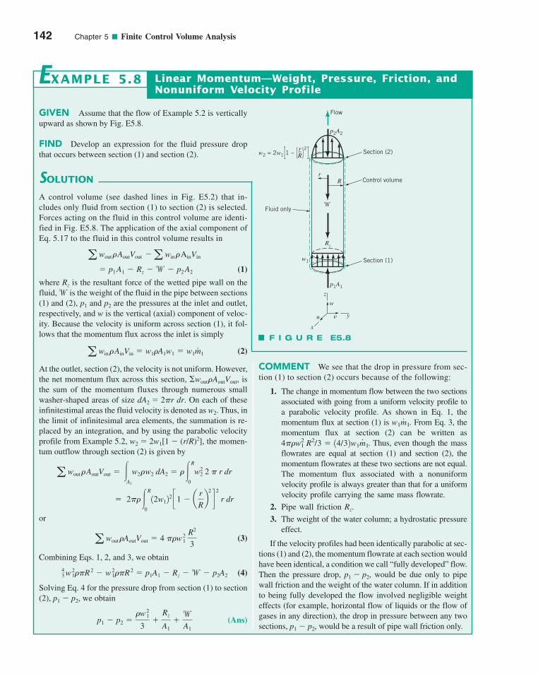
142 Chapter 5 ■ Finite Control Volume Analysis

GIVEN Assume that the flow of Example 5.2 is verticallyupward as shown by Fig. E5.8.

FIND Develop an expression for the fluid pressure dropthat occurs between section (1) and section (2).

SOLUTION

Linear Momentum—Weight, Pressure, Friction, andNonuniform Velocity Profile

EXAMPLE 5.8

A control volume (see dashed lines in Fig. E5.2) that in-cludes only fluid from section (1) to section (2) is selected.Forces acting on the fluid in this control volume are identi-fied in Fig. E5.8. The application of the axial component ofEq. 5.17 to the fluid in this control volume results in

(1)

where Rz is the resultant force of the wetted pipe wall on thefluid,w is the weight of the fluid in the pipe between sections(1) and (2), p1 and p2 are the pressures at the inlet and outlet,respectively, and w is the vertical (axial) component of veloc-ity. Because the velocity is uniform across section (1), it fol-lows that the momentum flux across the inlet is simply

(2)

At the outlet, section (2), the velocity is not uniform. However,the net momentum flux across this section, �wout�AoutVout, isthe sum of the momentum fluxes through numerous smallwasher-shaped areas of size dA2 � 2�r dr. On each of theseinfinitestimal areas the fluid velocity is denoted as w2. Thus, inthe limit of infinitesimal area elements, the summation is re-placed by an integration, and by using the parabolic velocityprofile from Example 5.2, w2 � 2w1[1 � (r/R)2], the momen-tum outflow through section (2) is given by

or

(3)

Combining Eqs. 1, 2, and 3, we obtain

(4)

Solving Eq. 4 for the pressure drop from section (1) to section(2), p1 � p2, we obtain

(Ans)p1 � p2 ��w 2

1

3�

Rz

A1�w

A1

43 w 2

1��R 2 � w 21��R 2 � p1A1 � Rz �w � p2A2

a wout�AoutVout � 4 ��w 21

R2

3

� 2���R

0

12w122 c1 � a

r

Rb

2

d2

r dr

a wout�AoutVout � �A2

w2�w2 dA2 � ��R

0

w22 2 � r dr

a win�AinVin � w1�A1w1 � w1m.

1

� p1 A1 � Rz �w � p2 A2

a wout�AoutVout �a win�AinVin

COMMENT We see that the drop in pressure from sec-tion (1) to section (2) occurs because of the following:

1. The change in momentum flow between the two sectionsassociated with going from a uniform velocity profile toa parabolic velocity profile. As shown in Eq. 1, themomentum flux at section (1) is . From Eq. 3, themomentum flux at section (2) can be written as

. Thus, even though the massflowrates are equal at section (1) and section (2), themomentum flowrates at these two sections are not equal.The momentum flux associated with a nonuniformvelocity profile is always greater than that for a uniformvelocity profile carrying the same mass flowrate.

2. Pipe wall friction Rz.

3. The weight of the water column; a hydrostatic pressureeffect.

If the velocity profiles had been identically parabolic at sec-tions (1) and (2), the momentum flowrate at each section wouldhave been identical, a condition we call “fully developed” flow.Then the pressure drop, p1 � p2, would be due only to pipewall friction and the weight of the water column. If in additionto being fully developed the flow involved negligible weighteffects (for example, horizontal flow of liquids or the flow ofgases in any direction), the drop in pressure between any twosections, p1 � p2, would be a result of pipe wall friction only.

4��w21 R2/3 � 14/32w1m

#1

w1m#

1

F I G U R E E5.8

Flow

p2A2

�

Rz

Rr

Fluid only

Control volume

Section (1)

Section (2)w2 = 2w1 1 – ( )[ ]r–R

2

p1A1

w1

x

u v y

w

z

c05FiniteControlVolumeAnalysis.qxd 9/24/10 1:22 PM Page 142

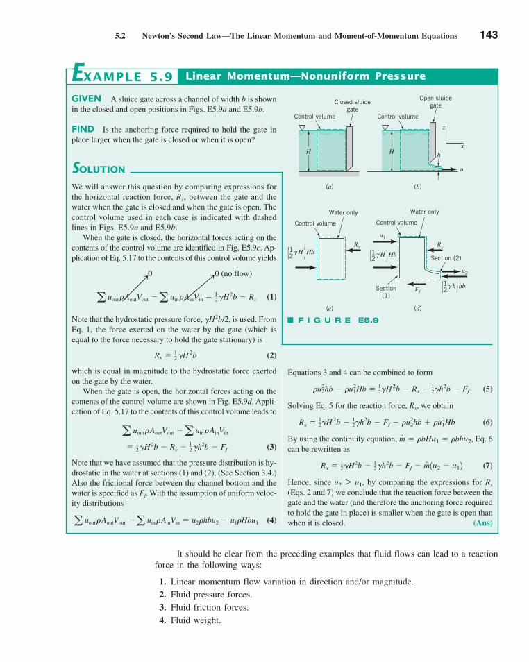
5.2 Newton’s Second Law—The Linear Momentum and Moment-of-Momentum Equations 143

It should be clear from the preceding examples that fluid flows can lead to a reactionforce in the following ways:

1. Linear momentum flow variation in direction and/or magnitude.

2. Fluid pressure forces.

3. Fluid friction forces.

4. Fluid weight.

GIVEN A sluice gate across a channel of width b is shownin the closed and open positions in Figs. E5.9a and E5.9b.

FIND Is the anchoring force required to hold the gate inplace larger when the gate is closed or when it is open?

SOLUTION

Linear Momentum—Nonuniform Pressure

Equations 3 and 4 can be combined to form

(5)

Solving Eq. 5 for the reaction force, Rx, we obtain

(6)

By using the continuity equation, Eq. 6can be rewritten as

(7)

Hence, since , by comparing the expressions for Rx

(Eqs. 2 and 7) we conclude that the reaction force between thegate and the water (and therefore the anchoring force requiredto hold the gate in place) is smaller when the gate is open thanwhen it is closed. (Ans)

u2 7 u1

Rx � 12 �H2b � 1

2 �h2b � Ff � m

#1u2 � u12

m#

� �bHu1 � �bhu2,

Rx � 12�H2b � 1

2�h2b � Ff � �u22hb � �u2

1Hb

�u22hb � �u2

1Hb � 12�H2b � Rx � 1

2�h2b � Ff

EXAMPLE 5.9

We will answer this question by comparing expressions forthe horizontal reaction force, Rx, between the gate and thewater when the gate is closed and when the gate is open. Thecontrol volume used in each case is indicated with dashedlines in Figs. E5.9a and E5.9b.

When the gate is closed, the horizontal forces acting on thecontents of the control volume are identified in Fig. E5.9c. Ap-plication of Eq. 5.17 to the contents of this control volume yields

0 0 (no flow)

(1)

Note that the hydrostatic pressure force, �H2b/2, is used. FromEq. 1, the force exerted on the water by the gate (which isequal to the force necessary to hold the gate stationary) is

(2)

which is equal in magnitude to the hydrostatic force exertedon the gate by the water.

When the gate is open, the horizontal forces acting on thecontents of the control volume are shown in Fig. E5.9d. Appli-cation of Eq. 5.17 to the contents of this control volume leads to

(3)

Note that we have assumed that the pressure distribution is hy-drostatic in the water at sections (1) and (2). (See Section 3.4.)Also the frictional force between the channel bottom and thewater is specified as Ff. With the assumption of uniform veloc-ity distributions

(4)a uout�AoutVout �a uin�AinVin � u2 �hbu2 � u1�Hbu1

� 12 �H 2b � Rx � 1

2 �h2b � Ff

a uout�AoutVout �a uin�AinVin

Rx � 12 �H2b

a uout�AoutVout �a uin�AinVin � 12 �H 2b � Rx

H

Control volume

Closed sluicegate

H

Control volume

Open sluicegate

hx

z

u

(a) (b)

Control volume

Water only

Control volume

Water only

u1

Rx

u2

( )1_2

γ H Hb( )1_2

γ H Hb

( )1_2

γ h hbFfSection

(1)

Section (2)

(c) (d)

Rx

F I G U R E E5.9

88888n

888888n

c05FiniteControlVolumeAnalysis.qxd 9/24/10 1:22 PM Page 143

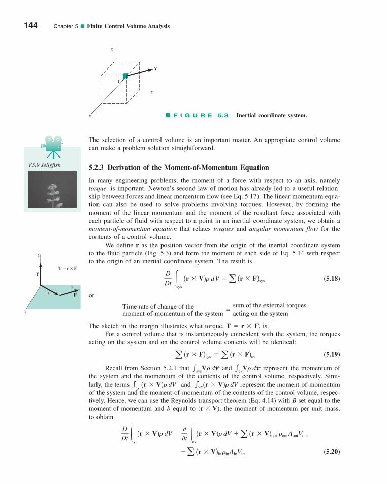
The selection of a control volume is an important matter. An appropriate control volumecan make a problem solution straightforward.

5.2.3 Derivation of the Moment-of-Momentum Equation

In many engineering problems, the moment of a force with respect to an axis, namelytorque, is important. Newton’s second law of motion has already led to a useful relation-ship between forces and linear momentum flow (see Eq. 5.17). The linear momentum equa-tion can also be used to solve problems involving torques. However, by forming themoment of the linear momentum and the moment of the resultant force associated witheach particle of fluid with respect to a point in an inertial coordinate system, we obtain amoment-of-momentum equation that relates torques and angular momentum flow for thecontents of a control volume.

We define r as the position vector from the origin of the inertial coordinate systemto the fluid particle (Fig. 5.3) and form the moment of each side of Eq. 5.14 with respectto the origin of an inertial coordinate system. The result is

(5.18)

or

The sketch in the margin illustrates what torque, T � r � F, is.For a control volume that is instantaneously coincident with the system, the torques

acting on the system and on the control volume contents will be identical:

(5.19)

Recall from Section 5.2.1 that and represent the momentum ofthe system and the momentum of the contents of the control volume, respectively. Simi-larly, the terms represent the moment-of-momentumof the system and the moment-of-momentum of the contents of the control volume, respec-tively. Hence, we can use the Reynolds transport theorem (Eq. 4.14) with B set equal to themoment-of-momentum and b equal to (r � V), the moment-of-momentum per unit mass,to obtain

(5.20)�a 1r � V2in�inAinVin

D

Dt �sys

1r � V2� dV �00t

�cv

1r � V2� dV �a 1r � V2out �outAoutVout

�sys1r � V2� dV and �cv1r � V2� dV

�cvV� dV�sysV� dV

a 1r � F2sys �a 1r � F2cv

Time rate of change of themoment-of-momentum of the system �

sum of the external torquesacting on the system

D

Dt �

sys

1r � V2� d V �a 1r � F2sys

144 Chapter 5 ■ Finite Control Volume Analysis

V5.9 Jellyfish

r

y

x

z

V

F I G U R E 5.3 Inertial coordinate system.

TT = r × F

Fry

x

z

c05FiniteControlVolumeAnalysis.qxd 9/24/10 1:22 PM Page 144

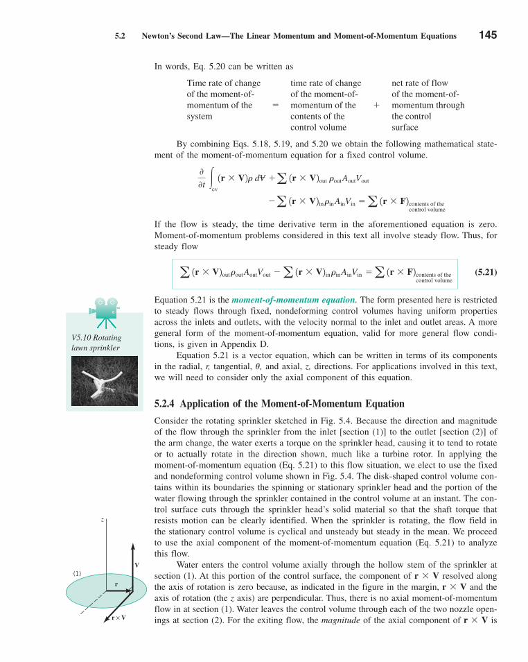
5.2 Newton’s Second Law—The Linear Momentum and Moment-of-Momentum Equations 145

In words, Eq. 5.20 can be written as

By combining Eqs. 5.18, 5.19, and 5.20 we obtain the following mathematical state-ment of the moment-of-momentum equation for a fixed control volume.

If the flow is steady, the time derivative term in the aforementioned equation is zero.Moment-of-momentum problems considered in this text all involve steady flow. Thus, forsteady flow

(5.21)

Equation 5.21 is the moment-of-momentum equation. The form presented here is restrictedto steady flows through fixed, nondeforming control volumes having uniform propertiesacross the inlets and outlets, with the velocity normal to the inlet and outlet areas. A moregeneral form of the moment-of-momentum equation, valid for more general flow condi-tions, is given in Appendix D.

Equation 5.21 is a vector equation, which can be written in terms of its componentsin the radial, r, tangential, �, and axial, z, directions. For applications involved in this text,we will need to consider only the axial component of this equation.

5.2.4 Application of the Moment-of-Momentum Equation

Consider the rotating sprinkler sketched in Fig. 5.4. Because the direction and magnitudeof the flow through the sprinkler from the inlet [section (1)] to the outlet [section (2)] ofthe arm change, the water exerts a torque on the sprinkler head, causing it to tend to rotateor to actually rotate in the direction shown, much like a turbine rotor. In applying themoment-of-momentum equation (Eq. 5.21) to this flow situation, we elect to use the fixedand nondeforming control volume shown in Fig. 5.4. The disk-shaped control volume con-tains within its boundaries the spinning or stationary sprinkler head and the portion of thewater flowing through the sprinkler contained in the control volume at an instant. The con-trol surface cuts through the sprinkler head’s solid material so that the shaft torque thatresists motion can be clearly identified. When the sprinkler is rotating, the flow field inthe stationary control volume is cyclical and unsteady but steady in the mean. We proceedto use the axial component of the moment-of-momentum equation (Eq. 5.21) to analyzethis flow.

Water enters the control volume axially through the hollow stem of the sprinkler atsection (1). At this portion of the control surface, the component of r � V resolved alongthe axis of rotation is zero because, as indicated in the figure in the margin, r � V and theaxis of rotation (the z axis) are perpendicular. Thus, there is no axial moment-of-momentumflow in at section (1). Water leaves the control volume through each of the two nozzle open-ings at section (2). For the exiting flow, the magnitude of the axial component of r � V is

a 1r � V2out�outAoutVout �a 1r � V2in�inAinVin �a 1r � F2contents of thecontrol volume

�a 1r � V2in�inAinVin �a 1r � F2contents of thecontrol volume

00t

�cv

1r � V2� dV �a 1r � V2out �outAoutVout

Time rate of changeof the moment-of-momentum of thesystem

�

time rate of changeof the moment-of-momentum of thecontents of thecontrol volume

�

net rate of flowof the moment-of-momentum throughthe controlsurface

V5.10 Rotatinglawn sprinkler

z

r

r × V

V(1)

c05FiniteControlVolumeAnalysis.qxd 9/24/10 1:22 PM Page 145

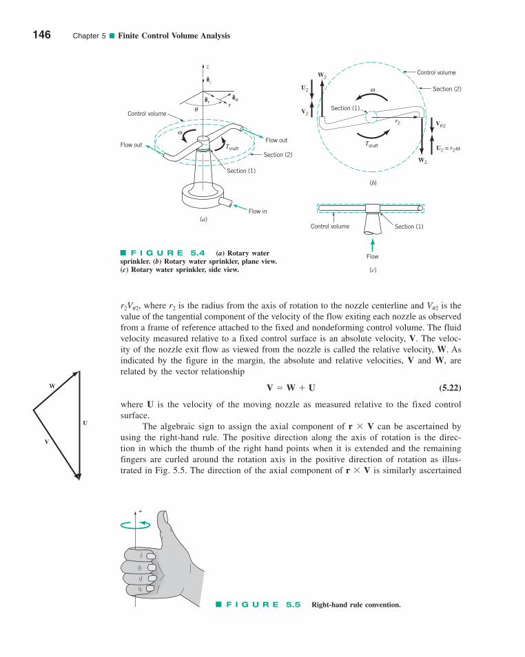
r2V�2, where r2 is the radius from the axis of rotation to the nozzle centerline and V�2 is thevalue of the tangential component of the velocity of the flow exiting each nozzle as observedfrom a frame of reference attached to the fixed and nondeforming control volume. The fluidvelocity measured relative to a fixed control surface is an absolute velocity, V. The veloc-ity of the nozzle exit flow as viewed from the nozzle is called the relative velocity, W. Asindicated by the figure in the margin, the absolute and relative velocities, V and W, arerelated by the vector relationship

(5.22)

where U is the velocity of the moving nozzle as measured relative to the fixed controlsurface.

The algebraic sign to assign the axial component of r � V can be ascertained byusing the right-hand rule. The positive direction along the axis of rotation is the direc-tion in which the thumb of the right hand points when it is extended and the remainingfingers are curled around the rotation axis in the positive direction of rotation as illus-trated in Fig. 5.5. The direction of the axial component of r � V is similarly ascertained

V � W � U

146 Chapter 5 ■ Finite Control Volume Analysis

F I G U R E 5.4 (a) Rotary watersprinkler. (b) Rotary water sprinkler, plane view.(c) Rotary water sprinkler, side view.

Control volume

Flow out

Section (1)

Section (2)

Flow out

Flow in

Tshaft

ω

(a)

z

rθ

êθ

êz

êr

V

W

U

F I G U R E 5.5 Right-hand rule convention.

+

Control volume

Section (2)

Section (1)

Tshaft

(b)

W2

U2

V2

W2

U2 = r2ω

ω

r2 V 2

Flow

Control volume

(c)

Section (1)

θ

c05FiniteControlVolumeAnalysis.qxd 9/24/10 1:23 PM Page 146

5.2 Newton’s Second Law—The Linear Momentum and Moment-of-Momentum Equations 147

by noting the direction of the cross product of the radius from the axis of rotation, rêr ,and the tangential component of absolute velocity, V�ê�. Thus, for the sprinkler of Fig. 5.4,we can state that

(5.23)

where, because of mass conservation, is the total mass flowrate through both nozzles. Aswas demonstrated in Example 5.4, the mass flowrate is the same whether the sprinklerrotates or not. The correct algebraic sign of the axial component of r � V can be easilyremembered in the following way: If V� and U are in the same direction, use �; if V� andU are in opposite directions, use �. For the sprinkler of Fig. 5.4

(5.24)

Note that we have entered Tshaft as a positive quantity in Eq. 5.24. This is equivalent toassuming that Tshaft is in the same direction as rotation.

For the sprinkler of Fig. 5.4, the axial component of the moment-of-momentum equa-tion (Eq. 5.21) is, from Eqs. 5.23 and 5.24,

(5.25)

We interpret Tshaft being a negative quantity from Eq. 5.25 to mean that the shaft torqueactually opposes the rotation of the sprinkler arms. The shaft torque, Tshaft, opposes rotationin all turbine devices.

We could evaluate the shaft power, , associated with shaft torque, Tshaft, byforming the product Tshaft and the rotational speed of the shaft, �. Thus, from Eq. 5.25we get

(5.26)

Since r2� is the speed, U, of each sprinkler nozzle, we can also state Eq. 5.26 in the form

(5.27)

Shaft work per unit mass, wshaft, is equal to . Dividing Eq. 5.27 by the mass flowrate,, we obtain

(5.28)

Negative shaft work as in Eqs. 5.26, 5.27, and 5.28 is work out of the control volume, thatis, work done by the fluid on the rotor and thus its shaft.

wshaft � �U2V�2

m# W

#shaft /m

#W#

shaft � �U2V�2m#

W#

shaft � Tshaft� � �r2V�2m#�

W#

shaft

�r2V�2m#

� Tshaft

a c 1r � F2contents of thecontrol volume

daxial

� Tshaft

m#

ca 1r � V2out�outAoutVout �a 1r � V2in�inAinVin daxial

� 1�r2V�22m#

V5.11 Impulse-typelawn sprinkler

GIVEN Water enters a rotating lawn sprinkler through itsbase at the steady rate of 1000 ml/s as sketched in Fig.E5.10a. The exit area of each of the two nozzles is 30 mm2 andthe flow leaving each nozzle is in the tangential direction. Theradius from the axis of rotation to the centerline of each nozzleis 200 mm.

FIND (a) Determine the resisting torque required to holdthe sprinkler head stationary.

(b) Determine the resisting torque associated with the sprin-kler rotating with a constant speed of 500 rev/min.

(c) Determine the speed of the sprinkler if no resisting torqueis applied.

Moment-of-Momentum—TorqueEXAMPLE 5.10

c05FiniteControlVolumeAnalysis.qxd 9/24/10 1:23 PM Page 147

148 Chapter 5 ■ Finite Control Volume Analysis

SOLUTION

or

Thus, using Eq. 3, with (as calculated previ-ously), we get

or

(Ans)

COMMENT Note that the resisting torque associatedwith sprinkler head rotation is much less than the resistingtorque that is required to hold the sprinkler stationary.

(c) When no resisting torque is applied to the rotating sprin-kler head, a maximum constant speed of rotation will occur asdemonstrated below. Application of Eqs. 3, 4, and 5 to the

Tshaft � �1.24 N # m

Tshaft � �1200 mm2 16.2 m/s2 0.999 kg/s 31 1N/kg2/ 1m/s22 4

11000 mm/m2

m#

� 0.999 kg/s

V2 � 16.7 m/s � 10.5 m/s � 6.2 m/s

To solve parts (a), (b), and (c) of this example we can use thesame fixed and nondeforming, disk-shaped control volume il-lustrated in Fig. 5.4. As indicated in Fig. E5.10a, the only ax-ial torque considered is the one resisting motion, Tshaft.

(a) When the sprinkler head is held stationary as specified inpart (a) of this example problem, the velocities of the fluid en-tering and leaving the control volume are shown in Fig.E5.10b. Equation 5.25 applies to the contents of this controlvolume. Thus,

(1)

Since the control volume is fixed and nondeforming and theflow exiting from each nozzle is tangential,

(2)

Equations 1 and 2 give

(3)

In Example 5.4, we ascertained that V2 � 16.7 m/s. Thus, fromEq. 3 with

we obtain

or

(Ans)

(b) When the sprinkler is rotating at a constant speed of500 rpm, the flow field in the control volume is unsteady butcyclical. Thus, the flow field is steady in the mean. The veloci-ties of the flow entering and leaving the control volume are asindicated in Fig. E5.10c. The absolute velocity of the fluidleaving each nozzle, V2, is from Eq. 5.22,

(4)

where

as determined in Example 5.4. The speed of the nozzle, U2, isobtained from

(5)

Application of the axial component of the moment-of-momentumequation (Eq. 5.25) leads again to Eq. 3. From Eqs. 4 and 5,

� 16.7 m/s �1200 mm2 1500 rev/min2 12� rad/rev2

11000 mm/m2 160 s/min2

V2 � 16.7 m/s � r2�

U2 � r2�

W2 � 16.7 m/s

V2 � W2 � U2

Tshaft � �3.34 N # m

Tshaft � �1200 mm2 116.7 m/s2 10.999 kg/s2 31 1N/kg2/ 1m/s22 4

11000 mm/m2

� 0.999 kg/s

m#

� Q� �11000 ml/s2 110�3 m3/liter2 1999 kg/m32

11000 ml/liter2

Tshaft � �r2V2m#

V�2 � V2

Tshaft � �r2V�2m#

F I G U R E E5.10

Control volume

Flow outFlow out

Tshaft

Q = 1000 ml/s

r2 =200 mm

Nozzle exitarea = 30 mm2

(a)

(b)

V2V2 = V 2θ

V1

(c)

W2W2

V1

U2V2

ω

V2 = V 2θU2 = r2ω

c05FiniteControlVolumeAnalysis.qxd 9/24/10 1:23 PM Page 148

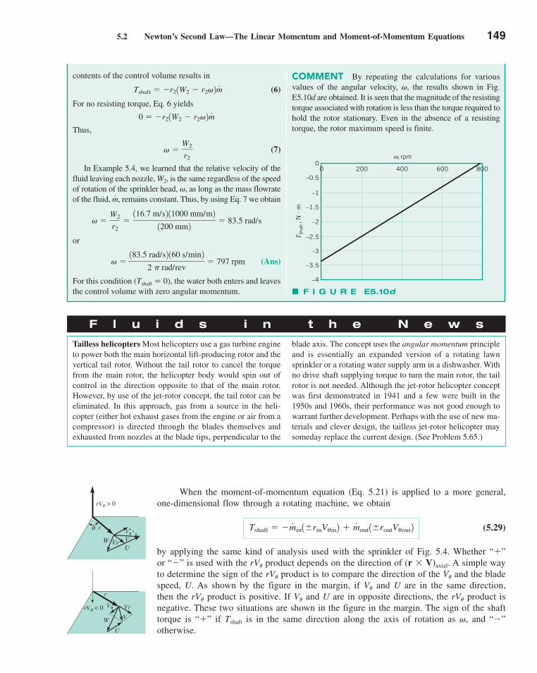
5.2 Newton’s Second Law—The Linear Momentum and Moment-of-Momentum Equations 149

When the moment-of-momentum equation (Eq. 5.21) is applied to a more general,one-dimensional flow through a rotating machine, we obtain

(5.29)

by applying the same kind of analysis used with the sprinkler of Fig. 5.4. Whether “�”or “�” is used with the rV� product depends on the direction of (r � V)axial. A simple wayto determine the sign of the rV� product is to compare the direction of the V� and the bladespeed, U. As shown by the figure in the margin, if V� and U are in the same direction,then the rV� product is positive. If V� and U are in opposite directions, the rV� product isnegative. These two situations are shown in the figure in the margin. The sign of the shafttorque is “�” if Tshaft is in the same direction along the axis of rotation as �, and “�”otherwise.

Tshaft � �m#

in1�rinV�in2 � m#

out1�routV�out2

COMMENT By repeating the calculations for variousvalues of the angular velocity, , the results shown in Fig.E5.10d are obtained. It is seen that the magnitude of the resistingtorque associated with rotation is less than the torque required tohold the rotor stationary. Even in the absence of a resistingtorque, the rotor maximum speed is finite.

v

contents of the control volume results in

(6)

For no resisting torque, Eq. 6 yields

Thus,

(7)

In Example 5.4, we learned that the relative velocity of thefluid leaving each nozzle, W2, is the same regardless of the speedof rotation of the sprinkler head, �, as long as the mass flowrateof the fluid, , remains constant. Thus, by using Eq. 7 we obtain

or

(Ans)

For this condition (Tshaft � 0), the water both enters and leavesthe control volume with zero angular momentum.

� �183.5 rad/s2 160 s/min2

2 � rad/rev� 797 rpm

� �W2

r2�116.7 m/s2 11000 mm/m2

1200 mm2� 83.5 rad/s

m#

� �W2

r2

0 � �r21W2 � r2�2m#

Tshaft � �r21W2 � r2�2m#

T Sha

ft ,

N .

m

–0.5

0

–1

–1.5

–2

–2.5

–3

–3.5

–4

ω, rpm

200 400 6000 800

F I G U R E E5.10d

F l u i d s i n t h e N e w s

Tailless helicopters Most helicopters use a gas turbine engineto power both the main horizontal lift-producing rotor and thevertical tail rotor. Without the tail rotor to cancel the torquefrom the main rotor, the helicopter body would spin out ofcontrol in the direction opposite to that of the main rotor.However, by use of the jet-rotor concept, the tail rotor can beeliminated. In this approach, gas from a source in the heli-copter (either hot exhaust gases from the engine or air from acompressor) is directed through the blades themselves and exhausted from nozzles at the blade tips, perpendicular to the

blade axis. The concept uses the angular momentum principleand is essentially an expanded version of a rotating lawnsprinkler or a rotating water supply arm in a dishwasher. Withno drive shaft supplying torque to turn the main rotor, the tailrotor is not needed. Although the jet-rotor helicopter conceptwas first demonstrated in 1941 and a few were built in the1950s and 1960s, their performance was not good enough towarrant further development. Perhaps with the use of new ma-terials and clever design, the tailless jet-rotor helicopter maysomeday replace the current design. (See Problem 5.65.)

rV� > 0

r�

UVr

V�

VW

rV� < 0 V�

r

U

Vr

VW

c05FiniteControlVolumeAnalysis.qxd 9/24/10 1:23 PM Page 149

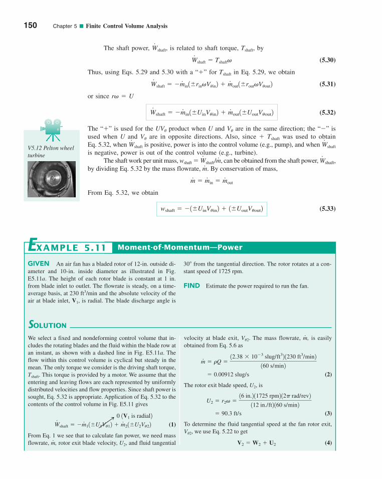
The shaft power, , is related to shaft torque, Tshaft, by

(5.30)

Thus, using Eqs. 5.29 and 5.30 with a “�” for Tshaft in Eq. 5.29, we obtain

(5.31)

or since r� � U

(5.32)

The “�” is used for the UV� product when U and V� are in the same direction; the “�” isused when U and V� are in opposite directions. Also, since � Tshaft was used to obtainEq. 5.32, when is positive, power is into the control volume (e.g., pump), and when is negative, power is out of the control volume (e.g., turbine).

The shaft work per unit mass, wshaft � / , can be obtained from the shaft power,by dividing Eq. 5.32 by the mass flowrate, . By conservation of mass,

From Eq. 5.32, we obtain

(5.33)wshaft � �1�UinV�in2 � 1�UoutV�out2

m#

� m#

in � m#

out

m# W

#shaft,m

#W#

shaft

W#

shaftW#

shaft

W#

shaft � �m#

in1�UinV�in2 � m#

out1�UoutV�out2

W#

shaft � �m#

in1�rin�V�in2 � m#

out1�rout�V�out2

W#

shaft � Tshaft�

W#

shaft

150 Chapter 5 ■ Finite Control Volume Analysis

V5.12 Pelton wheelturbine

GIVEN An air fan has a bladed rotor of 12-in. outside di-ameter and 10-in. inside diameter as illustrated in Fig.E5.11a. The height of each rotor blade is constant at 1 in.from blade inlet to outlet. The flowrate is steady, on a time-average basis, at 230 ft3/min and the absolute velocity of theair at blade inlet, V1, is radial. The blade discharge angle is

30 from the tangential direction. The rotor rotates at a con-stant speed of 1725 rpm.

FIND Estimate the power required to run the fan.

Moment-of-Momentum—PowerEXAMPLE 5.11

SOLUTION

velocity at blade exit, V�2. The mass flowrate, , is easilyobtained from Eq. 5.6 as

(2)

The rotor exit blade speed, U2, is

(3)

To determine the fluid tangential speed at the fan rotor exit,V�2, we use Eq. 5.22 to get

(4)V2 � W2 � U2

� 90.3 ft/s

U2 � r2� �16 in.2 11725 rpm2 12� rad/rev2

112 in./ft2 160 s/min2

� 0.00912 slug/s

m#

� �Q �12.38 � 10�3 slug/ft32 1230 ft3/min2

160 s/min2

m#

We select a fixed and nondeforming control volume that in-cludes the rotating blades and the fluid within the blade row atan instant, as shown with a dashed line in Fig. E5.11a. Theflow within this control volume is cyclical but steady in themean. The only torque we consider is the driving shaft torque,Tshaft. This torque is provided by a motor. We assume that theentering and leaving flows are each represented by uniformlydistributed velocities and flow properties. Since shaft power issought, Eq. 5.32 is appropriate. Application of Eq. 5.32 to thecontents of the control volume in Fig. E5.11 gives

(1)

From Eq. 1 we see that to calculate fan power, we need massflowrate, , rotor exit blade velocity, U2, and fluid tangentialm

#

W#

shaft � �m#

11�U1V�12 � m#

21�U2V�22

0 1V1 is radial2

888n

c05FiniteControlVolumeAnalysis.qxd 9/24/10 1:23 PM Page 150

5.2 Newton’s Second Law—The Linear Momentum and Moment-of-Momentum Equations 151

By using this value of W2 in Eq. 5 we get

Equation 1 can now be used to obtain

or

(Ans)

COMMENT Note that the “�” was used with the U2V�2

product because U2 and V�2 are in the same direction. This re-sult, 0.0972 hp, is the power that needs to be delivered throughthe fan shaft for the given conditions. Ideally, all of this powerwould go into the flowing air. However, because of fluid fric-tion, only some of this power will produce a useful effect (e.g.,pressure rise) in the air. How much useful effect depends onthe efficiency of the energy transfer between the fan bladesand the fluid.

W#

shaft � 0.0972 hp

U2V�2 �10.00912 slug/s2 190.3 ft/s2 164.9 ft/s2

31 1slug . ft/s22/lb 4 3550 1ft . lb2/ 1hp . s2 4� m

# W

#shaft

� 90.3 ft/s � 129.3 ft/s2 10.8662 � 64.9 ft/s

V�2 � U2 � W2 cos 30°

The vector addition of Eq. 4 is shown in the form of a “veloc-ity triangle” in Fig. E5.11b. From Fig. E5.11b, we can see that

(5)

To solve Eq. 5 for V�2 we need a value of W2, in addition to the valueof U2 already determined (Eq. 3). To get W2, we recognize that

(6)

where Vr2 is the radial component of either W2 or V2. Also,using Eq. 5.6, we obtain

(7)

or since

(8)

where h is the blade height, Eqs. 7 and 8 combine to form

(9)

Taking Eqs. 6 and 9 together we get

(10)

Substituting known values into Eq. 10, we obtain

� 29.3 ft/s

W2 �10.00912 slugs/s2 112 in./ft2 112 in./ft2

12.38 � 10�3 slugs/ft322�16 in.2 11 in.2 sin 30°

W2 �m#

�2�r2h sin 30°

m#

� �2�r2hVr 2

A2 � 2 �r2h

m#

� �A2Vr 2

W2 sin 30° � Vr 2

V�2 � U2 � W2 cos 30°

ω

Section (1)

Fixed control volume

Tshaft

V1

Section (2)

30°W2

ω

Tshaft

D2 = 2r2 = 12 in.

D1 = 2r1 = 10 in.

h =1 in.

Fixedcontrol volume

W2Wr2 Vr2

U2

V2

(b)(a)

30° V 2θ

F I G U R E E5.11

c05FiniteControlVolumeAnalysis.qxd 9/24/10 1:23 PM Page 151

152 Chapter 5 ■ Finite Control Volume Analysis

5.3 First Law of Thermodynamics—The Energy Equation

5.3.1 Derivation of the Energy Equation

The first law of thermodynamics for a system is, in words

In symbolic form, this statement is

or

(5.34)

Some of these variables deserve a brief explanation before proceeding further. The totalstored energy per unit mass for each particle in the system, e, is related to the internalenergy per unit mass, , the kinetic energy per unit mass, V2/2, and the potential energy perunit mass, gz, by the equation

(5.35)

Thus, is the total stored energy of the system.

The net heat transfer rate into the system is denoted with , and the net rate ofwork transfer into the system is labeled . Heat transfer and work transfer are consid-ered “�” going into the system and “�” coming out.

For the control volume that is coincident with the system at an instant of time

(5.36)

Furthermore, for the system and the contents of the coincident control volume that is fixed andnondeforming, the Reynolds transport theorem (Eq. 4.14 with the parameter B set equal to thetotal stored energy and, therefore, the parameter b set equal to e) allows us to conclude that

(5.37)

or, in words,

Combining Eqs. 5.34, 5.36, and 5.37, we get the control volume formula for the first lawof thermodynamics:

(5.38)00t

�cv

e� dV �a eout �outAoutVout �a ein�inAinVin � 1Q

#netin

� W#

netin2cv

Time rateof increaseof the totalstored energyof the system

�

time rate of increase of the total storedenergy of the contentsof the control volume

�

net rate of flowof the total stored energyout of the controlvolume through thecontrol surface

D

Dt �

sys

e� d V �00t

�cv

e� d V � a eout�outAoutVout �a ein�inAinVin

1Q#

netin

� W#

netin2sys � 1Q

#netin

� W#

netin2coincidentcontrol volume

W#

net in

Q#

net in

�sysep dV

e � u �V 2

2� gz

u

D

Dt �

sys

e� d V � 1Q#

netin

� W#

netin2sys

D

Dt �sys

e� d V � aa Q#

in �a Q#

outbsys

� aaW#

in �aW#

outbsys

Time rate ofincrease of thetotal stored energyof the system

�

net time rate ofenergy addition byheat transfer intothe system

�

net time rate ofenergy addition bywork transfer intothe system

c05FiniteControlVolumeAnalysis.qxd 9/24/10 1:23 PM Page 152

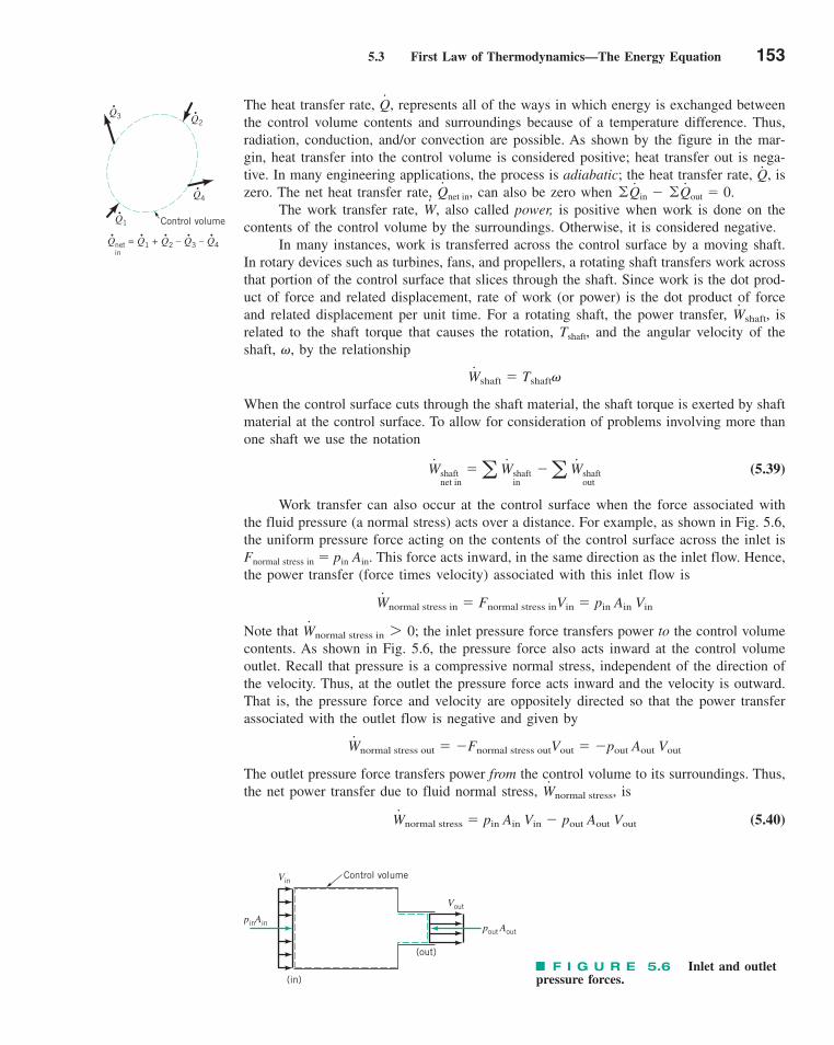
5.3 First Law of Thermodynamics—The Energy Equation 153

The heat transfer rate, , represents all of the ways in which energy is exchanged betweenthe control volume contents and surroundings because of a temperature difference. Thus,radiation, conduction, and/or convection are possible. As shown by the figure in the mar-gin, heat transfer into the control volume is considered positive; heat transfer out is nega-tive. In many engineering applications, the process is adiabatic; the heat transfer rate, , iszero. The net heat transfer rate, , can also be zero when

The work transfer rate, , also called power, is positive when work is done on thecontents of the control volume by the surroundings. Otherwise, it is considered negative.

In many instances, work is transferred across the control surface by a moving shaft.In rotary devices such as turbines, fans, and propellers, a rotating shaft transfers work acrossthat portion of the control surface that slices through the shaft. Since work is the dot prod-uct of force and related displacement, rate of work (or power) is the dot product of forceand related displacement per unit time. For a rotating shaft, the power transfer, , isrelated to the shaft torque that causes the rotation, Tshaft, and the angular velocity of theshaft, �, by the relationship

When the control surface cuts through the shaft material, the shaft torque is exerted by shaftmaterial at the control surface. To allow for consideration of problems involving more thanone shaft we use the notation

(5.39)

Work transfer can also occur at the control surface when the force associated withthe fluid pressure (a normal stress) acts over a distance. For example, as shown in Fig. 5.6,the uniform pressure force acting on the contents of the control surface across the inlet isFnormal stress in � pin Ain. This force acts inward, in the same direction as the inlet flow. Hence,the power transfer (force times velocity) associated with this inlet flow is

Note that the inlet pressure force transfers power to the control volumecontents. As shown in Fig. 5.6, the pressure force also acts inward at the control volumeoutlet. Recall that pressure is a compressive normal stress, independent of the direction ofthe velocity. Thus, at the outlet the pressure force acts inward and the velocity is outward.That is, the pressure force and velocity are oppositely directed so that the power transferassociated with the outlet flow is negative and given by

The outlet pressure force transfers power from the control volume to its surroundings. Thus,the net power transfer due to fluid normal stress, , is

(5.40)W#

normal stress � pin Ain Vin � pout Aout Vout

W#

normal stress

W#

normal stress out � �Fnormal stress outVout � �pout Aout Vout

W#

normal stress in 7 0;

W#

normal stress in � Fnormal stress inVin � pin Ain Vin

W#

shaftnet in

�aW#

shaftin

�aW#

shaftout

W#

shaft � Tshaft�

W#

shaft

W# ©Q

#in � ©Q

#out � 0.Q

#net in

Q#

Q#

pinAinpout Aout

Vout

Vin

(in)

Control volume

(out)

F I G U R E 5.6 Inlet and outlet pressure forces.

Control volume

Q•

4

Q•

2Q•

3

Q•

1

Q•

net = Q•

1 + Q•

2 – Q•

3 – Q•

4in

c05FiniteControlVolumeAnalysis.qxd 9/24/10 1:24 PM Page 153

Work transfer can also occur at the control surface because of tangential stressforces. For example, rotating shaft work is transferred by tangential stresses in the shaftmaterial. For fluid particles, the shear stress power, , is given by the productof the tangential stress force, Ftangential stress, and the component of velocity in the tangen-tial direction. At the inlet and outlet portions of the control volume, any tangential stressforce would be parallel to the inlet and outlet areas and, therefore, normal to the fluidvelocities. Hence, the shear stress power transfer at these locations is zero. As shown inthe figure in the margin, at other portions of the control surface where a shear force maybe developed, the velocity is zero because the viscous fluid sticks to the stationary sur-face. Thus, in general, we can consider the fluid tangential stress power transfer to benegligible.

Using the information we have developed about power, we can express the first lawof thermodynamics for the contents of a control volume by combining Eqs. 5.38, 5.39, and5.40 to obtain

(5.41)

When the equation for total stored energy (Eq. 5.35) is considered with Eq. 5.41, we obtainthe energy equation:

(5.42)

Equation 5.42 is restricted to flows through fixed, nondeforming control volumes havinguniform properties across the inlets and outlets, with the velocity normal to the inlet andoutlet areas. A more general form of the energy equation, valid for more general flow con-ditions, is given in Appendix D.

5.3.2 Application of the Energy Equation

For many applications, Eq. 5.42 can be simplified. For example, the term cv e�represents the time rate of change of the total stored energy, e, of the contents of thecontrol volume. This term is zero when the flow is steady. This term is also zero in themean when the flow is steady in the mean (cyclical). Furthermore, for many applica-tions, such as the hair dryer shown in Fig. 5.7, there is only one stream entering andleaving the control volume, and the properties are all assumed to be uniformly distrib-uted over the flow cross-sectional areas involved. For such flows the continuity equation(Eq. 5.10) gives

(5.43)

and Eq. 5.42 can be simplified to form

(5.44)m#c uout � uin � a

p

�b

out� a

p

�b

in�

V 2out � V 2

in

2� g1zout � zin2 d � Q

#netin

� W#

shaftnet in

�inAinVin � �outAoutVout � m#

dV�0/0t

� Q#

netin

� W#

shaftnet in

�a au �p

��

V 2

2� gzb

in�in AinVin

00t �

cv

e� dV �a au �p

��

V 2

2� gzb

out�out AoutVout

� Q#

netin

� W#

shaftnet in

�a pinAinVin �a poutAoutVout

00t

�cv

e� d V �a eout�out Aout Vout �a ein�in Ain Vin

W#

shear stress

154 Chapter 5 ■ Finite Control Volume Analysis

V = 0 Ftangential stress

c05FiniteControlVolumeAnalysis.qxd 9/24/10 1:24 PM Page 154

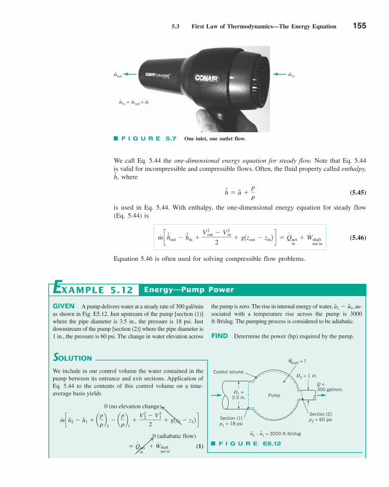
5.3 First Law of Thermodynamics—The Energy Equation 155

We call Eq. 5.44 the one-dimensional energy equation for steady flow. Note that Eq. 5.44is valid for incompressible and compressible flows. Often, the fluid property called enthalpy,, where

(5.45)

is used in Eq. 5.44. With enthalpy, the one-dimensional energy equation for steady flow(Eq. 5.44) is

(5.46)

Equation 5.46 is often used for solving compressible flow problems.

m#c hout � hin �

V 2out � V 2

in

2� g1zout � zin2 d � Q

#netin

� W#

shaftnet in

h � u �p�

h

m•in = m•

out = m•

m•out m•

in

F I G U R E 5.7 One inlet, one outlet flow.

GIVEN A pump delivers water at a steady rate of 300 gal/minas shown in Fig. E5.12. Just upstream of the pump [section (1)]where the pipe diameter is 3.5 in., the pressure is 18 psi. Justdownstream of the pump [section (2)] where the pipe diameter is1 in., the pressure is 60 psi. The change in water elevation across

the pump is zero. The rise in internal energy of water, , as-sociated with a temperature rise across the pump is 3000ftlb/slug. The pumping process is considered to be adiabatic.

FIND Determine the power (hp) required by the pump.

u2 � u1

Energy—Pump PowerEXAMPLE 5.12

SOLUTION

We include in our control volume the water contained in thepump between its entrance and exit sections. Application ofEq. 5.44 to the contents of this control volume on a time-average basis yields

0 (no elevation change)

0 (adiabatic flow)

� (1)shaftnet in

W#

netin

� Q#

m#c u2 � u1 � a

p

�b

2� a

p

�b

1�

V 22 � V 2

1

2� g1z2 � z12 d

F I G U R E E5.12

Control volume

Section (1)p1 = 18 psi

u2 – u1 = 3000 ft •lb/slug^ ^

D1 =3.5 in. Pump

W•

shaft = ?

D2 = 1 in.

Q =300 gal/min.

Section (2)p2 = 60 psi

88888n

88888n

c05FiniteControlVolumeAnalysis.qxd 9/24/10 1:24 PM Page 155

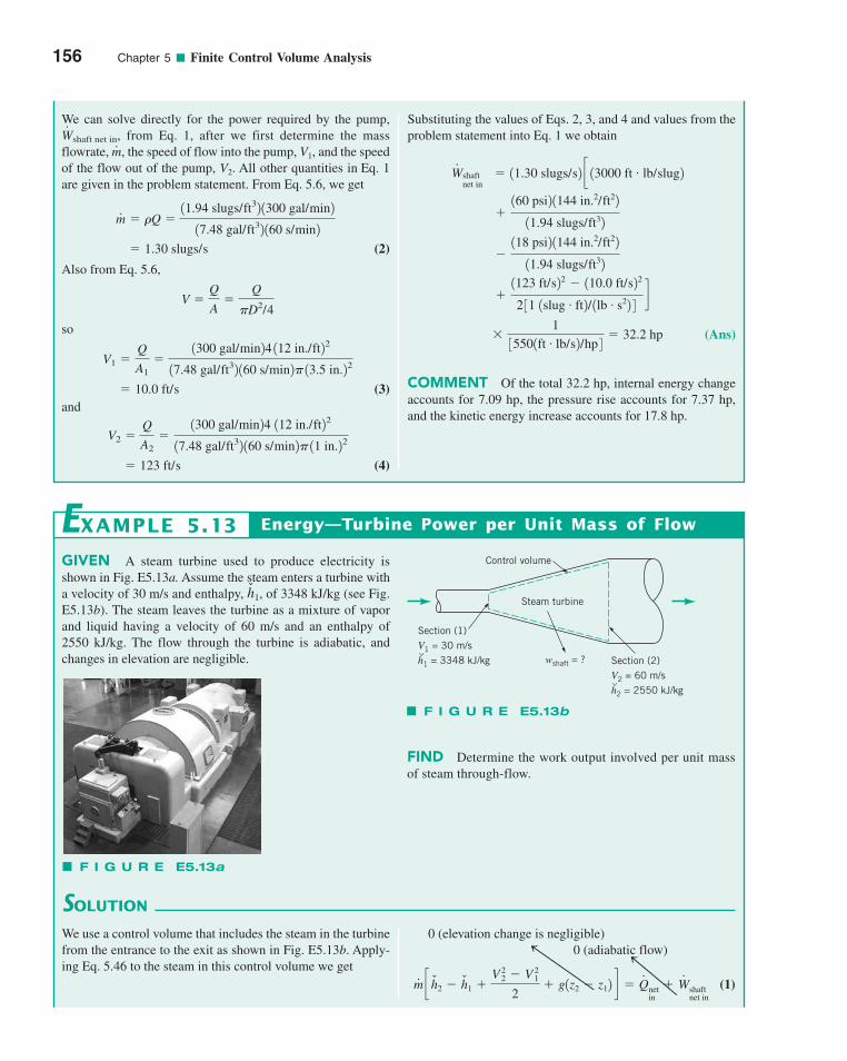
156 Chapter 5 ■ Finite Control Volume Analysis

Substituting the values of Eqs. 2, 3, and 4 and values from theproblem statement into Eq. 1 we obtain

(Ans)

COMMENT Of the total 32.2 hp, internal energy changeaccounts for 7.09 hp, the pressure rise accounts for 7.37 hp,and the kinetic energy increase accounts for 17.8 hp.

�1

35501ft . lb/s2/hp 4� 32.2 hp

�1123 ft/s22 � 110.0 ft/s22

2 31 1slug . ft2/ 1lb . s22 4d

�118 psi2 1144 in.2/ft22

11.94 slugs/ft32

�160 psi2 1144 in.2/ft22

11.94 slugs/ft32

� 11.30 slugs/s2 c 13000 ft . lb/slug2shaftnet in

W#

We can solve directly for the power required by the pump,, from Eq. 1, after we first determine the mass

flowrate, , the speed of flow into the pump, V1, and the speedof the flow out of the pump, V2. All other quantities in Eq. 1are given in the problem statement. From Eq. 5.6, we get

(2)

Also from Eq. 5.6,

so

(3)and

(4) � 123 ft/s

V2 �Q

A2�

1300 gal/min24 112 in./ft22

17.48 gal/ft32 160 s/min2� 11 in.22

� 10.0 ft/s

V1 �Q

A1�

1300 gal/min24 112 in./ft22

17.48 gal/ft32 160 s/min2� 13.5 in.22

V �Q

A�

Q

�D2/4

� 1.30 slugs/s

m#

� �Q �11.94 slugs/ft32 1300 gal/min2

17.48 gal/ft32 160 s/min2

m#W

#shaft net in

GIVEN A steam turbine used to produce electricity isshown in Fig. E5.13a. Assume the steam enters a turbine witha velocity of 30 m/s and enthalpy, , of 3348 kJ/kg (see Fig.E5.13b). The steam leaves the turbine as a mixture of vaporand liquid having a velocity of 60 m/s and an enthalpy of2550 kJ/kg. The flow through the turbine is adiabatic, andchanges in elevation are negligible.

h1

SOLUTION

We use a control volume that includes the steam in the turbinefrom the entrance to the exit as shown in Fig. E5.13b. Apply-ing Eq. 5.46 to the steam in this control volume we get

FIND Determine the work output involved per unit massof steam through-flow.

0 (elevation change is negligible)0 (adiabatic flow)

(1)m#c h2 � h1 �

V 22 � V 2

1

2� g1z2 � z12 d � Q

#netin

� W#

shaftnet in

Energy—Turbine Power per Unit Mass of FlowEXAMPLE 5.13

F I G U R E E5.13b

F I G U R E E5.13a

8888888n

88888n

Steam turbine

Control volume

Section (1)V1 = 30 m/sh1 = 3348 kJ/kg^

Section (2)V2 = 60 m/sh2 = 2550 kJ/kg^

wshaft = ?

c05FiniteControlVolumeAnalysis.qxd 9/24/10 1:24 PM Page 156

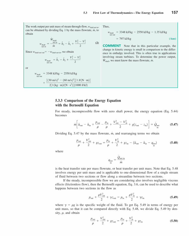
5.3 First Law of Thermodynamics—The Energy Equation 157

5.3.3 Comparison of the Energy Equation with the Bernoulli Equation

For steady, incompressible flow with zero shaft power, the energy equation (Eq. 5.44)becomes

(5.47)

Dividing Eq. 5.47 by the mass flowrate, , and rearranging terms we obtain

(5.48)

where

is the heat transfer rate per mass flowrate, or heat transfer per unit mass. Note that Eq. 5.48involves energy per unit mass and is applicable to one-dimensional flow of a single streamof fluid between two sections or flow along a streamline between two sections.

If the steady, incompressible flow we are considering also involves negligible viscouseffects (frictionless flow), then the Bernoulli equation, Eq. 3.6, can be used to describe whathappens between two sections in the flow as

(5.49)

where � � �g is the specific weight of the fluid. To get Eq. 5.49 in terms of energy perunit mass, so that it can be compared directly with Eq. 5.48, we divide Eq. 5.49 by den-sity, �, and obtain

(5.50)pout

��

V 2out

2� gzout �

pin

��

V 2in

2� gzin

pout ��V 2

out

2� �zout � pin �

�V 2in

2� �zin

qnetin

�Q#

net in

m#

pout

��

V 2out

2� gzout �

pin

��

V 2in

2� gzin � 1uout � uin � qnet

in2

m#

m#c uout � uin �

pout

��

pin

��

V 2out � V 2

in

2� g1zout � zin2 d � Q

#netin

Thus,

(Ans)

COMMENT Note that in this particular example, thechange in kinetic energy is small in comparison to the differ-ence in enthalpy involved. This is often true in applicationsinvolving steam turbines. To determine the power output,

, we must know the mass flowrate, .m#

W#

shaft

� 797 kJ/kg

wshaftnet out

� 3348 kJ/kg � 2550 kJ/kg � 1.35 kJ/kg

The work output per unit mass of steam through-flow, wshaft net in,can be obtained by dividing Eq. 1 by the mass flowrate, , toobtain

(2)

Since wshaft net out� �wshaft net in, we obtain

or

�3 130 m/s22 � 160 m/s22 4 31 J/ 1N . m2 4

2 31 1kg . m2/ 1N . s22 4 11000 J/kJ2

wshaftnet out

� 3348 kJ/kg � 2550 kJ/kg

wshaftnet out

� h1 � h2 �V 2

1 � V 22

2

wshaftnet in

�

W#

shaftnet in

m# � h2 � h1 �

V 22 � V 2

1

2

m#

c05FiniteControlVolumeAnalysis.qxd 9/24/10 1:24 PM Page 157

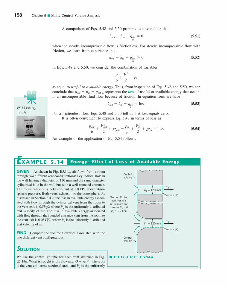
A comparison of Eqs. 5.48 and 5.50 prompts us to conclude that

(5.51)

when the steady, incompressible flow is frictionless. For steady, incompressible flow withfriction, we learn from experience that

(5.52)

In Eqs. 5.48 and 5.50, we consider the combination of variables

as equal to useful or available energy. Thus, from inspection of Eqs. 5.48 and 5.50, we canconclude that represents the loss of useful or available energy that occursin an incompressible fluid flow because of friction. In equation form we have

(5.53)

For a frictionless flow, Eqs. 5.48 and 5.50 tell us that loss equals zero.It is often convenient to express Eq. 5.48 in terms of loss as

(5.54)

An example of the application of Eq. 5.54 follows.

pout

��

V 2out

2� gzout �

pin

��

V 2in

2� gzin � loss

uout � uin � qnetin

� loss

uout � uin � qnet in

p

��

V 2

2� gz

uout � uin � qnetin

7 0

uout � uin � qnetin

� 0

158 Chapter 5 ■ Finite Control Volume Analysis

V5.13 Energytransfer

GIVEN As shown in Fig. E5.14a, air flows from a roomthrough two different vent configurations: a cylindrical hole inthe wall having a diameter of 120 mm and the same diametercylindrical hole in the wall but with a well-rounded entrance.The room pressure is held constant at 1.0 kPa above atmo-spheric pressure. Both vents exhaust into the atmosphere. Asdiscussed in Section 8.4.2, the loss in available energy associ-ated with flow through the cylindrical vent from the room tothe vent exit is 0.5V2

2/2 where V2 is the uniformly distributedexit velocity of air. The loss in available energy associatedwith flow through the rounded entrance vent from the room tothe vent exit is 0.05V2

2/2, where V2 is the uniformly distributedexit velocity of air.

FIND Compare the volume flowrates associated with thetwo different vent configurations.

SOLUTION

We use the control volume for each vent sketched in Fig.E5.14a. What is sought is the flowrate, Q � A2V2, where A2

is the vent exit cross-sectional area, and V2 is the uniformly

Energy—Effect of Loss of Available EnergyEXAMPLE 5.14

Controlvolume

Section (2)

V2

V2

Section (2)

Controlvolume

D2 = 120 mm

D2 = 120 mm

Section (1) forboth vents is

in the room andinvolves V1 = 0p1 = 1.0 kPa

F I G U R E E5.14a

c05FiniteControlVolumeAnalysis.qxd 9/24/10 1:24 PM Page 158

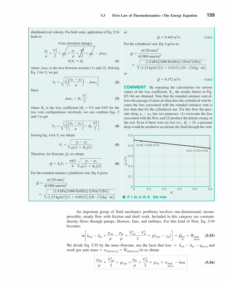
5.3 First Law of Thermodynamics—The Energy Equation 159

An important group of fluid mechanics problems involves one-dimensional, incom-pressible, steady flow with friction and shaft work. Included in this category are constant-density flows through pumps, blowers, fans, and turbines. For this kind of flow, Eq. 5.44becomes

(5.55)

We divide Eq. 5.55 by the mass flowrate, use the facts that andwork per unit to obtain

(5.56)pout

��

V 2out

2� gzout �

pin

��

V 2in

2� gzin � wshaft

net in� loss

mass � wshaft net in � W#

shaft net in /m# loss � uout � uin � qnet in

m#c uout � uin �

pout

��

pin

��

V 2out � V 2

in

2� g1zout � zin2 d � Q

#netin

� W#

shaftnet in

or

(Ans)

For the cylindrical vent, Eq. 6 gives us

or

(Ans)

COMMENT By repeating the calculations for variousvalues of the loss coefficient, KL, the results shown in Fig.E5.14b are obtained. Note that the rounded entrance vent al-lows the passage of more air than does the cylindrical vent be-cause the loss associated with the rounded entrance vent isless than that for the cylindrical one. For this flow the pres-sure drop, p1 � p2, has two purposes: (1) overcome the lossassociated with the flow, and (2) produce the kinetic energy atthe exit. Even if there were no loss (i.e., KL � 0), a pressuredrop would be needed to accelerate the fluid through the vent.

Q � 0.372 m3/s

� B

11.0 kPa2 11000 Pa/kPa2 311N/m22/ 1Pa2 4

11.23 kg/m32 3 11 � 0.52/2 4 311N . s22/ 1kg . m2 4

Q ��1120 mm22

411000 mm/m22

Q � 0.445 m3/s

distributed exit velocity. For both vents, application of Eq. 5.54leads to

0 (no elevation change)

(1)

where 1loss2 is the loss between sections (1) and (2). SolvingEq. 1 for V2 we get

(2)

Since

(3)

where KL is the loss coefficient (KL � 0.5 and 0.05 for thetwo vent configurations involved), we can combine Eqs. 2and 3 to get

(4)

Solving Eq. 4 for V2 we obtain

(5)

Therefore, for flowrate, Q, we obtain

(6)

For the rounded entrance cylindrical vent, Eq. 6 gives

� B

11.0 kPa2 11000 Pa/kPa2 311N/m22/ 1Pa2 4

11.23 kg/m32 3 11 � 0.052/2 4 311N . s22/ 1kg . m2 4

Q ��1120 mm22

411000 mm/m22

Q � A2V2 ��D 2

2

4 B

p1 � p2

� 3 11 � KL2/2 4

V2 �B

p1 � p2

� 3 11 � KL2/2 4

V2 �B

2 c ap1 � p2

�b � KL

V 22

2d

1loss2 � KL V 2

2

2

V2 �B

2 c ap1 � p2

�b � 1loss2 d

0 1V1 � 02

p2

��

V 22

2� gz2 �

p1

��

V 21

2� gz1 � 1loss2

F I G U R E E5.14b

0.4 0.50.30.20.10KL

Q, m

3/s

0.5

0.4

0.3

0.2

0.1

0

(0.05, 0.445 m3/s)

(0.5, 0.372 m3/s)

888n

c05FiniteControlVolumeAnalysis.qxd 9/24/10 1:25 PM Page 159

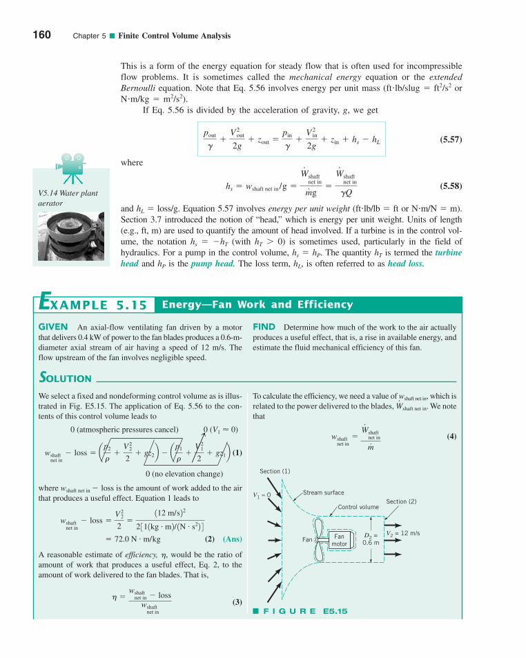
This is a form of the energy equation for steady flow that is often used for incompressibleflow problems. It is sometimes called the mechanical energy equation or the extendedBernoulli equation. Note that Eq. 5.56 involves energy per unit mass (ft�lb/slug � ft2/s2 orN�m/kg � m2/s2).

If Eq. 5.56 is divided by the acceleration of gravity, g, we get

(5.57)

where

(5.58)

and hL � loss/g. Equation 5.57 involves energy per unit weight (ft�lb/lb � ft or N�m/N � m).Section 3.7 introduced the notion of “head,” which is energy per unit weight. Units of length(e.g., ft, m) are used to quantify the amount of head involved. If a turbine is in the control vol-ume, the notation hs � �hT (with hT � 0) is sometimes used, particularly in the field ofhydraulics. For a pump in the control volume, hs � hP. The quantity hT is termed the turbinehead and hP is the pump head. The loss term, hL, is often referred to as head loss.

hs � wshaft net in /g �

W#

shaftnet in

m#g

�

W#

shaftnet in

�Q

pout

��

V 2out

2g� zout �

pin

��

V 2in

2g� zin � hs � hL

160 Chapter 5 ■ Finite Control Volume Analysis

V5.14 Water plantaerator

GIVEN An axial-flow ventilating fan driven by a motorthat delivers 0.4 kW of power to the fan blades produces a 0.6-m-diameter axial stream of air having a speed of 12 m/s. Theflow upstream of the fan involves negligible speed.

FIND Determine how much of the work to the air actuallyproduces a useful effect, that is, a rise in available energy, andestimate the fluid mechanical efficiency of this fan.

SOLUTION

We select a fixed and nondeforming control volume as is illus-trated in Fig. E5.15. The application of Eq. 5.56 to the con-tents of this control volume leads to

0 (atmospheric pressures cancel) 0 (V1 � 0)

(1)

0 (no elevation change)

where wshaft net in � loss is the amount of work added to the airthat produces a useful effect. Equation 1 leads to

(2) (Ans)

A reasonable estimate of efficiency, �, would be the ratio ofamount of work that produces a useful effect, Eq. 2, to theamount of work delivered to the fan blades. That is,

(3)� �

wshaftnet in � loss

wshaftnet in

� 72.0 N . m/kg

wshaftnet in

� loss �V 2

2

2�

112 m/s22

2 311kg . m2/ 1N . s22 4

wshaftnet in

� loss � ap2

��

V 22

2� gz2b � a

p1

��

V 21

2� gz1b

To calculate the efficiency, we need a value of wshaft net in, which isrelated to the power delivered to the blades, . We notethat

(4)wshaftnet in

�W#

shaftnet in

m#

W#

shaft net in

Energy—Fan Work and EfficiencyEXAMPLE 5.15

Fanmotor

Fan

V1 ≈ 0

Section (1)

Stream surface

Control volumeSection (2)

D2 =0.6 m

V2 = 12 m/s

F I G U R E E5.15

8888n

c05FiniteControlVolumeAnalysis.qxd 9/24/10 4:47 PM Page 160

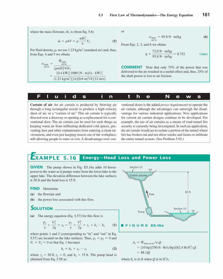
5.3 First Law of Thermodynamics—The Energy Equation 161

or

(6)

From Eqs. 2, 3, and 6 we obtain

(Ans)

COMMENT Note that only 75% of the power that wasdelivered to the air resulted in a useful effect and, thus, 25% ofthe shaft power is lost to air friction.

� �72.0 N . m/kg

95.8 N . m/kg� 0.752

wshaftnet in

� 95.8 N . m/kg

where the mass flowrate, , is (from Eq. 5.6)

(5)

For fluid density, �, we use 1.23 kg/m3 (standard air) and, thus,from Eqs. 4 and 5 we obtain

�

10.4 kW2 31000 1N . m2/ 1s . kW2 4

11.23 kg/m32 3 1�2 10.6 m22/4 4 112 m/s2

wshaftnet in

�W#

shaftnet in

1��D 22/42V2

m#

� �AV � � �D 2

2

4 V2

m#

F l u i d s i n t h e N e w s

Curtain of air An air curtain is produced by blowing airthrough a long rectangular nozzle to produce a high-velocitysheet of air, or a “curtain of air.” This air curtain is typically directed over a doorway or opening as a replacement for a con-ventional door. The air curtain can be used for such things askeeping warm air from infiltrating dedicated cold spaces, pre-venting dust and other contaminants from entering a clean en-vironment, and even just keeping insects out of the workplace,still allowing people to enter or exit. A disadvantage over con-

ventional doors is the added power requirements to operate theair curtain, although the advantages can outweigh the disad-vantage for various industrial applications. New applicationsfor current air curtain designs continue to be developed. Forexample, the use of air curtains as a means of road tunnel firesecurity is currently being investigated. In such an application,the air curtain would act to isolate a portion of the tunnel wherefire has broken out and not allow smoke and fumes to infiltratethe entire tunnel system. (See Problem 5.92.)

GIVEN The pump shown in Fig. E5.16a adds 10 horse-power to the water as it pumps water from the lower lake to theupper lake. The elevation difference between the lake surfacesis 30 ft and the head loss is 15 ft.

FIND Determine

(a) the flowrate and

(b) the power loss associated with this flow.

SOLUTION

(a) The energy equation (Eq. 5.57) for this flow is

(1)

where points 1 and 2 (corresponding to “in” and “out” in Eq.5.57) are located on the lake surfaces. Thus, and

so that Eq. 1 becomes

(2)

where and The pump head isobtained from Eq. 5.58 as

hL � 15 ft.z2 � 30 ft, z1 � 0,

hs � hL � z2 � z1

V1 � V2 � 0p1 � p2 � 0

p2

��

V 22

2g� z2 �

p1

��

V 21

2g� z1 � hs � hL

Energy—Head Loss and Power LossEXAMPLE 5.16

F I G U R E E5.16a

Control volume

Section (2)

Section (1)Pump

Flow30 ft

where is in ft when Q is in ft3/s.hs

� 88.1�Q � 110 hp2 1550 ft # lb�s�hp2�162.4 lb�ft32 Q

hs � W#

shaft net in �� Q

c05FiniteControlVolumeAnalysis.qxd 9/24/10 1:25 PM Page 161

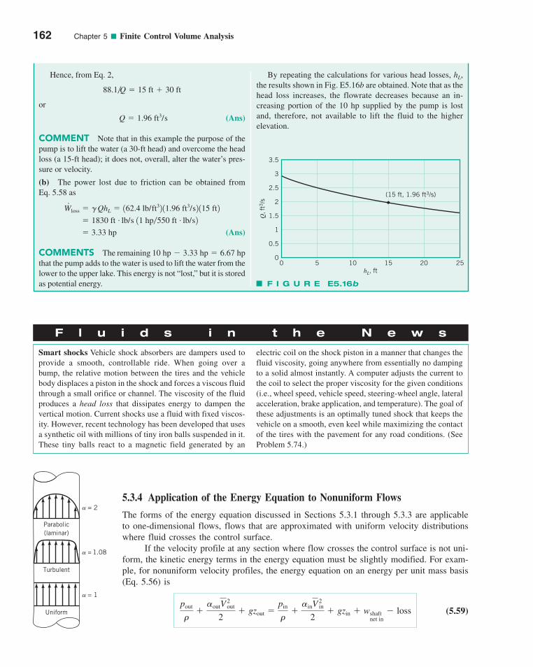
162 Chapter 5 ■ Finite Control Volume Analysis

By repeating the calculations for various head losses,the results shown in Fig. E5.16b are obtained. Note that as thehead loss increases, the flowrate decreases because an in-creasing portion of the 10 hp supplied by the pump is lostand, therefore, not available to lift the fluid to the higherelevation.

hL,Hence, from Eq. 2,

or

(Ans)

COMMENT Note that in this example the purpose of thepump is to lift the water (a 30-ft head) and overcome the headloss (a 15-ft head); it does not, overall, alter the water’s pres-sure or velocity.

(b) The power lost due to friction can be obtained fromEq. 5.58 as

(Ans)

COMMENTS The remaining that the pump adds to the water is used to lift the water from thelower to the upper lake. This energy is not “lost,” but it is storedas potential energy.

10 hp � 3.33 hp � 6.67 hp

� 3.33 hp

� 1830 ft # lb/s 11 hp�550 ft # lb/s2

W#

loss � � QhL � 162.4 lb/ft32 11.96 ft3/s2 115 ft2

Q � 1.96 ft3/s

88.1�Q � 15 ft � 30 ft

20 251510

(15 ft, 1.96 ft3/s)

50hL, ft

Q, f

t3/s

3.5

3

2.5

2

1.5

1

0.5

0

F I G U R E E5.16b

F l u i d s i n t h e N e w s

Smart shocks Vehicle shock absorbers are dampers used toprovide a smooth, controllable ride. When going over abump, the relative motion between the tires and the vehiclebody displaces a piston in the shock and forces a viscous fluidthrough a small orifice or channel. The viscosity of the fluidproduces a head loss that dissipates energy to dampen thevertical motion. Current shocks use a fluid with fixed viscos-ity. However, recent technology has been developed that usesa synthetic oil with millions of tiny iron balls suspended in it.These tiny balls react to a magnetic field generated by an

electric coil on the shock piston in a manner that changes thefluid viscosity, going anywhere from essentially no dampingto a solid almost instantly. A computer adjusts the current tothe coil to select the proper viscosity for the given conditions(i.e., wheel speed, vehicle speed, steering-wheel angle, lateralacceleration, brake application, and temperature). The goal ofthese adjustments is an optimally tuned shock that keeps thevehicle on a smooth, even keel while maximizing the contactof the tires with the pavement for any road conditions. (SeeProblem 5.74.)

5.3.4 Application of the Energy Equation to Nonuniform Flows

The forms of the energy equation discussed in Sections 5.3.1 through 5.3.3 are applicableto one-dimensional flows, flows that are approximated with uniform velocity distributionswhere fluid crosses the control surface.

If the velocity profile at any section where flow crosses the control surface is not uni-form, the kinetic energy terms in the energy equation must be slightly modified. For exam-ple, for nonuniform velocity profiles, the energy equation on an energy per unit mass basis(Eq. 5.56) is

(5.59)pout

��

�outV2out

2� gzout �

pin

��

�inV2in

2� gzin � wshaft

net in� loss

Parabolic(laminar)

Turbulent

Uniform

� = 2

� 1.08

� = 1

~~

c05FiniteControlVolumeAnalysis.qxd 9/24/10 1:25 PM Page 162

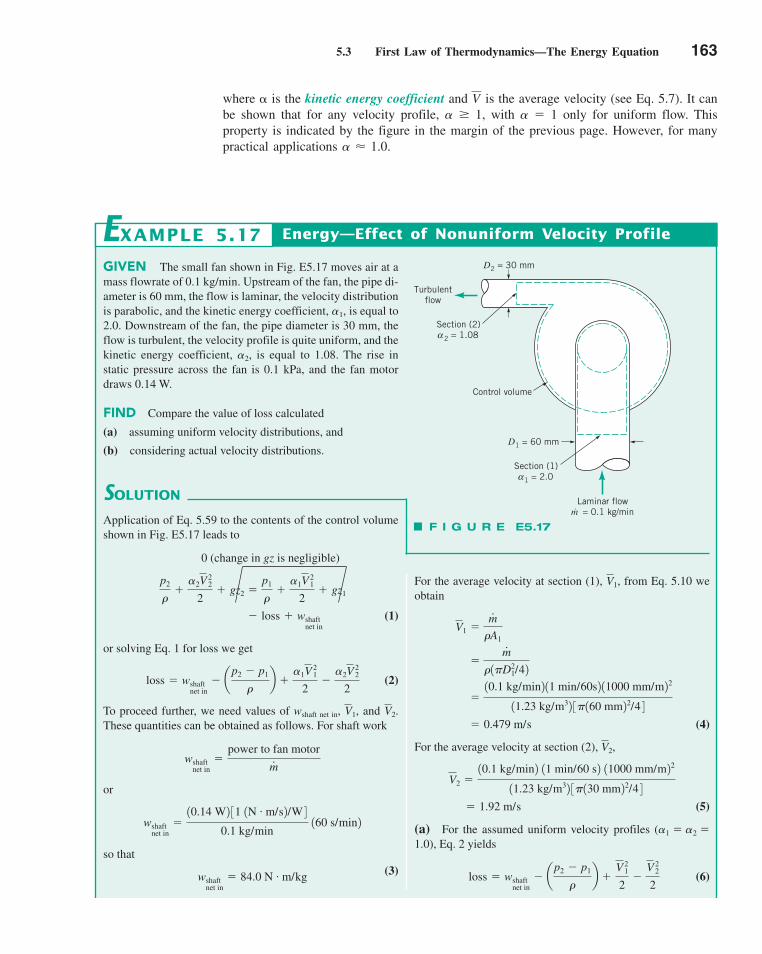
5.3 First Law of Thermodynamics—The Energy Equation 163

where is the kinetic energy coefficient and is the average velocity (see Eq. 5.7). It canbe shown that for any velocity profile, � � 1, with � � 1 only for uniform flow. Thisproperty is indicated by the figure in the margin of the previous page. However, for manypractical applications � � 1.0.

V

GIVEN The small fan shown in Fig. E5.17 moves air at amass flowrate of 0.1 kg/min. Upstream of the fan, the pipe di-ameter is 60 mm, the flow is laminar, the velocity distributionis parabolic, and the kinetic energy coefficient, �1, is equal to2.0. Downstream of the fan, the pipe diameter is 30 mm, theflow is turbulent, the velocity profile is quite uniform, and thekinetic energy coefficient, �2, is equal to 1.08. The rise instatic pressure across the fan is 0.1 kPa, and the fan motordraws 0.14 W.

FIND Compare the value of loss calculated

(a) assuming uniform velocity distributions, and

(b) considering actual velocity distributions.

SOLUTION

Application of Eq. 5.59 to the contents of the control volumeshown in Fig. E5.17 leads to

0 (change in gz is negligible)

(1)

or solving Eq. 1 for loss we get

(2)

To proceed further, we need values of wshaft net in, , and .These quantities can be obtained as follows. For shaft work

or

so that(3) wshaft

net in� 84.0 N . m/kg

wshaftnet in

�10.14 W2 31 1N . m/s2/W 4

0.1 kg/min 160 s/min2

wshaftnet in

�power to fan motor

m#

V2V1

loss � wshaftnet in

� ap2 � p1

�b �

�1V21

2�

�2V22

2

� loss � wshaftnet in

p2

��

�2V22

2� gz2 �

p1

��

�1V21

2� gz1

Energy—Effect of Nonuniform Velocity ProfileEXAMPLE 5.17

F I G U R E E5.17

For the average velocity at section (1), , from Eq. 5.10 weobtain

(4)

For the average velocity at section (2), ,

(5)

(a) For the assumed uniform velocity profiles (�1 � �2 �1.0), Eq. 2 yields

(6)loss � wshaftnet in

� ap2 � p1

�b �

V 21

2�

V 22

2

� 1.92 m/s

V2 �10.1 kg/min2 11 min/60 s2 11000 mm/m22

11.23 kg/m32 3�130 mm22/4 4

V2

� 0.479 m/s

�10.1 kg/min2 11 min/60s2 11000 mm/m22

11.23 kg/m32 3�160 mm22/4 4

�m#

�1�D21/42

V1 �m#

�A1

V1

Control volume

Turbulentflow

Section (2) 2 = 1.08α

D2 = 30 mm

D1 = 60 mm

Section (1) 1 = 2.0α

Laminar flowm = 0.1 kg/min#

c05FiniteControlVolumeAnalysis.qxd 9/24/10 1:26 PM Page 163

164 Chapter 5 ■ Finite Control Volume Analysis

If we use Eqs. 3, 4, and 5 and the given pressure rise, Eq. 7yields

or

(Ans)

COMMENT The difference in loss calculated assuminguniform velocity profiles and actual velocity profiles is notlarge compared to wshaft net in for this fluid flow situation.

� 0.940 N . m/kg

� 0.230 N . m/kg � 1.99 N . m/kg

loss � 84.0 N . m/kg � 81.3 N . m/kg

�1.0811.92 m/s22

2 31 1kg . m2/ 1N . s22 4 �

210.479 m/s22

2 31 1kg . m2/ 1N . s22 4

loss � 84 N . m/kg �10.1 kPa2 11000 Pa/kPa2 11 N/m2/Pa2

1.23 kg/m3

Using Eqs. 3, 4, and 5 and the pressure rise given in theproblem statement, Eq. 6 gives

or

(Ans)

(b) For the actual velocity profiles (�1 � 2, �2 � 1.08), Eq. 1gives

(7)loss � wshaftnet in

� ap2 � p1

�b � �1

V 21

2� �2

V 22

2

� 0.975 N . m/kg

� 0.115 N . m/kg � 1.84 N . m/kg

loss � 84.0 N . m/kg � 81.3 N . m/kg

�11.92 m/s22

2 31 1kg . m2/ 1N . s22 4�

10.479 m/s22

2 31 1kg . m2/ 1N . s22 4

loss � 84.0 N . m

kg�10.1 kPa2 11000 Pa/kPa2 11 N/m2/Pa2

1.23 kg/m3

conservation of mass

continuity equationmass flowratelinear momentum

equationmoment-of-

momentum equation

shaft powershaft torquefirst law of

thermo- dynamics

heat transfer rateenergy equationlossturbine and

pump headhead losskinetic energy

coefficient

5.4 Chapter Summary and Study Guide

In this chapter the flow of a fluid is analyzed by using the principles of conservation ofmass, momentum, and energy as applied to control volumes. The Reynolds transport theo-rem is used to convert basic system-orientated conservation laws into the correspondingcontrol volume formulation.

The continuity equation, a statement of the fact that mass is conserved, is obtained ina form that can be applied to any flows—steady or unsteady, incompressible or compress-ible. Simplified forms of the continuity equation are used to solve problems dealing withmass and volume flowrates.

The linear momentum equation, a form of Newton’s second law of motion applicableto flow through a control volume, is obtained and used to solve flow problems dealing withsurface and body forces acting on the fluid and its surroundings. The net flux of momentumthrough the control surface is directly related to the net force exerted on the contents of thecontrol volume.

The moment-of-momentum equation, which involves the relationship between torqueand angular momentum flowrate, is obtained and used to solve flow problems dealing withturbines (that remove energy from a fluid) and pumps (that supply energy to a fluid).

The steady-state energy equation, obtained from the first law of thermodynamics, iswritten in several forms. The first (Eq. 5.44) involves terms such as the mass flowrate, inter-nal energy per unit mass, heat transfer rate, and shaft work rate. The second form (Eq. 5.56or 5.57) is termed the mechanical energy equation or the extended Bernoulli equation. Itconsists of the Bernoulli equation with extra terms that account for losses due to friction inthe flow, as well as terms accounting for the existence of pumps or turbines in the flow.

The following checklist provides a study guide for this chapter. When your study ofthe entire chapter and end-of-chapter exercises has been completed you should be able to

write out meanings of the terms listed here in the margin and understand each of therelated concepts. These terms are particularly important and are set in color and boldtype in the text.

select an appropriate control volume for a given problem and draw an accuratelylabeled control volume diagram.

c05FiniteControlVolumeAnalysis.qxd 9/24/10 1:26 PM Page 164

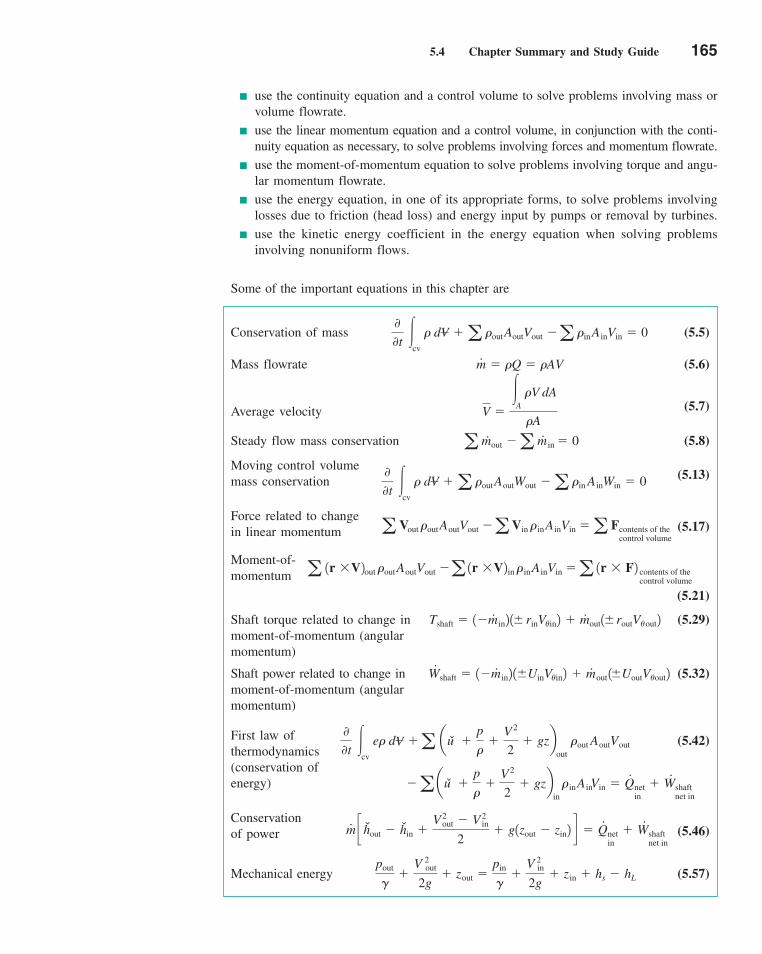
5.4 Chapter Summary and Study Guide 165

use the continuity equation and a control volume to solve problems involving mass orvolume flowrate.

use the linear momentum equation and a control volume, in conjunction with the conti-nuity equation as necessary, to solve problems involving forces and momentum flowrate.

use the moment-of-momentum equation to solve problems involving torque and angu-lar momentum flowrate.

use the energy equation, in one of its appropriate forms, to solve problems involvinglosses due to friction (head loss) and energy input by pumps or removal by turbines.

use the kinetic energy coefficient in the energy equation when solving problemsinvolving nonuniform flows.

Some of the important equations in this chapter are

Conservation of mass (5.5)

Mass flowrate (5.6)

Average velocity (5.7)

Steady flow mass conservation (5.8)

Moving control volume mass conservation (5.13)

Force related to change in linear momentum (5.17)

Moment-of-momentum

(5.21)

Shaft torque related to change in (5.29)moment-of-momentum (angular momentum)

Shaft power related to change in (5.32)moment-of-momentum (angular momentum)

First law of (5.42)thermodynamics (conservation of energy)

Conservation of power (5.46)

Mechanical energy (5.57)pout

��

V 2out

2g� zout �

pin

��

V 2in

2g� zin � hs � hL

m#c hout � hin �

V 2out � V 2

in

2� g1zout � zin2 d � Q

#netin

� W#

shaftnet in

�a au �p

��

V 2

2� gzb

in �inAinVin � Q

#netin

� W#

shaftnet in

00t

�cv

e� dV �a au �p

��

V 2

2� gzb

out �out AoutVout

W#

shaft � 1�m#

in2 1�UinV�in2 � m#

out 1�UoutV�out2

Tshaft � 1�m#

in2 1� rinV�in2 � m#

out1�routV�out2

a 1r �V2out � outA outV out �a 1r �V2in � inA inVin �a 1r � F2 contents of thecontrol volume

a Vout � outA outV out �a Vin � inA inVin �a Fcontents of thecontrol volume

00t

�cv

� dV �a �outAoutWout �a �in AinWin � 0

a m#out �a m

#in � 0

V �

�A

�V dA

�A

m#

� �Q � �AV

00t

�cv

� dV �a �outAoutVout �a �inAinVin � 0

c05FiniteControlVolumeAnalysis.qxd 9/24/10 1:26 PM Page 165

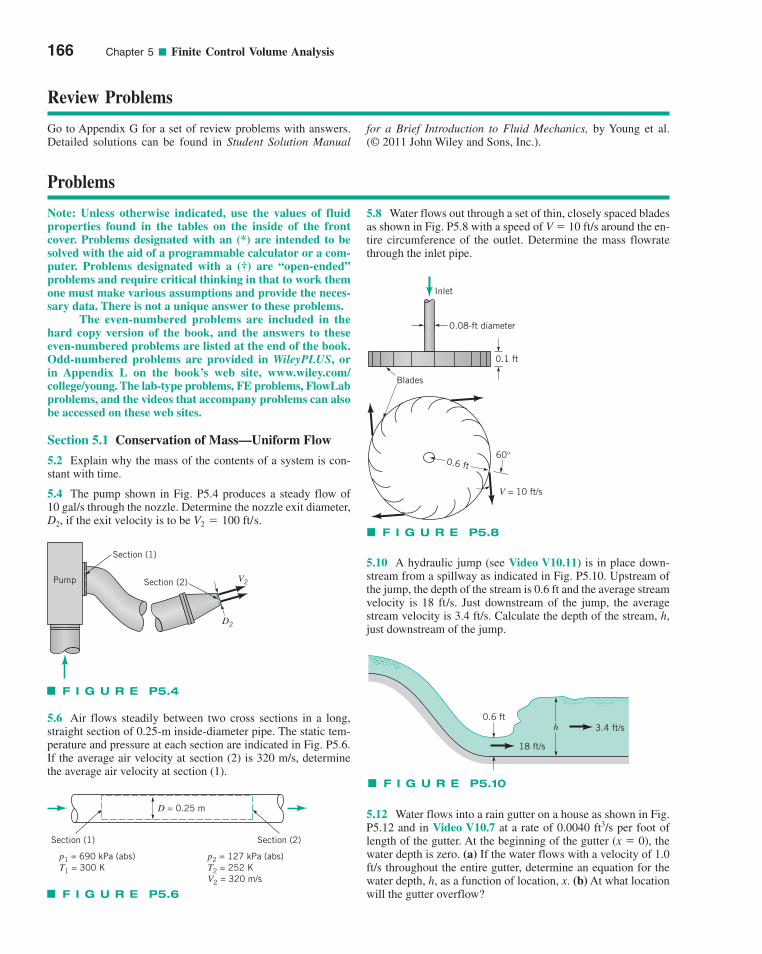
166 Chapter 5 ■ Finite Control Volume Analysis

Problems

Note: Unless otherwise indicated, use the values of fluidproperties found in the tables on the inside of the frontcover. Problems designated with an (*) are intended to besolved with the aid of a programmable calculator or a com-puter. Problems designated with a (†) are “open-ended”problems and require critical thinking in that to work themone must make various assumptions and provide the neces-sary data. There is not a unique answer to these problems.

The even-numbered problems are included in thehard copy version of the book, and the answers to theseeven-numbered problems are listed at the end of the book.Odd-numbered problems are provided in WileyPLUS, orin Appendix L on the book’s web site, www.wiley.com/college/young. The lab-type problems, FE problems, FlowLabproblems, and the videos that accompany problems can alsobe accessed on these web sites.

Section 5.1 Conservation of Mass—Uniform Flow

5.2 Explain why the mass of the contents of a system is con-stant with time.

5.4 The pump shown in Fig. P5.4 produces a steady flow of 10 gal/s through the nozzle. Determine the nozzle exit diameter,

if the exit velocity is to be .V2 � 100 ft/sD2,

5.8 Water flows out through a set of thin, closely spaced bladesas shown in Fig. P5.8 with a speed of V � 10 ft/s around the en-tire circumference of the outlet. Determine the mass flowratethrough the inlet pipe.

5.10 A hydraulic jump (see Video V10.11) is in place down-stream from a spillway as indicated in Fig. P5.10. Upstream ofthe jump, the depth of the stream is 0.6 ft and the average streamvelocity is 18 ft/s. Just downstream of the jump, the averagestream velocity is 3.4 ft/s. Calculate the depth of the stream, h,just downstream of the jump.

5.12 Water flows into a rain gutter on a house as shown in Fig.P5.12 and in Video V10.7 at a rate of 0.0040 ft3/s per foot oflength of the gutter. At the beginning of the gutter (x � 0), thewater depth is zero. (a) If the water flows with a velocity of 1.0ft/s throughout the entire gutter, determine an equation for thewater depth, h, as a function of location, x. (b) At what locationwill the gutter overflow?

Review Problems

Go to Appendix G for a set of review problems with answers.Detailed solutions can be found in Student Solution Manual

for a Brief Introduction to Fluid Mechanics, by Young et al. (© 2011 John Wiley and Sons, Inc.).

F I G U R E P5.4

Section (1)

Section (2)

D2

V2 Pump

F I G U R E P5.8

0.08-ft diameter

0.1 ft

Inlet

Blades

0.6 ft60°

V = 10 ft/s

F I G U R E P5.10

18 ft/s

3.4 ft/s0.6 ft

h

F I G U R E P5.6

D = 0.25 m

Section (1) Section (2)

p1 = 690 kPa (abs)T1 = 300 K

p2 = 127 kPa (abs)T2 = 252 KV2 = 320 m/s

5.6 Air flows steadily between two cross sections in a long,straight section of 0.25-m inside-diameter pipe. The static tem-perature and pressure at each section are indicated in Fig. P5.6.If the average air velocity at section (2) is 320 m/s, determinethe average air velocity at section (1).

c05FiniteControlVolumeAnalysis.qxd 10/18/10 7:59 AM Page 166

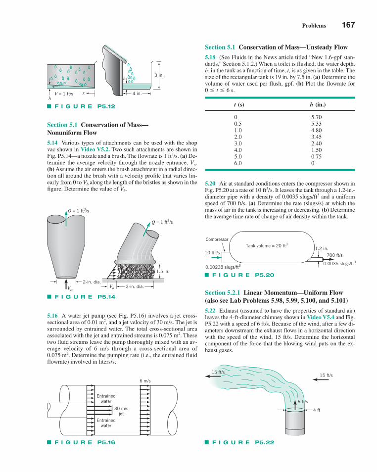
Problems 167

Section 5.1 Conservation of Mass—Nonuniform Flow

5.14 Various types of attachments can be used with the shopvac shown in Video V5.2. Two such attachments are shown inFig. P5.14—a nozzle and a brush. The flowrate is 1 ft3/s. (a) De-termine the average velocity through the nozzle entrance, Vn.(b) Assume the air enters the brush attachment in a radial direc-tion all around the brush with a velocity profile that varies lin-early from 0 to Vb along the length of the bristles as shown in thefigure. Determine the value of Vb.

5.16 A water jet pump (see Fig. P5.16) involves a jet cross-sectional area of and a jet velocity of 30 m/s. The jet issurrounded by entrained water. The total cross-sectional areaassociated with the jet and entrained streams is Thesetwo fluid streams leave the pump thoroughly mixed with an av-erage velocity of 6 m/s through a cross-sectional area of

Determine the pumping rate (i.e., the entrained fluidflowrate) involved in liters/s.0.075 m2.

0.075 m2.

0.01 m2,

Section 5.1 Conservation of Mass—Unsteady Flow

5.18 (See Fluids in the News article titled “New 1.6-gpf stan-dards,” Section 5.1.2.) When a toilet is flushed, the water depth,h, in the tank as a function of time, t, is as given in the table. Thesize of the rectangular tank is 19 in. by 7.5 in. (a) Determine thevolume of water used per flush, gpf. (b) Plot the flowrate for

.

t (s) h (in.)

0 5.700.5 5.331.0 4.802.0 3.453.0 2.404.0 1.505.0 0.756.0 0

5.20 Air at standard conditions enters the compressor shown inFig. P5.20 at a rate of It leaves the tank through a 1.2-in.-diameter pipe with a density of 0.0035 slugs/ft3 and a uniformspeed of 700 ft/s. (a) Determine the rate (slugs/s) at which themass of air in the tank is increasing or decreasing. (b) Determinethe average time rate of change of air density within the tank.

10 ft3/s.

0 � t � 6 s

Section 5.2.1 Linear Momentum—Uniform Flow(also see Lab Problems 5.98, 5.99, 5.100, and 5.101)

5.22 Exhaust (assumed to have the properties of standard air)leaves the 4-ft-diameter chimney shown in Video V5.4 and Fig.P5.22 with a speed of 6 ft/s. Because of the wind, after a few di-ameters downstream the exhaust flows in a horizontal directionwith the speed of the wind, 15 ft/s. Determine the horizontalcomponent of the force that the blowing wind puts on the ex-haust gases.

F I G U R E P5.12

V = 1 ft/s

3 in.

4 in. h

h

x

F I G U R E P5.14

Q = 1 ft3/s

Q = 1 ft3/s

Vn

2-in. dia.

1.5 in.

3-in. dia.Vb

F I G U R E P5.20

Tank volume = 20 ft31.2 in.

700 ft/s

0.0035 slugs/ft3

10 ft3/s

Compressor

0.00238 slugs/ft3

F I G U R E P5.22

15 ft/s15 ft/s

6 ft/s

4 ft

F I G U R E P5.16

30 m/s jet

6 m/s

Entrained water

Entrained water

c05FiniteControlVolumeAnalysis.qxd 9/24/10 1:27 PM Page 167

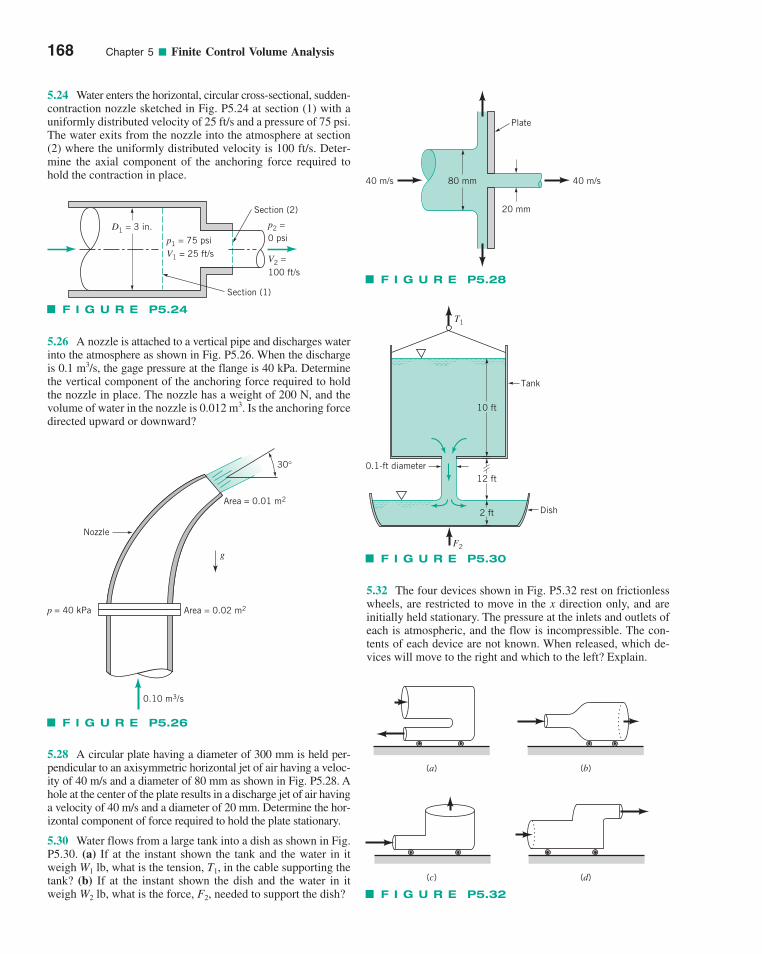
168 Chapter 5 ■ Finite Control Volume Analysis

5.24 Water enters the horizontal, circular cross-sectional, sudden-contraction nozzle sketched in Fig. P5.24 at section (1) with auniformly distributed velocity of 25 ft/s and a pressure of 75 psi.The water exits from the nozzle into the atmosphere at section(2) where the uniformly distributed velocity is 100 ft/s. Deter-mine the axial component of the anchoring force required tohold the contraction in place.

5.26 A nozzle is attached to a vertical pipe and discharges waterinto the atmosphere as shown in Fig. P5.26. When the dischargeis 0.1 m3/s, the gage pressure at the flange is 40 kPa. Determinethe vertical component of the anchoring force required to holdthe nozzle in place. The nozzle has a weight of 200 N, and thevolume of water in the nozzle is 0.012 m3. Is the anchoring forcedirected upward or downward?

5.28 A circular plate having a diameter of 300 mm is held per-pendicular to an axisymmetric horizontal jet of air having a veloc-ity of 40 m/s and a diameter of 80 mm as shown in Fig. P5.28. Ahole at the center of the plate results in a discharge jet of air havinga velocity of 40 m/s and a diameter of 20 mm. Determine the hor-izontal component of force required to hold the plate stationary.

5.30 Water flows from a large tank into a dish as shown in Fig.P5.30. (a) If at the instant shown the tank and the water in itweigh what is the tension, in the cable supporting thetank? (b) If at the instant shown the dish and the water in itweigh lb, what is the force, needed to support the dish?F2,W2

T1,W1 lb,

5.32 The four devices shown in Fig. P5.32 rest on frictionlesswheels, are restricted to move in the x direction only, and areinitially held stationary. The pressure at the inlets and outlets ofeach is atmospheric, and the flow is incompressible. The con-tents of each device are not known. When released, which de-vices will move to the right and which to the left? Explain.

F I G U R E P5.24

D1 = 3 in.

p1 = 75 psiV1 = 25 ft/s

p2 = 0 psi

V2 = 100 ft/s

Section (2)

Section (1)

F I G U R E P5.26

Area = 0.02 m2

Area = 0.01 m2

p = 40 kPa

Nozzle

0.10 m3/s

g

30°

F I G U R E P5.28

40 m/s 80 mm

20 mm

40 m/s

Plate

F I G U R E P5.30

0.1-ft diameter

Dish

Tank

10 ft

12 ft

2 ft

F2

T1

F I G U R E P5.32

(a)

(c)

(b)

(d)

c05FiniteControlVolumeAnalysis.qxd 9/24/10 1:27 PM Page 168

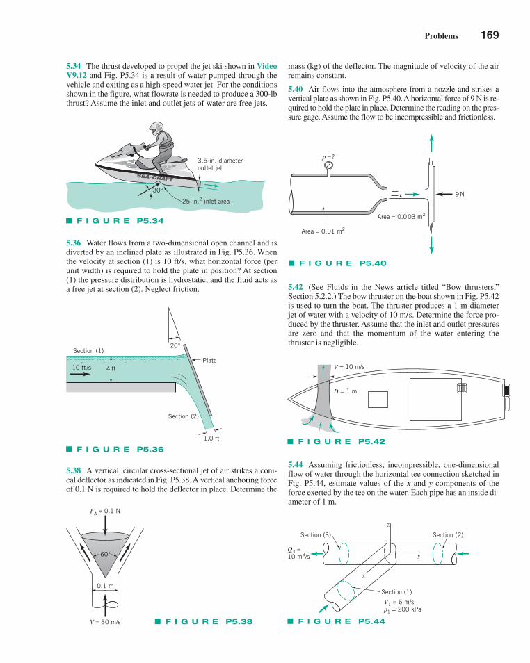
Problems 169

5.34 The thrust developed to propel the jet ski shown in VideoV9.12 and Fig. P5.34 is a result of water pumped through thevehicle and exiting as a high-speed water jet. For the conditionsshown in the figure, what flowrate is needed to produce a 300-lbthrust? Assume the inlet and outlet jets of water are free jets.

5.36 Water flows from a two-dimensional open channel and isdiverted by an inclined plate as illustrated in Fig. P5.36. Whenthe velocity at section (1) is 10 ft/s, what horizontal force (perunit width) is required to hold the plate in position? At section(1) the pressure distribution is hydrostatic, and the fluid acts asa free jet at section (2). Neglect friction.

5.38 A vertical, circular cross-sectional jet of air strikes a coni-cal deflector as indicated in Fig. P5.38. A vertical anchoring forceof 0.1 N is required to hold the deflector in place. Determine the

mass (kg) of the deflector. The magnitude of velocity of the airremains constant.

5.40 Air flows into the atmosphere from a nozzle and strikes avertical plate as shown in Fig. P5.40. A horizontal force of 9 N is re-quired to hold the plate in place. Determine the reading on the pres-sure gage. Assume the flow to be incompressible and frictionless.

5.42 (See Fluids in the News article titled “Bow thrusters,”Section 5.2.2.) The bow thruster on the boat shown in Fig. P5.42is used to turn the boat. The thruster produces a 1-m-diameterjet of water with a velocity of . Determine the force pro-duced by the thruster. Assume that the inlet and outlet pressuresare zero and that the momentum of the water entering thethruster is negligible.

10 m/s

5.44 Assuming frictionless, incompressible, one-dimensionalflow of water through the horizontal tee connection sketched inFig. P5.44, estimate values of the x and y components of theforce exerted by the tee on the water. Each pipe has an inside di-ameter of 1 m.

F I G U R E P5.34

3.5-in.-diameteroutlet jet

30°

25-in.2 inlet area

F I G U R E P5.40

Area = 0.01 m2

Area = 0.003 m2

9N

p =?

F I G U R E P5.42

D = 1 m

V = 10 m/s

F I G U R E P5.44

Section (3)

Q3 =10 m3/s

Section (2)

Section (1)

x

y

z

V1 = 6 m/sp1 = 200 kPa

F I G U R E P5.36

10 ft /s

Section (2)

Plate4 ft

1.0 ft

Section (1)20°

F I G U R E P5.38

0.1 m

V = 30 m/s

FA = 0.1 N

60°

c05FiniteControlVolumeAnalysis.qxd 9/24/10 1:27 PM Page 169

†5.46 A table tennis ball “balances” on a jet of air as shown inVideo V3.2 and in Fig. P5.46. Explain why the ball sits at theheight it does and why the ball does not “roll off” the jet.

Section 5.2.1 Linear Momentum—Nonuniform Flow

5.48 Water is sprayed radially outward over 180 as indicatedin Fig. P5.48. The jet sheet is in the horizontal plane. If the jetvelocity at the nozzle exit is 30 ft/s, determine the direction andmagnitude of the resultant horizontal anchoring force requiredto hold the nozzle in place.

5.50 A variable mesh screen produces a linear and axisymmet-ric velocity profile as indicated in Fig. P5.50 in the air flowthrough a 2-ft-diameter circular cross-sectional duct. The staticpressures upstream and downstream of the screen are 0.2 and 0.15psi and are uniformly distributed over the flow cross-sectionalarea. Neglecting the force exerted by the duct wall on the flow-ing air, calculate the screen drag force.

Section 5.2.4 Application of the Moment-of-Momentum Equation

5.52 Five liters per second of water enter the rotor shown inVideo V5.10 and Fig. P5.52 along the axis of rotation. Thecross-sectional area of each of the three nozzle exits normal tothe relative velocity is 18 mm2. How large is the resisting torquerequired to hold the rotor stationary if (a) � � 0, (b) � � 30,and (c) � � 60?

5.54 Five liters per second of water enter the rotor shown inVideo V5.10 and Fig. P5.54 along the axis of rotation. Thecross-sectional area of each of the three nozzle exits normal tothe relative velocity is 18 mm2. How fast will the rotor spinsteadily if the resisting torque is reduced to zero and (a) � � 0,(b) � � 30, or (c) � � 60?

5.56 A water turbine wheel rotates at the rate of 50 rpm in the di-rection shown in Fig. P5.56. The inner radius, r2, of the blade rowis 2 ft, and the outer radius, r1, is 4 ft. The absolute velocity vec-tor at the turbine rotor entrance makes an angle of 20 with thetangential direction. The inlet blade angle is 60 relative to thetangential direction. The blade outlet angle is 120. The flowrateis 20 ft3/s. For the flow tangent to the rotor blade surface at inlet

170 Chapter 5 ■ Finite Control Volume Analysis

F I G U R E P5.46

F I G U R E P5.48

8 in. 0.5 in.

V =30 ft/s

F I G U R E P5.52

Q = 5 liters/s

r = 0.5m Nozzle exit area normal torelative velocity = 18 mm2

θ

F I G U R E P5.54

0.5 m

Nozzle exit area normal torelative velocity = 18 mm2

θ

Q = 5 liters/s

F I G U R E P5.50

Section (1) Section (2)

Variable mesh screen

D = 2 ft

p1 = 0.2 psi V1 = 100 ft/s

p2 = 0.15 psi

c05FiniteControlVolumeAnalysis.qxd 9/24/10 1:27 PM Page 170

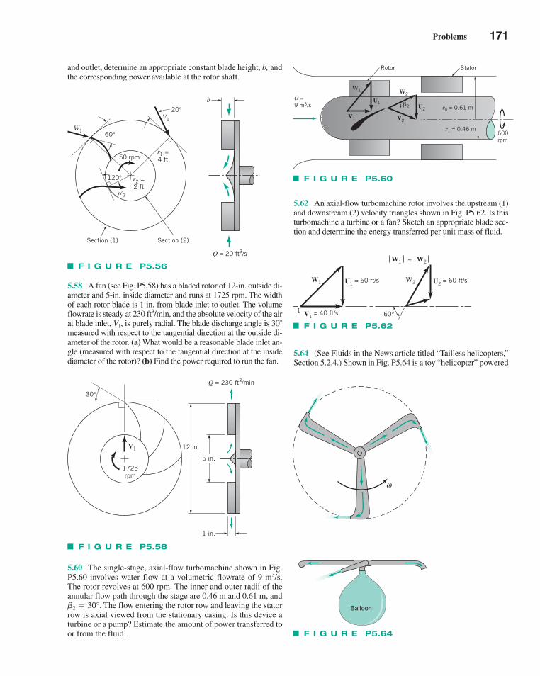
Problems 171

and outlet, determine an appropriate constant blade height, b, andthe corresponding power available at the rotor shaft.

5.58 A fan (see Fig. P5.58) has a bladed rotor of 12-in. outside di-ameter and 5-in. inside diameter and runs at 1725 rpm. The widthof each rotor blade is 1 in. from blade inlet to outlet. The volumeflowrate is steady at 230 ft3/min, and the absolute velocity of the airat blade inlet, V1, is purely radial. The blade discharge angle is 30measured with respect to the tangential direction at the outside di-ameter of the rotor. (a) What would be a reasonable blade inlet an-gle (measured with respect to the tangential direction at the insidediameter of the rotor)? (b) Find the power required to run the fan.

5.60 The single-stage, axial-flow turbomachine shown in Fig.P5.60 involves water flow at a volumetric flowrate of 9 m3/s.The rotor revolves at 600 rpm. The inner and outer radii of theannular flow path through the stage are 0.46 m and 0.61 m, and

The flow entering the rotor row and leaving the statorrow is axial viewed from the stationary casing. Is this device aturbine or a pump? Estimate the amount of power transferred toor from the fluid.

2 � 30°.

5.62 An axial-flow turbomachine rotor involves the upstream (1)and downstream (2) velocity triangles shown in Fig. P5.62. Is thisturbomachine a turbine or a fan? Sketch an appropriate blade sec-tion and determine the energy transferred per unit mass of fluid.

5.64 (See Fluids in the News article titled “Tailless helicopters,”Section 5.2.4.) Shown in Fig. P5.64 is a toy “helicopter” powered

F I G U R E P5.56

W1

W2

V1

50 rpm

r2 =2 ft

r1 =4 ft

60°

120°

20°

Section (1) Section (2)

Q = 20 ft3/s

b

F I G U R E P5.58

V1

1725rpm

Q = 230 ft3/min

1 in.

5 in.

12 in.

30°

F I G U R E P5.60

Q = 9 m3/s r0 = 0.61 m

600rpm

V1 V2

U2

Rotor Stator

U1

W2

�2

r1 = 0.46 m

W1

F I G U R E P5.62

W1

1

W2

W1

U1= 60 ft/s

V1= 40 ft/s

W2=

60°

U2= 60 ft/s

F I G U R E P5.64

Balloon

ω

c05FiniteControlVolumeAnalysis.qxd 9/24/10 1:27 PM Page 171

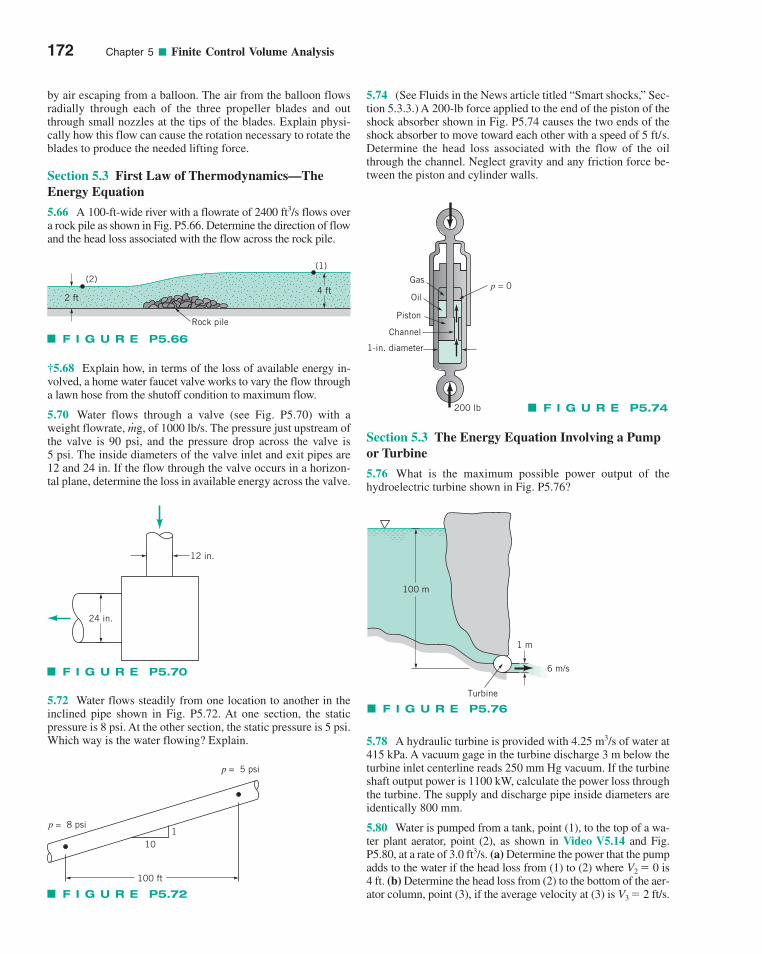
by air escaping from a balloon. The air from the balloon flowsradially through each of the three propeller blades and outthrough small nozzles at the tips of the blades. Explain physi-cally how this flow can cause the rotation necessary to rotate theblades to produce the needed lifting force.

Section 5.3 First Law of Thermodynamics—TheEnergy Equation

5.66 A 100-ft-wide river with a flowrate of 2400 ft3/s flows overa rock pile as shown in Fig. P5.66. Determine the direction of flowand the head loss associated with the flow across the rock pile.

†5.68 Explain how, in terms of the loss of available energy in-volved, a home water faucet valve works to vary the flow througha lawn hose from the shutoff condition to maximum flow.

5.70 Water flows through a valve (see Fig. P5.70) with aweight flowrate, m

.g, of 1000 lb/s. The pressure just upstream of

the valve is 90 psi, and the pressure drop across the valve is 5 psi. The inside diameters of the valve inlet and exit pipes are12 and 24 in. If the flow through the valve occurs in a horizon-tal plane, determine the loss in available energy across the valve.

5.72 Water flows steadily from one location to another in theinclined pipe shown in Fig. P5.72. At one section, the staticpressure is 8 psi. At the other section, the static pressure is 5 psi.Which way is the water flowing? Explain.

5.74 (See Fluids in the News article titled “Smart shocks,” Sec-tion 5.3.3.) A 200-lb force applied to the end of the piston of theshock absorber shown in Fig. P5.74 causes the two ends of theshock absorber to move toward each other with a speed of .Determine the head loss associated with the flow of the oilthrough the channel. Neglect gravity and any friction force be-tween the piston and cylinder walls.

5 ft/s

Section 5.3 The Energy Equation Involving a Pumpor Turbine

5.76 What is the maximum possible power output of the hydroelectric turbine shown in Fig. P5.76?

5.78 A hydraulic turbine is provided with 4.25 m3/s of water at415 kPa. A vacuum gage in the turbine discharge 3 m below theturbine inlet centerline reads 250 mm Hg vacuum. If the turbineshaft output power is 1100 kW, calculate the power loss throughthe turbine. The supply and discharge pipe inside diameters areidentically 800 mm.

5.80 Water is pumped from a tank, point (1), to the top of a wa-ter plant aerator, point (2), as shown in Video V5.14 and Fig.P5.80, at a rate of 3.0 ft3/s. (a) Determine the power that the pumpadds to the water if the head loss from (1) to (2) where V2 � 0 is4 ft. (b) Determine the head loss from (2) to the bottom of the aer-ator column, point (3), if the average velocity at (3) is V3 � 2 ft/s.

172 Chapter 5 ■ Finite Control Volume Analysis

F I G U R E P5.66

(2)

2 ft

Rock pile

4 ft

(1)

F I G U R E P5.70

24 in.

12 in.

F I G U R E P5.72

101

100 ft

p = 8 psi

p = 5 psi

F I G U R E P5.74

Gasp = 0

Oil

Piston

200 lb

Channel

1-in. diameter

F I G U R E P5.76

100 m

1 m

6 m/s

Turbine

c05FiniteControlVolumeAnalysis.qxd 9/24/10 1:27 PM Page 172

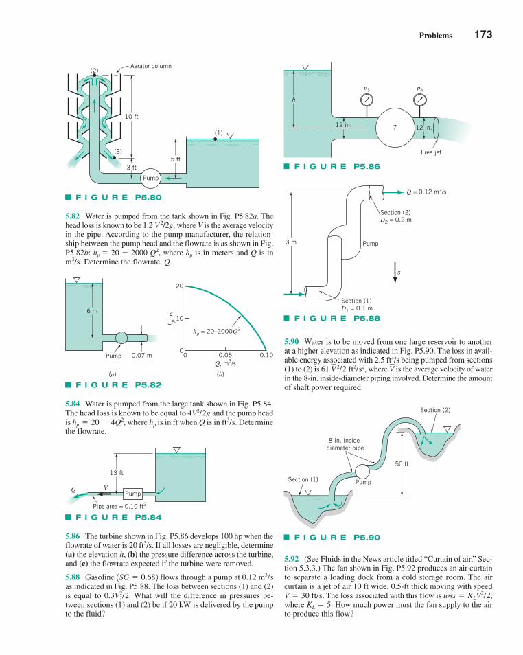
Problems 173

5.82 Water is pumped from the tank shown in Fig. P5.82a. Thehead loss is known to be 1.2 V 2/2g, where V is the average velocityin the pipe. According to the pump manufacturer, the relation-ship between the pump head and the flowrate is as shown in Fig.P5.82b: hp � 20 � 2000 Q2, where hp is in meters and Q is inm3/s. Determine the flowrate, Q.

5.84 Water is pumped from the large tank shown in Fig. P5.84.The head loss is known to be equal to and the pump headis , where is in ft when Q is in ft3/s. Determinethe flowrate.

hphp � 20 � 4Q24V2/2g

5.86 The turbine shown in Fig. P5.86 develops 100 hp when theflowrate of water is 20 ft3/s. If all losses are negligible, determine(a) the elevation h, (b) the pressure difference across the turbine,and (c) the flowrate expected if the turbine were removed.

5.88 Gasoline flows through a pump at as indicated in Fig. P5.88. The loss between sections (1) and (2)is equal to What will the difference in pressures be-tween sections (1) and (2) be if 20 kW is delivered by the pumpto the fluid?

0.3V21/2.

0.12 m3/s1SG � 0.682

5.90 Water is to be moved from one large reservoir to anotherat a higher elevation as indicated in Fig. P5.90. The loss in avail-able energy associated with 2.5 ft3/s being pumped from sections(1) to (2) is , where is the average velocity of waterin the 8-in. inside-diameter piping involved. Determine the amountof shaft power required.

V61 V 2/2 ft2/s2

5.92 (See Fluids in the News article titled “Curtain of air,” Sec-tion 5.3.3.) The fan shown in Fig. P5.92 produces an air curtainto separate a loading dock from a cold storage room. The aircurtain is a jet of air 10 ft wide, 0.5-ft thick moving with speed

. The loss associated with this flow is loss ,where . How much power must the fan supply to the airto produce this flow?

KL � 5� KLV2/2V � 30 ft/s

F I G U R E P5.80

Aerator column

(1)

(3)

(2)

Pump

5 ft3 ft

10 ft

F I G U R E P5.82

20

10

Pump00 0.050.07 m

Q, m3/s0.10

h p,

m

hp = 20–2000Q2

(b)(a)

6 m

F I G U R E P5.84

13 ft

Q V

Pipe area = 0.10 ft2

Pump

F I G U R E P5.86

T

Free jet

12 in. 12 in.

h

p3 p4

F I G U R E P5.88

Q = 0.12 m3/s

Section (2) D2 = 0.2 m

g

Pump3 m

Section (1) D1 = 0.1 m

F I G U R E P5.90

Pump

8-in. inside-diameter pipe

Section (1)

50 ft

Section (2)

c05FiniteControlVolumeAnalysis.qxd 9/24/10 1:27 PM Page 173

Section 5.3 The Energy and Linear MomentumEquations

5.94 Two water jets collide and form one homogeneous jet asshown in Fig. P5.94. (a) Determine the speed, V, and direc-tion, of the combined jet. (b) Determine the loss for a fluidparticle flowing from (1) to (3), from (2) to (3). Gravity isnegligible.

�,

5.96 Water flows steadily in a pipe and exits as a free jetthrough an end cap that contains a filter as shown in Fig. P5.96.The flow is in a horizontal plane. The axial component, , ofRy

■ Lab Problems

5.98 This problem involves the force that a jet of air exerts ona flat plate as the air is deflected by the plate. To proceed withthis problem, go to the book’s web site, www.wiley.com/college/young, or WileyPLUS.

5.100 This problem involves the force that a jet of water exertson a vane when the vane turns the jet through a given angle. Toproceed with this problem, go to the book’s web site, www.wiley.com/college/young, or WileyPLUS.

■ Lifelong Learning Problems

5.102 What are typical efficiencies associated with swimmingand how can they be improved?

5.104 Discuss the main causes of loss of available energy in aturbo-pump and how they can be minimized. What are typicalturbo-pump efficiencies?

■ FE Exam Problems

Sample FE (Fundamentals of Engineering) exam questions forfluid mechanics are provided on the book’s web site, www.wiley.com/college/young, or WileyPLUS.

174 Chapter 5 ■ Finite Control Volume Analysis

F I G U R E P5.92

Fan

10 ft

Air curtain (0.5-ft thickness)

Open door

V = 30 ft/s

F I G U R E P5.94

V2 = 6 m/s

V

V1 = 4 m/s

θ

0.12 m

0.10 m(1)

(2)

(3)

90°

F I G U R E P5.96

Area = 0.10 ft2

Area = 0.12 ft2

Ry = 60 lb

V = 10 ft/s

Rx

Pipe

Filter30°

the anchoring force needed to keep the end cap stationary is 60 lb. Determine the head loss for the flow through the end cap.

c05FiniteControlVolumeAnalysis.qxd 9/24/10 1:27 PM Page 174

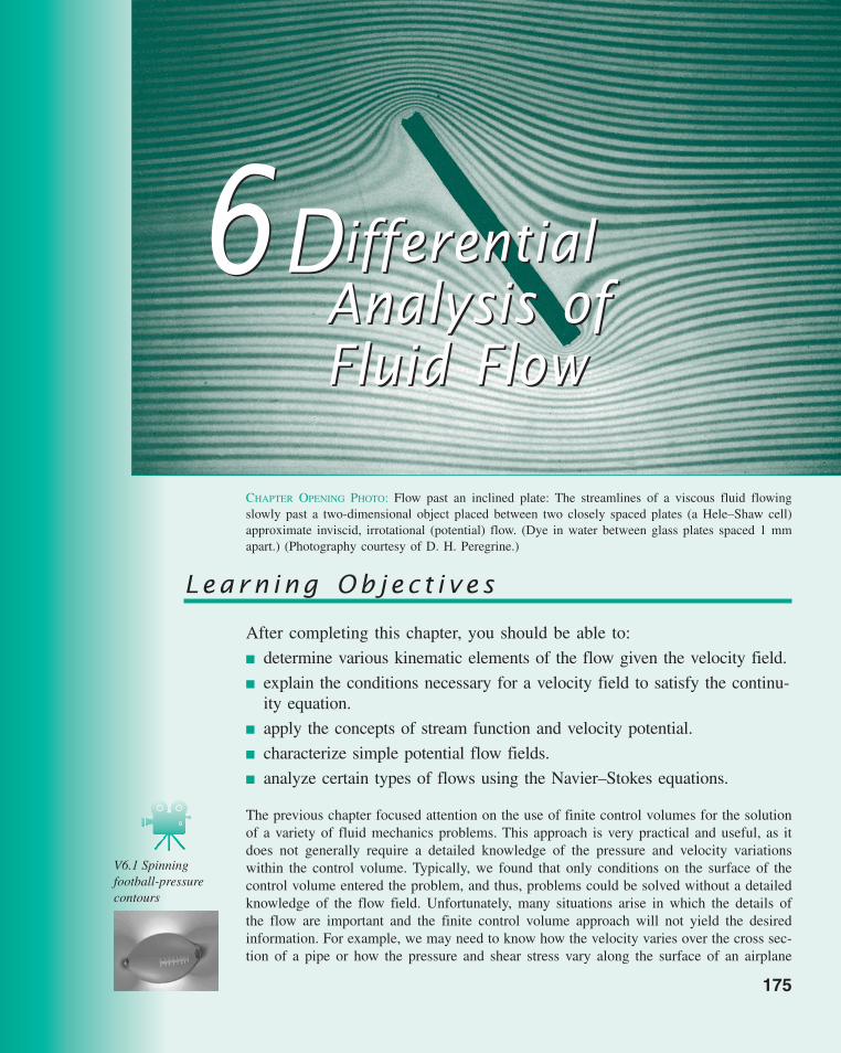
175

CHAPTER OPENING PHOTO: Flow past an inclined plate: The streamlines of a viscous fluid flowingslowly past a two-dimensional object placed between two closely spaced plates (a Hele–Shaw cell)approximate inviscid, irrotational (potential) flow. (Dye in water between glass plates spaced 1 mmapart.) (Photography courtesy of D. H. Peregrine.)

Learn ing Ob j ec t i v e s

After completing this chapter, you should be able to:

■ determine various kinematic elements of the flow given the velocity field.

■ explain the conditions necessary for a velocity field to satisfy the continu-ity equation.

■ apply the concepts of stream function and velocity potential.

■ characterize simple potential flow fields.

■ analyze certain types of flows using the Navier–Stokes equations.

The previous chapter focused attention on the use of finite control volumes for the solutionof a variety of fluid mechanics problems. This approach is very practical and useful, as itdoes not generally require a detailed knowledge of the pressure and velocity variationswithin the control volume. Typically, we found that only conditions on the surface of thecontrol volume entered the problem, and thus, problems could be solved without a detailedknowledge of the flow field. Unfortunately, many situations arise in which the details ofthe flow are important and the finite control volume approach will not yield the desiredinformation. For example, we may need to know how the velocity varies over the cross sec-tion of a pipe or how the pressure and shear stress vary along the surface of an airplane

66DifferentialAnalysis of Fluid Flow

DifferentialAnalysis of Fluid Flow

V6.1 Spinning football-pressurecontours

c06DifferentialAnalysisofFluidFlow.qxd 9/25/10 4:07 PM Page 175

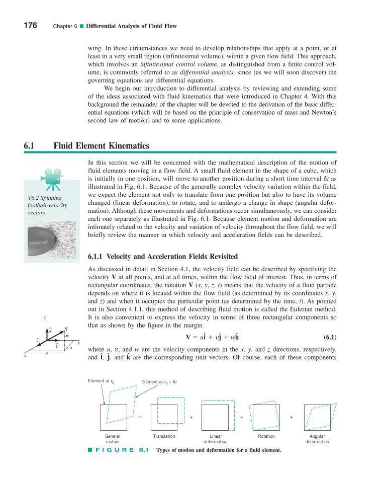
wing. In these circumstances we need to develop relationships that apply at a point, or atleast in a very small region (infinitesimal volume), within a given flow field. This approach,which involves an infinitesimal control volume, as distinguished from a finite control vol-ume, is commonly referred to as differential analysis, since (as we will soon discover) thegoverning equations are differential equations.

We begin our introduction to differential analysis by reviewing and extending someof the ideas associated with fluid kinematics that were introduced in Chapter 4. With thisbackground the remainder of the chapter will be devoted to the derivation of the basic differ-ential equations (which will be based on the principle of conservation of mass and Newton’ssecond law of motion) and to some applications.

176 Chapter 6 ■ Differential Analysis of Fluid Flow

6.1 Fluid Element Kinematics

In this section we will be concerned with the mathematical description of the motion offluid elements moving in a flow field. A small fluid element in the shape of a cube, whichis initially in one position, will move to another position during a short time interval �t asillustrated in Fig. 6.1. Because of the generally complex velocity variation within the field,we expect the element not only to translate from one position but also to have its volumechanged (linear deformation), to rotate, and to undergo a change in shape (angular defor-mation). Although these movements and deformations occur simultaneously, we can considereach one separately as illustrated in Fig. 6.1. Because element motion and deformation areintimately related to the velocity and variation of velocity throughout the flow field, we willbriefly review the manner in which velocity and acceleration fields can be described.

6.1.1 Velocity and Acceleration Fields Revisited

As discussed in detail in Section 4.1, the velocity field can be described by specifying thevelocity V at all points, and at all times, within the flow field of interest. Thus, in terms ofrectangular coordinates, the notation V (x, y, z, t) means that the velocity of a fluid particledepends on where it is located within the flow field (as determined by its coordinates x, y,and z) and when it occupies the particular point (as determined by the time, t). As pointedout in Section 4.1.1, this method of describing fluid motion is called the Eulerian method.It is also convenient to express the velocity in terms of three rectangular components sothat as shown by the figure in the margin

(6.1)

where u, v, and w are the velocity components in the x, y, and z directions, respectively,and , , and are the corresponding unit vectors. Of course, each of these componentskji

V � ui � vj � wk

= + + +

Generalmotion

Translation Lineardeformation

Rotation Angulardeformation

Element at t0 Element at t0 + tδ

F I G U R E 6.1 Types of motion and deformation for a fluid element.

V6.2 Spinning football-velocityvectors

^i

^k

^j

x

z

V

y

w

uv

c06DifferentialAnalysisofFluidFlow.qxd 9/24/10 1:35 PM Page 176

6.1 Fluid Element Kinematics 177

will, in general, be a function of x, y, z, and t. One of the goals of differential analysis isto determine how these velocity components specifically depend on x, y, z, and t for a par-ticular problem.

With this description of the velocity field it was also shown in Section 4.2.1 that theacceleration of a fluid particle can be expressed as

(6.2)

and in component form:

(6.3a)

(6.3b)

(6.3c)

The acceleration is also concisely expressed as

(6.4)

where the operator

(6.5)

is termed the material derivative, or substantial derivative. In vector notation

(6.6)

where the gradient operator, �( ), is

(6.7)

which was introduced in Chapter 2. As shown in the following sections, the motion anddeformation of a fluid element depend on the velocity field. The relationship between themotion and the forces causing the motion depends on the acceleration field.

6.1.2 Linear Motion and Deformation

The simplest type of motion that a fluid element can undergo is translation, as illustratedin Fig. 6.2. In a small time interval �t a particle located at point O will move to point O�as is illustrated in Fig. 6.2. If all points in the element have the same velocity (which isonly true if there are no velocity gradients), then the element will simply translate from oneposition to another. However, because of the presence of velocity gradients, the element willgenerally be deformed and rotated as it moves. For example, consider the effect of a sin-gle velocity gradient ∂u/∂x on a small cube having sides �x, �y, and �z. As is shown in Fig.6.3a, if the x component of velocity of O and B is u, then at nearby points A and C the xcomponent of the velocity can be expressed as u � (∂u/∂x) �x. This difference in velocitycauses a “stretching” of the volume element by an amount (∂u/∂x)(�x)(�t) during the short

�1 2 �0 1 20x

i �0 1 20y

j �0 1 20z

k

D1 2Dt

�0 1 20t

� 1V # �2 1 2

D1 2Dt

�0 1 20t

� u 0 1 20x

� v 0 1 20y

� w 0 1 20z

a �DVDt

az �0w

0t� u

0w

0x� v

0w

0y� w

0w

0z

ay �0v

0t� u

0v

0x� v

0v

0y� w

0v

0z

ax �0u

0t� u

0u

0x� v

0u

0y� w

0u

0z

a �0V0t

� u 0V0x

� v 0V0y

� w 0V0z

c06DifferentialAnalysisofFluidFlow.qxd 9/24/10 1:35 PM Page 177

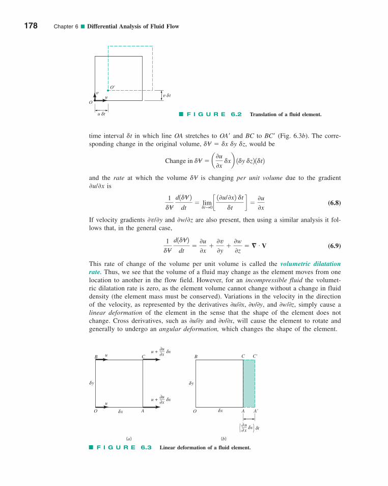
time interval �t in which line OA stretches to OA� and BC to BC� (Fig. 6.3b). The corre-sponding change in the original volume, �V � �x �y �z, would be

and the rate at which the volume �V is changing per unit volume due to the gradient∂u/∂x is

(6.8)

If velocity gradients ∂v/∂y and ∂w/∂z are also present, then using a similar analysis it fol-lows that, in the general case,

(6.9)

This rate of change of the volume per unit volume is called the volumetric dilatationrate. Thus, we see that the volume of a fluid may change as the element moves from onelocation to another in the flow field. However, for an incompressible fluid the volumet-ric dilatation rate is zero, as the element volume cannot change without a change in fluiddensity (the element mass must be conserved). Variations in the velocity in the directionof the velocity, as represented by the derivatives 0u/0x, 0y/0y, and 0w/0z, simply cause alinear deformation of the element in the sense that the shape of the element does notchange. Cross derivatives, such as 0u/0y and 0y/0x, will cause the element to rotate andgenerally to undergo an angular deformation, which changes the shape of the element.

1

�V d1�V2

dt�

0u

0x�

0v

0y�

0w

0z� � # V

1

�V d1�V 2

dt� lim

�tS0c10u/0x2 �t

�td �

0u

0x

Change in �V � a0u

0x �xb 1�y �z2 1�t2

178 Chapter 6 ■ Differential Analysis of Fluid Flow

A A'

δ

CB u

y

u

O Axδ

yδ

xδO

CB C'

u

x

__

xδ tδ))

(b)(a)

u + u

x

__

xδ∂

∂

u + u

x

__

xδ∂

∂

∂∂

F I G U R E 6.3 Linear deformation of a fluid element.

O

u tδ

vu

O'

v tδ

F I G U R E 6.2 Translation of a fluid element.

c06DifferentialAnalysisofFluidFlow.qxd 9/24/10 1:35 PM Page 178

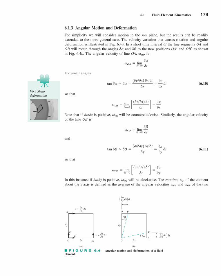
6.1 Fluid Element Kinematics 179

6.1.3 Angular Motion and Deformation

For simplicity we will consider motion in the x–y plane, but the results can be readilyextended to the more general case. The velocity variation that causes rotation and angulardeformation is illustrated in Fig. 6.4a. In a short time interval �t the line segments OA andOB will rotate through the angles �� and �� to the new positions OA� and OB� as shownin Fig. 6.4b. The angular velocity of line OA, �OA, is

For small angles

(6.10)

so that

Note that if ∂v/∂x is positive, �OA will be counterclockwise. Similarly, the angular velocityof the line OB is

and

(6.11)

so that

In this instance if ∂u/∂y is positive, �OB will be clockwise. The rotation, �z, of the elementabout the z axis is defined as the average of the angular velocities �OA and �OB of the two

�OB � lim�tS0

c10u/0y2 �t

�td �

0u

0y

tan �� � �� �10u/0y2 �y �t

�y�

0u

0y �t

�OB � lim�tS0

��

�t

�OA � lim�tS0

c10v/0x2 �t

�td �

0v

0x

tan �� � �� �10v/0x2 �x �t

�x�

0v

0x �t

�OA � lim�tS0

��

�t

V6.3 Shear deformation

v + v

x

__

x

u

y

__

yδ tδ))

yδ

xδ

yδ

xδ

v

x

__

xδ tδ))

δβ

δαA'

AO

B B'

AO

B

v

u

(a) (b)

u + u

y

__

yδ∂

∂

δ∂∂

∂∂

∂∂

F I G U R E 6.4 Angular motion and deformation of a fluidelement.

c06DifferentialAnalysisofFluidFlow.qxd 9/24/10 1:35 PM Page 179

mutually perpendicular lines OA and OB.1 Thus, if counterclockwise rotation is consideredto be positive, it follows that

(6.12)

Rotation of the fluid element about the other two coordinate axes can be obtained ina similar manner with the result that for rotation about the x axis

(6.13)

and for rotation about the y axis

(6.14)

The three components �x, �y, and �z can be combined to give the rotation vector, �, in theform

(6.15)

An examination of this result reveals that � is equal to one-half the curl of the velocity vec-tor. That is,

(6.16)

since by definition of the vector operator � � V

The vorticity, �, is defined as a vector that is twice the rotation vector; that is,

(6.17)

The use of the vorticity to describe the rotational characteristics of the fluid simply eliminatesthe factor associated with the rotation vector. The figure in the margin shows vorticitycontours of the wing tip vortex flow shortly after an aircraft has passed. The lighter colorsindicate stronger vorticity. (See also Fig. 4.3.)

We observe from Eq. 6.12 that the fluid element will rotate about the z axis as an unde-formed block (i.e., �OA � ��OB) only when ∂u/∂y � �∂v/∂x. Otherwise, the rotation willbe associated with an angular deformation. We also note from Eq. 6.12 that when ∂u/∂y �∂v/∂x the rotation around the z axis is zero. More generally if � � V � 0, then the rota-tion (and the vorticity) is zero, and flow fields for which this condition applies are termedirrotational. We will find in Section 6.4 that the condition of irrotationality often greatlysimplifies the analysis of complex flow fields. However, it is probably not immediately obvi-ous why some flow fields would be irrotational, and we will need to examine this conceptmore fully in Section 6.4.

112 2

� � 2 � � � � V

�1

2 a

0w

0y�

0v

0zb i �

1

2 a

0u

0z�

0w

0xb j �

1

2 a

0v

0x�

0u

0yb k

1

2 � � V �

1

24 i00x

u

j00y

v

k00z

w

4� � 1

2 curl V � 12� � V

� � �xi � �y j � �zk

�y �1

2 a

0u

0z�

0w

0xb

�x �1

2 a

0w

0y�

0v

0zb

�z �1

2 a

0v

0x�

0u

0yb

180 Chapter 6 ■ Differential Analysis of Fluid Flow

Wing

1With this definition can also be interpreted to be the angular velocity of the bisector of the angle between the lines OAand OB.

vz

c06DifferentialAnalysisofFluidFlow.qxd 9/24/10 1:36 PM Page 180

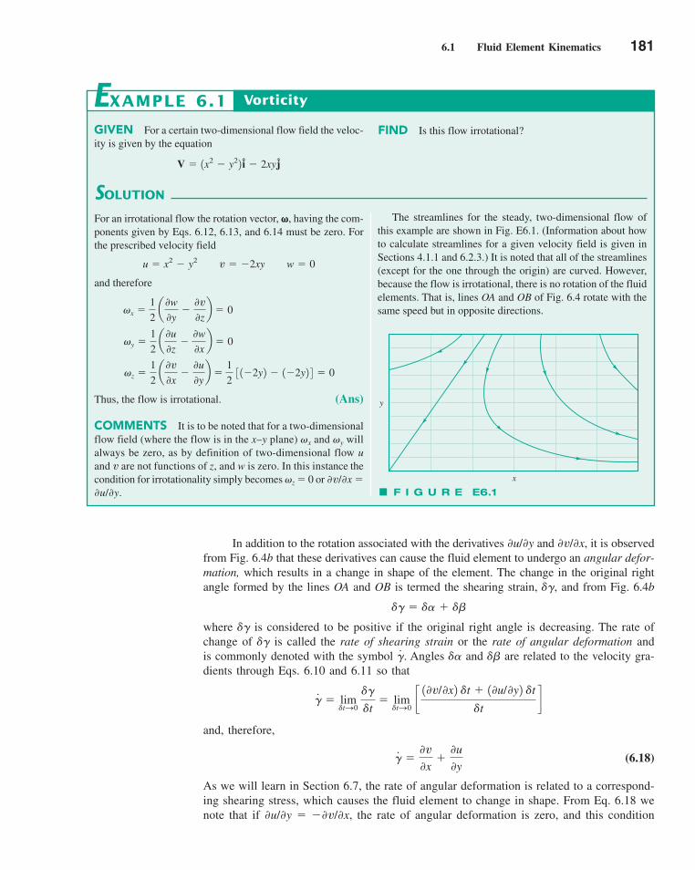
6.1 Fluid Element Kinematics 181

In addition to the rotation associated with the derivatives ∂u/∂y and ∂v/∂x, it is observedfrom Fig. 6.4b that these derivatives can cause the fluid element to undergo an angular defor-mation, which results in a change in shape of the element. The change in the original rightangle formed by the lines OA and OB is termed the shearing strain, ��, and from Fig. 6.4b

where �� is considered to be positive if the original right angle is decreasing. The rate ofchange of �� is called the rate of shearing strain or the rate of angular deformation andis commonly denoted with the symbol Angles �� and �� are related to the velocity gra-dients through Eqs. 6.10 and 6.11 so that

and, therefore,

(6.18)

As we will learn in Section 6.7, the rate of angular deformation is related to a correspond-ing shearing stress, which causes the fluid element to change in shape. From Eq. 6.18 wenote that if ∂u/∂y � �∂v/∂x, the rate of angular deformation is zero, and this condition

�� �0v

0x�

0u

0y

�� � lim�tS0

��

�t� lim

�tS0 c10v/0x2 �t � 10u/0y2 �t

�td

�� .

�� � �� � ��

GIVEN For a certain two-dimensional flow field the veloc-ity is given by the equation

V � 1x2 � y22 i � 2xy j

SOLUTION

Vorticity

FIND Is this flow irrotational?

The streamlines for the steady, two-dimensional flow ofthis example are shown in Fig. E6.1. (Information about howto calculate streamlines for a given velocity field is given inSections 4.1.1 and 6.2.3.) It is noted that all of the streamlines(except for the one through the origin) are curved. However,because the flow is irrotational, there is no rotation of the fluidelements. That is, lines OA and OB of Fig. 6.4 rotate with thesame speed but in opposite directions.

EXAMPLE 6.1

For an irrotational flow the rotation vector, �, having the com-ponents given by Eqs. 6.12, 6.13, and 6.14 must be zero. Forthe prescribed velocity field

and therefore

Thus, the flow is irrotational. (Ans)

COMMENTS It is to be noted that for a two-dimensionalflow field (where the flow is in the x–y plane) �x and �y willalways be zero, as by definition of two-dimensional flow uand v are not functions of z, and w is zero. In this instance thecondition for irrotationality simply becomes �z � 0 or ∂v/∂x �∂u/∂y.

�z �1

2 a

0v

0x�

0u

0yb �

1

2 3 1�2y2 � 1�2y2 4 � 0

�y �1

2 a

0u

0z�

0w

0xb � 0

�x �1

2 a

0w

0y�

0v

0zb � 0

u � x2 � y2 v � �2xy w � 0

y

x

F I G U R E E6.1

c06DifferentialAnalysisofFluidFlow.qxd 9/24/10 1:36 PM Page 181

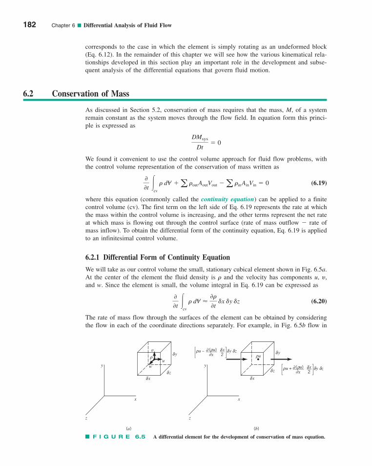
182 Chapter 6 ■ Differential Analysis of Fluid Flow

6.2 Conservation of Mass

As discussed in Section 5.2, conservation of mass requires that the mass, M, of a systemremain constant as the system moves through the flow field. In equation form this princi-ple is expressed as

We found it convenient to use the control volume approach for fluid flow problems, withthe control volume representation of the conservation of mass written as

(6.19)

where this equation (commonly called the continuity equation) can be applied to a finitecontrol volume (cv). The first term on the left side of Eq. 6.19 represents the rate at whichthe mass within the control volume is increasing, and the other terms represent the net rateat which mass is flowing out through the control surface (rate of mass outflow � rate ofmass inflow). To obtain the differential form of the continuity equation, Eq. 6.19 is appliedto an infinitesimal control volume.

6.2.1 Differential Form of Continuity Equation

We will take as our control volume the small, stationary cubical element shown in Fig. 6.5a.At the center of the element the fluid density is � and the velocity has components u, y,and w. Since the element is small, the volume integral in Eq. 6.19 can be expressed as

(6.20)

The rate of mass flow through the surfaces of the element can be obtained by consideringthe flow in each of the coordinate directions separately. For example, in Fig. 6.5b flow in

00t

�cv

� dV �0�

0t �x �y �z

00t

�cv

� dV �a �outAoutVout �a �inAinVin � 0

DMsys

Dt� 0

corresponds to the case in which the element is simply rotating as an undeformed block(Eq. 6.12). In the remainder of this chapter we will see how the various kinematical rela-tionships developed in this section play an important role in the development and subse-quent analysis of the differential equations that govern fluid motion.

v

uw

xδzδ

yδ

xδ

zδ

yδρ u

y y

z z

x x

ρρ u – ( u) x y z

_____

__

x

2

∂∂

δ δ δρ

(a) (b)

ρ u + ( u) x y z

_____

__

x

2

∂∂

δ δ δρ

F I G U R E 6.5 A differential element for the development of conservation of mass equation.

c06DifferentialAnalysisofFluidFlow.qxd 9/24/10 1:36 PM Page 182

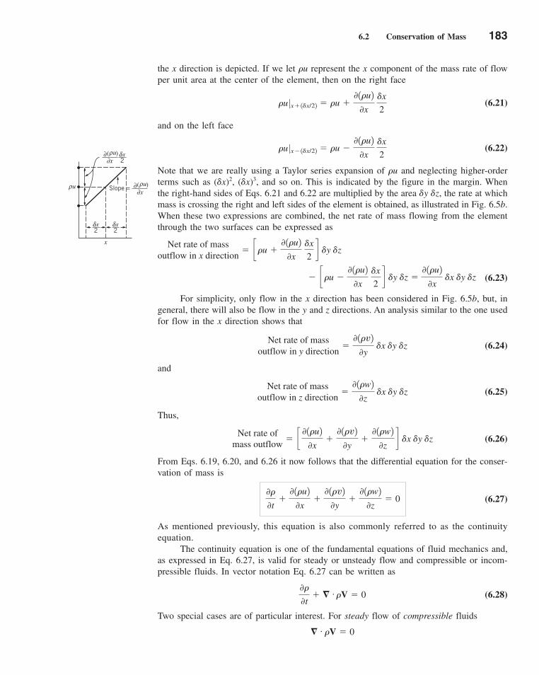
6.2 Conservation of Mass 183

the x direction is depicted. If we let �u represent the x component of the mass rate of flowper unit area at the center of the element, then on the right face

(6.21)

and on the left face

(6.22)

Note that we are really using a Taylor series expansion of �u and neglecting higher-orderterms such as (�x)2, (�x)3, and so on. This is indicated by the figure in the margin. Whenthe right-hand sides of Eqs. 6.21 and 6.22 are multiplied by the area �y �z, the rate at whichmass is crossing the right and left sides of the element is obtained, as illustrated in Fig. 6.5b.When these two expressions are combined, the net rate of mass flowing from the elementthrough the two surfaces can be expressed as

(6.23)

For simplicity, only flow in the x direction has been considered in Fig. 6.5b, but, ingeneral, there will also be flow in the y and z directions. An analysis similar to the one usedfor flow in the x direction shows that

(6.24)

and

(6.25)

Thus,

(6.26)

From Eqs. 6.19, 6.20, and 6.26 it now follows that the differential equation for the conser-vation of mass is

(6.27)

As mentioned previously, this equation is also commonly referred to as the continuityequation.

The continuity equation is one of the fundamental equations of fluid mechanics and,as expressed in Eq. 6.27, is valid for steady or unsteady flow and compressible or incom-pressible fluids. In vector notation Eq. 6.27 can be written as

(6.28)

Two special cases are of particular interest. For steady flow of compressible fluids

� # �V � 0

0�

0t� � # �V � 0

0�

0t�

0 1�u2

0x�

0 1�v2

0y�

0 1�w2

0z� 0

Net rate ofmass outflow

� c0 1�u2

0x�

0 1�v2

0y�

0 1�w2

0zd �x �y �z

Net rate of massoutflow in z direction

�0 1�w2

0z �x �y �z

Net rate of massoutflow in y direction

�0 1�v2

0y �x �y �z

� c�u �0 1�u2

0x �x

2d �y �z �

0 1�u2

0x �x �y �z

Net rate of massoutflow in x direction

� c�u �0 1�u2

0x �x

2d �y �z

� �u �0 1�u2

0x �x

2�u 0x� 1�x/22

� �u �0 1�u2

0x �x

2�u 0x� 1�x/22

uρu

x

ρ ( )∂Slope =

2

∂x

δx2δx

uρ( )∂∂x 2

δx

c06DifferentialAnalysisofFluidFlow.qxd 9/24/10 1:36 PM Page 183

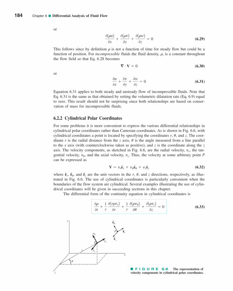
or

(6.29)

This follows since by definition � is not a function of time for steady flow but could be afunction of position. For incompressible fluids the fluid density, �, is a constant throughoutthe flow field so that Eq. 6.28 becomes

(6.30)

or

(6.31)

Equation 6.31 applies to both steady and unsteady flow of incompressible fluids. Note thatEq. 6.31 is the same as that obtained by setting the volumetric dilatation rate (Eq. 6.9) equalto zero. This result should not be surprising since both relationships are based on conser-vation of mass for incompressible fluids.

6.2.2 Cylindrical Polar Coordinates

For some problems it is more convenient to express the various differential relationships incylindrical polar coordinates rather than Cartesian coordinates. As is shown in Fig. 6.6, withcylindrical coordinates a point is located by specifying the coordinates r, �, and z. The coor-dinate r is the radial distance from the z axis, � is the angle measured from a line parallelto the x axis (with counterclockwise taken as positive), and z is the coordinate along the zaxis. The velocity components, as sketched in Fig. 6.6, are the radial velocity, yr, the tan-gential velocity, y�, and the axial velocity, yz. Thus, the velocity at some arbitrary point Pcan be expressed as

(6.32)

where êr, ê�, and êz are the unit vectors in the r, �, and z directions, respectively, as illus-trated in Fig. 6.6. The use of cylindrical coordinates is particularly convenient when theboundaries of the flow system are cylindrical. Several examples illustrating the use of cylin-drical coordinates will be given in succeeding sections in this chapter.

The differential form of the continuity equation in cylindrical coordinates is

(6.33)0�

0t�

1r 0 1r�vr2

0r�

1r 0 1�v�2

0��

0 1�vz2

0z� 0

V � vrer � v�e� � vzez

0u

0x�

0v

0y�

0w

0z� 0

� # V � 0

0 1�u2

0x�

0 1�v2

0y�

0 1�w2

0z� 0

184 Chapter 6 ■ Differential Analysis of Fluid Flow

z

y

x

θ

r vz

P vr

vθ

θ

P r

z

^

^

^

e

e

e

F I G U R E 6.6 The representation ofvelocity components in cylindrical polar coordinates.

c06DifferentialAnalysisofFluidFlow.qxd 9/24/10 1:36 PM Page 184

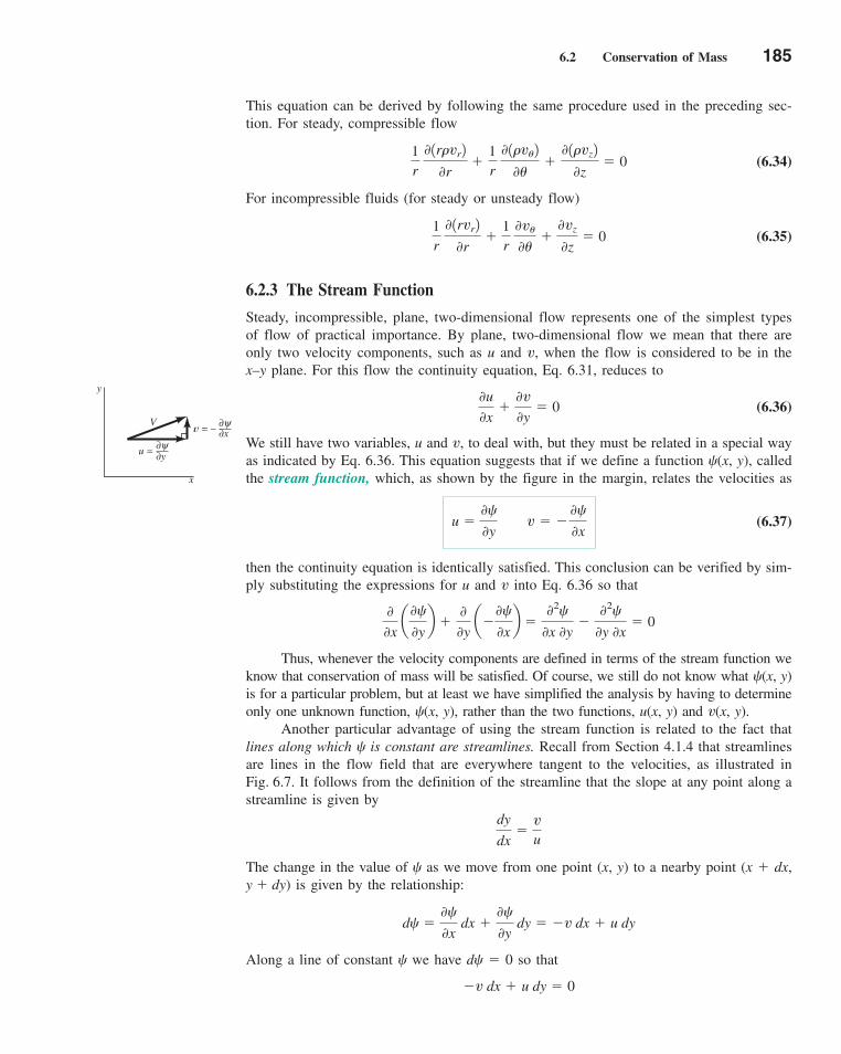
6.2 Conservation of Mass 185

This equation can be derived by following the same procedure used in the preceding sec-tion. For steady, compressible flow

(6.34)

For incompressible fluids (for steady or unsteady flow)

(6.35)

6.2.3 The Stream Function

Steady, incompressible, plane, two-dimensional flow represents one of the simplest typesof flow of practical importance. By plane, two-dimensional flow we mean that there areonly two velocity components, such as u and v, when the flow is considered to be in thex–y plane. For this flow the continuity equation, Eq. 6.31, reduces to

(6.36)

We still have two variables, u and v, to deal with, but they must be related in a special wayas indicated by Eq. 6.36. This equation suggests that if we define a function (x, y), calledthe stream function, which, as shown by the figure in the margin, relates the velocities as

(6.37)

then the continuity equation is identically satisfied. This conclusion can be verified by sim-ply substituting the expressions for u and v into Eq. 6.36 so that

Thus, whenever the velocity components are defined in terms of the stream function weknow that conservation of mass will be satisfied. Of course, we still do not know what (x, y)is for a particular problem, but at least we have simplified the analysis by having to determineonly one unknown function, (x, y), rather than the two functions, u(x, y) and v(x, y).

Another particular advantage of using the stream function is related to the fact thatlines along which is constant are streamlines. Recall from Section 4.1.4 that streamlinesare lines in the flow field that are everywhere tangent to the velocities, as illustrated inFig. 6.7. It follows from the definition of the streamline that the slope at any point along astreamline is given by

The change in the value of as we move from one point (x, y) to a nearby point (x � dx,y � dy) is given by the relationship:

Along a line of constant we have d � 0 so that

�v dx � u dy � 0

d �0

0x dx �

0

0y dy � �v dx � u dy

dy

dx�

vu

00x

a0

0yb �

00y

a�0

0xb �

02

0x 0y�

02

0y 0x� 0

u �0

0y v � �

0

0x

0u

0x�

0v

0y� 0

1r 0 1rvr2

0r�

1r 0v�

0��

0vz

0z� 0

1r 0 1r�vr2

0r�

1r 0 1�v�2

0��

0 1�vz2

0z� 0

V

y

x

u = y∂ψ∂

v = – x∂ψ∂

c06DifferentialAnalysisofFluidFlow.qxd 9/24/10 1:36 PM Page 185

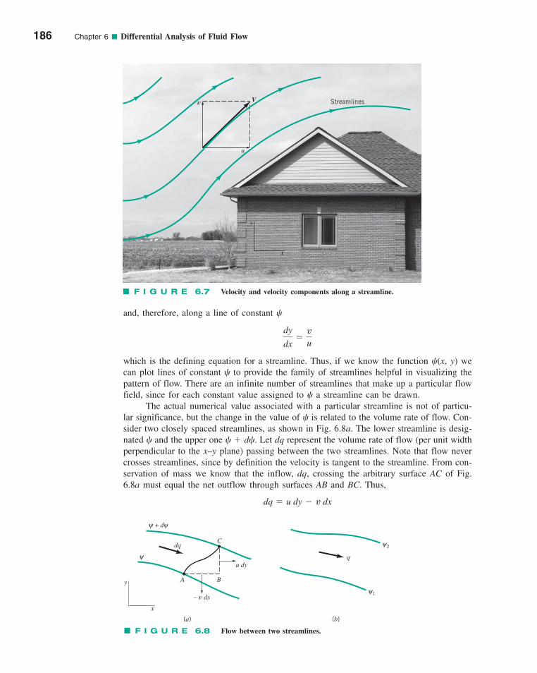
and, therefore, along a line of constant

which is the defining equation for a streamline. Thus, if we know the function (x, y) wecan plot lines of constant to provide the family of streamlines helpful in visualizing thepattern of flow. There are an infinite number of streamlines that make up a particular flowfield, since for each constant value assigned to a streamline can be drawn.

The actual numerical value associated with a particular streamline is not of particu-lar significance, but the change in the value of is related to the volume rate of flow. Con-sider two closely spaced streamlines, as shown in Fig. 6.8a. The lower streamline is desig-nated and the upper one � d. Let dq represent the volume rate of flow (per unit widthperpendicular to the x–y plane) passing between the two streamlines. Note that flow nevercrosses streamlines, since by definition the velocity is tangent to the streamline. From con-servation of mass we know that the inflow, dq, crossing the arbitrary surface AC of Fig.6.8a must equal the net outflow through surfaces AB and BC. Thus,

dq � u dy � v dx

dy

dx�

vu

186 Chapter 6 ■ Differential Analysis of Fluid Flow

F I G U R E 6.7 Velocity and velocity components along a streamline.

x

y

StreamlinesVv

u

+ dψ ψ

ψ

C

A B

dq

u dy

– v dx

x

yψ1

ψ2

q

(b)(a)

F I G U R E 6.8 Flow between two streamlines.

c06DifferentialAnalysisofFluidFlow.qxd 9/24/10 1:36 PM Page 186

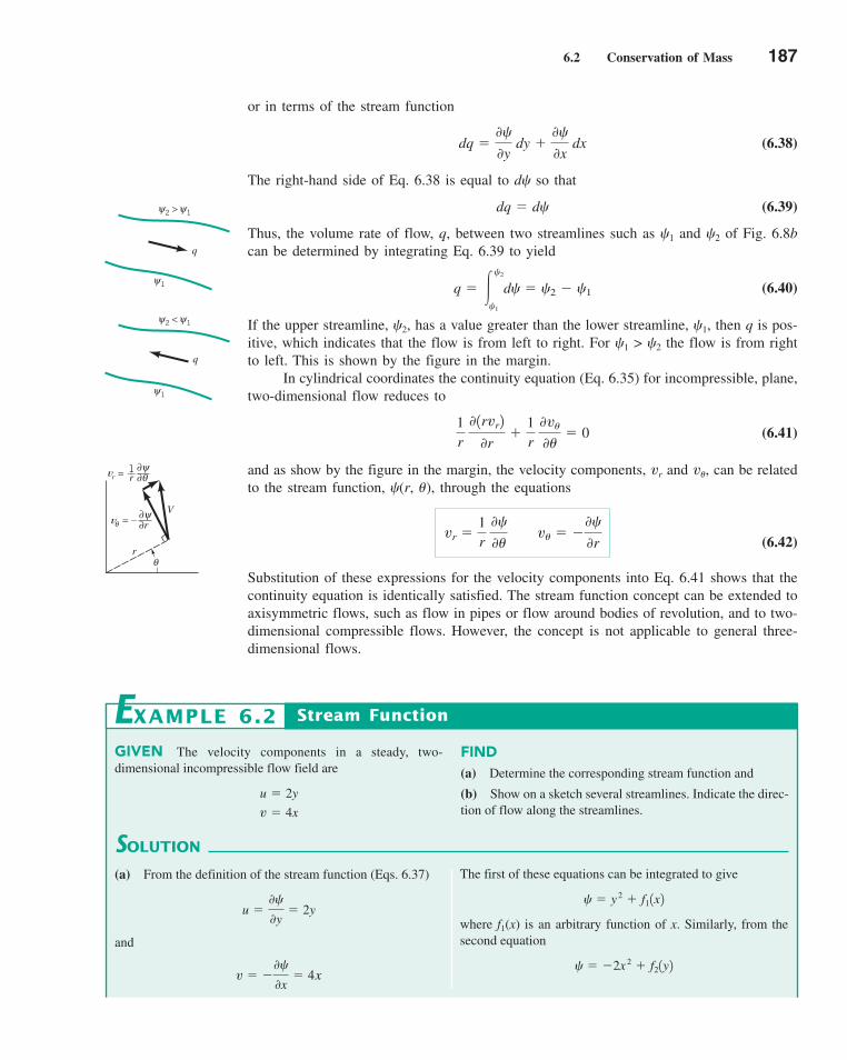
6.2 Conservation of Mass 187

or in terms of the stream function

(6.38)

The right-hand side of Eq. 6.38 is equal to d so that

(6.39)

Thus, the volume rate of flow, q, between two streamlines such as 1 and 2 of Fig. 6.8bcan be determined by integrating Eq. 6.39 to yield

(6.40)

If the upper streamline, 2, has a value greater than the lower streamline, 1, then q is pos-itive, which indicates that the flow is from left to right. For 1 > 2 the flow is from rightto left. This is shown by the figure in the margin.

In cylindrical coordinates the continuity equation (Eq. 6.35) for incompressible, plane,two-dimensional flow reduces to

(6.41)

and as show by the figure in the margin, the velocity components, vr and v�, can be relatedto the stream function, (r, �), through the equations

(6.42)

Substitution of these expressions for the velocity components into Eq. 6.41 shows that thecontinuity equation is identically satisfied. The stream function concept can be extended toaxisymmetric flows, such as flow in pipes or flow around bodies of revolution, and to two-dimensional compressible flows. However, the concept is not applicable to general three-dimensional flows.

vr �1r 0

0� v� � �

0

0r

1r 0 1rvr2

0r�

1r 0v�

0�� 0

q � �2

1

d � 2 � 1

dq � d

dq �0

0y dy �

0

0x dx

> ψ2 ψ1

ψ1

q

< ψ2 ψ1

ψ1

q

θr

Vv = – r

∂ψ∂θ

vr = 1__r∂ψ∂θ

GIVEN The velocity components in a steady, two-dimensional incompressible flow field are

v � 4x

u � 2y

Stream Function

FIND(a) Determine the corresponding stream function and

(b) Show on a sketch several streamlines. Indicate the direc-tion of flow along the streamlines.

EXAMPLE 6.2

SOLUTION

The first of these equations can be integrated to give

where f1(x) is an arbitrary function of x. Similarly, from thesecond equation

� �2x 2 � f21y2

� y 2 � f11x2

(a) From the definition of the stream function (Eqs. 6.37)

and

v � �0

0x� 4x

u �0

0y� 2y

c06DifferentialAnalysisofFluidFlow.qxd 9/24/10 1:37 PM Page 187

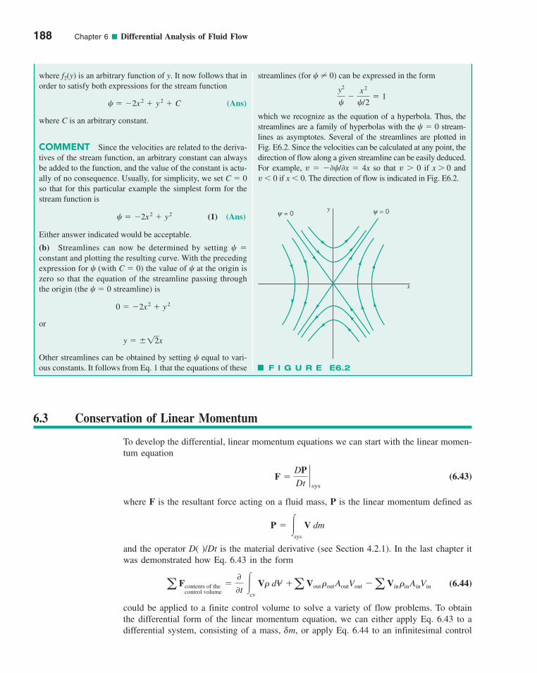
188 Chapter 6 ■ Differential Analysis of Fluid Flow

streamlines (for � 0) can be expressed in the form

which we recognize as the equation of a hyperbola. Thus, thestreamlines are a family of hyperbolas with the � 0 stream-lines as asymptotes. Several of the streamlines are plotted inFig. E6.2. Since the velocities can be calculated at any point, thedirection of flow along a given streamline can be easily deduced.For example, v � �∂/∂x � 4x so that v � 0 if x � 0 and v 0 if x 0. The direction of flow is indicated in Fig. E6.2.

y2

�

x 2

/2� 1

where f2(y) is an arbitrary function of y. It now follows that inorder to satisfy both expressions for the stream function

(Ans)

where C is an arbitrary constant.

COMMENT Since the velocities are related to the deriva-tives of the stream function, an arbitrary constant can alwaysbe added to the function, and the value of the constant is actu-ally of no consequence. Usually, for simplicity, we set C � 0so that for this particular example the simplest form for thestream function is

(1) (Ans)

Either answer indicated would be acceptable.

(b) Streamlines can now be determined by setting �constant and plotting the resulting curve. With the precedingexpression for (with C � 0) the value of at the origin iszero so that the equation of the streamline passing throughthe origin (the � 0 streamline) is

or

Other streamlines can be obtained by setting equal to vari-ous constants. It follows from Eq. 1 that the equations of these

y � 12x

0 � �2x 2 � y

2

� �2x 2 � y

2

� �2x 2 � y

2 � C

ψ = 0y ψ = 0

x

F I G U R E E6.2

6.3 Conservation of Linear Momentum

To develop the differential, linear momentum equations we can start with the linear momen-tum equation

(6.43)

where F is the resultant force acting on a fluid mass, P is the linear momentum defined as

and the operator D( )/Dt is the material derivative (see Section 4.2.1). In the last chapter itwas demonstrated how Eq. 6.43 in the form

(6.44)

could be applied to a finite control volume to solve a variety of flow problems. To obtainthe differential form of the linear momentum equation, we can either apply Eq. 6.43 to adifferential system, consisting of a mass, �m, or apply Eq. 6.44 to an infinitesimal control

a Fcontents of thecontrol volume

�00t

�cv

V� dV �a Vout�outAoutVout �a Vin�inAinVin

P � �sys

V dm

F �DPDt`sys

c06DifferentialAnalysisofFluidFlow.qxd 9/24/10 1:37 PM Page 188

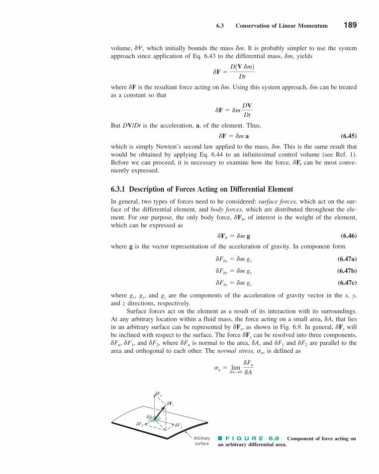
6.3 Conservation of Linear Momentum 189

volume, �V, which initially bounds the mass �m. It is probably simpler to use the systemapproach since application of Eq. 6.43 to the differential mass, �m, yields

where �F is the resultant force acting on �m. Using this system approach, �m can be treatedas a constant so that

But DV/Dt is the acceleration, a, of the element. Thus,

(6.45)

which is simply Newton’s second law applied to the mass, �m. This is the same result thatwould be obtained by applying Eq. 6.44 to an infinitesimal control volume (see Ref. 1).Before we can proceed, it is necessary to examine how the force, �F, can be most conve-niently expressed.

6.3.1 Description of Forces Acting on Differential Element

In general, two types of forces need to be considered: surface forces, which act on the sur-face of the differential element, and body forces, which are distributed throughout the ele-ment. For our purpose, the only body force, �Fb, of interest is the weight of the element,which can be expressed as

(6.46)

where g is the vector representation of the acceleration of gravity. In component form

(6.47a)

(6.47b)

(6.47c)

where gx, gy, and gz are the components of the acceleration of gravity vector in the x, y,and z directions, respectively.

Surface forces act on the element as a result of its interaction with its surroundings.At any arbitrary location within a fluid mass, the force acting on a small area, �A, that liesin an arbitrary surface can be represented by �Fs, as shown in Fig. 6.9. In general, �Fs willbe inclined with respect to the surface. The force �Fs can be resolved into three components,�Fn, �F1, and �F2, where �Fn is normal to the area, �A, and �F1 and �F2 are parallel to thearea and orthogonal to each other. The normal stress, n, is defined as

n � lim�AS0

�Fn

�A

�Fbz � �m gz

�Fby � �m gy

�Fbx � �m gx

�Fb � �m g

�F � �m a

�F � �m DVDt

�F �D1V �m2

Dt

Fsδ

Fnδ

F1δF2δAδ

Arbitrarysurface

F I G U R E 6.9 Component of force acting onan arbitrary differential area.

c06DifferentialAnalysisofFluidFlow.qxd 9/24/10 1:37 PM Page 189

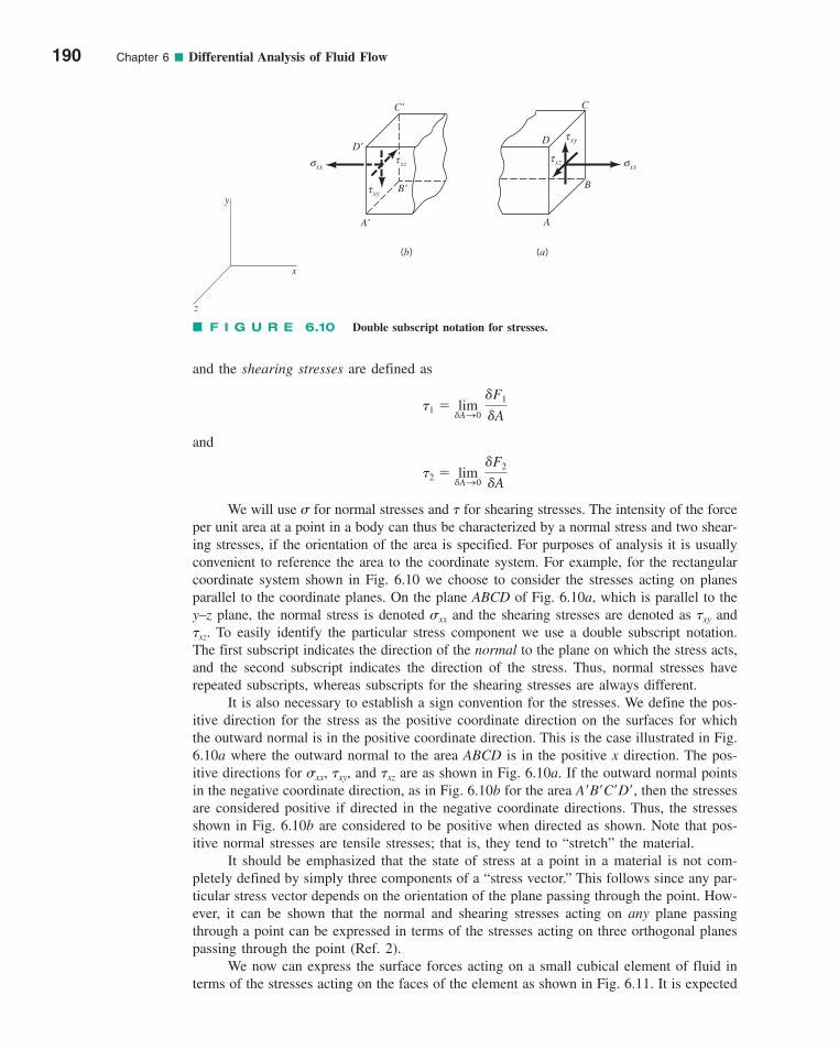
and the shearing stresses are defined as

and

We will use for normal stresses and � for shearing stresses. The intensity of the forceper unit area at a point in a body can thus be characterized by a normal stress and two shear-ing stresses, if the orientation of the area is specified. For purposes of analysis it is usuallyconvenient to reference the area to the coordinate system. For example, for the rectangularcoordinate system shown in Fig. 6.10 we choose to consider the stresses acting on planesparallel to the coordinate planes. On the plane ABCD of Fig. 6.10a, which is parallel to they–z plane, the normal stress is denoted xx and the shearing stresses are denoted as �xy and�xz. To easily identify the particular stress component we use a double subscript notation.The first subscript indicates the direction of the normal to the plane on which the stress acts,and the second subscript indicates the direction of the stress. Thus, normal stresses haverepeated subscripts, whereas subscripts for the shearing stresses are always different.

It is also necessary to establish a sign convention for the stresses. We define the pos-itive direction for the stress as the positive coordinate direction on the surfaces for whichthe outward normal is in the positive coordinate direction. This is the case illustrated in Fig.6.10a where the outward normal to the area ABCD is in the positive x direction. The pos-itive directions for xx, �xy, and �xz are as shown in Fig. 6.10a. If the outward normal pointsin the negative coordinate direction, as in Fig. 6.10b for the area A�B�C�D�, then the stressesare considered positive if directed in the negative coordinate directions. Thus, the stressesshown in Fig. 6.10b are considered to be positive when directed as shown. Note that pos-itive normal stresses are tensile stresses; that is, they tend to “stretch” the material.

It should be emphasized that the state of stress at a point in a material is not com-pletely defined by simply three components of a “stress vector.” This follows since any par-ticular stress vector depends on the orientation of the plane passing through the point. How-ever, it can be shown that the normal and shearing stresses acting on any plane passingthrough a point can be expressed in terms of the stresses acting on three orthogonal planespassing through the point (Ref. 2).

We now can express the surface forces acting on a small cubical element of fluid interms of the stresses acting on the faces of the element as shown in Fig. 6.11. It is expected

�2 � lim�AS0

�F2

�A

�1 � lim�AS0

�F1

�A

190 Chapter 6 ■ Differential Analysis of Fluid Flow

z

x

y

(a)

A

C

B

D

σxx

τxy

τxz

(b)

A'

C'

B'

D'

σxx

τxy

τxz

F I G U R E 6.10 Double subscript notation for stresses.

c06DifferentialAnalysisofFluidFlow.qxd 9/24/10 1:37 PM Page 190

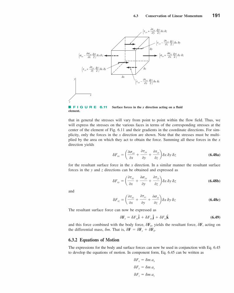
6.3 Conservation of Linear Momentum 191

that in general the stresses will vary from point to point within the flow field. Thus, wewill express the stresses on the various faces in terms of the corresponding stresses at thecenter of the element of Fig. 6.11 and their gradients in the coordinate directions. For sim-plicity, only the forces in the x direction are shown. Note that the stresses must be multi-plied by the area on which they act to obtain the force. Summing all these forces in the xdirection yields

(6.48a)

for the resultant surface force in the x direction. In a similar manner the resultant surfaceforces in the y and z directions can be obtained and expressed as

(6.48b)

and

(6.48c)

The resultant surface force can now be expressed as

(6.49)

and this force combined with the body force, �Fb, yields the resultant force, �F, acting onthe differential mass, �m. That is, �F � �Fs � �Fb.

6.3.2 Equations of Motion

The expressions for the body and surface forces can now be used in conjunction with Eq. 6.45to develop the equations of motion. In component form, Eq. 6.45 can be written as

�Fz � �m az

�Fy � �m ay

�Fx � �m ax

�Fs � �Fsxi � �Fsy j � �Fszk

�Fsz � a0�xz

0x�

0�yz

0y�

0zz

0zb �x �y �z

�Fsy � a0�xy

0x�

0yy

0y�

0�zy

0zb �x �y �z

�Fsx � a0xx

0x�

0�yx

0y�

0�zx

0zb �x �y �z

F I G U R E 6.11 Surface forces in the x direction acting on a fluidelement.

δ

( xx – xx x y z

____ __

x 2σ∂σ

∂ δ δ(δ

y

δz

δx

x

y

z

( zx + zx z x y

____ __

z 2τ∂τ∂ δ δ(δ

( yx – yx y x z

____ __

y 2τ∂τ∂ δ δ(δ

( zx – zx z x y

____ __

z 2τ∂τ∂ δ δ(δ

( yx + yx y x z

____ __

y 2τ∂τ∂ δ δ(δ

( xx + xx x y z

____ __

x 2σ∂σ∂ δ δ(δ

c06DifferentialAnalysisofFluidFlow.qxd 9/24/10 1:37 PM Page 191

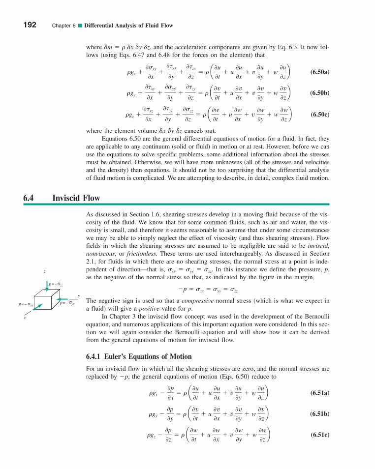
where �m � � �x �y �z, and the acceleration components are given by Eq. 6.3. It now fol-lows (using Eqs. 6.47 and 6.48 for the forces on the element) that

(6.50a)

(6.50b)

(6.50c)

where the element volume �x �y �z cancels out.Equations 6.50 are the general differential equations of motion for a fluid. In fact, they

are applicable to any continuum (solid or fluid) in motion or at rest. However, before we canuse the equations to solve specific problems, some additional information about the stressesmust be obtained. Otherwise, we will have more unknowns (all of the stresses and velocitiesand the density) than equations. It should not be too surprising that the differential analysisof fluid motion is complicated. We are attempting to describe, in detail, complex fluid motion.

�gz �0�xz

0x�

0�yz

0y�

0zz

0z� � a

0w

0t� u

0w

0x� v

0w

0y� w

0w

0zb

�gy �0�xy

0x�

0yy

0y�

0�zy

0z� � a

0v

0t� u

0v

0x� v

0v

0y� w

0v

0zb

�gx �0xx

0x�

0�yx

0y�

0�zx

0z� � a

0u

0t� u

0u

0x� v

0u

0y� w

0u

0zb

192 Chapter 6 ■ Differential Analysis of Fluid Flow

yyσp=–xxσp=–

y

zzσp=–

z

x

6.4 Inviscid Flow

As discussed in Section 1.6, shearing stresses develop in a moving fluid because of the vis-cosity of the fluid. We know that for some common fluids, such as air and water, the vis-cosity is small, and therefore it seems reasonable to assume that under some circumstanceswe may be able to simply neglect the effect of viscosity (and thus shearing stresses). Flowfields in which the shearing stresses are assumed to be negligible are said to be inviscid,nonviscous, or frictionless. These terms are used interchangeably. As discussed in Section2.1, for fluids in which there are no shearing stresses, the normal stress at a point is inde-pendent of direction—that is, xx � yy � zz. In this instance we define the pressure, p,as the negative of the normal stress so that, as indicated by the figure in the margin,

The negative sign is used so that a compressive normal stress (which is what we expect ina fluid) will give a positive value for p.

In Chapter 3 the inviscid flow concept was used in the development of the Bernoulliequation, and numerous applications of this important equation were considered. In this sec-tion we will again consider the Bernoulli equation and will show how it can be derivedfrom the general equations of motion for inviscid flow.

6.4.1 Euler’s Equations of Motion

For an inviscid flow in which all the shearing stresses are zero, and the normal stresses arereplaced by �p, the general equations of motion (Eqs. 6.50) reduce to

(6.51a)

(6.51b)

(6.51c) �gz �0p

0z� � a

0w

0t� u

0w

0x� v

0w

0y� w

0w

0zb

�gy �0p

0y� � a

0v

0t� u

0v

0x� v

0v

0y� w

0v

0zb

�gx �0p

0x� � a

0u

0t� u

0u

0x� v

0u

0y� w

0u

0zb

�p � xx � yy � zz

c06DifferentialAnalysisofFluidFlow.qxd 9/24/10 1:37 PM Page 192

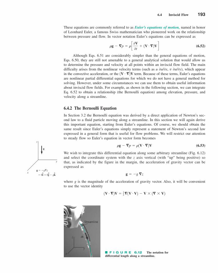
6.4 Inviscid Flow 193

These equations are commonly referred to as Euler’s equations of motion, named in honorof Leonhard Euler, a famous Swiss mathematician who pioneered work on the relationshipbetween pressure and flow. In vector notation Euler’s equations can be expressed as

(6.52)

Although Eqs. 6.51 are considerably simpler than the general equations of motion,Eqs. 6.50, they are still not amenable to a general analytical solution that would allow usto determine the pressure and velocity at all points within an inviscid flow field. The maindifficulty arises from the nonlinear velocity terms (such as u ∂u/∂x, v ∂u/∂y), which appearin the convective acceleration, or the term. Because of these terms, Euler’s equationsare nonlinear partial differential equations for which we do not have a general method forsolving. However, under some circumstances we can use them to obtain useful informationabout inviscid flow fields. For example, as shown in the following section, we can integrateEq. 6.52 to obtain a relationship (the Bernoulli equation) among elevation, pressure, andvelocity along a streamline.

6.4.2 The Bernoulli Equation

In Section 3.2 the Bernoulli equation was derived by a direct application of Newton’s sec-ond law to a fluid particle moving along a streamline. In this section we will again derivethis important equation, starting from Euler’s equations. Of course, we should obtain thesame result since Euler’s equations simply represent a statement of Newton’s second lawexpressed in a general form that is useful for flow problems. We will restrict our attentionto steady flow so Euler’s equation in vector form becomes

(6.53)

We wish to integrate this differential equation along some arbitrary streamline (Fig. 6.12)and select the coordinate system with the z axis vertical (with “up” being positive) sothat, as indicated by the figure in the margin, the acceleration of gravity vector can beexpressed as

where g is the magnitude of the acceleration of gravity vector. Also, it will be convenientto use the vector identity

1V # �2V � 12 �1V # V2 � V � 1� � V2

g � �g �z

�g � �p � �1V # �2V

1V # �2V

�g � �p � � c0V0t

� 1V # �2V d

z

x

y

Streamline

ds

z

x

y

g

g � �g�z

� 0i � 0j � gk^ ^ ^

F I G U R E 6.12 The notation fordifferential length along a streamline.

c06DifferentialAnalysisofFluidFlow.qxd 9/24/10 1:37 PM Page 193

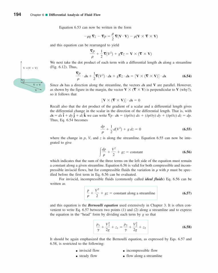
Equation 6.53 can now be written in the form

and this equation can be rearranged to yield

We next take the dot product of each term with a differential length ds along a streamline(Fig. 6.12). Thus,

(6.54)

Since ds has a direction along the streamline, the vectors ds and V are parallel. However,as shown by the figure in the margin, the vector V � (� � V) is perpendicular to V (why?),so it follows that

Recall also that the dot product of the gradient of a scalar and a differential length givesthe differential change in the scalar in the direction of the differential length. That is, withds � dx i � dy j � dz k we can write �p . ds � (∂p/∂x) dx � (∂p/∂y) dy � (∂p/∂z) dz � dp.Thus, Eq. 6.54 becomes

(6.55)

where the change in p, V, and z is along the streamline. Equation 6.55 can now be inte-grated to give

(6.56)

which indicates that the sum of the three terms on the left side of the equation must remaina constant along a given streamline. Equation 6.56 is valid for both compressible and incom-pressible inviscid flows, but for compressible fluids the variation in � with p must be spec-ified before the first term in Eq. 6.56 can be evaluated.

For inviscid, incompressible fluids (commonly called ideal fluids) Eq. 6.56 can bewritten as

(6.57)

and this equation is the Bernoulli equation used extensively in Chapter 3. It is often con-venient to write Eq. 6.57 between two points (1) and (2) along a streamline and to expressthe equation in the “head” form by dividing each term by g so that

(6.58)

It should be again emphasized that the Bernoulli equation, as expressed by Eqs. 6.57 and6.58, is restricted to the following:

■ inviscid flow ■ incompressible flow

■ steady flow ■ flow along a streamline

p1

��

V21

2g� z1 �

p2

��

V22

2g� z2

p�

�V2

2� gz � constant along a streamline

�dp

��

V 2

2� gz � constant

dp

��

1

2 d1V 22 � g dz � 0

3V � 1� � V2 4 # ds � 0

�p

�# ds �

1

2�1V 22 # ds � g�z # ds � 3V � 1� � V2 4 # ds

�p

��

1

2 �1V 22 � g�z � V � 1� � V2

��g �z � �p ��

2 �1V # V2 � �1V � � � V2

194 Chapter 6 ■ Differential Analysis of Fluid Flow

V

V �( � V)

Δ

� V

Δ

c06DifferentialAnalysisofFluidFlow.qxd 9/24/10 1:38 PM Page 194

6.4 Inviscid Flow 195

You may want to go back and review some of the examples in Chapter 3 that illustrate theuse of the Bernoulli equation.

6.4.3 Irrotational Flow

If we make one additional assumption—that the flow is irrotational—the analysis of invis-cid flow problems is further simplified. Recall from Section 6.1.3 that the rotation of a fluidelement is equal to 1

—

2(� � V), and an irrotational flow field is one for which � � V � 0.Since the vorticity, �, is defined as � � V, it also follows that in an irrotational flow fieldthe vorticity is zero. The concept of irrotationality may seem to be a rather strange condi-tion for a flow field. Why would a flow field be irrotational? To answer this question wenote that if 1

—

2(� � V) � 0, then each of the components of this vector, as are given by Eqs.6.12, 6.13, and 6.14, must be equal to zero. Since these components include the variousvelocity gradients in the flow field, the condition of irrotationality imposes specific rela-tionships among these velocity gradients. For example, for rotation about the z axis to bezero, it follows from Eq. 6.12 that

and, therefore,

(6.59)

Similarly from Eqs. 6.13 and 6.14

(6.60)

and

(6.61)

A general flow field would not satisfy these three equations. However, a uniform flow asis illustrated in Fig. 6.13 does. Since u � U (a constant), v � 0, and w � 0, it follows thatEqs. 6.59, 6.60, and 6.61 are all satisfied. Therefore, a uniform flow field (in which thereare no velocity gradients) is certainly an example of an irrotational flow.

For an inviscid fluid there are no shearing stresses—the only forces acting on a fluidelement are its weight and pressure forces. Because the weight acts through the elementcenter of gravity, and the pressure acts in a direction normal to the element surface, neitherof these forces can cause the element to rotate. Therefore, for an inviscid fluid, if some partof the flow field is irrotational, the fluid elements emanating from this region will not takeon any rotation as they progress through the flow field.

0u

0z�

0w

0x

0w

0y�

0v

0z

0v

0x�

0u

0y

�z �1

2 a

0v

0x�

0u

0yb � 0

u = U (constant)

v = 0

w = 0

x

y

zF I G U R E 6.13 Uniform flow in the x

direction.

c06DifferentialAnalysisofFluidFlow.qxd 9/24/10 1:38 PM Page 195

6.4.4 The Bernoulli Equation for Irrotational Flow

In the development of the Bernoulli equation in Section 6.4.2, Eq. 6.54 was integrated alonga streamline. This restriction was imposed so the right side of the equation could be setequal to zero; that is,

(since ds is parallel to V). However, for irrotational flow, � � V � 0, so the right side ofEq. 6.54 is zero regardless of the direction of ds. We can now follow the same procedureused to obtain Eq. 6.55, where the differential changes dp, d(V 2), and dz can be taken inany direction. Integration of Eq. 6.55 again yields

(6.62)

where for irrotational flow the constant is the same throughout the flow field. Thus, forincompressible, irrotational flow the Bernoulli equation can be written as

(6.63)

between any two points in the flow field. Equation 6.63 is exactly the same form as Eq.6.58 but is not limited to application along a streamline.

6.4.5 The Velocity Potential

For an irrotational flow the velocity gradients are related through Eqs. 6.59, 6.60, and 6.61.It follows that in this case the velocity components can be expressed in terms of a scalarfunction (x, y, z, t) as

(6.64)

where is called the velocity potential. Direct substitution of these expressions for thevelocity components into Eqs. 6.59, 6.60, and 6.61 will verify that a velocity field definedby Eqs. 6.64 is indeed irrotational. In vector form, Eq. 6.64 can be written as

(6.65)

so that for an irrotational flow the velocity is expressible as the gradient of a scalar function .The velocity potential is a consequence of the irrotationality of the flow field, whereas

the stream function (see Section 6.2.3) is a consequence of conservation of mass. It is tobe noted, however, that the velocity potential can be defined for a general three-dimensionalflow, whereas the stream function is restricted to two-dimensional flows.

For an incompressible fluid, we know from conservation of mass that

and therefore for incompressible, irrotational flow (with V � � ) it follows that

(6.66)

where �2( ) � � . �( ) is the Laplacian operator. In Cartesian coordinates

02

0x2�

02

0y2�

02

0z2� 0

�2 � 0

� # V � 0

V � �

u �0

0x v �

0

0y w �

0

0z

p1

��

V21

2g� z1 �

p2

��

V22

2g� z2

� dp

��

V 2

2� gz � constant

1V � � � V2 # ds � 0

196 Chapter 6 ■ Differential Analysis of Fluid Flow

c06DifferentialAnalysisofFluidFlow.qxd 9/24/10 1:38 PM Page 196

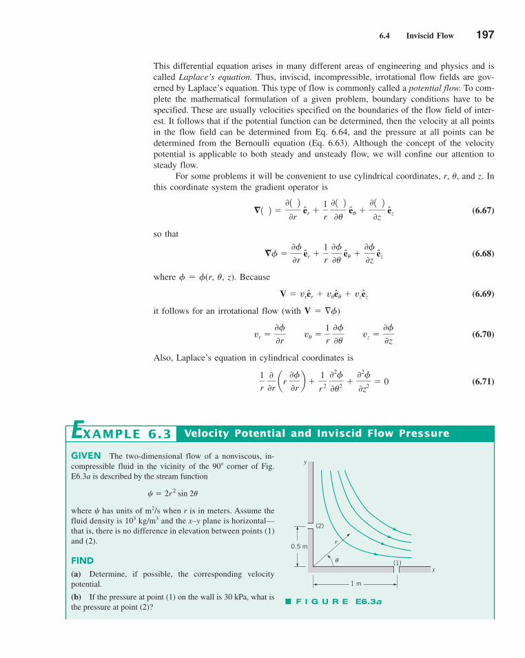
6.4 Inviscid Flow 197

This differential equation arises in many different areas of engineering and physics and iscalled Laplace’s equation. Thus, inviscid, incompressible, irrotational flow fields are gov-erned by Laplace’s equation. This type of flow is commonly called a potential flow. To com-plete the mathematical formulation of a given problem, boundary conditions have to bespecified. These are usually velocities specified on the boundaries of the flow field of inter-est. It follows that if the potential function can be determined, then the velocity at all pointsin the flow field can be determined from Eq. 6.64, and the pressure at all points can bedetermined from the Bernoulli equation (Eq. 6.63). Although the concept of the velocitypotential is applicable to both steady and unsteady flow, we will confine our attention tosteady flow.

For some problems it will be convenient to use cylindrical coordinates, r, �, and z. Inthis coordinate system the gradient operator is

(6.67)

so that

(6.68)

where � (r, �, z). Because

(6.69)

it follows for an irrotational flow (with V � � )

(6.70)

Also, Laplace’s equation in cylindrical coordinates is

(6.71)1r

00r

ar 0

0rb �

1

r 2 02

0�2�

02

0z2� 0

vr �0

0r v� �

1r 0

0� vz �

0

0z

V � vrer � v�e� � vzez

� �0

0rer �

1r 0

0�e� �

0

0zez

�1 2 �0 1 20r

er �1r 0 1 20�

e� �0 1 20z

ez

GIVEN The two-dimensional flow of a nonviscous, in-compressible fluid in the vicinity of the 90� corner of Fig.E6.3a is described by the stream function

where has units of m2/s when r is in meters. Assume thefluid density is 103 kg/m3 and the x–y plane is horizontal—that is, there is no difference in elevation between points (1)and (2).

FIND(a) Determine, if possible, the corresponding velocitypotential.

(b) If the pressure at point (1) on the wall is 30 kPa, what isthe pressure at point (2)?

� 2r 2 sin 2�

Velocity Potential and Inviscid Flow PressureEXAMPLE 6.3

(2)

0.5 m

θ

r

(1)

1 m

x

y

F I G U R E E6.3a

c06DifferentialAnalysisofFluidFlow.qxd 9/24/10 1:38 PM Page 197

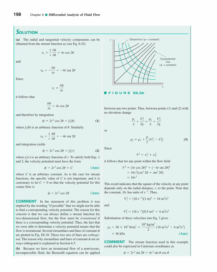
198 Chapter 6 ■ Differential Analysis of Fluid Flow

F I G U R E E6.3b

SOLUTION

between any two points. Thus, between points (1) and (2) withno elevation change

or

(3)

Since

it follows that for any point within the flow field

This result indicates that the square of the velocity at any pointdepends only on the radial distance, r, to the point. Note thatthe constant, 16, has units of s�2. Thus,

and

Substitution of these velocities into Eq. 3 gives

(Ans)

COMMENT The stream function used in this examplecould also be expressed in Cartesian coordinates as

� 2r 2 sin 2� � 4r 2 sin � cos �

� 36 kPa

p2 � 30 � 103 N/m2 �103 kg/m3

2 116 m2/s2 � 4 m2/s22

V 22 � 116 s�22 10.5 m22 � 4 m2/s2

V 21 � 116 s�22 11 m22 � 16 m2/s2

� 16r 2

� 16r 21cos2 2� � sin2 2�2

V 2 � 14r cos 2�22 � 1�4r sin 2�22

V 2 � v 2r � v 2

�

p2 � p1 ��

2 1V 2

1 � V 222

p1

��

V 21

2g�

p2

��

V 22

2g

(a) The radial and tangential velocity components can beobtained from the stream function as (see Eq. 6.42)

and

Since

it follows that

and therefore by integration

(1)

where f1(�) is an arbitrary function of �. Similarly

and integration yields

(2)

where f2(r) is an arbitrary function of r. To satisfy both Eqs. 1and 2, the velocity potential must have the form

(Ans)

where C is an arbitrary constant. As is the case for streamfunctions, the specific value of C is not important, and it iscustomary to let C � 0 so that the velocity potential for thiscorner flow is

(Ans)

COMMENT In the statement of this problem it wasimplied by the wording “if possible” that we might not be ableto find a corresponding velocity potential. The reason for thisconcern is that we can always define a stream function fortwo-dimensional flow, but the flow must be irrotational ifthere is a corresponding velocity potential. Thus, the fact thatwe were able to determine a velocity potential means that theflow is irrotational. Several streamlines and lines of constant are plotted in Fig. E6.3b. These two sets of lines are orthogo-nal. The reason why streamlines and lines of constant are al-ways orthogonal is explained in Section 6.5.

(b) Because we have an irrotational flow of a nonviscous,incompressible fluid, the Bernoulli equation can be applied

� 2r 2 cos 2�

� 2r 2 cos 2� � C

� 2r 2 cos 2� � f21r2

v� �1r 0

0�� �4r sin 2�

� 2r 2 cos 2� � f11�2

0

0r� 4r cos 2�

vr �0

0r

v� � �0

0r� �4r sin 2�

vr �1r 0

0�� 4r cos 2�

y Streamline ( = constant)ψ

Equipotentialline

( = constant)φ

x

c06DifferentialAnalysisofFluidFlow.qxd 9/24/10 1:38 PM Page 198

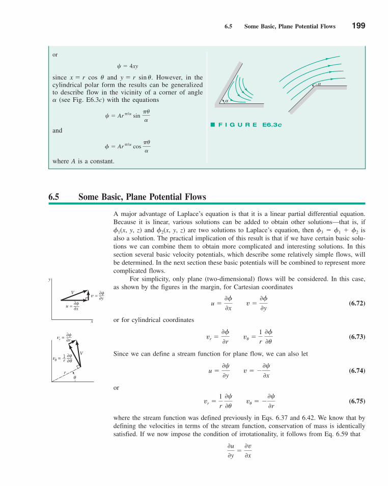
6.5 Some Basic, Plane Potential Flows 199

or

since x � r cos � and y � r sin �. However, in thecylindrical polar form the results can be generalizedto describe flow in the vicinity of a corner of angle� (see Fig. E6.3c) with the equations

and

where A is a constant.

� Ar �/� cos

��

�

� Ar �/� sin

��

�

� 4xy

F I G U R E E6.3c

α

α

6.5 Some Basic, Plane Potential Flows

A major advantage of Laplace’s equation is that it is a linear partial differential equation.Because it is linear, various solutions can be added to obtain other solutions—that is, if 1(x, y, z) and 2(x, y, z) are two solutions to Laplace’s equation, then 3 � 1 � 2 isalso a solution. The practical implication of this result is that if we have certain basic solu-tions we can combine them to obtain more complicated and interesting solutions. In thissection several basic velocity potentials, which describe some relatively simple flows, willbe determined. In the next section these basic potentials will be combined to represent morecomplicated flows.

For simplicity, only plane (two-dimensional) flows will be considered. In this case,as shown by the figures in the margin, for Cartesian coordinates

(6.72)

or for cylindrical coordinates

(6.73)

Since we can define a stream function for plane flow, we can also let

(6.74)

or

(6.75)

where the stream function was defined previously in Eqs. 6.37 and 6.42. We know that bydefining the velocities in terms of the stream function, conservation of mass is identicallysatisfied. If we now impose the condition of irrotationality, it follows from Eq. 6.59 that

0u

0y�

0v

0x

vr �1r 0

0� v� � �

0

0r

u �0

0y v � �

0

0x

vr �0

0r v� �

1r 0

0�

u �0

0x v �

0

0y

V

y

x

u = x∂φ∂

v = y∂φ∂

θr

Vv = ∂φ

θ∂θ

vr =

1__r

∂φ∂r

c06DifferentialAnalysisofFluidFlow.qxd 9/24/10 1:39 PM Page 199

and in terms of the stream function

or

Thus, for a plane, irrotational flow we can use either the velocity potential or thestream function—both must satisfy Laplace’s equation in two dimensions. It is apparentfrom these results that the velocity potential and the stream function are somehow related.We have previously shown that lines of constant are streamlines; that is,

(6.76)

The change in as we move from one point (x, y) to a nearby point (x � dx, y � dy) isgiven by the relationship:

Along a line of constant we have d � 0 so that

(6.77)

A comparison of Eqs. 6.76 and 6.77 shows that lines of constant (called equipotentiallines) are orthogonal to lines of constant (streamlines) at all points where they intersect.(Recall, as shown by the figure in the margin, that two lines are orthogonal if the productof their slopes is minus one.) For any potential flow field a “flow net” can be drawn thatconsists of a family of streamlines and equipotential lines. The flow net is useful in visu-alizing flow patterns and can be used to obtain graphical solutions by sketching in stream-lines and equipotential lines and adjusting the lines until the lines are approximately orthog-onal at all points where they intersect. An example of a flow net is shown in Fig. 6.14.Velocities can be estimated from the flow net, since the velocity is inversely proportional

dy

dx`along �constant

� �u

v

d �0

0x dx �

0

0y dy � u dx � v dy

dy

dx`along �constant

�vu

02

0x 2

�02

0y2� 0

00y

a0

0yb �

00x

a�0

0xb

200 Chapter 6 ■ Differential Analysis of Fluid Flow

y

x

a

a

b b

a_b

b_a×(– ) = –1

Streamline( = constant)ψ

d2 < dV2 > V

V2

V1V

V

d

dd1 > d

V1 < V

Equipotential line( = constant)φ

F I G U R E 6.14 Flow net for a 90� bend.(From Ref. 3, used by permission.)

c06DifferentialAnalysisofFluidFlow.qxd 9/24/10 1:39 PM Page 200

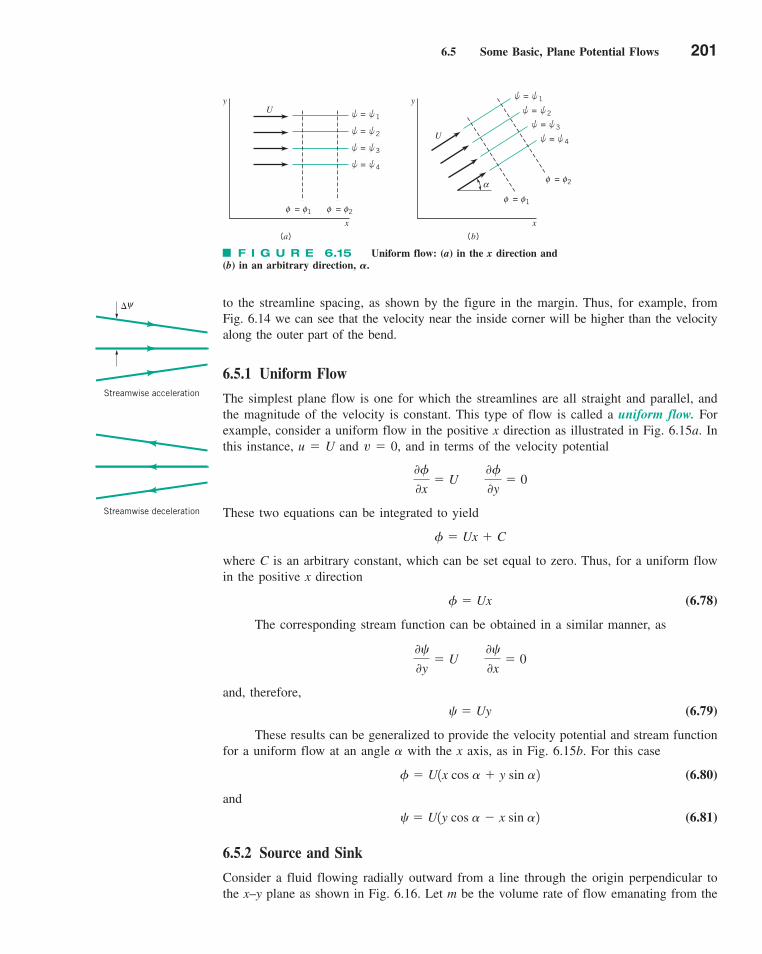
6.5 Some Basic, Plane Potential Flows 201

to the streamline spacing, as shown by the figure in the margin. Thus, for example, fromFig. 6.14 we can see that the velocity near the inside corner will be higher than the velocityalong the outer part of the bend.

6.5.1 Uniform Flow

The simplest plane flow is one for which the streamlines are all straight and parallel, andthe magnitude of the velocity is constant. This type of flow is called a uniform flow. Forexample, consider a uniform flow in the positive x direction as illustrated in Fig. 6.15a. Inthis instance, u � U and v � 0, and in terms of the velocity potential

These two equations can be integrated to yield

where C is an arbitrary constant, which can be set equal to zero. Thus, for a uniform flowin the positive x direction

(6.78)

The corresponding stream function can be obtained in a similar manner, as

and, therefore,

(6.79)

These results can be generalized to provide the velocity potential and stream functionfor a uniform flow at an angle � with the x axis, as in Fig. 6.15b. For this case

(6.80)

and

(6.81)

6.5.2 Source and Sink

Consider a fluid flowing radially outward from a line through the origin perpendicular tothe x–y plane as shown in Fig. 6.16. Let m be the volume rate of flow emanating from the

� U1y cos � � x sin �2

� U1x cos � � y sin �2

� Uy

0

0y� U

0

0x� 0

� Ux

� Ux � C

0

0x� U

0

0y� 0

y

x

U

φ = 1φ φ = 2φ

= 1

= 2

= 3

= 4

y

x

U

α

= 1= 2

= 3= 4

φ = 1φ

φ = 2φ

(a) (b)

F I G U R E 6.15 Uniform flow: (a) in the x direction and (b) in an arbitrary direction, �.

Streamwise acceleration

�ψ

Streamwise deceleration

c06DifferentialAnalysisofFluidFlow.qxd 9/24/10 1:39 PM Page 201

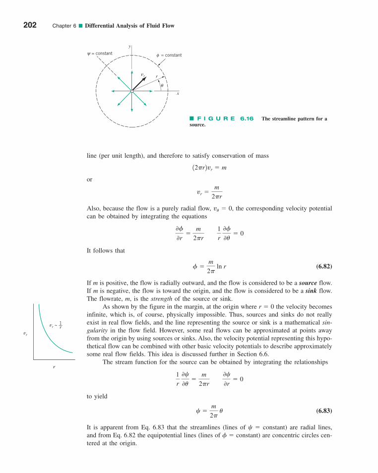
line (per unit length), and therefore to satisfy conservation of mass

or

Also, because the flow is a purely radial flow, v� � 0, the corresponding velocity potentialcan be obtained by integrating the equations

It follows that

(6.82)

If m is positive, the flow is radially outward, and the flow is considered to be a source flow.If m is negative, the flow is toward the origin, and the flow is considered to be a sink flow.The flowrate, m, is the strength of the source or sink.

As shown by the figure in the margin, at the origin where r � 0 the velocity becomesinfinite, which is, of course, physically impossible. Thus, sources and sinks do not reallyexist in real flow fields, and the line representing the source or sink is a mathematical sin-gularity in the flow field. However, some real flows can be approximated at points awayfrom the origin by using sources or sinks. Also, the velocity potential representing this hypo-thetical flow can be combined with other basic velocity potentials to describe approximatelysome real flow fields. This idea is discussed further in Section 6.6.

The stream function for the source can be obtained by integrating the relationships

to yield

(6.83)

It is apparent from Eq. 6.83 that the streamlines (lines of � constant) are radial lines,and from Eq. 6.82 the equipotential lines (lines of � constant) are concentric circles cen-tered at the origin.

�m

2� �

1r 0

0��

m

2�r

0

0r� 0

�m

2� ln r

0

0r�

m

2�r

1r 0

0�� 0

vr �m

2�r

12�r2vr � m

202 Chapter 6 ■ Differential Analysis of Fluid Flow

= constantφ

vr r

θ

x

y

ψ = constant

vr

r

~vr1__r

F I G U R E 6.16 The streamline pattern for asource.

c06DifferentialAnalysisofFluidFlow.qxd 9/24/10 1:39 PM Page 202

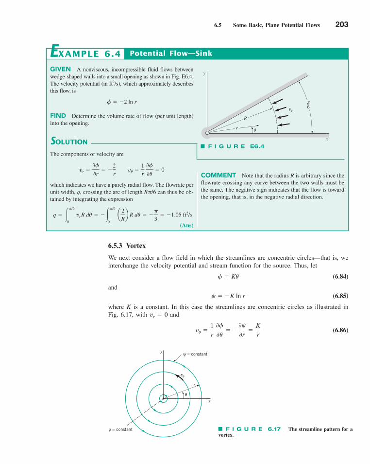
6.5 Some Basic, Plane Potential Flows 203

6.5.3 Vortex

We next consider a flow field in which the streamlines are concentric circles—that is, weinterchange the velocity potential and stream function for the source. Thus, let

(6.84)

and(6.85)

where K is a constant. In this case the streamlines are concentric circles as illustrated inFig. 6.17, with vr � 0 and

(6.86)v� �1r 0

0�� �

0

0r�

Kr

� �K ln r

� K�

φ = constant

θ

ψ = constanty

x

r

vθ

F I G U R E 6.17 The streamline pattern for avortex.

GIVEN A nonviscous, incompressible fluid flows betweenwedge-shaped walls into a small opening as shown in Fig. E6.4.The velocity potential (in ft2/s), which approximately describesthis flow, is

FIND Determine the volume rate of flow (per unit length)into the opening.

� �2 ln r

Potential Flow—SinkEXAMPLE 6.4

SOLUTION

COMMENT Note that the radius R is arbitrary since theflowrate crossing any curve between the two walls must bethe same. The negative sign indicates that the flow is towardthe opening, that is, in the negative radial direction.

The components of velocity are

which indicates we have a purely radial flow. The flowrate perunit width, q, crossing the arc of length R�/6 can thus be ob-tained by integrating the expression

(Ans)

q � ��/6

0

vrR d� � ���/6

0 a

2

Rb R d� � �

�

3� �1.05 ft2/s

vr �0

0r� �

2r v� �

1r 0

0�� 0

R

θr

vr

π_6

x

y

F I G U R E E6.4

c06DifferentialAnalysisofFluidFlow.qxd 9/24/10 1:39 PM Page 203

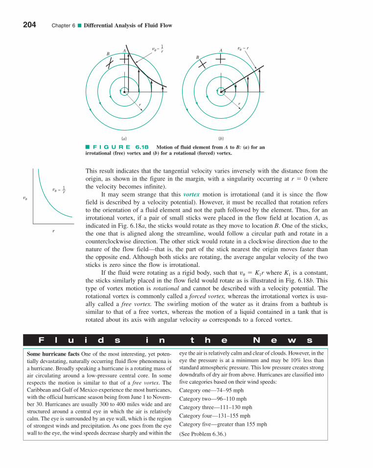
This result indicates that the tangential velocity varies inversely with the distance from theorigin, as shown in the figure in the margin, with a singularity occurring at r � 0 (wherethe velocity becomes infinite).

It may seem strange that this vortex motion is irrotational (and it is since the flowfield is described by a velocity potential). However, it must be recalled that rotation refersto the orientation of a fluid element and not the path followed by the element. Thus, for anirrotational vortex, if a pair of small sticks were placed in the flow field at location A, asindicated in Fig. 6.18a, the sticks would rotate as they move to location B. One of the sticks,the one that is aligned along the streamline, would follow a circular path and rotate in acounterclockwise direction. The other stick would rotate in a clockwise direction due to thenature of the flow field—that is, the part of the stick nearest the origin moves faster thanthe opposite end. Although both sticks are rotating, the average angular velocity of the twosticks is zero since the flow is irrotational.

If the fluid were rotating as a rigid body, such that v� � K1r where K1 is a constant,the sticks similarly placed in the flow field would rotate as is illustrated in Fig. 6.18b. Thistype of vortex motion is rotational and cannot be described with a velocity potential. Therotational vortex is commonly called a forced vortex, whereas the irrotational vortex is usu-ally called a free vortex. The swirling motion of the water as it drains from a bathtub issimilar to that of a free vortex, whereas the motion of a liquid contained in a tank that isrotated about its axis with angular velocity � corresponds to a forced vortex.

204 Chapter 6 ■ Differential Analysis of Fluid Flow

1_r

v ~θ v ~ rθB

A

r

(a) (b)

r

A

B

F I G U R E 6.18 Motion of fluid element from A to B: (a) for anirrotational (free) vortex and (b) for a rotational (forced) vortex.

r

vθ

1__r

vθ ~

F l u i d s i n t h e N e w s

Some hurricane facts One of the most interesting, yet poten-tially devastating, naturally occurring fluid flow phenomena isa hurricane. Broadly speaking a hurricane is a rotating mass ofair circulating around a low-pressure central core. In somerespects the motion is similar to that of a free vortex. TheCaribbean and Gulf of Mexico experience the most hurricanes,with the official hurricane season being from June 1 to Novem-ber 30. Hurricanes are usually 300 to 400 miles wide and arestructured around a central eye in which the air is relativelycalm. The eye is surrounded by an eye wall, which is the regionof strongest winds and precipitation. As one goes from the eyewall to the eye, the wind speeds decrease sharply and within the

eye the air is relatively calm and clear of clouds. However, in theeye the pressure is at a minimum and may be 10% less thanstandard atmospheric pressure. This low pressure creates strongdowndrafts of dry air from above. Hurricanes are classified intofive categories based on their wind speeds:

Category one—74–95 mph

Category two—96–110 mph

Category three—111–130 mph

Category four—131–155 mph

Category five—greater than 155 mph

(See Problem 6.36.)

c06DifferentialAnalysisofFluidFlow.qxd 9/24/10 1:39 PM Page 204

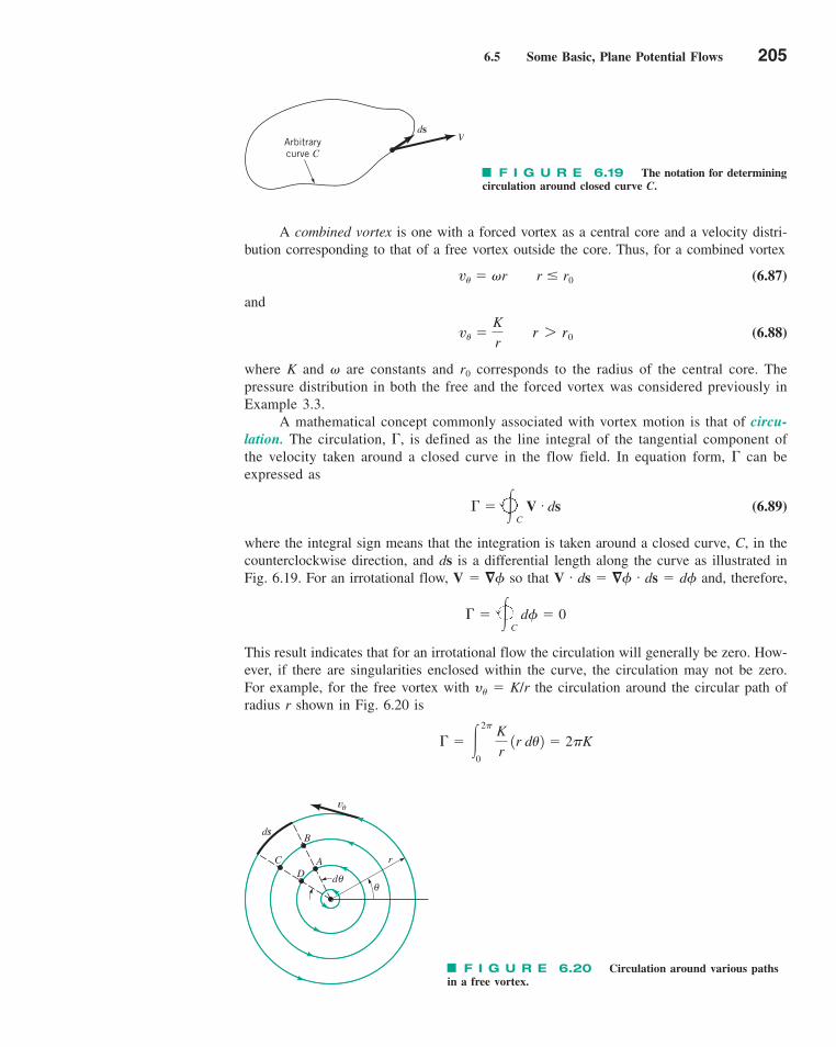
6.5 Some Basic, Plane Potential Flows 205

A combined vortex is one with a forced vortex as a central core and a velocity distri-bution corresponding to that of a free vortex outside the core. Thus, for a combined vortex

(6.87)

and

(6.88)

where K and � are constants and r0 corresponds to the radius of the central core. Thepressure distribution in both the free and the forced vortex was considered previously inExample 3.3.

A mathematical concept commonly associated with vortex motion is that of circu-lation. The circulation, , is defined as the line integral of the tangential component ofthe velocity taken around a closed curve in the flow field. In equation form, can beexpressed as

(6.89)

where the integral sign means that the integration is taken around a closed curve, C, in thecounterclockwise direction, and ds is a differential length along the curve as illustrated inFig. 6.19. For an irrotational flow, V � � so that V . ds � � . ds � d and, therefore,

This result indicates that for an irrotational flow the circulation will generally be zero. How-ever, if there are singularities enclosed within the curve, the circulation may not be zero.For example, for the free vortex with y� � K/r the circulation around the circular path ofradius r shown in Fig. 6.20 is

� �2�

0

K

r 1r d�2 � 2�K

� �C d � 0

� �C V # ds

v� �K

r r 7 r0

v� � �r r � r0

dsVArbitrary

curve C

F I G U R E 6.19 The notation for determiningcirculation around closed curve C.

θ

CD

A

Bds

vθ

r

θd

F I G U R E 6.20 Circulation around various pathsin a free vortex.

ff

c06DifferentialAnalysisofFluidFlow.qxd 9/24/10 1:39 PM Page 205

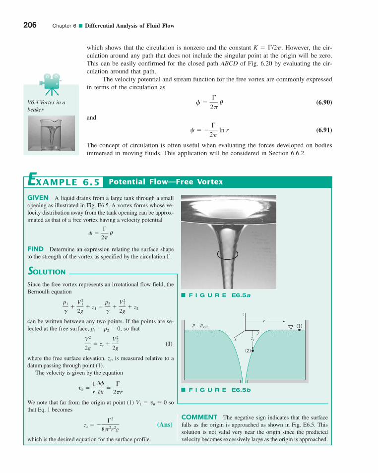
which shows that the circulation is nonzero and the constant K � /2�. However, the cir-culation around any path that does not include the singular point at the origin will be zero.This can be easily confirmed for the closed path ABCD of Fig. 6.20 by evaluating the cir-culation around that path.

The velocity potential and stream function for the free vortex are commonly expressedin terms of the circulation as

(6.90)

and

(6.91)

The concept of circulation is often useful when evaluating the forces developed on bodiesimmersed in moving fluids. This application will be considered in Section 6.6.2.

� �

2� ln r

�

2� �

206 Chapter 6 ■ Differential Analysis of Fluid Flow

V6.4 Vortex in abeaker

GIVEN A liquid drains from a large tank through a smallopening as illustrated in Fig. E6.5. A vortex forms whose ve-locity distribution away from the tank opening can be approx-imated as that of a free vortex having a velocity potential

FIND Determine an expression relating the surface shapeto the strength of the vortex as specified by the circulation .

�

2� �

Potential Flow—Free VortexEXAMPLE 6.5

SOLUTION

COMMENT The negative sign indicates that the surfacefalls as the origin is approached as shown in Fig. E6.5. Thissolution is not valid very near the origin since the predictedvelocity becomes excessively large as the origin is approached.

Since the free vortex represents an irrotational flow field, theBernoulli equation

can be written between any two points. If the points are se-lected at the free surface, p1 � p2 � 0, so that

(1)

where the free surface elevation, zs, is measured relative to adatum passing through point (1).

The velocity is given by the equation

We note that far from the origin at point (1) V1 � v� � 0 sothat Eq. 1 becomes

(Ans)

which is the desired equation for the surface profile.

zs � � 2

8� 2r 2g

v� �1r 0

0��

2�r

V 21

2g� zs �

V 22

2g

p1

��

V 21

2g� z1 �

p2

��

V 22

2g� z2

F I G U R E E6.5a

z

r

y

x zs

p = patm

(2)

(1)

F I G U R E E6.5b

c06DifferentialAnalysisofFluidFlow.qxd 9/24/10 1:39 PM Page 206

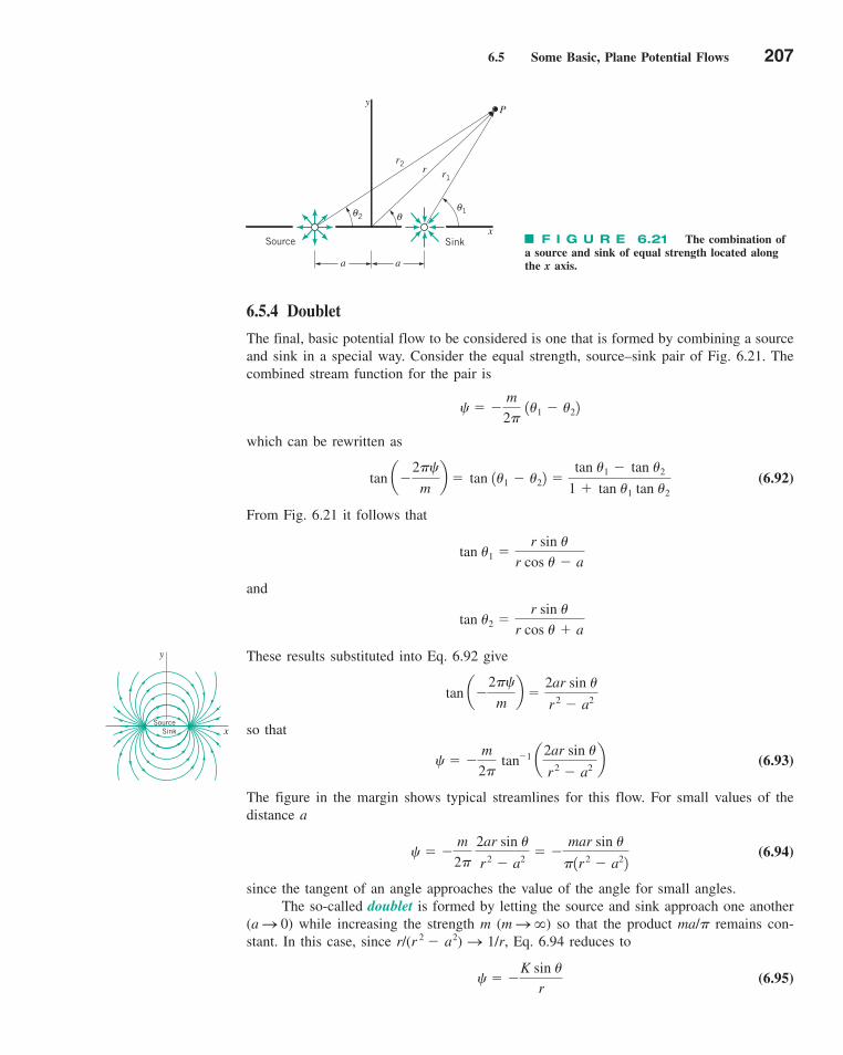
6.5 Some Basic, Plane Potential Flows 207

6.5.4 Doublet

The final, basic potential flow to be considered is one that is formed by combining a sourceand sink in a special way. Consider the equal strength, source–sink pair of Fig. 6.21. Thecombined stream function for the pair is

which can be rewritten as

(6.92)

From Fig. 6.21 it follows that

and

These results substituted into Eq. 6.92 give

so that

(6.93)

The figure in the margin shows typical streamlines for this flow. For small values of thedistance a

(6.94)

since the tangent of an angle approaches the value of the angle for small angles.The so-called doublet is formed by letting the source and sink approach one another

(a S 0) while increasing the strength m (m S �) so that the product ma/� remains con-stant. In this case, since r/(r 2 � a2) S 1/r, Eq. 6.94 reduces to

(6.95) � �K sin �

r

� �m

2� 2ar sin �

r 2 � a2� �

mar sin �

�1r 2 � a22

� �m

2� tan

�1 a2ar sin �

r 2 � a2b

tan a�2�

mb �

2ar sin �

r 2 � a2

tan �2 �r sin �

r cos � � a

tan �1 �r sin �

r cos � � a

tan a�2�

mb � tan 1�1 � �22 �

tan �1 � tan �2

1 � tan �1 tan �2

� �m

2� 1�1 � �22

Py

x

θ2θ1θ

r2

r1r

SinkSource

a a

F I G U R E 6.21 The combination ofa source and sink of equal strength located alongthe x axis.

x

y

SourceSink

c06DifferentialAnalysisofFluidFlow.qxd 9/24/10 1:40 PM Page 207

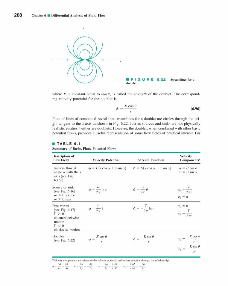
where K, a constant equal to ma/�, is called the strength of the doublet. The correspond-ing velocity potential for the doublet is

(6.96)

Plots of lines of constant reveal that streamlines for a doublet are circles through the ori-gin tangent to the x axis as shown in Fig. 6.22. Just as sources and sinks are not physicallyrealistic entities, neither are doublets. However, the doublet, when combined with other basicpotential flows, provides a useful representation of some flow fields of practical interest. For

�K cos �

r

208 Chapter 6 ■ Differential Analysis of Fluid Flow

x

y

F I G U R E 6.22 Streamlines for adoublet.

TA B L E 6 . 1

Summary of Basic, Plane Potential Flows

Description of VelocityFlow Field Velocity Potential Stream Function Componentsa

Uniform flow at angle with the xaxis 1see Fig.6.15b2

Source or sink 1see Fig. 6.162

source sink

Free vortex 1see Fig. 6.172

counterclockwise motion

clockwise motion

Doublet 1see Fig. 6.222

aVelocity components are related to the velocity potential and stream function through the relationships:

.u �0f0x

�0c0y

v �0f0y

� �0c0x

vr �0f0r

�1

r 0c0u

vu �1

r 0f0u

� �0c0r

v� � �K sin �

r 2

vr � �K cos u

r 2c � �K sin u

r f �

K cos ur

6 0

7 0

m 6 0m 7 0

v � U sin aau � U cos ac � U1 y cos a � x sin a2f � U1x cos a � y sin a2

v� �

2�r

vr � 0 � �

2� ln rf �

2p u

vu � 0

vr �m

2prc �

m

2p uf �

m

2p ln r

c06DifferentialAnalysisofFluidFlow.qxd 9/24/10 1:40 PM Page 208

6.6 Superposition of Basic, Plane Potential Flows 209

6.6 Superposition of Basic, Plane Potential Flows

As was discussed in the previous section, potential flows are governed by Laplace’s equa-tion, which is a linear partial differential equation. It therefore follows that the variousbasic velocity potentials and stream functions can be combined to form new potentials andstream functions. (Why is this true?) Whether such combinations yield useful resultsremains to be seen. It is to be noted that any streamline in an inviscid flow field can beconsidered as a solid boundary, as the conditions along a solid boundary and a streamlineare similar—that is, there is no flow through the boundary or the streamline. Thus, if wecan combine some of the basic velocity potentials or stream functions to yield a stream-line that corresponds to a particular body shape of interest, that combination can be usedto describe in detail the flow around that body. This method of solving some interestingflow problems, commonly called the method of superposition, is illustrated in the follow-ing three sections.

6.6.1 Source in a Uniform Stream—Half-Body

Consider the superposition of a source and a uniform flow as shown in Fig. 6.23a. Theresulting stream function is

(6.97)

and the corresponding velocity potential is

(6.98)

It is clear that at some point along the negative x axis the velocity due to the source will justcancel that due to the uniform flow and a stagnation point will be created. For the source alone

vr �m

2�r

� Ur cos � �m

2� ln r

� Ur sin � �m

2� �

� uniform flow � source

example, we will determine in Section 6.6.2 that the combination of a uniform flow and adoublet can be used to represent the flow around a circular cylinder. Table 6.1 provides asummary of the pertinent equations for the basic, plane potential flows considered in thepreceding sections.

F I G U R E 6.23 The flow around a half-body: (a) superposition of a source and a uniformflow; (b) replacement of streamline with solid boundary to form half-body.C � PbU

U

Stagnationpoint

y

x

r

θ

Source

b

bπ

bπ

b

Stagnation point

= bUψ π

(b)(a)

V6.5 Half-body

c06DifferentialAnalysisofFluidFlow.qxd 9/24/10 1:40 PM Page 209

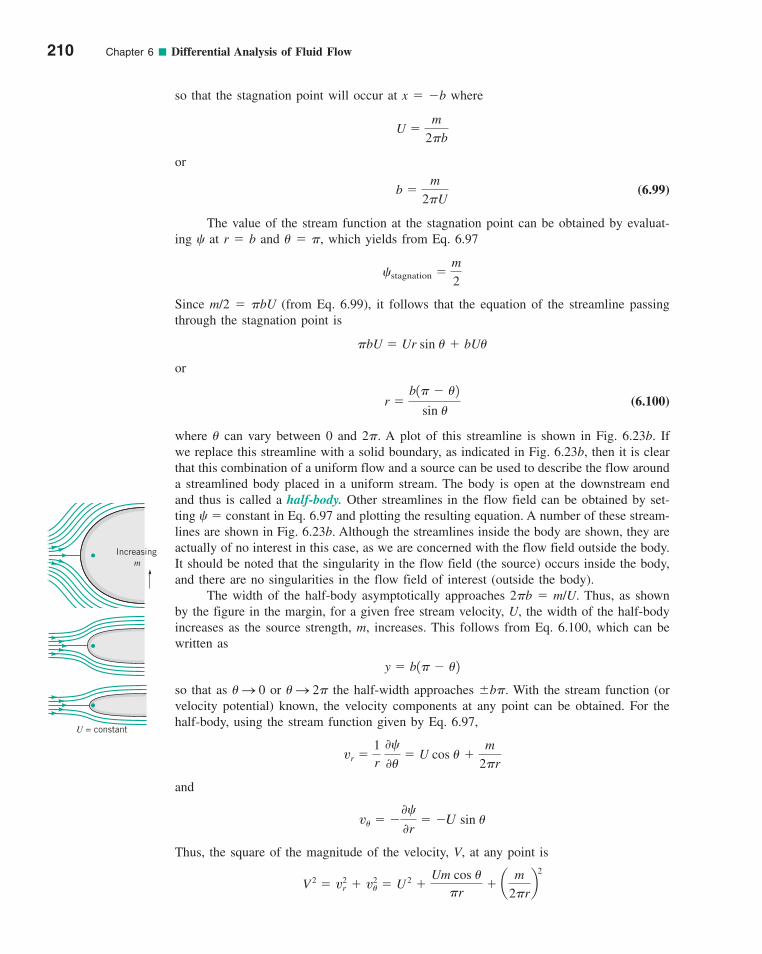
so that the stagnation point will occur at x � �b where

or

(6.99)

The value of the stream function at the stagnation point can be obtained by evaluat-ing at r � b and � � �, which yields from Eq. 6.97

Since m/2 � �bU (from Eq. 6.99), it follows that the equation of the streamline passingthrough the stagnation point is

or

(6.100)

where � can vary between 0 and 2�. A plot of this streamline is shown in Fig. 6.23b. Ifwe replace this streamline with a solid boundary, as indicated in Fig. 6.23b, then it is clearthat this combination of a uniform flow and a source can be used to describe the flow arounda streamlined body placed in a uniform stream. The body is open at the downstream endand thus is called a half-body. Other streamlines in the flow field can be obtained by set-ting � constant in Eq. 6.97 and plotting the resulting equation. A number of these stream-lines are shown in Fig. 6.23b. Although the streamlines inside the body are shown, they areactually of no interest in this case, as we are concerned with the flow field outside the body.It should be noted that the singularity in the flow field (the source) occurs inside the body,and there are no singularities in the flow field of interest (outside the body).

The width of the half-body asymptotically approaches 2�b � m/U. Thus, as shownby the figure in the margin, for a given free stream velocity, U, the width of the half-bodyincreases as the source strength, m, increases. This follows from Eq. 6.100, which can bewritten as

so that as � S 0 or � S 2� the half-width approaches b�. With the stream function (orvelocity potential) known, the velocity components at any point can be obtained. For thehalf-body, using the stream function given by Eq. 6.97,

and

Thus, the square of the magnitude of the velocity, V, at any point is

V 2 � v2r � v2

� � U 2 �Um cos �

�r� a

m

2�rb

2

v� � �0

0r� �U sin �

vr �1r 0

0�� U cos � �

m

2�r

y � b1� � �2

r �b1� � �2

sin �

�bU � Ur sin � � bU�

stagnation �m

2

b �m

2�U

U �m

2�b

210 Chapter 6 ■ Differential Analysis of Fluid Flow

Increasing m

U = constant

c06DifferentialAnalysisofFluidFlow.qxd 9/24/10 1:40 PM Page 210

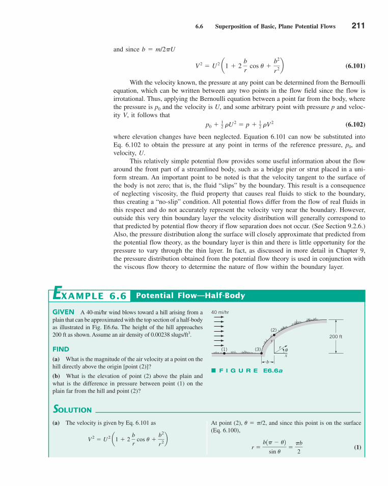
6.6 Superposition of Basic, Plane Potential Flows 211

and since b � m/2�U

(6.101)

With the velocity known, the pressure at any point can be determined from the Bernoulliequation, which can be written between any two points in the flow field since the flow isirrotational. Thus, applying the Bernoulli equation between a point far from the body, wherethe pressure is p0 and the velocity is U, and some arbitrary point with pressure p and veloc-ity V, it follows that

(6.102)

where elevation changes have been neglected. Equation 6.101 can now be substituted intoEq. 6.102 to obtain the pressure at any point in terms of the reference pressure, p0, andvelocity, U.

This relatively simple potential flow provides some useful information about the flowaround the front part of a streamlined body, such as a bridge pier or strut placed in a uni-form stream. An important point to be noted is that the velocity tangent to the surface ofthe body is not zero; that is, the fluid “slips” by the boundary. This result is a consequenceof neglecting viscosity, the fluid property that causes real fluids to stick to the boundary,thus creating a “no-slip” condition. All potential flows differ from the flow of real fluids inthis respect and do not accurately represent the velocity very near the boundary. However,outside this very thin boundary layer the velocity distribution will generally correspond tothat predicted by potential flow theory if flow separation does not occur. (See Section 9.2.6.)Also, the pressure distribution along the surface will closely approximate that predicted fromthe potential flow theory, as the boundary layer is thin and there is little opportunity for thepressure to vary through the thin layer. In fact, as discussed in more detail in Chapter 9,the pressure distribution obtained from the potential flow theory is used in conjunction withthe viscous flow theory to determine the nature of flow within the boundary layer.

p0 � 12 �U 2 � p � 1

2 �V 2

V 2 � U 2 a1 � 2 br

cos � �b2

r 2b

GIVEN A 40-mi/hr wind blows toward a hill arising from aplain that can be approximated with the top section of a half-bodyas illustrated in Fig. E6.6a. The height of the hill approaches200 ft as shown. Assume an air density of 0.00238 slugs/ft3.

FIND(a) What is the magnitude of the air velocity at a point on thehill directly above the origin [point (2)]?

(b) What is the elevation of point (2) above the plain andwhat is the difference in pressure between point (1) on theplain far from the hill and point (2)?

SOLUTION

Potential Flow—Half-Body

At point (2), � � �/2, and since this point is on the surface(Eq. 6.100),

(1)r �b1� � �2

sin ��

�b

2

EXAMPLE 6.6

(a) The velocity is given by Eq. 6.101 as

V2 � U2 a1 � 2 b

r cos � �

b2

r 2b

F I G U R E E6.6a

b

r

x

y

θ

40 mi/hr

(1) (3)

(2)200 ft

c06DifferentialAnalysisofFluidFlow.qxd 9/24/10 1:40 PM Page 211

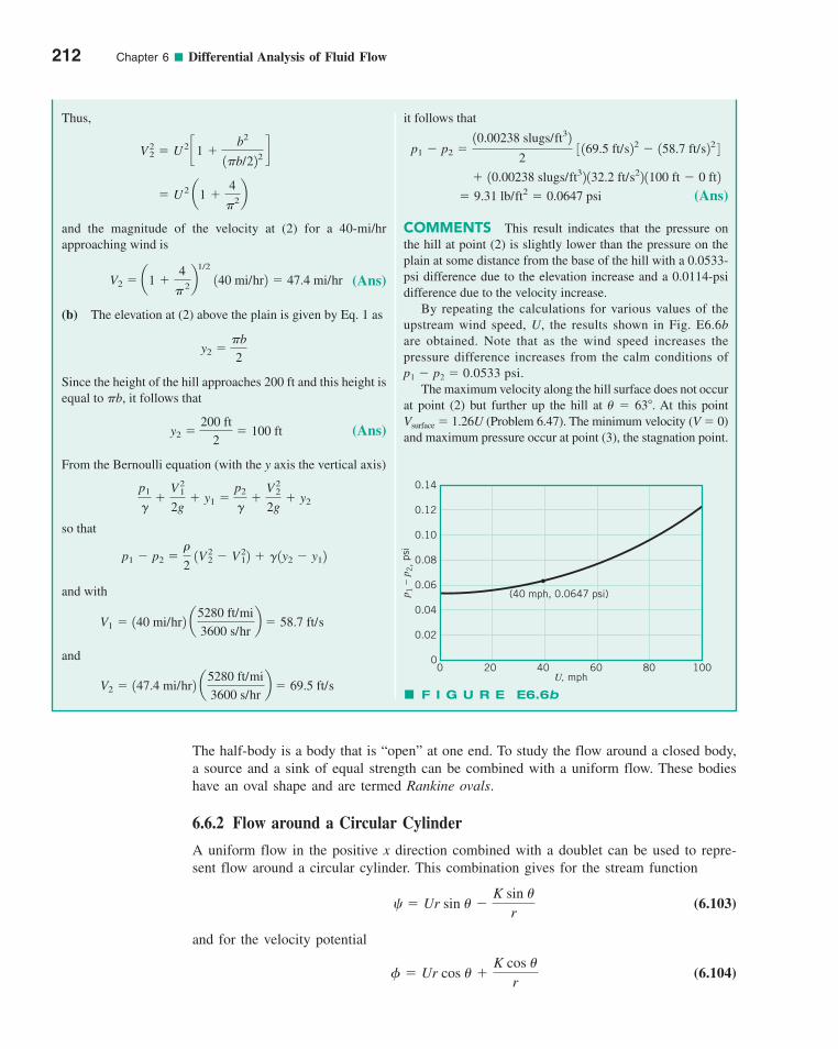
The half-body is a body that is “open” at one end. To study the flow around a closed body,a source and a sink of equal strength can be combined with a uniform flow. These bodieshave an oval shape and are termed Rankine ovals.

6.6.2 Flow around a Circular Cylinder

A uniform flow in the positive x direction combined with a doublet can be used to repre-sent flow around a circular cylinder. This combination gives for the stream function

(6.103)

and for the velocity potential

(6.104) � Ur cos � �K cos �

r

� Ur sin � �K sin �

r

212 Chapter 6 ■ Differential Analysis of Fluid Flow

Thus,

and the magnitude of the velocity at (2) for a 40-mi/hrapproaching wind is

(Ans)

(b) The elevation at (2) above the plain is given by Eq. 1 as

Since the height of the hill approaches 200 ft and this height isequal to �b, it follows that

(Ans)

From the Bernoulli equation (with the y axis the vertical axis)

so that

and with

and

V2 � 147.4 mi/hr2 a5280 ft/mi

3600 s/hrb � 69.5 ft/s

V1 � 140 mi/hr2 a5280 ft/mi

3600 s/hrb � 58.7 ft/s

p1 � p2 ��

2 1V2

2 � V212 � �

1y2 � y12

p1

��

V21

2g� y1 �

p2

��

V22

2g� y2

y2 �200 ft

2� 100 ft

y2 ��b

2

V2 � a1 �4

� 2b

1/2

140 mi/hr2 � 47.4 mi/hr

� U2 a1 �4

�2b

V22 � U2 c1 �

b2

1�b/222d

it follows that

(Ans)

COMMENTS This result indicates that the pressure onthe hill at point (2) is slightly lower than the pressure on theplain at some distance from the base of the hill with a 0.0533-psi difference due to the elevation increase and a 0.0114-psidifference due to the velocity increase.

By repeating the calculations for various values of theupstream wind speed, U, the results shown in Fig. E6.6bare obtained. Note that as the wind speed increases thepressure difference increases from the calm conditions ofp1 � p2 � 0.0533 psi.

The maximum velocity along the hill surface does not occurat point (2) but further up the hill at � � 63�. At this point Vsurface � 1.26U (Problem 6.47). The minimum velocity (V � 0)and maximum pressure occur at point (3), the stagnation point.

� 9.31 lb/ft2 � 0.0647 psi

� 10.00238 slugs/ft32 132.2 ft/s22 1100 ft � 0 ft2

p1 � p2 �10.00238 slugs/ft32

2 3 169.5 ft/s22 � 158.7 ft/s22 4

F I G U R E E6.6b

1008060402000

0.02

0.04

0.06

0.08

0.10

0.12

0.14

p 1 –

p2, ps

i

U, mph

(40 mph, 0.0647 psi)

c06DifferentialAnalysisofFluidFlow.qxd 9/24/10 1:41 PM Page 212

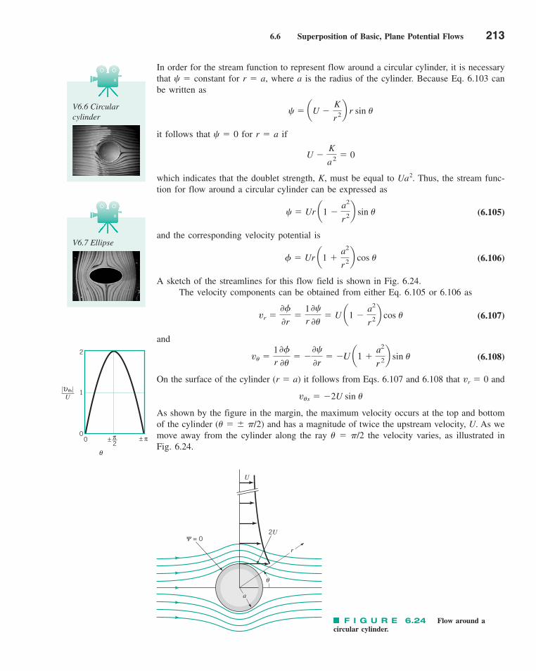
6.6 Superposition of Basic, Plane Potential Flows 213

In order for the stream function to represent flow around a circular cylinder, it is necessarythat � constant for r � a, where a is the radius of the cylinder. Because Eq. 6.103 canbe written as

it follows that � 0 for r � a if

which indicates that the doublet strength, K, must be equal to Ua2. Thus, the stream func-tion for flow around a circular cylinder can be expressed as

(6.105)

and the corresponding velocity potential is

(6.106)

A sketch of the streamlines for this flow field is shown in Fig. 6.24.The velocity components can be obtained from either Eq. 6.105 or 6.106 as

(6.107)

and

(6.108)

On the surface of the cylinder (r � a) it follows from Eqs. 6.107 and 6.108 that vr � 0 and

As shown by the figure in the margin, the maximum velocity occurs at the top and bottomof the cylinder (� � �/2) and has a magnitude of twice the upstream velocity, U. As wemove away from the cylinder along the ray � � �/2 the velocity varies, as illustrated inFig. 6.24.

v�s � �2U sin �

v� �1r

0

0�� �

0

0r� �U a1 �

a2

r 2b sin �

vr �0

0r�

1r

0

0�� U a1 �

a2

r 2b cos �

� Ur a1 �a2

r2b cos �

� Ur a1 �a2

r2b sin �

U �K

a 2 � 0

� aU �K

r2b r sin �V6.6 Circularcylinder

F I G U R E 6.24 Flow around acircular cylinder.

a

r

U

θ

Ψ = 02U

00

1

2

θ

± π

θsυU

± π2

V6.7 Ellipse

c06DifferentialAnalysisofFluidFlow.qxd 9/24/10 1:41 PM Page 213

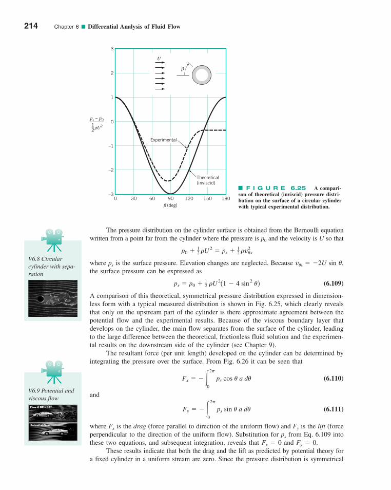
The pressure distribution on the cylinder surface is obtained from the Bernoulli equationwritten from a point far from the cylinder where the pressure is p0 and the velocity is U so that

where ps is the surface pressure. Elevation changes are neglected. Because v�s � �2U sin �,the surface pressure can be expressed as

(6.109)

A comparison of this theoretical, symmetrical pressure distribution expressed in dimension-less form with a typical measured distribution is shown in Fig. 6.25, which clearly revealsthat only on the upstream part of the cylinder is there approximate agreement between thepotential flow and the experimental results. Because of the viscous boundary layer thatdevelops on the cylinder, the main flow separates from the surface of the cylinder, leadingto the large difference between the theoretical, frictionless fluid solution and the experimen-tal results on the downstream side of the cylinder (see Chapter 9).

The resultant force (per unit length) developed on the cylinder can be determined byintegrating the pressure over the surface. From Fig. 6.26 it can be seen that

(6.110)

and

(6.111)

where Fx is the drag (force parallel to direction of the uniform flow) and Fy is the lift (forceperpendicular to the direction of the uniform flow). Substitution for ps from Eq. 6.109 intothese two equations, and subsequent integration, reveals that Fx � 0 and Fy � 0.

These results indicate that both the drag and the lift as predicted by potential theory fora fixed cylinder in a uniform stream are zero. Since the pressure distribution is symmetrical

Fy � ��2�

0

ps sin � a d�

Fx � ��2�

0

ps cos � a d�

ps � p0 � 12 �U211 � 4 sin

2 �2

p0 � 12 �U

2 � ps � 12 �v2

�s

214 Chapter 6 ■ Differential Analysis of Fluid Flow

F I G U R E 6.25 A compari-son of theoretical (inviscid) pressure distri-bution on the surface of a circular cylinderwith typical experimental distribution.

β

U

3

2

1

0

–1

–2

–30 30 60 90 120 150 180

(deg)β

ps – p0_______

U21_

2ρ

Experimental

Theoretical(inviscid)

V6.9 Potential andviscous flow

V6.8 Circularcylinder with sepa-ration

c06DifferentialAnalysisofFluidFlow.qxd 9/24/10 1:41 PM Page 214

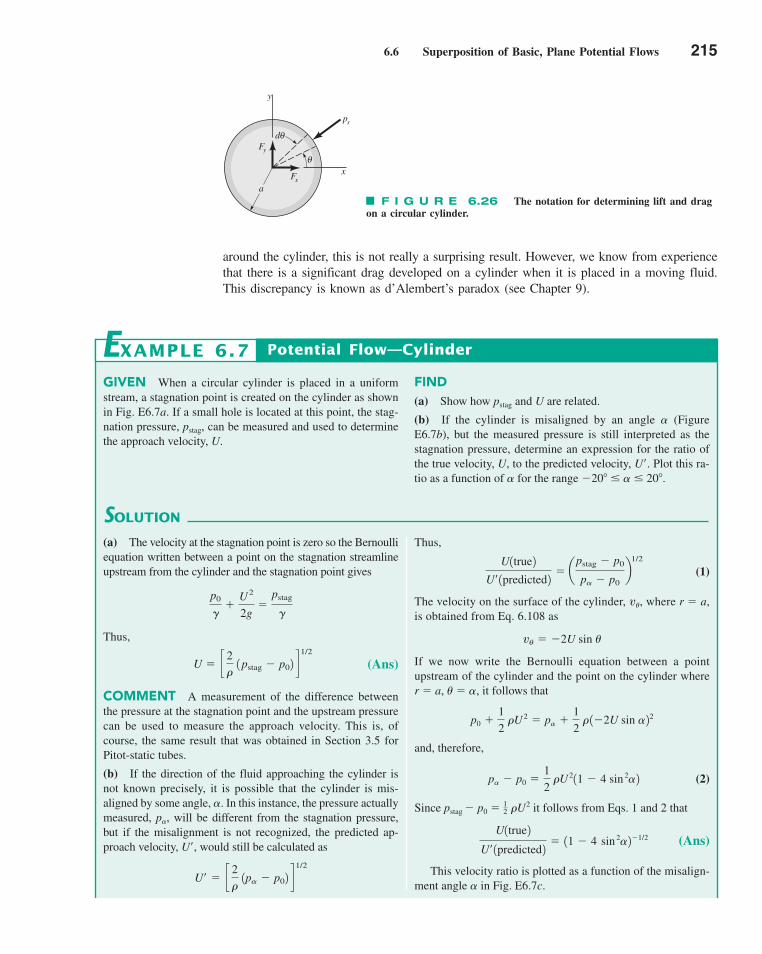
6.6 Superposition of Basic, Plane Potential Flows 215

around the cylinder, this is not really a surprising result. However, we know from experiencethat there is a significant drag developed on a cylinder when it is placed in a moving fluid.This discrepancy is known as d’Alembert’s paradox (see Chapter 9).

F I G U R E 6.26 The notation for determining lift and dragon a circular cylinder.

a

x

y

Fx

Fy

dθ

θ

ps

GIVEN When a circular cylinder is placed in a uniformstream, a stagnation point is created on the cylinder as shownin Fig. E6.7a. If a small hole is located at this point, the stag-nation pressure, pstag, can be measured and used to determinethe approach velocity, U.

FIND(a) Show how pstag and U are related.

(b) If the cylinder is misaligned by an angle � (FigureE6.7b), but the measured pressure is still interpreted as thestagnation pressure, determine an expression for the ratio ofthe true velocity, U, to the predicted velocity, U�. Plot this ra-tio as a function of � for the range �20� � � � 20�.

SOLUTION

Potential Flow—Cylinder

Thus,

(1)

The velocity on the surface of the cylinder, v�, where r � a,is obtained from Eq. 6.108 as

If we now write the Bernoulli equation between a pointupstream of the cylinder and the point on the cylinder where r � a, � � �, it follows that

and, therefore,

(2)

Since pstag � p0 � 1—2 �U2 it follows from Eqs. 1 and 2 that

(Ans)

This velocity ratio is plotted as a function of the misalign-ment angle � in Fig. E6.7c.

U1true2

U¿ 1predicted2� 11 � 4 sin

2�2�1/2

p� � p0 �1

2 �U 211 � 4 sin

2�2

p0 �1

2 �U 2 � p� �

1

2 � 1�2U sin �22

v� � �2U sin �

U1true2

U¿ 1predicted2� a

pstag � p0

p� � p0b

1/2

EXAMPLE 6.7

(a) The velocity at the stagnation point is zero so the Bernoulliequation written between a point on the stagnation streamlineupstream from the cylinder and the stagnation point gives

Thus,

(Ans)

COMMENT A measurement of the difference betweenthe pressure at the stagnation point and the upstream pressurecan be used to measure the approach velocity. This is, ofcourse, the same result that was obtained in Section 3.5 forPitot-static tubes.

(b) If the direction of the fluid approaching the cylinder isnot known precisely, it is possible that the cylinder is mis-aligned by some angle, �. In this instance, the pressure actuallymeasured, p�, will be different from the stagnation pressure,but if the misalignment is not recognized, the predicted ap-proach velocity, U�, would still be calculated as

U¿ � c2�

1p� � p02 d1/2

U � c2�

1pstag � p02 d1/2

p0

��

U2

2g�

pstag

�

c06DifferentialAnalysisofFluidFlow.qxd 9/24/10 1:41 PM Page 215

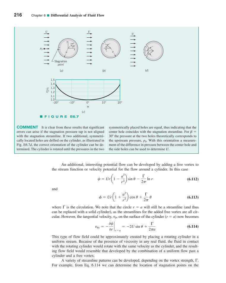
An additional, interesting potential flow can be developed by adding a free vortex tothe stream function or velocity potential for the flow around a cylinder. In this case

(6.112)

and

(6.113)

where � is the circulation. We note that the circle r � a will still be a streamline (and thuscan be replaced with a solid cylinder), as the streamlines for the added free vortex are all cir-cular. However, the tangential velocity, v�, on the surface of the cylinder (r � a) now becomes

(6.114)

This type of flow field could be approximately created by placing a rotating cylinder in auniform stream. Because of the presence of viscosity in any real fluid, the fluid in contactwith the rotating cylinder would rotate with the same velocity as the cylinder, and the result-ing flow field would resemble that developed by the combination of a uniform flow past acylinder and a free vortex.

A variety of streamline patterns can be developed, depending on the vortex strength, �.For example, from Eq. 6.114 we can determine the location of stagnation points on the

v�s � �0�

0r`r�a

� �2U sin � ��

2�a

� � Ur a1 �a2

r2b cos � ��

2� �

� � Ur a1 �a2

r2b sin � ��

2� ln r

216 Chapter 6 ■ Differential Analysis of Fluid Flow

COMMENT It is clear from these results that significanterrors can arise if the stagnation pressure tap is not alignedwith the stagnation streamline. If two additional, symmetri-cally located holes are drilled on the cylinder, as illustrated inFig. E6.7d, the correct orientation of the cylinder can be de-termined. The cylinder is rotated until the pressures in the two

symmetrically placed holes are equal, thus indicating that thecenter hole coincides with the stagnation streamline. For � �30� the pressure at the two holes theoretically corresponds tothe upstream pressure, p0. With this orientation a measure-ment of the difference in pressure between the center hole andthe side holes can be used to determine U.

F I G U R E E6.7

y

xa

θ

r

Stagnationpoint

U

p0

(a)

U

a

α

(b)

1.5

1.4

1.3

1.2

1.11.0

–20° –10° 0° 10° 20°α

U__U'

(c)

U

(d)

β

β

c06DifferentialAnalysisofFluidFlow.qxd 9/27/10 8:37 AM Page 216

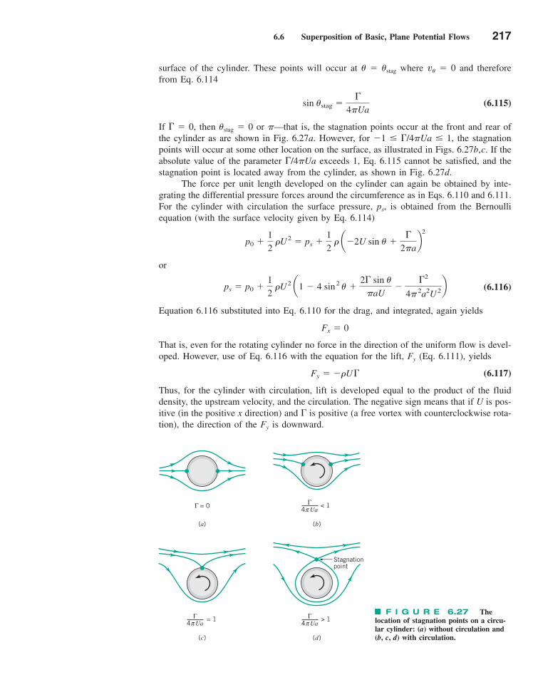
6.6 Superposition of Basic, Plane Potential Flows 217

surface of the cylinder. These points will occur at � � �stag where v� � 0 and thereforefrom Eq. 6.114

(6.115)

If � 0, then �stag � 0 or �—that is, the stagnation points occur at the front and rear ofthe cylinder as are shown in Fig. 6.27a. However, for �1 � /4�Ua � 1, the stagnationpoints will occur at some other location on the surface, as illustrated in Figs. 6.27b,c. If theabsolute value of the parameter /4�Ua exceeds 1, Eq. 6.115 cannot be satisfied, and thestagnation point is located away from the cylinder, as shown in Fig. 6.27d.

The force per unit length developed on the cylinder can again be obtained by inte-grating the differential pressure forces around the circumference as in Eqs. 6.110 and 6.111.For the cylinder with circulation the surface pressure, ps, is obtained from the Bernoulliequation (with the surface velocity given by Eq. 6.114)

or

(6.116)

Equation 6.116 substituted into Eq. 6.110 for the drag, and integrated, again yields

That is, even for the rotating cylinder no force in the direction of the uniform flow is devel-oped. However, use of Eq. 6.116 with the equation for the lift, Fy (Eq. 6.111), yields

(6.117)

Thus, for the cylinder with circulation, lift is developed equal to the product of the fluiddensity, the upstream velocity, and the circulation. The negative sign means that if U is pos-itive (in the positive x direction) and is positive (a free vortex with counterclockwise rota-tion), the direction of the Fy is downward.

Fy � ��U

Fx � 0

ps � p0 �1

2 �U2 a1 � 4 sin

2 � �2 sin �

�aU�

2

4� 2a2U2b

p0 �1

2 �U2 � ps �

1

2 � a�2U sin � �

2�ab

2

sin �stag �

4�Ua

F I G U R E 6.27 Thelocation of stagnation points on a circu-lar cylinder: (a) without circulation and(b, c, d) with circulation.

Γ = 0 < 1Γ4 Uaπ

> 1Γ4 Uaπ = 1Γ

4 Uaπ

(a) (b)

(c) (d)

Stagnationpoint

c06DifferentialAnalysisofFluidFlow.qxd 9/24/10 1:41 PM Page 217

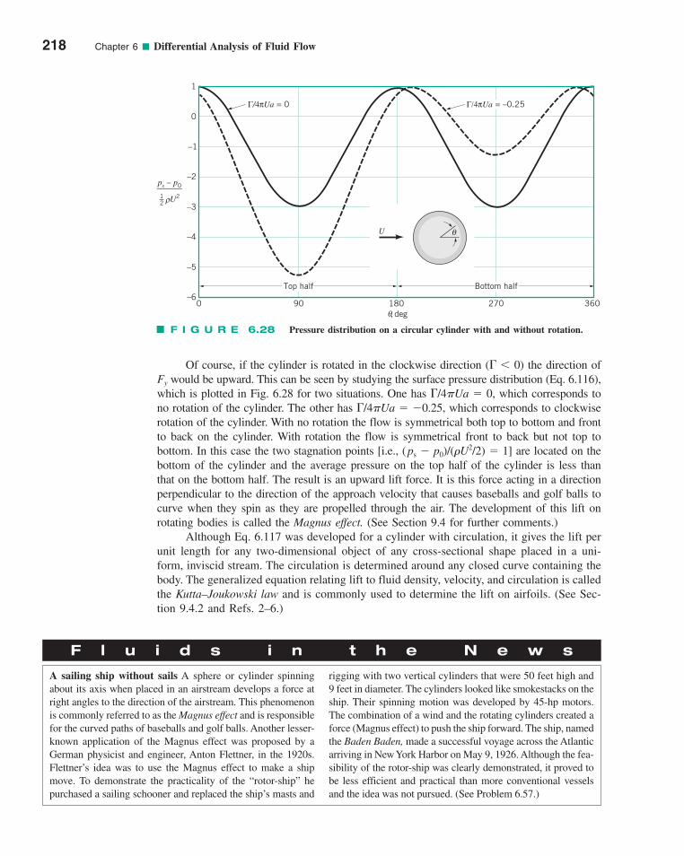
Of course, if the cylinder is rotated in the clockwise direction ( 0) the direction ofFy would be upward. This can be seen by studying the surface pressure distribution (Eq. 6.116),which is plotted in Fig. 6.28 for two situations. One has /4�Ua � 0, which corresponds tono rotation of the cylinder. The other has /4�Ua � �0.25, which corresponds to clockwiserotation of the cylinder. With no rotation the flow is symmetrical both top to bottom and frontto back on the cylinder. With rotation the flow is symmetrical front to back but not top tobottom. In this case the two stagnation points [i.e., (ps � p0)/(�U2/2) � 1] are located on thebottom of the cylinder and the average pressure on the top half of the cylinder is less thanthat on the bottom half. The result is an upward lift force. It is this force acting in a directionperpendicular to the direction of the approach velocity that causes baseballs and golf balls tocurve when they spin as they are propelled through the air. The development of this lift onrotating bodies is called the Magnus effect. (See Section 9.4 for further comments.)

Although Eq. 6.117 was developed for a cylinder with circulation, it gives the lift perunit length for any two-dimensional object of any cross-sectional shape placed in a uni-form, inviscid stream. The circulation is determined around any closed curve containing thebody. The generalized equation relating lift to fluid density, velocity, and circulation is calledthe Kutta–Joukowski law and is commonly used to determine the lift on airfoils. (See Sec-tion 9.4.2 and Refs. 2–6.)

218 Chapter 6 ■ Differential Analysis of Fluid Flow

F I G U R E 6.28 Pressure distribution on a circular cylinder with and without rotation.

1

0

–2

–3

–4

–5

–60 90 180 270 360

Γ/4πUa = 0

U θ

Γ/4πUa = –0.25

θ , deg

Top half Bottom half

–1

ps – p0_______

U2ρ1

2

F l u i d s i n t h e N e w s

A sailing ship without sails A sphere or cylinder spinningabout its axis when placed in an airstream develops a force atright angles to the direction of the airstream. This phenomenonis commonly referred to as the Magnus effect and is responsiblefor the curved paths of baseballs and golf balls. Another lesser-known application of the Magnus effect was proposed by a German physicist and engineer, Anton Flettner, in the 1920s.Flettner’s idea was to use the Magnus effect to make a shipmove. To demonstrate the practicality of the “rotor-ship” hepurchased a sailing schooner and replaced the ship’s masts and

rigging with two vertical cylinders that were 50 feet high and9 feet in diameter. The cylinders looked like smokestacks on theship. Their spinning motion was developed by 45-hp motors.The combination of a wind and the rotating cylinders created aforce (Magnus effect) to push the ship forward. The ship, namedthe Baden Baden, made a successful voyage across the Atlanticarriving in New York Harbor on May 9, 1926. Although the fea-sibility of the rotor-ship was clearly demonstrated, it proved tobe less efficient and practical than more conventional vesselsand the idea was not pursued. (See Problem 6.57.)

c06DifferentialAnalysisofFluidFlow.qxd 9/24/10 1:41 PM Page 218

6.8 Viscous Flow 219

6.7 Other Aspects of Potential Flow Analysis

In the preceding section the method of superposition of basic potentials has been used toobtain detailed descriptions of irrotational flow around certain body shapes immersed in auniform stream. It is possible to extend the idea of superposition by considering a distrib-ution of sources and sinks, or doublets, which when combined with a uniform flow candescribe the flow around bodies of arbitrary shape. Techniques are available to determinethe required distribution to give a prescribed body shape. Also, for plane, potential flowproblems, it can be shown that the complex variable theory (the use of real and imaginarynumbers) can be used effectively to obtain solutions to a great variety of important flowproblems. There are, of course, numerical techniques that can be used to solve not onlyplane two-dimensional problems but also the more general three-dimensional problems.Because potential flow is governed by Laplace’s equation, any procedure that is availablefor solving this equation can be applied to the analysis of the irrotational flow of friction-less fluids. The potential flow theory is an old and well-established discipline within thegeneral field of fluid mechanics. The interested reader can find many detailed references onthis subject, including Refs. 2–6 given at the end of this chapter.

An important point to remember is that regardless of the particular technique used toobtain a solution to a potential flow problem, the solution remains approximate because ofthe fundamental assumption of a frictionless fluid. The general differential equations thatdescribe viscous fluid behavior and some simple solutions to these equations are consid-ered in the remaining sections of this chapter.

6.8 Viscous Flow

To incorporate viscous effects into the differential analysis of fluid motion we must returnto the previously derived general equations of motion, Eqs. 6.50. Since these equationsinclude both stresses and velocities, there are more unknowns than equations and, therefore,before proceeding it is necessary to establish a relationship between stresses and velocities.

6.8.1 Stress–Deformation Relationships

For incompressible, Newtonian fluids it is known that the stresses are linearly related to therates of deformation and can be expressed in Cartesian coordinates as (for normal stresses)

(6.118a)

(6.118b)

(6.118c)

(for shearing stresses)

(6.118d)

(6.118e)

(6.118f) �zx � �xz � � a0w

0x�

0u

0zb

�yz � �zy � � a0v

0z�

0w

0yb

�xy � �yx � � a0u

0y�

0v

0xb

zz � �p � 2� 0w

0z

yy � �p � 2� 0v

0y

xx � �p � 2� 0u

0x

V6.10 Potentialflow

c06DifferentialAnalysisofFluidFlow.qxd 9/24/10 1:42 PM Page 219

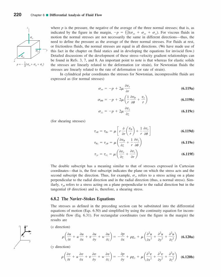
where p is the pressure, the negative of the average of the three normal stresses; that is, asindicated by the figure in the margin, �p � ( )(xx � yy � zz). For viscous fluids inmotion the normal stresses are not necessarily the same in different directions—thus, theneed to define the pressure as the average of the three normal stresses. For fluids at rest,or frictionless fluids, the normal stresses are equal in all directions. (We have made use ofthis fact in the chapter on fluid statics and in developing the equations for inviscid flow.)Detailed discussions of the development of these stress–velocity gradient relationships canbe found in Refs. 3, 7, and 8. An important point to note is that whereas for elastic solidsthe stresses are linearly related to the deformation (or strain), for Newtonian fluids thestresses are linearly related to the rate of deformation (or rate of strain).

In cylindrical polar coordinates the stresses for Newtonian, incompressible fluids areexpressed as (for normal stresses)

(6.119a)

(6.119b)

(6.119c)

(for shearing stresses)

(6.119d)

(6.119e)

(6.119f)

The double subscript has a meaning similar to that of stresses expressed in Cartesiancoordinates—that is, the first subscript indicates the plane on which the stress acts and thesecond subscript the direction. Thus, for example, rr refers to a stress acting on a planeperpendicular to the radial direction and in the radial direction (thus, a normal stress). Sim-ilarly, �r� refers to a stress acting on a plane perpendicular to the radial direction but in thetangential (� direction) and is, therefore, a shearing stress.

6.8.2 The Navier–Stokes Equations

The stresses as defined in the preceding section can be substituted into the differentialequations of motion (Eqs. 6.50) and simplified by using the continuity equation for incom-pressible flow (Eq. 6.31). For rectangular coordinates (see the figure in the margin) theresults are

(x direction)

(6.120a)

(y direction)

(6.120b)� a0v

0t� u

0v

0x� v

0v

0y� w

0v

0zb � �

0p

0y� �gy � � a

02v

0x2 �02v

0y2 �02v

0z2 b

� a0u

0t� u

0u

0x� v

0u

0y� w

0u

0zb � �

0p

0x� �gx � � a

02u

0x2 �02u

0y2 �02u

0z2 b

�zr � �rz � � a0vr

0z�

0vz

0rb

��z � �z� � � a0v�

0z�

1r 0vz

0�b

�r� � ��r � � c r 00r

av�

rb �

1r 0vr

0�d

zz � �p � 2� 0vz

0z

�� � �p � 2� a1r 0v�

0��

vr

rb

rr � �p � 2� 0vr

0r

13

220 Chapter 6 ■ Differential Analysis of Fluid Flow

y

x

z w

vu

x

sxx

syy

szz

y

z

p = – (sxx + syy + szz)13

c06DifferentialAnalysisofFluidFlow.qxd 9/24/10 1:42 PM Page 220

6.9 Some Simple Solutions for Laminar, Viscous, Incompressible Fluids 221

(z direction)

(6.120c)

where we have rearranged the equations so the acceleration terms are on the left side andthe force terms are on the right. These equations are commonly called the Navier–Stokesequations, named in honor of the French mathematician L. M. H. Navier and the Englishmechanician Sir G. G. Stokes, who were responsible for their formulation. These three equa-tions of motion, when combined with the conservation of mass equation (Eq. 6.31), pro-vide a complete mathematical description of the flow of incompressible, Newtonian fluids.We have four equations and four unknowns (u, v, w, and p), and therefore the problem is“well posed” in mathematical terms. Unfortunately, because of the general complexity ofthe Navier–Stokes equations (they are nonlinear, second order, partial differential equations),they are not amenable to exact mathematical solutions except in a few instances. However,in those few instances in which solutions have been obtained and compared with experi-mental results, the results have been in close agreement. Thus, the Navier–Stokes equationsare considered to be the governing differential equations of motion for incompressible,Newtonian fluids.

In terms of cylindrical polar coordinates (see the figure in the margin) theNavier–Stokes equations can be written as (r direction)

(6.121a)

(� direction)

(6.121b)

(z direction)

(6.121c)

To provide a brief introduction to the use of the Navier–Stokes equations, a few ofthe simplest exact solutions are developed in the next section. Although these solutions willprove to be relatively simple, this is not the case in general. In fact, only a few other exactsolutions have been obtained.

� �0p

0z� �gz � � c

1r

00r

ar 0vz

0rb �

1

r 2 02vz

0�2�

02vz

0z2d

� a0vz

0t� vr

0vz

0r�

v�

r 0vz

0�� vz

0vz

0zb

� �1r 0p

0�� �g� � � c

1r

00r

ar 0v�

0rb �

v�

r 2

�1

r 2 02v�

0�2�

2

r 2 0vr

0��

02v�

0z 2d

� a0v�

0t� vr

0v�

0r�

v�

r 0v�

0��

vrv�

r� vz

0v�

0zb

� �0p

0r� �gr � � c

1r

00r

ar 0vr

0rb �

vr

r 2

�1

r 2 02vr

0�2�

2

r 2 0v�

0��

02vr

0z 2d

� a0vr

0t� vr

0vr

0r�

v�

r0vr

0��

v2�

r� vz

0vr

0zb

� a0w

0t� u

0w

0x� v

0w

0y� w

0w

0zb � �

0p

0z� �gz � � a

02w

0x2 �02w

0y2 �02w

0z2 b

y

x

z

v

vz

vr

θ

θ

r

6.9 Some Simple Solutions for Laminar, Viscous, Incompressible Fluids

A principal difficulty in solving the Navier–Stokes equations is because of their nonlinearityarising from the convective acceleration terms (i.e., u 0u/0x, w 0v/0z). There are no generalanalytical schemes for solving nonlinear partial differential equations (e.g., superposition of solu-tions cannot be used), and each problem must be considered individually. For most practical

c06DifferentialAnalysisofFluidFlow.qxd 9/24/10 1:42 PM Page 221

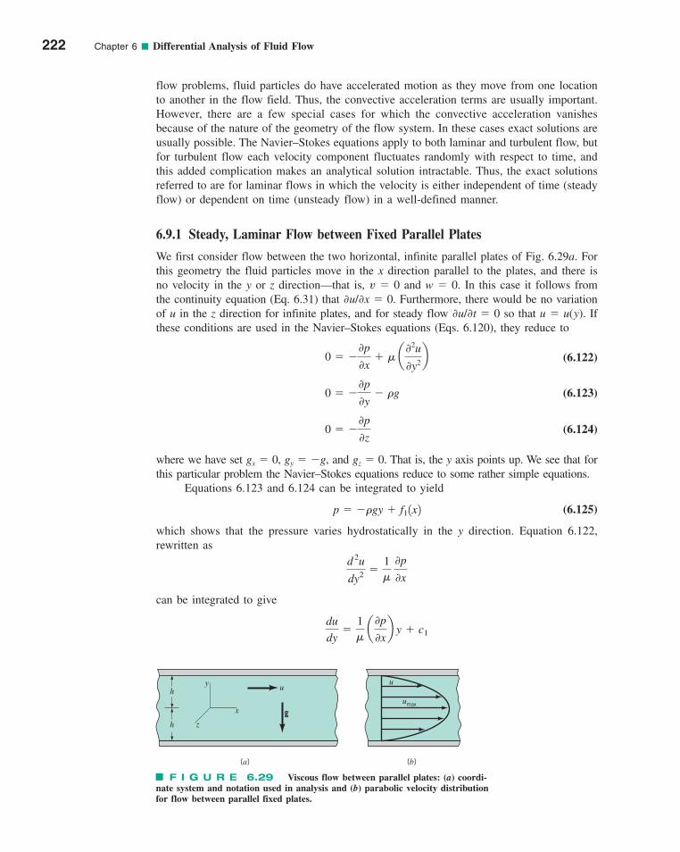
flow problems, fluid particles do have accelerated motion as they move from one locationto another in the flow field. Thus, the convective acceleration terms are usually important.However, there are a few special cases for which the convective acceleration vanishesbecause of the nature of the geometry of the flow system. In these cases exact solutions areusually possible. The Navier–Stokes equations apply to both laminar and turbulent flow, butfor turbulent flow each velocity component fluctuates randomly with respect to time, andthis added complication makes an analytical solution intractable. Thus, the exact solutionsreferred to are for laminar flows in which the velocity is either independent of time (steadyflow) or dependent on time (unsteady flow) in a well-defined manner.

6.9.1 Steady, Laminar Flow between Fixed Parallel Plates

We first consider flow between the two horizontal, infinite parallel plates of Fig. 6.29a. Forthis geometry the fluid particles move in the x direction parallel to the plates, and there isno velocity in the y or z direction—that is, v � 0 and w � 0. In this case it follows fromthe continuity equation (Eq. 6.31) that ∂u/∂x � 0. Furthermore, there would be no variationof u in the z direction for infinite plates, and for steady flow ∂u/∂t � 0 so that u � u(y). Ifthese conditions are used in the Navier–Stokes equations (Eqs. 6.120), they reduce to

(6.122)

(6.123)

(6.124)

where we have set gx � 0, gy � �g, and gz � 0. That is, the y axis points up. We see that forthis particular problem the Navier–Stokes equations reduce to some rather simple equations.

Equations 6.123 and 6.124 can be integrated to yield

(6.125)

which shows that the pressure varies hydrostatically in the y direction. Equation 6.122,rewritten as

can be integrated to give

du

dy�

1�

a0p

0xb y � c1

d2u

dy2 �1�

0p

0x

p � ��gy � f11x2

0 � �0p

0z

0 � �0p

0y� �g

0 � �0p

0x� � a

02u

0y2b

222 Chapter 6 ■ Differential Analysis of Fluid Flow

u

g

h

h z

x

y u

umax

(a) (b)

F I G U R E 6.29 Viscous flow between parallel plates: (a) coordi-nate system and notation used in analysis and (b) parabolic velocity distributionfor flow between parallel fixed plates.

c06DifferentialAnalysisofFluidFlow.qxd 9/24/10 1:42 PM Page 222

6.9 Some Simple Solutions for Laminar, Viscous, Incompressible Fluids 223

and integrated again to yield

(6.126)

Note that for this simple flow the pressure gradient, ∂p/∂x, is treated as constant as far asthe integration is concerned, as (as shown in Eq. 6.125) it is not a function of y. The twoconstants, c1 and c2, must be determined from the boundary conditions. For example, if thetwo plates are fixed, then u � 0 for y � h (because of the no-slip condition for viscousfluids). To satisfy this condition, c1 � 0 and

Thus, the velocity distribution becomes

(6.127)

Equation 6.127 shows that the velocity profile between the two fixed plates is parabolic asillustrated in Fig. 6.29b.

The volume rate of flow, q, passing between the plates (for a unit width in the z direc-tion) is obtained from the relationship

or

(6.128)

The pressure gradient ∂p/∂x is negative, as the pressure decreases in the direction of flow.If we let �p represent the pressure drop between two points a distance � apart, then

and Eq. 6.128 can be expressed as

(6.129)

The flow is proportional to the pressure gradient, inversely proportional to the viscosity, andstrongly dependent (�h3) on the gap width. In terms of the mean velocity, V, where V � q/2h,Eq. 6.129 becomes

(6.130)

Equations 6.129 and 6.130 provide convenient relationships for relating the pressure dropalong a parallel-plate channel and the rate of flow or mean velocity. The maximum veloc-ity, umax, occurs midway (y � 0) between the two plates so that from Eq. 6.127

or

(6.131)umax � 32V

umax � �h2

2� a

0p

0xb

V �h2 ¢p

3�/

q �2h3 ¢p

3�/

¢p

/� �

0p

0x

q � �2h3

3� a

0p

0xb

q � �h

�h

u dy � �h

�h

1

2� a

0p

0xb 1y

2 � h22 dy

u �1

2� a

0p

0xb 1y

2 � h22

c2 � �1

2� a

0p

0xb h2

u �1

2� a

0p

0xb y2 � c1y � c2

V6.12 Liquid–liquid no-slip

V6.11 No-slipboundary condition

c06DifferentialAnalysisofFluidFlow.qxd 9/24/10 1:43 PM Page 223

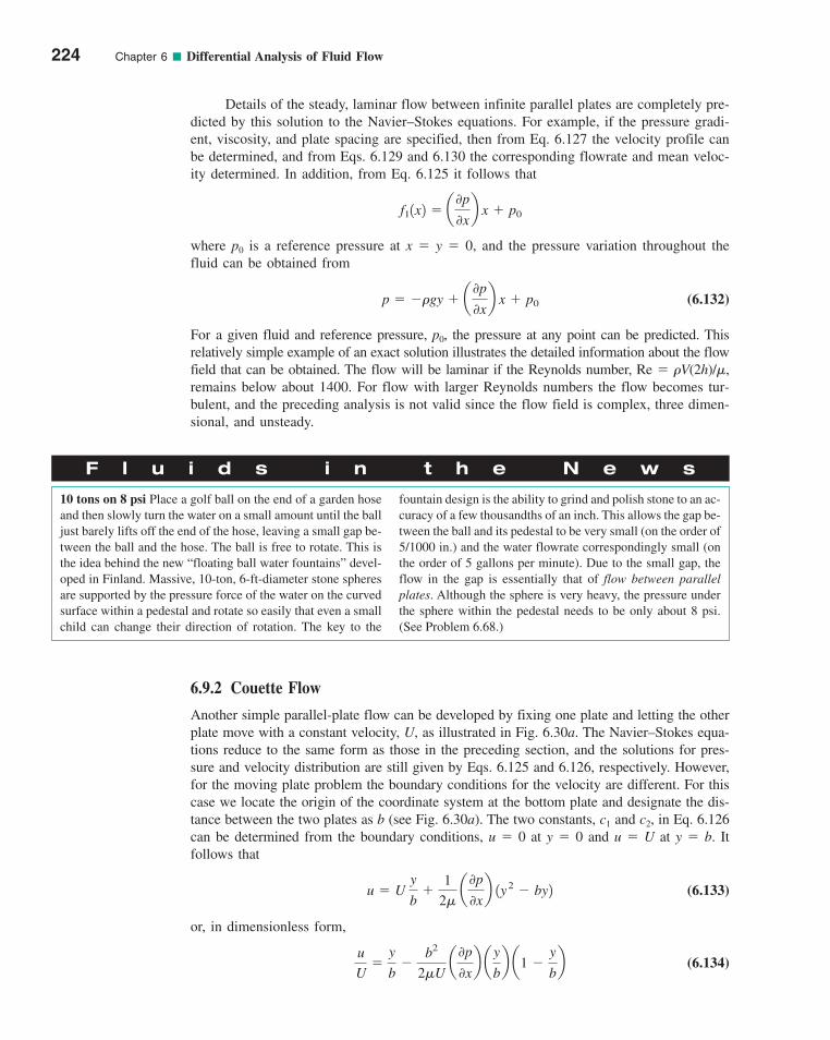
Details of the steady, laminar flow between infinite parallel plates are completely pre-dicted by this solution to the Navier–Stokes equations. For example, if the pressure gradi-ent, viscosity, and plate spacing are specified, then from Eq. 6.127 the velocity profile canbe determined, and from Eqs. 6.129 and 6.130 the corresponding flowrate and mean veloc-ity determined. In addition, from Eq. 6.125 it follows that

where p0 is a reference pressure at x � y � 0, and the pressure variation throughout thefluid can be obtained from

(6.132)

For a given fluid and reference pressure, p0, the pressure at any point can be predicted. Thisrelatively simple example of an exact solution illustrates the detailed information about the flowfield that can be obtained. The flow will be laminar if the Reynolds number, Re � �V(2h)/�,remains below about 1400. For flow with larger Reynolds numbers the flow becomes tur-bulent, and the preceding analysis is not valid since the flow field is complex, three dimen-sional, and unsteady.

p � ��gy � a0p

0xb x � p0

f11x2 � a0p

0xb x � p0

6.9.2 Couette Flow

Another simple parallel-plate flow can be developed by fixing one plate and letting the otherplate move with a constant velocity, U, as illustrated in Fig. 6.30a. The Navier–Stokes equa-tions reduce to the same form as those in the preceding section, and the solutions for pres-sure and velocity distribution are still given by Eqs. 6.125 and 6.126, respectively. However,for the moving plate problem the boundary conditions for the velocity are different. For thiscase we locate the origin of the coordinate system at the bottom plate and designate the dis-tance between the two plates as b (see Fig. 6.30a). The two constants, c1 and c2, in Eq. 6.126can be determined from the boundary conditions, u � 0 at y � 0 and u � U at y � b. Itfollows that

(6.133)

or, in dimensionless form,

(6.134)u

U�

y

b�

b2

2�U a

0p

0xb a

y

bb a1 �

y

bb

u � U y

b�

1

2� a

0p

0xb 1y

2 � by2

224 Chapter 6 ■ Differential Analysis of Fluid Flow

F l u i d s i n t h e N e w s

10 tons on 8 psi Place a golf ball on the end of a garden hoseand then slowly turn the water on a small amount until the balljust barely lifts off the end of the hose, leaving a small gap be-tween the ball and the hose. The ball is free to rotate. This isthe idea behind the new “floating ball water fountains” devel-oped in Finland. Massive, 10-ton, 6-ft-diameter stone spheresare supported by the pressure force of the water on the curvedsurface within a pedestal and rotate so easily that even a smallchild can change their direction of rotation. The key to the

fountain design is the ability to grind and polish stone to an ac-curacy of a few thousandths of an inch. This allows the gap be-tween the ball and its pedestal to be very small (on the order of5/1000 in.) and the water flowrate correspondingly small (onthe order of 5 gallons per minute). Due to the small gap, theflow in the gap is essentially that of flow between parallelplates. Although the sphere is very heavy, the pressure underthe sphere within the pedestal needs to be only about 8 psi.(See Problem 6.68.)

c06DifferentialAnalysisofFluidFlow.qxd 9/24/10 1:43 PM Page 224

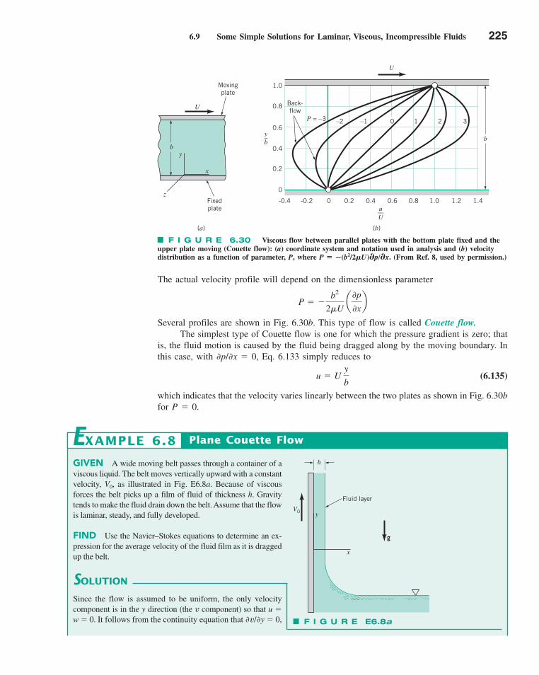
6.9 Some Simple Solutions for Laminar, Viscous, Incompressible Fluids 225

The actual velocity profile will depend on the dimensionless parameter

Several profiles are shown in Fig. 6.30b. This type of flow is called Couette flow.The simplest type of Couette flow is one for which the pressure gradient is zero; that

is, the fluid motion is caused by the fluid being dragged along by the moving boundary. Inthis case, with ∂p/∂x � 0, Eq. 6.133 simply reduces to

(6.135)

which indicates that the velocity varies linearly between the two plates as shown in Fig. 6.30bfor P � 0.

u � U y

b

P � �b2

2�U a

0p

0xb

U

U

1.0

0.8

0.6

0.4

0.2

-0.4 -0.2 0 0.2 0.4 0.6 0.8 1.0 1.2 1.4

b

3210–1–2P = –3

Back-flow

y_b

u__U

(b)(a)

Fixedplate

z

x

yb

Movingplate

0

F I G U R E 6.30 Viscous flow between parallel plates with the bottom plate fixed and theupper plate moving (Couette flow): (a) coordinate system and notation used in analysis and (b) velocitydistribution as a function of parameter, P, where P � �(b2/2�U) p/ x. (From Ref. 8, used by permission.)��

GIVEN A wide moving belt passes through a container of aviscous liquid. The belt moves vertically upward with a constantvelocity, V0, as illustrated in Fig. E6.8a. Because of viscousforces the belt picks up a film of fluid of thickness h. Gravitytends to make the fluid drain down the belt. Assume that the flowis laminar, steady, and fully developed.

FIND Use the Navier–Stokes equations to determine an ex-pression for the average velocity of the fluid film as it is draggedup the belt.

Plane Couette FlowEXAMPLE 6.8

F I G U R E E6.8a

y

x

h

Fluid layer

g

V0

SOLUTION

Since the flow is assumed to be uniform, the only velocitycomponent is in the y direction (the v component) so that u �w � 0. It follows from the continuity equation that ∂v/∂y � 0,

c06DifferentialAnalysisofFluidFlow.qxd 9/24/10 1:43 PM Page 225

226 Chapter 6 ■ Differential Analysis of Fluid Flow

and for steady flow ∂v/∂t � 0, so that v � v(x). Under theseconditions the Navier–Stokes equations for the x direction(Eq. 6.120a) and the z direction (perpendicular to the paper)(Eq. 6.120c) simply reduce to

This result indicates that the pressure does not vary over ahorizontal plane, and because the pressure on the surface ofthe film (x � h) is atmospheric, the pressure throughout thefilm must be atmospheric (or zero gage pressure). Theequation of motion in the y direction (Eq. 6.120b) thusreduces to

or

(1)

Integration of Eq. 1 yields

(2)

On the film surface (x � h) we assume the shearing stress iszero—that is, the drag of the air on the film is negligible. Theshearing stress at the free surface (or any interior parallel sur-face) is designated as �xy where from Eq. 6.118d

Thus, if �xy � 0 at x � h, it follows from Eq. 2 that

A second integration of Eq. 2 gives the velocity distribu-tion in the film as

At the belt (x � 0) the fluid velocity must match the belt ve-locity, V0, so that

and the velocity distribution is therefore

(3)v ��

2� x2 �

�h

� x � V0

c2 � V0

v ��

2� x2 �

�h

� x � c2

c1 � ��h

�

�xy � � adv

dxb

dv

dx�

�

� x � c1

d2v

dx2 ��

�

0 � ��g � � d2v

dx2

0p

0x� 0

0p

0z� 0

With the velocity distribution known we can determine theflowrate per unit width, q, from the relationship

and thus,

The average film velocity, V (where q � Vh), is therefore

(Ans)

COMMENT Equation (3) can be written in dimensionlessform as

where c � �h2/2�V0. This velocity profile is shown in Fig. E6.8b.Note that even though the belt is moving upward, for c � 1(e.g., for fluids with small enough viscosity or with a smallenough belt speed) there are portions of the fluid that flowdownward (as indicated by v/V0 0).

It is interesting to note from this result that there will be anet upward flow of liquid (positive V) only if V0 � �h2/3�. Ittakes a relatively large belt speed to lift a small viscosity fluid.

v

V0� c a

x

hb

2

� 2c ax

hb � 1

V � V0 ��h2

3�

q � V0h ��h3

3�

q � �h

0

v dx � �h

0

a�

2� x

2 ��h

� x � V0b dx

F I G U R E E6.8b

–0.2

00 0.2 0.4 0.6 0.8

c = 0

c = 0.5

c = 1.0

c = 1.5

c = 2.0

0.2

0.4

0.6

0.8

1

–0.4

–0.6

–0.8

–1xh

V0 1

v

c06DifferentialAnalysisofFluidFlow.qxd 9/24/10 1:43 PM Page 226

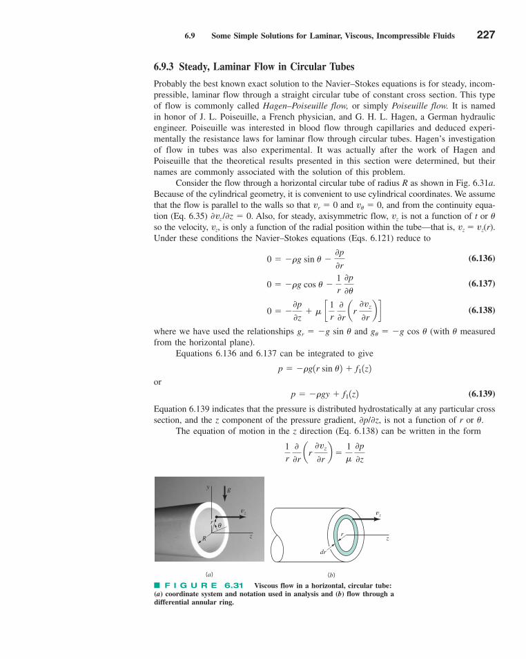
6.9 Some Simple Solutions for Laminar, Viscous, Incompressible Fluids 227

6.9.3 Steady, Laminar Flow in Circular Tubes

Probably the best known exact solution to the Navier–Stokes equations is for steady, incom-pressible, laminar flow through a straight circular tube of constant cross section. This typeof flow is commonly called Hagen–Poiseuille flow, or simply Poiseuille flow. It is namedin honor of J. L. Poiseuille, a French physician, and G. H. L. Hagen, a German hydraulicengineer. Poiseuille was interested in blood flow through capillaries and deduced experi-mentally the resistance laws for laminar flow through circular tubes. Hagen’s investigationof flow in tubes was also experimental. It was actually after the work of Hagen andPoiseuille that the theoretical results presented in this section were determined, but theirnames are commonly associated with the solution of this problem.

Consider the flow through a horizontal circular tube of radius R as shown in Fig. 6.31a.Because of the cylindrical geometry, it is convenient to use cylindrical coordinates. We assumethat the flow is parallel to the walls so that vr � 0 and v� � 0, and from the continuity equa-tion (Eq. 6.35) ∂vz /∂z � 0. Also, for steady, axisymmetric flow, vz is not a function of t or �so the velocity, vz, is only a function of the radial position within the tube—that is, vz � vz(r).Under these conditions the Navier–Stokes equations (Eqs. 6.121) reduce to

(6.136)

(6.137)

(6.138)

where we have used the relationships gr � �g sin � and g� � �g cos � (with � measuredfrom the horizontal plane).

Equations 6.136 and 6.137 can be integrated to give

or(6.139)

Equation 6.139 indicates that the pressure is distributed hydrostatically at any particular crosssection, and the z component of the pressure gradient, ∂p/∂z, is not a function of r or �.

The equation of motion in the z direction (Eq. 6.138) can be written in the form

1r

00r

ar 0vz

0rb �

1�

0p

0z

p � ��gy � f11z2

p � ��g1r sin �2 � f11z2

0 � �0p

0z� � c

1r

00r

ar 0vz

0rb d

0 � ��g cos � �1r 0p

0�

0 � ��g sin � �0p

0r

z

vz

dr

r

(b)

y

z

vz

g

R

r θ

(a)

F I G U R E 6.31 Viscous flow in a horizontal, circular tube: (a) coordinate system and notation used in analysis and (b) flow through adifferential annular ring.

c06DifferentialAnalysisofFluidFlow.qxd 9/24/10 1:43 PM Page 227

and integrated (using the fact that ∂p/∂z � constant) to give

Integrating again we obtain

(6.140)

As indicated by the figure in the margin, the shape of the velocity profile depends onthe values of the two constants c1 and c2.

Since we wish vz to be finite at the center of the tube (r � 0), it follows that c1 � 0[since ln (0) � ��]. At the wall (r � R) the velocity must be zero so that

and the velocity distribution becomes

(6.141)

Thus, at any cross section the velocity distribution is parabolic.To obtain a relationship between the volume rate of flow, Q, passing through the tube

and the pressure gradient, we consider the flow through the differential, washer-shaped ringof Fig. 6.31b. Since vz is constant on this ring, the volume rate of flow through the differ-ential area dA � (2�r) dr is

and therefore

(6.142)

Equation 6.141 for vz can be substituted into Eq. 6.142, and the resulting equation inte-grated to yield

(6.143)

This relationship can be expressed in terms of the pressure drop, �p, which occurs over alength, �, along the tube, as

and therefore

(6.144)

For a given pressure drop per unit length, the volume rate of flow is inversely proportionalto the viscosity and proportional to the tube radius to the fourth power. A doubling of thetube radius produces a sixteenfold increase in flow! Equation 6.144 is commonly calledPoiseuille’s law.

Q ��R4¢p

8�/

¢p

/� �

0p

0z

Q � ��R

4

8� a

0p

0zb

Q � 2� �R

0

vzr dr

dQ � vz12�r2 dr

vz �1

4� a

0p

0zb 1r2 � R22

c2 � �1

4� a

0p

0zb R2

vz �1

4� a

0p

0zb r2 � c1 ln r � c2

r 0vz

0r�

1

2� a

0p

0zb r2 � c1

228 Chapter 6 ■ Differential Analysis of Fluid Flow

V6.13 Laminarflow

vz

c1>0

c1 = 0, c2>0

0 R r0.5 R

V6.14 Complexpipe flow

c06DifferentialAnalysisofFluidFlow.qxd 9/24/10 1:44 PM Page 228

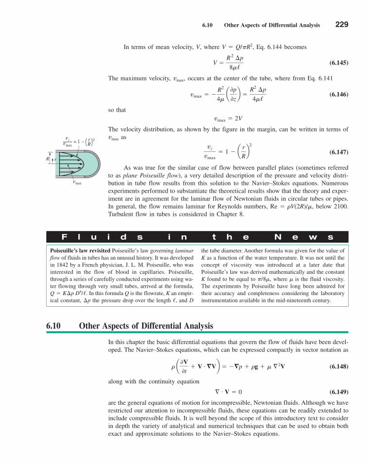
6.10 Other Aspects of Differential Analysis 229

In terms of mean velocity, V, where V � Q/�R2, Eq. 6.144 becomes

(6.145)

The maximum velocity, vmax, occurs at the center of the tube, where from Eq. 6.141

(6.146)

so that

The velocity distribution, as shown by the figure in the margin, can be written in terms ofvmax as

(6.147)

As was true for the similar case of flow between parallel plates (sometimes referredto as plane Poiseuille flow), a very detailed description of the pressure and velocity distri-bution in tube flow results from this solution to the Navier–Stokes equations. Numerousexperiments performed to substantiate the theoretical results show that the theory and exper-iment are in agreement for the laminar flow of Newtonian fluids in circular tubes or pipes.In general, the flow remains laminar for Reynolds numbers, Re � �V(2R)/�, below 2100.Turbulent flow in tubes is considered in Chapter 8.

vz

vmax� 1 � a

r

Rb

2

vmax � 2V

vmax � �R2

4� a

0p

0zb �

R2 ¢p

4�/

V �R2 ¢p

8�/

R r

vmax

vz r_R = 1 – ( )2

vmax

F l u i d s i n t h e N e w s

Poiseuille’s law revisited Poiseuille’s law governing laminarflow of fluids in tubes has an unusual history. It was developedin 1842 by a French physician, J. L. M. Poiseuille, who wasinterested in the flow of blood in capillaries. Poiseuille,through a series of carefully conducted experiments using wa-ter flowing through very small tubes, arrived at the formula,

. In this formula Q is the flowrate, K an empir-ical constant, the pressure drop over the length , and D/¢pQ � K¢p D4//

the tube diameter. Another formula was given for the value ofK as a function of the water temperature. It was not until theconcept of viscosity was introduced at a later date thatPoiseuille’s law was derived mathematically and the constantK found to be equal to , where is the fluid viscosity.The experiments by Poiseuille have long been admired fortheir accuracy and completeness considering the laboratoryinstrumentation available in the mid-nineteenth century.

��/8�

6.10 Other Aspects of Differential Analysis

In this chapter the basic differential equations that govern the flow of fluids have been devel-oped. The Navier–Stokes equations, which can be expressed compactly in vector notation as

(6.148)

along with the continuity equation

(6.149)

are the general equations of motion for incompressible, Newtonian fluids. Although we haverestricted our attention to incompressible fluids, these equations can be readily extended toinclude compressible fluids. It is well beyond the scope of this introductory text to considerin depth the variety of analytical and numerical techniques that can be used to obtain bothexact and approximate solutions to the Navier–Stokes equations.

§ # V � 0

� a0V0t

� V # �Vb � ��p � �g � � § 2V

c06DifferentialAnalysisofFluidFlow.qxd 9/24/10 1:44 PM Page 229

Numerical techniques using digital computers are, of course, used commonly to solvea wide variety of flow problems. Numerous laminar flow solutions based on the fullNavier–Stokes equations have been obtained by using both finite element and finite differencemethods. Flow characteristics of highly nonlinear problems can be obtained from numericalsolutions. However, these solutions typically require the use of powerful digital computers,and nonlinearities in the equations represent a complication that challenges the ingenuity ofthe numerical analyst. Practical turbulent flow problems are not amenable to a completelynumerical solution because of the extreme complexity of the motion. The solution of real tur-bulent flows usually involves the use of some type of empirical turbulence model.

The general field of computational fluid dynamics (CFD), in which computers and numer-ical analysis are combined to solve fluid flow problems, represents an extremely important sub-ject area in advanced fluid mechanics. A brief introduction to CFD is given in Appendix A.

230 Chapter 6 ■ Differential Analysis of Fluid Flow

V6.15 CFD example

F l u i d s i n t h e N e w s

MRI-CFD for arteries Researchers in the magnetic resonanceimaging (MRI) unit at Sheffield University in Sheffield, England,are using computational fluid dynamics (CFD) to study flowthrough the pulmonary artery in the lung. By using MRI to deter-mine the shape of the artery and CFD to model the flow through

it, they can determine locations of possible clotting sites andaneurysms. Clots are formed in low-flow and stagnant regions,where the blood remains for a longer period than at other placesin the bloodstream. High surface pressure and shear stress areascan result in aneurysms in which the vessel wall bulges outward.

6.11 Chapter Summary and Study Guide

Differential analysis of fluid flow is concerned with the development of concepts and tech-niques that can be used to provide a detailed, point by point, description of a flow field.Concepts related to the motion and deformation of a fluid element are introduced, includ-ing the Eulerian method for describing the velocity and acceleration of fluid particles. Lin-ear deformation and angular deformation of a fluid element are described through the useof flow characteristics such as the volumetric dilatation rate, rate of angular deformation,and vorticity. The differential form of the conservation of mass equation (continuity equa-tion) is derived in both rectangular and cylindrical polar coordinates.

Use of the stream function for the study of steady, incompressible, plane, two-dimensional flow is introduced. The general equations of motion are developed, and for invis-cid flow these equations are reduced to the simpler Euler equations of motion. The Eulerequations are integrated to give the Bernoulli equation, and the concept of irrotational flowis introduced. Use of the velocity potential for describing irrotational flow is considered indetail, and several basic velocity potentials are described, including those for a uniform flow,source or sink, vortex, and doublet. The technique of using various combinations of thesebasic velocity potentials, by superposition, to form new potentials is described. Flows arounda half-body and around a circular cylinder are obtained using this superposition technique.

Basic differential equations describing incompressible, viscous flow (the Navier–Stokesequations) are introduced. Several relatively simple solutions for steady, viscous, laminar flowbetween parallel plates and through circular tubes are included.

The following checklist provides a study guide for this chapter. When your study ofthe entire chapter and end-of-chapter exercises has been completed, you should be able to

write out meanings of the terms listed here in the margin and understand each of therelated concepts. These terms are particularly important and are set in color and boldtype in the text.

volumetric dilatation rate

vorticityirrotational flowcontinuity equationstream functionEuler’s equations

of motionideal fluidBernoulli equationvelocity potentialequipotential linesflow netuniform flowsource and sinkvortexcirculationdoubletmethod of

superpositionhalf-bodyNavier–Stokes

equationsCouette flowPoiseuille’s law

c06DifferentialAnalysisofFluidFlow.qxd 9/24/10 1:44 PM Page 230

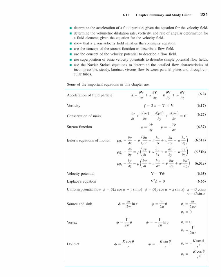
6.11 Chapter Summary and Study Guide 231

determine the acceleration of a fluid particle, given the equation for the velocity field.

determine the volumetric dilatation rate, vorticity, and rate of angular deformation fora fluid element, given the equation for the velocity field.

show that a given velocity field satisfies the continuity equation.

use the concept of the stream function to describe a flow field.

use the concept of the velocity potential to describe a flow field.

use superposition of basic velocity potentials to describe simple potential flow fields.

use the Navier–Stokes equations to determine the detailed flow characteristics ofincompressible, steady, laminar, viscous flow between parallel plates and through cir-cular tubes.

Some of the important equations in this chapter are

Acceleration of fluid particle (6.2)

Vorticity (6.17)

Conservation of mass (6.27)

Stream function (6.37)

Euler’s equations of motion (6.51a)

(6.51b)

(6.51c)

Velocity potential (6.65)

Laplace’s equation (6.66)

Uniform potential flow

Source and sink

Vortex

Doublet vr � �K cos u

r 2

vu � �K cos u

r 2

f �K cos u

r c � �

K sin ur

vr � 0

vu �

2pr

f �≠

2pu c � �

≠2p

ln r

vr �m

2pr

vu � 0

f �m

2pln r c �

m

2pu

u � U cos �v � U sin �

� U1y cos � � x sin �2 � U1x cos � � y sin �2

�2f � 0

V � �f

�gz �0p

0z� � a

0w

0t� u

0w

0x� v

0w

0y� w

0w

0zb

rgy �0p

0y� r a

0v

0t� u

0v

0x� v

0v

0y� w

0v

0zb

rgx �0p

0x� r a

0u

0t� u

0u

0x� v

0u

0y� w

0u

0zb

u �0c0y

v � �0c0x

0r0t

�0 1ru2

0x�

0 1rv20y

�0 1rw2

0z� 0

� � 2 � � § � V

a �0V0t

� u 0V0x

� v 0V0y

� w 0V0z

c06DifferentialAnalysisofFluidFlow.qxd 9/24/10 1:44 PM Page 231

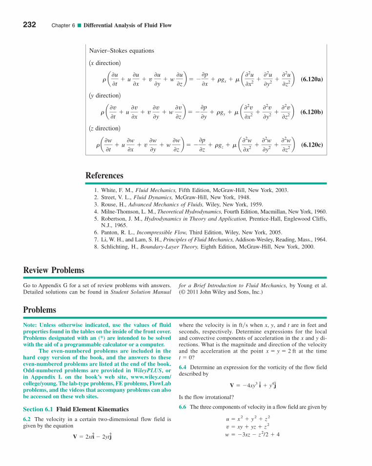
Navier–Stokes equations

1x direction2

(6.120a)

1y direction2

(6.120b)

1z direction2

(6.120c)

References

1. White, F. M., Fluid Mechanics, Fifth Edition, McGraw-Hill, New York, 2003.2. Street, V. L., Fluid Dynamics, McGraw-Hill, New York, 1948.3. Rouse, H., Advanced Mechanics of Fluids, Wiley, New York, 1959.4. Milne-Thomson, L. M., Theoretical Hydrodynamics, Fourth Edition, Macmillan, New York, 1960.5. Robertson, J. M., Hydrodynamics in Theory and Application, Prentice-Hall, Englewood Cliffs,

N.J., 1965.6. Panton, R. L., Incompressible Flow, Third Edition, Wiley, New York, 2005.7. Li, W. H., and Lam, S. H., Principles of Fluid Mechanics, Addison-Wesley, Reading, Mass., 1964.8. Schlichting, H., Boundary-Layer Theory, Eighth Edition, McGraw-Hill, New York, 2000.

r a0w

0t� u

0w

0x� v

0w

0y� w

0w

0zb � �

0p

0z� rgz � m a

02w

0x2 �02w

0y2 �02w

0z2 b

r a0v

0t� u

0v

0x� v

0v

0y� w

0v

0zb � �

0p

0y� rgy � m a

02v

0x2 �02v

0y2 �02v

0z2 b

r a0u

0t� u

0u

0x� v

0u

0y� w

0u

0zb � �

0p

0x� rgx � m a

02u

0x2 �02u

0y2 �02u

0z2 b

232 Chapter 6 ■ Differential Analysis of Fluid Flow

Review Problems

Go to Appendix G for a set of review problems with answers.Detailed solutions can be found in Student Solution Manual

for a Brief Introduction to Fluid Mechanics, by Young et al. (© 2011 John Wiley and Sons, Inc.)

Problems

Note: Unless otherwise indicated, use the values of fluidproperties found in the tables on the inside of the front cover.Problems designated with an (*) are intended to be solvedwith the aid of a programmable calculator or a computer.

The even-numbered problems are included in thehard copy version of the book, and the answers to theseeven-numbered problems are listed at the end of the book.Odd-numbered problems are provided in WileyPLUS, orin Appendix L on the book’s web site, www.wiley.com/college/young. The lab-type problems, FE problems, FlowLabproblems, and the videos that accompany problems can alsobe accessed on these web sites.

Section 6.1 Fluid Element Kinematics

6.2 The velocity in a certain two-dimensional flow field isgiven by the equation

V � 2xti � 2yt j

where the velocity is in ft�s when x, y, and t are in feet andseconds, respectively. Determine expressions for the localand convective components of acceleration in the x and y di-rections. What is the magnitude and direction of the velocityand the acceleration at the point at the time

6.4 Determine an expression for the vorticity of the flow fielddescribed by

Is the flow irrotational?

6.6 The three components of velocity in a flow field are given by

w � �3xz � z 2/2 � 4

v � xy � yz � z 2

u � x 2 � y

2 � z 2

V � �4xy3 i � y4j

t � 0?x � y � 2 ft

c06DifferentialAnalysisofFluidFlow.qxd 10/18/10 8:02 AM Page 232

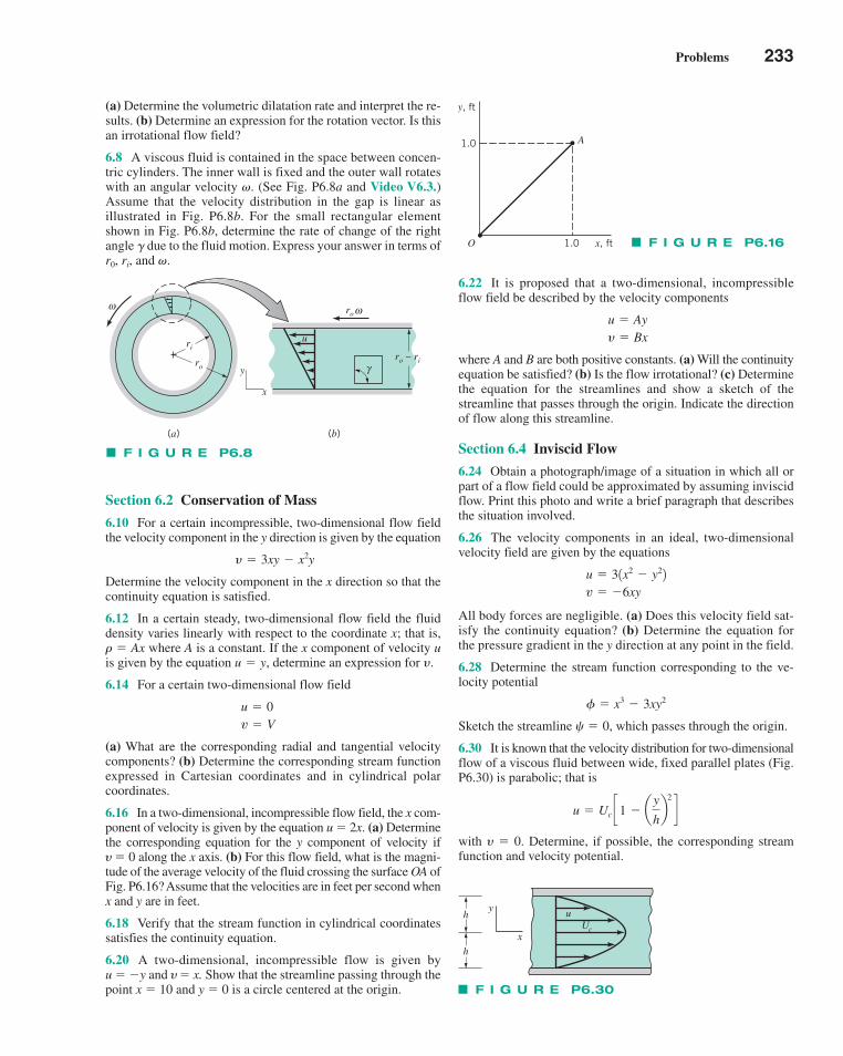
Problems 233

Section 6.2 Conservation of Mass

6.10 For a certain incompressible, two-dimensional flow fieldthe velocity component in the y direction is given by the equation

Determine the velocity component in the x direction so that thecontinuity equation is satisfied.

6.12 In a certain steady, two-dimensional flow field the fluiddensity varies linearly with respect to the coordinate x; that is,

where A is a constant. If the x component of velocity uis given by the equation determine an expression for y.

6.14 For a certain two-dimensional flow field

(a) What are the corresponding radial and tangential velocitycomponents? (b) Determine the corresponding stream functionexpressed in Cartesian coordinates and in cylindrical polarcoordinates.

6.16 In a two-dimensional, incompressible flow field, the x com-ponent of velocity is given by the equation u � 2x. (a) Determinethe corresponding equation for the y component of velocity if � � 0 along the x axis. (b) For this flow field, what is the magni-tude of the average velocity of the fluid crossing the surface OA ofFig. P6.16? Assume that the velocities are in feet per second whenx and y are in feet.

6.18 Verify that the stream function in cylindrical coordinatessatisfies the continuity equation.

6.20 A two-dimensional, incompressible flow is given by u � �y and � � x. Show that the streamline passing through thepoint x � 10 and y � 0 is a circle centered at the origin.

v � V u � 0

u � y,� � Ax

y � 3xy � x2y

6.22 It is proposed that a two-dimensional, incompressibleflow field be described by the velocity components

where A and B are both positive constants. (a) Will the continuityequation be satisfied? (b) Is the flow irrotational? (c) Determinethe equation for the streamlines and show a sketch of thestreamline that passes through the origin. Indicate the directionof flow along this streamline.

Section 6.4 Inviscid Flow

6.24 Obtain a photograph/image of a situation in which all orpart of a flow field could be approximated by assuming inviscidflow. Print this photo and write a brief paragraph that describesthe situation involved.

6.26 The velocity components in an ideal, two-dimensionalvelocity field are given by the equations

All body forces are negligible. (a) Does this velocity field sat-isfy the continuity equation? (b) Determine the equation forthe pressure gradient in the y direction at any point in the field.

6.28 Determine the stream function corresponding to the ve-locity potential

Sketch the streamline which passes through the origin.

6.30 It is known that the velocity distribution for two-dimensionalflow of a viscous fluid between wide, fixed parallel plates (Fig.P6.30) is parabolic; that is

with y � 0. Determine, if possible, the corresponding streamfunction and velocity potential.

u � Uc c1 � ay

hb

2

d

� 0,

� x3 � 3xy2

v � �6xy u � 31x2 � y22

y � Bx u � Ay

ro

ri

ω roω

x

y

u

γro – ri

(a) (b)

F I G U R E P6.8

A

O

y, ft

x, ft1.0

1.0

F I G U R E P6.16

Uc

uy

x

h

h

F I G U R E P6.30

(a) Determine the volumetric dilatation rate and interpret the re-sults. (b) Determine an expression for the rotation vector. Is thisan irrotational flow field?

6.8 A viscous fluid is contained in the space between concen-tric cylinders. The inner wall is fixed and the outer wall rotateswith an angular velocity �. (See Fig. P6.8a and Video V6.3.)Assume that the velocity distribution in the gap is linear asillustrated in Fig. P6.8b. For the small rectangular elementshown in Fig. P6.8b, determine the rate of change of the rightangle � due to the fluid motion. Express your answer in terms ofr0, ri, and �.

c06DifferentialAnalysisofFluidFlow.qxd 9/24/10 1:45 PM Page 233

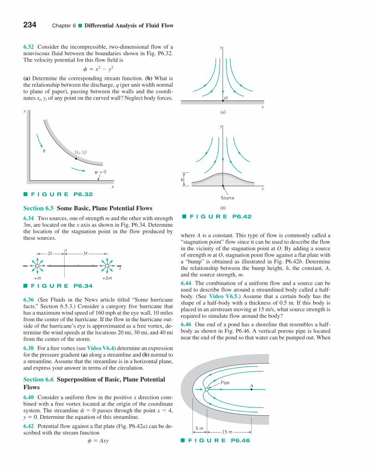
6.32 Consider the incompressible, two-dimensional flow of anonviscous fluid between the boundaries shown in Fig. P6.32.The velocity potential for this flow field is

(a) Determine the corresponding stream function. (b) What isthe relationship between the discharge, q (per unit width normalto plane of paper), passing between the walls and the coordi-nates xi, yi of any point on the curved wall? Neglect body forces.

� x2 � y2

6.36 (See Fluids in the News article titled “Some hurricanefacts,” Section 6.5.3.) Consider a category five hurricane thathas a maximum wind speed of 160 mph at the eye wall, 10 milesfrom the center of the hurricane. If the flow in the hurricane out-side of the hurricane’s eye is approximated as a free vortex, de-termine the wind speeds at the locations 20 mi, 30 mi, and 40 mifrom the center of the storm.

6.38 For a free vortex (see Video V6.4) determine an expressionfor the pressure gradient (a) along a streamline and (b) normal toa streamline. Assume that the streamline is in a horizontal plane,and express your answer in terms of the circulation.

Section 6.6 Superposition of Basic, Plane PotentialFlows

6.40 Consider a uniform flow in the positive x direction com-bined with a free vortex located at the origin of the coordinatesystem. The streamline passes through the point x � 4,y � 0. Determine the equation of this streamline.

6.42 Potential flow against a flat plate (Fig. P6.42a) can be de-scribed with the stream function

� Axy

� 0

where A is a constant. This type of flow is commonly called a“stagnation point” flow since it can be used to describe the flowin the vicinity of the stagnation point at O. By adding a sourceof strength m at O, stagnation point flow against a flat plate witha “bump” is obtained as illustrated in Fig. P6.42b. Determinethe relationship between the bump height, h, the constant, A,and the source strength, m.

6.44 The combination of a uniform flow and a source can beused to describe flow around a streamlined body called a half-body. (See Video V6.5.) Assume that a certain body has theshape of a half-body with a thickness of 0.5 m. If this body isplaced in an airstream moving at 15 m/s, what source strength isrequired to simulate flow around the body?

6.46 One end of a pond has a shoreline that resembles a half-body as shown in Fig. P6.46. A vertical porous pipe is locatednear the end of the pond so that water can be pumped out. When

234 Chapter 6 ■ Differential Analysis of Fluid Flow

= 0ψ

x

y

q (xi, yi)

F I G U R E P6.32

F I G U R E P6.34

x

y2� 3�

+m +3m

y

x

O

(a)

y

x

(b)

Source

h

F I G U R E P6.42

APipe

5 m15 m

F I G U R E P6.46

Section 6.5 Some Basic, Plane Potential Flows

6.34 Two sources, one of strength m and the other with strength3m, are located on the x axis as shown in Fig. P6.34. Determinethe location of the stagnation point in the flow produced bythese sources.

c06DifferentialAnalysisofFluidFlow.qxd 9/24/10 1:45 PM Page 234

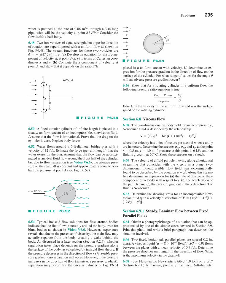
Problems 235

6.50 A fixed circular cylinder of infinite length is placed in asteady, uniform stream of an incompressible, nonviscous fluid.Assume that the flow is irrotational. Prove that the drag on thecylinder is zero. Neglect body forces.

6.52 Water flows around a 6-ft-diameter bridge pier with avelocity of 12 ft/s. Estimate the force (per unit length) that thewater exerts on the pier. Assume that the flow can be approxi-mated as an ideal fluid flow around the front half of the cylinder,but due to flow separation (see Video V6.6), the average pres-sure on the rear half is constant and approximately equal to one-half the pressure at point A (see Fig. P6.52).

6.54 Typical inviscid flow solutions for flow around bodiesindicate that the fluid flows smoothly around the body, even forblunt bodies as shown in Video V6.6. However, experiencereveals that due to the presence of viscosity, the main flow mayactually separate from the body, creating a wake behind thebody. As discussed in a later section (Section 9.2.6), whetherseparation takes place depends on the pressure gradient alongthe surface of the body, as calculated by inviscid flow theory. Ifthe pressure decreases in the direction of flow (a favorable pres-sure gradient), no separation will occur. However, if the pressureincreases in the direction of flow (an adverse pressure gradient),separation may occur. For the circular cylinder of Fig. P6.54

placed in a uniform stream with velocity, U, determine an ex-pression for the pressure gradient in the direction of flow on thesurface of the cylinder. For what range of values for the angle �will an adverse pressure gradient occur?

6.56 Show that for a rotating cylinder in a uniform flow, thefollowing pressure ratio equation is true.

Here U is the velocity of the uniform flow and q is the surfacespeed of the rotating cylinder.

Section 6.8 Viscous Flow

6.58 The two-dimensional velocity field for an incompressible,Newtonian fluid is described by the relationship

where the velocity has units of meters per second when x and yare in meters. Determine the stresses xx, yy, and �xy at the pointx � 0.5 m, y � 1.0 m if pressure at this point is 6 kPa and thefluid is glycerin at 20� C. Show these stresses on a sketch.

6.60 The velocity of a fluid particle moving along a horizontalstreamline that coincides with the x axis in a plane, two-dimensional incompressible flow field was experimentallyfound to be described by the equation u � x2. Along this steam-line determine an expression for (a) the rate of change of the �component of velocity with respect to y, (b) the acceleration ofthe particle, and (c) the pressure gradient in the x direction. Thefluid is Newtonian.

6.62 Determine the shearing stress for an incompressible New-tonian fluid with a velocity distribution of

.

Section 6.9.1 Steady, Laminar Flow between FixedParallel Plates

6.64 Obtain a photograph/image of a situation that can be ap-proximated by one of the simple cases covered in Section 6.9.Print this photo and write a brief paragraph that describes thesituation involved.

6.66 Two fixed, horizontal, parallel plates are spaced 0.2 in.apart. A viscous liquid (� � 8 � 10�3 lb�s/ft2, SG � 0.9) flowsbetween the plates with a mean velocity of 0.9 ft/s. Determinethe pressure drop per unit length in the direction of flow. Whatis the maximum velocity in the channel?

6.68 (See Fluids in the News article titled “10 tons on 8 psi,”Section 6.9.1.) A massive, precisely machined, 6-ft-diameter

112x2y � y32 jV � 13xy2 � 4x32 i �

V � 112xy2 � 6x32 i � 118x2y � 4y32j

ptop � pbottom

pstagnation�

8q

U

F I G U R E P6.48

y

x

UP(x, y)

H

H

A

U = 12 ft/s6 ft

A

F I G U R E P6.52

U

θ

a

F I G U R E P6.54

water is pumped at the rate of 0.06 m3/s through a 3-m-longpipe, what will be the velocity at point A? Hint: Consider theflow inside a half-body.

6.48 Two free vortices of equal strength, but opposite directionof rotation are superimposed with a uniform flow as shown inFig. P6.48. The stream functions for these two vorticies are

. (a) Develop an equation for the x com-ponent of velocity, u, at point in terms of Cartesian coor-dinates x and y. (b) Compute the x component of velocity atpoint A and show that it depends on the ratio . /H

P1x, y2c � � 3; �12p2 4 ln r

c06DifferentialAnalysisofFluidFlow.qxd 9/24/10 1:45 PM Page 235

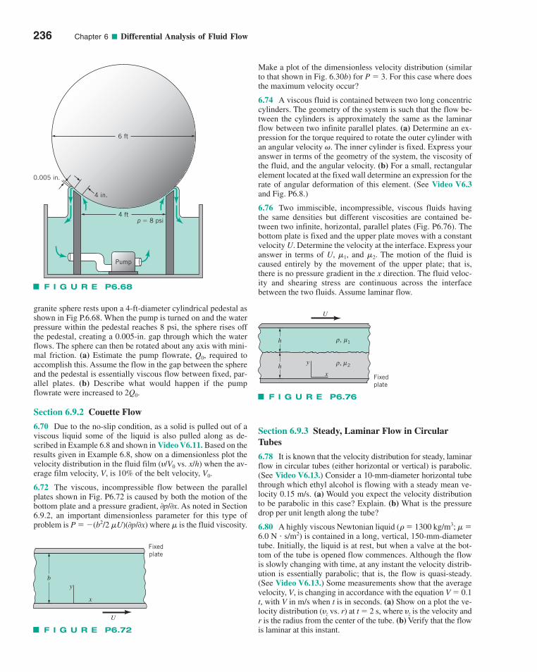
236 Chapter 6 ■ Differential Analysis of Fluid Flow

granite sphere rests upon a 4-ft-diameter cylindrical pedestal asshown in Fig P.6.68. When the pump is turned on and the waterpressure within the pedestal reaches 8 psi, the sphere rises offthe pedestal, creating a 0.005-in. gap through which the waterflows. The sphere can then be rotated about any axis with mini-mal friction. (a) Estimate the pump flowrate, , required toaccomplish this. Assume the flow in the gap between the sphereand the pedestal is essentially viscous flow between fixed, par-allel plates. (b) Describe what would happen if the pumpflowrate were increased to .

Section 6.9.2 Couette Flow

6.70 Due to the no-slip condition, as a solid is pulled out of aviscous liquid some of the liquid is also pulled along as de-scribed in Example 6.8 and shown in Video V6.11. Based on theresults given in Example 6.8, show on a dimensionless plot thevelocity distribution in the fluid film (�/V0 vs. x/h) when the av-erage film velocity, V, is 10% of the belt velocity, V0.

6.72 The viscous, incompressible flow between the parallelplates shown in Fig. P6.72 is caused by both the motion of thebottom plate and a pressure gradient, 0p/0x. As noted in Section6.9.2, an important dimensionless parameter for this type ofproblem is P � �(b2/2 �U)(0p/0x) where � is the fluid viscosity.

2Q0

Q0

Make a plot of the dimensionless velocity distribution (similarto that shown in Fig. 6.30b) for P � 3. For this case where doesthe maximum velocity occur?

6.74 A viscous fluid is contained between two long concentriccylinders. The geometry of the system is such that the flow be-tween the cylinders is approximately the same as the laminarflow between two infinite parallel plates. (a) Determine an ex-pression for the torque required to rotate the outer cylinder withan angular velocity �. The inner cylinder is fixed. Express youranswer in terms of the geometry of the system, the viscosity ofthe fluid, and the angular velocity. (b) For a small, rectangularelement located at the fixed wall determine an expression for therate of angular deformation of this element. (See Video V6.3and Fig. P6.8.)

6.76 Two immiscible, incompressible, viscous fluids havingthe same densities but different viscosities are contained be-tween two infinite, horizontal, parallel plates (Fig. P6.76). Thebottom plate is fixed and the upper plate moves with a constantvelocity U. Determine the velocity at the interface. Express youranswer in terms of U, and The motion of the fluid iscaused entirely by the movement of the upper plate; that is,there is no pressure gradient in the x direction. The fluid veloc-ity and shearing stress are continuous across the interfacebetween the two fluids. Assume laminar flow.

�2.�1,

Section 6.9.3 Steady, Laminar Flow in CircularTubes

6.78 It is known that the velocity distribution for steady, laminarflow in circular tubes (either horizontal or vertical) is parabolic.(See Video V6.13.) Consider a 10-mm-diameter horizontal tubethrough which ethyl alcohol is flowing with a steady mean ve-locity 0.15 m/s. (a) Would you expect the velocity distributionto be parabolic in this case? Explain. (b) What is the pressuredrop per unit length along the tube?

6.80 A highly viscous Newtonian liquid (� � 1300 kg/m3; � �6.0 N � s/m2) is contained in a long, vertical, 150-mm-diametertube. Initially, the liquid is at rest, but when a valve at the bot-tom of the tube is opened flow commences. Although the flowis slowly changing with time, at any instant the velocity distrib-ution is essentially parabolic; that is, the flow is quasi-steady.(See Video V6.13.) Some measurements show that the averagevelocity, V, is changing in accordance with the equation V � 0.1t, with V in m/s when t is in seconds. (a) Show on a plot the ve-locity distribution (�z vs. r) at t � 2 s, where �z is the velocity andr is the radius from the center of the tube. (b) Verify that the flowis laminar at this instant.

F I G U R E P6.68

0.005 in.

4 in.

6 ft

4 ftp � 8 psi

Pump

by

x

U

Fixedplate

F I G U R E P6.72

h

hy

x

U

, 1ρ μ

, 2ρ μ

Fixedplate

F I G U R E P6.76

c06DifferentialAnalysisofFluidFlow.qxd 9/24/10 1:45 PM Page 236

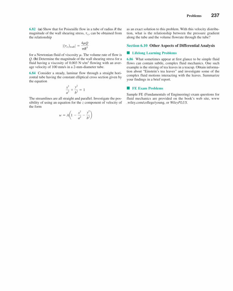
Problems 237

6.82 (a) Show that for Poiseuille flow in a tube of radius R themagnitude of the wall shearing stress, �rz, can be obtained fromthe relationship

for a Newtonian fluid of viscosity �. The volume rate of flow isQ. (b) Determine the magnitude of the wall shearing stress for afluid having a viscosity of 0.003 N�s/m2 flowing with an aver-age velocity of 100 mm/s in a 2-mm-diameter tube.

6.84 Consider a steady, laminar flow through a straight hori-zontal tube having the constant elliptical cross section given bythe equation

The streamlines are all straight and parallel. Investigate the pos-sibility of using an equation for the z component of velocity ofthe form

w � Aa1 �x2

a2 �y2

b2b

x2

a2 �y2

b2 � 1

0 1�rz2wall 0 �4�Q

�R3

as an exact solution to this problem. With this velocity distribu-tion, what is the relationship between the pressure gradientalong the tube and the volume flowrate through the tube?

Section 6.10 Other Aspects of Differential Analysis

■ Lifelong Learning Problems

6.86 What sometimes appear at first glance to be simple fluidflows can contain subtle, complex fluid mechanics. One suchexample is the stirring of tea leaves in a teacup. Obtain informa-tion about “Einstein’s tea leaves” and investigate some of thecomplex fluid motions interacting with the leaves. Summarizeyour findings in a brief report.

■ FE Exam Problems

Sample FE (Fundamentals of Engineering) exam questions forfluid mechanics are provided on the book’s web site, www.wiley.com/college/young, or WileyPLUS.

c06DifferentialAnalysisofFluidFlow.qxd 9/24/10 1:45 PM Page 237

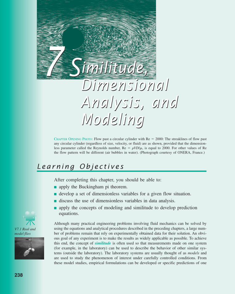
238

CHAPTER OPENING PHOTO: Flow past a circular cylinder with Re � 2000: The streaklines of flow pastany circular cylinder (regardless of size, velocity, or fluid) are as shown, provided that the dimension-less parameter called the Reynolds number, Re � �VD/�, is equal to 2000. For other values of Rethe flow pattern will be different (air bubbles in water). (Photograph courtesy of ONERA, France.)

Learn ing Ob j ec t i v e s

After completing this chapter, you should be able to:

■ apply the Buckingham pi theorem.

■ develop a set of dimensionless variables for a given flow situation.

■ discuss the use of dimensionless variables in data analysis.

■ apply the concepts of modeling and similitude to develop predictionequations.

Although many practical engineering problems involving fluid mechanics can be solved byusing the equations and analytical procedures described in the preceding chapters, a large num-ber of problems remain that rely on experimentally obtained data for their solution. An obvi-ous goal of any experiment is to make the results as widely applicable as possible. To achievethis end, the concept of similitude is often used so that measurements made on one system(for example, in the laboratory) can be used to describe the behavior of other similar sys-tems (outside the laboratory). The laboratory systems are usually thought of as models andare used to study the phenomenon of interest under carefully controlled conditions. Fromthese model studies, empirical formulations can be developed or specific predictions of one

Similitude,DimensionalAnalysis, andModeling

7 Similitude,DimensionalAnalysis, andModeling

7

V7.1 Real andmodel flies

c07Similitude,DimensionalAnalysis,andModeling.qxd 9/24/10 2:00 PM Page 238

7.1 Dimensional Analysis 239

or more characteristics of some other similar system can be made. To do this, it is necessaryto establish the relationship between the laboratory model and the “other” system. In the fol-lowing sections, we find out how this can be accomplished in a systematic manner.

F l u i d s i n t h e N e w s

Model study of New Orleans levee breach caused byHurricane Katrina Much of the devastation to New Orleansfrom Hurricane Katrina in 2005 was a result of flood watersthat surged through a breach of the 17 Street Outfall Canal.To better understand why this occurred and to determine whatcan be done to prevent future occurrences, the U.S. Army Engineer Research and Development Center Coastal and Hydraulics Laboratory is conducting tests on a large (1:50length scale) 15,000-square-foot hydraulic model that repli-cates 0.5 mile of the canal surrounding the breach and more

than a mile of the adjacent Lake Pontchartrain front. The ob-jective of the study is to obtain information regarding the effect that waves had on the breaching of the canal and to in-vestigate the surging water currents within the canals. Thewaves are generated by computer-controlled wave generatorsthat can produce waves of varying heights, periods, and direc-tions similar to the storm conditions that occurred during thehurricane. Data from the study will be used to calibrate andvalidate information that will be fed into various numericalmodel studies of the disaster.

7.1 Dimensional Analysis

To illustrate a typical fluid mechanics problem in which experimentation is required, con-sider the steady flow of an incompressible, Newtonian fluid through a long, smooth-walled,horizontal, circular pipe. An important characteristic of this system, which would be of inter-est to an engineer designing a pipeline, is the pressure drop per unit length that developsalong the pipe as a result of friction. Although this would appear to be a relatively simpleflow problem, it cannot generally be solved analytically (even with the aid of large com-puters) without the use of experimental data.

The first step in the planning of an experiment to study this problem would be todecide on the factors, or variables, that will have an effect on the pressure drop per unitlength, �p�, which has dimensions of (lb/ft2)/ft or (N/m2)/m. We expect the list to includethe pipe diameter, D, the fluid density, �, fluid viscosity, �, and the mean velocity, V, atwhich the fluid is flowing through the pipe. Thus, we can express this relationship as

(7.1)

which simply indicates mathematically that we expect the pressure drop per unit length tobe some function of the factors contained within the parentheses. At this point the natureof the function is unknown, and the objective of the experiments to be performed is to deter-mine the nature of this function.

To perform the experiments in a meaningful and systematic manner, it would benecessary to change one of the variables, such as the velocity, while holding all othersconstant and measure the corresponding pressure drop. This approach to determining thefunctional relationship between the pressure drop and the various factors that influenceit, although logical in concept, is fraught with difficulties. Some of the experimentswould be hard to carry out—for example, it would be necessary to vary fluid densitywhile holding viscosity constant. How would you do this? Finally, once we obtained thevarious curves, how could we combine these data to obtain the desired general func-tional relationship among �p�, D, �, �, and V that would be valid for any similar pipesystem?

Fortunately, there is a much simpler approach to this problem that will eliminate thedifficulties just described. In the following sections we will show that rather than workingwith the original list of variables, as described in Eq. 7.1, we can collect these into two

¢p/ � f 1D, �, �, V 2

c07Similitude,DimensionalAnalysis,andModeling.qxd 9/24/10 2:00 PM Page 239

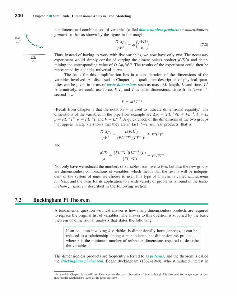
nondimensional combinations of variables (called dimensionless products or dimensionlessgroups) so that as shown by the figure in the margin

(7.2)

Thus, instead of having to work with five variables, we now have only two. The necessaryexperiment would simply consist of varying the dimensionless product �VD/� and deter-mining the corresponding value of D �p�/�V2. The results of the experiment could then berepresented by a single, universal curve.

The basis for this simplification lies in a consideration of the dimensions of thevariables involved. As discussed in Chapter 1, a qualitative description of physical quan-tities can be given in terms of basic dimensions such as mass, M, length, L, and time, T.1

Alternatively, we could use force, F, L, and T as basic dimensions, since from Newton’ssecond law

(Recall from Chapter 1 that the notation � is used to indicate dimensional equality.) Thedimensions of the variables in the pipe flow example are �p� � (FL�2)/L � FL�3, D � L,� � FL�4T 2, � � FL�2T, and V � LT�1. A quick check of the dimensions of the two groupsthat appear in Eq. 7.2 shows that they are in fact dimensionless products; that is,

and

Not only have we reduced the numbers of variables from five to two, but also the new groupsare dimensionless combinations of variables, which means that the results will be indepen-dent of the system of units we choose to use. This type of analysis is called dimensionalanalysis, and the basis for its application to a wide variety of problems is found in the Buck-ingham pi theorem described in the following section.

�VD�

�1FL�4T 22 1LT�12 1L2

1FL�2T 2� F 0L0T 0

D ¢p/

�V 2 �L1F/L32

1FL�4T 22 1LT�122� F 0L0T 0

F � MLT�2

D ¢p/

�V2 � � a�VD

�b

240 Chapter 7 ■ Similitude, Dimensional Analysis, and Modeling

VDρμ

ρDΔp�

V2______

7.2 Buckingham Pi Theorem

A fundamental question we must answer is how many dimensionless products are requiredto replace the original list of variables. The answer to this question is supplied by the basictheorem of dimensional analysis that states the following:

If an equation involving k variables is dimensionally homogeneous, it can bereduced to a relationship among k � r independent dimensionless products,where r is the minimum number of reference dimensions required to describe the variables.

The dimensionless products are frequently referred to as pi terms, and the theorem is calledthe Buckingham pi theorem. Edgar Buckingham (1867–1940), who stimulated interest in

1As noted in Chapter 1, we will use T to represent the basic dimension of time, although T is also used for temperature in ther-modynamic relationships (such as the ideal gas law).

c07Similitude,DimensionalAnalysis,andModeling.qxd 9/24/10 2:00 PM Page 240

7.3 Determination of Pi Terms 241

the use of dimensional analysis, used the symbol � to represent a dimensionless product,and this notation is commonly used. Although the pi theorem is a simple one, its proof isnot so simple and we will not include it here. Many entire books have been devoted to thesubject of similitude and dimensional analysis, and a number of these are listed at the endof this chapter (Refs. 1–5). Students interested in pursuing the subject in more depth (includ-ing the proof of the pi theorem) can refer to one of these books.

The pi theorem is based on the idea of dimensional homogeneity, which was intro-duced in Chapter 1. Essentially we assume that for any physically meaningful equationinvolving k variables, such as

the dimensions of the variable on the left side of the equal sign must be equal to the dimen-sions of any term that stands by itself on the right side of the equal sign. It then followsthat we can rearrange the equation into a set of dimensionless products (pi terms) so that

The required number of pi terms is fewer than the number of original variables by r, wherer is determined by the minimum number of reference dimensions required to describe theoriginal list of variables. Usually the reference dimensions required to describe the vari-ables will be the basic dimensions M, L, and T or F, L, and T. However, in some instancesperhaps only two dimensions, such as L and T, are required, or maybe just one, such asL. Also, in a few rare cases the variables may be described by some combination of basicdimensions, such as M/T 2, and L, and in this case r would be equal to two rather thanthree. Although the use of the pi theorem may appear to be a little mysterious and com-plicated, we will actually develop a simple, systematic procedure for developing the pi termsfor a given problem.

ß1 � �1ß2, ß3, p , ßk�r2

u1 � f 1u2, u3, p , uk2

7.3 Determination of Pi Terms

Several methods can be used to form the dimensionless products, or pi terms, that arise ina dimensional analysis. Essentially we are looking for a method that will allow us to system-atically form the pi terms so that we are sure that they are dimensionless and independent andthat we have the right number. The method we will describe in detail in this section is calledthe method of repeating variables.

It will be helpful to break the repeating variable method down into a series of dis-tinct steps that can be followed for any given problem. With a little practice you will beable to readily complete a dimensional analysis for your problem.

Step 1. List all the variables that are involved in the problem. This step is the most dif-ficult one, and it is, of course, vitally important that all pertinent variables beincluded. Otherwise the dimensional analysis will not be correct! We are using theterm variable to include any quantity, including dimensional and nondimensionalconstants, that plays a role in the phenomenon under investigation. All such quan-tities should be included in the list of variables to be considered for the dimen-sional analysis. The determination of the variables must be accomplished by theexperimenter’s knowledge of the problem and the physical laws that govern the phe-nomenon. Typically the variables will include those that are necessary to describethe geometry of the system (such as a pipe diameter), to define any fluid proper-ties (such as a fluid viscosity), and to indicate external effects that influence thesystem (such as a driving pressure). These general classes of variables are intended

c07Similitude,DimensionalAnalysis,andModeling.qxd 9/24/10 2:01 PM Page 241

as broad categories that should be helpful in identifying variables. It is likely, how-ever, that there will be variables that do not fit easily into one of these categories,and each problem needs to be analyzed carefully.

Since we wish to keep the number of variables to a minimum, so that we canminimize the amount of laboratory work, it is important that all variables be indepen-dent. For example, if in a certain problem the cross-sectional area of a pipe is an impor-tant variable, either the area or the pipe diameter could be used, but not both, since theyare obviously not independent. Similarly, if both fluid density, �, and specific weight,�, are important variables, we could list � and �, or � and g (acceleration of gravity), or� and g. However, it would be incorrect to use all three since � � �g; that is, �, �, andg are not independent. Note that although g would normally be constant in a given experiment, that fact is irrelevant as far as a dimensional analysis is concerned.

Step 2. Express each of the variables in terms of basic dimensions. For the typical fluidmechanics problem the basic dimensions will be either M, L, and T or F, L, and T.Dimensionally these two sets are related through Newton’s second law (F � ma) sothat F � MLT �2. For example, � � ML�3 or � � FL�4T 2. Thus, either set can beused. The basic dimensions for typical variables found in fluid mechanics problemsare listed in Table 1.1 in Chapter 1.

Step 3. Determine the required number of pi terms. This can be accomplished by meansof the Buckingham pi theorem, which indicates that the number of pi terms is equalto k � r, where k is the number of variables in the problem (which is determined fromStep 1) and r is the number of reference dimensions required to describe these vari-ables (which is determined from Step 2). The reference dimensions usually corre-spond to the basic dimensions and can be determined by an inspection of the dimen-sions of the variables obtained in Step 2. As previously noted, there may be occasions(usually rare) in which the basic dimensions appear in combinations so that the num-ber of reference dimensions is less than the number of basic dimensions.

Step 4. Select a number of repeating variables. The number required is equal to thenumber of reference dimensions. Essentially what we are doing here is selectingfrom the original list of variables, several of which can be combined with each of theremaining variables to form a pi term. All of the required reference dimensions mustbe included within the group of repeating variables, and each repeating variable mustbe dimensionally independent of the others (i.e., the dimensions of one repeating vari-able cannot be reproduced by some combination of products of powers of the remain-ing repeating variables). This means that the repeating variables cannot themselves becombined to form a dimensionless product.

For any given problem we usually are interested in determining how one partic-ular variable is influenced by the other variables. We would consider this variable to bethe dependent variable, and we would want this to appear in only one pi term. Thus, donot choose the dependent variable as one of the repeating variables, since the repeatingvariables will generally appear in more than one pi term.

Step 5. Form a pi term by multiplying one of the nonrepeating variables by the productof the repeating variables, each raised to an exponent that will make the combi-nation dimensionless. Essentially, each pi term will be of the form whereui is one of the nonrepeating variables; u1, u2, and u3 are the repeating variables; andthe exponents ai, bi, and ci are determined so that the combination is dimensionless.

Step 6. Repeat Step 5 for each of the remaining nonrepeating variables. The resulting setof pi terms will correspond to the required number obtained from Step 3. If not,check your work—you have made a mistake!

uiu1aiu2

biu3ci

242 Chapter 7 ■ Similitude, Dimensional Analysis, and Modeling

c07Similitude,DimensionalAnalysis,andModeling.qxd 9/24/10 2:01 PM Page 242

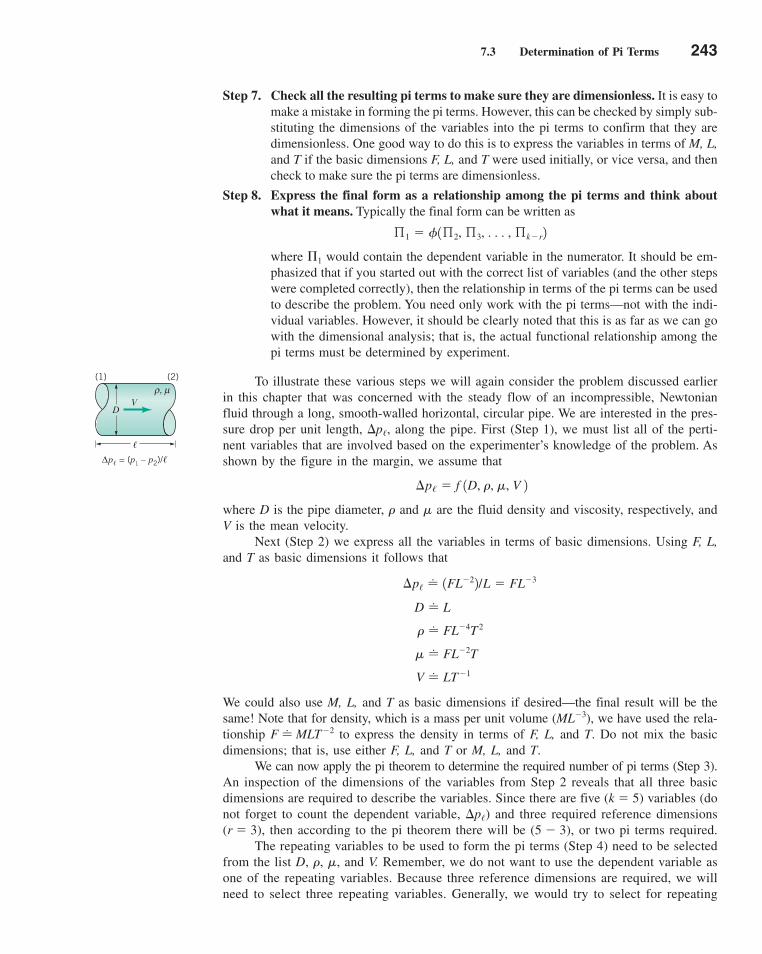
7.3 Determination of Pi Terms 243

Step 7. Check all the resulting pi terms to make sure they are dimensionless. It is easy tomake a mistake in forming the pi terms. However, this can be checked by simply sub-stituting the dimensions of the variables into the pi terms to confirm that they are dimensionless. One good way to do this is to express the variables in terms of M, L,and T if the basic dimensions F, L, and T were used initially, or vice versa, and thencheck to make sure the pi terms are dimensionless.

Step 8. Express the final form as a relationship among the pi terms and think aboutwhat it means. Typically the final form can be written as

where �1 would contain the dependent variable in the numerator. It should be em-phasized that if you started out with the correct list of variables (and the other stepswere completed correctly), then the relationship in terms of the pi terms can be usedto describe the problem. You need only work with the pi terms—not with the indi-vidual variables. However, it should be clearly noted that this is as far as we can gowith the dimensional analysis; that is, the actual functional relationship among thepi terms must be determined by experiment.

To illustrate these various steps we will again consider the problem discussed earlierin this chapter that was concerned with the steady flow of an incompressible, Newtonianfluid through a long, smooth-walled horizontal, circular pipe. We are interested in the pres-sure drop per unit length, �p�, along the pipe. First (Step 1), we must list all of the perti-nent variables that are involved based on the experimenter’s knowledge of the problem. Asshown by the figure in the margin, we assume that

where D is the pipe diameter, � and � are the fluid density and viscosity, respectively, andV is the mean velocity.

Next (Step 2) we express all the variables in terms of basic dimensions. Using F, L,and T as basic dimensions it follows that

We could also use M, L, and T as basic dimensions if desired—the final result will be thesame! Note that for density, which is a mass per unit volume (ML�3), we have used the rela-tionship F � MLT�2 to express the density in terms of F, L, and T. Do not mix the basicdimensions; that is, use either F, L, and T or M, L, and T.

We can now apply the pi theorem to determine the required number of pi terms (Step 3).An inspection of the dimensions of the variables from Step 2 reveals that all three basicdimensions are required to describe the variables. Since there are five (k � 5) variables (donot forget to count the dependent variable, �p�) and three required reference dimensions(r � 3), then according to the pi theorem there will be (5 � 3), or two pi terms required.

The repeating variables to be used to form the pi terms (Step 4) need to be selectedfrom the list D, �, �, and V. Remember, we do not want to use the dependent variable asone of the repeating variables. Because three reference dimensions are required, we willneed to select three repeating variables. Generally, we would try to select for repeating

V � LT�1

� � FL�2T

� � FL�4T 2

D � L

¢p/ � 1FL�22/L � FL�3

¢p/ � f 1D, �, �, V 2

ß1 � f1ß2, ß3, . . . , ßk�r2

(1) (2)

DV

ρ, μ

�

Δp� = (p1 – p2)/�

c07Similitude,DimensionalAnalysis,andModeling.qxd 9/24/10 2:01 PM Page 243

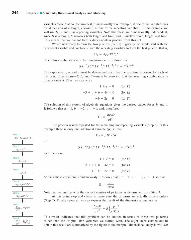
variables those that are the simplest, dimensionally. For example, if one of the variables hasthe dimension of a length, choose it as one of the repeating variables. In this example wewill use D, V, and � as repeating variables. Note that these are dimensionally independent,since D is a length, V involves both length and time, and � involves force, length, and time.This means that we cannot form a dimensionless product from this set.

We are now ready to form the two pi terms (Step 5). Typically, we would start with thedependent variable and combine it with the repeating variables to form the first pi term; that is,

Since this combination is to be dimensionless, it follows that

The exponents a, b, and c must be determined such that the resulting exponent for each ofthe basic dimensions—F, L, and T—must be zero (so that the resulting combination isdimensionless). Thus, we can write

(for F)

(for L)

(for T )

The solution of this system of algebraic equations gives the desired values for a, b, and c.It follows that a � 1, b � �2, c � �1, and, therefore,

The process is now repeated for the remaining nonrepeating variables (Step 6). In thisexample there is only one additional variable (�) so that

or

and, therefore,

(for F)

(for L)

(for T)

Solving these equations simultaneously it follows that a � �1, b � �1, c � �1 so that

Note that we end up with the correct number of pi terms as determined from Step 3.At this point stop and check to make sure the pi terms are actually dimensionless

(Step 7). Finally (Step 8), we can express the result of the dimensional analysis as

This result indicates that this problem can be studied in terms of these two pi termsrather than the original five variables we started with. The eight steps carried out toobtain this result are summarized by the figure in the margin. Dimensional analysis will not

¢p/D

�V2 � �~ a

�

DV�b

ß2 ��

DV�

1 � b � 2c � 0

�2 � a � b � 4c � 0

1 � c � 0

1FL�2T2 1L2a1LT�12b1FL�4T22c � F0L0T0

ß2 � �DaVb�c

ß1 �¢p/D

�V2

�b � 2c � 0

�3 � a � b � 4c � 0

1 � c � 0

1FL�32 1L2a1LT�12b1FL�4T22c � F0L0T0

ß1 � ¢p/DaVb�c

244 Chapter 7 ■ Similitude, Dimensional Analysis, and Modeling

Δp�D_____

V2ρ

= F0L0T0

Step 1

Δp� = f(D, r, m, V)

Step 2

Δp� = FL�3, ...

Step 3

k – r = 3

Step 4

D, V, r

Step 5

�1 = Δp�DaVbrc

Step 6

�2 = mDaVbrc

Step 7

Step 8Δp�D_____

V2ρ

= �~� �____

DVρm

c07Similitude,DimensionalAnalysis,andModeling.qxd 9/24/10 2:01 PM Page 244

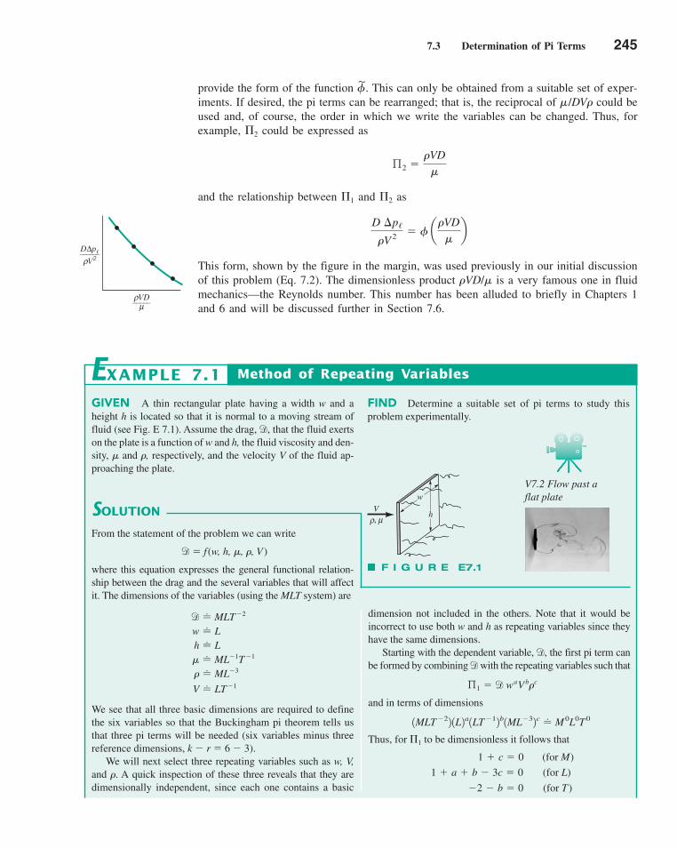
7.3 Determination of Pi Terms 245

provide the form of the function . This can only be obtained from a suitable set of exper-iments. If desired, the pi terms can be rearranged; that is, the reciprocal of �/DV� could beused and, of course, the order in which we write the variables can be changed. Thus, forexample, �2 could be expressed as

and the relationship between �1 and �2 as

This form, shown by the figure in the margin, was used previously in our initial discussionof this problem (Eq. 7.2). The dimensionless product �VD/� is a very famous one in fluidmechanics—the Reynolds number. This number has been alluded to briefly in Chapters 1and 6 and will be discussed further in Section 7.6.

D ¢p/

�V2 � � a�VD

�b

ß2 ��VD

�

�&

ρμVD_____

ρDΔp�

V2______

GIVEN A thin rectangular plate having a width w and aheight h is located so that it is normal to a moving stream offluid (see Fig. E 7.1). Assume the drag, d, that the fluid exertson the plate is a function of w and h, the fluid viscosity and den-sity, � and �, respectively, and the velocity V of the fluid ap-proaching the plate.

SOLUTION

Method of Repeating Variables

dimension not included in the others. Note that it would beincorrect to use both w and h as repeating variables since theyhave the same dimensions.

Starting with the dependent variable, d, the first pi term canbe formed by combining dwith the repeating variables such that

and in terms of dimensions

Thus, for �1 to be dimensionless it follows that

(for M)

(for L)

(for T) �2 � b � 0

1 � a � b � 3c � 0

1 � c � 0

1MLT �22 1L2a1LT �12b1ML�32c � M 0L0T 0

ß1 � d waVb�c

EXAMPLE 7.1

From the statement of the problem we can write

d� f(w, h, �, �, V)

where this equation expresses the general functional relation-ship between the drag and the several variables that will affectit. The dimensions of the variables (using the MLT system) are

We see that all three basic dimensions are required to definethe six variables so that the Buckingham pi theorem tells usthat three pi terms will be needed (six variables minus threereference dimensions, k � r � 6 � 3).

We will next select three repeating variables such as w, V,and �. A quick inspection of these three reveals that they aredimensionally independent, since each one contains a basic

V � LT �1

� � ML�3

� � ML�1T �1

h � L w � L d � MLT �2

F I G U R E E7.1

h

w

Vρ, μ

V7.2 Flow past aflat plate

FIND Determine a suitable set of pi terms to study thisproblem experimentally.

c07Similitude,DimensionalAnalysis,andModeling.qxd 9/24/10 2:01 PM Page 245

246 Chapter 7 ■ Similitude, Dimensional Analysis, and Modeling

Now that we have the three required pi terms we shouldcheck to make sure they are dimensionless. To make thischeck we use F, L, and T, which will also verify the correct-ness of the original dimensions used for the variables.Thus,

If these do not check, go back to the original list of variablesand make sure you have the correct dimensions for each of thevariables and then check the algebra you used to obtain the ex-ponents a, b, and c.

Finally, we can express the results of the dimensionalanalysis in the form

(Ans)

Since at this stage in the analysis the nature of the functionis unknown, we could rearrange the pi terms if we so de-sired. For example, we could express the final result in theform

(Ans)

which would be more conventional, since the ratio of the platewidth to height, w/h, is called the aspect ratio and �Vw/� is theReynolds number.

COMMENT To proceed, it would be necessary to performa set of experiments to determine the nature of the function

, as discussed in Section 7.7.�

d

w2�V 2 � � aw

h,

�Vw

�b

�&

d

w2V 2�� �

~ ah

w,

�

wV�b

ß3 ��

wV��

1FL�2T 2

1L2 1LT�12 1FL�4T 22� F 0L0T 0

ß2 �h

w�1L2

1L2� F 0L0T 0

ß1 �d

w2V 2��

1F2

1L221LT �1221FL�4T 22� F 0L0T 0

and, therefore, a � �2, b � �2, and c � �1. The pi termthen becomes

Next the procedure is repeated with the second nonrepeat-ing variable, h, so that

It follows that

and

(for M)

(for L)

(for T)

so that a � �1, b � 0, c � 0, and therefore

The remaining nonrepeating variable is � so that

with

and, therefore,

(for M)

(for L)

(for T)

Solving for the exponents we obtain a � �1, b � �1,c � �1 so that

ß3 ��

wV�

�1 � b � 0

�1 � a � b � 3c � 0

1 � c � 0

1ML�1T �12 1L2a1LT �12b1ML�32c � M 0L0T 0

ß3 � �waV b�c

ß2 �h

w

b � 0

1 � a � b � 3c � 0

c � 0

1L2 1L2a1LT �12b1ML�32c � M 0L0T 0

ß2 � hwaVb�c

ß1 �d

w2V 2�

7.4 Some Additional Comments about Dimensional Analysis

The preceding section provides a systematic procedure for performing a dimensional analy-sis. Other methods could be used, although we think the method of repeating variables isthe easiest for the beginning student to use. Pi terms can also be formed by inspection, asis discussed in Section 7.5. Regardless of the specific method used for the dimensionalanalysis, there are certain aspects of this important engineering tool that must seem a littlebaffling and mysterious to the student (and sometimes to the experienced investigator aswell). In this section we will attempt to elaborate on some of the more subtle points that,based on our experience, can prove to be puzzling to students.

c07Similitude,DimensionalAnalysis,andModeling.qxd 9/24/10 2:02 PM Page 246

7.4 Some Additional Comments about Dimensional Analysis 247

7.4.1 Selection of Variables

One of the most important and difficult steps in applying dimensional analysis to any givenproblem is the selection of the variables that are involved. As noted previously, for conveniencewe will use the term variable to indicate any quantity involved, including dimensional andnondimensional constants. There is no simple procedure whereby the variables can be eas-ily identified. Generally, one must rely on a good understanding of the phenomenon involvedand the governing physical laws.

For most engineering problems (including areas outside of fluid mechanics), pertinentvariables can be classified into three general groups—geometry, material properties, andexternal effects.

Geometry. The geometric characteristics can usually be prescribed by a series oflengths and angles. In most problems the geometry of the system plays an important role,and a sufficient number of geometric variables must be included to describe the system. Thesevariables can usually be readily identified.

Material Properties. Since the response of a system to applied external effectssuch as forces, pressures, and changes in temperature is dependent on the nature of thematerials involved in the system, the material properties that relate the external effects andthe responses must be included as variables. For example, for Newtonian fluids the vis-cosity of the fluid is the property that relates the applied forces to the rates of deformationof the fluid.

External Effects. This terminology is used to denote any variable that produces, ortends to produce, a change in the system. For example, in structural mechanics, forces (ei-ther concentrated or distributed) applied to a system tend to change its geometry, and suchforces would need to be considered as pertinent variables. For fluid mechanics, variables inthis class would be related to pressures, velocities, or gravity.

7.4.2 Determination of Reference Dimensions

For any given problem it is obviously desirable to reduce the number of pi terms to a min-imum and, therefore, we wish to reduce the number of variables to a minimum; that is, wecertainly do not want to include extraneous variables. It is also important to know how manyreference dimensions are required to describe the variables. As we have seen in the precedingexamples, F, L, and T appear to be a convenient set of basic dimensions for characterizingfluid-mechanical quantities. There is, however, really nothing “fundamental” about this setand, as previously noted, M, L, and T would also be suitable. Of course, in some problemsonly one or two of these is required.

7.4.3 Uniqueness of Pi Terms

A little reflection on the process used to determine pi terms by the method of repeatingvariables reveals that the specific pi terms obtained depend on the somewhat arbitrary selec-tion of repeating variables. For example, in the problem of studying the pressure drop in apipe, we selected D, V, and � as repeating variables. This led to the formulation of the prob-lem in terms of pi terms as

(7.3)¢p/D

�V2 � � a�VD

�b

c07Similitude,DimensionalAnalysis,andModeling.qxd 9/24/10 2:02 PM Page 247

What if we had selected D, V, and � as repeating variables? A quick check will reveal thatthe pi term involving �p� becomes

and the second pi term remains the same. Thus, we can express the final result as

(7.4)

Both results are correct, and both would lead to the same final equation for �p�. Note, how-ever, that the functions � and �1 in Eqs. 7.3 and 7.4 will be different because the depen-dent pi terms are different for the two relationships. As shown by the figure in the margin,the resulting graph of dimensionless data will be different for the two formulations. How-ever, when extracting the physical variable, pressure drop per unit length, from the tworesults, the values will be the same.

We can conclude from this illustration that there is not a unique set of pi terms thatarises from a dimensional analysis. However, the required number of pi terms is fixed.

¢p/D2

V�� �1 a

�VD�b

¢p/D2

V�

248 Chapter 7 ■ Similitude, Dimensional Analysis, and Modeling

D2Δp�

Vm

VD____μ

ρ

VD____μ

ρ

V2ρ

DΔp�

7.5 Determination of Pi Terms by Inspection

One method for forming pi terms, the method of repeating variables, has been presented inSection 7.3. This method provides a step-by-step procedure that, if executed properly, willprovide a correct and complete set of pi terms. Although this method is simple and straight-forward, it is rather tedious, particularly for problems in which large numbers of variablesare involved. Since the only restrictions placed on the pi terms are that they be (1) correctin number, (2) dimensionless, and (3) independent, it is possible to simply form the pi termsby inspection, without resorting to the more formal procedure.

To illustrate this approach, we again consider the pressure drop per unit length alonga smooth pipe. Regardless of the technique to be used, the starting point remains the same—determine the variables, which in this case are

�p/ � f(D, �, �, V)

Next, the dimensions of the variables are listed:

and subsequently the number of reference dimensions determined. Application of the pi the-orem then tells us how many pi terms are required. In this problem, since there are fivevariables and three reference dimensions, two pi terms are needed. Thus, the required num-ber of pi terms can be easily determined, and the determination of this number shouldalways be done at the beginning of the analysis.

Once the number of pi terms is known, we can form each pi term by inspection, sim-ply making use of the fact that each pi term must be dimensionless. We will always let �1

contain the dependent variable, which in this example is �p�. Since this variable has the

V � LT�1

� � FL�2T

� � FL�4T 2

D � L

¢p/ � FL�3

c07Similitude,DimensionalAnalysis,andModeling.qxd 9/24/10 2:02 PM Page 248

7.6 Common Dimensionless Groups in Fluid Mechanics 249

dimensions FL�3, we need to combine it with other variables so that a nondimensional productwill result. One possibility is

Next, we will form the second pi term by selecting the variable that was not used in �1,which in this case is �. We simply combine � with the other variables to make the combi-nation dimensionless (but do not use �p� in �2, since we want the dependent variable toappear only in �1). For example, divide � by � (to eliminate F), then by V (to eliminate T ),and finally by D (to eliminate L). Thus,

and, therefore,

which is, of course, the same result we obtained by using the method of repeating variables.Although forming pi terms by inspection is essentially equivalent to the repeating vari-

able method, it is less structured. With a little practice the pi terms can be readily formedby inspection, and this method offers an alternative to the more formal procedure.

¢p/D

�V 2 � � a�

�VDb

ß2 ��

�VD

ß1 �¢p/D

�V 2

7.6 Common Dimensionless Groups in Fluid Mechanics

At the top of Table 7.1 is a list of variables that commonly arise in fluid mechanics prob-lems. The list is obviously not exhaustive but does indicate a broad range of variables likelyto be found in a typical problem. Fortunately, not all of these variables would be encoun-tered in each problem. However, when combinations of these variables are present, it isstandard practice to combine them into some of the common dimensionless groups (piterms) given in Table 7.1. These combinations appear so frequently that special names areassociated with them as indicated in Table 7.1.

It is also often possible to provide a physical interpretation to the dimensionless groups,which can be helpful in assessing their influence in a particular application. For example,the Froude number is an index of the ratio of the force due to the acceleration of a fluid par-ticle (inertial force) to the force due to gravity (weight). A similar interpretation in terms ofindices of force ratios can be given to the other dimensionless groups, as indicated in Table7.1. The Reynolds number is undoubtedly the most famous dimensionless parameter in fluidmechanics. It is named in honor of Osborne Reynolds, a British engineer, who first demon-strated that this combination of variables could be used as a criterion to distinguish betweenlaminar and turbulent flow. In most fluid flow problems there will be a characteristic length,�, and a velocity, V, as well as the fluid properties of density, �, and viscosity, �, which arerelevant variables in the problem. Thus, with these variables the Reynolds number

arises naturally from the dimensional analysis. The Reynolds number is a measure of theratio of the inertia force on an element of fluid to the viscous force on an element. Whenthese two types of forces are important in a given problem, the Reynolds number will playan important role.

Re ��V/�

V7.3 Reynoldsnumber

V7.4 Froude number

c07Similitude,DimensionalAnalysis,andModeling.qxd 9/24/10 2:02 PM Page 249

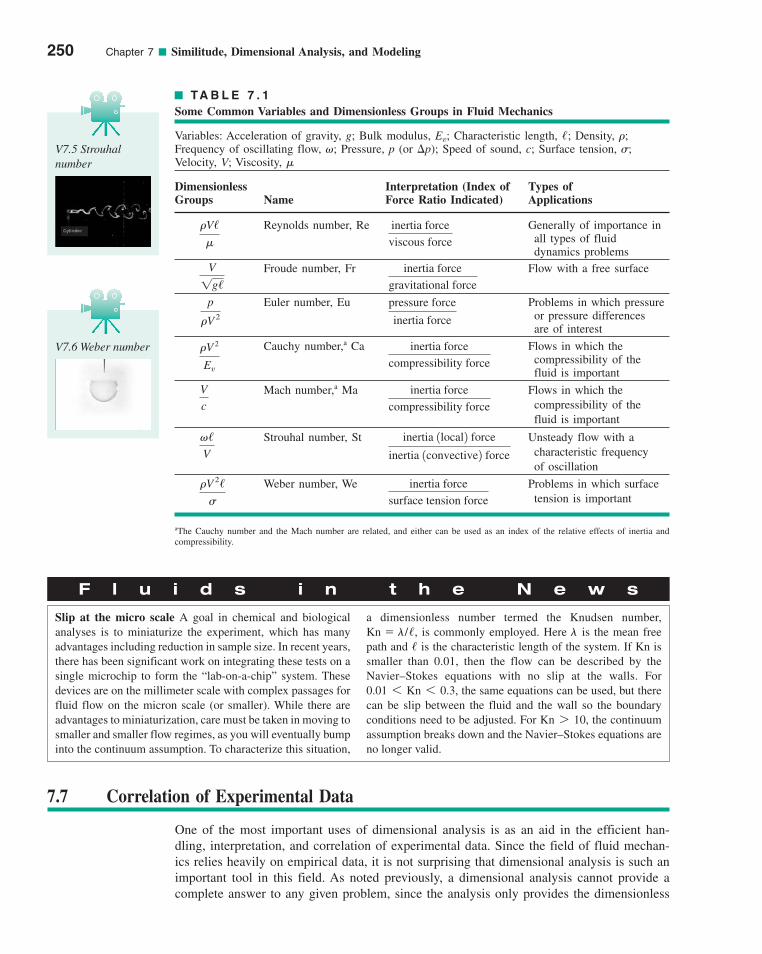
250 Chapter 7 ■ Similitude, Dimensional Analysis, and Modeling

TA B L E 7 . 1

Some Common Variables and Dimensionless Groups in Fluid Mechanics

Variables: Acceleration of gravity, g; Bulk modulus, Ev; Characteristic length, �; Density, �;Frequency of oscillating flow, �; Pressure, p (or �p); Speed of sound, c; Surface tension, �; Velocity, V; Viscosity, �

Dimensionless Interpretation (Index of Types ofGroups Name Force Ratio Indicated) Applications

Reynolds number, Re Generally of importance inall types of fluid dynamics problems

Froude number, Fr Flow with a free surface

Euler number, Eu Problems in which pressureor pressure differencesare of interest

Cauchy number,a Ca Flows in which thecompressibility of the fluid is important

Mach number,a Ma Flows in which thecompressibility of thefluid is important

Strouhal number, St Unsteady flow with acharacteristic frequencyof oscillation

Weber number, We Problems in which surfacetension is important

inertia force

surface tension force

�V 2/�

inertia 1local2 force

inertia 1convective2 force

�/V

inertia force

compressibility force

V

c

inertia force

compressibility force�V 2

Ev

pressure force

inertia force

p

�V 2

inertia force

gravitational force

V

1g/

inertia force

viscous force

�V/�

aThe Cauchy number and the Mach number are related, and either can be used as an index of the relative effects of inertia andcompressibility.

V7.5 Strouhal number

V7.6 Weber number

F l u i d s i n t h e N e w s

Slip at the micro scale A goal in chemical and biologicalanalyses is to miniaturize the experiment, which has manyadvantages including reduction in sample size. In recent years,there has been significant work on integrating these tests on asingle microchip to form the “lab-on-a-chip” system. Thesedevices are on the millimeter scale with complex passages forfluid flow on the micron scale (or smaller). While there areadvantages to miniaturization, care must be taken in moving tosmaller and smaller flow regimes, as you will eventually bumpinto the continuum assumption. To characterize this situation,

a dimensionless number termed the Knudsen number,, is commonly employed. Here is the mean free

path and is the characteristic length of the system. If Kn issmaller than 0.01, then the flow can be described by theNavier–Stokes equations with no slip at the walls. For

, the same equations can be used, but therecan be slip between the fluid and the wall so the boundaryconditions need to be adjusted. For , the continuumassumption breaks down and the Navier–Stokes equations areno longer valid.

Kn 7 10

0.01 6 Kn 6 0.3

/�Kn � �//

7.7 Correlation of Experimental Data

One of the most important uses of dimensional analysis is as an aid in the efficient han-dling, interpretation, and correlation of experimental data. Since the field of fluid mechan-ics relies heavily on empirical data, it is not surprising that dimensional analysis is such animportant tool in this field. As noted previously, a dimensional analysis cannot provide acomplete answer to any given problem, since the analysis only provides the dimensionless

c07Similitude,DimensionalAnalysis,andModeling.qxd 9/24/10 2:02 PM Page 250

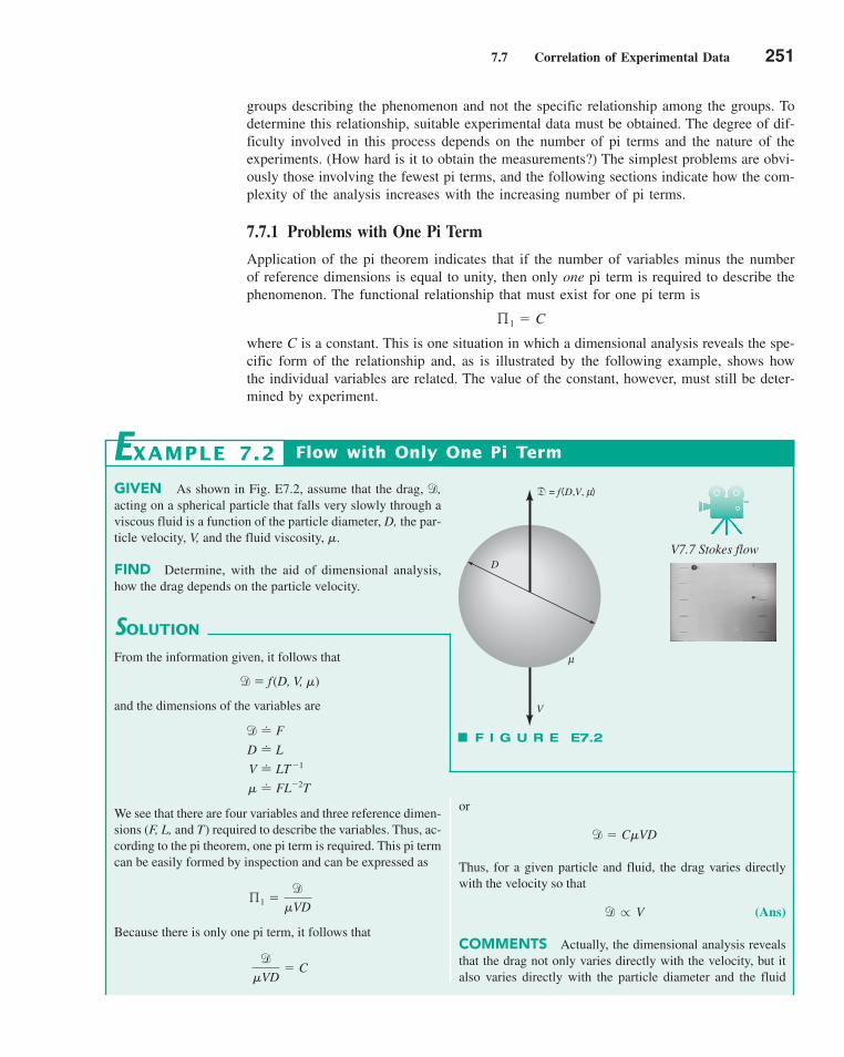
7.7 Correlation of Experimental Data 251

groups describing the phenomenon and not the specific relationship among the groups. Todetermine this relationship, suitable experimental data must be obtained. The degree of dif-ficulty involved in this process depends on the number of pi terms and the nature of theexperiments. (How hard is it to obtain the measurements?) The simplest problems are obvi-ously those involving the fewest pi terms, and the following sections indicate how the com-plexity of the analysis increases with the increasing number of pi terms.

7.7.1 Problems with One Pi Term

Application of the pi theorem indicates that if the number of variables minus the numberof reference dimensions is equal to unity, then only one pi term is required to describe thephenomenon. The functional relationship that must exist for one pi term is

where C is a constant. This is one situation in which a dimensional analysis reveals the spe-cific form of the relationship and, as is illustrated by the following example, shows howthe individual variables are related. The value of the constant, however, must still be deter-mined by experiment.

ß1 � C

GIVEN As shown in Fig. E7.2, assume that the drag, d,acting on a spherical particle that falls very slowly through aviscous fluid is a function of the particle diameter, D, the par-ticle velocity, V, and the fluid viscosity, �.

FIND Determine, with the aid of dimensional analysis,how the drag depends on the particle velocity.

SOLUTION

Flow with Only One Pi Term

or

Thus, for a given particle and fluid, the drag varies directlywith the velocity so that

(Ans)

COMMENTS Actually, the dimensional analysis revealsthat the drag not only varies directly with the velocity, but italso varies directly with the particle diameter and the fluid

d r V

d � C�VD

EXAMPLE 7.2

From the information given, it follows that

d� f(D, V, �)

and the dimensions of the variables are

We see that there are four variables and three reference dimen-sions (F, L, and T) required to describe the variables. Thus, ac-cording to the pi theorem, one pi term is required. This pi termcan be easily formed by inspection and can be expressed as

Because there is only one pi term, it follows that

d

�VD� C

ß1 �d

�VD

� � FL�2T

V � LT �1

D � L

d � F

� = f (D,V, )μ

μ

V

D

F I G U R E E7.2

V7.7 Stokes flow

c07Similitude,DimensionalAnalysis,andModeling.qxd 9/24/10 2:02 PM Page 251

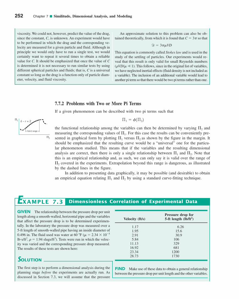
7.7.2 Problems with Two or More Pi Terms

If a given phenomenon can be described with two pi terms such that

the functional relationship among the variables can then be determined by varying �2 andmeasuring the corresponding values of �1. For this case the results can be conveniently pre-sented in graphical form by plotting �1 versus �2 as shown by the figure in the margin. Itshould be emphasized that the resulting curve would be a “universal” one for the particu-lar phenomenon studied. This means that if the variables and the resulting dimensionalanalysis are correct, then there is only a single relationship between �1 and �2. Note thatthis is an empirical relationship and, as such, we can only say it is valid over the range of�2 covered in the experiments. Extrapolation beyond this range is dangerous, as illustratedby the dashed lines in the figure.

In addition to presenting data graphically, it may be possible (and desirable) to obtainan empirical equation relating �1 and �2 by using a standard curve-fitting technique.

ß1 � �1ß22

252 Chapter 7 ■ Similitude, Dimensional Analysis, and Modeling

An approximate solution to this problem can also be ob-tained theoretically, from which it is found that C � 3 so that

This equation is commonly called Stokes law and is used in thestudy of the settling of particles. Our experiments would re-veal that this result is only valid for small Reynolds numbers(�VD/� � 1). This follows, since in the original list of variables,we have neglected inertial effects (fluid density is not included asa variable). The inclusion of an additional variable would lead toanother pi term so that there would be two pi terms rather than one.

d � 3�VD

viscosity. We could not, however, predict the value of the drag,since the constant, C, is unknown. An experiment would haveto be performed in which the drag and the corresponding ve-locity are measured for a given particle and fluid. Although inprinciple we would only have to run a single test, we wouldcertainly want to repeat it several times to obtain a reliablevalue for C. It should be emphasized that once the value of Cis determined it is not necessary to run similar tests by usingdifferent spherical particles and fluids; that is, C is a universalconstant so long as the drag is a function only of particle diam-eter, velocity, and fluid viscosity.

Valid range

Π1

Π2

k – r = 2

GIVEN The relationship between the pressure drop per unitlength along a smooth-walled, horizontal pipe and the variablesthat affect the pressure drop is to be determined experimen-tally. In the laboratory the pressure drop was measured over a5-ft length of smooth-walled pipe having an inside diameter of0.496 in. The fluid used was water at 60 �F (� � 2.34 10�5

lbs/ft2, � � 1.94 slugs/ft3). Tests were run in which the veloc-ity was varied and the corresponding pressure drop measured.The results of these tests are shown here:

Dimensionless Correlation of Experimental Data

Pressure drop forVelocity (ft/s) 5-ft length (lb/ft2)

1.17 6.261.95 15.62.91 30.95.84 106

11.13 32916.92 68123.34 120028.73 1730

FIND Make use of these data to obtain a general relationshipbetween the pressure drop per unit length and the other variables.

EXAMPLE 7.3

SOLUTION

The first step is to perform a dimensional analysis during theplanning stage before the experiments are actually run. Asdiscussed in Section 7.3, we will assume that the pressure

c07Similitude,DimensionalAnalysis,andModeling.qxd 9/24/10 2:02 PM Page 252

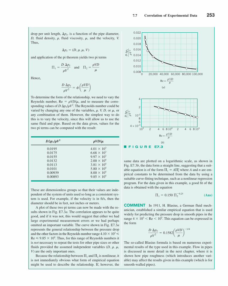
7.7 Correlation of Experimental Data 253

same data are plotted on a logarithmic scale, as shown inFig. E7.3b, the data form a straight line, suggesting that a suit-able equation is of the form �1 � A�n

2 where A and n are em-pirical constants to be determined from the data by using asuitable curve-fitting technique, such as a nonlinear regressionprogram. For the data given in this example, a good fit of thedata is obtained with the equation

(Ans)

COMMENT In 1911, H. Blasius, a German fluid mech-anician, established a similar empirical equation that is usedwidely for predicting the pressure drop in smooth pipes in therange 4 103 � Re � 105. This equation can be expressed inthe form

The so-called Blasius formula is based on numerous experi-mental results of the type used in this example. Flow in pipesis discussed in more detail in the next chapter, where it isshown how pipe roughness (which introduces another vari-able) may affect the results given in this example (which is forsmooth-walled pipes).

D ¢p/

�V2 � 0.1582 a�VD

�b

�1/4

ß1 � 0.150 ß�0.252

drop per unit length, �p�, is a function of the pipe diameter,D, fluid density, �, fluid viscosity, �, and the velocity, V.Thus,

�p/ � (D, �, �, V)

and application of the pi theorem yields two pi terms

Hence,

To determine the form of the relationship, we need to vary theReynolds number, Re � �VD/�, and to measure the corre-sponding values of D �p�/�V2. The Reynolds number could bevaried by changing any one of the variables, �, V, D, or �, orany combination of them. However, the simplest way to dothis is to vary the velocity, since this will allow us to use thesame fluid and pipe. Based on the data given, values for thetwo pi terms can be computed with the result:

D�p /�V2 �VD/�

0.0195 4.01 103

0.0175 6.68 103

0.0155 9.97 103

0.0132 2.00 104

0.0113 3.81 104

0.0101 5.80 104

0.00939 8.00 104

0.00893 9.85 104

These are dimensionless groups so that their values are inde-pendent of the system of units used so long as a consistent sys-tem is used. For example, if the velocity is in ft/s, then thediameter should be in feet, not inches or meters.

A plot of these two pi terms can now be made with the re-sults shown in Fig. E7.3a. The correlation appears to be quitegood, and if it was not, this would suggest that either we hadlarge experimental measurement errors or we had perhapsomitted an important variable. The curve shown in Fig. E7.3arepresents the general relationship between the pressure dropand the other factors in the Reynolds number range 4.10 103 �Re � 9.85 104. Thus, for this range of Reynolds numbers itis not necessary to repeat the tests for other pipe sizes or otherfluids provided the assumed independent variables (D, �, �,V) are the only important ones.

Because the relationship between �1 and �2 is nonlinear, itis not immediately obvious what form of empirical equationmight be used to describe the relationship. If, however, the

�

D ¢p/

�V2 � � a�VD

�b

ß1 �D ¢p/

�V 2 and ß2 �

�VD

�

F I G U R E E7.3

0.022

0.020

0.018

0.016

0.014

0.012

0.010

0.0080 20,000 40,000 60,000 80,000 100,000

VD_____μ

ρ

(a)

D Δ

p �__

____

V

2ρ

4

2

10–2

86

4 × 10–3

103 2 4 6 8 104 2 4 6 8 105

D Δ

p �__

____

V

2ρ

(b)

Re =

VD_____μ

ρRe =

c07Similitude,DimensionalAnalysis,andModeling.qxd 9/24/10 2:02 PM Page 253

As the number of required pi terms increases, it becomes more difficult to display theresults in a convenient graphical form and to determine a specific empirical equation thatdescribes the phenomenon. For problems involving three pi terms

it is still possible to show data correlations on simple graphs by plotting families of curvesas shown by the figure in the margin. This is an informative and useful way of representingthe data in a general way. It may also be possible to determine a suitable empirical equationrelating the three pi terms. However, as the number of pi terms continues to increase, cor-responding to an increase in the general complexity of the problem of interest, both the graph-ical presentation and the determination of a suitable empirical equation become intractable.For these more complicated problems, it is often more feasible to use models to predict spe-cific characteristics of the system rather than to try to develop general correlations.

ß1 � �1ß2, ß32

254 Chapter 7 ■ Similitude, Dimensional Analysis, and Modeling

7.8 Modeling and Similitude

Models are widely used in fluid mechanics. Major engineering projects involving structures,aircraft, ships, rivers, harbors, dams, air and water pollution, and so on frequently involvethe use of models. Although the term model is used in many different contexts, the “engi-neering model” generally conforms to the following definition. A model is a representationof a physical system that may be used to predict the behavior of the system in some desiredrespect. The physical system for which the predictions are to be made is called the proto-type. Although mathematical or computer models may also conform to this definition, ourinterest will be in physical models, that is, models that resemble the prototype but are gen-erally of a different size, may involve different fluids, and often operate under different con-ditions (pressures, velocities, etc.). Usually a model is smaller than the prototype. There-fore, it is handled more easily in the laboratory and is less expensive to construct and operatethan a large prototype. With the successful development of a valid model, it is possible topredict the behavior of the prototype under a certain set of conditions.

In the following sections we will develop the procedures for designing models so thatthe model and prototype will behave in a similar fashion.

7.8.1 Theory of Models

The theory of models can be developed readily by using the principles of dimensional analy-sis. It has been shown that any given problem can be described in terms of a set of pi terms as

(7.5)

In formulating this relationship, only a knowledge of the general nature of the physical phe-nomenon, and the variables involved, is required. Specific values for variables (size of com-ponents, fluid properties, and so on) are not needed to perform the dimensional analysis.Thus, Eq. 7.5 applies to any system that is governed by the same variables. If Eq. 7.5describes the behavior of a particular prototype, a similar relationship can be written for amodel of this prototype; that is,

(7.6)

where the form of the function will be the same as long as the same phenomenon is involvedin both the prototype and the model. As shown by the figure in the margin of the followingpage, variables or pi terms without a subscript will refer to the prototype, whereas the subscriptm will be used to designate the model variables or pi terms.

ß1m � �1ß2m, ß3m, . . . , ßnm2

ß1 � �1ß2, ß3, . . . , ßn2

V7.8 Model airplane

k – r = 3

1Π ΠΠΠ

Π2

3 = C3

3 = C2

3 = C1

c07Similitude,DimensionalAnalysis,andModeling.qxd 9/24/10 2:03 PM Page 254

7.8 Modeling and Similitude 255

The pi terms can be developed so that �1 contains the variable that is to be predictedfrom observations made on the model. Therefore, if the model is designed and operatedunder the following conditions

(7.7)

then with the presumption that the form of � is the same for model and prototype, it fol-lows that

(7.8)

Equation 7.8 is the desired prediction equation and indicates that the measured value of�1m obtained with the model will be equal to the corresponding �1 for the prototype aslong as the other pi terms are equal. The conditions specified by Eqs. 7.7 provide the modeldesign conditions, also called similarity requirements or modeling laws.

As an example of the procedure, consider the problem of determining the drag, d, ona thin rectangular plate (w h in size) placed normal to a fluid with velocity V as shownby the figure in the margin. The dimensional analysis of this problem was performed inExample 7.1, where it was assumed that

d � f(w, h, �, �, V)

Application of the pi theorem yielded

(7.9)

We are now concerned with designing a model that could be used to predict the drag on acertain prototype (which presumably has a different size than the model). Since the rela-tionship expressed by Eq. 7.9 applies to both prototype and model, Eq. 7.9 is assumed togovern the prototype, with a similar relationship

(7.10)

for the model. The model design conditions, or similarity requirements, are therefore

The size of the model is obtained from the first requirement, which indicates that

(7.11)

We are free to establish the height ratio hm/h, but then the model plate width, wm, is fixedin accordance with Eq. 7.11.

The second similarity requirement indicates that the model and prototype must beoperated at the same Reynolds number. Thus, the required velocity for the model is obtainedfrom the relationship

(7.12)Vm ��m

�

�

�m

wwm

V

wm �hm

h w

wm

hm

�w

h and

�mVmwm

�m�

�Vw

�

dm

w2m �mV 2

m

� � awm

hm

, �mVmwm

�mb

d

w2�V 2� � a

w

h,

�Vw

�b

ß1 � ß1m

ßnm � ßn

o

ß3m � ß3

ß2m � ß2

V

Prototype

Vm

Model

�m

�

h

w

Vρ, μ

c07Similitude,DimensionalAnalysis,andModeling.qxd 9/24/10 2:03 PM Page 255

Note that this model design requires not only geometric scaling, as specified by Eq. 7.11,but also the correct scaling of the velocity in accordance with Eq. 7.12. This result is typ-ical of most model designs—there is more to the design than simply scaling the geometry!

With the foregoing similarity requirements satisfied, the prediction equation for thedrag is

or

Thus, a measured drag on the model, dm, must be multiplied by the ratio of the square ofthe plate widths, the ratio of the fluid densities, and the ratio of the square of the veloci-ties to obtain the predicted value of the prototype drag, d.

Generally, as is illustrated in this example, to achieve similarity between model andprototype behavior, all the corresponding pi terms must be equated between model and pro-totype. Usually, one or more of these pi terms will involve ratios of important lengths (suchas w/h in the foregoing example); that is, they are purely geometrical. Thus, when we equatethe pi terms involving length ratios we are requiring that there be complete geometric sim-ilarity between the model and the prototype. This means that the model must be a scaledversion of the prototype. Geometric scaling may extend to the finest features of the system,such as surface roughness or small protuberances on a structure, since these kinds of geo-metric features may significantly influence the flow.

Another group of typical pi terms (such as the Reynolds number in the foregoingexample) involves force ratios as noted in Table 7.1. The equality of these pi terms requiresthe ratio of like forces in model and prototype to be the same. Thus, for flows in which theReynolds numbers are equal, the ratio of viscous forces in model and prototype is equal tothe ratio of inertia forces. If other pi terms are involved, such as the Froude number orWeber number, a similar conclusion can be drawn; that is, the equality of these pi termsrequires the ratio of like forces in model and prototype to be the same. Thus, when thesetypes of pi terms are equal in model and prototype, we have dynamic similarity betweenmodel and prototype. It follows that with both geometric and dynamic similarity the stream-line patterns will be the same and corresponding velocity ratios (Vm/V) and accelerationratios (am/a) are constant throughout the flow field. Thus, kinematic similarity existsbetween model and prototype. To have complete similarity between model and prototype,we must maintain geometric, kinematic, and dynamic similarity between the two systems.This will automatically follow if all the important variables are included in the dimensionalanalysis and if all the similarity requirements based on the resulting pi terms are satisfied.

d � aw

wmb

2

a�

�mb a

V

Vm

b2

dm

d

w2�V 2�

dm

w2m �mV 2

m

256 Chapter 7 ■ Similitude, Dimensional Analysis, and Modeling

F l u i d s i n t h e N e w s

Modeling parachutes in a water tunnel The first use of aparachute with a free-fall jump from an aircraft occurred in1914, although parachute jumps from hot-air balloons had oc-curred since the late 1700s. In more modern times parachutesare commonly used by the military and for safety and sport. Itis not surprising that there remains interest in the design andcharacteristics of parachutes, and researchers at the WorcesterPolytechnic Institute have been studying various aspects of theaerodynamics associated with parachutes. An unusual part oftheir study is that they are using small-scale parachutes tested

in a water tunnel. The model parachutes are reduced in size bya factor of 30 to 60 times. Various types of tests can be per-formed ranging from the study of the velocity fields in thewake of the canopy with a steady free-stream velocity to thestudy of conditions during rapid deployment of the canopy.According to the researchers, the advantage of using water asthe working fluid, rather than air, is that the velocities and de-ployment dynamics are slower than in the atmosphere, thusproviding more time to collect detailed experimental data.(See Problem 7.39.)

V7.9 Environmentalmodels

c07Similitude,DimensionalAnalysis,andModeling.qxd 9/24/10 2:03 PM Page 256

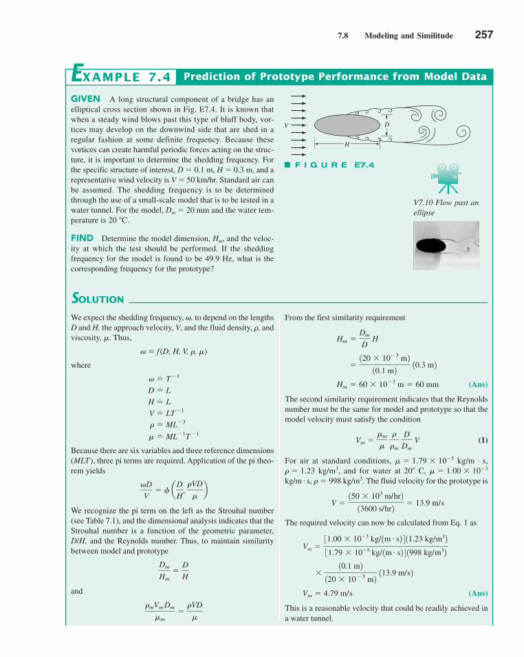
7.8 Modeling and Similitude 257

GIVEN A long structural component of a bridge has anelliptical cross section shown in Fig. E7.4. It is known thatwhen a steady wind blows past this type of bluff body, vor-tices may develop on the downwind side that are shed in aregular fashion at some definite frequency. Because thesevortices can create harmful periodic forces acting on the struc-ture, it is important to determine the shedding frequency. Forthe specific structure of interest, D � 0.1 m, H � 0.3 m, and arepresentative wind velocity is V � 50 km/hr. Standard air canbe assumed. The shedding frequency is to be determinedthrough the use of a small-scale model that is to be tested in awater tunnel. For the model, Dm � 20 mm and the water tem-perature is 20 �C.

FIND Determine the model dimension, Hm, and the veloc-ity at which the test should be performed. If the sheddingfrequency for the model is found to be 49.9 Hz, what is thecorresponding frequency for the prototype?

SOLUTION

Prediction of Prototype Performance from Model DataEXAMPLE 7.4

We expect the shedding frequency, �, to depend on the lengthsD and H, the approach velocity, V, and the fluid density, �, andviscosity, �. Thus,

� � f(D, H, V, �, �)

where

Because there are six variables and three reference dimensions(MLT ), three pi terms are required. Application of the pi theo-rem yields

We recognize the pi term on the left as the Strouhal number(see Table 7.1), and the dimensional analysis indicates that theStrouhal number is a function of the geometric parameter,D/H, and the Reynolds number. Thus, to maintain similaritybetween model and prototype

and

�mVm Dm

�m�

�VD

�

Dm

Hm�

D

H

�D

V� � a

D

H,

�VD

�b

� � ML�1T �1

� � ML�3

V � LT �1

H � L

D � L

� � T �1

From the first similarity requirement

(Ans)

The second similarity requirement indicates that the Reynoldsnumber must be the same for model and prototype so that themodel velocity must satisfy the condition

(1)

For air at standard conditions, � � 1.79 10�5 kg/m s,� � 1.23 kg/m3, and for water at 20� C, � � 1.00 10�3

kg/m s, � � 998 kg/m3. The fluid velocity for the prototype is

The required velocity can now be calculated from Eq. 1 as

(Ans)

This is a reasonable velocity that could be readily achieved ina water tunnel.

Vm � 4.79 m/s

10.1 m2

120 10�3 m2 113.9 m/s2

Vm �31.00 10�3 kg/ 1m # s2 4 11.23 kg/m32

31.79 10�5 kg/ 1m # s2 4 1998 kg/m32

V �150 103 m/hr2

13600 s/hr2� 13.9 m/s

#

#

Vm ��m

�

�

�m

D

Dm V

Hm � 60 10�3 m � 60 mm

�120 10�3 m2

10.1 m2 10.3 m2

Hm �Dm

D H

F I G U R E E7.4

V D

H

V7.10 Flow past anellipse

c07Similitude,DimensionalAnalysis,andModeling.qxd 9/24/10 2:03 PM Page 257

258 Chapter 7 ■ Similitude, Dimensional Analysis, and Modeling

COMMENT This same model could also be used topredict the drag per unit length, d�, on the prototype, sincethe drag would depend on the same variables as those usedfor the frequency. Thus, the similarity requirements wouldbe the same, and with these requirements satisfied it followsthat the drag per unit length expressed in dimensionlessform, such as d�/D�V2, would be equal in model and proto-type. The measured drag per unit length on the model couldthen be related to the corresponding drag on the prototypethrough the relationship

d/ � aD

Dm

b a�

�mb a

V

Vm

b2

d/m

With the two similarity requirements satisfied, it followsthat the Strouhal numbers for prototype and model will be thesame so that

and the predicted prototype vortex shedding frequency is

(Ans) � � 29.0 Hz

�113.9 m/s2

14.79 m/s2 120 10�3 m2

10.1 m2 149.9 Hz2

� �V

Vm Dm

D �m

�D

V�

�mDm

Vm

7.8.2 Model Scales

It is clear from the preceding section that the ratio of like quantities for the model and pro-totype naturally arises from the similarity requirements. For example, if in a given problemthere are two length variables �1 and �2, the resulting similarity requirement based on a piterm obtained from these variables is

so that

We define the ratio �1m/�1 or �2m/�2 as the length scale. For true models there will be onlyone length scale, and all lengths are fixed in accordance with this scale. There are, how-ever, other scales, such as the velocity scale, Vm/V, density scale, �m/�, viscosity scale, �m/�,and so on. In fact, we can define a scale for each of the variables in the problem. Thus, itis actually meaningless to talk about a “scale” of a model without specifying which scale.

We will designate the length scale as ��, and other scales as �V, ��, ��, and so on,where the subscript indicates the particular scale. Also, we will take the ratio of the modelvalue to the prototype value as the scale (rather than the inverse). Length scales are oftenspecified, for example, as 1:10 or as a model. The meaning of this specification isthat the model is one-tenth the size of the prototype, and the tacit assumption is that all rel-evant lengths are scaled accordingly so the model is geometrically similar to the prototype.

110-scale

/1m

/1�

/2m

/2

/1

/2�

/1m

/2m

F l u i d s i n t h e N e w s

“Galloping Gertie” One of the most dramatic bridge col-lapses occurred in 1940 when the Tacoma Narrows Bridge, lo-cated near Tacoma, Washington, failed due to aerodynamicinstability. The bridge had been nicknamed “Galloping Ger-tie” due to its tendency to sway and move in high winds. Onthe fateful day of the collapse the wind speed was .This particular combination of a high wind and the aeroelas-tic properties of the bridge created large oscillations leadingto its failure. The bridge was replaced in 1950, and a secondbridge parallel to the existing structure was opened in 2007.

65 km/hr

To determine possible wind interference effects due to twobridges in close proximity, wind tunnel tests were run in a

wind tunnel operated by the National ResearchCouncil of Canada. Models of the two side-by-side bridges,each having a length scale of 1:211, were tested under vari-ous wind conditions. Since the failure of the original TacomaNarrows Bridge, it is now common practice to use wind tun-nel model studies during the design process to evaluate anybridge that is to be subjected to wind-induced vibrations. (SeeProblem 7.54.)

9 m 9 m

V7.11 Model offish hatchery pond

c07Similitude,DimensionalAnalysis,andModeling.qxd 9/24/10 2:03 PM Page 258

7.8 Modeling and Similitude 259

7.8.3 Distorted Models

Although the general idea behind establishing similarity requirements for models is straight-forward (we simply equate pi terms), it is not always possible to satisfy all the knownrequirements. If one or more of the similarity requirements are not met, for example, if�2m � �2, then it follows that the prediction equation �1 � �1m is not true; that is,�1 � �1m. Models for which one or more of the similarity requirements are not satisfiedare called distorted models.

Distorted models are rather commonplace and can arise for a variety of reasons. Forexample, perhaps a suitable fluid cannot be found for the model. The classic example ofa distorted model occurs in the study of open channel or free-surface flows. Typically inthese problems both the Reynolds number, �V�/�, and the Froude number, areinvolved.

Froude number similarity requires

If the model and prototype are operated in the same gravitational field, then the requiredvelocity scale is

Reynolds number similarity requires

and the velocity scale is

Since the velocity scale must be equal to the square root of the length scale, it followsthat

(7.13)

where the ratio �/� is the kinematic viscosity, . Although it may be possible to satisfythis design condition in principle, it may be quite difficult, if not impossible, to find asuitable model fluid, particularly for small-length scales. For problems involving rivers,spillways, and harbors, for which the prototype fluid is water, the models are also rela-tively large so that the only practical model fluid is water. However, in this case (withthe kinematic viscosity scale equal to unity) Eq. 7.13 will not be satisfied, and a distortedmodel will result. Generally, hydraulic models of this type are distorted and are designedon the basis of the Froude number, with the Reynolds number different in model andprototype.

Distorted models can be used successfully, but the interpretation of results obtainedwith this type of model is obviously more difficult than the interpretation of results obtainedwith true models for which all similarity requirements are met.

�m /�m

�/��

m

� 1�/2

3/2

Vm

V�

�m

�

�

�m

//m

�mVm/m

�m�

�V/�

Vm

V�B

/m

/� 1�/

Vm

1gm/m

�V

1g/

V/1g�,

V7.12 Distortedriver model

c07Similitude,DimensionalAnalysis,andModeling.qxd 9/24/10 2:04 PM Page 259

260 Chapter 7 ■ Similitude, Dimensional Analysis, and Modeling

F l u i d s i n t h e N e w s

Old Man River in (large) miniature One of the world’slargest scale models, a Mississippi River model, resides nearJackson, Mississippi. It is a detailed, complex model that cov-ers many acres and replicates the 1,250,000-acre MississippiRiver basin. Built by the Army Corps of Engineers and usedfrom 1943 to 1973, today it has mostly gone to ruin. As withmany hydraulic models, this is a distorted model, with a hori-zontal scale of 1:2000 and a vertical scale of 1:100. Onestep along the model river corresponds to one mile along theriver. All essential river basin elements such as geological fea-

tures, levees, and railroad embankments were sculpted byhand to match the actual contours. The main purpose of themodel was to predict floods. This was done by supplying spe-cific amounts of water at prescribed locations along the modeland then measuring the water depths up and down the modelriver. Because of the length scale, there is a difference in thetime taken by the corresponding model and prototype events.Although it takes days for the actual floodwaters to travel fromSioux City, Iowa, to Omaha, Nebraska, it would take onlyminutes for the simulated flow in the model.

7.9 Some Typical Model Studies

Models are used to investigate many different types of fluid mechanics problems, and it isdifficult to characterize in a general way all necessary similarity requirements, as each prob-lem is unique. We can, however, broadly classify many of the problems on the basis of thegeneral nature of the flow and subsequently develop some general characteristics of modeldesigns in each of these classifications. The following sections consider models for the studyof (1) flow through closed circuits, (2) flow around immersed bodies, and (3) flow with afree surface. Turbomachine models are considered in Chapter 11.

7.9.1 Flow through Closed Conduits

Common examples of this type of flow include pipe flow and flow through valves, fittings,and metering devices. Although the conduits are often circular, they could have other shapesas well and may contain expansions or contractions. Since there are no fluid interfaces orfree surfaces, the dominant forces are inertial and viscous so that the Reynolds number isan important similarity parameter. For low Mach numbers (Ma � 0.3), compressibilityeffects are negligible for the flow of both liquids and gases. For this class of problems, geo-metric similarity between model and prototype must be maintained. Generally the geomet-ric characteristics can be described by a series of length terms, �1, �2, �3, . . . , �i, and �,where � is some particular length dimension for the system. Such a series of length termsleads to a set of pi terms of the form

where i � 1, 2, . . . , and so on. In addition to the basic geometry of the system, the rough-ness of the internal surfaces in contact with the fluid may be important. If the average heightof surface roughness elements is defined as �, then the pi term representing roughness wouldbe �/�. This parameter indicates that for complete geometric similarity, surface roughnesswould also have to be scaled.

It follows from this discussion that for flow in closed conduits at low Mach numbers,any dependent pi term (the one that contains the particular variable of interest, such as pres-sure drop) can be expressed as

(7.14)

This is a general formulation for this type of problem.

Dependent pi term � � a/i

/, e

/,

�V/�b

ßi �/i

/

c07Similitude,DimensionalAnalysis,andModeling.qxd 9/24/10 2:04 PM Page 260

7.9 Some Typical Model Studies 261

With the similarity requirements satisfied, it follows that the dependent pi term willbe equal in model and prototype. For example, if the dependent variable of interest is thepressure differential, �p, between two points along a closed conduit, then the dependent piterm could be expressed as

The prototype pressure drop would then be obtained from the relationship

so that from a measured pressure differential in the model, �pm, the corresponding pressuredifferential for the prototype could be predicted. Note that in general �p � �pm.

¢p ��

�m a

V

Vmb

2

¢pm

ß1 �¢p

�V2

GIVEN Model tests are to be performed to study the flowthrough a large check valve having a 2-ft-diameter inlet andcarrying water at a flowrate of 30 cfs as shown in Fig. E7.5a.The working fluid in the model is water at the same tempera-ture as that in the prototype. Complete geometric similarityexists between model and prototype, and the model inlet di-ameter is 3 in.

FIND Determine the required flowrate in the model.

SOLUTION

Reynolds Number Similarity

and for the data given

(Ans)

COMMENT As indicated by the foregoing analysis, tomaintain Reynolds number similarity using the same fluid inmodel and prototype, the required velocity scale is inverselyproportional to the length scale; that is, .This strong influence of the length scale on the velocityscale is shown in Fig. E7.5b. For this particular example,

and the corresponding velocity scale is 8(see Fig. E7.5b). Thus, with the prototype velocity equal to , the required model 1/42 12 ft22 � 9.50 ft/sV � 130 ft3/s2/

Dm/D � 0.125,

Vm/V � 1Dm/D2�1

Qm � 3.75 cfs

Qm �13/12 ft2

12 ft2 130 ft3/s2

EXAMPLE 7.5

To ensure dynamic similarity, the model tests should be run sothat

or

where V and D correspond to the inlet velocity and diameter,respectively. Since the same fluid is to be used in model andprototype, � m, and therefore

The discharge, Q, is equal to VA, where A is the inlet area, so

�Dm

D

Qm

Q�

Vm Am

VA� a

D

Dm

b 3 1/42D 2

m 4

3 1/42D 2 4

Vm

V�

D

Dm

VmDm

m�

VD

Rem � Re

F I G U R E E7.5a

Q = 30cfs

(Qm = ?)

D = 2 ft(Dm = 3 in.)

c07Similitude,DimensionalAnalysis,andModeling.qxd 9/24/10 2:04 PM Page 261

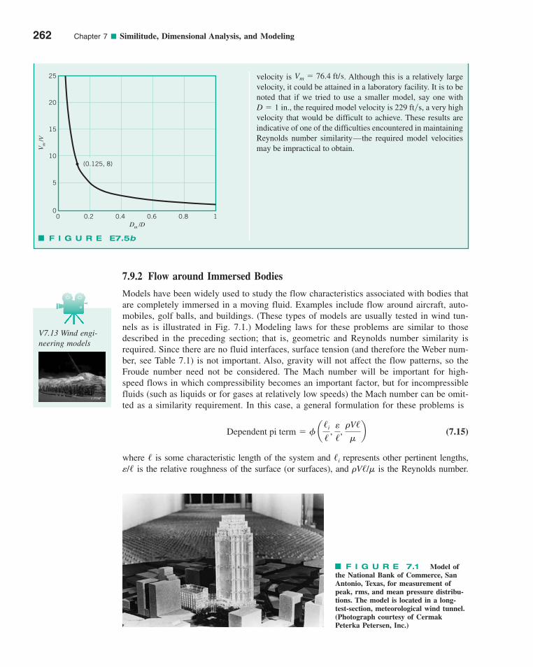
7.9.2 Flow around Immersed Bodies

Models have been widely used to study the flow characteristics associated with bodies thatare completely immersed in a moving fluid. Examples include flow around aircraft, auto-mobiles, golf balls, and buildings. (These types of models are usually tested in wind tun-nels as is illustrated in Fig. 7.1.) Modeling laws for these problems are similar to thosedescribed in the preceding section; that is, geometric and Reynolds number similarity isrequired. Since there are no fluid interfaces, surface tension (and therefore the Weber num-ber, see Table 7.1) is not important. Also, gravity will not affect the flow patterns, so theFroude number need not be considered. The Mach number will be important for high-speed flows in which compressibility becomes an important factor, but for incompressiblefluids (such as liquids or for gases at relatively low speeds) the Mach number can be omit-ted as a similarity requirement. In this case, a general formulation for these problems is

(7.15)

where � is some characteristic length of the system and �i represents other pertinent lengths,�/� is the relative roughness of the surface (or surfaces), and �V�/� is the Reynolds number.

Dependent pi term � � a/i

/, e

/,

�V/�b

262 Chapter 7 ■ Similitude, Dimensional Analysis, and Modeling

velocity is . Although this is a relatively large velocity, it could be attained in a laboratory facility. It is to benoted that if we tried to use a smaller model, say one with

the required model velocity is 229 ft�s, a very highvelocity that would be difficult to achieve. These results areindicative of one of the difficulties encountered in maintainingReynolds number similarity—the required model velocitiesmay be impractical to obtain.

D � 1 in.,

Vm � 76.4 ft/s25

20

15

10

5

00 0.2 0.4 0.6 0.8 1

Dm /D

Vm

/V

(0.125, 8)

F I G U R E E7.5b

F I G U R E 7.1 Model ofthe National Bank of Commerce, SanAntonio, Texas, for measurement ofpeak, rms, and mean pressure distribu-tions. The model is located in a long-test-section, meteorological wind tunnel.(Photograph courtesy of CermakPeterka Petersen, Inc.)

V7.13 Wind engi-neering models

c07Similitude,DimensionalAnalysis,andModeling.qxd 9/24/10 2:04 PM Page 262

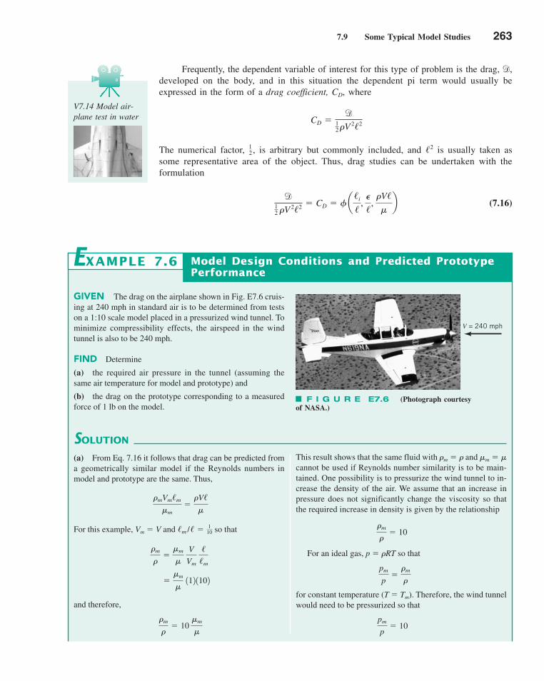
7.9 Some Typical Model Studies 263

Frequently, the dependent variable of interest for this type of problem is the drag, d,developed on the body, and in this situation the dependent pi term would usually beexpressed in the form of a drag coefficient, CD, where

The numerical factor, 1—

2, is arbitrary but commonly included, and �2 is usually taken assome representative area of the object. Thus, drag studies can be undertaken with theformulation

(7.16)d

12 �V 2/2 � CD � � a

/i

/,

�

/,

�V/�b

CD �d

12 �V 2/2

V7.14 Model air-plane test in water

GIVEN The drag on the airplane shown in Fig. E7.6 cruis-ing at 240 mph in standard air is to be determined from testson a 1:10 scale model placed in a pressurized wind tunnel. Tominimize compressibility effects, the airspeed in the windtunnel is also to be 240 mph.

FIND Determine

(a) the required air pressure in the tunnel (assuming thesame air temperature for model and prototype) and

(b) the drag on the prototype corresponding to a measuredforce of 1 lb on the model.

SOLUTION

Model Design Conditions and Predicted PrototypePerformance

This result shows that the same fluid with �m � � and �m � �cannot be used if Reynolds number similarity is to be main-tained. One possibility is to pressurize the wind tunnel to in-crease the density of the air. We assume that an increase inpressure does not significantly change the viscosity so thatthe required increase in density is given by the relationship

For an ideal gas, p � �RT so that

for constant temperature (T � Tm). Therefore, the wind tunnelwould need to be pressurized so that

pm

p� 10

pm

p�

�m

�

�m

�� 10

EXAMPLE 7.6

(a) From Eq. 7.16 it follows that drag can be predicted froma geometrically similar model if the Reynolds numbers inmodel and prototype are the same. Thus,

For this example, Vm � V and so that

and therefore,

�m

�� 10

�m

�

��m

� 112 1102

�m

��

�m

�

V

Vm

//m

/m // � 110

�mVm/m

�m�

�V/�

V = 240 mph

F I G U R E E7.6 (Photograph courtesy of NASA.)

c07Similitude,DimensionalAnalysis,andModeling.qxd 9/24/10 2:04 PM Page 263

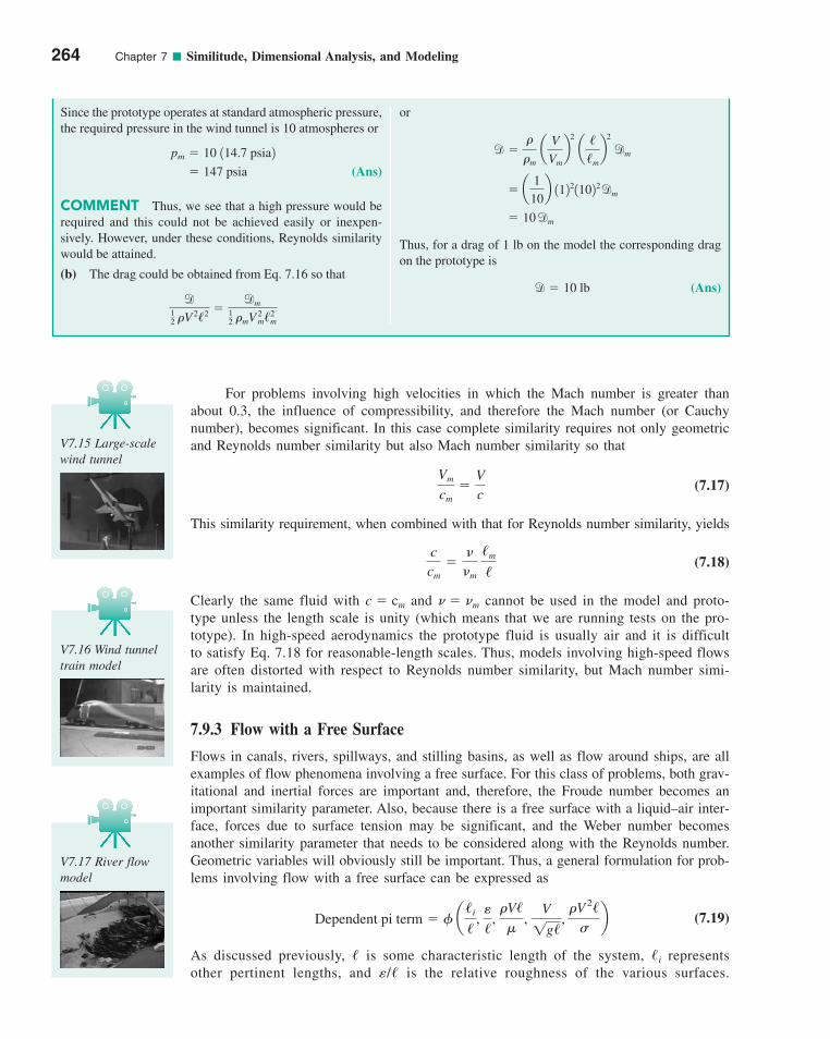
For problems involving high velocities in which the Mach number is greater thanabout 0.3, the influence of compressibility, and therefore the Mach number (or Cauchynumber), becomes significant. In this case complete similarity requires not only geometricand Reynolds number similarity but also Mach number similarity so that

(7.17)

This similarity requirement, when combined with that for Reynolds number similarity, yields

(7.18)

Clearly the same fluid with c � cm and � m cannot be used in the model and proto-type unless the length scale is unity (which means that we are running tests on the pro-totype). In high-speed aerodynamics the prototype fluid is usually air and it is difficultto satisfy Eq. 7.18 for reasonable-length scales. Thus, models involving high-speed flowsare often distorted with respect to Reynolds number similarity, but Mach number simi-larity is maintained.

7.9.3 Flow with a Free Surface

Flows in canals, rivers, spillways, and stilling basins, as well as flow around ships, are allexamples of flow phenomena involving a free surface. For this class of problems, both grav-itational and inertial forces are important and, therefore, the Froude number becomes animportant similarity parameter. Also, because there is a free surface with a liquid–air inter-face, forces due to surface tension may be significant, and the Weber number becomesanother similarity parameter that needs to be considered along with the Reynolds number.Geometric variables will obviously still be important. Thus, a general formulation for prob-lems involving flow with a free surface can be expressed as

(7.19)

As discussed previously, � is some characteristic length of the system, �i representsother pertinent lengths, and �/� is the relative roughness of the various surfaces.

Dependent pi term � � a/i

/, e

/,

�V/�

, V

1g/,

�V2/�b

ccm

�

m /m

/

Vm

cm�

Vc

264 Chapter 7 ■ Similitude, Dimensional Analysis, and Modeling

or

Thus, for a drag of 1 lb on the model the corresponding dragon the prototype is

(Ans)d � 10 lb

� 10dm

� a1

10b 112211022dm

d ��

�m a

V

Vm

b2

a//m

b2

dm

Since the prototype operates at standard atmospheric pressure,the required pressure in the wind tunnel is 10 atmospheres or

(Ans)

COMMENT Thus, we see that a high pressure would berequired and this could not be achieved easily or inexpen-sively. However, under these conditions, Reynolds similaritywould be attained.

(b) The drag could be obtained from Eq. 7.16 so that

d

12 �V 2/2 �

dm12 �mV 2

m/m2

� 147 psia

pm � 10 114.7 psia2

V7.15 Large-scalewind tunnel

V7.16 Wind tunneltrain model

V7.17 River flowmodel

c07Similitude,DimensionalAnalysis,andModeling.qxd 9/24/10 2:05 PM Page 264

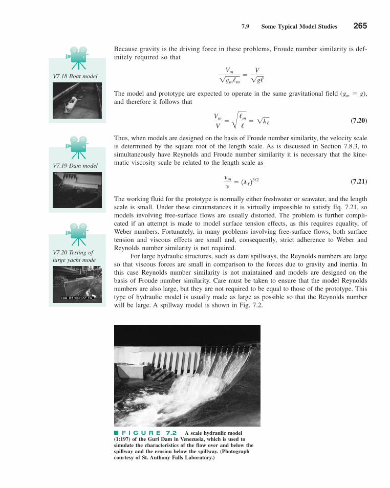
7.9 Some Typical Model Studies 265

Because gravity is the driving force in these problems, Froude number similarity is def-initely required so that

The model and prototype are expected to operate in the same gravitational field (gm � g),and therefore it follows that

(7.20)

Thus, when models are designed on the basis of Froude number similarity, the velocity scaleis determined by the square root of the length scale. As is discussed in Section 7.8.3, tosimultaneously have Reynolds and Froude number similarity it is necessary that the kine-matic viscosity scale be related to the length scale as

(7.21)

The working fluid for the prototype is normally either freshwater or seawater, and the lengthscale is small. Under these circumstances it is virtually impossible to satisfy Eq. 7.21, somodels involving free-surface flows are usually distorted. The problem is further compli-cated if an attempt is made to model surface tension effects, as this requires equality, ofWeber numbers. Fortunately, in many problems involving free-surface flows, both surfacetension and viscous effects are small and, consequently, strict adherence to Weber andReynolds number similarity is not required.

For large hydraulic structures, such as dam spillways, the Reynolds numbers are largeso that viscous forces are small in comparison to the forces due to gravity and inertia. Inthis case Reynolds number similarity is not maintained and models are designed on thebasis of Froude number similarity. Care must be taken to ensure that the model Reynoldsnumbers are also large, but they are not required to be equal to those of the prototype. Thistype of hydraulic model is usually made as large as possible so that the Reynolds numberwill be large. A spillway model is shown in Fig. 7.2.

m

� 1�/2

3/2

Vm

V�B

/m

/� 1�/

Vm

1gm/m

�V

1g/

F I G U R E 7.2 A scale hydraulic model(1:197) of the Guri Dam in Venezuela, which is used tosimulate the characteristics of the flow over and below thespillway and the erosion below the spillway. (Photographcourtesy of St. Anthony Falls Laboratory.)

V7.18 Boat model

V7.19 Dam model

V7.20 Testing oflarge yacht mode

c07Similitude,DimensionalAnalysis,andModeling.qxd 9/24/10 2:05 PM Page 265

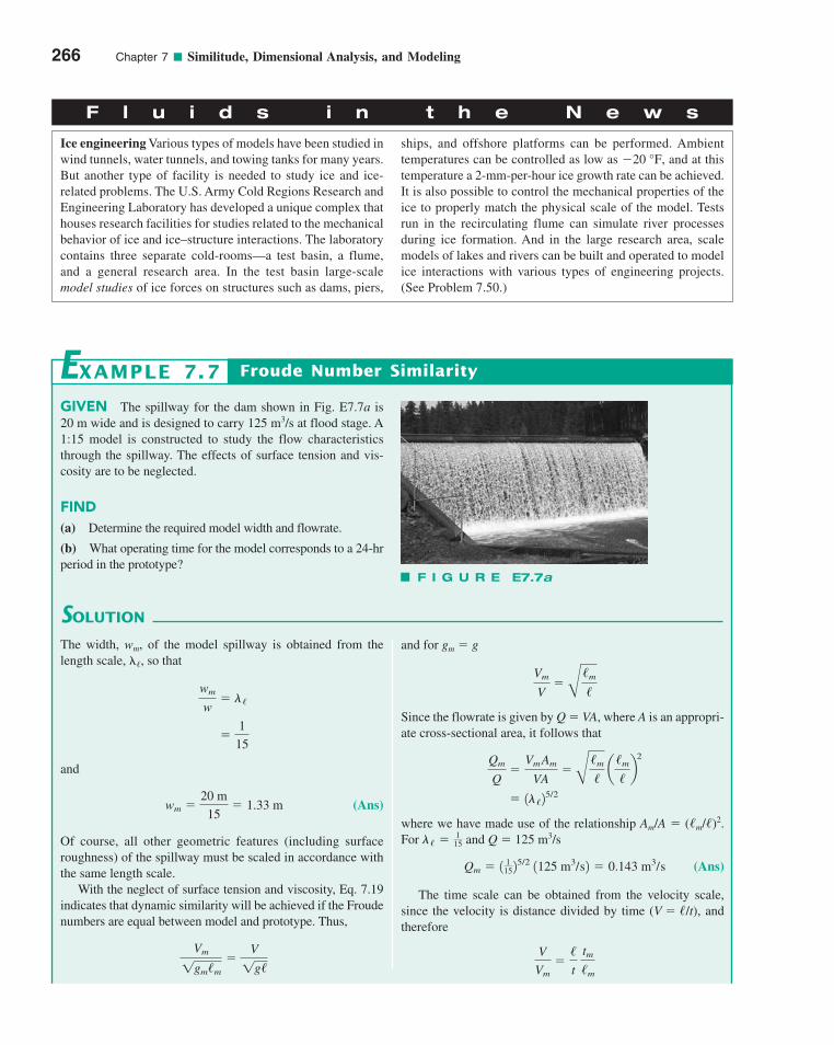
266 Chapter 7 ■ Similitude, Dimensional Analysis, and Modeling

F l u i d s i n t h e N e w s

Ice engineering Various types of models have been studied inwind tunnels, water tunnels, and towing tanks for many years.But another type of facility is needed to study ice and ice-related problems. The U.S. Army Cold Regions Research andEngineering Laboratory has developed a unique complex thathouses research facilities for studies related to the mechanicalbehavior of ice and ice–structure interactions. The laboratorycontains three separate cold-rooms—a test basin, a flume,and a general research area. In the test basin large-scalemodel studies of ice forces on structures such as dams, piers,

ships, and offshore platforms can be performed. Ambienttemperatures can be controlled as low as , and at thistemperature a 2-mm-per-hour ice growth rate can be achieved.It is also possible to control the mechanical properties of theice to properly match the physical scale of the model. Testsrun in the recirculating flume can simulate river processesduring ice formation. And in the large research area, scalemodels of lakes and rivers can be built and operated to modelice interactions with various types of engineering projects.(See Problem 7.50.)

�20 °F

GIVEN The spillway for the dam shown in Fig. E7.7a is 20 m wide and is designed to carry 125 m3/s at flood stage. A1:15 model is constructed to study the flow characteristicsthrough the spillway. The effects of surface tension and vis-cosity are to be neglected.

FIND(a) Determine the required model width and flowrate.

(b) What operating time for the model corresponds to a 24-hrperiod in the prototype?

SOLUTION

Froude Number Similarity

and for gm � g

Since the flowrate is given by Q � VA, where A is an appropri-ate cross-sectional area, it follows that

where we have made use of the relationship Am/A � (�m/�)2.For and Q � 125 m3/s

(Ans)

The time scale can be obtained from the velocity scale,since the velocity is distance divided by time (V � �/t), andtherefore

V

Vm�

/t tm/m

Qm � 1 115 2

5/2 1125 m3/s2 � 0.143 m3/s

�/ � 115

� 1�/25/2

Qm

Q�

Vm Am

VA�B

/m

/ a

/m

/b

2

Vm

V�B

/m

/

EXAMPLE 7.7

The width, wm, of the model spillway is obtained from thelength scale, ��, so that

and

(Ans)

Of course, all other geometric features (including surfaceroughness) of the spillway must be scaled in accordance withthe same length scale.

With the neglect of surface tension and viscosity, Eq. 7.19indicates that dynamic similarity will be achieved if the Froudenumbers are equal between model and prototype. Thus,

Vm

1gm/m

�V

1g/

wm �20 m

15� 1.33 m

�1

15

wm

w� �/

F I G U R E E7.7a

c07Similitude,DimensionalAnalysis,andModeling.qxd 9/24/10 2:05 PM Page 266

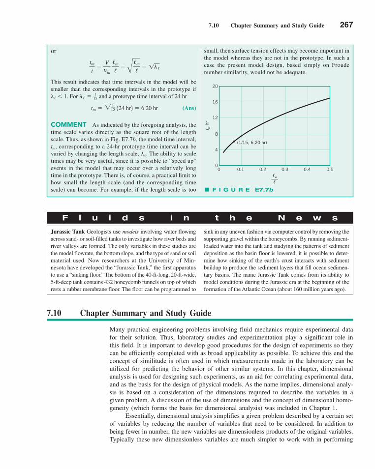
7.10 Chapter Summary and Study Guide 267

small, then surface tension effects may become important inthe model whereas they are not in the prototype. In such acase the present model design, based simply on Froudenumber similarity, would not be adequate.

or

This result indicates that time intervals in the model will besmaller than the corresponding intervals in the prototype if�� � 1. For and a prototype time interval of 24 hr

(Ans)

COMMENT As indicated by the foregoing analysis, thetime scale varies directly as the square root of the lengthscale. Thus, as shown in Fig. E7.7b, the model time interval,

, corresponding to a 24-hr prototype time interval can bevaried by changing the length scale, . The ability to scaletimes may be very useful, since it is possible to “speed up”events in the model that may occur over a relatively longtime in the prototype. There is, of course, a practical limit tohow small the length scale (and the corresponding timescale) can become. For example, if the length scale is too

l/

tm

tm � 2115 124 hr2 � 6.20 hr

�/ � 115

tmt

�V

Vm /m

/�B

/m

/� 1�/

16

12

8

4

00 0.1 0.2 0.3 0.4 0.5

t m, h

r

(1/15, 6.20 hr)

20

�m

�

F I G U R E E7.7b

F l u i d s i n t h e N e w s

Jurassic Tank Geologists use models involving water flowingacross sand- or soil-filled tanks to investigate how river beds andriver valleys are formed. The only variables in these studies arethe model flowrate, the bottom slope, and the type of sand or soilmaterial used. Now researchers at the University of Min-nesota have developed the “Jurassic Tank,” the first apparatusto use a “sinking floor.” The bottom of the 40-ft-long, 20-ft-wide,5-ft-deep tank contains 432 honeycomb funnels on top of whichrests a rubber membrane floor. The floor can be programmed to

sink in any uneven fashion via computer control by removing thesupporting gravel within the honeycombs. By running sediment-loaded water into the tank and studying the patterns of sedimentdeposition as the basin floor is lowered, it is possible to deter-mine how sinking of the earth’s crust interacts with sedimentbuildup to produce the sediment layers that fill ocean sedimen-tary basins. The name Jurassic Tank comes from its ability tomodel conditions during the Jurassic era at the beginning of theformation of the Atlantic Ocean (about 160 million years ago).

7.10 Chapter Summary and Study Guide

Many practical engineering problems involving fluid mechanics require experimental datafor their solution. Thus, laboratory studies and experimentation play a significant role inthis field. It is important to develop good procedures for the design of experiments so theycan be efficiently completed with as broad applicability as possible. To achieve this end theconcept of similitude is often used in which measurements made in the laboratory can beutilized for predicting the behavior of other similar systems. In this chapter, dimensionalanalysis is used for designing such experiments, as an aid for correlating experimental data,and as the basis for the design of physical models. As the name implies, dimensional analy-sis is based on a consideration of the dimensions required to describe the variables in agiven problem. A discussion of the use of dimensions and the concept of dimensional homo-geneity (which forms the basis for dimensional analysis) was included in Chapter 1.

Essentially, dimensional analysis simplifies a given problem described by a certain setof variables by reducing the number of variables that need to be considered. In addition tobeing fewer in number, the new variables are dimensionless products of the original variables.Typically these new dimensionless variables are much simpler to work with in performing

c07Similitude,DimensionalAnalysis,andModeling.qxd 9/24/10 2:05 PM Page 267

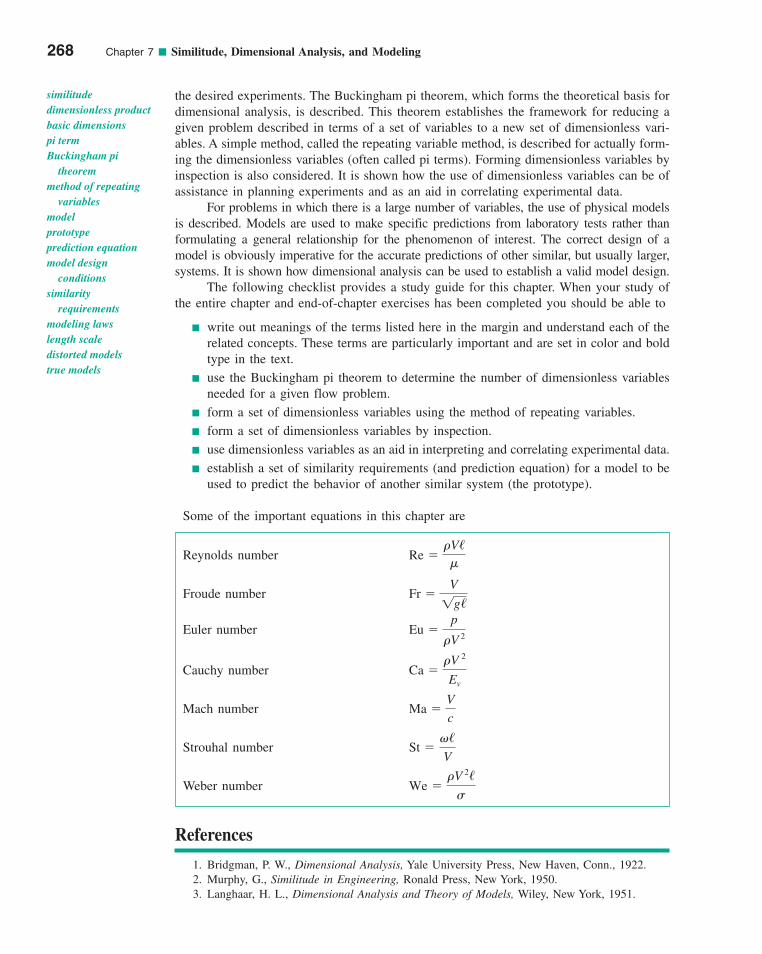
the desired experiments. The Buckingham pi theorem, which forms the theoretical basis fordimensional analysis, is described. This theorem establishes the framework for reducing agiven problem described in terms of a set of variables to a new set of dimensionless vari-ables. A simple method, called the repeating variable method, is described for actually form-ing the dimensionless variables (often called pi terms). Forming dimensionless variables byinspection is also considered. It is shown how the use of dimensionless variables can be ofassistance in planning experiments and as an aid in correlating experimental data.

For problems in which there is a large number of variables, the use of physical modelsis described. Models are used to make specific predictions from laboratory tests rather thanformulating a general relationship for the phenomenon of interest. The correct design of amodel is obviously imperative for the accurate predictions of other similar, but usually larger,systems. It is shown how dimensional analysis can be used to establish a valid model design.

The following checklist provides a study guide for this chapter. When your study ofthe entire chapter and end-of-chapter exercises has been completed you should be able to

write out meanings of the terms listed here in the margin and understand each of therelated concepts. These terms are particularly important and are set in color and boldtype in the text.

use the Buckingham pi theorem to determine the number of dimensionless variablesneeded for a given flow problem.

form a set of dimensionless variables using the method of repeating variables.

form a set of dimensionless variables by inspection.

use dimensionless variables as an aid in interpreting and correlating experimental data.

establish a set of similarity requirements (and prediction equation) for a model to beused to predict the behavior of another similar system (the prototype).

Some of the important equations in this chapter are

Reynolds number

Froude number

Euler number

Cauchy number

Mach number

Strouhal number

Weber number

References

1. Bridgman, P. W., Dimensional Analysis, Yale University Press, New Haven, Conn., 1922.2. Murphy, G., Similitude in Engineering, Ronald Press, New York, 1950.3. Langhaar, H. L., Dimensional Analysis and Theory of Models, Wiley, New York, 1951.

We �rV 2/s

St �v/V

Ma �V

c

Ca �rV 2

Ev

Eu �p

rV 2

Fr �V

1g/

Re �rV/m

268 Chapter 7 ■ Similitude, Dimensional Analysis, and Modeling

similitudedimensionless productbasic dimensionspi termBuckingham pi

theoremmethod of repeating

variablesmodelprototypeprediction equationmodel design

conditionssimilarity

requirementsmodeling lawslength scaledistorted modelstrue models

c07Similitude,DimensionalAnalysis,andModeling.qxd 9/24/10 2:05 PM Page 268

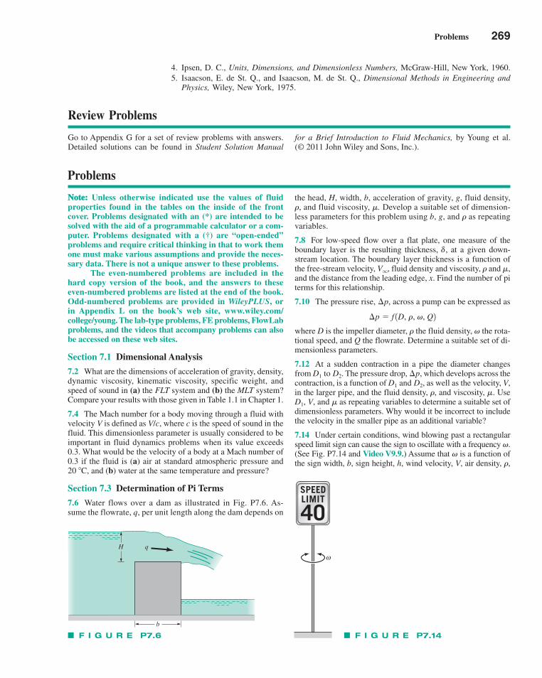
Problems 269

4. Ipsen, D. C., Units, Dimensions, and Dimensionless Numbers, McGraw-Hill, New York, 1960.5. Isaacson, E. de St. Q., and Isaacson, M. de St. Q., Dimensional Methods in Engineering and

Physics, Wiley, New York, 1975.

Review Problems

Go to Appendix G for a set of review problems with answers.Detailed solutions can be found in Student Solution Manual

for a Brief Introduction to Fluid Mechanics, by Young et al. (© 2011 John Wiley and Sons, Inc.).

Problems

NNoottee:: Unless otherwise indicated use the values of fluidproperties found in the tables on the inside of the frontcover. Problems designated with an (*) are intended to besolved with the aid of a programmable calculator or a com-puter. Problems designated with a (†) are “open-ended”problems and require critical thinking in that to work themone must make various assumptions and provide the neces-sary data. There is not a unique answer to these problems.

The even-numbered problems are included in thehard copy version of the book, and the answers to theseeven-numbered problems are listed at the end of the book.Odd-numbered problems are provided in WileyPLUS, orin Appendix L on the book’s web site, www.wiley.com/college/young. The lab-type problems, FE problems, FlowLabproblems, and the videos that accompany problems can alsobe accessed on these web sites.

Section 7.1 Dimensional Analysis

7.2 What are the dimensions of acceleration of gravity, density,dynamic viscosity, kinematic viscosity, specific weight, andspeed of sound in (a) the FLT system and (b) the MLT system?Compare your results with those given in Table 1.1 in Chapter 1.

7.4 The Mach number for a body moving through a fluid withvelocity V is defined as V/c, where c is the speed of sound in thefluid. This dimensionless parameter is usually considered to beimportant in fluid dynamics problems when its value exceeds0.3. What would be the velocity of a body at a Mach number of0.3 if the fluid is (a) air at standard atmospheric pressure and 20 �C, and (b) water at the same temperature and pressure?

Section 7.3 Determination of Pi Terms

7.6 Water flows over a dam as illustrated in Fig. P7.6. As-sume the flowrate, q, per unit length along the dam depends on

the head, H, width, b, acceleration of gravity, g, fluid density,�, and fluid viscosity, �. Develop a suitable set of dimension-less parameters for this problem using b, g, and � as repeatingvariables.

7.8 For low-speed flow over a flat plate, one measure of theboundary layer is the resulting thickness, , at a given down-stream location. The boundary layer thickness is a function ofthe free-stream velocity, , fluid density and viscosity, � and �,and the distance from the leading edge, x. Find the number of piterms for this relationship.

7.10 The pressure rise, across a pump can be expressed as

where D is the impeller diameter, the fluid density, the rota-tional speed, and Q the flowrate. Determine a suitable set of di-mensionless parameters.

7.12 At a sudden contraction in a pipe the diameter changesfrom The pressure drop, which develops across thecontraction, is a function of as well as the velocity, V,in the larger pipe, and the fluid density, and viscosity, Use

as repeating variables to determine a suitable set ofdimensionless parameters. Why would it be incorrect to includethe velocity in the smaller pipe as an additional variable?

7.14 Under certain conditions, wind blowing past a rectangularspeed limit sign can cause the sign to oscillate with a frequency .(See Fig. P7.14 and Video V9.9.) Assume that is a function ofthe sign width, b, sign height, h, wind velocity, V, air density, �,

��

D1, V, and ��.�,

D1 and D2,¢p,D1 to D2.

��

¢p � f 1D, r, v, Q2

¢p,

Vq

�

H q

b

F I G U R E P7.6 F I G U R E P7.14

ω

SPEEDLIMIT

40

c07Similitude,DimensionalAnalysis,andModeling.qxd 10/18/10 8:02 AM Page 269

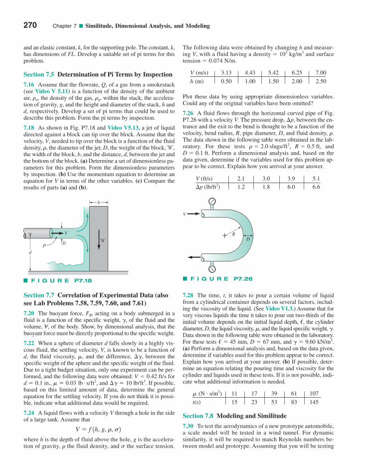
270 Chapter 7 ■ Similitude, Dimensional Analysis, and Modeling

and an elastic constant, k, for the supporting pole. The constant, k,has dimensions of FL. Develop a suitable set of pi terms for thisproblem.

Section 7.5 Determination of Pi Terms by Inspection

7.16 Assume that the flowrate, Q, of a gas from a smokestack(see Video V 5.11) is a function of the density of the ambientair, , the density of the gas, , within the stack, the accelera-tion of gravity, g, and the height and diameter of the stack, h andd, respectively. Develop a set of pi terms that could be used todescribe this problem. Form the pi terms by inspection.

7.18 As shown in Fig. P7.18 and Video V5.13, a jet of liquiddirected against a block can tip over the block. Assume that thevelocity, V, needed to tip over the block is a function of the fluiddensity, �, the diameter of the jet, D, the weight of the block,w,the width of the block, b, and the distance, d, between the jet andthe bottom of the block. (a) Determine a set of dimensionless pa-rameters for this problem. Form the dimensionless parametersby inspection. (b) Use the momentum equation to determine anequation for V in terms of the other variables. (c) Compare theresults of parts (a) and (b).

�g�a

Section 7.7 Correlation of Experimental Data (alsosee Lab Problems 7.58, 7.59, 7.60, and 7.61)

7.20 The buoyant force, FB, acting on a body submerged in afluid is a function of the specific weight, �, of the fluid and thevolume, , of the body. Show, by dimensional analysis, that thebuoyant force must be directly proportional to the specific weight.

7.22 When a sphere of diameter d falls slowly in a highly vis-cous fluid, the settling velocity, V, is known to be a function ofd, the fluid viscosity, �, and the difference, , between thespecific weight of the sphere and the specific weight of the fluid.Due to a tight budget situation, only one experiment can be per-formed, and the following data were obtained: for

If possible,based on this limited amount of data, determine the generalequation for the settling velocity. If you do not think it is possi-ble, indicate what additional data would be required.

7.24 A liquid flows with a velocity V through a hole in the sideof a large tank. Assume that

where h is the depth of fluid above the hole, g is the accelera-tion of gravity, � the fluid density, and � the surface tension.

V � f 1h, g, �, �2

lb # s/ft2, and ¢� � 10 lb/ft3.d � 0.1 in., � � 0.03V � 0.42 ft/s

¢�

V

The following data were obtained by changing h and measur-ing V, with a fluid having a density � 103 kg/m3 and surfacetension � 0.074 N/m.

V (m/s) 3.13 4.43 5.42 6.25 7.00

h (m) 0.50 1.00 1.50 2.00 2.50

Plot these data by using appropriate dimensionless variables.Could any of the original variables have been omitted?

7.26 A fluid flows through the horizontal curved pipe of Fig.P7.26 with a velocity V. The pressure drop, , between the en-trance and the exit to the bend is thought to be a function of thevelocity, bend radius, R, pipe diameter, D, and fluid density,The data shown in the following table were obtained in the lab-oratory. For these tests and

Perform a dimensional analysis and, based on thedata given, determine if the variables used for this problem ap-pear to be correct. Explain how you arrived at your answer.

V (ft/s) 2.1 3.0 3.9 5.1�p (lb/ft2) 1.2 1.8 6.0 6.6

D � 0.1 ft.R � 0.5 ft,� � 2.0 slugs/ft3,

�.

¢p

7.28 The time, t, it takes to pour a certain volume of liquidfrom a cylindrical container depends on several factors, includ-ing the viscosity of the liquid. (See Video V1.3.) Assume that forvery viscous liquids the time it takes to pour out two-thirds of theinitial volume depends on the initial liquid depth, �, the cylinderdiameter, D, the liquid viscosity, �, and the liquid specific weight, �.Data shown in the following table were obtained in the laboratory.For these tests � � 45 mm, D � 67 mm, and � � 9.60 kN/m3.(a) Perform a dimensional analysis and, based on the data given,determine if variables used for this problem appear to be correct.Explain how you arrived at your answer. (b) If possible, deter-mine an equation relating the pouring time and viscosity for thecylinder and liquids used in these tests. If it is not possible, indi-cate what additional information is needed.

� (N s/m2) 11 17 39 61 107

t(s) 15 23 53 83 145

Section 7.8 Modeling and Similitude

7.30 To test the aerodynamics of a new prototype automobile,a scale model will be tested in a wind tunnel. For dynamicsimilarity, it will be required to match Reynolds numbers be-tween model and prototype. Assuming that you will be testing

.

V

D

d

b

ρ�

F I G U R E P7.18

V

RD

F I G U R E P7.26

c07Similitude,DimensionalAnalysis,andModeling.qxd 9/24/10 2:05 PM Page 270

Problems 271

a -scale model and both model and prototype will be exposedto standard air pressure, will it be better for the wind tunnel airto be colder or hotter than standard sea-level air temperature of 15 �C? Why?

7.32 A liquid contained in a steadily rotating cylinder with avertical axis moves as a rigid body. In this case, as shown in Fig.P7.32 and Video V7.3, the fluid velocity, V, varies directly withthe radius r so that V � r� where � is the angular velocity of therotating cylinder. Assume that the characteristic Reynolds num-ber for this system is based on the radius and velocity at the wallof the cylinder. (a) For a 12-in.-diameter cylinder rotating withan angular velocity � � 0.4, rad/s, calculate the Reynolds num-ber if the liquid has a kinematic viscosity of (i) 0.33 ft2/s or (ii)0.33 10�2 ft2/s. (b) If the cylinder were suddenly stopped,would you expect the motion of the liquids to be similar for the twoliquids of part (a)? Explain. Do the results shown in Video V7.3support your conclusions?

110

7.34 The drag characteristics of a torpedo are to be studied ina water tunnel using a 1:5-scale model. The tunnel operateswith freshwater at , whereas the prototype torpedo is tobe used in seawater at To correctly simulate the behav-ior of the prototype moving with a velocity of 30 m/s, what ve-locity is required in the water tunnel? Assume Reynolds numbersimilarity.

7.36 Carbon tetrachloride flows with a velocity of 0.30 m/sthrough a 30-mm-diameter tube. A model of this system is to bedeveloped using standard air as the model fluid. The air velocityis to be 2 m/s. What tube diameter is required for the model if dynamic similarity is to be maintained between model andprototype?

7.38 The drag, on a sphere located in a pipe through whicha fluid is flowing is to be determined experimentally (see Fig.P7.38). Assume that the drag is a function of the sphere diame-ter, d, the pipe diameter, D, the fluid velocity, V, and the fluiddensity, (a) What dimensionless parameters would you usefor this problem? (b) Some experiments using water indicatethat for and the drag is

If possible, estimate the drag on a sphere locatedin a 2-ft-diameter pipe through which water is flowing with avelocity of 6 ft/s. The sphere diameter is such that geometricsimilarity is maintained. If it is not possible, explain why not.

1.5 10�3 lb.V � 2 ft/s,D � 0.5 in.,d � 0.2 in.,

�.

d,

15.6 °C.20 °C

7.40 The drag on a sphere moving in a fluid is known to be afunction of the sphere diameter, the velocity, and the fluid vis-cosity and density. Laboratory tests on a 4-in.-diameter spherewere performed in a water tunnel, and some model data are plot-ted in Fig. P7.40. For these tests the viscosity of the water was2.3 10�5 lb s/ft2 and the water density was 1.94 slugs/ft3. Es-timate the drag on an 8-ft-diameter balloon moving in air at a ve-locity of 3 ft/s. Assume the air to have a viscosity of 3.7 10�7

lb s/ft2 and a density of 2.38 10�3 slugs/ft3.#

#

7.42 A large, rigid, rectangular billboard is supported by anelastic column as shown in Fig. P7.42. There is concern aboutthe deflection, of the top of the structure during a high windof velocity V. A wind tunnel test is to be conducted with a 1:15-scale model. Assume the pertinent column variables are itslength and cross-sectional dimensions and the modulus of elas-ticity of the material used for the column. The only important“wind” variables are the air density and velocity. (a) Determinethe model design conditions and the prediction equation for thedeflection. (b) If the same structural materials are used for themodel and prototype, and the wind tunnel operates under stan-dard atmospheric conditions, what is the required wind tunnelvelocity to match an 80-km/hr wind?

,

†7.44 If a large oil spill occurs from a tanker operating near acoastline, the time it would take for the oil to reach shore is ofgreat concern. Design a model system that can be used to inves-tigate this type of problem in the laboratory. Indicate all assump-tions made in developing the design and discuss any difficulty

ω

V

r

F I G U R E P7.32

6

4

2

00 2 4 6 8 10 12

Model velocity, ft/s

Mod

el d

rag,

lb

F I G U R E P7.40

Billboard

V

Front view Side view

δ

F I G U R E P7.42

Vd DSphere

F I G U R E P7.38

c07Similitude,DimensionalAnalysis,andModeling.qxd 9/24/10 2:06 PM Page 271

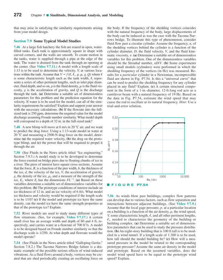
272 Chapter 7 ■ Similitude, Dimensional Analysis, and Modeling

that may arise in satisfying the similarity requirements arisingfrom your model design.

Section 7.9 Some Typical Model Studies

7.46 At a large fish hatchery the fish are reared in open, water-filled tanks. Each tank is approximately square in shape withcurved corners, and the walls are smooth. To create motion inthe tanks, water is supplied through a pipe at the edge of thetank. The water is drained from the tank through an opening atthe center. (See Video V7.11.) A model with a length scale of1:13 is to be used to determine the velocity, V, at various loca-tions within the tank. Assume that V � f (�, �i , �, �, g, Q) where �is some characteristic length such as the tank width, �i repre-sents a series of other pertinent lengths, such as inlet pipe diam-eter, fluid depth, and so on, � is the fluid density, � is the fluid vis-cosity, g is the acceleration of gravity, and Q is the dischargethrough the tank. (a) Determine a suitable set of dimensionlessparameters for this problem and the prediction equation for thevelocity. If water is to be used for the model, can all of the simi-larity requirements be satisfied? Explain and support your answerwith the necessary calculations. (b) If the flowrate into the full-sized tank is 250 gpm, determine the required value for the modeldischarge assuming Froude number similarity. What model depthwill correspond to a depth of 32 in. in the full-sized tank?

7.48 A new blimp will move at 6 m/s in 20 �C air, and we wantto predict the drag force. Using a 1:13-scale model in water at20 �C and measuring a 2500-N drag force on the model, deter-mine (a) the required water velocity, (b) the drag on the proto-type blimp, and (c) the power that will be required to propel itthrough the air.

7.50 (See Fluids in the News article titled “Ice engineering,”Section 7.9.3.) A model study is to be developed to determinethe force exerted on bridge piers due to floating chunks of ice ina river. The piers of interest have square cross sections. Assumethat the force, R, is a function of the pier width, b, the thickness ofthe ice, d, the velocity of the ice, V, the acceleration of gravity,g, the density of the ice, , and a measure of the strength of theice, , where has the dimensions (a) Based on thesevariables determine a suitable set of dimensionless variables forthis problem. (b) The prototype conditions of interest include anice thickness of 12 in. and an ice velocity of 6 ft/s. What modelice thickness and velocity would be required if the length scaleis to be 1/10? (c) If the model and prototype ice have the samedensity, can the model ice have the same strength properties asthat of the prototype ice? Explain.

7.52 River models are used to study many different types offlow situations. (See, for example, Video V7.17.) A certainsmall river has an average width and depth of 60 and 4 ft, re-spectively, and carries water at a flowrate of 700 ft3/s. A modelis to be designed based on Froude number similarity so that thedischarge scale is 1/250. At what depth and flowrate would themodel operate?

7.54 (See Fluids in the News article titled “Galloping Gertie,”Section 7.8.2.) The Tacoma Narrows Bridge failure is a dra-matic example of the possible serious effects of wind-inducedvibrations. As a fluid flows around a body, vortices may be cre-ated that are shed periodically creating an oscillating force on

FL�2.EiEi

�i

the body. If the frequency of the shedding vortices coincideswith the natural frequency of the body, large displacements ofthe body can be induced as was the case with the Tacoma Nar-rows bridge. To illustrate this type of phenomenon, considerfluid flow past a circular cylinder. Assume the frequency, n, ofthe shedding vortices behind the cylinder is a function of thecylinder diameter, D, the fluid velocity, V, and the fluid kine-matic viscosity, . (a) Determine a suitable set of dimensionlessvariables for this problem. One of the dimensionless variablesshould be the Strouhal number, . (b) Some experimentsusing small models (cylinders) were performed in which theshedding frequency of the vortices (in Hz) was measured. Re-sults for a particular cylinder in a Newtonian, incompressiblefluid are shown in Fig. P7.54. Is this a “universal curve” thatcan be used to predict the shedding frequency for any cylinderplaced in any fluid? Explain. (c) A certain structural compo-nent in the form of a 1-in.-diameter, 12-ft-long rod acts as acantilever beam with a natural frequency of 19 Hz. Based onthe data in Fig. P7.54, estimate the wind speed that maycause the rod to oscillate at its natural frequency. Hint: Use atrial-and-error solution.

nD/V

7.56 As winds blow past buildings, complex flow patternscan develop due to various factors, such as flow separation andinteractions between adjacent buildings. (See Video V7.9.)Assume that the local gage pressure, p, at a particular locationon a building is a function of the air density, �, the wind speed,V, some characteristic length, �, and all other pertinent lengths,�i, needed to characterize the geometry of the building orbuilding complex. (a) Determine a suitable set of dimension-less parameters that can be used to study the pressure distribu-tion. (b) An eight-story building that is 100 ft tall is to be mod-eled in a wind tunnel. If a length scale of 1:300 is to be used,how tall should the model building be? (c) How will a mea-sured pressure in the model be related to the correspondingprototype pressure? Assume the same air density in the modeland prototype. Based on the assumed variables, does themodel wind speed have to be equal to the prototype windspeed? Explain.

0.22

0.20

0.18

0.16

0.14

0.1210 100 1000 10,000

Re, VD/v

St, n

D/V

F I G U R E P7.54

c07Similitude,DimensionalAnalysis,andModeling.qxd 9/24/10 2:06 PM Page 272

Problems 273

■ Lab Problems

7.58 This problem involves the time that it takes water to drainfrom two geometrically similar tanks. To proceed with thisproblem, go to the book’s web site, www.wiley.com/college/young, or WileyPLUS.

7.60 This problem involves the determination of the head lossfor flow through a valve. To proceed with this problem, go to thebook’s web site, www.wiley.com/college/young, or WileyPLUS.

■ Lifelong Learning Problems

7.62 Microfluidics is the study of fluid flow in fabricated devicesat the micro scale. Advances in microfluidics have enhanced theability of scientists and engineers to perform laboratory experi-ments using miniaturized devices known as a “lab-on-a-chip.”

Obtain information about a lab-on-a-chip device that is availablecommercially and investigate its capabilities. Summarize yourfindings in a brief report.

■ FlowLab Problem

*7.64 This FlowLab problem involves investigation of theReynolds number significance in fluid dynamics through thesimulation of flow past a cylinder. To proceed with this prob-lem, go to the book’s web site, www.wiley.com/college/young,or WileyPLUS.

■ FE Exam Problems

Sample FE (Fundamentals of Engineering) exam questions forfluid mechanics are provided on the book’s web site, www.wiley.com/college/young, or WileyPLUS.

c07Similitude,DimensionalAnalysis,andModeling.qxd 9/24/10 2:06 PM Page 273

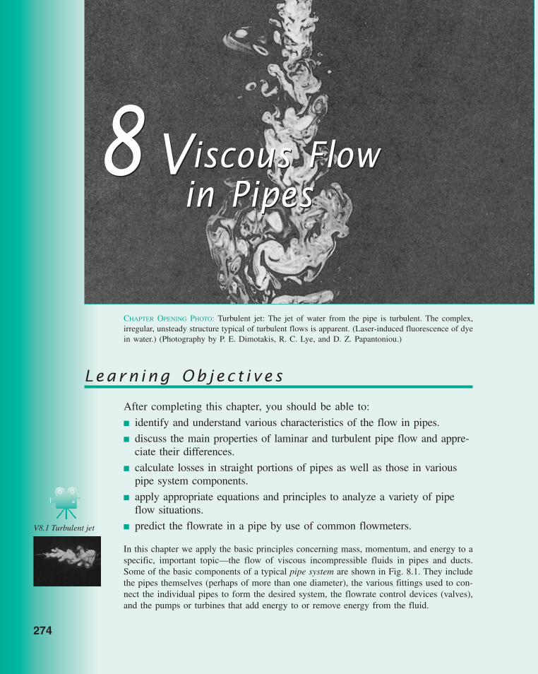
274

CHAPTER OPENING PHOTO: Turbulent jet: The jet of water from the pipe is turbulent. The complex,irregular, unsteady structure typical of turbulent flows is apparent. (Laser-induced fluorescence of dyein water.) (Photography by P. E. Dimotakis, R. C. Lye, and D. Z. Papantoniou.)

Learn ing Ob j ec t i v e s

After completing this chapter, you should be able to:

■ identify and understand various characteristics of the flow in pipes.

■ discuss the main properties of laminar and turbulent pipe flow and appre-ciate their differences.

■ calculate losses in straight portions of pipes as well as those in variouspipe system components.

■ apply appropriate equations and principles to analyze a variety of pipeflow situations.

■ predict the flowrate in a pipe by use of common flowmeters.

In this chapter we apply the basic principles concerning mass, momentum, and energy to aspecific, important topic—the flow of viscous incompressible fluids in pipes and ducts.Some of the basic components of a typical pipe system are shown in Fig. 8.1. They includethe pipes themselves (perhaps of more than one diameter), the various fittings used to con-nect the individual pipes to form the desired system, the flowrate control devices (valves),and the pumps or turbines that add energy to or remove energy from the fluid.

Viscous Flow in Pipes

8 Viscous Flow in Pipes

8

V8.1 Turbulent jet

c08ViscousFlowinPipes.qxd 9/28/10 10:21 AM Page 274

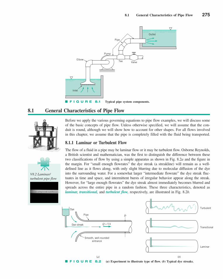
8.1 General Characteristics of Pipe Flow 275

8.1 General Characteristics of Pipe Flow

Before we apply the various governing equations to pipe flow examples, we will discuss someof the basic concepts of pipe flow. Unless otherwise specified, we will assume that the con-duit is round, although we will show how to account for other shapes. For all flows involvedin this chapter, we assume that the pipe is completely filled with the fluid being transported.

8.1.1 Laminar or Turbulent Flow

The flow of a fluid in a pipe may be laminar flow or it may be turbulent flow. Osborne Reynolds,a British scientist and mathematician, was the first to distinguish the difference between thesetwo classifications of flow by using a simple apparatus as shown in Fig. 8.2a and the figure inthe margin. For “small enough flowrates” the dye streak (a streakline) will remain as a well-defined line as it flows along, with only slight blurring due to molecular diffusion of the dyeinto the surrounding water. For a somewhat larger “intermediate flowrate” the dye streak fluc-tuates in time and space, and intermittent bursts of irregular behavior appear along the streak.However, for “large enough flowrates” the dye streak almost immediately becomes blurred andspreads across the entire pipe in a random fashion. These three characteristics, denoted as laminar, transitional, and turbulent flow, respectively, are illustrated in Fig. 8.2b.

Outlet

Pipe

Pump

ElbowTee Valve

Inlet

Q = VA

D

Dye streak

Dye

Smooth, well-roundedentrance

Pipe

(a) (b)

Laminar

Transitional

Turbulent

F I G U R E 8.2 (a) Experiment to illustrate type of flow. (b) Typical dye streaks.

V8.2 Laminar/turbulent pipe flow

F I G U R E 8.1 Typical pipe system components.

c08ViscousFlowinPipes.qxd 9/28/10 10:22 AM Page 275

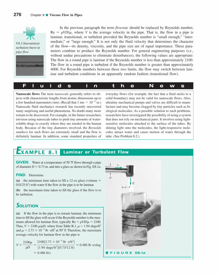
In the previous paragraph the term flowrate should be replaced by Reynolds number,Re � �VD/�, where V is the average velocity in the pipe. That is, the flow in a pipe islaminar, transitional, or turbulent provided the Reynolds number is “small enough,” “inter-mediate,” or “large enough.” It is not only the fluid velocity that determines the characterof the flow—its density, viscosity, and the pipe size are of equal importance. These para-meters combine to produce the Reynolds number. For general engineering purposes (i.e.,without undue precautions to eliminate disturbances), the following values are appropriate:The flow in a round pipe is laminar if the Reynolds number is less than approximately 2100.The flow in a round pipe is turbulent if the Reynolds number is greater than approximately4000. For Reynolds numbers between these two limits, the flow may switch between lam-inar and turbulent conditions in an apparently random fashion (transitional flow).

276 Chapter 8 ■ Viscous Flow in Pipes

F l u i d s i n t h e N e w s

Nanoscale flows The term nanoscale generally refers to ob-jects with characteristic lengths from atomic dimensions up toa few hundred nanometers (nm). (Recall that .)Nanoscale fluid mechanics research has recently uncoveredmany surprising and useful phenomena. No doubt many moreremain to be discovered. For example, in the future researchersenvision using nanoscale tubes to push tiny amounts of water-soluble drugs to exactly where they are needed in the humanbody. Because of the tiny diameters involved, the Reynoldsnumbers for such flows are extremely small and the flow isdefinitely laminar. In addition, some standard properties of

1 nm � 10�9 m

everyday flows (for example, the fact that a fluid sticks to asolid boundary) may not be valid for nanoscale flows. Also,ultratiny mechanical pumps and valves are difficult to manu-facture and may become clogged by tiny particles such as bi-ological molecules. As a possible solution to such problems,researchers have investigated the possibility of using a systemthat does not rely on mechanical parts. It involves using light-sensitive molecules attached to the surface of the tubes. Byshining light onto the molecules, the light-responsive mole-cules attract water and cause motion of water through thetube. (See Problem 8.2.)

GIVEN Water at a temperature of 50 �F flows through a pipeof diameter D � 0.73 in. and into a glass as shown in Fig. E8.1a.

FIND Determine

(a) the minimum time taken to fill a 12-oz glass (volume �0.0125 ft3) with water if the flow in the pipe is to be laminar.

(b) the maximum time taken to fill the glass if the flow is tobe turbulent.

SOLUTION

Laminar or Turbulent FlowEXAMPLE 8.1

(a) If the flow in the pipe is to remain laminar, the minimumtime to fill the glass will occur if the Reynolds number is the max-imum allowed for laminar flow, typically Re � �VD/� � 2100.Thus, V � 2100 �/�D, where from Table B.1, � � 1.94 slugs/ft3

and � � 2.73 � 10�5 lb s/ft2 at 50� F. Therefore, the maximumaverage velocity for laminar flow in the pipe is

� 0.486 ft/s

V �2100�

�D�

210012.73 � 10�5 lb # s/ft22

11.94 slugs/ft32 10.73/12 ft2� 0.486 lb # s/slug

#

F I G U R E E8.1a

�, �Q

D

V

V8.3 Intermittentturbulent burst inpipe flow

c08ViscousFlowinPipes.qxd 9/28/10 10:22 AM Page 276

8.1 General Characteristics of Pipe Flow 277

8.1.2 Entrance Region and Fully Developed Flow

Any fluid flowing in a pipe had to enter the pipe at some location. The region of flow nearwhere the fluid enters the pipe is termed the entrance region and is illustrated in Fig. 8.3.As shown, the fluid typically enters the pipe with a nearly uniform velocity profile at sec-tion (1). As the fluid moves through the pipe, viscous effects cause it to stick to the pipewall (the no-slip boundary condition). This is true whether the fluid is relatively inviscidair or a very viscous oil. Thus, a boundary layer in which viscous effects are important isproduced along the pipe wall such that the initial velocity profile changes with distance

matic viscosity, � � �/�, decreases and the correspondingtimes to fill the glass increase as indicated.

If the flowing fluid had been honey with a kinematic viscos-ity (� � �/�) 3000 times greater than that of water, the velocitiesgiven earlier would be increased by a factor of 3000 and thetimes reduced by the same factor. As shown in the following sec-tions, the pressure needed to force a very viscous fluid through apipe at such a high velocity may be unreasonably large.

With � volume of glass and � Qt we obtain

(Ans)

(b) If the flow in the pipe is to be turbulent, the maximumtime to fill the glass will occur if the Reynolds number is theminimum allowed for turbulent flow, Re � 4000. Thus, withthe given values of � and �, V � 4000 �/�D � 0.925 ft/s and

(Ans)

COMMENTS Note that because water is “not very vis-cous,” the velocity must be “fairly small” to maintain laminarflow. In general, turbulent flows are encountered more oftenthan laminar flows because of the relatively small viscosity ofmost common fluids (water, gasoline, air). By repeating thecalculations at various water temperatures, T (i.e., with differ-ent densities and viscosities), the results shown in Fig. E8.1bare obtained. As the water temperature increases, the kine-

� 4.65 s

t �V

Q�

V

1�/42D2V�

410.0125 ft32

1� 30.73/12 42ft22 10.925 ft/s2

� 8.85 s

t �V

Q�

V

1�/42D2V�

410.0125 ft32

1� 30.73/12 42ft22 10.486 ft/s2

VV

F I G U R E E8.1b

Laminar flow

Turbulent flow

40

30

20

10

00 50 100 150 200 250

(50 °F, 8.85 s)

(50 °F, 4.65 s)

T, °Ft,

s

Inviscid coreBoundary layer

Entrance regionflow

Fully developedflow

D

xr

(2)(1)

�e

(3)

(4)(5)(6)

x6 – x5

Fully developedflow

x5 – x4

Developingflow

F I G U R E 8.3 Entrance region, developing flow, and fully developed flow in a pipe system.

c08ViscousFlowinPipes.qxd 9/28/10 10:22 AM Page 277

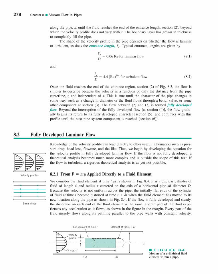
along the pipe, x, until the fluid reaches the end of the entrance length, section (2), beyondwhich the velocity profile does not vary with x. The boundary layer has grown in thicknessto completely fill the pipe.

The shape of the velocity profile in the pipe depends on whether the flow is laminaror turbulent, as does the entrance length, �e. Typical entrance lengths are given by

(8.1)

and

(8.2)

Once the fluid reaches the end of the entrance region, section (2) of Fig. 8.3, the flow issimpler to describe because the velocity is a function of only the distance from the pipecenterline, r, and independent of x. This is true until the character of the pipe changes insome way, such as a change in diameter or the fluid flows through a bend, valve, or someother component at section (3). The flow between (2) and (3) is termed fully developedflow. Beyond the interruption of the fully developed flow [at section (4)], the flow gradu-ally begins its return to its fully developed character [section (5)] and continues with thisprofile until the next pipe system component is reached [section (6)].

/e

D� 4.4 1Re21/6 for turbulent flow

/e

D� 0.06 Re for laminar flow

278 Chapter 8 ■ Viscous Flow in Pipes

8.2 Fully Developed Laminar Flow

Knowledge of the velocity profile can lead directly to other useful information such as pres-sure drop, head loss, flowrate, and the like. Thus, we begin by developing the equation forthe velocity profile in fully developed laminar flow. If the flow is not fully developed, atheoretical analysis becomes much more complex and is outside the scope of this text. Ifthe flow is turbulent, a rigorous theoretical analysis is as yet not possible.

8.2.1 From F � ma Applied Directly to a Fluid Element

We consider the fluid element at time t as is shown in Fig. 8.4. It is a circular cylinder offluid of length � and radius r centered on the axis of a horizontal pipe of diameter D.Because the velocity is not uniform across the pipe, the initially flat ends of the cylinderof fluid at time t become distorted at time t � �t when the fluid element has moved to itsnew location along the pipe as shown in Fig. 8.4. If the flow is fully developed and steady,the distortion on each end of the fluid element is the same, and no part of the fluid expe-riences any acceleration as it flows, as shown in the figure in the margin. Every part of thefluid merely flows along its pathline parallel to the pipe walls with constant velocity,

Velocity profiles

Streamlines

(1) (2)

D

Velocityprofile

V = u(r)i

r

Fluid element at time t Element at time t + tδ

x

�^ F I G U R E 8.4Motion of a cylindrical fluidelement within a pipe.

c08ViscousFlowinPipes.qxd 9/28/10 10:22 AM Page 278

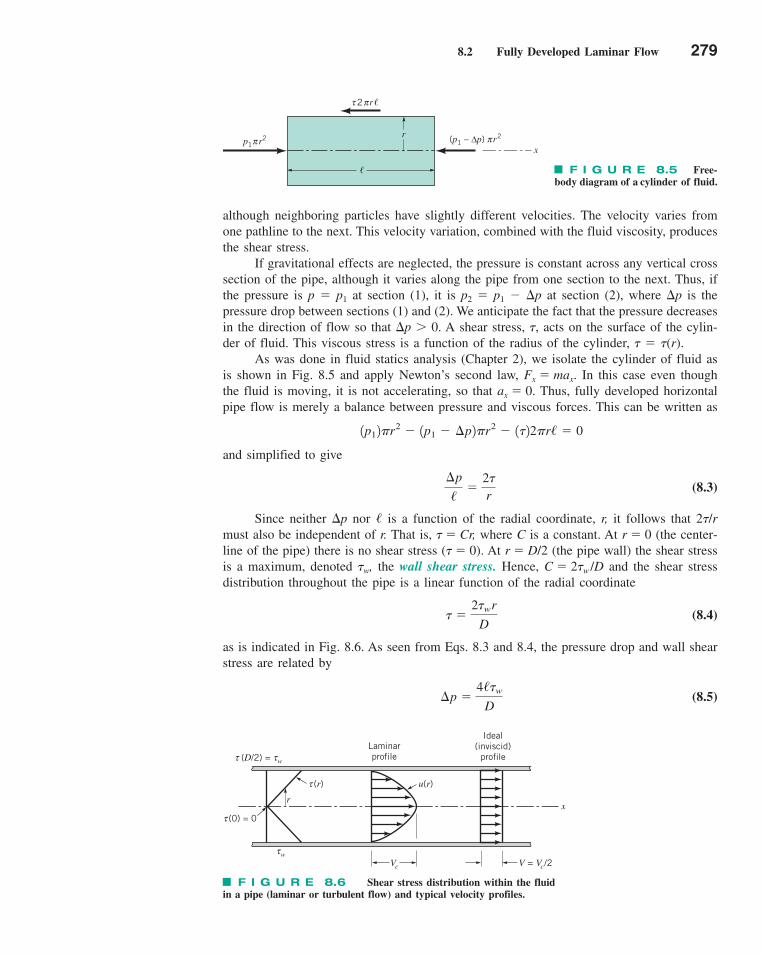
8.2 Fully Developed Laminar Flow 279

although neighboring particles have slightly different velocities. The velocity varies fromone pathline to the next. This velocity variation, combined with the fluid viscosity, producesthe shear stress.

If gravitational effects are neglected, the pressure is constant across any vertical crosssection of the pipe, although it varies along the pipe from one section to the next. Thus, ifthe pressure is p � p1 at section (1), it is p2 � p1 � �p at section (2), where �p is thepressure drop between sections (1) and (2). We anticipate the fact that the pressure decreasesin the direction of flow so that �p � 0. A shear stress, �, acts on the surface of the cylin-der of fluid. This viscous stress is a function of the radius of the cylinder, � � �(r).

As was done in fluid statics analysis (Chapter 2), we isolate the cylinder of fluid asis shown in Fig. 8.5 and apply Newton’s second law, Fx � max. In this case even thoughthe fluid is moving, it is not accelerating, so that ax � 0. Thus, fully developed horizontalpipe flow is merely a balance between pressure and viscous forces. This can be written as

and simplified to give

(8.3)

Since neither �p nor � is a function of the radial coordinate, r, it follows that 2�/rmust also be independent of r. That is, � � Cr, where C is a constant. At r � 0 (the center-line of the pipe) there is no shear stress (� � 0). At r � D/2 (the pipe wall) the shear stressis a maximum, denoted �w, the wall shear stress. Hence, C � 2�w /D and the shear stressdistribution throughout the pipe is a linear function of the radial coordinate

(8.4)

as is indicated in Fig. 8.6. As seen from Eqs. 8.3 and 8.4, the pressure drop and wall shearstress are related by

(8.5)¢p �4/�w

D

� �2�wr

D

¢p

/�

2�

r

1p12�r2 � 1p1 � ¢p2�r2 � 1�22�r/ � 0

2 r�τ π

(p1 – Δp) r2πx

r

�

p1 r2π

F I G U R E 8.5 Free-body diagram of a cylinder of fluid.

τVc

(r)τ

r

(0) = 0τ

(D/2) = w τ τLaminarprofile

u(r)

Ideal(inviscid)

profile

x

V = Vc/2w

F I G U R E 8.6 Shear stress distribution within the fluidin a pipe (laminar or turbulent flow) and typical velocity profiles.

c08ViscousFlowinPipes.qxd 9/28/10 10:22 AM Page 279

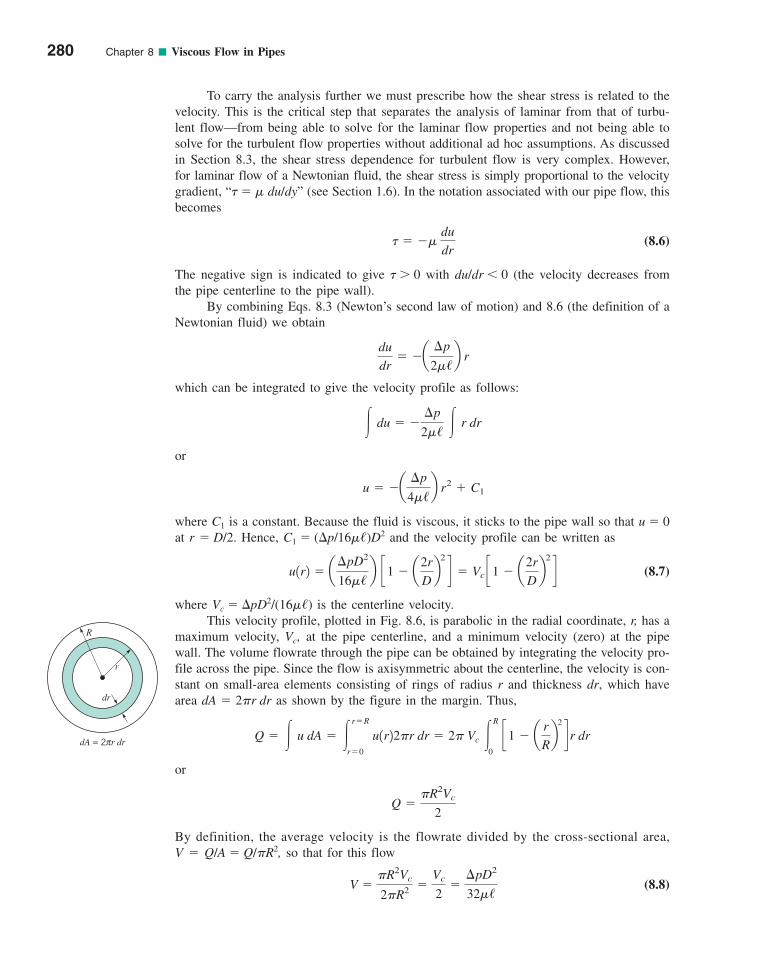
To carry the analysis further we must prescribe how the shear stress is related to thevelocity. This is the critical step that separates the analysis of laminar from that of turbu-lent flow—from being able to solve for the laminar flow properties and not being able tosolve for the turbulent flow properties without additional ad hoc assumptions. As discussedin Section 8.3, the shear stress dependence for turbulent flow is very complex. However,for laminar flow of a Newtonian fluid, the shear stress is simply proportional to the velocitygradient, “� � � du/dy” (see Section 1.6). In the notation associated with our pipe flow, thisbecomes

(8.6)

The negative sign is indicated to give � � 0 with du/dr 0 (the velocity decreases fromthe pipe centerline to the pipe wall).

By combining Eqs. 8.3 (Newton’s second law of motion) and 8.6 (the definition of aNewtonian fluid) we obtain

which can be integrated to give the velocity profile as follows:

or

where C1 is a constant. Because the fluid is viscous, it sticks to the pipe wall so that u � 0at r � D/2. Hence, C1 � (�p/16��)D2 and the velocity profile can be written as

(8.7)

where Vc � �pD2/(16��) is the centerline velocity.This velocity profile, plotted in Fig. 8.6, is parabolic in the radial coordinate, r, has a

maximum velocity, Vc, at the pipe centerline, and a minimum velocity (zero) at the pipewall. The volume flowrate through the pipe can be obtained by integrating the velocity pro-file across the pipe. Since the flow is axisymmetric about the centerline, the velocity is con-stant on small-area elements consisting of rings of radius r and thickness dr, which havearea as shown by the figure in the margin. Thus,

or

By definition, the average velocity is the flowrate divided by the cross-sectional area,V � Q/A � Q/�R2, so that for this flow

(8.8)V ��R2Vc

2�R2 �Vc

2�

¢pD2

32�/

Q ��R2Vc

2

Q � � u dA � �r�R

r�0

u1r22�r dr � 2� Vc �R

0 c1 � a

r

Rb

2

d r dr

dA � 2�r dr

u1r2 � a¢pD2

16�/b c1 � a

2r

Db

2

d � Vc c1 � a2r

Db

2

d

u � �a¢p

4�/b r2 � C1

� du � �¢p

2�/ � r dr

du

dr� �a

¢p

2�/b r

� � �� du

dr

280 Chapter 8 ■ Viscous Flow in Pipes

R

dr

r

dA = 2 r drπ

c08ViscousFlowinPipes.qxd 9/28/10 10:22 AM Page 280

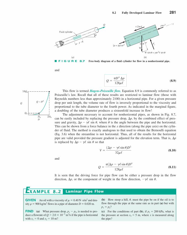
8.2 Fully Developed Laminar Flow 281

and

(8.9)

This flow is termed Hagen–Poiseuille flow. Equation 8.9 is commonly referred to asPoiseuille’s law. Recall that all of these results are restricted to laminar flow (those withReynolds numbers less than approximately 2100) in a horizontal pipe. For a given pressuredrop per unit length, the volume rate of flow is inversely proportional to the viscosity andproportional to the tube diameter to the fourth power. As indicated in the marginal figure,a doubling of the tube diameter produces a sixteenfold increase in flow!

The adjustment necessary to account for nonhorizontal pipes, as shown in Fig. 8.7,can be easily included by replacing the pressure drop, �p, by the combined effect of pres-sure and gravity, �p � �� sin , where is the angle between the pipe and the horizontal.This can be shown from a force balance in the x direction (along the pipe axis) on the cylin-der of fluid. The method is exactly analogous to that used to obtain the Bernoulli equation(Eq. 3.6) when the streamline is not horizontal. Thus, all of the results for the horizontalpipe are valid provided the pressure gradient is adjusted for the elevation term. That is, �pis replaced by �p � �� sin so that

(8.10)

and

(8.11)

It is seen that the driving force for pipe flow can be either a pressure drop in the flowdirection, �p, or the component of weight in the flow direction, ��� sin .

Q ��1¢p � �/ sin 2D4

128�/

V �1¢p � �/ sin 2D2

32�/

Q ��D 4 ¢p

128�/

�

� sin = r2� sinθ θγπ

πp r2

Fy

x

θ(p + Δp) r2

r

�

2 r�τ

(b)(a)

�

Fluid cylinderθ

Q

π

π

F I G U R E 8.7 Free-body diagram of a fluid cylinder for flow in a nonhorizontal pipe.

~ D4QQ

DD0

Q0

16Q0

2D0

GIVEN An oil with a viscosity of � � 0.40 N s/m2 and den-sity � � 900 kg/m3 flows in a pipe of diameter D � 0.020 m.

FIND (a) What pressure drop, p1 � p2, is needed to pro-duce a flowrate of Q � 2.0 � 10�5 m3/s if the pipe is horizontalwith x1 � 0 and x2 � 10 m?

# (b) How steep a hill, , must the pipe be on if the oil is toflow through the pipe at the same rate as in part (a) but withp1 � p2?

(c) For the conditions of part (b), if p1 � 200 kPa, what isthe pressure at section x3 � 5 m, where x is measured alongthe pipe?

Laminar Pipe FlowEXAMPLE 8.2

c08ViscousFlowinPipes.qxd 9/28/10 10:22 AM Page 281

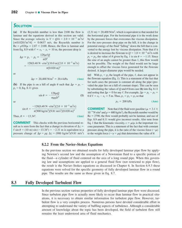
282 Chapter 8 ■ Viscous Flow in Pipes

(2.31 m) � 20,400 N/m2, which is equivalent to that needed forthe horizontal pipe. For the horizontal pipe it is the work doneby the pressure forces that overcomes the viscous dissipation.For the zero pressure drop pipe on the hill, it is the change inpotential energy of the fluid “falling” down the hill that is con-verted to the energy lost by viscous dissipation. Note that if itis desired to increase the flowrate to Q � 1.0 � 10�4 m3/s withp1 � p2, the value of given by Eq. 1 is sin � �1.15. Sincethe sine of an angle cannot be greater than 1, this flow wouldnot be possible. The weight of the fluid would not be largeenough to offset the viscous force generated for the flowratedesired. A larger-diameter pipe would be needed.

(c) With p1 � p2 the length of the pipe, �, does not appear inthe flowrate equation (Eq. 1). This is a statement of the fact thatfor such cases the pressure is constant all along the pipe (pro-vided the pipe lies on a hill of constant slope). This can be seenby substituting the values of Q and from case (b) into Eq. 8.11and noting that �p � 0 for any �. For example, �p � p1 � p3 �0 if � � x3 � x1 � 5 m. Thus, p1 � p2 � p3 so that

(Ans)

COMMENT Note that if the fluid were gasoline (� � 3.1 �10�4 Ns/m2 and � � 680 kg/m3), the Reynolds number would beRe � 2790, the flow would probably not be laminar, and use ofEqs. 8.9 and 8.11 would give incorrect results. Also note fromEq. 1 that the kinematic viscosity, v � �/�, is the important vis-cous parameter. This is a statement of the fact that with constantpressure along the pipe, it is the ratio of the viscous force (��)to the weight force (�� � �g) that determines the value of .

p3 � 200 kPa

SOLUTION

(a) If the Reynolds number is less than 2100 the flow islaminar and the equations derived in this section are valid.Since the average velocity is V � Q/A � 2.0 � 10�5 m3/s/[�(0.020)2m2/4] � 0.0637 m/s, the Reynolds number isRe � �VD/� � 2.87 2100. Hence, the flow is laminar andfrom Eq. 8.9 with � � x2 � x1 � 10 m, the pressure drop is

or

(Ans)

(b) If the pipe is on a hill of angle such that �p � p1 �p2 � 0, Eq. 8.11 gives

(1)

or

Thus, � �13.34�. (Ans)

COMMENT This checks with the previous horizontal re-sult as is seen from the fact that a change in elevation of �z �� sin � (10 m) sin (�13.34�) � �2.31 m is equivalent to apressure change of �p � �g �z � (900 kg/m3)(9.81 m/s2)

sin ��12810.40 N # s/m22 12.0 � 10�5 m3/s2

�1900 kg/m32 19.81 m/s22 10.020 m24

sin � �128�Q

��gD4

¢p � 20,400 N/m2 � 20.4 kPa

�12810.40 N # s/m22 110.0 m2 12.0 � 10�5 m3/s2

�10.020 m24

¢p � p1 � p2 �128�/Q

�D4

8.2.2 From the Navier–Stokes Equations

In the previous section we obtained results for fully developed laminar pipe flow by apply-ing Newton’s second law and the assumption of a Newtonian fluid to a specific portion ofthe fluid—a cylinder of fluid centered on the axis of a long round pipe. When this govern-ing law and assumptions are applied to a general fluid flow (not restricted to pipe flow),the result is the Navier–Stokes equations as discussed in Chapter 6. In Section 6.9.3 theseequations were solved for the specific geometry of fully developed laminar flow in a roundpipe. The results are the same as those given in Eq. 8.7.

8.3 Fully Developed Turbulent Flow

In the previous section various properties of fully developed laminar pipe flow were discussed.Since turbulent pipe flow is actually more likely to occur than laminar flow in practical situ-ations, it is necessary to obtain similar information for turbulent pipe flow. However, tur-bulent flow is a very complex process. Numerous persons have devoted considerable effort inattempting to understand the variety of baffling aspects of turbulence. Although a considerableamount of knowledge about the topic has been developed, the field of turbulent flow stillremains the least understood area of fluid mechanics.

c08ViscousFlowinPipes.qxd 9/28/10 10:22 AM Page 282

8.3 Fully Developed Turbulent Flow 283

8.3.1 Transition from Laminar to Turbulent Flow

Flows are classified as laminar or turbulent. For any flow geometry, there is one (or more)dimensionless parameter such that with this parameter value below a particular value the flowis laminar, whereas with the parameter value larger than a certain value it is turbulent. Forpipe flow this parameter is the Reynolds number. The value of the Reynolds number must beless than approximately 2100 for laminar flow and greater than approximately 4000 for tur-bulent flow.

A typical trace of the axial component of velocity, u � u(t), measured at a given loca-tion in turbulent pipe flow is shown in Fig. 8.8. Its irregular, random nature is the distin-guishing feature of turbulent flows. The character of many of the important properties ofthe flow (pressure drop, heat transfer, etc.) depends strongly on the existence and nature ofthe turbulent fluctuations or randomness indicated.

For example, mixing processes and heat and mass transfer processes are considerablyenhanced in turbulent flow compared to laminar flow. This is due to the macroscopic scaleof the randomness in turbulent flow. We are all familiar with the “rolling,” vigorous eddy-type motion of the water in a pan being heated on the stove (even if it is not heated to boil-ing). Such finite-sized random mixing is very effective in transporting energy and massthroughout the flow field, thereby increasing the various rate processes involved. Laminarflow, however, can be thought of as very small but finite-sized fluid particles flowingsmoothly in layers, one over another. The only randomness and mixing take place on themolecular scale and result in relatively small heat, mass, and momentum transfer rates.

u(t) _u = time average(or mean) value

u'

T

tO tO + T

u

t

F I G U R E 8.8 The time-averaged, u. and fluctuating, descrip-tion of a parameter for turbulent flow.

u�,

V8.4 Stirring colorinto paint

V8.5 Laminar andturbulent mixing

V8.6 Stirring creaminto coffee

F l u i d s i n t h e N e w s

Listen to the flowrate Sonar systems are designed to listen totransmitted and reflected sound waves in order to locate sub-merged objects. They have been used successfully for manyyears to detect and track underwater objects such as sub-marines and aquatic animals. Recently, sonar techniques havebeen refined so that they can be used to determine the flowratein pipes. These new flowmeters work for turbulent, not lami-nar, pipe flows because their operation depends strictly on the

existence of turbulent eddies within the flow. The flowmeterscontain a sonar-based array that listens to and interprets pres-sure fields generated by the turbulent motion in pipes. By lis-tening to the pressure fields associated with the movement ofthe turbulent eddies, the device can determine the speed atwhich the eddies travel past an array of sensors. The flowrateis determined by using a calibration procedure that links thespeed of the turbulent structures to the volumetric flowrate.

c08ViscousFlowinPipes.qxd 9/28/10 10:22 AM Page 283

8.3.2 Turbulent Shear Stress

The fundamental difference between laminar and turbulent flow lies in the chaotic, randombehavior of the various fluid parameters. As indicated in Fig. 8.8, such flows can bedescribed in terms of their mean values (denoted with an overbar) on which are superim-posed the fluctuations (denoted with a prime). Thus, if u � u(x, y, z, t) is the x componentof instantaneous velocity, then its time mean (or time average) value, , is

(8.12)

where the time interval, T, is considerably longer than the period of the longest fluctuationsbut considerably shorter than any unsteadiness of the average velocity. This is illustrated inFig. 8.8.

It is tempting to extend the concept of viscous shear stress for laminar flow (� � �du/dy) to that of turbulent flow by replacing u, the instantaneous velocity, by , the time-average velocity. However, numerous experimental and theoretical studies have shown thatsuch an approach leads to completely incorrect results.

That is, the shear stress in turbulent flow is not merely proportional to the gradientof the time-average velocity: � � � d /dy. It also contains a contribution due to the ran-dom fluctuations of the components of velocity. One could express the shear stress for tur-bulent flow in terms of a new parameter called the eddy viscosity, , where

(8.13)

Although the concept of an eddy viscosity is intriguing, in practice it is not an easyparameter to use. Unlike the absolute viscosity, �, which is a known value for a given fluid,the eddy viscosity is a function of both the fluid and the flow conditions. That is, the eddyviscosity of water cannot be looked up in handbooks—its value changes from one turbu-lent flow condition to another and from one point in a turbulent flow to another.

Several semiempirical theories have been proposed (Ref. 1) to determine approximatevalues of . For example, the turbulent process could be viewed as the random transport ofbundles of fluid particles over a certain distance, �m, the mixing length, from a region ofone velocity to another region of a different velocity. By the use of some ad hoc assump-tions and physical reasoning, the eddy viscosity is then given by

Thus, the turbulent shear stress is

(8.14)

The problem is thus shifted to that of determining the mixing length, �m. Further consider-ations indicate that �m is not a constant throughout the flow field. Near a solid surface theturbulence is dependent on the distance from the surface. Thus, additional assumptions aremade regarding how the mixing length varies throughout the flow.

The net result is that as yet there is no general, all-encompassing, useful model thatcan accurately predict the shear stress throughout a general incompressible, viscous turbu-lent flow. Without such information it is impossible to integrate the force balance equa-tion to obtain the turbulent velocity profile and other useful information, as was done forlaminar flow.

�turb � �/2m a

d u

dyb

2

� �/2m `

du

dy`

� � d u

dy

u

u

u �1

T �

t0�T

t0

u1x, y, z, t2 dt

u

284 Chapter 8 ■ Viscous Flow in Pipes

V8.7 Turbulence ina bowl

V8.8 Laminar toturbulent flow froma pipe

c08ViscousFlowinPipes.qxd 9/28/10 10:22 AM Page 284

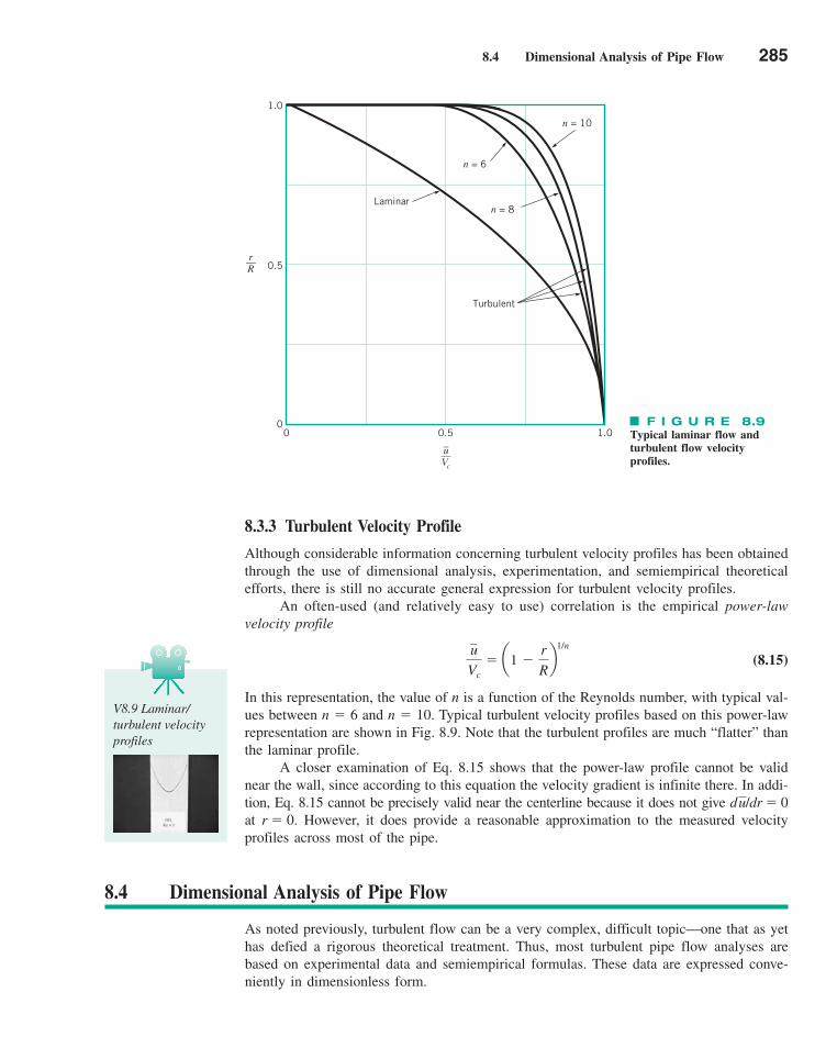
8.4 Dimensional Analysis of Pipe Flow 285

8.3.3 Turbulent Velocity Profile

Although considerable information concerning turbulent velocity profiles has been obtainedthrough the use of dimensional analysis, experimentation, and semiempirical theoreticalefforts, there is still no accurate general expression for turbulent velocity profiles.

An often-used (and relatively easy to use) correlation is the empirical power-lawvelocity profile

(8.15)

In this representation, the value of n is a function of the Reynolds number, with typical val-ues between n � 6 and n � 10. Typical turbulent velocity profiles based on this power-lawrepresentation are shown in Fig. 8.9. Note that the turbulent profiles are much “flatter” thanthe laminar profile.

A closer examination of Eq. 8.15 shows that the power-law profile cannot be validnear the wall, since according to this equation the velocity gradient is infinite there. In addi-tion, Eq. 8.15 cannot be precisely valid near the centerline because it does not give d /dr � 0at r � 0. However, it does provide a reasonable approximation to the measured velocityprofiles across most of the pipe.

u

u

Vc

� a1 �r

Rb

1/n

F I G U R E 8.9Typical laminar flow andturbulent flow velocityprofiles.

1.0

0.5

00 0.5 1.0

Turbulent

Laminarn = 8

n = 6

n = 10

r__R

_u__Vc

V8.9 Laminar/turbulent velocityprofiles

8.4 Dimensional Analysis of Pipe Flow

As noted previously, turbulent flow can be a very complex, difficult topic—one that as yethas defied a rigorous theoretical treatment. Thus, most turbulent pipe flow analyses arebased on experimental data and semiempirical formulas. These data are expressed conve-niently in dimensionless form.

c08ViscousFlowinPipes.qxd 9/28/10 10:22 AM Page 285

It is often necessary to determine the head loss, hL, that occurs in a pipe flow so thatthe energy equation, Eq. 5.57, can be used in the analysis of pipe flow problems. As shownin Fig. 8.1, a typical pipe system usually consists of various lengths of straight pipe inter-spersed with various types of components (valves, elbows, etc.). The overall head loss for thepipe system consists of the head loss due to viscous effects in the straight pipes, termed themajor loss and denoted hL major, and the head loss in the various pipe components, termedthe minor loss and denoted hL minor. That is,

The head loss designations of “major” and “minor” do not necessarily reflect the relativeimportance of each type of loss. For a pipe system that contains many components and arelatively short length of pipe, the minor loss may actually be larger than the major loss.

8.4.1 Major Losses

A dimensional analysis treatment of pipe flow provides the most convenient base fromwhich to consider turbulent, fully developed pipe flow. The pressure drop and head lossin a pipe are dependent on the wall shear stress, �w, between the fluid and the pipe sur-face. A fundamental difference between laminar and turbulent flow is that the shear stressfor turbulent flow is a function of the density of the fluid, �. For laminar flow, the shearstress is independent of the density, leaving the viscosity, �, as the only important fluidproperty.

Thus, as shown by the figure in the margin, the pressure drop, �p, for steady, incom-pressible turbulent flow in a horizontal round pipe of diameter D can be written in func-tional form as

(8.16)

where V is the average velocity, � is the pipe length, and � is a measure of the roughnessof the pipe wall. It is clear that �p should be a function of V, D, and �. The dependenceof �p on the fluid properties � and � is expected because of the dependence of � on theseparameters.

Although the pressure drop for laminar pipe flow is found to be independent ofthe roughness of the pipe, it is necessary to include this parameter when consideringturbulent flow. This can be shown to be due to the random velocity components thataccount for a momentum transfer (which is a function of the density) and, hence, ashear force.

Since there are seven variables (k � 7) that can be written in terms of the three ref-erence dimensions MLT (r � 3), Eq. 8.16 can be written in dimensionless form in termsof k � r � 4 dimensionless groups. One such representation is

This result differs from that used for laminar flow in two ways. First, we have chosen tomake the pressure dimensionless by dividing by the dynamic pressure, �V2/2, rather than acharacteristic viscous shear stress, �V/D. Second, we have introduced two additional dimen-sionless parameters, the Reynolds number, Re � �VD/�, and the relative roughness, /D,which are not present in the laminar formulation because the two parameters � and arenot important in fully developed laminar pipe flow.

As was done for laminar flow, the functional representation can be simplified by impos-ing the reasonable assumption that the pressure drop should be proportional to the pipe

e

e

¢p12 �V2 � �

� a

�VD�

, /D

, e

Db

¢p � F1V, D, /, e, �, �2

hL � hL major � hL minor

286 Chapter 8 ■ Viscous Flow in Pipes

(1) (2)

Dε

Qρ, μ

�

Δp = p1 – p2

c08ViscousFlowinPipes.qxd 9/28/10 10:22 AM Page 286

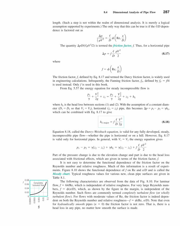
8.4 Dimensional Analysis of Pipe Flow 287

length. (Such a step is not within the realm of dimensional analysis. It is merely a logicalassumption supported by experiments.) The only way that this can be true is if the �/D depen-dence is factored out as

The quantity �pD/(��V2/2) is termed the friction factor, f. Thus, for a horizontal pipe

(8.17)

where

The friction factor, f, defined by Eq. 8.17 and termed the Darcy friction factor, is widely usedin engineering calculations. Infrequently, the Fanning friction factor, fF, defined by fF � f/4is used instead. Only f is used in this book.

From Eq. 5.57 the energy equation for steady incompressible flow is

where hL is the head loss between sections (1) and (2). With the assumption of a constant diam-eter (D1 � D2 so that V1 � V2), horizontal (z1 � z2) pipe, this becomes �p � p1� p2 � �hL,which can be combined with Eq. 8.17 to give

(8.18)

Equation 8.18, called the Darcy–Weisbach equation, is valid for any fully developed, steady,incompressible pipe flow—whether the pipe is horizontal or on a hill. However, Eq. 8.17is valid only for horizontal pipes. In general, with V1 � V2 the energy equation gives

Part of the pressure change is due to the elevation change and part is due to the head lossassociated with frictional effects, which are given in terms of the friction factor, f.

It is not easy to determine the functional dependence of the friction factor on theReynolds number and relative roughness. Much of this information is a result of experi-ments. Figure 8.10 shows the functional dependence of f on Re and �/D and is called theMoody chart. Typical roughness values for various new, clean pipe surfaces are given inTable 8.1.

The following characteristics are observed from the data of Fig. 8.10. For laminarflow, f � 64/Re, which is independent of relative roughness. For very large Reynolds num-bers, f � �(�/D), which, as shown by the figure in the margin, is independent of theReynolds number. Such flows are commonly termed completely turbulent flow (or whollyturbulent flow). For flows with moderate values of Re, the friction factor is indeed depen-dent on both the Reynolds number and relative roughness—f � �(Re, �/D). Note that evenfor hydraulically smooth pipes (� � 0) the friction factor is not zero. That is, there is ahead loss in any pipe, no matter how smooth the surface is made.

p1 � p2 � � 1z2 � z12 � �hL � �1z2 � z12 � f /D

�V2

2

hL major � f /D

V2

2g

p1

��

V21

2g� z1 �

p2

��

V22

2g� z2 � hL

f � � aRe, e

Db

¢p � f /D

�V2

2

¢p12 �V2 �

/D

� aRe, e

Db

0.00

001

0.00

01

0.00

1

0.01 0.1

0.08

0.06Completely

turbulent flow

0.04

0.02

0

f

eD

c08ViscousFlowinPipes.qxd 9/28/10 10:22 AM Page 287

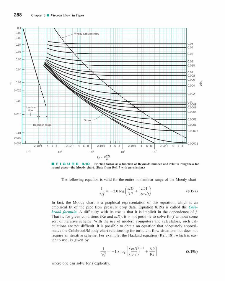
288 Chapter 8 ■ Viscous Flow in Pipes

The following equation is valid for the entire nonlaminar range of the Moody chart

(8.19a)

In fact, the Moody chart is a graphical representation of this equation, which is anempirical fit of the pipe flow pressure drop data. Equation 8.19a is called the Cole-brook formula. A difficulty with its use is that it is implicit in the dependence of f.That is, for given conditions (Re and �/D), it is not possible to solve for f without somesort of iterative scheme. With the use of modern computers and calculators, such cal-culations are not difficult. It is possible to obtain an equation that adequately approxi-mates the Colebrook/Moody chart relationship for turbulent flow situations but does notrequire an iterative scheme. For example, the Haaland equation (Ref. 18), which is eas-ier to use, is given by

(8.19b)

where one can solve for f explicitly.

1

1f� �1.8 log c a

e/D

3.7b

1.11

�6.9

Red

1

1f� �2.0 log a

e/D

3.7�

2.51

Re1fb

F I G U R E 8.10 Friction factor as a function of Reynolds number and relative roughness forround pipes—the Moody chart. (Data from Ref. 7 with permission.)

Transition range

Laminarflow

Smooth

Wholly turbulent flow

0.1

0.09

0.08

0.07

0.06

0.05

0.04

0.03

0.025

0.02

0.015

0.01

0.009

0.008

103

2(103) 4 6 8

104

2(104) 4 6 8

105

2(105) 4 6 8

106

2(106) 4 6 8

107

2(107) 4 6 8

0.050.04

0.03

0.02

0.015

0.010.008

0.006

0.004

0.002

0.0010.00080.0006

0.0004

0.0002

0.0001

0.00005

0.00001

f

Re = VD

_____μ

ρ

__De

c08ViscousFlowinPipes.qxd 9/28/10 10:22 AM Page 288

8.4 Dimensional Analysis of Pipe Flow 289

TA B L E 8 . 1

Equivalent Roughness for New Pipes. [From Moody (Ref. 2) and Colebrook (Ref. 3).]

Equivalent Roughness,

Pipe Feet Millimeters

Riveted steel 0.003–0.03 0.9–9.0Concrete 0.001–0.01 0.3–3.0Wood stave 0.0006–0.003 0.18–0.9Cast iron 0.00085 0.26Galvanized iron 0.0005 0.15Commercial steelor wrought iron 0.00015 0.045

Drawn tubing 0.000005 0.0015Plastic, glass 0.0 1smooth2 0.0 1smooth2

E

GIVEN Air under standard conditions flows through a4.0-mm-diameter drawn tubing with an average velocity ofV � 50 m/s. For such conditions the flow would normallybe turbulent. However, if precautions are taken to eliminatedisturbances to the flow (the entrance to the tube is very

smooth, the air is dust-free, the tube does not vibrate, etc.),it may be possible to maintain laminar flow.

FIND (a) Determine the pressure drop in a 0.1-m sectionof the tube if the flow is laminar.

(b) Repeat the calculations if the flow is turbulent.

SOLUTION

Comparison of Laminar or Turbulent Pressure Drop

(b) If the flow were turbulent, then f � (Re, /D), wherefrom Table 8.1, � 0.0015 mm so that /D � 0.0015 mm/4.0mm � 0.000375. From the Moody chart with Re � 1.37 � 104

and �D � 0.000375 we obtain f � 0.028. Thus, the pressuredrop in this case would be approximately

or

(Ans)

COMMENTS A considerable savings in effort to forcethe fluid through the pipe could be realized (0.179 kPa ratherthan 1.076 kPa) if the flow could be maintained as laminarflow at this Reynolds number. In general this is very difficult

¢p � 1.076 kPa

� 10.0282 10.1 m2

10.004 m2 1

2 11.23 kg/m32 150 m/s22

¢p � f /D

1

2 �V 2

e

ee

e�

� 179 N/m2

¢p �32�/

D2 V �3211.79 � 10�5 N # s/m22 10.1 m2 150 m/s2

10.004 m22

EXAMPLE 8.3

Under standard temperature and pressure conditions the den-sity and viscosity are � � 1.23 kg/m3 and � � 1.79 � 10�5

N s/m2. Thus, the Reynolds number is

which would normally indicate turbulent flow.

(a) If the flow were laminar, then f � 64/Re � 64/13,700 �0.00467 and the pressure drop in a 0.1-m-long horizontal sec-tion of the pipe would be

or

(Ans)

COMMENT Note that the same result is obtained fromEq. 8.8.

¢p � 0.179 kPa

� 10.004672 10.1 m2

10.004 m2 1

2 11.23 kg/m32 150 m/s22

¢p � f /D

1

2 �V2

� 13,700

Re ��VD

��11.23 kg/m32 150 m/s2 10.004 m2

1.79 � 10�5 N # s/m2

#

c08ViscousFlowinPipes.qxd 9/28/10 10:22 AM Page 289

8.4.2 Minor Losses

Most pipe systems consist of more than straight pipes. These additional components (valves,bends, tees, and the like) add to the overall head loss of the system. Such losses are gen-erally termed minor losses, with the corresponding head loss denoted hL minor.

Head loss information for essentially all components is given in dimensionless formand is based on experimental data. The most common method used to determine these headlosses or pressure drops is to specify the loss coefficient, KL, which is defined as

so that

or

(8.20)

The pressure drop across a component that has a loss coefficient of KL � 1 is equal to thedynamic pressure, �V2/2. As shown by Eq. 8.20 and the figure in the margin, for a givenvalue of KL the head loss is proportional to the square of the velocity.

Many pipe systems contain various transition sections in which the pipe diameterchanges from one size to another. Any change in flow area contributes losses that are not

hL minor � KL V2

2g

¢p � KL 12 �V 2

KL �hL minor

1V 2/2g2�

¢p12 �V 2

290 Chapter 8 ■ Viscous Flow in Pipes

For our case this gives

which is in agreement with the previous results. Note that thevalue of f is relatively insensitive to /D for this particularsituation. Whether the tube was smooth glass ( /D � 0) or thedrawn tubing ( /D � 0.000375) would not make much differ-ence in the pressure drop. For this flow, an increase in relativeroughness by a factor of 30 to /D � 0.0113 (equivalent to acommercial steel surface; see Table 8.1) would give f �0.043. This would represent an increase in pressure drop andhead loss by a factor of 0.043/0.0291 � 1.48 compared withthat for the original drawn tubing.

The pressure drop of 1.076 kPa in a length of 0.1 m ofpipe corresponds to a change in absolute pressure [assum-ing p � 101 kPa (abs) at x � 0] of approximately1.076/101 � 0.0107, or about 1%. Thus, the incompress-ible flow assumption on which the aforementioned calcula-tions (and all of the formulas in this chapter) are based isreasonable. However, if the pipe were 2 m long the pressuredrop would be 21.5 kPa, approximately 20% of the originalpressure. In this case the density would not be approxi-mately constant along the pipe, and a compressible flowanalysis would be needed.

e

e

e

e

f � 0.316113,7002�0.25 � 0.0292

to do, although laminar flow in pipes has been maintained upto Re � 100,000 in rare instances.

An alternate method to determine the friction factor for the turbulent flow would be to use the Colebrook formula,Eq. 8.19a. Thus,

or

(1)

By using a root-finding technique on a computer or calculator,the solution to Eq. 1 is determined to be , in agree-ment (within the accuracy of reading the graph) with the Moodychart method of Alternatively, the Haaland equation,Eq. 8.19b, could be used (without iteration) to obtain .

Numerous other empirical formulas can be found in theliterature (Ref. 4) for portions of the Moody chart. For example,an often-used equation, commonly referred to as the Blasiusformula, for turbulent flow in smooth pipes ( /D � 0) withRe � 105 is

f �0.316

Re1/4

e

f � 0.0289f � 0.028.

f � 0.0291

1

1f� �2.0 log a1.01 � 10�4 �

1.83 � 10�4

1fb

� �2.0 log a0.000375

3.7�

2.51

1.37 � 1041fb

1

1f� �2.0 log a

e/D

3.7�

2.51

Re1fb

~ V2hL minor

h L m

inor

V

c08ViscousFlowinPipes.qxd 9/30/10 7:15 AM Page 290

8.4 Dimensional Analysis of Pipe Flow 291

accounted for in the fully developed head loss calculation (the friction factor). The extremecases involve flow into a pipe from a reservoir (an entrance) or out of a pipe into a reser-voir (an exit).

A fluid may flow from a reservoir into a pipe through any number of different shapedentrance regions as are sketched in Fig. 8.11. Each geometry has an associated loss coeffi-cient. An obvious way to reduce the entrance loss is to round the entrance region as isshown in Fig. 8.11c. Typical values for the loss coefficient for entrances with variousamounts of rounding of the lip are shown in Fig. 8.12. A significant reduction in KL can beobtained with only slight rounding.

A head loss (the exit loss) is also produced when a fluid flows from a pipe into atank as is shown in Fig. 8.13. In these cases the entire kinetic energy of the exiting fluid(velocity V1) is dissipated through viscous effects as the stream of fluid mixes with the fluidin the tank and eventually comes to rest (V2 � 0). The exit loss from points (1) and (2) istherefore equivalent to one velocity head, or KL � 1.

(a) (b)

(c) (d)

F I G U R E 8.11 Entrance flow conditions and loss coefficient (Refs.12, 13). (a) Reentrant, KL � 0.8, (b) sharp edged, KL � 0.5, (c) slightly rounded,KL � 0.2 (see Fig. 8.12), and (d) well rounded, KL � 0.04 (see Fig. 8.12).

D

r

0.5

0.4

0.3

0.2

0.1

00 0.05 0.1 0.15 0.20 0.25

r__D

KL

F I G U R E 8.12Entrance loss coefficient as afunction of rounding of theinlet edge (Ref. 5).

V8.10 Entrance/exitflows

c08ViscousFlowinPipes.qxd 9/28/10 10:22 AM Page 291

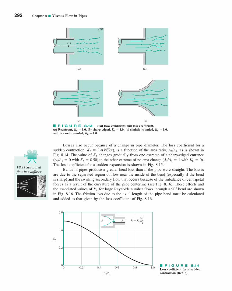
Losses also occur because of a change in pipe diameter. The loss coefficient for asudden contraction, KL � hL/(V 2

2/2g), is a function of the area ratio, A2/A1, as is shown inFig. 8.14. The value of KL changes gradually from one extreme of a sharp-edged entrance(A2/A1 � 0 with KL � 0.50) to the other extreme of no area change (A2/A1 � 1 with KL � 0).The loss coefficient for a sudden expansion is shown in Fig. 8.15.

Bends in pipes produce a greater head loss than if the pipe were straight. The lossesare due to the separated region of flow near the inside of the bend (especially if the bendis sharp) and the swirling secondary flow that occurs because of the imbalance of centripetalforces as a result of the curvature of the pipe centerline (see Fig. 8.16). These effects andthe associated values of KL for large Reynolds number flows through a 90� bend are shownin Fig. 8.16. The friction loss due to the axial length of the pipe bend must be calculatedand added to that given by the loss coefficient of Fig. 8.16.

292 Chapter 8 ■ Viscous Flow in Pipes

(a)

(c) (d)

(b)

(1)

(2)

F I G U R E 8.13 Exit flow conditions and loss coefficient.(a) Reentrant, KL � 1.0, (b) sharp edged, KL � 1.0, (c) slightly rounded, KL � 1.0,and (d ) well rounded, KL � 1.0.

A1 A2 hL = KL V2

2___2g

0.6

0.4

0.2

00 0.2 0.4 0.6 0.8 1.0

A2/A1

KL

F I G U R E 8.14Loss coefficient for a suddencontraction (Ref. 6).

V8.11 Separatedflow in a diffuser

c08ViscousFlowinPipes.qxd 9/28/10 10:22 AM Page 292

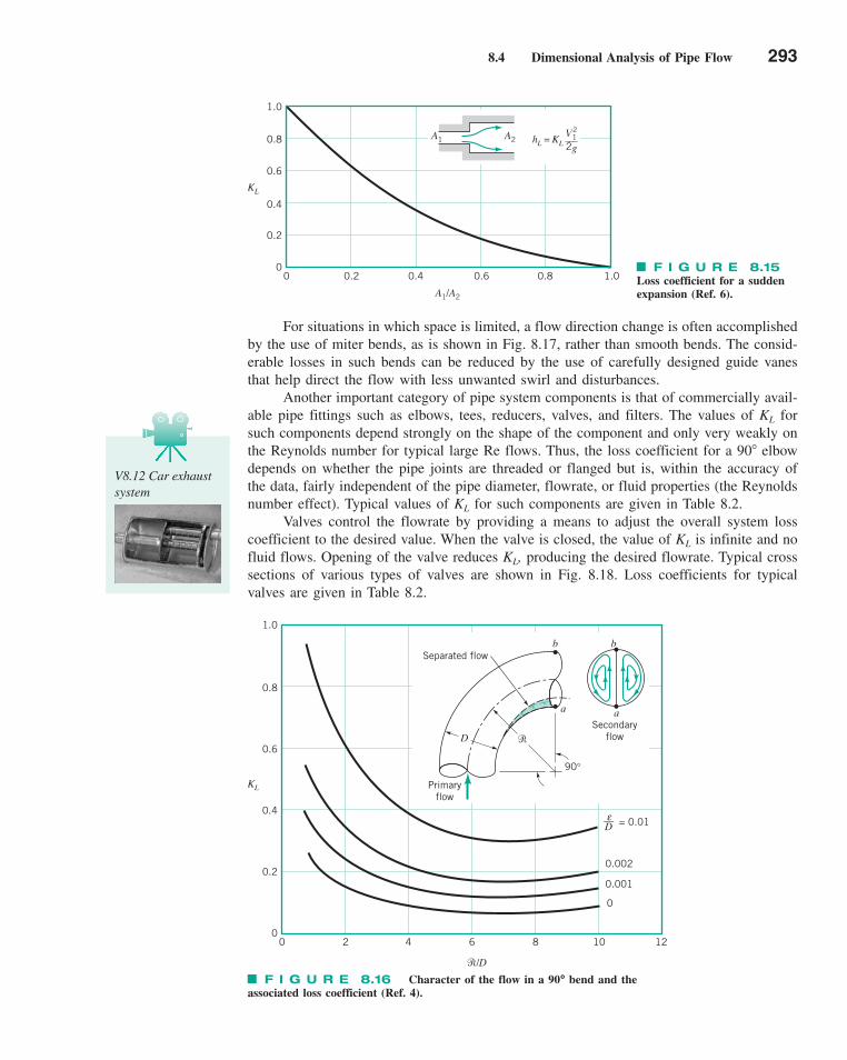
8.4 Dimensional Analysis of Pipe Flow 293

For situations in which space is limited, a flow direction change is often accomplishedby the use of miter bends, as is shown in Fig. 8.17, rather than smooth bends. The consid-erable losses in such bends can be reduced by the use of carefully designed guide vanesthat help direct the flow with less unwanted swirl and disturbances.

Another important category of pipe system components is that of commercially avail-able pipe fittings such as elbows, tees, reducers, valves, and filters. The values of KL forsuch components depend strongly on the shape of the component and only very weakly onthe Reynolds number for typical large Re flows. Thus, the loss coefficient for a 90� elbowdepends on whether the pipe joints are threaded or flanged but is, within the accuracy ofthe data, fairly independent of the pipe diameter, flowrate, or fluid properties (the Reynoldsnumber effect). Typical values of KL for such components are given in Table 8.2.

Valves control the flowrate by providing a means to adjust the overall system losscoefficient to the desired value. When the valve is closed, the value of KL is infinite and nofluid flows. Opening of the valve reduces KL, producing the desired flowrate. Typical crosssections of various types of valves are shown in Fig. 8.18. Loss coefficients for typicalvalves are given in Table 8.2.

A1 A2 hL = KL V1

2___2g

1.0

0.8

0.6

0.4

0.2

00 0.2 0.4 0.6 0.8 1.0

A1/A2

KL

F I G U R E 8.15Loss coefficient for a suddenexpansion (Ref. 6).

F I G U R E 8.16 Character of the flow in a 90°° bend and theassociated loss coefficient (Ref. 4).

Separated flowb b

a

Secondaryflow

90°

�

Primaryflow

D

a

__D = 0.01

0.002

0.001

0

1.0

0.8

0.6

0.4

0.2

00 2 4 6 8 10 12

�/D

KL

e

V8.12 Car exhaustsystem

c08ViscousFlowinPipes.qxd 9/28/10 10:22 AM Page 293

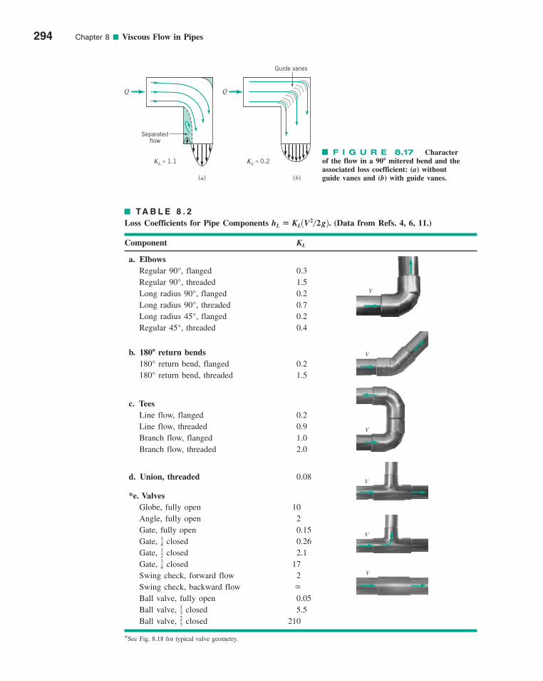
294 Chapter 8 ■ Viscous Flow in Pipes

KL ≈ 1.1

Q

Separatedflow

KL ≈ 0.2

Guide vanes

Q

(a) (b)

F I G U R E 8.17 Characterof the flow in a mitered bend and theassociated loss coefficient: (a) withoutguide vanes and (b) with guide vanes.

90�

TA B L E 8 . 2

Loss Coefficients for Pipe Components . (Data from Refs. 4, 6, 11.)

Component

a. ElbowsRegular flanged 0.3Regular threaded 1.5Long radius flanged 0.2Long radius threaded 0.7Long radius flanged 0.2Regular threaded 0.4

b. return bendsreturn bend, flanged 0.2return bend, threaded 1.5

c. TeesLine flow, flanged 0.2Line flow, threaded 0.9Branch flow, flanged 1.0Branch flow, threaded 2.0

d. Union, threaded 0.08

*e. ValvesGlobe, fully open 10Angle, fully open 2Gate, fully open 0.15Gate, closed 0.26Gate, closed 2.1Gate, closed 17Swing check, forward flow 2Swing check, backward flow

Ball valve, fully open 0.05Ball valve, closed 5.5Ball valve, closed 210

*See Fig. 8.18 for typical valve geometry.

23

13

34

12

14

180°180°180�

45°,45°,90°,90°,

90°,90°,

KL

hL � KL1V2�2g2

V

V

V

V

V

V

c08ViscousFlowinPipes.qxd 9/28/10 10:22 AM Page 294

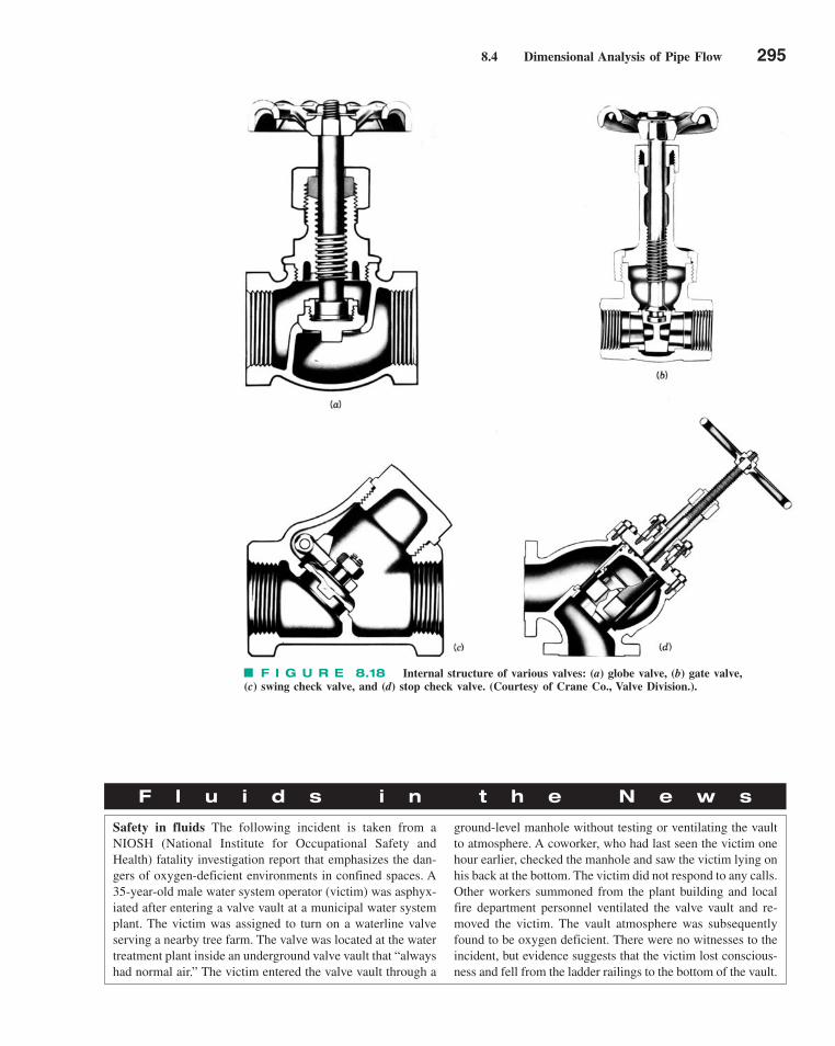
8.4 Dimensional Analysis of Pipe Flow 295

F I G U R E 8.18 Internal structure of various valves: (a) globe valve, (b) gate valve, (c) swing check valve, and (d) stop check valve. (Courtesy of Crane Co., Valve Division.).

F l u i d s i n t h e N e w s

Safety in fluids The following incident is taken from aNIOSH (National Institute for Occupational Safety andHealth) fatality investigation report that emphasizes the dan-gers of oxygen-deficient environments in confined spaces. A35-year-old male water system operator (victim) was asphyx-iated after entering a valve vault at a municipal water systemplant. The victim was assigned to turn on a waterline valveserving a nearby tree farm. The valve was located at the watertreatment plant inside an underground valve vault that “alwayshad normal air.” The victim entered the valve vault through a

ground-level manhole without testing or ventilating the vaultto atmosphere. A coworker, who had last seen the victim onehour earlier, checked the manhole and saw the victim lying onhis back at the bottom. The victim did not respond to any calls.Other workers summoned from the plant building and localfire department personnel ventilated the valve vault and re-moved the victim. The vault atmosphere was subsequentlyfound to be oxygen deficient. There were no witnesses to theincident, but evidence suggests that the victim lost conscious-ness and fell from the ladder railings to the bottom of the vault.

c08ViscousFlowinPipes.qxd 9/28/10 10:22 AM Page 295

296 Chapter 8 ■ Viscous Flow in Pipes

GIVEN The closed-circuit wind tunnel shown in Fig. E8.4ais a smaller version of that depicted in Fig. E8.4b in which air atstandard conditions is to flow through the test section [betweensections (5) and (6)] with a velocity of 200 ft/s. The flow isdriven by a fan that essentially increases the static pressure by

the amount p1 � p9 that is needed to overcome the head lossesexperienced by the fluid as it flows around the circuit.

FIND Estimate the value of p1 � p9 and the horsepowersupplied to the fluid by the fan.

SOLUTION

Minor Losses

where hp is the actual head rise supplied by the pump (fan) tothe air. Again since z9 � z1 and V9 � V1 this, when combinedwith Eq. 1, becomes

The actual power supplied to the air (horsepower, pa) is ob-tained from the fan head by

(2)

Thus, the power that the fan must supply to the air dependson the head loss associated with the flow through the windtunnel. To obtain a reasonable, approximate answer we makethe following assumptions. We treat each of the four turningcorners as a mitered bend with guide vanes so that from Fig.8.17 � 0.2. Thus, for each corner

hLcorner� KL

V2

2g� 0.2

V2

2g

KLcorner

pa � �Qhp � �A5V5hp � �A5V5hL1�9

hp �1 p1 � p92

�� hL1�9

p9

��

V29

2g� z9 � hp �

p1

��

V21

2g� z9

EXAMPLE 8.4

The maximum velocity within the wind tunnel occurs in thetest section (smallest area). Thus, the maximum Mach numberof the flow is Ma5 � V5/c5, where V5 � 200 ft/s and fromEq. 1.15 the speed of sound is c5 � (kRT )5

1/2 � {1.4(1716ft lb/slug � R) [(460 � 59)� R]}1/2 � 1117 ft/s. Thus, Ma5 �200/1117 � 0.179. As indicated in Chapter 3, most flows canbe considered as incompressible if the Mach number is lessthan about 0.3. Hence, we can use the incompressible formu-las for this problem.

The purpose of the fan in the wind tunnel is to provide thenecessary energy to overcome the net head loss experiencedby the air as it flows around the circuit. This can be found fromthe energy equation between points (1) and (9) as

where is the total head loss from (1) to (9). With z1 � z9

and V1 � V9 this gives

(1)

Similarly, by writing the energy equation (Eq. 5.57) acrossthe fan, from (9) to (1), we obtain

p1

��

p9

�� hL1�9

hL1 � 9

p1

��

V21

2g� z1 �

p9

��

V29

2g� z9 � hL1�9

##

F I G U R E E8.4a(Photograph courtesy of DELTALAB, France.)

(4)

V5 = 200 ft/s

(5) (6) (7)

(8)

Fan

Q (1)(9)(2)

Test sectionFlow-straightening

screens

(3)

F I G U R E E8.4b

c08ViscousFlowinPipes.qxd 9/28/10 10:22 AM Page 296

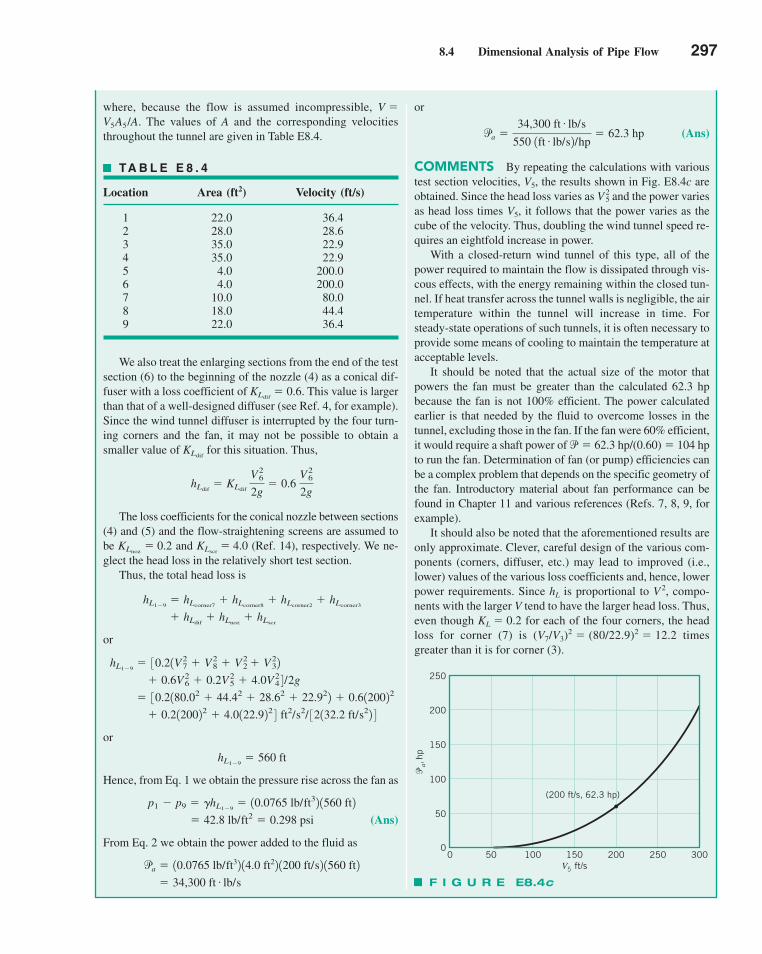
8.4 Dimensional Analysis of Pipe Flow 297

or

(Ans)

COMMENTS By repeating the calculations with varioustest section velocities, V5, the results shown in Fig. E8.4c areobtained. Since the head loss varies as and the power variesas head loss times V5, it follows that the power varies as thecube of the velocity. Thus, doubling the wind tunnel speed re-quires an eightfold increase in power.

With a closed-return wind tunnel of this type, all of thepower required to maintain the flow is dissipated through vis-cous effects, with the energy remaining within the closed tun-nel. If heat transfer across the tunnel walls is negligible, the airtemperature within the tunnel will increase in time. Forsteady-state operations of such tunnels, it is often necessary toprovide some means of cooling to maintain the temperature atacceptable levels.

It should be noted that the actual size of the motor thatpowers the fan must be greater than the calculated 62.3 hp because the fan is not 100% efficient. The power calculatedearlier is that needed by the fluid to overcome losses in thetunnel, excluding those in the fan. If the fan were 60% efficient,it would require a shaft power of p� 62.3 hp/(0.60) � 104 hpto run the fan. Determination of fan (or pump) efficiencies canbe a complex problem that depends on the specific geometry ofthe fan. Introductory material about fan performance can befound in Chapter 11 and various references (Refs. 7, 8, 9, forexample).

It should also be noted that the aforementioned results areonly approximate. Clever, careful design of the various com-ponents (corners, diffuser, etc.) may lead to improved (i.e.,lower) values of the various loss coefficients and, hence, lowerpower requirements. Since hL is proportional to V 2, compo-nents with the larger V tend to have the larger head loss. Thus,even though KL � 0.2 for each of the four corners, the headloss for corner (7) is (V7/V3)

2 � (80/22.9)2 � 12.2 timesgreater than it is for corner (3).

V 25

pa �34,300 ft # lb/s

550 1ft # lb/s2/hp� 62.3 hp

where, because the flow is assumed incompressible, V �V5A5/A. The values of A and the corresponding velocitiesthroughout the tunnel are given in Table E8.4.

TA B L E E 8 . 4

Location Area (ft2) Velocity (ft/s)

1 22.0 36.42 28.0 28.63 35.0 22.94 35.0 22.95 4.0 200.06 4.0 200.07 10.0 80.08 18.0 44.49 22.0 36.4

We also treat the enlarging sections from the end of the testsection (6) to the beginning of the nozzle (4) as a conical dif-fuser with a loss coefficient of � 0.6. This value is largerthan that of a well-designed diffuser (see Ref. 4, for example).Since the wind tunnel diffuser is interrupted by the four turn-ing corners and the fan, it may not be possible to obtain asmaller value of for this situation. Thus,

The loss coefficients for the conical nozzle between sections(4) and (5) and the flow-straightening screens are assumed tobe � 0.2 and � 4.0 (Ref. 14), respectively. We ne-glect the head loss in the relatively short test section.

Thus, the total head loss is

or

or

Hence, from Eq. 1 we obtain the pressure rise across the fan as

(Ans)

From Eq. 2 we obtain the power added to the fluid as

� 34,300 ft # lb/s

pa � 10.0765 lb/ft32 14.0 ft22 1200 ft/s2 1560 ft2

� 42.8 lb/ft2 � 0.298 psi

p1 � p9 � �hL1�9� 10.0765 lb/ft32 1560 ft2

hL1�9� 560 ft

� 0.2120022 � 4.0122.922 4 ft2/s2/ 32132.2 ft/s22 4

� 30.2180.02 � 44.42 � 28.62 � 22.922 � 0.6120022 � 0.6V2

6 � 0.2V25 � 4.0V2

4 4 /2g

hL1�9� 30.21V2

7 � V28 � V2

2 � V232

� hLdif� hLnoz

� hLscr

hL1�9� hLcorner7

� hLcorner8� hLcorner2

� hLcorner3

KLscrKLnoz

hLdif� KLdif

V2

6

2g� 0.6

V26

2g

KLdif

KLdif

V5 ft/s

�a, h

p

250

200

150

100

50

0 100 150 200 250 3000

(200 ft/s, 62.3 hp)

50

F I G U R E E8.4c

c08ViscousFlowinPipes.qxd 9/28/10 10:22 AM Page 297

8.4.3 Noncircular Conduits

Many of the conduits that are used for conveying fluids are not circular in cross section.Although the details of the flows in such conduits depend on the exact cross-sectional shape,many round pipe results can be carried over, with slight modification, to flow in conduitsof other shapes.

Practical, easy-to-use results can be obtained by introducing the hydraulic diameter,Dh � 4A/P, defined as four times the ratio of the cross-sectional flow area divided by thewetted perimeter, P, of the pipe as is illustrated in Fig. 8.19. The hydraulic diameter is usedin the definition of the friction factor, hL � f(�/Dh)V

2/2g, the Reynolds number, Reh ��VDh/�, and the relative roughness, �/Dh.

Calculations for fully developed turbulent flow in ducts of noncircular cross sectionare usually carried out by using the Moody chart data for round pipes with the diameterreplaced by the hydraulic diameter as indicated earlier. For turbulent flow such calculationsare usually accurate to within about 15%. If greater accuracy is needed, a more detailedanalysis based on the specific geometry of interest is needed.

298 Chapter 8 ■ Viscous Flow in Pipes

A = cross-sectionalarea

P = perimeterof pipe

Dh = 4A/P = hydraulicdiameter

(a) (b)

y

z

x

z V = u(y,z)

F I G U R E 8.19 Noncircular duct.

GIVEN Air at a temperature of 120 �F and standard pres-sure flows from a furnace through an 8-in.-diameter pipe withan average velocity of 10 ft/s. It then passes through a transi-tion section similar to the one shown in Fig. E8.5 and into asquare duct whose side is of length a. The pipe and duct sur-faces are smooth (� � 0). The head loss per foot is to be thesame for the pipe and the duct.

FIND Determine the duct size, a.

Noncircular ConduitEXAMPLE 8.5

F I G U R E E8.5

VSOLUTION

We first determine the head loss per foot for the pipe, hL/� �( f /D)V2/2g, and then size the square duct to give the samevalue. For the given pressure and temperature we obtain (from

c08ViscousFlowinPipes.qxd 9/28/10 10:22 AM Page 298

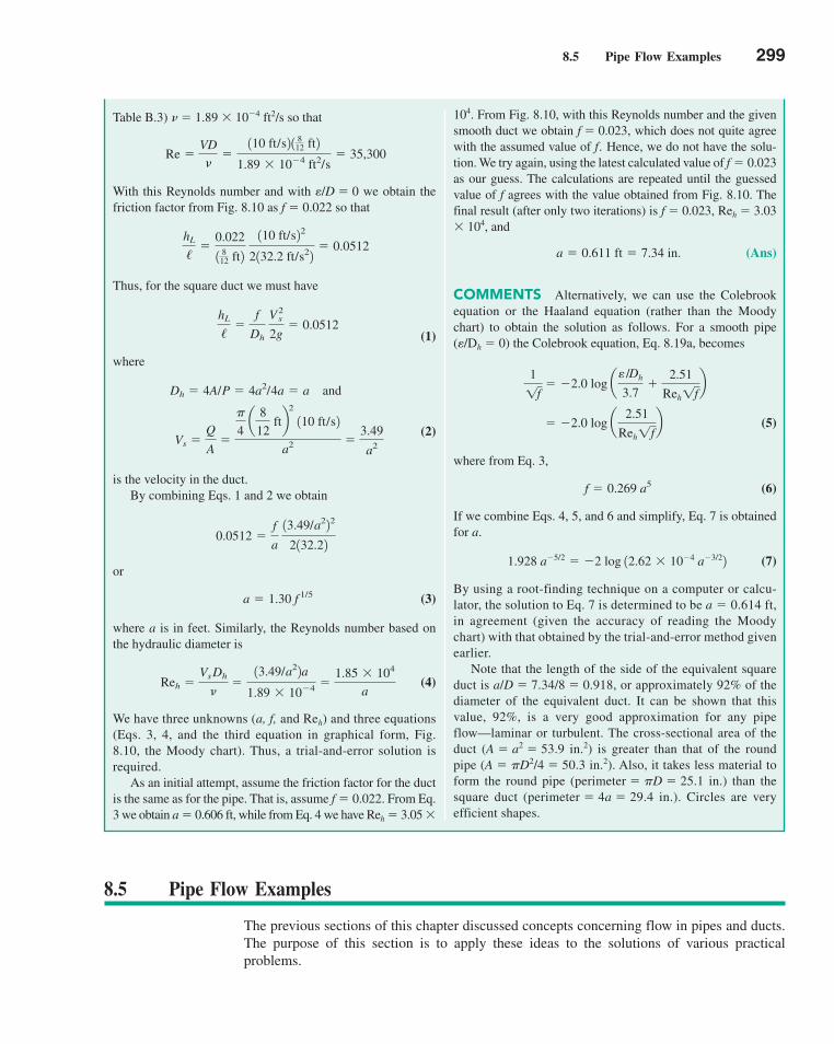
8.5 Pipe Flow Examples 299

104. From Fig. 8.10, with this Reynolds number and the givensmooth duct we obtain f � 0.023, which does not quite agreewith the assumed value of f . Hence, we do not have the solu-tion. We try again, using the latest calculated value of f � 0.023as our guess. The calculations are repeated until the guessedvalue of f agrees with the value obtained from Fig. 8.10. The final result (after only two iterations) is f � 0.023, Reh � 3.03� 104, and

(Ans)

COMMENTS Alternatively, we can use the Colebrookequation or the Haaland equation (rather than the Moodychart) to obtain the solution as follows. For a smooth pipe ( /Dh � 0) the Colebrook equation, Eq. 8.19a, becomes

(5)

where from Eq. 3,

(6)

If we combine Eqs. 4, 5, and 6 and simplify, Eq. 7 is obtainedfor a.

(7)

By using a root-finding technique on a computer or calcu-lator, the solution to Eq. 7 is determined to be a � 0.614 ft,in agreement (given the accuracy of reading the Moodychart) with that obtained by the trial-and-error method givenearlier.

Note that the length of the side of the equivalent squareduct is a/D � 7.34/8 � 0.918, or approximately 92% of thediameter of the equivalent duct. It can be shown that thisvalue, 92%, is a very good approximation for any pipeflow—laminar or turbulent. The cross-sectional area of theduct (A � a2 � 53.9 in.2) is greater than that of the roundpipe (A � �D2/4 � 50.3 in.2). Also, it takes less material toform the round pipe (perimeter � �D � 25.1 in.) than thesquare duct (perimeter � 4a � 29.4 in.). Circles are very efficient shapes.

1.928 a�5/2 � �2 log 12.62 � 10�4 a�3/22

f � 0.269 a5

� �2.0 log a2.51

Reh1fb

1

1f� �2.0 log a

e /Dh

3.7�

2.51

Reh1fb

e

a � 0.611 ft � 7.34 in.

Table B.3) � � 1.89 � 10�4 ft2/s so that

With this Reynolds number and with /D � 0 we obtain thefriction factor from Fig. 8.10 as f � 0.022 so that

Thus, for the square duct we must have

(1)

where

(2)

is the velocity in the duct.By combining Eqs. 1 and 2 we obtain

or

(3)

where a is in feet. Similarly, the Reynolds number based onthe hydraulic diameter is

(4)

We have three unknowns (a, f, and Reh) and three equations(Eqs. 3, 4, and the third equation in graphical form, Fig.8.10, the Moody chart). Thus, a trial-and-error solution isrequired.

As an initial attempt, assume the friction factor for the ductis the same as for the pipe. That is, assume f � 0.022. From Eq.3 we obtain a � 0.606 ft, while from Eq. 4 we have Reh � 3.05 �

Reh �VsDh

��13.49/a22a

1.89 � 10�4 �1.85 � 104

a

a � 1.30 f 1/5

0.0512 �f

a 13.49/a222

2132.22

Vs �Q

A�

�

4 a

8

12 ftb

2

110 ft/s2

a2 �3.49

a2

Dh � 4A/P � 4a2/4a � a and

hL

/�

f

Dh V2

s

2g� 0.0512

hL

/�

0.022

1 812 ft2

110 ft/s22

2132.2 ft/s22� 0.0512

e

Re �VD

��

110 ft/s2 1 812 ft2

1.89 � 10�4 ft2/s� 35,300

8.5 Pipe Flow Examples

The previous sections of this chapter discussed concepts concerning flow in pipes and ducts.The purpose of this section is to apply these ideas to the solutions of various practicalproblems.

c08ViscousFlowinPipes.qxd 9/28/10 10:22 AM Page 299

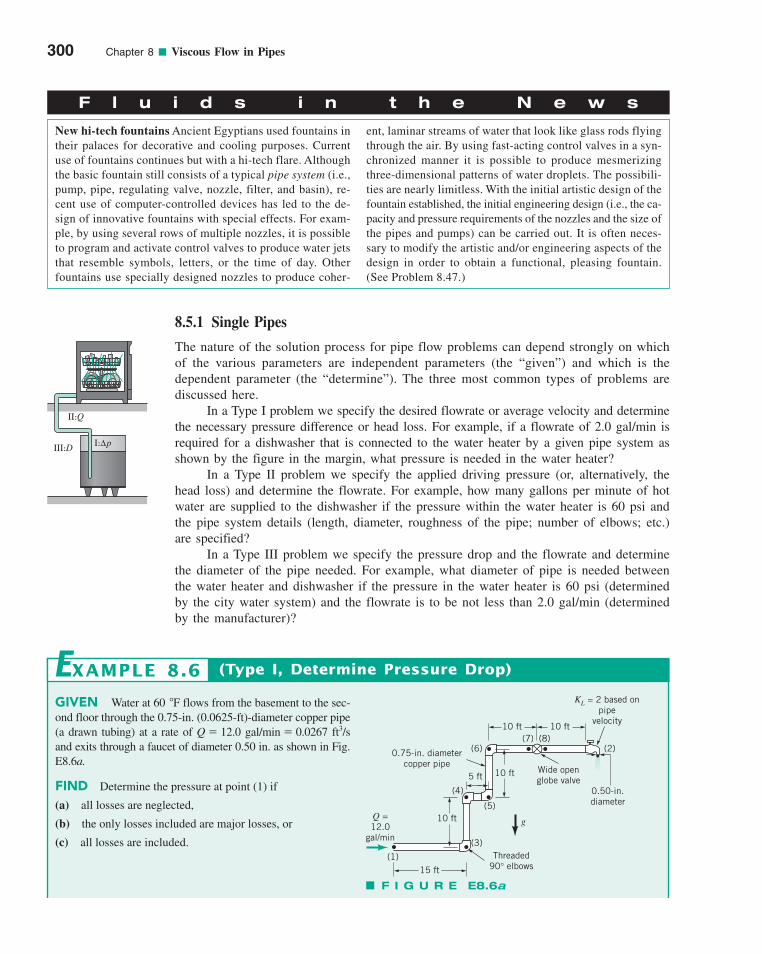
8.5.1 Single Pipes

The nature of the solution process for pipe flow problems can depend strongly on whichof the various parameters are independent parameters (the “given”) and which is thedependent parameter (the “determine”). The three most common types of problems arediscussed here.

In a Type I problem we specify the desired flowrate or average velocity and determinethe necessary pressure difference or head loss. For example, if a flowrate of 2.0 gal/min isrequired for a dishwasher that is connected to the water heater by a given pipe system asshown by the figure in the margin, what pressure is needed in the water heater?

In a Type II problem we specify the applied driving pressure (or, alternatively, thehead loss) and determine the flowrate. For example, how many gallons per minute of hotwater are supplied to the dishwasher if the pressure within the water heater is 60 psi andthe pipe system details (length, diameter, roughness of the pipe; number of elbows; etc.)are specified?

In a Type III problem we specify the pressure drop and the flowrate and determinethe diameter of the pipe needed. For example, what diameter of pipe is needed betweenthe water heater and dishwasher if the pressure in the water heater is 60 psi (determinedby the city water system) and the flowrate is to be not less than 2.0 gal/min (determinedby the manufacturer)?

300 Chapter 8 ■ Viscous Flow in Pipes

F l u i d s i n t h e N e w s

New hi-tech fountains Ancient Egyptians used fountains intheir palaces for decorative and cooling purposes. Currentuse of fountains continues but with a hi-tech flare. Althoughthe basic fountain still consists of a typical pipe system (i.e.,pump, pipe, regulating valve, nozzle, filter, and basin), re-cent use of computer-controlled devices has led to the de-sign of innovative fountains with special effects. For exam-ple, by using several rows of multiple nozzles, it is possibleto program and activate control valves to produce water jetsthat resemble symbols, letters, or the time of day. Otherfountains use specially designed nozzles to produce coher-

ent, laminar streams of water that look like glass rods flyingthrough the air. By using fast-acting control valves in a syn-chronized manner it is possible to produce mesmerizingthree-dimensional patterns of water droplets. The possibili-ties are nearly limitless. With the initial artistic design of thefountain established, the initial engineering design (i.e., the ca-pacity and pressure requirements of the nozzles and the size ofthe pipes and pumps) can be carried out. It is often neces-sary to modify the artistic and/or engineering aspects of thedesign in order to obtain a functional, pleasing fountain.(See Problem 8.47.)

I:ΔpIII:D

II:Q

GIVEN Water at 60 �F flows from the basement to the sec-ond floor through the 0.75-in. (0.0625-ft)-diameter copper pipe(a drawn tubing) at a rate of Q � 12.0 gal/min � 0.0267 ft3/sand exits through a faucet of diameter 0.50 in. as shown in Fig.E8.6a.

FIND Determine the pressure at point (1) if

(a) all losses are neglected,

(b) the only losses included are major losses, or

(c) all losses are included.

(Type I, Determine Pressure Drop)EXAMPLE 8.6

Q =12.0

gal/min

(1)

(2)

(3)

15 ft

10 ft

5 ft 10 ft

10 ft 10 ft(8)(7)

(6)

(4)

(5)

g

Threaded90° elbows

0.75-in. diametercopper pipe

Wide openglobe valve

0.50-in.diameter

KL = 2 based onpipe

velocity

F I G U R E E8.6a

c08ViscousFlowinPipes.qxd 9/28/10 10:22 AM Page 300

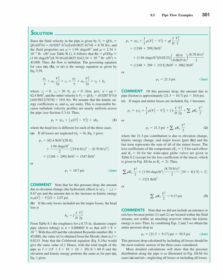
8.5 Pipe Flow Examples 301

SOLUTION

or

(Ans)

COMMENT Of this pressure drop, the amount due topipe friction is approximately (21.3 � 10.7) psi � 10.6 psi.

(c) If major and minor losses are included, Eq. 1 becomes

or

(2)

where the 21.3-psi contribution is due to elevation change,kinetic energy change, and major losses [part (b)] and thelast term represents the sum of all of the minor losses. Theloss coefficients of the components (KL � 1.5 for each elbowand KL � 10 for the wide-open globe valve) are given inTable 8.2 (except for the loss coefficient of the faucet, whichis given in Fig. E8.6a as KL � 2). Thus,

or

(3)

COMMENTS Note that we did not include an entrance orexit loss because points (1) and (2) are located within the fluidstreams, not within an attaching reservoir where the kineticenergy is zero. Thus, by combining Eqs. 2 and 3 we obtain theentire pressure drop as

(Ans)

This pressure drop calculated by including all losses should bethe most realistic answer of the three cases considered.

More detailed calculations will show that the pressuredistribution along the pipe is as illustrated in Fig. E8.6b forcases (a) and (c)—neglecting all losses or including all losses.

p1 � 121.3 � 9.172 psi � 30.5 psi

a �KL V 2

2� 9.17 psi

� 1321 lb/ft2

a �KL V 2

2� 11.94 slugs/ft32

18.70 ft/s22

2 310 � 411.52 � 2 4

p1 � 21.3 psi �a �KL V 2

2

p1 � �z2 �1

2 � 1V 2

2 � V 212 � f �

/D

V 2

1

2g�a �KL

V 2

2

p1 � 21.3 psi

� 11248 � 299 � 15152 lb/ft2 � 3062 lb/ft2

� 11.94 slugs/ft32 10.02152 a60 ft

0.0625 ftb 18.70 ft/s22

2

� 11248 � 2992 lb/ft2

p1 � �z2 �1

2 � 1V 2

2 � V 212 � �f

/D

V 2

1

2Since the fluid velocity in the pipe is given by V1 � Q/A1 �Q/(�D2/4) � (0.0267 ft3/s)/[�(0.0625 ft)2/4] � 8.70 ft/s, andthe fluid properties are � � 1.94 slugs/ft3 and � � 2.34 �10�5 lb s/ft2 (see Table B.1), it follows that Re � �VD/� �(1.94 slugs/ft3)(8.70 ft/s)(0.0625 ft)/(2.34 � 10�5 lb s/ft2) �45,000. Thus, the flow is turbulent. The governing equationfor case (a), (b), or (c) is the energy equation as given byEq. 5.59,

where z1 � 0, z2 � 20 ft, p2 � 0 (free jet), � � �g �62.4 lb/ft3, and the outlet velocity is V2 � Q/A2 � (0.0267 ft3/s)/[�(0.50/12)2ft2/4] � 19.6 ft/s. We assume that the kinetic en-ergy coefficients �1 and �2 are unity. This is reasonable be-cause turbulent velocity profiles are nearly uniform acrossthe pipe (see Section 5.3.4). Thus,

(1)

where the head loss is different for each of the three cases.

(a) If all losses are neglected (hL � 0), Eq. 1 gives

or

(Ans)

COMMENT Note that for this pressure drop, the amountdue to elevation change (the hydrostatic effect) is �(z2 � z1) �8.67 psi and the amount due to the increase in kinetic energyis �(V 2

2 � V 21)/2 � 2.07 psi.

(b) If the only losses included are the major losses, the headloss is

From Table 8.1 the roughness for a 0.75-in.-diameter copperpipe (drawn tubing) is � 0.000005 ft so that /D � 8 �10�5. With this /D and the calculated Reynolds number (Re �45,000), the value of f is obtained from the Moody chart as f �0.0215. Note that the Colebrook equation (Eq. 8.19a) wouldgive the same value of f. Hence, with the total length of thepipe as � � (15 � 5 � 10 � 10 � 20) ft � 60 ft and the elevation and kinetic energy portions the same as for part (a),Eq. 1 gives

eee

hL � f /D

V2

1

2g

p1 � 10.7 psi

� 11248 � 2992 lb/ft2 � 1547 lb/ft2

�1.94 slugs/ft3

2 3 119.6 ft/s22 � 18.70 ft/s22 4

p1 � 162.4 lb/ft32 120 ft2

p1 � �z2 � 12 � 1V

22 � V2

12 � �hL

p1

�� �1

V21

2g� z1 �

p2

�� �2

V22

2g� z2 � hL

##

c08ViscousFlowinPipes.qxd 9/28/10 10:22 AM Page 301

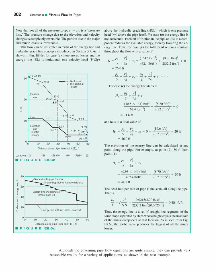
302 Chapter 8 ■ Viscous Flow in Pipes

above the hydraulic grade line (HGL), which is one pressurehead (�z) above the pipe itself. For case (c) the energy line isnot horizontal. Each bit of friction in the pipe or loss in a com-ponent reduces the available energy, thereby lowering the en-ergy line. Thus, for case (a) the total head remains constantthroughout the flow with a value of

For case (c) the energy line starts at

and falls to a final value of

The elevation of the energy line can be calculated at anypoint along the pipe. For example, at point (7), 50 ft frompoint (1),

The head loss per foot of pipe is the same all along the pipe.That is,

Thus, the energy line is a set of straight-line segments of thesame slope separated by steps whose height equals the head lossof the minor component at that location. As is seen from Fig.E8.6c, the globe valve produces the largest of all the minorlosses.

hL

/� f

V2

2gD�

0.021518.70 ft/s22

2132.2 ft/s22 10.0625 ft2� 0.404 ft/ft

� 44.1 ft

�19.93 � 1442 lb/ft2

162.4 lb/ft32�18.70 ft/s22

2132.2 ft/s22� 20 ft

H7 �p7

��

V27

2g� z7

� 26.0 ft

H2 �p2

��

V22

2g� z2 � 0 �

119.6 ft/s22

2132.2 ft/s22� 20 ft

� 71.6 ft

�130.5 � 1442lb/ft2

162.4 lb/ft32�18.70 ft/s22

2132.2 ft/s22� 0

H1 �p1

��

V21

2g� z1

�p2

��

V22

2g� z2 �

p3

��

V33

2g� z3 � p

� 26.0 ft

H �p1

��

V21

2g� z1 �

11547 lb/ft22

162.4 lb/ft32�18.70 ft/s22

2132.2 ft/s22� 0

Note that not all of the pressure drop, p1 � p2, is a “pressureloss.” The pressure change due to the elevation and velocitychanges is completely reversible. The portion due to the majorand minor losses is irreversible.

This flow can be illustrated in terms of the energy line andhydraulic grade line concepts introduced in Section 3.7. As isshown in Fig. E8.6c, for case (a) there are no losses and theenergy line (EL) is horizontal, one velocity head (V2/2g)

30

20

10

00 10 20 30 40 50 60

10.7 10.7

6.37

2.072.07

4.843.09

9.93

12.411.7

30.5 psi

27.127.8

20.221.0

18.519.3

(a) No losses(c) Including all

losses

Pressureloss

Elevationand

kineticenergy

p2 = 0

Distance along pipe from point (1), ft

p,

psi

Location: (1) (3) (4) (5) (6) (7) (8) (2)

6.37

F I G U R E E8.6b

80

60

40

20

00 10 20 30 40 50 60

Distance along pipe from point (1), ft

H,

elev

atio

n to

ene

rgy

line,

ft

Energy line with no losses, case (a)

Energy line including alllosses, case (c)

Sharp drop due to component lossSlope due to pipe friction

F I G U R E E8.6c

Although the governing pipe flow equations are quite simple, they can provide veryreasonable results for a variety of applications, as shown in the next example.

c08ViscousFlowinPipes.qxd 9/28/10 10:22 AM Page 302

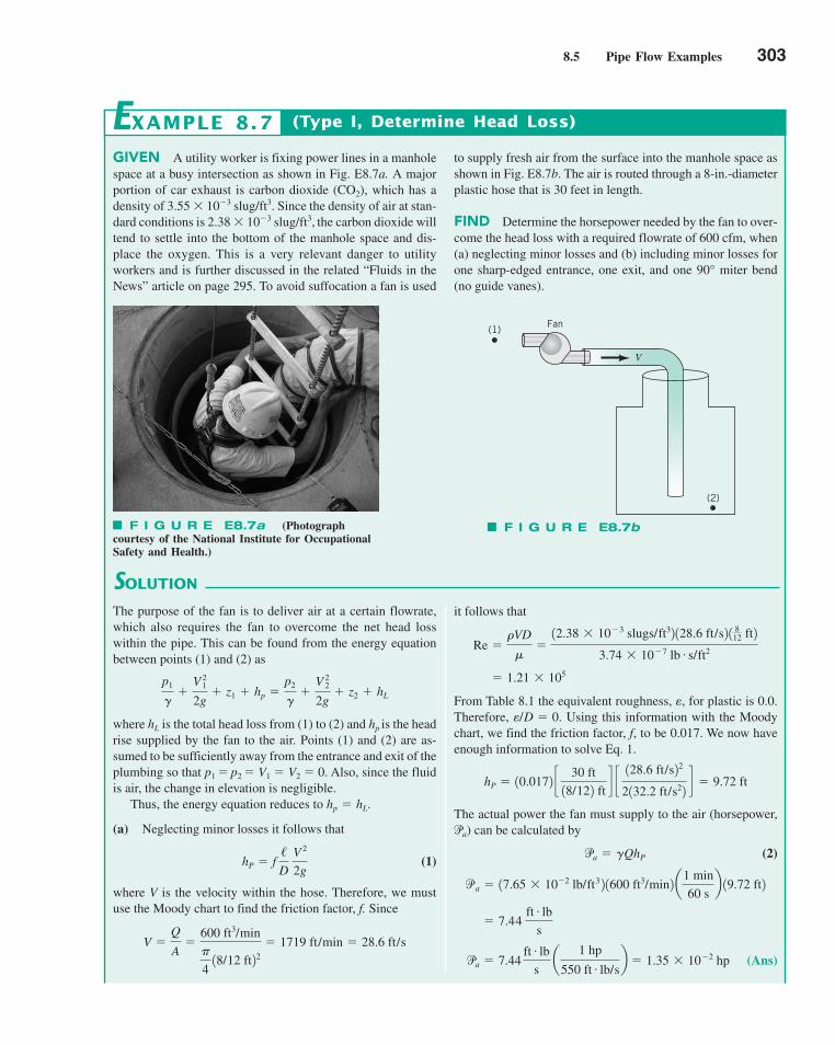
8.5 Pipe Flow Examples 303

GIVEN A utility worker is fixing power lines in a manholespace at a busy intersection as shown in Fig. E8.7a. A majorportion of car exhaust is carbon dioxide (CO2), which has adensity of 3.55 � 10�3 slug/ft3. Since the density of air at stan-dard conditions is 2.38 � 10�3 slug/ft3, the carbon dioxide willtend to settle into the bottom of the manhole space and dis-place the oxygen. This is a very relevant danger to utilityworkers and is further discussed in the related “Fluids in theNews” article on page 295. To avoid suffocation a fan is used

SOLUTION

(Type I, Determine Head Loss)

it follows that

From Table 8.1 the equivalent roughness, for plastic is 0.0.Therefore, Using this information with the Moodychart, we find the friction factor, f, to be 0.017. We now haveenough information to solve Eq. 1.

The actual power the fan must supply to the air (horsepower,) can be calculated by

(2)

(Ans)pa � 7.44ft # lb

sa

1 hp

550 ft # lb/sb � 1.35 � 10�2 hp

� 7.44 ft # lb

s

pa � 17.65 � 10�2 lb/ft3 2 1600 ft3/min2 a1 min

60 sb 19.72 ft2

pa � �QhP

pa

hP � 10.0172 c30 ft

18/122 ftd c128.6 ft/s22

2132.2 ft/s22d � 9.72 ft

e/D � 0.e,

� 1.21 � 105

Re ��VD

��12.38 � 10�3 slugs/ft32 128.6 ft/s2 1 8

12 ft2

3.74 � 10�7 lb # s/ft2

to supply fresh air from the surface into the manhole space asshown in Fig. E8.7b. The air is routed through a 8-in.-diameterplastic hose that is 30 feet in length.

FIND Determine the horsepower needed by the fan to over-come the head loss with a required flowrate of 600 cfm, when(a) neglecting minor losses and (b) including minor losses forone sharp-edged entrance, one exit, and one 90° miter bend(no guide vanes).

EXAMPLE 8.7

The purpose of the fan is to deliver air at a certain flowrate,which also requires the fan to overcome the net head losswithin the pipe. This can be found from the energy equationbetween points (1) and (2) as

where hL is the total head loss from (1) to (2) and hp is the headrise supplied by the fan to the air. Points (1) and (2) are as-sumed to be sufficiently away from the entrance and exit of theplumbing so that p1 � p2 � V1 � V2 � 0. Also, since the fluidis air, the change in elevation is negligible.

Thus, the energy equation reduces to

(a) Neglecting minor losses it follows that

(1)

where V is the velocity within the hose. Therefore, we mustuse the Moody chart to find the friction factor, f. Since

V �Q

A�

600 ft3/min�

418/12 ft22

� 1719 ft/min � 28.6 ft/s

hP � f/D

V 2

2g

hp � hL.

p1

��

V 21

2g� z1 � hp �

p2

��

V 22

2g� z2 � hL

V

(1)

(2)

Fan

F I G U R E E8.7bF I G U R E E8.7a (Photograph courtesy of the National Institute for Occupational Safety and Health.)

c08ViscousFlowinPipes.qxd 9/28/10 10:22 AM Page 303

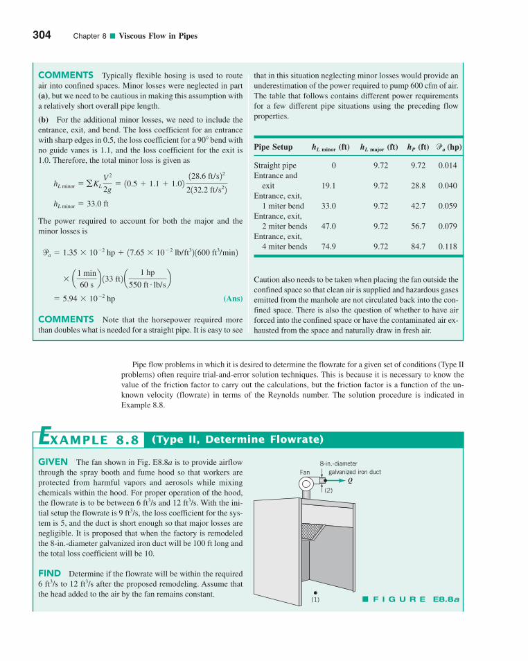
304 Chapter 8 ■ Viscous Flow in Pipes

Pipe flow problems in which it is desired to determine the flowrate for a given set of conditions (Type IIproblems) often require trial-and-error solution techniques. This is because it is necessary to know thevalue of the friction factor to carry out the calculations, but the friction factor is a function of the un-known velocity (flowrate) in terms of the Reynolds number. The solution procedure is indicated in Example 8.8.

that in this situation neglecting minor losses would provide anunderestimation of the power required to pump 600 cfm of air.The table that follows contains different power requirementsfor a few different pipe situations using the preceding flowproperties.

Caution also needs to be taken when placing the fan outside theconfined space so that clean air is supplied and hazardous gasesemitted from the manhole are not circulated back into the con-fined space. There is also the question of whether to have airforced into the confined space or have the contaminated air ex-hausted from the space and naturally draw in fresh air.

COMMENTS Typically flexible hosing is used to routeair into confined spaces. Minor losses were neglected in part(a), but we need to be cautious in making this assumption witha relatively short overall pipe length.

(b) For the additional minor losses, we need to include theentrance, exit, and bend. The loss coefficient for an entrancewith sharp edges in 0.5, the loss coefficient for a 90� bend withno guide vanes is 1.1, and the loss coefficient for the exit is1.0. Therefore, the total minor loss is given as

The power required to account for both the major and the minor losses is

(Ans)

COMMENTS Note that the horsepower required morethan doubles what is needed for a straight pipe. It is easy to see

� 5.94 � 10�2 hp

133 ft2 a1 hp

550 ft # lb/sb� a

1 min

60 sb

pa � 1.35 � 10�2 hp � 17.65 � 10�2 lb/ft32 1600 ft3/min2

hL minor � 33.0 ft

hL minor �gKL

V 2

2g� 10.5 � 1.1 � 1.02

128.6 ft/s22

2132.2 ft/s22

Pipe Setup hL minor (ft) hL major (ft) hP (ft) pa (hp)

Straight pipe 0 9.72 9.72 0.014Entrance and

exit 19.1 9.72 28.8 0.040Entrance, exit,

1 miter bend 33.0 9.72 42.7 0.059Entrance, exit,

2 miter bends 47.0 9.72 56.7 0.079Entrance, exit,

4 miter bends 74.9 9.72 84.7 0.118

GIVEN The fan shown in Fig. E8.8a is to provide airflowthrough the spray booth and fume hood so that workers areprotected from harmful vapors and aerosols while mixingchemicals within the hood. For proper operation of the hood,the flowrate is to be between 6 ft3/s and 12 ft3/s. With the ini-tial setup the flowrate is 9 ft3/s, the loss coefficient for the sys-tem is 5, and the duct is short enough so that major losses arenegligible. It is proposed that when the factory is remodeledthe 8-in.-diameter galvanized iron duct will be 100 ft long andthe total loss coefficient will be 10.

FIND Determine if the flowrate will be within the required6 ft3/s to 12 ft3/s after the proposed remodeling. Assume thatthe head added to the air by the fan remains constant.

(Type II, Determine Flowrate)EXAMPLE 8.8

(1)

(2)

FanQ

8-in.-diameter galvanized iron duct

F I G U R E E8.8a

c08ViscousFlowinPipes.qxd 9/30/10 7:16 AM Page 304

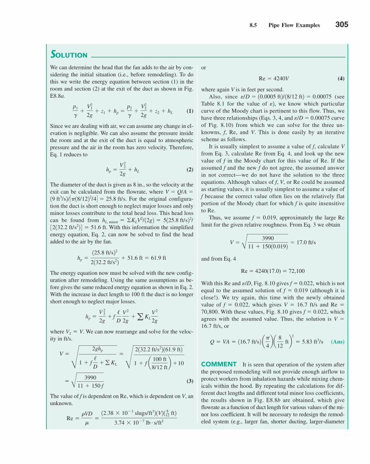
8.5 Pipe Flow Examples 305

SOLUTION

or

(4)

where again V is in feet per second.Also, since (see

Table 8.1 for the value of we know which particularcurve of the Moody chart is pertinent to this flow. Thus, wehave three relationships (Eqs. 3, 4, and �/D � 0.00075 curveof Fig. 8.10) from which we can solve for the three un-knowns, f, Re, and V. This is done easily by an iterativescheme as follows.

It is usually simplest to assume a value of f, calculate Vfrom Eq. 3, calculate Re from Eq. 4, and look up the newvalue of f in the Moody chart for this value of Re. If the assumed f and the new f do not agree, the assumed answerin not correct—we do not have the solution to the threeequations. Although values of f, V, or Re could be assumedas starting values, it is usually simplest to assume a value off because the correct value often lies on the relatively flatportion of the Moody chart for which f is quite insensitiveto Re.

Thus, we assume f � 0.019, approximately the large Relimit for the given relative roughness. From Eq. 3 we obtain

and from Eq. 4

Re � 4240(17.0) � 72,100

With this Re and �/D, Fig. 8.10 gives f � 0.022, which is notequal to the assumed solution of f � 0.019 (although it isclose!). We try again, this time with the newly obtainedvalue of f � 0.022, which gives V � 16.7 ft/s and Re �70,800. With these values, Fig. 8.10 gives f � 0.022, whichagrees with the assumed value. Thus, the solution is V �16.7 ft/s, or

(Ans)

COMMENT It is seen that operation of the system afterthe proposed remodeling will not provide enough airflow toprotect workers from inhalation hazards while mixing chem-icals within the hood. By repeating the calculations for dif-ferent duct lengths and different total minor loss coefficients,the results shown in Fig. E8.8b are obtained, which giveflowrate as a function of duct length for various values of the mi-nor loss coefficient. It will be necessary to redesign the remod-eled system (e.g., larger fan, shorter ducting, larger-diameter

Q � VA � 116.7 ft/s2 a�

4ba

8

12ftb

2

� 5.83 ft3/s

V �B

3990

11 � 15010.0192� 17.0 ft/s

e2,e/D � 10.0005 ft2/ 18/12 ft2 � 0.00075

Re � 4240V

We can determine the head that the fan adds to the air by con-sidering the initial situation (i.e., before remodeling). To dothis we write the energy equation between section (1) in theroom and section (2) at the exit of the duct as shown in Fig.E8.8a.

(1)

Since we are dealing with air, we can assume any change in el-evation is negligible. We can also assume the pressure insidethe room and at the exit of the duct is equal to atmosphericpressure and the air in the room has zero velocity. Therefore,Eq. 1 reduces to

(2)

The diameter of the duct is given as 8 in., so the velocity at theexit can be calculated from the flowrate, where

For the original configura-tion the duct is short enough to neglect major losses and onlyminor losses contribute to the total head loss. This head losscan be found from

With this information the simplifiedenergy equation, Eq. 2, can now be solved to find the headadded to the air by the fan.

The energy equation now must be solved with the new config-uration after remodeling. Using the same assumptions as be-fore gives the same reduced energy equation as shown in Eq. 2.With the increase in duct length to 100 ft the duct is no longershort enough to neglect major losses.

where We can now rearrange and solve for the veloc-ity in ft/s.

(3)

The value of f is dependent on Re, which is dependent on V, anunknown.

Re ��VD

��12.38 � 10�3 slugs/ft32 1V2 1 8

12 ft2

3.74 � 10�7 lb # s/ft2

�B

3990

11 � 150 f

V �

R

2ghp

1 � f/D

�g KL

�

R

2132.2 ft/s22 161.9 ft2

1 � f a100 ft

8/12 ftb �10

V2 � V.

hp �V 2

2

2g� f

/D

V 2

2g�a KL

V 2

2g

hp �125.8 ft/s22

2132.2 ft/s22� 51.6 ft � 61.9 ft

32132.2 ft/s22 4 � 51.6 ft.5125.8 ft/s22/hL, minor � ©KLV2/ 12g2 �

19 ft3/s2/��18/1222/4� � 25.8 ft/s.V � Q/A �

hp �V 2

2

2g� hL

p1

��

V21

2g� z1 � hp �

p2

��

V22

2g� z2 � hL

c08ViscousFlowinPipes.qxd 9/28/10 10:23 AM Page 305

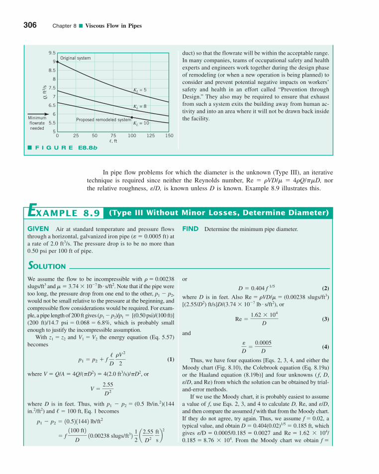
In pipe flow problems for which the diameter is the unknown (Type III), an iterativetechnique is required since neither the Reynolds number, Re � �VD/� � 4�Q/��D, northe relative roughness, �/D, is known unless D is known. Example 8.9 illustrates this.

306 Chapter 8 ■ Viscous Flow in Pipes

duct) so that the flowrate will be within the acceptable range.In many companies, teams of occupational safety and healthexperts and engineers work together during the design phaseof remodeling (or when a new operation is being planned) toconsider and prevent potential negative impacts on workers’safety and health in an effort called “Prevention through Design.” They also may be required to ensure that exhaustfrom such a system exits the building away from human ac-tivity and into an area where it will not be drawn back insidethe facility.

100 125 1507550250�, ft

9.5

8

8.5

9

7.5

7

6.5

6

5.5

5

Original system

Proposed remodeled system

KL = 5

KL = 8

KL = 10

Q, ft

3/s

Minimumflowrateneeded

F I G U R E E8.8b

GIVEN Air at standard temperature and pressure flowsthrough a horizontal, galvanized iron pipe ( � 0.0005 ft) ata rate of 2.0 ft3/s. The pressure drop is to be no more than0.50 psi per 100 ft of pipe.

e

SOLUTION

(Type III Without Minor Losses, Determine Diameter)

or

(2)

where D is in feet. Also Re � �VD/� � (0.00238 slugs/ft3)[(2.55/D2) ft/s]D/(3.74 � 10�7 lb s/ft2), or

(3)

and

(4)

Thus, we have four equations [Eqs. 2, 3, 4, and either theMoody chart (Fig. 8.10), the Colebrook equation (Eq. 8.19a)or the Haaland equation (8.19b)] and four unknowns ( f, D,e/D, and Re) from which the solution can be obtained by trial-and-error methods.

If we use the Moody chart, it is probably easiest to assumea value of f, use Eqs. 2, 3, and 4 to calculate D, Re, and e/D,and then compare the assumed f with that from the Moody chart.If they do not agree, try again. Thus, we assume f � 0.02, atypical value, and obtain D � 0.404(0.02)1/5 � 0.185 ft, whichgives e/D � 0.0005/0.185 � 0.0027 and Re � 1.62 � 104/0.185 � 8.76 � 104. From the Moody chart we obtain f �

e

D�

0.0005

D

Re �1.62 � 104

D

#

D � 0.404 f 1/5

FIND Determine the minimum pipe diameter.

EXAMPLE 8.9

We assume the flow to be incompressible with � � 0.00238slugs/ft3 and � � 3.74 � 10�7 lb s/ft2. Note that if the pipe weretoo long, the pressure drop from one end to the other, p1 � p2,would not be small relative to the pressure at the beginning, andcompressible flow considerations would be required. For exam-ple, a pipe length of 200 ft gives (p1 � p2)/p1 � [(0.50 psi)/(100 ft)](200 ft)/14.7 psi � 0.068 � 6.8%, which is probably smallenough to justify the incompressible assumption.

With z1 � z2 and V1 � V2 the energy equation (Eq. 5.57)becomes

(1)

where V � Q/A � 4Q/(�D2) � 4(2.0 ft3/s)/�D2, or

where D is in feet. Thus, with p1 � p2 � (0.5 lb/in.2)(144in.2/ft2) and � � 100 ft, Eq. 1 becomes

� f 1100 ft2

D 10.00238 slugs/ft32

1

2 a

2.55

D2 ft

sb

2

p1 � p2 � 10.52 11442 lb/ft2

V �2.55

D2

p1 � p2 � f /D

�V 2

2

#

c08ViscousFlowinPipes.qxd 9/28/10 10:23 AM Page 306

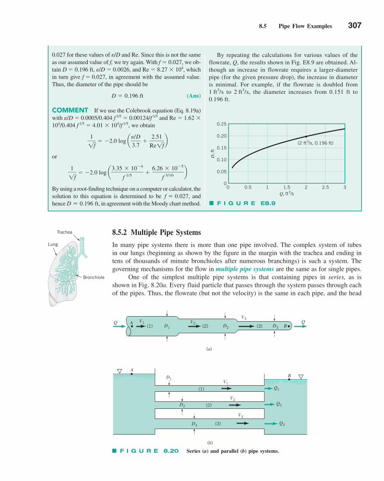
8.5 Pipe Flow Examples 307

8.5.2 Multiple Pipe Systems

In many pipe systems there is more than one pipe involved. The complex system of tubesin our lungs (beginning as shown by the figure in the margin with the trachea and ending intens of thousands of minute bronchioles after numerous branchings) is such a system. Thegoverning mechanisms for the flow in multiple pipe systems are the same as for single pipes.

One of the simplest multiple pipe systems is that containing pipes in series, as isshown in Fig. 8.20a. Every fluid particle that passes through the system passes through eachof the pipes. Thus, the flowrate (but not the velocity) is the same in each pipe, and the head

By repeating the calculations for various values of theflowrate, Q, the results shown in Fig. E8.9 are obtained. Al-though an increase in flowrate requires a larger-diameterpipe (for the given pressure drop), the increase in diameteris minimal. For example, if the flowrate is doubled from

to , the diameter increases from 0.151 ft to0.196 ft.

2 ft3/s1 ft3/s

0.027 for these values of e/D and Re. Since this is not the sameas our assumed value of f, we try again. With f � 0.027, we ob-tain D � 0.196 ft, e/D � 0.0026, and Re � 8.27 � 104, whichin turn give f � 0.027, in agreement with the assumed value.Thus, the diameter of the pipe should be

(Ans)

COMMENT If we use the Colebrook equation (Eq. 8.19a)with e/D � 0.0005/0.404 f 1/5 � 0.00124/f 1/5 and Re � 1.62 �104/0.404 f 1/5 � 4.01 � 104/f 1/5, we obtain

or

By using a root-finding technique on a computer or calculator, thesolution to this equation is determined to be andhence in agreement with the Moody chart method.D � 0.196 ft,

f � 0.027,

1

1f� �2.0 log a

3.35 � 10�4

f 1/5 �6.26 � 10�5

f 3/10 b

1

1f� �2.0 log a

e/D

3.7�

2.51

Re1fb

D � 0.196 ft

(2 ft3/s, 0.196 ft)

D, f

t

Q, ft3/s

0 0.5 1 1.5 2 2.5 3

0.25

0.20

0.15

0.10

0.05

0

F I G U R E E8.9

Bronchiole

Lung

Trachea

Q A V1(1) (2) (3)

V2D1 D2 D3 B Q

V3

(a)

V1

V2

V3

D3

D2

D1

(1)

(2)

(3)

Q1

Q2

Q3

BA

(b)

F I G U R E 8.20 Series (a) and parallel (b) pipe systems.

c08ViscousFlowinPipes.qxd 9/28/10 10:23 AM Page 307

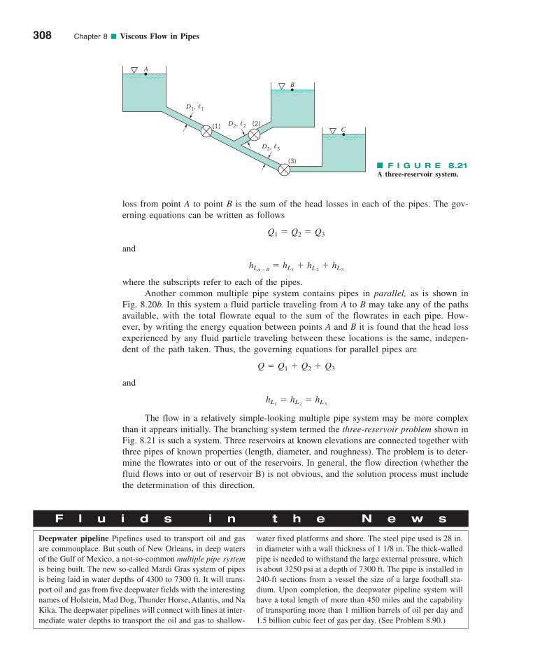
loss from point A to point B is the sum of the head losses in each of the pipes. The gov-erning equations can be written as follows

and

where the subscripts refer to each of the pipes.Another common multiple pipe system contains pipes in parallel, as is shown in

Fig. 8.20b. In this system a fluid particle traveling from A to B may take any of the pathsavailable, with the total flowrate equal to the sum of the flowrates in each pipe. How-ever, by writing the energy equation between points A and B it is found that the head lossexperienced by any fluid particle traveling between these locations is the same, indepen-dent of the path taken. Thus, the governing equations for parallel pipes are

and

The flow in a relatively simple-looking multiple pipe system may be more complexthan it appears initially. The branching system termed the three-reservoir problem shown inFig. 8.21 is such a system. Three reservoirs at known elevations are connected together withthree pipes of known properties (length, diameter, and roughness). The problem is to deter-mine the flowrates into or out of the reservoirs. In general, the flow direction (whether thefluid flows into or out of reservoir B) is not obvious, and the solution process must includethe determination of this direction.

hL1� hL2

� hL3

Q � Q1 � Q2 � Q3

hLA�B� hL1

� hL2� hL3

Q1 � Q2 � Q3

308 Chapter 8 ■ Viscous Flow in Pipes

F I G U R E 8.21A three-reservoir system.

A

B

C

(3)

(2)(1)

D1, �1

D2, �2

D3, �3

F l u i d s i n t h e N e w s

Deepwater pipeline Pipelines used to transport oil and gasare commonplace. But south of New Orleans, in deep watersof the Gulf of Mexico, a not-so-common multiple pipe systemis being built. The new so-called Mardi Gras system of pipesis being laid in water depths of 4300 to 7300 ft. It will trans-port oil and gas from five deepwater fields with the interestingnames of Holstein, Mad Dog, Thunder Horse, Atlantis, and NaKika. The deepwater pipelines will connect with lines at inter-mediate water depths to transport the oil and gas to shallow-

water fixed platforms and shore. The steel pipe used is 28 in.in diameter with a wall thickness of 1 1/8 in. The thick-walledpipe is needed to withstand the large external pressure, whichis about 3250 psi at a depth of 7300 ft. The pipe is installed in240-ft sections from a vessel the size of a large football sta-dium. Upon completion, the deepwater pipeline system willhave a total length of more than 450 miles and the capabilityof transporting more than 1 million barrels of oil per day and1.5 billion cubic feet of gas per day. (See Problem 8.90.)

c08ViscousFlowinPipes.qxd 9/28/10 10:23 AM Page 308

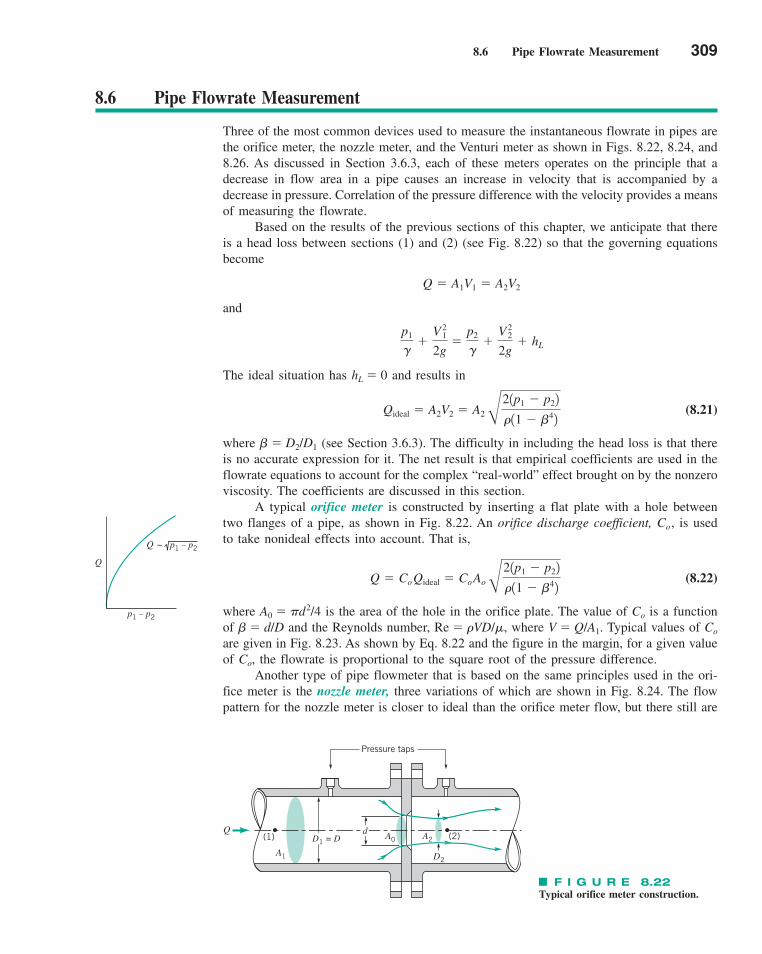
8.6 Pipe Flowrate Measurement 309

8.6 Pipe Flowrate Measurement

Three of the most common devices used to measure the instantaneous flowrate in pipes arethe orifice meter, the nozzle meter, and the Venturi meter as shown in Figs. 8.22, 8.24, and8.26. As discussed in Section 3.6.3, each of these meters operates on the principle that adecrease in flow area in a pipe causes an increase in velocity that is accompanied by adecrease in pressure. Correlation of the pressure difference with the velocity provides a meansof measuring the flowrate.

Based on the results of the previous sections of this chapter, we anticipate that thereis a head loss between sections (1) and (2) (see Fig. 8.22) so that the governing equationsbecome

and

The ideal situation has hL � 0 and results in

(8.21)

where � D2/D1 (see Section 3.6.3). The difficulty in including the head loss is that thereis no accurate expression for it. The net result is that empirical coefficients are used in theflowrate equations to account for the complex “real-world” effect brought on by the nonzeroviscosity. The coefficients are discussed in this section.

A typical orifice meter is constructed by inserting a flat plate with a hole betweentwo flanges of a pipe, as shown in Fig. 8.22. An orifice discharge coefficient, Co , is usedto take nonideal effects into account. That is,

(8.22)

where A0 � �d2/4 is the area of the hole in the orifice plate. The value of Co is a functionof � d/D and the Reynolds number, Re � �VD/�, where V � Q/A1. Typical values of Co

are given in Fig. 8.23. As shown by Eq. 8.22 and the figure in the margin, for a given valueof Co, the flowrate is proportional to the square root of the pressure difference.

Another type of pipe flowmeter that is based on the same principles used in the ori-fice meter is the nozzle meter, three variations of which are shown in Fig. 8.24. The flowpattern for the nozzle meter is closer to ideal than the orifice meter flow, but there still are

Q � Co Qideal � Co Ao B

21p1 � p22

�11 � 42

Qideal � A2V2 � A2 B

21p1 � p22

�11 � 42

p1

��

V 21

2g�

p2

��

V 22

2g� hL

Q � A1V1 � A2V2

Q

A1

A0(1) (2)A2

Pressure taps

dD1 = D

D2

F I G U R E 8.22Typical orifice meter construction.

~ p1 � p2Q

Q

p1 � p2

c08ViscousFlowinPipes.qxd 9/28/10 10:23 AM Page 309

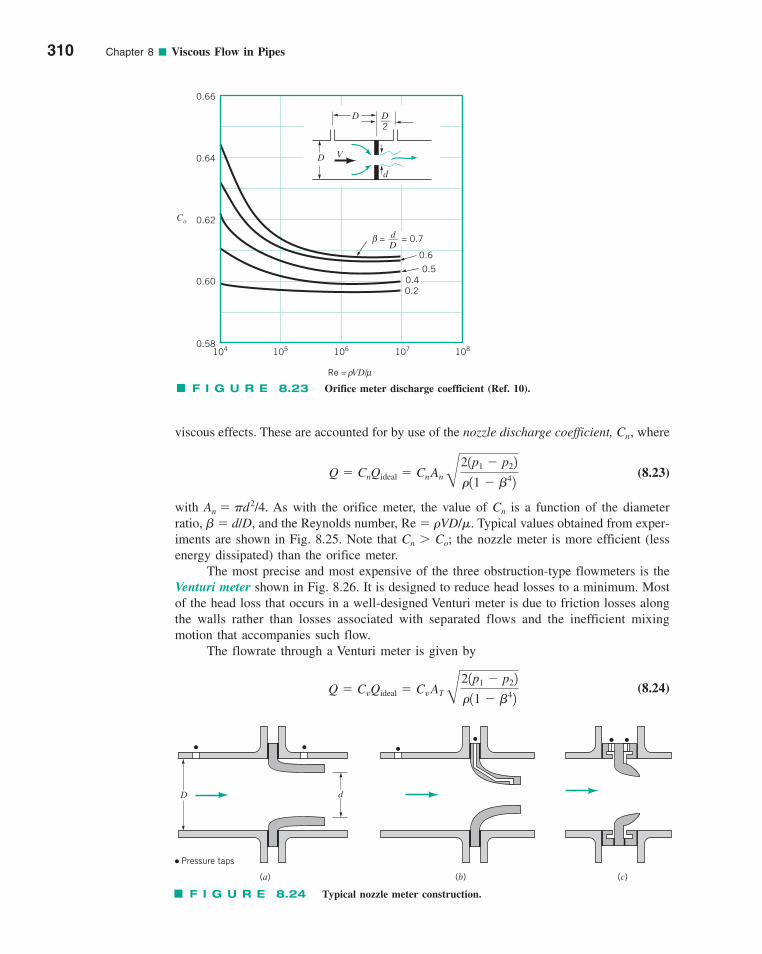
viscous effects. These are accounted for by use of the nozzle discharge coefficient, Cn, where

(8.23)

with An � �d2/4. As with the orifice meter, the value of Cn is a function of the diameterratio, � d/D, and the Reynolds number, Re � �VD/�. Typical values obtained from exper-iments are shown in Fig. 8.25. Note that Cn � Co; the nozzle meter is more efficient (lessenergy dissipated) than the orifice meter.

The most precise and most expensive of the three obstruction-type flowmeters is theVenturi meter shown in Fig. 8.26. It is designed to reduce head losses to a minimum. Mostof the head loss that occurs in a well-designed Venturi meter is due to friction losses alongthe walls rather than losses associated with separated flows and the inefficient mixingmotion that accompanies such flow.

The flowrate through a Venturi meter is given by

(8.24)Q � CvQideal � CvAT B

21p1 � p22

�11 � 42

Q � CnQideal � Cn An B

21p1 � p22

�11 � 42

310 Chapter 8 ■ Viscous Flow in Pipes

d__D

= = 0.7β

0.5

0.6

0.40.2

D V

d

D D__2

0.66

0.64

0.62

0.60

0.58104 105 106 107 108

Re = VD/ρ μ

Co

F I G U R E 8.23 Orifice meter discharge coefficient (Ref. 10).

F I G U R E 8.24 Typical nozzle meter construction.

dD

(a) (b) (c)

Pressure taps

c08ViscousFlowinPipes.qxd 9/28/10 10:23 AM Page 310

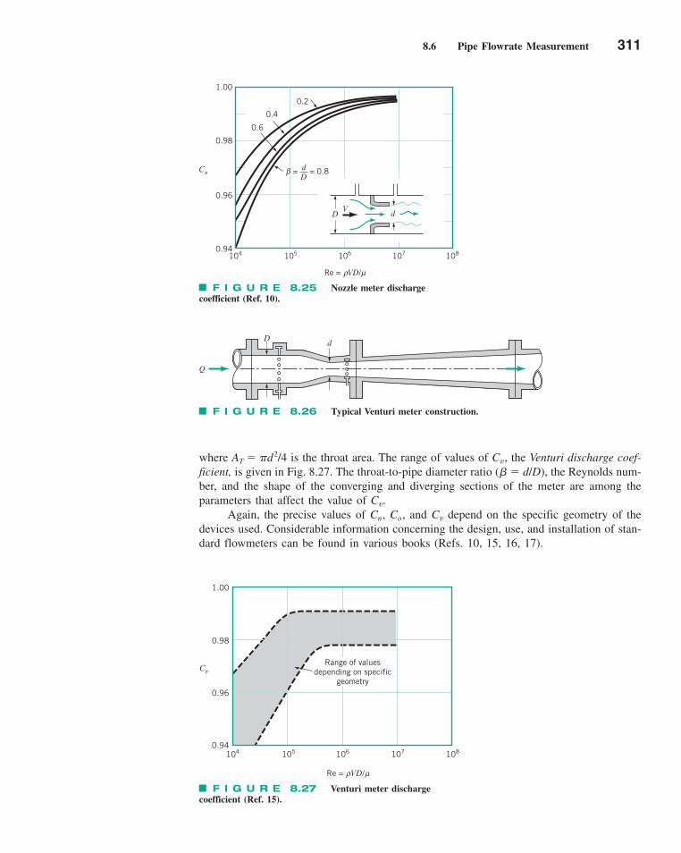
8.6 Pipe Flowrate Measurement 311

where AT � �d2/4 is the throat area. The range of values of Cv, the Venturi discharge coef-ficient, is given in Fig. 8.27. The throat-to-pipe diameter ratio ( � d/D), the Reynolds num-ber, and the shape of the converging and diverging sections of the meter are among theparameters that affect the value of Cv.

Again, the precise values of Cn, Co, and Cv depend on the specific geometry of thedevices used. Considerable information concerning the design, use, and installation of stan-dard flowmeters can be found in various books (Refs. 10, 15, 16, 17).

F I G U R E 8.25 Nozzle meter discharge coefficient (Ref. 10).

VD d

1.00

0.98

0.96

0.94104 105 106 107 108

Re = VD/ρ μ

Cn

0.6

0.4

0.2

= = 0.8d__D

β

F I G U R E 8.26 Typical Venturi meter construction.

Q

D d

F I G U R E 8.27 Venturi meter discharge coefficient (Ref. 15).

1.00

0.98

0.96

0.94104 105 106 107 108

Re = VD/ρ μ

CvRange of values

depending on specificgeometry

c08ViscousFlowinPipes.qxd 9/28/10 10:23 AM Page 311

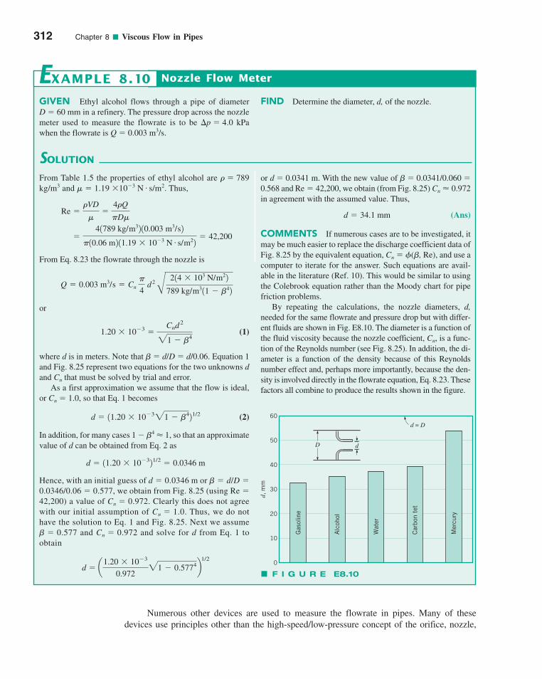
312 Chapter 8 ■ Viscous Flow in Pipes

GIVEN Ethyl alcohol flows through a pipe of diameterD � 60 mm in a refinery. The pressure drop across the nozzlemeter used to measure the flowrate is to be �p � 4.0 kPawhen the flowrate is Q � 0.003 m3/s.

SOLUTION

Nozzle Flow Meter

or d � 0.0341 m. With the new value of � 0.0341/0.060 �0.568 and Re � 42,200, we obtain (from Fig. 8.25) Cn � 0.972in agreement with the assumed value. Thus,

(Ans)

COMMENTS If numerous cases are to be investigated, itmay be much easier to replace the discharge coefficient data ofFig. 8.25 by the equivalent equation, Cn � �( , Re), and use acomputer to iterate for the answer. Such equations are avail-able in the literature (Ref. 10). This would be similar to usingthe Colebrook equation rather than the Moody chart for pipefriction problems.

By repeating the calculations, the nozzle diameters, d,needed for the same flowrate and pressure drop but with differ-ent fluids are shown in Fig. E8.10. The diameter is a function ofthe fluid viscosity because the nozzle coefficient, Cn, is a func-tion of the Reynolds number (see Fig. 8.25). In addition, the di-ameter is a function of the density because of this Reynoldsnumber effect and, perhaps more importantly, because the den-sity is involved directly in the flowrate equation, Eq. 8.23. Thesefactors all combine to produce the results shown in the figure.

d � 34.1 mm

FIND Determine the diameter, d, of the nozzle.

EXAMPLE 8.10

From Table 1.5 the properties of ethyl alcohol are � � 789kg/m3 and � � 1.19 �10�3 N s/m2. Thus,

From Eq. 8.23 the flowrate through the nozzle is

or

(1)

where d is in meters. Note that � d/D � d/0.06. Equation 1and Fig. 8.25 represent two equations for the two unknowns dand Cn that must be solved by trial and error.

As a first approximation we assume that the flow is ideal,or Cn � 1.0, so that Eq. 1 becomes

(2)

In addition, for many cases 1 � 4 � 1, so that an approximatevalue of d can be obtained from Eq. 2 as

Hence, with an initial guess of d � 0.0346 m or � d/D �0.0346/0.06 � 0.577, we obtain from Fig. 8.25 (using Re �42,200) a value of Cn � 0.972. Clearly this does not agreewith our initial assumption of Cn � 1.0. Thus, we do nothave the solution to Eq. 1 and Fig. 8.25. Next we assume � 0.577 and Cn � 0.972 and solve for d from Eq. 1 toobtain

d � a1.20 � 10�3

0.97221 � 0.5774b

1/2

d � 11.20 � 10�321/2 � 0.0346 m

d � 11.20 � 10�321 � 421/2

1.20 � 10�3 �Cnd2

21 � 4

Q � 0.003 m3/s � Cn �

4 d 2 B

214 � 103 N/m22

789 kg/m311 � 42

�41789 kg/m32 10.003 m3/s2

�10.06 m2 11.19 � 10�3 N # s/m22� 42,200

Re ��VD

��

4�Q

�D�

#

50

60

40

30

20

10

0

d, m

m

Gas

olin

e

Alc

ohol

Wat

er

Car

bon

tet

Mer

cury

dD

d = D

F I G U R E E8.10

Numerous other devices are used to measure the flowrate in pipes. Many of thesedevices use principles other than the high-speed/low-pressure concept of the orifice, nozzle,

c08ViscousFlowinPipes.qxd 9/28/10 10:23 AM Page 312

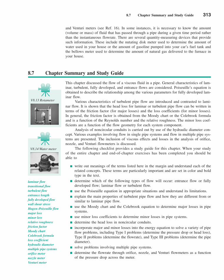
8.7 Chapter Summary and Study Guide 313

and Venturi meters (see Ref. 16). In some instances, it is necessary to know the amount(volume or mass) of fluid that has passed through a pipe during a given time period ratherthan the instantaneous flowrate. There are several quantity-measuring devices that providesuch information. These include the nutating disk meter used to determine the amount ofwater used in your house or the amount of gasoline pumped into your car’s fuel tank andthe bellows meter used to determine the amount of natural gas delivered to the furnace inyour house.

laminar flowtransitional flowturbulent flowentrance lengthfully developed flowwall shear stressHagen–Poiseuille flowmajor lossminor lossrelative roughnessfriction factorMoody chartColebrook formulaloss coefficienthydraulic diametermultiple pipe systemsorifice meternozzle meterVenturi meter

V8.14 Water meter

V8.13 Rotameter

8.7 Chapter Summary and Study Guide

This chapter discussed the flow of a viscous fluid in a pipe. General characteristics of lam-inar, turbulent, fully developed, and entrance flows are considered. Poiseuille’s equation isobtained to describe the relationship among the various parameters for fully developed lam-inar flow.

Various characteristics of turbulent pipe flow are introduced and contrasted to lami-nar flow. It is shown that the head loss for laminar or turbulent pipe flow can be written interms of the friction factor (for major losses) and the loss coefficients (for minor losses).In general, the friction factor is obtained from the Moody chart or the Colebrook formulaand is a function of the Reynolds number and the relative roughness. The minor loss coef-ficients are a function of the flow geometry for each system component.

Analysis of noncircular conduits is carried out by use of the hydraulic diameter con-cept. Various examples involving flow in single pipe systems and flow in multiple pipe sys-tems are presented. The inclusion of viscous effects and losses in the analysis of orifice,nozzle, and Venturi flowmeters is discussed.

The following checklist provides a study guide for this chapter. When your studyof the entire chapter and end-of-chapter exercises has been completed you should beable to

write out meanings of the terms listed here in the margin and understand each of therelated concepts. These terms are particularly important and are set in color and boldtype in the text.

determine which of the following types of flow will occur: entrance flow or fullydeveloped flow; laminar flow or turbulent flow.

use the Poiseuille equation in appropriate situations and understand its limitations.

explain the main properties of turbulent pipe flow and how they are different from orsimilar to laminar pipe flow.

use the Moody chart and the Colebrook equation to determine major losses in pipesystems.

use minor loss coefficients to determine minor losses in pipe systems.

determine the head loss in noncircular conduits.

incorporate major and minor losses into the energy equation to solve a variety of pipeflow problems, including Type I problems (determine the pressure drop or head loss),Type II problems (determine the flowrate), and Type III problems (determine the pipediameter).

solve problems involving multiple pipe systems.

determine the flowrate through orifice, nozzle, and Venturi flowmeters as a functionof the pressure drop across the meter.

c08ViscousFlowinPipes.qxd 9/28/10 10:23 AM Page 313

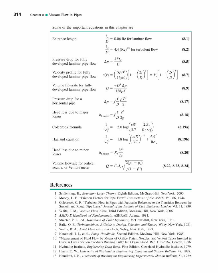
Some of the important equations in this chapter are

Entrance length (8.1)

(8.2)

Pressure drop for fully developed laminar pipe flow (8.5)

Velocity profile for fully developed laminar pipe flow (8.7)

Volume flowrate for fully developed laminar pipe flow (8.9)

Pressure drop for a horizontal pipe (8.17)

Head loss due to major losses (8.18)

Colebrook formula (8.19a)

Haaland equation (8.19b)

Head loss due to minor losses (8.20)

Volume flowrate for orifice,nozzle, or Venturi meter (8.22, 8.23, 8.24)

References

1. Schlichting, H., Boundary Layer Theory, Eighth Edition, McGraw-Hill, New York, 2000.2. Moody, L. F., “Friction Factors for Pipe Flow,” Transactions of the ASME, Vol. 66, 1944.3. Colebrook, C. F., “Turbulent Flow in Pipes with Particular Reference to the Transition Between the

Smooth and Rough Pipe Laws,” Journal of the Institute of Civil Engineers London, Vol. 11, 1939.4. White, F. M., Viscous Fluid Flow, Third Edition, McGraw-Hill, New York, 2006.5. ASHRAE Handbook of Fundamentals, ASHRAE, Atlanta, 1981.6. Streeter, V. L., ed., Handbook of Fluid Dynamics, McGraw-Hill, New York, 1961.7. Balje, O. E., Turbomachines: A Guide to Design, Selection and Theory, Wiley, New York, 1981.8. Wallis, R. A., Axial Flow Fans and Ducts, Wiley, New York, 1983.9. Karassick, I. J., et al., Pump Handbook, Second Edition, McGraw-Hill, New York, 1985.

10. “Measurement of Fluid Flow by Means of Orifice Plates, Nozzles, and Venturi Tubes Inserted inCircular Cross Section Conduits Running Full,” Int. Organ. Stand. Rep. DIS-5167, Geneva, 1976.

11. Hydraulic Institute, Engineering Data Book, First Edition, Cleveland Hydraulic Institute, 1979.12. Harris, C. W., University of Washington Engineering Experimental Station Bulletin, 48, 1928.13. Hamilton, J. B., University of Washington Engineering Experimental Station Bulletin, 51, 1929.

Q � Ci AiB

21p1 � p22

�11 � 42

hL minor � KL

V2

2g

1

1f� �1.8 log ca

e/D

3.7b

1.11

�6.9

Red

1

1f� �2.0 log a

e/D

3.7�

2.51

Re1fb

hL major � f/D

V2

2g

¢p � f/D

�V 2

2

Q ��D4 ¢p

128�/

u1r2 � a¢pD2

16�/b c1 � a

2r

Db

2

d � Vc c1 � a2r

Db

2

d

¢p �4/�w

D

/e

D� 4.4 1Re21/6 for turbulent flow

/e

D� 0.06 Re for laminar flow

314 Chapter 8 ■ Viscous Flow in Pipes

c08ViscousFlowinPipes.qxd 9/28/10 10:23 AM Page 314

Problems 315

14. Laws, E. M., and Livesey, J. L., “Flow Through Screens,” Annual Review of Fluid Mechanics,Vol. 10, Annual Reviews, Inc., Palo Alto, CA, 1978.

15. Bean, H. S., ed., Fluid Meters: Their Theory and Application, Sixth Edition, American Societyof Mechanical Engineers, New York, 1971.

16. Goldstein, R. J., ed., Fluid Mechanics Measurements, Second Edition, Taylor and Francis,Philadelphia, 1996.

17. Spitzer, D. W., ed., Flow Measurement: Practical Guides for Measurement and Control, Instru-ment Society of America, Research Triangle Park, North Carolina, 1991.

18. Haaland, S. E., “Simple and Explicit Formulas for the Friction-Factor in Turbulent Pipe Flow,”Transactions of the ASME, Journal of Fluids Engineering, Vol. 105, 1983.

Review Problems

Go to Appendix G for a set of review problems with answers.Detailed solutions can be found in Student Solution Manual

for a Brief Introduction to Fluid Mechanics, by Young et al. (© 2011 John Wiley and Sons, Inc.).

Problems

Note: Unless otherwise indicated use the values of fluidproperties found in the tables on the inside of the frontcover. Problems designated with an (*) are intended to besolved with the aid of a programmable calculator or a com-puter. Problems designated with a (†) are “open-ended”problems and require critical thinking in that to work themone must make various assumptions and provide the neces-sary data. There is not a unique answer to these problems.

The even-numbered problems are included in thehard copy version of the book, and the answers to theseeven-numbered problems are listed at the end of the book.Odd-numbered problems are provided in WileyPLUS, orin Appendix L on the book’s web site, www.wiley.com/college/young. The lab-type problems, FE problems, FlowLabproblems, and the videos that accompany problems can alsobe accessed on these web sites.

Section 8.1 General Characteristics of Pipe Flow(also see Lab Problem 8.105)

8.2 (See Fluids in the News article titled “Nanoscale flows,”Section 8.1.1.) (a) Water flows in a tube that has a diameter of

Determine the Reynolds number if the average ve-locity is 10 diameters per second. (b) Repeat the calculations ifthe tube is a nanoscale tube with a diameter of

8.4 Water flows through a 50-ft pipe with a 0.5-in. diameter at5 gal/min. What fraction of this pipe can be considered an en-trance region?

8.6 Carbon dioxide at and a pressure of 550 kPa (abs)flows in a pipe at a rate of 0.04 N/s. Determine the maximum di-ameter allowed if the flow is to be turbulent.

8.8 A soft drink with the properties of water is suckedthrough a 4-mm-diameter, 0.25-m-long straw at a rate of 4 cm3/s. Is the flow at the outlet of the straw laminar? Is it fullydeveloped? Explain.

10 °C

20 °C

D � 100 nm.

D � 0.1 m.

8.10 The pressure distribution measured along a straight, hori-zontal portion of a 50-mm-diameter pipe attached to a tank isshown below. Approximately how long is the entrance length?In the fully developed portion of the flow, what is the value ofthe wall shear stress?

x (m) (�0.01 m) p (mm H2O) (�5 mm)

0 (tank exit) 5200.5 4271.0 3511.5 2882.0 2362.5 1883.0 1453.5 1094.0 734.5 365.0 (pipe exit) 0

Section 8.2 Fully Developed Laminar Flow

8.12 Water flows in a constant-diameter pipe with the follow-ing conditions measured: At section (a) pa � 32.4 psi and za �56.8 ft; at section (b) pb � 29.7 psi and zb � 68.2 ft. Is the flowfrom (a) to (b) or from (b) to (a)? Explain.

8.14 A fluid flows through a horizontal 0.1-in.-diameter pipe.When the Reynolds number is 1500, the head loss over a 20-ftlength of the pipe is 6.4 ft. Determine the fluid velocity.

8.16 For fully developed laminar pipe flow in a circular pipe,the velocity profile is given by u(r) � 2 (1 � r2/R2) in m/s,where R is the inner radius of the pipe. Assuming that the pipe

c08ViscousFlowinPipes.qxd 10/18/10 8:03 AM Page 315

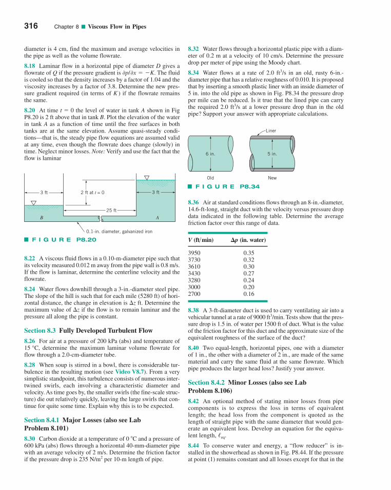
316 Chapter 8 ■ Viscous Flow in Pipes

diameter is 4 cm, find the maximum and average velocities inthe pipe as well as the volume flowrate.

8.18 Laminar flow in a horizontal pipe of diameter D gives aflowrate of Q if the pressure gradient is The fluidis cooled so that the density increases by a factor of 1.04 and theviscosity increases by a factor of 3.8. Determine the new pres-sure gradient required (in terms of K ) if the flowrate remainsthe same.

8.20 At time the level of water in tank A shown in FigP8.20 is 2 ft above that in tank B. Plot the elevation of the waterin tank A as a function of time until the free surfaces in bothtanks are at the same elevation. Assume quasi-steady condi-tions—that is, the steady pipe flow equations are assumed validat any time, even though the flowrate does change (slowly) intime. Neglect minor losses. Note: Verify and use the fact that theflow is laminar

t � 0

0p/0x � �K.

8.22 A viscous fluid flows in a 0.10-m-diameter pipe such thatits velocity measured 0.012 m away from the pipe wall is 0.8 m/s.If the flow is laminar, determine the centerline velocity and theflowrate.

8.24 Water flows downhill through a 3-in.-diameter steel pipe.The slope of the hill is such that for each mile (5280 ft) of hori-zontal distance, the change in elevation is �z ft. Determine themaximum value of �z if the flow is to remain laminar and thepressure all along the pipe is constant.

Section 8.3 Fully Developed Turbulent Flow

8.26 For air at a pressure of 200 kPa (abs) and temperature ofdetermine the maximum laminar volume flowrate for

flow through a 2.0-cm-diameter tube.

8.28 When soup is stirred in a bowl, there is considerable tur-bulence in the resulting motion (see Video V8.7). From a verysimplistic standpoint, this turbulence consists of numerous inter-twined swirls, each involving a characteristic diameter and velocity. As time goes by, the smaller swirls (the fine-scale struc-ture) die out relatively quickly, leaving the large swirls that con-tinue for quite some time. Explain why this is to be expected.

Section 8.4.1 Major Losses (also see Lab Problem 8.101)

8.30 Carbon dioxide at a temperature of 0 �C and a pressure of600 kPa (abs) flows through a horizontal 40-mm-diameter pipewith an average velocity of 2 m/s. Determine the friction factorif the pressure drop is 235 N/m2 per 10-m length of pipe.

15 °C,

8.32 Water flows through a horizontal plastic pipe with a diam-eter of 0.2 m at a velocity of 10 cm/s. Determine the pressuredrop per meter of pipe using the Moody chart.

8.34 Water flows at a rate of 2.0 ft3/s in an old, rusty 6-in.-diameter pipe that has a relative roughness of 0.010. It is proposedthat by inserting a smooth plastic liner with an inside diameter of5 in. into the old pipe as shown in Fig. P8.34 the pressure dropper mile can be reduced. Is it true that the lined pipe can carrythe required 2.0 ft3/s at a lower pressure drop than in the oldpipe? Support your answer with appropriate calculations.

8.36 Air at standard conditions flows through an 8-in.-diameter,14.6-ft-long, straight duct with the velocity versus pressure dropdata indicated in the following table. Determine the averagefriction factor over this range of data.

V (ft�min) �p (in. water)

3950 0.353730 0.323610 0.303430 0.273280 0.243000 0.202700 0.16

8.38 A 3-ft-diameter duct is used to carry ventilating air into avehicular tunnel at a rate of 9000 ft3/min. Tests show that the pres-sure drop is 1.5 in. of water per 1500 ft of duct. What is the valueof the friction factor for this duct and the approximate size of theequivalent roughness of the surface of the duct?

8.40 Two equal-length, horizontal pipes, one with a diameterof 1 in., the other with a diameter of 2 in., are made of the samematerial and carry the same fluid at the same flowrate. Whichpipe produces the larger head loss? Justify your answer.

Section 8.4.2 Minor Losses (also see Lab Problem 8.106)

8.42 An optional method of stating minor losses from pipecomponents is to express the loss in terms of equivalentlength; the head loss from the component is quoted as thelength of straight pipe with the same diameter that would gen-erate an equivalent loss. Develop an equation for the equiva-lent length, .

8.44 To conserve water and energy, a “flow reducer” is in-stalled in the showerhead as shown in Fig. P8.44. If the pressureat point (1) remains constant and all losses except for that in the

/eq

0.1-in. diameter, galvanized iron

25 ft

2 ft at t = 0 3 ft3 ft

B A

F I G U R E P8.20

6 in.

Old

5 in.

New

Liner

F I G U R E P8.34

c08ViscousFlowinPipes.qxd 9/28/10 10:23 AM Page 316

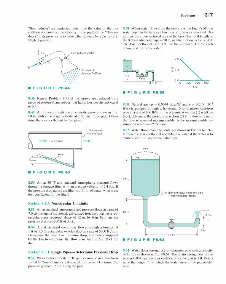
Problems 317

“flow reducer” are neglected, determine the value of the losscoefficient (based on the velocity in the pipe) of the “flow re-ducer” if its presence is to reduce the flowrate by a factor of 2.Neglect gravity.

8.46 Repeat Problem 8.45 if the straws are replaced by apiece of porous foam rubber that has a loss coefficient equalto 5.4.

8.48 Air flows through the fine mesh gauze shown in Fig.P8.48 with an average velocity of 1.50 m/s in the pipe. Deter-mine the loss coefficient for the gauze.

8.50 Air at 80 �F and standard atmospheric pressure flowsthrough a furnace filter with an average velocity of 2.4 ft/s. Ifthe pressure drop across the filter is 0.11 in. of water, what is theloss coefficient for the filter?

Section 8.4.3 Noncircular Conduits

8.52 Air at standard temperature and pressure flows at a rate of7.0 cfs through a horizontal, galvanized iron duct that has a rec-tangular cross-sectional shape of 12 in. by 6 in. Estimate thepressure drop per 200 ft of duct.

8.54 Air at standard conditions flows through a horizontal 1 ft by 1.5 ft rectangular wooden duct at a rate of Determine the head loss, pressure drop, and power suppliedby the fan to overcome the flow resistance in 500 ft of theduct.

Section 8.5.1 Single Pipes—Determine Pressure Drop

8.56 Water flows at a rate of 10 gal per minute in a new hori-zontal 0.75-in.-diameter galvanized iron pipe. Determine thepressure gradient, �p/�, along the pipe.

5000 ft3�min.

8.58 When water flows from the tank shown in Fig. P8.58, thewater depth in the tank as a function of time is as indicated. De-termine the cross-sectional area of the tank. The total length ofthe 0.60-in.-diameter pipe is 20 ft, and the friction factor is 0.03.The loss coefficients are 0.50 for the entrance, 1.5 for each elbow, and 10 for the valve.

8.60 Natural gas (� � 0.0044 slugs/ft3 and � � 5.2 � 10�5

ft2/s) is pumped through a horizontal 6-in.-diameter cast-ironpipe at a rate of 800 lb/hr. If the pressure at section (1) is 50 psi(abs), determine the pressure at section (2) 8 mi downstream ifthe flow is assumed incompressible. Is the incompressible as-sumption reasonable? Explain.

8.62 Water flows from the container shown in Fig. P8.62. De-termine the loss coefficient needed in the valve if the water is to“bubble up” 3 in. above the outlet pipe.

8.64 Water flows through a 2-in.-diameter pipe with a velocityof 15 ft/s as shown in Fig. P8.64. The relative roughness of thepipe is 0.004, and the loss coefficient for the exit is 1.0. Deter-mine the height, h, to which the water rises in the piezometertube.

Q

1__2

in.

(1)

Flow reducer washer

50 holes ofdiameter 0.05 in.

F I G U R E P8.44

Gauze overend of pipe

Water

8 mm

V = 1.5 m/s

F I G U R E P8.48

3 ftValve

h

2.0

1.5

1.00 100 200 300

t, s

h, f

t

F I G U R E P8.58

32 in.

18 in.

27 in.

Vent

3 in.

2 in.

-in.-diameter galvanized iron pipewith threaded fittings

1__2

F I G U R E P8.62

c08ViscousFlowinPipes.qxd 9/28/10 10:23 AM Page 317

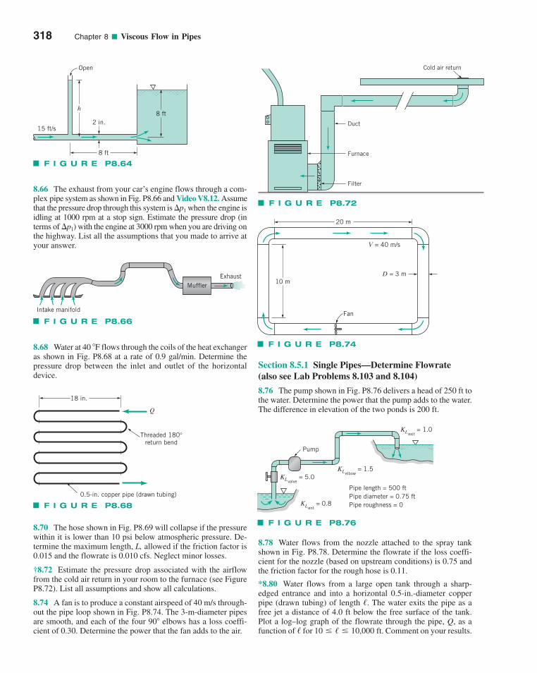
Section 8.5.1 Single Pipes—Determine Flowrate(also see Lab Problems 8.103 and 8.104)

8.76 The pump shown in Fig. P8.76 delivers a head of 250 ft tothe water. Determine the power that the pump adds to the water.The difference in elevation of the two ponds is 200 ft.

8.78 Water flows from the nozzle attached to the spray tankshown in Fig. P8.78. Determine the flowrate if the loss coeffi-cient for the nozzle (based on upstream conditions) is 0.75 andthe friction factor for the rough hose is 0.11.

*8.80 Water flows from a large open tank through a sharp-edged entrance and into a horizontal 0.5-in.-diameter copperpipe (drawn tubing) of length The water exits the pipe as afree jet a distance of 4.0 ft below the free surface of the tank.Plot a log–log graph of the flowrate through the pipe, Q, as afunction of for Comment on your results.10 � / � 10,000 ft./

/.

8.66 The exhaust from your car’s engine flows through a com-plex pipe system as shown in Fig. P8.66 and Video V8.12. Assumethat the pressure drop through this system is �p1 when the engine isidling at 1000 rpm at a stop sign. Estimate the pressure drop (interms of �p1) with the engine at 3000 rpm when you are driving onthe highway. List all the assumptions that you made to arrive atyour answer.

8.68 Water at 40 �F flows through the coils of the heat exchangeras shown in Fig. P8.68 at a rate of 0.9 gal/min. Determine thepressure drop between the inlet and outlet of the horizontal device.

8.70 The hose shown in Fig. P8.69 will collapse if the pressurewithin it is lower than 10 psi below atmospheric pressure. De-termine the maximum length, L, allowed if the friction factor is0.015 and the flowrate is 0.010 cfs. Neglect minor losses.

†8.72 Estimate the pressure drop associated with the airflowfrom the cold air return in your room to the furnace (see FigureP8.72). List all assumptions and show all calculations.

8.74 A fan is to produce a constant airspeed of 40 m/s through-out the pipe loop shown in Fig. P8.74. The 3-m-diameter pipesare smooth, and each of the four 90� elbows has a loss coeffi-cient of 0.30. Determine the power that the fan adds to the air.

318 Chapter 8 ■ Viscous Flow in Pipes

8 ft

8 ft

2 in.15 ft/s

h

Open

F I G U R E P8.64

F I G U R E P8.66

MufflerExhaust

Intake manifold

F I G U R E P8.68

Q

18 in.

0.5-in. copper pipe (drawn tubing)

Threaded 180°return bend

F I G U R E P8.72

Duct

Cold air return

Furnace

Filter

F I G U R E P8.74

Fan

V = 40 m/s

D = 3 m10 m

20 m

F I G U R E P8.76

KLvalve = 5.0

KLelbow = 1.5

Pipe length = 500 ftPipe diameter = 0.75 ftPipe roughness = 0

KLexit = 1.0

Pump

KLent = 0.8

c08ViscousFlowinPipes.qxd 9/28/10 10:23 AM Page 318

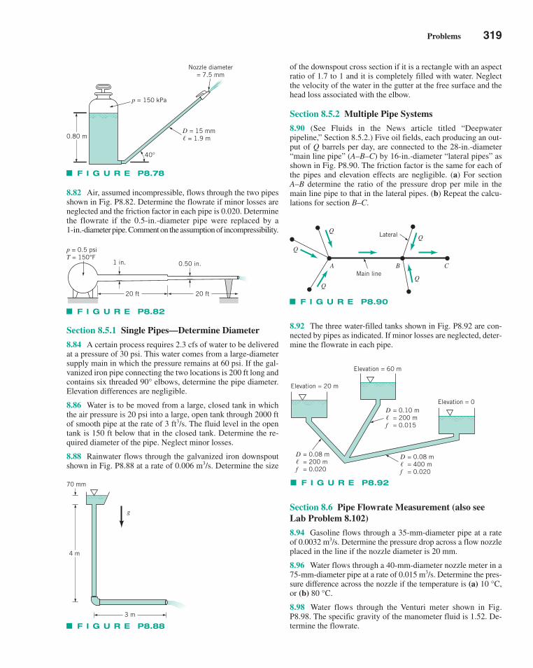
Section 8.5.1 Single Pipes—Determine Diameter

8.84 A certain process requires 2.3 cfs of water to be deliveredat a pressure of 30 psi. This water comes from a large-diametersupply main in which the pressure remains at 60 psi. If the gal-vanized iron pipe connecting the two locations is 200 ft long andcontains six threaded elbows, determine the pipe diameter.Elevation differences are negligible.

8.86 Water is to be moved from a large, closed tank in whichthe air pressure is 20 psi into a large, open tank through 2000 ftof smooth pipe at the rate of 3 ft3/s. The fluid level in the opentank is 150 ft below that in the closed tank. Determine the re-quired diameter of the pipe. Neglect minor losses.

8.88 Rainwater flows through the galvanized iron downspoutshown in Fig. P8.88 at a rate of 0.006 m3/s. Determine the size

90°

of the downspout cross section if it is a rectangle with an aspectratio of 1.7 to 1 and it is completely filled with water. Neglectthe velocity of the water in the gutter at the free surface and thehead loss associated with the elbow.

Section 8.5.2 Multiple Pipe Systems

8.90 (See Fluids in the News article titled “Deepwaterpipeline,” Section 8.5.2.) Five oil fields, each producing an out-put of Q barrels per day, are connected to the 28-in.-diameter“main line pipe” (A–B–C) by 16-in.-diameter “lateral pipes” asshown in Fig. P8.90. The friction factor is the same for each ofthe pipes and elevation effects are negligible. (a) For sectionA–B determine the ratio of the pressure drop per mile in themain line pipe to that in the lateral pipes. (b) Repeat the calcu-lations for section B–C.

8.92 The three water-filled tanks shown in Fig. P8.92 are con-nected by pipes as indicated. If minor losses are neglected, deter-mine the flowrate in each pipe.

Section 8.6 Pipe Flowrate Measurement (also seeLab Problem 8.102)

8.94 Gasoline flows through a 35-mm-diameter pipe at a rateof 0.0032 m3/s. Determine the pressure drop across a flow nozzleplaced in the line if the nozzle diameter is 20 mm.

8.96 Water flows through a 40-mm-diameter nozzle meter in a75-mm-diameter pipe at a rate of 0.015 m3/s. Determine the pres-sure difference across the nozzle if the temperature is (a)or (b)

8.98 Water flows through the Venturi meter shown in Fig.P8.98. The specific gravity of the manometer fluid is 1.52. De-termine the flowrate.

80 °C.10 °C,

Problems 319

8.82 Air, assumed incompressible, flows through the two pipesshown in Fig. P8.82. Determine the flowrate if minor losses areneglected and the friction factor in each pipe is 0.020. Determinethe flowrate if the 0.5-in.-diameter pipe were replaced by a 1-in.-diameter pipe. Comment on the assumption of incompressibility.

F I G U R E P8.78

Nozzle diameter= 7.5 mm

0.80 m

p = 150 kPa

D = 15 mm� = 1.9 m

40°

p = 0.5 psiT = 150°F

20 ft 20 ft

1 in. 0.50 in.

F I G U R E P8.82

g

70 mm

4 m

3 m

F I G U R E P8.88

Q

QQ

Q

Q

CBAMain line

Lateral

F I G U R E P8.90

Elevation = 20 m

Elevation = 60 m

Elevation = 0= 0.10 m= 200 m= 0.015

D�f

= 0.08 m= 400 m= 0.020

D�f

= 0.08 m= 200 m= 0.020

D�f

F I G U R E P8.92

c08ViscousFlowinPipes.qxd 9/28/10 10:23 AM Page 319

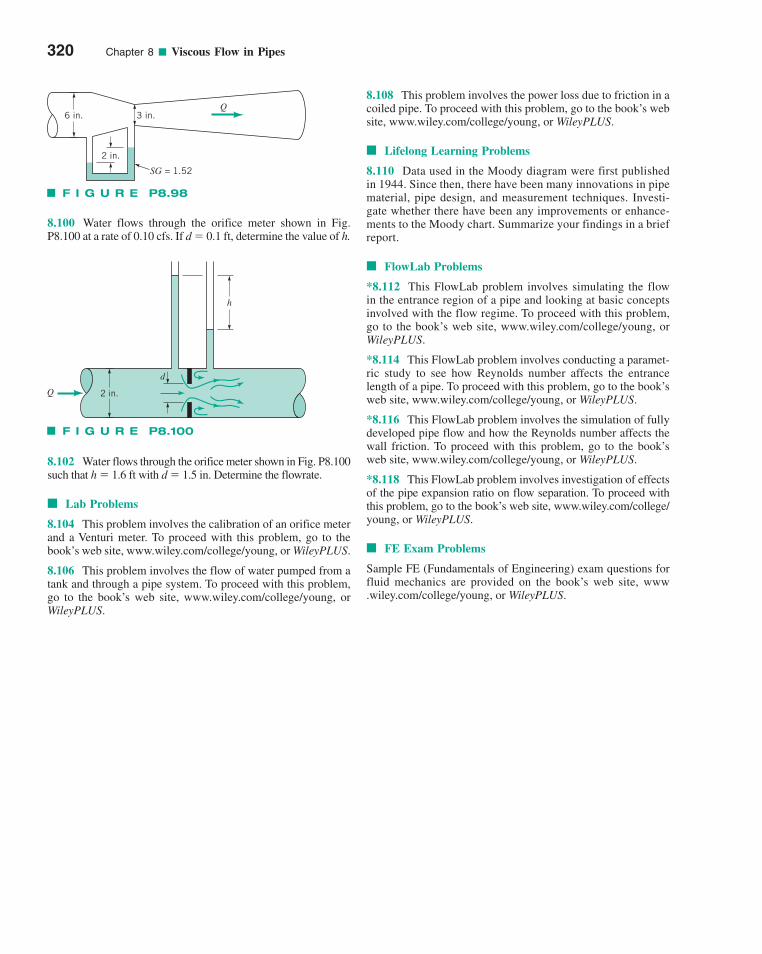
8.100 Water flows through the orifice meter shown in Fig.P8.100 at a rate of 0.10 cfs. If d � 0.1 ft, determine the value of h.

8.102 Water flows through the orifice meter shown in Fig. P8.100such that h � 1.6 ft with d � 1.5 in. Determine the flowrate.

■ Lab Problems

8.104 This problem involves the calibration of an orifice meterand a Venturi meter. To proceed with this problem, go to thebook’s web site, www.wiley.com/college/young, or WileyPLUS.

8.106 This problem involves the flow of water pumped from atank and through a pipe system. To proceed with this problem,go to the book’s web site, www.wiley.com/college/young, orWileyPLUS.

8.108 This problem involves the power loss due to friction in acoiled pipe. To proceed with this problem, go to the book’s website, www.wiley.com/college/young, or WileyPLUS.

■ Lifelong Learning Problems

8.110 Data used in the Moody diagram were first publishedin 1944. Since then, there have been many innovations in pipematerial, pipe design, and measurement techniques. Investi-gate whether there have been any improvements or enhance-ments to the Moody chart. Summarize your findings in a briefreport.

■ FlowLab Problems

*8.112 This FlowLab problem involves simulating the flowin the entrance region of a pipe and looking at basic conceptsinvolved with the flow regime. To proceed with this problem,go to the book’s web site, www.wiley.com/college/young, orWileyPLUS.

*8.114 This FlowLab problem involves conducting a paramet-ric study to see how Reynolds number affects the entrancelength of a pipe. To proceed with this problem, go to the book’sweb site, www.wiley.com/college/young, or WileyPLUS.

*8.116 This FlowLab problem involves the simulation of fullydeveloped pipe flow and how the Reynolds number affects thewall friction. To proceed with this problem, go to the book’sweb site, www.wiley.com/college/young, or WileyPLUS.

*8.118 This FlowLab problem involves investigation of effectsof the pipe expansion ratio on flow separation. To proceed withthis problem, go to the book’s web site, www.wiley.com/college/young, or WileyPLUS.

■ FE Exam Problems

Sample FE (Fundamentals of Engineering) exam questions forfluid mechanics are provided on the book’s web site, www.wiley.com/college/young, or WileyPLUS.

320 Chapter 8 ■ Viscous Flow in Pipes

3 in.6 in.

2 in.

SG = 1.52

Q

F I G U R E P8.98

h

Q

d

2 in.

F I G U R E P8.100

c08ViscousFlowinPipes.qxd 9/28/10 10:23 AM Page 320

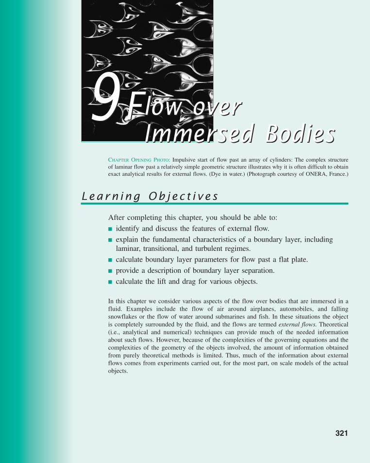
CHAPTER OPENING PHOTO: Impulsive start of flow past an array of cylinders: The complex structureof laminar flow past a relatively simple geometric structure illustrates why it is often difficult to obtainexact analytical results for external flows. (Dye in water.) (Photograph courtesy of ONERA, France.)

99Flow overImmersed Bodies

Flow overImmersed Bodies

Learn ing Ob j ec t i v e s

After completing this chapter, you should be able to:

■ identify and discuss the features of external flow.

■ explain the fundamental characteristics of a boundary layer, includinglaminar, transitional, and turbulent regimes.

■ calculate boundary layer parameters for flow past a flat plate.

■ provide a description of boundary layer separation.

■ calculate the lift and drag for various objects.

In this chapter we consider various aspects of the flow over bodies that are immersed in afluid. Examples include the flow of air around airplanes, automobiles, and fallingsnowflakes or the flow of water around submarines and fish. In these situations the objectis completely surrounded by the fluid, and the flows are termed external flows. Theoretical(i.e., analytical and numerical) techniques can provide much of the needed informationabout such flows. However, because of the complexities of the governing equations and thecomplexities of the geometry of the objects involved, the amount of information obtainedfrom purely theoretical methods is limited. Thus, much of the information about externalflows comes from experiments carried out, for the most part, on scale models of the actualobjects.

321

c09FlowoverImmersedBodies.qxd 9/28/10 10:27 AM Page 321

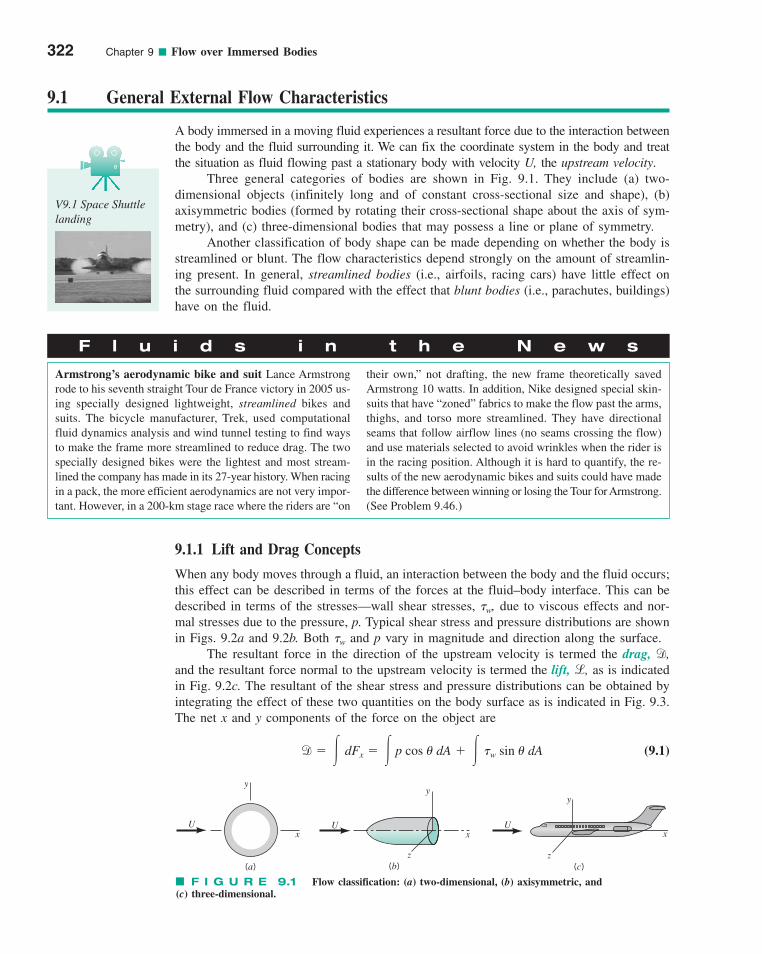
9.1.1 Lift and Drag Concepts

When any body moves through a fluid, an interaction between the body and the fluid occurs;this effect can be described in terms of the forces at the fluid–body interface. This can bedescribed in terms of the stresses—wall shear stresses, �w, due to viscous effects and nor-mal stresses due to the pressure, p. Typical shear stress and pressure distributions are shownin Figs. 9.2a and 9.2b. Both �w and p vary in magnitude and direction along the surface.

The resultant force in the direction of the upstream velocity is termed the drag, d,and the resultant force normal to the upstream velocity is termed the lift, l, as is indicatedin Fig. 9.2c. The resultant of the shear stress and pressure distributions can be obtained byintegrating the effect of these two quantities on the body surface as is indicated in Fig. 9.3.The net x and y components of the force on the object are

(9.1)d � � dFx � � p cos � dA � � �w sin � dA

322 Chapter 9 ■ Flow over Immersed Bodies

9.1 General External Flow Characteristics

A body immersed in a moving fluid experiences a resultant force due to the interaction betweenthe body and the fluid surrounding it. We can fix the coordinate system in the body and treatthe situation as fluid flowing past a stationary body with velocity U, the upstream velocity.

Three general categories of bodies are shown in Fig. 9.1. They include (a) two-dimensional objects (infinitely long and of constant cross-sectional size and shape), (b)axisymmetric bodies (formed by rotating their cross-sectional shape about the axis of sym-metry), and (c) three-dimensional bodies that may possess a line or plane of symmetry.

Another classification of body shape can be made depending on whether the body isstreamlined or blunt. The flow characteristics depend strongly on the amount of streamlin-ing present. In general, streamlined bodies (i.e., airfoils, racing cars) have little effect onthe surrounding fluid compared with the effect that blunt bodies (i.e., parachutes, buildings)have on the fluid.

F l u i d s i n t h e N e w s

Armstrong’s aerodynamic bike and suit Lance Armstrongrode to his seventh straight Tour de France victory in 2005 us-ing specially designed lightweight, streamlined bikes andsuits. The bicycle manufacturer, Trek, used computationalfluid dynamics analysis and wind tunnel testing to find waysto make the frame more streamlined to reduce drag. The twospecially designed bikes were the lightest and most stream-lined the company has made in its 27-year history. When racingin a pack, the more efficient aerodynamics are not very impor-tant. However, in a 200-km stage race where the riders are “on

their own,” not drafting, the new frame theoretically savedArmstrong 10 watts. In addition, Nike designed special skin-suits that have “zoned” fabrics to make the flow past the arms,thighs, and torso more streamlined. They have directionalseams that follow airflow lines (no seams crossing the flow)and use materials selected to avoid wrinkles when the rider isin the racing position. Although it is hard to quantify, the re-sults of the new aerodynamic bikes and suits could have madethe difference between winning or losing the Tour for Armstrong.(See Problem 9.46.)

U U Ux

z

y

z

y

xx

y

(c)(b)(a)

F I G U R E 9.1 Flow classification: (a) two-dimensional, (b) axisymmetric, and(c) three-dimensional.

V9.1 Space Shuttlelanding

c09FlowoverImmersedBodies.qxd 9/28/10 10:27 AM Page 322

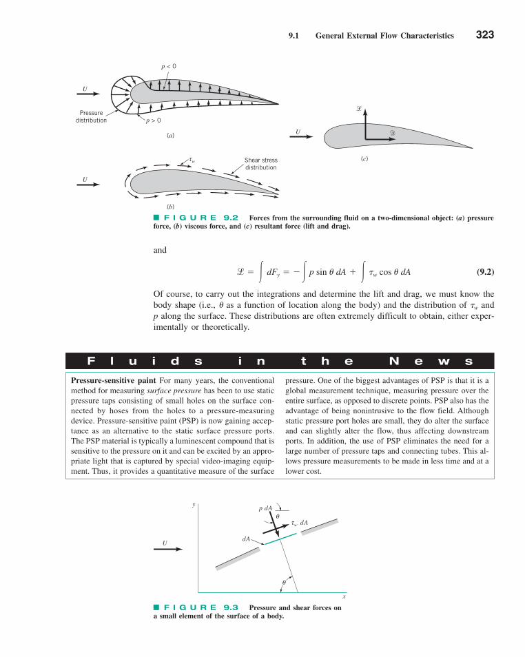
9.1 General External Flow Characteristics 323

and

(9.2)

Of course, to carry out the integrations and determine the lift and drag, we must know thebody shape (i.e., � as a function of location along the body) and the distribution of �w andp along the surface. These distributions are often extremely difficult to obtain, either exper-imentally or theoretically.

l � � dFy � �� p sin � dA � � �w cos � dA

F I G U R E 9.2 Forces from the surrounding fluid on a two-dimensional object: (a) pressureforce, (b) viscous force, and (c) resultant force (lift and drag).

U

U

U �

�

(c)

(b)

(a)

w Shear stressdistribution

τ

p > 0Pressure

distribution

p < 0

F I G U R E 9.3 Pressure and shear forces ona small element of the surface of a body.

U

p dAθ

dA

dAτw

θ

y

x

F l u i d s i n t h e N e w s

Pressure-sensitive paint For many years, the conventionalmethod for measuring surface pressure has been to use staticpressure taps consisting of small holes on the surface con-nected by hoses from the holes to a pressure-measuring device. Pressure-sensitive paint (PSP) is now gaining accep-tance as an alternative to the static surface pressure ports.The PSP material is typically a luminescent compound that issensitive to the pressure on it and can be excited by an appro-priate light that is captured by special video-imaging equip-ment. Thus, it provides a quantitative measure of the surface

pressure. One of the biggest advantages of PSP is that it is aglobal measurement technique, measuring pressure over theentire surface, as opposed to discrete points. PSP also has theadvantage of being nonintrusive to the flow field. Althoughstatic pressure port holes are small, they do alter the surfaceand can slightly alter the flow, thus affecting downstreamports. In addition, the use of PSP eliminates the need for alarge number of pressure taps and connecting tubes. This al-lows pressure measurements to be made in less time and at alower cost.

c09FlowoverImmersedBodies.qxd 9/28/10 10:27 AM Page 323

324 Chapter 9 ■ Flow over Immersed Bodies

GIVEN Air at standard conditions flows past a flat plateas is indicated in Fig. E9.1. In case (a) the plate is parallel tothe upstream flow, and in case (b) it is perpendicular to theupstream flow. The pressure and shear stress distributions onthe surface are as indicated (obtained either by experiment ortheory).

FIND Determine the lift and drag on the plate.

SOLUTION

Drag from Pressure and Shear Stress Distributions

we obtain the following drag

or

(Ans)

COMMENT Clearly two mechanisms are responsible forthe drag. On the ultimately streamlined body (a zero-thicknessflat plate parallel to the flow) the drag is entirely due to theshear stress at the surface and, in this example, is relativelysmall. For the ultimately blunted body (a flat plate normal tothe upstream flow) the drag is entirely due to the pressure dif-ference between the front and the back portions of the objectand, in this example, is relatively large.

If the flat plate were oriented at an arbitrary angle relative to theupstream flow as indicated in Fig. E9.1c, there would be both a liftand a drag, each of which would be dependent on both the shearstress and the pressure. Both the pressure and the shear stress dis-tributions would be different for the top and bottom surfaces.

d � 55.6 lb

� 1�0.8932lb/ft2 d 110 ft2 dy

d � �2 ft

y��2

c0.744 a1 �y2

4b lb/ft2

EXAMPLE 9.1

For either orientation of the plate, the lift and drag are ob-tained from Eqs. 9.1 and 9.2. With the plate parallel to the upstream flow we have � � 90� on the top surface and � � 270�on the bottom surface so that the lift and drag are given by

and

(1)

where we have used the fact that because of symmetry theshear stress distribution is the same on the top and the bottomsurfaces, as is the pressure also [whether we use gage (p � 0)or absolute (p � patm) pressure]. There is no lift generated—the plate does not know up from down. With the given shearstress distribution, Eq. 1 gives

or

(Ans)

With the plate perpendicular to the upstream flow, we have� � 0� on the front and � � 180� on the back. Thus, from Eqs.9.1 and 9.2

and

Again there is no lift because the pressure forces act parallel tothe upstream flow (in the direction of d not l) and the shearstress is symmetrical about the center of the plate. With thegiven relatively large pressure on the front of the plate (thecenter of the plate is a stagnation point) and the negative pres-sure (less than the upstream pressure) on the back of the plate,

d � �front

p dA � �back

p dA

l � �front

�w dA � �back

�w dA � 0

d � 0.0992 lb

d � 2 �4 ft

x�0

a1.24 � 10�3

x1/2 lb/ft2b

110 ft2 dx

d � �top

�w dA � �bottom

�w dA � 2 �top

�w dA

l � ��top

p dA � �bottom

p dA � 0

F I G U R E E9.1

U = 25 ft/s

p = 0 (gage)

y

x

p = p(x) = 0

4 ft

b = width = 10 ft

= (x) = (1.24 × 10 –3)/ x lb/ft2

where x is in feet√τ

(a)

w τw

ULow p

High p

� ≠ 0

� ≠ 0

(c)

τw

τw

U = 25 ft/s

(b)

p = 0

p = 0.744 1 – lb/ft2

where y is in feet

y2__4

yp = –0.893 lb/ft2

x

(y) =– (–y)

( )

τw

τwτw

c09FlowoverImmersedBodies.qxd 9/28/10 10:27 AM Page 324

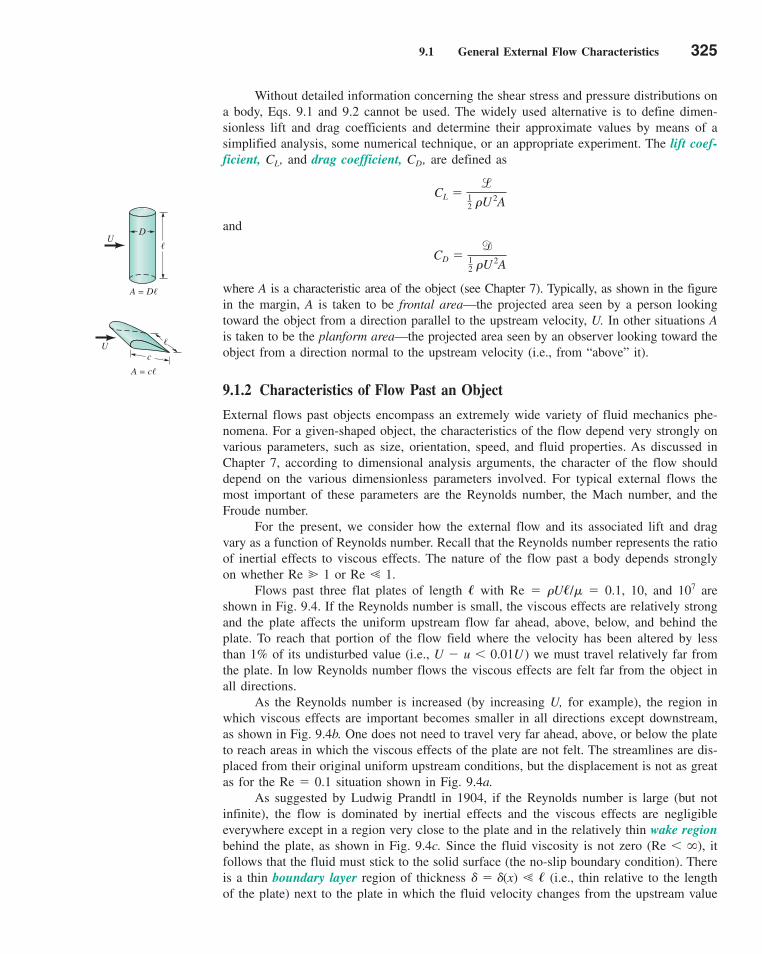
9.1 General External Flow Characteristics 325

Without detailed information concerning the shear stress and pressure distributions ona body, Eqs. 9.1 and 9.2 cannot be used. The widely used alternative is to define dimen-sionless lift and drag coefficients and determine their approximate values by means of asimplified analysis, some numerical technique, or an appropriate experiment. The lift coef-ficient, CL, and drag coefficient, CD, are defined as

and

where A is a characteristic area of the object (see Chapter 7). Typically, as shown in the figurein the margin, A is taken to be frontal area—the projected area seen by a person lookingtoward the object from a direction parallel to the upstream velocity, U. In other situations Ais taken to be the planform area—the projected area seen by an observer looking toward theobject from a direction normal to the upstream velocity (i.e., from “above” it).

9.1.2 Characteristics of Flow Past an Object

External flows past objects encompass an extremely wide variety of fluid mechanics phe-nomena. For a given-shaped object, the characteristics of the flow depend very strongly onvarious parameters, such as size, orientation, speed, and fluid properties. As discussed inChapter 7, according to dimensional analysis arguments, the character of the flow shoulddepend on the various dimensionless parameters involved. For typical external flows themost important of these parameters are the Reynolds number, the Mach number, and theFroude number.

For the present, we consider how the external flow and its associated lift and dragvary as a function of Reynolds number. Recall that the Reynolds number represents the ratioof inertial effects to viscous effects. The nature of the flow past a body depends stronglyon whether Re 1 or Re 1.

Flows past three flat plates of length � with Re � �U�/� � 0.1, 10, and 107 areshown in Fig. 9.4. If the Reynolds number is small, the viscous effects are relatively strongand the plate affects the uniform upstream flow far ahead, above, below, and behind theplate. To reach that portion of the flow field where the velocity has been altered by lessthan 1% of its undisturbed value (i.e., U � u 0.01U) we must travel relatively far fromthe plate. In low Reynolds number flows the viscous effects are felt far from the object inall directions.

As the Reynolds number is increased (by increasing U, for example), the region inwhich viscous effects are important becomes smaller in all directions except downstream,as shown in Fig. 9.4b. One does not need to travel very far ahead, above, or below the plateto reach areas in which the viscous effects of the plate are not felt. The streamlines are dis-placed from their original uniform upstream conditions, but the displacement is not as greatas for the Re � 0.1 situation shown in Fig. 9.4a.

As suggested by Ludwig Prandtl in 1904, if the Reynolds number is large (but notinfinite), the flow is dominated by inertial effects and the viscous effects are negligibleeverywhere except in a region very close to the plate and in the relatively thin wake regionbehind the plate, as shown in Fig. 9.4c. Since the fluid viscosity is not zero (Re �), itfollows that the fluid must stick to the solid surface (the no-slip boundary condition). Thereis a thin boundary layer region of thickness � � �(x) � (i.e., thin relative to the lengthof the plate) next to the plate in which the fluid velocity changes from the upstream value

CD �d

12 �U 2A

CL �l

12 �U 2A

A = D�

A = c�

�

�

U

U

c

D

c09FlowoverImmersedBodies.qxd 9/28/10 10:27 AM Page 325

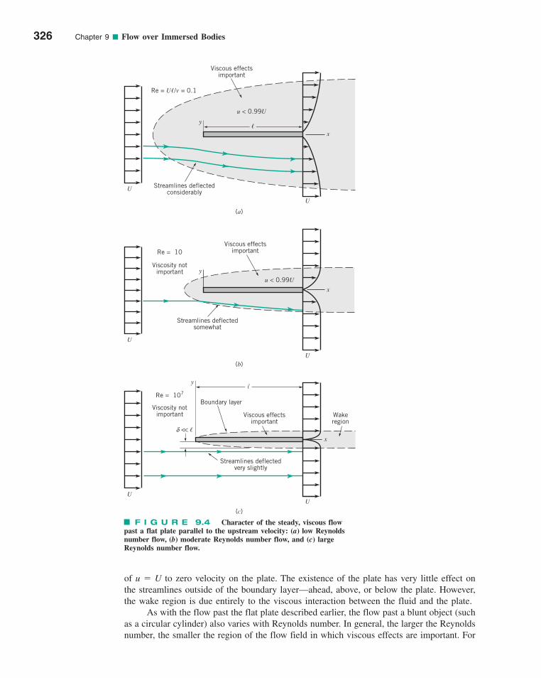
of u � U to zero velocity on the plate. The existence of the plate has very little effect onthe streamlines outside of the boundary layer—ahead, above, or below the plate. However,the wake region is due entirely to the viscous interaction between the fluid and the plate.

As with the flow past the flat plate described earlier, the flow past a blunt object (suchas a circular cylinder) also varies with Reynolds number. In general, the larger the Reynoldsnumber, the smaller the region of the flow field in which viscous effects are important. For

326 Chapter 9 ■ Flow over Immersed Bodies

Streamlines deflectedconsiderably

Re = U�/v = 0.1

U

Viscous effectsimportant

u < 0.99U

y

x

U

(a)

U

u < 0.99Uy

x

Viscous effectsimportant

Streamlines deflectedsomewhat

Re = 10

Viscosity notimportant

U

Viscosity notimportant

Re = 107

(b)

U

(c)

Viscous effectsimportant

Boundary layer

y

Streamlines deflectedvery slightly

δ << �

Wakeregion

U

x

�

F I G U R E 9.4 Character of the steady, viscous flowpast a flat plate parallel to the upstream velocity: (a) low Reynoldsnumber flow, (b) moderate Reynolds number flow, and (c) largeReynolds number flow.

c09FlowoverImmersedBodies.qxd 9/28/10 10:27 AM Page 326

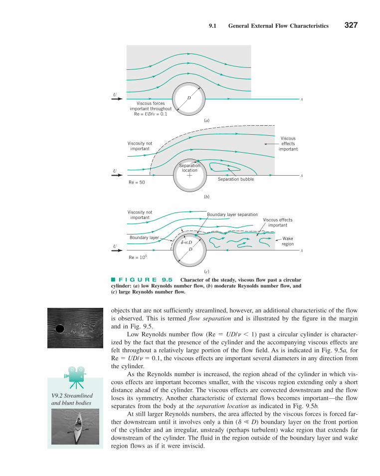
9.1 General External Flow Characteristics 327

objects that are not sufficiently streamlined, however, an additional characteristic of the flowis observed. This is termed flow separation and is illustrated by the figure in the marginand in Fig. 9.5.

Low Reynolds number flow (Re � UD/� 1) past a circular cylinder is character-ized by the fact that the presence of the cylinder and the accompanying viscous effects arefelt throughout a relatively large portion of the flow field. As is indicated in Fig. 9.5a, forRe � UD/� � 0.1, the viscous effects are important several diameters in any direction fromthe cylinder.

As the Reynolds number is increased, the region ahead of the cylinder in which vis-cous effects are important becomes smaller, with the viscous region extending only a shortdistance ahead of the cylinder. The viscous effects are convected downstream and the flowloses its symmetry. Another characteristic of external flows becomes important—the flowseparates from the body at the separation location as indicated in Fig. 9.5b.

At still larger Reynolds numbers, the area affected by the viscous forces is forced far-ther downstream until it involves only a thin (� D) boundary layer on the front portionof the cylinder and an irregular, unsteady (perhaps turbulent) wake region that extends fardownstream of the cylinder. The fluid in the region outside of the boundary layer and wakeregion flows as if it were inviscid.

F I G U R E 9.5 Character of the steady, viscous flow past a circularcylinder: (a) low Reynolds number flow, (b) moderate Reynolds number flow, and(c) large Reynolds number flow.

U

U

U

(c)

(b)

(a)

D

D

Boundary layer

Viscosity notimportant

Re = 105

δ <<D

Boundary layer separationViscous effects

important

Wakeregion

x

Separation bubble

Separationlocation

Viscosity notimportant

Re = 50

Viscous forcesimportant throughout

Re = UD/v = 0.1

x

x

Viscouseffects

important

V9.2 Streamlinedand blunt bodies

c09FlowoverImmersedBodies.qxd 9/28/10 10:27 AM Page 327

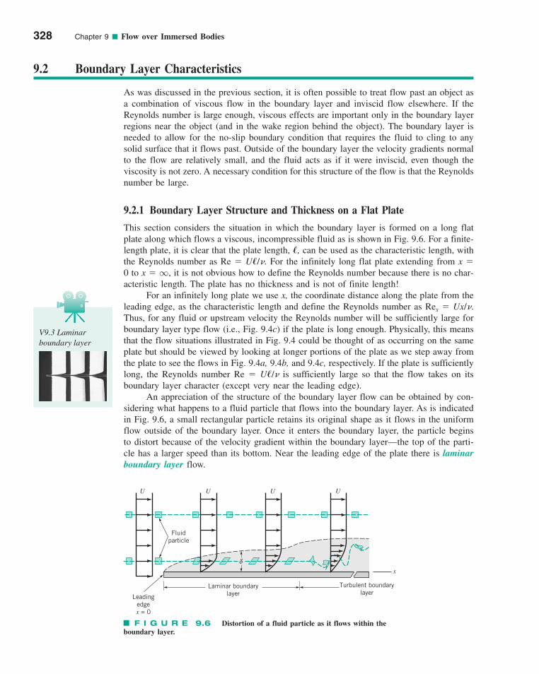
328 Chapter 9 ■ Flow over Immersed Bodies

9.2 Boundary Layer Characteristics

As was discussed in the previous section, it is often possible to treat flow past an object asa combination of viscous flow in the boundary layer and inviscid flow elsewhere. If theReynolds number is large enough, viscous effects are important only in the boundary layerregions near the object (and in the wake region behind the object). The boundary layer isneeded to allow for the no-slip boundary condition that requires the fluid to cling to anysolid surface that it flows past. Outside of the boundary layer the velocity gradients normalto the flow are relatively small, and the fluid acts as if it were inviscid, even though theviscosity is not zero. A necessary condition for this structure of the flow is that the Reynoldsnumber be large.

9.2.1 Boundary Layer Structure and Thickness on a Flat Plate

This section considers the situation in which the boundary layer is formed on a long flatplate along which flows a viscous, incompressible fluid as is shown in Fig. 9.6. For a finite-length plate, it is clear that the plate length, �, can be used as the characteristic length, withthe Reynolds number as Re � U�/�. For the infinitely long flat plate extending from x �0 to , it is not obvious how to define the Reynolds number because there is no char-acteristic length. The plate has no thickness and is not of finite length!

For an infinitely long plate we use x, the coordinate distance along the plate from theleading edge, as the characteristic length and define the Reynolds number as Rex � Ux/�.Thus, for any fluid or upstream velocity the Reynolds number will be sufficiently large forboundary layer type flow (i.e., Fig. 9.4c) if the plate is long enough. Physically, this meansthat the flow situations illustrated in Fig. 9.4 could be thought of as occurring on the sameplate but should be viewed by looking at longer portions of the plate as we step away fromthe plate to see the flows in Fig. 9.4a, 9.4b, and 9.4c, respectively. If the plate is sufficientlylong, the Reynolds number Re � U�/� is sufficiently large so that the flow takes on itsboundary layer character (except very near the leading edge).

An appreciation of the structure of the boundary layer flow can be obtained by con-sidering what happens to a fluid particle that flows into the boundary layer. As is indicatedin Fig. 9.6, a small rectangular particle retains its original shape as it flows in the uniformflow outside of the boundary layer. Once it enters the boundary layer, the particle beginsto distort because of the velocity gradient within the boundary layer—the top of the parti-cle has a larger speed than its bottom. Near the leading edge of the plate there is laminarboundary layer flow.

x � q

F I G U R E 9.6 Distortion of a fluid particle as it flows within theboundary layer.

δ

U U U U

Fluidparticle

Leadingedgex = 0

Laminar boundarylayer

Turbulent boundarylayer

x

V9.3 Laminarboundary layer

c09FlowoverImmersedBodies.qxd 9/28/10 10:27 AM Page 328

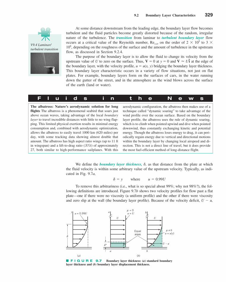
9.2 Boundary Layer Characteristics 329

At some distance downstream from the leading edge, the boundary layer flow becomesturbulent and the fluid particles become greatly distorted because of the random, irregularnature of the turbulence. The transition from laminar to turbulent boundary layer flowoccurs at a critical value of the Reynolds number, Rex,cr on the order of 2 � 105 to 3 �106, depending on the roughness of the surface and the amount of turbulence in the upstreamflow, as discussed in Section 9.2.4.

The purpose of the boundary layer is to allow the fluid to change its velocity from theupstream value of U to zero on the surface. Thus, V � 0 at y � 0 and V � U i at the edge ofthe boundary layer, with the velocity profile, u � u(x, y) bridging the boundary layer thickness.This boundary layer characteristic occurs in a variety of flow situations, not just on flatplates. For example, boundary layers form on the surfaces of cars, in the water runningdown the gutter of the street, and in the atmosphere as the wind blows across the surfaceof the earth (land or water).

V9.4 Laminar/turbulent transition

F l u i d s i n t h e N e w s

The albatross: Nature’s aerodynamic solution for longflights The albatross is a phenomenal seabird that soars justabove ocean waves, taking advantage of the local boundarylayer to travel incredible distances with little to no wing flap-ping. This limited physical exertion results in minimal energyconsumption and, combined with aerodynamic optimization,allows the albatross to easily travel 1000 km (620 miles) perday, with some tracking data showing almost double thatamount. The albatross has high aspect ratio wings (up to 11 ftin wingspan) and a lift-to-drag ratio (l/d) of approximately27, both similar to high-performance sailplanes. With this

aerodynamic configuration, the albatross then makes use of atechnique called “dynamic soaring” to take advantage of thewind profile over the ocean surface. Based on the boundarylayer profile, the albatross uses the rule of dynamic soaring,which is to climb when pointed upwind and dive when pointeddownwind, thus constantly exchanging kinetic and potentialenergy. Though the albatross loses energy to drag, it can peri-odically regain energy due to vertical and directional motionswithin the boundary layer by changing local airspeed and di-rection. This is not a direct line of travel, but it does providethe most fuel-efficient method of long-distance flight.

We define the boundary layer thickness, �, as that distance from the plate at whichthe fluid velocity is within some arbitrary value of the upstream velocity. Typically, as indi-cated in Fig. 9.7a,

where

To remove this arbitrariness (i.e., what is so special about 99%; why not 98%?), the fol-lowing definitions are introduced. Figure 9.7b shows two velocity profiles for flow past a flatplate—one if there were no viscosity (a uniform profile) and the other if there were viscosityand zero slip at the wall (the boundary layer profile). Because of the velocity deficit, U � u,

u � 0.99U� � y

F I G U R E 9.7 Boundary layer thickness: (a) standard boundarylayer thickness and (b) boundary layer displacement thickness.

U

U U

δ*

δ

a b

Equalareas

y a bu = 0.99 = 0u = Uμ

≠ 0u = u(y)μ

U – u

(a) (b)

c09FlowoverImmersedBodies.qxd 9/28/10 10:27 AM Page 329

within the boundary layer, the flowrate across section b–b is less than that across section a–a.However, if we displace the plate at section a–a by an appropriate amount �*, the boundarylayer displacement thickness, the flowrate across each section will be identical. This is true if

where b is the plate width. Thus,

(9.3)

The displacement thickness represents the amount that the thickness of the body mustbe increased so that the fictitious uniform inviscid flow has the same mass flowrate proper-ties as the actual viscous flow. It represents the outward displacement of the streamlinescaused by the viscous effects on the plate.

Another boundary layer thickness definition, the boundary layer momentum thickness,�, is often used when determining the drag on an object. Again because of the velocity deficit,U � u, in the boundary layer, the momentum flux across section b–b in Fig. 9.7 is less thanthat across section a–a. This deficit in momentum flux for the actual boundary layer flow isgiven by

which by definition is the momentum flux in a layer of uniform speed U and thickness �.That is,

or

(9.4)

All three boundary layer thickness definitions, �, �*, and �, are of use in boundary layeranalyses.

9.2.2 Prandtl/Blasius Boundary Layer Solution

In theory, the details of viscous incompressible flow past any object can be obtained bysolving the governing Navier–Stokes equations discussed in Section 6.8.2. For steady,two-dimensional laminar flows with negligible gravitational effects, these equations (Eqs.6.120a, b, and c) reduce to the following

(9.5)

(9.6)

which express Newton’s second law. In addition, the conservation of mass equation, Eq. 6.31,for incompressible flow is

(9.7)0u

0x�

0v

0y� 0

u 0v

0x� v

0v

0y� �

1�

0p

0y� � a

02v

0x2 �02v

0y2b

u 0u

0x� v

0u

0y� �

1�

0p

0x� � a

02u

0x2 �02u

0y2b

™ � �q

0

u

U a1 �

u

Ub dy

�bU2™ � �b �q

0

u1U � u2 dy

� �u1U � u2 dA � �b �q

0

u1U � u2 dy

�* � �q

0

a1 �u

Ub dy

�*bU � �q

0

1U � u2b dy

330 Chapter 9 ■ Flow over Immersed Bodies

c09FlowoverImmersedBodies.qxd 9/28/10 10:27 AM Page 330

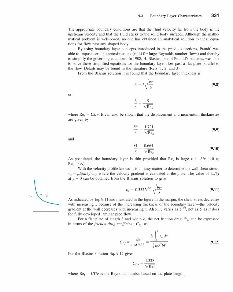
9.2 Boundary Layer Characteristics 331

The appropriate boundary conditions are that the fluid velocity far from the body is theupstream velocity and that the fluid sticks to the solid body surfaces. Although the mathe-matical problem is well-posed, no one has obtained an analytical solution to these equa-tions for flow past any shaped body!

By using boundary layer concepts introduced in the previous sections, Prandtl wasable to impose certain approximations (valid for large Reynolds number flows) and therebyto simplify the governing equations. In 1908, H. Blasius, one of Prandtl’s students, was ableto solve these simplified equations for the boundary layer flow past a flat plate parallel tothe flow. Details may be found in the literature (Refs. 1, 2, and 3).

From the Blasius solution it is found that the boundary layer thickness is

(9.8)

or

where Rex � Ux/�. It can also be shown that the displacement and momentum thicknessesare given by

(9.9)

and

(9.10)

As postulated, the boundary layer is thin provided that Rex is large (i.e., �/x S 0 asRex S �).

With the velocity profile known it is an easy matter to determine the wall shear stress,�w � �(�u/�y)y�0, where the velocity gradient is evaluated at the plate. The value of �u/�yat y � 0 can be obtained from the Blasius solution to give

(9.11)

As indicated by Eq. 9.11 and illustrated in the figure in the margin, the shear stress decreaseswith increasing x because of the increasing thickness of the boundary layer—the velocitygradient at the wall decreases with increasing x. Also, �w varies as U3/2, not as U as it doesfor fully developed laminar pipe flow.

For a flat plate of length � and width b, the net friction drag, df , can be expressedin terms of the friction drag coefficient, CDf , as

(9.12)

For the Blasius solution Eq. 9.12 gives

where Re� � U�/� is the Reynolds number based on the plate length.

CD f �1.328

1Re/

CDf �df

12 �U 2b/

�

b �/

0

�w dx

12 �U 2b/

�w � 0.332U3/2 B

��

x

™x

�0.664

1Rex

�*x

�1.721

1Rex

�

x�

5

1Rex

� � 5B

�x

U

x

τwτ ~w √x

1

c09FlowoverImmersedBodies.qxd 9/28/10 10:27 AM Page 331

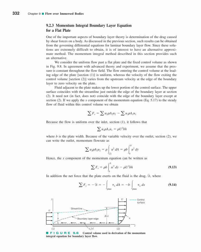
9.2.3 Momentum Integral Boundary Layer Equation for a Flat Plate

One of the important aspects of boundary layer theory is determination of the drag causedby shear forces on a body. As discussed in the previous section, such results can be obtainedfrom the governing differential equations for laminar boundary layer flow. Since these solu-tions are extremely difficult to obtain, it is of interest to have an alternative approxi-mate method. The momentum integral method described in this section provides suchan alternative.

We consider the uniform flow past a flat plate and the fixed control volume as shownin Fig. 9.8. In agreement with advanced theory and experiment, we assume that the pres-sure is constant throughout the flow field. The flow entering the control volume at the lead-ing edge of the plate [section (1)] is uniform, whereas the velocity of the flow exiting thecontrol volume [section (2)] varies from the upstream velocity at the edge of the boundarylayer to zero velocity on the plate.

Fluid adjacent to the plate makes up the lower portion of the control surface. The uppersurface coincides with the streamline just outside the edge of the boundary layer at section(2). It need not (in fact, does not) coincide with the edge of the boundary layer except atsection (2). If we apply the x component of the momentum equation (Eq. 5.17) to the steadyflow of fluid within this control volume we obtain

Because the flow is uniform over the inlet, section (1), it follows that

where b is the plate width. Because of the variable velocity over the outlet, section (2), wecan write the outlet, momentum flowrate as

Hence, the x component of the momentum equation can be written as

(9.13)

In addition the net force that the plate exerts on the fluid is the drag, d, where

(9.14)a Fx � �d � ��plate

�w dA � �b �plate

�w dx

a Fx � �b��

0

u 2 dy � �U

2bh

a u2�A2u2 � ��122

u2 dA � �b��

0

u2 dy

a u1�A1u1 � �U 2bh

a Fx �a u2 �A2u2 �a u1�A1u1

332 Chapter 9 ■ Flow over Immersed Bodies

F I G U R E 9.8 Control volume used in derivation of the momentumintegral equation for boundary layer flow.

Streamline

Boundary layer edge

Controlsurface

x

u

U

(2)(1)

U

y

hδ(x)

τw(x)

c09FlowoverImmersedBodies.qxd 9/28/10 10:28 AM Page 332

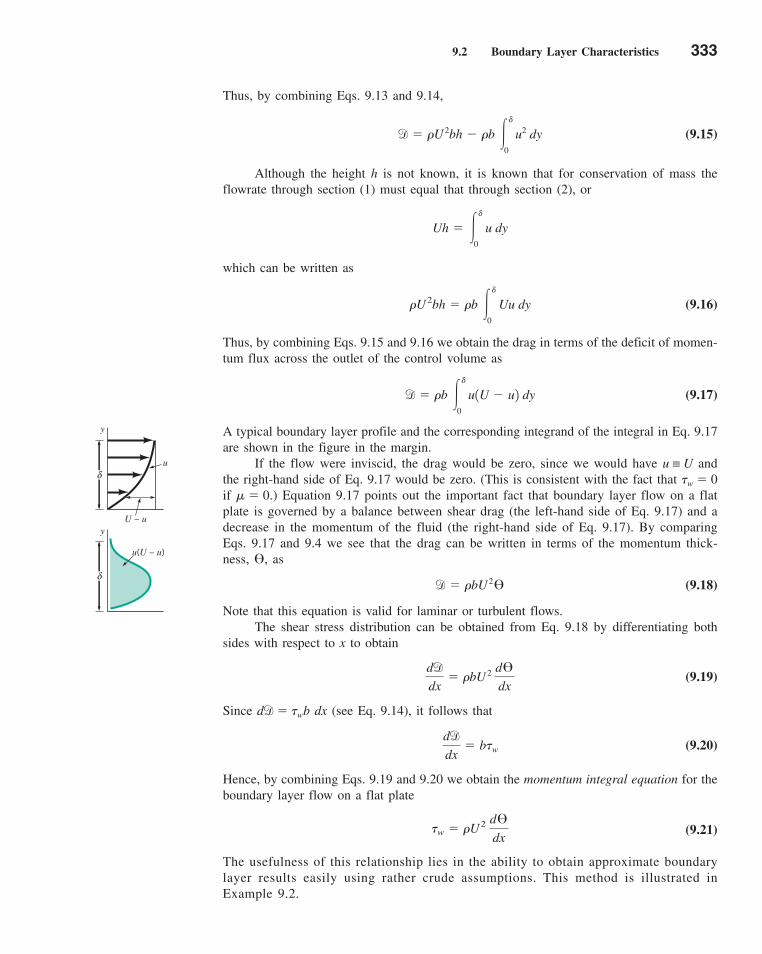
9.2 Boundary Layer Characteristics 333

Thus, by combining Eqs. 9.13 and 9.14,

(9.15)

Although the height h is not known, it is known that for conservation of mass theflowrate through section (1) must equal that through section (2), or

which can be written as

(9.16)

Thus, by combining Eqs. 9.15 and 9.16 we obtain the drag in terms of the deficit of momen-tum flux across the outlet of the control volume as

(9.17)

A typical boundary layer profile and the corresponding integrand of the integral in Eq. 9.17are shown in the figure in the margin.

If the flow were inviscid, the drag would be zero, since we would have u ≡ U andthe right-hand side of Eq. 9.17 would be zero. (This is consistent with the fact that �w � 0if � � 0.) Equation 9.17 points out the important fact that boundary layer flow on a flatplate is governed by a balance between shear drag (the left-hand side of Eq. 9.17) and adecrease in the momentum of the fluid (the right-hand side of Eq. 9.17). By comparingEqs. 9.17 and 9.4 we see that the drag can be written in terms of the momentum thick-ness, �, as

(9.18)

Note that this equation is valid for laminar or turbulent flows.The shear stress distribution can be obtained from Eq. 9.18 by differentiating both

sides with respect to x to obtain

(9.19)

Since dd� �wb dx (see Eq. 9.14), it follows that

(9.20)

Hence, by combining Eqs. 9.19 and 9.20 we obtain the momentum integral equation for theboundary layer flow on a flat plate

(9.21)

The usefulness of this relationship lies in the ability to obtain approximate boundarylayer results easily using rather crude assumptions. This method is illustrated inExample 9.2.

�w � �U2 d™dx

dd

dx� b�w

dd

dx� �bU 2

d™dx

d � �bU 2™

d � �b ��

0 u1U � u2 dy

�U2bh � �b ��

0

Uu dy

Uh � ��

0

u dy

d � �U 2bh � �b ��

0 u

2 dy

U – u

u(U – u)

u

y

y

δ

δ

c09FlowoverImmersedBodies.qxd 9/28/10 10:28 AM Page 333

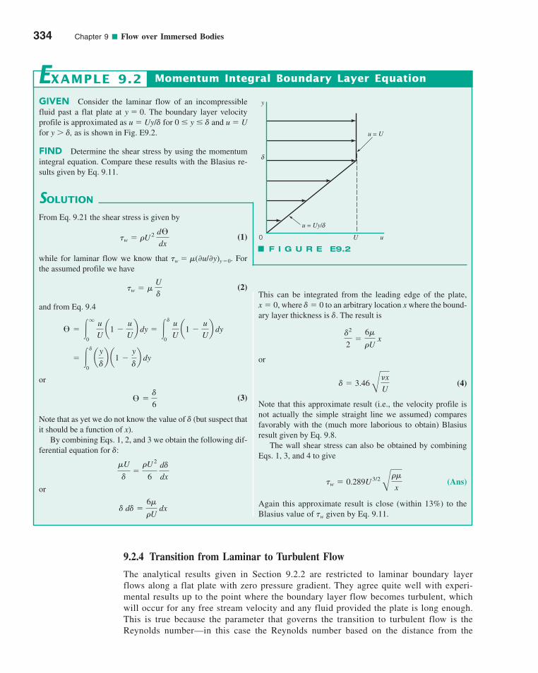
334 Chapter 9 ■ Flow over Immersed Bodies

GIVEN Consider the laminar flow of an incompressiblefluid past a flat plate at y � 0. The boundary layer velocityprofile is approximated as u � Uy/� for 0 � y � � and u � Ufor y � �, as is shown in Fig. E9.2.

FIND Determine the shear stress by using the momentumintegral equation. Compare these results with the Blasius re-sults given by Eq. 9.11.

Momentum Integral Boundary Layer EquationEXAMPLE 9.2

SOLUTION

This can be integrated from the leading edge of the plate,x � 0, where � � 0 to an arbitrary location x where the bound-ary layer thickness is �. The result is

or

(4)

Note that this approximate result (i.e., the velocity profile isnot actually the simple straight line we assumed) compares favorably with the (much more laborious to obtain) Blasius result given by Eq. 9.8.

The wall shear stress can also be obtained by combiningEqs. 1, 3, and 4 to give

(Ans)

Again this approximate result is close (within 13%) to theBlasius value of �w given by Eq. 9.11.

�w � 0.289U3/2 B

��

x

� � 3.46 B

�x

U

�2

2�

6�

�U x

From Eq. 9.21 the shear stress is given by

(1)

while for laminar flow we know that �w � �(�u/�y)y �0. Forthe assumed profile we have

(2)

and from Eq. 9.4

or

(3)

Note that as yet we do not know the value of � (but suspect thatit should be a function of x).

By combining Eqs. 1, 2, and 3 we obtain the following dif-ferential equation for �:

or

� d� �6�

�U dx

�U

��

�U2

6 d�

dx

™ ��

6

� ��

0

ay

�b a1 �

y

�b dy

™ � �q

0

u

U a1 �

u

Ub dy � �

�

0

u

U a1 �

u

Ub dy

�w � � U

�

�w � �U2 d™dx

F I G U R E E9.2

y

U u0

u = Uy/δ

δ

u = U

9.2.4 Transition from Laminar to Turbulent Flow

The analytical results given in Section 9.2.2 are restricted to laminar boundary layerflows along a flat plate with zero pressure gradient. They agree quite well with experi-mental results up to the point where the boundary layer flow becomes turbulent, whichwill occur for any free stream velocity and any fluid provided the plate is long enough.This is true because the parameter that governs the transition to turbulent flow is theReynolds number—in this case the Reynolds number based on the distance from the

c09FlowoverImmersedBodies.qxd 9/28/10 10:28 AM Page 334

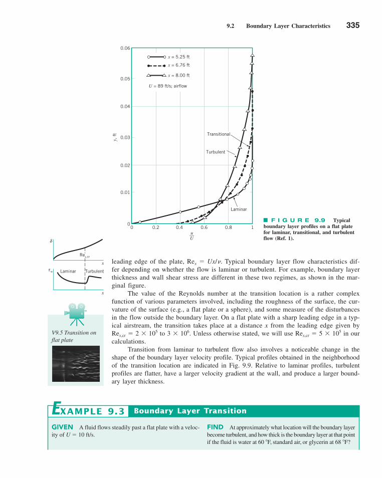
9.2 Boundary Layer Characteristics 335

leading edge of the plate, Rex � Ux/�. Typical boundary layer flow characteristics dif-fer depending on whether the flow is laminar or turbulent. For example, boundary layerthickness and wall shear stress are different in these two regimes, as shown in the mar-ginal figure.

The value of the Reynolds number at the transition location is a rather complexfunction of various parameters involved, including the roughness of the surface, the cur-vature of the surface (e.g., a flat plate or a sphere), and some measure of the disturbancesin the flow outside the boundary layer. On a flat plate with a sharp leading edge in a typ-ical airstream, the transition takes place at a distance x from the leading edge given byRex,cr � 2 � 105 to 3 � 106. Unless otherwise stated, we will use Rex,cr � 5 � 105 in ourcalculations.

Transition from laminar to turbulent flow also involves a noticeable change in theshape of the boundary layer velocity profile. Typical profiles obtained in the neighborhoodof the transition location are indicated in Fig. 9.9. Relative to laminar profiles, turbulentprofiles are flatter, have a larger velocity gradient at the wall, and produce a larger bound-ary layer thickness.

F I G U R E 9.9 Typicalboundary layer profiles on a flat platefor laminar, transitional, and turbulentflow (Ref. 1).

x = 5.25 ft

x = 6.76 ft

x = 8.00 ft

U = 89 ft/s; airflow

Transitional

Turbulent

Laminar

0.06

0.05

0.04

0.03

0.02

0.01

00 0.2 0.4 0.6 0.8 1

u__U

y, f

t

δ

τ w

x

x

Laminar Turbulent

Rex,cr

V9.5 Transition onflat plate

GIVEN A fluid flows steadily past a flat plate with a veloc-ity of U � 10 ft/s.

FIND At approximately what location will the boundary layerbecome turbulent, and how thick is the boundary layer at that pointif the fluid is water at 60 �F, standard air, or glycerin at 68 �F?

Boundary Layer TransitionEXAMPLE 9.3

c09FlowoverImmersedBodies.qxd 9/30/10 9:17 AM Page 335

9.2.5 Turbulent Boundary Layer Flow

The structure of turbulent boundary layer flow is very complex, random, and irregular. Itshares many of the characteristics described for turbulent pipe flow in Section 8.3. In par-ticular, the velocity at any given location in the flow is unsteady in a random fashion.The flow can be thought of as a jumbled mix of intertwined eddies (or swirls) of differentsizes (diameters and angular velocities). The figure in the margin shows a laser-inducedfluorescence visualization of a turbulent boundary layer on a flat plate (side view). Thevarious fluid quantities involved (i.e., mass, momentum, energy) are convected down-stream in the free-stream direction as in a laminar boundary layer. For turbulent flow theyare also convected across the boundary layer (in the direction perpendicular to the plate)by the random transport of finite-sized fluid particles associated with the turbulent eddies.There is considerable mixing involved with these finite-sized eddies—considerablymore than is associated with the mixing found in laminar flow where it is confined tothe molecular scale. Consequently, the shear force for turbulent boundary layer flow isconsiderably greater than it is for laminar boundary layer flow (see Section 8.3.2).

There are no “exact” solutions for turbulent boundary layer flow. As discussed in Sec-tion 9.2.2, it is possible to solve the Prandtl boundary layer equations for laminar flow pasta flat plate to obtain the Blasius solution. Since there is no precise expression for the shearstress in turbulent flow (see Section 8.3), solutions are not available for turbulent flow. Thus,it is necessary to use some empirical relationship for the wall shear stress and correspond-ing drag coefficient.

In general, the drag coefficient for a flat plate of length �, CDf � df /(1—

2 �U2A), is afunction of the Reynolds number, Re�, and the relative roughness, �/�. The results of numer-ous experiments covering a wide range of the parameters of interest are shown in Fig. 9.10.For laminar boundary layer flow the drag coefficient is a function of only the Reynoldsnumber—surface roughness is not important. This is similar to laminar flow in a pipe. How-ever, for turbulent flow, the surface roughness does affect the shear stress and, hence, thedrag coefficient. This is similar to turbulent pipe flow. Values of the roughness, �, for dif-ferent materials can be obtained from Table 8.1.

336 Chapter 9 ■ Flow over Immersed Bodies

SOLUTION

where � is in ft2/s and xcr and �cr are in feet. The values of thekinematic viscosity obtained from Tables 1.4 to 1.6 are listed inTable E9.3 along with the corresponding xcr and �cr.

COMMENT Laminar flow can be maintained on a longerportion of the plate if the viscosity is increased. However, theboundary layer flow eventually becomes turbulent, providedthe plate is long enough. Similarly, the boundary layer thick-ness is greater if the viscosity is increased.

For any fluid, the laminar boundary layer thickness is foundfrom Eq. 9.8 as

The boundary layer remains laminar up to

Thus, if we assume Rex,cr � 5 � 105 we obtain

and

�cr � ��x�xcr� 5 c

�

10 15 � 104 �2 d

1/2

� 354 �

xcr �5 � 105

10 ft /s � � 5 � 104 �

xcr ��Rex,cr

U

� � 5 B

�x

UTA B L E E 9 . 3

Fluid ( ) (ft) (ft)

Water 0.605 0.00428Air 7.85 0.0556Glycerin 640.0 4.53 1.28 � 10�2

1.57 � 10�4

1.21 � 10�5

�crxcrft2�sN

(Ans)

Plate

c09FlowoverImmersedBodies.qxd 9/28/10 10:28 AM Page 336

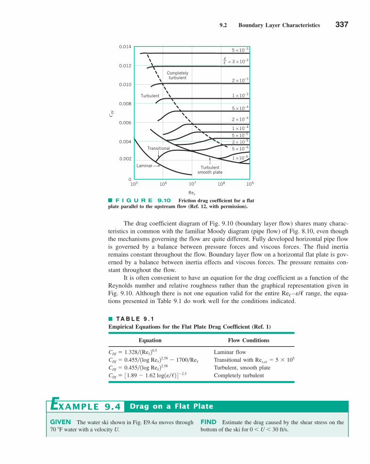
9.2 Boundary Layer Characteristics 337

The drag coefficient diagram of Fig. 9.10 (boundary layer flow) shares many charac-teristics in common with the familiar Moody diagram (pipe flow) of Fig. 8.10, even thoughthe mechanisms governing the flow are quite different. Fully developed horizontal pipe flowis governed by a balance between pressure forces and viscous forces. The fluid inertiaremains constant throughout the flow. Boundary layer flow on a horizontal flat plate is gov-erned by a balance between inertia effects and viscous forces. The pressure remains con-stant throughout the flow.

It is often convenient to have an equation for the drag coefficient as a function of theReynolds number and relative roughness rather than the graphical representation given inFig. 9.10. Although there is not one equation valid for the entire Re�–e/� range, the equa-tions presented in Table 9.1 do work well for the conditions indicated.

0.002

0

0.004

0.006

0.008

0.010

0.012

105 106 107 108 109

Re�

CD

f

Turbulent

Completelyturbulent

1 × 10–3

2 × 10–3

= 3 × 10–3

5 × 10–3

ε

Laminar

5 × 10–4

2 × 10–4

1 × 10–4

5 × 10–5

5 × 10–6

1 × 10–6

Transitional

Turbulentsmooth plate

2 × 10–5

�

0.014

F I G U R E 9.10 Friction drag coefficient for a flatplate parallel to the upstream flow (Ref. 12, with permission).

TA B L E 9 . 1

Empirical Equations for the Flat Plate Drag Coefficient (Ref. 1)

Equation Flow Conditions

Laminar flowTransitional with Turbulent, smooth plateCompletely turbulentCDf � 31.89 � 1.62 log1e�/2 4�2.5

CDf � 0.455� 1log Re/22.58

Rex,cr � 5 � 105CDf � 0.455� 1log Re/22.58 � 1700�Re/

CDf � 1.328� 1Re/20.5

GIVEN The water ski shown in Fig. E9.4a moves through70 �F water with a velocity U.

FIND Estimate the drag caused by the shear stress on thebottom of the ski for 0 U 30 ft/s.

Drag on a Flat PlateEXAMPLE 9.4

c09FlowoverImmersedBodies.qxd 9/28/10 10:28 AM Page 337

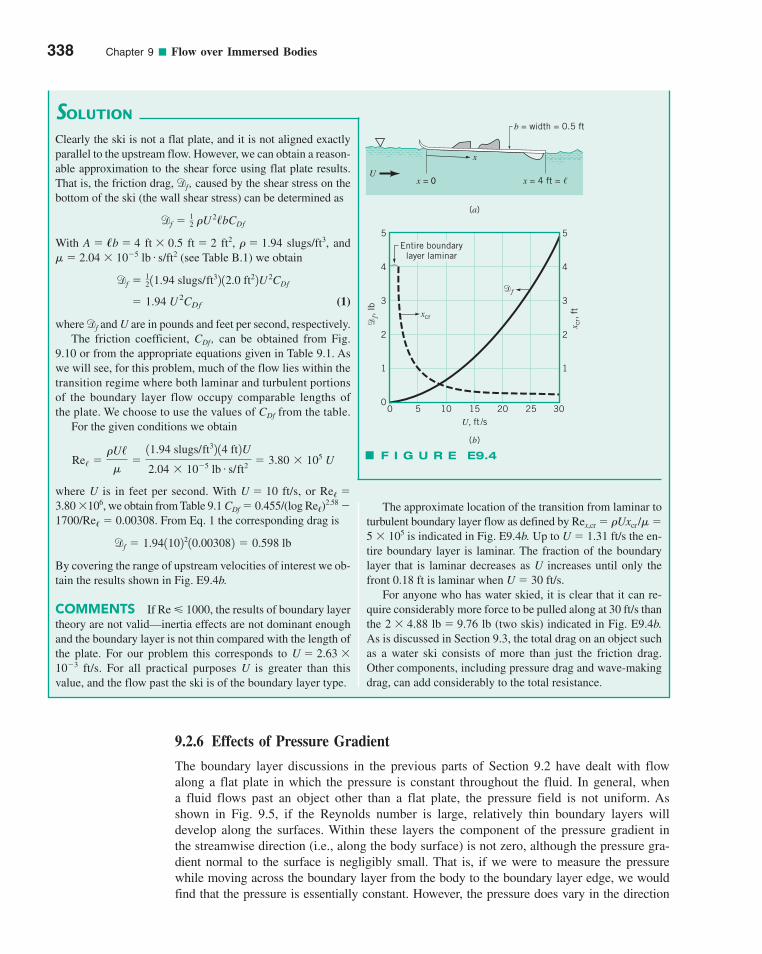
9.2.6 Effects of Pressure Gradient

The boundary layer discussions in the previous parts of Section 9.2 have dealt with flowalong a flat plate in which the pressure is constant throughout the fluid. In general, whena fluid flows past an object other than a flat plate, the pressure field is not uniform. Asshown in Fig. 9.5, if the Reynolds number is large, relatively thin boundary layers willdevelop along the surfaces. Within these layers the component of the pressure gradient inthe streamwise direction (i.e., along the body surface) is not zero, although the pressure gra-dient normal to the surface is negligibly small. That is, if we were to measure the pressurewhile moving across the boundary layer from the body to the boundary layer edge, we wouldfind that the pressure is essentially constant. However, the pressure does vary in the direction

338 Chapter 9 ■ Flow over Immersed Bodies

SOLUTION

The approximate location of the transition from laminar toturbulent boundary layer flow as defined by Rex,cr � �Uxcr /� �5 � 105 is indicated in Fig. E9.4b. Up to U � 1.31 ft/s the en-tire boundary layer is laminar. The fraction of the boundarylayer that is laminar decreases as U increases until only thefront 0.18 ft is laminar when U � 30 ft/s.

For anyone who has water skied, it is clear that it can re-quire considerably more force to be pulled along at 30 ft/s thanthe 2 � 4.88 lb � 9.76 lb (two skis) indicated in Fig. E9.4b.As is discussed in Section 9.3, the total drag on an object suchas a water ski consists of more than just the friction drag.Other components, including pressure drag and wave-makingdrag, can add considerably to the total resistance.

Clearly the ski is not a flat plate, and it is not aligned exactlyparallel to the upstream flow. However, we can obtain a reason-able approximation to the shear force using flat plate results.That is, the friction drag, df , caused by the shear stress on thebottom of the ski (the wall shear stress) can be determined as

With A � �b � 4 ft � 0.5 ft � 2 ft2, � � 1.94 slugs/ft3, and� � 2.04 � 10�5 lb s/ft2 (see Table B.1) we obtain

(1)

where df and U are in pounds and feet per second, respectively.The friction coefficient, CDf , can be obtained from Fig.

9.10 or from the appropriate equations given in Table 9.1. Aswe will see, for this problem, much of the flow lies within thetransition regime where both laminar and turbulent portionsof the boundary layer flow occupy comparable lengths ofthe plate. We choose to use the values of CDf from the table.

For the given conditions we obtain

where U is in feet per second. With U � 10 ft/s, or Re� �3.80 �106, we obtain from Table 9.1 CDf � 0.455/(log Re�)

2.58 �1700/Re� � 0.00308. From Eq. 1 the corresponding drag is

By covering the range of upstream velocities of interest we ob-tain the results shown in Fig. E9.4b.

COMMENTS If Re � 1000, the results of boundary layertheory are not valid—inertia effects are not dominant enoughand the boundary layer is not thin compared with the length ofthe plate. For our problem this corresponds to U � 2.63 �10�3 ft/s. For all practical purposes U is greater than thisvalue, and the flow past the ski is of the boundary layer type.

df � 1.941102210.003082 � 0.598 lb

Re/ ��U/

��11.94 slugs/ft32 14 ft2U

2.04 � 10�5 lb # s/ft2 � 3.80 � 105 U

� 1.94 U2CDf

df � 12 11.94 slugs/ft32 12.0 ft22U 2CDf

#

df � 12 �U 2/bCDf

00

1

2

3

4

5

5 10 15 20 25 30

1

2

3

4

5

U, ft /s

Entire boundarylayer laminar

xcr

�f

�f, l

b

xcr

, ft

b = width = 0.5 ft

x = 0 x = 4 ft = �U

x

(a)

(b)

F I G U R E E9.4

c09FlowoverImmersedBodies.qxd 9/28/10 10:28 AM Page 338

9.2 Boundary Layer Characteristics 339

along the body surface if the body is curved, as shown by the figure in the margin. Thevariation in the free-stream velocity, Ufs, the fluid velocity at the edge of the boundary layer,is the cause of the pressure gradient in the boundary layer. The characteristics of the entireflow (both within and outside of the boundary layer) are often highly dependent on the pres-sure gradient effects on the fluid within the boundary layer.

For a flat plate parallel to the upstream flow, the upstream velocity (that far ahead ofthe plate) and the free-stream velocity (that at the edge of the boundary layer) are equal—U � Ufs. This is a consequence of the negligible thickness of the plate. For bodies of nonzerothickness, these two velocities are different. This can be seen in the flow past a circular cylin-der of diameter D. The upstream velocity and pressure are U and p0, respectively. If the fluidwere completely inviscid (� � 0), the Reynolds number would be infinite (Re � �UD/� � �)and the streamlines would be symmetrical, as are shown in Fig. 9.11a. The fluid velocityalong the surface would vary from Ufs � 0 at the very front and rear of the cylinder (pointsA and F are stagnation points) to a maximum of Ufs � 2U at the top and bottom of the cylin-der (point C). This is also indicated in the figure in the margin. The pressure on the surfaceof the cylinder would be symmetrical about the vertical midplane of the cylinder, reachinga maximum value of p0 � �U2/2 (the stagnation pressure) at both the front and the back ofthe cylinder, and a minimum of p0 � 3�U2/2 at the top and bottom of the cylinder. The pres-sure and free-stream velocity distributions are shown in Figs. 9.11b and 9.11c. Because ofthe absence of viscosity (therefore, �w � 0) and the symmetry of the pressure distributionfor inviscid flow past a circular cylinder, it is clear that the drag on the cylinder is zero.

Consider large Reynolds number flow of a real (viscous) fluid past a circular cylin-der. As discussed in Section 9.1.2, we expect the viscous effects to be confined to thinboundary layers near the surface. This allows the fluid to stick (V � 0) to the surface—a

A F

C

θ

p0 + U 212

p0 – U 212

p0 – U 2

p0 – U 232

p0

p

2U

U

00 90 180

, degreesθ0 90 180

, degreesθ

Ufs

U, p0

A

C

F

C

FA

Ufs

(a)

(b) (c)

ρ

ρ

ρ

ρ

F I G U R E 9.11 Inviscid flow past a circularcylinder: (a) streamlines for the flow if there were no viscouseffects, (b) pressure distribution on the cylinder’s surface, and(c) free-stream velocity on the cylinder’s surface.

Ufs1 � Ufs2

p1 � p2

(1)

(2)

Ufs = U

Ufs = 0U

Ufs = 2U

c09FlowoverImmersedBodies.qxd 9/28/10 10:28 AM Page 339

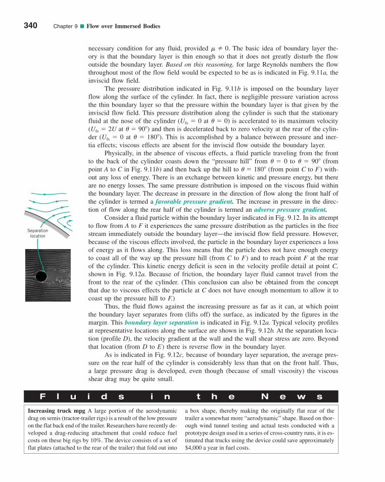
necessary condition for any fluid, provided . The basic idea of boundary layer the-ory is that the boundary layer is thin enough so that it does not greatly disturb the flowoutside the boundary layer. Based on this reasoning, for large Reynolds numbers the flowthroughout most of the flow field would be expected to be as is indicated in Fig. 9.11a, theinviscid flow field.

The pressure distribution indicated in Fig. 9.11b is imposed on the boundary layerflow along the surface of the cylinder. In fact, there is negligible pressure variation acrossthe thin boundary layer so that the pressure within the boundary layer is that given by theinviscid flow field. This pressure distribution along the cylinder is such that the stationaryfluid at the nose of the cylinder (Ufs � 0 at � � 0) is accelerated to its maximum velocity(Ufs � 2U at � � 90�) and then is decelerated back to zero velocity at the rear of the cylin-der (Ufs � 0 at � � 180�). This is accomplished by a balance between pressure and iner-tia effects; viscous effects are absent for the inviscid flow outside the boundary layer.

Physically, in the absence of viscous effects, a fluid particle traveling from the frontto the back of the cylinder coasts down the “pressure hill” from � � 0 to � � 90� (frompoint A to C in Fig. 9.11b) and then back up the hill to � � 180� (from point C to F) with-out any loss of energy. There is an exchange between kinetic and pressure energy, but thereare no energy losses. The same pressure distribution is imposed on the viscous fluid withinthe boundary layer. The decrease in pressure in the direction of flow along the front half ofthe cylinder is termed a favorable pressure gradient. The increase in pressure in the direc-tion of flow along the rear half of the cylinder is termed an adverse pressure gradient.

Consider a fluid particle within the boundary layer indicated in Fig. 9.12. In its attemptto flow from A to F it experiences the same pressure distribution as the particles in the freestream immediately outside the boundary layer—the inviscid flow field pressure. However,because of the viscous effects involved, the particle in the boundary layer experiences a lossof energy as it flows along. This loss means that the particle does not have enough energyto coast all of the way up the pressure hill (from C to F) and to reach point F at the rearof the cylinder. This kinetic energy deficit is seen in the velocity profile detail at point C,shown in Fig. 9.12a. Because of friction, the boundary layer fluid cannot travel from thefront to the rear of the cylinder. (This conclusion can also be obtained from the conceptthat due to viscous effects the particle at C does not have enough momentum to allow it tocoast up the pressure hill to F.)

Thus, the fluid flows against the increasing pressure as far as it can, at which pointthe boundary layer separates from (lifts off) the surface, as indicated by the figures in themargin. This boundary layer separation is indicated in Fig. 9.12a. Typical velocity profilesat representative locations along the surface are shown in Fig. 9.12b. At the separation loca-tion (profile D), the velocity gradient at the wall and the wall shear stress are zero. Beyondthat location (from D to E) there is reverse flow in the boundary layer.

As is indicated in Fig. 9.12c, because of boundary layer separation, the average pres-sure on the rear half of the cylinder is considerably less than that on the front half. Thus,a large pressure drag is developed, even though (because of small viscosity) the viscousshear drag may be quite small.

� � 0

340 Chapter 9 ■ Flow over Immersed Bodies

F l u i d s i n t h e N e w s

Increasing truck mpg A large portion of the aerodynamicdrag on semis (tractor-trailer rigs) is a result of the low pressureon the flat back end of the trailer. Researchers have recently de-veloped a drag-reducing attachment that could reduce fuelcosts on these big rigs by 10%. The device consists of a set offlat plates (attached to the rear of the trailer) that fold out into

a box shape, thereby making the originally flat rear of thetrailer a somewhat more “aerodynamic” shape. Based on thor-ough wind tunnel testing and actual tests conducted with aprototype design used in a series of cross-country runs, it is es-timated that trucks using the device could save approximately$4,000 a year in fuel costs.

Separationlocation

c09FlowoverImmersedBodies.qxd 9/28/10 10:28 AM Page 340

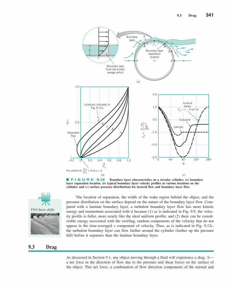
9.3 Drag 341

The location of separation, the width of the wake region behind the object, and thepressure distribution on the surface depend on the nature of the boundary layer flow. Com-pared with a laminar boundary layer, a turbulent boundary layer flow has more kineticenergy and momentum associated with it because (1) as is indicated in Fig. 9.9, the veloc-ity profile is fuller, more nearly like the ideal uniform profile, and (2) there can be consid-erable energy associated with the swirling, random components of the velocity that do notappear in the time-averaged x component of velocity. Thus, as is indicated in Fig. 9.12c,the turbulent boundary layer can flow farther around the cylinder (farther up the pressurehill) before it separates than the laminar boundary layer.

F I G U R E 9.12 Boundary layer characteristics on a circular cylinder: (a) boundarylayer separation location, (b) typical boundary layer velocity profiles at various locations on the cylinder, and (c) surface pressure distributions for inviscid flow and boundary layer flow.

Boundary layerfluid has kineticenergy deficit

C

δ

Boundarylayer

A

BC

D

E

F

Boundary layerseparationlocation

δ

(a)

(b) (c)

Locations indicated inFig. 9.12a

ED

CB

A

1.0

0.5

0–0.2 0.2 0.4 0.6 0.8 1.0

Separatedflow

y__δ

u___Ufs

For profile D, = 0 at y = 0 u___

y

∂∂

2.0

1.0

0.0

–1.0

–2.0

–3.00 45° 90° 135° 180°

Turbulent

Inviscidtheory

Cp = 1 – 4 sin2 θ

Cp =

p –

p 0__

____

_

U2

1 _ 2

θ

ρ Laminar

9.3 Drag

As discussed in Section 9.1, any object moving through a fluid will experience a drag, d—a net force in the direction of flow due to the pressure and shear forces on the surface ofthe object. This net force, a combination of flow direction components of the normal and

V9.6 Snow drifts

c09FlowoverImmersedBodies.qxd 9/28/10 10:28 AM Page 341

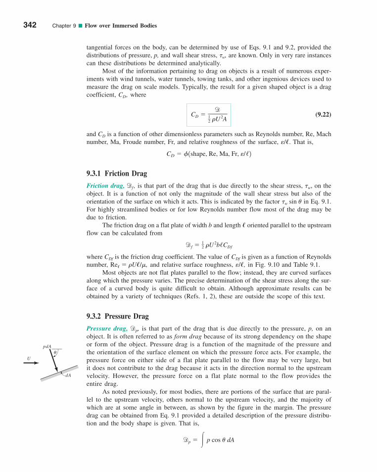
tangential forces on the body, can be determined by use of Eqs. 9.1 and 9.2, provided thedistributions of pressure, p, and wall shear stress, �w, are known. Only in very rare instancescan these distributions be determined analytically.

Most of the information pertaining to drag on objects is a result of numerous exper-iments with wind tunnels, water tunnels, towing tanks, and other ingenious devices used tomeasure the drag on scale models. Typically, the result for a given shaped object is a dragcoefficient, CD, where

(9.22)

and CD is a function of other dimensionless parameters such as Reynolds number, Re, Machnumber, Ma, Froude number, Fr, and relative roughness of the surface, e/�. That is,

9.3.1 Friction Drag

Friction drag, df , is that part of the drag that is due directly to the shear stress, �w, on theobject. It is a function of not only the magnitude of the wall shear stress but also of theorientation of the surface on which it acts. This is indicated by the factor �w sin � in Eq. 9.1.For highly streamlined bodies or for low Reynolds number flow most of the drag may bedue to friction.

The friction drag on a flat plate of width b and length � oriented parallel to the upstreamflow can be calculated from

where CDf is the friction drag coefficient. The value of CDf is given as a function of Reynoldsnumber, Re� � �U�/�, and relative surface roughness, �/�, in Fig. 9.10 and Table 9.1.

Most objects are not flat plates parallel to the flow; instead, they are curved surfacesalong which the pressure varies. The precise determination of the shear stress along the sur-face of a curved body is quite difficult to obtain. Although approximate results can beobtained by a variety of techniques (Refs. 1, 2), these are outside the scope of this text.

9.3.2 Pressure Drag

Pressure drag, dp, is that part of the drag that is due directly to the pressure, p, on anobject. It is often referred to as form drag because of its strong dependency on the shapeor form of the object. Pressure drag is a function of the magnitude of the pressure andthe orientation of the surface element on which the pressure force acts. For example, thepressure force on either side of a flat plate parallel to the flow may be very large, butit does not contribute to the drag because it acts in the direction normal to the upstreamvelocity. However, the pressure force on a flat plate normal to the flow provides theentire drag.

As noted previously, for most bodies, there are portions of the surface that are paral-lel to the upstream velocity, others normal to the upstream velocity, and the majority ofwhich are at some angle in between, as shown by the figure in the margin. The pressuredrag can be obtained from Eq. 9.1 provided a detailed description of the pressure distribu-tion and the body shape is given. That is,

dp � � p cos � dA

df � 12 �U 2b/CDf

CD � �1shape, Re, Ma, Fr, e//2

CD �d

12 �U 2A

342 Chapter 9 ■ Flow over Immersed Bodies

pdA

dA

θU

c09FlowoverImmersedBodies.qxd 9/28/10 10:28 AM Page 342

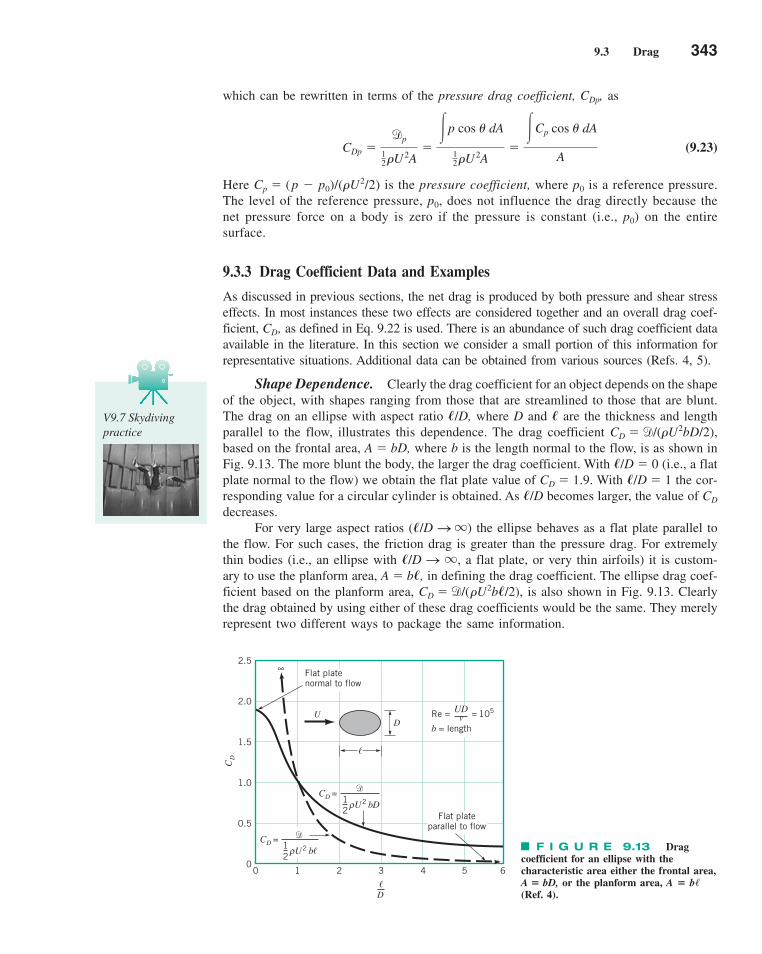
9.3 Drag 343

which can be rewritten in terms of the pressure drag coefficient, CDp, as

(9.23)

Here Cp � (p � p0)/(�U2/2) is the pressure coefficient, where p0 is a reference pressure.The level of the reference pressure, p0, does not influence the drag directly because thenet pressure force on a body is zero if the pressure is constant (i.e., p0) on the entiresurface.

9.3.3 Drag Coefficient Data and Examples

As discussed in previous sections, the net drag is produced by both pressure and shear stresseffects. In most instances these two effects are considered together and an overall drag coef-ficient, CD, as defined in Eq. 9.22 is used. There is an abundance of such drag coefficient dataavailable in the literature. In this section we consider a small portion of this information forrepresentative situations. Additional data can be obtained from various sources (Refs. 4, 5).

Shape Dependence. Clearly the drag coefficient for an object depends on the shapeof the object, with shapes ranging from those that are streamlined to those that are blunt.The drag on an ellipse with aspect ratio �/D, where D and � are the thickness and lengthparallel to the flow, illustrates this dependence. The drag coefficient CD � d/(�U2bD/2),based on the frontal area, A � bD, where b is the length normal to the flow, is as shown inFig. 9.13. The more blunt the body, the larger the drag coefficient. With �/D � 0 (i.e., a flatplate normal to the flow) we obtain the flat plate value of CD � 1.9. With �/D � 1 the cor-responding value for a circular cylinder is obtained. As �/D becomes larger, the value of CD

decreases.For very large aspect ratios (�/D S ) the ellipse behaves as a flat plate parallel to

the flow. For such cases, the friction drag is greater than the pressure drag. For extremelythin bodies (i.e., an ellipse with �/D S , a flat plate, or very thin airfoils) it is custom-ary to use the planform area, A � b�, in defining the drag coefficient. The ellipse drag coef-ficient based on the planform area, CD � d/(�U2b�/2), is also shown in Fig. 9.13. Clearlythe drag obtained by using either of these drag coefficients would be the same. They merelyrepresent two different ways to package the same information.

q

q

CDp �dp

12 �U

2A�

�p cos � dA

12 �U

2A�

�Cp cos � dA

A

V9.7 Skydivingpractice

F I G U R E 9.13 Dragcoefficient for an ellipse with thecharacteristic area either the frontal area,A � bD, or the planform area, A � b(Ref. 4).

/

2.5

2.0

1.5

1.0

0.5

00 1 2 3 4 5 6

DU

Flat plateparallel to flow

D

CD

Re = = 105UDv

b = length

U2 bD12

CD =

∞

U2 b12

CD =

Flat platenormal to flow

�

�

�

ρ �

ρ

�

c09FlowoverImmersedBodies.qxd 9/28/10 10:28 AM Page 343

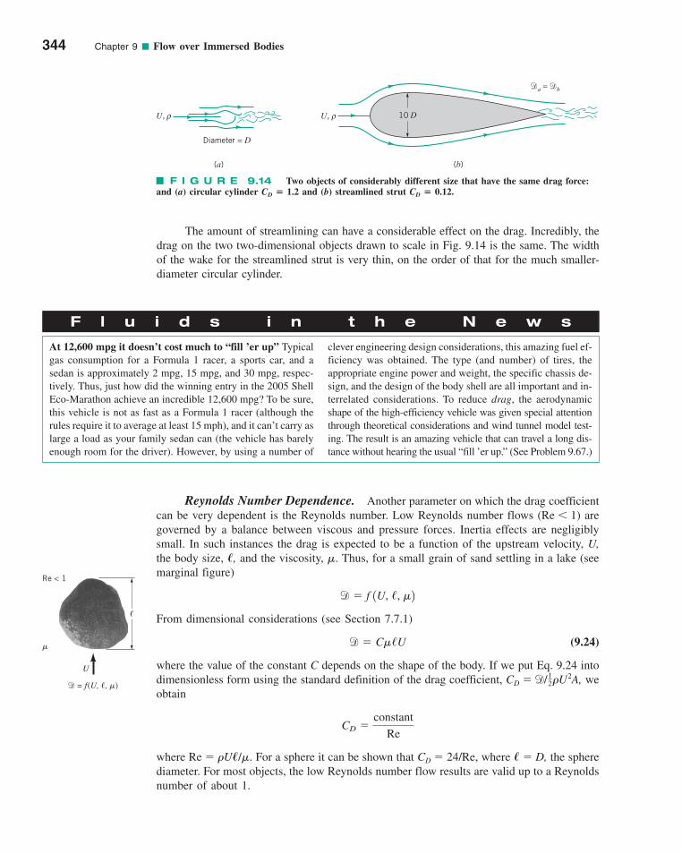
The amount of streamlining can have a considerable effect on the drag. Incredibly, thedrag on the two two-dimensional objects drawn to scale in Fig. 9.14 is the same. The widthof the wake for the streamlined strut is very thin, on the order of that for the much smaller-diameter circular cylinder.

Reynolds Number Dependence. Another parameter on which the drag coefficientcan be very dependent is the Reynolds number. Low Reynolds number flows (Re 1) aregoverned by a balance between viscous and pressure forces. Inertia effects are negligiblysmall. In such instances the drag is expected to be a function of the upstream velocity, U,the body size, �, and the viscosity, �. Thus, for a small grain of sand settling in a lake (seemarginal figure)

From dimensional considerations (see Section 7.7.1)

(9.24)

where the value of the constant C depends on the shape of the body. If we put Eq. 9.24 intodimensionless form using the standard definition of the drag coefficient, CD � d/ �U2A, weobtain

where Re � �U�/�. For a sphere it can be shown that CD � 24/Re, where � � D, the spherediameter. For most objects, the low Reynolds number flow results are valid up to a Reynoldsnumber of about 1.

CD �constant

Re

12

d � C�/U

d � f 1U, /, �2

344 Chapter 9 ■ Flow over Immersed Bodies

F I G U R E 9.14 Two objects of considerably different size that have the same drag force:and (a) circular cylinder CD � 1.2 and (b) streamlined strut CD � 0.12.

U, ρU, ρ

Diameter = D

(a) (b)

10 D

�a = �b

F l u i d s i n t h e N e w s

At 12,600 mpg it doesn’t cost much to “fill ’er up” Typicalgas consumption for a Formula 1 racer, a sports car, and asedan is approximately 2 mpg, 15 mpg, and 30 mpg, respec-tively. Thus, just how did the winning entry in the 2005 ShellEco-Marathon achieve an incredible 12,600 mpg? To be sure,this vehicle is not as fast as a Formula 1 racer (although therules require it to average at least 15 mph), and it can’t carry aslarge a load as your family sedan can (the vehicle has barelyenough room for the driver). However, by using a number of

clever engineering design considerations, this amazing fuel ef-ficiency was obtained. The type (and number) of tires, the appropriate engine power and weight, the specific chassis de-sign, and the design of the body shell are all important and in-terrelated considerations. To reduce drag, the aerodynamicshape of the high-efficiency vehicle was given special attentionthrough theoretical considerations and wind tunnel model test-ing. The result is an amazing vehicle that can travel a long dis-tance without hearing the usual “fill ’er up.” (See Problem 9.67.)

U

� = f(U, �, �)

Re < 1

�

�

c09FlowoverImmersedBodies.qxd 9/28/10 10:28 AM Page 344

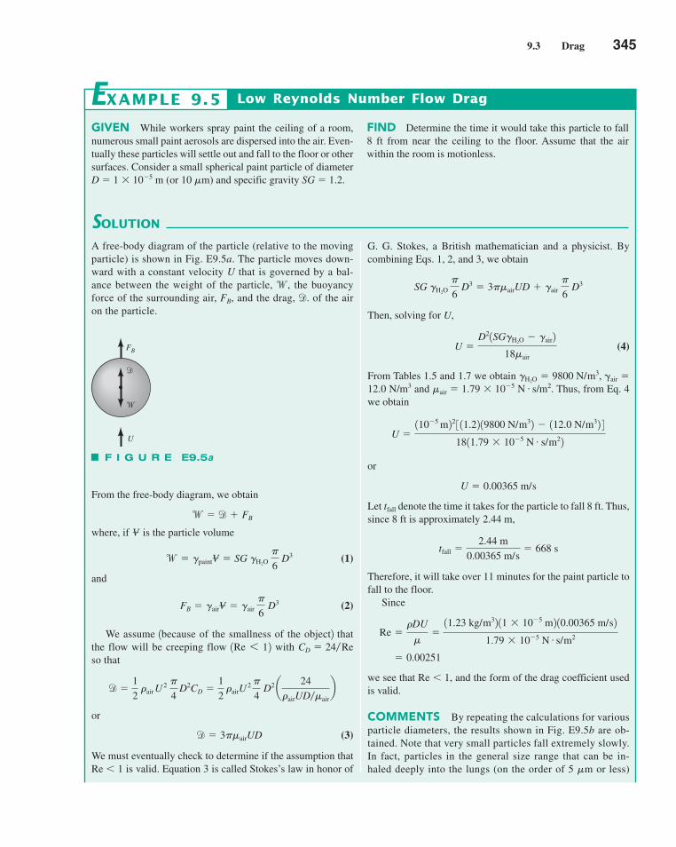
9.3 Drag 345

GIVEN While workers spray paint the ceiling of a room,numerous small paint aerosols are dispersed into the air. Even-tually these particles will settle out and fall to the floor or othersurfaces. Consider a small spherical paint particle of diameterD � 1 � 10�5 m (or 10 �m) and specific gravity SG � 1.2.

FIND Determine the time it would take this particle to fall8 ft from near the ceiling to the floor. Assume that the airwithin the room is motionless.

SOLUTION

Low Reynolds Number Flow Drag

G. G. Stokes, a British mathematician and a physicist. Bycombining Eqs. 1, 2, and 3, we obtain

Then, solving for U,

(4)

From Tables 1.5 and 1.7 we obtain , �air �12.0 N/m3 and �air � 1.79 � 10�5 N s/m2. Thus, from Eq. 4we obtain

or

Let tfall denote the time it takes for the particle to fall 8 ft. Thus,since 8 ft is approximately 2.44 m,

Therefore, it will take over 11 minutes for the paint particle tofall to the floor.

Since

we see that Re 1, and the form of the drag coefficient usedis valid.

COMMENTS By repeating the calculations for variousparticle diameters, the results shown in Fig. E9.5b are ob-tained. Note that very small particles fall extremely slowly.In fact, particles in the general size range that can be in-haled deeply into the lungs (on the order of 5 �m or less)

� 0.00251

Re ��DU

��11.23 kg/m32 11 � 10�5 m2 10.00365 m/s2

1.79 � 10�5 N # s/m2

tfall �2.44 m

0.00365 m/s� 668 s

U � 0.00365 m/s

U �110�5 m22 3 11.22 19800 N/m32 � 112.0 N/m32 4

1811.79 � 10�5 N # s/m22

#H2O � 9800 N/m3

U �D21SGH2O � air2

18�air

SG H2O

6 D3 � 3�airUD � air

6 D3

EXAMPLE 9.5

A free-body diagram of the particle (relative to the movingparticle) is shown in Fig. E9.5a. The particle moves down-ward with a constant velocity U that is governed by a bal-ance between the weight of the particle, the buoyancyforce of the surrounding air, FB, and the drag, of the airon the particle.

d.w,

From the free-body diagram, we obtain

where, if is the particle volume

(1)

and

(2)

We assume 1because of the smallness of the object2 thatthe flow will be creeping flow with so that

or

(3)

We must eventually check to determine if the assumption thatRe 1 is valid. Equation 3 is called Stokes’s law in honor of

d � 3�airUD

d �1

2 �air U

2

4 D2CD �

1

2 �airU

2

4 D2

a24

�airUD��airb

CD � 24�Re1Re 6 12

FB � airV� � air

6 D3

w � paintV� � SG H2O

6 D3

V�

w � d � FB

FB

d

w

U

F I G U R E E9.5a

c09FlowoverImmersedBodies.qxd 9/28/10 10:28 AM Page 345

Moderate Reynolds number flows tend to take on a boundary layer flow structure.For such flows past streamlined bodies, the drag coefficient tends to decrease slightly withReynolds number. The CD � Re�1/2 dependence for a laminar boundary layer on a flatplate (see Table 9.1) is such an example. Moderate Reynolds number flows past blunt bod-ies generally produce drag coefficients that are relatively constant. The CD values for thespheres and circular cylinders shown in Fig. 9.15a indicate this character in the range 103 Re 105.

The structure of the flow field at selected Reynolds numbers indicated in Fig. 9.15ais shown in Fig. 9.15b. For a given object there is a wide variety of flow situations, depend-ing on the Reynolds number involved. The curious reader is strongly encouraged to studythe many beautiful photographs and videos of these (and other) flow situations found inRefs. 6 and 19.

For many shapes there is a sudden change in the character of the drag coefficientwhen the boundary layer becomes turbulent. This is illustrated in Fig. 9.10 for the flat plateand in Fig. 9.15 for the sphere and the circular cylinder. The Reynolds number at whichthis transition takes place is a function of the shape of the body.

For streamlined bodies, the drag coefficient increases when the boundary layerbecomes turbulent because most of the drag is due to the shear force, which is greater forturbulent flow than for laminar flow. However, the drag coefficient for a relatively bluntobject, such as a cylinder or sphere, actually decreases when the boundary layer becomesturbulent. As discussed in Section 9.2.6, a turbulent boundary layer can travel further alongthe surface into the adverse pressure gradient on the rear portion of the cylinder beforeseparation occurs. The result is a thinner wake and smaller pressure drag for turbulentboundary layer flow. This is indicated in Fig. 9.15 by the sudden decrease in CD for 105 Re 106.

For extremely blunt bodies, such as a flat plate perpendicular to the flow, the flowseparates at the edge of the plate regardless of the nature of the boundary layer flow. Thus,the drag coefficient shows very little dependence on the Reynolds number.

The drag coefficients for a series of two-dimensional bodies of varying bluntness aregiven as a function of Reynolds number in Fig. 9.16. The characteristics described earlierare evident.

346 Chapter 9 ■ Flow over Immersed Bodies

will remain airborne most of the working day, thus contin-ually exposing workers to potential hazards. It is often thesmaller particles that cause the greatest health concerns,particularly to individuals exposed day after day for manyyears. In work environments that generate particle-ladenair, proper engineering controls are needed to reduce in-halation exposures (e.g., appropriate ventilation) or, in ex-treme cases, personal protective equipment (PPE, e.g., res-pirator) may be required. PPE is considered a last resortbecause in practice it is the least effective means to protectworkers. It is more effective and usually less expensive inthe long run to design out or control a problem with engi-neering ingenuity—prevention through design.

F I G U R E E9.5b

5

4.5

4

3.5

3

2.5

1.5

2

0.5

1

0

t fall,

hou

rs

0 4 8 12 16 182 6 10 14 20

D, m

10 m, 0.18 hourμ

μ

V9.8 Karman vortex street

V9.9 Oscillatingsign

c09FlowoverImmersedBodies.qxd 9/28/10 10:28 AM Page 346

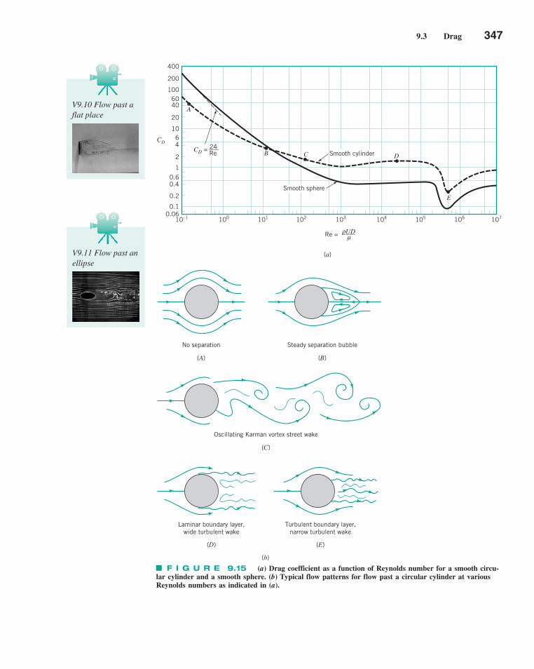
9.3 Drag 347

A

B C D

E

Smooth cylinder

Smooth sphere

CD = 24

___

Re

400

200

1006040

20

1064

2

1

0.60.4

0.2

0.10.06

10–1 100 101 102 103 104 105 106 107

Re = UD

____ρμ

(a)

CD

No separation

(A)

Steady separation bubble

(B)

Oscillating Karman vortex street wake

(C)

Laminar boundary layer,wide turbulent wake

(D)

Turbulent boundary layer,narrow turbulent wake

(E)

(b)

F I G U R E 9.15 (a) Drag coefficient as a function of Reynolds number for a smooth circu-lar cylinder and a smooth sphere. (b) Typical flow patterns for flow past a circular cylinder at variousReynolds numbers as indicated in (a).

V9.10 Flow past aflat place

V9.11 Flow past anellipse

c09FlowoverImmersedBodies.qxd 9/28/10 10:28 AM Page 347

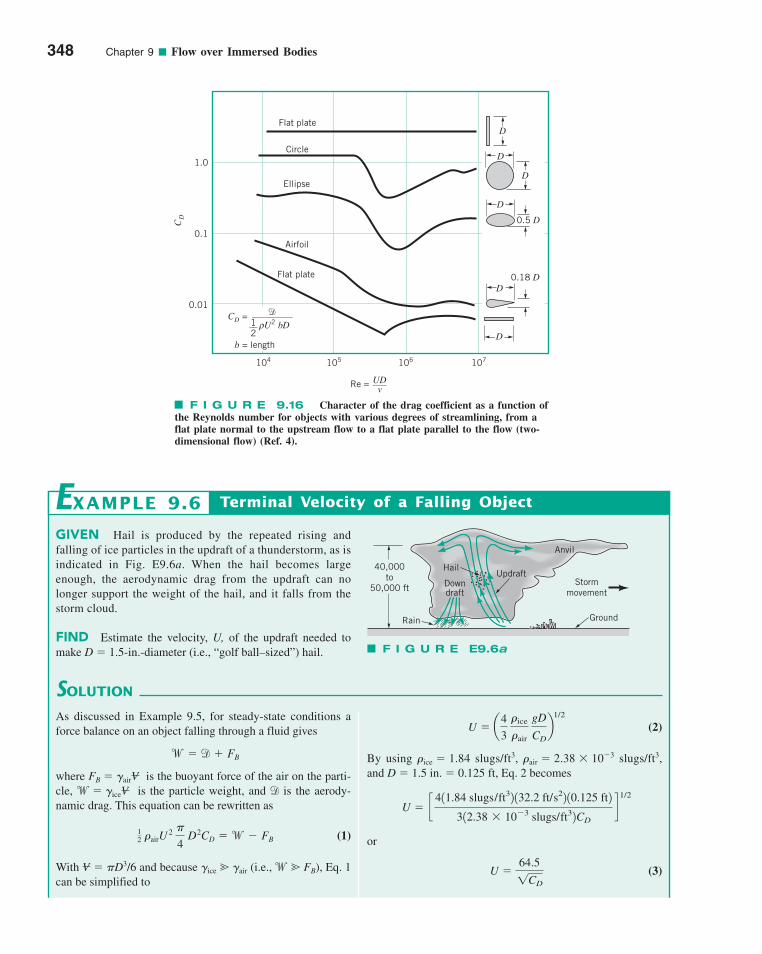
348 Chapter 9 ■ Flow over Immersed Bodies

Flat plate

Circle

Ellipse

Airfoil

Flat plate

CD = �_________

U2

bD1__

2ρ

D

D0.18 D

0.5 D

D

D

D

D

1.0

0.1

0.01

CD

104 105 106 107

Re = UD___v

b = length

F I G U R E 9.16 Character of the drag coefficient as a function ofthe Reynolds number for objects with various degrees of streamlining, from aflat plate normal to the upstream flow to a flat plate parallel to the flow (two-dimensional flow) (Ref. 4).

GIVEN Hail is produced by the repeated rising andfalling of ice particles in the updraft of a thunderstorm, as isindicated in Fig. E9.6a. When the hail becomes largeenough, the aerodynamic drag from the updraft can nolonger support the weight of the hail, and it falls from thestorm cloud.

FIND Estimate the velocity, U, of the updraft needed tomake D � 1.5-in.-diameter (i.e., “golf ball–sized”) hail.

SOLUTION

Terminal Velocity of a Falling Object

(2)

By using �ice � 1.84 slugs/ft3, �air � 2.38 � 10�3 slugs/ft3,and D � 1.5 in. � 0.125 ft, Eq. 2 becomes

or

(3)U �64.5

1CD

U � c411.84 slugs/ft32 132.2 ft/s22 10.125 ft2

312.38 � 10�3 slugs/ft32CD

d1/2

U � a4

3 �ice

�air gD

CDb

1/2

EXAMPLE 9.6

As discussed in Example 9.5, for steady-state conditions aforce balance on an object falling through a fluid gives

where FB � air is the buoyant force of the air on the parti-cle, w� ice is the particle weight, and d is the aerody-namic drag. This equation can be rewritten as

(1)

With � D3/6 and because ice air (i.e.,w FB), Eq. 1can be simplified to

V

12 �airU

2

4 D2CD �w � FB

VV

w � d � FB

Anvil

Stormmovement

Ground

HailUpdraft

Rain

40,000to

50,000 ft Downdraft

F I G U R E E9.6a

c09FlowoverImmersedBodies.qxd 9/28/10 10:28 AM Page 348

9.3 Drag 349

Compressibility Effects. If the velocity of the object is sufficiently large, compress-ibility effects become important and the drag coefficient becomes a function of the Mach num-ber, Ma � U/c, where c is the speed of sound in the fluid. For low Mach numbers, Ma 0.5or so, compressibility effects are unimportant and the drag coefficient is essentially indepen-dent of Ma. However, for larger Mach number flows, the drag coefficient can be stronglydependent on Ma.

For most objects, values of CD increase dramatically in the vicinity of Ma � 1 (i.e., sonicflow). This change in character, indicated by Fig. 9.17, is due to the existence of shock wavesas indicated by the figure in the margin. Shock waves are extremely narrow regions in the flowfield across which the flow parameters change in a nearly discontinuous manner. Shock waves,which cannot exist in subsonic flows, provide a mechanism for the generation of drag that is notpresent in the relatively low-speed subsonic flows. More information on these important topicscan be found in standard texts about compressible flow and aerodynamics (Refs. 7, 8, and 18).

Surface Roughness. In general, for streamlined bodies, the drag increases withincreasing surface roughness. Great care is taken to design the surfaces of airplane wings to beas smooth as possible, as protruding rivets or screw heads can cause a considerable increase in

roughness features. However, the calculated updraft velocitiesare in agreement with measured values.

where U is in feet per second. To determine U, we must knowCD. Unfortunately, CD is a function of the Reynolds number (seeFig. 9.15), which is not known unless U is known. Thus, we mustuse an iterative technique similar to that done with the Moodychart for certain types of pipe flow problems (see Section 8.5).

From Fig. 9.15 we expect that CD is on the order of 0.5.Thus, we assume CD � 0.5 and from Eq. 3 obtain

The corresponding Reynolds number (assuming � � 1.57 �10�4 ft2/s) is

For this value of Re we obtain CD � 0.5 from Fig. 9.15. Thus,our assumed value of CD � 0.5 was correct. The correspond-ing value of U is

(Ans)

COMMENTS By repeating the calculations for variousaltitudes, z, above sea level (using the properties of the U.S.Standard Atmosphere given in Appendix C), the results shownin Fig. E9.6b are obtained. Because of the decease in densitywith altitude, the hail falls even faster through the upper por-tions of the storm than when it hits the ground.

Clearly, an airplane flying through such an updraft would feelits effects (even if it were able to dodge the hail). As seen fromEq. 2, the larger the hail, the stronger the necessary updraft. Hail-stones greater than 6 in. in diameter have been reported. In real-ity, a hailstone is seldom spherical and often not smooth. Thehailstone shown in Fig. E9.6c is larger than golf-ball sized and isclearly ellipsoidal in shape with additional smaller-scale surface

U � 91.2 ft/s � 62.2 mph

Re �UD

��

91.2 ft /s 10.125 ft2

1.57 � 10�4 ft2/s� 7.26 � 104

U �64.5

10.5� 91.2 ft /s

140

120

100

80

60

40

20

0

U, m

ph

0 10,000 20,000 30,000 40,000

z, ft

(0, 62.2 mph)

F I G U R E E9.6b

F I G U R E E9.6c (Photograph courtesy of NOAA.)

Ma = 1.5U

Ma = 3U

Shockwave

c09FlowoverImmersedBodies.qxd 9/28/10 10:28 AM Page 349

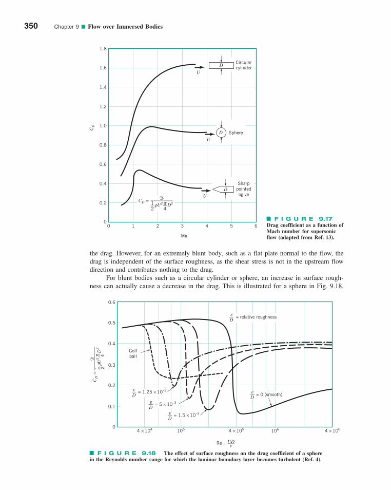
350 Chapter 9 ■ Flow over Immersed Bodies

F I G U R E 9.17Drag coefficient as a function ofMach number for supersonicflow (adapted from Ref. 13).

U

U

U

CircularcylinderD

SphereD

Sharppointedogive

D

CD = �___________

U2

D21__

2__4π

0 1 2 3 4 5 6

Ma

0

0.2

0.4

0.6

0.8

1.0

1.2

1.4

1.6

1.8

CD

ρ

0.6

0.5

0.4

0.3

0.2

0.1

04 × 104 105 106 4 × 105 4 × 106

Re = UD

___

v

Golfball

CD =

�__

____

____

_

U2

D

21 __ 2

__ 4π

ε__D

ε__D

ε__D

ε__D

ε__D

= 5 × 10–3

= 1.25 × 10–2= 0 (smooth)

= relative roughness

ρ

= 1.5 × 10–3

F I G U R E 9.18 The effect of surface roughness on the drag coefficient of a sphere in the Reynolds number range for which the laminar boundary layer becomes turbulent (Ref. 4).

the drag. However, for an extremely blunt body, such as a flat plate normal to the flow, thedrag is independent of the surface roughness, as the shear stress is not in the upstream flowdirection and contributes nothing to the drag.

For blunt bodies such as a circular cylinder or sphere, an increase in surface rough-ness can actually cause a decrease in the drag. This is illustrated for a sphere in Fig. 9.18.

c09FlowoverImmersedBodies.qxd 9/28/10 10:28 AM Page 350

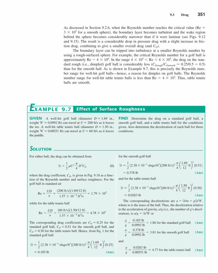
9.3 Drag 351

GIVEN A well-hit golf ball (diameter D � 1.69 in.,weight w� 0.0992 lb) can travel at U � 200 ft/s as it leavesthe tee. A well-hit table tennis ball (diameter D � 1.50 in.,weight w� 0.00551 lb) can travel at U � 60 ft/s as it leavesthe paddle.

FIND Determine the drag on a standard golf ball, asmooth golf ball, and a table tennis ball for the conditionsgiven. Also determine the deceleration of each ball for theseconditions.

SOLUTION

Effect of Surface Roughness

for the smooth golf ball

(Ans)

and for the table tennis ball

(Ans)

The corresponding decelerations are a � d/m � gd/w,where m is the mass of the ball. Thus, the deceleration relativeto the acceleration of gravity, a/g (i.e., the number of g’s decel-eration), is a/g � d/w or

(Ans)

(Ans)

and

(Ans)a

g�

0.0263 lb

0.00551 lb� 4.77 for the table tennis ball

a

g�

0.378 lb

0.0992 lb� 3.81 for the smooth golf ball

a

g�

0.185 lb

0.0992 lb� 1.86 for the standard golf ball

� 0.0263 lb

d �1

2 12.38 � 10�3 slugs/ft32 160 ft /s22

�

4 a

1.50

12 ftb

2

10.502

� 0.378 lb

d �1

2 12.38 � 10�3 slugs/ft32 1200 ft /s22

�

4 a

1.69

12 ftb

2

10.512

EXAMPLE 9.7

For either ball, the drag can be obtained from

(1)

where the drag coefficient, CD, is given in Fig. 9.18 as a func-tion of the Reynolds number and surface roughness. For thegolf ball in standard air

while for the table tennis ball

The corresponding drag coefficients are CD � 0.25 for thestandard golf ball, CD � 0.51 for the smooth golf ball, andCD � 0.50 for the table tennis ball. Hence, from Eq. 1 for thestandard golf ball

(Ans) � 0.185 lb

d �1

2 12.38 � 10�3 slugs/ft32 1200 ft /s22

�

4 a

1.69

12 ftb

2

10.252

Re �UD

��160 ft /s2 11.50/12 ft2

1.57 � 10�4 ft2/s� 4.78 � 104

Re �UD

��1200 ft /s2 11.69/12 ft2

1.57 � 10�4 ft2/s� 1.79 � 105

d �1

2 �U 2

�

4 D2CD

As discussed in Section 9.2.6, when the Reynolds number reaches the critical value (Re �3 � 105 for a smooth sphere), the boundary layer becomes turbulent and the wake regionbehind the sphere becomes considerably narrower than if it were laminar (see Figs. 9.12and 9.15). The result is a considerable drop in pressure drag with a slight increase in fric-tion drag, combining to give a smaller overall drag (and CD).

The boundary layer can be tripped into turbulence at a smaller Reynolds number byusing a rough-surfaced sphere. For example, the critical Reynolds number for a golf ball isapproximately Re � 4 � 104. In the range 4 � 104 � Re � 4 � 105, the drag on the stan-dard rough (i.e., dimpled) golf ball is considerably less (CDrough/CDsmooth � 0.25/0.5 � 0.5)than for the smooth ball. As is shown in Example 9.7, this is precisely the Reynolds num-ber range for well-hit golf balls—hence, a reason for dimples on golf balls. The Reynoldsnumber range for well-hit table tennis balls is less than Re � 4 � 104. Thus, table tennisballs are smooth.

c09FlowoverImmersedBodies.qxd 9/30/10 9:17 AM Page 351

352 Chapter 9 ■ Flow over Immersed Bodies

COMMENTS Note that there is a considerably smallerdeceleration for the rough golf ball than for the smooth one.Because of its much larger drag-to-mass ratio, the table tennisball slows down relatively quickly and does not travel as far asthe golf ball. (Note that with U � 60 ft/s the standard golf ballhas a drag of d � 0.0200 lb and a deceleration of a/g �0.202, considerably less than the a/g � 4.77 of the table tennisball. Conversely, a table tennis ball hit from a tee at 200 ft/swould decelerate at a rate of a � 1740 ft/s2, or a/g � 54.1. Itwould not travel nearly as far as the golf ball.)

By repeating the above calculations, the drag as a functionof speed for both a standard golf ball and a smooth golf ball isshown in Fig. E9.7.

The Reynolds number range for which a rough golf ballhas smaller drag than a smooth one (i.e., 4 � 104 to 3.6 � 105)corresponds to a flight velocity range of 45 � U � 400 ft/s.This is comfortably within the range of most golfers. (Thefastest tee shot by top professional golfers is approxi-mately 280 ft/s.) As discussed in Section 9.4.2, the dimples

(roughness) on a golf ball also help produce a lift (due tothe spin of the ball) that allows the ball to travel fartherthan a smooth ball.

1.2

1

0.8

0.6

0.4

0.2

0

�, lb

0 100 200 400 500

U, ft/s

300

Smoothgolf ball

Standardgolf ball

F I G U R E E9.7

F l u i d s i n t h e N e w s

Dimpled baseball bats For many years it has been knownthat dimples on golf balls can create a turbulent boundarylayer and reduce the aerodynamic drag, allowing longerdrives than with smooth balls. Thus, why not put dimples onbaseball bats so that tomorrow’s baseball sluggers can swingthe bat faster and, therefore, hit the ball farther? MIT instruc-tor Jeffery De Tullio pondered that question, performed

experiments with dimpled bats to determine the answer, andreceived a patent for his dimpled bat invention. The result isthat a batter can swing a dimpled bat approximately 3 to 5%faster than a smooth bat. Theoretically, this extra speed willtranslate to an extra 10- to 15-ft distance on a long hit. (SeeProblem 9.64.)

V9.12 Jet ski

�pole �flag

Froude Number Effects. Another parameter on which the drag coefficient may bestrongly dependent is the Froude number, As is discussed in Chapter 10, theFroude number is a ratio of the free-stream speed to a typical wave speed on the interface oftwo fluids, such as the surface of the ocean. An object moving on the surface, such as a ship,often produces waves that require a source of energy to generate. This energy comes from theship and is manifest as a drag. [Recall that the rate of energy production (power) equals speedtimes force.] The nature of the waves produced often depends on the Froude number of theflow and the shape of the object—the waves generated by a water skier “plowing” throughthe water at a low speed (low Fr) are different from those generated by the skier “planing”along the surface at a high speed (larger Fr).

Composite Body Drag. Approximate drag calculations for a complex body canoften be obtained by treating the body as a composite collection of its various parts. For exam-ple, the total force on a flagpole because of the wind (see the figure in the margin) can beapproximated by adding the aerodynamic drag produced by the various componentsinvolved—the drag on the flag and the drag on the pole. In some cases considerable care mustbe taken in such an approach because of the interactions between the various parts. It may

Fr � U/1g/.

c09FlowoverImmersedBodies.qxd 9/29/10 9:38 AM Page 352

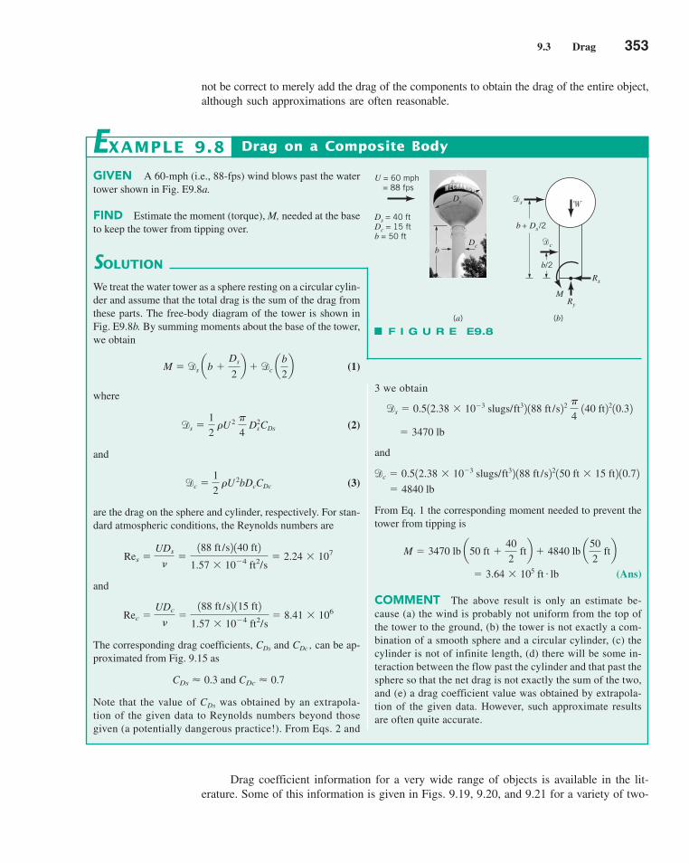
9.3 Drag 353

GIVEN A 60-mph (i.e., 88-fps) wind blows past the watertower shown in Fig. E9.8a.

FIND Estimate the moment (torque), M, needed at the baseto keep the tower from tipping over.

SOLUTION

Drag on a Composite Body

3 we obtain

and

From Eq. 1 the corresponding moment needed to prevent thetower from tipping is

(Ans)

COMMENT The above result is only an estimate be-cause (a) the wind is probably not uniform from the top ofthe tower to the ground, (b) the tower is not exactly a com-bination of a smooth sphere and a circular cylinder, (c) thecylinder is not of infinite length, (d) there will be some in-teraction between the flow past the cylinder and that past thesphere so that the net drag is not exactly the sum of the two,and (e) a drag coefficient value was obtained by extrapola-tion of the given data. However, such approximate resultsare often quite accurate.

� 3.64 � 105 ft # lb

M � 3470 lb a50 ft �40

2 ftb � 4840 lb a

50

2 ftb

� 4840 lb

dc � 0.512.38 � 10�3 slugs/ft32 188 ft /s22150 ft � 15 ft2 10.72

� 3470 lb

ds � 0.512.38 � 10�3 slugs/ft32 188 ft /s22

4 140 ft2210.32

EXAMPLE 9.8

We treat the water tower as a sphere resting on a circular cylin-der and assume that the total drag is the sum of the drag fromthese parts. The free-body diagram of the tower is shown inFig. E9.8b. By summing moments about the base of the tower,we obtain

(1)

where

(2)

and

(3)

are the drag on the sphere and cylinder, respectively. For stan-dard atmospheric conditions, the Reynolds numbers are

and

The corresponding drag coefficients, CDs and CDc , can be ap-proximated from Fig. 9.15 as

and

Note that the value of CDs was obtained by an extrapola-tion of the given data to Reynolds numbers beyond thosegiven (a potentially dangerous practice!). From Eqs. 2 and

CDc � 0.7CDs � 0.3

Rec �UDc

��188 ft /s2 115 ft2

1.57 � 10�4 ft2/s� 8.41 � 106

Res �UDs

��188 ft /s2 140 ft2

1.57 � 10�4 ft2/s� 2.24 � 107

dc �1

2 �U 2bDcCDc

ds �1

2 �U 2

4 D2

sCDs

M � ds ab �Ds

2b � dc a

b

2b

F I G U R E E9.8

�s

�c

b + D

s/2

b/2

Rx

Ry

M

(b)(a)

�

U = 60 mph = 88 fps

Ds = 40 ft

Dc = 15 ft

b = 50 ftD

c

Ds

b

Drag coefficient information for a very wide range of objects is available in the lit-erature. Some of this information is given in Figs. 9.19, 9.20, and 9.21 for a variety of two-

not be correct to merely add the drag of the components to obtain the drag of the entire object,although such approximations are often reasonable.

c09FlowoverImmersedBodies.qxd 9/28/10 10:29 AM Page 353

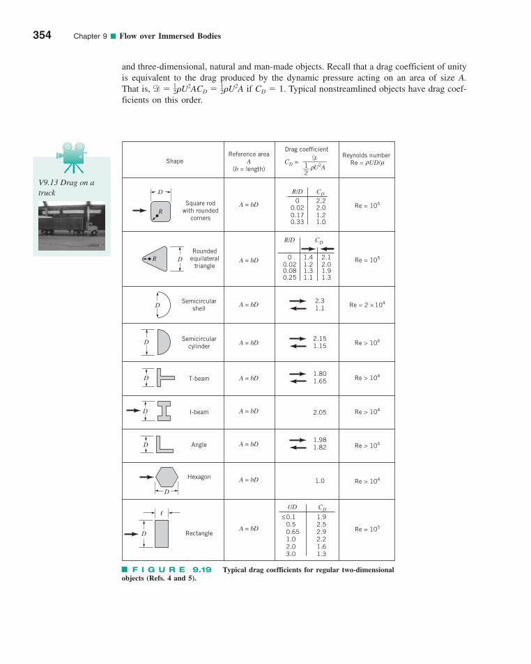
354 Chapter 9 ■ Flow over Immersed Bodies

D

RSquare rod

with roundedcorners

DRRounded

equilateraltriangle

DSemicircular

shell

Semicircularcylinder

D

D T-beam

I-beamD

D Angle

D

Hexagon

�

D Rectangle

ShapeReference area

A(b = length)

A = bD

A = bD

A = bD

A = bD

A = bD

A = bD

A = bD

A = bD

A = bD

Drag coefficient

CD = �________

U2A1__2

ρ

R/D CD

00.020.170.33

2.22.01.21.0

R/D CD

00.020.080.25

1.41.21.31.1

2.12.01.91.3

2.31.1

2.151.15

1.801.65

1.981.82

2.05

1.0

�/D CD

0.10.50.651.02.03.0

1.92.52.92.21.61.3

Reynolds numberRe = UD/ ρ

Re = 105

Re = 105

Re = 2 × 104

Re > 104

Re > 104

Re > 104

Re > 104

Re > 104

Re = 105

<

μ

F I G U R E 9.19 Typical drag coefficients for regular two-dimensionalobjects (Refs. 4 and 5).

V9.13 Drag on atruck

and three-dimensional, natural and man-made objects. Recall that a drag coefficient of unityis equivalent to the drag produced by the dynamic pressure acting on an area of size A.That is, if CD � 1. Typical nonstreamlined objects have drag coef-ficients on this order.

d � 12�U2ACD � 1

2�U2A

c09FlowoverImmersedBodies.qxd 9/28/10 10:29 AM Page 354

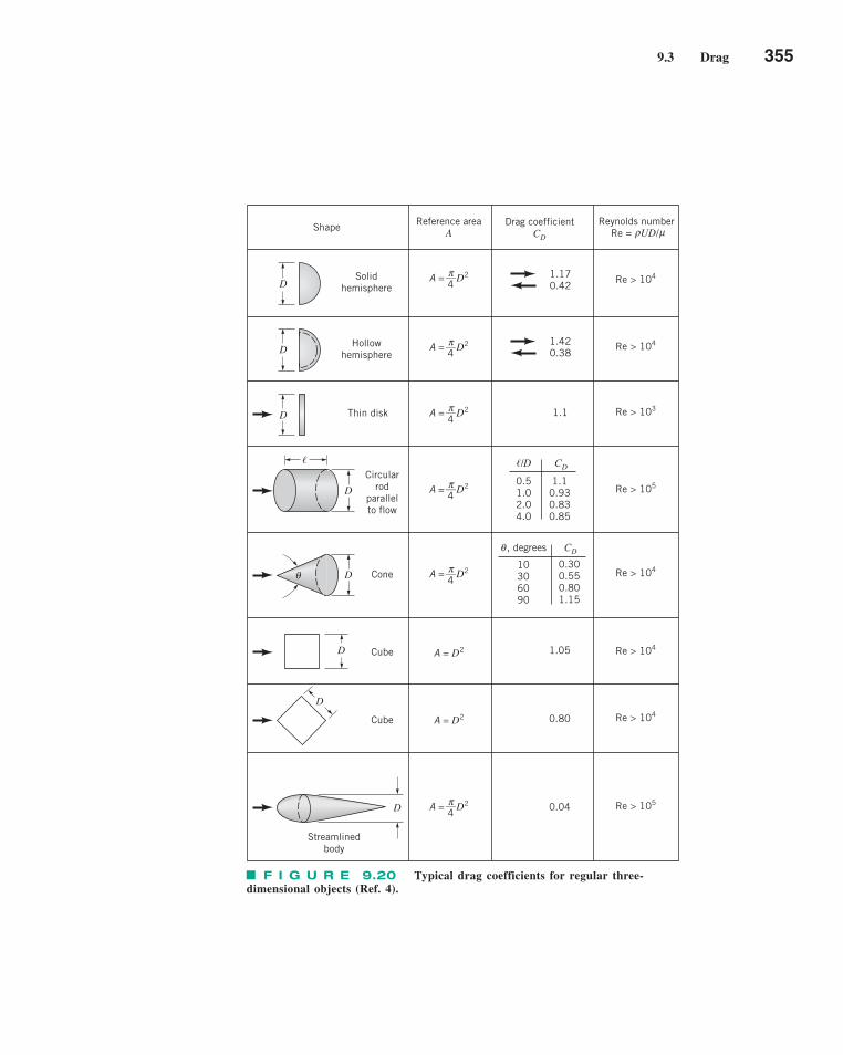
9.3 Drag 355

DSolid

hemisphere

DHollow

hemisphere

D Thin disk

�

D

Circularrod

parallelto flow

D Cone

CubeD

Cube

D

D

Streamlinedbody

Shape Reference areaA

A = D2__4π

A = D2__4π

A = D2__4π

A = D2__4π

A = D2__4π

A = D2

A = D2

A = D2__4π

Drag coefficientCD

1.170.42

1.420.38

1.1

, degrees CD

10306090

0.300.550.801.15

�/D CD

0.51.02.04.0

1.10.930.830.85

θ

1.05

0.80

0.04

Re > 104

Re > 104

Re > 103

Re > 105

Re > 104

Re > 104

Re > 104

Re > 105

Reynolds numberRe = UD/ ρ μ

θ

F I G U R E 9.20 Typical drag coefficients for regular three-dimensional objects (Ref. 4).

c09FlowoverImmersedBodies.qxd 9/28/10 10:29 AM Page 355

356 Chapter 9 ■ Flow over Immersed Bodies

U

D Parachute

D Porousparabolic

dish

Averageperson

Flutteringflag

D

l

EmpireState Building

Six-car passenger train

Bikes

Upright commuter

Racing

Drafting

Streamlined

Tractor-trailor tucks

Fairing

Gap seal

Standard

With fairing

Withfairing andgap seal

TreeU = 10 m/sU = 20 m/sU = 30 m/s

Dolphin

Largebirds

Shape Reference area

Frontal area

A = D2__4π

Frontal area

A = D2__4π

Standing

Sitting

Crouching

A = �D

Frontal area

Frontal area

A = 5.5 ft2

A = 3.9 ft2

A = 3.9 ft2

A = 5.0 ft2

Frontal area

Frontal area

Frontal area

Frontal area

Frontal area

Wetted area

Drag coefficientCD

1.4

Porosity

Porosity = open area/total area

0 0.2 0.5

1.42 1.20 0.82

0.95 0.90 0.80

CDA = 9 ft2

CDA = 6 ft2

CDA = 2.5 ft2

�/D CD

21

30.120.07

0.15

1.4

1.8

1.1

0.88

0.50

0.12

0.96

0.76

0.70

0.430.260.20

0.0036 at Re = 6 × 106

(flat plate has CDf = 0.0031)

0.40

V9.14 Automobilestreamlining

F I G U R E 9.21 Typical drag coefficients for objects of interest (Refs.4, 5, 11, and 14).

c09FlowoverImmersedBodies.qxd 9/28/10 10:29 AM Page 356

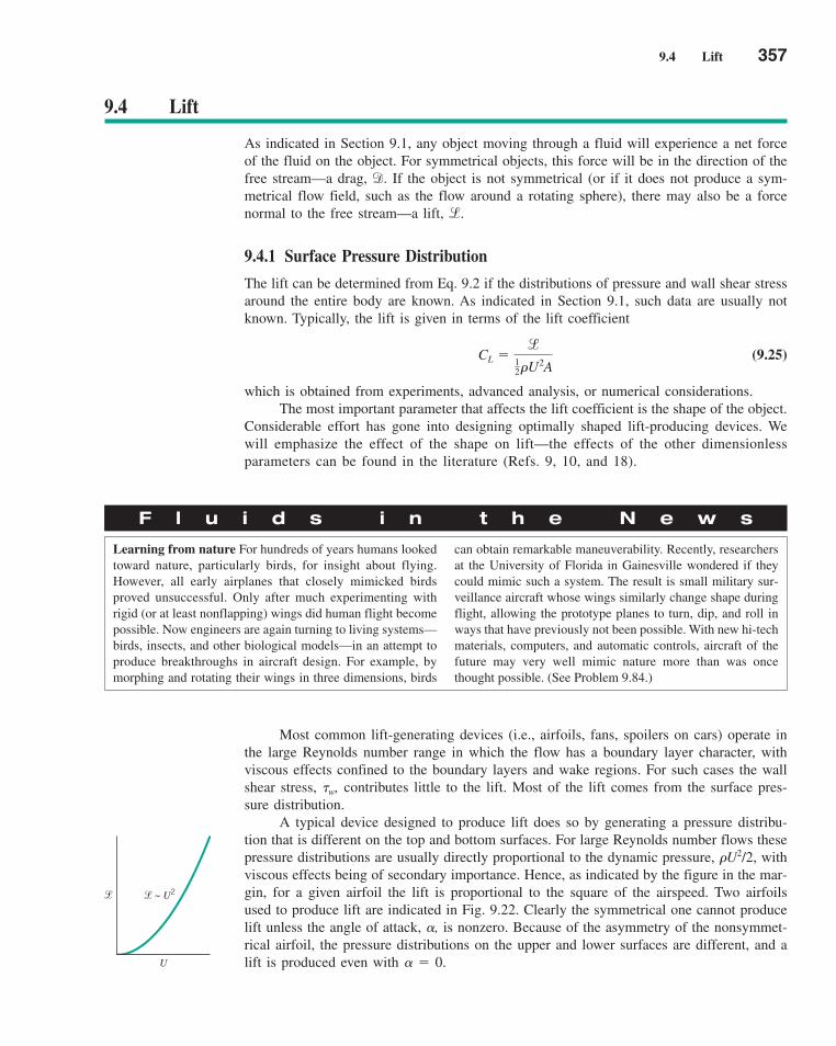
9.4 Lift 357

9.4 Lift

As indicated in Section 9.1, any object moving through a fluid will experience a net forceof the fluid on the object. For symmetrical objects, this force will be in the direction of thefree stream—a drag, d. If the object is not symmetrical (or if it does not produce a sym-metrical flow field, such as the flow around a rotating sphere), there may also be a forcenormal to the free stream—a lift, l.

9.4.1 Surface Pressure Distribution

The lift can be determined from Eq. 9.2 if the distributions of pressure and wall shear stressaround the entire body are known. As indicated in Section 9.1, such data are usually notknown. Typically, the lift is given in terms of the lift coefficient

(9.25)

which is obtained from experiments, advanced analysis, or numerical considerations.The most important parameter that affects the lift coefficient is the shape of the object.

Considerable effort has gone into designing optimally shaped lift-producing devices. Wewill emphasize the effect of the shape on lift—the effects of the other dimensionlessparameters can be found in the literature (Refs. 9, 10, and 18).

CL �l

12�U2A

Most common lift-generating devices (i.e., airfoils, fans, spoilers on cars) operate inthe large Reynolds number range in which the flow has a boundary layer character, withviscous effects confined to the boundary layers and wake regions. For such cases the wallshear stress, �w, contributes little to the lift. Most of the lift comes from the surface pres-sure distribution.

A typical device designed to produce lift does so by generating a pressure distribu-tion that is different on the top and bottom surfaces. For large Reynolds number flows thesepressure distributions are usually directly proportional to the dynamic pressure, �U2/2, withviscous effects being of secondary importance. Hence, as indicated by the figure in the mar-gin, for a given airfoil the lift is proportional to the square of the airspeed. Two airfoilsused to produce lift are indicated in Fig. 9.22. Clearly the symmetrical one cannot producelift unless the angle of attack, �, is nonzero. Because of the asymmetry of the nonsymmet-rical airfoil, the pressure distributions on the upper and lower surfaces are different, and alift is produced even with � � 0.

F l u i d s i n t h e N e w s

Learning from nature For hundreds of years humans lookedtoward nature, particularly birds, for insight about flying.However, all early airplanes that closely mimicked birdsproved unsuccessful. Only after much experimenting withrigid (or at least nonflapping) wings did human flight becomepossible. Now engineers are again turning to living systems—birds, insects, and other biological models—in an attempt toproduce breakthroughs in aircraft design. For example, bymorphing and rotating their wings in three dimensions, birds

can obtain remarkable maneuverability. Recently, researchersat the University of Florida in Gainesville wondered if theycould mimic such a system. The result is small military sur-veillance aircraft whose wings similarly change shape duringflight, allowing the prototype planes to turn, dip, and roll inways that have previously not been possible. With new hi-techmaterials, computers, and automatic controls, aircraft of thefuture may very well mimic nature more than was oncethought possible. (See Problem 9.84.)

U

� � ~ U2

c09FlowoverImmersedBodies.qxd 9/28/10 10:29 AM Page 357

358 Chapter 9 ■ Flow over Immersed Bodies

Because most airfoils are thin, it is customary to use the planform area, A � bc, inthe definition of the lift coefficient. Here b is the length of the airfoil and c is the chordlength—the length from the leading edge to the trailing edge as indicated in Fig. 9.22. Typ-ical lift coefficients so defined are on the order of unity (see Fig. 9.23). That is, the liftforce is on the order of the dynamic pressure times the planform area of the wing,

. The wing loading, defined as the average lift per unit area of the wing, l/A,therefore, increases with speed. For example, the wing loading of the 1903 Wright Flyeraircraft was 1.5 lb/ft2, whereas for the present-day Boeing 747 aircraft it is 150 lb/ft2. Thewing loading for a bumble bee is approximately 1 lb/ft2 (Ref. 11).

In many lift-generating devices the important quantity is the ratio of the lift to dragdeveloped, . Such information is often presented in terms of CL/CD versus �,as shown in Fig. 9.23a, or in a lift-drag polar of CL versus CD with � as a parameter, as

l/d � CL/CD

l � 1�U2/22A

F I G U R E 9.22 Symmet-rical and nonsymmetrical airfoils.

αU

Symmetrical

Nonsymmetrical

c

αU

120

100

80

60

40

20

0

–20

–40–8 –4 0 4 8

, degreesα

CL__CD

NACA 64(1) – 412 airfoilRe = 7 × 105

Stall 1.5

1.0

0.5

0

–0.50 0.005 0.010 0.015 0.02

CD

CL

(b)(a)

= –6°α

= –4°α

= –2°α

= 0°α

= 2°α

= 4°α

= 6°α= 8°α

F I G U R E 9.23 Two representations of the same lift and drag data for a typical airfoil:(a) lift-to-drag ratio as a function of angle of attack, with the onset of boundary layer separation on theupper surface indicated by the occurrence of stall, and (b) the lift and drag polar diagram with the angleof attack indicated (Ref. 17).

V9.15 Stalled airfoil

c09FlowoverImmersedBodies.qxd 9/28/10 10:29 AM Page 358

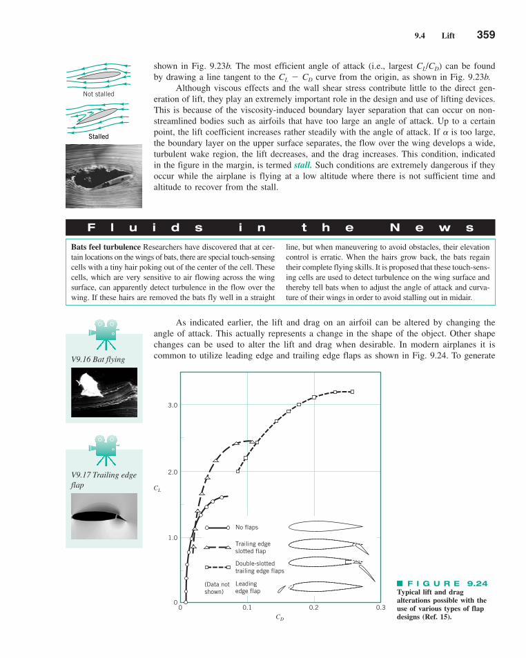
9.4 Lift 359

shown in Fig. 9.23b. The most efficient angle of attack (i.e., largest CL/CD) can be foundby drawing a line tangent to the CL � CD curve from the origin, as shown in Fig. 9.23b.

Although viscous effects and the wall shear stress contribute little to the direct gen-eration of lift, they play an extremely important role in the design and use of lifting devices.This is because of the viscosity-induced boundary layer separation that can occur on non-streamlined bodies such as airfoils that have too large an angle of attack. Up to a certainpoint, the lift coefficient increases rather steadily with the angle of attack. If � is too large,the boundary layer on the upper surface separates, the flow over the wing develops a wide,turbulent wake region, the lift decreases, and the drag increases. This condition, indicatedin the figure in the margin, is termed stall. Such conditions are extremely dangerous if theyoccur while the airplane is flying at a low altitude where there is not sufficient time andaltitude to recover from the stall.

V9.17 Trailing edgeflap

Not stalled

StalledStalled

V9.16 Bat flying

F l u i d s i n t h e N e w s

Bats feel turbulence Researchers have discovered that at cer-tain locations on the wings of bats, there are special touch-sensingcells with a tiny hair poking out of the center of the cell. Thesecells, which are very sensitive to air flowing across the wingsurface, can apparently detect turbulence in the flow over thewing. If these hairs are removed the bats fly well in a straight

line, but when maneuvering to avoid obstacles, their elevationcontrol is erratic. When the hairs grow back, the bats regaintheir complete flying skills. It is proposed that these touch-sens-ing cells are used to detect turbulence on the wing surface andthereby tell bats when to adjust the angle of attack and curva-ture of their wings in order to avoid stalling out in midair.

As indicated earlier, the lift and drag on an airfoil can be altered by changing theangle of attack. This actually represents a change in the shape of the object. Other shapechanges can be used to alter the lift and drag when desirable. In modern airplanes it iscommon to utilize leading edge and trailing edge flaps as shown in Fig. 9.24. To generate

F I G U R E 9.24Typical lift and dragalterations possible with theuse of various types of flapdesigns (Ref. 15).

No flaps

Trailing edgeslotted flap

Double-slottedtrailing edge flaps

(Data notshown)

Leadingedge flap

3.0

2.0

1.0

00 0.1 0.2 0.3

CD

CL

c09FlowoverImmersedBodies.qxd 9/28/10 10:29 AM Page 359

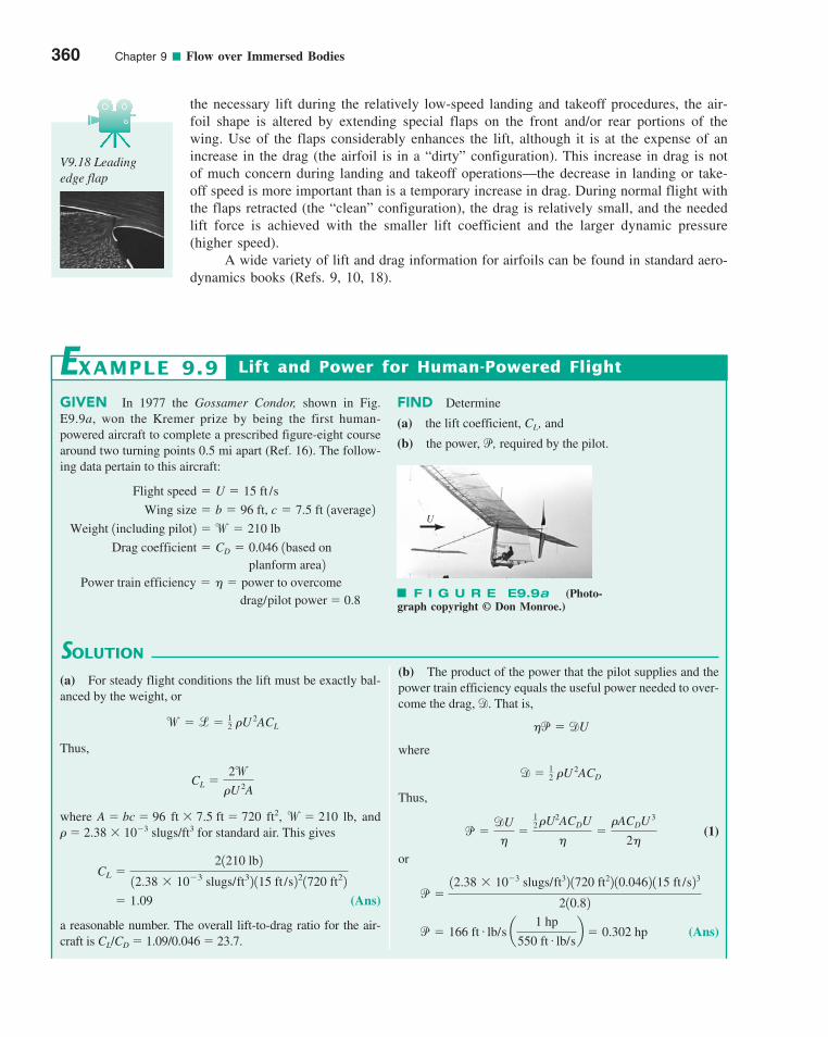
360 Chapter 9 ■ Flow over Immersed Bodies

the necessary lift during the relatively low-speed landing and takeoff procedures, the air-foil shape is altered by extending special flaps on the front and/or rear portions of thewing. Use of the flaps considerably enhances the lift, although it is at the expense of anincrease in the drag (the airfoil is in a “dirty” configuration). This increase in drag is notof much concern during landing and takeoff operations—the decrease in landing or take-off speed is more important than is a temporary increase in drag. During normal flight withthe flaps retracted (the “clean” configuration), the drag is relatively small, and the neededlift force is achieved with the smaller lift coefficient and the larger dynamic pressure(higher speed).

A wide variety of lift and drag information for airfoils can be found in standard aero-dynamics books (Refs. 9, 10, 18).

V9.18 Leadingedge flap

GIVEN In 1977 the Gossamer Condor, shown in Fig.E9.9a, won the Kremer prize by being the first human-powered aircraft to complete a prescribed figure-eight coursearound two turning points 0.5 mi apart (Ref. 16). The follow-ing data pertain to this aircraft:

Drag coefficient � CD � 0.046 1based on

Weight 1including pilot2 �w � 210 lb

Wing size � b � 96 ft, c � 7.5 ft 1average2

Flight speed � U � 15 ft /s

planform area2

drag/pilot power � 0.8� power to overcome Power train efficiency � �

Lift and Power for Human-Powered Flight

(b) The product of the power that the pilot supplies and thepower train efficiency equals the useful power needed to over-come the drag, d. That is,

where

Thus,

(1)

or

(Ans) p � 166 ft # lb/s a1 hp

550 ft # lb/sb � 0.302 hp

p �12.38 � 10�3 slugs/ft32 1720 ft22 10.0462 115 ft /s23

210.82

p �dU

��

12 �U2ACDU

��

�ACDU 3

2�

d � 12 �U 2ACD

�p � dU

EXAMPLE 9.9

(a) For steady flight conditions the lift must be exactly bal-anced by the weight, or

Thus,

where A � bc � 96 ft � 7.5 ft � 720 ft2, w � 210 lb, and� � 2.38 � 10�3 slugs/ft3 for standard air. This gives

(Ans)

a reasonable number. The overall lift-to-drag ratio for the air-craft is CL/CD � 1.09/0.046 � 23.7.

� 1.09

CL �21210 lb2

12.38 � 10�3 slugs/ft32 115 ft /s221720 ft22

CL �2w

�U 2A

w � l � 12 �U 2ACL

SOLUTION

U

F I G U R E E9.9a (Photo-graph copyright © Don Monroe.)

FIND Determine

(a) the lift coefficient, CL, and

(b) the power, p, required by the pilot.

c09FlowoverImmersedBodies.qxd 9/28/10 10:29 AM Page 360

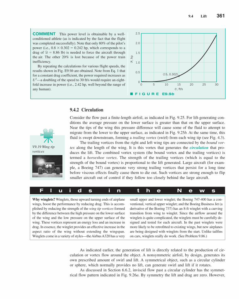
9.4 Lift 361

COMMENT This power level is obtainable by a well-conditioned athlete (as is indicated by the fact that the flightwas completed successfully). Note that only 80% of the pilot’spower (i.e., 0.8 � 0.302 � 0.242 hp, which corresponds to adrag of d� 8.86 lb) is needed to force the aircraft throughthe air. The other 20% is lost because of the power traininefficiency.

By repeating the calculations for various flight speeds, theresults shown in Fig. E9.9b are obtained. Note from Eq. 1 thatfor a constant drag coefficient, the power required increases asU3—a doubling of the speed to 30 ft/s would require an eight-fold increase in power (i.e., 2.42 hp, well beyond the range ofany human).

2.5

2.0

1.5

1.0

0.5

�, hp

015 20 25 30

U, ft/s

100 5

(15, 0.302)

F I G U R E E9.9b

V9.19 Wing tipvortices

9.4.2 Circulation

Consider the flow past a finite-length airfoil, as indicated in Fig. 9.25. For lift-generating con-ditions the average pressure on the lower surface is greater than that on the upper surface.Near the tips of the wing this pressure difference will cause some of the fluid to attempt tomigrate from the lower to the upper surface, as indicated in Fig. 9.25b. At the same time, thisfluid is swept downstream, forming a trailing vortex (swirl) from each wing tip (see Fig. 4.3).

The trailing vortices from the right and left wing tips are connected by the bound vor-tex along the length of the wing. It is this vortex that generates the circulation that pro-duces the lift. The combined vortex system (the bound vortex and the trailing vortices) istermed a horseshoe vortex. The strength of the trailing vortices (which is equal to thestrength of the bound vortex) is proportional to the lift generated. Large aircraft (for exam-ple, a Boeing 747) can generate very strong trailing vortices that persist for a long timebefore viscous effects finally cause them to die out. Such vortices are strong enough to flipsmaller aircraft out of control if they follow too closely behind the large aircraft.

F l u i d s i n t h e N e w s

Why winglets? Winglets, those upward turning ends of airplanewings, boost the performance by reducing drag. This is accom-plished by reducing the strength of the wing tip vortices formedby the difference between the high pressure on the lower surfaceof the wing and the low pressure on the upper surface of thewing. These vortices represent an energy loss and an increase indrag. In essence, the winglet provides an effective increase in theaspect ratio of the wing without extending the wingspan.Winglets come in a variety of styles—the Airbus A320 has a very

small upper and lower winglet; the Boeing 747-400 has a con-ventional, vertical upper winglet; and the Boeing Business Jet (aderivative of the Boeing 737) has an 8-ft winglet with a curvingtransition from wing to winglet. Since the airflow around thewinglets is quite complicated, the winglets must be carefully de-signed and tested for each aircraft. In the past winglets weremore likely to be retrofitted to existing wings, but new airplanesare being designed with winglets from the start. Unlike tailfinson cars, winglets really do work. (See Problem 9.86.)

As indicated earlier, the generation of lift is directly related to the production of cir-culation or vortex flow around the object. A nonsymmetric airfoil, by design, generates itsown prescribed amount of swirl and lift. A symmetrical object, such as a circular cylinderor sphere, which normally provides no lift, can generate swirl and lift if it rotates.

As discussed in Section 6.6.2, inviscid flow past a circular cylinder has the symmet-rical flow pattern indicated in Fig. 9.26a. By symmetry the lift and drag are zero. However,

c09FlowoverImmersedBodies.qxd 9/30/10 9:18 AM Page 361

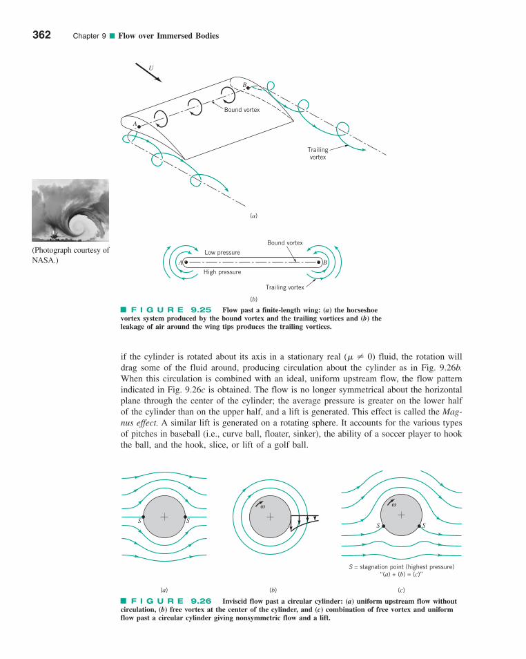
if the cylinder is rotated about its axis in a stationary real (� � 0) fluid, the rotation willdrag some of the fluid around, producing circulation about the cylinder as in Fig. 9.26b.When this circulation is combined with an ideal, uniform upstream flow, the flow patternindicated in Fig. 9.26c is obtained. The flow is no longer symmetrical about the horizontalplane through the center of the cylinder; the average pressure is greater on the lower halfof the cylinder than on the upper half, and a lift is generated. This effect is called the Mag-nus effect. A similar lift is generated on a rotating sphere. It accounts for the various typesof pitches in baseball (i.e., curve ball, floater, sinker), the ability of a soccer player to hookthe ball, and the hook, slice, or lift of a golf ball.

362 Chapter 9 ■ Flow over Immersed Bodies

U

A

B

Bound vortex

Trailingvortex

(a)

(b)

BA

Low pressure

High pressure

Bound vortex

Trailing vortex

F I G U R E 9.25 Flow past a finite-length wing: (a) the horseshoevortex system produced by the bound vortex and the trailing vortices and (b) theleakage of air around the wing tips produces the trailing vortices.

S S

ω ω

S S

S = stagnation point (highest pressure)“(a) + (b) = (c)”

(c)(b)(a)

F I G U R E 9.26 Inviscid flow past a circular cylinder: (a) uniform upstream flow withoutcirculation, (b) free vortex at the center of the cylinder, and (c) combination of free vortex and uniformflow past a circular cylinder giving nonsymmetric flow and a lift.

(Photograph courtesy ofNASA.)

c09FlowoverImmersedBodies.qxd 9/28/10 10:29 AM Page 362

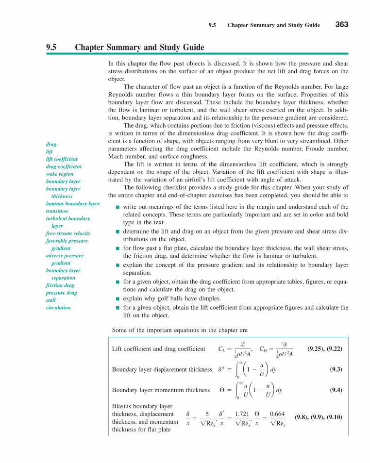
9.5 Chapter Summary and Study Guide 363

9.5 Chapter Summary and Study Guide

dragliftlift coefficientdrag coefficientwake regionboundary layerboundary layer

thicknesslaminar boundary layertransitionturbulent boundary

layerfree-stream velocityfavorable pressure

gradientadverse pressure

gradientboundary layer

separationfriction dragpressure dragstallcirculation

In this chapter the flow past objects is discussed. It is shown how the pressure and shearstress distributions on the surface of an object produce the net lift and drag forces on theobject.

The character of flow past an object is a function of the Reynolds number. For largeReynolds number flows a thin boundary layer forms on the surface. Properties of thisboundary layer flow are discussed. These include the boundary layer thickness, whetherthe flow is laminar or turbulent, and the wall shear stress exerted on the object. In addi-tion, boundary layer separation and its relationship to the pressure gradient are considered.

The drag, which contains portions due to friction (viscous) effects and pressure effects,is written in terms of the dimensionless drag coefficient. It is shown how the drag coeffi-cient is a function of shape, with objects ranging from very blunt to very streamlined. Otherparameters affecting the drag coefficient include the Reynolds number, Froude number,Mach number, and surface roughness.

The lift is written in terms of the dimensionless lift coefficient, which is stronglydependent on the shape of the object. Variation of the lift coefficient with shape is illus-trated by the variation of an airfoil’s lift coefficient with angle of attack.

The following checklist provides a study guide for this chapter. When your study ofthe entire chapter and end-of-chapter exercises has been completed, you should be able to

write out meanings of the terms listed here in the margin and understand each of therelated concepts. These terms are particularly important and are set in color and boldtype in the text.

determine the lift and drag on an object from the given pressure and shear stress dis-tributions on the object.

for flow past a flat plate, calculate the boundary layer thickness, the wall shear stress,the friction drag, and determine whether the flow is laminar or turbulent.

explain the concept of the pressure gradient and its relationship to boundary layer separation.

for a given object, obtain the drag coefficient from appropriate tables, figures, or equa-tions and calculate the drag on the object.

explain why golf balls have dimples.

for a given object, obtain the lift coefficient from appropriate figures and calculate thelift on the object.

Some of the important equations in the chapter are

Lift coefficient and drag coefficient (9.25), (9.22)

Boundary layer displacement thickness (9.3)

Boundary layer momentum thickness (9.4)

Blasius boundary layer thickness, displacement (9.8), (9.9), (9.10)thickness, and momentumthickness for flat plate

�

x�

5

1Rex

, �*

x�

1.721

1Rex

, ™x

�0.664

1Rex

™ � �q

0

u

Ua1 �

u

Ub dy

�* � �q

0

a1 �u

Ub dy

CL �l

12�U2A

, CD �d

12�U 2A

c09FlowoverImmersedBodies.qxd 9/28/10 10:29 AM Page 363

References

1. Schlichting, H., Boundary Layer Theory, Eighth Edition, McGraw-Hill, New York, 2000.2. Rosenhead, L., Laminar Boundary Layers, Oxford University Press, London, 1963.3. White, F. M., Viscous Fluid Flow, Third Edition, McGraw-Hill, New York, 2006.4. Blevins, R. D., Applied Fluid Dynamics Handbook, Van Nostrand Reinhold, New York, 1984.5. Hoerner, S. F., Fluid-Dynamic Drag, published by the author, Library of Congress No.

64, 19666, 1965.6. Van Dyke, M., An Album of Fluid Motion, Parabolic Press, Stanford, Calif., 1982.7. Thompson, P. A., Compressible-Fluid Dynamics, McGraw-Hill, New York, 1972.8. Zucrow, M. J., and Hoffman, J. D., Gas Dynamics, Vol. I, Wiley, New York, 1976.9. Shevell, R. S., Fundamentals of Flight, Second Edition, Prentice Hall, Englewood Cliffs, NJ,

1989.10. Kuethe, A. M., and Chow, C. Y., Foundations of Aerodynamics, Bases of Aerodynamics Design,

Fourth Edition, Wiley, New York, 1986.11. Vogel, J., Life in Moving Fluids, Second Edition, Princeton University Press, New Jersey, 1996.12. White, F. M., Fluid Mechanics, Fifth Edition, McGraw-Hill, New York, 2003.13. Vennard, J. K., and Street, R. L., Elementary Fluid Mechanics, Seventh Edition, Wiley, New

York, 1995.14. Gross, A. C., Kyle, C. R., and Malewicki, D. J., “The Aerodynamics of Human Powered Land

Vehicles,” Scientific American, Vol. 249, No. 6, 1983.15. Abbott, I. H., and Von Doenhoff, A. E., Theory of Wing Sections, Dover Publications, New

York, 1959.16. MacReady, P. B., “Flight on 0.33 Horsepower: The Gossamer Condor,” Proc. AIAA 14th

Annual Meeting (Paper No. 78-308), Washington, DC, 1978.17. Abbott, I. H., von Doenhoff, A. E. and Stivers, L. S., Summary of Airfoil Data, NACA Report

No. 824, Langley Field, Va., 1945.18. Anderson, J. D., Fundamentals of Aerodynamics, Fourth Edition, McGraw-Hill, New York,

2007.19. Homsy, G. M., et al., Multimedia Fluid Mechanics, CD-ROM, Second Edition, Cambridge

University Press, New York, 2008.

364 Chapter 9 ■ Flow over Immersed Bodies

Blasius wall shear stress for flat plate (9.11)

Drag on flat plate (9.18)

Blasius friction drag coefficient for flat plate (9.12)CDf �

1.328

2Ref

d � �bU 2™

�w � 0.332U3/2

B

��

x

Review Problems

Go to Appendix G for a set of review problems with answers.Detailed solutions can be found in Student Solution Manual for

a Brief Introduction to Fluid Michanics, by Young et al. (© 2011John Wiley and Sons, Inc.)

Problems

Note: Unless otherwise indicated use the values of fluidproperties found in the tables on the inside of the frontcover. Problems designated with an (*) are intended to be

solved with the aid of a programmable calculator or a com-puter. Problems designated with a (†) are “open-ended”problems and require critical thinking in that to work them

c09FlowoverImmersedBodies.qxd 10/18/10 8:06 AM Page 364

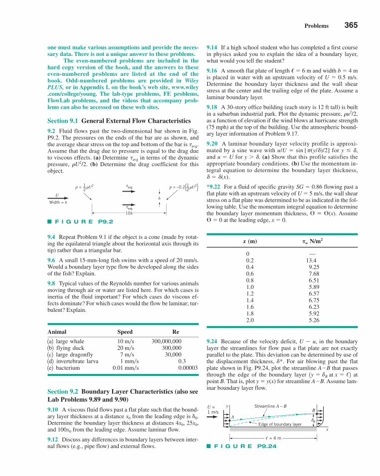
Problems 365

one must make various assumptions and provide the neces-sary data. There is not a unique answer to these problems.

The even-numbered problems are included in thehard copy version of the book, and the answers to theseeven-numbered problems are listed at the end of thebook. Odd-numbered problems are provided in WileyPLUS, or in Appendix L on the book’s web site, www.wiley.com/college/young. The lab-type problems, FE problems,FlowLab problems, and the videos that accompany prob-lems can also be accessed on these web sites.

Section 9.1 General External Flow Characteristics

9.2 Fluid flows past the two-dimensional bar shown in Fig.P9.2. The pressures on the ends of the bar are as shown, andthe average shear stress on the top and bottom of the bar is �avg.Assume that the drag due to pressure is equal to the drag dueto viscous effects. (a) Determine �avg in terms of the dynamicpressure, �U2/2. (b) Determine the drag coefficient for thisobject.

9.4 Repeat Problem 9.1 if the object is a cone (made by rotat-ing the equilateral triangle about the horizontal axis through itstip) rather than a triangular bar.

9.6 A small 15-mm-long fish swims with a speed of 20 mm/s.Would a boundary layer type flow be developed along the sidesof the fish? Explain.

9.8 Typical values of the Reynolds number for various animalsmoving through air or water are listed here. For which cases isinertia of the fluid important? For which cases do viscous ef-fects dominate? For which cases would the flow be laminar; tur-bulent? Explain.

Animal Speed Re

1a2 large whale 300,000,0001b2 flying duck 300,0001c2 large dragonfly 30,0001d2 invertebrate larva 0.31e2 bacterium 0.00003

Section 9.2 Boundary Layer Characteristics (also seeLab Problems 9.89 and 9.90)

9.10 A viscous fluid flows past a flat plate such that the bound-ary layer thickness at a distance from the leading edge is �0.Determine the boundary layer thickness at distances 4x0, 25x0,and 100x0 from the leading edge. Assume laminar flow.

9.12 Discuss any differences in boundary layers between inter-nal flows (e.g., pipe flow) and external flows.

x0

0.01 mm�s 1 mm�s 7 m�s

20 m�s 10 m�s

9.14 If a high school student who has completed a first coursein physics asked you to explain the idea of a boundary layer,what would you tell the student?

9.16 A smooth flat plate of length � � 6 m and width b � 4 mis placed in water with an upstream velocity of U � 0.5 m/s.Determine the boundary layer thickness and the wall shearstress at the center and the trailing edge of the plate. Assume alaminar boundary layer.

9.18 A 30-story office building (each story is 12 ft tall) is builtin a suburban industrial park. Plot the dynamic pressure, �u2/2,as a function of elevation if the wind blows at hurricane strength(75 mph) at the top of the building. Use the atmospheric bound-ary layer information of Problem 9.17.

9.20 A laminar boundary layer velocity profile is approxi-mated by a sine wave with u/U � sin [�(y/�)/2] for y � �,and u � U for y � �. (a) Show that this profile satisfies theappropriate boundary conditions. (b) Use the momentum in-tegral equation to determine the boundary layer thickness,� � �(x).

*9.22 For a fluid of specific gravity SG � 0.86 flowing past aflat plate with an upstream velocity of U � 5 m/s, the wall shearstress on a flat plate was determined to be as indicated in the fol-lowing table. Use the momentum integral equation to determinethe boundary layer momentum thickness, � � �(x). Assume� � 0 at the leading edge, x � 0.

x (m) �w N/m2

0 —0.2 13.40.4 9.250.6 7.680.8 6.511.0 5.891.2 6.571.4 6.751.6 6.231.8 5.922.0 5.26

9.24 Because of the velocity deficit, U � u, in the boundarylayer the streamlines for flow past a flat plate are not exactlyparallel to the plate. This deviation can be determined by use ofthe displacement thickness, �*. For air blowing past the flatplate shown in Fig. P9.24, plot the streamline A�B that passesthrough the edge of the boundary layer atpoint B. That is, plot y � y(x) for streamline A�B. Assume lam-inar boundary layer flow.

1y � �B at x � /2

F I G U R E P9.2

U

τavg

τavg

10h

Width = bh

p = �U212

p = –0.2 �U212

F I G U R E P9.24

yU =1 m/s

x

� = 4 m

Edge of boundary layer

Streamline A – B

δB

BA

c09FlowoverImmersedBodies.qxd 9/28/10 10:30 AM Page 365

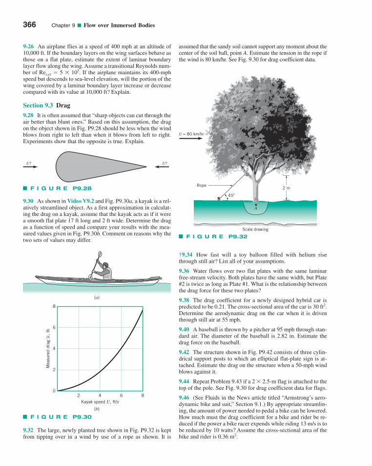
9-26 An airplane flies at a speed of 400 mph at an altitude of10,000 ft. If the boundary layers on the wing surfaces behave asthose on a flat plate, estimate the extent of laminar boundarylayer flow along the wing. Assume a transitional Reynolds num-ber of Rex,cr � 5 � 105. If the airplane maintains its 400-mphspeed but descends to sea-level elevation, will the portion of thewing covered by a laminar boundary layer increase or decreasecompared with its value at 10,000 ft? Explain.

Section 9.3 Drag

9.28 It is often assumed that “sharp objects can cut through theair better than blunt ones.” Based on this assumption, the dragon the object shown in Fig. P9.28 should be less when the windblows from right to left than when it blows from left to right.Experiments show that the opposite is true. Explain.

9.30 As shown in Video V9.2 and Fig. P9.30a, a kayak is a rel-atively streamlined object. As a first approximation in calculat-ing the drag on a kayak, assume that the kayak acts as if it werea smooth flat plate 17 ft long and 2 ft wide. Determine the dragas a function of speed and compare your results with the mea-sured values given in Fig. P9.30b. Comment on reasons why thetwo sets of values may differ.

assumed that the sandy soil cannot support any moment about thecenter of the soil ball, point A. Estimate the tension in the rope ifthe wind is 80 km/hr. See Fig. 9.30 for drag coefficient data.

†9.34 How fast will a toy balloon filled with helium risethrough still air? List all of your assumptions.

9.36 Water flows over two flat plates with the same laminarfree-stream velocity. Both plates have the same width, but Plate#2 is twice as long as Plate #1. What is the relationship betweenthe drag force for these two plates?

9.38 The drag coefficient for a newly designed hybrid car ispredicted to be 0.21. The cross-sectional area of the car is 30 ft2.Determine the aerodynamic drag on the car when it is driventhrough still air at 55 mph.

9.40 A baseball is thrown by a pitcher at 95 mph through stan-dard air. The diameter of the baseball is 2.82 in. Estimate thedrag force on the baseball.

9.42 The structure shown in Fig. P9.42 consists of three cylin-drical support posts to which an elliptical flat-plate sign is at-tached. Estimate the drag on the structure when a 50-mph windblows against it.

9.44 Repeat Problem 9.43 if a 2 � 2.5-m flag is attached to thetop of the pole. See Fig. 9.30 for drag coefficient data for flags.

9.46 (See Fluids in the News article titled “Armstrong’s aero-dynamic bike and suit,” Section 9.1.) By appropriate streamlin-ing, the amount of power needed to pedal a bike can be lowered.How much must the drag coefficient for a bike and rider be re-duced if the power a bike racer expends while riding 13 m/s is tobe reduced by 10 watts? Assume the cross-sectional area of thebike and rider is 0.36 m2.

366 Chapter 9 ■ Flow over Immersed Bodies

F I G U R E P9.28

U? U?

F I G U R E P9.30

8

6

4

2

02 4

Kayak speed U, ft/s6 8

Mea

sure

d dr

ag �

, lb

(b)

(a)

F I G U R E P9.32

2 mRope

Scale drawing

45�

U = 80 km/hr

A

9.32 The large, newly planted tree shown in Fig. P9.32 is keptfrom tipping over in a wind by use of a rope as shown. It is

c09FlowoverImmersedBodies.qxd 9/28/10 10:30 AM Page 366

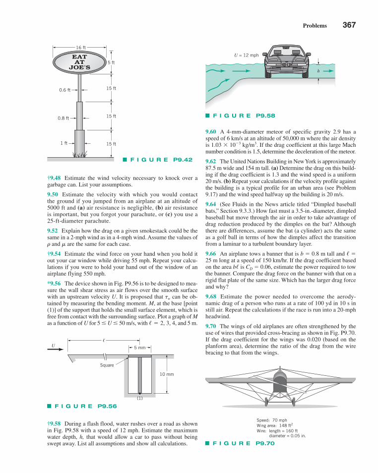
Problems 367

†9.48 Estimate the wind velocity necessary to knock over agarbage can. List your assumptions.

9.50 Estimate the velocity with which you would contactthe ground if you jumped from an airplane at an altitude of5000 ft and (a) air resistance is negligible, (b) air resistanceis important, but you forgot your parachute, or (c) you use a25-ft-diameter parachute.

9.52 Explain how the drag on a given smokestack could be thesame in a 2-mph wind as in a 4-mph wind. Assume the values of� and � are the same for each case.

†9.54 Estimate the wind force on your hand when you hold itout your car window while driving 55 mph. Repeat your calcu-lations if you were to hold your hand out of the window of anairplane flying 550 mph.

*9.56 The device shown in Fig. P9.56 is to be designed to mea-sure the wall shear stress as air flows over the smooth surfacewith an upstream velocity U. It is proposed that �w can be ob-tained by measuring the bending moment. M, at the base [point(1)] of the support that holds the small surface element, which isfree from contact with the surrounding surface. Plot a graph of Mas a function of U for 5 � U � 50 m/s, with and 5 m./ � 2, 3, 4,

†9.58 During a flash flood, water rushes over a road as shownin Fig. P9.58 with a speed of 12 mph. Estimate the maximumwater depth, h, that would allow a car to pass without beingswept away. List all assumptions and show all calculations.

9.60 A 4-mm-diameter meteor of specific gravity 2.9 has aspeed of 6 km/s at an altitude of 50,000 m where the air densityis 1.03 � 10�3 kg/m3. If the drag coefficient at this large Machnumber condition is 1.5, determine the deceleration of the meteor.

9.62 The United Nations Building in New York is approximately87.5 m wide and 154 m tall. (a) Determine the drag on this build-ing if the drag coefficient is 1.3 and the wind speed is a uniform20 m/s. (b) Repeat your calculations if the velocity profile againstthe building is a typical profile for an urban area (see Problem9.17) and the wind speed halfway up the building is 20 m/s.

9.64 (See Fluids in the News article titled “Dimpled baseballbats,” Section 9.3.3.) How fast must a 3.5-in.-diameter, dimpledbaseball bat move through the air in order to take advantage ofdrag reduction produced by the dimples on the bat? Althoughthere are differences, assume the bat (a cylinder) acts the sameas a golf ball in terms of how the dimples affect the transitionfrom a laminar to a turbulent boundary layer.

9.66 An airplane tows a banner that is b � 0.8 m tall and / �25 m long at a speed of 150 km/hr. If the drag coefficient basedon the area is CD � 0.06, estimate the power required to towthe banner. Compare the drag force on the banner with that on arigid flat plate of the same size. Which has the larger drag forceand why?

9.68 Estimate the power needed to overcome the aerody-namic drag of a person who runs at a rate of 100 yd in 10 s instill air. Repeat the calculations if the race is run into a 20-mphheadwind.

9.70 The wings of old airplanes are often strengthened by theuse of wires that provided cross-bracing as shown in Fig. P9.70.If the drag coefficient for the wings was 0.020 (based on theplanform area), determine the ratio of the drag from the wirebracing to that from the wings.

b/

16 ft

0.6 ft

0.8 ft

1 ft 15 ft

15 ft

15 ft

5 ft

F I G U R E P9.42

U�

(1)

Square

10 mm

5 mm

F I G U R E P9.56

h

U = 12 mph

F I G U R E P9.58

Speed: 70 mphWing area: 148 ft2

Wire: length = 160 ft diameter = 0.05 in.

F I G U R E P9.70

c09FlowoverImmersedBodies.qxd 9/28/10 10:30 AM Page 367

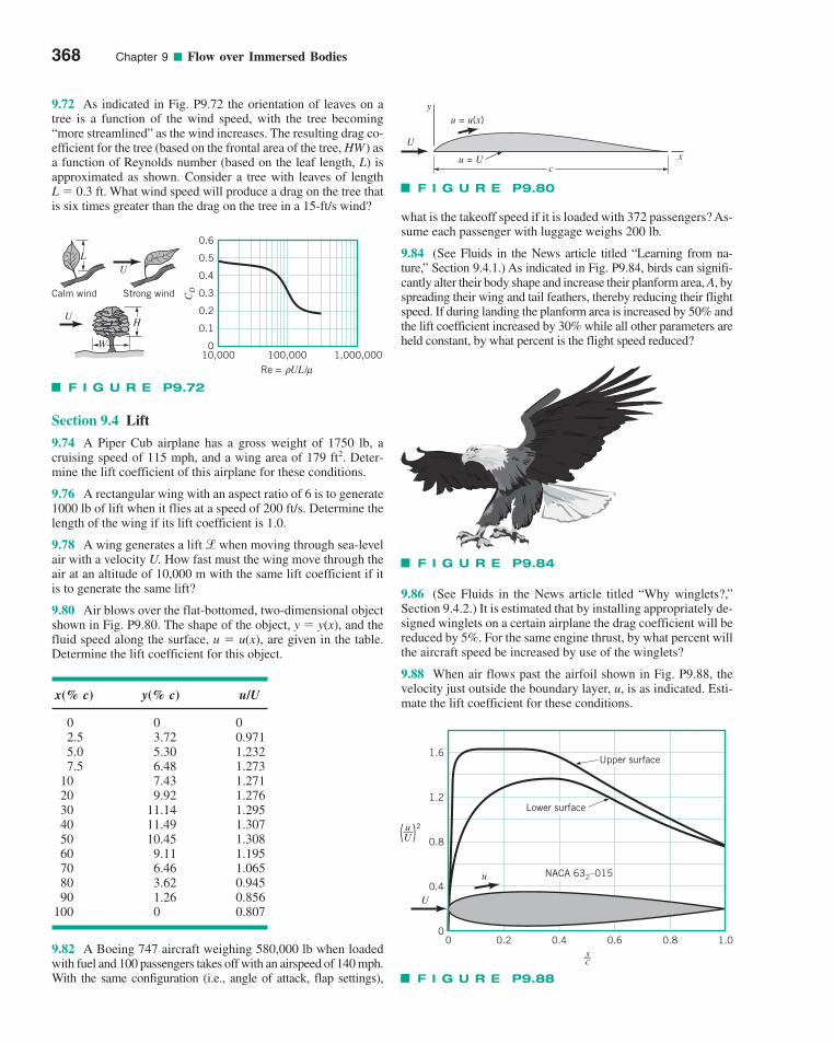
9.72 As indicated in Fig. P9.72 the orientation of leaves on atree is a function of the wind speed, with the tree becoming“more streamlined” as the wind increases. The resulting drag co-efficient for the tree (based on the frontal area of the tree, HW) asa function of Reynolds number (based on the leaf length, L) isapproximated as shown. Consider a tree with leaves of lengthL � 0.3 ft. What wind speed will produce a drag on the tree thatis six times greater than the drag on the tree in a 15-ft/s wind?

what is the takeoff speed if it is loaded with 372 passengers? As-sume each passenger with luggage weighs 200 lb.

9.84 (See Fluids in the News article titled “Learning from na-ture,” Section 9.4.1.) As indicated in Fig. P9.84, birds can signifi-cantly alter their body shape and increase their planform area, A, byspreading their wing and tail feathers, thereby reducing their flightspeed. If during landing the planform area is increased by 50% andthe lift coefficient increased by 30% while all other parameters areheld constant, by what percent is the flight speed reduced?

368 Chapter 9 ■ Flow over Immersed Bodies

U

y

x

c

u = u(x)

u = U

F I G U R E P9.80

F I G U R E P9.84

U

1.6

1.2

0.8

0.4

0

2uU

0 0.2 0.4 0.8 1.00.6xc

u

Upper surface

Lower surface

NACA 632–015

F I G U R E P9.88

Calm wind Strong wind

1,000,000100,000Re = UL/

10,000

0.6

0.5

0.4

0.3

0.2

0.1

0

ρ μ

CD

L

H

W

U

U

F I G U R E P9.72

Section 9.4 Lift

9.74 A Piper Cub airplane has a gross weight of 1750 lb, acruising speed of 115 mph, and a wing area of 179 ft2. Deter-mine the lift coefficient of this airplane for these conditions.

9.76 A rectangular wing with an aspect ratio of 6 is to generate1000 lb of lift when it flies at a speed of 200 ft/s. Determine thelength of the wing if its lift coefficient is 1.0.

9.78 A wing generates a lift l when moving through sea-levelair with a velocity U. How fast must the wing move through theair at an altitude of 10,000 m with the same lift coefficient if itis to generate the same lift?

9.80 Air blows over the flat-bottomed, two-dimensional objectshown in Fig. P9.80. The shape of the object, y � y(x), and thefluid speed along the surface, u � u(x), are given in the table.Determine the lift coefficient for this object.

x(% c) y(% c) u/U

0 0 02.5 3.72 0.9715.0 5.30 1.2327.5 6.48 1.273

10 7.43 1.27120 9.92 1.27630 11.14 1.29540 11.49 1.30750 10.45 1.30860 9.11 1.19570 6.46 1.06580 3.62 0.94590 1.26 0.856

100 0 0.807

9.82 A Boeing 747 aircraft weighing 580,000 lb when loadedwith fuel and 100 passengers takes off with an airspeed of 140 mph.With the same configuration (i.e., angle of attack, flap settings),

9.86 (See Fluids in the News article titled “Why winglets?,”Section 9.4.2.) It is estimated that by installing appropriately de-signed winglets on a certain airplane the drag coefficient will bereduced by 5%. For the same engine thrust, by what percent willthe aircraft speed be increased by use of the winglets?

9.88 When air flows past the airfoil shown in Fig. P9.88, thevelocity just outside the boundary layer, u, is as indicated. Esti-mate the lift coefficient for these conditions.

c09FlowoverImmersedBodies.qxd 9/28/10 10:30 AM Page 368

Problems 369

■ Lab Problems

9.90 This problem involves measuring the pressure distributionon a circular cylinder. To proceed with this problem, go to thebook’s web site, www.wiley.com/college/young, or WileyPLUS.

■ Lifelong Learning Problems

9.92 For typical aircraft flying at cruise conditions it is advanta-geous to have as much laminar flow over the wing as possible be-cause there is an increase in friction drag once the flow becomesturbulent. Various techniques have been developed to help promotelaminar flow over the wing, both in airfoil geometry configurationsas well as active flow control mechanisms. Obtain information onone of these techniques. Summarize your findings in a brief report.

■ FlowLab Problems

*9.94 This FlowLab problem involves simulation of flow past anairfoil and investigation of the surface pressure distribution as afunction of angle of attack. To proceed with this problem, go to thebook’s web site, www.wiley.com/college/young, or WileyPLUS.

*9.96 This FlowLab problem involves simulating the effects ofaltitude on the lift and drag of an airfoil. To proceed with thisproblem, go to the book’s web site, www.wiley.com/college/young, or WileyPLUS.

*9.98 This FlowLab problem involves simulating the pressuredistribution for flow past a cylinder and investigating the differ-ences between inviscid and viscous flows. To proceed with thisproblem, go to the book’s web site, www.wiley.com/college/young, or WileyPLUS.

*9.100 This FlowLab problem involves simulating the unsteadyflow past a cylinder. To proceed with this problem, go to thebook’s web site, www.wiley.com/college/young, or WileyPLUS.

■ FE Exam Problems

Sample FE (Fundamentals of Engineering) exam questions forfluid mechanics are provided on the book’s web site, www.wiley.com/college/young, or WileyPlus.

c09FlowoverImmersedBodies.qxd 9/28/10 10:30 AM Page 369

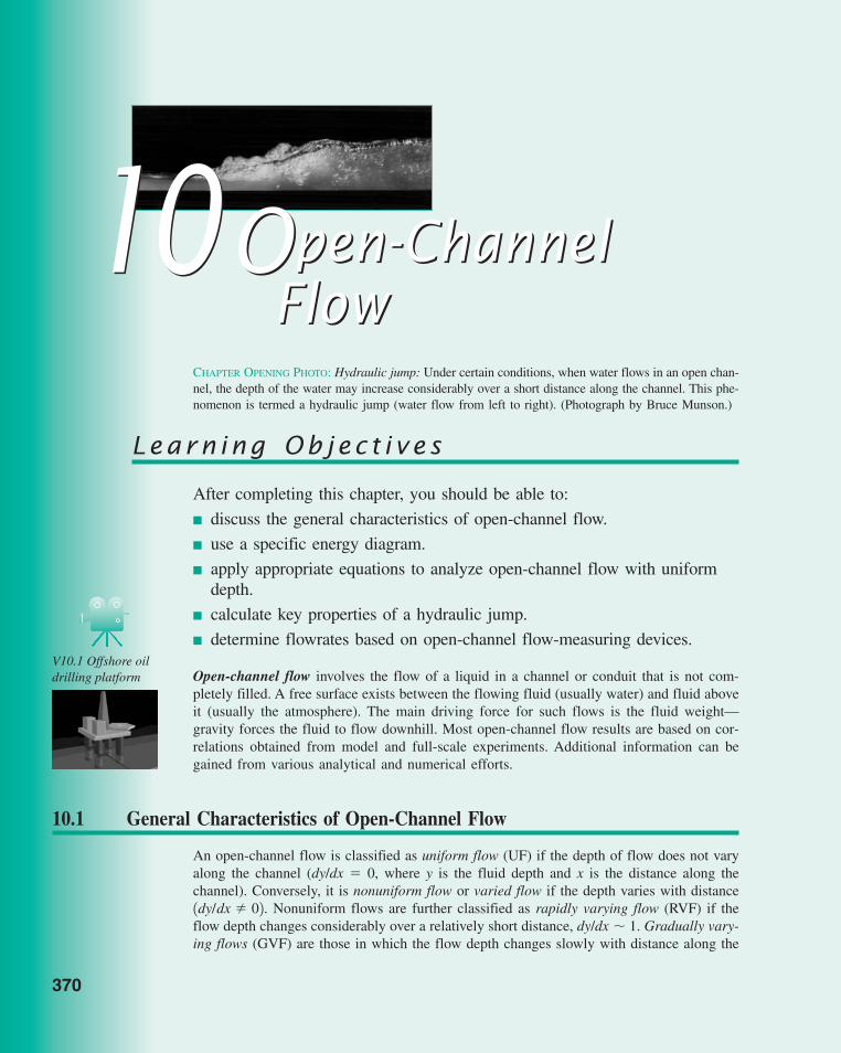
370

Learn ing Ob j ec t i v e s

After completing this chapter, you should be able to:

■ discuss the general characteristics of open-channel flow.

■ use a specific energy diagram.

■ apply appropriate equations to analyze open-channel flow with uniformdepth.

■ calculate key properties of a hydraulic jump.

■ determine flowrates based on open-channel flow-measuring devices.

Open-channel flow involves the flow of a liquid in a channel or conduit that is not com-pletely filled. A free surface exists between the flowing fluid (usually water) and fluid aboveit (usually the atmosphere). The main driving force for such flows is the fluid weight—gravity forces the fluid to flow downhill. Most open-channel flow results are based on cor-relations obtained from model and full-scale experiments. Additional information can begained from various analytical and numerical efforts.

1010Open-ChannelFlow

Open-ChannelFlow

CHAPTER OPENING PHOTO: Hydraulic jump: Under certain conditions, when water flows in an open chan-nel, the depth of the water may increase considerably over a short distance along the channel. This phe-nomenon is termed a hydraulic jump (water flow from left to right). (Photograph by Bruce Munson.)

10.1 General Characteristics of Open-Channel Flow

An open-channel flow is classified as uniform flow (UF) if the depth of flow does not varyalong the channel (dy/dx � 0, where y is the fluid depth and x is the distance along thechannel). Conversely, it is nonuniform flow or varied flow if the depth varies with distance

. Nonuniform flows are further classified as rapidly varying flow (RVF) if theflow depth changes considerably over a relatively short distance, dy/dx � 1. Gradually vary-ing flows (GVF) are those in which the flow depth changes slowly with distance along the

1dy/dx � 02

V10.1 Offshore oildrilling platform

c10OpenChannelFlow.qxd 9/28/10 10:33 AM Page 370

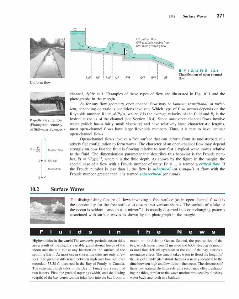
10.2 Surface Waves 371

channel, dy/dx � 1. Examples of these types of flow are illustrated in Fig. 10.1 and thephotographs in the margin.

As for any flow geometry, open-channel flow may be laminar, transitional, or turbu-lent, depending on various conditions involved. Which type of flow occurs depends on theReynolds number, Re � �VRh/�, where V is the average velocity of the fluid and Rh is thehydraulic radius of the channel (see Section 10.4). Since most open-channel flows involvewater (which has a fairly small viscosity) and have relatively large characteristic lengths,most open-channel flows have large Reynolds numbers. Thus, it is rare to have laminaropen-channel flows.

Open-channel flows involve a free surface that can deform from its undisturbed, rel-atively flat configuration to form waves. The character of an open-channel flow may dependstrongly on how fast the fluid is flowing relative to how fast a typical wave moves relativeto the fluid. The dimensionless parameter that describes this behavior is the Froude num-ber, Fr � V/(gy)1/2, where y is the fluid depth. As shown by the figure in the margin, thespecial case of a flow with a Froude number of unity, Fr � 1, is termed a critical flow. Ifthe Froude number is less than 1, the flow is subcritical (or tranquil). A flow with theFroude number greater than 1 is termed supercritical (or rapid).

Uniform flow

Rapidly varying flow(Photograph courtesyof Stillwater Sciences.)

10.2 Surface Waves

The distinguishing feature of flows involving a free surface (as in open-channel flows) isthe opportunity for the free surface to distort into various shapes. The surface of a lake orthe ocean is seldom “smooth as a mirror.” It is usually distorted into ever-changing patternsassociated with surface waves as shown by the photograph in the margin.

UF uniform flowGVF gradually varying flowRVF rapidly varying flow

RVF UF RVF UF RVF GVF RVF UF

y

F I G U R E 10.1Classification of open-channelflow.

Fr =√gy

V

0

1 Critical

Supercritical

Subcritical

F l u i d s i n t h e N e w s

Highest tides in the world The unsteady, periodic ocean tidesare a result of the slightly variable gravitational forces of themoon and the sun felt at any location on the surface of thespinning Earth. At most ocean shores the tides are only a fewfeet. The greatest difference between high and low tide everrecorded, 53.38 ft, occurred in the Bay of Fundy, in Canada.The extremely high tides in the Bay of Fundy are a result oftwo factors. First, the gradual tapering (width) and shallowing(depth) of the bay constricts the tidal flow into the bay from its

mouth on the Atlantic Ocean. Second, the precise size of thebay, which tapers from 62 mi wide and 600 ft deep at its mouthto mud flats 180 mi upstream at the end of the bay, causes aresonance effect. The time it takes water to flood the length ofthe Bay of Fundy (its natural rhythm) is nearly identical to thetime between high and low tides in the ocean. The closeness ofthese two natural rhythms sets up a resonance effect, enhanc-ing the tides, similar to the wave motion produced by sloshingwater back and forth in a bathtub.

c10OpenChannelFlow.qxd 9/28/10 10:33 AM Page 371

372 Chapter 10 ■ Open-Channel Flow

10.2.1 Wave Speed

Consider the situation illustrated in Fig. 10.2a in which a single elementary wave of smallheight, �y, is produced on the surface of a channel by suddenly moving the initially station-ary end wall with speed �V. The water in the channel was stationary at the initial time, t � 0.A stationary observer will observe a single wave move down the channel with a wave speedc, with no fluid motion ahead of the wave and a fluid velocity of �V behind the wave. Themotion is unsteady for such an observer. For an observer moving along the channel withspeed c, the flow will appear steady as shown in Fig. 10.2b. To this observer, the fluid veloc-ity will be V � �c i on the observer’s right and V � (�c � �V)i to the left of the observer.

The relationship between the various parameters involved for this flow can be obtainedby application of the continuity and momentum equations to the control volume shown inFig. 10.2b as follows. With the assumption of uniform one-dimensional flow, the continu-ity equation (Eq. 5.10) becomes

where b is the channel width. This simplifies to

or in the limit of small-amplitude waves with �y � y

(10.1)

Similarly, the momentum equation (Eq. 5.17) is

where we have written the mass flowrate as m � �bcy and have assumed that the pressurevariation is hydrostatic within the fluid. That is, the pressure forces on the channel acrosssections (1) and (2) are F1 � �yc1A1 � �(y � �y)2b/2 and F2 � �yc2A2 � �y2b/2, respectively.

12 �y2b � 1

2 � 1y � �y22b � �bcy 3 1c � �V2 � c 4

c � y �V

�y

c �1y � �y2 �V

�y

�cyb � 1�c � �V2 1y � �y2b

Controlsurface Stationary wave

V = (– c + V)iδy + yδ yV = – ci

x

x

Channel width = b

(1) (2)(b)

(a)

Movingend wall

Vδ yδ

Vδ

c = wave speed

yStationary

fluid

^

^

F I G U R E 10.2 (a) Production of a single elementary wave ina channel as seen by a stationary observer. (b) Wave as seen by an observermoving with a speed equal to the wave speed.

V10.2 Filling yourcar’s gas tank

CFX

V10.3 Water strider

c10OpenChannelFlow.qxd 9/28/10 10:33 AM Page 372

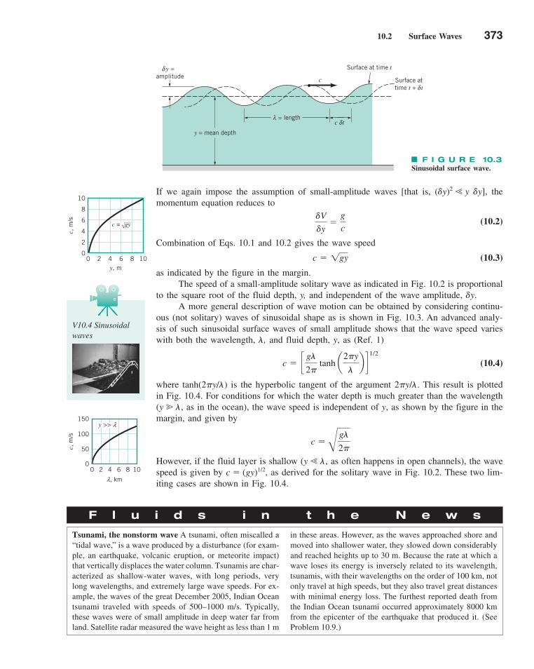
10.2 Surface Waves 373

If we again impose the assumption of small-amplitude waves [that is, (�y)2 � y �y], themomentum equation reduces to

(10.2)

Combination of Eqs. 10.1 and 10.2 gives the wave speed

(10.3)

as indicated by the figure in the margin.The speed of a small-amplitude solitary wave as indicated in Fig. 10.2 is proportional

to the square root of the fluid depth, y, and independent of the wave amplitude, �y.A more general description of wave motion can be obtained by considering continu-

ous (not solitary) waves of sinusoidal shape as is shown in Fig. 10.3. An advanced analy-sis of such sinusoidal surface waves of small amplitude shows that the wave speed varieswith both the wavelength, �, and fluid depth, y, as (Ref. 1)

(10.4)

where tanh(2�y/�) is the hyperbolic tangent of the argument 2�y/�. This result is plottedin Fig. 10.4. For conditions for which the water depth is much greater than the wavelength(y � �, as in the ocean), the wave speed is independent of y, as shown by the figure in themargin, and given by

However, if the fluid layer is shallow (y � �, as often happens in open channels), the wavespeed is given by c � (gy)1/2, as derived for the solitary wave in Fig. 10.2. These two lim-iting cases are shown in Fig. 10.4.

c �B

g�

2�

c � cg�

2� tanh a

2�y

�b d

1/2

c � 1gy

�V

�y�

g

c

10

8

6

4

2

00 2 4 6 8 10

c, m

/s

y, m

√c = gy

F I G U R E 10.3Sinusoidal surface wave.

c

y = mean depth

= lengthλc tδ

Surface at time t

Surface attime t + tδ

y =amplitude

δ

F l u i d s i n t h e N e w s

Tsunami, the nonstorm wave A tsunami, often miscalled a“tidal wave,” is a wave produced by a disturbance (for exam-ple, an earthquake, volcanic eruption, or meteorite impact)that vertically displaces the water column. Tsunamis are char-acterized as shallow-water waves, with long periods, verylong wavelengths, and extremely large wave speeds. For ex-ample, the waves of the great December 2005, Indian Oceantsunami traveled with speeds of 500–1000 m/s. Typically,these waves were of small amplitude in deep water far fromland. Satellite radar measured the wave height as less than 1 m

in these areas. However, as the waves approached shore andmoved into shallower water, they slowed down considerablyand reached heights up to 30 m. Because the rate at which awave loses its energy is inversely related to its wavelength,tsunamis, with their wavelengths on the order of 100 km, notonly travel at high speeds, but they also travel great distanceswith minimal energy loss. The furthest reported death fromthe Indian Ocean tsunami occurred approximately 8000 kmfrom the epicenter of the earthquake that produced it. (SeeProblem 10.9.)

V10.4 Sinusoidalwaves

150

50

100

00 2 4 6 8 10

c, m

/s

l, km

y >> l

c10OpenChannelFlow.qxd 9/28/10 10:33 AM Page 373

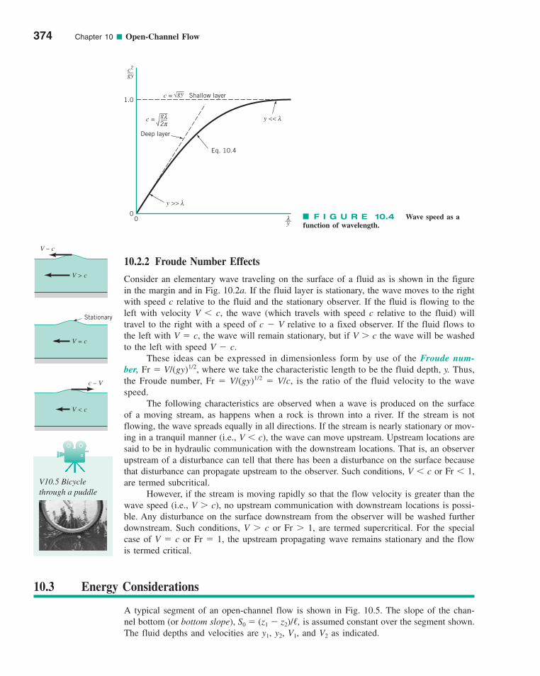
10.2.2 Froude Number Effects

Consider an elementary wave traveling on the surface of a fluid as is shown in the figurein the margin and in Fig. 10.2a. If the fluid layer is stationary, the wave moves to the rightwith speed c relative to the fluid and the stationary observer. If the fluid is flowing to theleft with velocity V � c, the wave (which travels with speed c relative to the fluid) willtravel to the right with a speed of c � V relative to a fixed observer. If the fluid flows tothe left with V � c, the wave will remain stationary, but if V c the wave will be washedto the left with speed V � c.

These ideas can be expressed in dimensionless form by use of the Froude num-ber, Fr � V/(gy)1/2, where we take the characteristic length to be the fluid depth, y. Thus,the Froude number, Fr � V/(gy)1/2 � V/c, is the ratio of the fluid velocity to the wavespeed.

The following characteristics are observed when a wave is produced on the surfaceof a moving stream, as happens when a rock is thrown into a river. If the stream is notflowing, the wave spreads equally in all directions. If the stream is nearly stationary or mov-ing in a tranquil manner (i.e., V � c), the wave can move upstream. Upstream locations aresaid to be in hydraulic communication with the downstream locations. That is, an observerupstream of a disturbance can tell that there has been a disturbance on the surface becausethat disturbance can propagate upstream to the observer. Such conditions, V � c or Fr � 1,are termed subcritical.

However, if the stream is moving rapidly so that the flow velocity is greater than thewave speed (i.e., V c), no upstream communication with downstream locations is possi-ble. Any disturbance on the surface downstream from the observer will be washed furtherdownstream. Such conditions, V c or Fr 1, are termed supercritical. For the specialcase of V � c or Fr � 1, the upstream propagating wave remains stationary and the flowis termed critical.

374 Chapter 10 ■ Open-Channel Flow

F I G U R E 10.4 Wave speed as afunction of wavelength.

c2__

gy

1.0

00 __

yλ

y >> λ

y << λ

Eq. 10.4

c = g __2

λπ√

Deep layer

c = gy √ Shallow layer

V > c

Stationary

V = c

V < c

c – V

V – c

V10.5 Bicyclethrough a puddle

10.3 Energy Considerations

A typical segment of an open-channel flow is shown in Fig. 10.5. The slope of the chan-nel bottom (or bottom slope), S0 � (z1 � z2)/�, is assumed constant over the segment shown.The fluid depths and velocities are y1, y2, V1, and V2 as indicated.

c10OpenChannelFlow.qxd 9/28/10 10:33 AM Page 374

10.3 Energy Considerations 375

With the assumption of a uniform velocity profile across any section of the channel,the one-dimensional energy equation for this flow (Eq. 5.57) becomes

(10.5)

where hL is the head loss due to viscous effects between sections (1) and (2) and z1 � z2 � S0�.Since the pressure is essentially hydrostatic at any cross section, we find that p1/� � y1 andp2/� � y2 so that Eq. 10.5 becomes

(10.6)

We write the head loss in terms of the slope of the energy line, Sf � hL/� (often termed thefriction slope), as indicated in Fig. 10.5. Recall from Chapter 3 that the energy line is locateda distance z (the elevation from some datum to the channel bottom) plus the pressure head(p/�) plus the velocity head (V 2/2g) above the datum.

10.3.1 Specific Energy

The concept of the specific energy, E, defined as

(10.7)

is often useful in open-channel flow considerations. The energy equation, Eq. 10.6, can bewritten in terms of E as

(10.8)

If we consider a simple channel whose cross-sectional shape is a rectangle of widthb, the specific energy can be written in terms of the flowrate per unit width, q � Q/b �Vyb/b � Vy, as

(10.9)

which is illustrated by the figure in the margin.

E � y �q2

2gy2

E1 � E2 � 1Sf � S02/

E � y �V2

2g

y1 �V2

1

2g� S0/ � y2 �

V22

2g� hL

p1

��

V21

2g� z1 �

p2

��

V22

2g� z2 � hL

E

y

q = constant

F I G U R E 10.5 Typical open-channel geometry.

1 Sf

Energy lineV12

___2g

y1 V1

(1)1

S0

z1

z2

V2

y2

V22

___2g

hL

Slope = Sf

Slope = S0

Horizontal datumx

(2)

�

c10OpenChannelFlow.qxd 9/28/10 10:33 AM Page 375

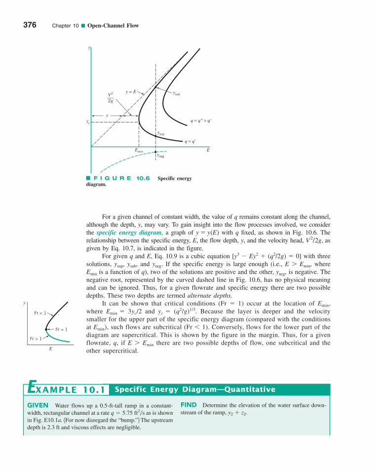
For a given channel of constant width, the value of q remains constant along the channel,although the depth, y, may vary. To gain insight into the flow processes involved, we considerthe specific energy diagram, a graph of y � y(E) with q fixed, as shown in Fig. 10.6. Therelationship between the specific energy, E, the flow depth, y, and the velocity head, asgiven by Eq. 10.7, is indicated in the figure.

For given q and E, Eq. 10.9 is a cubic equation [y3 � Ey2 � (q2/2g) � 0] with threesolutions, ysup, ysub, and yneg. If the specific energy is large enough (i.e., E Emin, whereEmin is a function of q), two of the solutions are positive and the other, yneg, is negative. Thenegative root, represented by the curved dashed line in Fig. 10.6, has no physical meaningand can be ignored. Thus, for a given flowrate and specific energy there are two possibledepths. These two depths are termed alternate depths.

It can be shown that critical conditions (Fr � 1) occur at the location of Emin,where Emin � 3yc/2 and yc � (q2/g)1/3. Because the layer is deeper and the velocitysmaller for the upper part of the specific energy diagram (compared with the conditionsat Emin), such flows are subcritical (Fr � 1). Conversely, flows for the lower part of thediagram are supercritical. This is shown by the figure in the margin. Thus, for a givenflowrate, q, if E Emin there are two possible depths of flow, one subcritical and theother supercritical.

V 2/2g,

376 Chapter 10 ■ Open-Channel Flow

F I G U R E 10.6 Specific energy diagram.

y = E ysub

ysup

yneg

yc

Emin E

q = q'

q = q" > q'

y

y

V2

___2g

GIVEN Water flows up a 0.5-ft-tall ramp in a constant-width, rectangular channel at a rate as is shownin Fig. E10.1a. 1For now disregard the “bump.”2 The upstreamdepth is 2.3 ft and viscous effects are negligible.

q � 5.75 ft2sFIND Determine the elevation of the water surface down-stream of the ramp, y2 � z2.

Specific Energy Diagram—QuantitativeEXAMPLE 10.1

E

Fr = 1

Fr < 1

Fr > 1

y

c10OpenChannelFlow.qxd 9/28/10 10:33 AM Page 376

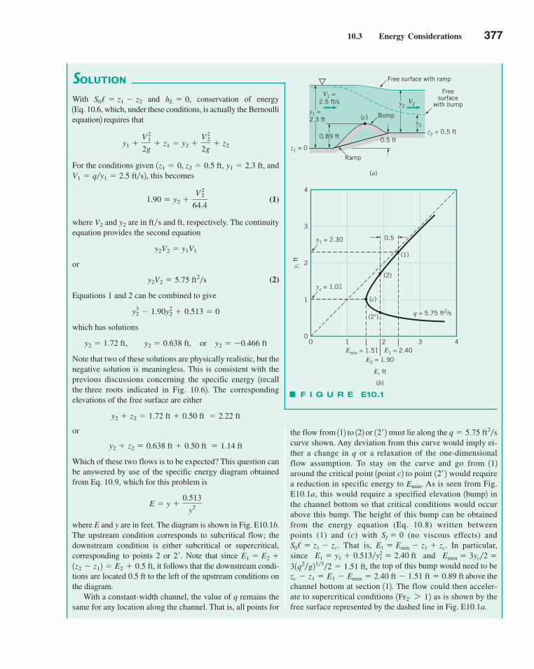
10.3 Energy Considerations 377

SOLUTION

the flow from 112 to 122 or must lie along the curve shown. Any deviation from this curve would imply ei-ther a change in q or a relaxation of the one-dimensionalflow assumption. To stay on the curve and go from 112around the critical point 1point c2 to point would requirea reduction in specific energy to As is seen from Fig.E10.1a, this would require a specified elevation 1bump2 inthe channel bottom so that critical conditions would occurabove this bump. The height of this bump can be obtainedfrom the energy equation (Eq. 10.8) written betweenpoints (1) and (c) with Sf � 0 (no viscous effects) and

That is, In particular,since and

the top of this bump would need to beabove the

channel bottom at section 112. The flow could then acceler-ate to supercritical conditions as is shown by thefree surface represented by the dashed line in Fig. E10.1a.

1Fr2¿ 7 12

ft � 1.51 ft � 0.89 ftzc � z1 � E1 � Emin � 2.4031q2g2132 � 1.51 ft,

Emin � 3yc2 �0.513y12 � 2.40 ftE1 � y1 �

E1 � Emin � z1 � zc.S0/ � z1 � zc.

Emin.12¿ 2

q � 5.75 ft2s12¿ 2

With and conservation of energy1Eq. 10.6, which, under these conditions, is actually the Bernoulliequation2 requires that

For the conditions given andthis becomes

(1)

where and are in ft�s and ft, respectively. The continuityequation provides the second equation

or

(2)

Equations 1 and 2 can be combined to give

which has solutions

Note that two of these solutions are physically realistic, but thenegative solution is meaningless. This is consistent with theprevious discussions concerning the specific energy 1recallthe three roots indicated in Fig. 10.62. The correspondingelevations of the free surface are either

or

Which of these two flows is to be expected? This question canbe answered by use of the specific energy diagram obtainedfrom Eq. 10.9, which for this problem is

where E and y are in feet. The diagram is shown in Fig. E10.1b.The upstream condition corresponds to subcritical flow; thedownstream condition is either subcritical or supercritical,corresponding to points 2 or Note that since

it follows that the downstream condi-tions are located 0.5 ft to the left of the upstream conditions onthe diagram.

With a constant-width channel, the value of q remains thesame for any location along the channel. That is, all points for

1z2 � z12 � E2 � 0.5 ft,E1 � E2 �2¿.

E � y �0.513

y2

y2 � z2 � 0.638 ft � 0.50 ft � 1.14 ft

y2 � z2 � 1.72 ft � 0.50 ft � 2.22 ft

y2 � 1.72 ft, y2 � 0.638 ft, or y2 � �0.466 ft

y23 � 1.90y2

2 � 0.513 � 0

y2V2 � 5.75 ft2s

y2V2 � y1V1

y2V2

1.90 � y2 �V2

2

64.4

V1 � qy1 � 2.5 fts2,y1 � 2.3 ft,1z1 � 0, z2 � 0.5 ft,

y1 �V2

1

2g� z1 � y2 �

V22

2g� z2

hL � 0,S0/ � z1 � z2

F I G U R E E10.1

y1 =2.3 ft

0.89 ft 0.5 ft

V1 =2.5 ft/s V2

z2 = 0.5 ft

z1 = 0

Free surface with ramp

Freesurface

with bump

Bump

Ramp

(c)

(a)

y2

y2

y1 = 2.30

E1 = 2.40Emin = 1.51

yc = 1.01

(2)

(2�)

(1)

0.5

0

1

2

3

4

0 1 2 3 4

y,

ft

E2 = 1.90

E, ft

(b)

(c)

q = 5.75 ft2/s

c10OpenChannelFlow.qxd 9/28/10 10:34 AM Page 377

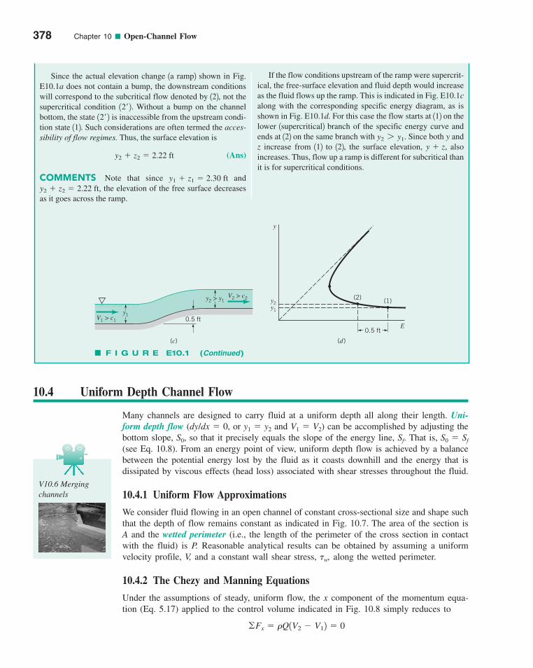
378 Chapter 10 ■ Open-Channel Flow

If the flow conditions upstream of the ramp were supercrit-ical, the free-surface elevation and fluid depth would increaseas the fluid flows up the ramp. This is indicated in Fig. E10.1calong with the corresponding specific energy diagram, as isshown in Fig. E10.1d. For this case the flow starts at 112 on thelower 1supercritical2 branch of the specific energy curve andends at 122 on the same branch with Since both y andz increase from 112 to 122, the surface elevation, alsoincreases. Thus, flow up a ramp is different for subcritical thanit is for supercritical conditions.

y � z,y2 7 y1.

Since the actual elevation change 1a ramp2 shown in Fig.E10.1a does not contain a bump, the downstream conditionswill correspond to the subcritical flow denoted by 122, not thesupercritical condition Without a bump on the channelbottom, the state is inaccessible from the upstream condi-tion state 112. Such considerations are often termed the acces-sibility of flow regimes. Thus, the surface elevation is

(Ans)

COMMENTS Note that since andthe elevation of the free surface decreases

as it goes across the ramp.y2 � z2 � 2.22 ft,

y1 � z1 � 2.30 ft

y2 � z2 � 2.22 ft

12¿ 212¿ 2.

F I G U R E E10.1 (Continued)

V2 > c2y2 > y1

y1V1 > c1

y1

y2

y

E

0.5 ft

(2) (1)

0.5 ft

(c) (d)

10.4 Uniform Depth Channel Flow

Many channels are designed to carry fluid at a uniform depth all along their length. Uni-form depth flow (dy/dx � 0, or y1 � y2 and V1 � V2) can be accomplished by adjusting thebottom slope, S0, so that it precisely equals the slope of the energy line, Sf. That is, S0 � Sf

(see Eq. 10.8). From an energy point of view, uniform depth flow is achieved by a balancebetween the potential energy lost by the fluid as it coasts downhill and the energy that isdissipated by viscous effects (head loss) associated with shear stresses throughout the fluid.

10.4.1 Uniform Flow Approximations

We consider fluid flowing in an open channel of constant cross-sectional size and shape suchthat the depth of flow remains constant as indicated in Fig. 10.7. The area of the section isA and the wetted perimeter (i.e., the length of the perimeter of the cross section in contactwith the fluid) is P. Reasonable analytical results can be obtained by assuming a uniformvelocity profile, V, and a constant wall shear stress, �w, along the wetted perimeter.

10.4.2 The Chezy and Manning Equations

Under the assumptions of steady, uniform flow, the x component of the momentum equa-tion (Eq. 5.17) applied to the control volume indicated in Fig. 10.8 simply reduces to

©Fx � �Q1V2 � V12 � 0

V10.6 Mergingchannels

c10OpenChannelFlow.qxd 9/28/10 10:34 AM Page 378

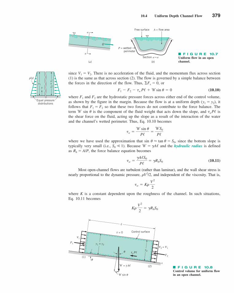
10.4 Uniform Depth Channel Flow 379

since V1 � V2. There is no acceleration of the fluid, and the momentum flux across section(1) is the same as that across section (2). The flow is governed by a simple balance betweenthe forces in the direction of the flow. Thus, �Fx � 0, or

(10.10)

where F1 and F2 are the hydrostatic pressure forces across either end of the control volume,as shown by the figure in the margin. Because the flow is at a uniform depth (y1 � y2), itfollows that F1 � F2 so that these two forces do not contribute to the force balance. Theterm w sin is the component of the fluid weight that acts down the slope, and �wP� isthe shear force on the fluid, acting up the slope as a result of the interaction of the waterand the channel’s wetted perimeter. Thus, Eq. 10.10 becomes

where we have used the approximation that sin � tan � S0, since the bottom slope istypically very small (i.e., S0 � 1). Because w� �A� and the hydraulic radius is definedas Rh � A/P, the force balance equation becomes

(10.11)

Most open-channel flows are turbulent (rather than laminar), and the wall shear stress isnearly proportional to the dynamic pressure, �V2/2, and independent of the viscosity. That is,

where K is a constant dependent upon the roughness of the channel. In such situations,Eq. 10.11 becomes

K� V2

2� �RhS0

�w � K� V2

2

�w ��A/S0

P/� �RhS0

�w �w sin

P/�wS0

P/

F1 � F2 � �w P/ �w sin � 0

p(y)

Equal pressuredistributions

y2 =

y1

y1

y

F I G U R E 10.7 Uniform flow in an openchannel.

Q

a

a

Free surface A = flow area

P = wetted perimeter

Section –a a

(a) (b)

F I G U R E 10.8Control volume for uniform flowin an open channel.

F1

V1

(1)θ

y1 = y2

= 0τ

�

y2τ P�

� = A�γ

� sin θ

(2)

F2

V2 = V1

x

Control surface

θw

c10OpenChannelFlow.qxd 9/28/10 10:34 AM Page 379

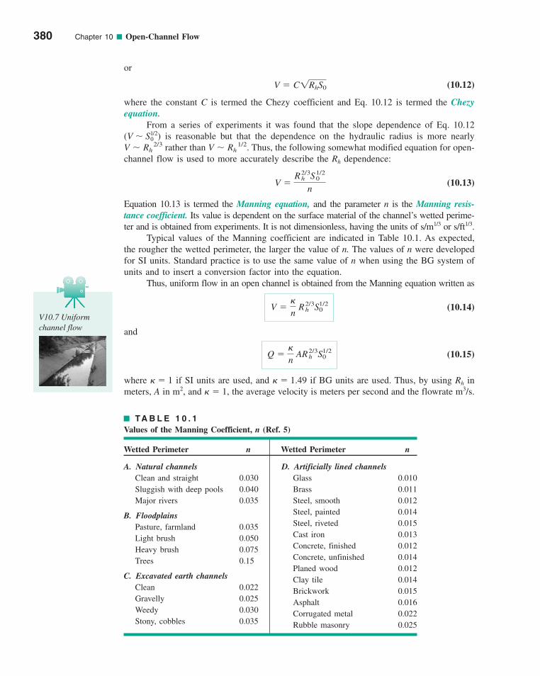
or

(10.12)

where the constant C is termed the Chezy coefficient and Eq. 10.12 is termed the Chezyequation.

From a series of experiments it was found that the slope dependence of Eq. 10.12(V � S1

0/2) is reasonable but that the dependence on the hydraulic radius is more nearly

rather than . Thus, the following somewhat modified equation for open-channel flow is used to more accurately describe the Rh dependence:

(10.13)

Equation 10.13 is termed the Manning equation, and the parameter n is the Manning resis-tance coefficient. Its value is dependent on the surface material of the channel’s wetted perime-ter and is obtained from experiments. It is not dimensionless, having the units of s/m1/3 or s/ft1/3.

Typical values of the Manning coefficient are indicated in Table 10.1. As expected,the rougher the wetted perimeter, the larger the value of n. The values of n were developedfor SI units. Standard practice is to use the same value of n when using the BG system ofunits and to insert a conversion factor into the equation.

Thus, uniform flow in an open channel is obtained from the Manning equation written as

(10.14)

and

(10.15)

where � 1 if SI units are used, and � 1.49 if BG units are used. Thus, by using Rh inmeters, A in m2, and � 1, the average velocity is meters per second and the flowrate m3/s.

Q �

n AR2/3

h S1/20

V �

n R2/3

h S1/20

V �R2/3

h S1/20

n

V � Rh 1/2V � Rh

2/3

V � C1RhS0

380 Chapter 10 ■ Open-Channel Flow

A. Natural channelsClean and straight 0.030Sluggish with deep pools 0.040Major rivers 0.035

B. FloodplainsPasture, farmland 0.035Light brush 0.050Heavy brush 0.075Trees 0.15

C. Excavated earth channelsClean 0.022Gravelly 0.025Weedy 0.030Stony, cobbles 0.035

TA B L E 1 0 . 1

Values of the Manning Coefficient, n (Ref. 5)

Wetted Perimeter n Wetted Perimeter n

D. Artificially lined channelsGlass 0.010Brass 0.011Steel, smooth 0.012Steel, painted 0.014Steel, riveted 0.015Cast iron 0.013Concrete, finished 0.012Concrete, unfinished 0.014Planed wood 0.012Clay tile 0.014Brickwork 0.015Asphalt 0.016Corrugated metal 0.022Rubble masonry 0.025

V10.7 Uniformchannel flow

c10OpenChannelFlow.qxd 9/28/10 10:34 AM Page 380

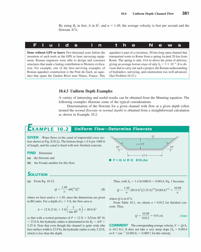
10.4 Uniform Depth Channel Flow 381

By using Rh in feet, A in ft2, and � 1.49, the average velocity is feet per second and theflowrate ft3/s.

10.4.3 Uniform Depth Examples

A variety of interesting and useful results can be obtained from the Manning equation. Thefollowing examples illustrate some of the typical considerations.

Determination of the flowrate for a given channel with flow at a given depth (oftentermed the normal flowrate or normal depth) is obtained from a straightforward calculationas shown in Example 10.2.

F l u i d s i n t h e N e w s

Done without GPS or lasers Two thousand years before theinvention of such tools as the GPS or laser surveying equip-ment, Roman engineers were able to design and constructstructures that made a lasting contribution to Western civiliza-tion. For example, one of the best-surviving examples of Roman aqueduct construction is the Pont du Gard, an aque-duct that spans the Gardon River near Nîmes, France. This

aqueduct is part of a circuitous, 50-km-long open channel thattransported water to Rome from a spring located 20 km fromRome. The spring is only 14.6 m above the point of delivery,giving an average bottom slope of only S0 � 3 10�4. It is ob-vious that to carry out such a project, the Roman understandingof hydraulics, surveying, and construction was well advanced.(See Problem 10.23.)

GIVEN Water flows in the canal of trapezoidal cross sec-tion shown in Fig. E10.2a. The bottom drops 1.4 ft per 1000 ftof length, and the canal is lined with new finished concrete.

FIND Determine

(a) the flowrate and

(b) the Froude number for this flow.

SOLUTION

Uniform Flow—Determine Flowrate

Thus, with S0 � 1.4 ft/1000 ft � 0.0014, Eq. 1 becomes

where Q is in ft3/s.From Table 10.1, we obtain n � 0.012 for finished con-

crete. Thus,

(Ans)

COMMENT The corresponding average velocity, V � QA,

Q �10.98

0.012� 915 cfs

Q �1.49

n 189.8 ft22 13.25 ft22/310.001421/2 �

10.98n

EXAMPLE 10.2

(a) From Eq. 10.15,

(1)

where we have used � 1.49, since the dimensions are givenin BG units. For a depth of y � 5 ft, the flow area is

so that with a wetted perimeter of P � 12 ft � 2(5/sin 40� ft)� 27.6 ft, the hydraulic radius is determined to be Rh � A/P �3.25 ft. Note that even though the channel is quite wide (thefree-surface width is 23.9 ft), the hydraulic radius is only 3.25 ft,which is less than the depth.

A � 12 ft 15 ft2 � 5 ft a5

tan 40° ftb � 89.8 ft2

Q �1.49

n AR 2/3

h S1/20

F I G U R E E10.2a

y = 5 ft40°40°

12 ft

is 10.2 ft�s. It does not take a very steep slope for this velocity.tan�1 10.00142 � 0.080°2or �

1S0 � 0.0014

c10OpenChannelFlow.qxd 9/28/10 10:34 AM Page 381

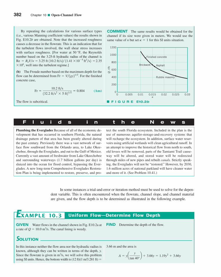
In some instances a trial-and-error or iteration method must be used to solve for the depen-dent variable. This is often encountered when the flowrate, channel slope, and channel materialare given, and the flow depth is to be determined as illustrated in the following example.

382 Chapter 10 ■ Open-Channel Flow

By repeating the calculations for various surface types(i.e., various Manning coefficient values) the results shown inFig. E10.2b are obtained. Note that the increased roughnesscauses a decrease in the flowrate. This is an indication that forthe turbulent flows involved, the wall shear stress increaseswith surface roughness. [For water at the Reynoldsnumber based on the 3.25-ft hydraulic radius of the channel is

well into the turbulent regime.]

(b) The Froude number based on the maximum depth for theflow can be determined from For the finishedconcrete case,

(Ans)

The flow is subcritical.

Fr �10.2 fts

132.2 fts2 5 ft212� 0.804

Fr � V 1gy212.

106,� 2.3511.41 10�5 ft2s23.25 ft 110.2 fts2Re � RhV� �

50 °F,

F I G U R E E10.2b

1200

1000

800

600

400

200

00 0.005 0.01 0.015 0.02 0.025 0.03

Q, cf

s

n

Finished concrete

Rubble masonry

Brickwork Asphalt

F l u i d s i n t h e N e w s

Plumbing the Everglades Because of all of the economic de-velopment that has occurred in southern Florida, the naturaldrainage pattern of that area has been greatly altered duringthe past century. Previously there was a vast network of sur-face flow southward from the Orlando area, to Lake Okee-chobee, through the Everglades, and out to the Gulf of Mexico.Currently a vast amount of freshwater from Lake Okeechobeeand surrounding waterways (1.7 billion gallons per day) issluiced into the ocean for flood control, bypassing the Ever-glades. A new long-term Comprehensive Everglades Restora-tion Plan is being implemented to restore, preserve, and pro-

tect the south Florida ecosystem. Included in the plan is theuse of numerous aquifer-storage-and-recovery systems thatwill recharge the ecosystem. In addition, surface water reser-voirs using artificial wetlands will clean agricultural runoff. Inan attempt to improve the historical flow from north to south,old levees will be removed, parts of the Tamiami Trail cause-way will be altered, and stored water will be redirectedthrough miles of new pipes and rebuilt canals. Strictly speak-ing, the Everglades will not be “restored.” However, by 2030,1.6 million acres of national parkland will have cleaner waterand more of it. (See Problem 10.41.)

GIVEN Water flows in the channel shown in Fig. E10.2a ata rate of Q � 10.0 m3/s. The canal lining is weedy.

FIND Determine the depth of the flow.

SOLUTION

Uniform Flow—Determine Flow Depth

3.66 m and the area is

A � y ay

tan 40°b � 3.66y � 1.19y2 � 3.66y

EXAMPLE 10.3

In this instance neither the flow area nor the hydraulic radius isknown, although they can be written in terms of the depth, y.Since the flowrate is given in m3/s, we will solve this problemusing SI units. Hence, the bottom width is (12 ft)(1 m/3.281 ft) �

COMMENT The same results would be obtained for thechannel if its size were given in meters. We would use thesame value of n but set for this SI units situation.k � 1

c10OpenChannelFlow.qxd 9/28/10 10:34 AM Page 382

10.4 Uniform Depth Channel Flow 383

In many man-made channels the surface roughness (and, hence the Manning coeffi-cient) varies along the wetted perimeter of the channel. In such cases the channel cross sec-tion can be divided into N subsections, each with its own wetted perimeter, Pi, and Ai, andManning coefficient, ni. The Pi values do not include the imaginary boundaries between thedifferent subsections. The total flowrate is assumed to be the sum of the flowrates througheach section. This technique is illustrated by Example 10.4.

GIVEN Water flows along the drainage canal having theproperties shown in Fig. E10.4a. The bottom slope is S0 �1 ft/500 ft � 0.002.

FIND Estimate the flowrate.

Uniform Flow—Variable RoughnessEXAMPLE 10.4

COMMENT By repeating the calculations for variousflowrates, the results shown in Fig. E10.3 are obtained.Note that the water depth is not linearly related to theflowrate. That is, if the flowrate is doubled, the depth is notdoubled.

where A and y are in square meters and meters, respectively.Also, the wetted perimeter is

so that

where Rh and y are in meters. Thus, with n � 0.030 (fromTable 10.1), Eq. 10.15 can be written as

which can be rearranged into the form

(1)

where y is in meters. The solution of Eq. 1 can be obtainedeasily by use of a simple root-finding numerical technique orby trial-and-error methods. The only physically meaningfulroot of Eq. 1 (i.e., a positive, real number) gives the solutionfor the normal flow depth at this flowrate as

(Ans)y � 1.50 m

11.19y2 � 3.66y25 � 51513.11y � 3.6622 � 0

10.001421/2

�1.0

0.030 11.19y2 � 3.66y2 a

1.19y2 � 3.66y

3.11y � 3.66b

2/3

Q � 10 �

n AR 2/3

h S1/20

Rh �A

P�

1.19y2 � 3.66y

3.11y � 3.66

P � 3.66 � 2 ay

sin 40°b � 3.11y � 3.66

F I G U R E E10.3

(10, 1.50)

3.0

2.5

2.0

1.5

1.0

0.5

00 5 10 15 20 25 30

y,

m

Q, m3/s

F I G U R E E10.4a

(2)

n2 =0.015

0.8 ft

(3)0.6 ft(1)

n1 = 0.020 n3 = 0.0303 ft2 ft3 ft

SOLUTION

The appropriate values of Ai, Pi, Rhi, and ni are listed inTable E10.4. Note that the imaginary portions of the perime-ters between sections (denoted by the dashed lines in Fig. E10. 4a)are not included in the Pi. That is, for section (2)

A2 � 2 ft 10.8 � 0.62 ft � 2.8 ft2

We divide the cross section into three subsections as is indi-cated in Fig. E10.4a and write the flowrate as Q � Q1 � Q2 �Q3, where for each section

Qi �1.49

ni AiR

2/3hi S1/2

0

c10OpenChannelFlow.qxd 9/28/10 10:34 AM Page 383

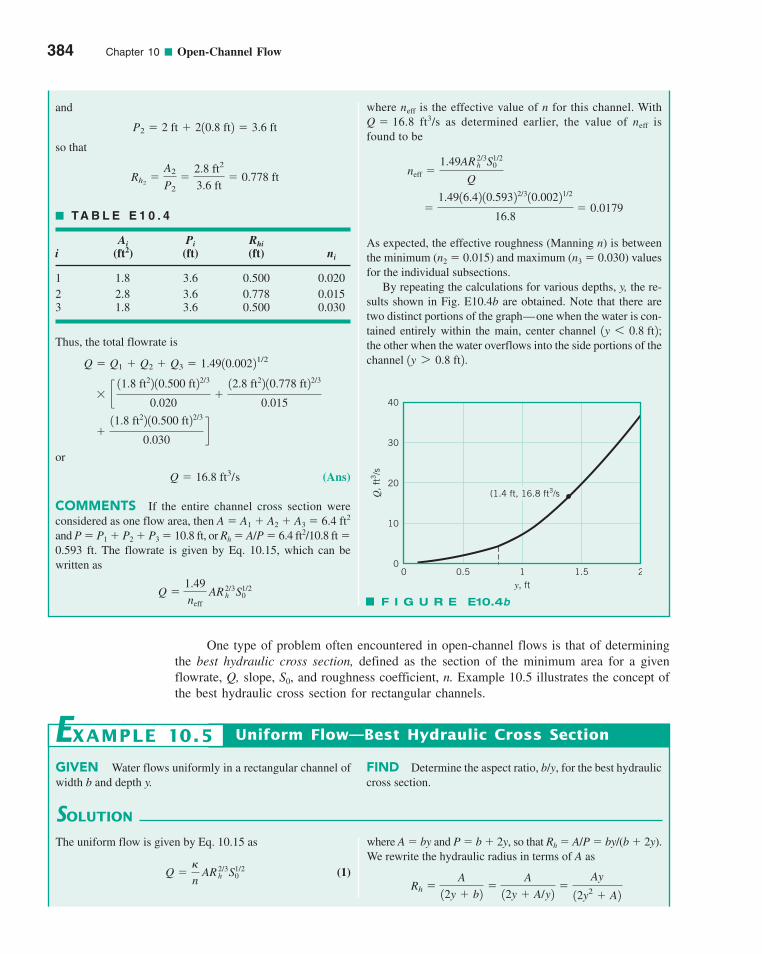
One type of problem often encountered in open-channel flows is that of determiningthe best hydraulic cross section, defined as the section of the minimum area for a givenflowrate, Q, slope, S0, and roughness coefficient, n. Example 10.5 illustrates the concept ofthe best hydraulic cross section for rectangular channels.

384 Chapter 10 ■ Open-Channel Flow

where neff is the effective value of n for this channel. WithQ � 16.8 ft3/s as determined earlier, the value of neff isfound to be

As expected, the effective roughness (Manning n) is betweenthe minimum (n2 � 0.015) and maximum (n3 � 0.030) valuesfor the individual subsections.

By repeating the calculations for various depths, y, the re-sults shown in Fig. E10.4b are obtained. Note that there aretwo distinct portions of the graph—one when the water is con-tained entirely within the main, center channel the other when the water overflows into the side portions of thechannel 1y 7 0.8 ft2.

1y 6 0.8 ft2;

�1.4916.42 10.59322/310.00221/2

16.8� 0.0179

neff �1.49AR 2/3

h S1/20

Q

and

so that

■ TA B L E E 1 0 . 4

Ai Pi Rhii (ft2) (ft) (ft) ni

1 1.8 3.6 0.500 0.0202 2.8 3.6 0.778 0.0153 1.8 3.6 0.500 0.030

Thus, the total flowrate is

or

(Ans)

COMMENTS If the entire channel cross section wereconsidered as one flow area, then A � A1 � A2 � A3 � 6.4 ft2

and P � P1 � P2 � P3 � 10.8 ft, or Rh � A/P � 6.4 ft2/10.8 ft �0.593 ft. The flowrate is given by Eq. 10.15, which can bewritten as

Q �1.49neff

AR 2/3h S1/2

0

Q � 16.8 ft3/s

�11.8 ft22 10.500 ft22/3

0.030d

c11.8 ft22 10.500 ft22/3

0.020�12.8 ft22 10.778 ft22/3

0.015

Q � Q1 � Q2 � Q3 � 1.4910.00221/2

Rh2�

A2

P2�

2.8 ft2

3.6 ft� 0.778 ft

P2 � 2 ft � 210.8 ft2 � 3.6 ft

40

30

20

0 0.5 1 1.5 2

10

0

(1.4 ft, 16.8 ft3/sQ,

ft3/s

y, ft

F I G U R E E10.4b

GIVEN Water flows uniformly in a rectangular channel ofwidth b and depth y.

FIND Determine the aspect ratio, b/y, for the best hydrauliccross section.

Uniform Flow—Best Hydraulic Cross SectionEXAMPLE 10.5

SOLUTION

where A � by and P � b � 2y, so that Rh � A/P � by/(b � 2y).We rewrite the hydraulic radius in terms of A as

Rh �A

12y � b2�

A

12y � A/y2�

Ay

12y2 � A2

The uniform flow is given by Eq. 10.15 as

(1)Q �

n AR 2/3

h S1/20

c10OpenChannelFlow.qxd 9/28/10 10:35 AM Page 384

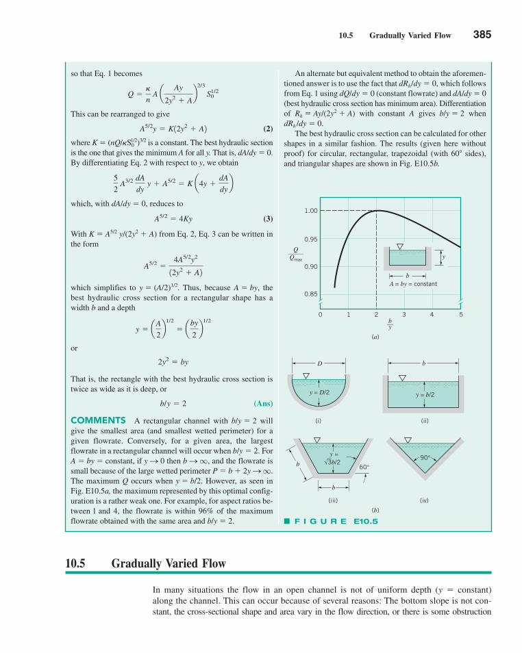
10.5 Gradually Varied Flow 385

An alternate but equivalent method to obtain the aforemen-tioned answer is to use the fact that dRh/dy � 0, which followsfrom Eq. 1 using dQ/dy � 0 (constant flowrate) and dA/dy � 0(best hydraulic cross section has minimum area). Differentiationof Rh � Ay/(2y2 � A) with constant A gives b/y � 2 whendRh /dy � 0.

The best hydraulic cross section can be calculated for othershapes in a similar fashion. The results (given here withoutproof) for circular, rectangular, trapezoidal (with 60� sides),and triangular shapes are shown in Fig. E10.5b.

so that Eq. 1 becomes

This can be rearranged to give

(2)

where K � (nQ/S01/2)3/2 is a constant. The best hydraulic section

is the one that gives the minimum A for all y. That is, dA/dy � 0.By differentiating Eq. 2 with respect to y, we obtain

which, with dA/dy � 0, reduces to

(3)

With K � A5/2 y/(2y2 � A) from Eq. 2, Eq. 3 can be written inthe form

which simplifies to y � (A/2)1/2. Thus, because A � by, thebest hydraulic cross section for a rectangular shape has awidth b and a depth

or

That is, the rectangle with the best hydraulic cross section istwice as wide as it is deep, or

(Ans)

COMMENTS A rectangular channel with b/y � 2 willgive the smallest area (and smallest wetted perimeter) for agiven flowrate. Conversely, for a given area, the largestflowrate in a rectangular channel will occur when b/y � 2. ForA � by � constant, if y S 0 then b S , and the flowrate issmall because of the large wetted perimeter P � b � 2y S .The maximum Q occurs when y � b/2. However, as seen inFig. E10.5a, the maximum represented by this optimal config-uration is a rather weak one. For example, for aspect ratios be-tween 1 and 4, the flowrate is within 96% of the maximumflowrate obtained with the same area and b/y � 2.

qq

b/y � 2

2y2 � by

y � aA

2b

1/2

� aby

2b

1/2

A5/2 �4A5/2y2

12y2 � A2

A5/2 � 4Ky

5

2 A3/2

dA

dy y � A5/2 � K a4y �

dA

dyb

A5/2y � K12y2 � A2

Q �

n A a

Ay

2y2 � Ab

2/3

S1/20

1.00

0.95

0.90

0.85

0 1 2 3 4 5b__y

Q_____Qmax

b

y

A = by = constant

(a)

y = D/2

D

(i)

y = b/2

b

(ii)

b

b

60°√

y =3b/2

(iii) (iv)

(b)

90°

F I G U R E E10.5

10.5 Gradually Varied Flow

In many situations the flow in an open channel is not of uniform depth (y � constant)along the channel. This can occur because of several reasons: The bottom slope is not con-stant, the cross-sectional shape and area vary in the flow direction, or there is some obstruction

c10OpenChannelFlow.qxd 9/28/10 10:35 AM Page 385

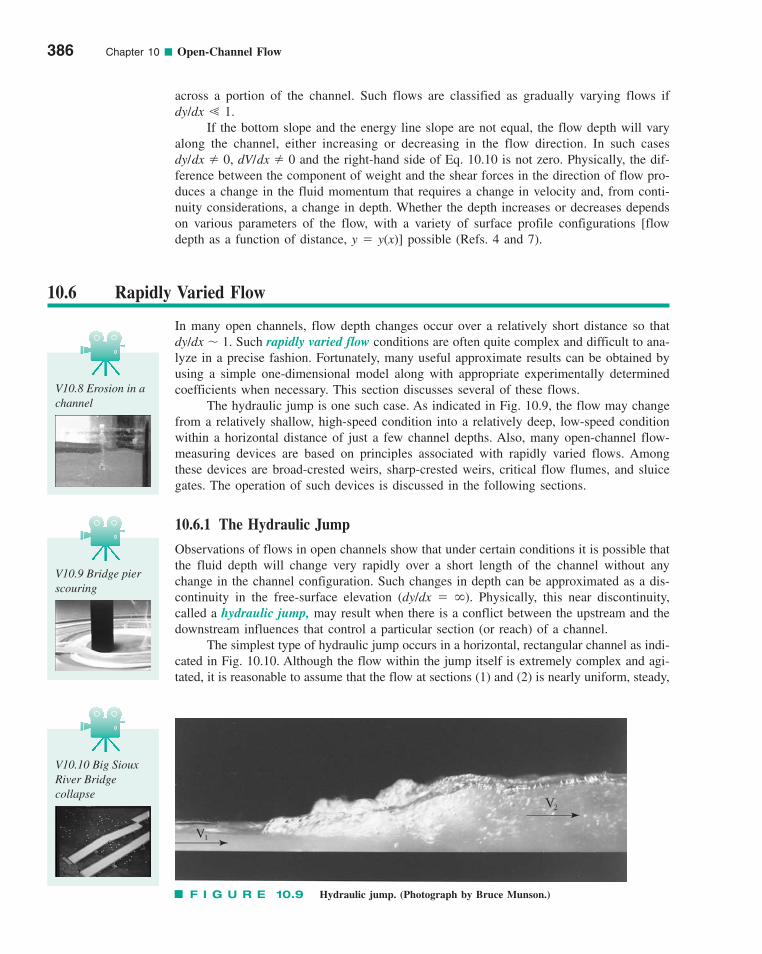
across a portion of the channel. Such flows are classified as gradually varying flows ifdy/dx � 1.

If the bottom slope and the energy line slope are not equal, the flow depth will varyalong the channel, either increasing or decreasing in the flow direction. In such cases

, and the right-hand side of Eq. 10.10 is not zero. Physically, the dif-ference between the component of weight and the shear forces in the direction of flow pro-duces a change in the fluid momentum that requires a change in velocity and, from conti-nuity considerations, a change in depth. Whether the depth increases or decreases dependson various parameters of the flow, with a variety of surface profile configurations [flowdepth as a function of distance, y � y(x)] possible (Refs. 4 and 7).

dV/dx � 0dy/dx � 0

386 Chapter 10 ■ Open-Channel Flow

10.6 Rapidly Varied Flow

In many open channels, flow depth changes occur over a relatively short distance so thatdy/dx � 1. Such rapidly varied flow conditions are often quite complex and difficult to ana-lyze in a precise fashion. Fortunately, many useful approximate results can be obtained byusing a simple one-dimensional model along with appropriate experimentally determinedcoefficients when necessary. This section discusses several of these flows.

The hydraulic jump is one such case. As indicated in Fig. 10.9, the flow may changefrom a relatively shallow, high-speed condition into a relatively deep, low-speed conditionwithin a horizontal distance of just a few channel depths. Also, many open-channel flow-measuring devices are based on principles associated with rapidly varied flows. Amongthese devices are broad-crested weirs, sharp-crested weirs, critical flow flumes, and sluicegates. The operation of such devices is discussed in the following sections.

10.6.1 The Hydraulic Jump

Observations of flows in open channels show that under certain conditions it is possible thatthe fluid depth will change very rapidly over a short length of the channel without anychange in the channel configuration. Such changes in depth can be approximated as a dis-continuity in the free-surface elevation (dy/dx � �). Physically, this near discontinuity,called a hydraulic jump, may result when there is a conflict between the upstream and thedownstream influences that control a particular section (or reach) of a channel.

The simplest type of hydraulic jump occurs in a horizontal, rectangular channel as indi-cated in Fig. 10.10. Although the flow within the jump itself is extremely complex and agi-tated, it is reasonable to assume that the flow at sections (1) and (2) is nearly uniform, steady,

V10.8 Erosion in achannel

V10.9 Bridge pierscouring

F I G U R E 10.9 Hydraulic jump. (Photograph by Bruce Munson.)

V10.10 Big SiouxRiver Bridge collapse

c10OpenChannelFlow.qxd 9/28/10 10:35 AM Page 386

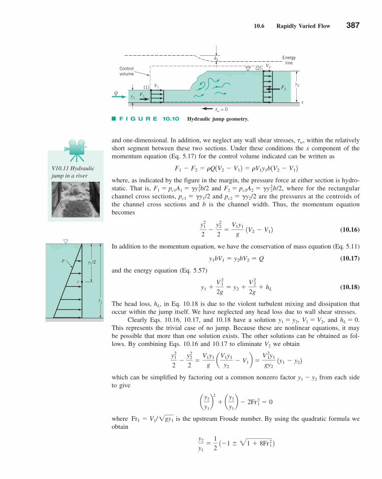
10.6 Rapidly Varied Flow 387

and one-dimensional. In addition, we neglect any wall shear stresses, �w, within the relativelyshort segment between these two sections. Under these conditions the x component of themomentum equation (Eq. 5.17) for the control volume indicated can be written as

where, as indicated by the figure in the margin, the pressure force at either section is hydro-static. That is, F1 � pc1A1 � �y 2

1b/2 and F2 � pc2A2 � �y 22b/2, where for the rectangular

channel cross sections, pc1 � �y1/2 and pc2 � �y2/2 are the pressures at the centroids ofthe channel cross sections and b is the channel width. Thus, the momentum equationbecomes

(10.16)

In addition to the momentum equation, we have the conservation of mass equation (Eq. 5.11)

(10.17)

and the energy equation (Eq. 5.57)

(10.18)

The head loss, hL, in Eq. 10.18 is due to the violent turbulent mixing and dissipation thatoccur within the jump itself. We have neglected any head loss due to wall shear stresses.

Clearly Eqs. 10.16, 10.17, and 10.18 have a solution y1 � y2, V1 � V2, and hL � 0.This represents the trivial case of no jump. Because these are nonlinear equations, it maybe possible that more than one solution exists. The other solutions can be obtained as fol-lows. By combining Eqs. 10.16 and 10.17 to eliminate V2 we obtain

which can be simplified by factoring out a common nonzero factor y1 � y2 from each sideto give

where is the upstream Froude number. By using the quadratic formula weobtain

y2

y1�

1

2 1�1 � 21 � 8Fr

21 2

Fr1 � V1/1gy1

ay2

y1b

2

� ay2

y1b � 2Fr

21 � 0

y21

2�

y22

2�

V1y1

g a

V1y1

y2� V1b �

V21y1

gy2 1y1 � y22

y1 �V2

1

2g� y2 �

V22

2g� hL

y1bV1 � y2bV2 � Q

y21

2�

y22

2�

V1y1

g 1V2 � V12

F1 � F2 � �Q1V2 � V12 � �V1y1b1V2 � V12

F I G U R E 10.10 Hydraulic jump geometry.

Q

Controlvolume

(1) V1

F1y1

y2F2

V2(2)

hL

Energyline

x

w = 0τ

p

c

y1

y1/2

V10.11 Hydraulicjump in a river

c10OpenChannelFlow.qxd 9/28/10 10:35 AM Page 387

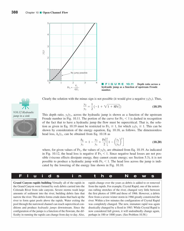
Clearly the solution with the minus sign is not possible (it would give a negative y2/y1). Thus,

(10.19)

This depth ratio, y2/y1, across the hydraulic jump is shown as a function of the upstreamFroude number in Fig. 10.11. The portion of the curve for Fr1 � 1 is dashed in recognitionof the fact that to have a hydraulic jump the flow must be supercritical. That is, the solu-tion as given in Eq. 10.19 must be restricted to Fr1 � 1, for which y2/y1 � 1. This can beshown by consideration of the energy equation, Eq. 10.18, as follows. The dimensionlesshead loss, hL/y1, can be obtained from Eq. 10.18 as

(10.20)

where, for given values of Fr1, the values of y2/y1 are obtained from Eq. 10.19. As indicatedin Fig. 10.12, the head loss is negative if Fr1 � 1. Since negative head losses are not pos-sible (viscous effects dissipate energy, they cannot create energy; see Section 5.3), it is notpossible to produce a hydraulic jump with Fr1 � 1. The head loss across the jump is indi-cated by the lowering of the energy line shown in Fig. 10.10.

hL

y1� 1 �

y2

y1�

Fr21

2c1 � a

y1

y2b

2

d

y2

y1�

1

2 1�1 � 21 � 8Fr

21 2

388 Chapter 10 ■ Open-Channel Flow

5

4

3

2

1

00 1 2 3 4

No jump possible

Fr1 =V1______

√gy1

y2__y1

F I G U R E 10.11 Depth ratio across ahydraulic jump as a function of upstream Froudenumber.

F l u i d s i n t h e N e w s

Grand Canyon rapids building Virtually all of the rapids inthe Grand Canyon were formed by rock debris carried into theColorado River from side canyons. Severe storms wash largeamounts of sediment into the river, building debris fans thatnarrow the river. This debris forms crude dams that back up theriver to form quiet pools above the rapids. Water exiting thepool through the narrowed channel can reach supercritical con-ditions and produce hydraulic jumps downstream. Since theconfiguration of the jumps is a function of the flowrate, the dif-ficulty in running the rapids can change from day to day. Also,

rapids change over the years as debris is added to or removedfrom the rapids. For example, Crystal Rapid, one of the notori-ous rafting stretches of the river, changed very little betweenthe first photos of 1890 and those of 1966. However, a debrisflow from a severe winter storm in 1966 greatly constricted theriver. Within a few minutes the configuration of Crystal Rapidwas completely changed. The new, immature rapid was againdrastically changed by a flood in 1983. While Crystal Rapid isnow considered full grown, it will undoubtedly change again,perhaps in 100 or 1000 years. (See Problem 10.58.)

V10.12 Hydraulicjump in a sink

c10OpenChannelFlow.qxd 9/28/10 10:35 AM Page 388

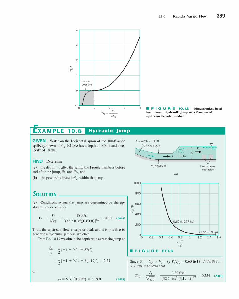
10.6 Rapidly Varied Flow 389

No jumppossible

Fr1 =V1______

√gy1

4

3

2

1

0

-10 1 2 3 4

hL__

y1

F I G U R E 10.12 Dimensionless headloss across a hydraulic jump as a function ofupstream Froude number.

GIVEN Water on the horizontal apron of the 100-ft-widespillway shown in Fig. E10.6a has a depth of 0.60 ft and a ve-locity of 18 ft/s.

FIND Determine

(a) the depth, y2, after the jump, the Froude numbers beforeand after the jump, Fr1 and Fr2, and

(b) the power dissipated, pd, within the jump.

Hydraulic JumpEXAMPLE 10.6

SOLUTION

Since Q1 � Q2, or V2 � (y1V1)/y2 � 0.60 ft(18 ft/s)/3.19 ft �3.39 ft/s, it follows that

(Ans)Fr2 �V2

1gy2

�3.39 ft /s

3 132.2 ft /s22 13.19 ft2 41/2 � 0.334

(a) Conditions across the jump are determined by the up-stream Froude number

(Ans)

Thus, the upstream flow is supercritical, and it is possible togenerate a hydraulic jump as sketched.

From Eq. 10.19 we obtain the depth ratio across the jump as

or

(Ans)y2 � 5.32 10.60 ft2 � 3.19 ft

�1

2 3�1 � 21 � 814.1022 4 � 5.32

y2

y1�

1

2 1�1 � 21 � 8Fr2

12

Fr1 �V1

1gy1

�18 ft /s

3 132.2 ft /s22 10.60 ft2 41/2 � 4.10

(a)

y1 = 0.60 ft Downstreamobstacles

b = width = 100 ft

Spillway apron

V1 = 18 ft/sy2

V2

1000

800

600

400

200

00 0.2 0.4 0.6 0.8 1 1.2 1.4 1.6

�d, h

p

y1, ft

(b)

(0.60 ft, 277 hp)

(1.54 ft, 0 hp)

F I G U R E E10.6

c10OpenChannelFlow.qxd 9/28/10 10:35 AM Page 389

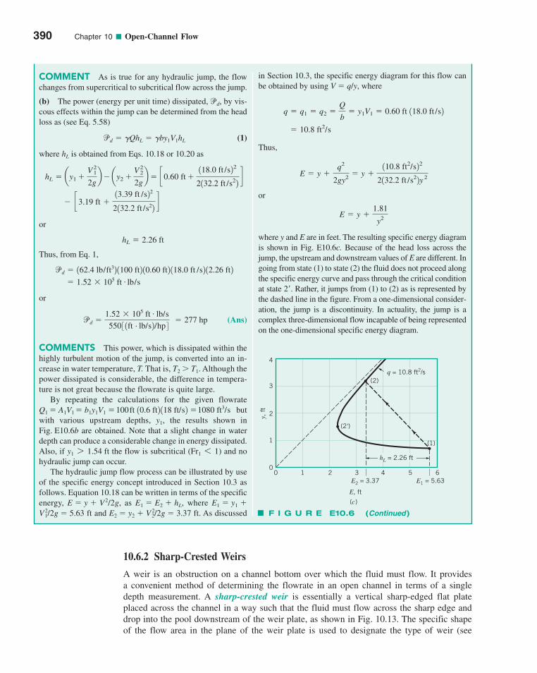
10.6.2 Sharp-Crested Weirs

A weir is an obstruction on a channel bottom over which the fluid must flow. It providesa convenient method of determining the flowrate in an open channel in terms of a singledepth measurement. A sharp-crested weir is essentially a vertical sharp-edged flat plateplaced across the channel in a way such that the fluid must flow across the sharp edge anddrop into the pool downstream of the weir plate, as shown in Fig. 10.13. The specific shapeof the flow area in the plane of the weir plate is used to designate the type of weir (see

390 Chapter 10 ■ Open-Channel Flow

in Section 10.3, the specific energy diagram for this flow canbe obtained by using V � q/y, where

Thus,

or

where y and E are in feet. The resulting specific energy diagramis shown in Fig. E10.6c. Because of the head loss across thejump, the upstream and downstream values of E are different. Ingoing from state (1) to state (2) the fluid does not proceed alongthe specific energy curve and pass through the critical conditionat state 2�. Rather, it jumps from (1) to (2) as is represented bythe dashed line in the figure. From a one-dimensional consider-ation, the jump is a discontinuity. In actuality, the jump is acomplex three-dimensional flow incapable of being representedon the one-dimensional specific energy diagram.

E � y �1.81

y2

E � y �q2

2gy2 � y �110.8 ft2/s22

2132.2 ft /s22y 2

� 10.8 ft2/s

q � q1 � q2 �Q

b� y1V1 � 0.60 ft 118.0 ft /s2

COMMENT As is true for any hydraulic jump, the flowchanges from supercritical to subcritical flow across the jump.

(b) The power (energy per unit time) dissipated, pd, by vis-cous effects within the jump can be determined from the headloss as (see Eq. 5.58)

(1)

where hL is obtained from Eqs. 10.18 or 10.20 as

or

Thus, from Eq. 1,

or

(Ans)

COMMENTS This power, which is dissipated within thehighly turbulent motion of the jump, is converted into an in-crease in water temperature, T. That is, T2 T1. Although thepower dissipated is considerable, the difference in tempera-ture is not great because the flowrate is quite large.

By repeating the calculations for the given flowratebut

with various upstream depths, y1, the results shown inFig. E10.6b are obtained. Note that a slight change in waterdepth can produce a considerable change in energy dissipated.Also, if the flow is subcritical ( ) and nohydraulic jump can occur.

The hydraulic jump flow process can be illustrated by useof the specific energy concept introduced in Section 10.3 asfollows. Equation 10.18 can be written in terms of the specificenergy, E � y � V2/2g, as E1 � E2 � hL, where E1 � y1 �V 2

1/2g � 5.63 ft and E2 � y2 � V 22/2g � 3.37 ft. As discussed

Fr1 6 1y1 7 1.54 ft

Q1 � A1V1 � b1y1V1 � 100 ft 10.6 ft2 118 ft/s2 �1080 ft3/s

pd �1.52 105 ft . lb/s

550 3 1ft . lb/s2/hp 4� 277 hp

� 1.52 105 ft . lb/s

pd � 162.4 lb/ft32 1100 ft2 10.60 ft2 118.0 ft /s2 12.26 ft2

hL � 2.26 ft

� c3.19 ft �13.39 ft /s22

2132.2 ft /s22d

hL � ay1 �V 2

1

2gb� ay2 �

V 22

2gb� c0.60 ft �

118.0 ft /s22

2132.2 ft /s22d

pd � �QhL � �by1V1hL

q = 10.8 ft2/s(2)

(2')

(1)

hL = 2.26 ft

4

3

2

1

00 1 2 3 4 5 6

y,

ft

E, ft

E2 = 3.37 E1 = 5.63

(c)

F I G U R E E10.6 (Continued)

c10OpenChannelFlow.qxd 9/28/10 10:35 AM Page 390

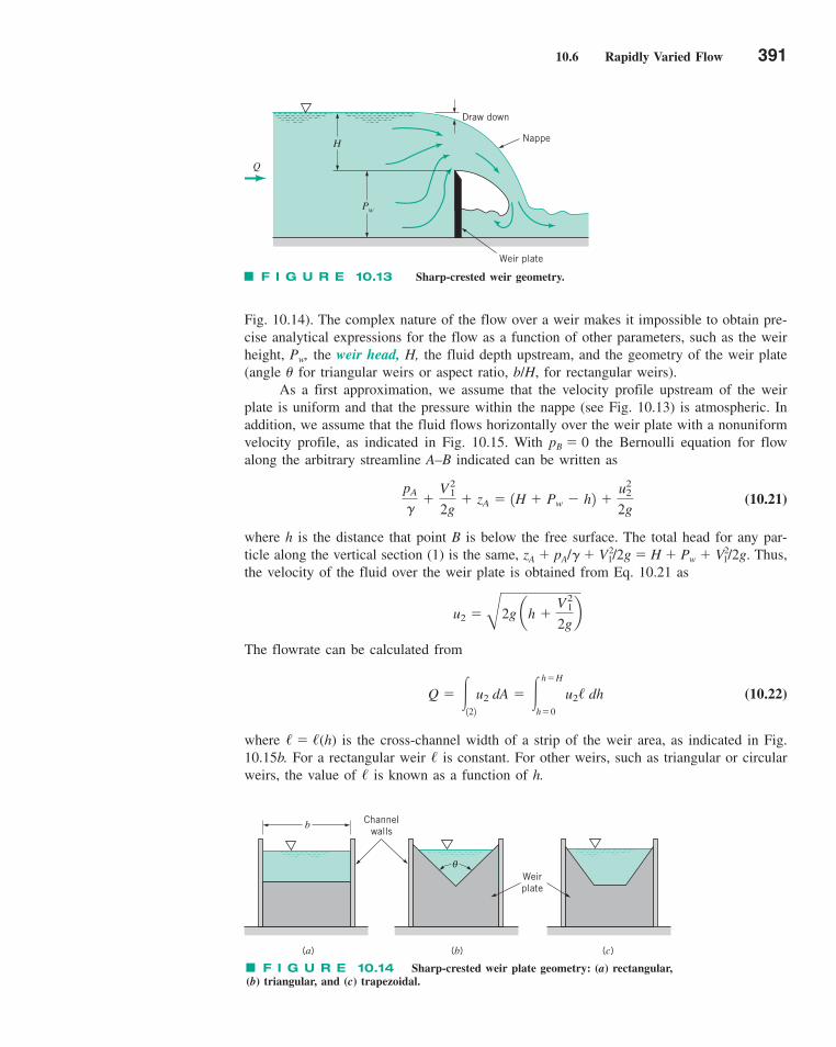
10.6 Rapidly Varied Flow 391

Fig. 10.14). The complex nature of the flow over a weir makes it impossible to obtain pre-cise analytical expressions for the flow as a function of other parameters, such as the weirheight, Pw, the weir head, H, the fluid depth upstream, and the geometry of the weir plate(angle for triangular weirs or aspect ratio, b/H, for rectangular weirs).

As a first approximation, we assume that the velocity profile upstream of the weirplate is uniform and that the pressure within the nappe (see Fig. 10.13) is atmospheric. Inaddition, we assume that the fluid flows horizontally over the weir plate with a nonuniformvelocity profile, as indicated in Fig. 10.15. With pB � 0 the Bernoulli equation for flowalong the arbitrary streamline A–B indicated can be written as

(10.21)

where h is the distance that point B is below the free surface. The total head for any par-ticle along the vertical section (1) is the same, zA � pA/� � V2

1/2g � H � Pw � V21/2g. Thus,

the velocity of the fluid over the weir plate is obtained from Eq. 10.21 as

The flowrate can be calculated from

(10.22)

where � � �(h) is the cross-channel width of a strip of the weir area, as indicated in Fig.10.15b. For a rectangular weir � is constant. For other weirs, such as triangular or circularweirs, the value of � is known as a function of h.

Q � �122

u2 dA � �h�H

h�0

u2/ dh

u2 �B

2g ah �V2

1

2gb

pA

��

V21

2g� zA � 1H � Pw � h2 �

u22

2g

F I G U R E 10.13 Sharp-crested weir geometry.

Q

H

Pw

Draw down

Nappe

Weir plate

F I G U R E 10.14 Sharp-crested weir plate geometry: (a) rectangular, (b) triangular, and (c) trapezoidal.

Weirplate

Channelwalls

(a) (b) (c)

b

θ

c10OpenChannelFlow.qxd 9/28/10 10:35 AM Page 391

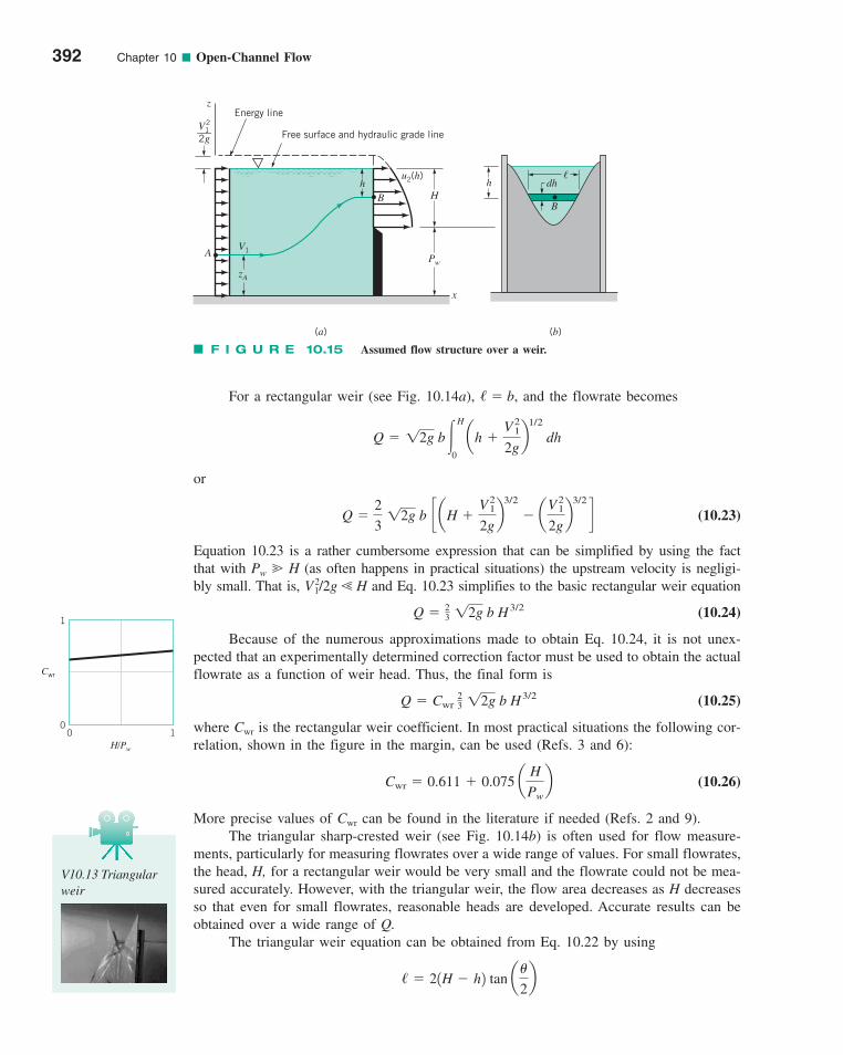
For a rectangular weir (see Fig. 10.14a), � � b, and the flowrate becomes

or

(10.23)

Equation 10.23 is a rather cumbersome expression that can be simplified by using the factthat with Pw � H (as often happens in practical situations) the upstream velocity is negligi-bly small. That is, V2

1/2g � H and Eq. 10.23 simplifies to the basic rectangular weir equation

(10.24)

Because of the numerous approximations made to obtain Eq. 10.24, it is not unex-pected that an experimentally determined correction factor must be used to obtain the actualflowrate as a function of weir head. Thus, the final form is

(10.25)

where Cwr is the rectangular weir coefficient. In most practical situations the following cor-relation, shown in the figure in the margin, can be used (Refs. 3 and 6):

(10.26)

More precise values of Cwr can be found in the literature if needed (Refs. 2 and 9).The triangular sharp-crested weir (see Fig. 10.14b) is often used for flow measure-

ments, particularly for measuring flowrates over a wide range of values. For small flowrates,the head, H, for a rectangular weir would be very small and the flowrate could not be mea-sured accurately. However, with the triangular weir, the flow area decreases as H decreasesso that even for small flowrates, reasonable heads are developed. Accurate results can beobtained over a wide range of Q.

The triangular weir equation can be obtained from Eq. 10.22 by using

/ � 21H � h2 tan a

2b

Cwr � 0.611 � 0.075 aH

Pwb

Q � Cwr 23 12g b H3/2

Q � 23 12g b H3/2

Q �2

3 12g b c aH �

V21

2gb

3/2

� aV2

1

2gb

3/2

d

Q � 12g b�H

0

ah �V2

1

2gb

1/2

dh

392 Chapter 10 ■ Open-Channel Flow

1

00 1

Cwr

H/Pw

V10.13 Triangularweir

F I G U R E 10.15 Assumed flow structure over a weir.

z

V12

___2g

Energy line

Free surface and hydraulic grade line

h

B

V1

zA

A

u2(h)

H

Pw

x

h

B

dh�

(b)(a)

c10OpenChannelFlow.qxd 9/28/10 10:36 AM Page 392

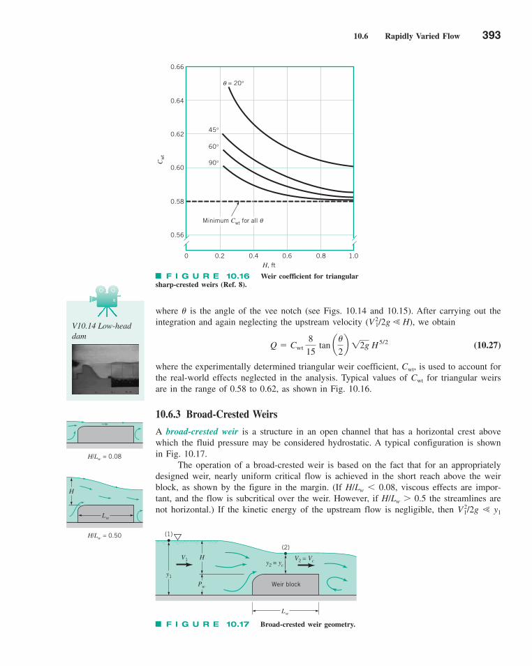
10.6 Rapidly Varied Flow 393

where is the angle of the vee notch (see Figs. 10.14 and 10.15). After carrying out theintegration and again neglecting the upstream velocity (V 2

1/2g � H), we obtain

(10.27)

where the experimentally determined triangular weir coefficient, Cwt, is used to account forthe real-world effects neglected in the analysis. Typical values of Cwt for triangular weirsare in the range of 0.58 to 0.62, as shown in Fig. 10.16.

10.6.3 Broad-Crested Weirs

A broad-crested weir is a structure in an open channel that has a horizontal crest abovewhich the fluid pressure may be considered hydrostatic. A typical configuration is shownin Fig. 10.17.

The operation of a broad-crested weir is based on the fact that for an appropriatelydesigned weir, nearly uniform critical flow is achieved in the short reach above the weirblock, as shown by the figure in the margin. (If H/Lw � 0.08, viscous effects are impor-tant, and the flow is subcritical over the weir. However, if H/Lw 0.5 the streamlines arenot horizontal.) If the kinetic energy of the upstream flow is negligible, then V 2

1/2g � y1

Q � Cwt 8

15 tan a

2b 12g H5/2

V10.14 Low-headdam

H/Lw = 0.08

H/Lw = 0.50

H

Lw

Minimum Cwt for all θ

0.66

0.64

0.62

0.60

0.58

0.56

0 0.2 0.4 0.6 0.8 1.0H, ft

Cw

t90°

60°

45°

= 20°θ

F I G U R E 10.16 Weir coefficient for triangularsharp-crested weirs (Ref. 8).

F I G U R E 10.17 Broad-crested weir geometry.

Weir block

V1 V2 = Vc

y2 = yc

Lw

Pw

H

y1

(1)

(2)

c10OpenChannelFlow.qxd 9/28/10 10:36 AM Page 393

and the upstream specific energy is E1 � V 21/2g � y1 � y1. Observations show that as the

flow passes over the weir block, it accelerates and reaches critical conditions, y2 � yc andFr2 � 1 (i.e., V2 � c2), corresponding to the nose of the specific energy curve (see Fig.10.6). The flow does not accelerate to supercritical conditions (Fr2 1).

The Bernoulli equation can be applied between point (1) upstream of the weir andpoint (2) over the weir where the flow is critical to obtain

or, if the upstream velocity head is negligible,

However, because V2 � Vc � (gyc)1/2, we find that V 2

c � gyc so that we obtain

or

Thus, the flowrate is

or

Again an empirical weir coefficient is used to account for the various real-world effects notincluded in the aforementioned simplified analysis. That is,

(10.28)

where approximate values of Cwb, the broad-crested weir coefficient shown in the figure inthe margin, can be obtained from the equation (Ref. 5)

(10.29)Cwb � 1.125 a1 � H/Pw

2 � H/Pwb

1/2

Q � Cwb b 1g a2

3b

3/2

H3/2

Q � b 1g a2

3b

3/2

H 3/2

Q � by2V2 � bycVc � byc1gyc21/2 � b1g yc

3/2

yc �2H

3

H � yc �yc

2

H � yc �1V2

c � V212

2g�

V2c

2g

H � Pw �V2

1

2g� yc � Pw �

V2c

2g

394 Chapter 10 ■ Open-Channel Flow

1

00 1

Cwb

H/Pw

GIVEN Water flows in a rectangular channel of widthb � 2 m with flowrates between Qmin � 0.02 m3/s and Qmax �0.60 m3/s. This flowrate is to be measured by using (a) a rec-tangular sharp-crested weir, (b) a triangular sharp-crested weirwith � 90�, or (c) a broad-crested weir. In all cases the bot-tom of the flow area over the weir is a distance Pw � 1 mabove the channel bottom.

FIND Plot a graph of Q � Q(H), flowrate as a function ofweir head, for each weir and comment on which weir wouldbe best for this application.

Sharp-Crested and Broad-Crested WeirsEXAMPLE 10.7

c10OpenChannelFlow.qxd 9/28/10 10:36 AM Page 394

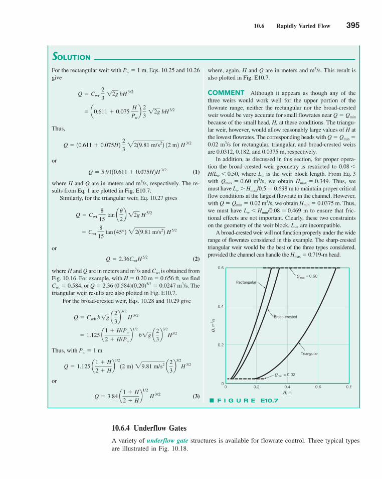
10.6 Rapidly Varied Flow 395

10.6.4 Underflow Gates

A variety of underflow gate structures is available for flowrate control. Three typical typesare illustrated in Fig. 10.18.

where, again, H and Q are in meters and m3/s. This result isalso plotted in Fig. E10.7.

COMMENT Although it appears as though any of thethree weirs would work well for the upper portion of theflowrate range, neither the rectangular nor the broad-crestedweir would be very accurate for small flowrates near Q � Qmin

because of the small head, H, at these conditions. The triangu-lar weir, however, would allow reasonably large values of H atthe lowest flowrates. The corresponding heads with Q � Qmin �0.02 m3/s for rectangular, triangular, and broad-crested weirsare 0.0312, 0.182, and 0.0375 m, respectively.

In addition, as discussed in this section, for proper opera-tion the broad-crested weir geometry is restricted to 0.08 �H/Lw � 0.50, where Lw is the weir block length. From Eq. 3with Qmax � 0.60 m3/s, we obtain Hmax � 0.349. Thus, wemust have Lw Hmax/0.5 � 0.698 m to maintain proper criticalflow conditions at the largest flowrate in the channel. However,with Q � Qmin � 0.02 m3/s, we obtain Hmin � 0.0375 m. Thus,we must have Lw � Hmin/0.08 � 0.469 m to ensure that fric-tional effects are not important. Clearly, these two constraintson the geometry of the weir block, Lw, are incompatible.

A broad-crested weir will not function properly under the widerange of flowrates considered in this example. The sharp-crestedtriangular weir would be the best of the three types considered,provided the channel can handle the Hmax � 0.719-m head.

SOLUTION

For the rectangular weir with Pw � 1 m, Eqs. 10.25 and 10.26give

Thus,

or

(1)

where H and Q are in meters and m3/s, respectively. The re-sults from Eq. 1 are plotted in Fig. E10.7.

Similarly, for the triangular weir, Eq. 10.27 gives

or

(2)

where H and Q are in meters and m3/s and Cwt is obtained fromFig. 10.16. For example, with H � 0.20 m � 0.656 ft, we findCwt � 0.584, or Q � 2.36 (0.584)(0.20)5/2 � 0.0247 m3/s. Thetriangular weir results are also plotted in Fig. E10.7.

For the broad-crested weir, Eqs. 10.28 and 10.29 give

Thus, with Pw � 1 m

or

(3) Q � 3.84 a1 � H

2 � Hb

1/2

H 3/2

Q � 1.125 a1 � H

2 � Hb

1/2

12 m2 29.81 m/s2 a2

3b

3/2

H 3/2

� 1.125 a1 � H/Pw

2 � H/Pw

b1/2

b1g a2

3b

3/2

H3/2

Q � Cwb b1g a2

3b

3/2

H 3/2

Q � 2.36Cwt H5/2

� Cwt 8

15 tan 145°2 2219.81 m/s22 H 5/2

Q � Cwt 8

15 tan a

2b 12g H 5/2

Q � 5.9110.611 � 0.075H2H 3/2

Q � 10.611 � 0.075H2 2

3 2219.81 m/s22 12 m2 H 3/2

� a0.611 � 0.075 H

Pw

b 2

3 12g bH 3/2

Q � Cwr 2

3 12g bH 3/2

F I G U R E E10.7

0.6

0.4

0.2

0 0.2 0.4 0.80.60

Q, m

3/s

H, m

Qmax = 0.60

Triangular

Rectangular

Broad-crested

Qmin = 0.02

c10OpenChannelFlow.qxd 9/28/10 10:36 AM Page 395

The flow under a gate is said to be free outflow when the fluid issues as a jet ofsupercritical flow with a free surface open to the atmosphere as shown in Fig. 10.18 andthe photograph in the margin. In such cases it is customary to write this flowrate as theproduct of the distance, a, between the channel bottom and the bottom of the gate timesthe convenient reference velocity (2gy1)

1/2. That is,

(10.30)

where q is the flowrate per unit width. The discharge coefficient, Cd, is a function of thecontraction coefficient, Cc � y2/a, and the depth ratio y1/a. Typical values of the dischargecoefficient for free outflow (or free discharge) from a vertical sluice gate are on the orderof 0.55 to 0.60 as indicated by the top line in Fig. 10.19 (Ref. 2).

As indicated in Fig. 10.20, in certain situations the jet of water issuing from underthe gate is overlaid by a mass of water that is quite turbulent. Typical values of Cd for thesedrowned outflow cases are indicated as the series of lower curves in Fig. 10.19.

q � Cd a12gy1

396 Chapter 10 ■ Open-Channel Flow

(Photograph courtesyof Pend Oreille PublicUtility District.)

V10.15 Spillwaygate

F I G U R E 10.18 Three variations of underflow gates: (a) vertical gate, (b) radial gate, and (c) drum gate.

(a) (b) (c)

y1y2

a

F I G U R E 10.19 Typical discharge coefficients for underflowgates (Ref. 3).

Free outflow

Drowned outflow

0.6

0.5

0.4

0.3

0.2

0.1

0 2 4 6 8 10 12 14 16

y1__a

Cd

y3__a

= 2 3 4 5 6 7 8

F I G U R E 10.20 Drowned outflowfrom a sluice gate.

q

a

y3

y1

V10.16 Unsteadyunder and over

c10OpenChannelFlow.qxd 9/28/10 10:36 AM Page 396

10.7 Chapter Summary and Study Guide 397

open-channel flowcritical flowsubcritical flowsupercritical flowwave speedFroude numberspecific energyspecific energy diagramuniform depth flowwetted perimeterhydraulic radiusChezy equationManning equationManning resistance

coefficientrapidly varied flowhydraulic jumpsharp-crested weirweir headbroad-crested weirunderflow gate

10.7 Chapter Summary and Study Guide

This chapter discussed various aspects of flows in an open channel. A typical open chan-nel flow is driven by the component of gravity in the direction of flow. The character ofsuch flows can be a strong function of the Froude number, which is the ratio of the fluidspeed to the free-surface wave speed. The specific energy diagram is used to provide insightinto the flow processes involved in open-channel flow.

Uniform depth channel flow is achieved by a balance between the potential energylost by the fluid as it coasts downhill and the energy dissipated by viscous effects. Alter-nately, it represents a balance between weight and friction forces. The relationship amongthe flowrate, the slope of the channel, the geometry of the channel, and the roughness ofthe channel surfaces is given by the Manning equation. Values of the Manning coefficientused in the Manning equation are dependent on the surface material roughness.

The hydraulic jump is an example of nonuniform depth open-channel flow. If theFroude number of a flow is greater than 1, the flow is supercritical, and a hydraulic jumpmay occur. The momentum and mass equations are used to obtain the relationship betweenthe upstream Froude number and the depth ratio across the jump. The energy dissipated inthe jump and the head loss can then be determined by use of the energy equation.

The use of weirs to measure the flowrate in an open channel is discussed. The rela-tionships between the flowrate and the weir head are given for both sharp-crested and broad-crested weirs.

The following checklist provides a study guide for this chapter. When your study ofthe entire chapter and end-of-chapter exercises has been completed, you should be able to

write out meanings of the terms listed here in the margin and understand each of therelated concepts. These terms are particularly important and are set in color and boldtype in the text.

determine the Froude number for a given flow and explain the concepts of subcriti-cal, critical, and supercritical flows.

plot and interpret the specific energy diagram for a given flow.

use the Manning equation to analyze uniform depth flow in an open channel.

calculate properties such as the depth ratio and the head loss for a hydraulic jump.

determine the flowrates over sharp-crested weirs, broad-crested weirs, and under theunderflow gates.

Some important equations in this chapter are:

Froude number

Wave speed (10.3)

Specific energy (10.7)

Manning equation (10.13)

Hydraulic jump depth ratio (10.19)

Hydraulic jump head loss (10.20)hL

y1� 1 �

y2

y1�

Fr12

2 c1 � a

y1

y2b

2

d

y2

y1�

1

2 1�1 � 21 � 8Fr1

2 2

V �k

n Rh

23S012

E � y �V 2

2g

c � 1gy

Fr � V 1gy212

c10OpenChannelFlow.qxd 9/28/10 10:36 AM Page 397

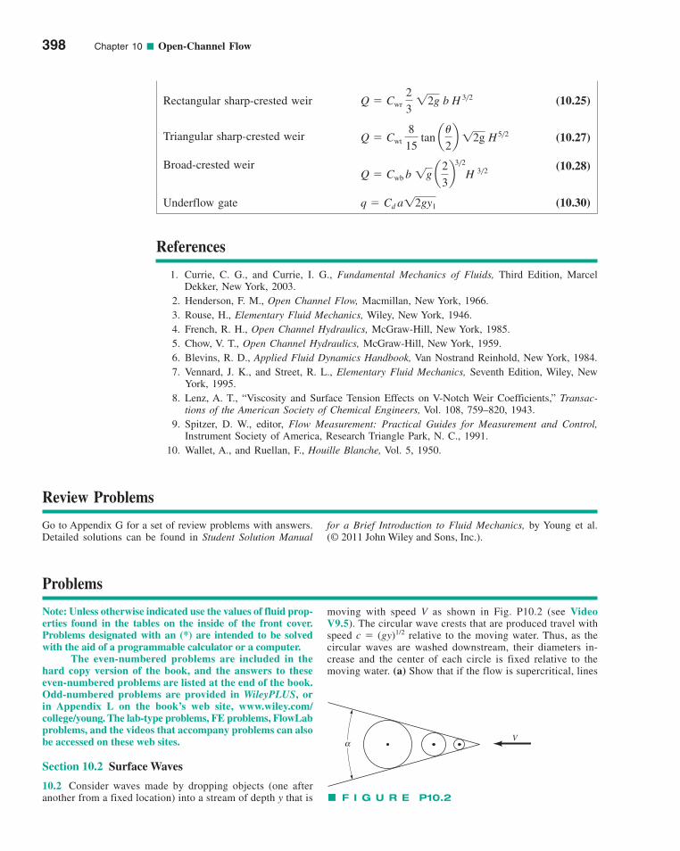
Rectangular sharp-crested weir (10.25)

Triangular sharp-crested weir (10.27)

Broad-crested weir (10.28)

Underflow gate (10.30)

References

1. Currie, C. G., and Currie, I. G., Fundamental Mechanics of Fluids, Third Edition, MarcelDekker, New York, 2003.

2. Henderson, F. M., Open Channel Flow, Macmillan, New York, 1966.3. Rouse, H., Elementary Fluid Mechanics, Wiley, New York, 1946.4. French, R. H., Open Channel Hydraulics, McGraw-Hill, New York, 1985.5. Chow, V. T., Open Channel Hydraulics, McGraw-Hill, New York, 1959.6. Blevins, R. D., Applied Fluid Dynamics Handbook, Van Nostrand Reinhold, New York, 1984.7. Vennard, J. K., and Street, R. L., Elementary Fluid Mechanics, Seventh Edition, Wiley, New

York, 1995.8. Lenz, A. T., “Viscosity and Surface Tension Effects on V-Notch Weir Coefficients,” Transac-

tions of the American Society of Chemical Engineers, Vol. 108, 759–820, 1943.9. Spitzer, D. W., editor, Flow Measurement: Practical Guides for Measurement and Control,

Instrument Society of America, Research Triangle Park, N. C., 1991.10. Wallet, A., and Ruellan, F., Houille Blanche, Vol. 5, 1950.

q � Cd a12gy1

Q � Cwb b 1g a2

3b

3�2

H 3�2

Q � Cwt 8

15 tan a

u

2b 12g H 5�2

Q � Cwr 2

3 12g b H 3�2

398 Chapter 10 ■ Open-Channel Flow

Review Problems

Go to Appendix G for a set of review problems with answers.Detailed solutions can be found in Student Solution Manual

for a Brief Introduction to Fluid Mechanics, by Young et al. (© 2011 John Wiley and Sons, Inc.).

Problems

Note: Unless otherwise indicated use the values of fluid prop-erties found in the tables on the inside of the front cover.Problems designated with an (*) are intended to be solvedwith the aid of a programmable calculator or a computer.

The even-numbered problems are included in thehard copy version of the book, and the answers to theseeven-numbered problems are listed at the end of the book.Odd-numbered problems are provided in WileyPLUS, orin Appendix L on the book’s web site, www.wiley.com/college/young. The lab-type problems, FE problems, FlowLabproblems, and the videos that accompany problems can alsobe accessed on these web sites.

Section 10.2 Surface Waves

10.2 Consider waves made by dropping objects (one afteranother from a fixed location) into a stream of depth y that is

moving with speed V as shown in Fig. P10.2 (see VideoV9.5). The circular wave crests that are produced travel withspeed c � (gy)1/2 relative to the moving water. Thus, as thecircular waves are washed downstream, their diameters in-crease and the center of each circle is fixed relative to themoving water. (a) Show that if the flow is supercritical, lines

F I G U R E P10.2

Vα

c10OpenChannelFlow.qxd 10/18/10 8:06 AM Page 398

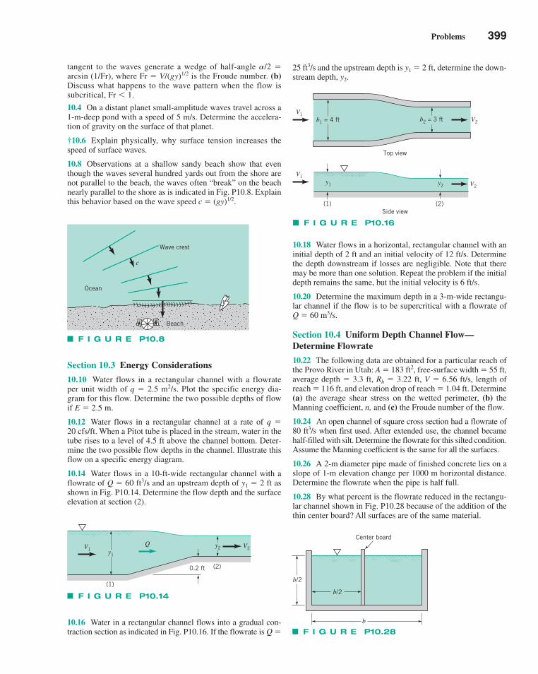
Problems 399

tangent to the waves generate a wedge of half-angle �/2 �arcsin (1/Fr), where Fr � V/(gy)1/2 is the Froude number. (b)Discuss what happens to the wave pattern when the flow issubcritical, Fr � 1.

10.4 On a distant planet small-amplitude waves travel across a1-m-deep pond with a speed of 5 m/s. Determine the accelera-tion of gravity on the surface of that planet.

†10.6 Explain physically, why surface tension increases thespeed of surface waves.

10.8 Observations at a shallow sandy beach show that eventhough the waves several hundred yards out from the shore arenot parallel to the beach, the waves often “break” on the beachnearly parallel to the shore as is indicated in Fig. P10.8. Explainthis behavior based on the wave speed c � (gy)1/2.

Section 10.3 Energy Considerations

10.10 Water flows in a rectangular channel with a flowrateper unit width of q � 2.5 m2/s. Plot the specific energy dia-gram for this flow. Determine the two possible depths of flowif E � 2.5 m.

10.12 Water flows in a rectangular channel at a rate of q �20 cfs/ft. When a Pitot tube is placed in the stream, water in thetube rises to a level of 4.5 ft above the channel bottom. Deter-mine the two possible flow depths in the channel. Illustrate thisflow on a specific energy diagram.

10.14 Water flows in a 10-ft-wide rectangular channel with aflowrate of Q � 60 ft3/s and an upstream depth of y1 � 2 ft asshown in Fig. P10.14. Determine the flow depth and the surfaceelevation at section (2).

10.16 Water in a rectangular channel flows into a gradual con-traction section as indicated in Fig. P10.16. If the flowrate is Q �

25 ft3/s and the upstream depth is y1 � 2 ft, determine the down-stream depth, y2.

10.18 Water flows in a horizontal, rectangular channel with aninitial depth of 2 ft and an initial velocity of 12 ft/s. Determinethe depth downstream if losses are negligible. Note that theremay be more than one solution. Repeat the problem if the initialdepth remains the same, but the initial velocity is 6 ft/s.

10.20 Determine the maximum depth in a 3-m-wide rectangu-lar channel if the flow is to be supercritical with a flowrate of Q � 60 m3/s.

Section 10.4 Uniform Depth Channel Flow—Determine Flowrate

10.22 The following data are obtained for a particular reach ofthe Provo River in Utah: A � 183 ft2, free-surface width � 55 ft,average depth � 3.3 ft, Rh � 3.22 ft, V � 6.56 ft/s, length ofreach � 116 ft, and elevation drop of reach � 1.04 ft. Determine(a) the average shear stress on the wetted perimeter, (b) theManning coefficient, n, and (c) the Froude number of the flow.

10.24 An open channel of square cross section had a flowrate of80 ft3/s when first used. After extended use, the channel becamehalf-filled with silt. Determine the flowrate for this silted condition.Assume the Manning coefficient is the same for all the surfaces.

10.26 A 2-m diameter pipe made of finished concrete lies on aslope of 1-m elevation change per 1000 m horizontal distance.Determine the flowrate when the pipe is half full.

10.28 By what percent is the flowrate reduced in the rectangu-lar channel shown in Fig. P10.28 because of the addition of thethin center board? All surfaces are of the same material.

F I G U R E P10.8

Wave crest

Ocean

c

Beach

F I G U R E P10.16

V1V2

V1

V2

(2)(1)

y1 y2

Side view

Top view

b2 = 3 ftb1 = 4 ft

F I G U R E P10.14

V1Q V2

y1

y2

0.2 ft (2)

(1)

F I G U R E P10.28

b/2

b/2

b

Center board

c10OpenChannelFlow.qxd 9/28/10 10:36 AM Page 399

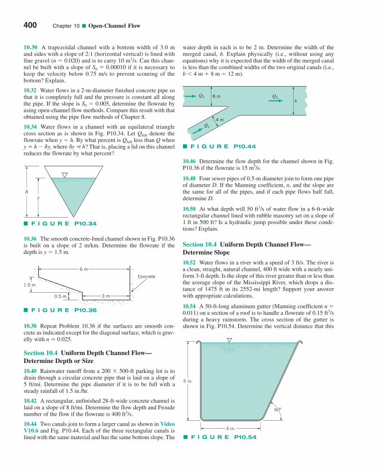
10.30 A trapezoidal channel with a bottom width of 3.0 mand sides with a slope of 2:1 (horizontal vertical) is lined withfine gravel (n � 0.020) and is to carry 10 m3/s. Can this chan-nel be built with a slope of S0 � 0.00010 if it is necessary tokeep the velocity below 0.75 m/s to prevent scouring of thebottom? Explain.

10.32 Water flows in a 2-m-diameter finished concrete pipe sothat it is completely full and the pressure is constant all alongthe pipe. If the slope is S0 � 0.005, determine the flowrate byusing open-channel flow methods. Compare this result with thatobtained using the pipe flow methods of Chapter 8.

10.34 Water flows in a channel with an equilateral trianglecross section as is shown in Fig. P10.34. Let Qfull denote theflowrate when y � h. By what percent is Qfull less than Q wheny � h � �y, where �y � h? That is, placing a lid on this channelreduces the flowrate by what percent?

10.36 The smooth concrete-lined channel shown in Fig. P10.36is built on a slope of 2 m/km. Determine the flowrate if thedepth is y � 1.5 m.

10.38 Repeat Problem 10.36 if the surfaces are smooth con-crete as indicated except for the diagonal surface, which is grav-elly with n � 0.025.

Section 10.4 Uniform Depth Channel Flow—Determine Depth or Size

10.40 Rainwater runoff from a 200 500-ft parking lot is todrain through a circular concrete pipe that is laid on a slope of 5 ft/mi. Determine the pipe diameter if it is to be full with asteady rainfall of 1.5 in./hr.

10.42 A rectangular, unfinished 28-ft-wide concrete channel islaid on a slope of 8 ft/mi. Determine the flow depth and Froudenumber of the flow if the flowrate is 400 ft3/s.

10.44 Two canals join to form a larger canal as shown in VideoV10.6 and Fig. P10.44. Each of the three rectangular canals islined with the same material and has the same bottom slope. The

water depth in each is to be 2 m. Determine the width of themerged canal, b. Explain physically (i.e., without using anyequations) why it is expected that the width of the merged canalis less than the combined widths of the two original canals (i.e.,b � 4 m � 8 m � 12 m).

10.46 Determine the flow depth for the channel shown in Fig.P10.36 if the flowrate is 15 m3/s.

10.48 Four sewer pipes of 0.5-m diameter join to form one pipeof diameter D. If the Manning coefficient, n, and the slope arethe same for all of the pipes, and if each pipe flows half full,determine D.

10.50 At what depth will 50 ft3/s of water flow in a 6-ft-widerectangular channel lined with rubble masonry set on a slope of1 ft in 500 ft? Is a hydraulic jump possible under these condi-tions? Explain.

Section 10.4 Uniform Depth Channel Flow—Determine Slope

10.52 Water flows in a river with a speed of 3 ft/s. The river isa clean, straight, natural channel, 400 ft wide with a nearly uni-form 3-ft depth. Is the slope of this river greater than or less thanthe average slope of the Mississippi River, which drops a dis-tance of 1475 ft in its 2552-mi length? Support your answerwith appropriate calculations.

10.54 A 50-ft-long aluminum gutter (Manning coefficient n �0.011) on a section of a roof is to handle a flowrate of 0.15 ft3/sduring a heavy rainstorm. The cross section of the gutter isshown in Fig. P10.54. Determine the vertical distance that this

400 Chapter 10 ■ Open-Channel Flow

F I G U R E P10.34

y

h

F I G U R E P10.44

8 m

4 m

b

Q2

Q1

Q3

F I G U R E P10.54

60�

3 in.

5 in.

F I G U R E P10.36

0.5 m

1.0 m

6 m

3 m

Concrete

c10OpenChannelFlow.qxd 9/28/10 10:36 AM Page 400

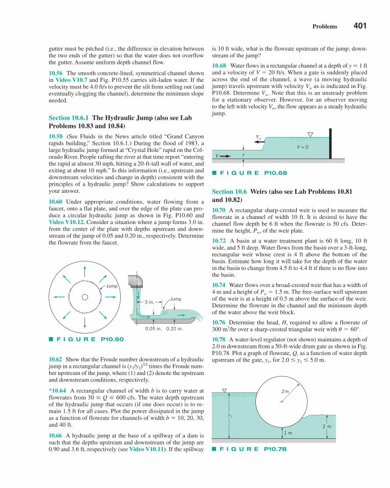
Problems 401

gutter must be pitched (i.e., the difference in elevation betweenthe two ends of the gutter) so that the water does not overflowthe gutter. Assume uniform depth channel flow.

10.56 The smooth concrete-lined, symmetrical channel shownin Video V10.7 and Fig. P10.55 carries silt-laden water. If thevelocity must be 4.0 ft/s to prevent the silt from settling out (andeventually clogging the channel), determine the minimum slopeneeded.

Section 10.6.1 The Hydraulic Jump (also see LabProblems 10.83 and 10.84)

10.58 (See Fluids in the News article titled “Grand Canyonrapids building,” Section 10.6.1.) During the flood of 1983, alarge hydraulic jump formed at “Crystal Hole” rapid on the Col-orado River. People rafting the river at that time report “enteringthe rapid at almost 30 mph, hitting a 20-ft-tall wall of water, andexiting at about 10 mph.” Is this information (i.e., upstream anddownstream velocities and change in depth) consistent with theprinciples of a hydraulic jump? Show calculations to supportyour answer.

10.60 Under appropriate conditions, water flowing from afaucet, onto a flat plate, and over the edge of the plate can pro-duce a circular hydraulic jump as shown in Fig. P10.60 andVideo V10.12. Consider a situation where a jump forms 3.0 in.from the center of the plate with depths upstream and down-stream of the jump of 0.05 and 0.20 in., respectively. Determinethe flowrate from the faucet.

10.62 Show that the Froude number downstream of a hydraulicjump in a rectangular channel is (y1/y2)

3/2 times the Froude num-ber upstream of the jump, where (1) and (2) denote the upstreamand downstream conditions, respectively.

*10.64 A rectangular channel of width b is to carry water atflowrates from 30 � Q � 600 cfs. The water depth upstreamof the hydraulic jump that occurs (if one does occur) is to re-main 1.5 ft for all cases. Plot the power dissipated in the jumpas a function of flowrate for channels of width b � 10, 20, 30,and 40 ft.

10.66 A hydraulic jump at the base of a spillway of a dam issuch that the depths upstream and downstream of the jump are0.90 and 3.6 ft, respectively (see Video V10.11). If the spillway

is 10 ft wide, what is the flowrate upstream of the jump; down-stream of the jump?

10.68 Water flows in a rectangular channel at a depth of y � 1 ftand a velocity of V � 20 ft/s. When a gate is suddenly placedacross the end of the channel, a wave (a moving hydraulicjump) travels upstream with velocity Vw as is indicated in Fig.P10.68. Determine Vw. Note that this is an unsteady problemfor a stationary observer. However, for an observer moving to the left with velocity Vw, the flow appears as a steady hydraulicjump.

Section 10.6 Weirs (also see Lab Problems 10.81 and 10.82)

10.70 A rectangular sharp-crested weir is used to measure theflowrate in a channel of width 10 ft. It is desired to have thechannel flow depth be 6 ft when the flowrate is 50 cfs. Deter-mine the height, Pw, of the weir plate.

10.72 A basin at a water treatment plant is 60 ft long, 10 ftwide, and 5 ft deep. Water flows from the basin over a 3-ft-long,rectangular weir whose crest is 4 ft above the bottom of thebasin. Estimate how long it will take for the depth of the waterin the basin to change from 4.5 ft to 4.4 ft if there is no flow intothe basin.

10.74 Water flows over a broad-crested weir that has a width of4 m and a height of Pw � 1.5 m. The free-surface well upstreamof the weir is at a height of 0.5 m above the surface of the weir.Determine the flowrate in the channel and the minimum depthof the water above the weir block.

10.76 Determine the head, H, required to allow a flowrate of300 m3/hr over a sharp-crested triangular weir with .

10.78 A water-level regulator (not shown) maintains a depth of2.0 m downstream from a 50-ft-wide drum gate as shown in Fig.P10.78. Plot a graph of flowrate, Q, as a function of water depthupstream of the gate, y1, for 2.0 � y1 � 5.0 m.

� 60°

F I G U R E P10.60

Jump

3 in.Jump

0.05 in. 0.20 in.

F I G U R E P10.78

1 m2 m

2m

y1

F I G U R E P10.68

V y

Vw

V = 0

c10OpenChannelFlow.qxd 9/28/10 10:36 AM Page 401

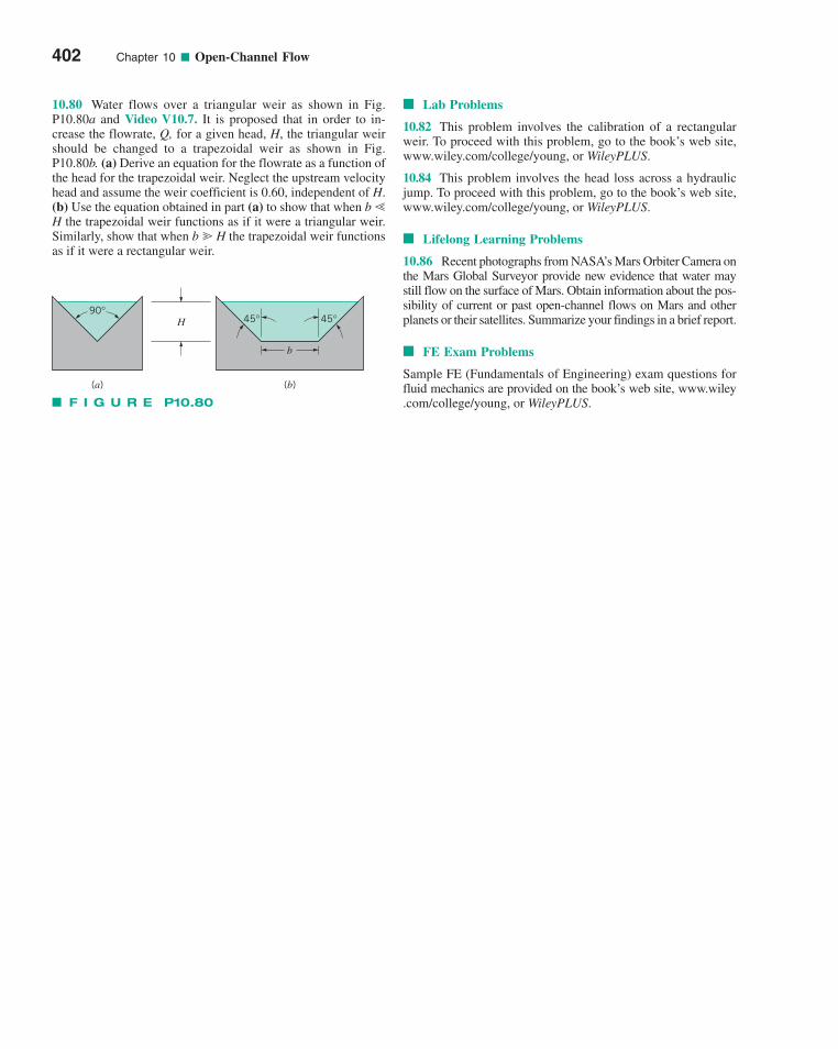
10.80 Water flows over a triangular weir as shown in Fig.P10.80a and Video V10.7. It is proposed that in order to in-crease the flowrate, Q, for a given head, H, the triangular weirshould be changed to a trapezoidal weir as shown in Fig.P10.80b. (a) Derive an equation for the flowrate as a function ofthe head for the trapezoidal weir. Neglect the upstream velocityhead and assume the weir coefficient is 0.60, independent of H.(b) Use the equation obtained in part (a) to show that when b �H the trapezoidal weir functions as if it were a triangular weir.Similarly, show that when b � H the trapezoidal weir functionsas if it were a rectangular weir.

■ Lab Problems

10.82 This problem involves the calibration of a rectangularweir. To proceed with this problem, go to the book’s web site,www.wiley.com/college/young, or WileyPLUS.

10.84 This problem involves the head loss across a hydraulicjump. To proceed with this problem, go to the book’s web site,www.wiley.com/college/young, or WileyPLUS.

■ Lifelong Learning Problems

10.86 Recent photographs from NASA’s Mars Orbiter Camera onthe Mars Global Surveyor provide new evidence that water maystill flow on the surface of Mars. Obtain information about the pos-sibility of current or past open-channel flows on Mars and otherplanets or their satellites. Summarize your findings in a brief report.

■ FE Exam Problems

Sample FE (Fundamentals of Engineering) exam questions forfluid mechanics are provided on the book’s web site, www.wiley.com/college/young, or WileyPLUS.

402 Chapter 10 ■ Open-Channel Flow

F I G U R E P10.80

90°45° 45°

b

H

(a) (b)

c10OpenChannelFlow.qxd 9/28/10 10:36 AM Page 402

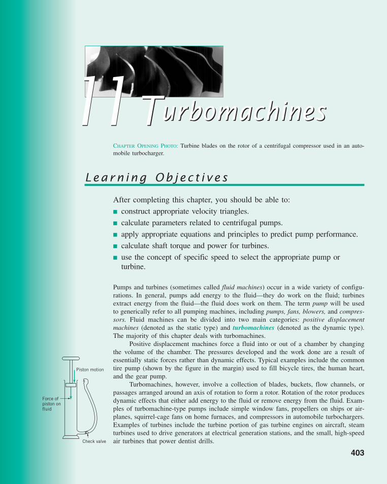
CHAPTER OPENING PHOTO: Turbine blades on the rotor of a centrifugal compressor used in an auto-mobile turbocharger.

1111TurbomachinesTurbomachines

Learn ing Ob j ec t i v e s

After completing this chapter, you should be able to:

■ construct appropriate velocity triangles.

■ calculate parameters related to centrifugal pumps.

■ apply appropriate equations and principles to predict pump performance.

■ calculate shaft torque and power for turbines.

■ use the concept of specific speed to select the appropriate pump orturbine.

Pumps and turbines (sometimes called fluid machines) occur in a wide variety of configu-rations. In general, pumps add energy to the fluid—they do work on the fluid; turbinesextract energy from the fluid—the fluid does work on them. The term pump will be usedto generically refer to all pumping machines, including pumps, fans, blowers, and compres-sors. Fluid machines can be divided into two main categories: positive displacementmachines (denoted as the static type) and turbomachines (denoted as the dynamic type).The majority of this chapter deals with turbomachines.

Positive displacement machines force a fluid into or out of a chamber by changingthe volume of the chamber. The pressures developed and the work done are a result ofessentially static forces rather than dynamic effects. Typical examples include the commontire pump (shown by the figure in the margin) used to fill bicycle tires, the human heart,and the gear pump.

Turbomachines, however, involve a collection of blades, buckets, flow channels, orpassages arranged around an axis of rotation to form a rotor. Rotation of the rotor producesdynamic effects that either add energy to the fluid or remove energy from the fluid. Exam-ples of turbomachine-type pumps include simple window fans, propellers on ships or air-planes, squirrel-cage fans on home furnaces, and compressors in automobile turbochargers.Examples of turbines include the turbine portion of gas turbine engines on aircraft, steamturbines used to drive generators at electrical generation stations, and the small, high-speedair turbines that power dentist drills.

403

Check valve

Piston motion

Force ofpiston onfluid

c11Turbomachines.qxd 9/28/10 10:38 AM Page 403

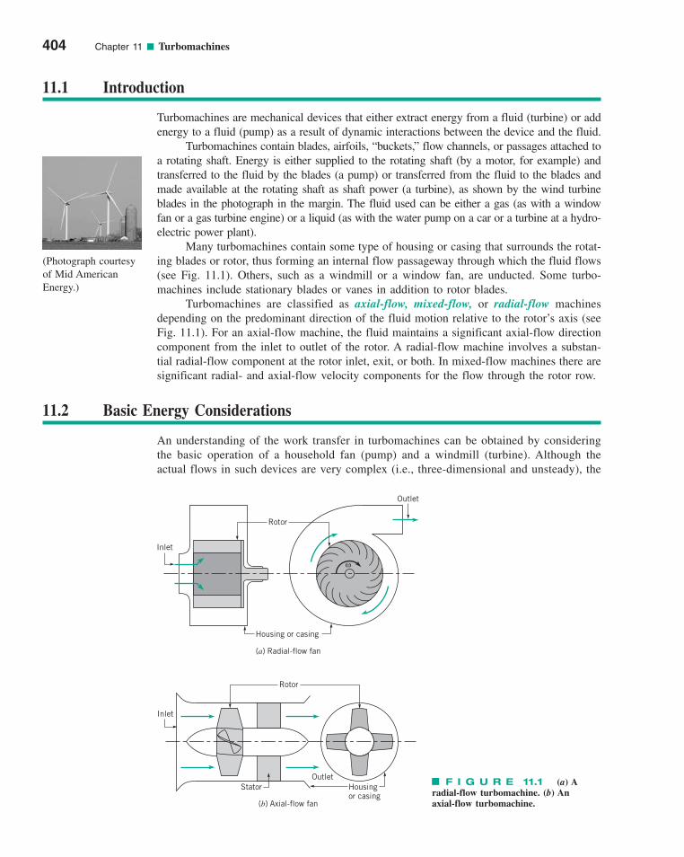
404 Chapter 11 ■ Turbomachines

11.1 Introduction

Turbomachines are mechanical devices that either extract energy from a fluid (turbine) or addenergy to a fluid (pump) as a result of dynamic interactions between the device and the fluid.

Turbomachines contain blades, airfoils, “buckets,” flow channels, or passages attached toa rotating shaft. Energy is either supplied to the rotating shaft (by a motor, for example) andtransferred to the fluid by the blades (a pump) or transferred from the fluid to the blades andmade available at the rotating shaft as shaft power (a turbine), as shown by the wind turbineblades in the photograph in the margin. The fluid used can be either a gas (as with a windowfan or a gas turbine engine) or a liquid (as with the water pump on a car or a turbine at a hydro-electric power plant).

Many turbomachines contain some type of housing or casing that surrounds the rotat-ing blades or rotor, thus forming an internal flow passageway through which the fluid flows(see Fig. 11.1). Others, such as a windmill or a window fan, are unducted. Some turbo-machines include stationary blades or vanes in addition to rotor blades.

Turbomachines are classified as axial-flow, mixed-flow, or radial-flow machinesdepending on the predominant direction of the fluid motion relative to the rotor’s axis (seeFig. 11.1). For an axial-flow machine, the fluid maintains a significant axial-flow directioncomponent from the inlet to outlet of the rotor. A radial-flow machine involves a substan-tial radial-flow component at the rotor inlet, exit, or both. In mixed-flow machines there aresignificant radial- and axial-flow velocity components for the flow through the rotor row.

11.2 Basic Energy Considerations

An understanding of the work transfer in turbomachines can be obtained by consideringthe basic operation of a household fan (pump) and a windmill (turbine). Although theactual flows in such devices are very complex (i.e., three-dimensional and unsteady), the

F I G U R E 11.1 (a) Aradial-flow turbomachine. (b) An axial-flow turbomachine.

Rotor

Inlet

Housing or casing

Outlet

(a) Radial-flow fan

(b) Axial-flow fan

Housingor casing

Inlet

Rotor

OutletStator

ω

(Photograph courtesyof Mid American Energy.)

c11Turbomachines.qxd 9/28/10 10:38 AM Page 404

11.2 Basic Energy Considerations 405

b c

a d

Axial

Tangential

U1

V1

W1

Blade motion

Inletsurface

Exit surface

Blade crosssection

U2

V2

W2

(1)

(2)

ad

c

r

Q

ω

(a)

(b)

essential phenomena can be illustrated by use of simplified considerations and velocitytriangles.

Consider a fan blade driven at constant angular velocity, �, by a motor as is shownin Fig. 11.2a. We denote the blade speed as U � �r, where r is the radial distance fromthe axis of the fan. The absolute fluid velocity (that seen by a person sitting stationary at

F I G U R E 11.2Idealized flow through a fan:(a) fan blade geometry and(b) absolute velocity, V; rela-tive velocity, W; and bladevelocity, U; at the inlet andexit of the fan blade section.

c11Turbomachines.qxd 9/28/10 10:38 AM Page 405

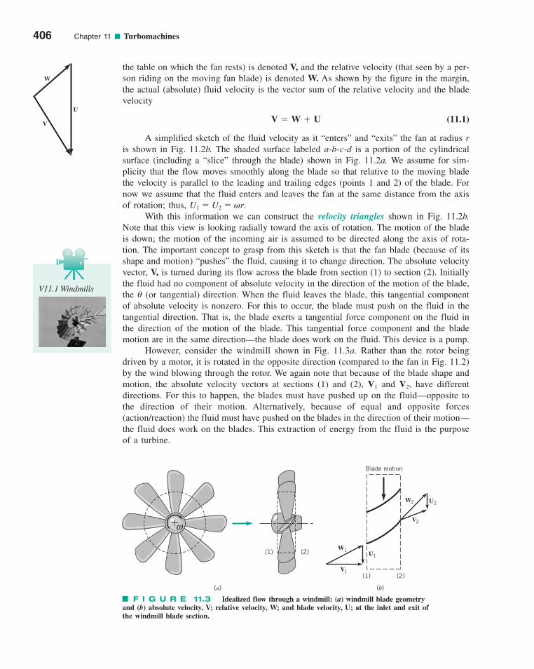
the table on which the fan rests) is denoted V, and the relative velocity (that seen by a per-son riding on the moving fan blade) is denoted W. As shown by the figure in the margin,the actual (absolute) fluid velocity is the vector sum of the relative velocity and the bladevelocity

(11.1)

A simplified sketch of the fluid velocity as it “enters” and “exits” the fan at radius ris shown in Fig. 11.2b. The shaded surface labeled a-b-c-d is a portion of the cylindricalsurface (including a “slice” through the blade) shown in Fig. 11.2a. We assume for sim-plicity that the flow moves smoothly along the blade so that relative to the moving bladethe velocity is parallel to the leading and trailing edges (points 1 and 2) of the blade. Fornow we assume that the fluid enters and leaves the fan at the same distance from the axisof rotation; thus, U1 � U2 � �r.

With this information we can construct the velocity triangles shown in Fig. 11.2b.Note that this view is looking radially toward the axis of rotation. The motion of the bladeis down; the motion of the incoming air is assumed to be directed along the axis of rota-tion. The important concept to grasp from this sketch is that the fan blade (because of itsshape and motion) “pushes” the fluid, causing it to change direction. The absolute velocityvector, V, is turned during its flow across the blade from section (1) to section (2). Initiallythe fluid had no component of absolute velocity in the direction of the motion of the blade,the � (or tangential) direction. When the fluid leaves the blade, this tangential componentof absolute velocity is nonzero. For this to occur, the blade must push on the fluid in thetangential direction. That is, the blade exerts a tangential force component on the fluid inthe direction of the motion of the blade. This tangential force component and the blademotion are in the same direction—the blade does work on the fluid. This device is a pump.

However, consider the windmill shown in Fig. 11.3a. Rather than the rotor being driven by a motor, it is rotated in the opposite direction (compared to the fan in Fig. 11.2)by the wind blowing through the rotor. We again note that because of the blade shape andmotion, the absolute velocity vectors at sections (1) and (2), V1 and V2, have differentdirections. For this to happen, the blades must have pushed up on the fluid—opposite tothe direction of their motion. Alternatively, because of equal and opposite forces(action/reaction) the fluid must have pushed on the blades in the direction of their motion—the fluid does work on the blades. This extraction of energy from the fluid is the purposeof a turbine.

V � W � U

406 Chapter 11 ■ Turbomachines

V

U

W

V11.1 Windmills

Blade motion

(2)(1)

(1) (2)

U2

V2

W2

U1

V1

W1

ω

(a) (b)

F I G U R E 11.3 Idealized flow through a windmill: (a) windmill blade geometryand (b) absolute velocity, V; relative velocity, W; and blade velocity, U; at the inlet and exit ofthe windmill blade section.

c11Turbomachines.qxd 9/28/10 10:38 AM Page 406

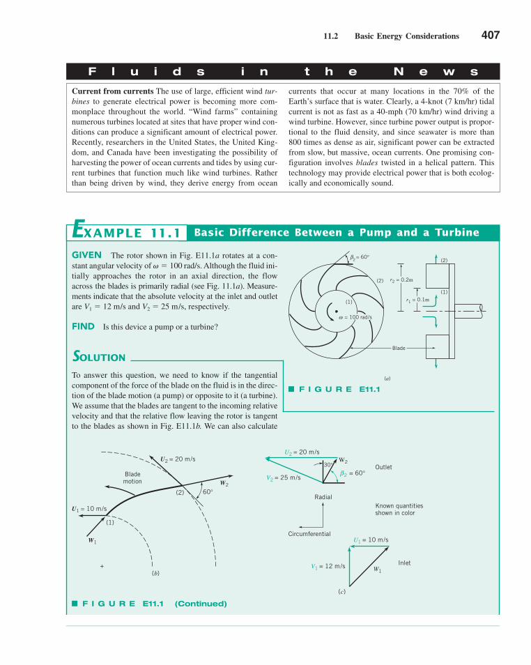
11.2 Basic Energy Considerations 407

F l u i d s i n t h e N e w s

Current from currents The use of large, efficient wind tur-bines to generate electrical power is becoming more com-monplace throughout the world. “Wind farms” containing numerous turbines located at sites that have proper wind con-ditions can produce a significant amount of electrical power.Recently, researchers in the United States, the United King-dom, and Canada have been investigating the possibility ofharvesting the power of ocean currents and tides by using cur-rent turbines that function much like wind turbines. Ratherthan being driven by wind, they derive energy from ocean

currents that occur at many locations in the 70% of theEarth’s surface that is water. Clearly, a 4-knot (7 km/hr) tidalcurrent is not as fast as a 40-mph (70 km/hr) wind driving awind turbine. However, since turbine power output is propor-tional to the fluid density, and since seawater is more than800 times as dense as air, significant power can be extractedfrom slow, but massive, ocean currents. One promising con-figuration involves blades twisted in a helical pattern. Thistechnology may provide electrical power that is both ecolog-ically and economically sound.

GIVEN The rotor shown in Fig. E11.1a rotates at a con-stant angular velocity of � � 100 rad/s. Although the fluid ini-tially approaches the rotor in an axial direction, the flowacross the blades is primarily radial (see Fig. 11.1a). Measure-ments indicate that the absolute velocity at the inlet and outletare V1 � 12 m/s and V2 � 25 m/s, respectively.

FIND Is this device a pump or a turbine?

SOLUTION

Basic Difference Between a Pump and a TurbineEXAMPLE 11.1

To answer this question, we need to know if the tangentialcomponent of the force of the blade on the fluid is in the direc-tion of the blade motion (a pump) or opposite to it (a turbine).We assume that the blades are tangent to the incoming relativevelocity and that the relative flow leaving the rotor is tangentto the blades as shown in Fig. E11.1b. We can also calculate

F I G U R E E11.1

F I G U R E E11.1 (Continued)

Blade

(1)

(2)

(1)

(2) = 60°β

= 100 rad/sω

r2 = 0.2m

r1 = 0.1m

2

(a)

(1)

(2) 60°W2

U2 = 20 m/s

Blademotion

W1

U1 = 10 m/s

+

W2

U2 = 20 m/s

V2 = 25 m/s= 60°β2

30°

Radial

Circumferential

W1V1 = 12 m/s

U1 = 10 m/s

Outlet

Known quantitiesshown in color

Inlet

(c)

(b)

c11Turbomachines.qxd 9/28/10 10:38 AM Page 407

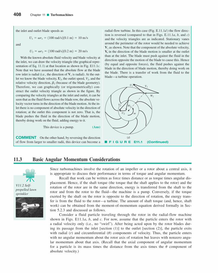
408 Chapter 11 ■ Turbomachines

radial-flow turbine. In this case (Fig. E.11.1d ) the flow direc-tion is reversed (compared to that in Figs. E.11.1a, b, and c)and the velocity triangles are as indicated. Stationary vanesaround the perimeter of the rotor would be needed to achieveV1 as shown. Note that the component of the absolute velocity,V, in the direction of the blade motion is smaller at the outletthan at the inlet. The blade must push against the fluid in thedirection opposite the motion of the blade to cause this. Hence(by equal and opposite forces), the fluid pushes against theblade in the direction of blade motion, thereby doing work onthe blade. There is a transfer of work from the fluid to theblade—a turbine operation.

the inlet and outlet blade speeds as

and

With the known absolute fluid velocity and blade velocity atthe inlet, we can draw the velocity triangle (the graphical repre-sentation of Eq. 11.1) at that location as shown in Fig. E11.1c.Note that we have assumed that the absolute flow at the bladerow inlet is radial (i.e., the direction of V1 is radial). At the out-let we know the blade velocity, U2, the outlet speed, V2, and therelative velocity direction, �2 (because of the blade geometry).Therefore, we can graphically (or trigonometrically) con-struct the outlet velocity triangle as shown in the figure. Bycomparing the velocity triangles at the inlet and outlet, it can beseen that as the fluid flows across the blade row, the absolute ve-locity vector turns in the direction of the blade motion. At the in-let there is no component of absolute velocity in the direction ofrotation; at the outlet this component is not zero. That is, theblade pushes the fluid in the direction of the blade motion,thereby doing work on the fluid, adding energy to it.

This device is a pump. (Ans)

COMMENT On the other hand, by reversing the directionof flow from larger to smaller radii, this device can become a

U2 � �r2 � 1100 rad/s2 10.2 m2 � 20 m/s

U1 � �r1 � 1100 rad /s2 10.1 m2 � 10 m/s

F I G U R E E11.1 (Continued)

ω

W1

W2

U2

V1U1

V2

(d)

11.3 Basic Angular Momentum Considerations

Since turbomachines involve the rotation of an impeller or a rotor about a central axis, itis appropriate to discuss their performance in terms of torque and angular momentum.

Recall that work can be written as force times distance or as torque times angular dis-placement. Hence, if the shaft torque (the torque that the shaft applies to the rotor) and therotation of the rotor are in the same direction, energy is transferred from the shaft to therotor and from the rotor to the fluid—the machine is a pump. Conversely, if the torqueexerted by the shaft on the rotor is opposite to the direction of rotation, the energy trans-fer is from the fluid to the rotor—a turbine. The amount of shaft torque (and, hence, shaftwork) can be obtained from the moment-of-momentum equation derived formally in Sec-tion 5.2.3 and discussed as follows.

Consider a fluid particle traveling through the rotor in the radial-flow machineshown in Figs. E11.1a, b, and c. For now, assume that the particle enters the rotor witha radial velocity only (i.e., no “swirl”). After being acted upon by the rotor blades dur-ing its passage from the inlet [section (1)] to the outlet [section (2)], the particle exitswith radial (r) and circumferential (�) components of velocity. Thus, the particle enterswith no angular momentum about the rotor axis of rotation but leaves with nonzero angu-lar momentum about that axis. (Recall that the axial component of angular momentumfor a particle is its mass times the distance from the axis times the � component ofabsolute velocity.)

V11.2 Self-propelled lawnsprinkler

c11Turbomachines.qxd 9/28/10 10:38 AM Page 408

11.3 Basic Angular Momentum Considerations 409

In a turbomachine a series of particles (a continuum) passes through the rotor. Thus,the moment-of-momentum equation applied to a control volume as derived in Section 5.2.3is valid. For steady flow Eq. 5.21 gives

Recall that the left-hand side of this equation represents the sum of the external torques(moments) acting on the contents of the control volume, and the right-hand side is thenet rate of flow of moment-of-momentum (angular momentum) through the controlsurface.

The axial component of this equation applied to the one-dimensional simplificationof flow through a turbomachine rotor with section (1) as the inlet and section (2) as theoutlet results in

(11.2)

where Tshaft is the shaft torque applied to the contents of the control volume. The “�” isassociated with mass flowrate into the control volume, and the “�” is used with the out-flow. The sign of the V� component depends on the direction of V� and the blade motion,U. If V� and U are in the same direction, then V� is positive. The sign of the torque exertedby the shaft on the rotor, Tshaft, is positive if Tshaft is in the same direction as rotation andnegative otherwise.

As seen from Eq. 11.2, the shaft torque is directly proportional to the mass flowrate,(It takes considerably more torque and power to pump water than to pump air

with the same volume flowrate.) The torque also depends on the tangential componentof the absolute velocity, V�. Equation 11.2 is often called the Euler turbomachineequation.

Also recall that the shaft power, is related to the shaft torque and angular veloc-ity by

(11.3)

By combining Eqs. 11.2 and 11.3 and using the fact that U � �r, we obtain

(11.4)

Again, the value of V� is positive when V� and U are in the same direction and negativeotherwise. Also, is positive when the shaft torque and � are in the same directionand negative otherwise. Thus, is positive when power is supplied to the contents of thecontrol volume (pumps) and negative otherwise (turbines). This outcome is consistent withthe sign convention involving the work term in the energy equation considered in Chapter 5(see Eq. 5.44).

Finally, in terms of work per unit mass, we obtain

(11.5)

where we have used the fact that by conservation of mass, Equations 11.3, 11.4,and 11.5 are the basic governing equations for pumps or turbines whether the machines areradial-, mixed-, or axial-flow devices and for compressible and incompressible flows. Notethat neither the axial nor the radial component of velocity enters into the specific work(work per unit mass) equation.

m� 1 � m� 2.

wshaft � �U1V�1 � U2V�2

wshaft � W#

shaft /m# ,

W.

shaft

W.

shaft

W#

shaft � �m#

11U1V�12 � m#

21U2V�22

W#

shaft � Tshaft �

W.

shaft,

m� � �Q.

Tshaft � �m� 11r1V�12 � m� 21r2V�22

a 1r � F2 �a 1r � V2out�outAoutVout �a 1r � V2in�inAinVin

c11Turbomachines.qxd 9/28/10 10:38 AM Page 409

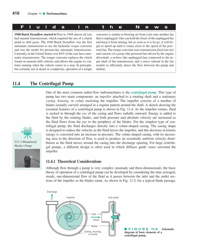
410 Chapter 11 ■ Turbomachines

F l u i d s i n t h e N e w s

1948 Buick Dynaflow started it Prior to 1948 almost all carshad manual transmissions, which required the use of a clutchpedal to shift gears. The 1948 Buick Dynaflow was the firstautomatic transmission to use the hydraulic torque converterand was the model for present-day automatic transmissions.Currently, in the United States over 84% of the cars have auto-matic transmissions. The torque converter replaces the clutchfound on manual-shift vehicles and allows the engine to con-tinue running when the vehicle comes to a stop. In principle,but certainly not in detail or complexity, operation of a torque

converter is similar to blowing air from a fan onto another fanthat is unplugged. One can hold the blade of the unplugged fanand keep it from turning, but as soon as it is let go, it will be-gin to speed up until it comes close to the speed of the pow-ered fan. The torque converter uses transmission fluid (not air)and consists of a pump (the powered fan) driven by the enginedriveshaft, a turbine (the unplugged fan) connected to the in-put shaft of the transmission, and a stator (absent in the fanmodel) to efficiently direct the flow between the pump andturbine.

11.4 The Centrifugal Pump

One of the most common radial-flow turbomachines is the centrifugal pump. This type ofpump has two main components: an impeller attached to a rotating shaft and a stationarycasing, housing, or volute enclosing the impeller. The impeller consists of a number ofblades (usually curved) arranged in a regular pattern around the shaft. A sketch showing theessential features of a centrifugal pump is shown in Fig. 11.4. As the impeller rotates, fluidis sucked in through the eye of the casing and flows radially outward. Energy is added tothe fluid by the rotating blades, and both pressure and absolute velocity are increased asthe fluid flows from the eye to the periphery of the blades. For the simplest type of cen-trifugal pump, the fluid discharges directly into a volute-shaped casing. The casing shapeis designed to reduce the velocity as the fluid leaves the impeller, and this decrease in kineticenergy is converted into an increase in pressure. The volute-shaped casing, with its increas-ing area in the direction of flow, is used to produce an essentially uniform velocity distri-bution as the fluid moves around the casing into the discharge opening. For large centrifu-gal pumps, a different design is often used in which diffuser guide vanes surround theimpeller.

11.4.1 Theoretical Considerations

Although flow through a pump is very complex (unsteady and three-dimensional), the basictheory of operation of a centrifugal pump can be developed by considering the time averaged,steady, one-dimensional flow of the fluid as it passes between the inlet and the outlet sec-tions of the impeller as the blades rotate. As shown in Fig. 11.5, for a typical blade passage,

F I G U R E 11.4 Schematicdiagram of basic elements of a centrifugal pump.

Discharge

Impeller

Eye

Inflow

Blade

Hub plate

Casing, housing,or volute

V11.3 WindshieldWasher Pump

c11Turbomachines.qxd 10/1/10 1:49 PM Page 410

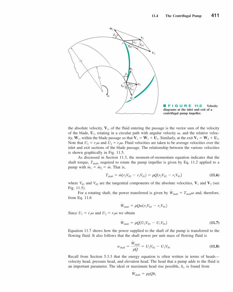
11.4 The Centrifugal Pump 411

the absolute velocity, V1, of the fluid entering the passage is the vector sum of the velocityof the blade, U1, rotating in a circular path with angular velocity �, and the relative veloc-ity, W1, within the blade passage so that V1 � W1 � U1. Similarly, at the exit V2 � W2 � U2.Note that U1 � r1� and U2 � r2�. Fluid velocities are taken to be average velocities over theinlet and exit sections of the blade passage. The relationship between the various velocitiesis shown graphically in Fig. 11.5.

As discussed in Section 11.3, the moment-of-momentum equation indicates that theshaft torque, Tshaft, required to rotate the pump impeller is given by Eq. 11.2 applied to apump with That is,

(11.6)

where V�1 and V�2 are the tangential components of the absolute velocities, V1 and V2 (seeFig. 11.5).

For a rotating shaft, the power transferred is given by and, therefore,from Eq. 11.6

Since U1 � r1� and U2 � r2� we obtain

(11.7)

Equation 11.7 shows how the power supplied to the shaft of the pump is transferred to theflowing fluid. It also follows that the shaft power per unit mass of flowing fluid is

(11.8)

Recall from Section 5.3.3 that the energy equation is often written in terms of heads—velocity head, pressure head, and elevation head. The head that a pump adds to the fluid isan important parameter. The ideal or maximum head rise possible, hi, is found from

W� shaft � �gQhi

wshaft �W� shaft

�Q� U2V�2 � U1V�1

W� shaft � �Q1U2V�2 � U1V�12

W� shaft � �Q�1r2V�2 � r1V�12

W� shaft � Tshaft�

Tshaft � m� 1r2V�2 � r1V�12 � �Q1r2V�2 � r1V�12

m� 1 � m� 2 � m� .

+

ω

r1

r2

W1

V1

U1

V 1θVr1

1β

α 1

U2

V2

W2

Vr2

2β

α 2V 2θ

F I G U R E 11.5 Velocitydiagrams at the inlet and exit of acentrifugal pump impeller.

c11Turbomachines.qxd 9/28/10 10:38 AM Page 411

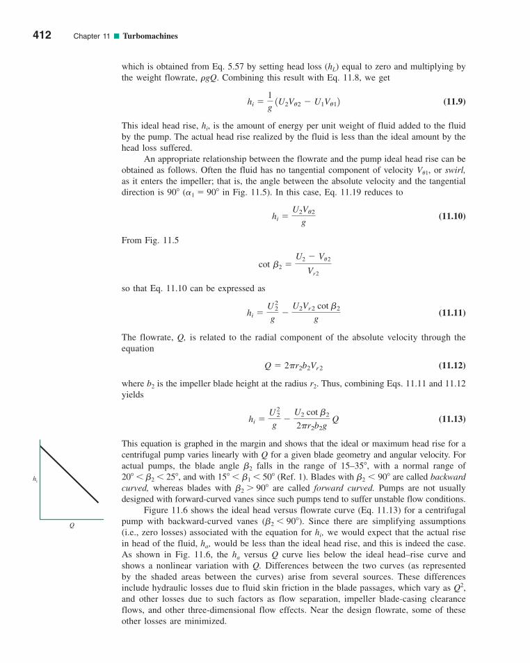
which is obtained from Eq. 5.57 by setting head loss (hL) equal to zero and multiplying bythe weight flowrate, �gQ. Combining this result with Eq. 11.8, we get

(11.9)

This ideal head rise, hi, is the amount of energy per unit weight of fluid added to the fluidby the pump. The actual head rise realized by the fluid is less than the ideal amount by thehead loss suffered.

An appropriate relationship between the flowrate and the pump ideal head rise can beobtained as follows. Often the fluid has no tangential component of velocity V�1, or swirl,as it enters the impeller; that is, the angle between the absolute velocity and the tangentialdirection is 90� (�1 � 90� in Fig. 11.5). In this case, Eq. 11.19 reduces to

(11.10)

From Fig. 11.5

so that Eq. 11.10 can be expressed as

(11.11)

The flowrate, Q, is related to the radial component of the absolute velocity through theequation

(11.12)

where b2 is the impeller blade height at the radius r2. Thus, combining Eqs. 11.11 and 11.12yields

(11.13)

This equation is graphed in the margin and shows that the ideal or maximum head rise for acentrifugal pump varies linearly with Q for a given blade geometry and angular velocity. Foractual pumps, the blade angle �2 falls in the range of 15–35�, with a normal range of20� � �2 � 25�, and with 15� � �1 � 50� (Ref. 1). Blades with �2 � 90� are called backwardcurved, whereas blades with �2 � 90� are called forward curved. Pumps are not usuallydesigned with forward-curved vanes since such pumps tend to suffer unstable flow conditions.

Figure 11.6 shows the ideal head versus flowrate curve (Eq. 11.13) for a centrifugalpump with backward-curved vanes (�2 � 90�). Since there are simplifying assumptions(i.e., zero losses) associated with the equation for hi, we would expect that the actual risein head of the fluid, ha, would be less than the ideal head rise, and this is indeed the case.As shown in Fig. 11.6, the ha versus Q curve lies below the ideal head–rise curve andshows a nonlinear variation with Q. Differences between the two curves (as representedby the shaded areas between the curves) arise from several sources. These differencesinclude hydraulic losses due to fluid skin friction in the blade passages, which vary as Q2,and other losses due to such factors as flow separation, impeller blade-casing clearanceflows, and other three-dimensional flow effects. Near the design flowrate, some of theseother losses are minimized.

hi �U2

2

g�

U2 cot �2

2�r2b2g Q

Q � 2�r2b2Vr 2

hi �U2

2

g�

U2Vr 2 cot �2

g

cot �2 �U2 � V�2

Vr2

hi �U2V�2

g

hi �1g

1U2V�2 � U1V�12

412 Chapter 11 ■ Turbomachines

hi

Q

c11Turbomachines.qxd 9/28/10 10:38 AM Page 412

11.4 The Centrifugal Pump 413

F I G U R E 11.6 Effect of losses on the pump head–flowrate curve.Flowrate

Hea

d

Otherlosses

Actual head, ha

Theoretical head, hi

Friction losses

GIVEN Water is pumped at the rate of 1400 gpm througha centrifugal pump operating at a speed of 1750 rpm. The im-peller has a uniform blade height, b, of 2 in. with r1 � 1.9 in.and r2 � 7.0 in., and the exit blade angle �2 is 23� (seeFig. 11.5). Assume ideal flow conditions and that the tangen-tial velocity component, V�1, of the water entering the bladeis zero (�1 � 90�).

SOLUTION

Centrifugal Pump Performance Based onInlet/Outlet Velocities

(b) From Eq. 11.10 the ideal head rise is given by

(Ans)

Alternatively, from Eq. 11.11, the ideal head rise is

(Ans)

(c) From Eq. 11.7, with V�1 � 0, the power transferred to thefluid is given by the equation

(Ans)

COMMENT Note that the ideal head rise and the powertransferred are related through the relationship

W� shaft � �gQhi

� 61,500 ft . lb/s 11 hp/550 ft . lb/s2 � 112 hp

�11.94 slugs/ft32 11400 gpm2 1107 ft /s2 195.0 ft /s2

311slug . ft /s22/lb 4 17.48 gal/ft32 160 s/min2

W� shaft � �QU2V�2

� 316 ft

�1107 ft /s22

32.2 ft /s2 �1107 ft/s2 15.11 ft /s2 cot 23°

32.2 ft /s2

hi �U 2

2

g�

U2Vr2 cot �2

g

� 316 ft

hi �U2V�2

g�1107 ft /s2 195.0 ft /s2

32.2 ft /s2

FIND Determine

(a) the tangential velocity component, V�2, at the exit,

(b) the ideal head rise, hi, and

(c) the power, transferred to the fluid.W� shaft,

EXAMPLE 11.2

(a) At the exit the velocity diagram is as shown in Fig. 11.5,where V2 is the absolute velocity of the fluid, W2 is the rela-tive velocity, and U2 is the tip velocity of the impeller with

Since the flowrate is given, it follows that Q � 2�r2b2Vr2 or

From Fig. 11.5, we see that

so that

(Ans) � 95.0 ft /s

� 1107 � 5.11 cot 23°2 ft /s

V�2 � U2 � Vr 2 cot �2

cot �2 �U2 � V�2

Vr 2

� 5.11 ft /s

�1400 gpm

17.48 gal /ft32 160 s /min2 12�2 17/12 ft2 12/12 ft2

Vr 2 �Q

2�r2b2

� 107 ft /s

U2 � r2� � 17/12 ft2 12� rad /rev2 11750 rpm2

160 s /min2

c11Turbomachines.qxd 9/28/10 10:39 AM Page 413

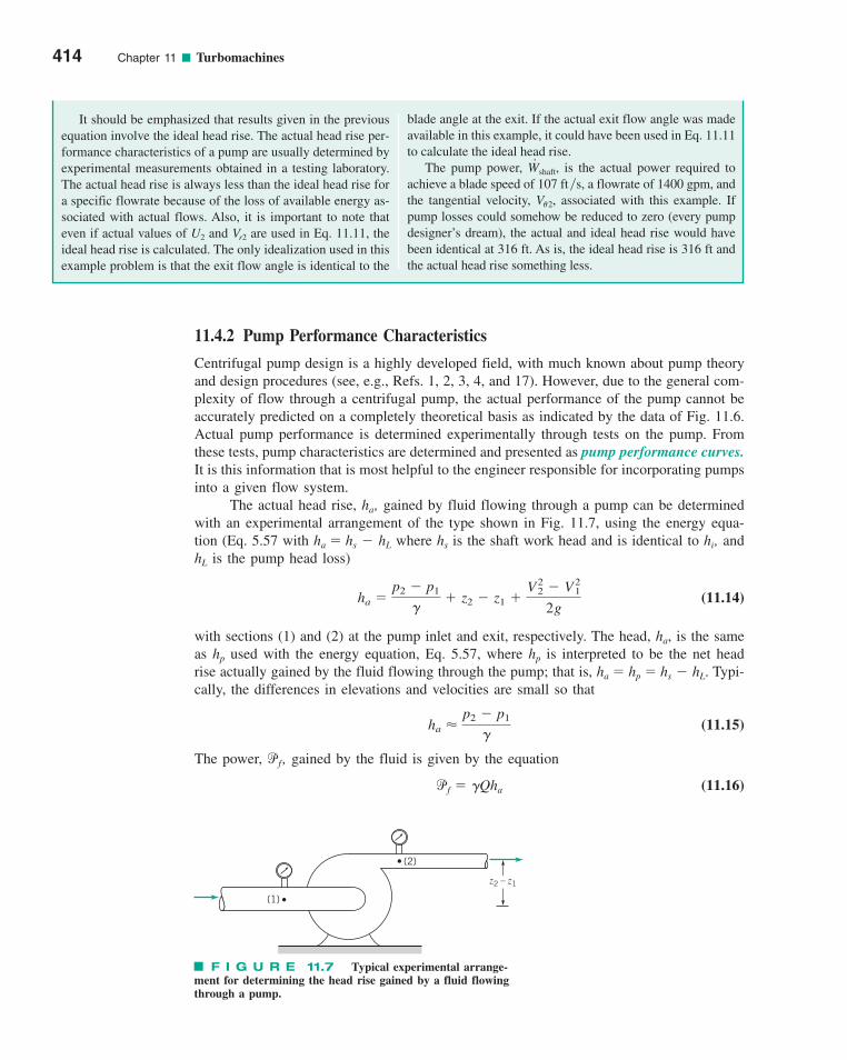
11.4.2 Pump Performance Characteristics

Centrifugal pump design is a highly developed field, with much known about pump theoryand design procedures (see, e.g., Refs. 1, 2, 3, 4, and 17). However, due to the general com-plexity of flow through a centrifugal pump, the actual performance of the pump cannot beaccurately predicted on a completely theoretical basis as indicated by the data of Fig. 11.6.Actual pump performance is determined experimentally through tests on the pump. Fromthese tests, pump characteristics are determined and presented as pump performance curves.It is this information that is most helpful to the engineer responsible for incorporating pumpsinto a given flow system.

The actual head rise, ha, gained by fluid flowing through a pump can be determinedwith an experimental arrangement of the type shown in Fig. 11.7, using the energy equa-tion (Eq. 5.57 with ha � hs � hL where hs is the shaft work head and is identical to hi, andhL is the pump head loss)

(11.14)

with sections (1) and (2) at the pump inlet and exit, respectively. The head, ha, is the sameas hp used with the energy equation, Eq. 5.57, where hp is interpreted to be the net headrise actually gained by the fluid flowing through the pump; that is, ha � hp � hs � hL. Typi-cally, the differences in elevations and velocities are small so that

(11.15)

The power, pf , gained by the fluid is given by the equation

(11.16)pf � �Qha

ha �p2 � p1

�

ha �p2 � p1

�� z2 � z1 �

V22 � V2

1

2g

414 Chapter 11 ■ Turbomachines

blade angle at the exit. If the actual exit flow angle was madeavailable in this example, it could have been used in Eq. 11.11to calculate the ideal head rise.

The pump power, is the actual power required toachieve a blade speed of 107 ft�s, a flowrate of 1400 gpm, andthe tangential velocity, V�2, associated with this example. Ifpump losses could somehow be reduced to zero (every pumpdesigner’s dream), the actual and ideal head rise would havebeen identical at 316 ft. As is, the ideal head rise is 316 ft andthe actual head rise something less.

W#

shaft,

It should be emphasized that results given in the previousequation involve the ideal head rise. The actual head rise per-formance characteristics of a pump are usually determined byexperimental measurements obtained in a testing laboratory.The actual head rise is always less than the ideal head rise fora specific flowrate because of the loss of available energy as-sociated with actual flows. Also, it is important to note thateven if actual values of U2 and Vr2 are used in Eq. 11.11, theideal head rise is calculated. The only idealization used in thisexample problem is that the exit flow angle is identical to the

F I G U R E 11.7 Typical experimental arrange-ment for determining the head rise gained by a fluid flowingthrough a pump.

(1)

(2)

z2 – z1

c11Turbomachines.qxd 9/28/10 10:39 AM Page 414

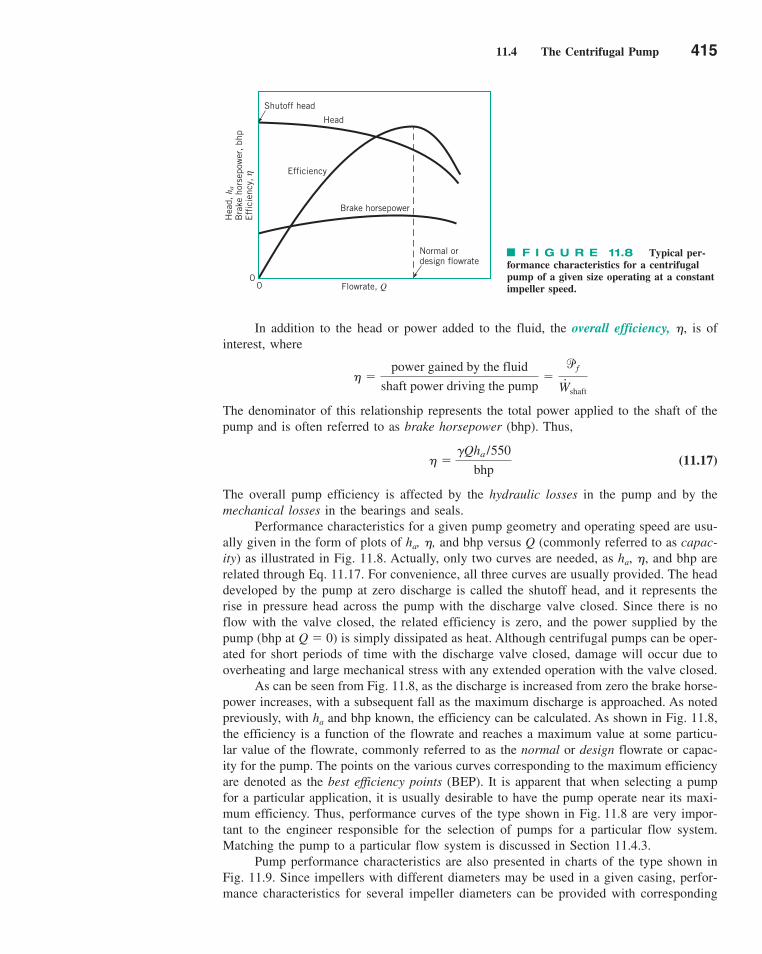
11.4 The Centrifugal Pump 415

In addition to the head or power added to the fluid, the overall efficiency, , is ofinterest, where

The denominator of this relationship represents the total power applied to the shaft of thepump and is often referred to as brake horsepower (bhp). Thus,

(11.17)

The overall pump efficiency is affected by the hydraulic losses in the pump and by themechanical losses in the bearings and seals.

Performance characteristics for a given pump geometry and operating speed are usu-ally given in the form of plots of ha, , and bhp versus Q (commonly referred to as capac-ity) as illustrated in Fig. 11.8. Actually, only two curves are needed, as ha, , and bhp arerelated through Eq. 11.17. For convenience, all three curves are usually provided. The headdeveloped by the pump at zero discharge is called the shutoff head, and it represents therise in pressure head across the pump with the discharge valve closed. Since there is noflow with the valve closed, the related efficiency is zero, and the power supplied by thepump (bhp at Q � 0) is simply dissipated as heat. Although centrifugal pumps can be oper-ated for short periods of time with the discharge valve closed, damage will occur due tooverheating and large mechanical stress with any extended operation with the valve closed.

As can be seen from Fig. 11.8, as the discharge is increased from zero the brake horse-power increases, with a subsequent fall as the maximum discharge is approached. As notedpreviously, with ha and bhp known, the efficiency can be calculated. As shown in Fig. 11.8,the efficiency is a function of the flowrate and reaches a maximum value at some particu-lar value of the flowrate, commonly referred to as the normal or design flowrate or capac-ity for the pump. The points on the various curves corresponding to the maximum efficiencyare denoted as the best efficiency points (BEP). It is apparent that when selecting a pumpfor a particular application, it is usually desirable to have the pump operate near its maxi-mum efficiency. Thus, performance curves of the type shown in Fig. 11.8 are very impor-tant to the engineer responsible for the selection of pumps for a particular flow system.Matching the pump to a particular flow system is discussed in Section 11.4.3.

Pump performance characteristics are also presented in charts of the type shown inFig. 11.9. Since impellers with different diameters may be used in a given casing, perfor-mance characteristics for several impeller diameters can be provided with corresponding

��Qha /550

bhp

�power gained by the fluid

shaft power driving the pump�pf

W.

shaft

F I G U R E 11.8 Typical per-formance characteristics for a centrifugalpump of a given size operating at a constantimpeller speed.

Shutoff head

Hea

d, h

a

Bra

ke h

orse

pow

er,

bhp

Eff

icie

ncy,

Head

Efficiency

Brake horsepower

00

Normal ordesign flowrate

Flowrate, Q

η

c11Turbomachines.qxd 9/28/10 10:39 AM Page 415

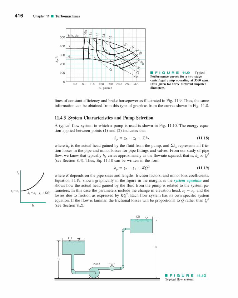
lines of constant efficiency and brake horsepower as illustrated in Fig. 11.9. Thus, the sameinformation can be obtained from this type of graph as from the curves shown in Fig. 11.8.

11.4.3 System Characteristics and Pump Selection

A typical flow system in which a pump is used is shown in Fig. 11.10. The energy equa-tion applied between points (1) and (2) indicates that

(11.18)

where hp is the actual head gained by the fluid from the pump, and hL represents all fric-tion losses in the pipe and minor losses for pipe fittings and valves. From our study of pipeflow, we know that typically hL varies approximately as the flowrate squared; that is, hL Q2

(see Section 8.4). Thus, Eq. 11.18 can be written in the form

(11.19)

where K depends on the pipe sizes and lengths, friction factors, and minor loss coefficients.Equation 11.19, shown graphically in the figure in the margin, is the system equation andshows how the actual head gained by the fluid from the pump is related to the system pa-rameters. In this case the parameters include the change in elevation head, z2 � z1, and thelosses due to friction as expressed by KQ2. Each flow system has its own specific systemequation. If the flow is laminar, the frictional losses will be proportional to Q rather than Q2

(see Section 8.2).

hp � z2 � z1 � KQ 2

r

hp � z2 � z1 � ©hL

416 Chapter 11 ■ Turbomachines

F I G U R E 11.9 TypicalPerformance curves for a two-stagecentrifugal pump operating at 3500 rpm.Data given for three different impellerdiameters.

40 80 120 160 200 240 280 320

8-in. dia

7

6

50%

55

60

63

65

50

556063

65

40 bhp30

2520

15

Q, gal/min

hp, ft

0

100

200

300

400

500

(1)

Pump

(2)

z1

z 2

F I G U R E 11.10Typical flow system.

hp

z2 – z1

Q

hp = z2 – z1 + KQ

2

c11Turbomachines.qxd 9/28/10 10:39 AM Page 416

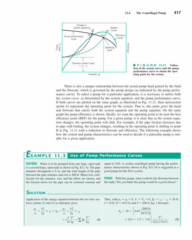
11.4 The Centrifugal Pump 417

There is also a unique relationship between the actual pump head gained by the fluidand the flowrate, which is governed by the pump design (as indicated by the pump perfor-mance curve). To select a pump for a particular application, it is necessary to utilize boththe system curve, as determined by the system equation, and the pump performance curve.If both curves are plotted on the same graph, as illustrated in Fig. 11.11, their intersection(point A) represents the operating point for the system. That is, this point gives the headand flowrate that satisfy both the system equation and the pump equation. On the samegraph the pump efficiency is shown. Ideally, we want the operating point to be near the bestefficiency point (BEP) for the pump. For a given pump, it is clear that as the system equa-tion changes, the operating point will shift. For example, if the pipe friction increases dueto pipe wall fouling, the system changes, resulting in the operating point A shifting to pointB in Fig. 11.11 with a reduction in flowrate and efficiency. The following example showshow the system and pump characteristics can be used to decide if a particular pump is suit-able for a given application.

Change insystem equation System

curve

Efficiencycurve

Operatingpoint

Pump performancecurve

Pum

phe

ad,

hp

Eff

icie

ncy

(A)(B)

Flowrate, Q

Elevation (static) head= z2 – z1 F I G U R E 11.11 Utiliza-

tion of the system curve and the pumpperformance curve to obtain the oper-ating point for the system.

GIVEN Water is to be pumped from one large, open tankto a second large, open tank as shown in Fig. E11.3a. The pipediameter throughout is 6 in. and the total length of the pipebetween the pipe entrance and exit is 200 ft. Minor loss coef-ficients for the entrance, exit, and the elbow are shown, andthe friction factor for the pipe can be assumed constant and

SOLUTION

Use of Pump Performance Curves

Thus, with p1 � p2 � 0, V1 � V2 � 0, z � z2 � z1 � 10 ft,f � 0.02, D � 6/12 ft, and � � 200 ft, Eq. 1 becomes

(2) � 10.5 � 1.5 � 1.02 d V 2

2132.2 ft /s22

hp � 10 � c0.02 1200 ft2

16/12 ft2

equal to 0.02. A certain centrifugal pump having the perfor-mance characteristics shown in Fig. E11.3b is suggested as agood pump for this flow system.

FIND With this pump, what would be the flowrate betweenthe tanks? Do you think this pump would be a good choice?

EXAMPLE 11.3

Application of the energy equation between the two free sur-faces, points (1) and (2) as indicated, gives

(1)� f /D

V 2

2g�a KL

V 2

2g

p1

��

V 21

2g� z1 � hp �

p2

��

V 22

2g� z2

c11Turbomachines.qxd 9/28/10 10:39 AM Page 417

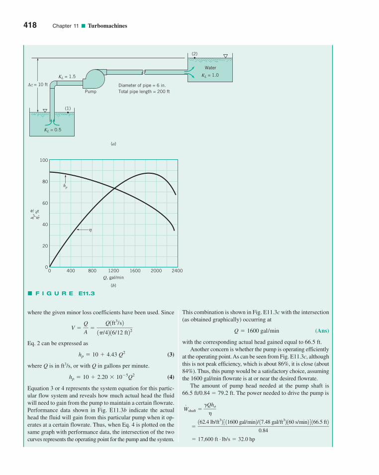
418 Chapter 11 ■ Turbomachines

This combination is shown in Fig. E11.3c with the intersection(as obtained graphically) occurring at

(Ans)

with the corresponding actual head gained equal to 66.5 ft.Another concern is whether the pump is operating efficiently

at the operating point. As can be seen from Fig. E11.3c, althoughthis is not peak efficiency, which is about 86%, it is close (about84%). Thus, this pump would be a satisfactory choice, assumingthe 1600 gal/min flowrate is at or near the desired flowrate.

The amount of pump head needed at the pump shaft is66.5 ft/0.84 � 79.2 ft. The power needed to drive the pump is

�

� 17,600 ft . lb/s � 32.0 hp

162.4 lb/ft32 3 11600 gal/min2/ 17.48 gal/ft32 160 s/min2 4 166.5 ft2

0.84

W� shaft ��Qha

Q � 1600 gal/min

where the given minor loss coefficients have been used. Since

Eq. 2 can be expressed as

(3)

where Q is in ft3/s, or with Q in gallons per minute.

(4)

Equation 3 or 4 represents the system equation for this partic-ular flow system and reveals how much actual head the fluidwill need to gain from the pump to maintain a certain flowrate.Performance data shown in Fig. E11.3b indicate the actualhead the fluid will gain from this particular pump when it op-erates at a certain flowrate. Thus, when Eq. 4 is plotted on thesame graph with performance data, the intersection of the twocurves represents the operating point for the pump and the system.

hp � 10 � 2.20 � 10�5Q2

hp � 10 � 4.43 Q2

V �Q

A�

Q1ft3/s2

1�/42 16/12 ft22

KL = 0.5

(1)

KL = 1.5

Pump

KL = 1.0

(2)

Water

Diameter of pipe = 6 in.Total pipe length = 200 ft

0 400 800 1200 1600 2000 24000

20

40

60

80

100

Q, gal/min

hp,

ft ,

%

hp

Δz = 10 ft

(b)

(a)

η

η

F I G U R E E11.3

c11Turbomachines.qxd 9/28/10 10:39 AM Page 418

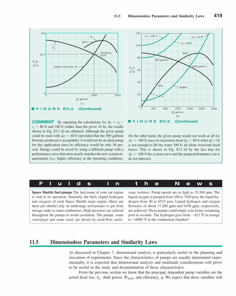
11.5 Dimensionless Parameters and Similarity Laws 419

On the other hand, the given pump would not work at all forsince its maximum head (hp � 88 ft when Q � 0)

is not enough to lift the water 100 ft, let alone overcome headlosses. This is shown in Fig. E11.3d by the fact that for

the system curve and the pump performance curvedo not intersect.¢z � 100 ft

¢z � 100 ft

COMMENT By repeating the calculations for z � z2 �z1 � 80 ft and 100 ft (rather than the given 10 ft), the resultsshown in Fig. E11.3d are obtained. Although the given pumpcould be used with (provided that the 500 gal/minflowrate produced is acceptable), it would not be an ideal pumpfor this application since its efficiency would be only 36 per-cent. Energy could be saved by using a different pump with aperformance curve that more nearly matches the new system re-quirements (i.e., higher efficiency at the operating condition).

¢z � 80 ft

(c)

0 1600 24000

66.5

100

Q, gal/min

hp

84%

Operatingpoint

System curve (Eq. 4)hp, ft

, %

ηη

F I G U R E E11.3 (Continued)

(d)

Q, gal/min

120

100

80

60

40

20

00 400 800 1200 1600 2000 2400

Δz = 80 ft

Δz = 10 ft

1600 gal/min

System

500 gal/min

84%

36%

Δz = 100 ft

hp, ft

, %

η

η

F I G U R E E11.3 (Continued)

F l u i d s i n t h e N e w s

Space Shuttle fuel pumps The fuel pump of your car engineis vital to its operation. Similarly, the fuels (liquid hydrogenand oxygen) of each Space Shuttle main engine (there arethree per shuttle) rely on multistage turbopumps to get fromstorage tanks to main combustors. High pressures are utilizedthroughout the pumps to avoid cavitation. The pumps, somecentrifugal and some axial, are driven by axial-flow, multi-

stage turbines. Pump speeds are as high as 35,360 rpm. Theliquid oxygen is pumped from 100 to 7420 psia, the liquid hy-drogen from 30 to 6515 psia. Liquid hydrogen and oxygenflowrates of about 17,200 gpm and 6100 gpm, respectively,are achieved. These pumps could empty your home swimmingpool in seconds. The hydrogen goes from �423 �F in storageto �6000 �F in the combustion chamber!

11.5 Dimensionless Parameters and Similarity Laws

As discussed in Chapter 7, dimensional analysis is particularly useful in the planning andexecution of experiments. Since the characteristics of pumps are usually determined exper-imentally, it is expected that dimensional analysis and similitude considerations will proveto be useful in the study and documentation of these characteristics.

From the previous section we know that the principal, dependent pump variables are theactual head rise, hp, shaft power, and efficiency, . We expect that these variables willW� shaft,

c11Turbomachines.qxd 9/28/10 10:39 AM Page 419

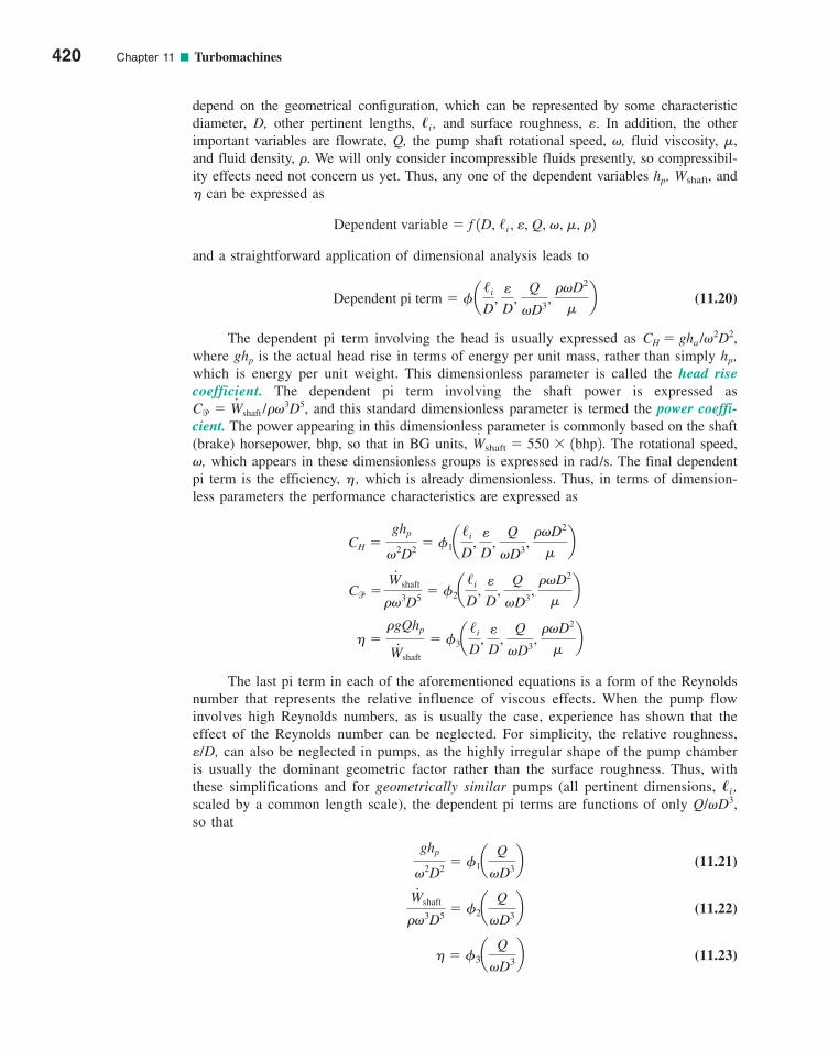
depend on the geometrical configuration, which can be represented by some characteristicdiameter, D, other pertinent lengths, �i , and surface roughness, �. In addition, the otherimportant variables are flowrate, Q, the pump shaft rotational speed, �, fluid viscosity, ,and fluid density, �. We will only consider incompressible fluids presently, so compressibil-ity effects need not concern us yet. Thus, any one of the dependent variables hp, and can be expressed as

and a straightforward application of dimensional analysis leads to

(11.20)

The dependent pi term involving the head is usually expressed as CH � gha /�2D2,where ghp is the actual head rise in terms of energy per unit mass, rather than simply hp,which is energy per unit weight. This dimensionless parameter is called the head risecoefficient. The dependent pi term involving the shaft power is expressed as

and this standard dimensionless parameter is termed the power coeffi-cient. The power appearing in this dimensionless parameter is commonly based on the shaft(brake) horsepower, bhp, so that in BG units, The rotational speed,�, which appears in these dimensionless groups is expressed in rad/s. The final dependentpi term is the efficiency, , which is already dimensionless. Thus, in terms of dimension-less parameters the performance characteristics are expressed as

The last pi term in each of the aforementioned equations is a form of the Reynoldsnumber that represents the relative influence of viscous effects. When the pump flowinvolves high Reynolds numbers, as is usually the case, experience has shown that theeffect of the Reynolds number can be neglected. For simplicity, the relative roughness,�/D, can also be neglected in pumps, as the highly irregular shape of the pump chamberis usually the dominant geometric factor rather than the surface roughness. Thus, withthese simplifications and for geometrically similar pumps (all pertinent dimensions, �i ,scaled by a common length scale), the dependent pi terms are functions of only Q/�D3,so that

(11.21)

(11.22)

(11.23) � �3aQ

�D3b

W.

shaft

��3D5� �2a

Q

�D3b

ghp

�2D2� �1a

Q

�D3b

��gQhp

W.

shaft

� �3a/i

D, e

D,

Q

�D3,

��D2

b

Cp �W.

shaft

��3D5� �2a

/i

D, e

D,

Q

�D3,

��D2

b

CH �ghp

�2D2� �1a

/i

D, e

D,

Q

�D3,

��D2

b

W� shaft � 550 � 1bhp2.

Cp � W#

shaft /��3D5,

Dependent pi term � �a/i

D, e

D,

Q

�D3,

��D2

b

Dependent variable � f 1D, /i , e, Q, �, , �2

W� shaft,

420 Chapter 11 ■ Turbomachines

c11Turbomachines.qxd 9/28/10 10:40 AM Page 420

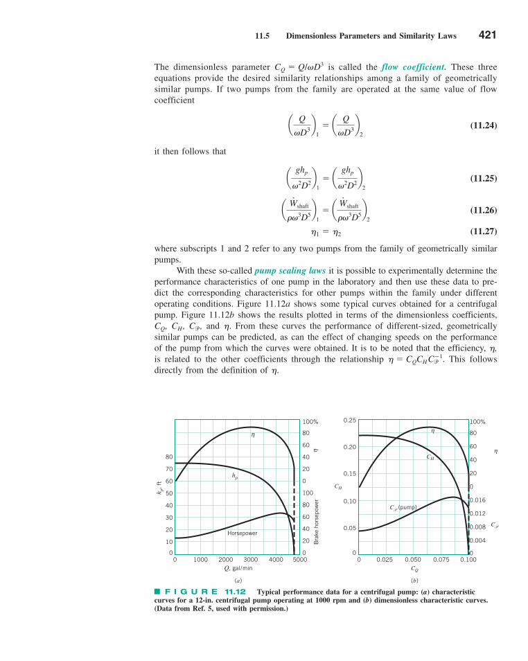
11.5 Dimensionless Parameters and Similarity Laws 421

The dimensionless parameter CQ � Q/�D3 is called the flow coefficient. These threeequations provide the desired similarity relationships among a family of geometricallysimilar pumps. If two pumps from the family are operated at the same value of flowcoefficient

(11.24)

it then follows that

(11.25)

(11.26)

(11.27)

where subscripts 1 and 2 refer to any two pumps from the family of geometrically similarpumps.

With these so-called pump scaling laws it is possible to experimentally determine theperformance characteristics of one pump in the laboratory and then use these data to pre-dict the corresponding characteristics for other pumps within the family under differentoperating conditions. Figure 11.12a shows some typical curves obtained for a centrifugalpump. Figure 11.12b shows the results plotted in terms of the dimensionless coefficients,CQ, CH, Cp, and . From these curves the performance of different-sized, geometricallysimilar pumps can be predicted, as can the effect of changing speeds on the performanceof the pump from which the curves were obtained. It is to be noted that the efficiency, ,is related to the other coefficients through the relationship � CQCH Cp

�1. This followsdirectly from the definition of .

1 � 2

aW.

shaft

��3D5b

1� a

.Wshaft

��3D5b

2

aghp

�2D2b

1� a

ghp

�2D2b

2

aQ

�D3b1

� aQ

�D3b2

100%

80

60

40

20

0

100

80

60

40

20

0

Bra

ke h

orse

pow

er

0

10

20

30

40

50

60

70

80

0 1000 2000 3000 4000 5000Q, gal/min

(a)

hp,

ft

Horsepower

hp

0

0.05

0.10

0.15

CH

0.20

0.25

0 0.025 0.050 0.075 0.100CQ

(b)

100%

80

60

40

20

0

0.016

0.012

0.008

0.004

0

C

η

C (pump)

CH

η

P

P

η

η

F I G U R E 11.12 Typical performance data for a centrifugal pump: (a) characteristiccurves for a 12-in. centrifugal pump operating at 1000 rpm and (b) dimensionless characteristic curves.(Data from Ref. 5, used with permission.)

c11Turbomachines.qxd 9/28/10 10:40 AM Page 421

11.5.1 Specific Speed

A useful pi term can be obtained by eliminating diameter D between the flow coefficientand the head rise coefficient. This is accomplished by raising the flow coefficient to anappropriate exponent (1/2) and dividing this result by the head coefficient raised to anotherappropriate exponent (3/4) so that

(11.28)

The dimensionless parameter Ns is called the specific speed. Specific speed varies withthe flow coefficient just as the other coefficients and efficiency discussed earlier do.However, for any pump it is customary to specify a value of specific speed at the flowcoefficient corresponding to peak efficiency only. For pumps with low Q and high hp,the specific speed is low compared to a pump with high Q and low hp. Centrifugalpumps typically are low-capacity, high-head pumps and, therefore, have low specificspeeds.

Specific speed as defined by Eq. 11.28 is dimensionless and therefore independent of the system of units used in its evaluation as long as a consistent unit system is used.

1Q/�D321/2

1ghp /�2D223/4�

�2Q

1ghp23/4

� Ns

422 Chapter 11 ■ Turbomachines

GIVEN An 8-in.-diameter centrifugal pump operating at1200 rpm is geometrically similar to the 12-in.-diameter pumphaving the performance characteristics of Figs. 11.12a and11.12b while operating at 1000 rpm. The working fluid iswater at 60 �F.

SOLUTION

Use of Pump Scaling Laws

Also,

(Ans)

COMMENT The last result gives the shaft horsepower,which is the power supplied to the pump shaft. The poweractually gained by the fluid is equal to �Qhp, which in thisexample is

Thus, the efficiency, , is

which checks with the efficiency curve of Fig. 11.12b.

�pf

W.

shaft

�6050

7150� 85%

pf � �Qhp � 162.4 lb/ft32 12.33 ft3/s2 141.6 ft2 � 6050 ft . lb/s

W.

shaft �7150 ft . lb/s

550 ft . lb/s/hp� 13.0 hp

� 7150 ft . lb/s

� 10.0142 11.94 slugs/ft32 1126 rad /s2318/12 ft25W#

shaft � Cp��3D5

FIND For peak efficiency, predict the discharge, actualhead rise, and shaft horsepower for this smaller pump.

EXAMPLE 11.4

As is indicated by Eq. 11.23, for a given efficiency the flowcoefficient has the same value for a given family of pumps.From Fig. 11.12b we see that at peak efficiency CQ � 0.0625.Thus, for the 8-in. pump

(Ans)

or in terms of gpm

(Ans)

The actual head rise and the shaft horsepower can be deter-mined in a similar manner since at peak efficiency CH � 0.19and Cp� 0.014, so that with �

(Ans)hp �CH �2D2

g�10.192 1126 rad/s2218/12 ft22

32.2 ft /s2 � 41.6 ft

12� rad/rev2� 126 rad/s� � 1200 rev/min 11 min/60 s2

� 1046 gpm

Q � 12.33 ft3/s2 17.48 gal/ft32 160 s/min2

Q � 2.33 ft3/s

� 10.06252 11200/60 rev/s2 12� rad /rev2 18/12 ft23Q � CQ�D3

c11Turbomachines.qxd 9/28/10 10:40 AM Page 422

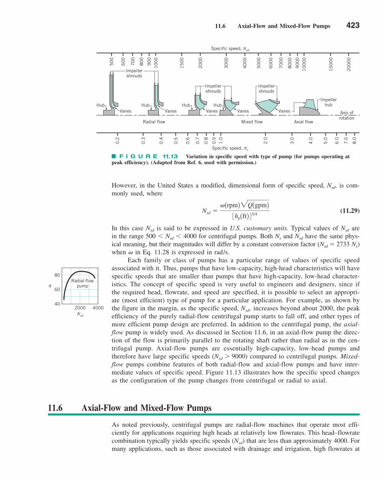
11.6 Axial-Flow and Mixed-Flow Pumps 423

However, in the United States a modified, dimensional form of specific speed, Nsd, is com-monly used, where

(11.29)

In this case Nsd is said to be expressed in U.S. customary units. Typical values of Nsd arein the range 500 � Nsd � 4000 for centrifugal pumps. Both Ns and Nsd have the same phys-ical meaning, but their magnitudes will differ by a constant conversion factor (Nsd � 2733 Ns)when � in Eq. 11.28 is expressed in rad/s.

Each family or class of pumps has a particular range of values of specific speedassociated with it. Thus, pumps that have low-capacity, high-head characteristics will havespecific speeds that are smaller than pumps that have high-capacity, low-head character-istics. The concept of specific speed is very useful to engineers and designers, since ifthe required head, flowrate, and speed are specified, it is possible to select an appropri-ate (most efficient) type of pump for a particular application. For example, as shown bythe figure in the margin, as the specific speed, Nsd, increases beyond about 2000, the peakefficiency of the purely radial-flow centrifugal pump starts to fall off, and other types ofmore efficient pump design are preferred. In addition to the centrifugal pump, the axial-flow pump is widely used. As discussed in Section 11.6, in an axial-flow pump the direc-tion of the flow is primarily parallel to the rotating shaft rather than radial as in the cen-trifugal pump. Axial-flow pumps are essentially high-capacity, low-head pumps andtherefore have large specific speeds (Nsd � 9000) compared to centrifugal pumps. Mixed-flow pumps combine features of both radial-flow and axial-flow pumps and have inter-mediate values of specific speed. Figure 11.13 illustrates how the specific speed changesas the configuration of the pump changes from centrifugal or radial to axial.

Nsd ��1rpm22Q1gpm2

3hp1ft2 43/4

50

0

60

0

70

0

80

0

90

0

10

00

15

00

20

00

30

00

40

00

50

00

60

00

70

00

80

00

90

00

10

00

0

15

00

0

20

00

0

0.2

0.3

0.4

0.5

0.6

0.7

0.8

0.9

1.0

2.0

3.0

4.0

5.0

6.0

7.0

8.0

Radial flow

Specific speed, Ns

Specific speed, Nsd

Mixed flow Axial flow

Axis ofrotation

VanesHub

Impellershrouds

VanesHub

VanesHub

VanesHub

Impellershrouds

Vanes

Impellershrouds

Impellerhub

F I G U R E 11.13 Variation in specific speed with type of pump (for pumps operating atpeak efficiency). (Adapted from Ref. 6, used with permission.)

80

60h

402000Nsd

4000

Radial-flowpump

11.6 Axial-Flow and Mixed-Flow Pumps

As noted previously, centrifugal pumps are radial-flow machines that operate most effi-ciently for applications requiring high heads at relatively low flowrates. This head–flowratecombination typically yields specific speeds (Nsd) that are less than approximately 4000. Formany applications, such as those associated with drainage and irrigation, high flowrates at

c11Turbomachines.qxd 9/28/10 10:40 AM Page 423

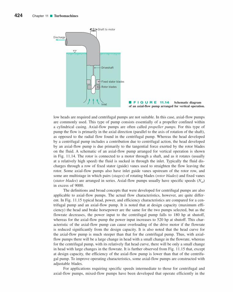
low heads are required and centrifugal pumps are not suitable. In this case, axial-flow pumpsare commonly used. This type of pump consists essentially of a propeller confined withina cylindrical casing. Axial-flow pumps are often called propeller pumps. For this type ofpump the flow is primarily in the axial direction (parallel to the axis of rotation of the shaft),as opposed to the radial flow found in the centrifugal pump. Whereas the head developedby a centrifugal pump includes a contribution due to centrifugal action, the head developedby an axial-flow pump is due primarily to the tangential force exerted by the rotor bladeson the fluid. A schematic of an axial-flow pump arranged for vertical operation is shownin Fig. 11.14. The rotor is connected to a motor through a shaft, and as it rotates (usuallyat a relatively high speed) the fluid is sucked in through the inlet. Typically the fluid dis-charges through a row of fixed stator (guide) vanes used to straighten the flow leaving therotor. Some axial-flow pumps also have inlet guide vanes upstream of the rotor row, andsome are multistage in which pairs (stages) of rotating blades (rotor blades) and fixed vanes(stator blades) are arranged in series. Axial-flow pumps usually have specific speeds (Nsd)in excess of 9000.

The definitions and broad concepts that were developed for centrifugal pumps are alsoapplicable to axial-flow pumps. The actual flow characteristics, however, are quite differ-ent. In Fig. 11.15 typical head, power, and efficiency characteristics are compared for a cen-trifugal pump and an axial-flow pump. It is noted that at design capacity (maximum effi-ciency) the head and brake horsepower are the same for the two pumps selected, but as theflowrate decreases, the power input to the centrifugal pump falls to 180 hp at shutoff,whereas for the axial-flow pump the power input increases to 520 hp at shutoff. This char-acteristic of the axial-flow pump can cause overloading of the drive motor if the flowrateis reduced significantly from the design capacity. It is also noted that the head curve forthe axial-flow pump is much steeper than that for the centrifugal pump. Thus, with axial-flow pumps there will be a large change in head with a small change in the flowrate, whereasfor the centrifugal pump, with its relatively flat head curve, there will be only a small changein head with large changes in the flowrate. It is further observed from Fig. 11.15 that, exceptat design capacity, the efficiency of the axial-flow pump is lower than that of the centrifu-gal pump. To improve operating characteristics, some axial-flow pumps are constructed withadjustable blades.

For applications requiring specific speeds intermediate to those for centrifugal andaxial-flow pumps, mixed-flow pumps have been developed that operate efficiently in the

424 Chapter 11 ■ Turbomachines

Inlet

Discharge

Rotor blades

Fixed stator blades

Driveshaft

Shaft to motor

F I G U R E 11.14 Schematic diagramof an axial-flow pump arranged for vertical operation.

c11Turbomachines.qxd 9/28/10 10:40 AM Page 424

11.6 Axial-Flow and Mixed-Flow Pumps 425

specific speed range 4000 � Nsd � 9000. As the name implies, the flow in a mixed-flowpump has both a radial and an axial component. Figure 11.16 shows some typical datafor centrifugal, mixed-flow, and axial-flow pumps, each operating at the same flowratefor peak efficiency. These data indicate that as we proceed from the centrifugal pump tothe mixed-flow pump to the axial-flow pump, the specific speed increases, the headdecreases, the speed increases, the impeller diameter decreases, and the eye diameterincreases. These general trends are commonly found when these three types of pumps arecompared.

The dimensionless parameters and scaling relationships developed in the previous sec-tions apply to all three types of pumps—centrifugal, mixed flow, and axial flow—since thedimensional analysis used is not restricted to a particular type of pump. Additional infor-mation about pumps can be found in Refs. 1, 7, 8, 9, and 10.

Brake horsepower

0 10 20 30 40 50 600

20

40

60

80

100

200

300

400

500

Q, 1000 gal/min

Per

cent

eff

icie

ncy

10

20

30

40

50

60

Bra

ke h

orse

pow

er

hp, ft

hp

Centrifugal pump

Axial-flow pump

ηF I G U R E 11.15 Comparison of

performance characteristics for a centrifugalpump and an axial-flow pump, each rated42,000 gal�min at a 17-ft head. (Data fromRef. 7, used with permission.)

A B C D

Runnervanes

Runnervanes

Type Centrifugal Mixed flow Axial flow

Nsd

Gal/min

Head, ft

Rpm

D, in.

Deye /D

Centrifugal

1,250

2,400

70

870

19

0.5

2,200

2,400

48

1,160

12

0.7

6,200

2,400

33

1,750

10

0.9

13,500

2,400

20

2,600

7

1.0

Eye

Radius D

2

F I G U R E 11.16 Comparison of different types of impellers. Specific speed for centrifugal pumps based on single suction. (Adapted from Ref. 7, used with permission.)

c11Turbomachines.qxd 9/28/10 10:40 AM Page 425

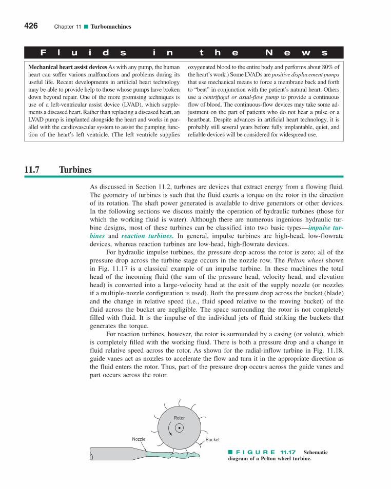
426 Chapter 11 ■ Turbomachines

F l u i d s i n t h e N e w s

Mechanical heart assist devices As with any pump, the humanheart can suffer various malfunctions and problems during itsuseful life. Recent developments in artificial heart technologymay be able to provide help to those whose pumps have brokendown beyond repair. One of the more promising techniques isuse of a left-ventricular assist device (LVAD), which supple-ments a diseased heart. Rather than replacing a diseased heart, anLVAD pump is implanted alongside the heart and works in par-allel with the cardiovascular system to assist the pumping func-tion of the heart’s left ventricle. (The left ventricle supplies

oxygenated blood to the entire body and performs about 80% ofthe heart’s work.) Some LVADs are positive displacement pumpsthat use mechanical means to force a membrane back and forthto “beat” in conjunction with the patient’s natural heart. Othersuse a centrifugal or axial-flow pump to provide a continuousflow of blood. The continuous-flow devices may take some ad-justment on the part of patients who do not hear a pulse or aheartbeat. Despite advances in artificial heart technology, it isprobably still several years before fully implantable, quiet, andreliable devices will be considered for widespread use.

11.7 Turbines

As discussed in Section 11.2, turbines are devices that extract energy from a flowing fluid.The geometry of turbines is such that the fluid exerts a torque on the rotor in the directionof its rotation. The shaft power generated is available to drive generators or other devices.In the following sections we discuss mainly the operation of hydraulic turbines (those forwhich the working fluid is water). Although there are numerous ingenious hydraulic tur-bine designs, most of these turbines can be classified into two basic types—impulse tur-bines and reaction turbines. In general, impulse turbines are high-head, low-flowratedevices, whereas reaction turbines are low-head, high-flowrate devices.

For hydraulic impulse turbines, the pressure drop across the rotor is zero; all of thepressure drop across the turbine stage occurs in the nozzle row. The Pelton wheel shownin Fig. 11.17 is a classical example of an impulse turbine. In these machines the totalhead of the incoming fluid (the sum of the pressure head, velocity head, and elevationhead) is converted into a large-velocity head at the exit of the supply nozzle (or nozzlesif a multiple-nozzle configuration is used). Both the pressure drop across the bucket (blade)and the change in relative speed (i.e., fluid speed relative to the moving bucket) of thefluid across the bucket are negligible. The space surrounding the rotor is not completelyfilled with fluid. It is the impulse of the individual jets of fluid striking the buckets thatgenerates the torque.

For reaction turbines, however, the rotor is surrounded by a casing (or volute), whichis completely filled with the working fluid. There is both a pressure drop and a change influid relative speed across the rotor. As shown for the radial-inflow turbine in Fig. 11.18,guide vanes act as nozzles to accelerate the flow and turn it in the appropriate direction asthe fluid enters the rotor. Thus, part of the pressure drop occurs across the guide vanes andpart occurs across the rotor.

F I G U R E 11.17 Schematicdiagram of a Pelton wheel turbine.

Rotor

BucketNozzle

c11Turbomachines.qxd 9/28/10 10:40 AM Page 426

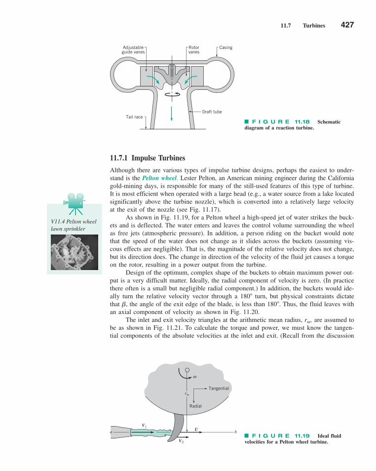
11.7 Turbines 427

11.7.1 Impulse Turbines

Although there are various types of impulse turbine designs, perhaps the easiest to under-stand is the Pelton wheel. Lester Pelton, an American mining engineer during the Californiagold-mining days, is responsible for many of the still-used features of this type of turbine.It is most efficient when operated with a large head (e.g., a water source from a lake locatedsignificantly above the turbine nozzle), which is converted into a relatively large velocityat the exit of the nozzle (see Fig. 11.17).

As shown in Fig. 11.19, for a Pelton wheel a high-speed jet of water strikes the buck-ets and is deflected. The water enters and leaves the control volume surrounding the wheelas free jets (atmospheric pressure). In addition, a person riding on the bucket would notethat the speed of the water does not change as it slides across the buckets (assuming vis-cous effects are negligible). That is, the magnitude of the relative velocity does not change,but its direction does. The change in direction of the velocity of the fluid jet causes a torqueon the rotor, resulting in a power output from the turbine.

Design of the optimum, complex shape of the buckets to obtain maximum power out-put is a very difficult matter. Ideally, the radial component of velocity is zero. (In practicethere often is a small but negligible radial component.) In addition, the buckets would ide-ally turn the relative velocity vector through a 180� turn, but physical constraints dictatethat �, the angle of the exit edge of the blade, is less than 180�. Thus, the fluid leaves withan axial component of velocity as shown in Fig. 11.20.

The inlet and exit velocity triangles at the arithmetic mean radius, rm, are assumed tobe as shown in Fig. 11.21. To calculate the torque and power, we must know the tangen-tial components of the absolute velocities at the inlet and exit. (Recall from the discussion

F I G U R E 11.19 Ideal fluidvelocities for a Pelton wheel turbine.

Tangential

V1

V2

U b

ω

Radial

rm

a

F I G U R E 11.18 Schematicdiagram of a reaction turbine.

Draft tubeTail race

Adjustableguide vanes

Rotorvanes

Casing

V11.4 Pelton wheellawn sprinkler

c11Turbomachines.qxd 9/28/10 10:40 AM Page 427

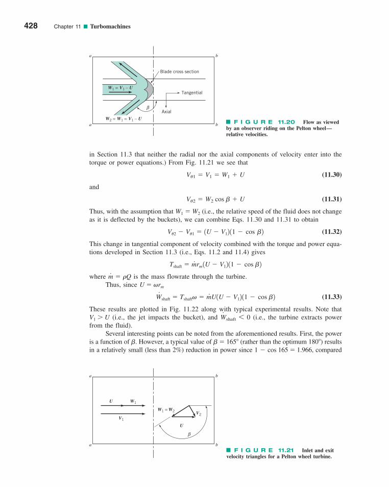
in Section 11.3 that neither the radial nor the axial components of velocity enter into thetorque or power equations.) From Fig. 11.21 we see that

(11.30)

and

(11.31)

Thus, with the assumption that W1 � W2 (i.e., the relative speed of the fluid does not changeas it is deflected by the buckets), we can combine Eqs. 11.30 and 11.31 to obtain

(11.32)

This change in tangential component of velocity combined with the torque and power equa-tions developed in Section 11.3 (i.e., Eqs. 11.2 and 11.4) gives

where is the mass flowrate through the turbine.Thus, since U � �rm

(11.33)

These results are plotted in Fig. 11.22 along with typical experimental results. Note thatV1 � U (i.e., the jet impacts the bucket), and (i.e., the turbine extracts powerfrom the fluid).

Several interesting points can be noted from the aforementioned results. First, the poweris a function of �. However, a typical value of � � 165� (rather than the optimum 180�) resultsin a relatively small (less than 2%) reduction in power since 1 � cos 165 � 1.966, compared

W� shaft 6 0

W#

shaft � Tshaft� � m#U1U � V12 11 � cos �2

m� � �Q

Tshaft � m.rm 1U � V12 11 � cos �2

V�2 � V�1 � 1U � V12 11 � cos �2

V�2 � W2 cos � � U

V�1 � V1 � W1 � U

428 Chapter 11 ■ Turbomachines

a

a

b

b

W1 = V1 – U

Blade cross section

W2 = W1 = V1 – U

β

Tangential

Axial

F I G U R E 11.20 Flow as viewed by an observer riding on the Pelton wheel—relative velocities.

a

a

b

b

W1

β

U

V1

W1 = W2

U

V2

F I G U R E 11.21 Inlet and exit velocity triangles for a Pelton wheel turbine.

c11Turbomachines.qxd 9/28/10 10:40 AM Page 428

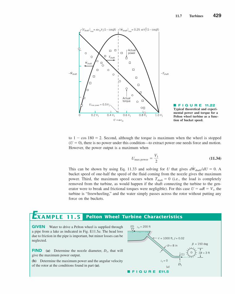
11.7 Turbines 429

to 1 � cos 180 � 2. Second, although the torque is maximum when the wheel is stopped(U � 0), there is no power under this condition—to extract power one needs force and motion.However, the power output is a maximum when

(11.34)

This can be shown by using Eq. 11.33 and solving for U that gives Abucket speed of one-half the speed of the fluid coming from the nozzle gives the maximumpower. Third, the maximum speed occurs when Tshaft � 0 (i.e., the load is completelyremoved from the turbine, as would happen if the shaft connecting the turbine to the gen-erator were to break and frictional torques were negligible). For this case U � �R � V1, theturbine is “freewheeling,” and the water simply passes across the rotor without putting anyforce on the buckets.

dW� shaft /dU � 0.

Umax power �V1

2

Actualpower

β

Tshaft

Actualtorque

0 0.2 V1 0.4 V1 0.6 V1 0.8 V1 1.0 V1

U = rm

shaft ⋅–W –Tshaft

⎥Tshaft⎥max= mrmV1(1– cos )⋅ ⎥ ⎥

max= 0.25 mV1

2(1– cos )⋅ β

Umax power = 0.5V1

shaft ⋅ W

shaft ⋅ W

ω

F I G U R E 11.22Typical theoretical and experi-mental power and torque for aPelton wheel turbine as a func-tion of bucket speed.

GIVEN Water to drive a Pelton wheel is supplied througha pipe from a lake as indicated in Fig. E11.5a. The head lossdue to friction in the pipe is important, but minor losses can beneglected.

FIND (a) Determine the nozzle diameter, D1, that willgive the maximum power output.

(b) Determine the maximum power and the angular velocityof the rotor at the conditions found in part (a).

Pelton Wheel Turbine CharacteristicsEXAMPLE 11.5

z0

= 200 ft

= 1000 ft, f = 0.02�

D = 8 in

z1 = 0

D1

β = 150 deg

(0)

2R = 3 ft(1)

(a)

F I G U R E E11.5

c11Turbomachines.qxd 9/28/10 10:40 AM Page 429

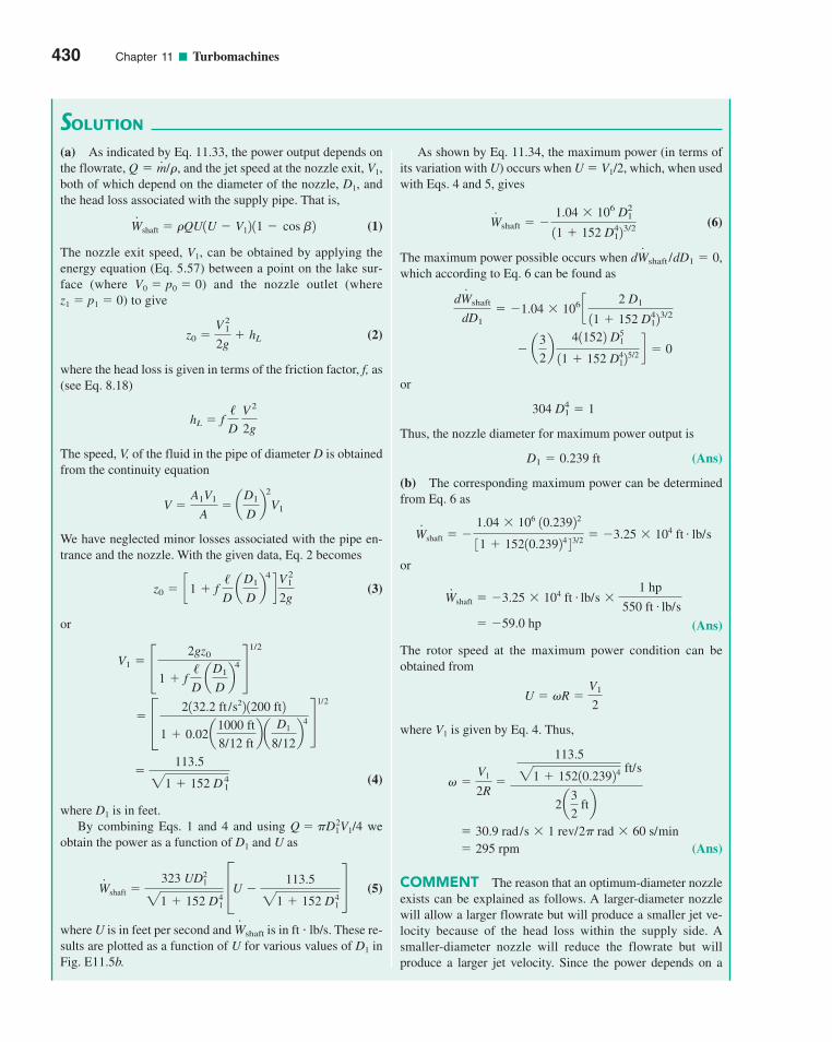
430 Chapter 11 ■ Turbomachines

As shown by Eq. 11.34, the maximum power (in terms ofits variation with U) occurs when U � V1/2, which, when usedwith Eqs. 4 and 5, gives

(6)

The maximum power possible occurs when which according to Eq. 6 can be found as

or

Thus, the nozzle diameter for maximum power output is

(Ans)

(b) The corresponding maximum power can be determinedfrom Eq. 6 as

or

(Ans)

The rotor speed at the maximum power condition can beobtained from

where V1 is given by Eq. 4. Thus,

(Ans)

COMMENT The reason that an optimum-diameter nozzleexists can be explained as follows. A larger-diameter nozzlewill allow a larger flowrate but will produce a smaller jet ve-locity because of the head loss within the supply side. Asmaller-diameter nozzle will reduce the flowrate but willproduce a larger jet velocity. Since the power depends on a

� 295 rpm � 30.9 rad /s � 1 rev/2� rad � 60 s/min

� �V1

2R�

113.5

21 � 15210.23924 ft/s

2a3

2 ftb

U � �R �V1

2

� �59.0 hp

W#

shaft � �3.25 � 104 ft . lb/s �1 hp

550 ft . lb/s

W#

shaft � �

1.04 � 106 10.23922

31 � 15210.23924 4 3/2 � �3.25 � 104 ft . lb/s

D1 � 0.239 ft

304 D41 � 1

� a3

2b

411522 D51

11 � 152 D412

5/2 d � 0

dW� shaft

dD1� �1.04 � 106 c

2 D1

11 � 152 D412

3/2

dW� shaft /dD1 � 0,

W� shaft � �

1.04 � 106 D21

11 � 152 D412

3/2

(a) As indicated by Eq. 11.33, the power output depends onthe flowrate, , and the jet speed at the nozzle exit, V1,both of which depend on the diameter of the nozzle, D1, andthe head loss associated with the supply pipe. That is,

(1)

The nozzle exit speed, V1, can be obtained by applying theenergy equation (Eq. 5.57) between a point on the lake sur-face (where V0 � p0 � 0) and the nozzle outlet (where z1 � p1 � 0) to give

(2)

where the head loss is given in terms of the friction factor, f, as(see Eq. 8.18)

The speed, V, of the fluid in the pipe of diameter D is obtainedfrom the continuity equation

We have neglected minor losses associated with the pipe en-trance and the nozzle. With the given data, Eq. 2 becomes

(3)

or

(4)

where D1 is in feet.By combining Eqs. 1 and 4 and using Q � �D2

1V1/4 weobtain the power as a function of D1 and U as

(5)

where U is in feet per second and is in ft � lb/s. These re-sults are plotted as a function of U for various values of D1 inFig. E11.5b.

W� shaft

W#

shaft �323 UD2

1

21 � 152 D41

CU �113.5

21 � 152 D41

§

�

113.5

21 � 152 D 41

� C 2132.2 ft /s22 1200 ft2

1 � 0.02 a1000 ft

8/12 ftb a

D1

8/12b

4 §

1/2

V1 �£

2gz0

1 � f /D

aD1

Db

4 §

1/2

z0 � c1 � f /D

aD1

Db

4

dV 2

1

2g

V �A1V1

A� a

D1

Db

2

V1

hL � f /D

V 2

2g

z0 �V 2

1

2g� hL

W#

shaft � �QU1U � V12 11 � cos �2

Q � m� /�

SOLUTION

c11Turbomachines.qxd 9/28/10 10:41 AM Page 430

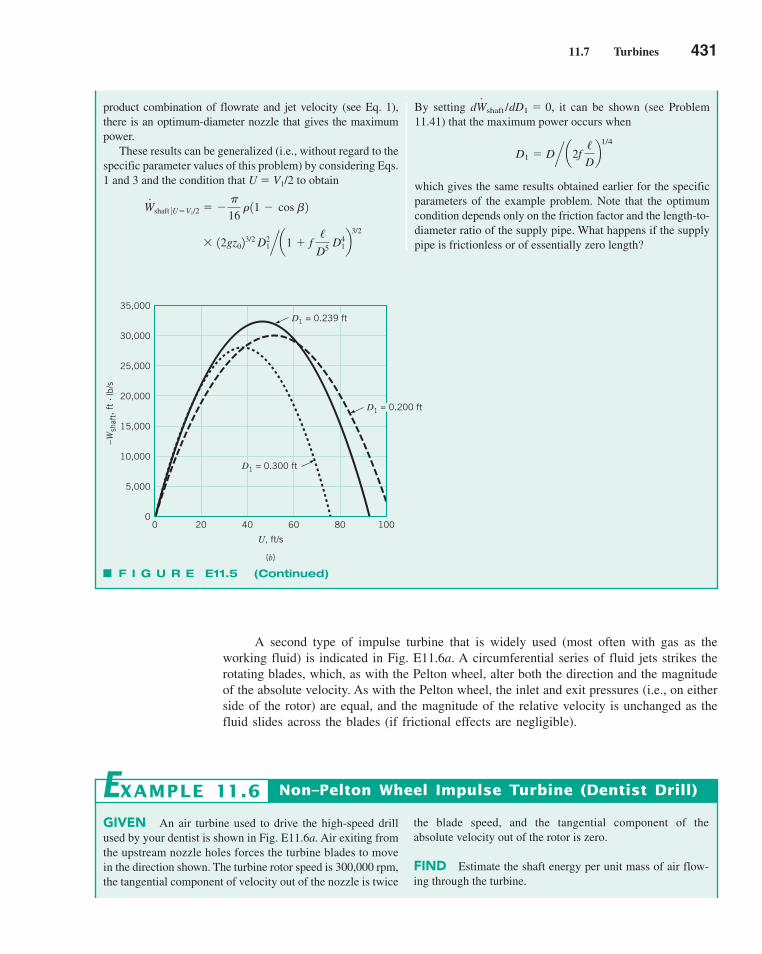
11.7 Turbines 431

A second type of impulse turbine that is widely used (most often with gas as theworking fluid) is indicated in Fig. E11.6a. A circumferential series of fluid jets strikes therotating blades, which, as with the Pelton wheel, alter both the direction and the magnitudeof the absolute velocity. As with the Pelton wheel, the inlet and exit pressures (i.e., on eitherside of the rotor) are equal, and the magnitude of the relative velocity is unchanged as thefluid slides across the blades (if frictional effects are negligible).

By setting it can be shown (see Problem11.41) that the maximum power occurs when

which gives the same results obtained earlier for the specificparameters of the example problem. Note that the optimumcondition depends only on the friction factor and the length-to-diameter ratio of the supply pipe. What happens if the supplypipe is frictionless or of essentially zero length?

D1 � D^a2f /Db

1/4

dW� shaft /dD1 � 0,product combination of flowrate and jet velocity (see Eq. 1),there is an optimum-diameter nozzle that gives the maximumpower.

These results can be generalized (i.e., without regard to thespecific parameter values of this problem) by considering Eqs.1 and 3 and the condition that U � V1/2 to obtain

� 12gz023/2 D2

1^a1 � f /

D5 D41b

3/2

W#

shaft �U�V1/2 � �

�

16 � 11 � cos �2

D1 = 0.239 ft

D1 = 0.200 ft

D1 = 0.300 ft

U, ft/s

35,000

30,000

25,000

20,000

15,000

10,000

5,000

0 20 40 60 80 1000

−Wsh

aft,

ft lb

/s

(b)

F I G U R E E11.5 (Continued)

GIVEN An air turbine used to drive the high-speed drillused by your dentist is shown in Fig. E11.6a. Air exiting fromthe upstream nozzle holes forces the turbine blades to movein the direction shown. The turbine rotor speed is 300,000 rpm,the tangential component of velocity out of the nozzle is twice

Non–Pelton Wheel Impulse Turbine (Dentist Drill)

the blade speed, and the tangential component of the absolute velocity out of the rotor is zero.

FIND Estimate the shaft energy per unit mass of air flow-ing through the turbine.

EXAMPLE 11.6

c11Turbomachines.qxd 9/28/10 10:41 AM Page 431

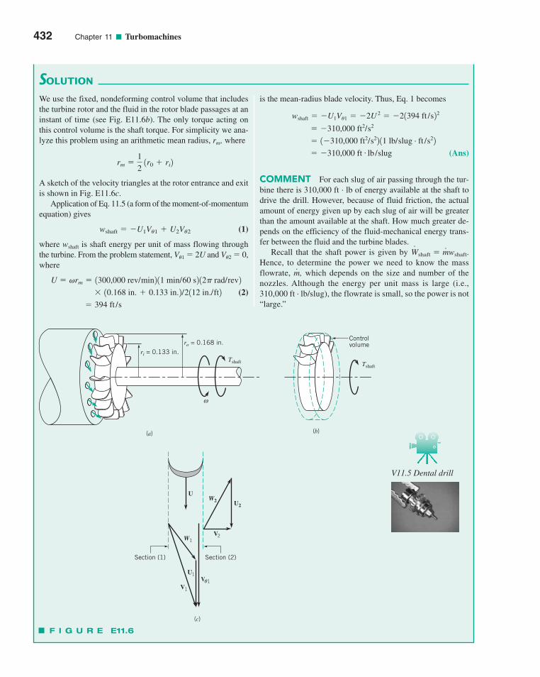
432 Chapter 11 ■ Turbomachines

is the mean-radius blade velocity. Thus, Eq. 1 becomes

(Ans)

COMMENT For each slug of air passing through the tur-bine there is 310,000 ft . lb of energy available at the shaft todrive the drill. However, because of fluid friction, the actualamount of energy given up by each slug of air will be greaterthan the amount available at the shaft. How much greater de-pends on the efficiency of the fluid-mechanical energy trans-fer between the fluid and the turbine blades.

Recall that the shaft power is given by Hence, to determine the power we need to know the massflowrate, , which depends on the size and number of thenozzles. Although the energy per unit mass is large (i.e.,310,000 ft . lb/slug), the flowrate is small, so the power is not“large.”

m�

W� shaft � m� wshaft.

� �310,000 ft . lb /slug

� 1�310,000 ft2/s22 11 lb/slug . ft /s22

� �310,000 ft2/s2

wshaft � �U1V�1 � �2U 2 � �21394 ft /s22

We use the fixed, nondeforming control volume that includesthe turbine rotor and the fluid in the rotor blade passages at aninstant of time (see Fig. E11.6b). The only torque acting onthis control volume is the shaft torque. For simplicity we ana-lyze this problem using an arithmetic mean radius, rm, where

A sketch of the velocity triangles at the rotor entrance and exitis shown in Fig. E11.6c.

Application of Eq. 11.5 (a form of the moment-of-momentumequation) gives

(1)

where wshaft is shaft energy per unit of mass flowing throughthe turbine. From the problem statement, V�1 � 2U and V�2 � 0,where

(2)

� 394 ft /s

� 10.168 in. � 0.133 in.2/2112 in./ft2

U � �rm � 1300,000 rev/min2 11 min/60 s2 12� rad/rev2

wshaft � �U1V�1 � U2V�2

rm �1

2 1r0 � ri2

SOLUTION

ri = 0.133 in.ro = 0.168 in.

Tshaft Tshaft

Controlvolume

Section (1) Section (2)

U

U1

V1

V 1θ

V2W1

U2W2

(a) (b)

(c)

ω

F I G U R E E11.6

V11.5 Dental drill

c11Turbomachines.qxd 9/28/10 10:41 AM Page 432

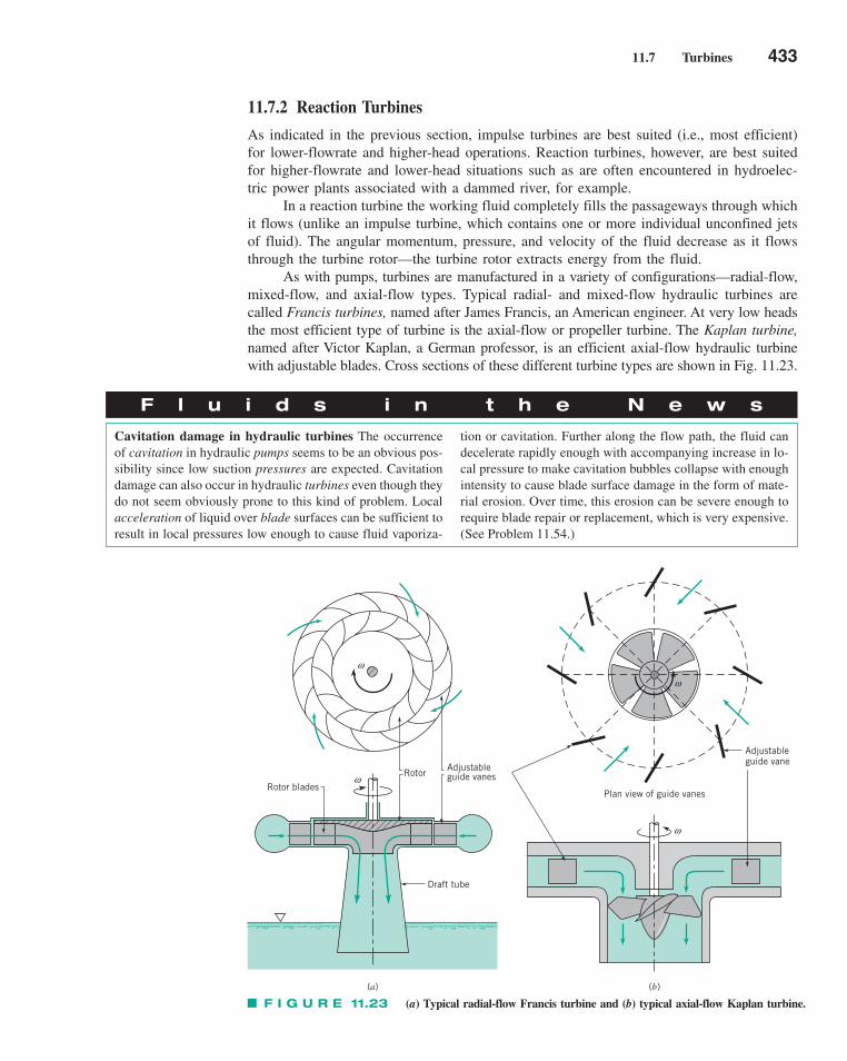
11.7 Turbines 433

11.7.2 Reaction Turbines

As indicated in the previous section, impulse turbines are best suited (i.e., most efficient)for lower-flowrate and higher-head operations. Reaction turbines, however, are best suitedfor higher-flowrate and lower-head situations such as are often encountered in hydroelec-tric power plants associated with a dammed river, for example.

In a reaction turbine the working fluid completely fills the passageways through whichit flows (unlike an impulse turbine, which contains one or more individual unconfined jetsof fluid). The angular momentum, pressure, and velocity of the fluid decrease as it flowsthrough the turbine rotor—the turbine rotor extracts energy from the fluid.

As with pumps, turbines are manufactured in a variety of configurations—radial-flow,mixed-flow, and axial-flow types. Typical radial- and mixed-flow hydraulic turbines arecalled Francis turbines, named after James Francis, an American engineer. At very low headsthe most efficient type of turbine is the axial-flow or propeller turbine. The Kaplan turbine,named after Victor Kaplan, a German professor, is an efficient axial-flow hydraulic turbinewith adjustable blades. Cross sections of these different turbine types are shown in Fig. 11.23.

F l u i d s i n t h e N e w s

Cavitation damage in hydraulic turbines The occurrenceof cavitation in hydraulic pumps seems to be an obvious pos-sibility since low suction pressures are expected. Cavitationdamage can also occur in hydraulic turbines even though theydo not seem obviously prone to this kind of problem. Localacceleration of liquid over blade surfaces can be sufficient toresult in local pressures low enough to cause fluid vaporiza-

tion or cavitation. Further along the flow path, the fluid candecelerate rapidly enough with accompanying increase in lo-cal pressure to make cavitation bubbles collapse with enoughintensity to cause blade surface damage in the form of mate-rial erosion. Over time, this erosion can be severe enough torequire blade repair or replacement, which is very expensive.(See Problem 11.54.)

Rotor blades

ω

RotorAdjustableguide vanes

Draft tube

ω

Adjustableguide vane

Plan view of guide vanes

ω

(a) (b)

ω

F I G U R E 11.23 (a) Typical radial-flow Francis turbine and (b) typical axial-flow Kaplan turbine.

c11Turbomachines.qxd 9/28/10 10:41 AM Page 433

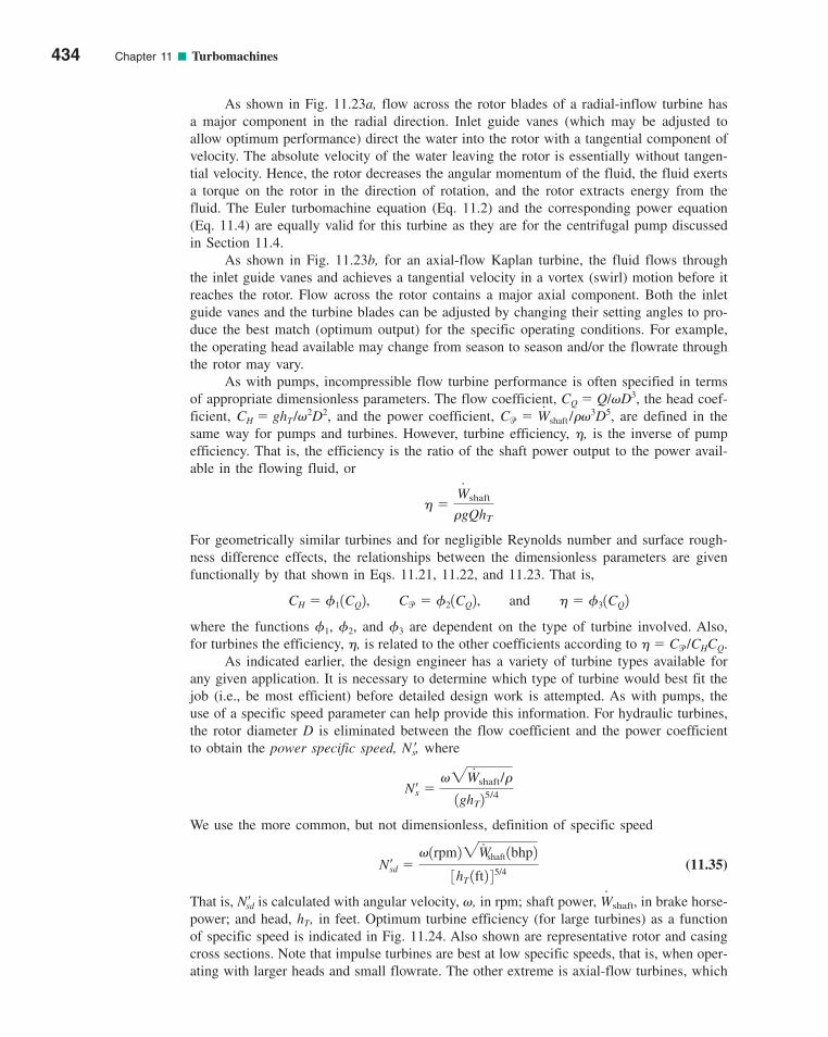
As shown in Fig. 11.23a, flow across the rotor blades of a radial-inflow turbine hasa major component in the radial direction. Inlet guide vanes (which may be adjusted toallow optimum performance) direct the water into the rotor with a tangential component ofvelocity. The absolute velocity of the water leaving the rotor is essentially without tangen-tial velocity. Hence, the rotor decreases the angular momentum of the fluid, the fluid exertsa torque on the rotor in the direction of rotation, and the rotor extracts energy from thefluid. The Euler turbomachine equation (Eq. 11.2) and the corresponding power equation(Eq. 11.4) are equally valid for this turbine as they are for the centrifugal pump discussedin Section 11.4.

As shown in Fig. 11.23b, for an axial-flow Kaplan turbine, the fluid flows throughthe inlet guide vanes and achieves a tangential velocity in a vortex (swirl) motion before itreaches the rotor. Flow across the rotor contains a major axial component. Both the inletguide vanes and the turbine blades can be adjusted by changing their setting angles to pro-duce the best match (optimum output) for the specific operating conditions. For example,the operating head available may change from season to season and/or the flowrate throughthe rotor may vary.

As with pumps, incompressible flow turbine performance is often specified in termsof appropriate dimensionless parameters. The flow coefficient, CQ � Q/�D3, the head coef-ficient, CH � ghT/�2D2, and the power coefficient, are defined in thesame way for pumps and turbines. However, turbine efficiency, , is the inverse of pumpefficiency. That is, the efficiency is the ratio of the shaft power output to the power avail-able in the flowing fluid, or

For geometrically similar turbines and for negligible Reynolds number and surface rough-ness difference effects, the relationships between the dimensionless parameters are givenfunctionally by that shown in Eqs. 11.21, 11.22, and 11.23. That is,

where the functions �1, �2, and �3 are dependent on the type of turbine involved. Also,for turbines the efficiency, , is related to the other coefficients according to � Cp/CHCQ.

As indicated earlier, the design engineer has a variety of turbine types available forany given application. It is necessary to determine which type of turbine would best fit thejob (i.e., be most efficient) before detailed design work is attempted. As with pumps, theuse of a specific speed parameter can help provide this information. For hydraulic turbines,the rotor diameter D is eliminated between the flow coefficient and the power coefficientto obtain the power specific speed, N s, where

We use the more common, but not dimensionless, definition of specific speed

(11.35)

That is, N sd is calculated with angular velocity, �, in rpm; shaft power, in brake horse-power; and head, hT, in feet. Optimum turbine efficiency (for large turbines) as a functionof specific speed is indicated in Fig. 11.24. Also shown are representative rotor and casingcross sections. Note that impulse turbines are best at low specific speeds, that is, when oper-ating with larger heads and small flowrate. The other extreme is axial-flow turbines, which

W� shaft,

N¿sd ��1rpm22W

#shaft 1bhp2

3hT 1ft2 45/4

N¿s ��2W� shaft/�

1ghT25/4

CH � �11CQ2, Cp � �21CQ2, and � �31CQ2

�W� shaft

�gQhT

Cp � W#

shaft /��3D5,

434 Chapter 11 ■ Turbomachines

c11Turbomachines.qxd 9/28/10 10:41 AM Page 434

11.7 Turbines 435

are the most efficient type if the head is low and if the flowrate is large. For intermedi-ate values of specific speeds, radial- and mixed-flow turbines offer the best performance.

Data shown in Fig. 11.24 are meant only to provide a guide for turbine-type selec-tion. The actual turbine efficiency for a given turbine depends very strongly on the detaileddesign of the turbine. Considerable analysis, testing, and experience are needed to producean efficient turbine. However, data of Fig. 11.24 are representative. Much additional infor-mation can be found in the literature (Refs. 11, and 17).

10 20 40 60 80 100

10 20 40 60 80 100

′Nsd

100

90

80

70

%η

Francis

Impulse

Kaplan

Impulse turbines

Radial flow Mixed flow Axial flow

Reaction turbines

′Nsd

F I G U R E 11.24 Typical turbine cross sections and maximumefficiencies as a function of specific speed.

GIVEN A hydraulic turbine is to operate at an angularvelocity of 6 rev/s, a flowrate of 10 ft3/s, and a head of 20 ft.

SOLUTION

Use of Specific Speed to Select Turbine Type

this amount by an assumed efficiency (94%).

Thus, for this turbine,

N¿sd ��2W� shaft

1hT25/4 �

1360 rpm2121.3 hp

120 ft25/4 � 39.3

W� shaft � 21.3 hp

W#

shaft � �Qz � 162.4 lb/ft32 110 ft3/s2 c20 ft10.942

550 ft . lb/s . hpd

FIND What type of turbine should be selected?

EXAMPLE 11.7

The most efficient type of turbine to use can be obtainedby calculating the specific speed, N sd, and using the infor-mation of Fig. 11.24. To use the dimensional form of thespecific speed indicated in Fig. 11.24 we must convert thegiven data into the appropriate units. For the rotor speedwe get

To estimate the shaft power, we assume all of the availablehead is converted into power (i.e., hT � z � 20 ft) and multiply

� � 6 rev/s � 60 s/min � 360 rpm

c11Turbomachines.qxd 9/28/10 10:42 AM Page 435

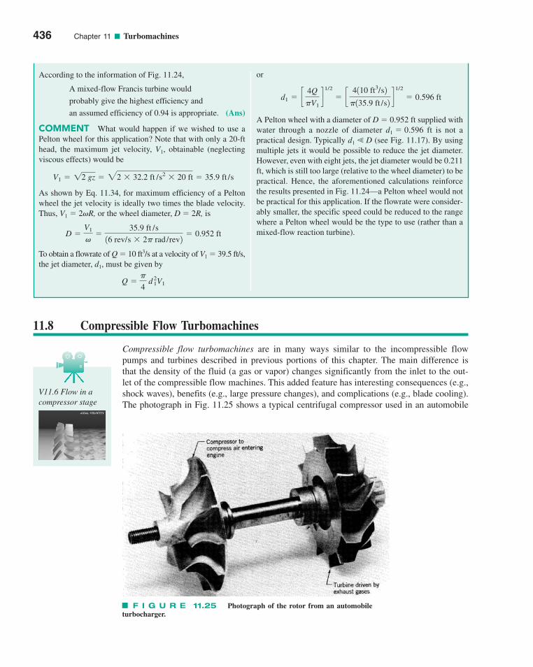
436 Chapter 11 ■ Turbomachines

or

A Pelton wheel with a diameter of D � 0.952 ft supplied withwater through a nozzle of diameter d1 � 0.596 ft is not apractical design. Typically d1 � D (see Fig. 11.17). By usingmultiple jets it would be possible to reduce the jet diameter.However, even with eight jets, the jet diameter would be 0.211ft, which is still too large (relative to the wheel diameter) to bepractical. Hence, the aforementioned calculations reinforcethe results presented in Fig. 11.24—a Pelton wheel would notbe practical for this application. If the flowrate were consider-ably smaller, the specific speed could be reduced to the rangewhere a Pelton wheel would be the type to use (rather than amixed-flow reaction turbine).

d1 � c4Q

�V1d

1/2

� c4110 ft3/s2

�135.9 ft /s2d

1/2

� 0.596 ft

According to the information of Fig. 11.24,

A mixed-flow Francis turbine would

probably give the highest efficiency and

an assumed efficiency of 0.94 is appropriate. (Ans)

COMMENT What would happen if we wished to use aPelton wheel for this application? Note that with only a 20-fthead, the maximum jet velocity, V1, obtainable (neglectingviscous effects) would be

As shown by Eq. 11.34, for maximum efficiency of a Peltonwheel the jet velocity is ideally two times the blade velocity.Thus, V1 � 2�R, or the wheel diameter, D � 2R, is

To obtain a flowrate of Q � 10 ft3/s at a velocity of V1 � 39.5 ft/s,the jet diameter, d1, must be given by

Q ��

4d 2

1V1

D �V1

��

35.9 ft /s

16 rev/s � 2� rad /rev2� 0.952 ft

V1 � 12 gz � 22 � 32.2 ft /s2 � 20 ft � 35.9 ft /s

11.8 Compressible Flow Turbomachines

Compressible flow turbomachines are in many ways similar to the incompressible flowpumps and turbines described in previous portions of this chapter. The main difference isthat the density of the fluid (a gas or vapor) changes significantly from the inlet to the out-let of the compressible flow machines. This added feature has interesting consequences (e.g.,shock waves), benefits (e.g., large pressure changes), and complications (e.g., blade cooling).The photograph in Fig. 11.25 shows a typical centrifugal compressor used in an automobile

F I G U R E 11.25 Photograph of the rotor from an automobileturbocharger.

V11.6 Flow in acompressor stage

c11Turbomachines.qxd 9/28/10 10:42 AM Page 436

11.9 Chapter Summary and Study Guide 437

turbocharger. Exhaust gases from the engine drive the turbine, which powers the compres-sor so that more air can be forced into the engine.

An in-depth understanding of compressible flow turbomachines requires the masteryof various thermodynamic concepts, as well as information provided earlier about basicenergy considerations (Section 11.2) and basic angular momentum considerations (Section 11.3).The interested reader is encouraged to read some of the references available for furtherinformation (Refs. 12, 13, 14, 15, 16, and 17).

11.9 Chapter Summary and Study Guide

This chapter discussed various aspects of turbomachine analysis and design. The conceptsof angular momentum and torque are key to understanding how such pumps and turbinesoperate.

The shaft torque required to change the axial component of angular momentum of afluid as it flows through a pump or turbine is described in terms of diagrams of inlet andoutlet velocity triangles. Such diagrams indicate the relationship among absolute, relative,and blade velocities.

Performance characteristics for centrifugal pumps are discussed. Standard dimension-less pump parameters, similarity laws, and the concept of specific speed are presented foruse in pump analysis. It is shown how to use the pump performance curve and the systemcurve for proper pump selection. A brief discussion of axial-flow and mixed-flow pumps isgiven.

The analysis of impulse turbines is provided, with emphasis on the Pelton wheel tur-bine. For impulse turbines there is negligible pressure difference across the blade; the torqueis a result of the impulse of the fluid jet striking the blade. Radial-flow and axial-flow reac-tion turbines are also discussed.

The following checklist provides a study guide for this chapter. When your studyof the entire chapter and end-of-chapter exercises has been completed, you should beable to

write out meanings of the terms listed here in the margin and understand each of therelated concepts. These terms are particularly important and are set in color and boldtype in the text.

draw appropriate velocity triangles for given pump or turbine configurations.

calculate the shaft torque, shaft power, and pump head for a given centrifugal pumpconfiguration.

use the pump performance curve and the system curve to predict the pump perfor-mance for a given system.

predict the performance characteristics for one pump based on the performance ofanother pump of the same family using the pump scaling laws.

use the specific speed to determine whether a radial flow, mixed flow, or axial flowpump would be most appropriate for a given situation.

calculate the shaft torque and shaft power for an impulse turbine of a given configu-ration.

calculate the shaft torque and shaft power for a given reaction turbine.

use the specific speed to determine whether an impulse or a reaction turbine wouldbe most appropriate for a given situation.

turbomachineaxial, mixed, and

radial flowvelocity triangleangular momentumshaft torqueEuler turbomachine

equationshaft powercentrifugal pumppump performance

curveoverall efficiencysystem equationhead rise coefficientpower coefficientflow coefficientpump scaling lawsspecific speedimpulse turbinereaction turbinePelton wheel

c11Turbomachines.qxd 9/28/10 10:42 AM Page 437

References

1. Stepanoff, H. J., Centrifugal and Axial Flow Pumps, Second Edition, Wiley, New York, 1957.

2. Shepherd, D. G., Principles of Turbomachinery, Macmillan, New York, 1956.

3. Wislicenus, G. F., Preliminary Design of Turbopumps and Related Machinery, NASA Refer-ence Publication 1170, 1986.

4. Neumann, B., The Interaction between Geometry and Performance of a Centrifugal Pump,Mechanical Engineering Publications Limited, London, 1991.

5. Rouse, H., Elementary Mechanics of Fluids, Wiley, New York, 1946.

6. Hydraulic Institute, Hydraulic Institute Pump Standards, CD-ROM, Hydraulic Institute, Cleve-land, Ohio, 2005.

438 Chapter 11 ■ Turbomachines

Some of the important equations in this chapter are

Vector addition of velocities (11.1)

Shaft torque (11.2)

Shaft power (11.3)

Shaft power (11.4)

Shaft work (11.8)

Pump ideal head rise (11.9)

Pump actual head rise (11.14)

Pump similarity relationship (11.21)

Pump similarity relationship (11.22)

Pump similarity relationship (11.23)

Pump scaling law (11.24)

Pump scaling law (11.25)

Pump scaling law (11.26)

Pump scaling law (11.27)

Specific speed (pumps) (11.29)

Specific speed (turbines) (11.35) N¿sd ��1rpm22W

#shaft 1bhp2

3hT 1ft2 45�4

Nsd ��1rpm21Q1gpm2

3hp 1ft2 43�4

h1 � h2

aW#

shaft

rv3D5b

1� a

W#

shaft

rv3D5b

2

aghp

�2D2b

1� a

ghp

�2D2b

2

aQ

vD3b

1� a

Q

vD3b

2

h � f3 aQ

vD3b

W#

shaft

rv3D5� f2 a

Q

vD3b

ghp

�2D2� �1 a

Q

�D3b

ha �p2 � p1

g� z2 � z1 �

V 22 � V 1

2

2g

hi �1g

1U2V�2 � U1V�12

wshaft � U2V�2 � U1V�1

W#

shaft � �m1#1U1Vu12 � m

#21U2Vu22

W#

shaft � Tshaft v

Tshaft � �m#

11r1Vu12 � m#

21r2Vu22

V � W � U

c11Turbomachines.qxd 9/28/10 10:42 AM Page 438

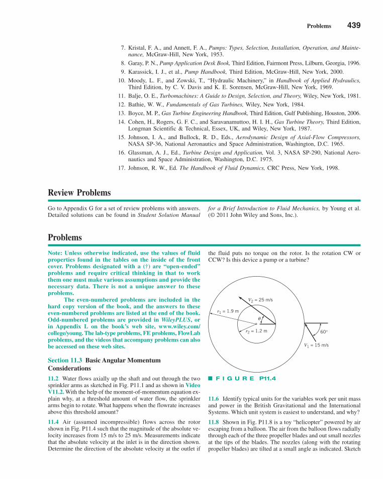
Problems 439

Review Problems

Go to Appendix G for a set of review problems with answers.Detailed solutions can be found in Student Solution Manual

for a Brief Introduction to Fluid Mechanics, by Young et al. (© 2011 John Wiley and Sons, Inc.).

7. Kristal, F. A., and Annett, F. A., Pumps: Types, Selection, Installation, Operation, and Mainte-nance, McGraw-Hill, New York, 1953.

8. Garay, P. N., Pump Application Desk Book, Third Edition, Fairmont Press, Lilburn, Georgia, 1996.

9. Karassick, I. J., et al., Pump Handbook, Third Edition, McGraw-Hill, New York, 2000.

10. Moody, L. F., and Zowski, T., “Hydraulic Machinery,” in Handbook of Applied Hydraulics,Third Edition, by C. V. Davis and K. E. Sorensen, McGraw-Hill, New York, 1969.

11. Balje, O. E., Turbomachines: A Guide to Design, Selection, and Theory, Wiley, New York, 1981.

12. Bathie, W. W., Fundamentals of Gas Turbines, Wiley, New York, 1984.

13. Boyce, M. P., Gas Turbine Engineering Handbook, Third Edition, Gulf Publishing, Houston, 2006.

14. Cohen, H., Rogers, G. F. C., and Saravanamuttoo, H. I. H., Gas Turbine Theory, Third Edition,Longman Scientific & Technical, Essex, UK, and Wiley, New York, 1987.

15. Johnson, I. A., and Bullock, R. D., Eds., Aerodynamic Design of Axial-Flow Compressors,NASA SP-36, National Aeronautics and Space Administration, Washington, D.C. 1965.

16. Glassman, A. J., Ed., Turbine Design and Application, Vol. 3, NASA SP-290, National Aero-nautics and Space Administration, Washington, D.C. 1975.

17. Johnson, R. W., Ed. The Handbook of Fluid Dynamics, CRC Press, New York, 1998.

Problems

Note: Unless otherwise indicated, use the values of fluidproperties found in the tables on the inside of the frontcover. Problems designated with a (†) are “open-ended”problems and require critical thinking in that to workthem one must make various assumptions and provide thenecessary data. There is not a unique answer to theseproblems.

The even-numbered problems are included in thehard copy version of the book, and the answers to theseeven-numbered problems are listed at the end of the book.Odd-numbered problems are provided in WileyPLUS, orin Appendix L on the book’s web site, www.wiley.com/college/young. The lab-type problems, FE problems, FlowLabproblems, and the videos that accompany problems can alsobe accessed on these web sites.

Section 11.3 Basic Angular MomentumConsiderations

11.2 Water flows axially up the shaft and out through the twosprinkler arms as sketched in Fig. P11.1 and as shown in VideoV11.2. With the help of the moment-of-momentum equation ex-plain why, at a threshold amount of water flow, the sprinklerarms begin to rotate. What happens when the flowrate increasesabove this threshold amount?

11.4 Air (assumed incompressible) flows across the rotorshown in Fig. P11.4 such that the magnitude of the absolute ve-locity increases from 15 m/s to 25 m/s. Measurements indicatethat the absolute velocity at the inlet is in the direction shown.Determine the direction of the absolute velocity at the outlet if

the fluid puts no torque on the rotor. Is the rotation CW orCCW? Is this device a pump or a turbine?

11.6 Identify typical units for the variables work per unit massand power in the British Gravitational and the International Systems. Which unit system is easiest to understand, and why?

11.8 Shown in Fig. P11.8 is a toy “helicopter” powered by airescaping from a balloon. The air from the balloon flows radiallythrough each of the three propeller blades and out small nozzlesat the tips of the blades. The nozzles (along with the rotatingpropeller blades) are tilted at a small angle as indicated. Sketch

F I G U R E P11.4

60°

V1 = 15 m/s

V2 = 25 m/s

r2 = 1.2 m

r1 = 1.9 m

θ

c11Turbomachines.qxd 10/18/10 8:08 AM Page 439

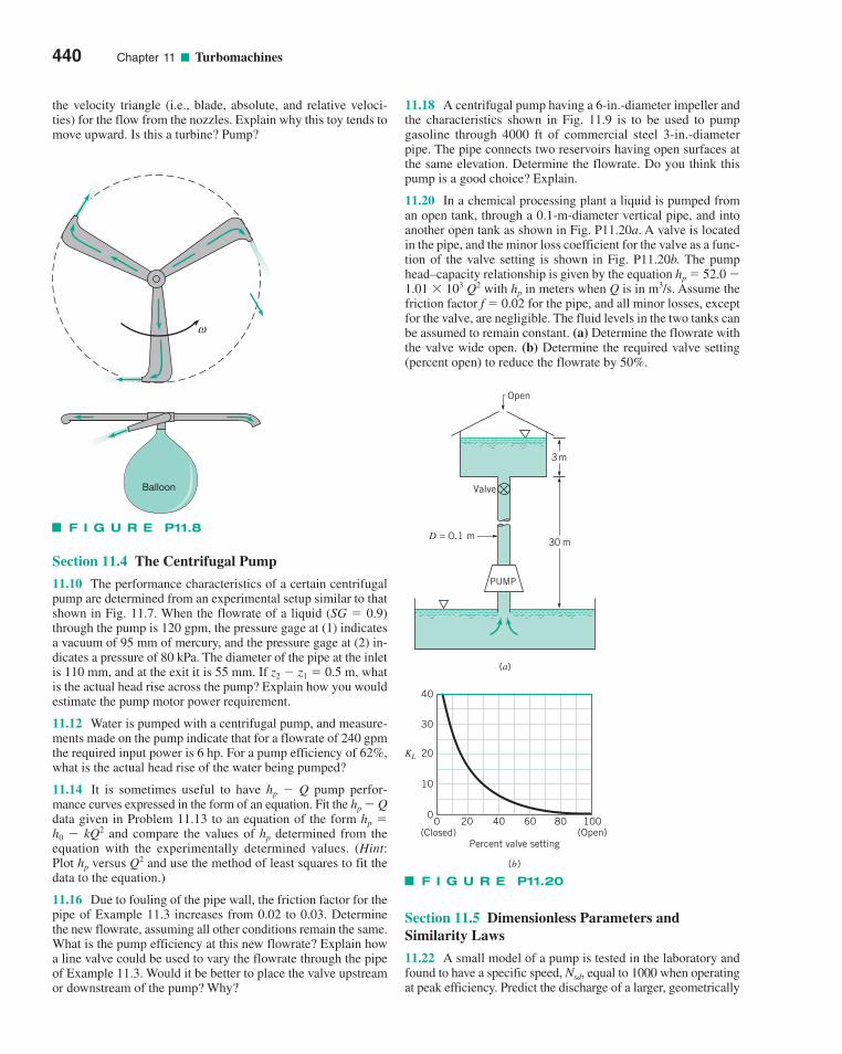
the velocity triangle (i.e., blade, absolute, and relative veloci-ties) for the flow from the nozzles. Explain why this toy tends tomove upward. Is this a turbine? Pump?

Section 11.4 The Centrifugal Pump

11.10 The performance characteristics of a certain centrifugalpump are determined from an experimental setup similar to thatshown in Fig. 11.7. When the flowrate of a liquid (SG � 0.9)through the pump is 120 gpm, the pressure gage at (1) indicatesa vacuum of 95 mm of mercury, and the pressure gage at (2) in-dicates a pressure of 80 kPa. The diameter of the pipe at the inletis 110 mm, and at the exit it is 55 mm. If z2 � z1 � 0.5 m, whatis the actual head rise across the pump? Explain how you wouldestimate the pump motor power requirement.

11.12 Water is pumped with a centrifugal pump, and measure-ments made on the pump indicate that for a flowrate of 240 gpmthe required input power is 6 hp. For a pump efficiency of 62%,what is the actual head rise of the water being pumped?

11.14 It is sometimes useful to have hp � Q pump perfor-mance curves expressed in the form of an equation. Fit the hp � Qdata given in Problem 11.13 to an equation of the form hp �h0 � kQ2 and compare the values of hp determined from theequation with the experimentally determined values. (Hint:Plot hp versus Q2 and use the method of least squares to fit thedata to the equation.)

11.16 Due to fouling of the pipe wall, the friction factor for thepipe of Example 11.3 increases from 0.02 to 0.03. Determinethe new flowrate, assuming all other conditions remain the same.What is the pump efficiency at this new flowrate? Explain howa line valve could be used to vary the flowrate through the pipeof Example 11.3. Would it be better to place the valve upstreamor downstream of the pump? Why?

11.18 A centrifugal pump having a 6-in.-diameter impeller andthe characteristics shown in Fig. 11.9 is to be used to pumpgasoline through 4000 ft of commercial steel 3-in.-diameterpipe. The pipe connects two reservoirs having open surfaces atthe same elevation. Determine the flowrate. Do you think thispump is a good choice? Explain.

11.20 In a chemical processing plant a liquid is pumped froman open tank, through a 0.1-m-diameter vertical pipe, and intoanother open tank as shown in Fig. P11.20a. A valve is locatedin the pipe, and the minor loss coefficient for the valve as a func-tion of the valve setting is shown in Fig. P11.20b. The pumphead–capacity relationship is given by the equation hp � 52.0 �1.01 � 103 Q2 with hp in meters when Q is in m3/s. Assume thefriction factor f � 0.02 for the pipe, and all minor losses, exceptfor the valve, are negligible. The fluid levels in the two tanks canbe assumed to remain constant. (a) Determine the flowrate withthe valve wide open. (b) Determine the required valve setting(percent open) to reduce the flowrate by 50%.

440 Chapter 11 ■ Turbomachines

F I G U R E P11.8

ω

Balloon

F I G U R E P11.20

020 40 60 80 100

10

20

30

40

0(Open)(Closed)

Percent valve setting

Valve

D = 0.1 m

Open

PUMP

KL

30 m

3 m

(a)

(b)

Section 11.5 Dimensionless Parameters andSimilarity Laws

11.22 A small model of a pump is tested in the laboratory andfound to have a specific speed, Nsd, equal to 1000 when operatingat peak efficiency. Predict the discharge of a larger, geometrically

c11Turbomachines.qxd 9/28/10 10:42 AM Page 440

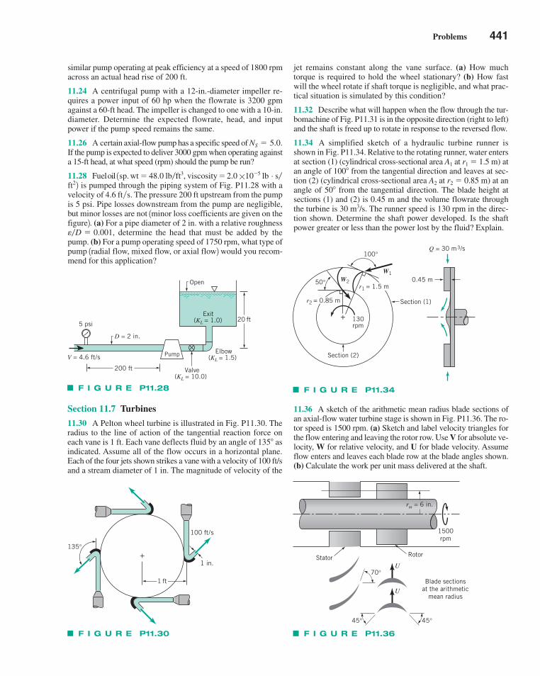
Problems 441

similar pump operating at peak efficiency at a speed of 1800 rpmacross an actual head rise of 200 ft.

11.24 A centrifugal pump with a 12-in.-diameter impeller re-quires a power input of 60 hp when the flowrate is 3200 gpmagainst a 60-ft head. The impeller is changed to one with a 10-in.diameter. Determine the expected flowrate, head, and inputpower if the pump speed remains the same.

11.26 A certain axial-flow pump has a specific speed of If the pump is expected to deliver 3000 gpm when operating againsta 15-ft head, at what speed (rpm) should the pump be run?

11.28 Fueloil �is pumped through the piping system of Fig. P11.28 with a

velocity of 4.6 ft�s. The pressure 200 ft upstream from the pumpis 5 psi. Pipe losses downstream from the pump are negligible,but minor losses are not 1minor loss coefficients are given on thefigure2. (a) For a pipe diameter of 2 in. with a relative roughness

determine the head that must be added by thepump. (b) For a pump operating speed of 1750 rpm, what type ofpump 1radial flow, mixed flow, or axial flow2 would you recom-mend for this application?

e�D � 0.001,

ft2210�5 lb # s�1sp. wt � 48.0 lb�ft3, viscosity � 2.0

NS � 5.0.

Section 11.7 Turbines

11.30 A Pelton wheel turbine is illustrated in Fig. P11.30. Theradius to the line of action of the tangential reaction force oneach vane is 1 ft. Each vane deflects fluid by an angle of 135� asindicated. Assume all of the flow occurs in a horizontal plane.Each of the four jets shown strikes a vane with a velocity of 100 ft/sand a stream diameter of 1 in. The magnitude of velocity of the

jet remains constant along the vane surface. (a) How muchtorque is required to hold the wheel stationary? (b) How fastwill the wheel rotate if shaft torque is negligible, and what prac-tical situation is simulated by this condition?

11.32 Describe what will happen when the flow through the tur-bomachine of Fig. P11.31 is in the opposite direction (right to left)and the shaft is freed up to rotate in response to the reversed flow.

11.34 A simplified sketch of a hydraulic turbine runner isshown in Fig. P11.34. Relative to the rotating runner, water entersat section (1) (cylindrical cross-sectional area A1 at r1 � 1.5 m) atan angle of 100� from the tangential direction and leaves at sec-tion (2) (cylindrical cross-sectional area A2 at r2 � 0.85 m) at anangle of 50� from the tangential direction. The blade height atsections (1) and (2) is 0.45 m and the volume flowrate throughthe turbine is 30 m3/s. The runner speed is 130 rpm in the direc-tion shown. Determine the shaft power developed. Is the shaftpower greater or less than the power lost by the fluid? Explain.

11.36 A sketch of the arithmetic mean radius blade sections ofan axial-flow water turbine stage is shown in Fig. P11.36. The ro-tor speed is 1500 rpm. (a) Sketch and label velocity triangles forthe flow entering and leaving the rotor row. Use V for absolute ve-locity, W for relative velocity, and U for blade velocity. Assumeflow enters and leaves each blade row at the blade angles shown.(b) Calculate the work per unit mass delivered at the shaft.

F I G U R E P11.28

D = 2 in.

Valve

Pump

(KL = 10.0)

(KL = 1.5) Elbow

(KL = 1.0) Exit

V = 4.6 ft/s

5 psi

Open

200 ft

20 ft

F I G U R E P11.30

1 in.+

1 ft

100 ft/s

135°

F I G U R E P11.34

Section (1)

Section (2)

130rpm

+

Q = 30 m3/s

0.45 m50° W2

W1

r2 = 0.85 m

r1 = 1.5 m

100°

F I G U R E P11.36

rm = 6 in.

U

U

70°

45° 45°

Blade sectionsat the arithmetic

mean radius

1500rpm

Stator Rotor

c11Turbomachines.qxd 9/28/10 10:42 AM Page 441

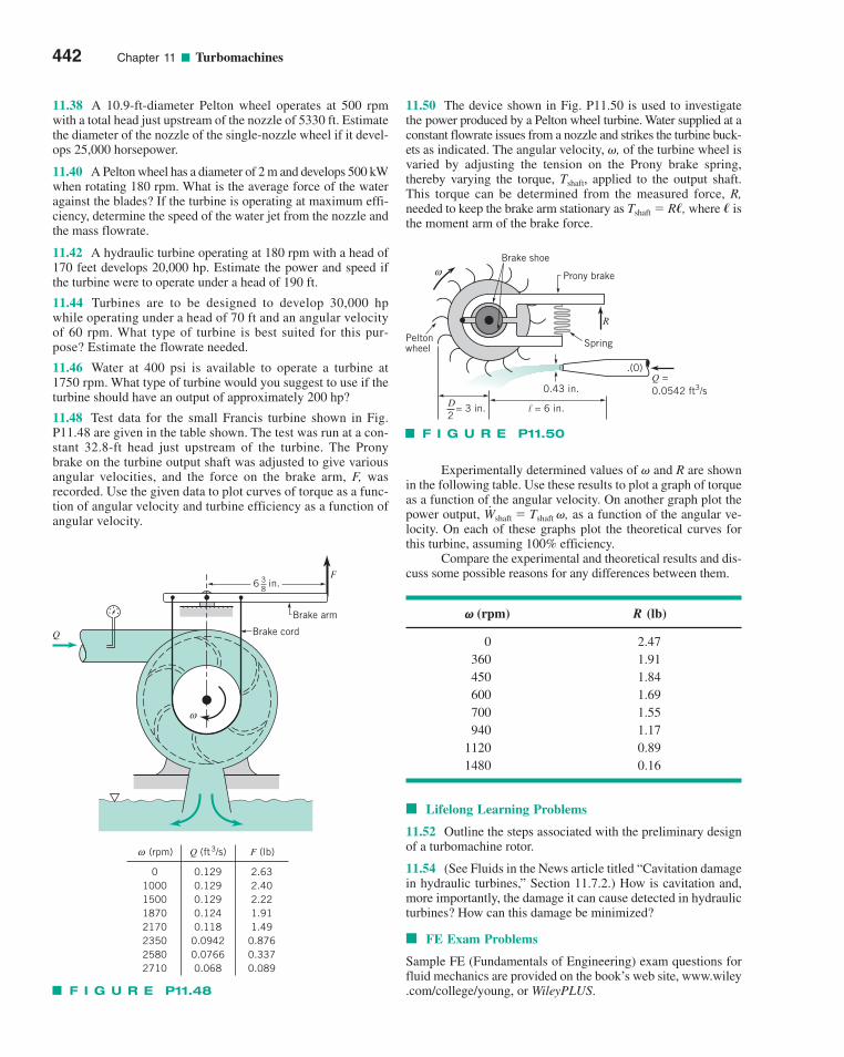
442 Chapter 11 ■ Turbomachines

11.38 A 10.9-ft-diameter Pelton wheel operates at 500 rpmwith a total head just upstream of the nozzle of 5330 ft. Estimatethe diameter of the nozzle of the single-nozzle wheel if it devel-ops 25,000 horsepower.

11.40 A Pelton wheel has a diameter of 2 m and develops 500 kWwhen rotating 180 rpm. What is the average force of the wateragainst the blades? If the turbine is operating at maximum effi-ciency, determine the speed of the water jet from the nozzle andthe mass flowrate.

11.42 A hydraulic turbine operating at 180 rpm with a head of170 feet develops 20,000 hp. Estimate the power and speed ifthe turbine were to operate under a head of 190 ft.

11.44 Turbines are to be designed to develop 30,000 hpwhile operating under a head of 70 ft and an angular velocityof 60 rpm. What type of turbine is best suited for this pur-pose? Estimate the flowrate needed.

11.46 Water at 400 psi is available to operate a turbine at1750 rpm. What type of turbine would you suggest to use if theturbine should have an output of approximately 200 hp?

11.48 Test data for the small Francis turbine shown in Fig.P11.48 are given in the table shown. The test was run at a con-stant 32.8-ft head just upstream of the turbine. The Pronybrake on the turbine output shaft was adjusted to give variousangular velocities, and the force on the brake arm, F, wasrecorded. Use the given data to plot curves of torque as a func-tion of angular velocity and turbine efficiency as a function ofangular velocity.

11.50 The device shown in Fig. P11.50 is used to investigatethe power produced by a Pelton wheel turbine. Water supplied at aconstant flowrate issues from a nozzle and strikes the turbine buck-ets as indicated. The angular velocity, �, of the turbine wheel isvaried by adjusting the tension on the Prony brake spring,thereby varying the torque, Tshaft, applied to the output shaft.This torque can be determined from the measured force, R,needed to keep the brake arm stationary as Tshaft � R�, where � isthe moment arm of the brake force.

Experimentally determined values of � and R are shownin the following table. Use these results to plot a graph of torqueas a function of the angular velocity. On another graph plot thepower output, shaft � Tshaft �, as a function of the angular ve-locity. On each of these graphs plot the theoretical curves forthis turbine, assuming 100% efficiency.

Compare the experimental and theoretical results and dis-cuss some possible reasons for any differences between them.

� (rpm) R (lb)

0 2.47360 1.91450 1.84600 1.69700 1.55940 1.17

1120 0.891480 0.16

■ Lifelong Learning Problems

11.52 Outline the steps associated with the preliminary designof a turbomachine rotor.

11.54 (See Fluids in the News article titled “Cavitation damagein hydraulic turbines,” Section 11.7.2.) How is cavitation and,more importantly, the damage it can cause detected in hydraulicturbines? How can this damage be minimized?

■ FE Exam Problems

Sample FE (Fundamentals of Engineering) exam questions forfluid mechanics are provided on the book’s web site, www.wiley.com/college/young, or WileyPLUS.

W#

F I G U R E P11.50

Prony brakeω

Peltonwheel Spring

Brake shoe

0.43 in.

.(0)

R

= 6 in.

Q =0.0542 ft3/s

D2

= 3 in.

F I G U R E P11.48

F

Q

Brake arm

Brake cord

(rpm) Q (ft3/s) F (lb)

01000150018702170235025802710

0.1290.1290.1290.1240.118

0.09420.07660.068

2.632.402.221.911.49

0.8760.3370.089

ω

ω

6 in.38

c11Turbomachines.qxd 9/28/10 10:42 AM Page 442

Appendix AComputational Fluid Dynamicsand FlowLab

A.1 Introduction

Numerical methods using digital computers are, of course, commonly utilized to solve a widevariety of flow problems. As discussed in Chapter 6, although the differential equations thatgovern the flow of Newtonian fluids [the Navier–Stokes equations (Eq. 6.120)] were derivedmany years ago, there are few known analytical solutions to them. However, with the adventof high-speed digital computers it has become possible to obtain approximate numerical solu-tions to these (and other fluid mechanics) equations for a wide variety of circumstances.

Computational fluid dynamics (CFD) involves replacing the partial differential equa-tions with discretized algebraic equations that approximate the partial differential equations.These equations are then numerically solved to obtain flow field values at the discrete pointsin space and/or time. Since the Navier–Stokes equations are valid everywhere in the flowfield of the fluid continuum, an analytical solution to these equations provides the solutionfor an infinite number of points in the flow. However, analytical solutions are available foronly a limited number of simplified flow geometries. To overcome this limitation, the gov-erning equations can be discretized and put in algebraic form for the computer to solve.The CFD simulation solves for the relevant flow variables only at the discrete points, whichmake up the grid or mesh of the solution (discussed in more detail later). Interpolationschemes are used to obtain values at non–grid point locations.

CFD can be thought of as a numerical experiment. In a typical fluids experiment, anexperimental model is built, measurements of the flow interacting with that model are taken,and the results are analyzed. In CFD, the building of the model is replaced with the formula-tion of the governing equations and the development of the numerical algorithm. The processof obtaining measurements is replaced with running an algorithm on the computer to simulatethe flow interaction. Of course, the analysis of results is common ground to both techniques.

CFD can be classified as a subdiscipline to the study of fluid dynamics. However, itshould be pointed out that a thorough coverage of CFD topics is well beyond the scope of thistextbook. This appendix highlights some of the more important topics in CFD but is onlyintended as a brief introduction. The topics include discretization of the governing equations,grid generation, boundary conditions, application of CFD, and some representative examples.Also included is a section on FlowLab, which is the educational CFD software incorporatedwith this textbook. FlowLab offers the reader the opportunity to begin using CFD to solve flowproblems as well as to reinforce concepts covered in the textbook. For more information, visitthe book web site, or WileyPLUS, to access the FlowLab problems, tutorials, and user’s guide.

VA.1 Pouring a liquid

A.2 Discretization

The process of discretization involves developing a set of algebraic equations (based on dis-crete points in the flow domain) to be used in place of the partial differential equations. Ofthe various discretization techniques available for the numerical solution of the governing

443

appAComputationalFluidDynamicsandFlowLab.qxd 9/28/10 4:43 PM Page 443

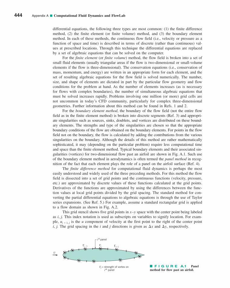
differential equations, the following three types are most common: (1) the finite differencemethod, (2) the finite element (or finite volume) method, and (3) the boundary elementmethod. In each of these methods, the continuous flow field (i.e., velocity or pressure as afunction of space and time) is described in terms of discrete (rather than continuous) val-ues at prescribed locations. Through this technique the differential equations are replacedby a set of algebraic equations that can be solved on the computer.

For the finite element (or finite volume) method, the flow field is broken into a set ofsmall fluid elements (usually triangular areas if the flow is two-dimensional or small-volumeelements if the flow is three-dimensional). The conservation equations (i.e., conservation ofmass, momentum, and energy) are written in an appropriate form for each element, and theset of resulting algebraic equations for the flow field is solved numerically. The number,size, and shape of elements are dictated in part by the particular flow geometry and flowconditions for the problem at hand. As the number of elements increases (as is necessaryfor flows with complex boundaries), the number of simultaneous algebraic equations thatmust be solved increases rapidly. Problems involving one million (or more) grid cells arenot uncommon in today’s CFD community, particularly for complex three-dimensionalgeometries. Further information about this method can be found in Refs. 1 and 2.

For the boundary element method, the boundary of the flow field (not the entire flowfield as in the finite element method) is broken into discrete segments (Ref. 3) and appropri-ate singularities such as sources, sinks, doublets, and vortices are distributed on these bound-ary elements. The strengths and type of the singularities are chosen so that the appropriateboundary conditions of the flow are obtained on the boundary elements. For points in the flowfield not on the boundary, the flow is calculated by adding the contributions from the varioussingularities on the boundary. Although the details of this method are rather mathematicallysophisticated, it may (depending on the particular problem) require less computational timeand space than the finite element method. Typical boundary elements and their associated sin-gularities (vortices) for two-dimensional flow past an airfoil are shown in Fig. A.1. Such useof the boundary element method in aerodynamics is often termed the panel method in recog-nition of the fact that each element plays the role of a panel on the airfoil surface (Ref. 4).

The finite difference method for computational fluid dynamics is perhaps the mosteasily understood and widely used of the three preceding methods. For this method the flowfield is dissected into a set of grid points and the continuous functions (velocity, pressure,etc.) are approximated by discrete values of these functions calculated at the grid points.Derivatives of the functions are approximated by using the differences between the func-tion values at local grid points divided by the grid spacing. The standard method for con-verting the partial differential equations to algebraic equations is through the use of Taylorseries expansions. (See Ref. 5.) For example, assume a standard rectangular grid is appliedto a flow domain as shown in Fig. A.2.

This grid stencil shows five grid points in x–y space with the center point being labeledas i, j. This index notation is used as subscripts on variables to signify location. For exam-ple, is the u component of velocity at the first point to the right of the center pointi, j. The grid spacing in the i and j directions is given as and , respectively.¢y¢x

ui � 1, j

444 Appendix A ■ Computational Fluid Dynamics and FlowLab

i – 1

i th panel

i = strength of vortex on i th panel

Γ

U

iΓi + 1 Γ

Γ F I G U R E A.1 Panelmethod for flow past an airfoil.

appAComputationalFluidDynamicsandFlowLab.qxd 9/28/10 4:43 PM Page 444

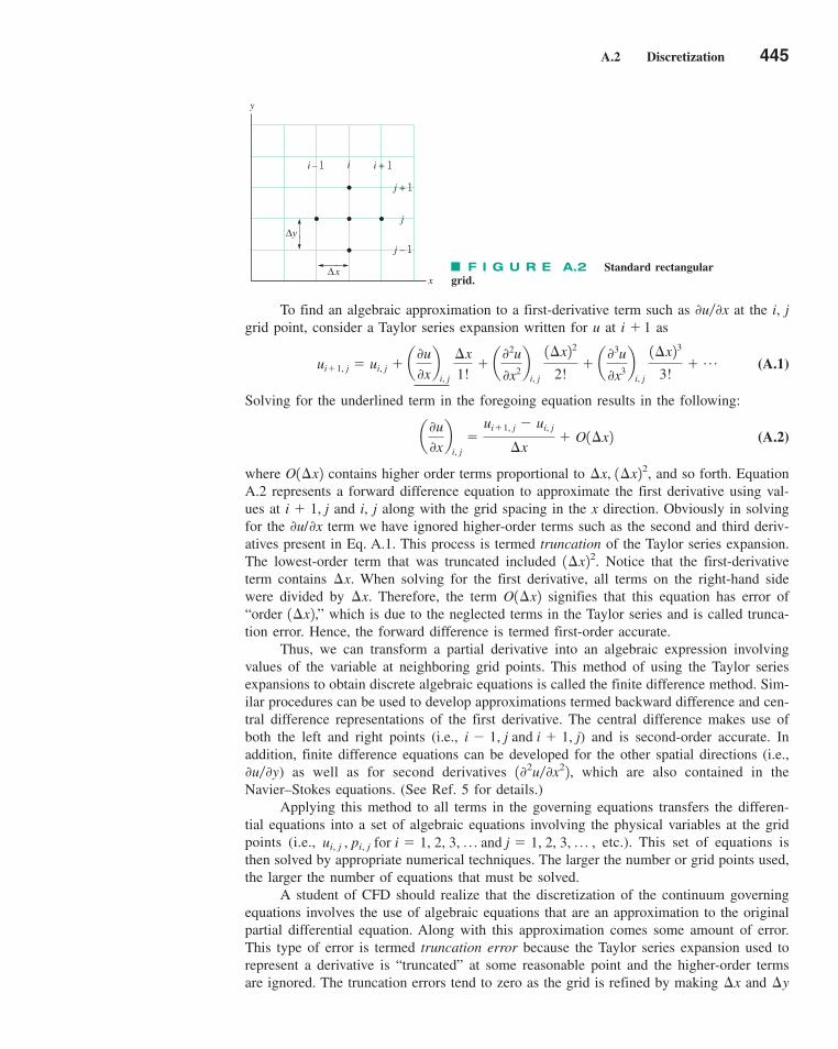
A.2 Discretization 445

To find an algebraic approximation to a first-derivative term such as at the i, jgrid point, consider a Taylor series expansion written for u at as

(A.1)

Solving for the underlined term in the foregoing equation results in the following:

(A.2)

where contains higher order terms proportional to , and so forth. EquationA.2 represents a forward difference equation to approximate the first derivative using val-ues at and i, j along with the grid spacing in the x direction. Obviously in solvingfor the term we have ignored higher-order terms such as the second and third deriv-atives present in Eq. A.1. This process is termed truncation of the Taylor series expansion.The lowest-order term that was truncated included . Notice that the first-derivativeterm contains . When solving for the first derivative, all terms on the right-hand sidewere divided by . Therefore, the term signifies that this equation has error of“order ,” which is due to the neglected terms in the Taylor series and is called trunca-tion error. Hence, the forward difference is termed first-order accurate.

Thus, we can transform a partial derivative into an algebraic expression involvingvalues of the variable at neighboring grid points. This method of using the Taylor seriesexpansions to obtain discrete algebraic equations is called the finite difference method. Sim-ilar procedures can be used to develop approximations termed backward difference and cen-tral difference representations of the first derivative. The central difference makes use ofboth the left and right points (i.e., ) and is second-order accurate. Inaddition, finite difference equations can be developed for the other spatial directions (i.e.,

) as well as for second derivatives , which are also contained in theNavier–Stokes equations. (See Ref. 5 for details.)

Applying this method to all terms in the governing equations transfers the differen-tial equations into a set of algebraic equations involving the physical variables at the gridpoints (i.e., etc.). This set of equations isthen solved by appropriate numerical techniques. The larger the number or grid points used,the larger the number of equations that must be solved.

A student of CFD should realize that the discretization of the continuum governingequations involves the use of algebraic equations that are an approximation to the originalpartial differential equation. Along with this approximation comes some amount of error.This type of error is termed truncation error because the Taylor series expansion used torepresent a derivative is “truncated” at some reasonable point and the higher-order termsare ignored. The truncation errors tend to zero as the grid is refined by making and ¢y¢x

ui, j , pi, j for i � 1, 2, 3, p and j � 1, 2, 3, p ,

102u�0x220u�0y

i � 1, j and i � 1, j

1¢x2O1¢x2¢x

¢x1¢x22

0u/0xi � 1, j

¢x, 1¢x22O1¢x2

a0u

0xb

i, j�

ui�1, j � ui, j

¢x� O1¢x2

ui�1, j � ui, j � a0u

0xb

i, j ¢x

1!� a

02u

0x2b

i, j 1¢x22

2!� a

03u

0x3b

i, j 1¢x23

3!� p

i � 10u�0x

y

i – 1 i + 1

j + 1

j – 1

j

i

x

Δy

Δx F I G U R E A.2 Standard rectangulargrid.

appAComputationalFluidDynamicsandFlowLab.qxd 9/28/10 4:43 PM Page 445

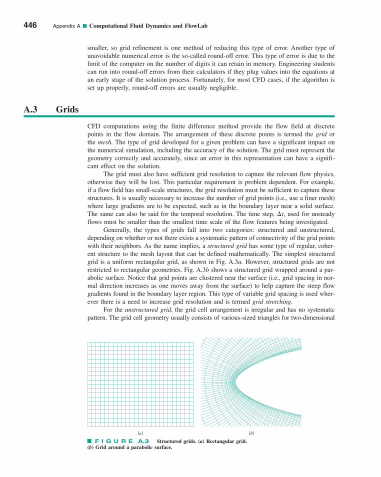
smaller, so grid refinement is one method of reducing this type of error. Another type ofunavoidable numerical error is the so-called round-off error. This type of error is due to thelimit of the computer on the number of digits it can retain in memory. Engineering studentscan run into round-off errors from their calculators if they plug values into the equations atan early stage of the solution process. Fortunately, for most CFD cases, if the algorithm isset up properly, round-off errors are usually negligible.

446 Appendix A ■ Computational Fluid Dynamics and FlowLab

A.3 Grids

CFD computations using the finite difference method provide the flow field at discretepoints in the flow domain. The arrangement of these discrete points is termed the grid orthe mesh. The type of grid developed for a given problem can have a significant impact onthe numerical simulation, including the accuracy of the solution. The grid must represent thegeometry correctly and accurately, since an error in this representation can have a signifi-cant effect on the solution.

The grid must also have sufficient grid resolution to capture the relevant flow physics,otherwise they will be lost. This particular requirement is problem dependent. For example,if a flow field has small-scale structures, the grid resolution must be sufficient to capture thesestructures. It is usually necessary to increase the number of grid points (i.e., use a finer mesh)where large gradients are to be expected, such as in the boundary layer near a solid surface.The same can also be said for the temporal resolution. The time step, , used for unsteadyflows must be smaller than the smallest time scale of the flow features being investigated.

Generally, the types of grids fall into two categories: structured and unstructured,depending on whether or not there exists a systematic pattern of connectivity of the grid pointswith their neighbors. As the name implies, a structured grid has some type of regular, coher-ent structure to the mesh layout that can be defined mathematically. The simplest structuredgrid is a uniform rectangular grid, as shown in Fig. A.3a. However, structured grids are notrestricted to rectangular geometries. Fig. A.3b shows a structured grid wrapped around a par-abolic surface. Notice that grid points are clustered near the surface (i.e., grid spacing in nor-mal direction increases as one moves away from the surface) to help capture the steep flowgradients found in the boundary layer region. This type of variable grid spacing is used wher-ever there is a need to increase grid resolution and is termed grid stretching.

For the unstructured grid, the grid cell arrangement is irregular and has no systematicpattern. The grid cell geometry usually consists of various-sized triangles for two-dimensional

¢t

(a) (b)

F I G U R E A.3 Structured grids. (a) Rectangular grid. (b) Grid around a parabolic surface.

appAComputationalFluidDynamicsandFlowLab.qxd 9/28/10 4:43 PM Page 446

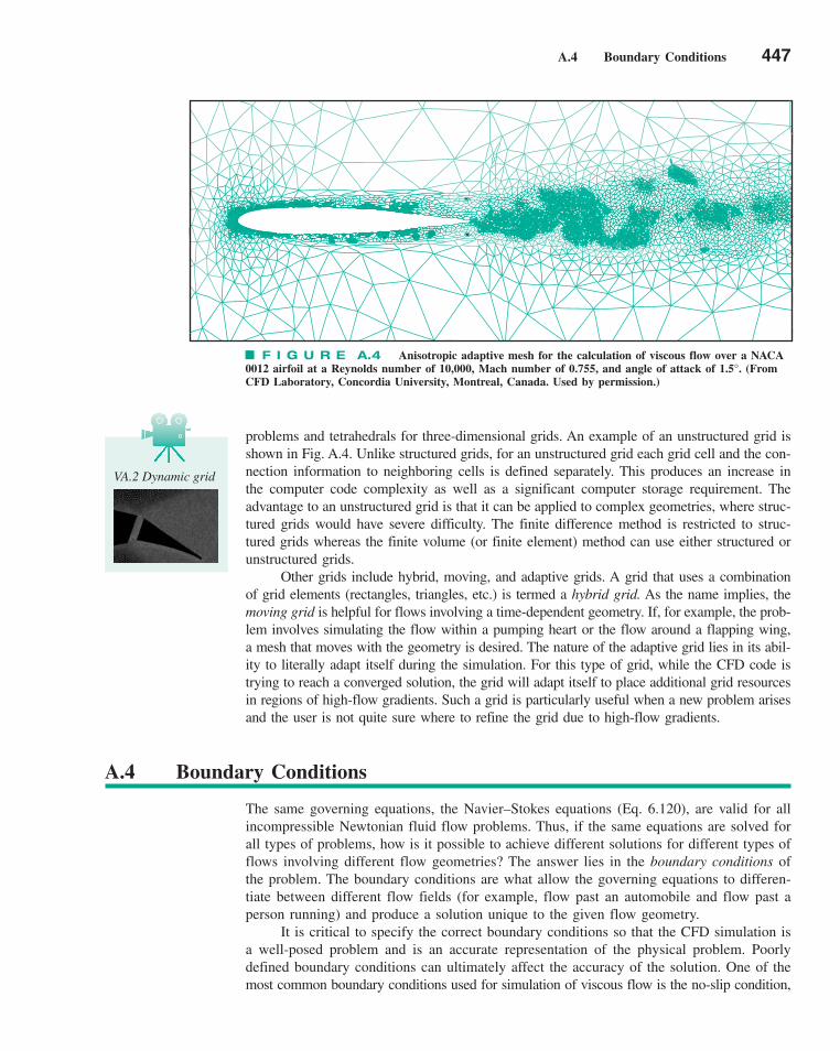
A.4 Boundary Conditions 447

problems and tetrahedrals for three-dimensional grids. An example of an unstructured grid isshown in Fig. A.4. Unlike structured grids, for an unstructured grid each grid cell and the con-nection information to neighboring cells is defined separately. This produces an increase inthe computer code complexity as well as a significant computer storage requirement. Theadvantage to an unstructured grid is that it can be applied to complex geometries, where struc-tured grids would have severe difficulty. The finite difference method is restricted to struc-tured grids whereas the finite volume (or finite element) method can use either structured orunstructured grids.

Other grids include hybrid, moving, and adaptive grids. A grid that uses a combinationof grid elements (rectangles, triangles, etc.) is termed a hybrid grid. As the name implies, themoving grid is helpful for flows involving a time-dependent geometry. If, for example, the prob-lem involves simulating the flow within a pumping heart or the flow around a flapping wing,a mesh that moves with the geometry is desired. The nature of the adaptive grid lies in its abil-ity to literally adapt itself during the simulation. For this type of grid, while the CFD code istrying to reach a converged solution, the grid will adapt itself to place additional grid resourcesin regions of high-flow gradients. Such a grid is particularly useful when a new problem arisesand the user is not quite sure where to refine the grid due to high-flow gradients.

VA.2 Dynamic grid

F I G U R E A.4 Anisotropic adaptive mesh for the calculation of viscous flow over a NACA0012 airfoil at a Reynolds number of 10,000, Mach number of 0.755, and angle of attack of 1.5°. (FromCFD Laboratory, Concordia University, Montreal, Canada. Used by permission.)

A.4 Boundary Conditions

The same governing equations, the Navier–Stokes equations (Eq. 6.120), are valid for allincompressible Newtonian fluid flow problems. Thus, if the same equations are solved forall types of problems, how is it possible to achieve different solutions for different types offlows involving different flow geometries? The answer lies in the boundary conditions ofthe problem. The boundary conditions are what allow the governing equations to differen-tiate between different flow fields (for example, flow past an automobile and flow past aperson running) and produce a solution unique to the given flow geometry.

It is critical to specify the correct boundary conditions so that the CFD simulation isa well-posed problem and is an accurate representation of the physical problem. Poorlydefined boundary conditions can ultimately affect the accuracy of the solution. One of themost common boundary conditions used for simulation of viscous flow is the no-slip condition,

appAComputationalFluidDynamicsandFlowLab.qxd 9/28/10 4:43 PM Page 447

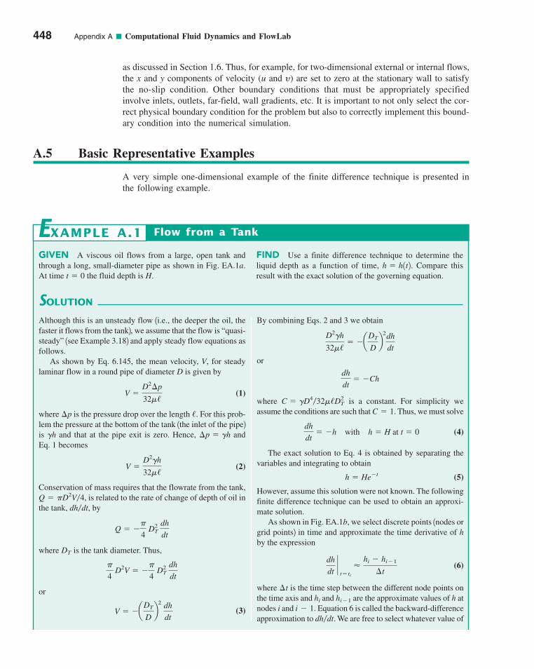
as discussed in Section 1.6. Thus, for example, for two-dimensional external or internal flows,the x and y components of velocity (u and y) are set to zero at the stationary wall to satisfythe no-slip condition. Other boundary conditions that must be appropriately specifiedinvolve inlets, outlets, far-field, wall gradients, etc. It is important to not only select the cor-rect physical boundary condition for the problem but also to correctly implement this bound-ary condition into the numerical simulation.

448 Appendix A ■ Computational Fluid Dynamics and FlowLab

A.5 Basic Representative Examples

A very simple one-dimensional example of the finite difference technique is presented inthe following example.

GIVEN A viscous oil flows from a large, open tank andthrough a long, small-diameter pipe as shown in Fig. EA.1a.At time the fluid depth is H. t � 0

FIND Use a finite difference technique to determine theliquid depth as a function of time, Compare this result with the exact solution of the governing equation.

h � h1t2.

SOLUTION

Flow from a Tank

By combining Eqs. 2 and 3 we obtain

or

where is a constant. For simplicity weassume the conditions are such that Thus, we must solve

(4)

The exact solution to Eq. 4 is obtained by separating thevariables and integrating to obtain

(5)

However, assume this solution were not known. The followingfinite difference technique can be used to obtain an approxi-mate solution.

As shown in Fig. EA.1b, we select discrete points 1nodes orgrid points2 in time and approximate the time derivative of hby the expression

(6)

where is the time step between the different node points onthe time axis and and are the approximate values of h atnodes i and Equation 6 is called the backward-differenceapproximation to We are free to select whatever value ofdh�dt.

i � 1.hi�1hi

¢t

dh

dt`t�ti

�hi � hi�1

¢t

h � He�t

dh

dt� �h with h � H at t � 0

C � 1.C � �D4�32�/D2

T

dh

dt� �Ch

D2�h

32�/� �a

DT

Db

2dh

dt

EXAMPLE A.1

Although this is an unsteady flow 1i.e., the deeper the oil, thefaster it flows from the tank2, we assume that the flow is “quasi-steady” 1see Example 3.182 and apply steady flow equations asfollows.

As shown by Eq. 6.145, the mean velocity, V, for steadylaminar flow in a round pipe of diameter D is given by

(1)

where is the pressure drop over the length For this prob-lem the pressure at the bottom of the tank 1the inlet of the pipe2is and that at the pipe exit is zero. Hence, and Eq. 1 becomes

(2)

Conservation of mass requires that the flowrate from the tank,is related to the rate of change of depth of oil in

the tank, by

where is the tank diameter. Thus,

or

(3)V � �aDT

Db

2

dh

dt

�

4 D2V � �

�

4 D2

T dh

dt

DT

Q � ��

4 D2

T dh

dt

dh�dt,Q � �D2V�4,

V �D2�h

32�/

¢p � �h�h

/.¢p

V �D2¢p

32�/

appAComputationalFluidDynamicsandFlowLab.qxd 9/28/10 4:43 PM Page 448

A.5 Basic Representative Examples 449

We cannot use Eq. 7 for since it would involve the non-existing Rather we use the initial condition 1Eq. 42, whichgives

The result is the following set of N algebraic equations for theN approximate values of h at times

hN � hN�1� 11 � ¢t2

. . .

. . .

h3 � h2� 11 � ¢t2

h2 � h1� 11 � ¢t2

h1 � H

1N � 12¢t.

� ¢t, . . . , tN �t1 � 0, t2

h1 � H

h0.i � 1that we wish. 1Although we do not need to space the nodes

at equal distances, it is often convenient to do so.2 Since thegoverning equation 1Eq. 42 is an ordinary differential equation,the “grid” for the finite difference method is a one-dimensionalgrid as shown in Fig. EA.1b rather than a two-dimensional grid1which occurs for partial differential equations2 as shown inFig. EA.2b, or a three-dimensional grid.

Thus, for each value of . . . we can approximatethe governing equation, Eq. 4, as

or

(7)hi �hi�1

11 � ¢t2

hi � hi�1

¢t� �hi

i � 2, 3, 4,

¢t

DT

H

h

t

h2

h3

hi – 1

hi

hi – hi – 1

i = 1 i – 1 i2 3

h

D

(a) (b)

(c)

V0 Δt

Δt

2Δt

H

0.8H

0.6H

0.4H

0.2H

00.0 0.2 0.4

Exact: h = He–1

0.6 0.8 1.0

h

t

Δt = 0.2

Δt = 0.1

�

F I G U R E EA.1

appAComputationalFluidDynamicsandFlowLab.qxd 9/28/10 4:43 PM Page 449

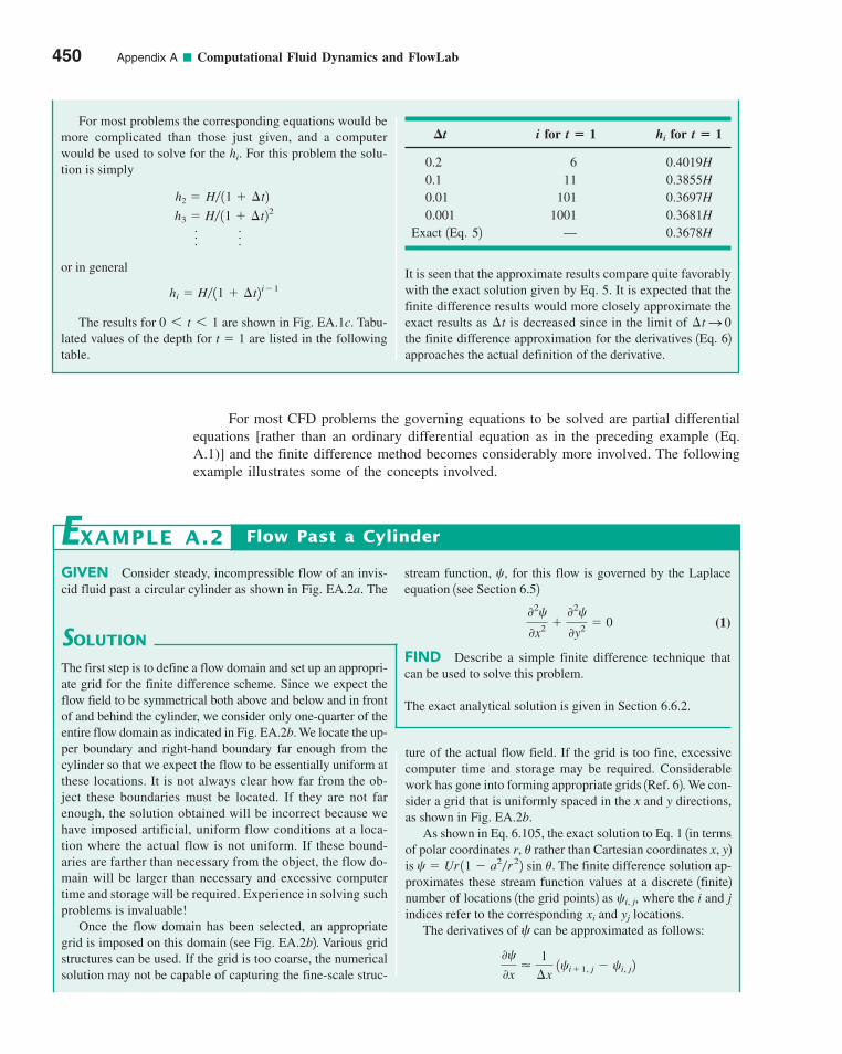
For most CFD problems the governing equations to be solved are partial differentialequations [rather than an ordinary differential equation as in the preceding example (Eq.A.1)] and the finite difference method becomes considerably more involved. The followingexample illustrates some of the concepts involved.

450 Appendix A ■ Computational Fluid Dynamics and FlowLab

t i for t � 1 hi for t � 1

0.2 6 0.4019H0.1 11 0.3855H0.01 101 0.3697H0.001 1001 0.3681H

Exact 1Eq. 52 — 0.3678H

It is seen that the approximate results compare quite favorablywith the exact solution given by Eq. 5. It is expected that thefinite difference results would more closely approximate theexact results as is decreased since in the limit of the finite difference approximation for the derivatives 1Eq. 62approaches the actual definition of the derivative.

¢t S 0¢t

�For most problems the corresponding equations would be

more complicated than those just given, and a computerwould be used to solve for the For this problem the solu-tion is simply

or in general

The results for are shown in Fig. EA.1c. Tabu-lated values of the depth for are listed in the followingtable.

t � 10 6 t 6 1

hi � H� 11 � ¢t2i�1

. . .

. . .

h3 � H� 11 � ¢t22h2 � H� 11 � ¢t2

hi.

GIVEN Consider steady, incompressible flow of an invis-cid fluid past a circular cylinder as shown in Fig. EA.2a. The

stream function, for this flow is governed by the Laplaceequation 1see Section 6.52

(1)

FIND Describe a simple finite difference technique thatcan be used to solve this problem.

The exact analytical solution is given in Section 6.6.2.

02�

0x2 �02�

0y2 � 0

c,

SOLUTION

Flow Past a Cylinder

ture of the actual flow field. If the grid is too fine, excessivecomputer time and storage may be required. Considerablework has gone into forming appropriate grids 1Ref. 62. We con-sider a grid that is uniformly spaced in the x and y directions,as shown in Fig. EA.2b.

As shown in Eq. 6.105, the exact solution to Eq. 1 1in termsof polar coordinates r, rather than Cartesian coordinates x, y2is The finite difference solution ap-proximates these stream function values at a discrete 1finite2number of locations 1the grid points2 as where the i and jindices refer to the corresponding and locations.

The derivatives of can be approximated as follows:

0�

0x�

1

¢x 1�i�1, j � �i, j2

�yjxi

�i, j,

� � Ur 11 � a2�r22 sin �.�

EXAMPLE A.2

The first step is to define a flow domain and set up an appropri-ate grid for the finite difference scheme. Since we expect theflow field to be symmetrical both above and below and in frontof and behind the cylinder, we consider only one-quarter of theentire flow domain as indicated in Fig. EA.2b. We locate the up-per boundary and right-hand boundary far enough from thecylinder so that we expect the flow to be essentially uniform atthese locations. It is not always clear how far from the ob-ject these boundaries must be located. If they are not farenough, the solution obtained will be incorrect because wehave imposed artificial, uniform flow conditions at a loca-tion where the actual flow is not uniform. If these bound-aries are farther than necessary from the object, the flow do-main will be larger than necessary and excessive computertime and storage will be required. Experience in solving suchproblems is invaluable!

Once the flow domain has been selected, an appropriategrid is imposed on this domain 1see Fig. EA.2b2. Various gridstructures can be used. If the grid is too coarse, the numericalsolution may not be capable of capturing the fine-scale struc-

appAComputationalFluidDynamicsandFlowLab.qxd 9/28/10 4:43 PM Page 450

A.5 Basic Representative Examples 451

Equation 4 can be solved for the stream function at and togive

(5)

Note that the value of depends on the values of the streamfunction at neighboring grid points on either side and aboveand below the point of interest 1see Eq. 5 and Fig. EA.2c2.

To solve the problem 1either exactly or by the finite differ-ence technique2 it is necessary to specify boundary conditionsfor points located on the boundary of the flow domain 1seeSection 6.6.32. For example, we may specify that on thelower boundary of the domain 1see Fig. EA.2b2 and aconstant, on the upper boundary of the domain. Appropriateboundary conditions on the two vertical ends of the flow do-main can also be specified. Thus, for points interior to theboundary Eq. 5 is valid; similar equations or specified valuesof are valid for boundary points. The result is an equalnumber of equations and unknowns, one for every gridpoint. For this problem, these equations represent a set of

�i, j,�i, j

� � C,� � 0

�i, j

� 1¢x221�i, j�1 � �i, j�12 4

�i, j �1

2 3 1¢x22 � 1¢y22 4 3 1¢y221�i�1, j � �i�1, j2

yjxiand

This particular approximation is called a forward-differenceapproximation. Other approximations are possible. By similarreasoning, it is possible to show that the second derivatives of

can be written as follows:

(2)

and

(3)

Thus, by combining Eqs. 1, 2, and 3 we obtain

(4)� �i, j�12 � 2 a1

1¢x22�

1

1¢y22b �i, j � 0

02�

0x2 �02�

0y2 �1

1¢x22 1�i�1, j � �i�1, j2 �

1

1¢y22 1�i, j�1

02�

0y2 �1

1¢y22 1�i, j�1 � 2�i, j � �i, j�12

02�

0x2 �1

1¢x22 1�i�1, j � 2�i, j � �i�1, j2

�

0�

0y�

1

¢y 1�i, j�1 � �i, j2

F I G U R E EA.2

θaU

(a)

(b)

y

xi

j

+x

yΔ

Δ

(c)

ψi – 1. j ψi + 1. j

ψi. j + 1

ψi. j – 1

ψi. j

xΔ xΔ

yΔ

yΔ

appAComputationalFluidDynamicsandFlowLab.qxd 9/28/10 5:27 PM Page 451

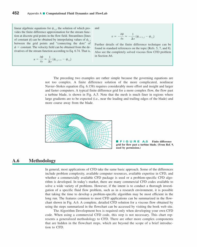
The preceding two examples are rather simple because the governing equations arenot too complex. A finite difference solution of the more complicated, nonlinearNavier–Stokes equation (Eq. 6.158) requires considerably more effort and insight and largerand faster computers. A typical finite difference grid for a more complex flow, the flow pasta turbine blade, is shown in Fig. A.5. Note that the mesh is much finer in regions wherelarge gradients are to be expected (i.e., near the leading and trailing edges of the blade) andmore coarse away from the blade.

452 Appendix A ■ Computational Fluid Dynamics and FlowLab

and

Further details of the finite difference technique can befound in standard references on the topic 1Refs. 5, 7, and 82.Also see the completely solved viscous flow CFD problemin Section A6.

v � �0�

0x� �

1

¢x 1�i�1, j � �i, j2

linear algebraic equations for the solution of which pro-vides the finite difference approximation for the stream func-tion at discrete grid points in the flow field. Streamlines 1linesof constant 2 can be obtained by interpolating values of between the grid points and “connecting the dots” of

The velocity field can be obtained from the de-rivatives of the stream function according to Eq. 6.74. That is,

u �0�

0y�

1

¢y 1�i, j�1 � �i, j2

� � constant.

�i, j�

�i, j,

A.6 Methodology

In general, most applications of CFD take the same basic approach. Some of the differencesinclude problem complexity, available computer resources, available expertise in CFD, andwhether a commercially available CFD package is used or a problem-specific CFD algo-rithm is developed. In today’s market, there are many commercial CFD codes available tosolve a wide variety of problems. However, if the intent is to conduct a thorough investi-gation of a specific fluid flow problem, such as in a research environment, it is possiblethat taking the time to develop a problem-specific algorithm may be most efficient in thelong run. The features common to most CFD applications can be summarized in the flow-chart shown in Fig. A.6. A complete, detailed CFD solution for a viscous flow obtained byusing the steps summarized in the flowchart can be accessed by visiting the book web site.

The Algorithm Development box is required only when developing your own CFDcode. When using a commercial CFD code, this step is not necessary. This chart rep-resents a generalized methodology to CFD. There are other more complex componentsthat are hidden in the flowchart steps, which are beyond the scope of a brief introduc-tion to CFD.

F I G U R E A.5 Finite differencegrid for flow past a turbine blade. (From Ref. 9,used by permission.)

appAComputationalFluidDynamicsandFlowLab.qxd 9/28/10 4:43 PM Page 452

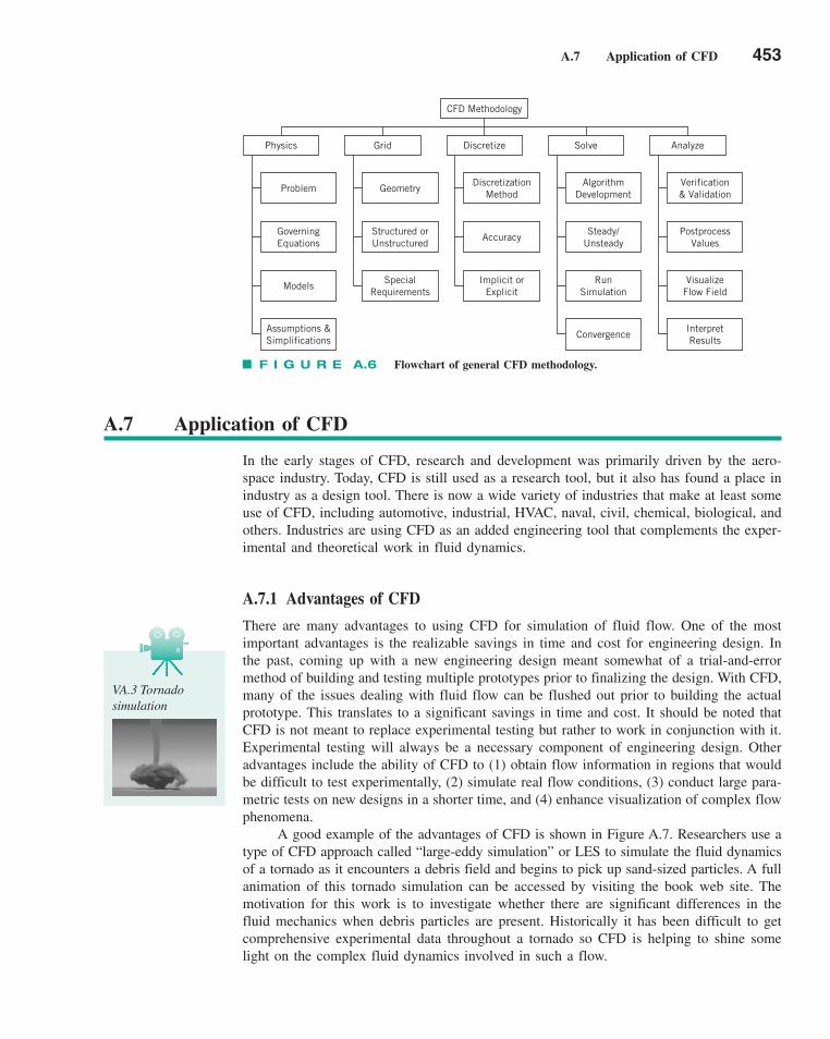
A.7 Application of CFD 453

A.7 Application of CFD

In the early stages of CFD, research and development was primarily driven by the aero-space industry. Today, CFD is still used as a research tool, but it also has found a place inindustry as a design tool. There is now a wide variety of industries that make at least someuse of CFD, including automotive, industrial, HVAC, naval, civil, chemical, biological, andothers. Industries are using CFD as an added engineering tool that complements the exper-imental and theoretical work in fluid dynamics.

A.7.1 Advantages of CFD

There are many advantages to using CFD for simulation of fluid flow. One of the mostimportant advantages is the realizable savings in time and cost for engineering design. Inthe past, coming up with a new engineering design meant somewhat of a trial-and-errormethod of building and testing multiple prototypes prior to finalizing the design. With CFD,many of the issues dealing with fluid flow can be flushed out prior to building the actualprototype. This translates to a significant savings in time and cost. It should be noted thatCFD is not meant to replace experimental testing but rather to work in conjunction with it.Experimental testing will always be a necessary component of engineering design. Otheradvantages include the ability of CFD to (1) obtain flow information in regions that wouldbe difficult to test experimentally, (2) simulate real flow conditions, (3) conduct large para-metric tests on new designs in a shorter time, and (4) enhance visualization of complex flowphenomena.

A good example of the advantages of CFD is shown in Figure A.7. Researchers use atype of CFD approach called “large-eddy simulation” or LES to simulate the fluid dynamicsof a tornado as it encounters a debris field and begins to pick up sand-sized particles. A fullanimation of this tornado simulation can be accessed by visiting the book web site. Themotivation for this work is to investigate whether there are significant differences in thefluid mechanics when debris particles are present. Historically it has been difficult to getcomprehensive experimental data throughout a tornado so CFD is helping to shine somelight on the complex fluid dynamics involved in such a flow.

Assumptions &Simplifications

ConvergenceInterpretResults

ModelsSpecial

RequirementsImplicit or

ExplicitRun

SimulationVisualize

Flow Field

GoverningEquations

Structured orUnstructured

AccuracySteady/

UnsteadyPostprocess

Values

Problem GeometryDiscretization

MethodAlgorithm

DevelopmentVerification& Validation

Physics Discretize Solve Analyze

CFD Methodology

Grid

F I G U R E A.6 Flowchart of general CFD methodology.

VA.3 Tornado simulation

appAComputationalFluidDynamicsandFlowLab.qxd 9/28/10 4:43 PM Page 453

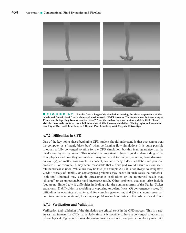
A.7.2 Difficulties in CFD

One of the key points that a beginning CFD student should understand is that one cannot treatthe computer as a “magic black box” when performing flow simulations. It is quite possibleto obtain a fully converged solution for the CFD simulation, but this is no guarantee that theresults are physically correct. This is why it is important to have a good understanding of theflow physics and how they are modeled. Any numerical technique (including those discussedpreviously), no matter how simple in concept, contains many hidden subtleties and potentialproblems. For example, it may seem reasonable that a finer grid would ensure a more accu-rate numerical solution. While this may be true (as Example A.1), it is not always so straightfor-ward; a variety of stability or convergence problems may occur. In such cases the numerical“solution” obtained may exhibit unreasonable oscillations or the numerical result may“diverge” to an unreasonable (and incorrect) result. Other problems that may arise include(but are not limited to) (1) difficulties in dealing with the nonlinear terms of the Navier–Stokesequations, (2) difficulties in modeling or capturing turbulent flows, (3) convergence issues, (4)difficulties in obtaining a quality grid for complex geometries, and (5) managing resources,both time and computational, for complex problems such as unsteady three-dimensional flows.

A.7.3 Verification and Validation

Verification and validation of the simulation are critical steps in the CFD process. This is a nec-essary requirement for CFD, particularly since it is possible to have a converged solution thatis nonphysical. Figure A.8 shows the streamlines for viscous flow past a circular cylinder at a

454 Appendix A ■ Computational Fluid Dynamics and FlowLab

F I G U R E A.7 Results from a large-eddy simulation showing the visual appearance of thedebris and funnel cloud from a simulated medium-swirl F3-F4 tornado. The funnel cloud is translating at15 m/s and is ingesting 1-mm-diameter “sand” from the surface as it encounters a debris field. Pleasevisit the book web site to access a full animation of this tornado simulation. (Photographs and animationcourtesy of Dr. David Lewellen, Ref. 10, and Paul Lewellen, West Virginia University.)

appAComputationalFluidDynamicsandFlowLab.qxd 9/28/10 4:43 PM Page 454

A.8 FlowLab 455

given instant after it was impulsively started from rest. The lower half of the figure representsthe results of a finite difference calculation; the upper half of the figure represents the photo-graph from an experiment of the same flow situation. It is clear that the numerical and experi-mental results agree quite well. For any CFD simulation, there are several levels of testing thatneed to be accomplished before one can have confidence in the solution. The most importantverification to be performed is grid convergence testing. In its simplest form, it consists of prov-ing that further refinement of the grid (i.e., increasing the number of grid points) does not alterthe final solution. When this has been achieved, the solution is termed a grid-independent solu-tion. Other verification factors that need to be investigated include the suitability of the conver-gence criterion, whether the time step is adequate for the time scale of the problem, andcomparison of CFD solutions to existing data, at least for baseline cases. Even when using acommercial CFD code that has been validated on many problems in the past, the CFD practi-tioner still needs to verify the results through such measures as grid-dependence testing.

A.7.4 Summary

In CFD, there are many different numerical schemes, grid techniques, and so on. They allhave their advantages and disadvantages. A great deal of care must be used in obtainingapproximate numerical solutions to the governing equations of fluid motion. The process isnot as simple as the often-heard “just let the computer do it.” Remember that CFD is a tooland as such needs to be used appropriately to produce meaningful results. The general fieldof computational fluid dynamics, in which computers and numerical analysis are combinedto solve fluid flow problems, represents an extremely important subject area in advancedfluid mechanics. Considerable progress has been made in the past relatively few years, butmuch remains to be done. The reader is encouraged to consult some of the available literature.

F I G U R E A.8 Streamlines forflow past a circular cylinder at a short timeafter the flow was impulsively started. Theupper half is a photograph from a flow visual-ization experiment. The lower half is from afinite difference calculation. (See the photo-graph at the beginning of Chapter 9.) (FromRef. 9, used by permission.)

A.8 FlowLab

The authors of this textbook are working in collaboration with Fluent, Inc., the largestprovider of commercial CFD software (www.fluent.com), to offer students the opportunityto use a new CFD tool called FlowLab. FlowLab is designed to be a virtual fluids labora-tory to help enhance the educational experience in fluids courses. It uses computational fluiddynamics to help the student grasp various concepts in fluid dynamics and introduces the

appAComputationalFluidDynamicsandFlowLab.qxd 9/28/10 4:43 PM Page 455

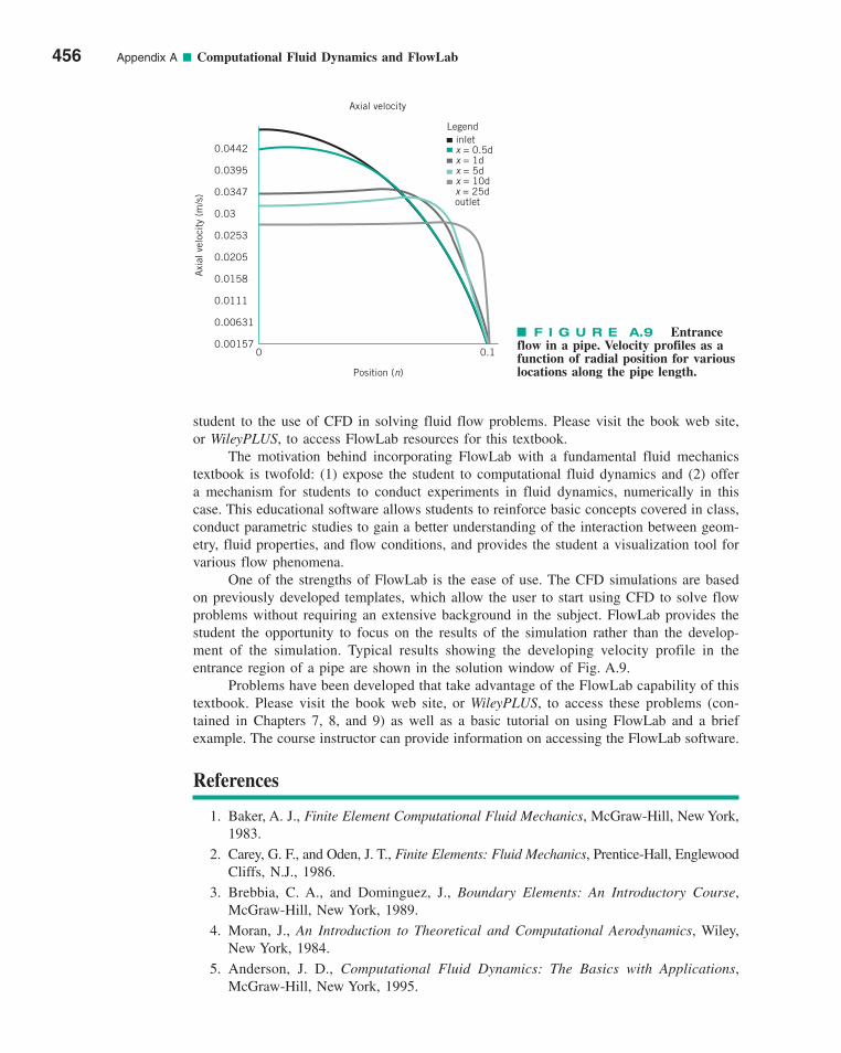
student to the use of CFD in solving fluid flow problems. Please visit the book web site,or WileyPLUS, to access FlowLab resources for this textbook.

The motivation behind incorporating FlowLab with a fundamental fluid mechanicstextbook is twofold: (1) expose the student to computational fluid dynamics and (2) offera mechanism for students to conduct experiments in fluid dynamics, numerically in thiscase. This educational software allows students to reinforce basic concepts covered in class,conduct parametric studies to gain a better understanding of the interaction between geom-etry, fluid properties, and flow conditions, and provides the student a visualization tool forvarious flow phenomena.

One of the strengths of FlowLab is the ease of use. The CFD simulations are basedon previously developed templates, which allow the user to start using CFD to solve flowproblems without requiring an extensive background in the subject. FlowLab provides thestudent the opportunity to focus on the results of the simulation rather than the develop-ment of the simulation. Typical results showing the developing velocity profile in theentrance region of a pipe are shown in the solution window of Fig. A.9.

Problems have been developed that take advantage of the FlowLab capability of thistextbook. Please visit the book web site, or WileyPLUS, to access these problems (con-tained in Chapters 7, 8, and 9) as well as a basic tutorial on using FlowLab and a briefexample. The course instructor can provide information on accessing the FlowLab software.

References

1. Baker, A. J., Finite Element Computational Fluid Mechanics, McGraw-Hill, New York,1983.

2. Carey, G. F., and Oden, J. T., Finite Elements: Fluid Mechanics, Prentice-Hall, EnglewoodCliffs, N.J., 1986.

3. Brebbia, C. A., and Dominguez, J., Boundary Elements: An Introductory Course,McGraw-Hill, New York, 1989.

4. Moran, J., An Introduction to Theoretical and Computational Aerodynamics, Wiley,New York, 1984.

5. Anderson, J. D., Computational Fluid Dynamics: The Basics with Applications,McGraw-Hill, New York, 1995.

456 Appendix A ■ Computational Fluid Dynamics and FlowLab

Axi

al v

eloc

ity

(m/s

)

0.0442

0.0395

0.0347

0.03

0.0253

0.0205

0.0158

0.0111

0.00631

0.00157

Axial velocity

inletLegend

x = 0.5dx = 1dx = 5dx = 10d

x = 25d outlet

Position (n)

0.10

F I G U R E A.9 Entranceflow in a pipe. Velocity profiles as afunction of radial position for variouslocations along the pipe length.

appAComputationalFluidDynamicsandFlowLab.qxd 9/28/10 4:43 PM Page 456

References 457

6. Thompson, J. F., Warsi, Z. U. A., and Mastin, C. W., Numerical Grid Generation:Foundations and Applications, North-Holland, New York, 1985.

7. Peyret, R., and Taylor, T. D., Computational Methods for Fluid Flow, Springer-Verlag,New York, 1983.

8. Tannehill, J. C., Anderson, D. A., and Pletcher, R. H., Computational Fluid Mechanicsand Heat Transfer, Second Edition, Taylor and Francis, Washington, D.C., 1997.

9. Hall, E. J., and Pletcher, R. H., Simulation of Time Dependent, Compressible ViscousFlow Using Central and Upwind-Biased Finite-Difference Techniques, TechnicalReport HTL-52, CFD-22, College of Engineering, lowa State University, 1990.

10. Lewellen, D. C., Gong, B., and Lewellen, W. S., Effects of Debris on Near-SurfaceTornado Dynamics, 22nd Conference on Severe Local Storms, Paper 15.5, AmericanMeteorological Society, 2004.

appAComputationalFluidDynamicsandFlowLab.qxd 9/28/10 4:43 PM Page 457

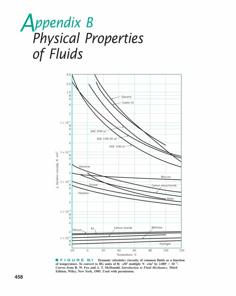
MethaneCarbon dioxide

Hydrogen

Helium

Heptane

Octane

Water

Carbon tetrachloride

Mercury

Kerosine

SAE 10W oil

SAE 10W-30 oil

SAE 30W oil

Castor oil

Glycerin

–20 0 20 40 60 80 100 120

Temperature, °C

4.0

2.0

1.086

4

2

1 × 10–1

86

4

2

1 × 10–2

86

4

2

1 × 10–3

86

4

2

1 × 10–4

86

4

2

1 × 10–5

86

,

Dyn

amic

vis

cosi

ty,

N .

s/m

2μ

Air

F I G U R E B.1 Dynamic (absolute) viscosity of common fluids as a functionof temperature. To convert to BG units of lb . s/ft2 multiply N . s/m2 by 2.089 � 10�2.Curves from R. W. Fox and A. T. McDonald, Introduction to Fluid Mechanics, ThirdEdition, Wiley, New York, 1985. Used with permission.

Appendix BPhysical Properties of Fluids

458

appBPhysicalPropertiesofFluids.qxd 9/28/10 4:43 PM Page 458

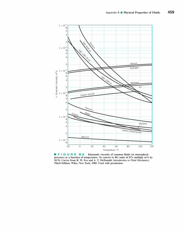
Appendix B ■ Physical Properties of Fluids 459

Carbon tetrachloride

Mercury

OctaneWater

Kerosine

Air

Carbon dioxide

Methane

Hydrogen

Helium

SAE 10W oil

SAE 10W–30 oil

SAE 30W oil

Glycerin

1 × 10–2

86

4

2

1 × 10–3

86

4

2

1 × 10–4

86

4

2

1 × 10–5

86

4

2

1 × 10–6

86

4

2

1 × 10–7

8

,

Kin

emat

ic v

isco

sity

, m

2/s

–20 0 20 40 60 80 100 120

Temperature, °C

Heptane

ν

F I G U R E B.2 Kinematic viscosity of common fluids (at atmospheric pressure) as a function of temperature. To convert to BG units of ft2/s multiply m2/s by10.76. Curves from R. W. Fox and A. T. McDonald, Introduction to Fluid Mechanics,Third Edition, Wiley, New York, 1985. Used with permission.

appBPhysicalPropertiesofFluids.qxd 9/28/10 4:43 PM Page 459

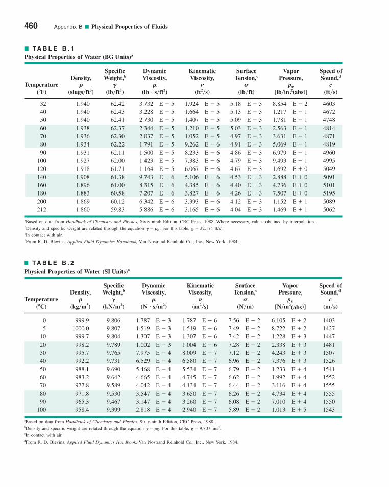
460 Appendix B ■ Physical Properties of Fluids

TA B L E B . 1

Physical Properties of Water ( )a

Specific Dynamic Kinematic Surface Vapor Speed ofDensity, Weight,b Viscosity, Viscosity, Tension,c Pressure, Sound,d

Temperature pv c( ) ( ) ( ) (lb . s ft2) ( ) (lb�ft) [ (abs)] (ft�s)

32 1.940 62.42 3.732 E � 5 1.924 E � 5 5.18 E � 3 8.854 E � 2 460340 1.940 62.43 3.228 E � 5 1.664 E � 5 5.13 E � 3 1.217 E � 1 467250 1.940 62.41 2.730 E � 5 1.407 E � 5 5.09 E � 3 1.781 E � 1 474860 1.938 62.37 2.344 E � 5 1.210 E � 5 5.03 E � 3 2.563 E � 1 481470 1.936 62.30 2.037 E � 5 1.052 E � 5 4.97 E � 3 3.631 E � 1 487180 1.934 62.22 1.791 E � 5 9.262 E � 6 4.91 E � 3 5.069 E � 1 481990 1.931 62.11 1.500 E � 5 8.233 E � 6 4.86 E � 3 6.979 E � 1 4960

100 1.927 62.00 1.423 E � 5 7.383 E � 6 4.79 E � 3 9.493 E � 1 4995120 1.918 61.71 1.164 E � 5 6.067 E � 6 4.67 E � 3 1.692 E � 0 5049140 1.908 61.38 9.743 E � 6 5.106 E � 6 4.53 E � 3 2.888 E � 0 5091160 1.896 61.00 8.315 E � 6 4.385 E � 6 4.40 E � 3 4.736 E � 0 5101180 1.883 60.58 7.207 E � 6 3.827 E � 6 4.26 E � 3 7.507 E � 0 5195200 1.869 60.12 6.342 E � 6 3.393 E � 6 4.12 E � 3 1.152 E � 1 5089212 1.860 59.83 5.886 E � 6 3.165 E � 6 4.04 E � 3 1.469 E � 1 5062

lb�in 2.ft2�s�lb�ft3slugs�ft3�FSNMGR

BG Units

aBased on data from Handbook of Chemistry and Physics, Sixty-ninth Edition, CRC Press, 1988. Where necessary, values obtained by interpolation.bDensity and specific weight are related through the equation � � �g. For this table, g � 32.174 ft/s2.cIn contact with air.dFrom R. D. Blevins, Applied Fluid Dynamics Handbook, Van Nostrand Reinhold Co., Inc., New York, 1984.

TA B L E B . 2

Physical Properties of Water ( )a

Specific Dynamic Kinematic Surface Vapor Speed ofDensity, Weight,b Viscosity, Viscosity, Tension,c Pressure, Sound,d

Temperature pv c( ) ( ) ( ) (N . s m2) ( ) (N�m) [ (abs)] (m�s)

0 999.9 9.806 1.787 E � 3 1.787 E � 6 7.56 E � 2 6.105 E � 2 14035 1000.0 9.807 1.519 E � 3 1.519 E � 6 7.49 E � 2 8.722 E � 2 1427

10 999.7 9.804 1.307 E � 3 1.307 E � 6 7.42 E � 2 1.228 E � 3 144720 998.2 9.789 1.002 E � 3 1.004 E � 6 7.28 E � 2 2.338 E � 3 148130 995.7 9.765 7.975 E � 4 8.009 E � 7 7.12 E � 2 4.243 E � 3 150740 992.2 9.731 6.529 E � 4 6.580 E � 7 6.96 E � 2 7.376 E � 3 152650 988.1 9.690 5.468 E � 4 5.534 E � 7 6.79 E � 2 1.233 E � 4 154160 983.2 9.642 4.665 E � 4 4.745 E � 7 6.62 E � 2 1.992 E � 4 155270 977.8 9.589 4.042 E � 4 4.134 E � 7 6.44 E � 2 3.116 E � 4 155580 971.8 9.530 3.547 E � 4 3.650 E � 7 6.26 E � 2 4.734 E � 4 155590 965.3 9.467 3.147 E � 4 3.260 E � 7 6.08 E � 2 7.010 E � 4 1550

100 958.4 9.399 2.818 E � 4 2.940 E � 7 5.89 E � 2 1.013 E � 5 1543

N�m2m2�s�kN�m3kg�m3�CSNMGR

SI Units

aBased on data from Handbook of Chemistry and Physics, Sixty-ninth Edition, CRC Press, 1988.bDensity and specific weight are related through the equation � � �g. For this table, g � 9.807 m/s2.cIn contact with air.dFrom R. D. Blevins, Applied Fluid Dynamics Handbook, Van Nostrand Reinhold Co., Inc., New York, 1984.

appBPhysicalPropertiesofFluids.qxd 9/28/10 4:43 PM Page 460

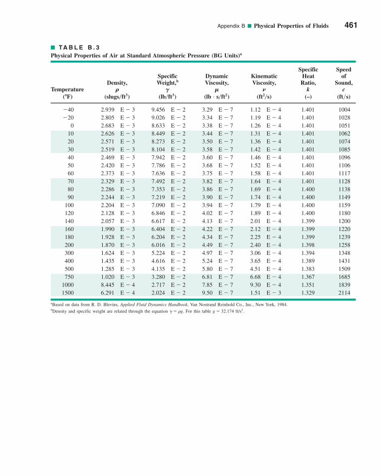
Appendix B ■ Physical Properties of Fluids 461

TA B L E B . 3

Physical Properties of Air at Standard Atmospheric Pressure (BG Units)a

Specific SpeedSpecific Dynamic Kinematic Heat of

Density, Weight,b Viscosity, Viscosity, Ratio, Sound,Temperature k c

( ) ( ) ( ) (lb . s ft2) ( ) (–) (ft�s)

�40 2.939 E � 3 9.456 E � 2 3.29 E � 7 1.12 E � 4 1.401 1004�20 2.805 E � 3 9.026 E � 2 3.34 E � 7 1.19 E � 4 1.401 1028

0 2.683 E � 3 8.633 E � 2 3.38 E � 7 1.26 E � 4 1.401 105110 2.626 E � 3 8.449 E � 2 3.44 E � 7 1.31 E � 4 1.401 106220 2.571 E � 3 8.273 E � 2 3.50 E � 7 1.36 E � 4 1.401 107430 2.519 E � 3 8.104 E � 2 3.58 E � 7 1.42 E � 4 1.401 108540 2.469 E � 3 7.942 E � 2 3.60 E � 7 1.46 E � 4 1.401 109650 2.420 E � 3 7.786 E � 2 3.68 E � 7 1.52 E � 4 1.401 110660 2.373 E � 3 7.636 E � 2 3.75 E � 7 1.58 E � 4 1.401 111770 2.329 E � 3 7.492 E � 2 3.82 E � 7 1.64 E � 4 1.401 112880 2.286 E � 3 7.353 E � 2 3.86 E � 7 1.69 E � 4 1.400 113890 2.244 E � 3 7.219 E � 2 3.90 E � 7 1.74 E � 4 1.400 1149

100 2.204 E � 3 7.090 E � 2 3.94 E � 7 1.79 E � 4 1.400 1159120 2.128 E � 3 6.846 E � 2 4.02 E � 7 1.89 E � 4 1.400 1180140 2.057 E � 3 6.617 E � 2 4.13 E � 7 2.01 E � 4 1.399 1200160 1.990 E � 3 6.404 E � 2 4.22 E � 7 2.12 E � 4 1.399 1220180 1.928 E � 3 6.204 E � 2 4.34 E � 7 2.25 E � 4 1.399 1239200 1.870 E � 3 6.016 E � 2 4.49 E � 7 2.40 E � 4 1.398 1258300 1.624 E � 3 5.224 E � 2 4.97 E � 7 3.06 E � 4 1.394 1348400 1.435 E � 3 4.616 E � 2 5.24 E � 7 3.65 E � 4 1.389 1431500 1.285 E � 3 4.135 E � 2 5.80 E � 7 4.51 E � 4 1.383 1509750 1.020 E � 3 3.280 E � 2 6.81 E � 7 6.68 E � 4 1.367 1685

1000 8.445 E � 4 2.717 E � 2 7.85 E � 7 9.30 E � 4 1.351 18391500 6.291 E � 4 2.024 E � 2 9.50 E � 7 1.51 E � 3 1.329 2114

ft2�s�lb�ft3slugs�ft3�FNMGR

aBased on data from R. D. Blevins, Applied Fluid Dynamics Handbook, Van Nostrand Reinhold Co., Inc., New York, 1984.bDensity and specific weight are related through the equation � � �g. For this table g � 32.174 ft/s2.

appBPhysicalPropertiesofFluids.qxd 9/28/10 4:43 PM Page 461

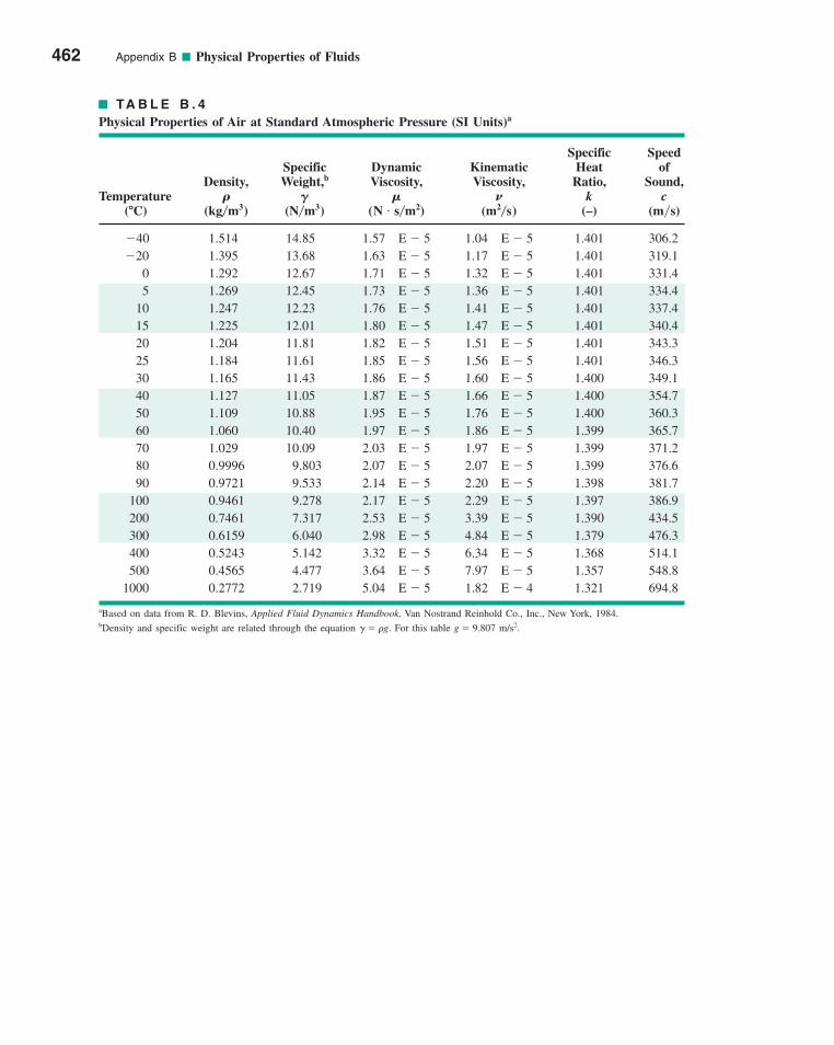
462 Appendix B ■ Physical Properties of Fluids

TA B L E B . 4

Physical Properties of Air at Standard Atmospheric Pressure (SI Units)a

Specific SpeedSpecific Dynamic Kinematic Heat of

Density, Weight,b Viscosity, Viscosity, Ratio, Sound,Temperature k c

( ) ( ) ( ) (N . s m2) ( ) (–) (m�s)

�40 1.514 14.85 1.57 E � 5 1.04 E � 5 1.401 306.2�20 1.395 13.68 1.63 E � 5 1.17 E � 5 1.401 319.1

0 1.292 12.67 1.71 E � 5 1.32 E � 5 1.401 331.45 1.269 12.45 1.73 E � 5 1.36 E � 5 1.401 334.4

10 1.247 12.23 1.76 E � 5 1.41 E � 5 1.401 337.415 1.225 12.01 1.80 E � 5 1.47 E � 5 1.401 340.420 1.204 11.81 1.82 E � 5 1.51 E � 5 1.401 343.325 1.184 11.61 1.85 E � 5 1.56 E � 5 1.401 346.330 1.165 11.43 1.86 E � 5 1.60 E � 5 1.400 349.140 1.127 11.05 1.87 E � 5 1.66 E � 5 1.400 354.750 1.109 10.88 1.95 E � 5 1.76 E � 5 1.400 360.360 1.060 10.40 1.97 E � 5 1.86 E � 5 1.399 365.770 1.029 10.09 2.03 E � 5 1.97 E � 5 1.399 371.280 0.9996 9.803 2.07 E � 5 2.07 E � 5 1.399 376.690 0.9721 9.533 2.14 E � 5 2.20 E � 5 1.398 381.7

100 0.9461 9.278 2.17 E � 5 2.29 E � 5 1.397 386.9200 0.7461 7.317 2.53 E � 5 3.39 E � 5 1.390 434.5300 0.6159 6.040 2.98 E � 5 4.84 E � 5 1.379 476.3400 0.5243 5.142 3.32 E � 5 6.34 E � 5 1.368 514.1500 0.4565 4.477 3.64 E � 5 7.97 E � 5 1.357 548.8

1000 0.2772 2.719 5.04 E � 5 1.82 E � 4 1.321 694.8

m2�s�N�m3kg�m3�CNMGR

aBased on data from R. D. Blevins, Applied Fluid Dynamics Handbook, Van Nostrand Reinhold Co., Inc., New York, 1984.bDensity and specific weight are related through the equation � � �g. For this table g � 9.807 m/s2.

appBPhysicalPropertiesofFluids.qxd 9/28/10 4:44 PM Page 462

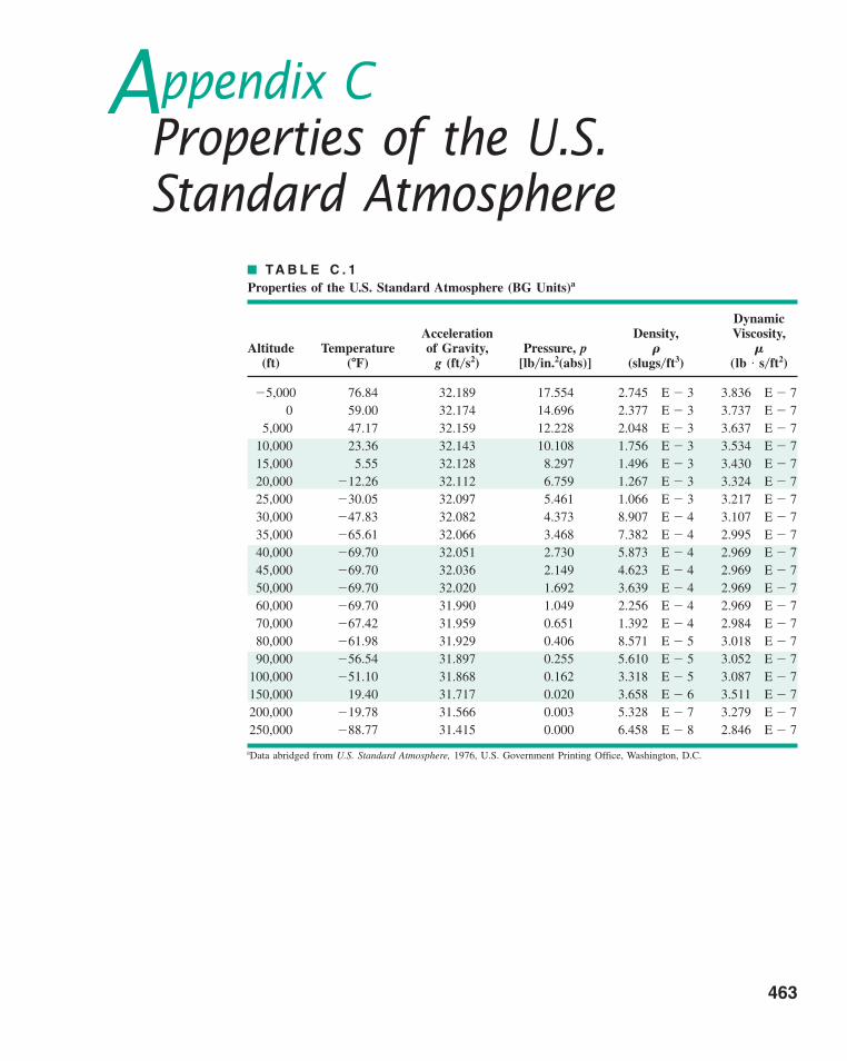
TA B L E C . 1

Properties of the U.S. Standard Atmosphere (BG Units)a

DynamicAcceleration Density, Viscosity,

Altitude Temperature of Gravity, Pressure, p(ft) ( ) g ( ) [ (abs)] ( ) (lb . s ft2)

�5,000 76.84 32.189 17.554 2.745 E � 3 3.836 E � 70 59.00 32.174 14.696 2.377 E � 3 3.737 E � 7

5,000 47.17 32.159 12.228 2.048 E � 3 3.637 E � 710,000 23.36 32.143 10.108 1.756 E � 3 3.534 E � 715,000 5.55 32.128 8.297 1.496 E � 3 3.430 E � 720,000 �12.26 32.112 6.759 1.267 E � 3 3.324 E � 725,000 �30.05 32.097 5.461 1.066 E � 3 3.217 E � 730,000 �47.83 32.082 4.373 8.907 E � 4 3.107 E � 735,000 �65.61 32.066 3.468 7.382 E � 4 2.995 E � 740,000 �69.70 32.051 2.730 5.873 E � 4 2.969 E � 745,000 �69.70 32.036 2.149 4.623 E � 4 2.969 E � 750,000 �69.70 32.020 1.692 3.639 E � 4 2.969 E � 760,000 �69.70 31.990 1.049 2.256 E � 4 2.969 E � 770,000 �67.42 31.959 0.651 1.392 E � 4 2.984 E � 780,000 �61.98 31.929 0.406 8.571 E � 5 3.018 E � 790,000 �56.54 31.897 0.255 5.610 E � 5 3.052 E � 7

100,000 �51.10 31.868 0.162 3.318 E � 5 3.087 E � 7150,000 19.40 31.717 0.020 3.658 E � 6 3.511 E � 7200,000 �19.78 31.566 0.003 5.328 E � 7 3.279 E � 7250,000 �88.77 31.415 0.000 6.458 E � 8 2.846 E � 7

�slugs�ft3lb�in.2ft�s2�FMR

aData abridged from U.S. Standard Atmosphere, 1976, U.S. Government Printing Office, Washington, D.C.

Appendix CProperties of the U.S.Standard Atmosphere

463

appCPropertiesofthe U.S.StandardAtmosphere.qxd 9/28/10 4:34 PM Page 463

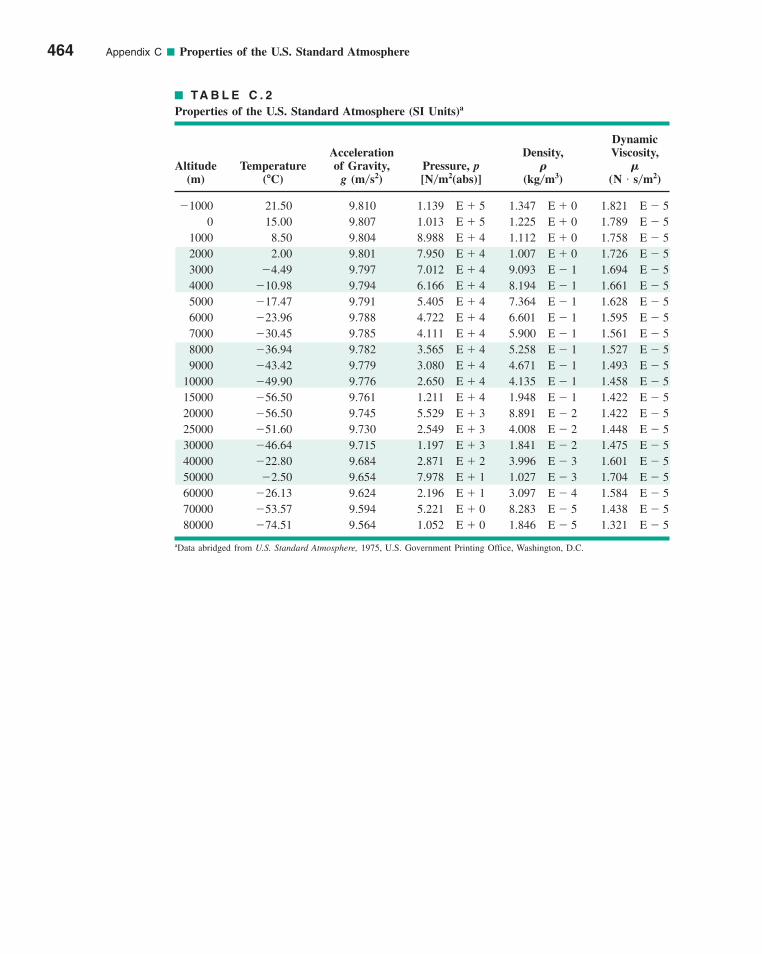
464 Appendix C ■ Properties of the U.S. Standard Atmosphere

TA B L E C . 2

Properties of the U.S. Standard Atmosphere (SI Units)a

DynamicAcceleration Density, Viscosity,

Altitude Temperature of Gravity, Pressure, p(m) ( ) g ( ) [ (abs)] ( ) (N . s m2)

�1000 21.50 9.810 1.139 E � 5 1.347 E � 0 1.821 E � 50 15.00 9.807 1.013 E � 5 1.225 E � 0 1.789 E � 5

1000 8.50 9.804 8.988 E � 4 1.112 E � 0 1.758 E � 52000 2.00 9.801 7.950 E � 4 1.007 E � 0 1.726 E � 53000 �4.49 9.797 7.012 E � 4 9.093 E � 1 1.694 E � 54000 �10.98 9.794 6.166 E � 4 8.194 E � 1 1.661 E � 55000 �17.47 9.791 5.405 E � 4 7.364 E � 1 1.628 E � 56000 �23.96 9.788 4.722 E � 4 6.601 E � 1 1.595 E � 57000 �30.45 9.785 4.111 E � 4 5.900 E � 1 1.561 E � 58000 �36.94 9.782 3.565 E � 4 5.258 E � 1 1.527 E � 59000 �43.42 9.779 3.080 E � 4 4.671 E � 1 1.493 E � 5

10000 �49.90 9.776 2.650 E � 4 4.135 E � 1 1.458 E � 515000 �56.50 9.761 1.211 E � 4 1.948 E � 1 1.422 E � 520000 �56.50 9.745 5.529 E � 3 8.891 E � 2 1.422 E � 525000 �51.60 9.730 2.549 E � 3 4.008 E � 2 1.448 E � 530000 �46.64 9.715 1.197 E � 3 1.841 E � 2 1.475 E � 540000 �22.80 9.684 2.871 E � 2 3.996 E � 3 1.601 E � 550000 �2.50 9.654 7.978 E � 1 1.027 E � 3 1.704 E � 560000 �26.13 9.624 2.196 E � 1 3.097 E � 4 1.584 E � 570000 �53.57 9.594 5.221 E � 0 8.283 E � 5 1.438 E � 580000 �74.51 9.564 1.052 E � 0 1.846 E � 5 1.321 E � 5

�kg�m3N�m2m�s2�CMR

aData abridged from U.S. Standard Atmosphere, 1975, U.S. Government Printing Office, Washington, D.C.

appCPropertiesofthe U.S.StandardAtmosphere.qxd 9/29/10 11:48 AM Page 464

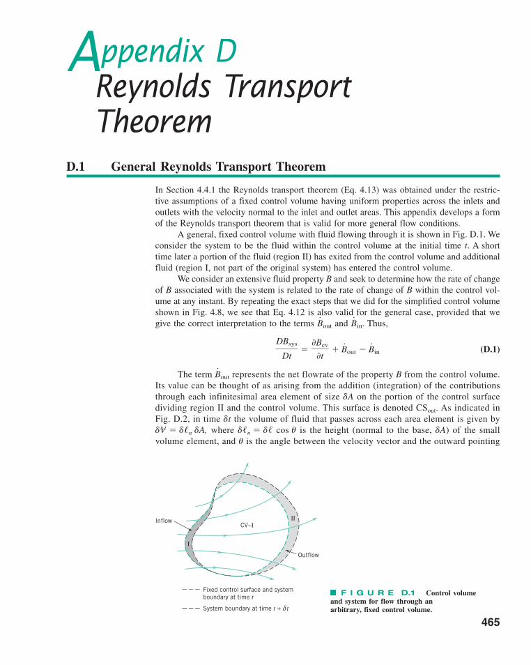
Appendix DReynolds Transport Theorem

D.1 General Reynolds Transport Theorem

In Section 4.4.1 the Reynolds transport theorem (Eq. 4.13) was obtained under the restric-tive assumptions of a fixed control volume having uniform properties across the inlets andoutlets with the velocity normal to the inlet and outlet areas. This appendix develops a formof the Reynolds transport theorem that is valid for more general flow conditions.

A general, fixed control volume with fluid flowing through it is shown in Fig. D.1. Weconsider the system to be the fluid within the control volume at the initial time t. A shorttime later a portion of the fluid (region II) has exited from the control volume and additionalfluid (region I, not part of the original system) has entered the control volume.

We consider an extensive fluid property B and seek to determine how the rate of changeof B associated with the system is related to the rate of change of B within the control vol-ume at any instant. By repeating the exact steps that we did for the simplified control volumeshown in Fig. 4.8, we see that Eq. 4.12 is also valid for the general case, provided that wegive the correct interpretation to the terms and Thus,

(D.1)

The term represents the net flowrate of the property B from the control volume.Its value can be thought of as arising from the addition (integration) of the contributionsthrough each infinitesimal area element of size �A on the portion of the control surfacedividing region II and the control volume. This surface is denoted CSout. As indicated inFig. D.2, in time �t the volume of fluid that passes across each area element is given by� � ��n �A, where ��n � �� cos � is the height (normal to the base, �A) of the smallvolume element, and � is the angle between the velocity vector and the outward pointing

V

B#out

DBsys

Dt�

0Bcv

0t� �Bout � �Bin

B#in.B

#out

CV–III

I

Inflow

Outflow

Fixed control surface and systemboundary at time t

System boundary at time t + tδ

F I G U R E D.1 Control volume and system for flow through an arbitrary, fixed control volume.

465

appDReynoldsTransportTheorem.qxd 9/28/10 7:05 PM Page 465

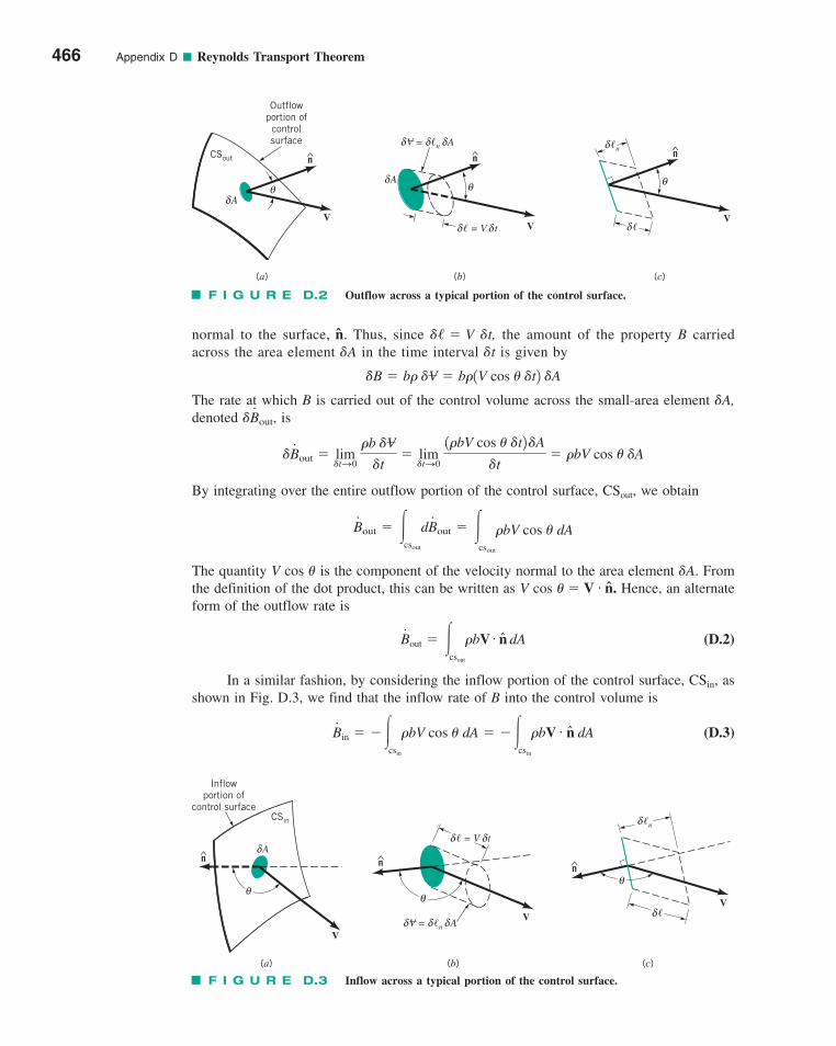
normal to the surface, n. Thus, since �� � V �t, the amount of the property B carriedacross the area element �A in the time interval �t is given by

The rate at which B is carried out of the control volume across the small-area element �A,denoted is

By integrating over the entire outflow portion of the control surface, CSout, we obtain

The quantity V cos � is the component of the velocity normal to the area element �A. Fromthe definition of the dot product, this can be written as V cos � � V . n. Hence, an alternateform of the outflow rate is

(D.2)

In a similar fashion, by considering the inflow portion of the control surface, CSin, asshown in Fig. D.3, we find that the inflow rate of B into the control volume is

(D.3)B#

in � ��csin

�bV cos � dA � ��csin

�bV . n dA

B#

out � �csout

�bV . n dA

B#out � �

csout

dB#out � �

csout

�bV cos � dA

�B#out � lim

�tS0 �b �V

�t� lim

�tS0 1�bV cos � �t2 �A

�t� �bV cos � �A

�B#out,

�B � b� �V � b�1V cos � �t2 �A

466 Appendix D ■ Reynolds Transport Theorem

n

V

Aδ

CSout

Outflowportion ofcontrolsurface

θ

(a) (b) (c)

� = V tδ δ

θ

^ n

V

V = �n Aδ δ δ

Aδ

V

n

�δ

�nδ

θ

F I G U R E D.2 Outflow across a typical portion of the control surface.

n

V

(a)

CSin

Inflowportion of

control surface

Aδ

θ

n

θ

� = V tδ δ

V = �n Aδ δδ VV

n

�δ

�nδ

θ

(b) (c)

F I G U R E D.3 Inflow across a typical portion of the control surface.

appDReynoldsTransportTheorem.qxd 9/28/10 7:05 PM Page 466

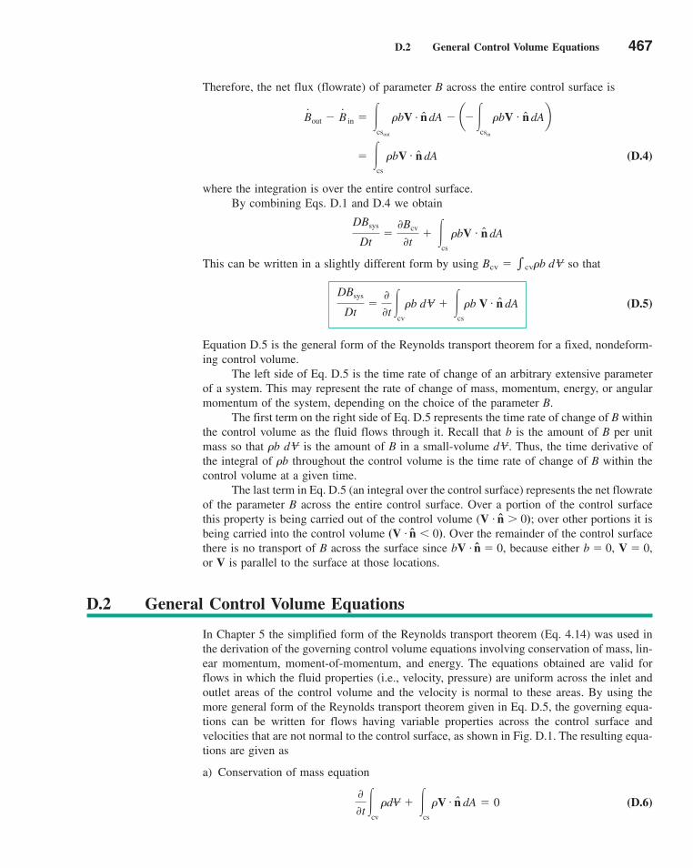
D.2 General Control Volume Equations 467

Therefore, the net flux (flowrate) of parameter B across the entire control surface is

(D.4)

where the integration is over the entire control surface.By combining Eqs. D.1 and D.4 we obtain

This can be written in a slightly different form by using so that

(D.5)

Equation D.5 is the general form of the Reynolds transport theorem for a fixed, nondeform-ing control volume.

The left side of Eq. D.5 is the time rate of change of an arbitrary extensive parameterof a system. This may represent the rate of change of mass, momentum, energy, or angularmomentum of the system, depending on the choice of the parameter B.

The first term on the right side of Eq. D.5 represents the time rate of change of B withinthe control volume as the fluid flows through it. Recall that b is the amount of B per unitmass so that �b d is the amount of B in a small-volume d . Thus, the time derivative ofthe integral of �b throughout the control volume is the time rate of change of B within thecontrol volume at a given time.

The last term in Eq. D.5 (an integral over the control surface) represents the net flowrateof the parameter B across the entire control surface. Over a portion of the control surfacethis property is being carried out of the control volume (V . n � 0); over other portions it isbeing carried into the control volume (V . n � 0). Over the remainder of the control surfacethere is no transport of B across the surface since bV . n � 0, because either b � 0, V � 0,or V is parallel to the surface at those locations.

VV

DBsys

Dt�

00t �

cv

�b d V � �cs

�b V . n dA

Bcv � �cv�b d V

DBsys

Dt�

0Bcv

0t� �

cs

�bV . n dA

� �cs

�bV . n dA

B#

out � B# #

in � �csout

�bV . n dA � a��csin

�bV . n dAb

D.2 General Control Volume Equations

In Chapter 5 the simplified form of the Reynolds transport theorem (Eq. 4.14) was used inthe derivation of the governing control volume equations involving conservation of mass, lin-ear momentum, moment-of-momentum, and energy. The equations obtained are valid forflows in which the fluid properties (i.e., velocity, pressure) are uniform across the inlet andoutlet areas of the control volume and the velocity is normal to these areas. By using themore general form of the Reynolds transport theorem given in Eq. D.5, the governing equa-tions can be written for flows having variable properties across the control surface andvelocities that are not normal to the control surface, as shown in Fig. D.1. The resulting equa-tions are given as

a) Conservation of mass equation

(D.6)00t �

cv �dV � �

cs �V . n dA � 0

appDReynoldsTransportTheorem.qxd 9/28/10 7:05 PM Page 467

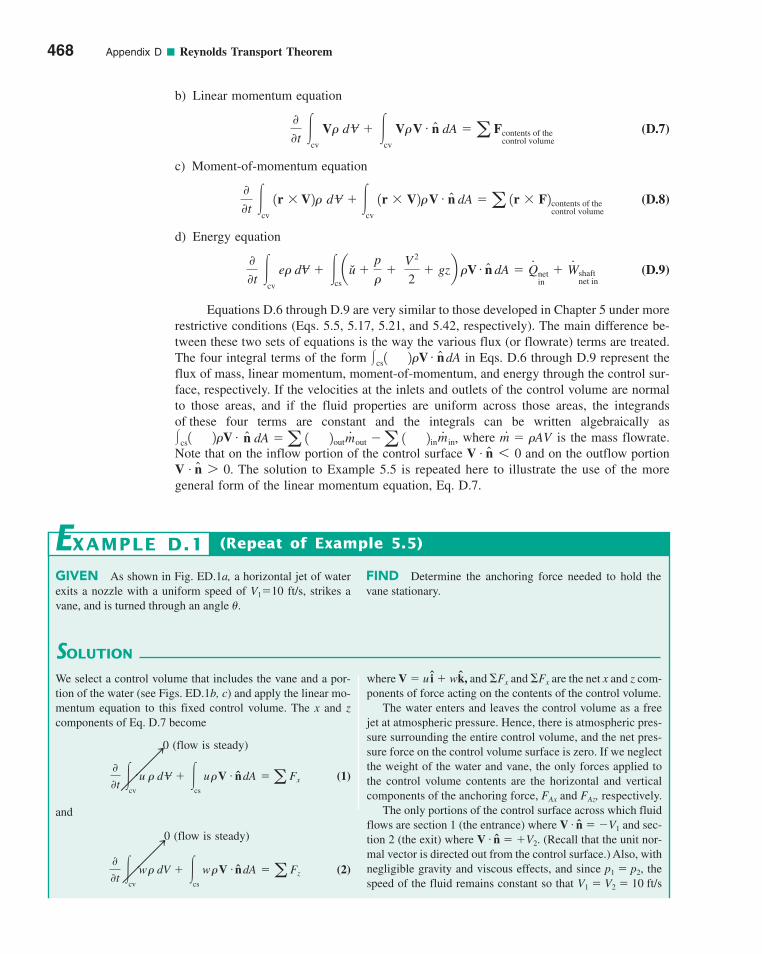
b) Linear momentum equation

(D.7)

c) Moment-of-momentum equation

(D.8)

d) Energy equation

(D.9)

Equations D.6 through D.9 are very similar to those developed in Chapter 5 under morerestrictive conditions (Eqs. 5.5, 5.17, 5.21, and 5.42, respectively). The main difference be-tween these two sets of equations is the way the various flux (or flowrate) terms are treated.The four integral terms of the form �cs in Eqs. D.6 through D.9 represent theflux of mass, linear momentum, moment-of-momentum, and energy through the control sur-face, respectively. If the velocities at the inlets and outlets of the control volume are normalto those areas, and if the fluid properties are uniform across those areas, the integrands of these four terms are constant and the integrals can be written algebraically as�cs where is the mass flowrate.Note that on the inflow portion of the control surface and on the outflow portion

. The solution to Example 5.5 is repeated here to illustrate the use of the moregeneral form of the linear momentum equation, Eq. D.7.V # n 7 0

V # n 6 0m#

� �AV1 2�V # n dA �a 1

2out m.

out �a 1 2inm

.in,

1 2�V . ndA

00t

�cv

e� dV � �csau �

p

��

V 2

2� gzb �V . n dA � Q

#netin

� W#

shaftnet in

00t

�cv

1r � V2� d V � �cv

1r � V2� V . n dA �a 1r � F2contents of thecontrol volume

00t

�cv

V� d V � �cv

V� V . n dA �a Fcontents of thecontrol volume

468 Appendix D ■ Reynolds Transport Theorem

GIVEN As shown in Fig. ED.1a, a horizontal jet of waterexits a nozzle with a uniform speed of V1�10 ft/s, strikes avane, and is turned through an angle �.

FIND Determine the anchoring force needed to hold thevane stationary.

SOLUTION

(Repeat of Example 5.5)

where V � u i � wk, and �Fx and �Fx are the net x and z com-ponents of force acting on the contents of the control volume.

The water enters and leaves the control volume as a freejet at atmospheric pressure. Hence, there is atmospheric pres-sure surrounding the entire control volume, and the net pres-sure force on the control volume surface is zero. If we neglectthe weight of the water and vane, the only forces applied tothe control volume contents are the horizontal and verticalcomponents of the anchoring force, FAx and FAz, respectively.

The only portions of the control surface across which fluidflows are section 1 (the entrance) where V n � �V1 and sec-tion 2 (the exit) where V n � �V2. (Recall that the unit nor-mal vector is directed out from the control surface.) Also, withnegligible gravity and viscous effects, and since p1 � p2, thespeed of the fluid remains constant so that V1 � V2 � 10 ft/s

##

EXAMPLE D.1

We select a control volume that includes the vane and a por-tion of the water (see Figs. ED.1b, c) and apply the linear mo-mentum equation to this fixed control volume. The x and zcomponents of Eq. D.7 become

0 (flow is steady)

V ndA (1)

and

0 (flow is steady)

V ndA (2) � a Fz#0

0t �

cv

w � dV � �cs

w �

�a Fx#0

0t �

cv

u � d V � �cs

u �

888888n

888888n

appDReynoldsTransportTheorem.qxd 9/28/10 7:05 PM Page 468

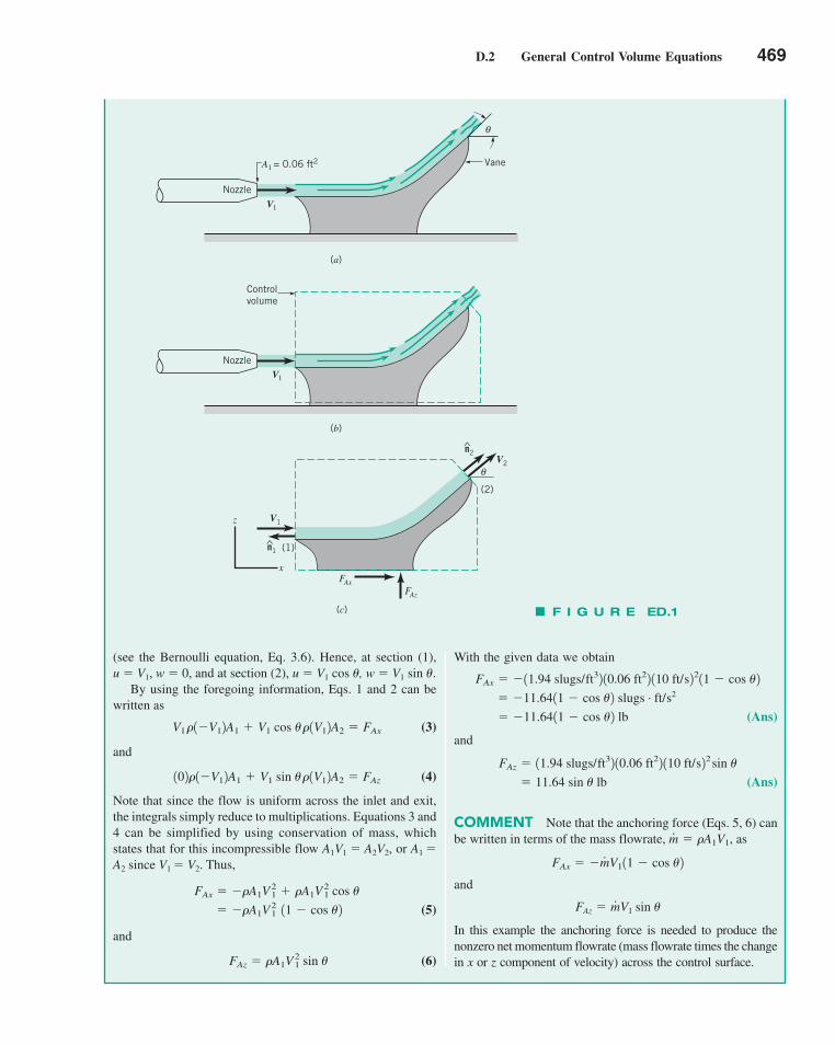
D.2 General Control Volume Equations 469

With the given data we obtain

(Ans)

and

(Ans)

COMMENT Note that the anchoring force (Eqs. 5, 6) canbe written in terms of the mass flowrate, as

and

In this example the anchoring force is needed to produce thenonzero net momentum flowrate (mass flowrate times the changein x or z component of velocity) across the control surface.

FAz � m#V1

sin �

FAx � �m#V111 � cos �2

m#

� �A1V1,

� 11.64 sin � lb

FAz � 11.94 slugs/ft32 10.06 ft22 110 ft/s22 sin �

� �11.6411 � cos �2 lb

� �11.6411 � cos �2 slugs # ft/s2

FAx � �11.94 slugs/ft32 10.06 ft22 110 ft/s2211 � cos �2

(see the Bernoulli equation, Eq. 3.6). Hence, at section (1),u � V1, w � 0, and at section (2), u � V1 cos �, w � V1 sin �.

By using the foregoing information, Eqs. 1 and 2 can bewritten as

(3)

and

(4)

Note that since the flow is uniform across the inlet and exit,the integrals simply reduce to multiplications. Equations 3 and4 can be simplified by using conservation of mass, whichstates that for this incompressible flow A1V1 � A2V2, or A1 �A2 since V1 � V2. Thus,

(5)

and

(6) FAz � �A1V 21 sin �

� ��A1V 21 11 � cos �2

FAx � ��A1V 21 � �A1V 2

1 cos �

102�1�V12A1 � V1 sin � �1V12A2 � FAz

V1 �1�V12A1 � V1 cos � �1V12A2 � FAx

Nozzle

A1 = 0.06 ft2 Vane

V1

(a)

θ

NozzleV1

(b)

Controlvolume

(c)

z

x

(2)

FAxFAz

V1

V2θ

(1)^

n2

n1

F I G U R E ED.1

appDReynoldsTransportTheorem.qxd 10/1/10 10:10 PM Page 469

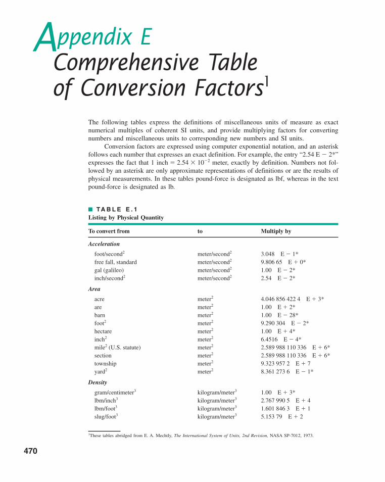
Appendix EComprehensive Table of Conversion Factors1

The following tables express the definitions of miscellaneous units of measure as exactnumerical multiples of coherent SI units, and provide multiplying factors for convertingnumbers and miscellaneous units to corresponding new numbers and SI units.

Conversion factors are expressed using computer exponential notation, and an asteriskfollows each number that expresses an exact definition. For example, the entry “2.54 E � 2*”expresses the fact that 1 inch � 2.54 � 10�2 meter, exactly by definition. Numbers not fol-lowed by an asterisk are only approximate representations of definitions or are the results ofphysical measurements. In these tables pound-force is designated as lbf, whereas in the textpound-force is designated as lb.

TA B L E E . 1

Listing by Physical Quantity

To convert from to Multiply by

Acceleration

foot/second2 meter/second2 3.048 E � 1*free fall, standard meter/second2 9.806 65 E � 0*gal (galileo) meter/second2 1.00 E � 2*inch/second2 meter/second2 2.54 E � 2*

Area

acre meter2 4.046 856 422 4 E � 3*are meter2 1.00 E � 2*barn meter2 1.00 E � 28*foot2 meter2 9.290 304 E � 2*hectare meter2 1.00 E � 4*inch2 meter2 6.4516 E � 4*mile2 (U.S. statute) meter2 2.589 988 110 336 E � 6*section meter2 2.589 988 110 336 E � 6*township meter2 9.323 957 2 E � 7yard2 meter2 8.361 273 6 E � 1*

Density

gram/centimeter3 kilogram/meter3 1.00 E � 3*lbm/inch3 kilogram/meter3 2.767 990 5 E � 4lbm/foot3 kilogram/meter3 1.601 846 3 E � 1slug/foot3 kilogram/meter3 5.153 79 E � 2

1These tables abridged from E. A. Mechtly, The International System of Units, 2nd Revision, NASA SP-7012, 1973.

470

appEComprehensiveTableofConversionFactors.qxd 9/28/10 4:35 PM Page 470

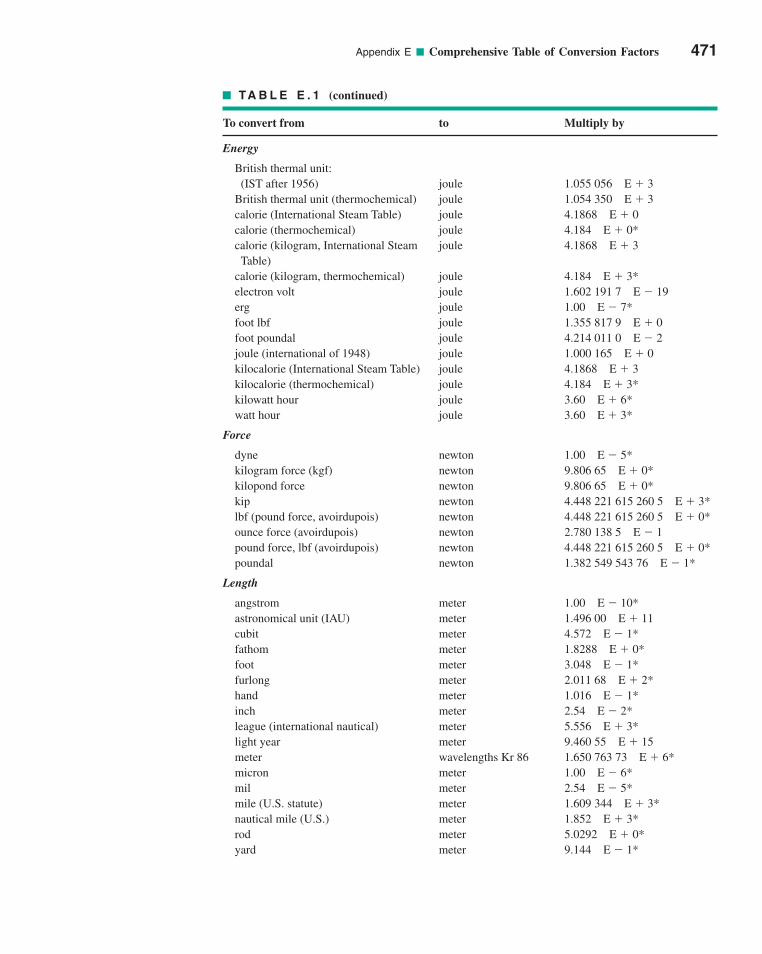
Appendix E ■ Comprehensive Table of Conversion Factors 471

TA B L E E . 1 (continued)

To convert from to Multiply by

Energy

British thermal unit:(IST after 1956) joule 1.055 056 E � 3

British thermal unit (thermochemical) joule 1.054 350 E � 3calorie (International Steam Table) joule 4.1868 E � 0calorie (thermochemical) joule 4.184 E � 0*calorie (kilogram, International Steam joule 4.1868 E � 3Table)

calorie (kilogram, thermochemical) joule 4.184 E � 3*electron volt joule 1.602 191 7 E � 19erg joule 1.00 E � 7*foot lbf joule 1.355 817 9 E � 0foot poundal joule 4.214 011 0 E � 2joule (international of 1948) joule 1.000 165 E � 0kilocalorie (International Steam Table) joule 4.1868 E � 3kilocalorie (thermochemical) joule 4.184 E � 3*kilowatt hour joule 3.60 E � 6*watt hour joule 3.60 E � 3*

Force

dyne newton 1.00 E � 5*kilogram force (kgf) newton 9.806 65 E � 0*kilopond force newton 9.806 65 E � 0*kip newton 4.448 221 615 260 5 E � 3*lbf (pound force, avoirdupois) newton 4.448 221 615 260 5 E � 0*ounce force (avoirdupois) newton 2.780 138 5 E � 1pound force, lbf (avoirdupois) newton 4.448 221 615 260 5 E � 0*poundal newton 1.382 549 543 76 E � 1*

Length

angstrom meter 1.00 E � 10*astronomical unit (IAU) meter 1.496 00 E � 11cubit meter 4.572 E � 1*fathom meter 1.8288 E � 0*foot meter 3.048 E � 1*furlong meter 2.011 68 E � 2*hand meter 1.016 E � 1*inch meter 2.54 E � 2*league (international nautical) meter 5.556 E � 3*light year meter 9.460 55 E � 15meter wavelengths Kr 86 1.650 763 73 E � 6*micron meter 1.00 E � 6*mil meter 2.54 E � 5*mile (U.S. statute) meter 1.609 344 E � 3*nautical mile (U.S.) meter 1.852 E � 3*rod meter 5.0292 E � 0*yard meter 9.144 E � 1*

appEComprehensiveTableofConversionFactors.qxd 9/28/10 4:35 PM Page 471

TA B L E E . 1 (continued)

To convert from to Multiply by

Mass

carat (metric) kilogram 2.00 E � 4*grain kilogram 6.479 891 E � 5*gram kilogram 1.00 E � 3*ounce mass (avoirdupois) kilogram 2.834 952 312 5 E � 2*pound mass, lbm (avoirdupois) kilogram 4.535 923 7 E � 1*slug kilogram 1.459 390 29 E � 1ton (long) kilogram 1.016 046 908 8 E � 3*ton (metric) kilogram 1.00 E � 3*ton (short, 2000 pound) kilogram 9.071 847 4 E � 2*tonne kilogram 1.00 E � 3*

Power

Btu (thermochemical)/second watt 1.054 350 264 488 E � 3calorie (thermochemical)/second watt 4.184 E � 0*foot lbf/second watt 1.355 817 9 E � 0horsepower (550 foot lbf/second) watt 7.456 998 7 E � 2kilocalorie (thermochemical)/second watt 4.184 E � 3*watt (international of 1948) watt 1.000 165 E � 0

Pressure

atmosphere newton/meter2 1.013 25 E � 5*bar newton/meter2 1.00 E � 5*barye newton/meter2 1.00 E � 1*centimeter of mercury (0 �C) newton/meter2 1.333 22 E � 3centimeter of water (4 �C) newton/meter2 9.806 38 E � 1dyne/centimeter2 newton/meter2 1.00 E � 1*foot of water (39.2 �F) newton/meter2 2.988 98 E � 3inch of mercury (32 �F) newton/meter2 3.386 389 E � 3inch of mercury (60 �F) newton/meter2 3.376 85 E � 3inch of water (39.2 �F) newton/meter2 2.490 82 E � 2inch of water (60 �F) newton/meter2 2.4884 E � 2kgf/centimeter2 newton/meter2 9.806 65 E � 4*kgf/meter2 newton/meter2 9.806 65 E � 0*lbf/foot2 newton/meter2 4.788 025 8 E � 1lbf/inch2 (psi) newton/meter2 6.894 757 2 E � 3millibar newton/meter2 1.00 E � 2*millimeter of mercury (0 �C) newton/meter2 1.333 224 E � 2pascal newton/meter2 1.00 E � 0*psi (lbf/inch2) newton/meter2 6.894 757 2 E � 3torr (0 �C) newton/meter2 1.333 22 E � 2

Speed

foot/second meter/second 3.048 E � 1*inch/second meter/second 2.54 E � 2*kilometer/hour meter/second 2.777 777 8 E � 1knot (international) meter/second 5.144 444 444 E � 1mile/hour (U.S. statute) meter/second 4.4704 E � 1*

472 Appendix E ■ Comprehensive Table of Conversion Factors

appEComprehensiveTableofConversionFactors.qxd 9/28/10 4:35 PM Page 472

Appendix E ■ Comprehensive Table of Conversion Factors 473

TA B L E E . 1 (continued)

To convert from to Multiply by

Temperature

Celsius kelvin TK � TC � 273.15Fahrenheit kelvin TK � (5/9)(TF � 459.67)Fahrenheit Celsius TC � (5/9)(TF � 32)Rankine kelvin TK � (5/9)TR

Time

day (mean solar) second (mean solar) 8.64 E � 4*hour (mean solar) second (mean solar) 3.60 E � 3*minute (mean solar) second (mean solar) 6.00 E � 1*year (calendar) second (mean solar) 3.1536 E � 7*

Viscosity

centistoke meter2/second 1.00 E � 6*stoke meter2/second 1.00 E � 4*foot2/second meter2/second 9.290 304 E � 2*centipoise newton second/meter2 1.00 E � 3*lbm/foot second newton second/meter2 1.488 163 9 E � 0lbf second/foot2 newton second/meter2 4.788 025 8 E � 1poise newton second/meter2 1.00 E � 1*poundal second/foot2 newton second/meter2 1.488 163 9 E � 0slug/foot second newton second/meter2 4.788 025 8 E � 1rhe meter2/newton second 1.00 E � 1*

Volume

acre foot meter3 1.233 481 837 547 52 E � 3*barrel (petroleum, 42 gallons) meter3 1.589 873 E � 1board foot meter3 2.359 737 216 E � 3*bushel (U.S.) meter3 3.523 907 016 688 E � 2*cord meter3 3.624 556 3 E � 0cup meter3 2.365 882 365 E � 4*dram (U.S. fluid) meter3 3.696 691 195 312 5 E � 6*fluid ounce (U.S.) meter3 2.957 352 956 25 E � 5*foot3 meter3 2.831 684 659 2 E � 2*gallon (U.K. liquid) meter3 4.546 087 E � 3gallon (U.S. liquid) meter3 3.785 411 784 E � 3*inch3 meter3 1.638 706 4 E � 5*liter meter3 1.00 E � 3*ounce (U.S. fluid) meter3 2.957 352 956 25 E � 5*peck (U.S.) meter3 8.809 767 541 72 E � 3*pint (U.S. liquid) meter3 4.731 764 73 E � 4*quart (U.S. liquid) meter3 9.463 529 5 E � 4stere meter3 1.00 E � 0*tablespoon meter3 1.478 676 478 125 E � 5*teaspoon meter3 4.928 921 593 75 E � 6*yard3 meter3 7.645 548 579 84 E � 1*

appEComprehensiveTableofConversionFactors.qxd 9/28/10 4:35 PM Page 473

Online Appendix List

See book web site, www.wiley.com/college/young, or WileyPLUS, for this material.

Appendix F: Video Library

Appendix G: Review Problems

Appendix H: Laboratory Problems

Appendix I: CFD-Driven Cavity Example

Appendix J: FlowLab Tutorial and User’s Guide

Appendix K: FlowLab Problems

Appendix L: Odd Numbered Homework Problems

474

OnlineAppendix.qxd 9/30/10 11:01 AM Page 474

Answers toSelected Even-Numbered Homework Problems

ANS-1

Chapter 11.2 (a) FL3, ML4T�2; (b) F 2L�5T 2, M 2L�3T �2;

(c) FT, MLT �1

1.4 Dimensionless1.8 Yes1.10 1 2, �1 21.14 (a) 4.66 � 104 ft; (b) 5.18 � 10�2 lb ft3;

(c) 3.12 � 10�3 slugs ft3;(d) 2.36 � 10�2 ft . lb s;(e) 5.17 � 10�6 ft s

1.16 1.25, 1.251.18 (a) 0.240 mi3; (b) 4.41 � 105 lb1.20 1150 kg m3, 11.3 kN m3

1.22 9770 N m3; 996 kg m3; 0.9961.24 12.0 kN m3; 1.22 � 103 kg m3; 1.221.28 0.335; 3290 N m3

1.30 oxygen1.34 668 lb1.36 893 s�1

1.38 6.44 � 10�3 slugs ft3; 0.622 lb2.60 � 10�3 N . s m2; � (blood) �(water)� 3.74

1.40 1841.42 0.6 N . s m2, 1.3 � 10�2 lb . s ft2

1.44 0.552 U � N m2 acting to left on plate1.461.48 7.22�1.50 (a) No; (b) Not correct

1.52

1.54 (a) 12.7 ft2 rev; 4.73 � 10�3 lb . s ft2

1.56 9.53 � 10�4 ft . lb1.60 1.061.62 1.78 kg m3

1.64 (a) 343 m s; (b) 1010 m s; (c) 446 m s1.66 4.74 psi (abs)1.68 0.842 psi (abs); 5.81 kPa (abs)1.70 1.80 � 10�2 ft1.72 (a) 24.5 deg

����

��

t �2� R3

i /��

Ro � Ri

d � 0.571 b�1/U3��

��

���

���

����

���

���

Chapter 22.2 505 kPa2.4 0.0797 psi2.6 1.532.8 No2.10 10.2 psia2.14 (a) 0.759 m, 0.759 m; (b) 10.1 m, 10.3 m;

(c) 12.3 m, 13.0 m2.16 �7.7 psi2.18 26.12.20 103 kPa; 230 mm2.22 �802 lb ft2

2.24 82.1 lb ft3

2.26 0.424 psi2.28 23.8 ft2.30 78.4 lb2.32 0.202 m2.34 1140 N2.362.38 9100 lb2.40 21,200 lb; 12.19 ft2.42 92.4 kN; 0.0723 m along gate below centroid2.46 33,900 lb2.50 8740 lb; 21,300 lb2.52 6300 lb2.54 941 kN2.56 1.88 ft2.58 426 kN; 2.46 m below surface2.60 48.2 ft; 61.1 ft; 71.8 ft; 81.1 ft; 89.1 ft2.62 294 kN; 328 kN; yes2.64 22,500 lb2.66 3370 lb, 882 lb2.68 64.4 kN2.70 585 lb acting vertically downward along

vertical axis of bottle2.72 46.8 lb/ft3

2.76 54,600 lb2.80 2480 kg2.82 (a) 68.9 lb ft2; (b) 57.4 lb�

/ � 3d 11.31�1d 2 18.61d 12821/2 4 �2

��

ans.qxd 9/28/10 9:22 PM Page ANS-1

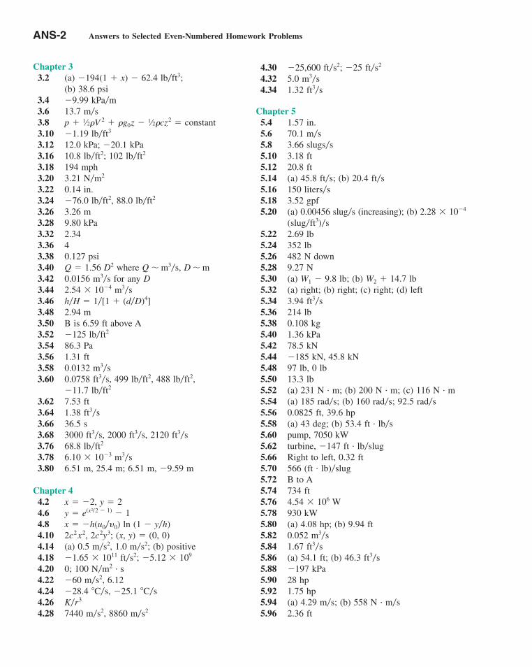
ANS-2 Answers to Selected Even-Numbered Homework Problems

Chapter 33.2 (a) �194(1 x) � 62.4 lb ft3;

(b) 38.6 psi3.4 �9.99 kPa m3.6 13.7 m s3.8 p 1⁄2�V 2 �g0z � 1⁄2�cz2 � constant3.10 �1.19 lb ft3

3.12 12.0 kPa; �20.1 kPa3.16 10.8 lb ft2; 102 lb ft2

3.18 194 mph3.20 3.21 N m2

3.22 0.14 in.3.24 �76.0 lb ft2, 88.0 lb ft2

3.26 3.26 m3.28 9.80 kPa3.32 2.343.36 43.38 0.127 psi3.40 Q � 1.56 D2 where Q m3 s, D m3.42 0.0156 m3 s for any D3.44 2.54 � 10�4 m3 s3.46 h H � 1 [1 (d D)4]3.48 2.94 m3.50 B is 6.59 ft above A3.52 �125 lb ft2

3.54 86.3 Pa3.56 1.31 ft3.58 0.0132 m3 s3.60 0.0758 ft3 s, 499 lb ft2, 488 lb ft2,

�11.7 lb ft2

3.62 7.53 ft3.64 1.38 ft3 s3.66 36.5 s3.68 3000 ft3 s, 2000 ft3 s, 2120 ft3 s3.76 68.8 lb ft2

3.78 6.10 � 10�3 m3 s3.80 6.51 m, 25.4 m; 6.51 m, �9.59 m

Chapter 44.2 x � �2, y � 24.6 y � e(x2/2 � 1) � 14.8 x � �h(u0 y0) ln (1 � y h)4.10 2c2x2, 2c2y3; (x, y) � (0, 0)4.14 (a) 0.5 m s2, 1.0 m s2; (b) positive4.18 �1.65 � 1011 ft s2; �5.12 � 109

4.20 0; 100 N m2 . s4.22 �60 m s2, 6.124.24 �28.4 �C s, �25.1 �C s4.26 K r3

4.28 7440 m s2, 8860 m s2���

���

��

��

��

��

���

�

����

�

�

����

����

��

�

��

�

��

�4.30 �25,600 ft s2; �25 ft s2

4.32 5.0 m3 s4.34 1.32 ft3 s

Chapter 55.4 1.57 in.5.6 70.1 m s5.8 3.66 slugs s5.10 3.18 ft5.12 20.8 ft5.14 (a) 45.8 ft s; (b) 20.4 ft s5.16 150 liters s5.18 3.52 gpf5.20 (a) 0.00456 slug s (increasing); (b) 2.28 � 10�4

(slug ft3) s5.22 2.69 lb5.24 352 lb5.26 482 N down5.28 9.27 N5.30 (a) W1 � 9.8 lb; (b) W2 14.7 lb5.32 (a) right; (b) right; (c) right; (d) left5.34 3.94 ft3 s5.36 214 lb5.38 0.108 kg5.40 1.36 kPa5.42 78.5 kN5.44 �185 kN, 45.8 kN5.48 97 lb, 0 lb5.50 13.3 lb5.52 (a) 231 N . m; (b) 200 N . m; (c) 116 N . m5.54 (a) 185 rad s; (b) 160 rad s; 92.5 rad s5.56 0.0825 ft, 39.6 hp5.58 (a) 43 deg; (b) 53.4 ft . lb s5.60 pump, 7050 kW5.62 turbine, �147 ft . lb slug5.66 Right to left, 0.32 ft5.70 566 (ft . lb) slug5.72 B to A5.74 734 ft5.76 4.54 � 106 W5.78 930 kW5.80 (a) 4.08 hp; (b) 9.94 ft5.82 0.052 m3 s5.84 1.67 ft3 s5.86 (a) 54.1 ft; (b) 46.3 ft3 s5.88 �197 kPa5.90 28 hp5.92 1.75 hp5.94 (a) 4.29 m s; (b) 558 N . m s5.96 2.36 ft

��

��

�

�

�

�

���

�

���

���

��

��

��

ans.qxd 9/28/10 9:22 PM Page ANS-2

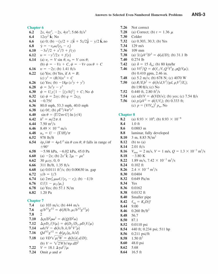
Answers to Selected Even-Numbered Homework Problems ANS-3

Chapter 66.2 2x, 4xt 2, �2y, 4yt 2; 5.66 ft s2

6.4 12xy2 ; No6.6 (a) 0; (b) 6.86.10 �3x2 2 x3 3 f (y)6.126.14 (a)

(b) 6.16 y � �2y; (b) 1.41 ft s6.22 (a) Yes; (b) Yes, if A � B;

(c) y2 � (B A)x2 C6.26 (a) Yes; (b) �18� (x2y y3)6.286.306.32 (a) (b) q � 2xiyj

6.346.36 80.0 mph, 53.3 mph, 40.0 mph6.38 (a) 0 ; (b) p�2 4�2r3

6.406.42 h2 � m 2 A6.44 7.50 m2 s6.46 8.49 � 10�4 m s6.486.52 978 lb ft6.54 falls in range of

6.58 �5.98 kPa, �6.02 kPa, 45.0 Pa6.60 (a) �2x; (b) 2� � �x3

6.62 30 �xy, 0, 06.66 311 lb ft, 1.35 ft s6.68 (a) 0.0111 ft3 s; (b) 0.00630 in. gap6.72 y b � 1 36.74 (a) (b) 6.766.78 (a) Yes; (b) 57.1 N m6.82 1.20 Pa

Chapter 77.4 (a) 103 m s; (b) 444 m s7.67.8 27.107.127.147.167.18 (a)

(b) 7.22 V � 18.1 ��d 2 �7.24 Omit � and �

�V � 22wb��� dD2

VD2��w � �1b�d, d�D2;Qd 5/2g1/2 � � 1�g��a, h�d2�b�V � �1h �b, k �b3V 2�2¢ pD1 � 1V�2 � �1D2 �D1, �D1V��2¢ p�D2��2 � � 1Q�D3�2

q�b3/2g1/2 � � 1H�b, ��b3/2g1/2�2��

�U� 11 � �2 ��12

�U�b2�r30 ��/� 1r0 � ri2;��

���

2x 3 i;

�90°�0ps/0� � 4�U 2

sin � cos �;�

uA � U � 1�/H2���

��

sin � � 1�/2�rU2 ln 1r�42�/

�0.75/� � 2xy;

� � Ucy 31 � 13 1y /h22 4 C ; No �

� � 3x2y � y3

�

�� � �Vx C, � � �Vr cos � Cyr � V sin �, y� � V cos �;

y � �y2�2x f 1x2��

#

� �r0�� 1r0 � ri2�1y�2 z2 i 5z�2 j � y�2 k, no

k�

7.26 Not correct7.28 (a) Correct; (b) t � 1.36 �7.30 Colder7.32 (a) 0.303, 30.3; (b) Yes7.34 129 m/s7.36 109 mm7.38 (a) (b) 31.1 lb7.40 0.274 lb7.42 (a) � � 15 �m; (b) 80 km/hr7.46 (a)

(b) 0.410 gpm, 2.46 in.7.48 (a) 5.2 m s; (b) 678 N; (c) 4070 W7.50 (a)

(b) 1.90 ft s; (c) No7.52 0.440 ft, 2.80 ft3 s7.54 (a) (b) yes; (c) 7.54 ft s7.56 (a) (b) 0.333 ft;

(c)

Chapter 88.2 (a) 8.93 � 104; (b) 8.93 � 10�8

8.4 1.0 ft8.6 0.0883 m8.8 laminar, fully developed8.10 3 m, 8.83 N m2

8.12 (b) to (a)8.14 2.01 ft s8.16 Vmax � 2 m s, V � 1 m/s, Q � 1.3 � 10�3 m3 s8.18 �3.80 K8.22 1.89 m s, 7.42 � 10�3 m3 s8.24 0.102 ft8.26 2.4 � 10�4 m3 s8.30 0.04048.32 0.649 Pa m8.34 Yes8.36 0.01628.38 0.0132 ft8.40 Smaller pipe8.428.44 9.008.46 0.260 lb ft2

8.48 56.78.50 87.18.52 0.0110 psi8.54 440 ft; 0.234 psi; 511 hp8.56 0.211 psi ft8.58 1.50 ft2

8.60 48.0 psi8.62 5.688.64 16.5 ft

�

�

/eq � KLD�f

�

�

��

���

�

p � 1V/Vm22 pm, No

p��V 2 � �1/�/i2;�nD�V � �1VD�2;

��

R �Eib2 � � 1b�d,V 2�gd, �iV

2�Ei2;�

V/2�Q � �1/i �/, Q 2/5g, �Q�/�2;

d��V 2D 2 � �1d�D2;

ans.qxd 9/30/10 10:50 AM Page ANS-3

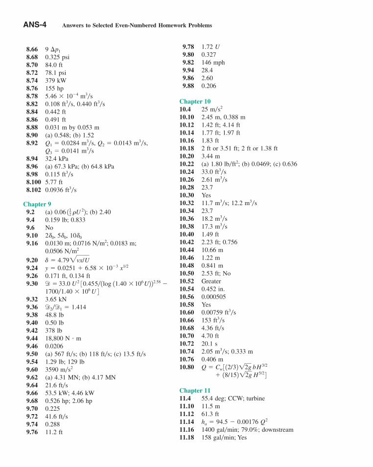
ANS-4 Answers to Selected Even-Numbered Homework Problems

8.66 9 �p1

8.68 0.325 psi8.70 84.0 ft8.72 78.1 psi8.74 379 kW8.76 155 hp8.78 5.46 � 10�4 m3 s8.82 0.108 ft3 s, 0.440 ft3 s8.84 0.442 ft8.86 0.491 ft8.88 0.031 m by 0.053 m8.90 (a) 0.548; (b) 1.528.92 Q1 � 0.0284 m3 s, Q2 � 0.0143 m3 s,

Q3 � 0.0141 m3 s8.94 32.4 kPa8.96 (a) 67.3 kPa; (b) 64.8 kPa8.98 0.115 ft3 s8.100 5.77 ft8.102 0.0936 ft3 s

Chapter 99.2 (a) (b) 2.409.4 0.159 lb; 0.8339.6 No9.10 2�0, 5�0, 10�0

9.16 0.0130 m; 0.0716 N m2; 0.0183 m; 0.0506 N m2

9.209.24 y � 0.0251 6.58 � 10�3 x1/2

9.26 0.171 ft, 0.134 ft9.30

9.32 3.65 kN9.36 d2 d1 � 1.4149.38 48.8 lb9.40 0.50 lb9.42 378 lb9.44 18,800 N � m9.46 0.02069.50 (a) 567 ft s; (b) 118 ft s; (c) 13.5 ft s9.54 1.29 lb; 129 lb9.60 3590 m s2

9.62 (a) 4.31 MN; (b) 4.17 MN9.64 21.6 ft s9.66 53.5 kW; 4.46 kW9.68 0.526 hp; 2.06 hp9.70 0.2259.72 41.6 ft s9.74 0.2889.76 11.2 ft

�

�

�

���

�

1700�1.40 � 106 U 4d � 33.0 U 2 30.455� 1log 11.40 � 106U2 22.58 �

� 4.792vx/U�

�

0.06 112 �U 22;

�

�

���

���

9.78 1.72 U9.80 0.3279.82 146 mph9.94 28.49.86 2.609.88 0.206

Chapter 1010.4 25 m s2

10.10 2.45 m, 0.388 m10.12 1.42 ft; 4.14 ft10.14 1.77 ft; 1.97 ft10.16 1.83 ft10.18 2 ft or 3.51 ft; 2 ft or 1.38 ft10.20 3.44 m10.22 (a) 1.80 lb ft2; (b) 0.0469; (c) 0.63610.24 33.0 ft3 s10.26 2.61 m3 s10.28 23.710.30 Yes10.32 11.7 m3 s; 12.2 m3 s10.34 23.710.36 18.2 m3 s10.38 17.3 m3 s10.40 1.49 ft10.42 2.23 ft; 0.75610.44 10.66 m10.46 1.22 m10.48 0.841 m10.50 2.53 ft; No10.52 Greater10.54 0.452 in.10.56 0.00050510.58 Yes10.60 0.00759 ft3 s10.66 153 ft3 s10.68 4.36 ft s10.70 4.70 ft10.72 20.1 s10.74 2.05 m3 s; 0.333 m10.76 0.406 m10.80

Chapter 1111.4 55.4 deg; CCW; turbine11.10 11.5 m11.12 61.3 ft11.14 ha � 94.5 � 0.00176 Q2

11.16 1400 gal min; 79.0%; downstream11.18 158 gal min; Yes�

�

18/15212g H 5/2 4Q � Cw 3 12/3212g b H 3/2

�

��

�

��

��

��

�

�

ans.qxd 9/28/10 9:22 PM Page ANS-4

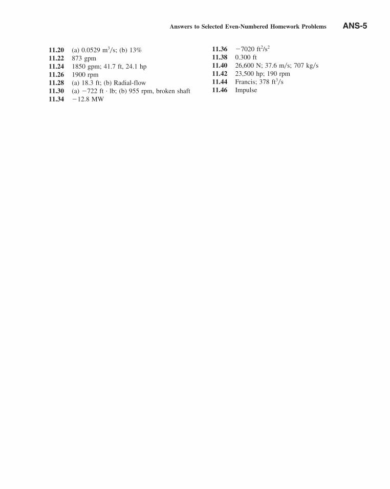
Answers to Selected Even-Numbered Homework Problems ANS-5

11.20 (a) 0.0529 m3 s; (b) 13%11.22 873 gpm11.24 1850 gpm; 41.7 ft, 24.1 hp11.26 1900 rpm11.28 (a) 18.3 ft; (b) Radial-flow11.30 (a) �722 ft . lb; (b) 955 rpm, broken shaft11.34 �12.8 MW

� 11.36 �7020 ft2/s2

11.38 0.300 ft11.40 26,600 N; 37.6 m s; 707 kg s11.42 23,500 hp; 190 rpm11.44 Francis; 378 ft3 s11.46 Impulse

�

��

ans.qxd 9/28/10 9:22 PM Page ANS-5

This page intentionally left blank

I-1

Index

Absolute pressure, 11, 39Absolute temperature, 7Absolute velocity, 131, 146Absolute viscosity, 14

of air, 461, 462of common gases, 11, 458of common liquids, 10, 458of U.S. Standard Atmosphere, 463, 464of water, 460

Acceleration, 69, 110centrifugal, 114convective, 113, 114field, 110, 176gravitational, 7, 463, 464local, 112normal, 69particle, 110streamwise, 69

Acoustic velocity, 19of air, 461, 462of water, 460

Adiabatic flow, 153Adverse pressure gradient, 340Air, table of properties of, 461, 462Airfoil, 357, video V3.1, video V9.18Alternate depths, 376Angle:

of attack, 357of contact, 22

Angular deformation, 178, 181, video V6.3Angular momentum, see Moment-of-momentumAngular momentum flow, 144, video V5.10Archimedes’ principle, 57, video V2.7Area:

centroid, 49, 51moment of inertia, 50, 51product of inertia, 50, 51

Aspect ratio, 246Atmosphere, standard, 39

properties of, 39, 463, 464Atmospheric pressure, 11

Available energy, 158Average velocity, 127, 280Axial-flow machine, 404Axial-flow pump, 423Axial-flow turbine, 434Axisymmetric flow, 322

Backward curved blade, 412Barometer, mercury, 41Basic differential equations of fluid

motion, 191Basic dimensions, 4, 240, 242Bends, 293Bernoulli equation, 73

derivation from F � ma, 70, 193, video V3.2derivation from first law of

thermodynamics, 157extended, 160irrotational flow, 196physical interpretation, 75restrictions on use of, 94, 194unsteady flow, 95

Best efficiency point, 415Best hydraulic cross section, 384BG units, see British gravitational system of unitsBlade velocity, 149Blasius, H., 253, 331Blasius formula, 253, 290Blasius solution, 331Blower, 403Blunt bodies, 322, video V9.2, video V9.10Body force, 34, 134, 189Boiling, 21, 87Bottom slope, 374Bound vortex, 361, video V4.6Boundary conditions:

inviscid flow, 211no-slip, 13, 211, video V1.4, video V6.11numerical methods, 443pipe exit, 81

Boundary element method, 444

BMIndx.qxd 10/1/10 8:46 AM Page I-1

Boundary layer:concept of, 277, 325, video V1.4, video V6.11, video

V6.12displacement thickness, 330effect of pressure gradient on, 338effect of wall roughness, 336, 349equations, 330flat plate, 328laminar:

approximate solution, 328, 333Blasius solution, 331

momentum integral equation for, 332, 333momentum thickness, 330pressure gradient, 338separation, 327, 340thickness, 329transition, 329, 334, video V9.5turbulent, 329, 336velocity profiles, 335, 341, video V9.3

Bourdon pressure gage, 47, video V2.3Brake horsepower, 415British gravitational system of units, 7Broad crested weir, 393, video V10.14Buckingham pi theorem, 240Bulk modulus, 17

of common liquids, 10of elasticity, 17

Buoyant force, 57, video V1.1, video V2.6,video V2.7

Canal, 381Capillary action, 22Capillary tube viscometer, video V1.5Casing, 410Cauchy number, 250Cavitation, 21, 87Center of buoyancy, 57Center of pressure, 50Centrifugal pump, 410Centroid, 49

of common areas, 51CFD, 230, 443, video V6.15Channel flow, see Open channel flowChezy coefficient, 378Chezy equation, 378, 380Chord length, 358Circulation, 205

about an airfoil, 361origin of, 361

Colebrook formula, 288Completely turbulent flow, 287Composite body drag, 352Compressibility criterion, 94Compressible flow, 94, 349

turbomachines, 436, video V11.6Compressible fluid, 17, 34, video V1.7Compressor, 403, video V11.6Computational fluid dynamics (CFD), 230, 443,

video V6.15Confined flow, 82Conservation:

of energy, see First law of thermodynamics of linear momentum, 188

of mass, 83, 126, 132, 182, 467, video V5.1,video V5.2

Contact angle, 22Continuity equation:

compressible flow, 84cylindrical coordinates, 184differential form, 183finite control volume, 84, 127

general, 467incompressible flow, 84, 131, video V5.3rectangular coordinates, 183unsteady flow, 127

Continuum hypothesis, 3Contraction coefficient, 82, 91, 396Control surface, 115Control volume, 115

fixed, 116, 126general, 465guidelines for selection, 120infinitesimal, 176moving, 131velocity, 131

Convective acceleration, 113Convective derivative, 113Conversion factors, 8, 470Core flow, 277Couette flow, 224Critical depth, 376, 393Critical flow, open channel, 371, 376Critical Reynolds number, 335Curl operator, 180Curved surface, forces on, 54Cylinder:

drag coefficient for, 347inviscid flow around, 212large Reynolds number flow around, 328,

video V6.15low Reynolds number flow around, 327pressure distribution on surface of, 214, 341rotating, 216, 362

Cylindrical coordinates, 184, 187

D’Alembert’s paradox, 215Darcy-Weisbach equation, 287Deep water wave, 373Deformation:

angular, 178, 181, video V6.3linear, 178rate of, 181volumetric, 178

Del (gradient) operator:cylindrical coordinates, 197rectangular coordinates, 35

Density, 9of air, 461, 462of common gases, 11of common liquids, 10of U.S. Standard Atmosphere, 463, 464of water, 10, 460

Derivative:convective, 113local, 113material, 111substantial, 111

Differential analysis, 176Dilatation rate, 178Dimensional analysis, 238, 239, 246Dimensional homogeneity, 3, 240Dimensionless groups, 240

list of, 250Dimensionless products, 240Dimensions:

basic, 3, 240, 242of common physical quantities, 4reference, 241, 242, 247

Discharge coefficient:nozzle, 310orifice, 309sluice gate, 396

I-2 Index

BMIndx.qxd 10/1/10 8:46 AM Page I-2

Venturi meter, 311weir, 392–394

Discretization, 430Displacement thickness, 330Distorted model, 259, video V7.12, video V7.20Doublet, 207

strength of, 208Drag, 321, 341

form, 342friction, 331, 342in potential flow, 214pressure, 342

Drag coefficient, 263, 325, 342, 343airfoil, 357composite body, 352cylinder, 347effect of compressibility on, 349effect of Froude number on, 352, video V9.12effect of Mach number on, 349effect of Reynolds number on, 344, 347effect of shape on, 343, 346, video V9.7,

video V9.13effect of surface roughness on, 260, 349ellipse, 343, video V9.11flat plate parallel to flow, 331, 337friction, 331, 337, 342from model studies, 263, video V7.15pressure, 342selected three-dimensional objects, 355selected two-dimensional objects, 354sphere, 347, 350, video V7.7streamlined body, 344

Drowned outflow, 396Drum gate, 396Duct, 298Dynamic pressure, 78Dynamic similarity, 256Dynamic viscosity, 14

of air, 461, 462of common gases, 11, 458of common liquids, 10, 458of U.S. Standard Atmosphere, 463, 464of water, 460

Eddy viscosity, 284Efficiency, 160, 420, 434

overall, 415Elbows, losses in, 293Elevation head, 76, 93Energy:

available, 158internal, 152kinetic, 76, 152per unit mass, 152per unit weight, 160specific, 375stored, 152useful, 158

Energy equation, see First law ofthermodynamics

Energy line, 92, 302, 375Enthalpy, 155Entrance length, 278Entrance loss, 291Entrance region, 277, 291, video V8.10Equations:

general homogeneous, 5of motion, 191restricted homogeneous, 5

Equation of state, 11Equipotential line, 200

Eulerian description of motion, 105Euler number, 250Euler turbomachine equation, 409Euler’s equations, 193Exit pipe loss, 292, video V8.10Extended Bernoulli equation, 160Extensive property, 116External flow, 321Eye, 410

Fan, 150, 403Favorable pressure gradient, 340Field representation, 103, 176, video V4.2Finite control volume analysis, 126, 465Finite difference:

grid method, 444Finite element:

mesh method, 444First law of thermodynamics, 152,

154, 468video V5.13, video V5.14

First moment of area, 49Fittings, losses in, 293Flap, airfoil, 359, video V9.17, video 9.18Flat plate:

Blasius solution, 331momentum integral equation, 332, 333roughness effect, 337

Floating body, 59, video V2.7Flow coefficient, 421, 434Flowfield, 103FlowLab, 443, 455Flow measurement:

external flow:Pitot-static tube, 79, video V3.8Pitot tube, 93, video V3.8

internal flow:nozzle meter, 89, 309nutating disk meter, 313, video V8.14orifice meter, 89, 309rotameter, video V8.13Venturi meter, 89, 310, video V3.10

open channel flow:sluice gate, 91, 394weir, 390, video V10.13

pipe, 309Flow meters, see Flow measurementFlow net, 200Flowrate, 111

mass, 82, 127volume, 82, 127

Flow separation, 327, video V9.6, video V9.8Flow visualization, 105, video V4.6, video V4.9,

video V7.16, video V9.13Fluid:

definition, 3ideal, 194inviscid, 192Newtonian, 14non-Newtonian, 14, video V1.6

Fluid dynamics, 9Fluid kinematics, 102, 176Fluid machines, 150, 403, videos V11.1–V11.6Fluid particle, 69Fluid properties:

graphs of, 458, 459tables of, 10, 11, 460–464

Fluid statics, 9, 32equilibrium in, 34forces in, 47pressure height relation, 36, 37

Index I-3

BMIndx.qxd 10/1/10 8:46 AM Page I-3

Force:anchoring, 134, 139body, 34, 134, 189buoyant, 57, video V2.7compressibility, 250drag, 214, 321, 341gravity, 134, 250hydrostatic:

on curved surfaces, 54, video V2.5on plane surfaces, 47, video V2.2

inertia, 249lift, 214, 217, 321, 357pressure, 47, 54, 322reaction, 139surface, 34, 134, 189surface tension, 21, video V1.9, video V1.10viscous, 13, 322

Forced vortex, 204Form drag, 342Forward curved blade, 412Forward difference, 445Francis turbine, 433Free jet, 81, video V3.9Free outflow, 396Free-stream velocity, 339Free surface, 37Free vortex, 75, 204, video V3.6, video V6.4Friction drag, see DragFriction factor, 287

data correlation for, 287Moody chart, 287, 288non circular duct, 298smooth pipe, 287wholly turbulent, 287

Friction slope, 375Frictionless, 192Frontal area, 325Froude number, 250, 352, 371, 374, video V7.4,

video V10.5Fully developed flow, 277

laminar, 278, video V8.9turbulent, 282

Gage fluid, 43Gage pressure, 11, 40, 139Gas constant, 11

for common gases, 11ideal gas equation of state, 11

Geometric similarity, 256Grade line:

energy, 92, 302, 379hydraulic, 92

Gradient:operator, 35, 111, 177pressure, 35

Gradually varied flow, 370, 385Gravity, acceleration of, 7, 189, 463, 464Grid, 446Guide vanes, 293

Haaland equation, 288Hagen, G., 227Hagen–Poiseuille flow, 227, 281,

video V6.13Half body, 209, video V6.5Head, 76, 92

coefficient, 420, 434elevation, 76, 93piezometric, 93pressure, 37, 76, 93, 160pump, 160, 419total, 92

turbine, 160, 434velocity, 76, 93weir, 391

Head loss, 160in enlargements and contractions, 292in entrances, 291, video V8.10in exits, 292, video 8.10in gradual contractions, 297in hydraulic jumps, 388, video V10.11,

video V10.12in mitered bends, 293in open channels, 375in pipe bends, 293in pipe entrances, 291in pipes, 286, 290in sudden area changes, 292in valves and fittings, 293major, 286minor, 286, 290, video V8.12

Head loss coefficient, 290Head rise coefficient, 420Heat transfer, 152

relationship between head loss, internal energy, and, 158

Horseshoe vortex, 361, video V4.6, video V9.1, videoV9.19, video V10.9

Hydraulically smooth wall, 287Hydraulic diameter, 298Hydraulic grade line, 92Hydraulic jump, 386, video V10.11,

video V10.12depth ratio across, 387head loss across, 388

Hydraulic radius, 379Hydrometer, video V2.7Hydrostatic force:

on curved surfaces, 54, video V2.5on plane surfaces, 47, video V2.4

Hydrostatic pressure, 36, 78Hydrostatic pressure distribution, 36

Ideal fluid, 194Ideal gas law, 11Impeller, 410Impulse turbine, 426, 427, video V11.5Inclined tube manometer, 46Incompressible flow, 94, 132Incompressible fluid, 17, 36, 94, 178, 184Infinitesimal control volume, 176Inlet guide vane, 294Intensive property, 116Internal energy, 152International system of units, 7Inviscid core, 277Inviscid flow, 69, 192

fluid, 192Irrotational flow, 180, 195, 196Irrotational vortex, 204, video V3.6, video V6.4Isentropic process, 18Isothermal:

atmosphere, 39process, 18

Jet exit pressure, 81Joule, 8Jump, hydraulic 386, video 10.11, video 10.12

Kaplan turbine, 433Karman vortex trail, 347, video V6.15, video V7.5, video

V9.8, video V9.8Kilogram, 8

I-4 Index

BMIndx.qxd 10/1/10 8:46 AM Page I-4

Index I-5

Kinematics of fluid flow, 102, 176Kinematic similarity, 256Kinematic viscosity, 15

of air, 461, 462of common gases, 11, 459of common liquids, 10, 459of water, 460

Kinetic energy, 76, 152coefficient, 163

Kutta–Joukowski law, 218

Lagrangian description of flow, 105, video V4.4, videoV4.5

Laminar boundary layer:Blasius solution, 331description of, 325effect of pressure gradient, 338flat plate:

approximate solution, 333exact solution, 331friction coefficient for, 331thickness of, 329

Laminar flow, 106, 275, video V4.7, video V8.4between parallel plates, 222in a boundary layer, 328in a pipe, 227, 275, video V6.13, video V8.2past a cylinder, 341

Laplace’s equation, 197Laplacian operator, 197Length scale, 258Lift, 217, 321, 357Lift coefficient, 325, 357

airfoil, 357rotating cylinder or sphere, 217

Lift/drag polar diagram, 358Lift/drag ratio, 358Linear deformation, 178Linear momentum, see Newton’s second law of motionLinear momentum equation, 133, 134, 468Linear momentum flow, 133, video V5.4,

video V5.11Local acceleration, 113Local derivative, 113Loss, 158Loss, major and minor, see Head lossLoss coefficient, 290Low Reynolds number flow, 325, 344, video V1.2, video

V7.7

Mach number, 20, 95, 250, 349, video V1.8Magnus effect, 218, 362Major loss, see Head lossManning coefficient, 380

values of, 380Manning equation, 378, 380Manometer, 42

differential, 45inclined tube, 46piezometer tube, 42, video V2.2U-tube, 43

Mass, units of, 7Mass flowrate, 82, 127Material derivative, 111, 177Measurement, flow, see Flow measurementMechanical energy equation, 160Meter, flow, see Flow measurementMethod of repeating variables, 241Method of superposition, 209, video V6.5Methods of description:

Eulerian, 105Lagrangian, 105

Minor loss, see Head lossMinor loss coefficient, see Head loss coefficientMixed-flow machine, 404Mixed-flow pump, 423Mixed-flow turbine, 433Mixing length, 284Model:

definition, 238, 254design conditions, 255distorted, 259, video V7.12, video V7.16,

video V7.18true, 259

Modeling laws, 255Model scales, 258, video V7.1Model studies, 260, videos V7.8–V7.20Moment of inertia, 50, 51

of common areas, 51Moment-of-momentum, 144, 145, 409, 468,

video V5.10Momentum:

angular, see Moment-of-momentumlinear, see Newton’s second law of motion

Momentum equation:for differential control volume, 188for inertial finite control volume, 133, 134, 468for inviscid flow, 192for viscous flow, 220

Momentum flux, 133, video V5.5, video V5.8Momentum integral equation, 332, 333Momentum thickness, 330Moody chart, 287, 288Multiple pipe system, see Pipe systems

Nappe, 391Navier, L., 220Navier–Stokes equations:

cylindrical coordinates, 221rectangular coordinates, 220

Newton, 8Newtonian fluid, 14, 219Newton’s second law of motion, 69, 133, 188Noncircular duct, 298Non-Newtonian fluid, 14, video V1.6Non uniform flow, 162, 370Non viscous, 192Normal depth, 380Normal stress, 153, 189, 219

in a Newtonian fluid, 219work, 153

No-slip condition, 13, 211, video V1.4,video V6.11, video V6.12

Nozzle, 136, video V5.3Nozzle discharge coefficient, 310Nozzle meter, 89, 309Numerical methods, 230, video V6.15Nutating disk meter, 313, video V8.14

One-dimensional flow, 105Open channel flow, 370

critical flow, 371energy equation for, 375gradually varied flow, 370, 385hydraulic jump, 386, video V10.11, video V10.12laminar, 371Manning equation for, 378most efficient, 385normal depth, 380rapidly varied flow, 370, 386, video V10.8surface wave propagation, 371uniform flow, 370, 378varied flow, 370, video V10.6

BMIndx.qxd 10/1/10 8:46 AM Page I-5

I-6 Index

Open channels:characteristics of, 370, video V10.6 geometric properties of, 379, video V10.7optimum cross sections, 385regimes of flow in, 370shear stress in, 379

Orifice:flow through, 82reentrant, 292

Orifice discharge coefficient, 309Orifice meter, 89, 309

Parallel plates, 222Pascal, 11Pascal’s law, 34Pathline, 108, video V4.11Pelton wheel, 426, 427, video V5.6, video

V5.12, video V11.4Perfect gas law, 11Physical properties of fluids:

of air, 461, 462of common gases, 11of common liquids, 10of U.S. Standard Atmosphere, 463, 464of water, 10, 460

Piezometer, 42, video V2.2Piezometric head, 93, video V2.2Pipe:

developing flow in, 277fittings, 293flowrate, 309fully developed flow in, 227, 278head loss, see Head losshydraulically smooth, 287laminar flow in, 227, 275, 278, video V6.13, video

V8.2noncircular, 298relative roughness of, 286smooth, 287transitional flow in, 275, video V8.2turbulent flow in, 275, 282, video V8.2

Pipe system components, 275Pipe systems, 274, 307, video V6.14

parallel, 307series, 307

Pi terms, 240, 241Pi theorem, 240Pitot-static tube, 79, video V3.8Pitot tube, 93, video V3.8Plane Poiseuille flow, 227Planform area, 325Poise, 15Poiseuille, J., 227Poiseuille flow, 227, 281, video V6.13

plane, 227Poiseuille’s law, 228, 281Polar coordinates, 184, 187Polar diagram, lift-drag, 358Position vector, 103Positive displacement machine, 403, video V11.3Potential, velocity, 196Potential energy, 76Potential flow theory, 197, 219

basic plane flows, 119, 208, video V6.10doublet, 207sink, 202source, 202uniform flow, 201vortex, 203

superposition of basic plane, 209flows, 209, video V6.5

flow past cylinder, 212, video V6.6,video V6.7

flow past half-body, 209, video V6.5flow past rotating cylinder, 216

Potential function, 196Pound force, 7Power, 147, 153, 411

coefficient, 420units of, 4

Power law velocity profile, 285Power specific speed, 443Prandtl, L., 325, 331Prandtl boundary layer equations, 330Prediction equation, 255Pressure:

absolute, 11, 39at a jet exit, 81, 139at a point, 33, 192, 220atmospheric, 11center of, 50coefficient, 343 definition, 11, 33, 220dynamic, 78gage, 11, 40, 139hydrostatic, 36, 78measurement of, 40, 78, video V2.2,

video V2.3stagnation, 78, video V3.7static, 78suction, 40total, 79vapor, 21vacuum, 40

Pressure coefficient, 343Pressure distribution, video V2.1, video V6.1

airfoil, 323cylinder, inviscid flow, 214, 341cylinder, viscous flow, 341hydrostatic, 36in a rotating fluid, 60in rigid-body motion, 60standard atmosphere, 39, 463, 464

Pressure drag, see DragPressure force, 47Pressure gradient, 36

adverse, 340effect on boundary layer, 338favorable, 340

Pressure head, 37, 76, 93, 160Pressure prism, 52Pressure tap, 93Pressure transducer, 47Primary quantities, 4Product of inertia, 50

of common areas, 51Profile, velocity, see Velocity profileProperties:

of air, 461, 462of common gases, 11of common liquids, 10of U.S. Standard Atmosphere, 39, 463, 464of water, 10, 460

Prototype, 254Pump, 403

axial-flow, 423blades, 424centrifugal, 410efficiency, 415geometrically similar, 420head, 160, 419mixed-flow, 423performance curve, 414

BMIndx.qxd 10/1/10 8:46 AM Page I-6

Index I-7

positive displacement, 403, video V11.3propeller, 424scaling laws, 421selection of, 416similarity laws, 419specific speed, 422stage, 424, video V11.6

Radial-flow machine, 404, 433Rankine oval, 212Rapidly varied flow, 370, 386Rate of angular deformation, 181,

video V6.3Rate of shearing strain, 13, 181Rate of work, 153Reaction turbine, 426, 433Rectangular weir, 391Reentrant entrance, 291Reference dimensions, 241, 242, 247Relative roughness, 286Relative velocity, 131, 146, 406Repeating variable, 241Reynolds, O., 249, 275Reynolds number, 15, 249, 250

critical, see Transition to turbulenceproperties of flows with low, 325, video V1.2, video

V7.3properties of flows with large, 325, video V1.1, video

V7.3Reynolds pipe flow experiment, 275,

video V8.2Reynolds transport theorem, 116, 119, 126, 465Rheology, 3Right-hand rule, 146Rigid body motion of fluid, 60Rotameter, video V8.13Rotating cylinder viscometer, 30Rotation, 179

vector, 180Rotor, 424Roughness:

effect on drag, 263, 349effect on models, 260, 262, video V7.13in open channels, 380in pipes, 286, 289on flat plates, 337relative, 286typical values of, 289

Roughness coefficient, Manning, 380Round-off error, 446

Scale:length, 258model, 258

Scaling laws for pumps, 421Second moment of area, 50

of common areas, 51Secondary flow, 292Secondary quantities, 4Separation, video V6.8, video V6.9, video V8.11, video

V9.6, video V9.13in a boundary layer, 327, 340in a pipe, 292on an airfoil, 359

Separation location, 327definition, 340on a cylinder, 327, 341

Shaft:power, 147, 409torque, 147, 153, 409work, 147, 153, 409

Shallow water wave, 373Sharp crested weir, 390, video V10.13Shearing strain, rate of, 13, 181, video V6.3Shearing stress, 13, 154, 189, 221

distribution in a pipe, 279in a boundary layer, 331in a Newtonian fluid, 14, 219in open channel flow, 389turbulent, 284

Shear stress work, 154Shock wave, 349, video V1.8Similarity:

dynamic, 256geometric, 256kinematic, 256pump, 419

Similarity requirements, 255Similitude, 238Sink, 202

strength of, 202Siphon, 88SI units, 7

prefixes, 8Slope:

energy line, 92, 302, 375of channel bottom, 374

Slug, 7Sluice gate:

discharge coefficient, 396flow rate under a, 91force on a, 143free outflow, 396submerged, 396

Sound, speed of, 19ideal gas, 19of air, 461, 462of water, 460

Source, 202, video V6.5strength of, 202

Specific energy, 375Specific energy diagram, 376Specific gravity, 10Specific heat:

constant pressure, 18constant volume, 18

Specific heat ratio, 18of air, 461, 462of common gases, 11

Specific speed, 422, 434Specific volume, 9Specific weight, 10

of air, 461, 462of common gases, 11of common liquids, 10of water, 460

Speed, 69Speed of sound, 19, video V1.8

ideal gas, 19of air, 461, 462of water, 459

Sphere:compressible flow past, 349drag coefficient for, 347, 350effect of surface roughness, 349low Reynolds number flow past, 344rotating, 362

Stability, 59, video V2.9, video V2.10Stagnation point, 78, video V3.3Stagnation pressure, 78, video V3.8Stagnation pressure probe, see Pitot tubeStagnation streamline, 78, video V3.3, video V3.3,

video V4.9

BMIndx.qxd 10/1/10 8:46 AM Page I-7

Stall, 359, video V9.15Standard atmosphere, 39

properties of, 40, 463, 464State, equation of, 11Static fluid, pressure variation in, 36Static pressure, 78Static pressure tap, 93Stator, 424Steady flow, 69, 105, video V4.7Stoke, 15Stokes, G., 220, 345Stokes’ law, 252, 345, video V7.7Stormer viscometer, 30Streakline, 107, video V3.1, video V4.1,

video V4.10Stream function, 185Streamline, 69, 106, video V4.9

equation of, 106, 186Streamline bodies, 322, 343, video V9.2,

video V9.14Streamline coordinates, 114, video V4.13Streamline curvature, 69Stress:

components, 219compressive, 153, 190Newtonian fluid, 14, 219normal, 153, 189, 219notation, 190shearing, 13, 154, 190, 219sign convention, 190tangential, 154

Stress field, 190Strouhal number, 250, video V7.5Structured grid, 446Subcritical flow, 371, 374, 376, video V10.5Submerged area, forces on, 47Substantial derivative, 111, 177Suction, 40Sudden contraction, 292Sudden expansion, 292Supercritical flow, 371, 374, 376, video V10.5Superposition, 209, video V6.5

direct method, 219inverse method, 219irrotational flow by method of, 209

Surface force, 34, 134, 189Surface tension, 21, video V1.9, video V1.10,

video V7.6, video V10.3effect on models, 264of common liquids, 10of water, 460

Surface wave, 371, video V9.12, video V10.1,video V10.2, video V10.4

System, 116relationship between control volume

and, 116System curve, 416, 417System equation, 416Systems of units, 6

Tangential stress work, 154Temperature:

absolute, 7Celsius, 7centigrade, 7Fahrenheit, 7Kelvin, 7Rankine, 7

Thermodynamics:first law of, 152

Three-dimensional flow, 105

Three-reservoir problem, 308Time average, 284Torque, 144, 147

shaft, 147, 153, 409Total head, 92Total pressure, 79Trailing vortex, 361, video V4.6, video V9.1,

video V9.19Tranquil flow, 371Transition to turbulence, video V9.4

in a boundary layer flow, 329, 334, video V9.5in a pipe flow, 275, 283, video V8.2, video V8.3, video

V8.8in an open channel flow, 371in flow past a sphere or cylinder, 341, 349

Triangular weir, 392, video V10.13True model, 256Turbine, 426

axial-flow, 434Francis, 433head, 160, 434impulse, 426, 427, video V11.5Kaplan, 433Pelton, 426, 427, video V5.6, video V11.4radial-flow, 433reaction, 426, 433specific speed, 434

Turbine head, 160, 434Turbomachine, 403

axial-flow 404, 423, 434compressible flow, 436efficiency, 420, 434flow coefficient, 421, 434head coefficient, 420, 434mixed-flow, 404, 423, 433power coefficient, 420, 434radial-flow, 404, 423, 433rotary sprinkler, 145, video V4.11, video V5.10, video

V11.2specific speed, 422, 434

Turbulence:characteristics of, 106, 283, 336, video V1.1,

video V8.1, video V8.7mixing in, 283, video V8.5, video, 8.6, video V8.7

Turbulent boundary layer, 329, 336effect on separation, 341velocity profiles in, 335

Turbulent pipe flow, 275, 282, video V8.2mean velocity, 285shear stress, 284velocity profile, 285, video V8.2

power law, 285Turbulent stresses, 284Two-dimensional flow, 105

U-tube manometer, 43Underflow gate, 396, video V10.15Uniform flow:

at a section, 127in a pipe, 279in an open channel, 370, 378potential, 201

Uniform flow field, 201U.S. Standard Atmosphere, see Standard atmosphereUnits, 4

conversion factors, 8, 470system of, 6

Unsteady flow, 95, 105, 112, video V4.7, video V4.12,video V5.7, video V5.9

Unstructured grid, 446Upstream velocity, 322

I-8 Index

BMIndx.qxd 10/1/10 8:46 AM Page I-8

Index I-9

Vacuum, 40Valve losses, 294Valves, 295Vane, 134Vapor pressure, 21, 41

in barometer tubes, 41effect on cavitation, 21of common liquids, 10of water, 460

Varied flow, 370Velocity:

absolute, 131, 146average, 127, 280particle, 103relative, 131, 146

Velocity distribution, see Velocity profileVelocity field, 103, 176, video V4.2, video V4.3,

video V6.2Velocity gradient, 13Velocity head, 76, 93Velocity measurement, see Flow measurementVelocity potential, 196Velocity profile:

in a boundary layer:between flat plates, 223, 225effect of pressure gradient on, 338laminar, 335turbulent, 335

in a pipe:laminar, 228, 280, video V8.9turbulent, 285, video V8.9

Velocity triangle, 406Vena contracta, 82, 91Venturi discharge coefficient, 311Venturi meter, 89, 310, video V3.10Viscometer:

capillary tube, video V1.5rotating cylinder, 30Stormer, 30

Viscosity, 12, video V1.3absolute or dynamic, 14eddy, 284kinematic, 15of air, 461, 462of common gases, 11, 458, 459of common liquids, 10, 458, 459of U.S. Standard Atmosphere, 463, 464of water, 460

Viscous flow, 219Viscous stresses, 219Visualization, flow, 105, video V4.6, video V4.9, video

V7.16, video V9.13Volume flowrate, 82, 127Volumetric dilatation, 178Volute, 410

Vortex:bound, 361, video V4.6, video V9.19combined, 205, video V3.4, video V4.8forced, 204free, 75, 204, video V3.6, video V6.4horseshoe, 361irrotational, 204Karman trail, 347, video V6.15, video V9.8,

video V9.8rotational, 204strength of, 206trailing, 361, video V3.5, video V4.6, video V9.1,

video V9.19Vortex street, 347, video V6.15, video V7.2, video V9.9Vorticity, 180

Wake, 325, video V9.6flat plate, 325streamlined object, 322vortex street, 347, video V6.15, video V9.9

Wall shear stress, 279Water, table of properties, 460Watt, 8Wave:

gravity, 371shock, 349surface, 371, video V9.12

Wave length, 373Wave motion, 371, video V7.4Wave speed:

open channel flow, 371sound, 19

Weber number, 250, video V7.6Weight, 7, 134Weir, 390

broad crested, 393, video V10.14head, 391rectangular, 391sharp crested, 390, video V10.13triangular, 392, video V10.13

Weir coefficient, 392–394Wetted perimeter, 378, 398Wholly turbulent flow, 287Wind tunnel, 296, video V7.15, video V9.7Wing loading, 358Windmill, 406, video V11.1Work, 152

normal stress, 153rate of, 153shaft, 147, 153shear stress, 154sign convention for, 153tangential stress, 154units of, 8

Work-energy equation, 154

BMIndx.qxd 10/1/10 8:46 AM Page I-9

Index of Fluids Phenomena VideosAvailable on www.wiley.com/college/young. In the ebook, these videos can be accessed by clicking on the videothumbnails shown below. Use the registration code included with this new text to access the videos.

V1.1Mt. St. Helens Eruption

V1.2E. coli swimming

V1.3Viscous fluids

V1.4No-slip condition

V1.5Capillary tube viscometer

V1.6Non-Newtonian behavior

V1.7Water balloon

V1.8As fast as a speedingbullet

V1.9Floating razor blade

V1.10Capillary rise

V2.1Pressure on a car

V2.2Blood pressure measurement

V2.3Bourdon gage

V2.4Hoover dam

V2.5Pop bottle

V2.6Atmospheric buoyancy

V2.7Cartesian Diver

V2.8Hydrometer

V2.9Stability of a floatingcube

V2.10Stability of a modelbarge

V3.1Streamlines past anairfoil

V3.2Balancing ball

V3.3Flow past a biker

V3.5Aircraft wing tip vortex

V3.6Free vortex

V3.7Stagnation point flow

V3.8Airspeed indicator

V3.9Flow from a tank

V3.10Venturi channel

V3.11Oscillations in a U-tube

V3.12Flow over a cavity

V4.1Streaklines

V4.2Velocity field

V4.3Cylinder-velocityvectors

V4.4Follow the particles(experiment)

V3.4Hydrocyclone separator

BMIndexofFluidsPhenomenaVideos.qxd 10/2/10 8:18 AM Page VI-2

V4.5Follow the particles(computer)

V4.6Flow past a wing

V4.7Flow types

V4.8Jupiter red spot

V4.9Streamlines

V4.10Streaklines

V4.11Pathlines

V4.12Unsteady flow

V4.13Streamline coordinates

V5.1Sink flow

V5.3Flow through a contraction

V5.4Smokestack plumemomentum

V5.5Marine propulsion

V5.6Force due to a waterjet

V5.7Running on water

V5.8Fire hose

V5.9Jelly fish

V5.10Rotating lawn sprinkler

V5.11Impulse-type lawnsprinkler

V5.12Pelton wheel turbine

V5.13Energy transfer

V5.14Water plant aerator

V6.2Spinning football-velocity vectors

V6.3Shear deformation

V6.4Vortex in a beaker

V6.5Half-body

V6.6Circular cylinder

V6.7Ellipse

V6.8Circular cylinderwith separation

V6.9Potential and viscousflow

V6.10Potential flow

V6.11No-slip boundarycondition

V6.12Liquid–liquid no-slip

V5.2Shop vac filter

V6.1Spinning football-velocity contours

V6.13Laminar flow

V6.14Complex pipe flow

V6.15CFD example

V7.1 Real and model flies

V7.2 Flow past a flat plate

V7.3 Reynolds number

V7.4Froude number

BMIndexofFluidsPhenomenaVideos.qxd 10/2/10 8:18 AM Page VI-3

V7.11 Model of fish hatchery pond

V7.12Distorted river model

V7.13 Wind engineeringmodels

V7.14Model airplane testin water

V7.15 Large scale windtunnel

V7.16 Wind tunnel trainmodel

V7.17 River flow model

V7.19 Dam model

V7.20 Testing of large yachtmodel

V8.1Turbulent jet

V8.2Laminar/turbulentpipe flow

V8.3Intermittent turbulentburst in pipe flow

V8.4Stirring color intopaint

V8.5Laminar and turbulent mixing

V8.6Stirring cream intocoffee

V8.7Turbulence in a bowl

V8.8Laminar to turbulentflow from a pipe

V8.9Laminar/turbulentvelocity profiles

V8.10Entrance/exit flows

V8.11Separated flow in adiffuser

V8.13Rotameter

V8.14Water meter

V9.1Space shuttle landing

V9.2Streamlined andblunt bodies

V9.3Laminar boundarylayer

V9.4Laminar/turbulenttransition

V9.5Transition on flatplate

V9.6Snow drifts

V9.7Skydiving practice

V9.8Karman vortex street

V9.9Oscillating sign

V9.10Flow past a flat plate

V7.18Boat model

V8.12Car exhaust system

V9.11Flow past an ellipse

V9.12Jet ski

V7.5 Strouhal number

V7.6 Weber number

V7.7 Stokes flow

V7.8 Model airplane

V7.9 Environmental models

V7.10Flow past an ellipse

BMIndexofFluidsPhenomenaVideos.qxd 10/2/10 8:18 AM Page VI-4

V10.3Water strider

V10.4Sinusoidal waves

V10.5Bicycle through apuddle

V10.6Merging channels

V10.8Erosion in a channel

V10.9Bridge pier scouring

V10.10Big Sioux Riverbridge collapse

V10.11Hydraulic jump in ariver

V10.12Hydraulic jump ina sink

V10.13Triangular weir

V10.14Low-head dam

V10.15Spillway gate

V10.16Unsteady under andover

V11.1Windmills

V10.7Uniform channelflow

V11.3Windshield WasherPump

V11.4Dental drill

V11.5Flow in a compressorstage

VA.1Pouring a liquid

VA.2Dynamic grid

VA.3Tornado simulation

V9.19Wing tip vortices

V10.1Off-shore oil drillingplatform

CFX

V10.2Filling your car’s gastank

V9.13Drag on a truck

V9.14Automobile streamlining

V9.15Stalled airfoil

V9.16Bat flying

V9.17Trailing edge flap

V9.18Leading edge flap

V11.2Self-propelled lawnsprinkler

BMIndexofFluidsPhenomenaVideos.qxd 10/2/10 8:18 AM Page VI-5

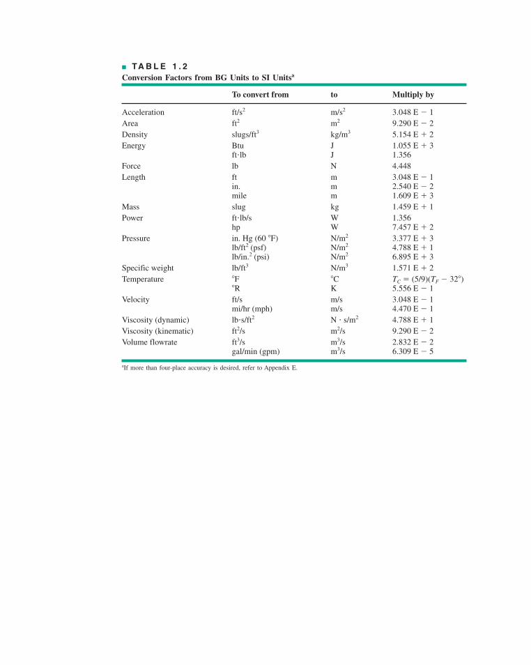
■ TA B L E 1 . 2

Conversion Factors from BG Units to SI Unitsa

To convert from to Multiply by

Acceleration ft/s2 m/s2 3.048 E � 1Area ft2 m2 9.290 E � 2Density slugs/ft3 kg/m3 5.154 E � 2Energy Btu J 1.055 E � 3

ft�lb J 1.356Force lb N 4.448Length ft m 3.048 E � 1

in. m 2.540 E � 2mile m 1.609 E � 3

Mass slug kg 1.459 E � 1Power ft�lb/s W 1.356

hp W 7.457 E � 2Pressure in. Hg (60 �F) N/m2 3.377 E � 3

lb/ft2 (psf) N/m2 4.788 E � 1lb/in.2 (psi) N/m2 6.895 E � 3

Specific weight lb/ft3 N/m3 1.571 E � 2Temperature �F �C TC � (5/9)(TF � 32�)

�R K 5.556 E � 1Velocity ft/s m/s 3.048 E � 1

mi/hr (mph) m/s 4.470 E � 1Viscosity (dynamic) lb�s/ft2 N � s/m2 4.788 E � 1Viscosity (kinematic) ft2/s m2/s 9.290 E � 2Volume flowrate ft3/s m3/s 2.832 E � 2

gal/min (gpm) m3/s 6.309 E � 5

aIf more than four-place accuracy is desired, refer to Appendix E.

ibc.qxd 9/21/10 10:01 PM Page 2

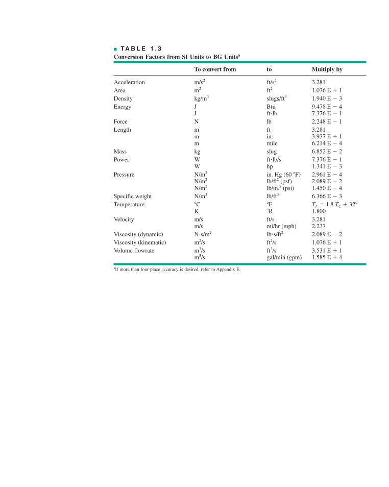
■ TA B L E 1 . 3

Conversion Factors from SI Units to BG Unitsa

To convert from to Multiply by

Acceleration m/s2 ft/s2 3.281Area m2 ft2 1.076 E � 1Density kg/m3 slugs/ft3 1.940 E � 3Energy J Btu 9.478 E � 4

J ft�lb 7.376 E � 1Force N lb 2.248 E � 1Length m ft 3.281

m in. 3.937 E � 1m mile 6.214 E � 4

Mass kg slug 6.852 E � 2Power W ft�lb/s 7.376 E � 1

W hp 1.341 E � 3Pressure N/m2 in. Hg (60 �F) 2.961 E � 4

N/m2 lb/ft2 (psf) 2.089 E � 2N/m2 lb/in.2 (psi) 1.450 E � 4

Specific weight N/m3 lb/ft3 6.366 E � 3Temperature �C �F TF � 1.8 TC � 32�

K �R 1.800Velocity m/s ft/s 3.281

m/s mi/hr (mph) 2.237Viscosity (dynamic) N�s/m2 lb�s/ft2 2.089 E � 2Viscosity (kinematic) m2/s ft2/s 1.076 E � 1Volume flowrate m3/s ft3/s 3.531 E � 1

m3/s gal/min (gpm) 1.585 E � 4

aIf more than four-place accuracy is desired, refer to Appendix E.

ibc.qxd 9/21/10 10:01 PM Page 3