A basis-set based Fortran program to solvethe Gross–Pitaevskii equation for dilute Bose gases

in harmonic and anharmonic traps ✩

Rakesh Prabhat Tiwari, Alok Shukla ∗

Physics Department, Indian Institute of Technology, Powai, Mumbai 400076, India

Abstract

Inhomogeneous boson systems, such as the dilute gases of integral spin atoms in low-temperature magnetic traps, are believed to be well de-scribed by the Gross–Pitaevskii equation (GPE). GPE is a nonlinear Schrödinger equation which describes the order parameter of such systemsat the mean field level. In the present work, we describe a Fortran 90 computer program developed by us, which solves the GPE using a basisset expansion technique. In this technique, the condensate wave function (order parameter) is expanded in terms of the solutions of the simple-harmonic oscillator (SHO) characterizing the atomic trap. Additionally, the same approach is also used to solve the problems in which the trapis weakly anharmonic, and the anharmonic potential can be expressed as a polynomial in the position operators x, y, and z. The resulting eigen-value problem is solved iteratively using either the self-consistent-field (SCF) approach, or the imaginary time steepest-descent (SD) approach.Iterations can be initiated using either the simple-harmonic-oscillator ground state solution, or the Thomas–Fermi (TF) solution. It is found thatfor condensates containing up to a few hundred atoms, both approaches lead to rapid convergence. However, in the strong interaction limit ofcondensates containing thousands of atoms, it is the SD approach coupled with the TF starting orbitals, which leads to quick convergence. Ourresults for harmonic traps are also compared with those published by other authors using different numerical approaches, and excellent agreementis obtained. GPE is also solved for a few anharmonic potentials, and the influence of anharmonicity on the condensate is discussed. Additionally,the notion of Shannon entropy for the condensate wave function is defined and studied as a function of the number of particles in the trap. It isdemonstrated numerically that the entropy increases with the particle number in a monotonic way.

Program summary

Title of program: bose.xCatalogue identifier: ADWZ_v1_0Program summary URL: http://cpc.cs.qub.ac.uk/summaries/ADWZ_v1_0Program obtainable from: CPC Program Library, Queen’s University of Belfast, N. IrelandDistribution format: tar.gzComputers: PC’s/Linux, Sun Ultra 10/Solaris, HP Alpha/Tru64, IBM/AIXProgramming language used: mostly Fortran 90Number of bytes in distributed program, including test data, etc.: 27 313Number of lines in distributed program, including test data, etc.: 28 015Card punching code: ASCIINature of physical problem: It is widely believed that the static properties of dilute Bose condensates, as obtained in atomic traps, can be describedto a fairly good accuracy by the time-independent Gross–Pitaevskii equation. This program presents an efficient approach of solving this equation.

967

Method of solution: The solutions of the Gross–Pitaevskii equation corresponding to the condensates in atomic traps are expanded as linearcombinations of simple-harmonic oscillator eigenfunctions. Thus, the Gross–Pitaevskii equation which is a second-order nonlinear differentialequation, is transformed into a matrix eigenvalue problem. Thereby, its solutions are obtained in a self-consistent manner, using methods ofcomputational linear algebra.Unusual features of the program: None

PACS: 02.70.-c; 02.70.Hm; 03.75.Hh; 03.75.Nt

Keywords: Bose–Einstein condensation; Gross–Pitaevskii equation; Anharmonic potential; Numerical solutions

1. Introduction

Ever since the discovery of Bose–Einstein condensation (BEC) in dilute atomic gases [1–3], theoretical studies of this and relatedphenomenon in such systems have grown exponentially [4]. For most of the theoretical studies of BEC in dilute gases, the startingpoint is the so-called Gross–Pitaevskii equation (GPE) [5,6], which is nothing but a mean-field Schrödinger equation for a systemof Bosons interacting through a two-body interaction described by δ-function. In all but the simplest of the cases, one needs tosolve the GPE using numerical methods. For problems involving the static properties of the condensate, the numerical solutions ofthe time-independent GPE are of interest. And, indeed, over last several years, a significant amount of work has been performedtowards developing novel approaches and algorithms meant for solving both time-dependent and independent GPE. Next we surveysome of the recent literature in the field, restricting ourselves to the methods aimed at solving the time-independent GPE, whichis the subject of the present paper. Edwards and Burnett developed a Runge–Kutta method based finite-difference approach forsolving the time-independent GPE for spherical condensates [7]. In another paper Edwards et al. used the basis set approach similarto the one presented here, to solve the GPE for anisotropic traps [8]. Dalfovo and Stringari developed a finite-difference basedmethod for solving the time-independent GPE both for the ground state, and the vortex states, in anisotropic traps [9]. Esry used afinite-element approach to solve for the both the time-independent GPE, as well as, the Hartree–Fock equations for bosons confinedin anisotropic traps [10]. Schneider and Feder used a discrete variable representation (DVR), coupled with a Gaussian quadratureintegration scheme, to obtain the ground and the excited states of GPE in three dimensions [11]. Adhikari used a finite-differencebased approach to solve the two-dimensional time-independent GPE [12,13]. Tosi and coworkers developed finite-difference, andimaginary-time, approach for solving the time-independent GPE [14]. Recently, Bao and Tang developed a novel scheme forobtaining the ground state of the GPE, by directly minimizing the corresponding energy functional [15]. Additionally, utilizingharmonic oscillator basis set, and Gauss–Hermite quadrature integration scheme, Dion and Cancès have proposed a scheme forsolving both the time-dependent and -independent GPE [16]. Earlier, we had also proposed an alternative scheme for dealing withcondensates with a large number of particles, and high number densities [17].

In this paper, we describe a Fortran program developed by us which solves time-independent GPE corresponding to bosonstrapped in Harmonic traps. Instead of using the more common finite-difference approach, we have chosen the basis-set basedapproach popular in quantum chemistry [18]. The basis set chosen for this case is the Cartesian simple-harmonic-oscillator (SHO)basis set. The choice of a Cartesian basis set allows us to treat the cases ranging from spherical condensates to completely anisotropiccondensates on an equal footing. Additionally, using the same approach our program allows to solve the time-independent GPE foranharmonic traps as well provided the anharmonic term can be expressed as a polynomial in various powers of coordinates x, y,and z. As far as the SCF solution of the GPE is concerned, our program allows both the matrix-diagonalization based scheme, aswell as the use of the imaginary-time steepest-descent method. Our program also allows the user to initiate the SCF process usingeither the SHO ground state orbital, or the Thomas–Fermi solution. We present the results of the calculations performed with ourcode for several interesting cases, and very good agreement is obtained with the existing results in the literature. Additionally, in thepresent paper we have defined the notion of Shannon entropy in the context of GPE, and presented various quantitative calculationsof the quantity.

Remainder of the paper is organized as follows. In the next section we discuss the basic theoretical aspects of our approach.Next, in Section 3, we briefly describe the most important subroutines that comprise our program. In Section 4 we provide detailedexplanation about installing and compiling our program. Additionally, in the same section we explain how to prepare an input file,and describe the contents of a typical output file. In Section 5 we discuss the convergence properties of the program with respect tothe: (a) size of the basis set, and (b) the method of solution. In Section 6, we discuss results of several example runs of our program,and compare them to those published earlier. Additionally, in the same section, we present our results on the Shannon entropy ofthe condensate, and on the solutions obtained in the presence of various anharmonic potentials. Finally, in Section 7, we present ourconclusions. In Appendix A we present the derivation of an analytical formula which we have used in our program to compute thetwo-particle interaction integrals.

968

2. Theory

For the present case, the time-independent Gross–Pitaevskii equation is

(1)

(− h2

2m∇2 + Vext(r) + 4πh2aN

m

∣∣ψ(r)∣∣2

)ψ(r) = μψ(r),

where ψ(r) is condensate wave function one is solving for, Vext(r) = 12m(ω2

xx2 + ω2

yy2 + ω2

zz2) + V anh(x, y, z) is the confining

potential for a general anisotropic trap (ωi ’s are the trap frequencies) with the anharmonic term V anh(x, y, z), a is the s-wavescattering length characterizing the two-body interactions among the atoms, N is the total number of bosons in the condensate, andμ is the chemical potential. We are assuming that the condensate wave function is normalized to unity. Before attempting numericalsolutions of Eq. (1), we cast it in a dimensionless form by making the transformations [15]

(2a)r = rax

,

(2b)ψ(r) = a3/2x ψ(r),

where ax = √h/mωx is the “harmonic oscillator length” in the x-direction. This finally leads to the dimensionless form of the GPE

(3)

(−1

2∇2 + Vext(r) + κ

∣∣ψ(r)∣∣2

)ψ(r) = μψ(r),

where μ is the chemical potential in the units of hωx , κ = 4πNa/ax is a dimensionless constant determining the strength of thetwo-body interactions in the gas, and for the harmonic oscillator potential Vext(r) = 1

2 (x2 + γ 2y y2 + γ 2

z z2) + V anh(x, y, z), withγy = ωy/ωx and γz = ωz/ωx being the two aspect ratios. We will now discuss the basis-set expansion technique, used for solvingthe GPE [8,11,16]. In this approach, one expands ψ(r) as a linear combination of basis functions of three-dimensional anisotropicsimple harmonic oscillator

(4)ψ(r) =Nbasis∑i=1

CiΦi(x, y, z) =Nbasis∑i=1

Ciφnxi(x)φnyi

(y)φnzi(z),

where φnxi(x), φnyi

(y), and φnzi(z), are the harmonic oscillator basis functions corresponding to x-, y-, and z-directions, respec-

tively, Ci is the expansion coefficient, and Nbasis is the total number of basis functions used. In dimensionless units, e.g., φnzi(z)

can be written as

(5)φnzi(z) =

(γz

π

)1/4 1√2nzi nzi !

Hnzi(z

√γz ) exp

(−γzz

2

2

),

where Hnzi(z

√γz ) is a Hermite polynomial of order nzi in the variable z

√γz. The form of the basis functions φnxi

(x) and φnyi(y)

can be easily deduced from Eq. (5). Upon substituting Eq. (4) in Eq. (3), then multiplying both sides with another basis functionΦj(x, y, z) and integrating with respect to x, y, and z the time-independent GPE is converted into an eigenvalue problem [18]

(6)F C = μC,

where C represents the column vector containing expansion coefficients Ci ’s as its components, and the elements of the matrix F

are given by

(7)Fi,j = Eiδi,j + V anhi,j + g

Nbasis∑k,l=1

Ji,j,k,lCkCl.

Above

(8)Ei =(

nxi + 1

2

)+

(nyi + 1

2

)γy +

(nzi + 1

2

)γz,

V anhi,j are the matrix elements of the anharmonic term in the confining potential, and Ji,j,k,l is the boson–boson repulsion matrix.

For anharmonic potentials which can be written as polynomials in x, y, and z, V anhi,j can be computed quite easily, while Ji,j,k,l can

be written as a product of three submatrices corresponding to the three Cartesian directions [8]

(9)Ji,j,k,l = Jnxinxj nxknxlJnyinyj nyknyl

Jnzinzj nzknzl .

969

It can be shown that the elements of submatrices J can be written in the form

(10)Jninj nknl=

∞∫−∞

dξ φnl(ξ)φnk

(ξ)φnj(ξ)φni

(ξ),

where φni(ξ)’s are the harmonic oscillator basis functions of Eq. (5). Integrals involved in Eq. (10) can be computed numerically

using the methods of Gaussian quadrature [11,16], or analytically [8] using the formulas derived by Busbridge [19]. In the presentwork, we have used this analytical expression—derived in the appendix for the sake of completeness—to compute the values ofJ integrals.

The eigenvalue problem of Eq. (6) has to be solved self-consistently. In our program, for fixed values of N , this equation can besolved for μ and C using either the iterative diagonalization common in quantum chemistry [18], or the steepest-descent approachas used by Dalfovo and Stringari [9]. In both the approaches, the onset of self-consistency is signaled once the energy per particleof the condensate converges to within a user-specified threshold. This approach is different from that of Edwards et al. [8] wherethey solved Eq. (6) for N , using fixed values of μ.

For the case of relatively small particle number, i.e. for a weakly interacting system, it does not matter what is the nature ofstarting guess for the condensate orbital for initiating the SCF cycles. However, for the case of systems with large particle number,the convergence obtained is very slow (if at all), in case the starting condensate is taken to be the ground state of the harmonic trap.In such cases, the convergence is easily obtained if the starting guess for the condensate is taken to be of the Thomas–Fermi form,obtained by setting the kinetic energy term in Eq. (3) to zero

(11)∣∣ψTF(r)

∣∣2 = μTF − 12 (x2 + γ 2

y y2 + γ 2z z2)

g,

where the Thomas–Fermi chemical potential μTF is given by

(12)μTF = hωx

2

(15Naγyγz

ax

)2/5

.

In our program, we can also compute the Shannon entropy associated with the condensate. The Shannon mixing entropy, for ageneral ensemble, is defined as [20]

(13)S = −∑

i

Pi logPi,

where Pi is the probability for a system to be in the ith state. Of course, in the present case, we do not have a thermodynamicsystem in which the mixing of various states will take place due to thermal fluctuations driven by its finite temperature. Thus, thequestion is as to how to define Shannon entropy for the present system, which is essentially being treated as a zero-temperaturequantum mechanical system. For the purpose we adopt an information theoretic point-of-view, and define the probability Pi as

(14)Pi = |Ci |2,where Ci are the expansion coefficients of various SHO eigenstates in the expression for the condensate wave function of Eq. (4).In this picture, ground state of the condensate is seen as a statistical mixture of the various eigenstates of SHO, with the mixingprobability Pi . It is important to realize that the reason behind this mixing of states is the inter-particle interaction in the condensate,because, in its absence, the condensate will be in the ground state of the SHO (Ci = δ1,i ) leading to S = 0. Thus, in a sense, entropydefined as per Eqs. (13) and (14) is a measure of inter-particle interactions in the system. Because, stronger the inter-particleinteractions, the condensate will be a mixture of larger number of states, leading to a larger entropy. From an information-theoreticpoint-of-view larger entropy implies loss of information about the system, because, in such a case, the system is a mixture of alarger number of states. The point to be remembered, however, is that this information loss is being driven by the inter-particleinteractions in the system while the corresponding information loss in a thermodynamic system is driven by its finite temperature,and the thermal fluctuations caused by it. In various contexts, other authors have also computed and discussed the informationentropy associated with interacting quantum systems [21–23].

3. Description of the program

In this section we briefly describe the main program and various subroutines which constitute the entire module. All the subrou-tines, except for the diagonalization subroutine taken from EISPACK [24], have been written in the Fortran 90 language.

970

3.1. Main program OSCL

The main program is called OSCL, and its task is to read all the input information, and, among other things, fix the dimensionsof various arrays. All the arrays needed in the program are dynamically allocated either in the main program, or in some of thesubroutines. By utilizing the dynamic array allocation facility of the Fortran 90 language, we have made the program independentof the size of the calculations undertaken. Because of this, the program needs to be compiled only once, and will run until thepoint the memory available on the computer is exhausted. Besides reading all the necessary input, program OSCL calls varioussubroutines in which different tasks associated with the calculation are performed.

3.2. XMAT_0

XMAT_0 is a small subroutine whose job is to compute the matrix elements of the position operator in harmonic oscillator units,with respect to the basis set of a one-dimensional SHO. This routine is called from the main program OSCL, and results are storedin a two-dimensional array called xmatrx.

3.3. Basis set generation

The calculations are performed using a basis set of a three-dimensional SHO consistent with the symmetry of the system. Thebasis set to be used is generated by calling one of the following three routines: (a) for a spherical condensate (complete isotropy)routine BASGEN3D_ISO is used, (b) for a cylindrical condensate routine BASGEN3D_CYL is called, and (c) the basis set fora completely anisotropic condensate is generated using the routine BASGEN3D_ANISO. In all the cases the basis functions arearranged in the ascending order of their harmonic oscillator energies and, if needed, a heap sort routine called HPSORT is used toachieve that. All these subroutines have the option of imposing parity symmetry on the basis set if the potential has that symmetry.This leads to a substantial reduction in the size of the basis set in most cases.

3.4. HAM0_3D

This subroutine is called from the main program OSCL and its purpose is to generate the matrix elements of the noninteracting(one-particle) part of the condensate Hamiltonian. If the condensate is confined in a perfectly harmonic trap, one-particle part ofthe Hamiltonian is trivial. However, for the case where the trap potential is anharmonic, the potential matrix elements are generatedfrom the position operator matrix elements xmatrx(i, j) mentioned above.

3.5. BEC_DRV

Subroutine BEC_DRV is called from the main program OSCL, and as its name suggests, it is the driver routine for performingcalculations of the condensate using the time-independent GPE. Apart from allocating a few arrays, the main task of this routine isto call either: (a) routine BOSE_SCF meant for solving for the condensate wave function using the iterative-diagonalization-basedSCF approach, or (b) routine BOSE_STEEP used for solving for the condensate wave function using the steepest-descent approachof Dalfovo and Stringari [9].

3.6. BOSE_SCF

This subroutine solves the time-independent GPE in a self-consistent manner using an iterative diagonalization approach. Itsmain tasks are as follows:

(1) Allocate various arrays needed for the SCF calculations.(2) Setup the starting orbitals. For this the options are: (i) diagonalize the one-particle part of the Hamiltonian, (ii) use the Thomas–

Fermi orbitals, or (iii) use the orbitals obtained in a previous run.(3) Perform the SCF calculations. For the purpose, the two-particle integrals Ji,j,k,l (cf. Eq. (9) are calculated on the fly during

each iteration using the formulas derived in Appendix A. In other words the storage of these matrix elements is completelyavoided, thereby saving substantial amount of memory and disk space. This approach is akin to the “direct SCF” approachutilized in quantum chemistry. Permutation symmetries of indices i, j, k, and l are utilized to reduce the number of integralsevaluated. Moreover, the evaluation of an integral is undertaken only if it is found to be nonzero as per the symmetry selectionrules. The integrals in question are evaluated in a subroutine called JMNPQ_CAL. The F matrix constructed in each iteration isdiagonalized through a Householder diagonalization routine called HOUSEH, which is from the EISPACK package of routines[24], and is written in Fortran 77.

(4) The chemical potential and the condensate wave function obtained after every iteration are written in various data files so thatthe progress of the calculation can be monitored.

971

3.7. BOSE_STEEP

Alternatively, the condensate wave function and the chemical potential can be obtained using the subroutine BOSE_STEEPwhich, instead of the iterative diagonalization approach, utilizes the steepest-descent approach to achieve convergence, startingfrom a given starting orbital. In this approach, as outlined by Dalfovo and Stringari [9], the starting orbitals are evolved towardsthe true orbitals in small imaginary time steps by repeated application of the Hamiltonian, i.e. the F operator. Here, the maincomputational step is the multiplication of a column vector by a matrix, which in the present version of the program is achievedby a call to the Fortran 90 intrinsic function MATMUL. However, one could certainly try to improve upon this by developinga subroutine which can utilize the symmetric nature of the Fock matrix. Apart from this, rest of the actions performed in thissubroutine are identical to those of BOSE_SCF.

3.8. THOMAS_FERMI

This subroutine is invoked either from the subroutine BOSE_SCF or from BOSE_STEEP in case the SCF calculations are to beinitiated by assuming Thomas–Fermi form of the starting orbitals. Upon invocation, this subroutine directly constructs the operatorF corresponding to the Thomas–Fermi orbitals. In this case, the r-space integration is performed using a trapezoidal-rule-basedscheme on a three-dimensional Cartesian grid.

3.9. ENTROPY

This subroutine is called if the entropy of the condensate needs to be computed with respect to the Harmonic oscillator basisfunctions, as per Eqs. (13) and (14). It is a very small subroutine with a straightforward implementation.

3.10. COND_PLOT

This subroutine computes the numerical values of the condensate wave function for a user-specified set of points in space. Thenumerical values of the Hermite polynomials needed for the purpose are computed using the subroutine HERMITE, describedbelow.

3.11. HERMITE

This subroutine computes the values of the Hermite polynomial Hn(x) for a set of user specified values of x, and order n. Fastcomputation of polynomials is achieved by using initializations H0(x) = 1, H1(x) = 2x, and the recursion relation Hn+1(x) =2xHn(x) − 2nHn−1(x).

4. Installation

All the files needed to install and run the program are kept in the gzipped, tarred archive bose.tar.gz. It consists of: (a) Allthe Fortran files containing the main program (file oscl.f90), and various subroutines, called by the main program, (b) fourversions of Makefiles which can be used for compiling the code on various Linux/Unix systems, and (c) several sample input andoutput files in a subdirectory called Examples. The program was developed on Pentium 4 based machine running Redhat Fedoracore 1 operating system using noncommercial version of the Intel Fortran compiler version 8.1. However, it has also been verifiedthat it runs on Sun Solaris Sparc based systems, Compaq alpha (now HP alpha) based systems running True Unix, and IBM PowerPC systems running AIX. For these systems, the Fortran 90 compilers supplied with those operating systems were used. In order toinstall and compile the program, following steps need to be followed:

(1) Uncompress the program files in a directory of user’s choice using the command gunzip bose.tar.gz followed by tar-xvf bose.tar.

(2) Verify that the four makefiles Makefile_linux, Makefile_solaris, Makefile_alpha, and Makefile_aix arepresent. Copy the suitable version of the make file to the file Makefile. For example, if the system is a Sun Solaris Sparcsystem, issue the command cp Makefile_solaris Makefile.

(3) Now issue the command make which will initiate the compilation. If everything is successful, upon completion bin directoryof your account will have the program execution file bose.x. If your account does not have a directory named bin, you willhave to either create this directory, or modify the Makefile to ensure that the file bose.x is created in the directory of yourchoice.

(4) If the bin directory is in your path, try running the program using one of the sample input files located in the subdirec-tory Examples. For example, by issuing the command bose.x < bec_iso.dat > x.out one can run the program

972

for an isotropic trap and the output will be written in a file called x.out. This should be compared with the supplied filebec_iso.out to make sure that results obtained agree with those of the example run.

Additionally, a file called README is also provided which lists and briefly explains all the files included in the package. Althoughwe have not investigated the installation of the program on operating systems other than Linux/Unix, we do not anticipate anyproblems with such operating systems.

4.1. Input files

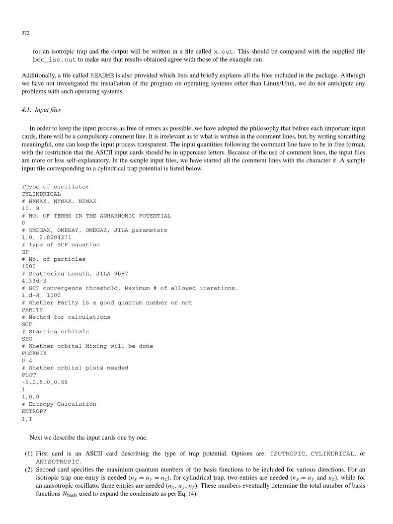
In order to keep the input process as free of errors as possible, we have adopted the philosophy that before each important inputcards, there will be a compulsory comment line. It is irrelevant as to what is written in the comment lines, but, by writing somethingmeaningful, one can keep the input process transparent. The input quantities following the comment line have to be in free format,with the restriction that the ASCII input cards should be in uppercase letters. Because of the use of comment lines, the input filesare more or less self-explanatory. In the sample input files, we have started all the comment lines with the character #. A sampleinput file corresponding to a cylindrical trap potential is listed below

#Type of oscillatorCYLINDRICAL# NXMAX, NYMAX, NZMAX10, 8# NO. OF TERMS IN THE ANHARMONIC POTENTIAL0# OMEGAX, OMEGAY, OMEGAZ, JILA parameters1.0, 2.8284271# Type of SCF equationGP# No. of particles1000# Scattering Length, JILA Rb874.33d-3# SCF convergence threshold, Maximum # of allowed iterations.1.d-8, 1000# Whether Parity is a good quantum number or notPARITY# Method for calculationsSCF# Starting orbitalsSHO# Whether orbital Mixing will be doneFOCKMIX0.4# Whether orbital plots neededPLOT-5.0,5.0,0.0511,0,0# Entropy CalculationENTROPY

1,1

Next we describe the input cards one by one.

(1) First card is an ASCII card describing the type of trap potential. Options are: ISOTROPIC, CYLINDRICAL, orANISOTROPIC.

(2) Second card specifies the maximum quantum numbers of the basis functions to be included for various directions. For anisotropic trap one entry is needed (nx = ny = nz), for cylindrical trap, two entries are needed (nx = ny and nz), while foran anisotropic oscillator three entries are needed (nx , ny , nz). These numbers eventually determine the total number of basisfunctions Nbasis used to expand the condensate as per Eq. (4).

973

(3) Third card deals with the anharmonic terms in the trap potential. Any potential of the form∑Nanh

i=1 Cixmx

i ymyi zmz

i can be addedto the Harmonic trap potential. The first entry here is Nanh after which Nanh entries consisting of {Ci,m

xi ,m

yi ,m

zi } are given.

In the example input, no anharmonicity was considered, thus Nanh has been set to zero.(4) Fourth card deals with the trap frequencies with the convention that ωx = 1, and rest of the frequencies measured in the units

of ωx . The example input corresponds to the trap frequencies of the JILA experiment with ωx = ωy = 1, ωz = 2.284271.(5) Fifth card specifies which mean-field equation is to be solved. Options are GP for the Gross–Pitaevskii equation, and HF for

the Hartree–Fock equation.(6) Sixth card reads the total number of bosons in the trap.(7) Seventh card is the value of the s-wave scattering length in the Harmonic oscillator units.(8) Eighth card inputs the convergence threshold, followed by the maximum number of iterations allowed to achieve convergence.(9) Ninth card specifies whether parity should be treated as a good quantum number or not. Options are PARITY and NOPARITY.

If the trap potential is invariant under the parity operation, use of this card leads to a tremendous reduction in the size of thebasis set needed to solve for the condensate wave function.

(10) Tenth card specifies as to which method is to be used for solving the mean-field equations. Options are SCF correspondingto the iterative diagonalization method, and STEEPEST-DESCENT corresponding to the use steepest-descent method ofDalfovo and Stringari [9]. In case one opts for the steepest-descent approach, the size of the time step to be used in thecalculations also needs to be specified.

(11) Eleventh card specifies as to what sort of starting guess for the condensate should be used to start the solution process. Validoptions are SHO corresponding to the simple-harmonic oscillator ground state and THOMAS-FERMI corresponding to theThomas–Fermi form of the condensate.

(12) It has been found that in several difficult cases, convergence can be achieved if one utilizes the techniques of Fock matrix mix-ing or condensate orbital mixing [9,10]. Valid options are (a) FOCKMIX for Fock matrix mixing, (b) ORBMIX for condensatemixing, (c) any other ASCII entry such as NOMIX for neither of these options. In case options (a) or (b) are chosen, one needsto specify the parameter xmix quantifying the mixing according to the formula

R(i) = xmixR(i) + (1 − xmix)R(i−1),

where R(i) is the quantity under consideration in the ith iteration. Thus, if Fock matrix mixing has been opted, xmix specifiesthe fraction of the new Fock matrix in the total Fock matrix in the ith iteration.

(13) This is the penultimate card which decides whether the user wants the numerical values of condensate wave function alonguser specified set of data points, such that the condensate could be plotted as a function of spatial coordinates. Keyword PLOTmeans that the answer is in affirmative while any other option such as NOPLOT will disable the numerical computation ofthe condensate. If the keyword PLOT has been supplied as in the example input, further data rmin, rmax, dr is specified nextwhich determines the starting position, ending position, and the step size for generating the points on which the condensateis to be computed. After these values, we need to specify variable ndir which is the number of directions along which thecondensate needs to be computed. Finally, ndir Cartesian directions have to be specified. The example input file instructs theprogram to compute the value of the condensate along the x axis, for −5.0 � x � 5.0, in the steps of 0.05.

(14) Final card specifies whether one wants to compute the mixing entropy. Valid options are ENTROPY and any other entry suchas NOENTROPY. If one opts for entropy calculation, one can do so for a whole range of eigenfunctions specified by theirlower bound and the upper bound. Entry 1,1 specifies that entropy of only the ground state needs to be computed.

4.2. Output file

Apart from the usual information related to various system parameters, the most important information that an output file con-tains is the approach (or lack thereof) to convergence of the calculations as far as the chemical potential is concerned. Besidesthat, any other computed quantity such as the entropy is also listed in the output file. The important portions of the output file,corresponding to the input file discussed in the previous section, are reproduced below. The complete sample output file is calledbec_cyl_jila.out, and is included in the tar archive.

SCF iterations beginStarting chemical potential= 2.4142135Iteration # Chem. Pot. Energy/particle Energy-Converg.

1 3.876643 5.3193762 5.31937622 4.271632 4.0689872 −1.25038903 4.517259 3.8580062 −0.21098104 4.619476 3.8439807 −0.01402555 4.689213 3.8418453 −0.0021354

974

6 4.720534 3.8413295 −0.00051597 4.743576 3.8411720 −0.00015758 4.753914 3.8411212 −0.00005089 4.761791 3.8411040 −0.000017210 4.765292 3.8410982 −0.000005911 4.768022 3.8410961 −0.000002012 4.769223 3.8410954 −0.000000713 4.770177 3.8410951 −0.000000314 4.770592 3.8410950 −0.000000115 4.770927 3.8410950 0.000000016 4.771071 3.8410950 0.000000017 4.771189 3.8410950 0.0000000

Convergence achieved on the BEC ground stateEigenstate # Information Entropy

1 0.7477159

The contents of the output file listed above are self-explanatory. It basically shows that after seventeen iterations, the total energyper particle of the condensate converges to the value 3.841095, leading to the chemical potential value of 4.771. Additionally, theentropy of the condensate is computed to be 0.744771.

In addition to the above mentioned main output file, there is another output file created in the ASCII format which contains thecondensate orbital obtained at the end of each iteration. This file is written in the logical unit 9, and is named orbitals.dat.When a new run is started, the program always looks for this file and tries to use the condensate solution present there to startthe iterations. In other words, condensate solution present in orbitals.dat is used to restart an old aborted run. If someincompatibility is found between the condensate solution, and the present run, the solution in the orbitals.dat is ignored anda new run is initiated. Thus, if one wants to start a completely new run, any old orbitals.dat file must first be deleted.

5. Convergence issues

In this section we compare the convergence of our results with respect to the size of the basis set used. We also compare theconvergence properties of different iterative approaches aimed at obtaining the condensate solutions.

5.1. Convergence with respect to the basis set

Before treating the results obtained as the true results, one must be sure as to convergence properties with respect to the sizeof the basis set. This aspect of the calculations is explored in the present section by means of two examples corresponding tocondensates in spherical and cylindrical traps, respectively, with fifteen hundred (N = 1500) bosons each.

First we discuss the case of the condensate in an isotropic trap, results for which are presented in Table 1. The value of thescattering length used in the calculations is listed in the caption of the table. For this case, only one value specifying the largestquantum number nmax for the basis functions, needs to be specified. It is obvious from the table that the results which haveconverged to three decimal places both in the chemical potential and the entropy require nmax = 8, leading to the total number ofbasis functions Nbasis = 35. This means that the size of the Fock matrix diagonalized during the iterative diagonalization is 35 × 35,which is computationally very inexpensive. It is also obvious from the table that in order to get four decimal place convergence, weonly need to use nmax = 10 corresponding to a 56 × 56 Fock matrix, whose diagonalization can also be carried out quite fast.

Table 1Convergence on the chemical potential and the mixing entropy of the condensate in an isotropic trap with scattering length a = 2.4964249 × 10−3ax and numberof bosons N = 1500, with respect to the basis set size. nmax is the maximum value of the quantum number of the SHO basis function in a given direction, Nbasis isthe total number of basis functions corresponding to a given value of nmax, and Niter represents the total number of SCF iterations needed to achieve convergenceon the condensate energy per particle. In all the calculations iterative diagonalization method, along with Fock matrix mixing with xmax = 0.6, was used. The SCFconvergence threshold was 1.0 × 10−7

nmax Nbasis Niter Chemical potential Entropy

2 4 19 2.939116 0.50836694 10 11 2.915046 0.53870746 20 14 2.911181 0.53969758 35 14 2.911278 0.539088

10 56 15 2.911375 0.539242312 84 15 2.911346 0.539277014 120 15 2.911337 0.539282216 165 13 2.911337 0.5392797

975

Table 2Convergence on the chemical potential and the mixing entropy of the condensate in a cylindrical trap with trap parameters corresponding to the JILA experiment[25], and the number of bosons N = 1500, with respect to the basis set size. nxmax is the maximum value of the quantum number of the SHO basis function in x-and y-direction, nzmax is the same number corresponding to the z-direction. Rest of the quantities have the same meaning as explained in the caption of Table 1. Inall the calculations iterative diagonalization, along with Fock matrix mixing with xmax = 0.3, was used. The SCF convergence threshold was 1.0 × 10−8

nxmax nzmax Nbasis Niter Chemical potential Entropy

4 0 6 39 5.786323 0.93871244 2 12 19 5.421930 0.93832274 4 18 27 5.423981 0.93800136 0 10 31 5.737602 0.97707276 2 20 19 5.405221 0.95491946 4 30 20 5.405440 0.95454416 6 40 20 5.404970 0.95459208 0 15 21 5.737074 0.97524918 2 30 20 5.404605 0.95465308 4 45 21 5.404691 0.95427738 6 60 21 5.404218 0.95432918 8 75 21 5.404147 0.9543239

10 0 21 21 5.736935 0.975536510 2 42 20 5.404741 0.954481410 4 63 20 5.404540 0.954104410 6 84 20 5.404066 0.954156110 8 105 18 5.403994 0.954150810 10 126 18 5.403991 0.954147712 0 28 21 5.736763 0.975653912 2 56 20 5.404636 0.954578912 4 84 20 5.404436 0.954200412 6 112 20 5.403962 0.954251712 8 140 20 5.403891 0.954246312 10 168 20 5.403888 0.954243212 12 196 18 5.403888 0.9542428

Similar results for the condensate in a cylindrical trap corresponding to the JILA parameters [25] are presented in Table 2.Because of the anisotropy of the trap, the convergence is to be judged with respect to two parameters nxmax deciding the highestquantum number of the basis functions for x- and y-directions, and nzmax the corresponding number for the z-direction. We willfirst try to understand the convergence properties using a few heuristic arguments. In the JILA experiment [25] the trap frequencyin the z-direction ωz was more than twice the value of the trap frequencies in the x- and y-directions, ωx and ωy . Therefore, dueto inter-particle repulsion, the condensate will be much more delocalized along the x/y-directions, as compared to the z-direction.This means that, in order to achieve convergence, one would expect to use higher-energy basis functions in the x/y-directions, ascompared to the z-direction. In other words, at convergence nxmax > nzmax. And when we examine Table 2, we find that this isindeed the case. We notice that the three-decimal place convergence in both the chemical potential, and the entropy, is obtained fornxmax = 8 and nzmax = 6, although the data presented in the table covers a much larger range of parameters. Thus, we concludethat reasonably accurate values of various physical quantities can be obtained with basis sets of modest sizes, both for the isotropicas well as for the cylindrical condensates.

5.2. Comparison of different numerical approaches

As mentioned earlier, our program can solve the GP equation using two numerical approaches: (a) Iterative diagonalization (ID)of the Fock matrix, and (b) steepest-descent (SD) method of Dalfovo et al. [9]. In the previous sections, all the presented resultswere obtained by the ID method. In the present section, we would like to present results based upon the steepest-descent approach,and compare them to those obtained using the iterative diagonalization method. We present our results for the cylindrical trapcorresponding to the JILA parameters [25], with an increasing number of particles in Table 3. Obviously, the numerical solutionof the GP equation becomes increasingly difficult as the number of particles in the condensate grows, because of the increasedcontribution of the inter-particle repulsion. Therefore, it is very important to know as to how various numerical approaches performas N is gradually increased.

As the results presented in the table suggest that for smaller values of N , neither of the two approaches have any problemsachieving convergence, and the results obtained were found to be in agreement with each other to three decimal places for the basisset used. We found that in most of the cases, the ID approach worked only when Fock-matrix mixing used. Although, we managedto achieve convergence for the cases depicted in Table 3 with the ID method; however, as the number of bosons in the condensategrows further, the convergence becomes slow and difficult to achieve by this method, a fact also emphasized by Schneider andFeder [11]. On the other hand, the SD approach did not have any convergence problems for the cases we investigated. As depicted

976

Table 3Comparison of the chemical potentials (μ) obtained using the iterative diagonalization (ID) technique, and the steepest-descent (SD) technique [9], for the conden-sates in a cylindrical trap with trap parameters corresponding to the JILA experiment [25], and a given number of bosons (N ). Quantities Niter, nxmax, and nzmaxhave the same meaning as in the caption of Table 2, and μ is expressed in the units of hωx . In the ID based calculations for N � 2000, SHO ground state solutionwas used to start the iterations, while for larger values of N the iterations were started using the Thomas–Fermi approximation. In all the cases corresponding to theID method, Fock matrix mixing was used, with 0.05 � xmax � 0.3. In the SD based calculations, the iterations were started using the Thomas–Fermi approximation,with the size of the time step being 0.02 units

N nxmax nzmax Niter (ID) Niter (SD) μ (ID) μ (SD)

500 8 6 16 62 3.938611 3.9388651000 8 6 14 88 4.770707 4.7720551500 8 6 21 95 5.404218 5.4054912000 12 8 23 104 5.931870 5.932878

10000 14 8 86 99 10.505267 10.50512415000 14 8 105 129 12.239700 12.23946520000 14 8 104 109 13.665923 13.665686

in Table 3, the SD approach led to convergence both with the SHO starting orbital, as well as the Thomas–Fermi starting orbital.However, for larger values of N , the use of Thomas–Fermi solution as the starting guess for the condensate, will lead to much fasterconvergence with this approach. Thus, we conclude that: (a) For smaller values of N , both the ID as well as the SD methods willlead to convergence, and (b) for really large values of N , the convergence is guaranteed only with the SD method. In the SD methodthe main computational operation is the multiplication of a vector by a matrix, which will be significantly faster as compared tothe matrix diagonalization procedure needed by the ID method for calculations involving large basis sets. Thus, for calculationsinvolving large basis sets, SD method will be faster as compared to the ID method. Therefore, all things considered, we believe thatthe SD method is the more robust of the two possible approaches.

6. Example runs

In this section we report the results of our calculations for a variety of trap parameters, and compare our results with thosepublished by other authors. We also study the behavior of the Shannon entropy of the condensate with respect to the number ofparticles it contains. Additionally, we also present our results for the cases of anharmonic traps.

6.1. Comparison with other works

In this section we present the results of several calculations performed on both isotropic and the cylindrical traps, and comparethem to the results obtained by other authors. Several authors have performed such calculations, however, for the sake of brevity,we restrict our comparisons mainly to the works of Bao and Tang [15] for the spherical condensate, and to the results of Dalfovoand Stringari [9] for the cylindrical condensate.

Recently, using finite-element based approach, Bao and Tang [15] performed calculations for condensates on a variety of har-monic traps, and presented results as a function of the interaction parameter κ = 4πaN/ax . In Table 4 our results for the chemicalpotentials of condensates in isotropic traps corresponding to increasing values of κ are compared with those reported by Bao andTang [15]. The agreement between the results obtained by two approaches is exact to the decimal places reported by Bao andTang [15]. Note that the aforesaid agreement was obtained for rather modest basis set sizes, and calculations were completed on apersonal computer in a matter of minutes.

Next we discuss the results obtained for a cylindrical trap corresponding to JILA parameters [25] for an increasing number ofbosons. Our results are presented in Table 5, where they are also compared to the results of Dalfovo and Stringari obtained usinga finite-difference based approach [9]. The agreement between our results and those of Dalfovo and Stringari is virtually exact forall their reported calculations [9]. Again, the noteworthy point is that this level of agreement was obtained with the use of modestsized basis sets, and the computer time running into a few minutes.

Thus, the excellent agreement between our results, and those obtained by other authors using different approaches, gives usconfidence about the essential correctness of our methodology. Now the question arises, will this numerical method work for valuesof the interaction parameter κ which are much larger than the ones considered here. The encouraging aspect of the approach is thatfor none of the larger values of κ which we considered did we experience a numerical breakdown of the approach. It is just thatfor larger values of κ , the total number of basis functions needed to achieve convergence on the chemical potential will be largeras compared to the smaller κ cases. This, of course, will also lead to an increase in the CPU time needed to perform convergedcalculations. For example, for the case of the spherical trap considered in Table 4, when we doubled κ to the value 6274, we neededto use basis functions corresponding to nmax = 20 with Nbasis = 286 to achieve two-decimal places convergence in the chemicalpotential. For κ = 9411, to achieve similar convergence, these numbers increased to nmax = 24 and Nbasis = 455. Finally, whenκ was increased to 15685, the corresponding numbers were nmax = 28 and Nbasis = 680, with the CPU time running into several

977

Table 4Comparison of the chemical potentials (in the units of hω) obtained from our program, and those reported by Bao and Tang [15], for an isotropic trap, with increasingvalues of interaction parameter κ . The negative value of κ implies attractive inter-particle interactions. For the value of scattering length stated in Table 1, κ = 3137.1corresponds to N = 1 × 105 bosons. Symbols nmax and Niter have the same meaning as in the previous tables. For the last two calculations, SD method with a timestep of 0.02 units, and Thomas–Fermi initial guess were employed. Our chemical potentials have been truncated to as many decimal places as reported by Bao andTang [15]

κ nmax Nbasis μ (This work) μ (Ref. [15])

−3.1371 14 120 1.2652 1.26523.1371 14 120 1.6774 1.6774

12.5484 14 120 2.0650 2.065031.371 14 120 2.5861 2.5861

125.484 14 120 4.0141 4.0141627.42 16 165 7.2485 7.2484

3137.1 16 165 13.553 13.553

Table 5Comparison of the chemical potentials (in the units of hωx ) obtained from our program, and those reported by Dalfovo and Stringari [9], for a cylindrical trapcorresponding to the JILA parameters [25], with increasing number N of bosons. Symbols nxmax, nzmax, and Niter have the same meaning as in the previoustables. Calculations for N � 10000 were performed by the SD method using Thomas–Fermi starting orbitals, a time-step of 0.02 units, and a convergence thresholdof 1.0 × 10−7. We have truncated our chemical potentials to as many decimal places as reported by Dalfovo and Stringari [9]

N nxmax nzmax Nbasis μ (This work) μ (Ref. [9])

100 8 6 60 2.88 2.88200 8 6 60 3.21 3.21500 8 6 60 3.94 3.94

1000 8 6 60 4.77 4.772000 8 6 60 5.93 5.935000 10 8 105 8.14 8.14

10000 10 8 105 10.5 10.515000 14 8 180 12.2 12.220000 14 8 180 13.7 13.7

hours. For the cylindrical trap (cf. Table 5), for N = 20000 bosons (κ = 1088.2) the convergence was achieved in a matter ofminutes with nxmax = 14, nzmax = 8 and Nbasis = 180. When the number of bosons in the trap was doubled such that κ = 2176.4,similar level of convergence on the chemical potential was obtained with nxmax = 18, nzmax = 8 and Nbasis = 275. Even with muchlarger values of κ (> 30000) both for the spherical, and the cylindrical traps, we did not encounter any convergence difficulties whenthe calculations were performed with the modest sized basis sets mentioned earlier. But it was quite obvious that, to obtain highlyaccurate values of chemical potentials for such cases, one will have to use basis sets running into thousands which will make thecalculations quite time consuming.

At this point, we would also like to compare our approach to that of Schneider and Feder [11], who used a DVR based techniqueto obtain accurate solutions of the time-independent GPE. In the DVR approach the basis functions are the so-called “coordinateeigenfunctions”, which, in turn, are assumed to be linear-combinations of other functions such as the SHO eigenstates, or theLagrange interpolating functions [11]. Thus in the DVR approach of Schneider and Feder [11], the SHO eigenstates are used asintermediate basis functions, and not as primary basis functions as is done in our approach. Using this approach, coupled with the“direct-inversion in the iterative space” (DIIS) method, Feder and Schneider managed to obtain accurate solutions for anisotropiccondensates for quite large values of the interaction parameter κ [11]. However, the price to be paid for this accuracy was the useof a very large basis set consisting of several thousands of basis functions [11] even for rather small values of κ .

Finally, we present the plots of the condensates in a spherical trap, for increasing values of N , in Fig. 1. As expected, the calcula-tions predict a depletion of central condensate density, and corresponding delocalization of the condensate, with increasing N . Theresults presented are in excellent agreement with similar results presented by various other authors [9,15]. Moreover, if we comparethe value of the condensate at the center of the trap (|ψ(0,0,0)|) for the isotropic trap with the published results of Bao and Tang[15], we again obtain excellent agreement for all values of N .

6.2. Anharmonic potentials

Recently, several studies have appeared in the literature studying the influence of trap anharmonicities on the condensates, inlight of rotating condensates, and the resultant vortex structure [26]. However, we approach the influence of trap anharmonicityfrom a different perspective, namely that of quantum chaos. Therefore, the anharmonicities considered here are in the absence ofany rotation, and the aim is to study their influence on the ground and the excited states of the condensate. We assume the unper-

978

Fig. 1. Plots of condensates along the x axis for an isotropic trap, with an increasing number of N of bosons. The trap parameters used were the same as in the dataof Tables 1 and 4. Lines correspond to N = 100,500,1000,5000, and 10000, and are in the descending order of the central condensate density, and distances are inthe units of ax .

Table 6Influence of trap anharmonicities on the chemical potential. The table presents results for the Henon–Heiles, and the Fourleg potentials, for cylindrical trap corre-sponding to JILA parameters [25], with N = 1000

α μ (Henon–Heiles) μ (Fourleg)

0.00 4.7712 4.77120.03 4.7662 4.82610.06 4.7497 4.87520.09 4.7207 4.92020.12 4.6764 4.96190.15 4.6131 5.0009

turbed harmonic trap to be the cylindrical one corresponding to the JILA parameters [25], and consider two types of anharmonicperturbations in the x–y plane: (a) the Henon–Heiles potential with V anh(x, y) = α(x2y − 1

3y3), and (b) the Fourleg potentialV anh(x, y) = αx2y2, where α is the anharmonicity parameter. Note that the Henon–Heiles potential reduces the circular symmetryof the cylindrical trap in the x–y plane to the triangular one (symmetry group C3v), and the Fourleg potential reduces the sym-metry to that of a square (group C4v). In case of Henon–Heiles potential the inversion symmetry of the cylindrical trap is alsodestroyed, while for the Fourleg potential, it is still preserved. The Henon–Heiles potential introduces deconfinement in the trap,the Fourleg potential, on the other hand, strengthens the confinement of the original trap. Both these potentials are known to leadto chaotic behavior for higher energy states, both at the classical and quantum-mechanical levels of theories [27,28]. In a separatework communicated elsewhere, we have examined the excited states of condensates under the influence of these potentials, in orderto analyze the signatures of chaotic behavior. In the present work, however, we intend only to demonstrate the capabilities of ourprogram as far as the anharmonicity is concerned, and restrict ourselves only to the ground states of the condensates in presenceof these potentials. Results of our calculations on the chemical potentials of condensates in a cylindrical trap corresponding tothe JILA experiment [25], and N = 1000, are presented in Table 6 as a function of anharmonicity α. Corresponding plots of thecondensate along the y axis are presented in Fig. 2. As far as the influence of anharmonicity on the chemical potential is concerned,from Table 6 we conclude that, for a given value of N , for increasing α, it increases for the Henon–Heiles potential, and decreasesfor the Fourleg potential. Similarly, upon examining Fig. 2, we conclude that for the Henon–Heiles potential, the central condensatedensity gets depleted with increasing α, while the behavior in case of the Fourleg potential is just the opposite. Additionally, thefact that the inversion symmetry is broken in case of Henon–Heiles potential, is obvious from the asymmetry of correspondingcondensate plots.

979

Fig. 2. Influence of various types of anharmonicities on condensates in cylindrical traps with N = 1000, and scattering length corresponding to the JILA parameters[25]. The plots correspond to: (a) the Henon–Heiles potential, and (b) the Fourleg potential. In each graph, solid, dotted, and dashed lines represent values ofanharmonicity parameter (see text) α = 0.0,0.05 , and 0.15, respectively. The y coordinate is measured in the units of ax .

Fig. 3. Plots of Shannon entropy of condensates in an isotropic trap (solid line) and cylindrical trap (dashed line), as a function of the dimensionless strengthparameter κ = 4πaN/ax .

6.3. Entropy calculations

Here we discuss the Shannon entropy of condensates in isotropic and cylindrical traps, as a function of the dimensionless strengthparameter κ = 4πaN/ax . Since the scattering length in most of the traps is fixed, for such cases the change in κ can be construed asdue to changes in N . In Fig. 3 we present the plots of Shannon entropy versus κ plots for the condensates trapped both in isotropic,as well as cylindrical traps. Although a detailed analysis of the Shannon entropy of condensates is being presented elsewhere, wemake a couple of important observations: (i) For both types of traps the entropy increases as a function of κ . Initially, the rate ofincrease is quite high, but for larger values of κ , it settles down to a much lower value. (ii) For a given nonzero value of κ , theentropy of a condensate in a cylindrical trap is always larger than that of a condensate in a spherical trap. In other words, the trapanisotropy appears to increase the Shannon entropy of the system.

980

7. Conclusions

In this paper we have reported a Fortran 90 implementation of a harmonic oscillator basis set based approach towards obtainingthe numerical solutions of time independent GPE. We have presented applications of our program to a variety of situations includinganharmonic potentials, and in calculations of the Shannon entropy of the condensate. We also compared the results obtained fromour program to those obtained by other authors, and found near-perfect agreement. Therefore, we encourage the users to apply ourprogram to a variety of situations, and contact us in case they encounter errors. We have extensive plans for further development ofour program. Some of the possible directions are: (a) Extension of our approach to time-dependent GPE, allowing one to deal withcondensate dynamics, (b) taking condensate rotation into account, allowing one to study the vortex phenomena, and (c) dealingwith condensates with nonzero spins, i.e. the so-called spinor condensates [29]. Work along these lines is presently in progress inour group, and, upon completion, will be reported in future publications.

Appendix A

Here our aim is to compute the two-particle integral of Eq. (10) defined as

(A.1)Jninj nknl=

∞∫−∞

dξ φnl(ξ)φnk

(ξ)φnj(ξ)φni

(ξ),

where, in terms of the dimensionless coordinates ξ , the single particle wave function φni(ξ) is given by

(A.2)φni(ξ) = 1√√

π2ni ni !Hni

(ξ)e−ξ2/2.

Substituting Eq. (A.2) in Eq. (10), we get

(A.3)Jninj nknl= 1

π

√2ni+nj +nk+nl ni !nj !nk!nl !

Ininj nknl,

where

(A.4)Ininj nknl=

∞∫−∞

e−2ξ2Hni

(ξ)Hnj(ξ)Hnk

(ξ)Hnl(ξ)dξ.

Since Hermite polynomials have a definite parity, the integral Ininj nknlwill be nonvanishing only if the sum ni + nj + nk + nl

is an even number. Now we will use a standard result for the product of two Hermite Polynomials,

(A.5)Hm(ξ)Hn(ξ) =min{m,n}∑

k=0

2kk!(

m

k

)(n

k

)Hm+n−2k(ξ),

where( m

k

)etc. are the binomial coefficients. Upon substituting Eq. (A.5) in Eq. (A.4), we obtain

(A.6)Im,n,q,r =min{m,n}∑

k=0

min{q,r}∑l=0

2k+lk!l!(

m

k

)(n

k

)(q

l

)(r

l

)×

∞∫−∞

e−2ξ2Hm+n−2k(ξ)Hq+r−2l (ξ )dξ.

In order to perform the integral above, we recall the result derived by Busbridge [19]

(A.7)

∞∫−∞

e−2ξ2Hm(ξ)Hn(ξ)dξ = (−1)(m−n)/22(m+n−1)/2�

(m + n + 1

2

),

for m + n = even. Substituting this we get

(A.8)Im,n,q,r = (−1)(m+n−p−q)/22(m+n+p+q−1)/2Km,n,q,r ,

where

(A.9)Km,n,q,r =min{m,n}∑

k=0

min{q,r}∑l=0

(−1)l−kk!l!(

m

k

)(n

k

)(q

l

)(r

l

)�

(m + n + q + r − 2k − 2l

2+ 1

2

).

981

Upon substituting Eqs. (A.8) and (A.9) in Eq. (A.3), we get

(A.10)Jm,n,q,r = (−1)(m+n−q−r)/2 1

π√

2(m!n!q!r!)Km,n,q,r .

On using the expression

(A.11)�

(2n + 1

2

)= 2n!

22nn!√

π,

and setting m + n + q + r = 2t , we have

(A.12)�

(m + n + q + r − 2k − 2l

2+ 1

2

)= (2t − 2k − 2l)!√π

22t−2k−2l (t − k − l)! .

Upon substituting Eq. (A.12) and the values of binomial coefficients in Eq. (A.9), we have

(A.13)Km,n,q,r =√

π

2m+n+q+rm!n!q!r!

∑k,l

(−1)l−k22(k+l)(2t − 2k − 2l)!(m − k)!(n − k)!(q − l)!(r − l)!(k!)(l!)(t − k − l)! ,

which, upon substitution in Eq. (A.10), leads to the final expression

(A.14)Jm,n,q,r = (−1)(m+n−q−r)/2

2m+n+q+r

√m!n!q!r!

2πLm,n,q,r ,

where

(A.15)Lm,n,q,r =min{m,n}∑

k=0

min{q,r}∑l=0

(−1)l−k22k+2l (2t − 2k − 2l)!(m − k)!(n − k)!(q − l)!(r − l)!(k!)(l!)(t − k − l)! .

Expressions of Eqs. (A.14) and (A.15) have been used in the function JINTT, which is called via subroutine JMNPQ_CAL,to compute these two-body integrals. We would like to emphasize that the series of Eq. (A.15) has terms with alternating signs,and, therefore, is potentially unstable for large values of m,n,q, and r . Thus, it is crucial to use high arithmetic precision whilesumming the series. With the usual double-precision arithmetic (REAL*8 variables), we found that the series was unstable forvalues of m,n,q, r larger than 16. To circumvent these problems, we used quadruple precision (REAL*16 variables) in functionJINTT to sum the series. Once the summation is performed, the results are converted into the double-precision format. We believethat this approach has made the two-particle integral calculation process very robust, and accurate.

References

[1] M.H. Anderson, J.R. Ensher, M.R. Matthews, C.E. Wieman, E.A. Cornell, Science 269 (1995) 198.[2] C.C. Bradley, C.A. Sackett, J.J. Tollett, R.G. Hulet, Phys. Rev. Lett. 75 (1995) 1687.[3] K.B. Davis, M.-O. Mewes, M.R. Andrews, N.J. van Druten, D.S. Durfee, D.M. Kurn, W. Ketterle, Phys. Rev. Lett. 75 (1995) 3969.[4] For a review, see, e.g., F. Dalfovo, S. Giorgini, L.P. Pitaevskii, S. Stringari, Rev. Modern Phys. 71 (1999) 463.[5] E.P. Gross, Nuovo Cimento 20 (1961) 454.[6] L.P. Pitaevskii, Zh. Eksp. Teor. Fiz. 40 (1961) 646.[7] M. Edwards, K. Burnett, Phys. Rev. A 51 (1995) 1382.[8] M. Edwards, R.J. Dodd, C.W. Clark, P.A. Ruprecht, K. Burnett, Phys. Rev. A 53 (1996) R1950.[9] F. Dalfovo, S. Stringari, Phys. Rev. A 53 (1996) 2477.

[10] B.D. Esry, Phys. Rev. A 55 (1997) 1147.[11] B.I. Schneider, D.L. Feder, Phys. Rev. A 59 (1999) 2232.[12] S.K. Adhikari, Phys. Lett. A 265 (2000) 91.[13] S.K. Adhikari, Phys. Rev. E 62 (2000) 2937.[14] M.L. Chiofalo, S. Succi, M.P. Tosi, Phys. Rev. E 62 (2000) 7438.[15] W. Bao, W. Tang, J. Comput. Phys. 187 (2003) 230.[16] C.M. Dion, E. Cancès, Phys. Rev. E 67 (2003) 046706.[17] K. Ziegler, A. Shukla, Phys. Rev. A 56 (1997) 1438.[18] See, e.g., A. Szabo, N.S. Ostlund, Modern Quantum Chemistry: Introduction to Advanced Electronic Structure Theory, Dover Publications, New York, 1996.[19] I.W. Busbridge, J. London Math. Soc. 23 (1948) 135.[20] C.E. Shannon, Bell System Tech. J. 27 (1948) 379, 623.[21] See, e.g., S.R. Gadre, Phys. Rev. A 30 (1984) 620;

S.R. Gadre, R.D. Bendale, Phys. Rev. A 36 (1987) 1932.[22] P. Ziesche, Int. J. Quantum Chem. 56 (1995) 363.[23] Ch.C. Moustakidis, S.E. Massen, Phys. Rev. B 71 (2005) 045102.[24] B. Smith, J. Boyle, J. Dongarra, B. Garbow, Y. Ikebe, V. Klema, C. Moler, Matrix Eigenvalues Routines, EISPACK Guide, Lecture Notes in Computer Science,

vol. 6, Springer-Verlag, 1976.

982

[25] These are the parameters used to describe the experiment of Anderson et al. on 87Rb [1]. They correspond to a frequency ratio ωz/ωx = √8, and the scattering

length a = 4.33 × 10−3ax . These parameters were also used by Dalfovo et al. in their calculations [9].[26] See, e.g., A.L. Fetter, Phys. Rev. A 64 (2001) 063608;

E. Lundh, Phys. Rev. A 65 (2002) 043604.[27] R.A. Pullen, A.R. Edmonds, J. Phys. A 14 (1981) L319.[28] R.A. Pullen, A.R. Edmonds, J. Phys. A 14 (1981) L477.[29] T.-L. Ho, Phys. Rev. Lett. 81 (1998) 742.