A 2-D hybrid technique to model the effect of topography on coseismic displacements. Application to...

Geophys. J. Int. (2002) 150, 542–557

A 2-D hybrid technique to model the effect of topographyon coseismic displacements. Application to the Umbria-Marche(central Italy) 1997 earthquake sequence

Stefano Tinti and Alberto ArmigliatoUniversita di Bologna, Dipartimento di Fisica, Settore di Geofisica, Viale Berti Pichat, 8-40127 Bologna, ItalyE-mails: [email protected]; [email protected]

Accepted 2002 March 22. Received 2002 March 22; in original form 2001 March 20

S U M M A R YWe face the problem of modelling the influence of the irregular topography of the Earth’s cruston coseismic displacements. The modelling technique we propose is valid for a homogeneouselastic 2-D domain and is based on a two-step approach that uses (1) the traditional analyticalresults valid for elastic spaces and elastic half-spaces with a flat free surface (FFS) and (2) afinite-element (FE) numerical code to compute the disturbance induced by the local topography.Attention is particularly focused on: (1) the comparison between the results obtained throughour method and the analytical formulae valid for FFS geometries, which are used extensivelytoday in both forward and inverse modelling even in the presence of irregular topographyand (2) the advantages of our hybrid approach over pure FE models. After discussing thetheoretical experiment of a Gaussian topography, we present an application to modelling thedisplacement fields induced by selected events of the earthquake sequence that hit the Umbria-Marche region in the central Apennines (Italy) in 1997, devoting major attention to the effectof the Apennines chain topography in the source region. In all cases the topography is foundto play an important role and to introduce non-negligible corrections to the coseismic surfacedisplacement components computed through the FFS approximation. The main effect is thattopography not only affects the magnitude of the surface signal, but it may also lead to high-frequency disturbances that tend to grow with the shallowness of the fault.

Key words: 1997–1998 Umbria-Marche earthquake sequence, coseismic deformations, finite-element method, seismic modelling, topography.

1 I N T R O D U C T I O N

One of the classical problems in seismology consists in comput-ing the coseismic deformation fields induced by an earthquakein the upper crust and in particular at the Earth’s free surface. Sincethe pioneering works of Steketee (1958a,b), who first introducedthe dislocation theory of Volterra (1907) in the seismological re-search field, a very large number of papers have been publishedwith different approaches and methods to solve the elastic equilib-rium equations in domains representing the structure of the Earthmore or less realistically.

The simplest model is the homogeneous and isotropic elastichalf-space bounded by a flat free surface (FFS). Making this as-sumption, Steketee (1958a,b) outlined a general method to calculatethe coseismic displacement and stress fields induced by an arbitrarydouble-couple point source, and applied it to deduce explicit ana-lytical formulae for the displacement fields in the case of a strike-slip point source. Afterwards, several authors adopted Steketee’sapproach and provided fully analytical solutions for displacements

and stresses associated with arbitrary double-couple point sources aswell as with rectangular faults. It suffices to recall here the papers byOkada (1985, 1992), where the general analytical solution for thedisplacement vector and its derivatives is provided for both pointsources and rectangular faults of generic mechanism and inclina-tion. The availability of this set of solutions is indeed very precious:Okada’s formulae have been and are still widely employed in bothforward and inverse modelling, mainly because of their relativelysimple implementation, the very light hardware requirements andthe possibility of obtaining fast results even in domains consistingof a very high number of grid points. Nonetheless, it is evident thatthe homogeneous FFS half-space model can only provide a grossrepresentation of the real geomorphological and geophysical struc-ture of the Earth’s crust and hence may lead to distorted pictures ofthe elastic deformation fields and of the seismic source.

In order to simulate the response of the Earth’s crust to a givenseismic dislocation in a more reliable way, more complicated mod-els have been introduced accounting for important features such asthe crustal heterogeneity and the topographic relief of the Earth’s

542 C© 2002 RAS

by guest on July 22, 2016http://gji.oxfordjournals.org/

Dow

nloaded from

http://gji.oxfordjournals.org/

2-D topography effects on coseismic displacements 543

surface. For instance, semi-analytical solutions (involving numer-ical computations of given integrals) have been deduced for lay-ered elastic and viscoelastic FFS half-spaces (e.g. Ben-Menahem& Singh 1968; Singh 1970; Matsu’ura et al. 1981; Savage 1987;Roth 1990; Ma & Kusznir 1992). Adopting perturbative schemes,various authors have addressed the problem of quantifying the ef-fect of small-magnitude topographies on surface displacements andstrains both in 2-D (e.g. McTigue & Mei 1981; McTigue & Stein1984; Meertens & Wahr 1986; McTigue & Segall 1988) and in 3-Dhomogeneous models (Voevoda & Volynets 1991).

We observe that only simple geological configurations andsmooth topographies can be modelled via these analytical or semi-analytical approaches. If we are interested in representing arbitrar-ily complex geological structures and/or irregular topographies, thesole possible choice is the search for a solution by means of nu-merical techniques. The literature concerning the application of nu-merical schemes in computational seismology is very rich, and acomplete review of the numerous results published so far is beyondthe scope of this introduction. We will simply note here that a veryrelevant part of the papers dealing with numerical modelling haspreferentially concentrated on crustal heterogeneities rather thanon surface topography effects. This is true for numerical mod-els dealing with seismic wave propagation on both regional andglobal scales, in two or three dimensions. It is only very recentlythat 3-D models including both features have been proposed (seee.g. Hestholm 1999, who uses the finite-difference technique, andKomatitsch & Tromp (1999), using the spectral-element method).A similar disparity is also noticed in the studies concerning staticdeformations: the interest in modelling the internal structure of thecrust overcomes that for the free-surface topography (see for ex-ample, the 3-D finite-element (FE) model by Yoshioka & Tokunaga(1998)).

The role played by the topographic relief of the Earth’s free sur-face, and in particular its effect on coseismic displacements, repre-sents the main topic of the present paper. We present a 2-D modelsolving the equations of elastic equilibrium in a homogeneous andisotropic half-space bounded by a free surface with irregular to-pography. Given a fault acting in the interior of a domain, which isassumed to be in a state of plane-strain, we look for the solution interms of the 2-D coseismic displacement vector both in the interiorand at the free surface. We adopt a hybrid method that makes use(1) of the analytical solutions by Volterra (1907, valid for an infi-nite space) and by Okada (1992, for FFS half-spaces), and (2) ofan FE scheme that allows one to model the detailed shape of anyirregular topography very satisfactorily and to compute the corre-sponding disturbances on the displacement vector. In the particularcase of a homogeneous medium considered here, this approach hastwo main advantages over the models based exclusively on the FEtechnique:

(1) The first advantage regards the representation of the displace-ment field corresponding to the fault itself. Bonafede & Neri (2000)and Armigliato et al. (2002a,b) have shown that, in the static limitand in the presence of a free surface, the fault undergoes displace-ments both in the tangential and in the normal directions, resultingfrom the sum of two distinct terms: one is related to the dislocationprocess itself, while the other is the free-surface correction that iscontinuous across the fault and is increasingly important, the shal-lower the fault. Typically the fault is modelled as an internal slitor hole in FE grids on which displacements have to be prescribedas known boundary conditions. The pure FE approaches can by nomeans account for the second of the above terms, since it is un-

known a priori, depending on the topography itself. As we willdiscuss later, this incorrectness can markedly affect the resultingdisplacements over the whole domain, and in particular at the freesurface, especially for shallow sources.

(2) The second advantage is of a practical nature, consisting ofthe fact that there is no need to model the fault as an explicit slitof the FE mesh, and as a major consequence, we are not forced tobuild a new grid each time we need to change the fault geometry.

The hybrid approach we propose was first tested successfully inthe case of an FFS, giving excellent agreement with the analyticalformulae of Okada. Then it has been applied to domains with non-trivial topographies, such as a Gaussian profile, and to cross-sectionsof the central part of the Apennine chain to study selected events ofthe Umbria-Marche (Italy) 1997 earthquake sequence.

2 T H E M O D E L

2.1 A two-step hybrid approach

In order to illustrate the modelling scheme adopted in our study,it is useful to recall briefly the basic procedure needed to derivethe final solution for the displacement field induced by a seismicdislocation in a homogeneous and isotropic half-space, which wasfirst introduced by Steketee (1958a,b) for the case of an FFS. Let usmake use of the test case illustrated in Fig. 1, where the displacementfield induced by a 1 km wide, 30◦-dipping thrust fault with relativeslip of 2 m (i.e. 1 m on each side of the fault) is depicted by meansof a vector representation.

The first step consists in computing the displacement field gen-erated by the fault in an infinite homogeneous space: its structureis portrayed in the leftmost panel of Fig. 1. This term representingthe source contribution will be hereaft called ‘source term’ and des-ignated by ST. Here it is interesting to point out that on the faultthe contribution ST has a discontinuous tangential displacementcomponent, which is equal to the imposed differential slip, and acontinuous and non-uniform normal component, which has beenstudied recently by Bonafede & Neri (2000) and by Armigliatoet al. (2002a,b). The nature of these two components, which areindependent of fault depth and dip, is intrinsically linked to thedouble-couple representation of the seismic source.If the domain is limited by a free surface, a second contributionmust be taken into account and added to ST: this second term, thatturns out to be the sum of different contributions, will be referredto as ‘free-surface correction’ and accordingly is denoted as FSC.As can be deduced by the vector field shown in the central panelof Fig. 1, FSC is continuous everywhere and in particular acrossthe fault. The nature of FSC, and more precisely of its normal andtangential components in correspondence with the source, has beeninvestigated extensively by Armigliato et al. (2002a,b) for faultsburied in homogeneous half-spaces; since their results are importantfor the following description of our method, we will summarize theirmain conclusions here. (1) On the fault the normal FSC componentis always non-vanishing, while the tangential component vanishesin the special case of vertical faults and FFS; (2) both normal andtangential FSCs are not uniform on the fault plane; (3) the normalFSC is not higher than a few per cent of the imposed shear slip;(4) the tangential FSC has an orientation that is consistent with thetangential ST slip on the fault upper surface, and its modulus can beas high as about 20 per cent of the imposed shear slip for very shallowsources: consequently, the typical across-fault antisymmetry of thetangential ST is significantly perturbed.

C© 2002 RAS, GJI, 150, 542–557


Dow

nloaded from


544 S. Tinti and A. Armigliato

Figure 1. Test-case to illustrate the standard procedure used in the traditional analytical modelling to compute displacement components produced by a faultin a homogeneous and isotropic half-space bounded by an FFS. The source adopted here is a thrust fault with width = 1 km, dip angle = 30◦, relative slip onthe fault = 2 m. ST and FSC stand, respectively, for ‘source term’ and ‘free-surface correction’ (see the text for details).

By looking at Fig. 1, it can be observed that both FSC and STsolutions induce concordant mass flows in the portion of the do-main between the fault plane and the free surface. In addition,FSC attains increasing magnitudes from the fault to the free sur-face. As a result, the total solution ST + FSC that is depictedin the rightmost panel of Fig. 1 is amplified in the part of themedium lying above the fault plane, and is reduced under thesource.

In the approach we present here, the total solution is calculated byfollowing a very similar procedure, that is by computing separately

Figure 2. Sketch of a typical configuration adopted in our approach. The homogeneous and elastic domain A is bounded by �1, representing the surfacetopography, and by �2, which is the crustal boundary. F indicates the fault, while �1 is the equivalent FFS boundary introduced in order to compute the Okada’ssolution on the crustal boundary �2.

the contribution of the source (ST) and of the correction owing tothe presence of the free surface (FSC). The former is calculatedanalytically, the latter numerically through an FE scheme. In Fig. 2,we consider a finite domain A limited by the boundary �, that ispartitioned into two pieces � = �1 ∪ �2, where �1 is the surfaceportion and �2 is the inner or crustal boundary. �1 is the boundaryrepresenting the surface topography and it is arbitrary in principle,though we impose the mild limitation that its right- and left-handends are placed at the same altitude, as will become clear later. Let usfurther suppose that a fault F with given dislocation d(F ) is entirely

C© 2002 RAS, GJI, 150, 542–557


Dow

nloaded from



comprised within A and that the total coseismic displacement vectorin the domain can be written as the sum of two terms:

u(A) = uST(A) + uFSC(A) (1)

corresponding, respectively, to the source and the free-surface cor-rection terms defined above. The former field uST is unequivocallydefined by d(F ) and can be computed analytically by means of theformulae valid for homogenous spaces (see Okada 1992; Armigliatoet al. 2002a). This contribution induces the tractions tST(�1) and thedisplacements uST(�2) on the domain boundary. Let us then com-plete the first step by introducing an ancillary solution according tothe following procedure: (1) we replace the domain A with the do-main AOK having the same crustal boundary, but with a free surface�1 that is horizontally flat and connects the same ends as �1; inthe special case where �1 itself is flat, then �1 ≡ �1 and A ≡ AOK;(2) we may view AOK as a limited portion of an infinite half-spacewith a given fault F and a given dislocation d(F ), which unequivo-cally identifies the ancillary Okada’s solution uOK(�2) on the crustalboundary.

In the second step, we compute uFSC(A) by solving a linear elas-ticity problem in the plane-strain approximation via an FE code withboundary conditions imposed as follows:

tFSC(�1) = −tST(�1) (2a)

.uFSC(�2) = uOK(�2) − uST(�2). (2b)

This problem is unequivocally defined and numerically well posed,providing a numerical solution in all the inner and boundary nodesof the FE grid. It is straightforward to see that the total solutiongiven by the definition (1) is characterized by null tractions on thesurface boundary �1, and by displacements equal to Okada’s in allnodes belonging to the crustal boundary �2. In other words, ourapproach assumes that the conditions ‘at infinity’ in the presence oftopography on �1 are identical to those determined in the case ofthe equivalent flat surface boundary �1.

2.2 The FE scheme

The FE method applied to calculate the term uFSC(A) is a traditionalscheme that is only briefly outlined here. It is based on the staticequilibrium equations of linear elasticity:

∂ jσi j = 0 i, j = 1, 2, (3)

where σi j is the 2-D stress tensor defined over the 2-D domain A, and∂ j denotes partial differentiation with respect to the jth Cartesianspace coordinate. Eq. (3) implies the condition that∫

As∗∂ jσi j d A = 0 (4)

for any arbitrary function s∗ defined on A. Taking into account thatlinear elasticity supposes that displacements uk and stresses σi j arelinked by a relationship of the form σi j = ai jkuk , where ai jk is alinear differential operator representing the rheological propertiesof the elastic medium, eq. (4) may be easily transformed into∫

Aai jkuk∂ j s

∗ d A =∫

�1

s∗ti d� +∫

�2

s∗ai jkukhj d� i, j, k = 1, 2,

(5)

where ti is the traction vector, hj is the unit outward normal and �1

and �2 form a partition of the boundary. Eq. (5) has a form suitablefor FE discretization. In fact, we may cover the domain A with amesh formed by triangular elements, and we may further suppose

that displacements and tractions within each triangle can be derivedfrom the values they take on the triangle vertices, i.e. on the gridnodes, by means of suitable known interpolation functions g∗. If weidentify g∗ with s∗, it is easy to understand that the integral overA on the left-hand side of eq. (5) may be approximated by a sumof integrals extended over the grid triangles that involve only thevalues of the displacement vector on the grid nodes. Likewise, theline integrals on the right-hand side can be approximated by a sumof integrals involving tractions and displacements associated withthe nodes lying on the subboundaries �1 and �2. If we prescribe thevalue of the traction vector on �1 and of the displacement vectoron �2, then the second member of eq. (5) is known and the onlyunknowns of the problem are the displacements in the inner nodesof the domain A and on the boundary �1. Owing to the linearity ofall the implied relationships, the problem can be given the generalform:

Ax = b (6)

where A is a linear constant-coefficients square matrix, x is thevector of the unknown node displacements and b is a known vector.If NG denotes the total number of grid nodes, and N1 and N2 are thenumber of nodes belonging to the grid subboundaries �1 and �2,respectively, then the size of the matrix A is N = 2(NG − N2) andthe problem can be solved by finding the N × N inverse of A, i.e.

x = A−1b. (7)

2.3 Test-case: comparison with FFS analytical solutions

To test our model, we consider the basic case of an FFS �1 and com-pare our results with those obtained through analytical modelling.The domain and the corresponding FE grid are depicted in Fig. 3, thehorizontal and vertical coordinates x and z run, respectively, from0 to 10 km and from 0 to −5 km. Like every other grid we present inthis paper, it has been built following the criterion that the portionof the domain that must be resolved better is found in correspon-dence with the region where the fault is to be placed: in other words,the size of the triangular elements is minimum in the source re-gion, while it increases progressively as we move away from thefault.

We performed several tests on a 1 km wide fault with 2 m ofslip, varying the dip angle and assuming both dip-slip and tensilemechanisms. To measure the quality of our solution, we computeseparate misfits µx and µz for the displacement components ux anduz , and total misfit µtot for the total displacement utot through thefollowing formulae:

µx =√√√√

∑Ni=1

(ut

x − ucx

)2

∑Ni=1

(ut

x

)2 ; µz =√√√√

∑Ni=1

(ut

z − ucz

)2

∑Ni=1

(ut

z

)2 ;

µtot =√√√√

∑Ni=1

(ut

x − ucx

)2 + ∑Ni=1

(ut

z − ucz

)2

∑Ni=1

(ut

x

)2 + ∑Ni=1

(ut

z

)2 , (8)

where utx and ut

z are the x and z components of the theoretical Okadaanalytical solution, while uc

x and ucz are the corresponding displace-

ments computed through our method.Tables 1(a) and (b) summarize the results obtained for dip-slip and

tensile faults, respectively. We call ‘total misfit’ the result derivingfrom applying formulae (8) to all the N nodes of the FE grid, while the‘surface misfit’ is measured only on the nodes belonging to the freesurface. In all the cases studied, the errors of our approximation areof the order of 10−3, which can be considered a very satisfactory

C© 2002 RAS, GJI, 150, 542–557


Dow

nloaded from



Figure 3. Basic test-model: a finite domain bounded by the flat free-surface boundary �1 and by the crustal interface �2 is discretized by means of an FEmesh that is composed by 1949 nodes and 3782 triangular elements. The tests have been performed by taking into account the class of faults characterized bya width of 1 km and an average slip of 2 m.

Table 1a. Misfits between Okada’s analytical solution and our so-lution in the case of flat topography for shear faults with differentdip angles.

DIP δ Total misfit (10−3) ‘Surface’ misfit (10−3)

µx µz µtot µx µz µtot

90◦ 2.4 2.4 2.4 8.0 5.9 6.960◦ 2.0 2.6 2.4 11.1 5.3 7.145◦ 1.7 2.7 2.3 13.9 5.0 7.130◦ 1.6 2.8 2.2 10.3 4.9 6.6

Table 1b. Misfits between Okada’s analytical solution and our so-lution in the case of flat topography for tensile faults with differentdip angles.

DIP δ Total misfit (10−3) ‘Surface’ misfit (10−3)

µx µz µtot µx µz µtot

90◦ 0.8 7.7 3.1 4.5 8.9 6.260◦ 1.2 5.2 3.4 5.2 6.1 5.745◦ 1.8 4.5 3.7 5.9 5.1 5.430◦ 2.7 4.3 4.0 7.2 4.7 5.4

result. It should also be noted that ‘surface misfits’ are typicallyhigher than the ‘total misfits’.

3 S Y N T H E T I C C A S E : G A U S S I A NT O P O G R A P H Y

The case we describe here is that of a topography of Gaussian shape.As may be seen in Fig. 4(a), the top of the Gaussian ‘hill’ is at thealtitude H = 3 km, the domain is 70 km long and 35 km deep,with symmetry around the x = 35 km vertical axis. The FE mesh isformed by 4721 nodes and 9268 elements. We compute the coseis-mic displacements generated by a 10 km wide, 40◦-dipping faultwith a uniform relative slip of 1 m. We will comment here on the

case of a normal dip-slip mechanism for two different depths ofthe fault top d, namely d = 400 and 2 km: the faults are graphed inFig. 4(b), which is a zoomed view of the domain in the region closeto the topography top. Note that the fault top depths are defined withrespect to the z = 0 reference level.

First of all, it is interesting to analyse separately the structureof the contributions ST and FSC, and of the final solution: Fig. 5shows the results for the shallower fault (d = 400 m). As expected,the source contribution ST is discontinuous across the fault: it in-duces a net vertical downdrop in the region between the fault andthe free surface, and an uplift underneath the fault. The correctionterm FSC is continuous across the fault: it induces a downdip dropbetween the fault and the free surface, which mimics the subsidenceproduced by the ST term above the fault. Because of the particularsource position, the correction is larger in the points belonging tothe interior and to the surface of the Gaussian relief. Consequently,the total solution is significantly greater than ST in all the pointsinterested by the Gaussian topography.

Let us now comment on Fig. 6, where the surface profiles of thehorizontal (top panel) and vertical (bottom panel) displacementscomputed through our code, i.e. accounting for the topographyeffect, are compared with Okada’s results. In computing Okada’sfields, we must choose a sort of ‘equivalent flat reference level’ he:for each choice of he, the depth of the top of the equivalent Okada’sfault will be given by he + d. Here we calculate three solutions cor-responding to three different choices of he, which are graphed inthe central panel of Fig. 6 together with the reference topographicGaussian relief: h1

e and h3e correspond to the bottom and to the top of

the Gaussian hill, respectively, while h2e is the elevation correspond-

ing to x = a ± σ , chosen to represent a sort of averaged topography(a = 35 km and σ = 2 km are the characteristic parameters of theGaussian curve). It may be seen that the solutions accounting forthe topographic effect are markedly different from each of Okada’scurves, the differences being more evident for the horizontal com-ponent. Considering the case he = h1

e (long dashed line), the maineffect of the topography is that of attenuating the signals at thefree surface: this is justified by the observation that owing to the

C© 2002 RAS, GJI, 150, 542–557


Dow

nloaded from



Figure 4. (a) FE-grid used to investigate the case of a Gaussian topography. The top of the Gaussian ‘hill’ is 3 km high. The mesh is composed of 4721 nodesand 9268 elements. (b) Zoom-in of the domain of Fig. 4(a) used to show the position and the depth of the two faults, represented by the two segments AB andCD. The two faults are equal as regards width (W = 10 km), dip angle (δ = 40◦) and shear slip (1 m), but their top edges are at different depths (400 m for ABand 2 km for CD).

assumed positive topography, the free surface is more distant fromthe fault. Furthermore, both the horizontal and the vertical signalsare slightly broadened. As far as the vertical component is con-cerned, it is interesting to observe that the signal with topographyis very close to Okada’s solution computed for he = h3

e (dash-dottedline) in the points corresponding with the relief top, while it ap-proaches Okada’s curve relative to he = h1

e as we move away fromthe topography maximum. It is relevant to emphasize that this ob-servation casts serious doubt on the possibility of obtaining correct

estimates for the fault depth by inverting geodetic data if Okada’smodel is used, as is usual practice today. Similar conclusions holdwhen we examine the case of the deeper fault (d = 2 km), whichis studied in Fig. 7. The same choices for he adopted in Fig. 6 areused here to compute Okada’s solutions to compare with our results.Clearly, when the fault is deeper, topography has less influence onthe surface displacements and consequently differences are smaller.Concerning the horizontal displacement component ux , good agree-ment is observed between the numerical solution and the analytical

C© 2002 RAS, GJI, 150, 542–557


Dow

nloaded from



Figure 5. Vector representation of ST, FSC and the total displacement fields induced by the shallower of the faults depicted in Fig. 4(b).

solution computed for he = h1e ; on the other hand, the trend of the

vertical component uz is characterized by a behaviour that is verysimilar to that observed in the case of the shallower fault.

Before concluding this section, we would like to show why ourapproach, which allows one to account for the complete coseismicdisplacement field experienced by a fault during the rupture pro-cess, is to be preferred to pure FE schemes. As already noticed,these schemes treat the slip as a prescribed boundary vector, andthe easiest choice is to set it to be equal to the ST displacementrather than to the complete ST + FSC deformation. We performeda theoretical test consisting of computing the displacements owingto the normal fault of Fig. 6 (W = 10 km, dip = 40◦, slip = 1 m,d = 400 m) placed under the same Gaussian topography through(1) our hybrid approach and (2) a pure FE code with ST assigned onthe fault. The results for the surface displacements obtained in thetwo cases are shown in Fig. 8. The clear difference on the extremesof the curves must be attributed to the FSC correction, the effect ofwhich is to reduce the maxima and to increase the absolute valueof the minima. This behaviour is immediately comprehensible if werecall the structure of the FSC displacement field depicted in thecentral panel of Fig. 5.

4 A P P L I C A T I O N T O A R E A L C A S E :T H E 1 9 9 7 U M B R I A - M A R C H EE A R T H Q U A K E S

In the period between 1997 September and 1998 April the Umbria-Marche region in central Italy was affected by a number of moderate-sized earthquakes that caused severe and extensive damage in manyvillages and cities, causing few casualties and hitting important his-torical monuments. The left-hand panel of Fig. 9 provides a geo-graphical sketch of the region together with the topographic reliefextracted from a recent Italian DTM provided by the Politecnico ofMilano. After a Mw = 4.7 foreshock occurred on 1997 September 3,two seismic events hit the region on September 26 at 00:33 GMT(Mw = 5.7) and 09:40 GMT (Mw = 6.0): the epicentres, representedas black stars in the left-hand panel of Fig. 9, were located near thevillage of Colfiorito. A third mainshock with magnitude Mw = 5.6occurred on October 14, with its epicentre located south of Colfior-ito, near the village of Sellano. The sequence continued for severalmonths, and other shocks with relevant magnitude were felt on 1998March 26 (Mw = 5.3) and 1998 April 3 (Mw = 5.1). All the momenttensor magnitudes cited here are derived from Ekstrom et al. (1998).

A large amount of experimental data for the Umbria-Marcheevents is available, ranging from geological field observations toseismic records and to surface deformations collected with differ-ent techniques such as levelling, GPS and differential interferom-etry. The sequence has been the object of intense research by sev-eral groups, who tried to estimate fault plane solutions and focalmechanisms of the main shocks on the basis of the analysis of thevarious data sets. Just to cite a few examples, we recall here thepapers by Hunstad et al. (1999), Stramondo et al. (1999) and Salviet al. (2000), focused on the inversion of GPS and SAR interfer-ometry data, the results based on the inversion of levelling data byDe Martini & Valensise (1999), the studies performed on strongmotion records by Zollo et al. (1999) and by Capuano et al. (2000)and the field observations to identify surface fissures and rupturingby Basili et al. (1998) and by Meghraoui et al. (1999). All stud-ies agree on the focal mechanisms of the main events, which werecharacterized by normal faulting on low-angle faults. Furthermore,all the events were associated with very shallow sources, with theexception of the 1998 March 26 event, for which the focal depth hasbeen estimated at about 50 km (e.g. Cocco et al. 2000).

From the point of view of the present study, the Umbria-Marcheseismic sequence represents a very interesting case for our modelsince it affected a region, the central part of the Apennines, thatpresents non-trivial topographic features. We focused our attentionon the two shocks that occurred on 1997 September 26 and on theevent registered on 1997 October 14. Obviously, we are interestedin quantifying the effect of the local topography on the coseismicdisplacements associated with each event rather than proposing amodel for the genetic fault. Hence, our approach consists in select-ing, for each of the three events, one of the fault models proposedin the literature and in applying our hybrid technique to it. Themodel we chose is that proposed by Salvi et al. (2000) on the ba-sis of the inversion of SAR interferometry and GPS data: the faultparameters for each of the three earthquakes are summarized inTable 2. Since we perform a 2-D analysis, the length of the faultsmust be taken as theoretically infinite; secondly, we can only simu-late pure dip-slip mechanisms, so we must assume a rake angle equalto −90◦ for each fault model; finally, as a first approximation weadopt a homogeneous slip distribution on the fault plane, which is inagreement with the slip distribution proposed for the September 26,00:33 GMT and the 1997 October 14 earthquakes, but not for theSeptember 26, 09:40 GMT event, for which a heterogeneous slippattern is widely accepted in the literature. Anyhow, in the context

C© 2002 RAS, GJI, 150, 542–557


Dow

nloaded from



Figure 6. Surface profile of the displacements computed for the shallower of the normal faults drawn in Fig. 4(b) (fault top depth d = 400 m) through ourhybrid technique (solid lines) and through Okada’s formulae for different values of he (h1

e = 0, h2e = 1820 m, h1

e = H = 3000 m). AB represents the surfaceprojection of the fault portrayed in Fig. 4(b). See the text for the meaning of he.

of the present study, this approximation is not so decisive. A sketchof the position and the dimension of the faults associated with eachevent is reproduced in the right-hand panel of Fig. 9: the white rect-angles represent the surface projections of the fault planes, whilethe white lines are the intersections with the free surface of thecross-sections on which we perform our simulations. All the pro-

files strike approximately SSW–NNE and are almost perpendicularto the Apennine chain.

The first step consists in building a suitable FE mesh, whichrepresents with sufficient accuracy and resolution at least the por-tion of the domain close to the source and the topographic relief incorrespondence with the fault. An example of a grid constructed

C© 2002 RAS, GJI, 150, 542–557


Dow

nloaded from



Figure 7. Same as in Fig. 6, but in the case of the deeper normal fault depicted in Fig. 4(b) (fault top depth d = 2 km). The segment CD is the surface projectionof the fault drawn in Fig. 4(b).

following the above requirements is shown in Fig. 10(a): it has beenused to compute the coseismic displacements for the fault that rup-tured on 1997 September 26 at 09:40 GMT, that is for the mostenergetic event in the entire sequence. For the sake of clarity, thefault has been drawn in Fig. 10(b), that is a close up of a smallportion of the global domain represented in Fig. 10(a). The resolu-tion corresponding to this subdomain is of the order of 200–250 m,

which is very similar to the characteristic horizontal resolution ofthe DTM we use for the surface topography. The upper panel ofFig. 10(a) shows the topographic relief along the cross-sectionshown in Fig. 9, right-hand panel. The minimum and maximumvalues along the profile are, respectively, about 210 and 1410 m.

Let us now comment on the results concerning the coseismicdisplacement components computed at the free surface for the three

C© 2002 RAS, GJI, 150, 542–557


Dow

nloaded from



Figure 8. Comparison of the displacement surface profiles computed for the Gaussian topography described in Fig. 4(a) by means of our hybrid approach(solid line) and of an FE code in which a displacement equal to ST is imposed as a boundary condition on the fault.

events. As we did for the synthetic case of the Gaussian topography,we compare the curves obtained through our technique with thosecomputed via Okada’s analytical formulae for different equivalentflat reference levels he. Fig. 11 summarizes the results relative tothe 1997 September 26 (00:33 GMT) earthquake. The segment ABin the top and bottom panels indicates the surface projection of

the fault. The central panel contains the shape of the free-surfacetopography along the chosen cross-section and three horizontal linescorresponding to the values of he used to compute the FFS analyticalresults: h1

e coincides with the level h = 0, h2e with the minimum of the

elevations of the left- and right-hand ends of the topographic profile,whereas h3

e is the level obtained by averaging the topography over

C© 2002 RAS, GJI, 150, 542–557


Dow

nloaded from



Fig

ure

9.M

apof

the

Um

bria

-Mar

che

regi

onaf

fect

edby

the

1997

–199

8ea

rthq

uake

sequ

ence

.The

shad

edre

lief

repr

esen

tsth

eto

pogr

aphy

deri

ved

from

the

Ital

ian

DT

Mpr

ovid

edby

the

Poli

tecn

ico

ofM

ilan

o.In

the

left

-han

dpa

nelt

hepo

siti

onof

the

epic

entr

esof

the

thre

eev

ents

cons

ider

edin

this

stud

yis

show

n,to

geth

erw

ith

the

posi

tion

ofth

eci

ties

and

vill

ages

that

suff

ered

the

high

estd

amag

e.In

the

righ

t-ha

ndpa

nel,

the

whi

tere

ctan

gles

repr

esen

tthe

surf

ace

proj

ecti

onof

the

faul

tmod

els

prop

osed

byS

alvi

etal

.(20

00),

whi

leth

ew

hite

line

sar

eth

epr

ofile

sal

ong

whi

chw

eco

mpu

tesu

rfac

eco

seis

mic

disp

lace

men

ts.

C© 2002 RAS, GJI, 150, 542–557


Dow

nloaded from



Figure 10. (a) Topographic relief (upper panel) and FE mesh (lower panel) used to compute the coseismic displacements for the 1997 September 26 earthquakeoccurred at 09:40 GMT (Mw = 6.0). The FE grid is formed by 4744 nodes and 9318 elements. (b) Close-up of the source region of the domain depicted inFig. 10(a). The resolution of the FE mesh corresponding to the fault is about 250 m.

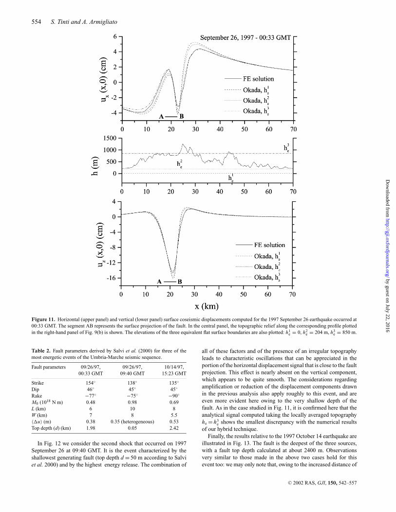
a local interval around the fault (x ∈ (10, 30) km). The top of thefault is d = 1980 m deep according to Salvi et al. (2000). The coseis-mic displacements obtained through our approach, thus accountingfor the effect of topography, are represented by solid lines. Thegeneral trend of all signals is similar, but some differences canbe appreciated. First, the minima and maxima are markedly dif-ferent from Okada’s computed for he = h1

e and he = h2e . In particu-

lar, the vertical signal accounting for topography is smaller thanthe FFS solution in both cases. The analysis is more tricky asregards the horizontal signal given in the upper panel. The posi-

tive peak found around the horizontal distance of 18 km is am-plified in comparison with Okada’s signals computed for he = h1

e

and he = h2e . Conversely, the negative and positive peaks corre-

sponding to distances of about 23 and 30 km are reduced. Thecase he = h3

e shows the best agreement with our numerical solution,especially regarding the vertical displacements. Some differencescan be appreciated for the horizontal component: these are morepronounced in correspondence with the negative local minimumfound at x ∼= 23 km, and also in the region to the left of the fault(x < 10 km).

C© 2002 RAS, GJI, 150, 542–557


Dow

nloaded from



Figure 11. Horizontal (upper panel) and vertical (lower panel) surface coseismic displacements computed for the 1997 September 26 earthquake occurred at00:33 GMT. The segment AB represents the surface projection of the fault. In the central panel, the topographic relief along the corresponding profile plottedin the right-hand panel of Fig. 9(b) is shown. The elevations of the three equivalent flat surface boundaries are also plotted: h1

e = 0, h2e = 204 m, h3

e = 850 m.

Table 2. Fault parameters derived by Salvi et al. (2000) for three of themost energetic events of the Umbria-Marche seismic sequence.

Fault parameters 09/26/97, 09/26/97, 10/14/97,00:33 GMT 09:40 GMT 15:23 GMT

Strike 154◦ 138◦ 135◦Dip 46◦ 45◦ 45◦Rake −77◦ −75◦ −90◦M0 (1018 N m) 0.48 0.98 0.69L (km) 6 10 8W (km) 7 8 5.5〈�u〉 (m) 0.38 0.35 (heterogeneous) 0.53Top depth (d) (km) 1.98 0.05 2.42

In Fig. 12 we consider the second shock that occurred on 1997September 26 at 09:40 GMT. It is the event characterized by theshallowest generating fault (top depth d = 50 m according to Salviet al. 2000) and by the highest energy release. The combination of

all of these factors and of the presence of an irregular topographyleads to characteristic oscillations that can be appreciated in theportion of the horizontal displacement signal that is close to the faultprojection. This effect is nearly absent on the vertical component,which appears to be quite smooth. The considerations regardingamplification or reduction of the displacement components drawnin the previous analysis also apply roughly to this event, and areeven more evident here owing to the very shallow depth of thefault. As in the case studied in Fig. 11, it is confirmed here that theanalytical signal computed taking the locally averaged topographyhe = h3

e shows the smallest discrepancy with the numerical resultsof our hybrid technique.

Finally, the results relative to the 1997 October 14 earthquake areillustrated in Fig. 13. The fault is the deepest of the three sources,with a fault top depth calculated at about 2400 m. Observationsvery similar to those made in the above two cases hold for thisevent too: we may only note that, owing to the increased distance of

C© 2002 RAS, GJI, 150, 542–557


Dow

nloaded from



Figure 12. Same as in Fig. 11, but for the event that occurred on 1997 September 26 at 09:40 GMT. In this case h1e = 0, h2

e = 210 m, h3e = 835 m.

the fault from the Earth’s surface, the correction introduced by thetopography is less pronounced than for the September 26 shocks.

5 D I S C U S S I O N A N D C O N C L U S I O N S

All of cases studied in the previous sections show clearly that the to-pographic relief of the Earth’s free surface influences the coseismicdisplacements generated by a seismic source acting in the Earth’scrust. The 2-D model we have introduced here to account for thetopographic effect is valid only for a homogeneous medium but canbe applied to topographies of arbitrary shapes. We have stressedthat, for this type of configurations and in the coseismic limit, our

hybrid approach presents some advantages over the numerical mod-els based on the mere FE technique: the most important of whichrelates to the representation of the coseismic displacement field cor-responding to the fault plane. Usually, a pure 2-D FE approachrequires displacement components at the fault to be assigned asboundary conditions corresponding to a given subset of the gridnodes: this is done by imposing the source term condition on thefault, which means that the correction induced on the source itself bysurface topography is completely neglected. On the other hand, ourhybrid approach is not affected by this inconvenience, since it canaccount for both the complete ST source term and for the FSC cor-rection. The difference between the results obtained through the two

C© 2002 RAS, GJI, 150, 542–557


Dow

nloaded from



Figure 13. Same as in Fig. 11, but for the event that occurred on 1997 October 14 at 15:23 GMT. In this case h1e = 0, h2

e = 245 m, h3e = 971 m.

approaches become increasingly important as we consider shallowerfaults.

An aspect we may have not sufficiently commented on in previoussections regards the boundary conditions we impose on the crustalboundary �2 (see Figs 2 and 3). Whatever the topographic relief is,the final solution we obtain is characterized by displacements thaton crustal boundary nodes are equal to Okada’s, that is equal to thedisplacement we would obtain in the case of a flat free surface. Usingthe notation introduced in Fig. 2, we assume that the behaviour of

the displacement field at infinity is equal both for a boundary �1

characterized by an irregular topography and for a flat boundary �1

connecting the same ends as �1. Clearly, this is an approximation,the correctness of which depends mainly on the spatial dimensionsof the selected domain and on the position of the fault with respectto the crustal boundaries: in principle, the larger the domain and themore distant the fault from the crustal boundary, the more reasonablethe approximation is in the region around the source. Needless tosay, since the domain must be discretized by means of an FE grid,

C© 2002 RAS, GJI, 150, 542–557


Dow

nloaded from



we need to find a compromise between the extension of the domainand the number of elements required to represent it, which is relatedto the computational costs necessary to obtain the final solution.

Let us now summarize the main conclusions regarding the effectof topography on coseismic displacements that descend from thecases analysed in the present study.

(1) The major effect is the amplification (or reduction) the to-pography applies to both the horizontal and vertical components ofthe surface displacement compared with the FFS case.

(2) Depending on the sign of the local topography, the surfacesignals can be ‘broadened’ or ‘shortened’ with respect to the curvescomputed for a flat topography.

(3) While the vertical displacement is mainly affected by theamplification/reduction effect, the horizontal component also ex-periences a high-frequency-content alteration in its shape (see, forinstance, Fig. 12): this alteration is particularly evident in the surfacepoints closer to the fault and in the presence of irregular topography.

(4) The best approximation to the numerical results accountingfor topography is obtained by computing the analytical Okada solu-tion corresponding to a fault-depth equivalent value he, which fitsthe average local topography around the fault.

Concerning the future developments of this work, we will move intwo main directions. The first explores the extension of our approachto three dimensions: this is a necessary step to gain a more completeand realistic view of the corrections induced by topography on co-seismic displacements at a regional scale. The second is related toa more detailed study of the conditions to be applied for the crustalboundary.

A C K N O W L E D G M E N T S

The authors are grateful to the DIIAR-Politecnico di Milano(Italy) for providing the Italian DTM, and particularly to ProfessorRiccardo Barzaghi and his collaborators. This work was financedby the Italian ‘Ministero dell’Universita e della Ricerca Scien-tifica e Tecnologica’ (MURST, now transformed into Ministerodell’Istruzione, dell’Universita e della Ricerca (MIUR)) with con-tract no MM04158184.

R E F E R E N C E S

Armigliato, A., Tinti, S. & Manucci, A., 2002a. Self-induced deformationon the fault plane during an earthquake. Part I: continuous normal dis-placements, Pageophys., in press.

Armigliato, A., Tinti, S. & Manucci, A., 2002b. Self-induced deformationon the fault plane during an earthquake. Part II: continuous tangentialdisplacements, Pageophys., in press.

Basili, R., Bosi, V., Galadini, F., Galli, P., Meghraoui, M., Messina, P.,Moro, M. & Sposato, A., 1998. The Colfiorito earthquake sequence ofSeptember–October 1997: Surface breaks and seismotectonics implica-tions for the central Apennines (Italy), J. Earthq. Engg., 2, 291–302.

Ben-Menahem, A. & Singh, S.J., 1968. Multipolar elastic fields in a layeredhalf-space, Bull. seism. Soc. Am., 58, 1519–1572.

Bonafede, M. & Neri, A., 2000. Effects induced by an earthquake on its faultplane: a boundary element study, Geophys. J. Int., 141, 43–56.

Capuano, P., Zollo, A., Emolo, A., Marcucci, S. & Milana, G., 2000. Rupturemechanism and source parameters of Umbria-Marche mainshocks fromstrong motion data, J. Seismol., 4, 463–478.

Cocco, M., Nostro, C. & Ekstrom, G., 2000. Static stress changes andfault interaction during the 1997 Umbria-Marche earthquake sequence,J. Seismol., 4, 501–516.

De Martini, P.M. & Valensise, G., 1999. Pre-seismic slip on the 26September 1997, Umbria-Marche earthquake fault? Unexpected cluesfrom the analysis of 1951–1992 elevation changes, Geophys. Res. Lett.,26, 1953–1956.

Ekstrom, G., Morelli, A., Boschi, E. & Dziewonski, A.M., 1998. Momenttensor analysis of the Central Italy earthquake sequence of September–October 1997, Geophys. Res. Lett., 25, 1971–1974.

Hestholm, S., 1999. Three-dimensional finite difference viscoelastic wavemodelling including surface topography, Geophys. J. Int., 139, 852–878.

Hunstad, I., Anzidei, M., Cocco, M., Baldi, P., Galvani, A. & Pesci, A., 1999.Modelling coseismic displacements during the 1997 Umbria-Marcheearthquake (central Italy), Geophys. J. Int., 139, 283–295.

Komatitsch, D. & Tromp, J., 1999. Introduction to the spectral elementmethod for three-dimensional seismic wave propagation, Geophys. J. Int.,139, 806–822.

Ma, X.Q. & Kusznir, N.J., 1992. 3-D subsurface displacement and strainfields for faults and fault arrays in a layered elastic half-space, Geophys.J. Int., 111, 542–558.

Matsu’ura, M., Tanimoto, T. & Iwasaki, T., 1981. Quasi-static displacementsdue to faulting in a layered half-space with an intervenient viscoelasticlayer, J. Phys. Earth, 29, 23–54.

McTigue, D.F. & Mei, C.C., 1981. Gravity-induced stresses near topographyof small slope, J. geophys. Res., 86, 9268–9278.

McTigue, D.F. & Segall, P., 1988. Displacements and tilts from dip-slip faultsand magma chambers beneath irregular surface topography, Geophys. Res.Lett., 15, 601–604.

McTigue, D.F. & Stein, R., 1984. Topographic amplification of tectonicdisplacement: implications for geodetic measurement of strain changes,J. geophys. Res., 89, 1123–1131.

Meertens, C.M. & Wahr, J.M., 1986. Topographic effect on tilt, strain, anddisplacement measurements, J. geophys. Res., 91, 14 057–14 062.

Meghraoui, M., Bosi, V. & Camelbeeck, T., 1999. Fault fragment control inthe 1997 Umbria-Marche, central Italy, earthquake sequence, Geophys.Res. Lett., 26, 1069–1072.

Okada, Y., 1985. Surface deformation due to shear and tensile faults in ahalf-space, Bull. seism. Soc. Am., 75, 1135–1154.

Okada, Y., 1992. Internal deformation due to shear and tensile faults in ahalf-space, Bull. seism. Soc. Am., 82, 1018–1040.

Roth, F., 1990. Subsurface deformations in a layered elastic half-space,Geophys. J. Int., 103, 147–155.

Salvi, S. et al., 2000. Modeling coseismic displacements resulting from SARinterferometry and GPS measurements during the 1997 Umbria-Marcheseismic sequence, J. Seismol., 4, 479–499.

Savage, J.C., 1987. Effect of crustal layering upon dislocation modelling,J. geophys. Res., 92, (B10), 10 595–10 600.

Singh, S.J., 1970. Static deformation of a multilayered half-space by internalsources, J. geophys. Res., 75, 3257–3263.

Steketee, J.A., 1958a. On Volterra’s dislocations in a semi-infinite elasticmedium, Can. J. Phys., 36, 192–205.

Steketee, J.A., 1958b. Some geophysical applications of the elasticity theoryof dislocations, Can. J. Phys., 36, 1168–1198.

Stramondo, S. et al., 1999. The September 26, 1997 Colfiorito, Italy, earth-quakes: modeled coseismic surface displacements from SAR interferom-etry and GPS, Geophys. Res. Lett., 26, 883–886.

Voevoda, O.D. & Volynets, L.N., 1991. The topography of the ground sur-face and postseismic displacements, Comput. Seism. Geodynam., 2, 58–63.

Volterra, V., 1907. Sur l’equilibre des corps elastiques multiplement con-nexes, Ann. Sci. Ecole Norm. Super., Paris, 24, 401–517.

Yoshioka, S. & Tokunaga, Y., 1998. Numerical simulation of displacementand stress fields associated with the 1993 Kushiro-oki, Japan, earthquake,Pageophys., 152, 443–464.

Zollo, A., Marcucci, S., Milana, G. & Capuano, P., 1999. The 1997 Umbria-Marche (central Italy) earthquake sequence: Insights on the mainshockruptures from near source strong motion records, Geophys. Res. Lett., 26,3165–3168.

C© 2002 RAS, GJI, 150, 542–557


Dow

nloaded from


A 2-D hybrid technique to model the effect of topography on coseismic displacements. Application to...

Documents

Transcript of A 2-D hybrid technique to model the effect of topography on coseismic displacements. Application to...