77 - World Bank Documents
446
77~~~~~~~- ill ~~)c c -- ;- -t Z- -" h c , ;I -. - -- ,,,- - - _CKv o ~CD: CD) co , 70 --- . .-- - - D I 7,~~~~~, Public Disclosure Authorized Public Disclosure Authorized Public Disclosure Authorized closure Authorized Public Disclosure Authorized Public Disclosure Authorized Public Disclosure Authorized closure Authorized
-
Upload
khangminh22 -
Category
Documents
-
view
0 -
download
0
Transcript of 77 - World Bank Documents

77~~~~~~~-ill ~~)c c --;- -t Z-
-" h c , ;I -. ---,,,- - - _CKv
o ~CD:CD)
co , 70 --- . .-- - - D
I 7,~~~~~,
Pub
lic D
iscl
osur
e A
utho
rized
Pub
lic D
iscl
osur
e A
utho
rized
Pub
lic D
iscl
osur
e A
utho
rized
Pub
lic D
iscl
osur
e A
utho
rized
Pub
lic D
iscl
osur
e A
utho
rized
Pub
lic D
iscl
osur
e A
utho
rized
Pub
lic D
iscl
osur
e A
utho
rized
Pub
lic D
iscl
osur
e A
utho
rized


THE IMPACT OFECONOMIC POLICIES
ON POVERTY ANDINCOME DISTRIBUTION
Evaluation Techniques and Tools


THE IMPACT OFECONOMIC POLICIES
ON POVERTY ANDINCOME DISTRIBUTION
Evaluation Techniques and Tools
Frangois Bourguignon
Luiz A. Pereira da Silva
Editors
A copublication of the World Bank and Oxford University Press

© 2003 The International Bank for Reconstruction and Development / The World Bank
1818 H Street, NWWashington, DC 20433Telephone 202-473-1000Internet www.worldbank.orgE-mail [email protected]
All rights reserved.First printing August 2003
1 2 3 4 06 05 04 03
A copublication of the World Bank and Oxford University Press.Oxford Universiry Press198 Madison AvenueNew York, NY 10016
The findings, interpretations, and conclusions expressed here are those of the authors anddo not necessarily reflect the views of the Board of Executive Directors of the World Bankor the governments they represent.
The World Bank cannot guarantee the accuracy of the data included in this work. Theboundaries, colors, denominations, and other information shown on any map in thiswork do not imply on the part of the World Bank any judgment of the legal status ofany territory or the endorsement or acceptance of such boundaries.
Rights and PermissionsThe material in this work is copyrighted. No part of this work may be reproducedor transmitted in any form or by any means, electronic or mechanical, includingphotocopying, recording, or inclusion in any information storage and retrieval system,without the prior written permission of the World Bank. The World Bank encouragesdissemination of its work and will normally grant permission promptly.
For permission to photocopy or reprint, please send a request with complete informationto the Copyright Clearance Center, Inc., 222 Rosewood Drive, Danvers, MA 01923,USA, telephone 978-750-8400, fax 978-750-4470, www.copyright.com.
All other queries on rights and licenses, including subsidiary rights, should be addressedto the Office of the Publisher, World Bank, 1818 H Street, NW, Washington, DC 20433,fax 202-522-2422, e-mail [email protected].
ISBN 0-8213-5491-4
Library of Congress Cataloging-in-Publication DataThe impact of economic policies on poverty and income distribution: evaluation
techniques and tools / edited by Francois Bourguignon, Luiz A. Pereira da Silva.p. cm.
Includes bibliographical references and index.ISBN 0-8213-5491-41. Economic assistance-Evaluation. 2. Poverty. 3. Income distribution.
1. Bourguignon, Francois. 11. Silva, Luiz A. Pereira da.
HC60.14146 2003339.4'6-dc2l
2003053508

Contents
Tables, Figures, and Boxes ixForeword xiiiAcknowledgments xviiAcronyms and Abbreviations xix
Introduction
Evaluating the Poverty and Distributional Impact 1of Economic Policies: A Compendium of ExistingTechniquesFrancois Bourguignon and Luiz A. Pereira da Silva
Part I. Microeconomic Techniques
1 Estimating the Incidence of Indirect Taxes 27in Developing CountriesDavid E. Sahn and Stepben D. Younger
2 Analyzing the Incidence of Public Spending 41Lionel Demery
3 Behavioral Incidence Analysis of Public Spending 69and Social ProgramsDominique van de Walle
4 Estimating Geographically Disaggregated Welfare 85Levels and ChangesPeter Lanjouw
5 Assessing the Poverty Impact of an Assigned Program 103Martin Ravallion
v

vi CONTENTS
6 Ex Ante Evaluation of Policy Reforms 123Using Behavioral ModelsFrancois Bourguiignon and Francisco H. G. Ferreira
7 Generating Relevant Household-Level Data: 143Multitopic Household SurveysKinnon Scott
8 Integrating Qualitative and Quantitative 165Approaches in Program EvaluationVijayendra Rao and Michael Woolcock
9 Survey Tools for Assessing Performance 191in Service DeliveryJan Dehn, Ritva Reinikka, and Jakob Svensson
Part hI. Macroeconomic Techniques
10 Predicting the Effect of Aggregate Growth on Poverty 215Gaurav Datt, Krishnan Ramadas, Dominique van derMensbrugghe, 'homas Walker, and Quentin Wodon
11 Linking Aggregate Macroconsistency Models 235to Household Surveys: A Poverty AnalysisMacroeconomic Simulator, or PAMSLuiz A. Pereira da Silva, B. Essama-Nssah,and Issouf Samake
12 Partial Equilibrium Multimarket Analysis 261Jehan Arulpragasam and Patrick Conway
13 The 123PRSP Model 277Shantayanan Devarajan and Delfin S. Go
14 Social Accounting Matrices and SAM-Based 301Multiplier AnalysisJeffery Round
15 Poverty and Inequality Analysis in a General 325Equilibrium Framework: The RepresentativeHousehold ApproachHans Lofgren, Sherman Robinson, and Moataz El-Said

CONTENTS vii
Conclusion
Where to Go from Here? 339Franfois Bourguignon and Luiz A. Pereira da Silva
Annex: Summary of Evaluation Techniques and Tools 353
Bibliography and References 369
Contributors 397
Index 403


Tables, Figures, and Boxes
Tables2.1 Benefit Incidence of Public Spending
on Education in Indonesia, 1989 462.2 Household and Government Spending
on Public Schooling in Indonesia, 1987 522.3 Benefit Incidence of Public Spending on Health,
by Quintile and Level, Ghana, 1992 542.4 Affordability Ratios for Publicly Subsidized
Health Care in Ghana, 1992 552.5 Net Fiscal Incidence in the Philippines, 1988-89 57
3.1 Distribution of Net Public and Private Transfersin Yemen in 1998 under Different Assumptionsabout the Propensity to Consume out of Transfers 71
3.2 Distribution of Social Transfer Income in Vietnam 773.3 The Incidence of Changes in Transfers by Initial
Consumption and Changes in Consumption over Time 783.4 The Baseline Discrete Joint Distribution 793.5 Joint Distribution without Transfers 80
4.1 Estimated Poverty Incidence in Ecuador, 1990 92
6.1 Simulated Effect on Schooling and WorkingStatus of Alternative Specifications of ConditionalCash Transfer Program 13S
6.2 Simulated Distributional Effect of AlternativeSpecifications of the Conditional CashTransfer Program 136
7.1 Modules Included in LSMS Surveys'Household Questionnaire 152
7.2 Quality Control Techniques 1587.3 Examples of Uses of Multitopic Household
Surveys for Poverty-Related Purposes 159

x TABLES, FIGURES, AND BOXES
10.1 Typical Data for SimSIP Poverty: PopulationShares and Per Capita Income by Decile,Sector, and Nationally, Paraguay 223
10.2 SimSIP Poverty: Comparing the FGT PovertyMeasures Obtained with Unit and GroupedData, Paraguay 226
10.3 Simulations for the Impact of Growth Patternson Poverty in Paraguay Using SimSIP Poverty:Some Examples 227
10.4 Input Settings for PovStat Runs, 1997 and 2000 22910.5 Results from PovStat Runs, Philippines 231
11.1 Poverty Line and Income Distribution, Burkina Faso,2002-2010 251
11.2 Occupational Categories, Representative Groups 255
13.1 Basic Equations in the Core Layer: The 1-2-3 Model 28113.2 Growth Coefficients of the Get Real Model 28513.3 Distribution of Income and Expenditure by
Household Groups, Zambia 28713.4 Consensus Forecast: Medium-Term
Macroeconomic Framework, Zambia 29013.5 Impact of Shocks in Government Expenditures
and Copper Price 29213.6 Alternative Long-Term Growth 295
14.1 A Basic Social Accounting Matrix (SAM) 30514.2 SAM: Endogenous and Exogenous Accounts 31114.3 Selected Multiplier Effects Derived from the
Ghana SAM 318
15.1 Poverty and Inequality Measures in theStandard Model 334
Figures1.1 Compensating Variation for an Ad Valorem
Tax on Good i 29
2.1 Indonesia, Benefit Incidence of EducationSpending, 1989 47
4.1 Health Spending and Poverty in Madagascar 93

TABLES, FIGURES, AND BOXES xi
5.1 Poverty Impacts of Disbursements underArgentina's Trabajar Program 105
5.2 Concentration Curve of Participation inArgentina's Trabajar Program 111
8.1 Types of Data and Methods 169
10.1 Decomposition of Change in Poverty into Growthand Distribution Effects 216
11.1 The Functioning of PAMS 23711.2 PAMS Baseline Projections on Poverty
in Burkina Faso, 2002-2010 252
13.1 A Schematic Representation of the Framework 27913.2 The 123PRSP Model 27913.3 A Diagrammatic Exposition of the 1-2-3 Model 28213.4 Copper Price and Zambia's Per Capita Income 288
14.1 The Economywide Circular Flow of Income 306
15.1 Households in a General Equilibrium Framework 32615.2 Structure of Payment Flows in the Standard
CGE Model 329
Boxes1.1 Recurrent Economic Policy Issues in Developing
Countries 3
2.1 Aggregating Unit Subsidies May Mask Inequality 482.2 Significance Tests for Differences between
Concentration Curves 51
4.1 The Basic Steps of Poverty Mapping: An Overview 88
5.1 Data for Impact Evaluation 1065.2 Propensity-Score Matching 1095.3 Graphical Representation of Poverty Impact 1125.4 Double Difference 116
8.1 Are Mixed-Methods Analyses Appropriateunder Severe Budget or Time Constraints? 181
8.2 Ten Principles of Conducting GoodMixed-Methods Evaluations 185

xii TABLES, FIGURES, AND BOXES
9.1 Public-Sector Agencies, Measurability, PETS,and QSDS 192
9.2 PETS, QSDS, and Other Tools to AssessService Delivery 195
9.3 Sample Frame, Sample Size, and Stratification 1999.4 QSDS of Dispensaries in Uganda 206
11.1 Key Equations of the Three Layers of thePAMS Framework 241
11.2 Mining a Household Data Set for PAMS Categories 245
12.1 A Simple Application of the Multimarket Model 266
14.1 Relationship between SAMs and theNational Accounts 307
14.2 Constructing a SAM 309
15.1 Social Accounting Matrices as DatabasesSupporting Poverty and Inequality Analysis 328

Foreword
Development is about fundamental change in economic structures,about the movement of resources out of agriculture to services andindustry, about migration to cities and international movement oflabor, and about transformations in trade and technology. Socialinclusion and change-change in health and life expectancy, in edu-cation and literacy, in population size and structure, and in genderrelations-are at the heart of the story. The policy challenge is tohelp release and guide these forces of change and inclusion. But howcan policymakers assess whether what they have done, or what theyare doing, is right?
Since the 1970s public economics has placed the serious analysisof growth at the center of its agenda. It has shown how to integrategrowth and distribution-in simple terms, the size of the cake, andthe distribution of the cake-rigorously into the discussion of pub-lic policy, both theoretically and empirically. This is an achievementof great importance. What is needed today is research that willextend this analysis of size and distribution to the more dynamicquestions of change and inclusion. Standard public economics hasmade a vital step forward by moving beyond traditional welfaretheory and examining problems of constraints on policy that arisefrom limitations on information. It has helped to discuss the role ofthe state and to view the provision of public goods both as a politi-cal process and as a budget process. But because our perspective ondevelopment has changed, our theories and tools for evaluation ofpolicies must also change.
In the past two decades we have begun to look beyond incomesto health and education. Indeed, we now look beyond the basic ele-ments of human well-being and see freedom as part of development.We see the state not as a substitute for the market, but as a criticalcomplement. We have learned that markets need government andgovernment needs markets-and that government action is crucialin enabling people to participate in the growth process and to takeadvantage of economic opportunities. Economic growth is the mostpowerful force for the reduction of income poverty. Countries that
xiii

xiv FOREWORD
have reduced income poverty the most effectively are those thathave grown the fastest, and poverty has expanded most widely incountries that have stagnated or fallen behind economically.
At the same time, we now know that social cohesion is an impor-tant foundation for sound policies and institutions. Societies func-tion more effectively when poor people are empowered with theability to shape the basic elements of their own lives. Empowermentthus requires not only that people be educated and healthy, but alsothat they be effective participants, which, in turn, depends on infor-mation, accountability, and the quality of local organizations.
These are the dimensions along which public economics, appliedto development and analytical tools for evaluating developmentpolicies, must evolve. In recent years much progress has been madein evaluating the impact of public programs. New methods haveemerged, and existing tools have been improved. Still more isneeded, and more will be done. Yet, before these innovations bearfruit, the existing tools must be used more extensively and system-atically so that policymakers can clearly see how the choices theymake accelerate growth and inclusion and thus reduce poverty. It isthe objective of this volume to make these tools for evaluating theeffect of policies on poverty available to practitioners, decision-makers, and scholars in the field of development.
This toolkit results from an extensive collaborative effort betweenpractitioners and researchers in government, universities, aid agen-cies, NGOs, and othcr development institutions to build and testvarious techniques to evaluate the poverty and distributional impactof economic policy choices. The resulting "tools" assembled in thisvolume represent the most robust, best-practice techniques availablefor conducting poverty and distributional analysis of a broad rangeof policies. These tools encompass methods that can be applied tovarious situations and policy experiments and that allow countriesto better quantify tradeoffs in alternative scenarios when exploringways to reduce poverty.
Analyzing the effects of economic policies on poverty and its dis-tribution requires that these effects be linked at some point to thecorresponding changes in income and expenditure of individualhouseholds as observed in household surveys. This is probably themost important lesson of this volume. It shows that one may goquite far using existing tools and, in particular, making more inten-sive use of existing household surveys than is currently the case foranalyses of the poverty and distributional effects of macro- andmicroeconomic policies.

FOREWORD xv
This volume also proposes directions for an ambitious but neces-
sary research agenda. First, there is a need to develop more empiri-cal surveys and gain a better analytical understanding of the dynam-ics of the investment climate, individual preferences, and political
reform. We hope that more work using microeconomic data at thefirm level-proposed at the end of this volume-will prove to be afruitful direction for future research. Second, the work presented
here suggests that more research is needed to improve the integra-tion of macroeconomic models and the models of household behav-ior as captured in household surveys. Such an integration is obvi-
ously crucial when the distributional incidence and macroeconomiceffects of key policies are being studied-as with taxation, tradebarriers, and many aspects of public spending-but also when major
structural reforms are being evaluated.This volume is not the end of the road. Innovative research is
under way that will permit analysts to go further and solve difficul-
ties raised throughout these pages. Yet, this volume is an importantmilestone in our effort to provide empirical tools that match thedevelopment challenges faced by policymakers and to satisfy their
need to evaluate complex public actions. Ultimately, the quality ofthe tools used depends on the intensity with which they are applied,and their use depends on their quality.
Nicholas SternChief EconomistThe World Bank


Acknowledgments
This volume originated from a joint initiative by Nicholas Stern,Chief Economist of the World Bank, and Stanley Fischer, then First-Deputy Managing Director of the International Monetary Fund. Itbegan with a series of workshops aimed at reviewing existing tech-niques for evaluating the poverty and distributional impact of vari-ous policies available for development, and was discussed both innational and international circles by national policymakers, multi-lateral institutions, the international community of donors, NGOs,and academics. The work was conducted under the overall guidanceof Nicholas Stern. Gobind Nankani and Frannie Leauthier broughtthe World Bank's operational and training perspective. Ian Goldinand John Page managed the discussions inside the World Bank, withthe help of Ines Garcia-Thoumi.
Naturally, this volume is above all the sum of the authors' contri-butions, and they must be the first to be thanked, both for their ownwork and for the comments they provided on their colleagues' work.
The volume also benefited from comments, suggestions and peerreview by Pierre-Richard Agenor, Benu Bidani, Shahrokh Fardoust,Hippolyte Foffack, Alan Gelb, Norman Hicks, Roumeen Islam, JenyKlugman, Phillippe Le Houerou, Phillippe Guimaraes Leite, MichaelLewin, Jeffrey Lewis, Tamar Manuelyan-Attinc, Ernesto May, BrianNgo, Martin Rama, Anne-Sophie Robillard, Sudhir Shetty, andJoachim Von Amsberg.
Alexandre Padolina Arenas, Aline Coudouel, and Stefano Paternos-tro assisted with the electronic and Web site version of this volume.
Roula I. Yazigi, Lucie Albert-Drucker, and Bilkiss Dhomun pro-vided administrative support. Martha Gottron was the copy editor,and Kim Kelley was the production editor for this publication.
xvii


Acronyms and Abbreviations
CDD community-driven developmentCES constant elasticity of substitutionCGE computable general equilibriumCPI consumer price index
DD double differenceDECRG Development Economics Research Group
(World Bank)DHS Demographic and Health Survey
FGT Foster-Greer-ThorbeckeFPM Financial Programming Model (FPM)FSC Fiscal Sustainability Credit
GAMS General Algebraic Modeling SystemGDP gross domestic productGIS Geographic Information System
HIMS Household Income MicrosimulationHIPC heavily indebted poor country
IEA Integrated Economic AccountsIES Income and Expenditure SurveyIFPRI International Food Policy Research InstituteIVE instrumental variables estimator
JSIF Jamaica Social Investment Fund
KDP Kecamatan Development Program (Indonesia)
LAV linkage aggregate variableLCU local currency unitLES Linear Expenditure SystemLFS Labor Force SurveyLSMS Living Standards Measurement Study
xix

xx ACRONYMS AND ABBREVIATIONS
MDG Millennium Development GoalsMS microsimulation
NSS National Sample Survey (India)
OLS ordinary least squares
PAMS Poverty Analysis Macroeconomic Simulator(Excel EViews application)
PDC poverty depth curvePETS Public Expenditure Tracking SurveyPFP Policy Framework PaperPIC poverty incidence curvePNAD Pesquisa Nacional por Amostra de Domicilios
(Brazil)PovStat Poverty Projection Toolkit (Excel-based software)PPA Participatory Poverty AssessmentPPP purchasing power parityPPV Pesquisa Sobre Padroes de Vida (Brazil)PRA Participatory Rural AppraisalPRGF Poverty Reduction and Growth Facility (IMF)PRSP Poverty Reduction Strategy PaperPSM propensity-score matching
QSDS Quantitative Service Delivery Survey
RH representative householdRRA Rapid Rural Appraisal
SAM social accounting matrixSEWA Self-Employed Women's Association (India)SimSIP Simulations for Social Indicators and Poverty
(Excel-based software)SNA System of National AccountsSUSENAS Survei Sosial Ekonomi Nasional (Indonesia)
UPPi Urban Poverty Project 1UPP2 Urban Poverty Project 2
VAR vector autoreggression
ZCCM Zambia Consolidated Copper Mines

Introduction
Evaluating the Poverty andDistributional Impactof Economic Policies:
A Compendiumof Existing Techniques
Franpois Bourguignon andLuiz A. Pereira da Silva
How do economic development policies affect poverty and distri-bution? In recent years that question has become a major focus ofnational and international approaches to development policies. Tobe fair, the debate on economic development policies has more orless continuously intertwined growth and distribution issues, butnever before have evaluations of the effects been so systematic or soprominent an element of the debate. This new approach is particu-larly evident in the emergence of a set of multiple development goals
that explicitly go beyond the narrow focus on aggregate outputmaximization. One example is the Millennium Development Goals
forged by the member countries of the United Nations. Another isthe Poverty Reduction Strategy Papers (PRSPs), the cornerstone of
the concessional lending by the International Monetary Fund (IMF)
and the World Bank to low-income countries.' PRSPs are explicitlyaimed at reducing poverty and meeting several social goals ratherthan exclusively maximizing economic growth. By definition then,
1

2 BOURGUIGNON AND PEREIRA DA SILVA
they require "poverty and distributional analysis" of a set of rec-ommended economic policies and strategies. Even though economicand social objectives are usually complements, they may producetradeoffs; for example, the pace of growth may have some influenceon the distribution of economic and social welfare, and vice versa.The demand for more poverty and distributional analysis that resultsfrom this change of focus is pressing. It comes from practically allquarters: civil society, national governments, nongovernmentalorganizations, bilateral aid agencies, international developmentagencies, and international financial institutions.
Whether reforms concern fiscal or monetary policy, shifts in par-ticular expenditures such as education or health, trade liberaliza-tion, financial sector liberalization, government decentralization, orthe regulation of utilities, economists and social scientists workingon developing countries are increasingly asked both to figure out thelikely aggregate effect of these policies and their effect on varioussocial groups-as well as their impact at the individual householdlevel. A casual observation of the decision process in national gov-ernments and international development institutions reveals thatsuch evaluations are not being conducted systematically, at least notfor all the policy changes most frequently discussed in developingcountries since the 1980s (box I-1). One reason may be that untilrecently poverty reduction was not included in the evaluation crite-ria. Another reason is technical: poverty and distribution evaluationtechniques were not widely used because they were not easily acces-sible or were unsatisfactory on theoretical grounds, or because lackof relevant data simply made them difficult to implement.
Indeed, analysts who evaluate the poverty and distributionalimpacts of economic policies face a big challenge. Because povertyis essentially an individual feature, they must necessarily operate atthe microeconomic level. Thus they require information or predic-tions on how individuals, rather than the whole population or evenany particular broad aggregate group, are likely to fare under thepolicy being investigated. Such an analytical tradition exists in thepublic finance literature under the heading incidence analysis. Thegoal of incidence analysis is to evaluate how particular individualsor households are affected by a change in the tax system or in theaccessibility of public services. However, this "micro-oriented"approach is far from relating immediately and directly to the macro-economic policies and structural reforms listed in box 1.1.
This volume is a compendium of techniques currently availablefor evaluating the impact of economic policies on poverty anddistribution of living standards. Experienced practitioners andresearchers will realize that these techniques are not original ornovel. All the techniques reviewed here are widely or increasingly

INTRODUCTION 3
Box I.1 Recurrent Economic Policy Issues inDeveloping Countries
Public Finance
Public expenditures, such as shifting the allocation of public spendingto specific public programs that affect particular sectors or targetedgroups through cash and/or in-kind transfer policies, loan guarantees,microfinance, or the provision of various types of infrastructureTax policy, including changing tax bases, bands, or rates of direct andindirect taxes and subsidiesManagement of pension and public insurance systems, includinghealth and unemployment insurancePricing of publicly provided goods and services
Structural Reforms
Liberalization and/or regulation of specific markets, including laborand basic commodity marketsTrade liberalization, through the elimination of tariff and nontariff bar-riers and other preferential agreements; and adherence to WTO rulesFinancial sector reforms, including regulation of the banking sector,openness of the capital account, availability of microcredit, andadherence to international financial codes and standards (such asthose of the Bank for International Settlements, or BIS)Public sector management, including the delivery of services, quality,and targeting of servicesPrivate and public governance reforms, including adherence to inter-national standardsRestructuring, privatization, and regulation of public utilities, infra-structure, and other firmsDecentralization and reforms in intergovernmental institutionalrelationsCivil service reforms, including the size and composition of publicsector employmentLand reform, such as negotiated voluntary land transfers
Environmental regulation, including pollution control and enforcement
Macro Policies(Alternative Frameworks and Responses to Shocks)
Fiscal policy, including appropriate deficit levels, controlling forcyclicalityMonetary policy, including Central Bank independence, inflation tar-geting, and interest rate policiesExchange rate regimes (fixed, crawling-peg, or floating), and effectsof a real devaluationPublic debt management, including the size and composition of pub-lic sector liabilities

4 BOURGUIGNON AND PEREIRA DA SILVA
used by academics and policy analysts. The review thus stops shortof discussing the cutting-edge field of distributional evaluation ofmicro- and macroeconomic policies. Cutting-edge analytical tech-niques will be the subject of a forthcoming volume. We deliberatelymade this choice to prevent readers from embarking on techniqueswith uncertain and ambiguous results. The originality of this firstvolume comes from its attempt to organize the analytics of all thesetechniques around the common thread of incidence analysis, and toshow that this basic microeconomic evaluation tool can be used inmany and very different ways to evaluate a wide range of macro-economic policies with some potential impact on poverty.
The annex at the end of this volume provides a short summary ofthe tool discussed in each chapter, including rationale for using thattechnique or tool; the main policy reforms that it can address; itsmost important requirements (data, timeframe, skills needed todevelop an application, and software supporting the tool); and theteam of experts who are familiar with the tool. This summarydescription of the tools covered in this volume is part of a broadeffort to provide guidance and a roadmap for practitioners whowant to conduct poverty and social impact analysis.2
Incidence Analysis as the Core Evaluation Frameworkfor Poverty and Distributional Analysis
Incidence analysis is a concept that is rooted in public finance. Itspolicy applications began with the study of the welfare impact oftaxation and were extended subsequently to that of public spend-ing. For taxation, it consists of identifying those economic agentsthat actually bear the cost of a particular tax, those who gain fromit, and the amount each group will gain or lose in terms of somemetric of welfare. The same issues arise with regard to social bene-fits and other transfer programs-who gains, who loses, how much.There are two main difficulties behind this exercise. First, gainersand losers may not be those who at first sight nominally benefitfrom the transfer or pay the tax. Behavioral and market responsesto taxes and transfers may shift their burden or their benefits toother agents through partial or general equilibrium mechanisms.For example, an indirect tax paid by producers may be partly orfully shifted onto consumers. Second, the identification of the gain-ers and losers is made difficult by the natural heterogeneity amongindividual economic agents, even when they belong to some appar-

INTRODUCTION S
ently well-defined sociodemographic group such as "unskilled urbanworkers" or "small farmers."
Evaluating the effect of economic policies on poverty has much todo with tax-benefit incidence analysis. However, poverty incidenceanalysis is more complex because it involves explicitly ranking gain-ers and losers of a policy against their initial individual welfare levelsor poverty status or, equivalently, concentrating on gains or losses ofpoor people. Also because the policies being evaluated may be dif-ferent from a standard tax or subsidy, the issue of identifying directand indirect gains or losses may also be much more complicated.
Identifying the poor in a population in order to gauge the povertyincidence of a particular policy requires the use of household- orindividual-level data. This need arises because the heterogeneityunderscored earlier implies that no single easily observable and ana-lytically relevant attribute is strictly equivalent to poverty. Poor peo-ple can be found in virtually all categories of agents that economicanalysis can distinguish. As a result, poverty incidence analysis mustbegin at the microeconomic level to identify those individuals whogain or lose because of a specific policy. Indeed, a common featureof the evaluation methods reviewed in this volume-whether theyfocus on microeconomic or macroeconomic phenomena-is thatthey are always somehow connected with individual or householdinformation coming from various types of sample surveys. Most ofthese are nationwide labor force and household expenditure sur-veys, but some are ad hoc surveys undertaken to evaluate specificpolicies or programs. Designing and taking surveys are a necessaryfirst step in poverty evaluation and must be considered as part of theevaluation methodology. Chapter 7 is devoted to this issue.
Measuring the actual monetary flows between the government(central or local), and the individuals, households, or entities thatprovide services directly to households is another type of data prob-lem confronting analysts. A substantial discrepancy often existsbetween flows that are budgeted, flows that are actually disbursed,and flows that actually reach the intended target, whether the targetis a specific group of households or a specific geographic area of thecountry. Of course, the second and third kinds of flow are the onesthat must be taken into account in incidence analysis. Following thefull path and examining the behavior of microeconomic agentsresponsible for managing and monitoring these policies are oftennecessary to understand where reallocation or leakages take place.These issues, which have a great deal to do with policy governancein general, are taken up in chapter 9.

6 BOURGUlGNON AND PEREIRA DA SILVA
Objectives and General Organization of the Volume
Relying on this proximity of incidence analysis and poverty evalu-ation techniques, the practical objective of this volume is to makethe most current poverty evaluation instruments accessible to allanalysts. The 15 chapters of this book give a full account of exist-ing basic techniques and the principles on which they are built,together with illustrative applications and practical tips on imple-mentation. Each chapter refers systematically to recent case stud-ies where the use of these methods can be best appreciated. At thesame time, both the presentation and the discussion are intendedto be as nontechnical as possible, although some technicality isunavoidable.
Two caveats apply to the practical use of the techniques describedhere. First, in many instances, using one technique alone allows onlya partial evaluation of the poverty impact of a particular policy. Amore comprehensive view may be obtained by using various tech-niques at the same time-or possibly by devising original methodsbased on existing techniques but better adapted to the policy underanalysis. Likewise, evaluating the poverty impact of a "complex" setof policies generally requires using various techniques at the sametime. For this reason, this volume provides some leads to cover thesemore complex cases. They should prove valuable in handling policyissues not directly concerned with the techniques being reviewed.
Second, we acknowledge that the set of poverty evaluation tech-niques currently available has serious gaps and weaknesses. Althoughwe are confident about the relevance of the general incidenceapproach, some policy reform areas cannot be evaluated with thetools described here (see our conclusions at the end of this volume). 3
Moreover, even for simple reforms, building a rigorous bridgebetween microeconomic phenomena taking place at the householdlevel and modeling at the macroeconomic level is recognized as oneof the big challenges of economic analysis. Some tools do exist tohandle "micro-macro" policy issues, and the most widely used onesare indeed reviewed in this volume. But they are imperfect and maybe unsatisfactory for particular applications. In some instances, solu-tions have been proposed in the literature, but not enough practicalexperience has been gained to make them suitable for systematic use.Therefore, no attempt is made in this volume to include either alleconomic policies with some possible impact on poverty and the dis-tribution of welfare or all possible evaluation techniques. We reviewhere only those that seemed to be broadly applicable and to haveacquired some robustness, noting the gaps they leave and, more gen-erally, the limits of these standard techniques. Filling some of thegaps and reducing the limitations are left for a further volume.

INTRODUCTION 7
The tools reviewed in this volume are organized in two parts andin each part arranged according to the policy being considered, theperspective taken, or their level of complexity. The chapters in part1 are exclusively microeconomically oriented and are devoted to theeffects of public expenditures, taxation, and redistribution policieson poverty and the distribution of economic welfare. The chaptersin part 2 focus on macroeconomic policies and the links that may beestablished between macroeconomic modeling and the distributionof economic welfare. The unifying link between the two parts is thesystematic reliance on microeconomic data sets that describe thedistribution of economic welfare in the population, that is, house-hold surveys of various types. As it turns out, the incidence analysis
developed in part 1 may also be used-albeit with more difficulty-to evaluate macroeconomic policies, which modify consumptionand factor prices (including their own labor) that households facemuch as tax and subsidy policies do. Moving to macroeconomicinstruments, such as fiscal or exchange rate policy, from thesechanges in prices and factor rewards may require the analyst to takenontrivial steps in modeling or to make strong simplifying assump-tions. In addition, other dimensions of individuals' economic envi-ronments must also be taken into account, which actually makesevaluation of macroeconomic policies more than the straight gener-alization of incidence analysis.
Each chapter discusses both a specific policy evaluation tech-nique and a particular policy instrument or situation to which thetechnique is adapted. The authors of each chapter carefully note thelimitations of the tools currently in use and the risks of pushingthem too far outside their limit of validity.
The techniques reviewed in both parts of this volume require theuser to make some methodological choices at the outset, dependingon the perspective adopted for poverty evaluation, the data at hand,the economic modeling capacity available, and the nature of thepolicy being studied. Having these constraints and issues in mindshould help users of this volume make the appropriate choice forevaluating a specific policy in a particular context.
Using the Incidence Framework at theMicroeconomic Level
Because poverty incidence analysis is initially focused on the micro-economic level, it is important to evaluate the immediate or directimpact of a policy on households and individuals as accurately aspossible. Even though this initial impact may quite possibly be mod-ified by market mechanisms induced by behavioral responses, it is

8 BOURGUIGNON AND PEREIRA DA SILVA
unlikely to be dominated by these indirect effects. Moreover, thissecond round of effects may be difficult to study at the same level ofdisaggregation as direct effects. This is the reason why direct micro-economic incidence analysis, possibly including direct behavioralresponses, is so important. It also explains why techniques that relyon this approach are best suited to evaluate policies with a markeddirect impact on households, such as reforms in the tax system or inthe structure of public spending, including cash or in-kind transfers.
It is not suggested, however, that second-round effects beneglected. Indeed, the indirect effects that arise from the behavioralresponses of microeconomic agents through market mechanismsmight be sizable. They may directly affect household welfare bymodifying the price system, the returns on productive assets, andthe overall conditions of the labor market. The distributional inci-dence analysis of those changes that take place at the aggregate levelis the subject of the second part of the volume.
The policies with some directly observable or easily conjecturedimpact at the household or personal level are typically tax, transfer,and, more generally, public spending policies. Poverty incidenceanalysis may be more or less difficult and more or less detaileddepending on the nature of the tax or public expenditure beingconsidered and the way in which policies are actually implemented.For example, evaluating the direct poverty impact of some transferpolicy conditional on some individual or household characteristicrequires only observing those characteristics as well as knowing thewelfare status of households. But an evaluation may also requireinformation on possible differences between the official transferrules and the actual implementation. Observing or inferring theactual impact of a policy may be more difficult in other instances.Evaluating the impact of building infrastructure in an area, such asa road or a sewer line, may require knowing who is using it orlikely to use it, information that is not always available in the datasources.
Several chapters in part 1 are defined by the policy being evalu-ated: taxes in chapter 1, public spending in chapter 2, and multifac-eted community programs in chapter 5. Other chapters are definedby the perspective that is adopted. For example, the implementationissues mentioned earlier are dealt with in chapter 9. Other perspec-tives are also considered. Incidence analysis may take an accountingor behavioral approach, it may be ex ante or ex post, it may bequantitative or qualitative, and it may be concerned with the aver-age or the margins. All these conceptual distinctions are importantfor knowing whether a given evaluation technique is appropriatefor dealing with the problem at hand. They are discussed next.

INTRODUCTION 9
Accounting versus Behavioral Approaches
The simplest type of incidence analysis is the accounting approach.Who pays what to the state, who receives what from it? In somecases, that information may be obtained directly from sample sur-veys that ask about cash transfers, income taxes, or the use of cer-tain public services. Some inference may be necessary, however. Avalue may have to be imputed to public services being consumed;transfers or taxes may not be directly observed in surveys and mayhave to be figured out indirectly. Indirect methods involve applyingofficial eligibility rules or official income tax schedules or imputingindirect taxes paid through observed spending.
Accounting approaches stop at that point. They ignore possiblebehavioral responses by agents that may modify the amounts theyactually pay or receive; an accounting approach would not detect taxevasion, for example, resulting from an increase in income tax rates.Better said, these approaches are limited to first-round effects anddisregard second-round effects attributable to behavioral responses.In contrast, behavioral approaches try to take those responses intoaccount. An individual may decide to work less than otherwise toavoid losing her eligibility for a means-tested transfer, parents maydecide to send their children to school to take advantage of freeschool lunches, or they may pay more attention to their children'shealth if a public dispensary is built in the neighborhood. Account-ing for behavioral responses is important for poverty incidence analy-sis since changes in behavior may compound or, more rarely, miti-gate the first-round effects revealed by the accounting approach. Thedifficulty, of course, comes in identifying the behavioral response andits determinants in order to integrate it properly into the analysis.
Behavioral considerations are also important in valuing publicservices for potential users. Offering free public education in a vil-lage means more to a household that was initially sending its chil-dren to a school 10 kilometers away from the village than to ahousehold whose children were initially not enrolled. Finding theright value of a free public service for actual users may thus requireestimating the "demand" for that service, or, equivalently, the "will-ingness to pay" for the service. Behavioral responses are discussedin various chapters and dealt with explicitly in chapters 3, 5, and 6.
Ex Ante versus Ex Post Analysis
Economic policies may be evaluated and monitored either beforethey are enacted (or implemented)-ex ante-or after they havebeen in place for some period of time-ex post. Ex ante evaluation

10 BOURGUIGNON AND PEREIRA DA SILVA
involves quantitative techniques that try to predict the variouseffects of policies including those on distribution and poverty. It isalso crucial to evaluate policies ex post to actually observe and pre-cisely identify the direct and indirect effects of a policy to seewhether the actual effects were those expected-and perhaps toreform those policies that did not produce the intended effects.
The distinction between ex ante and ex post analysis may notseem crucial for the accounting approaches mentioned earlier, whichsimply ignore all behavioral responses to the policy being evaluated.For example, one may evaluate ex ante the impact on poverty ofsome prospective means-tested cash transfer program by computingfor each household in a sample survey the change in its welfareattributable to the program. If implementation were to proceed asdescribed in official documents, and if behavioral response wereignored, then the results of the evaluation would be the samewhether it was conducted before or after the policy or the reformwas implemented. Matters would be quite different if the imple-mentation of a policy involved some departure from the officialintention; for example, one need only look at public finance wheredisbursed expenditures frequently differ from the budgeted expen-ditures. The same would be true where the actual effect of the pol-icy depended on whether targeted households actually seized theopportunities offered to them by the policy (the take-up rate). Actualtransfers to households and the characteristics of beneficiaries maybe observed ex post if the necessary data channels have been col-lected, as described in chapters 5, 7, 8, and 9. It is much more diffi-cult to figure the size of these corrections on an ex ante basis.
Even when implementation issues are ignored, the differencebetween ex ante and ex post approaches is more significant whencomplex behavioral responses are taken into account. Ex postapproaches try to compare individuals or households before andafter some policy change, or households involved in some specificprogram with households not involved in the program. In bothcases, one might assume that observed differences would reflect thedirect effect of the program or the policy reform as well as all pos-sible second-round behavioral effects. An important issue in thisrespect is whether households in the program or those concerned bythe reform may be considered as randomly selected in the popula-tion or as self-selected. This issue is discussed in detail in chapter 5.
Ex ante approaches that take into account behavioral responsesrely necessarily on some structural modeling of household behaviorin the field under scrutiny, such as labor supply or occupationalchoices, demand for schooling, or demand for health services. Thesemodels must be able to predict the likely response of households to

INTRODUCTION 11
a change in the set of alternatives offered to them because of theprogram or the reform being analyzed. At the same time they mustbe consistent with the characteristics and the behavior of the house-holds as they are observed in the sample survey used as a data base.Examples of the use of such models are given in chapters 3 and 6.
Average versus Marginal Effects
The incidence of public spending on poverty may be evaluated tak-ing into account all expenditures in a specific field such as primaryeducation or health care. Within an accounting, ex post framework,one may thus reach conclusions such as the poorest 20 percent ofthe population receives 25 percent of public spending in primaryeducation and 15 percent of spending on health care. Does thismean that switching some expenditures from health care to primaryeducation would improve the lot of the poor?
The answer is not necessarily yes. The preceding figures showwho benefits from public spending on average. They say nothingabout the effect of expanding, or contracting, public spending in aparticular field at the margin. Expanding or contracting spendingmay involve giving access to health care or primary education tosome part of the population that did not benefit from these servicesinitially. But that part of the population is rarely a random sampleof the population who originally had access to these services. To besure, expanding primary education in a poor country will predomi-nantly affect the poorest segments of the population because schoolenrollment is likely to be initially close to 100 percent for the richand the middle class. But that might not always be the case for otherpublic services, such as tertiary education or electrification. Identi-fying this marginal incidence and making the distinction with aver-age incidence is important in evaluating the actual impact of policyreforms on poverty. This does not mean, however, that average inci-dence is irrelevant in such a context. For example, evaluating thepoverty impact of a policy consisting of improving uniformly thequality of education for all children already enrolled clearly calls foran average incidence analysis. An explicit treatment of marginalincidence analysis is given in chapter 3.
Qualitative versus Quantitative Approaches
Poverty, or more generally distributional incidence analysis, tends tobe quantitative because poverty is often defined in terms of somemeasurable concept such as income or expenditure per capita. Insuch a framework, it makes sense to talk about the "bottom" 20 or

12 BOURGUIGNON AND PEREIRA DA SILVA
40 percent of a population in terms of its income or expenditureshares and how its (real) income or expenditure may be modifiedby taxation and various components of public spending. But, ofcourse, social public spending and social programs have manydimensions that cannot be reduced to an income measure but thatare nevertheless important in defining and evaluating the incidenceof poverty. Dealing with all these dimensions in quantitative termsis virtually impossible. Hence the importance of approaching inci-dence analysis also from a qualitative point of view. This is the sub-ject of chapter 8.
Partial versus Universal Coverage and the Spatial Dimensionof Public Spending
Incidence analysis and prospective policy evaluation based on house-hold surveys may be limited by the information available in thesesurveys. In particular, policies with some important geographicaldimensions-road construction, irrigation, or electrification, forexample-may be difficult to evaluate because household samplestypically cover a limited number of localities. Statistical techniquesthat match data in censuses with those found in household surveyspermit dealing partly with that difficulty. The analysis may then pro-ceed as if it had a universal rather than a partial coverage of the pop-ulation. These techniques and the possibilities offered by the exten-sive poverty maps they allow to draw are discussed in chapter 4.
Using the Incidence Framework at theMacroeconomic Level: Links betweenMacroeconomic and Microeconomic Techniques
In contrast to part 1 of the volume, which is focused on microeco-nomic techniques, part 2 considers techniques for evaluating eco-nomic policies that affect poverty through changes in the volume(growth), the structure (sectoral composition), and the parameters(prices, factor rewards) of the macroeconomy. These techniquescan be seen as an extension of the microeconomic analysis whereall effects on behavior and market equilibriums are taken intoaccount. In such a perspective, indirect tax reforms or large publicexpenditure programs are indeed likely to have sizable macroeco-nomic effects. But macroeconomic phenomena may affect prices,factor rewards, and other parameters through very different chan-nels, including foreign trade, the financial sector, and monetary and

INTRODUCTION 13
fiscal policies. In all cases, evaluating the poverty effect of macro-economic policies may require the analyst to move beyond thestraight incidence analysis reviewed in part 1. Not only may macro-economic phenomena affect the main parameters behind incidenceanalysis through very different channels, but they are also likely toaffect some dimensions of household welfare that were previouslyleft aside. That is especially true for changes in income-generationmechanisms either through the labor market or through returns onnonlabor assets.
The "ground floor" of the analysis can be found in the relation-ship between economic growth and poverty in aggregate models.From a distributional point of view, this may be considered the firstlevel of the analysis because the macroeconomic framework givesno information whatsoever on inequality-related variables. Ofcourse, inferences about the impact on (absolute) poverty are possi-ble if one is willing to make some necessarily arbitrary assumptionabout changes in the distribution. Two simple tools adapted to thisclass of models are discussed in chapter 10.
The next chapters move on to disaggregated models. Severalpossible linkages between poverty analysis based on household sur-vey data grouped into so-called "representative households" anddifferent classes of macroeconomic models are presented. First, inchapter 11 the household survey data are linked to a macroconsis-tency accounting framework with a simple representation of thelabor market. Second, in chapter 12 the focus is shifted to the dis-tribution and poverty impact on producers and consumers observedin a microeconomic database of changes in prices and quantitiesproduced in a set of related markets under partial equilibriumassumptions. Third, in chapter 13 the micro-macro linkage is donewith a simple three-sector-general equilibrium model with flexibleprices and wages. Fourth, in chapter 14 the link is made throughsocial accounting matrices (SAMs), which are useful for showinghow different household groups derive their incomes from differentsources and their spending patterns. Finally, in chapter 15 the link-age is established with a wider class of disaggregated general equi-librium models.
Regardless of its type-macroconsistency or general equilib-rium-the main role of the macroeconomic models described inpart 2 is to produce a set of macroconsistent changes of commodityand factor prices that can be used to extend the poverty incidenceapproach of part 1. Indeed, it is essentially through these channelsthat macroeconomic policies may affect the various components ofconsumption and revenue of individuals and households.

14 BOURGUIGNON AND PEREIRA DA SILVA
The extension of the microeconomic incidence framework to amacroeconomic level is important when the indirect effects of eco-nomic policies that arise from the behavioral responses of micro-economic agents through market mechanisms are sizable. Theseeffects may directly affect household welfare by modifying the pricesystem, the returns on productive assets, and the overall conditionsof the labor market. For instance, a change in the structure of indi-rect taxation may induce a sectoral reallocation of resources withsome effects on the structure of earnings or self-employment income.A tax incidence analysis that focused only on the effects of changingconsumer prices could thus miss the mark if it were not supple-mented by an analysis at the macroeconomic level.
The general approach, outlined in this part, consists of decom-posing these effects and of generalizing the standard incidence analy-sis of public spending and taxation to cover some, but not all, of themacroeconomic policy issues listed in box 1.1. To accomplish this,we suggest a three-layer methodology for evaluating the povertyeffect of economic policies. The bottom, or micro, layer (individualsin the household survey) consists of a microsimulation analysis,based on household microeconomic data, that permits analyzing thedistributional incidence not only of changes in social public spend-ing or taxation but also of changes in the structure of consumerprices and earnings, or more generally in the income-generationbehavior of households caused by some macroeconomic policy orshock. The top, macro aggregate, layer includes aggregate macro-economic modeling tools that permit evaluating the impact of exoge-nous shocks and policies on aggregates such as gross domestic prod-uct (GDP), its components, the general price level, the exchangerate, the rate of interest, and the like, either in the short run or in agrowth perspective. The intermediate, meso, layer consists of toolsthat permit disaggregating the predictions obtained with the toplayer into price, earning, employment, and asset returns in varioussectors of activity and various factors of production.
For the analysis to be conducted consistently between these threelayers, they should be linked with each other in some consistentway. For instance, studying some change in public spending in edu-cation at the bottom level should modify the rate of growth of theeconomy in the top layer as well as the structure of activity and offactor remunerations in the intermediate layer. In turn those latterchanges should affect the household income generation model in thebottom layer. Unfortunately, available analytical equipment for sucha full integration of these three analytical layers is far from com-plete. Techniques covered in this part of the volume typically coverpart of this general framework.

INTRODUCTION 15
The Relationship between Growth and Povertyin Aggregate Models
Any change in poverty may be decomposed into changes in growth(what is attributable to the uniform growth of income) and changesin distribution (what is attributable to changes in relative incomes),
see Datt and Ravallion (1992). Without information on changes indistribution, likely changes in poverty resulting from changes of xpercent in aggregate household income may be calculated by multi-
plying all incomes or consumption expenditures observed in ahousehold survey by x. This provides an extremely simple way ofmapping growth into poverty reduction. In terms of the incidenceanalysis reviewed in the first part of the volume, this procedure isequivalent to assuming that the rewards of all factors owned byindividuals or households rise by x percent.
Chapter 10 reports on two procedures based on this principle. Inthe first one the calculation can be made in the absence of householdsurvey data. All that is required is a set of assumptions on the distri-bution of income across specific groups of households. An Excel-based spreadsheet software-the SimSIP simulator-has recentlybeen built and made available to exploit that idea. This simulatorshould be useful to analysts who do not have access to the unit-levelrecords of household surveys but do have information by level ofincome, as often provided, for example, in published reports fromnational statistical offices.
Another similar procedure based on household survey data can befound in PovStat. PovStat is an Excel-based program that can simulatepoverty measures under alternative growth scenarios and over a user-specified projection horizon. Poverty projections are generated usingcountry-specific household survey data and a set of user-supplied pro-jection parameters for that country. The program can also handle
exogenous distributional changes that would accompany growth pro-vided they can be parameterized in an adequate way. PovStat may alsohandle some rough sectoral disaggregation of GDP growth in terms ofboth mean household income and sectors of employment.4 The pro-gram offers a wide variety of options in specifying projection parame-ters as well as an output datasheet capability.
Linking Household Survey Data to MacroeconomicallyConsistent Accounting Frameworks with a SimpleRepresentation of a Labor Market
As suggested by the example of PovStat, the preceding techniques forevaluating the incidence of growth on poverty could conceptually be

16 BOURGUIGNON AND PEREIRA DA SILVA
generalized to disaggregate representations of growth by sector orsocial group, or both. One need only observe the growth of specificsectors or be able to predict them with the appropriate modelingtools. Then, knowing the distribution within these sectors or groups,the same mechanism as above could be used to estimate the expen-diture or income of households within a group and then to estimatethe change in poverty in the entire survey sample. In terms of inci-dence analysis, it is now assumed that all the factors owned byhouseholds operating in a given sector have their rewards raised inthe same proportion as given by GDP per capita in that sector in themacroeconomic model.
This is the method used in chapter 11 by the Poverty AnalysisMacroeconomic Simulator, or PAMS, model. An Excel-EViewspackage, PAMS uses as a starting point a macroeconomic frame-work taken from any macroeconomically consistent model (forexample, the "traditional" World Bank RMSM-X) and disaggre-gates production into economic sectors (such as rural and urban,tradable and nontradable, formal and informal). Each sector, inturn, is assumed to employ only one type of labor extracted fromthe available household survey (regrouping individual observationsinto representative groups of households defined by the labor cate-gory of the head of the household). PAMS' labor market, disaggre-gated by economic sector, projects labor demand, which depends onthe growth of sectoral output, and unit labor cost for the relevantsector. Given the disaggregation by sector and skills explainedabove, PAMS then recalculates income growth for each labor cate-gory and feeds these growth rates back into the household survey.
The usefulness of all the preceding tools lies essentially in theirsimplicity. This simplicity entails some problems, though. First, theway in which macroeconomic levers produce changes in sectoralincome per capita is oversimplified. Second, assumptions aboutchanges in the distribution within sectors are totally arbitrary. Forinstance, no account is taken of the fact that the structure of factorrewards may change within sectors or that households are differentlyaffected by a change in the structure of consumption prices. Finally,the treatment of the distributional effects of changes in sectoral struc-tures is oversimplified. In particular, it is assumed that movementsbetween representative groups or sectors being considered in theanalysis are distribution neutral, which seems unlikely in reality.
Poverty Analysis with Partial Equilibrium(Multimarket) Models
The approaches described so far rely on the assumption of fixed pricesthat is present in most of the macroconsistency frameworks. Besides

INTRODUCTION 17
the effect of real unit labor cost on labor demand and the effect of thereal exchange rate on aggregate exports in PAMS, changes in relative
prices are ignored even though they directly affect household welfareon the consumption side and household income on the productionside. This approach can be misleading when evaluating the effects of
some policies that aim precisely at reallocating output more efficientlyand assessing the poverty impact of such moves.
Another route to link policy changes to their effect on households'
real income-and thus on poverty and distribution-is to use a dif-ferent class of model where prices are flexible. There are two mainclasses of such models in the literature. The first comprises sophisti-
cated computable general equilibrium (CGE) models, with goodsand factor markets modeled explicitly and wages, prices, and privateincome determined endogenously. The second class neglects some of
these indirect general equilibrium effects and focuses only on a set ofinterrelated markets where the policy under study is likely to have itsmain effects. This approach has been used primarily in analyzing theagricultural sector and agricultural commodities. The approach has
the advantage of simplicity, but it also has the (unknown since notcalculated) disadvantage of putting aside potentially large indirecteconomic and social effects of policies.
The use of such "multimarket models" for poverty and distribu-tion analysis is discussed in chapter 12. Whether they are called"limited general equilibrium" as in Mosley (1999) or "multimarketpartial equilibrium" as in Arulpragasam (1994), these models focusthe analysis on the combination of direct effects and indirect effectsthrough price and quantity changes in a small group of commoditiesor factors with strongly interlinked supply and demand. They aremost appropriate for the evaluation of policies that change the rela-tive price of a specific good-for example, the removal of a subsidy
or the elimination of a tariff or quota. The indirect effects explicitlymodeled are those resulting from relative price responsiveness ofdemand and supply in markets for substitute goods.
Once the direct effect on a market (or markets) of a policy reformis identified, one can also figure out (through data examination, sur-vey of experts, or other prior knowledge) which other markets arestrongly interlinked in demand or supply with the markets in whichthe direct effect is measured. The next step is to rely on householdsurvey information to estimate the shares of expenditures that areaffected by these changes through own-price and cross-price elastic-ities of demand for the entire set of interlinked markets. Producersurvey information is used to derive estimates of own-price andcross-price elasticities of supply for the set of interlinked markets.These estimates are combined to create a system of demand andsupply functions, and price- or quantity-clearing is imposed for each

18 BOURGUIGNON AND PEREIRA DA SILVA
good in the system of equations. This closure is made consistent withthe observed macroeconomic outcomes by requiring the resultingequilibrium to duplicate international relative prices and trade flowsin each good and other national statistics for the base year chosen.The impact of the policy reform in this system of equations is thencalculated by introducing the desired policy change. Relative pricesand quantities produced and consumed domestically are derived forthis new equilibrium. The derived relative prices and quantities arecombined with household survey information, households oftenbeing both consumers and producers, to determine the marginalimpact of the policy reform on the incidence and depth of poverty.
Poverty Analysis with a Simple Computable GeneralEquilibrium Model
Suppose now that available evidence suggests that the policies beingassessed have large indirect and second-round effects. A partial equi-librium approach such as the one described above would be inade-quate to measure the poverty and distributional consequences ofsuch policies. A general equilibrium approach is necessary.
Chapter 13 explores what can be done with what probably is thesimplest computable general equilibrium model of a complete econ-omy. This is the 1-2-3 model, by Devarajan and others (2000); themodel name stands for one country, two sectors, three commodities(such as exports, domestic goods, and imports). This is a static model(that is, it has to be "fed" with an exogenous growth path), but oneof its important aspects is that it captures the effects of macroeco-nomic policies on two critical relative prices, namely, the real exchangerate and the real remuneration rate of (wage) labor, and on the allo-cation of resources between tradable and nontradable sectors.Another important aspect is that the calibration of the model is rela-tively easy using national accounts data and simple assumptions ofequilibrium in labor and capital markets. The model's simulationspredict the effect of several types of macroeconomic policies on wages,sector-specific employment, self-employment income and profits, andrelative prices that are mutually consistent.
The link with poverty analysis is provided by plugging the model'sprojected changes in prices, wages, and profits into available dataon labor and profit income and on commodity demands for repre-sentative groups of households (or deciles of the welfare distribu-tion). In principle, the impact on each household in the sample canbe calculated so as to capture the effect of the policy under study onthe entire distribution of income. Thus changes in various povertymeasures can also be reported. In short, the 1-2-3 framework allows

INTRODUCTION 19
for a forecast of welfare measures and poverty outcomes consistentwith a set of macroeconomic policies and of their effect on key
macroeconomic variables such as the real exchange rate or the sec-
toral allocation of employment.
Poverty Analysis with Social Accounting Matrices(SAMs) Approaches
The "simplest" CGE model described above has obvious limita-
tions. For example, some policies will affect specific categories ofworkers and specific economic sectors within the broad aggregatesof the 1-2-3 approach, but the approach itself cannot measure these
specific changes. Much energy since the 1980s has been dedicatedto developing disaggregated models that would permit simultane-ous analysis of changes both in the structure of the economy due tosome specific macroeconomic policy and in the distribution ofincome within the population.
For more than three decades social accounting matrices have
been used as an integrating framework for data belonging to sepa-rate spheres-national accounts, social accounts, household sur-veys, and so forth-and as a basis for modeling the social conse-
quences of macroeconomic policies. A SAM is usually quite explicitin portraying the structural features of an economy, in particularhow different household groups derive their incomes from differentsources and their spending patterns. Chapter 14 sets out the basicframework of a SAM and shows how it has been used to computeKeynesian-like multipliers to help assess the impacts of policy andexternal shocks on household incomes and expenditures and onpoverty. SAM-based models show how the incomes of a particularhousehold group, say, small-scale farmers, may be affected by anincrease in, say, textile output. The method identifies all the variouspaths or channels of transmission of the effects of policies, from ori-gin to destination. For instance, it may be that an increase in theincome of unskilled workers arises directly, through the hiring ofunskilled labor in some unskilled-labor intensive sector, or indi-rectly, through a stimulus from increased spending on food crops,the increased production of which also needs unskilled labor (Thor-becke 1995). Structural path analysis computes the importance ofthe various paths relative to the global influence.
One major limitation of SAM multipliers, however, is their implicitreliance on fixed price Keynesian-like mechanisms. This has severaldrawbacks for the analysis of poverty, including the difficulty of sep-arating out whether the predicted change in the mean income of ahousehold group is due to price and wage or employment effects.

20 BOURGUIGNON AND PEREIRA DA SILVA
Poverty Analysis with More Disaggregated CGE ModelsUsing the Representative Household Approach
Since the pioneer work by Adelman and Robinson (1978) for Koreaand by Lysy and Taylor (1980) for Brazil, many CGE models fordeveloping countries combine a highly disaggregated representationof the economy within a consistent macroeconomic framework witha description of the distribution of income through a small numberof representative households meant to represent the main sources ofheterogeneity in the whole population with respect to the phenom-ena or the policies being studied. Models were initially static andrigorously Walrasian. They are now often dynamic-in the sense ofa sequence of temporary equilibriums linked by asset accumula-tion-and often depart from Walrasian assumptions to incorporatevarious macroeconomic features, or "closures," as well as imperfectcompetition features.
Several representative households are necessary to account forheterogeneity among the main sources of household income-oramong the changes in income-attributable to the phenomena or thepolicies being studied. Despite the need for variety, the number ofrepresentative households is generally small, however, usually fewerthan 10. The representative households are essentially defined by thecombination of the productive factors they own: farmers, rural wageworkers, skilled urban workers, unskilled urban workers in the for-mal sector, and so forth. Although simple, this disaggregationmethodology has proved to be very useful and has allowed manyinsights into a variety of issues. With time, this approach led to anincreasing degree of disaggregation of the production and thedemand sides of the economy, of the degree of heterogeneity amongagents (by explicitly considering that households within a represen-tative group were heterogeneous but in a "constant" way), of thespecification of government transfers and other types of expenditure,and of the structure and the functioning of factor and good markets.
CGE models with representative household groups already havea long history in taxation incidence analysis. In effect they may beconsidered as the logical extension of the microeconomic incidenceanalysis of the type reviewed in the first part of this volume to gen-eral equilibrium effects and to aggregate household groups.5 How-ever, the same models could be extended to provide inputs, such asthe precise consumption price vector, sectoral employment levels,and the like, to conduct incidence analysis of taxation at the house-hold level, as seen in part 1, rather than with representative groups.Another important field of application of CGE modeling with rep-resentative household groups is concerned with the distributional
INTRODUCTION 21
effects of trade reforms (for a recent example, see Yao and Liu2000). Non-Wairasian models, which incorporate some descriptionof the financial sector, have also been used extensively since the1990s to study the distributional effects of macroeconomic stabi-lization and structural adjustment (Bourguignon, Branson, and deMelo 1992; Decaluw6 and others 1998; and Ag6nor, Izquierdo, andFofack 2001).
Chapter 15 illustrates this macroeconomic approach to distribu-tional issues by presenting the structure of a standard CGE modelcombining sectoral disaggregation and representative householdgroups. Such models are calibrated on the basis of a social accountingmatrix, which provides the definition of factors, activities, commodi-ties, and institutions incorporated in the CGE model. The model itselfis written as a set of simultaneous equations that describe the behav-ior of producers and consumers. These equations also include a set ofconstraints that correspond to equilibrium conditions in the variousmarkets for factors and commodities, as well as for some macro-economic aggregates (savings-investment balance, the budget of thegovernment, and the current account of the balance of payments).
Like SAM multipliers, standard CGE with representative house-hold groups cannot account for heterogeneous effects of a givenpolicy within a heterogeneous group. Thus, they may miss impor-tant sources of change in poverty. Also, they do not quite complywith the three-layer structure for linking microeconomic and macro-economic aspects of the poverty effect of policies. With the CGEand SAM models, as well as with simpler approaches like PAMS,SimSIP, or PovStat, it is clearly the bottom layer that is unsatisfac-torily handled in the sense that a large part of microeconomic het-erogeneity is simply ignored.
Various attempts are being made to resolve this problem, andprogress will eventually remedy this weakness. 6 As mentioned ear-lier, however, it is not the intention of this volume to cover researchcurrently under way at the cutting edge of poverty evaluation tech-niques. The chapters presented here are more practical in that theydescribe techniques and tools on which some experience has alreadybeen accumulated in common work that World Bank teams havebeen conducting for years with governments in client countries, aca-demic researchers, bilateral aid agencies, and nongovernmentalorganizations.
That the tools described in this volume are not yet of universal orsystematic use in the poverty evaluation of development policiesshows the need to give them more exposure. At the same time, inher-ent weaknesses may explain why the use of these tools is not more

22 BOURGUIGNON AND PEREIRA DA SILVA
widespread. Greater reflection on these weaknesses was thus alsonecessary. We hope that this volume will achieve both objectives-and that the analytical tools summarized here will be more widelyused in the future. This is a necessary step in establishing firmground upon which to develop new tools that will fill the gaps in theexisting tools and will respond to unmet demand.
Notes
1. Poverty Reduction Strategy Papers (PRSPs) are the new general pol-icy documents elaborated by the governments of developing countries thatwant to access concessional resources from the International MonetaryFund (IMF) and the World Bank. The PRSPs replaced in 1999-2000 thePolicy Framework Papers (PFPs) written by the staff of the IMF and theWorld Bank in consultation with governments.
2. Other general presentations of instruments that are available for povertyand social impact analysis can be found at www.worldbank.org/poverty.
3. For example, it is still difficult to analyze the poverty effect of reformssuch as "privatization" or "land reform," which involve changes in owner-ship of assets. Similarly, there are dynamic effects (such as the accumulationof human capital through education) or the effects on agents' expectations(such as improvement in "investment climate") whose transmission mecha-nisms into income and expenditures of households are not fully understood.
4. SimSIP, which stands for Simulations for Social Indicators andPoverty, does the same but using standard decomposability properties ofsome inequality or poverty measures rather than the original microdata.
5. In effect, this may have been one of the first uses of computable gen-eral equilibrium models, but these tended to concentrate on industrial coun-tries; see, for example, Shoven and Whalley (1984). For an excellent appli-cation of this framework to developing countries, see the model ofDevarajan and Hossain (1998) for the Philippines.
6. See in particular Chen and Ravallion (2002) and Bourguignon, Robil-lard, and Robinson (2002).
References
The word processed describes informally reproduced works that may notbe commonly available through library systems.
Adelman, Irma, and Sherman Robinson. 1978. Income Distribution Policy:A Computable General Equilibrium Model of South Korea. Stanford,Calif.: Stanford University Press.

INTRODUCTION 23
Agenor, Pierre-Richard, Alejandro Izquierdo, and Hippolyte Fofack. 2000.
"IMMPA: A Quantitative Macroeconomic Framework for the Analysis
of Poverty Reduction Strategies." World Bank Institute, Washington,D.C. (www.worldbank.org/wbi/macroeconomics/modeling/immpa.htm).
Arulpragasam, Jehan, and Carlo del Ninno. 1996. "Do Cheap ImportsHarm the Poor? Rural-Urban Tradeoffs in Guinea." In David Sahn, ed.,
Economic Reform and the Poor in Africa. Oxford, U.K.: Oxford Uni-
versity Press.Bourguignon, Francois. 2003. "The Growth Elasticity of Poverty Reduc-
tion: Explaining Heterogeneity across Countries and Time Periods." In
T. Eicher and S. Turnovsky, eds., Inequality and Growth. Cambridge,Mass.: MIT Press.
Bourguignon, Francois, W. Branson, and J. DeMelo. 1989. "Macroeco-
nomic Adjustment and Income Distribution: A Macro-Micro Simula-tion Model." OECD Technical Paper 1. Organisation for Economic
Co-operation and Development, Paris.
Bourguignon, Francois, Anne-Sophie Robillard, and Sherman Robinson.2002. "Representative vs. Real Households in the Macroeconomic Mod-
eling of Inequality." International Food Policy Research Institute, Wash-
ington, D.C. Processed.Chen, Shaohua, and Martin Ravallion. 2002. "Household Welfare Impacts
of China's Accession to the WTO." Paper presented at the Fourth Asia
Development Forum, Seoul, Korea, November 3-5, 2002. In East Asia
Integrates: A Trade Policy Agenda for Shared Growth. Washington,
D.C.: World Bank. Forthcoming.
Datt, Gaurav, and Martin Ravallion. 1992. "Growth and RedistributionComponents of Changes in Poverty Measures: A Decomposition with
Applications to Brazil and India in the 1980s."Journal of Development
Economics 38 (April): 275-95.Datt, Gaurav, and Thomas Walker. 2002. "PovStat 2.10: A Poverty Projec-
tion Toolkit, User's Manual." World Bank, Washington, D.C. Processed.
(www.poverty.worldbank.org/library)Decaluwe, Bernard, A. Patry, and L. Savard. 1998. "Quand l'eau n'est plus
un don du ciel: Un MEGC applique au Maroc (When Water Is No
Longer a Gift of God: A CGE Applied to Morocco)." Revue d'Economie
du Developpement 0 (3-4, December): 149-87.
Devarajan, Shantayanan, and Shaikh I. Hossain. 1998. "The Combined
Incidence of Taxes and Public Expenditures in the Philippines." World
Development 26(6): 963-77.
Devarajan, Shantayanan, William R. Easterly, Delfin S. Go, C. Petersen, L.
Pizzati, C. Scott, and L. Serven. 2000. "A Macroeconomic Framework
for Poverty Reduction Strategy Papers." World Bank, Washington, D.C.
Processed.

24 BOURGUIGNON AND PEREIRA DA SILVA
Lysy, Frank J., and Lance Taylor. 1980. "The General Equilibrium Modelof Income Distribution." In Lance Taylor, E. Bacha, E. Cardoso, and
Frank J. Lysy, eds., Models of Growth and Distribution for Brazil.Oxford, U.K.: Oxford University Press.
Mosley, Paul. 1999. "Micro-Macro Linkages in Financial Markets: The
Impact of Financial Liberalization on Access to Rural Credit in FourAfrican Countries." Finance and Development Research ProgrammeWorking Paper 4. University of Manchester, Manchester, U.K. Processed.
Shoven, John B., and John Whalley. 1984. "Applied General EquilibriumModels of Taxation and International Trade: An Introduction and Sur-vey." Journal of Economic Literature 22(3): 1007-51.
Thorbecke, Erik. 1995. Intersectoral Linkages and Their Impact on RuralPolicy Alleviation: A Social Accounting Approach. Vienna: UnitedNations Development Organization.
Wodon, Quentin, Krishnan Ramadas, and Dominique van der Mensbrugghe.2002. "SimSIP Poverty: Poverty and Inequality Comparisons Using GroupData." World Bank, Washington, D.C. Processed. (www.worldbank.org/simsip)

PART I
Microeconomic Techniques


1
Estimating the Incidenceof Indirect Taxes
in Developing Countries
David E. Sahn and Stephen D. Younger
The distributional impact of the public sector's budget is a topic ofenduring interest for economists and policymakers. The more recentliterature on developing countries has focused almost exclusively onthe expenditure side of the budget, as discussed in chapter 2. But thefew available studies on tax incidence in developing countries showthat some tax policies have redistributive impacts-both positiveand negative-of a size comparable to the effects of the more com-monly studied social sector expenditures, justifying more equalattention from analysts interested in understanding the distribu-tional consequences of public policies.
The methods that we describe for tax incidence analysis are intu-itive and computationally straightforward. They have practical lim-itations, which we address in the final section of this chapter. Butone conceptual limitation should be addressed up front: these meth-ods are useful only for analyzing the equity consequences of publicpolicy. Yet good policy analysis requires consideration of both equityand efficiency consequences, and not necessarily in that order. Con-sequently, the type of analysis described here is only one input to acomplete analysis of tax policy.
27

28 SAHN AND YOUNGER
The Technique and Theoretical Background
The MIT Dictionary of Modern Economics defines tax incidence asdescribing "those who suffer a reduction in their real income result-ing from the imposition of a tax." (Pearce 1986, p. 192). To accom-plish this description, we use survey data to determine individualhouseholds' loss and then show how that loss is distributed acrossthe households in the sample. To measure each household's lossfrom a tax, we rely on basic duality theory. A household's expendi-ture function, y = e(p,u), is the minimum amount of money that itmust spend to generate utility level u given a vector of prices p forall goods and services consumed. A household's compensating vari-ation for a tax increase is the amount of income that it would needto keep its utility constant in the face of any price changes caused bythe tax:
(1.1) CV = e(pl,u0 ) -e(po,u0 )
where zero indicates the initial state and one indicates the state afterthe tax change.
Clearly, if we could estimate the household's expenditure func-tion, we could easily calculate the compensating variation and thusknow how much real income declines as a result of the tax. Unfor-tunately, that is a difficult task, both in terms of data and analysis,and the methods that we use avoid it entirely by approximating thecompensating variation. Consider for the moment the case in whichthe tax change affects only one price, pi. Recall that by Shephard'slemma, the derivative of the expenditure function with respect to piis the compensated demand function for good i. The Taylor expan-sion of equation 1.1 is therefore
(1.2) CV -x(po,u0)*ApAi + -*Ax, (p u ) *Ap2 +,,,2 apj
where xf(pOu 0 ) is the compensated demand function and Ap1 is thechange in the price of pi caused by the tax increase. The first term inthe Taylor expansion is the change in expenditure that the house-hold would have to undertake to keep utility constant withoutchanging its demand for good i (or any other), that being the initialquantity consumed times the price change. This is a first-orderapproximation to the compensating variation. Put otherwise, thecompensating variation of a marginal change in the price of a goodis simply the change in the consumption budget that is necessary tokeep the consumption basket constant. In other words, the demandresponse to the tax may be ignored as a first approximation.

ESTIMATING THE INCIDENCE OF INDIRECT TAXES 29
We can graph this approximation by noting that the difference inexpenditures noted in equation 1.1 is equal to the integral of the com-pensated demand function from po to pl, again by Shephard's lemma.
CV = e(p',') -e(p°,u') = |:: x2(p,uo)dPj
This integral is the area to the left of the compensated demand func-tion in figure 1.1, shown as ABDE. The first term in the Taylorexpansion in equation 1.2 is equal to the area ACDE, the originalquantity consumed times the price change. The second term is thetriangle BCD. Higher-order terms would capture the curvature ofthe demand curve.
The only information generally used in incidence analysis is thefirst-order approximation, area ACDE. As such, behavioral changesthat the tax change might induce are not accounted for.' We simplyobserve the existing pattern of demand, multiply it by a hypothesizedprice change, and use the result as an estimate of each household'sloss in real income. Finally, if a change in tax policy changes morethan one price, all the first-order terms in equation 1.2 for goodswhose price changes are summed together. While such an approachcannot tell us anything about the efficiency consequences of the taxchange-those depend entirely on its behavioral consequences-ithas been found to be a reasonably satisfactory shortcut for the studyof a policy's distributional impact.
Figure 1.1 Compensating Variation for an Ad Valorem Taxon Good i
Pi
p,A -- - - -- - -B -- -C
Pi ------------------ ID_
l\
XjC(p,uO)
xio
Source: Authors' illustration.

30 SAHN AND YOUNGER
How to Do a Tax Incidence Analysis
Most analyses of indirect tax incidence are concerned with the shareof taxes paid by different groups. For such analyses, the only datanecessary are a variable that defines the groups and an estimate ofthe taxes paid by each group, where "taxes paid" is understood tobe the loss in real income described above. The most common sourceof these data is a nationally representative household survey such asa Living Standards Measurement Survey (Grosh and Glewwe 2000)or a household income and expenditure survey. (Summaries of thesesurveys, as published by national statistical agencies, might suffice ifthey are disaggregated according to the grouping of interest.)
Usually, the groups are defined by welfare levels-poor and non-poor, or each quintile of the welfare distribution-so a variable isrequired that ranks people by welfare, and the preferred choice inthe vast majority of studies is household expenditures per capita orper adult equivalent. But other groupings are possible, such as geo-graphic location (by political region or urban-rural breakdown),gender, ethnicity, or age cohort. In all cases, these variables arealmost always readily available for each individual or household inthe survey data.
Estimates of the taxes paid by each group are more difficult, andit is helpful to explain first what to do with such an estimate, return-ing to the question of how to get it later. The simplest sort of com-parison notes that group A pays so much of a particular tax, groupB so much, and so forth. For the most common case, where we wantto group people by welfare status, the groups might be poor andnonpoor, or people in each quantile of the welfare distribution. Butin fact, it is easy to make a much more attractive comparison basedon the theory of welfare dominance, which also offers the advan-tage of involving individual agents rather than groups of agents.
The theory of welfare dominance provides general criteria thatallow us to conclude that one distribution of welfare is better thananother for broad classes of social welfare functions (Saposnik,1981; Shorrocks, 1983; Foster and Shorrocks, 1988; Yitzhaki andSlemrod, 1991; Lambert, 1993). One particular application of thistheory is particularly useful for tax incidence analysis. Shorrocks(1983) shows that if the generalized Lorenz curve for one distribu-tion of welfare is everywhere above the generalized Lorenz curve foranother, then the first distribution is preferable to the second underany social welfare function that is increasing in the welfare variable,anonymous, and equality-preferring. 2 By increasing we mean that alarger value of the welfare variable, wi, is better than a smaller onefor each individual i, that is, there is no satiation. By anonymous we

ESTIMATING THE INCIDENCE OF INDIRECT TAXES 31
mean that the welfare function does not pay attention to the iden-tity of each person in the ordering or to whether a person changesposition from one ordering to another. By equality-preferring wemean that if a distribution is generated by taking an existing distri-bution and transferring a small amount of welfare from a better-offindividual to a worse-off one, the new distribution is preferred tothe old. The generality of this comparison makes it quite attractive.To carry it out, we need to construct only two generalized Lorenzcurves, one before the tax and one after, and then see if one curve isclearly above the other.
In practice, however, we have found it useful to use a slightlymore restrictive condition. If we assume that the tax (change) ofinterest has no efficiency consequences, then the mean of the distri-bution of tax payments will be constant, allowing the use of Lorenzcurves rather than generalized Lorenz curves. In addition, the Lorenzcurves tend to be quite close together, even for major tax changes,so that visually, it is more attractive to work with concentrationcurves, defined as
C(i) = Tk n Tk=1 k=l
which is the same formula as the Lorenz curve with the total taxpaid substituted for welfare. Note that observations remain orderedby welfare, not by taxes paid, so that G(i) gives the share of taxespaid by the poorest i/n households or individuals in the sample. Ifthe concentration curve for a tax is everywhere below the Lorenzcurve of income/welfare, then increasing that tax by a small amountand refunding the proceeds in proportion to welfare (the Lorenzcurve) will increase social welfare for all social welfare functionsthat are increasing, anonymous, and equality-preferring. Similarly,if the concentration curve of one tax is everywhere below that ofanother tax, then increasing the first tax slightly and reducing thesecond tax such that total tax revenue is unchanged will improvesocial welfare for the same class of social welfare functions (Youngerand others 1999).
Note that it is possible to make poor-nonpoor comparisons basedon Lorenz and concentration curves, and also comparisons of eachquantile's share, but the use of the entire distribution is more gen-eral than either of these comparisons and equally easy to calculate.Standard errors for these curves are more difficult to calculate(Davidson and Duclos 1997), but a specialized software package,DAD, is now available to do this.3

32 SAHN AND YOUNGER
Calculating Taxes Paid by Households or Groups
We now return to the question of evaluating the cost to a givenhousehold of an ad valorem tax. Economists since David Ricardohave recognized that the statutory incidence of tax-those who haveto transfer the tax to the government-is not the same as the eco-nomic incidence of the tax-those whose real purchasing powerdeclines because of the tax. Much of public economics involvesunderstanding exactly how different statutory taxes are shiftedamong various agents, based on models of their behavioralresponses to the taxes. The type of empirical tax incidence studythat we describe here ignores all but the simplest aspects of thistheory. Typically, we assume that indirect taxes on goods are shiftedentirely to consumers, a standard result if markets are competitiveand the taxes apply only to final sales (or value added). This assump-tion ignores any effect that the taxes may have on firms' welfare (orrather, the welfare of the firm's owners) and, more important, anycascading of taxes through the economy's production structure. Forimport duties, we usually assume that all prices, including those fordomestically produced goods of the same type, rise in proportion tothe duty rate. Again, this is true in the simple case where marketsare competitive and the country is small (although in this case weshould note that some of the benefits of the tax go to domestic pro-ducers rather than the government).4
In addition to deciding whose purchasing power actually declineswhen a tax is increased, we also need to calculate how much theylose. In the simplest of cases, where taxes are collected according tothe letter of the law, this calculation is straightforward for ad val-orem taxes. The tax paid is simply the tax rate times the pretaxvalue of expenditures:
(1.3) T; i= tjpi,1xi X = ei1+tj
where T i is household i's total loss in purchasing power for a tax ongood j; PijxjX is household i's pretax amount of expenditure on goodj; t1 is the tax rate; and ei is the post-tax amount of expenditure ongood j. The fact that TJX is proportional to eiJ,, the expenditure thatwould be reported in a household survey, is convenient, for reasonsthat we come to shortly.
Unfortunately, taxes are not paid according to the letter of thelaw, both because of corruption and because many transactions indeveloping countries occur in informal markets not subject to thegovernment's tax handles, which are almost always formal sectorfirms or goods passing through the port. In Madagascar, for exam-

ESTIMATING THE INCIDENCE OF INDIRECT TAXES 33
pie, we found that actual value added tax (VAT) collections wereabout 8 percent of formal sector value added in 1995, even thoughthe official VAT rate was 25 percent. And of course, formal sectorvalue added is relatively small in Madagascar. Even if we assumethat tax evasion and avoidance occur in such a manner that theresult is an equiproportional increase in market prices for all con-sumers that is something less than the statutory tax rate, we face thepractical problem of deciding what tax rate to use in equation 1.3.Our sense is that probably the best one can do without expendingconsiderable resources is to gather information on tax revenues andtax bases from the authorities and use the ratios as estimates of the"effective" tax rate for that particular tax.
There is one case in which this problem can be avoided. If we assumethat a tax's incidence is proportional to expenditures, whatever theproportion, for all households, then we can simply use observedexpenditures in equation 1.3, because the proportion cancels out of thenumerator and denominator. This only works, however, for one taxrate. Any attempt to combine two or more items with different taxrates requires that the calculation of taxes paid be made.
Examples of Application
There is an emerging body of literature examining household taxincidence in developing countries that follows the framework pre-sented above. Most recently, using data on expenditures from the1992 Integrated Household Survey, Chen, Matovu, and Reinikka(2001) conduct a welfare dominance analysis of tax incidence inUganda. They find that the tax structure was progressive beforereforms and remained so after reforms, indicating that the burdenof tax reforms had not fallen disproportionately on the poor. Mostindividual tax categories were also progressive before reforms, withthe exception of the excise tax on paraffin (kerosene), which is heav-ily consumed by poor households. Export taxes on coffee, one ofUganda's main exports, remained highly regressive, as the burden ofthe tax is shifted to relatively poorer rural farmers. Petroleum taxes(except paraffin) remained progressive. 5 The study concludes thatreducing export taxes on coffee and taxes on paraffin would benefitthe poor. Other tax reforms implemented in the 1990s were gener-ally pro-poor. The pay-as-you-earn tax remains the most progres-sive tax, as it applies to the formal sector where the nonpoor areemployed. The study also finds that substituting value added taxesfor sales taxes does not necessarily worsen the welfare of the poor,since most goods consumed by the poor were zero-rated.

34 SAHN AND YOUNGER
A similar study by Younger and others (1999) examines house-hold tax incidence in Madagascar. The study finds that most taxesare progressive, with the exception of kerosene taxes and exportduties on vanilla. It proposes that a movement away from tradetaxes and toward broadly based value added or income taxes wouldbe both more equitable and efficient, since they would apply to theformal sector where the nonpoor are employed. It also concludesthat taxes on petroleum products (except kerosene, which is usedheavily by the poor) are highly progressive and also provide a goodtax handle for the government. Thus, it proposes concentration ofduties on gasoline and reduction of duties on kerosene. Similar tothe finding on export duties on coffee in Uganda, this study alsofinds that export duties on vanilla are more regressive than manyother taxes, because the burden is passed on to vanilla producerswho are rural farmers and not as wealthy as the population in gen-eral. Thus, the study concludes that a movement away from exportduties would have a positive distributional impact.
Using data from the 1988 Ghana Living Standards Survey,Younger (1993) presents a tax incidence analysis from Ghana. Itsfindings are similar to those from the studies conducted in Ugandaand Madagascar-broad-based taxes are either proportional (salestaxes) or progressive (income and property taxes), and a greaterreliance on broad-based taxes would improve both equity and effi-ciency. Petroleum taxes are proportional or slightly progressive,even after taking into account the intermediate effects (such as onthe cost of the public transit sector). However, the tax on kerosene,used heavily by poorer households, is regressive. As in the above-mentioned cases, this study also finds that the export duty on cocoain Ghana is regressive, placing an undue burden on rural farmers,and should be reduced to address equity considerations.
In the context of ongoing tax reforms in Papua New Guinea,Gibson (1998) discusses the impact of introducing VAT on con-sumer welfare. The paper uses a variant of the proposed technique,where the "distributional characteristic" of each good is defined asa measure of how heavily its consumption is concentrated amongthe poor.6 Gibson argues that instead of removing existing distor-tions by virtue of being a uniform consumption tax, a VAT intro-duces new distortions through the proposed "merit-good" exemp-tions: on financial services, health and educational services, andpublic road transport. Using data from the 1996 Papua New GuineaHousehold Survey, Gibson also finds that the proposed exemptionsare on commodities whose consumption is not concentrated amongthe poor, including axes, bush knives, and garden tools; school feesand children's clothing; pots and pans; and salt, rice, and tinned

ESTIMATING THE INCIDENCE OF INDIRECT TAXES 35
fish. He proposes that exemptions on rice and tinned fish fulfill bothmerit-good and poverty alleviation objectives and may be bettercandidates for VAT exemptions.
Using data from the 1993 Living Standards and DevelopmentSurvey for South Africa, Alderman and del Ninno (1999) employ asimilar methodology to assess how well VAT exemptions have beentargeted and also rank commodities in terms of tax efficiency andequity, as well as the impact of exemptions on household food con-sumption. They estimate the ratio of the "welfare cost" to the "rev-enue benefit," which gives a cost-benefit ratio to assess commodity-specific exemptions.7 A ratio larger than one indicates that thewelfare cost is greater relative to the revenue generated, which indi-cates that the commodity is a good candidate for tax exemption.They find that maize, which is currently exempted from VAT, is thebest choice for low tax rates from the standpoints of equity, effi-ciency, and the impact on the nutritional intake of the poor. In con-trast, they find that lower tax rates on fluid milk, which is currentlyexempted from VAT, and meat, for which an exemption has beenproposed, are not good instruments for achieving equity or nutri-tional objectives. This reflects the importance of maize in the con-sumption bundle of the poor, in contrast to other commodities, andthe fact that, for example, a tax exemption on maize and milk wouldhave the same effect on total revenues. Thus, a maize exemptionwould have a more positive impact on the nutrient consumption ofthose at the bottom end of the income distribution for a compara-ble cost in terms of forgone revenues. They also find that tax exemp-tions for beans, sugar, and kerosene have favorable rankings fromthe viewpoint of equity.
Ahmad and Stern conducted much of the pioneering work on taxincidence during the 1980s for India and Pakistan. Using 1979-80data, Ahmad and Stern (1984) show that taxes on cereals, fuel, and"light" are less socially desirable relative to a tax on clothing forsocial welfare functions that are averse to inequality. In one exer-cise, they show that raising the tax on cereals by one rupee and low-ering the tax on sugar and gur by one rupee maximizes revenue,while holding the welfare of all households constant. In another,they show that reducing the tax on cereals and increasing the tax onsugar while holding revenue constant increases the welfare of thepoorest rural household.
In a later study on India, Ahmad and Stern (1987) examine theeffect of replacing a number of direct and indirect taxes on con-sumption with a simple, proportional, value added tax. Using datafrom 1979-80, the authors find that switching to a VAT would beequivalent to reducing the real expenditures of the poorest rural

36 SAHN AND YOUNGER
households by as much as 6.8 percent and increasing those of therichest rural households by more than 3 percent. Similarly, the realexpenditures of the poorest urban households are reduced by about4.8 percent, whereas those of the richest are increased by 4.2 per-cent. This indicates that the welfare of the poor would be reduced ifa proportional VAT replaced existing indirect consumption taxes.
Ahmad and Stern (1987, 1991) also use a marginal analysis tocompare the distributional impact of taxes on income with that oftaxes on commodities. 8 At higher levels of inequality aversion, theyfind that an extra unit of revenue is socially much more desirable ifit comes from a tax on income rather than from a tax on cereals. Inaddition, the authors conclude that at higher levels of inequalityaversion, import duties are the most attractive form of indirect taxrevenue.
Ahmad and Stern (1990) conduct a similar study on marginal taxreform in Pakistan. First, under the assumption that shadow prices ofgoods are proportional to producer prices, where the shadow pricerepresents the increase in the value of the social welfare function whenan extra unit of public sector output is made available, the authorsshow that at higher levels of inequality aversion, wheat and pulses-which consume a large proportion of poor households' budgets-arenot desirable candidates for sources for additional tax revenue,whereas housing, fuel, and light are. After relaxing the assumptionthat shadow prices are proportional to producer prices, the authorssimilarly find that goods such as wheat and pulses are not desirablecandidates for additional tax revenue at high levels of inequality aver-sion. However, when shadow prices are incorporated for goods withhigh shadow prices, their desirability as candidates for taxationchanges. For example, rice becomes a relatively more attractive can-didate for taxation than it is when shadow prices are not taken intoconsideration. The reason, as the authors explain, is that rice has ahigh shadow price relative to the market price (since it is an ex-portable), which implies that the government should discouragedomestic consumption of this valuable commodity by taxing it. Inconclusion, the authors say that holding other things constant, a goodis a less desirable commodity for a tax increase if its consumption isconcentrated among the poor, if it has a low shadow price, and itsdemand is more price elastic in terms of revenue increase.
Ahmad and Stern (1991) also assess the utility of introducing aVAT in Pakistan to address distributional and revenue concerns.They state that a single-rate VAT for developing countries is inap-propriate, since a number of agricultural sectors cannot be coveredunder a uniform VAT. The authors suggest, however, that a tieredVAT system with zero rating for exports, exemptions for the agri-

ESTIMATING THE INCIDENCE OF INDIRECT TAXES 37
cultural sector, a standard rate of 10 percent, and a luxury rate of20 percent, together with excises, could be revenue-neutral whilehaving a progressive impact on income distribution.
General Evaluation and Operational Hints
The great advantage of the methods for tax incidence analysis dis-cussed here is their simplicity. With a standard household survey, ananalyst who is familiar with the tax system and market structure ofa country can usually obtain a sensible estimate of a tax's incidencein a few hours. The requisite programming skills are minimal, and aconvenient software package, DAD, is available that calculates con-centration curves and other summary measures of incidence easily,with standard errors.
The simplicity of the results--group k pays x percent of tax(change) j"-is also attractive to a broad public interested in eco-nomic policy. Even those who find most economic analysis incom-prehensible (or nonsensical) can easily understand the meaning andthe relevance of this type of result.
Of course, simplicity often comes with inaccuracy. There are sev-eral potential sources of inaccuracy in these methods. First, becausethe methods do not take into account behavioral responses to a taxchange, they provide only a first-order approximation of a tax's trueincidence. As such, they are more appropriate for the analysis ofmarginal changes (what happens if the VAT is raised from 15 per-cent to 16 percent?) than for large policy changes (what happens ifa VAT is substituted for import duties?). We are not aware of a lit-erature that tries to calibrate how inaccurate these methods mightbe in analyzing the incidence of large tax changes in developingcountries, although Banks, Blundell, and Lewbel (1996) found thatfirst-order approximations of a change in the United Kingdom'sVAT from 0.0 to 17.5 percent (the actual rate) were inaccurate.
A second source of inaccuracy is the use of simple assumptionsabout how statutory taxes translate into economic incidence.Almost uniformly, markets are assumed to be competitive so thatbuyers bear the burden of all consumption taxes. More egregiously,questions of tax avoidance through informal markets or corruptionare mostly ignored, even though the ratio of actual taxation toexpenditures is often a small fraction of the amount that the statu-tory rates suggest should be collected. Unfortunately, considerablymore complex analysis of the behavior of both consumers and pro-ducers in the relevant markets is required to address these limita-tions (see chapter 12 on multimarket models). Tax avoidance also
38 SAHN AND YOUNGER
complicates the analysis of taxes that ostensibly have the same taxrate. If evasion differs across products, then even estimation of auniform VAT faces the problems of aggregation across commoditieswith different effective tax rates.
A third source of inaccuracy comes from the fact that many indi-rect taxes, even those like the VAT that are intended to fall only onfinal sales, are effectively levied on intermediate goods. In thesecases, even with the simplifying assumptions of competitive mar-kets, one must take into account the nature of production in theeconomy to understand the incidence of the tax for consumers.While it is possible to approximate these indirect effects using onlyan input-output table (Rajemison and Younger 2000), most analy-ses use a computable general equilibrium model with the conse-quent increase in complexity and cost. This issue is handled in detailin chapters 13 and 15. An obvious recommendation, then, is thatthe methods are better applied to taxes whose burden clearly fallsdirectly on consumers, advice that excludes taxes such as exciseduties on petroleum products and import duties on productioninputs that are important in developing countries.
Given the uncertainty about effective tax rates in developing coun-tries, another recommendation is that these methods are more likelyto be accurate when considering taxes on individual goods or on setsof goods where effective tax rates are likely to be similar. That isbecause in these cases one does not need to know the tax rate, onlythat it is proportional to expenditures. Most analyses can then beconducted using only the household expenditure information.
Finally, we reiterate our caution from the introduction: thesemethods are about equity, but tax policy analysis must also considerboth economic and administrative efficiency. It must be clear in par-ticular that if demand responses may be ignored as a first approxi-mation when evaluating the welfare effects of a small change inindirect taxation, that is not the case for total tax receipts. Examin-ing the impact of large changes in tax receipts requires going beyonda first approximation to model economywide behavioral responsesto the policy changes.
Notes
The authors of chapter 1 thank Ruchira Bhattamishra for her researchassistance.
1. The second term in equation 1.2 does account for induced behavioralchanges, the move up the demand curve. Including it in our calculation

ESTIMATING THE INCIDENCE OF INDIRECT TAXES 39
would yield an improved, second-order approximation to the compensatingvariation, but it requires estimating a demand system.
2. The generalized Lorenz curve is defined by
L(i) =: iwk XWkJ*1Wtvk=l k=1l
where L(i) is the generalized Lorenz ordinate and p(w) is the mean of the
distribution W. In words, the generalized Lorenz curve plots the cumulative
share of individuals in the sample (indexed by i) on the X-axis against thecumulative share of the welfare variable multiplied by its mean on theY-axis. The Lorenz curve is identical but not scaled by the mean.
3. DAD is available on the Web at http://132.203.59.36:83/.4. We are not aware of an analysis that tries to calculate this aspect of
an import duty's incidence across households.
5. Taking into account the intermediate effects of a petroleum tax dimin-ished the progressivity of this result.
6. The welfare effect of a marginal price change is given by the weightedsum of each household's consumption of the taxed good(s). The weightsreflect the social marginal value of consumption by each household, withhigher weights given to consumption by the poor.
7. The "welfare cost" is based on the change in the unit cost of the
commodity multiplied by a welfare weight (with more weight being put onthe cost to poorer consumers) aggregated across all households. The "rev-
enue benefit" is based on the change in revenue from the new tax, aggre-gated across all goods and all households.
8. The commodities chosen for taxation are those with low demandelasticities.
References
The word processed describes informally reproduced works that may notbe commonly available through library systems.
Ahmad, Ehtisham, and Nicholas Stern. 1984. "The Theory of Reform andIndian Indirect Taxes." Journal of Public Economics 25(3): 259-98.
- . 1987. "Alternative Sources of Government Revenue: Illustrationsfrom India, 1979-80." In David Newbery and Nicholas Stern, eds. TheTheory of Taxation for Developing Countries. Oxford, U.K.: Oxford
University Press.. 1990. "Tax Reform and Shadow Prices for Pakistan." Oxford Eco-
nomic Papers 42(1): 135-S9.
.1991. The Theory and Practice of Tax Reform in Developing Coun-tries. Cambridge, U.K.: Cambridge University Press.

40 SAHN AND YOUNGER
Alderman, Harold, and Carlo del Ninno. 1999. "Poverty Issues for Zero Rat-ing VAT in South Africa." Journal of African Economies 8(2): 182-208.
Banks, James, Richard Blundell, and Arthur Lewbel. 1996. "Tax Reformand Welfare Measurement: Do We Need Demand System Estimates?"Economic Journal 106: 1227-41.
Chen, Duanije, John Matovu, and Ritva Reinikka. 2001. "A Quest for Rev-enue and Tax Incidence." In Ritva Reinikka and Paul Collier, eds.,Uganda's Recovery: The Role of Farms, Firms and Government. Wash-ington, D.C.: World Bank.
Davidson, Russell, and Jean-Yves Duclos. 1997. "Statistical Inference forthe Measurement of the Incidence of Taxes and Transfers." Economet-rica 65: 1453-65.
Foster, James E., and Anthony F. Shorrocks. 1988. "Poverty Orderings."Econometrica 56: 173-77.
Gibson, John. 1998. "Indirect Tax Reform and the Poor in Papua NewGuinea." Pacific Economic Bulletin 13(2): 29-39.
Grosh, Margaret E., and Paul Glewwe, eds. 2000. Designing HouseholdSurvey Questionnaires for Developing Countries: Lessons from FifteenYears of the Living Standards Measurement Study. Washington, D.C.:World Bank.
Lambert, Peter. 1993. The Distribution and Redistribution of Income: AMathematical Analysis. 2d ed. Manchester, U.K.: Manchester UniversityPress.
Pearce, David W 1986. The MIT Dictionary of Modern Economics. 3d ed.Cambridge, Mass.: MIT Press.
Rajemison, Harivelo, and Stephen D. Younger. 2000. "Indirect Tax Inci-dence in Madagascar: Estimations Using the Input-Output Table."CFNPP Working Paper 106. Cornell University, Cornell Food and Nutri-tion Policy Program, Ithaca, N.Y. Processed.
Saposnik, Rubin. 1981. "Rank-Dominance in Income Distributions." Pub-lic Choice 36: 147-51.
Shorrocks, Anthony F. 1983. "Ranking Income Distributions." Economica50: 3-17.
Shoven, John B., and John Whalley. 1984. "Applied General EquilibriumModels of Taxation and International Trade: An Introduction and Sur-vey." Journal of Economic Literature 22(3):1007-51.
Yitzhaki, Shlomo, and Joel Slemrod. 1991. "Welfare Dominance: AnApplication to Commodity Taxation." American Economic Review81:480-96.
Younger, Stephen D. 1993. Estimating Tax Incidence in Ghana: An ExerciseUsing Household Data." CFNPP Working Paper 48. Cornell University,Cornell Food and Nutrition Policy Program, Ithaca, N.Y.
Younger, Stephen D., David E. Sahn, Steven Haggblade, and Paul A.Dorosh. 1999. "Tax Incidence in Madagascar: An Analysis Using House-hold Data." World Bank Economic Review 13: 303-31.

2
Analyzing the Incidenceof Public Spending
Lionel Demery
This chapter is about public spending and how to assess who bene-fits from it. It describes benefit incidence analysis, highlights goodpractice, and provides some guidance on how to estimate and inter-pret its results. Public subsidies are justified on a number of grounds.Market failure and the presence of pure public goods call for gov-ernment intervention on efficiency grounds. But the case for publicsubsidies is also based on equity considerations. Helping the poorescape from poverty has traditionally been considered a responsibil-ity of the state. The provision of basic services for the poor is one ofthe most effective instruments governments have to achieve thisobjective. But it is not the only one. The analysis in this chapter isbased on the following premises:
- First, public expenditures can be effective in reducing povertyonly when the policy setting is right. It is hardly worth increasingspending on primary education for girls if distortions in labor mar-kets prevent female school graduates from securing employment. Itis futile to increase spending on agricultural extension or research ifovervalued exchange rates make agricultural activity unprofitable.Pro-poor expenditures must be accompanied by pro-poor policies.
* Second, it is assumed that the public expenditure process(including budget management, accountability, transparency, and soon) is based on outcomes and impacts and not just on line items and
41

42 DEMERY
inputs. Simply spending money on the provision of a service, with-out attending to the efficiency with which that spending generatesservices and to the impact on the intended beneficiaries, is not whatis recommended here (see Filmer, Hammer, and Pritchett 1998 andchapter 9 in this volume).
o Third, public policy in general, and public expenditure decisionsin particular, must be based on a sound understanding of the needsand preferences of the population at large. The provision of publicservices should be viewed as a collaboration between governments,on the one hand, and households on the other. To make this collabo-ration effective, there must be a two-way flow of information, withgovernments constantly "listening" to households, and households,in turn, being informed of government objectives and their rightsunder explicit contracts or covenants. This chapter is concerned withone dimension of the information flow: how can governments beinformed about the needs and behavior of their clients, especially thepoor? Who indeed benefits from public spending?
The Problem
Economists have long been interested in measuring the benefits thatare derived from public spending. For government expendituresthat simply involve income transfers, such measurement is not prob-lematic, since the monetary value of the benefit received is clear. Theproblem arises when governments subsidize the provision of goodsand services and particularly when governments take on responsi-bilities to provide them. When such services are provided by thestate, it is much more difficult to measure the benefit obtained byusers of the service. In standard microeconomic theory, the price isusually taken as a good measure of value. But for pure public goods,and for private goods that are provided by the state, price is not agood guide. Sometimes no price is charged, but this does not meanthat the service is not valued. Even when prices are charged, theprovision of the service is often rationed, so that the price paid doesnot necessarily reflect its value to the consumer. Yet in decidingwhich services to provide, and to gain some idea of which groups insociety benefit, some (monetary) measure of the distribution of thebenefits derived from publicly provided services is called for.
The Solutions
Much recent work stems from Aaron and McGuire (1970), who setout the basic principles to be followed in assessing how public expen-ditures benefit individuals. They argued that a rationed, publicly pro-

ANALYZING THE INCIDENCE OF PUBLIC SPENDING 43
vided good or service should be evaluated at the individual's ownvaluation of the good (the individual's demand, or virtual, price).Such prices will vary from individual to individual. But the difficul-ties inherent in estimating these valuations (reviewed by Cornes1995) led to'less demanding approaches, in which publicly providedgoods and services are valued at their marginal cost (Brennan 1976).Since then, 'the literature has been characterized by two broadapproaches. The first emphasizes the measurement of individual pref-erences for the goods in.question, based on refinements of the Aaronand McGuire methodology-what van de Walle (1998) terms the"behavioral" approach. These analyses are well founded in micro-economic theory, but they are data demanding, requiring, for exam-ple, knowledge of the underlying demand functions of individuals orhouseholds. The second approach is benefit incidence analysis, whichcombines the cost of providing public services with information ontheir use in order to generate distributions of the benefit of govern-ment spending. This has become an established approach in devel-oping countries since the pathbreaking work by Meerman (1979)on Malaysia and by Selowsky (1979) on Colombia. Note thatbecause this analysis calls for information on the use of subsidizedpublic services (or the receipt of public transfers), it can be appliedonly to "assignable" public expenditure-subsidies on private goodsand services. The fact that most government spending cannot bereadily assigned to individuals (being nonrival in nature) means thatincidence analysis can cover only a small proportion of the publicbudget (typically around one-third of the budget). It should also benoted that incidence analysis does not deal very well with issues ofservice quality. This issue is taken up in chapters 8 and 9 of this vol-ume. Finally, this chapter is concerned with the average incidence ofpublic spending. In other words, how does existing.spending affectthe distribution of income? The incidence of changes in publicspending-the marginal incidence-is distributed quite differently.Marginal incidence is reviewed in chapter 3.
The Technique: What Is Benefit Incidence?
Benefit incidence shows who is benefiting from public services anddescribes how government spending affects the welfare of differentgroups of people or indi'vidual households. It does this by combin-ing information about the unit costs of providing those services(obtained usually from government or service-provider data) withinformation on the use of these services (usually obtained from thehouseholds themselves through a sample survey). In effect, the

44 DEMERY
analysis imputes to those households using a particular service the
cost of providing that service. This imputation is the amount by
which household income would have to increase if it had to pay for
the service used.Taking the example of government spending on education, this
imputation can be formally written as:
(2.1) xi -Ei Ei i=1 Ei
where Xi is the amount of the education subsidy that benefits group,
j, S and E refer respectively to the government education subsidy
and the number of public school enrollments, and the subscript i
denotes the level of education (three levels are specified in equation.
2.1-primary, secondary, and tertiary).1 The benefit incidence of
total education spending imputed to group j is given by the number
of primary enrollments from the group (Epj) times the unit cost of a
primary school place, plus the number of secondary enrollments
times the secondary unit cost, plus the number of tertiary enroll-
ments times the unit cost of tertiary education. Note that Si /Ej is the
mean unit subsidy of an enrollment at education level i.
The share of total education spending imputed to group j (xi) is:
(2.2) xi E (
It can be seen that this share depends on two major determinants:
* The e11's, which are the shares of the group in total service use
(enrollments in this case). These reflect household behavior.
* The si's, or the shares of public spending across the different
types of service, reflecting government behavior.
Understanding how the benefits of public spending are distributed,
and doing something about it, therefore requires an understanding
of how both governments and households behave-including how
they are constrained in making choices.Equation 2.2 defines only one unit subsidy for each level of service.
In some applications regional and other (ethnic) variations in subsi-
dies are also taken into account. Equation 2.2 would then become:
n 3Eijk Sik Es
where the k subscript denotes the region specified in the unit cost
estimate, there being n regions. For simplicity the k subscript is
dropped throughout, althoug4 in some countries this distinction is

ANALYZING THE INCIDENCE OF PUBLIC SPENDING 45
important. A variant of this approach bypasses the need for esti-mating the unit subsidy and focuses only on whether a service isused or not. For each service, households are assigned an "accessi-bility dummy" taking the value of unity for those that used the ser-vice, and zero for those that did not (the si's are set to unity). Thedistribution of this dummy across income groups provides a mea-sure of the equity of service provision.
Examples of Benefit Incidence Analysis
There is now a large literature on the benefit incidence of govern-ment spending (Demery 2000). Here I emphasize mainly the benefitincidence of spending of the social sectors (health and education).One good example is selected from each sector to illustrate the nutsand bolts of estimating the incidence of public spending.
Education Spending
The incidence of education spending in Indonesia is taken to illus-trate the methodology (see World Bank 1993 and van de Walle1992). Table 2.1 provides estimates of the benefit incidence of edu-cation spending in Indonesia. The format of the table is important.The highlighted columns reflect the ei,'s-the shares of the quintilesin the use of services. The highlighted row shows the si's-the allo-cation of public spending across the services.
These results indicate:
* The poorest quintile benefits most from the primary schoolingsubsidy and least from tertiary spending. The opposite patternapplies to the richest quintile.
* The combination of the two sets of ratios (the eij's and si's)determines the overall benefit incidence of education spending.Given the quintile shares of enrollments and the allocations of pub-lic spending across the subsectors, the poorest quintile is shown togain just 15 percent of total education spending, compared with 29percent for the richest quintile. The fact that lower-income groupshardly use secondary and tertiary education services (which togetherabsorb just under two-fifths of the education budget) means thattheir share of the education budget is significantly less than that ofthe richer groups.
* Although spending on primary education is well targeted tothe poor, education spending as a whole is not. The Indonesia find-ings were based on mean unit subsidies for each education level.Disaggregating subsidies further can change the results (box 2.1).

Table 2.1 Benefit Incidence of Public Spending on Education in Indonesia, 1989Primary Secondary Tertiary All education
Junior Senior
Quintile Per Share Per Share Per Share Per Share Per Share of Subsidy as sharecapita of subsidy capita of subsidy capita of subsidy capita of subsidy capita total subsidy of total(Rp) (es,) (Rp.) (ei1) (Rp.) (eir) (Rp.) (eig) (Rp.) (%) household
(%) %) (%) (%) expenditure
1 2,179 22 179 7 56 3 0 0 2,414 15 122 2,111 22 354 t4 107 6 1 C) 2,573 17 93 2,094 22 508 C9 210 l l 17 1 2,830 18 84 1,828 'E 684 26 424 24. 88 7 3,025 20 65 1,285 14 867 34; 956 56 1,168 So 4,274 29 5Indonesia 1,892 100 523 100 358 100 264 100 3,037 100 7Memorandum: Government spending:(millions of Rp) 300,124 83,017 56,738 41,885 436,764% share (s1 ) 62 17 12 9 100
Source: World Bank (1993).

ANALYZING THE INCIDENCE OF PUBLIC SPENDING 47
* But the benefit incidence is progressive, because the subsidyreceived by the poor represents a larger share of the income (or totalexpenditure) of the poor compared with higher income groups (seethe final column in table 2.1).
USING GRAPHICS. Graphical presentation of benefit incidenceresults can be helpful in showing how targeted and progressive sub-sidies are. Figure 2.1 reports the Lorenz curve for Indonesia in 1989.This curve tracks the cumulative distribution of total householdexpenditures (or welfare) against the cumulative population rankedby per capita expenditures. The figure also shows the concentrationcurves of education subsidies. 2 A comparison of these curves conveyssome important messages. These curves are statistical estimates andas such allow for the estimation of standard errors (Davidson andDuclos 1997). That in turn allows testing of whether these curves arestatistically different-having different ordinates (box 2.2). Compar-isons with the Lorenz curve reveal how progressive or regressive thesubsidy is. Concentration curves lying above the Lorenz curve areprogressive, in that they indicate that the subsidy is more equally dis-tributed than income (or expenditure in this case). As a proportionof total income, poorer groups gain more than the better-off. Bycomparing the concentration curves with the 450 diagonal, analysts
Figure 2.1 Indonesia, Benefit Incidence of EducationSpending, 1989
+ Primary
100 -- Junior secondary-0- Senior secondary-- Tertiary
80 All educationC, ~----Expenditure
> ~
o 20
0 _0 20 40 60 80 100
Cumulative distribution of population (%)
Source: World Bank (1993).

48 DEMERY
Box 2.1 Aggregating Unit Subsidies MayMask Inequality
Where spending is very unevenly distributed geographically (or inother ways), the use of aggregate unit subsidies can mask inequality inpublic spending. But it need not. Twvo examples that illustrate thispoint are given here. In both South Africa and Madagascar, it waspossible to disaggregate unit subsidies on education. In South AfricaCastro-Leal (1996) obtained five levels of unit subsidy based on thebudgets of the different "Houses" of government, were divided alongracial grounds. Unit subsidies varied enormously. The primary educa-tion subsidy varied from just Rand 708 for i-lomeland Africans to R3,298 for whites. Despite these differences, enrollment rates werehigh, even among the poorest groups receiving the lowest subsidy.The net primary enrollment rate among Homeland Africans in thepoorest household quintile was 85 percent in 1994 (compared with90 percent for whites).
In Madagascar, it was possible to distinguish unit subsidies in thesix main regions of the country. The primary unit subsidy varied fromFMG 34 to FMG 71 (World Bank 1996). Enrollment rates werc lowfor the poor. The net primnary enrollment rate in the poorest popula-tion quintile was just 27 percent, compared with 72 percent for therichest quintile. This low rate might be a result of the lower unit sub-sidies in some regions. So in contrast to South Africa, unit subsidiesdid not vary as much in Madagascar, but enrollment rates declinedsharply at low-income levels.
Two estimates of the benefit incidence of education spending arereported in the box table. One is based on the disaggregated unit sub-sidies, while the other is computed using an average unit subsidy ateach education level. In South Africa the aggregation of unit subsidiesmakes a significant difference to benefit incidence. Whereas the poor-est quintile is shown to gain just 19 percent of primary spending in1994 using race-specific unit subsidies, the share increases to 26 per-cent if the unit subsidy is averaged across races. The share going tothe richest quintile is halved when aggregate unit subsidies areemployed. For education spending as a whole, the use of mean subsi-dies makes it appear as though each quintile received roughly its pro-portionate share of the education budget. But in actual fact, the poor-est quintile gained only 14 percent and the richest 35 percent of totaleducation spending when unit cost variations between the races weretaken into account.
The Madagascar estimates tell a quite different story. Here, the useof national average unit subsidies (at each level of schooling) changesthe benefit incidence estimates only marginally compared with the use

ANALYZING THE INCIDENCE OF PUBLIC SPENDING 49
of region-specific unit subsidies. The differences are literally mattersof decimal points. Why the difference with South Africa? Three fac-tors explain this different outcome. First, the unit subsidies were farmore variable in South Africa, reflecting as they did, the years of theapartheid regime. Although significant, the variations in unit subsidiesin Madagascar were modest in comparison. Second, the populationwithin the quintiles was distributed across regions in Madagascar, sothat there was some variability in the unit subsidies within quintiles.In South Africa the population in the poorest quintile was almostentirely black, so that only the lowest unit subsidy applied. Third,enrollment rates were uniformly high in South Africa, whereas inMadagascar the variations across income groups were significant. It islikely that the lower enrollment rates amnong the poorer groups inMadagascar resulted from the lower unit subsidies allocated to them.Thus when national average unit subsidies are used, although the unitsubsidy variations are missed, their effects on the enrollment patternsacross income are captured and reflected to some extent in the benefitincidence estimates (through the e variables).
Benefit Incidence of Education Spending in South Africaand Madagascar (percent)
Share of Sbare of Share of Share ofprinzary secondary tertiary eduicationsubsidy subsidy subsidy suibsidy
Dis- Dis- Dis- Dis-aggregated Mean aggregated Meant aggregated Mean aggregated Mean
Population unit unit unit ulntit ulnit uinit lunit unitquintile subsidies subsidy subsidies subsidy subsidies subsidy subsidies subsidy
South Afhica (1994)
I 18.9 25.8 11.5 18.8 6.1 6.1 14.1 19.9
2 17.7 23.3 15.0 22.6 9.9 10.0 15.4 20.7
3 16.5 19.7 16.3 22.7 14.0 14.3 16.0 19.7
4 19.1 17.8 18.6 19.4 22.9 22.5 19.6 19.1
5 27.8 13.5 38.6 16.6 47.2 47.1 34.9 20.3
Madagascar (1993)
1 16.8 17.2 1.9 2.0 0.0 0.0 8.2 8.3
2 24.6 24.7 12.3 12.3 1.6 1.6 15.1 15.2
3 21.3 21.0 14.8 15.3 0.6 0.6 14.3 14.0
4 23.0 23.1 29.2 28.9 9.2 9.2 21.3 21.4
S 14.4 14.0 41.8 41.5 88.6 88.6 41.2 41.0
Sources: Castro-Leal (1996); World Bank (1996).
50 DEMERY
can judge the targeting to poorer groups. If the curve lies above thediagonal, it means that the poorest (say) quintile gains more than 20percent of the total subsidy (and the richest quintile, less than 20 per-cent). Distributions below the diagonal signify weaker targeting.
In Indonesia the primary subsidy was well targeted and progres-sive, the concentration curve lying above the diagonal. The seniorsecondary and tertiary subsidies were not only poorly targeted (beingbelow the diagonal), but also regressive (below the Lorenz curve).The junior secondary subsidy concentration curve crosses the Lorenzcurve, so it is difficult to judge its progressivity. The overall educationsubsidy was not well targeted but was progressive.
BENEFIT INCIDENCE AND NEEDS. Poorer households gain a largeshare of the primary subsidy in part because they have a dispropor-tionate share of primary-school-age children. Their needs for suchservices are therefore greater than others. In Indonesia, for example,24 percent of primary-school-age children came from the poorestpopulation quintile, and only 14 percent from the richest quintile.Judged against this need, the poorest quintile's share of the primaryeducation subsidy (at 22 percent) does not appear quite so equi-table. The different demographic characteristics of the quintilesshould be taken into account when interpreting benefit incidence. Ifthe welfare indicator used to rank households is sensitive to thesedemographic characteristics, the results can be profoundly affected.Using household expenditures per adult equivalent (rather than percapita) often gives a completely different ranking of households andchanges the demographic characteristics of the quintiles (and thebenefit incidence of education spending). In Ghana, for example,the poorest quintile (based on a ranking by per capita expenditure)gained 22 percent of primary education spending in 1992. But withhouseholds ranked by adult equivalent expenditure, the share fallsto just 17 percent (Demery 2000).
HOUSEHOLD SPENDING. Households must incur out-of-pocketexpenses to obtain the in-kind subsidy embodied in education ser-vices, and these should be incorporated into benefit incidence analy-sis. Some can be considered as transactions costs (such as transportexpenses), while others add to the benefit that is obtained from theservice (such as spending on books or extra tuition). Together thesecosts can represent a serious burden, especially to low-incomehouseholds. Although benefit incidence refers only to the distribu-tion of the public subsidy, it is often useful to incorporate into theanalysis household spending on the service, to obtain a full account-ing of the service involved. Doing so often uncovers other layers of

ANALYZING THE INCIDENCE OF PUBLIC SPENDING 51
Box 2.2 Significance Tests for Differences betweenConcentration Curves
Judging whether or not one subsidy is more equally distributed thananother involves comparing two concentration curves. Such curvesare usually based on sample data and are subject to sampling errors.For any one concentration curve to dominate another (that is liesabove it at every point), there has to be a statistically significant dif-ference between the curves. Davidson and Duclos (1997) derive thestandard errors needed for such an assessment. The more commonapproach would be to reject the null hypothesis of nondominance ifthe difference between any one pair of ordinates is statistically signif-
icant and none of the other pairs of ordinates is statistically significantin the opposite direction. How many ordinates should be selected insuch a choice-and should these ordinates be defined for every decileor quintile? Taking wide quantiles (say, quintiles) makes the test lessdemanding. Finer disaggregation (say, percentiles) cannot be takentoo far because of the problem of small samples within each quantile.There is also the problem that differences between ordinates at theextremes of the distribution are rarely statistically different, whichhas led Howes (1996) to exclude the extremes in the dominance test.In their comparisons of concentration curves, Sahn and Younger(1999) exclude the top and bottom five percentiles of the distribu-tions, and compare 20 equally spaced ordinates from the 5th to the95th percentiles.
inequality, in addition to those found through the benefit incidenceof the public subsidy.
A useful way to set out the household education accounts is givenin table 2.2. Household spending per capita is decomposed into twocomponents-household spending per student, and students per
capita (that is, the percentage of students in the population of each
group). This reveals that the main reason why the richer quintiles
spend more per capita on education lies not in the fact that they
have significantly more children in school, but that they spend moreon each student. Spending per student by households in the top
quintile was almost ten times greater than spending by households
in the poorest quintile. As a result, these private expenditures dom-
inated spending among the top quintile, exceeding the governmentsubsidy. But for all other quintiles, the government subsidy was byfar the most important source of financing. This finding means thatthe provision of state-subsidized education services is more unequalthan the benefit incidence of the subsidy would suggest-children

Table 2.2 Household and Government Spending on Public Schooling in Indonesia, 1987Average Percent of Per capita spending
household studentsspending in quintile Household spending Government spending Total
Quintile perstudent population Rp. per Percent Rp. per Percent Rp. peror region (Rp.) (%) capita share capita share capita
1 584 25 146 8 1,602 92 1,7492 984 26 255 13 1,762 87 2,0173 1,398 27 374 23 1,227 77 1,6014 2,196 27 594 32 1,260 68 1,8545 5,619 29 1,632 53 1,471 47 3,104All Indonesia 2,147 27 600 29 1,465 71 2,065Urban 4,180 31 1,288 42 1,781 58 3,069Rural 1,348 25 342 20 1,346 80 1,688
Source: van de Walle (1992).

ANALYZING THE INCIDENCE OF PUBLIC SPENDING 53
from better-off households not only get a large share of the statesubsidy, they receive even greater benefits (relative to those frompoorer households) from their private spending.
Health Spending
As with education, one good example of the benefit incidence ofhealth spending is taken to illustrate the nuts and bolts-healthspending in Ghana in 1992. Unit subsidies for health care were notreadily available, and so a "mini public expenditure review" was
undertaken to obtain estimates in five regions (four predominantlyrural and one urban).3 These estimates revealed significantly higherrecurrent public spending per patient in the capital city than else-
where, as well as on inpatient hospital-based care. Information onthe use of health facilities was subject to two survey problems. Withillness being self-reported in the household survey, its incidence wasgreater among the rich than the poor, reflecting only perceptionbiases. And the survey did not pick up the relatively rare events ofinpatient hospital care. In all probability, the household surveyunderestimated both the incidence of illness among poor people(though not necessarily their use of health facilities) and the use ofinpatient services by the better-off urban populations.
Combining the unit subsidies with the use patterns reported inthe household survey reveals very unequally distributed healthspending in Ghana (table 2.3). Recall that the highlighted columnsindicate the ei,'s and the highlighted rows show the si's. The findingssuggest the following:
* The poorest quintile made little use of all publicly providedhealth facilities compared with the better-off. Health spending at alllevels was very poorly targeted to the poor. The poorest quintileobtained just 12 percent of overall health spending with little varia-tion across health subsectors.
* But as with education in Indonesia, the health subsidy wasprogressively distributed. For the poorest quintile it represented 3.5percent of total household expenditure, compared with just under 2percent for the richest 20 percent.
* A major source of the inequality in the benefit incidence ofhealth spending in Ghana was clearly the gender dimension (Demery2000). Although females gained more than males from hospital-based services overall, this gender advantage applied only to the toptwo quintiles. For the remaining population, a bias against femaleswas suggested. The low share of the poorest quintile in total healthspending was attributable in large part to the lack of use of hospital-based health services by poor females. Of the outpatient subsidy

Table 2.3 Benefit Incidence of Public Spending on Health, by Quintile and Level, Ghana, 1992Primary facilities Hospital outpatient Hospital inpatient All health
Subsidy asPer capita Share of Per capita Share of Per capita Share of Per capita Share of share of total
subsidy subsidy subsidy subsidy subsidy subsidy subsidy total subsidy householdQuintile (Cedis) (e,>) (%) (Cedis) (el,) (%) (Cedis) (ei) (%) (Cedis) (%) expenditure
1 661 10 1,079 13 555 11 2,296 12 3.52 1,082 17 1,242 15 741 14 3,065 15 3.13 1,202 A9 1,432 17 1,058 2l 3,692 19 2.84 1,460 23 1,564 19 1,203 2.3 4,228 21 2.35 1,966 i 2,883 35 1,666 32 6,515 33 1.8Ghana 1,274 100 1,640 100 1,045 100 3,959 100 2.4
Memorandum: Government spending:(m Cedis) 18,987 24,437 15,568 58,992 87 7% share (s,) 82 S 100
Notes: The Cedi is the official currency of Ghana. For details of meaning of e,1 and sp see text.Source: Demery and others (1995).

ANALYZING THE INCIDENCE OF PUBLIC SPENDING 55
received by males, 17 percent went to males in the poorest quintile.Their female counterparts gained just 10 percent. It is thereforeimpossible to understand the unequal benefit incidence of healthspending in Ghana in 1992 without reference to these critical genderdifferences.
HOUSEHOLD SPENDING. Households must incur out-of-pocketexpenses to gain subsidized health services and, as with education,these need to be taken into account to obtain a full accounting ofthe financing of health care and how the quintiles might be differ-ently affected. A useful construct to assess the burden of this spend-ing is the affordability ratio. This ratio compares household spend-ing per health visit with per capita nonfood expenditures of thehousehold. In the Ghana illustration, the former is simply totalhousehold spending on fees and medications for each visit to a pub-licly subsidized facility (table 2.4).
The burden of health care is significantly greater for the poorthan for the better-off in Ghana. Out-of-pocket expenses for evenan outpatient visit amount to more than 5 percent of nonfood house-hold spending per capita. Gertler and Van der Gaag (1990) suggestthat any ratio higher than 5 percent would imply too heavy a bur-den, since typically the price elasticity of demand exceeds unity atprices above this level. Hospital-based care is therefore likely to beparticularly burdensome for the poorest quintile in Ghana.
Table 2.4 Affordability Ratios for Publicly SubsidizedHealth Care in Ghana, 1992Quintile Household spending Percent ofor per visit nonfoodregion (Cedis)a expenditure
Hospital Hospital
Outpatient Inpatient Clinics Outpatient Inpatient Clinics
1 1,352 9,753 989 5.4 38.8 3.92 1,452 7,746 796 3.5 18.7 1.93 1,510 6,776 843 2.7 12.2 1.54 1,764 14,235 1,252 2.3 18.3 1.65 1,744 20,834 941 1.0 12.4 0.6Ghana 1,606 13,750 957 2.2 18.6 1.3Urban 1,916 11,598 1,167 1.7 10.2 1.0
Rural 1,355 14,919 856 2.5 27.7 1.6
a. Includes fees and medication costs only.Source: Demery (2000).

56 DEMERY
Comprehensive Coverage of Government Spending
The above estimates focus on spending on two important sectors-education and health. Benefit incidence estimates can also beobtained for other items of government spending, including socialassistance and other transfers, subsidies for other services (such asagricultural extension), and subsidies of private goods (such as foodor fuel subsidies). The decision of how comprehensive a benefit inci-dence study should bc clearly depends on the objectives of the analy-sis and on the available data. The earlier work by Meerman (1979)and Selowsky (1979) sought to be as comprehensive as possible andyet was finally restricted by the data and the time constraints of thestudy. Meerman distinguished between public expenditure itemsthat were, as he put it, potentially "chargeable" to households. Heclassified spending into items that were not chargeable in principle(such as defense, administration, and debt service), those chargeablein principle but not in practice, and those chargeable in practice andreported in his work. Items not chargeable amounted to 40 percentof total government spending. Items that were charged in his studyrepresented one-third of total government spending. The study,therefore, failed to deal with about a quarter of total spending,which was chargeable in principle.
Most studies fall short of estimating the full fiscal impact onincome groups, because they do not deal with the revenue side ofthe account. Adding the revenue side can change the picture quitesignificantly. Within the framework of a computable general equi-librium model with representative households (see chapter 15),Devarajan and Hossain (1995) provide estimates of full fiscal inci-dence for the Philippines. This study covered three main expendi-ture items that had potentially redistributive roles-education,health, and infrastructure, representing 30 percent of total govern-ment spending (about the same coverage as the Meerman study).Although spending in the social sectors was allocated according tohousehold utilization, as described above, the study was obliged toadopt ad hoc allocation rules for infrastructure. These results (table2.5) show the following.
o Taxation was marginally regressive, due mainly to the effect ofindirect taxes.
o Expenditures, especially education subsidies, were very pro-gressively distributed.
o The fiscal system in the Philippines was shown to be progres-sive mainly because of the incidence of spending rather than taxa-tion. Combined, the fiscal system implied net subsidies to the poor-est and increasing rates of net taxation with higher decile orders.

Table 2.5 Net Fiscal Incidence in the Philippines, 1988-89 (Percentage share of gross income of decile)Taxation Government expenditure Net fiscal incidence
Household Health Education Infrastructure Totaldecile (a) (b) (a) (b) (a) (b)
1 20.8 7.3 20.9 18.7 3.3 46.9 31.5 26.1 10.72 20.5 3.5 10.0 8.7 3.4 22.2 16.9 1.7 -3.63 20.1 2.8 7.8 6.9 3.4 17.5 14.0 -2.6 -6.14 20.0 2.3 6.2 5.9 3.3 14.4 11.8 -5.6 -8.25 19.8 2.0 5.1 5.1 3.2 12.2 10.3 -7.6 -9.56 19.9 1.7 4.1 4.4 3.2 10.2 9.0 -9.7 -10.97 20.1 1.5 3.4 3.8 3.3 8.7 8.2 -11.4 -11.98 19.7 1.2 2.5 3.2 3.2 6.9 6.9 -12.8 -12.89 19.7 0.9 1.8 2.4 3.3 5.1 6.0 -14.6 -13.710 19.6 0.02 0.04 0.05 3.4 0.1 3.5 -19.5 -16.1
Note: Benefit incidence of infrastructure spending is allocated in equal absolute amounts under (a) and equal percentages under (b).Source: Devarajan and Hossain (1995).

58 DEMERY
o Exactly how progressive the system was depended on howinfrastructure spending was treated. The two (ad hoc) alternativespresented in the table give slightly different degrees of progressivity.
Operational Hints for Calculating Benefit Incidence
Estimating the benefit incidence of public spending involves four steps.
Step 1: Estimating unit subsidies. The unit cost of providing aservice is defined as total government spending on a particular ser-vice divided by the number of users of that service (for example,total primary education spending divided by primary enrollment, ortotal outpatient hospital spending divided by outpatient visits). Esti-mating the cost of providing a service is not as easy as it sounds. Thefollowing issues usually have to be resolved:
o Should capital as well as recurrent spending on the service beincluded? Most recent studies cover only recurrent spending, but ifcapital spending is included, one must use only the service flowsfrom that spending and not the principal itself.
o How should administrative spending be incorporated? It isusually allocated using ad hoc rules (such as pro-rata allocations).
o How is cost recovery treated? That depends on whether thefees are returned to the treasury (in which case they are netted outfrom gross spending to get the public subsidy). But if they areretained by the providers (the schools or clinics), they should not benetted out since they enhance the flow of finance to the providers.
o Where do the data on service use come from? Usually officialdata on use (enrollments, visits to health facilities, and the like) areweak. Most applications use data from household surveys, butexactly how they are combined with official data can affect theresults.
o Should regional and other variations in unit costs be taken intoaccount? The answer depends on whether one thinks these varia-tions reflect benefits to households or just different transactions ordelivery costs. But using disaggregated unit costs can make a big dif-ference to the results.
As mentioned earlier, some analysts consider that the estimates ofunit subsidies are not sufficiently accurate for policy analysis, andthey assume that all unit subsidies are equal to unity. This assump-tion then focuses the attention of the analysis on the use of the ser-vice, rather than the level of the subsidy and the imputed incometransfer (see Younger 2003 for an example of such an approach).
Step 2: Identifying users. Information on who uses the service isusually obtained from a household survey. Even when the data from

ANALYZING THE INCIDENCE OF PUBLIC SPENDING 59
schools and clinics on service use are good, they are not much usefor benefit incidence. One needs to find out which types of house-hold get the service (rich or poor, male- or female-headed, size ofhousehold, occupation of members, and so forth), and this infor-mation is not usually obtained from clinics and schools. Two issuesinvariably arise:
* Biases in the data: for example, biases arising from the self-reporting of illness, and the "rare event" problem, with sample sur-veys failing to find such events (such as university enrollments).
* Matching data sources: information in the household surveydoes not always match public expenditure data. Typically surveysidentify the facility used by the household (a private or publicschool, a hospital, or a clinic, for example), so that the challenge isto estimate the unit costs of the facility using the public accounts.
Step 3: Aggregating users into groups. To describe how the bene-fits from public spending are distributed across the population, it isusually helpful to combine or aggregate individuals or householdsinto groups.4 The most common grouping is by income. This enablesthe policymaker to judge whether the distribution is progressive orregressive. Individuals are ranked according to income, usuallyproxied by the per capita expenditure of the household to whichthey belong. This ranking procedure can be complex. For example,the welfare measure on which it is based needs to include subsis-tence consumption and account for price variations across regions.Using different welfare measures (for example, using householdexpenditure per adult equivalent rather than per capita) can affectthe results significantly. It is customary to group individuals intodeciles or quintiles, although other groupings are possible-poor ornonpoor, for example. Note that for services provided to individu-als (such as school enrollments), it is better to use population quin-tiles. But for those provided to households (such as sanitation, water,electricity), household quintiles may be appropriate.
Analyzing benefit incidence by income or expenditure quintilemeans that the survey from which the information on service use isobtained must also gather the data needed to calculate the welfaremeasure. Often surveys that collect the latter (such as budget sur-veys) do not obtain information on service use. And surveys that aredesigned to get data on service use do not get information on theincome or expenditure of the users. The Living Standards Measure-ment Study survey design (and its African cousin, the IntegratedSurvey) provide the needed data. Recent approaches that use assetand household characteristic data to "instrument" for income canbe used to rank households (see, for example, the application of fac-tor analysis to Demographic and Health Survey data by Stifel, Sahn,and Younger 1999).

60 DEMERY
Other groupings can be as important for policy purposes. Theseinclude region, rural or urban location, poor or nonpoor, occupa-tion of household head, and ethnicity. An important grouping thatis usually ignored in the literature is gender, even though gender dif-ferences often hold the key to understanding why the targeting ofpublic spending is so weak. In many countries this weak targetingstems from household decisions discouraging females from seekingmedical care and girls from attending schools (Demery 2000).
Step 4: Accounting for household spending. Households mustincur out-of-pocket expenditures to gain access to subsidized gov-ernment services. Such spending extends beyond the cost-recoverycontributions that might have been netted out in the unit subsidydiscussed above. Whereas benefit incidence refers solely to the dis-tribution of the public subsidy, providing a full accounting of financ-ing a service-to account also for household or private spending-can give further policy insight into the extent of inequality in thesector concerned. Experience has shown that households contributesubstantially to service provision despite the large government sub-sidies involved, and that this contribution increases with income.The burden of these out-of-pocket costs (especially to low-incomehouseholds) can discourage the use of the services and lead to poortargeting of the government subsidy.
Interpretations and Limitations of Incidence Analysis
Having dealt with the nuts and bolts, we now come to the morechallenging part-the interpretation of the results. Benefit incidenceis a powerful instrument. When presented to government officialsand policymakers, it can have a profound effect on how a givencountry situation is perceived. It is therefore all the more importantfor analysts to take great care in drawing only valid inferences fromtheir results. The concern in this section is to highlight what benefitincidence analysis tells us-and what it leaves unresolved.
Limited Coverage
First, benefit incidence cannot hope to be exhaustive in its coverageof public expenditure. Studies that sought to be comprehensive intheir treatment of government accounts managed to include onlyabout one-third of them. And to achieve that coverage, some fairlyheroic assumptions were made to assign expenditures to individu-als. The fact that most government spending is not assignable (beingnonrival in nature) means that benefit incidence simply cannot beexhaustive.

ANALYZING THE INCIDENCE OF PUBLIC SPENDING 61
An Exercise in Current Accounting
Equations 2.1 and 2.2 were identities. That is because benefit inci-dence is best regarded as an exercise in accounting. These accountsconcern only current flows-the long-run or capital-account effectsbeing ignored. 5 And they are based on current costs. They measurehow much the current income of households would have to increaseif the households had to pay for the subsidized services at full cost.Thus the conclusions that can be drawn from the analysis are lim-ited in a number of ways.
First, the analysis does not necessarily measure the benefits house-holds and individuals receive. The reason why the approach istermed benefit incidence is simply to distinguish it from expenditure
incidence. The benefit flows to recipients of government services are
distinguished from the income flows government spending generatesto the providers of those services and other government administra-tors. This distinction should not be taken, however, to imply thatbenefit incidence analysis is an accurate tool for measuring benefitsto service recipients. Perhaps a better term to describe the techniqueis beneficiary incidence since that term avoids the suggestion thattrue benefits are measured but simply conveys the message thatspending is imputed to the beneficiaries.
Second, since the exercise does not take into account any long-run effects of government spending on the beneficiaries, its resultsmust be interpreted accordingly. At best, benefit incidence providesclues about which components of government spending have thegreatest impact on the current income and consumption levels ofhouseholds. Can income redistribution be effected through subsi-dized government services, rather than through direct income orconsumption transfers? When the World Bank (1993) investigatedhow well targeted government spending was in Indonesia by com-paring the benefit incidence of a selection of expenditure items (onhealth, education, and subsidies for kerosene and diesel fuel), it wasreally simply asking the question: which expenditure items are mosteffective in transferring current income (or expenditure) to the poor-est households? The finding that spending on health centers was themost targeted expenditure item is to be judged purely from this per-spective. Spending on health centers is recommended only because itis more efficient at transferring income to the poor. From the per-spective of benefit incidence, health spending has no special attrib-utes that make it more deserving than any other commodity. Thus,the finding that 12-13 percent of health spending reaches the poor-est quintile in Ghana may seem a remarkably high figure to some,since governments would be hard pressed to find another commod-ity where consumption by the poorest quintile approaches such alarge share of total consumption.

62 DEMERY
Why then might others consider that the 13 percent share is reallyfar too low? Clearly, such an opinion is based on the belief thathealth is not just another commodity and that the government pro-vision of such a good should be much more targeted to the poor-not simply to redistribute current consumption to such groups, butto raise health standards and help in achieving a permanent escapefrom poverty. There is nothing in the technique that makes health (oreducation or water or any other service) different from any othersubsidized commodity or other method of income transfer. To bringout the special nature of expenditures in these sectors, analysts mustgo beyond incidence analysis. So, for example, Hammer, Nabi, andCercone (1995), having established the benefit incidence of healthspending in Malaysia, go on to show that such spending is critical tohealth outcomes, and that is what makes the targeting of such spend-ing to the poor all the more important. Benefit incidence may givesome measure of targeting efficiency, but the basis for such targetingdoes not go beyond the objective of redistributing current income.
Are Unit Costs Good Proxies for Values?
Even within the confines of the current accounting framework, amajor limitation surrounds the use of average costs or subsidies as avaluation tool. Only under fairly heroic assumptions (as initiallyexpounded by Brennan 1976) can average costs be taken as reason-able proxies for values.6 Even then, they can represent only the aver-age values placed on services, and they ignore differences in valuesacross households. By ignoring individual preferences, the use ofcosts fails to recognize an important component of values. AsCornes (1995, p. 84) put it, "It cannot capture the fact that a sickindividual with no children may benefit from a diversion of publicexpenditure from education to health while a healthy family withchildren may lose out."
One of the main practical problems analysts face in using costs asproxies for values arises from the inefficiency of the public sector.The observed structure of costs may have as much or more to dowith government inefficiency as with society's value orderings.
What Is the Counterfactual?
Table 2.5 defines how far benefit incidence analysis can go. By com-paring income distributions before accounting for tax and spendingincidence, an assessment can be made of the pre- and post-fisc distri-butions, and thereby of the net effect of government interventions onthe distribution of current incomes. But note, the prefisc distributionwas taken as the currently observed income distribution. Is this really

ANALYZING THE INCIDENCE OF PUBLIC SPENDING 63
the appropriate counterfactual to take for assessing fiscal incidence?For it to be acceptable, the observed income distribution must be
shown to be unaffected by government spending and taxation-inother words, relative prices and relative primary income flows mustnot be particularly sensitive to government interventions. Theseassumptions will rarely if ever apply, so the true counterfactual (whatthe income distribution would be in the absence of government tax-ation and spending) will not be observed.
There are many reasons why observed household income (orexpenditures) will be affected by government spending. The provi-sion of services by the state can influence household spending deci-sions, in some cases displacing private spending and in others aug-menting it (van de Walle 1995). For instance, government spendingon secondary education may have the effect of reducing privatespending on such schooling, and government subsidies in healthmay induce households to spend on transportation to seek care.Moreover many programs, such as agricultural subsidies, are actu-
ally designed to influence incomes. Similarly, changes in privatetransfers between households may be induced through governmentsubsidies. Evidence suggests that such crowding out of private trans-
fers may be quantitatively important (Cox and Jimenez 1992).Despite these problems with the counterfactual, most analysts areobliged to use observed per capita expenditure (or per capitaincome) as the prefisc distribution with which to compare benefitincidence, mainly because there is really very little alternative; seechapter 3 for these alternatives.
Marginal versus Average Benefit
Benefit incidence provides a description of the situation as it is and
does not handle policy experiments (counterfactuals) very well. Itsays very little about what would happen if governments increasespending significantly on certain categories. The existing pattern ofdemand for services is useful only for analyzing certain types of pol-icy change-specifically changes that would affect only existingusers in proportion to their current level of use-such as a change inuser fees. But more commonly, changes in expenditure will havecomplex effects. As Younger (2003, p. 3) puts it, policymakers
implicitly view public services as rationed, and they think of
increased public expenditures that relax the rationing con-straint. In this case, the benefits do not go, by definition, toexisting beneficiaries, so the standard method, which maps
out the concentration of existing beneficiaries in the welfaredistribution, is misleading.

64 DEMERY
It is important therefore to distinguish the average benefit incidencefrom the marginal incidence-the latter incorporating the distribu-tional effects of changes in coverage.
The marginal gains are likely to be distributed quite differentlyfrom the average incidence. Lanjouw and Ravallion (1999) usecross-sectional data to assess the extent to which the marginal ben-efit incidence of primary school spending differs from average inci-dence. They regress the "odds of enrollment" (defined as the ratio ofthe quintile-specific enrollment rate to that of the population as awhole) against the instrumented mean enrollment ratio (the instru-ment being the average enrollment rate without the quintile in ques-tion). The estimated coefficient indicates the extent to which there isearly capture by the rich of primary school places. Under that cir-cumstance any increase in the average enrollment rate is likely tocome from proportionately greater increases in enrollment amongthe poorer quintiles. That would lead to higher marginal gains tothe poor from additional primary school spending than the gainsindicated by the existing enrollments across the quintiles. Whereasthe poorest quintile gains just 14 percent of the existing primaryeducation subsidy in rural India, it would most likely receive 22 per-cent of any additional spending. This result suggests that caution isneeded in drawing policy conclusions from average benefit inci-dence results. The distributional impact depends on how the moneyis actually spent.
Long on Problems, Short on Answers
The treatment of the proximate determinants of the benefit inci-dence of government spending to a particular group distinguishedtwo main factors-government spending allocations (si) and house-hold behavior (eii). These were combined to generate a currentaccounting of government spending. Yet benefit incidence says lit-tle if anything about the fundamental determinants of these twocomponents-especially about household behavior. Incidenceanalysis can thus be said to be helpful in identifying problems, butnot particularly useful in providing solutions.
Consider the gender incidence of education spending. The factthat girls often gain little from education spending is attributablealmost entirely to the decisions by households not to send their girlsto school-even to primary school. Incidence analysis has traced theproblem but does not provide the answer. That must be found in anunderstanding of the enrollment behavior of households. Unfortu-nately, incidence analysis itself says very little about how to changesuch behavior. It takes existing patterns of behavior as given. Bene-fit incidence has posed the problem very graphically but has not

ANALYZING THE INCIDENCE OF PUBLIC SPENDING 65
provided the solution. 7 As a practical and operational matter, bene-
fit incidence is usefully viewed as one input into a program of pol-
icy analysis that goes into greater depth on both the public expendi-ture and household use aspects. Such a program could include public
expenditure tracking, identifying leakage from the system that
reduces the benefits to consumers. Information on the views of thebeneficiaries about the service provided would also complement
incidence analysis. These data could come from qualitative empiri-
cal methods (see World Bank 1995 for an example from Ghana), orfrom structured surveys such as the Core Welfare Indicators Ques-tionnaire. The studies by Hammer, Nabi, and Cercone (1995) on
Malaysia, and Fofack, Ngong, and Obidegwu (2003) on Rwandaare examples of such a comprehensive approach.
I do not mean to suggest that benefit incidence studies never pro-
vide any answers. There are cases where the problem of weak tar-geting to the poor clearly lies in inappropriate budget allocationswithin a sector, such as education spending in Indonesia (see table
2.1). Here is a case where benefit incidence clearly signals the direc-tion in which policy should go. Finally, it is important to be aware
that government spending decisions and household behavior are not
independent of each other. Governments may well be responsive tobehavioral changes. And certainly a change in government subsidies
induces behavioral responses by households. One of the most pow-
erful uses of public spending incidence is to track changes overtime-showing whether public spending changes (for example inthe context of the Heavily Indebted Poor Countries (HIPC) debt ini-tiative and the Poverty Reduction Strategy Paper (PRSP) reforms)
improve the targeting of public subsidies to poorer groups. Younger(2003) discusses how to analyze the incidence of such changes inpublic spending.
Notes
1. Incidence is presented here in terms of groups. But, of course, groups
may be defined as single individuals or households.2. A concentration curve has the same formula as the Lorenz curve, but
with the subsidy benefit substituted for the welfare measure.3. For a more systematic treatment of issues linked to the measurement
of unit subsidies, see chapter 9.4. Analysts increasingly have access to unit record data, and so inci-
dence is estimated at the individual or household level. But to understandwhether there are systematic differences in the distribution of the subsidiesacross the population, it is analytically (as well as presentationally) helpful
to aggregate households into groups.

66 DEMERY
5. Note that capital spending by the government can be incorporatedinto the technique, but not the effects on the capital accounts of households(their human capital, for example).
6. These assumptions require that public goods are optimally suppliedso that on average marginal costs would equal the arithmetic mean of allthe individual marginal valuations-and of course that marginal cost wouldequal average cost.
7. The solution to problems of this sort involves estimating a behavioralmodel. On this, see chapters 3 and 6.
References
The word processed describes informally reproduced works that may notbe commonly available through library systems.
Aaron, Henry, and Martin C. McGuire. 1970. "Public Goods and IncomeDistribution." Econometrica 38: 907-20.
Brennan, Geoffrey. 1976. "The Distributional Implications of PublicGoods." Econometrica 44: 391-99.
Castro-Leal, Florencia. 1996. "Poverty and Inequality in the Distributionof Public Education Spending in South Africa." PSP Discussion Paper102. World Bank, Poverty and Social Policy Department, Washington,D.C. Processed.
Cornes, Richard. 1995. "Measuring the Distributional Impact of PublicGoods." In van de Walle and Nead (1995).
Cox, David, and Emmanuel Jimenez. 1992. "Social Security and PrivateTransfers: The Case of Peru." World Bank Economic Review 6(Janu-ary): 155-69.
Davidson, Russell, and Jean-Yves Duclos. 1997. "Statistical Inference forthe Measurement of the Incidence of Taxes and Transfers." Economet-rica 65: 1453-66.
Demery, Lionel. 2000. "Benefit Incidence: A Practitioner's Guide." WorldBank, Poverty and Social Development Group, Africa Region, Washing-ton, D.C. Processed.
Demery, Lionel, Shiyan Chao, Rene Bernier, and Kalpana Mehra. 1995."The Incidence of Social Spending in Ghana." PSP Discussion PaperSeries 82. World Bank, Poverty and Social Policy Department, Washing-ton, D.C. Processed.
Devarajan, Shantayanan, and Shaikh I. Hossain. 1995. "The CombinedIncidence of Taxes and Public Expenditures in the Philippines." PolicyResearch Working Paper 1543, World Bank, Policy Research Depart-ment, Washington, D.C. Processed.

ANALYZING THE INCIDENCE OF PUBLIC SPENDING 67
Filmer, Deon, Jeffrey Hammer, and Lant Pritchett. 1998. "Health Policy in
Poor Countries: Weak Links in the Chain." Policy Research Working
Paper 1874. World Bank, Policy Research Department, Washington, D.C.
Processed.Fofack, Hippolyte, Robert Ngong, and Chukwuma Obidegwu. 2003.
"Rwanda Public Expenditure Performance: Evidence from a Public
Expenditure Tracking Study in the Health and Education Sectors." Africa
Region Working Paper 45. World Bank, Washington, D.C. Processed.
Gertler, Paul, and Jacques Van der Gaag. 1990. The Willingness to Pay for
Medical Care: Evidence from Two Developing Countries. Baltimore:
Johns Hopkins University Press for the World Bank.
Hammer, Jeffrey, Ijaz Nabi, and James A. Cercone. 1995. "Distributional
Effects of Social Sector Expenditures in Malaysia, 1974 to 1989." In van
de Walle and Nead (1995).
Howes, Stephen. 1996. "The Influence of Aggregation on the Ordering of
Distributions." Economica 63(250): 253-72.
Lanjouw, Peter, and Martin Ravallion. 1999. "Benefit Incidence, Public
Spending Reforms, and the Timing of Program Capture." World Bank
Economic Review 13(May): 257-73.
Meerman, Jacob. 1979. Public Expenditure in Malaysia: Who Benefits and
Why? New York: Oxford University Press.
Sahn, David E., and Stephen D. Younger. 1999. "Dominance Testing of
Social Expenditures and Taxes in Africa." IMF Working Paper
WP/99/172. International Monetary Fund, Fiscal Affairs Department,
Washington, D.C. Processed.
Selowsky, Marcelo. 1979. Who Benefits from Government Expenditure?
New York: Oxford University Press.
Stifel, David, David E. Sahn, and Stephen D. Younger. 1999. "Inter-Tem-
poral Changes in Welfare: Preliminary Results from Ten African Coun-
tries." CFNPP Working Paper 94, Cornell University, Cornel Food and
Nutrition Policy Program, Ithaca, N.Y. Processed.
van de Walle, Dominique. 1992. "The Distribution of the Benefits from
Social Services in Indonesia, 1978-87." Policy Research Working Paper
871. World Bank, Country Economics Department, Washington, D.C.
Processed.. 1998. "Assessing the Welfare Impacts of Public Spending." World
Development 26(March): 365-79.van de Walle, Dominique, and Kimberly Nead, eds. 1995. Public Spending
and the Poor: Theory and Evidence. Baltimore: Johns Hopkins Univer-
sity Press for the World Bank.
World Bank. 1993. "Indonesia: Public Expenditures, Prices and the Poor."
Report 11293-IND. World Bank, Country Department III, East Asia
and Pacific Region, Washington, D.C. Processed.

68 DEMERY
. 199S. "Ghana: Poverty Past, Present and Future" Report 14504-GH. World Bank, West Central Africa Department, Washington, D.C.Processed.
. 1996. "Madagascar: Poverty Assessment." Report 14044 (vols. Iand II). World Bank, Central Africa and Indian Ocean Department,Washington, D.C. Processed.
Younger, Stephen D. 2003. "Benefits on the Margin: Observations on Mar-ginal versus Average Benefit Incidence." World Bank Economic Review17(1): 89-106.

3
Behavioral Incidence Analysisof Public Spending
and Social Programs
Dominique van de Walle
The ways in which participants and other agents respond to a pro-gram can matter greatly to its distributional outcomes. For exam-ple, recipients of a transfer payment may change their labor supplyor savings choices such that the net income gain is less than theamount of the transfer. Or the behavior of intervening agents (localgovernments in decentralized programs, for example) may be suchthat the incidence of a change in aggregate spending differs from theaverage incidence.
This chapter discusses some simple tools for introducing behav-ioral responses into the analysis of the incidence of public spendingor policy changes. The chapter looks at ways of incorporating twoquite distinct types of responses: first, those of the direct partici-pants and the people they interact with; and second, the responsesof administrative or political agents.
The approaches to incorporating behavioral responses reviewed inthis chapter tend to be ex post in that they study interventions thathave already occurred, though often drawing implications for futurepolicies. They also tend to be nonstructural, in that they do not traceall the behavioral interlinkages that may be involved, but focus instead
on the final "reduced form" relationships between outcomes andinterventions. More structural approaches to predicting the marginalincidence of reforms not yet implemented are discussed in chapter 6.
69

70 VAN DE WALLE
Assumptions about Behavioral Responses Do Matter
The key issue for all incidence analysis is how to define the counter-factual of what the income (or other welfare indicator) of beneficia-ries would be in the absence of the program. Only then can onedetermine how individuals should be ranked so as to infer programincidence. It is only by seeing the incidence of benefits according tohow poor people would have been without them that the distribu-tional impact of the benefits can be known.
So an appropriate indicator is needed to identify the poor. In con-ventional benefit incidence analysis of cash transfers or in-kind trans-fers whose cash value has been imputed, the without-interventionposition is often assumed to be given by the welfare indicator (suchas expenditures per capita) less the monetary value of the benefitssecured from the publicly provided good or program under study.Implicit in this practice is the strong assumption that there is noreplacement through household behavioral responses. Surely thereare underlying behavioral impacts of the benefits one is assigning.By the same token, the opposite assumption-treating post-transferconsumption as the welfare indicator for assessing incidence-isequally suspect. Ideally, one would like to subtract the interventionamount but add in the replacement income households would haveachieved through their behavioral responses had they not benefitedfrom the intervention.
Note that in the case of in-kind programs for which no imputedvalue has been included in consumption or income aggregates (as iscommonly the case for public education and health programs), onedoes not of course have to net them out in calculating the without-intervention position. However, the issue of behavioral responsesalso arises for such programs; consumption or income may well bevery different in the absence of publicly provided health or educa-tion, for example.
The assumptions made about behavioral responses can mattergreatly to the conclusions one draws from any benefit incidencestudy. Naturally, this is an empirical issue. Table 3.1 highlights thepotential sensitivity of the incidence of average mean per capitatransfers in Yemen in 1998. The table gives incidence results undertwo assumptions (fully excluding or fully including transfer incomeswhen assigning households to pre-intervention deciles). Whendeciles are defined net of transfers, the results suggest that transfersare well targeted to the very poorest households. The opposite con-clusion is reached when deciles are instead defined on the basis ofpost-transfer expenditures: transfer income is concentrated in therichest decile. Conclusions about targeting and incidence clearlydepend on how the counterfactual is defined.
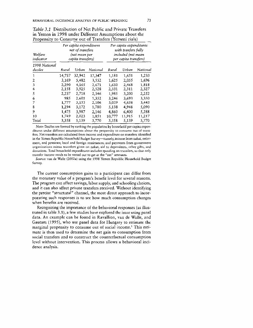
BEHAVIORAL INCIDENCE ANALYSIS OF PUBLIC SPENDING 71
Table 3.1 Distribution of Net Public and Private Transfersin Yemen in 1998 under Different Assumptions about thePropensity to Consume out of Transfers (Yemeni rials)
Per capita expenditures Per capita expenditures
net of transfers with tranfers fully
Welfare (net mean per included (net mean
indicator capita transfers) per capita transfers)
1998 Nationaldeciles Rural Urban National Rural Urban National
1 14,757 32,942 17,347 1,181 1,651 1,233
2 3,169 5,482 3,552 1,625 2,055 1,696
3 2,290 4,165 2,671 1,650 2,468 1,818
4 2,158 3,925 2,528 2,331 2,311 2,327
5 2,237 2,718 2,346 1,985 3,200 2,252
6 985 2,601 1,352 3,246 3,693 3,350
7 1,777 3,153 2,106 3,039 4,658 3,443
8 1,294 3,172 1,780 5,138 4,948 5,090
9 1,475 3,987 2,146 4,860 6,400 5,288
10 1,749 2,023 1,851 10,777 11,915 11,217
Total 3,358 5,139 3,770 3,358 5,139 3,770
Note: Deciles are formed by ranking the population by household per capita expen-
ditures under different assumptions about the propensity to consume out of trans-
fers. Net transfers are calculated from income and expenditure on transfers identified
in the Yemen Republic Household Budget Survey-namely, income from zakat, retire-
ment, and pensions; local and foreign remittances; and payments from government
organizations minus transfers given on zakat, aid to dependents, other gifts, and
donations. Total household expenditures includes spending on transfers, so that only
transfer income needs to be netted out to get at the "net" amounts.
Source: van de Walle (2002a) using the 1998 Yemen Republic Household Budget
Survey.
The current consumption gains to a participant can differ from
the monetary value of a program's benefit level for several reasons.
The program can affect savings, labor supply, and schooling choices,
and it can also affect private transfers received. Without identifying
the precise "structural" channel, the most direct approach to incor-
porating such responses is to see how much consumption changes
when benefits are received.
Recognizing the importance of the behavioral responses (as illus-
trated in table 3.1), a few studies have explored the issue using panel
data. An example can be found in Ravallion, van de Walle, and
Gautam (1995), who use panel data for Hungary to estimate the
marginal propensity to consume out of social income.' This esti-
mate is then used to determine the net gain to consumption from
social transfers and to construct the counterfactual consumption
level without intervention. This process allows a behavioral inci-
dence analysis.

72 VAN DE WALLE
In a similar vein, van de Walle (2002c) estimates the marginalpropensity to consume out of social income for Vietnam, wherehousehold surveys for 1993 and 1998 contain a panel of 4,308households. Consumption of household i at time t (t = 1993, 1998)(Ci,) is assumed to be represented as an additive function of publictransfers (Tit), observed household characteristics (Xi,), and timevarying (8t) and time invariant (Tli) latent factors:
(3.1) Ci, =a+ PTit + Xjt +n; +6, +Ej
There are a number of potential problems with estimating J with thisequation. An endogeneity concern arises if, as is likely, transfers arecorrelated with time invariant household characteristics [cov(Ti,71i)• 0], as could result from purposive targeting to the long-term poor.Endogeneity also arises if transfers are correlated with time-varyingdeterminants of consumption [cov(Tit5t) • 0 or cov(Ti,Ei,) • 0]. Thatwould occur if transfers target those who suffered a shock or simplyif transfer eligibility changes-for example, because of the death ofa pension-receiving elderly household member.
There is likely to be heterogeneity in the behavioral responseacross households. Differences in the impact of the transfers associ-ated with observable differences in the characteristics of individualscan be introduced by adding appropriate interaction effects in equa-tion 3.1, SO that it takes the form:
C; = oc + (Po + 30 X7 )T; + yX; + Ili + 6t + £;
One can also readily introduce random differences in impacts notcorrelated with the program assignment. There are also nonpara-metric methods (that do not need to postulate a parametric regres-sion equation for the outcome variable); these methods are reviewedin chapter 5. However, for the purpose of this exposition, attentionis confined to the simplest parametric model in equation 3.1.
A double differencing model, where all variables are expressed infirst differences, purges the estimate of fixed effects and thus dealswith the first source of endogeneity. Equation 3.1 becomes
AC, = IAT; + YXAX + A8, + Asi,
With only two rounds of data, the term A8, becomes an ordinaryintercept term in a regression of the change in consumption on thechange in transfers.
In the Vietnam example, this regression was initially run assum-ing that yAXit = 0 (characteristics do not change or do not have anyeffect), giving the standard "double difference" estimate of the con-sumption impact of transfers. This specification gives a ,3 estimate of0.45 with a heteroscedasticity and clustering-corrected t-statistic of4.3. A number of different regressions are run that control for time-
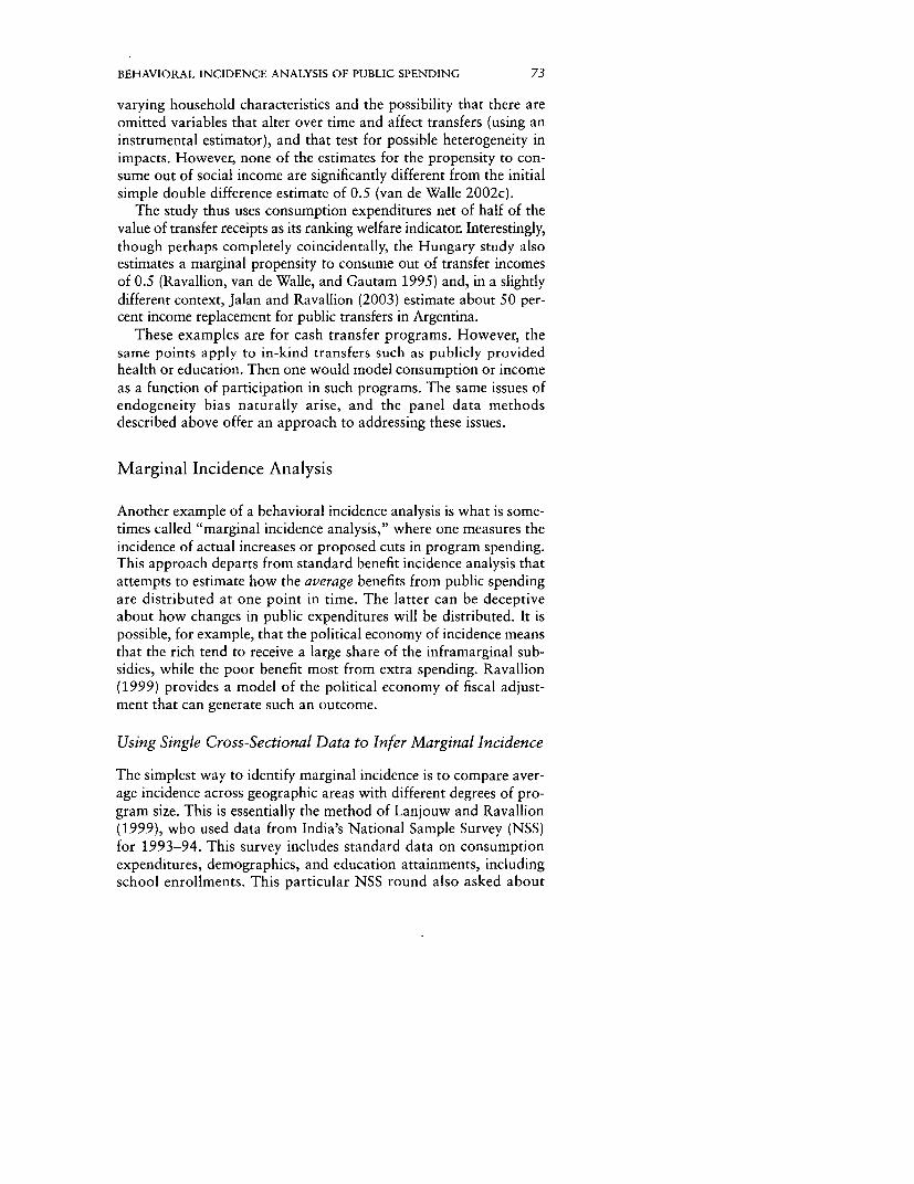
BEHAVIORAL INCIDENCE ANALYSIS OF PUBLIC SPENDING 73
varying household characteristics and the possibility that there areomitted variables that alter over time and affect transfers (using aninstrumental estimator), and that test for possible heterogeneity inimpacts. However, none of the estimates for the propensity to con-sume out of social income are significantly different from the initialsimple double difference estimate of 0.5 (van de Walle 2002c).
The study thus uses consumption expenditures net of half of thevalue of transfer receipts as its ranking welfare indicator. Interestingly,though perhaps completely coincidentally, the Hungary study alsoestimates a marginal propensity to consume out of transfer incomesof 0.5 (Ravallion, van de Walle, and Gautam 1995) and, in a slightlydifferent context, Jalan and Ravallion (2003) estimate about 50 per-cent income replacement for public transfers in Argentina.
These examples are for cash transfer programs. However, thesame points apply to in-kind transfers such as publicly providedhealth or education. Then one would model consumption or incomeas a function of participation in such programs. The same issues ofendogeneity bias naturally arise, and the panel data methodsdescribed above offer an approach to addressing these issues.
Marginal Incidence Analysis
Another example of a behavioral incidence analysis is what is some-times called "marginal incidence analysis," where one measures theincidence of actual increases or proposed cuts in program spending.This approach departs from standard benefit incidence analysis thatattempts to estimate how the average benefits from public spendingare distributed at one point in time. The latter can be deceptiveabout how changes in public expenditures will be distributed. It ispossible, for example, that the political economy of incidence meansthat the rich tend to receive a large share of the inframarginal sub-sidies, while the poor benefit most from extra spending. Ravallion(1999) provides a model of the political economy of fiscal adjust-ment that can generate such an outcome.
Using Single Cross-Sectional Data to Infer Marginal Incidence
The simplest way to identify marginal incidence is to compare aver-age incidence across geographic areas with different degrees of pro-gram size. This is essentially the method of Lanjouw and Ravallion(1999), who used data from India's National Sample Survey (NSS)for 1993-94. This survey includes standard data on consumptionexpenditures, demographics, and education attainments, includingschool enrollments. This particular NSS round also asked about

74 VAN DE WALLE
participation in three key antipoverty programs: public worksschemes, a means-tested credit scheme called the Integrated RuralDevelopment Programme, and a food-rationing scheme called thePublic Distribution System. The data on participation in these pro-grams can be collated with data on total consumption expenditureper person at the household level.
Sampled households in the NSS were ranked by total consump-tion expenditure per person normalized by state-specific povertylines. Quintiles were then defined over the entire rural population,with equal numbers of people in each. So the poorest quintile refersto the poorest 20 percent of the national rural population in terms ofconsumption per capita.2 The analysis was done at the level of theNSS region, of which there are 62 in India, spanning 19 states; eachNSS region belongs to only 1 state. So, for any given combination ofquintile and program, the participation rates across the 62 NSSregions were regressed on the average participation by state (irre-spective of quintile). The results provide estimates of the marginalincidence of participation across quintiles and indicate that expan-sion of primary schooling would be very pro-poor in contrast toaverage incidence figures that suggest the opposite. With regard tothe poverty schemes, additional spending would be significantly morepro-poor than suggested by the average incidence of participation.
Although the technique requires a cross-sectional household sur-vey only, it must contain information on program participation atthe household level and sufficient regional disaggregation and vari-ance in participation for estimation to be possible. The main con-cern with using a single cross-sectional survey is that there may beimportant state-level differences in the propensity to reach the poorthat are correlated with levels of social spending. One method forrevealing marginal incidence in a way that is more robust to latentheterogeneity in local political factors is to assess incidence at twoor more dates. This can be done using two cross-sections or paneldata (if they are available) on households or regions.
Marginal Incidence Analysis Using RepeatedCross-Sectional Data
Take the example of spending on education, and the case where twoconsecutive cross-sectional surveys are available with informationon households with children attending school in both years. Eachenrolled child is assumed to receive the same subsidy in a schoolinglevel i. The change in quantile specific participation in educationbetween the two years can then be represented by
(3.2) E,I2Ei2 -E E./Eil i= 1. 2,..

BEHAVIORAL INCIDENCE ANALYSIS OF PUBLIC SPENDING 75
where E,g is the number of children in a given level of schooling i inwelfare quantile j, at date t = 1, 2, and Ei, is total school enrollmentin that level at date t. Alternatively this can be interpreted as themarginal incidence of spending on education between the two yearswhere enrollments are multiplied by the appropriate subsidy level asin chapter 2. In the following the same simplified notation E is usedto refer to both representations. EjtIEt can be interpreted as theshare of total enrollments or education spending that goes to quan-tile j through the school attendance of its children. The expressionin equation 3.2 shows the change in each quantile's share of enroll-ments or spending. Alternatively, one might want to know the shareof a given quantile in the total change in enrollments or educationspending as given by:
(3.3) (Ej2 - E,l) / (F2 - E1)
The above approach can be applied to health care, social transfers,and other public spending programs for which participation at thehousehold or individual level can be identified and-if one wants toidentify public spending amounts-a benefit value attributed. Theimportant point is that there may be a big difference between aver-age incidence at a point in time (as indicated by Ej,/E 1 or Ej21E2and the marginal incidence defined by equation 3.2 or 3.3.
A number of studies have examined ex post marginal incidencein this way. Early examples looked at whether changes during the1980s were pro-poor for Indonesia's public health sector andMalaysia's health and education sectors (van de Walle 1994; Ham-mer, Nabi, and Cercone 1995, respectively) and found that theywere. Another study looked at the changing incidence of cash trans-fers in Hungary (van de Walle, Ravallion, and Gautam 1994). Amore recent example includes Younger (2001, 2002) for Peru.
The method has limitations. Simple comparisons of incidence atdifferent points in time do not reveal which factors are responsiblefor marginal incidence patterns. For example, a key question is oftento what degree government policy, as opposed to income growth,can be credited with improvements in equity. The Malaysia study(Hammer, Nabi, and Cercone 1995) supplements the incidenceanalysis with more detailed analysis of the underlying mechanisms.Success in the education sector is attributed to the government's pol-icy of ethnic targeting, while pro-poor improvements in the healthsector are attributable to the private sector's increasing ability toattract wealthier households. Another limitation is that when thedistribution of the underlying population alters between periods-due, for example, to urbanization-the technique is unable to dis-aggregate incidence results over time geographically, informationthat is typically of interest.

76 VAN DE WALLE
In implementing ex post marginal incidence analysis, an issuearises concerning the definition of the quantiles j. Is it changes in theamount going to the relatively poor or to the absolute poor that isof interest? The two could be quite different depending on howabsolute poverty is changing. Some studies simply define quantilesspecific to each date, so that they are not strictly comparable. Thisapproach helps answer questions concerning changes in incidencefor, say, the bottom 20 percent of the population at any one date.But often the interest is in how the amounts received, conditional onreal income, have changed. Then one would want to fix the cutoffboundaries in real income space rather than in relative income space.When a panel is used to study the incidence of the changes in socialspending, households can be ranked by three different definitions ofwelfare, which can be loosely viewed as delineating the initial, new,and long-term poor-namely, the welfare indicator in the initialperiod, the welfare indicator in the later period, and the mean overboth years (see table 3.2 for an example of the first two).
Marginal Incidence Analysis Using Panel Data
Two studies have explored the dynamic marginal impacts of publicexpenditures using ex post benefit incidence with data that followthe same households over time. Using a panel of Hungarian house-holds for 1987 through 1989, Ravallion, van de Walle, and Gautam(1995) devise a methodology to examine how well the social safetynet protected vulnerable households from falling into poverty ver-sus how well it promoted households out of poverty. The essentialidea is to simulate a counterfactual joint distribution of the welfareindicator over time without the change in transfers, using econo-metric methods similar to those described above.
Similar techniques were used in a study of the safety net in Viet-nam (van de Walle 2002b). Poverty fell quite dramatically in Viet-nam, and there was a clear expansion in the total outlays going tosocial welfare programs between 1993 and 1998. These events pro-vide an interesting backdrop for a number of questions concerningmarginal incidence: Was the expansion pro-poor? What role didtransfer programs play in the reduction in poverty? Does therevealed instability over time in who gets transfers reflect the sys-tem's response to changing household circumstances?
An important role for the public sector in a poor rural economylike Vietnam is to provide protection for those who are vulnerableto poverty due to uninsured shocks. The typical incidence picture isuninformative about whether transfers perform such a safety netfunction. The static average incidence may not seem particularlywell targeted, but it may be deceptive about the degree to which

BEHAVIORAL INCIDENCE ANALYSIS OF PUBLIC SPENDING 77
Table 3.2 Distribution of Social Transfer Incomein Vietnam (percent)
Share of Share of Share of total transfer
Net quintiles 1993 transfers 1998 transfers increase 1993-98
19931 13.3 13.1 12.8
2 15.2 15.5 15.73 16.9 17.5 17.94 21.2 22.4 23.4
5 33.3 31.6 30.2
Total 100.0 100.0 100.0
19981 15.3 15.7 16.02 14.0 15.4 16.63 20.5 19.6 18.9
4 19.8 19.9 20.0
5 30.4 29.3 28.5Total 100.0 100.0 100.0
Note: National population quintiles are constructed using per capita expendituresnet of half of social transfers.
Sources: 1993 and 1998 Vietnam Living Standards Survey.
outlays, coverage, and changes over time were perhaps correlated to
poverty-related shocks and changes in exogenous variables.Table 3.2 ranks households by two definitions of welfare as dis-
cussed above-namely, per capita expenditures (net of half of trans-fers) in the initial period and the same welfare indicator in the later
period-and presents a comparison of the average incidence of socialincome receipts in both years and the marginal incidence of thespending increase. The former is expressed as the percent of total
social income going to each quintile, while the latter is given by thepercent of the total increase going to each group. In this particularcase, little difference is found between the average and marginal inci-
dences for either definition of welfare. Expansion was more or lessproportional to base-year receipts across groups. The evidence does
not suggest that the poor were specifically targeted by the programexpansion.
Were changes in transfers responsive to poverty-related shocks?
Table 3.3 presents information on mean changes in transfersreceived by panel households classified into a three-by-three matrix.Households ranked into terciles of their initial 1993 level of per
capita consumption (low, middle, or high) are cross-tabbed againstthe change in their consumption between the two dates categorizedby whether consumption fell, stayed more or less the same, or rose

78 VAN DE WALLE
Table 3.3 The Incidence of Changes in Transfers by InitialConsumption and Changes in Consumption over TimeInitial Fall in Consumption Large rise inconsumption consumption stayed the same consumption
LowPercent receiving 34 27 27
transfersPer capita change, 111,901 246,476 241,658
Vietnamese dongNumber of 80 506 848
households
MiddlePercent receiving 32 30 30transfers
Per capita change, 408,469 251,619 296,513Vietnamese dong
Number of 240 422 772households
HighPercent receiving 33 36 32
transfersPer capita change, 481,618 343,329 367,991
Vietnamese dongNumber of 496 221 720
households
Note: The population is ranked into three equal groups based on 1993 per capitaexpenditures net of half of transfers and cross-tabbed against the level of their changein consumption over time net of half the change in transfers. The first number givesthe percentage of households in the cell that received transfers in 1998. The secondnumber gives the per capita amount, in Vietnamese dong, of the change in transfersreceived by those with positive receipts only. The final number gives the number ofhouseholds in the cell. Changes in transfers refer to changes in amounts receivedfrom social insurance, social subsidies, and school scholarships.
Source: van de Walle (2002b) using the 1993 and 1998 Vietnam Living StandardsSurvey.
significantly. The results strongly suggest that the programs wereunresponsive to consumption shocks. Neither starting out poor norexperiencing negative consumption shocks appear to have elicited aresponse from social welfare programs.
The study also examines the role transfers played in the impres-sive reduction in poverty that occurred over this period. The panelstructure is exploited to evaluate how well the safety net performeddynamically following the approach proposed in Ravallion, van deWalle, and Gautam (1995). In comparing joint distributions of con-

BEHAVIORAL INCIDENCE ANALYSIS OF PUBLIC SPENDING 79
sumption expenditures, such as with and without policy changes, theapproach tests a policy's ability to protect the poor (PROT) and itsability to promote the poor (PROM). It indicates which distribution
offered more protection and which offered more promotion and
allows a calculation of the statistical significance of the difference.The baseline joint distribution of consumption in the two years is
presented in table 3.4. Households are classified into four groups
according to whether they were poor or nonpoor in both years, andwhether they escaped or fell into poverty over the period. There isevidence both of a large drop in poverty and of considerable persis-
tent poverty.What was the effect of transfers on poverty? To answer this ques-
tion, it is necessary to simulate the counterfactual joint distribution
without transfers; as in the static incidence calculations, this is doneby subtracting half the transfers received in each respective yearfrom consumption in that year. Table 3.5 shows that transfers have
negligible impact on poverty. Without them, an additional 1 and 2percent of the population would have been poor in 1993 and 1998,respectively. Neither the degree of promotion or protection is statis-
tically different from zero.One can also assess the impact of changes in transfers between
the two dates by simulating the joint distribution had there been nochanges. Alternatively one could compare the current distributionrelative to a simulated uniform allocation of actual 1998 socialincome across the entire population to see if better targeting could
have improved impacts on poverty incidence. A number of targetingscenarios can be tested.
Table 3.4 The Baseline Discrete Joint Distribution (percent)
1998
1993 Poor Nonpoor Total
Poor 33.54 26.58 60.12(55.78) (44.22) 100
Nonpoor 4.84 35.04 39.88(12.14) (87.86) 100
Total 38.38 61.62 100
Note: The population is ranked into poor and nonpoor groups based on actual
per capita expenditures at each date and cross-tabbed. The first number in each cellgives the percentage of total population who were in that row's poverty group in1993 and that column's group in 1998. Numbers in parentheses give the proportion
of each row's population that is in each column's group in 1998, or the transition
probability.Source: van de Walle (2002b) using the 1993 and 1998 Vietnam Living Standards
Survey.
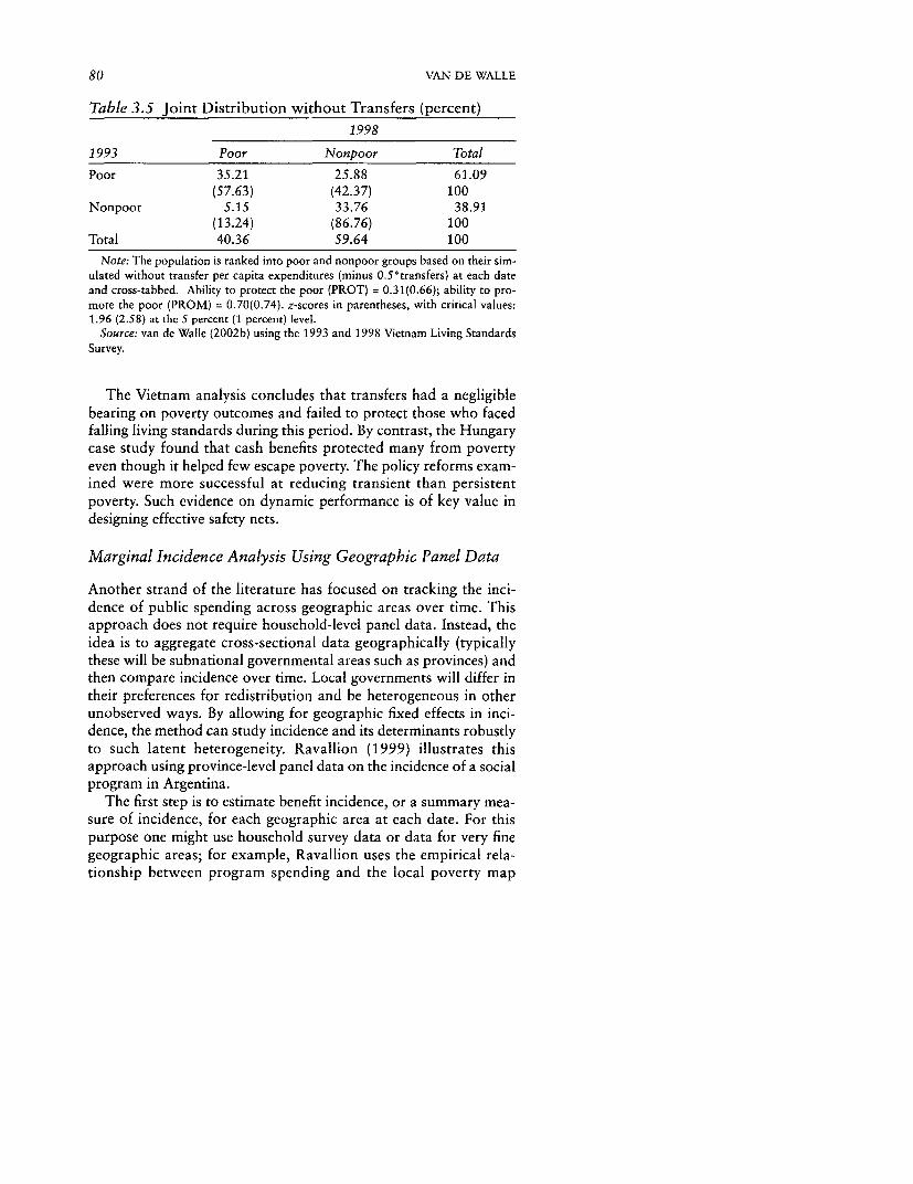
80 VAN DE WALLE
Table 3.5 Joint Distribution without Transfers (percent)
1998
1993 Poor Nonpoor Total
Poor 35.21 25.88 61.09(57.63) (42.37) 100
Nonpoor 5.15 33.76 38.91(13.24) (86.76) 100
Total 40.36 59.64 100
Note: The population is ranked into poor and nonpoor groups based on their sim-ulated without transfer per capita expenditures (minus 0.5Ptransfers) at each dateand cross-tabbed. Ability to protect the poor (PROT) = 0.31(0.66); ability to pro-mote the poor (PROM) = 0.70(0.74). z-scores in parentheses, with critical values:1.96 (2.58) at the 5 percent (1 percent) level.
Source: van de Walle (2002b) using the 1993 and 1998 Vietnam Living StandardsSurvey.
The Vietnam analysis concludes that transfers had a negligiblebearing on poverty outcomes and failed to protect those who facedfalling living standards during this period. By contrast, the Hungarycase study found that cash benefits protected many from povertyeven though it helped few escape poverty. The policy reforms exam-ined were more successful at reducing transient than persistentpoverty. Such evidence on dynamic performance is of key value indesigning effective safety nets.
Marginal Incidence Analysis Using Geographic Panel Data
Another strand of the literature has focused on tracking the inci-dence of public spending across geographic areas over time. Thisapproach does not require household-level panel data. Instead, theidea is to aggregate cross-sectional data geographically (typicallythese will be subnational governmental areas such as provinces) andthen compare incidence over time. Local governments will differ intheir preferences for redistribution and be heterogeneous in otherunobserved ways. By allowing for geographic fixed effects in inci-dence, the method can study incidence and its determinants robustlyto such latent heterogeneity. Ravallion (1999) illustrates thisapproach using province-level panel data on the incidence of a socialprogram in Argentina.
The first step is to estimate benefit incidence, or a summary mea-sure of incidence, for each geographic area at each date. For thispurpose one might use household survey data or data for very finegeographic areas; for example, Ravallion uses the empirical rela-tionship between program spending and the local poverty map

BEHAVIORAL INCIDENCE ANALYSIS OF PUBLIC SPENDING 81
across local government areas ("departments") within each provinceof Argentina. The poverty map uses the percent of households withunmet basic needs at departmental level based on census data. Thespatial variances in both spending and poverty incidence withineach province are exploited to measure targeting performance.
This estimation entails running an OLS regression for eachprovince of spending allocations across departments against povertyincidence. The regression coefficient gives a "targeting differential"interpretable as the mean difference in spending between the poorand nonpoor (Ravallion 2000). This regression is done for all datesfor which spending allocations are available. Thus a panel can beformed of these targeting differentials by provinces and over time.
Next the province- and date-specific targeting differentials areregressed on per capita spending allocations to the provinces in aregression that pools all dates and provinces and includes a provincefixed effect to capture province-specific factors that affect targeting.This estimation allows one to see what happens to targeting perfor-mance during program expansions and cutbacks. Ravallion (1999)finds that during a retrenchment period in Argentina's Trabajar pro-gram, a $1 cut in average spending reduced the targeting differentialby $3.55 on average. Hence, cuts were accompanied by worseningtargeting performance.
Conclusions
Ignoring behavioral responses to public spending or social programscan yield deceptive assessments of incidence because one does notcorrectly assign beneficiaries to the pre-intervention distribution.For example, by subtracting the full amount of a transfer received,one overestimates how poor beneficiaries will have been in theabsence of the intervention. Similarly, if one ignores the influence ofthe political economy on the assignment of beneficiaries and theincidence of program spending allocations, one can arrive at severelybiased estimates of impacts and hence incidence.
This chapter has reviewed some relatively simple methods thatcan help address these deficiencies of nonbehavioral incidence analy-sis. There is a large literature on reduced-form regression-basedmethods in which one essentially regresses the relevant outcomemeasure (income, for example) on program allocations with rele-vant controls. With household panel data one can exploit changesin program spending over time to obtain estimates that are robust topotential endogeneity of the program assignment across units (pro-vided the endogeneity is fully reflected in time-invariant factors).

82 VAN DE WALLE
These methods can be made more sophisticated, such as by incor-porating heterogeneity in impacts and allowing for more complexforms of endogeneity in program assignments or spending levels.Once one knows the impact on incomes, one can then work outwhat the income or other welfare indicator of program participantswould have been in the absence of the intervention and so estimatethe incidence of spending relative to that counterfactual.
Marginal benefit incidence analysis is another important exampleof how behavioral responses through the political economy of inci-dence can be incorporated. It can provide valuable information forcharting the course of pro-poor reforms in public spending. Themethod can be implemented using a single cross-sectional survey,but access to two or more consecutive household cross-sectionalsurveys with information on program participation usually providesestimates that are more robust. Household or regional panel dataallow an even richer analysis of policy and spending changes. Byexamining actual changes ex post, these methods provide a realitycheck for the results of methods that attempt to approximate or pre-dict reality ex ante.
Notes
1. The marginal propensity to consume out of social income can also beestimated using regression methods on a cross-section, but depending onhow well one can control for heterogeneity, the results are likely to bebiased by omitted variables. With a uniform benefit level, a third approachis to use propensity-score matching with a single difference estimator (as inJalan and Ravallion 2003). The advantage of the latter is that a model orstructure does not need to be imposed.
2. Note that, although this study does not allow for behavioral responseson the part of individuals and households in determining the welfare rank-ing indicator as above, there is nothing that prevents it from doing so.
References
The word processed describes informally reproduced works that may notbe commonly available through library systems.
Hammer, Jeffrey, Ijaz Nabi, and James Cercone. 1995. "Distributional Effectsof Social Sector Expenditures in Malaysia, 1974 to 1989." In Dominiquevan de Walle and Kimberly Nead, eds., Public Spending and the Poor:Theory and Evidence. Baltimore: Johns Hopkins University Press.

BEHAVIORAL INCIDENCE ANALYSIS OF PUBLIC SPENDING 83
Jalan, Jyotsna, and Martin Ravallion. 2003. "Estimating the Benefit Inci-
dence of an Antipoverty Program by Propensity Score Matching." Jour-
nal of Business and Economic Statistics 21(1): 19-30.Lanjouw, Peter, and Martin Ravallion. 1999. "Benefit Incidence, Public
Spending Reforms, and the Timing of Program Capture." World Bank
Economic Review 13(2): 257-74.Ravallion, Martin. 1999. "Is More Targeting Consistent with Less Spend-
ing?" International Tax and Public Finance 6: 411-19.
. 2000. "Monitoring Targeting Performance When DecentralizedAllocations to the Poor Are Unobserved." World Bank EconomicReview 14(2): 331-45.
Ravallion, Martin, Dominique van de Walle, and Madhur Gautam. 1995."Testing a Social Safety Net." Journal of Public Economics 57: 175-99.
van de Walle, Dominique. 1994. "The Distribution of Subsidies throughPublic Health Services in Indonesia 1978-87." World Bank EconomicReview 8(2): 279-309.
. 2002a. "Poverty and Transfers in Yemen." Middle East and NorthAfrica Working Paper Series 30. World Bank, Office of the Chief Econo-mist, Middle East and North Africa Region, Washington, D.C. Processed.
- . 2002b. "The Static and Dynamic Incidence of Viet Nam's PublicSafety Net." Policy Research Working Paper 2791. World Bank, Devel-opment Research Group, Washington, D.C. Processed.
- 2002c. "Viet Nam's Safety Net: Protection and Promotion fromPoverty?" World Bank, Development Research Group, Washington,D.C. Processed.
van de Walle, Dominique, Martin Ravallion, and Madhur Gautam. 1994."How Well Does the Social Safety Net Work? The Incidence of CashBenefits in Hungary 1987-89." Living Standards Measurement StudyWorking Paper 102. World Bank, Washington, D.C.
Younger, Stephen D. 2001. "Benefits on the Margin." Cornell University,Department of Economics, Ithaca, N.Y. Processed.
- 2002. "Public Social Sector Expenditures and Poverty in Peru." InChristian Morrisson, ed., Education and Health Expenditure, and Devel-opment: The Cases of Indonesia and Peru. Paris: Organisation for Eco-nomic Co-operation and Development, Development Center Studies.


4
Estimating GeographicallyDisaggregated Welfare
Levels and Changes
Peter Lanjouw
Welfare levels tend to vary among the regions of almost every coun-try of the world. Poverty is rarely distributed evenly within a coun-try; particularly in the developing world, where pockets of severedeprivation are no rare occurrence. The existence of such poor areascan result from differences in geographic capital-biophysicalendowment, access to infrastructure and markets, and so forth-aswell as from government policies, such as migration policies or thedistribution of centrally allocated resources.
In the face of such geographic heterogeneity, successful policy-making requires a good information base. For instance, an under-standing of poverty and inequality levels at detailed spatial scales isa prerequisite for fine geographic targeting of interventions aimed atimproving welfare levels. Decentralization in many countries hasmeant that decisionmaking for poverty alleviation programs is shift-ing from central government to regional or local levels. However,local decisionmaking, the design of the decentralization processes,and even the decision whether to pursue further decentralizationshould be based on reliable, locally relevant information on livingstandards and the distribution of wealth. In most countries suchinformation is not readily at hand.
85

86 LANJOUW
The problem of a lack of locally relevant poverty information iswell known. Two main types of welfare-related information sourcesare available to policymakers. Household surveys often include adetailed income or consumption expenditure module, or both. How-ever, because of relatively small sample size, the collected informa-tion is usually representative only for broad regions of the country.Census data (and sometimes large household sample surveys) areavailable for all households (or very large samples of households)and can provide reliable estimates at highly disaggregated levelssuch as small municipalities, towns, and villages. But censuses donot contain the income or consumption information necessary toyield reliable indicators of the level and distribution of welfare suchas poverty rates or inequality measures.
Recent research has explored a technique that addresses the prob-lem of lack of local data on poverty and inequality.' This methodcombines survey and census data to estimate consumption-basedwelfare indicators for small geographic areas such as districts andsubdistricts, that is, a poverty map. Testing of the method usingdata for a growing number of developing countries indicates thatstatistically reliable estimates of poverty and inequality are attain-able at encouragingly fine levels of spatial detail.
This research is closely related to the literature on small area sta-tistics, which is also concerned with deriving estimators of populationparameters at disaggregated levels using multiple data sources (forsurveys, see Ghosh and Rao 1994 and Rao 1999). Empirical Bayesand best linear unbiased prediction models have been used to estimatethe relationship between observables and a variable of interest at theunit record level. Together with the distribution of population covari-ates, these models are used to construct a "synthetic" estimator of anunobserved population parameter-a total, a mean, or more recently,proportions (see, for example, Malec, Davis, and Cao 1999). Thesynthetic estimator is typically used to "give strength" to a direct,sample-based estimator for the target area by lowering its variance.The current research extends this literature by developing estimatorsof population parameters that are nonlinear functions of the under-lying variable of interest (unit-level consumption or income) and thatderive from the full unit-level distribution of that variable. Followingthrough on this extension leads naturally to the consideration ofsemi-parametric techniques for calculating synthetic estimates, as isdone here. Finally, the focus of the attention here is almost entirelyon areas where no direct sample information is available.
Data sets have been combined to fill in missing information oravoid sampling biases in a variety of other contexts. Examples in the

ESTIMATING GEOGRAPHICALLY DISAGGREGATED WELFARE 87
econometric literature include Arellano and Meghir (1992), whoestimate a labor supply model combining two samples. They use theU.K. Family Expenditure Survey to estimate models of wages andother income conditioning on variables common across the twosamples. Hours and job search information from the much largerLabour Force Survey is then supplemented by predicted financialinformation. In a similar spirit, Angrist and Krueger (1992) com-bine data from two U.S. censuses. They estimate a model of educa-tional attainment as a function of school entry age, where the firstvariable is available in only one census and the second in another,but an instrument, birth quarter, is common to both. Lusardi (1996)applies this two-sample instrumental variable estimator in a modelof consumption behavior. Hellerstein and Imbens (1999) estimateweighted wage regressions using the U.S. National LongitudinalSurvey but incorporate aggregate information from the U.S. censusby constructing weights that force moments in the weighted sampleto match those in the census.
The method described in this chapter combines household andcensus data using statistical procedures aimed at taking advantage ofthe detailed information available in household sample surveys andthe comprehensive coverage of a census. Using a household survey toimpute missing information in the census, poverty and inequality areestimated (as opposed to directly measured) at a disaggregated levelbased on a household per capita measure of expenditure, Yhb Theidea is straightforward. First a model of Yh iS estimated using thesample survey data, restricting explanatory variables to those thatcan be observed and linked to households in both sets of data. Then,letting W represent an indicator of poverty or inequality in somelocality, the expected level of W is estimated given the census-basedobservable characteristics of the population of interest using para-meter estimates from the "first-stage" model of y.
Progress to date has been encouraging and has prompted theimplementation of the method in a growing number of developingcountries. In addition exploration of extensions of the poverty map-ping methodology is moving forward along a variety fronts. Elbersand others (2002a) apply the methodology to two household sur-veys, rather than a household survey and census, so as to imputeinto one survey a welfare indicator from another. Mistiaen (2002)explores the feasibility of applying poverty mapping techniques toevaluate geographic distribution of the impact on poverty of policyreforms. Efforts are also currently underway to explore the feasibil-ity of producing "maps" expressed in terms of alternative notions ofwelfare (nutritional status, health).

88 LANJOUW
Box 4.1 The Basic Steps of Poverty Mapping:An Overview
The poverty map methodology involves detailed analysis of two mainsoturces of data: a household survey, and the population censtus. In thefirst stage of the analysis, the tvo data sources are subjected to veryclose scrutiny with an eye toward identifying a set of conunon vari-ables. In the second stage, the survey is used to develop a series of sta-tistical models that relate per capita consumption to the set of com-mon variables identified in the preceding step. In the final stage of theanalysis, the parameter estimates from the previous stage are appliedto the population census and used to predict consumption for eachhousehold in the population census. Once such a predicted consLMp-tion measure is available for each household in the census, summarymeasures of poverty (or inequality) can be estimated for a set of house-holds in the census. Statistical tests can be performed to assess the reli-ability of the poverty estimates that have been produced. If the esti-mates are judged not to be sufficiently reliable, it may be necessary toreturn to the first stage for further experimentation with the modelspecification. Alternatively, it may be necessary to increase the num-ber of households over which the poverty measure is estimated (issuesof statistical reliability will guide whether the poverty map can be reli-ably produced at the region, district, or subdistrict level).
The three stages of analysis occur in sequence. The work involvedin these stages is distinct, but the outputs of the first two stages areeach key inputs into the subsequent stage. If the first stage cannot besatisfactorily carried out (for example, because of problems with thedata), there is no point in continuing on to the second stage. And sin-ilarly, if the statistical models of the second stage are not satisfactory,there is no point in continuing on to the third stage. The poverty mapexercise thus requires that progress be periodically assessed and eval-uated. One cannot rule out the possibility that the exercise may needto be abandoned before it is completed.
The First Stage
The first stage in the poverty mapping exercise involves a ratherpainstaking comparison of common variables across the householdsurvey and the population census. The idea here is to identify vari-ables at the household level that are defined in the same way in boththe household survey and the census. It is important that this commonsubset of variables be defined in exactly the same way across the twodata sources. The only way to check this is to look at means and per-centiles for each of the variables in both data sources and ensure thatin terms of these means and percentiles the variables are virtuallyidentical across the data sources. One can make this check rigorously,on the basis of statistical tests of differences, or informally, by simplymaking visual comparisons.

ESTIMATING GEOGRAPHICALLY DISAGGREGATED WELFARE 89
A concurrent exercise that can be carried out in parallel to the exer-cise described above is the compilation of a database at a level of aggre-gation higher than the household, which can be inserted into the house-hold level census and the household survey databases. One of themethodological concerns in the poverty mapping exercise is that thecommon pool of household variables will not suffice to capture unob-served geographic effects, such as agroclimatic conditions or quality oflocal government administration, which might still be very importantin predicting household-level consumption. In an effort to proxy theseunobserved factors, it is useful to merge, say, district or subdistrict datathat have been compiled separately into both the census and the house-hold survey. These subdistrict data may comprise a wide range of vari-ables (for example, construction of schools, public spending figures,infrastructure availability, and population estimates).
The Second Stage
Assuming that the two tasks described above yield a good and reason-ably large set of common household-level variables, supplemented by aseries of additional variables at a slightly higher level of disaggregation,the decision can then be made to proceed to the second-stage analysis.This stage involves the econometric estimation of models of consump-tion on the set of household-level and community variables. Most likely,a different model will be estimated for each stratum in the householdsurvey data set, possibly separately for rural and urban areas. A largenumber of diagnostic tests need to be carried out, and a large numberof different specifications are likely to be experimented with. It is possi-ble that there will be a need to return to the zero-stage analysis to ver-ify the construction of certain variables, to transform some variables, orto seek ways to add to the set of available regressors.
The Third Stage
Successsful completion of the second-stage analysis permits one totake the parameter estimates and attendent statistical outputs to thethird stage. This stage is associated with the imputation of consump-tion into the census data at the household level and the estimation ofpoverty and inequality measures at a variety of levels of spatial disag-gregation. Software has been developed that allows this phase of thework to be carried out mechanically
Once the poverty map exercise has been completed for all regionsin the country, the resulting databases that provide estimates ofpoverty and inequality (and their standard errors) at a variety of lev-els of geographic disaggregation can be projected onto geographicmaps using GIS (Geographic Information Systems) mapping tech-niques. This involves the application of GIS software (such asARCView), which merges information on the geographic coordinatesof localities such as the district or subdistrict with the poverty andinequality estimates produced by the poverty mapping methodology.

90 LANJOUW
The Technique
Survey data are first used to estimate a prediction model for con-sumption, and then the parameter estimates are applied to the cen-sus data to derive poverty statistics. A key assumption of themethodology is thus that the models estimated from the survey dataapply to census observations. This assumption is most reasonable ifthe survey and census years coincide. In this case, simple checks canbe conducted by comparing the estimates to basic poverty orinequality statistics in the sample data. If different years are usedbut the assumption is considered reasonable, then the welfare esti-mates obtained refer to the census year, whose explanatory vari-ables form the basis of the predicted expenditure distribution.
An important feature of the approach applied here involves theexplicit recognition that the poverty or inequality statistics esti-mated using a model of income or consumption are statisticallyimprecise. Standard errors must be calculated. The following sub-sections briefly summarize the discussion in Elbers, Lanjouw, andLanjouw (2002, 2003).
Definitions
Per capita household expenditure, Yb, is related to a set of observ-able characteristics, xb:2
In yb = E(ln Yh l Xh ) + Uh
Using a linear approximation, the observed log per capita expendi-ture for household h is modeled as:
(4.1) lnyb = Xh X+Uh
where 3 is a vector of parameters and uh is a disturbance term satis-fying E(uh I Xb) = 0. In applications we allow for location effects andheteroskedasticity in the distribution of the disturbances.3
The model in equation 4.1 is estimated using the household sur-vey data. We are interested in using these estimates to calculate thewelfare of an area or group for which there is no, or insufficient,expenditure information. Although the disaggregation may be alongany dimension-not necessarily geographic-the target populationis referred to as a "county." Household h has mb family members.Although the unit of observation for expenditure is the household,we are more often interested in welfare measures based on individ-uals. Thus we write W (m, X, 3, u), where m is a vector of house-hold sizes, X is a matrix of observable characteristics, and u is a vec-

ESTIMATING GEOGRAPHICALLY DISAGGREGATED WELFARE 91
tor of disturbances. Because the disturbances for households in thetarget population are always unknown, the expected value of theindicator is estimated given the census households' observable char-acteristics and the model of expenditure in equation 4.1.4 Thisexpectation is denoted as p = E(W I m, X, ,), where , is the vectorof all model parameters, including not only the coefficients 3, butalso the parameters describing the variance and the heteroskedastic-ity of the disturbance terms. In constructing an estimator of p, theunknown vector 4 is replaced with consistent estimators, 4, from thefirst-stage expenditure regression. This yields A = E(W I m, X, 4).This expectation is generally analytically intractable, so MonteCarlo simulation is used to obtain the estimator, p.
Estimating Error Components
The difference between p, the estimator of the expected value of Wfor the county, and the actual level of welfare for the county may bewritten:
W - = (W - p) + (P - p) + (A + p)
Thus the prediction error has three components: the first resultingfrom the presence of a disturbance term in the first-stage model thatimplies that households' actual expenditures deviate from theirexpected values (idiosyncratic error); the second resulting from vari-ance in the first-stage estimates of the parameters of the expendituremodel (model error); and the third resulting from using an inexactmethod to compute p (computation error).5
* Idiosyncratic Error. The variance in the estimator resultingfrom idiosyncratic error falls approximately proportionately in thenumber of households in the county. That is, the smaller the targetpopulation, the greater is this component of the prediction error,and there is thus a practical limit to the degree of disaggregationpossible. At what population size this error becomes unacceptablylarge depends on the explanatory power of the expenditure modeland, correspondingly, the importance of the remaining idiosyncraticcomponent of the expenditure.
* Model Error. The part of the variance attributable to modelerror is determined by the properties of the first-stage estimators.Therefore model error does not increase or fall systematically asthe size of the target population changes. Its magnitude dependson the precision of the first-stage coefficients and the sensitivity ofthe indicator to deviations in household expenditure. For a givencounty its magnitude will also depend on the distance of the

92 LANJOUW
Table 4.1 Estimated Poverty Incidence in Ecuador, 1990
Number of households
Estimates 100 1,000 15,000 100,000
Headcount 0.46 0.50 0.51 0.51Standard error 0.067 0.039 0.024 0.024Idiosyncratic variance/
total variance (%) 75 25 4 2
Source: Elbers, Lanjouw, and Lanjouw (2002).
explanatory variables for households in that county from the lev-els of those variables in the sample data.
o Computation Error. The variance in the estimator attributableto computation error depends on the method of computation usedand can be made as small as desired with sufficient resources.
The relationship between precision of the poverty estimates andthe population size of the locality for which the estimate is beingproduced can be readily observed it table 4.1. The table estimatesthe incidence of poverty in four populations (constructed out of ran-dom draws from the 1990 census population of the rural coastalregion of Ecuador) comprising, respectively, 100, 1,000, 15,000,and 100,000 households. The estimated incidence of poverty inthese four populations is identical (by construction), but the preci-sion of the estimate improves sharply as the population increases insize. This pattern arises from the relationship between populationsize and idiosyncratic error, described above. In the smallest popu-lation, the idiosyncratic error accounts for about 75 percent of thetotal variance around the poverty estimate (which corresponds to astandard error of 6.7 percentage points). As the population increasesin size from 100 to 1,000, the overall standard error declinesmarkedly, and the contribution attributable to the idiosyncraticerror also declines sharply. When the population is as large as100,000 households, the idiosyncratic error has virtually declinedto zero, and the overall standard error is effectively composed onlyof model error.6
An Example: Public Health Spending and theGeography of Poverty in Madagascar
Figure 4.1 presents two maps of Madagascar. The first depicts thespatial distribution of public spending on (nonsalary) health spending

ESTIMATING GEOGRAPHICALLY DISAGGREGATED WELFARE 93
Figure 4.1 Health Spending and Poverty in Madagascar
Madagascar: Per capita Madagascar: Incidence ofhealth spending per district poverty per district
m 468 - 1,707.2 a 0.191 - 0.566E: 1,707.2 - 2,216.1 0.566 - 0.6962 2,216.1 - 2,639.2 * 0.696 - 0.766
M 2,639.2 - 4,040.8 M 0.766 - 0.833
M 4,040.8 - 13,777.3 M . - 0.833 - 0.946
j / / _
- w1"4 ~ ~ ~ ~ ~ ~ ~ "
Notes: Health spending refers to per capita nonirecurrent public expenditures in
2000 Malagasi francs (US$1 is approximately FMG 6,000). Poverty data are for
1993, the year of the last population census.Souirce: Galasso (2002).
by district (fivondrona) in 2000. The second depicts the fivondrona-level poverty map of Madagascar in 1993, the year of the most recentpopulation census (Mistiaen and others 2002). Mistiaen and others(2002) demonstrate that predicted poverty measures in Madagascar's111 fivondronas are generally estimated with levels of precision thatare comparable to province-level estimates in the household survey.The gain from implementing this methodology is thus an increase indisaggregation from six provinces to 111 fivondronas without incur-ring any penalty in terms of precision.7

94 LANJOUW
Experience: Some Case Studies
Poverty mapping techniques are being applied in a rapidly growingnumber of countries. These exercises are yielding valuable newinsights into the geographic distribution of poverty and inequalitywithin countries. The basic methodology is also proving to be quiteflexible and can be readily extended and applied to other policy-relevant questions.
The Spatial Distribution of Poverty
A recent paper by Demombynes and others (forthcoming) takesthree developing countries, Ecuador, Madagascar, and South Africa,and implements the poverty mapping methodology in each to pro-duce estimates of poverty at a level of disaggregation that to datehas not generally been available. The countries are very unlike eachother-with different geographies, stages of development, qualityand types of data, and so on. Nonetheless the paper demonstratesthat the methodology works well in all three settings and can pro-duce valuable information about the spatial distribution of povertywithin those countries that was previously not known.
The paper demonstrates that the poverty estimates producedfrom census data are plausible in that they match well the estimatescalculated directly from the country's surveys (at levels of disaggre-gation that the survey can bear). The precision of the poverty esti-mates produced with this methodology varies with the degree of dis-aggregation. In all three countries considered, the method yieldssatisfactorily precise estimates of poverty at levels of disaggregationfar below that allowed by surveys.
The paper illustrates how the poverty estimates produced withthis method can be represented in maps, thereby conveying an enor-mous amount of information about the spread and relative magni-tude of poverty across localities, as well as about the precision ofestimates, in a way that is quickly and intuitively absorbed also bynontechnical audiences. Such detailed geographical profiles ofpoverty can inform a wide variety of debates and deliberations,among policymakers as well as civil society.
Finally, the paper notes that perceptions about the importance ofgeographical dimensions of poverty are themselves a function of thedegree of spatial disaggregation of available estimates of poverty.The smaller the localities into which a country can be broken down,the more likely one will conclude that geography matters.

ESTIMATING GEOGRAPHICALLY DISAGGREGATED WELFARE 95
The Spatial Distribution of Inequality
A paper by Elbers and others (2002b) implements the poverty map-ping methodology to produce disaggregated estimates of inequalityin Ecuador, Madagascar, and Mozambique. Just as Demombynesand others (forthcoming) show for poverty, the paper demonstratesthat inequality estimates produced from census data match well theestimates calculated directly from the country's surveys (at levels ofdisaggregation that the survey can bear). Again, in all three coun-tries considered, the inequality estimators allow one to work at alevel of disaggregation far below that allowed by surveys.
Interest among policymakers regarding local distributional out-comes has risen in recent years with the growing recognition thatcommunity-level income inequality can influence the extent andnature of capture of local government by local elites and therebyaffect the impact of decentralization initiatives (Bardhan 2002).Similarly, in a recent review of experience with community-drivendevelopment, Mansuri and Rao (2003) suggest that community-based targeting (whereby communities are asked to assist in the tar-geting of the poor within their communities) may be hampered byhigh levels of heterogeneity in living standards within those com-munities. In the study by Elbers and others (2002b), inequality inEcuador, Madagascar, and Mozambique is decomposed into pro-gressively more disaggregated spatial units, and even at a very highlevel of spatial disaggregation the contribution to overall inequalityof within-community inequality is found to be very high (75 percentor more). This finding illustrates the danger of simply assuming thatliving standards at the local level are more equally distributed thanat the national level. However, it is also shown that a high within-group decomposition result does not suffice to indicate that all com-munities in a given country are as unequal as the country as a whole.The paper shows that in all three countries examined, the amount ofvariation in inequality across communities is considerable. Manycommunities are rather more equal than their respective country asa whole, but many communities are not, and some may even beconsiderably more unequal. These findings may have importantimplications for the design of decentralized financing, for the designand implementation of policies, and for the success of community-driven development initiatives.
Given the spatial variation in inequality the paper explores somebasic correlates of local-level inequality in the three countries. Con-sistent patterns are observed. In all three countries, geographiccharacteristics are strongly correlated with inequality, even after

96 LANJOUW
controlling for demographic and economic conditions. The correla-tion with geography is observed in both rural and urban areas. Inrural areas population size and mean consumption at the commu-nity level are positively associated with inequality, indicating thatsmaller and poorer communities in rural areas tend to be moreequal. In urban areas this pattern is not observed-smaller andpoorer neighborhoods are as unequal as rich ones. In both rural andurban areas, populations with large shares of the elderly tend to bemore unequal.
Survey to Survey Imputations: A Case Study of BrazilianInequality and Poverty
A recent paper by Elbers and others (2002a) imputes a measure ofconsumption from a relatively small household survey in Brazil, thePesquisa Sobre Padroes de Vida (PPV), fielded in 1996, into themuch larger and more widely used Pesquisa Nacional por Amostrade Domicilios (PNAD) household survey for the same year. The pur-pose is to estimate measures of welfare, such as poverty and inequal-ity, defined in terms of consumption, at levels of disaggregation thatare permitted by the PNAD data set. 8 Standard errors on the con-sumption-based point estimates in the PNAD are shown to be quitereasonable-certainly compared with the standard of typical house-hold surveys. These standard errors reflect not only the errors pro-duced in the standard poverty mapping approach but also the factthat the PNAD survey, into which consumption is imputed, is asample survey, not a census.
This exercise was undertaken to address a concern in the litera-ture regarding PNAD-based distributional analysis. Although thePNAD underpins virtually all national-level analyses of poverty andinequality in Brazil, concerns have been raised that the income mea-sure in this survey might suffer from serious biases. In particular itis feared that the PNAD income concept does not capture wellincomes accruing from informal sector and self-employment activi-ties (Ferreira, Lanjouw, and Neri 2003).
The paper by Elbers and others (2002a) finds that poverty andinequality, estimated on the basis of consumption in the PNAD,tend to be much lower than estimates based on the income concept.This is not necessarily an indictment of income-based analysis, how-ever, as the two concepts of welfare are different and should not beexpected to yield the same quantitative estimates. To the extent,however, that consumption is viewed as a more appealing indicatorof welfare, the results do suggest that Brazil is less of an outlier, interms of inequality and poverty, compared with other countries in

ESTIMATING GEOGRAPHICALLY DISAGGREGATED WELFARE 97
the world, than is commonly thought. It should be noted, in addi-tion, that differences in estimates of poverty and inequality between
the PNAD and the PPV are not attributable to noncomparability of
these two surveys. The PNAD consumption-based estimates arevery close to those that obtain with the PPV.
Income and consumption-based analysis of the PNAD is found to
result in broadly similar qualitative conclusions regarding the spatialdistribution of poverty and inequality. In only a few cases do differ-
ences appear across the two approaches that merit further attention.
First, according to the consumption criterion, there is a clear basisfor viewing metropolitan areas in the northeast as less poor than
other areas. This distinction is less clear-cut according to the income
criterion. Second, within rural areas in the northeast, rural Paraiba isthe least poor state according to the PNAD consumption criterion
but the third poorest state according to the PNAD income criterion.Third, the PNAD consumption criterion finds that metropolitan areasin the northeast are markedly more equal than other urban areas in
this region. The PNAD income criterion finds the reverse. Fourth, theconsumption-based approach reflects much more strongly than theincome-based one the contribution of differences in average incomesacross states to overall rural inequality.
Mapping the Impact of Policy Reforms
In an ongoing research project, the poverty mapping methodologyis adopted to explore the impact of macroeconomic policy reformsat unprecedentedly low levels of spatial disaggregation. In a prelim-inary study, Mistiaen (2002) simulates the impact on poverty inurban Antananarivo, Madagascar, of a 15 percent decrease in theprice of rice (roughly equivalent to the elimination of the import tar-iff in that country in 1993) by recalculating net consumption expen-ditures based on these new prices. To provide a short-run bench-mark, he considers the case of a perfectly elastic labor supply andassumes that nonfood prices and other incomes remain constant;thus the impact of a marginal change in food prices depends onwhether the household is a net consumer or a net producer of food.
Mistiaen (2002) compares the poverty map based on the "post-reform" consumption measure against the poverty map based on theoriginal consumption definition, and finds evidence of considerablevariation in the magnitude of poverty impacts across neighborhoodsin urban Antananarivo. Thus, not only is there substantial variationin well-being among small areas, but these results also suggest that themicroeconomic-level welfare impact of macroeconomic-level policiescan exhibit a considerable degree of geographic heterogeneity.

98 LANJOUW
A number of methodological issues must be resolved before the"impact mapping" approach can be mainstreamed. An importantissue currently under scrutiny concerns the proper treatment ofinterdependence between actual and simulated expenditures and theimplications this interdependence will have for the precision of thesmall area impact estimates. Looking forward, the methodologyseems to offer a promising route toward linking macroeconomic-level policy reforms to microeconomic-level poverty impacts. Whilethe work to date has focused on rather simple policy reforms andhas assumed away many plausible behavioral responses, there isample scope for elaboration in the simulation scenarios, once out-standing methodological concerns are resolved.
Final Remarks
The poverty mapping methods outlined in this chapter are poten-tially of value in analyzing the geographic incidence of public spend-ing and its impact in reducing poverty. It is important to restate,however, that implementation of the method is predicated on theavailability of unit-record-level household survey and populationcensus data. Moreover the approach is built on the assumption thatthe household survey and census represent the same underlying pop-ulation. When the survey corresponds to exactly the same timeperiod as the census, this assumption is relatively innocuous. If sometime span separates the survey and the census, however, the assump-tion becomes stronger. The assumption is likely to become unten-able if the period separating the two data sources is characterized bymajor economic upheaval or some other dramatic event. Even wherethis assumption (and others that underpin the methodology) seemsplausible, exploring opportunities to validate results from thepoverty mapping exercise is advisable. It might be possible to iden-tify case-study opportunities to compare predictions of poverty fora specific locality with actual observed measures from detailedmicroeconomic studies. Such validation activities must be conductedwith care, but they could assist significantly in guiding interpreta-tion of the poverty mapping results and how they can best be used.
Finally, it is important to bear in mind that poverty maps, asdescribed in this chapter, are best seen as offering a snapshot of thegeographic distribution of poverty, corresponding to the date of thepopulation census. Policymakers are likely to be interested, as well,in tracing the evolution of this geographic profile of poverty overtime. Short of waiting for the next census (there is usually a 10-yearinterval between censuses), it is not obvious how a poverty map can

ESTIMATING GEOGRAPHICALLY DISAGGREGATED WELFARE 99
be updated over time. Current research is exploring methods toapply similar estimation techniques to predict changes in the povertymap, as a function of locational characteristics that can be trackedover time. Such methods appear to be promising but have not yetyielded any conclusive results.
Notes
1. Elbers, Lanjouw, and Lanjouw (2002, 2003) refine and extend con-siderably an approach first outlined in Hentschel and others (2000).
2. The explanatory variables are observed values and need to have the
same degree of accuracy in addition to the same definitions across datasources.
3. Consider the following model: lnyi,, = E(lnYCh I Xcb + Uch xchj + h +
where Ti and e are independent of each other and uncorrelated with observ-
ables. This specification allows for an intracluster correlation in the distur-bances. One expects location to be related to household income and con-sumption, and it is certainly plausible that some of the effect of location mightremain unexplained even with a rich set of regressors. For any given -distur-
bance variance, Gc2, the greater the fraction due to the common component 71,the less one benefits from aggregating over more households. Welfare esti-mates become less precise. Further, failing to account for spatial correlation inthe disturbances would result in underestimated standard errors on povertyestimates and possibly bias the inequality estimates.
4. If the target population includes sample survey households, thensome disturbances are known. As a practical matter we do not use these
few pieces of direct information on y.5. Elbers and others (2002a) use a second survey in place of the census,
which then also introduces sampling error.
6. Computation error has been set effectively to zero by means of a suf-ficiently large number of simulations.
7. The absence of a penalty in terms of statistical precision arises out ofthe fact that survey-based estimates are imprecise due to sampling error,while applying the poverty mapping methodology to project poverty esti-mates in the population census avoids sampling error but incurs prediction
error (comprising the idiosyncratic, model, and computation errorsdescribed in the text).
8. Fofack (2000) applies a related method to combine two householdsurveys in Ghana for the purpose of estimating the incidence of poverty in
one survey based on the welfare definition available in the second. Hisanalysis is confined to the headcount measure of poverty and does notaddress the question of statistical precision. See also Bigman and Fofack
(2000).

100 LANJOUW
References
The word processed describes informally reproduced works that may notbe commonly available through library systems.
Angrist, J., and A. Krueger. 1992. "The Effect of Age of School Entry onEducational Attainment: An Application of Instrumental Variables withMoments from Two Samples." Journal of the American Statistical Asso-ciation 87: 328-36.
Arellano, M., and C. Meghir. 1992. "Female Labour Supply and on the Job
Search: An Empirical Model Estimated Using Complementary DataSets." Review of Economic Studies 59: 537-59.
Bardhan, P. 2002. "Decentralization of Governance and Development."Journal of Economic Perspectives 16(4): 185-205.
Bigman, D., and Hippolyte Fofack. 2000. "Geographical Targeting forPoverty Alleviation." World Bank: Regional and Sectoral Studies, Wash-ington, D.C.
Demombynes, G., C. Elbers, J.O. Lanjouw, P Lanjouw, J. A Mistiaen, andB. Ozler. Forthcoming. "Producing an Improved Geographic Profile ofPoverty: Methodology and Evidence from Three Developing Countries."In Rolph van der Hoeven and Anthony Shorrocks, eds., Growth,Inequality and Poverty. Oxford, U.K.: Oxford University Press.
Elbers, C., J.0. Lanjouw, and Peter Lanjouw. 2002. "Welfare in Villagesand Towns: Micro-Level Estimation of Poverty and Inequality." PolicyResearch Working Paper 2911. World Bank, Development EconomicsResearch Group, Washington, D.C. Processed.
. 2003. "Micro-Level Estimation of Poverty and Inequality." Econo-metrica 71 (January): 355-64.
Elbers, C., J.O. Lanjouw, Peter Lanjouw, and P. G. Leite. 2002a. "Povertyand Inequality in Brazil: New Estimates from Combined PPV-PNADData." World Bank, Development Economics Research Group, Wash-ington, D.C. Processed.
Elbers, C., Peter Lanjouw, J. A. Mistiaen, B. Ozler, and K. Simler. 2002b."Are Neighbours Equal? Estimating Local Inequality in Three Develop-ing Countries." Paper presented at the conference on Spatial Distribu-tion of Inequality, sponsored by the London School of Economics, Cor-nell University, and World Institute for Development EconomicsResearch, London.
Ferreira, F., P. Lanjouw, and M. Neri. Forthcoming. "A New Poverty Pro-file for Brazil Using PPV, PNAD and Census Data." Revista Brasileira deEconomia.

ESTIMATING GEOGRAPHICALLY DISAGGREGATED WELFARE 101
Fofack, H. 2000. "Combining Light Monitoring Surveys with IntegratedSurveys to Improve Targeting for Poverty Reduction: The Case of
Ghana." World Bank Economic Review 14 (January): 195-219.Galasso, Emanuela. 2002. "The Geographical Dimension of Public Expen-
ditures and Its Link to Poverty: The Case of Madagascar." Paper pre-
sented at the conference on Public Expenditures and Poverty Reduction:Issues and Tools, sponsored by the World Bank Poverty Reduction and
Economic Management Network, Cape Town, South Africa. Processed.
Ghosh, M., and J.N.K. Rao. 1994. "Small Area Estimation: An Appraisal."
Statistical Science 9(1): 55-93.
Hellerstein, J., and G. Imbens. 1999. "Imposing Moment Restrictions from
Auxiliary Data by Weighting." Review of Economics and Statistics
81(1): 1-14.Hentschel, J., J.O. Lanjouw, P. Lanjouw, and J. Poggi. 2000. "Combining
Census and Survey Data to Trace the Spatial Dimensions of Poverty: A
Case Study of Ecuador." World Bank Economic Review 14(1): 147-65.
Lusardi, A. 1996. "Permanent Income, Current Income and Consumption:
Evidence from Two Panel Data Sets." Journal of Business and Economic
Statistics 14(1): 81-90.Malec, D., W. Davis, and X. Cao. 1999. "Model-based Small Area Esti-
mates of Overweight Prevalence Using Sample Selection Adjustment."
Statistics in Medicine 18: 3189-200.Mansuri, G. and V. Rao. 2003. "Evaluating Community Driven Develop-
ment: A Review of the Evidence." World Bank, Development Econom-
ics Research Group, Washington, D.C. Processed.Mistiaen, J.A. 2002. "Small Area Estimates of Welfare Impacts: The Case
of Food Price Changes in Madagascar." World Bank, Development Eco-nomics Research Group, Washington, D.C. Processed.
Mistiaen, J.A., B. Ozler, T. Razafimanantena, and J. Razafindravonona.2002. "Putting Welfare on the Map in Madagascar." World Bank, Devel-
opment Economics Research Group, Washington, D.C. Processed.
Rao, J.N.K. 1999. "Some Recent Advances in Model-Based Small Area
Estimation." Survey Methodology 25(2): 175-86.


5
Assessing the Poverty Impactof an Assigned Program
Martin Ravallion
Some public programs are assigned more or less exclusively to cer-tain units that are observable. These may be people, households, vil-lages, or larger geographic areas. The key point is that some unitsreceive the program and some do not. This chapter reviews tools thatcan help assess the impacts of such a program, judged against itsagreed objectives. The following are examples of the types of pro-grams that can be assessed with the tools discussed in this chapter:
* A social fund asks for proposals from community organiza-tions, with preference for proposals from poor areas. Some areas donot apply, and some do but are rejected.
* A workfare program entails extra earnings for participatingworkers and gains to the residents of the areas in which the work isdone. Others receive nothing from the program.
* Infrastructure projects (road or water connections, for exam-ple) are targeted to areas that are both poor and poorly endowed inthat infrastructure. Other areas do not participate.
Notice that in each of these examples, there may be some indirect(or second-round) effects on nonparticipants. A workfare programmay lead to higher earnings for nonparticipants. Or a road improve-ment project in one area might improve accessibility elsewhere.Depending on how important these indirect effects are thought tobe in the specific application, the "program" may need to be rede-fined to embrace the spillover effects. Or one might need to combine
103

104 RAVALLION
the type of evaluation discussed here with other tools, such as amodel of the labor market, to pick up other benefits.
The following discussion assumes that the program is already inplace, which makes this a case of ex post impact assessment.' Thatassessment includes the evaluation of a pilot project, as an input tothe ex ante assessment of whether the project should be scaled up.However, doing ex post evaluations does not mean that the evalua-tion should start after the program finishes, or even after it begins.Indeed, the best ex post evaluations are designed ex ante-oftenside-by-side with the program itself. This early planning can greatlyfacilitate the evaluation, for example, by allowing pre-interventiondata to be collected on probable participants and nonparticipants.
The indicators by which a program is to be assessed are taken tobe given, as appropriate to the type of program. For direct anti-poverty programs, for example, one is usually concerned about theprogram's impacts on incomes of the participants and possibly alsoon other indicators such as school attendance. Knowing the impactis of obvious interest in its own right as a means of measuring theaggregate benefits from the program. However, when reducingpoverty is the overall objective of the program, one also wants toknow the incidence of the welfare gains. Incidence can be knownonly by knowing the welfare impact at given values of the pre-intervention welfare indicator. To know incidence, one must knowimpact.
Figure 5.1 is an example of the type of "impact-incidence" assess-ment that might be made for an assignable antipoverty program; inthis example, it is Argentina's Trabajar program (a combination ofworkfare program and social fund). The figure gives the povertyincidence curves (PICs) showing how the headcount index ofpoverty (the percentage below the poverty line) varies across a widerange of possible poverty lines (when that range covers all incomes,it produces the standard cumulative distribution function). The ver-tical line is an indicative poverty line for Argentina. The figure alsogives the estimated counterfactual PIC, after deducting the imputedincome gains from the observed (postintervention) incomes of allthe sampled participants. Thus we can see the gain at each per-centile of the distribution (looking horizontally) or the impact onthe incidence of poverty at any given poverty line (looking verti-cally).
This chapter demonstrates how figure 5.1 is estimated. 2 Alongthe way, the chapter also discusses other tools used for impactassessments of assignable programs. The methods share some com-mon features related to their data requirements, as summarized inbox 5.1.

ASSESSING THE POVERTY IMPACT OF AN ASSIGNED PROGRAM 105
Figure 5.1 Poverty Impacts of Disbursements underArgentina's Trabajar Program
Poverty line
1 Pre-intervention
.8-
.6-
.4-Post intervention
.2-
0-l l l l l l I
0 100 200 300 400 500 600 700
Income per capita (pesos per person per month)
Source: Jalan and Ravallion (2003b).
Randomization
Clearly data are needed on an appropriate outcome indicator forthe participants. However, to assess impact, one also has to havesome way of inferring the counterfactual of what one expects thevalue of the outcome indicator would have been in the absence ofthe program. That calls for data on nonparticipants.
Even with good data on outcome measures for both participantsand nonparticipants, retrieving a reliable estimate of the program'simpact is far from easy. The main reason for the difficulty is thatpublic programs are generally not assigned randomly across thepopulation of units. So the observed differences in measured out-come indicators between units who receive the program and thosewho do not cannot be attributed to the program. The measured dif-ferences in the data could simply mean that the program partici-pants were purposely selected. This is often called selection bias.
Selection bias is not a problem with randomized assignment (agenuine experiment), because everyone then has the same chance ex

106 RAVALLION
Box 5.1 Data for Impact Evaluation
o Know the program well. It is risky to embark on an evaluationwithout knowing a lot about the administrative and institutionaldetails of the program. Such information typically comes from theprogram administration.
o It helps a lot to have a firm grip on the relevant "stylized facts"about the setting. The relevant facts might include the poverty map,the way the labor market works, the major ethnic divisions, other rel-evant public programs, and the like.
o Be eclectic about data. Sources can embrace informal, unstruc-tured, interviews with participants in the program as well as quanti-tative data from representative samples.
o However, it is extremely difficult to ask counterfactual questionsin interviews or focuis groups. Try asking someone who is currentlyparticipating in a public program: "what would you be doing now ifthis program did not exist?" Talking to program participants can hevaluable, but it is unlikely to provide a credible evaluation on its own.
o You also need data on the outcome indicators and relevantexplanatory variables. The latter are needed to deal with heterogeneityin outcomes conditional on program participation. Outcomes can differdepending on whether one is educated, say. It may not be possible to secthe impact of the program unless one controls for that heterogeneity.
o You might also need data on variables that influence participa-tion but do not influence outcomes given participation. Such instru-mental variables can be valuable in sorting out the likely causal effectsof nonrandom programs.
o The data on outcomes and other relevant explanatory variablescan be either quantitative or qualitative. But it has to be possible toorganize the data in some sort of systematic data structure. A simpleand common example is values of various variables including one ormore outcome indicators for various observation units (individuals,households, firms, communities).
o The variables you collect data on and the observation units youuse are often chosen as part of the evaluation method. These choicesshould be anchored to prior knowledge about the program (its objec-tives, of course, but also how it is run) and the setting in which it isintroduced.
o The specific data on outcomes and their determinants, includingprogram participation, typically come from survey data of some sort.The observation unit could be the household, firm, or geographicarea, depending on the type of program one is studying.
o Survey data can often be supplemented with other useful dataon the program (including the project monitoring database) or setting(including geographic databases).

ASSESSING THE POVERTY IMPACT OF AN ASSIGNED PROGRAM 107
ante of receiving the program. The distributions of both observedand unobserved attributes before the program intervention are the
same, whether or not a unit receives the program. In such cases theobserved ex post differences in the outcome indicators are attribut-able to the program.
Randomization is the theoretical ideal and a natural benchmarkfor assessing nonexperimental (sometimes called quasi-experimen-tal) methods. There are sometimes opportunities for randomizingthe assignment of an antipoverty program, possibly on a pilot basis.A number of evaluations of active labor market programs have usedrandomized assignment. In the case of training programs, two exam-ples are the U.S. Job Training Partnership Act (see, for example,Heckman, Ichimura, and Todd 1997) and the U.S. National Sup-ported Work Demonstration (studied by Lalonde 1986 and Dehejia
and Wahba 1999, among others). For wage subsidy programs, ran-domized evaluations have been done by Burtless (1985), Woodburyand Spiegelman (1987), and Dubin and Rivers (1993)-all for tar-
geted wage subsidy schemes in the United States. A recent examplefor a World Bank-supported program can be found in Galasso,Ravallion, and Salvia (2001), who randomized a wage subsidy and
training program to help workfare participants in Argentina findregular, private sector jobs. Besides labor market programs, ran-domization has also been used in assessing (inter alia) residentialrelocation programs (Katz, Kling, and Liebman 2001) and schoolvoucher programs (Angrist and others 2001).
In practice, the chosen participants sometimes do not want tocomply with the randomized assignment. That is to be expected in
almost any social experiment. Most analyses want to know the
impact of receiving the treatment, which clearly cannot be assumedto be exogenous when compliance is selective. Angrist, Imbens, andRubin (1996) have shown how one can correct for selective com-
pliance by using the randomized assignment as the instrumentalvariable for treatment in a regression for the outcome measure.Applications can be found in Galasso, Ravallion, and Salvia (2001)and Katz, Kling, and Liebman (2001).
Sometimes, however, randomization is not a feasible option. The
government does not want to assign the program randomly, butrather to target it purposively to certain groups, such as the incomepoor or those with low current access to the facilities provided by
the program. What can be done to assess impact when it is knownthat a program was not randomly placed? The rest of this chapter
aims to provide an overview of the best methods currently availablefor addressing this question.

108 RAVALLION
Propensity-Score Matching Methods
Along with randomization, matching is one of the oldest tools ofevaluation. The idea is to find a comparison group that looks likethe treatment group in all respects except one: the comparison groupdid not get the program. In practice, however, the problem wasalways how to define "looks like"; there are potentially many char-acteristics one might look for to match on, and it has not been clearwhether a match has to be "identical" in all these characteristics,and (if not) how each characteristic should be weighted.
The method of propensity-score matching (PSM), devised byRosenbaum and Rubin (1983), can justifiably claim to be the solu-tion to this problem-and thus the observational analog of a ran-domized experiment. The method balances the observed covariatesbetween the treatment group and a control group (sometimes calledcomparison group for nonrandom evaluations) based on similarityof their predicted probabilities of receiving the treatment (calledtheir propensity scores). The difference between PSM and a pureexperiment is that the latter also ensures that the treatment andcomparison groups are identical in terms of the distribution of unob-served characteristics. Box 5.2 summarizes the steps in PSM.
The key to PSM is understanding and modeling the assignmentmechanism for the program. Two groups are identified: those house-holds that have the treatment (denoted Di= 1 for household i) andthose that do not (Di= 0). Treated units are matched to nontreatedunits on the basis of the propensity score:
P(X,) = Prob(D, = 11 Xi) (O < P(X,) < 1)
where Xi is a vector of pre-exposure control variables. The choice ofvariables must be based on knowledge of the program and are oftenalso informed by theories of the economic, social, or political fac-tors influencing the assignment of a program. Clearly if the data donot include important determinants of participation, then the pres-ence of these unobserved characteristics means that PSM will not beable to reproduce the results of a pure experiment.
PSM uses P(X)-or a monotone function of P(X)-to select con-trols for each of the subjects treated. It is known from Rosenbaumand Rubin (1983) that if the Dis are independent over all i and ifoutcomes are independent of participation given Xi, then outcomesare also independent of participation given P(X1 ), just as they wouldbe if participation were assigned randomly.3 Exact matching onP(X) implies that the resulting matched control and treated subjectshave the same distribution of the covariates. This is the sense inwhich PSM is the observational analog to an experiment; just like

ASSESSING THE POVERTY IMPACT OF AN ASSIGNED PROGRAM 109
Box 5.2 Propensity-Score Matching
The aim of matching is to find the comparison group from a sampleof nonparticipants that is closest to the sample of program partici-
pants. "Closest" is measured in terms of observable characteristics. Ifthere are only one or two such characteristics, then matching shouldbe easy. But typically there are many potential characteristics. This iswhere propensity-score matching comes in. The main steps in match-
ing based on propensity scores are as follows:Step 1: You need a representative sample survey of eligible non-
participants as well as one for the participants. The larger the sample
of eligible nonparticipants the better, to facilitate good matching. Ifthe two samples come from different surveys, then they should behighly comparable surveys (same questionnaire, same interviewers or
interviewer training, same survey period, and so on).Step 2: Pool the two samples and estimate a logit model of pro-
gram participation as a function of all the variables in the data thatare likely to determine participation.
Step 3: Create the predicted values of the probability of participa-tion from the logit regression; these are called the propensity scores.You will have a propensity score for every sampled participant and
nonparticipant.Step 4: Some of the nonparticipants in the sample may have to be
excluded at the outset because they have a propensity score that is
outside the range (typically too low) found for the treatment sample.The range of propensity scores estimated for the treatment groupshould correspond closely to that for the retained subsample of non-participants. You may also want to restrict potential matches in otherways, depending on the setting. For example, you may want to allowmatches only within the same geographic area to help ensure that the
matches come from the same economic environment.Step 5: For each individual in the treatment sample, you now want
to find the observation in the nonparticipant sample that has the clos-est propensity score, as measured by the absolute difference in scores.This is called the nearest neighbor. You will get more precise estimatesif you use the nearest five neighbors, say.
Step 6: Calculate the mean value of the outcome indicator (or eachof the indicators if there is more than one) for the five nearest neigh-bors. The difference between that mean and the actual value for thetreated observation is the estimate of the gain attributable to the pro-gram for that observation.
Step 7: Calculate the mean of these individual gains to obtain theaverage overall gain, which can be stratified by some variable of inter-est such as incomes in the nonparticipant sample.

110 RAVALLION
an experiment, PSM equalizes the probability of participation acrossthe population-the difference is that with PSM, probability is con-ditional, and it is conditional on the X variables.
Common practice uses the predicted values from standard logit orprobit models to estimate the propensity score for each observation inthe participant and the comparison group samples.4 Using the esti-mated propensity scores, P(X), matched pairs are constructed on thebasis of how close the scores are across the two samples. The "near-est neighbor" to the ith participant is defined as the nonparticipantthat has the closest value of the propensity score among all partici-pants. One can apply caliper bounds; for example, matches might beaccepted only if the absolute difference in scores is less than, say, 0.01.
Letting AY, denote the gain in a welfare indicator for the jth unitattributable to access to the program, the PSM estimator of meanimpact is:
T C(5.1) A7 = I Co iYii - czwijyii°
i=1 i=1
where Y,1 is the postintervention outcome indicator, Yi,o is theoutcome indicator of the ith nontreated unit matched to the jth
treated unit, T is the total number of treatments, C is the totalnumber of nontreated households, cos are the sampling weightsused to construct the mean impact estimator, and the Wiqs are theweights applied in calculating the average income of the matchednonparticipants.
Several weights can be used, ranging from nearest-neighborweights to nonparametric weights based on kernel functions of thedifferences in scores (Heckman, Ichimura, and Todd 1997; Heck-man and others 1998).5 It is a good idea to use more than just thenearest neighbor; for example, one can use the mean for the nearestfive neighbors, that is, one can take the average outcome measure ofthe closest five matched nonparticipants as the counterfactual foreach participant. 6
One can also use a regression-adjusted estimator. This assumes aconventional linear model for outcomes in the matched comparisongroup, Y0 = X,3O + po in obvious notation. (The regression is onlyrun for the matched comparison group, so it is not contaminated bythe endogeneity of access to the program.) The impact estimator inthis case is then defined as:
Tr CAy=Do (Y,i -Xj3 0)-XW,(Y,, 0 XA3o)
j=1 Ii=1I
where 00 is the ordinary least squares (OLS) estimate for the com-parison group sample.

ASSESSING THE POVERTY IMPACT OF AN ASSIGNED PROGRAM 111
Conditional mean impact estimators can be obtained by calculat-ing equation 5.1 conditional on certain observed characteristics. For
antipoverty programs one is interested in comparing the conditionalmean impact across different pre-intervention income levels. Foreach sampled participant, the income gain from the program is esti-
mated by comparing that participant's income with the income formatched nonparticipants. Subtracting the estimated gain fromobserved postintervention income, it is then possible to know where
each participant would have been in the distribution of income with-out the program. Thus one can construct the empirical and counter-factual PICs, as in figure 5.1. (These PICs can be smoothed, by using
locally weighted means for example.) Box 5.3 summarizes the stepsfor doing this and for interpreting the results to form a qualitativeassessment of poverty impact. The same steps can all be repeated for
multiple programs, which can then be compared with each other.One can also construct a concentration curve, showing the cumu-
lative share of benefits going to the poorest x percent of the popula-
tion, ranked by household income per person, with x ranging from1 to 100. Figure 5.2 gives the concentration curve for the earningsgains from the Trabajar program. Of course, the concentration curve
does not give the impact on poverty; for that purpose one needs thePIC, as in figure 5.1.
Figure 5.2 Concentration Curve of Participation inArgentina's Trabajar Program
Proportion of peoplein participating households
100 -7
80
60-
40-
20
0 20 40 60 80 100
Proportion of people in Argentina(ranked by household income per person)
Note: Curve = cumulative share of benefits received by poorest x percent.Source: Author's computation.

112 RAVALLION
Box 5.3 Graphical Representation of Poverty Impact
The empirical and counterfactual poverty incidence curves (as in fig-ure 5.1) are constructed as follows:
Step 1: You should already have the postintervention income (orother welfare indicator) for each household in the whole sample (com-prising both participants and nonparticipants); this is data. You alsoknow how many people are in each household. And, of course, youknow the total number of people in the sample (N; or this might bethe estimated population size, if inverse sampling rates have been usedto "expend up" each sample observation).
Step 2: You can plot this information in the form of a poverty inci-dence curve (PIC). The curve gives (on the vertical axis) the percent-age of the population living in households with an income less than orequal to that value on the horizontal axis. To make this graph, youcan start with the poorest household, mark its income on the hori-zontal axis, and then count up on the vertical axis by 100 times thenumber of people in that household divided by N. The next point isthe proportion living in the two poorest households, and so on. Thisgives the postintervention PIC.
Step 3: Now calculate the distribution of pre-intervention income.Do this by subtracting the estimated gain for each household from itspostintervention income. You then have a list of pre-interventionincomes, one for each sampled household. Then repeat Step 2 to getthe pre-intervention PIC.
How should these curves be interpreted? If one thinks of any givenincome level on the horizontal axis as a poverty line, then the differencebetween the two PICs at that point gives the impact on the headcountindex for that poverty line. Alternatively, looking horizontally gives youthe income gain at that percentile. If none of the gains are negative, then
How Does PSM Compare with Other Methods?
Probably the most common method used to assess the impact of anassigned program is comparison of average outcome indicatorsbetween units that have the program and those that do not. Forexample, past methods of assessing health gains from water andsanitation programs have often compared villages with piped waterand those without. Similarly, assessments of the impacts of provid-ing new rural roads often compare the incomes or other outcomeindicators of villages with roads and those without. Clearly failureto control for differences in the pre-intervention characteristics ofthe participants and nonparticipants could severely bias such com-parisons. Van de Walle (2002) gives an example for rural road eval-

ASSESSING THE POVERTY IMPACT OF AN ASSIGNED PROGRAM 113
the postintervention PIC must lie below the pre-intervention on. Poverty
will have fallen no matter what poverty line is used. Indeed, this result
also holds for a broad class of poverty measures; see Atkinson (1987).
If some gains are negative, then the PICs will intersect. The poverty
comparison is then ambiguous; the answer will depend on which
poverty lines and which poverty measures are used. You might then usea priori restrictions on the range of admissible poverty lines. For exam-
ple, you may be confident that the poverty line does not exceed some
maximum value, and if the intersection occurs above that value, thenthe poverty comparison is unambiguous. If the intersection point (and
there may be more than one) is below the maximum admissible povertyline, then a robust poverty comparison is possible only for a restrictedset of poverty measures. To check how restricted the set needs to be,
you can calculate the poverty depth curves (PDCs). These are obtained
by simply forming the cumulative sum up to each point on the PIC, sothe second point on the PDC is the first point on the PIC plus the sec-
ond point, and so on.If the PDCs do not intersect, then the direction of the program's
impact on poverty is unambiguous as long as one restricts attention tothe poverty gap index or any of the distributioti-sensitive poverty
measures, such as the Watts (1968) measure or the squared povertygap index of Foster, Greer, and Thorbecke (1984). If the PDCs inter-sect then you can calculate the poverty severity cutrves with and with-out the program, by forming the cumulative sums under the PDCs. Ifthese do not intersect over the range of admissible poverty lines, thenthe direction of impact on any of the distribution-sensitive povertymeasures is unambiguous.
For further discussion, see Ravallion (1994).
uation in which a naive comparison of the incomes of villages that
get the program with those that do not indicates large income gains
when in fact there are none.7
Another method found in the literature is a regression of the out-
come indicator on a dummy variable for treatment or facility place-
ment, allowing for the observable covariates entering as linear con-
trols. The widely used OLS regression method requires the sameconditional independence assumption as PSM, but it also imposes
arbitrary functional form assumptions concerning the treatment
effects and the control variables. By contrast PSM does not requirea parametric model linking program participation to outcomes.
Thus PSM allows estimation of mean impacts without arbitrary
assumptions about functional forms and error distributions. As a

114 RAVALLION
result PSM can also facilitate testing for the presence of potentiallycomplex interaction effects; see, for example, the analysis in Jalanand Ravallion (2003a) of the interaction effects between incomeand education in influencing the gains to child health from access topiped water.
A variation on this regression method uses an instrumental vari-ables estimator (IVE), treating placement as endogenous. Thismethod also makes an untestable conditional independence assump-tion: the exclusion restriction that the instrumental variable is inde-pendent of outcomes given participation. And again the validity ofcausal inferences rests on the ad hoc functional form assumptionsrequired by standard (parametric) IVE. Under these assumptions,the IVE identifies the causal effect robustly to unobserved hetero-geneity. The validity of the exclusion restriction required by IVE isparticularly questionable with only a single cross-sectional data set.Although one can imagine many variables that are correlated withplacement, such as geographic characteristics of an area, it is ques-tionable on a priori grounds that those variables are uncorrelatedwith outcomes given placement.
PSM also differs from commonly used regression methods withrespect to the sample used. In PSM attention is confined to thematched subsamples; unmatched comparison units are dropped. (Inthe terminology of the literature on PSM, matching is confined tothe region of "common support," where "support" refers to theestimated propensity scores.) By contrast, the regression methodscommonly found in the literature use the full sample. The simula-tions in Rubin and Thomas (2000) indicate that impact estimatesbased on full (unmatched) samples are generally more biased, andless robust to misspecification of the regression function, than thosebased on matched samples.
A further difference relates to the choice of control variables. Inthe standard regression method, one looks for predictors of the out-come measure, with preference given to variables that are thoughtto be exogenous to outcomes. In PSM one is looking instead forexogenous variables ("covariates") of participation, possibly includ-ing variables that are poor predictors of outcomes. (Notice that it isimportant that the variables are exogenous to participation.) Indeed,simulations indicate that variables with weak predictive ability foroutcomes can still reduce bias in estimating causal effects using PSM(Rubin and Thomas 2000).
The possibility that some treatment units may have to be droppedfor lack of sufficiently similar comparators points to the possibilityof a tradeoff between two possible sources of bias in the resultingestimates of the mean impact. On the one hand, the need to ensure

ASSESSING THE POVERTY IMPACT OF AN ASSIGNED PROGRAM 115
comparability of initial characteristics speaks to the importance of
assuring common support. On the other hand, assuring common
support can create a sampling bias in inferences about impact, tothe extent that treatment units have to be dropped to achieve com-
mon support; this problem is well known in the evaluation litera-
ture.8 Recognizing this tradeoff, it is wise to check robustness of theestimates to eliminating only nonparticipating units that are outsidethe propensity-score range found for treatment units, while retain-
ing the original sample of treatment villages.9
There has been some recent work comparing PSM with other
methods. A classic study by Lalonde (1986) found large biases in
nonexperimental methods compared with a randomized evaluationof a U.S. training program. On the same data set, Dehejia andWahba (1999) found that propensity-score matching achieved a
good approximation-much better than the nonexperimental meth-
ods studied by Lalonde.10
Double Difference
A popular approach to nonexperimental evaluations in the litera-ture is the double difference (or "difference-in-difference," or DD)
method. This approach compares outcome changes over time for
treatment and comparison groups to the outcomes observed for apre-intervention baseline. DD allows for conditional dependence in
the levels arising from additive, time-invariant, latent heterogeneity.Box 5.4 summarizes the steps in constructing a DD estimate of pro-
gram impacts.Since PSM optimally balances observed covariates between the
treatment and comparison groups, it is the obvious method for select-
ing the comparison group in DD studies. The changes over time in
the outcome indicator will no doubt contain heterogeneity in observ-
ables that would bias an unmatched DD.1" PSM is the obvious
method to clean this out before doing the differencing. If there is noobservable heterogeneity in the differences (that is, if it has all been
washed out by differencing), then there is no gain from matching on
top of DD. Combining PSM for selecting the comparison group withDD can reduce (though probably not eliminate) the bias found in
other evaluation methods, including single-difference matching.Nonetheless, DD estimators have their limitations. In some cir-
cumstances it is implausible that the selection bias (attributable to
unobserved heterogeneity) is time invariant. DD estimators have a
potential bias when the changes over time are a function of initial
conditions that also influence program placement. There is also the
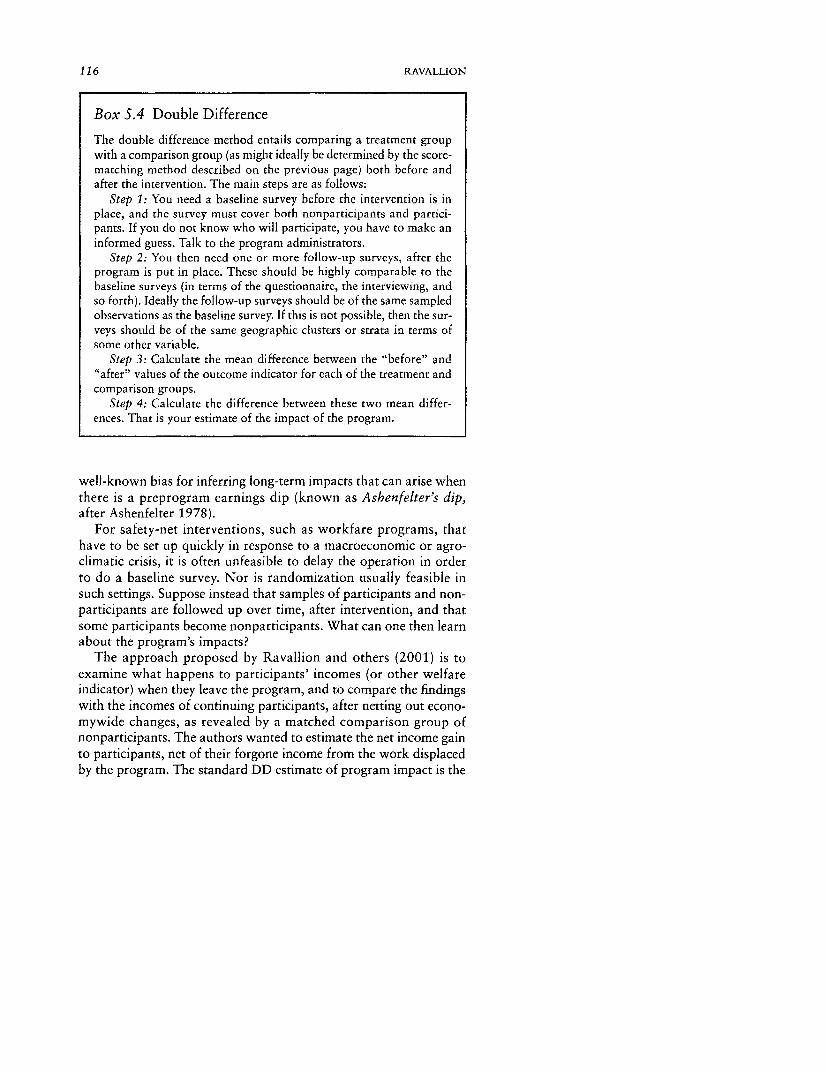
116 RAVALLION
Box 5.4 Double Difference
The double difference method entails comparing a treatment groupwith a comparison group (as might ideally be determined by the score-matching method described on the previous page) both before andafter the intervention. The main steps are as follows:
Step 1: You need a baseline survey before the intervention is inplace, and the survey must cover both nonparticipants and partici-pants. If you do not know who will participate, you have to make aninformed guess. Talk to the program administrators.
Step 2: You then need one or more follow-up surveys, after theprogram is put in place. These should be highly comparable to thebaseline surveys (in terms of the questionnaire, the interviewing, andso forth). Ideally the follow-up surveys should be of the same sampledobservations as the baseline survey. If this is not possible, then the sur-veys should be of the same geographic clusters or strata in terms ofsome other variable.
Step 3: Calculate the mean difference between the "before" and"after" values of the outcome indicator for each of the treatment andcomparison groups.
Step 4: Calculate the difference between these two mean differ-ences. That is your estimate of the impact of the program.
well-known bias for inferring long-term impacts that can arise whenthere is a preprogram earnings dip (known as Ashenfelter's dip,after Ashenfelter 1978).
For safety-net interventions, such as workfare programs, thathave to be set up quickly in response to a macroeconomic or agro-climatic crisis, it is often unfeasible to delay the operation in orderto do a baseline survey. Nor is randomization usually feasible insuch settings. Suppose instead that samples of participants and non-participants are followed up over time, after intervention, and thatsome participants become nonparticipants. What can one then learnabout the program's impacts?
The approach proposed by Ravallion and others (2001) is toexamine what happens to participants' incomes (or other welfareindicator) when they leave the program, and to compare the findingswith the incomes of continuing participants, after netting out econo-mywide changes, as revealed by a matched comparison group ofnonparticipants. The authors wanted to estimate the net income gainto participants, net of their forgone income from the work displacedby the program. The standard DD estimate of program impact is the

ASSESSING THE POVERTY IMPACT OF AN ASSIGNED PROGRAM 117
difference in the income gains over time between a treatment groupof program participants and the matched comparison group of non-participants. The double-matched triple difference estimator ofRavallion and others (2001) is the difference between the value ofthe double difference (between matched participants and nonpartici-pants) for the matched stayers and leavers. The difference betweenthe program's benefit level and the triple-difference estimate ofimpact gives an estimate of the mean gain to participants.
Although this approach is feasible without a baseline survey, itbrings its own problems. First, differencing over time can eliminatebias caused by latent (time-invariant) matching errors, but a poten-tial bias remains due to any selective retrenchment from the pro-gram based on unobservables. Ravallion and others (2001) arguethat the direction of bias can be determined under plausible assump-tions. Second, there may well be a postprogram Ashenfelter's dip,namely, when earnings drop sharply at retrenchment but thenrecover. As in the preprogram dip, this is a potential source of biasin assessing the longer-term impact; as with the preprogram version,however, to the extent that the dip entails a welfare change, it canstill be relevant to assessing the short-term impact of a safety-netintervention. And the postprogram dip is of interest in assessing thedynamics of recovery from retrenchment. To help address this issue,initial participants can be followed up over multiple survey rounds(Ravallion and others 2001).
Under certain conditions, this type of follow-up study of partici-pants can identify the gains to current participants from a program.There are concerns about selection bias, and there is the problemthat past participation may bring current gains to those who leavethe program. Assuming these lagged gains are positive, the net lossfrom leaving the program will be less than the gain from participa-tion relative to the counterfactual of never participating. Ravallionand others (2001) derive a test for the joint conditions needed toidentify the mean gains to participants from this type of study, alsoexploiting further follow-up surveys of past participants.
The study also illustrates the potential pitfalls of PSM when dataare weak. Compared with the study by Jalan and Ravallion (2003b)on the same program, Ravallion and others (2001) had no choicebut to use a lighter survey instrument, with far fewer questions onrelevant characteristics of participants and nonparticipants. Thisinstrument did not deliver plausible single-difference estimates usingPSM when compared with the Jalan and Ravallion estimates usingsingle-difference PSM for the same program on richer data. Thelikely explanation is that using the lighter survey instrument meant

118 RAVALLION
that there were many unobservable differences; in other words theconditional independence assumption of PSM was not valid. Itwould appear, however, that Ravallion and others were able toaddress this problem satisfactorily by tracking households over time,even using the lighter survey instrument. The follow-up evaluationdesign apparently was able to difference out the mismatching errors.From the point of view of evaluation design, this finding points tothe importance of tracking participants over time when there arethought to be important omitted variables in the cross-sectionaldata available for the purpose of single-difference matching.
On Behavioral Responses
Behavioral responses to a program can often be identified using thesame methods discussed above, but substituting some intermediateindicator(s) of behavior as the "outcome" variable(s), rather thanthe actual outcome variable(s) relevant to the program's objective(s).For example, Chen and Ravallion (2003) were interested in the sav-ings behavior of the participants in a World Bank-supported poor-area development program in China. They wanted to know howmuch of the income gains from the program the participants saved.It was agreed that the program's aim was to raise living standards ofthe poor, but there was also a concern about how well this outcomewould be captured within the evaluation period. Identifying the sav-ings response of participants provided a clue about the possiblefuture welfare gains beyond the project's life span. Indeed, Chenand Ravallion found that the participants saved about half of theincome gains from the program, as estimated using the matcheddouble-difference method described above.
This example also illustrates a common concern in evaluationstudies, given behavioral responses. The study period is rarely muchlonger than the period of the program's disbursements. However, ashare of the impact on peoples' living standards may occur beyondthe life of the project. This realization does not necessarily mean thatcredible evaluations need to track welfare impacts over much longerperiods than is typically the case-raising concerns about feasibility.But it does suggest that evaluations need to look carefully at impactson partial intermediate indicators of longer-term impacts-such asincomes in the Chen-Ravallion example-even when good measuresof the welfare objective are available within the project cycle. Thechoice of such indicators needs to be informed by an understandingof participants' behavioral responses to the program.

ASSESSING THE POVERTY IMPACT OF AN ASSIGNED PROGRAM 119
Conclusions
No single evaluation tool can claim to be ideal in all circumstances.The art of good evaluation is to draw carefully from the full rangeof tools available to deal pragmatically with the problem at hand inits specific context. The best evaluations often combine multiplemethods: randomizing some aspects and using econometric meth-ods to deal with the nonrandom elements, for example; or combin-ing score-matching methods with longitudinal observations to try toeliminate matching errors with imperfect data. Good evaluationsalso need to be designed early in the program cycle, both to ensurequality and to allow more rapid feedback into decisionmaking aboutthe program.
Notes
1. For an example of an ex ante impact assessment of an antipovertyprogram, see Ravallion (1999).
2. This article does not attempt to review all of the tools that have beenused for impact evaluation. The focus is on more recent developments thatappear likely to have relevance to the assessment of antipoverty programsand active labor market and other "social protection" programs in devel-
oping country settings. More comprehensive discussions of the methodsfound in practice can be found in Moffitt (1991); Blundell and Costa Dias(2000); and Ravallion (2001).
3. The second assumption is sometimes referred to in the literature asthe "conditional independence" assumption, and sometimes as "strongignorability."
4. Dehejia and Wahba (1999) report that their PSM results are robust toalternative estimators and alternative specifications for the logit regression.However, this may not hold in other applications.
S. Jalan and Ravallion (2003b) discuss the choice further. They used arange of weighting schemes, including nearest neighbor, nearest five neigh-bors, and a kernel-based weighting scheme in which the weight is a functionof the absolute difference in propensity scores. They found that their resultsfor estimating income gains from an antipoverty program are reasonablyrobust to the choice. However, that may not be so in other applications.
6. Rubin and Thomas (2000) use simulations to compare the bias inusing the nearest five neighbors to that in using just the nearest neighbor;
no clear pattern emerges.7. Van de Walle used simulation methods in which the data were con-
structed from a model in which the true benefits were known with certainty

120 RAVALLION
and the roads were placed in part as a function of the average incomes of
different villages.8. Also see the discussion of the problem of "nonoverlapping support
bias" in Heckman, Ichimura, and Todd (1997) and Heckman and others
(1998).9. For further discussion and an example, see Chen and Ravallion
(2003).10. Also see Heckman and others (1998) and Smith and Todd (2001),
who question the robustness of the Dehejia and Wahba PSM estimates tothe choices made in sample selection and model specification.
11. For example, Jalan and Ravallion (1998) show that this can seri-
ously bias evaluations of poor-area development programs that are targetedon the basis of initial geographic characteristics that also influence thegrowth process.
References
The word processed describes informally reproduced works that may notbe commonly available through library systems.
Angrist, Joshua, Eric Bettinger, Erik Bloom, Elizabeth King, and MichaelKremer. 2001. "Vouchers for Private Schooling in Colombia: Evidencefrom a Randomized Natural Experiment." NBER Working Paper 8343.
Cambridge, Mass.: National Bureau of Economic Research.Angrist, Joshua, Guido Imbens, and Donald Rubin. 1996. "Identification
of Causal Effects Using Instrumental Variables." Journal of the Ameri-
can Statistical Association 91: 444-55.Ashenfelter, Orley. 1978. "Estimating the Effect of Training Programs on
Earnings." Review of Economic Studies 60: 47-57.Atkinson, Anthony B. 1987. "On the Measurement of Poverty." Econo-
metrica 55: 749-64.Blundell, Richard, and Monica Costa Dias. 2000. "Evaluation Methods for
Non-Experimental Data." Fiscal Studies 21(4): 427-68.Burtless, Gary. 1985. "Are Targeted Wage Subsidies Harmful? Evidence
from a Wage Voucher Experiment." Industrial & Labor RelationsReview 39: 105-15.
Chen, Shaohua, and Martin Ravallion. 2003. "Hidden Impact? Ex-PostEvaluation of an Anti-Poverty Program." Policy Research Working Paper3049. World Bank, Development Research Group, Washington, D.C.Processed.
Dehejia, R. H., and S. Wahba. 1999. "Causal Effects in Non-experimentalStudies: Re-evaluating the Evaluation of Training Programs." Journal of
the American Statistical Association 94: 1053-62.

ASSESSING THE POVERTY IMPACT OF AN ASSIGNED PROGRAM 121
Dubin, Jeffrey A., and Douglas Rivers. 1993. "Experimental Estimates ofthe Impact of Wage Subsidies." Journal of Econometrics 56(1-2):
219-42.Foster, James E., Joel Greer, and Erik Thorbecke. 1984. "A Class of Decom-
posable Poverty Measures." Econometrica 52(3): 761-66.Galasso, Emanuela, Martin Ravallion, and Agustin Salvia. 2001. "Assisting
the Transition from Workfare to Work: A Randomized Experiment."Policy Research Working Paper 2738. World Bank, Washington, D.C.Processed.
Heckman, James, Hedehiko Ichimura, and Petra Todd. 1997. "Matching asan Econometric Evaluation Estimator: Evidence from Evaluating a JobTraining Programme." Review of Economic Studies 64: 605-54.
Heckman, James, Hedehiko Ichimura, James Smith, and Petra Todd. 1998."Characterizing Selection Bias Using Experimental Data." Economet-
rica 66: 1017-99.Jalan, Jyotsna, and Martin Ravallion. 1998. "Are There Dynamic Gains
from a Poor-Area Development Program?" Journal of Public Economics67(1): 65-86.
- 2003a. "Does Piped Water Reduce Diarrhea for Children in RuralIndia?" Journal of Econometrics 112: 153-73.
- 2003b. "Estimating Benefit Incidence for an Anti-poverty ProgramUsing Propensity Score Matching." Journal of Business and Economic
Statistics 21(1): 19-30.Katz, Lawrence E, Jeffrey R. Kling, and Jeffrey B. Liebman. 2001. "Mov-
ing to Opportunity in Boston: Early Results of a Randomized MobilityExperiment." Quarterly Journal of Economics 116(2): 607-54.
Lalonde, Robert. 1986. "Evaluating the Econometric Evaluations of Train-ing Programs." American Economic Review 76: 604-20.
Moffitt, Robert. 1991. "Program Evaluation with Nonexperimental Data."Evaluation Review 15(3): 291-314.
Ravallion, Martin. 1994. Poverty Comparisons, Fundamentals in Pureand Applied Economics vol. 56. Chur, Switzerland: Harwood Acade-mic Publishers.
- 1999. "Appraising Workfare." World Bank Research Observer14(1): 31-48.
. 2001. "The Mystery of the Vanishing Benefits: An Introduction to
Impact Evaluation." World Bank Economic Review 15(1): 115-40.Ravallion, Martin, Emanuela Galasso, Teodoro Lazo, and Ernesto Philipp.
2001. "Do Workfare Participants Recover Quickly from Retrench-ment?" Policy Research Working Paper 2672. World Bank, Washington,
D.C. Processed.Rosenbaum, Paul, and Donald Rubin. 1983. "The Central Role of the
Propensity Score in Observational Studies for Causal Effects." Bio-metrika 70: 41-55.

122 RAVALLION
- 1985. "Constructing a Control Group using Multivariate Matched
Sampling Methods that Incorporate the Propensity Score." AmericanStatistician 39: 35-39.
Rubin, Donald B., and N. Thomas. 2000. "Combining Propensity ScoreMatching with Additional Adjustments for Prognostic Covariates."
Journal of the American Statistical Association 95: 573-85.Smith, Jeffrey, and Petra Todd. 2001. "Reconciling Conflicting Evidence on
the Performance of Propensity-Score Matching Methods." American
Economic Review 91(2): 112-18.van de Walle, Dominique. 2002. "Choosing Rural Road Investments to
Help Reduce Poverty." World Development 30(4): 575-89.Watts, H. W 1968. "An Economic Definition of Poverty." In Daniel Patrick
Moynihan, ed., On Understanding Poverty. New York: Basic Books.Woodbury, Stephen, and Robert Spiegelman. 1987. "Bonuses to Workers
and Employers to Reduce Unemployment." American Economic Review77: 513-30.
6
Ex Ante Evaluationof Policy Reforms
Using Behavioral Models
Franfois Bourguignon andFrancisco H.G. Ferreira
The tools for incidence analysis of taxation and public spendingreviewed in the previous chapters are fundamentally ex post. Givensome tax or public expenditure, these tools show (a) who pays thetax or receives the benefits provided through public spending; (b)how much everyone pays or receives, in accounting terms; (c) howmuch everyone receives when taking into account behavioralresponses to taxes or the free delivery of public services; and (d)what the indirect effects of public programs are. This sort of ex postanalysis sheds valuable light on the actual distribution of a tax orpublic expenditure and thus improves policymakers' ability to judgewhether individual spending items are "worth their cost" or whethera reform of the instrument under analysis should be considered.
Ex post analyses have one significant limitation, however. Onlyexisting taxes or public programs may be analyzed in this way. Thischapter turns to techniques designed to shed light on the potentialdistributional impacts of policies or policy designs that do not cur-rently exist, but that might exist in the future. Suppose ex postanalysis of an existing program pointed to the necessity of reform-ing it. Suppose further that several alternative designs-rather thana single one-are suggested for the reform. The government might
123

124 BOURGUIGNON AND FERREIRA
find it helpful to have some estimate of how much each alternativereform would cost and of which households would be affected, andby how much, under each alternative. If pure experimentation onactual live subjects (such as people or communities of people) of allpossible reform designs is not possible or would take too much time,no actual data would be available to evaluate these hypotheticalreforms directly. Some counterfactual must be generated, showinghow each household in a sample survey would fare depending onthe reform being undertaken and how much the reform would cost.Since households respond to policy changes by changing their ownactions, this counterfactual must rely on some representation ofhousehold behavior.
Essentially, ex ante analysis is what if analysis. What if some fea-tures of the tax system or public spending were modified? Howwould the modification change the situation for individual house-holds from their initial situation, or status quo? As the introductionto this part of the volume explained, ex ante analysis is marginalbecause it is meant to capture differences between the proposedreform(s) and the status quo. And it is almost necessarily behav-ioral, because of the need to generate counterfactuals that take agentresponses into account.1
Like ex post analysis, ex ante policy evaluation that is concernedwith distributional or poverty outcomes generally relies on house-hold surveys. However, ex ante evaluation requires an additional andpreliminary use of the household survey data. Whereas the secret ofgood ex post impact evaluation is to identify which actual samplesshould be compared, ex ante analysis requires the simulation of acounterfactual sample, which should represent the population char-acteristics of interest, as they would be under the counterfactual pol-icy in question. To achieve that, some model is required that trans-forms the actual sample into the counterfactual one. At its simplest,this model may be a simple arithmetic representation of the incidenceof a tax or benefit, without simulating any policy response by theagents (that is, assuming that all relevant elasticities are zero).
If a simple arithmetic representation seems inadequate because,say, one believes that the policy change may have important price orincome effects on consumption or labor-supply behavior, then abehavioral model would be needed. Such a model may be obtainedin one of two basic ways: through the estimation of a structuraleconometric model on the cross-section of households provided bythe household survey; or through the calibration of a model with agiven structure so as to make it consistent with what is observed inthe survey.
The archetypal example of ex ante analysis of this kind is a tax-benefit model with labor-supply response, such as those commonly

EX ANTE EVALUATION OF POLICY REFORMS 125
estimated for industrial countries. Changes in the tax-benefit systemin these models have two general effects. First, tax or benefit changesmodify the disposable income of households with an unchangedlabor supply. Second, through this income effect as well as throughthe price effects induced by changes in the after-tax price of labor,they also modify labor-supply decisions. The quantitative extent ofthese effects-and their net impact-is determined through a behav-ioral model that is generally estimated econometrically across house-holds observed in the status quo.
There are many models of this type in industrial countries.2 Bycontrast, not much has been done along these lines in developingcountries, except perhaps for a few examples of the pure accountingmicrosimulation approach. One reason may be that the cash ele-ment of the redistribution system is not usually important enough tomodify labor supply significantly and to warrant this kind of analy-sis. It may also be that estimating structural econometric models oflabor supply is made complex because of the informality of a largepart of the labor market. Nevertheless, the growing importance ofcash transfers and the increasing concern for distributional issues isgenerating greater need for this kind of analysis. In addition, thereare dimensions of household behavior other than labor supply thatmatter from a welfare point of view and that may be affected bytransfers and other public policies. Demand for schooling or healthcare are some examples.
In this chapter we first present the basic workhorse structuralmodel used for ex ante evaluation of policy reforms: the tax-benefitmodel with labor-supply response. We use this model to illustratethe sequence of steps needed to build a model, generate the counter-factual distribution, and compare it with the actual in order to sim-ulate and evaluate the reform. We then introduce discrete choiceoccupational or labor-supply models to show how a change in themodel can be used to expand the set of policies that can be ana-lyzed. This methodology is then applied to the simulation of a tar-geted conditional cash transfer in a developing country to illustratethe final steps of the ex ante evaluation approach. Extensions andlimitations are considered in the last section of the chapter.
The Basic Model: Accounting for Labor-SupplyResponses to Changes in Taxes
This section outlines the logical sequence a practitioner should fol-low when using ex ante evaluation tools to simulate alternative out-comes for a policy or program reform. To make the approach asconcrete as possible, we base the discussion on a model of labor

126 BOURGUIGNON AND FERREIRA
supply decisions that are made when the budget constraints facingindividuals may be nonlinear because of taxes and transfers. Thebasic reference is the first model of this type, proposed by Hausman(1980). We break down the approach into five steps: definition ofthe problem; identification of the required data; specification of themodel; model estimation; and policy simulation.
Step 1: Identify a well-defined, tractable policy reform question.
For example, determine the likely effect of an increase in incometaxes or in benefits on the distribution of incomes, and on the gov-ernment's budget. The simulation approach has often been used toaddress fiscal questions of this type because actual tax experiments(such as the application of different tax rates to comparable popu-lation subgroups) are generally difficult to justify politically. Addi-tionally, a model that simulated such tax changes without takingagents' responses into account would be likely to generate wrongrevenue predictions.
Step 2: Find a data set that contains reliable informationon the variables that need to be included in the model.
In this case, one would need a household or labor force survey, withinformation on earnings and hours of work for a representativecross-section of the population of interest. Additionally, one wouldideally need information on which taxes each individual pays, andat what rates. If the best available surveys do not contain this infor-mation, then one would need a clear description of the tax rules tomake assumptions (such as 100 percent compliance) about howthose rules apply over the sample.
Step 3: Write the simplest economic model that containsenough structure to capture the mechanisms that are likely toaffect the agent responses to the policy under consideration.
In this case, the logical economic structure is that of the textbookutility-maximizing consumer. An economic agent with characteris-tics z chooses a volume of consumption, c, and a labor supply, L, soas to maximize the agent's preferences represented by the utilityfunction u( ) under a budget constraint that incorporates the tax-benefit system. The important point is that the taxes under consid-eration enter explicitly into the budget constraint, so that anychanges in the parameters of the tax system will affect the con-sumer's optimal choices. This model is written in a general formbelow, so that other tax or transfer changes can also be considered:

EX ANTE EVALUATION OF POLICY REFORMS 127
(6.1) Max u(c, L; z; 1, E) subject toc < yo + wL + NT(wL, L, yo; z; y), L Ž 0
In the budget constraint, yo stands for (exogenous) nonlaborincome, w for the wage rate and NT( ) for the net transfer definedby the tax-benefit schedule. Taxes and benefits depend on the char-acteristics of the agent, his nonlabor income and his labor income,wL. Taxes and benefits may also depend directly on the quantity oflabor being supplied, as in workfare programs. y stands for the para-meters of the tax-benefit system such as the various tax rates, means-testing of benefits, and the like. Likewise, ,B and £ are coefficientsthat parameterize preferences. The solution of that program yieldsthe following labor-supply function:
L = F (w, yo; z; 3, £; 7)
This function is nonlinear. In particular, it may be equal to zero forsome subset of the space of its arguments. The set of restrictionson the vector y that ensures that L > 0 is known as a participationcondition.
Step 4: Estimate the model.
Suppose now that a sample of agents (indexed by i) are observed insome household survey containing reliable information on L, w, yo,and z. The problem is now to estimate the function F( ) above or,equivalently, the preference parameters, j and £, since all the othervariables or tax-benefit parameters are actually observed. To do so,it is assumed that the set of coefficients I is common to all agents,whereas £ is idiosyncratic. It is not observed, but some assumptionscan be made on its statistical distribution in the sample. This leadsto the following econometric specification:
(6.2) Li = F(zi, wi, yoi; , £i; y)
where Ej plays the usual role of the random term in standardregressions.
Estimation proceeds as in standard models, minimizing the roleof the idiosyncratic preference term in explaining cross-sectionaldifferences in labor supply. This leads to a set of estimates f3 for thecommon preference parameters and ti for the idiosyncratic prefer-ence terms. By definition of the latter, it is true for each observationin the sample that
Li = flzi, wi, yoi; 5, £j; Y)
While the estimation process just described is conceptually simple,its implementation in practice is generally not so straightforward.

128 BOURGUIGNON AND FERREIRA
That is because of the nonlinearity of the budget constraint and itspossible nonconvexity due to the tax-benefit schedule, NT( ), andcorner solutions at L = 0. Functional forms must be chosen for pref-erences, which may introduce some arbitrariness in the procedure.Finally, it may be feared that imposing full economic rationality anda functional form for preferences severely restricts the estimates thatare obtained. There has been a debate on this point ever since thismodel first appeared in the literature.3 We return to this estimationproblem later, where we suggest a simple and robust alternative, thecost of which is discreteness.
Step 5: Simulate the policy reform using the empiricalestimate of the model.
It is now possible to simulate alternative tax-benefit systems, whichsimply requires modifying the set of parameters y.' In the absence ofgeneral equilibrium effects, the change in labor supply due to mov-ing to the set of parameters yS is given by
Ljs - Li = F(z,, wi, yoi; j, Ej; yS) - F(z;, wi, yoi; l, ei; r)
The change in the disposable income may also be computed forevery agent. It is given by
Ci'- Ci = wi(Lj- Li) + NT(y 0 i, w-, LV, zj; y') - NT(y 0i, wiLi, Li; zi; y)
At this point one may also derive changes in any measure of indi-vidual welfare, and construct from each of them a full counter-factual distribution over the sample.
Discrete Models of Labor Supply or Occupational Choice
We now return to the caveat made in the last paragraph of step 4,where we noted the main weakness of the approach outlined here sofar. That is, despite its conceptual simplicity, estimation of the non-linear (but piecewise continuous) labor-supply function is generallycomplex, often involving maximization of nontrivial likelihoodfunctions and requiring the specification of possibly arbitrary utilityfunctional forms.
It turns out that simpler and less restrictive specifications may beused that considerably reduce this problem. In particular, specifica-tions used in recent work consider labor supply as a discrete vari-able that may take only a few alternative values; these specificationsevaluate the utility of the agent for each of these values and the cor-responding disposable income given by the budget constraint. If this

EX ANTE EVALUATION OF POLICY REFORMS 129
discreteness is not seen as too costly in terms of the reliability of thepolicy simulation under consideration, it can buy a great deal ofsimplicity in estimation.
As before, the behavioral rule is simply that agents choose thevalue that leads to the highest level of utility. However, the utilityfunction may now be specified in a very general way. In particular,its parameters may be allowed to vary with the various quantities oflabor that may be supplied, with no restriction being imposed onthese coefficients. Such a representation is therefore as close as pos-sible to what is revealed by the data.
Formally, a specification that generalizes what is most often foundin the recent tax and labor-supply literature is the following:
(6.3) Li = Di if U/ = f(zi; Wi; ct; pi, t) UIk
= f(z,; wj; cik; Pk, E.k) for all k • j
where D, is the duration of work in the jth alternative, Uji the utilityassociated with that alternative, and ci the disposable income givenby the following budget constraint:
c= yo + wL + NT(wD, D, yo; zi; y)
When the function f( ) is linear with respect to its common prefer-ence parameters and when the idiosyncratic terms are assumed to beidentically and independently distributed with a double exponentialdistribution, this model is the standard multinomial logit. It mayalso be noted that it encompasses the initial model 6.1. It is suffi-cient to make the following substitution:
f(zw; wc; c/ PI, s!) = u(c|; Di; z-; , £-)
This specification, which involves restrictions across the variouslabor-supply alternatives, is actually the one that is most often used.
Even under this more general form, one might be tempted to arguethat the preceding specification is still too restrictive, because it relieson some utility-maximizing assumption. It turns out that ex anteincidence analysis or policy evaluation cannot dispense with such abasic assumption. The ex ante nature of the analysis requires thatsome assumption be made about the way agents choose between dif-ferent alternatives. Given that, assuming that agents maximize somecriterion defined in a different way for each alternative is not reallythat restrictive. It also should be clear that if no restriction is imposedacross alternatives, then the utility-maximizing assumption is com-patible with the most flexible representation of the way in whichlabor-supply choices observed in a survey are related to individualcharacteristics, including the wage rate and the disposable incomedefined by the tax-benefit system, NT( ).

130 BOURGUIGNON AND FERREIRA
The fact that model 6.3 can be interpreted as representing util-ity-maximizing behavior is to some extent secondary, although thisinterpretation permits implementing counterfactual simulations ina simple way. More important is that this model fits the data asclosely as possible. Interestingly enough, the only restriction affect-ing that objective is the assumption that the income effect in eachalternative-that is, the cl argument in f( )-depends on disposableincome as given by the budget constraint that incorporates the tax-benefit schedule, NT( ). The economic structure of this model thuslies essentially in the income effect. If it were not for that property,it would simply be a reduced-form model aimed at fitting the dataas well as possible.
In effect, the restriction that the income effect must be propor-tional to disposable income seems to be a minimal assumption toensure that this representation of cross-sectional differences inlabor-supply behavior may at the same time represent a rationalchoice among various labor-supply alternatives. After all, withinthis framework, the simulated effect on individual labor supply of areform of the tax-benefit system, NT( ), is estimated on the basis ofthe cross-sectional disposable income effect in the status quo.
The role of idiosyncratic terms, ei or £/, in the whole approachshould not be downplayed. They represent the unobserved hetero-geneity of agents' labor-supply behavior. Thus, they are responsiblefor some of the heterogeneity in responses to a reform of taxes andbenefits. It can be seen in equation 6.3 that agents who are other-wise identical might react differently to a change in disposableincomes, even though these changes are the same for all of them. Itis enough that the idiosyncratic terms, 9/, be sufficiently differentamong them.
Estimates of the idiosyncratic terms result directly from theeconometric estimation of the common preference parameters ,B oroi.s Note, however, that it is possible to use a "calibration" ratherthan an estimation approach. With the former, some of the coeffi-cients j or DI would not be estimated but given arbitrary valuesdeemed reasonable by the analyst. Then, as in the standard estima-tion procedure, estimates of the idiosyncratic terms would beobtained by requiring that predicted choices, under the status quo,and actual choices coincide.
Before closing this section, it is important to emphasize that thereis some ambiguity about who the "agents" behind the labor-supplymodel 6.1 should be. Traditionally, the literature considers individ-uals, even though the welfare implications of the analysis concernhouseholds. Extending the model to households requires consider-ing simultaneously the labor-supply decision of all household mem-bers of working age, a factor that makes the analysis more complex.

EX ANTE EVALUATION OF POLICY REFORMS 131
Applications of the preceding model are numerous in industrialcountries. Surveys are given in Blundell and MaCurdy (1999) and inCreedy and Duncan (2002). The discrete approach underlined aboveis best illustrated by Van Soest (1995), Hoynes (1996), or Keaneand Moffitt (1998). A nice application of this approach for predict-ing the likely effect of the introduction of the Working Families TaxCredit in the United Kingdom is Blundell and others (2000).
A Developing Country Application: Cash Transfers,Demand for Schooling, and Labor Supply
The preceding framework has not very often been applied to devel-oping countries, for a number of reasons. First, direct transfers tohouseholds, whether positive or negative, have usually been lessimportant in developing countries. Second, the functioning of thelabor market may make the concept of labor supply somewhat arti-ficial or insufficient in several instances. In particular, the distinctionbetween formal and informal employment is important, with theformer often being rationed and the latter often leading to an impre-cise observation of income and income effects. Both limitationsapply more strongly to the poorest segment of society.
Nevertheless, the broad issue of agent response to policychanges-which motivated the preceding models-is becomingincreasingly relevant in the developing world, as both tax and trans-fer systems develop. For instance, it was observed in South Africathat the payment of lump-sum pensions to elderly people withoutother resources was accompanied by changes in the labor supply ofthe households they belonged to (Bertrand, Mullainathan, andMiller 2002). As a result, the change in monetary income in poorhouseholds differed from what had been expected. The amplitudeof this phenomenon might be measured either through ex post "dif-ferences in differences" techniques of the type discussed in chapter5, or by ex ante models of the type shown here. Of course, the exante approach could be useful, say, in designing reforms to the exist-ing minimum pension system.
Progresa in Mexico, Bolsa Escola in Brazil, and similar condi-tional cash transfer programs in several other countries offer a sec-ond example of the ex ante evaluation approach. This section pro-vides a summary presentation of an ex ante evaluation of the effectsof Bolsa Escola in Brazil and of potential changes in the format ofthat program. This evaluation may be seen as an extension or avariation of the framework discussed in the previous section. Thediscussion is based on Bourguignon, Ferreira, and Leite (2002),where the exercise is described and analyzed in greater detail.

132 BOURGUIGNON AND FERREIRA
The Bolsa Escola program consists of transfers to householdswhose incomes per capita are below R$90-approximatelyUS$30-a month, provided that all children in the household ages 6to 15 are enrolled in a public school, and that their individual atten-dance rates do not fall below 85 percent in any given month. Themonthly transfer is equal to R$15 per child going to school, up to amaximum of R$45 per household. This program may be consideredas a conditional cash transfer program because it combines cashtransfers based on a means-test with some additional conditionality,that is, having children of school age actually attending school.
Because the main occupational alternative to school is work,evaluation of the Bolsa Escola program really is a labor-supplyproblem similar to the one analyzed above. The discrete approach isused for each child aged 10 to 15, with the following three labor-supply alternatives, indexed by k: k = 1 if the child has some marketearnings and does not go to school; k = 2 if the child has some earn-ings and goes to school; and finally k = 3 if the child does not workin the market but does go to school. Following equation 6.3, theutility of the household to which child i belongs is specified
(6.4) Uik = zi3k + Ck(yi + yi ) + FIk
for k = 1, 2, 3. As before, z, stands for characteristics of both thechild and the household; Yi is household income without the child'searnings; yi/ is the income earned by the child in alternative k; and£.k stands for idiosyncratic preferences.
The key variable for describing the conditional cash transfer pro-gram is clearly yik, since transfers depend on income per capita inthe household and on the schooling status of the child, which itselfaffects the child's earnings. Under the status quo-before the pro-gram was launched-and in the household survey being used forestimation, this variable is defined as follows. In alternative 1, yikequals the observed market earnings of the child, wi. In alternative2, the child is assumed to work only a proportion M of the timeavailable when not going to school. The child's observed earningstherefore are Mwi on average. In the third alternative, the child doesnot bring home any market earnings. But that does not prevent thechild from contributing to domestic production. Assume this con-tribution to be, on average, some fixed proportion of the earningsobtained from market work by children with the same observablecharacteristics. Let Awi be the corresponding amount. A differencewith model 6.3 is that A is not observed.
Substituting the preceding values of y into equation 6.4 leads to
(6.5) Ujk = Zjk + akyj + pkwj + Eik

EX ANTE EVALUATION OF POLICY REFORMS 133
where pk iS given by
(6.6) p1 =a 1,p2 ="A2 M,p3 = a3 A
Expression 6.5 is comparable to the discrete choice labor-supplymodel 6.3. It can be estimated by a multinomial logit model. Apotential problem might be that this model allows estimating thecoefficients corresponding to some alternative only as a deviationfrom those of some other alternative, which is taken as a reference.In this application, since the child's earnings variable differs acrossalternatives, it is necessary to estimate all three axk, k =1, 2, 3. In thiscase that is achieved through the restrictions given by equation 6.6,which allow the identification of the three coefficients ak and A.6 Itis those restrictions, and the fact that M can be estimated (as a coef-ficient on a dummy variable for school attendance in an earningsequation for children with positive earnings) that permits estimatingthe whole model. See Bourguignon, Ferreira, and Leite (2002) fordetails.
Estimates k, 6k, and 9# of the preferences may thus be obtainedfrom the observation of adult and child incomes, various householdand child attributes, and the demand for schooling and supply ofchild labor taken from a household survey conducted before theprogram began. Once these estimates have been obtained, the effectof Bolsa Escola on the decisions about children's occupations is easyto simulate. The alternative with the highest utility is chosen, withthe utility of each alternative being now given by:
ul = Zj,' + aYj + a w; + i,
U2 = Zj2 + &2 (y +Yl) + &2 Mwi + if Y+Mw; 2
(6.7) U,2 = Z,2 +&2 y +&2 Mw i + if Yi + Mwj > Y2
U=Z3 + 3 ( + y,) + &3 Aw + if Yi < 72
UW3 = ZjD,3 + C3yi + a3Aw + j3 if Y>372
In this system, y, and 72 stand for the parameters of the tax-benefit system being modeled. The former stands for the BolsaEscola transfer for each child in school, and the latter is the meanstest. Together, these conditions incorporate the fact that BolsaEscola can make the schooling alternatives 2 and 3 more attrac-tive for poorer families. Moving from alternative 1 to 2 (respec-tively alternative 3) increases or reduces monetary income accord-ing to whether the transfer Yi is above or below (1 - M) wi(respectively wi). In all cases, however, these moves potentiallymean a higher future income for the child.
This model was estimated on all children ages 10 to 15 in theBrazilian household survey sample PNAD 1999. The number of

134 BOURGUIGNON AND FERREIRA
children under age 10 involved in market activities and not enrolledin school was not sufficient to estimate the model. Results turnedout to be quite consistent. In particular, the value of M derived fromthe comparison of earnings among those working children who donot go to school and those who do go was found to be around 70percent. Likewise, the coefficient measuring the market equivalentof the domestic production of children going to school but not activein the labor market, A, was found to be 75 percent. Finally, it turnedout that, as in several other studies of the demand for schooling, theincome effect, as measured by differences oC2 - al and a3
- al, is
rather weak.After estimating all the coefficients of the model and the idiosyn-
cratic preference terms, 9,k, the Bolsa Escola program and alterna-tive formats of that program were simulated on each of the house-holds in the PNAD survey. Focusing on all children between ages 10and 15 led to a sample of 42,000 persons. However, only 26 percentof them passed the means test in Bolsa Escola and were thus poten-tially directly affected by the program.
Table 6.1 shows the effect of the Bolsa Escola program on theschooling of children ages 10-15 living in poor households, as simu-lated with the model sketched above. 7 The table shows that the pro-gram is indeed quite effective in reducing the number of poor chil-dren who do not go to school. Their proportion in the population ofpoor children ages 10-15 falls from 8.9 percent without the programto 3.7 percent under the simulated program. Interestingly enough,the proportion of children who both go to school and have someactivity in the labor market tends to increase, which suggests that theprogram has little effect on child labor when children are alreadygoing to school. Alternative specifications of the program scenarioshave the expected effect on schooling. In particular, raising theamount of the transfer or making it age-progressive further reducesthe proportion of children not going to school. However, making theprogram more generous by changing the level of the means test hasvery little effect. Another interesting finding is that the schoolingconditionality is extremely important to achieving the objective ofuniversal schooling. As shown by the last scenario, the income effectattributable to the cash transfer would have practically no effect onschooling without the conditionality of Bolsa Escola.
Table 6.2 shows the expected effect of the Bolsa Escola programon poverty, defined here for the whole population and on the basisof monetary income only. This effect turns out to be more muted.The poverty headcount goes down by only 1.3 percentage points,reflecting the moderate size of the program (shown in the last rowof the table), the substantial inequality within the poor segment of

Table 6.1 Simulated Effect on Schooling and Working Status of Alternative Specifications of Conditional CashTransfer Program
Poor Households
All children ages 10-15 Original Bolsa Escola program Scenario 1 Scenario 2 Scenario 3 Scenario 4 Scenario S
Not going to school 8.9 3.7 1.9 0.6 1.8 3.6 8.9Going to school and working 23.1 24.7 25.1 25.4 25.2 24.9 23.0Going to school and not working 68.1 71.6 72.9 74.0 73.0 71.4 68.2Total 100.0 100.0 100.0 100.0 100.0 100.0 100.0
Note: Scenario 1: Transfer equal R$30, maximum per household R$90 and means test R$90.Scenario 2: Transfer equal R$60, maximum per household R$180 and means test R$90.Scenario 3: Different values for each age, no household ceiling and means test R$90.Scenario 4: Transfer equal R$15, maximum per household R$45 and means test R$120.Scenario 5: Bolsa Escola without conditionality.
Sources: PNAD/IBGE 1999 and authors' calculation.

Table 6.2 Simulated Distributional Effect of Alternative Specifications of the Conditional Cash Transfer ProgramPoverty measures Original Bolsa Escola program Scenario 1 Scenario 2 Scenario 3 Scenario 4 Scenario S
Poverty headcount 30.1 28.8 27.5 24.6 27.7 28.8 28.9Poverty gap 13.2 11.9 10.8 8.8 10.9 11.9 12.0Total square deviation from 7.9 6.8 5.9 4.6 6.0 6.8 6.8
poverty lineAnnual cost of the program n.a. 2,076 4,201 8,487 3,905 2,549 2,009
(million Reals)
Note: n.a. = Not applicable.Scenario 1: Transfer equal R$30, maximum per household R$90 and means test R$90.Scenario 2: Transfer equal R$60, maximum per household RS180 and means test R$90.Scenario 3: Different values for each age, no household ceiling and means test R$90.Scenario 4: Transfer equal R$15, maximum per household R$45 and means test R$120.Scenario 5: Bolsa Escola without conditionality.
Sources: PNAD/IBGE 1999 and authors' calculation.

EX ANTE EVALUATION OF POLICY REFORMS 137
the population, and the negative (child) labor-supply effect of theprogram. The comparison of the Bolsa Escola simulation with theresults obtained under scenario S-no conditionality-suggests thatthis last effect is small, however. Indeed, there is almost no differ-ence in the poverty measures reported under the two scenarios.Other scenarios have the expected effect on poverty, with increasesin transfer amounts being once again more potent than hikes in thelevel of the means test.
A much more detailed analysis than the results shown in thesetwo tables is of course possible. Some additional detail is provided inBourguignon, Ferreira, and Leite (2002). Because the main purposeof this chapter is to present and discuss the methodology of ex anteevaluation approaches to public redistribution programs, we go nofurther here. The few results presented above are sufficient to illus-trate both the principles and the potential usefulness of the approach.
Despite the appeal of this methodology, few applications areavailable for developing countries. In most cases, applying it requiresonly a structural model of some dimension of household behaviorthat permits simulating a change in one or many policy parameters.Thus, models of demand for schooling along the lines of Gertler andGlewwe (1990) could be used to simulate the impact of several poli-cies in the field of education, such as reducing the direct cost ofschooling, providing school lunches, or changing the quality ofschooling. For example, Younger (2002) uses this kind of approachto analyze the consequences of uniformly reducing the distance toschool in rural Peru.
Conclusions, Extensions, and Limitations
A reliance on the multinomial logit model of discrete occupationalchoice (or labor supply) considerably facilitates the estimation of thiskind of structural model, which can then be used to simulate theimpact of policy or program reforms taking behavioral responsesinto account. Yet it is still probably true that starting such an exer-cise from scratch is not the easiest tool in this toolkit. It is thereforeworth considering pure accounting ex ante marginal incidence tech-niques, at least as an initial step. Even this (much simpler) approachis not yet of generalized use, and one can plausibly argue that inmany cases the first-order approximation generated by such a non-behavioral simulation might be informative in its own right; it mayalso serve as a learning stage before attempting the behavioral part ofthe model. A pure accounting approach to the evaluation of the BolsaEscola program, assuming 100 percent enrollment in the program,

138 BOURGUIGNON AND FERREIRA
would have led to a poverty simulation that was a bit-but notmassively-off the results obtained with the preceding simulation.
The most obvious field of application of the ex ante marginalincidence approach has to do with all the consequences of a changein the budget constraint faced by households, especially through alltypes of means-tested or conditional transfers. Behavioral featuresthat are the most sensitive to income changes are the safest to study,because strong estimates for cross-sectional income effects are themost likely to translate into actual responses to a program that mod-ifies the income of agents. Thus, labor supply and related behaviorsuch as schooling at one end of the active life cycle and inactivity atthe other end are the first candidates for behavioral analysis.
Ex ante simulations are less easy with other components of pub-lic finance because they generally involve price and quality dimen-sions that are very imperfectly observed. Public services financedthrough user fees are a case in point. If some health care facility ismade available in a locality, then it is most likely that users will firstbe differentiated by income. If there is some cost recovery, then reg-ular users will be those agents with an income above some thresh-old. Extending health care to poorer people could be done either bylowering cost recovery or by subsidizing low-income users on thebasis of some permanent income criterion. Such systems are used inseveral countries-one example is the SISBEN system for healthcare in Colombia. Under the assumption of fixed price and quality,these systems could be studied with the same techniques discussedhere. The problem is that quality and price are highly unlikely tostay fixed, and simulating the effects of variations in these twodimensions adds considerable complexity. Although some house-hold surveys record visits to health centers, they do not record priceand quality characteristics, or there may not be enough variationacross households to estimate demand elasticities in any convincingway. The analysis may thus be only partial.8
Consumption responses to changes in prices through taxes orsubsidies also face this problem of zero or unknown variation inprices within household surveys. From a welfare point of view, thedemand response need not be known because, as a first approxima-tion, the effect of a price change is simply the change in total expen-ditures that it causes at constant consumption behavior. Behavioralresponses are important only to figure out the change in net taxreceipts at the aggregate level. But then, aggregate demand analysisbased on time series may be used for this.9 The same applies tochanges in the prices of goods that are produced by households, thatis, the price of the output of self-employed households or simply thewage rate of those employed in the formal labor market. Overall,

EX ANTE EVALUATION OF POLICY REFORMS 139
analysis of indirect taxes, including labor taxes, thus differs sub-stantially from analysis of changes in direct taxes and transfers or inthe supply of public services. The latter are more susceptible to exante evaluation-or marginal incidence analysis-than the former.
To conclude, we stress some of the limitations of the ex ante eval-uation approach that have not been mentioned explicitly in this shortpresentation. First, this approach may be difficult to implementbecause it generally requires the estimation of an original behavioralmodel that fits the policy to be evaluated or designed, and of coursethe corresponding microeconomic data. It is thus unlikely that ananalysis conducted in a given country for a particular policy can beapplied without substantial modification to another country oranother type of policy. The methodological investment behind thisapproach may thus be important. Therefore, preceding this approachwith a pure accounting microsimulation based on simpler assump-tions can be useful. Second, we emphasize the fact that the behav-ioral approach relies necessarily on a structural model that requiressome minimal set of assumptions. In general, these assumptions aredifficult to test. In the labor-supply model with a discrete choice rep-resentation, the basic assumption is that net disposable income, asgiven by the tax-benefit system, is what matters for occupationaldecisions. A reduced form model would say that the exogenous idio-syncratic determinants of the budget constraint are what matters.Econometrically, the difference may be tenuous, but the implicationsin terms of simulation are huge. For instance, the modeling of BolsaEscola is based on the implicit assumption that income is pooled atthe household level. That is not a given, and simulation results wouldbe different if the model were specified otherwise.
Finally, the strongest hypothesis is that cross-sectional incomeeffects, as estimated on the basis of a standard household survey,coincide with the income effects that will be produced by the pro-gram under study or reforms in it. In other words, income effectsover time for a given agent should coincide with the effect of cross-sectional income differences. Here again, this is a hypothesis that ishard to test and yet rather essential for ex ante analysis. The onlytest we can think of would be to combine ex ante and ex post analy-sis. For instance, one could run some ex ante analysis on a Mexicanhousehold survey taken before the launching of Progresa and thencompare those results with the results obtained for schooling andincome in the ex post evaluations that have been made of that pro-gram. Combinations of ex ante and ex post evaluations-such asthe studies undertaken by Todd and Wolpin (2002) and Attanasio,Meghir, and Santiago (2002)-are at the cutting edge of the appliedmicroeconomics of development.

140 BOURGUIGNON AND FERREIRA
In the absence of such validation exercises, which are possibleonly in rather special circumstances, some uncertainty about thepredictions generated by ex ante evaluations based on structuralbehavioral modeling is bound to remain. That being said, ex anteevaluation can be a valuable tool to visualize the distributionalimpact of alternative designs of policies that are likely to generatestrong behavioral responses. A pure accounting approach to mar-ginal incidence analysis is often a useful first step. But, because peo-ple do generally change their behavior when the policy environmentaround them changes, introducing behavior on an ex ante basis isultimately desirable for simulating policy reform in most realms.
Notes
1. Pure accounting micro-simulation methods need not be totally dis-carded, at least as a first approximation. They may be useful to describefirst-round effects on a sample of households, at least when previous evi-dence suggests that behavioral responses may be slow to come or havesmall effects. We return to this point in the last section of the chapter.
2. See Creedy and Duncan (2002).3. See in particular MaCurdy, Green, and Paarsch (1990). For a survey
of empirical strategies suitable for estimating a nonlinear labor-supply func-tion such as 6.2, see Blundell and MaCurdy (1999).
4. Assuming indeed a structural specification of the NT( ) function gen-eral enough for all reforms to be represented by a change in parameters y.
5. They would be standard residuals with specification 6.2 and mostlikely pseudo residuals in the discrete formulation 6.3.
6. This is not true of coefficients Ok, but it may be seen from 6.7 thatonly the knowledge of differences of these coefficients across alternativesmatters when determining the utility-maximizing alternative.
7. Note that the definition of poverty used here does not coincide withthe means-test in Bolsa Escola.
8. Note that this issue is present in the demand for schooling problemtoo. Although public schools in Brazil do not charge user fees, the analysisdescribed above implicitly assumes that quality is maintained constanteverywhere. Effects of quality variations in the country are simply summa-rized by the idiosyncratic preference terms.
9. See chapter 1 in this volume.
EX ANTE EVALUATION OF POLICY REFORMS 141
References
The word processed describes informally reproduced works that may notbe commonly available through library systems.
Attanasio, O., C. Meghir, and A. Santiago. 2002. "Education Choices inMexico: Using a Structural Model and a Randomized Experiment toEvaluate Progresa." University College, London. Processed.
Bertrand, M., S. Mullainathan, and D. Miller. 2002. "Public Policy andExtended Families: Evidence from South Africa." University of Chicago.Processed.
Blundell, R., and T. MaCurdy. 1999. "Labor Supply: A Review of Alterna-tive Approaches." In 0. Ashenfelter and D. Card, eds., Handbook ofLabor Economics, Vol. 3A. Amsterdam: Elsevier.
Blundell, R., A. Duncan, J. McCrae, and C. Meghir. 2000. "Evaluating In-Work Benefit Reforms: The Working Families' Tax Credit in the UK."Discussion Paper, Institute for Fiscal Studies, London. Processed.
Bourguignon, Francois, Francisco H.G. Ferreira, and P. Leite. 2002. "ExAnte Evaluation of Conditional Cash Transfer Programs: The Case ofBolsa Escola." Policy Research Working Paper 2916. World Bank, Pol-icy Research Department, Washington, D.C.
Creedy, J., and A. Duncan. 2002. "Behavioral Micro-simulation with LaborSupply Responses." Journal of Economic Surveys 16(1): 1-39.
Gertler, P., and P. Glewwe. 1990. "The Willingness to Pay for Education inDeveloping Countries: Evidence from Rural Peru." Journal of PublicEconomics 42(3): 251-75.
Hausman, J. 1980. "The Effect of Wages, Taxes, and Fixed Costs on Women'sLabor Force Participation." Journal of Public Economics 14: 161-94.
Hoynes, H. 1996. "Welfare Transfers in Two-Parent Families: Labor Sup-ply and Welfare Participation under AFDC-UP." Econometrica 64(2):295-332.
Keane, M. P., and R. Moffitt. 1998. "A Structural Model of Multiple Wel-fare Program Participation and Labor Supply." International EconomicReview 39(3): 553-89.
MaCurdy, T., D. Green, and H. Paarsch. 1990. "Assessing EmpiricalApproaches for Analyzing Taxes and Labor Supply." Journal of HumanResources 25(3): 415-90.
Todd, Petra, and Kenneth I. Wolpin. 2002. "Using Experimental Data toValidate a Dynamic Behavioral Model of Child Schooling and Fertility:Assessing the Impact of a School Subsidy Program in Mexico." Depart-ment of Economics, University of Pennsylvania. Processed.
Van Soest, A. 1995. "A Structural Model of Family Labor Supply: A Dis-crete Choice Approach." Journal of Human Resources 30: 63-88.
Younger, S. 2002. "Benefits on the Margin: Observations on Marginal Ben-efit Incidence." Cornell University, Ithaca, N.Y. Processed.


7
Generating RelevantHousehold-Level Data:
Multitopic Household Surveys
Kinnon Scott
As the other chapters in this volume demonstrate, the evaluation ofthe poverty impact of social and economic policy creates substantialneeds for data from a variety of sources. Data needs range fromthose at the household level, to program and project specifics oninputs and outputs, to the administrative records maintained by lineministries, to national budget allocations and expenditures. Often itis the merger or combination of different data sources that leads tobreakthroughs in analysts' ability to evaluate and design effectivepolicy. Although the techniques outlined in this volume rely on var-ious sources and types of data, a common thread running throughthem is the need for household-level data.
Understanding household behavior is a critical ingredient formoving from stated goals and objectives to policies that will lead tothe attainment of such goals. One must be able to identify the con-straints that households face and the factors affecting observed out-comes. Only household-level data allow one to measure the actualimpact of policies and programs and to assess the distributionaleffects of public spending. To evaluate the poverty impact of poli-cies, one needs to be able to measure welfare and its changes overtime at the household level, identifying those households receivingbenefits from public spending and policies (direct and indirect) anddetermining the actual impact of such policies. Household surveys
143

144 scorr
have struggled to provide such data, but the reliance on single-topicor one-sector surveys has meant that information on households hastypically been collected in a piecemeal fashion. This chapter sum-marizes the key sources of household data, their strengths, and theirweaknesses, and argues for the need for multitopic surveys.
Household-Level Data in Developing Countries
Clearly for any country, there is no single method for collecting dataat the household level. Censuses and surveys come in a variety offorms and have very specific goals and purposes. Each country needsa system of surveys to meet the data requirements of policymakersand analysts. The adequacy of each survey is a function of its qual-ity, timeliness, and relevance as well as its contribution to filling theoverall data needs of the country. Because surveys in any given coun-try lack uniformity and are conducted relatively infrequently, a vari-ety of sources of household data have been used for measuring wel-fare and the poverty impact of policies. Unfortunately many,otherwise excellent, surveys are woefully inadequate for this pur-pose. Household data that can be used must meet certain require-ments. First they must allow for the measurement of household andindividual welfare, preferably using a money-metric measure of wel-fare. Second, the data collected should allow the correlation betweenthe welfare measure and other facets of welfare along with accessand use of government services and the degree to which these affectthe households' well-being.
The majority of the surveys available to analysts are of limitedusefulness for the purposes of assessing the poverty impact of pro-grams and policies either because they lack a decent measure of wel-fare or because they do not have the coverage of topics related tothe use of government services. A brief summary of the most preva-lent sources of household-level data in developing countries demon-strates this point.
Population and Housing Census
A census is designed to collect data from every household or personin a country with the goal of providing accurate measures of thedemographic status of a country. Some countries have added addi-tional questions to their censuses, such as the Eastern Caribbeancountries, which collected quite extensive information on health,education, and labor activities in the 2003 census. The typical cen-sus, however, is restricted to basic demographics-age, sex, familyand household composition, basic education levels-and housing

MULTITOPIC HOUSEHOLD SURVEYS 145
questions-quality and infrastructure. Given the universal coverage,the census is a staggeringly expensive undertaking. Thus, it is con-ducted infrequently: international recommendations are once every
ten years.To minimize both costs and the logistical burden, the contents of
a census, or the number of questions and topics covered, is minimal.The limited scope of the census, in terms of information collected,means that it is not useful for poverty measurement short of a basic-needs approach. Such a measure is of limited usefulness for several
reasons. First, the indicators captured in a census change slowly andthus make monitoring poverty impacts difficult in the short ormedium term. Second, the indicators typically used often reflect pat-
terns of government investment more than household welfare.Third, the basic-needs index suffers from the problems inherent inthe construction of an index based on subjective assessments ofneeds. And, finally, the infrequency of the census makes it impossi-
ble to measure or monitor poverty in the intercensal period. Recentwork linking census data to household surveys has increased theusefulness of census data (see chapter 4), but, again, its value comes
from the merger with household surveys that provide money-metricmeasures of welfare.
The crucial importance of a census for poverty monitoring and
evaluation is that it generates the frame for carrying out appropri-ate and accurate sampling of households for all types of householdsurveys. Thus the census is an integral part of any effort to evaluate
the poverty impact of policies, even if, by itself, it is not an adequatetool.
Labor Force Surveys
Labor force surveys (LFSs) are perhaps the most prevalent type ofhousehold survey done in many parts of the developing world.! AnLFS is designed to provide precise estimates of key labor market vari-
ables such as labor force participation rates, unemployment rates,sectoral distribution of employment, and characteristics of the laboractivities of the working age population. To obtain precise estimatesof employment and unemployment rates, samples are large. Ideallythe survey is carried out at various times throughout the year to cap-
ture seasonal differences. In many countries LFSs are the only sur-veys carried out systematically over time and thus have been used, in
the absence of other data, to measure welfare and monitor poverty.
However, these surveys are of limited or dubious use for such pur-poses for several reasons. First, to measure the welfare level of ahousehold, a comprehensive measure of household income is needed
that includes not just labor income, but also income from social

146 SCOTT
assistance (public and private transfers), home production (particu-larly in agriculture), rents, gifts, and the use value or flow of servicesfrom housing and durable goods. Although most Labor Force Sur-veys collect income data related to labor activities, seldom are datacollected concerning all sources of income. This lack leads to twoproblems. First, any measure of welfare constructed from LFS datawill underestimate the absolute level of income (welfare) in the coun-try. Second, and more problematic, is that the underestimation is notconsistent-some types of incomes and the incomes of some types ofhouseholds are likely to be underestimated more than others. Thisbias leads to the fatal problem of misranking of households by wel-fare level and misidentification of the poor.
Labor force surveys have a further problem that can seriouslyundermine efforts to use them for poverty measurement. This prob-lem is related more to practical than conceptual or definitional issuesand stems from the difficulties of accurately capturing income in ahousehold survey, especially when the bulk of the population doesnot participate in the formal sector. Often households at the bottomof the income distribution are unable to provide any reasonable esti-mate of net income because their "accounts" of household andinformal business activities cannot be disentangled. And those at thetop of the income distribution are often prone to underreportingdue to tax considerations or distrust of interviewers. Efforts tocompare income aggregates from household surveys with nationalaccounts estimates show that surveys underestimate income, oftensubstantially. Moreover a study of 45 LFSs in Latin America in the1990s (Feres 1998) showed that simple nonresponse (missing data)and the problems it creates were significant: on average more than10 percent of the income data was missing; in several surveys, morethan a quarter of all income data was missing.
Income and Expenditure Surveys
Most countries have implemented an Income and Expenditure Sur-vey (IES), often called Family or Household Budget Surveys. Inmany of the transition economies, these are often the only surveysbeing done and are carried out on a continuous basis (data are col-lected throughout the year, every year). IESs are common in otherregions of the world as well but are usually conducted only onceevery five or ten years. An IES is intended to provide inputs tonational accounts on consumer expenditures, track changes inexpenditures over time and in the relative share of different expen-ditures, and provide the weights for the consumer price index.Although often providing a more complete measure of income than

MULTITOPIC HOUSEHOLD SURVEYS 147
a Labor Force Survey, IESs may suffer from the same underreport-ing of income that LFSs do.2 The IESs offer the most complete mea-
sure of total consumption and from that perspective appear to be apotentially excellent source of data for poverty measurement.3 How-ever, some fundamental characteristics of IESs, based on their pur-
poses, make them inappropriate for poverty measurement withoutspecific changes.
The goal of an IES survey is not to measure household welfare,
but to measure, with precision, mean expenditures on specific goods
and services. As a result data collection methods are designed toenhance the latter goal, often at the expense of the former. That
raises two issues that must be resolved before IES data can be used
for evaluating the poverty impact of policy or even measuringpoverty. The first is tied to the issue of reference periods. To mini-
mize the amount of expenditures omitted, a very short referenceperiod is used in an IES. This short reference period helps to captureaccurate average expenditures at the national or regional level, but
it makes the measurement of an individual household's expendi-tures, and thus welfare, problematic. Households make purchasesat varying times, some items once a week, some only two or three
times a year. Thus, depending on when the household is interviewed,its expenditures may appear quite high or quite low, regardless ofwhat its actual annual consumption really is. Thus, for an IES sur-
vey to be useful for poverty measurement, longer reference periodsfor many items are required to avoid misranking of households andmisidentifying the poor.
A second feature of the IES that creates problems for measuringpoverty is that the survey is focused on expenditures, not consump-tion. This focus affects the usefulness, for poverty purposes, of thedata on durable goods and housing. The IES typically captures infor-
mation on purchases on durable goods. But durable goods are notconsumed in one year, and thus the entire expenditure cannot beconsidered part of annual total consumption. To do so would over-
state the welfare level of the household in a significant fashion.Instead, what is needed is a calculation of the use value or flow ofservices stemming from ownership of durable goods. Such a calcu-
lation requires two changes to the way data are collected in an IES.First, data need to be collected not only on goods purchased in thecurrent year, but on all durable goods owned by the household; sec-
ond, information is required on the age of the good and, at a mini-mum, the current value of the good in order to calculate the use
value of each good. To impute the use value of housing, informationis needed not only on monthly payments for owned housing, but
also on housing characteristics. 4

148 scorr
A third drawback of the Income and Expenditure Survey is thatit is simply what its name implies and has little or no information onother key issues such as education, labor activities, social protec-tion, and health. Often times, incorporating such topics into an IESis more difficult than the changes required to resolve the two previ-ous problems outlined above. That is largely because these othertopics are seen as unrelated to the purpose of the IES and threaten-ing to the integrity of the survey. Clearly any effort to append suchquestions to an IES needs to respect the original purpose of the sur-vey and not overburden respondents or interviewers. Making suchchanges must be seen as a long-term project, not a quick fix, as thechanges need to be discussed, tested, and revised. The work of theBangladesh Bureau of Statistics to revise and enhance its IES is oneexample of how this effort can be done successfully (World Bank1999). The changes were made over a period of seven years (in fact,changes are still being made), and the survey now incorporatesinformation on education, health, and social safety nets as well asallowing for poverty measurement. In other words, an IES can bemade to work for poverty measurement and the evaluation of thepoverty impact of programs and policies, but only with specific, andsometimes significant, revisions to the survey instruments.
Demographic and Health Surveys
Like Labor Force Surveys, Demographic and Health Surveys (DHSs)are focused primarily on one topic. These surveys are designed tolook at specific factors affecting health outcomes and fertility pat-terns. Because of their focus on one topic, the DHS, like other one-topic surveys, are able to provide much greater depth of informa-tion on the subject of interest and allow a more thorough analysisthan a multitopic survey would allow. To provide such in-depthcoverage, the DHS (and others of its kind) limit the amount of infor-mation on other topics that might be of interest. Of particular con-cern for analysts interested in poverty is that no effort is made tomeasure welfare levels of households included in the survey. Insteadit uses proxies of welfare, typically those requiring a minimum ofquestions and interviewing time to collect. The adequacy of thisapproach has been evaluated (Filmer and Pritchett 1998a, 1998b;Montgomery and others 2000) with mixed results. For poverty mea-surement itself, the proxies may not be adequate, although their usefor hypothesis testing may well be sufficient. Thus, the use of a DHSor other single-topic survey may be limited. If the policy of concernis health or demographics, the use of proxy welfare measures maybe enough to allow an assessment of welfare impacts, but the use-

MULTITOPIC HOUSEHOLD SURVEYS 149
fulness of the survey will need to be assessed on a case-by-case basis,depending on the analysis of interest. A final consideration is thatDHS surveys are also done infrequently, and thus data may not beavailable for any analytical technique requiring before and afterdata or panel data.
Multitopic Household Surveys
Each of the surveys listed above is valuable in its own right, buteven when taken together, they do not provide a comprehensive pic-ture of the population and how it lives. Policymakers find them-selves severely limited in their ability to understand the determi-nants of observed social and economic outcomes and hence theirability to design effective and efficient programs and policies.
Multitopic household surveys such as the National Socio-EconomicSurvey (SUSENAS) in Indonesia, the Integrated Surveys in manyAfrican countries, the Rand Family Life Surveys, and the Living Stan-dards Measurement Study surveys (LSMS) attempt to fill this gap.5
Specifically, these multitopic surveys have been designed to generatedata for the analysis of welfare levels and distribution; the linksbetween welfare and the characteristics of the population in poverty;the causes of observed social outcomes; the levels of access to, and useof, social services; and the impact of government programs.
Although designed to provide the data needed to measure welfareand assess the impact of policy on it, these surveys also suffer fromsome limitations. Given the complexity of the survey instruments,multitopic surveys tend to have small sample sizes, for both cost andquality considerations. That may limit their usefulness in assessingthe impact of policies that affect only a very small group in the coun-try or only one small geographic area. In such cases, oversampling inproject areas or among specific subgroups of the population isneeded. A second issue is that such surveys, with the exception of theSUSENAS in Indonesia, have, to date, been done only infrequently.Many of these surveys have been conducted only once or twice andare not an integral part of the statistics system. This lack of frequencyis a problem when the analytic tool employed requires before andafter data or panel data and is an issue that needs further attention.
Despite these flaws, multitopic surveys-either created as such orthose stemming from substantial revision of an IES-are the bestavailable data source for implementing most of the techniques dis-cussed in this volume. The remainder of this chapter outlines indetail the necessary characteristics of such surveys and how they canbe used to further the understanding of the links between policy andpoverty reduction.

150 scorr
Main Elements of Multitopic Surveys
What makes a survey of particular use for measuring welfare andassessing the poverty impact of government policies and pro-grams? In the broadest terms, it is a combination of the content ofthe survey-the data collected-and the methods used to collectthe data and ensure its quality. This section outlines the importantconsiderations related to the issues of content and quality.
To illustrate the points raised and to provide an example of whatcan and has been done, the experience with the Living StandardsMeasurement Study surveys is used. The LSMS is only one of thegroup of multitopic surveys available, but it provides a good pointof departure for discussing the needs of analysts and policymakersregarding multitopic surveys. The LSMS survey was developed inthe 1980s to fill the gaps in researchers' and policy analysts' knowl-edge of household behavior stemming from a lack of relevant data.Drawing on consultations with a wide range of researchers as wellas reviews of existing surveys, the LSMS was designed to provide acomprehensive picture of household welfare and the factors thataffect it. The first LSMS surveys were implemented in C6te d'Ivoireand Peru in the mid-1980s and demonstrated the feasibility of theapproach. Since then, more than 60 such surveys have been carriedout and the procedures used in the LSMS incorporated in manyother surveys.
Content
For the content of a multitopic survey to meet poverty-related ana-lytical needs, four elements need to be addressed. The first is simplythat the survey provide an adequate measure of poverty or welfareat the household level. Regardless of whether one is concerned withabsolute or relative measures of poverty, an accurate ranking ofhouseholds from poorest to least poor is fundamental. Thus, thesurvey needs to collect data on total consumption or total income.The preference is for total consumption for both theoretical andpractical reasons. It has been argued that consumption is a bettermeasure of actual welfare, while income reflects potential welfare.Additionally, households are usually able to smooth consumptionover a year's period. Thus measuring consumption is more likely togive a correct picture of a household's well-being, whereas income,because of its potential for large variations throughout a year, canlead to erroneous conclusions concerning individual households'welfare levels. Finally, as noted above in the discussion of LaborForce Surveys, total income is notoriously difficult to measure accu-

MULTITOPIC HOUSEHOLD SURVEYS 151
rately (at both ends of the distribution): consumption presents fewerproblems, although measuring consumption is not a simple task.
In the LSMS surveys, data on total consumption are collected ina variety of sections of the household questionnaire: in the housingmodule to obtain the expenditures on services and a measure of theuse value of housing; in the education module to obtain accurateinformation on out-of-pocket payments for all education and train-ing; in a special module on food and nonfood expenditures withvarying reference periods to aid recall; and in agriculture and house-hold business modules to capture home production. To enable thecomparison of total consumption by households across the country,a price questionnaire is administered in each area where householdsare surveyed. This instrument provides the data needed for makingspatial cost-of-living adjustments.
The second element is the subject coverage of the survey. A multi-topic survey, as its name implies, is designed to collect data on a widerange of topics related to welfare and government programs and thelinkages between them. These topics should include measures ofhuman capital in terms of health and education, access to and use ofgovernment services and infrastructure, economic activities of thehousehold, and other aspects of households and their membersaffected by government policies. The household survey instrumentcan be designed to capture all of the information from each house-hold, or a "core and rotating" questionnaire can be designed whereall households are asked the core questions and a subsample areasked more in-depth questions on a particular topic. It is importantto remember that the real value of a multitopic survey is the abilityto link a money-metric measure of welfare to other dimensions ofwelfare and the use of government programs and services. Thus, inthe core and rotating model, care is needed to ensure that the corequestionnaire has adequate coverage of all topics and that the rotat-ing model is used only to explore a specific topic in detail.
There is no "ideal" questionnaire. The content of any multitopicsurvey will vary by country and even over time in a given country.Data needs change, new policies are implemented that need to bestudied, new analytical techniques present additional data require-ments, and the results of one survey should feed into changes in thenext. Table 7.1 shows a list of the topics that have been covered inLSMS surveys over the past 17 years. Note that no one survey evercontained all these modules at once. The starred modules are themost common, some of the additional modules are less so, and somehave been implemented only in one country. For example, in Bosniaand Herzegovina in 2001, the concern with the lingering impact ofthe war led to the incorporation of 14 depression-screening ques-tions into the health module so as to be able both to measure the

152 scoTr
Table 7.1 Modules Included in LSMS Surveys'Household Questionnaire
Household demographics Agricultural activities*Housing* Nonfarm household businesses*Education * Food consumption
(purchase, produce, gift)*Health* Nonfood consumption and durables*Labor* Other income
(including public and private transfers)*Migration* Social capitalFertility* Shocks, vulnerabilityPrivatization Time useCredit Subjective measures of welfareAnthropometrics
Note: Starred modules are those most often used.Source: LSMS survey questionnaires.
incidence of this mental health condition and to identify the link-ages between it and other aspects of welfare. Efforts to understandthe vulnerability of the population to economic shocks led to theinclusion of a module on the topic in Peru in 1999 (among others).And a concern with the effect of AIDS-related mortality on house-holds led to significant changes in the Kagera (Tanzania) Survey in1991-94. A final example is the inclusion in the LSMS of a moduleon subjective welfare that allows this measure to be related to objec-tive measures and other indicators.6
LSMS surveys have also collected data from the community inwhich the household resides. A "community questionnaire" isadministered to collect complementary data on the environment inwhich households function. These questionnaires have been mostoften administered in rural areas, because the original assumptionwas that all services and infrastructure existed in cities. Recent sur-veys have added urban instruments at the level of the "neighbor-hood" to address the problem of differential access to serviceswithin a city.7 Also, in a few cases, facility questionnaires have beenadministered to local providers of health and education to gatherdata on the types and quality of services available to households.The community and facility instruments are used to capture policyvariables of interest to the analyst and allow these to be assessed inrelation to the households' characteristics and use of such servicesand programs.
The third element in a successful multitopic survey is the rele-vance of the data collected and the ownership of results. Relevance

MULTITOPIC HOUSEHOLD SURVEYS 153
is the fundamental reason that there is no single ideal questionnairethat can be taken off the shelf and administered in any given setting.Developing appropriate survey instruments requires identifying thekey policy issues and understanding the uses and limitations ofhousehold data to address them. Identifying the relevant issuesrequires a process of questionnaire design based on consultationwith data users and policymakers. To do this, one needs to create adata users' group or steering committee with members from differ-ent line ministries, donors, and academics along with the nationalstatistical office. This group should be responsible for identifyingthe appropriate data needed for evaluating or monitoring specificpolicies. In LSMS surveys the questionnaire design phase takes, onaverage, about eight months and involves a fairly large group. Thisrather lengthy process ensures that the right issues are covered. Asimportant, it also serves to generate demand for, and ownership of,the resulting data. This, in turn, leads to a greater use of the data inpolicy than would otherwise occur.
Not all policy questions can or should be addressed using house-hold data. A recent research project in the World Bank has led topublication of a new book outlining, by topic, the policy questionsthat can be addressed by LSMS data and providing guidance onquestionnaire design for multitopic household surveys (Grosh andGlewwe 2000). This volume should be a basic reference guide in thequestionnaire design process.
An additional input for the questionnaire design can come fromqualitative studies. Such studies typically do not attempt to measurethe incidence or occurrence of certain events but instead are designedto identify issues that might not be apparent from other sources.Insights gained from such studies can be used to improve the ques-tionnaire and its content.8 Such efforts can also serve to engageadditional sectors of government or researchers in the country, fur-thering the relevance of the resulting data and the demand for it.
A final point that needs to be considered in determining the con-tent of the questionnaire is comparability. This issue takes twoforms: ensuring comparability over time, and ensuring comparabil-ity across countries. The former is critical. Small changes in the wayin which welfare is measured can lead to large, spurious changes inthe welfare levels over time. Thus questionnaire design and fieldwork techniques need to be kept constant over time for all variablesfor which trend data are needed. The problem is easier dealt withwhen designing a new survey and planning for the future than try-ing to reconcile a new data set with a past one. There is often astrong temptation or pressure to look at trends in welfare over time.If the welfare measures are not the same, this tendency should be

154 scoTr
resisted because the results can be misleading at best and simplywrong at worst.
The second concern involves comparability across countries.Here the survey design team may be faced with having to maketradeoffs between having a questionnaire that meets all of its needsand having one that meets requirements at the international levelfor comparable data. In the simple case, no tradeoff is involved-both demands for data can be met. When that is not possible, themultitopic surveys have typically opted for the country-specificneeds over the international comparison needs. This is a choicethat must be addressed as it arises. But in the interests of providingcountry-relevant data and ownership of the data within the coun-try and among its policymakers, meeting local needs is often likelyto take precedence over international ones.
Quality
By its nature a multitopic household survey is complex. The house-hold questionnaire is lengthy and intricate, and multiple instru-ments are needed (price, community) to ensure the accuracy andscope of the analysis. The focus on the relationship among vari-ables, and not simply on measuring specific rates or averages,means that the completeness, consistency, and accuracy of the datacollected within each household is imperative. To achieve theseobjectives, attention has to be given to the quality of the surveyfrom the design to the analytical phase. Many of the proceduresused in single-topic surveys may be inadequate for multitopic sur-veys. This section summarizes important features of quality controlin multitopic surveys, focusing on sampling, field work, data entry,and data access.
Sample. In any survey two types of error are possible-samplingand nonsampling-and the two are inversely correlated. Nonsam-pling error, which consists of all errors that may occur during thesurvey implementation (interviewer errors, mistakes in data entry,and the like) are often hidden and can affect results in unknownways. Thus minimizing such errors is critical. The LSMS and othermultitopic surveys have focused on reducing this kind of error, andone result is that sample sizes are kept quite small. That, of course,increases sampling error, but unlike nonsampling error, there is aknown degree of sampling error that can be taken into account inthe analysis of the data. Samples in LSMS surveys are nationalprobability samples of between 2,000 and 6,000 households. The

MULTITOPIC HOUSEHOLD SURVEYS 155
sample is designed to allow results at the national, urban-rural, andregional levels. The sample sizes are too small, however, to providedata on more disaggregated levels. Analysis at more disaggregatedlevels requires a massively larger sample size that would have a sig-nificant negative impact on nonsampling errors and on data qual-ity and reliability.
The small sample size presents some limitations in data analysis.But since the emphasis in multitopic surveys is on exploring the rela-tionships among aspects of living standards, as opposed to measur-ing specific indicators or rates with great precision, the small samplesize is less of a hindrance than it might be in other surveys. A LaborForce Survey, for example, needs to show very small changes inunemployment rates over time. That requires quite a large sample.In contrast, the goal of a multitopic survey is to understand thedeterminants of unemployment: that can be done with a muchsmaller sample but with wider coverage in the questionnaire designof the factors that are likely to influence unemployment. Addition-ally, recent work in linking LSMS survey data to population cen-suses also eliminates some of the restrictions that a small sample sizemay impose.9
Field Work: Data Collection. The standard survey method ofhighly centralized procedures used in single-topic surveys may beinadequate for a multitopic survey if quality is to be maintained. Ina multitopic survey, interviewers and supervisors need to beextremely well trained and thus capable of decisionmaking as thework progresses. In LSMS surveys, for example, data are collectedby mobile interview teams throughout the country. Each surveyteam incorporates a supervisor, two or three interviewers, a dataentry operator, and computing equipment so that data can beentered concurrent to the interviews. Formally, each household isvisited by an interviewer at least twice with a two-week periodbetween visits. The first half of the questionnaire is completed in thefirst visit. Between visits, the data from the first visit is entered andchecked for errors. The second visit is used to correct errors fromthe first visit and to administer the second half of the survey.Although two visits are formally scheduled, the use of direct infor-mants for all sections of the questionnaire means that, in fact, inter-viewers visit each household as many times as are needed in orderto interview all household members personally. Community andprice questionnaires are administered by the team supervisors in thecommunities where the surveyed households live as are the facilityquestionnaires if these are included in the design.

156 SCOTr
Field Work: Data Entry. Traditionally, data are collected throughoral interviews with the completed questionnaires then passed to acentral unit for data entry and cleaning. When errors, missing data,or inconsistencies are detected, complex batch cleaning proceduresare employed to rectify the problems. This process creates internallyconsistent data sets, but not ones that best reflect each individualhousehold's situation. The other drawback of this system is thatlengthy gaps between data collection and the production of surveyresults often result.
To avoid these problems, a decentralized system of data entry isneeded, where data entry takes place in the field and error correc-tion is done by consulting the original informants. Computer-assisted personal interviewing techniques, such as that used by theU.S. Bureau of the Census for its Current Population Survey is theepitome of decentralized data entry. An alternative involves enteringdata in the field, concurrent to interviewing. Concurrent data entryentails using sophisticated data entry software in the field thatchecks for range errors, inter- and intrarecord inconsistencies and,when possible, checking data against external reference tables(anthropometrics, crop yield data, and prices, for example). Imme-diately after an interview is completed, the data from the question-naire are entered, and a list of errors, inconsistencies, and missinginformation is produced. The interviewer returns to the householdas needed to clarify any problems and to capture any missing infor-mation. This process avoids the lengthy gap between data collectionand data production and creates a data set that better reflects eachhousehold's characteristics.
To take into account issues of seasonality, field work is typicallydone over a 12-month period, although many countries have optedfor shorter periods. The concurrent data entry ensures that the lagbetween data collection and analysis is minimal. For surveys beingdone over a 12-month period, some countries have chosen to producea mid-term analysis based on the first 6 months of data collection.
Open Access to Data. One often-overlooked tool for improvingdata quality is the promotion of open access to the microeconomicdata resulting from the survey. The complexity and richness of themultitopic household survey data sets is such that no one user, andcertainly not the statistical office, will use all the resulting data.Obviously, ensuring the widespread use of the data sets by a rangeof researchers and policymakers increases the returns to the invest-ment in the survey. But what is often forgotten is that the greater useof the survey also improves its quality because it leads to carefulchecking of the data set. And creating a feedback loop from data

MULTITOPIC HOUSEHOLD SURVEYS 157
users to data producers is critical for increasing the quality (and rel-evance) of future surveys.
The open data access policy needs to be addressed in the veryearly stages of the survey. Statistical offices often resist openingaccess, because of issues of confidentiality and concern for misuse ofthe data. But confidentiality can be (must be) maintained by remov-ing names and addresses from the disseminated data set. And mis-use of data is something that is not restricted to users outside thegovernment. The concern should be for transparency in analysisand improving the data users' analytical skills. The Rand FamilyLife Surveys are all public access data sets, and the majority of theLSMS surveys done to date have open data access policies.
General Issues of Quality. In addition to the issues already dis-cussed, there are a variety of survey techniques that are needed toensure data quality. Many of these are standard, or should be, to all
surveys; some are more relevant for a multitopic survey. The controlstake a variety of forms, from the simplest-relying on verbatim ques-tions, explicit skip patterns, questionnaires translated into the rele-vant languages in a country, using direct informants (not only thehousehold head) to minimize informant fatigue and improve theaccuracy of the data provided, and close-ended questions to mini-mize interviewer error-to the more complex one of concurrent dataentry with immediate revisits to households to correct inconsistencyerrors or capture missing data. As an example, table 7.2 lists the keyfeatures of quality control incorporated into LSMS surveys.
Applications of Multitopic Household Surveys
Multitopic household survey data have been used to measure wel-fare levels, understand the determinants of observed social out-comes, carry out ex ante analysis of the impact of alternative poli-cies, and evaluate the impact of government programs and policies.Many of the other chapters in this volume provide specific examplesof how multitopic data can be, and have been, used to inform poli-cymaking. Table 7.3 lists a few interesting examples of how suchdata have been used in recent years to improve policy. The reader isalso referred to the overview of uses for household data done byGrosh (1997).
In addition to specific analyses of the data from one round of thesurvey, it is important to recognize other contexts in which the sur-vey can be implemented and used. Collecting panel data, wherehouseholds are reinterviewed at a later stage, provides information

1s8 Scorr
Table 7.2 Quality Control TechniquesArea of quality control Techniques
Questionnaire o Explicit skip patternso Limit number of open-ended questions
Format o One physical questionnaire for all membersof household
o Verbatim questionso Direct informants (interview all individuals
for individual-level data and then the bestinformed for household-level information)
o Formally translate questionnaire into allrelevant languages (use back translationto ensure accuracy); minimize use of fieldtranslations
Pilot test o Formally pilot test the questionnaires andfield work methodologies, including the con-current data entry
Sample o Small size to minimize nonsampling errorsField work o Intensive training (one month) of all field
staff, both theoretical and practicalo Decentralized field work with mobile teams
incorporating supervisor, interviewers, dataentry, and transportation
o Two-round format to reduce informantfatigue, create bounded recall period forconsumption, and allow for checking andcorrection in the field
o Concurrent data entry to check for rangeand consistency errors, to allow forcorrections in the household, and tominimize the lag between data collectionand analysis
o High supervision ratios: one supervisor forevery two or three interviewers
Data access o Agreement to ensure open access to the databy all users and to promote dissemination
Source: Scott, Steele, and Temesgten, forthcoming.
on how individuals and households move in and out of poverty (seechapter 3 and Glewwe and Nguyen 2002, for examples). In the caseof Nicaragua, a small panel was used to measure the effect of amajor shock to households. Shortly after the national LSMS hadbeen done, Hurricane Mitch hit the country. Recognizing the impor-tance of understanding the impact of this shock and the mechanisms
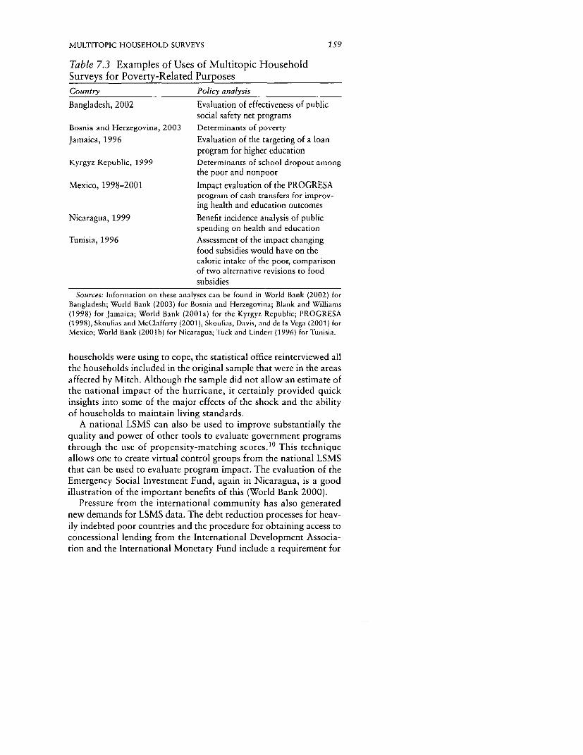
MULTITOPIC HOUSEHOLD SURVEYS 159
Table 7.3 Examples of Uses of Multitopic HouseholdSurveys for Poverty-Related Purposes
Country Policy analysis
Bangladesh, 2002 Evaluation of effectiveness of publicsocial safety net programs
Bosnia and Herzegovina, 2003 Determinants of poverty
Jamaica, 1996 Evaluation of the targeting of a loanprogram for higher education
Kyrgyz Republic, 1999 Determinants of school dropout amongthe poor and nonpoor
Mexico, 1998-2001 Impact evaluation of the PROGRESAprogram of cash transfers for improv-ing health and education outcomes
Nicaragua, 1999 Benefit incidence analysis of publicspending on health and education
Tunisia, 1996 Assessment of the impact changingfood subsidies would have on thecaloric intake of the poor, comparisonof two alternative revisions to foodsubsidies
Sources: Information on these analyses can be found in World Bank (2002) forBangladesh; World Bank (2003) for Bosnia and Herzegovina; Blank and Williams(1998) for Jamaica; World Bank (2001a) for the Kyrgyz Republic; PROGRESA(1998), Skoufias and McClafferty (2001), Skoufias, Davis, and de la Vega (2001) forMexico; World Bank (2001b) for Nicaragua; Tuck and Lindert (1996) for Tunisia.
households were using to cope, the statistical office reinterviewed all
the households included in the original sample that were in the areasaffected by Mitch. Although the sample did not allow an estimate ofthe national impact of the hurricane, it certainly provided quickinsights into some of the major effects of the shock and the abilityof households to maintain living standards.
A national LSMS can also be used to improve substantially thequality and power of other tools to evaluate government programsthrough the use of propensity-matching scores.1 0 This techniqueallows one to create virtual control groups from the national LSMSthat can be used to evaluate program impact. The evaluation of theEmergency Social Investment Fund, again in Nicaragua, is a goodillustration of the important benefits of this (World Bank 2000).
Pressure from the international community has also generatednew demands for LSMS data. The debt reduction processes for heav-ily indebted poor countries and the procedure for obtaining access toconcessional lending from the International Development Associa-tion and the International Monetary Fund include a requirement for

160 scorr
a government poverty reduction strategy. Such a strategy presup-poses the ability to measure and monitor poverty as well as othersocial indicators. In countries such as Bolivia, Bosnia and Herzegov-ina, Kyrgyz Republic, and Vietnam, for example, the LSMS data areproviding both the baseline data for measuring poverty and the toolto monitor the completion of the goals set out in the strategy.
The focus on the Millennium Development Goals (MDGs) havecreated another source of demand for timely, good quality, house-hold-level data. Several of the MDGs can be measured using datafrom LSMS surveys: access to education by males and females, andpoverty levels, for example. The small sample size does limit theability of the LSMS to provide data for all the MDGs: mortalityrates cannot be estimated from an LSMS survey as these ratesrequire a substantially larger sample size. But the LSMS is a usefultool to help countries generate the needed information to monitortheir progress in reaching the MDGs.
Capacity Building and Sustainability
There is often a discussion of the tradeoffs between short-term dataneeds and long-term capacity building. It is useful to recognize thatin many cases, the lack of data availability in the short run is simplythe result of previous planners not having invested in the long term.To avoid continuing this expensive focus on the short term, it isimperative to recognize the importance of capacity building when amultitopic household survey such as an LSMS is contemplated. Theprocess of designing, implementing, and analyzing the data is key tocreating a capacity for future quality survey work and analysis. It isa lengthy process, one often not suited to short project cycles, and itrequires explicit attention in the planning and budgeting phases.
The ultimate goal is to create some level of sustainability: theability of the country to produce and use policy relevant data overtime. Creating the capacity in both survey techniques and analysis isa necessary, albeit not sufficient, condition for sustainability tooccur. Experience with LSMS surveys (and others) has shown thatsustainability is a long-term effort and cannot be obtained in thecontext of a single survey. Instead, a program that contemplatesmultiple rounds of an LSMS, in conjunction with other surveysneeded by policymakers, is needed. Explicitly linking and involvingdata producers and users in both the design and the analysis of thedata has also proved to be a key ingredient. Again, this process oflearning to use microeconomic data is not achieved overnight. Pres-

MULTITOPIC HOUSEHOLD SURVEYS 161
sures will always exist to generate data quickly, but it is importantto maintain a long-term vision if the LSMS is truly to have an impacton government policy.
Conclusions
There is a strong need for increasing governments' use of empirical-based policymaking. Single-topic surveys are one tool, but they failto provide governments and researchers with a comprehensiveunderstanding of how households behave and the interaction ofhouseholds with government social and economic policy. Multi-topic household surveys, by explicitly linking the different factorsaffecting welfare, represent a potentially powerful tool for measur-ing how government policies affect households. By involving poli-cymakers in the design and analysis phases of the survey, both therelevance and quality of the data can be improved, as well as theextent to which data is used in policymaking. Part of the process ofcarrying out any multitopic survey should be to build the overallcapacity to design and implement the survey and to use the resultingdata. Although that requires a substantial investment, the return inthe form of increased effectiveness and efficiency of public spendingand policies can be substantial.
Notes
1. One of the positive results of the United Nations' National House-hold Survey Capability Programme has been that of institutionalizingthese surveys in many countries. In several countries in Latin America, for
example, this survey may be the only household survey that has been
done consistently.2. An example from Uruguay (Grosskoff 1998) illustrates this point. A
comparison of income estimates from a Labor Force Survey, an Income and
Expenditure Survey, and the relevant section of the national accounts in
Uruguay showed that although the IES did a better job of approximating
the national accounts figures than the LFS, both surveys underestimated
household income, relative to the national accounts.3. A nice summary of the reasons why total consumption might be pre-
ferred as a measure of welfare over total income can be found in Deaton
and Grosh (2000).
4. For a detailed discussion of the use value of durable goods and hous-ing and the date required to estimate these, see Deaton and Zaidi (2002).

162 scorr
S. For detailed information on the Family Life Surveys, see the RandCorporation Web site (www.rand.org); on Integrated Surveys, see WorldBank (1992); for Living Standards Measurement Study Surveys, see Grosh
and Munoz (1996) or the LSMS Web site (http://www.worldbank.orgflsms).6. See Pradham and Ravallion (2000) and Ravallion and Lokshin (2001,
2002) for examples of the use of such measures.
7. About half of all LSMS surveys administered community question-naires.
8. See chapter 8.9. See chapter 4.10. See chapter 5.
References
The word processed describes informally reproduced works that may notbe commonly available through library systems.
Blank, Lorraine, and Colin Williams. 1998. "Reanalysis of the First ImpactEvaluation Study of 1996." Students Loan Bureau, Kingstown, Jamaica.Processed.
Deaton, Angus, and Margaret Grosh. 2000. "Consumption." In Grosh andGlewwe, eds., (2000).
Deaton, Angus, and Salman Zaidi. 2002. "Guidelines for Constructing
Consumption Aggregates for Welfare Analysis." Living Standards Mea-surement Study Working Paper 135. World Bank, Development Eco-nomics Research Group, Washington, D.C. Processed.
Feres, Juan Carlos. 1998. "Falta de Respuesta a las Preguntas Sobre elingreso. Su magnitud y efectos en las Encuestas de Hogares en Am6ricaLatina." Programa para el Mejoramientos de las Encuestas y la Medici6nde las Condiciones de Vida en America Latina y el Caribe, 2° TallerRegional, Buenos Aires, Argentina, November 10-13, 1998.
Filmer, Deon, and Lant Pritchett. 1998a. "The Effect of Household Wealthon Educational Attainment around the World: Demographic and HealthSurvey Evidence." Policy Research Working Paper 1980. World Bank,
Development Economics Research Group, Washington, D.C. Processed.. 1998b. "Estimating Wealth Effects without Expenditure Data-or
Tears: An Application to Educational Enrollments in States of India."Policy Research Working Paper 1994. World Bank, Development Eco-nomics Research Department, Washington, D.C. Processed.
Glewwe, Paul, and Phong Nguyen. 2002. "Economic Mobility in Vietnamin the 1990s." Policy Research Working Paper 2838. World Bank, Devel-opment Economics Research Group, Washington, D.C. Processed.

MULTITOPIC HOUSEHOLD SURVEYS 163
Grosh, Margaret. 1997. "The Policymaking Uses of Multi-topic HouseholdSurvey Data: A Primer." World Bank Research Observer 12(2): 137-60.
Grosh, Margaret, and Paul Glewwe, eds. 2000. Designing Household Sur-vey Questionnaires for Developing Countries: Lessons from 15 Years ofthe Living Standards Measurement Study Surveys. Washington, D.C.:
World Bank.Grosh, Margaret, and Juan Munoz. 1996. "A Manual for Planning and
Implementing the Living Standards Measurement Study Survey." Living
Standards Measurement Study Working Paper 126. World Bank, Devel-opment Economics Research Group, Washington, D.C. Processed.
Grosskoff, Rosa. 1998. "Comparaci6n de las estadisticas de ingresos prove-nientes de encuestas de hogares con estimaciones externas." Programapara el Mejoramientos de las Encuestas y la Medici6n de las Condi-ciones de Vida en America Latina y el Caribe, 20 Taller Regional, BuenosAires, Argentina, November 10-13, 1998.
Montgomery, Mark, Kathleen Burke, Edmundo Paredes, and Salman Zaidi.2000. "Measuring Living Standards with Proxy Variables." Demogra-
phy 37(2): 155-74.Pradhan, Menno, and Martin Ravallion. 2000. "Measuring Poverty Using
Qualitative Perceptions of Consumption Adequacy." Review of Eco-
nomics and Statistics 82: 462-71.PROGRESA. 1998. Metodolog:a para la Identificacion de los Hogares Ben-
eficiarios del PROGRESA. Mexico City, Mexico.Ravallion, Martin, and Michael Lokshin. 2001. "Identifying Welfare Effects
Using Subjective Questions." Economica 68: 335-57.. 2002. "Self-Rated Economic Welfare in Russia." European Eco-
nomic Review 46(8): 1453-73.Scott, Kinnon, Diane Steele, and Tilahun Temesgten. Forthcoming. "Living
Standards Measurement Study Surveys." In Ibrahim-Sorie Yansaneh,ed., The Analysis of Operating Characteristics of Surveys in Developing
Countries. United Nations Technical Report, New York.Skoufias, Emmanuel, and B. McClafferty. 2001. "Is PROGRESA Working?
Summary of the Results of an Evaluation by IFPRI." FCND DiscussionPaper 118. International Food Policy Research Institute, Washington,
D.C. Processed.Skoufias, Emmanuel, Benjamin Davis, and Sergio de la Vega. 2001. "Tar-
geting the Poor in Mexico: An Evaluation of the Selection of Householdsinto PROGRESA." World Development 29(10): 1769-84.
Tuck, Laura, and Kathy Lindert. 1996. "From Universal Food Subsidies toa Self-Targeted Program: A Case Study in Tunisian Reform." DiscussionPaper 351. World Bank, Agricultural Operations Division, Middle Eastand North Africa Region, Washington, D.C. Processed.
World Bank. 1992. "The Social Dimensions of Adjustment Integrated Sur-vey: A Survey to Measure Poverty and Understand the Effects of Policy

164 scOTr
Change on Households." Social Dimensions of Adjustment in Sub-Saharan Africa Working Paper 14. Washington, D.C. Processed.
- 1999. "Bangladesh: From Counting the Poor to Making the PoorCount." Country Study 19648. Washington, D.C. Processed.
. 2000. "Nicaragua: Ex-Post Impact Evaluation of the EmergencySocial Investment Fund (FISE)." Report 20400-NI. Washington, D.C.Processed.
- 2001a. "Poverty in the 1990s in the Kyrgyz Republic." Report21721-KG. Human Development Department, Country DepartmentVIII, Europe and Central Asia Region, Washington, D.C. Processed.
- 2001b. "Nicaragua Poverty Assessment Challenges and Opportu-nities for Poverty Reduction." Report 20488-NI. Poverty Reduction andEconomic Management Sector Unit, Latin American and the CaribbeanRegion, Washington, D.C. Processed.
. 2002. "Poverty in Bangladesh: Building on Progress." Report24299-BO. Poverty Reduction and Economic Management Sector Unit,South Asia Region, Washington, D.C. Processed.
. 2003. "Bosnia and Herzegovina: Poverty Assessment." Report25343-BIH. Poverty Reduction and Economic Management Sector Unit,Europe and Central Asia, Washington, D.C. Processed.

8
Integrating Qualitative andQuantitative Approaches
in Program Evaluation
Vijayendra Rao and Michael Woolcock
This chapter outlines some of the ways and means by which inte-grating qualitative and quantitative approaches in developmentresearch and program evaluation can help yield insights that neitherapproach would produce on its own. In assessing the impact ofdevelopment programs and policies, it is important to recognizethat the quantitative methods emphasized in this tool kit, whileenormously useful, nonetheless have some important limitationsand that some of these can be overcome by incorporating comple-mentary qualitative approaches. An examination of the strengthsand weakness of orthodox stand-alone quantitative (and qualita-tive) approaches is followed by a basic framework for integratingdifferent approaches, based on distinguishing between data and themethods used to collect them. Some practical examples of "mixed-method" approaches to program evaluation are then given, andsome conclusions drawn.
Mixed Methods and Program Evaluation
The advantages of quantitative approaches to program evaluationare well known. Conducted properly, they permit generalizationsto be made about large populations on the basis of much smaller
165

166 RAO AND WOOLCOCK
(representative) samples. Given a set of identifying conditions, theycan help establish the causality of the impact of given variables onproject outcomes. And (in principle) they allow other researchersto validate the original findings by independently replicating theanalysis. By remaining several steps removed from the people fromwhom the data has been obtained, and by collecting and analyzingdata in numerical form, quantitative researchers argue that they areupholding research standards that are at once empirically rigorous,impartial, and objective.
The Case for Integrating Different Approaches
In social science research, however, these same strengths can also bea weakness. Many of the most important issues facing the poor-their identities, perceptions, and beliefs, for example-cannot bemeaningfully reduced to numbers or adequately understood with-out reference to the immediate context in which they live. Most sur-veys are designed far from the places where they will be adminis-tered and as such tend to reflect the preconceptions and biases of theresearcher; there is little opportunity to be "surprised" by new dis-coveries or unexpected findings. Although good surveys undergoseveral rounds of rigorous pretesting, the questions themselves areusually not developed using systematically collected insights fromthe field. Thus, while pretesting can identify and correct questionsthat show themselves to be clearly ill suited to the task, these prob-lems can be considerably mitigated by the judicious use of qualita-tive methods in the process of developing the questionnaire.
Qualitative methods can also help in circumstances where a quan-titative survey may be difficult to administer. Certain marginalizedcommunities, for example, are small in number (the disabled, wid-ows) or difficult for outsiders to access (sex workers, victims ofdomestic abuse), rendering them unlikely subjects for study througha large representative survey. In many developing country settings,central governments (let alone local nongovernmental organizationsor public service providers) may lack the skills and (especially) theresources needed to conduct a thorough quantitative evaluation.Moreover, external researchers with little or no familiarity witheven the country (let alone region or municipality) in question oftendraw on data from context-specific household surveys to makebroad "policy recommendations," yet rarely provide useful resultsto local program officials or the poor themselves. Scholars workingfrom qualitative research traditions in development studies like toproclaim that their approaches rectify some of these concerns byproviding more detailed attention to context, reaching out to mem-

QUALITATIVE AND QUANTITATIVE APPROACHES 167
bers of minority groups, working with available information andresources, and engaging the poor as partners in the collection, analy-sis, and interpretation of data (in all its many forms).'
Furthermore, in conducting evaluations, quantitative methodsare best suited to measuring levels and changes in impacts and todrawing inferences from observed statistical relations between thoseimpacts and other covariates. They are less effective, however, inunderstanding process-that is, the mechanisms by which a partic-ular intervention instigates a series of events that ultimately result inthe observed impact. For example, consider a community-drivendevelopment (CDD) project that sets up a committee in a villageand provides it with funds to build a primary school. Even if a per-fect quantitative impact evaluation were set up, it would typicallymeasure quantitative outcomes such as the causal impact of theCDD funds on increasing school enrollment or whether benefitswere well targeted to the poor. With some carefully constructedquestions, one could perhaps get at some more subtle issues, such asthe heterogeneity in levels of participation in decisionmaking acrossdifferent groups, or even more subjective outcomes, such as changesin levels of intergroup trust in the village. Nevertheless, the quanti-tative analysis would not be very effective at describing the localpolitics in the village that led to the formation of the committee orthe details pertaining to deliberations within it: How were certaingroups included and others excluded? How did some individualscome to dominate the process? These are called process issues, andthey can be crucial to understanding impact, as opposed to simplymeasuring it. Qualitative methods are particularly effective in delv-ing deep into issues of process; a judicious mix of qualitative andquantitative methods can therefore help provide a more compre-hensive evaluation of an intervention.
Qualitative approaches on their own, of course, also suffer froma number of important drawbacks. First, the individuals or groupsbeing studied are usually small in number or have not been ran-domly selected, making it highly problematic (though not impossi-ble) to draw generalizations about the wider population. Second,because groups are often selected idiosyncratically (for example, onthe basis of a judgment call by the lead investigator) or on the rec-ommendation of other participants (as with "snowball" samplingprocedures, in which one informant-say, a corrupt public official-agrees to provide access to the next one), it is difficult to replicate,and thus independently verify, the results. Third, the analysis ofqualitative analysis often involves interpretative judgments on thepart of the researcher, and two researchers looking at the same datamay arrive at different interpretations. (Quantitative methods are

168 RAO AND WOOLCOCK
relatively less prone to such subjectivities in interpretation, thoughnot entirely free of them.) Fourth, because of an inability to "con-trol" for other mitigating factors or to establish the counterfactual,it is hard (though again not impossible) to make compelling claimsregarding causality. 2
It should be apparent that the strengths of one approach poten-tially complement the weaknesses of the other, and vice versa. Unfor-tunately, however, research in development studies generally, andprogram evaluation in particular, tends to be heavily polarized alongquantitative and qualitative methodological lines. That is largelybecause researchers are recruited, trained, socialized, evaluated, andrewarded by single disciplines (and their peers and superiors withinthem) that have clear preferences for one research tradition overanother. This practice ensures intellectual coherence and "qualitycontrol" but comes at the expense of discouraging innovation andlosing any potential gains that could be derived from integrating dif-ferent approaches. We are hardly the first to recognize the limita-tions of different approaches or to call for more methodologicalpluralism in development research-indeed, notable individuals atleast since Epstein (1962) have made pathbreaking empirical contri-butions by working across methodological lines.3 What we are try-ing to do, however, is to take the strengths and weaknesses of eachapproach seriously and discern practical (if no less difficult) strate-gies for combining them on a more regular basis as part of the over-all program evaluation exercise (see also Kanbur 2003 and Rao2002).4 What might this entail?
Distinguishing between Data and Methodsin Program Evaluation
A possible point of departure for thinking more systematically aboutmixed-method approaches to program evaluation is to distinguishbetween forms of data and the methods used to collect them(Hentschel 1999). This distinction posits that data can be eitherquantitative (numbers) or qualitative (text), just as the methodsused to collect that data can also be quantitative (for example, largerepresentative surveys) or qualitative (such as interviews and obser-vation), giving rise to a simple 2 x 2 table (figure 8.1). Most devel-opment research and program evaluation strategies call upon quan-titative data and methods or qualitative data and methods (that is,the upper right or lower left quadrants), but it is instructive to notethat qualitative methods can also be used to collect quantitativedata-as is seen in the detailed household data reported in Bliss andStern (1982) and Lanjouw and Stern (1998) from a single village in

QUALITATIVE AND QUANTITATIVE APPROACHES 169
Figure 8.1 Types of Data and Methods
Methods
Quantity
Subjective welfare Standard Household Survey
Quality Quantity
Data
Ethnography Economic anthropologyRRE, PRA (Participatory econometrics)
Small-N matched comparisons
Quality
Source: Adapted from Hentschel (I1999).
India over several decades-and that quantitative methods can beused to collect qualitative data-as when open-ended or "subjec-tive" response questions are included in large surveys (Ravallionand Pradhan 2000, for example), or when quantitative measures arederived from a large number of qualitative responses (Isham,Narayan, and Pritchett 1995, for example). Other examples fromdevelopment that fall into this latter category include comparativecase-study research, where the number of cases is necessarily small,but the units of analysis are large (such as the impact of the EastAsian financial crisis on Korea, Thailand, and Indonesia).
Having made this distinction, it is instructive to consider in moredetail the nature of some of the qualitative methods that are avail-able to development researchers before exploring some of the waysin which they could be usefully incorporated into a more compre-hensive mixed-method strategy for evaluating programs and pro-jects. Three approaches are identified-participation, ethnography,and textual analysis. The particular focus of this chapter is on theuse of qualitative methods to generate more and better quantitativedata and to understand the process by which an intervention works,in addition to ascertaining its overall final impact.5
170 RAO AND WOOLCOCK
The first category of qualitative methods can be referred to asparticipatory approaches (Mikkelsen 1995; Narayan 1995; andRobb 2002). Introduced to scholars and practitioners largelythrough the work of Robert Chambers (see, most recently, Kumarand Chambers 2002), participatory techniques-such as RapidRural Appraisal (RRA) and Participatory Poverty Assessment(PPA)-seek to help outsiders learn about poverty and projectimpacts in cost-effective ways that reflect grounded experience.Since the Rapid Rural Appraisal is usually conducted with respon-dents who are illiterate, RRA researchers seek to learn about thelives of the poor using simple techniques such as wealth rankings,oral histories, role-playing, games, small group discussions, and vil-lage map drawings. These techniques permit respondents who arenot trained in quantitative reasoning, or who are illiterate, to pro-vide meaningful graphic representations of their lives in a mannerthat can give outside researchers a quick snapshot of an aspect oftheir living conditions. As such, RRA can be said to deploy instru-mental participation research-novel techniques are being used tohelp the researcher better understand her subjects. A relatedapproach is to use transformative participation techniques, such asParticipatory Rural Appraisal (PRA), in which the goal is to facili-tate a dialogue, rather than extract information, that helps the poorlearn about themselves and thereby gain new insights that lead tosocial change ("empowerment"). 6 In PRA exercises, a skilled facili-tator helps villagers or slum dwellers generate tangible visual dia-grams of the processes that lead to deprivation and illness, of thestrategies that are used in times of crisis, and of the fluctuation ofresource availability and prices across different seasons. Elicitinginformation in this format helps the poor to conceive of potentiallymore effective ways to respond (in ways that are not obvious exante) to the economic, political, and social challenges in their lives.
A crucial aspect of participatory methods is that they are con-ducted in groups. Therefore, it is essential that recruitment of par-ticipants be conducted so that representatives from each of the majorsubcommunities in the village are included. The idea is that if thegroup reaches a consensus on a particular issue after some discus-sion, then this consensus will be representative of views in the vil-lage because outlying views would have been set aside in the processof debate. For this technique to work, the discussion has to beextremely well moderated. The moderator must be dynamic enoughto steer the discussion in a meaningful direction, deftly navigatinghis or her way around potential conflicts and, by the end, establish-ing a consensus. The moderator's role is therefore key to ensuringthat high-quality data are gathered in a group discussion-a poor orinexperienced moderator can affect the quality of the data in a

QUALITATIVE AND QUANTITATIVE APPROACHES 171
manner that is much more acute than an equivalently poor inter-viewer working with a structured quantitative questionnaire.
Other often-used qualitative techniques that can be classified asethnographic face similar constraints. Focus-group discussions, forexample, in which small intentionally diverse or homogenous groupsmeet to discuss a particular issue, are also guided by a moderatortoward reaching consensus on key issues. Focus groups are thussimilarly dependent on the quality of the moderator for the qualityof the insights they yield. A focus group differs from a PRA in that itis primarily instrumental in its purpose and typically does not use themapping and diagramming techniques that are characteristic of aPRA or RRA. Here, however, it should be noted that divergencefrom the consensus can also provide interesting insights, just as out-liers in a regression can sometimes be quite revealing. Another impor-tant ethnographic technique that uses interview methods is the key-informant interview, which is an extended one-on-one exchange withsomeone who is a leader or unique in some way that is relevant tothe study. Finally, the ethnographic investigator can engage in vary-ing degrees of "participant observation," in which the researcherengages a community at a particular distance-as an actual member(for example, a biography of growing up in a slum), as a perceivedactual member (a spy or police informant in a drug cartel, for exam-ple), as an invited long-term guest (such as an anthropologist), or asa more distant and detached short-term observer.7
A third qualitative approach is textual analysis. Historians,archaeologists, linguists, and scholars in cultural studies use suchtechniques to analyze various forms of media, ranging from archivedlegal documents, newspapers, artifacts, and government records tocontemporary photographs, films, music, and television reports.(We provide an example below of the use of textual analysis in sup-plementing quantitative surveys in an evaluation of democraticdecentralization in India.) Participatory, ethnographic, and textualresearch methods are too often seen as antithetical to or a poor sub-stitute for quantitative approaches. In the examples that follow, weshow how qualitative and quantitative methods have been usefullycombined in development research and project evaluation, provid-ing in unison what neither could ever do alone.
Mixed Methods Research and Project Evaluation:Pitfalls, Principles, and Examples
Having briefly outlined the types of qualitative methods available inour tool kit, we now sketch the different methods of integrationbetween qualitative and quantitative techniques, providing examples

172 RAO AND WOOLCOCK
for each method. The examples presented below are drawn fromattempts to combine different methodological traditions in evalua-tion and policy research, but we stress from the outset that there areseveral good (as well as bad) reasons why mixed methods are notadopted more frequently. First, integrating different perspectives nec-essarily requires recruiting individuals with different skill sets, whichmakes such projects costly in terms of time, talent, and resources.Second, coordinating the large teams of people with diverse back-grounds that are often required for serious mixed-method projectsgenerates coordination challenges above and beyond those normallyassociated with program evaluation. Third, these challenges, com-bined with institutional imperatives for quick turnaround and"straightforward" policy recommendations, mean that mixed-method research is often poorly done. Fourth, we simply lack anextensive body of evidence regarding how different methods can bestbe combined under what circumstances; more research experience isneeded to help answer these questions and guide future efforts.
These concerns notwithstanding, it is nonetheless possible to dis-cern a number of core principles and strategies for successfully mix-ing methods in project evaluation. The most important of these is tobegin with an important, interesting, and researchable question andto then identify the most appropriate method (or combination ofmethods) that is likely to yield fruitful answers (Mills 1959). If takenseriously, this principle is actually remarkably difficult to live up to,since it is rare to find a good question that maps neatly and exclu-sively onto a single method. Three fields in which faithful effortshave been made, however, are comparative politics, anthropologicaldemography, and anthropological economics. The first concernsitself primarily with questions that give rise to small sample sizesand large units of analysis-most commonly case studies of coun-tries or large organizations studied historically-and is not discussedin detail here.8 The second and third, however, are better suited tolarger sample sizes and smaller units of analysis, and thus lessonsfrom them are especially relevant to efforts to mix methods inpoverty research and project evaluation.9
Methods of Integration
Qualitative and quantitative methods can be integrated in three dif-ferent forms, which for convenience we call parallel, sequential, anditerative. In parallel approaches, the quantitative and qualitativeresearch teams work separately but compare and combine findingsduring the analysis phase. This approach is best suited to very largeprojects, such as national level poverty assessments, where closer

QUALITATIVE AND QUANTITATIVE APPROACHES 173
forms of integration are precluded by logistical and administrativerealities. In "Poverty in Guatemala" (World Bank 2002), for exam-ple, two separate teams were responsible for collecting the qualita-tive and quantitative data. Previous survey material was used tohelp identify the appropriate sites for the qualitative work (five pairsof villages representing the five major ethnic groups in Guatemala),but the findings themselves were treated as an independent source ofdata and were integrated with the quantitative material only in thewrite-up phase of both the various background papers and the finalreport-that is, while useful in their own right, the qualitative datadid not inform the design or construction of the quantitative survey,which was done separately. These different data sources were espe-cially helpful in providing a more accurate map of the spatial anddemographic diversity of the poor, as well as, crucially, a sense ofthe immediate context within which poverty was experienced bydifferent ethnic groups, details of the local mechanisms thatexcluded them from participation in mainstream economic and civicactivities, and the nature of the barriers they encountered in theirefforts to advance their interests and aspirations. The final reportalso benefited from a concerted effort to place both the qualitativeand quantitative findings in their broader historical and politicalcontext, a first for a World Bank poverty study.
Sequential and iterative approaches-which we call more specif-ically participatory econometrics-seek varying degrees of dialoguebetween the qualitative and quantitative traditions at all phases ofthe research cycle and are best suited to projects of more modestscale and scope.10 Though the most technically complex and timeconsuming, these approaches are where the greatest gains are to befound from mixing methods in project and policy evaluation. Par-ticipatory econometrics works on the premise that
* The researcher should begin a project with some generalhypotheses and questions, but an open mind regarding the resultsand even the possibility that the hypotheses and questions them-selves may be in need of major revision.
* The researcher should both collect and analyze the data.* A mix of qualitative and quantitative data is typically used to
create an understanding of both measured impact and process.* Respondents should be actively involved in the analysis and
interpretation of findings.* It is desirable to make broad generalizations and discern the
nature of causality; consequently, relatively large sample sizes arelikely to be-needed (and thus the tools of econometrics employed onthem).

174 RAO AND WOOLCOCK
This approach characterizes recent research on survival and mobil-ity strategies in Delhi slums (Jha, Rao, and Woolcock 2002), inwhich extensive qualitative investigation in four different slum com-munities preceded the design of a survey that was then administeredto 800 randomly selected households from all (officially listed) Delhislums. The qualitative material not only helped design a better sur-vey, but was also drawn upon in its own right to explore governancestructures, migration histories, the nature and extent of propertyrights, and mechanisms underpinning the procurement of housing,employment, and public services.
The classical, or sequential, approach to participatory economet-rics entails three key steps:
o Using PRA-type techniques, focus-group discussions, in-depthinterviews, or all three to obtain a grounded understanding of issues.
o Constructing a survey instrument that integrates understand-ings from the field.
o Deriving hypotheses from qualitative work and testing withsurvey data. An intermediate step of constructing theoretical mod-els to generate hypotheses may also be added (Rao 1997).
An example of the use of sequential mixed methods in projectevaluation is a study of the impact of Social Investment Funds inJamaica (Rao and Ibafiez 2003). The research team compiled case-study evidence from five matched pairs of communities in Kingston,in which one community in the pair had received funds from theJamaica Social Investment Fund (JSIF) while the other had not-buthad been selected to match the funded community as closely as pos-sible in terms of its social and economic characteristics. The quali-tative data revealed that the JSIF process was elite-driven, with deci-sionmaking processes dominated by a small group of motivatedindividuals, but that by the end of the project there was nonethelessbroad-based satisfaction with the outcome. The quantitative datafrom 500 households mirrored these findings by showing that, exante, the social fund did not address the expressed needs of themajority of individuals in the majority of communities. By the endof the JSIF cycle, however, during which new facilities had been con-structed, 80 percent of the community expressed satisfaction with theoutcome. A quantitative analysis of the determinants of participationdemonstrated that individuals who had higher levels of education andmore extensive networks dominated the process. Propensity-scoreanalysis revealed that the JSIF had a causal impact on improvementsin trust and the capacity for collective action, but that these gainswere greater for elites within the community."1 This evidence suggeststhat both JSIF and non-JSIF communities are now more likely to

QUALITATIVE AND QUANTITATIVE APPROACHES 175
make decisions that affect their lives-a positive finding indicativeof widespread efforts to promote participatory development in thecountry-but that JSIF communities do not show higher levels ofcommunity-driven decisions than non-JSIF communities. A particu-lar strength of this analysis is that here a development project thatis by design both "qualitative" (participatory decisionmaking) and"quantitative" (allocating funds to build physical infrastructure)has been evaluated using corresponding methods.
The Bayesian, or iterative, approach to participatory economet-rics is similar to the sequential approach, but it involves regularlyreturning to the field to clarify questions and resolve apparent anom-alies. Here, qualitative findings can be regarded as a Bayesian Priorthat is updated with quantitative investigation. One example comesfrom an initial study of marriage markets among potters in ruralKarnataka, India, which led to work on domestic violence (Rao1998, Bloch and Rao 2002); unit price differentials in everydaygoods, that is, why the poor pay higher prices than the rich for thesame good (Rao 2000); and public festivals (Rao 2001a, 2001b).An initial interest in marriage markets thus evolved in several dif-ferent but unanticipated directions, uncovering understudied phe-nomena that were of signal importance in the lives of the peoplebeing studied. Moreover, the subjects of the research, with their par-ticipation in PRAs and PPAs, focus-group discussions, and in-depthinterviews, played a significant role in shaping how research ques-tions were defined, making an important contribution to the analy-sis and informing the subsequent econometric work, which testedthe generalizability of the qualitative findings, measuring the mag-nitude of the effects and their causal determinants.
Iterative mixed-method approaches to project evaluation aremost likely to be useful in situations where task managers are over-seeing projects that have a diverse range of possible impacts (someof which may be unknown or unintended), and where some form ofparticipation" has been a central component of project design and
implementation. Ideally an orthodox difference-in-difference strat-egy of collecting both baseline and follow-up data and identifyingcomparable program and nonprogram groups should be followed.But it is not always self-evident, a priori, how exactly one should goabout selecting communities for intensive qualitative work or whatprecise questions should be included on a household survey.
Two evaluations of participatory (community-driven develop-ment) projects currently under way in Indonesia demonstrate thebenefits of using iterative mixed-method approaches. The first isconcerned with designing a methodology for identifying the extentof a range of impacts associated with a project in urban areas

176 RAO AND WOOLCOCK
(known as the Urban Poverty Project 2, or UPP2); the second withassessing whether and how a similar project already operating forthree years in rural areas (the Kecamatan Development Program, orKDP) helps to mediate local conflict.
UPP2 is a CDD project that provides money directly to commu-nities to fund infrastructure projects and microcredit. To do this, theproject organizes an elected committee called the BKM. In additionto poverty alleviation and improvements in service delivery, one ofUPP2's goals is to create an accountable system of governance inpoor urban communities. Here, again, both outcomes and processare of interest and therefore the evaluation is a prime candidate fora mixed-methods approach. The evaluation follows a difference-in-difference approach. A baseline survey is being conducted in a ran-dom sample of communities that will benefit from the intervention.These communities have been matched using a poverty scoreemployed by the government to target UPP2 to poor communities.The "control" communities are those with low poverty scores in rel-atively rich districts, whereas the "experimental" communities arethose with high poverty scores in relatively poor districts.
Two rounds of field work were conducted by an interdisciplinaryteam of economists, urban planners, and social anthropologists.12
In the first round two to three days of field visits were conducted ineach of eight communities that had benefited from a similar project(UPP1). The aim of this initial round of field work was to under-stand the UPP2 process, identify "surprises" that could be incorpo-rated in the survey, and decide on a data collection methodology.Some of these unforeseen issues included the key role that facilita-tors played in the success or failure of a project at the local level, theinherent "competition" between BKMs and existing mechanismsfor governance (such as the municipal officer, or Pak Lurah), andthe crucial role that custom, tradition, and local religious institu-tions played in facilitating collective action. A quantitative surveymethodology was developed that would give key informants such asthe head of the BKM, the Pak Lurah, the community activist, andthe local facilitator an in-depth structured questionnaire. In addi-tion, a random sample of households within each community wouldreceive a household questionnaire. When microcredit groups wereformed in the experimental communities, they too would be given ahousehold questionnaire.
To supplement this material, a qualitative baseline was alsodesigned. The sample size of this baseline was limited by the highcost of conducting in-depth qualitative work in many communities.Therefore, it was decided to do a case-based comparative analysis:two "experimental communities" (one with a high degree of urban-

QUALITATIVE AND QUANTITATIVE APPROACHES 177
ization and the other with a low degree of urbanization) and two"control communities" (matched to the experimental communitiesusing the poverty score) were chosen in each province. Since UPP2 isworking in three provinces-Java, Kalimantan and Sulawesi-a totalof 12 communities are in the sample. A team of field investigatorswill spend one week in each community conducting a series of focus-group discussions, in-depth interviews, and key-informant interviewsin two groups. One group will snowball from the municipal office,focusing on the network of people who are centered around the for-mal government, while another group of investigators will snowballfrom the local mosque, church, or activist group to understand therole of informal networks and associations in the community."3 Theidea is that the qualitative work will provide in-depth insights intoprocesses of decisionmaking, the role of custom (adat) and traditionin collective action, and the propensity for elite capture in the com-munity. Hypotheses generated from the qualitative data will be testedfor their generalizability with the quantitative data.
Finally, the whole process will be repeated three years after theinitiation of the project to collect follow-up data. The follow-up willprovide a difference across control and experimental groups, and asecond difference across time to isolate the causal impact of UPP2on the community and to examine the process by which communi-ties changed because of the UPP2 intervention.
The Kecamatan Development Program in Indonesia-the modelon which the UPP2 program is based-is one of the world's largestsocial development projects, and Indonesia itself is a country expe-riencing wrenching conflict in the aftermath of the Suharto era andthe East Asian financial crisis. Although primarily intended as amore efficient and effective mechanism for getting targeted small-scale development assistance to poor rural communities, KDPrequires villagers to submit proposals for funding to a committee oftheir peers, thereby establishing a new (and, by design, inclusive)community forum for decisionmaking on key issues (Wetterbergand Guggenheim 2003). Given the salience of conflict as a politicaland development issue in Indonesia, the question is whether theseforums are able to complement existing local-level institutions forconflict resolution and in the process help villagers acquire a morediverse, peaceful, and effective set of civic skills for mediating localconflict. Such a question does not lend itself to an orthodox stand-alone quantitative or qualitative evaluation, but rather to an innov-ative mixed-method approach.
In this instance, the team decided to begin with qualitative work,since there was surprisingly little quantitative data on conflict inIndonesia and even less on the mechanisms (or local processes) by

178 RAO AND WOOLCOCK
which conflict is initiated, intensified, or resolved.1 4 Selecting a smallnumber of appropriate sites from across Indonesia's 13,500 islandsand 350 language groups was not an easy task, but the team decidedthat work should be done in two provinces that were very different(demographically), in regions within those provinces that (accord-ing to local experts) demonstrated both a "high" and "low" capac-ity for conflict resolution, and in villages within those regions thatwere otherwise comparable (as determined by propensity-scorematching methods) but that either did or did not participate in KDP.Such a design enables researchers to be confident that any commonthemes emerging from across either the program or nonprogramsites are not wholly a product of idiosyncratic regional or institu-tional capacity factors. Thus quantitative methods were used tohelp select the appropriate sites for qualitative investigation, whichthen entailed three months of intensive fieldwork in each of theeight selected villages (two demographically different regions bytwo high/low capacity provinces by two program/nonprogram vil-lages). The results from the qualitative work-useful in themselvesfor understanding process issues and the mechanisms by which localconflicts are created and addressed-will also feed into the design ofa new quantitative survey instrument, which will be administered toa large sample of households from the two provinces and used totest the generality of the hypotheses and propositions emerging fromthe qualitative work.
A recent project evaluating the impact of "panchayat (villagegovernment) reform"-democratic decentralization in rural India-also combines qualitative and quantitative data with a "naturalexperiment" design. 5 In 1994 the Indian government passed the73rd amendment to the Indian constitution to give more power todemocratically elected village governments by mandating that morefunds be transferred to their control and that regular elections beheld, with one-third of the seats in the village council reserved forwomen and another third for "scheduled castes and tribes" (groupswho have traditionally been targets of discrimination).
The four South Indian states of Karnataka, Kerala, AndhraPradesh, and Tamil Nadu have implemented the 73rd amendmentin different ways. Karnataka immediately began implementing thedemocratic reforms; Kerala emphasized greater financial autonomy,Tamil Nadu delayed elections by several years, and Andhra Pradeshemphasized alternative methods of village governance outside thepanchayat system. Thus, contrasting the experiences of the fourstates could provide a nice test of the role of decentralization on thequality of governance. The problem, of course, is that any differ-ences across the four states could be attributed to differences in theculture and history of the state (for instance, attributing Kerala's

QUALITATIVE AND QUANTITATIVE APPROACHES 179
outcomes to the famous "Kerala model"). Things like culture andhistory are difficult to observe, so the evaluation design exploitedthe following natural experiment.
The four states were created in a manner that made then linguis-tically homogenous in 1955. Before 1955, however, significant por-tions of the four states belonged to the same political entity andwere either ruled directly by the British or placed within a semi-autonomous "princely state." When the states were reorganized,"mistakes" were made along the border regions, with certain vil-lages that originally belonged to the same original political entityand sharing the same culture and language finding themselves placedin different states. Such villages along the border can be matchedand compared to construct a "first difference," which controls forthe effects of historical path dependency and culture. Data on levelsof economic development and other covariates that could affect dif-ferences across states are also being collected, as are data on severalquantitative outcomes, such as objective measures of the level andquality of public services in the village and perceptions on publicservice delivery at the village level.
One challenge is to study the extent of participation in public vil-lage meetings (gram sabhas) held to discuss the problems faced byvillagers with members of the governing committee. Increases in thequality of this form of village democracy would be a successful indi-cator of improvements in participation and accountability. Quanti-tative data, however, are very difficult to collect here because of theunreliability of people's memories about what may have transpiredat a meeting they may have attended. To address this issue, the teamdecided to record and transcribe village meetings directly. This tac-tic provides textual information that can be analyzed to observedirectly changes in participation. Another challenge was in collect-ing information on inequality at the village level. Some recent workhas found that sample-based measures of inequality typically havestandard errors that are too high to provide reliable estimates. PRAswere therefore held with one or two groups in the village to obtainmeasures of land distribution within the village. This approachproved to generate excellent measures of land inequality, and sincethese are primarily agrarian economies, measures of land inequalityshould be highly correlated with income inequality. Similar methodswere used to collect data on the social heterogeneity of the village.All this PRA information has been quantitatively coded, thusdemonstrating that qualitative tools can be used to collect quantita-tive data. In this example the fundamental impact assessment designwas kept intact, and both qualitative and quantitative data werecombined to provide insights into different aspects of interest in theevaluation of the intervention.

180 RAO AND WOOLCOCK
Using Mixed Methods in Time- andResource-Constrained Settings
Some final examples demonstrating the utility of mixed-methodapproaches come from settings where formal data (such as a census)is limited or unavailable and where there are few skilled or experi-enced staff and little resources or time. Such situations are commonthroughout the developing world, where every day many small (andeven not so small) organizations undertake good-faith efforts in des-perate circumstances to make a difference in the lives of the poor.Are they having a positive impact? How might their efforts andfinite resources be best expended? How might apparent failures belearned from, and successes be appropriately documented, and usedto leverage additional resources from governments or donors? Inthese circumstances, calls for or requirements of extensive technicalproject evaluation may completely overwhelm existing budgets andpersonnel, multiplying already strong disincentives to engage in anyform of evaluation (Pritchett 2002). The absence of formal data,skilled personnel, and long time horizons, however, should not meanthat managers of such programs should ignore evaluation entirely. Ifnothing else, managers and their staff have detailed contextualknowledge of the settings in which they do and do not work, as dothose people they are attempting to assist. From a basic commit-ment to "think quantitatively but act qualitatively" and to "startand work with what one has," local program staff have been able todesign and implement a rudimentary evaluation procedure that isnot a substitute for, but-we hope-a precursor to, a more thor-ough and comprehensive package (Woolcock 2001).
In St. Lucia, for example, the task manager preparing a socialanalysis had a budget to collect qualitative data from only 12 com-munities (from a sample size of 469) and wanted to ensure thatthose selected were as diverse as possible on seven key variables,namely, employment structure, poverty level, impact of a recenthurricane, access to basic services, proximity to roads, geography(regional variance, but with no two communities contiguous to oneanother), and exposure to the St. Lucia Social Development Pro-gram. How to choose these 12 communities so that they satisfiedthese criteria, with only a 10-year-old census to assist? The teamdecided to use the census data to make the first cuts in the selectionprocess, using income data to identify the 200 poorest communities(on the assumption that over a 10-year period, the ordinal rankingof the income levels of the communities would not have changedsignificantly). The census also contained data on the number ofhouseholds in each community receiving particular forms of waterdelivery and sewerage (public or private pipe, well, and so forth),

QUALITATIVE AND QUANTITATIVE APPROACHES 181
Box 8.1 Are Mixed-Methods Analyses Appropriateunder Severe Budget or Time Constraints?
If the major objective of an evaluation is measuring the impact of theintervention, rather than understanding the processes by which theevaluation worked, then qualitative work may be unnecessary. Quan-titative methods are not very effective at getting at process issues,however, so an exclusive dependence on them could give data that isincomplete for policy purposes. Mixed-methods evaluations can beconducted under a constrained budget-so long as there are enoughfunds to have a sample large enough to cover at least the primary het-erogeneity in the population and in project impacts that are of inter-est. Be aware that the more time spent in the community, the betterthe quality of the qualitative data, so a brief visit of one or two daysshould not be expected to reveal anything more subtle than basicopen-ended responses that could serve as a contextual accessory toquantitative findings. Participatory Rural Appraisal and ParticipatoryPoverty Assessment methods can be espccially useful under con-strained circumstances because they can help the community encap-sulate their points of view in a two-to-three hour group interview. Thereliability of this information, however, is strongly affected by thequality of the moderator. Therefore, if the budget is severely con-strained and skilled moderators are unavailable, it may not makesense to conduct qualitative work.
enabling a "quality of basic services" index to be constructed, andscored on a 1 (low) to 7 (high) scale. The 200 poorest communitiescould therefore be ranked according to their quality of basic services.
Finally, using geographical data, it was possible to measure thedistance of all 200 communities from the main ring road that cir-cumnavigates St. Lucia. Dividing the sample in half on the basis oftheir distance measure, those close to the road were labeled "urban,"and those far from the road "rural." The team was thus able toconstruct a simple 2 x 2 matrix, with quality of basic services (high-low) on one axis, and rural-urban on the other. St Lucia's 200 poor-est communities now fell neatly onto these axes, with 50 commu-nities in each cell.
This procedure was followed up the next day by a four-hour ses-sion with field staff-all St. Lucia nationals-narrowing the fielddown to 16 communities. Twenty field staff gathered for this meet-ing, and after a brief presentation on the task at hand and the steps
already taken with the census data, they were divided into fourgroups. Each group was given the names of 50 poor communitiesfrom one of the 2 x 2 cells above and was then asked to select five
182 RAO AND WOOLCOCK
communities from this list that varied according to exposure to therecent hurricane, major forms of employment, and whether or notthey had participated in the initial round of the St. Lucia SocialDevelopment Program. After two hours, the four groups recon-vened with the names of their five communities, and over the finalhour all field staff negotiated together to whittle the list of 20 namesdown to 16 to ensure that regional coverage was adequate and thatno two communities were contiguous across regional boundaries.After an additional round of negotiation with senior program staff,the list was reduced to the final 12 communities, a group that max-imized the variance according to the eight different criteria requiredby the task manager.
Reliance on quantitative or qualitative methods alone could neverhave achieved this result: formal data were limited and dated butnonetheless still useful; it was unrealistic and invalid to rely exclu-sively on local experts. Together, however, a superior outcome com-bining the best aspects of both methods enabled the selected sampleto have maximum diversity, validity, and (importantly) full localownership.
What Do Qualitative Methods Addto Quantitative Approaches?
There is clearly a large and important role for approaches to projectevaluation that are grounded exclusively in sophisticated quantita-tive methods. This chapter has endeavored to show that theseapproaches nonetheless have many limitations, and that consider-able value added can be gained by systematically and strategicallyincluding more qualitative approaches. By making a distinctionbetween data and the methods used to collect them, we have shownthat a range of innovative development research is currently underway in which qualitative data are examined using (or as part of)quantitative methods. The focus of this chapter, however, has beenon the use of qualitative methods to improve, complement, and sup-plement quantitative data. By way of summary and conclusion, weoutline six particular means by which qualitative methods demon-strate their usefulness in program evaluation.
By Generating Hypotheses Grounded in the Realityof the Poor
As the examples above demonstrate, when respondents are allowedto participate directly in the research process, the econometrician'swork will avoid stereotypical depictions of their reality. The result
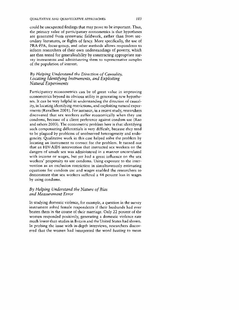
QUALITATIVE AND QUANTITATIVE APPROACHES 183
could be unexpected findings that may prove to be important. Thus,the primary value of participatory econometrics is that hypothesesare generated from systematic fieldwork, rather than from sec-ondary literatures, or flights of fancy. More specifically, the use ofPRA-PPA, focus-group, and other methods allows respondents toinform researchers of their own understandings of poverty, whichare then tested for generalizability by constructing appropriate sur-vey instruments and administering them to representative samplesof the population of interest.
By Helping Understand the Direction of Causality,Locating Identifying Instruments, and ExploitingNatural Experiments
Participatory econometrics can be of great value in improvingeconometrics beyond its obvious utility in generating new hypothe-ses. It can be very helpful in understanding the direction of causal-ity, in locating identifying restrictions, and exploiting natural exper-iments (Ravallion 2001). For instance, in a recent study, researchersdiscovered that sex workers suffer economically when they usecondoms, because of a client preference against condom use (Raoand others 2003). The econometric problem here is that identifyingsuch compensating differentials is very difficult, because they tendto be plagued by problems of unobserved heterogeneity and endo-geneity. Qualitative work in this case helped solve the problem bylocating an instrument to correct for the problem. It turned outthat an HIV-AIDS intervention that instructed sex workers on thedangers of unsafe sex was administered in a manner uncorrelatedwith income or wages, but yet had a great influence on the sexworkers' propensity to use condoms. Using exposure to the inter-vention as an exclusion restriction in simultaneously estimatingequations for condom use and wages enabled the researchers todemonstrate that sex workers suffered a 44 percent loss in wagesby using condoms.
By Helping Understand the Nature of Biasand Measurement Error
In studying domestic violence, for example, a question in the surveyinstrument asked female respondents if their husbands had everbeaten them in the course of their marriage. Only 22 percent of thewomen responded positively, generating a domestic violence ratemuch lower than studies in Britain and the United States had shown.In probing the issue with in-depth interviews, researchers discov-ered that the women had interpreted the word beating to mean

184 RAO AND WOOLCOCK
extremely severe beating-that is, when they had lost consciousnessor were bleeding profusely and needed to be taken to the hospital.Hair pulling and ear twisting, which were thought to be more every-day occurrences, did not qualify as beating. (Responses to a broaderversion of the abuse question, comparable to the questions asked inthe U.S. and U.K. surveys, elicited a 70 percent positive response.)Having tea with an outlier can be very effective in understandingwhy they are an outlier.
By Facilitating Cross-Checking and Replication
In participatory econometrics, the researcher has two sources ofdata, qualitative and quantitative, generated from the same popula-tion. That allows for immediate cross-checking and replication ofresults. If the qualitative and quantitative findings differ substan-tially, it could be indicative of methodological or data quality prob-lems in one or the other. In the Delhi slums project (Jha, Rao, andWoolcock 2002), for example, the focus-group discussions revealseveral narratives of mobility, that is, of people leaving the slums,but this mobility is not reflected in the quantitative data because thesample does not include households who live outside slums. Thisfinding indicates an important sample selection problem in the quan-titative data that limits its value in studying questions of mobility.At the same time, the qualitative data gave the impression that reli-gious institutions were an important source of credit and social sup-port for the urban poor. That this finding is not visible in the quan-titative data suggests that it may not be generalizable to all theresidents of Delhi slums but is particular to the families participat-ing in focus-group discussions and in-depth interviews.
By Providing a Sense of Context and Helping InterpretQuantitative Findings While Using Quantitative Datato Establish the Generalizability of Those Findings
Participatory econometrics allows the researcher to interpret thequantitative findings in context. The more narrative, personalizedinformation provided by open-ended focus-group discussions andin-depth interviews, the better the researcher can understand andinterpret a quantitative result. In the work on domestic violence, forinstance, a strong positive correlation was found between femalesterilization and risk of violence. This finding would have been verydifficult to explain without the qualitative data, which revealed thatwomen who were sterilized tended to lose interest in sex with theirhusbands. At the same time their husbands tended to suspect theirfidelity, fearing (unjustly) that the women would be unfaithful

QUALITATIVE AND QUANTITATIVE APPROACHES 185
Box 8.2 Ten Principles of Conducting GoodMixed-Methods Evaluations
1. Use "participatory econometrics," an iterative approach wherequalitative work informs the construction of a quantitative question-naire. Allow for findings from the field to broaden your set of out-come or explanatory variables. This broadening will improve theanalysis of possible externalities to the intervention as well as reducethe number of unobservables.
2. Unlike quantitative questionnaires, qualitative questions shouldbe open-ended to allow respondents to give relatively unconstrainedresponses. The question should be an opportunity to have an extendeddiscussion.
3. The data analyst should be closely tied to the data collectionprocess.
4. Qualitative work should follow principles of evaluation designsimilar to those for quantitative work; even when exclusively qualita-tive methods are used, the evaluator should "think quantitatively, butact qualitatively."
5. The qualitative sample should be large enough to reflect themajor elements of heterogeneity in the population.
6. Spend enough time in the community to allow an in-depth exam-ination. This may sometimes mean anything from a week to severalweeks depending upon the size and heterogeneity of the community.
7. Hypotheses derived from the qualitative work should be testedfor their generalizability with the more representative quantitativedata.
8. Use the qualitative information to interpret and contextualizequantitative findings.
9. A poor and inexperienced qualitative team can have a muchlarger adverse impact on the collection of good quality qualitativeinformation than on quantitative data.
10. Qualitative methods should be thought of not as an inexpen-sive alternative to large surveys, but as tools to collect informationthat is difficult to gather and analyze quantitatively.
because they were now able to have sex without getting pregnant.This caused sterilized women to be at much greater risk for violentconflicts within the home. The strong correlation between steriliza-tion and abuse observed in the quantitative data did not necessarily"prove" that the qualitative finding was generalizable, but, bydemonstrating that the average sterilized woman in the populationwas in a more conflictual relationship, the quantitative findings wereconsistent with the quantitative.

186 RAO AND WOOLCOCK
By Identifying Externalities to an Intervention, Improvingthe Measurement of Outcomes, and Finding Ways ofMeasuring "Unobservables"
In recent work looking at the relationship between prices andpoverty, qualitative work found that the poor were paying muchhigher unit prices for the same goods because the rich were able toobtain quantity discounts (Rao 2000). This finding led to the col-lection of a household-level consumer price index that corrected forthe purchasing power of households affected by the variation inhousehold-specific prices. The improved "real" income measures ofinequality were found to be 17-23 percent higher than conventionalinequality measures.
In the UPP2 evaluation in Indonesia, qualitative work helpedemphasize the crucial role that project facilitators played in theeffectiveness of CDD projects at the community level. This recogni-tion led to a special quantitative questionnaire being administeredto facilitators that would allow the team to examine the role of"street-level workers" in project effectiveness. "Unobservables" canalso be made observable through field investigations. In the pan-chayat project, focus-group discussions proved to be effective atuncovering villages that were oligarchic and ruled by a small groupof intermarrying families. This ability to see unobservables can bepotentially very important in determining the effectiveness of demo-cratic decentralization initiatives at the village level.
Notes
The authors of chapter 8 are grateful to Pierre-Richard Agenor, Benu Bidani,Hippolyte Fofack, and several other reviewers for their valuable commentsand suggestions.
1. On the specific role of qualitative methods in program evaluation, seePatton (1987).
2. On the variety of approaches to establishing "causality," see Salmon(1997); Mahoney (2000); and Gerring (2001).
3. See, for example, Tashakkori and Teddlie (1998); Bamberger (2000);and Gacitua-Mario and Wodon (2001).
4. King, Keohane, and Verba (1993) and Collier and Adcock (2001)provide a more academic treatment of potential commonalities amongquantitative and qualitative approaches.
5. For an extended discussion of the rationale for social analysis in pol-icy, see World Bank (2002a). More details on the qualitative tools and tech-niques described in their application to project impact are available inWorld Bank (2002b).

QUALITATIVE AND QUANTITATIVE APPROACHES 187
6. The Self-Employed Women's Association (SEWA) in India has used arelated approach with great success, helping poor slum dwellers to compilebasic data on themselves that they can then present to municipal govern-ments for the purpose of extracting resources to which they are legally enti-tled. On the potential abuse of participatory approaches, however, seeCooke and Kothari (2001) and Brock and McGee (2002).
7. See, for example, the exemplary anthropological research of Berry(1993) and Singerman (1996).
8. For a more extensive treatment of methodological issues in compar-ative politics, see Ragin (1987) and the collection of articles in Ragin andBecker (1992).
9. For more on methodological issues in anthropological demography,see Obermeyer and others (1997).
10. See Rao (2002) for more on participatory econometrics.11. See chapter 5.12. The manager of UPP2 is Aniruddha Dasgupta, and the evaluation
team includes Vivi Alatas, Victoria Beard, Menno Pradhan, and VijayendraRao.
13. This refers to a snowball sample, where new respondents are con-tacted on the basis of information collected from previous respondents.This method of sampling is useful in studying network interactions.
14. The task manager for KDP is Scott Guggenheim, and the evaluationteam includes Patrick Barron, David Madden, Claire Smith, and MichaelWoolcock.
15. This project is a collaboration among Tim Besley, Rohini Pande,and Vijayendra Rao.
References
The word processed describes informally reproduced works that may notbe commonly available through library systems.
Bamberger, Michael. 2000. Integrating Qualitative and Quantitative Researchin Development Projects. Washington, D.C.: World Bank.
Berry, Sara. 1993. No Condition Is Permanent: The Social Dynamics of Agrar-ian Change in Sub-Saharan Africa. Madison: University of Wisconsin Press.
Bliss, Christopher, and Nicholas Stern. 1982. Palanpur: The Economy of anIndian Village. New York: Oxford University Press.
Bloch, Francis, and Vijayendra Rao. 2002. "Terror as a Bargaining Instru-ment: A Case Study of Dowry Violence in Rural India." American Eco-nomic Review 92(4): 1029-43.
Brock, Karen, and Rosemary McGee. 2002. Knowing Poverty: CriticalReflections on Participatory Research and Policy. London: EarthscanPublications.

188 RAO AND WOOLCOCK
Collier, David, and Robert Adcock. 2001. "Measurement Validity: A Shared
Standard for Qualitative and Quantitative Research." American Politi-cal Science Review 9S(3): 529-46.
Cooke, Bill, and Uma Kothari. 2001. Participation: The New Tyranny?
London: Zed Books.Epstein, Scarlet. 1962. Economic Development and Social Change in South
India. Manchester, U.K.: University of Manchester Press.
Gacitua-Mario, Estanislao, and Quentin Wodon, eds. 2001. "Measurementand Meaning: Combining Quantitative and Qualitative Methods for theAnalysis of Poverty and Social Exclusion in Latin America." TechnicalPaper 518. World Bank, Washington, D.C. Processed.
Gerring, John. 2001. Social Science Methodology: A Criterial Framework.New York: Cambridge University Press.
Hentschel, Jesko. 1999. "Contextuality and Data Collection Methods: AFramework and Application to Health Service Utilization." Journal ofDevelopment Studies 35(4): 64-94.
Isham, Jonathan, Deepa Narayan, and Lant Pritchett. 1995. "Does Partici-pation Improve Performance? Establishing Causality with SubjectiveData." World Bank Economic Review 9(2): 175-200.
Jha, Saumitra, Vijayendra Rao, and Michael Woolcock. 2002. "Gover-nance in the Gullies: A Mixed-Methods Analysis of Survival and Mobil-ity Strategies in Delhi Slums." World Bank, Development Research
Group, Washington, D.C. Processed.Kanbur, Ravi, ed. 2003. Q-Squared: Qualitative and Quantitative Methods
of Poverty Appraisal. New Delhi: Permanent Black Publishers.King, Gary, Robert Keohane, and Sidney Verba. 1993. Designing Social
Inquiry: Scientific Inference in Qualitative Research. Princeton, N.J.:
Princeton University Press.Kumar, Somesh, and Robert Chambers. 2002. Methods for Community
Participation. London: Intermediate Technology Publications.Lanjouw, Peter, and Nicholas Stern. 1998. Economic Development in
Palanpur over Five Decades. New York: Oxford University Press.Mahoney, James. 2000. "Strategies of Causal Inference in Small-N Analy-
sis." Sociological Methods and Research 28(4): 387-424.Mikkelsen, Britha. 1995. Methods for Development Work and Research: A
Guide for Practitioners. New Delhi: Sage Publications.Mills, C. Wright. 19S9. The Sociological Imagination. New York: Oxford
University Press.Narayan, Deepa. 1995. Toward Participatory Research. Washington, D.C.:
World Bank.Obermeyer, Carla Makhlouf, Susan Greenhalgh, Tom Fricke, Vijayendra
Rao, David I. Kertzer, and John Knodel. 1997. "Qualitative Methods inPopulation Studies: A Symposium." Population and DevelopmentReview 23(4): 813-53.

QUALITATIVE AND QUANTITATIVE APPROACHES 189
Patton, Michael. 1987. How to Use Qualitative Methods in Evaluation.Newbury Park, Calif.: Sage Publications.
Pritchett, Lant. 2002. "It Pays to Be Ignorant: A Simple Political Economyof Program Evaluation." Harvard University, Kennedy School of Gov-ernment, Cambridge, Mass. Processed.
Ragin, Charles. 1987. The Comparative Method: Moving Beyond Qualita-tive and Quantitative Strategies. Berkeley: University of California Press.
Ragin, Charles, and Howard Becker, eds. 1992. What Is a Case? Exploringthe Foundations of Social Inquiry. New York: Cambridge UniversityPress.
Rao, Vijayendra. 1997. "Can Economics Mediate the Link between Anthro-pology and Demography?" Population and Development Review 23(4):833-38.
. 1998. "Wife-Abuse, Its Causes and Its Impact on Intra-HouseholdResource Allocation in Rural Karnataka: A 'Participatory' EconometricAnalysis." In Maithreyi Krishnaraj, Ratna Sudarshan, and AbusalehShariff, eds., Gender, Population, and Development. Oxford, U.K.:Oxford University Press.
- 2000. "Price Heterogeneity and Real Inequality: A Case-Study ofPoverty and Prices in Rural South India." Review of Income and Wealth46(2): 201-12.
- 2001a. "Poverty and Public Celebrations in Rural India." Annalsof the American Academy of Political and Social Science 573: 85-104.
. 2001b. "Celebrations as Social Investments: Festival Expenditures,Unit Price Variation and Social Status in Rural India." Journal of Devel-opment Studies 37(1): 71-97.
.2002. "Experiments in 'Participatory Econometrics': Improving theConnection Between Economic Analysis and the Real World." Economicand Political Weekly (May 18): 1887-91.
Rao, Vijayendra, and Ana Maria Ibafiez. 2003. "The Social Impact of SocialFunds in Jamaica: A Mixed-Methods Analysis of Participation, Targetingand Collective Action in Community-Driven Development." PolicyResearch Working Paper 2970. World Bank, Development ResearchGroup, Washington, D.C. Processed. Available at http://econ.worldbank.org/files/24159_wps2970.pdf.
Rao, Vijayendra, Indrani Gupta, Michael Lokshin, and Smarajit Jana.Forthcoming. "Sex Workers and the Cost of Safe Sex: The Compensat-ing Differential for Condom Use in Calcutta." Journal of DevelopmentEconomics.
Ravallion, Martin. 2001. "The Mystery of the Vanishing Benefits: An Intro-duction to Evaluation." World Bank Economic Review 15: 115-40.
Ravallion, Martin, and Menno Pradhan. 2000. "Measuring Poverty UsingQualitative Perceptions of Consumption Adequacy." Review of Eco-nomics and Statistics 82(3): 462-71.

190 RAO AND WOOLCOCK
Robb, Caroline. 2002. Can the Poor Influence Policy? Participatory PovertyAssessments in the Developing World. Rev. ed. Washington, D.C.: Inter-national Monetary Fund.
Salmon, Wesley. 1997. Causality and Explanation. New York: Oxford Uni-versity Press.
Singerman, Diane. 1996. Avenues of Participation. Princeton, N.J.: Prince-ton University Press.
Tashakkori, Abbas, and Charles Teddlie. 1998. Mixed Methodology: Com-bining Qualitative and Quantitative Approaches. Thousand Oaks,Calif.: Sage Publications.
Wetterberg, Anna, and Scott Guggenheim. 2003. "Capitalizing on LocalCapacity: Institutional Change in the Kecamatan Development Program,Indonesia." World Bank, East Asia Department, Jakarta, Indonesia.Processed.
White, Howard. 2002. "Combining Quantitative and QualitativeApproaches in Poverty Analysis." World Development 30(3): 511-22.
Woolcock, Michael. 2001. "Social Assessments and Program Evaluationwith Limited Formal Data: Thinking Quantitatively, Acting Qualita-tively." Social Development Briefing Note 68. World Bank, Social Devel-opment Department, Washington, D.C. Processed.
World Bank. 2002a. "Social Analysis Sourcebook: Incorporating SocialDimensions into Bank-Supported Projects." World Bank, Social Devel-opment Department, Washington, D.C. Processed. Available at http:H/www.worldbank.org/socialanalysissourcebook/Social %2OAnalysisSourcebookAug6.pdf.
- . 2002b. "User's Guide to Poverty and Social Impact Analysis of Pol-icy Reform." World Bank, Poverty Reduction Group and Social Devel-opment Department, Washington, D.C. Processed. Available at http://www.worldbank.org/poverty/psia/draftguide.pdf.
- . 2003. "Poverty in Guatemala." Report 24221-GU. World Bank,Washington, D.C. Available at http://wblnOO18.worldbank.org/LAC/LACInfoClient.nsf/Date/By+Author_Country/EEBA79SEOF22768D85256CE700772165?OpenDocument.

9
Survey Tools for AssessingPerformance in Service Delivery
Jan Dehn, Ritva Reinikka, and Jakob Svensson
It has become increasingly clear that budget allocations, when usedas indicators of the supply of public services, are poor predictors ofthe actual quantity and quality of public services, especially in coun-tries with poor accountability and weak institutions. At least fourbreaks in the chain can be distinguished between spending-meantto address efficiency and equity concerns-and its transformationinto services (Devarajan and Reinikka 2002). First, governmentsmay spend on the wrong goods or the wrong people. A large por-tion of public spending on health and education is devoted to pri-vate goods, where government spending is likely to crowd out pri-vate spending (Hammer, Nabi, and Cercone 1995). Furthermore,most studies of the incidence of public spending in health and edu-cation show that benefits accrue largely to the rich and middle-class;the share going to the poorest 20 percent is almost always less than20 percent (Castro-Leal and others 1999). The first three chapters inthis volume discuss benefit incidence analysis.
Second, even when governments spend on the right goods or theright people, the money may fail to reach the frontline serviceprovider. A study of Uganda in the mid-1990s, using a Public Expen-diture Tracking Survey (PETS)-the topic of this chapter-showedthat only 13 percent of nonwage recurrent expenditures for primaryeducation actually reached the primary school (Reinikka 2001).The considerable variation in grants received across schools wasdetermined more by the political economy than by efficiency and
191

192 DEHN, REINIKKA, AND SVENSSON
Box 9.1 Public-Sector Agencies, Measurability, PETS,and QSDS
The organizational structure of public sector agencies involves multi-ple tiers of management and frontline workers. Multiplicity is also akey aspect of the tasks they perform and the stakeholders they serve.For example, primary education teaches young children to read andwrite, and it also teaches social skills, instills citizenship, and so forth.The different tasks and interests at each tier may compete with eachother for limited resources in a finite time period. Moreover, the out-put of public service agencies is often difficult to measure, and sys-tematic information on specific inputs and outputs is rarely availablein developing countries. In many cases management information sys-tems are unreliable in the absence of adequate incentives to maintainthem. On closer observation, the characteristics of public service agen-cies and the nature of their tasks explain why traditional tools forpublic expenditure analysis alone may not be adequate for evaluatingperformance. Because the Public Expenditure Tracking Survey (PETS)and Quantitative Service Delivery Survey (QSDS) can bring togetherdata on inputs, outputs, user charges, quality, and other characteris-tics directly from the service-providing unit, more can be learnedabout the linkages, leakage, and the way spending is transformed intoservices.
Over and above the problem of vague output measures, the exis-tence of multiple principals reduces the agent's incentives, becauseactivities often desired by the principals to realize their respective
equity considerations. Larger schools and schools with wealthierparents received a larger share of the intended funds (per student),while schools with a higher share of unqualified teachers receivedless (Reinikka and Svensson 2002).
Third, even when the money reaches the primary school or healthclinic, the incentives to provide the service may be weak. Serviceproviders in the public sector may be poorly paid, hardly ever mon-itored, and given few incentives from the central governmentbureaucracy, which is mostly concerned with inputs rather than out-puts. The result can be a high absenteeism rate among frontlineworkers. The Quantitative Service Delivery Survey (QSDS)-theother instrument featured in this chapter-is a useful tool for get-ting at these issues. A survey in Bangladesh, described later, showedthat the absenteeism rate was 74 percent for doctors in primaryhealth care centers (Chaudhury and Hammer 2003).

SURVEY TOOLS FOR ASSESSING SERVICE DELIVERY 193
goals are substitutes for each other. Similarly, when some task out-
comes are verifiable and others are not, it may not be optimal to pro-vide explicit incentives for any tasks, as the agent would otherwisedivert all effort from unverifiable to verifiable tasks. In education, forexample, exam results would be disproportionately emphasized overaspects that lend themselves less easily to monitoring and measure-ment. Incentive schemes are most suitable when outcomes are clearlydefined, observable, and unambiguous, and become weak when nei-ther outcomes nor actions are observable, such as in a typical govern-ment ministry. Public service providers also often lack competitors.Although the introduction of competition does not in itself guaranteebetter performance, it places greater emphasis on other managementdevices.
PETS and QSDS can increase the observability of both outputs andactions and thereby provide new information about the complextransformation from public budgets to services. Tailored to the spe-cific circumstances, these tools can help identify incentives and shedlight on the interactions to which these incentives give rise, such ascollusion and bribery. They can also illuminate the political economy,such as the effect of interest groups. The novelty of the PETS-QSDSapproach lies not so much in the development of new methods ofanalysis per se, but in the application of known and proven methods(microsurveys) to service providers.
Sources: Bernheim and Whinston (1986); Dixit (1996, 1997, 2000).
Fourth, even if the services are effectively provided, householdsmay not take advantage of them. For economic and other reasons,parents pull their children out of school or fail to take them to theclinic. These demand-side failures often interact with the supply-side failures to generate a low level of public services and humandevelopment outcomes among the poor.
This chapter argues that microeconomic-level survey tools areuseful not only at the household or enterprise level but also at theservice provider level to assess the efficiency of public spending andthe quality and quantity of services. The two microlevel surveys dis-cussed here, the PETS and the QSDS, both obtain policy-relevantinformation on the agent (say, a district education office) and theprincipal (say, the ministry of finance or a parent-teacher associa-tion) (box 9.1). Similarly, repeat PETSs or QSDSs can be used astools to evaluate the impact of policy changes.

194 DEHN, REINIKKA, AND SVENSSON
Key Features of PETS and QSDS
Government resources earmarked for particular uses flow withinlegally defined institutional frameworks, often passing through sev-eral layers of government bureaucracy (and the banking system)down to service facilities, which are charged with the responsibilityof exercising the spending. But information on actual public spend-ing at the frontline level is seldom available in developing countries.A PETS-frequently carried out as part of a public expenditurereview-tracks the flow of resources through these strata to deter-mine how much of the originally allocated resources reaches eachlevel. It is therefore useful as a device for locating and quantifyingpolitical and bureaucratic capture, leakage of funds, and problemsin the deployment of human and in-kind resources, such as staff,textbooks, and drugs. It can also be used to evaluate impediments tothe reverse flow of information to account for actual expenditures.
The primary aim of a QSDS is to examine the efficiency of pub-lic spending and incentives and various dimensions of service deliv-ery in provider organizations, especially on the frontline. The QSDScan be applied to government as well as to private for-profit andnot-for-profit providers. It collects data on inputs, outputs, quality,pricing, oversight, and so forth. The facility or frontline serviceprovider is typically the main unit of observation in a QSDS in muchthe same way as the firm is in enterprise surveys and the householdis in household surveys. A QSDS requires considerable effort, cost,and time compared to some of its alternatives-surveys of percep-tions, in particular (box 9.2). As the example of Uganda, discussedlater, demonstrates, the benefits of quantitative data can easily off-set the cost.
Both tools explicitly recognize that an agent may have a strongincentive to misreport (or not report) key data. This incentive derivesfrom the fact that information provided, for example, by a healthfacility partly determines its entitlement to public support. In caseswhere resources (including staff time) are used for other purposes,such as shirking or corruption, the agent involved in the activity willmost likely not report it truthfully. Likewise, official charges mayonly partly capture what the survey intends to measure (such as theuser's cost of service). The PETS and QSDS deal with these dataissues by using a multiangular data collection strategy-that is, acombination of information from different sources-and by care-fully considering which sources and respondents have incentives tomisreport and identifying data sources that are the least contami-nated by these incentives. The triangulation strategy of data collec-tion serves as a means of cross-validating the information obtainedseparately from each source.

SURVEY TOOLS FOR ASSESSING SERVICE DELIVERY 195
Box 9.2 PETS, QSDS, and Other Tools to AssessService Delivery
The Public Expenditure Tracking Survey (PETS) and Quantitative Ser-vice Delivery Survey (QSDS) are distinct from other existing surveyapproaches, such as facility modules in household surveys or empiricalstudies to estimate hospital cost functions. Living Standards Measure-ment Study household surveys have included health facility modules onan ad hoc basis (Alderman and Lavy 1996). A number of the Demo-graphic and Health Surveys carried out in more than 50 developingcountries have also included a service provider component. Similarly,the Family Life Surveys implemented by RAND have combined healthprovider surveys with those of households. The rationale for includinga facility module in a household survey is to characterize the linkbetween access to and quality of public services and key household wel-fare indicators. Because the perspective in these surveys is that of thehousehold, they pay little attention to the question of why quality andaccess are the way they are. In most cases facility information collectedas a part of community questionnaires relies on the knowledge of oneor more informed individuals (Frankenberg 2000). Information sup-plied by informants is therefore heavily dependent on the perception ofa few individuals and not detailed enough to form a basis for analysisof service delivery parameters, such as operational efficiency, effort, orother performance indicators. To the extent that the information isbased on perceptions, there may be additional problems attributable tothe subjective nature of the data and its sensitivity to respondents'expectations. By contrast, the PETS-QSDS approach emphasizes andquantitatively measures provider incentives and behavior.
Unlike household surveys, the hospital cost function literature hasa clear facility focus analogous to that applied to private firms inenterprise surveys. This literature typically looks at cost efficiency-mostly in hospitals in the United Kingdom and the United States-although work on hospital performance has also been conducted indeveloping countries (Wagstaff 1989; Wagstaff and Barnum 1992;and Barnum and Kutzin 1993). Perhaps more relevant, though, is thebudding literature on cost efficiency and other performance indicatorsin clinics and primary health facilities in developing countries(McPake and others 1999; Somanathan and others 2000). In thePETS-QSDS approach, the main departure from the cost function lit-erature is the explicit recognition of the close link between the public-sector service provider and the rest of the public sector. Providers ofpublic services typically rely on the wider government structure forresources, guidance about what services to provide, and how to pro-vide them. This dependence makes them sensitive to systemwide prob-lems in transfer of resources, the institutional framework, and theincentive system, which private providers do not face.
Souirce: Lindel6w and Wagsraff (2003).

196 DEHN, REINIKIKA, AND SVENSSON
PETS and QSDS can also complement each other. Their combi-nation allows for the evaluation of wider institutional and resource-flow problems on the performance of frontline service providers.With more precise (quantitative) measures, it will be easier for poli-cymakers in developing countries to design effective policies andinstitutional reforms.
Design and Implementation
Like other microlevel surveys, PETS and QSDS require careful designand implementation. At least some members of the study team shouldhave prior experience with surveys. The intuitive appeal of PETS andQSDS can belie the complexity involved in their planning and imple-menting.' This section outlines the steps involved in successful designand implementation of PETS and QSDS in light of the experience todate. Most steps are common to both surveys, given that PETS typi-cally includes a facility component and that QSDS needs to relategovernment facilities to the public sector hierarchy.
Consultations and Scope of the Study
During the initial phase, the survey team needs to consult with in-country stakeholders, including government agencies (ministry offinance, sector ministries, and local governments), donors, and civilsociety organizations. Broad-based consultations are useful for:
o reaching agreement on the purpose and objectives of the study;and choosing the sector(s) for the study
o identifying key service delivery issues and problems (researchquestions) in the chosen sector(s)
o determining the structure of government's resource flow, rulesfor resource allocation to frontline facilities, and the accountabilitysystem
o obtaining a good understanding of the institutional setting ofgovernment and of private for-profit and not-for-profit providers
o checking data availability at various tiers of government orother provider organizations and at the facility level
o assessing available local capacity to carry out the survey and toengage in data analysis and research
o choosing the appropriate survey tool
A survey requires considerable effort, so it is advisable to limitthe number of sectors to one or two. Until now, PETS and QSDShave mostly been carried out in the "transaction-intensive" health

SURVEY TOOLS FOR ASSESSING SERVICE DELIVERY 197
and education sectors with clearly defined frontline service deliverypoints (clinics and schools), but there is no reason to limit the use ofthese tools to health and education.
Rapid Data Assessment
A rapid data assessment may be needed to determine the availabil-ity of records at various layers of the government-as well as in theprivate sector-particularly at the facility level. Some studies havefailed because the availability of records in local governments andfacilities was not assessed beforehand. It is important to verify theavailability of records early on, even if it means a delay and someextra up-front costs.
The consultations at the design stage often take place in the cap-ital city, so it is easy to visit facilities in its vicinity to check onrecords, with the proviso that they may not be representative offacilities in remote locations. It may be important to assess dataavailability in more than one location. A simple questionnaire isusually sufficient for a rapid data assessment.
Questionnaire Design
It is important to ensure that recorded data collected at one level inthe system can be cross-checked against the same information fromother sources. A PETS or QSDS typically consists of questionnairesfor interviewing facility managers (and staff) as well as separate datasheets to collect quantitative data from facility records. It also collectsdata from local, regional, and national provider organizations in threeownership categories: government, private for-profit providers, andprivate not-for-profit organizations. The combination of question-naires and datasheets is usually flexible enough to evaluate most ofthe problems under study. A beneficiary survey can also be added.
As mentioned earlier, a crucial component of PETS-QSDS is theexplicit recognition that respondents may have strong incentives tomisreport (or not report at all) certain information. As a generalguideline, information should be collected as close as possible to theoriginal source. Data are thus typically collected from records keptby the facility for its own use (for example, patient numbers can beobtained from daily patient records kept by staff for medical use,drug use can be derived from stock cards, and funding to schoolscan be recorded from check receipts). It is also important to keep inmind that some information (for instance on corruption) is almostimpossible to collect directly (especially from those benefiting fromit). Instead, different sources of information have to be combined.2

198 DEHN, REINIKKA, AND SVENSSON
To be comparable a core set of questions must remain unchangedacross waves of surveys, across sectors, and across countries. Sixcore elements for all facility questionnaires have been identified:
o Characteristics of the facility. Record the size; ownership; yearsof operation; hours of operation; catchment population; competi-tion from other service providers; access to infrastructure, utilitiesand other services; and range of services provided. Informationabout income levels and other features of the population living inthe vicinity of the facility may also be useful.
o Inputs. Because service providers typically have a large num-ber of inputs, it may not be feasible to collect data on all of them.Some inputs are typically more important than others. For example,labor and drugs account for 80-90 percent of costs in a typical pri-mary health care facility. In addition, there may be important capi-tal investments. The key point in the measurement of inputs is thatthey need to be valued in monetary terms. Where monetary valuesare not readily available, this requires that quantities be recordedcarefully and consistently and price information (for example, wagesand allowances for labor) be assembled for each key input.
o Outputs. Examples of measurable outputs include numbers ofinpatient and outpatients treated, enrollment rates, and numbers ofpupils completing final exams. Unlike inputs, outputs rarely convertto monetary values (public services are often free or considerablysubsidized). Efficiency studies frequently use hybrid input-outputmeasures, such as cost per patient.
o Quality. Quality is multidimensional, and an effort should bemade to capture this multidimensionality by collecting informationon different aspects of quality. Examples of these aspects of qualityinclude observed practice, staff behavior and composition, avail-ability of crucial inputs, and provision of certain services such aslaboratory testing. Information collected from users can also cap-ture aspects of quality.
o Financing. Information should be collected on sources offinance (government, donor, user charges), amounts, and type (in-kind versus financial support).
o Institutional mechanisms and accountability. Public facilitiesdo not face the same competitive pressures as private facilities.Instead, they are subject to supervision and monitoring by central,regional, or local government institutions, civil society, politicalleaders, and the press. That means collecting information on super-vision visits, management structures, reporting and record-keepingpractices, parent or patient involvement, and audits.
Variations to this basic template can include modules to test specifichypotheses. Box 9.3 discusses sampling issues for PETS and QSDS.

SURVEY TOOLS FOR ASSESSING SERVICE DELIVERY 199
Box 9.3 Sample Frame, Sample Size, and Stratification
Many developing countries have no reliable census on service facili-ties. An alternative is to create a sample frame from other sources(administrative records of some kind). A list of public facilities isoften available from the central government or donors active in thesector. However, creating a reliable list of private providers may be aconsiderable undertaking or may simply not be feasible. An alterna-tive is to mimic the two-stage design that is typically used in house-hold surveys. In other words information on the private facilities is, atthe first stage, gathered from randomly drawn sampling units (forexample, a district or the catchment population of a government facil-ity). At the second stage, the required number of private facilities isdrawn from a list of facilities in the sampling unit.
When determining sample size, a number of issues must be consid-ered. First, the sample should be sufficiently large and diverse enoughto represent the number and range of facilities in the specified cate-gories. Second, subgroups of particular interest (for example, rural andprivate facilities) may need to be more intensively sampled than others.Third, the optimal sample size is a tradeoff between minimizing sam-pling errors and minimizing nonsampling errors (the former typicallydecrease and the latter increase with the sample size). Arguably, in aPublic Expenditure Tracking Survey (PETS) or Quantitative ServiceDelivery Survey (QSDS), nonsampling error (caused by poor surveyimplementation) is more of a concern than sampling error, as the dataare often in a highly disaggregated form and hence labor-intensive tocollect. Enumerator training and field testing of the instrument aretherefore critical in obtaining high-quality data. Finally, these objec-tives must be achieved within a given budget constraint.
The above considerations often lead to a choice of a stratified ran-dom sample. Stratification entails dividing the survey population intosubpopulations and then sampling these subpopulations indepen-dently as if they were individual populations. Stratification reducessampling variance (increases sampling efficiency) and ensures a suffi-cient number of observations for separate analysis of different sub-populations. Stratification is an opportunity for the surveyor to useprior information about the population to improve the efficiency ofthe statistical inference about quantities that are unknown.
Sampling issues become more complicated when PETS and QSDSare combined. In PETS one may want to sample a relatively largenumber of local government administrations. But sampling a largenumber of districts reduces the number of facilities that can be sam-pled within each district for a given budget. From the perspective ofQSDS, it is desirable to have more facilities within fewer districts inorder to characterize the intradistrict variation among facilities.
Sources: Alreck and Settle (1995); Grosh and Glewwe (2000); Rossi and Wright (1 983).

200 DEHN, REINIKKA, AND SVENSSON
Training, Field Testing, and Implementation
Once the survey instruments (questionnaires and data sheets) aredrafted according to the specific needs of the study, the next steps arepiloting the questionnaire and then training the enumerators and theirsupervisors. Experience has shown that training is a crucial compo-nent and a significant amount of time has to be allocated for it. Aftercompletion of the training, survey instruments should be field tested.Supervision of enumerators is critical during implementation of thesurvey. It is also good practice to prepare a detailed implementationmanual for the survey personnel. Using local consultants to conductthe PETS or QSDS is likely to be more cost-effective as well as bene-ficial for capacity building. In-country consultants are likely to have acomparative advantage over their international counterparts regard-ing knowledge of local institutions.
All instruments should be field tested on each type of provider inthe sample (government, nongovernmental organization, and pri-vate), because different providers may have different practices ofrecord-keeping. In case the field test leads to major modifications inthe questionnaire, the modified questionnaire should be retestedbefore finalization. The field-testing procedure takes between twoweeks and one month to complete. More time is required if the finalquestionnaire is in more than one language, because changes madein one language need to be translated to the other.
Data Entry and Verification
Cost may limit the study team's ability to monitor the data collec-tion process continuously. In this case the team should do spotchecks during the early stages of data collection to discover possibleproblems and make the necessary adjustments in time. The teamwill also need to scrutinize the completed questionnaires and thedata files, and, where necessary, request return visits to facilities orto various levels of the government. The output from this stage isthe complete data set. It is also important to prepare comprehensivedocumentation of the survey soon after its completion.
Analysis, Report, and Dissemination
The analysis is typically done either by the study team or by the sur-vey consultant in collaboration with the team. The reports andanalysis should be widely disseminated to encourage debate and dis-cussion to facilitate the alleviation of the problems highlighted inthe survey.

SURVEY TOOLS FOR ASSESSING SERVICE DELIVERY 201
Findings from PETS
Several countries have implemented public expenditure trackingsurveys, including, Ghana, Honduras, Papua New Guinea, Peru,Rwanda, Tanzania, Uganda, and Zambia. This section summarizesfindings from these studies, focusing on the Uganda and ZambiaPETS in education, and a health and education PETS in Honduras.In the first two, leakage of public funds-defined as the share ofresources intended for but not received by the frontline service facil-ity-is the main issue. That was the main issue for the other PETSscarried out in Africa as well. The Honduras study diagnoses incen-tives that negatively affect staff performance, as manifested in ghostworkers, absenteeism, and job migration.
Capture of Public Funds
Uganda, in 1996, was the first country to do a PETS. The study wasmotivated by the observation that despite a substantial increase inpublic spending on education, the official reports showed no increasein primary school enrollment. The hypothesis of the study was thatactual service delivery, proxied by primary enrollment, was worsethan budgetary allocations implied because public funds were sub-ject to capture (by local government officials) and did not reach theintended facilities (schools). To test this hypothesis, a PETS was con-ducted to compare budget allocations to actual spending throughvarious tiers of government, including frontline service deliverypoints in primary schools (Ablo and Reinikka 1998; Reinikka 2001).
Adequate public accounts were not available to report on actualspending, so a survey collected a five-year panel data set on providercharacteristics, spending (including in-kind transfers), and outputsin 250 government primary schools. Initially, the objective of thePETS was purely diagnostic, that is, to provide a reality check onpublic spending. Subsequently, it became apparent that a quantita-tive tool like the PETS can provide useful microeconomic data foranalyses of service provider behavior and incentives.
As mentioned earlier, the Ugandan school survey provides a starkpicture of public funding on the frontlines. On average, only 13 per-cent of the annual capitation (per student) grant from the centralgovernment reached the schools in 1991-95. Eighty-seven percenteither disappeared for private gain or was captured by district offi-cials for purposes unrelated to education. Most schools (roughly 70percent) received very little or nothing. The picture looks slightlybetter when constraining the sample to the last year of the surveyperiod. Still, only 20 percent of the total capitation grant from the

202 DEHN, REINIKKA, AND SVENSSON
central government reached the schools in 1995 (Reinikka andSvensson 2002). About 20 percent of teacher salaries were paid toghost teachers-teachers who never appeared in the classroom. Sub-sequent PETSs in Tanzania and Ghana showed similar problems ofcapture in health care and education, although of a somewhatsmaller magnitude (Government of Tanzania 1999, 2001; Xiao andCanagarajah 2002).
Following publication of the findings, the central governmentmade a swift attempt to remedy the situation. It began publishingthe monthly intergovernmental transfers of public funds in the mainnewspapers, broadcasting information about them on radio, andrequiring primary schools to post information on inflows of fundsfor all to see. This tactic not only made information available toparent-teacher associations, but also signaled to local governmentsthat the center had resumed its oversight function. An evaluation ofthe information campaign (using a repeat PETS) reveals a largeimprovement. Although schools are still not receiving the entiregrant (and there are delays), capture was reduced from an averageof 80 percent in 1995 to 20 percent in 2001 (Reinikka and Svens-son, 2003a).3 A before-and-after assessment, comparing outcomesfor the same schools in 1995 and 2001-and controlling for a broadrange of school-specific factors, such as household income, teachereducation, school size, and degree of supervision-suggests that theinformation campaign can explain two-thirds of this massiveimprovement (Reinikka and Svensson 2003a). This finding is likelyto be an upper bound on the effect, since the effect of the informa-tion campaign cannot be distinguished from other policy actions orchanges that simultaneously influenced all schools' ability to claimtheir entitlement.
A key component in the information campaign was the newspa-per publication of monthly transfers of public funds to the districts.Thus schools with access to newspapers have been more exten-sively exposed to the information campaign. Interestingly, in 1995schools with access to newspapers and those with no newspapercoverage suffered just as much from local capture. From 1995 to2001, both groups experienced a large drop in leakage, which isconsistent with the before-and-after findings. However, the reduc-tion in capture is significantly higher for the schools with newspa-pers. On average these schools increased their funding by 12 per-centage points more than the schools that lacked newspapercoverage. The results hold also when controlling for differences inincome, school size, staff qualifications, and the incidence of super-vision across the two groups.
With a relatively inexpensive policy action-provision of massinformation-Uganda has managed dramatically to reduce capture

SURVEY TOOLS FOR ASSESSING SERVICE DELIVERY 203
of a public program aimed at increasing primary education. Beingless able to claim their entitlement from the district officials beforethe campaign, poor schools benefited most from the informationcampaign.
According to a recent PETS in primary education in Zambia-unlike in Uganda in the mid-1990s-rule-based allocations seem tobe reaching the intended beneficiaries well: more than 90 percent ofall schools received their rule-based nonwage allocations, and 95percent of teachers received their salaries (Das and others 2002).But rule-based funding accounts for only 30 percent of all funding.In discretionary allocations (70 percent of the total), the positiveresults no longer hold: fewer than 20 percent of schools receive anyfunding at all from discretionary sources. The rest is spent at theprovincial and district level. Similarly, in the case of overtimeallowances (which must be filed every term) or other discretionaryallowances, 50 percent were overdue by six months or more.
In conclusion, the PETS carried out in Africa found leakage ofnonwage funds on a massive scale. Salaries and allowances also suf-fer from leakage but to a much lesser extent. Given that availabilityof books and other instructional materials are key to improving thequality of schooling, the fact that between 87 percent (Uganda) and60 percent (Zambia) of the funding for these inputs never reach theschools makes leakage a major policy concern in the education sec-tor. Furthermore, there is clearly scope for better targeting of inter-ventions to improve public sector performance. Instead of institut-ing more general public sector reforms, the PETS in Uganda showsthat it may be more efficient to target reforms and interventions atspecific problem spots within the public hierarchy. For example, thePETS pointed to the fact that nonwage expenditures are more proneto leakage than salary expenditures. The PETS also demonstratedthat leakage occurred at specific tiers within the government. Thisknowledge can be exploited to effect more efficient interventions.
Ghost Workers, Absenteeism, and Job Migration
Honduras used the PETS to diagnose moral hazard with respect tofrontline health and education staff (World Bank 2001). The studydemonstrated that issues of staff behavior and incentives in publicservice can have adverse effects on service delivery, such as ghostworkers, absenteeism, and job capture by employees, even whensalaries and other resources reach frontline providers. One hypoth-esis was that the central payroll office had no means of ensuringthat public employees really exist (ghost workers). Another concernwas that employees were not putting in full hours of work (absen-teeism). Yet another question was whether workers were working

204 DEHN, REINIKKA, AND SVENSSON
where they were supposed to be working (migration of posts).Migration of posts was considered to pose a major problem, becausethe Honduran system of staffing does not assign posts to individualfacilities but rather to the central ministry. Given that the centralministry has discretion over the geographic distribution of posts, thesystem provides an incentive to frontline staff to lobby the ministryto have their posts transferred to more attractive locations, mostoften to urban areas. The implication is that posts migrate fromrural areas and primary health care and primary school jobs towardcities and higher levels of health care and schooling. Such migrationis neither efficient nor equitable.
The PETS set out to quantify the incongruity between budgetaryand real assignments of staff and to determine the degree of atten-dance at work. The PETS used central government informationsources and a nationally representative sample of frontline facilitiesin health and education. Central government payroll data indicatedeach employee's place of work. The unit of observation was not thefacility but the staff member, both operational and administrative,and at all levels of the two sectors from the ministry down to theservice facility level.4
In health, the study found that 2.4 percent of staff did not exist(ghost workers). For general practitioners (GPs) and specialists, 8.3percent and 5.1 percent of staff, respectively, were ghost workers.Second, absenteeism was generic, with an average attendance rateof 73 percent across all categories of staff in the five days before thesurvey date. Thirty-nine percent of absences were without justifi-able reason (such as sick leave, vacations, and compensation forextra hours worked). That amounts to 10 percent of total staffwork time. Third, many health care providers, especially GPs andspecialists, held multiple jobs. Fifty-four percent of specialist physi-cians had two or more jobs, of which 60 percent were in a relatedfield. Fourth, 5.2 percent of sampled staff members had migratedto posts other than the one to which they were assigned in the cen-tral database, while 40 percent had moved since their first assign-ment. The highest proportions of migrators were found amongGPs. Migration was typically from a lower-level to a higher-levelinstitution, although there was also some lateral migration. Jobmigration was found to reflect a combination of employee captureand budget inflexibility.
In education, 3 percent of staff members on the payroll werefound to be ghosts, while 5 percent of primary school teachers wereunknown in their place of work. Staff migration was highest amongnonteaching staff and secondary teachers. Absenteeism was less of aproblem than in the health sector, with an average attendance rate

SURVEY TOOLS FOR ASSESSING SERVICE DELIVERY 205
of 86 percent across all categories of staff. Fifteen percent of allabsences were unaccounted for. Multiple jobs in education weretwice as prevalent as in health, with 23 percent of all teachers doingtwo or more jobs. Finally, 40 percent of all education sector work-ers had administrative jobs, suggesting perhaps a preference fornonfrontline service employment or deliberate employment creationon the part of the government.
In conclusion, the Honduras study illustrates well that efforts toimprove public sector service delivery must consider not justresource flows, but also incentives the staff has to perform.
PETS and QSDS as Research Tools
For a careful policy evaluation, it is important to design the PETSand QSDS instruments in such a way that the data have enoughobservations (say, facilities) for robust statistical analyses.5 Unlessthe policy change affects a subset of facilities, it is generally not pos-sible to evaluate its effectiveness using only cross-sectional data.Hence, a panel data set is required. The first round of baselineQSDSs includes health care in Bangladesh, Chad, Madagascar,Mozambique, Nigeria, and Uganda.
The time dimension of the rounds of surveys depends on thespeed at which policy changes translate into outcomes, that is, thetime it takes for the policy change to be reflected in actual changesin spending, the speed at which the spending changes affect actualservice delivery, and the time it takes the changes in service deliveryto produce changes in outcomes. Several years of data may beneeded, either by returning to the facility each year or, in the case ofex post policy evaluations, by collecting data on several time peri-ods at once during the same visit. For example, five years of datawas collected from schools in the Uganda PETS during one survey(Ablo and Reinikka 1998; Reinikka 2001).
The not-for-profit sector plays an important role in provision ofsocial services in many developing countries. In the health sector,religious organizations are particularly prevalent. One of the pur-poses of the Uganda QSDS (box 9.4) was to examine the effect ofnot-for-profit providers on the quantity and quality of primaryhealth care. To find this effect, one needs to know how the not-for-profit actors are motivated as service providers: are they altruistic orare they maximizing perks (Reinikka and Svensson 2003b)? TheUganda QSDS provides data that can be used for such an evalua-tion, since the survey collected data from government, private for-profit providers, and private not-for-profit (religious) providers.

206 DEHN, REINIKKA, AND SVENSSON
Box 9.4 QSDS of Dispensaries in Uganda
A Quantitative Service Delivery Survey (QSDS) of dispensaries (withand without maternity units) was carried out in Uganda in 2000. Atotal of 155 dispensaries were surveyed, of which 81 were govern-ment facilities, 30 were private for-profit, and 44 were operated on anonprofit basis. The survey collected data at the level of the districtadministration, the health facility, and the beneficiary to capture thelinks between these three levels. Comparisons of data from differentlevels permitted-cross-validation (triangulation) of information. Atthe district level, a district health team questionnaire was adminis-tered to the district director of health services that included data onhealth infrastructure, staff training, supervision arrangements, andsources of financing for one fiscal year. A district health facility datasheet was also used to collect detailed information on the 155 healthunits, including staffing, salaries, the supply of vaccines and drugs tothe facilities, and the monthly statistics from each facility on the num-ber of outpatients, inpatients, immunizations, and deliveries.
At the facility level, a health facility questionnaire gathered a broadrange of information relating to the facility and its activities. Eachfacility questionnaire was supplemented with a facility data sheet toobtain data from the health unit records on staffing, salaries, dailypatient records, type of patients using the facility, immunization, anddrug supply and use. These data were obtained directly from therecords kept by facilities for their own use (medical records), ratherthan administrative records submitted to local government. Finally,also at the facility level, an exit poll was used to interview around 10patients per facility on cost of treatment, drugs received, perceivedquality of services, and reasons for preference for this unit instead ofalternative sources of health care.
Source: Lindel6w, Reinikka, and Svensson (2003).
In the cross-section, religious not-for-profit facilities were found tohire qualified workers below the market wage. Moreover, these facili-ties are more likely to provide pro-poor services and services with apublic good element and to charge strictly lower prices for servicesthan do for-profit units. Religious not-for-profit and for-profit facilitiesboth provide a better quality of care than their government counter-parts, although government facilities are better equipped. These find-ings are consistent with there being a religious premium in working ina religious, nonprofit facility (that is, staff in such facilities are pre-pared to work for a salary below the market rate) and with religiousnonprofits being driven (partly) by altruistic or religious concerns.

SURVEY TOOLS FOR ASSESSING SERVICE DELIVERY 207
Detailed knowledge of the institutional environment not only isimportant for identifying the right questions to ask, but can alsoassist in identifying causal effects in the data. The Uganda QSDS isan example. The year of the survey, the government of Uganda ini-tiated a program stipulating that each not-for-profit unit was toreceive a fixed grant for the fiscal year. However, because this was anew, and partly unanticipated, program and because communica-tions in general were poor, some not-for-profit facilities did notreceive their first grant entitlement until the following fiscal year.This de facto phasing of the grant program provides a near naturalpolicy experiment of public financial aid. Analysis of the QSDS datareveals that financial aid leads to more testing of suspected malariaand intestinal worm cases-an indication of quality-and lowerprices, but only in religious not-for-profit facilities. The estimatedeffects are substantial.
Another interesting pattern in the data is related to prescriptionantibiotics. Preliminary analysis shows that antibiotic prescriptionsare generally very high. In fact, almost half of the patients reportreceiving some antibiotic. In some cases, patients receive severaltypes at the same time. Government facilities are significantly morelikely to provide antibiotics than private providers, and the effect isparticularly strong in government facilities without qualified (med-ical) staff. Work is under way to distinguish between three (com-plementary) explanations for these patterns: the provision ofantibiotics is a substitute for effort; the provision of antibiotics ishigher in government units because the opportunity cost of provid-ing antibiotics is lower; and patients demand antibiotics whentreated and when the provider has a weak (bargaining) position, it(over)provides antibiotics.
A QSDS-type survey was conducted in Bangladesh, where unan-nounced visits were made to health clinics with the intention of dis-covering what fraction of medical professionals were present at theirassigned post (Chaudhury and Hammer 2003). The survey quanti-fied the extent of this problem on a nationally representative scale.The first notable result is that, nationwide, the average number ofunfilled vacancies for all types of providers is large (26 percent).Regionally, vacancy rates are generally higher in the poorer parts ofthe country. Absentee rates for medical providers in general arequite high (35 percent), and these rates are particularly high for doc-tors (40 percent; at lower levels of health facilities, the absentee ratefor doctors increases to 74 percent). When exploring determinantsof staff absenteeism, the authors find that whether the medicalprovider lives near the health facility, has access to a road, and haselectricity are important.

208 DEHN, REINIKKA, AND SVENSSON
Linkages to Other Tools
Facility-level analysis can be linked upstream to the public adminis-tration and political processes through public official surveys anddownstream to households through household surveys and therebycan combine supply of and demand for services. Linking the PETS-QSDS with the household surveys would include the demand forservices or outcomes, and linking it with public official surveyswould include political economy and administrative aspects. Takentogether, such data would allow a much more comprehensive analy-sis of service delivery performance and its determinants. The PETSsin Zambia and Laos (the latter is currently in the field) include ahousehold survey, while the ongoing QSDS in Nigeria incorporatesa survey of local officials. Reports on these studies will becomeavailable during 2003.
Benefit incidence analysis, common in many developing countries,combines household data on consumption of public goods withinformation on public expenditures. A unit subsidy per person isdetermined, and household usage of the service is then aggregatedacross key social groups to impute the pattern and distribution ofservice provision. A methodological problem in incidence analysis,however, is the practice of using budgeted costs as proxies for servicebenefits-see chapter 2 in this volume. The PETS approach permits abetter measurement of these benefits by relaxing the assumption thatbudgeted resources are automatically translated into actual services.Specifically, a PETS or QSDS can provide a "filter coefficient" forpublic expenditures, which can be used to deflate budget allocations.For example, such a coefficient in primary education in Uganda was0.2 for nonsalary spending and 0.8 for spending on teacher salariesin the mid-1990s (Reinikka 2001). In Zambia this coefficient wasaround 0.4 for nonwage public spending (average for rule-based anddiscretionary spending) in 2002. For salaries it was 0.95, apart fromallowances for which the coefficient ranged between 0.85 and 0.5(Das and others 2002). These examples are national averages. Theycan be further refined, because evidence from the PETS indicates thatpoorer schools tend to receive less funding (per student)-indeedsometimes no nonwage funding at all-than better-off and largerschools (Reinikka and Svensson 2002).
As mentioned above, the Zambia PETS includes a separate house-hold survey. In addition to PETS providing filter coefficients forbenefit incidence analysis, the combination of the household surveyand PETS allows an innovative analysis of funding equity: gaugingthe extent to which public funding can be regarded as progressive or

SURVEY TOOLS FOR ASSESSING SERVICE DELIVERY 209
regressive. The Zambia study finds, for example, that rule-basednonwage spending is progressive, while discretionary nonwagespending is regressive in rural areas and progressive in urban areas.Salary spending is regressive (Das and others 2002).
Conclusions
In countries with weak accountability systems, budget allocations
are a poor proxy for services actually reaching the intended benefi-
ciaries. PETS and QSDS are new tools for measuring the efficiencyof public spending and analyzing incentives for and the performance
of frontline providers in government and the private sector. Togetherthese tools can provide a better understanding of behavior of front-line providers and, by linking them to other surveys, the relation-ship between providers, policymakers, and users of services can bestudied.
Studies carried out so far point to ways to improve public sectorperformance. First, interventions can be targeted far better at vul-nerable types of expenditures, such as nonwage recurrent spending,and at weak tiers in the public sector hierarchy. This ensures moreaccurate interventions and a more efficient use of resources. Second,efforts to improve service delivery must consider not just resourceflows, but also the institutional framework and incentives. Ade-quate resources are not sufficient to guarantee performance if, as inHonduras, these resources migrate away from where they wereintended to be used. Third, information dissemination, both to vul-nerable tiers in the public hierarchy and to end-users, as done inUganda, can be a potent way to mitigate problems arising from theinformation asymmetries that characterize most public sectors.
Notes
The authors thank Magnus Lindelow and Aminur Rahman for their com-
ments and contributions.1. Information on survey design, sampling, implementation, and costs
as well as sample questionnaires are available at www.publicspending.org.2. Another approach is to observe providers over a longer period of
time on the assumption that the agent's behavior will revert to normal dueto economic necessity. But this can be expensive, limiting the sample size.The study by McPake and others (1999), which used this approach,included only 20 health facilities.

210 DEHN, REINIKKA, AND SVENSSON
3. Similar improvements are reported in Republic of Uganda in 2000and 2001.
4. The health sample frame consists of 14,495 staff members in 873workplaces. The education sample frame had 43,702 staff members in9,159 workplaces. The total sample is 1,465 staff nationwide with 805 staffmembers from health and 660 staff members from education. These areclustered within 35 health establishments and 44 education establishments.The samples were stratified by type of facility and by type of employee.Population weighting was used to determine how many of each type ofemployee to draw from each type of facility. Two questionnaires were usedfor each institution from which individual staff members were sampled.One questionnaire was for the institution's manager and one was for eachindividual employee working in the sampled institution on the day of thevisit. If the individual was not there, close colleagues filled in the requiredinformation about the employee.
5. In some cases, diagnostic PETSs have been carried out with, say,20-40 facilities (Government of Tanzania 1999, 2001), which is not enoughfor statistical analysis.
References
The word processed describes informally reproduced works that may notbe commonly available through library systems.
Ablo, Emmanuel, and Ritva Reinikka. 1998. "Do Budgets Really Matter?Evidence from Public Spending on Education and Health in Uganda."Policy Research Working Paper 1926. World Bank, DevelopmentResearch Group, Washington, D.C.
Alderman, Harold, and Victor Lavy. 1996. "Household Responses to Pub-lic Health Services: Cost and Quality Tradeoffs." World Bank ResearchObserver 11(1): 3-22.
Alreck, Pamela L., and Robert B. Settle. 1995. The Survey Research Hand-book, 2nd ed. Chicago: Irwin.
Barnum, Howard, and Joseph Kutzin. 1993. Public Hospitals in Develop-ing Countries: Resource Use, Cost, Financing. Baltimore: Johns Hop-kins University Press.
Bernheim, B. Douglas, and Michael D. Whinston. 1986. "CommonAgency." Econometrica 54(4): 923-42.
Castro-Leal, Florencia, Julia Dayton, Lionel Demery, and Kalpana Mehra.1999. "Public Spending in Africa: Do the Poor Benefit?" World BankResearch Observer 14(1): 49-72.
Chaudhury, Nazmul, and Jeffrey S. Hammer. 2003. "Ghost Doctors: Absen-teeism in Bangladeshi Health Facilities." Policy Research Working Paper3065. World Bank, Development Research Group, Washington, D.C.

SURVEY TOOLS FOR ASSESSING SERVICE DELIVERY 211
Das, Jishnu, Stefan Dercon, James Habyarimana, and Pramila Krishnan.
2002. "Rules vs. Discretion: Public and Private Funding in Zambian
Basic Education. Part I: Funding Equity." World Bank, Development
Research Group, Washington, D.C. Processed.
Devarajan, Shantanayan, and Ritva Reinikka. 2002. "Making Services
Work for Poor People." Paper presented at the African Economic
Research Consortium, Nairobi, May. Processed.
Dixit, Avinash. 1996. The Making of Economic Policy: A Transaction-Cost
Politics Perspective. Cambridge, Mass.: MIT Press.. 1997. "Power of Incentives in Public Versus Private Organizations."
American Economic Review Papers and Proceedings 87(2): 378-82.
. 2000. "Incentives and Organizations in the Public Sector: An Inter-pretative Review." Revised version of paper presented at the Conference
on Devising Incentives to Promote Human Capital. National Academy
of Sciences, Irvine, Calif., December 17-18. Processed.Frankenberg, Elizabeth. 2000. "Community and Price Data." In Margaret
E. Grosh and Paul Glewwe (2000).Government of Tanzania. 1999. "Tanzania Public Expenditure Review:
Health and Education Financial Tracking Study. Final Report, Vol. III."
Report by Price Waterhouse Coopers, Dar es Salaam. Processed.
. 2001. "ProPoor Expenditure Tracking." Report by Research on
Poverty Alleviation and Economic (REPOA) and Social Research Founda-
tion to Tanzania PER Working Group. March. Dar es Salaam. Processed.Grosh, Margaret E., and Paul Glewwe. 2000. Designing Household Survey
Questionnaires for Developing Countries: Lessons from 15 Years of the
Living Standards Measurement Study. Washington, D.C.: World Bank.Hammer, Jeffrey, Ijaz Nabi, and James Cercone. 1995. "Distributional
Effects of Social Sector Expenditures in Malaysia, 1974 to 1989." In
Dominique van de Walle and Kimberly Nead, eds., Public Spending and
the Poor: Theory and Evidence. Baltimore, Md.: Johns Hopkins Univer-
sity Press.Lindel6w, Magnus, and Adam Wagstaff. 2003. "Health Facility Surveys:
An Introduction." Policy Research Working Paper 2953. World Bank,
Development Research Group, Washington, D.C.
Lindel6w, Magnus, Ritva Reinikka, and Jakob Svensson. 2003. "Health
Care on the Frontline: Survey Evidence on Public and Private Providers
in Uganda." Africa Region Human Development Working Paper 38.
World Bank, Washington, D.C.
McPake, Barbara, Delius Asiimwe, Francis Mwesigye, Mathias Ofumbi,
Lisbeth Ortenblad, Pieter Streefland, and Asaph Turinde. 1999. "Infor-
mal Economic Activities of Public Health Workers in Uganda: Implica-
tions for Quality and Accessibility of Care." Social Science and Medicine
49(7): 849-67.Reinikka, Ritva. 2001. "Recovery in Service Delivery: Evidence from
Schools and Health Centers." In Ritva Reinikka and Paul Collier, eds.,

212 DEHN, REINIKKA, AND SVENSSON
Uganda's Recovery: The Role of Farms, Firms, and Government. WorldBank Regional and Sectoral Studies. Washington, D.C.: World Bank.
Reinikka, Ritva, and Jakob Svensson. 2002. "Explaining Leakage of PublicFunds." CEPR Discussion Paper 3227. Centre for Economic PolicyResearch, London, U.K.
. 2003a. "The Power of Information: Evidence from an InformationCampaign to Reduce Capture." World Bank, Development ResearchGroup, Washington, D.C. Processed.
. 2003b. "Working for God? Evaluating Service Delivery of Reli-gious Not-for-Profit Health Care Providers in Uganda." Policy ResearchWorking Paper 3058. World Bank, Development Research Group, Wash-ington, D.C.
Republic of Uganda. 2000. "Tracking the Flow of and Accountability forUPE Funds." Ministry of Education and Sports. Report by InternationalDevelopment Consultants, Ltd., Kampala.
- 2001. "Study to Track Use of and Accountability of UPE Capita-tion Grants." Ministry of Education and Sports. Report by InternationalDevelopment Consultants, Ltd., Kampala, October.
Rossi, Peter H., and J. D. Wright, eds. 1983. Handbook of Survey Research,Quantitative Studies in Social Relations. New York: Wiley.
Somanathan, A., K. Hanson, B. A. Dorabawila, and B. Perera. 2000. "Oper-ating Efficiency in Public Sector Health Facilities in Sri Lanka: Measure-ment and Institutional Determinants of Performance." Sri LankanHealth Reform Project (USAID). Processed.
Wagstaff, Adam. 1989. 'Econometric Studies in Health Economics: A Sur-vey of the British Literature." Journal of Health Economics 8: 1-51.
Wagstaff, Adam, and Howard Barnum. 1992. "Hospital Cost Functions forDeveloping Countries." Policy Research Working Paper 1044. WorldBank, Development Research Group, Washington, D.C.
World Bank. 2001. "Honduras: Public Expenditure Management forPoverty Reduction and Fiscal Sustainability." Report 22070. PovertyReduction and Economic Sector Management Unit, Latin America andthe Caribbean Region. Washington, D.C.
Xiao, Ye, and Sudharshan Canagarajah. 2002. "Efficiency of Public Expen-diture Distribution and Beyond: A Report on Ghana's 2000 PublicExpenditure Tracking Survey in the Sectors of Primary Health and Edu-cation." Africa Region Working Paper Series 31. World Bank, Washing-ton, D.C.

PART II
Macroeconomic Techniques

10
Predicting the Effectof Aggregate Growth on Poverty
Gaurav Datt, Krishnan. Ramadas,Dominique van der Mensbrugghe,
Thomas Walker, and Quentin Wodon
This chapter explains the functioning of two simple tools linkingpoverty analysis with the simplest, most aggregated, representationof economic growth. In short, both tools can be considered the"ground floor" for evaluating the poverty and distribution effects ofmacroeconomic policies. The insight upon which both tools arebuilt is that the change in poverty can be decomposed into twoparts: a component related to the uniform growth of income, and acomponent due to changes in relative incomes. The consequencesfor poverty of a policy affecting aggregate output growth can bepredicted using this insight, under the assumption that the policyunder scrutiny will be distribution neutral, or conversely assuming aspecific quantifiable form for the distributional change.
The basic principle of this decomposition is illustrated in figure10.1, taken from Bourguignon (2002). Income levels measured indollars per day (logarithmic scale) are ordered along the bottomaxis, from lowest to highest. The vertical axis measures the share ofpopulation at each income level. The figure decomposes the twoaforementioned components of poverty change under a log-normalincome distribution. The "growth effect" represents income growthwithout changes in distribution, and shifts the log-income distribu-tion to the right while leaving its shape unchanged. The share of the
215

216 DATI, RAMADAS, VAN DER MENSBRUGGHE, WALKER, AND WODON
Figure 10.1 Decomposition of Change in Poverty intoGrowth and Distribution Effects
- Growth effect Growth effect .;7j: Distribution
D Distribution on poverty ll 2l effect on poverty
effect
Density(share of population)
.------------------------0.6 --.-.-.-.-.-.-.-.-.-.-.----
0s 5New distribution
0.4
Initial distribution
0.3
0.1 Poverty line 1 10 100
Income ($ per day, logarithmic scale)
Source: Bourguignon (2002).
population below the poverty line (normalized at 1) decreases as aresult of the shift. The "distribution effect," meanwhile, representschanges in income distribution. The taller curve defines a newincome distribution with less dispersion around the mean, resultingin lower inequality. The distribution effect contributes to the povertyreduction by narrowing the dispersion of incomes, while holdingoverall mean income constant.
The two tools described below use the key idea of this decompo-sition to simulate the poverty effect of macroeconomic policies.Both develop this idea further to incorporate differential growthrates across major economic sectors. The two tools share similari-ties, and both are supported by the same software (Excel).

THE EFFECT OF AGGREGATE GROWTH ON POVERTY 217
The first tool is the Poverty Module of the Simulations for SocialIndicators and Poverty (SimSIP) provided by Wodon, Ramadas, andvan der Mensbrugghe (2003). This module is part of a broader fam-ily of user-friendly Excel-based simulators that facilitate the analysisof issues related to social indicators in general and poverty in partic-ular. ' The SimSIP Poverty Module is a spreadsheet Excel-based soft-ware program that was recently built and made available to exploitthe idea outlined above. The simulator can be useful to analysts whodo not have access to the unit-level records of household surveys, butdo have information by income level, as often provided, for example,in published reports from national statistical offices. The simulatorcan of course also be used for poverty estimations, decompositions,and simulations when access to the unit-level records from the house-hold survey is feasible. In this case, the user would first estimate themean consumption or income by, say, decile, and use that informa-tion for the simulations. However, a typically small error of approx-imation will then occur when using the simulator with the groupdata, as opposed to using the unit-level data directly.
The second tool, PovStat, relies on a similar procedure (see Dattand Walker 2002). PovStat generates poverty projections usinghousehold survey data and a set of user-supplied projection para-meters for the country under analysis. The program's methodologyassumes that the rate and sectoral pattern of growth determine howpoverty measures evolve over time. PovStat offers a wide variety ofoptions in specifying projection parameters, along with an outputdatasheet capability.
SimSIP Poverty
SimSIP Poverty uses group data, that is, it breaks down the totalpopulation originally observed in the survey data into ten or fivegroups (these can be deciles or quintiles, for examples). The usermust provide information on population shares and on mean incomeor consumption in the various groups. The information can be pro-vided nationally and by sector (such as urban and rural, or agricul-ture, manufacturing, and services). Using a parameterization of theLorenz curve, the simulator then computes poverty and inequalitymeasures nationally and within each of the sectors. Two ways ofparameterizing the Lorenz curve are available (GQ Lorenz curveand Beta Lorenz curve).
The simulator builds on previous work at the World Bank usinggroup data for the estimation of poverty and inequality, namely, thePOVCAL program, which was created by Datt and Ravallion (1992)

218 DATr, RAMADAS, VAN DER MENSBRUGGHE, WALKER, AND WODON
and written in DOS-Basic. One advantage of SimSIP Poverty overPOVCAL is that it is Excel-based and thus easier to use. Addition-ally, the simulator provides interesting functions apart from thebasic comparisons of poverty and inequality between sectors andover time. For example, the simulator provides various curves,including poverty dominance and Lorenz curves for robust compar-isons of poverty and inequality among sectors or over time. Cur-rently, the simulator reports only the most commonly used measuresof poverty and inequality, namely the headcount index (P0), thepoverty gap (P1), the squared poverty gap (P2) index for poverty(Foster, Greer, and Thorbecke 1984), and the Gini index for inequal-ity (nationally and within the defined groups). For poverty, the usermay specify two different poverty lines, to measure extreme povertyand overall poverty (the sum of extreme and moderate poverty).
Apart from providing sectoral and national measures of poverty,inequality, and social welfare, the simulator provides decomposi-tions of the change in poverty over time. The decompositions arebased on the additive property of the Foster-Greer-Thorbecke (FGT)class of poverty measures. This property ensures that any FGTpoverty measure for a group is equal to the sum of the poverty mea-sures for its subgroups when these subgroup poverty measures areweighted by the population shares of the subgroups. Denoting thepoverty measures and population shares of the subgroups by Pi andwi, we have P = Xi w; Pi. Two poverty decompositions based on thisproperty have been used to describe the dynamics of poverty in acountry. The first decomposition is sectoral (Ravallion and Huppi1991). It looks at the contributions of the urban and rural sectors tochanges in the national poverty rate, pt, between two dates t, and t2.Denote by P.tthe poverty measure for sector i (i = u, r) in year t, andby wit the population share of sector i in t. This gives:
pt 2
- ptl = wtl(pt2
- ptl) + w t(P:2
- Pt)
+ 1 't(WIPt2 _ wl!l)Pltl + itu, r(wt!2 _ WItl)(pIt2 - pItl)
The first term in this equation captures the intrasectoral changes inpoverty between the two years. The second term captures the effectof intersectoral population shifts. The third term is a covariancemeasure of the interaction between the intrasectoral and intersec-toral effects. The population shift component is often negative asthe migration from rural to urban areas where poverty is lowertends to decrease the national poverty rate (at least in the way migra-tion is captured in the decomposition).
The second decomposition consists of analyzing the contributionof growth and inequality to changes in poverty measures nationally

THE EFFECT OF AGGREGATE GROWTH ON POVERTY 219
or within the urban and rural sectors, along the lines of figure 10.1.Following Datt and Ravallion (1992), write the poverty measures asa function of the mean consumption and the Lorenz curve, so thatP' = P(pt, Lt), where p' denotes the mean consumption of house-holds at time t, and L' denotes the Lorenz curve of their consump-tion. Then define the growth component of a change in povertybetween two dates as the change attributable to a change in meanconsumption holding the Lorenz curve constant. The redistributioncomponent is the change resulting from a change in the Lorenz curve,holding mean consumption constant. With R as residual, we have:
p(p12, Lt2) - P(pt , Lt") = [p(pt2 , Lt ) - P(pt1 , Lt1)]
+ [P(p11, L'2) - P(p21, L't )] + R
The simulator also performs standard dominance analysis, fol-lowing Atkinson (1987). The objective is to assess the sensitivity ofpoverty comparisons to the choice of alternative poverty lines (andalternative poverty measures). For example, poverty incidence curvesmay plot on the vertical axis the headcount indices of poverty in twosectors or for two periods of time as functions, on the horizontalaxis, of the poverty line (these are essentially cumulative densityfunctions). For a given range of poverty lines, one sector (or timeperiod) will be said to have first-order dominance over the other if itspoverty incidence curve lies everywhere below that of the other sec-tor (time period). First-order dominance implies not only that theheadcount index of poverty, but also that a number of other povertymeasures, including those of the Foster-Greer-Thorbecke class, willbe lower in the first sector (time period) than in the other sector (timeperiod). If first-order dominance does not obtain, one can easilycheck for higher orders of dominance. Lorenz curves for testing dom-inance in terms of inequality comparisons are also provided.
The simulator can also be used to assess the impact on povertyand inequality of alternative growth patterns, with these patternsdefined using changes in income, distribution, and population invarious subsectors of the economy (say, urban and rural sectors, oragriculture, industry, and services). The overall impact on povertyof growth can then be measured and compared with, for example, apattern of growth identical in all sectors.
Finally, a new feature enables the user to test whether past pat-terns of growth or simulations for future growth can be deemed tobe pro-poor using alternative potential definitions of what pro-poorgrowth actually is or should be, following Duclos and Wodon(2003). Additional features are progressively introduced as the sim-ulator is developed further.

220 DATT, RAMADAS, VAN DER MENSBRUGGHE, WALKER, AND WODON
PovStat
PovStat is an Excel-based program designed to simulate povertymeasures under alternative growth scenarios and to forecast or pro-ject poverty measures over a future projection horizon (or, moregenerally, beyond the current household survey period). The needfor such projections naturally arises when assessing the povertyimplications of expected growth scenarios. But the need also arisesfrom another source. Poverty estimates are typically based on livingstandards data taken from national household surveys, which aregenerally available only on an infrequent basis. Even in countrieswith a well-established household survey tradition, it is not uncom-mon to find that these surveys are conducted only every two to fiveyears. For more up-to-date poverty monitoring, therefore, povertylevels often need to be projected beyond the most recent availablenational household survey data.
Poverty projections are generated using country-specific (unit-record) household survey data and a set of user-supplied projectionparameters for that country.2 The survey data provide the distribu-tion of household living standards in the country at a point in time,and the projection parameters characterize a particular projectionscenario. PovStat is designed to process data at the country level,but it can also be used at higher and lower levels of aggregation.The program incorporates a wide variety of options, allowing flexi-bility in data specification. Once the program and data are loaded,the user can change the projection settings and options and generatean immediate update of the calculated statistics. Since PovStat isExcel-based, it allows the user to format, print, or save results asdesired-making it a flexible simulation device for evaluating thepoverty implications of alternative growth scenarios.
Methodology
PovStat uses per capita consumption as the measure of welfare forpoverty calculations. The basic methodology underlying PovStat isthat the rate and sectoral pattern of growth determine how povertymeasures evolve over time. It distinguishes three major sectors,namely, agriculture, industry, and services. PovStat starts with theinitial assumption that household per capita consumption grows atthe same rate as that of per capita output in the sector of employ-ment of the household head.3 This assumption implies constant rel-ative inequalities within sectors. The assumption can be relaxed atthe user's discretion, however, by specifying a rate of increase ordecrease in inequality within any sector over the projection horizon.

THE EFFECT OF AGGREGATE GROWTH ON POVERTY 221
PovStat also allows poverty projections to be further conditionedby a number of projection parameters optionally supplied by theuser. These additional projection parameters relate to employmentshifts across sectors, changing terms of trade reflecting differentialprices faced by consumers and producers, changes in the relativeprice of food that is a prominent part of the poor's consumptionbundle, changes in inequality within sectors, changes in the average
consumption-income ratio, and statistical drift in consumptiongrowth between the national accounts and the surveys. By allowingthese adjustments to be built in, PovStat offers a flexible approach
to poverty projection that could help avoid the biases typically asso-ciated with the simple back-of-the-envelope forecasts relying onlyon per capita gross domestic product (GDP) growth and an empiri-
cal elasticity of poverty measures with respect to growth. Thus, Pov-Stat can produce forecasts at varying levels of complexity dependingupon the availability of reliable data for the postsurvey period andthe extent to which various factors influencing poverty levels areincorporated. Further details on the specification of these projectionparameters and their implementation within PovStat can be foundin Datt and Walker (2002).
How PovStat Works
PovStat uses Excel's Visual Basic macro language to compute vari-ous poverty and inequality measures over a user-specified projectionhorizon (of up to 10 years), using two main inputs: unit-record sur-vey data on household consumption from an input data file; anduser-supplied projection parameters (as discussed above), either pro-
vided interactively by the user or taken from a settings file.Once this information is loaded in, PovStat then calculates the
poverty measures and other indexes and displays these on screen.The user can change the projection settings as desired, and rerun thecalculations, or save the output and settings to a new Excel file forfurther manipulation.
Data Requirements for SimSIP Poverty
One of the advantages of SimSIP Poverty is that the data require-ment is light. With at least one poverty line, the average incomelevel of various groups in the economy, and their weight as a shareof the population, SimSIP Poverty can calculate the poverty andinequality indicators. In addition, with two sets of observations,the program can compare over time the changes in poverty and

222 DATT, RAMADAS, VAN DER MENSBRUGGHE, WALKER, AND WODON
inequality and run basic sectoral and growth-inequality decomposi-tions to explain changes in poverty over time.
The typical data required for using all the features of the simula-tor are illustrated in table 10.1 with the case of Paraguay. The tableprovides population shares by group (in this case, 10 differentgroups corresponding to national deciles were used, so that withinsectors, the share of the population in each group need not be equalto 10 percent) and mean income per capita. The user can then com-pute poverty for any set of two different poverty lines supposed tocapture extreme poverty and total poverty, and all the decomposi-tions and graphs will be provided automatically.
For simulations on the impact of future sectoral patterns ofgrowth, the user needs in addition to specify the total rate of growthin each sector or nationally. For example, to simulate the impact ofa growth rate of 1 percent in the per capita income or consumptionfor households occupied in agriculture over 10 years, the user wouldspecify a total growth rate for that sector of 10.46 percent in thesimulator, because (1.01)10 = 1.1046, and poverty and inequalitymeasures would be computed again assuming that the mean incomein each group (say, each decile) in the agriculture sector has beenmultiplied by 1.1046. Under such a scenario, inequality wouldremain unchanged within the agricultural sector. But if variousgrowth rates are applied to various sectors, then apart from changesin poverty, there will also implicitly be changes in inequality at thenational level. The same is true if the population shares in the vari-ous sectors are changing over time. In any case, to simulate futuregrowth patterns, only one initial set of data (that is, populationshares and mean income or consumption for one year in each group)are needed as a baseline. If data at the sectoral level are not avail-able, the simulator can still estimate poverty and inequality wherethe data are provided (say, nationally).
When testing whether growth has been pro-poor or not, orwhether a given expected sectoral growth pattern is likely to be pro-poor or not, the user must provide additional parameters that reflectthe normative judgments made as to how pro-poor growth should bedefined. Following Duclos and Wodon (2003), both relative andabsolute pro-poor standards can be defined. Modified stochasticdominance curves then enable the user to provide a robust evalua-tion (for various classes of poverty measures and a range of povertylines) as to whether growth can indeed be said to be pro-poor or not.
SimSIP Poverty also provides estimates of the elasticity of povertyto growth and to changes in inequality nationally and in the varioussectors. One of the additional features that will soon be integratedin the simulator consists of analyzing the relationships between thelevels of poverty, inequality, and growth on the one hand, and the

Table 10.1 Typical Data for SimSIP Poverty: Population Shares and Per Capita Income by Decile, Sector,and Nationally, Paraguay
Urban areas Rural areas Agriculture Industry Services National
Decile 1997-98 2000-01 1997-98 2000-01 1997-98 2000-01 1997-98 2000-01 1997-98 2000-01 1997-98 2000-01
Population shares (%)1 4.2 5.3 16.8 15.5 21.2 20.2 3.9 5.0 3.8 4.3 10.0 10.02 7.0 8.0 13.5 12.4 16.8 15.0 7.2 6.0 5.6 8.1 10.0 10.03 9.8 1O.S 10.3 9.4 12.1 12.8 10.9 10.3 7.9 7.5 10.0 10.04 10.0 11.4 10.0 8.3 11.2 8.9 9.9 13.3 9.0 9.1 10.0 10.0s 11.9 10.1 7.8 10.0 8.4 9.2 10.7 13.2 11.1 9.0 10.0 10.06 11.2 10.9 8.6 8.9 8.1 8.3 13.4 11.7 9.9 10.5 10.0 10.07 11.2 10.8 8.6 9.1 6.6 6.9 12.1 10.7 11.8 12.3 10.0 10.08 11.0 11.0 8.9 8.7 6.3 6.5 11.4 10.0 12.4 12.9 10.0 10.09 12.1 10.3 7.6 9.8 4.9 5.4 11.9 11.2 13.3 13.3 10.0 10.010 11.7 11.7 8.0 7.9 4.4 6.9 8.6 8.8 15.5 13.2 10.0 9.9
Mean per capita income (Paraguayan guaranis)1 53,656 105,296 45,354 56,875 44,899 73,152 56,910 76,337 53,055 75,722 47,217 73,9912 112,368 199,398 110,512 113,805 110,062 150,309 112,056 150,361 113,564 152202 111,208 150,9563 167,764 257,891 166,065 169,360 164,667 217,732 170,586 219,701 167,381 223,853 166,960 220,1324 223,450 309,650 223,548 231,906 222,748 281,709 222,959 272,289 224,586 281,683 223,495 2787705 286,824 376,107 286,177 308,177 286,125 342,981 286,989 342,653 286,691 338,435 286,590 341,1806 369,796 469,111 367,553 382,076 366,904 425,985 366,830 429,341 371,712 426,085 368,901 426,9467 472,701 582,079 469,738 490,590 470,586 536,797 474,108 534,657 470,604 539,889 471,519 537,8428 612,306 744,486 611,999 638,470 610,144 698,137 619,975 689,089 609,406 693,496 612,181 693,5109 851,704 1,048,397 842,560 865,519 848,408 958,671 832,688 926,985 855,711 971,235 848,496 957,38010 2,001,452 2,569,163 1,782,926 2,308,767 1,995,678 3,127,525 1,832,562 2,086,894 1,927,719 2,321,997 1,920,747 2,467,151
t'i Sources: Robles, Siaens, and Wodon (2003). Estimation using 1997-98 and 2000-01 household surveys from Direcci6n General de Estadistica,w Encuestas y Censos. Mean per capita incomes have been normalized to take regional poverty lines into account.

224 DATT, RAMADAS, VAN DER MENSBRUGGHE, WALKER, AND WODON
elasticities between any two of these three variables on the otherhand (holding the third variable constant.) It is well known that ahigher level of initial inequality reduces the elasticity of poverty togrowth. But other similar relationships are at work, which may beimportant for policy judgments. For example, one can show that inpoorer countries (such as many of the countries in Africa), every-thing else being equal, growth is more important than redistributionfor reducing poverty.
Data Requirements for PovStat
Two sets of data are needed to run PovStat. The first is householdsurvey data, which can be set up as a user-specified text data file.This file has actual household-level survey data for a particularcountry and year. For instance, for the Philippines the file may havehousehold-level data on selected variables from the 1997 FamilyIncome and Expenditure Survey. While PovStat uses unit-recorddata from household surveys, only a limited number of variablesfrom the survey are needed. The data file to be input into the pro-gram contains such variables as household identifier, per capita con-sumption in local currency units, sampling weight, an urban dummyvariable, household size, and the sector of employment of house-hold head.
Projection parameter settings are the second set of required data.The following set of projection parameters need to be specified fora PovStat run:
o Forecast horizon (up to 20 years beyond the survey year)o Poverty line (national or international poverty lines, based on
purchasing power parity, or PPP)o Survey year and base year for PPP (if relevant)o Survey year populationo If using an international poverty line, the country's PPP ex-
change rate, and base and survey year consumer price indexes (CPIs)o Output growth rates by sector for each projection yearo Population growth rates and employment growth rates by sec-
tor for each projection yearo Survey-year sectoral GDP and employment shares
In addition, the user can optionally incorporate further factorsinto poverty projections by specifying the following:
o If using the income-consumption terms of trade option, theGDP deflator and CPI for each projection year.

THE EFFECT OF AGGREGATE GROWTH ON POVERTY 225
* If using the food price option, changes in the relative price offood by year, and the shares of food in the poverty line consumptionbundle and CPI.
* If using the average propensity to consume option, changes inthe ratio of private consumption to GDP.
* If relaxing distribution neutrality, the percentage change inGini within each sector for each projection year.
* Drift between surveys and national accounts, allowing for cor-rection of any unaccounted discrepancy between survey-based andnational accounts-based growth in private consumption.
Illustrations and Case Studies for SimSIP Poverty
How good are the estimates provided by SimSIP Poverty? As men-tioned earlier, SimSIP Poverty uses group data, rather than the unit-level data available in the household surveys. This implies thatpoverty and inequality estimates are only approximations of the"true" values. Table 10.2 presents a comparison of the estimates ofpoverty obtained with the data presented in table 10.1 with the"true" measures estimated with the unit-level data. The parameter-izations used are the GQ and the Beta Lorenz curves (there is a sep-arate simulator for each parameterization). The estimates of theFGT poverty measures using SimSIP Poverty tend to be close to theactual values, but some differences are apparent. Overall, in mosttests for various countries, we did not find major issues with theestimates obtained with the group data, as opposed to the unit-leveldata. In some cases, however, the estimations based on the GQ orthe Beta parameterizations of the Lorenz curve may not respectsome conditions or may not converge. In those cases, the user willbe signaled because the estimates of poverty or inequality may thenbe somewhat off.
Table 10.3 presents the results of another exercise taking intoaccount different sectoral growth patterns using 1997-98 data forParaguay as a baseline. For example, holding inequality constant, a2 percent annual growth in per capita income in every sector (thatis, nationally) would lead to a headcount of 28.95 percent at theend of a five-year period (see column 2 of the table, second sce-nario), compared with 32.13 percent initially. The same result isobtained (with a small approximation error) when the same growthrate is applied to the various sectors and national poverty isobtained by summing poverty across sectors (see the headcount of28.97 percent in column 3, and 28.92 percent in column 4). Bycontrast, if the growth rate in industry and services were higher,

Table 10.2 SimSIP Poverty: Comparing the FGT Poverty Measures Obtained with Unit and Grouped Data,Paraguay
Urban areas Rural areas Agriculture Industry Services National
Poverty measures 1997-98 2000-01 1997-98 2000-01 1997-98 2000-01 1997-98 2000-01 1997-98 2000-01 1997-98 2000-01
Estimates with unit level data (1)Headcount of poverty 23.1 27.6 42.5 41.2 52.8 50.8 24.1 28.2 18.7 22.9 32.1 33.8Poverty gap 8.1 9.2 21.4 18.8 26.9 23.9 8.0 8.5 6.8 8.0 14.3 13.6Squared poverty gap 4.2 4.7 13.8 11.4 17.4 14.5 4.0 4.3 3.6 4.1 8.6 7.8
Estimates with data by per capita income decile-using GQ Lorenz curve (2)Headcount 23.8 28.7 42.0 40.6 52.4 51.1 23.5 28.2 20.0 23.8 32.1 34.2Poverty gap 8.3 9.7 21.4 18.8 26.9 24.1 8.2 9.0 6.9 8.2 14.4 13.9Squared poverty gap 3.8 4.3 13.9 11.4 17.4 14.3 3.9 3.9 3.2 3.8 8.5 7.5
Estimates with data by per capita income decile-using Beta Lorenz curve (3)Headcount 23.21 27.81 42.15 40.87 52.13 51.08 23.31 27.32 19.40 23.30 32.13 33.95Poverty gap 8.42 9.79 21.76 18.73 27.24 24.03 8.17 9.15 7.04 8.19 14.54 13.92Squared poverty gap 4.32 4.90 13.96 11.33 17.59 14.52 4.08 4.50 3.67 4.16 8.75 7.85
Difference in estimates (1) - (2)Headcount -0.7 -1.1 0.5 0.6 0.4 -0.3 0.6 0.0 -1.3 -0.9 0.0 -0.4Poverty gap -0.2 -0.5 0.0 0.0 0.0 -0.2 -0.2 -0.5 -0.1 -0.2 -0.1 -0.3Squared poverty gap 0.4 0.4 -0.1 0.0 0.0 0.2 0.1 0.4 0.4 0.3 0.1 0.3
Difference in estimates (1) - (3)Headcount -0.1 -0.2 0.4 0.3 0.7 -0.3 0.8 0.9 -0.7 -0.4 0.0 -0.2Poverty gap -0.3 -0.6 -0.4 0.1 -0.3 -0.1 -0.2 -0.6 -0.2 -0.2 -0.2 -0.3Squared poverty gap -0.1 -0.2 -0.2 0.1 -0.2 0.0 -0.1 -0.2 -0.1 -0.1 -0.1 -0.1
Sources: Robles, Siaens, and Wodon (2003). Estimations using 1997-98 and 2000-01 household surveys from Direcci6n General de Estadistica,Encuestas y Censos.

THE EFFECT OF AGGREGATE GROWTH ON POVERTY 227
Table 10.3 Simulations for the Impact of GrowthPatterns on Poverty in Paraguay Using SimSIP Poverty:Some Examples (percent)
National poverty headcount
Period 2 Period 2National as National as
weighted weightedPeriod 2 average of average ofNational urban/rural employment
Period 1 simulation sectors sectors
3% per sector, 32.13 27.46 27.48 27.42for 5 years
2% per sector, 32.13 28.95 28.97 28.92for S years
1% per sector, 32.13 30.51 30.53 30.49
for 5 years
2% in agriculture, 32.13 - 28.15 27.94
rural sectors;3% elsewherefor S years
1% in agriculture, 32.13 - 28.82 28.46
rural sectors;3% elsewherefor S years
3% in agriculture, 32.13 - 29.06 29.34rural sectors;1 % elsewherefor S years
- Not applicable.Source: Robles, Siaens, and Wodon (2003).
let's say at 3 percent, compared with 2 percent for the agriculturalsector, the headcount of poverty computed as the weighted averageof the predicted headcounts in each of the three sectors woulddecrease further to 27.94 percent (see the last column and thefourth simulation). More generally, the user can easily comparehow different growth patterns add up for poverty reduction andcompare these to the poverty reduction obtained with one aggre-gate equivalent rate of growth for the economy as a whole. Also,because poverty is higher in rural areas and in agriculture, any pop-ulation shift away from those sectors is likely to decrease poverty.Although not shown in the table, this type of simulation can easilybe conducted on top of the sectoral growth scenarios.

228 DATT, RAMADAS, VAN DER MENSBRUGGHiE, WALKER, AND WODON
Illustrations and Case Studies for PovStat
Although PovStat was designed primarily as a poverty forecastingtool over the short-to-medium term, it can also be used to projectpoverty over a historical period, where actual economic variables(as opposed to forecasts) are available as input. This situationoccurs frequently where up-to-date survey data are not availablefor a country, and a past survey is used. The benefit of hindsight,so to speak, is that the full range of PovStat's options can be used,whereas the inputs for these options-CPI and the GDP deflator,food prices, and so on-are hard to forecast for future years andtherefore are typically unavailable.
To illustrate the way PovStat works, we look at poverty projec-tions for the Philippines, for which household survey informationfrom the Family Income and Expenditure Surveys is available for1997 and 2000. We use the 1997 survey to obtain poverty projec-tions up to 2003, with historical inputs for the period 1997-2001and forecasts thereafter. The 2000 survey is used to obtain forecaststo 2003 using forecast economic variables only. We also commenton the comparison of the two sets of forecasts.
As noted earlier, PovStat requires several parameters to be inputbefore projections can be made. These input data for each of thetwo runs can be found in table 10.4. The poverty lines used for theforecasts are $1 a person a day and $2 a person a day, equivalent tomonthly values of $32.74 and $65.48 respectively (in 1993 PPP U.S.dollars). Population figures are required for the survey year to cal-culate the number of poor in each scenario. The PPP exchange rate,at 10.958 pesos to the dollar, is taken from the Penn World Tables.Output and employment growth rates up to 2001 are taken fromnational data sources, and from the World Bank Unified Surveythereafter. PovStat uses sectorally disaggregated data, if available, toincorporate differential growth rates and population shifts acrosssectors. For the Philippines, growth rates were used for three sec-tors: agriculture, industry, and services.
Five options are available in PovStat: adjustment for changes inincome-consumption terms of trade; changes in the relative price offood; changes in the average propensity to consume; relaxation ofdistribution neutrality within sectors; and drift between nationalaccounts and survey growth rates. Given the available data, the firstthree are used here for the historical period.
For the terms-of-trade adjustment, it is the ratio of the CPI to theGDP deflator that is important for projection purposes in PovStat.The data on the GDP deflator and the CPI are taken from nationalstatistical sources for the historical period, and the relative terms

Table 10.4 Input Settings for PovStat Runs, 1997 and 2000Input settings 1997 2000PPP rate (1993 LCU / US$) 10.958 10.958Survey year population (thousands) 73,527 78,231Base year CPI (1997=100) 73.44 61.40Food weight in poverty line 0.73 0.73Food weight in CPI 0.55 0.55Survey year sectoral labor sharesAgricultural sector 40.4 38.8Industry sector 16.7 16.8Services sector 42.9 44.4Output 1998 1999 2000 2001 2002 2003Annual output growth (percent)
Agricultural sector -6.6 6.9 3.5 3.9 2.5 2.7Industry sector -1.8 0.6 3.9 1.9 3.8 5.5Services sector 3.5 4.0 4.4 4.3 4.8 4.6GDP growth -0.5 3.3 4.0 3.4 4.0 4.5
Annual employment growth (percent)Agricultural sector 1.4 1.4 1.4 1.4 1.4 1.4Industry sector 3.0 3.0 3.0 3.0 3.0 3.0Services sector 4.0 4.0 4.0 4.0 4.0 4.0Population growth 2.2 2.1 2.1 2.1 2.0 2.0
CPI (1997=100) 109.7 117.0 122.0 128.2 128.2 128.2GDP deflator (1997=100) 111.2 119.6 127.6 136.1 136.1 136.1Change in relative price of food (percent) -2.1 -1.3 -2.3 -1.9 0.0 0.0Change in C/Y ratio (percent) 1.5 -2.4 -2.6 0.0 0.0 0.0Drift between national accounts and
survey growth rates (percentage points) 0.0 0.0 0.0 0.0 0.0 0.0Source: As discussed in text.

230 DATT, RAMADAS, VAN DER MENSBRUGGHE, WALKER, AND WODON
of trade are held constant beyond 2001. The relative price of foodoption requires the percentage change in the relative food priceindex (that is, the ratio of the food price index to the overall CPI)to be specified, along with the share of food in both the CPI andthe poverty line consumption bundle. The average propensity toconsume option adjusts for the specification of income growthrates rather than consumption growth rates and requires the userto provide the percentage change in the ratio of nominal GDP tonominal consumption in each year.
PovStat requires the user to specify the input data file (which con-tains the household-level survey data) and the settings file (contain-ing the projection settings discussed above). The user sets the pro-jection horizon (which was six years for the 1997 case, and threeyears for the 2000 case) and verifies the settings. PovStat calculatesthe poverty and inequality indexes, which are presented on the pro-gram's main worksheet. The user can choose to save these settingsand results to a new file for further manipulation.
The results of both runs, at the poverty lines of $1 a day and $2a day, are presented in table 10.5. Starting with the projectionsbased on the 1997 survey, note that these show an increase in head-count index for both poverty lines in 1998, reflecting the negativegrowth rates associated with the Asian financial crisis (see table10.4). Economic recovery since 1998 is then reflected in decliningpoverty levels.
However, a comparison of the results shows that the link-upbetween the 1997 and 2000 survey-based projections is not perfect.Thus, for instance, based on the 1997 survey, the predicted head-count for $1 a day ($2 a day) is 11.0 (43.6) percent against theactual 2000 estimate of 13.2 (46.8) percent. This discrepancy seemsto be mainly on account of an overestimation of the mean con-sumption for 2000 when national accounts-based growth rates areapplied to the 1997 survey mean consumption. Once we control forthis drift between national accounts growth rates and survey growthrates, the predicted headcount indexes for 2000 are 13.0 and 46.4percent respectively at $1-a-day and $2-a-day poverty lines. The dif-ference between predicted and actual poverty levels is almost fullyaccounted for. Beyond 2000 the projections (both those based onthe 1997 survey as well as those based on the 2000 survey) suggestcontinued reductions in poverty levels toward 2003.
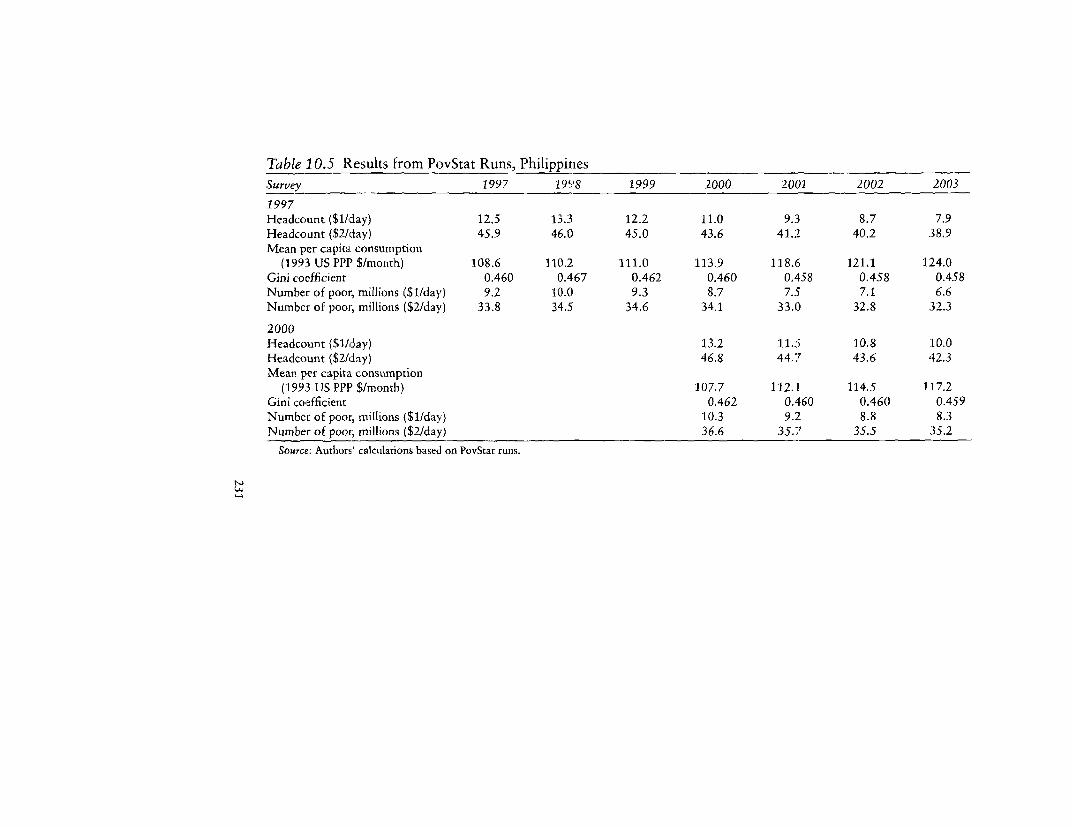
Table 10.5 Results from PovStat Runs, PhilippitiesSurvey 1997 1998 1999 .2000 20l)1 2002 20031997Headcount ($1/day) 12,5 13.3 12.2 11.0 9.3 8.7 7.9Headcount ($2/day) 45.9 46.0 45.0 43.6 41.2 40.2 38.9Mean per capitao consumption
(1993 US PPI' $/month) 108.6 110.2 111.0 113.9 118.6 121.1 124.0Gini coefficient 0.460 0.467 0.462 0.460 0.458 0.458 0.458Number of pool; millions ($1/day) 9.2 10.0 9.3 8.7 7.5 7.1 6.6Number of poor, millions ($2/day) 33.8 34.5 34.6 34.1 33.0 32.8 32.32000Headcount ($1/day) 13.2 11.5 10.8 10.0Headcount ($2/day) 46.8 44.;7 43.6 42.3Mean per capita consumption
(199.3 US PPF' $/month) 107.7 112.1 114.5 1'17.2Gini coefficient 0.462 0.460 0.460 0.459Number of poor, millions ($1/day) 10.3 9.2 8.8 8.3Number of poor, millions ($2/day) 36.6 35.;7 35.5 35.2
Source: Authors' calculations based on PovStat runs.

232 DATT, RAMADAS, VAN DER MENSBRUGGHE, WALIER, AND WODON
Conclusions
PovStat and SimSIP are two simple tools for projecting the poverty
effects of aggregate growth that exploit the idea that changes inpoverty measures depend on changes in mean incomes across sec-tors and changes in relative inequalities. These tools are relativelyeasy to use and have modest data requirements. Although the tools
are similar in nature, there are some differences in their application.PovStat is better geared to household-level data on income or con-sumption distribution, while SimSIP is better suited to grouped data.
Both tools impose minimal structure on the relationship betweeneconomic growth and poverty. This is their strength as well as theirweakness. For analyzing the poverty impact of a broad range of spe-cific macroeconomic policies, more complex tools would be needed
that can link relevant policy variables with average incomes and rel-ative inequalities through factor and product market channels. Butgreater complexity comes at a price, with heavier data requirements,a relative loss of transparency, and the need to make possibly lessrealistic assumptions.
Notes
1. Other SimSIP modules deal with, among other things, the evaluationof the impact of programs and policies on poverty and inequality, the costof reaching development targets (for example, in the education sector), debtprojections and fiscal sustainability analysis, and the impact of tax reformson poverty and inequality. Originally, the various simulators were designedto help governments preparing Poverty Reduction Strategies, but they canbe used for other purposes as well. Most simulators are "generic," hencethey can be used for any country. Two simulators are regional, meaningthat their applicability is restricted to the countries of a given region. Tech-nical explanations on the methodology underlying the various simulatorsare available in each simulator's manual available on the SimSIP Web site,at http://www.worldbank.org/simsip.
2. The program can be adapted for grouped data. That is done by firstfitting a parametric Lorenz curve to the grouped data and then generating,say, 100 or 1,000 points on the Lorenz curve, which are then used as syn-thetic household survey data for PovStat.

THE EFFECT OF AGGREGATE GROWTH ON POVERTY 233
3. The current version of PovStat does not capture heterogeneity withinhouseholds with multiple income earners in different sectors, primarilybecause of the nature of data available. Many countries do not provideinformation on the occupation of all (working age) household members. Ifsuch data were available, PovStat could easily be run with individual, ratherthan household-level, data.
References
The word processed describes informally reproduced works that may notbe commonly available through library systems.
Atkinson, Anthony. 1987. "On the Measurement of Poverty." Econometrica55: 749-64.
Bourguignon, Francois. 2003. "The Growth Elasticity of Poverty Reduc-tion: Explaining Heterogeneity across Countries and Time Periods." InT. Eicher and S. Turnovsky, eds., Inequality and Growth. Cambridge,
Mass.: MIT Press.Datt, Gaurav, and Martin Ravallion. 1992. "Growth and Redistribution
Components of Changes in Poverty Measures: A Decomposition withApplications to Brazil and India in the 1980s." Journal of DevelopmentEconomics 38(2): 275-95.
Datt, Gaurav, and Thomas Walker. 2002. "PovStat 2.12: A Poverty Projec-
tion Toolkit, User's Manual." World Bank, East Asia Poverty Reductionand Economic Management Unit, Washington, D.C. Processed.
Duclos, Jean-Yves, and Quentin Wodon. 2003. "Pro-poor Growth." WorldBank, Africa Poverty Reduction and Economic Management Depart-ment, Washington, D.C. Processed.
Foster, James, Joel Greer, and Erik Thorbecke. 1984. "A Class of Decom-posable Poverty Measures." Econometrica 52(3): 761-66.
Ravallion, Martin, and Monika Huppi. 1991. "Measuring Changes inPoverty: A Methodological Case Study of Indonesia during an Adjust-ment Period." World Bank Economic Review 5(1): 57-82.
Robles, Marcos, Corinne Siaens, and Quentin Wodon. Forthcoming."Poverty, Inequality and Growth in Paraguay: Simulations Using SimSIPPoverty." Economia & Sociedad.
Wodon, Quentin, Krishnan Ramadas, and Dominique van der Mensbrug-ghe. 2003. "SimSIP Poverty Module," available at www.worldbank.org/simsip.


11
Linking AggregateMacroconsistency Models to
Household Surveys: A PovertyAnalysis Macroeconomic
Simulator, or PAMS
Luiz A. Pereira da Silva, B. Essama-Nssah,and Issouf Samake
This chapter presents a simple technique, the Poverty AnalysisMacroeconomic Simulator, or PAMS, for linking household surveys(described in chapter 7) and average benefit or tax incidence analy-sis (described in chapters 1 and 2) to simple aggregate macroeco-nomic models of various types. The key feature of PAMS is the pos-sibility to infer changes in levels of disposable income for specificcategories of workers from expected changes in aggregate variablessuch as gross domestic product (GDP) by sector. The only require-ment concerning the aggregate variables is that they be consistent,as in national accounts. Such a link allows one to project ex antenational accounts and to conduct poverty and distributional analy-sis in a way that makes income growth, transfers, employment,poverty, and inequality estimates consistent with the macroeco-nomic framework. The basic idea in linking the macroeconomicframework to the household sector is to multiply the incomes orexpenditures of each household of a specific group by the relevant
235

236 PEREIRA DA SILVA, ESSAMA-NSSAH, AND SAMAKE
growth rate based on changes in disposable income of that specificgroup induced by changes in aggregate variables.1
PAMS has three recursive layers, as depicted in figure 11.1. Thefirst, or macro, layer features an aggregate macroeconomic frame-work that can be taken from any macroconsistency model (such asFinancial Programming, RMSM-X, or the simple 1-2-3 CGE [com-putable general equilibrium] model described in chapter 13 with anadditional "growth" story).2 The objective of this top layer is toproject GDP, national accounts, the national budget, balance-of-payments, aggregate price level, and so forth in consistent flow-of-funds accounts.
The second, or meso, layer is a simplified labor and earnings mar-ket model that calculates disposable income across representativegroups of households. Individuals and family units from the house-hold survey are grouped in several (country-specific) representativegroups of households defined by the labor category of the head ofthe household. Each of the representative household groups matchesone-and only one-economic productive sector. The sum of theproduction of all economic sectors is consistent with total output ofthe macroeconomic framework. Within each representative group,the disposable income of a typical household can be decomposedinto labor income, nonlabor income, average taxes, and averagetransfers. Labor demand in each economic sector depends on sec-toral output and real unit labor cost. Labor income in each eco-nomic sector can thus be determined by equilibrium on the labormarket. In addition, each representative group has exogenous aver-age nonlabor income. Finally, policy-based general tax rates and dif-ferent levels of budgetary transfers across representative groups canbe added to labor and nonlabor income. All these components ofhousehold income determine an average level of disposable incomefor each unit inside a representative group. Overall, a growth rate ofdisposable income can be calculated for each specific representativehousehold group.
The third, or micro, layer is a poverty and distribution simulator.The simulator follows the basic approach of incidence analysis ofpublic spending or taxation (see chapters 1 and 2) where changes intaxes or transfers can be transmitted into each household's incomeor expenditure according to some pre-defined characteristics (suchas income level). Here, what matters is the household's representa-tive group. PAMS uses the calculated average growth rate of dispos-able income for each representative group, determined in layer 2, tosimulate the income growth for each individual or family unit insideits own representative group. The key assumption is that the changein the disposable income for each individual or family unit in one

LINKING MACRO MODELS TO HOUSEHOLD SURVEYS 237
Figure 11.1 The Functioning of PAMS
Layer 1: (Macro) Macroeconomic Consistency Framework
||Output || |Balance of | |Budget | ||External |
W, A/ Layer 2: (Meso) The Labor and Earnings Model
Disaygregated 3 Derand and Average budgetaryproduction: supply of labor transfers:emAgriculture (unemployment): * Social expend.
tradable/ * Agriculture by group (aver.)nontradable tradable/ - Taxation by
P Urban nontradable group (avee )(manufacturing, c . Urbanservices) (manufacturing,tradable/ o services)nontradable / tradable/
/ nontra able 1
|Starting unit labor ' |v Unit labor | ,Dsposable income||_|cost by group cot_=:=upygru
Layer 3: (Micro) Poverty and the Distribiition of Living Standards
.Rural Rural Urban ||Urban ||||Urban ||||Etc.||self- worker self- || civil ||||worker||||ll
employed of employed | servant |||| of |||| ll\ tradable tradaLe
l Poverty and inequality indicators (headcount, Gini, etc.)
group will be the same as the change for the group itself. Hence theincome distribution within each of the representative householdgroups remains constant. Therefore, the income of each individual orfamily unit of the household survey can be projected using the group-specific rate of income growth and the average tax and budgetary

238 PEREIRA DA SILVA, ESSAMA-NSSAH, AND SAMAKt
transfer accruing to the group. It is assumed that there are no "leak-ages" in public spending (in contrast to the assumption described inchapter 9). After projecting individual incomes, PAMS calculatesthe incidence of poverty and intergroup inequality.
Naturally, the third layer of PAMS can be used independently asa stand-alone tool of incidence analysis. For each representativegroup, one can set exogenously (that is, without using a macroeco-nomic framework) the uniform growth of labor income and changesin other sources of income. Then the third, micro layer of PAMS canuse this information in the country-specific household survey toproject individual incomes and calculate the incidence of povertyand intergroup inequality as before.
A few important features and caveats need to be well understoodand kept in mind when using PAMS. First, to construct a linkagebetween a macroeconomically consistent framework and the house-hold survey, it is necessary to select a few appropriate "linkageaggregate variables," or LAVs, from the macroeconomic model (bydisaggregating its projected output level into different economic sec-tors) and to inject this information into the household survey data(rearranged by representative household groups). The LAVs used byPAMS are GDP, GDP and employment by economic sectors, thegeneral price level, the overall tax revenue, the overall budgetarytransfers to households, and the noninterest public expenditurelevel. Data in the household survey also need to be extracted in aspecific format (that is, income and expenditure and the occupationof the head of the household). The number of representative groupscorresponds to a breakdown by economic sectors that reflects thestructure of the economy being analyzed.
Second, PAMS works in a mechanical top-down fashion. Thedecomposition of GDP into its sectoral components and the accu-racy with which it depicts-at the top-the functioning of the econ-omy is key to determining the accuracy-at the bottom-of itspoverty and distributional analysis.
Third, if the macroeconomic framework running on top of PAMSdoes not take into account some degree of substitution between fac-tors of production caused by relative price changes, PAMS will notcapture any change that affects both sectoral output and relativefactor prices, resulting in a substitution between factors of produc-tion.3 Most of the action in PAMS happens through changes in sec-toral output levels. This analysis can explore the extent to whichdifferent sectoral growth patterns are "pro-poor," that is, whichsectoral growth patterns will affect economic sectors and represen-tative household groups that employ relatively more poor people.However, the different sectoral output levels are projected to be sim-ply consistent in terms of national accounting.

LINKING MACRO MODELS TO HOUSEHOLD SURVEYS 239
Fourth, and finally, the labor market in the second layer of PAMS,which is key to transforming macroeconomic variables into factorprices, is kept very simple. For instance, each sector of activity usesone category of workers only; there is no mobility of workersbetween sectors; the unit labor cost level for workers is determinedby historical trend or government intervention; and the rental priceof land and capital is obtained as a residual, without considerationgiven to the demand for these factors of production. Although thesefeatures have the advantage of keeping the model simple, they alsoconstitute its limitations. These limitations are particularly relevantto the analysis of second-round effects of reforms that involve sub-stitution of production factors. Traditional CGE models (such asthose discussed in chapter 15) tend to have a richer factor demandmodule, involving imperfect elasticity of substitution between cate-gories of workers, and factors of production more generally, at thesectoral level.
Structure of the PAMS Framework
As explained above and portrayed in figure 11.1, PAMS has threelayers:
* a top, macroeconomic layer where a macroeconomic frame-work imposes overall consistency;
* an intermediate, mesoeconomic layer describing both the func-tional distribution of income and various redistributive mechanismslinked to the budgetary policies; and
* a bottom, microeconomic or household layer that reflects themost recent size distribution of income and is used to predict thedistributional and poverty impact of events taking place in the toptwo layers of the economy.
Layer 1 (Macro): The Macroeconomic Framework
The macroeconomic framework is described by equations 11.1through 11.4 in box 11.1. It provides consistency in nationalaccounts and predicts, at an aggregate level, the changes in keymacroeconomic variables such as the production of goods and ser-vices, or gross domestic product (Y), public expenditure (G), overalltaxes (T), private consumption (C), savings and investment (I), thebalance of payments (exports, X, and imports, IM) and the aggregateprice level (p) that is used to project the poverty line (z). The fiscaldeficit (T-G) has to be financed by some sort of increase in domes-tic financial liabilities (here a full monetization, AM). The current

240 PEREIRA DA SIlVA, ESSAMA-NSSAH, AND SAMAKV
account deficit (X-M) has to be financed by some sort of an increasein external financial liabilities (here a change in reserves, AR). Theaggregate price level can be calculated in a variety of ways: in mostmacroeconomic frameworks usually correlated to changes in aggre-gate demand (such as gross domestic product, AY) and some mea-sure of the money supply (AM).
Layer 2 (Meso): The Labor and Earnings Model
The meso, or second, layer is summarized by equations 11.5 through11.10 in box 11.1. This layer models the labor demand and earningsthat simulate the functioning of a simplified labor market (this maybe modeled and calibrated econometrically with country-specifictime-series or using parameters estimated in cross-section; see Fallonand Verry 1988). The meso framework disaggregates Y into
o m adequate sectoral real components (Yk) (equation 11.5), usedin modeling labor demand (L*);
o m components (Gk) of average nominal public spending (equa-tion 11.6), accruing to each of the m representative groups;
o m components (Tk) of average nominal taxes (equation 11.7),paid by each of the households in each of the m representativegroups.
PAMS features taxes, transfers, and social expenditures (consis-tent with the macroeconomic model and the government's budgetconstraint in the macroeconomic framework). Each household in itsrepresentative group pays general taxes (on consumption, income,and so forth). Each household in its representative group alsoreceives lump sum budgetary transfers from the government's bud-get. The government is not capable of targeting the transfers andtherefore simply provides them on a per capita basis. For each of thecountry's m representative groups (along the lines of a macroconsis-tent incidence analysis, for example), the user of PAMS can estab-lish the average transfers or average taxation of that specific groupusing a country-specific average tax or average transfer rate. Theseinstruments determine the disposable income of each of the m rep-resentative groups.
A classic procedure (see Agenor, Izquierdo, and Fofack 2001) atthe meso level is to decompose Y into rural and urban GDPs; withineach component, the formal sector is then distinguished from theinformal sector; and within each one of these sectors, tradable goodsare distinguished from nontradable goods. The economic relevanceof the breakdown is key in linking each economic sector of the pro-duction side of PAMS to a specific segment of the labor market. In

LINKING MACRO MODELS TO HOUSEHOLD SURVEYS 241
Box 11.1 Key Equations of the Three Layers of thePAMS Framework
Layer 1 (Macro): The Macroeconomic Framework (NA, BOP, fiscal,general price level)
11.1 Yt =C, +19 +G, +(X, -IM,)
11.2 (X, - IM,) = AR,
11.3 (T, - GI) = AM,
11.4 p, =f(p,,AY, AM, etc.
Layer 2 (Meso): The Labor and Earnings Model
11.5 Y, =P,Iyk,k
11.6a G, = G",,
11.6b G,t = Lst(G, /Lt)
11.7a T,, T,
11.7b T*,, =L',(T, ILt)k,
11.8a DINCk, = (P,w )L -T1, + Gk, + OINCk,,
11.8b XDINCk, =Yt -T,k
11.9a L!,, = Kk Yk,, W;!
11 .9b 4'>, = 4k,,, (1 + n) - MIGRkl,
11.9c 1, =O, (POP,)=I4,k
flek
(l k ,t )4 ,
Layer 3 (Micro): Poverty and the Distribution of Living Standards
11.11 POt =f(POP, ,*,,,dincfr,,Z,)
11.12 GIN!1 = f(L!, dinck,)
11.13 z, = zt-, (1 + p)

242 PEREIRA DA SILVA, ESSAMA-NSSAH, AND SAMAKt
the modeling of the production side of PAMS, national accountidentities ensure cross-sectoral consistency with the aggregate grossdomestic product (Y) that is determined at the macro level. In otherwords, it is simply necessary to determine residually the productionof one subsector (for example, the urban informal sector, or therural subsistence sector). The simplest way to determine the trad-able portion of the formal rural and urban sectors is to look at theexport data (manufacturing and basic commodities, for example) atthe aggregate level. The projected level of activity for each tradablesector usually depends on foreign demand and the real exchangerate as determined by the aggregate domestic and foreign price lev-els. Then a simple way to model the rest of the urban and ruraleconomy would need to be found and set in the model (for example,simple elasticities of output to factors of production can be used).
Labor demand (equation 11.9a) is broken down by k sectoralcomponents. Even though each sector may employ both skilled andunskilled labor, PAMS assumes that each sector employs only onekind of labor. Thus, there is no substitution between types of laborin the production process except for the exogenous migrationdescribed earlier.4 Demand for labor in the kth sector (Lk) dependson the level of activity in the kth sector (Yk) and on the kth sector'sreal unit labor cost (Wk). The labor supply for each group k (inequation 11.9b) is driven by demographic considerations (an exoge-nous growth rate for each group that relates to total labor supply)and exogenous migrations of labor from one representative groupinto another. 5 Total labor supply (equation 11.9c) depends on aparticipation rate 0. As a result the unemployed workers (the differ-ence between supply and demand of labor in each sector) implicitlyremain in their sector of origin. Since PAMS does not model occu-pational choices inside each representative group, the unemployedcannot be identified at the household level. However, PAMS deter-mines the total labor income in each group that accrues only toactive workers. Accordingly it corrects the group's labor income byweighting the disposable income of households in each representa-tive group by the relative size of the active workers in the group. Ineach period, this weight is recalculated, meaning that the unem-ployed in each period are reposted in the sector's labor market.
PAMS (equation 11.8a) determines the level of disposable incomein the kth sector (DINCk) as the sum of labor income, average percapita taxes (TkILk), per capita transfers (Gk/Lk), and other, exoge-nous, average sector-specific nonlabor income (OINCk). To accountfor the changes in the relative share of each representative group inthe total labor force caused by changes in employment levels acrossthe groups, PAMS reweights the individual labor income in each
LINKING MACRO MODELS TO HOUSEHOLD SURVEYS 243
of the k sectors by the number of employed individuals in the sectordivided by total labor supply of that sector (equation 11.9b). As aresult the labor income of the unemployed is implicitly assumed notto grow.
The real labor income (equation 11.10) in each of the k sectors(Wk) is determined by a sector-specific general trend wk and by thelevel of unemployment in the same sector. This general trend shouldbe such that the level of unemployment in each sector remainsapproximately constant. There is, however, a "scale" in trend laborincome levels across sectors, starting from a low bottom in the ruralnontradable sectors moving up to the top urban tradable sector andthe civil service, that corresponds to a sector-specific return.
The excess of total disposable income (Y-T) generated in theeconomy over total labor income represents profits that are includedin other incomes. In other words, the difference between incometaken from the national accounts and income calculated from house-hold survey data is assigned to a class of rentiers (equation 11.8b).PAMS does not track down financial assets and their returns. How-ever, the interest revenue from the macroeconomic framework canconceivably be redistributed to various socioeconomic groupsaccording to some rule. Because the inequality indicator in PAMS isan intergroup Gini coefficient, the level and growth rate of profits isimportant.6
Layer 3 (Micro): Poverty and the Distributionof Living Standards
Knowing the disposable income received by each representativegroup allows the projection of income of each household or indi-vidual in the household survey. One needs to assume-as explainedabove-that the income or expenditure of each individual shifts inexactly the same proportion as it does for the representative groupto which the individual belongs.
Prices are an important linkage variable from the macroeconomicto the microeconomic layers of PAMS. The aggregate price level, p,of the macroeconomic framework applies to the calculation of nom-inal disposable incomes in equation 11.5 and to the determinationof how the poverty line, z, shifts in equation 11.13 (although p isnot specifically a consumption price).
The poverty headcount PO can be calculated (equation 11.11)once PAMS has established both the disposable income (DINC) ofeach individual in the household survey and the poverty line z. Thenumber of poor is computed from the projected disposable incomescompared with the projected poverty line. In parallel, the intergroup

244 PEREIRA DA SILVA, ESSAMA-NSSAH, AND SAMAKg
inequality (a Gini coefficient) is computed using the disposableincomes of each of the representative groups of the PAMS (equation11.12). However, to account for structural changes in the economy,coming from changes in the sectoral composition of the labor force(by representative group), its allocation across sectors (sectoral labordemand), and the relative shifts in the structure of production,PAMS reweights the number of households belonging to each groupfrom the original household survey to reflect the sectoral structureof production and employment in the simulated scenario.
Building and Running PAMS
Six steps must be followed to use PAMS.
Step 1: Data Requirement and Processing
PAMS is conceived as a shell that can host data from any typicaldeveloping country. The minimum data requirement consists of thedata necessary to construct a macroconsistency framework (such asnational accounts broken down into m economic sectors), employ-ment data (by the same m economic sectors), and a household survey.
The minimum data at the macroeconomic level can come fromany typical national accounts consistency framework: aggregate GDPdecomposed by the relevant m sectors mentioned before (includingan exogenous public sector and balance-of-payments data on exportsof agricultural and manufacturing goods); aggregate public expendi-ture G decomposed by the relevant m representative group benefi-ciaries mentioned earlier, possibly simply proportionally to theirpopulation or income size; and aggregate taxes T decomposed by therelevant m group taxpayers, as mentioned earlier.
PAMS is constructed to accommodate various degrees of complex-ity in modeling the functioning of the macroeconomy. One can decideto keep the simplicity of macroeconomic consistency frameworksused in many public and private agencies (such as the RMSM-Xs ofthe World Bank, the Financial Programming frameworks of the Inter-national Monetary Fund, or other typical macroconsistency models).
PAMS also requires a "good" household survey that includesinformation about household expenditure and income, as well asthe employment status and the sector of occupation for the head ofthe household (which allows one to allocate the household into aspecific production sector, see box 11.2). There is an alternative tothe method currently used by PAMS, in which changes in laborforces net incomes are transformed into changes in poverty. 7 PAMSrequires "mining" household data sets.

LINKING MACRO MODELS TO HOUSEHOLD SURVEYS 245
Box 11.2 Mining a Household Data Set for PAMSCategories
This box describes the basic steps involved in organizing the availableinformation from a household survey to fit the PAMS framework.Given the emphasis on earnings, it is important that the householdsurvey have a labor module as well, with sufficiently detailed (andreliable) information on the employment status of individuals, theeconomic sector (such as agriculture, industry, services) and the insti-tutional sector (public, private, formal, informal) of employment,earnings, and benefits. This information is then combined with thatfrom other modules of the survey such as geodemographic data (areaof residence, age, gender, and so forth), education, and expenditures.
In principle the data may be processed either at the individual orhousehold level. The real constraint is that some modules of the house-hold survey provide household-level data (such as expenditures),while others provide information at the individual level. Because thehousehold is generally chosen as the unit of analysis, individual levelinformation must be aggregated up to the household level, and socio-economic groups created on the basis of the characteristics of thehead of household. Clearly this approach leads to coarser results thanthe one based on relevant individual-level information.
After the necessary data have been pulled into a master file, one canthen create basic binary variables along the dimensions of interest.These might include, for example, working versus not working, ruralversus urban, public versus private, formal versus informal, tradableversus nontradable, and skilled versus unskilled. PAMS categories aresubsets of the cross-product (in the sense of Cartesian product) of theseelemental variables. To conduct the analysis at the individual level,household-level variables must be converted by dividing them by thehousehold size. The extraction technique is supported by an EViewsprogram that exports the data to Excel.
In its current version, PAMS' proposed method for mining datasets involves the following steps. First, data on each household areanalyzed to determine the household characteristics needed for thecreation of socioeconomic groups. Second, a variable is computedthat measures the disposable income or consumption of each of thehouseholds whose head belongs to the same category of workers.Third, this variable is adjusted by the change in the income of thecorresponding representative group category. Fourth, all householdsare pooled together again, and poverty indicators are computedbased on the adjusted income or consumption variable.
With the same basic information, and a comparable mining effort,the following strategy could be considered. First, the income of each

246 PEREIRA DA SILVA, ESSAMA-NSSAH , AND SAMAKt
household is decomposed into its main sources, according to the fac-tor prices considered in the PAMS (such as labor by sector, land, andcapital). This decomposition should take into account the labor earn-ings of other family members apart from the household head as wellas earnings resulting from any household business or farm. Second,the income from each of the sources is adjusted to reflect the changein the corresponding factors of production, resulting from the PAMS.Third, the income or consumption of the household is adjusted in thesame proportion as its total income, as computed in the previousstep. And fourth, poverty and inequality indicators are computedbased on the adjusted consumption variable.
The household survey needs to be the most recent one so as tomatch the most recent macroeconomic data. Alternatively, one canupdate an old data set-using available information on prices andincome and expenditure growth by representative group-to matchthe latest set of national accounts. The steps described in box 11.2should be followed. The household survey data are carefully ana-lyzed, and individuals and households are regrouped into represen-tative groups. These groups may be constructed on the basis of thesocioeconomic characteristics of the head of the household (otherbases for regrouping are also possible). The result of the processneeds to be stored in a specific data set.
Step 2: Selecting or Constructing a SimpleMacroeconomic Framework
PAMS can use various types of macroeconomic frameworks for itsfirst layer. If none is available, the construction of a simple macro-economic framework, such as the RMSM-X, involves three keysteps. The first is the construction of an accounting framework thatimposes consistency on real and financial transactions of agents(flow-of-funds consistency). The second is the specification of behav-ioral equations and projection rules for the variables (the mostfamous-and most criticized-one being the usage of a fixed linearrelationship to project GDP growth from the ratio of past invest-ment to GDP). The last step entails the choice of residual variablesused to satisfy underlying budget and macroeconomic constraints.Such constraints usually take the form of accounting identities.
Step 3: Establishing the Meso Layer: the Laborand Earnings Model
The first task in this third step involves the disaggregation of aggre-gate production into subsectors (such as rural or urban production,

LINKING MACRO MODELS TO HOUSEHOLD SURVEYS 247
tradable or nontradable goods, and formal or informal activities) tomatch the labor categories of the representative groups created fromthe household survey. One of the subsectors has to be modeled as aresidual, to ensure consistency with the macroeconomic model.
Once production is disaggregated and projections of sectoralgrowth are completed for each subsector (minus the residual), onecan model the functioning of a segmented labor market. There isonly "exogenous" mobility between labor categories (for example,from rural to urban areas) and each sector employs only one specifictype of labor (for example, the rural sectors employ only unskilledlabor). Sectoral output growth and its sector-specific real unit laborcost-cost that is sensitive to the sector-specific level of unemploy-ment, as in a wage curve specification (following Blanchflower andOswald 1994)-drive the demand for that sector-specific category oflabor. The supply of that specific category of labor is given by demo-graphic and exogenous variables that can mimic policies (for exam-ple, migration can be set to mimic expected income differentials as inthe Harris-Todaro model). The resulting unemployment levels by cat-egory of labor lowers unit labor costs and thus increases the demandfor that category of labor. Finally, the relevant elasticities used in theprojections can be estimated econometrically outside the model(using, for example, either time-series when available for the countrybeing studied, or a cross-section estimate; see Hamermesh 1993).
Step 4: Establishing a Baseline Scenario
A PAMS user must first construct a macroeconomic scenario usingthe first layer macroconsistency model. This scenario would com-prise, at a minimum, aggregate GDP growth (such as that associatedwith a program involving policy shifts, and a combination of infla-tion, fiscal balances, and current account balances; disaggregatedsectoral growth combining different paths for growth rates for agri-cultural or industrial, tradable or nontradable goods sectors withina given aggregate GDP growth rate; rates of general taxation by rep-resentative group (within the macroconsistent budget constraint);and different levels of social (budgetary) transfers to different repre-sentative groups (within the macroconsistent budget constraint).
PAMS then transmits the macroeconomic baseline scenario to theintermediate layer model to derive the corresponding labor demandsand earnings by sectors. The procedure captures the effect of averagetax and transfers for households in each of the representative groups.This meso layer produces the disposable income for each group,adding to wage and other nonwage income, the different (average)general tax rates and different (average) budgetary transfers across

248 PEREIRA DA SILVA, ESSAMA-NSSAH, AND SAMAKE
each of the representative group categories, all consistent with theoverall budget.
Finally, running the microeconomic layer, PAMS calculates dispos-able income growth rates for each representative group category anduses the average, group-specific growth rate to multiply the income ofeach unit of the household survey belonging to the same group. Eachhousehold in its specific category will see its income grow by the aver-age growth rate of its own category. PAMS takes these new levels ofincome for each household and, using the new poverty line z adjustedby the new price level p, simulates the new poverty headcount and thenew level of inequality. It should be noted that the procedure "pro-jects" the new poverty headcounts and the income distribution basedon the "old" household survey, reweighted according to the newstructure of the economy and its labor market. The pattern of incomedistribution within a representative group from the most recent house-hold survey is assumed to hold throughout the simulation period.Thus, the simulation process projects the mean income of each of therepresentative groups in the economy, assuming that there are nochanges in the intragroup distribution of income or expenditure.
Step 5: Establishing a Comparison Scenario
Step 4 can be conducted by making marginal changes to any of thefollowing instruments: aggregate GDP growth (caused by a domes-tic or external shock, for example, or a change in policies); disag-gregated sectoral growth (again, caused by a shock or a change insectoral policies); changes in the rates of general taxation by repre-sentative group (within the macroconsistent budget constraint);changes in the levels of social (budgetary) transfers to different rep-resentative groups (within the macroconsistent budget constraint);changes in the unit labor cost level in each economic sector; changesin migration of labor between sectors; or changes in the povertyline. Once the new scenario is run, one can compare the results ofthis scenario with the baseline scenario.
Step 6: Establishing a Target Scenario
One can use the third layer to establish a combination of economicgrowth rates for representative groups that will attain the country'spoverty reduction goal. Then, working backward, one can calculatethe required sectoral and overall GDP growth that needs to beachieved to reach the target. Finally, given the country's macroeco-nomic constraints and the overall macro framework, one could usePAMS to calculate the overall financing required.

LINKING MACRO MODELS TO HOUSEHOLD SURVEYS 249
An Application to Burkina Faso
Burkina Faso is a poor landlocked country in Sub-Saharan Africawith a limited resource base, high vulnerability to external shocks,and very low human development. Since 1991 the country hasembarked upon a comprehensive reform program and has madesome headway in its transition toward a market-oriented economyand a more appropriate role for the state. Despite the good progressachieved, the country remains one of the poorest in the world. Realgross national product per capita was estimated at US$230 in 2001.
Poverty Profile and Social Indicators for Burkina Faso
In 1996 and 2000 the government of Burkina Faso issued povertyprofiles based on the results of priority surveys conducted in 1994and 1998. Over this period poverty incidence remained broadly sta-ble (moving from 44.5 percent in 1994 to 45.3 percent in 1998).Rural poverty predominates in Burkina Faso, accounting for 94.5percent of national poverty, and the incidence of poverty is markedlyhigher in rural areas (estimated at 45.3 percent in 2002) than in urbanareas (28.9 percent). But the incidence of urban poverty increasedfrom 10 percent to 16 percent between 1994 and 1998 and wasaccompanied by an increase in urban inequality. The analysis ofpoverty among socioeconomic groups (based on source of income)shows that between 1994 and 1998 the incidence of poverty increasedfor all groups except cash crop farmers. It is highest among food cropfarmers, who account for most of the population living in poverty.
Burkina Faso's Poverty Reduction Strategy Paper (PRSP) sets anambitious target for the reduction of poverty incidence. 8 The propor-tion of people below the poverty line is supposed to decline from about45 percent to 30 percent between 2000 and 2015. In light of recentexogenous cotton price shocks and the continued vulnerability of theBurkinabe economy to other export shocks, this ambitious target maynot be attained unless significant efforts are taken to ensure that growthis both sustained and pro-poor. To do that, the government must findan appropriate mix of fiscal, monetary, and public investment policiesthat can bring the economy to a higher and stable growth path whilemaintaining an adequate level of consumption, and it must find a sec-toral growth composition that provides greater benefits for the poorestrepresentative household groups in the economy (in other words, acomposition that is pro-poor in the sense that the income of the poorgrows faster than income for other groups (Ravallion 2001).
Although final figures were not available when this chapterwas written, real GDP growth was expected to reach an estimated
250 PEREIRA DA SILVA, ESSAMA-NSSAH, AND SAMAKt
5.7 percent in 2002. Assuming a normal cereal crop, the primary sec-tor was expected to grow by 3.2 percent. Growth was expected to pickup in the secondary and tertiary sectors (6.6 percent and 7 percent,respectively) as a result of stronger demand linked to the economicrecovery. Inflation was forecast to decline to some 2 percent. The cur-rent account deficit, excluding current official transfers, was projectedto improve to 14.1 percent of GDP, as a result of substantial increasesin the volume of cotton harvested in late 2001 but exported in 2002.
The overriding fiscal objective for 2002 and the medium term isto consolidate Burkina Faso's budgetary position. Reaching thisobjective entails significant efforts to increase fiscal revenues,improve budgetary management, and introduce greater efficiency inpublic spending to support the government's poverty reduction pro-gram. For 2002 fiscal revenue was projected to rebound to 13.8 per-cent of GDP. Expenditure was forecast to continue to be containedat levels compatible with revenue performance, while social expen-diture would continue to increase in 2002. For the medium term,assuming no exogenous shocks and the maintenance of sound eco-nomic policies, growth could remain at around 5.5 percent.
Using PAMS in the Construction of a Baseline Scenario forBurkina Faso
PAMS is first used to provide a set of projections for some of theimportant macroeconomic and (some microeconomic) policy objec-tives stated in the PRSP, which is supported by an IMF program(PRGF, or Poverty Reduction and Growth Facility) and a series ofWorld Bank credits (three Poverty Reduction Strategy Credits). Arethe poverty reduction objectives achievable in the time frame that iscontemplated and with the stated policy mix? To illustrate our ear-lier explanation of PAMS, we use the technique to calibrate a base-line scenario on the macroeconomic assumptions of the PRSP.9 Themain "engine" for poverty reduction in this baseline scenario wouldbe the relatively high levels of growth projected under the macroeco-nomic framework behind the PRSP (an average of 5.5 percent overthe next decade). The poverty line shifts with the overall price level.
Table 11.1 provides medium-term (up to 2010) projections ofpoverty and social indicators and shows that there could be someprogress in the reduction of the poverty headcount over the nextdecade. Only a relatively minor reduction in the poverty headcountP0 of 4-5 percent is projected in the first two years, 2002 and 2003,compared with 2000.10 But then the poverty headcount falls to37.9 percent in 2004 and to 35.1 percent in 2010, only slightlyshort of the 30 percent level targeted for 2015. Graphical results ofthe simulation are given in figure 11.2a, b, and c. The high average

Table 11.1 Poverty Line and Income Distribution, Burkina Faso, 2002-2010Scenario with:Expenditure-Weighted 2002 2003 2004 2005 2006 2007 2008 2009 2010
Country:Poverty line (in LCU/day) 330 334 339 345 355 365 376 387 398Poverty line (in LCU/year) 79,313 80,190 81,448 82,875 85,209 87,699 90,263 92,904 95,622Poverty line (in current 112 116 118 121 122 124 126 128 129
US$/year)Total population* 11,593,626 11,923,095 12,261,513 12,608,879 12,966,088 13,331,400 13,705,679 14,089,102 14,483,255Total labor force 6,555,898 6,742,384 6,933,938 7,130,559 7,332,755 7,539,539 7,751,400 7,968,439 8,191,555Poor population* 4,991,270 4,852,755 4,646,164 4,534,156 4,590,408 4,716,309 4,838,967 4,960,182 5,086,595P0 (headcount index) (%) 43.1 40.7 37.9 36.0 35.4 35.4 35.3 35.2 35.1P1 (poverty gap) (%) 13.0 12.2 10.9 10.2 10.0 9.9 9.9 9.9 9.8P2 (%) 6.1 5.8 5.3 5.1 5.1 5.2 5.4 5.5 5.6Gini 0.382 0.392 0.400 0.409 0.417 0.427 0.435 0.444 0.452Theil 0.246 0.258 0.269 0.281 0.292 0.306 0.319 0.332 0.346Rural Areas:Rural population 10,023,187 10,329,100 10,643,607 10,966,705 11,299,282 11,639,592 11,988,493 12,346,158 12,714,167Poor population* 4,537,055 4,424,865 4,237,061 4,132,420 4,198,300 4,337,013 4,469,510 4,601,779 4,737,308P0 (headcount index) (%) 45.3 42.8 39.8 37.7 37.2 37.3 37.3 37.3 37.3Gini 0.360 0.357 0.352 0.349 0.345 0.342 0.339 0.336 0.333Urban Areas:Urban population (millions)* 1,570,439 1,593,995 1,617,905 1,642,174 1,666,807 1,691,809 1,717,186 1,742,944 1,769,088Urban labor force 867,170 907,660 949,472 992,655 1,037,247 1,083,292 1,130,822 1,179,879 1,230,505Poor population* 454,215 427,890 409,103 401,736 392,108 379,296 369,457 358,403 349,287PO (headcount index) (%) 28.9 26.8 25.3 24.5 23.5 22.4 21.5 20.6 19.7Gini 0.200 0.207 0.213 0.220 0.226 0.233 0.239 0.245 0.251
Note: * Weighted calculations show population (in millions) at the national level. Unweighted calculations show population at the sample level (in units).

252 PEREIRA DA SILVA, ESSAMA-NSSAH, AND SAMAKt,
Figure 11.2 PAMS Baseline Projections on Poverty inBurkina Faso, 2002-2010
a. Poverty headcount (P0)
Percent
50.0 -
40.0 -
30.0 -
20.0 --
10 - I I
2002 2004 2006 2008 2010
--C Total --- Rural Urban
b. Intergroup Gini
Percent
0.50
0.40 -
0.30-
0.20 -
0.10- - - - -- I I2002 2004 2006 2008 2010
-0- Total - - - Rural Urban

LINKING MACRO MODELS TO HOUSEHOLD SURVEYS 253
c. Poverty headcount (P0) by groupPercent
60.0-
30.0 -
0.0 04 b 4 , -~ -H 04 ,
D~~~~ ~~ C, E~ °-a O 0 u
04 0 0 "m ~ ~ -v)
*~~~ 0 200 S 000
6.0 -20 E q 0 0-"
00 * 0 0- 0 - - 0
H.0- _~~~~~~~~~~~~~~~
-9.0- _. I l l l l I~~~0. -~
'4. E4-. 0 - 0. 04
U2003 D200S
d. Difference baseline minus shock scenario (C6te d'lvoire crisis)
Percent
-3.0 -
2003 2004 2005 2006 2007 2008 2009 2010
* Poverty headcount - Gini coefficient

254 PEREIRA DA SILVA, ESSAMA-NSSAH, AND SAMAKt
output growth planned in the PRSP during the simulation period(up to 2010) boosts average nominal income from about Franc CFA100,000 to more than CFA 140,000, contributing to the fall in thepoverty headcount.
The rise in average income and the fall in poverty is accompaniedby some less positive signs. The baseline scenario projects an increasein urban inequality measured by the Gini, which increases from about0.20 to 0.25 in 2010. That explains the overall increase in the pro-jected national intergroup Gini for both the rural and urban areas,which rises from 0.39 in 2003 to 0.45 in 2010. Therefore, what thissimulation shows is that if sectoral growth and income distributionfollows the current projected baseline scenario, income poverty inBurkina Faso will decline-although not enough to meet the 2015target-at the expense of a significant increase in inequality.
Finally, the projected baseline scenario in PAMS shows thatpoverty varies across socioeconomic groups (table 11.2). Althoughpredominantly a rural phenomenon, poverty can reach very high lev-els (over 60 percent) among the unemployed in urban areas. Hencethe projection demonstrates the need for additional thinking aboutcomplementary policies that could help achieve the PRSP objectivesand lower poverty in specific areas and among specific groups.
Construction of a Sensitivity Analysis Scenario for BurkinaFaso with PAMS
Another important question is how realistic the GDP growth projec-tions in the baseline scenario are. Given the past volatility of GDPgrowth in Burkina Faso (in particular, the volatility of cotton prices,its main export product), reliance on strong output growth to achievethe PRSP objectives is risky. For example, figure 11.2d shows theincrease in poverty and inequality caused by a negative output shockof -3.2 percent in 2003, -1.7 percent in 2004, and -0.7 percent in2005 as a consequence of the 2002-03 political crisis in neighboringC6te d'Ivoire. The shock also entails a 5 percent decline in externaldemand for the country's exports. We assume that both shocks aresustained (that is, there is no subsequent recovery compared with thebase case). Even if the only socioeconomic effects of what appears tobe a serious regional crisis are the ones mentioned above, the attain-ment of the poverty reduction objective becomes quite problematic.By the end of 2005, the poverty headcount would still hover around39 percent overall, instead of 36 percent as in the base scenario, andreach a high of 41 percent in rural areas.
This type of analysis illustrates the fragility of social progress ina country such as Burkina Faso. Unfortunately, the likelihood of
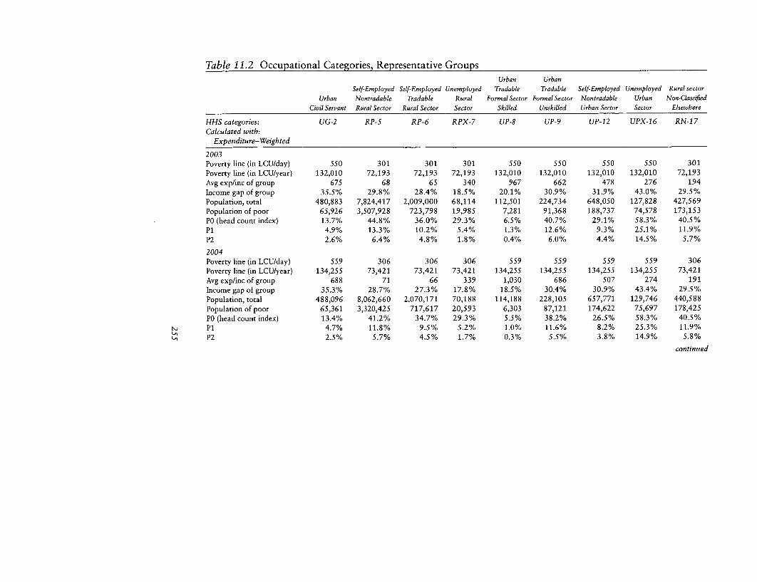
Table 11.2 Occupational Categories, Representative GroupsUrban Urban
Self-Employed Self-Employed Unemployed Tradable Tradable Self-Employed Unemployed Rural sectorUrban Nontradable Tradable Rural Formal Sector Formal Sector Nontradable Urban Non-Classified
Civil Servant Rural Sector Rural Sector Sector Skilled Unskilled Urban Sector Sector Elsewhere
HHS categories: UG-2 RP-S RP-6 RPX-7 UP-8 UP-9 UP-12 UPX-16 RN-17
Calculated with:Expenditure-Weighted
2003Poverty line (in LCU/day) 550 301 301 301 550 550 550 550 301Poverty line (in LCU/year) 132,010 72,193 72,193 72,193 132,010 132,010 132,010 132,010 72,193Avg exp/inc of group 675 68 65 340 967 662 478 276 194Income gap of group 35.5% 29.8% 28.4% 18.5% 20.1% 30.9% 31.9% 43.0% 29.5%Population, total 480,883 7,824,417 2,009,000 68,114 112,501 224,734 648,050 127,828 427,569Population of poor 65,926 3,507,928 723,798 19,985 7,281 91,368 188,737 74,578 173,153
P0 (head count index) 13.7% 44.8% 36.0% 29.3% 6.5% 40.7% 29.1% 58.3% 40.5%P1 4.9% 13.3% 10.2% 5.4% 1.3% 12.6% 9.3% 25.1% 11.9%P2 2.6% 6.4% 4.8% 1.8% 0.4% 6.0% 4.4% 14.5% 5.7%
2004Poverty line (in LCU/day) 559 306 306 306 559 559 559 559 306Poverty line (in LCU/year) 134,255 73,421 73,421 73,421 134,255 134,255 134,255 134,255 73,421Avg exp/inc of group 688 71 66 339 1,030 686 507 274 191Income gap of group 35.3% 28.7% 27.3% 17.8% 18.5% 30.4% 30.9% 43.4% 29.5%Population, total 488,096 8,062,660 2,070,171 70,188 114,188 228,105 657,771 129,746 440,588Population of poor 65,361 3,320,425 717,617 20,593 6,303 87,121 174,622 75,697 178,425P0 (head count index) 13.4% 41.2% 34.7% 29.3% 5.5% 38.2% 26.5% 58.3% 40.5%P1 4.7% 11.8% 9.5% 5.2% 1.0% 11.6% 8.2% 25.3% 11.9%P2 2.5% 5.7% 4.5% 1.7% 0.3% 5.5% 3.8% 14.9% 5.8%
continued

Table 11.2 Occupational Categories, Representative Groups (Continued)Urban Urban
Self-Employed Self-Employed Unemployed Tradable Tradable Self-Employed Unemployed Rural sectorUrban Nontradable Tradable Rural Formal Sector Formal Sector Nontradable Urban Non-ClassifiedCivil Servant Rural Sector Rural Sector Sector Skilled Unskilled Urban Sector Sector Elsewbere
HHS categories: UG-2 RP-S RP-6 RPX-7 UP-8 UP-9 UP-12 UPX-16 RN-17Calculated withExpenditure-Weighted
2005Poverry line (in LCU/day) 570 312 312 312 570 570 570 570 312Poverty line (in LCU/year) 136,782 74,803 74,803 74,803 136,782 136,782 136,782 136,782 74,803Avg exp/inc of group 701 73 66 335 1,096 713 537 272 189Income gap of group 34.7% 28.2% 27.0% 17.6% 13.6% 28.2% 29.6% 42.3% 29.5%Population, total 495,418 8,307,410 2,133,013 72,319 115,901 231,526 667,637 131,692 453,962Population of poor 65,536 3,213,114 714,246 21,219 6,397 87,557 162,385 79,861 183,842PO (head count index) 13.2% 38.7% 33.5% 29.3% 5.5% 37.8% 24.3% 60.6% 40.5%P1 4.6% 10.9% 9.0% 5.2% 0.8% 10.7% 7.2% 25.7% 11.9%P2 2.5% 5.4% 4.5% 1.8% 0.2% 5.1% 3.3% 15.4% 6.0%

LINKING MACRO MODELS TO HOUSEHOLD SURVEYS 257
events such as the one in 2002 affecting Cote d'Ivoire is not low,whether it is produced by political crisis, negative terms-of-tradeshocks, foreign demand shocks, or all of the above. The current cri-sis in C6te d'Ivoire can produce in 2003-04 an increase in thepoverty headcount in Burkina Faso of 6-9 percent and an increasein inequality, as measured by the Gini coefficient, of 2 to 3 percent-age points.
Construction of a "Flat' Scenario for Burkina Fasowith PAMS
The baseline scenario-projecting an average GDP growth of 5 per-cent over the next decade or so-can be considered optimistic. It istherefore useful to use the PAMS framework to check the room formaneuvering around this growth rate. Is there a way out? We definein this section a new base case with 0 percent GDP and incomegrowth for all agents throughout the simulation period. Poverty andinequality also remain identical to their 2000 values (43.1 percentfor P0 and 38.2 percent for the intergroup Gini). We want to findadjustments and policy instruments that will reduce poverty whileat the same time controlling the rise of inequality. PAMS has twoinstruments to do this (we assume that these instruments can beimplemented within the existing sociopolitical context, that is, thatlump-sum changes in taxes and transfers could be achieved with fewtransaction costs assuming some participation from all parties incivil society through some sort of a social compact).
We choose to use lump-sum transfers, and we construct a hypo-thetical sensitivity scenario for the new base (with zero GDP andincome growth) along the following lines. We project an increase insocial spending by reducing, say, military expenditures or generaland nonassignable expenditures by 1 percent every year and allocat-ing the resulting savings to a targeted transfer (say, a social fund) tothe poorest groups in Burkina-Faso: the self-employed in the ruralnontradable sector. As an example, in 2003, the transfer amount (a1 percent savings from all current public expenditures other thanwages) represents about 1,789 million LCUs (local currency units).Each of the 7,368,145 individuals of this group (recall that these arelump-sum average transfers that can reach only one representativehousehold group at a time) would receive 243 LCUs a year or about0.66 LCUs a day. That means each individual, including the3,624,908 who are counted as poor in this group, will have the aver-age daily income of 67 LCUs increase by about 1 percent.
PAMS simulates this new counterfactual scenario. Given thecharacteristics of this representative group in Burkina Faso (that is,

258 PEREIRA DA SILVA, ESSAMA-NSSAH, AND SAMAKE
with roughly three-fourths of the country's 4.9 million poor in thisgroup), we get the expected reduction in poverty despite the untar-geted nature of this kind of lump-sum transfer. The overall povertyheadcount declines by 1 percent a year. Overall, by 2010, about halfa million people are lifted out of poverty. This kind of exercise canbe replicated with various representative groups and combinationsof lump-sum tax and budgetary transfers.
Conclusion and Some Limitationsof the PAMS Approach
Three caveats about the PAMS approach must be mentioned. First,PAMS is constrained by the macroeconomic framework implied bythe macroeconomic model chosen for the first layer. In that sense, itinherits the strengths and weaknesses of the particular model selected.If the model is a simple macroeconomic accounting (RMSM-X) typeof framework, it will have inherent limitations such as the absence ofrelative price effects on the production side of the economy. Thus thesimulation of alternative sectoral growth stories will only be as goodas the macroeconomic sectoral framework that is used.
The second caveat comes from the assumption used to determineincome (wages, transfers) for each socioeconomic group. The simu-lations assume that the mean income growth of each representativegroup affects homogeneously all households in that particular group(that is, there are no changes in the intragroup distribution ofincome) and moreover that there are no changes in the compositionof the population of each group. For example, there is no endoge-nous shift between workers from one representative group toanother for those households that could migrate from one to anothergiven their characteristics and the incentives provided by relativeincome growth rates.
Third, the framework assumes simple labor demand functionsthat are sector- and skill-specific. It is equivalent to assuming a homo-geneous labor factor with different, sector-specific remuneration.
In conclusion, PAMS can be viewed as a first-order approxima-tion in linking alternative growth and labor-demand scenarios tohousehold survey data. The framework shows that the results thatcan be obtained from cross-section regressions-where aggregategrowth "by definition reduces poverty" (by the sign of the estimatedelasticity of growth to P 0 )-can sometimes hide contrasting situa-tions in terms of where (rural-urban) poverty is reduced, andwhether growth is accompanied by an increase or a decrease of

LINKING MACRO MODELS TO HOUSEHOLD SURVEYS 259
inequality. Although the simulations shown here are simple, theyillustrate well the usefulness of the model in policy dialogue and inthe design and evaluation of economic policies.
Notes
1. When the group is the entire population, we have the general aggre-gate analysis shown in Bourguignon (2002).
2. For the typical "work horse" models used by the International Mon-etary Fund and the World Bank to conduct macroeconomic projections, seeWorld Bank (1994).
3. For example, land reform would produce, supposedly, an increase inagricultural output, and this is the way PAMS would capture it. With agiven elasticity of labor demand in the rural sector, the output increasecould yield an increase in the demand for labor and, for a given supply, anincrease in the corresponding wage level. This would be the simple storyconsidered by the PAMS, but the true story could be more complex. Theredistribution of land increases productivity by changing incentives. It alsoyields a positive land rent, accruing to the farmers. The increase in produc-tivity could be translated into an increase in output. But the emergence of anew factor price, and the transfer of the usage of this factor to farmers,could have an effect on the demand for other factors of production thatwould be neglected by PAMS.
4. Precluding any substitution between skilled and unskilled laborwithin sectors can be interpreted as using one (homogeneous) labor input,whose return differs depending on the sector of occupation.
5. The migration movements, however, could be made compatible witha rationale a la Harris-Todaro (depending upon expected wage differentialsacross sectors).
6. Reconciling disposable income is a well-known difficulty when onecompares income data from national accounts and household surveys.PAMS implicitly assumes that the discrepancy accrues to rentiers and capi-talists only.
7. Suggested by Martin Rama. Problems might arise if the informationat the individual household level does not break down income by sourcesother than wage.
8. Poverty Reduction Strategy Papers (PRSPs) are the new general pol-icy documents elaborated by the governments of developing countries thatwant to access concessional resources from the International MonetaryFund and the World Bank. The PRSPs replaced in 1999-2000 the PolicyFramework Papers written by the staff of the IMF and the World Bank inconsultation with governments.

260 PEREIRA DA SILVA, ESSAMA-NSSAH, AND SAMAKt
9. For more details, see Pereira da Silva, Essama-Nssah, and Samake(2002).
10. Note that the departure 2000 number for the poverty headcount is aprojection from the 1998 actual number (from the 1998 household survey).There could be a difference between the projected and actual poverty head-count in 2002, which will only be known when the 2002-03 household sur-vey results become available. The 2000 number (45 percent) used by PAMSas the initial poverty headcount is the current best estimate and matchesofficial projections. There are also other minor differences between the waythe government projects its own poverty line over the simulation period,and PAMS' indexation of its two poverty lines to the RMSM-X inflationrate measured by the consumer price index.
References
The word processed describes informally reproduced works that may notbe commonly available through library systems.
Agenor, Pierre-Richard, Alejandro Izquierdo, and Hippolyte Fofack. 2000."IMMPA: A Quantitative Macroeconomic Framework for the Analysisof Poverty Reduction Strategies." World Bank Institute, Washington,D.C. Processed. (www.worldbank.org/wbi/macroeconomics/modeling/immpa.htm)
Blanchflower, D., and A. Oswald. 1994. The Wage Curve. Cambridge,Mass.: MIT Press.
Bourguignon, Francois. 2003. "The Growth Elasticity of Poverty Reduc-tion: Explaining Heterogeneity across Countries and Time Periods." InT. Eicher and S. Turnovsky, eds., Inequality and Growth. Cambridge,Mass.: MIT Press.
Fallon Peter R., and D. Verry. 1988. The Economics of Labor Markets.Oxford, U.K.: Philip Allan.
Hamermesh, Daniel S. 1993. Labor Demand. Princeton, N.J.: PrincetonUniversity Press.
Pereira da Silva, Luiz, B. Essama-Nssah, and Issouf Samak6. 2002. "APoverty Analysis Macroeconomic Simulator (PAMS): Linking House-hold Surveys with Macro-models." Working Paper 2888. World Bank,DEC-PREM (Poverty Reduction and Economic Management Network),Washington, D.C. Processed.
Ravallion, Martin. 2001. "Growth, Inequality and Poverty: LookingBeyond Averages." Policy Research Working Paper 2558. World Bank,Development Research Group, Washington, D.C. Processed.
World Bank. 1994. User's Guide, World Bank RMSM-X. Washington, D.C.

12
Partial EquilibriumMultimarket Analysis
Jeban Arulpragasam and Patrick Conway
This chapter presents a technique that links household incomes andexpenditures to changes in a limited number of markets in an econ-omy. Hence it uses partial equilibrium analysis of changes in pricesand quantities in markets affected by a change in economic policies.
Analysts charged with providing ex ante estimates of the impactof policy reform on the incidence and depth of poverty know thatthe phrase ceteris paribus, or all else being equal, can be an espe-cially worrisome part of the analysis. The reason is simple: each pol-icy reform has both direct effects and indirect effects on wages,prices, and private income. These indirect effects alter the incidenceand depth of changes in poverty attributable to the policy reform. Ifthe analyst reports estimates of policy effects that are derived forunchanging wages, prices, and private income, the estimates will bebiased in unknown directions.
There have been two dominant responses to this conundrum inthe policy analysis literature, and each is well-represented in this vol-ume. One response has been to create sophisticated computable gen-eral equilibrium (CGE) models of the economies in question, withgoods and factor markets modeled explicitly and wages, prices, andprivate income determined endogenously (see chapters 13 and 15).Although these models meet the ceteris paribus critique head-on,they have large data requirements and are quite involved to develop.The second response has been to assume away the indirect effects
261

262 ARULPRAGASAM AND CONWAY
through benefit incidence studies of the direct effect in isolation-totake all else being equal literally. This response has the advantages ofsimplicity and relatively small data demands, but it retains the disad-vantage of assuming away potentially large indirect effects.
Multimarket models are intermediate responses to this conun-drum. Whether they are called limited general equilibrium as inMosley (1999) or multimarket partial equilibrium as in Arulpra-gasam and del Ninno (1996) these models focus the analysis on thecombination of direct and indirect effects through price and quan-tity changes in a small group of commodities or factors with stronginterlinked supply and demand. They are most appropriate for theevaluation of policies that change the relative price of a specificgood-for example, the removal of a subsidy or the elimination ofa tariff or quota. The indirect effects explicitly modeled are thoseattributable to relative price responsiveness of demand and supplyin markets for substitute goods.
These models are improvements over the benefit incidence stud-ies: the indirect effects of the policy reform on poverty are explicitlytraced through the supply and demand responses for substitute andcomplement goods. By endogenizing prices through the equating ofsupply and demand in key markets, this approach goes a stepbeyond standard benefit incidence analysis that sets elasticities tozero. Multimarket models fall short of the general equilibrium mod-els: the impacts of policy reform on government budgets and onprices and quantities outside the group explicitly considered aretreated as unchanged. In short, the ceteris paribus restriction isrelaxed, but not eliminated, in the analysis. This class of models ismost useful in analysis when the policy reform under considerationis targeted to one commodity or factor for which there is a well-defined set of close substitutes or complements.
The Technique
The use of multimarket models in the economic development con-text can probably be traced to the estimation of agricultural house-hold models in the 1980s. These were integrated models of produc-tion and consumption of multiple crops by agricultural householdsand were estimated econometrically on agricultural sector surveys.The multimarket models of the 1980s, such as those used in theWorld Bank-sponsored research of Braverman and Hammer (1986,and succeeding papers with various co-authors), expanded this basisto include nonagricultural demands for these crops and a definitionof market equilibrium for each crop. Although the treatment of the

PARTIAL EQUILIBRIUM MULTIMARKET ANALYSIS 263
nonagricultural actors in the economy was rudimentary at first, thegrowing availability of Living Standards Measurement Study Sur-veys has made accurate modeling possible in both agricultural andnonagricultural sectors. Sadoulet and de Janvry (1995) provide anintroduction to this technique. They also compare the data require-ments and computational difficulty of multimarket models to bothagricultural household and CGE models.
Multimarket models have grown markedly in detail and sophis-tication since those early efforts. The early analyses focused on thesubstitution effects among a small number of agricultural productsin household demand in response to relative price changes, usingdemand and supply elasticities culled from others' work. The morerecent analyses, such as Dorosh, del Ninno, and Sahn (1995) andMinot and Goletti (1998), have introduced market-clearing condi-tions in a greater number of goods, sophisticated econometric esti-mation of demand and supply parameters, and an explicit consider-ation of the link between policy reform and poverty. These morerecent analyses have also gone beyond reform of a price-based pol-icy to consider quantity restrictions in markets, technologicalimprovements, and internal trading restrictions. The spatial multi-market analysis of Minot and Goletti (1998) extends the concept ofmarkets to include arbitrage conditions in individual goods acrossgeographic regions, thus admitting the possibility of partially inte-grated markets in a single commodity.
With a multimarket model, the analyst expands traditional bene-fit incidence analysis to capture the induced substitution effectsacross selected goods in response to policy reform. The procedurehas four steps:
* First, the analyst begins with the policy reform to be evaluated.She identifies the market (or markets) in which this policy reformwill have its direct effect. She also identifies (through data examina-tion, survey of experts, or other prior knowledge) those marketsstrongly interlinked in demand or supply with the markets in whichthe direct effect is measured.
* Second, household survey information is used to derive esti-mates of income and own-price and cross-price elasticities ofdemand for the entire set of interlinked markets. Producer surveyinformation is used to derive estimates of own-price and cross-priceelasticities of supply for the set of interlinked markets. These esti-mates are combined to create a system of demand and supply func-tions.
* Third, market closure (either price- or quantity-clearing) isimposed for each good in the system of equations. This closure ismade consistent with the observed macroeconomic outcomes
264 ARULPRAGASAM AND CONWAY
through requiring the resulting equilibrium to duplicate interna-tional relative prices and trade flows in each good and other nationalstatistics for the base year chosen. The impact of the policy reformin this system of equations is then calculated by introducing thedesired policy change. Relative prices and quantities produced andconsumed domestically are derived for this new equilibrium.
o Fourth, the derived relative prices and quantities are combinedwith household survey information, in which households can beconsumers and producers, to determine the marginal impact of thepolicy reform on the incidence and depth of poverty.
Data Requirements for the Technique
The data requirements for a multimarket analysis of the impact ofpolicy reform can be thought of as an extension of the data require-ment for standard incidence analysis. The following are needed:
o A defined poverty line and a disaggregated set of data onincome or consumption distribution across households to measurethe incidence and depth of poverty. These are common to all policyevaluation measures in this volume.
o Complete parameterization for supply and demand functionsin the market directly affected by policy reform. Supply and demandfunctions for goods in which strong interlinkages to the "direct"market are conjectured or known to exist are also required, as arethe relative prices of the goods and the quantities imported andexported at any relative price. These prices may be exogenous (asfor some prices of tradable goods) or endogenously determined (asfor the prices of nontraded goods or labor).
o A determination of the closures of the markets being modeled.For example, are they traded or nontraded goods? Is rationing a fea-ture of equilibrium? This determination, used to build market equi-librium conditions from the supply and demand functions, requiresaggregated data for the relevant factors and commodities.
o Software to solve a system of potentially nonlinear equationsfor the endogenous prices and quantities.
o A quantitative mapping of these endogenous variables into theincome and consumption of households.
It is rare to find all these data requirements in place for the coun-try and policy reform under study. In most cases, the researchermust devote time to the development of these components. The crit-ical difference in practice between this approach and otherapproaches is the complete specification of the supply and demand

PARTIAL EQUILIBRIUM MULTIMARKET ANALYSIS 265
behavior and the characteristics of market equilibrium for all thegoods or factors closely interlinked with the market in which reformoccurs. Those researchers with interest in an illustrative calibrationof such interlinkages could construct the supply and demand func-tions using parameters found in research on similar countries: forthese, the entire exercise could require less than a week's effort. Forthose researchers with an interest in more precise quantitative mea-surement, analysis of supply and demand behavior will require adetailed data set on prices, quantities produced and consumed, andinputs into production for each of the interlinked goods. These datacan then be analyzed through systems estimation to derive theappropriate supply and demand functions. This procedure typicallyrequires months of research effort. The "best-practice" case studiesby Dorosh, del Ninno, and Sahn (1995) and Minot and Goletti(1998) illustrate the application of this more accurate approach.The greater time commitment leads to greater confidence in theresults of the study, but as Sadoulet and de Janvry (1995) note, eventhe most rudimentary multimarket analysis performs a consistencycheck that is not available from other partial-equilibrium models.
There is no theoretical limit on the number of interlinked goodsor factors that can be considered in a multimarket model. However,the practical data requirements for accurate supply and demandconditions for each interlinked good place an upper bound on thenumber of simultaneously estimated functions. Analyses of agricul-tural market reforms have introduced the largest multimarket mod-els, and these have typically included no more than ten closely sub-stitutable foodstuffs. As institutional complexities (such asregionally distinct markets) are introduced, researchers have gener-ally narrowed the number of interlinked goods or factors consid-ered. Ultimately, a tradeoff must be recognized between a morecomprehensive and complex system of equations with more inter-linked markets and expositional simplicity focused on capturing themain indirect effects of most relevant interlinked markets. Indeedone of the strengths of multimarket models is their potential sim-plicity as expositional tools upon which to base policy dialogue.1
The advantages and disadvantages of multimarket analysis,examined in more detail below, are evident from the simple exam-ple in box 12.1. This example simulates the impact on income dis-tribution of the removal of a food subsidy. It then provides a sum-mary of the proportion of the policy impact that will be captured bysingle-market analysis, multimarket analysis, and full system analy-sis. The key advantage of multimarket analysis is the ability toinclude the interlinked nature of markets in policy evaluation: here,recognition that meat and bread are substitute goods corrects a bias

266 ARULPRAGASAM AND CONWAY
Box 12.1 A Simple Application of theMultimarket Model
Critical components in a multimarket model's application to the inci-dence of policy reform on poverty are a description of the currentincome distribution, a description of the supply characteristics for thegoods produced in the interlinked markets, a description of the pref-erences for those represented in the income distribution, definition ofmarket-clearing conditions, and a proposed policy reform. To illus-trate the technique, consider the following simple economy.
* Consumption characteristics. There are three goods produced andconsumed: meat (M), bread (B), and housing (H). The prices of thethree goods are defined as PM PB and PH. All individuals k in the econ-omy are assumed to have identical preferences over the three goods.These are summarized in the Almost Ideal Demand System of Deatonand Muellbauer (1980) as shares (Wi) of total expenditure. Xk is thereal wealth of individual k. P is the appropriate consumption-weightedprice index of the three consumer goods. Appropriate cross-equationrestrictions on the ot,, Di, and y,, are imposed.
* W,k = ai + Zgy,,n(P1) + Pln(Xk) for i, j = M, B, H* Current income distribution. There are 100 individuals in the
economy, and they have integer values of real income ranging from 11to 110 real pesos. The poverty line is defined in consumption terms:an individual falls below the poverty line if (MIB4 H4) < 15.
* Production characteristics. Bread is produced domestically andis also imported. Meat and housing are produced domestically andare nontraded goods. Each producer is assumed to have a nonzerosupply elasticity ai (for i = M, B, H). The exchange rate is set equal toone as a normalization, and there is a value added subsidy (s) to breadconsumption, so that PB = (1 - S)PB*. Scaling factors are chosen tocalibrate the model:
M = 1,247 PMB' = 572 PB6HI = 1,213 PH
. The markets for these three goods are governed by market-clearing conditions.
Ms= FkWMXP/PMB' = YkWBkXkP/PB + IMB
H' = WbkXkP/PH
with imports of bread (IMB) clearing the market of this traded good,and price adjusting in the other two markets. In addition to the incomedistribution and poverty line, then, the analyst will need estimates of

PARTIAL EQUILIBRIUM MULTIMARKET ANALYSIS 267
c,, (xi, P,, and y,i. The last three equations are solved for PM, PH, andIMB as functions of s.
o The policy reform in this example will be to shift the consump-tion subsidy s from 0.125 to zero.
The table below summarizes the results of this exercise for one setof parameters characterized by rather large own- and cross-elasticitiesin price between bread and the other two goods.
The parameter values chosen are oc, = 0.2, aB = 0.4, a, = 0.4, 1M =0°05, fH = °, fB = -0.05, YMM = YHH = -0.2, aBB =-0.28, 'YMB = YBM =
0.14, YMH = YHM = 0.06, BH = 'YlB = 0.14. 5;, = 0.3 for i = M, B, H. Thesevalues are consistent with a bread own-price elasticity of demand of-1.14, and cross-price elasticities of demand of 0.34 (with M) and 0.35(with H).
Table Box 12.1 Simulation Results
Single- Multi-Initial market mnarket Full-system
equilibrium analysis analysis analysis
PB 7 8 8 8PM 7.54 7.54 8.03 8.38PH 7.54 7.54 7.535 8.38XM 2,286 2,286 2,330 2,360XB 1,026 1,086 1,086 1,086XH 2,223 2,223 2,223 2,295IMB 358 -100 -23 232
Number below 37 41 39 38poverty lineNote: The initial equilibrium is characterized by a 12.5 percent subsidy in
bread, with endogenous values given in the first column. Bread is imported inthat equilibrium. Meat and housing prices adjust to clear their respectivemarkets. Of the 100 people in the economy, 37 cannot afford consumption
bundles above the poverty line. If the bread subsidy is removed but otherprices are assumed unchanging, the rcsults of the single-market analysis of
column two are derived. Bread is exported, and 41 of the population fallbelow the poverty line. A multimarket analysis can be represented by amodeling exercise that investigates the impact of removing the subsidy whileallowing the price of meat to clear its market-but ignoring the market-clearinig condition for housing. As is evident in the third column, the impacton poverty is smaller: the spillover effect of bread price increases in the meatmarket leads to higher PM and a supply response in that market as well. Ofthe population, 39 fall below the poverty line in this exercise. In the finalcolumn the results are reported if both meat and housing markets arerequired to clear. Note that all non-wage prices rise in this case relative to theinitial equilibrium, and all production rises as well.

268 ARULPRAGASAM AND CONWAY
in attributing poverty increases to removal of the subsidy. The dis-advantage of multimarket analysis is the exclusion of the remainingmarkets. In this case, the price in the housing market PH is treatedas unchanging in the multimarket analysis. The full-system analysisendogenizes PH, and it is in this case quite responsive to the policyreform. Holding PH constant leaves biases in policy evaluation,although these biases are less pronounced as price elasticities ofdemand approach zero.2 Also ignored in this example are the impactof removal of the subsidy on the government budget and on theexternal account of the economy.
Three Examples of the Use of Multimarket Modeling
The three studies described below illustrate not only good-practiceapplication of multimarket analysis, but also the evolution of theuse of this technique in the literature. The basic concept has notchanged: consistency conditions in interlinked markets always deter-mine endogenously relative prices and quantities. The change overtime has come in the focus of analysis-for example, from govern-ment expenditure to the incidence of poverty-in the growingsophistication of estimation techniques for the parameters of themodel, and in the increasing complexity of the market-closure con-ditions imposed.
Braverman, Hammer, and Gron (1987) note that in Cyprus in1985 the government sold barley as a feedstock for the livestocksector. The sales price to the livestock sector was 49 percent of theprice on world markets for barley. The government justified thissubsidy by noting its indirect effect in reducing consumer prices offoodstuffs. The authors consider the impact of removing this sub-sidy to barley on Cypriot welfare.
The authors construct equilibrium conditions for markets in beef,fresh lamb, frozen lamb, milk, pork, poultry, wheat, barley, and hay.They obtain estimates of own-price and cross-price elasticities ofdemand from agricultural sector surveys, and infer estimates of sup-ply elasticities from studies for neighboring countries. By equatingsupply and demand, they calculate the percentage change in relativeprices in the agricultural sector and the supply responses predictedfor a 1 percent reduction in the barley subsidy.
The authors do not examine the incidence of poverty. They exam-ine the budgetary saving associated with a reduction in the barleysubsidy. The authors conclude that if the analysis is limited to themarket for barley, then there will be budgetary savings of 1.21 per-cent for every 1 percent reduction in per unit subsidy. However,

PARTIAL EQUILIBRIUM MULTIMARKET ANALYSIS 269
once the interlinked markets are considered, the budgetary savingsshrink to 1.02 percent for every 1 percent reduction. Although stillsizeable, the quantitative impact is greatly altered by the considera-tion of interlinked markets.
Dorosh, del Ninno, and Sahn (1995) examine the impact of foodaid on the incidence of poverty in Mozambique. The proposed pol-icy reform is to increase the sale of donated foreign yellow maize atbelow-world price in the markets of the capital, Maputo. Such salesare anticipated to have a direct positive effect in reducing povertybecause of the expected reduction to urban residents in the cost ofpurchasing the poverty-line bundle of commodities and services.The authors also anticipate that the policy could have negative con-sequences through impoverishing the rural smallholders producingagricultural substitutes for the yellow maize.
The key indirect effects of the policy work through the channelsof consumer substitution among foodstuffs and supply responsive-ness of domestic farmers. The authors thus build a multimarketmodel of the food sector of Mozambique. Demand functions foryellow maize, white maize, rice, wheat, meat, and vegetables arederived from a theoretically consistent preference ordering. Theparameters of the demand system are estimated using data from asurvey of households in Maputo. These estimated demand functionsare equated to supply functions to determine endogenously thequantities produced domestically and the quantity imported andexported (for traded goods) or the quantities produced domesticallyand the market price (for nontraded goods). These effects, bothdirect and indirect, are then incorporated in a simulation study todetermine the impact of the yellow maize distribution on the inci-dence and depth of poverty.
The multimarket structure of the study provides important infor-mation about the ex ante evaluation of the food-aid policy. Mostcritical is the finding that yellow maize is not a close substitute indemand for any of the other foodstuffs, and that it is an inferiorgood for more affluent urban residents, while a normal good withsmall income elasticity for the poor. These features of the Maputoconsumer ensure that the negative indirect effects of the food-aidprogram are minimal. The authors find that a 15 percent increase infood-aid sales in Maputo will raise the real incomes of the urbanpoor by 3.6 percent. The incomes of the urban nonpoor rise onlyslightly, while the incomes of rural residents fall slightly. Using acaloric-intake poverty line, the authors find that the number of house-holds below the poverty lines falls from 34 percent to 23 percent.
This study illustrates both the advantages (relative to incidenceanalysis) and drawbacks (relative to general equilibrium modeling)

270 ARULPRAGASAM AND CONWAY
of the multimarket approach. The striking advantage is the explicitattention to the potential for poverty effects through interlinked mar-kets. An incidence analysis would simply assume that there are nosubstitute foodstuffs for yellow maize, whereas this study investi-gated the possibility systematically. The striking drawback is the lackof attention to alternative uses of scarce government funds or foreignaid. A general equilibrium model would consider those resources asfungible, so that the benefits from the food-aid program could beweighed against the opportunity cost of the scarce aid resources.
Minot and Goletti (1998) note that a binding export quota onrice in Vietnam in the mid-1990s had the effect of subsidizingdomestic consumption of rice. They estimate that the quota led toroughly a 30 percent subsidy to consumers, and their studyaddresses the impact of removing such a subsidy on the incidence ofpoverty in Vietnam. They consider a multimarket analysis with fourcommodities (rice, maize, sweet potatoes, and cassava) modeledexplicitly. They also introduce an important innovation-they allowregional disparities in prices through explicit modeling of transportcosts for the foodstuffs. The demand interlinkages among marketsare represented by the cross-price elasticities of the Almost IdealDemand System of Deaton and Muellbauer (1980), with parame-ters of the demand system estimated using household survey data.The supply decision for each region for each foodstuff is assumed torespond to both own-price and cross-price effects, and the parame-ters of the supply functions are derived from separate analysis byKhiem and Pingali (1995). Welfare is measured through use of anet-benefit metric, as in Deaton (1989b), with disaggregation byhousehold category (urban-rural or quintile of the income distribu-tion) and by region of the country.
Minot and Goletti (1998) begin with the presumption that anincrease in the rice price will make those households with net salesof rice (that is, production by the household exceeds the consump-tion of the household) better-off, while those with net purchases willbe disadvantaged. They reach a paradoxical conclusion: "less thana third of the households in Vietnam have net sales of rice, and yetthe rice price increases associated with export liberalization tend toreduce (slightly) the incidence and depth of poverty." (Minot andGoletti, 1998, p. 745.) One reason is straightforward: those house-holds with net sales of rice are disproportionately found among thepoor. The second reason relies upon the interlinkages captured inthe multimarket model: the ability to substitute demand away fromthe higher-priced rice to less-expensive foodstuffs provides house-holds with the opportunity to avoid poverty.
PARTIAL EQUILIBRIUM MULTIMARKET ANALYSIS 271
The advantage of the multimarket modeling approach is evidentin the second effect: the demand substitution effect will not be mea-sured if a multimarket analysis is not done. The disadvantage canonly be inferred: there is no attention given to the impact of the pol-icy on decisions in labor or credit markets, for example, nor is thereconsideration of the impact of the policy on the government budgetor external balances.
Operational Hints for Using the Technique
While the papers cited in the preceding section illustrate the con-ceptual advances in multimarket models, there are more practicalconcerns to keep in mind as the technique is implemented. Considera simple example, expanding upon the description of demand forfoodstuffs in Cote d'lvoire from Deaton (1989a). Suppose that thegovernment provides a subsidy to rice consumption: it buys rice at
the world market price and then provides it to consumers at a lowerprice. It absorbs the difference into its budget deficit. Domestic pro-ducers provide some of the rice, but the remainder is imported.Through the subsidy, some of those otherwise below the povertyline are raised above that line.
Removal of the rice subsidy would certainly affect the depth and
incidence of poverty. There are clear direct effects on those abovethe poverty line who must pay more for rice: these will, all else beingequal, drop into poverty. Those already below the poverty linewould sink further, increasing the depth of poverty.
This calculation would be an overstatement of the negative pol-icy impact, however, if agricultural commodity markets are inter-linked. Removal of the subsidy would raise the consumer price ofrice and would thus encourage substitution of yams or cassava inthe diet. The demand substitution would lessen the welfare impactof the rice price increase, while the resulting increase in prices ofsubstitute goods would induce a supply response among farmersproducing these substitute foodstuffs. The consumer's ability toremain above the poverty line would be enhanced by this substitu-tion, while the increased prices of substitute foodstuffs would raiseincomes of farmers and perhaps reduce poverty in that cohort.
The analyst in this instance runs through four steps.
* First, the policy reform will have its direct impact in the domes-tic market for rice. However, since rice consumption is potentiallysubstitutable for yams, cassava, and other starches, modeling the
272 ARULPRAGASAM AND CONWAY
indirect impacts of policy reform in those markets is important aswell. The analyst can determine whether many markets are impor-tant to the analysis through estimation of a system of demand equa-tions from household survey data. If cross-elasticities of demand orsupply are significant, then the added complexity will be worthwhile.
- Second, the analyst builds a model of these interlinked agricul-tural markets through a series of market equilibrium conditions.There is one for each good included: here the goods include rice,yams, and cassava. The estimates from systems estimation ofdemand and supply behavior can be used, or the analyst can use herown judgment or evidence from other countries to proxy for theunknown behavioral parameters. Although it is common to modelthese as neoclassical flexible-price markets, other techniques arealso available for handling multimarket disequilibrium models.
o Third, the rice subsidy is a parameter in this system of equa-tions. The analyst then removes the subsidy (that is, changes it tozero) and resolves the system of interlinked equations. The resultingsolution provides estimates of the relative prices of rice, yams, andcassava as well as the quantities supplied and demanded in equilib-rium. These equilibrium values reflect both the direct and indirecteffects of the policy reform.
o Fourth, the analyst already has a definition of the poverty lineand a representative sample of households for which the incidenceand depth of poverty can be calculated. She introduces this new setof equilibrium values into the sample and recalculates the povertyline and the distribution of households relative to that poverty linebased upon the new equilibrium values. The substitution away fromrice in this example could indeed fall on non-foodstuffs. If so, and ifthe analyst has defined the poverty line in caloric terms, then thecost of the market basket that satisfies the poverty line could wellrise with the reform.
The change in the number of households falling below thepoverty line and the changed depth of poverty for those below is theex ante forecast of the marginal impact of removing the rice subsidy.
Evaluation and Conclusion
Multimarket analysis as applied in the literature has been an effec-tive tool for ex ante analysis of policy reforms that involve changingthe relative price of a good in the economy. It is preferred to inci-dence analysis or to single-market analysis in cases when the gooddirectly affected by the reform is a close substitute or complement,
PARTIAL EQUILIBRIUM MULTIMARKET ANALYSIS 273
on either the demand or supply side, with other goods. The trans-mission of the effects of the policy through these other markets isthen an important component of policy evaluation.
The most impressive examples of the technique are currentlyfound in analyzing policy reforms to agricultural pricing or con-sumer subsidies. This is a natural application of the technique, asagricultural goods are substitutes both in household consumptionand in farm land allocation. Poverty lines are also sensitive to pricesof agricultural products, with some poverty lines defined explicitlyin term of calories consumed. Policy choices that result in changingfood prices, whether through elimination of consumer subsidies orprovision of food aid, will be naturally modeled in this framework.
The technique can be compared either to ex ante incidence analy-sis or to CGE modeling. Relative to incidence analysis, multimarketmodeling offers the greater precision of accounting for interlinkedmarkets. It also permits analyzing situations where price changesare nonmarginal and the first-order approximation used in tax-incidence analysis (chapter 1) is highly unsatisfactory. But multi-market modeling has the additional data cost of requiring knowl-edge of supply and demand functions in the interlinked markets.Relative to CGE modeling, multimarket modeling is more trans-parent in application and has less-demanding data requirements,but it neglects the interlinkages from the highlighted markets to allothers, both through cross-price substitution and through budgetand external account balances.
Although the technique has been most carefully developed inagricultural sector models, its potential application is much wider.One application is suggested by Mosley (1999) in his analysis of theimpact of financial liberalization on formal and informal credit mar-kets. He discusses the interlinked nature of the formal and informalcredit markets and the participation in each by the poor. If he wereto model explicitly the supply and demand for credit in each mar-ket, he could then provide an analysis similar to those cited earlier.The policy reform in this instance is the change in the real interestrate on formal-sector credit. As has been evident since Buffie (1984)and van Wijnbergen (1983), the interaction of the formal-sectorcredit rate with the rate in informal credit markets is central to theeffect of the policy reform on real incomes. Explicit consideration ofthis interlinkage would improve the standard incidence analysis offinancial liberalization reforms. Another application could be toevaluate the effect of removing a formal-sector minimum wage inthe presence of a large informal labor market. The interlinked natureof these markets implies that evaluation of policy reform shouldmodel the spillovers explicitly.

274 ARULPRAGASAM AND CONWAY
To have confidence in the results of multimarket modeling, twosets of parameters must be estimated with precision:
o The parameters of the demand and supply functions for thegoods explicitly modeled
o The parameters of the mapping from relative prices of thesegoods to the consumption or real income index to be compared tothe poverty line
The greatest confidence would of course come from econometricestimation on household and producer surveys for the country underconsideration. Estimation can be either parametric or nonparamet-ric and can be based on either linear or nonlinear supply anddemand functions. If the data are not available for such economet-ric work, or if an initial analysis needs to be completed under severetime pressure, it is also possible (although with less confidence) touse parameters derived for supply and demand in other countries.Clearly, such a short-cut would circumvent the microeconomic-leveldata and analysis requirements otherwise necessary to undertakethis approach. The sole requirement is that the estimation, model-ing, or borrowing yields an explicit quantitative prediction for quan-tities demanded and supplied that can be used in imposing a mar-ket-clearing closure. The resulting relative prices are then used withthe consumption index to derive the incidence and depth of poverty.
It is also prudent for the analyst to conduct a sensitivity analysisof the results for different values of these parameters. Estimationdefines confidence bounds of the coefficients, and these bounds canbe used to define alternate values for sensitivity analysis. If there is noestimation to guide the analyst, substantial changes to parametersshould be introduced. The goal is to observe whether the policy eval-uation is sensitive to the specific parameters estimated (or chosen).
Notes
1. Arulpragasam, Ajwad, and others are working on a generic multi-market template that can be reparameterized quickly for analysis on vari-ous countries. This template promises to capture some of the economies ofscale for future users and may reduce the time commitment to such a studyto a matter of weeks.
2. It appears from the change in the poverty measure from multimarketanalysis to full-system analysis that the bias is minimal. In fact, this is anartifact of the calculation of the consumption basket for each individual.

PARTLAL EQUILIBRIUM MULTIMARKET ANALYSIS 275
Given the PH assumed in the multimarket analysis, XH = 2,283 and aggre-
gate demand as given by equation 12.4 is CH = 2,684. There will be excessdemand for the nontraded housing good at that price.
References
The word processed describes informally reproduced works that may notbe commonly available through library systems.
Arulpragasam, Jehan, and Carlo del Ninno. 1996. "Do Cheap ImportsHarm the Poor? Rural-Urban Tradeoffs in Guinea." In David Sahn, ed.,Economic Reform and the Poor in Africa. Oxford, U.K.: Oxford Uni-
versity Press.Braverman, Avishay, and Jeffrey Hammer. 1986. "Multimarket Analysis of
Agricultural Pricing Policies in Senegal." In Inderjit Singh, Lyn Squire,
and John Strauss, eds., Agricultural Household Models: Extensions,Applications and Policy. Baltimore: Johns Hopkins University Press.
Braverman, Avishay, Jeffrey Hammer, and Anne Gron. 1987. "Multimarket
Analysis of Agricultural Price Policies in an Operational Context: TheCase of Cyprus." World Bank Economic Review 1(2): 337-56.
Buffie, Edward. 1984. "Financial Repression, the New Structuralists, and
Stabilization Policy in Semi-Industrialized Countries." Journal of Devel-opment Economics 14(3): 305-22.
Deaton, Angus 1989a. "Household Survey Data and Pricing Policies in
Developing Countries." World Bank Economic Review 3(2): 183-210.- 1989b. "Rice Prices and Income Distribution in Thailand: A Non-
Parametric Analysis." Economic Journal 99: 1-37.
Deaton, Angus, and J. Muellbauer. 1980. "An Almost Ideal Demand Sys-tem." American Economic Review 70(3): 312-26.
Dorosh, Paul, Carlo del Ninno, and David Sahn. 1995. "Poverty Allevia-tion in Mozambique: A Multimarket Analysis of the Role of Food Aid."Agricultural Economics 13: 89-99.
Khiem, N., and P. Pingali. 1995. "Supply Response of Rice and ThreeFoodcrops in Vietnam." In G. Denning and V. Xuan, eds., Vietnam andIRRI: A Partnership in Rice Research. Manila: International RiceResearch Institute.
Minot, N., and Francesci Goletti. 1998. "Export Liberalization and House-hold Welfare: The Case of Rice in Vietnam." American Journal of Agri-cultural Economics 80(4): 738-49.
Mosley, Paul. 1999. "Micro-Macro Linkages in Financial Markets: The
Impact of Financial Liberalization on Access to Rural Credit in Four

276 ARULPRAGASAM AND CONWAY
African Countries." Finance and Development Research ProgrammeWorking Paper 4. University of Manchester, Manchester, U.K. Processed.
Sadoulet, Elisabeth, and Alain de Janvry. 1995. Quantitative DevelopmentPolicy Analysis. Baltimore: Johns Hopkins University Press.
van Wijnbergen, Sweder. 1983. "Credit Policy, Inflation and Growth in aFinancially Repressed Economy." Journal of Development Economics13(1): 45-65.

13
The 123PRSP Model
Shantayanan Devarajan and Delfin S. Go
This chapter describes a quantitative framework to evaluate someof the macroeconomic aspects of Poverty Reduction Strategy Papers(PRSPs) and illustrates it with an application to Zambia.' Such aframework is necessary for at least two reasons. Existing macroeco-nomic models used in country economic work, such as the Interna-tional Monetary Fund's Financial Programming Model (FPM) orthe World Bank's RMSM-X, take economic growth and relativeprices as exogenous. The two most important determinants ofpoverty-growth and income distribution-are outside these mod-els. Second, the links between macroeconomic policies and povertyare complex-and likely to be contentious. 2 Fiscal sustainabilitymay dictate that a country cut its public expenditures, whereaspoverty concerns may require that these same expenditures beincreased. A quantitative framework that identifies the critical rela-tionships on which the outcome depends can make a useful contri-bution to the preparation of PRSPs.
Given that we need such a framework, what are some of its desir-able characteristics? First, as indicated above, the framework shouldbe capable of identifying some of the critical tradeoffs in poverty-reducing macroeconomic policies. For example, how do the costs (interms of poverty) of higher spending (and higher fiscal deficits) com-pare with the benefits of targeting that spending on the poor? Second,the framework should be consistent with economic theory on the onehand, and with basic data, such as national accounts and householdincome and expenditure surveys, on the other. Otherwise, the frame-work will not be able to foster a dialogue between conflicting parties
277

278 DEVARAJAN AND GO
on these issues. Third, the framework should be simple enough thatoperational economists can use it on their desktops. This means itshould not make undue demands on data; it should be based on read-ily available software, such as Microsoft Excel; and, most important,it should permit ready interpretation of model results.
In developing a framework with these characteristics, we makesome strategic simplifications. Instead of building a full-blown, mul-tisector, multihousehold, dynamic general equilibrium model, we optfor a modular approach.3 Specifically, the framework links togetherseveral existing models. One advantage of this approach is that theindividual component models already exist. Another is that, if a par-ticular component model is not available for data or other reasons,the rest of the framework can be implemented without it. The cost ofadopting this approach is that the causal chain from macroeconomicpolicies to poverty is in one direction only: we do not capture thefeedback effect of changes in the composition of demand (due toshifts in the distribution of income) on macroeconomic balances. Weemphasize that the modular approach means that different models(based on different views about how the economy functions) can beincorporated as alternative subcomponents of the framework.
Figure 13.1 is a schematic representation of our macroeconomicframework for PRSPs. Specifically, we link macroeconomic policiesto poverty (households) through two channels. First, we examinethe distributional consequences of policies, holding growth fixed.For instance, we look at the effect of an increase in governmentspending on distribution (through its effect on relative prices andwages), assuming the aggregate level of output remains unchanged.Next, we look at the growth consequences of the same policies,holding distribution fixed. Thus, we would calculate the impact ofthe increase in government spending on output, assuming no changein relative prices and wages. The overall effect on poverty wouldthen be the sum of these two impacts.
We turn now to a description of the individual modules of themacroeconomic framework for PRSPs, which we call the 123PRSPModel (figure 13.2). We begin with a static, aggregate, macroeco-nomic consistency framework, such as the IMF's Financial Pro-gramming Model. This model has the advantage of having a consis-tent set of national accounts, linked with fiscal, balance of payments,and monetary accounts. Most of the macroeconomic policies, suchas the level of government spending, taxation, and the compositionof deficit financing, will be contained (as exogenous variables) inthis module. Since the FPM is an accounting framework, with fewbehavioral assumptions, there are no real alternatives to this part ofthe framework. However, unlike the standard practice with theFPM, the economy's growth rate and its real exchange rate are not

THE 123PRSP MODEL 279
Figure 13.1 A Schematic Representation of the Framework
Macroeconomic policies
Distribution Growth
Poverty Poverty(Households) (Households)
Source: Authors' depiction.
Figure 13.2 The 123PRSP Model
Layer 1:IMF Financial Programming Model
macroeconomic consistency framework(macro policies, data, and medium-term projections)
Layer la: Layer I b:Get Real Model Trivariate VAR Modellong-run growth short-run growth
(determinants of growth: (key factors: terms-of-tradepolicy reforms, human capital, etc.) shocks and fiscal policy)
Layer 2 (core): Layer 2 (core):1-2-3 CGE Model 1-2-3 CGE Model
(relative prices and wages) (relative prices and wages)
Layer 3: Layer 3:Household data Household data
poverty poverty(income sources ... ... and expenditure shares)
Source: Authors' depiction.
taken as given (or as targets), but rather they are explicitly derivedin the models that follow.
The information, such as the reference medium-term economicprojections, in the financial programming module (layer 1), is thenread into each of the following models: the two growth models, the"Get Real" model (layer la), which is a long-run growth model, anda Trivariate VAR model (layer lb) that captures short-run growth

280 DEVARAJAN AND GO
effects; and the "1-2-3 Model," a static, multisector, general equilib-rium model, which is the core of the framework (layer 2). The 1-2-3Model assumes aggregate output is fixed, but it captures the effect ofmacroeconomic policies and shocks on relative prices and wages (aswell as on the composition of output). Conversely, the two growthmodels capture the effects of policies on growth, assuming that rela-tive prices, wages, and the composition of output are unchanged. Thelink with poverty analysis (layer 3) is made when the models' pro-jected changes in prices, wages, profits, and growth are plugged intohousehold data on wages, profits, and commodity demands of repre-sentative groups (or segments of the distribution, say, deciles). In prin-ciple, the model can calculate the impact on each household in thesample so as to capture the effect on the entire distribution of incomeor on the poverty rate. In sum, the 123PRSP framework allows for aforecast of household welfare measures and poverty outcomes consis-tent with a set of macroeconomic policies and shocks within the lim-ited time and resources usually available for the PRSP process.
The Layers in the 123PRSP Framework
In this section we describe the two sets of models in detail, as wellas the process of linking them with household survey data. Notethat in layer 1 the medium-term projections are taken as given andthe underlying macroeconomic consistency framework is notdescribed here.4
Starting at the Core Layer with the 1-2-3 Model
The 1-2-3 Model is one of the fiscal tools developed at the WorldBank (Devarajan, Lewis, and Robinson 1990, 1993; Devarajan andothers 1997). Despite (or perhaps because of) its simplicity, the 1-2-3Model has been applied to a variety of policy problems, includingthe pre-1994 overvaluation of the CFA franc (Devarajan 1997,1999), and regional integration (Addison 2000). The model has beenextended to incorporate rational-expectations dynamics (Devarajanand Go 1998) and export externalities (de Melo and Robinson1992). Finally, Devarajan, Go, and Li (1999) provide empirical esti-mates of the two critical parameters, the elasticities of substitutionand transformation between foreign and domestic goods, a and Q2,respectively, for 60 countries. Since the model is now well docu-mented, we provide only a thumbnail sketch here.
The key equations of the 1-2-3 Model are presented in table 13.1.The model takes the aggregate information from the FPM but then

THE 123PRSP MODEL 281
Table 13.1 Basic Equations in the Core Layer:The 1-2-3 Model
Real Flows Prices
(1) X = G(E,Ds;Q) (10) p' = (1 + t').R.pwm
(2) QS = F(M,DD;o) (11) pe = (1 + te).R.pwe(3) QD=C+Z+ G (12) p'=(1 +t).pq
(4) EIDs = g2 (pe,pd) (13) px g1 (pe, pd)
(5) M/DD f2(pm pd) (14) pq f (pm pd)
(15) R = 1
Nominal Flows Equilibrium Conditions(6) T= t".R.pw'.M (16) DD-Ds=O
+ ts.Pq.QD (17) QD -Q = 0
+ tP Y (18) pw".M - pwe.E - ft - re = B
- te.R.pwe.E (19) P'Z - S= 0
(7) Y=PX.X+trPq+reR (20) T-P'G-tr0Pq-ftR-S9=
(8) S= s Y+R.B+Sg
(9) C-P'= (1-s -PY) Y
Accounting Identities(i) px =peE + pd.Ds
(ii) Pq_Qs = pm M + Pt DD
Endogenous Variables: Exogenous Variables:E: Export good pw": World price of import goodM: Import good pwf: World price of export good
DS: Supply of domestic good t': Tariff rate
DD: Demand for domestic good te: Export subsidy rateQS: Supply of composite good te: sales/excise/value-added tax rate
Q 0: Demand for composite good ty: direct tax ratePe: Domestic price of export good tr: government transfers
P': Domestic price of import good ft: foreign transfers to government
pd: Producer price of domestic good re: foreign remittances to
P': Sales price of composite good private sector
PX: Price of aggregate output s: Average savings rate
Pq: Price of composite good X: Aggregate output
R: Exchange rate G: Real government demandT: Tax revenue B: Balance of trade
Sg: Government savings Q: Export transformation elasticity
Y: Total income a: Import substitution elasticity
C: Aggregate consumptionS: Aggregate savingsZ: Aggregate real investment

282 DEVARAJAN AND GO
Figure 13.3 A Diagrammatic Exposition of the 1-2-3 Model
1-2-3 ModelM
PM /PDJ......... E
…I_____ PMM=P~E
/ / ~~~~~~~~~PE/PD
D
Source: Authors' depiction.
divides the economy into two sectors: exports (E) and all other finalgoods produced, called domestic goods (D). Thus, gross domesticproduct, which is real GDP(X) multiplied by the GDP deflator (Px)can be expressed as
PxX = PEE + PDD
where PE and PD are the prices (in local currency) of exports anddomestic goods, respectively
The model makes the assumption that there is a constant elastic-ity of transformation function linking output in the two sectors,with the level of output determined by the point where the functionis tangent to the relative price of exports to domestic goods (see thelower right quadrant in figure 13.3). The price of exports is exoge-nous (small country assumption).
In symbols,
PE = RPE
where R is the nominal exchange rate and PE the world price ofexports; and
E/D = k(PE/PD)"
where Q is the (constant) elasticity of transformation.

THE 123PRSP MODEL 283
There is one other good in the economy, which is imports (M)-hence the name, "one country, two sectors, three commodities."Consumers have a constant elasticity of substitution utility functionin D and M, and the level of demand is determined by the highestindifference curve that is tangent to the consumer's budget line. Theprice of imports is also exogenous. That is,
PM = RPM
where P*M is the world price of imports; and
MID = K(PDIPM)G
where a is the (constant) elasticity of substitution. The price of D isdetermined by that price that equilibrates supply and demand for D.Inasmuch as D is a domestic good that is neither exported norimported, the relative price of D to E or M is a real exchange rate.The salient aspect of the 1-2-3 Model, therefore, is that it capturesthe effects of macroeconomic policies on a critical relative price,namely, the real exchange rate.
The transformation frontier between E and D is based on theallocation of factors between the two sectors. Thus behind this func-tion is a market for labor and capital. For simplicity, we assume thatthere is only one labor market in the economy and that it is a com-petitive one. We further assume there is full employment. Finally, weassume that capital is fixed and sector-specific in this static model.All these assumptions can be relaxed if there are data on differentlabor categories and information on how the factor markets oper-ate. In this simple model, the assumptions imply that associatedwith the equilibrium price of D is also an equilibrium wage rate.Profits in each sector are then the residual of output after the wagebill. To summarize, starting with a set of national accounts for agiven set of macroeconomic policies, the 1-2-3 Model generates aset of wages, sector-specific profits, and relative prices (of D, M, andE) that are mutually consistent. The 1-2-3 Model is but one way ofeliciting the relative-price implications of a set of macroeconomicpolicies. The particular sectors chosen-exports and domesticgoods-highlight one critical relative price, the real exchange rate.Other approaches would be consistent with this framework. Datapermitting and where structural details of the economy are important,a full-blown, multisector general equilibrium model could be insertedinto the framework at this stage (Devarajan, Lewis, and Robinson1990). The multisector version would capture the effects of thesemacroeconomic policies and shocks on several agricultural and man-ufacturing sectors, say. Some of these models also have a more com-plex treatment of labor markets, including the informal labor market,

284 DEVARAJAN AND GO
rural-urban migration, and labor unions (Agenor and Aizenman1999; Devarajan, Ghanem, and Theirfelder 1999). Other applicationslooking at the impact of trade reform have incorporated several occu-pational labor groups and detailed household information (Devarajanand van der Mensbrugghe 2000 for South Africa) or several fiscalinstruments and a complex import quota and rationing system (Goand Mitra 1999 for India). The additional cost of these complexitiesis, of course, the use of a more specialized programming language.
Layer la: The Get Real Model
As mentioned earlier, the 1-2-3 Model is a static model. For a givengrowth rate of the economy, it calculates the wages, profits, and rel-ative prices that are consistent with that rate. Also as mentionedearlier, this "given growth rate" is normally a forecast or a target inmost macroeconomic models used by country economists. Yet, thereis reason to believe that the macroeconomic policies in questionmay have an impact on the economy's long-run growth rate. Pre-sumably that is why policies such as trade liberalization, infrastruc-ture development, and monetary and fiscal stability are advocated.The Get Real Model (Easterly 2001) presents a parsimonious set ofcross-country growth regressions that capture the long-run growtheffect of these policies. The coefficients of an extended version thatincludes long-term trade and debt factors are given in table 13.2.Note, for example, that the long-run growth effects of increases insecondary-school enrollment and in infrastructure stocks (telephonelines) are captured by this model.
Again, we emphasize that the Get Real Model is one alternativefor capturing the long-run growth effects of macroeconomic policies.It is a reduced-form model, and since it is based on cross-countryregressions, the coefficients are the same for all countries.5 Anotheralternative would be to estimate a country-specific model. The prob-lem here is that there is not enough intertemporal variation in poli-cies to obtain significant coefficients. Nevertheless, if the analyst hasan alternative model of long-run growth determination, there isnothing stopping him or her from inserting it in place of the GetReal Model at this stage in the framework.
Layer lb: Trivariate VAR Model
The Get Real Model captures the long-run effects of macroeco-nomic policies-approximately five years after the policies havebeen enacted. What about the first five years? One option is to usethe consensus forecast for growth in those five years. However, this

THE 123PRSP MODEL 285
Table 13.2 Growth Coefficients of the Get Real Model(Layer la)Variable Coefficient t statistic
Policy determinantsBlack market premium -0.0153 (-4.02)M2/GDP 0.0004 (3.31)Inflation -0.0014 (-0.21)Real exchange rate -0.0087 (-2.36)Secondary enrollment 0.0003 (2.40)Telephone lines/1,000 0.0054 (2.13)
ShocksTerms of trade as % of GDP 0.2125 (2.45)Interest on external debt as % of GDP -0.0029 (-3.28)OECD trading partner growth 0.0210 (3.56)
Initial conditionsInitial income -0.0105 (-2.33)Intercept 0.0236 (0.71)Shifts 1980s -0.0021 (-0.41)Shifts 1990s 0.0046 (0.60)
Zambia's economic growth
Actual, 1990s -1.5%Estimated -2.1%
Source: Easterly (2001).
forecast would not show the short-run growth impact of, say, aterms-of-trade shock or an increase in government expenditure. Tocapture these impacts, we estimate a trivariate vector autoregression(VAR), where the three variables are the exogenous shock or policy(terms of trade or government expenditure), the real exchange rate,and growth. For Zambia, for example, the short-run growth elas-ticity of the trivariate VAR (from the impulse response) for a terms-of-trade shock (the price of copper) is 0.053 in the first year and0.024 in the second year; for government spending, it is 0.038 in thefirst year and -0.033 in the second year.
Since the 1-2-3 and Get Real (or Trivariate VAR) models renderendogenous relative prices and growth (respectively), the resultingprojections may not match those generated by the IMF's FinancialProgramming Model that takes these variables as exogenous. Forinstance, the projections on tax collections may be different fromthose obtained by projecting an exogenous growth rate. The discrep-ancy can only be reconciled by examining the assumptions underlyingthe models that endogenize these variables and comparing them withthe (implicit) assumptions behind the IMF's exogenous forecasts.

286 DEVARAJAN AND GO
Finally, the division between short- and long-term growth is nec-essarily arbitrary and depends on what works best-for example,the long-term growth may be applied right after the medium-termprojections. Ideally, what is needed is a dynamic or intertemporaltransition from the short-term adjustment to the long-term steadystate, as has been incorporated in Devarajan and Go (1998). Suchdynamic extension, however, would require specialized implementa-tion beyond a spreadsheet program.
Layer 3: Household Data
So far, we have not mentioned poverty, and yet this framework is sup-posed to capture the effects of macroeconomic policies on poverty.We turn therefore to the final (and most important) module, which islabeled "household data" in figure 13.2. Consider each of the house-holds in the household survey. If each household maximizes its utility(over labor supply and consumption), the indirect utility function, v,is a function of wages, w, profits, x, and prices, p: v = v(w, t, p).
To look at the impact of small changes in prices on this utility, wedifferentiate v and apply Shephard's lemma:
dvlk = wL(dw/w) + di -pC(dp/p)
where X = av/air, the marginal utility of income, L is net labor sup-ply, and C is net commodity demand.
Each of the variables on the right-hand side is portrayed by theresults of the combined 1-2-3 and Get RealVTrivariate VAR models.Thus, with the information on changes in wages, profits, and theprices of the three goods given by the models, and with the initiallevels of labor income and commodity consumption given by thehousehold surveys, we can calculate the impact of macroeconomicpolicies on household welfare.
Table 13.4 shows the information on wages, profits, and com-modity demands for the ten deciles in Zambia. An examination oftable 13.3 reveals several interesting features of the distribution ofincome and expenditures in Zambia. First, note that the poor spendmore of their income on domestic goods, whereas the rich spendmore on imported goods. A policy that leads to an appreciation ofthe real exchange rate (increased government spending on nontrad-ables, for instance) would favor the rich over the poor. On theincome side, the poor get more of their nonwage income from thedomestic sector, so a real depreciation would hurt the poor.
In principle, we can calculate the impact on each household inthe sample so as to capture the effect on the entire distribution ofincome. Of course, for a given poverty line, the effect on differentpoverty measures can also be reported. In short, the framework

THE 123PRSP MODEL 287
Table 13.3 Distribution of Income and Expenditureby Household Groups, Zambia (Layer 3)
Share of income Share of expenditure
Deciles W rD lE ExpM ExpD
1 (poorest) 0.00 0.98 0.02 0.23 0.772 0.01 0.92 0.07 0.24 0.763 0.06 0.82 0.13 0.26 0.744 0.33 0.52 0.15 0.28 0.725 0.55 0.34 0.11 0.28 0.726 0.83 0.14 0.04 0.29 0.717 0.88 0.09 0.02 0.30 0.708 0.89 0.09 0.02 0.30 0.709 0.90 0.09 0.02 0.31 0.6910 (richest) 0.64 0.13 0.23 0.30 0.70Average 0.71 0.14 0.16 0.30 0.70
Note: W = wage income, nD = profit income from nontradable good supply, nE =profit income from export good supply, ExpM = import good, ExpD = domestic good.
Source: Zambia Household Survey.
described so far allows for a forecast of welfare measures andpoverty outcomes consistent with a set of macroeconomic policies.Since the model is quite flexible, it will eventually permit the analy-sis of poverty across different regions in a country, when the dataallow for such a level of disaggregation.
Application of the Technique: Zambia
Zambia represents an extraordinary case of an undiversified and land-locked economy, exhibiting a very high dependence on mineralresources and exports, subject to external price shocks as well astransport problems throughout its history. With a per capita incomeof US$300, Zambia is among the poorest countries in Africa.6 It isalso one of the most heavily indebted and recently qualified for debtrelief under the Heavily Indebted Poor Countries (HIPC) Initiative.Not surprisingly, Zambia's poverty has remained high; poverty inci-dence is over 70 percent measured by the national poverty line andnear 64 percent based on $1 a day (purchasing power parity). Its pop-ulation, about 10 million in 2000, is highly urbanized, and large partsof the country are thinly populated. Population is concentrated alongthe "Line of Rail" that links the Copperbelt with Lusaka, the capital,and with the border town of Livingstone. Apart from South Africa,Zambia is the most urbanized country in Southern Africa. At 20 per-cent, it also has one of the highest prevalence rates of HIV/AIDS.

288 DEVARAJAN AND GO
Figure 13.4 Copper Price and Zambia's Per Capita Income
Copper price index GDP per capita(1985 = 100) in PPP or U.S. dollars
600 - 2,000
Soo - IN - ~~~~~~~~~~~~1,600
300-
800
200-
100 -400
0 0~~~~~~~~~~~~~~~~~~
1960 1970 1980 1990 2000
= Real price of copper (U.S. MUV deflated)
--- GDP per capita (constant U.S. dollars)- GDP per capita (constant PPP prices)
Zambia's lack of per capita growth is not a recent problem and iswidely documented.7 The long-term economic decline is closelyassociated with the deterioration of copper fortunes (figure 13.4). Ithas brought about painful contractions to a predominantly urban-based wage economy, which was once relatively rich in the region.It has also made unaffordable previously high levels of public expen-diture, public employment, and social assistance. Outside of copperdependence and the long-term decline in the price of copper, keyconstraints to Zambia's growth include transportation problemsand disruptions arising from regional circumstances, ineffective pub-lic expenditure by a dominant but inefficient public sector, and thedebt overhang. This anemic growth has continued despite significantliberalization in the 1990s. The large quasi-fiscal deficit stemmingfrom losses of large parastatals and the delays in the privatization ofthe largest state-owned enterprise, Zambia Consolidated CopperMines Limited (ZCCM), until the late 1990s were key factors.
Zambia's Medium-Term Macroeconomic Framework
Zambia's economic outlook continues to depend on the supplyresponse of the copper mines to the recent privatization of ZCCM,better copper prices, and the debt relief brought about by HIPC.Moreover, much remains to be done to ensure that the government

THE 123PRSP MODEL 289
continues with economic reforms, including governance reforms.Key aspects of the consensus forecast include the following points(table 13.4):
* GDP growth is projected to rise to a modest 5.5 percent in2003. Inflation is expected to go down to about 10 percent in 2003.The overall fiscal deficit (cash basis), about 7.3 percent of GDP in2000, is expected to fall to about 4.5 percent by 2003.
* Public revenue and expenditure as a percent of GDP willremain relatively stable at about 18 and 30 percent, respectively.
* Extrabudgetary headroom is created, however, with HIPC debtrelief, amounting to about 2.7 percent of GDP in 2001 and rising to3.2 percent in 2003. The government has identified about US$86million (about 2.7 percent of GDP) in poverty-related activities thatwill be funded by HIPC resources.
The consensus forecast is contingent on the realization of key reformmeasures identified in the credits and should therefore be interpretedas policy target.
The two main risk factors to the consensus forecast in the shortand medium-term are weakening of copper prices because of a pos-sible slowdown in world demand, and expenditure pressures fromthe presidential election in late 2001.
Over the long run, failure to implement the structural and policyreform measures are key risks. Additionally, the benefits of reformsmay not be realized quickly or within the time horizon of themedium-term framework. We explore the factors that may elevatethe long-term growth of Zambia by considering the lessons and deter-minants of growth compiled from many countries and their implica-tions to the composition of public expenditure and policy reform.
Deviations from the Medium-Term Projections
The main short-run risk factors are expenditure pressures and acopper price shock.8
Shocks in Public Expenditure. The growth elasticities from theTrivariate VAR analysis indicate that increases in governmentconsumption do not have much short-term beneficial impact ongrowth-the slight positive effect in the first year is offset by thesecond year. In fact, the cyclical behavior between GDP andshocks to government consumption was broken in 1987, whenmacroeconomic balances deteriorated rapidly. Before 1987 theconnection was more positive and significant; after 1987 it beganto move in opposite directions when large swings in governmentexpenditure occurred, particularly between 1987 and 1992.

290 DEVARAJAN AND GO
Table 13.4 Consensus Forecast: Medium-TermMacroeconomic Framework, Zambia (IMF FinancialProgramming/Bank RSMS-X) (percent change unless otherwise specified)
Category 1999 2000 2001 2002 2003
Real GDP 2.4 3.6 5.0 5.0 5.5Inflation-end year CPI 20.6 30.1 17.5 12.0 10.0Inflation-average annual CPI 26.8 26.1 22.5 13.7 10.8
GDP deflator 21.7 27.9 24.9 17.2 13.2
Term of trade -5.7 1.9 3.1 3.5 2.4Copper price (US$/lb) 0.70 0.83 0.87 0.91 0.92End-period exchange rate 2630 4160 - - -
(kwacha/US$)Average exchange rate 2380 3110 - - -
(kwacha/US11$)Current account balance -15.2 -18.5 -19.9 -21.1 -19.3
(percent of GDP)
Broad money 29.2 67.5 17.1 - -
Net foreign assets -14.7 63.9 16.3 - -
Net domestic assets 43.9 1.6 0.8 - -
Net claims on government 10.2 12.4 -4.2 - -
Claims on public enterprises 12.0 3.6 -4.4 - -
Revenue and grants 25.5 25.4 26.7 23.5 23.4(percent of GDP)
Revenue (percent of GDP) 17.6 19.6 17.3 17.7 18.1Expenditure (percent of GDP) 29.2 31.2 31.3 29.7 28.2Overall balance -4.0 -7.1 -5.0 -6.6 -5.2
(cash basis-percent of GDP)Overall balance w/o grants -11.9 -12.9 -14.5 -12.4 -10.5
(cash basis-percent of GDP)Domestic balance 0.4 -3.4 -3.3 -2.2 -1.2
(cash basis-percent of GDP)
-Not available.Note: The figures and ratios to GDP may differ from PRGF/FSC numbers for a
number of reasons-the assumptions of the consensus forecast are run through to the123PRSP model to derive the reference run numbers; the tax rates are smoothed outif the implied taxes from the revenue to GDP ratios suggest wide variations in the taxrates.
Source: Authors' calculations.

THE 123PRSP MODEL 291
Shocks in Copper Prices. Changes in Zambia's GDP can be tracedalmost completely to changes in the world price of copper (exceptfor a brief period between 1970 and 1974). The response of GDP tochanges in copper prices persists for two to three years, but theresponse has been tighter since the balance-of-payments situationdeteriorated in the late 1980s.
The results of two simulations are shown in table 13.5. The firstsimulation is the expenditure shock.
* Using the consensus forecast as a reference run, election pres-sures raise expenditure (government consumption) by 15 percent inthe first year and by 10 percent in the next year. The mode of adjust-ment to the shocks assumed is to keep foreign borrowing as a per-cent of GDP constant relative to the reference run (that is, a con-straint); investment adjusts to available savings.
* Relative to the consensus forecast, the small Keynesian effectof additional expenditure on GDP, a percentage point deviation of0.6 in the first year, is largely dissipated by the second year.
* Even without the availability of additional foreign financing,the overall fiscal deficit of the central government deteriorates to 6.0percent of GDP in 2001, 7.8 percent in 2002, and 6.3 percent in2003, raising issues of sustainability.
* With no room to expand the current account deficit (byassumption), macroeconomic adjustment falls heavily on invest-ment, crowding out private investment in particular. Investmentfalls from the reference run by about 4 to 5 percent in general.
* The effects in the external sector are very small in terms of thereal exchange rate or relative price of exports and imports and thevolume of exports and imports.
Consumption and household incomes increase slightly relative tothe reference run, but nowhere near the magnitude of the expendi-ture increase. In fact, if fiscal or tax adjustment is needed to reducethe fiscal deficit, the small gains will be reversed.9
The findings confirm the arguments about expenditure policy inZambia-the benefits are few, but the risks of fiscal deficit and thecrowding of investment are high. We return later to the issues aboutthe links between public expenditure, growth and poverty.
In the second simulation, a terms-of-trade shock is added to theabove:
* Over the first simulation, the copper price also deviates fromthe medium-term framework by -20 percent in the first year, -15percent in the second year, and -10 percent in the third year. For

292 DEVARAJAN AND GO
Table 13.5 Impact of Shocks in Government Expendituresand Copper Price (percent deviation from the reference run unless otherwise stated)
Indicator 2001 2002 2003
Real GDP (percentage point +/-)Expenditure shock 0.6 -0.1 0.1Expenditure + TOT shock -0.5 -1.4 -1.3
Overall fiscal balance (cash basis-% of GDP)Reference run -5.0 -6.6 -5.2Expenditure shock -6.0 -7.8 -6.3Expenditure + TOT shock -7.3 -9.8 -8.6
Real exchange rate of imports (depreciation >0)Expenditure shock 0.0 0.0 0.0Expenditure + TOT shock 21.8 35.9 35.8
Real exchange rate of exports (depreciation>0)Expenditure shock 0.0 0.0 0.0Expenditure + TOT shock 7.9 12.7 13.6
Imports (real)Expenditure shock 0.5 0.4 0.6Expenditure + TOT shock -12.8 -20.1 -21.2
Exports (real)Expenditure shock 0.6 0.4 0.6Expenditure + TOT shock 2.7 3.2 2.2
Investment (real)Expenditure shock -4.3 -4.9 -4.5Expenditure + TOT shock -14.6 -25.3 -25.1
Consumption (real)Expenditure shock 0.6 0.4 0.6Expenditure + TOT shock -7.6 -11.6 -13.0
Household income in real termsExpenditure shock
Decile 1 (poorest) 0.5 0.4 0.6Decile 2 0.6 0.6 0.7Decile 3 0.6 0.6 0.7Decile 4 0.6 0.5 0.7Decile 5 0.6 0.5 0.7Decile 6 0.6 0.5 0.7Decile 7 0.6 0.5 0.7Decile 8 0.6 0.5 0.7Decile 9 0.6 0.5 0.7Decile 10 0.6 0.5 0.7Total 0.6 0.5 0.7
Expenditure + TOT shockDecile 1 (poorest) -4.6 -8.0 -9.8Decile 2 -4.2 -7.4 -9.2Decile 3 -4.0 -7.0 -8.8Decile 4 -3.6 -6.4 -8.2Decile 5 -3.4 -6.1 -7.8Decile 6 -2.6 -5.0 -6.6Decile 7 -2.4 -4.7 -6.3Decile 8 -2.7 -5.1 -6.7Decile 9 -2.5 -4.8 -6.4Decile 10 -1.7 -3.7 -5.3Total -2.1 -4.4 -5.8
TOT-terms of trade.Source: Authors' calculations.

THE 123PRSP MODEL 293
comparison, the average volatility of the spot price of copper isabout 23 percent; during 1997-99 copper prices fell by more than45 percent from peak to trough.
* The adverse effects of such a copper price shock will be devas-tating in Zambia. GDP growth will fall by -0.5 percentage pointimmediately, -1.4 percentage points in the second year, and a fur-ther -1.3 percentage points in the third year.
* The loss of tax base means that the fiscal deficit will rise to 7.3percent of GDP immediately and to about 10 percent eventually.
* Triggered by the need for the economy to adjust to this sharpdrop in terms of trade, the depreciation of the real exchange rate orrelative price of foreign goods will be high, particularly for imports.Imports will be much more expensive relative to domestic goods by22 percent in the second year and by more than 35 percent in thethird year. The relative price of exports over nontraded goods alsorises by about 8-13 percent.
* As a consequence, expenditure and production switching willtake place. Imports fall strongly relative to the reference run, byabout 13 percent in the first year and by more than 20 percent thenext two years. As the economy contracts but the real exchangerates of exports rise, exports will rise slightly in real terms, by about2-3 percent despite the general fall in their dollar prices.
* The contraction in aggregate demand is strongest in invest-ment, which deviates from the reference run by 15-25 percent.Aggregate consumption falls by 8-13 percent.
* As a consequence, household welfare generally declines. Rel-ative to the reference run, household incomes in general will fallby 2 percent immediately, accumulating to about 6 percent in thethird year. The impact on each income decile is shown in table13.6. The results generally confirm that such a terms-of-tradeshock will be hard on all household groups, particularly the poor-est. They also show how a "macro shock," even if it is accommo-dated by a real exchange rate depreciation, can have severe distri-butional consequences.
Deviations from the Long-Term Growth Path
Is it possible for the government of Zambia to undertake furtherreforms and reallocate public expenditure in order to raise long-term aggregate growth? We turn to that important question nextand examine possible deviations from the long-term growth or his-torical trends.

294 DEVARAJAN AND GO
Get Real Model. To derive alternative long-term growth in Zam-bia, we employ an extended version of the Get Real Model (seetable 13.2), which presents a parsimonious set of cross-countrygrowth regressions and captures the long-run growth impact of keyeconomic policies and factors. Determinants generally fit in fourbroad groups-physical capital, human capital, policy, and shocks.
Alternative Long-Term Growth Rate. Strictly speaking, there is nolong-term growth rate in the consensus forecast, a medium-termframework covering the next three years from 2001 to 2003. TheGDP growth rate of 5.5 percent in 2003 is therefore assumed tocontinue and is taken as the implied long-term growth rate in theconsensus forecast. It should be noted further that initial conditionsand inertia are significant factors in the Get Real Model, and sub-stantial reforms are necessary to attain such a growth rate. Startingfrom the realities of the 1990s, a 5.5 percent GDP growth wouldrequire, for example, the following: no economic distortions (zeroblack market premium and zero overvaluation of the real exchangerate); HIPC debt relief that reduced the interest payment as a ratioto GDP by more than half; an inflation rate of less than 10 per-cent;10 a very favorable export environment; and substantialincreases (over 30 percent) in the school enrollment rate and invest-ment in infrastructure.
Two alternative long-term growth paths are examined (countingthe two VAR simulations, simulation 3 is the starting point):
o Simulation 3: A 10 percent improvement across the board onall the underlying variables in the Get Real Model (except initialincome). The net effect is to add 0.9 percentage point to the eco-nomic growth of Zambia. Household income in all deciles increasesby about 1 percent relative to the reference run.
o Simulation 4: As a policy target, the consensus forecast is gen-erally higher and more optimistic than the historical trends or whatthe Get Real Model would suggest."1 In Zambia's case, the Get RealModel would imply a lower long-term GDP growth of less than 2percent a year and a negative growth for GDP per capita. If progressis not made and all growth determinants remain the same as in the1990s, a -4.6 percentage point reduction in GDP growth from thereference long-term growth is projected (that is, 0.9 percent GDPgrowth). The negative deviations of household incomes from thereference run are generally of the same magnitude for all householdgroups (table 13.6), and they measure the income forgone from areform program that is seriously off track.

THE 123PRSP MODEL 295
Table 13.6 Alternative Long-Term Growth(percent deviation from the reference run)
Sim 3 Sim 4
Real GDP (percentage point +/-) 0.9 -4.6
Household income in real terms (by decile)1 (poorest) 1.1 -4.72 1.0 -4.73 1.0 -4.64 1.0 -4.6S 1.0 -4.66 1.0 -4.67 1.0 -4.58 1.0 -4.S9 1.0 -4.510 0.9 -4.5Total 0.9 -4.5
Source: Authors' calculations.
Concluding Remarks
As we said in the introduction, the PRSP process emphasizes countryownership, consultation, and a poverty focus for all policies. In par-ticular, the poverty focus of macroeconomic policies calls for a newframework that can capture some of the tradeoffs and distributionalimplications of traditional macroeconomic policies and shocks. Theframework presented here, the 123PRSP Model, attempts to portraysome of these effects. For instance, in an application to Zambia, themodel showed that a terms-of-trade shock (a fall in the price of cop-per) could have adverse distributional consequences, harming thepoor more than the rich, even if the shock were fully accommodatedby macroeconomic policies. This outcome was caused by differencesin the sectoral composition of income sources in Zambia between thepoor and the rich. Similarly, the model showed that in the case ofZambia at least, greater fiscal flexibility may not be so desirable. Thefirst-round Keynesian multiplier effects of an increase in governmentspending (financed domestically) are offset by the crowding-outeffects of higher fiscal deficits in the near term. That this model couldbe put together in a relatively short time, in a country with limiteddata, and that policy-relevant results could be generated and used by

296 DEVARAJAN AND GO
policymakers in their PRSP, is evidence that the first objective of thePRSP, country ownership, could also be reinforced with the currentexercise.
To be sure, the framework presented here, while tractable, is apatchwork of models with different philosophies. For instance, theneoclassical structure of the 1-2-3 Model is based on a different phi-losophy from the reduced-form Get Real Model. Future work willaim to better integrate the various pieces. For example, a more sat-isfactory description of the labor market-keeping in mind therequirement that the model be applicable in countries with poordata-is a high priority. A second task is to develop some two-wayinteractions between at least some of the model's building blocks, sothat eventually a fully simultaneous system can be developed.
Nevertheless, the model fulfills many of the criteria for a macro-economic framework for PRSPs: it is capable of identifying someof the salient tradeoffs; it is based on solid economic foundations;it can be estimated with data from low-income countries; and-perhaps more important-it is simple enough that model resultsare easy to interpret. Alternative frameworks will have to ensurethey do not sacrifice these desirable characteristics.
Notes
The authors thank Florence M. Charlier, Leonid Koryukin, Andrew
Dabalen, William R. Easterly, Hippolyte Fofack, and Alejandro Izquierdofor their contributions; and are grateful to Pierre-Richard Agenor, JeffreyLewis, Luiz Pereira da Silva, Christian Petersen, Kaspar Richter, and LuisServ6n for their comments and suggestions.
1. In October 1999, the executive boards of the World Bank and Inter-national Monetary Fund decided to base future assistance to low-incomecountries on the country's Poverty Reduction Strategy Paper (PRSP). Thisdecision represented a shift in policy along several dimensions. First, unlikeits predecessor (the Policy Framework Paper), which was a tripartite docu-ment, the PRSP has to be prepared by the country (country ownership). Sec-ond, the PRSP has to be the result of a consultative process, involving notjust the government, but also the private sector and civil society. Finally, thePRSP has to show the implications for poverty reduction of all aspects ofthe government's program. In particular, it has to gauge the impact onpoverty of macroeconomic policies. To date, the model has been developedand used by teams from low-income countries, such as Cameroon, Mauri-tania, Senegal, and Zambia, in their PRSP process and policy analysis.
2. See, for example, World Bank (2000); Dollar and Kraay (2000).3. Examples of the full-blown approach include Adelman and Robinson
(1978); Lysy and Taylor (1979); Sahn (1996); Benjamin (1996); Devarajan

THE 123PRSP MODEL 297
and van der Mensbrugghe (2000); and Agenor, Izquierdo, and Fofack(2001). The approach adopted here is closer to the tradition of microsimu-lation models (Bourguignon, Robinson, and Robillard 2002).
4. See Khan, Montiel, and Haque (1990) for a description and compar-ison between the analytical approaches of the IMF and the World Bank.
5. Although the coefficients are the same for all countries, the long-rungrowth rates will be different since the levels of the explanatory variableswill be different. Other growth regressions or models that account for dif-ferent sets of determinants or factors such as HIV/AIDS may also be used;see, for example, Barro (1997); Bonnel (2000); and other works listed in thereferences.
6. 2000 GDP per capita converted to U.S. dollars using the World BankAtlas method.
7. See, for example, World Bank (2001) and Go (2003).8. A third possible risk is shock in the agriculture sector. Random
weather changes such as drought continue to be important factors in agri-cultural production and its impact to GDP. However, we generally did notfind that agricultural value added was a good predictor of the underlyingshocks to agricultural production and GDP. Nevertheless, the responsive-ness of GDP growth to changes to the value added in agriculture has beenstronger since the late 1980s.
9. A fiscal adjustment simulation (not shown) confirms the results.10. Note that the coefficient for inflation is not significant. The variable
may be multicolinear with other determinants. The growth effects of infla-tion may also cancel our over the cycle of inflation crises.
11. In many countries, there is a tendency for overestimation withregard to the execution of reforms and the impact of future investments ongrowth. See, for example, Easterly (1998).
References
The word processed describes informally reproduced works that may notbe commonly available through library systems.
Addison, Douglas. 2000. "A Preliminary Investigation of the Impact ofUEMOA Tariffs on the Fiscal Revenues of Burkina Faso." In Shan-tayanan Devarajan, Lyn Squire, and E Halsey Rogers, eds., World BankEconomists Forum. Washington, D.C.: World Bank.
Adelman, Irma, and Sherman Robinson. 1978. Income Distribution Policyin Developing Countries: A Case Study of Korea. Stanford: StanfordUniversity Press and Oxford University Press.
Agenor, Pierre-Richard, and Joshua Aizenman. 1999. "MacroeconomicAdjustment with Segmented Labor Markets." Journal of DevelopmentEconomics 58 (April): 277-96.

298 DEVARAJAN AND GO
Agenor, Pierre-Richard, Alejandro Izquierdo, and Hippolyte Fofack. 2001.
"IMMPA: A Quantitative Framework for Poverty Reduction Strate-gies." World Bank Institute, Washington, D.C. (www.worldbank.org/wbi/
macroeconomics/modeling/immpa.htm).
Barro, Robert J. 1997. Determinants of Economic Growth-A Cross-Country Empirical Study. Cambridge: MIT Press.
Benjamin, Nancy. 1996. "Adjustment and Income Distribution in an Agri-
cultural Economy: A General Equilibrium Analysis of Cameroon."World Development 24(6): 1003-13.
Bonnel, Rene. 2000. "HIV/AIDS and Economic Growth: A Global Per-
spective." South African Journal of Economics 68(5): 820-35.Bourguignon, Francois, Anne-Sophie Robillard, and Sherman Robinson.
2002. "Representative vs. Real Households in the MacroeconomicModeling of Inequality." International Food Policy Research Institute,
Washington, D.C. Processed.de Melo, Jaime, and Sherman Robinson. 1992. "Productivity and Exter-
nalities: Models of Export-Led Growth." Journal of International Trade
and Economic Development 1:41-68.Devarajan, Shantayanan. 1997. "Real Exchange Rate Misalignment in the
CFA Zone." Journal of African Economies 6(10): 35-53.
. 1999. "Estimates of Real Exchange Rate Misalignment with a Sim-ple General-Equilibrium Model." In Lawrence E. Hinkle and Peter J.
Montiel, Exchange Rate Misalignment: Concepts and Measurement for
Developing Countries. Washington, D.C.: World Bank and Oxford Uni-
versity Press.Devarajan, Shantayanan, and Delfin S. Go. 1998. "The Simplest Dynamic
General Equilibrium Model of an Open Economy." Journal of Policy
Modeling 29(6): 677-714.Devarajan, Shantayanan, and Dominique van der Mensbrugghe. 2000.
"Trade Reform in South Africa: Impact on Households." World Bank,
Development Research Group, Washington, D.C. Processed.
Devarajan, Shantayanan, Hafez Ghanem, and Karen Theirfelder. 1997."Economic Reform and Labor Unions: A General Equilibrium Analysis
Applied to Bangladesh and Indonesia." World Bank Economic Review
11(1): 145-70.- . 1999. "Labor Market Regulations, Trade Liberalization, and the
Distribution of Income in Bangladesh." Joturnal of Policy Reform 3(1):
1-28.Devarajan, Shantayanan, Delfin S. Go, and Hongyi Li. 1999. "Quantifying
the Fiscal Effect of Trade Reform: A General Equilibrium Model Esti-mated for 60 Countries." Policy Research Working Paper 2162. World
Bank, Development Research Group, Washington, D.C.

THE 123PRSP MODEL 299
Devarajan, Shantayanan, Jeffrey D. Lewis, and Sherman Robinson. 1990."Policy Lessons from Trade-focused, Two-sector Models." Journal ofPolicy Modeling 12(4): 625-57.
. 1993. "External Shocks, Purchasing Power Parity, and the Equilib-rium Real Exchange Rate." World Bank Economic Review 7(1): 45-63.
Devarajan, Shantayanan, Delfin S. Go, Jeffrey D. Lewis, Sherman Robin-son, and Pekka Sinko. 1997. "Simple General Equilibrium Modeling."In Joseph F. Francois and Kenneth A. Reinert, eds., Applied Methods for
Trade Policy Analysis: A Handbook. Cambridge: Cambridge UniversityPress.
Devarajan, Shantayanan, Sherman Robinson, A. Yunez-Naude, Ra6l
Hinojosa-Ojeda, and Jeffrey D. Lewis. 1999. "From Stylized to
Applied Models: Building Multisector CGE Models for Policy." North
American Journal of Economics and Finance 10 (1999): 5-38.Dollar, David, and Aart Kraay. 2000. "Growth Is Good for the Poor." Pol-
icy Research Working Paper 2587. World Bank, Development Research
Group, Washington, D.C. Processed.Easterly, William R. 1998. "The Ghost of Financing Gap: Testing the
Growth Model Used in the International Financial Institutions." Inter-
national Monetary Fund Seminar Series 1998-2:1-29.- 2001. "The Lost Decades: Developing Countries' Stagnation in
Spite of Policy Reform 1980-1998." Journal of Economic Growth
6(2):135-57.Go, Delfin S. Forthcoming. "Public Expenditure, Growth, and Poverty in
Zambia."Go, Delfin S., and Pradeep Mitra. 1999. "Trade Liberalization, Fiscal
Adjustment, and Exchange Rate Policy in India." In G. Ranis and L.
Raut, eds., Trade, Growth, and Development (Essays in Honor of Pro-
fessor TN. Srinivasan). New York: North-Holland.Khan, Mohsin S., Peter Montiel, and Nadeem U. Haque. 1990. "Adjust-
ment with Growth: Relating the Analytical Approaches of the IMF and
the World Bank." Journal of Development Economics 32: 155-79.Lysy, Frank J., and Lance Taylor. 1979. "Vanishing Income Redistributions:
Keynesian Clues About Model Surprises in the Short Run." Journal of
Development Economics 6: 11-29.
Sahn, David E., ed. 1996. Economic Reform and the Poor in Africa.
Oxford: Clarendon Press.World Bank. 2000. World Development Report: Attacking Poverty. Wash-
ington, D.C.. 2001. Zambia Public Expenditure Review: Public Expenditure,
Growth and Poverty. Report 22543-ZA. Washington, D.C. Processed.


14
Social Accounting Matrices andSAM-Based Multiplier Analysis
Jeffery Round
This chapter sets out the framework of a social accounting matrix(SAM) and shows how it can be used to construct SAM-basedmultipliers to analyze the effects of macroeconomic policies ondistribution and poverty. Estimates provided by a social account-ing matrix can be useful-even essential-for calibrating a muchbroader class of models having to do with monitoring poverty andincome distribution. But this chapter is limited to a review of theway SAMs are used to develop simple economywide multipliersfor poverty and income distribution analysis.
What is a SAM? A SAM is a particular representation of themacroeconomic and mesoeconomic accounts of a socioeconomicsystem, which capture the transactions and transfers between all eco-nomic agents in the system (Pyatt and Round 1985; Reinert andRoland-Holst 1997). In common with other economic accountingsystems, a SAM records transactions taking place during an account-ing period, usually one year. The main features of a SAM are three-fold. First, the accounts are represented as a square matrix, wherethe incomings and outgoings for each account are shown as a corre-sponding row and column of the matrix. The transactions are shownin the cells, so the matrix displays the interconnections betweenagents in an explicit way. Second, it is comprehensive, in the sensethat it portrays all the economic activities of the system (consump-tion, production, accumulation, and distribution), although not nec-essarily in equivalent detail. Third, the SAM is flexible, in that,
301

302 ROUND
although it is usually set up in a standard, basic framework, there isa large measure of flexibility both in the degree of disaggregationand in the emphasis placed on different parts of the economic sys-tem. Because it is an accounting framework, not only the SAMsquare, but also the corresponding row and column totals must beequal. Clearly, at one extreme, any set of macroeconomic aggregatescan be set out in a matrix format. But it would not be a "social"accounting matrix in the sense in which the term is usually used. Anoverriding feature of a SAM is that households and householdgroups are at the heart of the framework; only if some detail existson the distributional features of the household sector can the frame-work truly earn the label social accounting matrix. Also a SAM typ-ically shows much more detail about the circular flow of income,including transactions between different institutions (including dif-ferent household groups) and between production activities. In par-ticular it records the interactions between both these sets of agentsthrough the factor and product markets.
The origins of matrix accounting go back a long way, but SAMsare generally attributed to Sir Richard Stone, who did his initial andpioneering work for the United Kingdom and some other industri-alized countries. Pyatt, Thorbecke, and others (Pyatt and Thorbecke1976; Pyatt and Round 1977) further developed these ideas andused them to help address poverty and income distribution issues indeveloping countries from the early 1970s onward. A large numberof SAM-based multiplier studies have since followed, some of theearliest being for Sri Lanka (Pyatt and Round 1979), Malaysia(Chander and others 1980), Botswana (Hayden and Round 1982),Republic of Korea (Defourny and Thorbecke 1984), Indonesia(Thorbecke and others 1992), and more recently, for Ghana (Pow-ell and Round 1998, 2000) and Vietnam (Tarp, Roland-Holst, andRand 2002). In all of these studies the aim has been to examine thenature of the multiplier effects of an income injection in one part ofan economic system on the functional and institutional distributionin general and on the incomes of socioeconomic groups of house-holds in particular. It should be noted that some similar multiplieranalyses that aimed to close the input-output model with respect tohouseholds by incorporating a (Keynesian-type) income-expenditureloop within an input-output framework were proposed byMiyazawa (1976) and others also in the early 1970s (see Pyatt 2001for a discussion of this earlier history).
Three principal motivations underlie the development of SAMs.First, the construction of a SAM helps to bring together data frommany disparate sources that describe the structural characteristicsof an economy. A SAM can also be used to good effect in helping to

SOCIAL ACCOUNTING MATRICES 303
improve the range and quality of estimates by highlighting dataneeds and identifying key gaps. Second, SAMs are a very good wayof displaying information; the structural interdependence in aneconomy at both the macroeconomic and mesoeconomic levels areshown in a SAM in a simple and illuminating way. A SAM showsclearly the linkage between income distribution and economic struc-ture, which is, of course, especially important in the context of thisvolume. Third, SAMs represent a useful analytical framework formodeling; that is, they provide a direct input into a range of models,including fixed-price multiplier models, and are also an integral partof the benchmark data set required to calibrate computable generalequilibrium (CGE) models (Pyatt 1988).
In summary, a suitably designed and disaggregated SAM shows agreat deal about the structural features and interdependencies of aneconomy. It represents a snapshot of the transactions (flows) takingplace in a given year. The SAM is a mesoeconomic framework: itserves as a useful bridge between a macroeconomic framework anda more detailed description of markets and institutions. Of coursethe detail in the SAM might not be limited to the real economy, andthere are some notable examples of SAMs and SAM-based modelsthat incorporate the financial sectors and the flow of funds (seeSadoulet and de Janvry 1995). Clearly the economic structure of theSAM may change just as the economy changes and responds toshocks. A more formal modeling approach should therefore includestructural or behavioral specifications for the various groups oftransactions. This is especially true, for example, if the structurechanges as a result of changes in relative prices.
Often as a first-cut ex ante analysis, however, a SAM is frequentlyused to examine the partial equilibrium consequences of real shocks,using a multiplier model that treats the circular flow of incomeendogenously. The circular flow captures the generation of incomeby activities in producing commodities, the mapping of these incomepayments to factors of production of various kinds, the distributionof factor and nonfactor income to households, and the subsequentspending of income by households on commodities. These patternsof payments are manifested in the structure of the SAM and aremodeled analogously to the input structure of activities in an input-output model based only on interindustry transactions. However, itis important to stress that the results differ from input-output byvirtue of the fact that input-output multipliers are augmented by addi-tional multiplier effects induced by the circular flow of income amongactivities, factors, and households. A main outcome of the SAM-based multiplier analysis is an examination of the effects of real eco-nomic shocks on the distribution of income across socioeconomic

304 ROUND
groups of households. One other important feature of SAM-basedmultiplier analysis is that it lends itself easily to decomposition,thereby adding an extra degree of transparency in understanding thenature of linkage in an economy and the effects of exogenous shockson distribution and poverty.
SAM-Based Techniques
A simple, stylized SAM framework is shown in table 14.1. It is asquare matrix that represents the transactions taking place in aneconomy during an accounting period, usually one year. Table 14.1shows a matrix of order 8 by 8. Without further detail the table rep-resents a macroeconomic framework of an economy with three insti-tutions: households, corporate enterprises, and government. Eachaccount is represented twice; once as a row (showing receipts) andonce as a column (showing payments). The SAM records the trans-actions between the accounts in the cells of the matrix (Tjj). So apayment from the jth account to the ith account is shown in cell Tijaccording to the standard accounting convention in an input-outputtable. The ordering of the rows and columns is not crucial, althoughthe rows are always ordered in the same way as the columns. Inmany SAMs and SAM-based analyses, the leading accounts are cho-sen to reflect a primary interest in living standards and distribu-tional issues, so that institutions (households) or factors of produc-tion are ordered first. In table 14.1 the ordering begins withproduction, as it does in an input-output table, although this orderdoes not affect the data structure or the modeling techniques in anyother way.
Viewed as a macroeconomic SAM, table 14.1 shows clearly thethree basic forms of economic activity-production (accounts 1, 2,and 3), consumption (accounts 4, 5, and 6), and accumulation(account 7)-plus the transactions with the rest of the world(account 8). It is a simple and comprehensive framework corre-sponding directly to a flow chart of the same transactions shown infigure 14.1. The main economic aggregates can be ascertaineddirectly from the macroeconomic SAM. Thus, the generation ofvalue added by domestic activities of production, which constitutesgross domestic product (GDP), is found in cell 32; final consump-tion expenditure by households is shown in cell 14, and so on. It hasbeen conventional for quite some time to distinguish production activ-ities from the commodities that they produce. That means that theunderlying input-output tables come with two components: a matrixof "uses" of commodities, and a matrix of commodity "supplies"

Table 14.1 A Basic Social Accounting Matrix (SAM)Account (1) (2) (3) (4) (5) (6) (7) (8) Totals
ProductionCommodities (1) Intermediate Household Government Fixed capital Exports Demand for
consumption consumption consumption formation and productschange in stocks
Activities (2) Domestic Sales ofsales commodities
Factors of production (3) Gross value Net factor Factoradded payments income incometo factors from RoW receipts
Institutions (current accounts)Households (4) Labor and Inter- Distributed Current Labor and Net current Current
mixed household profits to transfers to mixed transfers householdincome transfers households households income from RoW receipts
Corporate enterprises (S) Operating Current Operating Net current Currentsurplus transfers to surplus transfers enterprise
enterprises from RoW receiptsGovernment (&NPISH) (6) Net Direct Direct Net current Current
taxes on taxes taxes transfers governmentproducts from RoW receipts
Combined capital (7) Household Enterprise Government Capital Net capital Capitalaccounts savings savings savings transfers transfers receipts
from RoWRest of world (RoW) (8) Imports Current Aggregate(combined account) external receipts
balance from RoWTOTALS Supply of Costs of Factor Current Current Current Capital Aggregate
products production income household enterprise government outlays outlaysactivities payments outlays outlays outlays to RoW
Note: NPISH: Nonprofit institutions serving households.Source: Round (2003).

306 ROUND
Figure 14.1 The Economywide Circular Flow of Income
Valuade Savings
taxes § Taxes
Aciite Househod Enepie Goenmn CapitalEIntermediate Tconsumption Sales .O ral,tere
t i et Final goodsImpr artaie ports
_ r I ~~~~~~~~~CurrentRest of the Transfers external
world s t balanceIndirecttaxes
Tariffs
Note: The arrows show direction of payments.Source: Adapted from Chung-I Li (2002).
(that is, supply-use tables). Overall, therefore, there is a clear rela-tionship between a SAM and the national accounts; the latter can bedirectly ascertained from the former (box 14.1).
The main interest in compiling and using a SAM is to engage infurther disaggregation of certain accounts in the macroeconomicsystem and to estimate the transactions in more detail. Thus themacroeconomic SAM evolves into a mesoeconomic SAM. It recordsconsistent and sometimes quite detailed sets of transactions andtransfers between different kinds of agents often interacting throughdifferent markets, especially the commodity and factor markets. Inprinciple, there is no limitation on the extent to which accounts maybe disaggregated. However, for the purpose of tracing the process ofincome generation, its distribution and redistribution across house-holds, and the structure of production in multiplier models, theaccounts that have typically been subject to most disaggregation arethe production accounts (activities and commodities), factoraccounts, and household and other institution accounts. Extendedmodeling and analysis may require further disaggregation of the tax

SOCIAL ACCOUNTING MATRICES 307
Box 14.1 Relationship between SAMs and the NationalAccounts
It is highly desirable that a SAM should be consistent with the nationalaccounts, and an aggregate SAM is a particular way of representingthe national accounts within a matrix framework. This is sometimesreferred to as a macroeconomic SAM, although it has few of thesocioeconomic details and features of a true mesoeconomic SAM.
The System of National Accounts (SNA 1993) is an internationalsystem that is now in the process of being implemented by many devel-oping countries. It is based around a set of Integrated EconomicAccounts (IEA) defined by transactor (that is, institutional sector).There are sets of current accounts, accumulation accounts, and bal-ance sheets. In common with current national accounting practice,most of the detailed estimates are compiled for the current accounts,including summary accumulation accounts, that is the summary flowaccounts for capital transactions. As yet, the balance sheets, recordingthe changes in the values of stocks of assets and liabilities held byinstitutions, are rarely estimated for countries. Each flow account inthe system tracks a particular kind of economic activity such as pro-duction, or the generation, distribution, redistribution, and use ofincome. In each account individual kinds of transactions are recordedby transactor of origin (resource) or destination (use), or both, and abalancing item carries forward from one account in the sequence tothe next. Thus, "value added" is the balancing item in the productionaccount, which is carried forward to the generation of incomeaccount; and "disposable income" is carried forward from the (re)dis-tribution of income account to the use of income account. It can be
viewed as a system whereby income "cascades" from one account toanother. In this respect, although the SNA is not explicitly organizedinto a matrix format, there are features that can be helpful in derivinga SAM from it. But not all transactions are identifiable by origin andby destination, so additional work has to be done in deriving a fullSAM, even confining it to the broad institutional level.
Preparing a more detailed SAM, highlighting detailed householdgroups and factor accounts, that is consistent with the nationalaccounts is even more problematic (see box 14.2). National account-ing handbooks, now being prepared and becoming available, are veryhelpful in providing a bridge between the national accounts and SAMs(Leadership Group on Social Accounting Matrices 2003).
and government accounts (say, to distinguish taxes for tax incidence
analysis), capital accounts (to identify the flow of funds and to depictdifferent kinds of financial and asset markets), and external accounts
(to show more detail of external transactions for trade analysis).

308 ROUND
More disaggregation and increased detail in the SAM does notcome without a cost. The SAM has a voracious appetite for data,although it must be said that much can be (and has been) achievedwith small data sets, a careful choice of classifications, and few sim-plifying assumptions. The single-entry system means that with moretransactors (such as households or production activities), there is aneed to identify the origins and destinations of a much greater set oftransactions in the system. This requirement is often nontrivial. Thecompilation process requires detailed information from productionsurveys and household and labor force surveys (such as Living Stan-dards Measurement Studies or Integrated Household Surveys)alongside the national accounts, balance of payments statistics, anda supply-use table. (See box 14.2 for an illustration of some compi-lation issues.) Some basic guiding principles for choosing the classi-fications for the household and factor disaggregations have evolvedand suggest the following:
Households. These are usually represented by socioeconomicgroup, classified according to characteristics of either the house-hold head or the principal earner (gender, employment status),often by locations (rural-urban, for example), and sometimes othercharacteristics including assets or main income source (such asfarm-nonfarm). Income level is usually avoided as a criterionbecause individual households may be mobile between incomegroups, thus creating difficulties in targeting specific households orany analysis of changes in poverty or distribution (Pyatt and Thor-becke 1976). Nevertheless it is possible to disaggregate the socio-economic groups further, according to their income distribution,and therefore to show the within-group characteristics of povertyand inequality. Based on real observations over time, this level ofdisaggregation would give some comparative measure of changesin poverty and inequality within groups.1
Factors. These accounts record the income generated by produc-tion activities in employing various kinds of factors of production.Income is mapped to those households and other institutions thatsupply these factor services in accordance with their factor endow-ments and their access to factor markets. Apart from broad func-tional distinctions between labor, capital, and land, the laboraccounts are usually disaggregated (by gender, skill, education level,location, and the like) relatively more than are the capital accounts(by domestic and foreign capital, for example). The main aim is usu-ally to focus on any labor market segmentation that might havestructural consequences, especially in determining impacts on dif-ferent groups of households.

SOCIAL ACCOUNTING MATRICES 309
Box 14.2 Constructing a SAM
The construction of a SAM with any significant degree of disaggrega-tion of the principal accounts (activities, commodities, factors, andhouseholds) requires the availability of some key data sets. Princi-pally, these include:
o supply and use tables (input-output tables), or the necessary pri-
mary survey data to compile them.o a household survey incorporating a labor force survey (a multi-
purpose, integrated household survey).o government budget accounts, trade statistics, and balance of
payments statistics.o national accounts.
If any components of these key data sets are not available, then a fullycomprehensive SAM cannot be constructed. Not all surveys are neces-sarily available for the same year, but if they are, or are available for aproximate year, then that usually provides sufficient usable information.
Many compilers begin by assembling a macroeconomic SAM fromthe national accounts. The macroeconomic SAM defines a set of con-trol totals for the subsequent disaggregations and means that the SAMis consistent with any macroeconomic analysis. Often macroeconomicSAMs are available for a more recent year than are the detailed datasets, such as input-output tables and household surveys. Therefore thelatter essentially provide shares to recalibrate and fit to the macroeco-nomic aggregates.
In contrast, Pyatt and Round (1984) have pointed out that compilingdetailed SAMs can be part of a process to improve the national accountsestimates. Many countries now rebase their national accounts periodi-cally in accordance with a set of commodity balances (input-outputtable). Otherwise household survey data are not always fully utilized inestimating the national accounts (for example, consumer expenditure isobtained as a residual in the commodity balances), so there might be acase for adjusting the macroeconomic SAM in some circumstances. Oneparticular area concerns the coverage of subsistence and informal sectoractivities. Household surveys provide a unique source of information onthis household sector activity. Nevertheless there are some continuingwell-known problems in deriving estimates at the individual household,or even at the household group level, such as the tendency for respon-dents to underreport incomes and transfer income (Round 2003).
Estimates from primary or disparate secondary sources are ofteninconsistent, and several alternative matrix balancing methods are avail-able to adjust the initial estimates for consistency (Byron 1978; Robin-son, Cattaneo, and El-Said 2001; Round 2003). A good example ofconstructing a SAM is described in Chung-I Li (2002). Several similarexamples can be found on the International Food Policy Research Insti-tute Web site http:/Hwww.ifpri.org/ and Powell and Round (1998).

310 ROUND
SAM-Based Multiplier Models
The SAM is not, in itself, a model. It is simply a representation of aset of macro- and mesoeconomic data for an economy. However,suitably designed and supported by survey data and other informa-tion, it does suggest some important and useful features aboutsocioeconomic structure in general, and the relationship betweenthe structure of production and the distribution of income in partic-ular. The basic approach to SAM-based multiplier models is to com-pute column shares (column coefficients) from a SAM to representstructure and, analogous to an input-output model, to computematrix multipliers. In doing so, one or more of the accounts must bedesignated as being exogenous; otherwise the matrix is not invert-ible, and there are no multipliers to be had. Therefore, in develop-ing a simple multiplier model, the first step is to decide whichaccounts should be exogenous and which are to be endogenous. Ithas been customary to regard transactions in the governmentaccount, the capital account, and the rest-of-the-world account tobe exogenous. That is because government outlays are essentiallypolicy-determined, the external sector is outside domestic control,and because the model has no dynamic features, investment is exoge-nously determined. The corporate enterprise outlays (such as dis-tributed profits and property incomes) are variously treated as beingeither exogenously or endogenously determined. The endogenousaccounts are therefore usually limited to those of production (activ-ities and commodities), factors, and households. Defining theendogenous transactions in this way helps to focus on the interac-tion between two sets of agents (production activities and house-holds) interacting through two sets of markets (factors and com-modities). For simplicity the exogenous accounts may be aggregatedinto a single account, which records an aggregate set of injectionsinto the system and the leakages from it (table 14.2).
Like an input-output model, the matrix of endogenous transac-tions, which are represented in summary form by the matrix T, canbe used to define a matrix A of column shares by dividing elementsin each column of T by the column total: T = Ay, where T and, cor-respondingly, A, have the partitioned structure shown in table 14.2.The component submatrices of A show, for example, that A32 is thematrix of value added shares of factor incomes generated by activi-ties, A43 is the shares of factor incomes distributed across house-holds, and A14 shows the pattern of expenditures by each householdgroup. Several submatrices show no transactions in the SAM, andthese are recorded as zeros. Similarly x and y are, respectively, thevectors of exogenous injections and account totals, where, for exam-

Table 14.2 SAM: Endogenous and Exogenous AccountsEndogenous Exogenous
Account (1) (2) (3) (4) (5) Total
Commodities (1) Intermediate Household Other Total demandsconsumption consumption final for productsT12 expenditures demands Yi
T14 xi
Activities (2) Domestic Total activitysupplies outputsT21rY2
Factors (3) Value added Factor income Total factorT32 from abroad income receipts
x3 Y3
Households (4) Factor Interhousehold Nonfactor Totalincome to transfers income householdhouseholds T44 receipts incomesT43 x4 Y4
Other accounts (5) Imports, Indirect taxes Other factor Savings, etc. Total(exogenous) indirect taxes 12 payments 14 exogenous
'1 13 receiptsXI
TOTAL Total supply of Total activity Total factor Total Totalproducts outputs income household exogenousYi Y2 payments outlays payments
Y3 Y4Source: Adapted from Pyatt and Round (1979; table 2).

312 ROUND
pie, x1 is the vector of all purchases of final goods and services otherthan those by households and y1 is the total demand for products.The endogenous row accounts in table 14.1 can then be written asa series of linear identities, and the system can be solved to give
(14.1) y=Ay+x=(I-A)-'=MAx
where MA is the SAM multiplier matrix. More precisely, it is amatrix of "accounting" multipliers. If A represents the pattern ofoutlays (that is, expenditure and distribution coefficients) and isassumed to be fixed, then MA is fixed, and equation 14.1 determinesthe equilibrium total outputs and incomes y consistent with any setof injections x. To illustrate its use, suppose we examine the possi-ble effects of a reduction of government expenditure, including areduction in wage and salary payments to government employees.Government expenditure is part of the exogenous accounts so,assuming the same endogenous patterns of expenditures and incomepayments hold elsewhere in the economy, equation 14.1 computesthe simple multiplier effects (which would be reductions in this case)on outputs of activities of production and, importantly, on incomesof household groups. In more detail, the reductions in governmentexpenditures reduce the activity levels and household incomes notonly directly but also indirectly (the multiplier effects) in that valueadded is reduced, lowering factor incomes and reducing householdincomes according to the combination of factors each householdowns. The latter translates into changes in the total income of eachgroup, or equivalently, in the mean household group income. Thisexample is illustrative of the focus of SAM multipliers in determin-ing the total income effects on different household groups that arisefrom an exogenous (policy-determined or external) shock. Input-output multipliers capture only the interindustry effects, eventhough these propagate some income effects insofar as changes inoutputs directly and indirectly affect incomes. However, SAM-basedmultipliers account not only for the direct and indirect effects butalso for the induced effects on factor and household incomes andactivity outputs due to the (Keynesian) income-expenditure multi-pliers (Robinson 1989; Adelman and Robinson 1989).
"Fixed-price" multipliers, based on marginal responses, are distin-guished from "accounting" multipliers, based on average patterns,although both sets of multipliers are derived in constant prices andare therefore fixed price in a formal sense. The distinction simply rec-ognizes that the marginal responses in the system, even in a fixed-price world, may be different from what they are on average. Thus
dy = (I- C)-hdx = Mcdx

SOCIAL ACCOUNTING MATRICES 313
where C is the matrix of marginal propensities and Mc is now themultiplier matrix. C is computed from A as follows: Ci) = rljjwhere rlij is the elasticity of i with respect to j. Pyatt and Round(1979) computed both kinds of multipliers in a study for Sri Lanka,by using data on income elasticities for one part of the SAM, namelyhousehold expenditures on commodities. All other elasticities were
effectively set at unity, so the numerical differences between the twosets of multipliers were very small, but conceptually this helps to
break away from relying on the outlay patterns portrayed by theSAM per se. In most studies accounting multipliers are used asthough they are fixed-price multipliers, and equivalently the incomeelasticities are set at one.
SAM-based multipliers rely on some strong assumptions; so,rather like the data side, simplicity and transparency do not comewithout cost either. First, using the model to explore the distribu-tional consequences of positive shocks (that is, expansion of exportdemand, or increases in either government spending or investment),the implicit assumption is that there is excess capacity in all sectorsand unemployed (or underemployed) factors of production. In thiscase the multipliers work through to the equilibrium solution, but ifthere are capacity constraints of any kind, then the multipliers willoverestimate the total effects, and the final distributional effects will
be uncertain. Second, because prices are fixed, there is no allowancefor substitution effects anywhere or at any stage, a fact that mayalso lead to an overestimation of the total response. Third, whenprices are not fixed, they may be expected to rise (fall) to offsetexcess demands (supplies) in any of the markets. Therefore any pricechanges would tend to mitigate the total effects implied by the fixed-price model. Fourth, the distinction between endogenous and exoge-nous accounts naturally means that there is a limit to the endogenousresponses that are captured in the multiplier model.
Clearly, the exogenous accounts will be affected by the initialshock and by changes in the leakages from the endogenous to theexogenous accounts to balance the exogenous accounts as a group.But other than that, no other responses can occur within the exoge-nous accounts, whereas in practice they may-government expendi-tures might change as a result of a trade shock as well as having aneffect on the trade balance. So to this extent, the multiplier effectswill be underestimated. Overall it is obviously difficult to generalizeabout the validity of the SAM multipliers in all settings. In somecases the assumption of a perfectly elastic supply of outputs and fac-tors is reasonable, while in others it is not. At best, SAM multipliersprovide a first-cut estimate of the effects of a policy or externalshock, relying only on the SAM structure. It is an appealing, though

314 ROUND
somewhat limited, analytical technique, which should not be appliedmechanically without due care.
Decomposing Multipliers
The SAM multiplier analysis may, under the circumstances describedabove, give some indication of the possible resultant effects of anexogenous shock on the functional (factoral) and institutional dis-tributions of income as well as on the structure of output. However,to create more transparency and, in particular, to examine the natureof linkage in the economy that leads to these outcomes, it is possi-ble to decompose the SAM multipliers further.
The simplest decomposition of all can be obtained by reducingthe SAM to two endogenous accounts, activities and households(institutions), by solving out the accounts for the factor and com-modity markets.2 In this, and similar cases, the SAM multiplier canbe shown to be decomposable into three multiplicative components(Pyatt and Round 1979):
(14.2) dy = MCdy = M3 M2Mldx
where Ml, M2 , and M3 are all "multiplier" matrices.3 In this case theinterpretation of the matrices is direct. Ml represents the "within-account" effects, that is, the multiplier effects an exogenous injec-tion into one set of accounts (say, either the activities account or thehousehold accounts) will have on that same set of accounts. Foractivities this component is the input-output multiplier; for house-holds this component will reflect any interdependencies that arisefrom the patterns of transfers of income between households (such asurban-to-rural remittances). M2 captures the "cross" (or spillover)effects, whereby an injection of income into one set of accounts (say,activities) has effects on the other set of accounts (say, households),with no reverse effects. M3 shows the multiplier effects attributableto the full circular flow, these are the "between-account" effects,after extracting the within-account multipliers.
It is of interest to ascertain what might be the relative magnitudesof these component multipliers in order to understand more aboutthe nature of linkage and to identify areas of duality in the economy.For example, the multiplier effects attributable to input-output link-ages (activity to activity) may be small relative to the effects attrib-utable to the linkages from activity outputs to factor incomes,through to household incomes and back to activity outputs viahousehold demands for products. Also, these linkages may bestronger for some parts of the economy than for others, showingdifferent values for the different multipliers for rural households,

SOCIAL ACCOUNTING MATRICES 315
say, than for urban households. Though simple in concept, equation14.2 is difficult to examine in practice. Therefore Stone (1985) pro-posed an additive variant that is used in most practical studies:4
(14.3) dy = [I + (M1 - I) + (M2 - I)M1 + (M3 - I)M2 M1]dx
Although this decomposition shows the broad linkage betweenindividual accounts, Defourny and Thorbecke (1984) have arguedthat even more operational usefulness can be gained by seeking toidentify the strength of the various paths along which an injectiontravels. They proposed an alternative decomposition using struc-tural path analysis that identifies a whole network of paths by whichan exogenous injection into one account reaches its endogenousdestination account. Thus, in understanding how the incomes of aparticular household group, say small-scale farmers, may be affectedby an exogenous increase in, say, textile output, the method identi-fies all the various paths from origin to destination. It may be thatthe income effects arise directly (through the hiring of unskilledlabor supplied by these households in the textile sector) or indirectly(through a stimulus from increased spending on food crops result-ing from the increased incomes of unskilled labor, the increased pro-duction of which also needs unskilled labor) (Thorbecke 1995).Structural path analysis computes the importance of the variouspaths relative to the global influence. For example, the global influ-ence of a one-unit increase in textile output on the incomes of small-scale farmers may be computed (from the multiplier matrix Mc) tobe, say 0.05. Of this total increase in small-scale farmer householdincomes, 35 percent might be attributable to the relatively directpath of the hiring of unskilled labor, 10 percent to a more indirectpath of the increased spending on food crops and the hiring ofunskilled labor in its production, and the remaining 55 percent to avariety of other indirect paths.
One major limitation of the application of SAM multipliers forpoverty analysis is that, no matter how disaggregated the accountsof a SAM, the multiplier effects are confined to determining theincome effects of (socioeconomic) household groups. The intra-group income distributions are not generated directly. Clearly, ifpoverty is largely identifiable with certain socioeconomic groupsand not with others then the group effects can be informative. Atthe same time, it is necessary to try to link the multiplier effects onhousehold group incomes to possible changes in poverty withingroups. To do so usually requires some assumption to be madeabout the income distribution parameters within household groups(variance or Lorenz parameters). Thorbecke and Jung (1996) pro-posed such a method based on estimated poverty elasticities (in their

316 ROUND
case for Indonesia) that are in turn defined for the three FGT (Pa)poverty ratios. Elasticities of the poverty ratios PO, Pl, and P2,
defined with respect to the mean per capita income of each house-hold group, assuming distributionally neutral effects, are estimatedindependently of the SAM. These elasticities are then linked throughthe household group incomes and fixed-price multipliers to unitexpansions in the output of each activity. As a result Thorbecke andJung (1996) were able to derive a set of activity-specific povertyelasticities, which they termed "poverty alleviation effects." Theseshow the poverty alleviation responses that arise from unit expan-sions of each activity, taking account of the various multiplier effectsdescribed above. This is a good illustration of a practical use ofSAM-based multipliers in the context of poverty analysis.
Application of SAM Multiplier Analysis
Many SAMs have now been compiled, and it is a fairly routine pro-cedure to compute the SAM-based multipliers at an early stage ofanalysis. The methodology is so straightforward (an Excel spread-sheet will suffice to compute multipliers for even moderately largedimensional SAMs) that few multiplier analyses are now publishedbut are often available as unpublished studies. Four studies selectedhere illustrate some best-practice methods and provide examples ofsome results.
Sri Lanka
A pioneering study that computed not only accounting and fixed-price multipliers but also the multiplier decompositions outlinedearlier (equations 14.2 and 14.3) was based on an early and quiterudimentary SAM for Sri Lanka for 1970 (Pyatt and Round 1979).The methodology has since been replicated on numerous occasionsusing SAMs for other economies. The SAM was fairly aggregativeby current standards; only three labor accounts and three householdgroups were distinguished-representing urban, rural, and estatehouseholds and workers-alongside twelve production sectors. In1970 poverty incidence in Sri Lanka was especially high among theestate workers, and one notable outcome from the multiplier analy-sis was to demonstrate just how dualistic the structure of the econ-omy was. The income multiplier was considerably lower for estatehouseholds than for urban or rural households, except when theinjection was in the tea or rubber sectors (such as an increase in

SOCIAL ACCOUNTING MATRICES 317
exports of tea or rubber). This finding suggested that indirect effectscould not be relied upon to alleviate poverty in this, the poorest,sector and that estate households needed to be targeted directly. Asecond observation, again repeated since, was to show that theinput-output multipliers (M1) were low relative to the between-account multipliers (M3). This finding further suggested that moreemphasis needed to be placed on tracing and mapping the incomegenerated to factors and the transmission of this factor income tohouseholds, rather than estimating interindustry linkages as the lat-ter are so weak.
Ghana
The general features of the SAM multiplier and multiplier decom-position analysis can be illustrated by a study based on a 1993 SAMfor Ghana by Powell and Round (2000). Table 14.3 shows anextract from the results using the Stone additive decomposition pro-cedure (equation 14.3). Consider the first panel for illustration. Onthe basis of the linkage structure shown in the SAM, an exogenousinjection of an extra 100 units of income into the cocoa sector (aris-ing, say, from additional cocoa exports) might lead to additionalhousehold incomes of 107 in urban areas and 71 in rural areas,after taking into account the various transfer (within-account),spillover, and feedback effects. In this case the cross-effects (M2, orspillover effects) account for income effects of 40 (urban) and 28(rural), while the between-account (M3) multipliers account for afurther 67 and 43, respectively. The effects of the injection on fac-toral incomes are also shown; again the M3 multipliers account forthe largest component, and the effects of 83 through the "mixedincome" category is particularly noteworthy. The second panelshows that the effect on household incomes from an exogenousinjection into mining is far lower; the incomes of urban householdsrise by 63 and of rural households by only 43. This is largelyexplained by the reduced effects on the mixed income category offactor incomes, which amount to 58. In both cases (cocoa and min-ing), notice how large the between-account (M3) effect is relative tothe spillover effect from the receipts of factor incomes (M2).
Now consider the third panel, which looks at the impacts of socialexpenditures. In terms of overall income effects, the SAM structuresuggests that an exogenous injection of 100 units of income into thehealth and education sector would have larger effects on householdincomes than an injection into either cocoa or mining (urban 132and rural 84). But this finding illustrates the need to exercise cautionin interpreting the results. Clearly, the public expenditure injections

w Table 14.3 Selected Multiplier Effects Derived from the Ghana SAM (Injections of 100 Units of Income)
Account in which injection originates Account affected by injection I Ml - I (M2 - I)M1 (M3 - I)M2 MI MCocoa Employees: skilled, male 10 9 18
Employees: unskilled, male 21 13 34Employees: skilled, female I 1 3Employees: unskilled, female 4 2 6Mixed income 31 83 115Operating surplus 8 12 20Urban households 40 67 107Rural households 28 43 71Cocoa 100 7 108Total activity impact 100 62 244 406
Mining Employees: skilled, male 9 6 15Employees: unskilled, male 17 8 25Employees: skilled, female I 1Employees: unskilled, female 1 2 3Mixed income 9 50 58Operating surplus 32 7 40Urban households 22 41 63Rural households 17 26 43Mining 100 3 4 107Total activity impact 100 36 148 284
Education and health Employees: skilled, male 33 11 44Employees: unskilled, male 15 15 30Employees: skilled, female 19 2 21Employees: unskilled, female 13 3 15Mixed income 1 101 102Operating surplus 13 15 28Urban households 50 81 132Rural households 32 52 84Health and education 100 9 109Total activity impact 100 14 296 410
Source: Powell and Round (2000, table 5).

SOCIAL ACCOUNTING MATRICES 319
have to be financed in a way that the increased exports of cocoa orminerals do not. At the same time, the income effects of the healthand education injections indicated here are quite separate from, andadditional to, the health and education benefits that might accrue tothe recipients of these services. Finally, it can be noted that, as in thecases of cocoa and mining, the overall results indicate relatively lowinput-output linkages. The input-output multiplier for health andeducation is zero, and the total activity multiplier for all sectorsattributable to this injection is only 14. Thus, in general, for the sec-tors in which the injections take place, the multipliers are extremelysmall and the total activity multipliers are also small (M1), substan-tially boosted in each case by the between-account effects (M3).
Korea
Defourny and Thorbecke (1984) have computed detailed structuralpath multipliers based on a 1968 SAM for Korea. One significanceof their study is to demonstrate the methodology, which is far morecomplex than the calculation of the matrix multipliers in the Pyatt-Round procedure. A key table in Defourny and Thorbecke (1984)shows a selection of global influences (total multipliers) for variouspaths of injections and account destinations. For each global influ-ence, there may be several alternative loops (elementary paths), andthe method computes the percentage of the global influenceaccounted for by one or more elementary paths. In particular theloops that define connections between an exogenous injection andthe effects of a particular household group (such as a poor house-hold) help to provide insights into the income transmission channels.
For example, Defourny and Thorbecke show the relative impor-tance of paths of the multiplier effects on households headed byunskilled workers that arise from an injection in the processed foodssector. They show first that it matters whether the injection isthrough a large-scale or a small-scale activity. Not surprisingly, themultiplier is higher in the latter case, but not by much. Second, ineach case the direct elementary path to unskilled worker house-holds, through the activity demand for unskilled labor, allowing formultiplier effects along the way, accounts for no more than 25 per-cent of the global effect. The remaining portion of the global effectis attributable to the contribution of indirect paths.
Indonesia
As part of a series of country case studies on "Adjustment and Equity"by the Development Centre of the Organisation for Economic

320 ROUND
Co-operation and Development, Keuning and Thorbecke (1992)used SAM-based multipliers to trace through the effects of govern-ment budget retrenchment in Indonesia in the 1980s on each of tensocioeconomic household groups. The SAM is more disaggregated,the income mappings are more detailed, and the effects on incomedistribution are therefore much more sensitive to the exogenousshocks. A further novelty is that, unlike the Ghana example givenearlier, the study also builds in the loss of imputed benefits to house-holds attributable to a reduction of health and education expendi-tures; it therefore attempts to construct a more complete estimate ofthe impact of budget retrenchment on households. Finally, the analy-sis of base-year structure is extended to show the relative influenceof the different components of exogenous expenditures on differenthousehold groups.
The results show, for instance, that higher-income rural andurban households were more influenced by government currentexpenditure injections than by exports. They contrast with theresults for the rural and urban poor, who were more equally affectedby all components. Finally the extension by Thorbecke and Jung(1996), based on the same Indonesian SAM, sought to determinethe poverty-alleviation consequences of sectoral growth, taking intoaccount the SAM-based multiplier effects and the poverty elastici-ties. As noted earlier the poverty elasticities define the P, responsescaused by changes in mean per capita incomes and are derived inde-pendently of the SAM. The case study for Indonesia showed thatgrowth in agriculture and agriculture-related activities tends to domore to alleviate poverty than growth in industrial, or even service,activities, even after accommodating the various multiplier effects.
Conclusions
This chapter has shown how a social accounting matrix can beused to provide a bridge between macroeconomic and microeco-nomic analysis of the poverty impacts of policy through socioeco-nomic household groups. As a data and economic accountingframework, which integrates the macroeconomic accounts withkey microeconomic data sets, especially household and labor forcesurveys, many of its virtues are self-evident. As a single-entryaccounting system in which the transactions between agents aretraced through explicitly, the SAM has additional appeal as a basisfor simple macro- and mesoeconomic-level analysis and multipliermodeling. Nevertheless some important limitations should be bornein mind by a new analyst.

SOCIAL ACCOUNTING MATRICES 321
First, there is no single, definitive SAM: the framework is flexiblyset around a standard core structure. The detailed classificationsshould be chosen according to country-specific criteria to best reflectthe economy in question. That means that a SAM can be compiledquite readily and without too much difficulty given the main dataingredients, using the (by now) standard procedures describedabove. However, to be really informative, the mapping of incomearound the system needs to be relatively detailed and complete; oth-erwise the information content will be constrained by the weakestlink in the chain.
Second, it should be emphasized that the data sets cannot alwaysbe used without a certain amount of adjustment. For instance,because the national accounts are not always compiled from house-hold survey data, it is not easy to rationalize the two data sources,and this difficulty applies not only to household expenditures butalso (and especially) to incomes. Although the tendency is to cali-brate a disaggregated SAM to a macroeconomic SAM that is con-sistent with the national accounts, it may well be that it is thenational accounts that ought to be adjusted in some circumstances.
Third, SAM-based multiplier models do have a role to play inexamining the nature of the socioeconomic structure of an econ-omy. Their main virtue is simplicity and transparency, and thedecomposition analyses certainly assist further. The models providea simple structure for examining the potential effects of exogenouspolicy (or external) shocks on incomes, expenditures, and employ-ment (among other things) of different household groups, in a fixed-price setting. It is tempting to assume that these models work outthe broad orders of magnitude and directions of effect. But whetherthey do so depends crucially upon whether the underlying assump-tions are met. There are circumstances when they are not. If aneconomy is constrained or faces bottlenecks in any sector in the sup-ply of goods or services or in key factors of production, then themultiplier analysis needs to be viewed with caution. Also, multipli-ers are only useful in examining the real-side effects of quantity-based shocks, they are not especially good at handling price shocksor ascertaining price effects.
Notes
1. Even if within-group distributions are available only for one (base-year) SAM, then the multiplier models subsequently discussed, based onconstant within-group distributional patterns, would provide some meansof linking macroeconomic shocks with poverty and distributional analysis.

322 ROUND
2. The four simultaneous equations can be reduced to two by eliminat-ing two of the variables (factors and commodities) by substitution.
3. M is a multiplier matrix if M 2 1.4. Unlike the multiplicative decomposition, the additive decomposition
is not unique.
References
The word processed describes informally reproduced works that may notbe commonly available through library systems.
Adelman, Irma, and Sherman Robinson. 1989. "Income Distribution andDevelopment." In Hollis Chenery and T. N. Srinivasan, eds., Handbook
of Development Economics, vol. I. Amsterdam: North-Holland.Byron, Ray P. 1978. "The Estimation of Large Social Account Matrices,"
Journal of the Royal Statistical Society, Series A, 141(3): 359-67.
Chander, Ramesh, S. Gnasegarah, Graham Pyatt, and Jeffery Round. 1980."Social Accounts and the Distribution of Income: The Malaysian Econ-
omy in 1970." Review of Income and Wealth 26(1): 67-85.Chung-I Li, Jennifer. 2002. "A 1998 Social Accounting Matrix (SAM) for
Thailand." Trade and Macroeconomic Division Discussion Paper 95.
International Food Policy Research Institute, Washington D.C. Processed.Defourny, Jacques, and Erik Thorbecke. 1984. "Structural Path Analysis
and Multiplier Decomposition within a Social Accounting Matrix." Eco-
nomic Journal 94: 111-36.Hayden, Carol, and Jeffery Round. 1982. "Developments in Social
Accounting Methods as Applied to the Analysis of Income Distributionand Employment Issues." World Development 10: 451-65.
Keuning, Steven, and Erik Thorbecke. 1992. "The Social AccountingMatrix and Adjustment Policies: The Impact of Budget Retrenchmenton Income Distribution." In Thorbecke and others (1992).
Leadership Group on Social Accounting Matrices. 2003. Handbook on
Social Accounting Matrices and Labour Accounts. Eurostat WorkingPapers 3/2003/E/23. Luxembourg.
Miyazawa, Kenichi. 1976. Input-Output Analysis and the Structure of
Income Distribution. Berlin: Springer.Powell, Matthew, and Jeffery Round. 1998. A Social Accounting Matrix for
Ghana, 1993. Accra: Ghana Statistical Service.. 2000. "Structure and Linkage in the Economy of Ghana: A SAM
Approach." In Ernest Aryeetey, Jane Harrigan, and Machiko Nissanke,eds., Economic Reforms in Ghana: The Miracle and the Mirage. Oxford,U.K.: James Currey Press.

SOCIAL ACCOUNTING MATRICES 323
Pyatt, Graham. 1988. "A SAM Approach to Modelling." Journal of PolicyModeling 10(3): 327-52.
. 2001. "Some Early Multiplier Models of the Relationship betweenIncome Distribution and Production Structure." Economic SystemsResearch 13(2): 139-64.
Pyatt, Graham, and Jeffery Round. 1977. "Social Accounting Matrices forDevelopment Planning." Review of Income and Wealth 23(4): 339-64.
. 1979. "Accounting and Fixed Price Multipliers in a SAM Frame-work." Economic Journal 89: 850-73.
Pyatt, Graham, and Jeffery Round, with Jane Denes. 1984. "Improving theMacroeconomic Database: A SAM for Malaysia, 1970." Staff WorkingPaper 646. World Bank, Washington, D.C. Processed.
Pyatt, Graham, and Jeffery Round, eds. 1985. Social Accounting Matrices:A Basis for Planning. Washington, D.C.: World Bank.
Pyatt, Graham, and Erik Thorbecke. 1976. Planning Techniques for a Bet-ter Future. Geneva: International Labour Organization.
Reinert, Kenneth A., and David Roland-Holst. 1997. "Social AccountingMatrices." In Joseph F. Francois and Kenneth A. Reinert, eds., AppliedMethods for Trade Policy Analysis: A Handbook. Cambridge, U.K.:Cambridge University Press.
Robinson, Sherman. 1989. "Multisectoral Models." In Hollis Chenery and
T. N. Srinivasan, eds., Handbook of Development Economics, vol II.Amsterdam: North-Holland.
Robinson, Sherman, Andrea Cattaneo, and Moataz El-Said. 2001. "Updat-ing and Estimating a Social Accounting Matrix Using Cross EntropyMethods." Economic Systems Research 13(1): 47-64.
Round, Jeffery. 2003. "Constructing SAMs for Development Policy Analy-sis: Lessons Learned and Challenges Ahead." Economic SystemsResearch 15(2): 161-83.
Sadoulet, Elisabeth, and Alain de Janvry. 1995. Quantitative DevelopmentPolicy Analysis. Baltimore: Johns Hopkins University Press.
SNA. 1993. System of National Accounts. Washington, D.C.: Commissionof the European Communities, International Monetary Fund, Organisa-tion for Economic Co-operation and Development, United Nations,World Bank.
Stone, Richard. 1985. "The Disaggregation of the Household Sector in theNational Accounts." In Graham Pyatt and Jeffery Round, eds. (1985).
Tarp, Finn, David Roland-Hoist, and John Rand. 2002. "Trade and IncomeGrowth in Vietnam: Estimates from a New Social Accounting Matrix."Economic Systems Research 14(2): 157-84.
Thorbecke, Erik. 1995. Intersectoral Linkages and Their Impact on RuralPoverty Alleviation: A Social Accounting Approach. Vienna: UnitedNations Development Organization.

324 ROUND
Thorbecke, Erik, and Hong-Sang Jung. 1996. "A Multiplier Decomposi-
tion Method to Analyse Poverty Alleviation." Journal of Development
Economics 48(2): 279-300.Thorbecke, Erik, with Roger Downey, Steven Keuning, David Roland-
Holst, and David Berrian. 1992. Adjustment and Equity in Indonesia.
Paris: OECD Development Centre.

15
Poverty and InequalityAnalysis in a General
Equilibrium Framework:The Representative
Household Approach
Hans Lofgren, Sherman Robinson,and Moataz El-Said
This chapter presents a technique for evaluating the impact of eco-nomic "shocks"-policy changes and exogenous events-onpoverty and inequality. The technique is based on a computablegeneral equilibrium (CGE) model with representative households(RHs) that are linked to a household module.
Any analysis of the impact of major economic shocks (for exam-ple, a significant change in the world price of a major export) onpoverty and inequality requires an economywide framework thatincorporates considerable detail on how households earn and spendtheir incomes. Figure 15.1 presents a simple schema delineating thelinks between households and the economic context within whichthey operate. The framework must incorporate the sorts of shocksthat are of interest. Since most household income typically stemsfrom production factors, the framework should capture the impactof shocks on the distribution of incomes across disaggregated fac-tors (for example, labor differentiated by skill, education, sex,
325

326 LOFGREN, ROBINSON, AND EL-SAID
Figure 15.1 Households in a General Equilibrium Framework
Economic Policy instruments
environment Sectoral structureProduction techniques
;<, < Macro constraints
Factor market functioning
Factor markets Segmentation=> Wage determination
HetorogeneityFactor endowmentsConsumption patterns
Households Market access
Source: Authors.
region, or sector of employment; capital by type, sector or region;and land by region, type, or quality)-the "extended" functionaldistribution. It is important not only to disaggregate the factors, butalso to capture the details of the operation of their markets. Finally,the framework must map from the extended functional distributionto household incomes with enough detail to provide informationabout the size distribution (the distribution of incomes across house-holds) needed to compute poverty and inequality indexes.1
At the economywide level, a CGE model is a good starting point.This class of models explicitly incorporates markets for factors andcommodities and their links to the rest of the economy, providing anatural framework for generating the extended functional distribu-tion as well as data on employment, wages, and commodity prices.
There are basically two different approaches to modeling thelinks between the extended functional distribution and the size dis-tribution, a microsimulation (MS) approach and a representativehousehold (RH) approach. Under an MS approach, the size distrib-ution of incomes is generated by a household module (typically esti-mated with econometric techniques) in which the units correspondto individual household observations in a survey (see chapter 6).Different approaches may be followed when linking the MS moduleto the CGE model. The module may be fully integrated with theCGE model, permitting full interaction between the two levels ofanalysis. Alternatively, under a sequential approach, the CGE modelsupplies a separate MS module with data on employment, wages,and consumer prices.

POVERTY AND INEQUALITY ANALYSIS AND CGE MODELS 327
Under an RH approach, the RHs that appear in the CGE model(corresponding to aggregates or averages of groups or households ina survey) play a crucial role: the size distribution is generated byfeeding data on the simulated outcomes for the RHs into a separatemodule that contains additional information about each RH, eithersummary statistics or disaggregated survey data where each house-hold observation is mapped to an RH.
This chapter provides a detailed description of the RH approach.First, we describe a "standard" CGE model developed at the Inter-national Food Policy Research Institute (IFPRI), which provides theframework for capturing the extended functional distribution (Lof-gren and others 2002). We then describe how the standard model,which incorporates RHs, can feed a separate household module toprovide measures of poverty and inequality. Software is availablefrom IFPRI for both the standard CGE model and the separatehousehold module.
A Standard CGE Model
CGE models are solvable numerically and provide a full account ofproduction, consumption, and trade in the modeled economy. Sincethe first applications in the mid-1970s, this class of models hasbecome widely used in policy analysis in developing countries.IFPRI has developed a standard CGE model written in the GAMS(General Algebraic Modeling System) software with the aim ofmaking CGE analysis more cost effective and more accessible to awider group of analysts. The computer code separates the modelfrom the database-with a social accounting matrix (SAM) as itsmain component (box 15.1)-making it easy to apply the model innew settings.2 Since its introduction in 2001, the model has beenapplied to a large number of countries, a development that reflectsa rapid increase in the number of developing countries for whichSAMs are available.3
The standard model follows the disaggregation of a SAM andexplains all payments that are recorded in the SAM. It is written as aset of simultaneous equations, many of which are nonlinear. There isno objective function. The equations define the behavior of the dif-ferent actors. In part, this behavior follows simple rules captured byfixed coefficients (for example, value added tax rates). For produc-tion and consumption decisions, behavior is captured by nonlinear,first-order optimality conditions of profit and utility maximization.The equations also include a set of constraints that have to be satis-fied by the system as a whole but that are not necessarily considered

328 LOFGREN, ROBINSON, AND EL-SAID
Box 15.11 Social Accounting Matrices as DatabasesSupporting Poverty and Inequality Analysis
A social accounting matrix (SAM) provides much of the data neededto implement a computable general equilibrium (CGE) model. A SAMis a square matrix that, for a period of time (typically one year),accounts for the economy-wide circular flow of incomes and pay-ments. It summarizes the structure of an economy, its internal andexternal links, and the roles of different actors and sectors. Its disag-gregation is flexible and may depend on data availability and the pur-poses for which the SAM will be used. If the SAM is to support analy-ses of poverty and inequality, it must include a detailed disaggregationof households and the factors, activities, and commodities that areimportant in their income generation and consumption. The house-holds may be classified on the basis of their income sources or othersocioeconomic characteristics. A SAM brings disparate data (includ-ing input-output tables, household surveys, producer surveys, tradestatistics, national accounts data, balance of payments statistics, andgovernrment budget information) into a unified framework. In orderto overcome data inconsistencies, IFPRI has extended estimationmethods in maximum entropy econometrics (appropriate in data-scarce contexts) and applied them to SAM estimation (Robinson andothers 2001). Entropy methods have also been used to reconcilenational accounts and household survey data (Robillard and Robin-son 1999). Reconciliation of data of these two types is important, notonly for analyses based on economywide models, but also for micro-economic-level policy analyses based on survey data since their resultsmay be misleading if the data used do not aggregate to plausiblenational totals.
by any individual actor. These "system constraints" define equilib-rium in markets for factors and commodities as well as macroeco-nomic aggregates (balances for savings and investment, the govern-ment, and the current account of the rest of the world).
The standard model is characterized by flexible disaggregation,preprogrammed alternative rules for clearing factor markets andmacroeconomic accounts, transactions costs, and household homeconsumption. Transactions costs, which tend to be high and a sourceof significant welfare losses in developing countries, are incurredwhen commodities are marketed (with separate treatments forexports, imports, and domestic sales of domestic output), leading togaps between supply and demand prices. Home-consumed outputsare demanded at supply (farm- or factory-gate) prices. All othercommodities (domestic output and imports) enter markets and are

POVERTY AND INEQUALITY ANALYSIS AND CGE MODELS 329
demanded at prices that include transactions costs. The inclusion inthe model of home consumption and (often high) transactions costsallows the model to capture structural features characteristic ofmany developing countries that condition the impact of economicshocks on the poor. 4
Figure 15.2 provides a simplified picture of the links between themajor building blocks of the model. The disaggregation of activities,(representative) households, factors, and commodities-the blockson the left side and in the middle of the figure-is determined by thedisaggregation of the SAM. When the model is applied to analysisof poverty and inequality, the disaggregation must be sufficientlydetailed to be able to discern, for the shock(s) of interest, the pat-terns of impacts across different real-world categories of activities,commodities, factors, and households. The arrows represent pay-ment flows. With the exception of taxes, transfers, and savings, themodel also includes "real" flows (a factor service or a commodity)that go in the opposite direction.
The activities (which carry out production) allocate their income,earned from output sales, to intermediate inputs and factors. Theproducers are assumed to maximize profits subject to prices and anested technology in two levels. At the top of the nest, output is aLeontief or constant elasticity of substitution (CES) function ofaggregates of value added and intermediate inputs. At the bottom,aggregate value added is a CES function of primary factors, whereas
Figure 15.2 Structure of Payment Flows in the StandardCGE Model
cto Domestic private savings
|costs m rents Government savingsIntermediate 4 ae
input cost ousehol overnment I Savings, inven
ansrsInvestments , Pnrvate Government dmn
ales marketsForeign transfers
Exports Imports
Rest of the Foreign savingsworld
Source: Authors' depiction.

330 LOFGREN, ROBINSON, AND EL-SAID
the aggregate intermediate input is a Leontief function of disaggre-gated intermediate inputs. This specification supports a detailedspecification of factors of production, which is required to generatethe extended functional distribution. Each activity produces one ormore commodities, and any commodity may be produced by morethan one activity. The model thus supports disaggregation of pro-duction activities (for example, by region, firm size, formal versusinformal, or land category) that permits analysis of "livelihoodstrategies" by different groups of producers-an important issue inthe analysis of distributional issues.
Given the assumption that they are small relative to the market,producers take prices as given when making their decisions. Aftermeeting home consumption demands, the outputs are allocatedbetween the domestic market and exports in shares that respond tochanges in the ratio between the prices that the producers receivewhen selling domestically and the prices they receive when sellingabroad. In the world markets, the supplies of exports are absorbedby infinitely elastic demands at fixed prices (the small countryassumption). Domestic market demands (for investment, privateconsumption, government consumption, and intermediate inputuse) are met by supplies from domestic producers and the rest of theworld (imports). For any commodity, the ratio between the demandfor imports and demand for domestic output responds to changes inthe relative prices of imports and domestic output that is sold athome. In world markets import demand is met by an infinitely elas-tic supply of imports at fixed prices. In the domestic markets forproducts of domestic origin, flexible prices ensure that the quanti-ties demanded and supplied are equal.'
For the factors, alternative mechanisms for market clearing havebeen preprogrammed. The alternatives, which have different impli-cations for the effects of shocks on the extended functional distrib-ution of income, cover situations with fixed (possibly full) employ-ment (the standard neoclassical assumption), unemployment, anddifferent degrees of mobility or segmentation within the market forany given factor.
The factor costs of the producers are passed on as receipts to thehousehold block in shares that reflect endowments. The householdblock is defined broadly. Apart from RHs, it may also include othernongovernmental institutions-most important, one or more"enterprises" (which also may be labeled "firms" or "corpora-tions"). In addition to factor incomes, the different entities withinthe block may receive transfers from the government (which areindexed by the Consumer Price Index, or CPI), the rest of the world(fixed in foreign currency), and other institutions within the house-

POVERTY AND INEQUALITY ANALYSIS AND CGE MODELS 331
hold block. These incomes may be spent on savings, direct taxes,transfers to other institutions, and, for the RHs, consumption. Sav-ings, direct taxes, and transfers are modeled as fixed income shares.Consumption is split across different commodities, both home-consumed and market-purchased, according to LES (Linear Expen-diture System) demand functions (derived from utility maximiza-tion). Enterprise transfers to RHs represent distributed profits.
The government receives direct taxes from the households andtransfers from the rest of the world (fixed in foreign currency). Itthen spends this income on consumption (typically fixed in realterms), transfers to households, and savings. The rest of the world(more specifically, the current account of the balance of payments)receives foreign currency for the imports of the model country andthen spends these earnings on exports from the model country, ontransfers to the model country's government, and on "foreign sav-ings" (that is, the current account deficit). Together the government,enterprises, and the rest of the world may play an important role inthe distributional process by "filtering" factor incomes on their wayto the RHs and by directly taxing or transferring resources to theRHs. Finally, the savings and investment account collects savingsfrom all institutions and uses these to finance domestic investment.
The user can choose among a relatively large number of prepro-grammed alternative closure rules for the three macroeconomicaccounts of the model-the (current) government balance, the bal-ance of the rest of the world (the current account of the balance ofpayments, which includes the trade balance), and the savings-invest-ment balance. These closures can be adapted to incorporate thebehavior of most macroeconometric models. The appropriate choicebetween the different macroeconomic closures depends on the con-text of the analysis. For example, in welfare analysis, it is commonlyassumed that the account-clearing variables are government savings(a residual given the prior specification of rules for the determina-tion of all other government receipts and expenditures), theexchange rate (given a fixed level for the current account deficit),and the savings rates of selected RHs and enterprises (given rulesdetermining all other savings flows and the need to finance a fixedbundle of investment goods).
The standard model is used for comparative static analysis,implying that the impact of the shock (or the combination of shocks)that is being simulated is found by comparing the model solutionswith and without the shock(s). It is straightforward to simulate awide range of shocks, including changes in the rates of direct taxes,trade taxes, other indirect taxes (or subsidies), world prices, factorproductivity, technologies, transactions costs, and transfers to

332 LOFGREN, ROBINSON, AND EL-SAID
households from government or the rest of the world. Each modelsolution provides an extensive set of economic indicators, includinggross domestic product, sectoral production and trade volumes, fac-tor employment, consumption and incomes for representativehouseholds, commodity prices, and factor wages. Extensions of themodel to dynamic analysis, needed to analyze long-run strategiesfor poverty reduction, are also available on request from the authors(including computer code).
A Representative Household Module for Povertyand Inequality Analysis
Any simulation with the CGE model generates, for each RH, data onincomes (total and disaggregated by source), consumption (meanquantities, prices, and mean values), and factors (mean employment,wages or rents, and mean incomes). Under the RH approach, the sizedistribution is generated by feeding selected parts of this databaseinto a separate household module in which the size distribution andselected poverty and inequality indicators are computed, drawing onadditional information on the individual units within each RH group.The details depend on the specific approach that is followed.
In essence, there are two approaches to specifying the within-group distributions and generating measures of the overall size dis-tribution. The first is to specify each within-group distribution by aprobability distribution such as the lognormal frequency function,which is commonly used to portray the distribution of income.Under this approach, the CGE model supplies the household mod-ule with mean income (or mean consumption) for each RH. Thehousehold module requires the following additional data for eachRH: poverty line (or the information needed to generate it endoge-nously), population size, and dispersion (for example, the log vari-ance for the lognormal distribution, preferably estimated fromhousehold survey data), which is assumed to be fixed across the dif-ferent simulations. The overall distribution of income is generatedempirically by summing the separate within-group distributions andis then used to generate measures of overall inequality and poverty.This approach was first used by Adelman and Robinson (1978) in amodel of the Republic of Korea and later by Dervis, de Melo, andRobinson (1982). More recently, Decaluwe and others (1999) havealso followed this approach, specifying the within-group distribu-tions by Beta distributions.
The second approach uses disaggregated household survey data(which should be consistent with the more aggregated information

POVERTY AND INEQUALITY ANALYSIS AND CGE MODELS 333
that is found in the SAM). Each survey observation is allocated toan RH in the CGE model. Assuming that the stratification of thesurvey by these groups has enough data points to represent the var-ious within-group distributions accurately, the approach is simplyto feed the individual survey observations with information fromthe CGE model.6
In terms of the details, different alternatives are possible underthe second approach, depending on the quality and disaggregationof available survey data. The simplest alternative requires house-hold-level data on total consumption spending (or total income)and size, as well as data on the poverty lines. For each simulation,individual household total consumption (or income) data are gener-ated by scaling survey (base-year) observations on individual house-hold total consumption (or income) by the relative real changesfrom base income (or consumption) for the RH to which the sur-veyed household belongs. That is, in terms of relative change, eachRH is assumed to be representative of all households in its group.Alternatively, if the survey includes disaggregated income data thatfollow the classification in the CGE model and the SAM (in terms offactor types and transfer sources), individual household income datamay be generated by drawing on information on the relative changesfor each income type. If, in addition, the survey includes appropri-ately disaggregated information on household consumption, thecommodity prices generated by the CGE model can be used to com-pute household-specific cost-of-living indexes, used to adjust realincomes. Given data on consumption of home-produced commodi-ties, these can be properly valued at supply (or producer) pricesrather than demand (or retail) prices. As the final step, under all RHapproaches that use individual observations from a household sur-vey, adjusted individual household data on real consumption orincome are used to generate, for each simulation, the overall sizedistribution, which is used to compute measures of poverty andoverall inequality.
The second approach is followed by Coady and Harris (2001) intheir analysis of the welfare impact of the cash transfers of the PRO-GRESA program in Mexico. In a first step, the transfers are fed intothe CGE model, which generates the resulting impact on RHincomes and commodity prices. In a second step, RH incomes andcommodity prices are superimposed on the household survey datato generate the total impact on household real incomes, poverty,inequality, and a measure of aggregate welfare.
Among the two RH approaches, the first has the advantage ofsparseness-the only additional data required are a summary mea-sure of dispersion for each within-group distribution. The CGE

334 LOFGREN, ROBINSON, AND EL-SAID
model generates changes in the distribution of income betweengroups, while the within-group distributions are assumed to be unaf-fected by the shocks under consideration. However, for this assump-tion to be a close approximation of reality, the RHs in the CGEmodel must be highly disaggregated (assuring that the relativechange in real income for each RH closely matches the relativechange for the real-world households that fall under each RH).
The distinctions between the RH and MS approaches are notalways sharp. Household data from a survey are assumed to be rep-resentative, with weights that represent their estimated share of theoverall population. It is certainly feasible to use many representativehouseholds in a CGE model, in the limit approaching the full house-hold detail of an integrated CGE-MS model.7 Moreover, the secondRH approach moves closer to an explicit MS model in that it useshousehold survey data directly, incorporating more information onhousehold heterogeneity. Less information is lost through assumingthat the within-group distributions follow a smooth probability dis-tribution. But the household module includes less behavioral detailthan under available MS applications. Compared with an integratedMS model, the second RH approach is more "top down" in that itdoes not capture feedbacks between the household module and theCGE model. At the same time, the RH approach may well be ableto capture the important features of the interactions between thehouseholds and the rest of the economy at the level of the RHs inthe CGE model, which would make the approach less top down.
Table 15.1 lists the poverty and inequality measures that are pre-programmed in the household module that is linked to the standardmodel.8 For poverty the module covers the three measures of theFoster, Greer, and Thorbecke family.
Table 15.1 Poverty and Inequality Measures in theStandard Model
Poverty measures Inequality measures
Po- headcount Squared coefficient of variationP1 - poverty gap Variance of the logarithms of incomesP2 - squared poverty gap Gini coefficient
Atkinson measureGeneralized entropy measureTheil (normalized and nonnormalized)
entropy measuresSource: Authors.

POVERTY AND INEQUALITY ANALYSIS AND CGE MODELS 335
Conclusions
This chapter has presented an approach for evaluating the impact ofeconomic "shocks" on poverty and inequality that is based on aCGE model with RHs linked to a household module. The approachhas been contrasted with the alternative of linking (including fullyintegrating) a CGE model and a household module that includes anMS model.
There are tradeoffs between the two approaches, although theseare not yet well understood and blurred by the fact that eachapproach covers a potentially wide range of alternatives with over-lapping boundaries. Additional research is needed, comparing thedifferent alternatives and assessing the costs and benefits of addi-tional complexity. A crucial issue is to determine the degree of house-hold and factor heterogeneity that should be accounted for in orderto capture the essential livelihood strategies pursued by differentkinds of households in coping with changes in economic structure(production, employment, prices, and wages) arising from economicshocks and policy changes. On one hand, the MS approach maybetter capture the impact of shocks as long as its household moduleincorporates heterogeneous household objectives and constraints ina realistic way and is fed income information that is sufficientlydetailed. On the other hand, the RH approach requires fewerresources in terms of data, time, and skill, making it feasible to pro-duce timely and cost-effective analyses in a wider range of policy-making settings.
Notes
1. Work on these issues is surveyed by Adelman and Robinson (1989).2. In addition to a SAM, the standard model requires elasticity data (for
production, consumption, and trade). Data on physical factor quantitiesare optional.
3. A large number of developing country SAMs can be accessed throughthe Web site of the International Food Policy Research Institute, atwww.ifpri.org. Chapter 14 of this volume covers SAMs and SAM-basedtechniques.
4. The inclusion of home consumption and transactions costs in themodel and the database is optional-the model also works in their absence.Note that transactions costs are not value added-the rates (the ratiobetween the margin and the price without the margin) change when there

336 LOFGREN, ROBINSON, AND EL-SAID
are changes in the prices of transactions services or the commodities thatare marketed, or both.
5. In terms of functional forms, the standard model uses a constant elas-ticity of substitution function to capture the aggregation of imports andoutput sold domestically to a composite commodity, and a constant elastic-ity of substitution function to capture the transformation of output intoexports and domestic sales. Without any change in the General AlgebraicModeling System code, the model can handle databases with commoditiesthat are only exported (no domestic sales of output), only sold domestically(no exports), or only imported (no domestic production).
6. An approach of this type is followed in Agenor, Izquierdo, and Fofack(2002, pp. 50-53).
7. In a CGE model of Denmark, G0rtz and others (2000) include 613households, each of which corresponds to a scaled observation in a house-hold survey.
8. Cowell (1995) and Fields (2001) list most of the commonly usedmeasures, discuss their properties, and address a number of issues related tothe analysis of income distribution. See also Foster, Greer, and Thorbecke(1984) for more on the properties of the Pa poverty measures.
References
The word processed describes informally reproduced works that may notbe commonly available through library systems.
Adelman, Irma, and Sherman Robinson. 1978. Income Distribution Policyin Developing Countries: A Case Study of Korea. Stanford, Calif.: Stan-ford University Press.
. 1989. "Income Distribution and Development." In H. Chenery andT. N. Srinivasan, eds., Handbook of Development Economics. Amster-dam: North-Holland Publishing Co.
Agenor, Pierre-Richard, Alejandro Izquierdo, and Hippolyte Fofack. 2002."IMMvIPA: A Quantitative Macroeconomic Framework for the Analysisof Poverty Reduction Strategies." World Bank Institute, Washington,D.C. (www.worldbank.org/wbi/macroeconomics/modeling/immpa.htm).
Coady, David P., and Rebecca Lee Harris. 2001. "A Regional General Equi-librium Analysis of the Welfare Impact of Cash Transfers: An Analysisof PROGRESA in Mexico." Trade and Macroeconomics Division Dis-cussion Paper 76. International Food Policy Research Institute, Wash-ington, D.C. (http://www.ifpri.cgiar.org/divs/tmd/ tmdpubs.htm).

POVERTY AND INEQUALITY ANALYSIS AND CGE MODELS 337
Cowell, Frank A. 1995. Measuring Inequality. 2d ed. LSE Handbooks in
Economics Series. London: Prentice Hall.Decaluwe, Bernard, Andre Patry, Luc Savard, and Erik Thorbecke. 1999.
"Poverty Analysis within a General Equilibrium Framework." Working
Paper 99-06. Universit6 Laval, CRtFA (Centre de Recherche en Economieet Finance Appliquees), Quebec, Canada (http://www.crefa.ecn.ulaval.ca/).
Dervis, Kemal, Jaime de Melo, and Sherman Robinson. 1982. General
Equilibrium Models for Development Policy. Cambridge, U.K.: Cam-bridge University Press.
Fields, Gary S. 2001. Distribution and Development: A New Look at the
Developing World. Cambridge, Mass.: Russell Sage Foundation andMIT Press.
Foster, James E., Joel Greer, and Erik Thorbecke. 1984. "A Class of Decom-
posable Poverty Measures." Econometrica 52(3): 761-66.Gortz, Mette, Glenn W. Harrison, Claus K. Nielsen, and Thomas E Ruther-
ford. 2000. "Welfare Gains of Extending Opening Hours in Denmark."
Economics Working Paper B-00-03. University of South Carolina, DarlaMoore School of Business, Columbia, South Carolina.
Lofgren, Hans, Rebecca Lee Harris, and Sherman Robinson with assistance
from Marcelle Thomas and Moataz El-Said. 2002. A Standard Com-putable General Equilibrium (CGE) Model in GAMS. Microcomputers
in Policy Research, vol. 5. Washington, D.C.: International Food Policy
Research Institute (http://www.ifpri.org/pubs/microcom./micro5.htm).Robillard, Anne-Sophie, and Sherman Robinson. 1999. "Reconciling
Household Surveys and National Accounts Data Using a Cross EntropyEstimation Method." Discussion Paper 50. International Food PolicyResearch Institute, Washington, D.C. (http://www.ifpri.org/divs/tmd/
tmdpubs.htm).Robinson, Sherman, Andrea Cattaneo, and Moataz El-Said. 2001. "Updat-
ing and Estimating a Social Account Matrix Using Cross Entropy Meth-
ods." Economic Systems Research 13: 47-64.


Conclusion
Where to Go from Here?
Franfois Bourguignon andLuiz A. Pereira da Silva
The 15 chapters of this volume have shown how active the field ofpoverty evaluation of economic policies is. Reflecting the generalconcern for poverty reduction, a great deal has been and continuesto be done. A variety of tools are now available or are being devel-oped to meet a wide array of needs. Experience with these tools hasalready taught several lessons that are summarized here. It has alsoexposed several limitations. Further experience will no doubt revealothers and will strengthen the need for improving the tools. The pri-ority for more efficient poverty reduction policies must therefore betwofold: more systematic use of all these tools and constant dia-logue between users and the designers, aimed at identifying the mostpromising directions for further research.
It is not necessary to wait for the results of this dialogue to spotobvious weaknesses and omissions in the toolkit that is currentlyavailable. After reviewing several findings drawn from the tools andexperiences discussed in this volume, this conclusion stresses threeneeds for further research: a tighter and more rigorous macro-microlinkage; a way for dealing with dynamic issues and integrating long-run growth considerations; and the incorporation of firms into theanalysis.
339

340 BOURGUIGNON AND PEREIRA DA SILVA
Some General Lessons
The first and most important lesson to be derived from the preced-ing 15 chapters is that poverty and distributional analysis of mosteconomic policies requires at some point that the effect of the poli-cies be linked to corresponding changes in the income and expendi-ture of individual households as they are observed in household sur-veys. The link applies to proposed economic policies at differentstages of development, including those in the recent Poverty Reduc-tion Strategy Papers. The link can be accomplished in many ways.The suggestion throughout this volume is that a common underly-ing "incidence" framework can be used as a general "approach."
The second lesson is that that existing tools can carry a researcherquite far in poverty and distributional analysis. This lesson in turnimplies that more intensive use could be made of existing householdsurveys in analyzing both macroeconomic and microeconomic poli-cies. Household surveys not only permit the analyst to measure theextent of poverty and establish poverty profiles, but also can bereadily used to evaluate the effect of policies on poverty and distri-bution. Tax and benefit incidence analysis is an obvious example,which has been conducted in many, but not all, countries and oftenonly at a single point in time.
A related lesson is that poverty evaluation of economic policiesoften requires planning and preparing for the evaluation before thepolicy itself is launched. That is certainly the case for all ex postevaluations, as chapter 5 emphasizes. When they are correctly imple-mented, ex post evaluations are the most robust and preciseapproach to policy evaluation, but that precision requires that ran-domized experiments be planned or that appropriate baseline sur-veys be taken before the policy is implemented so that the observedeffects can be corrected for all sorts of bias.
A fourth lesson is that general incidence analysis is also useful forevaluating the effects of macroeconomic policies and shocks onpoverty. Applying the changes in prices, earnings, nonlabor incomes,and possibly employment constraints to households observed in atypical household survey may take the analyst a long way in evalu-ating the poverty impact of a macroeconomic policy. Several macro-economic frameworks can be used to link macroeconomic eventsand instruments to those variables that directly affect the realincome or welfare of households, and not all of them seem to beconsistent with the incidence perspective on poverty evaluation.More is said on this issue of consistency later, but the general orga-nization of the approaches that combine macro- and microeconomicmodels to evaluate poverty impacts is rather clear, whether the link-

CONCLUSION 341
age is made through computable general equilibrium (CGE) model-ing or some other representation of macroeconomic forces.
This being said, there is room for a great deal of analytical andtechnical improvement in several areas. By and large, the lack ofadequate information is the main limitation on the satisfactoryimplementation of techniques for evaluating the effects of micro-economic policies. Our main concern, however, is with the evalua-tion of policies that have some important macroeconomic dimen-sions. The available analytical tools are raising issues that are notnow being handled satisfactorily. Following are brief descriptions ofvarious research directions that might improve the situation.
Improving the Integration of Macroeconomicand Microeconomic Models
The analysis conducted in this book suggests that the main weak-ness of poverty evaluation of policies lies in the difficulty of inte-grating macroeconomic models and the heterogeneity of householdsas observed in household surveys. Such an integration is necessaryon the microeconomic side when policies whose distributional inci-dence is being studied are likely to have sizable macroeconomiceffects-as with taxation, for example, but also with educational orinfrastructure expenditures. Integration is equally necessary whenmacroeconomic policies that affect the whole economy are evalu-ated. An attractive and probably the most obvious way of integrat-ing macroeconomic and distributional issues relies on representativegroups of households (RHs)-an approach used in one way oranother by many of the tools discussed in part 2 of this volume.However, the RH approach suffers from several limitations, whichneed to be overcome.
Limitations of the RH Approach and the Difficultyof a True Macro-Micro Integration
Mean income differences across a few RH groups may explain a sub-stantial part of overall inequality at a single point in time but may beunable to do so for changes in inequality at the margin between twopoints of time. Most decomposition studies of change in inequalitysuggest that changes in the distribution are attributable largely tochanges in the distribution within RH groups; see, for example, thepioneer study by Mookherjee and Shorrocks (1982) for the UnitedKingdom. Decomposition studies of changes in inequality in devel-oping countries-such as the work by Ahuja and others (1997) in

342 BOURGUIGNON AND PEREIRA DA SILVA
Thailand and Ferreira and Litchfield (2001) in Brazil-show analo-gous results. The reason is the pronounced heterogeneity of severalmacroeconomic phenomena; simply put, income or employmentshocks do not affect all individuals or households belonging to thesame RH group in the same way. Occupational changes, transitionsacross labor-force status, and migrations from rural to urban areastypically are individual- or household-specific and are likely to beextremely income selective. Likewise, two members of a given house-hold may earn income from different sources or sectors, producingsome heterogeneity in the way households in a RH group are affectedby a change in the structure of earnings or income with a macro-economic origin. For all these reasons, in isolation or combined, theassumption that relative incomes are constant within RH groupsmay be misleading in several circumstances.
This problem is especially serious when studying poverty. Forexample, a change-a decline, for example-in the mean income ofan RH, as simulated by the kind of model sketched in all the chap-ters of part 2, may be relatively limited. Yet if income is averagedover households among which the macroeconomic shock underscrutiny had very heterogeneous effects, then poverty might beshown to have increased much more than suggested by the fall inthe mean income and the corresponding translation of the densitycurve of the income distribution. Individuals in some households,but not in others, may have lost their jobs, or some households mayhave had more difficulty diversifying their activity or smoothingtheir consumption than others. For individuals in those households,the relative fall in real income is necessarily larger than for the wholegroup. If their initial income was low, then poverty might increaseby much more than expected under the assumption of distribution-neutral shocks within RH groups-that is, under the assumptionsused by the methodology reviewed in chapters 10 and 11. By assum-ing that shocks affect the income of all households belonging to thesame group in the same proportion as the "average," the RHapproach may drive analysts and policymakers to the wrong con-clusions regarding the poverty effect of economic policies.
Even when disaggregated macroeconomic models are explicitlydesigned so that the household population is broken into a largenumber of RH groups covering a large number of possible distribu-tion effects of policies and shocks, they might run into trouble. Onthe one hand, the number of RH groups is likely to be much toolarge for practical purposes. On the other hand, one may want tofollow the fate of individuals rather than households, as would bethe case if one were studying the effects of macroeconomic shocksand policies on the empowerment of women, for example, or some

CONCLUSION 343
other specific category of the population. Again, this is somethingthat is not possible with the RH approach.
How can we go further then? The first possibility consists in mov-ing from "representative" to "real" households within the com-putable general equilibrium-representative households groups(CGE-RH) type of model or any other macroeconomic model withsome RH structure. This move is theoretically possible.but empiri-cally difficult even though advances in computational capability arelikely to make it easier to use such an approach in the future. Indeed,replacing a small number of RHs with all households in a samplesurvey also requires having individual- or household-level modelsequivalent to the RH type of models used in the CGE-RH approach.That could be achieved by estimating structural-form microeco-nomic models of occupational choice, labor supply, and consump-tion behavior while allowing for appropriate individual fixed effects.To do so would generally require assuming that all individuals arerational, operate in perfect markets, and are unconstrained in theirchoices. Such assumptions are probably valid for aggregate RHgroups but may be quite debatable at a truly individual level.
Full general equilibrium models based on actual households insample surveys and an adequate representation of heterogeneity inpreferences already exist in the literature, but they are generallybased on a very simplified representation of unconstrained house-hold behavior and a fully aggregated production side (Browning,Hansen, and Heckman 1999). As such, they are adapted to a spe-cific set of macroeconomic issues and not so much to structural andsectoral problems that are typical of development. From that per-spective, a great deal of the work necessary to achieve full integra-tion in these models remains to be done.
The Sequential Macro-Micro Approach (Top-Down)
A second possibility generalizes the household income microsimula-tion approach (HIMS) developed in recent work to explain observedchanges in the distribution of income over time in a specific country(Bourguignon, Fournier, and Gurgand 2001, for Taiwan; and Ferreiraand Paes de Barros 1999, for Brazil). The idea behind this approachis to use an income generation model comprising individual occupa-tional choice models as well as individual earning or self-employmentequations and individual fixed effects in all these equations. The linkwith a macroeconomic model is then obtained by changing the coef-ficients of earning, self-employment income, and occupational choicefunctions to fit the counterfactual simulated with the macroeconomicmodel. In addition, consumer prices obtained in the macroeconomic

344 BOURGUIGNON AND PEREIRA DA SILVA
model may be used to define real income in the microsimulationmodel. Because changes in earning levels and prices are, at the end ofthe day, accounting operations at the microeconomic level, the maindifficulty is to ensure consistency of employment volumes by sectorand type of labor between the two levels of analysis. Bourguignon,Robillard, and Robinson (2002a, 2002b) have developed a methodfor implementing changes in occupation in the microeconomic data-base-caused, for example, by the contraction of the formal sectorand employment substitution in the informal sector in the macroeco-nomic model-while maintaining the essence of the original micro-economic occupational model. Their model simulated the effects ofthe 1997-98 financial crisis in Indonesia. Other applications are cur-rently underway (Ferreira and others 2002).
This top-down approach can work with very different types ofmacroeconomic frameworks. The choice of one particular macro-economic model to sit at the top depends on the specific issue beingstudied and the availability of modeling tools. CGE models are typ-ically used to study the effect of "structural reforms" such as tradepolicies or indirect taxation, whereas disaggregated macroecono-metric models might be preferred when dealing with aggregatedemand issues, such as financial or exchange rate crises. However,as discussed later, other tools might be necessary for dealing withlong-run growth issues.
It is interesting to note that the layered framework discussed inchapters 11, 12, and 13-consisting of a macroeconomic modelplus a consistent disaggregation into sectors and RHs-becomesnow explicitly the three-layer structure referred to in the introduc-tion to this volume. The top layer is a model providing predictionsor counterfactuals on standard macroeconomic aggregates, such asgross domestic product, price levels, exchange rates, and rates ofinterest. In the middle layer lies a disaggregated, multisectoral, CGE-type of model, whose closures should be consistent with the macro-economic results in the upper layer. The bottom is the householdincome microsimulation framework with rules that make its predic-tions consistent with the predictions or counterfactuals provided bythe intermediate layer.
The construction of this three-layer structure results directly fromthe logic of the phenomenon being studied. In one way or another,the analysis of distributional issues must rely on some kind of HIMSframework. The RH approach is one example of that framework,but as mentioned above, such an approach could hide importantchanges in the distribution of living standards or in poverty. Changesin household (real) income are derived, by definition, from changesin relative prices, on both the consumption and the production sides,

CONCLUSION 345
as well as the structure of wages, self-employment income, and occu-pational shifts. Changes in household income may also result fromchanges in idiosyncratic income determinants. But it is the first setof changes that a micro-macro bridge must explain. Clearly thatrequires some disaggregated macroeconomic representation of theeconomy and the labor markets on top of the HIMS. This role isplayed by the intermediate layer. For several policy issues, in partic-ular those concerned with structural reforms, this intermediate layermight be sufficient. Other macroeconomic issues may require thetop layer that deals with aggregate demand, the credit market, exter-nal balance, and the price of domestic and foreign assets.
Dynamics and Long-Run Growth
There are more challenges still. Much of what was said above aboutthe linkage between microeconomic and macroeconomic levels ofanalysis refers to a static framework. At least, that seems true of thetwo bottom layers of the three-layer structure just described. Boththe intermediate, disaggregated, multisector, CGE-like model andthe HIMS framework are likely to rely on some kind of medium-runequilibrium assumptions. That is certainly true for the allocation offlexible factors of production across sectors in the intermediatemodel, and it is also true for occupational choices and earning equa-tions in the HIMS. Even though the usual residuals of econometricestimation might reflect microeconomic adjustment mechanisms,they are interpreted in the HIMS framework as individual fixedeffects and are thus implicitly considered as stationary componentsof the distribution of standards of living.
Introducing Dynamics
Such a static framework may be inappropriate in situations wherethe upper layer of the structure is meant to describe phenomenawhere dynamics are important, as for instance in cases of macro-economic crises. If the upper layer describes the dynamic adjust-ment of the economy to a new equilibrium, it might be necessary tohave this adjustment path reflected both in the intermediate and themicroeconomic part of the model. But analysts do not have theappropriate tools for dealing with dynamic situations. AugmentedCGE models, meant to handle this kind of situation, are most oftenbased on ad hoc assumptions, which may not always be consistentwith the modeling choices made in the upper layer. IntertemporalCGE models might be a better tool, but they rely on assumptions

346 BOURGUIGNON AND PEREIRA DA SILVA
about expectation formation that may not be very realistic in theshort run and that make the models more appropriate for the analy-sis of long-run phenomena. The microsimulation of household deci-sions can be made truly dynamic by representing saving behavior orchanges in family composition. But then some particular phenom-ena remain difficult to model given the data that are available. Howdoes one estimate consumption smoothing or migration behaviorwithout panel data, for instance? At the same time, reconciling thisdynamic microsimulation with the dynamics of both the intermedi-ate CGE-like model and the upper layer of the three-layer structureis likely to raise difficult issues.
In view of the difficulty of maintaining the three-layer structure ina truly dynamnic framework, some might argue that poverty analysisshould rely predominantly on the lower layer of this structure after itis made properly dynamic. Townsend (see, for example, Townsendand Ueda 2001) is following such an approach by simulating thedynamics of income, consumption, and labor supply of cohorts ofhouseholds facing uncertainty and an imperfect credit market. Sev-eral policies of interest may be simulated in such a framework, butthey are, for the moment, limited in scope. Here again, more work isneeded to see how far it is possible to go in that direction.
Introducing Long-Run Growth
It should be possible to use the three-layer structure to analyzemedium-run growth and the effects of both its pace and its structureon poverty and the distribution of living standards. However, mat-ters are likely to be more difficult when a longer perspective is needed,as would be the case with any investment of a long maturity.
Education and other human capital policies provide good exam-ples of that difficulty. The main effect of increasing public spendingin these areas today-both in terms of the rate of growth of totalincome and its distribution-will appear only in the distant future,say, at least 10 to 15 years after the policy is implemented. There-fore, a complete analysis of these policies requires a truly dynamicframework in which one can evaluate the effects of such a policyon the distribution today, particularly the negative effect on currentincome and poverty of financing the policy, as well as on the distri-bution 10 or 15 years from now. In turn the long-run analysisrequires projections about what the economy and the whole house-hold population will look like in 10 or 15 years, depending onsome assumptions about the structure of both economic and demo-graphic growth. Here again, such an analysis may rely on dynamicmicrosimulation analysis, although with a longer horizon than in

CONCLUSION 347
the case considered above. Such microsimulation techniques areavailable for a constant economic environment. Linking them sat-isfactorily with the evolution of the economy and the structure ofeconomic growth requires much effort.
Incorporating Firms into the Evaluation Techniques
As pointed out earlier, all the progress made or envisaged so farwith the three-layer framework has consisted of ensuring that ade-quate, issue-specific, macroeconomic frameworks could be adaptedto provide a guide for microsimulations while fully utilizing the het-erogeneity found in household surveys. Although it allows for amuch more detailed representation of occupational choices, incomegeneration, and the like, the microsimulation layer remains confinedto the activity, income, and expenditure of households in the econ-omy. In other words, the microsimulation ultimately deals only withprivate consumption, the labor market, and in some cases wealthaccumulation.
Similarly, one may want to apply the same kind of techniques toa population of firms-using industrial survey data, for example,instead of household surveys. Indeed, it is well known that a con-siderable proportion of the heterogeneity in individual earnings thatis not explained by observed individual characteristics, such as age,area of residence, and education, corresponds to heterogeneity inthe firms where those individuals are employed, including familyfirms. The heterogeneity of firms' individual decisions regardingemployment, wages, and investment can also affect the overallanalysis of poverty in a given economic environment. The effectmay be direct through changes in the earnings, number, and charac-teristics of their employees. It may also be indirect through the con-tribution of individual firms to aggregate growth.
Extending Incidence Analysis and Microsimulationto a Sample of Firms
The first level of incidence analysis for a sample of firms wouldsimply consist of measuring the effect of subsidies and taxes ontheir income (profit) and the profitability of their investments.With simple assumptions about average tax rates, the average inci-dence analysis conducted for households could be replicated forfirms. An analyst might ask: by how much is the tax system mod-ifying the structure of prices and possibly the investment and pro-duction decision of firms? This kind of analysis might include, but

348 BOURGUIGNON AND PEREIRA DA SILVA
quite distinctly, a study of the direct effect of the cost of "corrup-tion" (or "quasi-tax") when the appropriate data are available, ashas been done in the recent microeconomic "investment climate"studies undertaken by the World Bank (Dollar 2002; Batra, Kauff-man, and Stone 2003).
The second level would also replicate the path followed forhouseholds. Firms' output and demand for inputs (capital and labor)could be modeled as depending upon the levels of subsidies, taxes,and the cost of corruption. In particular, a relationship betweenfirms' output and investment levels could be feeding back into theeconomy's price levels and hence into the type of analysis conductedwith households.
The major caveat to extending the household methodologies tofirms is that the demographics of the creation and destruction offirms is more complex than that of a population of households, anddata are not always readily available.
Firm Heterogeneity, Institutions, and Investment Climate
The third level of the approach would consist of extending to firmsthe type of interaction with macroeconomic models currently used forhouseholds. Being able to disaggregate the productive sectors in thesecond layer of models by the size of the firm could be significantlyimportant. In particular, accounting for different investment, borrow-ing, or hiring behavior by size of firms within the same sector couldpermit understanding the interaction between small- and medium-sizeenterprises and larger firms. These interactions could have implica-tions both at the macroeconomic level and for distribution (wage dif-ferentiation, profit distribution, exit and entry of firms).
While it could be cumbersome to try to match for firms the exactapproach followed for households, one could envisage using theinformation on firm heterogeneity in the second layer of the frame-work. There, one would find, for example, that large and smallfirms in the same sector would react differently to macroeconomicpolicies and shocks.
This type of analysis could also enable more precise evaluation ofthe effect of policies that change the institutional environment firmsface. Based on the incidence analysis of investment climate variableson firms' investment, pricing, and hiring behavior, one could firstmeasure the different types of effects of the investment climate onthe level and structure of economic activity and then, descending tothe bottom layer, the effect of these changes on households.
Implicit in this conclusion is a call for additional efforts by thedevelopment research community to address analytical issues linked

CONCLUSION 349
to the poverty evaluation of policies that have some importantmacroeconomic dimensions. But there also are microeconomicallyoriented policies that call for additional efforts. A careful perusal ofthe annex tables that summarize the techniques reviewed in this vol-ume reveals that these analytical tools do not cover some importantpolicies that have been at the center of the development policydebate, including some policies listed in the introduction (see page351). For instance, how should one evaluate the effect on poverty ofprivatization policies in the field of utilities? How can we best eval-uate the poverty and distribution effects of decentralization policies,empowerment strategies, and more generally all attempts at reform-ing governance? What is the impact of investing in more infrastruc-ture such as roads, urban transportation, or irrigation?
For some of these policies, extension of the techniques reviewedin this volume might be envisaged. Ex post, and provided that allprecautions have been taken, it should be possible to evaluate mostkinds of policies, at least if their macroeconomic repercussion is lim-ited. But more or quicker evaluation of these policies may be needed.The 15 preceding chapters show what is available, operationally rel-evant, and more or less robust in the field of poverty evaluation forsome subset of policies. This exercise was probably the easy part.Clearly, many gaps remain that most likely can be filled only withmore elaborate techniques. It is hoped that the current attempt atsurveying available tools will prove useful in filling the most impor-tant of these gaps.
References
The word processed describes informally reproduced works that may notbe commonly available through library systems.
Ahuja, Vinod, B. Bidani, Francisco H. G. Ferreira, and M. Walton. 1997.Everyone's Miracle? Revisiting Poverty and Inequality in East Asia.
Washington, D.C.: World Bank.Batra, Geeta, Daniel Kauffman, and Andrew H. W. Stone. 2003. Invest-
ment Climate Around the World: Voices of the Firms from the World
Business Environment Survey. Washington, D.C.: World Bank.Bourguignon, Francois, M. Fournier, and M. Gurgand. 2001. "Fast Devel-
opment with a Stable Income Distribution: Taiwan, 1979-94." Review
of Income and Wealth 47(2): 139-63.Bourguignon, Francois, Anne-Sophie Robillard, and Sherman Robinson.
2002. "Representative vs. Real Households in the Macroeconomic Mod-eling of Inequality." International Food Policy Institute, Washington,D.C. Processed.

350 BOURGUIGNON AND PEREIRA DA SILVA
Browning, Martin, Lars Hansen, and James J. Heckman. 1999. "Micro Dataand General Equilibrium Models." In Handbook of Macroeconomics.Volume 1A: 543-633. New York: Elsevier Science, North-Holland.
Dollar, David. 2002. "Investment Climate Assessments, A Global Initia-tive," World Bank, Washington, D.C. (http://www.worldbank.org/htmnlfpd/privatesector/ic/).
Ferreira, Francisco H. G., and J. A. Litchfield. 2001. "Education or Infla-
tion? The Micro and Macroeconomics of the Brazilian Income Distribu-tion during 1981-1995." Cuadernos de Economia 38: 209-38.
Ferreira, Francisco H. G., and R. Paes de Barros. 1999. "The Slippery Slope:Explaining the Increase in Extreme Poverty in Urban Brazil, 1976-1996."Revista de Econometrica 19(2): 211-96.
Ferreira, Francisco H. G., P. Leite, Luiz A. Pereira da Silva, and P. Picchetti.2002. "Financial Volatility and Income Distribution: Assessing Winnersand Losers of the Brazilian 1999 Devaluation Using a Macro-financialEconometric Model Linked to Microsimulations." Paper presented atthe FIPE (Fundacao Instituto de Pesquisas Econ6micas) World BankConference, July, Sao Paulo. Processed.
Mookherjee, Dilip, and Anthony F. Shorrocks. 1982. "A DecompositionAnalysis of the Trend in U.K. Income Inequality." Economic Journal 92
(December): 886-902.Townsend, Robert M., and Kenichi Ueda. 2001. "Transitional Growth with
Increasing Inequality and Financial Deepening." IMF Working Paper
WP/01/108. International Monetary Fund, Research Department, Wash-ington, D.C. Processed.

ANNEX
Summary of EvaluationTechniques and Tools
Related information and interactive Web tools are availableon the World Bank's Development Economics Research
Web site: http://econ.worldbank.org/.
Note: See chapters and references cited for discussion of countryapplications mentioned in this annex.


ANNEX: SUMMARY OF EVALUATION TECHNIQUES AND TOOLS 353
Chapter 1Estimating the Incidence of Indirect Taxes in Developing Countries
David E. Sahn and Stephen D. Younger
Contact: [email protected]; [email protected]
The first-order effect of a price change on the welfare of a consumer is the resulting change in theconsumption budget when consumption is kept constant, that is, when demand responses areignored. This intuitive property is used to evaluate, in a very simple way, the distributional inci-dence of indirect taxation or reforms in it. Basic tools for that evaluation are introduced here,along with the limitations of the first-order approximation and some other simplifying assump-tions implicit in the tools.
Use of the ToolMost important To assess the distributional impact of indirect taxes
policy application or subsidies.
Other important uses To assess the distributional impact of direct taxes,publicly provided services, and exogenous changesin prices (see also chapter 2).
Main transmission to First-order effect of changes in prices and incomespoverty/distribution on households' real purchasing power.
RequirementsMost important requirement Information on tax and subsidy changes of interest,
along with data cited below.
Data Nationally representative household income orexpenditure survey data, including informationon specific items to be taxed or subsidized.
Development timneframe One month, provided data are clean and includea calculated welfare variable (household incomeor expenditures).
Necessary skills Familiarity with statistical software.
Software Any statistical software can easily calculate the pointestimates. A matrix programming language (Gauss,Matlab, SAS IML) is useful to calculate variancesalthough the DAD software package also calculatesvariances in a canned program.
Country Applications Ghana, ISSER; Madagascar, INSTAT; Uganda, EPRC.

354 ANNEX: SUMMARY OF EVALUATION TECHNIQUES AND TOOLS
Chapter 2Analyzing the Incidence of Public Spending
Lionel Demery
Contact: [email protected]
Public spending in social services such as education and health care is generally considered to bethe main redistributive or antipoverty policy instrument in developing countries. Yet evaluatingthe redistribution or poverty reduction that is actually achieved through these so-called socialexpenditures raises several important problems. Benefit incidence analysis techniques can be usedto determine who actually benefits from public transfers and subsidies.
Use of the ToolMost important To assess whether public spending that is allocated to
policy application transfers and subsidies benefits poorer households.Such an evaluation is crucial when public spendingreforms are included in policy reforms.
Other important uses To assess whether sectoral reform programs benefit thepoor and which subsectors benefit the poor the most.
Main transmission to Estimates the distributional impact of public transferspoverty/distribution and subsidies. Transfers can be direct and conditional
on entitlement (income transfers, for example), or theycan be obtained by consuming subsidized goods andservices (such as food subsidies and health spendingbenefits).
RequirementsMost important requirement Information about the use of public services. Best
obtained from a household survey or census so thatusage can be linked to household characteristics suchas income.
Data Data from household surveys on the use of publicservices and receipts of public subsidies; informationon the allocation of public expenditure.
Development timeframe Household survey data can take time to analyze,depending on how clean and accurate the data are.Obtaining reliable estimates of public spending inci-dence can take four to eight weeks, depending on thecondition of the household survey data and the accessi-bility of public sector accounts. If a household surveymust be conducted before the analysis can begin, thenthe project could take as long as two years.
Necessary skills Good data handling skills, and experience withanalyzing large household survey data sets.Familiarity with statistical software.
Software SPSS, SAS, STATA
Country Applications Madagascar, 2001, local team and researchersfrom Cornell University.

ANNEX: SUMMARY OF EVALUATION TECHNIQUES AND TOOLS 355
Chapter 3Behavioral Incidence Analysis of Public Spending
and Social ProgramsDominique van de Walle
Contact: [email protected]
Standard benefit incidence analysis, as presented in chapter 2, is concerned with the distributionof total expenditures or subsidies provided by some specific program. Chapter 3 reviews varioustechniques that have been used to incorporate behavioral responses into such assessments.Responses can take many forms, ranging from changes in the labor supply or savings of benefi-ciaries to actions by political or bureaucratic agents that influence the final spending or programincidence. Behavioral responses can greatly influence spending incidence. For example, averageincidence can differ appreciably from the incidence of the marginal dollar being added to or sub-tracted from the budget once one takes account of the political economy of fiscal adjustment.Incorporating the responses of beneficiaries or other agents can sometimes be done with singlecross-sectional surveys, though this often requires restrictive assumptions. It is better to have twoor more household surveys (taken before and after the policy change) or, better still, panel data.
Use of the ToolMost important To introduce behavioral responses into the incidence
policy application analysis discussed in chapters 1 and 2 and to examinethe marginal incidence across households and individu-als or geographic areas of increases or cuts in spendingon social programs such as education, health, and cashtransfer programs.
Other important uses To evaluate the distributional impact of policies suchas land reform, pension reform, and microfinancereform allowing for behavioral responses.
Main transmission to Assesses the incidence of public spending policiespoverty/distribution allowing for behavioral responses and examining
marginal, rather than average, incidence.
RequirementsMost important requirement Data on program participation and welfare for individ-
uals and households or geographic areas; data allowingan imputation of program and policy benefits.
Data Behavioral marginal incidence analysis can be done usinga single household survey cross-section with sufficientregional disaggregation and variance in participation;two or more comparable household cross-sections;household-level panel data; or geographical-level datafor dynamic marginal incidence.
Development timeframe A few weeks to a month depending on the state ofthe data and the number of public programs to beanalyzed.
Necessary skills Working with large household data sets.
Software EXCEL and STATA (or other spreadsheet andmicroeconomic software).
Country Applications India, 1994 NSS; Indonesia, 1981, 1987 SUSENAS;Vietnam, panel data from 1993, 1998 VLSS; Argentina,public spending and census data, Ministry of Laborteam.

356 ANNEX: SUMMARY OF EVALUATION TECHNIQUES AND TOOLS
Chapter 4Estimating Geographically Disaggregated Welfare Levels
and Changes (Poverty Maps and Impact Maps)Peter Lanjouw
Contact: [email protected]
Public spending has an important geographical dimension such as the spacial distribution ofhealth care clinics, schools, roads, or water projects. Evaluating the impact of this dimension onpoverty involves examining the overlap between the geographical distribution of poverty andthat of public services or infrastructure or changes in them. Household surveys contain too fewdata points to be of much use in this respect. Censuses would seem more promising, but theyoften do not include the information needed to convincingly assess the welfare level of house-holds or individuals. The matching techniques between household surveys and censuses pre-sented in this chapter can compensate for these information gaps. In particular, these techniquespermit estimating with a reasonable degree of accuracy poverry and welfare distribution statisticsfor relatively small localities. Reliable poverry maps can thus be drawn that may be used to studythe geographical incidence of public spending.
Use of the ToolMost important To assess geographic targeting of public resources.
policy application
Other important uses To simulate the geographic effect of policy reformssuch as decentralization schemes, community-basedtargeting initiatives, other community-driven develop-ment schemes, and the removal or imposition of tradebarriers.
Main transmission to Policy reforms lead to a projected change in incomepoverty/distribution or consumption at the household level. These welfare
levels are then 'imputed" into the population censusand assessed at the local level.
RequirementsMost important requirement Availability of concurrent population census and
household survey data.
Data Census and household survey data.
Development timeframe A minimum of two months; six months on average.
Necessary skills Full grounding in poverty and inequality measurement;extensive experience with statistics and econometricanalysis.
Software SAS, STATA, purpose-written software produced inDECRG.
Country Applications Bolivia, Ecuador, Guatemala, Mexico, Nicaragua,Panama; Kenya, Madagascar, Malawi, Mozambique,South Africa, Tanzania, Uganda; Albania, Bulgaria;Cambodia, China, Indonesia, Thailand, Vietnam.

ANNEX: SUMMARY OF EVALUATION TECHNIQUES AND TOOLS 357
Chapter SAssessing the Poverty Impact of an Assigned Program
(Ex Post Evaluation Methods)Martin Ravallion
Contact: [email protected]
Ex post analysis of the effects of public programs on poverty or any other dimension of individ-ual welfare or behavior must take into account that the program participants or public servicebeneficiaries being evaluated are not selected randomly in the population. Under these condi-tions, it is difficult to distinguish the outcomes of the programs from the effects of the selectiolnprocess. Evaluating a program by simply comparing participants and nonparticipants, withoutany correction for the "selection bias" may thus be extremely misleading. An ideal situation iswhere the program is offered only to a random segimienlt of the population. Comnparing that seg-ment with a sample taken in the rest of the population would eventually reveal the true effects ofthe program. When this "randomization" procedure is not feasible, however, other ex postimpact evaluation methods can be used.
Use of the ToolMost important To assess the impact in situations where a policy,
policy application program, or economic shock is assigned to someobservational units but not others, and the units notassigned are largely unaffected. The units might bepeople, households, firms, communities, provinces,or even countries.
Other important uses To understand behavioral responses to a program.
Mai,, transmission to Can be used to assess program impacts on poverty orpoverty/distribution or other welfare objectives, but a common feature is
that behavioral responses by participants or interveningagents are involved in the linkage. These responses mayor may not be identified in the evaluation design.
RequirementsMost important requirement Data oni relevant outcome indicators for those units
who participate versus those who do not, plus an iden-tification strategy for inferring impact from the data.The identification strategy establishes the assumptionsunder which observed outcomes for participants andnonparticipants can be used (often in combinationwith other data) to infer impact. Examples include,randomization, propensity-score matching, "difference-in-difference," and instrumental variables.
Data Survey or census data covering participants and non-participants. The data must include relevant outcomeindicators and (depending on the identification strat-egy) other relevant covariates for either participationor outcomes.
Development tinieframe Evaluation ideally begins at the earliest stage of projectdesign and continues through the disbursement cycleand beyond.
Necessary skills Knowledge of statistics and econometrics andquantitative data skills. Knowledge of the programbeing studied and its setting is important. Knowledgeof microeconomics is often helpful.
Software STATA or similar standard statistical software pro-grams. Several special-purpose STATA routines areavailable.
Country Applications See references in chapter.

358 ANNEX: SUMMARY OF EVALUATION TECHNIQUES AND TOOLS
Chapter 6Ex Ante Evaluation of Policy Reforms Using Behavioral Models
(Microeconomic Behavior and Ex Ante Marginal IncidenceAnalysis of Policies)
Fran,ois Bourguignon and Francisco H. G. Ferreira
Contact: [email protected]; [email protected]
The tools for policy evaluation and analysis reviewed so far are essentially ex post, in that theycompare the distribution of welfare in the presence of a given policy or program, some suitablecounterfactual for the absence of the program. These tools are therefore not very helpful indesigning new policies and programs so as to maximize their effect on poverty or to minimizetheir cost, since experimentation before implementation is usually too costly. Program planningcan be aided by ex ante evaluation techniques that rely on the estimation and simulation of struc-tural econometric models of household behavior. The archetypal example of such techniques isthe modeling of the labor supply effect of tax-benefit systems in industrial countries and the sim-ulation of reforms in those systems. The development of conditional transfer programs currentlyobserved in developing countries is likely to make these behavioral microsimulation techniquesincreasingly relevant there, too.
Use of the ToolMost important To assess all types of transfer programs with an
policy application expected impact on some dimension of householdbehavior, such as occupational choices, schooling, ordemand for various goods or services.
Other important uses To evaluate any exogenous changes in the environmentof a household likely to trigger a non-negligible behav-ioral response. Such changes might include accessibilityof various types of services, conditions in the labormarket, or changes in producer and consumer prices.
Main transmission to Linked to chapters 1, 2, 3, and 5. The main differencepovertyldistribution is that the approach is ex ante, rather than ex post,
and that the emphasis is on behavioral response.
RequirementsMost important requirement Microeconomic modeling of various dimensions of
household or individual economic behavior.
Data Household surveys, plus specific surveys or questions,depending on the area of interest.
Development timeframe Six months with an experienced microeconomicmodeler.
Necessary skills Microeconometric modeling
Software STATA, SAS, or similar software used inmicroeconometrics.
Country Applications Brazil, based on 1999 household survey.

ANNEX: SUMMARY OF EVALUATION TECHNIQUES AND TOOLS 359
Chapter 7Generating Relevant Household-Level Data:
Multitopic Household SurveysKinnon Scott
Contact: [email protected]
All poverty evaluation techniques in the preceding chapters rely on the use of household or indi-vidual level data. Several microeconomic data sources may be available in a given country: laborforce surveys, income and expenditure surveys, demographic and health surveys. In general,however, these surveys do not cover all of the information needed for accurately measuring indi-vidual welfare and evaluating microeconomically oriented public policies. Multipurpose surveysthat gather information not only on households' welfare, but also on their economic and socialenvironment are thus highly desirable. This chapter summarizes characteristics of the range ofsurveys available to the analyst in developing countries and outlines the key features of multi-topic household surveys and their advantages for evaluating the poverty impacts of policies andprograms.
Use of the ToolMost important For use with Poverty Assessments and Poverty
policy application Reduction Strategies. Measuring and monitoringMillennium Development Goals: the fundamentalgoal of halving poverty as well as three other MDGscan only be done if such survey data are available.
Other important uses To provide inputs for incidence analysis, povertymapping, ex ante and ex post assessments of programsand policies, sectoral specific analysis, inter alia.
Main transmission to Understanding the causes of poverty and observedpoverty/distribution social sector outcomes.
RequirementsMost important requirement Trained survey team, including members of data users'
community, to ensure relevance of questionnairecontent to policymakers.
Development timeframe Depends on team expertise (national statistical officeor other institution implementing the survey) but, ifstarting from scratch, 18 months. The time frame canbe reduced with an experienced team.
Necessary skills Expertise in questionnaire design, sampling, fieldwork, and data entry management (to collect data);standard household survey skills; solid grounding inmicro-economic theory; and sectoral specialization(to ensure relevant questionnaire content). Analysisrequires sectoral knowledge and grounding ineconomics.
Software For analysis, SPSS, SAS, or STATA.
Country Applications Multitopic household surveys along the lines of LSMSsurveys have been done in over 60 countries, with theresulting data applied widely. Examples include:Colombia, 1998, used to establish eligibility for socialassistance programs; Bosnia and Herzegovina, 2001,data a key input to the Poverty Reduction Strategy;Bangladesh, 2000, data used to evaluate the effective-ness of the public social safety net; Albania 2003, dataused with census data to construct poverty maps usedto target resources; Guatemala 2002, data used toevaluate transportation and poverty linkages.

360 ANNEX: SUMMARY OF EVALUATION TECHNIQUES AND TOOLS
Chapter 8Integrating Qualitative and Quantitative Approaches
in Program EvaluationVijayendra Rao and Michael Woolcock
Contact: [email protected]; [email protected]
In evaluating the poverty reduction impact of development programs and policies, the quantita-tive methods emphasized in previous chapters, while enormously useful, have some importantlimitations. In particular, many of the most important issues facing the poor that policy tries toremedy cannot be meaningfully reduced to mere numbers or adequately understood without ref-erence to the immediate context in which the poor live. The tools discussed here to integrate qual-itative and quantitative approaches in program evaluation can yield insights that neither approachwould produce on its own.
Use of the ToolMost important For use with poverty assessments, social assessments,
policy application community-driven development projects, and PovertyReduction Strategy Papers.
Other important uses To evaluate education and health programs, policiesto redress social exclusion, impact of structuraladjustment programs or economic crises, microcreditprograms, and the like.
Main transmission to Understanding processes by which reforms andpoverty/distribution interventions supplement quantitative measurement
of the impact of a program.
RequirementsMost important requirement Skilled and experienced qualitative teams.
Data Primary qualitative and quantitative data at thecommunity and household level. The minimumrequirement is qualitative data combined withexisting representative household surveys.
Development timeframe Minimum of four to six months.
Necessary skills Experience with qualitative work and quantitativesurveys; may require multidisciplinary teams.
Software For qualitative data: not essential, but Ethnograph orQSR-Nudist can be used; for quantitative data: STATA,SAS, SPSS, etc.
Country Applications Indonesia: (a) evaluation of Urban Poverty Project 2,2003, local team in place; (b) evaluation of impact ofKecamatan Development Program on local conflict res-olution, 2003, local team in place. India: (a) evaluationof Democratic Decentralization in Rural India, 2003,local team in place; (b) understanding urban poverty,2000, local team in place; (c) social and economicinterdependence in poor rural households, 1992-2003,local teams employed. Jamaica: evaluation of JamaicaSocial Investment Fund, 2001, local team employed.Guatemala: poverty assessment, 2001-02, local teamemployed.

ANNEX: SUMMARY OF EVALUATION TECHNIQUES AND TOOLS 361
Chapter 9
Survey Tools for Assessing Performance in Service DeliveryJan Dehn, Ritva Reinikka, and Jacob Svensson
Contact: [email protected]; [email protected]; jakob.svensson.iies.su.se
In countries with weak accountability systems, budget allocations tend to be poor proxies for theservices that beneficiaries receive, and data on actual spending are seldom available. Two newsurvey tools-the public expenditure tracking survey and the quantitative service delivery sur-vey-have been designed to generate such data on actual public spending and a variety of aspectsof provider behavior on the frontlines (such as schools and health clinics). Beyond measuringactual spending or aspects of provider behavior, these survey techniques allow a study of themechanisms responsible for the observed spending outcomes (including leakage of funds) andpatterns of provider behavior, in both public and private sectors.
Use of the ToolMost important To assess efficiency of public spending and service
policy application delivery, in public and private sectors. Can be usedin public expenditure reviews, sector analyses, andpoverty assessments.
Other important uses To assess aspects of service provider behavior (such asmotivations or absenteeism), and to measure andexplain corruption at the micro level.
Main transmissiotn to To assess benefit incidence of public expenditure usingpoverty/distribution actual spending data instead of budget allocations,
which tend to be poor proxies for the servicesbeneficiaries receive.
RequirementsMost important requirement Skilled and experienced teams to design surveys
and collect quantitative data from frontline serviceproviders, including information on actual spending,sources of finiance, user fees, inputs, service outputs(such as outpatients and enrollment), and staffing.Public expenditure tracking also requires spendingand other data on different levels of government.
Data Quantitative survey data from frontline serviceproviders (see above), which can be linked to surveysof households and/or inldividuals and to surveys ofpuiblic officials. Multi-angular data collection (dataon same units are collected from different sources toavoid misreporting) often required in the public sector,including local governments, facilities, and users.
Development timeframe Three months for survey design, implementation, anddata enitry once the scope and sector have been defined.One month for data analysis, provided data are clean.
Necessary skills Micro survey skills, including design of questionnairesand data sheets, survey implementation, and datamanagement. Familiarity with statistical software fordata analysis.
Software EXCEL, STATA, SPSS, SAS
Country Applications Albania, Bangladesh, Brazil, Chad, Ecuador, Ethiopia,Honduras, India, Kenya, Laos, Madagascar,Mozambique, Nigeria, Papua New Guinea, Peru,Rwanda, Tanzania, Uganda, and Zambia.

362 ANNEX: SUMMARY OF EVALUATION TECHNIQUES AND TOOLS
Chapter 10Predicting the Effect of Aggregate Growth on Poverty
(SimSIP Poverty)Quentin Wodon, Krishnan Ramadas,and Dominique van der Mensbrugghe
Contact: [email protected]; [email protected];[email protected]
Predicting the effect of aggregate economic growth on poverty can be done through a proce-dure where the change in poverty can be decomposed into the change related to the uniformgrowth of income and the change in relative incomes. Two softwares are based on this idea.One, SimSIP Poverty can be useful to analysts who do not have access to the unit-level recordsof household surveys but do have at their disposal a population breakdown by level of income.
Use of the ToolMost important To evaluate changes in poverty over time using various
policy application decompositions. To simulate future poverty andinequality following exogenous changes in sector-leveloutput and employment growth rates.
Other imnportant uses To assess changes in inequality due to sectoral patternsof changes in income or consumption and in occupa-tional distribution across sectors; to assess whethergrowth patterns (observed in the past or simulated forthe future) are pro-poor.
Main transmission to Differential output (and employment) growth acrosspoverty/distribution sectors translates into differential growth in per capita
income or consumption of households across those sec-tors. Changes in occupational distribution are accom-modated by reweighting saniple households.
RequirementsMost important requirement Group-level household survey data (typically by quin-
tile or decile) on population shares and mean incomeor consumption by group.
Data Apart from data listed above, macroeconomic variablesat a nationally aggregated or sectorally disaggregatedlevel are necessary to make simulations realistic. Exam-ples are past or expected growth rates of income orconsumption, employment, and population by sector.The population level is also necessary to calculate thenumber of poor.
Development timeframe One day to gather data on population shares and meanincome or consumption by group, check realism ofscenarios, and enter the data in SimSIP Poverty.
Necessary skills Basic familiarity with EXCEL is sufficient. The goal isfor noneconomists to be able to use this tool.
Software EXCEL
Country Applications SimSIP has been used so far mainly in Latin America,Africa, and South Asia, but the tool has no definedgeographical limits.

ANNEX: SUMMARY OF EVALUATION TECHNIQUES AND TOOLS 363
Chapter 10Predicting the Effect of Aggregate Growth on Poverty
(PovStat)Gaurav Datt and Thomas Walker
Contact: [email protected]; [email protected]
PovStat is another tool that can be used to predict the effect of aggregate economic growth onpoverty by decomposing the change in poverty into the change related to the uniform growth ofincome and the change in relative incomes. This tool uses country-specific household survey dataand a set of user-supplied projection parameters for that country.
Use of the ToolMost important To evaluate exogenous changes in sector-level output
policy application and employment growth rates and their impact onpoverty and inequality.
Other important uses To evaluate changes in within-sector inequality andchanges in occupational distribution across sectors.
Main transmission to Differential output (and employment) growth acrosspoverty/distribution sectors translates into differential growth in per capita
consumption of households across those sectors.Changes in occupational distribution are accommo-dated by reweighting sample households.
RequirementsMost important requirement Unit-record household survey data. Alternatively, syn-
thetic data from a grouped distribution, which can begenerated in PovCal.
Data Macroeconomic variables at a nationally aggregated orsectorally disaggregated level; growth rates of income,employment, and population; and, optionally, changesin CPI and GDP deflator, changes in relative price offood and shares of food in CPI and poverty-line con-sumption bundle, changes in ratio of private consump-tion to GDP, and changes in within-sector inequality.A population level is needed to calculate the numberof poor.
Development timeframe One to rwo days to format the household survey data,collate and check exogenous economic variables, andenter the data into PovStat.
Necessary skills Familiarity with EXCEL and appropriate householddata-handling software, such as STATA. Familiaritywith PovCal is necessary if synthetic data from agrouped distribution is used.
Software EXCEL
Country Applications Used in East Asia poverty projections, but the tool hasno defined geographic limits.

364 ANNEX: SUMMARY OF EVALUATION TECHNIQUES AND TOOLS
Chapter 1 1Linking Aggregate Macroconsistency Models to HFousehold
Surveys: A Poverty Analysis Macroeconomic Simulator (PAMS)Luiz A. Pereira da Silva, B. Essama-Nssah, and Issouf Samake
Contact: [email protected]; [email protected]; [email protected]
Predicting the effect of disaggregated sectoral growth rates on poverty can be done with the
Poverty Analysis Macroeconomic Simulator (PAMS). This tool provides a framework that linkshousehold surveys with macroeconomic frameworks to allow macroeconomic forecasts that
yield consistent poverty and inequality indicators. The key feature of PAMS is that it enables the
analyst to infer changes in disposable income levels for specific categories of workers fromexpected changes in aggregate variables, especially changes in the gross domestic product by sec-tors. The only requirement for the aggregate variables is that they be consistent, as in a national
accounts framework. The user of PAMS has to translate a set of economic reforms, such as thoseproposed in Poverty Reduction Strategy Papers, into a GDP growth rate, a change in the secaoralstructure of output, and a new set of taxes and government transfers. The cornerstone of thePAMS is a series of independent labor market models, whereby the demand for labor in each sec-
tor is derived from the corresponding output level, and the unit labor cost in each sector is
affected by the gap between this demand and the (exogenous) labor supply. Changes in the earn-ings of other factors of production (capital) are obtained as a residual. Finally, the new income
levels for each labor category are used to generate poverty and inequality indicators, using micro-
economic data from household surveys. This is done by shifting the distribution of income orconsumption for each unit of the household survey and within each labor category in the sameproportion as the corresponding income level of the sector to which the unit belongs.
Use of the ToolMost important To evaluate poverty and distributional impact of
policy application changes in sector-level output, employment, and unitlabor cost or income consistent with a macroeconomicgrowth path.
Other important uses To evaluate the impact of changes in average incometax rates or average transfers to a homogeneous groupof households.
Main transmission to Macro-consistenr differential output, employment,poverty/distribution and labor revenue growth across sectors translates into
differential growth in revenue or consumption ofhouseholds across these sectors. Changes in occupa-tional distribution are obtained by reweighting the rela-tive size of the group in the sample households.
RequirementsMost important requirement A household survey with income or expenditure data
by unit, and an available macroeconomic model withoutput, labor income, and employment by sector.
Data A household survey with income or expenditure databy household unit, national accounts broken down bysector, and labor income and employment by sector.
Development timeframe Assuming the availability of a macroeconomic model thatcan be used to ensure consistency, about two weeks toselect and extract categories of households from the sur-vey and match the economic sectors from the macroeco-nomic model; about one week to link the model to thesurvey data; and about two wveeks to run the macroeco-nomic and survey data together and make adjustments.
Necessary skills Knowledge of national accounts-based macroeconomicmodels, basic labor demand models, and the structureof household surveys.
Software EXCEL, EVIEWS
Country Applications Burkina Faso, using a 1998 household survey, with ateam from the Ministry of Planning. PAMS has also beenused in Albania, Cameroon, Indonesia, and Mauritania.

ANNEX: SUMMARY OF EVALUATION TECHNIQUES AND TOOLS 365
Chapter 12Partial Equilibrium Multimarket AnalysisJehan Arulpragasam and Patrick Conway
Contact: [email protected]; [email protected]
Predicting the effect on poverty of changes in somiie markets without using a macroeconiomicgeneral equilibrium model can be done using a multimarket analysis. The effect on poverty anddistribution of changes in the price and quantity of a small group of commodities-producedand consumed-can be assessed through "partial equilibrium" or "multimarket models." Thesemodels are most appropriate for evaluatinig policies that change the relative price of a specificgood, such as the removal of a subsidy or the elimination of a tariff or quota. The starting pointis identification of the direct effect on a market (or markets) of a policy reform. Then one canuse data examination, survey of experts, or other prior knowledge to figure out which othermarkets are strongly interlinked in demand or supply with the market(s) in which the directeffect is measured. The next step is to rely on household survey information to estimate theshare(s) of income that is affected by these changes through own-price and cross-price elastici-ties of demand for the entire set of interlinked markets. The impact of the policy reform in thissystem of equations is then calculated.
Use of the ToolMost important To analyze the effect of any imposition or change in
policy application taxes, subsidies, quotas, tariffs on specific commodities,or change in the price of an imported or exportedcommodity.
Other important uses To assess the impact of any factor that shifts thedemand or ssipply curve for the commodities of interestor exogenously changes their prices.
Main transsnission to Changes in demand and supply of interlinked marketspoverty/distribution results in changes in the vector of prices, which can
reduce or increase welfare and poverty.
RequirementsMost important requirement Partial equilibrisim modeling of the key interlinked
markets in question; supply and demand parametersfor relevant markets.
Data Aggregate data (such as social accounting matrix-typedata) and supply and demand parameters for thecommodity markets in question; household surveydata to estimate these parameters, if necessary.
Development timeframe One week using existing or "borrowed" supply anddemand parameters; one to two months if estiniatingsupply and demaisd parameters from householdsurvey data.
Necessary skills Familiarity with basic partial equilibrium modelingand microeconomic estimation techniques.
Software STATA, SAS, and GAMS
Country Applications Vietnam, 2001; Malawi and Madagascar, 2002;Guinea, 1993.

366 ANNEX: SUMMARY OF EVALUATION TECHNIQUES AND TOOLS
Chapter 13The 123PRSP Model
Shantayanan Devarajan and Delfin S. Go
Contact: [email protected]; [email protected]
This technique captures the effects of macroeconomic policies and shocks on poverty by linking asimple static computable general equilibrium (CGE) model, long- and short-term growth models,and household surveys. Designed to respond to the new demands created by the Poverty ReductionStrategy Paper (PRSP) process, the 123PRSP Model represents the middle ground between twoapproaches: existing macroeconomic-consistency frameworks that take the two most importantdeterminants of poverty-economic growth and relative prices-as exogenous; and more sophisti-cated approaches, such as multisector CGE models, that can capture the poverty impacts of policiesbut that are too data intensive and difficult to employ in the timeframe of most policymakers. The1-2-3 model (the model name stands for one country, two sectors, three commodities, such asexports, a domestic good, and imports) is a simple, static CGE model that captures the effects ofpolicies and shocks on the real excharige rate of resource allocation between tradable and nontrad-able goods. The model is calibrated with aggregate data normally released by governments, such asnational income, fiscal, and balance-of-payments accounts, and can be solved numerically by widelyavailable spreadsheet programs in a user-friendly format. For a given set of macroeconomic policiesor external shocks, the 1-2-3 model generates a set of wages, sector-specific profits, and relativeprices that are mutually consistcnt. The same policies and shocks generate a set of short- and long-term GDP growth rates for the economy from the two growth models in the framework. The linkwith poverty analysis is made when the projected changes in prices, wages, profits, and growth ratesare plugged into household data on wages, profits, and commodity demands for representativegroups (or segments of the distribution, say deciles). In principle, the model can also calculate theimpact on each household in the sample so as to capture the effect on the entire distribution ofincome or on the poverty rate. In sum, the 123PRSP framework allows for a forecast of householdwelfare measures and poverty outcomes consistent with a set of macroeconomic policies and shocks.
Use of the ToolMost important To evaluate general equilibrium effects of fiscal and
policy application trade policies and exogenous shocks such as changesin terms of trade and changes in foreign capital inflowsor outflows.
Other important uses
Main transmission to Policy changes or external shocks produce changes inpoverty/distribution short- or long-term aggregate economic growth and in
the real exchange rate between aggregate tradable andnontradable goods that affect households' real incomesand consumption.
RequirementsMost important requirement Shell or prototype EXCEL file, plus data and skills
listed below.
Data Readily available national income, fiscal, and balance-of-payments accounts from government, World Bank'sRMSM-X or IMF's Financial Programming framework,and household income and expenditure data.
Development timeframe Less than a day to set up with minimal data and makesimulations. Additional time may be needed to tabulatehousehold data, to estimate short- and long-term growthmodels, and to gain expertise in use or to add features.
Necessary skills Familiarity with EXCEL at a minimum; familiarity withEVIEWS or other econometric packages to estimate vec-tor autoregression for short-term growth analysis.
Software Prototype EXCEL implementation of the 123PRSPModel; optional software includes EVIEW file availablefor standard short-term growth estimation. Other long-term growth regressions from the growth literature mayalso be added.
Country Applications Cameroon, Malawi, Mauritania, Mozambique,Senegal, and Zambia, all from 2000 or later.

ANNEX: SUMMARY OF EVALUATION TECHNIQUES AND TOOLS 367
Chapter 14Social Accounting Matrices and SAM-Based Multiplier Analysis
Jeffery Round
Contact: [email protected]
Social accounting matrices (SAMs) have been used for more than three decades as an integratingframework for data and as a basis for modeling. It is a macro-meso-level accounting frameworkembracing both the macroeconomic accounts and detailed household and labor force surveydata. A SAM is usually quite explicit in portraying the structural features of an economy, in par-ticular how different household groups derive their incomes from different sources and theirspending patterns. A SAM can be used to construct simple multiplier models to help assess theimpacts of policy and external shocks on household incomes and expenditures and on poverty.SAMs also have some important limitations; althotigh simple and transparent the multipliers maynot be useful in all circumstances and at all times.
Use of the ToolMost important To evaluate the distributional impact of real shocks,
policy application such as government expenditures, investment, andexports, across incomes of factors and socioeconomicgroups of households.
Other important uses To evaluate distributional effects of changes in incometransfers (such as those from government programs),actual or imputed.
Main transmission to Fixed-price multiplier effects based on existingpoverty/distribution structural patterns, and economywide linkages
derived from the social accounting matrix.
RequirementsMost important requirement A comprehensive range of economywide data and a
household income and expenditure survey with a laborforce survey module.
Data Macroeconomic data, commodity supply and usetables, household income and expenditure survey, laborforce survey, and balance-of-payments and detailedexternal accounts. Ideally these data should be for thesame or contiguous years.
Development timeframe At least three months for a moderately detailed SAM,but the time required varies because the SAM compila-tion depends on data availability and the level of detailand degree of reliability desired.
Necessary skills Familiarity with large household data sets, strongknowledge of national accounts, and familiaritywith EXCEL and maybe GAMS (for using dedicatedsoftware).
Software EXCEL and GAMS-based dedicated software, SAS orSPSS for working with household data sets.
Country Applications Bangladesh, 1997, SHD and Planning Commission;Ghana, 1997, Ghana Statistical Service; Vietnans, 1999,CIEM Hanoi.

368 ANNEX: SUMMARY OF EVALUATION TECHNIQUES AND TOOLS
Chapter 15Poverty and Inequality Analysis in a General Equilibrium
Framework: The Representative Household ApproachHans Lofgren, Sherman Robinson, and Moataz El-Said
Contact: [email protected]; [email protected]; [email protected]
This tool can be used to evaluate the impact of a wide range of economic shocks-policy changesand exogenous events-on poverty and inequality. The approach is based on a standard com-putable general equilibrium model with representative households that is linked to a householdmodule. An economywide approach wirh considerable detail on how households earn and spendtheir incomes is needed to understand how households are affected by shocks. In the computationof poverty and inequality indexes, the household module uses additional information about eachrepresentative household, either the parameters of a probability distribution or disaggregated sur-vey data where each household observation is mapped to a representative household. Comparedwith this approach, the alternative microsimulation approach may better capture the impact ofshocks on poverty and inequality if the income information that is fed to the microsimulationmodule is sufficiently disaggregated and if its household module adequately captures heteroge-neous household objectives and constraints. Still, the representative household approach requiresfewer data, time, and skill resources, making it feasible to produce timely analyses in a wider rangeof policymaking settings.
Use of the ToolMost important To evaluate the impact of a wide range of "shocks"-
policy application changes in taxes, subsidies, world prices, productiontechnologies, transfers to households from governmentand the rest of world, and transaction costs-onmacro and micro (including poverty and inequality)indicators.
Other important uses If data are available, the tool may be used to analyzemore specific issues in different areas (such as agricul-ture or gender). In addition to the country level, it mayalso be applied to villages or other regions withincountries.
Main transmission to A change in policy leads to changes in factor andpoverty/distribution commodity prices and in factor employment, which in
turn lead to changes in household real incomes andconsumption.
RequirementsMost important requirement The International Food Policy Research Institute's
standard CGE model in GAMS, including module forgenerating poverty and inequality indicators.
Data SAM; population and income or consumption distribu-tion data for each representative household in the SAMor a household survey with income, consumption, andsize data.
Development timeframe Only a few days are needed to generate a base solutionif data and skills listed below are available. Substantialtime input is needed in the postdevelopment 'use"phase: selection and implementation of simulations,analysis, and write-up.
Necessary skills Familiarity with GAMS and EXCEL, and CGE model-ing (including IFPRI's standard model).
Software GAMS, EXCEL
Country Applications Malawi, 1998, local team in place; similar applicationsand teams exist for many Latin American andCaribbean countries.

Bibliography and References
The word processed describes informally reproduced works that may notbe commonly available through library systems.
Aaron, Henry, and Martin C. McGuire. 1970. "Public Goods and IncomeDistribution." Econometrica 38: 907-20.
Ablo, Emmanuel, and Ritva Reinikka. 1998. "Do Budgets Really Matter?Evidence from Public Spending on Education and Health in Uganda."Policy Research Working Paper 1926. World Bank, DevelopmentResearch Group, Washington, D.C.
Addison, Douglas. 2000. "A Preliminary Investigation of the Impact ofUEMOA Tariffs on the Fiscal Revenues of Burkina Faso." In Shan-tayanan Devarajan, Lyn Squire, and F. Halsey Rogers, eds., World BankEconomists Forum. Washington, D.C.: World Bank.
Adelman, Irma, and Sherman Robinson. 1978. Income Distribution Policyin Developing Countries: A Case Study of Korea. Stanford: StanfordUniversity Press and Oxford University Press.
- 1988. "Macroeconomic Adjustment and Income Distribution:Alternative Models Applied to Two Economies." Journal of Develop-ment Economics 29(1): 23-44.
- 1989. "Income Distribution and Development." In Hollis Chenery
and T. N. Srinivasan, eds., Handbook of Development Economics, vol.II. Amsterdam: North-Holland.
Agenor, Pierre-Richard. 2002. "Macroeconomic Adjustment and the Poor:Analytical Issues and Cross-Section." Policy Research Working Paper2788. World Bank, Washington, D.C. Processed.
Agenor, Pierre-Richard, and Joshua Aizenman. 1999. "MacroeconomicAdjustment with Segmented Labor Markets." Journal of DevelopmentEconomics S8 (April): 277-96.
Agenor, Pierre-Richard, Alejandro Izquierdo, and Hippolyte Fofack. 2003."IMMPA: A Quantitative Macroeconomic Framework for the Analysisof Poverty Reduction Strategies." World Bank Institute, Washington, D.C.
(www.worldbank.org/wbi/macroeconomics/modeling/immpa.htm).Aghion, Philippe, E. Caroli, and C. Garcia-Penalosa. 1999. "Inequality and
Economic Growth: The Perspective of the New Growth Theories." jour-nal of Economic Literature 37: 1615-60.
369

370 BIBLIOGRAPHY AND REFERENCES
Ahluwalia, M., and Hollis Chenery. 1974. "The Economic Framework." InHollis Chenery, M. Ahluwalia, C. Bell, J. Duloy, and R. Jolly, eds., Redis-tribution with Growth. London: Oxford University Press for the WorldBank.
Ahmad, Ehtisham, and Nicholas Stern. 1984. "The Theory of Reform and
Indian Indirect Taxes." Journal of Public Economics 25(3): 259-98.. 1987. "Alternative Sources of Government Revenue: Illustrations
from India, 1979-80." In David Newbery and Nicholas Stern, eds. TheTheory of Taxation for Developing Countries. Oxford, U.K.: OxfordUniversity Press.
- . 1990. "Tax Reform and Shadow Prices for Pakistan." Oxford Eco-
nomic Papers 42(1): 135-59.. 1991. The Theory and Practice of Tax Reform in Developing Coun-
tries. Cambridge, U.K.: Cambridge University Press.Ahuia, Vinod, B. Bidani, Francisco H.G. Ferreira, and M. Walton. 1997.
Everyone's Miracle? Revisiting Poverty and Inequality in East Asia.
Washington, D.C.: World Bank.Alderman, Harold, and Carlo del Ninno. 1999. "Poverty Issues for Zero
Rating VAT in South Africa." Journal of African Economies 8(2):182-208.
Alderman, Harold, and Victor Lavy. 1996. "Household Responses to Pub-lic Health Services: Cost and Quality Tradeoffs." World Bank ResearchObserver 11(1): 3-22.
Alreck, Pamela L., and Robert B. Settle. 1995. The Survey Research Hand-book, 2d ed. Chicago: Irwin.
Anand, Ritu, and Ravi Kanbur. 1993. "Inequality and Development: A Cri-tique." Journal of Development Economics (Netherlands) 41(June):19-43.
Angrist, Joshua, and A. Krueger. 1992. "The Effect of Age of School Entryon Educational Attainment: An Application of Instrumental Variableswith Moments from Two Samples." Journal of the American Statistical
Association 87: 328-36.Angrist, Joshua, Guido Imbens, and Donald Rubin. 1996. "Identification
of Causal Effects Using Instrumental Variables." Journal of the Ameri-
can Statistical Association 91: 444-55.Angrist, Joshua, Eric Bettinger, Erik Bloom, Elizabeth King, and Michael
Kremer. 2001. "Vouchers for Private Schooling in Colombia: Evidencefrom a Randomized Natural Experiment." NBER Working Paper 8343.Cambridge, Mass.: National Bureau of Economic Research.
Arellano, M., and C. Meghir. 1992. "Female Labour Supply and on the JobSearch: An Empirical Model Estimated Using Complementary DataSets." Review of Economic Studies 59: 537-59.
Artus, P., M. Deleau, and P. Malgrange. 1986. Modelisation macroe-conomique. Paris: Economica.

BIBLIOGRAPHY AND REFERENCES 371
Aruipragasam, Jehan, and Carlo del Ninno. 1996. "Do Cheap ImportsHarm the Poor? Rural-Urban Tradeoffs in Guinea." In David Sahn, ed.,Economic Reform and the Poor in Africa. Oxford, U.K.: Oxford Uni-
versity Press.Arulpragasam, Jehan, and David Sahn. 1997. Economic Transition in
Guinea: Implications for Growth and Poverty. New York: New York
University Press.Ashenfelter, Orley. 1978. "Estimating the Effect of Training Programs on
Earnings." Review of Economic Studies 60: 47-57.Atkinson, Anthony B. 1981. Handbook on Income Distribution Data.
World Bank, Economic and Social Data Division, Washington, D.C.. 1983. The Theory of Tax Design for Developing Countries. New
York: Social Science Research Council.1987. "On the Measurement of Poverty." Econometrica S5: 749-64.
Attanasio, O., C. Meghir, and A. Santiago. 2002. "Education Choices inMexico: Using a Structural Model and a Randomized Experiment toEvaluate Progresa." University College, London. Processed.
Auerbach, Alan J., and Laurence J. Kotlikoff. 1987. Dynamic Fiscal Policy.
Cambridge, U.K.: Cambridge University Press.Auerbach Alan J., Laurence J. Kotlikoff, and Willi Leibfritz, eds. 1999.
Generational Accounting around the World. Chicago: University of
Chicago Press.Bagchi, Amaresh, and Nicholas Stern. 1994. Tax Policy and Planning in
Developing Countries. Oxford, U.K.: Oxford University Press.
Bamberger, Michael. 2000. Integrating Qualitative and QuantitativeResearch in Development Projects. Washington, D.C.: World Bank.
Banerjee, Abhijit V., and Andrew E Newman. 1993. "Occupational Choice
in the Process of Development." Journal of Political Economy 101:274-98.
Banks, James, Richard Blundell, and Arthur Lewbel. 1996. "Tax Reform
and Welfare Measurement: Do We Need Demand System Estimates?"Economic Journal 106: 1227-41.
Bardhan, P. 2002. "Decentralization of Governance and Development."Journal of Economic Perspectives 16(4): 185-205.
Barnum, Howard, and Joseph Kutzin. 1993. Public Hospitals in Develop-ing Countries: Resource Use, Cost, Financing. Baltimore: Johns Hop-kins University Press.
Barro, Robert J. 1997. Determinants of Economic Growth-A Cross-
Country Empirical Study. Cambridge: MIT Press.Batra, Geeta, Daniel Kauffman, and Andrew H.W. Stone. 2003. Invest-
ment Climate Around the World: Voices of the Firms from the WorldBusiness Environment Survey. Washington, D.C.: World Bank.
Benabou, R. 1996. "Inequality and Growth." In NBER MacroeconomicsAnnual 1996. Cambridge, Mass.: MIT Press.

372 BIBLIOGRAPHY AND REFERENCES
Benjamin, Nancy. 1996. "Adjustment and Income Distribution in an Agri-cultural Economy: A General Equilibrium Analysis of Cameroon."World Development 24(6): 1003-13.
Bernheim, B. Douglas, and Michael D. Whinston. 1986. "CommonAgency." Econometrica 54(4): 923-42.
Berry, Sara. 1993. No Condition Is Permanent: The Social Dynamics of
Agrarian Change in Sub-Saharan Africa. Madison: University of Wis-consin Press.
Bertrand, M., S. Mullainathan, and D. Miller. 2002. "Public Policy andExtended Families: Evidence from South Africa." University of Chicago.
Processed.Bigman, D., and Hippolyte Fofack. 2000. "Geographical Targeting for
Poverty Alleviation." World Bank: Regional and Sectoral Studies, Wash-ington, D.C.
Blanchflower, D., and A. Oswald. 1994. The Wage Curve. Cambridge,Mass.: MIT Press.
Blank, Lorraine, and Colin Williams. 1998. "Reanalysis of the First ImpactEvaluation Study of 1996." Students Loan Bureau, Kingstown, Jamaica,Processed.
Bliss, Christopher, and Nicholas Stern. 1982. Palanpur: The Economy of anIndian Village. New York: Oxford University Press.
Bloch, Francis, and Vijayendra Rao. 2002. "Terror as a Bargaining Instru-ment: A Case Study of Dowry Violence in Rural India." American Eco-nomic Review 92(4): 1029-43
Blundell, Richard, and Monica Costa Dias. 2000. "Evaluation Methods forNon-Experimental Data." Fiscal Studies 21(4): 427-68.
Blundell, Richard, and T. MaCurdy. 1999. "Labor Supply: A Review ofAlternative Approaches." In Orley Ashenfelter and D. Card, eds., Hand-book of Labor Economics, vol. 3A. Amsterdam: Elsevier.
Blundell, Richard, A. Duncan, J. McCrae, and C. Meghir. 2000. "Evaluat-ing In-Work Benefit Reforms: The Working Families' Tax Credit in theU.K." Discussion Paper, Institute for Fiscal Studies, London. Processed.
Bonnel, Rene. 2000. "HIV/AIDS and Economic Growth: A Global Per-spective." South African Journal of Economics 68(5): 820-35.
Bourguignon, Francois. 2001. "The Distributional Effects of Growth:Micro vs. Macro Approaches." Paper presented at the Prebisch centen-nial conference, CEPAL (Comisi6n Econ6mica para Am6rica Latina y el
Caribe), Santiago, July.Bourguignon, Francois. 2003. "The Growth Elasticity of Poverty Reduc-
tion: Explaining Heterogeneity across Countries and Time Periods." InT. Eicher and S. Turnovsky, eds., Inequality and Growth. Cambridge,
Mass.: MIT Press.Bourguignon, Francois, W. Branson, and Jaime de Melo. 1989. "Macro-
economic Adjustment and Income Distribution: A Macro-Micro Simu-lation Model." OECD Technical Paper 1. Organisation for EconomicCo-operation and Development, Paris.

BIBLIOGRAPHY AND REFERENCES 373
Bourguignon, Francois, Jaime de Melo, and C. Morrisson. 1991. "Poverty
and Income Distribution during Adjustment: Issues and Evidence from
the OECD Project." World Development 19(l): 1485-1508.
Bourguignon, Francois, Francisco H.G. Ferreira, and P. Leite. 2002. "Ex
Ante Evaluation of Conditional Cash Transfer Programs: The Case of
Bolsa Escola." Policy Research Working Paper 2916. World Bank,
Washington, D.C.- Forthcoming. Demand for Schooling, Public Policy, and Income
Distribution. Washington, D.C.: World Bank.
Bourguignon, Francois, Francisco H. G. Ferreira, and Nora Lustig. 1998.
"The Microeconomics of Income Distribution Dynamics in East Asia
and Latin America." World Bank Research Proposal 638-18. The World
Bank, Washington, D.C. Processed.
Bourguignon Francois, M. Fournier, and M. Gurgand. 2001. "Fast Devel-
opment with a Stable Income Distribution: Taiwan, 1979-94." Review
of Income and Wealth 47(2): 139-63.Bourguignon, Francois, Luiz A. Pereira da Silva, and Nicholas Stern. 2002.
"Evaluating the Poverty Impact of Economic Policies: Some Analytical
Challenges." World Bank, DECVP, Washington, D.C. Processed.
Bourguignon, Francois, Anne-Sophie Robillard, and Sherman Robinson.
2002. "Representative vs. Real Households in the Macroeconomic Mod-
eling of Inequality." International Food Policy Research Institute, Wash-
ington, D.C. Processed.Braverman, Avishay, and Jeffrey Hammer. 1986. "Multimarket Analysis of
Agricultural Pricing Policies in Senegal." In Inderjit Singh, Lyn Squire,
and John Strauss, eds., Agricultural Household Models: Extensions,Applications and Policy. Baltimore: Johns Hopkins University Press.
Braverman, Avishay, Jeffrey Hammer, and Anne Gron. 1987. "Multimarket
Analysis of Agricultural Price Policies in an Operational Context: TheCase of Cyprus." World Bank Econormic Review 1(2): 337-56.
Brennan, Geoffrey. 1976. "The Distributional Implications of Public
Goods." Econometrica 44: 391-99.Brock, Karen, and Rosemary McGee. 2002. Knowing Poverty: Critical
Reflections on Participatory Research and Policy. London: Earthscan
Publications.Browning, Martin, Lars Peter Hansen, and James J. Heckman. 1999.
"Micro Data and General Equilibrium Models." In Handbook of
Macroeconomics. vol. 1A. New York: Elsevier Science.
Buffie, Edward. 1984. "Financial Repression, the New Structuralists, and
Stabilization Policy in Semi-Industrialized Countries." Journal of Devel-
opment Economics 14(3): 305-22.
Burgess, Robin, and Nicholas Stern. 1993. "Taxation and Development."
Journal of Economic Literature 31(June): 762-830.Burtless, Gary. 1985. "Are Targeted Wage Subsidies Harmful? Evidence
from a Wage Voucher Experiment." Industrial & Labor Relations
Review 39: 105-15.

374 BIBLIOGRAPHY AND REFERENCES
Byron, Ray P. 1978. "The Estimation of Large Social Account Matrices."Journal of the Royal Statistical Society, Series A, 141(3): 359-67.
Castro-Leal, Florencia. 1996. "Poverty and Inequality in the Distributionof Public Education Spending in South Africa." PSP Discussion Paper102. World Bank, Poverty and Social Policy Department, Washington,D.C. Processed.
Castro-Leal, Florencia, Julia Dayton, Lionel Demery, and Kalpana Mehra.1999. "Public Spending in Africa: Do the Poor Benefit?" World BankResearch Observer 14(1): 49-72.
Chander, Ramesh, S. Gnasegarah, Graham Pyatt, and Jeffery Round. 1980."Social Accounts and the Distribution of Income: The Malaysian Econ-omy in 1970." Review of Income and Wealth 26(1): 67-85.
Chattopadhyay, Raghabendra, and Esther Duflo. 2001. "Women as PolicyMakers: Evidence from an India-Wide Randomized Policy Experiment.NBER Working Paper w8615. National Bureau of Economic Research,Cambridge, Mass.
Chaudhury, Nazmul, and Jeffrey S. Hammer. 2003. "Ghost Doctors: Absen-teeism in Bangladeshi Health Facilities." Policy Research Working Paper3065. World Bank, Development Research Group, Washington, D.C.
Chen, Duanije, John Matovu, and Ritva Reinikka. 2001. "A Quest for Rev-enue and Tax Incidence." In Ritva Reinikka and Paul Collier, eds.,Uganda's Recovery: The Role of Farms, Firms and Government. Wash-ington, D.C.: World Bank.
Chen, Shaohua, and Martin Ravallion. 2003. "Are the Income Gains froma Development Project Consumed or Saved?" World Bank, Develop-ment Research Group, Washington, D.C. Processed.
- 2003. "Hidden Impact? Ex-Post Evaluation of an Anti-PovertyProgram." Policy Research Working Paper 3049. World Bank, Develop-ment Research Group, Washington, D.C.
. 2002. "Household Welfare Impacts of China's Accession to theWTO." Paper presented at the Fourth Asia Development Forum, Seoul,Korea, November 3-5, 2002. In East Asia Integrates: A Trade PolicyAgenda for Shared Growth. Washington, D.C.: World Bank. Forthcoming.
Chenery, Hollis, M. Ahluwalia, C. Bell, H. Duloy, and R. Jolly. 1974. Redis-tribution with Growth. New York: Oxford University Press for theWorld Bank.
Chu, Ke-young, Hamid Davoodi, and Sanjeev Gupta. 2000. "Income Dis-tribution and Tax and Government Social Spending Policies in Develop-ing Countries." IMF Policy Working Paper WP/00/62. InternationalMonetary Fund, Washington, D.C.
Chung-I Li, Jennifer. 2002. "A 1998 Social Accounting Matrix (SAM) forThailand." Trade and Macroeconomic Division Discussion Paper 95.International Food Policy Research Institute, Washington D.C. Processed.
Coady, David P., and Rebecca Lee Harris. 2001. "A Regional General Equi-librium Analysis of the Welfare Impact of Cash Transfers: An Analysis

BIBLIOGRAPHY AND REFERENCES 375
of PROGRESA in Mexico." Trade and Macroeconomics Division Dis-cussion Paper 76. International Food Policy Research Institute, Wash-
ington, D.C. (http://www.ifpri.cgiar.org/divs/tmd/tmdpubs.htm).
Collier, David, and Robert Adcock. 2001. "Measurement Validity: A Shared
Standard for Qualitative and Quantitative Research." American Politi-
cal Science Review 95(3): 529-46.
Cooke, Bill, and Uma Kothari. 2001. Participation: The New Tyranny?
London: Zed Books.Cornes, Richard. 1995. "Measuring the Distributional Impact of Public
Goods." In Dominique van de Walle and Kimberly Nead, eds., Public
Spending and the Poor: Theory and Evidence. Baltimore: Johns Hopkins
University Press for the World Bank.Cowell, Frank A. 1995. Measuring Inequality. 2d ed. LSE Handbooks in
Economics Series. London: Prentice Hall.
Cox, David, and Emmanuel Jimenez. 1992. "Social Security and Private
Transfers: The Case of Peru." World Bank Economic Review 6 (Janu-
ary): 155-69.Creedy, J., and A. Duncan. 2002. "Behavioral Micro-simulation with Labor
Supply Responses." Journal of Economic Surveys 16(1): 1-39.
Das, Jishnu, Stefan Dercon, James Habyarimana, and Pramila Krishnan.
2002. "Rules vs. Discretion: Public and Private Funding in Zambian
Basic Education. Part I: Funding Equity." World Bank, Development
Research Group, Washington, D.C. Processed.Datt, Gaurav, and Martin Ravallion. 1992. "Growth and Redistribution
Components of Changes in Poverty Measures: A Decomposition with
Applications to Brazil and India in the 1980s." Journal of DevelopmentEconomics 38(2): 275-95.
Datt, Gaurav, and Thomas Walker. 2002. "PovStat 2.12: A Poverty Projec-
tion Toolkit, User's Manual." World Bank, East Asia Poverty Reduction
and Economic Management Unit, Washington, D.C. Processed.
. 2002. "PovStat 2.10: A Poverty Projection Toolkit, User's Man-
ual." World Bank, Washington, D.C. Processed.Davidson, Russell, and Jean-Yves Duclos. 1997. "Statistical Inference for
the Measurement of the Incidence of Taxes and Transfers." Economet-
rica 65: 1453-66.Deaton, Angus. 1989. "Household Survey Data and Pricing Policies in
Developing Countries." World Bank Economic Review 3(2): 183-210.
- 1989. "Rice Prices and Income Distribution in Thailand: A Non-
Parametric Analysis." Economic Journal 99: 1-37.
Deaton, Angus, and Margaret Grosh. 2000. "Consumption." In Margaret
E. Grosh and Paul Glewwe, eds., Designing Household Survey Ques-
tionnaires for Developing Countries: Lessons from 15 Years of the Liv-
ing Standards Measurement Study. Washington, D.C.: World Bank.
Deaton, Angus, and J. Muellbauer. 1980. "An Almost Ideal Demand Sys-
tem." American Economic Review 70(3): 312-26.

376 BIBLIOGRAPHY AND REFERENCES
Deaton, Angus, and Salman Zaidi. 2002. "Guidelines for ConstructingConsumption Aggregates for Welfare Analysis." Living Standards Mea-surement Study Working Paper 135. World Bank, Development Eco-nomics Research Group, Washington, D.C. Processed.
Decaluwe, Bernard, Andre Patry, and Luc Savard. 1998. "Quand l'eau n'estplus un don du ciel: Un MEGC appliqu6 au Maroc (When Water Is NoLonger a Gift of God: A CGE Applied to Morocco)." Revue d'Economie
du Developpement 0(3-4, December): 149-87.Decaluwe, Bernard, Andre Patry, Luc Savard, and Erik Thorbecke. 1999.
"Poverty Analysis within a General Equilibrium Framework." WorkingPaper 99-06. Universite Laval, CREFA (Centre de Recherche en tconomieet Finance Appliquees), Quebec, Canada (http://www.crefa.ecn.ulaval.ca/).
Defourny, Jacques, and Erik Thorbecke. 1984. "Structural Path Analysis
and Multiplier Decomposition within a Social Accounting Matrix."Economic Journal 94: 111-36.
Dehejia, R. H., and S. Wahba. 1999. "Causal Effects in Non-experimentalStudies: Re-evaluating the Evaluation of Training Programs." Journal ofthe American Statistical Association 94: 1053-62.
Dehn Jan, Ritva Reinikka, and Jakob Svensson. 2001. "Basic Service Deliv-ery: A Quantitative Survey Approach." World Bank, Washington, D.C.Processed.
Deininger, Klaus, and Lyn Squire. 1998. "New Ways of Looking at OldIssues: Inequality and Growth." Journal of Development Economics57(2): 259-87.
de Janvry, Alain, and Elisabeth Sadoulet. 2000. "Growth, Poverty, andInequality in Latin America: A Causal Analysis, 1970-94." Review ofIncome and Wealth 46(3): 267-87.
de Melo, Jaime, and Sherman Robinson. 1992. "Productivity and Exter-nalities: Models of Export-Led Growth." Journal of International Tradeand Economic Development 1:41-68.
Demery, Lionel. 2000. 'Benefit Incidence: A Practitioner's Guide." WorldBank, Poverty and Social Development Group, Africa Region, Washing-ton, D.C. Processed.
Demery, Lionel, Shiyan Chao, Rene Bernier, and Kalpana Mehra. 1995."The Incidence of Social Spending in Ghana." PSP Discussion PaperSeries 82. World Bank, Poverty and Social Policy Department, Washing-ton, D.C. Processed.
Demombynes, G., C. Elbers, J. 0. Lanjouw, P. Lanjouw, J. A Mistiaen, andB. Ozler. Forthcoming. "Producing an Improved Geographic Profile ofPoverty: Methodology and Evidence from Three Developing Countries."In Rolph van der Hoeven and Anthony Shorrocks, eds., Growth,Inequality and Poverty. Oxford, U.K.: Oxford University Press.
Dervis, Kemal, Jaime de Melo, and Sherman Robinson. 1982. GeneralEquilibrium Models for Development Policy. Cambridge, U.K.: Cam-bridge University Press.

BIBLIOGRAPHY AND REFERENCES 377
Devarajan, Shantayanan. 1997. "Real Exchange Rate Misalignment in the
CFA Zone." Journal of African Economies 6(10): 35-53..1999. "Estimates of Real Exchange Rate Misalignment with a Sim-
ple General-Equilibrium Model." In Lawrence E. Hinkle and Peter J.Montiel, Exchange Rate Misalignment: Concepts and Measurement forDeveloping Countries. Washington, D.C.: World Bank and Oxford Uni-versity Press.
Devarajan, Shantayanan, and Delfin S. Go. 1998. "The Simplest DynamicGeneral Equilibrium Model of an Open Economy." Journal of PolicyModeling 29(6): 677-714.
.2002. "A Macroeconomic Framework for Poverty Reduction Strat-egy Papers, with Application to Zambia." Africa Region Working Paper38. World Bank, Washington, D.C.
Devarajan, Shantayanan, and Shaikh I. Hossain. 1995. "The CombinedIncidence of Taxes and Public Expenditures in the Philippines." PolicyResearch Working Paper 1543, World Bank, Policy Research Depart-ment, Washington, D.C. Processed.
. 1998. "The Combined Incidence of Taxes and Public Expendituresin the Philippines." World Development 26(6): 963-77.
Devarajan Shantayanan, and Jeffrey D. Lewis. 1991. "Structural Adjust-ment and Economic Reform in Indonesia: Model-Based Policies vs. Rulesof Thumb." In Dwight H. Perkins, and Michael Roemer, eds., Reform-
ing Economic Systems in Developing Countries. Cambridge, Mass.:Harvard Institute for International Development.
Devarajan, Shantayanan, and Dominique van der Mensbrugghe. 2000.
"Trade Reform in South Africa: Impact on Households." World Bank,Development Research Group, Washington, D.C. Processed.
Devarajan, Shantanayan, and Ritva Reinikka. 2002. "Making Services
Work for Poor People." Paper presented at the African EconomicResearch Consortium, Nairobi, May. Processed.
Devarajan, Shantayanan, Hafez Ghanem, and Karen Theirfelder. 1997."Economic Reform and Labor Unions: A General Equilibrium AnalysisApplied to Bangladesh and Indonesia." World Bank Economic Review
11(1): 145-70..1999. "Labor Market Regulations, Trade Liberalization, and the Dis-
tribution of Income in Bangladesh." Journal of Policy Reform 3(1): 1-28.Devarajan, Shantayanan, Delfin S. Go, and Hongyi Li. 1999. "Quantifying
the Fiscal Effect of Trade Reform: A General Equilibrium Model Esti-mated for 60 Countries." Policy Research Working Paper 2162. WorldBank, Development Research Group, Washington, D.C.
Devarajan, Shantayanan, Jeffrey D. Lewis, and Sherman Robinson. 1990."Policy Lessons from Trade-focused, Two-sector Models." Journal ofPolicy Modeling 12(4): 625-57.
. 1993. "External Shocks, Purchasing Power Parity, and the Equilib-
rium Real Exchange Rate." World Bank Economic Review 7(1): 45-63.

378 BIBLIOGRAPHY AND REFERENCES
Devarajan, Shantayanan, Delfin S. Go, Jeffrey D. Lewis, Sherman Robin-
son, and Pekka Sinko. 1997. "Simple General Equilibrium Modeling."
In Joseph F. Francois and Kenneth A. Reinert, eds., Applied Methods for
Trade Policy Analysis: A Handbook. Cambridge: Cambridge University
Press.Devarajan, Shantayanan, Sherman Robinson, A. Yunez-Naude, Raul Hino-
josa-Ojeda, and Jeffrey D. Lewis. 1999. "From Stylized to Applied Mod-
els: Building Multisector CGE Models for Policy." North American Jour-
nal of Economics and Finance 10 (1999): 5-38.Devarajan, Shantayanan, William R. Easterly, Delfin S. Go, C. Petersen, L.
Pizzati, C. Scott, and Luc Serven. 2000. "A Macroeconomic Framework
for Poverty Reduction Strategy Papers." World Bank, Washington, D.C.Processed.
Dixit, Avinash. 1996. The Making of Economic Policy: A Transaction-Cost
Politics Perspective. Cambridge, Mass.: MIT Press.. 1997. "Power of Incentives in Public Versus Private Organizations."
American Economic Review Papers and Proceedings 87(2): 378-82.
. 2000. "Incentives and Organizations in the Public Sector: An Inter-
pretative Review." Revised version of paper presented at the Conference
on Devising Incentives to Promote Human Capital. National Academy
of Sciences, Irvine, Calif., December 17-18. Processed.Dollar, David, and Art Kraay. 2000. "Growth Is Good for The Poor." Pol-
icy Research Working Paper 2587. World Bank, Development Research
Group, Washington, D.C. Processed.Dorosh, Paul A., and David E. Sahn. 2000. "General Equilibrium Analysis
of the Effect of Macroeconomic Adjustment on Poverty in Africa." Jour-
nal of Policy Modeling 22(6): 753-76.
Dorosh, Paul A., Carlo del Ninno, and David E. Sahn. 1995. "Poverty Alle-
viation in Mozambique: A Multimarket Analysis of the Role of FoodAid." Agricultural Economics 13: 89-99.
Dubin, Jeffrey A., and Douglas Rivers. 1993. "Experimental Estimates of
the Impact of Wage Subsidies." Journal of Econometrics 56(1-2):219-42.
Duclos, Jean-Yves, and Quentin Wodon. 2003. "Pro-poor Growth." World
Bank, Africa Poverty Reduction and Economic Management Depart-
ment, Washington, D.C. Processed.
Easterly, William R. 1998. "The Ghost of Financing Gap: Testing the
Growth Model Used in the International Financial Institutions." Inter-
national Monetary Fund Seminar Series 1998-2:1-29.
. 2001. "The Lost Decades: Developing Countries' Stagnation in
Spite of Policy Reform 1980-1998." Journal of Economic Growth
6(2):135-57.Elbers, C., J. 0. Lanjouw, and Peter Lanjouw. 2002. "Welfare in Villages
and Towns: Micro-Level Estimation of Poverty and Inequality." Policy

BIBLIOGRAPHY AND REFERENCES 379
Research Working Paper 2911. World Bank, Development Economics
Research Group, Washington, D.C. Processed.- 2003. "Micro-Level Estimation of Poverty and Inequality." Econo-
metrica 71 (January): 355-64.Elbers, C., Jean 0. Lanjouw, Peter Lanjouw, and P. G. Leite. 2002. "Poverty
and Inequality in Brazil: New Estimates from Combined PPV-PNAD
Data." World Bank, Development Economics Research Group, Wash-
ington, D.C. Processed.Elbers, C., Peter Lanjouw, J. A. Mistiaen, B. Ozler, and K. Simler. 2002.
"Are Neighbours Equal? Estimating Local Inequality in Three Develop-
ing Countries." Paper presented at the conference on Spatial Distribu-
tion of Inequality, sponsored by the London School of Economics, Cor-
nell University, and the World Institute for Development Economics
Research, London, U.K.Epstein, Scarlet. 1962. Economic Development and Social Change in South
India. Manchester, U.K.: University of Manchester Press.
Fallon, Peter R., and Luiz A. Pereira da Silva. 1994. "South Africa: Eco-
nomic Performance and Policies." Southern African Department Discus-
sion Paper 7. World Bank, Washington, D.C. Processed.
Fallon, Peter R., and D. Verry. 1988. The Economics of Labor Markets.Oxford, U.K.: Philip Allan
Feres, Juan Carlos. 1998. "Falta de Respuesta a las Preguntas Sobre el
ingreso. Su magnitud y efectos en las Encuestas de Hogares en AmericaLatina." Programa para el Mejoramientos de las Encuestas y la Medici6n
de las Condiciones de Vida en America Latina y el Caribe, 2° Taller
Regional, Buenos Aires, Argentina, November 10-13, 1998.Ferreira, Francisco H.G., and J.A. Litchfield. 2001. "Education or Infla-
tion?: The Micro and Macroeconomics of the Brazilian Income Distrib-
ution during 1981-1995." Cuadernos de Economia 38: 209-38.Ferreira, Francisco H.G., and R. Paes de Barros. 1999. "The Slippery Slope:
Explaining the Increase in Extreme Poverty in Urban Brazil, 1976-1996."
Revista de Econometria 19(2): 211-96.Ferreira, Francisco H.G., Peter Lanjouw, and M. Neri. Forthcoming. "A
New Poverty Profile for Brazil Using PPV, PNAD and Census Data."
Revista Brasileira de Economfa.
Ferreira, Francisco H.G., P. Leite, Luiz A. Pereira da Silva, and P. Picchetti.
2002. "Financial Volatility and Income Distribution: Assessing Winners
and Losers of the Brazilian 1999 Devaluation Using a Macro-financial
Econometric Model Linked to Microsimulations." Paper presented at
the FIPE (Fundacao Instituto de Pesquisas Econ6micas) World Bank
Conference, July, Sao Paulo. Processed.Fields, Gary S. 2001. Distribution and Development: A New Look at the
Developing World. Cambridge, Mass.: Russell Sage Foundation and
MIT Press.

380 BIBLIOGRAPHY AND REFERENCES
Filmer, Deon, and Lant Pritchett. 1998. "The Effect of Household Wealthon Educational Attainment around the World: Demographic and HealthSurvey Evidence." Policy Research Working Paper 1980. World Bank,Development Economics Research Group, Washington, D.C. Processed.
- 1998. "Estimating Wealth Effects without Expenditure Data-or
Tears: An Application to Educational Enrollments in States of India."Policy Research Working Paper 1994. World Bank, Development Eco-nomics Research Department, Washington, D.C. Processed.
Filmer, Deon, Jeffrey Hammer, and Lant Pritchett. 1998. "Health Policy inPoor Countries: Weak Links in the Chain." Policy Research WorkingPaper 1874. World Bank, Policy Research Group, Washington, D.C.
Processed.Fofack, Hippolyte. 2000. "Combining Light Monitoring Surveys with Inte-
grated Surveys to Improve Targeting for Poverty Reduction: The Case of
Ghana." World Bank Economic Review 14 (January): 195-219.Fofack, Hippolyte, Robert Ngong, and Chukwuma Obidegwu. 2003.
"Rwanda Public Expenditure Performance: Evidence from a PublicExpenditure Tracking Study in the Health and Education Sectors." AfricaRegion Working Paper 45. World Bank, Washington, D.C. Processed.
Foster, James E., and Anthony E Shorrocks. 1988. "Poverty Orderings."Econometrica 56: 173-77.
Foster, James E., Joel Greer, and Erik Thorbecke. 1984. "A Class of Decom-posable Poverty Measures." Econometrica 52(3): 761-66.
Frankenberg, Elizabeth. 2000. "Community and Price Data." In MargaretE. Grosh and Paul Glewwe, eds., Designing Household Survey Ques-tionnaires for Developing Countries: Lessons from 15 Years of the Liv-ing Standards Measurement Study. Washington, D.C.: World Bank.
Gacitua-Mario, Estanislao, and Quentin Wodon, eds. 2001. "Measurementand Meaning: Combining Quantitative and Qualitative Methods for theAnalysis of Poverty and Social Exclusion in Latin America." TechnicalPaper 518. World Bank, Washington, D.C. Processed.
Galasso, Emanuela. 2002. "The Geographical Dimension of Public Expen-ditures and Its Link to Poverty: The Case of Madagascar." Paper pre-sented at the conference on Public Expenditures and Poverty Reduction:Issues and Tools, sponsored by the World Bank Poverty Reduction andEconomic Management Network, Cape Town, South Africa. Processed.
Galasso, Emanuela, Martin Ravallion, and Agustin Salvia. 2001. "Assistingthe Transition from Workfare to Work: A Randomized Experiment."Policy Research Working Paper 2738. World Bank, Washington, D.C.Processed.
Galor, Oded, and Joseph Zeira. 1993. "Income Distribution and Macro-economics." Review of Economic Studies 60: 35-52.
Gerring, John. 2001. Social Science Methodology: A Criterial Framework.
New York: Cambridge University Press.

BIBLIOGRAPHY AND REFERENCES 381
Gertler, Paul, and Paul Glewwe. 1990. "The Willingness to Pay for Educa-
tion in Developing Countries: Evidence from Rural Peru." Journal of
Public Economics 42(3): 251-75.
Gertler, Paul, and Jacques Van der Gaag. 1990. The Willingness to Pay for
Medical Care: Evidence from Two Developing Countries. Baltimore:
Johns Hopkins University Press for the World Bank.
Ghosh, M., andJ. N. K. Rao. 1994. "Small Area Estimation: An Appraisal."
Statistical Science 9(1): 55-93.
Gibson, John. 1998. "Indirect Tax Reform and the Poor in Papua New
Guinea." Pacific Economic Bulletin 13(2): 29-39.
Giovanni, Andrea Cornia, Richard Jolly, and Frances Stewart. 1987.
"Adjustment with a Human Face." Oxford, U.K.: Oxford University
Press for UNICEF
Glewwe, Paul, and Phong Nguyen. 2002. "Economic Mobility in Vietnam
in the 1990s." Policy Research Working Paper 2838. World Bank, Devel-
opment Economics Research Group, Washington, D.C. Processed.
Go, Delfin S. Forthcoming. "Public Expenditure, Growth, and Poverty in
Zambia."Go, Delfin S., and Pradeep Mitra. 1999. "Trade Liberalization, Fiscal
Adjustment, and Exchange Rate Policy in India." In G. Ranis and L.
Raut, eds., Trade, Growth, and Development (Essays in Honor of Pro-
fessor TN. Srinivasan). New York: North-Holland.
Goletti, Francesco, Karl Rich, and C. Wheatley. 2001. "The Cassava Starch
Industry in Viet Nam: Can Small Firms Survive and Prosper?" Interna-
tional Food and Agribusiness Management Review 2 (3/4): 345-57.
Gortz, Mette, Glenn W Harrison, Claus K. Nielsen, and Thomas F Ruther-
ford. 2000. "Welfare Gains of Extending Opening Hours in Denmark."
Economics Working Paper B-00-03. University of South Carolina, Darla
Moore School of Business, Columbia, South Carolina.
Government of Tanzania. 1999. "Tanzania Public Expenditure Review:
Health and Education Financial Tracking Study. Final Report, Vol. III."
Report by Price Waterhouse Coopers, Dar es Salaam. Processed.- . 2001. "ProPoor Expenditure Tracking." Report by Research on
Poverty Alleviation and Economic (REPOA) and Social Research Founda-
tion to Tanzania PER Working Group. March. Dar es Salaam. Processed.
Grosh, Margaret. 1997. "The Policymaking Uses of Multi-topic Household
Survey Data: A Primer." World Bank Research Observer 12(2): 137-60.
Grosh, Margaret. E., and Paul Glewwe, eds. 2000. Designing Household Sur-
vey Questionnaires for Developing Countries: Lessons from 15 Years of
the Living Standards Measurement Study. Washington, D.C.: World Bank.
Grosh, Margaret, and Juan Munoz. 1996. "A Manual for Planning and
Implementing the Living Standards Measurement Study Survey." Living
Standards Measurement Study Working Paper 126. World Bank, Devel-
opment Economics Research Group, Washington, D.C. Processed.

382 BIBLIOGRAPHY AND REFERENCES
Grosskoff, Rosa. 1998. "Comparaci6n de las estadisticas de ingresos prove-nientes de encuestas de hogares con estimaciones externas." Programapara el Mejoramientos de las Encuestas y la Medici6n de las Condi-ciones de Vida en America Latina y el Caribe, 2° Taller Regional, BuenosAires, Argentina, November 10-13, 1998.
Hamermesh, Daniel S. 1993. Labor Demand. Princeton, N.J.: Princeton
University Press.Hammer, Jeffrey, Ijaz Nabi, and James Cercone. 1995. "Distributional
Effects of Social Sector Expenditures in Malaysia, 1974 to 1989." InDominique van de Walle and Kimberly Nead, eds., Public Spending andthe Poor: Theory and Evidence. Baltimore: Johns Hopkins UniversityPress for the World Bank.
Harding, Ann. 1993. Lifetime Income Distribution and Redistribution:Applications of a Microsimulation Model. Amsterdam: North-Holland.
Hausman, Jerry. 1980. "The Effect of Wages, Taxes, and Fixed Costs onWomen's Labor Force Participation." Journal of Public Economics 14:161-94.
Hayden, Carol, and Jeffery Round. 1982. "Developments in SocialAccounting Methods as Applied to the Analysis of Income Distributionand Employment Issues." World Development 10: 451-65.
Heckman, James, Hedehiko Ichimura, and Petra Todd. 1997. "Matching asan Econometric Evaluation Estimator: Evidence from Evaluating a JobTraining Programme." Review of Economic Studies 64: 605-54.
Heckman, James, Hedehiko Ichimura, James Smith, and Petra Todd. 1998."Characterizing Selection Bias Using Experimental Data." Economet-rica 66: 1017-99.
Hellerstein, J., and G. Imbens. 1999. "Imposing Moment Restrictions fromAuxiliary Data by Weighting." Review of Economics and Statistics81(1): 1-14.
Hentschel, Jesko. 1999. "Contextuality and Data Collection Methods: AFramework and Application to Health Service Utilization." Journal ofDevelopment Studies 3S(4): 64-94.
Hentschel, Jesko, Jean Olson Lanjouw, Peter Lanjouw, and Javier Poggi.1998. "Combining Census and Survey Data to Study Spatial Dimen-sions of Poverty: A Case Study of Ecuador." Policy Research WorkingPaper 1928. World Bank, Washington, D.C. Processed.
. 2000. "Combining Census and Survey Data to Trace the SpatialDimensions of Poverty: A Case Study of Ecuador." World Bank Eco-nomic Review 14(1): 147-65.
Howes, Stephen. 1996. "The Influence of Aggregation on the Ordering ofDistributions." Economica 63(250): 253-72.
Hoynes, H. 1996. "Welfare Transfers in Two-Parent Families: Labor Sup-ply and Welfare Participation under AFDC-UP." Econometrica 64 (2):295-332.

BIBLIOGRAPHY AND REFERENCES 383
Isham, Jonathan, Deepa Narayan, and Lant Pritchett. 1995. "Does Partici-pation Improve Performance? Establishing Causality with SubjectiveData." World Bank Economic Review 9(2): 175-200.
Jalan, Jyotsna, and Martin Ravallion. 1998. "Are There Dynamic Gainsfrom a Poor-Area Development Program?" Journal of Public Economics
67(1): 65-86.. 2003. "Does Piped Water Reduce Diarrhea for Children in Rural
India?" Journal of Econometrics 112: 153-73.. 2003. "Estimating the Benefit Incidence of an Antipoverty Program
by Propensity Score Matching." Journal of Business and Economic Sta-tistics 21(1): 19-30.
Jha, Saumitra, Vijayendra Rao, and Michael Woolcock. 2002. "Gover-nance in the Gullies: A Mixed-Methods Analysis of Survival and Mobil-ity Strategies in Delhi Slums." World Bank, Development ResearchGroup, Washington, D.C. Processed.
Kakwani, N. 1993. "Poverty and Economic Growth with Application toC6te d'lvoire." Review of Income and Wealth 39: 121-39.
Kanbur, Ravi, ed. 2003. Q Squared: Qualitative and Quantitative Methodsof Poverty Appraisal. New Delhi: Permanent Black Publishers.
Katz, Lawrence E, Jeffrey R. Kling, and Jeffrey B. Liebman. 2001. "Mov-
ing to Opportunity in Boston: Early Results of a Randomized MobilityExperiment." Quarterly Journal of Economics 116(2): 607-54.
Keane, M. P., and R. Moffitt. 1998. "A Structural Model of Multiple Wel-
fare Program Participation and Labor Supply." International EconomicReview 39(3): 553-89.
Keuning, Steven, and Erik Thorbecke. 1992. "The Social AccountingMatrix and Adjustment Policies: The Impact of Budget Retrenchmenton Income Distribution." In Erik Thorbecke, with Roger Downey, Steven
Keuning, David Roland-Holst, and David Berrian, Adjustment andEquity in Indonesia. Paris: OECD Development Centre.
Khan, Mohsin S., Peter Montiel, and Nadeem U. Haque. 1990. "Adjust-ment with Growth: Relating the Analytical Approaches of the IMF andthe World Bank." Journal of Development Economics 32: 155-79.
Khiem, N., and P. Pingali. 1995. "Supply Response of Rice and Three Food-crops in Vietnam." In G. Denning and V. Xuan, eds., Vietnam and IRRI:A Partnership in Rice Research. Manila: International Rice ResearchInstitute.
King, Gary, Robert Keohane, and Sidney Verba. 1993. Designing SocialInquiry: Scientific Inference in Qualitative Research. Princeton, N.J.:Princeton University Press.
Kumar, Somesh, and Robert Chambers. 2002. Methods for Community
Participation. London: Intermediate Technology Publications.Kuznets, Simon. 1955. "Economic Growth and Income Inequality." Amer-
ican Economic Review 45(1): 1-28.

384 BIBLIOGRAPHY AND REFERENCES
Lalonde, Robert. 1986. "Evaluating the Econometric Evaluations of Train-ing Programs." American Economic Review 76: 604-20.
Lambert, Peter. 1993. The Distribution and Redistribution of Income: AMathematical Analysis. 2d ed. Manchester, U.K.: Manchester UniversityPress.
Lanjouw, Peter, and Martin Ravallion. 1999. "Benefit Incidence, PublicSpending Reforms, and the Timing of Program Capture." World BankEconomic Review 13: 257-73.
Lanjouw, Peter, and Nicholas Stern. 1998. Econonmic Development inPalanpur over Five Decades. New York: Oxford University Press.
Laroque, G., and B. Salanie. 1984. "Estimation of Multi-Market Fix-PriceModels: An Application of Pseudo Maximum Likelihood Methods."Econometrica 57(4): 831-60.
Leadership Group on Social Accounting Matrices. 2003. Handbook onSocial Accounting Matrices and Labour Accounts. Eurostat WorkingPapers 3/2003/E/23. Luxembourg.
Lindelow, Magnus, and Adam Wagstaff. 2003. "Health Facility Surveys:An Introduction." Policy Research Working Paper 2953. World Bank,Development Research Group, Washington, D.C.
Lindelow, Magnus, Ritva Reinikka, and Jakob Svensson. 2003. "HealthCare on the Frontline: Survey Evidence on Public and Private Providersin Uganda." African Region Human Development Working Paper 38.World Bank, Africa Region, Washington, D.C.
Lofgren, Hans, Rebecca Lee Harris, and Sherman Robinson with assistancefrom Marcelle Thomas and Moataz El-Said. 2002. A Standard Com-putable General Equilibrium (CGE) Model in GAMS. Microcomputersin Policy Research, vol. 5. Washington, D.C.: International Food PolicyResearch Institute. (http://www.ifpri.org/pubs/microcom/micro5.htm).
Lusardi, A. 1996. "Permanent Income, Current Income and Consumption:Evidence from Two Panel Data Sets." Journal of Business and EconomicStatistics 14(1): 81-90.
Lysy, Frank J., and Lance Taylor. 1979. "Vanishing Income Redistributions:Keynesian Clues About Model Surprises in the Short Run." Journal ofDevelopment Economics 6: 11-29.
. 1980. "The General Equilibrium Model of Income Distribution."In Lance Taylor, E. Bacha, E. Cardoso, and Frank J. Lysy, eds., Modelsof Growth and Distribution for Brazil. Oxford, U.K.: Oxford UniversityPress.
MaCurdy, T., D. Green, and H. Paarsch. 1990. "Assessing EmpiricalApproaches for Analyzing Taxes and Labor Supply." Journal of HumanResources 25(3): 415-90.
Mahoney, James. 2000. "Strategies of Causal Inference in Small-N Analy-sis." Sociological Methods and Research 28(4): 387-424.
BIBLIOGRAPHY AND REFERENCES 385
Malec, D., W. Davis, and X. Cao. 1999. "Model-based Small Area Esti-mates of Overweight Prevalence Using Sample Selection Adjustment."
Statistics in Medicine 18: 3189-3200.Mansuri, Ghazala, and Vijayendra Rao. 2003. "Evaluating Community
Driven Development: A Review of the Evidence." World Bank, Devel-
opment Economics Research Group, Washington, D.C. Processed.
McPake, Barbara, Delius Asiimwe, Francis Mwesigye, Mathias Ofumbi,
Lisbeth Ortenblad, Pieter Streefland, and Asaph Turinde. 1999. "Infor-
mal Economic Activities of Public Health Workers in Uganda: Implica-
tions for Quality and Accessibility of Care." Social Science and Medicine
49(7): 849-67.Meerman, Jacob. 1979. Public Expenditure in Malaysia: Who Benefits and
Why? New York: Oxford University Press for the World Bank.
Meier, G. M., and Joseph E. Stiglitz J. 2001. Frontiers of Development Eco-
nomics. New York: Oxford University Press.
Mercenier, Jean, and Maria da Conceicao Sampaio de Souza. 1994. "Struc-
tural Adjustment and Growth in a Highly Indebted Market Economy:
Brazil." In Jean Mercenier and T. N. Srinivasan, eds., Applied General
Equilibrium and Economic Development: Present Achievements and
Future Trends. Ann Arbor: University of Michigan Press.
Mikkelsen, Britha. 1995. Methods for Development Work and Research: A
Guide for Practitioners. New Delhi: Sage Publications.
Mills, Bradford, and David E. Sahn. 1996. "Life after Public Sector Job
Loss in Guinea." In David Sahn, ed., Economic Reform and the Poor in
Africa. Oxford, UK: Oxford University Press.
Mills, C. Wright. 1959. The Sociological Imagination. New York: Oxford
University Press.Minot, N., and Francesco Goletti. 1998. "Export Liberalization and House-
hold Welfare: The Case of Rice in Vietnam." American Journal of Agri-
cultural Economics 80(4): 738-49.Mistiaen, J. A. 2002. "Small Area Estimates of Welfare Impacts: The Case
of Food Price Changes in Madagascar." World Bank, Development Eco-
nomics Research Group, Washington, D.C. Processed.
Mistiaen, J. A., B. Ozler, T. Razafimanantena, and J. Razafindravonona.
2002. "Putting Welfare on the Map in Madagascar." World Bank, Devel-
opment Economics Research Group, Washington, D.C. Processed.
Miyazawa, Kenichi. 1976. Input-Output Analysis and the Structure of
Income Distribution. Berlin: Springer.Moffitt, Robert. 1991. "Program Evaluation with Nonexperimental Data."
Evaluation Review 15(3): 291-314.Montgomery, Mark, Kathleen Burke, Edmundo Paredes, and Salman Zaidi.
2000. "Measuring Living Standards with Proxy Variables." Demogra-
phy 37(2): 155-74.

386 BIBLIOGRAPHY AND REFERENCES
Mookherjee, Dilip, and Anthony F. Shorrocks. 1982. "A DecompositionAnalysis of the Trend in U.K. Income Inequality." Economic Journal 92
(December): 886-902.Mosley, Paul. 1999. "Micro-Macro Linkages in Financial Markets: The
Impact of Financial Liberalization on Access to Rural Credit in FourAfrican Countries." Finance and Development Research ProgrammeWorking Paper 4. University of Manchester, Manchester, U.K. Processed.
Narayan, Deepa. 1995. Toward Participatory Research. Washington, D.C:World Bank.
Newbery, David M. G., and Nicholas H. Stern, eds. 1987. The Theory ofTaxation for Developing Countries. Oxford, U.K.: Oxford University
Press.Obermeyer, Carla Makhlouf, Susan Greenhalgh, Tom Fricke, Vijayendra
Rao, David I. Kertzer, and John Knodel. 1997. "Qualitative Methods inPopulation Studies: A Symposium." Population and DevelopmentReview 23(4): 813-53.
Omoregie, E. M., and K. Thomson. 2001. "Measuring Regional Competi-tiveness in Oilseeds Production and Processing in Nigeria: A Spatial Equi-librium Modelling Approach." Agricultural Economics 26(3): 281-94.
Patton, Michael. 1987. How to Use Qualitative Methods in Evaluation.
Newbury Park, Calif.: Sage Publications.Pearce, David W. 1986. The MIT Dictionary of Modern Economics. 3d ed.
Cambridge, Mass.: MIT Press.Pereira da Silva, Luiz, B. Essama-Nssah, and Issouf Samake. 2002. "A
Poverty Analysis Macroeconomic Simulator (PAMS): Linking House-hold Surveys with Macro-models." Working Paper 2888. World Bank,DEC-PREM (Poverty Reduction and Economic Management Network),Washington, D.C. Processed.
Persson, Torsten, and Guido Tabellini. 1994. "Is Inequality Harmful forGrowth? Theory and Evidence." American Economic Review 94: 600-21.
Powell, Matthew, and Jeffery Round. 1998. A Social Accounting Matrix for
Ghana, 1993. Accra: Ghana Statistical Service.. 2000. "Structure and Linkage in the Economy of Ghana: A SAM
Approach." In Ernest Aryeetey, Jane Harrigan, and Machiko Nissanke,eds., Economic Reforms in Ghana: Miracle or Mirage. Oxford, U.K.:James Currey Press.
Pradhan, Menno, and Martin Ravallion. 2000. "Measuring Poverty UsingQualitative Perceptions of Consumption Adequacy." Review of Eco-nomics and Statistics 82: 462-71.
Pritchett, Lant. 2002. "It Pays to Be Ignorant: A Simple Political Economyof Program Evaluation." Harvard University, Kennedy School of Gov-ernment, Cambridge, Mass. Processed.
PROGRESA. 1998. Metodologia para la Identificaci6n de los Hogares Ben-eficiarios del PROGRESA. Mexico City, Mexico.
BIBLIOGRAPHY AND REFERENCES 387
Pyatt, Graham. 1988. "A SAM Approach to Modelling." Journal of PolicyModelling 10(3): 327-52.
. 2001. "Some Early Multiplier Models of the Relationship betweenIncome Distribution and Production Structure." Economic SystemsResearch 13(2): 139-64.
Pyatt, Graham, and Jeffery Round. 1977. "Social Accounting Matrices forDevelopment Planning." Review of Income and Wealth 23(4): 339-64.
. 1979. "Accounting and Fixed Price Multipliers in a SAM Frame-work." Economic Journal 89: 850-73.
Pyatt, Graham, and Jeffery Round, with Jane Denes. 1984. "Improving theMacroeconomic Database: A SAM for Malaysia, 1970." Staff WorkingPaper 646. World Bank, Washington, D.C. Processed.
Pyatt, Graham, and Jeffery Round, eds. 1985. Social Accounting Matrices:A Basis for Planning. Washington, D.C.: World Bank.
Pyatt, Graham, and Erik Thorbecke. 1976. Planning Techniques for a Bet-ter Future. Geneva: International Labour Organization.
Quiz6n, J., and Hans Binswanger. 1986. "Modeling the Impact of Agricul-tural Growth and Government Policy on Income Distribution in India."World Bank Economic Review 1(1): 103-48.
Ragin, Charles. 1987. The Comparative Method: Moving Beyond Qualita-tive and Quantitative Strategies. Berkeley: University of California Press.
Ragin, Charles, and Howard Becker, eds. 1992. What Is a Case? Exploringthe Foundations of Social Inquiry. New York: Cambridge UniversityPress.
Rajemison, Harivelo, and Stephen D. Younger. 2000. "Indirect Tax Inci-dence in Madagascar: Estimations Using the Input-Output Table."CFNPP Working Paper 106. Cornell University, Cornell Food and Nutri-tion Policy Program, Ithaca, N.Y. Processed.
Rao, J.N.K. 1999. "Some Recent Advances in Model-Based Small AreaEstimation." Survey Methodology 25(2): 175-86.
Rao, Vijayendra. 1997. "Can Economics Mediate the Link between Anthro-pology and Demography?" Population and Development Review 23(4):833-38.
. 1998. "Wife-Abuse, Its Causes and Its Impact on Intra-HouseholdResource Allocation in Rural Karnataka: A 'Participatory' EconometricAnalysis." In Maithreyi Krishnaraj, Ratna Sudarshan, and AbusalehShariff, eds., Gender, Population, and Development. Oxford, U.K.:Oxford University Press.
. 2000. "Price Heterogeneity and Real Inequality: A Case-Study ofPoverty and Prices in Rural South India." Review of Income and Wealth46(2): 201-12.
. 2001. "Celebrations as Social Investments: Festival Expenditures,Unit Price Variation and Social Status in Rural India." Journal of Devel-opment Studies 37(1): 71-97.
388 BIBLIOGRAPHY AND REFERENCES
- . 2001. "Poverty and Public Celebrations in Rural India." Annals of
the American Academy of Political and Social Science 573: 85-104.
-2002. "Experiments in 'Participatory Econometrics': Improving the
Connection Between Economic Analysis and the Real World.' Economic
and Political Weekly (May 18): 1887-91.
Rao, Vijayendra, and Ana Maria Ibainez. 2003. "The Social Impact of Social
Funds in Jamaica: A Mixed-Methods Analysis of Participation, Target-
ing and Collective Action in Community-Driven Development." Policy
Research Working Paper 2970. World Bank, Development Research
Group, Washington, D.C. Processed. (http://econ.worldbank.org/files/
241 59_wps2970.pdf).Rao, Vijayendra, Indrani Gupta, Michael Lokshin, and Smarajit Jana.
Forthcoming. "Sex Workers and the Cost of Safe Sex: The Compensat-
ing Differential for Condom Use in Calcutta." Journal of Development
Economics.Ravallion, Martin. 1994. Poverty Comparisons, Fundamentals in Pure and
Applied Economics, vol. 56. Chur, Switzerland: Harwood Academic
Publishers.- . 1999. "Is More Targeting Consistent with Less Spending?" Inter-
national Tax and Public Finance 6: 411-19.
- 1999. "Appraising Workfare." World Bank Research Observer
14(1): 31-48.. 2000. "Monitoring Targeting Performance When Decentralized
Allocations to the Poor Are Unobserved." World Bank Economic
Review 14(2): 331-45.- . 2001. "Growth, Inequality and Poverty: Looking Beyond Aver-
ages." Policy Research Working Paper 2558. World Bank, Development
Research Group, Washington, D.C. (www.econ.worldbank.org/files/
271.7_Beyond_Averages.pdf).- . 2001. "The Mystery of the Vanishing Benefits: An Introduction to
Impact Evaluation." World Bank Economic Review 15(1): 115-40.
- . 2001. "Tools for Monitoring Progress and Evaluating Impact."
Paper presented at the World Bank-IMF Workshop, Processed.
Ravallion, Martin, and Shaohua Chen. 1997. "What Can New Survey Data
Tell Us about Recent Changes in Distribution and Poverty?" World Bank
Economic Review 11(2): 357-82.
Ravallion, Martin, and Monika Huppi. 1991. "Measuring Changes in
Poverty: A Methodological Case Study of Indonesia during an Adjust-
ment Period." World Bank Economic Review 5(1): 57-82.
Ravallion, Martin, and Michael Lokshin. 2001. "Identifying Welfare Effects
Using Subjective Questions." Economica 68: 335-57.
- . 2002. "Self-Rated Economic Welfare in Russia." European Eco-
nomic Review 46(8): 1453-73.
Ravallion, Martin, and Menno Pradhan. 2000. "Measuring Poverty Using
Qualitative Perceptions of Consumption Adequacy." Review of Eco-
nomics and Statistics 82(3): 462-71.

BIBLIOGRAPHY AND REFERENCES 389
Ravallion, Martin, Emanuela Galasso, Teodoro Lazo, and Emesto Philipp. 2001."Do Workfare Participants Recover Quickly from Retrenchment?" PolicyResearch Working Paper 2672. World Bank, Washington, D.C. Processed.
Ravallion, Martin, Dominique van de Walle, and Madhur Gautam. 1995."Testing a Social Safety Net." Journal of Public Economics 57: 175-99.
Reinert, Kenneth A., and David Roland-Holst. 1997. "Social AccountingMatrices." In Joseph F. Francois and Kenneth A. Reinert, eds., AppliedMethods for Trade Policy Analysis: A Handbook. Cambridge, U.K.:Cambridge University Press.
Reinikka, Ritva. 2001. "Recovery in Service Delivery: Evidence fromSchools and Health Centers." In Ritva Reinikka and Paul Collier, eds.,Uganda's Recovery: The Role of Farms, Firms, and Government. WorldBank Regional and Sectoral Studies. Washington, D.C.: World Bank.
Reinikka, Ritva, and Jakob Svensson. 2002. "Explaining Leakage of PublicFunds." CEPR Discussion Paper 3227. Centre for Economic PolicyResearch, London, U.K.
- . 2003. "The Power of Information: Evidence from an InformationCampaign to Reduce Capture." World Bank, Development ResearchGroup, Washington, D.C. Processed.
- . 2003. "Working for God? Evaluating Service Delivery of ReligiousNot-for-Profit Health Care Providers in Uganda." Policy Research Work-ing Paper 3058. World Bank, Development Research Group, Washing-ton, D.C. Processed.
Republic of Uganda. 2000. "Tracking the Flow of and Accountability forUPE Funds." Ministry of Education and Sports. Report by InternationalDevelopment Consultants, Ltd., Kampala.
- . 2001. "Study to Track Use of and Accountability of UPE Capita-tion Grants." Ministry of Education and Sports. Report by InternationalDevelopment Consultants, Ltd., Kampala.
Robb, Caroline. 2002. Can the Poor Influence Policy? Participatory PovertyAssessments in the Developing World. Rev. ed. Washington, D.C.: Inter-national Monetary Fund.
Robillard, Anne-Sophie, and Sherman Robinson. 1999. "ReconcilingHousehold Surveys and National Accounts Data Using a Cross EntropyEstimation Method." Discussion Paper 50. International Food PolicyResearch Institute, Washington, D.C. (http://www.ifpri.cgiar.org/divs/tmd/tmdpubs.htm).
Robillard Anne-Sophie, Francois Bourguignon, and Sherman Robinson.2001. "Crisis and Income Distribution, A Micro-Macro Model forIndonesia." World Bank, Washington, D.C. Processed.
Robinson, Sherman. 1989. "Multisectoral Models." In Hollis Chenery andT. N. Srinivasan, eds., Handbook of Development Economics, vol. II.Amsterdam: North-Holland.
Robinson, Sherman, Andrea Cattaneo, and Moataz El-Said. 2001. "Updat-ing and Estimating a Social Accounting Matrix Using Cross EntropyMethods." Economic Systems Research 13(1): 47-64.

390 BIBLIOGRAPHY AND REFERENCES
Robles, Marcos, Corinne Siaens, and Quentin Wodon. Forthcoming. "Poverty,
Inequality and Growth in Paraguay: Simulations Using SimSIP Poverty."
Economia & Sociedad.Rosenbaum, Paul, and Donald Rubin. 1983. "The Central Role of the
Propensity Score in Observational Studies for Causal Effects." Bio-
metrika 70: 41-55.. 1985. "Constructing a Control Group using Multivariate Matched
Sampling Methods that Incorporate the Propensity Score." American
Statistician 39: 35-39.Rossi, Peter H., and J. D. Wright, eds. 1983. Handbook of Survey Research,
Quantitative Studies in Social Relations. New York: Wiley.
Round, Jeffery. 2003. "Constructing SAMs for Development Policy Analy-
sis: Lessons Learned and Challenges Ahead." Economic Systems
Research 15(2): 161-83.
Rubin, Donald B., and N. Thomas. 2000. "Combining Propensity Score
Matching with Additional Adjustments for Prognostic Covariates."
Journal of the American Statistical Association 95: 573-85.
Ryten, Jacob. 2000. " The MECOVI Program: Ideas for the Future: A Mid-
term Evaluation." Consultant Report to the Inter-American Develop-
ment Bank. Processed.
Sadoulet, Elisabeth, and Alain de Janvry. 1995. Quantitative Development
Policy Analysis. Baltimore: Johns Hopkins University Press.
Sahn, David E., ed. 1994. Adjusting to Policy Failure in African Economies.
Ithaca, NY: Cornell University Press, 1994.
. 1996. Economic Reform and the Poor in Africa. Oxford: Claren-
don Press.Sahn, David E., and Stephen D. Younger. 1999. "Dominance Testing of
Social Expenditures and Taxes in Africa." IMF Working Paper
WP/99/172. International Monetary Fund, Fiscal Affairs Department,
Washington, D.C. Processed.Salmon, Wesley. 1997. Causality and Explanation. New York: Oxford Uni-
versity Press.Saposnik, Rubin. 1981. "Rank-Dominance in Income Distributions." Pub-
lic Choice 36: 147-51.
Scott, Kinnon, Diane Steele, and Tilahun Temesgten. Forthcoming. "Living
Standards Measurement Study Surveys." In Ibrahim-Sorie Yansaneh,
ed., The Analysis of Operating Characteristics of Surveys in Developing
Countries. United Nations Technical Report, New York.
Selowsky, Marcelo. 1979. Who Benefits from Government Expenditure?
A Case Study of Colombia. New York: Oxford University Press.
Shorrocks, Anthony E 1983. "Ranking Income Distributions." Economica
50: 3-17.Shoven, John B., and John Whalley. 1984. "Applied General Equilibrium
Models of Taxation and International Trade: An Introduction and Sur-
vey." Journal of Economic Literature 22(3): 1007-51.
BIBLIOGRAPHY AND REFERENCES 391
Singerman, Diane. 1996. Avenues of Participation. Princeton, N.J.: Prince-ton University Press.
Singh, Inderjit, Lyn Squire and John Strauss. 1986. "A Survey of Agricul-tural Household Models: Recent Findings and Policy Implications."World Bank Economic Review 1(1): 149-80.
Skoufias, Emmanuel, and B. McClafferty. 2001. "Is PROGRESA Working?Summary of the Results of an Evaluation by IFPRI." FCND DiscussionPaper 118. International Food Policy Research Institute, Washington,D.C. Processed.
Skoufias, Emmanuel, Benjamin Davis, and Sergio de la Vega. 2001. "Tar-geting the Poor in Mexico: An Evaluation of the Selection of Householdsinto PROGRESA." World Development 29(10): 1769-84.
Slack, Enid, and Richard M. Bird. 2002. "Land and Property Taxation."World Bank, Washington, D.C. Processed.
Smith, Jeffrey, and Petra Todd. 2001. "Reconciling Conflicting Evidence onthe Performance of Propensity-Score Matching Methods." AmericanEconomic Review 91(2): 112-18.
SNA. 1993. System of National Accounts. Washington, D.C.: Commissionof the European Communities, International Monetary Fund, Organisa-tion for Economic Co-operation and Development, United Nations,World Bank.
Somanathan, A., K. Hanson, B. A. Dorabawila, and B. Perera. 2000."Operating Efficiency in Public Sector Health Facilities in Sri Lanka:Measurement and Institutional Determinants of Performance." SriLankan Health Reform Project (USAID). Processed.
Stern, Nicholas. 2002. "Strategy for Development." In Boris Pleskovic andNicholas Stern, eds., Annual World Bank Conference on DevelopmentEconomics, 2001/2002. Washington, D.C.: World Bank.
Stifel, David, David E. Sahn, and Stephen D. Younger. 1999. "Inter-Tem-poral Changes in Welfare: Preliminary Results from Ten African Coun-tries." CFNPP Working Paper 94, Cornell University, Cornell Food andNutrition Policy Program, Ithaca, N.Y. Processed.
Stone, Richard. 1985. "The Disaggregation of the Household Sector in theNational Accounts." In Graham Pyatt and Jeffery Round, eds., SocialAccounting Matrices: A Basis for Planning. Washington, D.C.: WorldBank.
Tarp, Finn, David Roland-Hoist, and John Rand. 2002. "Trade and IncomeGrowth in Vietnam: Estimates from a New Social Accounting Matrix."Economic Systems Research 14(2): 157-84.
Tashakkori, Abbas, and Charles Teddlie. 1998. Mixed Methodology: Com-bining Qualitative and Quantitative Approaches. Thousand Oaks,Calif.: Sage Publications.
Thorbecke, Erik. 1995. Intersectoral Linkages and Their Impact on RuralPoverty Alleviation: A Social Accounting Approach. Vienna: UnitedNations Development Organization.

392 BIBLIOGRAPHY AND REFERENCES
Thorbecke, Erik, and Hong-Sang Jung. 1996. "A Multiplier Decomposi-tion Method to Analyse Poverty Alleviation." Journal of DevelopmentEconomics 48(2): 279-300.
Thorbecke, Erik, with Roger Downey, Steven Keuning, David Roland-Hoist, and David Berrian. 1992. Adjustment and Equity in Indonesia.Paris: OECD Development Centre.
Todd, Petra, and Kenneth 1. Wolpin. 2002. "Using Experimental Data toValidate a Dynamic Behavioral Model of Child Schooling and Fertility:Assessing the Impact of a School Subsidy Program in Mexico." Depart-ment of Economics, University of Pennsylvania. Processed.
Townsend, Robert M., and Kenichi Ueda. 2001. "Transitional Growth withIncreasing Inequality and Financial Deepening." IMF Working PaperWP/01/108. International Monetary Fund, Research Department,Wash-ington, D.C. Processed.
Tuck, Laura, and Kathy Lindert. 1996. "From Universal Food Subsidies toa Self-Targeted Program: A Case Study in Tunisian Reform." DiscussionPaper 351. World Bank, Agricultural Operations Division, Middle Eastand North Africa Region, Washington, D.C. Processed
UNICEF. Adjustment with a Human Face. Giovanni Andrea Cornia,Richard Jolly, and Frances Stewart. Oxford, U.K.: Oxford UniversityPress.
van de Walle, Dominique. 1992. "The Distribution of the Benefits fromSocial Services in Indonesia, 1978-87." Policy Research Working Paper871. World Bank, Country Economics Department, Washington, D.C.Processed.
.1994. "The Distribution of Subsidies through Public Health Servicesin Indonesia 1978-87." World Bank Economic Review 8(2): 279-309.
. 1998. "Assessing the Welfare Impacts of Public Spending." World
Development 26(March): 365-79.. 2002. "Choosing Rural Road Investments to Help Reduce
Poverty." World Development 30(4): 575-89.2002. "Poverty and Transfers in Yemen." Middle East and North
Africa Working Paper Series 30. World Bank, Office of the Chief Econ-omist, Middle East and North Africa Region, Washington, D.C.Processed.
. 2002. "The Static and Dynamic Incidence of Viet Nam's Public
Safety Net." Policy Research Working Paper 2791. World Bank, Devel-opment Research Group, Washington, D.C. Processed.
. 2002. "Viet Nam's Safety Net: Protection and Promotion fromPoverty?" World Bank, Development Research Group, Washington,D.C. Processed.
van de Walle, Dominique, and Kimberly Nead, eds. 1995. Public Spendingand the Poor: Theory and Evidence. Baltimore: Johns Hopkins Univer-sity Press for the World Bank.
van de Walle, Dominique, Martin Ravallion, and Madhur Gautam. 1994."How Well Does the Social Safety Net Work? The Incidence of Cash

BIBLIOGRAPHY AND REFERENCES 393
Benefits in Hungary 1987-89." Living Standards Measurement StudyWorking Paper 102. World Bank, Washington, D.C.
Van Soest, A. 1995. "A Structural Model of Family Labor Supply: A Dis-crete Choice Approach." Journal of Human Resources 30: 63-88
van Wijnbergen, Sweder. 1983. "Credit Policy, Inflation and Growth in aFinancially Repressed Economy." Journal of Development Economics.
13(1): 45-65.Wagstaff, Adam. 1989. "Econometric Studies in Health Economics: A Sur-
vey of the British Literature." Journal of Health Economics 8: 1-51.
Wagstaff, Adam, and Howard Barnum. 1992. "Hospital Cost Functions forDeveloping Countries." Policy Research Working Paper 1044. WorldBank, Development Research Group, Washington, D.C.
Watts, H. W. 1968. "An Economic Definition of Poverty." In Daniel PatrickMoynihan, ed., On Understanding Poverty. New York: Basic Books.
Wetterberg, Anna, and Scott Guggenheim. 2003. "Capitalizing on LocalCapacity: Institutional Change in the Kecamatan Development Program,Indonesia." World Bank, East Asia Department, Jakarta, Indonesia.Processed.
White, Howard. 2002. "Combining Quantitative and QualitativeApproaches in Poverty Analysis." World Development 30(3): 511-22.
Wodon, Quentin, Krishnan Ramadas, and Dominique van der Mensbrugghe.2002. "SimSIP Poverty: Poverty and Inequality Comparisons Using GroupData." World Bank, Washington, D.C. (www.worldbank.org/simsip).
Wodon, Quentin, Krishnan Ramadas, and Dominique van der Mensbrug-ghe. 2003. "SimSIP Poverty Module." (www.worldbank.org/simsip).
Woodbury, Stephen, and Robert Spiegelman. 1987. "Bonuses to Workersand Employers to Reduce Unemployment." American Economic Review77: 513-30.
Woolcock, Michael. 2001. "Social Assessments and Program Evaluationwith Limited Formal Data: Thinking Quantitatively, Acting Qualita-tively." Social Development Briefing Note 68. World Bank, Social Devel-opment Department, Washington, D.C. Processed.
World Bank. 1992. "The Social Dimensions of Adjustment Integrated Sur-vey: A Survey to Measure Poverty and Understand the Effects of PolicyChange on Households." Social Dimensions of Adjustment in Sub-Saha-ran Africa Working Paper 14. Washington, D.C. Processed.
. 1993. "Indonesia: Public Expenditures, Prices and the Poor."Report 11293-IND. World Bank, Country Department III, East Asiaand Pacific Region, Washington, D.C. Processed.
1994. User's Guide, World Bank RMSM-X. Washington, D.C.1995. "Ghana: Poverty Past, Present and Future" Report 14504-
GH. World Bank, West Central Africa Department, Washington, D.C.
Processed.- 1996. "Madagascar: Poverty Assessment." Report 14044 (vols. I
and II). World Bank, Central Africa and Indian Ocean Department,Washington, D.C. Processed.

394 BIBLIOGRAPHY AND REFERENCES
- 1999. "Bangladesh: From Counting the Poor to Making the Poor
Count." Country Study 19648. Washington, D.C. Processed.. 2000. World Development Report: Attacking Poverty. Washing-
ton, D.C.
. 2000. "Nicaragua: Ex-Post Impact Evaluation of the EmergencySocial Investment Fund (FISE)." Report 20400-NI. Washington, D.C.Processed.
. 2001. "Honduras: Public Expenditure Management for PovertyReduction and Fiscal Sustainability." Report 22070. Poverty Reduction
and Economic Sector Management Unit, Latin America and theCaribbean Region, Washington, D.C.
. 2001. "Nicaragua Poverty Assessment Challenges and Opportuni-ties for Poverty Reduction." Report 20488-NI. Poverty Reduction andEconomic Management Sector Unit, Latin America and the CaribbeanRegion, Washington, D.C. Processed.
. 2001. "Poverty in the 1990s in the Kyrgyz Republic." Report21721-KG. Human Development Department, Country DepartmentVIII, Europe and Central Asia Region, Washington, D.C. Processed.
. 2001. Zambia Public Expenditure Review: Public Expenditure,
Growth and Poverty. Report 22543-ZA. Washington, D.C. Processed.- . 2002. "Poverty in Bangladesh: Building on Progress." Report
24299-BO. Poverty Reduction and Economic Management Sector Unit,
South Asia Region, Washington, D.C. Processed.. 2002. "Social Analysis Sourcebook: Incorporating Social Dimen-
sions into Bank-Supported Projects." World Bank, Social DevelopmentDepartment, Washington, D.C. Processed. (http://www.worldbank.org/socialanalysissourcebook/Social%2OAnalysisSourcebookAug6.pdf).
- . 2002. "User's Guide to Poverty and Social Impact Analysis of PolicyReform." World Bank, Poverty Reduction Group and Social Development
Department, Washington, D.C. Processed. (http://www.worldbank.org/poverty/psia/draftguide.pdf).
. 2003. "Bosnia and Herzegovina: Poverty Assessment." Report25343-BIH. Poverty Reduction and Economic Management Sector Unit,Europe and Central Asia, Washington, D.C. Processed.
. 2003. "Poverty in Guatemala." Report 24221-GU. World Bank,Washington, D.C. (http://wbln0018.worldbank.org/LAC/LACInfo-Client.nsf/Date/By+Author_Country/EEBA795EOF22768D85256CE700772165 ?OpenDocument).
Xiao, Ye, and Sudharshan Canagarajah. 2002. "Efficiency of Public Expen-
diture Distribution and Beyond: A Report on Ghana's 2000 Public Expen-diture Tracking Survey in the Sectors of Primary Health and Education."Africa Region Working Paper Series 31. World Bank, Washington, D.C.
Yao, Shujie, and Aying Liu. 2000. "Policy Analysis in a General Equilib-rium Framework." Journal of Policy Modeling 22(5): 589-610.

BIBLIOGRAPHY AND REFERENCES 395
Yitzhaki, Shlomo, and Joel Slemrod. 1991. "Welfare Dominance: An Appli-cation to Commodity Taxation." American Economic Review 81:480-96.
Younger, Stephen D. 1993. "Estimating Tax Incidence in Ghana: An Exer-cise Using Household Data." CFNPP Working Paper 48. Cornell Uni-versity, Cornell Food and Nutrition Policy Program, Ithaca, N.Y.
. 2002. "Public Social Sector Expenditures and Poverty in Peru." InChristian Morrisson, ed., Education and Health Expenditure and Devel-opment: The Cases of Indonesia and Peru. Paris: Organisation for Eco-nomic Co-operation and Development, Development Center Studies.
- 2003. "Benefits on the Margin: Observations on Marginal versusAverage Benefit Incidence." World Bank Economic Review 17(1): 89-106.
Younger, Stephen D., David E. Sahn, Steven Haggblade, and Paul A.Dorosh. 1999. "Tax Incidence in Madagascar: An Analysis Using House-hold Data." World Bank Economic Review 13: 303-31.


Contributors
Francois Bourguignon is director of research in the DevelopmentEconomics Vice-Presidency of the World Bank. He is on leave fromEcoles des Hautes Etudes en Sciences Sociales where he has been aprofessor since 1985. He holds a Ph.D. in economics from the Uni-versity of Western Ontario and a Doctorat d'Etat en economie fromthe Universit6 d'Orleans, France. His work is both theoretical andempirical and bears mostly on distribution and redistribution ofincome and economic development.
Luiz A. Pereira da Silva is currently a lead economist in the ResearchDepartment of the World Bank, and his areas of work are macro-economic modeling of financial crises and poverty. He holds a Ph.D.in economics from the University of Paris-I (Sorbonne). He hasworked for the French central statistical office (INSEE) and the gov-ernments of South Africa, Brazil, and Japan, and has been a visitingprofessor at the University of Sao Paulo, Brazil.
Jehan Arulpragasam is a senior economist at the World Bank, wherehe has worked at the Bank's Poverty Reduction Group and as acountry economist since 1995. He was a researcher at the CornellUniversity Food and Nutrition Policy Program from 1988 to 1993,where he published a book, journal articles, and chapters of editedvolumes on the impacts of economic reforms on the poor in severalAfrican countries. He received a Ph.D. in economics from the Uni-versity of North Carolina.
Patrick Conway is professor of economics at the University of NorthCarolina at Chapel Hill, where he has been on the faculty since1983. His research has focused on the international aspects of tradeand finance with developing countries. His current research inter-ests include the impact of IMF lending programs on developingcountry welfare, the development of financial markets in transitioneconomies, and the welfare impact of exchange rate depreciation indeveloping countries. He holds a Ph.D. in economics from Prince-ton University.
397

398 CONTRIBUTORS
Gaurav Datt is senior economist at the Poverty Reduction and Eco-nomic Management Unit in East Asia and the Pacific Region at theWorld Bank. He has a Ph.D. in economics from the AustralianNational University. His research interests are in the areas of poverty,income distribution, and labor markets.
Jan Dehn currently works as an economist in Latin AmericaResearch at Credit Suisse First Boston in New York. Previously, heworked for the World Bank's Research Department. He has alsoworked as an economic advisor to the Ministry of Finance and Eco-nomic Development in Uganda. He holds a doctorate in economicsfrom Oxford University with emphasis on applied econometrics.His research interests include public sector service delivery and themacroeconomic effects of commodity price shocks.
Lionel Demery works in the Africa Region of the World Bank, spe-cializing on poverty issues. Previously he taught economics at Uni-versity College Cardiff and at the University of Warwick in theUnited Kingdom. He has also worked for the International LabourOrganization in Bangkok and at the Overseas Development Insti-tute in London. He holds a master's degree in economics from theLondon School of Economics, and has published widely on policyreform, inequality, and poverty.
Shantayanan Devarajan is chief economist of the World Bank'sHuman Development Network and editor of the World BankResearch Observer. His recent research has focused on variousaspects of public expenditures in developing countries, including thelinks with growth, project appraisal, and foreign aid. Before joiningthe Bank, he was on the faculty of Harvard University's John F.Kennedy School of Government. He has a Ph.D. in economics fromthe University of California at Berkeley.
Moataz El-Said is a research analyst in the Development Strategyand Governance Division of the International Food Policy ResearchInstitute (IFPRI), where he works on research projects related toagricultural development, income distribution, poverty, and inter-national trade. He received a master's degree in economics from theAmerican University in Cairo.
B. Essama-Nssah is a senior economist with the Poverty ReductionGroup at the World Bank, working on the distributional implica-

CONTRIBUTORS 399
tions of public policy. He is the author of a book on analytical andnormative underpinnings of poverty, inequality, and social well-being. He was a senior research associate with the Cornell Univer-sity Food and Nutrition Program from 1990 to 1992. From 1984and 1989 he was vice dean of the Faculty of Law and Economics,and head of the Economics Department at the University of Yaounde(Cameroon). He holds a Ph.D. in Economics from the University ofMichigan.
Francisco H.G. Ferreira is currently a senior economist in theResearch Department of the World Bank and a regular visiting pro-fessor at the Pontificia Universidade Cat6lica do Rio de Janeiro. Hisresearch focuses on income distribution dynamics during economicdevelopment. He sits on the boards of the Latin American andCaribbean Economic Association (LACEA), the Instituto de Estudosdo Trabalho e da Sociedade (Rio de Janeiro, Brazil) and the Institutefor Public Policy and Development Studies (Puebla, Mexico), and isan associate editor of Economia, the journal of LACEA. He holds aPh.D. in economics from the London School of Economics.
Delfin S. Go is a senior country economist for South Africa at theWorld Bank, specializing in macroeconomics, public finance, andSouthern Africa. He was formerly with the Development Econom-ics Research Group of the World Bank, where his principal areas ofresearch were taxation, investment, growth, and economic model-ing. He received his Ph.D. in political economy and governmentfrom Harvard University.
Peter Lanjouw works in the Poverty and the Rural Developmentclusters of the World Bank's Development Research Group. His cur-rent research focuses on issues in the measurement of poverty andinequality and on the role of the nonagricultural sector in rural eco-nomic development. He holds a Ph.D. in economics from the Lon-don School of Economics.
Hans Lofgren is a senior research fellow in the Development Strat-egy and Governance Division of the International Food PolicyResearch Institute (IFPRI), where he leads a multicountry program,"Macroeconomic Policies, Growth and Poverty Reduction." Hisresearch focuses on the analysis of food, agriculture, and trade poli-cies in an economywide context. He received a Ph.D. in economicsfrom the University of Texas at Austin.

400 CONTRIBUTORS
Krishnan Ramadas is a consultant in the Poverty Reduction andEconomic Management Unit of the Africa Region at the WorldBank. He received a master's degree in mechanical engineering fromRensselaer Polytechnic Institute.
Vijayendra Rao is with the Development Research Group of theWorld Bank. He received his Ph.D. in economics from the Universityof Pennsylvania and previously worked at the University of Chicago,Michigan, and Williams College. He mixes the field-oriented analy-sis of qualitative data with quantitative methods to study topics thatinclude dowries, domestic violence, sex work, community develop-ment, and the role of culture in development.
Martin Ravallion is research manager for poverty and inequality inthe Development Research Group of the World Bank. He holds aPh.D. in economics from the London School of Economics and hastaught economics at a number of universities. His main researchinterests over the last 20 years have concerned poverty and policiesfor fighting it. He has advised numerous governments and inter-national agencies on this topic and written extensively on this andother subjects in economics.
Ritva Reinikka is research manager in the Development ResearchGroup of the World Bank and codirector of the 2004 World Devel-opment Report, Making Services Work for Poor People. Her researchhas focused on trade policy, public expenditures, and service deliveryin developing countries. She previously worked in the World Bank'sEastern Africa Department and, before joining the Bank, in theHelsinki School of Economics and UNICEF. She has a Ph.D. in eco-nomics from Oxford University.
Sherman Robinson is an institute fellow at the International FoodPolicy Research Institute (IFPRI). He received a Ph.D. in economicsfrom Harvard University, and before joining IFPRI in 1993 as direc-tor of the Trade and Macroeconomics Division, he taught agricul-tural and resource economics at the University of California, Berke-ley. He has held visiting senior-staff appointments at the EconomicResearch Service, U.S. Department of Agriculture; the U.S. Con-gressional Budget Office; and the President's Council of EconomicAdvisers (in the Clinton administration).
Jeffery L. Round holds a Ph.D. from the University of Wales and iscurrently a reader in economics at the University of Warwick, U.K.;and has been a visiting associate professor at the Woodrow Wilson

CONTRIBUTORS 401
School, Princeton; a Harkness Fellow at Harvard; and a consultantfor the World Bank and the Department for International Develop-ment. His research interests include social accounting matrices,poverty and inequality analysis, and CGE and regional modeling.
David E. Sahn is a professor of economics at Cornell University. Hehas published widely on issues of poverty, inequality, education, andhealth, as well as having worked extensively with numerous inter-national organizations, such as the Organisation for Economic Co-operation and Development, the International Monetary Fund, theWorld Bank, and the U.S. Agency for International Development.He has a Ph.D. from MIT.
Issouf Samake is an economist and a consultant in the Africa Regionand the World Bank Institute at the World Bank. He is currently com-pleting a Ph.D. in economics at the George Washington University.
Kinnon Scott is a senior economist in the Research Group onPoverty in the Development Economics Vice-Presidency in the WorldBank. She manages the Living Standards Measurement Study teamin addition to carrying out research on poverty issues.
Jakob Svensson is a senior economist in the Development ResearchGroup (public services team) at the World Bank and an assistantprofessor in economics at the Institute for International EconomicStudies, Stockholm University, Sweden. His research focuses on thepolitical economy of public service delivery and corruption.
Dominique van der Mensbrugghe is senior economist in theProspects Group of the Development Economics Vice-Presidencyat the World Bank. He received a Ph.D. in economics from theUniversity of California at Berkeley.
Dominique van de Walle is lead economist in the World Bank'sDevelopment Research Group. She received her Ph.D. in 1989 fromthe Australian National University. Her research interests are in thegeneral area of poverty and public expenditures. The bulk of herrecent research has been on Vietnam, covering rural development,infrastructure (rural roads and irrigation), safety nets, and impactevaluation.
Thomas Walker is an economist in the Economic Research Depart-ment at the Reserve Bank of Australia, and a consultant in the EastAsia and Pacific Region at the World Bank. His research interests

402 CONTRIBUTORS
include macroeconomic modeling and forecasting, poverty andinequality analysis, and the role of private transfers in developingcountries.
Quentin Wodon is lead specialist in the Poverty Reduction and Eco-nomic Management Unit of the Africa Region at the World Bank.He worked in the private sector and spent five years with an inter-national NGO working with families in extreme poverty beforecompleting a Ph.D. in economics at American University. He taughtat the University of Namur before joining the World Bank in 1998.
Michael Woolcock is a social scientist in the World Bank's Develop-ment Research Group and an adjunct lecturer in public policy atHarvard University's Kennedy School of Government. His workfocuses on the role of social institutions in shaping survival andmobility strategies. He received his Ph.D. in sociology from BrownUniversity.
Stephen D. Younger is associate director of the Cornell UniversityFood and Nutrition Policy Program. He holds a Ph.D. from Stan-ford University. His research interests include the incidence of taxesand public expenditures, poverty and inequality analysis of nontra-ditional measures of well-being such as health or educational status,and poverty and inequality analysis for multivariate definitions ofwell-being.
Index
Note: f indicates figures, n indicates notes (nn more than one note), and tindicates tables.
Aaron, Henry, 42-43 Argentina, 80-81, 104, 105f5.1,absenteeism, 192, 203-05, 207 111f5.2accounting, 344 Arulpragasam, Jehan, 17, 261-76,
and benefit incidence 274nlanalysis, 61 Ashenfelter's dip, 116, 117
framework linking assignable public expenditures, 43household data to, 15-16 Atkinson, Anthony, 219
for household spending, 60 average incidence analysis, vs.vs. behavioral approaches, 9 marginal effects, 11
accounting multipliers, 312-13accumulation, 304-09 Bangladesh, 148, 159t7.3, 192, 207Adelman, Irma, 20 Banks, James, 37ad valorem tax, compensating barley subsidies, 268-69
variation for, 29fl.1 baseline surveys, 117affordability ratio, 55 basic-needs index, 145aggregate unit subsidies, behavior, and the CGE model,
48-49b2.1 327-28agriculture sector, 220, 320 behavioral approaches, 9, 43
analysis of reforms in, 265 behavioral modelsgrowth in Burkina Faso, accounting for labor-supply
249-50 responses to tax changes,impact on GDP in Zambia, 125-28
297n8 cash transfers, 131-37,use of multimarket models 140nn6-8
in, 262-63 demand for schooling,Ahmad, Ehtisham, 35-37 131-37,140nn6-8Alderman, Harold, 35 labor supply, 128-30,Almost Ideal Demand System, 131-37,140nnS-8
266-67bl2.1, 270 occupational choices,Angrist, Joshua, 87, 107 128-31,140n5anonymous welfare variable, 30-31 See also marginal incidenceArellano, M., 87 analysis
403

404 INDEX
behavioral responses, 10 budgetsassumptions about, 70-73 and ex ante evaluations, 138and income loss, 28-29, impact on research
38-39nl approaches, 180-82overview, 69, 118 Buffie, Edward, 273to tax, 37-38 Burkina Faso, PAMS application,
benefit incidence analysis, 43, 70 249-58,259n8,260nl0calculation of, 58-60demographics and, 50 capacity building, 160-61description, 43-45, 65nl case-study research, 169, 176-77education spending, 45-53 cash transfers, 10, 71-73, 131-37,graphical presentation of, 47 140nn6-8health spending, 53-55 Castro-Leal, Florencia, 48-49b2.1and household behavior, CDD. See community-driven
64-65 development (CDD)interpretations and limitations census data, 86, 144-45
of, 60-65, 66nnS-6 used in poverty mapping, 87,marginal vs. average benefit, 88-89b4.1
63-64 Cercone, James A., 62of other government CES. See constant elasticity of
spending, 56-57 substitution (CES) functionBeta Lorenz curves, 225 CGE. See computable generalbiases, 86-87 equilibrium (CGE) models
and double difference Chen, Duanije, 33approach, 115, 117, Chen, Shaohua, 118120nll China, 118
gender, 53, 55 closure rules, 331illness reporting, 53, 59 Coady, David P., 333selection, 105, 106, 117 cocoa, 318-19See also sampling coffee exports, 33
Bliss, Christopher, 168-69 Colombia, health care system, 138Blundell, Richard, 37 commodities, 18Bolivia, 160 and CGE model, 326, 329,Bolsa Escola, Brazil, ex ante 330,336nS
evaluation of, 131-37, 139, consumption relationship to140nn6-8 tax on, 36
Bosnia and Herzegovina, 151-52, and RH module, 333159t7.3, 160 and taxation, 35, 36, 39n7,
Bourguignon, Francois, 1-24, 39n8123-41,215,259nl,339-SO community-based targeting, 95
Braverman, Avishay, 262, 268 community-driven developmentBrazil (CDD), 167,176-77
Bolsa Escola evaluation, community questionnaires, 152,131-37,139,140nn6-8 15S
consumption-based analysis comparative static analysis,of poverty and inequality 331-32in, 96-97 competition, and taxation, 32

INDEX 405
computable general equilibrium propensity to consume,(CGE) models, 17-19, 239, 71t3.1, 73261, 273, 303, 341, 343 RH module for poverty and
description, 327-32, 334, inequality, 332, 333335nn2-3 and taxation, 35-36
and dynamic situations, and use of PovStat, 220-21345-46 Conway, Patrick, 261-76
and MS model, 334, 336n7 copper, prices in Zambia,and RH data, 20-21, 22n5, 288f13.4, 291-93
325, 332-34 core and rotating questionnaires,
and structural reforms 65, 151studies, 344 Core Welfare Indicators
computation errors, 92, 99n6 Questionnaire, 65
concentration curves, 111 cost-benefit ratio, 35, 39n7of education subsidies, 47, costs, as valuation tool, 62, 66n6
50, 65n2 C6te d'lvoire, 253f11.2d, 257, 271significance tests for counterfactuals, 62-63
difference between, generation of, 12451b2.2 CPI. See consumer price index
for tax, 31 (CPI)conditional independence, 119n3 cross-sectional surveys, 73-76conflict, as research issue, 177-78 culture, role of, 179conflict resolution, 177-78 Current Population Survey, Unitedconstant elasticity of substitution States, 156
(CES) function, 329-30 custom, role of, 177consumer price index (CPI), 186, Cyprus, 168-69
228-30consumption, 96, 147, 220, DAD software, 31, 37, 39n3
304-09 data, 106b5.1, 126, 155, 177,analysis of in Vietnam 184, 197
households, 77-78, comparability of, 153-5478t3.3 cross-sectional, 73-76
behavioral incidence analysis distinguishing fromof, 71-73 collection methods,
and CGE model, 327-32, 168-71335nn2-3, 335-36n4 and field work, 155-56
distributional characteristic frequency of collection, 145,of, 34, 39n6 146, 149
and ex ante evaluations, geographical, 80-81, 181138-39 household data sheets for
and expenditures in India, PAMS, 244-4673-74, 82n2 labor supply or occupational
impact of policy reforms on, choice, 128-31, 140nS97-98 multiangular collection
measure of, 150-51 strategy, 194multimarket analysis of, open access to, 156-57
266-67bl2.1 ownership of results, 152-53

406 INDEX
panel data, 76-80, 157-58 disaggregationPovStat, 224-25, 228, and CGE model, 328-30
229t10.4 disaggregated factors,required for multimarket 325-26
models, 164-68 and growth, 16SimSIP, 217-19, 221-24, and labor model, 236
226tlO.2, 227t10.3 of macroeconomic models,sources for analysis of tax 342-43
incidences, 30 of survey data, 332-33types and methods, 167, discrete models, 128-31, 140n5
168f8.1 dispensaries, in Uganda, 206b9.4Uganda QSDS, 206b9.4 disposable income, 242-43, 259n6verification of, 200 disturbances, distribution of,See also household surveys 90-91, 99nn3-4
Datt, Gaurav, 215-33 domestic violence, 184-85Davidson, Russell, 51b2.2 Dorosh, Paul, 263, 265, 269DD. See double difference (DD) double difference (DD) model,
model 72-73, 115-18, 131, 175Deaton, Angus, 266-67bl2.1, double-matched triple difference
270, 271 estimator, 117debt reduction, 159-60 duality theory, 28decentralization, 85, 95 Duclos, Jean-Yves, 51b2.2,decomposition 219, 222
of changes in poverty,215-17, 218-19 earnings dips, 116, 117
decomposing multipliers, economic shocks, 325-36, 335314-16, 322nn2-4 and CGE model, 328-29
and growth-inequality, 222 evaluation of effects of,Defourny, Jacques, 315, 319 340-41Dehejia, R.H., 115 and SAM-based multipliers,Dehn, Jan, 191-212 303-14de Janvry, Alain, 263, 265 Ecuador, poverty incidence, 92t4.1,Delhi, India, 174, 184 94-96del Ninno, Carlo, 35, 262, 263, education sector, 9, 191, 196-97,
265, 269 317-19, 320, 346demand function, 28-29, 38-39nl benefit incidence analysis ofDemery, Lionel, 41-68 spending for, 45-53Demographic and Health Surveys enrollment ratios, 64
(DHSs), 148-49, 195b9.2 equity of grants for, 191-92Demombynes, G., 94 ex ante evaluation of,Denmark, 336n7 131-37, 140nn6-8Devarajan, Shantayanan, 56, ghost workers, 202, 203-05
277-96 Honduras PETS, 203-05DHSs. See Demographic and salaries, 202, 203, 208
Health Surveys (DHSs) spending imputationdifference-in-difference. See double calculations, 44-45, 65nl
difference (DD) model Uganda PETS, 201-03

INDEX 407
unit subsidies on, 48-49b2.1 and consumption in India,and use of repeated cross- 73-74, 82n2
sectional data, 74-75 data for, 30Zambia PETS, 203 of poor households, 36
Elbers, C., 87, 95, 96, 99n5 See also public spendingEl-Said, Moataz, 325-37 exports, 33, 34, 330, 336n5Emergency Social Investment Fund, ex post analysis, 9-11, 76, 104,
Nicaragua, 159 123-24, 131-37, 140nn6-8,employment. See labor and 272-73
laboring classes extended functional distribution,empowerment, xiv 326-27endogeneity, 72-73 externalities, identification of, 186endogenous accounts, 310-14enrollment ratios, 64 facilitators, 186entropy econometrics, 328bl5.1 facility-level analysisEpstein, Scarlet, 168 links to other research tools,equality-preferring welfare 208-09
variable, 30-31 PETS findings, 201-05error of approximation, 217 questionnaires, 152errors research tools for, 205-07
computational, 92, 99n6 factor markets, 326-27, 329-31,error components, 91-92, 332, 333
99nn5-6 factors, 306f14.1, 308nonsampling, 154-55 Family Expenditure Survey, U.K., 87prediction, 99n7 Family Household Budget Surveys,sampling, 99nS, 99n7 146-48, 161n2
Essama-Nssah, B., 235-60 Family Income and Expenditureethnographic methods, 171 Surveys, 224, 228evaluations. See ex ante Ferreira, Francisco H.G., 123-41
evaluations; policy evaluations; fertility patterns, 148program evaluations FGT. See Foster-Greer-Thorbecke
ex ante evaluations, 9-11 (FGT) poverty measureaccounting for labor-supply field testing, 199b9.3, 200
responses to tax changes, field work, 155-56, 158t7.2125-28 filter coefficient, 208
of cash transfers, schooling, Financial Programming Modeland labor supply, 131-37, (FPM), 277, 278, 280-81,140nn6-8 290t13.4
labor supply or first-order dominance, 219occupational choice, fixed-price multipliers, 312128-31, 140nS focus groups, 171, 183, 184, 186
overview, 124-25, 140nl Fofack, H., 99n8exit polls, Uganda QSDS, 206b9.4 food aid, 269-70expenditure function, 28-29 Foster-Greer-Thorbecke (FGT)expenditures, xiv, 61, 277 poverty measure, 218, 219,
assignable public 225, 226tlO.2expenditures, 43 FPM. See Financial Programming
at frontline level, 194 Model (FPM)

408 INDEX
Gautam, Madhur, 71, 76, 78-79 impact of poverty on,general equilibrium model, 270 215-16, 219, 227t10.3generalizability, 184-85 long-term, 293-94, 295t13.6geographical data, 80-81, 181 PovStat measure of, 220-21Geographic Information Systems relationship to poverty, 15
(GIS), 88-89b4.1 sectoral patterns of, 222geographic maps, 88-89b4.1 Guatemala Poverty Assessment, 173Gertler, Paul, 55, 137Get Real Model, 279, 279f13.2, Habi, Ijaz, 62
284, 285t13.2, 294, 297n5, Hammer, Jeffrey, 62, 262, 268297nll Harris, Rebecca Lee, 333
Ghana, 34, 61, 99n8 health sector, 61, 196-97,equitability of education 317-19, 320
subsidies, 50, 52t2.2 antibiotics use, 207inequality of health benefit incidence analysis of
spending, 53-55 spending for, 53-55SAM multiplier analysis, cost efficiency of hospitals,
317-19 195b9.2Ghana Living Standards Survey and ex ante evaluations, 138
(1988), 34 facilities use in Ghana, 53-55ghost workers, 202, 203-05 Honduras PETS, 203-05Gibson, John, 34 Madagascar, 92-93, 93f4.1,Gini, 252fl 1.2b, 254 99n7Glewwe, P., 137 questionnaire module, 151-52Go, Delfin S., 277-96 spending on, 92-93, 191Goletti, Francesci, 263, 270 Uganda QSDS, 205, 206b9.4Gortz, Mette, 336n7 Heavily Indebted Poor Countriesgovernance, Indian villages, 178-79 (HIPC) Initiative, 287, 288, 289government services, information Hellerstein, J., 87
on, 59 HIMS. See household incomegovernment spending microsimulation approach
benefit incidence analysis of, (HIMS)56-57, 61-62 HIPC. See Heavily Indebted Poor
education in Indonesia, Countries (HIPC) Initiative52t2.2 Honduras, PETS, 203-05
See also public spending; Hossain, Shaikh I., 56subsidies household behavior, 10, 44,
grants, 207 64-65, 124Gron, Anne, 268 Household Budget Surveys,gross domestic product (GDP), 146-48, 161n2
14, 221 household income microsimulationand 123PRSP Model, 282 approach (HIMS), 343-45and PAMS, 238 householdsused in PovStat poverty aggregating into groups for
projections, 228-30 benefit incidence analysis,growth 59-60, 65n4
agriculture in Burkina Faso, calculating taxes paid by,249-50 32-33

INDEX 409
in CGE model, 326-27 idiosyncratic errors, 91, 92impact of VAT on, 35-36 IEA. See Integrated Economiclosses from taxation, 28-29 Accounts (IEA)and SAM-based framework, IES. See income and expenditure
308, 321nl survey (IES)spending on education, IFPRI. See International Food
50-53 Policy Research Institutespending on health services (IFPRI)
in Ghana, 53-55 Imbens, Guido, 87,107household surveys, xiv, 1, 5,12, impact assessments
86,208,220,308 compared to PSM, 112-15in developing countries, double difference, 115-18
144-49,161nnl-2 and PICs, 104, 10Sf5.1, 111,and ex ante evaluations, 124 112-13b5.3extended use of, 340 propensity-score matching,facility modules, 195b9.2 70-71,82nl,108-11,income and expenditure, 119nn4-6
30-31 randomization, 105,linking to labor market, 107,116
15-16 and standards of livinglink to accounting changes, 118
framework, 15-16 impact mapping, 98and national accounts, imports, and CGE model, 330,
309b14.2 336n5123PRSP Model, 279fl3.2, incidence analysis, 2, 270
286-87 at macroeconomic level,and PAMS, 244-46 12-14Papua New Guinea, 34-35 at microeconomic level, 7-12Pesquisa Nacional por description, 4-5
Amostra de Domicilios for evaluation of policies and(PNAD), Brazil, 96-97, shocks on poverty,133-34 340-41
Pesquisa Sobre Padroes de incorporating firms inVida (PPV), Brazil, 96 evaluations, 347-49
and taxation issues, 37, 126 key issues involved in, 70use by PovStat, 224-25 income and expenditure surveyused in poverty mapping, 87, (IES), 146-48, 161n2
88-89b4.1 index of poverty, 218, 219used to identify users of India
services, 58-59 data collection and methods,See also multitopic 168-71
household surveys education subsidies, 64housing, 144-45 impact of village governmentHowes, Stephen, 51b2.2 reform, 178-79Hungary, 71, 73, 75 marriage markets, 175Hurricane Mitch, 158-59 National Sample Survey,hypotheses, 182-83, 185b8.2 73-74

410 rNDEX
Indonesia, 75 Jamaica Social Investment Fundbenefit incidence analysis of (JSIF), 174-75
education spending, Jung, Hong-Sang, 31S-16, 32045-53
conflict as issue, 177-78 Kagera Survey, Tanzania, 152equitability of education Karnataka, India, marriage
subsidies, 50, 52t2.2 markets, 175government spending in, 61 Kecamatan Development Programhealth spending, 53 (KDP), Indonesia, 176-77,SAM multiplier analysis, 187n14
319-20 kernel-based weighting scheme,SUSENAS, 149 110, 119n5
industrial sector, 220 kerosene taxes, 33, 34inequality aversion, 36 Keuning, Steven, 320inequality indexes, 230 Keynesian-like multipliers, 19
calculation of, 221-24 Korea, 319PAMS, 243, 244 Krueger, A., 87and poverty mapping, 95-96 Kyrgyz Republic, 159t7.3, 160
inflation rate, 294, 297nlOin-kind programs, 70 labor force surveys (LFSs), 87,input-output models, 303 145-46, 149, 150-51, 155,instrumental participation 161nl
research, 170 labor and laboring classes, 107,instrumental variables estimator 145-46, 243
(IVE), 114 absenteeism, 192,Integrated Economic Accounts 203-05, 207
(IEA), 307b14.1 ex ante evaluation of,Integrated Household Survey, 33 131-37, 140nn6-8Integrated Rural Development ghost workers, 202, 203-05
Programme, India, 74 Honduras, 203-05Integrated Surveys, 149 linking household data to,International Development 15-16
Association, 159-60 migration of, 203-05, 242,International Food Policy Research 259nn4-5
Institute (IFPRI), 309bl4.2, PAMS, 237f11.1, 239,327, 328bl5.1, 335n3 240-43, 241b1.1,
International Monetary Fund 246-47, 259nn3-5(IMF), 159-60, 296nl responses to tax changes,
Financial Programming 125-28Model, 277, 278, segmentation of, 208280-81, 290t13.4 and tax benefit model,
PRSPs, 1, 22nl, 250, 259n8 124-25IVE. See instrumental variables workfare programs, 116-17
estimator (WVE) Labour Force Survey, U.K., 87Lalonde, Robert, 115
Jalan, Jyotsna, 73, 114, 117, land reform, 22n3120nll language, 179
Jamaica, 151-52, 159t7.3, Lanjouw, Peter, 64, 73, 85-101,174-75 168-69

INDEX 411
Laos, 208 SAM, 301, 303, 304-06,Latin America, 146, 161nl 309b14.2LAVs. See linkage aggregate macroeconomics, 3bl.1
variables (LAVs) micro-macro policy issues,Leite, P., 131, 137 6, 12-14Leontief function, 329-30 and PRSPs schematicLewbel, Arthur, 37 framework, 278,LFSs. See labor force surveys 279f13.1
(LFSs) Madagascarlimited general equilibrium, health spending and poverty,
17,262 92-93,99n7linkage aggregate variables, poverty mapping of, 94-96
(LAVs), 238 prices impact on poverty, 97Living Standards and Development taxation in, 32-33, 34
Survey (1993), South Africa, 35 unit subsidies for education,Living Standards Measurement 48-49b2.1
Study (LSMS), 30, 59, 149, 263 Malaysia, 75application of, 157-60 management information systems,capacity building and 192b9.1
sustainability, 160-61 Mansuri, G., 95content, 150-54 marginal incidence analysisdesign and implementation, ex post, 76
106-200,209nl overview, 73health facility modules, using geographic panel data,
195b9.2 80-81Nicaragua, 158-59 using panel data, 76-80overview, 150 using repeatedquality of, 154-57, 158t7.2 cross-sectional data,topic modules in, 151, 74-76
152t7.1 using single cross-sectionalLofgren, Hans, 325-37 data, 73-74Lorenz curves, 225 vs. average incidence
for Indonesia expenditures, analysis, 1147,50 Matovu, John, 33
parameterization of, 217, matrix accounting, 301-02219,232n2 Meerman, Jacob, 43, 56
and tax incidence analysis, Meghir, C., 8730-31,39n2 merit-good exemptions, 34
LSMS. See Living Standards mesoeconomic SAM, 301, 303,Measurement Study (LSMS) 306-07
Lusardi, A., 87 Mexico, 131-37, 140nn6-8,Lysy, Frank J., 20 159t7.3, 333
microeconomic databases, andMcGuire, Martin C., 42-43 occupational changes, 344macroeconomic models microeconomic incidence analysis,
incorporating firms in 5, 6,7-12,14evaluations, 348-49 microsimulation (MS) approach,
link with HIMS approach, 326,334,336n7,344-45,343-45 346-49

412 INDEX
Millennium Development Goals Vietnam commodities(MDGs), 1, 160 market, 270
mining, 317-19 multimarket partial equilibrium,Minot, N., 263, 270 17, 262Mistiaen, J.A., 87, 93, 97 multiplier models, SAM-based,MIT Dictionary of Modern 310-14
Economics, 28 multitopic household surveys, 149,mixed-method evaluations 150-54, 157-60
integration of methods,171-79 national accounts
principles of, 185b8.2 data, 18model errors, 91-92 relationship with SAMs,models 306, 307bl4.1,
behavioral, 125-37, 309b14.2140nn5-8 National Sample Survey, India,
double difference, 72-73, 73-74115-18 nearest neighbor, 109b5.2, 110,
input-output, 303 119n6macro econometric, 124 Nicaragua, 158-59, 159t7.3multiplier models, 310-14 Nigeria, 208prediction, 86 nonexperimental methods, 107tax-benefit, 124-25, 128, nonparticipant data, 105, 109b5.2
129, 130, 140n4 nonsampling errors, 154-55See also computable general
equilibrium (CGE) occupational choices, models of,models; multimarket 128-31, 140nS, 343models; 123PRSP Model; OLS. See ordinary least squaresPoverty Analysis (OLS)Macroeconomic I23PRSP Model, 18-19, 278-84Simulator (PAMS); application in Zambia,poverty mapping; Social 287-95, 297n6Accounting Matrices household data, 279fl3.2,(SAMs) 286-87
Monte Carlo simulation, 91 Trivariate VAR Model,Mosley, Paul, 17, 262, 273 279-80, 284-86, 289Mozambique, multimarket analysis open data access policy, 157
of food aid in, 269-70 ordinary least squares (OLS), 81,Muellbauer, J., 266-67bl2.1, 270 110, 113multimarket models, 16-18 Organisation for Economic Co-
application of, 266-67bl2.1 operation and Development,data requirements for, 319-20
264-68, 274nl, outcomes274-75n2 heterogeneity of, 106b5.1
evaluation of, 272-74 measurement of, 186overview, 261-62 and task incentives,use of, 263-64, 268-71, 192-93b9.1
271-72 See also impact assessments

INDEX 413
Pakistan, 35, 36-37 See also ex ante evaluations;Pak Lurab, 176 modelsPAMS. See Poverty Analysis Policy Framework Papers (PFPs),
Macroeconomic Simulator 22n1(PAMS) policymakers and policymaking
panchayat reform, 178-79, 186 and equity, 75panel data, 76-81, 157-58 and income inequalities, 95Papua New Guinea Household uses of household data for,
Survey (1996), 34-35 157-60Paraguay, SimSIP data, 222, view of public services, 63
223t1O.1, 226t10.2, 227t10.3 policy reforms
partial equilibrium models, 16-18 accounting for labor-supply
participant observation, 171 responses to tax changes,participatory econometrics, 125-28
173-76, 183-86 data required for multimarketParticipatory Poverty Assessment analysis of, 264-68
(PPA), 170-71, 181b8.1, 183 ex ante analysis of, 131-37,participatory research, 170-71, 140nn6-8, 272-73
187n6 ex post analysis and, 123-24Participatory Rural Appraisal impact of, 178-79
(PRA), 170, 179, 181b8.1, 183 labor supply or occupationalPDCs. See poverty depth curves choice, 128-31, 140n5
(PDCs) linked to income andPereira da Silva, Luiz A., 1-24, expenditures, 340
235-60, 339-50 maize sales in Mozambique,Peru, LSMS survey modules, 152 269petroleum taxes, 33, 34, 39n5 mapping impact of, 97-98PETS. See Public Expenditure and multitopic household
Tracking Survey (PETS) surveys, 149PFPs. See Policy Framework political economy, 193b9.1
Papers (PFPs) population, 144-45Philippines models for construction of
incidence analysis of parameters for, 86government spending, 56, and poverty incidence,57t2.5 92t4.1
PovStat poverty projections, POVCAL program, 217228-31 Poverty Analysis Macroeconomic
PICs. See poverty incidence Simulator (PAMS), 14, 16, 17curves (PICs) Burkina Faso application,
pilot test, quality control, 158t7.2 249-58, 259n8, 260nlOpolicy evaluations, xiv considerations in use of,
decomposition of poverty 238-39principle, 215-17 equations for, 241b1l.1
pre-evaluation process, 340 framework for, 246use of DGE model, 18-19 functioning of, 237f11.1using PETS and QSDS as key features of, 235-36,
research tools, 205-07 259nl, 259n3

414 INDEX
Layer 1, 236, 237f11.1, copper, 288f13.4, 289,241bll.1, 247 291-93
Layer 2, 236, 237f11.1, 239, multimarket analysis of,240-43, 246-47 266-67bl2.1, 268
Layer 3, 236-38, 241b1l.1 producer, 36limitations of, 258-59 shadow prices, 36steps for use of, 244-46, privatization, 22n3
259n7 production, 266-67bl2.1,poverty depth curves (PDCs), 304-09, 325
113b5.3 and CGE model, 327-32,poverty incidence curves 335nn2-3, 335-36n4
(PICs), 104, 105f5.1, 111, program evaluations, 165-79,112-13b5.3, 218 180-82
poverty mapping, 86-87 See also modelsdefinitions, 90-91, 99nn2.4 Progresa program, Mexico,error components, 91-92, 131-37, 140nn6-8, 333
99n5 propensity-score matching (PSM),and impact of economic 70-71, 82nl, 108-11, 109b5.2,
policies, 97-98 119nn4-6,159Madagascar, 92-93, 99n7 compared to other impactspatial distribution of assessments, 112-15
inequality, 95-96 and DD, 115steps of, 88-89b4.1 pitfalls of, 117
Poverty Reduction Strategy Papers single-difference matching,(PRSPs), 1, 22nl, 277-80, 117296nl, 340 province-level panel data, 80-81
Burkina Faso, 249-50, 254, PRSPs. See Poverty Reduction259n8 Strategy Papers (PRSPs)
macroeconomic framework PSM. See propensity-scorefor, 278, 279f13.1 matching (PSM)
overview, 277-80, 296nl Public Distribution System,poverty severity curves, 113bS.3 India, 74PovStat, 1S, 217, 220-21, Public Expenditure Tracking
232n2, 233n3 Survey (PETS), 106-200,case studies, 228-31 191-96, 209nldata requirements for, 224-25 findings in Uganda study,
Powell, Matthew, 317 201-03PPA. See Participatory Poverty Honduras, 203-05, 210n4
Assessment (PPA) links to other research tools,PRA. See Participatory Rural 208-09
Appraisal (PRA) as research tools, 205-07prediction errors, 99n7 Zambia education study, 203price questionnaires, 155 public policy, 2, 3bl.1, 42prices public services, 9, 138, 191-93,
and CGE model, 328-29, 195b9.2330 public spending, 11, 41-42
changes caused by taxation, aggregating unit subsidies28-39 for, 48-49b2.1

INDEX 415
and benefit incidence Rapid Rural Appraisal (RRA),analysis, 60-65, 66nn5-6 170, 171
for education, 201-03, 208 Ravallion, Martin, 72, 73-74, 76,efficiency of, 194-96 78-79,80-81on health care in Ghana, assessing poverty impact
53-55 of assigned program,inequalities in, 48-49b2.1 103-19measuring benefits of, 42-43 POVCAL program,
and poverty in Madagascar, 217-18, 21992-93,99n7 use of cross-sectional
See also government data, 64spending; subsidies; redistribution of income, 61, 62transfers regression-adjusted estimators, 110
Pyatt, Graham, 302, 309b14.2, 313 Reinikka, Ritva, 33, 191-212religious organizations, 205, 206
qualitative research, 169-71 representative households (RHs)integration with quantitative approach, 13, 25n, 325,
methods, 166-68, 173 326-27,343mixed methods in time- and and CGE model, 20-21,
resource-constraint 22n5,325,332-34settings, 180-82 limitations of, 341-43
vs. quantitative research, rice, price of, 3611-12,166-68,172-79, RMSM-X, 13,246,290tl3.4182-86 road evaluations, 112-13, 119n7
quality of services, 43, 181 Robinson, Sherman, 20, 325-37Quantitative Service Delivery Rosenbaum, Paul, 108
Survey (QSDS), 192, 194-96 Round, Jeffrey, 301-24and research tools, 205-07, RRA. See Rapid Rural Appraisal
208-09 (RRA)as research tool, 205-07 Rubin, Donald, 107,108, 114,sampling, 199b9.3 119n6
questionnaires, 151-53, 185b8.2 rule-based allocations, 203community, 152, 155core and rotating, 65, 151 Sadoulet, Elisabeth, 263, 265design, 153, 197-98, Sahn, David E., 27-40, 51b2.2,
199b9.3 263,265,269for health care facilities, 198, St. Lucia Social Development
199b9.3 Program, 180-82open-ended vs. subjective Samake, Issouf, 235-60
questions, 169 sample-based estimators, 86quality of, 154-57, 158t7.2 sampling, 154-55, 184Uganda QSDS, 206b9.4 errors, 91-92, 99n, 99n7
quality control, 158t7.2Ramadas, Drishnan, 215-33 service facilities, 199b9.3Rand Family Life Surveys, 149, size, 155, 209n2
157, 195b9.2 stratified random sample,randomization, 105, 107, 116 199b9.3Rao, Vijayendra, 95, 165-90 See also biases

416 1NDEX
SAMS. See social accounting South Africamatrices (SAMs) poverty mapping of, 94-96
Scott, Kinnon, 140-64 unit subsidies for education,seasonality issues, 156 48-49b2.1selection bias, 105, 106, 117 spatial distributionSelf-Employed Women's of inequality, 95-96
Association, India, 187n6 of poverty, 94Selowsky, Marcelo, 43, 56 spatial multimarket analysis, 263service facilities, sampling of, Sri Lanka, 313, 316-17
199b9.3 standards of living, 220service providers, 192, 195b9.2 and double differenceservice sector, 220, 223tl 0.1, models, 118
226tlO.2, 227tlO.3 local vs. national level, 95Shephard's lemma, 28-29 Stern, Nicholas, 35-37, 168-69shocks. See economic shocks stochastic dominance curves, 222Shorrocks, Anthony E, 30 Stone, Richard, 302Simulations for Social Indicators stratified random sample, 199b9.3
and Poverty (SimSIP), 15, strong ignorability, 119n322n4, 217-19, 232nl structural econometric model, 124
case studies for, 225-27 structural reforms, 3bl.1data requirement for, 221-24 subsidies, 43
single-difference matching, 117 on barley in Cyprus, 268-69single-topic survey, 155 education, 44, 45-53SNA. See System of National equitability of, 48-49b2.1,
Accounts (SNA) 50, 52t2.2snowball sample, 177, 1 87nl3 health care, 53social accounting matrices and private transfers, 63
(SAMs), 19 progressive vs. regressive, 47,construction of, 309b14.2 53, 58decomposing multipliers, on rice in Vietnam, 270
314-16, 322nn2-4 as valuation tool, 62, 66n6development of, 302-03 supply and demand functions,framework for, 304, 264-65
305tl4.1 surveys, 87, 146-48, 161n2,major features of, 301-02 224, 228relationship to CGE model, See also household surveys;
327-28 labor force surveysrelationship with national (LFSs); Public
accounts, 306, 307b14.1, Expenditure Tracking309b14.2 Survey (PETS);
SAM-based multiplier Quantitative Servicemodels, 304-09, 310-14, Delivery Survey (QSDS);316-20 Rand Family Life Surveys
social income, 71-73, 77t3.2, 82nl survey teams, 155-56social welfare, 30-31, 76-80 SUSENAS, Indonesia, 149socioeconomics, 301, 302, 303-04, sustainability, 160-61
308, 321nl Svensson, Jakob, 191-212

INDEX 417
synthetic estimators, 86 effect on poverty, 79System of National Accounts incomes, 70, 71t3.1
(SNA), 306, 307bl4.1 transformative participationtechniques, 170
targeting differential, 81 transparency, 157taxation, 4-5 Tunisia, 159t7.3
accounting for labor-supplyresponses to changes in, Uganda, 33, 194, 201-03, 208125-28 unemployment, 145-46
by households or groups, United Kingdom, 37, 87, 131, 183,32-33 195b9.2
cascading of, 32 United Nations, Nationalindirect, 32, 38 Household Survey Capabilityprogressivity of structure, Programme, 161nl
33-34 United Statesregressive nature of, 33, 34 Bureau of the Census, 156
tax-benefit model, 124-25, 128, cost efficiency of hospitals,129, 130, 140n4 195b9.2
tax incidence, 28-29 domestic violence, 183India, 35-36 Job Training PartnershipMadagascar, 33, 34 Act, 107Pakistan, 35, 36-37 National LongitudinalPapua New Guinea, 34 Survey, 87South Africa, 35 National Supported Workstatutory vs. economic, Demonstration, 107
32-33, 37 unit-level data, 217-19, 224, 225,tax incidence analysis, 27, 30-31 226t10.2
in developing countries, unit subsidies, 48-49b2.133-37, 39n5 estimating cost of, 58
evaluation of, 37-38 for health care, 53-55Taylor, Lance, 20 unobservables, measuringTaylor expansion, 28-29 of, 186terms-of-trade shock, 291-93 Urban Poverty Project 2 (UPP2),Thomas, N., 114, 119n6 176-77, 186, 187nl2Thorbecke, Erik, 302, 315-16, user fees, 140n8
319, 320Trabajar program, Argentina, 104, value-added tax (VAT)
105f5.1, 111fS.2 impact on poor vs. richtrade, and CGE model, 327-32, households, 35-36
335-36n4 in Madagascar, 32-33training, 199b9.3, 200 in Pakistan, 36transaction costs, 50, 328-29, in Papua New Guinea,
335-36n4 34-35transfers in South Africa, 35
and behavioral responses in the U.K., 37to, 70-73 Van der Gaag, Jacques, 55
cash, 10, 71-73, 75, 131-37, van der Mensbrugghe, Dominique,140nn6-8 215-33

418 INDEX
van de Walle, Dominique, 43, Wodon, Quentin, 215-33, 219,
112-13, 119n7 222behavioral incidence Woolcock, Michael, 165-90
analysis, 69-83 workfare programs, and DDbenefit incidence analysis, estimates of impact on, 116-17
45-47, 50-S3 Working Families Tax Credit,vanilla, 34 United Kingdom, 131van Wijnbergen, Sweder, 273 World Bank, 21, 262, 296nl, 348VAR. See vector autoregression and government spending in
(VAR) Indonesia, 61VAT. See value added tax (VAT) multitopic householdvector autoregression (VAR), surveys, 153
279-80, 285, 289 POVCAL program, 217Vietnam, 72-73, 76-80, 160 PRSPs, 1, 22nl, 250, 259n8
multimarket analysis of RMSM-X, 13, 246, 290t13.4commodities, 270 Unified Survey, 228
Wahba, S., 115 Yemen, 70, 71t3.1Walker, Thomas, 215-33 Younger, Stephen D., 27-40,Walrasian assumptions, 20 51b2.2, 63, 137welfare
measure of, 145-46, 148-49 Zambiaand taxes paid, 30 copper price relationship
welfare dominance theory, 30-31 to per capita income,welfare indicators, 71, 72 288f13.4
and consumption, 73 long-term growth, 295tI3.6and demographics, 50 123PRSP Model, 285, 286,joint distribution of, 76, 287-95, 297n6
78-80 PETS, 203, 208-09within-group distribution, 332, Zambia Consolidated Copper
333-34 Mines Limited (ZCCM), 288


|'lb I:3tolfl' ''''I i'M' 'I I3i; li'Iui li i!: J f.' 41,3i .IjunI 'I ' rI I iE it, F.4 olli ', ,il,
i1IVIll 'a I'I ii 'IOuri e , iihi Rln ii -7 iii ; LIII IlI I A: . iIlri V ' IlI i: .;I lJf l I'iiVp'ii;c.
Oa' o* 0 ,. iln ,I fiIliui I'- i fr 'Fill iti pni.h'' - +' ,.i9
' i Ii : .
u-f 0* mom- ~M Cci&D-LaftfJtai~ft .si.i10 oi ii ,'13Ju1Fmi-v A..I.iiinll iiii-')l
at?I4i' :'.vi5iujii)l'ih ;ilUSt.4~Wii .I11i 1 l i/' Iirill I ' O l'. . ""ii '1. lii ii itv1 4ii 'lvi' aIi'iI
1 M,1 .0h owu -l , ;ppL I iFI-ti:7.,|1t-Ald ;1, II.-F. '1 1.:1 ,l -i, F, 11,00, ,;l Ii,l L.i. l 1: *ll i, ,li, 1i . 4 - ,, 1.l7 ; Il Il: ld I I *1011'g;i .oo7 . a \ a4r lilI-ui-ol;ih ii+'l ' I'Jl,aq' 'fkl fi *''i.t-i''' *f ' IA1,L lI iWha *31 'v: bIl;F l 1' .' .l't u * P
AhIj. 1; 1 i- :1 'tR.s'IT i oiA14P. id'F' v'i di h m d' Iai- n 'lh 1 '1 '. I I l
&IO ~ ~ ~3 W(68' vpLwII 3'!O . In~l3it q '.'3rl' ''ti;N IIo iA( d'.'Jr 1T - ' 'l m4i-v Iii
WgTrowft ftapo* w .W&l o. i';i,. 1-.;lti,,>,, ,,1,||ll lil ff!l141I,ll -
0 X-*3 -1 'V -r6:;tl4;in l;217' fi i 10 1 OIT, i Ifi 'ilt 11-41,1li 11i4TH11 .: ' ti'iA 14,, -dItil Alul. Ti,1li - 1;,71 i: oid'ili i' i . 1; .jI 1. rJl.
i ' i4;.R iW 1.1,j,1,,11 , in ., i mom ''i-ii4tfnl :v 11 . ''i.i i liv . fu: i .I liI, il:1 3 IA i 1:
'Iij P:.i)P :: .[i a(i1Iil 1'L ~vi 1. F3i4 iiv'i ' "Ji C' 'Ii :ul.IiiiT71 4'1 IF''" I fi'rii:'aic
nlki~ ;la i: ov,w 1i;D u1 uD.e.1 rI;,.i Id4il w1 I I : ;,1IUJ:I-lu e luiR Ir i>"i, *rf;liv,mM
BgL8r&Pf;t~ @tgFfl8t rt__ a
- lo 11 ! gLS >t*£S*roll ,|~~~~~~~~~~:, *10, ,1 F1 Ils,rs| 1,1'. I, I l n l. , l , , r 1 -1 '
Jeannette Marie Smith
MC C3~01 WASINGTON DC
9 780821 354919,
0sm MQR =0itI6 -!