60860760.pdf - ARLIS
160
A GUIDE FOR THE SELECTION OF STANDARD METHODS FOR QUANTIFYING SPORTFISH HABITAT CAPABILITY AND SUITABILITY IN STREAMS AND LAKES OF BRITISH COLUMBIA Submitted to B.C. Environment, Fisheries Branch Research and Development Section Vancouver, B.C. Prepared by J. Korman School of Resource and Environmental Management Simon Fraser University Burnaby, B.C. C.J. Perrin T. Lekstrum Limnotek Research and Development Inc. Vancouver, B.C. LIMNOTEK RESEARCH AND DEVELOPMENT INC. March 28, 1994
-
Upload
khangminh22 -
Category
Documents
-
view
1 -
download
0
Transcript of 60860760.pdf - ARLIS

A GUIDE FOR THE SELECTION OF STANDARDMETHODS FOR QUANTIFYING SPORTFISH
HABITAT CAPABILITY AND SUITABILITYIN STREAMS AND LAKES OF
BRITISH COLUMBIA
Submitted to
B.C. Environment, Fisheries BranchResearch and Development Section
Vancouver, B.C.
Prepared by
J. KormanSchool of Resource and Environmental Management
Simon Fraser UniversityBurnaby, B.C.
C.J. PerrinT. Lekstrum
Limnotek Research and Development Inc.Vancouver, B.C.
LIMNOTEK RESEARCH AND DEVELOPMENT INC.March 28, 1994

Canadian Cataloguing in Publication DataKorman, Joshua, 1962-
A guide for the selection of standard methods forquantifying sportfish habitat capability andsuitability in streams and lakes of B.C. [computerfile]
Available through the Internet.Issued also in printed format on demand.Includes bibliographical references.ISBN 0-7726-3785-7
1. Fishes - Habitat - Research - British Columbia.2. Fishes - Habitat suitability index models -British Columbia. I. Perrin, Christopher John,1954- . II. Lekstrum, T. III. ResourcesInventory Committee (Canada). IV. Title.
QH77.C3K67 1999 333.95'616'09711 C99-960061-3

Habitat Capability and Suitability MethodsMarch 28, 1994
LIMNOTEK
Preamble
The Resources Inventory Committee consists of representatives from various ministries andagencies of the Canadian and the British Columbia governments. First Nations peoples arerepresented in the Committee. RIC objectives are to develop a common set of standards andprocedures for the provincial resources inventories, as recommended by the Forest ResourcesCommission in its report The Future of Our Forests.
Funding of the Resources Inventory Committee work, including the preparations of this document,is provided by the Columbia-British Columbia Partnership Agreement on Forest ResourcesDevelopment: FRDA II – a five year (1991-1996) $200 million program cost-shared equally by thefederal and provincial governments.
Contents of this report are presented for discussion purposes only. A formal technical review of thisdocument has not yet been undertaken. Funding from the partnership agreement has not yet beenundertaken. Funding from the partnership agreement does not imply acceptance or approval of anystatements or information contained herein by either government. This document is not officialpolicy of Canadian Forest Service nor of any British Columbia Government Ministry or Agency.
For additional copies, and/or further information about the Resources Inventory Committee and itsvarious Task Forces, please contact:
The Executive SecretariatResources Inventory Committee840 Cormorant StreetVictoria, BC V8W 1R1
Fax: (604) 384-1841
Citation: Korman, J., C.J. Perrin, and T. Lekstrum. 1994. A Guide for theSelection of Standard Methods for Quantifying Sportfish HabitatCapability and Suitability in Streams and Lakes of British Columbia.Report prepared by Limnotek Research and Development Inc. Vancouver,B.C. for B.C. Environment, Fisheries Branch, Research and DevelopmentSection, Vancouver, B.C. 87 pages and appendices.

Habitat Capability and Suitability MethodsMarch 28, 1994
LIMNOTEK
EXECUTIVE SUMMARY
The protection and management of fish habitat is presently considered a priorityfor integrated resource management within provincial and federal agencies. Habitatcapability and suitability models are needed to assist in management decisions, explorerelative benefits of mitigation techniques, evaluate new stream and lake restorationmethods, and assist in evaluation of habitat impacts. The purpose of this guide is toidentify the most appropriate capability and suitability models for use in B.C., reviewtheir limitations and benefits, and provide recommendations on model application,model validation, and future analysis.
We reviewed 91 stream, and 87 lake capability models and synthesizedinformation which could be used to evaluate the predictive abilities of each. Within lakeand stream categories, each model was ranked according to a single statistical indicator,the product of the coefficient of determination and degrees of freedom. For the top-ranked models, a more detailed evaluation was used to determine the most likelycandidates for use in the province. This model selection process was repeated withineach of the 4 model use categories (stock management, recreational and regionalplanning, habitat impacts and mitigation, habitat restoration and improvement). Thetop-ranked models fell into one or more of 3 spatial scales defined by the ResourceInventory Committee:
1) Overview Level for regional or sub-regional applications used to identifywhere to manage rather than how to manage.
2) Reconnaissance Level for local/basin applications used in theclassification and management of groups with similar features.
3) Intensive Level for operational applications used in the management ofindividual stocks.
The top-ranked models at the overview and reconnaissance levels wereconsidered potentially useful as interim methods, however validation and additionalmodel analyses using B.C. data were strongly recommended. The intensive levelcapability models reviewed were considered inadequate because they have not beenvalidated in B.C., yet the management level requires precise and accurate predictions. Itwas recommended that experimental manipulations be used to evaluate habitat impactsand mitigative measures for high-value resources.

Habitat Capability and Suitability MethodsMarch 28, 1994
LIMNOTEK
Process-oriented models may include empirical relationships relating populationsto habitat capability or suitability, together with a representation of populationdynamics. Process models fill 3 different niches with respect to fish habitat issues: 1) toevaluate fisheries policies in relation to a specific site's capability; 2) to estimate theimpact of watershed disturbances and the potential benefit of mitigative measures; or 3)to improve understanding of ecological processes. We have provided a review of differentprocess models in each of these 3 categories as examples of these different approaches.We have also provided recommendations concerning the development, refinement, andanalysis of future process models to be used within the B.C. Ministry of Environment,Lands, and Parks.
Six suitability methods were evaluated for application in B.C. These are theHabitat Evaluation Procedure (HEP), the Instream Flow Incremental Methodology (IFIM),the Missouri Stream Habitat Evaluation Procedure (SHEP), the Fish Habitat Index (FHI),the Planned Reservoir Habitat Suitability Index, and the Tennant Flow Index. TheHabitat Evaluation Procedure (HEP) has been tested at a few sites in British Columbiawith poor results due to inappropriate selection of habitat variables and a general lackof site specific SI curves. The biggest problem with HEP is that it requires extensive apriori knowledge of factors that limit fish abundance at a given site. At the intensivemanagement level, the Instream Flow Increment Methodology (IFIM) can be immediatelyused in the province, but only for large, big budget projects requiring an estimate of thechange in suitability with respect to a flow manipulation. The Tennant Flow Index hasbeen picked up as a quick approach for estimating suitability in various regions in B.C.However, it has never been formally validated and this testing must be completed beforeit can be recommended for routine use. Each of SHEP, FHI, and the planned reservoirHSI were developed primarily as concepts that the authors have indicated requirefurther research and testing before they can be applied elsewhere with confidence.These methods have never been applied to sites in British Columbia and as part of along term strategy for methods development, they should be considered for additionaltesting. However, they do have problems other than the lack of validation that must alsobe considered as part of any testing initiative.

Habitat Capability and Suitability MethodsMarch 28, 1994
LIMNOTEK
Table of Contents
1.0 INTRODUCTION..................................................................................................... 1
2.0 SELECTION OF EMPIRICAL CAPABILITY MODELS............................................... 52.1 Issues in Interpreting Models for Estimating Habitat Capability.............. 52.2 Statistical Issues for Evaluating Predictive Capabilities of
Regression Models ................................................................................... 82.3 Methods for Model Evaluation ................................................................. 9
2.3.1 Literature Collection...................................................................... 92.3.2 Literature Classification and Model Cataloguing.......................... 10
2.4 Results of Model Evaluation ................................................................... 132.4.1 Stream Capability Models ............................................................ 16
2.4.1.1 Overall Model Ranking ................................................... 162.4.1.2 Model Ranking By Use Category .................................... 222.4.1.3 Additional Models........................................................... 27
2.4.2 Lake Models ................................................................................. 302.5 Recommendations .................................................................................. 32
3.0 A BRIEF REVIEW OF PROCESS MODELS IN REFERENCE TOESTIMATION OF HABITAT CAPABILITY......................................................... 353.1. Models for Evaluating Fisheries Regulations........................................ 383.2. Models for Impact Assessment and Evaluation of Mitigation
Opportunities ...................................................................................... 403.3. Models to Increase Mechanistic Understanding of Ecological
Processes............................................................................................. 423.4 Recommendations for Future Modelling Efforts ................................... 43
4.0 REVIEW AND SELECTION OF SUITABILITY MODELS....................................... 474.1 Overview and Analytical Approach....................................................... 474.2 Methods Review .................................................................................. 49
4.2.1 Habitat evaluation procedure (HEP) .......................................... 504.2.2 Instream Flow Incremental Methodology (IFIM) ......................... 574.2.3 Missouri Stream Habitat Evaluation Procedure (SHEP) ............. 644.2.4 Fish Habitat Index (FHI) ............................................................ 664.2.5 Planned Reservoir HSI............................................................... 674.2.6 Tennant flow method................................................................. 68
4.3 Methods Recommendations ................................................................. 70
5.0 LIST OF REFERENCES...................................................................................... 75
APPENDIX A DETAILED LISTING OF EMPIRICAL HABITAT CAPABILITYMODELS......................................................................................................... 1

Habitat Capability and Suitability MethodsMarch 28, 1994
LIMNOTEK
APPENDIX B ABSTRACTS OF PROCESS MODELS................................................. 21
List of Figures
Figure 1.1 Decision tree for selecting alternate approaches for habitatmanagement and stock assessment. See text for details. ........................ 3
Figure 2.1 Theoretical relationships between abundance (e.g., standing stock) andrecruitment to the population in stream habitats affected by logging. ..... 6
Figure 2.2 A Ricker stock-recruitment function showing the spawner biomass formaximum sustainable yield (MSY)........................................................... 8
Figure 2.3 The relationship between the coefficient of determination and degrees offreedom in lake (a) and stream (b) capability models reviewed................ 14
Figure 2.4 Cumulative frequency distributions of the composite rankingindicator R2*degrees of freedom by lakes and streams. ........................... 15
Figure 4.1. A generic mechanistic model used to determine HSI in the HabitatEvaluation Procedure (HEP).................................................................... 55
Figure 4.2. A comparison of published and site specific SI curves that can beused to determine HSI in the Habitat Evaluation Procedure and fordetermination of weighted usable area (WUA) in the IFIM. ..................... 56

Habitat Capability and Suitability MethodsMarch 28, 1994
LIMNOTEK
List of Tables
Table 2.1. Summary of empirical capability models by habitat, dependentvariable, and species category................................................................. 13
Table 2.2. Summary of the overall top-ranked stream capability models. ............... 17Table 2.3. Summary of the 5 top-ranked stream capability models within the
Stock Management category ................................................................... 22Table 2.4. Summary of the 5 top-ranked stream capability models within the
Recreational/Regional Planning category ............................................... 23Table 2.5. Summary of the 5 top-ranked stream capability models within the
Habitat Impacts and Mitigation category ................................................ 24Table 2.6. Summary of the 5 top-ranked stream capability models within the
Habitat Restoration and Improvement category...................................... 25Table 2.7. Summary of top-ranked lake capability models. ..................................... 30Table 4.1. Listing of available habitat suitability indices for B.C. sportfishes
used in HEP............................................................................................ 53

Habitat Capability and Suitability MethodsMarch 28, 1994
LIMNOTEK
1.0 INTRODUCTIONThe protection and management of fish habitat is considered a priority for
integrated resource management within Provincial and Federal policy documents. In
British Columbia, the Aquatic Inventory Task Force (AITF) of the Resources Inventory
Committee (RIC) is currently reviewing all aspects of aquatic inventory data collection
and interpretation in order to establish standardized methods to assess habitat
suitability (a measure of habitat quality usually expressed in terms of an index or
relative value) and capability (measure of carrying capacity, density, number of fish,
biomass, etc.) for freshwater sportfish in B.C. The AITF recognizes that approaches to
assess habitat suitability and capability are controversial. Practical applications of the
Instream Flow Incremental Methodology (Bovee 1982) have been criticized regarding
violation of assumptions (Mathur et al.1985, Shirvell 1986). These criticisms have been
countered (Orth and Maughan 1986), and the debate continues. A general finding that
habitat models are poor predictors of habitat capability when applied to sites other than
where they were developed (Shirvell 1989) has raised concern over the liberal use of
models as predictive tools in fisheries management (Bisson 1992). However, habitat
capability and suitability models are needed to assist in management decisions, explore
relative benefits of mitigation techniques, evaluate new stream and lake restoration
techniques, assist in the evaluation of impacts, help in providing a focus for research
needs, and contribute to habitat protection planning. Faced with these demands,
fisheries managers cannot ignore modelling tools. Instead there is a need to actively
contribute to the development or improvement of assessment techniques. Critical review
of existing approaches is essential, but when it uncovers problems the inevitable
statement in the decision making process is, "I know the model has problems but show
me something better." That comment clearly instills the fact that habitat models will
continue to be used and effort must go towards improvement, not outright rejection.

Habitat Capability and Suitability MethodsMarch 28, 1994
LIMNOTEK
In the process of developing management tools, the AITF has identified the need
for standard methods and interpretations that can be applied at the overview,
reconnaissance, and intensive levels of management in anadromous rivers, inland rivers,
and lake habitats. The three management levels are defined by RIC as follows (Anon.
1992):
Overview Level is for regional or sub-regional applications used to identify where
to manage rather than how to manage.
Reconnaissance Level is for local/basin scale applications used for classification
and management of groups of similar features.
Intensive Level is for operational applications used for the management of
individual stocks.
To begin the process of developing standard methods, a bibliography of capability
and suitability methods was prepared (Aquatic Resources Ltd. 1993). With that
information compiled, an evaluation was required to select the most appropriate habitat
methodologies for use in British Columbia which in turn, could be used to focus RIC
data collection efforts.
In this report, we describe the results of a process to evaluate habitat capability
and suitability models. In Section 2.0, we describe the set of quantitative and qualitative
criteria used to select the most appropriate habitat capability models or approaches for
use in B.C. For the top-ranked capability models, we discuss the benefits and
limitations of each approach, and compared the model data requirements with the
information currently available for B.C. We provide recommendations and cautions for
applying the top-ranked models and for the development of new models based on B.C.
data. In Section 3.0, we provided an overview of process models which can be used to
estimate habitat capability and discuss the advantages and drawbacks of process vs.
empirical approaches. In Section 4.0, we review different habitat suitability methods,
and describe their limitations and key assumptions.

Habitat Capability and Suitability MethodsMarch 28, 1994
LIMNOTEK
A decision tree, structured similarly to this report, can be used to select the most
appropriate methodologies for different stock management/habitat management
situations (Fig. 1.0). Habitat capability methods can be selected based on 4 possible use
categories:
1. Stock Management, where measured fish population status is compared to estimates of predictive capability;
2. Recreational/Regional Planning, where coarse estimates of stock capacity are estimated from map-based or
easily obtained information;
3. Habitat Impacts and Mitigation, where predictions of impacts of logging and flow reductions are required; and
4. Habitat Restoration and Improvement, where predictions of benefits from managed changes in habitat
complexity (restoring large woody debris in historically logged or channelized streams, adding boulder clusters,
and stream fertilization) are required.
Process models developed within the B.C. Fisheries Branch may be employed by those
with a thorough understanding of the models for a detailed evaluation of fisheries
regulatory policies at the intensive management level. Habitat suitability methods fall
into 2 basic categories. Instream Flow Incremental Methodology is the recommended
approach for detailed investigations of large projects with sufficient resources (in the
$100,000's) for the impact assessment. Other habitat suitability assessments can use a
variety of simpler approaches which are summarized in Section 4.0.
Figure 1.1 Decision tree for selecting alternate approaches for habitat management
and stock assessment. See text for details.

Habitat Capability and Suitability MethodsMarch 28, 1994
LIMNOTEK
2.0 SELECTION OF EMPIRICALCAPABILITY MODELS
Prediction of fish yield or biomass in aquatic environments has long been a goal
of fisheries managers as evidenced by the great number of capability models in the
literature. In this section of our analysis, we have sorted through a vast number of
empirical models which have been developed to predict habitat capability, and selected
the most suitable ones for use in B.C. Many of the empirical models we evaluated were
intended only to describe the data the investigators measured, and the danger of
applying empirical models to conditions other than the ones under which they were
developed (e.g., different geographic locations) is well recognized. Despite the danger or
uncertainty of applying models to other systems, an evaluation of their relative merits is
nevertheless useful and required for two reasons. First, existing empirical models can
provide a rough index of habitat capability to resource managers who have no other
estimates of capability. Second, and more important, an evaluation of existing models
will identify which variables and approaches have been the most successful at
predicting habitat capability in other areas. These variables and approaches can then be
used to guide: 1) analysts in developing capability models specific to B.C. and 2) the
Aquatic Task Force of the Resource Inventory Committee (RIC) in future data collection
initiatives.
This section of the report is divided into five parts. We first discuss key
assumptions implicit in the use of empirical models to predict habitat capability.
Second, we provide a brief review of the statistical measures used to evaluate the
predictive abilities of capability models. Third, we describe our methods for qualitatively
evaluating the capability models. Fourth, we describe the results of our evaluation, and
provide brief reviews of the top-ranked models. Finally, we provide some general
recommendations and cautions for using these models and ideas for developing similar
predictive relationships using B.C. data.
2.1 Issues in Interpreting Models for Estimating Habitat Capability
Population responses to changes in habitat capability can manifest themselves as

Habitat Capability and Suitability MethodsMarch 28, 1994
LIMNOTEK
changes in:
1. carrying capacity, the maximum population size (maximum density or biomass) that can be sustained in a
habitat over the long term; and/or
2. the intrinsic growth rate of the population, the doubling time at very low population densities (affected by
survival, growth, and fecundity).
When using models to predict habitat capability it is very important to distinguish
whether the model predicts true carrying capacity or the expected population size at a
given recruitment (which is determined by the intrinsic growth rate and carrying
capacity). A model which predicts egg to fry survival as a function of sediment levels
increased by logging, for example, quantifies changes in the intrinsic population growth
rate. Increase sediment levels reduces survival rates, but does not change the carrying
capacity of the habitat affected (Figure 2.1a). It quantifies the change in the number of
fish produced for a given egg deposition. In such a situation, carrying capacity is a not a
good indicator of the influence of the perturbation on habitat capability. On the other
end of the spectrum, if logging leads to a reduction in the amount of large organic debris
in a stream and reduces habitat complexity, the system may still be able to support the
same number of fish at very low egg deposition rates relative to an unlogged watershed,
yet the true carrying capacity of the system is reduced (Figure 2.1b). In this case, a
model which predicts changes in carrying capacity is an effective tool for predicting the
impact of logging on habitat capability. In this example, both models predicted a change
in habitat capability resulting from an impact, but tracked different population
responses to that change.
Figure 2.1 Theoretical relationships between abundance (e.g., standing stock) and
recruitment to the population in stream habitats affected by logging In a)

Habitat Capability and Suitability MethodsMarch 28, 1994
LIMNOTEK
reduced egg-fry survival resulting from sedimentation has no effect on
carrying capacity, but does reduce the intrinsic rate of population
increase. In b) decreases in large organic debris (LOD) reduces the
carrying capacity of the population.
A second set of issues to keep in mind when evaluating capability models is that
the vast majority of models are based on observational, rather than experimental data.
The lack of control across systems on processes such as juvenile recruitment, fishing
mortality, catchability, interspecific competition, or predation introduce considerable
noise into the models and affects their predictive abilities. In spite of the limitations and
problems of empirical predictive models to assess habitat capability they have been
extensively employed in freshwater fisheries management because they are easy to use
and can provide coarse estimates of abundance. Potential users of these models
should be aware however, that the predictions may have little to do with the absolute
carrying capacity, and may be biased due to uncontrolled factors.
A third set of issues is unique to capability models based on harvest indicators
(e.g., catch per unit effort, maximum sustainable yield). These types of models can be
biased by differences in fishing mortality rates among systems. Figure 2.2 depicts a
typical stock-recruit (S-R) curve, in this instance, specified as a Ricker model. Catch is
the height of the Ricker function above the replacement line. MSY is the maximum
distance between the S-R curve and the replacement line. The spawning stock biomass
at catch=0 where the S-R function crosses the replacement line, is the unfished
equilibrium or carrying capacity of the system. From this figure, it is clear that harvest-
based indicators do not represent the carrying capacity of the system (i.e. the unfished
equilibrium). Since catch can be produced through a range of spawning stock densities
in a single system (as determined by the fishing mortality rate), one does not know how
close the catch indicator is to the carrying capacity. This problem can introduce
considerable bias into harvest-based models where sites with different fishing
mortalities are used to generate the predictive relationship. Notwithstanding these
problems, models between harvest and easy-to-measure variables are abundant in the
literature, principally because of the availability of catch data. Harvest-based regression
models generally have larger sample sizes than non-harvest models and to some extent
this may offset the increased variability associated with harvest-based indicators for
tracking capability.

Habitat Capability and Suitability MethodsMarch 28, 1994
LIMNOTEK
Figure 2.2 A Ricker stock-recruitment function showing the spawner biomass for
maximum sustainable yield (MSY). The unfished equilibrium, or carrying
capacity, is the point where the recruitment function crosses the
population replacement line.
2.2 Statistical Issues for Evaluating Predictive Capabilities of Regression
Models
When evaluating a regression model two questions naturally arise:
1. Does the model fit the data adequately?
2. Will the model predict responses (either through interpolation or extrapolation) adequately?
A number of different regression statistics can be used to evaluate the model fit and its
predictive abilities. These include the coefficient of determination (the proportion of
explained variance in the dependent variable), prediction variance, and other indicators
such as confidence limits. The probability of the regression slope being significantly
different from 0 is the P value commonly reported with regression output. The rejection
of the null hypothesis means that a statistically significant trend is detected, however

Habitat Capability and Suitability MethodsMarch 28, 1994
LIMNOTEK
nothing is implied concerning the quality of fit of the regression line or its ability to
predict (Myers 1986). P and R2 are related since the lower the P value, the greater the
ratio of explained variance to residual variance. The prediction capabilities of a
regression model are influenced by the sample size and spread of the data range of the
regressor variable. Prediction capabilities are improved by an increase in the sample size
(assuming all other things are equal) and when the input value of the regressor variable
is close to the average of the regressor values (Myers 1986).
It is important to make the distinction between fitted values from a regression
model and prediction. Prediction applies to regressor values where interpolation or
extrapolation is necessary, i.e., where a value of the regressor variable is not contained
in the data set used to derive the model. Statistics such as the standard error of the
predicted values or confidence limits do give some indication of the model for
interpolation but say nothing about the model's performance in the area of extrapolation
(Myers 1986).
2.3 Methods for Model Evaluation
2.3.1 Literature Collection
In 1993, Aquatic Resources Limited completed a project commissioned by the
Aquatic Task Force of the Resource Inventory Committee to assemble, organize, and
summarize existing methods for assessing habitat capability and suitability methods for
freshwater sportfish in British Columbia. This report, "Sportfish Habitat Suitability and
Capability Literature Review" (Aquatic Resources Ltd. 1993), accompanying bibliography
and collection of references was used as a basis for our model review. In total, we
reviewed 119 papers in our search for the best habitat capability methods. These papers
were collected from three sources:
1) Aquatic Resources Ltd. (1993);
2) references cited in the Aquatic Resources Ltd. bibliography, but not compiled; and
3) recent references (as of September 1993) catalogued on the BIOSIS database using the search strategy
reported by Aquatic Resources Ltd. 1993.
2.3.2 Literature Classification and Model Cataloguing

Habitat Capability and Suitability MethodsMarch 28, 1994
LIMNOTEK
Each paper was briefly reviewed to select those which contained empirical
capability models. The significant regressions in each paper were first classified in an
EXCEL database according to habitat and one of the species groupings listed below.
This list is a subset of highly-valued freshwater sportfish managed by the Province
agreed upon during the first project scoping meeting on November 23, 1993. These are:
1. Trout rainbow trout (RBT), steelhead trout (SHT), brown trout (BNT), cutthroat trout
(CT), and those species reported as "trout" (T);
2. Char lake trout (LT), brook trout (BKT), and bulltrout/Dolly Varden (Bull/DV);
3. Salmon pink (PS), coho, chinook (CHIN), and those species reported as "salmonids"
(S);
4. Other . Other northern pike (NP), walleye (wall), whitefish (WF), arctic grayling
(AG), white sturgeon (WS), and kokanee (KOK);
5. Mixed a combination of 2 or more of the above species groups, or those models which
reported the dependent variable as mixed species.
Information describing the dependent variable, independent variables, the area
for which the model was developed, related papers, and whether the model was
validated was also summarized in the database. A printout of the database is provided
in Appendix A.
The capability models were preliminarily ranked using statistical descriptors to
assess each model's prediction abilities. Our approach was similar to that of Fausch et
al. (1988) who reviewed 99 stream habitat models. Although we compiled a variety of
statistical descriptors for each model reviewed (e.g., N, P, EMS, SE, R2) we found that
only 3 descriptors were consistently reported. Thus our preliminary ranking process
was limited the three statistical criteria: sample size (N); the number of terms used in
the model; and the coefficient of determination or multiple determination (r2 or R2,
referred to hereafter as R2). Papers which contained capability models but did not report
these 3 statistics used in the ranking process (i.e., they instead reported statistics such
as confidence limits, standard error of slope, standard error of prediction, or coefficient
of variation) were reclassified and not included in the analysis.

Habitat Capability and Suitability MethodsMarch 28, 1994
LIMNOTEK
To incorporate the ranking criteria R2, N, and the number of terms into a single
index, we multiplied the coefficient of determination by the degrees of freedom (DF = N
minus the number of terms) remaining after the model was specified (residual DF). R2
describes how well the data fit the model. Degrees of freedom is an index of sample size
adjusted for the number of terms used in each model. Our composite indicator R2*DF
has no theoretical basis, however it is appealing because it weights explained variance
and degrees of freedom equally. This estimator provides a conservative means of
assessing the "transportability" of existing models to other systems because generally,
as sample size increases, the range of the regressor variable also increases. Thus when
applying the model in other systems, it is more likely that independent variables fall
within the data range used to derive the model coefficients. In other words, we assumed
that larger data sets increase the chances that the model will be used to interpolate,
rather than extrapolate estimates of the dependent variable. A larger sample size will
also reduce the chances of bias in model coefficients resulting from a few anomalous
data points providing that the distribution of the regressor variables meets the
assumptions of least squares regression.
Within the stream and lake habitat-type categories, the models were sorted by
the composite indicator R2*DF. We then evaluated the top-ranked lake and stream
models based on qualitative criteria, essentially looking for reasons to exclude each
model. These qualitative exclusion criteria fell into four general categories:
• Large differences between the geographic location where the model was developed and B.C. For
example, predictive models based on reservoirs in the southeastern U.S. were not considered
transferrable to B.C. systems due to differences in the length of the growing season and species
assemblages.
• Large differences in the range of the regressor variables relative to the range of the variable in B.C. For
example, we excluded a model which predicted lake harvest based on elevation developed from a set of
lakes in Ontario. Clearly, the range in altitude of B.C. lakes would exceed the range in the regressor
variable from the Ontario-based relationship.
• Limited potential utility of the model For example, models that predict lake harvest using only effort or
fish weight were excluded, since catches would generally be known for systems where effort or fish size
data were available.
• Poor application of statistical methods For example, we excluded stream habitat models which used
many variables when no assessment or correction of potential collinearity problems was made.

Habitat Capability and Suitability MethodsMarch 28, 1994
LIMNOTEK
Our reasons for rejecting top-ranked models were recorded in the capability model
database (Appendix A).
To determine if the data requirements of the model were compatible with the
present biophysical inventory of B.C., we compared the input variables of each model to
the environmental parameters catalogued in existing databases and information
sources. Information on existing databases (e.g., Fish Information Summary System,
B.C. Lakes Database, SEAM) and other sources (paper files and future developments)
was provided primarily by Dave Tredger (Fish and Wildlife Branch, MOE, Victoria). This
comparison was done to assess the ease of using the model in terms of currently
available data, not to rank the model. More importantly however, this comparison was
used to highlight inventory needs for RIC planning purposes. Data availability
information (classified as yes, no, unknown) is included in the database tables in
Appendix A. The reader should be aware that this was a "loose classification" and was in
many cases simply Dave Tredger's best estimate of what has already been collected for
at least some systems and years.
We classified the top-ranked models into one or more of the 3 management levels
overview, reconnaissance, and intensive defined by RIC (Anon. 1992). Because the
classification of each model was based on the data requirements and spatial scale of the
model, there can be some overlap in the classification. According to RIC definitions
(Anon. 1992), overview level models are those which can be applied on a province-wide
basis and require data that are primarily office-generated or exist in electronic
databases, most often derived from maps, small-scale photographic imagery, and lake
and stream surveys. Overview models identify where to manage rather than how to
manage. Reconnaissance models need to be widely applicable to high value/high
potential impact areas. They have greater data requirements (than overview models)
which are met through relatively inexpensive field programs. These models are used at
the local/basin scale for classification and management of groups of similar features.
Intensive models are used for high priority areas at specific sites for the management of
individual stocks. These models generally use data based on extensive field work where
biological and physical variables are measured in detail.
2.4 Results of Model Evaluation

Habitat Capability and Suitability MethodsMarch 28, 1994
LIMNOTEK
In total, 87 lake and 91 stream capability models applicable to highly-valued
freshwater B.C. sportfish were catalogued. This total includes 40 stream capability
models which were reviewed by Fausch et al. (1988). Table 2.1 summarizes these
models by capability models by habitat, dependent variable, and species group.
Table 2.1. Summary of empirical capability models by habitat,
dependent variable, and species category
Habitat Dependent
Variable
Species Total
trout char salmon other mixed
Lake harvest 5 14 1 15 41 76
production 8 8
standing crop 1 2 3
TOTAL LAKE 6 14 1 15 51 87
Stream harvest 2 2
standing crop 42 9 20 18 89
TOTAL STREAM 42 9 22 0 18 91
TOTAL LAKE + STREAM 48 23 23 15 69 178
To describe the collection of models in our database using the statistical
measures in our composite ranking indicator (R2*DF), we plotted the relationship
between the coefficient of determination and the degrees of freedom for all lake and
stream models (Figure 2.3). In both habitat types it is clear that models with the highest
R2 have relatively small sample sizes. Clearly, the best models from a predictive
standpoint would have a high R2 and large sample size and would therefore be located
in the upper right quadrants of the figures. We have also categorized the data points on
the graphs by comparing the model input requirements with the present biophysical
inventory of B.C. Only 16% of the lake capability models require data that are not
available in one of the provincial data sources. Up to 39% of the stream capability
models require data which may not be in one of the provincial data sources (18% data

Habitat Capability and Suitability MethodsMarch 28, 1994
LIMNOTEK
not available, 20% unknown data requirements, 62% data available). This is to be
expected since the stream models generally have many more terms relative to the lake
models (stream avg.=3.6 terms, max.= 21; lake avg.=3.2 terms, max.=6). Examination of
the cumulative frequency distribution of the R2*DF indictor by habitat-type shows that
there is a clear break between the top-ranked models and the majority of other models
(Figure 2.4). Less than 5% of the models within the lake or stream habitat categories
had R2*DF values greater than 60. Our method has separated the top-ranked models
quite distinctly.
Figure 2.3 The relationship between the coefficient of determination and degrees of
freedom in lake (a) and stream (b) capability models reviewed Data are
segregated according to availability in existing provincial databases. To
increase resolution for the majority of data points, we do not show
extreme values for the stream models (max DF=1588).

Habitat Capability and Suitability MethodsMarch 28, 1994
LIMNOTEK
Figure 2.4 Cumulative frequency distributions of the composite ranking indicator
R2*degrees of freedom by lakes and streams. To increase resolution for the
majority of data points, we did not show extreme values (maximum R2*DF
for lakes = 100.5, maximum R2*DF for streams =1328)
In the next two sections we summarize the details of the top-ranked models in
terms of their predictive ability, their applicability at different management levels
(overview, reconnaissance, intensive), what they can be used to predict, general benefits
of the approaches, and their limitations. For the top-ranked models which are described
below, we have highlighted their limitations and recommendations for use in italics for
emphasis. The detail of our review varies considerably between papers and reflects the
amount of detail and discussion provided by the authors in their publications.

Habitat Capability and Suitability MethodsMarch 28, 1994
LIMNOTEK
2.4.1 Stream Capability Models
Our review of stream capability models was conducted in two stages. First, we
ranked the models in an overall sense, that is, independent of the intended use of the
models. Second, we ranked the models within the 4 main use categories: These are:
1) Stock Management, where measured fish population status is compared to estimates of predictive capability;
2) Recreational/Regional Planning, where coarse estimates of stock capacity are estimated from map-based or
easily obtained information for planning purposes;
3) Habitat Impacts and Mitigation, where predictions of impacts of logging and flow reductions are required; and
4) Habitat Restoration and Improvement, where predictions of benefits from managed changes in habitat
complexity (restoring large woody debris in historically logged or channelized streams, adding boulder clusters,
stream fertilization) are required.
2.4.1.1 Overall Model Ranking
For our overall ranking, we selected seven stream habitat capability papers
containing a number of models. The models in these papers cover a broad spectrum of
approaches, from remote techniques which are highly useful at an overview level, to very
intensive methods requiring detailed information on flow, temperature, channel
morphology, and cover characteristics. All predict standing crop and it is believed that
the input data are available for all models (except 114) for at least some systems and
years. The model descriptions in this section are presented in the order that the papers
first appear in the table summary below.

Habitat Capability and Suitability MethodsMarch 28, 1994
LIMNOTEK
Table 2.2. Summary of the overall top-ranked stream capability models. Management
level: O=Overview, R=Reconnaissance, I=Intensive. Model use categories:
SM=Stock Management; RP=Recreational/Regional Planning; HI=Habitat
Impacts and Mitigation; HR= Habitat Restoration and Improvement. See
Section 2.3.2 for species abbreviations.
Author Mod.#
Spp. Independent Variables R 2 N R2DF Mod.Use
Cat.
Man.Lev.
AreaDeveloped
1 2 3 4
Ptolemyet al.1991
162.2 S fishwgt.
alkalinity
fixednon-filter.residue
0.84 1592
1327.6 SM R diverseeco-regions ofB.C.
Fraley &Graham1981
69 CT,BULL
overhead cover
instream cover
streamorder
substrate
0.64 134 83.2 HR R,I FlatheadR.drainage(Mont.)
Sekulich1980
114 CHIN 3 variables (not specified) are somecombination of number of eggs deposited+ channel morphometry, flow,temperature, and/or biological variables
0.89 80 67.6 HI I Idaho
Oswood &Barber1982
105.1(61.1)
COHO substratediameter
area ofoverhang. rip.veg.
season 0.76 76 54.7 HR O,R S.E. Alaska
Ptolemyet al.1991
162.1 COHO fishwgt.
alkalinity
0.68 64 41.5 SM R diverseeco-regions ofB.C.
Barberet al.1981
61.2 CT channelwidth
bankstability
0.56 76 40.9 HI R S.E. Alaska
Barberet al.1981
61.3 DV poolwidth
rifflewidth
0.54 76 39.4 HI R S.E. Alaska
Jowett1992
202.1 BNT watertemp.
mean/medianflow
% lakearea
%flatslope
0.44 89 37.6 RP R NewZealand
Oswood &Barber1982
105.3 DV surfacearea
area w/forestdebrisinriffles
0.49 76 35.8 HR O,R S.E.Alaska
Oswood &Barber1982
105.2(61.4)
COHO gradient
area w/depth<0.5m,velocity<0.3m/s
area ofoverhangriparian veg.
areaundercut banks
0.49 76 34.8 HI O,R S.E. Alaska
Lanka etal. 1987
83.1 BNT,RBT,BKT,CT
elevation
reliefratio
drainagedensity
avg.reachwidth
0.51 65 30.6 RP O Colorado &Missouririverdrainagein Wyo.
Oswood &Barber1982
105.4 trout area w/forestdebrisinriffles
area w/depth>0.5m,velocity>0.3m/s
area w/forestdebrisinpools
area ofoverhangriparian veg.inriffles
0.43 76 30.5 HI O,R S.E. Alaska
Ptolemy et al. 1991. (models 162.1, 162.2)

Habitat Capability and Suitability MethodsMarch 28, 1994
LIMNOTEK
In the stream habitat category Ptolemy et al.'s relationship predicting salmonid
density based on fish weight, stream alkalinity and suspended sediment
concentrations (model 162.2) was the highest ranked based on the R2*DF indicator.
The model predicting coho density (162.1) also ranked very highly. An advantage of
these models is that the independent variables are measured with reasonable
accuracy compared to independent variables used in other stream models (Oliver
1994). Measurements of commonly used habitat variables such as % cover can vary
considerably between survey crews which results in poor repeatability. Because the
general salmonid model (162.2) predicts total biomass by using mean size per size
category, its applicability can be extended to resident trout streams with multiple
species complexes (Oliver 1994). The model can be used to compare measured
production estimates to gauge the status of particular index sites.
Perhaps the key limitation of Ptolemy et al.'s approach is that it only predicts fish
abundance in "prime" or suitable habitat. The data used to develop the models
included very few adult trout (>20 cm) density estimates. Oliver (1994) has shown that
a large number of stream transects are required to use the model in conjunction with
WUA to estimate reach-wide or stream-wide salmonid standing crop capacity. Oliver
(1994) points out however, that this method could be useful for annual assessments of
stock status within discrete replicated sample sites. There is concern within the
Fisheries Branch regarding the screening criteria used to select data to develop the
regressions and the statistical approach used to develop the models. The authors used
only 20% of the total records with the highest densities. This arbitrary criteria was
used to infer that these observations represented maximum salmonid densities (e.g.,
carrying capacity). No other support for this data screening procedure was provided,
and it is anticipated that the analysis will be repeated using more defensible criteria
within 6 months (M. Labelle, pers. comm.). While these issues raise concern over the
models as currently parameterized, the revised models will be potentially valuable.
The advantage of using an "in-house" method is that the assumptions and limitations
are clearly understood within the Fisheries Branch relative other models where only
published information is available. Because the input requirements of these models are
compatible with the existing biophysical inventory of B.C., these models are widely
applicable throughout the province at the reconnaissance level.

Habitat Capability and Suitability MethodsMarch 28, 1994
LIMNOTEK
Fraley and Graham 1981 (model 69)
This model predicts cutthroat and bull trout standing crop in Montana
tributaries of the Flathead River drainage. This model uses 4 independent variables:
overhead cover; instream cover; stream order; and, substrate. These variables are
currently measured by the Province. About 2/3 of the stream reaches in the study
were located in protected areas and were therefore not affected by development. The
remaining 1/3 has been impacted to some degree by road building or logging. The
investigators compared predicted and observed standing crop in 23 tributary reaches
not included in the dataset (but within the Flathead system) used to develop the
model. Predicted and observed densities at these sites were well correlated. Estimates
of overhead and instream cover measures used in this model will vary between
individuals, which may limit its predictive ability. This model falls into the
reconnaissance or intensive management category and could potentially be used
(following validation in B.C. ) for assessment of logging impacts for inland rivers
containing cutthroat and bull trout.
Sekulich 1980 (model 114)
As described by Fausch et al. (1988), this model predicts the standing crop of
chinook age 0 in pools in several Idaho streams using 3 independent variables. The 3
variables used in the model were not specified by Fausch et al., but are reported to be
some combination of: number of eggs deposited, channel morphometry, flow,
temperature, and biological variables. The number of eggs deposited was reported as
the most important variable in all the models Sekulich developed. Although the egg
deposition input requirements of this model would limit its potential application, and
clearly places this model in the intensive management category, two sites could be
compared under an assumed egg deposition. This would potentially provide a
comparative assessment between sites. Readers wishing to apply this method should
obtain this publication to assess the model more thoroughly, as it was not available to
us during our assessment.

Habitat Capability and Suitability MethodsMarch 28, 1994
LIMNOTEK
Oswood and Barber 1982 (models 105.1-105.4)
Oswood and Barber (1982) describe a stream survey technique and model
which predicted fish abundance in 1st to 3rd order streams in the Tongass National
Forest in southeastern Alaska. Individual models were developed for coho age 0, coho
age 1+, Dolly Varden, and trout using 3 to 4 variables. Variables used in the models
were: available spawning area (gravel size); area of overhanging vegetation; season
(days since June 1); gradient; area of shallow slow water; area of deep fast water; area
of undercut banks; and stream size. Their technique was based on diagrammatic
maps of stream sections (of streams 1-30 m in width) emphasizing measurement of
stream features rather than subjective judgements so that consistent results were
produced over time and in relation to other survey crews. This technique was
recommended by the investigators as especially appropriate for remote areas because:
it provides a visual record of stream habitat; minimal time is required for the survey;
and, time consuming and expensive laboratory analysis or time-series data are not
required. These models falls into the reconnaissance management level (and potentially
the overview level) since the input requirements are minimal but on-site data collection
is needed. The approach is particularly appropriate for remote areas and in situations
where a visual record of stream habitat is required for management or legal purposes.
These data are currently collected by the Province but it is unknown whether similar
mapping techniques are employed.
Barber et. al. 1981 (models 61.2, 61.3)
As reported by Fausch et al. (1988), Barber et al. (1981) developed regression
models for Dolly Varden and cutthroat trout in southeastern Alaska using the
transect methods described for Oswood and Barber 1982. The variables used to
predict cutthroat trout (model 61.2) were channel width at bankfull flow and bank
stability, and those used to predict Dolly Varden standing crop (model 61.3) were pool
width and riffle width. As discussed above, these models fall into the reconnaissance
management level (and potentially the overview level) since the input requirements are
low but do require on-site data collection. These data are currently collected by the
Province but it is unknown whether similar mapping techniques are employed. Readers
wishing to apply this method should obtain this publication to assess the model more

Habitat Capability and Suitability MethodsMarch 28, 1994
LIMNOTEK
thoroughly, as it was not available to us during our assessment.

Habitat Capability and Suitability MethodsMarch 28, 1994
LIMNOTEK
Jowett 1993 (model 202.1)
Jowett presents 4 models predicting brown trout standing crop in New Zealand
streams from various combinations of hydrological, catchment, water quality,
biological, and physical variables. The top-ranked Jowett model (202.3) uses water
temperature, % WUA, instream trout cover grade, and gradient. Although many other
authors have shown that IFIM methodology cannot be used to predict standing crop,
Jowett validates his predictions. Given the many examples which demonstrate the
problems inherent in this approach (discussed in detail in Section 3), Jowett's model
(202.1) which does not include WUA, but which ranks closely behind the WUA model
would seem to be a safer approach. This relationship uses water temperature, ratio of
mean/median flow, % lake area, and % flat slope. This model does not require
expensive instream surveys, but does require some on-sight data collection, and
therefore falls into the reconnaissance category. Because of the few brown trout
streams in B.C. (Adam and Cowichan rivers), the model would have limited application
in the province.
Lanka et al. 1987 (model 83.1)
Relationships between fish standing stock and stream habitat and
geomorphological measures were examined in high elevation (coniferous) Rocky
Mountain streams in Wyoming. Estimates of standing stock included rainbow, brown,
brook, and cutthroat trout longer than 100 mm. The dependent variables for the
forested watershed model with the highest predictive abilities (model 83.1) were reach
elevation, relief ratio, drainage density, and average reach width.
The principal advantage of Lanka et al.'s approach is that it has the potential to
estimate standing stock using map-based information available for B.C. (either from
TRIM maps or the B.C. Stream Atlas). This makes it a useful capability model at the
overview management level despite its relatively low R2 (0.51). The map-based
information used by Lanka et al. was derived from 1:24,000 or 1:62,500 scale maps.
The authors provide sufficient detail on how to derive their map-based and stream
habitat measures. Although the models were developed using data from Rocky
Mountain streams there is no indication of how the fish sampling sites were selected,

Habitat Capability and Suitability MethodsMarch 28, 1994
LIMNOTEK
so we do not how representative the relationships are across different habitats.

Habitat Capability and Suitability MethodsMarch 28, 1994
LIMNOTEK
2.4.1.2 Model Ranking By Use Category
The habitat capability models were also ranked within each of the four model
use categories (stock management, recreational/regional planning, habitat impact and
mitigation, and habitat restoration and improvement). The 5 top-ranked models in
each category are summarized in Tables 2.3 - 2.6. For brevity, we have provided
detailed descriptions for only the top 2 models/papers from each category.
Table 2.3. Summary of the 5 top-ranked stream capability models within the Stock
Management category to compare measured fish population status with
predicted capability. Management levels: O=Overview,
R=Reconnaissance, I=Intensive. See Section 2.3.2 for species
abbreviations.
Author Mod.#
Spp. Independent Variables R 2 N R2DF Man.Lev.
Area Developed
1 2 3 4
Ptolemy etal. 1991
162.2 salmonids
fishwgt.
alkalinity
fixednon-filter.residue
0.84 1592
1327.6 R diverse eco-regions of B.C.
Ptolemy etal. 1991
162.1 COHO fishwgt.
alkalinity
0.68 64 41.5 R diverse eco-regions of B.C.
Rosenau &Slaney 1983
54.1 mixed area ofcover/tot.area
nitrate 0.92 24 20.2 R data from mainlyWyoming w/ a fewB.C. streams
Jowett 1993 202.2 BNT watertemp.
benthicinvert.bio-mass
0.45 42 17.9 O,R New Zealand
Milner etal. 1985
49.7 AS,BNT
waterhardness
meanwidth
meandepth
depthvariance
0.53 38 16.9 I Wales (5thvariable is %46-60cm depth)
Table 2.4. Summary of the 5 top-ranked stream capability models within the
Recreational/Regional Planning category, where coarse estimates of
stock capacity are estimated from map-based or easily obtained
information. Management levels: O=Overview, R=Reconnaissance,

Habitat Capability and Suitability MethodsMarch 28, 1994
LIMNOTEK
I=Intensive. See Section 2.3.2 for species abbreviations.
Author Mod.#
Spp. Independent Variables R 2 N R2DF Man.Lev.
Area Developed
1 2 3 4
Jowett 1992 202.1 BNT watertemp.
mean/medianflow
% lakearea
%flatslope
0.44 89 37.6 O,R New Zealand
Lanka et al.1987
83.1 BNT,RBT,BKT,CT
elevation
reliefratio
drainagedensity
avg.reachwidth
0.51 65 30.6 O,R Colorado andMissouri riverdrainages in Wyoming
Marshall &Britton 1990
24.2 COHO streamlength
0.88 24 19.4 R Pacific Northwestcoastal streams,ponds and sidechannels. Mainlysites on VancouverIsland
Lanka 1985 82.1 T basinperimeter
reachgradient
meanbasinelev.
width:depthratio
0.64 26 13.4 O rangeland streams
Chisholm &Hubert 1986
65 BKT meandepth
meanwidth
sectiongradient
width:depthratio
0.69 24 13.1 R Snowy Range ofWyoming
Table 2.5. Summary of the 5 top-ranked stream capability models within the
Habitat Impacts and Mitigation category, where predictions of impacts
of logging and flow reductions are required. Management levels:
O=Overview, R=Reconnaissance, I=Intensive. See Section 2.3.2 for
species abbreviations.
Author Mod.#
Spp. Independent Variables R 2 N R2DF Man.Lev.
AreaDeveloped
1 2 3 4
Sekulich1980
114 CHIN 3 variables (not specified) are somecombination of number of eggs deposited +channel morphometry, flow, temperature,and/or biological variables
0.89 80 67.6 I Idaho
Barber etal. 1981a
61.2 CT channelwidth atbank-full
bankstability
0.56 76 40.9 I SoutheasternAlaska

Habitat Capability and Suitability MethodsMarch 28, 1994
LIMNOTEK
flow
Barber etal. 1981a
61.3 DV poolwidth
rifflewidth
0.54 76 39.4 I SoutheasternAlaska
Barber etal. 1981a
61.4 COHO gradient area w/D depth<0.5m,velocity<0.3m/s
area ofoverhang.riparianveg.
area ofundercutbanks
0.49 76 34.8 I SoutheasternAlaska
Oswood &Barber1982
105.4 trout area w/forestdebrisinriffles
area w/depth>0.5m,velocity>0.3m/s
area w/forestdebrisin pools
area ofoverhang. rip.veg. inriffles
0.43 76 30.5 I SoutheasternAlaska
Table 2.6. Summary of the 5 top-ranked stream capability models within the
Habitat Restoration and Improvement category, where predictions of
benefits from managed changes in habitat complexity (restoring large
woody debris in historically logged or channelized streams, adding
boulder clusters, and stream fertilization) are required. Management
levels: O=Overview, R=Reconnaissance, I=Intensive. See Section 2.3.2 for
species abbreviations.
Author Mod. # Spp. Independent Variables R 2 N R2DF Man.Lev.
Area Developed
1 2 3 4
Fraley &Graham1981
69 CT,BULL
overheadcover
instreamcover
streamorder
substrate
0.64 134 83.2 I Flathead Riverdrainage
Barber etal. 1981 a
61.1(105.1)
COHO substratediameter
area ofoverhang. rip.veg.
season 0.76 76 54.7 I SoutheasternAlaska
Oswood &Barber1982
105.3 DV surfacearea
area w/for.debrisinriffles
0.49 76 35.8 I SoutheasternAlaska
Binns &Eiserman1979
36 T 5 variables (not specified) describingdrainage basin, channel morphometry & flow,habitat structure (bio./phys./chem.)
0.97 29.1 38 I Wyoming
Nickelsonet al.1979
101.1 CT 1 variable, "total cover," calculated fromthe abundance of suitable depths, instreamcover, overhanging cover, surfaceturbidity, and velocity refuge
0.91 24.6 29 I Oregon

Habitat Capability and Suitability MethodsMarch 28, 1994
LIMNOTEK
Stock Management Category
Ptolemy et al. 1991. (models 162.1, 162.2) See description in Section
2.4.1.1 above.
Rosenau and Slaney 1983 (model 54.1)
A model predicting sustained standing crop (standing crop remaining after
moderate fishing pressure) was developed for trout and char in streams. The
regression was based on published data collected primarily from Wyoming and
Wisconsin (n=39). Fish cover, nitrate concentration, total dissolved solids, alkalinity,
and wetted width were found to be of predictive value. Using forward stepwise
regression, the fish cover and nitrate explained 92% of the variability in standing crop
(n=24). This capability model is only applicable in late summer - early autumn, the
period when the data were collected. As most streams in B.C. are phosphorous limited,
this model should only be applied to streams that are nitrogen limited, which are
typically lake headed. The model could be applied at the reconnaissance level where
water chemistry is sampled and cover roughly estimated (Aquatic Resources Ltd. 1993).
Recreational/Regional Planning Category
Jowett 1993 (model 202.1) See description in Section 2.4.1.1 above.
Lanka et al. 1987 (model 83.1) See description in Section 2.4.1.1 above.
Habitat Impact and Mitigation Category
Sekulich 1980 (model 114) See description in Section 2.4.1.1 above.
Barber et. al. 1981 (models 61.2, 61.3) See description in Section 2.4.1.1
above.

Habitat Capability and Suitability MethodsMarch 28, 1994
LIMNOTEK
Habitat Restoration and Improvement Category
Fraley and Graham 1981 (model 69) See description in Section 2.4.1.1
above.
Barber et al. 1981a (model 61.1) See description in Section 2.4.1.1 above.
2.4.1.3 Additional Models
Following the technical workshop, a few capability models were identified by
participants as having potential applicability in B.C. These models were either not
included in our review prior to the workshop, or did not fall within the top-ranked
group according to the R2*DF indicator. Below we briefly describe these models.
Keogh Steelhead Model (P. Slaney, pers. comm.)
This model, when revised, could be used to predict mean annual steelhead parr
and smolt yields, and perhaps juvenile production from nursery recruitment tributaries
to lakes and rivers in the interior. This model falls within all the model use categories,
but may be especially applicable to the habitat restoration and improvement category.
The model's independent variables include, boulders, over-stream cover, and in-
stream debris. Correlations (R2) between age-specific steelhead densities and these
variables ranged from 0.60 to 0.93. The data are currently being re-analyzed, using
smaller subsets of independent variables to fill out the regressions for habitat units
other than riffles. Sample size for the initial model was 116 habitat units sampled over
4 years. The number of streams with smolts and TDS, alkalinity, or nutrients has
increased considerably since 1981, so the revised model should be more robust. A
negative relationship between parr density and stream width will be used to permit
expansion to larger streams since parr do not use mid-channel area in large streams.
Some testing of the revised model is anticipated.

Habitat Capability and Suitability MethodsMarch 28, 1994
LIMNOTEK
Binns and Eiserman, 1979 (Model 36)
This model predicts trout standing crop based on late summer stream flow,
annual stream flow variation, maximum summer stream temperature, a food index, a
shelter index, nitrate concentration, cover, eroding stream banks, substrate, water
velocity, and stream depth. This model ranked poorly according to our R2*DF indicator
(29.1), principally due to the small sample size used in the analysis (n=38), especially
in relation to the large number (8) of independent variables. One of the major criticisms
of the model is that it consists of subjective ratings which are converted into logarithmic
values. However, this model was applied to the Nechako River and did well. It
predicted 14.7 kg/ha trout compared to the 12 kg/ha wild trout measured (after
fishery closure) and the 3 kg/ha hatchery trout planted (1 yr after stocking yearlings)
or 15 kg/ha in total. This model is applicable to nitrogen-limited streams only,
especially the interior inland rivers and lake outlet streams (and not far from Wyoming)
and could be used as a secondary method for stock management, recreational/regional
planning, and habitat impact assessment until an improved methodology is developed
in B.C. See the Habitat Quality Procedures Manual by Binns (1982) for a detailed
description of the model and how to use it.
Marshall and Britton, 1990 (Model 24)
Simple linear and curvilinear regressions were used to relate coho smolt yield
and rearing space (stream area or length) based on data collected from 21 streams, 2
ponds, and 2 side channels within B.C. The objective was to determine carrying
capacities based on stream size. The authors concluded that:
• the curvilinear equation was a better descriptor of the yield - rearing space relationship than the linear
form when coho numbers or biomass was examined in relation to stream area;
• smolt biomass was a better measure of carrying capacity that total number; and
• for small streams (<4 km in length or <20,000 m2 in area), area was more representative of carrying
capacity than length. Overall however, stream length proved to be a better predictor of capacity than
area.
The model could be useful at the recreational/regional planning level for coho

Habitat Capability and Suitability MethodsMarch 28, 1994
LIMNOTEK
habitat capability. No indices of stream productivity were incorporated in the original
model, however inclusion of these parameters could potentially increase the predictive
power of these regressions. Dr. Mike Bradford (Department of Fisheries and Oceans,
West Vancouver) has extended the approach of Marshall and Britton by increasing the
size of the data set and including additional explanatory variables. His analysis
included 99 streams from B.C., Washington, Oregon, and California. In addition to
stream length and area used in the Marshall and Britton analysis, latitude, water
yield (mean annual discharge/watershed area), a minimum flow index, and valley floor
slope were examined for their ability to predict coho smolt production. These
additional variables did not increase the predictive ability of Marshall and Britton's
original models. The best model using the extended data set predicted coho smolt
production based solely on stream length (R2=0.7). The analysis is currently being
reviewed within DFO and will be prepared for publication in the fall.
B.C. M.E.L.P Steelhead Production Modelling
The Fisheries Improvement Unit has been involved in the development of
steelhead production models for application to B.C. streams. The objective of these
models is to estimate the production capacity and eventually harvestable surplus of
all steelhead streams in the province for management purposes. The following
information was taken from an unpublished report prepared by Ron Ptolemy ("Present
status of steelhead production modelling," Fisheries Improvement Unit, June 1987)
The overview approach used drainage basin area or mean annual discharge
(M.A.D.) estimated from maps to predict smolt yield capacity. 28 streams were used in
the development of the models. The advantage of this approach is that it gives a
production estimate to use as a reference which is easily obtainable at low cost. The
disadvantages are that fish distribution, habitat quality, or productivity differences
between streams are not addressed.
The more detailed approach uses a step-wise methodology which addresses the
distribution and abundance of juvenile rearing habitat and populations based on
stream size and flow. The method is step-wise in the sense that it uses various
relationships to link topographic mapping to habitat and fish populations. The 4 steps

Habitat Capability and Suitability MethodsMarch 28, 1994
LIMNOTEK
in the model are:
1) determine likely distribution of steelhead rearing habitat based on stream order, M.A.D., or water yield
(information obtained from maps);
2) estimate wetted area of rearing habitat using M.A.D. and stream width relationships based on stream length,
M.A.D., or water yield;
3) estimate fry and/or parr populations using either average fish density and stream width relationships, or
weighted useable area predicted from summer flow stage and stream alkalinity;
4) estimate smolt yield by applying survival rates from smolt age and survival relationships based on stream
temperature or smolt age.
Tautz et al. (1992-Appendix B, model 1.7) applied this approach to estimate steelhead
carrying capacity for the Skeena River.
2.4.2 Lake Models
Our ranking of lake models distinguished two methods which are both
applicable at the overview management level (Table 2.7). Because the fisheries branch
has two in-house process models (Large Lakes Kokanee Model, Small Lakes Integrated
Management Model) which will be used for evaluating policy options at the intensive
management level, we did not attempt to evaluate empirically-based intensive
management models which ranked poorly (due to low sample sizes) in our procedure
(Appendix A). All lake capability models fell within the Recreational/Regional
Planning model use category.
Table 2.7. Summary of top-ranked lake capability models Management levels:
O=Overview, R=Reconnaissance, I=Intensive. See Section 2.3.2 for
species abbreviations
Author Mod.#
Spp. Independent Variables R2 N R2DF Man.Lev.
Area Developed
1 2 3 4
Godbout &Peters 1980
1.5 BKT TP effort area 0.88 66 58.0 O,R Laurentian Shield lakes(Quebec)
Scarborough &Peters (unpubl.)
201.1 mixed effort depth TP 0.85 46 35.7 O lakes of various trophic levelslying on both igneous and

Habitat Capability and Suitability MethodsMarch 28, 1994
LIMNOTEK
sedimentary drainage in Ontario

Habitat Capability and Suitability MethodsMarch 28, 1994
LIMNOTEK
Godbout and Peters 1988 (model 1.5)
The best model selected from Godbout and Peters (1988) predicts stable catch
of brook trout in Laurentian Shield lakes in Quebec from total phosphorus (TP),
fishing effort, and lake area. A number of other models from this paper were ranked
higher in our scoring system, but they either used regressor variables whose ranges
are not applicable to B.C. (e.g., altitude), or additional variables which added little
explanatory power to the models but reduced their application potential (e.g., required
mean weight). The principal disadvantage of using Godbout and Peters model(s) in B.C.
is that rainbow trout, rather than brook trout, are the dominant sportfish in the province.
Godbout and Peters' (1988) models were validated using an Ontario mixed
species dataset (Scarborough and Peters, unpubl.). In this validation, the model
predictions were well correlated with observed catch, but were consistently higher.
Unlike most other lake capability models, Godbout and Peters' data set consisted
entirely of small lakes (<100 ha) without commercial fisheries and which had not been
stocked. The authors only used data from lakes from which at least 5 consecutive
years of catch statistics had been collected, and where no significant trends in catch
were detected. This data screening procedure minimizes parameter bias inherent in
other lake capability models and provides predictions which are more indicative of long-
term stable catch. This model would seem useful for determining where to manage
among the 1000's of small lakes in B.C. and is applicable at the overview (or
reconnaissance) level. The model should not be used to predict absolute stable catch
estimates as shown by the Scarborough and Peters (unpubl.) analysis, but may be
used to compare relative fisheries potential among different systems.
Scarborough and Peters, unpublished (model 201.1)
The model selected from Scarborough and Peters (unpubl.) predicts sportfish
catch based on angler effort, TP, and mean depth. Two other models from this paper
using different combinations of these regressor variables (e.g., effort and TP, effort, TP-
area, and depth) rated very closely to this model. Scarborough and Peters' (unpubl.)
dataset consisted of 46 Ontario lakes whose fisheries were comprised mainly of
smallmouth bass and lake trout with minor components of rainbow trout, whitefish,
and northern pike. This model may be more appropriate for predicting rough estimates
Habitat Capability and Suitability MethodsMarch 28, 1994
LIMNOTEK
of absolute catch in mixed species lakes (overview level) than Godbout and Peters
(1988), especially in northern lakes larger than 100 hectares. This paper is currently
an unpublished manuscript, and we are unaware of its status vis-a-vis publication.
2.5 Recommendations
Below we provide some recommendations concerning the immediate use of the
top-ranked models in B.C., as well as suggestions for the development of future
models using data collected within the province.
1. Experience has shown that models applied outside of the geographical area where they were developed often
give poor predictions. If the models are to be used prior to validation, users must ensure that the range of
independent variables in the target system is within the range used to calculate the regression. At this stage, the
models should be used only to achieve "ballpark" estimates which need to be confirmed from field observations
or alternative assessment methods.
2. Use provincial databases to develop predictive relationships based on B.C. data. Information in the B.C. lakes
database together with Small Lakes Integrated Management catch data could be used to develop lake overview
capability models relatively easily. Development of stream capability models will require more effort in terms of
data synthesis. The B.C. Stream Atlas and TRIM maps combined with fish abundance data could be used to
generate predictive relationships at the overview level. Existing methods such as Ptolemy et al.'s (1991) model
could possibly be enhanced by adding additional explanatory variables such as stream gradient or elevation.
3. Our system of ranking and evaluating the models is just one of many possible methods for selecting the best
models specific to the scope of this project. An analyst with different needs and priorities should review the
database tables in Appendix A (available as an EXCEL 4.0 file) using alternate criteria to identify other useful
approaches. As Fausch et al. (1988) recommend, stratify the analysis of regression models by regions of
homogeneous climate, geology, landform and soils to reduce residual variance.

Habitat Capability and Suitability MethodsMarch 28, 1994
LIMNOTEK
4. The intensive capability models reviewed here are considered inadequate for the management of high-value
resources because the models have not been validated in B.C. It is recommended that experimental
manipulations be used to evaluate the impact of watershed disturbances in these situations.
5. Assess the predictive ability of the models using non-parametric methods. Estimates of model prediction
variance are very sensitive to linear regression assumptions. Bootstrapping and jacknife approaches can provide
confidence limits and other uncertainty measures which are not dependent on these assumptions. For example,
the jacknife method involves estimating model coefficients after deleting each record sequentially and replacing
the record with a another randomly selected point from the dataset. For each set of model coefficients, the
residual for the predicted point which was deleted is calculated. This procedure is repeated for all records in the
dataset. The distribution of residuals from this analysis provides a good measure of the prediction variance
which reflects the underlying distribution of the data.
6. Validate the models by applying them in systems which were not included in the development datasets and
compare predicted and observed values. For initial model testing, estimate model coefficients using a fraction of
the total dataset (say 50%) and test the model predictions using the remaining fraction (cross-validation).

Habitat Capability and Suitability MethodsMarch 28, 1994
LIMNOTEK

Habitat Capability and Suitability MethodsMarch 28, 1994
LIMNOTEK
3.0 A BRIEF REVIEW OF PROCESSMODELS IN REFERENCE TOESTIMATION OF HABITATCAPABILITY
This chapter will provide an overview of the different types of process models
which can be used to predict habitat capability in freshwater habitat. In the context of
this review, we define process models as those models which simulate fish populations,
bioenergetics and growth, or ecosystem-trophic processes. Like the empirical models
which were ranked in the Section 2, process models use input data in some form to
make a prediction, and in many cases process models can be made up of a set of linked
empirical regressions. However process models can also be composed of relationships
which have a underlying theoretical, rather than empirical basis. Process models can be
deterministic or stochastic in nature.
The intent of this review is not to summarize all process models which can be
used to estimate habitat capability in freshwater systems. Rather, our goal is to review a
representative subset of available process models in order to demonstrate various
approaches which have been used to model capability. The strengths and data
requirements of these general approaches will be summarized but we make no attempt
to rank the process models in terms of their applicability for estimating capability in
B.C. streams and lakes. The use of process models will be productive only if those
making management decisions engage in the modelling process directly (Walters 1986).
That is, if they contribute to the conceptual structure and formulation of the model, as
well as participate in gaming and analysis using the model. There are three basic
reasons why process models which are to be used for management purposes must be
"home-grown":
1. In order for model users to understand and trust the model, they must have some input into its development;
2. management policies, the spatial and temporal scales of information to be used as input to the model, and the
required resolution of predictions are generally quite specific to individual management agencies; and
3. the underlying structure and functional relationships used in the model must reflect the hypotheses of the
managers/scientists who are making policy decisions, or providing advice for these decisions.

Habitat Capability and Suitability MethodsMarch 28, 1994
LIMNOTEK

Habitat Capability and Suitability MethodsMarch 28, 1994
LIMNOTEK
There are many good reasons to build process models. The development and use of
process models can be used to:
1) increase understanding of the system by making mental models explicit;
2) improve communication among researchers and managers;
3) identify knowledge gaps;
4) explore alternative hypotheses concerning system response;
5) help design management experiments;
6) assess/refine experimental designs;
7) provide teaching/training; and
8) assess the implications of alternative management policies or mitigation options.
This discussion will focus on the last item of this list, that is, the predictive capabilities
of process models. It should be noted that in many cases the most beneficial product
generated from a modelling exercise is not the predictive tool, but the insights and
synthesis gained through the development of the tool and the model gaming/analysis
which often follows.
The value of process modelling in fisheries management is to provide clear
caricatures of nature against which to test and expand experience. This is the key
advantage of process models over simple regression models. Take for example, the
situation where a fisheries biologist is trying to evaluate the potential of a lake to
support a put-and-take fishery based on a prediction of carrying capacity. The biologist
retrieves basic physical-chemical information from a centralized database and plugs the
lake's MEI into a regression which predicts biomass. Based on a promising result, the
biologist surveys the lake to verify his prediction. To his surprise, biomass is much
lower than predicted. At this point all that the biologist can do is come up with a list of
hypotheses explaining why biomass in this system is so much lower than the predicted
value based on MEI. Using the empirical regression, the biologist has no way of
evaluating the relative likelihood of the different hypotheses explaining the low standing
crop in the lake. However, if the biologist used a process model, he/she would have a
tool to evaluate the different hypotheses. For example, he/she could ask, "how low do
survival rates have to be to reproduce the observed abundance estimate?" These types
of analyses help the biologist narrow down the range of likely hypotheses to help explain
what is happening in the system. This process of simulated hypothesis testing
encourages the biologist to develop management experiments to help test these

Habitat Capability and Suitability MethodsMarch 28, 1994
LIMNOTEK
hypotheses. In addition, the biologist can explore different stocking rates using the
simulation model and compare his projections with those based on standard provincial
stocking formula. Hopefully, this scenario has demonstrated how much more useful,
from a decision making perspective, a process model can be relative to a empirical
capability regression model.
The process models we reviewed were classified into 3 groups according to the
objectives for their development:
1) to evaluate fisheries policy;
2) to estimate the impact of watershed disturbances; or to
3) improve understanding of ecological processes.
Below we discuss the general advantages and data requirements of a selection models
in each of these 3 categories. In total, 27 models were reviewed, and abstracts or
summaries of these models are provided in Appendix B. 11 models were selected from
the grey literature and 16 were selected from an electronic search on the BIOSIS
Database (1991-Sept.1993). The following search parameters were used (* denotes
wildcard):
(TROUT or SALM* or FISH*) and
(STREAM* or RIVER* or LAKE*) and
(PROCESS or ECOSYSTEM or STOCHASTIC or (LIFE HISTORY) or PRODUCTION) and (MODEL* or SIMULATION)
The numbering sequence of citations used in this chapter corresponds to the numbers
beside each reference in Appendix B.
3.1. Models for Evaluating Fisheries Regulations
Of the 3 categories, models within this group are most homogenous in terms of
their structure and objectives. Typically, these are age-structured models with seasonal
or annual timesteps where survival, recruitment, and sometimes growth are simulated.
These models provide more than an estimate of habitat capability; they often simulate
age-structured abundance and growth responses of populations to management actions
and the subsequent effects on angling quality. As such they are a much more useful

Habitat Capability and Suitability MethodsMarch 28, 1994
LIMNOTEK
interpretive tool compared to individual empirical models since it is often the overall
population response and its effect on angling, and not just the capability of a given
system, which determines the success or failure of specific policy options. The objectives
of the management-based process we reviewed

Habitat Capability and Suitability MethodsMarch 28, 1994
LIMNOTEK
are listed below:
1.1 Evaluate the viability of Colorado trout populations across a range of size and
slot limit regulations and angling intensities.
1.2 Assess alternative harvesting and stocking strategies on catch rates, growth,
and effort of rainbow trout at both single-lake and regional (multi-lake) scales
1.3 Examine kokanee growth and density responses to changes in lake trophic
status, predator and competitor abundances, and alternative stocking rates and
harvesting regulations of kokanee and predators.
1.4 Assess the potential effects of a number of management actions on single fish
populations.
1.5 Assist fisheries biologists and managers in making decisions regarding the
management and assessment of lake trout populations in Ontario.
1.6 Assess salmon population viability in the Columbia River System in relational to
natural escapement and hatchery broodstock needs
1.7 Estimate steelhead carrying capacity for the Skeena River
1.8 Predict the response of native steelhead to long-term supplementation with
hatchery fry and smolts.
1.9 Evaluate the potential for exploitation of northern squawfish to reduce predation
rates on salmonid smolts.
1.10 Evaluate walleye stocking strategies in relation to release timing and size at
release
1.11 Evaluate the dependence of a perch population and yield on management and
fishing rules.
1.12 Assess the effects of stocking and harvest regulations on walleye populations
and fishery characteristics.
The data requirements for these management-based process models are
dependent on both the stage of model development (e.g., formulation,
validation/calibration) and the spatial coverage over which the model will be applied.
The initial development of relationships and overall model structure is usually based on
experience with a few intensively studied systems. Data from these systems are used to
define the shapes and baseline parameter values for key functional relationships in the
model such as density-dependent survival and/or growth rates. For example, the

Habitat Capability and Suitability MethodsMarch 28, 1994
LIMNOTEK
prediction of growth rates in the Large Lakes Kokanee Model is based on a functional
relationship which uses secchi depth and kokanee density-at-age. This function was
parameterized using data principally from Idaho lakes which had been synthesized into
a well documented and publicly available database. A similar synthesis of information
specific to B.C. small lakes was undertaken to help develop/parameterize the key
functions and rate constants of the Small Lakes Integrated Management Model. The
construction of a database which synthesizes growth and survival information from
intensively studied systems would greatly facilitate the development of future models, or
more detailed analyses (e.g., sensitivity analysis) of existing models used within the
fisheries branch. Development of such a database is no trivial task; great care must be
taken to ensure that data are corrected to account for differences in sampling
methodology or timing of collection between systems. A synthesis of information on
fishing quality (fish size and CPUE) and effort would greatly facilitate the analysis and
modelling of angler response in response to regulations and population characteristics.
The second stage of model development usually consists of testing the model
predictions and refining the structure. Given sufficient information, validation sites
should be excluded during the development of the process model's functional
relationships. The more detailed the validation dataset, the more rigorous the tests of
model predictions. Ideally, these data reflect not only current conditions, but the
response of the system to actions which are being modelled.
The third stage of model development consists of applying the model to target
systems to evaluate specific policy options. A certain amount of data is needed to
calibrate the model so that it reflects current conditions in the target system. Process
models which are intended to be applied to many systems (e.g., SLIM) should be
designed so that the calibration data requirements are realistic relative to what data are
currently available, or what will likely be available in the future. One of the advantages
of process models is that they can be applied to systems with little baseline data if the
user is willing to live with the uncertainty in the predictions.
3.2. Models for Impact Assessment and Evaluation of Mitigation
Opportunities
Simulation models in this category are used to assess the impact of
environmental perturbations on fish populations. The models reviewed reflect a wide

Habitat Capability and Suitability MethodsMarch 28, 1994
LIMNOTEK
range of perturbations, ranging from regional-scale impacts (global warming, acid rain)
to very localized problems (e.g., declining nutrient inputs to Kootenay Lake). These
models do not always estimate habitat capability, and sometimes provide only an index
of the impact's magnitude on a particular life stage or biological rate (e.g., egg-fry
survival as a function of area logged). It is often easier to accurately model the impact of
a perturbation on an indicator such as juvenile survival rather than on habitat
capability, since the latter indicator requires incorporating some method for simulating
compensatory population responses. However, from a management perspective, models
which predict the net effect of an impact on stock productivity or habitat capability are
more useful, since they incorporate hypotheses concerning the extent of compensatory
responses to the impact.
Another useful benefit of impact assessment models is their ability to assess
alternate mitigation options. For instance, application of the Kootenay Lake Fertilization
Response Model suggests lake fertilization will not improve kokanee abundance or
growth because of the competitive effects of Mysis. This hypothesis has been helpful in
managing expectations for the outcome of the experimental fertilization program, and
has supported the development of a rigorous monitoring program. In some instances,
impact-based models can help managers adjust fisheries regulations in relation to the
effects of a perturbation on stock productivity or carrying capacity. The Atlantic Salmon
Regional Acidification Model has been used to identify optimal stocking rates and
harvesting regimes across systems of different acidity in order to meet target
escapement goals. The objectives of the impact-based process models we reviewed are
listed below.
2.1 Simulate long term changes in plankton, kokanee, and Gerrard trout
populations in response to changes in lake fertility associated with phosphorous
loading.
2.2 Partition the variability in adult returns between the effects of climatic variability
in the stream and ocean, changes in stream conditions caused by logging, and
variation in fishing mortality.
2.3 Simulate the effects of streamflow and sediment transport on survival of
salmonid embryos incubating in spawning gravels.
2.4 Estimate monetary loss and fish loss of catchable trout due to livestock impacts.
2.5 Assess the recovery potential and mitigation opportunities for Atlantic salmon

Habitat Capability and Suitability MethodsMarch 28, 1994
LIMNOTEK
stocks depleted due to acid rain.
2.6 Assess the effects of electric power stations and hydropower plants on
recruitment of walleye.
2.7 Simulate the impact of global warming on the production of spring chinook
salmon in the Columbia River System.
2.8 Evaluate the effectiveness of management actions that are designed to improve
migration survival of smolts in the Columbia River System.
2.9 Assess the potential effects of temporal changes in carrying capacities on a
fishery resource resulting from a proposed hydroelectric project.
The data requirements of impact-based models are more variable relative to the
management-based ones, principally due to the variety of modelling approaches
employed. The temporal and spatial scales of the models are often finer since they must
capture the appropriate scale for the dynamics of the impact being simulated. Because
of this, the number of sampling locations and frequency of samples required as input or
validation will often be higher. In addition, good contrast in validation/calibration
datasets are required to test the model's ability to simulate the extent of an impact and
the potential for recovery. This includes estimates of the change in predicted and model
input variables upstream/downstream or before/after the perturbation in question. For
example, the time course change in TP loadings in Kootenay Lake provided a good
dataset to test the Kootenay Lake Fertilization Response Model which predicts the
trophic response to changes in nutrient loading.
3.3. Models to Increase Mechanistic Understanding of Ecological
Processes
The variety of models developed to gain insights into ecological mechanisms is
limitless. We reviewed a tiny sample of models in this category to provide some
examples of the breadth of questions being addressed. The objectives of the ecologically-
based process models that we reviewed are listed below.
3.1 Evaluate the capture rate and timing of prey captures on juvenile salmonids by
norther squawfish.
Habitat Capability and Suitability MethodsMarch 28, 1994
LIMNOTEK
3.2 Assess the relative influence of deterministic vs. stochastic process on stream
community structure.
3.3 Quantify the effects of diet shifts on growth rates of chinook salmon.
3.4 Assess the effect of growth rate on recruitment variability in walleye populations
3.5 Evaluate the efficiency of compass movement as a migratory mechanism in the
coastal homeward migration of Fraser River sockeye salmon.
3.6 Quantify the effect of forage fish community structure on piscivore production
based on a biomass size spectrum approach.
Although the insights gained by such modelling exercises may ultimately lead to
improved management, models within this category cannot generally be used to directly
assess management policy, the impact of watershed disturbances, or habitat capability.
The data needs for the development of ecologically-based process models are as varied
as the objectives of the models, and we feel they are outside the scope of RIC data
inventory concerns.
3.4 Recommendations for Future Modelling Efforts
This review has highlighted the benefits and data requirements of process models
for estimating habitat capability and evaluating fishery management options. This
review can also be informative to those considering the development of future process
models. Below we provide some recommendations concerning process model
development and analysis. These recommendations are based on our direct experience
with modelling projects within the B.C. Fisheries Branch as well as within other
agencies (e.g., Department of Fisheries and Oceans).
Consider the Detail of Model Structure Carefully
One of the greatest challenges in systems analysis applied to resource
management is deciding on the required level of complexity for the model. The spatial
and temporal resolution of the model and its underlying structure should be determined
based on the questions being asked. The tendency is to put in everything we know, even
if some of the details are irrelevant to the problem being considered. Be aware that by
increasing model complexity unnecessarily, you may:

Habitat Capability and Suitability MethodsMarch 28, 1994
LIMNOTEK
1) reduce the portability of the model to other lakes/rivers;
2) reduce the number of potential model users;
3) hamper the development of sensitivity analyses which incorporate the effects of model
uncertainty into policy projections; and
4) increase the chance of not detecting errors in model formulation or programming.
The challenge for those designing the model is to develop a tool that is sufficiently
sophisticated to deal with most of the variation in biological systems and policy options,
while at the same time being simple enough for routine application by decision-makers.
Choose Your Target Audience Carefully
Developing a model to be used by all of the people, all of the time comes at a
considerable cost. Generally, the greater the number of potential users, the more
difficult it will be to keep the model simple. Understandably, everybody wants their pet
process or policy action included. On the other hand, if a simulation model is to be used
by a wide-range of biologists and decision-makers, their input is critical if you want
them to trust and use the model. In this situation, be prepared to spend a considerable
amount of time addressing the users' specific needs and pet ideas, some of which could
provide valuable additions to the model.
In some instances, models are designed as tools specifically for research
scientists to explore policy options for important assessment problems. Since this
represents a much smaller group who are generally more comfortable with models,
these tools tend to be more streamlined and require less resources in terms of 1) user-
interface development and 2) including all possible policy levers for every situation
which can be encountered within the province.
Don't Underestimate the Time for Model Debugging and Refinement
Model development is an iterative process. Only after the working model is
produced can the designers see how well their representation of system processes mimic
reality. After the reality check, refinements are usually needed to improve the model and
increase its ability to simulate our observations. This process not only improves the
Habitat Capability and Suitability MethodsMarch 28, 1994
LIMNOTEK
structure of the model, but roots-out programming errors. The process of refinement
and debugging requires close cooperation between the modeller/programmer and the
core group of managers/scientists who are developing the simulation.
Don't Neglect the Importance of Incorporating Uncertainty into Policy Analysis
In a world of limited resources, modelling projects are often considered complete
once the core group of model developers are happy with the software product. However
detailed policy analysis which incorporates model uncertainty is critical for testing
different management decisions. Rather than asking, "what is the single best stocking
rate for Lake X based on the results of the most likely (i.e. baseline) simulation?" it may
be more appropriate to ask, "which stocking rate (or set of stocking rates) is best across
different assumptions about the true state of nature?" Different states of nature can
include alternate representations of important processes (e.g., strong density dependent
growth vs. weak density dependence), or alternate scenarios which can explain the
current condition of the system (high natural mortality vs. high fishing mortality vs.
poor natural recruitment). From this type of analysis, one may decide that the best
stocking policy is the one which is most robust to different possible states of nature,
rather than the one which produces the best response based on the biologists guess of
the most likely single state of the system.
Training Model Users Takes Time
The people who initiate modelling projects, and who spearhead the development
of the model within an agency generally have some experience with the use of models in
biology. However many of the potential users will not have this advantage and will
require a certain amount of training before they feel comfortable including the model as
part of their everyday toolbox for dealing with assessment problems. This should come
as no surprise since the use of computers in resource management is a relatively recent
occurrence. The core group of model builders should be prepared to invest the time and
effort into training. The use of workshops has been the traditional way for training
model users, however one-on-one strategies may be more effective. Members of the core
modelling group should plan on travelling to regional offices where they can help set-up

Habitat Capability and Suitability MethodsMarch 28, 1994
LIMNOTEK
the model for local lakes/rivers and demonstrate how to game with the model. More
detailed sensitivity analyses performed by the core group on specific regional problems
will demonstrate alternative ways of using the model in policy analysis.
The training investment needs to be seriously considered by those thinking about
incorporating a decision support system into the assessment process. Will the regional
biologists have sufficient time to adequately understand and use the model? Are there
adequate resources to support more detailed policy analysis? To get the most out of
process models, those supporting the project need to understand that these issues are
as important as the production of the software itself.

Habitat Capability and Suitability MethodsMarch 28, 1994
LIMNOTEK

Habitat Capability and Suitability MethodsMarch 28, 1994
LIMNOTEK
4.0 REVIEW AND SELECTION OFSUITABILITY MODELS
4.1 Overview and Analytical Approach
There are relatively few suitability models compared to the large number of
potential capability models. The literature is dominated by discussion of the Habitat
Evaluation Procedure (HEP) and the Instream Flow Incremental Methodology (IFIM),
both of which were developed by the Western Energy and Land Use Team of the U.S.
Fish and Wildlife Service based in Fort Collins, Colorado. HEP (Terrell et al. 1982) is
considered a generalized method for examining habitat suitability in both lakes and
streams using comparisons of "habitat units" which are indices of available habitat. It
does not provide absolute measures of usable habitat. It is useful for relative
comparisons of undisturbed conditions between ecosystems and for examining relative
change in indices of available habitat at different times. It fundamentally relies on
habitat suitability curves (those that describe the relative suitability of use by a given
species and life stage over a range of values of a given parameter). These curves may or
may not require new data collected from the field as they can be developed using
existing information or "expert opinion". IFIM (Bovee 1982) is specifically used to explore
effects of flow manipulations in streams. It is primarily a negotiating tool that can be
used to examine the relative change in habitat indices associated with a flow
manipulation and mitigation techniques. It is not used to define flow needs to protect a
fish population. Like HEP, output is in terms of relative indices, not absolute units.
Unlike HEP, IFIM can simulate changes in physical and chemical parameters that are
affected by a change in flow. The method is fundamentally based on the use of
suitability index (SI) curves for four variables (velocity, depth, substrate, and cover) for
which the data must be collected in the field using a standardized protocol. Computer
simulations are necessary to examine changes in physical habitat as a function of flow
manipulation. Details on the respective uses of HEP and IFIM have been described by
Armour et al. (1984). In summary they indicate that:
• HEP applies to all habitat types;
• IFIM only applies to streams in which flow manipulations are negotiable in a potential impact or
mitigation;
Habitat Capability and Suitability MethodsMarch 28, 1994
LIMNOTEK
• HEP can be applied where impacts are wide ranging, including changes in flow, chemical loading,
temperature, etc.; and
• HEP and IFIM can be used in combination to develop mitigation recommendations that may include
channel design.
HEP and IFIM have received unprecedented attention in the United States mainly
due to the Water Policy Initiatives of President Carter (Wesche and Rechard 1980) in
which maintenance of instream values was considered important. Implementation of
those policies began in 1978 with the creation of 19 task forces, one of which was given
the responsibility of addressing questions related to what are acceptable in-stream
flows. A result of task force activities was that water flow was recognized as a
fundamental component of planning for large project developments. The initiative
produced an acute need for methods to explore effects of flow manipulation on fish
habitat in freshwater systems. Although many methods were reviewed (Wesche and
Rechard 1980), the main focus in the United States to the present is development of
HEP and IFIM. IFIM in particular, is used almost exclusively for assisting with water
management decisions, not only in the United States but now in Canada as part of large
water flow manipulation studies and projects. Examples include:
• Several hundred applications indicated in Armour et al. (1984) and many more in NERC (1992);
• Interagency analyses of hydro developments in the Columbia Basin (K. Stein, US Forest Service,
Portland, Or.);
• Analyses contributing to regulation of altered Columbia River flows (M. Henry, Fed. Energy
Regulatory Commission, Portland, Or.);
• Kalamath Basin Adjudication Project (D. Ford, Portland, Or);
• Analyses by Northern California In-stream Flow Group (J. Steele, California Fish and Game,
Environmental Services Branch);
• Kemano Completion Project (Triton Environmental Consultants, Richmond, B.C.); and
• B.C. Hydro Project Team for Fish Habitat Suitability (G. Matthews, Project Head, B.C. Hydro,
Burnaby, B.C.).
In addition to the HEP and IFIM, only four other suitability models were found.
The Missouri "Stream Habitat Evaluation Procedure (SHEP)" (Fajen and Wehnes 1981)
combines an independent ranking of habitat quality parameters and habitat alteration
parameters to determine a habitat quality index. Another approach has been called the

Habitat Capability and Suitability MethodsMarch 28, 1994
LIMNOTEK
Fish Habitat Index (FHI) in which geomorphic parameters including streamflow, pool-
riffle ratio, surface shading, pool quality, and riffle quality are used to determine a
habitat condition score (Parsons et al. 1981). Habitat condition score (HCS) is weighted
by reach length and summed to determine an overall HCS for a stream. No biological
criteria are included. A habitat suitability index (HSI) for reservoirs that are being
designed was proposed by McConnell et al. (1984). A composite score is developed from
a series of primary "attributes" (temperature, turbidity, nonliving cover, drawdown, and
shallow cove frequency). The value of each attribute is determined from a series of
secondary attributes that are thought to determine the suitability of reservoir habitat for
a given species. The secondary attributes are determined from "opinion", engineering
plans, climate records, on-site inspections, and published literature. The composite
score is a numerical index that is compared against a series of suitability tables that
provide a measure of suitability to be used as a guide in the selection of design and
operation strategies for proposed reservoirs. Finally, Tennant (1975) proposed a method
for recommending flows necessary for the protection of fish habitat. Based on empirical
relationships, the Tennant method recommends maintenance of flows above a critical
proportion of mean annual flow to provide suitable habitat for fish.
Given these limited numbers of suitability models, a ranking that we applied to
the capability models was not appropriate. Instead, we examined each model
independently to examine how it works and determine if or how it may be applied to
lakes and streams in British Columbia. Information was taken from the bibliography
prepared by Aquatic Resources Ltd. (1993), personal communications with users of the
various methods, and other references found in manual and computer assisted
searches of the literature.
4.2 Methods Review
The first step in the selection of any suitability model is a scoping process in
which study objectives are defined, the study area is delineated, and the fish species of
interest is selected. A scoping process is specifically laid out for HEP and IFIM and
although it is not identified in the other methods, it is a necessary step, mainly to avoid
the wrong selection of a method.
For HEP, factors that potentially limit fish abundance in the given habitat should

Habitat Capability and Suitability MethodsMarch 28, 1994
LIMNOTEK
be included in the variable list that is compiled in the scoping process. Final indices
that are generated by both HEP and IFIM result from the product of HSI or suitability
indices (SI) with habitat area which assumes that habitat area has some relationship
with fish abundance or production. Unfortunately, determination of whether area or
other factors actually do limit fish abundance can be time consuming and may require
site specific sampling or experimentation. Normally such effort is avoided, but in so
doing, the results may be misleading. Bisson (1992) comments that identification of
limiting factors is chronically avoided in impact or baseline analyses due to:
• excessive reliance on professional judgement in the absence of site-specific data;
• extrapolation in space and time using data from a remote site despite the fact that limiting factors are
difficult to identify even in long term studies of salmonids (e.g., Alsea watershed study, Carnation
Creek study);
• focussing on only one part of life history when overall production may also be limited by other factors
in another life stage;
• failure to consider important limiting factors in systems which are poorly understood; and
• oversimplification of relationships in complex systems.
All of these concerns are particularly important when an objective is to quantify fish
abundance or production. However, suitability models are not intended to provide
absolute estimates of fish abundance or unequivocal predictions. They are not intended
to provide unequivocal functional relationships between limiting factors and indices of
fish abundance. There would be no need to run a suitability model if that was the goal.
Rather, suitability models must only be considered tools to explore scenarios of relative
change in characteristics of fish habitat in relation to potential impact, mitigation,
management action, etc.. In the scoping process, this limit to the capability of the model
must be clearly established. For HEP, identification of factors that best enable the model
to achieve the goal of relative comparison are what must be identified.
4.2.1 Habitat evaluation procedure (HEP
Detailed descriptions of HEP methods are provided by Terrell et al. (1982) and
Armour et al. (1984). The following summary is taken from these reports.

Habitat Capability and Suitability MethodsMarch 28, 1994
LIMNOTEK
After the initial scoping session, a habitat suitability index (HSI) is developed. HSI
can either be empirical regressions, mechanistic models, or descriptions (a judgement
call based on opinion, literature, or other data). Mechanistic approaches are most
commonly used (Figure 4.1) and require the use of suitability index (SI) curves (Figure
4.2). A mechanistic model is structured as a tree diagram in which the variable at the
end of every branch is thought or known to relate to the suitability of a given habitat for
the given fish species and life stage. For example, in Figure 4.1, percent cover is
represented by V2 and percent pools is represented by V1. V1 and V2 can contribute to
the life requisites of cover and reproduction. For any one habitat variable there may be
more than one symbol, each representing a different life stage (i.e., a separate symbol
representing a separate SI curve for adult, juvenile, and fry for any one variable name).
SI curves that are required for variable symbols are determined from literature sources,
expert opinion, and field studies. The SI curves are then used to determine the value to
assign to each variable symbol. For example, in Figure 4.2 (top figure), the SI for
cutthroat trout in the 0-9cm size category would be about 53% if there was a mean
depth of 30 cm.
The SI's are then aggregated to determine the HSI. This can be done in one of
three ways. The average value method (AVM) simply calculates the geometric mean:
AVM = (V1 x V2 x Vi...n)1/n
The interactive limiting factor (ILF) method weights low SI's heavily which means all of
the SI variables are considered equally important and if any receive a low SI value, that
will pull overall suitability down. It is calculated as:
ILF = (V1 x V2 x Vi...n)
Third is the lowest SI (LSI) method in which HSI is assigned the lowest SI score. This
approach assumes that the variable having the lowest SI will limit overall habitat
suitability.
The next step is to calculate habitat units (HU). The area of each habitat type that is
used by the given species is measured and HU is then determined as:
HU = HSI x area

Habitat Capability and Suitability MethodsMarch 28, 1994
LIMNOTEK
HU's are simply compared in space for baseline estimates or site comparisons at any
point in time, and through time as part of mitigation or impact assessments.
The application of HEP (and also IFIM (Section 4.2)) is based on an extrapolation
of suitability indices to areal units. This calculation implies that a linear relationship
exists between fish abundance and habitat area. However, Mathur et al. (1985), Scott
and Shirvell (1987), Bisson (1992), and others, have shown this generally not to be true.
Others have shown that it does exist on a site specific basis (Jowett 1992, others
discussed in Section 4.2). Because of this disparity, it is clear that HSI may only be
extrapolated to HA if the linear relationship has been established for the study area.
Otherwise HSI should not be extrapolated to HA and HSI should be discussed as an
index of potential suitability for the fish species and life stage of interest, not one of
absolute suitability. The success of HEP is also dependant on accurate SI curves. Any
error with these will be multiplied through to the determination of HSI. This concern is
well known and certainly at the intensive level of study, site specific SI curves must be
produced to have any confidence in HSI. Awareness of limiting factors in the original
selection of variables is also crucial since the calculation of HSI can heavily weight low
or minimum SI scores, which are those which should determine habitat suitability. The
range of variables that are selected in the initial scoping process must include
potentially limiting factors. Otherwise comparisons of HSI between locations and
through a time series could lead to erroneous management decisions.
An alternate approach to using SI curves in the HEP is the application of
regression models to determine HSI. In developing models of suitability in reservoirs
Aggus and Bivin (1982) defined habitat suitability as a direct measure of fish biomass
estimated from harvest data. The assumption here is that the suitability of a reservoir to
support fish is reflected in the creel harvest which targets only the older age classes.
The method applies to coho, kokanee, cutthroat, rainbow, brook, brown, and lake trout,
northern pike, yellow perch, and walleye. Aggus and Bivin used a stepwise regression
analysis to select the three independent variables that produced the highest r2 for all
species. A cumulative frequency plot was then developed for use in changing harvest
predictions from the regression models into a rating scale (0 to 1) that would be
synonymous with HSI. Harvest estimates for a given species were ranked in increasing
order. The cumulative frequency was the proportion of harvest estimates that were less
than or equal to a harvest estimate.

Habitat Capability and Suitability MethodsMarch 28, 1994
LIMNOTEK
The advantage of this approach over the use of SI curves is that actual harvest
data or that from the pertinent regression model can be used to estimate HSI. There
may be less uncertainty than may be present in SI curves, particularly if they must be
determined on the basis of expert opinion. A basic assumption, however, is that harvest
data give an index of suitability, which means that exploitation must not have reduced
population numbers below a level that the habitat is capable of supporting and that
harvesting pressure must be the same between systems and times that are being
compared. If this is not true or harvesting information is not available, there may be
considerable risk in applying the technique. In such a case, the use of SI curves may be
more reliable.
In a brief review of trials using HEP in British Columbia, Levy (1993) cited
generally poor results. To avoid calculation of HSI every time the HEP is used, the US
Fish and Wildlife Service has developed HSI's for several sport and commercially
harvested fish (Table 4.1). The HSI models taken from US sources tend to emphasize
limitations on suitability by summer habitat. But, suitability of coastal B.C. habitat for
coho, for example, is thought to be more limited by winter processes (Hartman and
Scrivener 1990). Hence, it was not surprising that no correlation was found between
HSI and fall coho abundance measures in work cited by Levy. In tests on the Coldwater
River, HSI's developed in the US for coho and chinook were found to contain too many
irrelevant variables. Models developed for coastal streams were not considered
appropriate for interior systems based on the analyses cited by Levy (1993).
Table 4.1. Listing of available habitat suitability indices for B.C. sportfishes used inHEP
Species Reference
Rainbow trout Raleigh et al. (1984)
Brown trout Raleigh et al. (1986)
Brook trout Raleigh (1982)
Cutthroat trout Bovee (1978)
Lake trout Marcus et al. (1984)
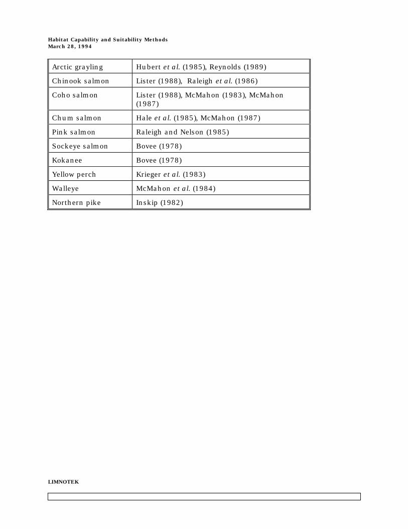
Habitat Capability and Suitability MethodsMarch 28, 1994
LIMNOTEK
Arctic grayling Hubert et al. (1985), Reynolds (1989)
Chinook salmon Lister (1988), Raleigh et al. (1986)
Coho salmon Lister (1988), McMahon (1983), McMahon(1987)
Chum salmon Hale et al. (1985), McMahon (1987)
Pink salmon Raleigh and Nelson (1985)
Sockeye salmon Bovee (1978)
Kokanee Bovee (1978)
Yellow perch Krieger et al. (1983)
Walleye McMahon et al. (1984)
Northern pike Inskip (1982)

Habitat Capability and Suitability MethodsMarch 28, 1994
LIMNOTEK
In any application of HEP to British Columbia lakes and streams it is apparent
that preliminary site specific development of SI curves and careful selection of an
aggregation method to determine HSI will be required. At the intensive level of
management, this a priori work will be essential. Assuming that mechanistic methods
would be used in determination of HSI, it is clear that SI curves developed in the US can
not be extrapolated to B.C. with confidence. New SI curves determined either by
experimentation, or from site specific investigations already reported in the literature
must be completed before HEP can be applied.
There may, however, be an exception to this requirement. At the reconnaissance
level, HEP estimates need not be precise but "reasonable" accuracy is important. Most
applications will involve repeated estimates of HSI through time to explore impact
hypotheses or effects of mitigation techniques at the basin scale. Hence, consistent
sensitivity to relative change is important, which means that consistency in the
accuracy of repeated estimates over the range of values described in SI curves is
important. If this condition can be met by many of the SI curves already available from
work in the US, the development of new curves may not be necessary. However, their
use must be restricted to "gaming" or exploratory investigation of "ball park" change in
suitable habitat in relation to a stress or mitigation imposed within a drainage basin.
Where major shifts in HSI are detected, more detailed work using site specific SI curves
to improve accuracy and precision of HEP estimates and establish greater insight into
the relative importance of various control variables will be required.

Habitat Capability and Suitability MethodsMarch 28, 1994
LIMNOTEK
Figure 4.1. A generic mechanistic model used to determine HSI in the Habitat
Evaluation Procedure (HEP). Solid lines show how habitat variables arecombined to estimate HSI. Dashed lines indicate optional variables. Reproduced from Levy (1993).

Habitat Capability and Suitability MethodsMarch 28, 1994
LIMNOTEK
Figure 4.2. A comparison of published and site specific SI curves that can be used to
determine HSI in the Habitat Evaluation Procedure and for determinationof weighted usable area (WUA) in the IFIM The dashed line indicates how aSI value is determined from an independent microhabitat variable.Reproduced from Oliver (1994).
4.2.2 Instream Flow Incremental Methodology (IFIM)

Habitat Capability and Suitability MethodsMarch 28, 1994
LIMNOTEK
Detailed descriptions of IFIM are provided by Bovee (1982) and Armour et al.
(1984). The following summary is taken from these reports.
After the initial scoping is complete, an initial field reconnaissance is conducted
to delineate study reaches and select sampling sites. Four features must be identified on
maps:
• the confluence of major tributaries and diversions;
• spacial zonation of gradient, fish species distribution, and values of water quality parameters that are
observed in the field or measured in more detail;
• delineation of unique habitat types that are essential for any life stage of the target species but are
limited in areal extent in the reach(es) potentially influenced by changes in flow; and
• random selection of reaches to be sampled having habitat types that are relatively abundant.
Sampling sites are selected to ensure that data can be extrapolated over the
entire project area. Transects are then laid out to characterize the hydraulic
microhabitat conditions. Microhabitat refers to the aggregate of the three dimensional
distribution of velocity, depth, substrata characteristics (e.g., identification of mud,
sand, cobble, bedrock), and cover. Repeated measurements are then taken of the
microhabitat variables to document their longitudinal and lateral distribution at several
different stream flows. All procedures for data collection are specified in IFIM methods
documentation (e.g., NERC 1992) to ensure that the data are compatible with input
formats to the computer models that must read that information.
The physical data (velocity, depth, substrata, and cover) are then used by a
physical habitat simulation model (PHABSIM) which determines the velocity, depth,
substrata, and cover at various flows. If other factors are also thought to change and
potentially affect habitat suitability for the target species, associated models can be run
with PHABSIM. For example, temperature (Theurer et al. 1984) and water quality
(Brown and Barnwell (1987) include dissolved oxygen, biological oxygen demand, total
ammonia, nitrate, and total phosphorus as water quality descriptors) models that can
be linked to PHABSIM are available to simulate effects of variation in flow on those
parameters. Output from the simulations separates the study reach into a series of
adjoining cells. Any one cell contains homogeneous microhabitat and macrohabitat
(variables other than velocity, depth, substrata, and cover) conditions for a given flow.

Habitat Capability and Suitability MethodsMarch 28, 1994
LIMNOTEK
Suitability curves (Figure 4.3) are then used to determine the suitability of a simulated
velocity, depth, substrata, and cover, for a given species and life stage. These SI curves
for the microhabitat variables only apply to cells for which there are suitable conditions
of temperature, water quality, food production, or any other macrohabitat variable. A
fundamental component of PHABSIM is that a suitability index must be assigned to
each simulated variable for the species and life stage that is being investigated. This is
the same SI that is used to determine HSI in the HEP method. Unlike HEP in which SI
curves are selected for any variables that are thought to best represent factors that limit
suitable habitat, SI curves in IFIM only pertain to velocity, depth, substrata, and cover.
These SI's are then aggregated by multiplication to determine a composite suitability
(CSIi):
CSIi = fv(Vi) x fd(Di) x fs(Si) x fc(Ci)
where V = velocity, D = depth, S = substrata, C = cover and fv, fd, fs, and fc are weighting
factors that quantify probability of use as a function of velocity, depth, substrata, and
cover respectively within a given cell (i) as determined from the suitability curves. These
curves which have become known as probability of use (Bovee and Cochnauer 1977) or
suitability index (SI) curves (Bovee 1982) are thought to describe the behavioral
characteristics of a life stage of a particular species with respect to each of the
microhabitat variables. The peak of the curve gets a weighting value of 1 and represents
the optimum value of a variable for use by a given life stage of a given fish species. The
tails of the curve get a weighting of 0. Where possible, the curves are empirically
determined using instantaneous measurements of the distribution of fish over the range
of the variable being examined at carrying capacity and without exploitation. If data are
not available, the USFWS describes a procedure known as the "Delphi technique"
(Crance 1987) which relies on expert opinion to develop the SI curves. Alternatively
Thielke (1985) proposed a logistic model to predict the probability that a fish will occupy
a specific location:
S(f/n) = exp(X)/(1 + exp(X))
where S(f/n) is the predicted proportion of fish (f) in sample size n and X is a linear
function of independent physical measurements. Using a stepwise regression
procedure, X was best determined as a function of categorical values of velocity cover,

Habitat Capability and Suitability MethodsMarch 28, 1994
LIMNOTEK
depth class, and substrate code. Thielke (1985) points out, however, that the approach
has only been introduced and without testing and further development at sites other
than where it was initially developed, it may not be appropriate for estimating suitability
of use. Clearly it should not be used in B.C. until testing suggests it may be a reliable
predictor of SI for B.C. species.
The composite suitability index is then multiplied by the area of the cell to obtain
the weighted usable area for the cell. The weighted usable area for the study reach
(WUA) is the sum of composite indices multiplied by cell area for all cells in the reach:
where Ai is the area of cell i and n is the number of cells in the reach. WUA is
determined for each life stage and each flow of interest. Change in WUA as a function of
microhabitat can then be examined in a series of two dimensional plots that can be
produced for each species and life stage. The lineal extent of an acceptable range of
temperatures, water quality conditions, or any other macrohabitat feature that can be
modelled and will vary as a function of flow is then determined for given time periods.
For example, the temperature of water withdrawn from the hypolimnion of a reservoir
will increase as a unit volume of that water is entrained in a downstream river. That
hypolimnetic water may also have been characterized by high dissolved phosphorus
concentrations, but in the river, the P concentrations are reduced due to uptake
processes by the benthic community in the river. If those lineal changes can be
modelled or they are known, the lineal extent of acceptable temperatures and P
concentrations for usable habitat for a given fish species can be defined for given time
period of interest. Separate lineal distances can be determined for every time period of
interest. Total habitat area (HA) is then determined as:
HA = usable length x WUA
Effects of flow manipulation or mitigation can then be explored with plots of HA or WUA
against flow for specific reaches. Longitudinal profiles of WUA for given flow regimes can
be examined. Time series plots that include reach comparisons or implementation of

Habitat Capability and Suitability MethodsMarch 28, 1994
LIMNOTEK
some management action on flow can also be examined. These and several other
approaches (NERC 1992) can be used to provide information for optimization of flow
regimes for protection of usable habitat and time series changes in usable habitat area
with and without flow manipulations or mitigation actions.
Soon after IFIM was formally introduced (Bovee 1982), numerous criticisms
appeared in the literature indicating that crucial assumptions of the method could not
be upheld in actual practice (Mathur et al. 1985, Shirvell 1986, Scott and Shirvell
(1987)). There were three main points which are presented below.
SI curves are not probability functions.
The calculation of the composite suitability for fish of a given life stage in a given
cell assumes that weighting factors are based on probability distributions. Mathur et al.
(1985) point out that SI curves are not probability functions but only ratios based on
counts of fish relative to a maximum that was encountered on dates of observations.
Further, the SI curve may change from one date to the next and from one river to the
next, thus introducing considerable uncertainty in determining what is the real
"preference of use". Also, a requirement of PHABSIM is that the SI curves are
determined from an unexploited population at carrying capacity. Mathur et al. (1985)
argue that such a condition is rare and usually unknown if modelling approaches must
be used to examine functional responses in streams. If reaches that are sampled to
determine the curves are not at carrying capacity, the "preference curve" may be flawed
and variation in curves determined at different times and locations should be expected.
Indeed, Mathur et al. (1985) show considerable variation in cited SI curves determined
for the same species and life stage and recently, Oliver (1994) also showed considerable
variation between published (Bovee 1978) and site specific SI curves for westslope
cutthroat trout.
There is no consistent positive linear relationship between WUA and fish
abundance.
The biggest criticism is that the assumption of a positive linear relationship
between WUA and fish abundance is fundamentally flawed. Although such a

Habitat Capability and Suitability MethodsMarch 28, 1994
LIMNOTEK
relationship has been found for some streams in Colorado (Nehring 1979, in Conder and
Annear 1987), Wyoming (Stalnaker 1979, in Conder and Annear 1987), Tennessee and
North Carolina (Loar 1984, in Conder and Annear 1987), and New Zealand (Jowett
1992) there many more observations of poor or negative correlations (e.g., Orth and
Maughan 1982, Shirvell and Morantz 1983, Irvine et al. 1987). Scott and Shirvell (1987)
suggest that the frequency of finding a positive linear relationship between WUA and
fish abundance or biomass is so low, that it can be due to chance alone. In rebuttal,
Orth (1987) stated that the reason a consistent relationship between WUA and fish
biomass cannot be measured is that instantaneous counts of fish are related to past
habitat limitations for any life stage. Hence, instantaneous estimates of suitability
should not be related to instantaneous population size. Orth's article may be viewed as
a more detailed explanation of ecological processes to support the initial rebuttal (Orth
and Maughan 1986) of the criticism by Mathur et al. (1985). Orth clearly stated that
users of IFIM must consider factors other than WUA that may limit fish abundance to
be successful in applying IFIM concepts. Those other factors may include food
deficiency (Irvine et al. 1987, Jowett 1992), predator-prey interactions (Bowlby and Roff
1986), "bottleneck effects" between winter and summer habitat (Nickelson et al. 1992),
and macrohabitat conditions not considered in supplementary IFIM models including
turbidity, available spawning area, and others (e.g., Levy 1993).
Component variables of WUA are not independent.
The derivation of WUA assumes independence of component variables (velocity,
depth, substrata, cover). However, depth and velocity are known to be related (Mathur et
al. 1985) which means that the selection of a certain velocity by a fish may not be
unrelated to the effect of depth and vice versa. This relationship, however, is largely
academic since SI curves used to determine WUA are not probability functions, which,
from a statistical viewpoint, means it doesn't matter how the components of WUA
interact.
Despite these major criticisms, IFIM continues to be applied to virtually all flow
manipulation projects in the US and many in Canada (Reiser et al. 1989). Although this
fact appears to contradict common sense, another fact is that the Instream Flow Group
of USFWS continues to make modifications and attempts to improve on the original

Habitat Capability and Suitability MethodsMarch 28, 1994
LIMNOTEK
IFIM. They also offer extensive training programs and courses on IFIM and in-stream
methodology in general which are advertised and attended widely. To date this exposure
has relegated other techniques for estimating suitability to a less prominent position
and produced a "popularism" for use of IFIM or parts thereof. Hence, any development
of alternate approaches is less well known. The fact that there is considerable pressure
in the northwestern US and British Columbia to implement small hydro projects to feed
a demanding power grid (M. Henry, Federal Energy Review Commission, Portland, OR.
pers comm.; K. Stein, USFS, Portland, OR, pers comm; G. Mathews, B.C. Hydro,
Burnaby, B.C. pers comm) has also helped to fuel the use of IFIM. When asked why
IFIM continues to be so popular, given its problems, every response is "I know it has
problems, but show me something better". This is a reasonable comment that highlights
the problem. There is a need for alternative methods but, to date, the infrastructure
supporting IFIM appears to preclude any new initiative. There is a "momentum" for use
of IFIM that defies logic, is increasing, and excluding development of reasonable
alternatives.
Given that IFIM appears to be here to stay, at least for the near future, it is
absolutely critical that it be applied to problems for which it is designed. It was not
designed to provide a definitive answer for application to flow disputes (Armour and
Taylor 1991). It was designed to provide a tool to systematically evaluate alternative flow
regimes for people involved in stream flow decision processes. The main focus must be
on exploring relative change in "potentially usable area" of habitat that can change in
relation to manipulation of flows. Whether fish abundance actually does change with
shifts in that habitat area is the subject of other study that may accompany IFIM or can
be established from the literature or in site specific experimentation. By combining IFIM
with other approaches to examine alternative variables that may affect fish abundance,
the importance of the inherent assumption of a positive linear relationship between
WUA and fish biomass is reduced. Limiting factors that determine fish abundance must
be assigned to another process of site specific experimentation, monitoring, or other
modelling techniques. This flow of information from IFIM and other sources supports
the view of Orth (1987) that IFIM is not a quantitative model; it is a process to assist
with decision making. WUA must only be considered a relative index of potentially
suitable habitat for fish to use that can be compared in time and space. From this
interpretation, WUA should properly be considered an index of weighted potentially
useable area.

Habitat Capability and Suitability MethodsMarch 28, 1994
LIMNOTEK
The misuse of IFIM when applied to large projects can result in large
expenditures of time and money involved with dispute resolution, extensive technical
debate, media coverage that is suspicious of science, and little contribution to resolving
uncertainty in effects of changes in flow on salmonine habitat. A classic example of
misuse in British Columbia is the application by the Aluminum Company of Canada
(Alcan) to divert flows from the Nechako River through a tunnel to the Kemano power
station; known as the Kemano Completion Project (KCP). Various impact assessments
were well underway in the early 1980's, at the same time that the Bovee (1982)
monograph describing IFIM methods became available. Alcan used the basic concept of
IFIM, with modifications of the physical models, to predict the effects of reduced
streamflow on the abundance of anadromous salmonines (Shirvell 1987). That objective
inferred quantitative predictions that were more demanding than IFIM concepts were
capable of providing. Hence, criticism that was already encircling IFIM at the time was
easily directed to KCP and now exists as formal expert reporting (Shirvell 1987). Aside
from uncertainty with the application of physical models that were used in place of
those usually associated with PHABSIM (Shirvell 1987), three general and conceptual
criticisms were outlined, all of which pointed to inappropriate use of IFIM or its
components.
• The objective assumes a positive linear relationship between WUA and fish abundance but this is not
known to exist in the Nechako River. This fact invalidates inference between flow manipulation and
salmonine abundance using IFIM.
• PHABSIM cannot make predictions about habitat area after change in flow.
• Abundance of salmonines in the Nechako River may be limited by factors other than microhabitat
variables. PHABSIM fails to include other factors and thus cannot be applied to the Nechako River.
Food limitation, temperature, and total dissolved gas saturation were variables cited as potentially
important but they were not included with PHABSIM simulations.
In another analysis of IFIM data developed for the Nechako, Slaney et al. (1984)
indicated that in addition to the problems cited by Shirvell (1987), its use was very
limited due to sources of error from the influence of anchor and frazil ice formation on
physical model predictions, inadequate amount of sampling, and potential alteration of
the river channel which was not accommodated in the physical simulation models.

Habitat Capability and Suitability MethodsMarch 28, 1994
LIMNOTEK
With the introduction of IFIM, a single technique was suddenly available for an
environmental assessment that was needed on the Nechako. In retrospect, users
appeared to jump at the opportunity to apply a tool that would "answer all the
important questions" without detailed consideration that there were very good reasons
why such a tool had not been previously available. The approach provided a framework
for bias to be an integral part of the analysis. Error can easily be introduced into the
outcome of IFIM analyses unless the fundamental details of the functioning of the
approach are well understood. In this case, error (although it may have been
unintentional) was introduced by not relating intended objectives to the capabilities of
IFIM. As cited by Lamb (1989) in his essay on complex system analysis, error and
uncertainty can haunt analysts when they overlook "fuzziness", view data as pure,
ignore important variables, and accept model outputs as truth. This lack of attention to
detail in the use of IFIM has certainly come to haunt Alcan as the company is now faced
with extensive construction delays, repeated public hearings, unnecessary costs, and a
degree of uncertainty in the fate of the KCP. This example should be a warning to
anyone interested in the application of the IFIM process to any water manipulation
project to be absolutely certain what IFIM is capable of providing and not to push it any
further.
An example of testing assumptions of IFIM before its potential use was in a study
of factors determining brown trout abundance in New Zealand streams by Jowett
(1992). Multiple regression models of brown trout abundance were developed from
independent variables describing hydrology, temperature, physical characteristics,
weighted usable area (based on IFIM criteria), fish food organism biomass, chemistry,
and catchment characteristics. In selecting variables that best explained variability in
brown trout abundance, WUA combined with food abundance were found to be the
most important variables. A significant linear relationship between WUA and trout
abundance was confirmed. The SI curves that showed the best correlation with trout
abundance were those developed in Brown trout streams of New Zealand, thus
indicating the value of developing site specific SI before determination of WUA. Jowett
also found that WUA for food production (following methods described by Waters, 1976)
was an important determinant of fish abundance. Consideration of factors other than a
simple relationship between fish abundance and habitat area that may limit fish
abundance was thus applied, and the regression models showed that food production
plus space was crucial. This a priori assessment thus dealt with the most important

Habitat Capability and Suitability MethodsMarch 28, 1994
LIMNOTEK
criticism of IFIM (that habitat area and fish biomass may not be related). Assuming
there is confidence with the physical modelling in PHABSIM, output from an IFIM
application in these New Zealand streams could be related to trout abundance. A
similar approach will be required in B.C. if IFIM is to applied to projects where a
quantitative relationship between WUA and fish abundance is required. It requires a
"bundled" approach of IFIM with quantitative analyses of empirical data or experiments
to establish relationships between fish abundance and indices of suitability.
4.2.3 Missouri Stream Habitat Evaluation Procedure (SHEP)
A detailed description of SHEP is provided by Fajen and Wehnes (1981). It applies
only to streams. The following summary is taken from this report.
SHEP assigns a rating (0-10) to the quality of fish habitat for 6 parameters.
1. Barriers to fish migration. Barriers are considered dams or other structures that produce vertical
drops. The rating applies to the relative amount of vertical drop; 10 is no obstruction, zero is several
obstructions causing a drop of more than 3m at low flow. Data can be collected from maps or in field
observations.
2. Percent of watershed in urban development. Development of communities are inferred to reduce
the quality of streams. A 10 is <5% of the watershed is in urban development; zero is >70% is in urban
development. Information is determined from maps and air photos.
3. Condition of riparian vegetation. The riparian zone is recognized for moderating water
temperature, providing protection from adjacent land use activities, and providing cover for fish. A 10
means that riparian vegetation covers all stream banks in the study reach. Zero means <10% has riparian
vegetation. The rating is determined from air photos and on-site observations of vegetation cover within
30m of the stream bank.
4. Degree of erosion in the flood plain. This is mainly a rating of channel stability and potential to
produce turbidity. A 10 means there is no evidence of erosion. Zero means the floodplain is severely eroded
and the stream channel is poorly defined. The rating is determined from air photos, on-site observations,
and reference to soils data if available.
5. Percent protected from land use impacts. Soil and vegetation conservation practices are recognized

Habitat Capability and Suitability MethodsMarch 28, 1994
LIMNOTEK
to influence water quality, substrata characteristics, flow variation, and potential for erosion. A 10 means
that the watershed has >80% undisturbed forest, improved pasture terraces, or other conservation practice.
Zero is for no mitigation and extreme land disturbance. The rating is determined from air photos and on-site
observations.
6. Flow alteration. This parameter mainly applies to the number of flow control structures that may
influence the natural stream hydrograph. These include ponds with flow control structures and other
impoundments used for irrigation or domestic water supply. A 10 means that <10% of the watershed is
controlled by impoundments. Zero means that >95% of water flow in the watershed is controlled by
impoundments.
In addition to these habitat quality parameters, SHEP uses 4 habitat alteration
functions which act to alter the habitat quality indices depending on the type and extent
of a habitat alteration. Channel modification rate (f1) is used to adjust suitability based
on an arbitrary assignment of percent fish reduction associated with removal of riparian
vegetation (25% fish reduction), intentional alteration of channel geomorphology (80%
fish reduction), and changing a natural channel to a paved conduit (95% fish reduction).
Channel modification rate is determined as:
f1 = 1.0 - (% modification x % fish reduction)
Impoundment rate (f2) assigns an arbitrary type of degradation (0% is no impoundment;
100% is stream is fully impounded for water conservation) associated with habitat loss
with the amount of impoundment and is determined as:
f2 = 1 - (% degradation x rating of type of degradation)
Water quality (f3) is simply another rating from pristine water (rating of 1) to polluted
water that causes fish kills (rating of zero). No input parameters or measurements are
required. This is only a subjective scale that must be based on expert opinion.
Streambed condition (f4) is still another rating extending from stable substrata (rating of
1) to a reach filled with unconsolidated fines and unstable material (rating of zero).
A habitat index is then determined as:

Habitat Capability and Suitability MethodsMarch 28, 1994
LIMNOTEK
HI = (ΣPi/Np) x f1 x f2 x f3 x f4
where Pi is the individual parameter values and Np is the number of parameters used.
HI varies from 0 to 10 and gives a relative index of "habitat quality". It has several
shortcomings that make it inappropriate for use in British Columbia. The index has
only been used in catfish and bass streams of Missouri. It has never been tested on
streams that support sportfish found in B.C. and thus requires validation. HI is an
arbitrary index based on ratings scales that are largely subjective and can be biased by
opinion. Hence, the system lacks any basis, statistical or otherwise, for space and time
comparisons which are essential for suitability estimates in B.C. The rating scales
always assume linear associations between any disturbance and the suitability of
habitat for fish but the authors provide no supportive evidence, even for the sites from
which the method was developed. Hence, any relationship between HI and fish habitat
characteristics is unknown. It is also unknown if HI has any relevance to the suitability
of habitat for fish in British Columbia. We are not aware of the method being applied
outside of Missouri. Although a similar rating scheme may be considered for fish species
in specific regions of British Columbia, the basic problem of user bias, lack of
comparability, and uncertainty of the relevance of HI makes the approach inappropriate
at this time.
4.2.4 Fish Habitat Index (FHI)
A preliminary description of FHI is provided by Parsons et al. (1981). It applies
only to streams in forested watersheds with and without forest harvesting activities. The
following summary is taken from that article.
FHI is derived by multiplying habitat area by habitat quality (a numerical
indicator of habitat condition). FHI is determined in both undisturbed and harvested
conditions. Area is the area of fish bearing streams which is assumed to decrease with
harvesting activities due to stream blockages from log jams. Habitat quality is a rating
from 0 to 10 that is determined using a regression equation that is based on geomorphic
parameters. This quality is assumed to decrease in harvested drainage due to

Habitat Capability and Suitability MethodsMarch 28, 1994
LIMNOTEK
sedimentation, increases in water temperature, debris torrents, slope failures, etc.
The regression model for undisturbed watersheds was developed by the authors
to predict the quality value using four independent geomorphic parameters:
Quality Value = 6.56 + 1.44(basin perimeter) + 0.00089(basin relief) - 2.02(basin
area) - 5.62 (compactness coefficient).
Total FHI for a landtype association is determined by multiplying the quality
value from the regression model by area of landtype. The authors indicate that separate
regressions for areas disturbed by forest harvesting activities have been developed but
these were not included in the article.
The approach may be appealing for overview techniques if the geomorphological
data were available. It is simple to use and can be compared spatially and temporally.
However, the model has not been used except in the location where it was developed
and thus it has not been tested and verified for use elsewhere. Consequently the model
is not recommended for use in B.C. at this time. It may, however, be considered if any
new model development is planned at the overview level of management. It is
recommended that the developers of the model be contacted to determine if the model is
still in use and if so, find out if it has changed and verified at other locations. If so, it
may be worth testing in forested watersheds in B.C.
4.2.5 Planned Reservoir HIS An index used to rate the suitability of planned reservoirs for rainbow trout and
yellow perch was developed by McConnell et al. (1984). The following summary is taken
from the McConnell paper.
Habitat suitability is determined from rating 5 main "attributes" including
temperature, mineral turbidity, structural cover, maximum drawdown and timing of
drawdown, and frequency of shallow coves. Each primary attribute is scored within one
or more matrices that include cross comparisons of secondary attributes that require
input of data. For example a temperature score for rainbow trout requires information

Habitat Capability and Suitability MethodsMarch 28, 1994
LIMNOTEK
on three secondary attributes (why three are determined and not others is not
described) including a climate score (matrix of mean July air temperature versus length
of growing season), operations score (a matrix of storage ratio versus depth of outlet),
and stratification score (a matrix of maximum fetch versus mean depth). There are three
ratings for each variable on the matrix borders, resulting in a matrix for each secondary
attribute containing nine squares that represent cross comparisons in the matrix.
Within each box a rating of 1,2, or 3 is assigned on the basis of local knowledge or
opinion of the interactions of boxes within the matrix. Data for the matrices can be
available climate data, and engineering plans for the reservoir. The 1, 2, or 3 code for
each of the 5 main attributes is then compiled to form a 5 digit code. A series of tables
are provided which give a suitability rating for all combinations of the 5 digit code.
Although this system is appealing for overview estimates of suitability, it is
entirely based on subjective ratings. Hence the approach has no basis for spatial and
temporal comparisons. Although simplistic, it is not clear in the evidence presented by
McConnell et al. (1984) why certain attributes were selected for a given species. These
may also have been subjective assignments. Given these uncertainties, the inability to
reliably use the method for site and time course comparisons, and that it can only be
applied to sites for reservoirs that presently do not exist, it is not recommended for use
in British Columbia.
4.2.6 Tennant flow method The Tennant method is very simplistic and has received appeal in regions of
British Columbia as a quick and easy-to-understand method of determining habitat and
recreational suitability of stream habitat. The method is based on the assumption that
flows that are satisfactory for needs of fish and other aquatic biota will also be sufficient
for maintaining recreational and aesthetic qualities. Based upon empirical relationships
and observations, Tennant suggests that minimum flows at any time of the year must
be >10% of mean annual discharge. Below the 10% threshold, fish habitat and
recreational value will be severely degraded. Above 10%, habitat and recreational quality
increases in a range from fair conditions (10% in winter and 30% in summer) to
outstanding (40% in winter and 60% in summer). An optimum range is considered 60-
100% of mean annual flow at any time of the year.

Habitat Capability and Suitability MethodsMarch 28, 1994
LIMNOTEK
This approach is very appealing due to its simplicity and for this reason it has
been applied in British Columbia. Many regional fisheries biologists have used it for
obtaining rough estimates of suitability where the flow data are available. Where
validated, it is appropriate for use at the overview and reconnaissance levels of
management. However, we are not aware of projects in which it has been validated.
Hence, the collection of observational or ideally experimental data similar to that
compiled by Tennant (1975) from sites in warm and cold water streams of the US
midwest, great plains, and western mountain ranges are required for validation
purposes before the method can be recommended for routine use in British Columbia.
The method is further limited by the availability of annual flow records. In British
Columbia, however, the province-wide network of flow monitoring sites managed by the
Water Survey of Canada may provide adequate records for sites in close proximity to a
gauged location.
4.3 Methods Recommendations
Of the six suitability methods outlined in Section 4.2, only IFIM can be
immediately used in British Columbia, but only in large, big budget projects requiring
an intensive method to examine relative change in habitat suitability with respect to a
flow manipulation. IFIM can be used as a tool to systematically evaluate alternative flow
regimes for people involved in stream flow decision processes at the reconnaissance and
intensive levels of management. It is not a quantitative tool used to provide a definitive
answer to flow disputes. To develop confidence and reliability in IFIM, the following
recommendations must be followed:
• recognize that IFIM is a "process" to assist with decision making. It does not produce decisions and it
does not provide data to quantify change in fish abundance as a function of flow manipulation;
• there must be some evidence either in empirical data or literature sources that the abundance of a life
stage of the fish that is being examined is not limited by macrohabitat conditions (e.g., food production,
predator-prey interactions, temperature, etc.). This is very difficult to resolve unequivocally without
extensive experimentation or data collection (e.g., Jowett 1992) but at very least, some effort must go
into this analysis to set "reasonable" spacial and temporal bounds first on the determination of WUA
and then on the extrapolation to HU;

Habitat Capability and Suitability MethodsMarch 28, 1994
LIMNOTEK
• where possible, site specific data should be collected to examine the relationship between fish
abundance and WUA. If it is not linear, WUA can only be considered an index of potential suitability
and it cannot be directly related to fish abundance;
• site specific SI curves should be determined for the study area; and
• ensure that there are no confounding factors (e.g., ice formations) that may interfere with the ability of
PHABSIM to correctly predict change in microhabitat variables with varying flow. If confounding
factors are present, models that are sensitive to the effect of all factors should be used in place of
PHABSIM or the entire process should not be used.
These recommendations require considerable effort on behalf of potential users of
IFIM even before the first output of WUA can be used. For example, Oliver (1994)
suggested that sampling effort required to obtain reasonable precision in determining SI
curves was "unrealistic for most management purposes" and due to inherent variability
between habitats within a stream reach, IFIM procedures should be restricted to
assessments in discrete habitat units, not whole streams or whole reaches. Given this
constraint, IFIM is not a technique that can be run quickly. It is suitable only as part of
detailed analyses of large projects that require detailed investigations.
HEP has been tested at a few sites in British Columbia will poor results (Levy
1993) due to inappropriate selection of habitat variables and a general lack of site
specific SI curves. The biggest problem with HEP is that it requires extensive a priori
knowledge of factors that limit fish abundance at a given site. This requirement is much
more important for HEP than for IFIM since variables must be selected for HEP that
actually do limit fish abundance. As pointed out by Bisson (1992), an unequivocal
determination of limiting factors requires extensive experimentation. If this research
effort is required, it is likely that the suitability of habitat to support fish will be
determined long before one is ready to apply HEP. This requirement for substantial
insight into limiting factors is the fundamental problem with HEP, regardless of other
difficulties in providing reliable SI curves and an appropriate method of aggregating SI
data to determine the habitat suitability index. We regard these problems intractable for
present or future application of the method in British Columbia and thus HEP should
not be considered for any application in the province. This finding is consistent with
recent evaluations in the US where HEP is also falling out of favour for use in assessing
fish habitat suitability (K. Fausch, Colorado State University, Pers. Comm).

Habitat Capability and Suitability MethodsMarch 28, 1994
LIMNOTEK
Of the simpler approaches described in section 4.2, the Tennant method has
been picked up as a quick approach for estimating suitability in various regions of the
province. However, it has never been formally validated and this testing must be
completed before it can be recommended for routine use.
Each of SHEP, FHI, and the planned reservoir HSI were developed primarily as
concepts that the authors have indicated require further research and testing before
they can be applied elsewhere with confidence. These methods have never been applied
to sites in British Columbia and as part of a long term strategy for methods
development, they should be considered for additional testing. However, they do have
problems other than the lack of validation that must be considered as part of any
testing initiative. As discussed in Section 4.2.3 SHEP:
• has not been tested using species that are found in B.C.;
• it is subject to bias in the assignment of rating scores;
• lacks statistical rigor for any time and space comparisons; and
• was developed only for agricultural areas having impacts from urban development and stream
channelization.
However, the basic concept of assigning quick rating scores is appealing for application
to overview and reconnaissance applications and thus we recommend this method be
considered as part of methods development and validation. Existing parameters in the
method will likely have to be changed, tested, and verified to reflect conditions of B.C.
waters. The quantitative scoring system used in the fish habitat index may be suitable
for spatial and temporal comparisons and is also appropriate for further testing and
verification. Resolution is at the basin or watershed scale, making it suitable for
overview and reconnaissance level estimates of suitability. The planned reservoir HSI
may have big problems with user bias and appears to lack a clear process for the
selection of "attributes" in applications remote from where it was developed. However,
the concept is novel and it should not be discarded outright from future testing. With
work, the process may be standardized to minimize potential bias and provide a tool for
exploring change in habitat suitability with various scenarios of reservoir size and
operational strategy.
Our analysis indicates there is no readily available "off the shelf" method to

Habitat Capability and Suitability MethodsMarch 28, 1994
LIMNOTEK
estimate habitat suitability quickly, on a low budget, in any habitat and at any
management level. When these estimates are required, which is likely to be most of the
time, capability estimates will presently have to be substituted, where possible. This
recommendation is based on the view that if an area is capable of supporting fish, then
the habitat is also suitable as fish habitat. The reverse may not be true. Recommended
methods of estimating capability for all management levels are provided in Section 2.0.
Given the limited availability of suitability models, it is recommended that a
program of verification and testing that is required for most existing models also
consider the development of new methods for use in British Columbia. There are at least
two and probably more concepts to consider in this process. One is to develop a rating
of habitat that is unsuitable for the growth of fish in early life stages. There are volumes
of empirical relationships in the literature describing physiological and pathological
responses of organisms or populations to chemical and physical manipulation of lake
and stream habitat. It may be easier to apply these findings to rank habitat according to
tolerance levels by lake and stream biota. This approach is the basis of toxicity
guidelines in both the US and Canada (e.g., CCREM 1993) and it may be appropriate for
ranking habitat suitability as well. A comprehensive approach may be to combine
CCREM criteria (which provides threshold data for all chemical and some physical
variables), with a ranking for flow (e.g., Tennant 1975), and habitat complexity. Where
forest harvesting practices may be producing fines in stream substrata, estimates of
embeddedness (e.g., MacDonald et al. 1991) may also be considered in a ranking
scheme to increase sensitivity to forest management practices. Another approach may
be to develop a decision tree that helps determine if a habitat is suitable to support fish.
Discussion with regional biologists as part of this project revealed that a standard series
of questions are often asked with respect to lake suitability for stocked fish:
• Are seasonal changes in the profile of dissolved oxygen and temperature within the range that can be
tolerated by fish?
• Is toxicity from any contaminants an issue?
• Is there a history of winter kill?
• Are there adequate spawning areas?
• Are there abundant fish food organisms present?
Questions pertaining to stream habitat might include:

Habitat Capability and Suitability MethodsMarch 28, 1994
LIMNOTEK
• Is there adequate cover in rearing habitat?
• Is adequate spawning area present?
• Are summer temperatures and low flow adequate to support fish?
Each of these questions require presence/absence or yes/no type answers and can be
resolved with limited field work and reference to standards that are either presently
available (e.g., SEP biostandards in the Fish Habitat Enhancement Manual (Adams and
Whyte 1990) or can be developed from existing literature. Answers to these questions
structured in a decision tree could provide a relatively rapid yet comprehensive
approach to assessing habitat suitability. An approach like this may, in fact, be
informally already in use in many regions of the province. What is now required is a
process to formalize these methods for routine use.

Habitat Capability and Suitability MethodsMarch 28, 1994
LIMNOTEK

Habitat Capability and Suitability MethodsMarch 28, 1994
LIMNOTEK
5.0 LIST OF REFERENCES
Adams, G.F. and C.H. Olver. 1977. Yield properties and structure of boreal percidcommunities in Ontario. J. Fish. Res. Board Can. 34: 1613-1625.
Adams, M.A. and I.W. Whyte. 1990. Fish habitat enhancement: a manual forfreshwater, estuarine, and marine habitats. Department of Fisheries and OceansCanada. DFO 4474. 330p.
Aggus, L.R. and W.M. Bivin. 1982. Habitat suitability index models: Regression modelsbased on harvest of coolwater and coldwater fishes in reservoirs. U.S. Department ofInterior Fish and Wildlife Service. FWS/OBS-82/10.25. 38 p.
Anon. 1992. Fisheries conservation and management inventories for the future. Reportof the Fisheries Inventory Task Force. RIC Report 005.
Aquatic Resources Limited. 1993. Sportfish Habitat Suitability and CapabilityLiterature Review. Prepared for Ministry of Environment, Lands, and Parks, FisheriesSection, Vancouver, B.C. 90 p. plus appendices.
Armour, C.L., R.J. Fisher, and J.W. Terrell. 1984. Comparison of the use of thehabitat evaluation procedures (HEP) and the instream flow incremental methodology(IFIM) in aquatic analysis. U.S. Department of Interior, fish and Wildlife Service. FWS/OBS-84/11. 30 p.
Armour, C.L. and J.G. Taylor. 1991. Evaluation of the instream flow incrementalmethodology by U.S. Fish and Wildlife Service field users. Fisheries 16: 36-43.
Barber, W.E., M.E. Oswood, and S.J. Deschermeler. 1981. Validation of two habitatfish stream survey techniques: the area and transect methods. Final Report. U.S.Department of Agriculture, Forest Service. Ketchikan, AK . Contract 53-0109-0-00054.64 p.
Binns, N.A. and F.M. Eiserman. 1979. Quantification of fluvial habitat in Wyoming.Trans. Am. Fish. Soc. 108: 215-228.
Binns, N.A. 1982. Habitat quality index: procedure manual. Wyoming Fish and GameDepartment. Cheyenne, Wyoming. 209 pages.
Bisson, P.A. 1992. Importance of identification of limiting factors in an evaluationprogram. In J.W. Buell (Ed.) Proceedings of the stream habitat evaluation workshop,October 1986. U.S. Dept. of Energy, Bonneville Power Administration, Portland, OR. 22p.

Habitat Capability and Suitability MethodsMarch 28, 1994
LIMNOTEK

Habitat Capability and Suitability MethodsMarch 28, 1994
LIMNOTEK
Bovee, K.D. 1978. probability-of-use criteria for the family Salmonidae. Instream FlowInformation Paper No. 4. Cooperative Instream Flow Service Group, Fort Collins,Colorado. 80 p.
Bovee, K.D. 1982. A guide to stream habitat analysis using the instream flowincremental methodology. Instream Flow Information Paper No. 12. Western Energy andLand Use Team. U.S. Fish and Wildlife Service. Fort Collins, CO. 248p.
Bovee, K.D. and T. Cochnauer. 1977. Development and evaluation of weighted criteria,probability of use curves for instream flow assessment: fisheries. Instream FlowInformation Paper No. 3. Cooperative Instream Flow Service Group, Fort Collins, CO. 40p.
Bowlby, J.N. and J.C. Roff. 1986. Trout biomass and habitat relationships in southernOntario streams. Trans. Am. Fish. Soc. 115: 503-514.
Brown, L.C. and T.O. Barnwell. 1987. The enhanced stream water quality modelsQUAL2E and QUAL2E-UNCAS: documentation and user manual. U.S. EnvironmentalProtection Agency. EPA/600/3-87/007. Athens, GA.
Burns, J.W. 1971. The carrying capacity for juvenile salmonids in some northernCalifornia streams. Calif. Fish and Game 57: 44-57.
Burton, R.A., and T.A. Wesche. 1974. Relationship of duration of flows and selectedwatershed parameters to the standing crop estimates of trout populations. Water Res.Ser. No. 52. Water Resources Institute, University of Wyoming, Laramie, Wyoming. 86 p.
Buttiker, B. and E. Staub. 1992. Simulation of perch (Perca fluviatilis L.) populationdynamics in Lake Constance. Bulletin de la Societe Vaudoise des Sciences Naturelles82(1): 67-85.
Byrne, A., T.C. Bjornn, and J.D. McIntyre. 1992. Modeling the response of nativesteelhead to hatchery supplementation programs in an Idaho river. North AmericanJournal of Fisheries Management 12(1): 62-78.
Carlander, K.D. 1977. Biomass, production, and yields of walleye (Stizostedion vitreumvitreum) and yellow perch (Perca flavescens) in North American Lakes. J. Fish. Res.Board Can. 34: 1602-1612.
CCREM. 1993. Canadian Water Quality Guidelines. Task force on water qualityguidelines of the Canadian Council of Resource and Environment Ministers. Ottawa.
Chatters, J.C., D.A. Neitzel, M.J. Scott, and S.A. Shankle. 1991. Potential impacts ofglobal climate change on Pacific Northwest spring chinook salmon (Oncorhynchustshawytscha): An exploratory case study. Northwest Environmental Journal 7(1): 71-92.

Habitat Capability and Suitability MethodsMarch 28, 1994
LIMNOTEK
Cheslak, E.F. and A.S. Jacobson. 1990. Integrating the Instream Flow IncrementalMethodology with a population response model. Rivers 1(4): 264-288.
Chisholm, I.M. and W.A. Hubert. 1986. Influence of stream gradient on standingstock of brook trout in the Snowy Range, Wyoming. Northwest Science 60: 137-139.
Conder, A.L. and T.C. Annear. 1987. Test of weighted usable area estimates derivedfrom PHABSIM model for instream flow studies on trout streams. North. Am. J. Fish.Manage. 7: 339-350.
Contor, C.R. and W.S. Platts. 1991. Assessment of COWFISH for predicting troutpopulations in grased watersheds of the intermountain west. U.S. Dept. of Agriculture,Forest Service, Intermountain Reserach Station. General Technical Report INT-278. 28p.
Crance, J.H. 1987. Guidelines for using the DELPHI technique to develop habitatsuitability index curves. U.S. Fish and Wildlife Service. Biological Report 82(10.134). 21p.
Dowing, J.A., C. Plante, and S. Lalonde. 1990. Fish production correlated withprimary productivity, not the morphoedaphic index. Can. J. Fish. Aquat. Sci. 47: 1929-1936.
Eifert, W.H. and T.A. Wesche. 1982. Evaluation of the stream reach inventory andchannel stability index for instream habitat analysis. Water Resource Service Report82. Water Resources Research Institute, University of Wyoming, Laramie, Wyoming. 106p.
Enk, M.D. 1977. Instream overhead bank cover and trout abundance in two Michiganstreams. M.Sc. Thesis, Michigan State University (East Lansing, MI). 127 p.
Espegren, G.D., D.D. Miller, and R.B. Nehring. 1990. Modeling the effects of variousangling regulations on trout populations in Colorado streams. Colorado Division ofWildlife, Aquatic Research. Special Report Number 67. 24 p.
Fajen, O.F. and R.E. Wehnes. 1981. Missouri's method of evaluating stream habitat.In: Acquisition and utilization of aquatic habitat inventory information. (N.B.Armantrout, (Ed.)) Western Division of American Fisheries Society, Bethesda, MD., 117-123.
Fausch, K.D., C.L. Hawkes, and M.G. Parsons. 1988. Models that predict standingcrop of stream fish from habitat variables: 1950-85. Oregon Gen. Tech. Rept. PNW-GTR-213. U.S. Dept. Agriculture, Forest Service, Pacific Northwest Research Station,Portland, Oregon. 52 p.

Habitat Capability and Suitability MethodsMarch 28, 1994
LIMNOTEK
Fraley, J.J. and P.J. Graham 1981. Physical habitat, geologic bedrock type and troutdensities in tributaries of the Flathead River drainage, Montana. In: Acquisition andutilization of aquatic habitat inventory information. (N.B. Armantrout, (Ed.)) WesternDivision, American Fisheries Society, Bethesda, MD., 178-185.
Godbout, L. and R.H. Peters. 1988. Potential determinants of stable catch in the Brooktrout (Salvelinus fontinalis) sport fishery in Quebec. Can. J. Fish. Aquat. Sci. 45: 1771-1778.

Habitat Capability and Suitability MethodsMarch 28, 1994
LIMNOTEK
Gordon, D.J. and H.R. MacCrimmon. 1982. Juvenile salmonid production in a LakeErie nursery stream. J. Fish. Biol. 21: 455-473.
Hale, S.S., T.E. McMahon, and P.C. Nelson. 1985. Habitat suitability models andinstream flow suitability curves: chum salmon. U.S. Fish and Wildlife Service BiologicalReport 82(10.108). 48 p.
Hanson, J.M. and W.C. Leggett 1982. Empirical prediction of fish biomass and yield.Can. J. Fish. Aquat. Sci. 38: 257-263.
Harshbarger, T.J. and H. Bhattacharyya. 1981. An application of factor analysis in anaquatic habitat study. In: The use of multivariate statistics in studies of wildlife habitat. Gen. Tech. Rep. RM-87. (D.E. Capen (Ed.)) U.S. Department if Agriculture, ForestService, Rocky Mountain Forest and Range Experiment Station, Fort Collins, CO, 180-184.
Hartman, G.F. and J.C. Scrivener. 1990. Impacts of forestry practices on a coastalstream ecosystem, Carnation Creek, British Columbia. Can. Bull. Fish. Aquat. Sci. 223:148p.
Havey, K.A. and R.M.Davis. 1970. Factors influencing standing crop and survival ofjuvenile salmon at Barrows Stream, Maine. Trans. Am. Fish. Soc. 99: 297-311.
Hawkins, C.P., M.L. Murphy, N.H. Andersonn, and M.A.. Wilzbach. 1983. Density offish and salamanders in relation to canopy and physical habitat in streams of thenorthwestern United States. Can. J. Fish. Aquat. Sci. 40: 1173-1185.
Henderson [Ed.] Proceedings of the National Workshop on Effects of Habitat Alterationon Salmonid Stocks. Can. Spec. Publ. Fish. Aquat. Sci. 105.
Holtby, L. B. and J. C. Scrivener. 1989. Observed and simulated effects of climaticvariabliltiy, clear-cut logging, and fishing on the numbers of chum salmon(Oncorhynchus keta) and coho salmon (O. kisutch) returning to Carnation Creek,British Columbia, p. 62-81. In C.D. Levings, L. B. Holtby, and M. A. Henderson Can.Spec. Publ. Fish. Aquat. Sci. 105, Ottawa, 173-179.
Hubert, W.A., R.S. Helzner, L.A. Lee, and P.C. Nelson. 1985. Habitat suitability indexmodels and instream flow suitability curve: Arctic grayling riverine populations. U.S.Fish and Wildlife Service. FWS/OBS-82/10.110.
Hunt, R.L. 1979. Removal of woody streambank vegetation to improve trout habitat. Tech. Bull. 115. Wisconsin Department of Natural Resources, Madison, WI. 35 p.
Inskip, P.D. 1982. Habitat suitability index models: Northern Pike. U.S. Fish and

Habitat Capability and Suitability MethodsMarch 28, 1994
LIMNOTEK
Wildlife Service. FWS/OBS-82.10.17. 40 p.

Habitat Capability and Suitability MethodsMarch 28, 1994
LIMNOTEK
Irvine, J.R., I.G. Jowett, and D. Scott. 1987. A test of the instream flow incrementalmethodology for underyearling rainbow trout, Salmo gairdnerii, in experimental NewZealand streams. New Zealand J. Mar. Freshwater Res. 21:35-40.
Jenkins, R.M. 1977. Prediction of fish biomass, harvest, and prey-predator relations inreservoirs. In: Proceedings of the conference of assessing the effects of power-plantinduced mortality on fish populations. (Ed: Van Winkle,W.) Pergamon Press, New York,282-293.
Jenkins, R.M. 1982. The morphoedaphic index and reservoir fish production. Trans.Am. Fish. Soc. 111: 133-140.
Jenkins, R.M. and D.I. Morais. 1971. Reservoir sportfishing effort and harvest inrelation to environmental variables. Amer. Fish. Soc. Spec. Publ. 8: 371-384.
Jensen, A.L. 1992. Relation between mortality of young walleye (Stizostedion vitreum)and recruitment with different forms of compensation. Environmental Pollution 76(2):177-181.
Johnson, B.M., C Luecke, R.S. Stewart, M.D. Staggs, S.J. Gilbert, and J.F. Kitchell.1992. Forecasting effects of harvest regulations and stocking of walleyes on prey fishcommunities in Lake Mendota, Wisconsin. North American Journal of FisheriesManagement 12(4): 797-807.
Jones, J.R. and M.V. Hoyer. 1982. Sportfish harvest predicted by summer chlorophylla concentration in midwestern lakes and reservoirs. Trans. Am. Fish. Soc. 111: 176-180.
Jowett, I.G. 1992. Models of the abundance of large brown trout in New Zealand rivers.Amer. J. Fish. Management. 12:417-432.
Klamt, R.R. 1976. The effects of coarse granitic sediment on the distribution andabundance of salmonids in the central Idaho batholith. M.Sc. Thesis, University ofIdaho, Moscow, ID. 85 p.
Konopacky, R.C. 1984. Sedimentation and productivity in salmonid streams. Ph.D.Dissertation, University of Idaho, Moscow, ID. 197 p.
Korman, J. and E. Parkinson. 1993. Application of the Large Lakes Kokanee Model toKootenay Lake, Okanagan Lake, and the Williston Reservoir. B.C. Ministry ofEnvironment, Lands, and Parks. 21 p.
Korman, J., D.R. Marmorek, G.L. Lacroix, P.G. Amiro, J.A. Ritter, W.D. Watt, R.E.Cutting, and D.C.E. Robinson. 1994. Development and evaluation of a biological modelto assess regional-scale effects of acidification on Atlantic salmon. Canadian Journal of

Habitat Capability and Suitability MethodsMarch 28, 1994
LIMNOTEK
Fisheries and Aquatic Sciences. 51. (In Press).
Korman, J., T.M. Webb, and E. Parkinson. 1993a. Large Lakes Kokanee Model,Version 2.0, User's Guide. B.C. Ministry of Envirnoment, Lands, and Parks. 70 p.
Korman, J., Webb, T. Walters, C.J., Digisi, J., J. Sawada, and L. Huato. 1993b.Small Lakes Integrated Management Model, Version 1.0: User's Guide. B.C. Ministry ofEnvironment, Lands and Parks, Fisheries Branch. 26 p.
Korver, R. 1992a. Lake Trout Management Support System User's Guide. OntarioMinistry of Natural Resources. 57 p.
Korver, R. 1992b. MANSIM: A fairly generic computer model for simulationmanagement actions on single fish populations. Version 3.0. Ontario Ministry of NaturalResources. 36 p.
Kraft, M.E. 1972. Effects of controlled flow reduction on a trout stream. J. Fish. Res.Board Can. 29: 1405-1411.
Kreiger, D.A. J.W. Terrell, and P.C. Nelson. 1983. Habitat suitability information:Yellow perch. U.S. Fish and Wildlife Service. FWS/OBS-82/10.55. 37 p.
Lamb, B.L. 1989. Comprehensive technologies and decision-making: reflections on theinstream flow incremental methology. Fisheries 14(5):12-16.
Lanka, R.P. 1985. Modeling trout standing stock in small Wyoming streams based oneasily measured habitat and geomorphological characteristics. M.Sc. Thesis, Univ. ofWyoming, Laramie, WY. 102 p.
Lanka, R.P., W.A. Hubert, and T.A. Wesche. 1987. Relations of geomorphology tostream habitat and trout standing stock in small Rocky Mountain streams. Trans. Am.Fish. Soc. 116: 21-28.
Lanno,R. and C. Wren. 1992. Predictive modeling of fisheries habitat loss andreplacement. Research and Development Branch, Ontario Ministry of Transportation,Toronto, Ontario. 54 p.
Leathe, S.A. and M.D. Enk. 1985. Cumulative effects of micro-hydro development onthe fisheries of the Swan River drainage, Montana. Vol. 1: Summary Report. PortlandOR: U.S. Department of Energy, Bonneville Power Administration; final report, project82-19. 114p and app.
Lee, D.C. 1991. A stochastic, compartmental model of the migration of juvenileanadromous salmonids in the Columbia River Basin. Ecological Modelling 54(3-4):227-246.

Habitat Capability and Suitability MethodsMarch 28, 1994
LIMNOTEK
Lee, D.C. and J.B. Hyman. The stochastic life-cycle model (SLCM): Simulating thepopulaion dynamics of anadromous salmonids. U.S. Dept. of Agriculture, ForestService, Intermountain Research Station. Reserach Paper INT-459. 30 p.
Levy, D.A. 1993. A review of habitat capability for salmon spawning and rearing.Prepared by Levy Research Services Ltd. for B.C. Resources Inventory Committee,Vancouver, B.C. 45p.
Lewis, S.L. 1969. Physical factors influencing fish populations in pools of a troutstream. Trans. Am. Fish. Soc. 98: 14-19.

Habitat Capability and Suitability MethodsMarch 28, 1994
LIMNOTEK
Lisle, T.E. and J. Lewis. 1992. Effects of sediment transport on survival of salmonidembryos in a natural stream: A simulation approach. Canadian Journal of Fisheries andAquatic Sciences 49(11): 2337-2344.
Lister, D.B. 1988. Evaluation of HSI models for juvenile chinook and coho salmonusing data from Coldwater River, B.C. D.B. Lister & Associates Ltd., Clearbrook, B.C.
Loar, V. 1984. editor. Application of habitat evaluation models in southern Appalachiantrout streams. Oak Ridge National Laboratory, ORNL/TM-9323, Oak Ridge, Tennessee.
MacDonald, L.H., A.W. Smart, and R.C. Wissmar. 1991. Monitoring guidelines toevaluate effects of forestry activities on streams in the Pacific Northwest and Alaska.EPA/910/9-91-001. U.S. Environmental Protection Agency, Seattle, WA.
Madenjian, C.P. and S.R. Carpenter. 1991. Individual-based model for growth ofyoung-of-the-year walleye: A piece of the recruitment puzzle. Ecological Applications1(3): 268-279.
Madenjian, C.P., B.M. Johnson, and S.R. Carpenter. 1991. Stocking strategies forfingerling walleyes: An individual-based model approach. Ecological Applications 1(3):280-288.
Marcus, M.D., W.A. Hubert, and S.H. Anderson. 1984. Habitat suitability models:Lake trout (exclusive of the Great Lakes). U.S. Fish and Wildlife Service. FWS/OBS-82/10.84.
Marshall, D.E. and E.W. Britton. 1990. Carrying capacity of coho salmon streams.Can. MS Rep. Fish. Aquat. Sci. 2058, 32p.
Marshall, S.A. 1985. Survival, movement, and habitat utilization of spring-stockedfingerling brown trout (Salmo trutta) in six northeast Iowa streams. M.Sc. Thesis, IowaState University, Ames, IA. 42 p.
Marshall, T.R. and P.A. Ryan. 1987. Abundance patters and community attributes offishes relative to environmental gradients. Can. J. Fish. Aquat. Sci. 44(Suppl. 2): 198-215.
Mathur, D., W.H. Bason, E.J. Purdy, and C.A. Silver. 1985. A critique of the instreamflow incremental methodology. Can. J. Fish. Aquat. Sci. 42: 825-831.
Matuszek, J.E. 1978. Empirical predictions of fish yields of large North American lakes.Trans. Am. Fish. Soc. 107: 385-394.
McConnell, W.J., E.P. Bergersen, K.L. Williamson, and J.W. Terrell 1984. Habitat

Habitat Capability and Suitability MethodsMarch 28, 1994
LIMNOTEK
suitability index models: a low effort system for planned coolwater and coldwaterreservoirs (Revised). FWS/OBS-82/10.3A.
McConnell, W.J., S. Lewis, and J.E. Olson. 1977. Gross photosynthesis as anestimator of potential fish production. Trans. Am. Fish. Soc. 106: 417-423.
McFadden, J.T. and E.L. Cooper. 1962. An ecological comparison of six populations ofbrown trout (Salmo trutta). Trans. Am. Fish. Soc. 91: 53-62.
McMahon, T.E. 1983. Habitat suitability index models: coho salmon. U.S. Departmentof Interior, Fish and Wildlife Service. FWS/OBS-82/10.49. 29 p.
McMahon, T.E. 1987. Assessment of the habitat Evaluation Procedures (HEP) approachto measuring environmental impacts: Testing the coho and chum salmon HabitatSuitability Index (HSI) models with Carnation Creek data. Prepared for Dept. ofFisheries and Oceans, Vancouver, B.C. 54p. + tables and figures.
McMahon, T.E., J.W. Terrell, and P.C. Nelson. 1984. Habitat suitability information:Walleye. U.S. Fish and Wildlife Service. FWS/OBS-82.10.56. 43 p.
Milner, N.J., R.J. Hemsworth, and B.E. Jones. 1985. Habitat evaluation as fisheriesmanagement tool. J. Fish. Biol. 27(Suppl.): 85-108.
Myers, Raymond H. 1986. Classical and Modern Regression With Applications.Duxbury Press. Boston, Mass. 359 p.
Nehring, R. 1979. Evaluation of instream flow methods and determination of waterquantity needs for streams in the state of Colorado. Colorado Division of Wildlife, FortCollins.
Nehring, R.D. and R.M. Anderson. 1981. Stream fisheries investigations. For CollinsCO: Colorado Division of Wildlife. Job progress report. Federal aid project F-51-R. 161 p.
Nelson, F.A. 1980. Evaluation of for instream flow methods applied to four trout riversin southwest Montana. Bozeman, MT: Montana Department of Fish, Wildlife, and Parks.Final report to U.S. Fish and Wildlife Service; contract 14-16-0006-78-046. 101p.
NERC. 1992. Designing and negotiating studies using IFIM. Nat. Ecology ResearchCenter. U.S. Fish Wildl. Serv. Fort Collins, CO. IF 200 Readings.
Nickelson, T.E., J.D. Rodgers, S.L. Johnson, and M.F. Solazzi. 1992. Seasonalchanges in habitat use by juvenile coho salmon (Oncorhynchus kisutch) in Oregoncoastal streams. Can. J. Fish. Aquat. Sci. 49: 783-789.
Oglesby, R.T. 1977. Relationships of fish yield to lake phytoplankton standing crop,

Habitat Capability and Suitability MethodsMarch 28, 1994
LIMNOTEK
production and morphoedaphic factors. J. Fish. Res. Board Can. 34: 2271-2279.
Oliver, G.G. 1994. Application of useable habitat assessments to adjust modeledestimates of the carrying capacity of trout streams. In press to Fish. Mgmt. Rep. No. xxx.B.C. Ministry of Environment, Victoria, B.C.
Orth, D.J. 1987. Ecological considerations in the development and application ofinstream flow-habitat models. Regulated Rivers: Research and Management 1:171-181.
Orth, D.J. and O.E. Maughan. 1982. Evaluation of the incremental methodology forrecommending instream flows for fisheries. Trans. Amer. Fish. Soc. 111:413-445.
Orth, D.J. and O.E. Maughan. 1986. In defense of the instream flow incrementalmethodology. Can. J. Fish. Aquat. Sci. 43:1092-1093.
Oswood, M.E. and W.E. Barber. 1982. Assessment of fish habitat in streams: goals,constraints, and a new technique. Fisheries 7(4): 8-11.
Parsons, M.G., J.R. Maxwell, and D. Heller. 1981. A predictive fish habitat indexmodel using geomorphic parameters. In: Acquisition and utilization of aquatic habitatinventory information. (Ed: Armantrout,NB) Western Division, American FisheriesSociety, Bethesda, MD, 85-91.
Pascual, M.A. and T.P. Quinn. 1991. Evaluation of alternative models of the coastalmigration of adult Fraser River (British Columbia, Canada) sockeye salmon(Oncorhynchus nerka). Canadian Journal of Fisheries and Aquatic Sciences 48(5):799-810.
Petersen, J.H. and D.L.Deangelis. 1992. Functional response and capture timing in anindividual-based model: Predation by northern squawfish (Ptychocheilus oregonensis)on juvenile salmonids in the Columbia River. Canadian Journal of Fisheries andAquatic Sciences 49(12): 2551-2565.
Platts, W.S. 1976. Validity of methodologies to document stream environments forevaluating fishery conditions. In: Instream flow needs. Vol. 2. (Eds: Orsborn, JF. andC.H. Allman) American Fisheries Society, Bethesda, MD, 267-284.
Platts, W.S. and R.L. Nelson. 1989. Stream canopy and its relationship to salmonidbiomass in the Intermountain West. North. Am. J. Fish. Manage. 9: 446-457.
Ptolemy, R.A., D.C. Sebastion, and C.D. Tredger. 1991. Draft Report: Maximumsalmonid densities in fluvial habitats in British Columbia. Fisheries Branch, Ministry ofEnvironment, Lands and Parks. 36 p.
Raleigh, R.F. 1982. Habitat suitability index models: Brook trout. U.S. Fish and

Habitat Capability and Suitability MethodsMarch 28, 1994
LIMNOTEK
Wildlife Service, FWS/OBS-82/10.24. 42 p.
Raleigh, R.F., Hickman, T., Soloman, R.C., and P.C. Nelson. 1984. Habitat suitabilityinformation: Rainbow trout. U.S. Fish and Wildlife Service. FWS/OBS-82/10.62. 64 p.
Raleigh, R.F., Miller, W.J., and P.C. Nelson. 1986. Habitat suitability index modelsand instream flow suitability curves: Chinook salmon. U.S. Fish and Wildlife Service. FWS/OBS-82/10.122. 64 p.
Raleigh, R.F. and P.C. Nelson. 1985. Habitat suitability models and instream flowcurves: pink salmon. U.S. Fish and Wildlife Service Biological Report 82(10.109). 36 p.
Raleigh, R.F., Zuckerman, L.D., and P.C. Nelson. 1986. Habitat suitability indexmodels and instream flow curves: Brown trout. U.S. Fish and Wildlife Service, BiologicalServices Program FWS/OBS-82/10.71.
Randolph, C.L. and R.G. White. 1984. Validity of the wetted perimeter method forrecommending instream flows for salmonids in small streams. Bozeman, MT: MontanaWater Resources Research Center, Montana State University; research project technicalcompletion report. 103p.
Rawson, D.S. 1952. Mean depth and fish production in large lakes. Ecology 33: 513-521.
Rempel, R.S., and P.J. Colby. 1991. A statistically valid model of the morphoedaphicindex. Can. J. Fish. Aquat. Sci. 48: 1937-1943.
Reiser, D.W., T.A Wesche, and C. Estes. 1989. Status of instream flow legislation andpractices in North America. Fisheries (Bethesda) 14(2):22-29.
Rieman, B.E. and R.C. Beamesderfer. 1990. Dynamics of a northern squawfishpopulation and the potential to reduce predation on juvenile salmonids in a ColumbiaRiver reservoir (Oregon, USA). North American Journal of Fisheries Management 10(2):228-241.
Rinne, J.N. 1978. Development of methods of population estimation and habitatevaluation for management of the Arizona and Gila trouts. In: Proceedings of the wildtrout-catchable trout symposium; 1978 February 15-17; Eugene, OR. (Ed: Moring, J.R.)Oregon Department of Fish and Wildlife, Portland, OR .
Rosenau, M.L. and P.A. Slaney. 1983. A preliminary model for estimating standingcrop of resident salmonids in streams. Prov. B.C. Fish. Res. Develop. Proj. Rept. 10, 23p.
Ryder, R.A. 1965. A method for estimating the potential fish production of north-temperate lakes. Trans. Am. Fish. Soc. 94: 214-218.

Habitat Capability and Suitability MethodsMarch 28, 1994
LIMNOTEK
Scarborough, G.C. and R. H. Peters. n.d. Empirical relationships for sport fish yieldbased on manipulable variables.Unpublished manuscript.
Scarnecchia, D.L. 1983. Trout and char production in Colorado's small streams. Ph.D.Dissertation, Colorado State University, Fort Collins, CO. 190 p.
Schlesinger, D.A. and H.A. Regier. 1983. Relationship between environmentaltemperature and yields of subarctic and temperate zone fish species. Can. J. Fish.Aquat. Sci. 40: 1829-1837.

Habitat Capability and Suitability MethodsMarch 28, 1994
LIMNOTEK
Scott, D. and C.S. Shirvell. 1987. A critique of the instream flow incrementalmethodology and observations on flow determination in New Zealand. Pages 27-43 InJ.F. Craig and J.R. Kemper, eds. Regulated Streams Advances in Ecology. PlenumPress, NY.
Sekulich, P.T. 1980. The carrying capacity of infertile forest streams for rearing juvenilechinook salmon. Ph.D. Dissertation, University of Idaho, Moscow, ID. 156 p.
Shirvell, C.S. 1986. Pitfalls of physical habitat simulation in the instream flowincremental methodology. Can. Tech. Rep. Fish. Aquat. Sci. 1460, 68p.
Shirvell, C.S. 1987. Modelling of fish habitat in the Nechako River. DFO ExpertReports. Necahko River Court Action. Vol 8 of 8. Fisheries and Oceans, Nanaimo, B.C.310p.
Shirvell, C.S. 1989. Habitat models and their predictive capability to infer habitateffects on stock size, p. 173-179. In C.D. Levings, L.B. Holtby, and M.A. Henderson (Ed).Proceedings of the National Workshop on Effects of Habitat Alteration on SalmonidStocks. Can. Spec. Publ. Fish. Aquat. Sci. 105.
Shirvell, C. and D. Morantz. 1983. Assessment of the instream flow incrementalmethodology for Atlantic salmon in Nova Scotia. Transactions of the Canadian ElectricalAssociation, Engineering and Operating Division 22:83-H-108.
Slaney, P.A., M.L. Rosenau, D.H.G. Ableson, and R.L. Morley. 1984. Habitatcapability of the Nechako River for rainbow trout and char and the effects of various flowregimes. B.C. Ministry of Environment Fish. Tech. Circ. No. 63. 34p.
Sprules, W.G., S.B. Brandt, D.J. Stewart, M. Munawar, E.H. Jin, and J. Love. 1991.Biomass size spectrum of the Lake Michigan (USA) pelagic food web. Canadian Journalof Fisheries and Aquatic Sciences 48(1): 105-115.
Stalnaker, C.B. 1979. The use of habitat structure preferenda for establishing flowregimes necessary for maintenance of fish habitat. In: The ecology of regulated streams.(Eds: Ward, J.V. and J.A. Stanford) Plenum Press, New York, 321-337.
Stewart, D.J. and M. Ibarra. 1991. Predation and production by salmonine fishes inLake Michigan, (USA) 1978-88. Canadian Journal of Fisheries and Aquatic Sciences48(5): 909-922.
Stewart, P.A. 1970. Physical factors influencing trout density in a small stream. M.Sc.Thesis, Colorado State University, Fort Collins, CO. 78 p.
Stowell, R., A. Espinosa, and T.C. Bjornn. [and others]. 1983. Guide for predictingsalmonid response to sediment yields in Idaho batholith watersheds. U.S. Department

Habitat Capability and Suitability MethodsMarch 28, 1994
LIMNOTEK
of Agriculture, Forest Service, Northern and Intermountain Regions, Ogden, UT. 95 p.

Habitat Capability and Suitability MethodsMarch 28, 1994
LIMNOTEK
Strange, E.M., P.B. Moyle, and T.C. Foin. 1993. Interactions between stochastic anddeterministic processes in stream fish community assembly. Environmental Biology ofFishes 36(1): 1-15.
Tautz, A.F., B.R. Ward, and R.A. Ptolemy. 1992. Steelhead trout productivity andstream carrying capacity for rivers of the skeena drainage. PSARC Working Paper S92-6and 8.
Tennant, D.L. 1975. Instream flow regimens for fish, wildlife, recreation, and relatedenvironmental resources. Unpubl. MS cited In: Stalnaker, C.B. and J.L. Arnette.Methodologies for the determination of stream resource flow requirements: Anassessment. U.S. Fish and Wildlife Service. Office of Biological Services. Western WaterAllocation.
Terrell, J.W., T.E. McMahon, P.D. Inskip, R.F. Raleigh, and K.L. Williamson. 1982.Habitat suitability index models: Appendix A. Guidelines for riverine and lacustrineapplications of fish HSI models with the Habitat Evaluation Procedures. U.S. Dept. Int.Fish. Wildl. Ser. FWS/OBS-82/10.A. 54p.
Theurer, F.D., K.A. Voos, and W.J. Miller. 1984. Instream water temperature model.Instream Flow Information Paper No. 16. U.S. Fish Wildl. Serv. FWS/OBS-84(15).
Thielke, J. 1985. A logistic regression approach for developing suitability-of-usefunctions for fish habitat. In: Symposium on small hydropower and fisheries. (Eds:Olson, F.W., R.G. White, and R.H. Hamre) Western Division of American FisheriesSociety, Bethesda, MD, 497 p.
Ward, B.R. and P.A. Slaney. 1980. Evaluation of instream enhancement structures forthe production of juvenile steelhead trout and coho salmon in the Keogh River: progressin 1977 and 1978. In: Proceedings of the trout stream habitat improvement workshop.1980 November 3-6; Ascheville NC. (Ed: Anon.) U.S. Department of Agriculture, ForestService. Trout Unlimited, [Publisher's location unknown], 8-15.
Waters, B.F. 1976. A methodology for evaluating the effects of different steamflows onsalmonid habitat. In J.F. Osborn and C.H. Allman (Ed). Instream Flow Needs, volume 2.American Fisheries Society, Western Div. Bethesda, Maryland.
Walters, C.J. 1986. Adaptive management of renewable resources. MacmillanPublishing Company, New York. 374 p.
Walters, C.J., J. Digisi, J. Post, and J. Sawada. 1991. Kootenay Lake FertilizationResponse Model. BC Ministry of Environment Fisheries Management Reportn. No. 98.36 p.

Habitat Capability and Suitability MethodsMarch 28, 1994
LIMNOTEK
Wesche, T.A. 1980. The WRRI trout cover rating method: development and application. Water Resour. Ser. 78. Water Resources Research Institute, Laramie, WY. 46 p.

Habitat Capability and Suitability MethodsMarch 28, 1994
LIMNOTEK
Wesche, T.A. and P.A. Rechard. 1980. A summary of instream flow methods forfisheries and related research needs. In: Designing and Negotiating Studies Using IFIM.National Ecology Research Center. U.S. Fish Wildlife Serv. Fort Collins, CO.
White, R.J., E.A. Hansen, and G.R. Alexander. 1976. Relationship of trout abundanceto stream flow in midwestern streams. In: Instream Flow Needs. Vol. 2. (Eds: Orsborn,J.F. and C.H. Allman) American Fisheries Society, Bethesda, MD, 597-615
Youngs, W.D. and D.G. Heimbuch. 1982. Another consideration of the morphoedaphicindex. Trans. Am. Fish. Soc. 111, 151-153.
Ziemer, G.L. 1973. Quantitative geomorphology of drainage basins related to fishproduction. Inf. Leafl. 162. Alaska Department of Fish and Game, Juneau, AK. 26 p.

Habitat Capability and Suitability MethodsMarch 28, 1994
LIMNOTEK

Habitat Capability and Suitability MethodsMarch 28, 1994
LIMNOTEK
APPENDIX A DETAILED LISTING OFEMPIRICAL HABITAT CAPABILITYMODELS

Habitat Capability and Suitability MethodsMarch 28, 1994
LIMNOTEK

Habitat Capability and Suitability MethodsMarch 28, 1994
LIMNOTEK

Habitat Capability and Suitability MethodsMarch 28, 1994
LIMNOTEK

Habitat Capability and Suitability MethodsMarch 28, 1994
LIMNOTEK

Habitat Capability and Suitability MethodsMarch 28, 1994
LIMNOTEK

Habitat Capability and Suitability MethodsMarch 28, 1994
LIMNOTEK

Habitat Capability and Suitability MethodsMarch 28, 1994
LIMNOTEK

Habitat Capability and Suitability MethodsMarch 28, 1994
LIMNOTEK

Habitat Capability and Suitability MethodsMarch 28, 1994
LIMNOTEK

Habitat Capability and Suitability MethodsMarch 28, 1994
LIMNOTEK

Habitat Capability and Suitability MethodsMarch 28, 1994
LIMNOTEK

Habitat Capability and Suitability MethodsMarch 28, 1994
LIMNOTEK

Habitat Capability and Suitability MethodsMarch 28, 1994
LIMNOTEK
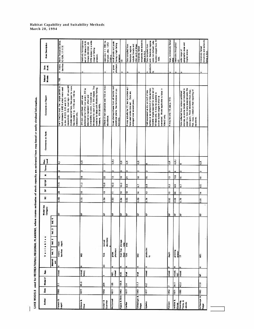
Habitat Capability and Suitability MethodsMarch 28, 1994
LIMNOTEK

Habitat Capability and Suitability MethodsMarch 28, 1994
LIMNOTEK

Habitat Capability and Suitability MethodsMarch 28, 1994
LIMNOTEK

Habitat Capability and Suitability MethodsMarch 28, 1994
LIMNOTEK

Habitat Capability and Suitability MethodsMarch 28, 1994
LIMNOTEK

Habitat Capability and Suitability MethodsMarch 28, 1994
LIMNOTEK

Habitat Capability and Suitability MethodsMarch 28, 1994
LIMNOTEK
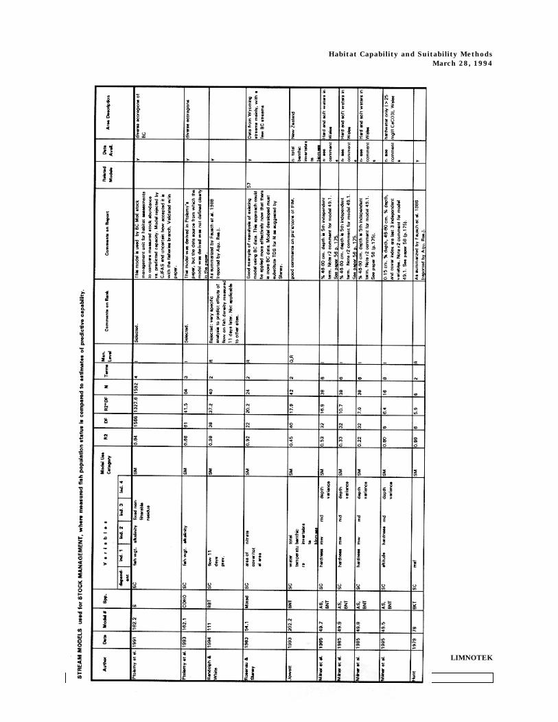
Habitat Capability and Suitability MethodsMarch 28, 1994
LIMNOTEK

Habitat Capability and Suitability MethodsMarch 28, 1994
LIMNOTEK

Habitat Capability and Suitability MethodsMarch 28, 1994
LIMNOTEK

Habitat Capability and Suitability MethodsMarch 28, 1994
LIMNOTEK

Habitat Capability and Suitability MethodsMarch 28, 1994
LIMNOTEK

Habitat Capability and Suitability MethodsMarch 28, 1994
LIMNOTEK

Habitat Capability and Suitability MethodsMarch 28, 1994
LIMNOTEK

Habitat Capability and Suitability MethodsMarch 28, 1994
LIMNOTEK

Habitat Capability and Suitability MethodsMarch 28, 1994
LIMNOTEK

Habitat Capability and Suitability MethodsMarch 28, 1994
LIMNOTEK

Habitat Capability and Suitability MethodsMarch 28, 1994
LIMNOTEK

Habitat Capability and Suitability MethodsMarch 28, 1994
LIMNOTEK

Habitat Capability and Suitability MethodsMarch 28, 1994
LIMNOTEK

Habitat Capability and Suitability MethodsMarch 28, 1994
LIMNOTEK

Habitat Capability and Suitability MethodsMarch 28, 1994
LIMNOTEK
APPENDIXB ABSTRACTS OFPROCESS

Habitat Capability and Suitability MethodsMarch 28, 1994
LIMNOTEK

Habitat Capability and Suitability MethodsMarch 28, 1994
LIMNOTEK
1.1 FISHREGSEspegren et al. 1990
FISHREGS is a computer model designed to simulate the effects of various anglingregulations (size and slot limits) on fish populations. The model accounts for recruitment, fishgrowth rate, a number of mortality factors, and population size and age structure.Parameterization of the model can range from very simplistic to extremely complex dependingupon the amount of information known about the population under consideration. The modeluses a saturating function to predict egg numbers at high spawner densities. FISHREGS requiresage-specific, average fish length and size ranges. Within-cohort growth distributions aresimulated using a beta distribution and can assume various shapes. Natural and fishingmortality parameters are estimated by combining life table and creel survey data. Life table dataprovides estimates of within-cohort total annual mortality. Creel survey data provides estimates ofwithin-cohort mortality under the angling regulation currently in effect. The model is calibratedby revising the mortality rates to match available creel survey and life table data collected in thefield. The model has been applied to rainbow trout and Brown trout in Colorado streams.
1.2 Small Lakes Integrated Management Model (SLIM)Korman et al. 1993b
The motivation for creating SLIM is to provide a tool for regional management biologists toassess alternative management actions such as harvesting and stocking policies at both site(single-lake) and regional (multi-lake) scales. SLIM contains 3 basic elements:
1) a dynamic age-structured salmonid population model which simulates the response of wild and hatchery
populations to management actions influencing density and age-specific mortality;
2) a linkage to a database of physical, limnological and biological information for over 3,000 lakes in BC(
Lakes Database) which is used to provide input information required by the population model for lake-
specific simulations; and
3) a Graphical User Interface (GUI) which allows SLIM user's to implement different management actions,
alter assumptions and / or structural relationships within the population model, access the database, and
view the results of model simulations.
Version 2.0 of SLIM has recently been completed and incorporates refinements suggestedby user's following the first release of the model. Version 2.0 is currently being used andevaluated by a 'test' group of regional managers (Parkinson, pers. comm.).

Habitat Capability and Suitability MethodsMarch 28, 1994
LIMNOTEK
1.3 Large Lakes Kokanee Model (LLKM)Korman et al. 1993aKorman and Parkinson 1993
LLKM is a dynamic age-structured fisheries model designed to examine a variety ofmanagement actions and problems common to kokanee fisheries in the Pacific Northwest. Themodel can be used to examine the effects of harvest regulations, predator introductions, spawningchannels, sockeye enhancement, and lake fertilization on kokanee populations. The five majorcomponents of the kokanee model simulate:
• kokanee population dynamics;
• competition between kokanee and whitefish or sockeye;
• predator population dynamics;
• predation on kokanee and competitors; and
• fishing mortality on kokanee and predators.
LLKM tracks the growth and survival of stream-, shore-, and channel-spawningpopulations and hatchery fish on and independent basis. Changes in growth and survival arecalculated on an annual timestep. Intra- and interspecific competition are modelled based on asemi-empirical bioenergetic approach which is based on food conversion efficiencies of each sizeclass. The growth response to changes in kokanee production and lake productivity is determinedbased on an empirical function similar to the one derived by Rieman and Meyers (1992).
LLKM uses three alternative methods for simulating predator dynamics. Predator size isnot dynamic, but densities are either: 1) controlled by a Ricker-type response in juvenile survivalto adult biomass (cannibalism); 2) controlled by a Beverton-Holt-type response in yearlingproduction to egg deposition (rearing-habitat limitation); or are 3) held constant for the durationof a simulation.
The consumption of kokanee is dependent on the biomass gain between predator sizeclasses and their food conversion efficiencies. Faster growing and/or longer-lived predators will,over their lifetime, eat more kokanee than slower growing and/or shorter-lived ones. Thepredators maximum kokanee diet is reduced based on a logistic function of total kokanee density;the greater the density, the closer the predator will come to achieving its maximum requirement.
The raw output of the model is a time series plot of various indicators such as populationdensities, length at age, CPUE, etc. The model has been applied to (Korman and Parkinson,1993): 1) assess the impacts of a spawning channel on natural populations of kokanee inKootenay Lake; 2) the impact of alternative Gerrard trout yearling production on kokanee inKootenay Lake; 3) assess the effects of kokanee density and fishing effort on fishing quality inOkanagan Lake; and to 4) to quantify verbal models of the processes that are felt to be importantvis-a-vis increasing kokanee production in Williston Lake.
1.4 MANSIM: A fairly generic computer model for simulation management actions onsingle fish populations (Version 3.0)Korver 1992b

Habitat Capability and Suitability MethodsMarch 28, 1994
LIMNOTEK
MANSIM is a generalized computer simulation model for assessing the potential effects ofa number of management actions on fish populations. The model has been used as a basis forconstructing a harvest management model for walleye in eastern Lake Ontario. Features of themodel include: assessment of effects of changes in nominal fishing effort, fishing seasons, bagand size-limits, fishable and protected slots; a monthly time step for calculating effects of growth,fishing and natural mortality; annual data summaries; separate density-dependent growth termsfor age-1 recruits and the rest of the population; and a generalized stock-recruitment functionwith a random error-term; and separate evaluation of "trophy"-sized fish.
1.5 Lake Trout Management Support System (LTMSS)Korver 1992a
LTMSS is a customized, "home-grown" software package designed to assist fisheriesbiologists and managers in making decisions regrading the management and assessment of laketrout lakes in Ontario. It contains several important features specifically included to make ituseful to Ontario Ministry of Natural Resources field staff throughout the province:
1) It is general. LTMSS is designed to work for all lake trout lakes in Ontario between 50 and 25,000 ha in
surface area.
2) It is Flexible. You can run LTMSS even if all you know about the lake is its surface area and a "ball-park"
estimate of summer and winter effort. Whenever you have more information such as growth data, maturity,
stocking rates, etc., it can accommodate this information. Obviously the more information you have, the
more accurate the output of LTMSS is likely to be.
3) It is Comprehensive. The primary purpose of LTMSS is to allow its users to ask "what if" style
management questions. A wide range of management options can be examined, including effort controls,
size-based regulations, and stocking.
LTMSS is a product of the Lake Trout Synthesis. The model consists of a generalized laketrout population (simulation) model which separately accounts for both stocked and naturallyproduced populations, embedded within a menu-based framework that allows user control ofboth inputs to and outputs from the model.
1.6 Stochastic Life-Cycle Model (SLCM)Lee and Hyman 1992
SLCM is a stochastic process model which simulates the life cycle of anadromoussalmonids and is designed to mimic the basic mechanisms regulating populations of Pacificsalmon, while capturing some of the intra-annual and interannual variation inherent in thesepopulations. The model was designed for population viability assessments combining advancedmodelling techniques with concepts from the field of conservation biology.

Habitat Capability and Suitability MethodsMarch 28, 1994
LIMNOTEK
While the basic structure of SLCM is similar to other life-cycle models, it differs in severalways. First, SLCM incorporates stochastic or probabilistic processes at each step in the life cycle.The binomial distribution is used extensively to introduce demographic stochasticity in survival;the beta distribution is used to introduce environmental stochasticity. Because of its stochasticnature, the model's predictions must be expressed in probabilistic terms. Multiple games are runusing a Monte Carlo approach to generate probability distributions for future outcomes. Second,the model is designed to use inputs from more detailed models for specific life stages, incombination with a minimum number of empirically based parameters. SLCM users can chooseamong alternative models for the more contentious life stages, such as juvenile migration andadult harvest, incorporating the results of their preferred models. An ancillary calibration modelhas been developed that allows the SLCM to be fitted to a historical time trace of populationestimates, constraining expectations of survival and their variances to historical levels.
The model also allows considerable flexibility in describing the dynamics of juvenileproduction. Users can choose among three density-dependent relationships to describe egg-to-smolt survival, including the Beverton-Holt, the Ricker, and a logistic response function, or useempirically based conditional probabilities. A variety of scenarios involving hatchery and naturalproduction are possible, ranging from natural production only, to a combination of hatchery andnatural production involving supplementation of adults, fry, or smolts. Allocation of naturallyproduced and hatchery-produced adults among terminal harvest and hatchery and naturalspawning follows a set of adjustable rules that affords priority to natural escapement andhatchery broodstock needs.
1.7 Skeena River Steelhead Trout Capacity ModelTautz et al. 1992
Estimation of steelhead carrying capacity for the Skeena River involved the construction ofa number of submodels organized into three general areas: distribution, fish use, and fishproductivity. Stream order, measured from 1:50,000 scale maps in conjunction with a climaticindex based on annual water yield and juvenile surveys were used to provide estimates of thelengths of systems containing steelhead. Total stream area at low summer flow for each of thesereaches was estimated based on a relationship between stream width at mean annual discharge.In the next step, total area was adjusted downward to estimate useable area based on habitatsuitability where useable area is predicted as a function of mean annual discharge and low flowstage (derived from a large B.C. data set).
Having obtained estimates of useable area, carrying capacity was estimated by calculatingthe number of smolts expected per unit of habitat. Two approaches based on smolt productionvalues derived from the Keogh River were used:
1) a linear model which extrapolates the number of Keogh adults (or smolts) produced per kilometer of stream
length to the Skeena systems; or
2) a similar model which extrapolates the number of adults or smolts produced per m2 of total habitat and
usable habitat to obtain estimates for the Skeena;
Two methods were used to adjust estimates from 1) or 2) to account for productivity differencesbetween the Keogh and Skeena Rivers. A regression model of steelhead standing crop vs. totalalkalinity was used to develop a calibration factor which accounted for different nutrient levels

Habitat Capability and Suitability MethodsMarch 28, 1994
LIMNOTEK
between the two systems. An alternate method based on a regression between required territorysize and fish length was used to estimate the space required per fish. This regression, inconjunction with life history information was used to derive an adjustment factor for smoltproduction estimates/ unit area or length.
1.8 Modelling the response of native steelhead to hatchery supplementation programs inan Idaho riverByrne et al. 1992
A life history model was used to predict the response of native steelhead Oncorhynchusmykiss in the Lochsa River, Idaho, (Idaho), to long-term supplementation with hatchery fry andsmolts. The four key factors affecting the response of the native fish to a stocking program were(1) the number of native spawners, (2) the number of stocked fish, (3) the number and fitness ofprogeny from stocked fish, and (4) the amount of mating between hatchery and native fish.Long-term stocking of fry or smolts led to the extinction of native fish in some scenarios. Themodel can be used to help assess the risks and benefits of proposed stocking programs.
1.9 Dynamics of a northern squawfish population and the potential to reduce predationon juvenile salmonids in a Columbia River reservoir (Oregon, USA)Rieman and Beamesderfer 1990
Northern squawfish Ptychocheilus oregonensis prey on salmonid smolts (Oncorhynchusspp.) in Columbia River reservoirs. We used simulation models to determine the potentialinfluence of exploitation of northern squawfish on that predation. We also used correlationanalysis to examine factors that may influence predation through predator recruitment. We basedour simulations on estimates of mortality, relative year-class strength, and growth made from a4-year study of resident fish predators in John Day Reservoir. Simulated predation declined withexploitation of fish longer than 275 mm (fork length) such that sustained exploitation of 10-20%annually reduced predation by 50% or more. The magnitude of change was related to the type ofreproductive compensation. Recruitment was not obviously related to any environmental variablewe examined, although year-class strength was negatively correlated with concurrent year-classstrength of walleye Stizostedion vitreum. We believe that limited, but sustained, exploitation ofnorthern squawfish provides an alternative to more radical control measures. We are uncertainabout the potential recovery rate of exploited northern squawfish populations, however, and thereis some risk that unsustained exploitation could aggravate predation. Any control program shouldevaluate density-dependent responses of predators.
1.10 Stocking strategies for fingerling walleyes: An individual-based model approachMadenjian et al. 1991
The success of any program for stocking walleye (Stizostedion vitreum vitreum) fingerlingsis strongly dependent on growth of the stocked fish during the summer and early fall monthsimmediately following their release into lakes, reservoirs, or rivers. An individual-based model(IBM) was developed to describe growth of the young-of-the-year (YOY) walleyes in Lake Mendota(Wisconsin, USA). The IBM was used to evaluate stocking strategies for walleye fingerlings.According to the rules of this simulation model, predation by a walleye would occur only if thewalleye was sufficiently large relative to the prey individual. The length-frequency distribution of

Habitat Capability and Suitability MethodsMarch 28, 1994
LIMNOTEK
the YOY walleye population at the end of the 1989 growing season was predicted accurately bythe model. During 1989, walleye fingerlings with a mean total length of 50 mm were stocked intoLake Mendota on 28 June. Simulations were performed to investigate the effects of the size ofstocked fingerlings and the timing of stocking on subsequent YOY walleye growth. Thesestimulations revealed that if walleye fingerlings were stocked on 28 June, at an average totallength of 60 mm rather than 50 mm, then the proportion of large (total length of XX 175 mm) fishin the YOY walleye population at the end of the growing season would have increased threefoldover the observed proportion. Economic cost per large walleye was minimized when average totallength at stocking was 62 mm. Stocking 50-mm walleye fingerlings on 14 June instead of 28 Juneresulted in a tripling of the percentage of large walleyes at the end of the growing season.

Habitat Capability and Suitability MethodsMarch 28, 1994
LIMNOTEK
1.11 Simulation of perch (Perca fluviatilis L.) population dynamics in Lake ConstanceButtiker and Staub 1992
The fishing of perch (Perca fluviatilis L.) is of major importance in the larger Swiss lakes.Perch populations in these lakes are characterized by high natural mortality and growth rates. Toget a better understanding on how a perch population and its fishing yield are dependent uponmanagement and fishing rules, a computer program for the simulation of perch populations wasdeveloped and tested. First results concerning the management of perch in Lake Constance(Switzerland) are presented. They show that the minimum legal mesh size of 32 mm for gillnets isa good policy and should not be increased.
1.12 Forecasting effects of harvest regulations and stocking of walleyes on prey fishcommunities in Lake Mendota, WisconsinJohnson et al. 1992
Two commonly used simulation models were combined to assess the effects of stockingand harvest regulations on the consumption dynamics of walleyes Stizostedion vitreum in LakeMendota, Wisconsin (USA). An age-structured population model was used to estimate the effectsof five harvest scenarios on walleye population and fishery characteristics. Implementation of a15-in minimum size limit resulted in increases in total yield (by weight), average weight of fishharvested, and walleye biomass remaining in the lake. Changes in walleye age structure resultingfrom various harvest scenarios were used as inputs to an energetics model to estimate how preyconsumption by walleyes would vary under different harvest regulations. Simulations indicatedthat a stocking program that produced 8,000 yearling recruits annually would double walleyepredation on planktivorous fish compared with predation estimated in 1987, when the studybegan. The modelling further indicated that a 15-in minimum size limit in conjunction with astocking program would triple predation rates. This increase would be sufficient to reducerecruitment of yellow perch Perca flavescens in Lake Mendota in most years. Combining these twomodelling techniques provides a framework for fishery managers to forecast how prey populationsmight respond to harvest regulations for gamefish.
2.1 Kootenay Lake Fertilization Response Model (KLFRM)Walters et al. 1991
The general aim of KLFRM is to simulate long term (30+ years) changes in plankton,kokanee, and Gerrard trout populations in response to changes in lake fertility associated withphosphorus loading. The model also tries to simulate effects of strategic fisheries managementoptions such as varying exploitation rates and enhancement of spawning success throughtechnologies such as spawning channels. The model is provided with historical inputs (nutrientloadings, water flow patterns, changes in kokanee spawning habitat) for the baseline simulationperiod 1960-89 so that its predictions can be compared with various data time series available forthat period; it can extend the predictions out to the year 2010 using assumed input patternsprovided by the model user.
The simulation program has five basic submodels for key components of the KootenayLake production system:

Habitat Capability and Suitability MethodsMarch 28, 1994
LIMNOTEK
1) nutrient budgets (inflows, mixing processes, losses);2) phytoplankton/grazing zooplankton production;3) Mysis energetics and population dynamics;4) kokanee energetics and population dynamics; and5) Gerrard trout energetics and population dynamics.
The key use of the model has been to trace the impacts of experimental fertilization of KootenayLake through the pelagic food web. KLFRM had been used to identify gaps in our understandingof Kootenay Lake dynamics and to recommend research priorities. Model predictions suggest thatfertilization will increase Mysis production and increase the competitive effects on kokaneeproduction. However, given the considerable uncertainties identified by the authors around thisprediction, an experimental fertilization program coupled with intensive monitoring wasrecommended, and is currently in its third year.
2.2 Carnation Creek Chum and Coho Salmon ModelsHoltby and Scrivener 1989
The population dynamics of coho and chum salmon have been studied at Carnation Creeksince 1970 as part of a multi-disciplinary study of the effects of logging on a small salmon streamin a coastal rainforest. The Carnation Creek salmon models predict the numbers of chum andcoho salmon from correlative (empirical) relationships between survival and growth at various lifestages and (1) climatic, hydrologic and physical variables, (2) indices of those features of streamhabitat that were affected by logging, and (3) exploitation rates in the fishery. The models wereused to partition the variability in adult returns between the effects of climatic variability in thestream and ocean, changes in stream conditions caused by logging and variations in fishingmortality.
2.3 Effects of sediment transport on survival of salmonid embryos in a natural stream: Asimulation approachLisle and Lewis 1992
A model is presented that simulates the effects of streamflow and sediment transport onsurvival of salmonid embryos incubating in spawning gravels in a natural channel. Componentsof the model include a 6-yr streamflow record, an empirical bedload-transport function, a relationbetween transport and infiltration of sandy bedload into a gravel bed, effects of fine-sedimentinfiltration on gravel properties, and functions relating embryo survival to gravel properties.High-flow events drive temporal variations in survival; cross-channel variations in bedloadtransport cause spatial variations. Expected survival as a result, varies widely from year to yearand between spawning runs in a single year. Alternative functions from previous research thatrelate survival to fine-sediment concentration in spawning gravel and to intergravel rates of flowyield categorically different results. The relative uncertainty of the components of this modelindicates that the greatest research needs are to understand how sediment transport affects theintergravel environment and how these changes affect embryo development and survival.
2.4 COWFISHContor and Platts, 1991

Habitat Capability and Suitability MethodsMarch 28, 1994
LIMNOTEK
COWFISH estimates monetary loss and fish loss due to livestock impacts based on sevenhabitat attributes by comparing estimates of optimum and existing numbers of catchable trout (>6 inches) in a stream reach, regardless of species. Optimum number of catchable trout is definedas the number that would have been present if the stream had never been grazed by domesticlivestock. Existing numbers of catchable trout are the numbers present under the currentmanagement situation. COWFISH then estimates the difference between the estimated optimumand estimated existing number of catchable trout. This difference is the estimated fish loss due tolivestock use. To calculate total economic loss, COWFISH assigns $10.65 for each fish lost.Recreational loss is also estimated.
The seven input variables for the models empirical relationships are estimated ocularly. Theinputs are:
1. % of undercut bank;
2. % of overhanging vegetation;
3. % of trampled vegetation or exposed soil on the bank;
4. % of riffle area covered by fine sediments;
5. stream width-depth ratio;
6. stream gradient; and
7. parent rock type
COWFISH is:
1. applicable throughout the Western U.S. (with adjustments);
2. useful any time there is not snow cover, but it is best if used immediately after the grazing
season;
3. useful to evaluate large homogeneous stream sections (data collected from 5 different
sites per stream mile are needed to provide a 10% sample of the study area);
4. suitable for streams less than 18 feet wide with low channel gradients, erodible banks, and
grass-forb-sedge riparian areas; and
5. successfully used by untrained personnel using ocular estimations.
COWFISH limitations are that the:
1. accuracy of results diminishes when estimation of grazing impacts of fish production does
not immediately follow the grazing season;
2. the model is less accurate for those streams with rocky streambanks, widths greater than
18 feet, channel gradients over 5%, and with forested riparian zones; and
3. the model outputs reflect population numbers for the immediate area sampled and not for
the complete stream.
COWFISH appears to work satisfactorily in Montana for rainbow and cutthroat trout butperformed poorly in validation systems within Idaho, Utah, and Nevada.

Habitat Capability and Suitability MethodsMarch 28, 1994
LIMNOTEK
2.5 Atlantic Salmon Regional Acidification Model (ASRAM)Korman et al. 1994
ASRAM is an age-structured salmonid life history model designed to examine alternativemanagement (stocking, harvesting, liming) scenarios in Atlantic salmon rivers of the Maritimes.The model combines pH-dependent toxicity relationships, habitat-preference models, density-dependent processes, and natural and fishing mortality rates to predict annual smolt productionand adult returns at site and river system levels. The spatial structure of the model is based on adatabase separating rivers into reaches where length, width and surface grade are approximatedfrom orthophotographic maps and aerial photographs (available for 120 rivers in Nova Scotia). Anempirical relationship between parr density and stream surface grade is used to distribute theinitial number of fish for a simulation among reaches in the modelled river system. Annual pHtime series collected from monitoring stations distributed throughout a river system are assignedto a set of spatially-linked reaches to predict tributary-specific pH-driven mortality rates.Relationships predicting parr size from density, and early marine survival from smolt size are thekey density dependent functions which limit stream carrying capacity.
2.6 Relation between mortality of young walleye (Stizostedion vitreum) and recruitmentwith different forms of compensation.Jensen 1992
The relation between mortality of young fish and recruitment is important for assessmentof the environmental effects of facilities that kill large numbers of young fish, such as electricpower stations and hydropower plants. A simulation model with a bioenergetic growth componentwas applied to examine the relation between mortality of young and recruitment of walleye(Stizostedion vitreum) with different forms of population regulation, including: food limitedgrowth, food limited growth with size-dependent mortality, and food limited growth with age atmaturity dependent on size. With food limited growth small increases in mortality of youngreduced recruitment considerably, but the population slowly approached a new equilibrium. Ifmortality of young increased when growth was food limited, the population approached a newequilibrium of natality and mortality because with fewer individuals there was more food perindividual, and individuals were larger in size and produced more eggs; this feedback adjustednatality to equal mortality. With either mortality or age at maturity dependent on size, largeincreases in mortality of young resulted in only small decreases in recruitment.
2.7 Potential impacts of global climate change on Pacific Northwest spring chinooksalmon (Oncorhynchus tshawytscha): An exploratory case studyChatters et al. 1991
Increases in atmospheric concentrations of greenhouse gases are predicted to raise globaltemperatures by up to 3 degree C over the next one-hundred years, which may have significanteffects on natural resources. Even a smaller (2 degree C) temperature change may impact oneprominent Pacific Northwest natural resource, the spring chinook salmon, Oncorhynchustshawytscha. A computer model was developed by the Northwest Power Planning Council (NPPC)for use in developing the NPPC salmon enhancement plan for their Fish and Wildlife Program.Using this model, we investigate the impact of global warming on the production of springchinook salmon in the Yakima subbasin of the Columbia River System. The model stimulatescurrent prevailing environmental conditions and the implementation of improvements in salmon

Habitat Capability and Suitability MethodsMarch 28, 1994
LIMNOTEK
habitat planned by the NPPC. The data are then changed to reflect conditions that we infer tohave existed between 6,000 and 8,000 years ago, when temperatures were approximately 2 degreeC warmer than today. When the NPPC computer model is run under these altered conditions, itshows that projected climate change might reduce by half the Yakima River spring chinooksalmon production predicted under both current and NPPC-improved conditions. These resultsstrongly support the need for planned improvements in the fishery, since a 50% decline inexisting fish populations could decrease spring chinook salmon abundance and possibly othersalmonid populations beneath levels needed for the survival of the species. More broadly, theresults suggest that if future global warming takes a form similar to that of 6,000 years ago, itcould have major effects on the salmon population of the Pacific Northwest. Although some racesof salmon might have their survival enhanced, others might be harmed. We recognize that allspecies and races would not be affected in the same way as Yakima River spring chinook, yetglobal warming is still a matter of concern because many of the Pacific Northwest salmon stocksare already under stress from other causes. A more comprehensive and thorough analysis isurgently needed.
2.8 A stochastic, compartmental model of the migration of juvenile anadromoussalmonids in the Columbia River BasinLee 1991
A probabilistic model is developed which describes the juvenile migration of Pacific salmonand steelhead trout (Oncorhynchus spp.) in the Columbia River Basin in western North America.The downstream passage of smolts through a series of reservoirs or river reaches is modeled as anirreversible particle diffusion process through a series of compartments. The probability of livepassage from one compartment to the next t time units after having entered the compartment canbe viewed as the product of the probability of having survived to time t, the probability oftransiting the compartment in t time units, and the probability of a successful transition betweencompartments at time t. From this basic premise, a general passage model is developed. Focusingon survival through Columbia and Snake River reservoirs (as opposed to dam-related mortality), aspecific model which uses a Poisson death process and a gamma distribution to describe transmittimes is presented. Analytical solutions to the single-compartment system are derived withextensions to the multi-compartment system. Empirical data from the Columbia River is used todemonstrate the utility of the model as well as to highlight problems that exist in fitting the modelusing existing data. Graphical techniques are presented for using the model to assess theeffectiveness of management actions that are designed to improve the reservoir survival of smolts.
2.9 Integrating the Instream Flow Incremental Methodology with a populationresponse model.
Cheslak and Jacobson 1990
The Instream Flow Incremental Methodology (IFIM) assumes that flow-dependent physicalhabitat and water temperature determine the carrying capacity of streams for fish. We haveconstructed a mechanistic simulation model that integrates the results of an IFIM PhysicalHabitat Simulation model (PHABSIM), a network hydrological model (NETWORK), an IFIM streamtemperature model (SNTEMP), and field fishery studies to evaluate the potential effects oftemporal changes in carrying capacities on a fishery resource. As an example of the methodology,the model was applied to an IFIM analysis of rainbow trout (Oncorhynchus mykiss) for a proposedhydroelectric project. Analysis of model performance indicates that it was well behaved, with

Habitat Capability and Suitability MethodsMarch 28, 1994
LIMNOTEK
reasonable, valid dynamics for each life stage and reach in the model structure. The model wasused to compare population dynamics under natural and post-project conditions, and it indicatedthat a substantial enhancement in the fishery resource could be expected from instream flowsproposed for the project. Inspection of reach-specific behavior was used to determine the basis ofthe predicted enhancement. These predictions are verifiable through a well-designed monitoringprogram, and a sensitivity analysis indicates that they are valid over a wide range of possibleparameter values.
3.1 Functional response and capture timing in an individual-based model: Predation bynorthern squawfish (Ptychocheilus oregonensis) on juvenile salmonids in theColumbia River.Petersen and Deangelis 1992
The behavior of individual northern squawfish (Ptychocheilus oregonensis) preying onjuvenile salmonids was modeled to address questions about capture rate and the timing of preycaptures (random versus contagious). Prey density, predator weight, prey weight, temperature,and diel feeding pattern were first incorporated into predation equations analogous to HollingType 2 and Type 3 functional response models. Type 2 and Type 3 equations fit field data from theColumbia River (USA) equally well, and both models predicted predation rates on five of sevenindependent dates. Selecting a functional response type may be complicated by variable predationrates, analytical methods, and assumptions of the model equations. Using the Type 2 functionalresponse, random versus contagious timing of prey capture was tested using two related models.In the simpler model, salmon captures were assumed to be controlled by a Poisson renewalprocess; in the second model, several salmon captures were assumed to occur during brief"feeding bouts", modeled with a compound Poisson process. Salmon captures by individualnorthern squawfish were clustered through time, rather than random, based on comparison ofmodel simulations and field data. The contagious-feeding result suggests that salmonids may beencountered as patches or schools in the river.
3.2 Interactions between stochastic and deterministic processes in stream fishcommunity assemblyStrange et al. 1993
Numerous studies have attempted to determine whether stream fish communities arestructured primarily by deterministic or stochastic processes. Previous work has assumed thatstream fish communities will show either persistence about an equilibrium because of strongdensity-dependent processes or random variation in structure as a result of environmentalstochasticity. In a 10-year study of a California (USA) stream, fish community structure changedunder the influence of storm-induced high discharge events that impacted recruitment. Species'relative abundances were altered as pre-recruitment stream discharges differentially influencedyear-class strength among species with contrasting life histories. Simulation of stream fishcommunity assembly under flow-driven recruitment variation indicates that community structurewill vary depending on how particular high-flow events affect species' relative abundances andongoing density-dependent processes, including competition and predation. Results suggest thatstream fish communities are likely to show alternate states rather than a single persistentequilibrium. However, community assembly will not be random but will depend onsituation-specific interactions between density-independent and density-dependent processes.

Habitat Capability and Suitability MethodsMarch 28, 1994
LIMNOTEK
3.3 Predation and production by salmonine fishes in Lake Michigan, (USA) 1978-88Stewart and Ibarra 1991
A marked decline of alewife in Lake Michigan during 1981-83 led to diet shifts by coho(Oncorhynchus kisutch) and chinook salmon (O. tshawytscha) from feeding primarily on largealewife to eating proportionately more immature alewives and other prey. Diets of lake trout(Salvelinus namaycush) did not change greatly during that period. Population biomass conversionefficiency averaged 24.5% for coho and 16.6% for lake trout. Chinook salmon suffered anapparent 20% decline in gross conversion efficiency of biomass (25.1 to 20.8%) and a 25% declinein average weight of sport-caught fish. We infer that chinook salmon growth was inhibited byinsufficient forage available to them. A simulation of chinook salmon feeding on bloater(Coregonus hoyi) at 8 degree C suggested that such behavior could lead to further declines ingrowth rates. Extension of modelling results to include approximations for brown trout (Salmotrutta) and rainbow trout (O. mykiss) revealed peaks in total annual salmonine predation of71,000 t in 1983 and 76,000 t in 1987. The alewife was 70% of all prey eaten by salmonines in1987-88. Lakewide gross production by salmonines was 15,300 t (or 0.27 g/ m2) in 1987. Ratiosof annual gross production to average monthly population biomass were 1.6 for chinook, 1.15 forcoho, and only 0.6 for lake trout.

Habitat Capability and Suitability MethodsMarch 28, 1994
LIMNOTEK
3.4 Individual-based model for growth of young-of-the-year walleye: A piece of therecruitment puzzleMadenjian and Carpenter 1991
Young-of-the-year (YOY) walleye (Stizostedion vitreum vitreum) growth is a vital step inwalleye recruitment. An individual-based model (IBM) was developed to describe the growth ofYOY walleye in Oneida Lake (New York, USA) and Lake Mendota (Wisconsin, USA). In OneidaLake the only prey species included in the model was yellow perch (Perca flavescens), whereasboth yellow perch and bluegill (Lepomis macrochirus) were prey species in the model for LakeMendota. IBM predictions for length frequencies of the YOY walleye population at the end of thegrowing season showed good agreement with observed length frequencies. A theoreticalrelationship was derived between the encounter rate, lambda, used in the IBM and thehalf-saturation constant, kappa, used in a type II functional response model. Estimates of kappafrom the two models showed good agreement, thus corroborating the value of lambda chosen forthe IBM application to Oneida Lake. The mean length of the YOY walleye cohort and thepercentage of larger (175 mm in total length) walleyes in the cohort at the end of the growingseason were most sensitive to gross growth efficiency, bioenergetics parameters for maximumdaily consumption by walleyes, and the ratio of prey length to predator length at which the prey issusceptible to predation. In Lake Mendota the vulnerability of bluegills to predation by YOYwalleyes was especially important in determining the growth of walleyes during their first growingseason. The IBM approach was valuable for modelling those stages of life history in whichcharacteristics of the individual were critical in determining recruitment.
3.5 Evaluation of alternative models of the coastal migration of adult Fraser River(British Columbia, Canada) sockeye salmon (Oncorhynchus nerka)Pascual and Quinn 1991
A set of stochastic discrete step models of individual fish movement was developed toinvestigate the efficiency of compass orientation as a migratory mechanism in the coastalhomeward migration of Fraser River sockeye salmon (Oncorhynchus nerka). Ultrasonic trackingdata provided empirical values for the required parameters. Alternative movement models werevalidated by comparing the results of Monte Carlo simulations and known features of sockeyemigration: general aspect of individual trajectories, timing, success in reaching the goal, andspatial occurrence. The effect of different headings and directional precisions on the probability ofsuccess in reaching the goal were considered. The more complex models captured the essence ofobserved movement patterns, but the number of fish getting to the goal was lower than expected.Many "modeled" fish were lost in the complex web of channels and inlets characteristic of thisarea. We conclude that the preference of a compass direction is not a sufficient mechanism toexplain the observed migratory behavior of Fraser River sockeye salmon in coastal areas. Othermechanisms, such as negative kinetic responses to water from nonnatal rivers or short-termlearning, may prevent the fish from being trapped in complex areas.
3.6 Biomass size spectrum of the Lake Michigan (USA) pelagic food webSprules et al. 1991
Biomass size spectra for the complete Lake Michigan pelagic food web from picoplanktonto salmonids were constructed for nine sampling transects around the lake in May and inSeptember 1987. Size spectra were typical for freshwater, having distinct peaks corresponding to
Habitat Capability and Suitability MethodsMarch 28, 1994
LIMNOTEK
major size groups. Biomass concentration of algae, zooplankton, and planktivores conformed toparticle-size model predictions, but piscivore biomass was lower than predicted because thesespecies are stocked. Mean annual total pelagic biomass was 72.3 g m-2 compared with apredicted range of 78.8-85.3 g m-2. Potential production of piscivores, Mysis, and Pontoporeiawas in agreement with model predictions. No estimates of zooplankton or planktivore productionwere available, but we calculated that these could be 72.1-91.6 and 2.5-4.1 g m-2 yr-1,respectively. Our analyses suggest that piscivore production is constrained by food web structure.Bloater, which comprise 72% of planktivore biomass, make up less than 20% of salmon diets. Weestimate that piscivore production could be double the current value of 0.27 g m-2 yr-1 if theforage fish community changed to include species more available to salmon.