3D finite-difference dynamic-rupture modeling along nonplanar faults

3

V

pTmsmsigotmpec

C

©

GEOPHYSICS, VOL. 72, NO. 5 �SEPTEMBER-OCTOBER 2007�; P. SM123–SM137, 13 FIGS., 4 TABLES.10.1190/1.2766756

D finite-difference dynamic-rupture modeling along nonplanar faults

íctor M. Cruz-Atienza1, Jean Virieux2, and Hideo Aochi3

fpooiosmn7tafsg

ABSTRACT

Proper understanding of seismic emissions associated with thegrowth of complexly shaped microearthquake networks andlarger-scale nonplanar fault ruptures, both in arbitrarily hetero-geneous media, requires accurate modeling of the underlying dy-namic processes. We present a new 3D dynamic-rupture, finite-difference model called the finite-difference, fault-element�FDFE� method; it simulates the dynamic rupture of nonplanarfaults subjected to regional loads in complex media. FDFE isbased on a 3D methodology for applying dynamic-ruptureboundary conditions along the fault surface. The fault is dis-cretized by a set of parallelepiped fault elements in which specif-ic boundary conditions are applied. These conditions are appliedto the stress tensor, once transformed into a local fault reference

2qdp

g2eoprast2bh

t receiveesently

[email protected]

SM123

rame. Numerically determined weight functions multiplyingarticle velocities around each element allow accurate estimatesf fault kinematic parameters �i.e., slip and slip rate� independentf faulting mechanism. Assuming a Coulomb-like slip-weaken-ng friction law, a parametric study suggests that the FDFE meth-d converges toward a unique solution, provided that the cohe-ive zone behind the rupture front is well resolved �i.e., four orore elements inside this zone�. Solutions are free of relevant

umerical artifacts for grid sizes smaller than approximately0 m. Results yielded by the FDFE approach are in good quanti-ative agreement with those obtained by a semianalytical bound-ry integral method along planar and nonplanar parabola-shapedaults. The FDFE method thus provides quantitative, accurate re-ults for spontaneous-rupture simulations on intricate faulteometries.

INTRODUCTION

The permeability of oil reservoirs represents one of the mostrominent characterization parameters for hydrocarbon production.his parameter evolves with time during oil extraction as a result oficroearthquake activity and rock compaction induced by hydraulic

tress changes �Royer and Voillemont, 2005�. The variation of per-eability may induce fluid migration and extraction mitigation. A

eismicity-based methodology allowing global reservoir character-zation may help track fluid migration and adapt exploitation strate-ies �Shapiro et al., 2002; Shapiro et al., 2005�. The dynamic growthf complexly shaped fracture networks is thus a fundamental issuehat should be understood. In the last few years, efforts have been

ade to develop new 3D numerical methods when considering non-lanar rupture propagation. Important implications in the fracturenergy balance have been identified when the rupture front abruptlyhanges its direction of propagation �Adda-Bedia and Madariaga,

Manuscript received by the Editor November 29, 2006; revised manuscrip1Formerly GéosciencesAzur, UNSA-CNRS, Sophia-Antipolis, France; pr

alifornia. E-mail: [email protected]éosciencesAzur, UNSA-CNRS, Sophia-Antipolis, France. E-mail: virie3Bureau de Recherches Géologiques et Minières, Orléans, France. E-mail:2007 Society of Exploration Geophysicists.All rights reserved.

005; Madariaga and Ampuero, 2005; Vilotte et al., 2005�. Conse-uently, the absence of realistic fault geometries when modeling realata may result in misleading conclusions, especially when inter-reting seismic emissions.

Fault interaction and branching may be enhanced by specific re-ional loads �Aochi et al., 2002; Oglesby et al., 2003; Ando et al.,004; Aochi et al., 2005�. In these cases, rupture propagation is gov-rned mainly by the friction parameters, the rupture velocity, and therientation of fault branches, which entirely determine the two com-eting forces: the fault strength and the shear stresses ahead of theupture front �Kame et al., 2003; Cruz-Atienza et al., 2004; Aochi etl., 2005�. The dynamic fault-normal stress changes translated intotrength fluctuations are often negligible in realistic nonplanar rup-ure conditions if they occur far from the free surface �Aochi et al.,000a; Aochi and Fukuyama, 2002�.Almost all of these results haveeen obtained with boundary integral methods �BIE�, which areighly adapted and accurate approaches for solving geometrically

d June 5, 2007; published onlineAugust 23, 2007.San Diego State University, Department of Geological Sciences, San Diego,

[email protected].

cpttbwofs

�Vgpeepthees

m1V1�puAft2fie

rcltDfuisde

sataf

totbp

asfptqi

e�ddreibtssb

sdarcmt

u�eia

dt�oSddtOvsfitoFp

SM124 Cruz-Atienza et al.

omplex problems. However, most of them may become rapidly ex-ensive because the spatiotemporal convolution involved in the in-egral equations often requires a total calculation time proportionalo the square of the number of grid elements multiplied by the num-er of time steps. Moreover, they use analytical Green functions,hich directly depend on properties of the propagation medium; sonly homogeneous full spaces can be considered. In other words,eedback interactions between the source and its environment aretrongly constrained to simple, often unrealistic conditions.

On the other hand, standard and spectral finite-element methodse.g., Oglesby, 1999; Aagaard, 2000; Ampuero and Vilotte, 2002;ilotte et al., 2005; Ely et al., 2006�, which handle arbitrarily hetero-eneous media as finite-difference methods do, are generally com-utationally intensive. This limitation has prevented scientists fromxploring systematically different mechanical models in large-scalearthquake simulations to perform statistical analysis of results. Aromising, fast, and accurate 2D dynamic-rupture, finite-volumeechnique is proposed by Benjemaa et al. �2007�. This techniqueandles unstructured mesh refinement around nonplanar free surfac-s and faults embedded in arbitrarily heterogeneous materials. Nev-rtheless, until the 3D extension exists, it cannot be used to analyzeeismic data.

For many years, finite-difference methods have been used forodeling earthquake rupture dynamics on planar faults �Andrews,

976b; Madariaga, 1976; Mikumo and Miyatake, 1978; Day, 1982;irieux and Madariaga, 1982; Olsen et al., 1997; Madariaga et al.,998�. Nonuniform grid spacing has allowed Mikumo and Miyatake1993� to study rupture processes of real earthquakes on planar dip-ing faults. A similar technique is proposed by Zhang et al. �2006�sing the standard staggered grid �Madariaga, 1976; Virieux, 1986�.few years ago, Cruz-Atienza et al. �2002� introduced a finite-dif-

erence approach capable of modeling the dynamic rupture of arbi-rary nonplanar faults �for details, see Cruz-Atienza and Virieux,004�. Preliminary results in three dimensions with this model wererst obtained for the 1992 Landers �Mw = 7.3� earthquake, consid-ring its real geometry �Cruz-Atienza et al., 2004�.

However, recent validation efforts conducted for the dynamic-upture problem have revealed that several well-established numeri-al models have important accuracy problems �Harris and Archu-eta, 2004�, especially those finite-difference approaches describinghe source with a thick-fault numerical discretization �Dalguer anday, 2006�. Most of the methods mentioned above belong to this

amily of approaches. Particular attention should then be paid whensing them and, even more, when introducing new methodologiesnspired by the thick-fault strategy. Validation of these methodshould necessarily include comparisons with completely indepen-ent methods, such as semianalytical boundary integrals or spectral-lement approaches.

In this paper, we introduce, analyze, and validate, in three dimen-ions, the finite-difference methodology proposed by Cruz-Atienzand Virieux �2004� in two dimensions. Thus, our approach allowshe dynamic-rupture simulation of 3D nonplanar faults embedded inrbitrarily heterogeneous media and governed by slip-dependentriction laws.

We first state the elastodynamic equations for the dynamic-rup-ure problem and the way rupture boundary conditions are applied inur 3D finite-difference technique. After a convergence analysis inerms of the cohesive-zone resolution, we validate the methodologyy comparing results for spontaneous slip-weakening ruptures alonglanar and nonplanar �curvilinear� faults against those obtained with

n independent BIE approach �Aochi et al., 2000b�. This compari-on shows that our finite-difference rupture model, based on a thick-ault source description, is accurate enough to perform these com-lex simulations. Moreover, it confirms that finite-difference �FD�echniques still represent a viable and reliable way to model earth-uake dynamics along nonplanar complexly shaped fault networksn three dimensions.

NUMERICAL MODEL

The numerical approach introduced in this section is basically anxtension to three dimensions of the finite-difference fault-elementFDFE� model proposed by Cruz-Atienza and Virieux �2004� in twoimensions. In that work, Cruz-Atienza and Virieux show that finite-ifference approaches in a regular grid are able to model the dynamicupture of faults having nonplanar �curvilinear� geometries. A keylement of that approach is the way rupture-boundary conditions aremplemented. The two-dimensional analysis shows that the scalingetween grid size and number of grid nodes within a source controlshe accuracy of the method and makes it possible to discretize theame source in many equivalent ways by reducing the spatial gridtep and increasing the number of stress grid points involved inoundary conditions.

When modeling huge 3D rupture scenarios, computational re-ources prevent the use of extremely fine meshes; however, fractureiscretizations with moderate numbers of stress grid points are suit-ble for obtaining accurate enough results.As we shall see, other pa-ameters also play an important role, especially in the numericalonvergence of the method. Before introducing the dynamic-ruptureodel, let us first state the equations for this problem and the way

hey are approximated numerically.Consider a linearly elastic 3D homogeneous and isotropic medi-

m, fully described by the Lamé coefficients � and � and the density. Following Madariaga �1976�, in the absence of body forces, thelastodynamic equations governing the P- and S-wave propagationn such a medium may be expressed in terms of the velocity vector vi

nd the stress tensor �ij as

��vi

�t= �ij,j , �1a�

��ij

�t= �vk,k�ij + ��vi,j + v j,i� . �1b�

System 1 contains nine partial differential equations that may beiscretized in a partly staggered finite-difference grid where veloci-ies and stresses are known in two separated, regular latticesSaenger et al., 2000� as shown in Figure 1. The spatial differentialperators of system 1 are deduced by Cruz-Atienza �2006� followingaenger et al. �2000�. Numerical finite-difference stencils for firsterivatives along the three Cartesian directions are given in Appen-ix A. Note that the current leapfrog partly staggered approach re-ains the efficiency of the standard finite-difference staggered grid:ne must estimate stress derivatives at velocity grid points, and con-ersely, velocity derivatives at stress locations. Figure 1 shows thetencil of the second-order spatial operators applied to the velocityeld �black spheres� to compute a stress-point value �gray cube�. In

he present work, we apply both second- and fourth-order accurateperators in the space increment �Cruz-Atienza and Virieux, 2004�.or the sake of computational efficiency, time derivatives are alwayserformed with a second-order-accurate leapfrog integration.

pVfipsmarcs�mscndstpw

tVtppiaoo

hbtosAral

S

VcfAtat

osscmadptmr

fopte

Fusal��p�

a

Ft�FasTm

3D nonplanar dynamic-rupture model SM125

Two main advantages of the partly staggered finite-difference ap-roach with respect to the standard staggered grid �Madariaga, 1976;irieux, 1986� should be pointed out: �1� the stress and the velocityelds are defined in different nodes, each field having all of its com-onents at the same node, and �2� the stability condition is less re-trictive. As we shall see, the first advantage leads us to one funda-ental aspect of the proposed finite-difference approach because it

llows the stress-tensor transformation needed for the application ofupture boundary conditions of an arbitrary nonplanar-orientedrack. Concerning the second one, the von Neumann stability analy-is shows that the magic time step given by �t�h/Vmax, where h andt are, respectively, the spatial and time steps and Vmax is the maxi-um P-wave speed in the model, satisfies the stability condition if

econd-order spatial operators are applied �Saenger et al., 2000�. Inontrast with the standard staggered grid, the stability condition doesot depend on the problem dimension. Moreover, if using fourth-or-er spatial operators in their stability limit, the time step on the partlytaggered grid is 1.7 times higher than that of the standard grid. Thisranslates into 40% fewer iterations to achieve the same simulationroblem. Of course, these are theoretical values computed for planaraves propagating in homogeneous unbounded spaces.Imposing dynamic rupture-boundary conditions always makes

he stability criteria more restrictive. Values for the Courant numbermax�t/h up to 0.66 yield stable solutions when simulating the spon-

aneous rupture in the partly staggered grid with our numerical ap-roach. This limit is at least 1.5 times greater than those reported inrevious finite-difference rupture models �e.g., Virieux and Madar-aga, 1982; Madariaga et al., 1998�. Even if higher-order schemesre expected to verify more restrictive stability conditions than thosef low order, this Courant value is valid for the fourth-order spatialperators we use throughout this study.

z

x

y

d2

h

d1

d3

( ij, , ) µ λ ττ (vi, )ρ

d4

igure 1. Three-dimensional second-order, finite-difference stencilsed for computing spatial derivatives of the velocity field vi in atress tensor �ij location along the three Cartesian directions. Annalogous stencil is used for computing stress derivatives in velocityocations. Second-order finite differences involved in this stencilAppendix A� are calculated along the four Cartesian axis bisectorsdi�. The quantity h is the spatial grid step, whereas the mediumroperties are given by the Lamé coefficients � and � and the density.All velocity and stress components are known at one single node.

To simulate an unbounded space without loss of accuracy, weave implemented the perfectly matched layer �PML� absorbingoundary conditions in every external boundary of the 3D computa-ional domain �Berenger, 1994; Collino and Tsogka, 2001; Marcink-vich and Olsen, 2003�. Numerical tests in heterogeneous mediahow an effective energy absorption greater than 99% �Cruz-tienza, 2006�. Before analyzing the numerical properties of the

upture model, let us first introduce the way a source is discretizednd how rupture-boundary conditions are applied along an arbitrari-y shaped 3D surface.

ource discretization

Following the 2D strategy introduced by Cruz-Atienza andirieux �2004�, a given finite-rupture surface is represented numeri-ally by a set of neighboring fault elements placed alongside this sur-ace. �In the 2D model, the fault elements are called numerical cells.�

source fault element is a well-structured set of stress grid pointshat acts as an elementary source unity. This means that local bound-ry conditions are applied on each element, depending on the orien-ation of the local fault-normal vector.

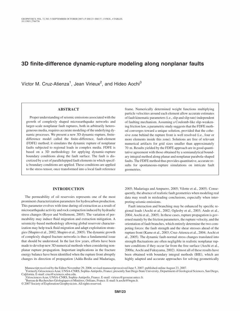
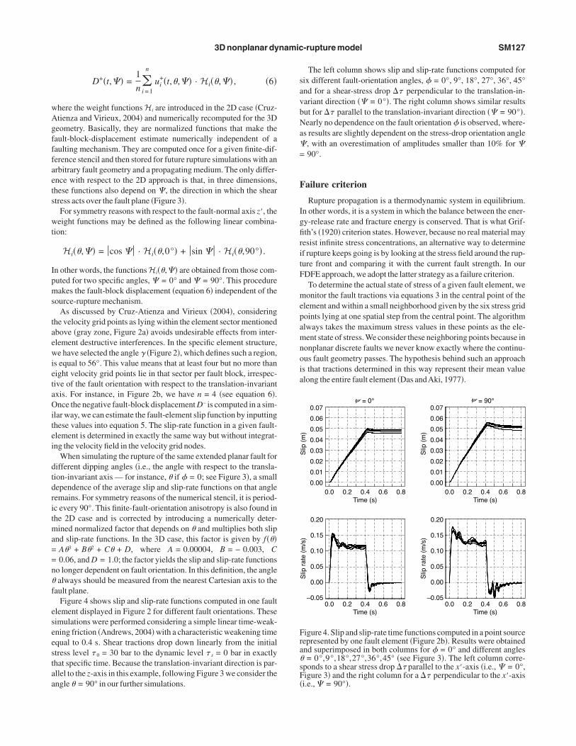
A fault element describes a 45° rotated parallelepiped such as thene shown in Figure 2 �gray cubes�. We found this specific elementtructure, with 65 stress grid points, achieved the best results for gridizes ranging from 20 to 70 m �Cruz-Atienza, 2006�. As we con-lude in the Resolution and Convergence section, high-order ele-ents �i.e., elements with a large number of stress grid points� in rel-

tively coarse meshes affect rupture solutions because of the longistances separating their central points. The number of stress gridoints along the diagonals parallel to the x- and y-axes is the same ashe stress grid layers perpendicular to the z-axis. In this case, the ele-

ent rotation is with respect to the z-axis. However, for symmetryeasons, it may be with respect to any of the three Cartesian axes.

Note also that this element configuration results in only two of itsaces �i.e., the upper and bottom faces in Figure 2b� being parallel tone of the Cartesian planes. Consequently, the way to discretize non-lanar fault surfaces is by forcing the source geometry to have aranslation-invariant direction parallel to the rotation axis of the faultlements. In our example, such a translation-invariant direction is

z

z

x

x

y

y

ui

ui

Faultsurface

Stress nodes Velocity nodes

γ θ

) b)

igure 2. �a� Upper view of one fault element. In this example, theranslation-invariant axis is parallel to the z Cartesian axis. The anglegives the fault-plane orientation with respect to that axis �see alsoigure 3�. The angle � determines the spacial sector �gray region�round the fault-normal direction �dotted line� used to compute thelip and slip-rate functions �see section on Rupture Kinematics�. �b�hree-dimensional perspective view of one individual fault ele-ent.

tfmmStfg

mesb

R

tbnMvtnwftdmms

cfoxftl�

wrgm3

tf

tto

fiweacttri

R

s2saftta

m�e

wndTt

tcff

Fias


he z-axis. The discretization of a finite source may then be per-ormed in two stages. First, the nonplanar source geometry isapped over the x-y Cartesian plane by a succession of fault ele-ents placed beside each other in a way similar to the 2D model.econd, the discretized 2D geometry is then extended along the

ranslation-invariant direction �i.e., the z-axis� by superimposingault elements over their horizontal faces without shearing any stressrid point.

As discussed by Cruz-Atienza �2006�, many different fault-ele-ent structures may be considered. However, the structure present-

d in this section �Figure 2� offers the best compromise betweentress-field resolution ahead of the rupture front and geometric flexi-ility to discretize nonplanar faults.

upture-boundary conditions

Because our rupture model should handle nonplanar faults in arbi-rarily heterogeneous media, we do not solve for the Cauchy-mixedoundary-value problem associated with planar faults in a homoge-eous space �e.g., Madariaga, 1976; Das and Aki, 1977; Virieux andadariaga, 1982�. On the contrary, we solve for a simpler boundary-

alue problem in which only the stress drop associated with the ma-erial dislocation is considered as a boundary condition. We assumeo opening in the rupture process, so the associated stress drop al-ays takes place in the tangential fault direction describing either

racture modes II or III �i.e., in-plane and antiplane modes, respec-ively�. In our rupture model, every fault element acts as an indepen-ent unit, inside which the same boundary condition is applied. Thiseans that, depending on the local fault orientation in a given ele-ent, the same shear-stress drop �� is imposed on the entire set of

tress grid points contained in that element �cubes in Figure 2b�.Following the procedure introduced in the 2D formulation, let us

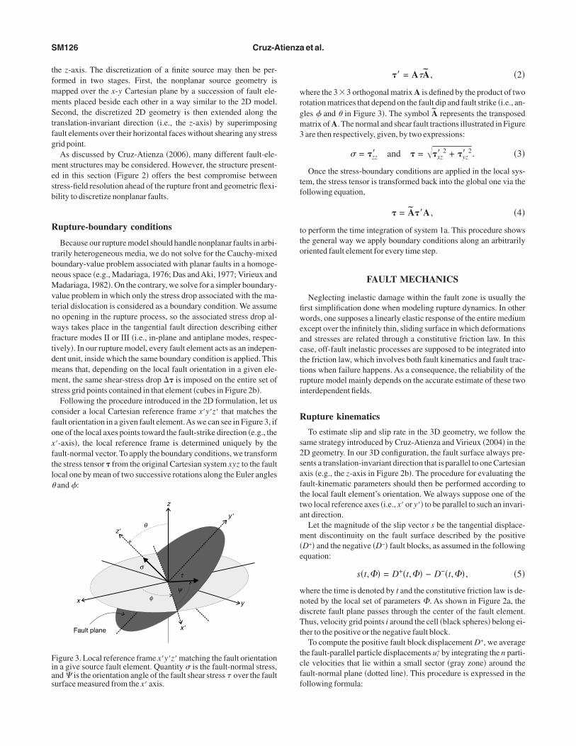
onsider a local Cartesian reference frame x�y�z� that matches theault orientation in a given fault element.As we can see in Figure 3, ifne of the local axes points toward the fault-strike direction �e.g., the�-axis�, the local reference frame is determined uniquely by theault-normal vector. To apply the boundary conditions, we transformhe stress tensor � from the original Cartesian system xyz to the faultocal one by mean of two successive rotations along the Euler anglesand :

z

z

x

x

y

y

Fault plane

θ

σ

φ ψ

τ

`

`

`

igure 3. Local reference frame x�y�z� matching the fault orientationn a give source fault element. Quantity � is the fault-normal stress,nd � is the orientation angle of the fault shear stress over the faulturface measured from the x axis.
�
�� = AA , �2�

here the 3�3 orthogonal matrix A is defined by the product of twootation matrices that depend on the fault dip and fault strike �i.e., an-les and � in Figure 3�. The symbol A represents the transposedatrix of A. The normal and shear fault tractions illustrated in Figureare then respectively, given, by two expressions:

� = �zz� and � = ��xz�2 + �yz�

2. �3�

Once the stress-boundary conditions are applied in the local sys-em, the stress tensor is transformed back into the global one via theollowing equation,

� = A��A , �4�

o perform the time integration of system 1a. This procedure showshe general way we apply boundary conditions along an arbitrarilyriented fault element for every time step.

FAULT MECHANICS

Neglecting inelastic damage within the fault zone is usually therst simplification done when modeling rupture dynamics. In otherords, one supposes a linearly elastic response of the entire medium

xcept over the infinitely thin, sliding surface in which deformationsnd stresses are related through a constitutive friction law. In thisase, off-fault inelastic processes are supposed to be integrated intohe friction law, which involves both fault kinematics and fault trac-ions when failure happens. As a consequence, the reliability of theupture model mainly depends on the accurate estimate of these twonterdependent fields.

upture kinematics

To estimate slip and slip rate in the 3D geometry, we follow theame strategy introduced by Cruz-Atienza and Virieux �2004� in theD geometry. In our 3D configuration, the fault surface always pre-ents a translation-invariant direction that is parallel to one Cartesianxis �e.g., the z-axis in Figure 2b�. The procedure for evaluating theault-kinematic parameters should then be performed according tohe local fault element’s orientation. We always suppose one of thewo local reference axes �i.e., x� or y�� to be parallel to such an invari-nt direction.

Let the magnitude of the slip vector s be the tangential displace-ent discontinuity on the fault surface described by the positive

D+� and the negative �D−� fault blocks, as assumed in the followingquation:

s�t, � = D+�t, � − D−�t, � , �5�

here the time is denoted by t and the constitutive friction law is de-oted by the local set of parameters . As shown in Figure 2a, theiscrete fault plane passes through the center of the fault element.hus, velocity grid points i around the cell �black spheres� belong ei-

her to the positive or the negative fault block.To compute the positive fault block displacement D+, we average

he fault-parallel particle displacements ui+ by integrating the n parti-

le velocities that lie within a small sector �gray zone� around theault-normal plane �dotted line�. This procedure is expressed in theollowing formula:

wAgfffaets

wt

Ipms

taewietaOitei

dtdritma==n�f

eseestaa

savbNa�=

F

IgfiritF

mepamnoia

Fra�sF�


D+�t,�� =1

n�i =1

n

ui+�t,�,�� · Hi��,�� , �6�

here the weight functions Hi are introduced in the 2D case �Cruz-tienza and Virieux, 2004� and numerically recomputed for the 3Deometry. Basically, they are normalized functions that make theault-block-displacement estimate numerically independent of aaulting mechanism. They are computed once for a given finite-dif-erence stencil and then stored for future rupture simulations with anrbitrary fault geometry and a propagating medium. The only differ-nce with respect to the 2D approach is that, in three dimensions,hese functions also depend on �, the direction in which the sheartress acts over the fault plane �Figure 3�.

For symmetry reasons with respect to the fault-normal axis z�, theeight functions may be defined as the following linear combina-

ion:

Hi��,�� = �cos �� · Hi��,0°� + �sin �� · Hi��,90°� .

n other words, the functions Hi��,�� are obtained from those com-uted for two specific angles, � = 0° and � = 90°. This procedureakes the fault-block displacement �equation 6� independent of the

ource-rupture mechanism.As discussed by Cruz-Atienza and Virieux �2004�, considering

he velocity grid points as lying within the element sector mentionedbove �gray zone, Figure 2a� avoids undesirable effects from inter-lement destructive interferences. In the specific element structure,e have selected the angle � �Figure 2�, which defines such a region,

s equal to 56°. This value means that at least four but no more thanight velocity grid points lie in that sector per fault block, irrespec-ive of the fault orientation with respect to the translation-invariantxis. For instance, in Figure 2b, we have n = 4 �see equation 6�.nce the negative fault-block displacement D− is computed in a sim-

lar way, we can estimate the fault-element slip function by inputtinghese values into equation 5. The slip-rate function in a given fault-lement is determined in exactly the same way but without integrat-ng the velocity field in the velocity grid nodes.

When simulating the rupture of the same extended planar fault forifferent dipping angles �i.e., the angle with respect to the transla-ion-invariant axis — for instance, � if = 0; see Figure 3�, a smallependence of the average slip and slip-rate functions on that angleemains. For symmetry reasons of the numerical stencil, it is period-c every 90°. This finite-fault-orientation anisotropy is also found inhe 2D case and is corrected by introducing a numerically deter-

ined normalized factor that depends on � and multiplies both slipnd slip-rate functions. In the 3D case, this factor is given by f��A�3 + B�2 + C� + D, where A = 0.00004, B = − 0.003, C0.06, and D = 1.0; the factor yields the slip and slip-rate functions

o longer dependent on fault orientation. In this definition, the anglealways should be measured from the nearest Cartesian axis to the

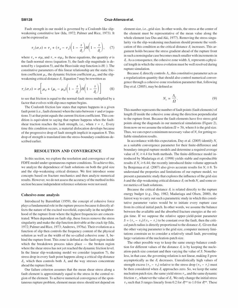
ault plane.Figure 4 shows slip and slip-rate functions computed in one fault

lement displayed in Figure 2 for different fault orientations. Theseimulations were performed considering a simple linear time-weak-ning friction �Andrews, 2004� with a characteristic weakening timequal to 0.4 s. Shear tractions drop down linearly from the initialtress level 0 = 30 bar to the dynamic level s = 0 bar in exactlyhat specific time. Because the translation-invariant direction is par-llel to the z-axis in this example, following Figure 3 we consider thengle � = 90° in our further simulations.

The left column shows slip and slip-rate functions computed forix different fault-orientation angles, = 0°, 9°, 18°, 27°, 36°, 45°nd for a shear-stress drop � perpendicular to the translation-in-ariant direction �� = 0°�. The right column shows similar resultsut for � parallel to the translation-invariant direction �� = 90°�.early no dependence on the fault orientation is observed, where-

s results are slightly dependent on the stress-drop orientation angle, with an overestimation of amplitudes smaller than 10% for �90°.

ailure criterion

Rupture propagation is a thermodynamic system in equilibrium.n other words, it is a system in which the balance between the ener-y-release rate and fracture energy is conserved. That is what Grif-th’s �1920� criterion states. However, because no real material mayesist infinite stress concentrations, an alternative way to determinef rupture keeps going is by looking at the stress field around the rup-ure front and comparing it with the current fault strength. In ourDFE approach, we adopt the latter strategy as a failure criterion.To determine the actual state of stress of a given fault element, weonitor the fault tractions via equations 3 in the central point of the

lement and within a small neighborhood given by the six stress gridoints lying at one spatial step from the central point. The algorithmlways takes the maximum stress values in these points as the ele-ent state of stress. We consider these neighboring points because in

onplanar discrete faults we never know exactly where the continu-us fault geometry passes. The hypothesis behind such an approachs that tractions determined in this way represent their mean valuelong the entire fault element �Das andAki, 1977�.

Slip

(m

)

0.07

0.06

0.05

0.04

0.03

0.02

0.01

0.00

Slip

rat

e (m

/s)

0.20

0.15

0.10

0.05

0.00

–0.05

= 0°ψ = 90°

0.0 0.2 0.4 Time (s)

0.6 0.8

0.0 0.2 0.4 Time (s)

0.6 0.8

Slip

(m

)

0.07

0.06

0.05

0.04

0.03

0.02

0.01

0.00

Slip

rat

e (m

/s)

0.20

0.15

0.10

0.05

0.00

–0.05

0.0 0.2 0.4 Time (s)

0.6 0.8

0.0 0.2 0.4 Time (s)

0.6 0.8

ψ

igure 4. Slip and slip-rate time functions computed in a point sourceepresented by one fault element �Figure 2b�. Results were obtainednd superimposed in both columns for = 0° and different angles= 0°,9°,18°,27°,36°,45° �see Figure 3�. The left column corre-

ponds to a shear stress drop � parallel to the x�-axis �i.e., � = 0°,igure 3� and the right column for a � perpendicular to the x�-axisi.e., � = 90°�.

wc

wtnctw

tf

ftdstods

Fwacrs

C

pfhts1fshwwIs�a

fgt

etwlcgi�cr

agD

TltpfTl

abvtrbuphr

eftfbgScttl

talasbnf


Fault strength in our model is governed by a Coulomb-like slip-eakening constitutive law �Ida, 1972; Palmer and Rice, 1973�. It

an be expressed as

c��,s� = s + � u − s��1 −s

�c�H�1 −

s

�c� , �7�

here u = ��s and s = ��d. In these equations, the quantity � ishe fault-normal stress �equation 3�, the fault-slip magnitude is de-oted by s �equation 5�, and the Heaviside step function is H�·�. Theonstitutive parameters of this linear relationship are the static fric-ion coefficient �s, the dynamic friction coefficient �d, and the slip-eakening critical distance �c. Equation 7 may be rewritten as

c��,s� = ��d + ��s − �d��1 −s

�c�H�1 −

s

�c� �8�

o see that friction is equal to the normal-fault stress multiplied by aactor that evolves with slip once rupture begins.

The Coulomb friction law states that rupture happens in a givenault point �i.e., fault element� when the ratio between and � �equa-ions 3� at that point equals the current friction coefficient. This con-ition is equivalent to saying that rupture happens when the fault-hear traction reaches the fault strength, i.e., when = c. Everyime this condition occurs, a material dislocation develops becausef the progressive drop of fault strength implicit in equation 8. Thisrop of strength is translated into the stress-boundary conditions de-cribed earlier.

RESOLUTION AND CONVERGENCE

In this section, we explore the resolution and convergence of ourDFE model under spontaneous rupture conditions. To achieve this,e analyze the dependence of fault solutions on both the grid size

nd the slip-weakening critical distance. We first introduce someoncepts based on fracture mechanics and then analyze numericalesults. However, we do not assess the accuracy of the method in thisection because independent reference solutions were not used.

ohesive-zone analysis

Introduced by Barenblatt �1959�, the concept of cohesive forcelays a fundamental role in the rupture process because it directly af-ects the nature of the excited wavefield, especially in the neighbor-ood of the rupture front where the highest frequencies are concen-rated. When dependent on fault slip, these forces remove the stressingularity and make the slip function derivable at the crack tip �Ida,972; Palmer and Rice, 1973; Andrews, 1976a�. Their evolution as aunction of slip then controls the frequency content of the physicalolution as well as the width of the so-called cohesive zone �c be-ind the rupture front. This zone is defined as the fault region insidehich the breakdown process takes place — the broken regionhere the shear stress has not yet reached the dynamic friction level.

n the linear slip-weakening model we consider �equation 7�, thetress drop in every fault point happens along a critical slip distancec, which then controls both �c and the way stresses concentratehead the rupture front.

Our failure criterion assumes that the mean shear stress along aault element is approximately equal to the stress in the central re-ion of the element. To achieve numerical convergence of the spon-aneous rupture problem, element mean stress should not depend on

lement size, i.e., grid size. In other words, the stress at the center ofhe element must be representative of the mean value along thehole element �see Das and Aki, 1977�. Removing the stress singu-

arity via the slip-weakening mechanism should promote the verifi-ation of this condition as the critical distance �c increases. This ar-ument holds because the stress gradient ahead of the rupture frontn such a nonsingular case becomes much smaller with increments in

c.As a consequence, the cohesive zone width �c represents a physi-al length in which the stress evolution must be well resolved duringupture simulation.

Because �c directly controls �c, this constitutive parameter acts asregularization quantity that should also control numerical conver-ence through a cohesive-zone resolution parameter that, followingay et al. �2005�, may be defined as

Nc =�c

�. �9�

his number represents the number of fault points �fault elements� ofength � inside the cohesive zone along the direction perpendicularo the rupture front. Because the fault elements have five stress gridoints along the diagonals in our numerical simulations �Figure 2�,rom now on we assume the relation � = 5h, where h is the grid size.hus, we can expect a minimum necessary value of Nc for getting re-

iable simulation results.In accordance with this expectation, Day et al. �2005� identify Nc

s a suitable convergence parameter for their finite-difference andoundary-integral rupture models and determine a required averagealue of Nc �4.4 for both methods. The finite-difference model in-roduced by Madariaga et al. �1998� yields stable and reproducibleesults if Nc �6.44; the recently introduced finite-volume approachy Benjemaa et al. �2007� also gives accurate results for Nc �8. Tonderstand the properties and limitations of our rupture model, weresent a parametric study that explores the influence of the grid sizeand the slip-weakening critical distance �c on both Nc and some er-

or metrics of fault solutions.Because the critical distance �c is related directly to the rupture

nergy budget �e.g., Day, 1982; Madariaga and Olsen, 2000�, theairest way to carry out such a parametric study in which this consti-utive parameter varies would be to initiate every rupture caserom its critical initial patch. In other words, we assume the balanceetween the available and the absorbed fracture energies at the ori-in time. If we suppose the relative upper-yield-point parameter= � u − 0�/� 0 − s� to be constant over the fault, then the criti-

al patch radius is directly proportional to the distance �c. Given thathe other varying parameter is the grid size, computer memory limi-ations constrain us to consider a relatively small fault, preventingarge variations of the nucleation-patch size.

The other possible way to keep the same energy-balance condi-ion for different values of the distance �c is by keeping the nucle-tion-patch size constant and then varying the value of S. Nonethe-ess, in that case, the governing relation is not linear, making S growsymptotically as the �c decreases. Unrealistically high values oftrength excess � u − 0� relative to the stress drop � 0 − s� muste then considered when �c approaches zero. So, we keep the sameucleation patch size, the same yield stress u, and the same dynamicriction s, whatever the value of �c. We only change the initial stress

such that S ranges linearly from 0.2 for �max to 1.0 for �min. These
0 c c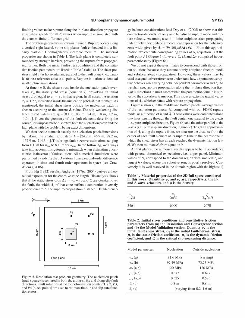

lat

aepritsli

tsmct

sf

b

fttpoA

rttp

gctizmfp

oautwxjt

omt�xtcwe

wvlv

Tia

�

3

F�dat

Tpai�c

M


imiting values make rupture along the in-plane direction propagatet subshear speeds for all �c values when rupture is simulated withhe coarsest finite-difference grid.

The problem geometry is shown in Figure 5. Rupture occurs alongvertical right-lateral, strike-slip planar fault embedded into a lin-

arly elastic 3D homogeneous, isotropic medium. The materialroperties are shown in Table 1. The fault plane is completely sur-ounded by strength barriers, preventing the rupture from propagat-ng further. Both the initial fault-stress conditions and the constitu-ive friction parameters are listed in Table 2 �label a�. The shear pre-tress field 0 is horizontal and parallel to the fault plane �i.e., paral-el to the x reference axis� at all points. Rupture initiation is identicaln all rupture simulations.

At time t = 0, the shear stress inside the nucleation patch over-akes u, the static yield stress �equation 7�, provoking an initialtress drop equal to 0 − u in that region. In all cases, the relation0 = 1.2 u is verified inside the nucleation patch at that moment. Asentioned, the initial shear stress outside the nucleation patch is

hosen according to the current �c value. The slip-weakening-dis-ance tested values are �c = 0.1 m, 0.2 m, 0.4 m, 0.8 m, 1.2 m,1.6 m�. Given the geometry of the fault elements describing theource, it is impossible to discretize both the nucleation patch and theault plane with the problem being exact dimensions.

We then decide to match exactly the nucleation-patch dimensionsy taking the spatial grid steps h = 24.2 m, 46.9 m, 88.2 m,157.9 m, 214.3 m�. This brings fault-size overestimations rangingrom 100 m for hmin to 800 m for hmax. In the following, we alwaysake into account this geometric mismatch when estimating uncer-ainties in the error of fault solutions.All numerical simulations wereerformed by solving the 3D system 1 using second-order differenceperators in time and fourth-order operators in space �see Cruz-tienza, 2006�.From Ida �1972� results, Andrews �1976a, 2004� derives a theo-

etical expression for the cohesive-zone length. His analysis showshat if the static-stress drop � = 0 − s and �c are constant overhe fault, the width �c of that zone suffers a contraction inverselyroportional to L, the rupture-propagation distance. Detailed ener-

z

x y

Fault plane

15 km

3 km

5 km

P1

P3

P2

P4

3 km

15 k

m 5

km

igure 5. Resolution test problem geometry. The nucleation patchgray square� is centered in both the along-strike and along-dip faultirections. Fault solutions at the four observation points P1, P2, P3,nd P4 �black points� are used to estimate the slip and slip-rate func-ion errors.

y-balance considerations lead Day et al. �2005� to show that thisontraction depends not only on L but also on rupture mode and rup-ure velocity. Assuming a semi-infinite antiplane crack propagatingndefinitely, they deduce a theoretical expression for the cohesive-one width given by �c = �9/16��c/� �2L−1. From this approxi-ation, we compute corresponding values of Nc �equation 9� at the

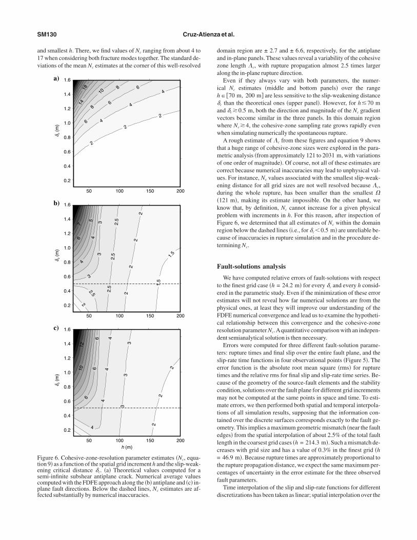
ault point P1 �Figure 5� for every �c, �, and � comprised in our-arametric study �Figure 6a�.

We do not expect these estimates to correspond with those fromur solutions because they assume purely antiplane fracture modend subshear steady propagation. However, these values may besed as a qualitative reference to understand how a spontaneous rup-ure behaves when varying both independent parameters h and �c.Ase shall see, rupture propagation along the in-plane direction �i.e.,

-axis direction� in most cases within the parametric domain is sub-ect to the supershear transition. This induces extreme spatial varia-ions of �c, which expands with rupture propagation.

Figure 6 shows, in the middle and bottom panels, average valuesf the resolution parameter Nc computed with our FDFE ruptureodel as a function of h and �c. These values were computed along

wo lines passing through the fault center, one parallel to the z-axisi.e., pure antiplane direction, Figure 6b� and the other parallel to the-axis �i.e., pure in-plane direction, Figure 6c�. To get an approxima-ion of �c along the rupture front, we measure the distance from theenter of each fault element at its rupture time to the nearest one inhich the shear stress has already reached the dynamic friction lev-

l. We then estimate Nc from equation 9.At first glance, the numerical results appear to be in accordance

ith general theoretical expectations, i.e., upper panel. Minimumalues of Nc correspond to the domain region with smallest �c andargest h values, where the cohesive zone is poorly resolved. Con-ersely, it is well resolved in the domain region with the highest �c

able 1. Material properties of the 3D full space consideredn this work. Quantities vp and vs are, respectively, the P-nd S-wave velocities, and � is the density.

vs

m/s�vp

�m/s��

�kg/m3�

464 6000 2670

able 2. Initial stress conditions and constitutive frictionarameters from (a) the Resolution and Convergence sectionnd (b) the Model Validation section. Quantity � 0 is thenitial fault shear stress, �0 is the initial fault-normal stress,

s is the static friction coefficient, �d is the dynamic frictionoefficient, and �c is the critical slip-weakening distance.

odel parameters Nucleation Outside nucleation

0 �a� 81.6 MPa �varying�

0 �b� 97.49 MPa 73.73 MPa

�0 �a,b� 120 MPa 120 MPa

�s �a,b� 0.677 0.677

�d �a,b� 0.525 0.525

�c �b� 0.8 m 0.8 m

�c �a� �varying from 0.2–1.6 m�

a1v

daza

ih�avww

tmocued�kpFrct

F

teepFcrd

tsetccmmttoelc=tcf

d

Ftescpf


nd smallest h. There, we find values of Nc ranging from about 4 to7 when considering both fracture modes together. The standard de-iations of the mean Nc estimates at the corner of this well-resolved

a)

h (m)

50

1814

10

76

5

8

8

6

6

6

4

4

33

3

4

4

4

22

22

2.5

2

2.5

2.5

1.5

1.5

2.5

2

2

1210

6

66

4

4

44

33

22

2

3

2

100 150 200

1.6

1.4

1.2

1.0

0.8

0.6

0.4

0.2

δ c (

m)

b)

50 100 150 200

1.6

1.4

1.2

1.0

0.8

0.6

0.4

0.2

δ c (

m)

c)

50 100 150 200

1.6

1.4

1.2

1.0

0.8

0.6

0.4

0.2

δ c (

m)

igure 6. Cohesive-zone-resolution parameter estimates �Nc, equa-ion 9� as a function of the spatial grid increment h and the slip-weak-ning critical distance �c. �a� Theoretical values computed for aemi-infinite subshear antiplane crack. Numerical average valuesomputed with the FDFE approach along the �b� antiplane and �c� in-lane fault directions. Below the dashed lines, Nc estimates are af-ected substantially by numerical inaccuracies.

omain region are ± 2.7 and ± 6.6, respectively, for the antiplanend in-plane panels. These values reveal a variability of the cohesiveone length �c, with rupture propagation almost 2.5 times largerlong the in-plane rupture direction.

Even if they always vary with both parameters, the numer-cal Nc estimates �middle and bottom panels� over the range� 70 m, 200 m� are less sensitive to the slip-weakening distancec than the theoretical ones �upper panel�. However, for h�70 mnd �c �0.5 m, both the direction and magnitude of the Nc gradientectors become similar in the three panels. In this domain regionhere Nc �4, the cohesive-zone sampling rate grows rapidly evenhen simulating numerically the spontaneous rupture.A rough estimate of �c from these figures and equation 9 shows

hat a huge range of cohesive-zone sizes were explored in the para-etric analysis �from approximately 121 to 2031 m, with variations

f one order of magnitude�. Of course, not all of these estimates areorrect because numerical inaccuracies may lead to unphysical val-es. For instance, Nc values associated with the smallest slip-weak-ning distance for all grid sizes are not well resolved because �c,uring the whole rupture, has been smaller than the smallest �121 m�, making its estimate impossible. On the other hand, wenow that, by definition, Nc cannot increase for a given physicalroblem with increments in h. For this reason, after inspection ofigure 6, we determined that all estimates of Nc within the domainegion below the dashed lines �i.e., for �c �0.5 m� are unreliable be-ause of inaccuracies in rupture simulation and in the procedure de-ermining Nc.

ault-solutions analysis

We have computed relative errors of fault-solutions with respecto the finest grid case �h = 24.2 m� for every �c and every h consid-red in the parametric study. Even if the minimization of these errorstimates will not reveal how far numerical solutions are from thehysical ones, at least they will improve our understanding of theDFE numerical convergence and lead us to examine the hypotheti-al relationship between this convergence and the cohesive-zoneesolution parameter Nc.Aquantitative comparison with an indepen-ent semianalytical solution is then necessary.

Errors were computed for three different fault-solution parame-ers: rupture times and final slip over the entire fault plane, and thelip-rate time functions in four observational points �Figure 5�. Therror function is the absolute root mean square �rms� for ruptureimes and the relative rms for final slip and slip-rate time series. Be-ause of the geometry of the source-fault elements and the stabilityondition, solutions over the fault plane for different grid incrementsay not be computed at the same points in space and time. To esti-ate errors, we then performed both spatial and temporal interpola-

ions of all simulation results, supposing that the information con-ained over the discrete surfaces corresponds exactly to the fault ge-metry. This implies a maximum geometric mismatch �near the faultdges� from the spatial interpolation of about 2.5% of the total faultength in the coarsest grid cases �h = 214.3 m�. Such a mismatch de-reases with grid size and has a value of 0.3% in the finest grid �h46.9 m�. Because rupture times are approximately proportional to

he rupture propagation distance, we expect the same maximum per-entages of uncertainty in the error estimate for the three observedault parameters.

Time interpolation of the slip and slip-rate functions for differentiscretizations has been taken as linear; spatial interpolation over the

rcw

Ituf=uni

pctnltciahdrgos

trggTsimocpw

atp�diitttbt8v1

atlfcsa0s

Ftwt


upture surface has been carried out in a regular grid with a spatial in-rement of 100 m. Interpolation values f int of fault-solutions fields ui

ere computed as

f int = �i = 1,n

ui

ai, where ai = �

j = 1,n� di

dj�m

. �10�

n these equations, quantities ai are weighting factors that multiplyhe n punctual fault-solutions lying inside spherical supports of radi-s r centered at the interpolated values f int and di are the distancesrom f int to each one of these punctual solutions. We always took m

0.5 in this work and r = 1000 m in this parametric study. This val-e of r is the same for all grid sizes and corresponds to the minimumecessary for having at least one fault element inside the sphericalnterpolation support.

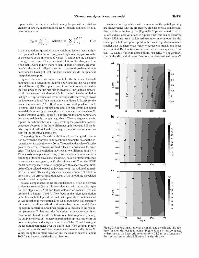
Figure 7 shows error-estimate results for the three selected faultarameters as a function of the grid size h and the slip-weakeningritical distance �c. The rupture time of one fault point is defined ashe time at which the slip rate first exceeds 0.01 m/s at that point. Fi-al slip is measured over the entire fault at the end of each simulationasting 5 s. Slip-rate function errors correspond to the average rms ofhe four observational fault points shown in Figure 5. Except for theoarsest simulations �h�150 m�, almost no error dependence on �c

s found. The biggest rupture-time and slip-rate errors are foundround the bottom-right corner, �i.e., the parameter domain where Nc

as the smallest values, Figure 6�. The error in the three parametersecreases mainly with the spatial grid step. The convergence rate forupture times diminishes as h→hmin, evoking the power-law conver-ence rate observed in the finite-difference split-node and BIE meth-ds �Day et al., 2005�. On the contrary, it remains more or less con-tant for the other two parameters.

Comparing Figure 6b and c with Figure 7, we find good correla-ion between the cohesive-zone-resolution parameter Nc and the er-or estimates for grid sizes h�70 m: The smaller the value of Nc, thereater the error. However, we find a lack of correlation for finerrids. This lack of correlation may reveal two different things: �1�here exists an upper value of Nc ��4� for which there is an over-ampling of the cohesive zone, making Nc have no further influencen numerical convergence, or �2� the influence of Nc on the FDFEodel convergence is always negligible with respect to other first-

rder effects related to mesh refinements �e.g., reduction of numeri-al oscillations�. This ambiguity may be a consequence of a lack inrecision of the error estimate as a result of the smoothing associatedith the spatial interpolation.Several comparisons for the critical distance �c = 0.8 m between

reference solution �i.e., a solution calculated with the smallest spa-ial grid step h = 24.2 m� and those obtained on coarser grids areresented in Figures 8 and 9. If we focus on the reference solutionsolid lines in both figures�, we find that rupture-time contours starteveloping the supershear transition lobes around 0.5 s after rupturenitiation in the along-strike direction �in-plane rupture mode�. Dur-ng rupture acceleration, we find a progressive increase in the resolu-ion parameter Nc that, near the fault edges, exceeds several timeshose values found outside the transitional fault region �e.g., alonghe antiplane direction�. When comparing the slip-rate rms errors onoth the in-plane and antiplane directions �Table 3� and looking athe resolution parameter over the entire fault �right column, Figure�, we find a good correlation between the systematically higher Nc

alues along the in-plane direction and the smaller misfits of about0% for all but one grid size in that direction.

Rupture-time degradation with increments of the spatial grid stepre in accordance with the progressive drop in cohesive-zone resolu-ion over the entire fault plane �Figure 8�. Slip-rate numerical oscil-ations induce local variations in rupture times that can be observedor h�157.9 m as small spikes in the rupture-time contours. We alsoan appreciate how rupture speed in the coarsest grid case remainsmaller than the shear-wave velocity because no transitional lobesre exhibited. Rupture time rms errors for these examples are 0.04,.11, 0.28, and 0.41s from top to bottom, respectively. The compari-on of the slip and slip-rate functions in observational point P1

a)

h (m)

50 100 150 200

(s)

1.6

1.4

1.2

1.0

0.8

0.6

0.4

0.2

0.5

0.4

0.3

0.2

0.1

0.0

δ c (

m)

b)

50 100 150 200

(%)

1.6

1.4

1.2

1.0

0.8

0.6

0.4

0.2

8070605040302010

0

δ c (

m)

c)

50 100 150 200

(%)

1.6

1.4

1.2

1.0

0.8

0.6

0.4

0.2

14

12

10

8

6

4

2

0

δ c (

m)

0.05

0.05

0.15

0.15

0.25

0.25

0.1

1010

2020

3030

30

4040

5050

60

50

60

70

10

1088

8

66

44

4

22

10

0.1

0.1

0.2

0.3

0.3

0.4

0.2

0.2

igure 7. Rupture times �all over the fault� and the slip and slip-rateime function �in four fault points, Figure 5� rms errors computedith respect to the finest grid solutions �h = 24.2 m� as a function of

he slip-weakening critical distance � and grid size h.
c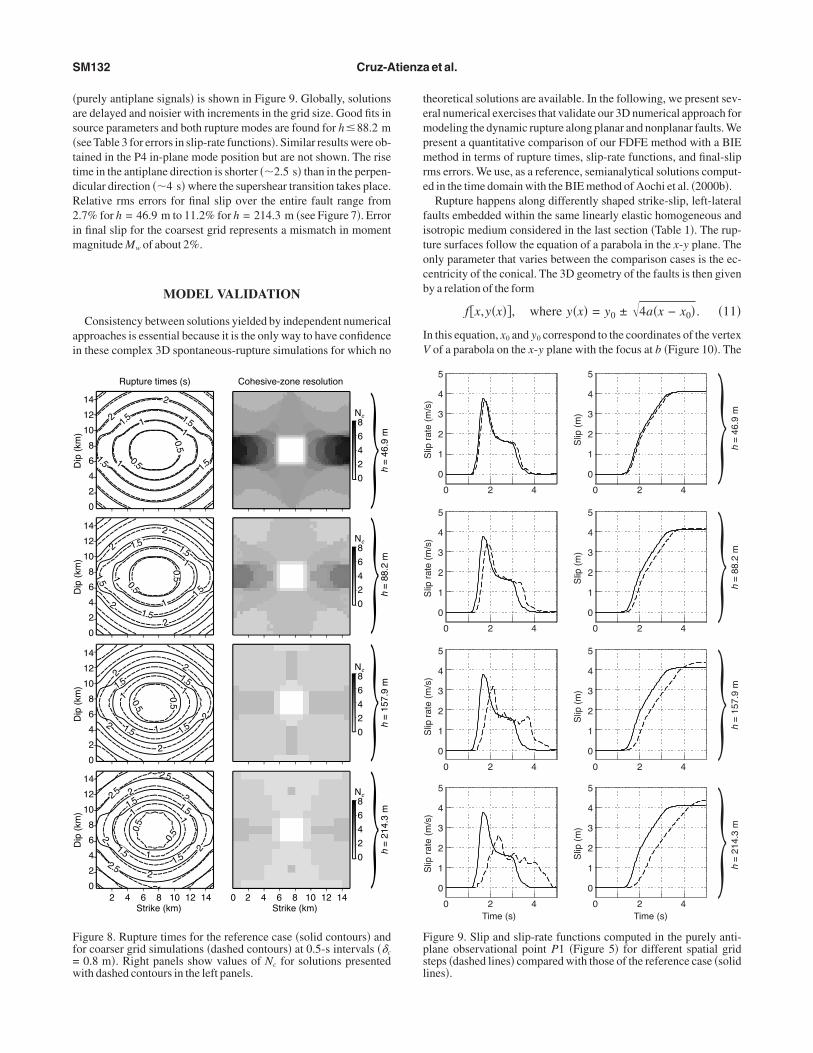

�as�ttdR2im

ai

tempmre

fitocb

IV

Ff=w

Fps


purely antiplane signals� is shown in Figure 9. Globally, solutionsre delayed and noisier with increments in the grid size. Good fits inource parameters and both rupture modes are found for h�88.2 msee Table 3 for errors in slip-rate functions�. Similar results were ob-ained in the P4 in-plane mode position but are not shown. The riseime in the antiplane direction is shorter ��2.5 s� than in the perpen-icular direction ��4 s� where the supershear transition takes place.elative rms errors for final slip over the entire fault range from.7% for h = 46.9 m to 11.2% for h = 214.3 m �see Figure 7�. Errorn final slip for the coarsest grid represents a mismatch in moment

agnitude Mw of about 2%.

MODEL VALIDATION

Consistency between solutions yielded by independent numericalpproaches is essential because it is the only way to have confidencen these complex 3D spontaneous-rupture simulations for which no

Dip

(km

)

h =

46.

9 m

h =

88.

2 m

h =

157

.9 m

h =

214

.3 m

2 4 6

2

2

1.5

0.5

0.5

1

1

11.5

1.51.5

8 10 12 14Strike (km)

20 4 6 8 10 12 14Strike (km)

Rupture times (s) Cohesive-zone resolution

14

12

10

8

6

4

2

0

8

6

4

2

0

Nc

8

6

4

2

0

Nc

8

6

4

2

0

Nc

8

6

4

2

0

Nc

Dip

(km

)

2

2

2

2

1.5

0.5

0.5

1

1

1

1.5

1.5

1.5

1.5

14

12

10

8

6

4

2

0

Dip

(km

)

2

2

2

2

2

1.5

0.50.51

1

1

1.5

1.5 1.5

14

12

10

8

6

4

2

0

Dip

(km

)

2

2

2

2

2.5

2.5

2.5

2

1.5

0.50.

5

1

1

11.5

1.51.5

14

12

10

8

6

4

2

0

igure 8. Rupture times for the reference case �solid contours� andor coarser grid simulations �dashed contours� at 0.5-s intervals ��c

0.8 m�. Right panels show values of Nc for solutions presented
l
heoretical solutions are available. In the following, we present sev-ral numerical exercises that validate our 3D numerical approach forodeling the dynamic rupture along planar and nonplanar faults. We

resent a quantitative comparison of our FDFE method with a BIEethod in terms of rupture times, slip-rate functions, and final-slip

ms errors. We use, as a reference, semianalytical solutions comput-d in the time domain with the BIE method of Aochi et al. �2000b�.

Rupture happens along differently shaped strike-slip, left-lateralaults embedded within the same linearly elastic homogeneous andsotropic medium considered in the last section �Table 1�. The rup-ure surfaces follow the equation of a parabola in the x-y plane. Thenly parameter that varies between the comparison cases is the ec-entricity of the conical. The 3D geometry of the faults is then giveny a relation of the form

fx,y�x��, where y�x� = y0 ± �4a�x − x0� . �11�

n this equation, x0 and y0 correspond to the coordinates of the vertexof a parabola on the x-y plane with the focus at b �Figure 10�. The

Slip

rat

e (m

/s)

0 2

Time (s) Time (s)

4 0 2 4

5

4

3

2

1

0

Slip

(m

)

h =

46.

9 m

h

= 8

8.2

m

h =

157

.9 m

h

= 2

14.3

m

5

4

3

2

1

0

Slip

rat

e (m

/s)

0 2 4 0 2 4

5

4

3

2

1

0

Slip

(m

)

5

4

3

2

1

0

Slip

rat

e (m

/s)

0 2 4 0 2 4

5

4

3

2

1

0

Slip

(m

)

5

4

3

2

1

0

Slip

rat

e (m

/s)

0 2 4 0 2 4

5

4

3

2

1

0

Slip

(m

)

5

4

3

2

1

0

igure 9. Slip and slip-rate functions computed in the purely anti-lane observational point P1 �Figure 5� for different spatial gridteps �dashed lines� compared with those of the reference case �solid

ith dashed contours in the left panels.
ines�.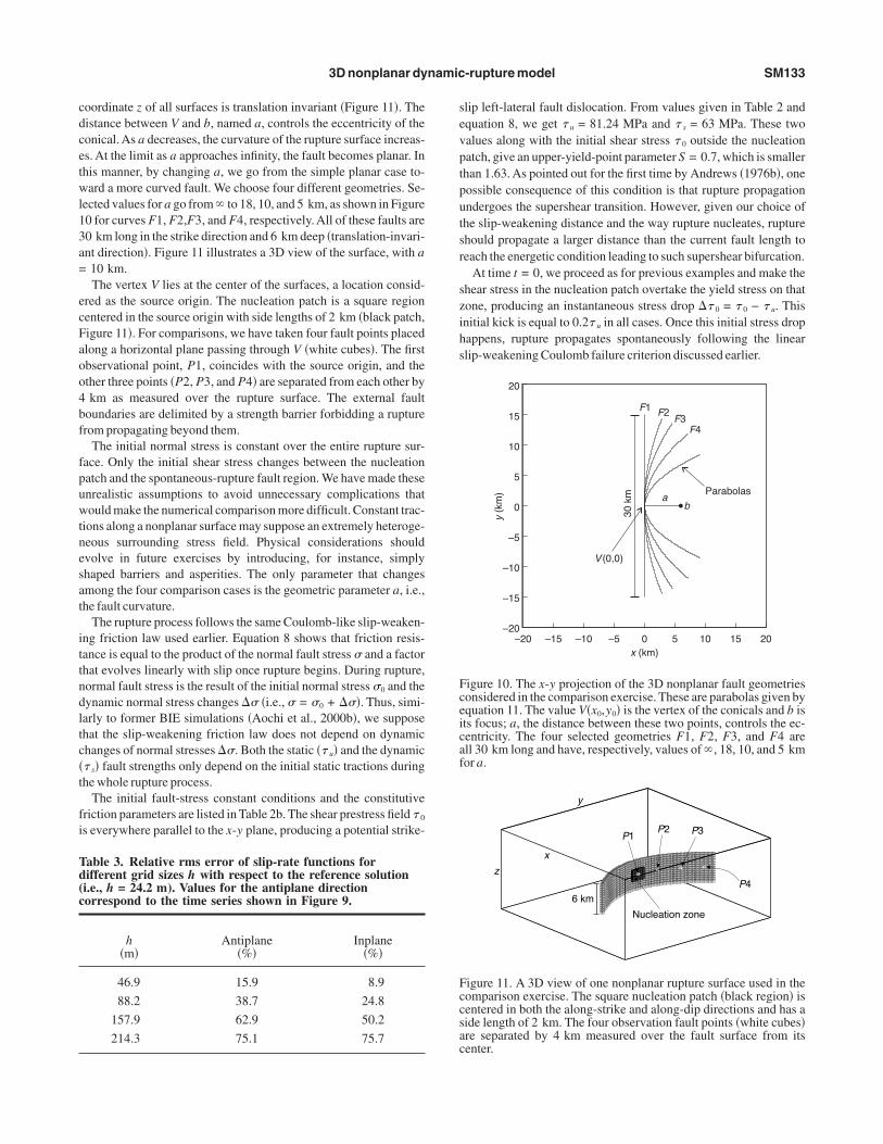

cdcetwl13a=

ecFaoo4bf

fpuwtnesat

ittndltc�t

fi

sevptputsr

szihs

Td(c

Fceicaf

Fccsac


oordinate z of all surfaces is translation invariant �Figure 11�. Theistance between V and b, named a, controls the eccentricity of theonical. As a decreases, the curvature of the rupture surface increas-s. At the limit as a approaches infinity, the fault becomes planar. Inhis manner, by changing a, we go from the simple planar case to-ard a more curved fault. We choose four different geometries. Se-

ected values for a go from � to 18, 10, and 5 km, as shown in Figure0 for curves F1, F2,F3, and F4, respectively. All of these faults are0 km long in the strike direction and 6 km deep �translation-invari-nt direction�. Figure 11 illustrates a 3D view of the surface, with a10 km.The vertex V lies at the center of the surfaces, a location consid-

red as the source origin. The nucleation patch is a square regionentered in the source origin with side lengths of 2 km �black patch,igure 11�. For comparisons, we have taken four fault points placedlong a horizontal plane passing through V �white cubes�. The firstbservational point, P1, coincides with the source origin, and thether three points �P2, P3, and P4� are separated from each other bykm as measured over the rupture surface. The external fault

oundaries are delimited by a strength barrier forbidding a rupturerom propagating beyond them.

The initial normal stress is constant over the entire rupture sur-ace. Only the initial shear stress changes between the nucleationatch and the spontaneous-rupture fault region. We have made thesenrealistic assumptions to avoid unnecessary complications thatould make the numerical comparison more difficult. Constant trac-

ions along a nonplanar surface may suppose an extremely heteroge-eous surrounding stress field. Physical considerations shouldvolve in future exercises by introducing, for instance, simplyhaped barriers and asperities. The only parameter that changesmong the four comparison cases is the geometric parameter a, i.e.,he fault curvature.

The rupture process follows the same Coulomb-like slip-weaken-ng friction law used earlier. Equation 8 shows that friction resis-ance is equal to the product of the normal fault stress � and a factorhat evolves linearly with slip once rupture begins. During rupture,ormal fault stress is the result of the initial normal stress �0 and theynamic normal stress changes �� i.e., � = �0 + ��. Thus, simi-arly to former BIE simulations �Aochi et al., 2000b�, we supposehat the slip-weakening friction law does not depend on dynamichanges of normal stresses ��. Both the static � u� and the dynamic s� fault strengths only depend on the initial static tractions duringhe whole rupture process.

The initial fault-stress constant conditions and the constitutiveriction parameters are listed in Table 2b. The shear prestress field 0

s everywhere parallel to the x-y plane, producing a potential strike-

able 3. Relative rms error of slip-rate functions forifferent grid sizes h with respect to the reference solutioni.e., h = 24.2 m). Values for the antiplane directionorrespond to the time series shown in Figure 9.

h�m�

Antiplane�%�

Inplane�%�

46.9 15.9 8.9

88.2 38.7 24.8

157.9 62.9 50.2

214.3 75.1 75.7

lip left-lateral fault dislocation. From values given in Table 2 andquation 8, we get u = 81.24 MPa and s = 63 MPa. These twoalues along with the initial shear stress 0 outside the nucleationatch, give an upper-yield-point parameter S = 0.7, which is smallerhan 1.63. As pointed out for the first time by Andrews �1976b�, oneossible consequence of this condition is that rupture propagationndergoes the supershear transition. However, given our choice ofhe slip-weakening distance and the way rupture nucleates, rupturehould propagate a larger distance than the current fault length toeach the energetic condition leading to such supershear bifurcation.

At time t = 0, we proceed as for previous examples and make thehear stress in the nucleation patch overtake the yield stress on thatone, producing an instantaneous stress drop � 0 = 0 − u. Thisnitial kick is equal to 0.2 u in all cases. Once this initial stress dropappens, rupture propagates spontaneously following the linearlip-weakening Coulomb failure criterion discussed earlier.

y (k

m)

x (km)

V (0,0)

a b

F1 F2 F3

F4

20 15 10

Parabolas

30 k

m

5 0 –5 –10 –15 –20

20

15

10

5

0

–5

–10

–15

–20

igure 10. The x-y projection of the 3D nonplanar fault geometriesonsidered in the comparison exercise. These are parabolas given byquation 11. The value V�x0,y0� is the vertex of the conicals and b ists focus; a, the distance between these two points, controls the ec-entricity. The four selected geometries F1, F2, F3, and F4 arell 30 km long and have, respectively, values of � , 18, 10, and 5 kmor a.

y

x

z

P1P2 P3

P4

Nucleation zone

6 km

igure 11. A 3D view of one nonplanar rupture surface used in theomparison exercise. The square nucleation patch �black region� isentered in both the along-strike and along-dip directions and has aide length of 2 km. The four observation fault points �white cubes�re separated by 4 km measured over the fault surface from itsenter.

stfou=niCp

e�tctss1cpss�lf

masmsqpup

fcg�orFocwto

vacsoprrbilcf2a7lo

t

Tfitrowr

F

P

N

N

N

Ftlp


The uniform BIE grid interval was fixed to �s = 0.15 km, so faulturfaces were discretized by 200�40 square elements in such a wayhat those element boundaries parallel to the translation-invariantault axis are contained within the analytic 3D parabolic function. Inther words, the centers of the squares shift slightly from the contin-ous-fault geometry. The corresponding time step was �t0.0125 s. Nonplanar fault discretization with our FDFE model is

ot as simple as that because rupture surfaces are represented numer-cally by parallelepiped fault elements in a regular volumetric grid.onsequently, the distance between the center of these elements de-ends on the orientation of the fault within the grid.

able 4. Absolute (rupture times) and relative (slip rate andnal fault slip) rms errors of our FDFE method with respecto the BIE reference solutions (dx = 250 m). Finite-differenceesults were obtained with second order in time and fourthrder in space accuracy operators (2,4) in a discrete latticeith spatial and time steps of h = 45.45 m and �t = 0.005 s,

espectively.

ault geometryRupture times

�s�Slip rate

�%�Final slip

�%�

lanar �F1� 0.03 32.7 23.1

onplanar �F2� 0.10 33.3 15.7

onplanar �F3� 0.05 30.4 19.9

onplanar �F4� 0.04 27.1 25.7

Dip

(km

)

Pla

nar

faul

tN

onpl

anar

faul

ts

0 2 4 6

5

5

4

4

3

3

2

2 5

5

4

4

3

3

2

2

1

1 1

1

1 1

8 10 12 14 16Strike (km)

18 20 22 24 26 28 30

F16

4

2

0

Dip

(km

)

0 2 4 6

5

5

4

4

3

3

2

2 5

5

4

4

3

3

2

2

1

1 1

1

1 1

8 10 12 14 16Strike (km)

18 20 22 24 26 28 30

F26

4

2

0

Dip

(km

)

0 2 4 6

5

5

4

4

3

3

2

2 5

5

4

4

3

3

2

2

1

1 1

1

1 1

8 10 12 14 16Strike (km)

18 20 22 24 26 28 30

F36

4

2

0

Dip

(km

)

0 2 4 6

5

5

4

4

3

3

2

2 5

5

4

4

3

3

2

2

1

1 1

1

1 1

8 10 12 14 16

FDFE BIE

Strike (km)18 20 22 24 26 28 30

F46

4

2

0

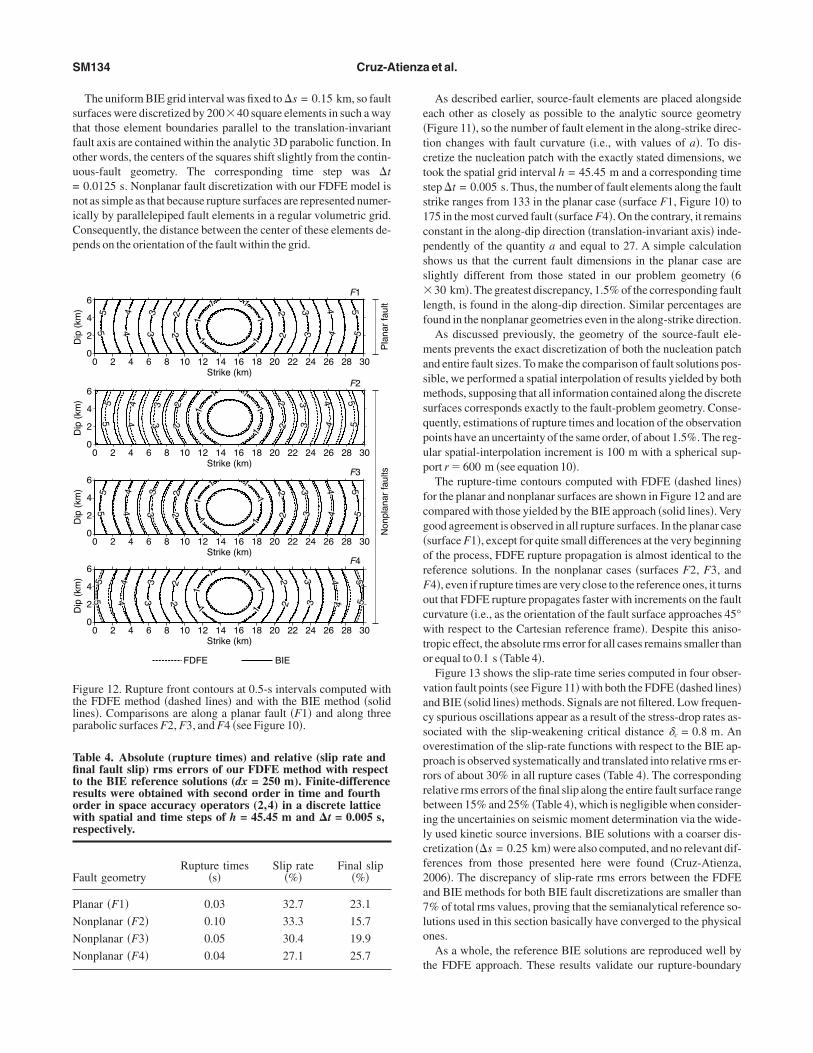
igure 12. Rupture front contours at 0.5-s intervals computed withhe FDFE method �dashed lines� and with the BIE method �solidines�. Comparisons are along a planar fault �F1� and along threearabolic surfaces F2, F3, and F4 �see Figure 10�.

As described earlier, source-fault elements are placed alongsideach other as closely as possible to the analytic source geometryFigure 11�, so the number of fault element in the along-strike direc-ion changes with fault curvature �i.e., with values of a�. To dis-retize the nucleation patch with the exactly stated dimensions, weook the spatial grid interval h = 45.45 m and a corresponding timetep �t = 0.005 s. Thus, the number of fault elements along the faulttrike ranges from 133 in the planar case �surface F1, Figure 10� to75 in the most curved fault �surface F4�. On the contrary, it remainsonstant in the along-dip direction �translation-invariant axis� inde-endently of the quantity a and equal to 27. A simple calculationhows us that the current fault dimensions in the planar case arelightly different from those stated in our problem geometry �6

30 km�. The greatest discrepancy, 1.5% of the corresponding faultength, is found in the along-dip direction. Similar percentages areound in the nonplanar geometries even in the along-strike direction.

As discussed previously, the geometry of the source-fault ele-ents prevents the exact discretization of both the nucleation patch

nd entire fault sizes. To make the comparison of fault solutions pos-ible, we performed a spatial interpolation of results yielded by bothethods, supposing that all information contained along the discrete

urfaces corresponds exactly to the fault-problem geometry. Conse-uently, estimations of rupture times and location of the observationoints have an uncertainty of the same order, of about 1.5%. The reg-lar spatial-interpolation increment is 100 m with a spherical sup-ort r � 600 m �see equation 10�.

The rupture-time contours computed with FDFE �dashed lines�or the planar and nonplanar surfaces are shown in Figure 12 and areompared with those yielded by the BIE approach �solid lines�. Veryood agreement is observed in all rupture surfaces. In the planar casesurface F1�, except for quite small differences at the very beginningf the process, FDFE rupture propagation is almost identical to theeference solutions. In the nonplanar cases �surfaces F2, F3, and4�, even if rupture times are very close to the reference ones, it turnsut that FDFE rupture propagates faster with increments on the faulturvature �i.e., as the orientation of the fault surface approaches 45°ith respect to the Cartesian reference frame�. Despite this aniso-

ropic effect, the absolute rms error for all cases remains smaller thanr equal to 0.1 s �Table 4�.

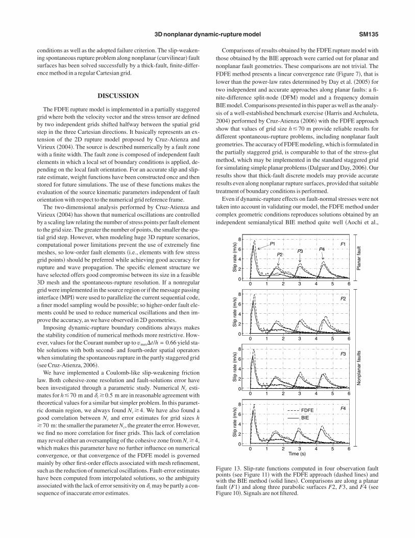
Figure 13 shows the slip-rate time series computed in four obser-ation fault points �see Figure 11� with both the FDFE �dashed lines�nd BIE �solid lines� methods. Signals are not filtered. Low frequen-y spurious oscillations appear as a result of the stress-drop rates as-ociated with the slip-weakening critical distance �c = 0.8 m. Anverestimation of the slip-rate functions with respect to the BIE ap-roach is observed systematically and translated into relative rms er-ors of about 30% in all rupture cases �Table 4�. The correspondingelative rms errors of the final slip along the entire fault surface rangeetween 15% and 25% �Table 4�, which is negligible when consider-ng the uncertainies on seismic moment determination via the wide-y used kinetic source inversions. BIE solutions with a coarser dis-retization ��s = 0.25 km� were also computed, and no relevant dif-erences from those presented here were found �Cruz-Atienza,006�. The discrepancy of slip-rate rms errors between the FDFEnd BIE methods for both BIE fault discretizations are smaller than% of total rms values, proving that the semianalytical reference so-utions used in this section basically have converged to the physicalnes.

As a whole, the reference BIE solutions are reproduced well byhe FDFE approach. These results validate our rupture-boundary

cise

gbstVweprseo

Vbttcmgrh3giamp

tebw�

lbmtrg�wmwcmshas

tnFltnBs2sdgtmfrrt

tci

FpwfF


onditions as well as the adopted failure criterion. The slip-weaken-ng spontaneous rupture problem along nonplanar �curvilinear� faulturfaces has been solved successfully by a thick-fault, finite-differ-nce method in a regular Cartesian grid.

DISCUSSION

The FDFE rupture model is implemented in a partially staggeredrid where both the velocity vector and the stress tensor are definedy two independent grids shifted halfway between the spatial gridtep in the three Cartesian directions. It basically represents an ex-ension of the 2D rupture model proposed by Cruz-Atienza andirieux �2004�. The source is described numerically by a fault zoneith a finite width. The fault zone is composed of independent fault

lements in which a local set of boundary conditions is applied, de-ending on the local fault orientation. For an accurate slip and slip-ate estimate, weight functions have been constructed once and thentored for future simulations. The use of these functions makes thevaluation of the source kinematic parameters independent of faultrientation with respect to the numerical grid reference frame.

The two-dimensional analysis performed by Cruz-Atienza andirieux �2004� has shown that numerical oscillations are controlledy a scaling law relating the number of stress points per fault elemento the grid size. The greater the number of points, the smaller the spa-ial grid step. However, when modeling huge 3D rupture scenarios,omputational power limitations prevent the use of extremely fineeshes, so low-order fault elements �i.e., elements with few stress

rid points� should be preferred while achieving good accuracy forupture and wave propagation. The specific element structure weave selected offers good compromise between its size in a feasibleD mesh and the spontaneous-rupture resolution. If a nonregularrid were implemented in the source region or if the message passingnterface �MPI� were used to parallelize the current sequential code,finer model sampling would be possible; so higher-order fault ele-ents could be used to reduce numerical oscillations and then im-

rove the accuracy, as we have observed in 2D geometries.Imposing dynamic-rupture boundary conditions always makes

he stability condition of numerical methods more restrictive. How-ver, values for the Courant number up to vmax�t/h = 0.66 yield sta-le solutions with both second- and fourth-order spatial operatorshen simulating the spontaneous rupture in the partly staggered grid

see Cruz-Atienza, 2006�.We have implemented a Coulomb-like slip-weakening friction

aw. Both cohesive-zone resolution and fault-solutions error haveeen investigated through a parametric study. Numerical Nc esti-ates for h�70 m and �c �0.5 m are in reasonable agreement with

heoretical values for a similar but simpler problem. In this paramet-ic domain region, we always found Nc �4. We have also found aood correlation between Nc and error estimates for grid sizes h70 m: the smaller the parameter Nc, the greater the error. However,e find no more correlation for finer grids. This lack of correlationay reveal either an oversampling of the cohesive zone from Nc �4,hich makes this parameter have no further influence on numerical

onvergence, or that convergence of the FDFE model is governedainly by other first-order effects associated with mesh refinement,

uch as the reduction of numerical oscillations. Fault-error estimatesave been computed from interpolated solutions, so the ambiguityssociated with the lack of error sensitivity on �c may be partly a con-equence of inaccurate error estimates.

Comparisons of results obtained by the FDFE rupture model withhose obtained by the BIE approach were carried out for planar andonplanar fault geometries. These comparisons are not trivial. TheDFE method presents a linear convergence rate �Figure 7�, that is

ower than the power-law rates determined by Day et al. �2005� forwo independent and accurate approaches along planar faults: a fi-ite-difference split-node �DFM� model and a frequency domainIE model. Comparisons presented in this paper as well as the analy-

is of a well-established benchmark exercise �Harris and Archuleta,004� performed by Cruz-Atienza �2006� with the FDFE approachhow that values of grid size h�70 m provide reliable results forifferent spontaneous-rupture problems, including nonplanar faulteometries. The accuracy of FDFE modeling, which is formulated inhe partially staggered grid, is comparable to that of the stress-glut

ethod, which may be implemented in the standard staggered gridor simulating simple planar problems �Dalguer and Day, 2006�. Ouresults show that thick-fault discrete models may provide accurateesults even along nonplanar rupture surfaces, provided that suitablereatment of boundary conditions is performed.

Even if dynamic-rupture effects on fault-normal stresses were notaken into account in validating our model, the FDFE method underomplex geometric conditions reproduces solutions obtained by anndependent semianalytical BIE method quite well �Aochi et al.,

Time (s)

FDFE

BIE

Slip

rat

e (m

/s)

Pla

nar

faul

tN

onpl

anar

faul

ts

0

P1

P2P3 P4

F1

F2

F3

F4

1 2 3 4 5 6

8

6

4

2

0

Slip

rat

e (m

/s)

0 1 2 3 4 5 6

8

6

4

2

0

Slip

rat

e (m

/s)

0 1 2 3 4 5 6

8

6

4

2

0

Slip

rat

e (m

/s)

0 1 2 3 4 5 6

8

6

4

2

0

igure 13. Slip-rate functions computed in four observation faultoints �see Figure 11� with the FDFE approach �dashed lines� andith the BIE method �solid lines�. Comparisons are along a planar

ault �F1� and along three parabolic surfaces F2, F3, and F4 �seeigure 10�. Signals are not filtered.

2aacno

encdt

aosictfr

eewnmtrue

etNtsin

mtgt

wfs

A

A

A

A

A

—

—

A

A

—

A

A

B


000b�. We notice Aochi et al. �2002� show that rupture propagationlong nonplanar faults is mainly governed by the shear-stress fieldhead of the rupture front even when the Coulomb failure criterion isonsidered. Dynamic variations of fault strength associated withormal stress changes away from the free surface only cause second-rder effects.

CONCLUSION

We have introduced a numerical method based on finite differenc-s in a partially staggered grid for modeling the dynamic rupture ofonplanar faults in three dimensions. This FDFE approach has a spe-ific way of handling boundaries in which a local set of rupture con-itions is applied, depending on both the local fault orientation andhe constitutive friction law.

The most important feature of the FDFE model is not its accuracyt a given discretization level but the ability to go beyond simple andften unrealistic planar fault geometries. This model has been de-igned for solving the dynamic rupture problem of nonplanar faultsn arbitrarily heterogeneous media. For this reason, validating it inonditions more complex than planar is fundamental. Results ob-ained for spontaneous slip-weakening ruptures along parabolicaults with a translation-invariant axis are in good agreement withesults obtained by a semianalytical BIE method.

The analysis of more realistic nonplanar fault simulations, consid-ring heterogeneous stress fields and variations on the medium prop-rties, are the next modeling target for the 3D FDFE approach,hich benefits partially staggered finite-different efficiency. Thisumerical tool may be applied for studying the dynamic develop-ent of complex microfracture networks in oil reservoirs subjected

o some regional load by analyzing the associated seismic emissionsecorded in both the earth’s surface and boreholes. It may be alsosed to analze nonplanar fault interaction and for the dynamic mod-ling of large-scale seismic events.

ACKNOWLEDGMENTS

The authors are grateful for discussions and comments of review-rs R. Madariaga and L. Dalguer, which helped us a lot in improvinghe document. The authors would also like to thank T. Rodríguez-ikl for outstanding editorial suggestions and R. Mellors for his

echnical support. This work has been partly supported by the Con-ejo Nacional de Ciencia y Tecnología �CONACyT�, Mexico, underts international fellowship program, as well as by the QSHAproject,umberANR-05-CATT-011, and the GIS CURARE.

APPENDIX A

A PARTIALLY STAGGERED SECOND-ORDER OPERATOR

If second-order centered finite differences are used to approxi-ate first-order spatial differentiations of a discrete field i,j,k along

he three Cartesian directions x, y, and z within the partially stag-ered lattice shown in Figure 1 �Saenger et al., 2000�, we get, respec-ively, the following formula:

� i,j,k

�x

1

4h� i+1/2,j+1/2,k+1/2 − i−1/2,j−1/2,k−1/2

+ i+1/2,j+1/2,k−1/2 − i−1/2,j−1/2,k+1/2

+ i+1/2,j−1/2,k+1/2 − i−1/2,j+1/2,k−1/2

+ i+1/2,j−1/2,k−1/2 − i−1/2,j+1/2,k+1/2� ,

�12a�

� i,j,k

�y

1

4h� i+1/2,j+1/2,k+1/2 − i−1/2,j−1/2,k−1/2

+ i+1/2,j+1/2,k−1/2 − i−1/2,j−1/2,k+1/2

− i+1/2,j−1/2,k+1/2 + i−1/2,j+1/2,k−1/2

− i+1/2,j−1/2,k−1/2 + i−1/2,j+1/2,k+1/2� ,

�12b�

� i,j,k

�z

1

4h� i+1/2,j+1/2,k+1/2 − i−1/2,j−1/2,k−1/2

− i+1/2,j+1/2,k−1/2 + i−1/2,j−1/2,k+1/2

+ i+1/2,j−1/2,k+1/2 − i−1/2,j+1/2,k−1/2

− i+1/2,j−1/2,k−1/2 + i−1/2,j+1/2,k+1/2� ,

�12c�

here h is the grid size of the regular mesh. The discrete expressionsor the entire system 1 with second order in time and fourth order inpace accuracies are reported by Cruz-Atienza �2006�.

REFERENCES

agaard, B., 2000, Finite-element simulation of earthquakes: Ph.D. thesis,California Institute of Technology.

dda-Bedia, M., and R., Madariaga, 2005, Dynamic rupture of a fault kink inantiplane model: EOS Transactions of the American Geophysical Union,86, S52A-01.

mpuero, J. P., J. P. Vilotte, and F.-J. Sánchez-Sesma, 2002, Nucleationof rupture under slip dependent friction law: Simple models of faultzone: Journal of Geophysical Research, 107, http://dx.doi.org/10.1029/2001JB000452.

ndo, R., T. Tada, and T. Yamashita, 2004, Dynamic evolution of a fault sys-tem through interactions between fault segments: Journal of GeophysicalResearch, 109, B05303, http://dx.doi.org/10.1029/2003JB002665.

ndrews, D. J., 1976a, Rupture propagation with finite stress in antiplanestrain: Journal of Geophysical Research, 81, 3575–3582.—–, 1976b, Rupture velocity of plane strain shear cracks: Journal of Geo-physical Research, 81, 5679–5687.—–, 2004, Rupture models with dynamically determined breakdown dis-placement: Bulletin of the Seismological Society of America, 94,769–775.

ochi, H., and E. Fukuyama, 2002, Three-dimensional nonplanar simulationof the 1992 Landers earthquake: Journal of Geophysical Research, 107,http://dx.doi.org/10.1029/2000JB000061.

ochi, H., E. Fukuyama, and M. Matsu’ura, 2000a, Selectivity of spontane-ous rupture propagation on a branched fault: Geophysical Research Let-ters, 27, 3635–3638.—–, 2000b, Spontaneous rupture propagation of on a non-planar fault in3D elastic medium: PAGEOPH, 157, 2003–2027.

ochi, H., R. Madariaga, and E. Fukuyama, 2002, Effect of normal stressduring rupture propagation along nonplanar faults: Journal of GeophysicalResearch, 107, http://dx.doi.org/10.1029/2001JB000500.

ochi, H., O. Scotti, and C. Berge-Thierry, 2005, Dynamic transfer of rup-ture across differently oriented segments in a complex 3-D fault system:Geophysical Research Letters, 32, http://dx.doi.org/10.1029/2005GL024158.

arenblatt, G. I., 1959, Concerning equilibrium cracks forming during brittle

B

B

C

C

C

C

C

D

D

D

D

E

G

H

I

K

M

M

M

M

M

M

—

O

O

O

P

R

S

S

S

V

V

V

Z


fracture: The stability of isolated cracks, relationships with energetic theo-ries: Journal ofApplied Mathematics and Mechanics, 23, 1273–1282.

enjemaa, M., N. Glinsky-Olivier, V. M. Cruz-Atienza, J. Virieux, and S.Piperno, 2007, Dynamic non-planar crack rupture by a finite volume meth-od: Geophysical Journal International, http://dx.doi.org/10.1111/j.1365–246X.2006.03500.x.

erenger, J. P., 1994, Aperfectly matched layer for the absorption of electro-magnetic waves: Journal of Computational Physics, 114, 185–200.

ollino, F., and C. Tsogka, 2001, Application of the perfectly matched ab-sorbing layer model to the linear elastodynamic problem in anisotropicheterogeneous media: Geophysics, 66, 294–307.

ruz-Atienza, V. M., 2006, Rupture dynamique des faille non-planaires endifférences finies: Ph.D. thesis, University of Nice Sophia.

ruz-Atienza, V. M., and J. Virieux, 2004, Dynamic rupture simulation ofnon-planar faults with a finite-difference approach: Geophysical JournalInternational, 158, 939–954.

ruz-Atienza, V. M., J. Virieux, H. Aochi, and S. Peyrat, 2004, 3D non-pla-nar finite difference dynamic rupture: Application to the Landers earth-quake: Geophysical Journal International, 158, 939–954.

ruz-Atienza, V. M., J. Virieux, and S. Operto, 2002, Dynamic rupture simu-lation of bending faults with a finite difference approach: EOS Transac-tions of theAmerican Geophysical Union, 83, NG21B-0941.

alguer, L. A., and S. M. Day, 2006, Comparison of fault representationmethods in finite difference simulations of dynamic rupture: Bulletin ofthe Seismological Society ofAmerica, 96, 1764–1778.

as, S., and K. Aki, 1977, A numerical study of two-dimensional spontane-ous rupture propagation: Geophysical Journal of the Royal AstronomicalSociety, 50, 643–668.

ay, S. M., 1982, Three-dimensional simulation of spontaneous rupture: Theeffect of nonuniform prestress: Bulletin of the Seismological Society ofAmerica, 72, 1881–1902.

ay, S. M., L. A. Dalguer, N. Lapusta, and Y. Liu, 2005, Comparison of finitedifference and boundary integral solutions to three-dimensional spon-taneous rupture: Journal of Geophysical Research, 110, B12307, http://dx.doi.org/10.1029/2005JB003813.

ly, G., B. Minster, and S. Day, 2006, Large scale dynamic rupture modelingwith realistic geometry: EOS Transactions of the American GeophysicalUnion, 87, S41C-1350.

riffith, A. A., 1920, The phenomena of rupture and flow in solids: Philo-sophical Transactions of the Royal Society of London, A221, 163–198.

arris, R. A., and R. J. Archuleta, 2004, Earthquake rupture dynamics: Com-paring the numerical simulation methods: EOS, 85, 321.

da, Y., 1972, Cohesive force across the tip of a longitudinal-shear crack andgriffith’s specific surface energy: Journal of Geophysical Research, 77,3796–3805.

ame, N., J. Rice, and R. Dmowska, 2003, Effect of prestress state and rup-ture velocity on dynamic fault branching: Journal of Geophysical Re-search, 108, http://dx.doi.org/10.1029/2002JB002189.adariaga, R., 1976, Dynamics of an expanding circular fault: Bulletin ofthe Seismological Society ofAmerica, 66, 639–666.adariaga, R., and J. Ampuero, 2005, Rupture dynamics of a geometrically
complex fault: EOS Transactions of theAmerican Geophysical Union, 86,
S34A-01.adariaga, R., and K. B. Olsen, 2000, Criticality of rupture dynamics in 3-D:Pure andApplied Geophysics, 157, 1981–2001.adariaga, R., K. B. Olsen, and R. J. Archuleta, 1998, Modeling dynamicrupture in a 3D earthquake fault model: Bulletin of the Seismological So-ciety ofAmerica, 88, 1182–1197.arcinkovich, C., and K. Olsen, 2003, On the implementation of perfectlymatched layers in a three-dimensional fourth-order velocity-stress finitedifference scheme: Journal of Geophysical Research, 108, http://dx-.doi.org/10.1029/2002GB002235.ikumo, T., and T. Miyatake, 1978, Dynamical rupture process on a three-dimensional fault with non-uniform frictions and near field seismic waves:Geophysical Journal of the RoyalAstronomical Society, 54, 417–438.—–, 1993, Dynamic rupture processes on a dipping fault, and estimate ofstress drop and strength excess from the results of waveform inversion:Geophysical Journal International, 112, 481–496.

glesby, D., 1999, Earthquake dynamics on dip-slip faults: Ph.D. thesis,University of California.

glesby, D. D., S. M. Day, and D. R. H. O’Connell, 2003, Dynamic andstatic interaction of two thrust faults: A case study with general implica-tions: Journal of Geophysical Research, 108, http://dx.doi.org/10.1029/2002JB002228.

lsen, K. B., R. Madariaga, and R. J. Archuleta, 1997, Three-dimensionaldynamic simulation of the 1992 Landers earthquake: Science, 278,834–838.

almer, A., and J. R. Rice, 1973, The grow of slip surfaces in the progressivefailure of overconsolidated clay: Proceedings of the Royal Society of Lon-don, seriesA, 332, 527–548.

oyer, J.-J., and J.-C. Voillemont, 2005, Estimating heterogeneous reservoirpermeability from induced microseismicity: 75th Annual InternationalMeeting, SEG, ExpandedAbstracts, 1393–1396.

aenger, E. H., N. Gold, and S. A. Shapiro, 2000, Modeling the propagationof elastic waves using a modified finite-difference grid: Wave Motion, 31,77–92.

hapiro, S. A., S. Rentsch, and E. Rothert, 2005, Characterization of hydrau-lic properties of rocks using probability of fluid-induced microearth-quakes: Geophysics, 70, no. 2, F27–F34.

hapiro, S. A., E. Rothert, V. Rathz, and J. Rindschwentner, 2002, Character-ization of fluid transport properties of reservoirs using induced microseis-micity: Geophysics, 67, 212–220.

ilotte, J., G. Festa, and R. Madariaga, 2005, Spectral element simulations ofrupture dynamics along kinked faults: EOS Transactions of the AmericanGeophysical Union, 86, S34A-02.

irieux, J., 1986, P-SV wave propagation in heterogeneous media, velocity-stress finite difference method: Geophysics, 51, 889–901.

irieux, J., and R. Madariaga, 1982, Dynamic faulting studied by a finite dif-ference method: Bulletin of the Seismological Society of America, 72,345–369.

hang, W., T. Iwata, and K. Irikura, 2006, Dynamic simulation of a dippingfault using a three-dimensional finite difference method with nonuniformgrid spacing: Journal of Geophysical Research, 111, B05301, http://
dx.doi.org/10.1029/2005JB003725.

3D finite-difference dynamic-rupture modeling along nonplanar faults

Documents

Transcript of 3D finite-difference dynamic-rupture modeling along nonplanar faults