at SciVerse ScienceDirect

Animal Behaviour 85 (2013) 483e492

Contents lists available

Animal Behaviour

journal homepage: www.elsevier .com/locate/anbehav

Analysing small-scale aggregation in animal visits in space and time:the ST-BBD method

Tyler R. Bonnell a,*, Pierre Dutilleul b, Colin A. Chapman c,d, Rafael Reyna-Hurtado e,Raul Uriel Hernández-Sarabia f, Raja Sengupta a

aDepartment of Geography, McGill University, Montreal, QC, CanadabDepartment of Plant Science, McGill University, Montreal, QC, CanadacDepartment of Anthropology & McGill School of Environment, McGill University, Montreal, QC, CanadadWildlife Conservation Society, Bronx, NY, U.S.A.e EL Colegio de la Frontera Sur ECOSUR, Unidad Campeche, Campeche, MexicofUniversidad Veracruzana, Departamento de Neuroetología, Xalapa, Veracruz, Mexico

a r t i c l e i n f o

Article history:Received 13 July 2012Initial acceptance 19 September 2012Final acceptance 28 November 2012Available online 9 January 2013MS. number: A12-00542R

Keywords:agent-based modelanimal movementbeta-binomial distributionfolivorefrugivorehabitat usemonkeysmall-scale aggregationspatiotemporal point pattern analysis

* Correspondence: T. R. Bonnell, Department of G805 Sherbrooke Street West, Montreal, QC H3A 0B9,

E-mail address: tyler.bonnell@mail.mcgill.ca (T. R.

0003-3472/$38.00 � 2012 The Association for the Stuhttp://dx.doi.org/10.1016/j.anbehav.2012.12.014

Movement behaviour plays an important role in many ecological interactions. As animals move throughthe environment, they generate movement patterns, which are a combined result of landscape charac-teristics and species-specific behaviour. Measuring these ranging patterns is being facilitated by tech-nological advances in collection methods, such as GPS collars, that are capturing movement on finerspatial and temporal scales. We propose the use of a novel spatiotemporal analytical framework(ST-BBD), based on the beta-binomial distribution (BBD) model, to measure small-scale aggregation inanimal movement data sets, including two simulated and three collected primate data sets. We use thisapproach to distinguish different habitat uses of three primate species (red colobus, Procolobus rufomi-tratus, black howler, Alouatta pigra, and spider monkey, Ateles geoffroyi) and quantify their specific use ofthe landscape in space and in time, using a parameter of the BBD that measures the variation in sitesvisited on a landscape. We found that estimates of aggregation in habitat use were higher in thefrugivorous spider monkey, compared to the more folivorous howler monkey, and that in the redcolobus, aggregation in site visits was dependent on group size and food availability. Applications of thisframework to animal movement data could be useful in understanding ecological systems where habitatuse is an important factor, such as the relationships between hosts and parasites, or parent plants andseed dispersers.� 2012 The Association for the Study of Animal Behaviour. Published by Elsevier Ltd. All rights reserved.

Movement is a vital process for many animals, affecting a broadspectrum of ecological processes and patterns observed in nature(Nathan et al. 2008). The study of animal movement behaviour hasled to much insight into such fields as foraging ecology (Orians &Pearson 1979; Humphries et al. 2010), wildlife management(Chetkiewicz et al. 2006), plant seed dispersal (Vellend et al. 2003)and disease dynamics (Bartel et al. 2011).

With technological advances providing the increasing availabilityof high-resolution animal movement data, both in time and in space,there is a need to advance methodologies for analysing movementdata. Movement is a spatiotemporal process in which an animalmovesoveraheterogeneous landscape through time. Thus, states and

eography, McGill University,Canada.Bonnell).

dy of Animal Behaviour. Published

conditions of both the animal in question and the landscape arecontinuously changing. Different methods have been developed tomeasure movement characteristics, each capturing some aspect ofmovement. These different measurements can be separateddepending onwhether the focus is on space, time, or space and time.

One main branch of spatial approaches focuses on point patternanalysis,wheremovementdataare treatedas (x,y) locationsmeasuredin a two-dimensional space (e.g. home range; Millspaugh et al. 2004).These methods search for patterns, or structure, in the distribution ofpoints, which can provide insight into the behavioural ecology of thestudy species. Another, more complete approach is followed whena temporal component is added to points, tying them together by thesequence inwhich theyweremeasured. This approach is characterizedby themeasurement of ‘between-step characteristics’ (e.g. step lengthor angle) at similar time periods. In analysing between-stepmeasurements, the results are often compared to theoretical distri-butions as a means of interpretation, such as the Lévy walk, random

by Elsevier Ltd. All rights reserved.

T. R. Bonnell et al. / Animal Behaviour 85 (2013) 483e492484

walk or correlated-random walk (Viswanathan et al. 1996; Edwardset al. 2007; Humphries et al. 2010). Methods focusing more specifi-cally on the temporal aspects of the data havemade use of time seriesanalysis, in which between-step measures (e.g. distance or turningangle) are examined through time to test for autocorrelation inmovementbehaviour (Drayetal. 2010).Kernelmethodshavealsobeenapplied, classically to (x, y) locations in two-dimensional space, toderive the probability of occurrence on a landscape, and has recentlybeen extended to estimate probability of occurrence in space and time(Keating & Cherry 2009).

Using animal movement data, we were interested in developinga measure to characterize an animal’s use of habitats; specifically, tomeasure the spatiotemporal variation in use of sites within a habitat.In examiningmovement data, or following an animal in the field, it isoften apparent that some sites are used more intensely and moreoften than others. It is possible that there exists a cyclical pattern ofsite use, one based on seasons or depletionereplenishment ofresources, so that the animal in questionmayormay not followalongsimilar routes on the landscape. The relevant method should allowthe estimation of variation in these patterns of habitat use in spaceand time, and provide a statistically soundway to test for differences,for example, among comparable species. Existing approaches toexamine spatiotemporal variation (e.g.Mantel test and correlograms;see below, Variability and Autocorrelation in Animal Visits ofa Landscape) do not capture and compare variation betweenspecific areas and periods, and as a whole are more global than thesmall-scale focus desired here. Therefore, we evaluated a newapproach that uses the beta-binomial distribution (BBD) in a frame-work where a spatiotemporal grid is created to measure habitat use.Basically, the spaceandtime inwhich theanimal ismovingarebrokeninto spaceetime cubes inwhicheitherpresenceorabsenceof passage(i.e. Bernoulli trial) is recorded. Spaceetime cubes have been intro-duced as sampling units in thefield of time geography, and have beenused to map spatiotemporal data for subsequent analysis (Miller2005). Subdividing the spaceetime cubes into cells within samplingunits following the BBD opens the door to the quantification ofspatiotemporal aggregation at smaller scales.

The BBDwas applied by Hughes & Madden (1993) in an epidemi-ological context for investigating the aggregationof diseasedplants onagricultural landscapes. These authors showed that when there isuneven chance of finding an infected plant through the landscape (i.e.it is more likely to find an infected plant near another infected plant),the BBD can be useful in quantifying the spatial aggregation of infec-tion occurrences. In a spatiotemporal context, the BBD has been sug-gested for usewith animalmovement data (Dutilleul 2011, Chapter 4).In this approach, Dutilleul (2011) proposes an extension on theframework ofMadden&Hughes (1995) that consists inmeasuring thedisplacementof a spatial unit (i.e. point) through timeandquantifyingthe aggregation of visited areas in space and time.

The objective of our paper is to evaluate the spatiotemporalversion of the BBD framework (ST-BBD hereafter), as a tool to esti-mate the intensity to which an animal uses its home range. We firstapply the ST-BBD framework to primate movement data simulatedunder two behaviour models. We then apply it to movement datacollected for three primate species in the field, and quantify theintensity of habitat use within each species and compare it betweenspecies. The three species chosen vary in the degrees of frugivory andfolivory: spider monkeys, Ateles geoffroyi, rely heavily on fruitresources (frugivorous), whereas howler monkeys, Alouatta pigra,and red colobus, Procolobus rufomitratus, typically rely on leaves(folivorous). Foraging for fruits in a tropical forest requires findingthe few dispersed trees that produce fruit intermittently. Bycomparison, when foraging for good-quality leaves, trees arethought to be less dispersed, offering food more often than do fruittrees. Given the varying distribution of resources, both spatially and

temporally, we used the ST-BBD framework to quantify spatiotem-poral aggregation accordingly and determine differences in habitatuse by these two folivorous and one frugivorous primate species.

Data Sets

Simulated dataWe first simulated movement data with an agent-based model

(ABM) of primate group foraging, which approximates primategroup movement behaviour for use in a spatially explicit epide-miological study (Bonnell et al. 2010). In general, ABMs definecharacteristics and behaviours of individual agents (e.g. primates,fish, farmers, companies) within a simulation environment, andallow them to interact to create system-level outcomes (for use ofABM in behavioural studies, see: Hemelrijk 2002; Bryson et al.2007). The ABM here was constructed as a general model, madeto fit a wide range of primate group foraging behaviours. In thisstudy, we focus on the effect that a foraging trait called ‘weight ofremembered sites’ has on overall movement behaviour. This trait isa key model component that affects each primate’s foraging deci-sion making. In the model, the primate agents use a food site indexto assess which site, seen or remembered, is the best site to movetowards. This food site index is based on the expected amount offood and the distance to such sites, while the parameter ‘weight ofremembered sites’ gives extra weight to sites that are familiar (i.e.remembered) to the primate agent (equation 1).

The food site index value at site (x0, y0) from site (x, y) is given by

Iðx0; y0Þ ¼ Dððx0; y0Þ; ðx; yÞÞFðx0; y0Þ*w (1)

where D($) represents the Euclidean distance between two points,F($) is the primate’s evaluation of the amount of food at a given site,and w is the weight parameter applied to remembered sites.

When preference for remembered sites is increased, simulatedprimates tend to use selected sites intensively, visiting familiar sitesoften, and travelling along similar routes connecting these sites. Wewill thus refer to this behaviour model as the ‘routing model’,because it creates travel routes. On the other hand, with low pref-erence for remembered sites, groups show nonspecific rangingbehaviours and no heavy use of a specific area. Accordingly, we willrefer to that behaviour model as the ‘nonrouting model’.

For each type of model, one simulated group of primates (groupsize¼ 72) was made to forage on a 1.5� 1.5 km landscape for 6months. Movement data were recorded for 5 months, after the firstmonth was discounted to sufficiently initialize the memory of indi-viduals in the simulated group. The position of the simulated groupwas taken every 30min during the active hours of the day (0700e2000 hours), and recorded as a point (x, y) with a time component(t). The 30min interval was selected because it is very feasiblelogistically speaking and is therefore often used in field studies(Chapman et al. 2002), and it is a crude time period to avoid auto-correlation given the distances animals can cover in half an hour(Reyna-Hurtado et al. 2009). With the chosen total duration(5 months) and sampling time interval (30 min), the final set of simu-lateddatawas composed of twopoint patterns, eachwith 3900pointlocations in spaceetime (Fig. 1).

Collected dataOur second data source consists of GPS points or tracks taken

from field measurements of primate group movement. We makeuse of movement data collected from a highly folivorous primate(red colobus), a folivoreefrugivore primate (black howler), anda highly frugivorous primate (spider monkey). Red colobus datawere collected from August 2006 to June 2010 in Kibale National

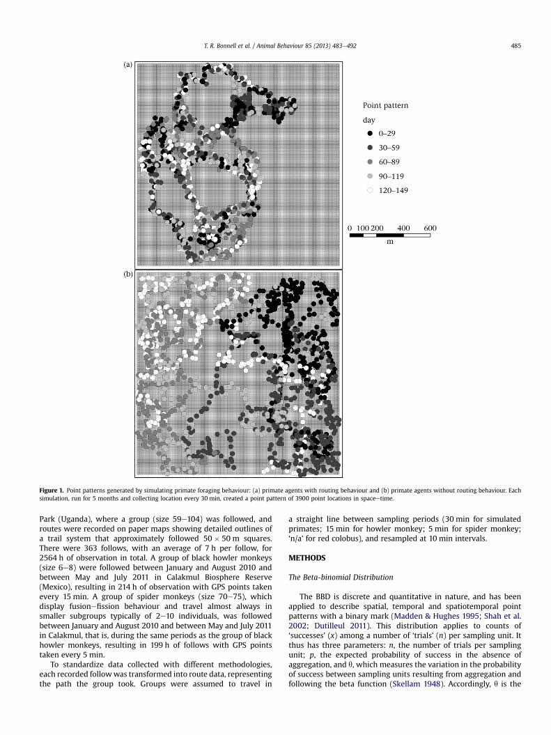
Figure 1. Point patterns generated by simulating primate foraging behaviour: (a) primate agents with routing behaviour and (b) primate agents without routing behaviour. Eachsimulation, run for 5 months and collecting location every 30 min, created a point pattern of 3900 point locations in spaceetime.

T. R. Bonnell et al. / Animal Behaviour 85 (2013) 483e492 485

Park (Uganda), where a group (size 59e104) was followed, androutes were recorded on paper maps showing detailed outlines ofa trail system that approximately followed 50 � 50 m squares.There were 363 follows, with an average of 7 h per follow, for2564 h of observation in total. A group of black howler monkeys(size 6e8) were followed between January and August 2010 andbetween May and July 2011 in Calakmul Biosphere Reserve(Mexico), resulting in 214 h of observation with GPS points takenevery 15 min. A group of spider monkeys (size 70e75), whichdisplay fusionefission behaviour and travel almost always insmaller subgroups typically of 2e10 individuals, was followedbetween January and August 2010 and between May and July 2011in Calakmul, that is, during the same periods as the group of blackhowler monkeys, resulting in 199 h of follows with GPS pointstaken every 5 min.

To standardize data collected with different methodologies,each recorded followwas transformed into route data, representingthe path the group took. Groups were assumed to travel in

a straight line between sampling periods (30 min for simulatedprimates; 15 min for howler monkey; 5 min for spider monkey;‘n/a’ for red colobus), and resampled at 10 min intervals.

METHODS

The Beta-binomial Distribution

The BBD is discrete and quantitative in nature, and has beenapplied to describe spatial, temporal and spatiotemporal pointpatterns with a binary mark (Madden & Hughes 1995; Shah et al.2002; Dutilleul 2011). This distribution applies to counts of‘successes’ (x) among a number of ‘trials’ (n) per sampling unit. Itthus has three parameters: n, the number of trials per samplingunit; p, the expected probability of success in the absence ofaggregation, and q, which measures the variation in the probabilityof success between sampling units resulting from aggregation andfollowing the beta function (Skellam 1948). Accordingly, q is the

T. R. Bonnell et al. / Animal Behaviour 85 (2013) 483e492486

aggregation index parameter (Griffiths 1973; Madden & Hughes1995). The probability function of the BBD is given by

PðX ¼ xÞ ¼ n!x!ðn� xÞ!

Yxi¼1

ðpþ ði� 1ÞqÞYn�x

i¼1

ð1� pþ ði� 1ÞqÞ

Yni¼1

ð1þ ði� 1ÞqÞ

for x ¼ 0;1;2;.; n

(2)

where ! denotes the factorial function;Q

is the multiplicationoperator; P(X ¼ x) is the probability of x successes occurring in ntrials. The mean and variance parameters of the BBD are np andnp(1 � p)(1 þ nq)/(1 þ q), respectively (Madden & Hughes 1995). Inthe context of the application of the BBD to analysemovement data,sampling units can be seen as N quadrats of equal area, into whichthe landscape is first divided and where movement is beingobserved. Each of the quadrats is then subdivided into n cells ofequal area. A cell that has been visited at least once by an animal isconsidered as ‘visited’, and x represents the number of such cells(x ¼ 0, 1, 2, ., n) (Fig. 2). Thus, the landscape is divided intoquadrats where the probability of success (i.e. chance of beingvisited) may be higher or lower depending on the quadrat. Themagnitude of this variation in visit frequency is measured by q,which can also be used as an aggregation index in the analysis ofhabitat use. This measure of aggregation does not capture thespatial relationships between quadrat counts, but captures thevariability in the counts themselves (i.e. how variable are visits on

Extent 1.5 x 1.5 km(2500 quadrats)

Month 1 Month 2 Month 3

Cell (n)10 x 10 m

Within quadrat

Landscape

Figure 2. Diagram of the spatiotemporal analytical framework (ST-BBD), based on the beta-bsized quadrats (N ¼ 2500, 30 � 30 m), quadrats are then subdivided into cells (n ¼ 9, 10 �visited during each time period are combined to provide the final visit count per quadrat.

the landscape, and is the variation greater than expected if therewere no aggregation?).

The addition of a temporal component to this approach was firstsuggested by Dutilleul (2011, Chapter 4), and consists in furthersubdividing the data set into equal time units (e.g. days, months,years), making each quadrat a spaceetime cube. It follows that thenumber of quadrats (N) remains the same, but the total number ofcells is equal to the number of cells within a quadrat multiplied bythe number of temporal divisions. Accordingly, the point patterncan be analysed temporally, by counting the number of visits pertime period (i.e. visits in month 1 are counted on the first layer ofcells, visits in month 2 in the second layer, etc.; Fig. 2).

Variability and Autocorrelation in Animal Visits of a Landscape

The variance parameter of a beta-binomial distribution iscalculated differently than that for a binomial distribution becausethe calculation of the former does not assume that the ‘trials’ areindependent (i.e. an animal’s visits of cells within a quadrat can becorrelated). If Yi denotes the Bernoulli distribution (visit/no visit)for cell i ¼ 1, ., n in a given quadrat, X denotes the number of cellsvisited within the quadrat and X follows a BBD, then

VarðXÞ ¼ Var

Xni¼1

Yi

!þ 2

Xni¼1

Xnj¼ iþ1

Cov�Yi; Yj

�

¼ npð1� pÞ ð1þ nqÞð1þ qÞ

(3)

After isolating the covariances and standardizing them intocorrelations, it becomes clear that the autocorrelation within

Quadrat (N)30 x 30 m

Month 4 Month 5 Combined

inomial distribution (BBD). In this example, the landscape is first subdivided into equal-10 m), and time is divided into equal units (1 month). Within each quadrat, the cells

T. R. Bonnell et al. / Animal Behaviour 85 (2013) 483e492 487

a quadrat, through the correlations between visits and no visits ofcells, is a function of n and q:

2Xni¼1

Xnj¼ iþ1

Corr�Yi; Yj

� ¼ ð1þ qÞð1þ nqÞ � 1 (4)

Accordingly, q can be said to be a measure of the autocorrelationof animal movement within quadrats, and as the variability inquadrat counts grows, so too will the autocorrelation between cellvisits within quadrats. If n remains constant in the proposedspatiotemporal framework, the parameter q can thus be used toanswer the following question: ‘If a primate has visited a quadratbefore, is it more likely to visit it again?’

Another approach, based on the so-called ‘Mantel correlograms’,has been proposed to characterize autocorrelation in animalmovement data sets (Cushman et al. 2005); theMantel correlogramwas originally derived by Oden & Sokal (1986) and Sokal (1986)from Mantel’s (1967) test statistic. Whereas the Mantel teststatistic essentially is a correlation coefficient between spatialdistances and corresponding temporal distances (e.g. times takenduring travels), the hypotheses tested in the analysis of Mantelcorrelograms concern differences in mean time travelled amonga certain number of spatial distance classes (Dutilleul et al. 2000,page 149). This approach has been used to assess how reliant thecurrent movement is on past movements (Cushman et al. 2005).The ST-BBD method proposed here and the Mantel correlogramsmeasure autocorrelation in two different aspects of the samephenomenon: habitat use (ST-BBD) versus movement patterns(Mantel correlograms). Given the application or question ofinterest, it would be important to know which type of autocorre-lation it would be better to measure. To highlight the differences inthe two approaches, consider an example in which the resultswould be drastically different. If animals travelled in paths thatwere similar to previous paths, but were shifted in space, thiswould result in a significant result in the Mantel test (relationshipbetween distances in space and time), whereas in the ST-BBDapproach, since paths did not pass over the same area, it wouldmeasure no small-scale aggregation (habitat use).

Variograms and spatial correlograms based on Moran’s I andGeary’s c statistics (instead of Mantel’s test statistic) can be used toanalyse and quantify autocorrelation among quadrats, using thenumber of cells per quadrat visited by animals as raw data orquadrat counts (Madden & Hughes 1995; Dutilleul 2011, Chapter 5).This is likely to be an important factor to consider when addressingquestions related to the definition of quadrat size and how theprobability of quadrat visit varies with landscape properties (seebelow).

Implementation of the Spatiotemporal BBD Framework

To create the ST-BBD framework, a program was written in theJava programing language with GeoTools (geotools.org), in whichthe movement data (e.g. route data) and grid characteristics (i.e.number of quadrats, quadrat and cell sizes, temporal division) arethe inputs. The program uses the scale inputs provided by the userto generate a spatiotemporal sampling framework, and outputs thenumber of cells visited in each quadrat. The analysis of the quadratcounts was then performed with the SAS v.9.2 software (SASInstitute, Chicago, IL, U.S.A.), using a code graciously provided by L.V. Madden, as well as in the R programing language. The SAS codecalls the procedure NLMIXED to fit the BBD to the count data ofvisits per quadrat, where the estimation of p and q is performed bymaximum likelihood. The Bayesian Information Criterion (BIC),a measure of the goodness of fit of a model that incorporatesa relevant penalty for the number of parameters (Schwarz 1978),

was used to determine whether the BBD was more appropriatethan the binomial distribution. When this was found to be the case,it meant there was sufficient aggregation in the movement data towarrant the use of the BBD.

Analyses

We first evaluated the ST-BBD framework by applying it to thesimulated data, using a timescale of 30 days and a spatial grid of50 � 50 quadrats (30 � 30 m each), with 3 � 3 cells (10 � 10 meach). The simulated data are controlled in terms of samplingregimes, and include very different movement behaviours, offeringideal data sets to explore the use of the new framework.

We then applied the ST-BBD framework to estimate the levels ofaggregation in monthly movement data from the three primatespecies individually to analyse within-species variation. To controlfor differences in sampling effort between months, monthlymovement patterns were first produced from five follows withineach month. Movement patterns were then sampled usinga minimum bounding grid, with 30 � 30 m quadrats subdividedinto nine 10 � 10 m cells, to obtain visit counts per quadrat for thered colobus and the howler monkey (ranges of spatial autocorre-lation in counts: red colobus, 51 m; howler monkey, 47 m); thespider monkey was sampled with 60 � 60 m quadrats subdividedinto 36 10 � 10 m cells (range of spatial autocorrelation in counts:80 m). For the red colobus, we estimated monthly aggregationwithin 3-month periods. For the howler and spider monkeys,monthly aggregationwas estimated within 2-month periods due tosmaller samples sizes.

To compare levels of habitat use between species, samplingeffort was controlled by resampling species data to equal obser-vation times. Given the limited data available for the spider andhowler monkeys (FebruaryeApril, June and July), a time spancovering 5 months was chosen. A subsample was taken from eachprimate species, resulting in an average of 176 h of follows for eachprimate (howlermonkey: 174 h, spidermonkey: 177 h, red colobus:178 h). A minimum bounding grid of 25 � 25 quadrats (60 � 60 m),with 6 � 6 cells (10 � 10 m), was used to obtain spatial andtemporal counts for each species (Fig. 2).

Comparisons between q estimates, obtained by maximumlikelihood, are based on 95% confidence intervals, assuming esti-mates are normally distributed (i.e. an asymptotic property ofmaximum likelihood estimators).

RESULTS

Simulated Data

Movement data generated with the routing model producedquadrat counts inwhich a few quadrats had a high number of visitsand many quadrats had zero visits (Fig. 3). Comparatively, move-ment data generated with the nonrouting model produced morequadrats with low numbers of visits and less quadrats with highnumbers of visits, but fewer quadrats with no visits (Fig. 3).

When fitting the BBD to quadrat counts, we found that the BBDconsistently fitted better than the binomial distribution, indicatingaggregation in the data (i.e. the probability of visit was uneventhroughout the landscape; Table 1). This difference was lessstriking, though, in the data simulated with the nonrouting model(Table 1). At the scale of 1 month, when considering movementpatterns for each month separately (purely spatial analysis), therewas no consistent trend in the aggregation index estimates fromthe two simulated movement data sets (Fig. 4). When consideringall 5 months together (spatiotemporal analysis), the differencebetween the two estimated measures of aggregation was

2000

Routing

Nonrouting

1500

1000

500

00 1 2 3 4 5 6

Visits per quadrat

Freq

uen

cy

7 8 9 10

Figure 3. Histograms of the number of visits within quadrats for the simulated data,obtained with the routing versus nonrouting model. A count of visits for each quadratwas done each month (n ¼ 9 cells), then all 5 months were combined for the finalquadrat count presented in this figure (n ¼ 45 cells).

T. R. Bonnell et al. / Animal Behaviour 85 (2013) 483e492488

statistically significant (Fig. 4), the estimate dropping in the case ofthe nonrouting model (88% lower) compared to the routing model(10% lower); this result clearly reflects the amount of overlapbetween months in the latter case.

Collected Data

To obtain visit counts per quadrat, themovement patterns of thethree primate species were sampled for an appropriate quadrat sizetaking into account differences in spatial autocorrelation and fieldextent (Fig. 5). Monthly estimates of the visit aggregation index forthe red colobus were made for all the months with more than fivefollows per month (35 months in total; Fig. 6a). Estimates werethen computed over 3-month periods, capturing habitat reuse bythe red colobus between months (Fig. 6b). This revealed largefluctuations in aggregation over time, with a peak of index esti-mates in AugusteFebruary 2008 (Fig. 6b). The estimated aggrega-tion index for all months combined, capturing habitat reuse overthe 35 months, was 0.076, that is, 63% lower than the mean (0.204)of estimates over 3-month periods. Sampling effort was notsignificantly correlated with movement aggregation index esti-mates (Spearman rank correlation: rS ¼ 0.32, sample size ¼ 35,P ¼ 0.07).

Spider monkey movement data showed significantly higherlevels of aggregation during the dry season (MarcheApril) than

Table 1Estimates of the index of aggregation parameter (q) for the data simulated using twobehaviour models: considering individual months and combined months (All)

Month Binomial(BIC)

Beta-binomial(BIC)

q Lower95% CI

Upper95% CI

Meannp

Nonrouting behaviour model1st 2224.3 2043.9 0.085 0.058 0.111 0.1372nd 2081.4 2014.6 0.042 0.026 0.059 0.1303rd 1858.8 1750.4 0.063 0.040 0.086 0.1084th 1798.7 1764.5 0.031 0.016 0.046 0.1075th 2001.7 1911.8 0.052 0.032 0.071 0.121All 5524.2 5321.7 0.012 0.010 0.015 0.603Routing behaviour model1st 1891.9 1786.2 0.061 0.038 0.083 0.1112nd 2066.6 1934 0.067 0.044 0.090 0.1253rd 1912.6 1734.4 0.092 0.062 0.123 0.1104th 1819.2 1750.8 0.046 0.027 0.065 0.1075th 1780.5 1729.7 0.039 0.022 0.056 0.104All 6080.2 4737.9 0.055 0.046 0.064 0.554

The Bayesian information criterion (BIC) is presented for the fitted beta-binomialand binomial distributions; lower scores imply a better fit.

during the wet season (JulyeAug) (95% CI for the differencebetween 2-month means: MarcheApril and JulyeAug ¼ 0.058,0.358). The aggregation index estimated by using all months was0.12, that is, 54% lower than the mean (0.27) of 2-month estimates(Fig. 6c). Sampling effort was not correlated with movementaggregation index estimates (Spearman rank correlation: rS ¼ 0.50,sample size ¼ 5, P ¼ 0.45).

Howler monkey movement data showed no significant differ-ence in aggregation between months, February versus March andMarch versus April (Fig. 6d). The month of April had a total of 36 h,compared to 37 h in March and 40 h in February. The overall esti-mate of aggregation was 0.23, that is, 22% lower than the mean(0.29) of 2-month estimates.

In between-species comparisons, movement aggregation of thespider monkey (mean index value: 0.192) differed from that of thehowler monkey (mean: 0.107) (Table 2). The value for red colobusfell between these values, with a mean aggregation index of 0.157(Table 2). Again, raising the temporal scale to 5 months (as with thesimulated data; see Fig. 4), the aggregation index estimates drop-ped compared to the average of individual monthly estimates for allthree species (red colobus 45%, spider monkey 38%, and howlermonkey 33%).

DISCUSSION

Within the ST-BBD framework, movement behaviour thatfrequently reuses specific areas results in higher variation in theprobability of visits on the landscape. Movement behaviour thatdoes not reuse the same areas results in lower values and variabilityof the probability of visits on the landscape. Using the BBDparameter q, alias ‘aggregation index’, as a measure of this vari-ability, we were able to quantify differences in habitat use andassess their significance.

The differences in movement behaviour between the routing andnonrouting models were successfully distinguished as a result of thespatiotemporal nature of the ST-BBD. By breaking up space intospaceetime cubes, movement patterns that overlapped in the samequadrat at different times were captured. In contrast, the purelyspatial approach, in which no temporal component was considered,did not reveal important differences between models. This wasshown with simulated data, by comparing monthly estimates of qwith ‘combined’ estimates obtained over 5 months (Fig. 4).

The spatiotemporal approach, which incorporates an overlap ofmonths, was useful in distinguishing movement behaviours withineach primate species (Fig. 5). In the case of the red colobus, itallowed the detection of significant fluctuations through time,a peak in aggregation centred on August 2007eFebruary 2008, anda slight decrease overall in the aggregation of movement patternson a monthly basis, suggesting a decrease in revisits to similar sitesbetween months over a long period (Fig. 6b). Spider monkeysshowed a significantly higher level of aggregation during the dryseason. This could be a consequence of the high use of a single treespecies (Ficus spp.) during the dry season, whereas fruit resourcesin the wet season are generally highly available due to the mastfructification of another highly preferred species (Brosimum ali-castrum: R. U. Hernández-Sarabia, unpublished data). Similarsignificant variation was not found within the howler monkeymovement patterns (Fig. 6d).

Comparisons between the three species showed that spidermonkeys had the highest movement aggregation (Table 2). Overall,spider monkeys travelled farther (w34.8 km during the 177 hsubsample) than howler monkeys (w5.3 km) and red colobus(w4.5 km). Such interspecific differences are likely partiallyinduced by the more dispersed food sources for frugivorousprimates. The spider monkey movement patterns suggest the

0.14

0.12

0.1

0.08

0.06

0.04

0.02

Routing behaviour

Ind

ex o

f ag

greg

atio

n (

θ)

Nonrouting behaviour

0

M.1

M.2

M.3

M.4

M.5

Combi

ned M.1

M.2

M.3

M.4

M.5

Combi

ned

Figure 4. Aggregation index estimates for each month (n ¼ 9, N ¼ 2500) and for all 5 months combined (n ¼ 45, N ¼ 2500), for both types of simulated movement behaviour. Barsrepresent 95% confidence intervals.

T. R. Bonnell et al. / Animal Behaviour 85 (2013) 483e492 489

heavy use of a central area (sleeping sites), with forays to theperiphery, suggesting a central foraging strategy (Chapman 1988).The fact that spider monkeys started at, and often returned to, a fewmain sleeping areas each night resulted in a few quadrats withhigher numbers of visits. Routing behaviour was evident in themovement from and to these central areas (Fig. 5). Also, fruits aremore patchily distributed than leaves, and visits of fruit patchescould influence the level of aggregation in spider monkey move-ment data, compared to the other two species, which are morefolivorous. Howler monkeys moved more slowly through thelandscape and revisited sites less often. Aggregation index esti-mates for the red colobus showed higher variability within a monthand through the standard error of the combined estimate, with nosignificant difference with the spider and howler monkeys, though.

The amount of data collected for the red colobus allowedexploration of habitat use over a longer temporal extent than thatfor the howler and spider monkeys, in search of possible explana-tions for the observed variability in movement aggregation. Theobserved red colobus group has gone through substantial sizechanges, from an initial group size of about 59 in July 2006 to about104 in September 2011. Along with this increase in group size overtime, we observed a global decreasing trend in the aggregationindex estimates (Fig. 6b). Using a simple linear regression, pre-dicting q by time since data collection started (31 months) revealeda significant decrease (intercept ¼ 0.248, slope ¼ �0.002,F1,29 ¼ 5.48, R2 ¼ 0.16, P ¼ 0.03). The increasing group size couldhave influenced this decrease in aggregation by depleting foodsources to a greater spatial extent (i.e. increasing revisit times), orby causing the group to travel farther because of increased intra-group feeding competition (i.e. selecting new areas). Large oscil-lations in the estimates of q were also seen at smaller timescales(Fig. 6b), suggesting other influencing factors. The inclusion in theregression of an estimate of food availability, derived fromphenology data of tree species in the study area (Chapman et al.2005), provided gains in predictive power (F2,28 ¼ 7.3,R2adj ¼ 0:30, P ¼ 0.003). This measure of food availability was alsosignificantly correlated with estimates of q once the globaldecreasing trend was removed (Pearson’s sample simple linearcorrelation coefficient: r ¼ 0.41, t29 ¼ 2.44, P ¼ 0.02). This suggeststhat both group size and food availability could be affecting the re-

use of habitat by the group between months, and fits with currenttheory regarding the group foraging behaviour of the red colobus(Snaith & Chapman 2008).

The temporal and spatial scales chosen in applications of the ST-BBD method will affect the aggregation measured. In our study, theanalyses of movement data at a spatial scale of 60 � 60 m quadratsand on a timescale of 1 month revealed higher levels of spatio-temporal aggregation for the spider monkey. However, the cate-gorization of landscape as visited or not visited during a month didnot permit us to determine the type of use of the visited area. Ananimal simply passing by an area and an animal spending much ofthe day within a given area would both be considered visiting thesite at the time of observation. To capture residency time withinpatches for primates, temporal scales shorter than 1 month shouldbe considered, thereby measuring a different type of aggregationand habitat use.

Looking further at effects of spatial and temporal sampling andsubsampling units on estimates of q, we varied quadrat and cell sizechoices using simulated data (routing and nonrouting behaviours)and estimated q each time. We found that increasing cell size andthe total number of quadrats separately produced increased qestimates; conversely, increasing quadrat size spatially andtemporal division separately resulted in decreased q estimates.These trends make sense when thinking about what q measures,variability of the probability of visit among quadrats and autocor-relation among cells within a quadrat, and how this variabilityrelates to the within-quadrat spatiotemporal resolution defined bythe number of cells within a quadrat for a given quadrat size. If cellsare made successively smaller, resulting in more and more cells perquadrat, more detail will be captured in space and time withina quadrat (increased spatiotemporal resolution). Conversely, ifspatiotemporal resolution is lowered, there will be less detail inspace and time within a quadrat. At the extremes, quadrats wouldsimply be either visited or not visited (lowest spatiotemporalresolution), or there would be an overdetailed gradient in quadratvisits (very high spatiotemporal resolution). Direct comparisonsbetween estimates of q should therefore be limited to those ob-tained with the same or similar scale choices (e.g. Table 2).

For between-species comparisons of the level of aggregation invisits, the sampling effort would also need to be controlled as much

0

0.2

0.4

0.6

0.8

1

1.2

1.4

Feb/

2007

Mar

/200

7A

pr/

2007

May

/200

7Ju

n/2

007

Jul/

2007

Au

g/20

07Se

p/2

007

Oct

/200

7N

ov/2

007

Dec

/200

7Ja

n/2

008

Feb/

2008

Mar

/200

8A

pr/

2008

May

/200

8Ju

n/2

008

Jul/

2008

Au

g/20

08Se

p/2

008

Oct

/200

8N

ov/2

008

Dec

/200

8Ja

n/2

009

Feb/

2009

Mar

/200

9A

pr/

2009

May

/200

9Ju

n/2

009

Jul/

2009

Au

g/20

09Se

p/2

009

Oct

/200

9N

ov/2

009

Dec

/200

9Ja

n/2

010

Feb/

2010

Mar

/201

0A

pr/

2010

May

/201

0

00.05

0.10.15

0.20.25

0.30.35

0.40.45

0.5

Feb−

May

200

7

May

−Ju

l 20

07

Jul−

Sep

200

7

Sep

−Nov

200

7

Nov

−Mar

200

8

Mar

−May

200

8

May

−Ju

l 20

08

Jul−

Sep

200

8

Sep

−Nov

200

8

Nov

−Jan

200

9

Jan

−Mar

200

9

Mar

−May

200

9

May

−Au

g 20

09

Au

g−O

ct 2

009

Oct

−Dec

200

9

Dec

−Feb

201

0

Feb−

May

201

0

Ind

ex o

f ag

greg

atio

n (

θ)

(a)

(b)

00.10.20.30.40.50.6

Feb−

Mar

201

0

Mar

−Ap

r 20

10

July

−Au

g 20

10

Com

bin

ed

0

0.1

0.2

0.3

0.4

0.5

Feb−

Mar

201

0

Mar

−Ap

r 20

10

Com

bin

ed(c) (d)

Figure 5. Index of aggregation for monthly movement patterns of the red colobus, spider and howler monkeys. Aggregation index estimates for the red colobus are presented:(a) for each month (purely spatial approach) and (b) for 3-month periods (spatiotemporal approach). Aggregation of movements for (c) the spider monkey and (d) the howlermonkey are estimated over 2-month periods (spatiotemporal approach). The ‘combined’ value is an estimate over all months. Bars represent 95% confidence intervals for the true,but unknown, aggregation index values.

T. R. Bonnell et al. / Animal Behaviour 85 (2013) 483e492490

as possible, for example by resampling to equal observation times.Within the red colobus species, a minimum of about 60 h of followtime per month was sufficient for obtaining significant aggregationindex estimates; this number of hours might be used as a basis forminimum sampling regime in future studies (Fig. 7).

Sampling rates of movement could also affect the estimatedmean visit count of the BBD, as a group would likely visit morenovel areas over time. Madden & Hughes (1995) have shown that,although there is no mathematical relationship between the esti-mated mean of the BBD and the q estimate, they are often related.From the plant disease literature, wewould expect that as themeannumber of animal visits (or disease incidents in the plant diseaseliterature) increases, estimates of q would be increasing first and

then decreasing, following an upside-down U-shaped relationship.In our sampling conducted in space and time (i.e. using spaceetimecubes), the number of cells per quadrat (n) increased withincreasing sampling in time, resulting in shifting values of themean(np). The resulting trend in q estimates obtained from 1, 3 or 6months of collected data was a decreasing parabolic one, as moresampling time was added. Madden & Hughes (1995) suggested theuse of the binary power law to examine the relationship betweenthe expected mean and the observed variance.

The results of our evaluation of the ST-BBDmethod clearly showthat it can help develop insight into a species’ use of habitat byestimating spatial and temporal aggregation in movement data.Furthermore, the corresponding approach could be useful in

Quadrat

Visit count (a)0

1 − 3

4 − 9

10 − 25

26 − 67

0 125 250 500 750 1000m

Quadrat

Visit count (b,c)0

1 − 4

5 − 10

11 − 16

17 − 25

(a) (b)

(c)

Figure 6. Movement patterns of three primate species: (a) spider monkey, (b) red colobus and (c) howler monkey. The spider monkey sample grid is composed of 25 � 25 quadrats(N ¼ 625, 60 � 60 m). The red colobus and howler monkey sample grids are composed of 45 � 45 quadrats (N ¼ 2500, 30 � 30 m). Quadrats are shaded based on the number ofvisited 10 � 10 m cells (a: n ¼ 1296; b, c: n ¼ 45); quadrats were resampled every month during a 5-month period.

T. R. Bonnell et al. / Animal Behaviour 85 (2013) 483e492 491

estimating the effects of varying resource distributions (e.g.seasonal) or landscape structures (e.g. corridors, fragmentation) onhabitat use. In the near future, especially relevant applicationscould examine the landscape effects on hosteparasite interactionswhen movement behaviour and habitat use are important factors

Table 2Estimates of the index of aggregation (q) for the three primate species

Timescale Primate q estimate Lower CI Upper CI Mean ordifferenceof means

5 months Spider monkey 0.192 0.137 0.246 0.018Howler monkey 0.107 0.049 0.166 0.003Red colobus 0.157 0.063 0.252 0.003

Differences SpidereHowler 0.085 0.005 0.164 0.015SpidereRedcolobus

0.035 �0.075 0.143 0.015

Red colobuseHowler

0.050 �0.061 0.161 <0.000

Theta estimates based on 5-month movement patterns are given, together withtheir 95% confidence intervals. In all cases, the beta-binomial distribution provideda better fit than the binomial distribution based on Bayesian information criterion(BIC).

(e.g. with gastrointestinal parasites with a free-living stage in theexternal environment, or with tick-borne diseases such as the Lymedisease), and the impact of seed disperser movement on therecruitment of plant seedlings.

0.3

0.25

0.2

0.15P

0.1

0.05

0 24 48

Follow time per month (h)

72 96

Figure 7. Effect of sampling effort (number of hours of follows per month) on theprobability of significance of monthly aggregation index estimates. The effect wastested on the red colobus data (total of 46 months). The grey line represents thesignificance level of 0.05.

T. R. Bonnell et al. / Animal Behaviour 85 (2013) 483e492492

Acknowledgments

Funding for the long-term Ugandan research was provided byCanada Research Chairs Program, Natural Science and EngineeringResearch Council of Canada, National Geographic, the NationalScience Foundation and by National Institutes of Health (NIH) grantTW00927 as part of the joint NIHeNational Science FoundationEcology of Infectious Disease Program and the U.K. Economic andSocial Research Council to C.C. Funding for field work inMexico andUganda was provided by Primate Conservation, Inc., and by a Ruf-ford Small Grant to R.R.H. and U.H.S. Support for the analysis andwriting was provided by Natural Science and Engineering ResearchCouncil of Canada (Raja Sengupta and C.C.) and Fonds de RechercheNature et Technologies (Tyler Bonnell). Permission to conduct theresearch in Uganda was given by the National Council for Scienceand Technology and the Uganda Wildlife Authority. We would liketo extend special thanks to Juan Carlos Serio-Silva for providingfundamental help with the Mexican part of this project, and to MelLefebvre and Lauren Chapman for helpful comments on thismanuscript.

References

Bartel, R. A., Oberhauser, K. S., De Roode, J. C. & Altizer, S. M. 2011. Monarchbutterfly migration and parasite transmission in eastern North America.Ecology, 92, 342e351.

Bonnell, T. R., Sengupta, R. R., Chapman, C. A. & Goldberg, T. L. 2010. An agent-based model of red colobus resources and disease dynamics implicates keyresource sites as hot spots of disease transmission. Ecological Modelling, 221,2491e2500.

Bryson, J. J., Ando, Y. & Lehmann, H. 2007. Agent-based modelling as scientificmethod: a case study analysing primate social behaviour. Philosophical Trans-actions of the Royal Society B, 362, 1685e1698.

Chapman, C. A. 1988. Patterns of foraging and range use by three species ofneotropical primates. Primates, 29, 177e194.

Chapman, C. A., Chapman, L. J. & Gillespie, T. R. 2002. Scale issues in the study ofprimate foraging: red colobus of Kibale National Park. American Journal ofPhysical Anthropology, 117, 349e363.

Chapman, C. A., Chapman, L. J., Struhsaker, T. T., Zanne, A. E., Clark, C. J. &Poulsen, J. R. 2005. A long-term evaluation of fruiting phenology: importanceof climate change. Journal of Tropical Ecology, 21, 31e45.

Chetkiewicz, C. L. B., Clair, C. C. S. & Boyce, M. S. 2006. Corridors for conservation:integrating pattern and process. Annual Review of Ecology, Evolution andSystematics, 37, 317e342.

Cushman, S. A., Chase, M. & Griffin, C. 2005. Elephants in space and time. Oikos,109, 331e341.

Dray, S., Royer-Carenzi, M. & Calenge, C. 2010. The exploratory analysis of auto-correlation in animal-movement studies. Ecological Research, 25, 673e681.

Dutilleul, P. R. L. 2011. Spatio-temporal Heterogeneity: Concepts and Analyses. NewYork: Cambridge University Press.

Dutilleul, P., Stockwell, J. D., Frigon, D. & Legendre, P. 2000. The Mantel testversus Pearson’s correlation analysis: assessment of the differences for

biological and environmental studies. Journal of Agricultural, Biological andEnvironmental Statistics, 5, 131e150.

Edwards, A. M., Phillips, R. A., Watkins, N. W., Freeman, M. P., Murphy, E. J.,Afanasyev, V., Buldyrev, S. V., da Luz, M. G. E., Raposo, E. P., Stanley, H. E., etal. 2007. Revisiting Levy flight search patterns of wandering albatrosses,bumblebees and deer. Nature, 449, 1044e1045.

Griffiths, D. A. 1973. Maximum likelihood estimation for the beta-binomialdistribution and an application to the household distribution of the totalnumber of cases of a disease. Biometrics, 29, 637e648.

Hemelrijk, C. 2002. Despotic societies, sexual attraction and the emergence of male‘tolerance’: an agent-based model. Behaviour, 139, 729e747.

Hughes, G. & Madden, L. V. 1993. Using the beta-binomial distribution to describeaggregated patterns of disease incidence. Phytopathology, 83, 759e763.

Humphries, N. E., Queiroz, N., Dyer, J. R., Pade, N. G., Musyl, M. K., Schaefer, K. M.,Fuller, D. W., Brunnschweiler, J. M., Doyle, T. K., Houghton, J. D., et al. 2010.Environmental context explains Levy and Brownian movement patterns ofmarine predators. Nature, 465, 1066e1069.

Keating, K. A. & Cherry, S. 2009. Modeling utilization distributions in space andtime. Ecology, 90, 1971e1980.

Madden, L. V. & Hughes, G. 1995. Plant disease incidence: distributions, hetero-geneity, and temporal analysis. Annual Review of Phytopathology, 33, 529e564.

Mantel, N. 1967. The detection of disease clustering and a generalized regressionapproach. Cancer Research, 27, 209e220.

Miller, H. J. 2005. A measurement theory for time geography. Geographical Analysis,37, 17e45.

Millspaugh, J. J., Gitzen, R. A., Kernohan, B. J., Larson, M. A. & Clay, C. L. 2004.Comparability of three analytical techniques to assess joint space use. WildlifeSociety Bulletin, 32, 148e157.

Nathan, R., Getz, W. M., Revilla, E., Holyoak, M., Kadmon, R., Saltz, D. &Smouse, P. E. 2008. A movement ecology paradigm for unifying organismalmovement research. Proceedings of the National Academy of Sciences, U.S.A., 105,19052e19059.

Oden, N. L. & Sokal, R. R. 1986. Directional autocorrelation: an extension of spatialcorrelograms to two dimensions. Systematic Zoology, 35, 608e617.

Orians, G. H. & Pearson, N. E. 1979. On the theory of central place foraging. In:Analysis of Ecological Systems (Ed. by D. J. Horn, R. D. Mitchell & G. R. Stairs),pp. 155e177. Columbus: Ohio University Press.

Reyna-Hurtado, R., Rojas-Flores, E. & Tanner, G. W. 2009. Home range and habitatpreferences of white-lipped peccaries (Tayassu pecari) in Calakmul, Campeche,Mexico. Journal of Mammalogy, 90, 1199e1209.

Schwarz, G. E. 1978. Estimating the dimension of a model. Annals of Statistics, 6,461e464.

Shah, D. A., Clear, R. M., Madden, L. V. & Bergstrom, G. C. 2002. Summarizing theregional incidence of seed-borne fungi with the beta-binomial distribution.Canadian Journal of Plant Pathology, 24, 168e175.

Skellam, J. G. 1948. A probability distribution derived from the binomial distribu-tion by regarding the probability of success as variable between sets of trials.Journal of the Royal Statistical Society, Series B, 10, 257e261.

Snaith, T. V. & Chapman, C. A. 2008. Red colobus monkeys display alternativebehavioural responses to the costs of scramble competition. Behavioral Ecology,19, 1289e1296.

Sokal, R. R. 1986. Spatial data analysis and historical processes. Proceedings of theInternational Symposium on Data Analysis and Informatics, 4, 29e43.

Vellend, M., Myers, J. A., Gardescu, S. & Marks, P. L. 2003. Dispersal of trilliumseeds by deer: implications for long-distance migration of forest herbs. Ecology,84, 1067e1072.

Viswanathan, G. M., Afanasyev, V., Buldyrev, S. V., Murphy, E. J., Prince, P. A. &Stanley, H. E.1996. Levy flight search patterns of wandering albatrosses. Nature,381, 413e415.