c©Copyright 2012

Tyler D. Robinson

Simulating and Characterizing the Pale Blue Dot

Tyler D. Robinson

A dissertation submitted in partial fulfillmentof the requirements for the degree of

Doctor of Philosophy

University of Washington

2012

Reading Committee:

Victoria S. Meadows, Chair

David Crisp

David Catling

Program Authorized to Offer Degree:Department of Astronomy

University of Washington

Abstract

Simulating and Characterizing the Pale Blue Dot

Tyler D. Robinson

Chair of the Supervisory Committee:

Professor Victoria S. Meadows

Department of Astronomy

The goal of this work is to develop and validate a comprehensive model of Earth’s

disk-integrated spectrum. Earth is our only example of a habitable planet, or a planet

capable of maintaining liquid water on its surface. As a result, Earth typically serves as

the archetypal habitable world in conceptual studies of future exoplanet characterization

missions, or in studies of techniques for the remote characterization of potentially habitable

exoplanets. Using spacecraft to obtain disk-integrated observations of the distant Earth

provides an opportunity to study Earth as might an extrasolar observer. However, such ob-

servations are rare, and are often limited in wavelength range, spectral resolution, temporal

coverage, and viewing geometry. As a result, modeled observations of the distant Earth

provide the best means for understanding the appearance of the Pale Blue Dot across a

wide range of wavelengths, times, and viewing geometries. In this work, I discuss a gener-

alized approach to modeling disk-integrated spectra of planets. This approach is then used

to develop a model capable of simulating the appearance of Earth to a distant observer—

the Virtual Planetary Laboratory (VPL) three-dimensional, line-by-line, multiple-scattering

spectral Earth model. This comprehensive model incorporates absorption and scattering

by the atmosphere, clouds, and surface, including specular reflectance from the ocean, and

direction-dependent scattering by clouds. Data from Earth-observing satellites are used to

specify the time- and location-dependent state of the surface and atmosphere. Following the

description of this tool, I validate the model against several datasets: visible photometric

and near-infrared (NIR) spectroscopic observations of Earth from NASA’s EPOXI mission,

mid-infrared spectroscopic observations of Earth from the Atmospheric Infrared Sounder

(AIRS) aboard NASA’s Aqua satellite, and broadband visible observations of Earth’s bright-

ness from Earthshine observations. The validated model provides a simultaneous fit to the

time-dependent visible and NIR EPOXI observations, reproducing the normalized shape of

the multi-wavelength lightcurves with a root-mean-square error of typically less than 3%,

and residuals of ∼10% for the absolute brightness throughout the visible and NIR spectral

range. Comparisons of the model to the mid-infrared Aqua/AIRS observations yield a fit

with residuals of ∼7%, and brightness temperature errors of less than 1 K in the atmo-

spheric window. There is also good agreement between the Earthshine observations and the

model over a wide range of phase angles, with the model always being within one standard

deviation of the observations. The validated Earth model is used to study techniques for

detecting oceans on Earth-like exoplanets, and for detecting moons around such planets.

The former study shows that glint, or specular reflection of sunlight, off Earth’s oceans can

reveal the presence of oceans on exoplanets. I find that the simulated glinting Earth can be

as much as 100% brighter at crescent phases than simulations that do not include glint, and

that the effect is dependent on both orbital inclination and wavelength, where the latter

dependence is caused by Rayleigh scattering limiting sensitivity to the surface. The latter

study shows that, for an extrasolar twin Earth-Moon system observed at full phase at IR

wavelengths, the Moon consistently comprises about 20% of the total signal, approaches

30% of the signal in the 9.6 µm ozone band and the 15 µm carbon dioxide band, makes

up as much as 80% of the total signal in the 6.3 µm water band, and more than 90% of

the signal in the 4.3 µm carbon dioxide band. These excesses translate to inferred bright-

ness temperatures for Earth that are too large by about 20–40 K, and demonstrate that

the presence of an undetected satellite can have a significant impact on the spectroscopic

characterization of terrestrial exoplanets. However, since the thermal flux contribution from

an airless companion depends strongly on phase, it may be possible to detect such a com-

panion by differencing IR observations of an Earth twin with a companion taken at both

gibbous phase and at crescent phase. In general, the VPL three-dimensional spectral Earth

model is a well-validated tool which the exoplanetary science community can use to better

understand techniques for the remote characterization of habitable worlds.

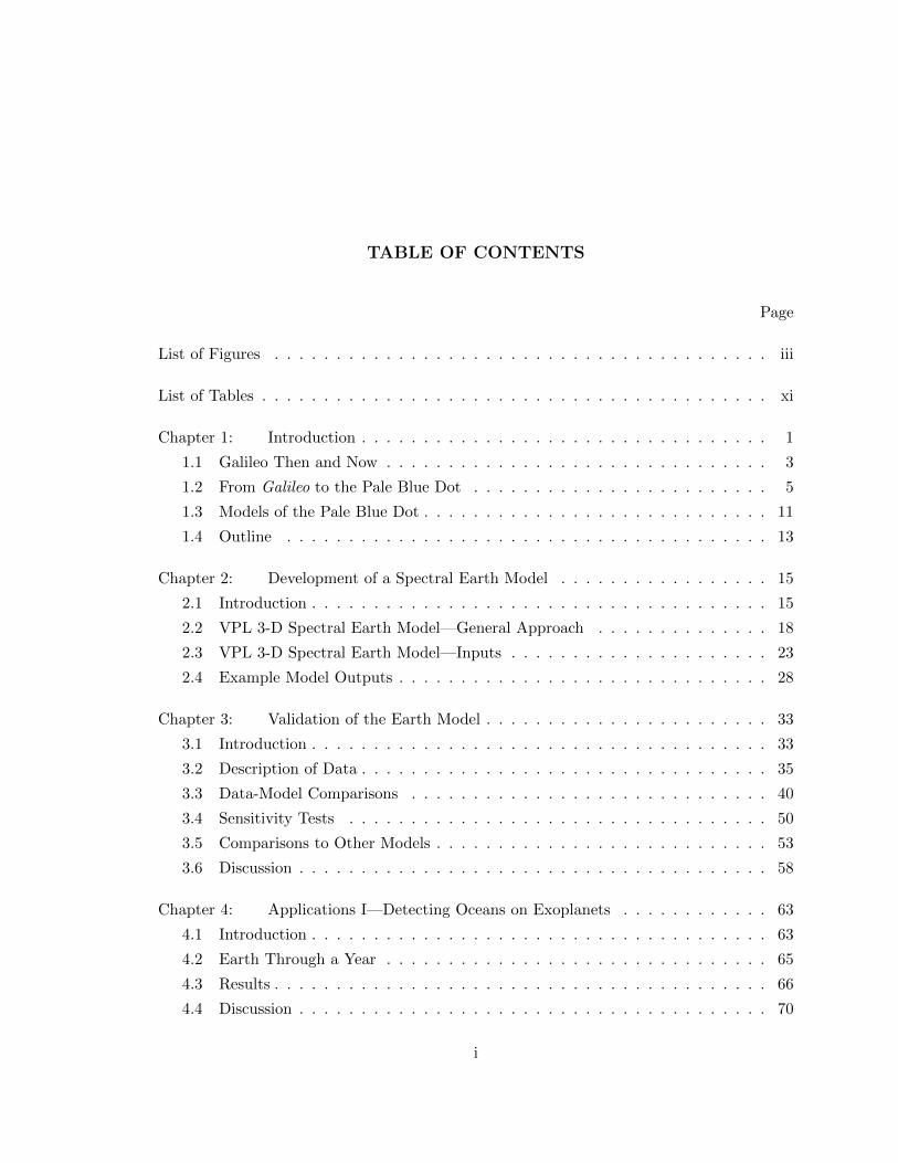
TABLE OF CONTENTS

Page

List of Figures . . . . . . . . . . . . . . . . . . . . . . . . . . . . . . . . . . . . . . . . iii

List of Tables . . . . . . . . . . . . . . . . . . . . . . . . . . . . . . . . . . . . . . . . . xi

Chapter 1: Introduction . . . . . . . . . . . . . . . . . . . . . . . . . . . . . . . . . 1

1.1 Galileo Then and Now . . . . . . . . . . . . . . . . . . . . . . . . . . . . . . . 3

1.2 From Galileo to the Pale Blue Dot . . . . . . . . . . . . . . . . . . . . . . . . 5

1.3 Models of the Pale Blue Dot . . . . . . . . . . . . . . . . . . . . . . . . . . . . 11

1.4 Outline . . . . . . . . . . . . . . . . . . . . . . . . . . . . . . . . . . . . . . . 13

Chapter 2: Development of a Spectral Earth Model . . . . . . . . . . . . . . . . . 15

2.1 Introduction . . . . . . . . . . . . . . . . . . . . . . . . . . . . . . . . . . . . . 15

2.2 VPL 3-D Spectral Earth Model—General Approach . . . . . . . . . . . . . . 18

2.3 VPL 3-D Spectral Earth Model—Inputs . . . . . . . . . . . . . . . . . . . . . 23

2.4 Example Model Outputs . . . . . . . . . . . . . . . . . . . . . . . . . . . . . . 28

Chapter 3: Validation of the Earth Model . . . . . . . . . . . . . . . . . . . . . . . 33

3.1 Introduction . . . . . . . . . . . . . . . . . . . . . . . . . . . . . . . . . . . . . 33

3.2 Description of Data . . . . . . . . . . . . . . . . . . . . . . . . . . . . . . . . . 35

3.3 Data-Model Comparisons . . . . . . . . . . . . . . . . . . . . . . . . . . . . . 40

3.4 Sensitivity Tests . . . . . . . . . . . . . . . . . . . . . . . . . . . . . . . . . . 50

3.5 Comparisons to Other Models . . . . . . . . . . . . . . . . . . . . . . . . . . . 53

3.6 Discussion . . . . . . . . . . . . . . . . . . . . . . . . . . . . . . . . . . . . . . 58

Chapter 4: Applications I—Detecting Oceans on Exoplanets . . . . . . . . . . . . 63

4.1 Introduction . . . . . . . . . . . . . . . . . . . . . . . . . . . . . . . . . . . . . 63

4.2 Earth Through a Year . . . . . . . . . . . . . . . . . . . . . . . . . . . . . . . 65

4.3 Results . . . . . . . . . . . . . . . . . . . . . . . . . . . . . . . . . . . . . . . . 66

4.4 Discussion . . . . . . . . . . . . . . . . . . . . . . . . . . . . . . . . . . . . . . 70

i

Chapter 5: Applications II—Detecting Exomoons . . . . . . . . . . . . . . . . . . 77

5.1 Introduction . . . . . . . . . . . . . . . . . . . . . . . . . . . . . . . . . . . . . 77

5.2 Moon Model . . . . . . . . . . . . . . . . . . . . . . . . . . . . . . . . . . . . 79

5.3 Results . . . . . . . . . . . . . . . . . . . . . . . . . . . . . . . . . . . . . . . . 83

5.4 Discussion . . . . . . . . . . . . . . . . . . . . . . . . . . . . . . . . . . . . . . 94

Chapter 6: Conclusions . . . . . . . . . . . . . . . . . . . . . . . . . . . . . . . . . 98

ii

LIST OF FIGURES

Figure Number Page

1.1 An image representing the first ever glimpse by a human of Earth’s disk,acquired during NASA’s Apollo 8 mission on December 21, 1968. The centrallandmass is South America, the southern portion of which is at the top ofthe image. North America is obscured by a cloud in the lower right portionof the image, and Africa can be seen to the lower left. Habitable exoplanetswill possess many features like those seen in this image, including the surfaceoceans and clouds formed via a hydrological cycle. Image credit NASA. . . . 4

1.2 An image of Earth acquired by the SSI aboard the Galileo spacecraft throughthe “infrared” filter (centered at 1,000 nm, bandpass width of 50 nm) onDecember 11, 1990. The distance between Earth and the spacecraft is 2.2×106 km. . . . . . . . . . . . . . . . . . . . . . . . . . . . . . . . . . . . . . . . 6

1.3 An image of Earth at 4.6 µm acquired by the NIMS instrument aboard theGalileo spacecraft on December 8, 1990. Warm regions appear bright, andclouds appear as dark features. Note the numerous data dropouts that oc-curred over many positions on the disk. Adapted from Drossart et al. (1993). 7

1.4 The famous Pale Blue Dot image of Earth acquired by the Voyager 1 space-craft at a distance of about 40 AU. Earth can be seen as a blue pixel (at thelower right portion of the image) which is caught in a ray of sunlight thatwas internally-scattered by the instrumentation. Observations of exoplanetswill be similar to this in that they will not provide spatial resolution. Imagecredit NASA. . . . . . . . . . . . . . . . . . . . . . . . . . . . . . . . . . . . . 8

1.5 The geometry of viewing the disk of a planet of radius R from an altitudeabove the surface z. . . . . . . . . . . . . . . . . . . . . . . . . . . . . . . . . 10

2.1 Geometry for computing the disk-integrated flux reflected and/or emitted bya world. The surface normal vector, and the vectors in the direction of theobserver and Sun (or host star) are n, o, and s, respectively. The angle α isthe phase angle, while φ and θ are the coordinates of latitude and longitude,respectively. . . . . . . . . . . . . . . . . . . . . . . . . . . . . . . . . . . . . . 19

2.2 Divisions of a sphere into equal-area pixels at various resolutions (12, 48, 192,and 768 pixels) according to the HEALPix scheme. Image from Gorski et al.(2005). . . . . . . . . . . . . . . . . . . . . . . . . . . . . . . . . . . . . . . . . 22

iii

2.3 Mixing ratio (top) and temperature (bottom) profiles from a single mid-latitude atmospheric pixel in our model for 2008-Mar-18 UT. High spatialresolution data are obtained from a variety of Earth observing satellites. . . . 24

2.4 Liquid (left column) and ice (right column) cloud extinction optical depthdistributions (top) and cumulative distributions (bottom) on 2008-Mar-19UT (solid) and 2008-Jun-5 UT (dashed) from MODIS data. Shaded regionsrepresent the cuts that are placed on the data to separate moderately opticallythick and optically thick cloud types. Vertical dotted lines represent theoptical depths that are used in the model to represent these categories ofclouds. . . . . . . . . . . . . . . . . . . . . . . . . . . . . . . . . . . . . . . . 27

2.5 Albedo spectra of the five surface types used in the model. Data for forestsare taken from the ASTER Spectral Library while all other data are takenfrom the USGS Digital Spectral Library. Water reflectivity in our model isrepresented with a Cox-Munk glint model, which is a function of viewinggeometry. The ocean data shown in this figure is representative of the albedoof ocean water averaged over all viewing angles. . . . . . . . . . . . . . . . . 29

2.6 A variety of reflected light images from our model, all taken at full phaseat the same time in mid-northern winter. The image on the left is in true-color (using filters centered at 0.45 µm, 0.55 µm, and 0.65 µm), the imagein the center is in false-color (using filters centered at 0.45 µm, 0.55 µm, and0.85 µm to highlight the continents), and the image on the right is taken at1.4 µm in a water absorption band, which increases the sensitivity to highclouds. . . . . . . . . . . . . . . . . . . . . . . . . . . . . . . . . . . . . . . . . 30

2.7 A true-color image of Earth (left) and the corresponding thermal infraredimage (right). The true-color image was constructed using filters centered at0.45 µm, 0.55 µm, and 0.65 µm), while the infrared image uses a filter near10 µm, in the atmospheric window region. The infrared image clearly showsthe atmospheric pixelization, which captures a gradient in surface tempera-tures from the equator to the poles, and clouds appear as dark features inthis image. . . . . . . . . . . . . . . . . . . . . . . . . . . . . . . . . . . . . . 31

2.8 An example high resolution, disk-integrated spectrum of Earth from ourmodel, shown as wavelength multiplied by the specific radiance. The viewinggeometry is identical to that of Figure 2.7, and notable features have beenlabeled. . . . . . . . . . . . . . . . . . . . . . . . . . . . . . . . . . . . . . . . 32

3.1 The thermal infrared spectrum of Earth obtained by Mars Global Surveyorwhile it was en route to Mars. The observation occurred on November 24th,1996, and the sub-observer latitude and longitude were 18◦ N and 152◦ W,respectively. Blackbody curves (dashed) for Earth’s equilibrium temperature(255 K) and, roughly, for the temperature observed in the infrared windowregion (270 K) are also shown. . . . . . . . . . . . . . . . . . . . . . . . . . . 34

iv

3.2 Example near-infrared spectrum of Earth on 2008-Mar-18 UT from NASA’sEPOXI mission. Note the different scales used for the y-axes on the leftand right sides of the spectrum. Prominent absorption features have beenlabeled, and the sub-observer latitude and longitude are 0◦ N and 214◦ W,respectively. Instrument calibration uncertainties are typically 10%, and tendto increase below 2.0 µm and above 4.3 µm (Klaasen et al., 2008). Earth viewgenerated by the Earth and Moon Viewer, first implemented by J. Walker1. . 36

3.3 Lightcurves of data for EPOXI Earth observations from March, which be-gin at 2008-Mar-18 18:18 UT. Different line colors correspond to differentfilters, and the filter center wavelength is noted in the lower right. Data havebeen normalized to their respective 24 hour averages. The vertical gray lineindicates where the observations begin and, 24 hours later, end. The dis-continuity here is a real effect due to time varying cloud structures and is oforder 2–3%. . . . . . . . . . . . . . . . . . . . . . . . . . . . . . . . . . . . . . 37

3.4 Mid-infrared, 24 hour average spectrum of Earth from March 19th, 2008, asgenerated from Aqua/AIRS observations (Hearty et al., 2009). Large gapsare regions where the instrument does not return data. Important absorptionfeatures have been labeled. . . . . . . . . . . . . . . . . . . . . . . . . . . . . 38

3.5 Apparent albedos of Earth as measured by observing Earthshine from thedark side of the Moon. Data were recorded between November 1998 andJanuary 2005, and span 0.4 µm to 0.7 µm. The rise in apparent albedotowards crescent phases (large phase angles) is due to forward scatteringfrom clouds, glint, and Rayleigh scattering. For more information, please seeQiu et al. (2003) and Palle et al. (2003). Data were generously provided byE. Palle. . . . . . . . . . . . . . . . . . . . . . . . . . . . . . . . . . . . . . . . 39

3.6 Lightcurves of data (solid) and baseline model (dashed) for EPOXI observa-tions from March (left), May (center), and June (right). March observationsbegin at 2008-Mar-18 18:18 UT, May observations begin at 2008-May-2820:05 UT,and June observations begin at 2008-Jun-4 16:57 UT. The filtercenter wavelength is noted in the central column. Model values and datahave been normalized to their respective 24 hour averages. The shaded re-gion in the central column marks a Lunar transit of Earth’s visible disk, whichis an effect not included in our spectral model. The vertical gray line indicateswhere the observations begin and, 24 hours later, end. The discontinuity hereis a real effect due to time varying cloud structures and is of order 2–3% inMarch. The discontinuity tends to be smaller in the May observations andlarger in the June observations. The model generally reproduces the scaleand sense of these discontinuities. . . . . . . . . . . . . . . . . . . . . . . . . . 42

v

3.7 Comparison of the 24-hour averaged signal for the model (dashed) with theEPOXI data (solid) for the March (upper) and June (lower) dates of obser-vation, demonstrating our fit to the data on an absolute scale. Note thatthe June observations are overall dimmer than the March observations dueto Earth phase. The largest discrepancies are typically in the 450 nm filterand are ∼ 8% for both observations, within the 10% absolute error in theHRI calibration (Klaasen et al., 2008). The average spectrum of the Mayobservations is similar to that of the June observations (i.e., within a fewpercent) and were omitted for clarity. . . . . . . . . . . . . . . . . . . . . . . 45

3.8 Near-infrared spectral comparison of the model (dashed) with EPOXI data(solid) for a variety of observations. Note the different scales used for they-axes on the left and right sides of the plots. Date indicators and sub-observer longitudes are given at the top of each plot. Prominent absorptionfeatures have been labeled in the upper-left plot. May (middle-right) andJune (lower-right) observations are dimmer in reflected light due to Earthphase. Residuals for the data-model comparison are shown below each plotand are typically less than about 15%. Stronger disagreements tend to oc-cur between 1.1–1.2 µm (water), between 1.35–1.5 µm (water), and between3.9–4.15 µm (N2O, wing of CO2 feature). Extremely low signal levels andinstrument artifacts lead to large residuals in the 2.5–3.25 µm range. Instru-ment calibration uncertainties are typically 10%, and tend to increase below2.0 µm and above 4.3 µm. Earth views generated by the Earth and MoonViewer. . . . . . . . . . . . . . . . . . . . . . . . . . . . . . . . . . . . . . . . 46

3.9 Mid-infrared, 24 hour average spectra of Earth from our March model (gray)and as generated from Aqua/AIRS observations (solid) (Hearty et al., 2009).In general, the agreement is quite good, with residuals (lower panel) beingtypically ∼ 7%. Large gaps are regions where the instrument does not returndata. . . . . . . . . . . . . . . . . . . . . . . . . . . . . . . . . . . . . . . . . . 47

3.10 Comparison between the apparent albedos of Earth from Earthshine mea-surements and our model. Data were recorded between November 1998and January 2005, while the model observations correspond to monitoringEarth every four hours during a six month period in 2008 while the planetgoes through a range of phases. Also shown is an attempt by Williams &Gaidos (2008) to reproduce the Earthshine observations using a reflectancemodel that ignored both direction-dependent scattering from clouds as wellas Rayleigh scattering. Data and model observations span 0.4 µm to 0.7 µm.Variability at short timescales in the model is from Earth’s rotation and time-varying cloud structures. The rise in apparent albedo towards larger phaseangles is due to forward scattering by clouds and glint as well as Rayleighscattering. . . . . . . . . . . . . . . . . . . . . . . . . . . . . . . . . . . . . . . 49

vi

3.11 Comparison between the EPOXI data (solid) and a variety of models con-sidered in this work through a subset of the EPOXI filters for the Marchset of observations. Filter center wavelength is noted on each plot. Thedetails of the models shown are outlined in Table 3.1. Model “a”: standardmodel; model “e”: single cloud category; model “f”: single atmospheric pixel;model “g”: 48 surface pixels. Filters were selected to demonstrate the effectsof Rayleigh scattering (350 nm) and water absorption (950 nm). The 650 nmfilter is relatively free of atmospheric extinction. . . . . . . . . . . . . . . . . . 51

3.12 Comparison between the EPOXI data (solid), our standard model (dashed),a model run with a single cloud category (dotted), and a model run withtwo cloud categories (dot-dashed) for a view over the Pacific Ocean on 2008-Mar-18 UT. Note the different scales used for the y-axes on the left and rightsides of the spectral plots. While the single cloud model and the two cloudmodel can reproduce the visible EPOXI lightcurves, they cannot reproducethe NIR data. Earth view generated by the Earth and Moon Viewer . . . . . 52

3.13 Comparison between the Tinetti et al. (2006a) model and our model. Ameasure of Earth’s reflectivity, taken as π times the disk-integrated radiance(in W/m2/µm/sr) divided by the Solar flux at 1 A.U (inW/m2/µm), is shownfor the planet viewed at full phase, gibbous phase, quadrature (i.e., halfilluminated, or a phase angle of 90◦), and crescent phase. Both models userealistic cloud cover, and the data for the Tinetti et. al model is taken fromTinetti et al. (2006b). An EPOXI observation taken near half illuminationand our model of the observation are shown as dashed lines in the quadraturecase, demonstrating that our model correctly reproduces the data at thisphase. In general, the Earth model from Tinetti et al. (2006a,b) is about100% to 400% too bright, and is unrealistically blue at phases near quadratureand crescent. . . . . . . . . . . . . . . . . . . . . . . . . . . . . . . . . . . . . 55

3.14 Comparison between the EPOXI data (solid), our standard model (“a”), theTinetti et al. model (“d”), and a model that ignores atmospheric extinctionand scattering (i.e., a reflectance model, “h”). Models and data correspondto the March set of EPOXI observations. Filter center wavelength is notedon each plot. The details of the models shown are outlined in Table 3.1. . . . 56

3.15 Comparison of the 24 hour averaged signal (top) for the EPOXI data (solid),our standard model (dashed), and a model where atmospheric absorptionand scattering has been removed and clouds have been treated as a Lam-bertian surface with an albedo of 0.60 (dotted). The data and models havebeen converted to a measure of reflectance (bottom) in the same fashion asin Figure 3.13. The effects of ignoring Rayleigh scattering can be seen in theshortest wavelength filters while the lack of atmospheric absorption is espe-cially apparent in the 950 nm filter, which includes a strong water absorptionfeature. Data and models are all for the March EPOXI observations. . . . . . 57

vii

4.1 A true-color image from our model (left) compared to a view of Earth fromthe Earth and Moon Viewer1. A glint spot in the Indian Ocean can be clearlyseen in the model image. . . . . . . . . . . . . . . . . . . . . . . . . . . . . . . 66

4.2 Simulation of Earth’s brightness through a year. Earth is brightest at fullphase (orbital longitudes near 180◦) and faintest near crescent phase (orbitallongitudes near 0◦ and 360◦). Variability at small time scales (see inset) is dueto Earth’s rotation and time-varying cloud formations (noise is not included insimulations). Model “observations” are recorded every four hours, the systemis viewed edge-on (i = 90◦), and an orbital longitude of 0◦ corresponds toJanuary 1, 2008. All model observations are integrated over the wavelengthrange 0.4–0.7 µm. . . . . . . . . . . . . . . . . . . . . . . . . . . . . . . . . . . 67

4.3 Simulation of Earth’s brightness through a year for models run with andwithout glint (black and gray, respectively). Viewing geometry, timing, andwavelength coverage are the same as in Figure 4.2. The bottom sub panelshows the brightness excess in the glinting model over the non-glinting model. 68

4.4 Variability in brightness for our glinting model (black) and our non-glintingmodel (grey), which are both shown in Figure 4.3. Variability is defined asthe ratio between the standard deviation of all model observations from a24-hour period and the 24-hour average brightness from the same timespan. . 69

4.5 Normalized spectra of glinting and non-glinting Earth at crescent phase.Spectra are an average over all observations from Figure 4.3 at orbital longi-tudes between 315–345◦ and are normalized to the average full-phase flux be-tween 0.4–0.6 µm from the models with and without glint, respectively. Thecontinuum regions in the spectrum without glint simply fall off in brightnesswith wavelength, while the spectrum from the glinting Earth peaks between0.7–0.8 µm before falling off, which is due to the added contribution from theglint spot. . . . . . . . . . . . . . . . . . . . . . . . . . . . . . . . . . . . . . . 72

4.6 Spectrum of the excess brightness due to glint obtained by subtracting thecrescent-phase spectrum of the glinting Earth from the non-glinting Earth inFigure 4.3. Outside of absorption bands, this spectrum is well matched bythe solar spectrum scaled by e−k/λ

4) (to represent a modulation by Rayleigh

scattering). . . . . . . . . . . . . . . . . . . . . . . . . . . . . . . . . . . . . . 73

viii

4.7 Earth’s brightness through the JWST/NIRCam F115W filter (spanning 1.0–1.3 µm) relative to its brightness at gibbous phase (135◦ and 225◦ orbitallongitude) for orbital inclinations of 90◦ (top), 75◦ (middle), and 60◦ (bot-tom). Glinting model is in black and non-glinting model is in grey. Verticalshaded regions indicate the portions of the orbit for which a planet orbitingat 1 AU from its host star is within 85 milli-arcseconds, which is a standardIWA for an occulter paired with JWST (Brown & Soummer, 2010), for a sys-tem at a distance of 5 parsecs (darkest), 7.5 parsecs (medium), and 10 parsecs(lightest). Planet-star separation at a distance of 10 parsecs is shown on theupper x-axis. The SNR required to distinguish the glinting model from thenon-glinting model at the 1-σ level is shown along the right y-axis and cor-responds to the dashed line. Observations have been averaged over 24-hourperiods. . . . . . . . . . . . . . . . . . . . . . . . . . . . . . . . . . . . . . . . 75

5.1 Comparison between our spectral Moon model and EPOXI observations. Ob-servations are from 2008-05-29 UTC at a phase angle of 75.1◦ (Livengoodet al., 2011). . . . . . . . . . . . . . . . . . . . . . . . . . . . . . . . . . . . . . 83

5.2 True color image of the Earth-Moon system, taken as part of NASA’s EPOXImission compared to a simulated image using 10 µm brightness temperaturesfrom our models. The spectra on the right shows the corresponding flux at10 pc from the Moon (gray), Earth (blue), and the combined Earth-Moon flux(black), not including transit effects. The panel below the spectra shows thewavelength dependent lunar fraction of the total signal. Images and spectraare for a phase angle of 75.1◦. . . . . . . . . . . . . . . . . . . . . . . . . . . . 84

5.3 Infrared spectra of the Moon (gray), Earth (blue), and the combined Earth-Moon system (black) at full phase (top) and quadrature (bottom). Spectraare averaged over 24 hours at Earth’s vernal equinox, and the spectral res-olution is 50. The panels below the spectra show the wavelength dependentlunar fraction of the total signal. . . . . . . . . . . . . . . . . . . . . . . . . . 86

5.4 Earth’s 6.3 µm water band with and without the full phase flux from theMoon (black and solid blue, respectively, from Figure 5.3). Also shown areIR spectra of Earth with artificially lowered amounts of water vapor in theatmosphere generated using a one-dimensional, line-by-line radiative transfermodel (Meadows & Crisp, 1996). The dashed blue line shows the case wherewater vapor mixing ratios are at 10% their present day levels and the dottedblue line is for 1% present day levels. The addition of the Moon’s flux fills inthe water absorption feature, causing the feature to more closely mimic anEarth with roughly 90% less water vapor in the atmosphere. . . . . . . . . . . 87

ix

5.5 Brightness temperature spectra for Earth (blue) as well as for the combinedEarth-Moon system at full phase (black, solid) and at quadrature (black,dashed). Brightness temperatures were calculated using the correspondingfluxes from Figure 5.3, one Earth radius was used in the conversion from fluxto intensity, and the spectral resolution is 50. . . . . . . . . . . . . . . . . . . 88

5.6 Simulated observations of both an exoEarth-Moon system (top) as well asan exoEarth (bottom), both at a distance of 10 pc, demonstrating the phasedifferencing technique which could be used to detect exomoons. Observationsare averaged over 24 hours and the spectral resolution is 50. One observationis taken at a small phase angle (gibbous phase, solid blue) and another obser-vation is taken half an orbit later (crescent phase, dashed blue). The gibbousobservations occur in the middle of northern summer while the crescent ob-servations occur in the middle of northern winter. The system is assumedto be viewed edge on (inclination of 90◦) (where gibbous and crescent phaseobservations actually refer to full and new phase, respectively). In the “NoMoon” cases, the difference between gibbous and crescent observations (blackline) shows only seasonal variability, which is very small in the 4.3 µm carbondioxide band and the 6.3 µm water band. For the observations in which theMoon is present, these bands are filled in by the lunar flux at gibbous phase,and the difference between the gibbous and crescent observations shows muchlarger variability within the absorption bands. . . . . . . . . . . . . . . . . . . 90

5.7 The same as Figure 5.6 except for a system viewed at an inclination of 60◦. . 91

x

LIST OF TABLES

Table Number Page

2.1 Summary of Trace Gas Input Data . . . . . . . . . . . . . . . . . . . . . . . . 25

3.1 Validation and Sensitivity Test Results . . . . . . . . . . . . . . . . . . . . . . 43

5.1 Phase Differencing Technique for Detecting Exomoons: Thermal Fluxes, FluxRatios, Brightness Temperatures, and Estimated SNR Requirements . . . . . 93

xi

ACKNOWLEDGMENTS

This work would not have been possible if not for the care and support of many indi-

viduals. I’d like to thank my parents for always expecting the best from me—from grade

school “invention fairs” to undergraduate academics. My advisor, Vikki Meadows, has been

a constant source of ideas and advice. (I promise I’ll get to the climate model sometime

next week.) Dave Crisp has been an excellent source of knowledge and right answers. David

Catling helped me to walk the line between planetary science and astronomy. Finally, I’m

especially grateful to my wife Rachel, who has been there through all of the ups and downs

of being a graduate student.

xii

DEDICATION

To Rachel.

xiii

1

Chapter 1

INTRODUCTION

Astrobiology is the study of life in the Universe—its origin, evolution distribution, and

future (Des Marais et al., 2008). The search for both habitable1 and inhabited worlds beyond

Earth is an integral part of understanding life’s potential distribution in the Universe. This

search seeks to answer profound questions: Are we alone? How rare is our Earth? If the

hunt for life beyond Earth finds many habitable worlds and few (if any) inhabited ones, then

we know just how uncommon our situation is. On the other hand, if the search yields many

inhabited worlds, then we’ll begin to understand something about the diversity, ingenuity,

resiliency, and tenacity of life.

The astrobiological search for life does not typically focus on intelligent life, but on

microbial life—things akin to the bacteria and archaea that inhabit our planet. This em-

phasis is driven primarily by detectability and probability. We know that simple life, due

to sheer biomass and persistence over large fractions of a planet’s history, has the ability to

make large-scale changes to a planet’s surface and atmosphere (Lenton, 1998), the kinds of

changes one could spot with a telescope peering across lightyears of interstellar space. In

addition, some authors have proposed that simple life is likely to be far more common than

intelligent, multicellular life (Ward & Brownlee, 2000).

Within the Solar System, our understanding of habitable environments has changed

dramatically over the last century. Hopes for regions with temperate, Earth-like climates

on Venus (Proctor, 1883) evaporated with the discovery of the planet’s extreme surface

environment (Drake, 1962; Sagan, 1962). The Cytherean surface, at a pressure of 93 bar

and a temperature of 730 K, is widely believed to be uninhabitable, although some have

suggested that regions of the atmosphere might be habitable (Morowitz & Sagan, 1967;

Schulze-Makuch et al., 2004). Mars has remained an exciting prospect for habitability,

1A habitable environment (or world) is one capable of supporting life.

2

although much has changed since Lowell’s discussion of Martian canals(Lowell, 1906). It

may be possible for a subsurface biosphere to exist on modern Mars (McKay & Stoker,

1989), which could indicate its presence through atmospheric biosignatures (Summers et al.,

2002; Mumma et al., 2009). Other potentially habitable environments in the Solar System

include Europa’s subsurface oceans (Lewis, 1971; Reynolds et al., 1983; Zelenyi et al., 2010),

Titan’s hydrocarbon lakes (Fortes, 2000; Benner et al., 2004; Lunine, 2008), and Enceladus’

subsurface, where internal energy sources create liquid water reservoirs (Porco et al., 2006;

Parkinson et al., 2008).

The common factor in the potential habitability of these worlds is the presence of a

liquid. While life’s requirements generally include (i) an energy source, (ii) chemical building

blocks, and (iii) a liquid, it is typically the latter that is considered the most significant

limiting factor (Mazur, 1980; McKay, 1991) due to the likely prevalence of energy sources

and chemical building blocks in planetary environments. Life beyond Earth may be able to

use a variety of chemistries and liquids (Bains, 2004; Benner et al., 2004; Ward & Benner,

2007, see also the National Research Council’s 2007 report The Limits of Organic Life in

Planetary Systems2), but liquid water has become the primary focus of the hunt for life

beyond Earth (McKay, 2004). While this focus is certainly Earth-centric, it is also quite

pragmatic, as we stand the best chance of identifying extraterrestrial life when it shares

fundamental properties with the kind of life we already know and understand.

The list of potentially habitable worlds within the Solar System is quite short, and, if

life is a rare phenomenon, then the odds are against finding life beyond Earth in the Solar

System. However, given that there are hundreds of billions of stars in our galaxy, and that

each of these stars, on average, hosts at least one planet (Cassan et al., 2012), then exoplan-

ets provide an important opportunity to perform a large, statistically significant search for

both habitable worlds and life beyond Earth. At the time of writing this document, there

are over 700 known exoplanets (see exoplanet.eu/catalog). Most of these worlds have been

detected using the radial velocity technique, but NASA’s Kepler mission, which detects

planets using the transit technique, has announced over 2,000 candidate exoplanets, the

2http://www.nap.edu/catalog.php?record id=11919

3

vast majority of which still await confirmation by follow-up observations or analysis (Torres

et al., 2011).

Since the first detection of an exoplanet occurred almost two decades ago (Mayor &

Queloz, 1995), the field of exoplanetary science has been marked by two clear trends. The

first is the steady discovery of smaller and smaller worlds, especially since the launch of Ke-

pler. The second trend is towards an ever-increasing quality of observational data suitable

for characterizing these worlds, including wavelength-dependent photometry and true spec-

tra, obtained using secondary eclipse observations and transit transmission spectroscopy

(Seager & Sasselov, 2000; Brown et al., 2001; Charbonneau et al., 2002; Deming et al.,

2005; Charbonneau et al., 2005; Grillmair et al., 2007; Knutson et al., 2008). A number of

planned and proposed NASA missions will improve and expand our ability to characterize

exoplanet atmospheres and surfaces, including the James Webb Space Telescope (JWST)

(Gardner et al., 2006), the Fast Infrared Exoplanet Spectroscopy Survey Explorer (FINESSE

(Swain, 2010), and the Terrestrial Planet Finder (TPF) (Beichman et al., 1999).

Given the accelerating pace at which exoplanet characterization is progressing, it is

timely to ask two important questions: How do we recognize a distant exoplanet as being

habitable? And how can we best equip the next generation of exoplanet characterization

missions to find and characterize Earth-like worlds? To answer these questions, we first turn

to Earth—the only example we have of a habitable planet. Although extrasolar habitable

planets are unlikely to look exactly like Earth, they may share some key characteristics,

including the presence of an ocean, clouds, surface inhomogeneity, and, potentially, life

(see Figure 1.1). Studying the Earth’s globally-averaged characteristics within the context

of remote observation therefore provides insights into the best measurements to identify

planetary habitability from data-limited exoplanet observations.

1.1 Galileo Then and Now

In his Dialogue Concerning the Two Chief World Systems, Galileo Galilei records what

is likely to be the first attempt to remotely characterize habitability. By observing the

brightness of the dark side of the Moon, which is illuminated by reflected light from Earth,

Galileo noted that the Earth was darker when the Moon was to the west of Europe (over

4

Figure 1.1 An image representing the first ever glimpse by a human of Earth’s disk, acquiredduring NASA’s Apollo 8 mission on December 21, 1968. The central landmass is SouthAmerica, the southern portion of which is at the top of the image. North America isobscured by a cloud in the lower right portion of the image, and Africa can be seen to thelower left. Habitable exoplanets will possess many features like those seen in this image,including the surface oceans and clouds formed via a hydrological cycle. Image credit NASA.

5

the Atlantic) than when it was to the east (over the Asian continent). This led Galileo to

conclude that “the surface of the seas would appear darker, and that of the land brighter”

to someone who could view Earth from afar (Galilei, 1632).

It was especially fitting, then, that the first attempt to remotely characterize Earth as if

it were a newly-discovered planet was performed by using data acquired by NASA’s Galileo

spacecraft (Sagan et al., 1993) . While designed as a mission to orbit and study Jupiter,

Galileo performed two flybys of Earth, one in December 1990, and the other in December

1992, which were both used as gravitational assists to push the spacecraft out towards

Jupiter’s orbit (Johnson et al., 1992). The data that were acquired included spatially- and

temporally-resolved observations with the Near Infrared Mapping Spectrometer (NIMS,

Carlson et al., 1992), the Ultraviolet Spectrometer (UVS, Hord et al., 1992), and the Solid

State Imaging experiment (SSI, Belton et al., 1992). Figure 1.2 shows an image of Earth

acquired by the Galileo/SSI during the 1990 flyby, and Figure 1.3 shows an image at 4.6 µm

acquired by Galileo/NIMS during the same flyby.

Using spatial resolution to their advantage, Sagan et al. (1993) and Drossart et al. (1993)

were able to (i) detect specular reflectance from a surface liquid in the Galileo/SSI images,

(ii) use Galileo/NIMS spectra to map surface temperatures over portions of the disk, and

(iii) retrieve abundance profiles for a number of atmospheric constituents. Relatively large

abundances of water vapor in the near-surface atmosphere, coupled with a range of surface

temperatures found to all be near the freezing point of water (273 K), argued that the liquid

detected in the Galileo/SSI images was water (Sagan et al., 1993). Furthermore, the lower

limit on surface pressure from the Galileo observations (∼ 0.2 bar) and the measured range

of surface temperatures placed portions of Earth’s surface within the liquid range of the

water phase diagram.

1.2 From Galileo to the Pale Blue Dot

The characterization of Earth using Galileo data presented in Sagan et al. (1993) and

Drossart et al. (1993) relied very heavily on the spatially resolved nature of the obser-

vations. Their arguments for detecting surface liquid water hinged on the detection of spec-

ular reflection by visual inspection of the resolved reflected light images. Furthermore, their

6

Figure 1.2 An image of Earth acquired by the SSI aboard the Galileo spacecraft throughthe “infrared” filter (centered at 1,000 nm, bandpass width of 50 nm) on December 11,1990. The distance between Earth and the spacecraft is 2.2× 106 km.

7

Figure 1.3 An image of Earth at 4.6 µm acquired by the NIMS instrument aboard theGalileo spacecraft on December 8, 1990. Warm regions appear bright, and clouds appearas dark features. Note the numerous data dropouts that occurred over many positions onthe disk. Adapted from Drossart et al. (1993).

8

Figure 1.4 The famous Pale Blue Dot image of Earth acquired by the Voyager 1 spacecraftat a distance of about 40 AU. Earth can be seen as a blue pixel (at the lower right portionof the image) which is caught in a ray of sunlight that was internally-scattered by theinstrumentation. Observations of exoplanets will be similar to this in that they will notprovide spatial resolution. Image credit NASA.

characterization of the surface environment used clear-sky soundings, which were identified

by inspecting the reflected light images for cloud-free scenes.

Unfortunately, observations of exoplanets are likely to be spatially-unresolved, providing

views much like the famous Pale Blue Dot image of Earth, which is shown in Figure 1.4.

Under these circumstances, the entire disk of the planet falls into a single resolution element,

and the observations are referred to as being disk-integrated. The loss of spatial resolution

introduces a great deal of complexity into the interpretation of planetary observations, since

the entire three-dimensional complexity of a world is collapsed into a single point of light. In

the case of an Earth-like planet, this means that clear-sky scenes are averaged with cloudy

scenes, warm and moist tropical regions are integrated with cold and dry arctic regions,

and land surfaces blend with ocean surfaces. Furthermore, the viewing geometry of the

observation plays a critical role, as regions on the limb of the planet or that experience

less incident solar (or stellar) flux contribute proportionally less flux to the disk-integrated

observation, depending on the wavelength of observation.

In general, there are three ways to obtain disk-integrated observations of Earth, which

can then be used to understand the optimum techniques for detection of planetary envi-

9

ronmental characteristics from spatially-unresolved observations. First, one can observe

reflected light from Earth by observing the night side of the Moon, which is referred to as

an Earthshine observation (Danjon, 1928; Dubois, 1947; Woolf et al., 2002; Qiu et al., 2003;

Palle et al., 2003; Turnbull et al., 2006a; Sterzik et al., 2012). Second, one can use satellites

in Earth orbit to assemble a disk-integrated view of Earth (Hearty et al., 2009). Finally,

spacecraft observations of the distant Earth, like those acquired by Galileo, can also provide

disk-integrated data. Each of these different approaches has its own set of advantages and

disadvantages.

Since Earthshine observations are acquired from the ground, they are relatively inexpen-

sive data to collect. Furthermore, the observations can be taken at high spectral resolution,

since ground-based spectrometers tend to provide higher resolution than their space-based

counterparts. However, Earthshine observations are limited to wavelengths at which Earth’s

atmosphere is not opaque, and cannot provide temporal coverage longer than one night from

most locations . Furthermore, Earthshine observations are seldom reported as calibrated

data (see e.g., Woolf et al., 2002; Turnbull et al., 2006a).

Observations of Earth from orbit benefit from the sheer number of satellites which are

continuously monitoring the planet. Since these satellites collectively span a wide range

of observed wavelengths at a variety of spectral resolutions, disk-integrated observations of

Earth assembled from these datasets will share these properties. Furthermore, since Earth

observing satellites are launched for and serve the Earth science community, using these

satellites to create disk-integrated views of Earth, in a sense, piggy-backs on an existing

mission, and offers an opportunity to perform interdisciplinary science. Unfortunately, such

an approach has seen little attention in the literature, primarily because creating a disk-

integrated view of Earth from these datasets is quite challenging. Earth observing satellites

don’t simultaneously view the entire disk of the Earth—they typically only see a narrow

range of latitude and longitude around the spacecraft’s nadir, often at a fixed local time.

As a result, the observations must be processed into a disk-integrated observation, which

includes making assumptions about how certain sub-spacecraft observations would appear

if the illumination or observation geometry changes (Hearty et al., 2009).

Figure 1.5 demonstrates the geometry of observing the disk of a planet of radius R from

10

Figure 1.5 The geometry of viewing the disk of a planet of radius R from an altitude abovethe surface z.

an altitude z, measured from the surface. The portion of the disk that is observable is the

conical region within the angle φ, which is given by

cosφ =1

1 + z/R, (1.1)

so that φ→ 90◦ when z � R. Thus, the observable fractional area of the disk is simply

A (z)

2πR2=

z

z +R, (1.2)

which approaches unity for z � R. For a typical Earth-observing satellite, parked at an

altitude of 700 km, the observable fractional area of the disk is only 10%. This value grows

to 85% from geostationary orbit, at altitudes near 36,000 km, which is an orbit used by

many weather satellites.

The ideal approach to obtaining full-disk observations of Earth would then be to actually

view the planet from a distance where the entire disk is both observable and within the

telescope’s field of view. While a mission dedicated to such observations has been proposed

11

and built (Valero et al., 2000), no dedicated mission for observing the distant Earth has ever

been launched. As a result, space-based observations of the distant Earth only occur on the

rare occasions that spacecraft add such observations to their primary mission objectives.

These situations are rare, and published, scientifically useful observations of the distant

Earth only exist for the Galileo Earth encounters (Sagan et al., 1993), snapshot observations

of Earth in the near-infrared and thermal infrared by ESA’s Mars Express (Tinetti et al.,

2006a) and NASA’s Mars Global Surveyor (Christensen & Pearl, 1997), respectively, and

the EPOXI dataset (Livengood et al., 2011) (discussed in depth later in this document).

1.3 Models of the Pale Blue Dot

Given that spacecraft observations of the distant Earth are very scarce, the best method

for understanding the appearance of the Pale Blue Dot over a range of wavelengths and

viewing geometries is to use models. A versatile and general model of Earth’s disk-integrated

spectrum can avoid all of the aforementioned issues with wavelength coverage, spectral

resolution, temporal resolution, and viewing geometry. However, generalized models can

be computationally expensive, so there exists a number of approaches in the literature that

attempt to simplify the problem.

Existing Earth models for exoplanet characterization studies are largely dominated by

computationally inexpensive specular reflectance models (e.g., Ford et al., 2001). In general,

these models do not solve the radiative transfer equation for locations on the planet, but

instead parameterize how clouds and different surfaces scatter sunlight. These models do

not include atmospheric absorption and emission, so they are most effective at visible light

wavelengths, where few gaseous species in Earth’s atmosphere absorb light. Ford et al.

(2001) used a reflectance model to study variability in visible-light observations of Earth-

like planets, and showed that a wide range of values for rotational flux variability is possible,

depending on cloud coverage and on the composition of the surface. Williams & Gaidos

(2008) used a similar model to investigate the significance of mirror-like reflection of sunlight

off an ocean, or “glint”, in reflected-light observations of Earth at different phases. These

authors were able to show that glint can cause the reflectivity of an Earth-like planet to

increase at crescent phases, but the lack of directionally-dependent scattering from clouds

12

and the atmosphere in their model prevented these authors from realistically predicting how

important the glint effect is at crescent phases.

Another category of spectral Earth models seeks to simulate our planet’s disk-integrated

spectrum using a 1-D model (e.g., Woolf et al., 2002; Stam, 2008). These models can gener-

ate high-resolution spectra over a broad range of wavelengths, but must employ certain as-

sumptions or simplifications for reducing the full 3-D complexity of Earth into a 1-D model.

(Woolf et al., 2002) (at visible wavelengths) and (Turnbull et al., 2006b) (at near-infrared

wavelengths), use tuning parameters to match their 1-D models to Earthshine observations,

which are inherently 3-D. Using a more rigorous approach, Montanes-Rodrıguez et al. (2006)

modeled Earth’s disk-integrated spectrum with a 1-D model that assumed globally aver-

aged atmospheric, surface, and cloud properties. In their model, standard atmospheric

composition and temperature profiles were assumed and Earth’s spectrum was obtained by

averaging different component spectra based on data from the International Satellite Cloud

Climatology Project. In general, the primary limitation associated with 1-D approaches to

modeling Earth’s disk-integrated spectrum is that these models do not capture latitudinal

and longitudinal variations in the composition and temperature of Earth’s atmosphere, and

thus cannot be used to accurately quantify the impact of spatial variations in temperature

and composition on the information content of simulated observations.

A third category of spectral Earth models utilize bi-directional reflectance distribution

functions (BRDFs) to simulate the appearance of regions on Earth’s disk, which can then

be combined to generate a disk-integrated observation (Palle et al., 2003; Oakley & Cash,

2009; Fujii et al., 2010). Typically, the BRDFs come from, or are designed to match,

data which have been measured by Earth-observing satellites (e.g., Manalo-Smith et al.,

1998). Palle et al. (2003) used a model of this type to investigate variability in Earthshine

observations, and Oakley & Cash (2009) used a BRDF model to simulate lightcurves of

Earth, allowing them to investigate the detectability of rotation and surface features to a

TPF-like mission. Fujii et al. (2010) used a cloudless BRDF model to investigate techniques

for mapping Earth-like planets from disk-integrated observations. In general, BRDF models

tends to have poor wavelength coverage, as the input satellite data are typically broadband

observations (see e.g., Manalo-Smith et al., 1998). Furthermore, since the input BRDFs are

13

derived from satellite observations, this category of models suffers from similar limitations

to disk-integrated observations of Earth assembled from satellite data—the BRDFs tend to

apply only over a limited range of illumination and viewing geometries.

A final category of spectral Earth model seeks to treat the full 3-D complexity of the

planet while retaining broad wavelength coverage and high spectral resolution. This cate-

gory of 3-D spectral models was pioneered by the Virtual Planetary Laboratory (VPL) in

Tinetti et al. (2005) and Tinetti et al. (2006a). This category of model captures spatial

variations in the state of Earth’s atmosphere and surface, thereby accurately simulating the

effects of rotation and seasonality on time resolved observations of Earth. In contrast to

BRDF models, 3-D spectral models use radiative transfer models to simulate the brightness

of regions on the planet’s disk, allowing them to obtain realistic results for geometries not

accessible to the Earth-observing satelllites that are used to define the BRDFs. These capa-

bilities make 3-D models an ideal choice for concept studies for TPF-class missions, which

have yet to fully define their wavelength coverage, typical integration times, and observing

cadences, and for exoplanet observations where the viewing geometry will be limited by the

planet’s orbital parameters (e.g., inclination).

In summary, spatially- and spectrally-resolved models of Earth’s disk-integrated spec-

trum are currently the best means of exploring remotely-observable planetary characteris-

tics, and a wide range of techniques and approaches have been developed for these models.

Furthermore, by validating such simulations against available Earth observations, from the

ground, orbit, and space, these models can become reliable predictive tools. This disser-

tation describes the construction, validation, and application of the most comprehensive

spectral Earth model to date—the NASA Astrobiology Institute’s Virtual Planetary Labo-

ratory 3-D spectral Earth model.

1.4 Outline

In Chapter 2, I introduce the VPL 3-D spectral Earth model. A general theory of modeling

disk-integrated spectra is described in Section 2.2. I discuss inputs to the 3-D spectral

Earth model in Section 2.3, and model outputs are demonstrated and briefly discussed in

Section 2.4. Chapter 3 presents the validation of the 3-D spectral Earth model, where we

14

compare the model to observations of Earth from satellites, Earthshine measurements, and

spacecraft. The specific data used for validation purposes are described in Section 3.2, and

detailed data-model comparisons are shown in Section 3.3. I perform a number of sensitivity

tests on model parameters in Section 3.4, and the model is compared to other spectral Earth

models in Section 3.5.

Applications of the VPL 3-D spectral Earth model are presented in Chapters 4 and 5.

In the former chapter, I apply the model to the problem of detecting oceans on Earth-like

exoplanets. This application includes a year-long simulation of Earth’s disk-integrated spec-

trum, shown in Section 4.2, and results and discussion are presented in Sections 4.3 and 4.4,

respectively. In the latter chapter, I combine the spectral Earth model with a model of

the Moon’s disk-integrated spectrum. The Moon model is described and validated in Sec-

tion 5.2, and results as well as implications for the characterization of Earth-like exoplanets

and their moons are discussed in Sections 5.3 and 5.4. General conclusions from all chapters

are presented in Chapter 6.

15

Chapter 2

DEVELOPMENT OF A SPECTRAL EARTH MODEL

In this chapter, I describe a forward model designed specifically to simulate disk-integrated

observations of Earth, which can serve as a theoretical “laboratory” for the accurate sim-

ulation of Earth’s appearance at arbitrary viewing geometries and phases. These simu-

lations can be used to explore and identify the best observational approach to searching

for planetary characteristics of habitability and life, such as the presence of an ocean or a

photosynthetic biosphere, and can also be used to generate test data to challenge proposed

observational and retrieval techniques for extrasolar planet characterization. Portions of

this chapter were originally published in collaboration with V. S. Meadows, D. Crisp, et al.

in the June 2011 edition of the journal Astrobiology (Robinson et al., 2011, Astrobiology,

Vol. 11, pp. 393–408); c© 2011 Mary Ann Liebert, Inc.), and are reproduced below with

permission of Mary Ann Liebert, Inc.

2.1 Introduction

After an initial decade dominated by the discovery of Jupiter-mass planets, the next frontier

of exoplanet research will be the detection and characterization of terrestrial-mass planets.

NASA’s Kepler spacecraft has begun to make the first comprehensive estimates of the

prevalence of extrasolar terrestrial planets (Borucki et al., 2003, 2011a,b), while searching

for Earth-mass planets in the habitable zones of their parent stars (Basri et al., 2005). In the

coming decades more ambitious planet detection and characterization missions for habitable

Earth-mass planets are planned, such as NASA’s Terrestrial Planet Finder mission (Beich-

man et al., 1999; Cash, 2006; Beichman et al., 2006; Traub et al., 2006). These missions will

be designed to detect and characterize nearby habitable planets, with the capability to ob-

tain direct imaging, as well as photometric and spectroscopic data for extrasolar terrestrial

planets

16

The observational challenges inherent in characterizing a terrestrial exoplanet are sig-

nificant, and carefully considered trade-offs must be made to maximize the science return.

Even with the most ambitious telescopes planned, terrestrial exoplanets will remain faint,

spatially unresolved point sources. The principal challenge is to determine the minimum

and optimum sets of observational parameters that can best characterize the environment

of an unresolved planet, which may be spatially inhomogeneous, clouded, and temporally

variable. For example, the combination of temporal resolution and multi-wavelength pho-

tometry could disentangle phase- or rotation-dependent differences in surface properties

from variable cloud cover. The resulting maps could discriminate between large scale sur-

face inhomogeneities such as continents and oceans (Palle et al., 2008; Cowan et al., 2009;

Kawahara & Fujii, 2010; Fujii et al., 2011). Disk-integrated spectroscopy can potentially de-

termine globally averaged atmospheric and surface composition to verify habitability and to

search for global evidence of life in the planetary environment (Seager et al., 2005; Montanes-

Rodrıguez et al., 2006; Meadows, 2006).

New tools are needed to obtain quantitative information about the environments of ter-

restrial planets that can only be studied as unresolved point sources. A typical approach to

understanding a world from disk-integrated observations consists of a “forward model”, an

“instrument model”, and an “inverse model” (e.g., Line et al., 2012). The forward model

is typically a radiative transfer model designed to generate a synthetic spectrum, given an

assumed surface-atmospheric state and viewing geometry. The instrument model simulates

the spectral and spatial resolution and other properties of the observing system. The in-

verse model adjusts surface or atmospheric state to yield a better fit to the observations.

Given a candidate observing system design, refinements in both forward models and inverse

methods are needed to fully exploit the information content of disk-integrated observations

of terrestrial planets.

Most existing forward models are designed to analyze soundings taken with adequate

spatial resolution to yield a sounding footprint with a homogenous atmospheric and surface

state (e.g., Boesch et al., 2011). Forward models designed for surface or “clear sky” remote

sensing applications rarely perform well with cloudy soundings. Those designed for land

remote sensing observations rarely simulate the reflection from the ocean surface. In short,

17

few if any forward models have been designed to yield accurate observations over the full

range of solar illumination angles, observation angles, or surface and atmospheric properties

present in a single, integrated, full-disk observation of an extrasolar planet.

In this chapter, I present the most comprehensive spectral Earth model to date for

the prediction of the photometric and spectroscopic characteristics of Earthlike exoplanets.

This model is a forward model, used to simulate the appearance of Earth to an observer for

the purpose of exploring the detectability of Earth’s planetary characteristics as a function

of observational geometry and time. Forward models, such as the model presented in this

work, are distinct from retrieval models designed to retrieve atmospheric characteristics from

observations of extrasolar planets (e.g., Madhusudhan & Seager, 2009; Lee et al., 2012; Line

et al., 2012). Instead, forward models can provide input into retrieval tools. Thus, it is

important that forward models be as realistic as possible so that they accurately represent

the appearance of planet, and, as a result, do not bias the observed planetary properties

inferred when using the model as a predictive tool.

A previous, more limited version of this model, published in Tinetti et al. (2006a,b),

has been corrected, and significantly updated and improved to allow accurate predictions

of Earth’s time- and phase-dependent photometric and spectroscopic brightness, on hourly

to yearly timescales, through realistic modeling of the radiative effects of a surface ocean,

atmosphere, and clouds. The previous model allowed for an arbitrary scaling of its input

cloud coverage data, and it also used the optical thickness of clouds as free parameters.

By tuning the previous model, snapshot disk-integrated observations of Earth could be

reproduced and the model could then be used to explore certain characteristics of Earth,

such as how the planet’s brightness changes with phase.

The model presented here has been modified to self-consistently use satellite derived

cloud data. Cloud coverage is now taken from Earth observing satellite maps and is no

longer scaled to reproduce disk-integrated Earth observations. The optical thickness of

clouds in our new model is also provided by Earth observing satellites, rather than being

tunable free parameters. This work also corrects an error in the model presented in Tinetti

et al. (2006a,b) which effectively confused forward scattering with backward scattering from

the atmosphere and surface, thus causing the model to produce unphysical simulated ob-

18

servations of Earth, especially as a function of phase. Our Earth model is based on a fully

multiple-scattering, line-by-line radiative transfer model, SMART (Meadows & Crisp, 1996;

Crisp, 1997), which is at the core of the exoplanet simulations generated by the VPL.

2.2 VPL 3-D Spectral Earth Model—General Approach

A model of the disk-integrated spectrum of a world must simulate (or approximate) the

integral of the projected area weighted intensity in the direction of the observer, which can

be written as

Fλ (o, s) =R2

d2

∫2πIλ (n, o, s) (n · o) dω , (2.1)

where Fλ is the disk-integrated specific flux density (“flux” hereafter) received from a world

of radius R at a distance d from the observer, Iλ (n, o, s) is the location-dependent specific

intensity in the direction of the observer, dω is an infinitesimally small unit of solid angle

on the globe, n is a surface normal unit vector for the portion of the surface corresponding

to dω, and o and s are unit vectors in the direction of the observer and the Sun (or host

star), respectively. The integral in Equation 2.1 is over the entire observable hemisphere

(2π steradians) and the dot product at the end of the expression ensures that an element of

area R2dω near the limb is weighted less than an element of equal size near the sub-observer

point. Note that, for reflected light, Iλ will be zero at locations on the night side of the world

(i.e., where n · s < 0), but is non-zero at all locations when considering thermal emission.

2.2.1 Analytic Solutions

Before describing the full complexity of our 3-D model, it is educational to investigate a

few simple solutions to Equation 2.1. Following Sobolev (1975), consider the geometry

in Figure 2.1, where the vectors in the direction of the observer and Sun are shown, and

the angle between these is taken to be α, the phase angle. The surface normal vector is

also shown, located at a longitude θ (measured from the sub-observer point) and latitude

φ (measured from the great arc connecting the sub-observer and sub-solar points). For

this geometry, we have that n · o = cos θ cosφ and dω = cosφdφdθ, so that we can write

19

Figure 2.1 Geometry for computing the disk-integrated flux reflected and/or emitted by aworld. The surface normal vector, and the vectors in the direction of the observer and Sun(or host star) are n, o, and s, respectively. The angle α is the phase angle, while φ and θare the coordinates of latitude and longitude, respectively.

Equation 2.1 as

Fλ =R2

d2

∫ π/2

−π/2

∫ π/2

−π/2Iλ (θ, φ) cos θ cos2 φdφdθ , (2.2)

First, let’s consider the simple case where the specific intensity in the direction of the

observer is independent of location and is given by the Planck function

Bλ (T ) =2hc2

λ51

ehc/λkbT − 1, (2.3)

where T is the blackbody temperature, h is the Planck constant, c is the speed of light, and

kB is the Boltzmann constant. In this case, Equation 2.3 simplifies to

Fλ = Bλ (T )R2

d2

∫ π/2

−π/2

∫ π/2

−π/2cos θ cos2 φdφdθ = πBλ (T )

R2

d2, (2.4)

which is the expected result since πBλ is the specific flux emitted by a blackbody. If,

for example, R equals Earth’s radius (6378 km) and T equals the effective temperature of

Earth (∼ 255 K), then this relation gives you a means of producing a rough estimate of the

specific flux you would receive from Earth if you were observing it from some distance d.

20

A more complicated example is the specific flux received from a body whose surface

reflects equally well in all directions (i.e., a Lambertian surface). If the incident specific

solar flux is F�λ , then the specific intensity in the direction of the observer is

Iλ (θ, φ) = AλF�λπ

cos (α− θ) cosφ , (2.5)

where Aλ is the wavelength dependent surface albedo. Noting that the lower limit for θ in

Equation 2.2 is now the terminator (α− π/2), we can write

Fλ (α) = AλF�λπ

R2

d2

∫ π/2

α−π/2

∫ π/2

−π/2cos θ cos (α− θ) cos3 φdφdθ

=2

3AλF

�λ

R2

d2sinα+ (π − α) cosα

π, (2.6)

where the final fraction is the well-known Lambert phase function. By inserting reasonable

numbers for Aλ and F�λ , one can easily use this expression to compute the phase-dependent

flux reflected by a planet (under the assumption of Lambertian scattering). This expression

will be useful for discussing Earth’s wavelength and phase dependent reflectivity in later

sections.

2.2.2 Numerical Solutions

Many of the key properties that describe both the state and appearance of Earth’s at-

mosphere and surface (e.g., composition, cloudiness, temperature, top-of-atmosphere spec-

trum) depend strongly on position, necessitating numerical approaches to computing Earth’s

disk-integrated spectrum. By dividing Earth into a grid of pixels, we can convert the in-

tegral in Equation 2.1 into a weighted sum over the observable pixels when provided a

sub-observer latitude and longitude. The atmospheric and surface state of any individual

pixel determines the spectrum emerging from it, and, thus, the sum over the observable

pixels incorporates the wealth of diversity in Earth’s position-dependent atmospheric and

surface state.

Note that that specific radiance Iλ arriving from a source at distance d with radius R is

related to the disk-integrated specific flux by

Iλ = Fλd2

πR2, (2.7)

21

where the solid angle subtended by the source is taken simply as πR2/d2. Inserting this

into Equation 2.1 yields

Iλ (o, s) =1

π

∫2πIλ (n, o, s) (n · o) dω . (2.8)

If we divide the world into N equal-area pixels, then the solid angle of any individual pixel

is simply 4π/N , and we can convert the integral in Equation 2.8 into a sum in the form

Iλ (o, s) =4

π

∑i∈O

Iλ (ni, o, s) (ni · o) , (2.9)

where ni describes the location on the sphere of pixel i, and O is the set of indices of all

observable pixels (i.e., all pixels with ni · o > 0).

In our model, the geometry of dividing Earth into a collection of equal-area pixels is

performed according to the Hierarchical Equal Area isoLatitude Pixelization (HEALPix)

model1 (Gorski et al., 2005), a demonstration of which is shown in Figure 2.2. An important

aspect of our model is that it maintains two different pixelizations, or resolutions—an at-

mospheric pixelization and a surface pixelization, which is nested beneath the atmospheric

pixels. Atmospheric properties (e.g., temperature profiles, gas mixing ratio profiles) are

mapped at the resolution of the atmospheric pixels, while surface and cloud coverages are

mapped at the (much higher) surface resolution. Using this nested pixelization scheme al-

lows us to capture a large dynamic range in surface coverage and cloudiness (which vary on

relatively small spatial scales), while still maintaining short model runtimes (which depend

primarily on the atmospheric resolution, as the radiative transfer equation is solved for a

grid of properties for each atmospheric pixel). Thus, the sum in Equation 2.9 is over the

surface pixels, while the atmospheric properties that define the pixel radiances are mapped

at the atmospheric resolution.

Note that the full complexity of Earth’s 3-D appearance is hidden in the expression

of Iλ (ni, o, s) in Equation 2.9, which describes the location dependent, top-of-atmosphere

specific intensity in the direction of the observer, and which is a function of the sub-observer

and sub-solar locations. This term is further complicated by the desire to produce a general

1http://healpix.jpl.nasa.gov

22

Figure 2.2 Divisions of a sphere into equal-area pixels at various resolutions (12, 48, 192,and 768 pixels) according to the HEALPix scheme. Image from Gorski et al. (2005).

3-D spectral model, which should be able to compute the disk-integrated spectrum for any

arbitrary user specification of the sub-observer and sub-solar locations. To accomplish this

generality, our model computes the top-of-atmosphere spectrum of each atmospheric pixel

for a grid of observer and solar orientations, as well as for a grid of surface types (e.g.,

ocean, snow, forest) and cloud types (e.g., thick ice clouds, thin water clouds). These

gridded results for all atmospheric pixels are then a “spectral database” from which the

model can determine the value of Iλ (ni, o, s) for each surface pixel (which are nested below

the atmospheric pixels) once o and s have been specified.

To generate this spectral database, we run a fully multiple-scattering, line-by-line (LBL)

radiative transfer model, the SMART model (Meadows & Crisp, 1996), for each atmospheric

pixel over a grid of observer and solar zenith angles and a grid of azimuth angles. A typical

grid for reflected light calculations consists of nine solar zenith angles (0◦, 15◦, 30◦, 45◦, 60◦,

75◦, 80◦, 85◦, 90◦), four observer zenith angles (21.5◦, 47.9◦, 70.7◦, 86.0◦), and seven azimuth

angles (0◦, 30◦, 60◦, 90◦, 120◦, 150◦, 180◦), where an azimuth angle of 0◦ corresponds to

the observer looking directly towards the Sun, and 180◦ directly away. For thermal-only

calculations (which are applicable to the night side of the planet), the solar orientation is

23

irrelevant, so the grid is only over the observer zenith angles. Of course, the LBL model

requires the atmospheric and surface state of each pixel to be specified, which we describe

in the following section.

2.3 VPL 3-D Spectral Earth Model—Inputs

A full description of the atmospheric and surface state of each atmospheric pixel starts with

the vertical temperature profile, trace gas mixing ratio profiles, and surface temperature.

The grid for the spectral database also requires specifying a number of surface types and

cloud types (e.g., thick ice clouds, thin water clouds). In this section, I describe how the

model determines the atmospheric and surface state, as well as our handling of surface and

cloud types.

2.3.1 Description of Atmospheric State—Temperature and Gases

To simulate molecular absorption in Earth’s visible and NIR disk-integrated spectra, and

to accurately predict planetary brightness temperature in the mid-IR, we require the three-

dimensional distribution of atmospheric gases and temperatures as input to the model.

These inputs are averaged over each pixel in the atmospheric grid, and then fed to the LBL

model, which computes the database of spectra associated with that pixel (i.e., computed

over the grid of observer and solar angles, and the various surface and cloud type categories).

We include both Rayleigh scattering by air molecules as well as absorption from H2O, CO2,

O3, N2O, CO, CH4 and O2 in our LBL calculations.

Spatially resolved mixing ratio profiles for atmospheric gases are obtained from the

Microwave Limb Sounder2 (MLS) (Waters et al., 2006), the Tropospheric Emission Spec-

trometer3 (TES) (Beer et al., 2001) (both aboard NASA’s Aura satellite) and from the

Atmospheric Infrared Sounder4 (AIRS) (Aumann et al., 2003) aboard NASA’s Aqua and

Terra satellites. An abridged list of the species investigated by these instruments and the

valid ranges for profile retrievals are shown in Table 2.1 (Livesey et al., 2007; Payne et al.,

2http://mls.jpl.nasa.gov/data/

3http://tes.jpl.nasa.gov/data/

4http://airs.jpl.nasa.gov/

24

Figure 2.3 Mixing ratio (top) and temperature (bottom) profiles from a single mid-latitudeatmospheric pixel in our model for 2008-Mar-18 UT. High spatial resolution data are ob-tained from a variety of Earth observing satellites.

2009). Data from AIRS and Aura/MLS are combined to produce spatially resolved temper-

ature profiles. These atmospheric properties are averaged over each atmospheric pixel and

resolved onto a vertical grid (typically with 40–50 layers) prior to input to the LBL model.

Absorption cross sections for gases are generated using the HITRAN 2004 or 2008 line list

databases5 (Rothman et al., 2005, 2009). Line profiles are simulated using a line-by-line

absorption coefficient model (LBLABC) developed by D. Crisp (Meadows & Crisp, 1996).

2.3.2 Description of Atmospheric State—Clouds

The reflectivities, optical depths, and the spatial and vertical distribution of clouds have a

profound effect on Earth’s time variable spectrum. In our model, the spatial distribution

5http://www.cfa.harvard.edu/hitran/

25

Table 2.1 Summary of Trace Gas Input Data

Typical Mass Mixing Ratio

Species Instrument Valid Range [Pa] Surface Tropopause Stratopause

CH4 Aura/TES 1× 105 – 5× 102 1× 10−6 1× 10−6 2× 10−7

CO Aura/MLS 1× 104 – 1× 102 10−8 – 10−7 10−8 – 10−7 1× 10−7

H2O AIRS 1× 105 – 1× 104 10−3 – 10−2 4× 10−6 4× 10−6

H2O Aura/MLS 3× 104 – 2× 10−1

N2O Aura/MLS 1× 104 – 1× 101 5× 10−7 4× 10−7 2× 10−8

O3 Aura/MLS 2× 104 – 2× 100 10−8 – 10−7 10−7 – 10−6 5× 10−6

CO2 CarbonTracker 1× 105 – 1× 100 5× 10−4 5× 10−4 5× 10−4

of clouds is straightforwardly obtained from cloud coverage maps provided by the MODIS

instruments6. In addition to spatial distributions, MODIS provides cloud phase assignments

(liquid, ice, and undetermined), optical depth measurements, and cloud top pressure. How-

ever, MODIS does not directly report cloud altitude. Other data sets (e.g., CloudSat or the

International Satellite Cloud Climatology Project) can provide more detailed information

about cloud distribution but suffer from either poor spatial coverage or a large lag time

between data acquisition and release, which tend to make these data sets a poor choice for

the simulations presented in this work, which need to be both accurate and generated in a

timely manner.

Not all locations on the planet have MODIS data recorded within a given 24 hour period.

To generate a disk-integrated spectrum at an arbitrary, user-defined time, we interpolate

cloud coverage and optical depths using the closest Aqua/MODIS and Terra/MODIS data

that bracket the requested observation time (Wolfe, 2006). Our spectral model has been

improved to allow for an arbitrary number of cloud types, where a cloud type is defined

according to its phase (liquid or ice), altitude, and optical thickness, whereas the previous

6http://modis-atmos.gsfc.nasa.gov/

26

model (Tinetti et al., 2006a,b) used a fixed number of cloud types. The previous model used

simulated as well as satellite observed cloud locations, but allowed the global coverage and

optical thickness of each cloud type to be a free parameter. Our new model now fixes cloud

coverage and optical depth based purely on satellite measurements, instead of allowing these

to be free parameters that can be tuned to fit an observation.

To model the clouds, we used the MODIS cloud phase identification to categorize

a cloud at a given spatial location as either liquid or ice. MODIS has a third cate-

gory,“undetermined”, which covers ∼ 1% of the planet and is neglected in our simulations.

Different cloud phases in our model are assigned to user-defined altitudes (or pressures).

These placements cannot be entirely arbitrary, as the average cloud-top pressure in the

model must agree with the average cloud top pressure reported by MODIS. Typically,

model ice clouds were placed near 8.5km (0.331 bars) altitude, and model water clouds were

placed near 1.5km (0.847 bars).

Liquid and ice clouds are further sub-divided using MODIS optical depth measurements,

allowing us to resolve different cloud thicknesses in the model. These divisions are user-

defined, but are influenced by the cloud optical depth distributions in the MODIS data.

Typically the model divides both the liquid and ice clouds into two sub-categories (these

can be thought of as moderately optically thick, and optically thick clouds), for a total

of four cloud types. This sub-division occurs at an optical depth of 10 for both liquid

and ice clouds, since roughly half of all liquid and ice clouds within the MODIS data have

optical depths smaller than this value, as is shown in Figure 2.4. A weighted average of

the cloud data within these sub-categories yields best-fit optical depths of 5 and 15 for

our two liquid cloud types, and optical depths of 5 and 20 for our ice clouds types. While

cloud coverages and optical thicknesses are constantly changing on Earth, our approach and

derived mean optical thickness values appear to be general enough to hold across all dates

for which we have produced models. Wavelength dependent optical properties for liquid

clouds are derived using a Mie theory model (Crisp, 1997) and ice clouds are parametrized

using geometric optics (Muinonen et al., 1989). The cloud scattering properties are assumed

to be defined strictly by cloud phase (i.e., liquid or ice).

27

Figure 2.4 Liquid (left column) and ice (right column) cloud extinction optical depth dis-tributions (top) and cumulative distributions (bottom) on 2008-Mar-19 UT (solid) and2008-Jun-5 UT (dashed) from MODIS data. Shaded regions represent the cuts that areplaced on the data to separate moderately optically thick and optically thick cloud types.Vertical dotted lines represent the optical depths that are used in the model to representthese categories of clouds.

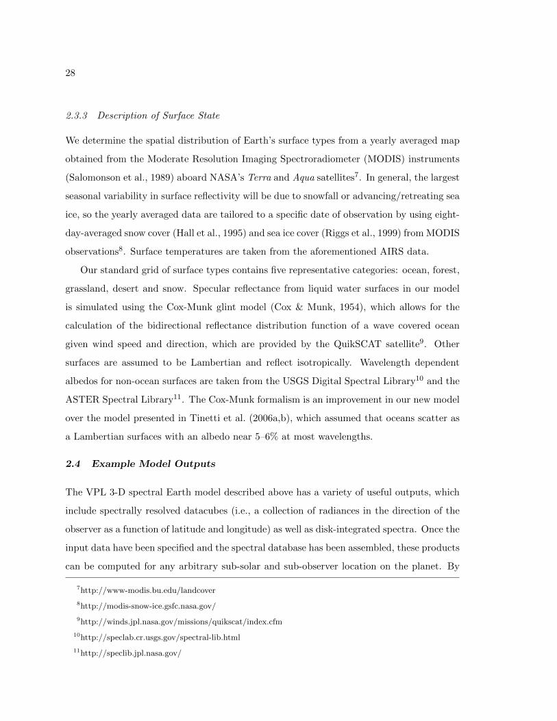
28

2.3.3 Description of Surface State

We determine the spatial distribution of Earth’s surface types from a yearly averaged map

obtained from the Moderate Resolution Imaging Spectroradiometer (MODIS) instruments

(Salomonson et al., 1989) aboard NASA’s Terra and Aqua satellites7. In general, the largest

seasonal variability in surface reflectivity will be due to snowfall or advancing/retreating sea

ice, so the yearly averaged data are tailored to a specific date of observation by using eight-

day-averaged snow cover (Hall et al., 1995) and sea ice cover (Riggs et al., 1999) from MODIS

observations8. Surface temperatures are taken from the aforementioned AIRS data.

Our standard grid of surface types contains five representative categories: ocean, forest,

grassland, desert and snow. Specular reflectance from liquid water surfaces in our model

is simulated using the Cox-Munk glint model (Cox & Munk, 1954), which allows for the

calculation of the bidirectional reflectance distribution function of a wave covered ocean

given wind speed and direction, which are provided by the QuikSCAT satellite9. Other

surfaces are assumed to be Lambertian and reflect isotropically. Wavelength dependent

albedos for non-ocean surfaces are taken from the USGS Digital Spectral Library10 and the

ASTER Spectral Library11. The Cox-Munk formalism is an improvement in our new model

over the model presented in Tinetti et al. (2006a,b), which assumed that oceans scatter as

a Lambertian surfaces with an albedo near 5–6% at most wavelengths.

2.4 Example Model Outputs

The VPL 3-D spectral Earth model described above has a variety of useful outputs, which

include spectrally resolved datacubes (i.e., a collection of radiances in the direction of the

observer as a function of latitude and longitude) as well as disk-integrated spectra. Once the

input data have been specified and the spectral database has been assembled, these products

can be computed for any arbitrary sub-solar and sub-observer location on the planet. By

7http://www-modis.bu.edu/landcover

8http://modis-snow-ice.gsfc.nasa.gov/

9http://winds.jpl.nasa.gov/missions/quikscat/index.cfm

10http://speclab.cr.usgs.gov/spectral-lib.html

11http://speclib.jpl.nasa.gov/

29

Figure 2.5 Albedo spectra of the five surface types used in the model. Data for forests aretaken from the ASTER Spectral Library while all other data are taken from the USGSDigital Spectral Library. Water reflectivity in our model is represented with a Cox-Munkglint model, which is a function of viewing geometry. The ocean data shown in this figureis representative of the albedo of ocean water averaged over all viewing angles.

30

Figure 2.6 A variety of reflected light images from our model, all taken at full phase atthe same time in mid-northern winter. The image on the left is in true-color (using filterscentered at 0.45 µm, 0.55 µm, and 0.65 µm), the image in the center is in false-color (usingfilters centered at 0.45 µm, 0.55 µm, and 0.85 µm to highlight the continents), and the imageon the right is taken at 1.4 µm in a water absorption band, which increases the sensitivityto high clouds.

inputting time-resolved satellite data, we can then generate realistic, time-dependent images

and spectra of Earth. In this section I will demonstrate some of these model outputs, which

will hopefully aid readers in understanding the model validations and applications that

appear in later chapters.

The term Iλ (ni, o, s) in Equation 2.9 defines the datacube. By visualizing these radi-

ances at a particular wavelength, or by combining radiance values from several different

wavelengths to create true- and false-color visualizations, we can generate images of Earth’s

disk from the user-defined sub-solar and sub-observer locations. Figure 2.6 shows a few

example model images of Earth at full phase in reflected light. The images include: a

true-color image assembled from datacube radiances at 0.45 µm, 0.55 µm, and 0.65 µm, a

false-color image assembled in a similar fashion except using radiances at 0.45 µm, 0.55 µm,

and 0.85 µm to highlight the continents, and an image of Earth at 1.4 µm, which is in a

water absorption band, thus increasing the sensitivity to high clouds.

Figure 2.7 shows images of Earth in true-color (assembled as described previously) and

at 10 µm, which is in the infrared atmospheric window region where Earth’s atmosphere is

relatively transparent. The observer is at 0◦ latitude and longitude, and the Sun is at 0◦

latitude and 300◦ longitude, giving a phase angle of about 60◦. Note that the infrared image

31

Figure 2.7 A true-color image of Earth (left) and the corresponding thermal infrared image(right). The true-color image was constructed using filters centered at 0.45 µm, 0.55 µm,and 0.65 µm), while the infrared image uses a filter near 10 µm, in the atmospheric windowregion. The infrared image clearly shows the atmospheric pixelization, which captures agradient in surface temperatures from the equator to the poles, and clouds appear as darkfeatures in this image.

shows the atmospheric pixelization, with surface temperatures decreasing towards the poles

and with clouds appearing as dark features due to their temperatures being cooler than the

surface. The disk-integrated spectrum which corresponds to this viewing geometry is shown

in Figure 2.8. Notable features have been labeled, and include: a deep absorption feature

from ozone at ultraviolet wavelengths, a slope in the continuum near 0.4 µm increasing

towards the blue due to Rayleigh scattering, many strong absorption features from water

vapor throughout the near-infrared and thermal infrared, the 7.7 µm methane band, the

9.7 µm ozone band, and the 15 µm carbon dioxide band.

32

Figure 2.8 An example high resolution, disk-integrated spectrum of Earth from our model,shown as wavelength multiplied by the specific radiance. The viewing geometry is identicalto that of Figure 2.7, and notable features have been labeled.

33

Chapter 3

VALIDATION OF THE EARTH MODEL

In this chapter, I use a combination of satellite observations, Earthshine observations,

and spacecraft observations to validate our 3-D spectral Earth model. I also present a suite

of sensitivity studies performed on the model. This combination of validation and sensitivity

studies will lend credibility to the scientific investigations performed in later chapters and

in the future. Portions of this chapter were originally published in collaboration with V. S.

Meadows, D. Crisp, et al. in the June 2011 edition of the journal Astrobiology (Robinson

et al., 2011, Astrobiology, Vol. 11, pp. 393–408); c© 2011 Mary Ann Liebert, Inc.), and are

reproduced below with permission of Mary Ann Liebert, Inc.

3.1 Introduction

A model is only as good as it’s validation, and, all too often, unvalidated models or, worse

yet, models that have been shown to perform poorly when compared to data, are used in

scientific studies. Such practices can lead to incorrect predictions, the misinterpretation

of data, and biases. To prevent such problems, predictive models should be compared

to the available data, and should undergo a rigorous set of sensitivity studies, both of

which demonstrate the range of parameter space over which the model generates physically

accurate predictions.

A number of datasets are available for the purposes of validating our 3-D spectral Earth

model. These include assemblages of data from Earth-observing satellites, measurements

of Earth’s brightness from observations of the night side of the Moon (i.e., Earthshine

measurements), and observations of the distant Earth from spacecraft. Since they are taken

from ground-based observatories, Earthshine observations tend to be limited in wavelength

and temporal coverage (Goode et al., 2001; Arnold et al., 2002; Woolf et al., 2002; Turnbull

et al., 2006b; Montanes-Rodrıguez et al., 2006), but have access to nearly the entire range of

34

Figure 3.1 The thermal infrared spectrum of Earth obtained by Mars Global Surveyor whileit was en route to Mars. The observation occurred on November 24th, 1996, and the sub-observer latitude and longitude were 18◦ N and 152◦ W, respectively. Blackbody curves(dashed) for Earth’s equilibrium temperature (255 K) and, roughly, for the temperatureobserved in the infrared window region (270 K) are also shown.

Earth’s phases. Examples of spacecraft observations of Earth include the flyby observations

of Earth acquired by the Galileo spacecraft (Sagan et al., 1993), and the single snapshot

observation of Earth’s thermal infrared spectrum taken by the Mars Global Surveyor mission

while it was en route to Mars (Christensen & Pearl, 1997), which is shown in Figure 3.1. The

most relevant datasets for validating our Earth model are those which observe Earth’s full

disk with wide wavelength coverage, high temporal resolution, and broad temporal coverage,

such as the observations of Earth acquired by NASA’s EPOXI mission (Livengood et al.,

2011).

The EPOXI mission, a reuse of NASA’s Deep Impact flyby spacecraft, provided a com-

prehensive set of observations of the distant Earth. The EPOXI observations contain several

days of time resolved, multi-wavelength visible photometry and near-infrared spectroscopy

of Earth’s disk through a full 24-hour rotation period. As a result, the EPOXI dataset

35

offers an opportunity to perform a rigorous model validation, as no previous spectral Earth

models have been compared to datasets that both span a wide range of wavelengths and

are time-resolved.

3.2 Description of Data

The EPOXI Earth dataset is our primary tool for model validation. These observations

were acquired with the High Resolution Instrument (HRI) on board the Deep Impact flyby

spacecraft, and are described in (Livengood et al., 2011). The HRI is a 0.3m f/35 telescope

with nine square-bandpass filters and a NIR spectrometer (Hampton et al., 2005). Seven

filters are ∼ 100 nm wide and are centered at 350, 450, 550, 650, 750, 850 and 950 nm,

segmenting the visual spectral range. The NIR spectrometer covers the wavelength range

from 1.05–4.5 µm with a maximum resolution (R = λ/∆λ) of 750 at the shortest wave-

lengths, a minimum resolution of 200 at about 2.6 µm, and a resolution of 350 at the longest

wavelengths (Klaasen et al., 2008).

During the primary portion of the EPOXI mission, Earth was observed with the HRI

in three separate 24-hour periods: 2008-Mar-18 18:18 UT – 2008-Mar-19 18:18 UT, 2008-

May-28 20:05 UT – 2008-May-29 20:05 UT, and 2008-Jun-4 16:57 UT – 2008-Jun-5 16:57

UT. The star-planet-telescope angle (phase angle) for the three sets of observations were

57.7◦, 75.1◦, and 76.6◦, respectively. NIR spectra of Earth were taken every two hours (30◦

rotation) a total of 13 times, to cover a full rotation of Earth from the viewpoint of the

spacecraft. The NIR spectrometer slit was oriented perpendicular to the terminator, due to

spacecraft constraints. To avoid saturation and to obtain globally averaged spectra, rapid

scans were made alternating between south to north and north to south across Earth to limit

the amount of time any part of Earth was within the slit of the spectrometer. Photometry

in the 450, 550, 650 and 850 nm filters was taken every fifteen minutes (∼ 4◦ rotation)

and every hour (15◦ rotation) for the 350, 750 and 950 nm filters. Note that calibration

errors as large as 10% are present in the EPOXI observations (Klaasen et al., 2008). An

example near-infrared from the March observations is shown in Figure 3.2, and normalized

36

Figure 3.2 Example near-infrared spectrum of Earth on 2008-Mar-18 UT from NASA’sEPOXI mission. Note the different scales used for the y-axes on the left and right sides of thespectrum. Prominent absorption features have been labeled, and the sub-observer latitudeand longitude are 0◦ N and 214◦ W, respectively. Instrument calibration uncertainties aretypically 10%, and tend to increase below 2.0 µm and above 4.3 µm (Klaasen et al., 2008).Earth view generated by the Earth and Moon Viewer, first implemented by J. Walker1.

37

Figure 3.3 Lightcurves of data for EPOXI Earth observations from March, which beginat 2008-Mar-18 18:18 UT. Different line colors correspond to different filters, and the filtercenter wavelength is noted in the lower right. Data have been normalized to their respective24 hour averages. The vertical gray line indicates where the observations begin and, 24 hourslater, end. The discontinuity here is a real effect due to time varying cloud structures andis of order 2–3%.

lightcurves from this dataset for the broadband visible observations are shown in Figure 3.3.

We validate our model in the thermal infrared by comparing to observations acquired

by Aqua/AIRS (Aumann et al., 2003). The AIRS instrument does not record full disk

observations of Earth, but instead scans along its orbital path from ±50◦

about nadir

from an altitude of 700 km. These observations were stitched together to produce a disk-

integrated infrared spectrum of Earth by T. Hearty following the procedure described in

Hearty et al. (2009). Note that the limited range of nadir angles accessible to Aqua/AIRS

requires a limb adjustment to be applied to some of the observations when producing a disk-

integrated spectrum, which is accomplished using a simple limb darkening parameterization

from Hodges et al. (2000). An example thermal infrared spectrum of Earth from March 19th,

2008, is shown in Figure 3.4.

1http://www.fourmilab.ch/cgi-bin/Earth/

38

Figure 3.4 Mid-infrared, 24 hour average spectrum of Earth from March 19th, 2008, asgenerated from Aqua/AIRS observations (Hearty et al., 2009). Large gaps are regions wherethe instrument does not return data. Important absorption features have been labeled.

Finally, we extend our validation to a wider range of phase angles than those of the

EPOXI observations by comparing our model to Earthshine measurements of Earth’s bright-

ness at a variety of phases between gibbous and crescent (Qiu et al., 2003; Palle et al., 2003).

The ∼ 500 Earthshine observations used in this work were recorded between November

1998 through January 2005 at Big Bear Solar Observatory, and span a range of phase an-

gles between 30◦ and 140◦. The data are broadband visible observations, spanning 0.4 µm

to 0.7 µm, have a stated accuracy of 2%, and are reported as measurements of apparent

albedo. These observations are shown in Figure 3.5.

Apparent albedo is defined as the albedo of a perfect Lambert sphere that would give

the same brightness of a body at a given phase angle, so that the apparent albedo of a

Lambert sphere would be constant through all phases. Recall that Equation 2.6 describes

the flux Fλ received from a Lambert-reflecting sphere of radius R at a distance d and phase

angle α, and with a wavelength-dependent albedo Aλ. Thus, we can solve Equation 2.6 for

39

Figure 3.5 Apparent albedos of Earth as measured by observing Earthshine from the darkside of the Moon. Data were recorded between November 1998 and January 2005, andspan 0.4 µm to 0.7 µm. The rise in apparent albedo towards crescent phases (large phaseangles) is due to forward scattering from clouds, glint, and Rayleigh scattering. For moreinformation, please see Qiu et al. (2003) and Palle et al. (2003). Data were generouslyprovided by E. Palle.

40

Aλ, so that, if Fλ is measured, then the apparent albedo is given by

Aλ (α, Fλ) =3

2

Fλ

F�λ

d2

R2

π

sinα+ (π − α) cosα, (3.1)

where F�λ is the top-of-atmosphere incident specific solar (or stellar) flux.

3.3 Data-Model Comparisons

In this section we compare our baseline 3-D spectral Earth model to the EPOXI, Aqua/AIRS,

and Earthshine observations. The baseline model assumes 48 atmospheric pixels, 192 sur-

face pixels, 5 surface types (ocean, ice, forest, grassland, and ground), and 4 cloud types

(described in Section 2.3.2). Later sections will test the sensitivity of the baseline model to

these various resolutions and parameterizations.

3.3.1 Validation in the UV, Visible, and Near-Infrared with EPOXI Observations

Comparisons between EPOXI photometric light curves and our baseline model for all three

epochs of observation are shown in Figure 3.6. These plots demonstrate the brightness of

Earth through seven EPOXI bandpasses over the duration of the 24 hour observation period.

Both the data and the model have been normalized to their respective 24 hour averages

through these filters. The vertical gray line marks the beginning and end of the observations.

The discontinuity in normalized intensity between beginning and end is real, and is due

to Earth’s time varying cloud formations, which typically produce a 3–5% change in the

lightcurve over all wavelengths (relative errors for an individual bandpass are typically much

less than 1%). The model generally reproduces the sign and magnitude of this discontinuity.

The shaded region of the lightcurves for the May set of observations marks a Lunar transit

of Earth’s disk, which is an effect not included in our model. The comparison between the

24 hour averaged radiance from the data and our model for the March and June epochs

of observation is shown in Figure 3.7. Table 3.1 shows the percent difference between the

24 hour average radiance data and the baseline March, May, and June models (models “a”,

“b”, and “c”, respectively). The model reproduces the data on an absolute scale of radiance

to within the ∼ 10% uncertainty in EPOXI/HRI calibration accuracy (Klaasen et al., 2008).

Root-mean-square (RMS) errors for the lightcurve comparisons are also shown in Table 3.1.

41

These errors measure the goodness of fit of the model lightcurves and are computed by

comparing the data to the model for each bandpass at each observation within the 24 hour

observing sequence. Our model reproduces the time dependent variability to within 3% in

most cases. Note the trend in the data of larger peak-to-trough variability with increasing

wavelength, with roughly 10–15% variability at shorter wavelengths and over 20% variability

(in some cases) at longer wavelengths.

42

Figure 3.6 Lightcurves of data (solid) and baseline model (dashed) for EPOXI observationsfrom March (left), May (center), and June (right). March observations begin at 2008-Mar-18 18:18 UT, May observations begin at 2008-May-28 20:05 UT,and June observations beginat 2008-Jun-4 16:57 UT. The filter center wavelength is noted in the central column. Modelvalues and data have been normalized to their respective 24 hour averages. The shadedregion in the central column marks a Lunar transit of Earth’s visible disk, which is an effectnot included in our spectral model. The vertical gray line indicates where the observationsbegin and, 24 hours later, end. The discontinuity here is a real effect due to time varyingcloud structures and is of order 2–3% in March. The discontinuity tends to be smaller inthe May observations and larger in the June observations. The model generally reproducesthe scale and sense of these discontinuities.

43

Tab

le3.

1V

alid

atio

nan

dS

ensi

tivit

yT

est

Res

ult

s

Mod

ela

bc

de

fg

h

Ob

serv

atio

nM

onth

Mar

chM

ayJu

ne

Mar

chM

arch

Mar

chM

arch

Marc

h

Atm

.R

es.

[pix

els]

4848

4848

481

48n

/a

Srf

.R

es.

[pix

els]

192

192

192

>3,

000

192

192

48192

Clo

ud

Typ

es4

44

31

44

1(L

am

ber

t)

Fil

ter

Cen

ter

[nm

]24

-hr

Avg.

Rad

.E

rror

2[%

]:

Lig

htc

urv

eR

MS

Err

or3

[%]

350

6.7

:1.

48.

1:

3.4

5.5

:3.

33.

1:

4.5

4.8

:1.

76.

5:

1.4

1.0

:1.

631

:3.1

450

7.0

:2.

08.

1:

3.4

7.1

:3.

51.

3:

5.3

3.2

:2.

36.

7:

1.9

0.9

:2.

113

:1.6

550

2.1

:2.

34.

0:

3.8

2.9

:3.

89.

8:

5.1

3.6

:2.

60.

8:

2.2

4.8

:2.

519

:1.4

650

4.2

:2.

05.

8:

3.7

5.3

:3.

77.

6:

4.2

2.8

:2.

33.

0:

1.9

2.5

:2.

627

:1.7

750

0.5

:4.

30.

5:

5.7

0.5

:5.

85.

7:

5.1

8.7

:3.

80.

5:

4.1

6.6

:2.

934

:2.3

850

0.2

:5.

51.

3:

7.2

0.3

:7.

22.

6:

6.6

8.4

:4.

60.

4:

5.4

5.2

:3.

727

:2.7

950

5.7

:2.

16.

3:

4.2

3.3

:4.

013

.5:

5.1

7.2

:2.

87.

3:

2.2

0.1

:2.

356

:3.0

2p

erce

nt

erro

rfo

r24

hour

aver

age

radia

nce

,a

mea

sure

of

abilit

yto

repro

duce

vis

ible

radia

nce

of

Eart

h;

com

pare

to∼

10%

inst

rum

ent

abso

lute

calibra

tion

unce

rtain

ty

3ro

ot-

mea

n-s

quare

erro

rfo

rnorm

alize

dm

odel

lightc

urv

es,

am

easu

reof

abilit

yto

repro

duce

lightc

urv

esh

ap

e

44

In addition to fitting lightcurve time variability and absolute brightness in the visible, our

model simultaneously reproduces the EPOXI NIR spectral data, shown in Figure 3.8. This

figure shows comparisons between our model and the EPOXI data for a variety of viewing

geometries from the March set of observations as well as for data from the May and June

sets of observations, which are dimmer in reflected light due to Earth phase. Residuals

from the data-model comparison are also shown and are typically less than about 15%,

demonstrating the the ability of the model to reproduce spectral observations on timescales

from hours to months. Notable disagreements occur near the center of the 1.4 µm and

1.9 µm water bands and near 4.1 µm, in the short wavelength wing of the 4.3 µm CO2

feature. The absolute magnitude of the 4.1 µm defect is much smaller than the 1.4 µm and

1.9 µm defects. Instrument calibration uncertainties are typically 10%, and tend to increase

below 2.0 µm and above 4.3 µm (Klaasen et al., 2008).

3.3.2 Validation in the Thermal Infrared with Aqua/AIRS Observations

Figure 3.9 shows a comparison between the 24 hour average mid-infrared spectrum from

our March model and a spectrum of Earth generated from Aqua/AIRS observations taken

over the same timeframe (Hearty et al., 2009). Recall that Aqua/AIRS does not record

true full disk observations of Earth, and that the Aqua/AIRS spectrum is assembled from

multiple scenes recorded over the observational period. Furthermore, there are wavelength

regions (e.g., near the bottom of the 7.7 µm methane band) where Aqua/AIRS does not

record data, which causes the large gaps in the data shown in Figure 3.9. In general, the

model reproduces the Aqua/AIRS observations quite well, with residuals being, on average,

about 7%, and with brightness temperature errors less than 1K in the atmospheric window.

Some of the largest discrepancies between the Aqua/AIRS data and our spectral model

occur near 14.5 µm, in 15 µm carbon dioxide band. This disagreement is likely caused

by the limb adjustments applied to the Aqua/AIRS observations, which assumed a simple,

wavelength-independent parametrization for limb darkening. Near 14.5 µm, Earth’s disk

would appear limb brightened, since the long path lengths through the atmosphere for the

limb observations would reach optical depth unity higher in the stratosphere, where tem-

45

Figure 3.7 Comparison of the 24-hour averaged signal for the model (dashed) with theEPOXI data (solid) for the March (upper) and June (lower) dates of observation, demon-strating our fit to the data on an absolute scale. Note that the June observations are overalldimmer than the March observations due to Earth phase. The largest discrepancies aretypically in the 450 nm filter and are ∼ 8% for both observations, within the 10% absoluteerror in the HRI calibration (Klaasen et al., 2008). The average spectrum of the May ob-servations is similar to that of the June observations (i.e., within a few percent) and wereomitted for clarity.

46

Figure 3.8 Near-infrared spectral comparison of the model (dashed) with EPOXI data (solid)for a variety of observations. Note the different scales used for the y-axes on the left andright sides of the plots. Date indicators and sub-observer longitudes are given at the topof each plot. Prominent absorption features have been labeled in the upper-left plot. May(middle-right) and June (lower-right) observations are dimmer in reflected light due toEarth phase. Residuals for the data-model comparison are shown below each plot andare typically less than about 15%. Stronger disagreements tend to occur between 1.1–1.2 µm (water), between 1.35–1.5 µm (water), and between 3.9–4.15 µm (N2O, wing ofCO2 feature). Extremely low signal levels and instrument artifacts lead to large residualsin the 2.5–3.25 µm range. Instrument calibration uncertainties are typically 10%, and tendto increase below 2.0 µm and above 4.3 µm. Earth views generated by the Earth and MoonViewer.

47

Figure 3.9 Mid-infrared, 24 hour average spectra of Earth from our March model (gray)and as generated from Aqua/AIRS observations (solid) (Hearty et al., 2009). In general,the agreement is quite good, with residuals (lower panel) being typically ∼ 7%. Large gapsare regions where the instrument does not return data.

48

peratures are larger than the tropopause temperatures probed near this wavelength. Thus,

applying a wavelength-dependent limb darkening/brightening scheme to the Aqua/AIRS

observations would likely improve the data-model comparison in the 15 µm carbon dioxide

band.

3.3.3 Phase Validation using Earthshine Observations

While the wavelength coverage and resolution as well as the time resolution of the EPOXI

Earth observations are an excellent dataset for validating our spectral Earth model, they

only span a narrow range of phase angles (57.7◦, 75.1◦, and 76.6◦). We expand our validation

to a much wider range of phase angles in Figure 3.10, where we compare our model to the

Earthshine dataset, which cover the range of phase angles between 30◦ and 140◦. Recall

that the Earthshine observations are broadband, spanning 0.4 µm to 0.7 µm.

The model observations shown in Figure 3.10 come from the simulation of Earth through

a year presented in Robinson et al. (2010). This large simulation used daily-resolved cloud

coverage and thickness data as well as weekly-resolved snow and sea ice coverage data from

2008. Thus, the simulation is not expected to model any individual observation in the

Earthshine dataset, but is meant to reproduce the trends and behaviors seen in the dataset.

For expediency, the model also assumed a standard mean Earth atmosphere, since the 3-

D water vapor and temperature distributions have only negligible effects in the 0.4 µm to

0.7 µm range. Model spectra were recorded every four hours while Earth progressed through

the entire range of phase angles (0◦ to 180◦). The high-resolution, disk-integrated spectra

were then integrated over the same wavelength range as the Earthshine observations.

In general, there is good agreement between the data and the model, demonstrating the

ability of the model to properly simulate Earth’s phase-dependent brightness. At gibbous

phases where Earthshine data were recorded, the mean apparent albedo of the model Earth

is 0.29±0.02 and is 0.26±0.03 for the Earthshine data. Thus, while the Earthshine data are

systematically lower than the EPOXI observations and the model at gibbous phases, they

are all in agreement to within one standard deviation. At crescent phases the Earthshine

observations are systematically larger than the model. However, an analysis where the

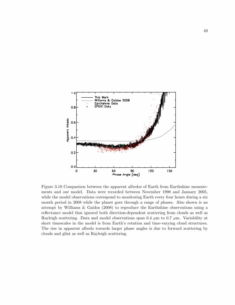
49

Figure 3.10 Comparison between the apparent albedos of Earth from Earthshine measure-ments and our model. Data were recorded between November 1998 and January 2005,while the model observations correspond to monitoring Earth every four hours during a sixmonth period in 2008 while the planet goes through a range of phases. Also shown is anattempt by Williams & Gaidos (2008) to reproduce the Earthshine observations using areflectance model that ignored both direction-dependent scattering from clouds as well asRayleigh scattering. Data and model observations span 0.4 µm to 0.7 µm. Variability atshort timescales in the model is from Earth’s rotation and time-varying cloud structures.The rise in apparent albedo towards larger phase angles is due to forward scattering byclouds and glint as well as Rayleigh scattering.

50

Earthshine data were divided into 10◦-wide bins in phase angle shows that the model is

always within a single standard deviation of the observations.

3.4 Sensitivity Tests

Our selected atmospheric and surface resolution (48 pixels and 192 pixels, respectively)

and our set of four cloud categories represent our standard model. The following set of

investigations aim to determine the level of detail required in the model to reproduce both

the visible and NIR EPOXI observations while remaining consistent with the input data.

We emphasize the EPOXI observations as they are the most comprehensive dataset available

for the purposes of sensitivity studies. The parameters used in these studies and a summary

of the results are shown in Table 3.1. Lightcurves for a subset of the studies through three

EPOXI visible-light filters are shown in Figure 3.11. Results are presented and discussed in

greater depth below.

Cloud Categories: The Importance of Spectra

The characteristics that define our selected cloud sub-categories are based on MODIS data,

but the number of cloud categories in our model is arbitrary. While our standard model

utilizes four cloud sub-categories, it is useful to know how sensitive the model is to the

chosen number of cloud sub-categories. To test this, the model was run with only a single

cloud sub-category (model “e” in Table 3.1) and with two cloud sub-categories. The single

cloud model uses a cloud extinction optical depth of 10 and places the liquid water cloud in

the middle of the troposphere while the two cloud model uses liquid water clouds with an

extinction optical depth of 5 and ice clouds with an extinction optical depth of 15, placed at

the same altitudes as the liquid and ice water clouds in the standard model. In all cases the

characteristics of the cloud sub-categories were derived from MODIS observations. Example

NIR spectra from these low “cloud resolution” models are compared to the EPOXI data

and our standard model in Figure 3.12. In general, the models with less than four cloud

sub-categories are poorer fits to the NIR data. The single cloud model is too bright in the

continuum regions, underestimates water vapor absorption near 1.4 µm, and overestimates

water vapor absorption near 1.1 µm. Furthermore, this model cannot reproduce the shape

51

Figure 3.11 Comparison between the EPOXI data (solid) and a variety of models consideredin this work through a subset of the EPOXI filters for the March set of observations. Filtercenter wavelength is noted on each plot. The details of the models shown are outlined inTable 3.1. Model “a”: standard model; model “e”: single cloud category; model “f”: singleatmospheric pixel; model “g”: 48 surface pixels. Filters were selected to demonstrate theeffects of Rayleigh scattering (350 nm) and water absorption (950 nm). The 650 nm filteris relatively free of atmospheric extinction.

52

Figure 3.12 Comparison between the EPOXI data (solid), our standard model (dashed), amodel run with a single cloud category (dotted), and a model run with two cloud categories(dot-dashed) for a view over the Pacific Ocean on 2008-Mar-18 UT. Note the different scalesused for the y-axes on the left and right sides of the spectral plots. While the single cloudmodel and the two cloud model can reproduce the visible EPOXI lightcurves, they cannotreproduce the NIR data. Earth view generated by the Earth and Moon Viewer

of the continuum region near 1.6 µm, where water ice absorbs. Thus, the EPOXI disk-

integrated NIR spectra contain evidence for the presence of both liquid and ice water clouds.

The two cloud model is an improved fit, but struggles to reproduce the measured intensity

within the 1.1 µm and 1.4 µm water features. A six cloud model was run and did not offer

significant improvements over the four cloud model when compared to the EPOXI data set.

The visible EPOXI lightcurves are less of a challenge to models due to their broadband

nature and the fact that these data are relatively insensitive to atmospheric absorbers. Thus,

the single cloud model can still reproduce the absolute brightness and temporal variability

seen in the low spectral resolution, visible EPOXI data, as shown in Table 3.1 and in the

filters presented in Figure 3.11 (the two cloud model can reproduce the visible data, and is

not shown for clarity). These results emphasize the crucial role that spectra play, especially

53

in the NIR, in disentangling the effects of clouds; the EPOXI visible, broadband data can

be fit with a single cloud category while four cloud varieties were required to fit the NIR

data. It may also be possible to optimize the optical depths of the clouds in the two cloud

or the four cloud model to improve the fit to the NIR spectra while remaining consistent

with MODIS data.

Sensitivity to Atmospheric and Surface Resolution

The atmospheric resolution determines the scale at which temperature and gas mixing

ratio profiles are resolved while the surface resolution determines the scale at which surface

features are resolved. To test our sensitivity to these parameters, we ran a model with a

single atmospheric pixel as well as a model with 48 surface pixels (models “f” and “g” in

Table 3.1, respectively). Using a single atmospheric pixel amounts to assuming there is

no spatial variability in the temperature and composition of Earth’s atmosphere. Earth’s

surface exhibits large variations in both water vapor mixing ratios and surface temperatures,

making a single atmospheric pixel a poor choice for a model that aims to simulate these

variations. For example, a model with a single atmospheric pixel would incorrectly produce

polar and equatorial thermal IR spectra that are nearly identical, even though, in reality,

these regions can differ in surface temperature by over 100K. In general, though, the model

with a single atmospheric pixel can still reproduce the visible EPOXI data reasonably well

since the visible data is relatively insensitive to atmospheric/surface temperature as well as

water vapor distribution. Regarding surface resolution, the coarse resolution of the 48 pixel

model (surface pixels are several thousand kilometers in size) leads to a poor reproduction

of the longitudinal variations in brightness in the lightcurves at all wavelengths, which is

shown in Fig. 3.14. The visible disk of Earth in this low resolution model is dominated by

∼ 10 pixels, which leads to unrealistic periodicities in the lightcurves as relatively bright

surface pixels rotate into and out of view.

3.5 Comparisons to Other Models

To demonstrate the significant improvements in our model over previous models, we compare

spectral, phase dependent results from our model to both the model described in Tinetti

54

et al. (2006a), which was only validated with single snapshots of Earth, as well as to EPOXI

observations in Fig. 3.13. In this figure, we show Earth’s wavelength dependent reflectivity

at visible and NIR wavelengths for a variety of different phases (full, gibbous, half illumi-

nated or quadrature, and crescent). Both models assume realistic clouds. In general, the

model described in Tinetti et al. (2006a) is significantly brighter than our model, with the

most extreme discrepancy occurring at 0.5 µm in the crescent view, where the Tinetti et. al

model is about 400% brighter than our model. Also, the Tinetti et. al model is distinctly

bluer than our new model at phases between half illumination and crescent. EPOXI obser-

vations taken at gibbous phase and near half illumination (phase angles of 57.7◦ and 76.6◦,

respectively) and our model of the observations are shown as dashed lines in the gibbous and

quadrature plots, demonstrating our ability to reproduce Earth’s brightness and reflectivity

at these phases.

Some of the differences between the two models shown in Fig. 3.13 can be accounted for

by an error in the model described in Tinetti et al. (2006a) which rotated the angle between

the Sun and the observer by 180◦, effectively confusing forward scattering with backward

scattering. Inserting this error into our model allows us to reproduce the excess brightness

in the old model near full phase, and also allows us to reproduce the incorrect blue nature

of the old model near quadrature and crescent phases. We have not, however, been able to

reproduce the excess brightness in the old model at phases away from full phase, indicating

that other problems exist in the model described in Tinetti et al. (2006a).

For further comparison, we ran the Tinetti et al. model using input cloud coverage

maps as well as atmospheric composition and temperature data for the appropriate dates of

EPOXI observation. As the core radiative transfer model is the same in our model and the

Tinetti et al. model, this experiment primarily tests the cloud parametrization in the two

models. The comparisons between EPOXI data from March and the Tinetti et al. model

are shown in Fig. 3.14 (model “d”). Discrepancies in the 24 hour average radiance and the

RMS errors for the lightcurves are also shown in Table 3.1. The inability of the Tinetti et al.

model to reproduce the lightcurves indicates problems with the cloud parametrization, and

demonstrates the importance of validating spectral Earth models against time and phase

resolved data. These comparisons indicate that, in general, measures of Earth’s brightness

55

Figure 3.13 Comparison between the Tinetti et al. (2006a) model and our model. A mea-sure of Earth’s reflectivity, taken as π times the disk-integrated radiance (in W/m2/µm/sr)divided by the Solar flux at 1 A.U (in W/m2/µm), is shown for the planet viewed at fullphase, gibbous phase, quadrature (i.e., half illuminated, or a phase angle of 90◦), and cres-cent phase. Both models use realistic cloud cover, and the data for the Tinetti et. al modelis taken from Tinetti et al. (2006b). An EPOXI observation taken near half illuminationand our model of the observation are shown as dashed lines in the quadrature case, demon-strating that our model correctly reproduces the data at this phase. In general, the Earthmodel from Tinetti et al. (2006a,b) is about 100% to 400% too bright, and is unrealisticallyblue at phases near quadrature and crescent.

56

Figure 3.14 Comparison between the EPOXI data (solid), our standard model (“a”), theTinetti et al. model (“d”), and a model that ignores atmospheric extinction and scattering(i.e., a reflectance model, “h”). Models and data correspond to the March set of EPOXIobservations. Filter center wavelength is noted on each plot. The details of the modelsshown are outlined in Table 3.1.

from the Tinetti et al. model should not be used.

To compare our model to previously published reflectance models (e.g., Williams &

Gaidos, 2008), we removed atmospheric absorption and scattering from our simulations

and replaced the Mie scattering clouds in our model with a Lambertian surface with a

visible albedo of 0.60, which is a typical value assumed in reflectance models (model “h” in

Table 3.1). By definition, a reflectance model cannot reproduce spectral data, like the NIR

EPOXI data, because such models explicitly ignore atmospheric absorption. The 24-hour

average radiance is shown for the reflectance model, the EPOXI data, and our standard

model in Figure 3.15. The reflectance model clearly struggles to reproduce the radiance

data (quantified in Table 3.1), especially in the 350 nm and 950 nm filters, which are

strongly affected by extinction due to Rayleigh scattering and water vapor, respectively.

However, the reflectance model can reproduce the relative variations in brightness in the

EPOXI lightcurves, as shown in Table 3.1 and in Figure 3.14.

57

Figure 3.15 Comparison of the 24 hour averaged signal (top) for the EPOXI data (solid),our standard model (dashed), and a model where atmospheric absorption and scatteringhas been removed and clouds have been treated as a Lambertian surface with an albedoof 0.60 (dotted). The data and models have been converted to a measure of reflectance(bottom) in the same fashion as in Figure 3.13. The effects of ignoring Rayleigh scatteringcan be seen in the shortest wavelength filters while the lack of atmospheric absorption isespecially apparent in the 950 nm filter, which includes a strong water absorption feature.Data and models are all for the March EPOXI observations.

58

3.6 Discussion

Earth is a complex system and, as a result, any model which aims to simulate Earth’s ap-

pearance to a distant observer should reflect this complexity. Our spectral Earth model aims

to accurately simulate Earth’s disk-integrated spectrum at any arbitrary viewing geometry

and wavelength, necessitating a comprehensive and rigorous treatment of a large number

of physical processes (e.g., ocean glint, realistic cloud scattering, vertically and spatially

resolved temperature and gas mixing ratio profiles). However, and as we have shown, this

does not necessarily imply that more simplified models cannot reproduce specific details

of Earth’s appearance (e.g., ocean glint in Williams & Gaidos (2008)). In either case, any

model of Earth’s appearance should be validated against observational data, ensuring its

accuracy as a predictive or interpretive tool.

Our new model is capable of reproducing the time variable color and absolute brightness

of Earth, as observed in the visible and NIR EPOXI data, and can do so for multiple dates

of EPOXI observations. Typical RMS errors for the model lightcurves are within 3–4%,

and the 24 hour average visible radiance for the model matches the EPOXI observations to

within calibration uncertainties. The model also simultaneously provides a good fit to the

shape and absolute brightness of the high resolution Aqua/AIRS mid-IR observations.

The visible and NIR EPOXI data provided only limited phase coverage, as the obser-

vations were all acquired near quadrature. However, the model was able to reproduce the

broadband visible Earthshine observations, which span a range of phases from crescent to

gibbous. As the Earthshine dataset contains hundreds of observations acquired over a pe-

riod of about seven years, they capture a range of measured apparent albedos at any given

phase angle, and our simulations (for the year of 2008) all lie within a single standard de-

viation of these measurements. The model is systematically dimmer than the observations

at crescent phases, however. It is unclear whether this is due to systematic errors in the

observations or a bias in the model. Comparisons of the model to space-based observations

of the crescent Earth, such as those acquired by NASA’s LCROSS mission, will provide an

independent test of the model’s performance at large phase angles (Robinson et al., 2012).

Although our fit to the lightcurves is generally good (Figure 3.6), the largest root-mean-

59

square errors are seen for the 750 nm and the 850 nm filters, indicating that our poorest

match to the shapes of the EPOXI lightcurves occurs at these wavelengths. These filters are

relatively clear of atmospheric absorbers and are largely unaffected by the strong Rayleigh

scattering seen in bluer filters. As a result, these filters are the most sensitive to the surface,

and mismatches in these filters may indicate that more than five surface types are needed

to better reproduce the EPOXI data at these wavelengths.

Even though our model reproduces the 24 hour average visible radiance of Earth to

within instrument uncertainties (Figure 3.7), discrepancies at short wavelengths are typically

in the sense of the data being brighter than the model, suggesting either a systematic

calibration error or residual minor defects in the model. The difference in the 24 hour

average brightness between the data and the model is largest in the 350 nm and 450 nm

filters. A small fraction of the light incident on an ocean surface actually enters the water

and is scattered back out (Cox & Munk, 1954), which is an effect not accounted for in

our model. As water is most transparent in the 350 nm and 450 nm filters, including this

ocean “volume scattering” behavior in our simulations could improve our fits to the Earth’s

radiance. Note that a model similar to ours, described and validated in Fujii et al. (2011),

also struggled to reproduce EPOXI observations of Earth’s brightness in these filters, which

could indicate a systematic error in the data.

Notable disagreements between the model and data in the NIR spectra occurred near

1.4 µm, 1.9 µm, and 4.1 µm. The 1.4 µm and 1.9 µm discrepancies occur at the base of

water vapor absorption features, indicating problems with the input MODIS water vapor

distribution data, the HITRAN line lists, and/or the vertical placement of clouds in our

model. The height of clouds in the atmosphere controls the column depth of water vapor that

is available to absorb radiation incident on the top of the atmosphere. For this reason, low

clouds allow a longer column through the atmosphere and more absorption by water vapor

in the spectrum than high clouds. MODIS data does not contain a complete description of

the full three-dimensional distribution of clouds in Earth’s atmosphere and we must estimate

standard altitudes for our liquid and ice clouds. While the altitudes that we assumed seem

to offer a reasonably good fit overall to the NIR data, these fits could be improved by

allowing our clouds to have a varying vertical distribution that is determined by CloudSat

60

data (Stephens et al., 2002).

The disagreement near 4.1 µm is in the wing of a CO2 absorption feature. Efforts

to fit this shape by altering cloud coverage and thickness were unsuccessful. N2O has

a weak absorption feature between 4.0–4.1 µm, but altering atmospheric N2O levels also

failed to reproduce the observed shape. SO2 absorbs in this region, but the strength of

this feature is even less than the N2O feature. Recent work has shown that including an

N2-N2 collision-induced absorption feature, which is centered near 4.2 µm, dramatically

improves the data-model comparison in this wavelength region (E. Schwieterman, personal

communication).

The original version of the model (Tinetti et al., 2006a,b) failed to reproduce the observed

lightcurves primarily because this version of the model used a less rigorous parametrization

of clouds to reproduce limited Earth-observing data sets. Most importantly, this earlier

version of the model assumed that all ice clouds were quite thin with an extinction optical

depth of order unity, which is true for only ∼ 10 % of all ice clouds in the MODIS data. The

model presented in this work has a much improved treatment of spatially and temporally

varying clouds, and parametrizes them based solely on input data collected from the MODIS

instruments. Our cloud parametrization technique is rigorous and versatile, allowing us to

reproduce all three sets of EPOXI observations, which span almost three months in time,

without needing to tune model parameters to each dataset.

In summary, our model is designed to be comprehensive and versatile enough to model

the Earth’s appearance over a very large wavelength range and at arbitrary viewing angle

and phase. The level of model complexity required to simultaneously simulate Earth’s

spectrum over a large wavelength range, where different physical processes dominate, may

at first appear daunting. Especially if considering the reverse problem of retrieval of the

correct planetary characteristics from a limited data set. However the more optimistic view

is that in cases where a more comprehensive model is required to accurately fit Earth data,

this indicates that the data contained enough information to allow us to discriminate the

more complex environmental characteristics from more simplistic models. This would be

a desirable circumstance when attempting to learn about extrasolar planet environments

from observations. Additionally, in the process of fitting the EPOXI data we have been

61

able to quantify when model complexity is and isn’t required for a particular application or

wavelength range subset.

For example, modeling moderate resolution NIR spectra does require multiple categories

of clouds, providing cloud altitude, phase, and optical thickness resolution. As demonstrated

in Figure 3.12, a single cloud category produces a disk-integrated spectrum that is too bright

in the NIR continuum and underestimates water vapor absorption in some regions (near

1.4 µm) while overestimating water vapor absorption at other wavelength regions (near

1.1 µm). The lack of ice clouds leads to discrepancies near 1.5 µm where ice particles

absorb. A model with two cloud categories reproduces the spectral data more accurately

than the single cloud model, but struggles with the shape of the 1.1 µm and 1.4 µm water

features. Residuals for the two cloud model can be over 40% larger than the residuals

for the four cloud model in these regions. The four cloud model therefore appears to be

optimal for simultaneously fitting both the visible and NIR spectral regions, and would be

most useful for studying the detectability of Earth’s globally averaged characteristics for

TPF-like designs that span both the visible and NIR.

The absolute brightness and temporal variability of the EPOXI lightcurves can be repro-

duced by models without a large number of cloud categories due to the broadband nature of

these data and the fact that observations at these wavelengths are relatively insensitive to

atmospheric absorption. In essence, the broadband lightcurves provide evidence for white,

highly reflective structures that vary in time on the planet, and observations in the 950 nm

filter demonstrate an absorption feature from water vapor. The higher spectral resolution

NIR data provide information regarding the phase and vertical distribution of these struc-

tures. Furthermore, insofar as both liquid water and ice clouds are required to reproduce the

observations near 1.5 µm, the broadband data and moderate resolution spectra demonstrate

that water is found in the atmosphere as vapor, liquid, and ice.

Sensitivity tests indicate that high atmospheric resolution is not needed to reproduce

the EPOXI visible photometric data. This is not surprising as at visible the temperature

structure and distribution of trace gases within the atmosphere should have only small

effects on the lightcurves. Even data in the 950 nm filter, which contains a large water vapor

absorption feature, can still be fit due to variations in the brightness of the continuum outside

62

the absorption feature and the fact that clouds control the column depth of water vapor that

is available to absorb radiation. Earth exhibits large variations in both water vapor mixing

ratios and surface temperatures, indicating that models with low atmospheric resolution

are poor choices for modeling high resolution spectral data or mid-IR data, especially if

the model aims to generate observations for arbitrary viewing geometries (e.g, polar versus

equatorial views).

Reflectance models that ignore scattering and absorption in the atmosphere and which

treat clouds as Lambertian reflectors cannot reproduce the 24 hour averaged brightness of

Earth. The short wavelength filters have lower reflectivity than the data because Rayleigh

scattering has been ignored while longer wavelength filters (e.g., the 950 nm filter, which

contains a strong water feature) show enhanced reflectivity because atmospheric absorption

has been ignored. Reflectance models can, however, reproduce the shapes of the EPOXI

lightcurves as these models are designed to reproduce relative brightness variations due to

structures (e.g., clouds, continents) rotating into and out of view. While simple, compu-

tationally inexpensive models, like reflectance models, may be useful as retrieval tools in

scenarios where observational data are limited or of poor quality, these models are not op-

timal when compared to more rigorous and comprehensive spectral models for applications

which require accurate predictions.

63

Chapter 4

APPLICATIONS I—DETECTING OCEANS ON EXOPLANETS

In this chapter, I use the NASA Astrobiology Institute’s Virtual Planetary Laboratory

(NAI-VPL) 3-D spectral Earth model to simulate Earth’s disk-integrated spectrum as it

would appear to a distant observer watching the planet through an orbit. This set of

simulations allows us to address the significance of ocean glint in disk-integrated, phase-

dependent observations of Earth, thus quantifying an effect that could provide a means

for detecting oceans on an exoplanet. Portions of this chapter were originally published

in collaboration with V. S. Meadows, and D. Crisp in the September 2010 edition of the

Astrophysical Journal Letters (Robinson et al., 2010, ApJL, Vol. 721, L67); c© 2010 Amer-

ican Astronomical Society), and are reproduced below with permission of the American

Astronomical Society.

4.1 Introduction

A major goal in the study of extrasolar planets is the detection and recognition of a “hab-

itable” world, or a planet capable of maintaining liquid water on its surface. A variety of

direct and indirect approaches could be used to determine if a planet is habitable. Indi-

rect approaches focus on characterizing the surface environment of a planet, which would

constrain the likelihood that the planet could maintain liquid water on its surface. Direct

approaches aim to detect signs that indicate the presence of water on the surface of a planet

(e.g., Cowan et al., 2009).

One direct indicator of surface bodies of water is specular reflection, or the “glint effect”.

While specular reflection is not unique to liquid surfaces (e.g., Dumont et al., 2010), liquids

are distinguished from other surfaces by their contrast between weak specular reflectance

at direct illumination angles and strong specular reflectance at glancing illumination an-

gles. Recently, Stephan et al. (2010) used the enhanced reflectivity of liquids at glancing

64

illumination angles to provide evidence for liquid hydrocarbon lakes on the surface of Titan.

Sagan et al. (1993) argued that the presence of a specularly-reflecting region (or “glint

spot”) in spatially-resolved images of Earth taken by the Galileo spacecraft, combined with

detections of atmospheric water vapor and surface temperatures near the melting point

of water, was evidence for the presence of liquid water oceans on Earth’s surface. Unfor-

tunately, obtaining spatially-resolved images of terrestrial extrasolar planets presents an

engineering challenge that will not be met in the near future. The first measurements that

aim to detect glint must rely on how it affects the brightness of a planet in a disk-integrated

sense.

The relative size of Earth’s glint spot compared to the illuminated portion of the disk

increases at crescent phases, and the reflectivity of water increases at glancing illumination

angles, affecting Earth’s phase curve. The detectability of this effect was first investigated

by Williams & Gaidos (2008), who used a simple model of Earth’s reflectance coupled to a

3-D climate model to predict Earth’s appearance over the course of an orbit. Their model

showed that Earth’s reflectivity increases into crescent phases, but was unable to reproduce

Earthshine observations of Earth’s reflectivity (Palle et al., 2003). This discrepancy was at-

tributed to the absence of Rayleigh scattering in their model and the assumption that clouds

reflect isotropically (Lambertian). In reality, liquid droplets and ice crystals preferentially

scatter light in the forward direction, which can mimic the glint effect.

Oakley & Cash (2009) modeled Earth’s brightness over the course of an orbit with an

emphasis on characterization by the New Worlds Observer mission concept (Cash, 2006).

Their model simulated Earth’s reflectivity using satellite-measured bidirectional reflectance

distribution functions (BRDFs) for a variety of scenes (e.g., thick cloud over ocean) (Manalo-

Smith et al., 1998), and used satellite observations to evolve clouds, snow, and ice in their

simulations. Their model also demonstrated an increase in Earth’s reflectivity into crescent

phases, but was not compared to the phase-dependent Earthshine measurements. The

authors proposed that the bright glint spot increases the variability in Earth’s brightness at

crescent phases, which could serve as an indicator of surface oceans. However, the BRDFs

used in their model were not valid at extreme crescent phases, requiring assumptions about

cloud scattering and ocean reflectivity at glancing illumination angles.

65

Here, we use the VPL 3-D spectral Earth model to investigate the significance of glint

in Earth’s phase curve by discriminating between the competing effects of cloud scattering

and glint. This model was extensively validated in the previous chapter, and was shown to

reproduce the phase-dependent Earthshine observations reported in Palle et al. (2003). In

this chapter I also discuss the observing requirements for glint detection using the JWST

paired with an external occulter.

4.2 Earth Through a Year

A distant observer viewing Earth’s orbit edge-on would need to monitor the planet for

at least six months to acquire observations through an entire range of phases (i.e., from

new phase to full phase). To simulate such a dataset, we have run the NAI-VPL 3-D

spectral Earth model (Robinson et al., 2011) through a full year (2008) for several different

viewing inclinations (90◦, or edge-on, 75◦, 60◦, and 45◦). The model runs use realistic,

time-resolved observations of Earth’s snow cover and sea ice cover as well as cloud cover and

optical thickness, all taken from observations acquired by the Moderate Resolution Imaging

Spectroradiometer (MODIS) instruments (Salomonson et al., 1989) aboard NASA’s Terra

and Aqua satellites (Hall et al., 1995; Riggs et al., 1999). Including these data allow the

model to capture variability in Earth’s appearance at timescales from hours (due to time-

varying cloud structures) to months (due to seasonality). To prevent long model runtimes,

mean Earth atmospheric composition and temperatures are used, with the consequence

that the model runs do not capture time variability in these quantities. Although this

approximation will not significantly affect the visible light photometry needed for this study,

it does imply that our results are not completely realistic in the thermal infrared, where

seasonal variations in surface and atmospheric temperatures are important.

Figure 4.1 shows a true-color, crescent phase image from our model, demonstrating a

strong glint spot. Note also that the clouds near the glint spot are relatively bright, which

shows the ability of clouds to mimic the glint effect through forward scattering. Figure 4.2

shows an example of one of our year-long datasets. Earth’s brightness in the 0.4–0.7 µm

range is shown over the course of one orbit as seen from the edge-on perspective. Variability

at large timescales is due to Earth’s changing phase, so that Earth appears brightest at full

66

Figure 4.1 A true-color image from our model (left) compared to a view of Earth from theEarth and Moon Viewer1. A glint spot in the Indian Ocean can be clearly seen in the modelimage.

phase and faintest near crescent phases, and variability at small timescales (see inset) is due

to Earth’s rotation and time-varying cloud formations.

4.3 Results

Figure 4.3 shows our simulation of Earth’s brightness and corresponding apparent albedo as

it would appear over the course of one year to a distant observer for models run both with and

without glint (black and gray, respectively). The viewing geometry, timing, and wavelength

coverage are the same as in Figure 4.2. The non-glinting model uses an isotropically-

scattering ocean reflectance model whose albedo reproduces Earth’s geometric albedo to

within about one percent. The subpanel of Figure 4.3 demonstrates the brightness excess

in the glinting model over the non-glinting model, which can be almost as large as 50%.

The excess brightness increases into crescent phases as the contribution of the glint spot

to Earth’s disk-integrated brightness grows, peaking at orbital longitudes near 20–30◦ from

1http://www.fourmilab.ch/cgi-bin/Earth/

67

Figure 4.2 Simulation of Earth’s brightness through a year. Earth is brightest at full phase(orbital longitudes near 180◦) and faintest near crescent phase (orbital longitudes near0◦ and 360◦). Variability at small time scales (see inset) is due to Earth’s rotation andtime-varying cloud formations (noise is not included in simulations). Model “observations”are recorded every four hours, the system is viewed edge-on (i = 90◦), and an orbitallongitude of 0◦ corresponds to January 1, 2008. All model observations are integrated overthe wavelength range 0.4–0.7 µm.

68

Figure 4.3 Simulation of Earth’s brightness through a year for models run with and withoutglint (black and gray, respectively). Viewing geometry, timing, and wavelength coverageare the same as in Figure 4.2. The bottom sub panel shows the brightness excess in theglinting model over the non-glinting model.

new phase. The brightness excess declines as the illuminated crescent shrinks further. This

is due to a wave-surface “hiding” effect discussed in Cox & Munk (1954), where ocean waves

block rays of light at glancing illumination angles.

The brightness difference between the glinting and non-glinting model is a strong func-

tion of wavelength. If we instead choose a filter that spans 1.0–1.1 µm, the peak brightness

excess increases to about 100%. This behavior arises because glint occurs at the surface

and some wavelength ranges are more sensitive to Earth’s surface than others.

Near 90◦ orbital longitude, both models in Figure 4.3 have apparent albedos that are

about 15–20% larger than those near 270◦. This is due to Earth’s seasons, as was noted

in Williams & Gaidos (2008), and was determined by comparing to a model run without

any seasonal evolution of snow and ice. As Earth moves from northern winter to northern

summer (0◦ to 180◦ orbital longitude in these simulations, respectively), the illumination of

the northern polar region, which is tilted towards the observer, increases. Since this region

69

Figure 4.4 Variability in brightness for our glinting model (black) and our non-glinting model(grey), which are both shown in Figure 4.3. Variability is defined as the ratio between thestandard deviation of all model observations from a 24-hour period and the 24-hour averagebrightness from the same timespan.

of Earth is more snow- and ice-covered prior to northern summer than following northern

summer, the planet appears more reflective heading into full phase than moving out of full

phase. The magnitude of this asymmetry in the lightcurve agrees with the simulations of

Oakley & Cash (2009). In general, the effects of seasons on Earth’s lightcurve depend on

viewing geometry, but are small compared to the effects of cloud scattering and glint at

crescent phases.

The variability of both models in Figure 4.3, defined as the ratio between the standard

deviation of all model observations from a 24-hour period and the 24-hour average brightness

from the same timespan, is shown in Figure 4.4. The variability steadily increases from about

5% near full phase to about 30–40% near crescent phase. Brightness is more variable at

crescent phases since the illuminated portion of the disk represents a relatively small fraction

of the planet’s surface area and, thus, is easily dominated by clouds that rotate into view or

a cloud-free view of the glint spot. Variability at gibbous phases following northern summer

70

is slightly larger than variability at gibbous phases prior to northern summer (4% versus

6%, respectively), which is a seasonal effect. The magnitude of the variability in our models

agrees well with the simulations of Oakley & Cash (2009). However, these authors did not

find a seasonal dependence in variability measurements. Furthermore, their simulations

show a sharp increase in variability as the planet moves into crescent phases (variability

increases from 5–10% to 40% over about 10◦ of orbital longitude) while our models show a

gradual increase in variability into crescent phases.

4.4 Discussion

4.4.1 Earth With and Without Glint

Including phase-dependent reflection from oceans and clouds as well as Rayleigh scattering

has allowed us to reproduce both the brightness and phase dependence of Earthshine obser-

vations (see Section 3.2). Williams & Gaidos (2008) explicitly ignored Rayleigh scattering

and phase-dependent scattering from clouds and were unable to reproduce Earthshine ob-

servations, demonstrating the importance of including these effects in a realistic spectral

Earth model. A model that only includes phase-dependent Rayleigh scattering produces an

increase in apparent albedo at crescent phases (due to weak forward and backward scatter-

ing lobes in the Rayleigh scattering phase function), but the upturn occurs only at extreme

crescent phases (at orbital longitudes within 30◦ of new phase), which is not seen in Earth-

shine observations. This argues that the lack of phase-dependent cloud scattering in the

model presented in Williams & Gaidos (2008) was the primary reason why their model

could not reproduce Earthshine observations. Thus, predictions regarding the behavior of

Earth’s brightness at crescent phases are especially reliant on realistic cloud modeling.

Models that do not include the “hiding” effect of ocean waves will over-estimate the

brightness of water surfaces at glancing reflection angles. For edge-on orbits (inclination,

i = 90◦), this effect becomes especially important at orbital longitudes within about 30◦

of new phase, in agreement with Cox & Munk (1954). The phase-dependent relative size

of the glint spot, the tendency of water to be more reflective at glancing reflection angles,

and the “hiding” effect all combine to produce a maximum brightness excess for a realistic

71

Earth over an Earth without glint near 30◦ from new phase (for an orbit viewed edge-on).

Varying ocean wind speeds in our model show that the location of this peak is only weakly

dependent on surface wind conditions. Previous models used to investigate the detection of

surface oceans (Williams & Gaidos, 2008; Oakley & Cash, 2009) do not include the “hiding”

effect and cannot make strong statements about glint detection at extreme crescent phases.

The season- and phase-dependent variability of Earth’s brightness, shown in Figure 4.4

and taken from the edge-on simulations shown in Figure 4.3, is due to contrast between

highly reflective surfaces and surfaces with low reflectivity. Following full phase, which

corresponds to northern summer in our simulations, snow and sea ice in the northern polar

region have been replaced by darker surfaces (e.g., grassland) which provide greater contrast

to clouds as compared to the snow and ice present prior to full phase. Thus, variability

is larger following northern summer in our simulations. At crescent phases, contrast is

provided by bright, forward-scattering clouds, and/or the bright glint spot, against relatively

dark, Lambertian-scattering surfaces. The illuminated sliver of the planet at crescent phases

represents a relatively small amount of surface area so that the illuminated disk at these

phases can become dominated by large cloud features (or the glint spot), leading to large

variability. Near full phase, the illuminated disk represents a large amount of surface area,

averaging over clouded and non-clouded scenes, leading to relatively low variability.

Our simulations without glint produce the same rise in variability into crescent phases

as our simulations with glint, which indicates that variability at crescent phases is not

completely driven by glint. Thus, the trend of increasing variability into crescent phases

is not a clear indicator of surface oceans, as was proposed by Oakley & Cash (2009). Any

planet that can achieve sufficient contrast between bright and dark surfaces will produce a

variability signal that increases into crescent phases, regardless of the presence of oceans.

Our glinting model demonstrates a wavelength-dependent brightness excess over our

non-glinting model, since some wavelengths are more sensitive to surface effects than oth-

ers. The excess shrinks to less than 10% for the wavelength range 0.3–0.4 µm, where

Rayleigh scattering obscures the surface. At wavelengths that correspond to relatively deep

absorption bands, like the 1.4 µm water band, the excess shrinks to nearly zero because

observations are mostly insensitive to the surface. Figure 4.5 shows the crescent-phase spec-

72

Figure 4.5 Normalized spectra of glinting and non-glinting Earth at crescent phase. Spectraare an average over all observations from Figure 4.3 at orbital longitudes between 315–345◦

and are normalized to the average full-phase flux between 0.4–0.6 µm from the modelswith and without glint, respectively. The continuum regions in the spectrum without glintsimply fall off in brightness with wavelength, while the spectrum from the glinting Earthpeaks between 0.7–0.8 µm before falling off, which is due to the added contribution fromthe glint spot.

tra of the glinting and non-glinting Earth from the observations in Figure 4.3. The spectra

are normalized to the respective full-phase flux from the glinting and non-glinting models,

integrated between 0.4–0.6 µm (which are wavelengths primarily sensitive to Rayleigh scat-

tering and clouds). The shape of the spectrum from the glinting model is distinct from the

spectrum from the non-glinting model due to the added contribution from the glint spot.

At crescent phases, pathlengths through the atmosphere are relatively large and optical

depths to Rayleigh scattering can be larger than unity even at longer wavelengths. This

indicates that observations which aim to detect the brightness excess due to glint should be

made at wavelengths in the near-infrared range. Earth’s brightness drops by over an order

of magnitude between 1–2 µm, arguing that searches for glint should occur below 2 µm for

higher signal-to-noise ratio (SNR) detections. Since glint is a broad feature in wavelength

73

Figure 4.6 Spectrum of the excess brightness due to glint obtained by subtracting thecrescent-phase spectrum of the glinting Earth from the non-glinting Earth in Figure 4.3.Outside of absorption bands, this spectrum is well matched by the solar spectrum scaledby e−k/λ

4) (to represent a modulation by Rayleigh scattering).

space (it is the reflected solar spectrum, modulated by Rayleigh scattering, liquid water

absorption at the surface, and atmospheric absorption), photometry can be used to detect

glint provided that strong absorption features are avoided. Figure 4.6 shows the difference

between the non-normalized spectra in Figure 4.3, which is simply the excess brightness due

to glint. The continuum regions of this spectrum are well fit by the solar spectrum scaled

by a function of the form e−k/λ4) (where k is a constant), which represents the modulation

of the solar signal by Rayleigh scattering.

Recently, Cowan et al. (2012) proposed that geometric effects could lead to a false

positive for ocean glint. In their model, the viewing geometry for a distant observer is

such that the most reflective portions of a planet are also those which contribute most to

the observed reflected light flux at crescent phases, which they refer to as the “latitude-

albedo effect”. This situation could arise, for example, for a world with large polar caps

and where an external observer is oriented so that a polar region is tilted in their direction

74

at crescent phases. In these situations, the observer would see an increase in the planet’s

reflectivity towards crescent phases simply because more reflective portions of the planet

are dominating the observed flux.

Cowan et al. (2012) emphasize surface ice as leading to a pronounced latitude-albedo

effect. However, the NIR wavelengths that we propose as being ideal for glint detection

are also wavelengths where water ice is not particularly reflective (especially longward of

1.3 µm). This leads us to conclude that, at NIR wavelengths, the latitude-albedo effect will

not be an important consideration with regards to surface water ice. However, if particular

latitudes of a planet exhibit larger cloud coverage fractions, then the latitude-albedo effect

may contribute to a rise in reflectivity towards crescent phases, as will direction-dependent

scattering by the atmosphere and clouds. Directional scattering effects may outweigh those

of the latitude-albedo effect and were not fully investigated by Cowan et al. (2012).

4.4.2 Observing Requirements for Glint Detection with JWST

The glint effect is strongest at NIR wavelengths, so that pairing JWST (Gardner et al.,

2006) with an external occulter (e.g., Soummer et al., 2009; Cash, 2006) would present a

near-term opportunity for the detection of oceans on extrasolar planets. Here we discuss

optimal filter selection and inner working angle (IWA) and SNR requirements for glint

detection at wavelengths accessible to JWST.

The JWST Near Infrared Camera (NIRCam) (Horner & Rieke, 2004) offers several

medium and wide band filters suitable for glint detection, with the F115W, F150W, and

F162M filters (spanning 1.0–1.3 µm, 1.3–1.7 µm, and 1.55–1.70 µm, respectively) being

most ideal. The F115W and F150W filters partially overlap water absorption features but

experience a photon flux 3-4 times larger than the F162M filter, which does not span any

strong water features and, thus, has an increased sensitivity to surface effects.

Figure 4.7 demonstrates a strategy that could be used to observe the brightness ex-

cess from glint. We show the 24-hour average brightness of Earth through the F115W

NIRCam filter normalized to an observation at gibbous phase for several different orbital

inclinations. Also shown is the SNR required to distinguish our glinting model from our

75

Figure 4.7 Earth’s brightness through the JWST/NIRCam F115W filter (spanning 1.0–1.3 µm) relative to its brightness at gibbous phase (135◦ and 225◦ orbital longitude) fororbital inclinations of 90◦ (top), 75◦ (middle), and 60◦ (bottom). Glinting model is in blackand non-glinting model is in grey. Vertical shaded regions indicate the portions of the orbitfor which a planet orbiting at 1 AU from its host star is within 85 milli-arcseconds, whichis a standard IWA for an occulter paired with JWST (Brown & Soummer, 2010), for asystem at a distance of 5 parsecs (darkest), 7.5 parsecs (medium), and 10 parsecs (lightest).Planet-star separation at a distance of 10 parsecs is shown on the upper x-axis. The SNRrequired to distinguish the glinting model from the non-glinting model at the 1-σ level isshown along the right y-axis and corresponds to the dashed line. Observations have beenaveraged over 24-hour periods.

76

non-glinting model at the 1-σ level assuming that high SNR observations (SNR=20) have

been made at gibbous phase. For the inclination equals 90◦ and 75◦ cases, the glinting

model shows a distinct leveling-off of its normalized brightness at crescent phases. Rela-

tive to its brightness at gibbous phase, the planet’s brightness can remain roughly constant

through certain phases due to the competing effects of the falling stellar illumination and

the rising reflectivity due to glint. The glint effect becomes difficult to detect for the case

where inclination equals 60◦ because the planet never becomes a small enough crescent to

produce a strong glint effect. Minimum SNRs between 5–10 are required for glint detection,

depending on viewing geometry and telescope IWA. Note that roughly 25% of all exoplan-

ets will have orbital inclinations between 75–105◦ and 50% will have inclinations between

60–120◦, as viewed from Earth.

Observations of Earth-like exoplanets at crescent phases can be difficult due to IWA

constraints. Vertical shaded regions in Figure 4.7 represent portions of the planet’s orbit

that cannot be observed for an Earth-twin at different distances assuming an IWA of 85 milli-

arcseconds (Brown & Soummer, 2010), demonstrating that the glint effect could be detected

for near edge-on orbits out to a distance of about 8 parsecs for this IWA. The measure of

planet-star separation shown along the top of the sub-figures indicates that an IWA of about

50 milli-arcseconds would allow for the easiest detection of the glint effect for planets within

10 parsecs. Note that angular separation will scale inversely with distance to the system,

and that the IWA constraints become significantly less strict for an Earth-like planet at the

outer edge of the Habitable Zone of a Sun-like star. However, IWA constraints become more

strict for habitable planets around stars cooler than the Sun, since the Habitable Zone sits

closer to such stars.

77

Chapter 5

APPLICATIONS II—DETECTING EXOMOONS

In this chapter, I use spectrally resolved models to determine the significance of the

Moon’s contribution to spatially unresolved IR observations of the Earth-Moon system, and

the extent to which a Moon twin (or exoMoon) may influence spectroscopic characterization

of an Earth twin (or exoEarth). Portions of this chapter were originally published in the

November 2011 edition of the Astrophysical Journal (Robinson, 2011, ApJ, Vol. 741, 51);

c© 2011 American Astronomical Society), and are reproduced below with permission of the

American Astronomical Society.

5.1 Introduction

The Moon has played a crucial role in maintaining the long term stability of Earth’s obliquity

and, thus, climate (Laskar et al., 1993), although the presence of a large satellite does not

always guarantee such stability (Ward et al., 2002). Furthermore, simulations indicate that

the Moon forming impact (Hartmann et al., 1986) could have driven away a significant mass

of volatiles, such as water, from the proto-Earth (Genda & Abe, 2005). Thus, the presence

of a large moon has important consequences for our characterization and understanding of

terrestrial extrasolar planets.

Planet formation simulations show that giant impacts like the Moon forming impact

may be common (Ida et al., 1997; Canup, 2004; Elser et al., 2011). Consequently, moons

are likely to contribute to observations of exoplanets, and these satellites are likely to be

unresolved from their host. For example, the angular separation of the Earth and Moon

at a distance of five parsecs is smaller than 0.5 mas, which is below the angular resolution

of future exoplanet characterization missions (Beichman et al., 1999; Cash, 2006; Beichman

et al., 2006; Traub et al., 2006). Recent near infrared (IR) observations of the Earth-Moon

system from NASA’s EPOXI mission (Livengood et al., 2011) demonstrated that the Moon

78

can contribute a significant amount of the combined flux at wavelengths where Earth’s

atmosphere is strongly absorbing, an effect mentioned in Des Marais et al. (2002). Thus, an

exomoon can affect our understanding of its host, be it through clarification or obfuscation,

making it prudent to investigate how the presence of an exomoon may be detected or

inferred, and how the presence of an undetected moon could confound our intrepretation of

observations of terrestrial exoplanets.

To date, ideas for detecting exomoons have focused on transit phenomena or bolometric

IR lightcurves. In general, the detection of exomoons may be possible through transit tim-

ing/duration variations and/or transits of the satellite across the host planet (Sartoretti &

Schneider, 1999; Kipping, 2009; Sato & Asada, 2010). However, these detection scenarios

are improbable, as target star lists for future exoplanet characterization missions usually

contain about 100 stars (Beichman et al., 1999; Brown, 2005), while the transit probability

of an Earth-twin across the disk of a Sun-like star is about 1/200, and the transit proba-

bility of a Moon-twin across the disk of an Earth-twin is about 1/50. Scenarios where a

moon casts a shadow on the disk of its planetary host, or vice versa, can reveal the presence

of the satellite and has a high geometric probability of occurring (Cabrera & Schneider,

2007). Unfortunately, detecting such an event would require a duty cycle of nearly 100%

of the moon’s orbit, which, for the Earth-Moon system, would consume nearly a month of

continuous monitoring. It may be possible to detect Earth-sized satellites with distinct at-

mospheres from their host planet in reflected light at wavelengths where the host is strongly

absorbing (Williams & Knacke, 2004), but more work is required to quantify the effect and

to identify techniques for discrimination.

Moskovitz et al. (2009) investigated the effects of airless satellites on IR lightcurves of

planets similar to Earth (i.e., Earthlike planets) using an energy balance model to simulate

climate on the planet and bolometric thermal flux models to simulate observations of the

planet and satellite (Gaidos & Williams, 2004). The contribution of the airless compan-

ion depends on phase and, thus, varies smoothly over an orbital period, which causes the

satellite’s emission to mimic seasonal variations in the planet’s emitted thermal flux. These

authors found that the detection of a satellite around an Earthlike planet is only feasible

for Mars-sized moons, and that the nondetection of a satellite can lead to the mischaracter-

79

ization of the host planet’s obliquity, orbital longitude of vernal equinox relative to inferior

conjunction, and thermal properties. However, direct IR observations of exoplanets will

likely be spectrally resolved, not bolometric. Thus, it is important to investigate how the

addition of spectral resolution will change these conclusions.

Here, we derive and validate a model of the disk-integrated spectrum of the Moon,

and combine this model with our previously-discussed spectral Earth model. We use these

models to investigate how the thermal flux from a world similar to the Moon (i.e., a Moon-

like world), and its phase dependence, can be used to detect moons orbiting Earth-like

exoplanets. Finally, we discuss the implications of our findings for future exoplanet detection

and characterization missions.

5.2 Moon Model

Our model of the disk-integrated spectrum of the Moon computes the integral of the pro-

jected area weighted intensity in the direction of the observer (see Equation 2.2), which can

be written as

Fλ (o, s) =R2

d2

∫2πIλ (n, o, s) (n · o) dω , (5.1)

where Fλ is the disk-integrated specific flux density received from a world of radius R at a

distance d from the observer, Iλ (n, o, s) is the location dependent specific intensity in the

direction of the observer, dω is an infinitesimally small unit of solid angle on the globe, n is

a surface normal unit vector for the portion of the surface corresponding to dω, and o and

s are unit vectors in the direction of the observer and the Sun (or host star), respectively.

We divide the spectrum into two components—reflected solar and emitted thermal. The re-

flected component dominates at wavelengths below about 3 µm and the emitted component

dominates at wavelengths above about 4 µm. Note that we can generalize the expressions

below to Moon-like worlds, which we take to be similar to the Moon in all ways except size,

by varying the value of R.

80

5.2.1 Reflected Light

The lunar phase function is markedly non-Lambertian, so we use empirical models of the

Moon’s phase-dependent reflectivity to simulate the shortwave component of the lunar spec-

trum. Spectrally-resolved measurements of the lunar surface phase function from RObotic

Lunar Observatory (ROLO) data are used to simulate the reflected light component of the

lunar spectrum at star-planet-observer angles (i.e., phase angles) between 0◦ and 97◦, which

are the phase angles for which the surface phase function has been published (Buratti et al.,

2011). For reflected light, the specific intensity emerging from a surface element is given by

(Chandrasekhar, 1960)

Iλ(α, µ0, µ) = f(α)µ0

(µ+ µ0)

F�λπ

, (5.2)

where α is the phase angle, µ0 and µ are the cosines of the incident solar angle and the

emission angle, respectively, f(α) is the surface solar phase function (which is distinct from

the planetary phase function), the ratio µ0/(µ + µ0) provides the functional form of the

lunar scattering law, and F�λ is the incident specific solar flux. The ROLO data provide

f(α), so that we can integrate Iλ(α, µ0, µ) from Equation 5.2 over the illuminated portion

of the disk, which eliminates the dependence on µ0 and µ, and allows us to compute the

phase-dependent, reflected light spectrum of the Moon, Iλ(α). Note that, for the vectors

defined in Equation 5.1, we have µ0 = s · n and µ = o · n.

At phase angles larger than 97◦, where f(α) is not reported from the ROLO data, we

model the Moon’s reflected light spectrum using the lunar phase functions of Lane & Irvine

(1973), who measured the Moon’s brightness over a wide range of phases through a series of

broadband filters from the near-ultraviolet to the near-infrared. By pairing these measure-

ments of the Moon’s phase function with a medium-resolution (λ/∆λ ∼ 500) measurement

of the disk-integrated lunar spectrum from NASA’s EPOXI mission (Livengood et al., 2011),

we can infer the Moon’s spectrum at phase angles other than that at which the EPOXI data

were acquired. Thus, for large phase angles, we take the phase-dependent, disk-integrated

specific brightness of the Moon to be

Iλ(α) = Iλ(α′)Φ(α)

Φ(α′), (5.3)

81

where α′ is the phase angle of the EPOXI observations, and Φ is the planetary phase

function measured by Lane & Irvine (1973). The EPOXI observations span 0.3 µm to

about 4.5 µm in wavelength, and were taken at a phase angle of 75.1◦. In general, our two

approaches to simulating the reflected-light component of the Moon’s spectrum agree to

within measurement error at phase angles near the transition between our two approaches

(i.e., near 97◦).

5.2.2 Emitted Light

A key component in computing the emitted thermal spectrum of the Moon is the lunar

surface temperature, which can vary dramatically over the lunar disk. Day side temperatures

on the Moon are predominantly determined by the radiative equilibrium established between

absorbed solar radiation and emitted thermal radiation (Lawson et al., 2000). Thus, the

radiative equilibrium temperature, T , at any location on the sunlit portion of the Moon is

given by

T (n, s) =

((n · s) 1−A

σεS

)1/4

, (5.4)

where A is the surface Bond albedo, σ is the Stefan-Boltzmann constant, ε is the bolometric

emissivity of the surface, and S is the bolometric solar flux density at the Moon’s orbital

distance from the Sun (i.e., 1 AU). Since we are focusing on spatially unresolved observations

in this study, we assume that A and ε do not vary with location on the Moon, using standard

globally averaged values of 0.127 and 0.95, respectively (Racca, 1995).

Assuming a spatially non-varying Bond albedo and bolometric emissivity allows us to

use Equation 5.1 to write the disk-integrated thermal flux density from the Moon, Fλ, as a

function of the star-Moon-observer angle (i.e., the phase angle), α. Thus,

Fλ =R2M

d2

[ ∫ π/2

α−π/2

∫ π/2

−π/2ελBλ (θ, φ) cos θ cos2 φdφdθ +

π

2ελBλ (Tn) (1− cosα)

], (5.5)

where RM is the radius of the Moon, ελ is the wavelength dependent, global average surface

emissivity, Bλ is the Planck function, and Tn is the lunar nightside temperature (taken to

be constant). Note that cosα = o · s and, following Sobolev (1975), we can write n · s as

cos (α− θ) cosφ. We take ελ to be an admixture of 17% lunar mare material and 83% lunar

82

highland material, whose emissivity spectra were measured from Apollo lunar samples and

taken from the ASTER Spectral Library1.

The lunar nightside temperature is measured to be roughly 100 K (Racca, 1995), but

our model is not sensitive to the specific value that we choose for the nightside temperature

since the wavelength dependent thermal flux coming from such a cold blackbody is more

than 100 times smaller than the thermal flux coming from Earth or the full phase Moon.

As noted by Moskovitz et al. (2009), a large day-night temperature contrast for a Moonlike

body can be maintained as long as its rotational period is above a certain threshold. For

the average lunar surface heat capacity and temperature, this timescale is about 20 hours.

Longer rotational periods than this are likely for Moonlike companions to extrasolar Earth-

like planets as the timescale for synchronous rotation due to tidal forces is small when

compared to the lifetime of a low mass star (Gladman et al., 1996).

Our model does not include a phase dependent correction to the Moon’s thermal flux that

is sometimes incorporated into parameterized spectral models of airless bodies to account

for the so-called beaming effect. The effect amounts to corrections at roughly the 10% level

or less (Morrison, 1973; Mendell & Lebofsky, 1982; Lebofsky et al., 1986; Rozitis & Green,

2011), which is small enough to be ignored for this study. We note that by integrating

Equation 5.5 over wavelength to produce an analytic expression for the bolometric thermal

flux, we were able to reproduce the bolometric IR lightcurves for the Moon from Moskovitz

et al. (2009).

5.2.3 Validation

Figure 5.1 shows a comparison between our Moon model and EPOXI observations of the

Moon. The observations were acquired on 2008-05-29 UTC at a phase angle of 75.1◦, and

span the wavelength range from 0.3–4.5 µm. The model, which uses the ROLO-measured

lunar surface phase function to simulate the reflected-light spectrum, agrees well with the

data at wavelengths longer than 1 µm. At wavelengths shorter than this, the model spectrum

is systematically smaller than the observations, with the largest discrepancy being roughly

1http://speclib.jpl.nasa.gov/

83

Figure 5.1 Comparison between our spectral Moon model and EPOXI observations. Obser-vations are from 2008-05-29 UTC at a phase angle of 75.1◦ (Livengood et al., 2011).

10% in the 0.95 µm filter. This can be compared to the 10% calibration uncertainty for

the EPOXI observations (Klaasen et al., 2008; Livengood et al., 2011). The remainder of

this chapter focuses on the thermal portions of the spectra of Earth and the Moon, where

the lunar spectrum demonstrates large variations with phase, with a particular emphasis

on wavelengths near 4–8 µm. Thus, it is comforting to note the agreement between the

observations and the model is especially good longward of about 3 µ

5.3 Results

Temperatures near the sub-solar point on the Moon reach nearly 400 K. As a result, at

thermal wavelengths, the brightness of some regions on the Moon can be much greater

than any region on Earth. In Figure 5.2, we demonstrate this behavior by comparing a

visible light, true color image from NASA’s EPOXI mission, taken at a phase angle of

75.1◦, and the same image in 10 µm brightness temperatures from our Earth and Moon

models. Note that intensities from the Moon are quite small in the true color visible image,

84

Figure 5.2 True color image of the Earth-Moon system, taken as part of NASA’s EPOXImission compared to a simulated image using 10 µm brightness temperatures from ourmodels. The spectra on the right shows the corresponding flux at 10 pc from the Moon(gray), Earth (blue), and the combined Earth-Moon flux (black), not including transiteffects. The panel below the spectra shows the wavelength dependent lunar fraction of thetotal signal. Images and spectra are for a phase angle of 75.1◦.

which is due to the relatively low average visible albedo of the Moon (about 7%, compare

to about 30% for Earth). In the thermal image, though, regions near the sub-solar point

on the Moon appear brighter than any regions on Earth’s disk. Also shown in Figure 5.2

is the corresponding disk-integrated flux received at 10 pc for the Moon, Earth, and the

combined system. As might be expected, the disk-integrated Earth significantly outshines

the disk-integrated Moon, with the Moon typically accounting for less than 10% of the

combined flux at most IR wavelengths. However, the Moon contributes as much as 50% of

the flux at wavelengths near the 6.3 µm water band. The following subsections explore the

lunar contribution to IR observations of the Earth-Moon system and, furthermore, how the

wavelength and phase dependent nature of this contribution can be used to detect Moonlike

satellites around terrestrial exoplanets.

85

5.3.1 Lunar Contribution to Combined Flux

To investigate the extent to which an exoMoon could influence measurements of the disk-

integrated spectrum of an exoEarth, we ran our Earth model for a variety of different dates

(vernal equinox, as well as mid-northern summer and winter) in 2008 (the most recent

year for which CarbonTracker data were available at the time of preparation). Seasonal

variability in disk integrated fluxes from Earth were roughly 10–15% in the 10–12 µm

window region and were generally much smaller at other IR wavelengths, which agrees with

the observations published by Hearty et al. (2009).

Figure 5.3 shows the fluxes received from the Moon, Earth, and the combined Earth-

Moon system at two different viewing geometries; full phase and quadrature (50% illumi-

nation, phase angle of 90◦). In both cases, the observations are averaged over 24 hours at

Earth’s vernal equinox, and the observer is viewing Earth’s orbit edge on and is located

over the Equator. The spectral resolution (λ/∆λ) in this figure, and all subsequent figures

in this chapter, is taken to be 50, which is consistent with the resolution for an IR exo-

planet characterization mission (Beichman et al., 2006). In the quadrature case, the Moon

contributes less than 10% of the net flux from the combined Earth-Moon system at most

wavelengths, but contributes nearly 40% of the flux within the 6.3 µm water band and as

much as 60% of the flux in the 4.3 µm carbon dioxide band.

The full phase case presented in Figure 5.3 shows that it is possible for the Moon

to contribute a significant amount of flux to combined Earth-Moon observations. In this

scenario, the lunar thermal radiation consistently comprises about 20% of the total signal,

approaches 30% of the signal in the 9.6 µm ozone band and the 15 µm carbon dioxide band,

makes up as much as 80% of the total signal in the 6.3 µm water band, and exceeds 90% of

the signal in the 4.3 µm carbon dioxide band. The added flux within the water band causes

the feature to more closely resemble a spectrum of Earth with water vapor mixing ratios

artificially lowered to 10% of their present level, creating the appearance of a much drier

planet. This effect is demonstrated in Figure 5.4, where we show the 6.3 µm water band

from the full phase case in Fig. 5.3 along with spectra in which Earth’s water vapor mixing

ratios have been artificially scaled to 10% and 1% of their present day levels.

86

Figure 5.3 Infrared spectra of the Moon (gray), Earth (blue), and the combined Earth-Moon system (black) at full phase (top) and quadrature (bottom). Spectra are averagedover 24 hours at Earth’s vernal equinox, and the spectral resolution is 50. The panels belowthe spectra show the wavelength dependent lunar fraction of the total signal.

87

Figure 5.4 Earth’s 6.3 µm water band with and without the full phase flux from the Moon(black and solid blue, respectively, from Figure 5.3). Also shown are IR spectra of Earthwith artificially lowered amounts of water vapor in the atmosphere generated using a one-dimensional, line-by-line radiative transfer model (Meadows & Crisp, 1996). The dashedblue line shows the case where water vapor mixing ratios are at 10% their present day levelsand the dotted blue line is for 1% present day levels. The addition of the Moon’s flux fillsin the water absorption feature, causing the feature to more closely mimic an Earth withroughly 90% less water vapor in the atmosphere.

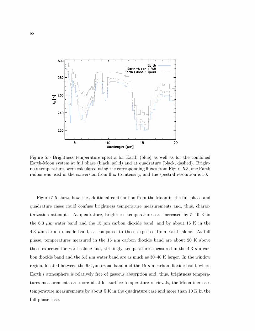
88

Figure 5.5 Brightness temperature spectra for Earth (blue) as well as for the combinedEarth-Moon system at full phase (black, solid) and at quadrature (black, dashed). Bright-ness temperatures were calculated using the corresponding fluxes from Figure 5.3, one Earthradius was used in the conversion from flux to intensity, and the spectral resolution is 50.

Figure 5.5 shows how the additional contribution from the Moon in the full phase and

quadrature cases could confuse brightness temperature measurements and, thus, charac-

terization attempts. At quadrature, brightness temperatures are increased by 5–10 K in

the 6.3 µm water band and the 15 µm carbon dioxide band, and by about 15 K in the

4.3 µm carbon dioxide band, as compared to those expected from Earth alone. At full

phase, temperatures measured in the 15 µm carbon dioxide band are about 20 K above

those expected for Earth alone and, strikingly, temperatures measured in the 4.3 µm car-

bon dioxide band and the 6.3 µm water band are as much as 30–40 K larger. In the window

region, located between the 9.6 µm ozone band and the 15 µm carbon dioxide band, where

Earth’s atmosphere is relatively free of gaseous absorption and, thus, brightness tempera-

tures measurements are more ideal for surface temperature retrievals, the Moon increases

temperature measurements by about 5 K in the quadrature case and more than 10 K in the

full phase case.

89

Clear differences can be seen in Figure 5.5 between the Earth-only spectrum as com-

pared to Earth-Moon system spectra in both the shapes and depths of absorption features.

The first indications that an undetected exomoon may be orbiting a directly imaged exo-

planet may come from such discrepancies. For example, the 6.3 µm water band is quite

symmetric about its center in the Earth-only spectrum (at wavelengths shortward of the

7.7 µm methane band), but the feature appears strongly asymmetric when the flux from

the full phase Moon is added. Furthermore, the bases of the 4.3 µm and 15 µm carbon

dioxide features are sensitive to similar pressure levels in Earth’s atmosphere and, thus,

return similar brightness temperatures in the Earth-only spectrum. When the thermal flux

from the full phase or quadrature Moon is added, though, the temperatures recorded in

the 4.3 µm band are greatly increased, leading to a discrepant appearance between the two

carbon dioxide bands.

5.3.2 Detecting Exomoons via Phase Differencing

The thermal flux from a slowly rotating, airless companion depends strongly on phase angle

(Equation 5.5). As a result, an exomoon can present a time varying signature with a

period equal to the host’s orbital period which can be masked by (or mimic) any seasonally

dependent thermal flux variations from the host planet. However, the phase dependent

contribution from an exomoon may be detectable by differencing IR observations taken at

two different phase angles at wavelengths where the moon is relatively bright and the host

planet’s spectrum exhibits only small seasonal variations.

In Figures 5.6 and 5.7 we demonstrate the differencing approach. An exoEarth (bottom,

“No Moon”) as well as a exoEarth-Moon system (top, “Moon”) are observed at a distance of

10 pc at an inclination of 90◦ (edge on, Figure 5.6) and 60◦ (Figure 5.7). The observations are

averaged over 24 hours in either mid-northern summer or winter. One observation is taken

at the smallest possible phase angle, which is determined by the inclination, and another

observation is taken half an orbit later when the planet/system are at the largest possible

phase angle. The difference between these two observations shows only seasonal variability

in the Earth-alone case, and shows a combination of the variability from seasons and the

90

Figure 5.6 Simulated observations of both an exoEarth-Moon system (top) as well as anexoEarth (bottom), both at a distance of 10 pc, demonstrating the phase differencing tech-nique which could be used to detect exomoons. Observations are averaged over 24 hoursand the spectral resolution is 50. One observation is taken at a small phase angle (gib-bous phase, solid blue) and another observation is taken half an orbit later (crescent phase,dashed blue). The gibbous observations occur in the middle of northern summer while thecrescent observations occur in the middle of northern winter. The system is assumed to beviewed edge on (inclination of 90◦) (where gibbous and crescent phase observations actuallyrefer to full and new phase, respectively). In the “No Moon” cases, the difference betweengibbous and crescent observations (black line) shows only seasonal variability, which is verysmall in the 4.3 µm carbon dioxide band and the 6.3 µm water band. For the observations inwhich the Moon is present, these bands are filled in by the lunar flux at gibbous phase, andthe difference between the gibbous and crescent observations shows much larger variabilitywithin the absorption bands.

91

Figure 5.7 The same as Figure 5.6 except for a system viewed at an inclination of 60◦.

92

Moon in the Earth-Moon case. Without the presence of the Moon, variability within the

4.3 µm carbon dioxide band and the 6.3 µm water band is quite small; on its own, Earth’s

spectrum is both dark and stable within these bands. However, when the phase dependent

lunar flux is included, variability in these bands is much larger, and the difference between

the small phase angle observation and the large phase angle observation closely resembles

the small phase angle contribution from the Moon at these wavelengths. Thus, variability

within the 4.3 µm carbon dioxide band and the 6.3 µm water is an indicator of the presence

of a moon.

We investigate the differencing approach for a wider range of planetary system inclina-

tions and summarize the results in Table 5.1. Except for inclination, the system parameters

are the same as in the previous paragraph. The exoEarth-Moon system is observed at the

smallest possible phase angle in northern summer and at the largest possible phase angle in

northern winter, and the observer is placed over the northern hemisphere. Note that system

inclination affects the range of possible phase angles that can be observed, and that an in-

clination of 0◦ corresponds to viewing the system face on. Bands spanning 4.2–4.5 µm and

5.0–7.5 µm (in the 4.3 µm carbon dioxide band and 6.3 µm water band, respectively) were

found to be ideal for detecting the lunar signal, where a balance must be achieved between

a wide enough band for photon collection and a narrow enough band to exclude seasonal

variability outside the absorption feature. In addition, Table 5.1 shows flux ratios for the

exoEarth-Moon system, which demonstrates the significance of the exoMoon’s brightness at

some wavelengths, as well as inferred brightness temperatures for the Earth twin (assuming

the observer is ignorant of the contamination by, and presence of, the companion).

93

Tab

le5.

1P

has

eD

iffer

enci

ng

Tec

hn

iqu

efo

rD

etec

tin

gE

xom

oon

s:T

her

mal

Flu

xes

,F

lux

Rat

ios,

Bri

ghtn

ess

Tem

per

atu

res,

an

dE

stim

ated

SN

RR

equ

irem

ents Flu

xat10

pc,exoM

oon/exoEarth

Flu

xRatio

(FM/FE),

and

Brightn

ess

Tempera

ture

2[%

](T

b)

SNR

forDete

ction3

[%]

Gib

bous(C

resc

ent)

Bolometric

4.2

–4.5µm

5.0

–7.5µm

4.2–4.5µm

(5.0–7.5µm)

Flu

x/

10−

20

[W/m

2]

FM/FE

Tb

Flu

x/

10−

23

[W/m

2]

FM/FE

Tb

Flu

x/

10−

21

[W/m

2]

FM/FE

Tb

Inc[◦

]Earth

Moon

[%]

[K]

Earth

Moon

[%]

[K]

Earth

Moon

[%]

[K]

RM

2R

M

90

10.6

(9.6)

2.6

(<0.1)

24

(<1)

272

(251)

3.0

(2.4)

14.1

(<0.1)

480

(<1)

272

(234)

3.6

(3.2)

3.8

(<0.1)

110

(<1)

266

(241)

12

(22)

11

(13)

75

10.6

(9.3)

2.5

(<0.1)

23

(<1)

271

(249)

3.0

(2.2)

13.7

(<0.1)

450

(<1)

271

(232)

3.6

(3.0)

3.7

(<0.1)

100

(<1)

266

(240)

12

(21)

11

(13)

60

10.5

(8.9)

2.3

(0.1)

21

(1)

270

(247)

3.2

(2.0)

12.3

(<0.1)

390

(2)

270

(231)

3.6

(2.9)

3.3

(<0.1)

90

(1)

264

(239)

13

(23)

11

(13)

45

10.5

(8.6)

1.9

(0.1)

18

(2)

267

(245)

3.2

(1.8)

10.2

(0.2)

320

(10)

266

(231)

3.5

(2.7)

2.8

(0.1)

80

(4)

261

(238)

14

(25)

11

(14)

30

10.5

(8.4)

1.6

(0.3)

15

(4)

265

(245)

3.3

(1.7)

7.8

(0.7)

240

(40)

262

(234)

3.5

(2.6)

2.2

(0.3)

60

(1)

258

(239)

16

(33)

12

(17)

15

10.5

(8.4)

1.2

(0.5)

11

(6)

263

(246)

3.3

(1.7)

5.4

(1.7)

170

(100)

257

(240)

3.5

(2.6)

1.6

(0.6)

50

(2)

255

(241)

25

(60)

18

(28)

010.5

(8.5)

0.8

(0.8)

8(8

)261

(249)

3.2

(1.8)

3.3

(3.3)

100

(180)

252

(247)

3.5

(2.7)

1.0

(1.0)

30

(4)

251

(245)

2B

rightn

ess

tem

per

atu

res

are

com

pute

dusi

ng

the

net

flux

from

the

syst

emass

um

ing

asi

zeof

one

Eart

hra

diu

sin

the

conver

sion

from

flux

toin

tensi

ty.

3A

“det

ecti

on”

const

itute

sm

easu

ring

the

exce

ssgib

bous

phase

lunar

flux

at

aSN

Rof

10,

whic

his

acc

om

plish

edby

diff

eren

cing

the

gib

bous

and

cres

cent

phase

obse

rvati

ons

of

the

syst

em.

Est

imate

sof

the

requir

edSN

Rare

show

nfo

ra

body

wit

ha

radiu

seq

ual

toth

eM

oon’s

radiu

s(R

M),

and

for

ab

ody

twic

eas

larg

eas

the

Moon.

SN

Rca

lcula

tions

are

furt

her

des

crib

edin

the

text.

94

Table 5.1 also shows an estimate of the minimum required SNR for the gibbous and cres-

cent phase observations such that their difference would measure the gibbous phase lunar

flux at a SNR of 10. By simple error propagation, this SNR is given by SNR′√F 2G + F 2

C/(FG−

FC), where SNR′ is the SNR for the measurement of the gibbous phase lunar flux (which

we take to be 10), and FG and FC are the gibbous and crescent phase fluxes, respectively,

for the planet-moon system through a given bandpass. Table 5.1 shows SNR estimates for

detections in the 4.3 µm carbon dioxide band and the 6.3 µm water band for a Moon twin

and for a body twice the size of the Moon.

In the 4.2–4.5 µm range, the gibbous phase flux from the exoMoon is more than 300%

larger than the exoEarth’s variability for a wide range of phases. As a result, the SNR

required to detect the exoMoon’s thermal signal is rather small (between 10–20) for all

inclinations above 30◦. At inclinations below about 30◦, the crescent phase lunar flux is a

sizeable fraction of the gibbous phase flux, causing the crescent phase flux to contaminate

the measurement of the gibbous phase lunar flux when subtracting the observations taken

at different phases. In the 5.0–7.5 µm range, the exoEarth’s variability begins to wash

out the gibbous phase thermal flux from the exoMoon at inclinations below about 45◦. At

inclinations above this, the required SNR for detection is only slightly larger than 20, and is

close to 10 for companions twice the size of the Moon. In general, contamination from the

exoEarth’s seasonal variability and the crescent phase lunar signal cause the differencing

technique to work poorly for inclinations below about 30–45◦. For inclinations above this,

detecting Moonlike satellites via the differencing technique is feasible.

5.4 Discussion

Surface, tropospheric, and stratospheric temperatures on Earth are typically within the

range of 200–300 K, and drastic day/night temperature differences do not occur due to

atmospheric circulation as well as relatively large surface and atmospheric heat capacities.

The Moon, in contrast, has a relatively low surface heat capacity and lacks an atmosphere

with which to redistribute energy from the day side to the night side of the world. As

a result, surface temperatures on the Moon are as high as 400 K at the sub-solar point,

allowing the Moon to contribute a significant amount of flux to IR observations of the Earth-

95

Moon system (depending on phase). Furthermore, the large lunar day side temperatures

cause the peak of the lunar thermal spectrum to be located at wavelengths distinct from the

peak of Earth’s thermal spectrum. Near full phase, the peak of the lunar thermal spectrum

occurs near the 6.3 µm water band, causing the Moon to outshine Earth both at these

wavelengths as well as in the 4.3 µm carbon dioxide band.

When observing an unresolved Earth-Moon system, thermal flux from the Moon dispro-

portionately affects regions of Earth’s spectrum where Earth has strong absorption bands.

As a result, characterization of Earth’s atmospheric composition and temperature from IR

observations taken by a distant observer could be strongly influenced by the Moon. For

example, for full phase observations of the Earth-Moon system, lunar thermal radiation

consistently comprises about 20% of the total signal, makes up as much as 80% of the total

signal in the 6.3 µm water band (creating the appearance of a much drier planet), and over

90% of the signal in the 4.3 µm carbon dioxide band. Current models predict that large

impacts like the Moon forming impact should be common and that conditions present in

the debris disk following such an impact cause any companions formed from debris material

to be depleted in volatiles. Thus, contamination of IR observations of extrasolar terrestrial

planets due to unresolved, airless companions may be a common reality, and the discussion

in the previous paragraphs will generally apply to thermal observations taken by future

exoplanet detection and characterization missions.

It is important to point out that contamination from airless companions can be min-

imized by taking observations at the largest feasible phase angles. Such a configuration

maximizes the flux from the companion’s cold night side, and minimizes flux from the

warmer day side. However, depending on the orbital inclination of the system, large phase

angles may not be accessible. In this case, the contribution from the companion will be

nearly constant and relatively small, except in some absorption bands (Figure 5.3, second

panel).

The contribution from an airless companion depends strongly on phase angle and, thus,

can mimic seasonally dependent thermal variations from the host planet. Figure 5.6 demon-

strates how drastic this effect can be for Earth and the Moon. An exoEarth-Moon system

was observed at gibbous phase in the middle of northern summer so that the lunar signal

96

adds to the seasonal variability in the exoEarth’s spectrum, causing the flux variations in

the atmospheric window region to appear roughly twice as large as the Earth-only case. If

the presence of the companion goes undetected, then it appears as though the exoEarth

has very exaggerated seasons. If the gibbous observation were to occur instead in the mid-

dle of northern winter, then the lunar contribution would wash out the seasonal variations

from the exoEarth, and the variability in the atmospheric window region would decrease

to nearly zero. This would create the false appearance of a planet with almost no seasonal

climate variability. These findings further demonstrate how the presence of an undetected

companion can interfere with the measurement of the obliquity and thermal properties of

the host planet, and are in good agreement with the bolometric results in Moskovitz et al.

(2009).

The ability of a companion to an extrasolar terrestrial planet to outshine its host at

some wavelengths proves to be useful as the phase dependent variability in the companion’s

brightness can impart a detectable signal in spatially unresolved observations of the planet-

companion system. The broadband models of Moskovitz et al. (2009) did not capture this

important behavior, causing them to conclude that only large satellites (roughly Mars sized)

of Earthlike exoplanets could be detected by a TPF-like mission. As shown in Table 5.1, it is

actually quite feasible to detect exomoons by differencing gibbous phase and crescent phase

observations of the planet-moon system at wavelengths where the moon is bright and the

planet’s spectrum is relatively dark and stable. A band spanning 4.2–4.5 µm is well suited to

detecting exomoons as the flux from an exoEarth is quite small and sTable 5.1n this region,

and variability from an exoMoon could be detected with observations taken at a SNR of

about 10. Note that the SNRs presented in Table 5.1 are close to or within the capabilities

of current TPF strategies, but that current TPF-Interferometer science requirements use a

shortwave cutoff at 6.5 µm, which does not reach the bottom of the 6.3 µm water band or

the 4.3 µm carbon dioxide band (Beichman et al., 2006).

The phase differencing technique outlined in this paper should function generally for

terrestrial exoplanets and their airless moons provided that there exists a wavelength range

where the moon contributes a significant amount of the gibbous phase flux from the un-

resolved system and where the flux from the host planet is relatively stable. The peak in

97

the gibbous phase Moon’s spectrum is at about 7 µm, which is near the 4.3 µm carbon

dioxide band and the 6.3 µm water band, where the escaping flux from Earth is coming

from cold regions of the atmosphere near the upper troposphere and lower stratosphere, at

which temperature variability is quite small as compared to surface temperature variations.

Searching for excesses due to an exomoon in the 4.3 µm carbon dioxide band is attractive

since CO2 is a common well mixed gas in terrestrial planetary atmospheres. Using the

6.3 µm water band will be useful for habitable exoplanets which, almost by definition, will

present a deep water band and whose moons will be receiving a stellar flux similar to what

the Moon receives, heating these companions to temperatures similar to our Moon. The

7.7 µm methane band would be highly suitable for detecting thermal excesses from moons

orbiting planets analogous to the early Earth, which was expected to have much higher

atmospheric methane concentrations than the modern Earth (Kasting et al., 2001).

Interesting investigations for the future include pairing our models with reverse/retrieval

models for terrestrial exoplanets to further explore the extent to which an exomoon could

confound spectroscopic characterization of an exoEarth. Our Earth model is dependent

on input data from Earth observing satellites, so that we cannot apply the current model

to terrestrial planets with seasonal cycles different from those on Earth. However, pairing

our spectral model of Earth to a three-dimensional general circulation model for Earthlike

planets is a task that would enable us to model time dependent, high resolution spectra

of terrestrial planets with distinct climates from Earth. Such a study would allow us to

understand whether or not the 6.3 µm water band is stable enough to allow for the detection

of exomoons around planets with high obliquity angles or planets with eccentric orbits (i.e.,

planets with more extreme seasons than Earth).

98

Chapter 6

CONCLUSIONS

Following the discovery of the first exoplanet (Mayor & Queloz, 1995), the field of exo-

planetary science has been marked by two clear trends. The first is the steady discovery of

smaller and smaller worlds, especially since the launch of NASA’s Kepler mission (Borucki

et al., 2003). The second trend is towards an ever-increasing quality of observational data

suitable for characterizing these worlds, which is best exemplified in the impressive collec-

tion of transit transmission spectra of the exoplanet GJ 1214b acquired both from space

and from the ground (Charbonneau et al., 2009; Bean et al., 2010; Desert et al., 2011; Berta

et al., 2011; Croll et al., 2011; Crossfield et al., 2011; Berta et al., 2012). Given these two

trends, it is only a matter of time before we will be asked to characterize an Earth-like

world, including a determination of its habitability.

In this work I have developed a model that is ideally suited to the task of planning

and designing future exoplanet characterization missions which aim to observe Earth-like

exoplanets. The Virtual Planetary Laboratory 3-D spectral Earth model will be a valuable

tool for the interpretation of such observations, and our comprehensive model is uniquely

capable of investigating a variety of Earth’s traits over wavelength ranges, synoptic views,

and vantage points that are unavailable to Earth observing spacecraft or satellites.

To generate disk-integrated spectra of Earth, we pixelate the atmosphere and nest a set

of surface pixels beneath these atmospheric pixels. Earth-observing satellites provide the

necessary information for defining the state of each atmospheric pixel, including temperature

and gas mixing ratio profiles, as well as cloud coverage and optical thickness. Similarly, these

satellites provide information on surface snow and sea ice coverage. After generating a look-

up table of spectra for a variety of surface and cloud coverage scenarios over a grid of viewing

geometries, we interpolate and combine 1-D spectra onto a sphere to generate a 3-D view

of Earth.

99

Our three-dimensional spectral model of Earth is capable of reproducing the variabil-

ity and brightness of observations throughout the visible, NIR, and MIR. Earth’s visible

lightcurves, as observed by NASA’s EPOXI mission, are strongly dependent on cloud spatial

distribution and reflectivity. The time-averaged, broadband (R ∼ 6), visible-light EPOXI

observations can only be reproduced by models that include both atmospheric scattering

and gas absorption. These observations, as well as their variations in time, can be simu-

lated by our model using only a single cloud category, with RMS errors comparable to those

of our more complex and realistic models, but this is likely due to their extremely coarse

wavelength resolution. The time-resolved, moderate resolution (R ∼ 500), NIR EPOXI ob-

servations could be fit by a model with two cloud categories (one liquid water cloud and one

water ice cloud), and a model with four cloud categories offered an improved fit. These find-

ings stress the importance of incorporating realistic gas absorption as well as atmospheric

and cloud scattering into spectral models of Earth.

We find that our simulations are relatively insensitive to variations in the surface res-

olution, except at very coarse resolutions, indicating a minimum required resolution over

Earth’s surface of 100 pixels or more. Our model can also reproduce the EPOXI visible

lightcurves at a very low atmospheric resolution as these observations are relatively insen-

sitive to atmospheric composition and temperature. Atmospheric resolutions of roughly 50

pixels were used to reproduce the EPOXI NIR spectra and the Aqua/AIRS MIR observa-

tions, which are datasets that are quite sensitive to viewing geometry and the spatially-

resolved atmospheric state.

The new, self-consistent treatment of clouds in our model has not only allowed us to

match the EPOXI Earth observations, which span almost three months in time and a variety

of phases, without tuning from one dataset to the next, but has also allowed us to reproduce

broadband, visible-light Earthshine observations over a wide range of phase angles. Our

fit to these data is much improved over the work of Williams & Gaidos (2008), who did

not include realistic atmospheric and cloud scattering in their models. While our model

is systematically 10–20% dimmer than the Earthshine observations at the largest phase

angles, our results indicate that atmospheric and cloud scattering are a critical component

of Earth’s appearance in reflected light at phases between quadrature and new.

100

We have shown that it is possible to disentangle the effects of specular reflection from

Earth’s oceans, or glint, and forward-scattering from clouds in phase-dependent observations

of Earth. Glint increases the planet’s brightness by as much as 100% at crescent phases,

and that this effect is strongest in wavelength regions that are unaffected by Rayleigh

scattering and atmospheric absorption. I show that the glint effect may be detectable

using JWST/NIRCam paired with an external occulter. Depending on viewing geometry,

minimum SNRs of 5–10 are required for glint detection, and an optimal IWA for detection

is about 50 milli-arcseconds for an Earth-twin at 10 parsecs.

By pairing our spectral Earth model to a validated model of the Moon’s disk-integrated

spectrum, I conclude that, depending on viewing geometry, the Moon can contribute a sig-

nificant amount of flux to IR observations of a spatially unresolved Earth-Moon system,

especially at wavelengths where there are strong absorption bands in Earth’s spectrum.

Thermal flux from an airless exomoon depends strongly on phase angle, so that large moons

can mimic or obscure seasonal variations in thermal flux from their host planet. The con-

fusing effects of an airless companion can be minimized by taking observations of exoplanets

at the largest feasible phase angle. By differencing observations taken at small phase angles

from those taken at large phase angles, at wavelengths where the host planet’s spectrum is

relatively stable over seasonal timescales, it is possible to detect the excess thermal radiation

coming from a Moon-sized companion in the gibbous phase observations.

Our models can now be used as predictive tools to explore the detectability of planetary

characteristics by generating synthetic observations of Earth, or the Earth-Moon system,

from the far ultraviolet to the far IR for any given viewing geometry and at a variety

of spectral and temporal resolutions. As an example, future applications could include

model generated disk-integrated, ultraviolet, visible or IR spectra of Earth for a variety

of sub-observer points and phases. These simulated datasets could be used for a variety

of applications, including to investigate the wavelength-dependent effect of clouds on our

ability to measure thermal radiation from the surface, or to simulate Earth as seen from a

lunar vantage point over a complete lunar orbit to provide data for proposed Moon-based

Earth-observing telescopes. Our Earth model could also be used to generate synthetic ob-

servations to better understand limitations and optimal algorithms for retrieval of planetary

101

properties from exoplanet spectra, as was done in Cowan et al. (2011) Model data can also

be used in “blind” tests of retrieval models, where other individuals or teams attempt to

retrieve planetary characteristics without knowing the input to our Earth model (e.g., sea-

son, viewing geometry, phase). In general, our simulated Earth data can be used to test

techniques aimed at characterizing habitable planets that may be employed by TPF-class

missions.

102

BIBLIOGRAPHY

Arnold, L., Gillet, S., Lardiere, O., Riaud, P., & Schneider, J. 2002, A&A, 392, 231

Aumann, H. H., et al. 2003, IEEE Transactions on Geoscience and Remote Sensing, 41, 253

Bains, W. 2004, Astrobiology, 4, 137

Basri, G., Borucki, W. J., & Koch, D. 2005, New Astronomy Review, 49, 478

Bean, J. L., Miller-Ricci Kempton, E., & Homeier, D. 2010, Nature, 468, 669

Beer, R., Glavich, T. A., & Rider, D. M. 2001, Appl. Opt., 40, 2356

Beichman, C., Lawson, P., Lay, O., Ahmed, A., Unwin, S., & Johnston, K. 2006, Proc.

SPIE, 6268, 62680S

Beichman, C. A., Woolf, N. J., & Lindensmith, C. A., eds. 1999, The Terrestrial Planet

Finder (TPF): A NASA Origins Program to Search for Habitable Planets (NASA Jet

Propulsion Laboratory)

Belton, M. J. S., et al. 1992, Space Sci. Rev., 60, 413

Benner, S., Ricardo, A., & Carrigan, M. 2004, Current Opinion in Chemical Biology, 8, 672

Berta, Z. K., Charbonneau, D., Bean, J., Irwin, J., Burke, C. J., Desert, J.-M., Nutzman,

P., & Falco, E. E. 2011, ApJ, 736, 12

Berta, Z. K., et al. 2012, ApJ, 747, 35

Boesch, H., Baker, D., Connor, B., Crisp, D., & Miller, C. 2011, Remote Sensing, 3, 270

Borucki, W. J., et al. 2011a, ApJ, 728, 117

—. 2011b, ApJ, 736, 19

103

—. 2003, Proc. SPIE, 4854, 129

Brown, R. A. 2005, ApJ, 624, 1010

Brown, R. A., & Soummer, R. 2010, ApJ, 715, 122

Brown, T. M., Charbonneau, D., Gilliland, R. L., Noyes, R. W., & Burrows, A. 2001, ApJ,

552, 699

Buratti, B. J., Hicks, M. D., Nettles, J., Staid, M., Pieters, C. M., Sunshine, J., Boardman,

J., & Stone, T. C. 2011, Journal of Geophysical Research (Planets), 116, E00G03

Cabrera, J., & Schneider, J. 2007, A&A, 464, 1133

Canup, R. M. 2004, Icarus, 168, 433

Carlson, R. W., Weissman, P. R., Smythe, W. D., & Mahoney, J. C. 1992, Space Sci. Rev.,

60, 457

Cash, W. 2006, Nature, 442, 51

Cassan, A., et al. 2012, Nature, 481, 167

Chandrasekhar, S. 1960, Radiative Transfer (Dover)

Charbonneau, D., et al. 2005, ApJ, 626, 523

—. 2009, Nature, 462, 891

Charbonneau, D., Brown, T. M., Noyes, R. W., & Gilliland, R. L. 2002, ApJ, 568, 377

Christensen, P. R., & Pearl, J. C. 1997, J. Geophys. Res., 102, 10875

Cowan, N. B., Abbot, D. S., & Voigt, A. 2012, ApJL, 752, L3

Cowan, N. B., et al. 2009, ApJ, 700, 915

—. 2011, ApJ, 731, 76

Cox, C., & Munk, W. 1954, Journal of the Optical Society of America (1917-1983), 44, 838

104

Crisp, D. 1997, Geophys. Res. Lett., 24, 571

Croll, B., Albert, L., Jayawardhana, R., Miller-Ricci Kempton, E., Fortney, J. J., Murray,

N., & Neilson, H. 2011, ApJ, 736, 78

Crossfield, I. J. M., Barman, T., & Hansen, B. M. S. 2011, ApJ, 736, 132

Danjon, A. 1928, Ann. Obs. Strasbourg, 2, 165

Deming, D., Seager, S., Richardson, L. J., & Harrington, J. 2005, Nature, 434, 740

Des Marais, D. J., et al. 2002, Astrobiology, 2, 153

—. 2008, Astrobiology, 8, 715

Desert, J.-M., et al. 2011, ApJL, 731, L40

Drake, F. D. 1962, Nature, 195, 894

Drossart, P., et al. 1993, Planet. Space Sci., 41, 551

Dubois, J. 1947, Bulletin Astronomique, 13, 193

Dumont, M., Brissaud, O., Picard, G., Schmitt, B., Gallet, J. C., & Arnaud, Y. 2010,

Atmospheric Chemistry & Physics, 10, 2507

Elser, S., Moore, B., Stadel, J., & Morishima, R. 2011, Icarus, 214, 357

Ford, E. B., Seager, S., & Turner, E. L. 2001, Nature, 412, 885

Fortes, A. D. 2000, Icarus, 146, 444

Fujii, Y., Kawahara, H., Suto, Y., Fukuda, S., Nakajima, T., Livengood, T. A., & Turner,

E. L. 2011, ApJ, 738, 184

Fujii, Y., Kawahara, H., Suto, Y., Taruya, A., Fukuda, S., Nakajima, T., & Turner, E. L.

2010, ApJ, 715, 866

Gaidos, E., & Williams, D. M. 2004, New Astron., 10, 67

105

Galilei, G. 1632, Dialogue Concerning the Two Chief Worlds Systems (Giovanni Battista

Landini)

Gardner, J. P., et al. 2006, Space Sci. Rev., 123, 485

Genda, H., & Abe, Y. 2005, Nature, 433, 842

Gladman, B., Dane Quinn, D., Nicholson, P., & Rand, R. 1996, Icarus, 122, 166

Goode, P. R., Qiu, J., Yurchyshyn, V., Hickey, J., Chu, M., Kolbe, E., Brown, C. T., &

Koonin, S. E. 2001, Geophys. Res. Lett., 28, 1671

Gorski, K. M., Hivon, E., Banday, A. J., Wandelt, B. D., Hansen, F. K., Reinecke, M., &

Bartelmann, M. 2005, ApJ, 622, 759

Grillmair, C. J., Charbonneau, D., Burrows, A., Armus, L., Stauffer, J., Meadows, V., Van

Cleve, J., & Levine, D. 2007, ApJL, 658, L115

Hall, D. K., Riggs, G., & Salomonson, V. V. 1995, Remote Sensing of Environment, 54, 127

Hampton, D. L., Baer, J. W., Huisjen, M. A., Varner, C. C., Delamere, A., Wellnitz, D. D.,

A’Hearn, M. F., & Klaasen, K. P. 2005, Space Science Reviews, 117, 43

Hartmann, W. K., Phillips, R. J., & Taylor, G. J., eds. 1986, Origin of the Moon

Hearty, T., Song, I., Kim, S., & Tinetti, G. 2009, ApJ, 693, 1763

Hodges, K. I., Chappell, D. W., Robinson, G. J., & Yang, G. 2000, Journal of Atmospheric

and Oceanic Technology, 17, 1296

Hord, C. W., et al. 1992, Space Sci. Rev., 60, 503

Horner, S. D., & Rieke, M. J. 2004, Proc. SPIE, 5487, 628

Ida, S., Canup, R. M., & Stewart, G. R. 1997, Nature, 389, 353

Johnson, T. V., Yeates, C. M., & Young, R. 1992, Space Sci. Rev., 60, 3

106

Kasting, J., Pavlov, A., & Siefert, J. 2001, Origins of Life and Evolution of Biospheres, 31,

271

Kawahara, H., & Fujii, Y. 2010, ApJ, 720, 1333

Kipping, D. M. 2009, MNRAS, 392, 181

Klaasen, K. P., et al. 2008, Review of Scientific Instruments, 79, 091301

Knutson, H. A., Charbonneau, D., Allen, L. E., Burrows, A., & Megeath, S. T. 2008, ApJ,

673, 526

Lane, A. P., & Irvine, W. M. 1973, AJ, 78, 267

Laskar, J., Joutel, F., & Robutel, P. 1993, Nature, 361, 615

Lawson, S. L., Jakosky, B. M., Park, H.-S., & Mellon, M. T. 2000, J. Geophys. Res., 105,

4273

Lebofsky, L. A., et al. 1986, Icarus, 68, 239

Lee, J.-M., Fletcher, L. N., & Irwin, P. G. J. 2012, MNRAS, 420, 170

Lenton, T. M. 1998, Nature, 394, 439

Lewis, J. 1971, Icarus, 15, 174

Line, M. R., Zhang, X., Vasisht, G., Natraj, V., Chen, P., & Yung, Y. L. 2012, ApJ, 749,

93

Livengood, T. A., et al. 2011, Astrobiology, 11, 907

Livesey, N. J., et al. 2007, Aura Microwave Limb Sounder Level 2 Data Quality and De-

scription, Tech. rep., Jet Propulsion Laboratory

Lowell, P. 1906, Mars and Its Canals (The Macmillan Company)

Lunine, J. I. 2008, Proceedings of the American Philosphical Society, 153, 404

Madhusudhan, N., & Seager, S. 2009, ApJ, 707, 24

107

Manalo-Smith, N., Smith, G. L., Tiwari, S. N., & Staylor, W. F. 1998, J. Geophys. Res.,

103, 19733

Mayor, M., & Queloz, D. 1995, Nature, 378, 355

Mazur, P. 1980, Origins of Life and Evolution of Biospheres, 10, 137

McKay, C. 1991, Icarus, 91, 93

—. 2004, PLoS Biology, 2, e302

McKay, C. P., & Stoker, C. R. 1989, Reviews of Geophysics, 27, 189

Meadows, V. S. 2006, in IAU Colloq. 200: Direct Imaging of Exoplanets: Science and

Techniques, ed. C. Aime & F. Vakili, 25–34

Meadows, V. S., & Crisp, D. 1996, J. Geophys. Res., 101, 4595

Mendell, W. W., & Lebofsky, L. A. 1982, in Bulletin of the American Astronomical Society,

Vol. 14, 726

Montanes-Rodrıguez, P., Palle, E., Goode, P. R., & Martın-Torres, F. J. 2006, ApJ, 651,

544

Morowitz, H., & Sagan, C. 1967, Nature, 215, 1259

Morrison, D. 1973, Icarus, 19, 1

Moskovitz, N. A., Gaidos, E., & Williams, D. M. 2009, Astrobiology, 9, 269

Muinonen, K., Lumme, K., Peltoniemi, J., & Irvine, W. M. 1989, Appl. Opt., 28, 3051

Mumma, M. J., Villanueva, G. L., Novak, R. E., Hewagama, T., Bonev, B. P., DiSanti,

M. A., Mandell, A. M., & Smith, M. D. 2009, Science, 323, 1041

Oakley, P. H. H., & Cash, W. 2009, ApJ, 700, 1428

Palle, E., Ford, E. B., Seager, S., Montanes-Rodrıguez, P., & Vazquez, M. 2008, ApJ, 676,

1319

108

Palle, E., et al. 2003, Journal of Geophysical Research (Atmospheres), 108, 4710

Parkinson, C., Liang, M., Yung, Y., & Kirschivnk, J. 2008, Origins of Life and Evolution of

Biospheres, 38, 355

Payne, V. H., Clough, S. A., Shephard, M. W., Nassar, R., & Logan, J. A. 2009, Journal of

Geophysical Research (Atmospheres), 114, 10307

Porco, C. C., et al. 2006, Science, 311, 1393

Proctor, R. A. 1883, Other Worlds Than Ours (D. Appleton and Company)

Qiu, J., et al. 2003, J. Geophys. Res, 108, 1999

Racca, G. D. 1995, Planet. Space Sci., 43, 835

Reynolds, R., Squyres, S., Colburn, D., & McKay, C. 1983, Icarus, 56, 246

Riggs, G., Hall, D. K., & Ackerman, S. A. 1999, Remote Sensing of Environment, 68, 152

Robinson, T. D., Meadows, V. S., & Crisp, D. 2010, ApJL, 721, L67

Robinson, T. D., et al. 2011, Astrobiology, 11, 393

Robinson, T. D., Meadows, V. S., Sparks, W. B., & Ennico, K. 2012, in prep.

Rothman, L. S., et al. 2009, Journal of Quantitative Spectroscopy and Radiative Transfer,

110, 533

—. 2005, Journal of Quantitative Spectroscopy and Radiative Transfer, 96, 139

Rozitis, B., & Green, S. F. 2011, MNRAS, 415, 2042

Sagan, C. 1962, Icarus, 1, 151

Sagan, C., Thompson, W. R., Carlson, R., Gurnett, D., & Hord, C. 1993, Nature, 365, 715

Salomonson, V. V., Barnes, W. L., Maymon, P. W., Montgomery, H. E., & Ostrow, H.

1989, IEEE Transactions on Geoscience and Remote Sensing, 27, 145

109

Sartoretti, P., & Schneider, J. 1999, A&AS, 134, 553

Sato, M., & Asada, H. 2010, PASJ, 62, 1203

Schulze-Makuch, D., Grinspoon, D., Abbas, O., Irwin, L., & Bullock, M. 2004, Astrobiology,

4, 11

Seager, S., & Sasselov, D. D. 2000, ApJ, 537, 916

Seager, S., Turner, E. L., Schafer, J., & Ford, E. B. 2005, Astrobiology, 5, 372

Sobolev, V. 1975, Light scattering in planetary atmospheres, International series of mono-

graphs in natural philosophy (Pergamon)

Soummer, R., et al. 2009, Proc. SPIE, 7440, 74400A

Stam, D. M. 2008, A&A, 482, 989

Stephan, K., et al. 2010, Geophys. Res. Lett., 37, 7104

Stephens, G. L., et al. 2002, Bulletin of the American Meteorological Society, 83, 1771

Sterzik, M. F., Bagnulo, S., & Palle, E. 2012, Nature, 483, 64

Summers, M. E., Lieb, B. J., Chapman, E., & Yung, Y. L. 2002, Geophys. Res. Lett., 29,

240000

Swain, M. R. 2010, in Bulletin of the American Astronomical Society, Vol. 42, 1064

Tinetti, G., Meadows, V. S., Crisp, D., Fong , W., Velusamy, T., & Snively, H. 2005,

Astrobiology, 5, 461

Tinetti, G., Meadows, V. S., Crisp, D., Fong, W., Fishbein, E., Turnbull, M., & Bibring,

J.-P. 2006a, Astrobiology, 6, 34

Tinetti, G., Meadows, V. S., Crisp, D., Kiang, N. Y., Kahn, B. H., Fishbein, E., Velusamy,

T., & Turnbull, M. 2006b, Astrobiology, 6, 881

Torres, G., et al. 2011, The Astrophysical Journal, 727, 24

110

Traub, W. A., et al. 2006, Proc. SPIE, 6268, 62680T

Turnbull, M. C., Traub, W. A., Jucks, K. W., Woolf, N. J., Meyer, M. R., Gorlova, N.,

Skrutskie, M. F., & Wilson, J. C. 2006a, ApJ, 644, 551

—. 2006b, ApJ, 644, 551

Valero, F. P. J., Herman, J., Minnis, P., Collins, W. D., Sadourny, R., Wiscombe, W.,

Lubin, D., & Ogilvie, K. 2000, National Academy of Sciences Reports

Ward, P., & Brownlee, D. 2000, Rare Earth : Why Complex Life is Uncommon in the

Universe (Springer)

Ward, P. D., & Benner, S. A. 2007, in Planets and Life: The Emerging Science of Astrobi-

ology, ed. W. T. Sullivan III & J. A. Baross (Cambridge University Press), 537–544

Ward, W. R., Agnor, C. B., & Canup, R. M. 2002, in Lunar and Planetary Institute Science

Conference Abstracts, Vol. 33, 2017

Waters, J. W., et al. 2006, IEEE Transactions on Geoscience and Remote Sensing, 44, 1075

Williams, D. M., & Gaidos, E. 2008, Icarus, 195, 927

Williams, D. M., & Knacke, R. F. 2004, Astrobiology, 4, 400

Wolfe, R. E. 2006, in Science and Instruments, Vol. 1, Earth Science Satellite Remote

Sensing, ed. J. J. Qu, W. Gao, M. Kafatos, R. E. Murphy, & V. V. Salomonson (Springer

Berlin Heidelberg), 50–73

Woolf, N. J., Smith, P. S., Traub, W. A., & Jucks, K. W. 2002, ApJ, 574, 430

Zelenyi, L., Korablev, O., Vorobyova, E., Martynov, M., Akim, E., & Zakahrov, A. 2010,

Proceedings of the International Astronomical Union, 6, 115

111

VITA

Tyler D. Robinson

Education

• Ph.D. in Astronomy and Astrobiology, University of Washington (UW) (2012)

• B.S. with Honors in Physics and Mathematics, Summa Cum Laude, University of

Arizona (2006)

Honors and Awards

• NSF IGERT Trainee, UW (2006-2011)

• Student Poster Prize, Origins 2011 ISSOL and Bioastronomy Joint Conference (2011)

• NASA Outstanding Achievement Award, as Member of EPOXI Mission Team (2009)

• Achievement Awards for College Scientists (ARCS) Fellow, Seattle Chapter (2006-

2009)

Teaching

• Guest Lecturer, ESS 306 “Planetary Geology”, undergraduate lecture entitled “De-

tecting Habitability” (2012)

• Guest Lecturer, BISSTS 397a “Communicating Science”, undergraduate lecture enti-

tled “The Role of Storytelling in Science Communication” (2012)

• Primary Instructor, ASTR 599 “Communicating Science to the Public Effectively”

(2011)

112

• Guest Lecturer, ESS 495 “NASA Space Grant Seminar: Rocks-n-Stars”, undergradu-

ate lecture entitled “The Search for Other Earths Begins at Home” (2011)

• Guest Lecturer, ASTR 599 “Communicating Science to the Public”, graduate lecture

entitled “Jargon: Big Words, Little Comprehension” (2010)

• Editor and Contributing Author to The Astrobiology Activities Manual, a suite of

hands-on exercises for an introductory course on astrobiology (2009)

• Instructor, ASTR 190 “Astronomy and Astrobiology” (2009)

• Co-Instructor, ASTBIO 115 “Introduction to Astrobiology” (2009)

• Teaching Assistant, ASTBIO 115 “Introduction to Astrobiology” (2008)

• Teaching Assistant, ASTR 101 “Astronomy” (2007)

• Teaching Assistant, ASTR 150 “The Planets” (2006-2007)

Service

• Reviewer for Astrobiology (2012-present)

• Session Co-Chair for “Exoplanet Habitability” at the Astrobiology Science Conference

(2012)

• Graduate Student Representative to Astronomy Faculty Hiring Committee (2011-

present)

• Executive Secretary, NASA Origins of the Solar System Panel (2011)

• Secretary and A/V Assistant for the Revisiting the Habitable Zone workshop (2010)

• Graduate Student Representative to Astronomy Department Faculty (2008-2010)

113

• Meadows, V. S., et al. “The Search for Habitable Environments and Life in the

Universe.” Astro2010 Science White Paper, no. 201 (2009)

Public Outreach

• Science Communication Fellow, Pacific Science Center (2009-present)

• Co-Director of “Engage”, a program to educate and involve graduate students in

public outreach (2011-present)

• Co-Organizer of “UW Science Now”, a public lecture series at Seattle Town Hall

(2011-present)

• Lakewood High School, “The Pale Blue Dot” (2011)

• Hillside School, “Worlds Apart: Extrasolar Planets and the Hunt for Life Beyond

Earth” (2011)

• Appearance on Academia Nut! radio program (2011)

• Science on Tap presentation in local pub, “A Cornucopia of Worlds: Extrasolar Plan-

ets and the Search for Life Beyond Earth” (2010)

• Lakewood High School, “Finding Other Earths” (2010)

• Engage: The Science Speakers Series, “Earth as an Extrasolar Planet” (2010)

Mentor at Big Picture High School (2008-2009)

• Rose City Astronomers, Portland, OR, “Earth as an Extrasolar Planet” (2008)

Refereed Publications

• Robinson, T. D., and Catling, D. “An Analytic Radiative-Convective Model for

Planetary Atmospheres.” ApJ, in press

114

• Tian, T., Wolf, E., Robinson, T. D., Kasting, J. F., and Toon, O. B. “Contribution

of Ammonia to Warming the Archean Earth.” Astrobiology, in review

• Robinson, T. D.. “Modeling the Infrared Spectrum of the Earth-Moon System:

Implications for the Detection and Characterization of Earthlike Planets and their

Moonlike Companions.” ApJ, 741, 51, 2011

• Livengood, T. A., and 10 co-authors (including T. D. Robinson). “Properties of an

Earth-Like Planet Orbiting a Sun-Like Star: Earth Observed by the EPOXI Mission.”

Astrobiology, 11, 907, 2011

• Robinson, T. D., Meadows, V. S., Crisp, D., et al. “Earth as an Extrasolar Planet:

Earth Model Validation Using EPOXI Earth Observations.” Astrobiology, 11, 393,

2011 (issue cover)

• Cowan, N. B., Robinson, T. D., Livengood, T. A., et al. “Rotational Variability of

Earth’s Polar Regions: Implications for Detecting Snowball Planets.” ApJ, 731, 76,

2011

• Crow, C. A., McFadden, L. A., Robinson, T. D., et al. “Views from EPOXI: Colors

in Our Solar System as an Analog for Extrasolar Planets.” ApJ, 729, 130, 2011

• Robinson, T. D., Meadows, V. S., and Crisp, D. “Detecting Oceans on Extrasolar

Planets Using the Glint Effect.” ApJL, 721, L67, 2010

• Cowan, N. B., Agol, E., Meadows, V. S., Robinson, T. D., et al. “Alien Maps of an

Ocean-bearing World.” ApJ, 700, 915, 2009

Conference Publications (Oral)

• Robinson, T. D., and Meadows, V. S. “Once in a Pale Blue Dot: Simulated Ob-

servations of an Extrasolar Earth-Moon System.” American Geophysical Union, San

Francisco, CA, December 2011

115

• Robinson, T. D. “Once in a Pale Blue Dot: Simulated Observations of an Extrasolar

Earth-Moon System.” Astrobiology Graduate Conference, Bozeman, MT, June 2011

• Robinson, T. D. “The Strange World We Call Home: Earth in the Context of an

Exoplanet.” Strange New Worlds, Flagstaff, AZ, May 2011

• Crow, C., McFadden, L. A., Robinson, T. D., et al. “Views from EPOXI: Colors in

our Solar System as an Analog for Extrasolar Planets.” Division of Planetary Sciences,

Pasadena, CA, October 2010

• Livengood, T. A., and 10 co-authors (including T. D. Robinson). “EPOXI Ob-

servations of Mars: Distinguishing Exo-Mars from Exo-Earth.” Division of Planetary

Sciences, Pasadena, CA, October 2010

• Robinson, T. D., Meadows, V. S., Crisp, D. “Detecting Oceans on Extrasolar Plan-

ets.” Astrobiology Science Conference, League City, TX, April 2010

• Domagal-Goldman, S. D., Robinson, T. D., and Haqq-Misra, J. “Hazes at the

Inner Edge of the Habitable Zone.” American Geophysical Union, San Francisco, CA,

December 2009

• Robinson, T. D., Meadows, V. S., et al. “Modeling Earth as an Extrasolar Planet:

The VPL Earth Model Validated Against EPOXI Observations.” Division of Planetary

Sciences, Fajardo, PR, October 2009

• Robinson, T. D., Meadows, V. S., et al. “Simulating Earth as an Extrasolar Planet.”

Division of Planetary Sciences, Ithaca, NY, October 2008

• Deming, D., and 21 co-authors (including T. D. Robinson). “The EPOXI/EPOCh

Investigation of Transiting Extrasolar Planets.” American Astronomical Society, St.

Louis, MO, June 2008

116

Conference Publications (Poster)

• Robinson, T. D., Meadows, V. S., Catling, D. C., and Crisp, D. “Towards a Mod-

eling Hierarchy: Two New General-Purpose, 1-D Planetary Climate Models.” Astro-

biology Science Conference, Atlanta, GA, April 2012

• Domagal-Goldman, S. D., Meadows, V. S., Robinson, T. D. “Pale Orange Dot:

The Meso-Archean Earth from Afar.” Astrobiology Science Conference, Atlanta, GA,

April 2012

• Schwieterman, E. W., Robinson, T. D., et al. “Characterizing Terrestrial Exoplan-

ets: Evaluating Temperature and Albedo Retrieval Methods with Near-IR EPOXI

Earth and Mars Spectra.” Astrobiology Science Conference, Atlanta, GA, April 2012

• Rosenfield, P. A., Mitchell, R. M., Robinson, T. D., et al. “Turning Graduate

Student Research into an Engaging Public Talk.” AAAS, Vancouver, BC, February

2012

• Robinson, T. D., Meadows, V. S., and Agol, E. “Simulated Observations of an

Extrasolar Earth-Moon System.” Exoclimes, Aspen, CO, January 2012

• Robinson, T. D., and Meadows, V. S. “Astrobiology from Earth-Sun L1.” American

Geophysical Union, San Francisco, CA, December 2011

• Goldblatt, C., Crisp, D., and Robinson, T. D. “The Runaway Greenhouse - Towards

a Quantitative Assessment of the Risk from Anthropogenic Global Change.” American

Geophysical Union, San Francisco, CA, December 2011

• Robinson, T. D., Meadows, V. S., and Agol, E. “Once in a Pale Blue Dot: Simulated

Observations of an Extrasolar Earth-Moon System.” Origins, Montpellier, FR, July

2011

117

• Meadows, V. S., and Robinson, T. D. “Determining Extrasolar Planetary Habit-

ability: Sensitivity to Surface Temperature.” Strange New Worlds, Flagstaff, AZ, May

2011

• Shields, A., Meadows, V. S., Robinson, T. D., et al. “Earth as an Extrasolar

Planet: Comparing Polar and Equatorial Views of Modern Day and Snowball Earth.”

American Astronomical Society, Seattle, WA, January 2011

• Robinson, T. D., Meadows, V. S., Crisp, D. “Earth as an Extrasolar Planet” Divi-

sion of Planetary Sciences, Pasadena, CA, October 2010

• Robinson, T. D. “Simulating Earth as an Extrasolar Planet.” Exoclimes, Exeter,

UK, September 2010

• Robinson, T. D., Meadows, V. S., and Crisp, D. “Earth as an Extrasolar Planet.”

Revisiting the Habitable Zone workshop, Seattle, WA, August 2010

• Shields, A., Meadows, V. S., Robinson, T. D., et al. “Earth as an Extrasolar

Planet: Comparing Polar and Equatorial Views.” Astrobiology Science Conference,

League City, TX, April 2010

• Robinson, T. D., Anderson, R. E., and Meadows, V. S. “A Suite of Activities Devel-

oped for an Introductory Astrobiology Course for non-Science Majors” Astrobiology

Graduate Conference, Seattle, WA, July 2009

• Robinson, T. D., Meadows, V. S., Deming, D., and Crisp, D. “Simulating EPOXI

Full-Disk Earth Data: Do the Models Stick to the Observations?” Astrobiology Grad-

uate Conference, Santa Clara, CA, April 2008

Invited Talks

• “So you want to find an exoplanet and say something about its habitability?”, Astro-

biology Science Conference, Atlanta, GA, April 2012

118

• “Detecting Planetary Habitability”, American Astronomical Society, Seattle, WA,

January 2011 (written and presented on behalf of V. S. Meadows)

• “Earth as an Extrasolar Planet: Modeling EPOXI Earth Observations”, Goddard

Space Flight Center, Greenbelt, MD, January 2010

Academic Seminars

• “Understanding Temperature Profiles in Planetary Atmospheres of the Solar System

and Beyond”, UW Atmospheric Sciences colloquium, UW, May 2012 (co-delivered

with D. C. Catling)

• “Understanding the Pale Blue Dot: From Galileo to EPOXI”, UCSC Planetary Lunch

& NASA Ames Special Seminar, CA, May 2012

• “Temperature Profiles in Planetary Atmospheres: What the Solar System Can Teach

Us About Exoplanets”, UW Astrobiology Program research rotation talk, UW, Novem-

ber 2011

• “Understanding the Pale Blue Dot: From Galileo to EPOXI”, Yuk Lunch talk, Cal-

tech, October 2011

• “Once in a Pale Blue Dot: Simulated Observations of an Extrasolar Earth-Moon

System”, UW Astrobiology Program student orientation talk, UW, October 2011

• “The Search for Other Earths Begins at Home”, LSST lunch talk, UW, June 2011

• “Once in a Pale Blue Dot: Modeling the Spectrum of an Unresolved Earth-Moon

System”, Planetaryum talk, UW, December 2010

• “Detecting Oceans on Extrasolar Planets”, UW Astrobiology Program student orien-

tation talk, UW, October 2010

119

• “Earth as an Extrasolar Planet”, presentation to NASA Astrobiology Institute’s Ex-

ecutive Council, UW, February 2010

• “Earth as an Extrasolar Planet: The Virtual Planetary Laboratory’s 3-D Spectral

Earth Model”, Planetaryum talk, UW, December 2009

• “Climatic Effects of Large Impacts on Earth”, general exam, UW, November 2009

• “Modeling Earth as an Extrasolar Planet”, UW Astrobiology In-House Seminar, UW,

June 2009

Grants

• 2012 NASA Astrobiology Institute Cooperative Agreement Notice 6 - The Virtual

Planetary Laboratory, Co-I (submitted)

• 2009 UW Student Technology Fee Grant - Graduate Student Disk Space ($80K), Co-I