2D waveform tomography applied to long-streamer MCS data from the Scotian Slope

Case History

2D waveform tomography applied to long-streamer MCS data from theScotian Slope

Matthias Delescluse1, Mladen R. Nedimovic2, and Keith E. Louden3

ABSTRACT

Detailed velocity models of the earth’s subsurface can be

obtained through waveform tomography. The accuracy of the

long-wavelength component of such velocity models, which is

the background velocity field, is particularly sensitive to mod-

eling low-frequency refracted waves that have long paths

through target structures. Thus, field examples primarily have

focused on the analysis of long-offset wide-angle data sets col-

lected using autonomous receivers, in which refractions arrive

at significantly earlier times than reflections. Modern marine

acquisition with long streamers now offers the ability to record

refracted waves with high spatial density and uniform source,

both in shallow and deep water. We used 2D multichannel

seismic (MCS) data acquired with a 9-km-long streamer over

the Scotian Slope in water depths of �1600 m. The refracted

arrivals, although mostly restricted to far-offset receivers, pro-

vided sufficient information to successfully invert for a high-

resolution background velocity field. Using a frequency-do-

main acoustic code over frequencies from 8 to 24 Hz on two

crossing profiles, we found that the limited refracted waves

can constrain the velocity field above the depth of the turning

waves (�1.5 km below seafloor). Several important features

were resolved by the waveform velocity model that were not

present in the initial traveltime model. In particular, a high-ve-

locity layer at 300 m below the seafloor, interpreted as gas

hydrates, was imaged even where a characteristic bottom-sim-

ulating reflector was not visible. At 750-m depth, a strong ve-

locity increase of 300 m/s existed beneath a gently dipping

reflector along which low-velocity zones, possibly related to

gas, were present. Velocity models were highly consistent at

the crossing point between the two profiles. The depth extent

of the MCS waveform tomography constrained by refractions

could be extended by even longer streamers (e.g., 15 km) or

by joint inversion with data from ocean-bottom seismographs.

INTRODUCTION

Applications of frequency-domain 2D acoustic waveform to-

mography inversion (Pratt and Worthington, 1990; Pratt, 1999)

to field seismic data are few and limited to the two end-

members of seismic-acquisition techniques: (1) long-offset wide-

angle refraction experiments using individual land or ocean-bottom

stations (Dessa et al., 2004; Operto et al., 2004; Ravaut et al.,

2004; Operto et al., 2006; Bleibinhaus et al., 2007, 2009) and

(2) high-resolution, short-streamer marine reflection seismics

(Hicks and Pratt, 2001; Shin and Min, 2006; Wang and Rao,

2009). The two cases offer opposite advantages and drawbacks.

In the “refraction” case, the monoparameter inversion of P-wave

velocities is questionable because of attenuation variations, typi-

cally limiting the inversion to phase only (Bleibinhaus et al.,

2007), whereas good starting models obtained from traveltime

tomography and low frequencies offer excellent control on the

velocity field (Brenders and Pratt, 2007b). In the “reflection”

case, small offsets and small-scale targets with simple structures

ensure a good validity of the acoustic approximation (Barnes

and Charara, 2009; Virieux and Operto, 2009), and the high

density of shots and receivers allow very high resolution.

Manuscript received by the Editor 12 July 2010; revised manuscript received 2 March 2011; published online 13 June 2011.1Formerly Dalhousie University, Department of Oceanography, Halifax, Nova Scotia, Canada; presently, Ecole Normale Superieure de Paris, Laboratoire

de Geologie. E-mail: [email protected] University, Department of Oceanography, Halifax, Nova Scotia, Canada; and Columbia University, Lamont-Doherty Earth Observatory, Pali-

sades, New York, U.S.A. E-mail: [email protected] University, Department of Oceanography, Halifax, Nova Scotia, Canada. E-mail: [email protected].

VC 2011 Society of Exploration Geophysicists. All rights reserved.

B151

GEOPHYSICS, VOL. 76, NO. 4 (JULY-AUGUST 2011); P. B151–B163, 15 FIGS., 1 TABLE.10.1190/1.3587219

However, the background velocity field is not well constrained

by reflection waveform tomography, and a degree of structural

interpretation is necessary to obtain a useful result (Hicks and

Pratt, 2001; Wang and Rao, 2009). Although fewer studies using

long-offset multichannel seismic (MCS) data have been

attempted, such data are increasingly available, and the applic-

ability of the waveform inversion to these data sets needs fur-

ther study (a review of industry efforts in applying waveform to-

mography to field data can be found in Williamson et al., 2010).

In this paper, we attempt 2D waveform tomography inversion

in the frequency domain using a long-streamer MCS data set,

which represents an intermediate situation between the two pre-

viously cited cases. An earlier attempt to use full waveform to-

mography for long-streamer data (Shipp and Singh, 2002) was

done in the time-space domain, but the huge computational cost

associated with this method required severe decimation of the

input data, thus limiting the results.

The 2D MCS data with a 9-km-long streamer were acquired

on the Scotian Slope (Figure 1a) on a thick sedimentary basin

formed after Mesozoic rifting between North America and Africa.

The stack section along line 5300 (Figure 1b) shows subparallel

layers deposited from the Pliocene in an area with known accu-

mulations of gas hydrates and free gas (Leblanc et al., 2007).

Shot gathers include refracted waves arriving earlier than the sea-

floor reflection and later than the direct wave (Figure 2). These

waves constrain the background velocity field above their turning

depth, while the simple, slowly varying sedimentary environment

(Figure 1b) minimizes the limitation with the acoustic approxima-

tion. This configuration is then likely to combine the strengths of

reflection and refraction cases of waveform inversion while limit-

ing their drawbacks. We first present the method and the data set

and then describe the preconditioning and inversion strategy.

Finally, we discuss the results in terms of limitations of the wave-

form tomography method applied to MCS data, possible targets

of MCS waveform tomography, and the addi-

tional information it can provide when compared

to a prestack depth-migration image.

FREQUENCY-DOMAIN WAVEFORM

TOMOGRAPHY APPLIED TO MCS

DATA

General method

In this section we briefly describe the wave-

form inversion methodology that is used. The

reader can find further details in Pratt et al.

(1998), or Sirgue and Pratt (2004).

The wavefield u can be defined as the solu-

tion to a set of nonlinear equations (here the

frequency-domain acoustic wave equation g)

depending on parameters m (the P-wave veloc-

ities in every cell of a grid):

gðmÞ ¼ u;

Several possibilities exist to measure the misfit

E(m) between the field data and the synthetic

data, such as the L1-Norm (Brossier et al., 2010),

the logarithmic approach (Shin et al., 2007), or

the more classical L2-Norm (Tarantola, 1987),

where

EðmÞ ¼ 1

2odTod;

with od ¼ gðmÞ � dobs being the difference

between the forward model using parameters mand the data dobs; odT is the complex conjugate

of this difference. The goal of the inversion is

to find the parameters m that minimize this mis-

fit function. To do this, we introduce the gradi-

ent of the misfit function rmE ¼ oE=om, which

gives the direction of increase of the misfit in

the parameter space. In the linear case, the mis-

fit function is quadratic and can be expressed as

a Taylor series of the second order. The model

update om is derived in the Newton method as

om� H�1rmEðm0Þ;

Figure 1. (a) Location of the Novaspan 2D lines acquired by GXT in 2003 on the Sco-tian Slope using a 9-km-long streamer (dashed lines). The inset shows the location ofNova Scotia on the east coast of North America. The crossing red sections of lines5300 and 1400 are used in this study. White areas represent salt. (b) Stack of the sec-tion of line 5300 investigated in this study. Seafloor multiples (M) are visible. Theturning depth of the recorded refraction waves is at �3.5 s two-way traveltime(TWTT).

B152 Delescluse et al.

with H being the Hessian, oðrEÞ=om, and m0 representing the

parameters of the initial model.

In the nonlinear case the Hessian is challenging to obtain

even if the misfit function is assumed to be locally linear near

the model m0. It can be, at best, only approximated, and several

iterations are necessary. If the problem is strongly nonlinear, the

gradient is not in the steepest ascent direction after the first iter-

ation, and it needs to be updated. To avoid calculating the Hes-

sian, the gradient method is used, where

mðkÞ ¼ mðk�1Þ � cðk�1ÞrmEðk�1Þ:

With this method, the model is updated in the direction of the

steepest descent and assures that the new misfit at iteration k is

smaller than the misfit at iteration k � 1. The step-length c has

to be estimated either by a line search (which is computationally

expensive) or by a new Newton calculation requiring only one

new forward model where the model is perturbed in the gradient

direction.

Calculating the gradient rmE would normally require perturb-

ing every parameter to compute all the partial derivatives as

rmE ¼ JTod, with Ji;j ¼ oui

�omj being the Frechet derivative

matrix. This approach is computationally expensive. Using the

adjoint-state method, it can be shown that, instead, the gradient

can be expressed as a product of the forward-propagated wave-

field of the source term,

Pf ðx; sÞ ¼ Gðx; sÞSðxÞ;and the back-propagated wavefield of the resid-

uals from the receiver location,

Pbðx; r; sÞ ¼ Gðx; rÞtodðr; sÞ:Gðx; rÞ and Gðx; sÞ are Green’s functions, SðxÞis the source term, and odðr; sÞ are the residuals

for the source s and receiver r. Note that this

gradient calculation is similar to prestack migra-

tion (Lailly, 1983; Tarantola, 1984).

In summary, three forward models are needed

for each iteration: one to compute the wavefield

in the initial model, another to calculate the

back-propagated residuals, and a final one to

compute the step length.

Field data application challenges

The success of the inversion depends on the

accuracy of the starting velocity model. Because

the problem is nonlinear, the gradient may point

toward a local minimum. Finding a starting

model that at long to intermediate wavelengths

agrees with the true one is the best approach to

counter the nonlinearity of the inversion and

find a global minimum.

A standard method to obtain an accurate

starting velocity model is to use traveltime to-

mography. However, streamer traveltime to-

mography using refracted arrivals constrains

only large wavelengths of the velocity model,

typically around 1 km for the shallow part and

wavelengths greater than 1–2 km at depth (see

Canales et al., 2008; Newman et al., 2011).

Applying waveform tomography afterward may be challenging

if a gap in the intermediate wavelengths exists (see the Mar-

mousis example in Sirgue [2003] and Shin et al. [2007]). In

other words, if the lowest usable signal frequency in the data set

does not cover the highest wavelength extracted by the travel-

time tomography. Short-streamer reflection seismics is typically

a high-frequency acquisition that will not allow the reconstruc-

tion of intermediate wavelengths (Jannane et al., 1989). Long-

offset seismic data introduce nonlinearity (Sirgue, 2006) because

the misfit results from the sum of the slowness error along the

wave path. The longer the wave path, the more nonlinear the

problem is. However, long-streamer seismic data sets provide

more information on the low wavenumbers (Sirgue, 2006),

which are essential to the success of waveform inversion.

To successfully invert for a velocity field, it is also essential

to have a field data set that can be compared with the synthetic

data produced by the finite-difference forward modeling. We

summarize four main issues that need attention when comparing

field and synthetic data: (1) Is the field data set significantly

affected by elastic effects? This is important because we only

model acoustic wave propagation. The risk is that amplitudes

may not be useable. If this is the case, only the phase informa-

tion of the wavefield can be used, which requires that the syn-

thetic and field amplitudes are normalized to one. (2) Although

densities and attenuation vary in the subsurface, only P-wave

velocities are inverted for. This means that the constant density

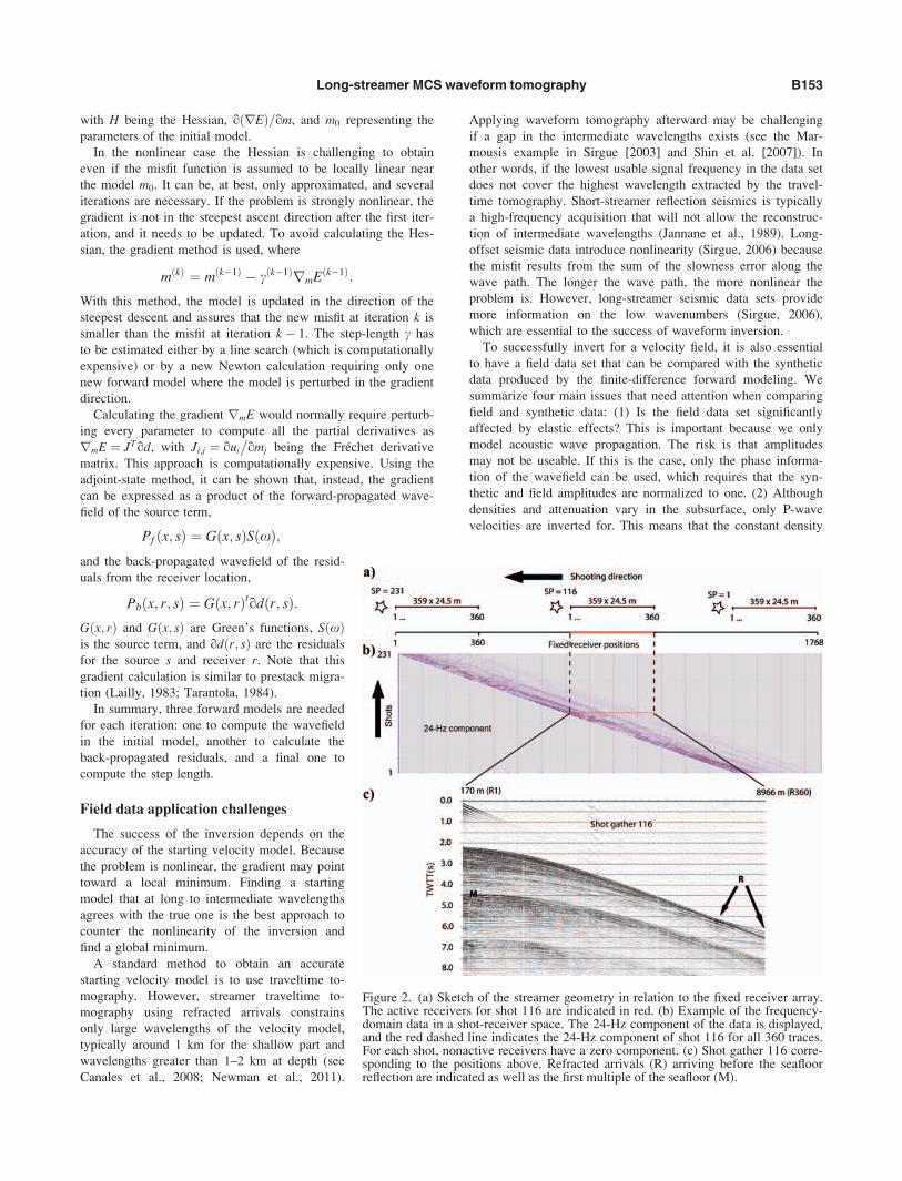
Figure 2. (a) Sketch of the streamer geometry in relation to the fixed receiver array.The active receivers for shot 116 are indicated in red. (b) Example of the frequency-domain data in a shot-receiver space. The 24-Hz component of the data is displayed,and the red dashed line indicates the 24-Hz component of shot 116 for all 360 traces.For each shot, nonactive receivers have a zero component. (c) Shot gather 116 corre-sponding to the positions above. Refracted arrivals (R) arriving before the seafloorreflection are indicated as well as the first multiple of the seafloor (M).

B153Long-streamer MCS waveform tomography

of the subsurface used for the inversion will mostly affect the

reflectivity part of the data set, with the reflectors being inter-

preted as pure velocity contrasts. Attenuation will affect the

amplitudes if there are strong attenuation variations that are not

taken into account. This last problem can also potentially

require phase-only inversion even if the acoustic approximation

is valid. (3) The modeled acoustic energy propagation is 2D,

whereas a field data set records energy propagating in 3D. To

compare the two data sets, the field data have to be corrected

for cylindrical instead of spherical energy propagation. (4) The

signal-to-noise ratio of the field data must be high to avoid arti-

facts because noise is not modeled by the acoustic code.

Smoothing the gradient and using many frequencies can help

reduce artifacts.

The case of an MCS data set from a simple geologicalframework

The intermediate wavelength problem and the other issues

cited above can be minimized by applying waveform tomogra-

phy to a data set acquired from a simple geological environ-

ment. The Ion-GXT data set was acquired along the Scotian

Slope. This area of the slope is composed of a thick (�7 km),

Triassic to Quaternary, postrift sedimentary section. The upper

2 km, which were modeled in our study, are composed of

interbedded horizontal layers of prodeltaic mudstone, clay-

stone, and siltstone deposited since the Miocene as a result of

events such as the late Tertiary sea-level lowstands (Piper and

Normark, 1989; Leblanc et al., 2007). Recent mud depositions

from the last interglacial period (12 ka; Mosher et al., 1994)

were cored and show soft, water-saturated seafloor properties

(VP¼ 1530 6 20 m/s, density¼ 1680 6 50 kg/m3) (Leblanc

et al., 2007). More-complex structures related to salt tectonics

like diapirs (Figure 1) are too deep on line 5300 to be of

concern.

This simple environment is then likely to minimize challenges

during inversion for the following reasons: (1) Sudden and sig-

nificant lateral variation of attenuation is not likely to occur as

the sedimentary deposition system is the same over the length

of the profile. (2) The S-wave velocity is likely to be slow and

smoothly increasing with depth, which will limit elastic effects.

(3) Horizontal to subhorizontal layers will allow correction for

the 2D instead of 3D propagation of energy. (4) It is simpler to

find an accurate starting velocity model because there are no

complex structures, and thus, intermediate wavelengths are min-

imal. Basically, we expect a 2D final model that does not differ

greatly from a 1D velocity model but that still includes addi-

tional information from the inversion. These considerations will

be detailed and explained in the following sections.

DATA PRECONDITIONING

Data and geometry

We use two crossing sections of the Novaspan profiles (lines

1400 and 5300; see Figure 1) acquired by Ion-GXT in 2003.

The streamer is composed of 360 receiver groups with 25-m

spacing. The shot spacing is 50 m. For the investigated 44-km-

long section of strike line, line 5300, we decimate the data for

computational reasons to 231 shots spaced every 150 m (every

third shot) and use all receivers. For the crossing 29-km-long

section of the dip line, line 1400, we use 196 shots spaced every

100 m (every second shot) and all receivers. Although 94 m is

the ideal spacing, to avoid aliasing for our lowest frequency

available (Nyquist criterion is met for an 8-Hz signal), Brenders

and Pratt (2007b) show that the sampling theory criterion may

be too conservative (see Table 1 for a summary of the sampling

of different synthetic and real survey configurations). The

impact of the data decimation is further discussed in the

“Inversion Strategy” section, where we describe a test inversion

of the entire, nondecimated data set for line 5300 (691 shots).

Feathering of the streamer is limited to a maximum 10� angle

but is generally less. The nominal geometry implies a 170-m

minimum offset for the first receiver and, consequently, a 9145-m

maximum offset for receiver 360. However, streamer bending

also occurs, which shortens the effective maximum offset to an

average of 8966 m. To account fully for the effects of feathering

and bending would be equivalent to the definition of 83,160 in-

dependent receivers positions for line 5300 (248,760 in the non-

decimated line 5300) and 70,560 for line 1400 and would

Table 1. Aliasing number Na 5 2Dsampf/Vmin in a selection of studies involving different real and synthetic data sets. The Dsamp

column is the source or receiver interval, and Vmin is the minimum velocity in the model. An aliasing number higher than one theo-retically produces some aliasing. In practice, inversion results can be satisfactory with sparser sampling (Brenders and Pratt, 2007a).

Study Data Geometry Vmin (m/s) Dsamp (m) f (Hz) Na

Hicks and Pratt (2001) real reflection 1560 12.5 10–60 0.16–1

Operto et al. (2006) real refraction 2000 1000 3–15 3–15

Sirgue and Pratt (2004) synthetic refraction 1500 100 5–10 0.7–1.3

Ravaut et al. (2004) real refraction 2000 90 5.4–20 0.5–1.8

Brenders and (2007b) synthetic refraction 4000 5000 0.8–7 2–18

Bleibinhaus et al. (2009), SAF real refraction 2000 500–1000 3–14 1.5–14

Bleibinhaus et al. (2009), CBI real refraction 1500 1000 3–16 4–21

This study, line 5300 real MCS 1500 150 8–24 1.6–4.8

This study, line 5300 (nondecimated) real MCS 1500 50 8–24 0.5–1.6

This study, line 1400 real MCS 1500 100 8–24 1.1–3.2


require 3D codes. Considering the resulting requirement for

computer memory and the fact that we need to approximate our

geometry to a 2D straight line, we choose to define fixed re-

ceiver positions with constant spacing that will be reused by dif-

ferent shots. For each shot, only 360 fixed receivers will be

active (see sketch on Figure 2). In our case, an average 24.5-m

spacing between receivers matches the average length of the

streamer. Although the average maximum-offset length is only

shortened by 2%, this is a very sensitive parameter for travel-

time and waveform tomography, and it is crucial to take this

shortening into account. In this respect, focusing on short sec-

tions of profiles helps to avoid potentially large changes in the

geometry due to ocean currents. Finally, for line 5300, the inde-

pendent receiver positions are reduced to 1768 fixed positions

(Figure 2).

Amplitudes

Free-surface-related multiples (Figure 1) can be a problem in

seismic data inversion if they overprint useful data. A free sur-

face is used to compute the synthetic data so that the multiples

are modeled. The frequency-domain code requires using a

damping factor to remove late phases that cannot be modeled in

the inversion. For wide-angle refraction studies, this is particu-

larly useful for removing S-converted phases. In our case, we

damp arrivals later than 2.5 s in our 4-s-long traces (having

applied a 2000-m/s reduced velocity), which includes damping

of the multiple. Moreover, the average seafloor depth of the

investigated profiles is �1600 m, which means that multiples

are not a problem (Figure 1) because they arrive later than the

turning waves and therefore are beneath the region where the

velocity is constrained (Brenders and Pratt, 2007c). Thus, no

multiple attenuation is applied.

Amplitude corrections, however, must be applied because the

observed data are acquired with a point source, corresponding to

a 3D geometrical spreading of the acoustic energy, while the

acoustic forward-modeling code is 2D and assumes a line source

with cylindrical spreading. In the near-offset domain and for

horizontal layers, a simple correction can be applied as a func-

tion of VrmsðtÞffiffitp

(Wang and Rao, 2009), where Vrms is the rms

velocity, or, more simply, justffiffitp

(Hicks and Pratt, 2001). How-

ever, in our case, the time t cannot be approximated as the

normal incidence time, as for the formulas above. A simple so-

lution (Ursin, 1990) is to apply an offset-dependent correction Cafter normal moveout (NMO) adjustment to normal incidence

traveltime, followed by reverse NMO:

C ¼ VrmsðtÞ t2 þ x2

VrmsðtÞ2

" #1=4

;

where x is the offset, t is the normal incidence traveltime, and

the propagation medium is assumed to be composed of horizon-

tal layers. Resampling of the data to 0.5 ms has been applied so

that the NMO–reverse NMO application has no significant effect

on the amplitudes of the data set.

In previous large-offset studies, refraction amplitudes were

adjusted to the initial smooth forward model (Brenders and

Pratt, 2007a) because of the attenuation issue. In our simple

case, however, this method is not necessary and would also

destroy the relative variation of the refraction amplitudes along

the profile, which would result in a loss of information.

STARTING MODEL

Seismic source

Once the raw data have been processed to correspond to the

2D acoustic code approximation, the next step is to find an

accurate initial velocity field in which the modeled first reflec-

tion and refraction waves arrive within half a cycle of the

observed data at the lowest frequency available (i.e., 8 Hz). If

the half-wavelength criterion is not respected, cycle skipping

will occur, and the waveform inversion will converge toward a

local minimum. To obtain the initial forward model, a source

wavelet is necessary. Previous studies using frequency-domain

waveform tomography (Pratt, 1999) usually estimate the source

wavelet by solving a linear inverse problem progressively updat-

ing the source to fit the data from an initial estimation. This

approach assumes that the velocity model used for the source

estimation produces synthetic data that match reasonably well

the field data used for the source inversion. As the subseafloor

reflectivity is not present in the initial velocity model, we cannot

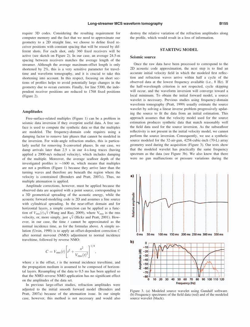
perform the source inversion. Consequently, we use a synthetic

source modeled for the 32-air-gun, 4258-cubic-inch (70-L) array

geometry used during the acquisition (Figure 3). Our tests show

that the modeled wavelet has practically the same frequency

spectrum as the data (see Figure 3b). We also know that there

were no gun malfunctions or pressure variations during the

Figure 3. (a) Modeled source wavelet using Gundalf software.(b) Frequency spectrums of the field data (red) and of the modeledsource wavelet (black).


acquisition, which yields constant signal strength from shot to

shot.

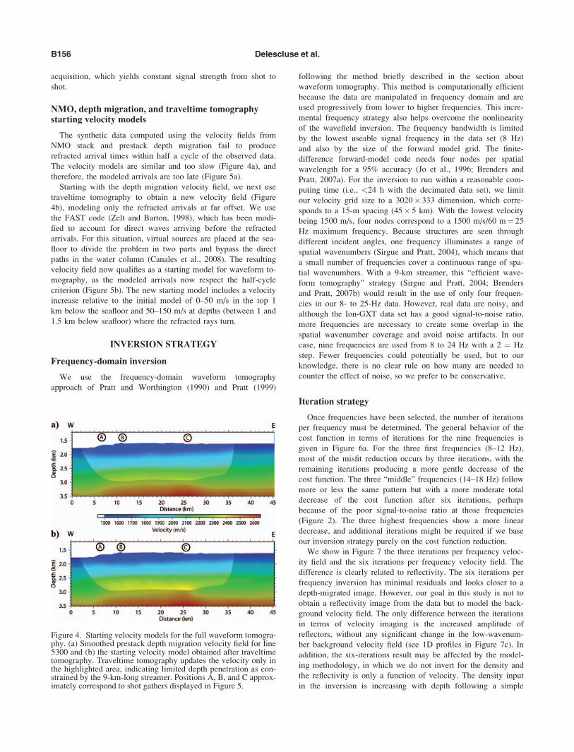
NMO, depth migration, and traveltime tomographystarting velocity models

The synthetic data computed using the velocity fields from

NMO stack and prestack depth migration fail to produce

refracted arrival times within half a cycle of the observed data.

The velocity models are similar and too slow (Figure 4a), and

therefore, the modeled arrivals are too late (Figure 5a).

Starting with the depth migration velocity field, we next use

traveltime tomography to obtain a new velocity field (Figure

4b), modeling only the refracted arrivals at far offset. We use

the FAST code (Zelt and Barton, 1998), which has been modi-

fied to account for direct waves arriving before the refracted

arrivals. For this situation, virtual sources are placed at the sea-

floor to divide the problem in two parts and bypass the direct

paths in the water column (Canales et al., 2008). The resulting

velocity field now qualifies as a starting model for waveform to-

mography, as the modeled arrivals now respect the half-cycle

criterion (Figure 5b). The new starting model includes a velocity

increase relative to the initial model of 0–50 m/s in the top 1

km below the seafloor and 50–150 m/s at depths (between 1 and

1.5 km below seafloor) where the refracted rays turn.

INVERSION STRATEGY

Frequency-domain inversion

We use the frequency-domain waveform tomography

approach of Pratt and Worthington (1990) and Pratt (1999)

following the method briefly described in the section about

waveform tomography. This method is computationally efficient

because the data are manipulated in frequency domain and are

used progressively from lower to higher frequencies. This incre-

mental frequency strategy also helps overcome the nonlinearity

of the wavefield inversion. The frequency bandwidth is limited

by the lowest useable signal frequency in the data set (8 Hz)

and also by the size of the forward model grid. The finite-

difference forward-model code needs four nodes per spatial

wavelength for a 95% accuracy (Jo et al., 1996; Brenders and

Pratt, 2007a). For the inversion to run within a reasonable com-

puting time (i.e., <24 h with the decimated data set), we limit

our velocity grid size to a 3020� 333 dimension, which corre-

sponds to a 15-m spacing (45� 5 km). With the lowest velocity

being 1500 m/s, four nodes correspond to a 1500 m/s/60 m¼ 25

Hz maximum frequency. Because structures are seen through

different incident angles, one frequency illuminates a range of

spatial wavenumbers (Sirgue and Pratt, 2004), which means that

a small number of frequencies cover a continuous range of spa-

tial wavenumbers. With a 9-km streamer, this “efficient wave-

form tomography” strategy (Sirgue and Pratt, 2004; Brenders

and Pratt, 2007b) would result in the use of only four frequen-

cies in our 8- to 25-Hz data. However, real data are noisy, and

although the Ion-GXT data set has a good signal-to-noise ratio,

more frequencies are necessary to create some overlap in the

spatial wavenumber coverage and avoid noise artifacts. In our

case, nine frequencies are used from 8 to 24 Hz with a 2 ¼ Hz

step. Fewer frequencies could potentially be used, but to our

knowledge, there is no clear rule on how many are needed to

counter the effect of noise, so we prefer to be conservative.

Iteration strategy

Once frequencies have been selected, the number of iterations

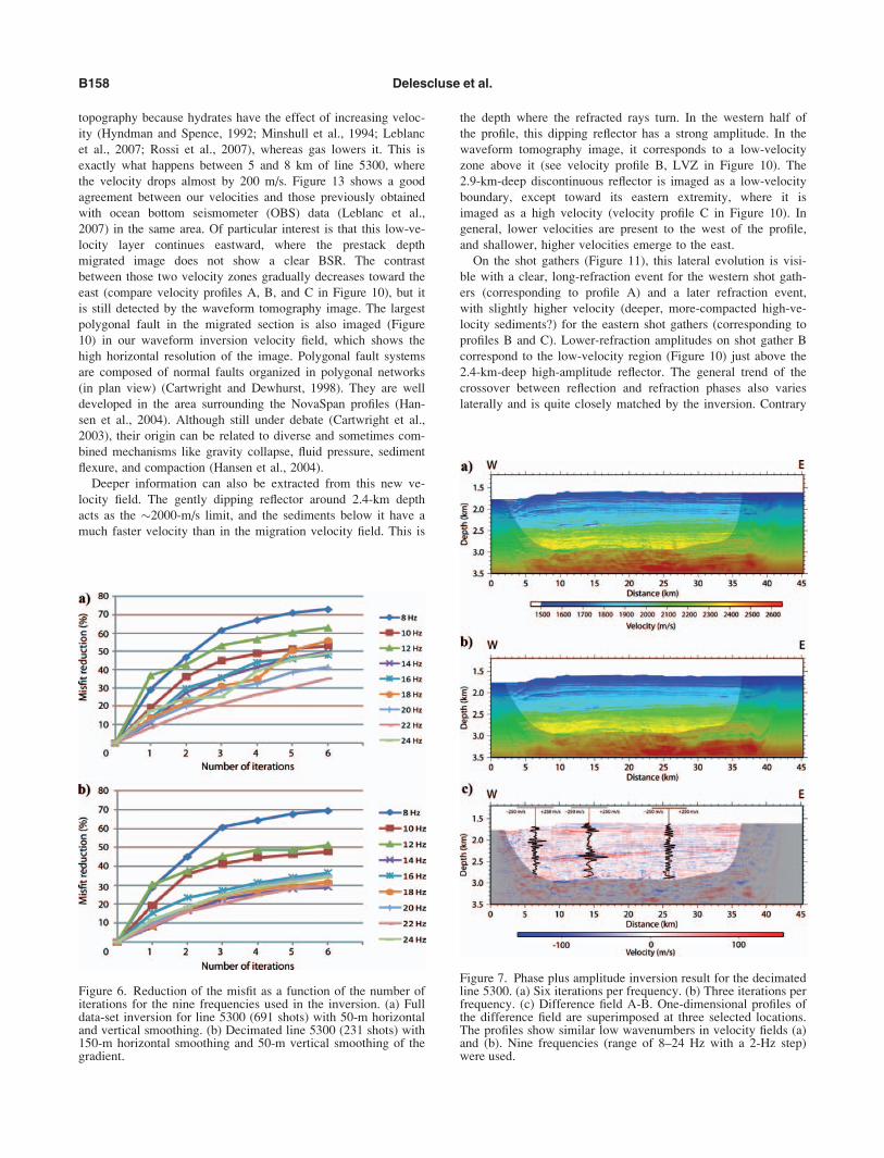
per frequency must be determined. The general behavior of the

cost function in terms of iterations for the nine frequencies is

given in Figure 6a. For the three first frequencies (8–12 Hz),

most of the misfit reduction occurs by three iterations, with the

remaining iterations producing a more gentle decrease of the

cost function. The three “middle” frequencies (14–18 Hz) follow

more or less the same pattern but with a more moderate total

decrease of the cost function after six iterations, perhaps

because of the poor signal-to-noise ratio at those frequencies

(Figure 2). The three highest frequencies show a more linear

decrease, and additional iterations might be required if we base

our inversion strategy purely on the cost function reduction.

We show in Figure 7 the three iterations per frequency veloc-

ity field and the six iterations per frequency velocity field. The

difference is clearly related to reflectivity. The six iterations per

frequency inversion has minimal residuals and looks closer to a

depth-migrated image. However, our goal in this study is not to

obtain a reflectivity image from the data but to model the back-

ground velocity field. The only difference between the iterations

in terms of velocity imaging is the increased amplitude of

reflectors, without any significant change in the low-wavenum-

ber background velocity field (see 1D profiles in Figure 7c). In

addition, the six-iterations result may be affected by the model-

ing methodology, in which we do not invert for the density and

the reflectivity is only a function of velocity. The density input

in the inversion is increasing with depth following a simple

Figure 4. Starting velocity models for the full waveform tomogra-phy. (a) Smoothed prestack depth migration velocity field for line5300 and (b) the starting velocity model obtained after traveltimetomography. Traveltime tomography updates the velocity only inthe highlighted area, indicating limited depth penetration as con-strained by the 9-km-long streamer. Positions A, B, and C approx-imately correspond to shot gathers displayed in Figure 5.


porosity law. It is not updated. This can lead to an overestima-

tion of velocity changes that are needed to match the reflection

amplitudes. Therefore, we stop after three iterations per fre-

quency because the low-wavenumber background velocity (such

as the low velocity at around 2-km depth discussed in the next

section) is successfully retrieved.

In an effort to further limit the weight of reflections in the

inversion, we also ignore the first 160 near-offset traces of each

shot gather and only consider the 200 receivers from offsets of

4–9 km. The weight of near-offset reflections is high in the

inversion gradient, although they carry little low-wavenumber

background velocity information. The high amplitudes of the

near-offset sea-bottom reflection are also unlikely to be correctly

modeled by the 2D acoustic code (Hicks and Pratt, 2001). The

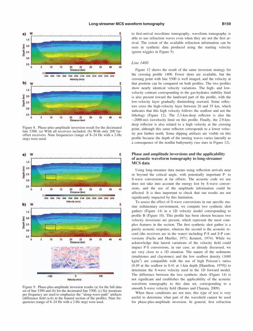
difference between a velocity field obtained with all the

receivers and a velocity field obtained with far-offset receivers

is minimal (Figure 8). Moreover, with inversions using all the

receivers, a few diverging iterations appear and slow the inver-

sion, which does not happen when using only the far-offset

receivers. This effect may be due to anisotropy with low-

incidence reflection rays travelling slower than higher-incidence

wide-angle reflections or refractions as a result of horizontal

layering with embedded low velocities (Figure 7 and next

sections).

Full versus decimated data set

It is useful to compare the behavior of the

cost functions for high frequencies with those in

the decimated inversion (every third shot). Fig-

ure 6b shows a smaller reduction of the cost

functions for frequencies higher than 14 Hz. For

an average 2000-m/s velocity, 14 Hz illuminates

wavelengths around 150 m, which is precisely

the distance between the shots. In this case, hor-

izontal smoothing of the inversion gradient fil-

ters wavelengths smaller than 150 m so that

“along-wave-path” artifacts are minimized (see

Figure 9). This can explain why the inversion is

less efficient for these high frequencies. In the

nondecimated, full data-set inversion (Figure

6a), the behavior of the 22- and 24-Hz cost

functions can be interpreted as the result of the

50-m smoothing of the gradient we apply in

this case. This shows that even with a finer

grid, inversion of frequencies far beyond 25 Hz

would not be useful.

While the decimated inversion is smoothed

and still shows along-wave-path artifacts (Fig-

ure 9), those are moderate. In this case of a

very simple geological setting, it is hard to jus-

tify the high computational cost of the full data-

set inversion. We are using a sequential code

and the full data-set inversion can take up to a

week. The three iterations per frequency inver-

sion of the decimated data set takes a bit less

than 24 h to run, which is much more efficient.

The results of the phase and amplitude inver-

sion for line 5300 are shown in Figures 10 and

11. The results for line 1400 are displayed in

Figure 12. All these figures show three iterations per frequency

inversion. The velocities at the crossing between the two lines

are in very good agreement (Figure 12). The next section will

discuss those results in terms of comparison with the migrated

section and the validity of the acoustic approximation in this

specific sedimentary environment.

DISCUSSION

Interpretation of the results and comparison with themigrated section

Line 5300

Figure 10 shows the result of our inversion for line 5300

derived using 9 frequencies and a total of 27 iterations. Several

significant features are now derived that did not exist in the ini-

tial smooth velocity model from traveltime tomography. First, a

velocity contrast appears around 2-km depth. On the migrated

section (Figure 10), it clearly corresponds to the bottom-simulat-

ing reflector (BSR) that is visible at the same depth between 5

and 8 km. A BSR marks the thermal and pressure stability limit

of gas hydrates, which can trap some free gas underneath. As a

result, a velocity inversion is expected to follow the seafloor

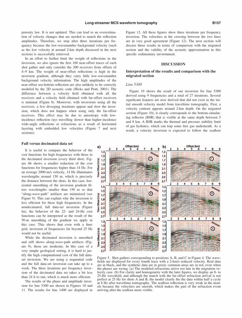
Figure 5. Shot gathers corresponding to positions A, B, and C in Figure 4. The wave-fields are displayed for every fourth trace with a 2-km/s reduced velocity. Real dataare in black, and the synthetic data are in green; common areas are in red, even whenthe phases are wrong. (a) The modeled refractions arrive too late in the migration ve-locity case. (b) For clarity and homogeneity with the later figures, we display an 8- to25-Hz wavefield, and although the match with the far-offset refraction arrival is notperfect at 25 Hz for shots A and B, the model clearly fits the data within half a cycleat 8 Hz after traveltime tomography. The seafloor reflection is very weak in the mod-els because the velocities are smooth, which makes the part of the refraction eventarriving after the seafloor more visible.


topography because hydrates have the effect of increasing veloc-

ity (Hyndman and Spence, 1992; Minshull et al., 1994; Leblanc

et al., 2007; Rossi et al., 2007), whereas gas lowers it. This is

exactly what happens between 5 and 8 km of line 5300, where

the velocity drops almost by 200 m/s. Figure 13 shows a good

agreement between our velocities and those previously obtained

with ocean bottom seismometer (OBS) data (Leblanc et al.,

2007) in the same area. Of particular interest is that this low-ve-

locity layer continues eastward, where the prestack depth

migrated image does not show a clear BSR. The contrast

between those two velocity zones gradually decreases toward the

east (compare velocity profiles A, B, and C in Figure 10), but it

is still detected by the waveform tomography image. The largest

polygonal fault in the migrated section is also imaged (Figure

10) in our waveform inversion velocity field, which shows the

high horizontal resolution of the image. Polygonal fault systems

are composed of normal faults organized in polygonal networks

(in plan view) (Cartwright and Dewhurst, 1998). They are well

developed in the area surrounding the NovaSpan profiles (Han-

sen et al., 2004). Although still under debate (Cartwright et al.,

2003), their origin can be related to diverse and sometimes com-

bined mechanisms like gravity collapse, fluid pressure, sediment

flexure, and compaction (Hansen et al., 2004).

Deeper information can also be extracted from this new ve-

locity field. The gently dipping reflector around 2.4-km depth

acts as the �2000-m/s limit, and the sediments below it have a

much faster velocity than in the migration velocity field. This is

the depth where the refracted rays turn. In the western half of

the profile, this dipping reflector has a strong amplitude. In the

waveform tomography image, it corresponds to a low-velocity

zone above it (see velocity profile B, LVZ in Figure 10). The

2.9-km-deep discontinuous reflector is imaged as a low-velocity

boundary, except toward its eastern extremity, where it is

imaged as a high velocity (velocity profile C in Figure 10). In

general, lower velocities are present to the west of the profile,

and shallower, higher velocities emerge to the east.

On the shot gathers (Figure 11), this lateral evolution is visi-

ble with a clear, long-refraction event for the western shot gath-

ers (corresponding to profile A) and a later refraction event,

with slightly higher velocity (deeper, more-compacted high-ve-

locity sediments?) for the eastern shot gathers (corresponding to

profiles B and C). Lower-refraction amplitudes on shot gather B

correspond to the low-velocity region (Figure 10) just above the

2.4-km-deep high-amplitude reflector. The general trend of the

crossover between reflection and refraction phases also varies

laterally and is quite closely matched by the inversion. Contrary

Figure 7. Phase plus amplitude inversion result for the decimatedline 5300. (a) Six iterations per frequency. (b) Three iterations perfrequency. (c) Difference field A-B. One-dimensional profiles ofthe difference field are superimposed at three selected locations.The profiles show similar low wavenumbers in velocity fields (a)and (b). Nine frequencies (range of 8–24 Hz with a 2-Hz step)were used.

Figure 6. Reduction of the misfit as a function of the number ofiterations for the nine frequencies used in the inversion. (a) Fulldata-set inversion for line 5300 (691 shots) with 50-m horizontaland vertical smoothing. (b) Decimated line 5300 (231 shots) with150-m horizontal smoothing and 50-m vertical smoothing of thegradient.


to first-arrival traveltime tomography, waveform tomography is

able to use refraction waves even when they are not the first ar-

rival. The extent of the available refraction information can be

seen in synthetic data produced using the starting velocity

(green wiggles in Figure 5).

Line 1400

Figure 12 shows the result of the same inversion strategy for

the crossing profile 1400. Fewer shots are available, but the

crossing point with line 5300 is well imaged, and the velocity at

that position can be compared on both profiles. The two profiles

show nearly identical velocity variations. The high- and low-

velocity contrast corresponding to the gas-hydrates stability limit

is also present toward the landward part of the profile, with the

low-velocity layer gradually diminishing seaward. Some reflec-

tors cross the high-velocity layer between 26 and 35 km, which

indicates that this high velocity follows the seafloor and not the

lithology (Figure 12). The 2.3-km-deep reflector is also the

�2000-m/s isovelocity limit on this profile. Finally, the 2.9-km-

deep reflector is also related to a high velocity at the crossing

point, although this same reflector corresponds to a lower veloc-

ity just farther north. Some dipping artifacts are visible on this

profile because the depth of the turning waves varies laterally as

a consequence of the nonflat bathymetry (see stars in Figure 12).

Phase and amplitude inversions and the applicabilityof acoustic waveform tomography to long-streamerMCS data

Using long-streamer data means using reflection arrivals near

or beyond the critical angle, with potentially important P- to

S-wave conversions at far offsets. The acoustic code we use

does not take into account the energy lost by S-wave conver-

sions, and the use of the amplitude information could be

affected. It is thus important to check that our results are not

significantly impacted by this limitation.

To assess the effect of S-wave conversions in our specific ma-

rine sedimentary environment, we compute two synthetic shot

gathers (Figure 14) in a 1D velocity model corresponding to

profile B (Figure 10). This profile has been chosen because two

velocity inversions are present, which represent the most com-

plex features in the section. The first synthetic shot gather is a

purely acoustic response, whereas the second is the acoustic re-

cord (the receivers are in the water) including P-S and S-P con-

versions (Fuchs and Mueller, 1971; Kennett, 1974). While we

acknowledge that lateral variations of the velocity field could

impact P-S conversions, in our case, as already discussed, we

are very close to a 1D situation. The nature of the sediments

(mudstones and claystones) and the low seafloor density (1680

kg/m3) are compatible with the use of high Poisson’s ratios

(0.49 at the seafloor to 0.41 at 1-km depth [Hamilton, 1979]) to

determine the S-wave velocity used in the 1D forward model.

The difference between the two synthetic shots (Figure 14) is

not significant and establishes the applicability of the acoustic

waveform tomography to this data set, corresponding to a

smooth S-wave velocity field (Barnes and Charara, 2009).

When these conditions are not met, this type of test is very

useful to determine what part of the wavefield cannot be used

for phase-plus-amplitude inversion. In general, first refraction

Figure 9. Phase-plus-amplitude inversion results (a) for the full dataset of line 5300 and (b) for the decimated line 5300. (c) Six iterationsper frequency are used to emphasize the “along-wave-path” artifacts(difference field (a-b) in the framed section of the profile). Nine fre-quencies (range of 8–24 Hz with a 2-Hz step) were used.

Figure 8. Phase-plus-amplitude inversion result for the decimatedline 5300. (a) With all receivers included. (b) With only 200 far-offset receivers. Nine frequencies (range of 8–24 Hz with a 2-Hzstep) were used.


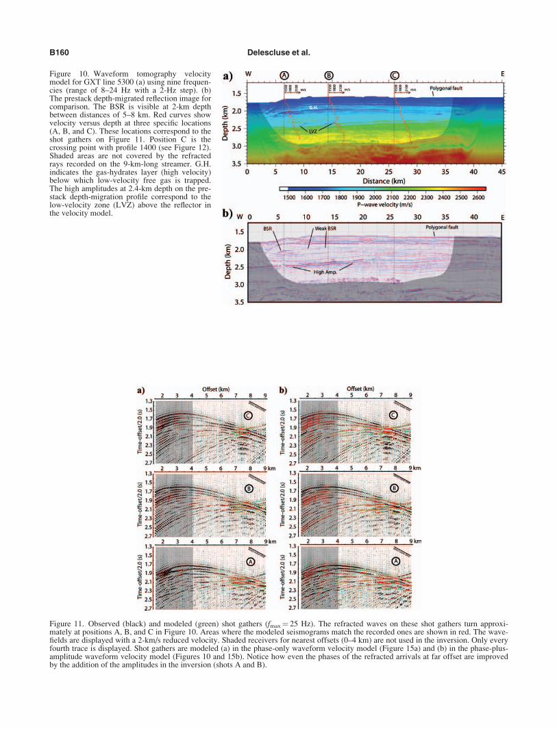
Figure 10. Waveform tomography velocitymodel for GXT line 5300 (a) using nine frequen-cies (range of 8–24 Hz with a 2-Hz step). (b)The prestack depth-migrated reflection image forcomparison. The BSR is visible at 2-km depthbetween distances of 5–8 km. Red curves showvelocity versus depth at three specific locations(A, B, and C). These locations correspond to theshot gathers on Figure 11. Position C is thecrossing point with profile 1400 (see Figure 12).Shaded areas are not covered by the refractedrays recorded on the 9-km-long streamer. G.H.indicates the gas-hydrates layer (high velocity)below which low-velocity free gas is trapped.The high amplitudes at 2.4-km depth on the pre-stack depth-migration profile correspond to thelow-velocity zone (LVZ) above the reflector inthe velocity model.

Figure 11. Observed (black) and modeled (green) shot gathers (fmax¼ 25 Hz). The refracted waves on these shot gathers turn approxi-mately at positions A, B, and C in Figure 10. Areas where the modeled seismograms match the recorded ones are shown in red. The wave-fields are displayed with a 2-km/s reduced velocity. Shaded receivers for nearest offsets (0–4 km) are not used in the inversion. Only everyfourth trace is displayed. Shot gathers are modeled (a) in the phase-only waveform velocity model (Figure 15a) and (b) in the phase-plus-amplitude waveform velocity model (Figures 10 and 15b). Notice how even the phases of the refracted arrivals at far offset are improvedby the addition of the amplitudes in the inversion (shots A and B).


arrivals have a small incident angle and thus can often be used

if there are no strong lateral variations of attenuation, which is a

potential problem with OBS data sets (Bleibinhaus et al., 2007,

2009) because long profiles may cross very different geological

terrains. Gas hydrates and free-gas presence can imply a large

change in attenuation (Guerin and Goldberg, 2002; Rossi et al.,

2007; Madrussani et al., 2010). However, in our case, the con-

centration of free gas and hydrates in the area

calculated by Leblanc et al. (2007) and based

on a model by Helgerud et al. (1999) are only

2%–6% and <1%, respectively. This implies

only moderate attenuation without any sudden

lateral change because the amount of free gas is

only slowly evolving and the gas-hydrate layer

shows almost constant velocity along the pro-

files. The low concentration and smooth lateral

evolution of gas hydrates and free gas do not

lead to a significant lateral change in attenuation

along the profiles, as earlier assumed.

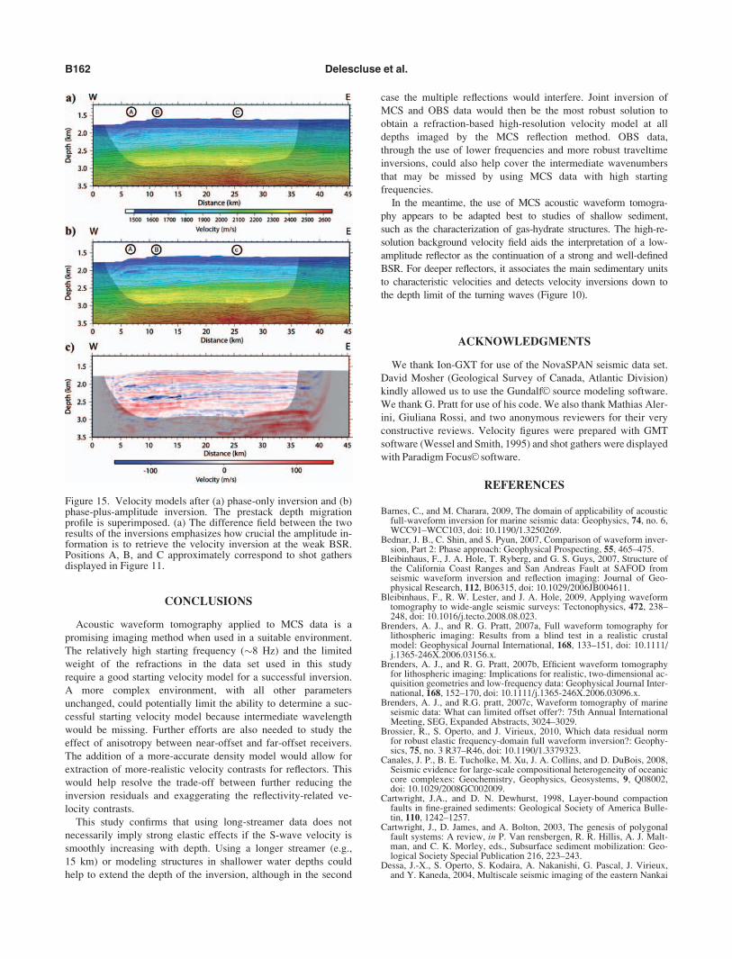
Figure 15 shows the phase-only inversion of

line 5300, with all other parameters unchanged.

Comparison with the phase-plus-amplitude

inversion shows a large improvement of the

result relative to phase only, which is another

indication of the validity of the acoustic approx-

imation in our specific case. Inversions of data

sets with significant elastic effects (Bednar

et al., 2007; Shin et al., 2007) can lead to a bet-

ter result of the phase-only tomography when

compared to the phase-plus-amplitude tomogra-

phy, which is clearly not our case. We are con-

fident that unmodeled parameters (small lateral

variations, higher S-wave velocity contrasts at

the BSR) do not significantly impact the validity of the acoustic

approximation. Comparing the synthetic wavefields in the

“phase” and “phase-plus-amplitude” waveform-inverted veloc-

ities (Figure 11) shows a much better fit of the refraction event

when using the amplitude information. This improvement of the

modeled wavefield corresponds to a clear improvement of the

velocity contrast below the hydrate layer (see difference field in

Figure 15) and a much more detailed image in general.

Figure 12. (a) Waveform tomography velocity model for GXT line 1400 using ninefrequencies (range of 8–24 Hz with a 2-Hz step) superimposed on the prestack depth-migrated reflection image. Shaded areas are not covered by the refracted rays recordedon the 9-km-long streamer. Dipping artifacts are visible between 25 and 35 km justabove the shaded area limit (stars). (b) Velocity at the crossing point C with line 5300(Figure 10). The NMO (blue), migration (green), traveltime tomography (orange), andwaveform tomography velocities for lines 1400 (black) and 5300 (red) are displayed.Note the excellent agreement between the waveform inversion models at the crossingpoint.

Figure 13. OBS velocities from Leblanc et al. (2007) (solid anddashed black lines) superimposed with velocities (A, red; B, purple;C, blue) of Figure 10. The gray line is a reference velocity consider-ing sediment compaction (see details in Leblanc et al., 2007).

Figure 14. Acoustic synthetic shot gather (gray) computed in a 1Dvelocity model representative of profile B in Figure 10. The redwiggles are the difference field between the purely acoustic caseand the acoustic part of the full seismic case including S-wave con-version at the horizontal layer interfaces. The part of the wavefieldwhere the difference is noticeable, but not significant, is circled.The critical angle for the seafloor is 74�, using velocities and den-sities derived from cores, corresponding to an offset of 11 km.


CONCLUSIONS

Acoustic waveform tomography applied to MCS data is a

promising imaging method when used in a suitable environment.

The relatively high starting frequency (�8 Hz) and the limited

weight of the refractions in the data set used in this study

require a good starting velocity model for a successful inversion.

A more complex environment, with all other parameters

unchanged, could potentially limit the ability to determine a suc-

cessful starting velocity model because intermediate wavelength

would be missing. Further efforts are also needed to study the

effect of anisotropy between near-offset and far-offset receivers.

The addition of a more-accurate density model would allow for

extraction of more-realistic velocity contrasts for reflectors. This

would help resolve the trade-off between further reducing the

inversion residuals and exaggerating the reflectivity-related ve-

locity contrasts.

This study confirms that using long-streamer data does not

necessarily imply strong elastic effects if the S-wave velocity is

smoothly increasing with depth. Using a longer streamer (e.g.,

15 km) or modeling structures in shallower water depths could

help to extend the depth of the inversion, although in the second

case the multiple reflections would interfere. Joint inversion of

MCS and OBS data would then be the most robust solution to

obtain a refraction-based high-resolution velocity model at all

depths imaged by the MCS reflection method. OBS data,

through the use of lower frequencies and more robust traveltime

inversions, could also help cover the intermediate wavenumbers

that may be missed by using MCS data with high starting

frequencies.

In the meantime, the use of MCS acoustic waveform tomogra-

phy appears to be adapted best to studies of shallow sediment,

such as the characterization of gas-hydrate structures. The high-re-

solution background velocity field aids the interpretation of a low-

amplitude reflector as the continuation of a strong and well-defined

BSR. For deeper reflectors, it associates the main sedimentary units

to characteristic velocities and detects velocity inversions down to

the depth limit of the turning waves (Figure 10).

ACKNOWLEDGMENTS

We thank Ion-GXT for use of the NovaSPAN seismic data set.

David Mosher (Geological Survey of Canada, Atlantic Division)

kindly allowed us to use the GundalfVC source modeling software.

We thank G. Pratt for use of his code. We also thank Mathias Aler-

ini, Giuliana Rossi, and two anonymous reviewers for their very

constructive reviews. Velocity figures were prepared with GMT

software (Wessel and Smith, 1995) and shot gathers were displayed

with Paradigm FocusVC software.

REFERENCES

Barnes, C., and M. Charara, 2009, The domain of applicability of acousticfull-waveform inversion for marine seismic data: Geophysics, 74, no. 6,WCC91–WCC103, doi: 10.1190/1.3250269.

Bednar, J. B., C. Shin, and S. Pyun, 2007, Comparison of waveform inver-sion, Part 2: Phase approach: Geophysical Prospecting, 55, 465–475.

Bleibinhaus, F., J. A. Hole, T. Ryberg, and G. S. Guys, 2007, Structure ofthe California Coast Ranges and San Andreas Fault at SAFOD fromseismic waveform inversion and reflection imaging: Journal of Geo-physical Research, 112, B06315, doi: 10.1029/2006JB004611.

Bleibinhaus, F., R. W. Lester, and J. A. Hole, 2009, Applying waveformtomography to wide-angle seismic surveys: Tectonophysics, 472, 238–248, doi: 10.1016/j.tecto.2008.08.023.

Brenders, A. J., and R. G. Pratt, 2007a, Full waveform tomography forlithospheric imaging: Results from a blind test in a realistic crustalmodel: Geophysical Journal International, 168, 133–151, doi: 10.1111/j.1365-246X.2006.03156.x.

Brenders, A. J., and R. G. Pratt, 2007b, Efficient waveform tomographyfor lithospheric imaging: Implications for realistic, two-dimensional ac-quisition geometries and low-frequency data: Geophysical Journal Inter-national, 168, 152–170, doi: 10.1111/j.1365-246X.2006.03096.x.

Brenders, A. J., and R.G. pratt, 2007c, Waveform tomography of marineseismic data: What can limited offset offer?: 75th Annual InternationalMeeting, SEG, Expanded Abstracts, 3024–3029.

Brossier, R., S. Operto, and J. Virieux, 2010, Which data residual normfor robust elastic frequency-domain full waveform inversion?: Geophy-sics, 75, no. 3 R37–R46, doi: 10.1190/1.3379323.

Canales, J. P., B. E. Tucholke, M. Xu, J. A. Collins, and D. DuBois, 2008,Seismic evidence for large-scale compositional heterogeneity of oceaniccore complexes: Geochemistry, Geophysics, Geosystems, 9, Q08002,doi: 10.1029/2008GC002009.

Cartwright, J.A., and D. N. Dewhurst, 1998, Layer-bound compactionfaults in fine-grained sediments: Geological Society of America Bulle-tin, 110, 1242–1257.

Cartwright, J., D. James, and A. Bolton, 2003, The genesis of polygonalfault systems: A review, in P. Van rensbergen, R. R. Hillis, A. J. Malt-man, and C. K. Morley, eds., Subsurface sediment mobilization: Geo-logical Society Special Publication 216, 223–243.

Dessa, J.-X., S. Operto, S. Kodaira, A. Nakanishi, G. Pascal, J. Virieux,and Y. Kaneda, 2004, Multiscale seismic imaging of the eastern Nankai

Figure 15. Velocity models after (a) phase-only inversion and (b)phase-plus-amplitude inversion. The prestack depth migrationprofile is superimposed. (a) The difference field between the tworesults of the inversions emphasizes how crucial the amplitude in-formation is to retrieve the velocity inversion at the weak BSR.Positions A, B, and C approximately correspond to shot gathersdisplayed in Figure 11.


trough by full waveform inversion: Geophysical Research Letters, 31,L18606, doi: 10.1029/2004GL020453.

Fuchs, K., and G. Mueller, 1971, Computation of synthetic seismogramsby the reflectivity method and comparison with observations: Geophysi-cal Journal of the Royal Astronomical Society, 23, 417–433.

Guerin, G., and D. Goldberg, 2002, Sonic waveform attenuation in gashydrate-bearing sediments from the Mallik 2L-38 research well, Mack-enzie Delta, Canada: Journal of Geophysical Research, 107, no. B5,2088, doi: 10.1029/2001JB000556.

Hamilton, E. L., 1979, Vp/Vs and Poisson’s ratios in marine sedimentsand rocks: Journal of the Acoustical Society of America, 66, 1093–1101.

Hansen, D. M., J. W. Shimeld, M. A. Williamson, and H. Lykke-Ander-sen, 2004, Development of a major polygonal fault system in UpperCretaceous chalk and Cenozoic mudrocks of the Sable Subbasin, Cana-dian Atlantic margin: Marine and Petroleum Geology, 21, 1205–1219,doi: 10.1016/j.marpetgeo.2004.07.004.

Helgerud, M. B., J. Dvorkin, A. Nur, A. Sakai, and T. Collett, 1999, Elas-tic-wave velocity in marine sediments with gas hydrates: Effective me-dium modeling: Geophysical Research Letters, 26, 2021–2024.

Hicks, G., and R. G. Pratt, 2001, Reflection waveform inversion usinglocal descent methods: Estimating attenuation and velocity over a gassand deposit: Geophysics, 66, 770–780.

Hyndman, R. D., and G. D. Spence, 1992, A seismic study of methanehydrate marine bottom simulating reflectors: Journal of GeophysicalResearch, 97, 6683–6698.

Jannane, M., W. Beydoun, E. Crase, D. Cao, Z. Koren, E. Landa, M.Mendes, A. Pica, M. Noble, G. Roeth, S. Singh, R. Snieder, A. Tarantola,D. Trezeguet, and M. Xie, 1989, Wavelengths of earth structures that canbe resolved from seismic-reflection data: Geophysics, 54, 906–910.

Jo, C. H., C. S. Shin, and J. H. Su, 1996, An optimal 9-point, finite-differ-ence, frequency-space, 2-D scalar wave extrapolator: Geophysics, 61,529–537.

Kennett, B. L. N., 1974, Reflections, rays and reverberations: Bulletin ofthe Seismological Society of America, 64, 1685–1696.

Lailly, P., 1983, The seismic inverse problem as a sequence of beforestack migrations, in J. B. Bednar, R. Redner, E. Robinson, and A.Weglein, eds., Conference on inverse scattering: Theory and applica-tion: Society for Industrial and Applied Mathematics, 206–220.

LeBlanc, C., K. Louden, and D. Mosher, 2007, Gas hydrates off easternCanada: Velocity models from wide-angle seismic profiles on the Sco-tian Slope: Marine and Petroleum Geology, 24, 321–335, doi: 10.1016/j.marpetgeo.2006.05.008.

Madrussani, G., G. Rossi, and A. Camerlenghi, 2010, Gas hydrates, freegas distribution and fault pattern on the west Svalbard continental mar-gin: Geophysical Journal International, 180, 666–684, doi: 10.1111/j.1365-246X.2009.04425.x.

Minshull, T. A., S. C. Singh, and G. K. Westbrook, 1994, Seismic velocitystructure at a gas hydrate reflector, offshore western Colombia, from full-wave-form inversion: Journal of Geophysical Research, 99, 4715–4734.

Mosher, D.C., K. Moran, and R. N. Hiscott, 1994, Late Quaternary sedi-ment, sediment mass-flow processes and slope stability on the ScotianSlope: Sedimentology, 41, 1039–1061.

Newman, K. R., M. R. Nedimovic, J. P. Canales, and S. M. Carbotte,2011, Evolution of seismic layer 2B across the Juan de Fuca Ridge fromhydrophone streamer 2D traveltime tomography: Geochemistry, Geo-physics, Geosystems, 12, doi: 10.1029/2010GC003462.

Operto, S., C. Ravaut, L. Improta, J. Virieux, A. Herrero, and P. Dell’Aversana, 2004, Quantitative imaging of complex structures from densewide-aperture seismic data by multiscale traveltime and waveforminversions: A case study: Geophysical Prospecting, 52, 625–651.

Operto, S., J. Virieux, J. X. Dessa, and G. Pascal, 2006, Crustal seismicimaging from multifold ocean bottom seismometer data by frequencydomain full waveform tomography: Application to the eastern Nankaitrough: Journal of Geophysical Research, 111, B09306, doi: 10.1029/2005JB003835.

Piper, D. J. W., and W. R. Normark, 1989, Late Cenozoic sea-levelchanges and the onset of glaciation: Impact on continental slope progra-dation off eastern Canada: Marine Petroleum and Geology, 6, 336–348.

Pratt, R. G., 1999, Seismic waveform inversion in the frequency domain;Part 1, Theory and verification in a physical scale model: Geophysics,64, 888–901.

Pratt, R. G., C. Shin, and G. Hicks, 1998, Gauss-Newton and full Newtonmethods in frequency-space seismic waveform inversion: GeophysicalJournal International, 133, 341–362.

Pratt, R. G., and M. H. Worthington, 1990, Inverse theory applied tomulti-source cross-hole tomography. Part I: Acoustic wave-equationmethod: Geophysical Prospecting, 38, 287–310.

Ravaut, C., S. Operto, L. Improta, J. Virieux, A. Herrero, and P. Dell’Aversana, 2004, Multiscale imaging of complex structures from multi-fold wide-aperture seismic data by frequency-domain full-waveform to-mography: Application to a thrust belt: Geophysical JournalInternational, 159, 1032–1056, doi: 10.1111/j.1365-246X.2004.02442.x.

Rossi, G., D. Gei, G. Bohm, G. Madrussani, and J. M. Carcione, 2007,Attenuation tomography: An application to gas-hydrate and free-gasdetection: Geophysical Prospecting, 55, 655–669.

Shin, C., and D.-J. Min, 2006, Waveform inversion using a logarithmicwavefield: Geophysics, 71, No. 3, R31–R42.

Shin, C., S. Pyun, and J. B. Bednar, 2007, Comparison of waveform inver-sion, part 1: Conventional wavefield vs logarithmic wavefield: Geo-physical Prospecting, 55, 449–464.

Shipp, R. M., and S. C. Singh, 2002, Two-dimensional full wavefieldinversion of wide-aperture marine seismic streamer data: GeophysicalJournal International, 151, 325–344.

Sirgue, L., 2003, Inversion de la forme d’onde dans le domaine frequentielde donnees sismiques grands offsets: Ph.D. thesis, Universite; Paris XI.

Sirgue, L., 2006, The importance of low frequency and large offset inwaveform inversion: 68th Conference and Exhibition, EAGE, ExtendedAbstracts, A037.

Sirgue, L., and R. G. Pratt, 2004, Efficient waveform inversion and imag-ing: A strategy for selecting temporal frequencies: Geophysics, 60,1870–1874, doi: 10.1190/1.1649391.

Tarantola, A., 1984, Inversion of seismic reflection data in the acousticapproximation: Geophysics, 49, 1259–1266.

———, 1987, Inverse problem theory: Methods for data fitting and pa-rameter estimation: Elsevier Science Publishers.

Ursin, 1990, Offset-dependent geometrical spreading in a layered medium:Geophysics, 55, 492–496.

Virieux, J., and S. Operto, 2009, An overview of full-waveform inversionin exploration geophysics: Geophysics, 74, No. 6, WCC1–WCC26, doi:10.1190/1.3238367.

Wang, Y., and Y. Rao, 2009, Reflection seismic waveform tomography:Journal of Geophysical research, 114, B03304, doi: 10.1029/2008JB005916.

Wessel, P., and W. H. F. Smith, 1995, New version of the Generic Map-ping Tool released: Eos, Transactions of the American GeophysicalUnion, 76, no. 33, 329.

Williamson, P., B. Wang, B. Bevc, and I. Jones, 2010, Full wave-equationmethods for complex imaging challenges: The Leading Edge, 29, 264–268.

Zelt, C. A., and P. J. Barton, 1998, Three-dimensional seismic refractiontomography: A comparison of two methods applied to data from theFaeroe Basin: Journal of Geophysical Research, 103, 7187–7210.


2D waveform tomography applied to long-streamer MCS data from the Scotian Slope

Documents

Transcript of 2D waveform tomography applied to long-streamer MCS data from the Scotian Slope