285583.pdf - University of Bristol Research Portal
192
This electronic thesis or dissertation has been downloaded from Explore Bristol Research, http://research-information.bristol.ac.uk Author: Froggatt, Edith Sarah Title: An investigation of scrambling in Langmuir-Blodgett films using neutron and x-ray reflectivity. General rights Access to the thesis is subject to the Creative Commons Attribution - NonCommercial-No Derivatives 4.0 International Public License. A copy of this may be found at https://creativecommons.org/licenses/by-nc-nd/4.0/legalcode This license sets out your rights and the restrictions that apply to your access to the thesis so it is important you read this before proceeding. Take down policy Some pages of this thesis may have been removed for copyright restrictions prior to having it been deposited in Explore Bristol Research. However, if you have discovered material within the thesis that you consider to be unlawful e.g. breaches of copyright (either yours or that of a third party) or any other law, including but not limited to those relating to patent, trademark, confidentiality, data protection, obscenity, defamation, libel, then please contact [email protected] and include the following information in your message: • Your contact details • Bibliographic details for the item, including a URL • An outline nature of the complaint Your claim will be investigated and, where appropriate, the item in question will be removed from public view as soon as possible.
-
Upload
khangminh22 -
Category
Documents
-
view
0 -
download
0
Transcript of 285583.pdf - University of Bristol Research Portal

This electronic thesis or dissertation has beendownloaded from Explore Bristol Research,http://research-information.bristol.ac.uk
Author:Froggatt, Edith Sarah
Title:An investigation of scrambling in Langmuir-Blodgett films using neutron and x-rayreflectivity.
General rightsAccess to the thesis is subject to the Creative Commons Attribution - NonCommercial-No Derivatives 4.0 International Public License. Acopy of this may be found at https://creativecommons.org/licenses/by-nc-nd/4.0/legalcode This license sets out your rights and therestrictions that apply to your access to the thesis so it is important you read this before proceeding.
Take down policySome pages of this thesis may have been removed for copyright restrictions prior to having it been deposited in Explore Bristol Research.However, if you have discovered material within the thesis that you consider to be unlawful e.g. breaches of copyright (either yours or that ofa third party) or any other law, including but not limited to those relating to patent, trademark, confidentiality, data protection, obscenity,defamation, libel, then please contact [email protected] and include the following information in your message:
•Your contact details•Bibliographic details for the item, including a URL•An outline nature of the complaint
Your claim will be investigated and, where appropriate, the item in question will be removed from public view as soon as possible.

AN INVESTIGATION OF SCRAMBLING IN LANGMUIR-BLODGETT FILMS USING NEUTRON AND X-RAY REFLECTIVITY
by Edith Sarah Froggatt
A thesis submitted to the University of Bristol in accordance with the requirements of the degree of Doctor of Philosophy in the School of
Chemistry, Faculty of Science.
January, 1999.
Abstract
The problem of scrambling or interlayer mixing in alternating Langmuir-Blodgett (LB) films is a serious hindrance to the application of the technique to the formation of molecular-scale devices which fully exploit the possibilities of molecular electronics. Neutron reflectivity is used here, in conjunction with X-ray reflectivity, to investigate order within fatty acid LB films. Samples with only one deuteriumlabelled mono- or bilayer are shown to give the required information on the distribution of that labelled layer through the film, which is not possible with alternating structures. The X-ray data give information on total film thickness and density, enabling monolayer thicknesses to be calculated. This information is used to deduce the phase of the dipped monolayers and hence put forward a possible explanation of how and why scrambling occurs. For the neutron data, a new modelling approach is described which uses a gaussian to model the distribution of deuteriumlabelled material within the sample, and very good fits to the data have been obtained. The results from this approach are not only consistent with the conclusions of other workers to date, but by enabling better quality fits to be obtained they greatly enhance understanding of the scrambling phenomenon, and some very positive results are described, namely, the preparation of several unscrambled LB films.
By varying the experimental parameters, such as monolayer pressure, subphase pH, temperature or ion composition, dipping speed, time under water and position of the labelled layer, one at a time, it is shown that consideration of both dipping speed and film viscosity enables LB films to be prepared in which the labelled layer has not mixed with the surrounding layers. This is explained in terms of the Langmuir film of a fatty acid having to be in the S phase, and having to be dipped at a rate which ensures complete and uniform transition to the L2 phase during deposition, or the L2' phase if increased head-head binding is present, e.g. dipping against an amine, to obtain an unscrambled LB film. Surface potential results are used to provide qualitative macroscopic illustrations of the different monolayer phases, which are then used to explain the above observations. A high surface pressure monolayer must therefore be dipped slowly, whilst a lower surface pressure monolayer can be dipped faster, to give unscrambled films.
The preparation of LB films of eicosylamine alternating with docosanoic acid shows that with the increased headgroup interaction, scrambling is totally eliminated, whereas with docosanoic acid as the first layer, no order is seen. This is explained in terms of differences in film phase when compared with acid-acid films. The current theory on the origin of pyroelectricity in such amine-acid films (changes in molecular dipole moment) is given further support by the observation of an increase in film thickness on heating.
Three polysiloxane molecules with side chains having terminal carboxylic acid groups are shown to form LB films with insufficient layer structure to allow a labelled layer to remain unmixed.

Memorandum
The work described in this thesis was undertaken in the Department of Physical and Theoretical Chemistry within the School of Chemistry at the University of Bristol under the supervision of Dr. R. M. Richardson between October 1993 and September 1996 and is the original work of the author unless stated otherwise in the text. No part of this work has previously been submitted for a degree at this or any other university. The views expressed in this thesis are those of the author and not of the University.
Sarah Froggatt.

Acknowledgements
I would like to thank my supervisor, Dr. Rob Richardson, for his help and guidance
throughout, and Drs. Jeff Penfold, John Webster and Dave Bucknall at ISIS for their
help through many neutron experiments, especially during SURF commissioning time.
Thanks are also due to Dr. Tim Richardson at Sheffield and Dr. Dave Lacey at Hull for
provision of the polymeric pyroelectric molecules and the perdeuterated amine.
Thanks to Mum and Dad, my brothers and all my friends for moral support and
encouragement, particularly during my writing up, and special thanks to Stephen for
some very impromptu and frantic maths lessons, Helen for a vast amount of expert
typing and invaluable help with graph-plotting software, and Jack for supportive
comments and superbly constructive criticism.
Thanks to the Chemistry Workshops for helping me to get my equipment working,
sometimes doing it for me yesterday. Thanks too to Dr. Silas Ndiye for some very
stimulating discussions on life, the universe and molecules.
And how could I forget my fellow inhabitants of E004, past a~d present? Simon, Jason,
Lesley, Ali the mad Zog, Pepe the mad triathlete, Sam the body builder, Adam the
footballer and lain the (definitely mad) climber - cheers, guys, and thanks for
everything!
ESF.
This thesis uses the non-standard unit of the Angstrom (1 A = 10- 10 m) instead of the
SI-preferred unit of the nanometre.
CHAPTER 1. INTRODUCTION.
1.1. Introduction
1.2. History
1.3 Molecular Electronics.
1.4 Reasons for This Work.
1.5 Outline of Thesis.
1.6 References
CHAPTER 2. THE NATURE OF SPREAD AND DIPPED FILMS.
2.1 Introduction.
2.2 Langmuir Films.
2.2.1 General Aspects.
2.2.2 Current View of Monolayer Phases.
2.2.3 Monolayer Flow and Viscosity.
2.2.4 The Effect of Subphase Cations.
2.3 Langmuir-Blodgett Films.
2.3.1 Introduction.
2.3.2 Dipping Speed.
2.3.3 Contrast Between Acid and Salt Films.
2.3.4 Summary of Dipping Parameters.
2.4 Characterisation of LB Films.
2.4.1 Previous Work and Current Theories on LB Film Scrambling.
2.4.2 Summary.
2.5 References.
5
5
5
6
7
8
9
10
10
10
10
16
20
23
24
24
26
31
31
32
34
37
38
CHAPTER 3. THE THEORY OF X-RAY AND NEUTRON REFLECTIVITY. 42
3.1 Introduction.
3.2 Interaction of X-rays and Neutrons with Matter.
42
42

3.2.1 X-rays.
3.2.2 Neutrons.
3.2.3 Scattering Length Density.
3.2.4 Scattering from a Bulk Material.
3.3 Reflectivity.
3.3.1 Basic Concepts.
3.3.2 The Kinematic Approximation.
3.3.3 The Optical Matrix Method.
3.4 Summary of Approaches to Interpreting the Data.
3.5 References
CHAPTER 4. EXPERIMENTAL
4.1 Introduction
4.2 Preparation and Cleaning
4.2.1 Trough Cleaning
4.2.2 Cleaning of Glassware and Other Implements
4.2.3 Cleaning of Substrates for Dipping.
4.3 Langmuir Film Isotherms
4.4 Surface Potential Measurement.
4.5 Langmuir-Blodgett Films.
4.6 X-ray Reflectivity.
4.7 Neutron Reflectivity.
4.8 References
CHAPTER 5. SIMPLE FATTY ACID FILMS.
5.1 Introduction.
5.2 Experimental.
5.3 Modelling.
5.4 Results.
2
42
46
48
49
52
52
54
58
66
67
68
68
68
70
72
73
74
76
78
81
83
85
86
86
86
91
101
5.4.1 X-ray and Neutron Results. 101
5.4.2 Surface Potential Measurements. 116
5.5 Discussion and Conclusions. 120
5.5.1 Film Thickness. 120
5.5.2 Film Density. 123
5.5.3 DSUB and 0'. 129
5.5.3.1 Dipping Pressure. 130
5.5.3.2 Dipping Speed. 133
5.5.3.3 Temperature. 140
5.5.3.4 Time Under Water. 141
5.5.3.5 Effect of Subphase Ions. 141
5.5.4 Surface Potential Results. 142
5.5.5 Samples with large errors. 143
5.6 Summary. 145
5.7 Further Work. 146
5.8 References. 147
CHAPTER 6. CARBOXYLIC ACID-FATTY AMINE ALTERNATING LANGMUIR-BLODGETT FILMS. 148
6.1 Introduction. 148
6.2 Background. 148
6.3 Experimental. 149
6.4 Modelling the Data. 156
6.5 Results. 156
6.6 Discussion and Conclusions. 168
6.7 Summary. 170
6.8 Further Work. 170
6.8 References. 171
3
CHAPTER 7. CONCLUSIONS
7.1 Introduction.
7.2 Modelling the Data.
7.3 Acid-Acid Films.
7.3.1 Phase Change on Dipping.
7.3.2 Position of Labelled Layer.
7.3.3 Subphase Cations.
7.3.4 Surface Pressure.
7.3.5 Dipping Speed.
7.3.6 Time Under Water.
7.3.7 Temperature.
7.3.8 Surface Potential.
7.3.9 The Polysiloxane.
7.3.10 Summary of Acid Films.
7.4 Amine-Acid Films.
7.4.1 Rationale
7.4.2 Amine and Monomeric Acid.
7.4.3 Amine and Polymeric Acids.
7.4.4 Summary of Amine-Acid Films.
7.5 Overall Conclusions.
APPENDIX 1. SECOND HARMONIC GENERATION.
References
APPENDIX 2. PYROELECTRICITY.
References
4
172
172
172
174
174
174
175
175
175
176
176
177
177
177
178
178
178
179
180
180
182
184
185
186

Chapter 1. Introduction.
1.1. Introduction
This chapter gives a brief history of the study of Langmuir-Blodgett films and discusses
their potential in molecular electronics applications, together with a summary of why this
work was undertaken.
1.2. History
Thin films of oils or other molecules floating on water have been used for millennia. The
ancient Babylonians used the patterns formed by pouring oils on water as a form of
divination, and the Japanese used dyes floating on water to deposit patterns on paper by
laying the paper on the water-and-dye surface. However, little was understood about the
phenomenon.
Benjamin Franklin carried out several experiments on the calming effect of oil on water
but it was not until the end of the nineteenth century that serious scientific study began.
Agnes Pockels carried out a rigorous series of experiments (in her kitchen!) looking at
fatty acids and her results correlate extremely well with modem work carried out on far
more sophisticated equipment. Lord Rayleigh began working on such films at around the
same time and he suspected that they were monomolecular, i.e. one molecule thick.
Workers recognised the need for molecules to have a hydrophilic and a hydrophobic end
for films to form. For a fuller introduction to the early history of the field, the interested
reader is referred to the first chapter of [1] and references therein.
At the beginning of the twentieth century Irving Langmuir was working on gas
adsorption at the General Electric Laboratories in Schenectady, NY. A natural
progression from this was to look at liquid adsorption at the air-water interface and the
study of monomolecular films gathered momentum. Such films are now called Langmuir
films and the apparatus he devised is known as the Langmuir trough. His first paper on
the subject [2] was published in 1917 and after this initial study he revisited the area
several times over the next 20 years or so. His work in this field is reviewed in [3].
5

In 1935 Katherine Blodgett, working in the same laboratory as Langmuir, published the
first paper describing the technique of preparing multilayer films on solid substrates by
dipping them through the floating monolayer [4] and such films are known as Langmuir
Blodgett or LB films. There was much excitement about the commercial potential of LB
films and Blodgett published several patents on a wide variety of applications, most
exploiting the optical properties of the films and the precise thickness control available
with the technique. For instance, by varying the pH of the subphase and its known metal
ion content at the time of dipping, different proportions of fatty acid and salt can be
incorporated into the LB film. The acid can be dissolved out, leaving a "skeleton" film of
salt, whose refractive index can thus be varied directly in relation to the dipping
conditions [5].
Blodgett and Langmuir both moved on to study other areas and interest waned until
Hans Kuhn started investigating such films in the late 1960s. Other groups followed suit
and work now focused on widening the types of system studied to include di-chained
molecules, complex headgroups, branched chains and mixed films containing two or
more compounds. An excellent review of this period is given in [3].
1.3 Molecular Electronics.
In the 1970s and 1980s, increasing interest in electronics prompted a rapid awakening to
the potential of the LB technique for producing highly ordered systems with the desired
properties "built-in", as Blodgett had foreseen 40 years earlier.
As molecular modelling and organic synthesis become more sophisticated, molecules
can be designed and built to maximise certain properties, for example dipole moment,
optically-triggered bistable conformational changes or electrical conductivity. Combined
with the LB technique, this opens up a wide range of potential applications in the field of
Molecular Electronics, where building devices up from particular molecules means that
such devices can be made extremely small, thus providing faster switching and response
times, lower power requirement and less heat dissipation than current silicon-based
technology. In addition, since it is possible to ensure by design that these molecules are
transparent in either the visible or infra-red part of the spectrum, the possibility of
6

addressing components by laser beam becomes a reality. This wou ld gIve additional
speed benefits as well as eliminating the need for hard-wiring components to the outside
world . Other applications closer to commercial exploitation include forming sensors out
of molecules sensitive to particular gases using the LB technique [61 , and a range of
biochemical uses, such as enzyme assays or drug screening, can be addre sed by
immobilising the molecule under study in an LB film which mimics its normal in vivo
environment [6]. An excellent summary of these and other potenti al app lications is given
in the final chapter of reference [1] .
1.4 Reasons for This Work.
Two particularly promising molecular electronics applications for LB films are Second
Harmonic Generation (SHG) [I] and pyroelectric effects [I], as outlined in Appendices 1
and 2. Both of th se phenomena rely on a noncentrosymmetric arrangement of their
constituent molecules, with all dipole moments pointing in th same direction. This can
be achieved in either of two ways (Fig. 1.1).
dipole moment = () dipole moment = O.
Resultant dipole =
•
I ~ +0+ I ~ +0+
dipole moment = dipole moment =
Resultant dipole = I ~ + I ~ + 1 ~ + 1 ~ + 1 ~
Figure 1.1 Schematic diagram of the two types of alternating LB films 011 hydrophilic
suhstrates.
7
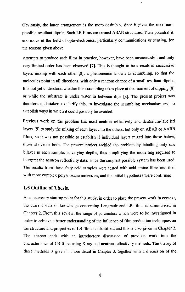
Obviously, the latter arrangement is the more desirable, since it gives the maximum
possible resultant dipole. Such LB films are termed ABAB structures. Their potential is
enormous in the field of opto-electronics, particularly communications or sensing, for
the reasons given above.
Attempts to produce such films in practice, however, have been unsuccessful, and only
very limited order has been observed [7]. This is thought to be a result of successive
layers mixing with each other [8], a phenomenon known as scrambling, so that the
molecules point in all directions, with only a random chance of a small resultant dipole.
It is not yet understood whether this scrambling takes place at the moment of dipping [8]
or while the substrate is under water in between dips [8]. The present project was
therefore undertaken to clarify this, to investigate the scrambling mechanism and to
establish ways in which it could possibly be avoided.
Previous work on the problem has used neutron reflectivity and deuterium-labelled
layers [9] to study the mixing of each layer into the others, but only on ABAB or AABB
films, so it was not possible to establish if individual layers mixed into those below,
those above or both. The present project tackled the' problem by labelling only one
bilayer in each sample, at varying depths, thus simplifying the modelling required to
interpret the neutron reflectivity data, since the simplest possible system has been used.
The results from these fatty acid samples were tested with acid-amine films and then
with more complex polysiloxane molecules, and the initial hypotheses were confirmed.
1.5 Outline of Thesis.
As a necessary starting point for this study, in order to place the present work in context,
the current state of knowledge concerning Langmuir and LB films is summarised in
Chapter 2. From this review, the range of parameters which were to be investigated in
order to achieve a better understanding of the influence of film production techniques on
the structure and properties of LB films is identified, and this is also given in Chapter 2.
The chapter ends with an introductory discussion of previous work into the
characteristics of LB films using X-ray and neutron reflectivity methods. The theory of
these methods is given in more detail 'in Chapter 3, together with a discussion of the
8
.'
various methods of analysing the data which are produced, to yield information on
sample structure. The actual equipment used for the production of these films, and for
their subsequent analysis by X-ray and neutron reflectivity, is described in Chapter 4,
and results are given for the fatty acid films in Chapter 5 and for acid-amine films in
Chapter 6. Chapter 7 gives the conclusions, including, inter alia, guidelines on how best
to prepare films with the properties and unscrambled structure required for use in
optoelectronic devices. Additional theory for SHG and pyroelectric effects is discussed
briefly in the two Appendices.
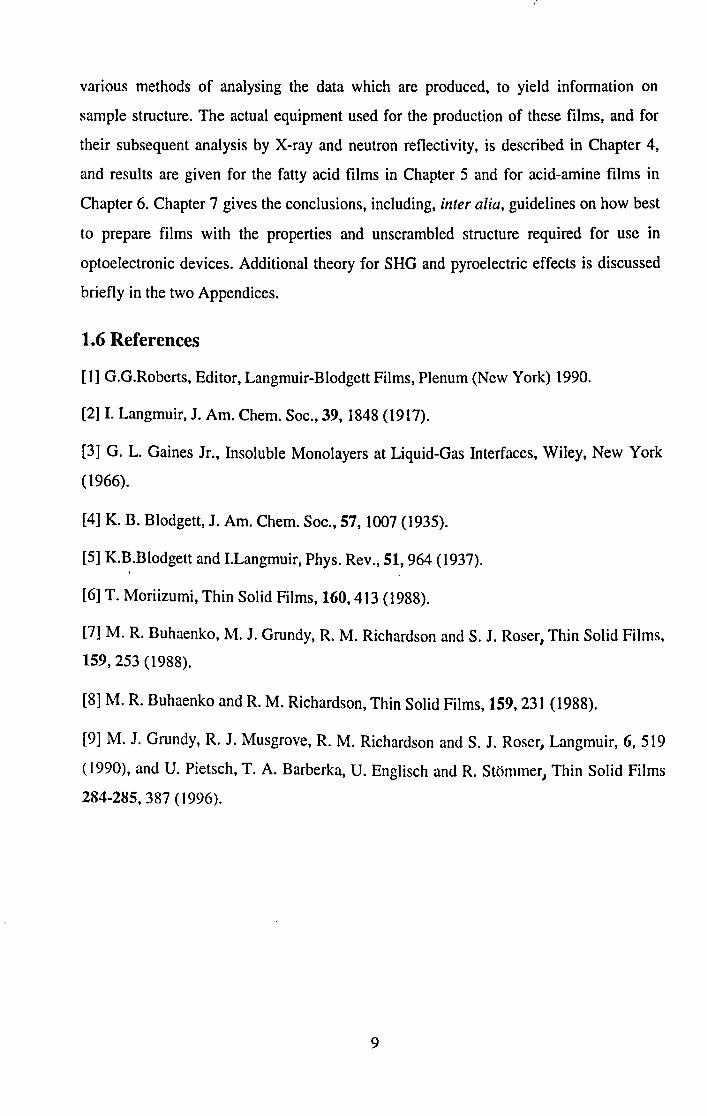
1.6 References
[1] G.G.Roberts, Editor, Langmuir-Blodgett Films, Plenum (New York) 1990.
[2] I. Langmuir, J. Am. Chern. Soc., 39, 1848 (1917).
[3] G. L. Gaines Jr., Insoluble Monolayers at Liquid-Gas Interfaces, Wiley, New York
(1966).
[4] K. B. Blodgett, J. Am. Chern. Soc., 57, 1007 (1935).
[5] K.B.Blodgett and I.Langmuir, Phys. Rev., 51, 964 (1937).
[6] T. Moriizumi, Thin Solid Films, 160,413 (1988).
[7] M. R. Buhaenko, M. J. Grundy, R. M. Richardson and S. J. Roser, Thin Solid Films,
159,253 (1988).
[8] M. R. Buhaenko and R. M. Richardson, Thin Solid Films, 159,23 t (1988).
[9] M. 1. Grundy, R. J. Musgrove, R. M. Richardson and S. J. Roser, Langmuir, 6, 519
( 1990), and U. Pietsch, T. A. Barberka, U. Englisch and R. StOmmer" Thin Solid Films
284-285, 387 (1996).
9

Chapter 2. The Nature of Spread and Dipped Films.
2.1 Introduction.
This chapter discusses the various factors which affect Langmuir-Blodgett (LB) film
formation, such as the subphase conditions, monolayer state and monolayer treatment
during dipping. It begins by describing in detail the individual film phases of a Langmuir
film to facilitate an understanding, on both the molecular and macroscopic levels, of the
importance of monolayer state on the subsequent structure of the LB film. In particular,
monolayer viscosity is discussed as perhaps the most salient parameter to be considered
in appreciating Langmuir and LB film behaviour. The chapter then reviews previous
work on LB films, concentrating on the techniques and approaches which have been
used to measure and characterise scrambling in LB films. Finally, it reviews the current·
theories on the causes of LB film scrambling, to place the present work in context.
2.2 Langmuir Films.
2.2.1 General Aspects.
An amphiphilic molecule is one with both hydrophobic ("water-hating") and hydrophilic
("water-loving") character. Typically, such a molecule has a hydrophilic head group and
a hydrophobic tail, and its shape is therefore approximately cylindrical. An excellent
example is a fatty acid such as docosanoic acid, whose structure is given schematically
in Figure 1. The chain region of the molecule is approximately 27 A long, while the
headgroup region is approximately 3A long.
10

~~~--------------------------------~~:~ ~ alkyl chain - hydrophobic : carboxylic
: acid : headgroup ~ . hydrophilic
Figure 1. Schematic diagram of the structure of docosanoic acid, showing the two
different regions of the molecule.
Molecules such as these spread spontaneously on a clean water surface, with the
headgroup in the water and the tail away from the interface [1], thus reducing the surface
tension 'Yor, conversely, increasing the surface pressure 1t:
1t = 'Yo - 'Y
where 'Yo is the surface tension of the pure subphase.
Surface pressure is usually measured using the Wilhelmy plate technique [2], whereby
the apparent buoyancy of a porous plate (e.g. filter paper), suspended from an analogue
microbalance and partially immersed in the subphase, has a linear dependency on the
surface pressure.
The surface pressure of the spread film can be manipulated by altering the area available
using either rigid booms or continuous flexible barriers. If the area is reduced slowly and
steadily, the pressure changes may be recorded against area and the resultant plot is
known as a 1t - A isotherm ("isotherm" because the temperature is kept constant during a
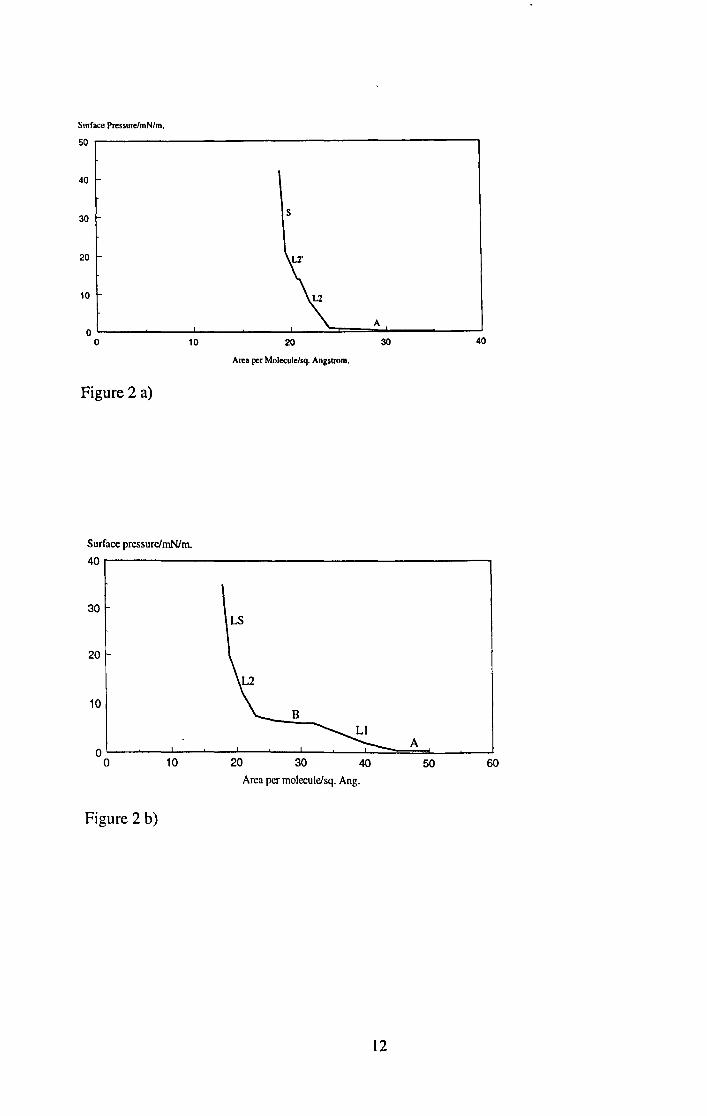
particular run). Some examples are shown in Figure 2.
I I
5111face Pressure/mN/m.
50 r---------------------------------------------------,
40
30 s
20 U'
10 L2
A OL---~----~----~----~--~~==~----------~
o 10 20 30 40
Area per Molecule/sq. Angstrom.
Figure 2 a)
Surface pressure/mN/m.
40r-------------------------------------------~
30
20
10 B
Area per molecule/sq. Ang.
Figure 2 b)
12
Surface pressure/mN/m
50.-----------------------------------------~
40
30
20
10
5 \0 IS 20 25 30
Area per molecule/sq. Ang.
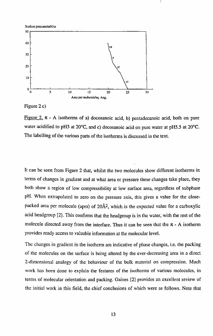
Figure 2 c)
Figure 2. 7t - A isotherms of a) docosanoic acid, b) pentadecanoic acid, both on pure
water acidified to pH3 at 20°C, and c) docosanoic acid on pure water at pHS.S at 20°C.
The labelling of the various parts of the isotherms is discussed in the text.
It can be seen from Figure 2 that, whilst the two molecules show different isotherms in
terms of changes in gradient and at what area or pressure these changes take place, they
both show a region of low compressibility at low surface area, regardless of subphase
pH. When extrapolated to zero on the pressure axis, this gives a value for the close
packed area per molecule (apm) of 20..\2, which is the expected value for a carboxylic
acid headgroup [2]. This confirms that the headgroup is in the water, with the rest of the
molecule directed away from the interface. Thus it can be seen that the 7t - A isotherm
provides ready access to valuable information at the molecular level.
The changes in gradient in the isotherm are indicative of phase changes, i.e. the packing
of the molecules on the surface is being altered by the ever-decreasing area in a direct
2-dimensional analogy of the behaviour of the bulk material on compression. Much
work has been done to explain the features of the isotherms of various molecules, in
terms of molecular orientation and packing. Gaines [2] provides an excellent review of
the initial work in this field, the chief conclusions of which were as follows. Note that
13

this is a very simple picture; it will be consolidated and brought up to date a little later in
this discussion.
a) The monolayer is only truly gaseous at very large apm; in some cases this can be as
large as 50ooA2, for fatty acids it is - 400 A2.
b) At apm below this, but still in the flat zero-measurable-7t region, the monolayer is
historically referred to as "liquid-expanded" (I-e). It has long been regarded as an
intermediate phase, where the molecular arrangement is not fixed and is constantly
moving, in other words a very fluid phase. The molecules were historically regarded
as lying flat on the subphase in this region, although it is now thought that they are
approximately perpendicular to the subphase throughout the isotherm, from the
largest apm to the smallest.
c) Once the pressure starts to rise, the isotherm shows a region of constant gradient, in
the case of fatty acids up to - 20-25 rnNm-1• This was historically referred to as the
"liquid-condensed" (I-c) phase, i.e. the molecules were regarded as being ordered
compared to the liquid-expanded phase, but still with considerable freedom. It is
comparable to a 2D smectic liquid crystal phase, in that all the molecules point in
roughly the same direction, away from the subphase, but at a range of angles and with
plenty of freedom to move in two dimensions. Nevertheless, since they are much
closer together than in the liquid-expanded phase, a surface pressure is generated,
which increases steadily as the apm is reduced.
d) Inevitably, a point is reached when the molecules are forced so close together that the
random packing of a liquid is superseded by the ordered packing of a solid. The
pressure continues to rise, as more and more of the monolayer adopts the close
packing, but it rises very steeply, since the already close-packed areas will naturally
resist any further compression. The bulk pressure on a monolayer 30A thick at
40mN/m is equivalent to approximately 133 atmospheres (P = 7tlo, 0 is the monolayer
thickness ).
e) Finally, there comes a point where all the material in the monolayer has adopted the
closest packing arrangement available to that molecule. If the monolayer is
14

compressed still further, the forces in the film, by now of the order of the 2D
equivalent of 230 atmospheres, cause buckling and crumpling at any weak spots
which are inevitably present in a crystalline structure. The monolayer becomes an
uneven multilayer and is said to have collapsed.
Whilst this picture, as was stated earlier, is very simplistic, it will be seen to be readily
analogous to the behaviour of fatty acids in the bulk. The packing at low 1t is dom~nated
by the headgroups and in the liquid-expanded, liquid-condensed, solid and collapsed
phases it is dominated by the packing of the hydrocarbon chains. This behaviour is
analogous to that shown by similar molecules on heating, for example T g marks the
transition between different packing modes of the hydrocarbon chains. Therefore, as
might be expected, monolayer packing is strongly susceptible to subphase temperature
and these effects will be discussed in more detail shortly.
As will be seen in Chapters 5 and 6, some molecules, notably polymeric ones, form
monolayers whose isotherms show none of these features. In this case, the size of the
molecules, and the stoichiometry of the backbone and sidegroups, prevents them from
adopting a truly close-packed arrangement, at least under the conditions available in a
Langmuir trough, and the monolayer remains in a fluid phase (liquid-condensed) until it
collapses into a disordered multilayer.
Other molecules, notably those with ring structures such as phthalocyanines, are
prevented from adopting a fluid arrangement by their various pendant groups, and the
monolayer is rigid (solid) throughout almost the entire 1t range of the isotherm.
To return to the discussion of fatty acids and their monolayer phases, the three basic
categories described above (I-e, l-c and solid) are not able to explain the various "kinks"
in the gradient within a particular isotherm region, nor the plateaux which are sometimes
observed. Both of these are illustrated in Figure 2. The irreproducible nature of these
features from worker to worker led to them being ascribed to impurities, either in the
monolayer or the subphase. However, as techniques and materials improved, these
features continued to be seen by increasing numbers of workers, and effort was devoted
to studying and explaining them.
15

2.2.2 Current View of Monolayer Phases.
The culmination of this line of study was careful and detailed work by Bibo and Peterson
[3] which, with scrupulous attention to purity of materials, has established what phases
occur, dependant on molecular chain length and subphase temperature, and which built
on the above 3-phase picture to include other phases, which explain the extra isotherm
features consistently. The present discussion will use their terminology. Broadly
speaking, at very low 1t, i.e. very high area per molecule, the molecule is in the gaseous
state. At areas per molecule below about 100A2 (region A in Figure 2) it forms islands in
the liquid state on the micron scale, surrounded by a clean water surface, with little
interaction between them (i.e. a two-phase system). This arrangement holds until the area
per molecule approaches 30A, when the increasing proximity forces the molecules to
adopt a closer packing. Brewster Angle Microscopy (BAM) [4] and glancing angle X-ray
scattering [5] have been used to elucidate these packing arrangements and also,
particularly BAM, to illustrate the two-phase regions of the isotherm. For instance, the
islands mentioned above are known to be approximately circular for a straight-chain
fatty acid at 1t < ImN/m [4], and the packing within them is the same as for the L2 part
of the isotherm, i.e. the hydrocarbon chains are tilted at about 30° to the surface normal
[5].
16
a) e----e-- b) r- ---r ~ r
_--e-- l- --r c) e- - --e d) e- --e
,
e e
e- --e ~- - --e
e) e- - --e , , , .
e e , e
e- - --e
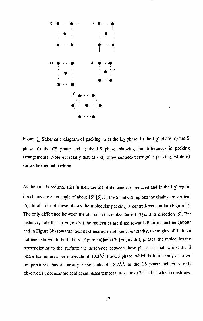
Figure 3 Schematic diagram of packing in a) the L2 phase, b) the Li phase, c) the S
phase, d) the CS phase and e) the LS phase, showing the differences in packing
arrangements. Note especially that a) - d) show centred-rectangular packing, while e)
shows hexagonal packing.
As the area is reduced still further, the tilt of the chains is reduced and in the Li region
the chains are at an angle of about 15° [5]. In the Sand CS regions the chains are vertical
[5]. In all four of these phases the molecular packing is centred-rectangular (Figure 3).
The only difference between the phases is the molecular tilt [3] and its direction [5]. For
instance, note that in Figure 3a) the molecules are tilted towards their nearest neighbour
and in Figure 3b) towards their next-nearest neighbour. For clarity, the angles of tilt have
not been shown. In both the S [Figure 3c)]and CS [Figure 3d)] phases, the molecules are
perpendicular to the surface; the difference between these phases is that, whilst the S
phase has an area per molecule of 19.2A2, the CS phase, which is found only at lower
temperatures, has an area per molecule of 18.7A2. In the LS phase, which is only
observed in docosanoic acid at subphase temperatures above 25°C, but which constitutes
17

the entire high-pressure region in stearic acid isotherms at all temperatures between 10
and 30°C [3], the molecules are packed hexagonally, with the chains perpendicular to the
surface [5]; this is illustrated in Figure 3e).
These workers [5] also used the evanescent wave, arising from an X-ray beam incident at
a grazing angle below the value for total internal reflection, to investigate the in-plane
features of these Langmuir films. They found that the peak width from the CS phase
corresponded to order on the scale of more than 160 lattice spacings, whereas for the k,
L2', LS and S phases, the peak width corresponded to order on the scale of less than 54
lattice spacings. This is a significant difference in long-range behaviour, and implies that
only the CS phase may be regarded as an ordered close-packed crystalline solid. The
remaining phases correspond well with the various smectic phases of liquid crystals.
Considering Bibo and Peterson's work in more detail [3 and references therein], the
effect of temperature on the monolayer must not be underestimated. The magnitude of
this effect is in tum related to the length of the hydrocarbon chain of the acid. As
illustrated in Figure 2, shorter chains, e.g. C I4 or C 16, show different phases than do
longer chains such as CIS' C20 or C22, and the effect of temperature is therefore different
in each case. For instance, the very short chain myristic (C I4) acid, which is incidentally
the shortest that can form a monolayer without excessive dissolution into the subphase,
shows the same phases at 13°C as does palmitic (C I6) acid at 34°C, namely LI, L2 and
LS. In other words, the very short chain endows the monolayer with the degree of
fluidity the slightly longer chain can only attain at a much higher temperature.
Lengthening the chain further, to stearic (C IS) acid, the monolayer phases are different
again and the LI phase is not present. Consequently, there is no plateau region in the
isotherm as there is for the shorter-chain acids, and the isotherm is the simplest of all in
this series of molecules, with only the A region, the ~ phase and the LS (superliquid)
phase. The presence of only this fluid hexagonally packed region at higher 7t is the most
likely reasoli for the difficulty experienced by all workers in obtaining stable monolayers
of stearic acid or the two shorter ones (C14 and CI6), and hence the subsequent difficulty
18

of dipping them as an LB film, without introducing ions into the subphase. The effect of
such ions will be discussed later, in Section 2.2.4.
Continuing the homologous series still further, Bibo and Peterson found that arachidic
(C20) acid showed phases different from stearic acid, with the appearance of the ~'
phase at temperatures below 19°C, and that docosanoic (C22) acid showed a still-wider
range of phases, namely the S phase shown in Figure 2a). Their phase diagrams show
that docosanoic acid has an ~' phase at all temperatures between 9 and 28°C, although
at the extremes of this range the phase is a very short part of the isotherm. In addition, at
temperatures between 14 and 16°C, the S phase is also a very short part of the isotherm,
being followed almost immediately by the CS (condensed-solid) phase. This last
dominates the isotherm below 14°C, and at a subphase temperature of 8°C it is present at
a surface pressure of only lOmN/m. This evolution of phases with temperature serves to
illustrate the effect of chain length and temperature on the packing of the monolayer:
short chains and high temperatures lead to the formation of more loosely-packed films,
whilst long chains or lower temperatures enable more close-packed films to be formed.
In other words, the high surface pressure phase varies according to temperature or chain
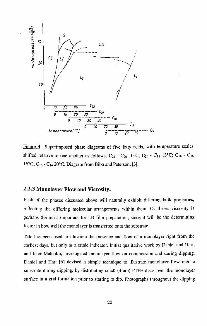
length. These results are summarised in the phase diagram shown in Figure 4.
19
LS
o
tem.oeraturef or J
Figure 4 Superimposed phase diagrams of five fatty acids, with temperature scales
shifted relative to one another as follows: C22 - C20 lOoC; C20 - CI8 13°C; CI8 - CI6
16°C; CI6 - CI4 20°C. Diagram from Bibo and Peterson, [3].
2.2.3 Monolayer Flow and Viscosity.
Each of the phases discussed above will naturally exhibit differing bulk properties,
reflecting the differing molecular arrangements within them. Of these, viscosity is
perhaps the most important for LB film preparation, since it will be the determining
factor in how well the monolayer is transferred onto the substrate.
Talc has been used to illustrate the presence and flow of a monolayer right from the
earliest days, but only as a crude indicator. Initial qualitative work by Daniel and Hart,
and later Malcolm, investigated monolayer flow on compression and during dipping.
Daniel and Hart [6] devised a simple technique to illustrate monolayer flow onto a
substrate during dipping, by distributing small (4mm) PTFE discs over the monolayer
surface in a grid formation prior to starting to dip. Photographs throughout the dipping
20

process illustrated the flow of the monolayer onto the substrate. The idea has been
extended by Malcolm [7a, 7b], who used sulphur powder to form the grid. As this
material is less dense than PTFE, and since it is also easy to form lines rather than a
series of points, the technique enables yet clearer visualisation of the monolayer flow.
Malcolm took the work further by designing a parallelogram-shaped trough in which the
sides moved parallel to the direction of monolayer flow revealed by the grid of sulphur
powder, thus reducing the monolayer distortion resulting from drag along the trough
sides [7c].
These two pieces of work show that, at least on the scale of a 1 cm grid, a monolayer
moves as a sheet during dipping, with shear and compressional forces acting as far away
as 5cm from the moving substrate. This vivid, if arguably crude, visualisation gives a
readily accessible broad-brush picture of what is happening to the monolayer. Buhaenko
et al. [8a-c] carried out more quantitative studies and examined the variation in viscosity
of monolayers of docosanoic acid and a few other materials with surface pressure,
subphase pH, subphase temperature and subphase cations. Their main conclusion was
that, ~s might be expected, a monolayer becomes more viscous as surface pressure is
increased, reflecting the ever-closer packing. Conversely, reducing the pH (and hence
reducing repulsion between neighbouring COO- headgroups) or increasing the
temperature both make the monolayer more fluid.
These authors used both canal viscometry and an oscillating knife-edge bob to measure
the surface viscosity of a range of fatty acids (C 17 - C26, [8a, 8cn, and later studied a
variety of other materials [8b, 8c] using relaxation and resonance techniques. In addition
[8b], they used a transducer to measure the forces acting during LB deposition, and this
work will be discussed in Section 2.3. Their experimental conditions, of pure fatty acid
over pure water acidified to pH3, are the· same as those used in the present work,
although beyond this direct comparison is difficult, since they measured surface
viscosities only up to 30 mNm- l, and the present work used surface pressures up to
40mN/m- l• In addition, the dipping speeds they investigated were of the order of 120
times faster than the fastest used in the present work. Nevertheless, their conclusions are
extremely useful, because they aid the understanding of monolayer behaviour in the
21

work done up to 30mNm- l_ Firstly, they found that 1'\s (the surface viscosity of a
monolayer) was independent of 1t for acid monolayers in the LI and L2 phases,
suggesting Newtonian behaviour, i.e. the viscosity is independent of shear rate. Thus,
acid monolayers in these phases are truly fluid and able to flow readily. 1'\5 for
docosanoic acid in these phases is between 5.9 - 7.S x 10-4 SP for Ll1t = 5 mNm-1 , and
-12 x 10-4 SP for Ll1t = 10 mNm- l. However, above the L2' ~ S transition, i.e. above 1t
:::::: 30 mNm-1 for docosanoic acid, the monolayer becomes non-Newtonian, deduced from
the fact that the viscosity could not be measured using these techniques.
Log lO1'\5 was found to increase linearly with n, the number of hydrocarbons in the chain,
and this is explained in terms of increased cohesion between the chains in a two
dimensional system such as a monolayer. They also found that a large contribution to 1'\5
is made by the hydrogen-bond interaction between the headgroup and the subphase,
based on their investigation of 1'\5 with T, directly in line with Bibo and Peterson's
findings on the effect of T on the phase changes revealed by isotherms [3]. The
magnitude of this effect is of the order of a 50% reduction in 1'\5 (12.3 x 1 0-4 ~ 6.1 x 10⁻⁴
SP) on raising T from 19°C to 30°C, for docosanoic acid at pH3.
In the course of this work on viscosity, Buhaenko also studied monolayer stability [Scl·
The chief findings of relevance to the present work were in relation to docosanoic acid
and stearylamine. Specifically, a docosanoic acid monolayer, pH3, 1t = 35 mNm- l, loses
only S% of its area over a period of -so minutes. At pH5_60, with no subphase ions, the
area change was <5% over 60 minutes. For the amine (two CH2 units shorter than the
eicosylamine used in the present work), the figures were 12% of area lost over 72
minutes at pH5.5, and 9% over 130 minutes on pH2.S4. Since the oldest monolayers
used for dipping in the present work were only 32 minutes old (5 mm/min dip speed x 4
em dip length x 4 dips) before the monolayer needed replenishing, Buhaenko's data fully
support the 1t and pH values used here.
22

2.2.4 The Effect of Subphase Cations.
Introducing subphase cations such as Cd2+ has a marked effect on the behaviour of a
Langmuir film. For instance, the isotherm of docosanoic acid is altered (Figure 5) in
such a way that the L2 a,nd L2' phases are much less obvious and the transition to the S
phase occurs at a much lower surface pressure than over pure water.
Surface pressure/mN!m.
60r-----------------------------------------~
50
40
30
20
10
O~--~--~--~--_L __ ~==== ________ L_ __ ~ __ ~
o 10 20 30 40 50
Area per molecule! sq. Ang.
Figure 5 Isotherm of docosanoic acid on a subphase containing 0.25 mM cadmium
chloride, 20°C, pH6.3.
The reason for the earlier onset of the S region in Figure 5 is that the Cd2+ ions each
require two carboxylate ions for electrical neutrality, thus drawing the molecules of the
monolayer closer together even at low surface pressures. At pH below 4.8, however, this
effect is over-ridden by the pH effect mentioned earlier, whereby H+ ions screen the
headgroup charges, and the cadmium soap is not formed [9].
From these considerations it will be clear that even a "simple" fatty acid monolayer is a
complex system and the various parameters must be carefully chosen if the monolayer is
to have the required properties for successful manipulation into an LB film. In addition,
23

attention must always be paid to the phase of the monolayer, since this will ultimately be
the single most important factor affecting the structure of any LB film dipped
subsequently. Since the phase of the monolayer is necessarily affected by a variety of
experimental conditions, and in order to make a rigorous study of the effect of varying
each parameter that affects the monolayer, the samples in the present work were
prepared at different surface pressures, different pH, different temperatures and either
with or without subphase cations, and only one parameter was varied at a time, while the
others were kept constant. The parameters were carefully cho. en by this author to cover
as wide a range of experimental conditions as possible in the time available, in order to
'nsure a thorough and rigorou approach to addres. ing the problem of scrambling in LB
films.
2.3 Langmuir-Blodgett Films.
2.3.1 Introduction.
Building up multilayers by successive transfer of Langmuir films onto a solid substrate
was fir. t describ d by Blodgett in 1935 [10] . The principle is ex tremely simple and
legant. Figure 6 illustrates the process schematically :
b)
etc.
Figure 6 howin g the principle of Langmuir-Blodgett (LB) deposition onto a hydrophobic substrate
24
Quite simply, the substrate to be coated is passed vertically, at an even rate, through the
compressed Langmuir film and a one-molecule-thick layer is deposited with each pass
through the interface. The pressure of the Langmuir film is monitored using a Wilhelmy
plate and kept constant via a feedback loop (for further details see Chapter 4). If the
trough has its water surface divided into two compartments, separated by a suitable gate
to avoid mixing of the mono layers, alternating ABAB structures may be readily prepared
by moving the sample between the compartments as required, either under water or in
the air. Deposition of the monolayer on both down- and up-strokes is known as V-type
dipping. Monolayers which only transfer on the downstroke are known as X-type, while
those which only transfer on the upstroke are Z-type [2]. The present work is solely
concerned with Y -type dipping.
The change in area of the monolayer on the water is easily measured for each dip stroke
and, ideally, should equal the immersed area of the substrate, i.e. the transfer ratio should
be 1.0, thus providing a rapid measure of LB film quality. In this work, however, the
transfer ratio could not be accurately calculated because the rear face of the substrates
used was very rough. Whilst there is evidence that a dipped monolayer can bridge
defects due to surface roughness on the Angstrpm scale [2 and I I], it is unlikely that
macroscopic features can be bridged. Therefore, transfer ratios were used here simply as
a measure of relative quality between layers and between samples, since all the
substrates used were similar silicon wafers. Further details of the transfer ratios from this
work are given in Table 4 in Chapter 5 and Table 4 in Chapter 6.
The deposited film must be thought of as a crystal. There are three weB-known bulk
crystal phases of long-chain fatty acids, labelled A, Band C [16]. The repeat distances
within these phases are shown in Table 1 below. These three phases only occur in even
chain acids; odd-chain acids have a further three different phases, namely, A', B' and C.
These will not be discussed further.
25

Acid chain length PhaseNA Phase B/A Phase CIA
CIS (not found in lit.) 43.8 39.9
C20 52.5 48.4 44.1
C22 56.2 53.0 48.2
Table I. Showing the repeat distances in the three phases within the bulk crystals of
three even-chain fatty acids.
von Sydow [17] noted that the phase formed depends on the crystallisation route, and
more than one phase may be formed together. The factors affecting crystallisation are
temperature, purity, rate of crystallisation and solvent used. For example, crystallisation
from the melt gives the C form, which also forms on rapid crystallisation from solution;
the B form crystallises slowly from solution, while forms Band C may be obtained as a
mixture from solution in petroleum. Both Band C forms have orthorhombic packing.
The C form is the most stable at room temperature.
2.3.2 Dipping Speed.
The dipping speed used for LB deposition has not received much systematic attention to
date. Blodgett [10] found that the first layer needed to be dipped "fairly slowly (5 to 10
cm/min)" for satisfactory drainage to occur, whereas subsequent layers could be
deposited at speeds of the order of 25-37cmlmin. This was based solely on observations
of drainage during dipping, since subsequent characterisation of the films optically [12]
and using X-ray diffraction [13] showed they consisted of ordered layers. Chollet and
Messier [14] studied docosanoic and 22-tricosenoic acids using X-ray and electron
diffraction and infrared spectroscopy and found that LB films of these molecules were
formed of adjoining crystallites, of maximum size 100l1m. Because of its terminal
double bond, and hence its different packing in the monolayer, 22-tricosenoic acid forms
more fluid monolayers than docosanoic acid does. These workers [14] found a
26
correlation between this increased fluidity and increased anisotropy in the LB film, both
in-plane and between layers, compared with docosanoic acid, when both were dipped at
30mN/m (at this 1t, docosanoic acid is in the S phase, whereas 22-tricosenoic acid is still
in the L2' phase).They used speeds of between 0.1 and 5 cm/min, but do not state
anything more specific. Nevertheless, -these speeds cover a slower range than those used
by Blodgett [10].
Peterson and Russell [15] used polarising microscopy and electron diffraction to study
structure further. Their results substantiate those of Chollet and Messier [14] and show
that the crystal packing of the first layer determines the packing of subsequent layers,
hence the desirability of using a single crystal substrate, such as a silicon wafer.
Closely linked with dipping speed is the effect on the already-dipped LB film of different
times under water during subsequent dips. Obviously, a fast dipping speed will result in
shorter times under water between dips than will slower speeds. Any effect would be
exaggerated by deliberately leaving the sample under water for, say, 10 minutes or more
between dips. The nature of the dipped film was observed to change by Blodgett in 1935
[10] and she established that the poor quality of some films was a direct result of the
time spent under water, all other conditions being equal. Following initial attempts by
Langmuir [18] to explain the deposition of some materials on the downstroke only (X
type) in terms of overturning of molecules under water, Honig [19] proposed a
mechanism showing that the energetics were feasible for half of the X-type layer to
overturn under water and. form a Y -type film covering half the substrate. Overturning on
this scale is required in order to explain two decisive experimental observations. The
first is that X-type films have very nearly the same X-ray diffraction repeat distance as
Y-type films [20], i.e. twice the molecular length. This is surprising for a film which dips
only on the downstroke and which would therefore be expected to have a repeat distance
of only one molecular length. The second observation is that X-type films are
hydrophobic on the surface, as are Y-type films [10]. Dipping only on the downstroke
would, in theory, result in an LB film with the headgroups to the outside, which would
be hydrophilic. Therefore, an explanation is needed which takes account of these
observations. Overturning of molecules under water answers both, but the various
27

mechanisms proposed did not take energetics into account. Honig's proposal of half the
molecules overturning under water and attaching themselves head-to-head with the half
that stays put means that the surface would be hydrophobic, which would explain why
no pick-up occurs on the upstroke, and it would also explain why the films have a repeat
distance the same as a Y -type film of the same material. The vacancies left by the
overturned molecules in their original layer might then be filled by molecules from the
next dipped layer, resulting in a very uneven structure. If less than half overturned, some
pick-up would occur on the upstroke and a mixed X-Y film would result, again with a
very uneven structure. This would explain Blodgett's observation [10] that film quality
deteriorated with the number of dips. Also, Honig's theory would predict that a longer
time under water would allow more overturning to occur, resulting once more in a very
uneven structure.
The energetics of overturning depend on the relative strengths of the following
interactions: tail-tail, head-head, tail-water and head-water. The energies of these
interactions may be expressed as EtI, Ehh. Etw and Ehw. If the sum
(2.1)
is positive, the film will be X-type; if negative, Y -type. Thus, an overturning layer is
explained by considering a film which dips X-type, i.e. for which the sum in Eq. 2.1 is
positive: the tails are more strongly attracted to other tails than to water, while the heads
are more strongly attracted to water than to other heads. Thus, the head-head attraction
between neighbouring molecules within the plane of the downstroke layer is weaker than
the attraction of the heads for the water, so any which are not completely surrounded by
fellow molecules within the plane of that particular layer, either at the edges of the
substrate or due to uneven deposition, can detach themselves while the substrate is under
water. These detached molecules, freely moving in the subphase, now have their tails
surrounded by water on all sides, which is not energetically favourable, so they readily
turn over and redeposit head-head on the substrate, either immediately on top of their
original layer or to fill in holes in a previous uneven layer, so as to surround their tails by
other tails. This then alters the nature of the outermost surface of the film from
hydrophilic to hydrophobic, and no material is deposited on the upstroke: an X-type film
28

results. For a film which dips Y -type, the head-head interaction dominates the four terms
to render the sum of Eq. 2.1 negative, the molecules remain firmly bound within the
layer in which they were dipped and deposition occurs in both directions. The energies
involved are typically a few kT. The equation given also explains the differences
Blodgett observed [10] with changes in ionic strength and pH, as these would affect the
Ehw and Ehh terms. Because this theory answers all the observations satisfactorily, it has
long been regarded as the best explanation of what happens during the LB dipping
process. The present work adds an extra dimension, in terms of the requirement also to
consider the phase the Langmuir film is in during dipping.
Honig went on [21] to try to quantify the effect of time under water on this overturning
mechanism, using as a starting point the results of Peng et al. [22], which showed a close
correlation between time under water and the extent of X-type behaviour. Based on the
SEM micrographs taken by Peng et al., which show X-type films to be very uneven,
Honig proposed that this unevenness itself affected the degree of X-type behaviour in an
autocatalytic fashion, i.e. the more irregular the surface, the easier it would be for
molecules to overturn. Honig's mechanism influenced thinking towards minimising the
time under water, i.e. increasing the dipping speed, to minimise the chances of this
under-water scrambling taking place. However, scrambling could still not be eliminated,
so it is clear that other mechanisms are involved. Therefore, the present work
investigated the effects of time under water and dipping speed.
With Honig's mechanism in mind, Buhaenko et a1. [23] and Grundy et al. [24], inter
alia, prepared LB films with alternating ABAB or AABB structures, in order to
investigate the scrambling effect and the influence of time under water. However,
because of the repeating nature of their samples they were unable to establish
conclusively whether molecules mixed into the layer above or into that below. Their
work will be discussed more fully in section 2.4. In another paper [25], Buhaenko and
Richardson investigated dipping speed more thoroughly, using the measurement of
contact angles and of the force of emersion and immersion. Contact angles were
recorded photographically, and a transducer was used to measure the forces. Samples
were prepared on hydrophobed glass. Films were eicosanoic (C20) acid dipped at
29
30mN/m over subphases containing O.3mM CdCh, with the pH ranging from 2.4 to 6.0,
i.e. pure fatty acid to mixed acid/salt films. The forces measured were in the range 30-
50mN/m. They found that the force increased with pH, so it is sensitive to increased ion
binding and hence film viscosity [8]. In addition, subphase ions increase the viscosity of
the subphase, and the ion concentration immediately beneath the monolayer will increase
with pH, due to increased binding to the headgroups. This would make the subphase
more difficult to expel at the three-phase contact line, and hence increase the force of
emersion.
The dipping speed used also affected the force of emersion: between 6 and 60mrnlmin,
the force increases rapidly with speed, with the increase slowing down above
60mrnlmin. This suggests a critical speed above which the meniscus moves faster than
the monolayer can adsorb onto the substrate. The critical speed, Verit. marks this
transition between reactive and nonreactive dipping. Reactive dipping means the
monolayer is spontaneously adsorbed. Non-reactive means the monolayer is forced onto
the substrate as a result of its rapid withdrawal; this traps the subphase, which would
normally drain away, and this in turn increases the force measured since it introduces
extra viscous drag. An alternative explanation is that a high monolayer viscosity would
give rise to a drop in 7t near the point of deposition, since the monolayer would not be
able to flow to replace that which had just been taken up by the substrate. This would
render the monolayer inhomogeneous at high dipping speeds. This author favours the
latter interpretation.
Verit is not to be confused with the highest speed at which a substrate may be withdrawn
dry. For acid films, this is of the order of 1800mrnlmin; for salt films, of the order of
1080mrnlmin.
Buhaenko et at. [23] also found that below Verit. the reactive deposition that occurred
appeared to lead to a mixing up of A and B layers, but they point out the preliminary
nature of their results and the need for further work. Their conclusion is that a higher
Verit indicates greater attraction between headgroups on the substrate and in the
monolayer, thus increasing the likelihood of good deposition.
30
2.3.3 Contrast Between Acid and Salt Films.
It must be pointed out that nearly all the work described above was done using fatty acid
salt films, since pure fatty acid films were thought to be difficult and irreproducible to
dip. For instance, at pH7, Peng et al. [22] were unable to dip more than one layer of
stearic acid at all. In fact, this bias towards salt films shows a failure to appreciate and
take account of headgroup/water interactions and the screening effect of low pH [9], and
the present author considers that more work needs to be done on plain fatty acid films, to
increase our understanding of these simple systems, before complexities such as metal
ions are introduced. Hence, in the present work, only two samples were dipped over a
subphase containing metal ions, allowing an objective comparison to be made between
the present experimental techniques and those of previous workers, and the remainder
were pure fatty acid films dipped over water at pH3, where all the headgroup charges are
screened by H+ ions and the monolayer is stable.
Buhaenko et al. [23] also found that acid films have the greatest attraction between the
headgroups and hence the highest Verit. while salt films have the least headgroup
attraction and hence the lowest Verit. This result fully supports the present approach to
the merits of studying pure acid films.
2.3.4 Summary of Dipping Parameters.
Given the above considerations, therefore, in this present work samples were dipped not'
only at different speeds, but also with only one bilayer of the labelled ("B") material
within the overall structure. The position of this B bilayer was also varied, from the
substrate interface to the centre of the sample to the air interface, in order to elucidate
just where the scrambled molecules come from and go to. The effect of 10 minutes under
water was also investigated, bringing the total number of parameters varied in monolayer
formation and dipping to seven (dipping pressure, subphase pH, subphase ions and
subphase temperature have already been mentioned), although due to time constraints
the complete matrix of possible samples could not be prepared and studied. Chapters 5
and 6 list the two series of samples prepared and studied in this work.
31

2.4 Characterisation of LB Films.
The most fruitful methods of studying order on the molecular scale within organic
systems are X-ray and neutron reflectivity. The great advantage of these te~hniques is
that the supporting substrate can be readily accounted for and hence excluded from the
analysis. A brief resume of these techniques and the information they can yield will be
given here, and a more detailed description of the theory and practicalities will be given
in Chapters 3 and 4. Both techniques rely on exactly the same physics as that which
causes white light to be split into its component colours by a thin film of petrol on a
puddle of water, namely refractive index variations and the interference resulting from
differences in path length between waves reflected from the top surface of the film and
those reflected from within the film or from the substrate.
X-rays are susceptible to the electron density gradients within a structure, whereas
neutrons are affected by nuclear scattering length density gradients. These are analogous
to the refractive index changes that a material presents to light. The scattering length that
a material presents to neutrons may be described as the extent to which the nuclei of that
material divert the neutrons from their incident path; the electron density of a material
affects X-rays in the same way. However, whilst electron density varies linearly and
predictably with the number of electrons, i.e. with atomic number (e.g. for H, the X-ray
scattering length is 2.8 x 10,5 A, for D it is the same since the atomic number is the same,
and for C it is 16.8 x 10,5 A), neutron scattering lengths are rather more random. The
particular usefulness of neutrons for the study of organic systems arises from the fact that
hydrogen and deuterium have very different scattering lengths (H -3.73 x 1O,5A, D 6.67
x 10,5A, C 6.65 x 10,5 A), and so by simply deuterating one type of molecule or part of a
molecule in the system under study, one can use neutron techniques to access very
detailed information on the structure being investigated.
As mentioned in the previous section, X-ray diffraction work has established that LB
films are planar in structure, with the chains and headgroups in ordered layers [13]. The
various crystal phases already discussed have been observed and are ascribed to the
method of formation of the initial Langmuir film as much as to the dipping conditions
32

used [26]. Subphase cations are known to affect the tilt angle of the molecules within the
dipped film, since samples prepared over a calcium solution, for instance, have a larger
repeat distance than those dipped over plain water [13], i.e. the salt molecules are tilted
less. However, by its very nature, X-ray reflectivity is unable to provide information on
inter-layer mixing. It is, nevertheless, a very useful technique and complementary to
neutron reflectivity, because the information it provides about film thicknesses and
repeat distances greatly simplifies the interpretation of neutron data.
Neutron reflectivity has been applied to many LB film systems in an attempt to
understand the inter-layer scrambling that is observed, and systems using deuterated and
protonated fatty acids have been more popular than those using the active molecules that
might be used in a commercial application. This is chiefly because the former have been
perceived as easier to model, but also to attempt to establish the mechanisms involved in
scrambling by simplifying the system under study, prior to moving on to commercial and
more complex molecules.
Brief reference has already been made to the initial work in this field by Buhaenko et at.
[23]. They used neutron and X-ray diffraction to study cadmium docosanoate LB films,
dipped under a variety of conditions, to investigate changes in structure and how these
were affected by temperature. Using X-ray diffraction, they found that pure acid films
deposited in the B form, i.e. with a 53A repeat, and that this changed to the C form, i.e.
with a 48A repeat, at 55°C. Pure salt films were found to deposit with the chains
perpendicular to the substrate, i.e. with a 60A repeat, and retained this structure up to
90°C. Mixed films [9], dipped at pH5.3, were found to deposit with both 58 and 60A
repeats, and the 58A phase disappeared as the temperature rose. Silicon wafers were
found to be the best substrate in terms of subsequent film quality and order, compared
with di-methyl or tri-methyl silanised glass, and this is perhaps not surprising, given the
increased order found on the single-crystal face of a wafer, compared with the large
defect densities of a glass surfac~ [27].
33
2.4.1 Previous Work and Current Theories on LB Film Scrambling.
Using neutron diffraction, Buhaenko et al. [23] studied films of alternating hydrogenous
and deuterated cadmium docosanoate, either as HHDD or HDHD type. For pure acid
films, the HHDD structure showed a repeat of 105.A, and the HDHD structure a repeat of
52A. Both structures showed only a repeat of 60A. in pure soap films, and the reasons for
this were not clear. Mixed films showed a 59.A phase, and the instrument resolution was
not good enough to resolve if this was the 58 or 60.A repeat. As they increased the
temperature, they found the acid film structure disappeared at T > 60°C, whereas the
soap structure peaks simply broadened, at T > 90°C. They were hoping to use the
presence of deuterated material to establish whether these phase changes are caused by
diffusion of bilayers or of single molecules, but were unable to ascertain the mechanism
by which the phase changes occur. All their samples were dipped at 120mmlmin, except
for one at lOmmlmin to investigate the effect of dipping speed. There was a variation in
peak intensities with dipping speed, but they regarded their results as inconclusive with
regard to the effect of speed on film quality. A sharp, intense peak would indicate that
the Hand D layers had not intermixed and that the D-acid remained in the single layer or
bilayer in which it was dipped. A broad, shallow peak would indicate the D-acid had
mixed with one or other, or both, of the surrounding H-acid layers, according to the
theory put forward by Honig [19], thus rendering the D/H boundary somewhat blurred.
A fast speed of 120mmlmin gave a sharper peak than a slow speed of lOmmlmin. They
concluded, as has been mentioned, that a fast dipping speed was required to maintain
order in a film dipped at 30mN/m, and this supported the theory on the effect of time
under water. Grundy et at. [24] confirmed this result.
It must be pointed out, however, that these experiments again used a Cd2+ subphase at
pH6.2, which gives a pure salt film. No critical speed was observed by Buhaenko et al.
[25] for a pure acid film, and this author concludes that the phenomenon of critical speed
is linked to the increased viscosity and generally different phases of salt films, and as
such is of limited relevance to the acid films studied in the present work.
34

Musgrove [26] studied the different crystal phases that occur in fatty acid and salt LB
films, as well as order in ABAB films, but the experimental details of the LB film
preparation are unfortunately not given in sufficient detail to be sure of consistency.
Various other attempts have been made to measure the extent of scrambling, but all to
date have used ABAB and salt films. Indeed, the approach of some authors is,
surprisingly, that scrambling is inevitable and that it is therefore a useful tool to show the
sensitivity of their techniques. The most important of the work which has been carried
out in an attempt to shed light on the problem of LB film scrambling is now reviewed.
In an elegant experiment, Pietsch et al. [28] used Mg to label one headgroup region in a
multilayer film of lead stearate, and investigated the structure using X-ray reflectivity.
They found that the position of the Mg layer, a region of about 2A thickness, could be
pinpointed with an accuracy of between 1 and 3A, depending on the position of the layer
within the film "sandwich": it was easier to pinpoint the layer if it was at the air or the
substrate, than if it was in the centre of the sandwich. Interestingly, they also found that
thicker films have a more disordered top layer, and that this top layer was often
apparently thinner than those below. They explained this apparent thinness in terms of
the reduced density of the top layer, which would reduce its effective scattering intensity.
This result is in line with Honig's theory that overturning becomes worse in thicker films
[19and21].
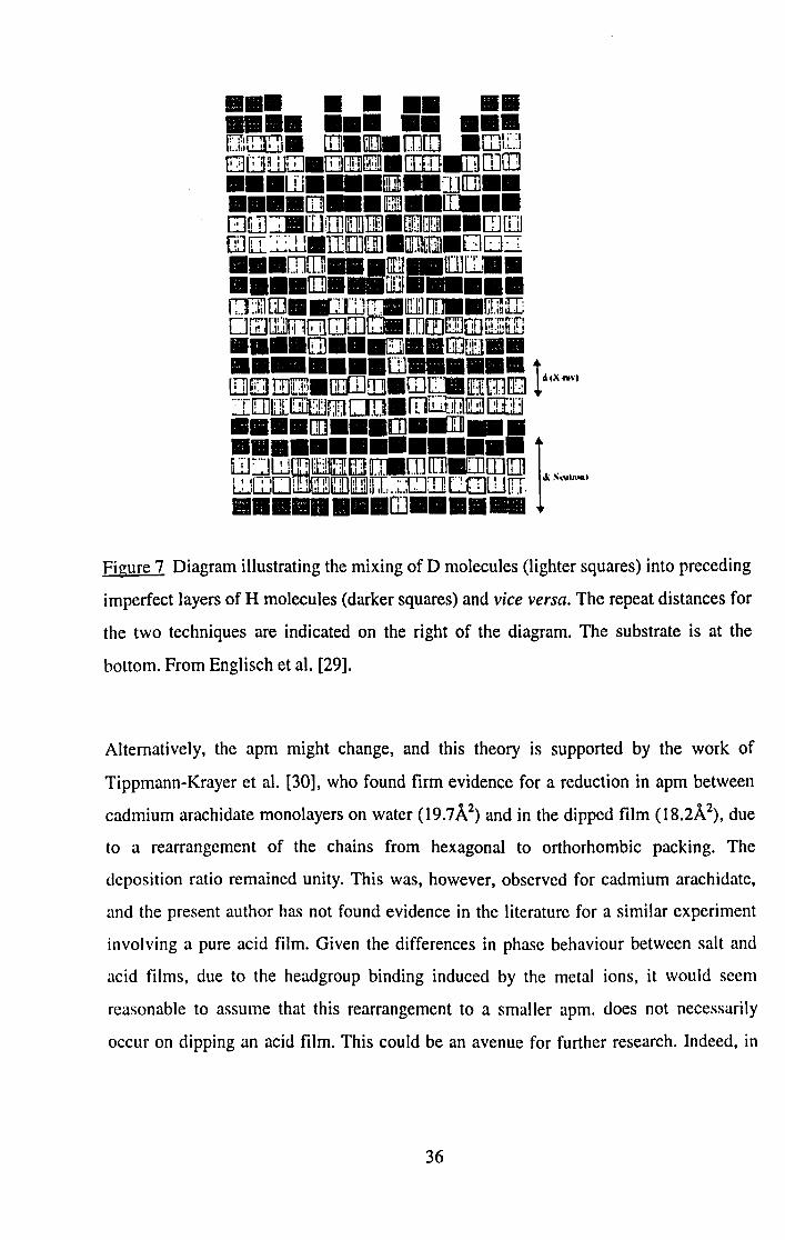
Englisch et al. [29] used both X-ray and neutron reflectivity to study HHDD films of
lead stearate on silicon wafers. They used a 7t of 25mN/m and a speed of 6-lOmmlmin.
The pH of 6.9 means that the film was entirely salt [9]. They found that the CH3-CD3
interfaces were blurred, either through diffusion or through exchange of complete
molecules. The extent of exchange was 20%, and this increased as films became thicker.
The fuzziness could be explained by holes appearing in each monolayer after dipping,
which would then be filled by the next layer to be dipped. This is illustrated in Figure 7.
In order to establish whether this is in fact the case, an accurate measure of the
deposition ratio would be required.
35
••• •••• •• •••• ••• •• ..I!!I il'!!1fT"'!tT'"T1. m.l'IT1I. mrn .ml' ,. li .• !~L!...!l!...L! t W8l .: .. LiJ .1 •• .1
E3tJtiliJ.ITJI[]]IlElI.[I[[J1IIJ] OJ CD ••• w .... [ifi-]J[] •• •••• [l] ... rn •• ~ •• [!]!ll] :JIW!IIlI[]!]Iill] • []f]EIlJl •• CJ IIil m IiI ~JJ.1JIJJ[[] .0000000.OD' ; ••• mm __ nrur.[]]ll.J •• •••• [IJ]._DIJI _ ••• rr-r.:i!l rna .'TI"! 'l~m'l'l ~.flO1iTT' I ; .. :Ii .• iil ',: I ilL_1l!..Jl.IIJI.i_ 1;t.i!hLL;
D r:"H"!"!,rn r'lrni"4 rnrnr:'l!lrnm'r""'r!"1 , W WUll It ~E]UJUJI.!...!J •.. : i I L:!J I l11!lW •••• EJJ •• .:J •• rnlfl •• •• - •••• UJ •••••• !IJl[!) mICE. OI1IIDJ.mc. [Hn 83 t dlXft~1 ':"T' [J]1iJ[:'l" tril'1II:;I: Ir,:ifI lin. mi I ;fill! I Ij17tl r;n-;r;1 _I UJli.:.il:Jj:,i:,IL-I.L.I .. ~, ... ~LL1liLI
i~il;li;ll·<~-' Figure 7 Diagram illustrating the mixing of D molecules (lighter squares) into preceding
imperfect layers of H molecules (darker squares) and vice versa. The repeat distances for
the two techniques are indicated on the right of the diagram. The substrate is at the
bottom. From Englisch et al. [29].
Alternatively, the apm might change, and this theory is supported by the work of
Tippmann-Krayer et al. [30], who found firm evidence for a reduction in apm between
cadmium arachidate monolayers on water (19.7A2) and in the dipped film (l8.2A2), due
to a rearrangement of the chains from hexagonal to orthorhombic packing. The
deposition ratio remained unity. This was, however, observed for cadmium arachidate,
and the present author has not found evidence in the literature for a similar experiment
involving a pure acid film. Given the differences in phase behaviour between salt and
acid films, due to the headgroup binding induced by the metal ions, it would seem
reasonable to assume that this rearrangement to a smaller apm. does not necessarily
occur on dipping an acid film. This could be an avenue for further research. Indeed, in
36

the present work, neutron and X-ray data revealed molecules in individual layers to be
tilted at 23° to the surface normal, implying that, in acid films at least, the phase change
on dipping is one of relaxing to a less close-packed phase, namely from the S phase to
the L2 phase (see Chapter 5, Section 5.5.1). This is in direct contrast to the observations
described above for salt films, once again emphasising the need for further study of acid
films.
Vierheller et al. [31] also found Hand D intermixing of the order of 20%, in samples
with six H layers followed by six D layers. As well as D molecules having filled holes in
the H layers below, they also found H molecules within the top six D layers, suggesting a
very high molecular mobility. With reference to Grundy et al. [24], they explained this in
terms of the length of time their samples spent under water, which was between 10 and
20 minutes for each dipping cycle. After heating at 70°C for 600+ mins, they found that
some D molecules had diffused right down through the film to the silicon substrate.
Heating at 84°C for a week resulted in the loss of most of the HID contrast, due to
almost complete mixing of the H and D molecules.
Englisch et al. [32] used mixed acid/salt films of stearic acid/barium stearate at pH 6.3,
41 mN/m and at IOmmlmin. Again, they found an initial DIH exchange of 25%, similar
to that found by Vierheller et al. [31]. This proportion increased on heating, to 35% at
65°C and 50%, i.e. no HID contrast, at 90°C. Since they used a mixed film, there are free
acid molecules in the dipped film which are unbound by the metal ions, and these are
therefore free to move within the lattice. They needed 33% free acid to explain their
results, although this seems an improbably high proportion at pH6.3 [9].
2.4.2 Summary.
It will be clear from the above review that the vast majority of work to date has used
fatty acid salts and there is thus a gap in our knowledge of pure fatty acid systems, which
the present work is designed to address. Despite the apparent coherence between all
these results and the conclusions drawn from them, it must be stressed that none of the
above arguments has so far enabled a distinction to be made between a layer mixing into
the layer below, the one above, or both, and it would clearly be difficult to establish this
37
for sure with ABAB films. Hence, in this work, only one layer was labelled. Nor has it
been possible so far to produce truly ordered alternating LB films. Some explanation for
this is provided by the work of Tippmann-Krayer et al. [30], mentioned above, who
found firm evidence for a reduction in molecular area on transfer of a monolayer from
water to a solid substrate. Given that the transfer ratio remains at 1.0 then the conclusion
is that the dipped film has "holes" where the substrate is uncoated. Such holes have been
found by several groups using Atomic Force Microscopy (AFM) [33a - e], including one
group who found holes in a cadmium arachidate monolayer on water at 25mN/m [33e].
These holes could have two effects on subsequent dipped monolayers. The first
possibility, as proposed by Englisch et al. [29], is that they would be filled in by the next
layer, the molecules of which would have to turn over to achieve this, invoking the
mechanism proposed by Honig [19]. The holes would then be perpetuated throughout
the structure. Alternatively, the next layer might bridge the holes (the AFM data suggest
they are of the order of 300A across), thus preventing them from having any further
effect on the structure beyond reducing the density of the layer in which they are present.
A third possibility, and the most likely, is that a com~ination of both these mechanisms
is involved and it might be expected that this would in turn be affected by dipping
conditions. The present work, by probing more fully the correspondence between surface
pressure (and hence viscosity), dipping speed and film quality, brings new light to bear
on the problem of scrambling and shows a means of solving it.
2.5 References.
[I] I. 1. Langmuir, 1. Am. Chern. Soc., 39,1848 (1917).
[2] G. L. Gaines, Insoluble Monolayers at the Air-Water Interface, Wiley (New York)
1966.
[3] A. M. Bibo and 1. R. Peterson, Adv. Mater., 2, 309 (1990).
[4] D. Honig and D. Mobius, Thin Solid Films, 210/211, 64 (1992).
38

[5] R. M. Kenn, C. Bohm, A. M. Bibo, I. R. Peterson, H. Mohwald, J. Als-Nielsen and
K. Kjaer, J. Phys. Chern. 95, 2092 (1991).
[6] M. F. Daniel and J. T. T. Hart, J. Mol. Electron. 1,97 (1985).
[7a] B. R. Malcolm, J. Phys. E, 21,603 (1988).
[7b] B. R. Malcolm, Thin Solid Films 178, 17 (1989) and references therein.
[7c] B. R. Malcolm, Thin Solid Films, 178, 191 (1989).
[8a] M. Buhaenko, J. W. Goodwin, R. M. Richardson and M. F. Daniel, Thin Solid
Films) 134)217 (1985).
[8b] M. R. Buhaenko, J. W. Goodwin and R. M. Richardson, Thin Solid Films 159, 171
(1988).
[8c] M. Buhaenko, PhD thesis, University of Bristol, 1988, and references therein.
[9] H. Hasmonay, M. Vincent and M Dupeyrat, Thin Solid Films 68, 21 (1980).
[10] K. B. Blodgett, J. Am. Chern. Soc. 57, 1007 (1935).
[11] M. Pomerantz and A. Segmiiller, Thin Solid Films, 68, 33 (1980).
[12] K. Blodgett and I. Langmuir, Phys. Rev. 51, 964 (1937).
[ 13] G. L. Clark, R. R. Sterrett and P. W. Leppla, J. Am. Chern. Soc. 57, 330 (1935).
[14] P. A. Chollet and 1. Messier, Thin Solid Films, 99, 197 (1983).
[15] I. R. Peterson and G. 1. Russell, Thin Solid Films, 134, 143 (1985).
[16] A. I. Kitaigorodsky, "Organic Chemical Crystallography". Consultants Bureau,
New York (1961).
[17] E. von Sydow, a) Acta Cryst. 8, 557 (1955); b) Ark. Kemi. 9, 231 (1956).
[18] I. Langmuir, Science, 87, 493 (1938).
[19] E. P. Honig, J. ColI. Int. Sci. 43, 66 (1972).
[20] R. C. Ehlert, J. ColI. Sci. 20, 387 (1965).
39
[21] E. P. Honig, Langmuir, 5, 882 (1989).
[22] 1. B. Peng, 1. B. Ketterson and P. Dutta, Langmuir, 4, 1198 (1988).
[23] M. Buhaenko, M. J. Grundy, R. M. Richardson and S. J. Roser, Thin Solid Films,
159,253 (1988).
[24] M. J. Grundy, R. J. Musgrove, R. M. Richardson and S. J. Roser, Langmuir, 6, 519,
( 1990).
[25] M. Buhaenko and R. M. Richardson, Thin Solid Films 159,231 (1988).
[26] R. J. Musgrove, PhD thesis, University of Bristol, 1990.
[27] V. Vogel, Proc. 1st Eur. Conf. on Langmuir-Blodgett Films, Munich, 1986.
[28] U. Pietsch, U. Hohne and H. Mohwald, Langmuir, 9, 208 (1993).
[29] U. Englisch, T. A. Barberka, U. Pietsch and U. Hohne, Thin Solid Films, 266, 234
(1995).
[30] P. Tippmann-Krayer, R. M. Kenn and H. Mohwald, Thin Solid Films, 210/211, 577
(1992).
[31] T. R. Vierheller, M. D. Foster, H. Wu, A Schmidt, W. Knoll, S. Satija and C. F.
Majkrzak, Langmuir, 12,5156 (1996).
[32] U. Englisch, T." GutberIet, R. Steitz, R. Oeser and U. Pietsch, Phys. Stat. Sol. B,
201,67 (1997).
[33a] E. Meyer, L. Howald, R. M. Overney, H. Heinzelmann, J. Frommer, H. 1.
Gtintherodt, T. Wagner, H. Schier and S. Roth, Nature, 349, 398 (1991).
[33b] L. Bordieu, P. Silberzan and D. Chatenay, Phys. Rev. Lett. 67,2029 (1991).
[33c] H. G. Hansma, S. A. C. Gould, P. K. Hansma, H. E. Gaub, M. L. Longo and
J. A. N. Zasadzinski, Langmuir, 7, 1051 (1991).
[33d] D. K. Schwartz, J. Garnaes, R. Viswanathan and J. A. N. Zasadzinski, Science,
257,508 (1992).
40
[33e] O. Mori and T. Imae, Langmuir, 11,4779 (1995).
41

Chapter 3. The Theory of X-Ray and Neutron Reflectivity.
3.1 Introduction.
As mentioned in Chapter 2, X-ray and neutron reflectivity techniques are extremely
useful for the study of a variety of organic systems, especially lamellar systems such as
Langmuir or LB films. This is primarily because the supporting substrate, whether it is
water or a silicon wafer, can be allowed for very readily, so that special preparation
techniques are not required, and also because deuterium has a very different effect on an
incident beam of neutrons than does hydrogen, so that deuterium can be used to
highlight particular aspects of the internal structure. Selective deuteration of the organic
component is relatively straightforward in terms of chemical synthesis, making neutron
reflectivity an easily accessible and widely used technique for the study of organic
systems. X-ray reflectivity complements the neutron technique by providing information
about the bulk sample, such as overall thickness, which makes subsequent analysis of the
neutron data much simpler. This is because analysis of the neutron data is not trivial, and
as much information as possible about the likely structure of the film must be included
from the start in any model used.
In order to understand specular neutron and X-ray reflectivity, it is necessary to develop
the basic theory behind these two experimental techniques, and this is the purpose of the
first part of this chapter. The discussion then covers the currently available approaches to
the modelling process required for data analysis, and their respective advantages and
limitations. The complementarity of the two techniques is illustrated throughout.
3.2 Interaction of X-rays and Neutrons with Matter.
3.2.1 X-rays.
When a beam of electrons is fired at a metallic target under an applied voltage, they
excite electrons in the outer shells up to higher energy levels. When these decay back to
42

their original level, the excess energy is released as photons of particular wavelengths,
characteristic of the target metal. For copper, the brightest of these is at 1.54 A (Ka),
representing the drop from...1he 2p level (L shell) to the I s level (K shell), and this is
commonly used for investigating structure on the atomic and molecular scale. The K~
peak represents the drop from 2s to 1 s. In addition, the incident electrons are subject to
deceleration by the nuclei of the metal. The excess energy is given off as photons with a
wide range of wavelengths, thus giving rise to a broad spectrum of X-rays known as
Bremsstrahlung ("braking radiation"). The short-wavelength (i.e. maximum energy)
limit of the Bremsstrahlung radiation is determined by the accelerating voltage, as given
in Eq. 3.1. Figure 1 shows the X-ray spectrum for copper.
where
A. = hc Ve
A. = wavelength, m.
h = Planck's constant, 6.63 X 10 ·34 Js.
c = velocity of light, 3.00 X 10 8 mls.
v = applied voltage, eV.
e = charge on an electron, 1.60 X 10 ·19 C.
(3.1)
43
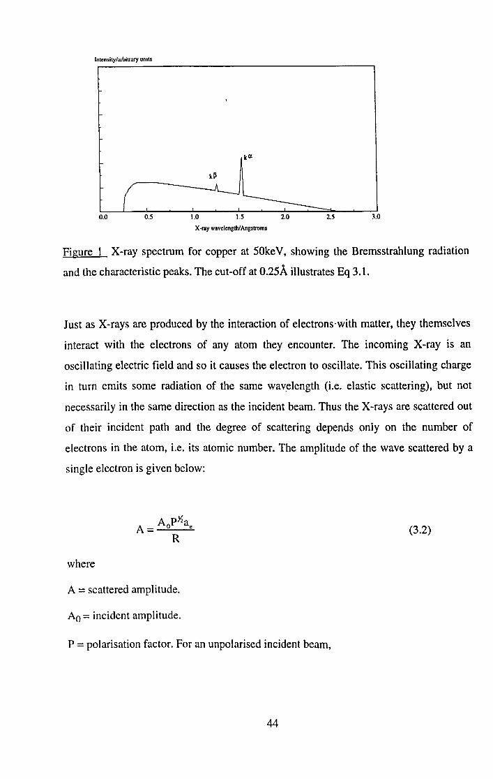
Intensity/arl>itrary umlS
0.0 0.5 3.0
X-ray wavelength/Angstroms
Figure 1 X-ray spectrum for copper at 50keV, showing the Bremsstrahlung radiation
and the characteristic peaks. The cut-off at 0.25.A illustrates Eq 3.1.
Just as X-rays are produced by the interaction of electrons' with matter, they themselves
interact with the electrons of any atom they encounter. The incoming X-ray is an
oscillating electric field and so it causes the electron to oscillate. This oscillating charge
in turn emits some radiation of the same wavelength (i.e. elastic scattering), but not
necessarily in the same direction as the incident beam. Thus the X-rays are scattered out
of their incident path and the degree of scattering depends only on the number of
electrons in the atom, i.e. its atomic number. The amplitude of the wave scattered by a
single electron is given below:
(3.2)
where
A = scattered amplitude.
Ao = incident amplitude.
P = polarisation factor. For an unpolarised incident beam,
44
p = ..!..+..!..cos28, where 28 = scattering angle. 2 2
R = distance from the electron.
J.le2
ae = scattering length of an electron. ae = -- = 2.8 x 10⁻⁵ A, where 4mn
J.l = magnetic permeability of a vacuum, 1.26 x 1 0~6 HIm,
e = charge on an electron; 1.60 x 10⁻¹⁹ C,
m = rest mass of an electron, 9.10 x 1O-31kg.
(This is the basis for ignoring the effect of the nucleus on the X-rays, since its mass m is
very large compared with the mass of an electron.)
The intensity of the scattered X-ray is given by
(3.3)
where 10 is the incident intensity.
Considering the case of X-rays scattered from the whole atom, only the effect of the
electrons is taken into account as mentioned above, and the overall effect is obtained by
simply adding up the amplitude from the different electrons within the atom, taking
account of the interference between waves from different parts of the electron cloud:
A pX The term 0 is known as Astandard'
R
Q is the scattering vector, i.e. the change in wave-vector on scattering.
Q = 41tsin8 'A.
45
(3.4)
(3.5)

f(Q) is the atomic fonn factor, which depends on the distribution of the electrons. At low
Q, f(Q) = atomic number, Z.
Hence at low Q, the X-ray scattering length of an atom = Z3e.
3.2.2 Neutrons.
There are two mechanisms whereby neutrons are scattered. In the first, the magnetic
moment of the neutron causes it to be scattered by unpaired electrons in the atom. This is
a very useful phenomenon for the investigation of the magnetic properties of materials,
but it is not used for this work, although two samples were prepared on Ni (Le.
ferromagnetic) substrates as a courtesy to RAL scientists investigating this phenomenon.
In the second mechanism, neutrons are scattered by nuclear forces, which are very strong
and very short range. The neutrons may be scattered coherently, i.e. in a known and
constant direction, giving a high intensity in that direction, or incoherently, i.e. in
random directions, giving a very low intensity in anyone direction.
For neutrons, the scattered amplitude is similar to that in the case of X-rays, namely:
where
A=Aob R
A = scattered amplitude.
Ao = incident amplitude.
b = nuclear scattering length, i.e. the effective diameter of the nucleus.
R = distance from the atom.
Astandard in the case of neutrons is given by:
Ao Astandard = R
Again, similar to X-rays, the scattered intensity is given by:
46
(3.6)
(3.7)
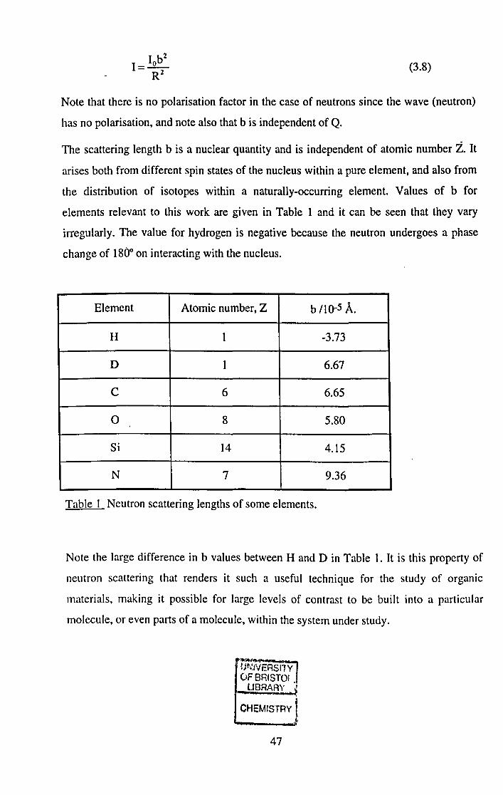
(3.8)
Note that there is no polarisation factor in the case of neutrons since the wave (neutron)
has no polarisation, and note also that b is independent of Q.
The scattering length b is a nuclear quantity and is independent of atomic number i. It arises both from different spin states of the nucleus within a pure element, and also from
the distribution of isotopes within a naturally-occurring element. Values of b for
elements relevant to this work are given in Table I and it can be seen that they vary
irregularly. The value for hydrogen is negative because the neutron undergoes a phase
change of 18Do on interacting with the nucleus.
Element Atomic number, Z b 110-5 A.
H I -3.73
D I 6.67
C 6 6.65
0 8 5.80
Si 14 4.15
N 7 9.36
Table 1 Neutron scattering lengths of some elements.
Note the large difference in b values between Hand D in Table 1. It is this property of
neutron scattering that renders it such a useful technique for the study of organic
materials, making it possible for large levels of contrast to be built into a particular
molecule, or even parts of a molecule, within the system under study.
""----IjtJ.iVERSITY 0FBRfSTOI.
UORARY "
CHEMISTRY t
47

For most of the elements relevant to this work, the contribution to b from incoherent
scattering is negligible. The exception is hydrogen, where it is the coherent contribution
to b that is by far the smaller.
3.2.3 Scattering Length Density.
Scattering lengths only apply to individual atoms. To apply the theory to bulk systems
we must use scattering length densities, p, which take into account the number density of
each scattering atom. Thus for a pure element:
p=Nb for neutrons (3.9)
P =NZae for X-rays. (3.10)
N is the number of atoms per unit volume, i.e. the number density, and it is typically
gi ven as the number per A 3.
For a compound with several types of atom,
for neutrons (3.11)
for X-rays (3.12)
where
N j is the number density of atom type i,
hi is the neutron scattering length of atom type i
Zj is the atomic number of atom type i.
Examples of scattering length densities of some relevant compounds for both neutrons
and X-rays are given in Table 2.
48

Compound p (neutrons) 110-5 A,-2 P (X-rays) 110-5 A,-2
H2O -0.05 0.94
D20 0.64 0.94
-CH2- -0.06 0.65
-CD2- 0.61 0.65
Table 2 Scattering length densities (SLDs) of some relevant materials, showing the
neutron contrast of deuterated compounds.
3.2.4 Scattering from a Bulk Material.
Each portion of the whole makes its own contribution to the total scattered amplitude.
These contributions may be calculated for each portion, summed over the whole and
converted to intensity, for direct comparison with the intensity that is measured by the
apparatus.
The scattering length of each portion = p(r) dr, where p(r) is the scattering length
density of the portion and r is the vector representing the position of that portion within
the whole.
49
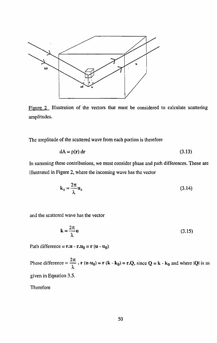
Figure 2 lllustration of the vectors that must be considered to calculate scattering
amplitudes.
The amplitude of the scattered wave from each portion is therefore
dA = per) dr (3.13)
In summing these contributions, we must consider phase and path differences. These are
illustrated in Figure 2, where the incoming wave has the vector
and the scattered wave has the vector
27t k=-u
A
Path difference = r.u - r.uo = r (u - uo)
(3.14)
(3.15)
Phase difference = 27t • r (u-uo) = r (k - ko) = r.Q, since Q = k - ko and where IQI is as A
given in Equation 3.5.
Therefore
50

dA = p(r)dr eiQr (3.16)
where eiQ.r is the phase term, representing a phase shift of Q-r radians. Hence a
variation in r yields a sinusoidal amplitude.
The scattered amplitude is given by
A(Q) = Iv dA = Iv per) eiQ.r dr (3.17)
where v is the sample volume.
To convert amplitude to intensity, use I = IAI2 and express I(Q) relative to a unit
scattering length at the origin:
I(Q) = I Iv per) eiQ.r dr 12 (3.18)
In practice, the volume is infinite compared to the portion of interest. With to we have
the Fourier Transform.
51
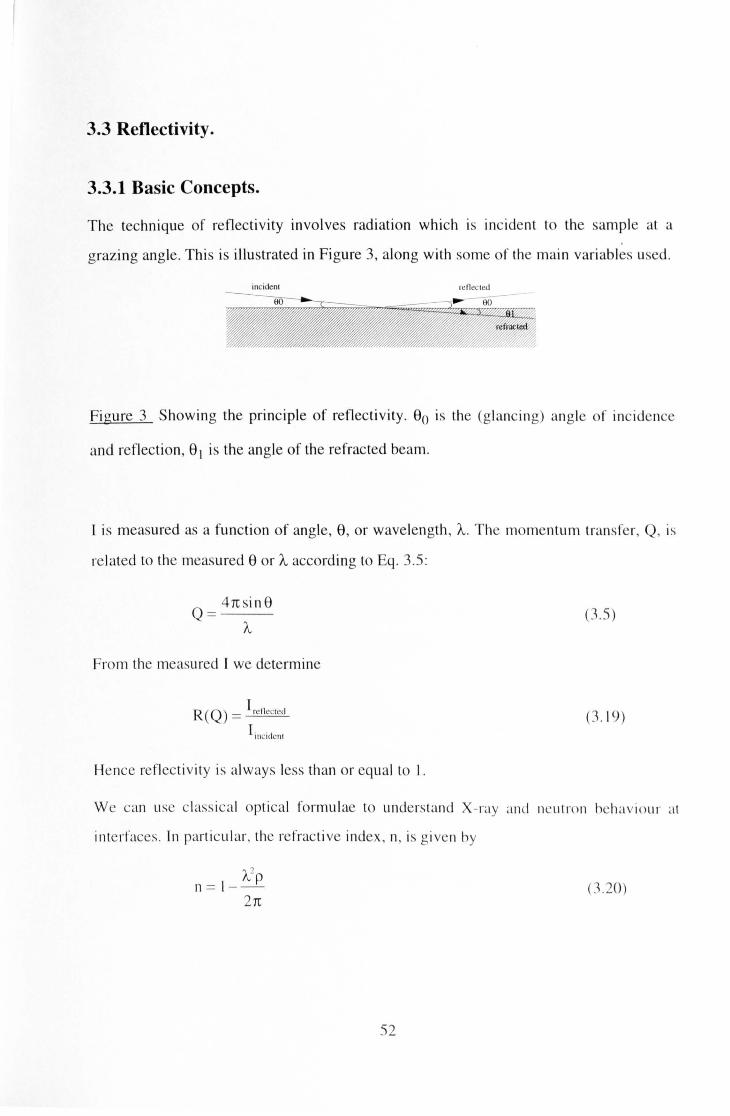
3.3 Reflectivity.
3.3.1 Basic Concepts.
The technique of reflectivity involves radiation which is incident to the sample at a
grazing angle. This is illustrated in Figure 3, along with some of the main variables used .
incident Icll c!c led
Figure 3 Showing the principle of reflectivity. 80 is the (glan ing) angle f incid nc
and reflection, 8 1 is the angle of the refracted beam.
I is measured as a function of angle, 8, or wavelength , A. The mom ntum transfer, Q, is
related to the measured 8 or A according to q. 3.5 :
Q = 47tsi n8
A
Fr m the measured I we determine
R( Q) = T reflcclcd
I lllci dclll
Hence reflectivity is always less than or equal to I.
(3 .5)
(3 . 19)
We can use 'Iassical optical formulae to understand X-ray and neulron h ' haviour al
interfaces. In particular, the refractive index. n, is given by
(3 .20 )
52
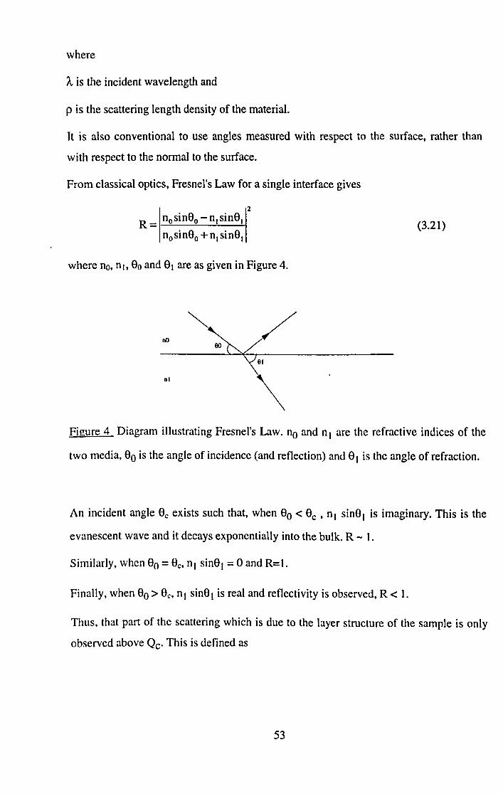
where
A is the incident wavelength and
P is the scattering length density of the material.
It is also conventional to use angles measured with respect to the surface, rather than
with respect to the normal to the surface.
From classical optics, Fresnel's Law for a single interface gives
R = nosinSo - n l sinSI
nosinSo + n l sinSI
2
where no, nt. So and SI are as given in Figure 4.
nO 00
nl
(3.21)
Figure 4 Diagram illustrating Fresnel's Law. no and n I are the refractive indices of the
two media, So is the angle of incidence (and reflection) and SI is the angle of refraction.
An incident angle Sc exists such that, when So < Sc , nl sinSI is imaginary. This is the
evanescent wave and it decays exponentially into the bulk. R - 1.
Similarly, when So = Se, n) sinS) = 0 and R=1.
Finally, when So> Se, nl sinSI is real and reflectivity is observed, R < l.
Thus, that part of the scattering which is due to the layer structure of the sample is only
observed above Qc. This is defined as
53

where
k = 21t A
9, = ,-f; and hence
(since Oc in radians == sin Oc for low Oc ' i.e. grazing angles.)
(3.22)
The point at which R becomes less than 1 is termed the critical edge and its position in
Q, A or 0 may be used to calculate the SLD of the substrate, or of the film if it is thick
enough to produce a discernible edge of its own. It can thus be seen that allowing for the
supporting substrate is a straightforward part of the data analysis, and this is one of the
main reasons why these techniques are so useful for studying organic systems.
There are different approaches to generating a model to fit the data: the kinematic
approximation is the easiest to visualise, while the optical matrix method is the most
accurate.
3.3.2 The Kinematic Approximation.
This approach calculates approximate reflectivity profiles using Fourier transforms to
represent changes in SLD through the sample.
I(Q) = 1 J per) ei Q.r dr 12 (3.23)
where per) is independent of x and y, i.e. it only varies perpendicular to the substrate, in
the z direction.
54

The Fourier transfonn (FT) of a constant is a a-function, and in this case it is given by
27t a (Ql.). A sharp peak is seen at Ql. = 0, i.e. reflection is only seen if Q is exactly
perpendicular to the surface. Hence
I(Q) = (27t)2 1 J p(z) eiQ.'z dz 12 a (Q.l) (3.24)
The delta function, a (~), defines the specular peak in the scattered beam. To calculate
the reflectivity we must convert this to a function of scattered beam direction and then
integrate over the peak. These steps introduce a factor of (27t)2 (from integration over a
2D a-function) and a factor of ~ (the Jacobian arising from integration over dB, dep, Qz
i.e. the conversion factor when changing from rectangular to. polar coordinates).
Simplifying:
R(Qz) =: (27t)2 ~ 1 J p(z) eiQ.,z dz 12
Qz (3.25)
(3.26)
The kinematic approximation is not valid in the low Q region around Qc , where total
external reflection is approached. However, it has the advantage that it provides a simple
formula to relate surface structure to reflectivity, and interface roughness can be built in
to the model very readily. It is extremely useful for the ease with which the contribution
to the reflectivity profile from given parts of the structure can be visualised. This is now
illustrated with a worked example.
The reflectivity profile from a film is modulated by a cosine wave. Consider neutron
reflection from a monolayer of surfactant on air-contrast-matched (acm) water, i.e. a
mixture of H20 and D20 such that the resultant neutron SLD is zero (92% H20 and 8%
D20). This is illustrated in Figure 5.
55
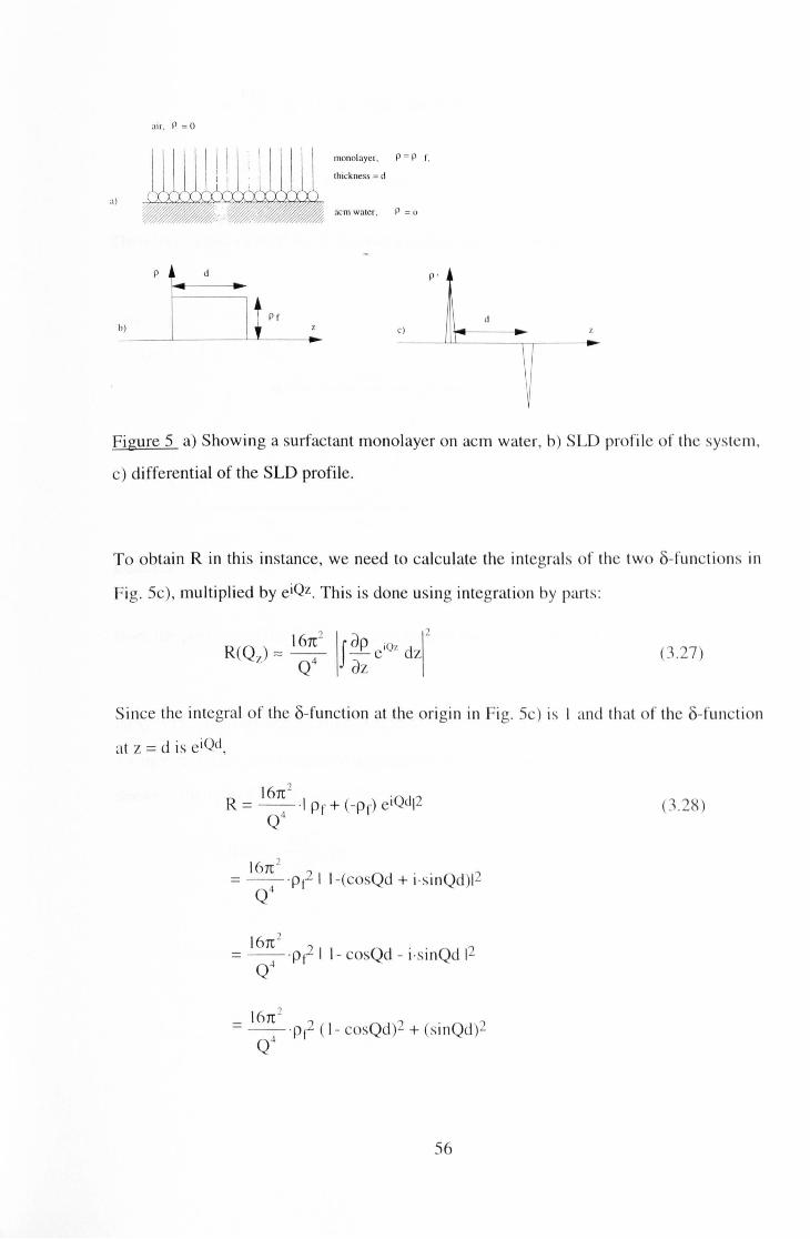
air, P = 0
a)
P d
h)
monolayer, r = P r,
Ihickness = d
"em water, P = 0
p '
c) d
114---'-
Figure 5 a) Showing a surfactant monolayer on acm water, b) SLD profile of the system,
c) differential of the SLD profile.
To obtain R in this instance, we need to calculate the integra ls of the two b-functions in
Fig. 5c), multiplied by eiQz. This is done using integration by parts :
? d 2 R(Q ) ::::: 167C f-.2. eiQz dz
7. Q4 dZ (3 .27)
Since the integral of the b-function at the origin in Fig. 5c) is I and that of the b-function
at z = d is eiQd,
16rr2
= -- 'Pt2 I 1-(cosQd + i·si nQd )12 Q4
16rr2
= -- ,pt2 1 1- cosQd - i· sinQd 12 Q~
56
0 .28)
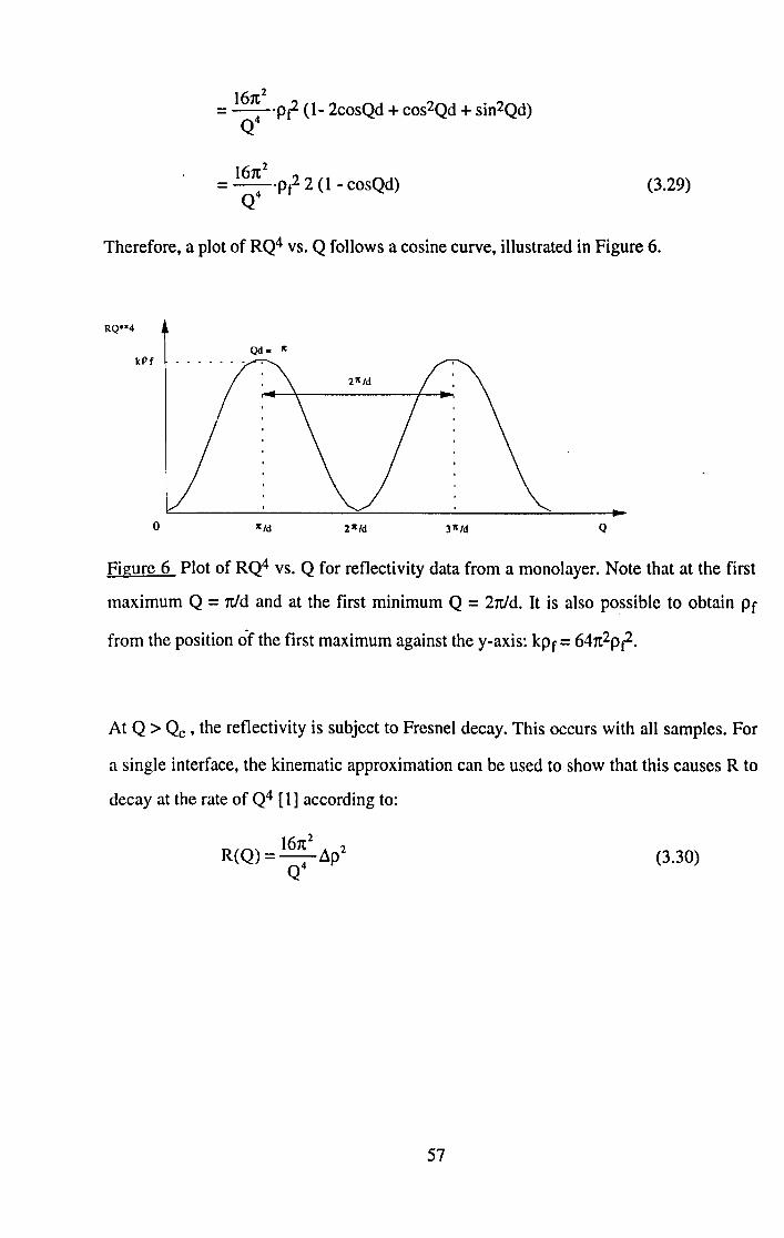
161t2
= --,pr (1- 2cosQd + cos2Qd + sin2Qd) Q4
(3.29)
Therefore, a plot of RQ4 vs. Q follows a cosine curve, illustrated in Figure 6.
RQ**4
Qdm It
kPf
o Q
Figure 6 Plot of RQ4 vs. Q for reflectivity data from a monolayer. Note that at the first
maximum Q = 7tld and at the first minimum Q = 27t1d. It is also possible to obtain Pr
from the position of the first maximum against the y-axis: kpr = 641t2pr.
At Q > Qc ' the reflectivity is subject to Fresnel decay. This occurs with all samples. For
a single interface, the kinematic approximation can be used to show that this causes R to
decay at the rate of Q4 [1] according to:
R(Q) = 161t2
f1 2 Q4 P (3.30)
57

3.3.3 The Optical Matrix Method.
This . method uses classical optics, and a matrix to describe each layer within the film in
terms of thickness and SLD. It is therefore an exact method, but one which cannot
generally be expressed as a simple formula.
The refractive index of a material for neutrons and X-rays was given in Eq. 3.20, Section
3.3.1:
,),} n = l---.e.
21t
In all other respects the beams may be treated as visible light.
Referring back to Figure 4 for definitions, for a single uniform layer:
where
p-p. fij = I J , the reflection coefficient at each boundary
Pi +Pj
Pi = nj sin8j
~ = 21tn)dsin8) . A
~ is the phase difference across the layer.
This expression for R may be restated as
58
(3.20)
(3.31)
(3.32)

For a multilayer film, a matrix Mj is defined for the jth layer as follows:
and the resultant reflectivity for 2 layers is given by:
2
R = (Mil + M 12Ps)Pa -(M21 + M22 Ps)
(Mil + M 12P.)Pa +(M21 + M22P.)
(3.33)
(3.34)
where the subscripts s and a refer to substrate and air respectively. The reflectivity for a
multilayer is obtained by multiplying the matrices for each layer in the same way.
To include roughness at the interfaces, fjj is replaced by the following expression [1]:
(3.35)
The optical matrix method was used for all the modelling in the present work. Some
simulations using the optical matrix method are now presented, for illustrative purposes.
In addition to the common features discussed above, the factors which affect the shape
of the reflectivity profile from a particular individual sample are substrate and sample
roughnesses and SLDs, overall thickness, and internal structure, such as repeat distances
within a multilayer sample.
Roughness affects the reflected intensity by scattering the incident beam more widely
than would a smooth surface, causing the measured intensity to fall off more rapidly in
Q.
1= 10 exp (_Q2 cr2) (3.36)
where
To = incident intensity
I = reflected intensity
Q = 2k sinS
59

k = 27t A
cr = rms Gaussian roughness.
SLD values also affect the intensity of the reflected beam, and the effects of coherent and
incoherent scattering have already been mentioned in Section 3.2.2. For instance, a
deuterium-labelled sample will give a higher re~ected intensity in a neutron beam than
will a straightforward hydrocarbon sample. The presence of a heavy metal such as Cd
will introduce similar contrast in X-ray reflectivity, while it will absorb strongly in a
neutron beam. The difference in SLD values between the various components of the
sample is also important - if two adjacent parts of the sample have very similar SLDs,
they will be difficult to distinguish. This is why neutron reflectivity is so useful for
studying scrambling in Hand D LB films - if the layers have mixed, their SLDs will be
averaged out, and the reflected intensity will be very much less than for unmixed layers.
The SLD of the substrate also affects the profile over the very low Q range where total
external reflection takes place, i.e. where R = 1.
The overall thickness of the sample and internal layer order affect the reflected intensity
via interference effects. Chief among these is the Bragg relation,
nA = 2d sinS
where
n = order of Bragg peak
A = incident wavelength
d = layer thickness
S = angle of incidence
Given that
47tsinS Q=-
A
(3.37)
(3.5)
60

it is straightforward to show that at a Bragg peak,
Q= 2n7t
d (3.38)
Similarly, interference from the entire sample thickness also gives rise to fringes, known
as Kiessig fringes. Since Q is inversely proportional to d, these fringes are narrow for
thick ( -1000 A) films and broad for thin (-50 A) films.
These two separate sets of fringes are superimposed on each other in the measured
reflectivity profile and this must be taken into account when analysing the data.
The influence of each of these factors on the shape of an example reflectivity profile is
shown in Figure 7a) - 7d). These are simulations, using values of SLD for film and
substrate which are applicable to neutrons.
61
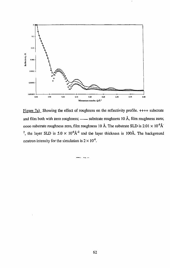
11.1
1101
co: >. .~
IIWI .'" u .. .., " co:
1I.IXKlI
1I.IUKKlI -I-----+---~f__--_+_--_+---I__--_+_--_+--__I
IIJKI IIII~ 11.10 II.I~ lI.lO O.2.~ OJII 11.411
Momentum transfer, Qlk'
Figure 7a) Showing the effect of roughness on the reflectivity profile. ++++ substrate
and film both with zero roughness; - substrate roughness 10 A, film roughness zero;
0000 substrate roughness zero, film roughness loA. The substrate SLD is 2.01 x 10⁻⁶ A-2, the layer SLD is 5.0 x 1O-6A-2 and the layer thickness is 100A. The background
neutron intensity for the simulation is 2 x 10⁻⁶•
62
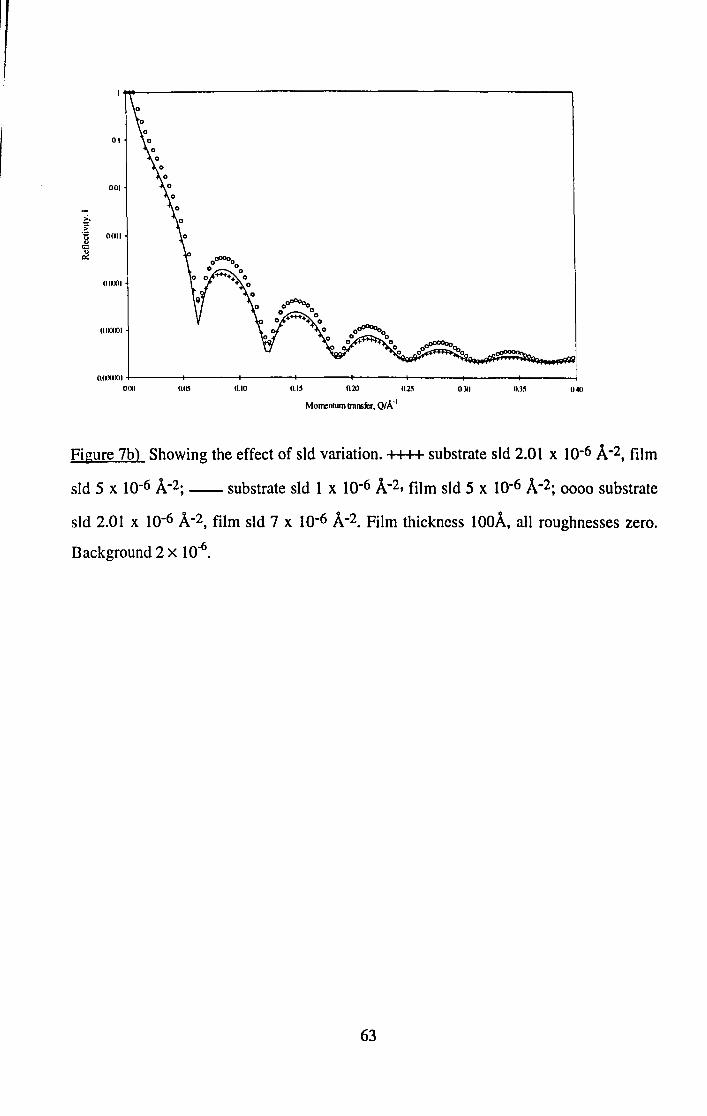
01
OUI
-& .~ tl OIXII
" 0::: 1J
'" OIXJOI
O,lXJOOI
O.IXXXXII +----+----+---_---+----+----+---_--~ OIX) II.I~ IUO 0.15 11.20 O.2.~ Oll) OJ5 040
Morrentum Irn~ilr. QI A·1
Figure 7b) Showing the effect of sId variation. ++++ substrate sId 2.01 x 10⁻⁶ A-2, film
sId 5 x 10⁻⁶ A-2; -- substrate sId 1 x 10⁻⁶ A-2, film sId 5 x 10⁻⁶ A-2; 0000 substrate
sId 2.01 x 10⁻⁶ A-2, film sId 7 x 10⁻⁶ A-2. Film thickness 100A. all roughnesses zero.
Background 2 x 10⁻⁶•
63

"I
ont
"""'" -1----+----+----+----_+_---_+_---_+_---_+_-----1 Uti) 005 010 11.15 0.20
MorrenlUm Ir.wrer, QI).'I
o.~ 0.111 0411
Figure 7c) Showing the effect of total film thickness. ++++ film 50 A thick; -- film
100 A thick; 0000 film 200 A thick. Roughnesses zero; film and substrate SLDs and
background as in Figures 7a) and 7b).
64

0.1
11.111
'" ;i.
i O,lXII
.:!
O,lXIOI
O.(XXXII
O,lXXXXlI .J.----+----+---+----+----+---+-----+----l n O.ns 0.1 O.U 0.2 0.25 0.) 0.)5 04
~.ncnfUl1llraMtcr. QlA··-1
Figure 7d) Showing how internal repeats produce Bragg peaks. ++++ single film 297.5
A thick, sId = 1.57 x 10 -6 A-2 ; -- II-layer film, similar to a fatty acid LB film, with
a 26 A tail region, sId = I x 10 -6 A-2 , and a 7.5 A double headgroup region, sId = 5.5 x
10 -6 A-2 . Roughnesses zero; substrate SLD and background as in Figures 7a) - 7c). The
dipping process results in only the first and final tail regions being 26 A thick: the
remainder are bilayers, and therefore 52 A thick. The three large (first, second and third
order) Bragg peaks arise from this 52 A repeat distance. The Kiessig fringes are
particularly clear between the first and second order Bragg peaks.
65

3.4 Summary of Approaches to Interpreting the Data.
As has been seen, direct inversion of the data to yield a sample structure is not generally
possible, because of the large number of possible solutions to each reflectivity profile,
even given restrictions based on a priori knowledge of the system being studied. A
theoretical profile is therefore generated, as in the above examples, from estimates of
parameters such as layer thickness, roughness and scattering length density (SLD),
compared with the data and refined by adjusting the input parameters until a fit with the
data is obtained. However, even a good fit cannot be assumed to represent a unique
solution, since it might only be a local minimum. Solution space must be explored
thoroughly to look for other minima before any confidence can be placed in a particular
structure.
There are currently four main methods used to generate the theoretical profiles needed
for this fitting process. These are the kinematic approximation [2] and the optical matrix
method [3], both of which have already been discussed in detail, the maximum entropy
method, MaxEnt [4] and the cubic splines method [5]. The third method, MaxEnt, starts
from a fixed sample thickness and substrate SLD which have been chosen by the user,
assumes the sample is a one-layer slab and explores roughnesses and film SLD on this
basis. If no fit is found it then assumes the sample is made up of two distinct layers
consistent with the fixed total thickness and again explores roughnesses and film SLDs.
It can continue up to a maximum of 20 layers. Even disregarding the very long
computing times required for this process, 20 layers proved insufficient to fit the data in
this work, so after a brief trial MaxEnt was not used in the present work. Similarly for
the method of cubic splines - it generated an excellent fit, but with an SLD profile
involving physically unreasonable SLD values given the known nature of the samples, so
it too was not used and will not be discussed further. The kinematic approximation and
the optical matrix method therefore formed the backbone of the modelling approach
used to analyse the data from the present work. Further details may be found in [2] and
[3], and the evolution of the particular method used here'is described in Chapter 5.
66

3.5 References
[1] L. Nevot and P. Croce, Phys. Appl. 15, 761 (1980) and R. A. Cowley and T. W.
Ryan, J. Phys. D: Appl. Phys. 20, 61 (1987).
[2] J. Penfold and R. K. Thomas, J. Phys.: Condensed Matterf 2, 1369 (1990).
[3] M. Born and E. Wolf, Principles of Optics, Pergamon, Oxford (1970) and O. S.
Heavens, Optical Properties of Thin Films, Butterworth ,London (1955).
[4] D. S. Sivia, W. A. Hamilton and G. S. Smith, Physica B, 173, 121 (1991).
[5] J. S. Pedersen, J. Appl. Cryst. 25, 129 (1992).
67
Chapter 4. Experimental
4.1 Introduction
This chapter gives details of all the apparatus and techniques used in the present work. It
starts by describing the necessary preparation of the equipment prior to experimentation,
then discusses the procedures required for the fonnation and manipulation of Langmuir
films and the dipping of Langmuir-Blodgett films, and finally details the techniques
which have been used in this work to characterise the LB films which have been
prepared.
4.2 Preparation and Cleaning
Since Langmuir films consist of a one-molecule-thick layer of an amphiphile floating on
water, it will be clear that contamination is to be avoided and that cleanliness is
paramount. To this end, the amphiphiles used were obtained at the highest available
purity (99+%, Fluka or Larodan). Water was first distilled, and then filtered by an
Elgastat Spectrum B water purification system (Elga) to provide water with a resistivity
in the range 16-18 MOm and a surface tepsion between 70-71.9 mN/m. The pure water
thus obtained has a pH of 5.5 due to dissolution of atmospheric carbon dioxide and it is a
potent cleaning solvent in its own right. The chloroform used was Aristar grade, ex
Merck, and all other solvents were HPLC grade ex Aldrich. The Langmuir troughs
themselves were housed in cabinets to minimise airborne contamination, although
obviously working in a clean room is the ideal, if facilities are available. Troughs were
cleaned immediately before embarking on a series of experiments and on a weekly basis
for the duration of that series. Glassware and other implements were cleaned at the end
of a series of experiments and stored in a clean, segregated cupboard. If necessary, they
were cleaned again immediately before use. All the procedures for these cleaning
arrangements will be given in detail in subsequent sections. Schematic diagrams of the
Langmuir trough used for the bulk of this work are shown in Figure I. A diagram of the
two-compartment trough used for alternating films will be given later, in the section on
dipping (Section 4.5).
68

PTFE-coated flexible barrier
fixtures for posts: a = fixed b, C = motor-driven
bphase
Figure 1 a) Schematic plan view of a Langmuir trough with the barriers closed.
r --,
:c
Figure 1 b) Schematic plan view of a Langmuir trough with the barriers open.
69
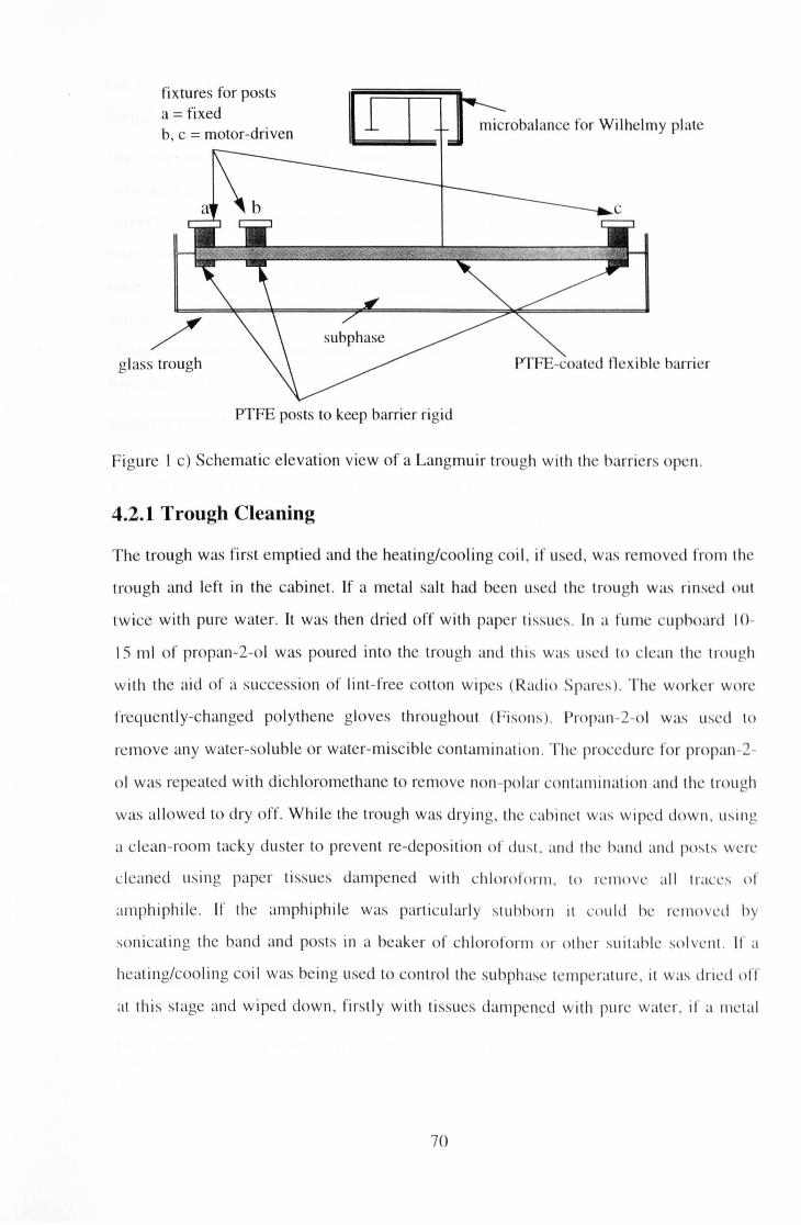
fixtures for posts a = fixed b, c = motor-driven
glass trough
PTFE posts to keep barrier rigid
microbalance for Wilhelmy plate
PTFE-coa ted flexib le barrier
Figure I c) Schematic elevation view of a Langmuir trough with the barri rs op n.
4.2.1 Trough Cleaning
The trough was first emptied and the heating/cooling coi l, if used, was r moved from the
trough and left in the cabinet. If a metal salt had been used th trough was rinsed out
twice with pure water. It was then dried off with paper ti ssues. In a fume cupboard lO-
15 ml of propan-2-01 was poured into th trough and thi s was us d to clean th trou h
with the aid of a succession of linl- free cotton wip s (Radio Spares) . Th work r wor
frequently-changed polythene gloves throughout (Fisons). Propan -2-01 was used to
remove any water-soluble or water-miscible contamination . Th ' pro 'cdur for propan-2-
01 was repeated with dichloromethane to remove non-polar contam inati n and the trough
was al lowed to dry off. Whi le the trough was drying, the cabinet was wiped d )wn , usin 1
a clean-room tacky duster to prevent re-deposition of dust. and th' band and posts wen:
cleaned using paper ti ssues dampened with chloroform, to r ' move all Ira ' 's or amphiphi le. If the amphiphile was particularly stubborn it could be removed by
sonicating the band and posts in a beaker of chloroform or other suitable so lvent. If a
healing/cooling co il was being used to control the subphase temp rature, it was drie l oll
at this stage and wiped down, firstly with tissues dampened with pur wat r, if a III tal
70

salt had been used. and then with tissues dampened in chloroform. and left to dry in the
trough cabinet.
Once the trough was dry of all solvent it was rinsed three times with distilled water and
once with pure water. If the water droplets did not reveal a hydrophilic glass surface the
solvent cleaning was repeated. If this second attack failed the trough was left full of pure
water for 12-24 hours to leach out contaminants. rinsed, dried and cleaned with solvents
once more. This process could continue for 7-10 days before the trough was
satisfactorily clean, particularly if it had not been used for some time. If used and
cleaned regularly, however, once through the cycle was enough to give reproducible
experimental results.
Once cleaned. the trough was replaced in the cabinet, the band was fitted, it was checked
with a spirit level to make sure it was level and filled with freshly-drawn pure water. On
a monthly basis the microbalance and plotter signals were calibrated, including the ratio
of the barrier-potentiometer volts to the trough area (this mV/cm2 ratio was required for
calculation of deposition ratios). If required, the subphase pH was adjusted to the desired
value. e.g. pH3 using Aristar hydrochloric acid (Merck). If a metal salt was to be used it
was added at this stage. e.g. 0.25 mM cadmium chloride (AnalaR, Merck) and the pH
adjusted to 6.3 or above using AnalaR sodium hydroxide (May and Baker). The
temperature of the subphase was allowed to stabilise, to room temperature or according
to the heating/cooling coil, as appropriate. The trough was then ready for use.
The dimensions of the trough used for the bulk of the samples prepared here were 1.20 x
0.20 x 0.09 m. It was a gift from ICI Corporate Colloid Science Group and had been
made there. The alternating trough used for ABAB samples was 0.80 x 0040 x 0.12 m. It
had been made and provided by DERA. Malvern (formerly RSRE). Both troughs
consisted of a U-shaped piece of glass. with two glass end pieces held in place using a
metal frame which could be tightened as necessary. A watertight seal was provided by
mouldable expanded PTFE strip. 3-4mm diameter. All microbalances used had been
purchased from CI Instruments. Motors and electronic components were standard off
the-shelf items. of good quality. and the circuitry, in particular the feedback loops. had
been optimised for monolayer experiments through trial and error.
71
4.2.2 Cleaning of Glassware and Other Implements
The 2 ml volumetric flasks used to make up solutions of the amphiphiles were cleaned
by sonicating for 30 minutes in a beaker containing a 2% solution of Decon90 (Merck)
in distilled water. They were then rinsed by sonicating, in the same beaker, for 10
minutes in each of six changes of water, the first four being distilled water and the final
two being pure water, and left to dry upside-down. Using the same beaker for all the
sonicating steps helps to minimise contamination, especially from the stainless steel of
the ultrasonic bath itself. The plastic tops were cleaned by soaking in a beaker of
dichloromethane - since they float they were weighed down by a smaller beaker. They
were then left to dry.
Spatulae used for weighing out were cleaned with a scouring powder such as Ajax and
rinsed thoroughly with distilled water before being left to dry.
Larger items of glassware were soaked in a bucket filled with a 2% solution of Decon90
in distilled water for at least 12 hours, rinsed thoroughly under running distilled water
and left to dry upside-down. All traces of surfactant had to be removed by rinsing: once
dried on they were difficult to remove, even by sonicating.
The glass Agla micrometer syringes (Well come) were cleaned immediately after use by
repeatedly drawing up and expelling clean chloroform, and then dried by drawing up and
expelling air. Syringe needles were cleaned by sonicating for 10-15 minutes in each of
three batches of chloroform and left to dry.
Wilhelmy plates were cut to the required size (1 cm x 2 cm) in large batches from
Whatman filter paper, Qualitative grade. Each was rinsed in chloroform immediately
prior to use and air-dried before immersion in the trough.
If drying of any of the above needed to be accelerated, cylinder nitrogen was used.
If any spatula or item of glassware was not uniformly hydrophilic after two or three
cleans it was discarded from use in Langmuir trough experiments.
72

4.2.3 Cleaning of Substrates for Dipping.
The two most common dipping substrates are glass slides and silicon wafers. The former
have a hydrophilic surface, and hence only pick up an odd number of layers, since no
pick-up occurs on the first downstroke. The latter have a hydrophobic surface and so
pick up an even number of layers.
Glass slides were purchased unwashed (e.g. Chance-Propper, UK), since residual
surfactant from the manufacturer's cleaning process is too difficult to remove. They were
first degreased by wiping with dichloromethane and then sonicated for 10 minutes in a
bath of pure solvents, in the following order:
dichloromethane - propan-2-01. - water - propan-2-01 - dichloromethane - propan-2-01 -
water - water.
Note that each solvent was miscible with the previous and the next in the sequence.
The slides were then sonicated for 30 minutes (or soaked overnight) in a O.lM solution
of sodium hydroxide. After this treatment the slides should be completely hydrophilic. If
any were not they were discarded, as a second run through the procedure does not
remove any further contamination. Finally, they were rinsed by sonicating for 10 minutes
in each of 6 changes of water and dried with cylinder nitrogen before storing in a dust
free box.
Silicon wafers were purchased as reclaimed (e.g. Speedfam, UK) and a)) used in the
present work were 4", (100) orientation, polished on one side only and doped n-type.
First they were trimmed, to optimise the use of the compressed monolayer given the
sampling area required by the neutrons and X-rays. They were then degreased, by
rubbing first with chloroform and then with propan-2-01, using lint-free wipes, before
rinsing with distilled water. They were then etched for 10 minutes in 5% hydrofluoric
acid to remove any remaining contaminants and the native oxide layer. A final rinse in
water was used as the test to see how effective the cleaning had been - the surface should
be completely hydrophobic. with no drops of water adhering at all. Note that the rear
face of the wafers was ground and would therefore always be hydrophilic due to
73

capillary action. Each wafer was cleaned immediately before use, since the oxide would
re-form over a period of about 10 minutes.
4.3 Langmuir Film Isotherms
Monolayers and their isotherms were produced as follows. Firstly, the water surface
within the barrier was cleaned to remove surface-active contamination. This was done
using a glass Pasteur pipette connected to a vacuum line and a water trap. The bulk of
the surface was "hoovered" first, then all around the edges. The barrier was opened and
closed rapidly, to dislodge any clinging dirt, and the "hoovering" was repeated. A fresh
Wilhelmy plate was pierced at the top with a clean needle, cleaned in chloroform, dried
in a paper tissue or in the air, attached to the microbalance using a length of cotton with
wire hooks at each end and suspended into the water. It was handled throughout with
clean tweezers. A final quick "hoover" removed any loose fibres of paper. The barrier
was expanded, and on closing rapidly the microbalance signal was recorded. If the
surface pressure increased by more than 0.1 mN/m the surface was re-hoovered and
rechecked. It might be necessary to change the Wilhelmy plate or the chloroform it was
cleaned in, or to clean the syringe needle used to make the hole for attachment to the
microbalance. If the surface contamination persisted it might be necessary to empty the
trough and clean it again, paying special attention to cleaning the flexible barrier (see
section 4.2.1), and to check the quality of the pure water from the filters.
Once the water surface was satisfactory, the Langmuir film could be spread. A solution
of the molecule under study was made up in chloroform or whatever solvent or mixture
of solvents was appropriate. More than 10% alcohol in the mixture should be avoided,
though, otherwise the material would be dissolved into the subphase by the alcohol and
no monolayer would be formed. The solutions should be stored in the refrigerator, or the
freezer for preference, to minimise concentration changes due to solvent evaporation
from the flask. Next, the amount to be applied to the trough had to be calculated, using
the simple formula shown below:
74

initial trough area in sq uare Angstroms x RMM of molecule Amount=----------~--------~----~~----------------------
Avogadro's n umber x initial area per molec ule in sq uare Angstroms
The initial area per molecule should be chosen so that the monolayer is well into the
liquid-expanded region (Chapter 2, Section 2.2), and it should ideally be twice the c1ose
packed area per molecule.
This equation gives the amount, in litres, of Imglml solution to be applied to the trough.
Use of an Agla micrometer syringe minimised errors in this process, since one complete
turn of the micrometer ( = a half-division) has been calibrated by the manufacturer to be
0.01 ml; this calibration was readily confirmed gravimetrically. The syringe needle was
held about 3-5mm above the water surface and the solution was added dropwise. Each
drop was allowed to spread (this was easily visible from the correct angle) before adding
the next. If the needle was held too far above the water, the drops would fall straight
through to the bottom of the trough without spreading, and thus introduce unknown
errors in the intended area per molecule. If a drop failed to spread it was usually because
there was already too much material on the surface. This would be confirmed by a
significant surface pressure being observed, and would be the result of a wrongly-chosen
initial area per molecule. Alternatively, the molecule may be sufficiently water-soluble
to dissolve straightaway without spreading, and no amount of material would generate a
significant surface pressure. Both situations are common when investigating unknown
molecules.
Once the required amount of solution had been applied to the water surface, a minimum
of 5 minutes was allowed for the solvent to evaporate. A longer time, say 10-15 minutes,
might be needed if the subphase was below room temperature or if the solvent
evaporated more slowly than chloroform. The barriers were then compressed slowly,
typically 10% of the maximum area per minute, with area and surface pressure signals
constantly monitored on the plotter. The resulting surface pressure versus area plot is
termed an isotherm, since the data are collected at a constant subphase temperature. As
discussed in Chapter 2, it reveals a wealth of information about the behaviour of the
molecule under study. It must be stressed, however, that all experimental conditions
75

should be recorded for each isotherm, as this greatly simplifies the identification of any
problems that may occur, such as with reproducibility. For example, a subphase
temperature change of a few degrees or a difference of 0.5 pH units could have a marked
effect on monolayer behaviour, with serious consequences for the understanding of a
novel molecule. Similarly, irreproducible isotherms might be caused by trapped solvent,
arising from inconsistent evaporation times. Rigorous attention to detail is therefore
required at all times.
4.4 Surface Potential Measurement.
In addition to the information provided by isotherms, a further technique for studying
monolayers is the use of surface potential [1], since fatty-acid monolayers floating on
water are charged due to ionisation by the water. This technique measures the potential
of a floating monolayer, using an ionised air gap. The circuit is completed by an
Ag/AgCh electrode immersed in the trough. A diagram of the apparatus is shown in
Figure 2.
--f~--.- .. ~ . --- ---------1---- U
Figure 2 . Schematic diagram (elevation view) of the apparatus used for the
measurement of surface potential. For clarity, the monolayer compression barriers have
been omitted.
76
The air gap was ionised by an 241 Am a.-source, which was used in preference to other
radioactive elements because its y-rays are very weak and so shielding and handling are
comparatively straightforward. The trough was cleaned as usual and the probe was
positioned over the centre of the trough, close to the Wilhelmy plate, at a height of 5 - 10
mm from the water surface, using a clamp and stand. It must stay at the same height
throughout an experiment, in order to maintain the air gap at a constant thickness. If the
probe is too close to the water, condensation affects the measurements.
The AgI AgCh electrode was filled with fresh electrolyte, rinsed thoroughly and placed
in the trough. It was removed from the trough at the end of an experiment in order to
minimise ions leaching into the subphase. A Keithley electrometer, model 61OC, was
used to provide the necessary resistance in the circuit, and the signal was recorded on an
x-y-t plotter. One further point which must be made is that even with a low-noise coaxial
cable connecting the probe to the electrometer, the movement of the operator close by
can give rise to spikes in the signal, so it is important to remain at least 2m from the
cable during an experiment, and to indicate any such artefacts on the plotter trace.
A measurement was first made of the clean water surface and typically this is -300 m V,
although any steady value is acceptable, within the range ±500mV. The monolayer was
then spread in the usual way, and after evaporation was complete, compression was
started at the usual rate for an isotherm. There are two main ways to record the surface
potential characteristics of a monolayer. The first is a surface potential isotherm, and the
second is to monitor the surface potential, "', with time at a series of fixed surface
pressures. The latter is more useful for providing data which will tie in with dipping
results, and was the approach used here. The procedure used in the present work, and the
results obtained, will be discussed in Chapter 5.
77
4.5 Langmuir-Blodgett Films.
Once a molecule had been well characterised as a monolayer and at least two isotherms
were obtained which gave reproducible results within experimental error (typically 0.1
mN/m and 0.5 - 1.0 A2 ), LB film formation might be attempted. This level of
reproducibility also shows that the trough is satisfactorily clean. First of all, a suitable
surface pressure (It) value was chosen. This was usually a region of the isotherm where
the monolayer was neither too fluid nor too stiff. For a fatty acid, this is in the S or LS
region (see Chapter 2, section 2.2) and so 1t is generally 30 mN/m, at least for initial
investigations. For dipping experiments it was not necessary to have an initial area per
molecule as large as that used for isotherms - a value that was just in the liquid-expanded
region was sufficient. This maximised the area available for dipping before a fresh
monolayer needed to "be spread, an important consideration for large substrates if they
were not to take too long to dip. In order to establish the suitability of the material for
dipping, the monolayer was compressed slowly to the chosen 1t (set point) using the
Forward setting and held there using the Control setting (negative feedback loop) in the
trough control box. Note that the Control dial setting is in mg, not mN/m (mg = 2 x
mN/m for a 1 cm-wide filter paper Wilhelmy plate [1]).
If compression was too fast, or the Control setting was switched in too soon, the
feedback loop would become unstable, since it was designed so that the speed which the
Control setting used to approach the set point was directly proportional to the difference
between the current 1t and the set point. For instance, if a fatty acid was being used and a
set point of 35 mN/m was required, the Control setting must not be switched in before
30-33 mN/m. If it were switched in earlier, compression would be too rapid since the 1t
difference would be too great. The set point would then be overshot, since the monolayer
would be in its most rigid region where very little change in area produces a very large
change in lt, and the feedback loop would try to compensate, oscillating about the finallt
value. Under these circumstances the loop could easily go from negative feedback to
positive. This would render the monolayer useless, since the amplitude of the
78
oscillations would have been sufficient to compress it into its collapsed region, so that it
would no longer be homogeneous. For very rigid monolayers it might not be possible to
reach equilibrium at all.
The pressure and trough area were monitored, over time using an x-y-t plotter and the
drift in area over, say, 30 - 60 minutes was noted. If this was significant, i.e. > 3 - 5
cm2/min, the,monolayer would be too unstable: It might be collapsing, or it might be
dissolving into the subphase. If the latter, the trough surface would be difficult to clean,
since the di~solved material would re-appear at the surface once the pressure was
reduced. If the former, the barrier would be difficult to clean. Either way, it would be
unsuitable for dipping at that pressure and alternatives would have to be investigated.
For some molecules, there is no pressure at which a monolayer is stable, even if
subphase temperature, pH or metal ion concentration are altered. For the remainder,
stability may usually be achieved under a variety of different experimental conditions,
and may be enhanced further by "annealing". This is the process whereby a monolayer is
compressed to a low 1t, say 5 mN/m, expanded again and allowed to relax for 10 minutes
before being compressed up to the dipping 1t. It makes the monolayer more stable by
gently forcing it into a loosely-packed version of the configuration it will adopt later. It is
then relaxed at 1t = 0, to minimise the formation of microcrystallites, before being
compressed up to the final pressure, at which it is now more stable. This treatment of the
monolayer is particularly important when dipping fatty amines or phospholipids, and
was used for the amines in the present work.
Once a suitable 1t had been determined, the first few samples could be dipped. The
dipping speed was the next factor to optimise - some molecules need a very slow speed,
of the order of 1-2 mmlmin, while others might need to be dipped fast, at 20mmlmin or
faster. The meniscus was an excellent qualitative guide to the evenness of transfer. On
the downstroke it should be downwards, on the upstroke it should be upwards, and in
both directions it should be smooth - if there was any unevenness, static or moving, it
was indicative of poor deposition and this would be borne out by the transfer ratio and
any subsequent film characterisation~
79
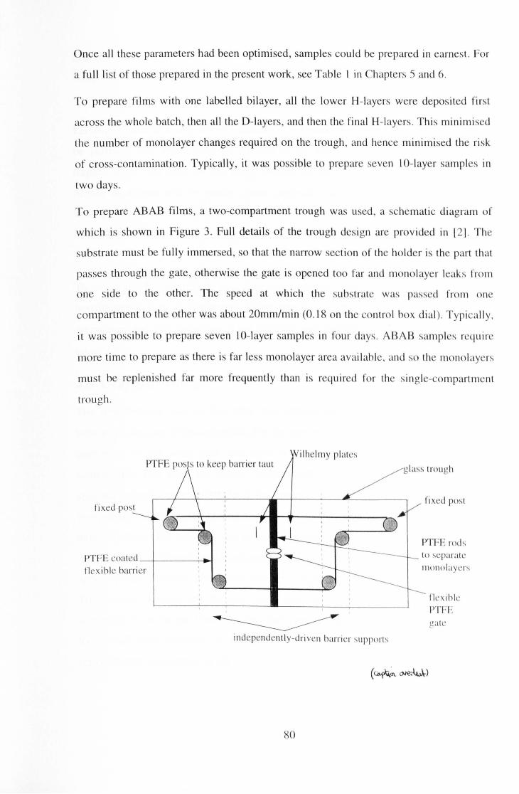
Once all these parameters had been optimised, samples could be prepared in earnest. For
a full li st of those prepared in the present work, see Table I in Chapters 5 and 6.
To prepare films with one labelled bilayer, all the lower H-Iayers were deposited first
across the whole batch, then all the D-Iayers, and then the final H-Iayers. This minimised
the number of monolayer changes required on the trough, and hence minimised the ri sk
of cross-contamination. Typically, it was possible to prepare seven 10- layer samples in
two days.
To prepare ABAB films, a two-compartment trough was used, a schematic diagram f
which is shown in Figure 3. Full details of the trough design are provided in l21. The
substrate must be fully immersed, so that the narrow section of th ho lde r is the part that
passes through the gate, otherwise the gate is opened too far and monolayer leaks from
one side to the other. The speed at which the substrate was passed from on
compartment to the other was about 20mm/min (0. 18 on the contro l box dial) . Typically ,
it was possible to prepare seven 10-layer samples in four days . ABAB samp les rcquir
more time to prepare as there is far less monolayer area avai lable, and so the monolay rs
must be replenished far more frequently than is required for thc s ing le-compartmcnt
trou gh.
PTFE posts to keep barrier taut
fixed post
PTFE coated -+--------r~ Ikxib le barrier
i ndependently-dri veil barrier Sllpr()rl ~
80
glass trough
fixed post
PTFF- rod s to separate
ll1ono I aye r~
l'kxihlc PTFE gall'
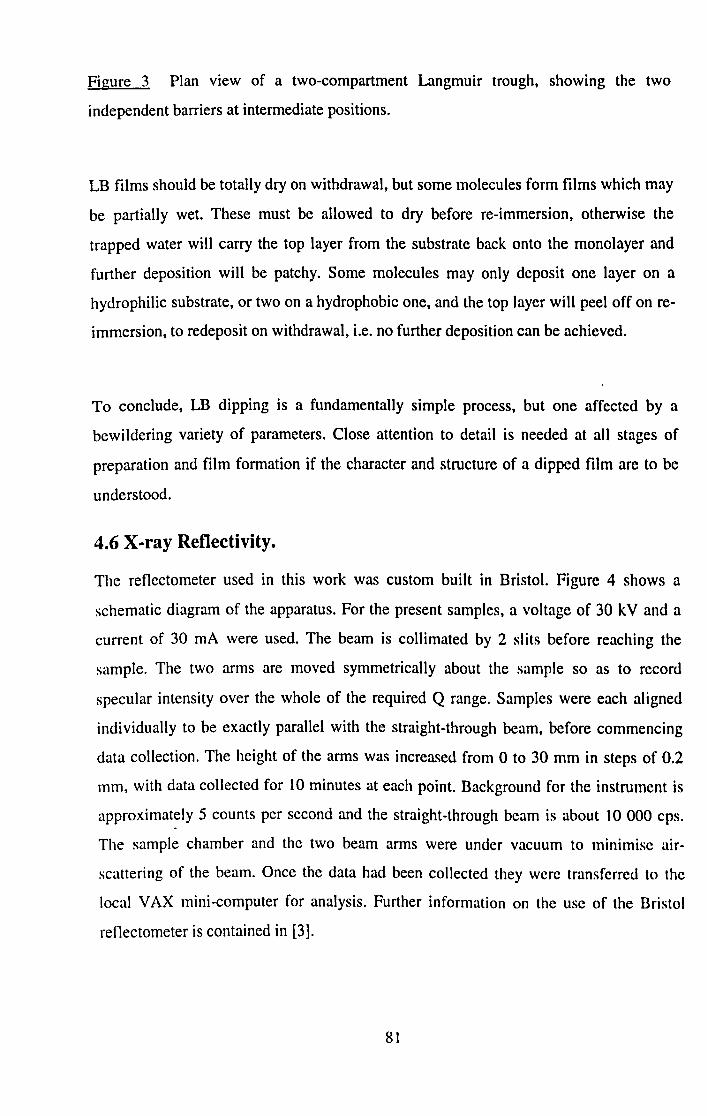
Figure 3 Plan view of a two-compartment Langmuir trough, showing the two
independent barriers at intermediate positions.
LB films should be totally dry on withdrawal, but some molecules form films which may
be partially wet. These must be allowed to dry before re-immersion, otherwise the
trapped water will carry the top layer from the substrate back onto the monolayer and
further deposition will be patchy. Some molecules may only deposit one layer on a
hydrophilic substrate, or two on a hydrophobic one, and the top layer will peel off on re
immersion, to redeposit on withdrawal, i.e. no further deposition can be achieved.
To conclude, LB dipping is a fundamentally simple process, but one affected by a
bewildering variety of parameters. Close attention to detail is needed at all stages of
preparation and film formation if the character and structure of a dipped film are to be
understood.
4.6 X-ray Reflectivity.
The reflectometer used in this work was custom built in Bristol. Figure 4 shows a
schematic diagram of the apparatus. For the present samples, a voltage of 30 kV and a
current of 30 rnA were used. The beam is collimated by 2 slits before reaching the
sample. The two arms are moved symmetrically about the sample so as to record
specular intensity over the whole of the required Q range. Samples were each aligned
individually to be exactly parallel with the straight-through beam, before commencing
data collection. The height of the arms was increased from 0 to 30 mm in steps of 0.2
mm, with data collected for 10 minutes at each point. Background for the instrument is
approximately 5 counts per second and the straight-through beam is about 10 000 cps.
The sample chamber and the two beam arms were under vacuum to minimise air
scattering of the beam. Once the data had been collected they were transferred to the
local V AX mini-computer for analysis. Further information on the use of the Bristol
reflectometer is contained in [3].
81
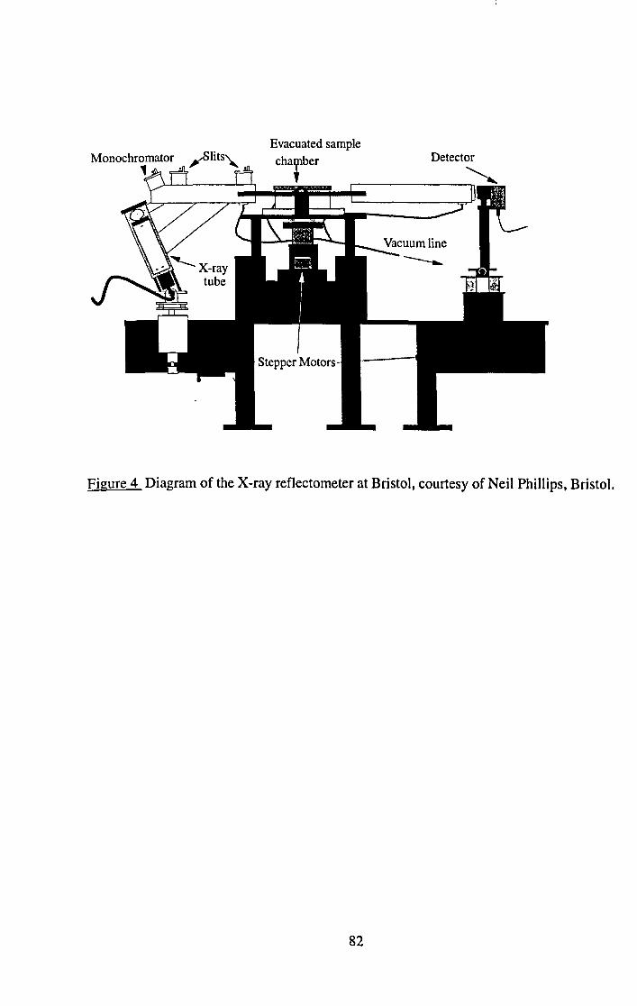
Monochromator , Evacuated sample
Charber
~-~-;=
Detector
Figure 4 Diagram of the X-ray refiectometer at Bristol, courtesy of Neil Phillips, Bristol.
82

4.7 Neutron Reflectivity.
If a beam of protons is fired at a tantalum or uranium target, neutrons are produced with
high energies and hence very short wavelengths. At the Rutherford Appleton Laboratory,
UK, the pulsed neutron spallation source, ISIS, directs these neutrons at a variety of
instruments which are used to study atomic and molecular structure. The moderator used
by each instrument determines the wavelengths available to it. For the two reflectometers
used in this work, CRISP [4] and the new instrument SURF [5], the moderator is liquid
hydrogen (25K) and the beamlines have a wavelength range of 0.5 - 6.5 A. when a 50Hz
chopper is used. Since the beam is white, the sample does not need to be moved during
an experiment. The pulsed nature of the beam means that the time-of-flight of the
neutrons enables their energy, and hence their wavelength, to be calculated. Slow
neutrons are removed from the beam using a chopper and a frame-overlap mirror, thus
preventing them from overlapping with neutrons in the next pulse. The beam is
collimated using two slits before the sample, and off-specular neutrons are eliminated by
two slits after the sample (not shown in Figure 5). The widths of these slits must be
adjusted for each incident angle to ensure that the experimental resolution remains
constant throughout the experiment. The reflected beam is normalised against the
incident beam to obtain reflectivity values. Figure 5 shows a generic diagram of a
reflectometer at the Rutherford Appleton Laboratory (RAL). In practice, for LB film
systems there is very little difference between CRISP and SURF and the use thereof.
83

B
~ I ~--~
·s I
Figure 5 Diagram of a neutron reflectometer at RAL. C is the chopper, B the beryllium
filter, J the coarse collimating jaws, S 1, S2 the collimating slits, F the frame overlap -
mirrors, R the downstream collimation, M the neutron beam monitor, S the sample and
D the He detector. Diagram courtesy of RAL.
Each sample is aligned individually on the sample changer before starting data
collection. In order to sample the whole Q range, data must be collected at several
different incident angles. For LB films these are typically 0.25°, 0.6° and 1.5°, giving a Q
range of 0.008 - 0.6 A-I. Once collected, data must first be reduced and normalised with
respect to the incident beam, and subsequent analysis was done either on the computers
at RAL or locally in Bristol. Details of the data analysis are given in Chapters 5 and 6,
the relevant theory having been discussed in Chapter 3.
84
4.8 References
[1] G. L. Gaines, Monolayers at Liquid-Gas Interfaces, p.46 (Wiley, New York, 1966).
[2] M. F. Daniel, J. C. Dolphin, A. J. Grant, K. E. N. Kerr and G. W. Smith, Thin Solid
Films, 133,235 (1985).
[3] A. Zarbakhsh, Instructions for Using the Bristol X-ray Reflectometer, 1995.
[4] J. Penfold, R. C. Ward and W. G. Williams, J. Phys E, 20, 1411 (1987).
[5a] D. G. Bucknall, J. Penfold, J. R. P. Webster, A. Zarbakhsh, R. M. Richardson, A.
Rennie, J. S. Higgins, R. A. L. Jones, P. Fletcher, R. K. Thomas, S. Roser and E.
Dickinson. "SURF - A Second Generation Neutron Reflectometer". Paper presented at
the 13th Meeting of the International Collaboration on Advanced Neutron Sources,
Switzerland, October 11th - 14th, 1995.
[5b] 1. Penfold, R. M. Richardson, A. Zarbakhsh, J. R. P. Webster, D. G. Bucknall, A. R.
Rennie, R. A. L. Jones, T. Cosgrove, R. K. Thomas, J. S. Higgins, P. D. I. Fletcher, E.
Dickinson, S. J. Roser, I. A. McLure, A. R. Hillman, R. W. Richards, E. J. Staples, A. N.
Burgess, E. A. Simister and J. W. White, J. Chern. Soc. Faraday Trans. 93, 3899 (1997).
85

Chapter 5. Simple Fatty Acid Films.
5.1 Introduction.
This chapter describes the work done with simple fatty acids, and illustrates the
importance of dipping conditions in determining the quality and structural integrity of an
LB film. It also illustrates the inadequacies of using over-simplified modelling
approaches to analysing the data and describes the evolution of a satisfactory model to fit
the data more completely than has hitherto been achieved for LB films.
5.2 Experimental.
As mentioned in Chapter 2, section 2.3, a total of seven parameters were varied
independently: dipping speed, dipping pressure, position of labelled layer. subphase pH,
temperature and ions, and time under water. Table 1 lists the samples prepared for this
part of the work. All were examined by both neutron and X-ray reflectivity, with the
exception of S8 and S9 which were prepared on nickel substrates for instrument
scientists at ISIS studying polarised neutrons. They are mentioned here simply for the
sake of completeness. In addition, due to time constraints at ISIS there are no neutron
data for samples S5 and S6, although the structure of S5 was repeated at a later date as
S 12. The polymer referred to as P in Table 1. illustrated diagrammatically in Figure 1,
was used in this work with the aim of linking in to previous work done by Dr
Richardson's group. [1]
All samples were dipped onto silicon wafer substrates, prepared as described in Chapter
4, Section 4.2.3. The subphase used was 18 Mil water, with the pH adjusted to pH -3
and at ambient temperature, Le.I7-I9°C, with the following exceptions:
S 10 and S 11 were dipped over a subphase containing 2 x 10⁻⁴ M cadmium chloride at
pH 6.3. S6, SI4 and SI5 were left underwater for to minutes between the downstroke
and upstroke of the deuterated bilayer. S24 was dipped over a subphase at 30°C.
86

Sample number Structure Dipping pressure, Dipping speed,
mN/m. mm/min
SI HHDHH 40 15
S2 HHHHD 40 15
S3 HHDHH 30 5
S4 HHHHDHHHH 40 15
S5 . HHDHH 40 15
S6 HHHHDHHHH 40 15
-S7 DHHHH 40 15
S8 (Ni) HHHHD 40 15
S9 (Ni) DHHHH 40 15
SlO HHHHD 40 15
S 11 DHHHH 40 15
S12 HHDHH 40 15
S13 HHHHDHHHH 35 15
S14 HHDHH 35 15
S15 HHHHDHHHH 35 15
S16 HHDHH 40 5
S17 HHDHH 30 15
... cont.
87
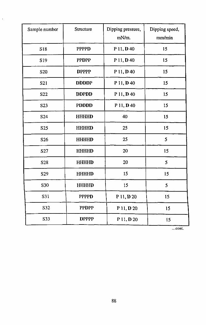
Sample number Structure Dipping pressure, Dipping speed,
mN/m. mm/min
S18 PPPPD P 11, D40 15
S19 PPDPP P II, D 40 15
S20 DPPPP Pll,D40 15
S21 DDDDP P 11, D 40 15
S22 DDPDD P 11, D 40 15
S23 PDDDD P 11, D40 15
S24 HHHHD 40 15
S25 HHHHD 25 15
S26 HHHHD 25 5
S27 HHHHD 20 15
S28 HHHHD 20 5
S29 HHHHD 15 15
S30 HHHHD 15 5
S31 PPPPD P 11, D 20 15
S32 PPDPP P 11, D 20 15
S33 DPPPP P 11, D 20 15
... cont.
88
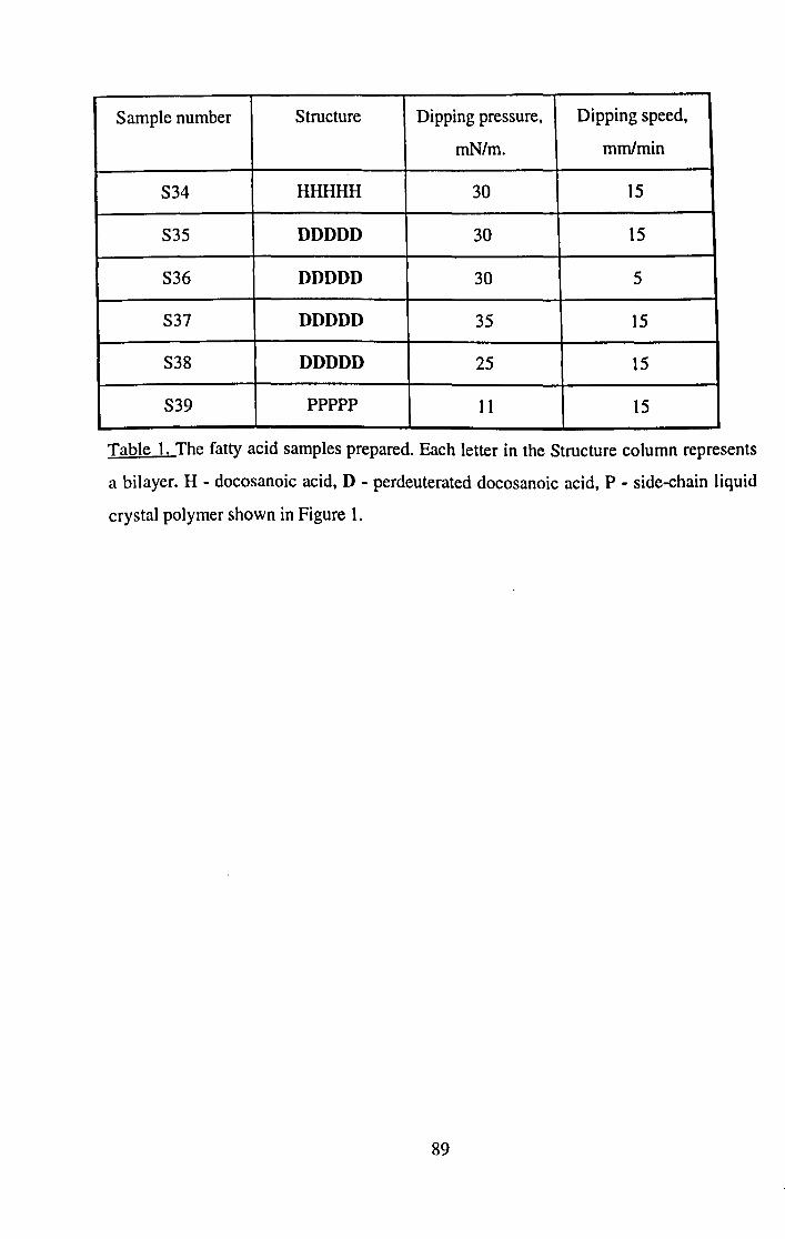
Sample number Structure Dipping pressure, Dipping speed,
mN/m. mm/min
S34 HHHHH 30 15
S35 DDDDD 30 15
S36 DDDDD 30 5
S37 DDDDD 35 15
S38 DDDDD 25 15
S39 PPPPP 11 15
Table 1. The fatty acid samples prepared. Each letter in the Structure column represents
a bilayer. H - docosanoic acid, D - perdeuterated docosanoic acid, P - side-chain liquid
crystal polymer shown in Figure 1.
89
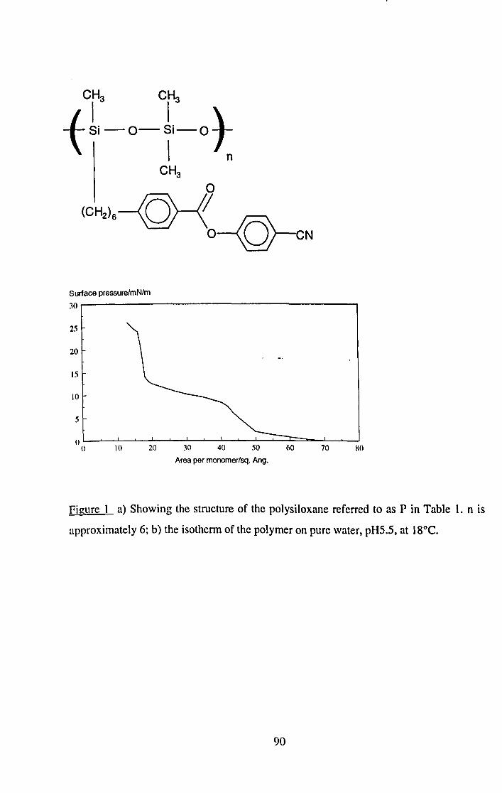
o
(CH,,)6---©---{ ~ O----Q-cN
Surface pressure/mN/m
JO
25
20
15
10
5
()L-~-L __ ~~~~ __ ~~~ __ ~~~~ __ ~~~
() 10 20 JO 40 50 60 70 HI)
Area per monomer/sq. Ang.
Figure 1 a) Showing the structure of the polysiloxane referred to as P in Table 1. n is
approximately 6; b) the isotherm of the polymer on pure water, pHS.S, at 18°C.
90

5.3 Modelling.
Reference [2] gives an excellent overview of the main problems encountered in fitting
reflectivity data. The discussion here will be restricted to those problems relating solely
to LB film-type structures.
The MULF multi-layer fitting routine in the Genie suite of programs at.ISIS was used
initially to try to fit the neutron data, but proved inadequate due to the limitations of the
slab-wise approach to SLD profiles. If the SLD of each slice is left to float
independently, there are not enough constraints available to keep the model within the
bounds of reasonable film and layer thickness and SLD values, given the known nature
of the LB films. MULF proved extremely cumbersome even for fitting the X-ray data,
where there is less complexity in the structure than with neutrons; again, it was difficult
to constrain the model to reasonableness. This is illustrated in Figure 2, which shows
clearly how limited the modelling is.
10
0.1
..: 001 ,;, '!: g t:
~ O.IXII
O.IXXII
o (KKKII
1l.(KKKXII
o
~f;. ... -; ~s -. -.- .. -.. .-.. +. -.. •• •• ;t:..#,.. -t.i"..!t .... ~+_ +.+ ~~~" •• .;. +! ~_.+ ~-.... ,;; + • + ~_ • + _.."..~ • ~ + + "to •
• -.;_.: -. : _:.: + :. .+-. "t+ -+ .~:. -.:- -+. . -. - . ...
- ----t-.------I--.-.---+___ I ---+----- -. .. ( (1.11~ 0.1 (US 0.2 1l2S 0\
MllIncnlum Irun~lcr. Q/A···I
I
(I\S
Figure 2a) Showing the best fit (solid line) obtainable using MULF to fit X-ray
reflectivity data for S2 (points) using a single-layer model. Errors are shown by the small
dashes above and below each data point.
91
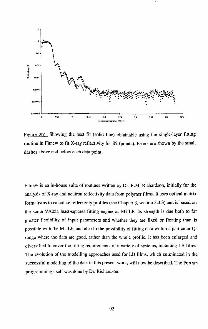
III
11.1
rr: 1101 ,;., ~ '9 t::
<i II.{KII
1I.(KlOl
II.IXlOIIl
II (KKKKlI
II 1105 0.1 0.15 0.2 0.25 0.) 0.4 0.45
Momenlum transfer. QlA •• -1
Figure 2b) Showing the best fit (solid line) obtainable using the single-layer fitting
routine in Fitnew to fit X-ray reflectivity for S2 (points). Errors are shown by the small
dashes above and below each data point.
Fitnew is an in-house suite of routines written by Dr. R.M. Richardson, initially for the
analysis of X-ray and neutron reflectivity data from polymer films. It uses optical matrix
formalisms to calculate reflectivity profiles (see Chapter 3, section 3.3.3) and is based on
the same V AOSa least-squares fitting engine as MULF. Its strength is due both to far
greater flexibility of input parameters and whether they are fixed or floating than is
possible with the MULF, and also to the possibility of fitting data within a particular Q
range where the data are good, rather than the whole profile. It has been enlarged and
diversified to cover the fitting requirements of a variety of systems, including LB films.
The evolution of the modelling approaches used for LB films, which culminated in the
successful modelling of the data in this present work, will now be described. The Fortran
programming itself was done by Dr. Richardson.
92

Using the same approach as Chapter 3, to facilitate comprehension the kinematic
approximation will be used to describe and illustrate the evolution of the model used in
this work. The Fitnew suite itself, as stated above, uses optical matrix methods
exclusively for the calculations and the results are, therefore, valid over the entire Q
range. Where the gaussian model was used, the number of discrete layers for the optical
matrix model was optimised to give a smooth variation in scattering length from step to
step without requiring excessive computer processing time. This was of the order of 100
layers for a 250A. thick film, i.e. each layer encompasses approximately two CHz units.
Typical times to run a model on the DEC Alpha VAX in the University of Bristol
Physics Department varied from one or two minutes to several hours, depending on how
many parameters were floating. Most of the models were chosen and set up so as only to
require computing times of the order of 2 - 5 minutes, since a large number of rapid
results such as these enabled faster solution overall than a few models floating several
parameters at once and waiting rather longer per model, as well as enabling the author to
maintain close control over the ranges of the parameters, given the known isotopic
composition of the films.
The first step was the introduction of a repeating nature within the model, enabling
hydrocarbon chains and headgroups to be more easily fitted. In addition, the percentage
of deuterated chain in each monolayer could be varied and floated. However, the model
still assumed that the deutero-Iayer was a definite slab, and so no satisfactory fits to
neutron data were obtained, although X-ray data were fittable with this model.
Having established that a slab approach did not allow close fitting of LB film neutron
reflectivity data, the next idea was to try to model the deutero-Iayer as a triangular
function in SLD. This looked promising and was made more realistic by using a gaussian
to describe the SLD profile around the deutero-Iayer and smaller gaussians to describe
the SLD profile of the headgroups. Figure 3 defines the parameters used and the
mathematics of the model are given below.
93

The equation for a gaussian curve has the general form
y=exp-(;~ ) (5.1)
where a is as defined in Figure 3 and is given below.
Where a gaussian of width a is used to approximate a block function of width d, the
relationship between their respective widths is gi~en by
NBSUB
d a---- J12
DSUB
(5.2)
DTOT
NBAIR=O.O
....... L
Figure 3a) Schematic diagram defining the parameters used in the gaussian model for
fitting LB film reflectivity data. NBSUB is the SLD of the substrate, NBHF is the SLD
of the non-deuterated component of the film, DSUB is the distance from the substrate to
the centre of the gaussian, DTOT is the total thickness of the film and a, is the
parameter for the width of the gaussian.
94

NBSUB
OMON ah
.. 7-............ : .. : ... /NBAIR = 0.0 . -.......... .....
Figure 3b) Schematic diagram defining the parameters used to model the headgroups.
NBSUB and NBHF as in Figure 3a). DMON is the monolayer height, i.e. half the Bragg
repeat distance. O'h is the parameter describing the width of the gaussians representing
the headgroup regions. This model is superimposed on the one in Figure 3a) to give a
full description of the structure of the LB film.
First define the SLD profile of the film, p(z):
p(z) = pas t [1 - H(z)] + PH (z) + Po (z) (5.3)
where
POs is the SLD of the substrate
t [1 - H(z)] is the Heaviside function describing the drop in SLD between the substrate
and the LB film
PH (z) is the SLD of the non-deuterated part of the film, calculated in two parts as
follows:
If there is no scrambling and the H-film is pure, PH (z) is given by
(2.bH ) 1
PH(Z) = A x OMON
where
:EbH is the sum of scattering lengths for the H-molecule and
A is the area per molecule within the film.
(5.4)
If some of the H-molecules have been displaced by D-molecules, PII (z) is given by
95

(~bH) {I 1 ((z- d)2 J~ PH (Z) = A x DMON crJ2i exp - 2cr- If (5.5)
where d is the position of the maximum of the gaussian in the z-direction.
Po (z) is the SLD of the deuterated part of the film, and is given by
(5.6)
where l:bo is the sum of scattering lengths over the D-molecule and
S(z-d) is the delta-function at the centre of the gaussian.
Hence
(5.7)
and p(z) is given by
(5.8)
~bD-~bH The term A is denoted by B_A in the parameter lists and is the quantity that
determines the area under the gaussian.
1 The term _ r;:;:: is required to keep the area under the gaussian constant for a particular
Chf21t
fit, regardless of how cr changes in the course of that fit.
~bH 1 . h " The term ON IS t e SLD of the pure H-fllm and IS denoted by NBHF in the
A DM
parameter lists.
The reflectivity from this SLD profile is given by the kinematic approximation, as
follows:
96

167t2 I" 12 R(Q) == Q2 p(Q) (5.9)
where p(Q) denotes the one-dimensional Fourier Transform of p(z) and p(Q) is given
by
p(Q) == Jexp(iQz) p(z) dz (5.10)
Substituting for p(z) in the above integral, and using the standard result for the Fourier
Transform of a gaussian,
,,{ i} Lb (Q2d ) p(Q)==ps 27tO(Q)-7tO(Q)+ Q +Texp- -2- exp-iQd
(5.11 )
Using de Moivre's theorem, namely eiS = cosS + isinS,
(5.12)
Hence
(5.13)
The term p~7tO(Q) == 0 at Q > 0, giving
(5.14)
substituting for Ip(Qt in the equation for R(Q),
97

(5.15)
161t2 2 --4~P,:;"S is the substrate term
Q
(:b J exp - ( Q'o') is the monotonic term arising from the D-Iabelled layer
Ps Lb Q2crz , Qd' h d 'b' h d d f' f h 2---exp ---sm IS t e term escn 109 t e ampe nnges rom t e Q A 2
interference between the substrate and the D-Iayer.
A further refinement was the two-sided gaussian model, where the deutero-layer is
de~cribed by a non-symmetrical function consisting of two half-gaussians of the same
height and the headgroup gaussians are again superimposed. Figure 4 shows the extra
definitions introduced, This proved much better for the acid-amine data discussed in
Chapter 6, where the deutero-Iayer was deposited as a single monolayer, but still did not
give close fits over the whole Q-range for samples with the deuterated material deposited
as a bilayer. For these samples, the two-sided gaussian model proves somewhat
insensitive to whether a. or a2 is the larger, unless 'the difference in size i~ greater than
8 - loA, and so the symmetrical gaussian model has been used for preference, except for
those samples where the D-Iayer is at the air-film interface. In the case of these, a2 was
fixed at a value representing one monolayer while a. was floated independently.
98
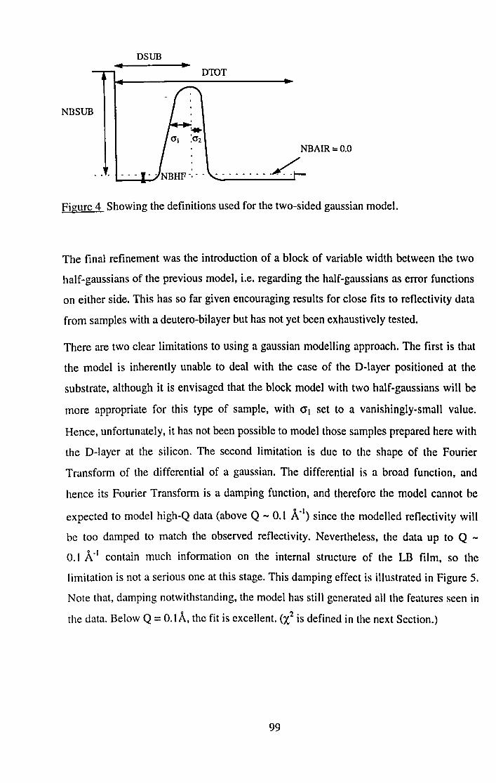
DSUB
DTOT
NBSUB
NBAIR=O.O
......... L Figure 4 Showing the definitions used for the two-sided gaussian model.
The final refinement was the introduction of a block of variable width between the two
half-gaussians of the previous model, i.e. regarding the half-gaussians as error functions
on either side. This has so far given encouraging results for close fits to reflectivity data
from samples with a deutero-bilayer but has not yet been exhaustively tested.
There are two clear limitations to using a gaussian modelling approach. The first is that
the model is inherently unable to deal with the case of the D-layer positioned at the
substrate, although it is envisaged that the block model with two half-gaussians will be
more appropriate for this type of sample, with 0'1 set to a vanishingly-small value.
Hence, unfortunately, it has not been possible to model those samples prepared here with
the D-Iayer at the silicon. The second limitation is due to the shape of the Fourier
Transform of the differential of a gaussian. The differential is a broad function, and
hence its Fourier Transform is a damping function, and therefore the model cannot be
expected to model high-Q data (above Q - 0.1 A·I) since the modelled reflectivity will
be too damped to match the observed reflectivity. Nevertheless, the data up to Q -
0.1 A· I contain much information on the internal structure of the LB film, so the
limitation is not a serious one at this stage. This damping effect is illustrated in Figure 5.
Note that, damping notwithstanding, the model has still generated all the features seen in
the data. Below Q = 0.1 A, the fit is excellent. (X2 is defined in the next Section.)
99
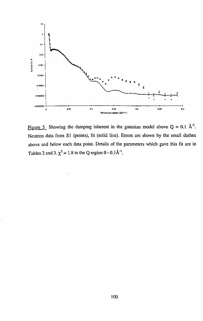
Itl
01
001
~
>, .:
~ U(KII
c f},
U (KKlI
U(KKKII
(HKKKKlI
UJKKX'OOI U
Figure 5 Showing the damping inherent in the gaussian model above Q = 0.1 A-I.
Neutron data from S I (points), fit (solid line). Errors are shown by the small dashes
above and below each data point. Details of the parameters which gave this fit are in
Tables 2 and 3. X2 = 1.8 in the Q region 0 - O.IA-I.
tOO

5.4 Results.
5.4.1 X-ray and Neutron Results.
The X-ray data were fitted using the single-layer option in the Fitnew suite, to keep the
models extremely simple and therefore extract the required information more easily. The
. details of the large-scale structure of the films, such as the total thickness DTOT and the
mean electron density NBHF, are contained in the low-Q part of the reflectivity profile,
owing to the reciprocal relationship between Q and feature size. Thus DTOT and NBHF
may be extracted by fitting X-ray data in the Q region 0.0 to 0.1 A-I.
The neutron data were fitted over the same Q-range, for the reason discussed at the end
of the previous section. The symmetrical gaussian model was used to extract information
on DSUB and neutron B_A.
Examples of the quality of fit obtained are shown in Figures 6 and 7 for X-ray data and
Figures 8 and 9 for neutron data. DTOT values are shown in Table 2 along with DSUB
values, while X-ray NBHF and neutron B_A values are shown in Table 3, along with the
film densities calculated therefrom.
The errors quoted in the tables are a measure of confidence in the fits - if a small change
in a particular parameter causes the quality of the fit (as measured by the least-squares
method) to deteriorate significantly, the confidence in that fit is high and the error
concomitantly low. This may be rephrased as the contours around that particular
minimum in solution space being very steep, increasing the confidence in that minimum
being a global one for the sample concerned. Conversely, if a small change in a
parameter has no significant effect on the quality of the fit then confidence in that fit is
low and the error large - the minimum in solution space is shallow and broad and
therefore unlikely to be global. For comparison, y} values are given for each fit in the
•• ., • ~)observed - expecled)l respectIve fIgures. X- IS the value of number 01 dala POIOIS • For a perfect fit between model
., and data, X-= 1.
101

10
11.1
'" OOI
~ .~
~ IUKII
- .......... .,.:~~ ~~ +~ __ ;~4+~ __ -:;-_~ ; -.-_
•• -- -.. -. +. • 1I.IKIIJIlI +
+
O.IKKXKII -I----+----+---+----+----+---+----+---~--~ o 11.05 0.1 11.15 0.1 IUS lI.l 0.4 0.45
Mlllnentum tramter. 01"·· .. 1
Figure 6 Showing the high quality fit (solid line) obtained using a single-layer model,
for the X-ray data from S14 (points). X2=13.5. Errors are shown by the small dashes
above and below each data point.
102

10
I ""' ... ~ ...
0.1
'" lUll > . . ,. .~ <= ;z O.IKII
o (KKlI
• + ••••• ... -..... _. - ..... _.. .... ... ._ •• +.+-_ •• -+- .. -++++- ~i-_. ! .:- .+ __ ..... -+ .... +..,. +' +""._' ••
• • + • - • ...+ .. .. + • + IUKKMII
• + •
o (OKlO I
0 0.05 0.1 0.15 0.1 0.15 0.3 0.35 0.4 0.45
Mumentum transfer, QlA"-1
Figure 7 Showing the best fit obtained (solid line) using a single-layer model for X-ray
data for S23 (points). Note how poor alignment has resulted in poor data around Qc , and
how this has been prevented from being a problem by de-emphasising the data in that
region within the model. X2=21.8. Errors are shown by the small dashes above and below
each data point.
103
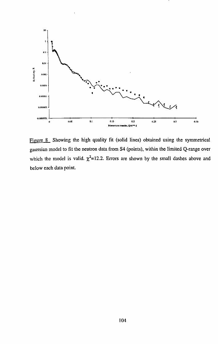
10
01
lUll
'" ,;.
.~ OIMII
'" (:;.
O.IMXII
OIXXXII
O.IMXXlOI
O.lOMXlOI
0 Il.IIS 0.1 O.IS 0.1 lI.l~ lI.l O.l~
Figure 8 Showing the high quality fit (solid lines) obtained using the symmetrical
gaussian model to fit the neutron data from S4 (points), within the limited Q-range over
which the model is valid. X2=12.2. Errors are shown by the small dashes above and
below each data point.
104
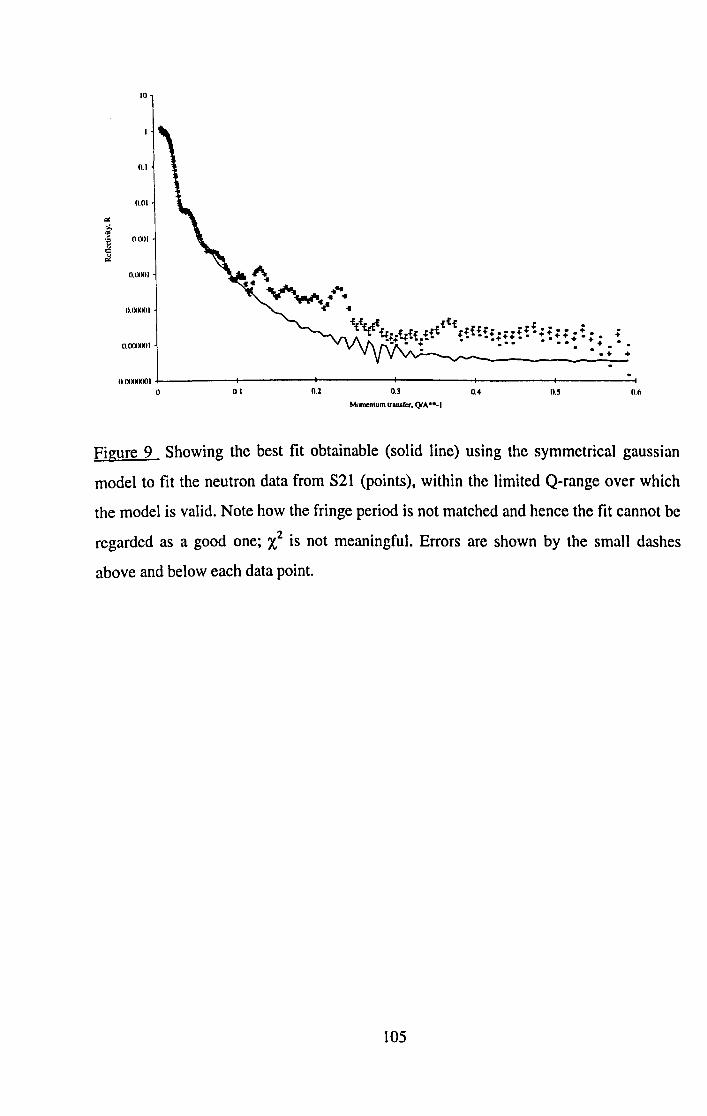
III
11.1
11.(1I .. i-." II IX) I 'il c /i.
1I.IXXlI
II.lXXXII
1I.IXXXXlI
II OtXXXIOI II 01 0.2 0.3 11.4 II.S o.~
M<.llentum tr .... rer. QI A 00·1
Figure 9 Showing the best fit obtainable (solid line) using the symmetrical gaussian
model to fit the neutron data from S21 (points), within the limited Q-range over which
the model is valid. Note how the fringe period is not matched and hence the fit cannot be
regarded as a good one; X2 is not meaningful. Errors are shown by the small dashes
above and below each data point.
105
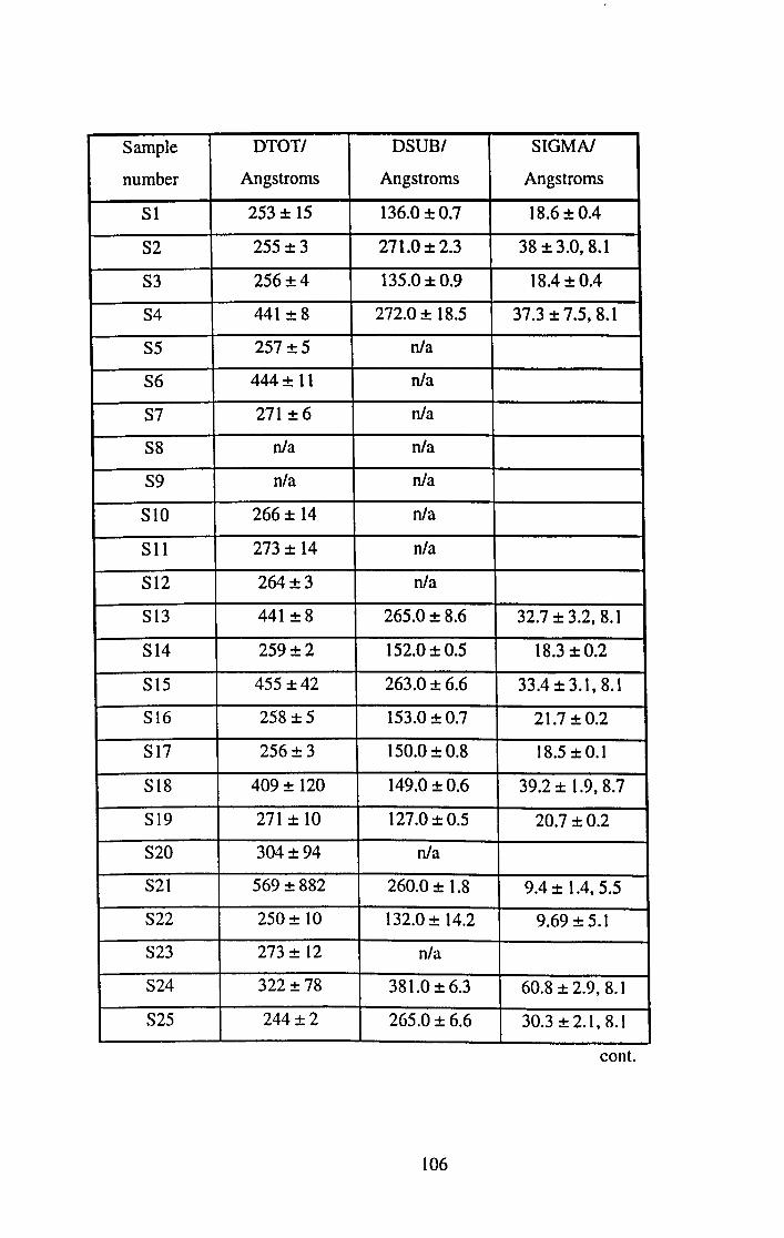
Sample DTOTf DSUBf SIGMN
number Angstroms Angstroms Angstroms
SI 253 ± 15 136.0 ±0.7 18.6 ± 0.4
S2 255 ±3 271.0 ±2.3 38 ± 3.0,8.1
S3 256±4 135.0 ± 0.9 18.4 ± 0.4
S4 441 ±8 272.0 ± 18.5 37.3 ± 7.5,8.1
S5 257 ±5 nla
S6 444± 11 nla
S7 271 ±6 nla
S8 nla nla
S9 nla nfa
SIO 266 ± 14 nfa
Sll 273 ± 14 nfa
S12 264±3 nla
SI3 441 ± 8 265.0 ± 8.6 32.7 ± 3.2, 8.1
S14 259±2 152.0±0.5 18.3 ± 0.2
S15 455 ±42 263.0± 6.6 33.4 ± 3.1, 8.1
S16 258±5 153.0 ± 0.7 21.7 ± 0.2
SI7 256±3 150.0 ± 0.8 18.5 ± 0.1
SI8 409 ± 120 149.0 ±0.6 39.2 ± 1.9, 8.7
SI9 271 ± 10 127.0 ± 0.5 20.7 ±0.2
S20 304 ± 94 nfa
S21 569 ± 882 260.0 ± 1.8 9.4 ± 1.4, 5.5
S22 250 ± 10 132.0 ± 14.2 9.69 ± 5.1
S23 273 ± 12 nfa
S24 322 ± 78 381.0 ± 6.3 60.8 ± 2.9,8.1
S25 244±2 265.0 ± 6.6 30.3 ± 2.1, 8. I
cont.
106

Sample DTOTI DSUBI SIGMN
number Angstroms Angstroms Angstroms
S26 253±3 277.0 ± 13.0 35.6 ± 4.3,8.1
S27 253 ±6 256.0±0.7 27.3 ± 0.2,8.1
S28 244±5 263.0 ± 1.2 30.6 ± 0.5, 8.1
S29 nla 227.0 ± 1.0 32.4 ± 0.7,8.1
S30 266±4 248.0 ± 1.3 32.1 ± 0.5, 8.1
S31 312±9 141.0 ± 0.4 25.0 ± 1.3, 8.1
S32 298±6 131.0 ± 0.4 18.5 ±0.06
S33 407 ±209 nla
S34 258±2 n/a
S35 246±2 n/a
S36 256±3 nla
S37 253 ±5 nla
S38 243 ± 10 n/a
S39 247 ± 10 nla
Table 2. DTOT values from fits to the X-ray data and DSUB and SIGMA values from
fits to the neutron data. Where two values are given in the SIGMA column, the two
sided gaussian model was used; otherwise the symmetrical gaussian model was used.
Where no error is quoted in SIGMA, the value was fixed during the fit.
107

Sample number X-ray NBHFI x Coverage Neutron B_AI Coverage
10-5 A-2• determined by x 10-;\ A· I . determined by
X-rays/% neutrons/%.
SI 0.893 ± 0.391 79±35 0.339 ± 0.002 75.7 ± 0.4
S2 0.865 ± 0.049 76±4 0.353 ± 0.002 78.8 ±0.4
S3 1.07 ±0.394 95 ±35 0.331 ± 0.002 73.9 ±0.4
S4 0.915 ± 0.122 81 ± 11 0.372 ± 0.007 83.0±2
S5 1.17 ± 0.200 103 ± 18 n/a
S6 1.21 ± 0.322 107 ±28 n/a
S7 1.70 ± 0.084 150±7 n/a
S8 n/a n/a
S9 n/a n/a
SlO 1.30 ± 0.471 103 ± 37 n/a
Sl1 1.71 ± 0.133 136 ± 11 n/a
S12 0.830 ± 0.037 73 ±3 n/a
S13 1.22 ± 0.127 108 ± II 0.453 ± 0.006 101.1 ± 1.0
S14 1.08 ± 0.050 96±4 0.358 ± 0.001 79.9±0.2
SIS 1.23 ± 0.590 109 ±52 0.407 ± 0.004 90.8 ±0.9
S16 1.14 ± 0.184 101 ± 16 0.442 ± 0.002 98.7 ± 0.4
S17 1.01 ± 0.064 89±6 0.417 ± 0.002 93.1 ± 0.4
S18 1.65 ±0.062 169±6 0.254 ± 0.002 127.6 ± 1.0
S19 1.32 ± 0.965 135 ± 99 0.275 ± 0.001 138.2 ± 0.5
S20 2.17 ± 0.195 223 ±20
S21 1.69 ± 0.159 155 ± 15 -0.079 ± 0.003 39.7 ± 1.5
S22 1.33 ± 0.251 122 ± 23 -0.459 ± 0.00 I 230.6 ±0.5
S23 2.02 ± 0.174 185 ± 16
S24 1.35 ± 0.099 119 ± 9
... cont.
to8
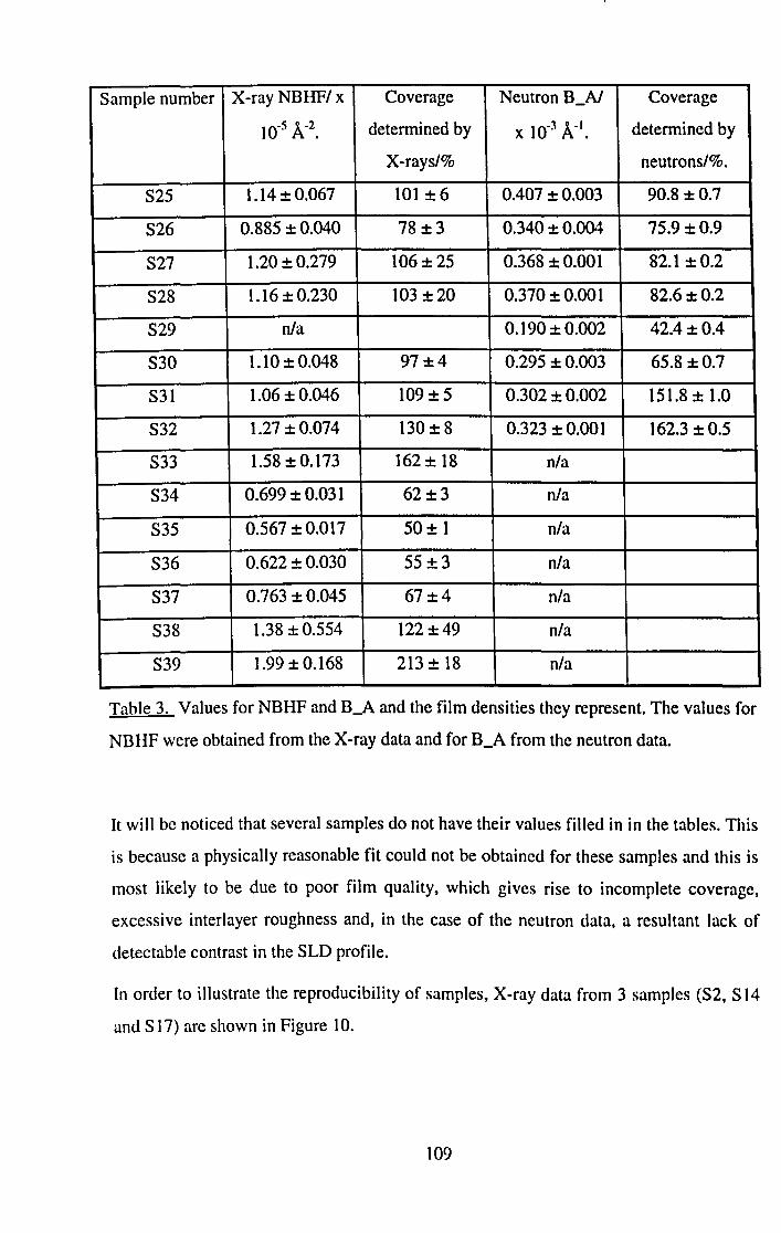
Sample number X-ray NBHFI x Coverage Neutron B_N Coverage
10-5 A-2• determined by x 10-3 A-I. determined by
X-rays/% neutrons/%.
S25 1.14 ± 0.067 101 ±6 00407 ± 0.003 90.8 ±0.7
S26 0.885 ± 0.040 78 ±3 0.340 ± 0.004 75.9 ±0.9
S27 1.20 ±0.279 106 ± 25 0.368 ± 0.001 82.1 ±0.2
S28 1.16 ± 0.230 103 ± 20 0.370 ± 0.001 82.6±0.2
S29 n/a 0.190 ± 0.002 42.4 ±0.4
S30 1.10 ±0.048 97±4 0.295 ± 0.003 65.8 ±0.7
S31 1.06 ±0.046 109±5 0.302 ± 0.002 151.8 ± 1.0
S32 1.27 ±0.074 130±8 0.323 ± 0.001 162.3 ± 0.5
S33 1.58 ± 0.173 162 ± 18 n/a
S34 0.699 ± 0.031 62±3 n/a
S35 0.567 ± 0.017 50± 1 n/a
S36 0.622 ± 0.030 55 ±3 n/a
S37 0.763 ±0.045 67±4 n/a
S38 1.38 ±0.554 122 ±49 n/a
S39 1.99 ± 0.168 213 ± 18 n/a
Table 3. Values for NBHF and B_A and the film densities they represent. The values for
NBHF were obtained from the X-ray data and for B_A from the neutron data.
It will be noticed that several samples do not have their values filled in in the tables. This
is because a physically reasonable fit could not be obtained for these samples and this is
most likely to be due to poor film quality, which gives rise to incomplete coverage,
excessive interlayer roughness and, in the case of the neutron data, a resultant lack of
detectable contrast in the SLD profile.
In order to illustrate the reproducibility of samples, X-ray data from 3 samples (S2, S 14
and S 17) are shown in Figure 10.
109

10
11.1
'" 11.111 ,:. .~
'B c (i II.lKII
II.IKKII
II.(KKIIJI
o o
II.OIKMKII
II 0.05 0.1 0.15 0.2 0.25 03 0.4 ou "menlum II'lInIifcr. QI A "·1
Figure 10 Showing the reproducibility of S2 (++++), S14 (-) and S17 (0000). X-ray
data.
A selection of neutron reflectivity profiles are shown in Figures 11 - 15. These show the
sensitivity of the technique to the effects of different dipping speeds (Figure 11),
different dipping pressures (Figure 12), the presence of cadmium ions (Figure 13), time
under water (Figure 14) and the position of the D-Iabelled layer (Figure 15). Figure 5 has
already illustrated the limitations of the gaussian model when data above Q = 0.1 A-I are
included in the fit, showing clearly how the calculated reflectivity is damped .
•
110

III
n.1
nO!
'" >. '1: nlKlI
~ <J.
nlKKII
+ + n.IKKXlI
+
1l.IXKXKlI
IlIKXXXXll
0 O.OS 0.1 O.IS 11.2 0.25 O.l Mtwnenlum trander, QlA·· ••
Figure 11 Neutron data from SI (+++) and S16 (-), showing the effect of dipping
speed. SI was dipped at 40mNm'! and 15 mmlmin; S16 was dipped at 40mNm'! and
5 mmlmin. Both sample structures HHDHH (nomenclature as in Table 1).
III
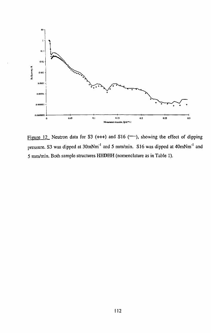
10
0.1
001
'" ,;, ];
OIXH ij 0:::
~
O.IXXH
+ OIXNXII +
o IXNXXH
O.lXXXXlOl
0 11.115 0.1 0.15 II,Z IUS lI,l
Mumenlum Ir ... rcr, QlAoo_1
Figure 12 Neutron data for S3 (+++) and S16 (-), showing the effect of dipping
pressure. S3 was dipped at 30mNm-1 and 5 mmlmin. S] 6 was dipped at 40mNm-1 and
5 mmlmin. Both sample structures HHDHH (nomenclature as in Table ]).
112
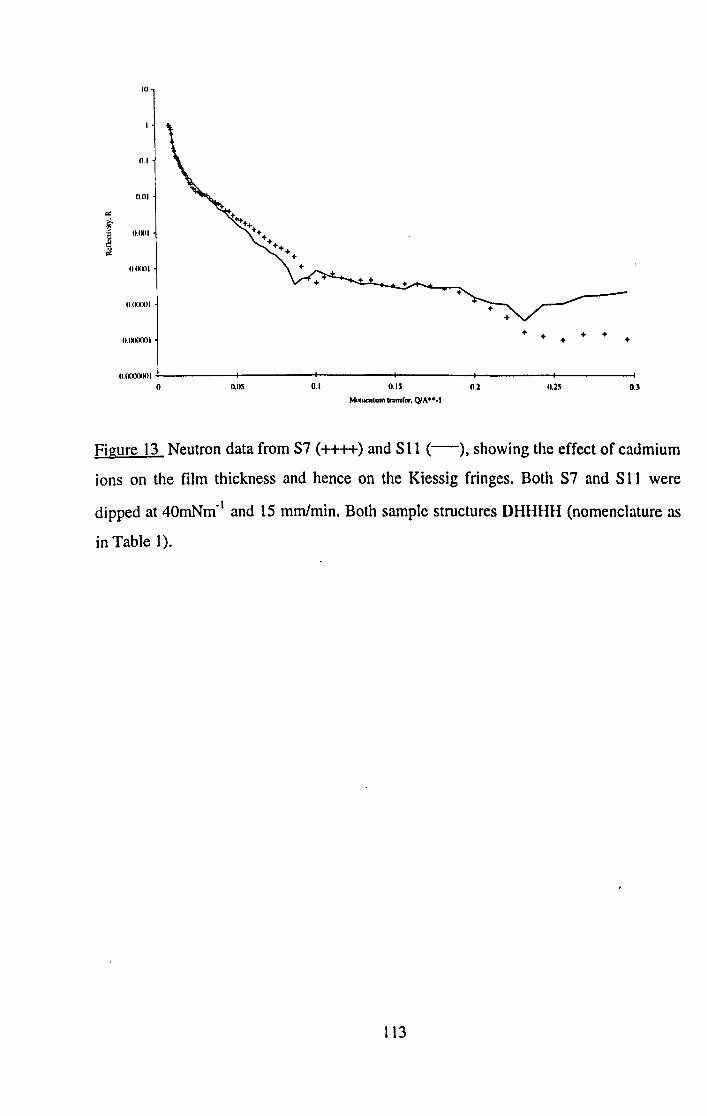
III
0.1
lUll
'" ;;, ''e O.IXII 'il c::: <l.
OIXXIl
+ +
OIXXXIl
O.IXXXlOI + + + + + +
O.IXXKXXII
0 O.OS 0.1 O.IS 0.1 II.~ 0.3
M< .. 1Chlum I",ml .. , QlA**-1
Figure 13 Neutron data from S7 (++++) and S11 (-), showing the effect of cadmium
ions on the film thickness and hence on the Kiessig fringes. Both S7 and S 11 were
dipped at 40mNm-1 and 15 mmlmin. Both sample structures DHHHH (nomenclature as
in Table 1).
113

10
0,1
001
'" ;;., .~
O,IMII ii c iJ.
O.lMMIi
OIKKMII
O,IMKMXlI + ++
O.lMMMOIi
0 0,1 0,1 0,3 0,4 0,5
Ml.lInenlurn tranarcr, QlA···l
Figure 14 Neutron data from S13 (+++) and S15 (-), showing the negligible effect of
time underwater on intensity or fringe spacing. Both S 13 and S 15 were dipped at
35mNm-1 and 15 mm/min; S 15 was left under water for 10 minutes between dipping.the
two deuterated monolayers. Both sample structures HHHHDHHHH (nomenclature as in
Table 1).
t 14
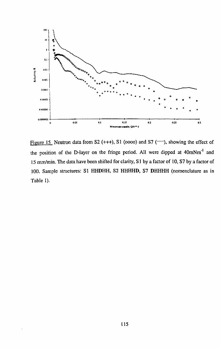
n.1
~ nOI ,:, ~ 'g <: (I.IKlI ;;. 0 0
0 0 0
0 0
(I.IKKII
(lIKKKlI
+ ++++++ 0
+ + + + + + + 0
0 + +
0 0 0 0 + 0
+
(lIKKlIKlI + + + +
+ +
(I.IKKKIOOI (I OOS 0.1 O.IS 0.2 (I.2S 0.1
Munten1urn tranlrer, QlA ···1
Figure 15 Neutron data from S2 (+++), SI (0000) and S7 (-), showing the effect of
the position of the D-layer on the fringe period. All were dipped at 40mNm-1 and
15 mm/min. The data have been shifted for clarity, SI by a factor of 10, S7 by a factor of
100. Sample structures: S 1 HHDHH, S2 HHHHD, S7 DHHHH (nomenclature as in
Table 1).
115
5.4.2 Surface Potential Measurements.
Section 4.4 outlined the basics of the experimental procedure required for surface
potential ('II) measurement. Further details of the experiment performed are given here.
A very simple experiment was carried out, to investigate whether any extra information
about monolayer states could be gleaned from a study of 'II at various values of 1t. A
monolayer of docosanoic acid was spread on pure water, pH3, 20°C. It was compressed
to 25mN/m and left there for approximately 35 minutes, with the Control setting keeping
1t constant, and'll was monitored throughout on the x-y-t plotter. The monolayer was
then compressed to 30mN/m and again'll was recorded for 35 minutes. Finally, it was
compressed to 40mN/m and 'II was again recorded for 35 minutes. The layer was very
stable in 1t for each of these measurements, but distinct differences may be observed in
the 'II-traces. Due to the nature of the data record, a photocopy of the plotter traces is the
clearest way of presenting the results, and this is shown in Figure 16.
116
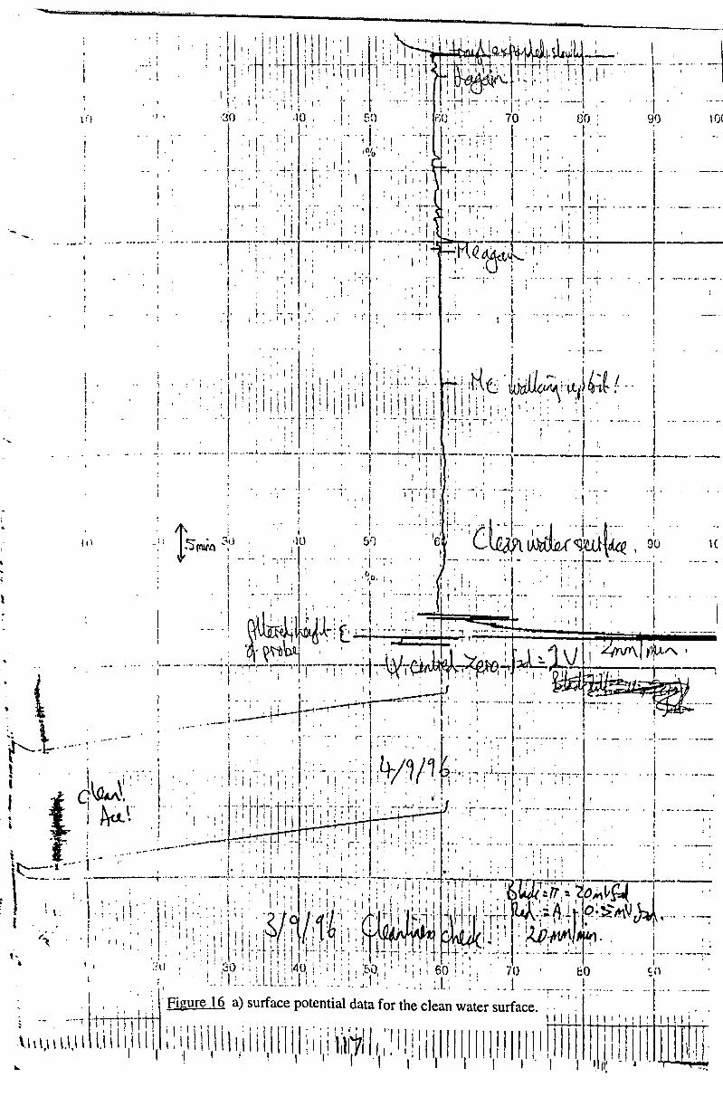
'-
1
. .. . __ ..
, I j , ! . j
, . .•• : i
, , . ; ..
',' ~
I I I,
I : I' I
. -~ .--.. , . 1-
1C
i ._--.. __ ._-I'
• I ,

, . ,
, t
.1.
· .. ' - I : ' : : !
" Figure 16 b) surface potential data for the monolayer at the various surface pressures .' discussed in the text.
__ I ., .
, : i
--1---

It will be seen that the signal from the clean water surface is very steady (Figure 16a), at
+200mV. Once the monolayer has stabilised at 25mN/m (Figure 16b), the \jI signal has
an average value of +250mV, with fluctuations of the order of ±lOmV, and the time
scale of these fluctuations is of the order of 30 - 60s. At 30mN/m, \jI is much steadier, at
+260 ± 5mV: with a time scale for the fluctuations of approximately 5 minutes. At
40mN/m, \jI has an average value of +240 ± 20mV, with a time scale for the fluctuations
of 1 minute.
These observations are readily understood in terms of the monolayer phases discussed in
Chapter 2 [4]. At 25mN/m, the monolayer is in the k' phase, where the chains are at an
angle of 15° and the monolayer is fluid, displaying Newtonian behaviour [5a-c]; it is
rapidly mobile, on a scale visible to the surface potential technique, which is in the 5mm
size range. At 30mN/m, the monolayer is just into the S phase: the chains are upright and
the film close-packed; its mobility is noticeably less in size terms, and slower in time. At
40mN/m, the monolayer is well into the S-phase and displays non-Newtonian flow
characteristics (Chapter 2, Section 2.2.3, [5a-cD; it is rigid and appears to be susceptible
to all vibrations, mirroring them with large and rapid fluctuations. Thus previous work
[4; 5a-c] is confirmed, lending support to these surface potential data. Therefore, this
simple and non-invasive technique provides a qualitative picture of the monolayer at
these three surface pressures, and this picture is consistent with the observations and
conclusions of previous workers.
119

5.5 Discussion and Conclusions.
5.5.1 Film Thickness.
The values for DTOT from the X-ray fitting were used to calculate layer thickness
(DMON) values for each all-acid sample, for comparison with the literature value. Given
that X-rays will not be sensitive to the outermost hydrocarbon layer, due to the low
electron density contrast with air, the DTOT values were taken to represent 9
monolayers, plus the headgroup region of the 10th• From CPK space-filling molecular
models, the headgroup region is measured to be 3.1A. Ten headgroups will therefore
account for 31A of DTOT, with the remainder representing 9 hydrocarbon chain regions.
The DTOT values from the all-H and all-D samples (S34 - S38) are very close within
their errors and yield a mean DTOT of 250.5A. This gives a value of 24.5A for each
chain, and hence 27.6A for each acid molecule, on average. The error in this value for
the length is OAA. Since the length of docosanoic acid is 30A [3], this implies the
molecules are tilted by 23 ± 2° from the surface normal. This is intermediate between the
L2 and k' phase tilts of 30° and 15°, respectively (see Chapter 2, section 2.2.2), and it is
clear that the film packing has relaxed from the S phase in the Langmuir film as a
consequence of the dipping process.
This value of 27.6A for DMON agrees very well with the values from the other samples,
as can be seen from Table 2, implying a good degree of reproducibility between samples
prepared under similar dipping conditions, and no appreciable differences in the packing
of those films which were prepared under different dipping conditions. This is to be
expected, given the samples were all dipped at pH3, where all the headgroups are fully
protonated and where the isotherm shows no phase change over the 1t-range used. The
exceptions are S29 and S30, which were dipped at 15mN/m. S29 could not be fitted, and
given the sample was dipped at 1t = 15mNm· I , the phase change on dipping will have
been from the L2' phase. What this packing would have changed to on the substrate is
120

not clear, although one probable conclusion is that the monolayer has become disordered
or has collapsed, and this would explain the inability to fit this particular sample.
S30 yielded anomalous values for DTOT and hence for Q~~f.~iY8IbtJHel~umJe
was also dipped at 7t = 15 mNm- l , although at a much .~l<>N\M~Qu{4 mtniPMONs
15 mm/min for S29) an element of disorder is again prob'lble.ml~rMmi~iI)g:.thftbllle
slower dipping speed used for S30 has apparently yielded aJdilbtb:t!\lP~libtlltlt . .
this very low 7t. Unfortunately, time did not allow for this d~~tioodCl"\Udd~fidain
more depth; this could be a fruitful experiment in the futuretle subs(rote~- and these are
These two results lend support to the conclusion that thel'thfbiMllyeY E~i~iIlp ~£tJhBn dipping. No firm conclusion can be inferred from the resullk fHfrH~~~tft;1sc~_~ dipped. at 30°C and 40 mNm- l . Even at this 7t, the monoUye<f~~iWbY [rlbge~aMaktRg dipping difficult and the data unreliable. At this tempedafreWt~~ m'6W&Pl§e~jf'Ui~e gone straight from ~ to S [4] with no ~' phase (see Fig.I'f7~~bU'ft~~YPe~li{h~s°Q,~llld
. ,~n) face of th~ Si Wilfers is have on the dipping behaviour is an unknown. Clearly, an apparent film thickness of
tuanlit~tiy~' ~omptuison with 322 ± 78 A is a meaningless result for a film nominally 276 ± 7 A thick, al1d some other
. . ,led here simply for- ease of mechamsm, most hkely severe disorder, must be involved.
Surface pressure/mN/m
60
50
40
30
20
10
~ Si wafers· used an' had the
\th sides. were, not used was
whereas wafers, polished on
Ite . n absolute value for the
r m y be observed in Table 4.
o L----'---IL...--'--~ _ _'_____'__...o...__..l.._"__.....L...___i:::..........I_ _ _UL~n· ~ubsequent dips. in () 5 10 15 20 25 30 35
Area per molecule/sq. Ang. It onwards.
., . . on the downstroke This is FIgure 17 The Isotherm of docosanOIc aCId on pure water, pH3, 30°C.
liter.1ture theorie..'l. disC't.lS.~ed
121
S 14 and SIS both yield values of DMON (28.4A and 26.6 A respectively) which, within
errors, show no appreciable deviation from the other samples, despite these two having
been left under water for 10 minutes between the down- and up-strokes of the D-Iayer
deposition. Thus, swelling of the films due to trapped water may be ruled out, as
confirmed by [6]. This is a surprising result in the light of the conclusions of previous
workers discussed in Chapter 2, Sections 2.3.2 and 2.4.1, but it is a very encouraging
observation for the present thesis.
Using the figure of 27.6A for the length of the acid in the film, the thicker samples (S4,
S6, S13 and SIS) would have an actual thickness of approximately 471A, and therefore
an expected X-ray DTOT of 446A. They are found to have actual X-ray DTOT values of
441,444,441 and 455A, respectively, giving a mean of 445 ± 17A, which is a very close
agreement between theory and practice. This suggests that the phase change on dipping
and the subsequent packing remain constant over several layers, which in tum suggests
that the structure of the LB film is determined at the point of dipping, rather than by any
later treatment of the film, such as time under water. It would be interesting to study still
thicker films in order to confirm this.
To calculate DMON for the polysiloxane shown in Figure 1, for comparison with the
value obtai~ed in [1], the X-ray value for DTOT from S39 (the all-polymer sample) was
taken to be the true thickness of the dipped film, yielding a value for the polysiloxane of
24.7 A, which compares favourably with the value from a Langmuir film of the molecule
in [1] of 17 - 28..\ over a 1t-range which includes the dipping pressure used here
(11 mN/m). This approach was taken due to the fact that the electron density of the
pendant chain regions of this molecule is much higher than that of a hydrocarbon chain
(X-ray SLD 1.69 x 10⁻⁵.-\"2, compared with 0.85 x 10⁻⁵ A-2 for a hydrocarbon chain) and
so the outermost layer is detected by the X-rays.
122
5.5.2 Film Density.
The expected values for X-ray NBHF and neutron B_A were calculated from molecular
structure and volume, using isotherm values for the area per molecule and the DMON
values calculated in the previous section. NBHF values for mixed films, i.e. those
incorporating P or D molecules, were calculated as a weighted average. These were then
used as one of the starting parameters in the fitting of each data set, and allowed to float
to give a measure of film density, i.e. of coverage of the substrate, and these are
tabulated in Table 3. Table 4 shows the relative amount picked up on each dip and the
total coverage, both in cm2, and the mean % coverage overall, for qualitative comparison
with the X-ray and neutron data. It must be stressed that these deposition ratio data can
only be used to compare sample with sample, or molecule type with molecule type. They
can in no way be said to represent actual coverage, due to the fact that deposition on the
rear (i.e. the ground and therefore macroscopically uneven) face of the Si wafers is
uncertain, and was not measured in this work. Therefore, quantitative comparison with
NBHF and B_A is not meaningful. The data are presented here simply for ease of
qualitative comparisons, which is perfectly valid since the Si wafers used all had the
same morphology. The reason why wafers polished on both sides were not used was
simply one of cost: single sided wafers cost only £5 each, whereas wafers polished on
both sides cost around £100 each. Unfortunately, insufficient funds were available to this
project to purchase one of the latter in order to investigate an absolute value for the
deposition ratio. It is to be hoped that this issue can be addressed by a future project.
Despite the caveat above, there are some general trends that may be observed in Table 4,
as follows:
a) deposition on the first downstroke is generally poorer than on subsequent dips, in
line with observations from other workers, from Blodgett onwards.
b) deposition is generally higher on the upstroke than on the downstroke This IS
extremely supportive evidence in favour of the various literature theories, discussed
123
in Chapter 2, on why scrambling occurs, suggesting as it does that, whilst individual
layers might be incomplete, holes in one layer are filled in by the subsequent layer.
c) the mean % coverage is frequently less than 100%, sometimes as much as SO% less,
but it does not greatly exceed 100%: the largest value observed here was 113%. This
is a very wide range of values, and even given the inherently qualitative nature of the
data, it suggests a wide range of film qualities should be expected.
d) the effect of increased temperature has had a very large effect on the dipping
behaviour of the monolayer in S24 (30°C).
e) on the whole, the polysiloxane does not deposit as effectively as the fatty acid,
presumably due to the differences in head-to-head interactions. It dips better on the
upstroke than on the downstroke, although the precise reason for this is not clear.
There are nine samples with errors in NBHF that are unreasonably large (>20%),
indicating that more parameters need to be floated to allow a fit to these samples with
any degree of confidence, or that a more sophisticated model than the Volume Fraction
one needs to be used. Alternatively, excessive disorder has resulted in extremely uneven
films. These nine samples are SI, S3, S6, SlO, SIS, S19, S22, S27 and S38, and they
will be discussed in Section S.S.4.
Of the remaining 30, all but seven show very good agreement between the neutron and
X-ray results. This is a very encouraging result in terms of further highlighting the
complementarity of the two techniques, and it justifies a high degree of confidence in
using data from one as starting points for the other. The discrepancies are most likely to
arise from interfacial roughnesses, especially at the air-film interface where the electron
density contrast is greatly reduced for a rough surface, thus increasing the error in the
X-ray fits. As already mentioned, this should be a solvable problem given greater use of
more flexible models, for all but the roughest films.
124

~~ I""Jll"""'"'''"'',',I'''I:''' ..... J"" "'r, •• "...,......." ~"f'
',',,,
Sample It 21 3! 41 5!
cm2 cm2 cm2 cm2 cm2
SI 44.6 100.4 92.1 96.2 86.5
S2 55.8 68.4 113.0 68.4 108.8
S3 54.4 72.5 97.7 92.1 104.6
S4 61.4 64.2 104.6 89.3 . 75.3
S5 61.4 108.8 78.1 75.3 108.8
S6 60 80.9 80.9 103.2 78.1
1IJ, 121 13! 141 IS!
cm2 cm2 cm2 cm2 cm2
103.2 78.1 89.3 100.4 80.9
S7 90.7 76.7 87.9 113 72.5
S10 53.0 65.6 101.8 62.8 67.0
Sl1 61.4 53.0 79.5 51.6 76.7
; ..-"".",.,.,,.,, ,"f'II'~ '.',Ii' I,> "'" """" ·H"'~'" .. ,'"
61 7! 81 9!
cm2 cm2 cm2 cm2
72.5 85.1 106.0 76.7
68.4 97.7 92.1 108.8
76.7 92.1 76.7 78.1
65.6 76.7 73.9 73.9
72.5 92.1 100.4 71.1
75.3 75.3 79.5 85.1
161 17! 181
cm2 cm2 cm2
72.5 96.3 83.7
72.5 99.0 80.9 32.3
62.8 76.7 83.7 68.4
54.4 79.5 61.4 72.5 -- -- -
125
101 Total
cm2 cm2
73.9 834
76.7 858
75.3 820
76.7 762
67 836
72.5
1495
100.4 876
62.8 705
58.6 649
Mean
Coverage
%
108
111
106
98
108
107
113
91
84
~.
!
I
II,' :j
li ! i ,j
" j
I 'lj il, Ii

Sample I! 2i 3! 4i 5! 6i 7! 8i 9! lOi Total Mean
cm2 cm2 cm2 cm2 cm2 cm2 cm2 cm2 cm2 cm2 cm2 Coverage
% I
S12 78.1 82.3 78.1 90.7 99.0 92.1 76.7 78.1 75.3 79.5 830 107 I
S13 82.3 83.7 76.7 79.5 71.1 75.3 71.1 76.7 75.3 78.1
11! 12i 13! 14i 15! 16i 17! 18i
76.7 79.5 76.7 79.5 75.3 78.1 76.7 76.7 1393 100
S14 76.7 86.5 80.9 80.9 73.9 78.1 73.9 79.5 72.5 75.3 778 101
S15 69.8 78.1 72.5 78.1 67.0 69.8 69.8 75.3 73.9 76.7
ll! 12i 13! 14i 15! 16i 17! 18i
75.3 82.3 72.5 78.1 72.5 75.3 75.3 78.1 1340 96
S16 72.5 80.9 76.7 78.1 85.1 85.1 64.2 65.6 72.5 72.5 753 97
S17 73.9 80.9 72.5 80.9 75.3 82.3 72.5 82.3 73.9 79.5 774 100
S18 51.6 68.4 43.2 62.8 46 57.2 48.8 40.5 82.3 82.3 583 75 ---- '-------
Cctol:.
126

Sample IJ- 21 3-1- 41 5-1- 61 7-1- 81 9-1- WI Total Mean
cm2 cm2 cm2 cm2 cm2 cm2 cm2 cm2 cm2 cm2 cm2 Coverage
%
S19 53 68.4 41.9 64.2 80.9 83.7 43.2 68.4 57.2 68.4 629 81
S20 72.5 72.5 30.7 39.1 61.4 76.7 54.4 73.9 48.8 61.4 591 76
S21 76.7 85.1 103.2 86.5 78.1 75.3 71.1 75.3 55.8 72.5 780 101
S22 75.7 83.7 96.3 80.9 46.0 64.2 72.5 75.3 72.5 72.5 741 96
S23 57.2 72.5 76.7 80.9 101.8 80.9 69.8 72.5 72.5 72.5 757 98
I
S24 83.7 27.9 33.5 29.3 19.5 25.1 27.9 33.5 55.8 55.8 392 51
S25 75.3 80.9 72.5 78.1 71.1 79.5 69.8 78.1 78.1 87.9 771 100
S26 71.1 83.7 71.1 76.7 69.8 76.7 69.8 76.7 75.3 83.7 755 98
S27 72.5 83.7 76.7 79.5 72.5 78.1 72.5 78.1 76.7 83.7 774 100
S28 72.5 85.1 73.9 80.9 72.5 80.9 72.5 78.1 75.3 80.9 773 100
S29 68.4 86.5 72.5 33.5 71.1 27.9 72.5 39.1 73.9 55.8 601 78
S30 67.0 75.3 68.4 73.9 68.4 41.9 68.4 53 71.1 61.4 649 84
~.
127

Sample IJ, 2i 3J, 4i 5J, 6i 7J, 8i 9J, lOi Total Mean
cm2 cm2 cm2 cm2 cm2 cm2 cm2 cm2 cm2 cm2 cm2 Coverage
%
S31 33.5 27.9 30.7 36.3 32.1 33.5 32.1 30.7 78.1 86.5 421 54
S32 26.5 27.9 25.1 29.3 75.3 86.5 54.4 39.1 53.0 43.2 460 59
S33 76.7 87.9 54.4 71.1 53.0 68.4 51.6 67.0 55.8 67.0 653 84
S34 86.5 92.1 80.9 86.5 80.9 90.7 82.3 89.3 80.9 87.9 858 111
S35 73.9 85.1 76.7 87.9 72.5 75.3 72.5 76.7 73.9 79.5 774 100
S36 83.7 92.1 80.9 100.4 82.3 89.3 82.3 85.1 80.9 86.5 864 112
S37 86.5 87.9 80.9 93.5 78.1 82.3 78.1 83.7 78.1 82.3 831 107
S38 80.9 94.9 82.3 89.3 78.1 85.1 79.5 86.5 79.5 86.5 843 109
S39 (all 39.1 43.2 26.5 46.0 36.3 51.6 36.3 50.2 40.5 48.8 419 54
P) --- -- - -- - -- - - - -- -- - ---- - --- ----
Table 4. Relative coverage for each layer of each sample (cm2), the total relative coverage (cm2
) and the mean relative coverage (%). As in Table
1, bold type indicates a deuterated layer.
128
5.5.3 DSUB and 0'.
If no mixing has occurred between layers, DSUB is expected to be in the centre of the
D-Iayer, and cr to be in agreement with the thickness of a bilayer. Hence, for a to-layer
film of docosanoic acid, DSUB is expected to be 138;\, i.e. 5 x 27.6;\, and cr to be
15.9;\, i.e. (27.6 x 2)/VI2. (from Eq. 5.2)
Deviations from these values would indicate that the centre of gravity of the gaussian,
i.e. DSUB, has been shifted within the LB film due to scrambling, most likely due to
D-molecules filling up holes in the H-Iayer immediately below [7]. The next D-Iayer
may well fill in holes in the first, so that the centre of gravity of the gaussian is not at the
geometrical centre of the D-bilayer. This does, therefore, mean that the symmetrical
gaussian model is only an approximation to the structure, and further work on the block
model with two half-gaussians will be needed to clarify the picture further.
If DSUB is significantly lower in the structure than expected, then the integrity of the
dipped layers below the D-Iayer must be questioned, since the most logical explanation
for such a value of DSUB is that the D-molecules are distributed thoroughly through the
film via holes in each layer, some of which must be large enough to overlap layer-to
layer. If cr remains low, the D-Iayer has remained in a region approximately a bilayer in
width. However, if cr becomes large the D-Iayer is distributed through a much wider
region and the scrambling is more extreme. This is illustrated clearly by S24: DSUB is at
the air-film interface, as expected from the film structure, but cr is 60.8;\, representing a
breadth of 211;\ for the extent of the D-Iayer, which implies significant penetration into
the film. This may be contrasted with S25, where again DSUB is at the air-film interface
but cr is only 30.3;\, representing a depth of 105;\, i.e. approximately four layers, for
penetration of the D-Iayer.
Referring to Table 2, it will be seen that most values of DSUB are very close to the
expected positions, whilst most cr are slightly larger than expected. For instance for S 1,
DSUB is 136;\, compared with the expected 138;\, whereas cr is 18.6;\, representing a
distribution of the D-Iayer 64.4;\ thick, compared with the expected value of 55;\,
129

suggesting that the deuterated material has spread slightly beyond the dipped bilayer.
This is readily explained by the first D-Iayer being diluted into the preceding H-Iayer,
while the second D-Iayer fills in any holes in the first, resulting in a defect-free D-Iayer.
The second D-Iayer will in tum be diluted by H-molecules from the subsequent layer.
The broader-than-expected cr simply reflects this mixing into the preceding H-Iayer. As
has been mentioned above, a symmetrical gaussian is not a strictly accurate
representation of this, and more work on the block model with two unsymmetrical half
gaussians is needed.
Having described the interpretation of DSUB and cr, the discussion will now consider
how they are affected by different dipping conditions, if at all.
5.5.3.1 Dipping Pressure.
Consider samples S2, S13, S17, S25, S27, and S29, covering 1t from 15mN/m to
40mN/m but keeping the dipping speed constant at 15mmlmin. S 17 has been included as
the only sample dipped at 30mN/m at this speed, although its structure does not match
the others directly. For ease of reference the relevant figures are given again in Table 5
below. S24 has been omitted from this particular part of the discussion because of the
temperature difference in the dipping conditions; it will be covered in Section 5.5.3.3.
130
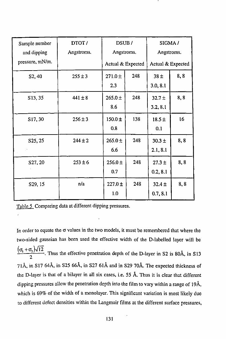
Sample number DTOT/ DSUB/ SIGMA/
and dipping Angstroms. Angstroms. Angstroms.
pressure, roN/m. Actual & Expected Actual & Expected
S2,40 255±3 271.0± 248 38± 8,8
2.3 3.0,8.1
S13,35 441 ±8 265.0± 248 32.7± 8,8
8.6 3.2,8.1
S17,30 256±3 150.0± 138 18.5 ± 16
0.8 0.1
S25,25 244±2 265.0± 248 30.3± 8,8
6.6 2.1,8.1
S27,20 253±6 256.0± 248 27.3± 8,8 >
0.7 0.2,8.1
S29, 15 n/a 227.0± 248 32.4± 8,8
1.0 0.7,8.1
Table 5 Comparing data at different dipping pressures.
In order to equate the 0' values in the two models, it must be remembered that where the
two-sided gaussian has been used the effective width of the D-Iabelled layer will be
(0') + O'JJi2. ! ~-"::":--. Thus the effective penetration depth of the D-Iayer in S2 is 801\, in S 13
2
711\, in S17 641\, in S25 661\, in S27 611\ and in S29 70A. The expected thickness of
the D-layer is that of a bilayer in all six cases, i.e. 55 A. Thus it is clear that different
dipping pressures allow the penetration depth into the film to vary within a range of 191\,
which is 69% of the width of a monolayer. This significant variation is most likely due
to different defect densities within the Langmuir films at the different surface pressures,
131

thus presenting different numbers or sizes of holes for the subsequent dipped layer to fill.
This is consistent with the theory on monolayer phases discussed in Chapter 2, and also
with the experiment done in the course of the present work, on surface potential
measurement. This will be discussed in Section 5.5.4.
It will be noted, however, that even within errors, DSUB is approximately one
monolayer thickness higher than expected, for all samples except S 17 and S29. The
central position of the D-Iayer in S 17 is clearly modelled more closely by the gaussian
model than is the D-Iayer at the air interface, except in the case of S29, where the very
low dipping pressure has perhaps resulted in a more open film structure for the D
molecules to penetrate, giving a D-Iayer as wide as in the other samples, but lower down
in the film and hence easier for the gaussian profile to model. The fact that no DTOT
value could be obtained for this sample lends support to this theory of an open film
structure, as it suggests there was insufficient electron density contrast for the X-rays to
be affected. However, see Section 5.5.3.2 for further comment on this matter. As to the
remaining four samples, it must be inferred that the gaussian model used here is still not
quite satisfactory for completely modelling a D-Iayer at the air interface, although the
basic approach shows considerable promise.
Despite this limitation, much useful information has been extracted from the data, in
terms of the distribution of the D-Iayer and hence the structure and integrity of the films
at the various dipping pressures, and these results are consistent with the previous work
discussed in Chapter 2.
132

5.5.3.2 Dipping Speed.
Consider SI against S16, i.e. 40mN/m and 15 and 5 mmlmin, and S3 against S17, i.e.
30mN/m and 5 and 15mmlmin. All four samples have the structure HHDHH
(nomenclature as in Table 1).
S 1 has a DSUB of 136 A and a cr of IS.6 A.
S 16 has a DSUB of 153 A and a cr of 21.7 A.
S3 has a DSUB of 135 A and a cr of IS.4 A.
S 17 has a DSUB of 150 A and a cr of IS.5 A.
These figures show that, whilst cr is relatively unaffected by dipping 7t and speed, DSUB
is profoundly affected, to the extent of 15 - 17 A. Being much' closer to the air/film
interface implies greater order in the layers underneath, since the deuterated material will
truly be in a bilayer, best represented by a block, and the gaussian model cannot reflect
the consequent delta-functions in SLD very accurately. Indeed, this author was able to
produce a model for S17, using a block model in an early version of Fitnew. This used
an 11 layer model for the LB film, with a tail thickness of 25.6A and a headgroup
thickness of I.S9A, both of which are rather smaller than the values from the X-ray data
given in Section 5.5.3. However, the block model also required a sublayer of silicon
dioxide, 11.9 A thick, which the later gaussian models did not need. Thus the total film
thickness is 277.4A, which is very close to the value expected for a ten-monolayer
sample. It is possible that the block model requires this "sublayer" in order to match
overall thickness and mean SLD values to the data, highlighting a limitation of this rigid
approach.
The fit obtained by the block model to S 17 is shown in Figure lSa), while that obtained
using the gaussian model is shown in Figure ISb). In confirmation of the acknowledged
limitation of the gaussian approach beyond Q = O.1A-\, it will be noted that Figure lSa)
illustrates a model which has the potential to fit the data over the whole Q range,
whereas Figure ISb) shows a more limited model. The overriding advantage of the
133
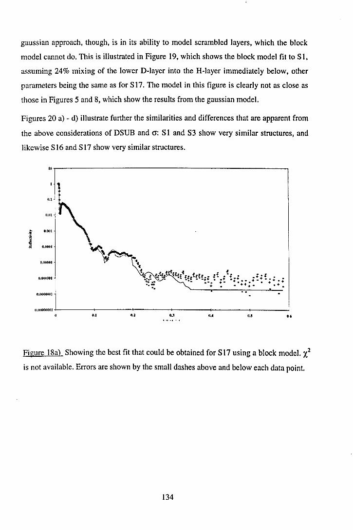
gaussian approach, though, is in its ability to model scrambled layers, which the block
model cannot do. This is illustrated in Figure 19, which shows the block model fit to S 1,
assuming 24% mixing of the lower D-layer into the H-Iayer immediately below, other
parameters being the same as for S 17. The model in this figure is clearly not as close as
those in Figures 5 and 8, which show the results from the gaussian model.
Figures 20 a) - d) illustrate further the similarities and differences that are apparent from
the above considerations of DSUB and <1: S 1 and S3 show very similar structures, and
likewise S 16 and S 17 show very similar structures.
10,-----------------------------,
0.1
11.111
~ . . 'f; 0.001
~ Iii
O.IMIOI ~
O'(MIOOI
O.IKMHKII
O.IKKIIMMI1
O.IMMIIMNIllI
0 0.1 0.2 0.) 0 ••
Figure 18a) Showing the best fit that could be obtained for S 17 using a block model. '1: is not available. Errors are shown by the small dashes above and below each data point.
134
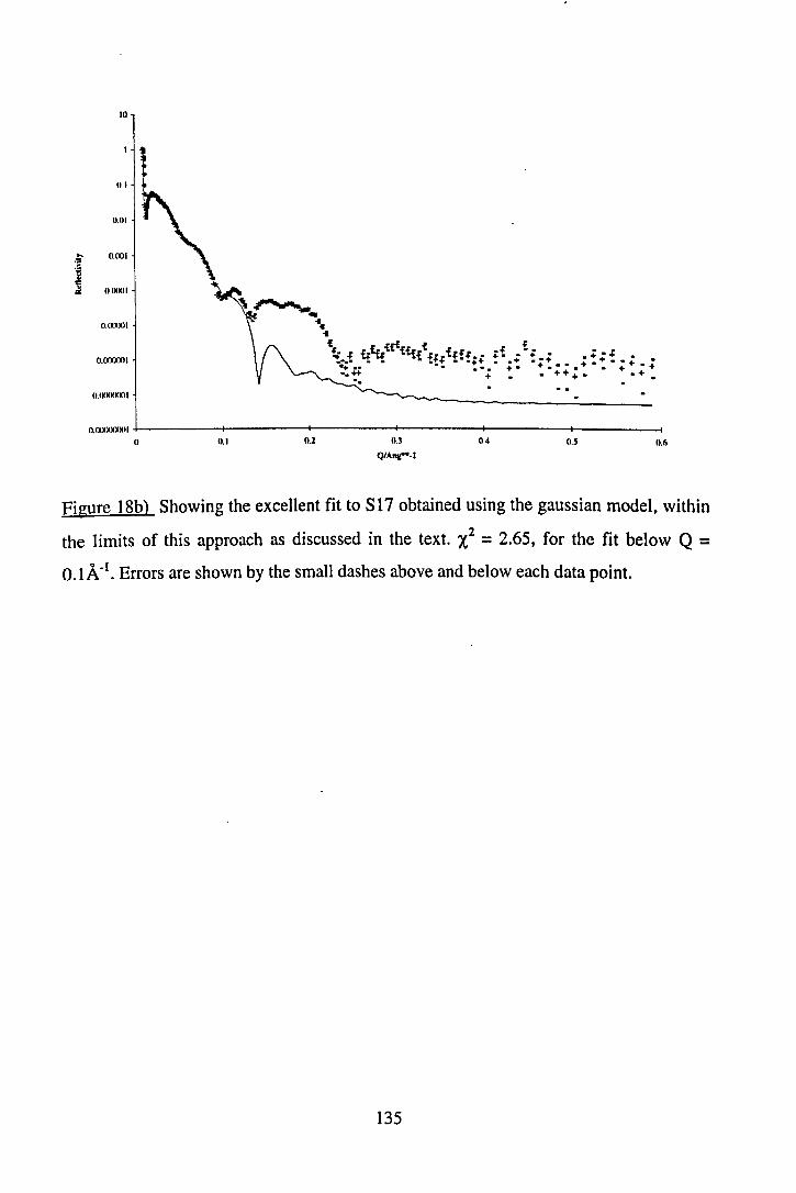
10
I
01
(WI
... O.O()l
'" .~
~ o (KJOI
O.(KKXlI
II.IKKXlOI
II.(KKXKJOI
O.(XXMKKXlI
1 ~
0 (U 0.2 0.3
Q/A"I:*°-l
+ • + • + •
04 11.5 0.6
Figure ISb) Showing the excellent fit to S 17 obtained using the gaussian model, within
the limits of this approach as discussed in the text. X2 = 2.65, for the fit below Q = o.lA- I . Errors are shown by the small dashes above and below each data point.
135

III
1l.1
001
.~. ~
~ O.'lOl 'ii
'" O.'KlOl
O'KKKlI
O.'KKKKlI
1l.'KKKKlOl
•
1
Il O.OS 0.1 O.U
Q/A"1I"°.1
0.2 11.25 0.)
Fi gure 19 Showing the fit available to S 1, using the block model and assuming 24%
mixing. as detailed in the text. X2 is not available. Errors are shown by the small dashes
above and below each data point.
136
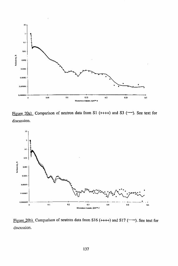
10
n.1
(1.(11
'" i-
" n.lXII 'il c ?i.
n.llOOl
n.lXXlOl
n.(XXXXII
O.(XXXXXII n n.os 0.1 (l.IS
M(.menIUIlI transler, QlA··.1
+ +
n.2
+ + +;----,~~~+--~
+
n.2S 0.3
Figure 20a) Comparison of neutron data from Sl (++++) and S3 (-). See text for
discussion.
nl
(WI
'" .~ n.onl 'il
~ n.(XXlI
n.lXXKII
II (KKKXll
n.lXKKKKII . -----II~-----+-I ------+------......... - - _.-- - ---I-.-----.:!:. - I
n n.1 n.2 n,! n,. n,s n,~
Momentum trander. OIA·· .. I
Figure 20b) Comparison of neutron data from S16 (++++) and S17 (-). See text for
discussion.
137
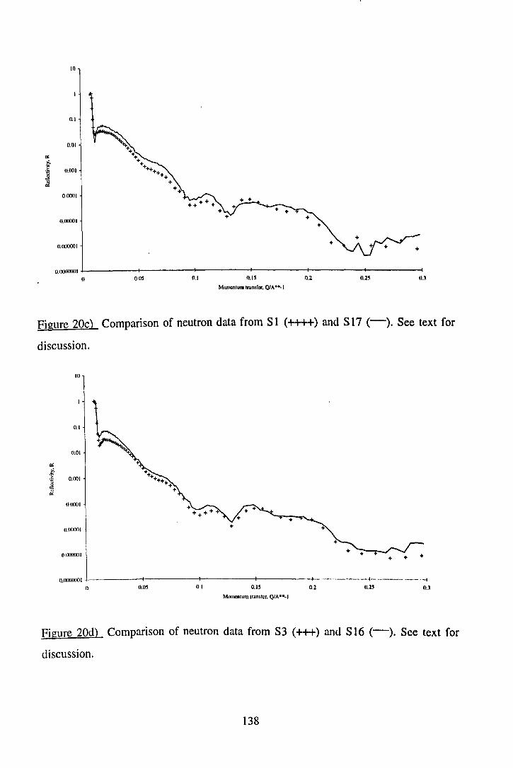
10
11.1
0.01
~ >. s: O.(lOl .~
~ o (XlOl
II.(XXXII
1I.(XXXlOl
II.(XXXXXII
0 005 0.1 0.15 0.2 0.25 II.)
MtmlClltum 'naMecr, QlA···1
Figure 20c) Comparison of neutron data from Sl (++++) and S17 (-). See text for
discussion.
10
11.1
(tol
~ >.
'1: II.(XII .~
'" ii. II (XXII
+ O.(KKXII +
() (KKKKII
O.lKKKNKlI ~ ______ t-_____ t-l ------+------+-.--.------i- ---.- ---- --I
() (1.05 0.1 O.U 0.2 11.25 (I.]
Mtllncntum (ranster. QlA···1
Figure 20d) Comparison of neutron data from S3 (+++) and S 16 (-). See text for
discussion.
138

It should be noted that a Langmuir film of docosanoic acid at 40mN/m is very much
more rigid (viscous) than a Langmuir film of the same molecule at 30mN/m and has very
different flow characteristics, chiefly that the rigid film is non-Newtonian, whereas the
fluid film shows Newtonian behaviour [Sa-c]. Thus, it may be seen that dipping pressure
(i.e. film viscosity) must be matched with an appropriate dipping speed in order to
achieve similar film structures and degrees of order. This observation is readily
explained by considering the flow of the Langmuir monolayer onto the substrate. If a
rigid film is dipped too fast, e.g. 1Smmlmin, it is easy to envisage the film being
"ripped" rather than flowing smoothly, resulting in holes throughout the structure and a
more scrambled film, as evidenced by a larger cr and lower DSUB. The holes in the
Langmuir film, since they would inevitably be close to the dipped substrate, would not
register a drop in 1t at the Wilhelmy plate. Hence the feedback loop would not be
activated, 1t would not be kept completely constant over this small region and the holes
would be transferred onto the substrate with the surrounding monolayer.
Conversely, dipping a rigid-film at 5mmlmin gives an ordered structure, explained by the
slower speed allowing the monolayer to flow onto the substrate more smoothly and thus
resulting in fewer holes through the structure of the dipped film.
Dipping the fluid film at the faster speed (S 17) also results in fewer holes and hence less
mixing, as shown by the higher DSUB.
Dipping the fluid film at the slower speed results in a more scrambled film (lower
DSUB) and this is probably due to the slow speed interfering with the rearrangement of
the molecules from their Langmuir film S phase to their LB film ~ phase, causing
"buckling" of the film. This would very much increase the interfacial roughnesses, and
consequently increase the internal disorder of the film. See also the surface potential
results, Section S.S.4.
A further pair of samples which illustrate the effect of dipping speed is S29 and S30.
These were both dipped at ISmN/m, at which point the monolayer is making the
transition from Lz to L2' , and both samples have the deuterated bilayer as the final pair of
layers. S29 was dipped at ISmmlmin and S30 at Smm/min. DSUB would be expected to
139
be 248A for these samples, and indeed it is 248A for S30, whereas DSUB for S29 is
227 A, implying a greater extent of mixing, since the centre of gravity of the gaussian is
lower than expected. Values for a are very similar, at 32.4A, 8.1 A and 32.1 A, 8.1 A (the
two-sided gaussian model was used for these samples, since the D-Iayer is at the air).
showing up a further potential shortcoming of the gaussian approach, which would be
rectified by the extra flexibility of the block model with two half-gaussians. See also the
discussion in Section 5.5.3.1. Nevertheless, a useful conclusion can be drawn, namely
that this very fluid film, on the cusp of two phases, needs to be dipped slowly if an
ordered film is to result, providing further evi~ence that the phase of the monolayer
requires consideration, and confirming the theory outlined above on how scrambling
could occur at the point of dipping.
5.5.3.3 Temperature.
Consider S2 (18°C) against S24 (30°C), otherwise identical dipping conditions, i.e.
40mN/m, 15mmlmin and HHHHD (nomenclature as in Table I).
S2 has a DSUB of 271 A and as of 38 A and 8.1 A.
S24 has a DSUB of 381 A and as of 60.8 and 8.1 A.
As has already been mentioned, the docosanoic acid Langmuir film at 30°C was
extremely fluid and this has caused the effective thickness of the film to be much larger
than expected, most likely due to the buckling proposed in the previous section. lienee.
while DSUB remains at the air-film interface, the D-Iayer has penetrated down into the
film by 119 A, compared with 80 A for S2. Thus DSUB and a continue to give
consistent results. The sample also shows that a certain amount of order is rcquircd in
the Langmuir film, if the subsequent LB film is to have order.
140

5.5.3.4 Time Under Water.
Consider S 13 against SIS, the latter having been left under water for 10 minutes between
the down and up-strokes of the D-Iayer deposition. Otherwise identical dipping
conditions, i.e. 35mN/m, 15mmlmin and HHHHDHHHH (nomenclature as in Table 1).
S 13 has a DSUB of 265 A and as of 32.7 and 8.1 A.
SIS has a DSUB of 263 A and as of 33.4 and 8.1 A.
Thus it is clear that, well within errors (see Table 2), the extra time under water has had
no effect whatsoever on the distribution of the D-Iayer within the LB film. An interesting
further experiment would be to use a hydrophilic substrate, so that one monolayer of D
acid could be dipped rather than a bilayer.
5.5.3.5 Effect of Subpbase Ions.
The plot of X-ray data from S7 and S 11 in Figure 21 illustrates the di fference due to the
presence of cadmium ions, which are known to make the molecules more perpendicular
(Chapter 2, Section 2.2.4) and hence make the dipped film thicker. The DTOT values for
the two Cd2+ films, i.e. S 10 and S 11, give a mean DMON of 29.6A, compared with 30A
for the fully-extended molecule, and the value of DMON of 27.6A for the acid dipped
over plain water. This result is very close to that of other workers, and is therefore
helpful in showing that the experimental technique used here is of the same standard as
that of other published work.
141

10
n.1
'" .~ 0.01 'il
~
n.OOI
n'(KKH
n.(KK)()1 -I----+----I-----+----+----+----------+---~ () 0.05 0.1 O.IS 0.2 0.25 o.~ D.4
MnrnClllum transfer. QlA···1
Figure 21 X-ray data from S7 (++++) and SIO (-), illustrating the effect of cadmium
ions on the film thickness. It can be seen that the Kiessig fringes in the S 10 data are
shifted to slightly lower Q than those in the S7 data, indicating that S lOis a thicker film.
5.5.4 Surface Potential Results.
As discussed earlier in this chapter, in Section 5.4.2, the qualitative picture of the
monolayer that this technique provides, namely of a film at 25mN/m being fluid and in
constant motion, one at 30mN/m being steady and one at 40mN/m picking up all
external vibrations, gives very useful evidence of the influence of the phase of the
monolayer on its dipping behaviour. These results therefore fully support the
observations on film quality at different surface pressures, as discussed in the previous
sections, and help to explain them. For instance, at 25mN/m, the monolayer appears to
be moving constantly, and it follows that this would produce uneven films, whatever the
dipping speed. At 30mN/m, the film has no obvious internal movement on the scale
detectable by the surface potential technique, i.e. of the order of 2-5mm, and it will
142
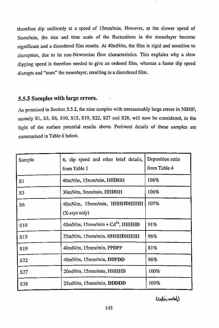
therefore dip uniformly at a speed of lSmmlmin. However, at the slower speed of
Smmlmin, the size and time scale of the fluctuations in the monolayer become
significant and a disordered film results. At 40mN/m, the film is rigid and sensitive to
disruption, due to its non-Newtonian flow characteristics. This explains why a slow
dipping speed is therefore needed to give an ordered film, whereas a faster dip speed
disrupts and "tears" the monolayer, resulting in a disordered film.
5.5.5 Samples with large errors.
As promised in Section S.S.2, the nine samples with unreasonably large errors in NBHF,
namely S 1, S3, S6, S 10, SIS, S 19, S22, S27 and S28, will now be considered, in the
light of the surface potential results above. Pertinent details of these samples are
summarised in Table 6 below.
Sample 1t, dip speed and other brief details, Deposition ratio
from Table 1 from Table 4
SI 40mN/m, lSmmlmin, HHDHH 108%
S3 30mN/m, Smmlmin, HHDHH 106%
S6 40mN/m, lSmmlmin, HHHHDHHHH 107%
(X-rays only)
SID 40mN/m, ISmmlmin + Cd2+, HHHHD 91%
SIS 3SmN/m, I5mmlmin, HHHHDHHHH 96%
SI9 40mN/m, lSmmlmin, PPDPP 81%
S22 40mN/m, lSmmlmin, DDPDD 96%
S27 20mN/m, lSmmlmin, HHHHD 100%
S38 2SmN/m, lSmmlmin, DDDDD 109%
143

Table 6 Brief preparation details summarised for the nine samples which show large
errors in NBHF values.
It will be readily observed that most of these samples fall into one or other of the
disordered monolayer categories above: S 1, S6, S 10, S 19 and S22 were all a viscous
film dipped fast, while S3 was a fluid film dipped too slowly. The remaining three
samples shed interesting light on two regions of the isotherm which have not been
explored as thoroughly. Given that S15, i.e. 35mN/m, produces a disordered film at
15mrnlmin, the monolayer must be much more viscous at this 7t than a monolayer at
30mN/m. It would be fruitful to extend the viscosity measurements reported in [5a-c]
into this surface pressure range. In a similar vein, S27 and S38 lend support to the theory
outlined in Section 5.5.3.2, namely, that such fluid monolayers require a slower dipping
speed to produce ordered layers, due to phase changes in those regions of the isotherm.
These are very consistent and encouraging results, and it would be helpful to do more
work to verify these conclusions.
144

'5.6 Summary.
'It has been shown that, by having only one D-Iabelled bilayer in an LB film, a greater ,
u-nderstanding may be reached of the factors affecting the scrambling of that D-layer into
th~' surrounding film. It has also been shown that, as is to be expected, each dipped layer
fills up the holes in preceding layers, and dipping conditions have been found which
optimise the integrity of the monolayer, thus reducing the formation of those holes and
consequently reducing scrambling of the D-Iayer. These conditions rely on a thorough
, understanding of the monolayer being used and on a balance being struck between film
. fluidity and dipping speed, i.e. a fluid film (30mN/m) can be dipped fast (lSmrnlmin) to
gi've an unscrambled film, whereas a more rigid viscous film (40mN/m) needs to be
dipped slowly (Smrnlmin) to give an unscrambled film. Under these conditions,
~~rambling of the D-Iayer may be reduced to a minimum, as shown by the DSUB and cr
values obtained from fits to the neutron reflectivity data, and five samples have been
prepared where this is the case, covering a range of preparation conditions. These five
samples are SI, S3, S14, S16 and SI7.
Musgrove [8] found evidence of mixed phases in all the films examined in that work.
The present work has extended this and established a link between these phases and the
experimental conditions, with the result that it is possible to prepare LB films of a single
phase by rigorous and systematic control of the dipping conditions. In addition, and in
contrast with the findings of Musgrove [8], it has been shown that it is possible to use
acid rather than salt Langmuir films to produce reproducible, ordered LB films. This
removal of metal ions from the system is a further simplification, making the modelling
more straightforward and hence, in principle at least, more reliable. This in turn has led
to a more fundamental understanding of the dipping process, with encouraging results
for producing ordered alternating LB films. In conclusion, it can be stated, with a high
, degree of confidence, that the results from the present work show that a Langmuir film
- - . of a fatty acid has to be in the S phase, and must be dipped at a rate which ensures
145
complete and uniform transition to the k phase during deposition, to achieve an
unscrambled LB film.
5.7 Further Work.
As mentioned in several of the preceding sections, it would be desirable to take the
modelling further, for instance to obtain fits out to higher Q and thus gain information on
the smaller-scale structure of the samples. More development work is needed on the
block model with two half-gaussians. On the practical side, the conclusions would be
strengthened by increasing the number of samples within the dipping parameter matrix,
and the work described in the next chapter will start this process. It would be particularly
interesting to investigate a broader range of dipping speeds. The surface potential
measurements need to be verified, and Brewster angle microscopy could be a useful
technique for this, particularly if a video camera were used. The viscosity of films at
high (above 30mN/m) pressures could be usefully measured, to add to general
monolayer understanding. Low pressure monolayers (below 2SmN/m) could also be
investigated, using a technique such as Brewster angle microscopy, with a view to
verifying the theory on the importance of monolayer phase in this lower region of the
isotherm. As to characterising LB films, infra-red spectroscopy is now a highly sensitive
technique which could usefully be applied to LB films to aid further study into molecular
orientation in the 'y~rious phases, especially the technique of attenuated total reflection,
which is particularly suited to thin layers such as LB films. As mentioned in Chapter 2,
atomic force microscopy is also applicable to LB films, and could be used to quantify
monolayer and LB film integrity. X-ray and neutron reflectivity are the most informative
techniques for the study of the internal layer structure of an LB film; a technique such as
ellipsometry is not so useful, as it gives only information on the bulk of the sample and
cannot resolve individual parts of the system, due to their very similar refractive indices
to the light wavelengths used. Finally, it would be very useful to quantify the deposition
ratios of the samples prepared in the present work, by dipping samples under identical
conditions but on a wafer polished on both sides.
146
5.8 References.
[1] c. Bower, S. Froggatt, R. Laycock, R. J. Musgrove, R. M. Richardson, G. Rozario,
A. Zarbakhsh, J. P. R. Webster, J. S. Hill, D. Lacey and G. Nestor, Mol. Cryst. Liq.
Cryst. 261,437 (1995).
[2] J. R. Lu and R. K. Thomas, Nucl. Instr. Meth. in Phys. Res. A, 354, 149 (1995).
[3] M. J. Grundy, R. J. Musgrove, R. M. Richardson, S. J. Roser and J. Penfold,
Langmuir, 6, 519 (1990).
[4] A. M. Bibo and I. R. Peterson, Adv. Mater. 2, 309 (1990).
[Sa] M. Buhaenko, 1. W. Goodwin, R. M. Richardson and M. F. Daniel, Thin Solid
Films, 134, 217 (1985).
[5b] M. R. Buhaenko, J. W. Goodwin and R. M. Richardson, Thin Solid Films 159, 171
(1988).
[5c] M. Buhaenko, PhD thesis, University of Bristol, 1988, and references therein.
[6] S. J. Roser and M. R. Lovell, Thin Solid Films, 285, 166 (1996).
[7] U. Englisch, T. A. Barberka, U. Pietsch and U. Hohne, Thin Solid Films, 266, 234
(1995).
[8] R. J. Musgrove, PhD Thesis, Bristol 1990.
147
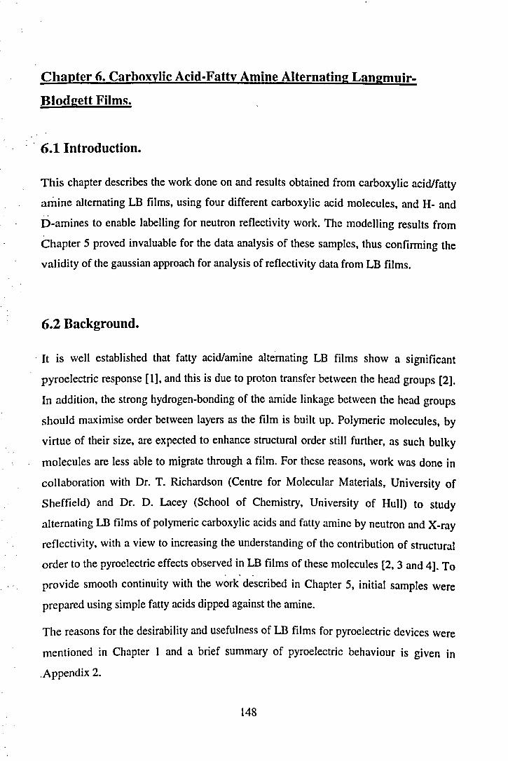
Chapter 6. Carboxylic Acid-Fatty Amine Alternating Langmuir
Blodgett Films.
6.1 Introduction.
This chapter describes the work done on and results obtained from carboxylic acid/fatty
amine alternating LB films, using four different carboxylic acid molecules, and H- and
ri-amines to enable labelling for neutron reflectivity work. The modelling results from
Chapter 5 proved invaluable for the data analysis of these samples, thus confirming the
validity of the gaussian approach for analysis of reflectivity data from LB films.
6.2 Background.
, It is well established that fatty acid/amine alternating LB films show a significant
pyroelectric response [1], and this is due to proton transfer between the head groups [2].
In addition, the strong hydrogen-bonding of the amide linkage between the head groups
should maximise order between layers as the film is built up. Polymeric molecules, by
virtue of their size, are expected to enhance structural order still further, as such bulky
molecules are less able to migrate through a film. For these reasons, work was done in
collaboration with Dr. T. Richardson (Centre for Molecular Materials, University of
Sheffield) and Dr. D. Lacey (School of Chemistry, University of Hull) to study
alternating LB films of polymeric carboxylic acids and fatty amine by neutron and X-ray
reflectivity. with a view to increasing the understanding of the contribution of structural
order to the pyroelectric effects observed in LB films of these molecules [2,3 and 4]. To
provide smooth continuity with the work described in Chapter 5, initial samples were
prepared using simple fatty acids dipped against the amine.
The reasons for the desirability and usefulness of LB films for pyroelectric devices were
mentioned in Chapter 1 and a brief summary of pyroelectric behaviour is given in
,Appendix 2.
148
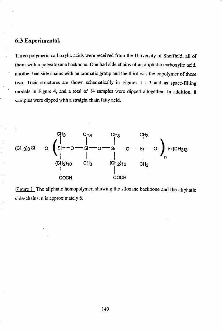
6.3 Experimental.
Three polymeric carboxylic acids were received from the University of Sheffield, all of
them with a polysiloxane backbone. One had side chains of an aliphatic carboxylic acid,
another had side chains with an aromatic group and the third was the copolymer of these
two. Their structures are shown schematically in Figures 1 - 3 and as space-filling
models in Figure 4, and a total of 14 samples were dipped altogether. In addition, 8
samples were dipped with a straight chain fatty acid.
CH3 CH3 CH3 CH3
{CH3)3 Si -0-( ~i-O - ~i-O -s; -0-s;-o"* Si (CH3l3
(CH2)10 CH3 (CH2)10 CH3
I I COOH COOH
Figure 1 The aliphatic homopolymer, showing the siloxane backbone and the aliphatic
side-chains. n is approximately 6.
149
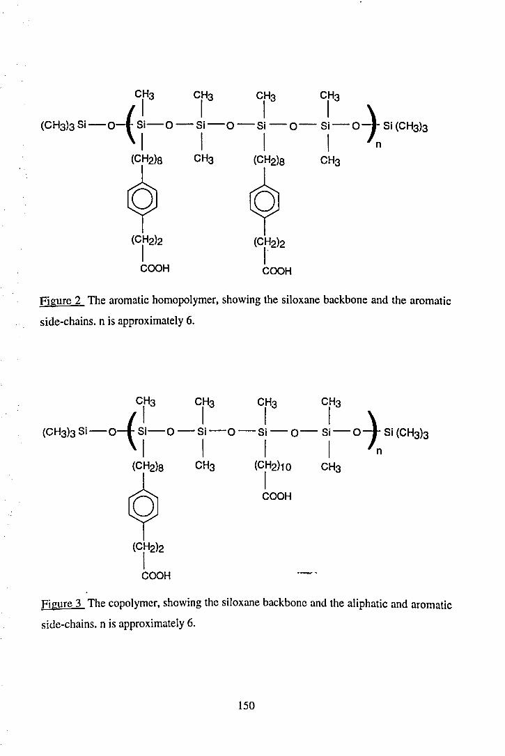
CH3 CH3 CH3 CH3
(CH3}JSi-O-(~'-O-"-O-S:-o-si-OiS'(CH3)J (CH2)S CH3 (CH2)S CH3
Figure 2 The aromatic homopolymer, showing the siloxane backbone and the aromatic
side-chains. n is approximately 6.
CH3 CH3 CH3 CH3
(CH3)3Si-O-(~I-O-'I-O-S:-o-s:-oiSI(CH3)J (CH2)S CH3 (CH2h 0 CH3
I COOH
Figure 3 The copolymer, showing the siloxane backbone and the aliphatic and aromatic
side-chains. n is approximately 6.
150
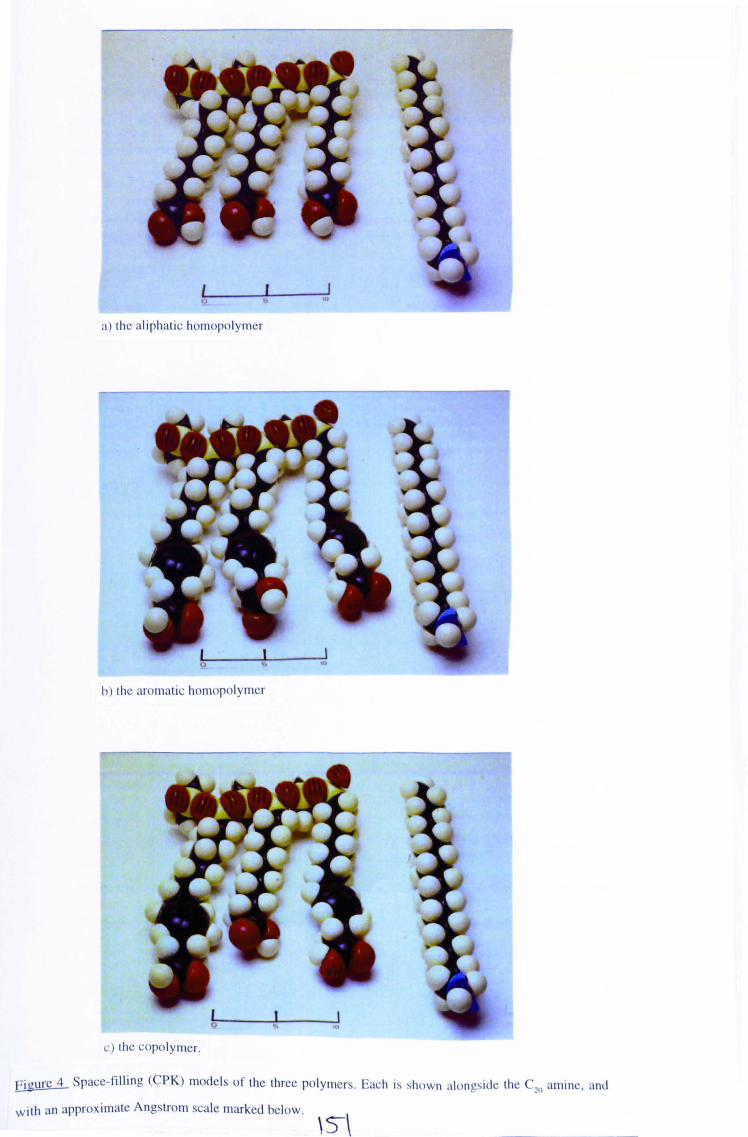
<>
a) the aliphati c homopolymer
h) the aromatic homopolymer
c) the copo lymer.
flgure 4 Space-filling (CPK) mode ls o f the three polymers. Each is shown alongs ide the 211 amine, and
w ith an approx imate Angstrom sca le marked below.
\S-\
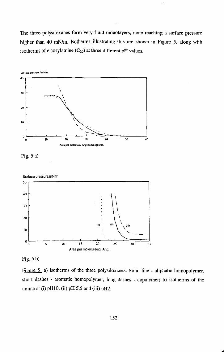
The three polysiloxanes form very fluid monolayers, none reaching a surface pressure
higher than 40 mN/m. Isotherms illustrating this are shown in Figure 5, along with
isotherms of eicosylamine (C20) at three different pH values.
Surface pressure I mN/m.
40~-----------------------------------------'
30
20
10
oL-~---L--~--J---~~~~~~~~--~--~~ o 10 20 30 40 SO 60
Fig. 5 a)
Surface pressure/mN/m
50
40
30
20 -
to
Fig. 5 b)
Area per molecule I Angstroms squared.
(i) , ,
Area per molecule/sq. Ang.
\
(ii)
\ \ \ \
\(iii)
'-. - --
Figure 5 a) Isotherms of the three polysiloxanes. Solid line - aliphatic homopolymer,
short dashes - aromatic homopolymer, long dashes - copolymer; b) isotherms of the
amine at (i) pHI0, (ii) pH 5.5 and (iii) pH2.
152
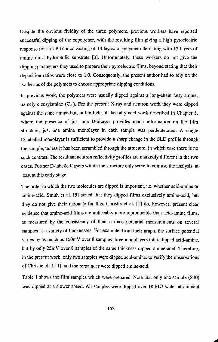
Despite the obvious fluidity of the three polymers, previous workers have reported
successful dipping of the copolymer, with the resulting film giving a high pyroelectric
response for an LB film consisting of 13 layers of polymer alternating with 12 layers of
amine on a hydrophilic substrate [3]. Unfortunately, these workers do not give the
dipping parameters they used to prepare their pyroelectric films, beyond stating that their
deposition ratios were close to 1.0. Consequently, the present author had to rely on the
isotherms of the polymers to choose appropriate dipping conditions.
In previous work, the polymers were usually dipped against a long-chain fatty amine,
namely eicosylamine (C20). For the present X-ray and neutron work they were dipped
against the same amine but, in the light of the fatty acid work described in Chapter 5,
where the presence of just one D-bilayer provides much information on the film
structure, just one amine monolayer in each sample was perdeuterated. A single
D-Iabelled monolayer is sufficient to provide a sharp change in. the SLD profile through
the sample, unless it has been scrambled through the structure, in which case there is no
such contrast. The resultant neutron reflectivity profiles are markedly different in the two
cases. Further D-Iabelled layers within the structure only serve to confuse the analysis, at
least at this early stage.
The order in which the two molecules are dipped is important, i.e. whether acid-amine or
amine-acid. Smith et at. [5] stated that they dipped films exclusively amine-acid, but
they do not give their rationale for this. Christie et at. [1] do, however, present clear
evidence that amine-acid films are noticeably more reproducible than acid-amine films,
as measured by the consistency of their surface potential measurements on several
samples at a variety of thicknesses. For example, from their graph, the surface potential
varies by as much as I50mV over 8 samples three monolayers thick dipped acid-amine,
but by only 25mV over 8 samples of the same thickness dipped amine-acid. Therefore,
in the present work, only two samples w<Ere dipped acid-amine, to verify the observations
of Christie et at. [1], and the remainder were dipped amine-acid.
Table 1 shows the film samples which were prepared. Note that only one sample (S40)
was dipped at a slower speed. All samples were dipped over 18 Mil water at ambient
153

temperature (18°C) and pH (- 5.1 - 5.5). The pH could not be adjusted to pH3 as for the
samples in Chapter 5, because at such a low pH the amine monolayer is completely
ionised and hence expanded over the un-ionised state, affecting monolayer behaviour
([6] and see Fig. 5b above). However, the optimum pH for amines is at or above pHlO,
at which point the acid headgroups would be completely ionised. Ambient pH was
chosen as a compromise, and monolayer stability was found to be very good for both
docosanoic acid and the eicosylamine. The polymeric acids were not found to be
particularly affected by pH, so ambient pH was appropriate for them too. Samples S40,
S41 and S42 were not examined by X-rays, since they had been examined by neutrons at
both room temperature and 50°C, which affected their structures: subsequent X-ray
experiments would not have yielded information on the initial order of the films. Due to
time constraints, samples S56, S57, S60 and S61 were not examined by neutrons. With
these exceptions, all samples were examined both by neutrons at RAL and subsequently
by X-rays in-house at Bristol.
154
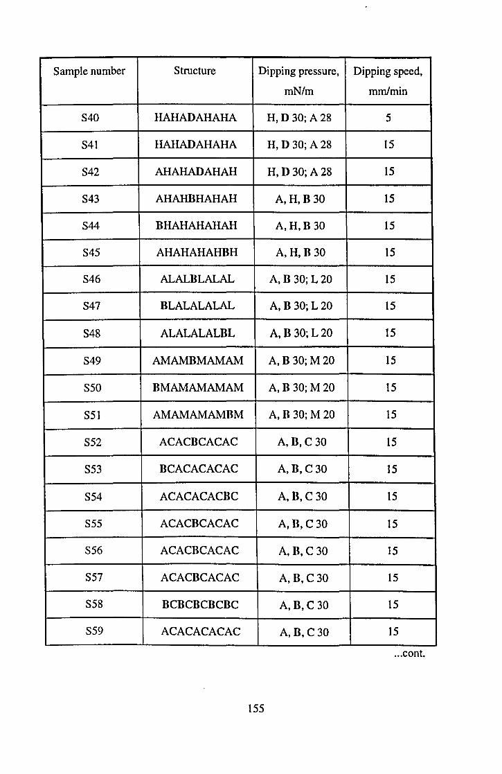
Sample number Structure Dipping pressure, Dipping speed,
mN/m mm/min
S40 HAHADAHAHA H,D30;A28 5
S41 HAHADAHAHA H, D 30; A 28 15
S42 AHAHADAHAH H, D30; A28 15
S43 AHAHBHAHAH A, H, B 30 15
S44 BHAHAHAHAH A, H,B 30 15
S45 AHAHAHAHBH A, H, B 30 15
S46 ALALBLALAL A, B 30; L 20 15
S47 BLALALALAL A, B 30; L 20 15
S48 ALALALALBL A, B 30; L20 15
S49 AMAMBMAMAM A,B 30;M20 15
S50 BMAMAMAMAM A, B 30; M 20 15
S51 AMAMAMAMBM A, B 30; M 20 15
S52 ACACBCACAC A, B, C 30 15
S53 BCACACACAC A, B, C 30 15
S54 ACACACACBC A, B, C 30 15
S55 ACACBCACAC A, B,C 30 15
S56 ACACBCACAC A, B, C 30 15
S57 ACACBCACAC A, B, C 30 15
S58 BCBCBCBCBC A, B, C 30 15
S59 ACACACACAC A, B, C 30 15
... cont.
155

Sample number Structure Dipping pressure, Dipping speed,
mN/m mm/min
S60 AHAHAHAHAH A,H30 15
S61 BHBHBHBHBH B,H30 15
Table 1 The samples prepared. Each letter in the structure column represents a
monolayer. H is the fatty acid, D is the perdeuterated fatty acid, A is the amine, B is the
perdeuterated amine, L is the aliphatic homopolymer, M is the aromatic homopolymer
and C is the copolymer.
6.4 Modelling the Data.
Again, a layer-by-Iayer approach resulted in too many independent parameters and
consequently very unwieldy modelling. The approach described in Chapter 5, namely the
gaussian model, enables the main features of the reflectivity profiles to be fitted with far
fewer parameters.
6.5 Results.
As in Chapter 5, the X-ray data were fitted using the single-layer option in Fitnew, to
extract DTOT and NBHF, and then the gaussian routine was used to fit the neutron data,
to obtain values for DSUB and cr. These results are shown in Tables 2 and 3, and
examples of the quality of the fits are shown in Figure 6 for the X-ray data and in Figure
7 for the neutron data. Table 4 gives the relative values for the deposition ratios for these
samples, and as in Chapter 5, it must again be stressed that these deposition ratio data
can only be used to compare sample with sample and molecule type with molecule type.
They can in no way be said to represent actual coverage, due to the fact that deposition
on the rear (i.e. ground and hence macroscopically uneven) face of the Si wafers is
156
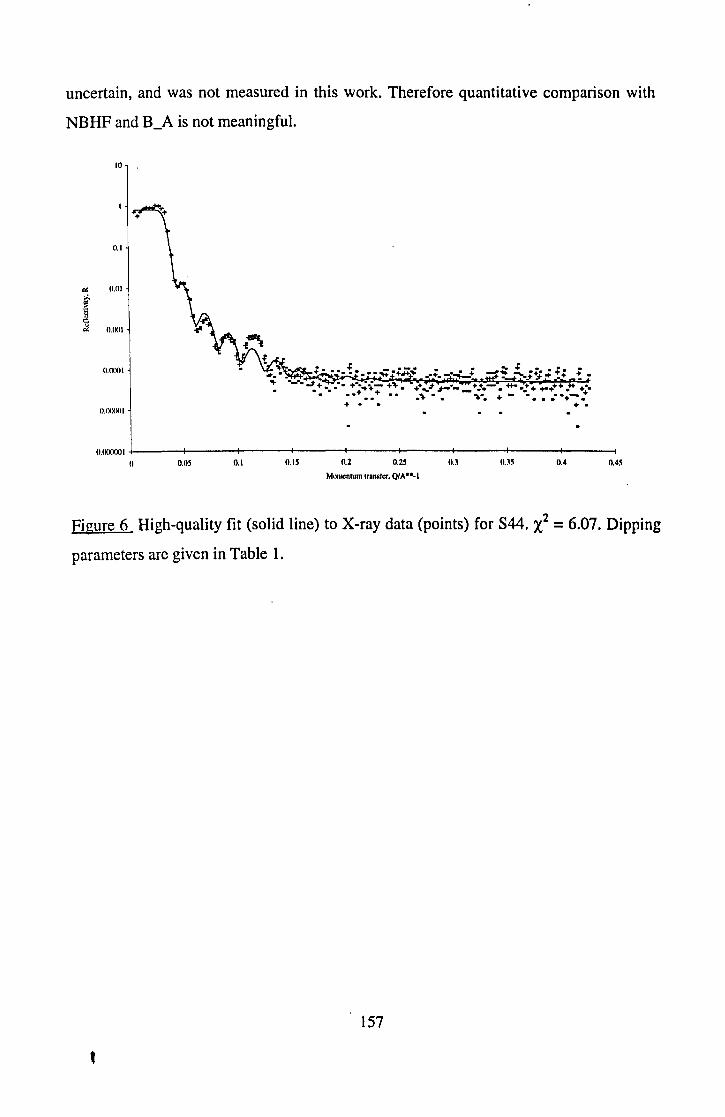
uncertain, and was not measured in this work. Therefore quantitative comparison with
NBHF and B_A is not meaningful.
HI .
0.1
'" (1.01
.~ ~ Ci O.(KlI
-- + - --- - - ~ + - - -•• + e_ • ••••• ~.+.t+::tt- •• +.~+ ___ ...,. ~;~ .. ~+ +.
-.... ~+ ..... +-.;i:- +'" . . ++ .. ~ ;---_+!+- ....... : ... +++.++ +-. • ..+ +.. ". ..... + -. • -.-- + + •••• •• • • •• + -.
O.lKKH
O.lKKKH
O.lKKKlOl -I----+-----i---+----+----~--_+_--_+---_--__1
o 0.05 0.1 0.15 0.2 0.25 n.) 0.4 0.45
Momentum tran,ler, Q/A"-I
Figure 6 High-quality fit (solid line) to X-ray data (points) for S44. X2 = 6.07. Dipping
parameters are given in Table 1.
157
t
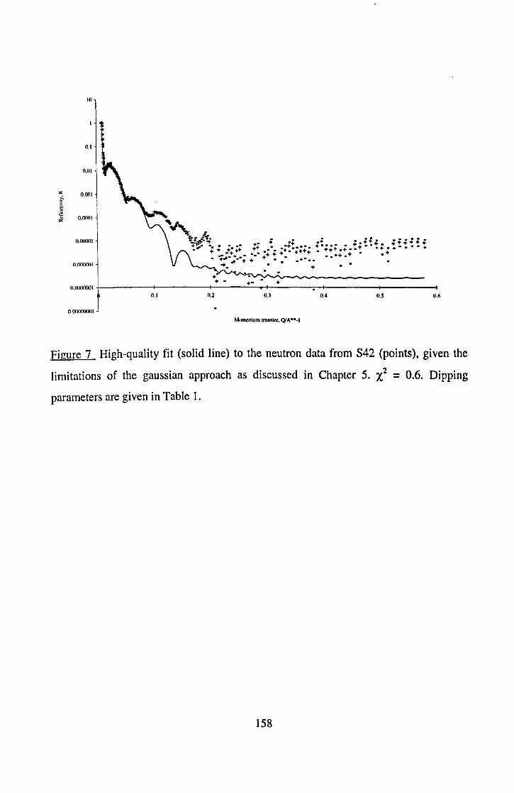
10
0.1
(1.01
'" 0.001 i-
~ c 0.0001 ri
O.(X)()()I
O,(XXXXH
'" -ru .... .t\ ."" .. "H" "." ... " ~. • • ..- -..; • .. + • • .. • • •• • + .... +. +. + •• + .' ';+ +';++ -+ .-. -•• -';++'; • +++.+.. -+.;-. •
• -;.; ••• -; ;_. + + + + • • • • • • •• + • +. • .... .... • +
+" + O,(XXKKKH
0.1 0.2 0.3 0.4 0.5 O.lI
o (XXKKKlOl
Momentum trAnsfer, QlA···1
Figure 7 High-quality fit (solid line) to the neutron data from S42 (points), given the
limitations of the gaussian approach as discussed in Chapter 5. X2 = 0.6. Dipping
parameters are given in Table 1.
158
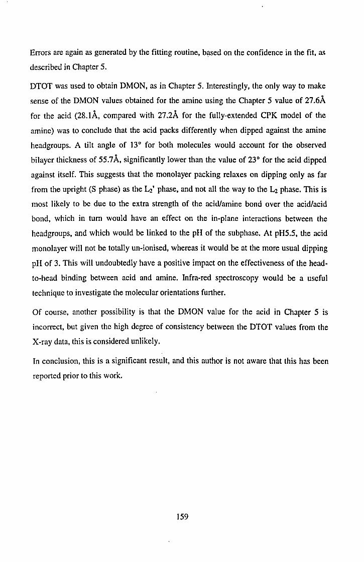
Errors are again as generated by the fitting routine, b~sed on the confidence in the fit, as
described in Chapter 5.
DTOT was used to obtain DMON, as in Chapter 5. Interestingly, the only way to make
sense of the DMON values obtained for the amine using the Chapter 5 value of 27.6A
for the acid (28.1A, compared with 27.2A for the fully-extended CPK model of the
amine) was to conclude that the acid packs differently when dipped against the amine
headgroups. A tilt angle of 13° for both molecules would account for the observed
bilayer thickness of 55.7 A, significantly lower than the value of 23° for the acid dipped
against itself. This suggests that the monolayer packing relaxes on dipping only as far
from the upright (S phase) as the k' phase, and not all the way to the L2 phase. This is
most likely to be due to the extra strength of the acid/amine bond over the acid/acid
bond, which in turn would have an effect on the in-plane interactions between the
headgroups, and which would be linked to the pH of the subphase. At pH5.5, the acid
monolayer will not be totally un-ionised, whereas it would be at the more usual dipping
pH of 3. This will undoubtedly have a positive impact on the effectiveness of the head
to-head binding between acid and amine. Infra-red spectroscopy would be a useful
technique to investigate the molecular orientations further.
Of course, another possibility is that the DMON value for the acid in Chapter 5 is
incorrect, but given the high degree of consistency between the DTOT values from the
X-ray data, this is considered unlikely.
In conclusion, this is a significant result, and this author is not aware that this has been
reported prior to this work.
159

-
Sample DTOTI DSUBI SIGMN
number Angstroms Angstroms. Angstroms.
S40 n/a n/a
S41 n/a 131.0 ± 0.8 15.3±0.4
S42 nla 153.0 ± 0.3 16.3 ± 0.2
S42,50°C nla 160.0 ± 0.3 19.4 ± 0.2
S43 272±3 128.0±0.3 12.9 ± 0.1
S44 281 ±2 n/a
S45 269±4 240.0 ± 0.6 10.5 ± 0.4
S46 289±4 74.7 ±0.5 45.6 ± 1.8
S47 230±3 n/a
S48 302±42 62.6 ± 1.0 49.8 ± 1.0
S49 nla 102.0 ±2.0 59.3 ±0.9
S50 21O±7 n/a
S51 n/a 132.0 ± 3.4 131.0 ± 12.5
S52 216±4 102.0 ± 2.2 74.6 ± 1.9
S53 216 ± 13 n/a
S54 220±9 n/a
S55 216±5 107.0±2.0 77.6 ± 3.2
S56 215 ±7 n/a
S57 218 ± 21 n/a
S58 n/a n/a
S59 235 ±7 n/a
S60 284±7 n/a
S61 287±4 n/a
Table 2 DTOT values from fits to the X-ray data and DSUB and SIGMA values from
fits to the neutron data.
160
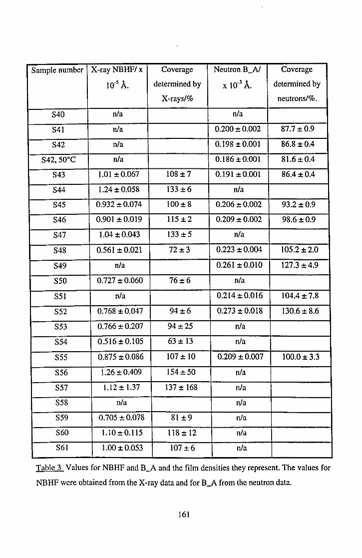
Sample number X-ray NBHFI x Coverage Neutron B_N Coverage
10-5 A. determined by x 10-3 A. determined by
X-rays/% neutrons/%.
S40 nla n/a
S41 n/a 0.200 ± 0.002 87.7 ± 0.9
S42 nla 0.198 ± 0.001 86.8 ±0.4
S42,50°C nla 0.186 ± 0.001 81.6 ± 004
S43 1.01 ± 0.067 108 ±7 0.191 ± 0.001 86.4 ±OA
S44 1.24 ± 0.058 133 ±6 n/a
S45 0.932 ± 0.074 100±8 0.206 ± 0.002 93.2 ±0.9
S46 0.901 ± 0.019 115±2 0.209 ± 0.002 98.6±0.9
S47 1.04 ±0.043 133 ±5 n/a
S48 0.561 ± 0.021 72±3 0.223 ± 0.004 105.2 ± 2.0
S49 nla 0.261 ± 0.010 127.3 ±4.9
S50 0.727 ± 0.060 76±6 n/a
S51 n/a 0.214 ± 0.016 104.4 ± 7.8
S52 0.768 ± 0.047 94±6 0.273 ± 0.018 130.6 ± 8.6
S53 0.766 ± 0.207 94±25 n/a
S54 0.516±0.105 63 ± 13 n/a
S55 0.875 ± 0.086 107 ± 10 0.209 ± 0.007 100.0± 3.3
S56 1.26 ± 00409 154 ± 50 n/a
S57 1.12 ± 1.37 137 ± 168 n/a
S58 n/a n/a
S59 0.705 ± 0.078 81 ±9 n/a
S60 1.10 ± 0.115 118 ± 12 n/a
S61 1.00 ± 0.053 107 ±6 n/a
Table 3 Values for NBHF and B_A and the film densities they represent. The values for
NBHF were obtained from the X-ray data and for B_A from the neutron data.
161

Sample It 2i 3t 4i 5t 6i 7t 8i 9t lOi Total Mean
cm2 .,
cm2 cm2 cm2 cm2 cm2 cm2 cm2 cm2 cm2 Coverage cm-%
S40 88.5 79.8 75.4 79.8 74.0 78.3 72.5 78.3 75.4 78.3 780 101
S41 76.9 81.2 71.1 79.8 78.3 78.3 74.0 79.8 75.4 79.8 775 100
S42 60.9 78.3 74.0 81.2 78.3 79.8 78.3 79.8 78.3 84.1 773 100
S43 66.7 79.8 76.9 82.7 75.4 82.7 76.9 81.2 75.4 82.7 780 101
S44 65.3 79.8 76.9 81.2 75.4 81.2 74.0 81.2 74.0 82.7 772 100
S45 63.8 78.3 72.5 82.7 72.5 78.3 72.5 81.2 75.4 79.8 757 98
S46 68.2 81.2 62.4 74.0 72.5 69.6 74.0 34.8 72.5 39.2 648 84
S47 58.0 71.1 71.1 66.7 72.5 76.9 71.1 69.6 74.0 81.2 712 92
S48 62.4 76.9 62.4 74.0 74.0 68.2 69.6 78.3 76.9 8.7 651 84
S49 60.9 74.0 66.7 66.7 75.4 62.4 75.4 71.1 75.4 72.5 701 91 - ~- - _.-
For Table caption, see two pages on. CIrk.
162
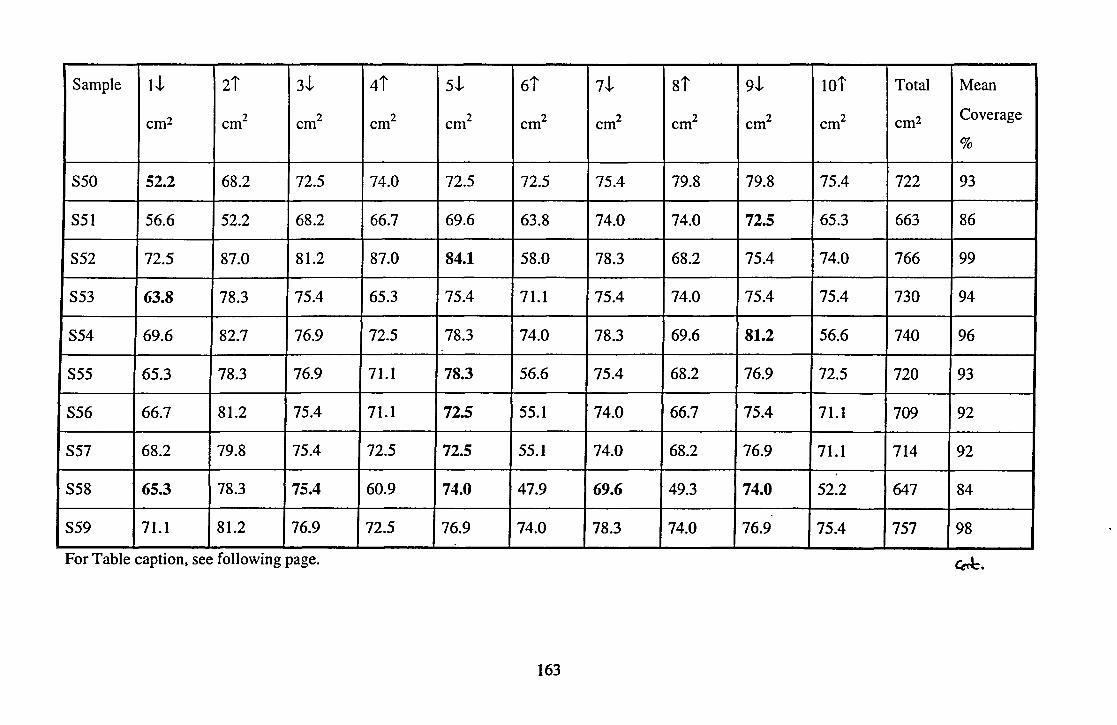
Sample IJ.. 21 3J.. 41 5J.. 61 7J.. 81 9J.. 101 Total Mean
em2 , ,
em2 em2 em2 em2 em2 em2 em2 em2 Coverage em- em-%
S50 52.2 68.2 72.5 74.0 72.5 72.5 75.4 79.8 79.8 75.4 722 93
S51 56.6 52.2 68.2 66.7 69.6 63.8 74.0 74.0 72.5 65.3 663 86
S52 72.5 87.0 81.2 87.0 84.1 58.0 78.3 68.2 75.4 74.0 766 99
S53 63.8 78.3 75.4 65.3 75.4 71.1 75.4 74.0 75.4 75.4 730 94 ,
S54 69.6 82.7 76.9 72.5 78.3 74.0 78.3 69.6 81.2 56.6 740 96
S55 65.3 78.3 76.9 71.1 78.3 56.6 75.4 68.2 76.9 72.5 720 93
I S56 66.7 81.2 75.4 71.1 72.5 55.1 74.0 66.7 75.4 71.1 709 92
S57 68.2 79.8 75.4 72.5 72.5 55.1 74.0 68.2 76.9 71.1 714 92
S58 65.3 78.3 75.4 60.9 74.0 47.9 69.6 49.3 74.0 52.2 647 84
S59 71.1 81.2 76.9 72.5 76.9 74.0 78.3 74.0 76.9 75.4 757 98
For Table caption, see follOWIng page. ~.
163
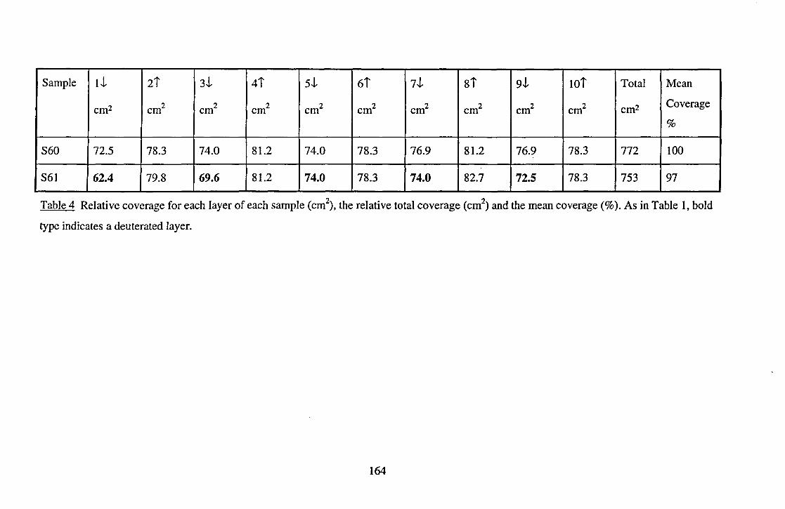
Sample IJ. 2! 3J. 4! 5J. 6! 7J. 8! 9J. IO! Total Mean
cm2 cm2 cm2 cm2 cm2 cm2 cm2 cm2 cm2 cm2 cm2 Coverage
%
S60 72.5 78.3 74.0 81.2 74.0 78.3 76.9 81.2 76.9 78.3 772 100 I
S61 62.4 79.8 69.6 81.2 74.0 78.3 74.0 82.7 72.S 78.3 753 9~ ___ j ------ - ---- -_ .. - ------ --- --- ---
Table 4 Relative coverage for each layer of each sample (cm2), the relative total coverage (cm2
) and the mean coverage (%). As in Table 1, bold
type indicates a deuterated layer.
164
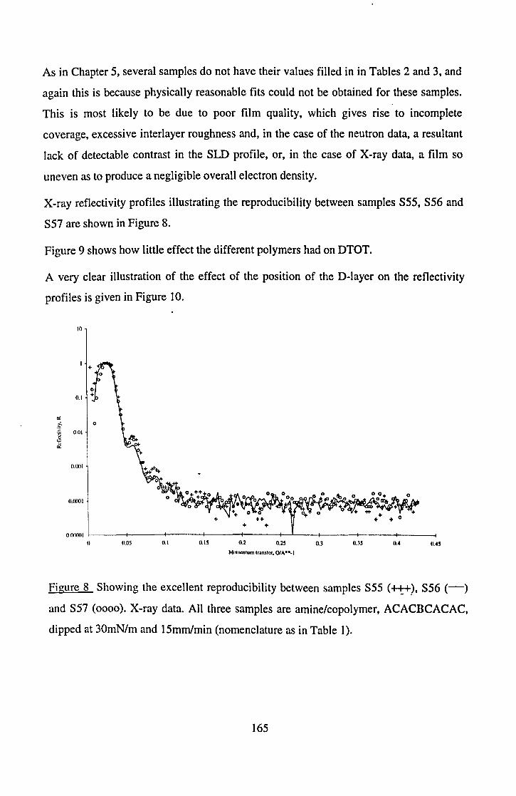
As in Chapter 5, several samples do not have their values filled in in Tables 2 and 3, and
again this is because physically reasonable fits could not be obtained for these samples.
This is most likely to be due to poor film quality, which gives rise to incomplete
coverage, excessive interlayer roughness and, in the case of the neutron data, a resultant
lack of detectable contrast in the SLD profile, or, in the case of X-ray data, a film so
uneven as to produce a negligible overall electron density.
X-ray reflectivity profiles illustrating the reproducibility between samples S55, S56 and
S57 are shown in Figure 8.
Figure 9 shows how little effect the different polymers had on DTOT.
A very clear illustration of the effect of the position of the D-layer on the reflectivity
profiles is given in Figure 10.
10
0.1
0/
i> :~ OUI c:: ~
O.lXII
n.lXlOl
U(XKMII e---f----f----+----+----i--'---i----+---+----I n O.US 0.1 0.15 0.2 0.25 0.3 0.35 n .•
MnlUcnIUl11lran!ilcr. QlA"'.1
Figure 8 Showing the excellent reproducibility between samples S55 (+t+), S56 (-)
and S57 (0000). X-ray data. All three samples are amine/copolymer, ACACnCACAC,
dipped at 30mN/m and 15mmlmin (nomenclature as in Table 1).
165

UKI
10 0#'0 0
.1'0
0.1
'" ·F (1.(11 il c ~
O.lKII
O.lXXII
O.lXXMII +
O.lXMMMH
0 O.OS 0.1 O.IS 0.2 0.2S 0.] O.]S 0.4 0.4S
Mnmencum transfer. Q/A··-I
Figure 9 X-ray data from S48 (++++), S56 (-) and S49 (0000) to show the constancy
of I?TOT regardless of the polymer type. S49 is shifted by a factor of 10 for clarity. The
lack of fringes in S48 and S49 is due to large air-film roughnesses with these samples.
S48 ALALALALBL, S56 ACACBCACAC, S49 AMAMBMAMAM; all amine layers
and C dipped at 30mN/m, Land M dipped at 20mN/m; dipping speed 15mmlmin for all
three (nomenclature as in Table 1).
166
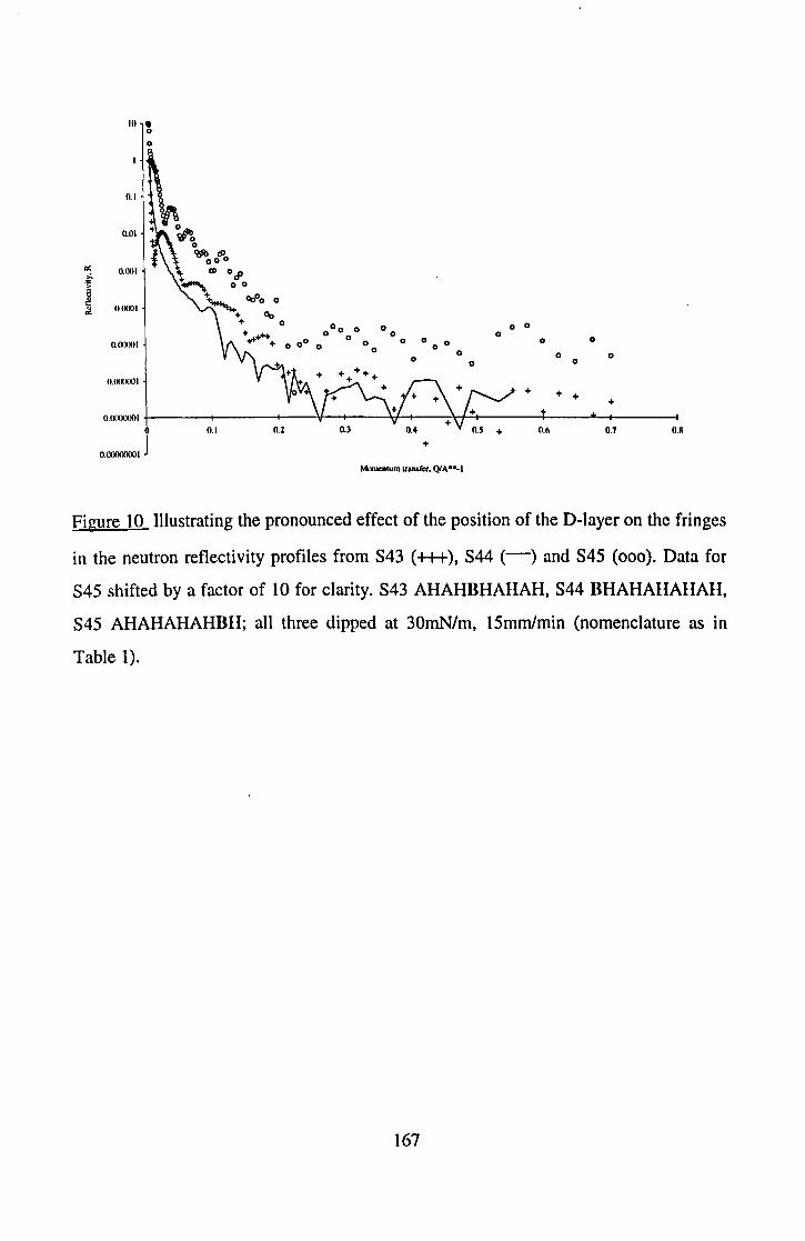
J() • o o
0.1
0.1lI
..: O.(XlI >. .'" > .~ c:
o (XIOI :z
O.(XXXlI
0 00 0 0 0 0
o 0 0 0 o 00 0 0 0 0
0 0 o 0 0 0 0 0 0
0 0
O.(XXXXlI
+ + + O.<mXIOI
0.1 0.2 0.7 O.M
+ 0.00000001
Mnrncntum traMfcr, QlA·· .. 1
Figure 10 Illustrating the pronounced effect of the position of the D-layer on the fringes
in the neutron reflectivity profiles from S43 (+++), S44 (-) and S45 (000). Data for
S45 shifted by a factor of 10 for clarity. S43 AHAHBHAHAH, S44 BHAHAHAHAH,
S45 AHAHAHAHBH; all three dipped at 30mN/m, 15mrnlmin (nomenclature as in
Table 1).
167
6.6 Discussion and Conclusions.
The data for samples 540 and- 541 were inconclusive because of the difficulty of
obtaining fits to the data. However, 542 was much easier to fit, and since this sample
reversed the dipping order of acid and amine it must be concluded that the 542
orientation (amine first, then acid) confers greater order on the structure, enabling a
sensible fit to be more easily obtained. This result thus confirms the work of Christie et
al. [1], by reinforcing the evidence in favour of amine-acid versus acid-amine films in
terms of reproducibility. The present observation is also in agreement with the theory
outlined in section 6.5, concerning the change in packing of the acid - if it is dipped first,
it will be in the ~ phase, and therefore not be in the optimum orientation with respect to
the amine headgroups; if dipped second,it will be free to adopt the ~t phase imposed by
the amine headgroups. Therefore, this dipping order was used in subsequent amine-acid
samples. This head group binding is very likely due to the slightly raised pH of 5.5,
compared with pH3 for the samples in Chapter 5. At pH5.5, the acid headgroups are not
completely un-ionised, and so binding to the amine headgroups will be stronger.
Whilst the increased temperature has caused cr to increase in S42, 05UB has also
increased. This is best explained by the temperature rise causing the molecules to
"straighten out", thus increasing OMON and hence both 05UB and cr. This conclusion is
consistent with the accepted mechanism for the pyroelectric effect, whereby the dipole of
the film changes with molecular tilt, i.e. with the vector of the molecular dipole moment
(see Appendix 2). In order to confirm this, an identical sample would need to he dipped
and examined by X-rays both before and after heating, to obtain values for OTOT and
hence confirm any change in molecular orientation. This author was unable to perform
this obvious experiment, due to the very much delayed arrival of the deuterated amine,
very shortly before the scheduled beamtime at RAL, which left no time for preliminary
X-ray investigations.
In support of the theory on stronger headgroup bonds between acid and amine, the
OSUB and cr values in Table 2 for 543 and 545 (128A and 12.9A, and 240A and to.5A,
168

respectively) are very close to the theoretical values of 125A. and 7.6A. for aD-labelled
amine monolayer dipped in the fifth layer and 236A. and 7.6A. for a D-labelled amine
monolayer dipped in the ninth layer. This is a very encouraging result and is further
concrete evidence, in addition to that presented in Chapter 5, that an un-scrambled
alternating LB film may readily be prepared under the correct conditions. The samples
discussed here, and the five in Chapter 5, are the first instances of which this author is
aware, that a labeIIed layer has been shown to have remained in its dipped layer and not
to have scrambled into the layer below. In the case of S43 and S45, which are two
samples for which there is particularly strong evidence of no scrambling at all, the
avoidance of scrambling wiII almost certainly have been aided by the strong amine-acid
headgroup binding, but it wiII also have been affected by the phase of the acid monolayer
after dipping: it is only in the ~' phase, as evidenced by the layer and film thickness
data, and hence has not relaxed as far as the acid films discussed in Chapter 5. This is
therefore a major result and adds considerably to current knowledge of LB film
scrambling.
The very large cr values for the polymer samples, coupled with the fact that DSUB for
these samples is central regardless of where the D-Iayer was actually deposited, are
strong evidence that with all three polymers the film structure is too open to allow the
single D-amine monolayer to remain in a discrete layer. This is not surprising, given the
extremely fluid nature of the films, as shown by the isotherms in section 6.3. This result
also explains the empirical observation made in reference [7], namely, that to optimise
the pyroelectric signal in a 13-monolayer film built from one of these molecules and
eicosylamine, three bilayers of a fatty acid must be deposited after six active monolayers.
From the above and the discussion in Chapter 5, it will be seen that this is readily
explained by the fatty acid possessing sufficient monolayer integrity to bridge the defects
in the polymer layers, while itself possessing holes too smaIl to aIlow the next layer of
polymer to mix with it.
Given this evidence of extreme mixing of the D-amine layer throughout the polymer LB
film, the fact of high pyroelectric coefficients for these materials [3] is somewhat
169
surprising. It is a natural extrapolation to envisage yet higher pyroelectric coefficients if
similar materials could be synthesised with better LB film-forming properties.
6.7 Summary.
It has been shown conclusively that scrambling in an alternating LB film is not a
foregone conclusion. Usi.ng two molecules whose headgroups bind strongly, namely
COOH and NH2, two samples have been prepared, over a pure water subphase, for
which no scrambling at all is needed for an excellent fit to the neutron data. This is a
significant result, with implications for the design of appropriate molecules for
pyroelectric and SHG applications. Contrary to expectations, large polymeric molecules
do not form ordered layers, and this result is supported by empirical observations from
other workers [7].
6.8 Further Work.
As in Chapter 5, further work is needed on the modelling, particularly on the block
model with two half-gaussians. It may also be a fruitful exercise to attempt to model the
totally unscrambled samples S43 and S45 using a layer by layer model, as the step-wise
approach to SLD variation is expected to be an accurate model of these samples. It
would be helpful to evolve the models to obtain good fits out to higher Q, so as to
extract the maximum amount of information from the reflectivity data, and hence
establish the smaller-scale structure of the samples. On the experimental side, repeating
the fatty acid-fatty amine samples as outlined in section 6.6 would give invaluable extra
information on the order within these films and the effect of temperature thereon. It
would be extremely interesting to prepare ABAB samples of deuterated amine and
hydrogenous acid under the same dipping conditions as S43 and S45, and use neutron
reflectivity to provide rigorous confirmation of the unscrambled nature of the films.
Pyroelectric measurements would also confirm the unscrambled nature of the films. and
infra-red spectroscopy would be a useful tool to investigate the molecular orientations in
acid/acid, acid/amine and amine/acid films. A broader temperature range would be a
170

very interesting study. In the longer term, the design and synthesis of polysiloxanes
which exhibit improved LB film-forming characteristics would have promising
implications for the future application of LB films in thermal imaging devices.
6.8 References.
[1] P. Christie, G. G. Roberts and M. C. Petty, Appl. Phys. Lett. 48, 1101 (1986).
[2] c. A. Jones, M. C. Petty, G. G. Roberts, G. Davies, J. Yarwood, N. M. Ratcliffe and
J. W. Barton, Thin Solid Films, 155, 187, (1987).
[3] T. Richardson, W. H. A. Majid, E. C. A. Cochrane, S. Holder and D. Lacey, Thin
Solid Films, 242, 61 (1994).
[4] T. Richardson, W. H. A. Majid, R. Capan, D. Lacey and S. Holder, Supramolecular
Science, 1, 39 (1994).
[5] G. W. Smith, M. F. Daniel, J. W. Barton and N. Ratcliffe, Thin Solid Films, 132, 125
(1985).
[6] "G. L. Gaines Jr., Insoluble Monolayers at Liquid-Gas Interfaces, Wiley, New York (1966).
[7] S. V. Batty, R. Capan, T. Richardson, T. E. Mann and D. Lacey, Thin Solid Films,
284.285, 919 (1996).
171

Chapter 7. Conclusions
7.1 Introduction.
X-ray and neutron reflectivity have been used to study the internal order of labelled
alternating LB films prepared under a variety of experimental conditions. These
experimental parameters, namely dipping speed, dipping pressure, temperature, time
under water, the presence or absence of subphase cations and the position of the labelled
layer, have been investigated methodically, one by one, to establish which parameters
affect the order of the films and how. A new modelling approach has been evolved to fit
the reflectivity data, using a gaussian profile for the labelled layer. The materials used to
form the LB films have been C22 fatty acid, C20 fatty amine, a liquid crystal polysiloxane
and three polymeric fatty acids, with deuterated e22 acid and C20 amine being used to
label one monO: or -bilayer in each sample, at varying positions. Samples have been
prepared, of both pure fatty acid and of acid-amine, which are completely unscrambled,
i.e. in which the neutron reflectivity data show. that the labelled layer has remained in the
layer where it was dipped and has not mixed in with the surrounding film. This is a very
significant and hugely encouraging result for the future use of the LB technique in
pyroelectrics, second harmonic generation and other molecular electronics applications.
7.2 Modelling the Data.
The commonly used layer-by-Iayer approach to modelling reflectivity data proved
inadequate for providing close fits to the neutron data, although single-layer models were
perfectly adequate for fitting the X-ray data. This is readily explained by considering the
likely distribution of the labelled material in a scrambled film. It is unlikely to have
mixed with neighbouring layers in the step-wise fashion inherent in a slab approach,
which can only take a relatively small number of slices through the sample before the
processing time becomes excessive due to the number of parameters being handled, and
172

the logical extension is to use a gaussian profile to model a smooth variation in labelled
layer content within the thickness of the film. Optical Matrix techniques have been used
throughout to maintain the required accuracy, but the Kinematic Model has proved
invaluable for visualising the profile and evolving the model. The illustration of the
model and its evolution are given in detail in Chapter 5. Initial results with a symmetrical
gaussian were promising, and the principle was extended to two half-gaussians, the
better to model the likely scenario of labelled material mixing more into the layers below
than those above. The bulk of the data were modelled using this approach, with the final
evolution of the model consisting of a central block and two independent half-gaussians,
one on either side of the block. It will be readily seen that this would provide a yet more
representative profile, and would be of particular use in analysing samples where only
partial mixing has occurred.
As with all modelling approaches, however, there are limitations to the one used here.
Chief among these arises from the Fourier Transform element of the Kinematic Theory.
The gaussian profile has a very broad differential function, and the Fourier Transform of
this will be therefore be a damping function. This means that data above Q - 0.1A-1
cannot be modelled, since the model decays faster than the RQ4 decay of the data beyond
this Q-range, and so no information on the very small-scale structure of the samples is
available. Another limitation is the inherent inability of the gaussian profile to represent
the situation of the labelled layer dipped directly onto the substrate as the first layer or
bilayer. For this reason, several of the samples prepared (before the introduction of the
gaussian model) could not be fitted. A further limitation is the situation with the labelled
layer at the air-film interface, although the model with two half-gaussians was able to
deal with this considerably better than the symmetrical gaussian model, which is as
expected. In any further work in this area it would be interesting to test and develop the
block plus two half-gaussians, specifically for films with non-central labelled layers, and
to continue to use the simpler two half-gaussians for the study of the majority of other
film architectures. Ways of overcoming the damping limitation are not obvious at
present.
173
7.3 Acid-Acid Films.
7.3.1 Phase Change on Dipping.
The film thicknesses obtained from the X-ray data show that the acid monolayer has
relaxed from the S phase of the Langmuir film, with upright chains, to a mixture of k
and L2' phases, with a mean chain tilt of 23°. This is contrary to the behaviour observed
with salt films, which deposit with a smaller molecular area than in the Langmuir film,
and is therefore an important result in terms of new information on the behaviour of acid
films. It highlights the fact that they show very different characteristics than do salt films
and hence underlines the importance of a thorough understanding of the monolayer
phases of the molecule being studied, in order to understand its LB dipping behaviour.
7.3.2 Position of Labelled Layer.
A novel feature of this work was that only one bilayer or monolayer was labelled. This is
in contrast to previous work, which has concentrated exclusively on architectures with
alternating labelled and non-labelled layers. The present strategy was chosen in order to
establish the extent of scrambling and its mechanism more accurately than alternating
architectures allow. The deuterated material was deposited as the first, the central or the
final bilayer in five- or nine-bilayer samples, or the first, fourth and ninth monolayer in
) O-monolayer samples. These differences of position were readily modelled by the
gaussian profile technique, with the exception of the situation of the labelled layer being
at the substrate. Thus, the gaussian profile is shown to be sensitive to the position of just
one monolayer of labelled material, and the present combination of techniques and
modelling is shown to be a powerful method for analysing the structure of LB films.
174

7.3.3 Subphase Cations.
Since the main aim of this work was to study the hitherto neglected pure fatty acid films,
only two samples were dipped as salts, over a subphase containing cadmium. These gave
data from both X-ray and neutron reflectivity experiments which agree extremely closely
with literature values for similar samples. This is helpful in showing that the
experimental technique used here is of the same standard as that of other published
work. This is a useful benchmark, given the lack of literature data on pure fatty acid
films as opposed to salts.
7.3.4 Surface Pressure.
Differences were observed between films prepared at different monolayer surface
pressures. Films dipped at 40mN/m were found to be more susceptible to forming
disordered films than those dipped at 30mN/m: only one ordered sample was prepared
out of 19 labelled samples at 40mN/m, compared with one out of two labelled samples at
30mN/m. This is thought to be due to the increased viscosity of the film at 40mN/m,
rendering it less able to flow smoothly onto the substrate during dipping, and hence more
likely to have holes within it. Surface pressures below 30mN/m were also unsuccessful
for producing ordered films, and in this case it is thought to be because the Langmuir
monolayers are in a phase which does not possess sufficient order to transfer as a
contiguous film. If the first layer does not deposit in an ordered fashion, the head groups
of the second layer will not have a suitable ordered template for deposition, nor will the
chains of the third layer have an even surface to deposit onto, and the disorder will thus
be perpetuated throughout the film.
7.3.5 Dipping Speed.
Some very interesting results were obtained from the investigation of this parameter,
especially given the consensus in the literature that dipping must proceed at speeds of
175

around 60mmlmin and above in order to minimise the time available under water for
molecules to overturn and thus scramble the film. The speeds used here were Sand
ISmmlmin, yet even over this small range significant differences were observed. These
were that an ordered film resulted if a 30mN/m film was dipped at lSmmlmin, whereas a
40mN/m film had to be dipped at Smmlmin if an ordered film was to be obtained. These
results are readily explained by consideration of the viscosity of the monolayer. The
40mN/m film is viscous, but can flow smoothly onto the substrate if a dipping speed of
only Smmlmin is used; a more rapid speed would cause the substrate to move faster than
the monolayer could flow onto it, resulting in holes in the monolayer as it reached the
substrate and hence a disordered LB film. Conversely, dipping the 30mN/m film at only
Smmlmin allows the phase change on dipping to produce disordered films, whereas at
] Smmlmin the phase change is reproducible and gives ordered films. The surface
potential measurements discussed later (Section 7.3.8) shed extra light on this behaviour.
7.3.6 Time Under Water.
Contrary to the literature consensus, films left under water for 10 mins in between the
down- and upstrokes of the labelled bilayer were shown to be identical to films of
similar structure which were not subjected to extra time under water, as revealed by the
neutron reflectivity profiles. This finding casts doubt on the theory that scrambling is
caused by molecules overturning whilst under water.
7.3.7 Temperature.
One sample was dipped at 30°C, at which temperature the monolayer is extremely fluid
and in the L2 phase. It was found to have no internal. order, with the labelled bilayer
(dipped as the topmost bilayer) distributed throughout the whole of the preceding film.
This is further evidence that a certain amount of monolayer order is required to dip an
ordered LB film, and is consistent with previous work on viscosity, which found that for
C22 acid at pH3, the viscosity was halved when the temperature changed from 19 to
30°C.
176
7.3.8 Surface Potential.
This non-invasive technique gave a very clear macroscopic picture of the behaviour of a
monolayer at different surface pressures. At 25mN/m, the film was obviously fluid, and
showed evidence of rapid motion, presumably due to extraneous vibrations in the
apparatus. At 30mN/m, the film was steady and it did not reflect any vibrations <?n the
time scale observed at 25mN/m; rather, it showed fluctuations on the time scale of
minutes. At 40mN/m, the film was again observed to fluctuate rapidly, and in this case it
is thought that the increased viscosity of the monolayer has rendered it rigid, and
therefore caused it to mirror the apparatus vibrations to a larger extent than did the
2SmN/m film. This confirms the theory in Section 7.3.5, on why the 40mN/m film needs
to be dipped slowly. The observation at 30mN/m also helps to explain the fact that a
30mN/m film cannot be dipped slowly. A dipping speed of 5mmlmin means the
substrate is picking up monolayer on the same time scale as the fluctuations in surface
potential, thus giving a disordered film.
7.3.9 The Polysiloxane.
This molecule was studied to provide continuity with previous work in the group. The
monolayer thickness obtained from the LB film samples agrees well with the previous
values obtained from the neutron reflectivity experiments on Langmuir films of the
molecule.
7.3.10 Summary of Acid Films.
As a result of this study of the parameters affecting the formation of ordered LB films of
fatty acids, it is concluded that the most important parameter is the monolayer phase,
which is determined by the surface pressure of the monolayer and the temperature of the
subphase. The monolayer phase will affect the speed at which an ordered, unscrambled
177

film may be prepared, and for given values of surface pressure and temperature, the
dipping speed required for the formation of an ordered film can be experimentally
determined. Surface potential data have been used to provide a qualitative illustration of
the structure of the monolayer at three surface pressure values relevant to the present
work, and this picture supports the theory on why scrambling occurs at certain
combinations of surface pressure and dipping speed and not others. The time between
the down- and upstrokes of a labelled layer has been found to have little or no effect on
the extent of scrambling, for times as long as minutes. Two samples across the phase
(Le. surface pressure)/speed matrix have been shown to be completely unscrambled, with
a further three showing only slight scrambling. The conclusion from these results is that
the Langmuir film has to be in the S phase, and must be dipped at a rate which ensures
complete and uniform transition to the k phase during deposition, in order to produce an
unscrambled film.
7.4 Amine-Acid Films.
7.4.1 Rationale
Amine-acid films were dipped to provide an alternative molecular architecture with
which to test the modelling, as well as to provide useful supporting data for pyroelectric
studies carried out by collaborating groups. The series of samples began with the
monomeric fatty acid used in the previous series, to facilitate direct comparisons.
Subsequently, samples were dipped with polymeric fatty acids, which have previously
produced good pyroelectric films.
7.4.2 Amine and Monomeric Acid.
It was found that films dipped with the acid on the first downstroke were disordered,
whereas films dipped with the amine first were ordered, with no scrambling. This is
explained in terms of the evidence obtained from the thickness values from the X-ray
178
data, for a different phase change for the acid when dipped against the amine, namely
from the S phase in the monolayer to the L2' phase in the dipped film, compared with S
to ~ for the acid dipped against itself. If dipped first, the acid adopts the usual L2' phase,
the amine deposits in the equivalent of the L2 phase and a disordered film results. If, on
the other hand, the amine is dipped first, it dictates the phase adopted by the subsequent
acid layer and an ordered film results. This pronounced effect of the amine on the
packing of the acid is due to the strong headgroup binding between the COOH and NH2
moieties, especially at the pH of 5.5 which was used as a compromise between the
requirements of the acid and those of the amine. Thus it would seem that, under most
conditions, relaxation to the L2 phase, and therefore 30° chain tilt, results in an open and
disordered layer, and hence a disordered and scrambled film, although even in this phase
of the monolayer, films have been prepared which remain unscrambled. This is further
confirmation of the conclusions drawn from the acid-acid samples with regard to poor
quality films from monolayers with little or no long-range order. The current theory on
the origin of the pyroelectric effect, namely changes in molecular dipole moment, was
confirmed by a sample which showed increased thickness on heating.
7.4.3 Amine and Polymeric Acids.
Isotherms of these molecules showed them to be very fluid, and so it was not surprising
to find that LB films of them dipped against the amine showed no internal order at all,
with the labelled layer distributed throughout the preceding layers. Given that these
molecules are known to show good pyroelectric responses, there is potential for LB films
with even better response if the molecules could be designed to dip more efficiently
against the amine headgroups. This result also explains why other workers have needed
to dip layers of fatty acid interleaved between the polymer, in order to obtain a good
pyroelectric response - the acid introduces the required measure of order for the polymer
dipole moments to be effective.
179
7.4.4 Summary of Amine-Acid Films.
Increased head-to-head interaction, such as is achieved by dipping acid against amine, is
shown to result in ordered, unscrambled films. Three polymers are shown to be too fluid,
i.e. not to possess sufficient long-range order, to dip ordered films.
7.5 Overall Conclusions.
Neutron reflectivity has been used, in conjunction with X-ray reflectivity, to investigate
order within alternating LB films. Single-layer models were satisfactory for fitting the X
ray data. For the neutron data, a new modelling approach has been developed, which
uses a gaussian profile to model the distribution of deuterium-labelled material within
the sample. The results from this approach are consistent with the conclusions of other
workers, but by enabling better-quality fits to be obtained have greatly enhanced
understanding of the scrambling phenomenon.
Samples with only one deuterium-labelled layer have been shown to give the required
information on the distribution of that labelled layer through the film, which is not
possible with alternating structures. By varying the experimental parameters, it has been
shown that consideration of both dipping speed and film viscosity (i.e. monolayer phase)
enables LB films to be prepared in which the labelled layer has not mixed with the
surrounding layers. A Langmuir film of a fatty acid has to be in the S phase, and must be
dipped at a rate which ensures complete and uniform transition to the L2 phase during
deposition, or the L2' phase if the head-head binding is significant, e.g. dipping against
an amine, in order to produce an unscrambled film.
The preparation of LB films of docosanoic acid alternating with eicosylamine has shown
that with increased head group interaction, scrambling is totally eliminated. This has been
explained in terms of differences in film phase and head-to-head interactions when
compared with acid-acid films.
180

Polysiloxane molecules with side chains having terminal carboxylic acid groups are
shown to form LB films with insufficient layer structure to allow a labelled layer to
remain unmixed. This result is used to explain the empirical result of workers at
Sheffield and Hull ([7] in Chapter 6), that the pyroelectric effect of films of such
molecules is enhanced by the periodic inclusion of bilayers of a fatty acid.
181

Appendix 1. Second Harmonic Generation.
Second Harmonic Generation (SHG) is most simply described as two incoming photons
of frequency co combining to give one emerging photon of frequency 2m. The physical
basis for this is as follows:
The molecular polarisation p due to an electro-m'agnetic wave is
p = aE + f3E2 + 'YE3 + ....... .
where
E is the applied field
a, ~ and 'Yare constants for a particular molecule, the hyperpolarisability ~ being the
most interesting quantity for the present discussion. a is the linear polarisability and is
the origin of refractive index.
~E2 and )'E3 are non-linear terms. Terms higher in E make a negligible contribution to
the polarisation.
The macroscopic polarisation P in a linear optically-active material may therefore be
expressed as
where
EO is the permittivity of free space
x( 1) is the first order susceptibility tensor and is the contribution from the molecular as
over the bulk.
Similarly, the bulk polarisation in a material with non-linear optical (NLO) properties is
given by
P = EO (X(l) E +X(2) E2 + X(3) E3 + .... )
182

where
X(2) is the second order susceptibility tensor and is the contribution from the molecular
ps over the bulk
X(3) is the third order susceptibility tensor and is the contribution from the molecular "(S
over the bulk.
Again, terms higher than the third in E are negligible in practice.
The second order term is the one of interest here. If E is from an electromagnetic wave,
as it will be in the present case of light incident on an active material, it is described by
Hence
E = Eo (cos rot)
E2 = E02 (cos2 rot)
= E02 (1. + 1. cos (2rot)) 2 2
This is therefore the origin of the frequency doubling effect i.e. second harmonic
generation, and
p = t X(2) E02 + X(l) Eo cos rot + t(X(2) E02 cos 2rot)
A noncentrosymmetric material is needed: if a symmetric material is used, the direction
cosine terms of the molecular dipole moments cancel out and the X(2) component is
equal to zero. Alternating LB films would be a very useful means of engineering such a
structure, especially given the difficulty of the alternative, namely designing materials
that naturally crystallise with their molecular dipoles in a noncentrosymmetric lattice.
Also, if the sample is bulky a large part of the signal will be lost by absorption and again
LB films would provide a solution to the problem, by means of their thinness.
The chief application of ro ~ 2ro frequency doubling is infra-red up-conversion: for
instance, laser light at 1.064 ~m (IR) can be frequency-doubled up to 532 nm (visible,
green). This principle has great potential in the field of night vision and mountain rescue
situations, where the small size and low weight of an LB-film-based system would be an
183

advantage over current lithium niobate-based apparatus. Since the emergent light is
coherent, any laser radiation may be similarly frequency doubled to provide laser
radiation at much shorter wavelengths thari are obtainable by other means, although
obviously intensity is halved at each frequency doubling.
A further application is the Pockels or electro-optic effect, whereby the refractive index
of the material changes following a change in the surrounding electric field. This can be
used to switch optical signals in telecommunications, for example, and again the
thinness of LB films is an advantage, ensuring fast response times.
The third order hyperpolarisability, X(3), although as yet very small in even the most
advanced materials, is nevertheless a useful property due to its far less stringent lattice
requirements: a centrosymmetric system will not cancel it out. It has potential uses in
optical bistability, since the refractive index changes with the intensity of the incoming
light (Kerr effect), although since the emergent intensity will be only one third of the
jncident intensity, the material must be able to withstand high intensity illumination if
the effect is to be of practical use.
References
I. R. Girling et al., Thin Solid Films, 132, 101 (1985).
G. Ashwell et al., Proc SPIE - Int. Soc. Opt. Eng. 1361,589 (1991).
R. Tredgold, Order in Thin Organic Films, Cambridge University Press (1994), pp. 105-
107.
184
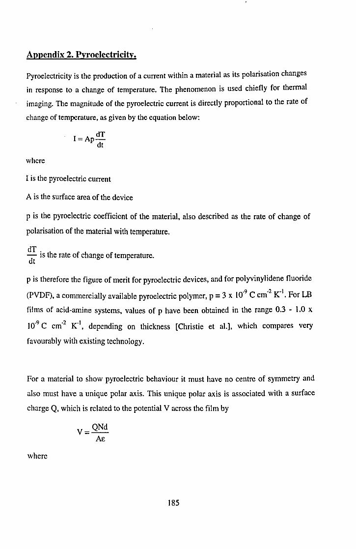
Appendix 2. Pyroelectricity.
Pyroelectricity is the production of a current within a material as its polarisation changes
in response to a change of temperature. The phenomenon is used chiefly for thermal
imaging. The magnitude of the pyroelectric current is directly proportional to the rate of
change of temperature, as given by the equation below:
where
dT I=Ap
dt
I is the pyroelectric current
A is the surface area of the device
P is the pyroelectric coefficient of the material, also described as the rate of change of
polarisation of the material with temperature.
dT. h - IS t e rate of change of temperature. dt
p is therefore the figure of merit for pyroelectric devices, and for polyvinylidene fluoride
(PVDF), a commercially available pyroelectric polymer, p = 3 X 10⁻⁹
C cm-2
K-1• For LB
films of acid-amine systems, values of p have been obtained in the range 0.3 - 1.0 x
10-9 C cm-2 Kl, depending on thickness [Christie et a1.]. which compares very
favourably with existing technology.
For a material to show pyroelectric behaviour it must have no centre of symmetry and
also must have a unique polar axis. This unique polar axis is associated with a surface
charge Q. which is related to the potential V across the film by
where
V=QNd AE
185

N is the number of bilayers deposited, i.e. repeat units within the structure
d is the bilayer thickness
A is again the area of the device
E is the electric permittivity of the material.
The surface charge Q is in tum associated with proton transfer between the molecules of
the material, for instance the amine-acid headgroups of the molecules used in the present
work, and the temperature-dependence of this transfer is the origin of the pyroelectric
current. Alternatively, the change in temperature may change the tilts of the molecular
dipoles within the material, thus changing the normal component of the polarisation and
hence generating a pyroelectric current.
The requirement for a noncentrosymmetric structure, and the ease with which the
thickness of an LB film may be ordained at the molecular level, make it highly desirable
to use the LB technique to fabricate pyroelectric devices whose properties may thus be
precisely tuned to the intended application.
References
P. Christie, G. G. Roberts and M. C. Petty, Appl. Phys. Lett. 48, 1101 (1986).
T. Richardson, W. H. A. Majid, E. C. A. Cochrane, S. Holder and D. Lacey, Thin Solid
Films, 242, 61 (1994).
186
UNIVERSITY OF BRISTOl
U2P;\RY 'e... _ ..............