JW_thesis_corrected.pdf - University of Bristol Research Portal
188
This electronic thesis or dissertation has been downloaded from Explore Bristol Research, http://research-information.bristol.ac.uk Author: Wilcox, Joe Title: Investigation of Energy Gap Structure of Strongly Correlated Superconductors Using Linear and Nonlinear Magnetic Penetration Depth Measurements General rights Access to the thesis is subject to the Creative Commons Attribution - NonCommercial-No Derivatives 4.0 International Public License. A copy of this may be found at https://creativecommons.org/licenses/by-nc-nd/4.0/legalcode This license sets out your rights and the restrictions that apply to your access to the thesis so it is important you read this before proceeding. Take down policy Some pages of this thesis may have been removed for copyright restrictions prior to having it been deposited in Explore Bristol Research. However, if you have discovered material within the thesis that you consider to be unlawful e.g. breaches of copyright (either yours or that of a third party) or any other law, including but not limited to those relating to patent, trademark, confidentiality, data protection, obscenity, defamation, libel, then please contact [email protected] and include the following information in your message: • Your contact details • Bibliographic details for the item, including a URL • An outline nature of the complaint Your claim will be investigated and, where appropriate, the item in question will be removed from public view as soon as possible.
-
Upload
khangminh22 -
Category
Documents
-
view
1 -
download
0
Transcript of JW_thesis_corrected.pdf - University of Bristol Research Portal

This electronic thesis or dissertation has beendownloaded from Explore Bristol Research,http://research-information.bristol.ac.uk
Author:Wilcox, Joe
Title:Investigation of Energy Gap Structure of Strongly Correlated Superconductors UsingLinear and Nonlinear Magnetic Penetration Depth Measurements
General rightsAccess to the thesis is subject to the Creative Commons Attribution - NonCommercial-No Derivatives 4.0 International Public License. Acopy of this may be found at https://creativecommons.org/licenses/by-nc-nd/4.0/legalcode This license sets out your rights and therestrictions that apply to your access to the thesis so it is important you read this before proceeding.
Take down policySome pages of this thesis may have been removed for copyright restrictions prior to having it been deposited in Explore Bristol Research.However, if you have discovered material within the thesis that you consider to be unlawful e.g. breaches of copyright (either yours or that ofa third party) or any other law, including but not limited to those relating to patent, trademark, confidentiality, data protection, obscenity,defamation, libel, then please contact [email protected] and include the following information in your message:
•Your contact details•Bibliographic details for the item, including a URL•An outline nature of the complaint
Your claim will be investigated and, where appropriate, the item in question will be removed from public view as soon as possible.
Investigation of Energy Gap Structure of StronglyCorrelated Superconductors Using Linear and
Nonlinear Magnetic Penetration Depth Measurements
Joseph Alec Wilcox
December 2018
A dissertation submitted to the University of Bristol in accordance with the requirements foraward of the degree of Doctor of Philosophy in the Faculty of Science, School of Physics.
42402 words.

ii

Abstract
In the field of unconventional superconductivity, identifying the pairing mechanism is one of the biggestchallenges facing the condensed matter community. The magnetic penetration depth has been wellestablished as a powerful method of probing the gap structure, which is closely related to the pairingmechanism. In this thesis, we present measurements of the magnetic penetration depth to very lowtemperature in three low-Tc unconventional compounds.
Historically, the prototypical heavy fermion compound and unconventional superconductor CeCu2Si2was identified as a nodal d-wave superconductor. Recent measurements of the specific heat found asurprising absence of quasi-particle excitations that would be expected in such a pairing state. Wepresent penetration depth measurements down to 50 mK that also indicate the absence of nodal quasi-particles, ruling out a nodal d-wave state in favour of a fully-gapped state and requiring a re-evaluationof heavy Fermion superconductivity in this compound.
In the iron-based superconductors, KFe2As2 is the end member of the Ba1-xKxFe2As2 series.Uniquely, KFe2As2 remains superconducting unlike other typical end members. Due to the com-plex evolution of the Fermi surface topology in this system, suggestions have been made for both anextended s± state or a nodal d-wave state. Experimental evidence also suggests nodes in this com-pound, though disagreement surrounds the symmetry. We present penetration depth measurementsdown to 50 mK in samples in a pristine state and after intentionally exposing to air. This creates achange in the response at low temperature that is consistent with accidental nodes or deep minima,ruling out a nodal d-wave state. In addition, we present novel nonlinear measurements that are alsoconsistent with a gap structure with deep minima.
One of the key predictions regarding the nodal d-wave superconducting state is the nonlinearMeissner effect. Despite extensive work in a number of cuprate superconductors, this effect has yetto be convincingly observed. We present novel nonlinear measurements in CeCoIn5, a superconductorwith a well established dx2−y2 pairing state. The observed response is consistent with predictions fromthe Yip-Sauls theory, confirming for the first time the existence of this effect.
In addition, a novel technique for measuring the lower critical field under hydrostatic pressure ispresented. This technique utilises an array of Hall bars to locally probe the magnetic induction inproximity to a superconducting sample, all located within the sample space of a piston cylinder cell.The technique is validated through measurements of Hc(T ) in lead under pressure. We also presentpreliminary measurements in under-doped YBa2Cu3O7-x.
iii

iv

Declaration
I declare that the work in this dissertation was carried out in accordance with the requirements of theUniversity’s Regulations and Code of Practice for Research Degree Programmes and that it has notbeen submitted for any other academic award. Except where indicated by specific reference in thetext, the work is the candidate’s own work. Work done in collaboration with, or with the assistanceof, others, is indicated as such. Any views expressed in the dissertation are those of the author.
Signed:
Date:
v

vi

Acknowledgements
First and foremost, I would like to thank my partner, Abbie, without whom I could not have done this.Thank you for understanding and supporting my work, for putting up with late nights and weekendsin the lab, and especially for keeping me on track while writing this thesis. I know it has not beeneasy and I owe you a great debt of gratitude.
Secondly, I would like to thank my supervisor, Prof. Antony Carrington. We have been workingtogether for quite a few years now and I have learned much more than I ever thought I could. Thankyou for all the fruitful discussions and sound guidance. I hope we continue to do some good researchtogether.
My thanks also go to Carsten Putzke for all the help in the lab, for keeping me motivated and alsofor all the beers. Likewise, thanks to Sven Badoux, Sven Friedemann, Chris Bell and Stephen Haydenfor their help and advice. Special thanks go to Lauren Cane, Richard Waite, Maud Barthelemy andEmma Gilroy for proofreading. Thanks to Matt Bird, Harry Gordon-Moys, Tom Croft, Jake Ayres,Paolo Abrami, Owen Taylor and everyone else in CES, past and present, for their help and theircamaraderie.
I would also like to extend my gratitude to the Center for Doctoral Training in Condensed MatterPhysics for giving me the opportunity to do a PhD. In particular, Jude Laverock, Briony Spraggon,Simon Bending and Jessica Ohren for all their work and organisation. Thanks also to Lewis, David,Rebecca, Chaz and all the other students in the CDT - it has been a lot of fun!
I am also thankful to Bob, James and Simon for keeping the liquefier going, keeping us suppliedwith helium and for their technical insight too. Similarly, thanks to Adrian, Bart and Patrick andeveryone else in the workshop for all their hard and careful work.
Finally, my thanks go to my family who have always supported me and certainly without whom Iwould not be where I am today.
vii

viii

Contents
1 Introduction 1
1.1 A Short History of Superconductivity . . . . . . . . . . . . . . . . . . . . . . . . . . . 1
1.2 Conventional and Unconventional Superconductivity . . . . . . . . . . . . . . . . . . . 5
1.3 Probing the Energy Gap Structure . . . . . . . . . . . . . . . . . . . . . . . . . . . . . 7
1.4 Outline of Thesis . . . . . . . . . . . . . . . . . . . . . . . . . . . . . . . . . . . . . . . 11
2 Theoretical Background 13
2.1 The BCS Theory of Superconductivity . . . . . . . . . . . . . . . . . . . . . . . . . . . 13
2.1.1 Excitations . . . . . . . . . . . . . . . . . . . . . . . . . . . . . . . . . . . . . . 13
2.1.2 Temperature Evolution of the Energy Gap . . . . . . . . . . . . . . . . . . . . . 13
2.1.3 Quasiparticle Density of States . . . . . . . . . . . . . . . . . . . . . . . . . . . 15
2.2 The London Equation and the Meissner Effect . . . . . . . . . . . . . . . . . . . . . . 17
2.3 Flux Quantization and the Ginzberg-Laundau theory of Superconductivity . . . . . . 18
2.4 Temperature Dependence of λ . . . . . . . . . . . . . . . . . . . . . . . . . . . . . . . . 20
2.5 Effects of Impurities . . . . . . . . . . . . . . . . . . . . . . . . . . . . . . . . . . . . . 25
2.6 The Nonlinear Meissner Effect . . . . . . . . . . . . . . . . . . . . . . . . . . . . . . . 29
3 Experimental Details 33
3.1 Low Temperature Techniques . . . . . . . . . . . . . . . . . . . . . . . . . . . . . . . . 33
3.1.1 Dewars and Cryostats . . . . . . . . . . . . . . . . . . . . . . . . . . . . . . . . 34
3.1.2 4 K ‘Dipper’ Cryostat . . . . . . . . . . . . . . . . . . . . . . . . . . . . . . . . 36
3.1.3 1 K Cryostat . . . . . . . . . . . . . . . . . . . . . . . . . . . . . . . . . . . . . 36
3.1.4 3He Cryostat . . . . . . . . . . . . . . . . . . . . . . . . . . . . . . . . . . . . . 38
3.1.5 3He-4He Dilution Refrigerator . . . . . . . . . . . . . . . . . . . . . . . . . . . . 39
3.1.6 Thermometry . . . . . . . . . . . . . . . . . . . . . . . . . . . . . . . . . . . . . 43
3.2 Magnetic Penetration Depth Measurements . . . . . . . . . . . . . . . . . . . . . . . . 44
3.2.1 Principle of Operation . . . . . . . . . . . . . . . . . . . . . . . . . . . . . . . . 44
3.2.2 Tunnel Diode Oscillator Circuit . . . . . . . . . . . . . . . . . . . . . . . . . . . 44
3.2.3 Room Temperature Electronics . . . . . . . . . . . . . . . . . . . . . . . . . . . 46
3.2.4 Temperature Stabilisation . . . . . . . . . . . . . . . . . . . . . . . . . . . . . . 47
3.2.5 Sample Holders . . . . . . . . . . . . . . . . . . . . . . . . . . . . . . . . . . . . 48
3.2.6 Sample Rod Contribution to Measured Frequency Shift . . . . . . . . . . . . . 50
3.2.7 Measurement and Analysis . . . . . . . . . . . . . . . . . . . . . . . . . . . . . 53
3.2.8 Determining ∆λ from ∆f . . . . . . . . . . . . . . . . . . . . . . . . . . . . . . 54
3.3 Lower Critical Field Measurements . . . . . . . . . . . . . . . . . . . . . . . . . . . . . 57
3.3.1 Experimental Procedure . . . . . . . . . . . . . . . . . . . . . . . . . . . . . . . 57
3.3.2 Hp and Hc1 . . . . . . . . . . . . . . . . . . . . . . . . . . . . . . . . . . . . . . 60
ix

0.0 CONTENTS
3.3.3 Magnetic Field and Electromagnets . . . . . . . . . . . . . . . . . . . . . . . . 633.3.4 Magnetic field due to a ring of current . . . . . . . . . . . . . . . . . . . . . . . 643.3.5 Short Solenoid for 3He Cryostat . . . . . . . . . . . . . . . . . . . . . . . . . . 653.3.6 Miniature Short Solenoid for 3He-4He dilution refrigerator . . . . . . . . . . . . 653.3.7 Horizontal Helmholtz Magnet for PCC . . . . . . . . . . . . . . . . . . . . . . . 663.3.8 Hydrostatic Pressure Generation . . . . . . . . . . . . . . . . . . . . . . . . . . 71
4 Full-gap superconductivity in heavy-fermion compound CeCu2Si2 774.1 Introduction . . . . . . . . . . . . . . . . . . . . . . . . . . . . . . . . . . . . . . . . . . 774.2 Results . . . . . . . . . . . . . . . . . . . . . . . . . . . . . . . . . . . . . . . . . . . . . 80
4.2.1 Magnetic Penetration Depth . . . . . . . . . . . . . . . . . . . . . . . . . . . . 804.2.2 Lower Critical Field and Superfluid Density . . . . . . . . . . . . . . . . . . . . 90
4.3 Conclusion . . . . . . . . . . . . . . . . . . . . . . . . . . . . . . . . . . . . . . . . . . 94
5 Possible evidence against d-wave pairing in KFe2As2 975.1 Introduction . . . . . . . . . . . . . . . . . . . . . . . . . . . . . . . . . . . . . . . . . . 975.2 Results . . . . . . . . . . . . . . . . . . . . . . . . . . . . . . . . . . . . . . . . . . . . . 104
5.2.1 Sample Preparation . . . . . . . . . . . . . . . . . . . . . . . . . . . . . . . . . 1045.2.2 Magnetic Penetration Depth . . . . . . . . . . . . . . . . . . . . . . . . . . . . 1055.2.3 Nonlinear Response . . . . . . . . . . . . . . . . . . . . . . . . . . . . . . . . . 113
5.3 Conclusion . . . . . . . . . . . . . . . . . . . . . . . . . . . . . . . . . . . . . . . . . . 115
6 Nonlinear response of d-wave superconductor CeCoIn5 1196.1 Introduction . . . . . . . . . . . . . . . . . . . . . . . . . . . . . . . . . . . . . . . . . . 1196.2 Results . . . . . . . . . . . . . . . . . . . . . . . . . . . . . . . . . . . . . . . . . . . . . 125
6.2.1 Sample Preparation . . . . . . . . . . . . . . . . . . . . . . . . . . . . . . . . . 1256.2.2 Magnetisation Measurements . . . . . . . . . . . . . . . . . . . . . . . . . . . . 1286.2.3 Linear and Nonlinear Measurements . . . . . . . . . . . . . . . . . . . . . . . . 129
6.3 Conclusion . . . . . . . . . . . . . . . . . . . . . . . . . . . . . . . . . . . . . . . . . . 134
7 Critical Fields under Pressure 1397.1 Introduction . . . . . . . . . . . . . . . . . . . . . . . . . . . . . . . . . . . . . . . . . . 1397.2 Lead . . . . . . . . . . . . . . . . . . . . . . . . . . . . . . . . . . . . . . . . . . . . . . 1417.3 YBa2Cu3O7-x . . . . . . . . . . . . . . . . . . . . . . . . . . . . . . . . . . . . . . . . . 147
7.3.1 Motivation . . . . . . . . . . . . . . . . . . . . . . . . . . . . . . . . . . . . . . 1477.3.2 Results . . . . . . . . . . . . . . . . . . . . . . . . . . . . . . . . . . . . . . . . 149
8 Conclusion 155
A Publications 157
x

xi

xii

Chapter 1
Introduction
1.1 A Short History of Superconductivity
In 1911, Heike Kamerlingh Onnes made the startling observation that the electrical resistance of
mercury vanished when cooled below 4.2 K [1], marking the discovery of the phenomenon of super-
conductivity. Now over one hundred years later, superconductivity is a well known quantum phase of
matter and has been found to exist in hundreds of different materials, ranging from elements and alloys
to complex compounds and even organic molecules1. In a number of these systems, superconductivity
can be accompanied by a number of other interesting and distinct phases, such as magnetism, charge
ordering, and quantum criticality, adding to the richness of these materials.
Following Kamerlingh Onnes’ initial discovery, superconductivity was found in a number of other
elements and binary alloys [2], but it was not until 1933 that the second, distinct property of super-
conductivity was discovered, the first property being perfect conductivity. Meissner and Ochsenfeld
showed that a superconductor will expel a (weak) magnetic field from within it, regardless of whether
the field is applied before or after cooling through the transition temperature Tc [3]. This prop-
erty, known as the Meissner effect, is not simply the result of perfect conductivity and is generally
thought to be the more significant of the two properties [4,5]. The expulsion of a magnetic field from
the interior of the superconductor, i.e. B = 0, implies that superconductors are perfect diamagnets.
1The breadth of physics related to superconductivity, and the history of the topic, is far too large to be given justicehere. Rather, this introduction should serve as a reminder for some of the key moments in history from the perspectiveof this author.
1

1.1 A Short History of Superconductivity
This suggests that the electrons respond in a collective manner, leading to the idea of a macroscopic
wavefunction [6].
Shortly following the discovery of the Meissner effect, the two brothers Fritz and Heinz London,
proposed a phenomenological theory motivated by ideas from the two-fluid model of superfluid 4He [7].
Though the theory is somewhat simplistic, it was able to account for the Meissner effect as well as
make a number of other correct predictions regarding the electrodynamics of a superconductor [4].
In 1950, a different kind of theory was proposed by Vitaly Lazarevich Ginzburg and Lev Davidovich
Landau based on a thermodynamic point of view. The Ginzburg-Landau theory (GL) was also able to
make a number of useful predictions, such as the quantisation of magnetic flux in a superconducting
ring. However, being a mean-field theory of the thermodynamic state it provided no microscopic
explanation for the mechanism of superconductivity. Indeed, many notable physicists had attempted
to formulate microscopic theories of superconductivity, but they were met with little success [8].
Finally, in 1957, a successful microscopic theory of superconductivity was delivered in the form of
the Bardeen-Cooper-Schrieffer (BCS) theory [9]. The theory explained superconductivity as the result
of pairing of electrons (so-called Cooper pairs [10]) at the Fermi surface due to an effective attractive
electron-electron interaction resulting from electron-phonon coupling. This landmark theory was able
to explain a number of effects, such as the dependence of Tc on isotopic mass, the existence of an
energy gap 2∆ at the Fermi level, nuclear spin relaxation times and ultrasonic attenuation [4, 11].
Importantly, it was also possible to derive from the BCS theory the existence of the Meissner state,
and the theory itself was developed using the idea of a macroscopic coherent wavefunction. The BCS
theory was not developed in a vacuum, and was built on a number of existing ideas and observations at
the time [12]. However, its ability to bring the ideas together and make precise quantitative predictions
clearly justified its significance and proved to be a breakthrough in understanding.
Despite its many successes, the BCS theory was not able to explain all known superconductors. For
instance, the BCS theory makes the prediction (in the weak-coupling limit) that the superconducting
gap should have a magnitude of ∆ = 1.76 kBTc . However, in some systems, such as lead, this value
is considerably larger [2]. In a similar manner, the BCS theory makes the prediction for the isotope
effect
Tc ∝M−α , (1.1)
2

1.1 A Short History of Superconductivity
where M is the mass of the ion in the crystal, that the exponent α is 1/2. But, in a number of cases, α
is much less than 1/2, and for some is nearly zero. These discrepancies can be explained by extending
the BCS theory to include the effects of strong coupling [4] and phonon retardation [2], known as the
Eliashberg theory [13] . In general, solving the Eliashberg equations requires numerical approaches,
but McMillan [14], and later Allen and Dynes [15], solved the equations analytically in some simplified
scenarios. These approaches have shown to provide better predictive power than the weak-coupling
version of BCS itself.
For a number of years following the BCS theory, superconductivity was considered to be more
or less understood and any disagreements between theory and experiment was due to lack of precise
knowledge of the input parameters needed for the theories [16]. Additionally, Gor’kov showed that the
BCS theory could be used to recover the GL equations [17], making a connection between the order
parameter ψ in the GL theory and the Cooper pair wavefunction [4]. Thus, the abstract parameters
of the GL theory were given a microscopic counterpart.
This period of understanding, however, did not last for long. In 1979, Steglich et al. made the
surprising discovery of superconductivity in the heavy fermion compound CeCu2Si2 with Tc ' 0.51
K [18]. This was remarkable as it showed that superconductivity could occur in a system where
strong electron-electron interactions led to a large renormalisation of the electronic effective mass. In
particular, the characteristic energy scales involved showed a different ordering than expected for a
BCS superconductor. In the BCS model, it would be expected that Tc < ΘD < TF, where ΘD is
the Debye temperature of the material and TF is the Fermi energy divided by kB [19]. However, in
the case of CeCu2Si2, ΘD ≈ 200 K and TF ≈ 85 K and so Tc < TF < ΘD. The conclusion was
that the superconductivity in CeCu2Si2 could not be described by the conventional BCS theory since
the characteristic phonon energies, as given by ΘD, were much larger than the characteristic fermion
energies. This discovery marked the beginning of the age of unconventional superconductivity2.
In the following years, a number of other superconducting materials were discovered exhibiting
similar characteristics to CeCu2Si2, and so formed the group of so-called heavy fermion supercon-
ductors (HFS) [22]. Then in 1986, superconductivity was discovered in a CuO2 containing material,
La2-xBaxCuO4 with Tc ≈ 38 K [23]. This was the first of many superconductors containing CuO2,
2It should be noted that the compound BaPb1-xBixO3 was discovered before CeCu2Si2 in 1975 [20], but it wouldseem there is less consensus on it unequivocally being an unconventional superconductor [21].
3
1.1 A Short History of Superconductivity
and so they are collectively known as the cuprates, forming another important group of unconven-
tional superconductors. They are also referred to as ‘high-temperature superconductors’ as, up until
a few years ago at least, they exhibited the highest known critical temperatures: ≈ 130 K at ambient
pressure, or > 160 K under high pressure, in the Hg-Ba-Ca-Cu-O system [24, 25]. They were also
the first to have Tc > 77 K, the boiling point of nitrogen, making a significant impact on possible
applications of superconductors in industry and future technologies. Prior to the cuprates, the highest
Tc superconductor was Nb3Ge with a critical temperature of 23 K. Thus, this represented a giant step
in Tc in a relatively short period of time. As well as superconductivity, the cuprates display many
other interesting properties and phases, and have been the focus of intense research ever since their
initial discovery [19,26].
Following the cuprates, there were a number of other notable discoveries, such as the candidate
p-wave superconductor Sr2RuO4 [27] with Tc = 1.5 K, and the surprisingly high Tc of ≈ 40 K in
MgB2 [28], which transpired to be a conventional superconductor [29]. However, these were more or
less isolated incidents and did not lead on to any new families of superconductor.
The next big family to be discovered were the iron-based superconductors (IBS), beginning tech-
nically with LaFePO in 2006 [30], but not picking up much traction until 2008 with LaO1-xFxFeAs
with a maximum Tc of ≈ 26 K [31]. Much like the cuprates, many more IBS were discovered rapidly
after the initial finding, exhibiting a richness in physics comparable to the cuprates, often drawing
comparison between the two [32]. Conventional wisdom originally suggested that Fe, and generally
any magnetic ion, would be detrimental to superconductivity, so it was very surprising to find super-
conductivity in so many IBS, and with fairly high critical temperatures (the highest being 55 K in
SmO1-xFxFeAs [33]).
The rate of discovery of new superconducting systems does not seem to be abating, with supercon-
ductivity found in a number of interesting and unusual systems, including twisted bilayer graphene,
with a maximum Tc of 1.7 K [34]. Perhaps more excitingly are the high pressure hydride systems. In
2015, Drozdov et al. achieved superconductivity at 205 K in H3S under very high pressures [35]. Then,
just this year, the same group found superconductivity at 215 K in lanthanum hydride under similarly
high pressures [36]. However, this new record wasn’t to last long as very soon afterwards another
group, Somayazulu et al., seem to have achieved a Tc of 260 K in so-called lanthanum superhydride,
4

1.2 Conventional and Unconventional Superconductivity
also under very high pressures [37]. This work is very exciting as it seems that the holy grail of the
field, a room temperature superconductor, is within reach. Obviously, it might not prove to be useful,
technologically speaking, since these compounds only seem to form under very high pressures and
require non-trivial methods to produce them. However, it will be no less historical if it is achieved.
What is also remarkable about these compounds is that there is evidence that they are more like
the BCS-type conventional superconductors than like the unconventional superconductivity of the
cuprates or IBS.
1.2 Conventional and Unconventional Superconductiv-
ity
When it comes to classifying superconductors and grouping those that have similar characteristics,
the main discriminant is that of conventionality. That is, conventional or unconventional supercon-
ductivity. Unfortunately, the definition of these terms is not entirely rigid, and, worse, it is not always
possible to say whether a superconductor is definitely one or the other. However, the more commonly
accepted definition relates to the pairing mechanism of the Cooper pairs, whereby in a conventional
superconductor the pairing results from electron-phonon coupling and can generally be well described
by the BCS theory (weak or strong coupling) [38]. Therefore, in an unconventional superconductor
it is suspected that the pairing of electrons is due to some other interaction, e.g. spin fluctuations.
Actually confirming a superconductor as unconventional can be challenging as there are many possible
signatures of unconventionality. However, individual compounds, or families, tend to only exhibit a
subset of these signatures [19], meaning that there is not a single universal model of an unconventional
superconductor. As such, it is generally accepted that there is no reason that there should be just one
mechanism that can give rise to superconductivity in the different families.
An alternative criterion for classifying unconventional superconductors relates to the symmetry of
the pair wavefunction. The wavefunction for the Cooper pair Ψ, composed of a particle at r1 with
spin σ1, and a particle at r2 with spin σ2, can be expressed as
Ψ(r1, σ1, r2, σ2) ∝ ψ(r1 − r2)ϕσ1,σ2 , (1.2)
5

1.2 Conventional and Unconventional Superconductivity
where ψ(r1− r2) is the spatial part and ϕσ1,σ2 is the spin part of the wavefunction [4]. The fermionic
nature of the wavefunction requires that it must be antisymmetric with respect to interchange of the
two identical particles, i.e.
Ψ(r2, σ2, r1, σ1) = −Ψ(r1, σ1, r2, σ2) , (1.3)
and so if the spatial part is even then the spin part must be odd.
In the absence of spin-orbit coupling, the two spins can be arranged as a spin singlet (total spin
S = 0):
ϕσ1,σ2 =1√2
(|↑↓〉 − |↓↑〉) , (1.4)
or as a spin triplet (total spin S = 1) :
ϕσ1,σ2 =
|↑↑〉
1√2(|↑↓〉+ |↓↑〉)
|↓↓〉
. (1.5)
The singlet state is antisymmetric whereas the triplet state is symmetric.
The spatial part can also be considered in terms of its total angular momentum, L. This is most
easily seen in terms of spherical harmonics:
ψ(r1 − r2) = f(|r1 − r2|)Ylm(θ, φ) , (1.6)
where Ylm is a spherical harmonic function. The labelling of the l states is the same as for electronic
orbitals, so states with l = 0, 1, 2, 3 etc. are labelled as s, p, d, f -wave, and so on. Remembering the
antisymmetric nature of the pair wavefunction, then a spin singlet state corresponds to a symmetric
spatial state, meaning l = 0, 2, 4 and so on. By contrast, a spin triplet state requires an antisymmetric
spatial part, and so corresponds to values of l = 1, 3, 5 etc3.
Coming back to conventional superconductivity, the BCS pairing state is a singlet s-wave state.
This is a consequence of the effective interaction arising from electron-phonon coupling, which is
independent of the phonon wave vector q. However, other kinds of interactions may allow other spin
3The numbers L and S are actually not good quantum numbers in the case of a crystalline solid. Despite this, thisis the convention used in the literature and has been shown to be a reasonable approximation [39].
6

1.3 Probing the Energy Gap Structure
states and orbital symmetries, e.g. p-wave and d-wave. All superconductors break the one-dimensional
global gauge symmetry, U(1), but for a BCS superconductor (i.e. l = 0) there are no more broken
symmetries; the wave function has the same point group symmetry as the crystal. Thus, a definition
for an unconventional superconductor could be where there is an additional broken symmetry, such
as the dx2−y2 symmetry of the cuprates [4]. However, this seems to be a more contentious definition,
especially when there is a lot of debate over the exact pairing symmetry in many systems, and so the
non-BCS definition is preferred, and will be adopted here.
1.3 Probing the Energy Gap Structure
Superconductors consist of a macroscopic number of Cooper pairs, forming a coherent wave function.
Thus, the fundamental aspects of any superconductor are the spin state (singlet or triplet) and the
symmetry (s, p, d-wave etc.), as determined by the pairing mechanism, of the Cooper pairs. Therefore,
any pairing theory will put constraints on the possible spin states and symmetries allowed in the
system. Determining the symmetry of a superconductor is thus of great importance in order to
validate or rule out any theories, and to progress the community’s understanding of unconventional
superconductors.
When a system becomes superconducting, the quasiparticles near the Fermi surface condense into
Cooper pairs due to the attractive interaction. The Cooper pair is a bound state and so has lower
energy than the single particle states, and the overall minimum energy occurs when the states have
opposite momenta, i.e. for a singlet state k↑ = −k↓ [40]. This condensation leaves an energy gap,
∆, at the Fermi energy in the single particle density of states (DOS). This gap is also the binding
energy of the Cooper pairs, and describes how much energy (2∆) is required to excite the pair into
two separate quasiparticles.
In the BCS formalism (at zero temperature), the relationship between the energy gap and the
pairing potential is given by
∆(k) = −1
2
∑k′
Vkk′∆k′
Ek′. (1.7)
In this expression, Vkk′ are the matrix elements of the interaction potential, which describes the
strength of the potential to scatter a pair of electrons with momenta (k′,−k′) to momenta (k,−k),
7

1.3 Probing the Energy Gap Structure
(a) (b) (c)
Figure 1.1: Schematic drawings of three different ∆k in a tetragonal crystal. The colours indicate the phase ofthe gap. (a) Fully isotropic. (b) dx2−y2 , where nodes exist along the diagonals kx = −ky and there is a π
phase difference between the orange and blue portions. (c) Anisotropic but finite everywhere (‘fully gapped’).
and Ek′ is the energy of an elementary excitation from the condensate [40]. This equation must be
solved self-consistently. In a conventional weak-coupling superconductor, the interaction is taken to
be constant and isotropic, i.e. Vkk′ = V , within some energy scale (set by the Debye frequency) and
zero above it, resulting in an isotropic gap, ∆, around the Fermi surface, as in figure 1.1 (a). However,
in principle there is no reason that, in a non-BCS superconductor, the pairing should be isotropic,
opening up to the possibility of an anisotropic gap ∆k (figures 1.1 (b) and (c)). In fact, the resulting
energy gap has the same symmetry as the pair wavefunction [41] and so is described in the same
manner, e.g. an s-wave gap.
This leads to the important concept of gap nodes. Under certain circumstances, it is possible for
the k-dependence of the gap to be such that there are points, or lines, at which the gap has zero
magnitude. These are known as gap nodes. An example is the dx2−y2 gap, as shown in figure 1.1
(b). In this instance, the gap must transform under the relevant symmetry operations of the point
group [42]. An s-wave gap, rotated by 90 will not change sign (where the sign is the phase of the
gap, which can be complex), whereas the d-wave gap must. In order for this to happen, the gap must
go through zero, producing nodes on the Fermi surface (in the case of a single Fermi sheet) and in
the case of the dx2−y2 state, this occurs along the diagonals of the Brillouin zone, i.e. kx = −ky. The
presence of nodes in the gap structure can thus reveal information about the pairing interaction, since
the gap symmetry and structure is a direct consequence of the pairing interaction.
There are a number of ways in which the gap structure of a superconductor might be probed.
These include spectroscopic measurements, like angle-resolved photoemission spectroscopy (ARPES)
and scanning tunnelling spectroscopy (STS), which can identify gaps in the single particle energy
spectrum. The existence of a node in the gap structure means that Cooper pairs exist with arbitrarily
8

1.3 Probing the Energy Gap Structure
(a)(b)
Figure 1.2: (a) Penetration depth data for optimally doped YBa2Cu3O7-x. The data shows a strong lineartemperature dependence. From ref. [44]. (b) Penetration depth data for BaFe2(As1-xPx)2 before (blue) and
after (red) electron irradiation, from ref. [46]. The resulting impurity scattering causes a topological change inthe gap structure leading to different temperature dependences.
low binding energy. The consequence of this can be seen in thermodynamic measurements, such as
specific heat, thermal conductivity and, the technique utilised in this thesis, magnetic penetration
depth. Of these probes, the magnetic penetration depth is an interesting quantity as, compared to
heat capacity or thermal conductivity, there is no normal state analogue; it is only found in the
superconducting state. It is also only dependent on the electronic response so it is not complicated by
additional contributions, e.g. from phonons [43], and it is very closely related to the superfluid density,
which describes the number of Cooper pairs in the superconducting state.
For these reasons, magnetic penetration depth measurements have played an important role in
identifying and probing the nature of the superconducting state in many different systems. For in-
stance, figure 1.2a shows data for the temperature dependence of the magnetic penetration depth,
∆λ(T ), for optimally doped YBa2Cu3O7-x [44]. In an isotropic s-wave superconductor, the tempera-
ture dependence of the penetration depth is known to vary exponentially with the temperature, i.e.
∆λ(T ) ∝ exp(−∆/T ), at asymptotically low temperatures [45]. However, as seen in the data, the
penetration depth varies linearly with temperature at low temperatures. This is taken as being strong
evidence for line nodes in the gap function, which could be consistent with the dx2−y2 state [44].
9
1.4 Probing the Energy Gap Structure
Unfortunately, identifying nodes in a gap is not sufficient evidence for determining the symmetry
of the pairing state. There are situations in which it is possible for nodes to occur in the gap that
are not due to the symmetry requirements of the pair wavefunction (so-called accidental nodes) [47].
Additional evidence is then required in order to make a confident identification of the symmetry
of the state. For instance, Mizukami et al. showed in the IBS BaFe2(As1-xPx)2 that ∆λ(T ) would
go from a linear temperature dependence to an exponential temperature dependence after samples
had been incident to electron irradiation [46]. The irradiation causes disorder and introduces impurity
scattering into the samples. In the case of symmetry imposed nodes, such as the dx2−y2 state, impurity
scattering cannot change the topology of the gap [48]. By contrast, if the nodes are accidental, then
impurity scattering can cause an averaging of the gap around the Fermi surface, ultimately leading to
the ‘lifting’ of the nodes and leaving a fully-gapped, though not necessarily isotropic, state. In this
particular case, this was taken as evidence that a d-wave state would not be consistent with what was
observed, and, owing to the multiband nature of the material, an extended s-wave picture would be
more appropriate.
Though the magnetic penetration depth is a powerful probe in itself, there exists an additional
aspect which has so far been unsuccessfully exploited as a method of probing the energy gap structure.
This is the nonlinear response of the supercurrent to the application of a magnetic field - the so-called
nonlinear Meissner effect. In a superconductor that has a full gap everywhere on the Fermi surface, this
effect is essentially absent. However, in the case that nodes exists in the gap structure, then Doppler
shifting of the quasi-particle energies should lead to a correction to the magnetic penetration depth
when a weak magnetic field H is applied [49]. The size of the nonlinear correction is also predicted to
depend on the orientation of the applied field with respect to the gap nodes, thus providing not only
evidence for gap nodes, but also possibly identifying their position with respect to the crystal axes,
helping to narrow down the precise structure of the energy gap. To date, however, an unambiguous
and convincing observation of the nonlinear Meissner effect has yet to be made, raising the question
of whether the effect is practically unobservable [50].
10

1.4 Outline of Thesis
1.4 Outline of Thesis
Establishing the structure and symmetry of the superconducting gap is a key aspect of determin-
ing the nature of superconductivity in unconventional systems. The work presented in this thesis
is predominantly concerned with using magnetic penetration depth measurements to elucidate the
gap structure in three strongly correlated systems: CeCu2Si2 (chapter 4), KFe2As2 (chapter 5) and
CeCoIn5 (chapter 6). Also as part of these studies, a number of measurements were made of the lower
critical field Hc1(T ) to complement the magnetic penetration depth measurements. The motivation
and background for studying each system is given in the respective chapters, while chapters 2 and 3
cover the relevant theory and experimental details relating to the measurements that are presented.
While not strongly related to the main theme of the thesis, chapter 7 is a report of the development
of an experimental technique that can be used to measure the lower critical field (and also the critical
field in type I superconductors) whilst under hydrostatic pressure. Measurements of the critical field of
lead are used to confirm the correct function of the technique, and some preliminary data of Hc1(T, p)
in under-doped YBa2Cu3O7-x is also presented.
11

1.4 Outline of Thesis
12

Chapter 2
Theoretical Background
2.1 The BCS Theory of Superconductivity
2.1.1 Excitations
As discussed in the introduction, the BCS theory is a microscopic theory of superconductivity in which
pairs of electrons form a bound state due to an attractive interaction. We also considered a number of
details regarding the pairing state of a single Cooper pair. In a superconductor there are a macroscopic
number of electrons and so the ground state of the superconductor as a whole is a coherent state of
Cooper pairs due to the large overlap of the individual pairs. An important result of the theory is
that the excitations of the ground state are broken pairs, i.e. quasiparticles, and that these states are
separated from the ground state by an energy gap ∆ [40]. The energy of the excitations Ek are related
to the normal state quasiparticle energies εk according to
Ek =√ε2k + ∆2
k . (2.1)
2.1.2 Temperature Evolution of the Energy Gap
The BCS gap equation, also known as the self-consistent gap equation, describes the relationship
between the energy gap and the pairing potential at zero temperature, and was given in equation 1.7.
The full temperature dependence can be determined by considering the Fermi-Dirac occupation of the
13
2.1 The BCS Theory of Superconductivity
0 . 0 0 . 2 0 . 4 0 . 6 0 . 8 1 . 00 . 0
0 . 5
1 . 0
1 . 5
2 . 0
2 . 5
i s o t r o p i c s - w a v e n o d a l d - w a v e a n i s o t r o p i c s - w a v e
∆ / (k
BTc)
T / T c
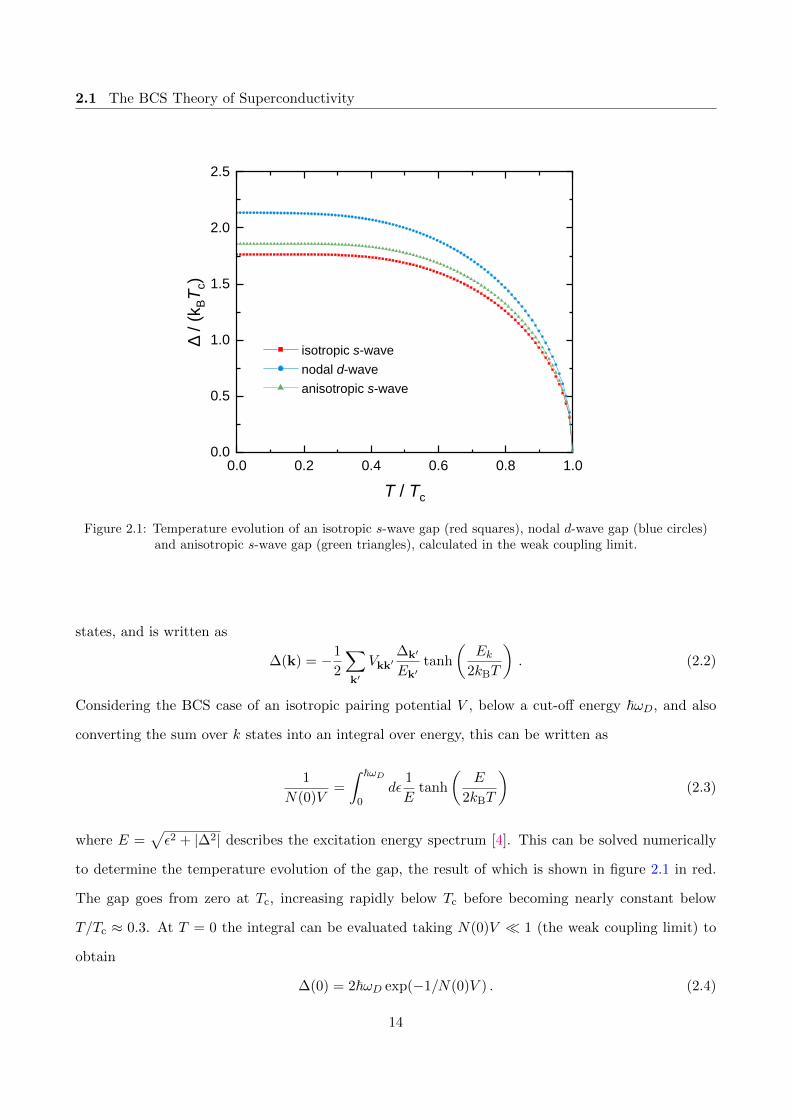
Figure 2.1: Temperature evolution of an isotropic s-wave gap (red squares), nodal d-wave gap (blue circles)and anisotropic s-wave gap (green triangles), calculated in the weak coupling limit.
states, and is written as
∆(k) = −1
2
∑k′
Vkk′∆k′
Ek′tanh
(Ek
2kBT
). (2.2)
Considering the BCS case of an isotropic pairing potential V , below a cut-off energy ~ωD, and also
converting the sum over k states into an integral over energy, this can be written as
1
N(0)V=
∫ ~ωD
0dε
1
Etanh
(E
2kBT
)(2.3)
where E =√ε2 + |∆2| describes the excitation energy spectrum [4]. This can be solved numerically
to determine the temperature evolution of the gap, the result of which is shown in figure 2.1 in red.
The gap goes from zero at Tc, increasing rapidly below Tc before becoming nearly constant below
T/Tc ≈ 0.3. At T = 0 the integral can be evaluated taking N(0)V 1 (the weak coupling limit) to
obtain
∆(0) = 2~ωD exp(−1/N(0)V ) . (2.4)
14
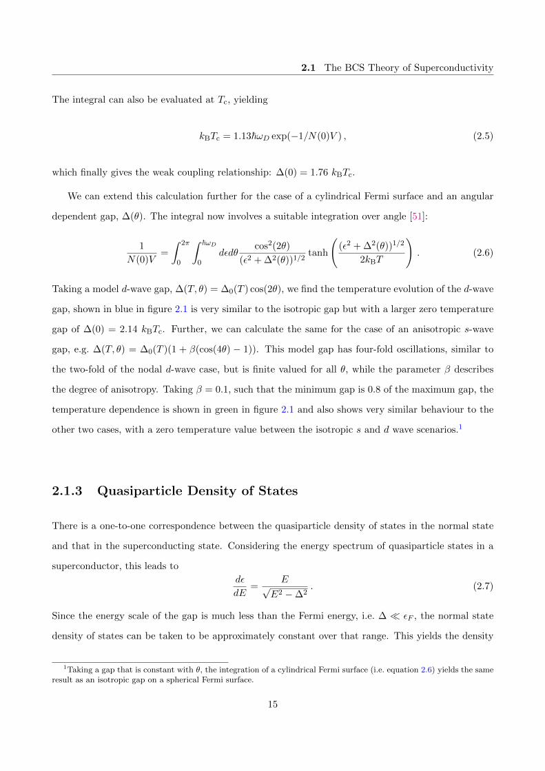
2.1 The BCS Theory of Superconductivity
The integral can also be evaluated at Tc, yielding
kBTc = 1.13~ωD exp(−1/N(0)V ) , (2.5)
which finally gives the weak coupling relationship: ∆(0) = 1.76 kBTc.
We can extend this calculation further for the case of a cylindrical Fermi surface and an angular
dependent gap, ∆(θ). The integral now involves a suitable integration over angle [51]:
1
N(0)V=
∫ 2π
0
∫ ~ωD
0dεdθ
cos2(2θ)
(ε2 + ∆2(θ))1/2tanh
((ε2 + ∆2(θ))1/2
2kBT
). (2.6)
Taking a model d-wave gap, ∆(T, θ) = ∆0(T ) cos(2θ), we find the temperature evolution of the d-wave
gap, shown in blue in figure 2.1 is very similar to the isotropic gap but with a larger zero temperature
gap of ∆(0) = 2.14 kBTc. Further, we can calculate the same for the case of an anisotropic s-wave
gap, e.g. ∆(T, θ) = ∆0(T )(1 + β(cos(4θ) − 1)). This model gap has four-fold oscillations, similar to
the two-fold of the nodal d-wave case, but is finite valued for all θ, while the parameter β describes
the degree of anisotropy. Taking β = 0.1, such that the minimum gap is 0.8 of the maximum gap, the
temperature dependence is shown in green in figure 2.1 and also shows very similar behaviour to the
other two cases, with a zero temperature value between the isotropic s and d wave scenarios.1
2.1.3 Quasiparticle Density of States
There is a one-to-one correspondence between the quasiparticle density of states in the normal state
and that in the superconducting state. Considering the energy spectrum of quasiparticle states in a
superconductor, this leads to
dε
dE=
E√E2 −∆2
. (2.7)
Since the energy scale of the gap is much less than the Fermi energy, i.e. ∆ εF , the normal state
density of states can be taken to be approximately constant over that range. This yields the density
1Taking a gap that is constant with θ, the integration of a cylindrical Fermi surface (i.e. equation 2.6) yields the sameresult as an isotropic gap on a spherical Fermi surface.
15
2.1 The BCS Theory of Superconductivity
(a) (b)
Figure 2.2: Normalised density of states for (a) an isotropic s-wave gap, and (b) a nodal d-wave gap.
of states in the isotropic case as
N(E) = N(0)
E√
E2−∆2(E > ∆)
0 (E < ∆). (2.8)
This is plotted in figure 2.2a and shows that there are no states below the energy of the gap. Consid-
ering again the case of a d-wave superconductor, since the gap has nodes there will be some k states
that exist below the gap and others that do not. This is not especially useful. However, by taking a
suitable angular average of the form
< N(E) >
N(0)=
∫ 2π
0
dθ
2π
E
(E2 −∆20 cos2(2θ))1/2
, (2.9)
this provides the following description of the DOS in a d-wave superconductor:
< N(E) >
N(0)=
2πE∆0K( E
∆0) (E < ∆0)
2πK(∆0
E ) (E > ∆0), (2.10)
where K is the complete elliptic integral of the first kind. This is shown in blue in figure 2.2b. This
contrasts strongly with the s-wave case, and shows that quasiparticle states exist within an arbitrarily
16

2.2 The London Equation and the Meissner Effect
small energy of the Fermi surface. As E → 0, K( E∆0
) ≈ π2 and so
< N(E) >
N(0)≈ E
∆0(E ∆0) . (2.11)
This has significant implication for thermodynamic quantities, such as specific heat and penetration
depth, as quasiparticle excitations will exist even to very low temperatures, modifying their response
from the fully gapped behaviour.
2.2 The London Equation and the Meissner Effect
As discussed in the introduction, the London theory of superconductivity was the first to successfully
account for the Meissner effect [7], in which a superconductor expels any magnetic field from within
it. In a normal metal, the conductivity σ is described by the Drude formula:
j = σE , (2.12)
where j is the current density and E is the electric field. However, in the London equation, the current
is proportional to the magnetic vector potential, B = ∇ ×A, rather than the electric field. This is
often written as
j = −nse2
m∗A , (2.13)
where e is the electronic charge, m∗ is the effective mass of the charge carriers and ns is the number
density of superconducting pairs. This is only true provided the correct gauge is chosen, so that
∇ ·A = 0, known as the London gauge. Taking the curl of both sides, and using the Maxwell relation
∇×B = µ0j (2.14)
we arrive at
∇2B = − 1
λ2B . (2.15)
17

2.3 Flux Quantization and the Ginzberg-Laundau theory of Superconductivity
Here we have identified the penetration depth as
λ =
(m∗
µ0nse2
)1/2
. (2.16)
The reason for doing so is because the solution to equation 2.15 is a field which decays exponentially
with depth into the superconductor [4], i.e. :
B = B0 exp(−x/λ) . (2.17)
Thus the penetration depth is the characteristic length scale over which the magnetic field is screened,
and which is set by material parameters. This is also why λ is often referred to as the London
penetration depth.
2.3 Flux Quantization and the Ginzberg-Laundau the-
ory of Superconductivity
In SI units, the magnetic induction B is related to the magnetic field H and the magnetization M
according to B = µ0(H +M), where µ0 is the permeability of free space. Thus, in a superconductor
B = 0 (due to the Meissner effect) and so M = −H, implying that the susceptibility χ = −1 of
a perfect diamagnet. However, this is only true for sufficiently weak magnetic fields. In a type I
superconductor, superconductivity will eventually be destroyed at a critical field Hc, above which the
magnetisation will become that of the normal state. This is sketched in figure 2.3.
The majority of superconductors, however, exhibit different behaviour. In type II superconductors,
there two different critical fields known as the lower critical field Hc1 and the upper critical field
Hc2. For small H, type II superconductors exhibit perfect diamagnetism in the same way as type I
superconductors. Above Hc1, however, superconductivity is not destroyed and magnetic flux, in the
form of vortices, begins to enter into the superconductor such that B 6= 0. The magnetisation deviates
from its M = −H behaviour and begins to approach zero as more magnetic flux enters the sample in
the form of vortices. Eventually, at Hc2, the superconductivity is destroyed completely. The overall
behaviour is shown in figure 2.3.
18

2.3 Flux Quantization and the Ginzberg-Laundau theory of Superconductivity
H
-M
M = -H
Hc H
-M
M = -H
Hc2Hc1
Type I Type II
Figure 2.3: Illustrative plots showing how the magnetisation M varies with magnetic field H for type I andtype II superconductors (with zero demagnetising factor).
An understanding of the differences between type I and type II superconductors was given by
the Ginzburg-Landau (GL) theory of superconductivity [4] and also by Abrikosov’s prediction of the
existence of vortices of magnetic flux in type II superconductors [52]. As discussed, the BCS theory
provides a microscopic explanation for superconductivity and its associated phenomena. The GL
theory, however, approaches superconductivity from a thermodynamic perspective of a second order
phase transition. The theory postulates the existence of an order parameter ψ that characterises the
superconducting state such that it is zero above Tc and takes on some finite value below Tc, e.g. ψ(T ).
By assuming that the free energy of a superconductor depends on |ψ| (ψ can be complex but the free
energy must be real) it is possible to Taylor expand the free energy in powers of |ψ| close to Tc. Then,
by considering how the coefficients of these powers of |ψ| must behave near Tc it is possible to derive
a number of properties of superconductors.
One particular property is that of magnetic flux quantization. Applying the GL theory to the
case of a superconducting ring, it can be shown that only certain quantisations of magnetic flux are
allowed to thread the superconducting ring, i.e. Φ = nΦ0, where Φ0 = h/2e is one quantum of flux.
Importantly, this shows that the relevant charge in a superconductor is 2e, corresponding to a Cooper
pair of electrons. No assumption is made about the nature of pairing and so this applies equally
to conventional as well as unconventional superconductivity. Using the GL theory, Abrikosov found
a solution describing the behaviour of a bulk superconductor in a magnetic field [52]. He showed
that in type II superconductors magnetic flux can enter in the form of vortices, each containing a
quantum of flux. Additionally, the difference between type I and type II is determined by the GL
parameter κ = λ/ξ, where ξ is the GL coherence length and λ is the penetration depth. Thus, type I
19

2.4 Temperature Dependence of λ
superconductors are those with κ < 1/√
2 and type II are those with κ > 1/√
2.
In a type I superconductor, the critical field Hc occurs at the point where the energy difference
between the normal and superconducting state becomes zero. By contrast, in a type II superconductor,
the energy cost associated with creating small amounts of normal state is outweighed by the energy
gained by allowing the field H to penetrate at the normal-superconducting interfaces, leading to the
entry of flux vortices. By considering the energy associated with a single, well-separated vortex, it is
possible to derive an expression determining the field at which the entry of flux becomes energetically
favourable; that is, the lower critical field, Hc1 :
µ0Hc1 =φ0
4πλ2
ln
(λ
ξ
)+ 0.5
. (2.18)
The GL theory is very powerful and provides an alternative method for approaching the problem
of superconductivity without any assumption of the underlying mechanism. It does, however, possess
some drawbacks. The theory is purely a mean-field theory and does not take into account the effects of
thermal fluctuations. The derivation is also based on the assumption that the temperature is close to
Tc, and so its applicability below Tc is questionable. Furthermore, the Abrikosov solution is for fields
close to Hc2 and so the expression for the lower critical field is more of an estimation. Nonetheless,
in systems where thermal fluctuations are small, e.g. superconductors with low Tc, it is expected that
the GL theory will be qualitatively correct [53].
2.4 Temperature Dependence of λ
How many Cooper pairs can form is determined by the temperature and the density of states at the
Fermi surface, and is described by the quantity ns. Above Tc no pairing takes place, and so the
penetration depth is infinite2. Then, as the temperature falls below Tc, the number of pairs ns will
increase until, at zero temperature, it reaches some saturation value and the penetration depth takes
on the value from equation 2.16. This quantity is often thought of as the supercurrent, or superfluid,
density, borrowing some terminology from the theory of superfluid 4He.
2This statement is not quite true as the skin depth of the normal state will inhibit the ability of a field to penetratewithin the sample. However, this is due to the response of the single quasi-particles to a varying magnetic field, and notto any coherent supercurrent response.
20

2.4 Temperature Dependence of λ
A semi-classical approach from Chandrasekhar and Einzel provides a generalised relationship be-
tween the supercurrent response to the magnetic vector potential given an arbitrary band structure
and energy gap [54]. The supercurrent density is related to the vector potential by a response tensor
T so that
J = −TA . (2.19)
The response tensor is composed of a diamagnetic part (TD) and a paramagnetic part (TP ), such that
T = TD + TP . (2.20)
In the two fluid model of superfluid 4He, these two terms are akin to the superflow and backflow
portions of the total response (though there is no equivalent to the London equation for superfluids).
The two components are related to the normal and superconducting state properties according to
TD 'e2
4π3~c
∮dSF
vFvFvF
(2.21)
and
TP ' 2 · e2
4π3~c
∮dSF
vFvFvF
∫ ∞∆k
dEk
(−∂f(Ek)
∂Ek
)Ek√
E2k −∆2
k
. (2.22)
From these it can be seen that the diamagnetic portion TD is dependent only on the normal state
properties and is independent of temperature. The paramagnetic portion is dependent on anisotropies
in both the normal state and superconducting state, and is also dependent on temperature.
The normalised superfluid density is related to the response tensor by
ρ(T ) =ns(T )
ns(0)=
T(T )
T(0)=λ2(0)
λ2(T ). (2.23)
It can be shown in the case of a spherical Fermi surface with an isotropic gap that, at low temperatures,
the superfluid density varies as [51]
ρ(T ) = 1−
√2π∆(0)
kBTexp
(−∆(0)
kBT
). (2.24)
Considering equation 2.16, and writing λ(T ) = λ(0) + ∆λ(T ), at low temperatures the penetration
21
2.4 Temperature Dependence of λ
depth varies as
∆λ(T )
λ(0)≈
√π∆(0)
2kBTexp
(−∆(0)
kBT
)(2.25)
The gap has been taken as the zero temperature value since it does not vary strongly over the temper-
ature range considered (see figure 2.1). Contrastingly, taking the model d-wave gap with line nodes,
and a cylindrical Fermi surface, the low temperature superfluid density varies as
ρ(T ) ≈ 1− 2 ln 2
∆0T (T Tc) (2.26)
leading to the penetration depth at low temperature given by:
∆λ(T )
λ(0)≈ ln 2
∆(0)T . (2.27)
These results show very different behaviour at low temperatures for the case of a full gap and a gap with
nodes. As discussed in the introduction, this is why determining the temperature dependence of the
penetration depth can aid in identifying the existence of nodes in the gap structure. Fundamentally,
this is due to the very different quasiparticle DOS in the two superconductors (figures 2.2 (a) and
(b)).
The calculation for the full temperature dependence of the normalised superfluid density can
be performed numerically for the same two scenarios (isotropic s and nodal d), as well as for the
anisotropic s-wave state described in section 2.1.2 [51]. The result of this is shown in figure 2.4a,
which shows striking difference between the two s-wave cases and the nodal d-wave case. In the d-
wave case, thermal depopulation of the pair states exists for all temperatures whereas the s-wave cases
show an activated behaviour above some characteristic temperature, approximately T/Tc ≈ 0.3. This
characteristic temperature is slightly lower in the anisotropic case than in the isotropic case, but is
influenced by the degree of anisotropy (described by β) as well as the functional form of the gap ∆(θ).
In the measurements presented in this thesis, it is not the superfluid density itself that is measured
but rather the change in the penetration depth measured with respect to some temperature (usually
taken to be the low temperature achieved). Thus it is useful to present the results of figure 2.4a in a
22

2.4 Temperature Dependence of λ
0 . 0 0 . 2 0 . 4 0 . 6 0 . 8 1 . 00 . 0
0 . 2
0 . 4
0 . 6
0 . 8
1 . 0
ρ (T)
T / T c
i s o t r o p i c s - w a v e n o d a l d - w a v e a n i s o t r o p i c s - w a v e
(a)
0 . 0 0 . 1 0 . 2 0 . 3 0 . 4 0 . 50 . 0 0
0 . 0 5
0 . 1 0
0 . 1 5
0 . 2 0
0 . 2 5
0 . 3 0
∆λ(T)
/ λ(0)
T / T c
i s o t r o p i c s - w a v e n o d a l d - w a v e a n i s o t r o p i c s - w a v e
(b)
Figure 2.4: (a) Temperature evolution for the superfluid density ρ corresponding to an isotropic s-wave gap(red squares), a nodal d-wave gap (blue circles) and an anisotropic s-wave gap. (b) The lower temperature
portion of the magnetic penetration depth for the same scenarios as (a).
way that is easier to compare. Taking equation 2.23, and writing λ(T ) = λ(0) + ∆λ(T ), we find
1√ρ(T )
− 1 =∆λ(T )
λ(0). (2.28)
Thus, figure 2.4b is the same data from figure 2.4a but plotted in this more easily comparable manner.
The fundamental difference in behaviours between the nodal d-wave and s-wave scenarios is maintained
when viewed this way.
Thus far we have restricted the analysis to the case of a single superconducting gap on a single
Fermi surface. However, the concept of multigap / multiband superconductivity has been shown to
exist in the case of MgB2 [55] as well as in a number of the iron-based superconductors [42, 56]. The
overall measured superfluid response in such a system is then influenced by each gap and how much of
the total superfluid it possesses. Possible behaviours can in general be quite complex as finite coupling
between the different bands can lead to non-weak-coupling temperature evolution of each gap, which
in turn influences the temperature evolution of each superfluid component [57].
Limiting the situation to the case of two superconducting gaps, it is typical to take the so-called
α model approach, where the two gaps are described by the BCS weak-coupling evolution, ∆1,2(T ) =
(α1,2/1.76)∆BCS(T ). The superfluid response for each gap, ρ1,2, is computed according to equation
23

2.5 Temperature Dependence of λ
0 . 0 0 . 1 0 . 2 0 . 3 0 . 4 0 . 5 0 . 6 0 . 7 0 . 8 0 . 9 1 . 00 . 0
0 . 2
0 . 4
0 . 6
0 . 8
1 . 0
ρ t o t a lρ(T
)
T / T c
( 1 - x ) ρ 1
x ρ 2
i s o t r o p i cs - w a v e
Figure 2.5: Alpha model determination of the superfluid response of an isotropic two gap superconductor,using α1 = 1.76, α2 = 0.7 and x = 0.65 (red). Despite 65% of the superfluid belonging to the large gap (green
dashed line), the low temperature behaviour is dominated by the characteristics of the smaller gap (yellowdash-dot line). The case for a single isotropic gap is also shown in blue dots.
2.23 using ∆1,2(T ), and the total response is determined according to ρ = xρ1 + (1 − x)ρ2, where
x describes proportion of the total superfluid density that each gap possesses. Given the number of
parameters, and introducing the possibility of anisotropic gaps, the range of possible behaviours of
ρ(T ) becomes quite large.
For the sake of simplicity, it is illustrative to consider the case of two isotropic gaps with α1 =
1.76, α2 = 0.7 and x = 0.65, as shown in figure 2.5. While the large gap exhibits a response that
is the same as the normal isotropic case, just scaled by the factor x, the smaller gap displays a
temperature dependence that is substantially different from the isotropic case. Instead of the typical
convex shape, the curve is concave at higher temperatures, before saturating at some constant value
at about T/Tc = 0.1. Importantly, even though the small gap only possesses a smaller fraction of the
total superfluid density, the total response is influenced significantly by this smaller gap. Moreover, at
low temperatures the response is almost entirely dominated by the characteristics of the smaller gap,
showing a saturation at a similar temperature.
24
2.5 Effects of Impurities
2.5 Effects of Impurities
Whilst the temperature dependence of certain quantities can provide insight into the gap structure in
a superconductor, it is important to consider the role of impurity scattering in these processes. Specif-
ically, impurity scattering due to chemical impurities or physical disorder can change the expected
temperature dependence of the magnetic penetration depth, due to the impact of scattering on the
low energy density of states relative to the Fermi level. The precise nature depends explicitly on the
structure and symmetry of the superconducting energy gap ∆.
In most superconductors, Cooper pairs are formed from time-reversed one-particle states, i.e.
with opposite momenta and spin. Considering a superconductor with a single isotropic gap (e.g. a
conventional superconductor), these pairs are robust to impurity scattering provided the perturbation
is time-reversal invariant [58, 59]. However, it was established that conventional superconductors
are very sensitive to paramagnetic impurities [60] due to the non-time-reversal invariant nature of
the exchange interaction between the conduction electrons and the paramagnetic impurity. As a
consequence, pairs are easily broken leading to a rapid reduction in Tc with impurity concentration
as well as a reduction in the energy gap ∆. At a critical pair-breaking parameter, a superconductor
will enter a gapless regime, in which there is no gap in the excitation spectrum [59] despite still
exhibiting superconducting behaviour. The consequence of this is that the magnetic penetration
depth will change from an activated behaviour, i.e. equation 2.25, to a T 2 power law behaviour at low
temperatures [43,61,62].
Non-magnetic impurities, on the other hand, have little effect on Tc for comparable concentrations
and generally weaken the effective electron-electron attraction by a small amount. In the case of an
anisotropic but still fully-gapped state (as in figure 1.1 (c)), scattering from non-magnetic impurities
is expected to ‘smear out’ the momentum dependence of the gap, eventually resulting in an isotropic
gap [46,48]. Since the density of states does not change in this scenario, except for the size of the gap,
an exponentially activated temperature dependence of ∆λ(T ) is still expected.
As discussed in section 2.4, the penetration depth is expected to vary linearly at low temperatures
when line nodes are present in the gap structure. It is important, however, to consider the differences
between symmetry imposed nodes, where the gap is required to change sign under some operation
25

2.5 Effects of Impurities
Figure 2.6: The normalised density of states of a nodal d-wave superconductor in the clean regime and also inthe case of weak (Born) and strong (unitary) scattering. These results were calculated using the SCTMA and
reproduced from ref. [63].
such as rotation or translation, and so-called accidental nodes, which can occur due to momentum
dependence of the pairing interaction. The dx2−y2 state of the cuprate superconductors is such an
example of symmetry imposed nodes. It was shown that when a small amount of Zn was substituted
for Cu in YBa2Cu3O7-x, the temperature dependence of ∆λ changed from linear to quadratic at low
temperature [43]. By contrast, a relatively large amount of Ni substitution produced essentially no
effect on the penetration depth. These differences were attributed to the nature of the scattering
caused by the substitution.
The self-consistent t-matrix approximation (SCTMA) is a theoretical framework that can be used
to determine the effects of impurity scattering in a d-wave superconductor [63–65], though a full
treatment will not be given here. Within the SCTMA, impurities are treated as isotropic point-
scatterers and are characterised by a scattering strength, c, which is the cotangent of the s-wave
scattering phase shift. SCTMA calculations are typically performed in two extreme limits: the first is
the case of weak scattering, where c 1 (also known as the Born approximation), and the second is
the case of strong scattering, where c = 0 (also known as the unitary limit). Both kinds of scattering
26

2.5 Effects of Impurities
Figure 2.7: Some schematic gap structures for the IBS with one hole and two electron pockets. The colourindicates a relative π phase difference between the gaps. Reproduced from ref. [42].
will cause pair-breaking and lead to ∆λ ∝ T 2 below some crossover temperature T ∗, and a linear
behaviour above this temperature. The temperature T ∗ can be estimated by fitting data to the
empirically determined formula [65,66]
∆λ(T ) ≈ A T 2
(T + T ∗), (2.29)
where A is some scaling factor. Importantly, the crossover temperature T ∗ will be much lower (possibly
immeasurably low) in the case of weak scattering, compared to strong scattering at a comparable
scattering rate Γ [43]. Furthermore, the effect of strong scattering is localised to low energies, inducing
a residual zero-energy DOS, whereas weak scattering induces a change at all energies, as shown in
figure 2.6. This means that a only a relatively small amount of strong scattering is required to
induce an observable effect in any quantity sensitive to the low energy DOS, such as the penetration
depth. On the other hand, a large amount of weak scattering would be required to produce a similar
effect, but this would be accompanied by a much larger reduction in Tc. The T 2 behaviour occurs
due to the induced gapless states, i.e. the presence of a finite DOS at zero energy whilst still in the
superconducting phase, with the impurity scattering essentially causing pair-breaking near the nodes
of the gap structure.
So far we have only considered superconducting states with a single Fermi sheet and accompanying
energy gap. However, in some systems, such as the IBS, there exist multiple Fermi sheets of which
some or all could possess an energy gap [42, 47]. These sheets are located at the center and corners
of the Brillouin zone, and are fairly well separated in momentum. A number of model gap structures
27
2.5 Effects of Impurities
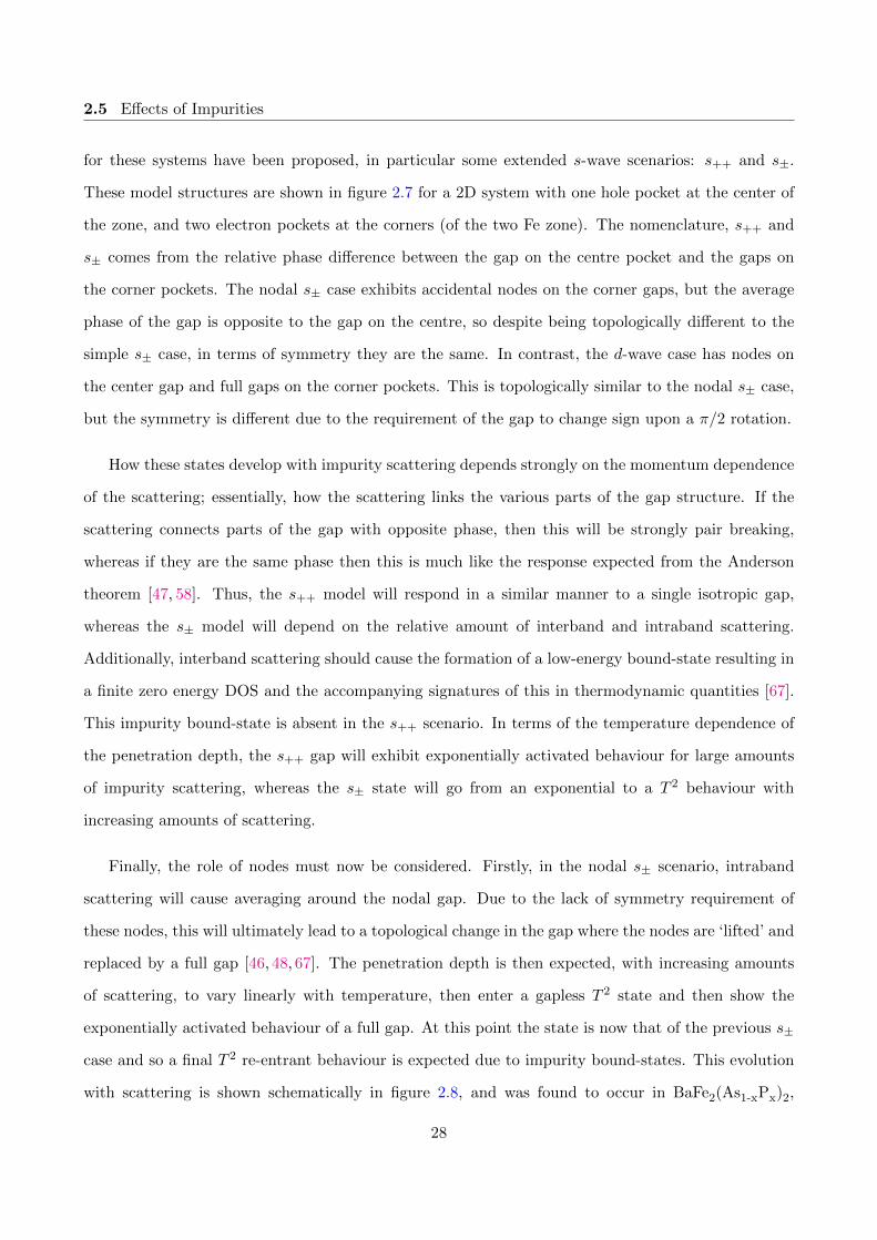
for these systems have been proposed, in particular some extended s-wave scenarios: s++ and s±.
These model structures are shown in figure 2.7 for a 2D system with one hole pocket at the center of
the zone, and two electron pockets at the corners (of the two Fe zone). The nomenclature, s++ and
s± comes from the relative phase difference between the gap on the centre pocket and the gaps on
the corner pockets. The nodal s± case exhibits accidental nodes on the corner gaps, but the average
phase of the gap is opposite to the gap on the centre, so despite being topologically different to the
simple s± case, in terms of symmetry they are the same. In contrast, the d-wave case has nodes on
the center gap and full gaps on the corner pockets. This is topologically similar to the nodal s± case,
but the symmetry is different due to the requirement of the gap to change sign upon a π/2 rotation.
How these states develop with impurity scattering depends strongly on the momentum dependence
of the scattering; essentially, how the scattering links the various parts of the gap structure. If the
scattering connects parts of the gap with opposite phase, then this will be strongly pair breaking,
whereas if they are the same phase then this is much like the response expected from the Anderson
theorem [47, 58]. Thus, the s++ model will respond in a similar manner to a single isotropic gap,
whereas the s± model will depend on the relative amount of interband and intraband scattering.
Additionally, interband scattering should cause the formation of a low-energy bound-state resulting in
a finite zero energy DOS and the accompanying signatures of this in thermodynamic quantities [67].
This impurity bound-state is absent in the s++ scenario. In terms of the temperature dependence of
the penetration depth, the s++ gap will exhibit exponentially activated behaviour for large amounts
of impurity scattering, whereas the s± state will go from an exponential to a T 2 behaviour with
increasing amounts of scattering.
Finally, the role of nodes must now be considered. Firstly, in the nodal s± scenario, intraband
scattering will cause averaging around the nodal gap. Due to the lack of symmetry requirement of
these nodes, this will ultimately lead to a topological change in the gap where the nodes are ‘lifted’ and
replaced by a full gap [46, 48, 67]. The penetration depth is then expected, with increasing amounts
of scattering, to vary linearly with temperature, then enter a gapless T 2 state and then show the
exponentially activated behaviour of a full gap. At this point the state is now that of the previous s±
case and so a final T 2 re-entrant behaviour is expected due to impurity bound-states. This evolution
with scattering is shown schematically in figure 2.8, and was found to occur in BaFe2(As1-xPx)2,
28

2.6 The Nonlinear Meissner Effect
Amount of scattering
Figure 2.8: Top row: schematic of a nodal s± gap vs. azimuthal angle φ and, bottom row: correspondingsingle particle DOS, both with increasing amounts of impurity scattering. Adapted from ref. [47].
where scattering was induced by electron irradiation [46]. In comparison, the multi-gap d-wave model
from figure 2.7 would initially show ∆λ(T ) ∝ T behaviour that would enter a gapless T 2 state when
scattering is introduced, much like the single gap nodal d-wave scenario. Importantly, due to the
symmetry imposed nature of the nodes, no further evolution in the penetration depth is expected
with increased amounts of impurities.
To summarise, the temperature dependence of the penetration depth, and anything else sensitive
to changes in the low energy DOS, can provide important information regarding the structure and
symmetry of the pairing state. In the clean limit, i.e. with no impurity scattering, certain temperature
dependences are expected depending on the presence or absence of nodes in the gap structure. The
evolution of the temperature dependence of λ with impurity scattering can then provide further
information that can help to resolve the symmetry of the gap state.
2.6 The Nonlinear Meissner Effect
So far we have considered the effects of temperature and scattering on the penetration depth. The
final aspect to consider is how a finite magnetic field H affects the supercurrent response, known as the
nonlinear Meissner effect. This effect was originally proposed by Yip and Sauls as a method with which
to test for the presence of nodes in the gap structure of cuprates, and also to resolve their orientation
in momentum space [49,68]. In the case of a finite superflow vs, the energy levels of the QP excitations
are Doppler shifted by an amount δE ∝ vs · vf , where vF is the Fermi velocity. For an isotropic,
29

2.6 The Nonlinear Meissner Effect
fully-gapped superconductor this will have little effect at low temperature since the finite gap will still
prevent these states from becoming occupied. However, in a nodal d-wave superconductor, where QP
states exist at very low energies, the field-shifted states will change the size of the zero energy DOS,
which in turn will impact the penetration depth even at T = 0. An important consequence of this is
that, for the dx2−y2 pairing state, the size of the change from the H = 0 response should depend on
the orientation of the field with respect to the crystal axes. Specifically, at T = 0 the result is
1
λ(T = 0, H)=
1
λ(0)
[1− 2
3HH0
], H‖node
1λ(0)
[1− 1√
223HH0
], H‖antinode
, (2.30)
where H0 = 3φ0/π2λξ is of the order of the thermodynamic critical field (Hc ≈
√Hc1Hc2) [51]. Thus,
for fields less then Hc1, a linear correction to the penetration depth is expected that should become
weakened with temperature, as the nonlinear response will compete with thermal depopulation. Above
Hc1, flux vortices will enter the sample and complicate the response of the supercurrent.
Stojkovic et al. performed calculations of the expected superfluid density for a number of different
pairing states at finite field and temperature [69], including a clean dx2−y2 state, a dirty d-wave (i.e.
with impurities) and a very anisotropic s+ id state, where the nodes are moved radially away from the
Fermi surface, forming a finite gap at all points on the Fermi surface. The results of these calculations
were originally presented in terms of the normalised superfluid density ρ = λ2(0, 0)/λ2(T,H). However,
in figure 2.9, the data has been replotted in the more familiar form of ∆λ(T,H)/λ(0, 0), which will
allow for more convenient comparison with measurements. The zero field and finite field curves have
also been offset such that they coincide at the highest temperature.
Figure 2.9a shows the expected response for a clean, nodal d-wave state. The effect of the field is to
change the response from linear in T to something resembling the power law response of the zero field
dirty d-wave case. This is expected as both the Doppler shifted states and the presence of impurities
will cause the zero energy DOS to change from vanishing at the Fermi surface to some finite amount.
The low energy states in the DOS come from the nodes in the gap structure, and therefore the effect of
both the field and the impurities is to break these pairs near the nodes [70]. In figure 2.9b, we then see
that there is little difference between the zero field and finite field response precisely due to the same
reason. That is, the impurities have already caused pair breaking near the nodes such that the shifted
30

2.6 The Nonlinear Meissner Effect
(a) (b) (c)
Figure 2.9: Results from calculations performed by Stojkovic et al. of the nonlinear supercurrent response fordifferent pairing states [69]. The field H is in units of the characteristic field H0 (see main text).
QP states do not cause any further change in the occupancy at low temperatures. Finally, figure 2.9c
shows the expected response for the very anisotropic but finite-gapped state. The zero field response
is as expected, showing essentially no change at low temperatures due to the exponentially activated
behaviour. This response is replaced with a much more temperature dependent behaviour when in
finite field. In zero field, there will be portions of the Fermi surface around which the magnitude of the
gap is very small. The effect of the shifted QP states will then be to effectively reduce the magnitude
of this gap even further3, altering the characteristic activation energy. It is conceivable then that at
sufficiently large H, but less than Hc1, the gap could be reduced to zero at certain points of the Fermi
surface, producing nodes and the associated response.
Despite the substantial effort to identify the nonlinear corrections to λ, the NLME has yet to
be convincingly observed. Part of the difficulty is in the limited energy range in which nonlinear
corrections are expected to appear; below Hc1(T ) but also above the impurity scattering limit T ∗.
The effect is largest at T = 0 so the best quality samples are required. Some measurements did at
first seem to show the linear field dependence expected [71], but more careful observation revealed an
unexpected temperature dependence of the the field response [70]. Since the size of the field response
is expected to decrease rapidly when δE kBT , the observed response was attributed to extrinsic
effects, possibly due to vortex motion. Some suggestion was also made that nonlocal effects could
3Strictly speaking, it will also increase the gap on other parts of the Fermi surface as states are shifted both up anddown in energy depending on their relative direction to the superflow. However, the response will be sensitive to theportions where the gap is reduced, not increased.
31

2.6 The Nonlinear Meissner Effect
cause a suppression of the NLME for fields H < Hc1, essentially rendering the NLME unobservable
for certain field orientations [50].
Due to the absence of a convincing observation, little published work on the NLME has appeared
in recent years. However, the Doppler shifting of QP energies is not restricted to the NLME alone and
has been exploited effectively in angle-resolved specific heat measurements Ce(φ) [72], e.g. to identify
line nodes in the gap structure of CeCoIn5 [73]. Thus, it is not obvious why field corrections to the
zero energy DOS should not be apparent in the penetration depth, excluding factors that may obscure
it. The NLME was originally presented in terms of the d-wave cuprate superconductors, and so the
majority of attempts to observe the NLME have been made in the cuprate superconductors, as well
as some organic compounds [51]. In recent years other nodal compounds have been identified, e.g. the
IBS LaFePO [74] and the above mentioned heavy fermion CeCoIn5. The NLME is not limited to the
d-wave pairing state but is a consequence of the nodes in the gap structure. Thus it may be worth
revisiting the effect, especially in systems where gap nodes seem to be accidental instead of symmetry
imposed.
32

Chapter 3
Experimental Details
The experimental results concerning the various superconducting compounds presented within this
thesis are predominantly of two different kinds of measurement: those of the temperature dependence
of the magnetic penetration depth, ∆λ(T ), and those of the lower critical field, Hc1(T ). Each mea-
surement involves a number of components in terms of the experimental set-up and also acquiring
and interpreting the measured data. Common to both of these measurements is the requirement for
low temperatures, varying from 50 mK to nearly 100 K. Finally, for the results presented in chapter
7, there was the additional requirement for the generation of hydrostatic pressures of up to 2.5 GPa
using a piston-cylinder cell (PCC).
In this chapter I will describe the various techniques and equipment required in order to make
these measurements and interpret the measured data.
3.1 Low Temperature Techniques
It is worth reflecting that as well as discovering the phenomenon of superconductivity [1], we also owe
Heike Kamerlingh Onnes for being the first to successfully liquefy helium three years prior [40]. It
was while Kamerlingh Onnes was investigating the properties of materials at these newly available low
temperatures that he made his discovery. In the years since, the field of low temperature physics has
expanded and matured significantly, with many new techniques for achieving even lower temperatures
and numerous applications to go with them. Suffice to say, there are many texts available that describe
33

3.1 Low Temperature Techniques
Liquid 4He(4.2 K)
Insulating Material
Radiation Shields
Magnet(Optional)
Vacuum Wall
Cryostat
Figure 3.1: Simplified schematic drawing of a dewar containing a reservoir of liquid 4He. A number ofcomponents help to thermally isolate the reservoir from any heat coming from the outer room. Cryostats aresuspended within the dewar, with the experimental portion immersed in the liquid 4He. Magnets can also be
hung from the top of the dewar.
good experimental practices for carrying out low temperature measurements (e.g. references [75–78]).
It is therefore not my intention to describe in great detail many of these aspects, but to provide some
overall context as well as focus on a few of the more non-trivial elements.
3.1.1 Dewars and Cryostats
All of the low temperature systems used were of the ‘wet’ kind, in the sense that they rely on the
continuous evaporation of liquid 4He (at atmospheric pressure), contained in a vacuum-walled dewar,
to cool a cryostat suspended within it to 4.2 K [79], as depicted in figure 3.1. Naturally, the dimensions
and construction of each dewar used are different but they can be considered to be functionally the
same and serve the same purpose. The vacuum wall, which normally also contains superinsulation,
helps to minimise the amount of heat travelling from the outer room to the 4He reservoir [75]. The
insulating material and radiation shields in the neck of the dewar also have the same purpose. The
cryostat is suspended in the neck of the dewar, with the lower part usually fully or partially immersed
in the liquid 4He. Optionally, a magnet (superconducting or otherwise) can also be suspended in the
dewar, such that the experimental stage of the cryostat is located at the field center.
34

3.1 Low Temperature Techniques
Pumping lines,electrical access etc
Vacuum Canister
4 K Flange Experimental stage
Figure 3.2: Simplified drawing of a low temperature cryostat. A number of stainless steel pipes connect fromroom temperature to the brass 4 K flange. These enable pumping and electrical access to the inside of the
vacuum canister. The experimental stage (also inside the vacuum canister) can be connected directly to the 4K flange, though a number of additional stages may be present between the flange and the experiment, such
as a 1 K pot.
In its most simple form, a typical cryostat consists of a canister containing the experimental
stage and then multiple pipes, usually stainless steel, that allow electrical wires to be run from room
temperature to the far side of the 4 K flange as well as allow pumping access to the inside of the
vacuum cannister. In actuality, numerous different and more sophisticated cryostat designs exist, but
this serves as a generic description for the kinds used for the purpose of this thesis. Indeed, there also
exist cryostats in which the experiment or sample is exposed to the liquid or gaseous 4He, and the
temperature is varied by changing the position of the cryostat within the dewar. However, only the
types involving vacuum canisters were used in this thesis.
At this point, a simple experimental stage could be connected to the the 4 K flange1. However,
it would not be especially easy to vary smoothly the temperature of the experimental stage due to
its strong thermal coupling to the flange, essentially clamping it to the temperature of the reservoir.
Thus, it is typical to thermally separate the experimental stage from the flange using a less thermally
conductive material. In this way, the experimental stage can be varied in temperature using a heater,
as shown in figure 3.3 (this particular set-up is described in more detail in section 3.1.2). The vacuum
canister must be pumped down to a low pressure, usually of the order of 10−5 mbar, removing any
air or gas that might serve to provide a thermal connection between the experimental stage and the
canister walls (helium is particularly effective at this) and it must be sealed against any possible
leaks [75]. Additional stages of varying complexity can also be incorporated in between the main 4 K
flange and the experimental stage to further reduce the base temperature of the experiment.
1So named since it is in direct contact with the liquid 4He reservoir.
35

3.1 Low Temperature Techniques
The different experimental stages tend to be made from oxygen-free high thermal conductivity
copper (OFHC) due to its superior thermal conductivity down to low temperatures [77]. The various
machined components are polished to a mirror finish and then gold plated. The polishing ensures
that surfaces are nominally flat and without scratches or flaws, so that when they mate there is good
thermal contact between them. The gold plating further helps in this regard but also protects the
copper from oxidising at its surface, resulting in worsened thermal conductivity [75].
Different kinds of cryostats lend themselves to some temperature ranges better than others, as well
as varying considerably in complexity and time required to cool down and operate. As such, a number
of different cryostats were used to meet the various requirements set by each measurement and also
the superconducting material in question.
3.1.2 4 K ‘Dipper’ Cryostat
The simplest cryostat used was the affectionately named ‘dipper’ cryostat. It is very simple in design
and, due to its low mass, it can be cooled rapidly to base temperature (approximately 5 K). A
schematic is shown in figure 3.3. The sample stage is separated from the 4 K flange by a rod of G10
(a glass epoxy laminate) which has a very low thermal conductivity at low temperatures [77]. The
heater, wound non-inductively from high resistance Constantan wire (a Cu-Ni alloy), then allows the
temperature to be varied independently from ≈ 5 K and above. The flange is shaped like a truncated
cone with the vacuum canister shaped in the inverse fashion. This allows the canister to be sealed
onto the flange using a small amount of vacuum grease.
This particular cryostat was used for making ambient pressure lower critical field measurements
(described in more detail in section 3.3). The Hall array device was mounted onto the sample stage
using a thin layer of GE 7031 varnish. Its orientation was such that the magnetic field was applied
into (or out of) the page as it is shown in figure 3.3. This was done using the horizontal Helmholtz
magnet (section 3.3.7).
3.1.3 1 K Cryostat
The 1 K cryostat increases a small amount in complexity from the 4 K dipper by introducing an
additional stage between the experiment stage and the 4 K flange. This so-called 1 K pot [76] works
36
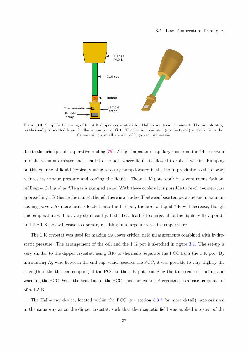
3.1 Low Temperature Techniques
Thermometer
Hall-bararray
Flange(4.2 K)
G10 rod
Heater
Samplestage
Figure 3.3: Simplified drawing of the 4 K dipper cryostat with a Hall array device mounted. The sample stageis thermally separated from the flange via rod of G10. The vacuum canister (not pictured) is sealed onto the
flange using a small amount of high vacuum grease.
due to the principle of evaporative cooling [75]. A high-impedance capillary runs from the 4He reservoir
into the vacuum canister and then into the pot, where liquid is allowed to collect within. Pumping
on this volume of liquid (typically using a rotary pump located in the lab in proximity to the dewar)
reduces its vapour pressure and cooling the liquid. These 1 K pots work in a continuous fashion,
refilling with liquid as 4He gas is pumped away. With these coolers it is possible to reach temperature
approaching 1 K (hence the name), though there is a trade-off between base temperature and maximum
cooling power. As more heat is loaded onto the 1 K pot, the level of liquid 4He will decrease, though
the temperature will not vary significantly. If the heat load is too large, all of the liquid will evaporate
and the 1 K pot will cease to operate, resulting in a large increase in temperature.
The 1 K cryostat was used for making the lower critical field measurements combined with hydro-
static pressure. The arrangement of the cell and the 1 K pot is sketched in figure 3.4. The set-up is
very similar to the dipper cryostat, using G10 to thermally separate the PCC from the 1 K pot. By
introducing Ag wire between the end cap, which secures the PCC, it was possible to vary slightly the
strength of the thermal coupling of the PCC to the 1 K pot, changing the time-scale of cooling and
warming the PCC. With the heat-load of the PCC, this particular 1 K cryostat has a base temperature
of ≈ 1.5 K.
The Hall-array device, located within the PCC (see section 3.3.7 for more detail), was oriented
in the same way as on the dipper cryostat, such that the magnetic field was applied into/out of the
37
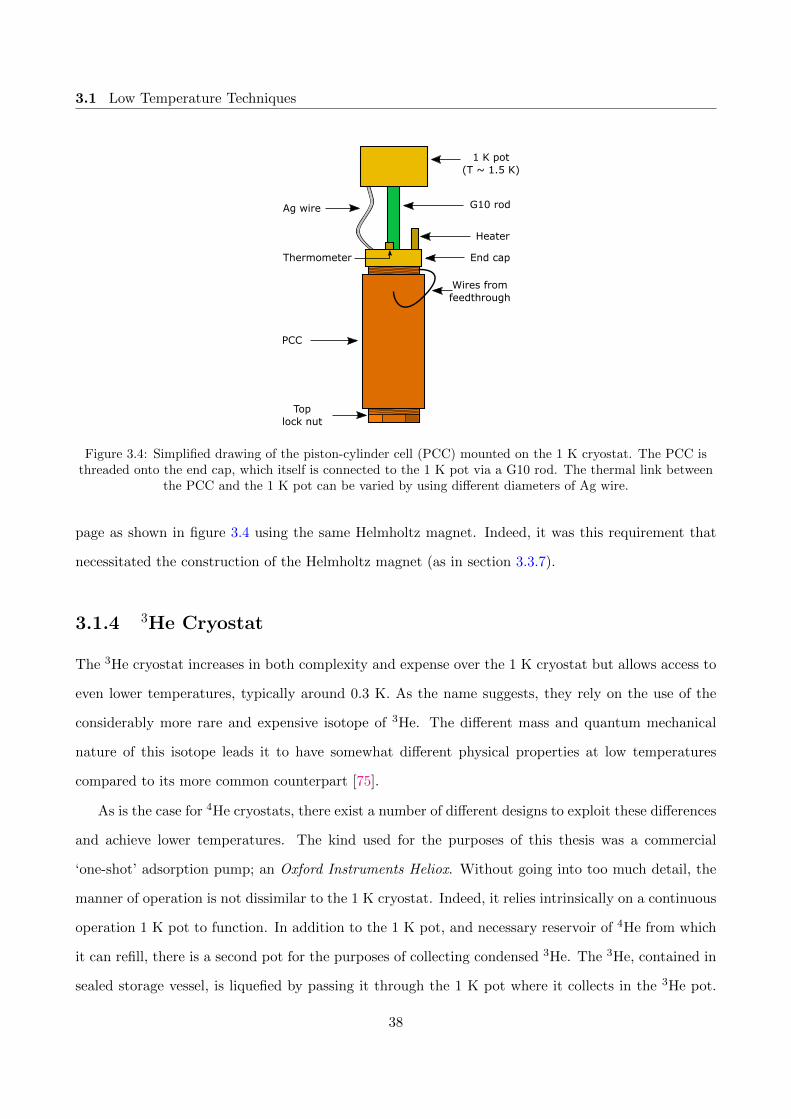
3.1 Low Temperature Techniques
End cap
1 K pot(T ~ 1.5 K)
G10 rod
Heater
Wires from feedthrough
PCC
Toplock nut
Thermometer
Ag wire
Figure 3.4: Simplified drawing of the piston-cylinder cell (PCC) mounted on the 1 K cryostat. The PCC isthreaded onto the end cap, which itself is connected to the 1 K pot via a G10 rod. The thermal link between
the PCC and the 1 K pot can be varied by using different diameters of Ag wire.
page as shown in figure 3.4 using the same Helmholtz magnet. Indeed, it was this requirement that
necessitated the construction of the Helmholtz magnet (as in section 3.3.7).
3.1.4 3He Cryostat
The 3He cryostat increases in both complexity and expense over the 1 K cryostat but allows access to
even lower temperatures, typically around 0.3 K. As the name suggests, they rely on the use of the
considerably more rare and expensive isotope of 3He. The different mass and quantum mechanical
nature of this isotope leads it to have somewhat different physical properties at low temperatures
compared to its more common counterpart [75].
As is the case for 4He cryostats, there exist a number of different designs to exploit these differences
and achieve lower temperatures. The kind used for the purposes of this thesis was a commercial
‘one-shot’ adsorption pump; an Oxford Instruments Heliox. Without going into too much detail, the
manner of operation is not dissimilar to the 1 K cryostat. Indeed, it relies intrinsically on a continuous
operation 1 K pot to function. In addition to the 1 K pot, and necessary reservoir of 4He from which
it can refill, there is a second pot for the purposes of collecting condensed 3He. The 3He, contained in
sealed storage vessel, is liquefied by passing it through the 1 K pot where it collects in the 3He pot.
38
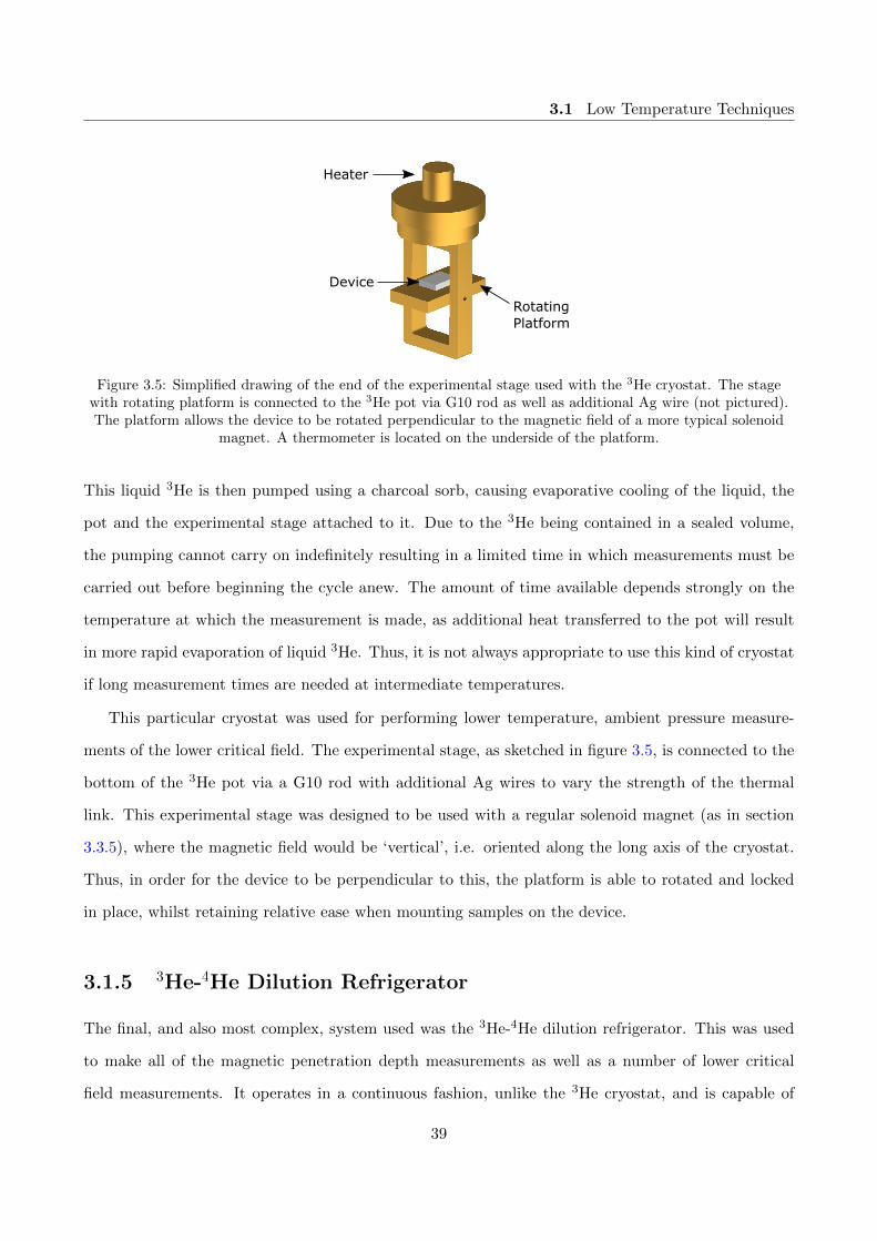
3.1 Low Temperature Techniques
Heater
Device
RotatingPlatform
Figure 3.5: Simplified drawing of the end of the experimental stage used with the 3He cryostat. The stagewith rotating platform is connected to the 3He pot via G10 rod as well as additional Ag wire (not pictured).The platform allows the device to be rotated perpendicular to the magnetic field of a more typical solenoid
magnet. A thermometer is located on the underside of the platform.
This liquid 3He is then pumped using a charcoal sorb, causing evaporative cooling of the liquid, the
pot and the experimental stage attached to it. Due to the 3He being contained in a sealed volume,
the pumping cannot carry on indefinitely resulting in a limited time in which measurements must be
carried out before beginning the cycle anew. The amount of time available depends strongly on the
temperature at which the measurement is made, as additional heat transferred to the pot will result
in more rapid evaporation of liquid 3He. Thus, it is not always appropriate to use this kind of cryostat
if long measurement times are needed at intermediate temperatures.
This particular cryostat was used for performing lower temperature, ambient pressure measure-
ments of the lower critical field. The experimental stage, as sketched in figure 3.5, is connected to the
bottom of the 3He pot via a G10 rod with additional Ag wires to vary the strength of the thermal
link. This experimental stage was designed to be used with a regular solenoid magnet (as in section
3.3.5), where the magnetic field would be ‘vertical’, i.e. oriented along the long axis of the cryostat.
Thus, in order for the device to be perpendicular to this, the platform is able to rotated and locked
in place, whilst retaining relative ease when mounting samples on the device.
3.1.5 3He-4He Dilution Refrigerator
The final, and also most complex, system used was the 3He-4He dilution refrigerator. This was used
to make all of the magnetic penetration depth measurements as well as a number of lower critical
field measurements. It operates in a continuous fashion, unlike the 3He cryostat, and is capable of
39

3.1 Low Temperature Techniques
reaching a base temperature of just below 50 mK. The particular system used was a commercial Oxford
Instruments Kelvinox 100.
As the name suggests, the 3He-4He dilution refrigerator relies on a mixture of both isotopes of
helium and the fact that they have different masses as well as obey different quantum mechanical
statistics. 4He has a nuclear spin of I = 0 and so obeys Bose statistics. On the other hand, 3He has a
nuclear spin of I = 1/2 and thus obeys Fermi statistics and the Pauli exclusion principle. These facts
lead to a number of interesting results, most important of which for our purposes is the finite solubility
of 3He in 4He at T = 0 (the limiting value being 6.6%). Thus, by taking a mixture of the two isotopes,
with greater than 6.6% 3He, and cool below 0.87 K (both now liquid), the mixture will phase separate
into different phases. One is rich in 3He (the so-called concentrated phase) and the other is mostly 4He
with a small amount of 3He (the so-called dilute phase). The cooling in a 3He-4He dilution refrigerator
occurs due to the heat of mixing of the two isotopes, rather than due to evaporative cooling like in
the 1 K pot or 3He system. In order to produce the cooling effect, 3He atoms must be transferred
from the concentrated phase into the dilute phase. This is achieved by osmotic pressure. The dilute
phase is pumped on to reduce the amount of 3He present in the phase. The vapour pressure of 3He is
higher than for 4He at low temperatures (T < 1 K) and so pumping will preferentially extract 3He.
This is done at a separate location to where the phase boundary occurs, causing an osmotic pressure
difference to occur. 3He will be driven to the other location to restore the concentration of 3He, and
in the process will ‘suck’ 3He across the phase boundary into the dilute phase, causing cooling in the
process2.
In a 3He-4He dilution refrigerator, the phase boundary occurs in a location called the mixing
chamber and the location where the dilute phase is pumped is called the still. As well as these, a
number of other components are required, such as a 1 K pot to cool the recirculating gas, impedances
to increase the pressure of the gas and heat exchangers between incoming and outgoing gases. The
mixing chamber is thus the location which cools to lowest temperature and is where the experimental
stage is attached. The still is usually heated to about 0.7 K to increase the vapour pressure of the
3He and increase the circulation rate of the gas. The impedance of the inlet for the 1 K pot can be
varied using a needle valve, thus allowing fine tuning of base temperature versus cooling power, and
2This is not a complete description of the process but captures sufficient detail for the purpose of this thesis.
40

3.1 Low Temperature Techniques
MixingChamber(<50 mK)
Sample Holder(~ 50 mK)
Ag Wires
CoaxialCable
Electronics Stage(~ 2.00 K)
Sense Coil & SC Magnet(~ 1.10 K)
ScrewMechanism
InsulatingStruts
Guide &Sample Stage
(<50mK)
Screw Driver
Ag Wire
Ag wirethermal
connectionsCoax cable to
4 K flange
Driver Shaftto RT
Figure 3.6: Simplified schematic drawing of the penetration depth experiment, which is located on the bottomof the dilution refrigerator’s mixing chamber. The coil stage is thermally connected with silver wire to thestill, which is located toward the top of the dilution refrigerator. The electronics stage is connected in a
similar manner to the 1 K pot.
41

3.1 Low Temperature Techniques
is usually set to give Tpot ≈ 1.4 K.
Figure 3.6 shows a schematic drawing of the penetration depth experiment and how it is arranged
on the 3He-4He dilution refrigerator. The main sample stage is connected via OFHC screws and
an intermediary Au plated Cu disc to the mixing chamber, giving very good thermal connection.
Below the sample stage is connected the coil stage and below that the electronics stage. Each stage
is separated by thermally insulating struts to help prevent heat from flowing from the hotter stages
to the cold sample stage. To further aid this, and to help stabilise the temperatures of the coil and
electronics stage, each is thermally coupled via Ag wire to different thermal anchors. The coil stage
is connected to the still and is typically maintained at a temperature of 1.10 K and the electronics
stage is coupled to the 1 K pot and maintained at roughly 2.00 K. The coil and electronics stage each
possess a Cernox 1050 thermometer and a heater. Additionally, a rigid coaxial cable runs from the 4
K flange to near the electronics stage, where the final part is semi-rigid. The rigid coax is made from
stainless steel and so does not couple the two sections very strongly.
The sample holder is held by the screw mechanism, which itself is located on the plate connected
to the mixing chamber. Additionally, the sample holder is coupled to the sample stage by a Ag wire.
For a typical measurement, the sample holder will be fully inserted into the guide, such that the
metallic faces of the sample holder and guide make contact. The sample holder can be driven in and
out of the guide using the driver for the screw mechanism. This mechanical driver can be engaged
and disengaged as needed while the 3He-4He dilution refrigerator is cold. As the shaft extends all the
way to room temperature, it was heat sunk at the 4 K flange as well as at the 1 K pot to minimise
any heat leak from room temperature to the sample stage. A germanium thermometer and heater are
mounted on the sample stage, and each sample holder also has a separate thermometer (see section
3.2.5).
The sense coil (i.e. L1 in figure 3.8) takes the form of a short solenoid. In a typical measurement,
the sample holder is fully inserted into the guide so that the sample is at the centre of the sense
coil. In addition, there is another short solenoid located around the sense coil, with its magnetic
field aligned colinearly. This solenoid is wound using superconducting wire and is used to provide a
small, additional DC field to the sample, as used in the non-linear measurements. This magnet has a
calibration of 65.4 mT A−1 and its field centre coincides with the field center of the sense coil.
42

3.2 Low Temperature Techniques
HDevice with
sample
Figure 3.7: Simplified drawing of the sample stage for measuring Hc1 on the dilution refrigerator. The stage isbolted onto the main stage of the refrigerator, and a small solenoid is located around it.
For the lower critical field measurements, a separate stage, consisting of the device holder and
superconducting short solenoid, was mounted directly to the sample stage. This stage was also made
of Au-plated Cu and is pictured in figure 3.7. This stage has a moderately large and flat bottom to
enable good thermal contact between it and the sample stage’s plate, and is bolted down using a brass
screw.
3.1.6 Thermometry
In general, Cernox 1050 thermometers were used for temperature ranges between 300 K and ≈ 1 K in
combination with a Lakeshore 340 temperature controller. For temperatures below 1 K, a number of
different thermometers were used. For the 3He cryostat sample stage a Cernox 1030 was used, and for
the penetration depth sample rods, a Cernox 1010 was used for the H‖ab rod and a RuO2 thermometer
was used for the H‖c rod. As well as the sample rods, there was a secondary germanium thermometer
mounted on the sample stage. For the low temperature thermometers, a Stanford Research SIM921
AC resistance bridge was used. When measuring at temperatures < 1 K it is important to consider
the effects of self-heating due to the excitation from the measuring instrument. It was found that for
an excitation of 100 µV did not introduce self-heating for all of the thermometers, apart from the
germanium thermometer for which an excitation of 30 µV was used. As well as avoiding self-heating,
good practices were followed to ensure good thermalisation of the thermometer with the various stages
and that appropriate wiring was used to avoid any issues with noise pick-up [75].
43

3.2 Magnetic Penetration Depth Measurements
R1
C1
R2C2
R3 C3
L1L2
CoaxcoretoRT
electronics
ElectronicsStage CoilStage
D1
Figure 3.8: Tunnel diode oscillator (TDO) circuit diagram. R1 = 1 kΩ, R2 = R3 = 500 Ω, C1 = 20 pF,C2 = 10 nF, C3 = 100 pF, D1 = BD3.
3.2 Magnetic Penetration Depth Measurements
3.2.1 Principle of Operation
The technique employed for the purposes of this thesis is a radio frequency tunnel diode oscillator
technique. In brief, the superconducting sample is located inside (but not in contact with) an inductive
coil, which forms part of a very stable resonant LC circuit. The magnetic field due to the inductor,
which is in the form of a solenoid, is very small and so the sample remains in the Meissner state.
Additionally, the vacuum canister of the 3He-4He dilution refrigerator is shielded in mu-metal to help
further shield the set-up from extrinsic magnetic fields. Changes in the penetration depth, e.g. due to
changing temperature of the sample, are measured directly as changes in the resonant frequency of the
LC circuit. To ensure low noise in the measurement, the temperature of the coil and electronic stages
must be stabilised very carefully as the resonant frequency is also sensitive to temperature changes at
these locations. This particular technique is well established and has been described in considerable
detail elsewhere [80–82].
3.2.2 Tunnel Diode Oscillator Circuit
The core of this technique is the tunnel diode oscillator (TDO) circuit, as shown in figure 3.8. This
circuit was designed to allow precise measurements of very small changes in the resonant frequency
of an LC circuit, and its design and operation is described in detail in the original work by van
Degrift [83]. Given proper implementation, the TDO circuit can reach sensitivities of 1 ppb.
44

3.2 Magnetic Penetration Depth Measurements
0 . 0 0 0 . 0 5 0 . 1 0 0 . 1 5 0 . 2 0 0 . 2 5 0 . 3 00 . 0 0
0 . 0 5
0 . 1 0
0 . 1 5
0 . 2 0
0 . 2 5
I d (mA
)
V d ( V )
d I d / d V < 0
m a x s l o p e
T = 4 . 2 2 K
Figure 3.9: I-V curve for a BD3 tunnel diode measured while immersed in liquid helium (T = 4.22 K). Thecharacteristic negative differential resistance portion of the data is indicated between the dashed black lines,
as is the position of maximum slope. The shape of the graph is typical of tunnel diodes in general.
In a simple LC circuit, the interaction between the inductor and capacitor will lead to a resonant
frequency to occur at f0 = 1/(2π√LC). However, resistive losses in the circuit will result in the
eventual decay of any resonance. In the TDO circuit, this is compensated for by the tunnel diode,
D1, due to the very non-ohmic I-V behaviour, particularly that of negative differential resistance,
as shown in figure 3.9. As indicated, when in the appropriate part of the I-V curve, an increase in
current results in a decrease in voltage, and vice versa. Thus, when biased appropriately, the tunnel
diode acts like a negative ac resistance and can prevent the decay of the resonance by compensating
for any losses.
The resonant frequency of the TDO is largely determined by the values of L1 and C3, which form
the series LC sub-circuit, though it is also affected to a lesser degree by the other components. van
Degrift found that the best performance of the circuit is achieved when the bias current is adjusted to
the point of maximum slope, which corresponds to the minimum value of negative ac resistance [83].
Additionally, the second inductor, L2, serves to minimise the ac voltage excursions around the bias
point, causing the oscillation to become ‘marginal’, and achieving the greatest sensitivity. The exact
inductance of the tapping coil (L2) is found using trial-and-error, though typically it has a value of
45

3.2 Magnetic Penetration Depth Measurements
L2 ≈ L1/4.
The remaining components serve to stabilise the circuit and to set proper operating conditions.
R3 is present to dampen parasitic oscillations occurring due to the combined inductance of L1 and L2
with the stray capacitance from the p-n junction within the diode. R1 and R2 form a potential divider
for the DC bias current, which originates at room temperature, setting the correct operating point for
the diode as well as sinking the remaining current to ground. The capacitors C1 and C2 also form a
potential divider, but for the AC part of the signal, allowing only a small part of the signal to return
up the coaxial cable to room temperature. The core of the coaxial cable carries the bias current and
signal, and the shield is connected to electric ground.
The exact values of the components can be determined by a formula given in [83], and the values
determined for the 3He-4He dilution refrigerator are given in the caption of figure 3.8. The operating
frequency of this version of the TDO was typically ≈ 14 MHz.
3.2.3 Room Temperature Electronics
The room temperature electronics serve to provide a DC bias current for the diode and to process
the resulting AC signal. A block diagram is shown in figure 3.10. The bias current is supplied from
a home-built precision current source. The signal is capacitively coupled to two Mini-Circuits ZFL-
500N+ fixed-gain high-frequency amplifiers, which provide a gain factor of approximately 250. The
signal then enters a Mini-Circuits ZLW-2 mixer, where it is modulated with a signal from a local
oscillator (LO), provided by a IFR 2023A. The resulting signal is then composed of frequencies equal
to the sum and difference of the signal and LO frequencies. If the LO is set to be close to the signal
frequency, the sum component will be very high while the difference will be much lower. This also has
the effect of separating, in the frequency domain, the fundamental of the signal from its harmonics.
After the mixer, the signal is amplified once more by a fixed gain amount of 1000 before it is
put through a narrow band-pass filter centred at 3 kHz. The LO is typically set to a frequency
such that the resulting mixed frequency is ∼ 3 kHz, so that it coincides with the center of the filter.
The band-pass filter is formed by setting the high and low cut-off frequencies to be the same. The
particular filter used (a Signal Recovery Model 5113 Pre-amp) has a roll-off of 6 db per octave either
side in this setting. Centering the frequency of the post-mixer signal at ∼ 3 kHz allows it to pass
46

3.2 Magnetic Penetration Depth Measurements
Coax core to electronics stage
DC bias from current source
Fixedgain
amplifiersMixer
x1000 Gain
& 3kHzband-pass
LocalOscillator
FrequencyCounter
10 MHz Reference Signal
Figure 3.10: Functional diagram of the room temperature electronics, showing the order in which the signalfrom the TDO is processed.
nominally unattenuated3, but filters out any high and low frequency content, such as the frequency
sum component from the mixer or other extraneous noise. As the measured frequency shifts during a
typical measurement are only on the order of a few Hz, the signal tends to remain close to the center
of the filter and so is largely unaffected. However, when measuring superconducting transitions, or
sample extractions, the frequency can vary by up to tens of kHz. Thus the filter will cause undesirable
attenuation of the signal when the frequency moves away from the passband. In this case, the width
of the passband is increased, with a low frequency cut-off of 3 kHz and a high frequency cut-off of 10
or 100 kHz, as circumstance dictates. This allows the frequency of the signal to change significantly
and remain unattenuated. This will also increase the noise content of the signal, but this is normally
insignificant compared to the larger overall frequency shifts.
The final part of the signal chain is the frequency counter; a HP 53131A. As well as determining
the frequency of the resulting signal, this also provides an oven-stabilised 10 MHz reference signal for
the IFR 2023A. The data from the frequency counter is then logged using a PC and a control program
written in Delphi.
3.2.4 Temperature Stabilisation
The TDO circuit is inherently an active circuit and so heat is dissipated throughout. This is particu-
larly important as the resonant frequency is very sensitive to changes in temperature of the electronics
stage, at approximately 100 Hz K−1, and can completely dominate the measured signal if not stabilised
appropriately. Stabilisation of the electronics stage is achieved using a Cernox thermometer, located
3In reality, there is some attenuation even at the middle of the passband. However, this is a small amount and canbe compensated for with increasing the pre-filter gain.
47

3.2 Magnetic Penetration Depth Measurements
on the electronics stage, in a three-lead bridge configuration. The resistance of the thermometer is
compared to the resistance of a high-precision variable resistor at room temperature. The difference
is output from the bridge set-up as an error signal which is processed by an analogue PI circuit. This
then supplies a current for a heater also located on the electronics stage, changing the temperature
until the resistances of the thermometer and reference resistor are equal and the error signal is zero.
The temperature stabilisation of the electronics stage was typically 10-20 µK, resulting in a noise
contribution of ≤ 2 mHz.
As well as the electronics stage, the resonant frequency of the TDO is also sensitive to the temper-
ature of the coil stage, though to a somewhat lesser extent. Stabilisation was achieved using a Cernox
thermometer and heater, both located on the coil stage, in a feedback loop using a Lakeshore 340
temperature controller. Typical temperature stabilisation was with temperature variation less than
10 mK, contributing less than 1 mHz to the noise of the measured signal.
3.2.5 Sample Holders
The sample holder is what is used to suspend the sample within the sense coil (L1 in figure 3.8). It
consists of a high-purity sapphire rod, with a diameter of 0.8 mm, set into the Au-plated Cu plug
with Stycast 1266 epoxy. On a flattened portion of the Cu plug a thermometer is mounted with GE
varnish. Directly behind this a Ag wire is clamped to this plug, the other end of which is bolted to
the sample stage using a brass screw and washer. Samples are mounted to the end of the sapphire
rod using a small amount of Dow Corning vacuum grease.
There are two versions of the sample holder where the end of the sapphire rod has been cut into
different shapes. This allows samples to be oriented differently within the magnetic field of the sense
coil, which results in different components of the penetration depth being measured. The first shape,
as in 3.11 (a), is a flat, polished end. As a typical sample is usually a thin, rectangular platelet, the
plane of the sample is perpendicular to the field. For the second shape, (b), a part of the cylinder has
been cut and polished enabling the sample to be mounted with the plane parallel to the field. The
two orientations have different effects on the measured signal, as explained in section 3.2.8, and will
be referred to as the H‖c and H‖ab configurations.
Rather than there being a heater located directly on the sample rod, the heater is in fact located
48

3.2 Magnetic Penetration Depth Measurements
Thermometer Sapphire
Au plated CuAg Wire
(a) (b)
Sample
H || c H || ab
Figure 3.11: Diagram of the two geometries of sample rod used, (a) and (b). Both consist of a sapphire rod setinto a tight-fitting hole using Stycast 1266. The metallic component of the rod is Au plated OFHC. A
thermometer is mounted onto the Cu, and a Ag wire thermally couples the rod to the sample stage. The endof the sapphire rod is a different shape for the two rods, allowing different sample orientations within the sense
coil.
on the sample stage. The temperature of the sample holder, and by virtue the sample, is then varied
by heating the whole of the sample stage in a feedback loop with the thermometer located on the
sample holder. The Ge thermometer is used to confirm the temperature of the sample stage and can
be used as a backup if need be.
At this point, a concern arises about whether the thermometer and sample are in good thermal
connection and whether the temperature reported by the thermometer is also true for the sample.
This is a legitimate concern due to the diminishing thermal conductivity of the sapphire rod at low
temperatures, the limited thermal coupling of the grease used to secure the sample and also the
possibility of rf heating of the sample by the sense coil. These factors could lead to a difference in
temperature to appear between the sample and the thermometer. It is difficult to estimate the size
of these effects, particularly since the precise magnitude of the rf field is not known (though it is of
the order of 1 µT) and it would require a priori knowledge of the surface resistance of the sample in
question.
As it is not possible to determine the precise extent of this problem, it is necessary to make a
49
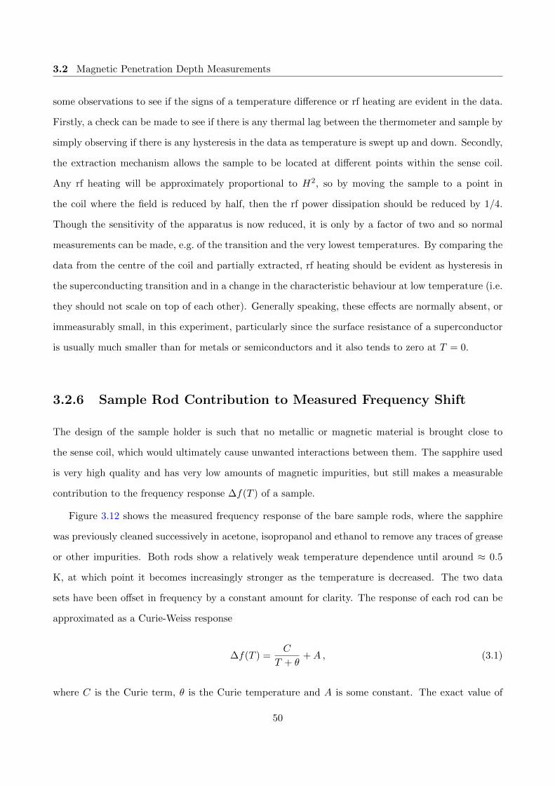
3.2 Magnetic Penetration Depth Measurements
some observations to see if the signs of a temperature difference or rf heating are evident in the data.
Firstly, a check can be made to see if there is any thermal lag between the thermometer and sample by
simply observing if there is any hysteresis in the data as temperature is swept up and down. Secondly,
the extraction mechanism allows the sample to be located at different points within the sense coil.
Any rf heating will be approximately proportional to H2, so by moving the sample to a point in
the coil where the field is reduced by half, then the rf power dissipation should be reduced by 1/4.
Though the sensitivity of the apparatus is now reduced, it is only by a factor of two and so normal
measurements can be made, e.g. of the transition and the very lowest temperatures. By comparing the
data from the centre of the coil and partially extracted, rf heating should be evident as hysteresis in
the superconducting transition and in a change in the characteristic behaviour at low temperature (i.e.
they should not scale on top of each other). Generally speaking, these effects are normally absent, or
immeasurably small, in this experiment, particularly since the surface resistance of a superconductor
is usually much smaller than for metals or semiconductors and it also tends to zero at T = 0.
3.2.6 Sample Rod Contribution to Measured Frequency Shift
The design of the sample holder is such that no metallic or magnetic material is brought close to
the sense coil, which would ultimately cause unwanted interactions between them. The sapphire used
is very high quality and has very low amounts of magnetic impurities, but still makes a measurable
contribution to the frequency response ∆f(T ) of a sample.
Figure 3.12 shows the measured frequency response of the bare sample rods, where the sapphire
was previously cleaned successively in acetone, isopropanol and ethanol to remove any traces of grease
or other impurities. Both rods show a relatively weak temperature dependence until around ≈ 0.5
K, at which point it becomes increasingly stronger as the temperature is decreased. The two data
sets have been offset in frequency by a constant amount for clarity. The response of each rod can be
approximated as a Curie-Weiss response
∆f(T ) =C
T + θ+A , (3.1)
where C is the Curie term, θ is the Curie temperature and A is some constant. The exact value of
50

3.2 Magnetic Penetration Depth Measurements
Figure 3.12: Graph showing the measured background response of the two sample rods. The red squares showthe data for the H‖c rod, and blue circles for the H‖ab rod. The grey lines are the results from fitting a
Curie-Weiss type behaviour, as described in the main text.
51

3.2 Magnetic Penetration Depth Measurements
Figure 3.13: The measured frequency shift as the sapphire rods were extracted from the sense coil, wherex = 0 is full insertion. The red squares are for the H‖c rod (performed at 1.00 K), and blue circles for theH‖ab rod (performed at 0.60 K). The profiles are slightly different, but the overall shift after extraction is
nominally the same for the two.
A is not important because it is only the change in frequency against some arbitrary temperature
(usually chosen to be the lowest T achieved) that is actually measured. Fitting to this form then
yields parameters than can be used to correct the measured ∆f(T ) for a superconducting sample. For
the H‖ab rod this gives C = 0.037± 0.001 Hz K and θ = 0.093± 0.005 K. For the H‖c rod this gives
C = 0.067 ± 0.002 Hz K and θ = 0.163 ± 0.006 K. The results of the fit are plotted as grey lines in
figure 3.12.
As well as contributing to the measured temperature dependence, the sample rods also make a
contribution to the measured frequency jump (i.e. the extraction value, section 3.2.8) when the sample
is fully removed from the sense coil. Figure 3.13 shows how the measured frequency changes as the
sample rod is extracted from the sense coil, where x = 0 is the rod fully inserted. Due to the different
shapes of the rods, the extraction profiles are not exactly the same. However, the total frequency
shifts once the rods are fully extracted are almost equal. The extraction value (∆f0) for the H‖c rod
is ≈ 807 Hz and for the H‖ab rod is ≈ 813 Hz.
52

3.2 Magnetic Penetration Depth Measurements
For the non-linear penetration depth measurements, an additional DC field is applied to the sample
in addition to the radio frequency AC field. The magnitude of this field was typically not greater than
6 mT, and it was found that the additional DC field did not modify the background contribution of
the sapphire rods.
3.2.7 Measurement and Analysis
Though considerable effort is made to ensure good temperature stabilisation and to reduce sources of
noise, the frequency as measured by the frequency counter (and logged by the PC) typically shows
Gaussian noise of 10-20 mHz. As well as this, the TDO exhibits a drift in frequency over a time period
of many hours - approximately 0.5 Hz in 12 hours. A number of steps are taken in the acquisition and
analysis stages to account for this.
The measurement process is largely controlled and automated by a program running on a PC.
The temperature is swept smoothly between a minimum and a maximum multiple times, with hold
times in between each sweep, and the corresponding frequency is logged on the PC. The range and
rate of each sweep is chosen bearing in mind the cooling rate of the 3He-4He dilution refrigerator and
also ensuring the total time of one sweep is not more than ≈ 1 hour, as it can then be difficult to
distinguish the signal from any long-term drift.
Once complete, the data is inspected for any signs of drift. If present, an attempt is made to remove
it by approximating it with a linear or a smoothly, and slowly, varying function, so as not include
contributions from the more quickly varying signal from the sample. After this, the remaining data
is due to the sample alone and the different sweeps are averaged together, improving the signal-noise
ratio.
For the nonlinear penetration depth measurements, it is important to avoid unintentionally intro-
ducing any flux vortices into the sample. Thus, before each measurement the sample must be warmed
above Tc and then zero-field cooled to ensure no flux is trapped in the sample. Once the sample has
cooled to base temperature, of ≈ 50 mK, a few initial temperature sweeps are performed with no DC
field to ensure that the behaviour is consistent with previous measurements (as a full measurement
up to Tc would have already been measured). Then, once the sample has cooled to base temperature
once more, the DC field is applied and temperature sweeps are performed over the desired range.
53

3.2 Magnetic Penetration Depth Measurements
Once more, it is important to consider what Hc1(T ) is along with possible demagnetising effects of
the sample so that magnetic flux does not enter the sample, contributing to the measured frequency
shift and obscuring the results.
3.2.8 Determining ∆λ from ∆f
The presence of a sample inside the sense coil modifies the resonant frequency, f0, of the empty coil
by an amount ∆f that is proportional to the volume susceptibility,
∆f
f0=
1
H2
∫Mac ·H dV . (3.2)
This occurs because the superconductor is diamagnetic and so screens some fraction of the volume of
the coil. However, some of the volume of the sample is penetrated by the magnetic field due to the
finite penetration depth, λ. In general, this penetrated volume Vλ is given by
Vλ =
∮SdS λ
Hs
H0, (3.3)
where Hs is the field at the surface and H0 is the applied field. As general analytical solutions to the
London equations, for a sample of arbitrary shape and hence demagnetising factor, do not exist this
problem becomes difficult to evaluate. Thus, a different approach is required.
The volume of the sample penetrated by the field as a proportion of the effective sample volume
V0 is related to two quantities: the change in resonant frequency of the coil due to the presence of the
sample, ∆f0 (termed as the extraction value), and the shift in the extraction value due to the small
volume of sample penetrated by the field, ∆fλ. The proportion of each is equal, i.e.
∆fλ∆f0
=VλV0
. (3.4)
From this it is possible to relate changes in the resonant frequency ∆f to changes in the penetrated
volume, Vλ, as a function of temperature. It is useful to define these fractional changes with respect
to some minimum temperature, e.g. δfλ(T ) = ∆fλ(Tmin)−∆fλ(T ), ∆Vλ(T ) = Vλ(Tmin)− Vλ(T ) and
∆λ(T ) = λ(Tmin)− λ(T ).
54
3.2 Magnetic Penetration Depth Measurements
Hrf
c
a/b
a
(a) (b)
c
a/b
a
lx lz
ly
lx ly
lz
Figure 3.14: Diagram showing how screening currents run in a platelet sample oriented two ways to themagnetic field. (a) H‖ab: the currents are mostly along the front-back and side faces. (b) H‖c: currents run
along the edges and also around the top-bottom faces.
Of the unconventional superconducting compounds measured, it was very typical for a sample
(a single crystal) to be in the shape of a thin platelet with a high aspect ratio. Depending on the
orientation of the crystal within the field, different components of the penetration depth are probed.
This is shown in figure 3.14. Correspondingly, this would be done in conjunction with the two different
sample rods, H‖ab and H‖c (figure 3.11).
For the first orientation (H‖ab, figure 3.14(a)), the plane of the sample is parallel to the field and
the corresponding demagnetising factor is very small, i.e. N ≈ 0. Screening currents will run around
the faces of the sample, along the a and c axes. Ignoring the top and bottom faces, as the field will
be nominally zero across these faces, the penetrated volume will be proportional to the product of the
penetration depth and the corresponding surface area of the face. In general the penetration depth
can be anisotropic, with different values along each of the crystal axes. Thus,
δfλ∆f0
=∆VλV0
=2lxly∆λa + 2lylz∆λc
lxlylz. (3.5)
Depending on the degree of anisotropy in the particular system, and also the aspect ratio of the
sample, the contribution of the c axis may be very small, and so it is possible to define an effective
penetration depth as
∆λeff =δfλ
2∆f0lz. (3.6)
55
3.3 Magnetic Penetration Depth Measurements
If the sensitivity of the sense coil is already known, then this can be written as
∆λ =−δf2αA
, (3.7)
where α is the sensitivity and A is the surface area of a face, i.e. lx× ly. For this particular sense coil,
a sensitivity value of ≈ 230 kHz mm−3 was established by observing the frequency shift due to the
presence of an aluminium sphere of known volume, taking into account the skin depth of aluminium
at the corresponding frequency.
For the second orientation (H‖c, figure 3.14(b)), the high aspect ratio leads to large demagnetis-
ing effects, so as well as along the edges, screening currents will also circulate on the top and bottom
faces. Prozorov et al. attempted a solution to this problem by numerically solving the London equa-
tions for a semi-infinite superconductor with rectangular cross section, and then extending the solution
analytically to three dimensions [84] . This approach was found to be sufficiently effective when com-
pared to results obtained for samples of different shapes and aspect ratios, including high temperature
superconductors as well as lower Tc conventional systems.
For a sample in which λ << an effective dimension R, they give the relation of the penetration
depth to the shifted frequency as
∆λ(T ) = − R
∆f0δfλ(T ) . (3.8)
The effective dimension R arises from part of the approximation of the sample being a 3D disk of
radius w and thickness 2d, and that can be determined as follows:
R =w
2
1 +[1 +
(2dw
)2]arctan
(w2d
)− 2d
w
. (3.9)
As samples tend to be rectangular and not circular, the ‘radius’ can be thought of as the equivalent
value given from the surface area, i.e.
w ≈ 1
2
√lxly . (3.10)
56

3.3 Lower Critical Field Measurements
3.3 Lower Critical Field Measurements
Accurate determination of the lower critical field, Hc1, of a type-II superconductor can be challenging.
Bulk measurements of the magnetisation can be made using vibrating sample magnetometers (VSMs)
or superconducting quantum interference devices (SQUIDs), but in the case of strong vortex pinning
these can lead to an overestimation of Hc1 [85].
An alternative method is to observe the local magnetic induction and determine the field at which
flux first penetrates at the edge of the sample, Hp. The measurement of the local magnetic induction
is done using a device containing a miniature array of Hall sensors. The sample is placed on top
of the array and a magnetic field H is applied. The device can then resolve the resulting magnetic
induction at multiple locations beneath the sample. This technique has been effective at determining
the behaviour of the lower critical field in both strong-pinning and weak-pinning systems [86–89] and
is the technique used for the purpose of this thesis.
3.3.1 Experimental Procedure
Figure 3.15 shows a schematic drawing of a sample mounted on top of a Hall-sensor array device.
The device consists of a heterostructure on top of an insulating substrate that is patterned into a
long current channel and multiple voltage channels oriented perpendicular to this (as in 3.15 (b)).
Neglecting the sample for the time being, when a current I is run along the channel and a field H
is applied perpendicularly to the plane of the device, then a Hall voltage VH will appear across the
voltage channel, i.e. between V+ and V−, given by
VH = −Iµ0H
nde, (3.11)
where d is the thickness of the active Hall area, n is the carrier density of the material and e is the
electronic charge. The highest device sensitivities occurs when the thickness of the active area is low
and for low carrier densities. The devices used were based on a two dimensional electron gas (2DEG)
heterostructures, originally fabricated for a different study [88].
The devices typically consisted of seven separate Hall sensors, each ≈ 10µm wide and separated
57
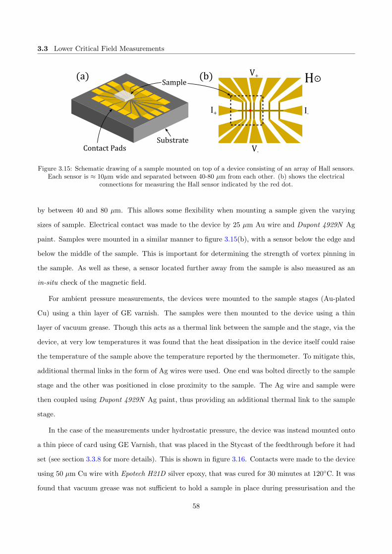
3.3 Lower Critical Field Measurements
I+ I-
V+
V-
H(a) (b)
ContactPads
Sample
Substrate
Figure 3.15: Schematic drawing of a sample mounted on top of a device consisting of an array of Hall sensors.Each sensor is ≈ 10µm wide and separated between 40-80 µm from each other. (b) shows the electrical
connections for measuring the Hall sensor indicated by the red dot.
by between 40 and 80 µm. This allows some flexibility when mounting a sample given the varying
sizes of sample. Electrical contact was made to the device by 25 µm Au wire and Dupont 4929N Ag
paint. Samples were mounted in a similar manner to figure 3.15(b), with a sensor below the edge and
below the middle of the sample. This is important for determining the strength of vortex pinning in
the sample. As well as these, a sensor located further away from the sample is also measured as an
in-situ check of the magnetic field.
For ambient pressure measurements, the devices were mounted to the sample stages (Au-plated
Cu) using a thin layer of GE varnish. The samples were then mounted to the device using a thin
layer of vacuum grease. Though this acts as a thermal link between the sample and the stage, via the
device, at very low temperatures it was found that the heat dissipation in the device itself could raise
the temperature of the sample above the temperature reported by the thermometer. To mitigate this,
additional thermal links in the form of Ag wires were used. One end was bolted directly to the sample
stage and the other was positioned in close proximity to the sample. The Ag wire and sample were
then coupled using Dupont 4929N Ag paint, thus providing an additional thermal link to the sample
stage.
In the case of the measurements under hydrostatic pressure, the device was instead mounted onto
a thin piece of card using GE Varnish, that was placed in the Stycast of the feedthrough before it had
set (see section 3.3.8 for more details). This is shown in figure 3.16. Contacts were made to the device
using 50 µm Cu wire with Epotech H21D silver epoxy, that was cured for 30 minutes at 120C. It was
found that vacuum grease was not sufficient to hold a sample in place during pressurisation and the
58

3.3 Lower Critical Field Measurements
Figure 3.16: Photographs showing the front and back of the feedthrough with a Hall array device mounted.Cu wires run up the back of the card and then are contacted to the device with silver epoxy. On the back side
a manganin wire is connected in a four point measurement as a pressure gauge.
subsequent cool-down of the experiment, and so the sample was secure instead by a small amount of
GE varnish.
The current I was supplied using the sinusoidal output of a Stanford Research Systems SR830
lock-in amplifier (LIA) set at f = 72.0 Hz. This potential was applied across the current channel of
the device in series with a large resistor (usually 500 kΩ). As the resistance of the current channel was
≈ 10 kΩ, the resistance is dominated by the larger resistor, resulting in an approximation of a current
source. To monitor the consistency of this current, an additional 10 Ω 1% resistor was connected in
series with the I channel and the large resistor. The voltage drop across this resistor was monitored
using the input of the original LIA, allowing the current to be monitored. The Hall voltages of the
desired sensors were then measured using additional LIAs using the TTL output of the first LIA to
provide the lock-in frequency. The current in the device was usually not more than 2 µA, and was
varied depending on the temperature of the particular measurement.
Figure 3.17 shows data for the Hall resistance, RH = VH/I, as a function of temperature and
hydrostatic pressure (section 3.3.8 for more details). The data shows that there is a decrease in
sensitivity with decreasing temperature, but not to prohibitive levels. With increasing pressure, the
59
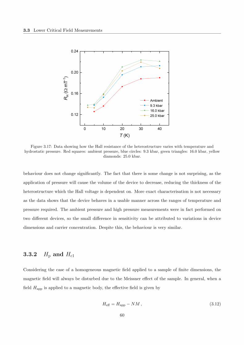
3.3 Lower Critical Field Measurements
Figure 3.17: Data showing how the Hall resistance of the heterostructure varies with temperature andhydrostatic pressure. Red squares: ambient pressure, blue circles: 9.3 kbar, green triangles: 16.0 kbar, yellow
diamonds: 25.0 kbar.
behaviour does not change significantly. The fact that there is some change is not surprising, as the
application of pressure will cause the volume of the device to decrease, reducing the thickness of the
heterostructure which the Hall voltage is dependent on. More exact characterisation is not necessary
as the data shows that the device behaves in a usable manner across the ranges of temperature and
pressure required. The ambient pressure and high pressure measurements were in fact performed on
two different devices, so the small difference in sensitivity can be attributed to variations in device
dimensions and carrier concentration. Despite this, the behaviour is very similar.
3.3.2 Hp and Hc1
Considering the case of a homogeneous magnetic field applied to a sample of finite dimensions, the
magnetic field will always be disturbed due to the Meissner effect of the sample. In general, when a
field Happ is applied to a magnetic body, the effective field is given by
Heff = Happ −NM , (3.12)
60

3.3 Lower Critical Field Measurements
where M is the magnetisation of the body and N is the demagnetising factor. In the case that M
is linear in H (e.g. in a superconductor sufficiently small H) then M = χH. For a superconductor,
χ = −1, and so
Heff =Happ
1−N. (3.13)
Since N ≥ 0, the effective field is always enhanced when compared to the applied field. In the
case of the lower critical field, this means that the field at which flux enters a sample, Hp, is always
reduced compared to the real value of the lower critical field, the extent of which depends on the
demagnetising factor. In general, this quantity can be difficult to determine. However, a numerical
estimate is provided by Brandt in the case of a thin platelet [90]. By determining the thickness lc
and length la of the sample, the penetration field can be used to determine the lower critical field as
follows:
Hc1 =Hp
tanh√
0.36lc/la. (3.14)
This relationship has been shown to provide a good estimate of the lower critical field in a number
of systems [86], producing consistent values of Hc1(T ) in a sample that was cut into different aspect
ratios [88].
Care must be taken to ensure that the Hp observed is the true field of first flux penetration and
that it is not altered by either strong pinning or enhanced by the presence of a Bean-Livingston
(BL) surface barrier. Strong pinning tends to prevent the flux from migrating through the sample
easily after the field reaches Hp, and so the apparent Hp at the center of the sample will be increased
relative to the Hp at the edge of the sample [86,88], which can be determined for by observing the local
induction at multiple points beneath the sample. Okazaki et al. observed the temperature dependence
of the penetration field at the edge and center of a sample of PrFeAsO1-y and found that while Hp(T )
at the edge saturated at low temperature, in the expected manner of Hc1(T ), Hp(T ) at the center
showed a large upturn. By considering the local screening current density, they concluded that, while
there was clearly strong pinning, the penetration field measured at the edge was very close to the true
penetration field.
The BL surface barrier can also cause an enhancement of the apparent Hp. In samples with very
smooth and perfect surfaces, the magnetic vortices must overcome an additional energy barrier that
61
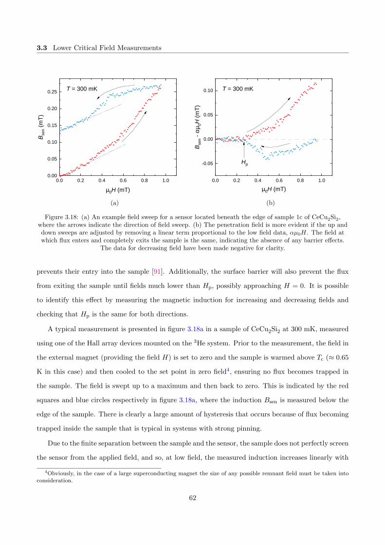
3.3 Lower Critical Field Measurements
0 . 0 0 . 2 0 . 4 0 . 6 0 . 8 1 . 00 . 0 0
0 . 0 5
0 . 1 0
0 . 1 5
0 . 2 0
0 . 2 5
B sen (m
T)
µ0 H ( m T )
T = 3 0 0 m K
(a)
0 . 0 0 . 2 0 . 4 0 . 6 0 . 8 1 . 0
- 0 . 0 5
0 . 0 0
0 . 0 5
0 . 1 0
B sen -
αµ0H
(mT)
µ0 H ( m T )
T = 3 0 0 m K
H p
(b)
Figure 3.18: (a) An example field sweep for a sensor located beneath the edge of sample 1c of CeCu2Si2,where the arrows indicate the direction of field sweep. (b) The penetration field is more evident if the up anddown sweeps are adjusted by removing a linear term proportional to the low field data, αµ0H. The field atwhich flux enters and completely exits the sample is the same, indicating the absence of any barrier effects.
The data for decreasing field have been made negative for clarity.
prevents their entry into the sample [91]. Additionally, the surface barrier will also prevent the flux
from exiting the sample until fields much lower than Hp, possibly approaching H = 0. It is possible
to identify this effect by measuring the magnetic induction for increasing and decreasing fields and
checking that Hp is the same for both directions.
A typical measurement is presented in figure 3.18a in a sample of CeCu2Si2 at 300 mK, measured
using one of the Hall array devices mounted on the 3He system. Prior to the measurement, the field in
the external magnet (providing the field H) is set to zero and the sample is warmed above Tc (≈ 0.65
K in this case) and then cooled to the set point in zero field4, ensuring no flux becomes trapped in
the sample. The field is swept up to a maximum and then back to zero. This is indicated by the red
squares and blue circles respectively in figure 3.18a, where the induction Bsen is measured below the
edge of the sample. There is clearly a large amount of hysteresis that occurs because of flux becoming
trapped inside the sample that is typical in systems with strong pinning.
Due to the finite separation between the sample and the sensor, the sample does not perfectly screen
the sensor from the applied field, and so, at low field, the measured induction increases linearly with
4Obviously, in the case of a large superconducting magnet the size of any possible remnant field must be taken intoconsideration.
62

3.3 Lower Critical Field Measurements
the applied field. Once the field reaches Hp then the induction increases strongly as the magnetisation
of the sample drops from −H. This is more easily seen by removing the small linear term proportional
to the field, αµ0H, from the induction. This is estimated using a least-squares fit of the low field data,
both for the increasing and decreasing field, as indicated by the dashed lines in figure 3.18a. The
result of this is shown in figure 3.18b, where Hp has been indicated. The penetration field is now very
clear and is the same for both increasing and decreasing field, indicating the absence of any energy
barrier effects.
3.3.3 Magnetic Field and Electromagnets
In the lower critical field measurements, a magnetic field is applied to the sample and Hall array device.
Thus, the production of an accurate and homogeneous magnetic field is required. This is typically
achieved through the use of an electromagnet, usually in the form of a solenoid or a Helmholtz pair.
This magnet could be small enough to be located directly on the low temperature probe, or it could
be large enough to allow the probe to be inserted within it, suspending it in the dewar (figure 3.1).
Electromagnets can be wound using resistive or superconducting wire, each presenting advantages
over the other. All these aspects must be considered when designing a magnet that is required for
a particular measurement in mind. Though commercial electromagnets are readily available, it is
relatively straightforward to design and build bespoke magnets oneself.
In a normal electromagnet, in which the current carrying wire is metallic, it is typical that that
some kind of iron yoke or core is used to decrease the number of turns in the magnet, reducing
power loss and thus improving efficiency [92]. In the case of a superconducting magnet, or indeed
magnets designed for low temperature purposes, this is not necessarily the case as use of a core may
be impractical. Additionally, there is no associated power loss for the superconducting wire and so
increasing the number of turns does not affect it in the same way. As such, it is typical to maximise
the field strength of the magnet by ensuring a high density of turns, often by wrapping each turn
directly next to the previous turn and even by incorporating multiple layers. In this case, provided
the pitch of the wrapping is sufficiently low, each turn of wire on the magnet can be approximated
as a single ring of current, as illustrated in figure 3.19, and the magnet as a whole is then simply the
sum of all the individual rings.
63

3.3 Lower Critical Field Measurements
x
r
BrBx
Bp
aI
Figure 3.19: A diagram showing the field B produced by a circular ring of radius a with a current of I flowingaround it. The field produced at point p can be projected into an axial and radial component, Bx and Br.
3.3.4 Magnetic field due to a ring of current
The magnetic field B produced at a point p by a circular ring of radius a and with current I, as in
figure 3.19, can be projected into two orthogonal components, Bx and Br. The value x is the axial
displacement of the point p as measured from the center of the ring, and r is the radial displacement
of the same point as measured from the central axis of the ring (i.e. the axis running through x). Due
to the symmetry of the situation there is no third, tangential component, and so the two components
are given by
Bx = B01
π√Q
E(k)
1− α2 − β2
Q− 4α+K(k)
(3.15)
and
Br = B0γ
π√Q
E(k)
1 + α2 + β2
Q− 4α−K(k)
, (3.16)
where the following parameterisations have been used: α = r/a, β = x/a, γ = x/r, Q = (1 + α)2 + β2,
k =√
4α/Q and B0 = µ0I/2a [93]. K(k) and E(k) are the complete elliptic integrals of the first and
second kind, respectively, and µ0 is the permeability of free space.
In the case of considering the field produced along the axis, with r = 0, then Br is zero for all x
64

3.3 Lower Critical Field Measurements
and the expression for the axial field simplifies to
Bx(x) =µ0Ia
2
2(a2 + x2)3/2. (3.17)
3.3.5 Short Solenoid for 3He Cryostat
For the initial lower critical field measurements with the 3He system, a resistive short solenoid was
used, suspended within the helium dewar. This was built and calibrated by C. Putzke and determined
to produce a field of 20.6 mT A−1 [89]. The current for the magnet was controlled by using a 16 bit
digital-to-analogue converter that was input into a voltage-current converter. The current was also
monitored using a Keithley 2000 bench multi-meter.
3.3.6 Miniature Short Solenoid for 3He-4He dilution refrigerator
For the critical field measurement adapted for use on the dilution refrigerator, a new magnet was re-
quired since it was not possible to use any of the existing magnets in combination with the refrigerator.
Moreover, a large external magnet was not an option since there was not sufficient space within the
refrigerator’s dewar and special effort had been taken to screen the vacuum canister of the refrigerator
with mu metal. Thus, it was decided that a small solenoid located within the vacuum canister, directly
on the refrigerator would be suitable, large enough to surround the Hall-array device set-up.
Though, in principle, an infinite solenoid (i.e. infinite in length but with a finite radius) produces
a homogeneous field within itself, this is difficult to achieve in practice and requires a solenoid many
times longer than its radius. However, a short solenoid can still produce a good approximation with
a small amount of variation over a sufficiently large region.
In this case, the solenoid was made with a radius of 14 mm and a single layer of 324 turns of
0.102mm Nb-Ti superconducting wire, giving an overall length of 33.05 mm. The calculated field
profile, or more exactly, the magnetic field reduced by the current (i.e. Bx/I), along the central axis
of the solenoid (i.e. r = 0) is shown in figure 3.20a. It can be seen that though the field never plateaus,
the variation near the center around x = 0 is very small, with the inset showing a variation of less
than 1% of the x = 0 value across the central 4 mm. As the extent of the sample and Hall array device
in this direction is less than 1 mm, this shows that the field can be considered to be homogeneous
65

3.3 Lower Critical Field Measurements
(a) (b)
Figure 3.20: (a) The calculated axial field along the central axis for a short solenoid with radius R = 14.0 mmand total number of turns N = 324 . Though the field never becomes constant, the variation around the
center is very small. The field at the center has a strength of 9.40 mT A−1. (b) The calculated axial field atthe center of the solenoid as a function of the radial direction. Similarly, though the field is not constant, the
variation is small enough over the extent of the active portion of the device and sample (< 1 mm) to benegligible.
across the device.
In a similar fashion, the axial magnetic field profile as a function of the radial direction, with x = 0,
is shown in figure 3.20b. In this instance, the field varies only a small amount, increasing away from
the center of the solenoid towards the edge. The inset shows that the field varies by less than 2% of
the r = 0 value across the central 10 mm of the solenoid. As the extent of the sample and device is
also < 1 mm in this plane,the field can be considered to be homogeneous.
The calibration of the solenoid was confirmed, using a commercial FW Bell Sypris 5170 Gauss/Tesla
meter, to be (9.4± 0.1) mT A−1 at its center. When in use, the current for the magnet was supplied
by a Keithley 6221 current source, again using a Keithley 2000 multimeter to monitor the supply
current.
3.3.7 Horizontal Helmholtz Magnet for PCC
It was not possible to use the short solenoid from section 3.3.5 in conjunction with a PCC as the
devices are too wide to be oriented appropriately inside the PCC. The devices measure approximately
66

3.3 Lower Critical Field Measurements
II
R
R
x
(a)
r,x=0
H
(b)
Figure 3.21: (a) Diagram showing the arrangement of a Helmholtz coil electromagnet. Two rings of radius Rare separated laterally by R. A current I flows through both rings in the same sense. (b) Schematic diagram
showing how the device, within the PCC, is located within the Helmholtz magnet.
2.5× 4.3 mm whereas the internal diameter of the Teflon cap (necessary for the pressure cell) is ≈ 2.9
mm. Instead, the device would have to be rotated by 90to fit in the Teflon cap and the magnetic
field would have to be applied horizontally, as shown in figure 3.21b. For this reason, it was necessary
to construct a new magnet that would allow the PCC to be inserted into it from the side.
A Helmholtz coil is a particular variation of an electromagnetic that consists of two identical rings
of radius R and current I separated laterally by R, as shown in figure 3.21a. Helmholtz coils have
the particular property of producing a region of nearly constant magnetic field around the center of
the pair. This can be easily shown by calculating the axial field profile of the axial component of the
field. Due to the symmetry, the expression for the axial field for a single ring is
Bx(x) =µ0NIR
2
2(R2 + x2)3/2, (3.18)
where N is the total number of turns in each coil [93]. Due to the symmetry, the radial component
is zero along the central axis of the coil. The field then in the Helmholtz coil is just the sum of two
identical rings positioned at x = ±R/2. At the midpoint between the two rings, the expression for
the field is reduced to
Bx =
(4
5
)3/2 µ0NI
R. (3.19)
67

3.3 Lower Critical Field Measurements
- 1 0 0 - 5 0 0 5 0 1 0 04
5
6
7
8
9
1 0
B x / I
(mT A
-1 )
x ( m m )(a)
- 1 0 0 - 5 0 0 5 0 1 0 0- 0 . 0 5
0 . 0 0
0 . 0 5
0 . 1 0
B xideal -
B xreal (%
)x ( m m )
(b)
Figure 3.22: (a) The calculated axial field along the central axis for a Helmholtz coil with R = 80.96 mm andN = 841. The dotted lines indicate the position of each ring of the electromagnet. The field produced is verynearly flat around the midpoint of the magnet. (b) The difference between the calculated field profiles of an
‘ideal’ Helmholtz coil and a more realistic Helmholtz coil, with the same R and N as (a). The differencebetween the two is very small at a maximum of only 0.1%.
Figure 3.22a shows the calculated field profile Bx(x) using equation 3.19 for R = 80.96 mm and
N = 841, where the units of the field have been reduced by the current I (these particular values of
R and N (841 = 292) correspond to the actual magnet that was built). The magnetic field is almost
flat over a large range of x. In a similar manner, figure 3.23 shows the axial field as a function of the
radial distance, i.e. Bx(x = 0, r), using equation 3.15 for N winds in each coil. The magnetic field
is also very nearly flat along this axis. Thus, even moderate misplacement of the device within the
magnetic field will only result in a very small error in the actual value of the field.
The requirements that influenced the design of the magnet were that there had to be enough
clearance between the two coils to allow a cryostat to be inserted between (≈ 51 mm) and that a
modest magnetic field could be achieved with a general-use power supply. After consideration, it was
determined that a magnet with R = 80.96 mm and 29 layers of 29 turns (i.e. 841) of wire should
produce a magnetic field of 9.34 mT A−1. The wire to be used was 0.55 mm diameter Supercon Inc.
54S43 multi-filament Nb-Ti superconducting wire. However, this raised the question of how applicable
the ‘ideal’ Helmholtz magnet approximation would be, considering that the turns of wire would occupy
68

3.3 Lower Critical Field Measurements
- 8 0 - 6 0 - 4 0 - 2 0 0 2 0 4 0 6 0 8 00
2
4
6
8
1 0B x
/ I (m
T A-1 )
r ( m m )Figure 3.23: The axial field profile for the path that the device, within the PCC, will take through the
Helmholtz magnet. The field is very nearly flat around the center of the magnet over approximately 40 mm,which is significantly larger than the device.
a cross-section of 15.95× 15.95 mm2. A more realistic approximation would be to consider each turn
of the magnet separately and sum the contribution from each turn together. This can be done using
equations 3.15 and 3.16, considering the various radii and separations of each turn. Figure 3.22b shows
the percentage difference (compared to the center value) between the ‘ideal’ and ‘realistic’ calculations
for the same Helmholtz magnet. The variation across a considerable difference is very small, at ≈ 0.1%
in the worst case, illustrating that the magnet would still make a sufficiently homogeneous field.
The former for the magnet was machined out of a single piece of aluminium. The wire was wrapped
by hand and secured using GE varnish. However, it was found that due to small cracks in the enamel
of the wire, and the electrically conductive nature of the varnish, that the wire was making electrical
contact with the former. In order to prevent this, the bare former was anodized to produce an
electrically insulating layer on the entirety of the surface. This is described by the following chemical
reaction:
2 Al + 3H2O −−→ Al2O3 + 6 H+ + 6 e–
69

3.3 Lower Critical Field Measurements
(a)
- 1 0 0 - 5 0 0 5 0 1 0 00 . 0 0
0 . 0 5
0 . 1 0
0 . 1 5
0 . 2 0
B x (m
T)r ( m m )
I = 2 0 0 m A
(b)
Figure 3.24: Data for the Bx as measured (a) along the axial direction (r = 0) and (b) the radial direction(x = 0) with the magnet supplied with I = 200 mA. The inset for (a) shows how the field varied with different
amounts of current I in the magnet.
Practically this was carried out using electrolysis. The former is suspended in 10% H2SO4 with the
former connected as the anode and an additional aluminium plate, also in the acid, as the cathode.
A current of 10 A was supplied and the reaction was allowed to proceed for ≈ 1 hour5. The reaction
produced a moderately thick insulating layer of Al2O3 that had to be scratched quite hard before
electrical contact could be made with the unreacted aluminium underneath.
Once the former was suitably insulated, the magnet was wound with the intention of 29 layers of
29 turns in each coil. The turns were secured with GE varnish, though strips of electrical tape and
Kapton tape were also used to provide some structural support. However, due to tolerances in the
machining process, it was not possible to wrap the turns in the ideal configuration (a square array
of 29 × 29). As such, each coil resulted in 843 turns over 30 layers. Clearly, this was not exactly as
intended and so it was important to determine the actual profile of the magnetic field. This was done
at room temperature using a Toshiba THS118 Hall sensor that was calibrated using a long solenoid
of known field strength. The magnet was supplied of a constant current of (200 ± 0.1) mA using
a Keithley 6221 current source. The axial field as a function of the axial and radial directions was
measured, and is shown in figure 3.24. It can be seen that there is a bit of asymmetry, but overall the
5The exact amount of time and current required will depend on the surface area of the part to be anodized.
70

3.3 Lower Critical Field Measurements
Cell body(CuBe)
Insert(MP35N)
Outer piston
Roller
Inner piston
Top lock nut
Bottomlock nut
Feedthrough
Cu ring
Teflon cap
CuBe disc
Electricalwires
Figure 3.25: Cutaway sketch of the assembled piston-cylinder cell (PCC). Dashed lines indicate a threadedsurface.
profiles are mostly as expected. Importantly, there is a large area of almost constant magnetic field
around the center of the magnet. The calibration for the magnet was determined by positioning the
Hall sensor at the center of the magnet and then measuring the field for multiple supplied currents.
This is shown in the inset of figure 3.24a. A least-squares fit was made to the data which yielded a
calibration of Bx/I = (9.22± 0.05) mT A−1.
3.3.8 Hydrostatic Pressure Generation
The device used for generating the required hydrostatic pressures was a clamped piston-cylinder cell
(PCC), a sketch of which is shown in figure 3.25. The clamped PCC is a well established high-pressure
device that has found to be well suited for low temperature measurements [94,95]. This is in part due to
its relatively simple design and also because high pressure can be generated at room temperature and
then sealed within the cell allowing the cell to be transferred to the desired measurement apparatus,
thus reducing overall experimental complexity.
The pressure is generated by applying a load to the outer piston using a press. The outer piston
transfers this load to the roller, which itself transfers to the inner piston. The inner piston then applies
a compressive force to the pressure medium (in this case, encased in the Teflon cap) located at the
center of the cell body. The pressure medium translates the uniaxial stress into a hydrostatic pressure
71

3.3 Lower Critical Field Measurements
around the sample space. The other end of the cell is sealed by the feedthrough, which is held in place
by the bottom lock nut. Once the desired load has been applied, or internal pressure achieved (as
determined by some pressure gauge), the top lock nut is tightened until it bears the load and relieves
the press. The applied load from the press can then be released, slowly, and the outer piston removed,
at which point the pressure has been sealed within the cell, though it is typical that a small amount
of pressure is lost during the sealing process [94].
For mechanical reasons, the cell is a double wall design where the outer body is made of CuBe
and the insert is made of the alloy MP35N. In addition, the feedthrough, inner and outer pistons, and
the roller are also made of MP35N. CuBe is commonly used for pressure cells due to its high yield
strength, and it is also only very weakly paramagnetic [95, 96]. The CuBe body is heated and then
the insert is positioned within the body to create an interference fit upon cooling. This is important
to increase the upper limit of the pressure generation that the cell is capable of producing before
deforming.
In this case, a Teflon cap is used to contain the pressure medium and also the sample or device
under measurement, an enlarged view of which is shown in figure 3.26. The use of a Teflon cap helps to
further simplify the apparatus and presents a number of advantages [94,97]. Firstly, it is easier to seal
the pressure medium within in the bore of the cell with the use of a Teflon cap, and only simple anti-
extrusion rings and discs are required. It also prevents electrical shorts between the internal wiring
and the cell body. Assembly is also simplified as the cap can be filled with the pressure medium and
then sealed with the feedthrough, containing the wiring and sample and such. The rest of the cell is
then easily assembled.
As shown in figure 3.26, the feedthrough itself contains a cylindrical channel within it to allow
electrical wires to be introduced into the sample space. The wires and the channel are sealed using
the epoxy Stycast 2850 FT with catalyst 9. When preparing the feedthrough it was very important
to ensure that the feedthrough itself and also the wires (twisted Cu pairs) were clean of grease and
dirt. Also, it is important that the channel was completely filled with Stycast and there are no voids
or pockets of air. Grease or dirt can prevent the Stycast from sticking firmly to the surfaces, whereas
voids can collapse when under high pressure. In either case this can result in the violent ejection of the
epoxy, along with the sample, through the back of the feedthrough, often resulting in the destruction
72

3.3 Lower Critical Field Measurements
Sample / device
Teflon cap
Feedthrough
Cu ring
Electricalwires
Pressuremedium
Stycast 2850
Figure 3.26: An enlarged cutaway of the feedthrough and Teflon cap from figure 3.25. The pressure medium(Daphne 7373) is enclosed within the Teflon cap. The feedthrough, along with the sample, is inserted and
sealed into the cap. Electrical wires are connected to the sample or device and sealed in the feedthrough usingStycast epoxy (2850 FT with catalyst 9).
of the sample or device. The channel within the feedthrough is shaped in such a way to further help
prevent ejection of the Stycast plug at high pressures6.
The pressure medium chosen for this experiment was Daphne 7373, a mixture of olefin olygomers,
which is suitable for the pressure range of this particular design of PCC and also low temperature
measurements due to its good hydrostaticity [98]. In particular, it was found that there is no discon-
tinuity in pressure when cooled through the solidification point and that the observed loss of pressure
between 300 K and 4.2 K in a clamped-type cell was about 1.5 kbar, independent of the pressure
applied at room temperature [99]. Additionally, it also has a moderately high solidification pressure of
2.2 GPa at room temperature [98], ensuring hydrostatic conditions can be maintained when the cell is
pressurised at room-temperature. It is also important to cool the cell slowly from room temperature
through the solidification temperature otherwise it is possible to create non-hydrostatic components
on the sample if the medium solidifies unevenly. Daphne 7373 is also quite easy to work with - its
relatively high viscosity makes it easier to seal the pressure cell when assembling.
In order to estimate the pressure within the pressure cell, a piece of manganin wire was used as a
pressure gauge. This is because, for small enough pressures, the pressure dependence of the resistance
6It is good practice to test a newly prepared feedthrough to high pressure before mounting a sample.
73

3.3 Lower Critical Field Measurements
Figure 3.27: Figure showing how the pressure, as determined by the manganin pressure gauge varies with theload applied to the pressure cell. The sets of data are for two separate cycles of loading and unloading of
pressure. The red squares indicate the initial loading and unloading, and the blue circles indicate thesubsequent cycle. There is a small difference in the onset of the pressurisation with the load, but the
behaviour is nominally the same.
of manganin is approximately linear [94] and can be approximated as such:
p =α∆R
R0, (3.20)
where p is the pressure, R0 is the resistance of the wire at ambient pressure, ∆R is the measured change
in resistance and α is the coefficient of the wire in question. The exact coefficient of the manganin will
depend on the particular brand and composition, though typical values have been found to be around
0.403 to 0.419 GPa per % change in resistance from the ambient pressure value [100]. For the wire
used it was found that the coefficient was α ≈ 0.405 GPa per % change (4.05 kbar per %) at room
temperature, close to the value found by Zeto et al. [100].
The pressure gauge is formed by connecting a piece of enamelled 50 µm manganin wire in a four-
point resistance measurement, with 25 µm Au wire as the electrical leads. The Au wire is soldered to
the manganin at a low temperature to make an effort to avoid introducing stress locations into the
wire. The gauge is then annealed at 200 C to further aid in the reduction of stresses in the wire. The
gauge is placed within the sample space. In this instance, it was secured to the reverse of the card with
74
3.3 Lower Critical Field Measurements
a small amount of GE varnish, as shown in figure 3.16. Figure 3.27 shows the pressure in the PCC,
as determined from the manganin gauge, for different loads applied to the cell via the hydraulic press.
The red squares are for an initial pressurisation up to ≈ 6 kbar, after which point it was released. The
blue circles show a subsequent pressurisation up to almost 20 kbar. The behaviours are very similar,
with a small difference at the point at which pressure begins to be produced with the applied load.
75

3.3 Lower Critical Field Measurements
76

Chapter 4
Full-gap superconductivity in
heavy-fermion compound CeCu2Si2
4.1 Introduction
CeCu2Si2, a heavy-fermion compound, is generally considered to be the first example of a truly uncon-
ventional superconductor [18]. In heavy-fermion materials, strong electron-electron correlations lead
to large renormalisations in the electronic effective mass, as evident in the typically large Sommer-
feld coefficients of their specific heat [19]. In heavy-fermion superconductors (HFSs), the size of the
specific heat anomaly at Tc is of the order of the normal state specific heat, γTc, implying the role of
heavy QPs in the superconducting state. At the time of discovery, previously known superconductors
tended to have far less strong electronic correlations, aside from the weak electron-phonon coupling,
and so it was a surprise to see superconductivity emerge in such a system. Furthermore, the ordering
of the characteristic energy scales in CeCu2Si2 does not follow the conventional picture of the phonon
energies being significantly smaller than the electronic energies, dictated by TF [22], leading to the
idea of unconventional pairing.
Synthesis of high-quality crystals of CeCu2Si2 has always presented a challenge, and a long time
was spent trying to produce samples with specific heat anomalies approaching a value of 1 [19].
Additionally, it was found that the system is very sensitive to small changes in the stoichiometry. A
small excess of Cu is required to produce a bulk superconducting transition, known as the S phase.
77

4.1 Introduction
Ce
Cu
Si
Figure 4.1: The body-centred tetragonal crystal structure of CeCu2Si2.
Figure 4.2: The Fermi surface of CeCu2Si2 determined from an LDA+ U band structure calculation. TheFermi surface is coloured according to the Fermi velocity. Reproduced from ref. [103]’s supplementary material.
In contrast, a slight deficit of Cu will produce the antiferromagnetic A phase [101]. CeCu2Si2 is also
very sensitive to non-magnetic impurities, as demonstrated by the effect on Tc from substitution of
La for Ce [102].
The fact that superconductivity emerges in this system in close proximity to an antiferromagnetic
phase naturally leads to the speculation of the role of magnetism in the mechanism of superconductiv-
ity, especially if there is evidence of quantum critical fluctuations associated with a quantum critical
point (QCP) [101, 104, 105]. Indeed, there is evidence of non-Fermi liquid behaviour in the zero-field
in-plane resistivity [106] as well as in the heat capacity just above Hc2 [103]. Inelastic neutron scat-
tering measurements revealed spin excitations in the S phase with the same Q vector associated with
the antiferromagnetic A phase, such that antiferromagnetic quantum critical fluctuations could be
78

4.1 Introduction
Figure 4.3: Electronic specific heat for a single crystal of S type CeCu2Si2. Reproduced from ref. [103]’ssupplementary material.
responsible for superconductivity [105, 107, 108]. Fermi liquid behaviour in the resistivity was also
seen to recover with the application of a magnetic field [106], strongly reminiscent of CeCoIn5 [109]
and YbRh2Si2 [110], providing further cause to believe the role of antiferromagnetic fluctuations in
superconductivity in CeCu2Si2.
CeCu2Si2 forms in the body centred tetragonal, I4/mmm crystal structure, as shown in figure 4.1.
Despite the quasi-2d structure, the upper critical field Hc2 displays only moderate anisotropy [111]
and seems to be Pauli limited [112]. Additionally, the slope of Hc2 with temperature at Tc is very
similar both perpendicular and parallel to the c-axis, implying an almost isotropic Fermi surface in the
renormalised state, further supported by the isotropy evident in the residual resistivities [111]. Band
structure calculations also show weak anisotropy in the Fermi surface in both nonrenormalised and
renormalised calculations [103,113]. Figure 4.2 shows the result of an LDA+ U calculation, showing
the renormalised Fermi surface coloured by the Fermi velocity [103]. The Fermi surface consists of a
heavy, tubular electron sheet around the X point, and two hole sheets, one of which shows a more
complex structure with much lower effective mass.
The pairing symmetry in CeCu2Si2 was generally considered to be d-wave with some form of line
nodes. Evidence to support this was found in the decrease in the NMR Knight shift below Tc, usually
indicative of spin singlet pairing [114]. Additionally, the observed T 3 dependence of 1/T1 [115–117]
79
4.2 Results
and power law behaviour to ∼ 0.1 K in the specific heat [118] was suggestive of nodes in the energy
gap. Measurements of the penetration depth in polycrystalline samples observed T 2 behaviour that
could be consistent with point nodes or line nodes with strong impurity scattering [119].
Recently, with the advent of improved sample quality, Kittaka et al. revisited the specific heat in
CeCu2Si2 and found a surprising absence of signatures of nodal superconductivity. The measurements
were performed on a single crystal of S type CeCu2Si2, with Tc ≈ 0.6 K, slightly below optimum,
but showing a sharp transition and lower residual DOS than previous measurements, the main results
of which are shown in figure 4.3. They were able to measure to lower temperatures than reported
previously, and found strong positive curvature below 0.1 K that was found to fit well to a two-gap
BCS model. Additionally, the electronic specific heat Ce(H) was found to vary with H, not√H as
would be expected for a nodal gap. The signature of line nodes in the form of oscillations was absent
from angle resolved specific heat measurements leading to the overall conclusion of nodeless multiband
superconductivity at quite stark contrast to previous conventionally held wisdom. As the heat capacity
is more sensitive to heavy QPs, the absence of nodes would then rule out a dx2−y2 pairing state. This
then raises the question of whether the signature of a nodal gap would be absent in other probes,
such as the magnetic penetration depth. As demonstrated by the specific heat measurements, it is
important to make measurements to as low temperatures as possible in order to distinguish what could
be thought of as signatures of nodes from what is really the manifestation of a full gap at sufficiently
low energies, especially in the case of multi-gap systems [19].
4.2 Results
4.2.1 Magnetic Penetration Depth
In order to investigate this question of the unexpected absence of nodal QPs, magnetic penetration
depth measurements down to 50 mK were performed on two high-quality, single crystal S type sam-
ples of CeCu2Si2 using the 3He-4He dilution refrigerator TDO technique. This study was initiated by
the group of Takasada Shibauchi from the University of Tokyo in Japan and initial penetration depth
measurements of sample 1c were performed in collaboration with a visiting student, Takaaki Takenaka.
Due to problems with the dilution refrigerator, in which it was not reaching a sufficiently low base
80

4.2 Results
(a) (b)
Figure 4.4: The magnetic penetration depth for sample 1c of CeCu2Si2, measured in the H‖c orientation. (a)Part of the superconducting transition can be seen, but it was not possible to observe the full transition to dueto eddy current heating in the normal state above Tc. (b) the lower temperature portion of the data is plotted,
showing a saturated behaviour from ≈ 0.10 K.
temperature, it was not possible to complete the measurements during the two months in which T.
Takenaka was in Bristol. With the assistance of Carsten Putzke (of Bristol) and T. Takenaka, the
base temperature of the dilution refrigerator was improved to reliably achieve 50 mK. This was done
by reducing the heat load on the mixing chamber through the use of silver wire to thermally anchor
elsewhere the various parts of the refrigerator (see section 3.1.5). By the time this was resolved, there
was only a short window of time left in which T. Takenaka would be in Bristol. Thus, further measure-
ments of the penetration depth on sample 1c and 1D-b were performed, by myself, after the departure
of T. Takenaka for approximately four additional months. During this time, measurements of the lower
critical field were also performed using a set-up established by C. Putzke. Initial measurements on
sample 1c were performed with his guidance, with the remaining measurements performed by myself.
As a result of the collaboration with Takasada Shibauchi’s group, some of the results presented within
this chapter were included in a Science Advances publication (see reference [106]).
The samples were provided by T. Shibauchi’s group and were originally grown by the group of Silvia
Seiro using the flux method [120]. These samples are thick platelets and have typical dimensions of
0.30×0.40×0.10 mm3, with the c-axis in the shorter direction. Figure 4.4 shows the in-plane response
(i.e. the H‖c orientation) from the first sample (known as 1c) (a) over the whole superconducting range
81

4.2 Results
Figure 4.5: The measured frequency shift through Tc when the sample was retracted ≈ 5.8 mm from thecenter of the sense coil (also in the H‖corientation), reducing the strength of the RF field. There is still a
small amount of hysteresis due to eddy current heating in the sample in the normal state.
and (b) at lower temperatures. What is immediately apparent is the strong positive curvature below
≈ 0.15 K that is not indicative of nodes in the gap structure and consistent with a full gap picture.
The full superconducting transition is not shown in figure 4.4a due to strong eddy current heating
in the normal state above Tc. When the sample rod is cooled through the transition, the heating
prevents the sample from cooling and becoming superconducting. This is remedied by switching off
the oscillator to cool the sample into the superconducting state.
In order to fully determine the transition in this sample, the rod was retracted partly within the
sense coil to reduce the strength of the RF field, reducing the amount of eddy current heating but
also reducing the signal from the sample. As shown in figure 4.5, the transition is now clear at ≈ 0.64
K, indicating the high quality of the sample. There is still some hysteresis in the measurement due
to the effect of eddy current heating, but it is no longer strong enough to completely prevent cooling
into the superconducting state.
Measurement of ∆λab(T ) were repeated for a second sample, known as 1D-b, and the results are
shown in figure 4.6. The superconducting transition is now clear even with the sample fully inserted
within the sense coil, showing a very large jump of ≈ 30000 nm at Tc ≈ 0.65 K. In figure 4.6b, the low
temperature data for 1D-b is shown in comparison to sample 1c. Qualitatively the behaviour is the
82

4.2 Results
(a)
0 . 0 0 0 . 0 5 0 . 1 0 0 . 1 5 0 . 2 0 0 . 2 5 0 . 3 00
5 0
1 0 0
1 5 0
∆λab
(nm)
T ( K )
S a m p l e 1 c S a m p l e 1 D - b
(b)
Figure 4.6: The magnetic penetration depth from a second sample (1D-b) of CeCu2Si2. (a) The full transitionis visible here, showing a very sharp onset at ≈ 0.65 K. (b) The low temperature data compared to sample 1c.
Qualitatively they are very similar with a small difference in the absolute value.
same, exhibiting a lack of linear behaviour associated with line nodes but also showing strong curvature
that is indicative of a full gap. There is a small discrepancy between the absolute magnitude that is
a result of determining the correspondence between the measured frequency shift and the change in
the penetration depth.
Qualitatively, it can immediately be seen that the low temperature penetration depth for both
samples does not follow the linear temperature dependence of a gap structure with line nodes (as
shown in figure 1.2a and 2.4b), and is more similar to the activated behaviour of a full gap. However,
it would be preferable to make more quantitative statements about the data and so some method of
analysis is required. It is also desirable to do this in a way that introduces as little bias as possible
and without assuming a priori the functional form that the data should take. One possible method
is the so-called power law exponent analysis, which is as follows. The data is fit to a power law of the
form:
∆λ(T ) = A+BTn , (4.1)
where A is an offset, B is a scaling parameter and n is the power law exponent. An example of this
fit is shown in figure 4.7, where the fitting is performed using the Levenberg-Marquadt Algorithim
(LMA) [121]. The analysis is performed by determining n from the data while varying the upper limit
83

4.2 Results
0 . 0 0 . 1 0 . 2 0 . 3
0
5 0
1 0 0
1 5 0
2 0 0
∆λab
(nm)
T ( K )
M o d e l P o w e r L a w ( U s e r )E q u a t i o n c + a * x ^ nP l o t D Ln 3 . 3 2 1 3 4 ± 0 . 0 2 3 5 8a 9 1 2 5 . 7 5 5 8 1 ± 2 6 4 . 0 0 7 3 1c - 1 . 9 4 0 7 ± 0 . 2 5 6 0 9R e d u c e d C h i - S q r 1 . 2 9 9 6 5R - S q u a r e ( C O D ) 0 . 9 9 9 4 9A d j . R - S q u a r e 0 . 9 9 9 4 8
M o d e l E f f e c t i v e G a p ( U s e r )E q u a t i o n c + a * x ^ - 0 . 5 * e x p ( - g a p / x * T c )P l o t D Lc 1 . 9 2 5 4 9 ± 0 . 3 1 4 8 3a 2 1 6 1 . 6 4 5 6 3 ± 6 7 . 9 8 0 5 4g a p 0 . 2 7 5 5 5 ± 0 . 0 0 2 5 5R e d u c e d C h i - S q r 2 . 9 6 8 2 2R - S q u a r e ( C O D ) 0 . 9 9 8 8 4A d j . R - S q u a r e 0 . 9 9 8 8 1
∆λ( T ) ∝ T n
∆λ( T ) ∝ T - 1 / 2 e x p ( - ∆ e f f / k B T )
T m a x = 0 . 3 K
Figure 4.7: An example of the two functions fitted to the data for sample 1c using the LMA, varying theupper limit of the fit. In this case, Tmax = 0.3 K. The two forms give reasonable fits to the data, with a
reduced-χ2 of ≈ 1.30 for the power law form and ≈ 2.97 for the single effective gap form.
of the fit (keeping the lower limit fixed at the minimum temperature). As the upper limit, Tmax, is
reduced then one of two things is expected. If the data follows a power law temperature dependence,
e.g. n = 1 for clean line nodes, then we expect n to approach the associated value. On the other hand,
if the data does not follow a power law dependence, but follows instead an exponential dependence,
as for a full gap, then n is expected to diverge at lower and lower temperatures.1
As a demonstration, this analysis is first performed on the numerically determined ∆λ(T ) of the
model gap structures from figure 2.4 and 2.5 (see section 2.4 for details). The result of the analysis is
shown in figure 4.8a.2 As expected, the fully gapped models start at a lower value of n, and show an
increasing exponent n with decreasing Tmax, though the two gap model to a somewhat lesser extent.
Contrastingly, the nodal gap structure begins around n ≈ 1.5, and approaches n = 1 as anticipated
for a gap with line nodes, as Tmax decreases. Importantly, for all cases there is some evolution of n
depending on the range of temperature included in the fit, such that it is how n varies with Tmax that
1This is obvious when considering the expansion for exp(x) ≈ 1 + x+ x2
2+ x3
6+ ....
2In this analysis, and that which follows, it would be possible to include certain metrics such as the standard erroror goodness-of-fit for each point. However, this is not exactly relevant as the point is not to compare the power law andeffective gap forms in how well they describe the data, but rather to see what insight they can provide compared to thesame analysis of the model gap structures. As such, further discussion of these quantities will not be included.
84

4.2 Results
can give some insight into the gap structure.
This same analysis is then performed on ∆λab(T ) for samples 1c and 1D-b, and is shown in figure
4.8b. Comparing with figure 4.8a, it is clear that the two samples of CeCu2Si2 are more similar to
the fully gapped models, with n > 3 for the entire range, and do not approach either n = 1 or n = 2
expected for the clean or dirty nodal cases. In particular, sample 1c shows an increase of n as Tmax
is decreased in the same manner as the fully gapped models of figure 4.8a, though admittedly sample
1D-b does not show exactly the same trend.
Having established more empirically the similarity between the measured data and the model fully-
gapped systems, it is then more reasonable to assume that the data also follows the same analytical
BCS form at low temperature. Without assuming the possibility of anisotropy or multiple gaps, the
simplest form to compare to is a single effective gap, described by:
∆λ(T ) = A+BT−1/2 exp(−∆eff/kBT ) , (4.2)
where A is an offset, B is a scaling parameter and ∆eff is the effective gap. An example of this form
fitted to the data is also shown in figure 4.7. Though there is an exact form expected for a single
isotropic gap in the BCS formalism (i.e. equation 2.25), the effective gap form combines the terms in
front of the exponential, excluding the T−1/2 term, into a single scaling parameter B. This helps to
relax the process as anisotropic or multigap systems may not follow this BCS form exactly.
Once again, it is important to observe how the determined effective gap varies with the upper limit
of the fit, Tmax, and this is also performed first on the model gaps from figure 4.8a (excluding the
nodal d-wave model). The result of this analysis is shown in figure 4.8c. Beginning with the isotropic
gap, the size of the apparent gap begins at slightly larger than the expected weak-coupling value of
1.76 kBTc, but as Tmax is reduced ∆eff takes on exactly that value. Similarly, for the two-gap system,
though the apparent gap appears larger for higher Tmax, ∆eff clearly approaches the same value as the
smaller gap of 0.7 kBTc. As discussed in section 2.4, the two gap system is essentially dominated by
the character of the smaller gap at lower temperatures. Interestingly, the single anisotropic gap shows
qualitatively different behaviour than for the other two models. Instead of appearing to approach a
single value for ∆eff , there seems to be a nearly linear decrease with decreasing Tmax. Furthermore, as
described in more detail in section 2.1.2, this particular model has a minimum gap of 0.8 the weak-
85

4.2 Results
0 . 2 0 . 3 0 . 4 0 . 50
2
4
6
8
1 0
1 2
Expo
nent
n
T m a x / T c
I s o t r o p i c s A n i s o t r o p i c s T w o G a p I s o t r o p i c s N o d a l d
∆λ( T ) ∝ T n
(a)
0 . 1 0 0 . 1 5 0 . 2 0 0 . 2 5 0 . 3 00
1
2
3
4
5
S a m p l e 1 c S a m p l e 1 D - b
Expo
nent
n
T m a x ( K )
C l e a n N o d a l
D i r t y N o d a l
F u l l y G a p p e d
∆λ( T ) ∝ T n
(b)
0 . 2 0 . 3 0 . 4 0 . 50 . 60 . 81 . 01 . 21 . 41 . 61 . 82 . 0
I s o t r o p i c s A n i s o t r o p i c s T w o G a p I s o t r o p i c s
∆ eff (k
BTc)
T m a x / T c
∆λ( T ) ∝ T - 1 / 2 e x p ( - ∆ e f f / k B T )
(c)
0 . 1 5 0 . 2 0 0 . 2 5 0 . 3 00 . 6
0 . 8
1 . 0
1 . 2
1 . 4
1 . 6
S a m p l e 1 c S a m p l e 1 D - b∆ e
ff (kBT
c)
T m a x ( K )
∆λ( T ) ∝ T - 1 / 2 e x p ( - ∆ e f f / k B T )
(d)
Figure 4.8: The result of the power law exponent analysis for (a) the model gap structures described in section2.4, and (b) for ∆λab(T ) for samples 1c and 1D-b. Additionally, the result of fitting the (c) model gaps and
(d) the measured data to a single effective gap BCS form.
86

4.2 Results
0 . 0 0 . 1 0 . 2 0 . 3 0 . 4 0 . 5 0 . 6 0 . 7
0
5 0 0 0
1 0 0 0 0
1 5 0 0 0
2 0 0 0 0
∆λ (n
m)
T ( K )
∆λe f f , H | | a b ∆λa b , H | | c
(a)
0 . 0 0 0 . 0 5 0 . 1 0 0 . 1 5 0 . 2 0 0 . 2 5 0 . 3 0
0
5 0
1 0 0
1 5 0
2 0 0
∆λ (n
m)T ( K )
∆λe f f , H | | a b ∆λa b , H | | c
(b)
Figure 4.9: (a) The effective penetration depth determined from the H‖ab measurement of sample 1c. Thein-plane response is also plotted in blue. (b) At low temperature the behaviour is very different, showing a
much stronger temperature dependence down to 50 mK, with no obvious saturation.
coupling value, or approximately 1.41kBTc. However, the effective gap reaches a value of ∼ 1.28kBTc
at Tmax/Tc = 0.15, somewhat less than the minimum gap.
Once more, this analysis is then repeated using the measured ∆λab(T ) for samples 1c and 1D-b,
which is shown in figure 4.8d. Both samples show very similar behaviour, with the size of the effective
gap reducing approximately linearly with decreasing Tmax, from approximately 1.5 kBTc to 0.9kBTc.
The rate of decrease is actually much larger than any of the model gap systems from figure 4.8c, but
there is more similarity between the anisotropic case than either of the other two. Indeed, this two
gap α-model system was constructed using the values of α1, 2 = 1.76, 0.7 and x = 0.65 determined
by Kittaka et al. using the same α-model approach with their recent heat capacity measurements.
However, though at low Tmax the effective gap is of a similar magnitude to the smaller of their two
gaps, the general behaviour of the data is not entirely similar to the model. This suggests there may
be further components in the model to take into account, such as anisotropy on one or both of the
gaps, or non-BCS temperature evolution of either of the gaps.
A measurement of the H‖ab response was made in sample 1c, which was first analysed as an
effective penetration depth using equation 3.6, shown in figure 4.9. Over the whole temperature
range, the response is quite similar, but at lower temperatures the out-of-plane response shows a
87

4.2 Results
0 . 0 0 . 1 0 . 2 0 . 3 0 . 4 0 . 5 0 . 6 0 . 70
1 0 0 0
2 0 0 0
3 0 0 0
4 0 0 0
5 0 0 0
∆λ (n
m)
T ( K )
∆λ c : ∆ f 0 = 1 0 4 0 H z , l z = 4 1 µ m ∆λ c : ∆ f 0 = 1 0 0 0 H z , l z = 4 1 µ m ∆λ c : ∆ f 0 = 1 1 0 0 H z , l z = 4 1 µ m ∆λ c : ∆ f 0 = 1 0 4 0 H z , l z = 3 5 µ m ∆λ c : ∆ f 0 = 1 0 4 0 H z , l z = 4 5 µ m ∆λ a b
(a)
0 . 0 0 0 . 0 5 0 . 1 0 0 . 1 5 0 . 2 00
1 0 02 0 03 0 04 0 05 0 06 0 07 0 08 0 0
∆λ (n
m)T ( K )
∆λ c : ∆ f 0 = 1 0 4 0 H z , l z = 4 1 µ m ∆λ c : ∆ f 0 = 1 0 0 0 H z , l z = 4 1 µ m ∆λ c : ∆ f 0 = 1 1 0 0 H z , l z = 4 1 µ m ∆λ c : ∆ f 0 = 1 0 4 0 H z , l z = 3 5 µ m ∆λ c : ∆ f 0 = 1 0 4 0 H z , l z = 4 5 µ m ∆λ a b
(b)
Figure 4.10: The c-axis penetration depth determined from the out-of-plane response using different values ofthe extraction value and thickness. The derived behaviour is very sensitive to these values, though converges
below ≈ 0.20 K.
much stronger temperature dependence all the way to 50 mK, compared to the clear saturation of the
in-plane response. The out-of-plane response is a weighted sum of λab and λc, which means the strong
temperature dependence is due to the c-axis penetration depth. It is possible to estimate ∆λc(T )
using equation 3.5, which when rearranged is written as
∆λc = lx
(δfλ
2∆f0− ∆λab
lz
), (4.3)
where δfλ is the measured out-of-plane response for the sample with dimensions lx× ly× lz and H‖ly.
From this expression it can be seen that the behaviour of ∆λc(T ) is determined by the terms inside
the parentheses, with lx acting as a scaling parameter. Within the parentheses, the measured response
is reduced according to the extraction value of the sample, and from this reduced quantity the already
known (and previously determined) behaviour of ∆λab is scaled by the thickness lz and subtracted.
Thus, the determined ∆λc(T ) will be very sensitive to the extraction value and the thickness of the
sample, and their associated errors.
This is indeed true, as is shown in figure 4.10. The data plotted as red squares shows ∆λc(T ) for
the experimentally determined extraction value of ∆f0 = 1040Hz and thickness of lz = 41µm. The
result is somewhat unusual, showing non-monotonic behaviour and a very sharp downturn near Tc.
88

4.2 Results
Figure 4.11: Despite the strong temperature dependence, the BCS form for a full gap fits the derived ∆λc(T )behaviour well (indicated by the solid green line).
Also plotted are ∆λc(T ) using different values for ∆f0 and lz, which show how sensitive this procedure
is, and also the in-plane ∆λab. Generally speaking, it seems that this yields mostly unphysical and
unlikely behaviour over the majority of the temperature range. However, for T < 0.20 K, the different
parameter sets begin to converge into a single behaviour, the shape of which is very much the same as
the effective behaviour from figure 4.9. This suggests that the data from below approximately 0.20 K
corresponds to the actual c-axis penetration depth. Focusing on the low temperature behaviour, as in
figure 4.10b, it can be seen that the magnitude of ∆λc changes much more rapidly with temperature
than does the in-plane ∆λab.
The data with the nominal values of ∆f0 = 1040 Hz and lz = 41µm was analysed for temperatures
below 0.20 K using the same effective gap and power law procedures as before. Though there is no
obvious saturation visible in the data at low temperature, the BCS effective gap does describe the
data well, as can be seen in figure 4.11, and is essentially constant with Tmax, as shown in figure 4.12b,
maintaining a value of ∆eff ≈ 0.51 kBTc. The power law exponent, in figure 4.12a, shows a rapid
increase with decreasing Tmax, beginning near 1 and then seeming to diverge into the n > 3 territory.
This also is consistent with the idea of a very small gap that is only evident in the penetration depth
at low temperature.
89
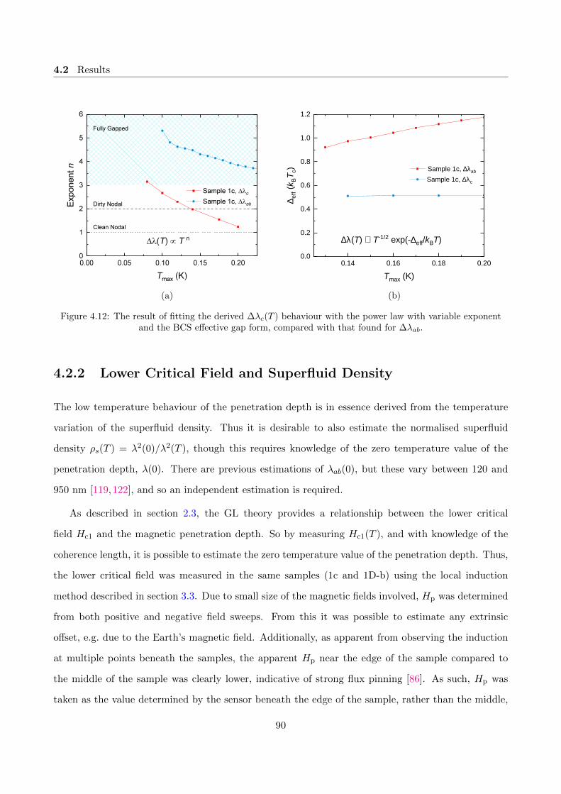
4.2 Results
(a)
0 . 1 4 0 . 1 6 0 . 1 8 0 . 2 00 . 0
0 . 2
0 . 4
0 . 6
0 . 8
1 . 0
1 . 2
S a m p l e 1 c , ∆λ a b S a m p l e 1 c , ∆λ c
∆ eff (k
BTc)
T m a x ( K )
∆λ( T ) ∝ T - 1 / 2 e x p ( - ∆ e f f / k B T )
(b)
Figure 4.12: The result of fitting the derived ∆λc(T ) behaviour with the power law with variable exponentand the BCS effective gap form, compared with that found for ∆λab.
4.2.2 Lower Critical Field and Superfluid Density
The low temperature behaviour of the penetration depth is in essence derived from the temperature
variation of the superfluid density. Thus it is desirable to also estimate the normalised superfluid
density ρs(T ) = λ2(0)/λ2(T ), though this requires knowledge of the zero temperature value of the
penetration depth, λ(0). There are previous estimations of λab(0), but these vary between 120 and
950 nm [119,122], and so an independent estimation is required.
As described in section 2.3, the GL theory provides a relationship between the lower critical
field Hc1 and the magnetic penetration depth. So by measuring Hc1(T ), and with knowledge of the
coherence length, it is possible to estimate the zero temperature value of the penetration depth. Thus,
the lower critical field was measured in the same samples (1c and 1D-b) using the local induction
method described in section 3.3. Due to small size of the magnetic fields involved, Hp was determined
from both positive and negative field sweeps. From this it was possible to estimate any extrinsic
offset, e.g. due to the Earth’s magnetic field. Additionally, as apparent from observing the induction
at multiple points beneath the samples, the apparent Hp near the edge of the sample compared to
the middle of the sample was clearly lower, indicative of strong flux pinning [86]. As such, Hp was
taken as the value determined by the sensor beneath the edge of the sample, rather than the middle,
90

4.2 Results
0 . 3 0 . 4 0 . 5 0 . 60 . 0
0 . 1
0 . 2
0 . 3
0 . 4
µ 0H p
(mT)
T ( K )
S a m p l e 1 c S a m p l e 1 D - b
H | | c
(a)
0 . 3 0 . 4 0 . 5 0 . 60 . 0
0 . 4
0 . 8
1 . 2
1 . 6
µ 0H c
1 (mT)
T ( K )
S a m p l e 1 c S a m p l e 1 D - b
H | | c
(b)
Figure 4.13: (a) The field of first flux penetration Hp for samples 1c and 1D-b. (b) The lower critical fielddetermined from (a) using the Brandt formula (equation 3.14). The two samples show nominally the same
behaviour, though there is somewhat more scatter for sample 1c than 1D-b.
and this is what is shown in figure 4.13a. The observed behaviour does not show any sign of a strong
upturn that would be associated with the effects of strong pinning, and so it can be concluded that
the trend in Hp(T ) reflects the trend in Hc1(T ). Finally, as shown in figure 3.18a, the field of first flux
penetration did not seem to be in any way affected by an additional BL energy barrier.
The results of the measurements for samples 1c and 1D-b are between Tc and 0.30 K, being limited
by the base temperature of the cryostat. For these measurements, the applied dc field was applied
parallel to the c-axis so that screening currents would circulate within the ab-plane, thus corresponding
to λab(0). The sample dimensions were determined using a high magnification optical microscope and
digital camera. The samples were found to have dimensions of 0.35 × 0.32 × 0.04 mm3 for 1c and
0.29×0.40×0.09 mm3 for 1D-b. The lower critical field was then calculated using the Brandt formula
(equation 3.14), the result of which is shown in figure 4.13b. The two samples exhibit very similar
trends with temperature, which strongly suggests that the observed penetration fields do correspond
to the lower critical field. Though sample 1D-b yielded results with more precision and less scatter,
this is likely due to Hp being larger in sample 1D-b due to its aspect ratio, making Hp easier to resolve.
With this data, we can estimate µ0Hc1(T = 320mK) = 1.20 ± 0.10 mT for sample 1D-b and
µ0Hc1(T = 300mK) = 1.27 ± 0.20 mT for sample 1c, where the error reflects uncertainties in the
91

4.2 Results
0 . 0 0 . 1 0 . 2 0 . 3 0 . 4 0 . 5 0 . 6 0 . 70 . 00 . 10 . 20 . 30 . 40 . 50 . 60 . 70 . 8
µ 0H p
(mT)
T ( K )
H | | c
(a)
0 . 0 0 . 1 0 . 2 0 . 3 0 . 4 0 . 5 0 . 6 0 . 70 . 00 . 20 . 40 . 60 . 81 . 01 . 21 . 41 . 61 . 82 . 0
µ 0H c
1 (mT)
T ( K )
S a m p l e 1 D - d S a m p l e 1 D - b
H | | c
(b)
Figure 4.14: (a) The field of first flux penetration for sample 1D-d determined using the 3He-4He dilutionrefrigerator and (b) the corresponding Hc1(T ) determined using the Brandt formula, compared with the
previously determined behaviour for sample 1D-b made on the 3He system.
sample dimensions and also in determining Hp. An estimate for the in-plane coherence length can
be made from the orbital limited upper critical field of 14.7 T, giving ξab = 4.7 nm [103]. With this
information, the GL equation for Hc1 can be solved (equation 2.18), yielding λ(T = 320mK) = 890±40
nm for sample 1D-b. Repeating for sample 1c yields λ(T = 300mK) = 860 ± 70 nm. Finally, this is
combined with the change in the penetration depth ∆λ(T ) determined from the TDO measurements,
for temperatures between 50 mK and 300 mK / 320 mK. Thus for sample 1D-b, ∆λ(T = 320mK) =
190 ± 20 nm and so λ(T = 0) = 700 ± 50 nm. Likewise, for sample 1c, ∆λ(T = 300mK) = 165 ± 25
nm and λ(T = 0) = 695± 75 nm.
Additionally, the whole process was repeated for a third sample (1D-d) using the version of the
experiment developed for the 3He-4He dilution refrigerator, with measurements of Hp(T ) down to ∼ 50
mK. The results of this measurements are shown in figure 4.14a, and the corresponding Hc1(T ) in
figure 4.14b, for sample dimensions 0.30×0.18×0.10 mm3. Due to the increased sample thickness, the
values of Hp were larger than for the other two samples. However, despite numerous measurements,
the data shows a moderate amount of noise and uncertainty, indicating that the set-up was not quite
optimised on the 3He-4He dilution refrigerator. Nonetheless, the resulting Hc1(T ) for 1D-d agrees very
well with 1D-b. Extrapolating the trend to zero temperature yields µ0Hc1(0) ≈ 1.7± 0.3 mT. Solving
92
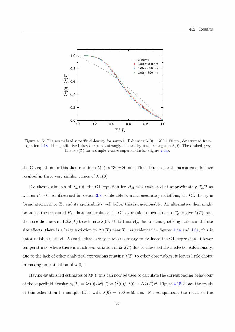
4.2 Results
Figure 4.15: The normalised superfluid density for sample 1D-b using λ(0) = 700± 50 nm, determined fromequation 2.18. The qualitative behaviour is not strongly affected by small changes in λ(0). The dashed grey
line is ρ(T ) for a simple d-wave superconductor (figure 2.4a).
the GL equation for this then results in λ(0) ≈ 730±80 nm. Thus, three separate measurements have
resulted in three very similar values of λab(0).
For these estimates of λab(0), the GL equation for Hc1 was evaluated at approximately Tc/2 as
well as T → 0. As discussed in section 2.3, while able to make accurate predictions, the GL theory is
formulated near to Tc, and its applicability well below this is questionable. An alternative then might
be to use the measured Hc1 data and evaluate the GL expression much closer to Tc to give λ(T ), and
then use the measured ∆λ(T ) to estimate λ(0). Unfortunately, due to demagnetising factors and finite
size effects, there is a large variation in ∆λ(T ) near Tc, as evidenced in figures 4.4a and 4.6a, this is
not a reliable method. As such, that is why it was necessary to evaluate the GL expression at lower
temperatures, where there is much less variation in ∆λ(T ) due to these extrinsic effects. Additionally,
due to the lack of other analytical expressions relating λ(T ) to other observables, it leaves little choice
in making an estimation of λ(0).
Having established estimates of λ(0), this can now be used to calculate the corresponding behaviour
of the superfluid density ρs(T ) = λ2(0)/λ2(T ) ≈ λ2(0)/(λ(0) + ∆λ(T ))2. Figure 4.15 shows the result
of this calculation for sample 1D-b with λ(0) = 700 ± 50 nm. For comparison, the result of the
93

4.3 Conclusion
Figure 4.16: The normalised superfluid density for sample 1c (red) using the value of λ(0) = 695 nm,determined in the same manner as for 1D-b, which is also plotted in blue for λ(0) = 700 nm. The agreement is
very good between the two samples.
weak-coupling d-wave calculation is also plotted. Very clearly, CeCu2Si2 does not resemble the d-wave
behaviour, showing a saturation for T < 0.2 K more indicative of a fully-gapped superconductor.
Additionally, small changes in λ(0) do not alter the resulting behaviour very much. Figure 4.16 shows
the result for sample 1c compared to 1D-b; both samples agree very well and show essentially the
same behaviour. Noticeably, both samples show convex curvature near Tc, which has been interpreted
as a signature of multigap superconductivity in the case of the IBS [123], and not entirely dissimilar
from MgB2 [124].
4.3 Conclusion
While specific heat measurements are more sensitive to the parts of the Fermi surface with the highest
effective mass, the penetration depth is weighted towards the parts of the Fermi surface with the lowest
effective mass and highest Fermi velocity. Thus, Kittaka et al. concluded from their measurements
that nodes would be absent on the heavy electron band surrounding the X point (see figure 4.2), ruling
out the dx2−y2 state [103].
The behaviour shown in the in-plane penetration depth and superfluid density also shows no
94

4.3 Conclusion
indication of nodes in the gap structure that would be apparent by the expected power law temperature
dependence. Indeed, ∆λab(T ) fits very well to an effective BCS gap up to Tc/2, and exhibits a high
power law exponent n > 3 for the same temperature range. The superfluid density also does not
resemble what would be expected for a nodal d-wave state, showing saturation at low temperature
and also a convex shape near Tc that is indicative of multiple full-gaps [123]. This evidence would
then rule out the existence of nodes on the light-mass hole bands for the in-plane superfluid response
that would occur due to, e.g. a dxy state.
In contrast, the behaviour observed in the out-of-plane response, ∆λc(T ), shows a very strong
temperature dependence down to 50 mK. This could possibly be interpreted as evidence for a gap
node with a crossover to impurity scattering at very low temperature. Alternatively, this behaviour
can also be fitted with a BCS effective gap that is significantly smaller than what was found from
the in-plane response, and so could result from strong anisotropy in the superconducting pairing
state. Given that the out-of-plane response only made a small contribution to the particular H‖ab
measurement, and the derived result’s sensitivity to experimental parameters, it is hard to decide how
much weight should be given to this result. In reality, this measurement would need to be performed
again on an additional sample with a much larger dimension in the c-axis to increase the size of its
contribution to the measured H‖ab response.
Focusing on the in-plane behaviour, the results presented here indicate that gap nodes are absent
on the light hole bands as well as on the heavy electron bands (as determined from the specific
heat measurements [103]). In strong contrast, it appears that CeCu2Si2 possesses a pairing state in
which there is a finite superconducting gap at all points on the Fermi surface. This surprising result
challenges the long-standing belief of unconventional d-wave superconductivity in this heavy fermion
compound, and opens up the possibility of an extended s-wave state [125–127].
The results presented here also strongly contrast with the previous reported measurements of the
magnetic penetration depth, in which a T 2 temperature dependence was observed [119]. However, the
previous measurements were made on significantly lower-quality, poly-crystalline samples. Given the
strong anisotropy observed here between ∆λab and ∆λc, it is not surprising that there was no clear
fully-gapped behaviour observed. It is possible that the T 2 behaviour could arise from an average of in-
plane and out-of-plane responses, but this is difficult to estimate without knowledge of the distribution
95

4.3 Conclusion
of grain sizes within the polycrystalline sample.
96

Chapter 5
Possible evidence against d-wave
pairing in KFe2As2
5.1 Introduction
Since their initial discovery, the iron-based superconductors (IBS) have emerged as one of the largest
families of unconventional superconductors, exhibiting a wide array of interesting physical phenomena
with superconductivity often emerging in the vicinity of a magnetically ordered phase [19,56,128]. The
discovery of superconductivity with high Tc’s in these compounds was surprising due to the ubiquitous
presence of Fe that was generally considered to otherwise be detrimental to superconductivity due to
its large magnetic spin moment. However, far from being hindered, the superconductivity in these
compounds is strongly dependent on the 3d orbitals of the Fe atoms [47, 129] that are also largely
responsible for the compounds’ electronic structures. A common aspect of the IBS are their layered
structure, featuring stacked layers of Fe atoms separated by layers of pnictogen or chalcogen atoms
(hence they are often called iron-pnictides and iron-chalcogenides). As such, there are a number of
different structures in which IBS can be formed, named according to the ratio of the elements in
their formulae, e.g. FeSe is a ‘11’ compound. Furthermore, NMR spin susceptibility measurements
in a number of compounds [130,131], including Ba1-xKxFe2As2 [132], found the NMR Knight shift to
decrease below Tc. This is usually taken as evidence against a spin-triplet pairing state, such that the
general consensus is that the IBS possess a spin-singlet superconducting state [47].
97

5.1 Introduction
(a) (b)
Figure 5.1: Phase diagrams for (a) Ba1-xKxFe2As2 and (b) BaFe2(As1-xPx)2, showing the proximity of thesuperconducting phase to the antiferromagnetic spin-density wave phase. Reproduced from references [133]
and [134].
BaFe2As2 is a member of the 122 family and displays a concurrent transition to an antiferro-
magnetic spin density wave, as well as a tetragonal to orthorhombic structural transition, below the
temperature TS ≈ 140 K [133, 135]. Superconductivity can be induced a number of ways: by hole
doping through the substitution of Ba2+ for K+ resulting in Ba1-xKxFe2As2 [136] and through iso-
valent substitution of either As with P in BaFe2(As1-xPx)2 [134] or Fe2+ (3d6) with Co2+ (3d7) in
Ba(Fe1-xCox)As2 [137]. Each method produces a very similar phase diagram, two of which are shown
in figure 5.1, where as x is increased, TS is suppressed along with the emergence of superconductivity.
The highest Tc’s are found once the magnetic phase has been completely suppressed, such that beyond
this end point the compound remains in the body-centred tetragonal structure, as shown in figure 5.2.
A unique aspect of Ba1-xKxFe2As2 is that, unlike BaFe2(As1-xPx)2 or Ba(Fe1-xCox)As2, the end mem-
ber, KFe2As2, remains superconducting. It is the nature of the superconductivity in KFe2As2, and
the transition from the optimally-doped region of Ba1-xKxFe2As2, that has been the topic of much
debate over recent years.
A common feature of the IBS is their quasi-2D Fermi surfaces (FS), often featuring a number of
separate sheets surrounding the central Γ point and the corner point of the Brillouin zone (M or X
depending on whether the 1 or 2-Fe unit cell is being used) [47,129]. The sheets at the center and the
corner are typically well separated in reciprocal space and so are often referred to as pockets, and in the
98

5.1 Introduction
Ba
Fe
As
Figure 5.2: The body-centred tetragonal structure of Ba1-xKxFe2As2.
1-Fe unit cell they are separated by wavevector Q = (π, 0). The electronic structure is such that the
central hole pockets are largely of xz and yz orbital character. The electron sheets are also largely xz
and yz but also posses more xy character [42]. In optimally-doped Ba1-xKxFe2As2 (x ≈ 0.4) ARPES
measurements identified two hole-like sheets surrounding the Γ point and a third electron-like sheet
surrounding the M point [138]. In this work they also identified three nearly isotropic superconducting
gaps on each sheet of FS, exhibiting a ratio of approximately 2:1 between the two larger gaps and the
smaller gap. However, ARPES measurements in a slightly different doping with Tc ≈ 32 K, found,
in addition to the two zone-centred pockets, two FS sheets at the corner, the so-called barrel and
blade, each of which also possess an isotropic superconducting gap (shown in figure 5.3) [139]. A
more recent ARPES study also suggests the presence of a more 3D hole sheet at the centre of the
zone, in addition to the four other FS sheets [140]. Specific heat measurements in a nearby doping
of x ≈ 0.32 suggested the presence of two full superconducting gaps [141], while thermal conductivity
measurements on slightly under-doped compounds found a lack of nodal quasiparticles and possible
indications of anisotropy in the gap structure [142]. Low-temperature measurements of the magnetic
penetration depth have also found behaviour consistent with a full gap [143,144].
Thus, there is a large body of evidence that strongly suggests the existence of multiple isotropic
superconducting gaps in the optimally-doped region of Ba1-xKxFe2As2. Given the structure of the
Fermi surface, either of the allowed d-wave states, dx2−y2 and dxy, would necessitate the presence of
99

5.1 Introduction
Figure 5.3: The momentum dependence of the superconducting gaps in Ba1-xKxFe2As2 (Tc ≈ 32 K) asdetermined by ARPES. The gaps are projected according to their magnitude above the Fermi surface intensity
map. Reproduced from ref. [139].
gap nodes on at least the central hole bands and also possibly on the corner pockets as well [47]. The
evidence then implies that the pairing must have s-wave symmetry, though it is hard to distinguish
between s± and s++ pairing as they often give rise to the same behaviour.
Probably the most popular theory regarding the pairing mechanism in Ba1-xKxFe2As2, and more
generally in IBS, is through spin fluctuations arising from repulsive Coulomb interactions [42,47,145].
This interaction is repulsive and so in order to stabilise a superconducting state it is necessary for the
superconducting gap to change sign somewhere in reciprocal space. In the case of the single band in
cuprate superconductors this manifests as the existence of line nodes in the dx2−y2 state. However, due
to the multiband nature of the IBS, this could be achieved in a number of ways, though the leading
contender is s± pairing by Q = (π, 0) between the hole and electron pockets. Indeed, a number of
theories successfully predict the observed Fermi surface and gap structure as seen in optimally-doped
Ba1-xKxFe2As2 [146, 147] . Alternative theories based on orbital fluctuations tend to predict an s++
state [148]. However, Cho et al.’s investigation of the effect of electron irradiation on Tc and the
low temperature penetration depth across the phase diagram, concluded that the observed behaviour
could rule out a possible s++ state in favour of s±pairing, particularly in the under-doped region in
which superconductivity coexists with an antiferromagnetic state where robust nodes should appear
in the s++ case [144,149].
Moving into the over-doped region of the phase diagram, there is a dramatic change in the topology
100
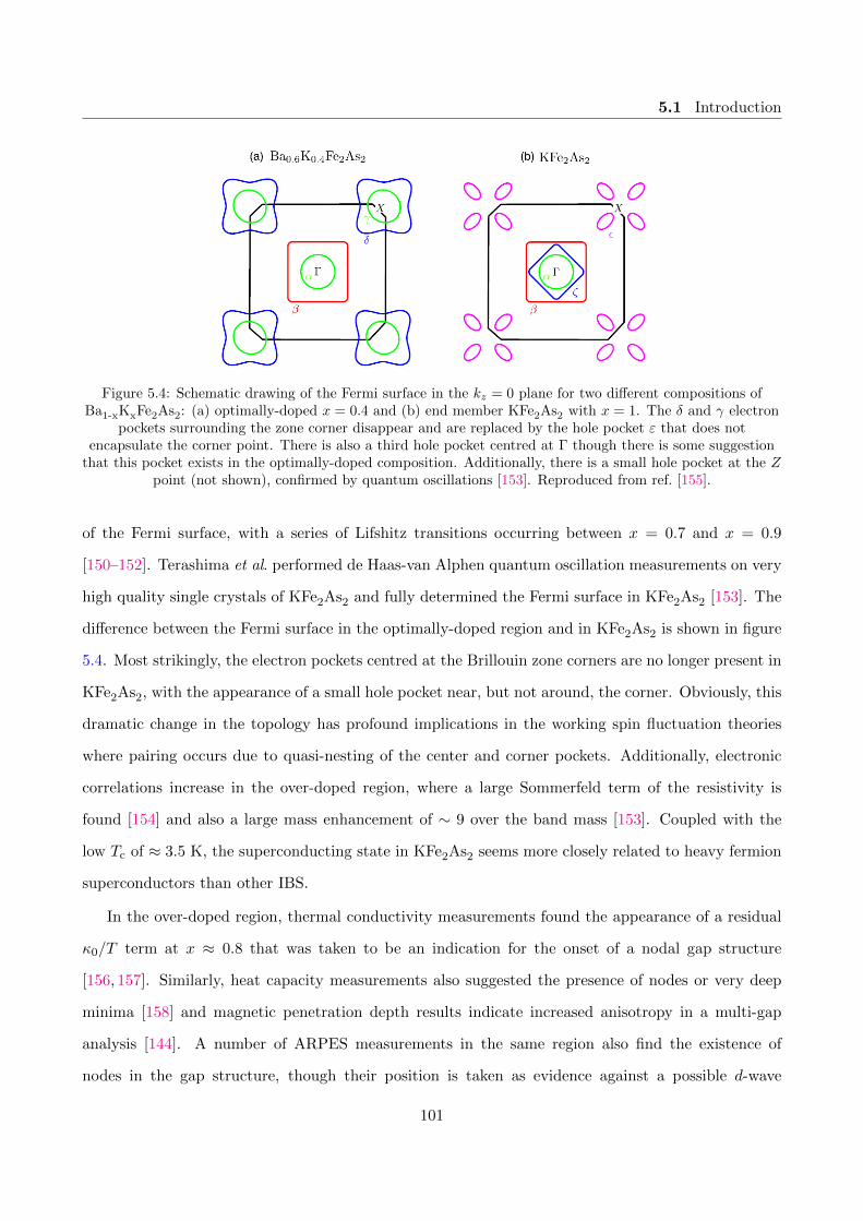
5.1 Introduction
Figure 5.4: Schematic drawing of the Fermi surface in the kz = 0 plane for two different compositions ofBa1-xKxFe2As2: (a) optimally-doped x = 0.4 and (b) end member KFe2As2 with x = 1. The δ and γ electron
pockets surrounding the zone corner disappear and are replaced by the hole pocket ε that does notencapsulate the corner point. There is also a third hole pocket centred at Γ though there is some suggestion
that this pocket exists in the optimally-doped composition. Additionally, there is a small hole pocket at the Zpoint (not shown), confirmed by quantum oscillations [153]. Reproduced from ref. [155].
of the Fermi surface, with a series of Lifshitz transitions occurring between x = 0.7 and x = 0.9
[150–152]. Terashima et al. performed de Haas-van Alphen quantum oscillation measurements on very
high quality single crystals of KFe2As2 and fully determined the Fermi surface in KFe2As2 [153]. The
difference between the Fermi surface in the optimally-doped region and in KFe2As2 is shown in figure
5.4. Most strikingly, the electron pockets centred at the Brillouin zone corners are no longer present in
KFe2As2, with the appearance of a small hole pocket near, but not around, the corner. Obviously, this
dramatic change in the topology has profound implications in the working spin fluctuation theories
where pairing occurs due to quasi-nesting of the center and corner pockets. Additionally, electronic
correlations increase in the over-doped region, where a large Sommerfeld term of the resistivity is
found [154] and also a large mass enhancement of ∼ 9 over the band mass [153]. Coupled with the
low Tc of ≈ 3.5 K, the superconducting state in KFe2As2 seems more closely related to heavy fermion
superconductors than other IBS.
In the over-doped region, thermal conductivity measurements found the appearance of a residual
κ0/T term at x ≈ 0.8 that was taken to be an indication for the onset of a nodal gap structure
[156, 157]. Similarly, heat capacity measurements also suggested the presence of nodes or very deep
minima [158] and magnetic penetration depth results indicate increased anisotropy in a multi-gap
analysis [144]. A number of ARPES measurements in the same region also find the existence of
nodes in the gap structure, though their position is taken as evidence against a possible d-wave
101

5.1 Introduction
state [150,159]. Therefore, the evidence suggests that there is a transition from isotropic fully-gapped
superconductivity in the optimally-doped region to a nodal state in the over-doped region where the
Lifshitz transitions change the topology of the Fermi surface.
In the fully hole-doped KFe2As2, there is more contention about the structure, and symmetry, of
the pairing state. Magnetic penetration depth measurements indicated a strong linear term in the
temperature dependence that was taken as evidence for nodes in the gap structure, but without any
strong suggestion of the symmetry [66]. Reid et al. compared thermal conductivity measurements
in KFe2As2 for different crystal purities, indicated by the residual resistivity ratios, and concluded
that there was evidence of so-called universal heat conduction. This is the observation of a residual
κ0/T term than is independent of purity as it occurs due to symmetry imposed nodes, such that their
conclusion was for a d-wave state [155,160]. In strong contrast, specific heat measurements by Hardy
et al., along with a four gap analysis, found evidence for a large isotropic gap and additional possibly
very small gaps, approaching the immeasurable size, that dictate the low temperature thermodynamic
behaviour. This analysis rules out a d-wave state as it would not allow the necessary presence of
gap nodes on all Γ centred sheets. However, the analysis would allow accidental nodes on some of
the remaining sheets. This is qualitatively consistent with laser ARPES measurements that found
accidental nodes on one of the zone centred hole bands, positioned in such a way to create an octet
of line nodes [161]. As well as this, moderate anisotropy was found in the other gaps that was linked
to the change in the orbital character around the Fermi surface. Furthermore, Hardy et al. argued
against the findings by Reid et al. by noting that the small magnetic field required to suppress the su-
perconductivity in the electrical contacts made to the sample would be large enough to induce induce
a moderate zero energy DOS that could be confused as being due to a possible d-wave state. Thus,
though there is generally a lot of evidence for the case of anisotropic, and likely nodal, superconduc-
tivity, there is still some debate about the band and position at which the nodes appear. Though the
laser ARPES study at first seems quite conclusive in this regard, it should be noted that the data
were collected at 1.5 K, or T/Tc ≈ 0.43, meaning there is still a relatively large fraction of Tc over
which a very small gap might appear, or in which time the strength of competing interactions could
change resulting in a different structure at T = 0.
Despite the strong evidence against it, there are some theoretical suggestions that a d-wave state
102

5.1 Introduction
could be stabilised in KFe2As2. In even the simplest spin fluctuation models, it is found that as doping
is increased, the s-wave channel becomes increasingly anisotropic and the d-wave channel becomes close
in energy to the s-wave state [42,162]. Additionally, as there is no longer any quasi-nesting of electron
and hole pockets, the nature of the leading pairing interaction will necessarily change. Thus, some
theoretical examinations suggest a transition from s-wave in optimally-doped Ba1-xKxFe2As2, to d-
wave in KFe2As2 via an intermediate time-reversal symmetry breaking s+id state [163–165]. If, on the
other hand, an s± state is still present in KFe2As2 then it is not clear how this is realised. A possibility
is that this is achieved between the Γ centred hole pockets through small Q scattering processes [42].
Clearly, in order to develop an accurate theory regarding the pairing in Ba1-xKxFe2As2 it is imperative
to clearly establish the symmetry and structure of the gap in KFe2As2 given the multitude of current
suggestions.
More pragmatically, the original impetus for re-investigating the magnetic penetration depth in
KFe2As2 was due to some disagreement in the literature about the magnitude of ∆λ(T ), though less
so regarding the temperature dependence. Specifically, the data reported by Hashimoto et al. [66]
is approximately twice the magnitude of that reported by Kim [166] et al.. Given that the two
separate studies were performed using nominally the same TDO technique, this inconsistency had no
obvious explanation. Thus, performing a third individual study would hopefully clarify the situation.
Additionally, the previous data was down to about 100 mK, so there was a small range of temperature
that could possibly provide important information, especially given the suggestion of very small gaps
that would only appear in thermodynamic measurements at the lowest temperatures [154]. However,
after having performed many of the measurements presented in this chapter, new data from Cho et
al. largely resolved the inconsistency, with data consistent with what was found by Hashimoto et
al., as well as with data down to 50 mK. A comparison of these three studies is shown in figure
5.5b, where the data from Kim et al. has been scaled up by a factor of 2. It can be seen that there is
generally good consistency between the three independent measurements and with the same conclusion
made of the indication of a nodal gap structure. Additionally, Cho et al. used electron irradiation
in order to observed the change in Tc and the low temperature behaviour of ∆λ(T ). From this they
observed that irradiation that reduced Tc by approximately half was accompanied by T 2 dependence
of the penetration depth, which is consistent with the expected behaviour from the appearance of
103

5.2 Results
bound states due to a sign change in the superconducting gap. However, it is also the expected
dependence in the case of impurity scattering in a nodal d-wave superconductor. It would have been
more illuminating to see the evolution with much smaller amounts of irradiation so as not to induce
such a large change in Tc.
It is generally known that a number of IBS will react adversely when exposed to air, such that
samples are often kept under nitrogen or argon atmosphere in order to preserve them. Reid et al. noted
that the residual resistivity ρ0 was found to change substantially over time between measurements in
their samples of KFe2As2 [155, 160]. Given the contentious nature of their conclusion, and generally
the lack of explicit mention of how samples in the various measurements in KFe2As2 reported in
the literature were handled or preserved, it was decided that it would be illuminating to investigate
what effect intentional exposure to air would have in KFe2As2, which forms the majority of the focus
of this chapter. Additionally, in principle, nonlinear measurements should be able to provide some
distinction between deep minima and true nodes, which is also a contentious aspect of the gap structure
in KFe2As2. Thus nonlinear measurements were performed in addition in the hopes of providing more
insight into the superconducting state.
5.2 Results
5.2.1 Sample Preparation
Samples of single crystal KFe2As2 were provided to us from the group of Frederic Hardy at the Karlruhe
Institute for Technology, Germany as part of a collaboration to investigate the gap structure. These
samples were grown by Thomas Wolf, also of Karlsruhe, using a self-flux method described in ref. [154].
Initial sample preparations were performed with the assistance of Carsten Putzke, of Bristol. Magnetic
penetration depth and lower critical field measurements were performed by myself over a period of
approximately four months.
Since there was some question about the sensitivity of KFe2As2, as well as other compounds, to air,
the first objective was to determine the response in a single crystal of KFe2As2 with the absence of any
exposure to air. This was done by taking a parent sample, which was stored under argon atmosphere,
and encapsulating it in vacuum grease. Then, all six sides were cleaved using a razor blade to expose
104

5.2 Results
(a) (b)
Figure 5.5: (a) The H‖c response of the pristine K1 sample of KFe2As2. The transition is relatively wide,with a midpoint of ≈ 3.5 K. (b) The low temperature portion of the data plotted in comparison to previousmeasurements by Hashimoto et al. [167], Kim et al. [166] and Cho et al. [144]. The solid line is a fit to theempirical dirty nodal formula (equation 2.29). The inset is an expansion of the same plot, but at very low
temperatures. The data series have been offset by 2, 4 and 7 nm from K1 for clarity.
fresh surfaces. The resulting sample had approximate dimensions of 0.6× 0.6× 0.05 mm3, with the c-
axis along the shortest direction. The sample was then encapsulated in grease before being transferred
to the TDO apparatus and subsequently cooled to base temperature, thus ensuring the newly exposed
surfaces experienced minimal exposure to air.
5.2.2 Magnetic Penetration Depth
This first sample, known as K1, was measured in the H‖c orientation, such that the in-plane super-
fluid response ∆λab was probed. The result of this measurement is shown in figure 5.5a, where the
relatively wide superconducting transition can be seen at approximately 3.5 K, in line with previous
measurements [167]. In figure 5.5b the low temperature portion of the data is plotted, along with data
from work by Hashimoto et al. [167], Kim et al. [166] and Cho et al. [144]. Thus it can be seen that
the measured response agrees very well with the previous measurements, particularly from Hashimoto
and Cho. The data from Kim et al. [166] has been multiplied by a factor of 2 to account for the
apparent error in the calibration factor. In the work by Hashimoto et al., they analyse their data
using the empirical dirty nodal formula (equation 2.29) [66]. In figure 5.5b, this is repeated for all of
105

5.2 Results
the data sets and is shown by the solid lines, and the fit was made up to a maximum temperature
of 0.8 K. Doing so yields T ∗ values of 0.67 K (sample K1), 0.33 K (Hashimoto), 0.43 K (Cho) and
0.54 K (Kim). Thus, sample K1 has the highest apparent crossover temperature, which would usually
be taken as indication that the quality of the sample is lower than the others, where Hashimoto’s
T ∗ of 0.33 K indicates a higher quality. However, in the inset of figure 5.5b, the same data and fits
are plotted but expanded between 50 and 250 mK. It can be seen that, particularly for the sample
K1, the data is not especially well described by the fit. It is also worth noting that when the upper
limit of the fit is changed so does the determined T ∗, typically decreasing, indicating that it is not
a particularly robust method in this instance. Cho et al. performed a more sophisticated multi-gap
analysis of their data using the self-consistent t-matrix approximation and report better agreement
with their data than the dirty nodal formula, especially at low temperature, but also conclude that
the data suggests a nodal gap structure.
Having established the in-plane response from the pristine sample, K1 was removed from the
apparatus and cleaned of all vacuum grease. It was then stored in a desiccator for a period of 24 hours
in which time it was completely exposed to the air. After this period, the sample was re-measured
in the same configuration to try to observe any change in the sample. After this, the sample was
removed and cleaned once more, and stored for a further nine days (ten days cumulative) exposed to
air in the desiccator. The sample was then measured once again in the same orientation. The effect
of this exposure on the measured response is shown in figure 5.6.
Firstly, it can be seen in figure 5.6a that after one day there is only a small change in the transition
and the overall response of ∆λab(T ). However, after ten days, there is a more noticeable change in
Tc and also in the general shape of ∆λab(T ). Secondly, in figure 5.6b, the low temperature portion
of the data is plotted, in which it is very clear that the exposure to air has induced a change in the
response at the very lowest temperatures. Compared to the strong variation with temperature all the
way down to 50 mK in the pristine sample, the response in the one day sample seems to saturate
below about 0.10 K. In addition, the response in the ten days sample also seems to saturate over a
similar temperature range, with an increased temperature dependence above ≈ 0.15 K. The flat region
of the ten day response is not perfectly flat and looks as if there is a very small upturn below 0.10 K.
A second sample (K2) was prepared using the same method as for K1. This time, the pristine
106

5.2 Results
(a) (b)
Figure 5.6: The measured response of sample K1 after no exposure (pristine), one day and ten days exposureto air over (a) the full superconducting range and (b) over the lowest temperature range (vertically offset for
clarity).
(a) (b)
Figure 5.7: The pristine response of sample K2 measured in the H‖c and H‖ab orientations, as well as the oneday response of sample K2 in the H‖ab orientation over (a) the full superconducting temperature range and
(b) over the lower temperature range (with comparison to sample K1). Data has been offset vertically forclarity.
107

5.2 Results
response was measured in both the H‖c and H‖ab orientations, as shown in figures 5.7a and 5.7b.
The response from the H‖ab measurement has been left in terms of an effective penetration depth
∆λeff(T ), according to equation 3.6, and it can be seen that at low temperature there is very little
difference between ∆λab(T ) and ∆λeff(T ), thus implying that there is very little contribution from the
c-axis response over this temperature range. Furthermore, in figure 5.7b the pristine ∆λab response
from sample K1 is also plotted, showing qualitatively the same behaviour as K2, though with a small
difference in the absolute magnitude that can be attributed to error in determining the calibration
factor between ∆f(T ) and ∆λ(T ). However, in figure 5.7a, it does appear that the apparent Tc for
the H‖c orientation is slightly higher than in the H‖ab orientation, which could be due to anisotropy
between λab and λc near Tc.
In the same manner as for sample K1, sample K2 was also cleaned of all grease and left exposed to
air for one day. Following this, K2 was measured in the H‖ab orientation, which is shown in (a) and
(b) of figure 5.7. Also in the same manner as sample K1, there is not a large change in Tc between the
pristine and one day responses while there is a noticeable change in the response at low temperature.
Indeed, there is a change from a strong variation with temperature to an almost saturated behaviour
after exposure to air. This can be made more evident by fitting the data to a power law dependence
with variable upper limit (as described in section 4.2.1). Thus, figure 5.8a shows the result of this
fitting process for sample K1’s pristine, one day and ten day response, while figure 5.8b shows the
results for sample K2’s pristine response in the H‖c and H‖ab orientations, as well as the one day
response in the H‖ab orientation. In both samples and orientations it can be seen that the higher
temperature response is dominated by an exponent n ≈ 1.5, which is none of the simple expected
power law exponents, as indicated in the figures. As the upper limit of the fit Tmax is reduced, the
pristine responses show a small increase in n to approximately 2.5 around 0.20 K. Contrastingly, the
responses after exposure to air show a much more rapid increase into the n > 3 region that is usually
associated with fully gapped behaviour. Without making any firm commitment with regards to the
origin of this effect, the data shown in figure 5.8 at least shows that this effect is reproducible.
At this point, it is now necessary to consider what effect the exposure to air is having on the
samples and whether the observed effects are intrinsic to the superconducting state or of extrinsic
origin. The measurement of the magnetic penetration depth is inherently a surface measurement, and
108

5.2 Results
(a) (b)
Figure 5.8: The result of making the power law with varying upper limit, as described in section 4.2.1, for (a)sample K1 and (b) sample K2. Both samples show very similar in the pristine and exposed states.
while it is possible to make measurements of the bulk superconducting state, it is also possible to
measure a response from the surface that is not reflective of the bulk, especially when the length scale
of λ is of the order of 100s of nanometres. Thus, in this instance, we could believe that the observed
changes, especially at low temperature, are due to changes in the surface of the samples.
Given that a number of IBS are known to react with air, and that KFe2As2 contains the magnetic
ion Fe, one possible origin of the effect could be due to the generation of magnetic ions on the surface
of the sample due to this reaction. In this instance, the measured penetration depth is expected to
be modified by the presence of these paramagnetic ions according to λm(T ) = λL(T )√
1 + χN (T ),
where λm is the measured penetration depth, λL is the London (magnetic) penetration depth and
χN is the normal state susceptibility of the ions [168, 169]. In terms of the measured change in the
penetration depth, ∆λm, and provided χN (T ) 1, the two contributions should simply sum, i.e.
∆λm(T ) = ∆λL(T ) + ∆λN (T ), where ∆λN is the term due to the normal state susceptibility [169]1.
So by firstly assuming that the pristine behaviour can be described by a power law dependence,
and that the susceptibility takes a Curie form [169], it should be possible to estimate the magnetic
1This is the assumption made about the paramagnetic contribution from the sapphire sample rod. See section 3.2.6.
109

5.2 Results
contribution to the measure signal by fitting the data to the follow form:
∆λm = ATn +C
T+ λoffset , (5.1)
where A is a scaling factor, n is the power law exponent, C is the Curie term and λoffset is an offset.
Considering sample K1 in the H‖c orientation, and starting with the pristine behaviour, it is possible
to fit a normal power law dependence (∆λ ∝ Tn) over the range 0 to 0.30 K, which yields an exponent
of n = 2.03±0.02. The data are shown as red squares and the fit as a red dashed line in figures 5.9 (a)
and (b). Trying to fit a larger range of data yields a less representative fit, with large deviations from
the data at the lower temperatures. In figure 5.9a, the one day response (blue circles) has been fitted
with the form in equation 5.1 (blue dashed line) yielding an exponent n = 2.09 ± 0.03, very similar
to the pristine fit, and a Curie term C = 0.10± 0.01 nm K−1. It can be seen that this form describes
the measured behaviour quite well, with some deviation only at the very lowest temperature points.
It is also possible to then subtract the C/T behaviour, which should in principle yield the pristine
response. In doing so, shown as green triangles in figure 5.9a, it can been seen that this yields quite
a good agreement with the pristine behaviour, at least above about 0.075 K. This process is then
repeated for the ten day response in figure 5.9b, with the data shown as yellow diamonds, the fit as
a brown dashed line and the data with the C/T term subtracted in cyan hexagons. From the fit, it
is found n = 2.24 ± 0.04 and C = 0.14 ± 0.01 nm K−1. Thus, the underlying power law is described
by a slightly higher exponent and the magnitude of the paramagnetic contribution has increased by
approximately 40%. However, it is evident that the fit does not describe the data especially well over
an increased temperature range, notably for T < 0.12 K. This is also seen by the downturn in the
data with the magnetic contribution subtracted.
Alternatively, we could consider that the susceptibility takes a Curie-Weiss form, e.g. C/(T + θ).
However, trying to fit the data to this form over the same temperature range, as well as both smaller
and larger ranges of T , the Levenberg-Marquadt algorithm is unable to yield realistic results, or
without large associated errors for a number of the parameters. Additionally, fixing the exponent
to n = 2 does not yield satisfactory results, with the fit grossly misrepresenting the data at low
temperatures. Thus the Curie form seems to be the more appropriate in this situation, given no other
input into the normal state susceptibility, and provides an acceptable explanation of the evolution
110

5.2 Results
(a) (b)
Figure 5.9: Data for sample K1 in the H‖c orientation, between 0 and 0.30 K, offset vertically for clarity. Thepristine behaviour is in red, where the dashed line is a fit to a power law dependence. In (a) the one day
response (blue) has been fitted with the form in equation 5.1 (dotted line), and then plotted with the C/Tterm subtracted (green). In (b) the same is plotted but for the ten day response (yellow, brown and cyan).
of the response seen. However, in this assumption the underlying superconducting state should not
change, but in figure 5.6a, it is evident that there is a change in Tc and also the overall behaviour. It is
not clear how paramagnetic moments could influence the behaviour at higher temperatures following
this simple model.
A more radical suggestion would be to consider that the consequence of exposing the sample to
air is to cause a change in the superconducting state itself. Reaction with the air could lead to the
creation of defects or vacancies in the crystal structure near the surface, such that they act like sources
of impurity scattering. This change would not need to extend throughout the bulk of the sample since,
as discussed before, the penetration depth measurement is essentially reflective of the superconducting
state within λ of the surface. Then, depending on the gap structure in the pristine state, impurity
scattering could lead to a number of possible observed responses (as discussed in section 2.5). With
this in mind, the consequence of exposing to air seems to be to change the n = 2 power law dependence
at low temperature to something that resembles a fully gapped response, as indicated by the high value
of the exponent and the saturation of the response below ∼ 0.15 K. Thus, it is illuminating to fit the
one day and ten day responses of sample K1 in the H‖c orientation with the BCS effective gap form
(as described in section 4.2.1). The result of this is shown in figure 5.10, with the fit yielding effective
111

5.2 Results
Figure 5.10: The result of fitting the one day and ten day response of sample K1, H‖c orientation, with theBCS effective gap form (offset vertically for clarity). The fits describe the data well and yield gaps
∆eff = 0.21 kBTc (one day) and 0.24 kBTc (ten days).
gaps of ∆eff = 0.21 kBTc and 0.24 kBTc for the one day and ten days data respectively. The form
does seem to describe the data well and there is good agreement in the magnitude of the apparent
gap between the one day and ten days data.
Considering that Tc was also seen to decrease due to the exposure of the samples to air (figure
5.6a), the change from a power law dependence to an exponentially activated behaviour is consistent
with a change from a nodal gap structure, or possibly one with very deep minima [154], to a structure
with a full gap, reminiscent of what was observed in BaFe2(As1-xPx)2 [46]. This is possible if the
disordering causes strong (unitary) scattering as only a small concentration would be required to
lift a small portion of the gap of opposite sign [47, 48]. If this is indeed what is occurring then
this would imply that any nodes are not symmetry imposed and are accidental, as a number of
groups have argued [154, 161]. Therefore the symmetry of the order parameter could not be d-wave
due to the unavoidable requirement of symmetry imposed nodes on such a Fermi surface. This is
also consistent with the observed T 2 dependence in electron irradiated KFe2As2 [144] as this is the
expected temperature dependence for an s± pairing state due to the appearance of bound states with
112

5.2 Results
0 . 0 0 . 5 1 . 0 1 . 5 2 . 0 2 . 5 3 . 0 3 . 50
2
4
6
8µ 0
H p (m
T)
T ( K )
H || a b
Figure 5.11: Lower critical field measurements of pristine sample K2, with the field applied parallel to the abplane. The data has been left in terms of the observed penetration field, though due to the low demagnetising
factor in this orientation this should be very similar to the actual lower critical field Hc1(T ). The shadedregion indicates the range over which nonlinear measurements were made.
large amounts of impurity scattering (see section 2.5).
5.2.3 Nonlinear Response
Given this interesting possible result regarding the nature of the nodes in the gap structure of KFe2As2,
it was decided that investigating the nonlinear response could provide further insight. It was decided
that it would be best to perform the field dependent measurements in the H‖ab orientation such
that the lower demagnetisation factor of the sample would cause less disturbance of the applied field
compared to the H‖c orientation. This choice is also justified given that the low temperature response
of ∆λab and ∆λeff are almost identical, so that any change in response from the c-axis component
would be very small.
Before performing any field dependent measurements of the penetration depth, it was necessary
to establish the field and temperature range over which these measurements could be made without
exceeding Hc1(T ) so as not to allow magnetic flux to enter the sample and contribute to the measured
response. This was done using the lower critical field setup for use with the 3He system (see section 3.3
113

5.2 Results
(a) (b)
Figure 5.12: (a) Field dependent (i.e. nonlinear) measurements of the magnetic penetration depth. Anadditional dc field is applied and temperature sweeps are performed. The data have been offset such that they
coincide at the highest temperature of 0.30 K. (b) Result of making a power law exponent analysis on theH = 0 and H = 6 mT data from (a).
for details of the method and measurement process), with the sample mounted such that the applied
field was parallel to the ab-plane. The measurement was carried out on sample K2 in the pristine
state, before it was exposed to air, the results of which are shown in figure 5.11. The data has been
left in terms of the determined penetration field for each temperature, rather than trying to determine
the corresponding values of Hc1(T ). This is because it was only necessary to establish the area of
the H − T diagram in which the nonlinear measurements could be made. However, given the low
demagnetising factor of the sample in this orientation, there would have been little enhancement of
the field such that the actual values of Hc1(T ) likely only differ by a small factor.
Nonlinear measurements, as described in sections 2.6 and 3.2, were then carried out on the pristine
sample K2 for a maximum field of µ0Hdc = 6 mT and maximum temperature sweep of 0.30 K, well
within the boundaries established in figure 5.11 and indicated by the shaded region. The resulting
behaviour is shown in figure 5.12a, where the different data sets have been adjusted vertically such
that they all coincide at 0.30 K. It can be seen that with increasing field the change in the measured
penetration depth, between the base temperature (≈ 50mK) and the maximum temperature (300mK),
increases continuously in magnitude. That is, in zero field, the change in ∆λeff across this range is
approximately 8 nm, whereas in 6 mT this increases to approximately 11 nm. Additionally, making a
114

5.3 Conclusion
similar power law exponent analysis, it can be seen that there is a subtle change in the temperature
dependence, as shown in figure 5.12b. For the µ0Hdc = 0 measurement, decreasing Tmax has the
effect of yielding an increasing value for the exponent, though this increase is quite gradual. For the
µ0Hdc = 6 mT data, the exponent begins already slightly lower at n ≈ 2 and does not exhibit any
particular trend with decreasing Tmax.
Comparing the observed nonlinear response with the calculations performed by Stojkovic et al. [69],
shown in figure 2.9, there is a strong resemblance between the data and what would be expected for
a highly anisotropic but non-nodal gap. Certainly, much more so than for the clean or dirty d-wave
scenarios. However, there is some inconsistency since the zero field response observed does not so
clearly demonstrate the saturated behaviour associated with a full gap. An explanation for this
could be that the size of the gap is smaller than it is possible to resolve using this measurement,
i.e. the characteristic thermal activation energy is less than 50 mK. Indeed, the suggestion of almost
immeasurably small gaps has been made before [154]. This would be consistent with the observation
of increasing exponents with decreasing Tmax in figures 5.8a and 5.12b.
5.3 Conclusion
In order to find an interpretation to consistently explain all of the observed behaviour, it is necessary
to emphasize a number of aspects. Firstly, in a superconductor with multiple superconducting gaps,
the magnetic penetration depth, as well as other thermodynamic quantities, will be sensitive to the
smallest gap at low temperatures. This is because the penetration depth is essentially a measure of the
superfluid density and probes the thermal depopulation of Cooper pairs. The smallest gap will have
the lowest characteristic activation energy, such that at temperatures higher than this thermal energy
the superconductor will no longer appear to be gapped, even if there exists a larger gap that is yet to
be depopulated. This is the kind of behaviour seen in MgB2, where the low temperature behaviour
is dictated by the smallest gap [55, 170]. Further analysis of the full temperature dependence is then
required to determine the nature of any additional gaps [154].
Secondly, the ‘expected’ behaviours in the cases of a full gap, clean and dirty nodes, as discussed in
sections 2.4 and 2.5, are made on the assumption that the magnitude of the gap remains fairly constant
over a sufficiently large temperature range, e.g. for T/Tc < 0.2 in figure 2.1. However, if the gap shows
115

5.3 Conclusion
a much stronger temperature dependence as T → 0, due to some details of the pairing interaction,
then these simple behaviours will no longer be true and the general form of ρs(T ) will become more
complex as the measured response will be a combination of the structure and temperature evolution of
the gap(s). This kind of non-BCS evolution of the gap was also seen in one of the gaps in MgB2 [55].
With these two points in mind, one possible interpretation is as follows. In the pristine state
the structure of at least one of the gaps is highly anisotropic such that at some point on the Fermi
surface there exists a very small gap, ∆min, that dominates the low temperature measured response
of ∆λ(T ). This is consistent with the observation of more complex low temperature behaviour of
the pristine zero-field response (figure 5.5b). Performing the power law exponent analysis on this
measurement (figure 5.8), the determined exponents are not the same as for a clean nodal, dirty
nodal or fully gapped system. However, as the limit of the fit is decreased, n is seen to increase
to ≈ 2.5, which could be extrapolated to higher values at lower temperatures. Following this, on
the assumption that the exposure to air does induce some amount of impurity scattering, the very
low temperature behaviour in the samples following exposure changes to fully-gapped behaviour, as
evidenced by successful fitting of the BCS form and from the power law exponent analysis (figures
5.8 and 5.10). This assumption is plausible since impurity scattering is expected to average out any
anisotropy in the gaps, effectively increasing ∆min, while also causing a small reduction in Tc. Finally,
in the nonlinear response there is qualitative agreement with the expected response from an anisotropic
but fully-gapped superconducting state (figures 2.9 and 5.12a). The additional magnetic field causes
a Doppler shifting of the quasi-particle energies that, due to the very small size of ∆min, manifests as
a breaking of the pairs located in the minima of the gap. The temperature evolution then follows a T 2
dependence over this temperature range due to these broken pairs. If this scenario is true, then this
would imply that the pairing symmetry in KFe2As2 cannot be d-wave due to the absence of symmetry
imposed nodes in the gap structure, meaning that KFe2As2 more than likely shares the same pairing
symmetry as the rest of the Ba1-xKxFe2As2 series.
It is difficult, however, to be able to say confidently that this is a more correct interpretation.
In order to clarify this, a number of additional investigations need to be performed. Firstly, if the
exposure to air does induce a large minimum gap, then nonlinear measurements in this system should
produce a larger response more akin to the calculations by Stojkovic et al. [69]. If, on the other
116

5.3 Conclusion
hand, the behaviour with field was seen to ‘increase’ then this would help to determine the presence
of paramagnetic moments in the exposed samples. Secondly, though the work by Cho et al. [171] went
some way to revealing more information about the gap structure in KFe2As2, the smallest dosage
of electron irradiation was sufficient to reduce Tc by nearly a factor of 2, clearly causing a large
amount of disorder in the system. Repeating this with significantly smaller dosages would hopefully
reveal better insight by being able to view the evolution of the temperature dependence with smaller
amounts of induced disorder [46]. If there is indeed an accidental node then a similar scenario to
BaFe2(As1-xPx)2 should be observed [46]. Lastly, the nature of the reaction of KFe2As2 with air needs
to characterised. In particular, it would be illuminating to determine how localised to the surface the
effect is by attempting to remove some surface material either mechanically or by etching.
117

5.3 Conclusion
118

Chapter 6
Nonlinear response of d-wave
superconductor CeCoIn5
6.1 Introduction
Pressure induced superconductivity was initially discovered in the antiferromagnetic heavy fermion
compound CeIn3 [172]. With the application of hydrostatic pressure, the ordering temperature TN
was found to be suppressed towards zero at a critical pressure pc. However, before reaching zero
temperature it was found that a dome of superconductivity appeared around pc, with a maximum
Tc of ≈ 0.2 K. Soon after, similar behaviour was found in another Ce-based heavy fermion material,
CeRhIn5, though with a maximum Tc around 10 times higher than for CeIn3 [173]. This higher Tc
is often attributed to the increased two-dimensionality of the system, which, in terms of magnetically
mediated superconductivity, strengthens the pairing interaction [174]. Shortly after superconductivity
was then discovered at ambient pressure in two other so-called ‘115’ compounds: CeIrIn5 [175] at
∼ 0.40 K and CeCoIn5 [176] ∼ 2.30 K. Collectively, these compounds are part of the tetragonal
CeM In5 compounds, where M = Co, Rh, Ir, Pd and Pt, and all share the same crystal structure, as
shown in figure 6.1. This 115 structure is often viewed as layers of CeIn3 separated by layers of M In2,
leading to their increased two-dimensional properties.
Of the 115 compounds, CeCoIn5 has been the most intensively studied. This is in part due to
the fact that it has the highest Tc of the 115’s, and of any other Ce-based HFS at ambient pressure,
119

6.1 Introduction
Ce
In
Co
Figure 6.1: The tetragonal crystal structure of CeCoIn5 (and other CeM In5 compounds).
and also due to the comparative ease with which very high quality crystals can be grown [19, 22],
though typical residual resistivity ratios (RRRs) often underestimate the ‘super-clean’ state of these
samples [177]. As mentioned, CeCoIn5 is a heavy fermion compound and, in a similar manner to
CeCu2Si2, displays a very large jump in the specific heat at the critical temperature (∆C/γTc ≈ 4.5)
indicating the role of massive quasi-particles in the superconducting state. As well as this, CeCoIn5
exhibits a large superconducting gap to Tc ratio that places it in the strong coupling regime, and
the observation of a decrease in the Knight shift below Tc is taken as evidence for a spin-singlet
superconducting state [178].
In CeCoIn5, the superconducting state emerges out of a non-Fermi liquid (NFL) normal state as
indicated by the temperature dependence of the electronic specific heat [179], the resistivity [176] and
NMR relaxation rate [178]. This NFL behaviour is suggested to occur due to the proximity of CeCoIn5
to an antiferromagnetic quantum critical point typical heavy Fermi liquid behaviour is restored with
the application of pressure [180], drawing a comparison with the pressure induced superconductivity
in CeIn3 that emerges near the end point of an antiferromagnetic phase. This behaviour has been
taken as a strong indication that magnetism is connected to the superconducting states in the 115
compounds.
Measurements of the size of the Fermi surfaces in the 115s have found some contrasting behaviour.
de Haas-van Alphen measurements determined that CeRhIn5 has a relatively small Fermi volume,
120

6.1 Introduction
Figure 6.2: The three Fermi sheets of CeCoIn5 determined from band structure calculations. Adapted fromref. [183].
comparable to the 4f electron-less compound LaRhIn5 [180]. On the other hand, CeIrIn5 and CeCoIn5
exhibit much larger Fermi volumes, indicating the hybridisation of Ce’s f electron states with p and
d orbitals and their contribution the Fermi sea, whereas these f states remain nominally localised in
CeRhIn5. Despite this difference, the Fermi surfaces in the 115s are qualitatively similar, exhibiting
multiple sheets with quasi-2D structure. Though DFT calculations do not correctly capture the
mass renormalisation of the heavy QP states, the resulting band structures are consistent with the
experimentally determined Fermi surfaces [181]. The Fermi surface in CeCoIn5 consists of three
sheets, one of which is much smaller and forms around the Γ point while the other two sheets are
much larger and are centred around the corner of the Brillouin zone, as shown in figure 6.2. Though
the FS is clearly quite anisotropic, this is not as strongly evident in quantities such as the resistivity,
susceptibility [182] and the upper critical field [180].
Aside from the cuprate superconductors (e.g. YBa2Cu3O7-x) there are not many other compounds
in which there is strong evidence for d-wave pairing; this is not true of CeCoIn5, for which there
is a large amount of evidence that is largely in favour of the nodal dx2−y2 order parameter. Nodes
in the gap structure were first suggested from the power law behaviour of the specific heat, and
also in the thermal conductivity, though over a much smaller range of temperature than the specific
heat [184]. This was further supported by thermal conductivity measurements in a rotating magnetic
field, which identified four-fold oscillations consistent with nodes in the same positions as the dx2−y2
gap structure, i.e. along kx = ±ky [185]. However, complementary measurements of angle-resolved
specific heat concluded in favour of the dxy state in which the nodes are along the kx = 0 and ky = 0
directions, 45 to the dx2−y2 state [186]. This apparent discrepancy was later explained as being due
121
6.1 Introduction
to the reversal of the nodal and anti-nodal directions (which indicate the direction of the gap nodes)
above a certain crossover temperature [187]. Repeat measurements at lower temperature observed this
change in the nodal and anti-nodal direction, providing further evidence for the dx2−y2 state [73,188].
Due to the disagreement between the angle resolved thermal conductivity [185] and original angle
resolved specific heat measurements [186], as well as the somewhat uncharacteristic power law be-
haviours that were observed, alternative explanations were sought to resolve the discrepancy concern-
ing the orientation of the nodes. Notably, Tanatar et al.’s observation of the simultaneous reduction
in the residual resistivity and increase in residual thermal conductivity in samples where La was sub-
stituted for Ce led to the suggestion that superconductivity was limited to the two quasi-2D cylinders
but where the more 3D sheet remained gapless [189]. However, this was argued against as unlikely due
to the complexity of the Fermi surface and the requirement for there to be zero interaction between
different sheets in order for a sheet to remain gapless [190]. Following calculations, it was shown that
even a very small amount of coupling between bands would induce a finite order parameter to develop
below Tc on the ‘gapless’ sheet. It is also worth noting that Tanatar et al.’s estimation of the κ0/T
term was made from an extrapolation of the data at higher temperature than the work by Movshovich
et al. (50 mK compared with 33 mK), which was sufficient to lead to an estimation of a residual
term twice as large as what was previously found. Following this period of doubt surrounding the
symmetry of the pairing in CeCoIn5, a number of more recent measurements have all concluded in
favour of the dx2−y2 state, including point contact spectroscopy and tunnelling spectroscopy [191,192].
It is therefore fair to say that the majority of the community accepts the dx2−y2 structure as being
correct, though there is also some suggestion of an IBS-like s± pairing scenario [183].
Given the large amount of evidence supporting the existence of the dx2−y2 state in CeCoIn5, this
presents a possibly interesting and as yet unexplored system in which to investigate the nonlinear
Meissner effect. As described in section 2.6, despite a number of diligent studies, the NLME has yet
to be unambiguously observed. However, it is important to first consider the expected size of the
nonlinear response and whether this would be experimentally resolvable. In the Yip-Sauls theory, the
field dependence of the penetration depth is expected to vary as
∆λ(H)
λ(0)= α
H
H0, (6.1)
122

6.1 Introduction
(a) (b)
Figure 6.3: Previous measurements of the magnetic penetration depth in CeCoIn5. In (a) Chia et al. identifylinear behaviour in the out-of-plane response [193]. In (b) Ozcan et al. show the in-plane response is well
described by a dirty d-wave form (solid line) as well as by T 1.5 power law behaviour (inset) [194]. (Adaptedfrom refs. [193,194].)
where α depends on the relative orientation of the field with respect to the nodes and H0 is of the
order of the thermodynamic critical field [49,70]. Observation of this effect is limited to fields less than
Hc1, as above this field contribution to the measured penetration depth from magnetic vortices will
mask the contribution from the NLME. Additionally, the range of temperature over which the NLME
should be observable is limited by the equivalent impurity scattering temperature T ∗, as unitary
scattering is predicted to rapidly destroy the nonlinear corrections [51], such that measurements need
to be performed above this temperature. In YBa2Cu3O7-x, this limits the temperature range to be
between approximately 1 and 4 K. Therefore, the maximum expected ∆λ is for H = Hc1, such that
Hc1/H0 ≈ 10−2, corresponding to ∆λ ∼ 1% of λ(0) [84].
In CeCoIn5 we can make a similar estimation of the expected ∆λ. Taking µ0Hc2(0) ≈ 5 T
(11.5 T) for H‖c (for H‖ab) [182,195], and also estimating µ0Hc1(0) ≈ 16.3 mT (4.5 mT) for H‖c (for
H‖ab) [196] (see figure 6.7), it is possible to estimate the thermodynamic critical field using the relation
for a type II superconductor Hc ≈√Hc1Hc2. For the H‖c orientation, we find µ0Hc ≈ 0.28 T and
similarly ≈ 0.23 T for the H‖ab orientation. Then assuming H0 ∼ Hc, this yields ∆λ ∼ Hc1/Hc ∼ 6
% of λab (∼ 2 % of λc). Given the larger values of λab ≈ 190 nm and λc ≈ 270 nm in CeCoIn5 [193],
this compares favourably with YBa2Cu3O7-x with an expected shift in the penetration depth of 5 - 10
123

6.2 Introduction
nm. Admittedly this is not a particularly robust calculation, but it shows that the size of the effect
in CeCoIn5 is of a similar size to what was expected in YBa2Cu3O7-x, and certainly not significantly
smaller. Furthermore, CeCoIn5 is completely stoichiometric and samples can be grown with very high
electronic mean-free paths [19], whereas the tuning of the oxygen content in YBa2Cu3O7-x invariably
leads to some amount of impurity scattering at low temperature even in the best samples [51]. Thus
the NLME should be apparent in CeCoIn5 even to very low temperatures before impurity scattering
becomes an issue.
Interestingly, despite the strong evidence for the nodal dx2−y2 state in CeCoIn5, measurements
of the magnetic penetration depth have found unexpected, though not necessarily inconsistent be-
haviour. Initial measurements of the microwave surface impedance down to ≈ 250 mK by Ormeno et
al. suggested an almost linear temperature dependence, though arguably with some curvature, that
suggests a nodal gap structure [197]. From their measurements they were also able to determine the
behaviour of the superfluid density which was strongly reminiscent of what is found in the cuprate
d-wave superconductors. TDO measurements by Chia et al. down to 140 mK, however, identified
somewhat different behaviour [193]. They found that the out-of-plane response exhibited a linear de-
pendence below ≈ 1 K, as shown in figure 6.3a, but the in-plane response clearly demonstrated some
curvature. Chia et al. interpreted this as a crossover from T -linear to T 2 either due to impurity scat-
tering or possibly due to nonlocal effects [198]. Equally, they found that the data was well described
by a T 1.5 power law behaviour. However, shortly following these results, Ozcan et al. performed TDO
measurements down to 100 mK using a novel technique involving a micro-coil as part of the resonating
circuit, the results of which are shown in figure 6.3b. The small spatial extent of the coil means that
screening currents would only be produced in a small loop on the surface of their sample, which was
larger than the size of the coil. Additionally, due to the orientation of the sample and coil, they argue
that their measurements are inherently insensitive to nonlocal effects. As a result, they determine
that the T 1.5 behaviour is due to some other intrinsic aspect of CeCoIn5 itself, such as the observed
quantum critical behaviour of the normal state, and ruling out the effects of nonlocality. Indeed,
measurements performed by Hashimoto et al. in CeCoIn5and Ce2PdIn8 also demonstrated strong T 1.5
behaviour. They argued that, due to the proximity of these compounds to a quantum critical point,
strong critical fluctuations cause a renormalisation in the Fermi velocity and effective mass ultimately
124

6.2 Results
Figure 6.4: Photographs of sample C1 mounted on the H‖ab sample rod at (a) ∼0 to the sample’s facets and(b) rotated ∼45 in-plane. The orientation of the crystal axes, determined by x-ray diffraction, are indicated.
changing the temperature dependence of the nodal d-wave state from T -linear to T 1.5.
6.2 Results
6.2.1 Sample Preparation
In order to carry out the investigation into the nonlinear response of CeCoIn5, samples were kindly pro-
vided by Dariusz Kaczorowski of the Institute of Low Temperature and Structure Research, Wroclaw,
Poland. These samples were single crystals grown using the self-flux method [180] and had typical
dimensions of ∼ 2 × 2 × 0.5 mm3. However, the samples were not used as-grown in the penetration
depth measurements for two reasons. The first was simply that they were too large to fit within the
experimental apparatus - the inside diameter of the sense coil is only 2 mm itself. The second reason
was that when the samples were originally received they appeared to be very shiny on the surface with
a silvery colour. The samples were then stored in a desiccator for approximately 3 months. Upon
inspection after this time it could be clearly seen that the surfaces of the samples had become much
less shiny and had taken on a dull grey colour, indicating that some sort of reaction had taken place
between the compound and the surrounding air.
Following what was learned during the study on KFe2As2 (chapter 5), care was taken when prepar-
ing the samples to minimise exposure of freshly exposed surfaces to the surrounding air. Three samples
125

6.2 Results
Figure 6.5: Photographs of (a) sample C2 and (b) sample C3, both mounted on the H‖ab sample rod. Scratchmarks are clearly visible in the surface of C3.
for penetration depth measurements were derived from a single parent sample. Initially, I attempted to
cleave the sample of CeCoIn5 with a razor blade in a similar manner to KFe2As2. However, CeCoIn5 is
mechanically very hard and brittle and so it is prone to cracking and breaking into very small shards,
making this a difficult process. Through this method it was possible to cleave a single sample (known
as C1), which is a thin platelet with dimensions 200×310×5 µm3. The orientation of the crystal axes
within the sample were determined by Dr Natalie Pridmore, University of Bristol, using a four-circle
x-ray diffractometer. From this, it was found that the sample cleaved in such a way that the shortest
dimension corresponds to the c-axis, in the same manner as the parent sample, and with the a-axes
parallel to the facets, as indicated in figure 6.4. Upon cleaving, the sample was placed immediately
under vacuum grease to prevent exposure to air. This sample is shown in figure 6.4 and it can be seen
that it has very smooth and shiny surfaces.
A second sample (C2) was prepared in a slightly different manner. This time a piece of the
parent sample (from which C1 was cleaved) was stuck to a glass microscope slide using crystal bond.
Using a scalpel blade, the sample was incrementally chipped and cut, resulting in a significantly
smaller and shinier sample, shown in figure 6.5 (a). This sample is a thick platelet with dimensions
140 × 100 × 45 µm3, again with the shorter dimension corresponding to the c-axis, and was stored
under vacuum grease.
A third sample (C3) was prepared, this time in an entirely different way. A piece of the same
126

6.2 Results
(a) (b)
Figure 6.6: (a) Zero-field cooled measurement of the magnetisation of sample C4. (b) Magnetisationmeasurements as a function of field for different temperatures, with H‖ab.
parent sample was taken and secured to a metal post using crystal bond. It was then cut into a
rectangle, cutting off all four sides, using a wire saw with 25 µm Au-plated tungsten wire and some
diamond abrasive. This cut piece was then removed from the post and secured to a polishing jig
and the surfaces of the sample were polished using 0.3 µm alumina paper. The sample was turned
over in order to polish both sides. The resulting sample is shown in figure 6.5(b) and has dimensions
175 × 420 × 10 µm3, also with the c-axis along the shorter dimension. Scratch marks in the surface
of the sample are clearly visible and the appearance is generally much less shiny than the other two
samples.
Magnetic penetration depth measurements were performed on these three samples over the course
of approximately seven months. In addition, magnetisation measurements were made on a fourth
sample (C4), which was an as-grown crystal taken from the batch provided by D. Kaczorowski. This
sample was also a platelet with dimensions 1.8 × 0.84 × 0.55 mm3. Magnetisation measurements
were made using a Quantum Design MPMS SQUID magnetometer. Magnetisation measurements,
penetration depth measurements and sample preparation were performed by myself.
127

6.2 Results
6.2.2 Magnetisation Measurements
Since the aim of this study was to investigate the possible nonlinear response of CeCoIn5, it was first
necessary to establish the area in H − T space in which measurements could be performed without
exceeding Hc1(T ). Following on from the method used for KFe2As2 (see section 5.2.3), it was decided
that it would be most productive to perform the nonlinear measurements in the H‖ab orientation in
order to minimise the demagnetising effect of the sample. Preferably, this would have been done in
the same manner as for KFe2As2, i.e. using the Hall device technique to determine the lower critical
field. However, for the sake of speed and simplicity, these measurements were made instead using a
SQUID magnetometer.
An initial measurement of Tc was made by cooling sample C4 in zero field to 1.8 K. A small field of
0.5 mT was then applied parallel to the ab-plane and the magnetic moment was measured for increasing
temperature. The response is shown in figure 6.6a. Though the nominal Tc for CeCoIn5 is reported
as 2.3 K, it is clear that the Tc for this sample is slightly lower at 2.25 K (this is confirmed later in
the penetration depth measurements, e.g. figure 6.8a). Following this, magnetisation measurements
as a function of field were made, again with the field applied parallel to the ab-plane for temperatures
down to 1.80 K. This data is shown in figure 6.6b. The sample was heated above Tc and cooled in zero
field between each measurement. It can clearly be seen that at low fields the response is diamagnetic
until, at Hc1, the magnetisation deviates from being perfectly diamagnetic.
The values for Hc1(T ) were extracted by determining the field at which the data deviated from the
diamagnetic behaviour, and this is shown as red squares in figure 6.7. A drawback of this method is
obviously the very small temperature range over which this can be measured. However, it is possible
to make an estimation of the zero temperature lower critical field by fitting the data to the empirical
form [40]
Hc1(T ) = Hc1(0)
(1−
(T
Tc
)2). (6.2)
For this fit, Tc was fixed at 2.25 K according to the value determined from figure 6.6a. The result
of the fit is shown as a solid red line in figure 6.7, and yielded a value of Habc1 (0) = 5.89 ± 0.06 mT.
Also shown in figure 6.7 are data determined by Majumdar et al. for both H‖ab and H‖c [196].
Performing the same fit for their data yields Habc1 (0) = 4.52 ± 0.02 mT and Hc
c1(0) = 16.3 ± 0.1 mT.
128

6.2 Results
Figure 6.7: Hc1(T ) determined from magnetisation measurements of CeCoIn5 in H‖ab orientation. Alsoplotted are Hc1(T ) as determined by Majumdar et al. for both H‖ab and H‖c orientations [196].
The zero-temperature critical field is about 30% smaller than what was determined from sample C4.
The discrepancy can likely be attributed to the general shortcomings of determining the critical field
in this way. That is, it being a bulk measurement that can suffer from the overestimation of Hc1 due
to the effects of strong vortex pinning. Furthermore, it is questionable whether the empirical form
of equation 6.2 is really appropriate, but without measurements to sufficiently low temperatures it is
probably safe to estimate Habc1 (0) ≥ 4 mT.
6.2.3 Linear and Nonlinear Measurements
Linear (i.e. zero-field) measurements of the magnetic penetration depth were made in samples C1, C2
and C3 in the H‖ab orientation. Additionally, measurements were made for sample C1 in the same
orientation, though with the sample rotated 45 to its initial position, as shown in figure 6.4. Further
measurements were also made for sample C1 in the H‖c orientation. These measurements were all
made for the temperature range of 2.5 K to ≈ 50 mK, and the data from the H‖ab measurements
have been left in terms of an effective penetration depth, ∆λeff (see section 3.2.8). Having established
the zero-field response, nonlinear measurements were made for each sample (and orientation for C1)
following the same method as described in sections 3.2 and 5.2.3.
129

6.2 Results
(a) (b)
Figure 6.8: (a) The measured ∆λ(T ) for sample C1 in the H‖c configuration (green triangles) and in theH‖ab configuration at two relative orientations to the sapphire rod (red squares: 0, blue circles: 45). The
inset shows the same data with the full transition for H‖c now clear. (b) The low temperature portion of thesame data, and where the inset shows an expansion for the data below 300 mK. The different data sets have
been vertically offset for clarity.
Sample C1
The results for the zero-field measurements for all three orientations in sample C1 are shown in figure
6.8a over the whole temperature range. It can be seen that the two H‖ab measurements yield very
similar, though not quite identical, behaviours. The onset of the superconducting state is the same
for both at ≈ 2.25 K. The H‖c measurement also yields very similar behaviour, though with a much
larger jump at Tc (as shown in the inset).
In figure 6.8b, and its inset, the low temperature portion of the data for C1 is plotted. It is evident
that the in-plane response (∆λab) displays some gentle curvature not typically indicative of a nodal gap
structure, but consistent with previous measurements [193, 194, 199]. The two H‖ab measurements,
however, clearly show quasi-linear behaviour over a limited temperature range of approximately 0.2 <
T < 0.7 K. Below 0.20 K there is a rapid change in the behaviour to something that seems almost
saturated, which is more apparent in the inset of the figure.
At first this seems to contradict the numerous other measurements that identified the gap structure
as the nodal dx2−y2 state (as discussed in the introduction to this chapter). However, it is important to
remember that in this orientation (H‖ab) the measured response is a combination of in-plane (∆λab)
130

6.2 Results
(a) (b)
Figure 6.9: The same data as figure 6.8b but plotted against (a) (T/Tc)1/2 and (b) (T/Tc)2. The plots areacross the same range of 0 to 1 K.
and out-of-plane (∆λc) components. Thus, at intermediate temperatures, e.g. 0.2 to 0.7 K, the linear
∆λc behaviour is more apparent, while at lower temperatures it is evidently influenced more by the
T 1.5 behaviour of ∆λab, resulting in the crossover behaviour. Due to the very thin nature of the
sample, it is not possible to accurately separate the two components from the H‖ab data.
It is also illuminating to view the data in other ways. In figures 6.9 (a) and (b), the data has been
replotted as a function of (T/Tc)1.5 and (T/Tc)
2, respectively. From figure 6.9a, it is clear that while
the in-plane response is well described by T 1.5 behaviour, the downwards curvature of the H‖ab data
indicates a power law exponent less than 1.5. Furthermore, the curvature in all three data sets in
figure 6.9b indicates that they do not follow T 2 behaviour.
The field dependent, i.e. nonlinear, measurements for sample C1 for all three orientations are shown
in figure 6.10. These measurements were made between ≈ 60 to 300 mK and up to a maximum field
of 3 mT. In the two H‖ab orientations, a very strong nonlinear response is observed with a maximum
shift in the penetration depth of ≈ 10 nm at 3.0 mT. The response is stronger with the sample oriented
at 0 compared to the 45 data. Unexpectedly, the data show a clear upturn below ≈ 150 mK that is
not expected within the Yip-Sauls theory [49,69]. In figure 6.10d, the size of the field induced shift is
estimated as ∆λ(H) −∆λ(0), evaluated at the minimum temperature of ≈ 60 mK. The 0 and 45
data display similar behaviour, increasing approximately linearly and at the same rate with field. The
131

6.2 Results
(a) (b)
(c) (d)
Figure 6.10: Nonlinear penetration depth measurements for sample C1 in (a) H‖ab and 0, (b) H‖ab and 45
and (c) H‖c orientations. The measurements were made between ≈ 60 mK and 300 mK and with a maximumapplied field of 3mT. (d) The shift in the penetration depth ∆λ(H), evaluated at T = 60 mK.
132
6.2 Results
response for both slows significantly above ≈ 2.0 mT and ≈ 1.5 mT for 0 and 45 measurements.
Also somewhat unexpectedly, despite the large demagnetising effects of the sample in the H‖c
orientation, figure 6.10c also shows a clear response in an applied field. Contrastingly to the H‖ab
measurements, there is no sign of an upturn in the data at low temperature. Performing the same
analysis, the shift in the penetration with field is also plotted in figure 6.10d. The data follows very
similar behaviour to the other two measurements, though with a significantly reduced slope.
It is important to consider what the lower critical field would be for the sample in this orientation.
Due to its high aspect ratio, the field at which the vortices enter the sample will be significantly
reduced in the same manner as for the various lower critical field measurements (see section 3.3). This
can be estimated using the Brandt formula (equation 3.14) using la = 200 µm and lc = 5 µm, giving
a reduction factor of ≈ 10.6, i.e. Hp ≈ Hc1/10.6 . Using the estimation of Hc1(0) = 16.3 mT, this
gives Hp ≈ 1.54 mT. Considering figure 6.10d again, it is possible that the field exceeds Hc1 for some
of the field dependent measurements.
Samples C2 and C3
The results of the zero-field magnetic penetration depth measurements for samples C2 and C3 in the
H‖ab orientation are shown in figure 6.11a over the full temperature range, and in figure 6.11b at
lower temperature. Tc is nominally the same for both at 2.25 K, the same as was found for C1, and
the different magnitude of the jump at Tc can be attributed to the sizes of the samples. At lower
temperature, it can be seen that both samples show signs of curvature, with C3 exhibiting much
stronger curvature, indicating the absence of T -linear behaviour.
The same data is plotted again against (T/Tc)1.5 and (T/Tc)
2 in figures 6.12a and 6.12b respectively.
From these it can be seen that sample C2 evidently follows a T 1.5 power law behaviour, while C3 follows
T 2 behaviour all the way up to 1.0 K. Compared to sample C1, this then suggests that the response
in C2 is either mostly dominated by the in-plane behaviour, or that there is some amount of impurity
scattering at low temperature. The crossover between T and T 2 can often appear as T 1.5 [51, 193].
However, trying to fit the data with the typical crossover behaviour always yields a T ∗ much higher
than the upper limit of the fit, suggesting that this is not an appropriate way to analyse the data [65].
Contrastingly, the observed T 2 behaviour in C3, over a large temperature range, is consistent with
133

6.3 Conclusion
(a) (b)
Figure 6.11: (a) The measured ∆λeff(T ) for samples C2 and C3, both measured in the H‖ab configuration.(b) The low temperature portion of the same data, vertically offset for clarity. The two samples evidently
display different temperature dependences.
large amounts of impurity scattering in a nodal superconductor, i.e. dirty d-wave (see section 2.5).
Given that there is little observed change in Tc this implies that the scattering is strong, i.e. in the
unitary limit.
Nonlinear measurements were made for samples C2 and C3 in the same manner as for sample C1.
The results of these measurements are shown in figures 6.13a and 6.13b. The observed response in
sample C2 is considerably smaller than in C1 in the same orientation, and is more of the order of the
response of C1 in the H‖c orientation. Strikingly, the response is, within the experimental resolution,
completely absent for sample C3, with each data set lying on top of one another.
6.3 Conclusion
Considering the zero-field and field dependent results for all three samples, the question now arises
whether the observed response is intrinsic or extrinsic in nature. That is, the response due to the
nonlinear Meissner effect, or something altogether unrelated. Specifically, there is possibly the presence
of magnetic impurities, e.g. Ce ions, in the samples. In particular, the upturn observed in figures
6.10a and 6.10b could be suggestive of this. However, no upturn is seen in the H‖c measurements on
the same sample, nor in samples C2 and C3. The strong response is also only observed up to a certain
134

6.3 Conclusion
(a) (b)
Figure 6.12: The same data from figure 6.11b plotted against (a) (T/Tc)1/2 and (b) (T/Tc)2. Sample C2seems to follow a T 1.5 dependence while C3 is better described by a T 2 dependence.
(a) (b)
Figure 6.13: Nonlinear penetration depth measurements for samples (a) C2 and (b) C3, both in the H‖aborientation. Measurements were made in the same fashion as for sample C1.
135

6.3 Conclusion
field, at which the response either slows or saturates, and there is no sign of it in zero-field. This is
inconsistent with the presence of paramagnetic impurities as an upturn would be expected even for
Hdc = 0 [169], and it is expected the effect would continue to scale with increasing field.
Ruling out paramagnetic impurities, there is good agreement between the data and what is ex-
pected from the theory. Taking sample C1 as being a clean sample of CeCoIn5, we see the strong
nonlinear response is in qualitative agreement with the calculations by Stojkovic et al. (figure 2.9a) [69].
Admittedly, there is no precedent for the upturn in the H‖ab measurements, but the fact that the
behaviour moves ‘upwards’ is qualitatively the same. The linear behaviour of ∆λ(H) is, however, in
good agreement with what is expected from the Yip-Sauls theory.
The reason for performing two sets of measurements with the field applied in-plane, but at different
angles to the crystal axes, is due to the prediction in the Yip-Sauls theory that the size of the response
should depend on the relative orientation of the field with respect to the gap nodes. Specifically, the
response should differ by a factor of 1/√
2 if the field is applied along the nodal or antinodal direction.
However, as shown in figure 6.10d, the slope of the response for the two angles is nominally the same,
and certainly not ∼ 30% as predicted from the theory.
It is also not clear whether the response in the H‖c orientation is as expected. The Yip-Sauls result
is for fields applied along either the nodal or antinodal direction. However, in the H‖c orientation it
is neither of these, but rather parallel to the line nodes. The small response could possible come from
the fact that the FS in CeCoIn5 has some warping in the kz direction, so that there is some finite
nonlinear response.
An additional consideration is that the nonlinear response seems to become saturated, or change
rate, at fields of approximately 1.5 to 2 mT. The nonlinear response is expected to become much
smaller once the field exceeds Hc1, but this seems to occur at a field approximately half of what was
estimated. A possible explanation is that Hc1(T ) could vary more strongly at low temperature than
assumed from the empirical form, such that Hc1 was exceeded at some point during the temperature
sweep up to 300 mK. Evidently further measurements of Hc1 to lower temperature are required to
establish this. Possible enhancement of the field near the edges could also lead to magnetic flux
entering the sample at a lower field than expected. This may also explain why the field at which this
saturation occurs is slightly smaller for the sample angled at 45. It was assumed that the sample
136

6.3 Conclusion
was thin enough for demagnetisation effects to be essentially negligible, but it may be necessary to
establish whether this is a valid assumption, possibly through finite element analysis of the scenario.
In samples C2 and C3, the nonlinear response can be seen to correlate with the zero-field tem-
perature dependence that can be interpreted as being due to impurity scattering. That is, it would
appear that the response is strongest in C1, which shows a quasi-linear zero-field response, whereas
the response is reduced in C2, which shows a more pronounced T 1.5 dependence. The response is com-
pletely absent for C3, which shows T 2 behaviour in zero field that is usually associated with strong
impurity scattering in nodal d-wave states. Within the theory, the NLME is expected to be destroyed
rapidly due to impurity scattering [51]. This is because, in a clean d-wave superconductor, the field
shifts the energies of the QP states leading to a finite zero energy DOS that was otherwise absent.
However, impurity scattering also leads to a finite zero energy DOS, such that the energy shifting of
the states does nothing to contribute to or alter this. This is also shown in figure 2.9b. Assuming
that samples C1, C2 and C3 are clean, intermediate and dirty d-wave states then this explains the
observed nonlinear responses very well.
It is not necessarily obvious what the source of the impurity scattering might be for C2 and C3,
as it could arise a number of ways. However, the three samples were all prepared in different ways.
Sample C1 was cleaved from within the parent sample and was visibly shiny and without scratches.
Samples C2 and C3, contrastingly, were prepared in a more mechanically stressful way. In particular,
C3 was polished using 0.3 µm alumina paper, which left visible scratch marks in the surface of the
sample. Furthermore, the zero-temperature penetration depth in CeCoIn5 is estimated as 190 nm and
270 nm for the in-plane and out-of-plane components [193]. As discussed in the conclusion of chapter
5, measurements of the penetration depth are naturally sensitive to the superconducting state within
≈ λ of the surface of the sample. Thus, physical disordering of the length scale of λ could possibly be
the cause of the strong impurity scattering evident in sample C3.
These results lead me to tentatively conclude this as a positive observation of the nonlinear Meissner
effect in CeCoIn5. This is particularly well supported by the linear change in the penetration depth
with field (figure 6.10d) as well as the qualitative agreement with calculations by Stojkovic et al.(figure
2.9). Additionally, the strength of the response correlates with the underlying zero-field behaviour
that can be interpreted as due to impurity scattering. The observed upturn in the H‖ab measurements
137

6.3 Conclusion
is not explained within the current theory, however, and so it may be that further work is needed to
understand the nonlinear response in a multiband superconductor such as CeCoIn5.
138

Chapter 7
Critical Fields under Pressure
7.1 Introduction
In a similar manner to low temperatures, high pressure studies of condensed matter have revealed a
wealth of interesting behaviour and new phenomena that are otherwise inaccessible under ambient
conditions, not least in the area of superconductivity. Indeed, the application of pressure has become
an almost ubiquitous tool in the effort to understand unconventional superconductivity providing an
additional parameter space to explore. Over the years, many technological progressions have enabled
increasingly higher pressures to be achieved in the lab [94], with pressures of hundreds of GPa now
possible [35–37]. However, these techniques, coupled with the requirement of low temperatures, pose
additional experimental challenges that can limit the types of measurements that can be made, that
might otherwise be possible at ambient pressure.
In the field of superconductivity, pressure can cause many different effects in both conventional
and unconventional systems. For instance, in simple metals such as lead, Tc is found to decrease
with applied pressure. Within the BCS theory, this can be understood as a reduction in the coupling
constant λ, which wins out against the increase of the Debye frequency ωD of the phonons [200–202].
Contrastingly, in a number of other elements and compounds, pressure can lead to an increase in Tc or
can even lead to the emergence of superconductivity in an otherwise non-superconducting compound at
ambient pressure [201,202]. Understanding how pressure affects the various parameters of conventional
superconductivity, such as the phonon spectra or the Fermi surface topology, can be very complex and
139
7.1 Introduction
not at all trivial. Thus, being able to explain the various trends with pressure presents a challenge
even in the realm of conventional superconductivity.
Pressure can also induce a number of profound effects in unconventional systems, including many
heavy fermion compounds [22, 203–205], the iron-based superconductors [206–208] and the cuprates
[209–211], as well as numerous others. The strength and nature of these pressure-induced effects can
vary dramatically between different compounds and families, and reflect the diversity and breadth of
the physical parameters that influence the underlying superconductivity. Thus, being able to probe
as many aspects of the superconducting and normal states under pressure is pivotal in gaining further
insight into unconventional superconductivity. In particular, measurements of the critical fields can
yield information relating to the coherence length (from Hc2), the penetration depth and the effective
mass (from Hc1) in the superconducting state [4], and being able to do this whilst under pressure
could prove to be very useful.
In terms of the kind of high-pressure magnetic measurements available, there exist a few options
[96], such as dc magnetisation [212,213] and ac susceptibility. Of these, the dc magnetisation technique
is one that can allow an estimation of Hc1(T ) by looking at the deviation of the magnetisation from
M = −H. However, these measurements are typically performed using a SQUID magnetometer, which
places a number of constraints on the experimental setup, such as the size and material of the pressure
cell [95], and the available sample space inside the cell [213]. Additionally, in the same manner as
ambient pressure measurements, determining Hc1(T ) from bulk magnetisation measurements can lead
to an overestimation of Hc1 if strong pinning effects are present in the sample (as discussed in section
3.3, also [85]).
In this chapter, I present an extension of the local induction method of determining Hc1(T ) to
high pressure, along with some preliminary measurements. This method has the same advantages over
the bulk magnetisation method as discussed in section 3.3, namely, being able to resolve and account
for the additional effects of vortex pinning and energy barriers. Additionally, it does not present
as tight constraints on the size and construction of the cell as if using a SQUID magnetometer,
though consideration should be made for any kind of magnetic screening due to the materials used. A
limitation, however, is the magnitude of magnetic field available due to the requirement of a Helmholtz
magnet, though this was not found to be a limitation in the test cases and could be changed. A number
140

7.2 Lead
of the experimental details have been included in the experimental chapter (chapter 3) as they are
closely related to many of the aspects already discussed there. Instead, the results of two sets of
measurements are presented. The first is a study of the critical field of lead under pressure as a
proof of principle of the technique. The second set are some preliminary measurements of Hp(T )
under pressure in underdoped YBa2Cu3O7-x. To the knowledge of this author, neither this kind of
measurement, nor these specific measurements on YBa2Cu3O7-x, have been reported before.
Due to other ongoing research projects, it took approximately one year to prepare the required
components and determine the viability of the technique. The design, anodizing and winding of the
Helmholtz magnet was done by myself, as was the preparation of the feedthrough with the Hall bar de-
vice. The characterisation of the device under pressure and preparation of the sample of YBa2Cu3O7-x
were performed with the assistance of Sven Badoux, of Bristol. The majority of the measurements on
lead and YBa2Cu3O7-x were carried out by myself with occasional assistance from S. Badoux.
7.2 Lead
In order to determine the correct functionality of this new measurement of Hc1 under hydrostatic
pressure, it was decided it would be better to start with a simpler measurement of the pressure
dependence of the critical field of lead, Hc(T, p). Lead is a type I conventional superconductor that
is well described by strong-coupling extensions to the BCS theory [2]. Its superconducting properties
have already been well studied since its initial discovery, both under ambient conditions [214] and at
high pressure [215–217], and so it provides a suitable point of reference with which to confirm the
correct functionality of the technique.
Due to the isotropic nature of its superconductivity it is not necessary to use a single crystal
of lead; a high purity polycrystalline sample is sufficient. The particular lead used was Alfa Aesar
99.9999% purity lead shot. As lead is a type I superconductor the typical response as measured by the
Hall array is somewhat different than for a type II superconductor. Rather than measuring the point
at which flux vortices first enter the sample and then relating this value to Hc1 using an appropriate
geometrical factor, the Hall array now directly measures the critical field, Hc.
A typical measurement is shown in figure 7.1, for a temperature of 5.2 K and a pressure of 5.97
kbar. The red squares and blue circles indicate the up and down field-sweeps respectively. Considering
141

7.2 Lead
0 1 0 2 0 3 0 4 0 5 00
2 0
4 0B se
n (mT)
µ0 H ( m T )
H c
Figure 7.1: An example response of one sensor of the Hall array with a sample of lead, with p = 5.9 kbar andT = 5.2 K. The sample screens the sensor from the applied field H up until the critical field Hc at which point
the measured field is the same as the applied field. Red squares and blue circles indicate increasing anddecreasing field respectively.
the up sweep first, initially the sample screens the applied magnetic field due to being in the Meissner
state, resulting in only a small increase of B with H. The fact that it is not exactly zero is due
to the incomplete shielding provided by the sample such that the particular Hall bar experiences a
finite magnetic flux density. As the field is increased there is a clear sudden increase in magnetic
flux density with magnetic field at approximately 12 mT, which might at first glance be considered
to be the value for Hc. However, this is not the true critical field but is due to the enhancement of
the field due to the demagnetisation factor of the sample, in the same way in which the penetration
field of a type II superconductor is always lower than the true lower critical field (see section 3.3.2).
This leads to the destruction of superconductivity where the enhancement is greatest, resulting in the
formation of separate domains of normal and superconducting material within the sample. Due to
these domains, the sample’s ability to screen the field from the Hall array is now significantly reduced,
resulting in a much more rapid increase of magnetic flux density with increasing magnetic field. The
formation of domains will also cause any enhancement of the field to be reduced due to the lower
effective demagnetisation factor. As such, the magnetic flux density proceeds to increase smoothly
142

7.2 Lead
Figure 7.2: The data set from figure 7.1 where the linear behaviour, Bsen = µ0H, has been subtracted. Thevalue of Hc is more easily determined, as indicated by the dashed line. Red squares and blue circles indicate
increasing and decreasing field respectively, and the up-sweep data has been negated for clarity.
with magnetic field until the field reaches the value of Hc as indicated by the arrow in figure 7.1,
after which point the magnetic flux density becomes equal to the magnetic field, i.e. Bsen = µ0H, and
superconductivity is completely destroyed, as indicated by the dotted line. The down-sweep follows a
nominally identical behaviour, though there is a finite magnetic flux density once the magnetic field
reaches zero, implying that possibly some amount of the sample remains in the normal state.
It is not easy to identify by eye the precise point at which superconductivity is completely destroyed,
i.e. Hc, from the raw data, as in figure 7.1. However, it is possible to make this clearer by removing
the linear behaviour B = µ0H, indicated by the dotted line. The result of this is shown in figure 7.2,
with red squares and blue circles indicating the up and down field sweeps respectively, and where the
up-sweep data has been made negative for clarity. The location of Hc, indicated by the dashed line,
can now easily be identified as the point at which the data deviate from the zero line, indicated by
the dotted line. The similarity between the up and down field sweeps is also more apparent, with the
reduced critical field being evident at about 11 to 12 mT, and the true critical field is also observable
at the same point. Thus, this method for identifying Hc is robust and unambiguous, and there is only
143
7.2 Lead
a small uncertainty in the value due to the point density of the particular measurement. Moreover,
the response is very similar whether the sensor is below the middle or closer to the edge of the sample,
unlike the case of strong pinning in a type II superconductor.
Before performing any measurements under pressure, it was necessary to establish the ambient
pressure behaviour. This was done using a Hall array mounted on the 4-K cone-seal probe with a base
temperature of ≈ 5 K. The sample was mounted with a small amount of vacuum grease onto the chip.
Due to the use of the horizontal magnet (described in section 3.3.7), it was important to establish
that the probe was mounted at the correct position to be at the field-center of the magnet, as well as
at the correct angle. The probe was located in the middle of the magnet using a Nylon disc attached
to the bottom of the probe. The correct angle was established by measuring the the Hall response of
the device above Tc - the correct angle induces the strongest response in the device.
Each individual measurement consisted of warming the sample above Tc, setting the current in the
magnet to zero, cooling to the desired temperature and then sweeping the field up to a maximum and
back to zero. The maximum field sweep rate used was not more than 0.5 mT per minute, partly to
ensure good noise rejection using a longer time constant on the lock-in amplifier and also to mitigate
the possibility of eddy current heating in the sample. Each temperature was measured twice, once
with the field in one direction (i.e. positive) and then once with the opposite polarity (i.e. negative).
It was found that the behaviour was almost identical between the two directions, with only a very
small difference in the value of Hc, which could be due to random noise or a very small offset due to
the Earth’s magnetic field. The value of Hc was taken to be the average of the two directions, Hc+
and Hc−.
The measured ambient pressure response is shown as the red squares in figure 7.3a, where the
black curve is the behaviour of Hc(T ) as measured by Chanin et al. at ambient pressure [214]. As can
be seen, the agreement between the measured ambient pressure behaviour and the literature data is
very good, illustrating that this is a valid method for measuring Hc(T ).
Having established the expected ambient pressure response, the measurement was repeated using
the same sample under hydrostatic pressure. The sample was mounted onto the Hall array of the PCC
feedthrough, as described in section 3.3.8. Due to the adverse reaction of the pressure medium (Daphne
7373 ) and the vacuum grease (Dow Corning), the sample was mounted instead with a small amount
144

7.2 Lead
(a) (b)
Figure 7.3: (a) The measured values of Hc(T ) in a sample of lead under different amounts of hydrostaticpressure - red squares: ambient, blue circles: 5.97 kbar, green triangles: 12.54 kbar, yellow diamonds: 18.40kbar. The black curve is the ambient pressure response as measured by Chanin et al. [214]. (b) MeasuredHc(T ) scaled by Tc and Hc(0). The different curves from each pressure now collapse onto a single curve.
of GE varnish to ensure it would stay in position during the assembly of the PCC and subsequent
cooldown. Effort was made to ensure the sample was mounted in the same orientation and position
on the feedthrough Hall array as on the ambient pressure array.
Initially, the PCC was pressurised up to p = 5.97 kbar, estimated from the resistance of the
manganin wire located within the pressure cell. The PCC was mounted onto the 1-K probe with a
base temperature of ≈ 1.55 K. Again, care was taken to ensure the cell, and the array within it, was at
the correct height and angle. The measurement procedure was in essence the same as for the ambient
pressure measurement. Due to the large mass of the PCC the time required to thermally cycle the
sample was increased substantially, and extra waiting time was needed to accommodate the thermal
lag of the system.
The measured values for Hc(T ) for p = 5.97 kbar are shown in figure 7.3a, plotted as blue circles.
The data follow the same curve as for the ambient pressure measurement, only with a reduced Tc and
a reduced zero-temperature critical field, Hc0. The same measurements were performed for further
pressures of 12.54 kbar and 18.40 kbar, also shown in figure 7.3a as green triangles and yellow diamonds
respectively. There is no obvious change in the behaviour other than the suppression of Hc(T ) and
Tc, as is expected over this pressure range [216]. Indeed, by scaling the data according to the zero
145

7.2 Lead
(a)
6 . 2 5 6 . 5 0 6 . 7 5 7 . 0 0 7 . 2 5 7 . 5 06 0
6 5
7 0
7 5
8 0
8 5
H c(0)
(mT)
T c ( K )(b)
Figure 7.4: (a) The values of Tc(p) and Hc0(p) used to scale the data shown in figure 7.3b. The straight linesare least-squares fits to the data, yielding dTc/dp = −0.0358± 0.003 K kbar−1 and
dHc(0)/dp = −0.87± 0.07 mT kbar−1. (b) The determined values of Hc0 plotted against Tc, indicating theabsence of a clear linear relationship.
temperature critical field Hc(0) and Tc, we find that the data all collapse onto a single curve, as shown
in figure 7.3b. At higher pressures, it has been observed that the shape of the critical field curve does
change subtly such that this collapsing would not occur [216].
The values of Tc(p) and Hc(0, p) used to scale the data are shown in figure 7.4a. For each set a least-
squares fit to a linear behaviour has been made, as indicated by the straight lines. From these, the Tc
suppression rate with pressure is found to have a value of dTc/dp = −0.0358± 0.003 K kbar−1 that is
slightly smaller than the canonical value of−0.0386 K kbar−1 provided by Lorenz and Chu [200]. There
are a number of contributions that may explain this discrepancy. Firstly, there is almost invariably a
small loss in pressure from room temperature to low temperature, which has not been accounted for
in the data in any way. Thus, this would increase the Tc suppression rate by some factor. Indeed, the
Tc of lead is often used as a low temperature manometer for precisely this reason. However, a variety
of Tc suppression rates have been found for lead depending on the precise nature of the pressure cell
and medium used [217]. It also appears that lead is quite sensitive to the degree of non-hydrostatic
forces present within the cell. A second contribution is the fact that determining Tc from this method
is less precise than an electrical transport measurement and determining Hc(T ) becomes increasingly
difficult as T approaches Tc.
146

7.3 YBa2Cu3O7-x
From the data in figure 7.4a, a value for the suppression of the zero temperature critical field was
found to be dHc(0)/dp = −0.87 ± 0.07 mT kbar−1. This value is somewhat larger than the value
determined by Garfinkel and Mapother of 0.790 ± 0.021 mT kbar−1 [215], though it is within the
combined uncertainty. It does, however, compare more favourably with a faster initial suppression
found by Brandt et al. of ∼ 0.9 mT kbar−1 [216]. Unfortunately it is difficult to make an exact like-
for-like comparison between either of the two previous works as the work by Garfinkel was performed
at somewhat lower pressures with a maximum of ≈ 690 bar, and, contrastingly, the work by Brandt
was performed at much higher pressures, with only the lowest pressure of 16 kbar having been mea-
sured. However, despite these small discrepancies, these results show that the technique does work in
principle.
Figure 7.4b shows the determined values of Hc0 plotted against the respective Tc, which over the
limited range appears to show a nonlinear relationship. It is possible to make a simple estimate of
the expected behaviour by considering the energy difference between the normal and superconducting
states. Thermodynamically, in zero field this quantity is approximately µ0H2c0 [40], which, within
a weak coupling BCS scenario, is approximately equivalent to the condensation energy, ∼ N(0)∆20.
Using the weak coupling result ∆0 = 1.76 kBTc, and assuming a constant DOS N(0), we would expect
Hc0 ∝ Tc. This expected behaviour is not easily seen within the data, but this is not especially
surprising as the strength of the electron-phonon coupling in lead is known to change with pressure,
as is the density of states, due to the change in the orbital overlap as well as changes in both the
coherence length and penetration depth [216].
7.3 YBa2Cu3O7-x
7.3.1 Motivation
The cuprate superconductor YBa2Cu3O7-x is arguably the most famous and intensively studied of
all the cuprates, of which there are very many [26], due to its high transition temperature of ∼ 95
K and a detailed and feature-rich phase diagram [218]. Indeed, the extent of the literature on just
YBa2Cu3O7-x alone is too vast and ever expanding to be given any justice in just a short introduction,
and I will defer the reader to the large number of textbooks and review papers on the subject,
147

7.3 YBa2Cu3O7-x
e.g. [19,26,219]. Instead, I will just say that while there already has been a lot of time and effort spent
understanding unconventional superconductivity in YBa2Cu3O7-x, there are still numerous aspects
that remain unclear and avenues of investigation that can be pursued.
The critical temperature of YBa2Cu3O7-x can be varied dramatically by varying the amount of
oxygen present in the sample, i.e. the x is YBa2Cu3O7-x [220], that is typically achieved by annealing
the sample at high temperatures in a certain gas composition and for a length of time dependent
on the desired result [210, 221]. Precisely how the remaining oxygen is distributed within the crystal
structure, and the resulting effect on the superconductivity, is also a complex and contentious subject.
A common interpretation is that the superconductivity, and correspondingly Tc, is dependent on the
hole concentration p in the CuO2 planes [218, 222]. Thus, optimal doping in YBa2Cu3O6.95 with
Tc ≈ 95 K corresponds to p ' 0.16.
High pressure can also induce a large change in Tc, though, interestingly, the size of this change
is strongly dependent on the particular doping. Near optimal doping, pressure only increases Tc
very slightly before it begins to decrease [223]. Contrastingly, large increases in Tc are observed for
underdoped (p < 0.16) samples [210,224]. Thus, there appears to be some correspondence between p
and pressure due to the similar manner in which they affect Tc, with a number of attempts to unify
the effects [200, 225]. Thus, pressure presents an attractive method with which to continuously tune
Tc rather than preparing a number of samples with different dopings.
The behaviour of the lower critical field has been investigated for optimal doping [226] and very
underdoped YBa2Cu3O7-x [227]. The general behaviour with temperature seems to be similar across
the phase diagram, showing a more pronounced linear dependence on T below ≈ 0.6Tc, rather than
the typical parabolic behaviour expected for a conventional superconductor. The zero temperature
value of Hc1 also scales with Tc, though the rate at which it increases varies non-trivially across the
phase diagram, eventually reaching a maximum of Hc1(T = 0) ≈ 110 mT at optimal doping.
At present, there is a portion of the phase diagram which has yet to be investigated, corresponding
to Tc > 60 K, or p > 0.10. This portion of the phase diagram is particularly interesting as there is an
anomalous dip in the anticipated superconducting dome describing Tc(p) [222], the origin of which is
the subject of much debate [26]. Additionally, there is also a strong pressure dependence on Tc around
this doping [210, 224], such that it would be possible to probe a comparatively large portion of the
148

7.3 YBa2Cu3O7-x
phase diagram with a single sample. Thus, it was decided for the first true test of this new technique
that this would be a suitable, and hopefully interesting, initial measurement to make.
7.3.2 Results
A sample of single crystal YBa2Cu3O7-x was prepared by taking an as-grown crystal with dimensions
of approximately 1 × 1 × 0.1 mm3, with the shortest direction along the c-axis. These samples were
grown by Paolo Abrami, of Bristol, using a method utilised by the Carrington group for almost 20
years [70, 228]. This sample was then polished using 0.3 µm alumina paper into a smooth pebble
shape. Ensuring smooth surfaces and absences of sharp corners has been found to be important in
these kinds of measurements of YBa2Cu3O7-x due to the possibility of the presence of a vortex energy
barrier at low temperatures [91,226]. In order to obtain the desired doping of p ≈ 0.11, or Tc ≈ 62 K,
the sample was annealed for 1 week at 680C in 100% O2 [229]. At the end of the annealing period,
the sample was quenched in liquid nitrogen in an attempt to prevent any absorption of oxygen while
the sample cooled. As an additional precaution, the sample was etched in 10% HNO2 for 10 seconds in
order to remove the top layer of material on the sample which may have possessed a slightly different
oxygen doping from the bulk.
This sample was mounted onto the Hall device in the same manner as in section 7.2, and mea-
surements with the magnetic field applied parallel to the c-axis were carried out at ambient pressure,
9.79 kbar and 19.84 kbar, where the experimental procedure was also the same as in sections 3.3 and
7.2. An example measurement for a sensor beneath the edge of the sample is shown in figure 7.5 for a
temperature of 45 K and a pressure of 19.84 kbar. This is a very typical response where the measured
induction increases linearly with the applied field, due to the imperfect shielding from the sample in
the Meissner state, until H surpasses Hp, at which point the induction increases more rapidly with
field. This is evident by the deviation of Bsen away from the straight dashed lines, indicating the linear
behaviour.
Determining the exact value of Hp from the raw data is challenging and so it is typical to subtract
a linear term αµ0H that represents the incomplete shielding of the sample. This is done by making
a least-squares fit to the data for H < Hp to estimate the value of α for both the increasing and
decreasing field data. The result of this subtraction is shown in figure 7.6a, where the behaviour of
149
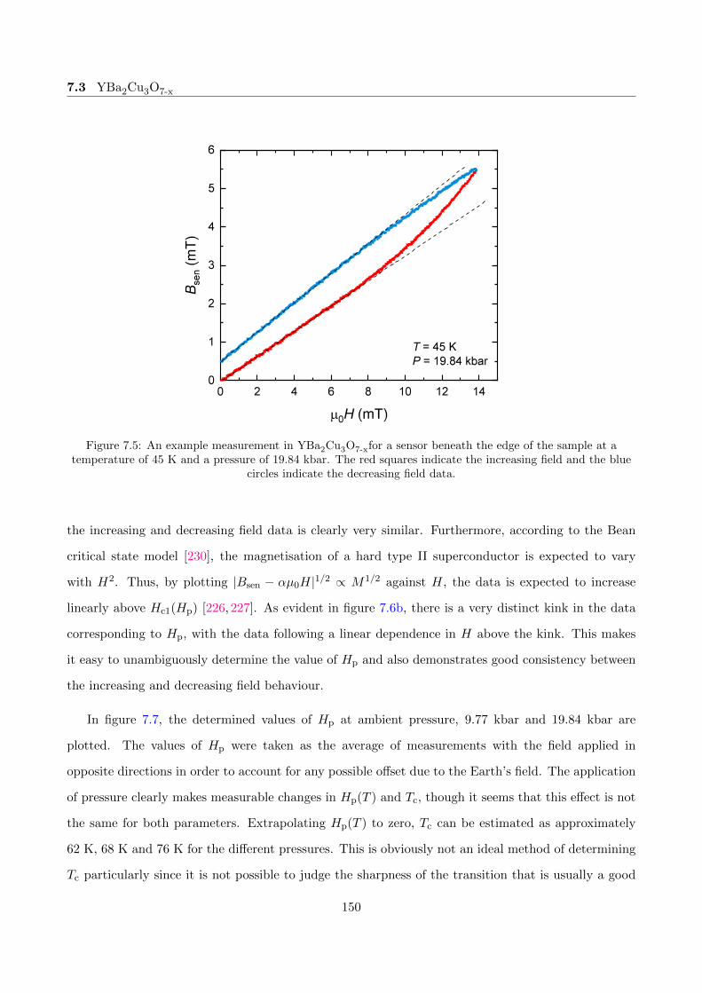
7.3 YBa2Cu3O7-x
Figure 7.5: An example measurement in YBa2Cu3O7-xfor a sensor beneath the edge of the sample at atemperature of 45 K and a pressure of 19.84 kbar. The red squares indicate the increasing field and the blue
circles indicate the decreasing field data.
the increasing and decreasing field data is clearly very similar. Furthermore, according to the Bean
critical state model [230], the magnetisation of a hard type II superconductor is expected to vary
with H2. Thus, by plotting |Bsen − αµ0H|1/2 ∝ M1/2 against H, the data is expected to increase
linearly above Hc1(Hp) [226, 227]. As evident in figure 7.6b, there is a very distinct kink in the data
corresponding to Hp, with the data following a linear dependence in H above the kink. This makes
it easy to unambiguously determine the value of Hp and also demonstrates good consistency between
the increasing and decreasing field behaviour.
In figure 7.7, the determined values of Hp at ambient pressure, 9.77 kbar and 19.84 kbar are
plotted. The values of Hp were taken as the average of measurements with the field applied in
opposite directions in order to account for any possible offset due to the Earth’s field. The application
of pressure clearly makes measurable changes in Hp(T ) and Tc, though it seems that this effect is not
the same for both parameters. Extrapolating Hp(T ) to zero, Tc can be estimated as approximately
62 K, 68 K and 76 K for the different pressures. This is obviously not an ideal method of determining
Tc particularly since it is not possible to judge the sharpness of the transition that is usually a good
150

7.3 YBa2Cu3O7-x
(a) (b)
Figure 7.6: (a) The data from figure 7.5 corrected by a term proportional to µ0H due to the incompleteshielding of the sensor by the sample. The point at which the measured induction begins to deviate is now
more evident. (b) The same data as (a) but plotted as the square root of the absolute value (where thenegative of the decreasing field data has been plotted). The data shows essentially linear dependence in H
above Hp in line with the Bean critical state model [226,230].
indication of homogeneity within the sample.
An unfortunate limitation of the data is that there is clearly an upturn in Hp for T < 20 K
for all pressures that is not consistent with the behaviour already observed for optimally and very
underdoped samples [226, 227]. One possibility is that this upturn occurs due to the presence of a
Bean-Livingston energy barrier [91]. However, this would have the effect of enhancing Hp for the
increasing field portion, and suppressing Hp towards zero for the decreasing field. While there was
occasionally a difference between Hp for increasing and decreasing field, this was typically never more
than 1 mT and so while this effect may be present it is likely not the dominant factor. Alternatively,
if the sensor was not sufficiently close to the edge of the sample then it is possible that this effect is
occurring due to strong vortex pinning in the sample, which limits the rate at which flux can migrate
through the sample [86, 226]. This effect becomes stronger at lower temperatures due to the lower
thermal energy of the flux vortices. Given the difficulty in positioning the sample accurately just
above the sensor, especially given that the sample was intentionally given a non-rectilinear shape, this
is likely a contributing factor. As such, the data has been left in terms of Hp instead of trying to
relate it to Hc1 since it does not follow the expected behaviour of Hc1(T ).
151
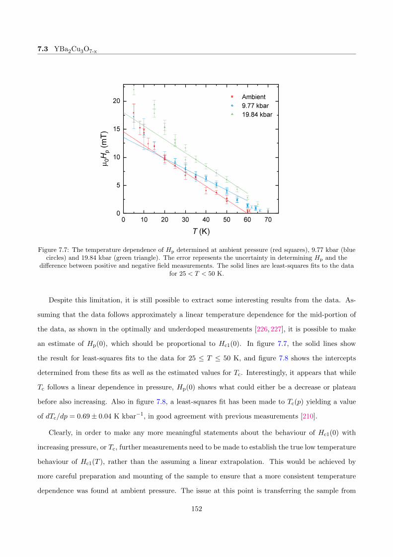
7.3 YBa2Cu3O7-x
Figure 7.7: The temperature dependence of Hp determined at ambient pressure (red squares), 9.77 kbar (bluecircles) and 19.84 kbar (green triangle). The error represents the uncertainty in determining Hp and the
difference between positive and negative field measurements. The solid lines are least-squares fits to the datafor 25 < T < 50 K.
Despite this limitation, it is still possible to extract some interesting results from the data. As-
suming that the data follows approximately a linear temperature dependence for the mid-portion of
the data, as shown in the optimally and underdoped measurements [226, 227], it is possible to make
an estimate of Hp(0), which should be proportional to Hc1(0). In figure 7.7, the solid lines show
the result for least-squares fits to the data for 25 ≤ T ≤ 50 K, and figure 7.8 shows the intercepts
determined from these fits as well as the estimated values for Tc. Interestingly, it appears that while
Tc follows a linear dependence in pressure, Hp(0) shows what could either be a decrease or plateau
before also increasing. Also in figure 7.8, a least-squares fit has been made to Tc(p) yielding a value
of dTc/dp = 0.69± 0.04 K kbar−1, in good agreement with previous measurements [210].
Clearly, in order to make any more meaningful statements about the behaviour of Hc1(0) with
increasing pressure, or Tc, further measurements need to be made to establish the true low temperature
behaviour of Hc1(T ), rather than the assuming a linear extrapolation. This would be achieved by
more careful preparation and mounting of the sample to ensure that a more consistent temperature
dependence was found at ambient pressure. The issue at this point is transferring the sample from
152

7.3 YBa2Cu3O7-x
Figure 7.8: The values for Tc and the zero temperature penetration field Hp as a function of pressure, asestimated from the data in figure 7.7. A straight line fit to Tc(p) yields dTc/dp ≈ 0.69± 0.04 K kbar−1.
the ambient pressure apparatus to the high pressure apparatus, as it is challenging to ensure the same
relative position of the sample on the Hall device. This could be aided through the use of a micro-
manipulator and reference photographs in order to be more precise with this process. Alternatively,
it may be necessary to mount the sample on the device for the high pressure measurement from the
outset and to create additional apparatus to make measurements with this device at ambient pressure,
thus removing the possibility of a change in the relative position of the sample to the sensors.
153

7.3 YBa2Cu3O7-x
154

Chapter 8
Conclusion
In this thesis I have presented low temperature penetration depth measurements on a number of
unconventional, strongly correlated superconductors. I have also detailed a method for measuring the
lower critical field under hydrostatic pressure, along with some preliminary results. Chapters 4 and 7
are thus mostly self-contained and do not require any further discussion.
I will finish, however, with a short discussion the work in chapter 5 on KFe2As2 and in chapter 6
on CeCoIn5. As discussed in the introduction, the nonlinear corrections to the magnetic penetration
depth is a potential probe of superconducting gap structure which has yet to be exploited. This effect
is caused by the Doppler shifting of the quasi-particle energies, which, in a nodal superconductor,
gives rise to a finite zero energy density of states. This should manifest as either a linear response
of ∆λ with H, or a change in the temperature dependence in an applied field. Despite a number
of careful investigations, this effect was concluded to be either absent or unobservably small in the
cuprate superconductors.
The data presented in chapter 6 provides strong evidence for the existence of the nonlinear Meissner
effect in the d-wave compound CeCoIn5. As discussed in that chapter, there are some inconsistencies
that may be due to multiband effects. However, the observed response is in agreement with predictions
from the Yip-Sauls theory [49] and from calculations of the expected response [69]. In particular, there
is qualitative agreement in the data for the clean and dirty nodal case.
This positive result now gives the technique some validation as an additional probe of the gap
structure, in addition to the well-established temperature dependence analysis of ∆λ(T ). Considering
155

.0
the nonlinear measurements on KFe2As2 (section 5.2.3), we also see there is good qualitative agreement
between the observed response and what is predicted for a highly anisotropic but fully-gapped state
(figure 2.9c). This then suggests that gap nodes are absent in KFe2As2, at least on the lighter Fermi
surface sheets. However, this is not consistent with the laser ARPES results of Okazaki et al. [161].
It may be that a similar response is expected for a gap structure that possesses nodes but with only a
very small gap of opposite phase, as suggested by Okazaki et al.. Further calculations for the expected
nonlinear response are required for the various possible gap structures. Indeed, much of the theoretical
work on the nonlinear Meissner effect (NLME) was established before the discovery of the iron-based
superconductors (IBS), and so do not include aspects such as multiple gaps or accidental nodes.
In order to further solidify the NLME as a reliable probe, a number of other systems could be
investigated. The NLME is not phase sensitive, so the results given for the nodal d-wave state are
also applicable for a gap structure with accidental nodes. Both LaFePO [74] and BaFe2(As1-xPx)2 [66]
have been identified as nodal IBS. Additionally, there is some suggestion of universal d-wave pairing
in the 115 compounds [183]. It would also be illuminating to investigate the nonlinear response in a
compound which is known to have large anisotropy, but no nodes, such as over-doped Ba1-xKxFe2As2.
There still, unfortunately, remains the question as to why the effect was found to be either absent
or unobservably small in the cuprate superconductors [50]. It may be that further theoretical work is
required to understand this in more detail, and revisiting experimental results may also provide some
insight into this mystery.
156

Appendix A
Publications
“Fully Gapped Superconductivity with No Sign Change in the Prototypical Heavy-Fermion CeCu2Si2”T. Yamashita, T. Takenaka, Y. Tokiwa, J. A. Wilcox, Y. Mizukami, D. Terazawa, Y. Kasahara, S.Kittaka, T. Sakakibara, M. Konczykowski, S. Seiro, H. S. Jeevan, C. Geibel, C. Putzke, T. Onishi, H.Ikeda, A. Carrington, T. Shibauchi and Y. MatsudaScience Advances, 2017, 3, e1601667
“Full-Gap Superconductivity Robust against Disorder in Heavy-Fermion CeCu2Si2”T. Takenaka, Y. Mizukami, J. A. Wilcox, M. Konczykowski, S. Seiro, C. Geibel, Y. Tokiwa, Y.Kasahara, C. Putzke, Y. Matsuda, A. Carrington and T. ShibauchiPhysical Review Letters, 2017, 119, 077001
157

158

Bibliography
[1] H. Kamerlingh Onnes, “On the sudden change in the rate at which the resistance of mercurydisappears,” in KNAW, Proceedings, vol. 14, pp. 818–821, 1911.
[2] G. Webb, F. Marsiglio, and J. Hirsch, “Superconductivity in the elements, alloys and simplecompounds,” Physica C: Superconductivity and its Applications, vol. 514, pp. 17–27, jul 2015.
[3] W. Meissner and R. Ochsenfeld, “Ein neuer effekt bei eintritt der supraleitfahigkeit,” Die Natur-wissenschaften, vol. 21, pp. 787–788, nov 1933.
[4] J. A. Annett, Superconductivity, Superfluids and Condensates. Oxford University Press, 2004.
[5] L. N. Cooper, BCS: 50 Years, ch. 1. Remembrance of Superconductivity Past, pp. 3–19. WorldScientific, 2011.
[6] F. London, Superfluids. Wiley, New York, 1950.
[7] F. London and H. London, “The electromagnetic equations of the supraconductor,” Proceedingsof the Royal Society A: Mathematical, Physical and Engineering Sciences, vol. 149, pp. 71–88,mar 1935.
[8] J. Schmalian, BCS: 50 Years, ch. 4. Failed Theories of Superconductivity, pp. 41–55. WorldScientific, 2011.
[9] J. Bardeen, L. N. Cooper, and J. R. Schrieffer, “Microscopic theory of superconductivity,”Physical Review, vol. 106, pp. 162–164, apr 1957.
[10] L. N. Cooper, “Bound Electron Pairs in a Degenerate Fermi Gas,” Physical Review, vol. 104,pp. 1189–1190, Nov. 1956.
[11] C. P. Slichter, BCS: 50 Years, ch. 5. Nuclear Magnetic Resonance and the BCS Theory, pp. 57–83. World Scientific, 2011.
[12] J. Bardeen, BCS: 50 Years, ch. 3. Development of Concepts in Superconductivity, pp. 33–40.World Scientific, 2011.
[13] G. M. Eliashberg, “Interactions between Electrons and Lattice Vibrations in a Superconductor,”Soviet Physics JETP, vol. 11, no. 3, p. 696, 1960.
[14] W. L. McMillan, “Transition temperature of strong-coupled superconductors,” Physical Review,vol. 167, pp. 331–344, mar 1968.
[15] P. B. Allen and R. C. Dynes, “Transition temperature of strong-coupled superconductors rean-alyzed,” Physical Review B, vol. 12, pp. 905–922, aug 1975.
159

[16] M. L. Cohen, BCS: 50 Years, ch. 15. Predicting and Explaining Tc and Other Properties of BCSSuperconductors, pp. 375–389. World Scientific, 2011.
[17] L. P. Gor’kov, “Microscopic Derivation of the Ginzburg-Landau Equations in the Theory ofSuperconductivity,” Soviet Physics JETP, 1959.
[18] F. Steglich, J. Aarts, C. D. Bredl, W. Lieke, D. Meschede, W. Franz, and H. Schfer, “Supercon-ductivity in the Presence of Strong Pauli Paramagnetism: CeCu2Si2,” Physical Review Letters,vol. 43, pp. 1892–1896, dec 1979.
[19] G. R. Stewart, “Unconventional Superconductivity,” Advances in Physics, vol. 66, pp. 75–196,Apr. 2017.
[20] A. Sleight, J. Gillson, and P. Bierstedt, “High-temperature superconductivity in theBaPb1−xBixO3 systems,” Solid State Communications, vol. 17, pp. 27–28, jul 1975.
[21] A. W. Sleight, “Bismuthates: BaBiO3 and related superconducting phases,” Physica C: Super-conductivity and its Applications, vol. 514, pp. 152–165, jul 2015.
[22] B. White, J. Thompson, and M. Maple, “Unconventional superconductivity in heavy-fermioncompounds,” Physica C: Superconductivity and its Applications, vol. 514, pp. 246–278, jul 2015.
[23] J. G. Bednorz and K. A. Muller, “Possible High Tc Superconductivity in the Ba-La-Cu-OSystem,” Zeitschrift fur Physik B - Condensed Matter, vol. 64, p. 189, 1986.
[24] A. Schilling, M. Cantoni, J. D. Guo, and H. R. Ott, “Superconductivity above 130 K in theHg-Ba-Ca-Cu-O system,” Nature, vol. 363, pp. 56–58, may 1993.
[25] C. W. Chu, L. Gao, F. Chen, Z. J. Huang, R. L. Meng, and Y. Y. Xue, “Superconductivityabove 150 K in HgBa2Ca2Cu3O8+δ at High Pressures,” Nature Letters, vol. 365, p. 323, Sept.1993.
[26] C. W. Chu, L. Z. Deng, and B. Lv, “Hole-doped cuprate high temperature superconductors,”Physica C: Superconductivity and its Applications, vol. 514, pp. 290–313, jul 2015.
[27] Y. Maeno, H. Hashimoto, K. Yoshida, S. Nishizaki, T. Fujita, J. G. Bednorz, and F. Lichtenberg,“Superconductivity in a Layered Perovskite without Copper,” Nature Latters, vol. 372, p. 532,Dec. 1994.
[28] J. Nagamatsu, N. Nakagawa, T. Muranaka, Y. Zenitani, and J. Akimitsu, “Superconductivityat 39 K in magnesium diboride,” Nature, vol. 410, pp. 63–64, 2001.
[29] S. L. Bud’ko and P. C. Canfield, “Superconductivity of magnesium diboride,” Physica C: Su-perconductivity and its Applications, vol. 514, pp. 142–151, jul 2015.
[30] Y. Kamihara, H. Hiramatsu, M. Hirano, R. Kawamura, H. Yanagi, T. Kamiya, and H. Hosono,“Iron-Based Layered Superconductor: LaOFeP,” Journal of the American Chemical Society,vol. 128, pp. 10012–10013, Aug. 2006.
[31] Y. Kamihara, T. Watanabe, M. Hirano, and H. Hosono, “Iron-Based Layered SuperconductorLa[O1−xFx]FeAs (x = 0.05-0.12) with Tc = 26 K,” Journal of the American Chemical Society,vol. 130, pp. 3296–3297, Mar. 2008.
160

[32] M. R. Norman, “The Challenge of Unconventional Superconductivity,” Science, vol. 332,pp. 196–200, Apr. 2011.
[33] R. Zhi-An, L. Wei, Y. Jie, Y. Wei, S. Xiao-Li, Zheng-Cai, C. Guang-Can, D. Xiao-Li, S. Li-Ling, Z. Fang, and Z. Zhong-Xian, “Superconductivity at 55 K in Iron-Based F-Doped LayeredQuaternary Compound Sm[O1−xFx]FeAs,” Chinese Physics Letters, vol. 25, pp. 2215–2216, June2008.
[34] Y. Cao, V. Fatemi, S. Fang, K. Watanabe, T. Taniguchi, E. Kaxiras, and P. Jarillo-Herrero,“Unconventional superconductivity in magic-angle graphene superlattices,” Nature, vol. 556,pp. 43–50, mar 2018.
[35] A. P. Drozdov, M. I. Eremets, I. A. Troyan, V. Ksenofontov, and S. I. Shylin, “Conventionalsuperconductivity at 203 kelvin at high pressures in the sulfur hydride system,” Nature, vol. 525,pp. 73–76, aug 2015.
[36] A. P. Drozdov, C. S. Minkov, S. P. Besedin, P. P. Kong, M. A. Kuzovnikov, D. A. Knyazev, andM. I. Eremets, “Superconductivity at 215 K in lanthanum hydride at high pressures,” arXiv,2018.
[37] M. Somayazulu, M. Ahart, A. K. Mishra, Z. M. Geballe, M. Baldini, Y. Meng, V. V. Struzhkin,and R. J. Hemley, “Evidence for superconductivity above 260 K in lanthanum superhydride atmegabar pressures,” arXiv, 2018.
[38] M. Sigrist and K. Ueda, “Phenomenological Theory of Unconventional Superconductivity,” Re-views of Modern Physics, vol. 63, pp. 239–311, Apr. 1991.
[39] A. P. Mackenzie and Y. Maeno, “The Superconductivity of Sr2RuO4 and the Physics of Spin-Triplet Pairing,” Reviews of Modern Physics, vol. 75, pp. 657–712, May 2003.
[40] M. Tinkham, Introduction to Superconductivity. McGraw-Hill, 1975.
[41] A. Alexandrov, Theory of Superconductivity: From Weak to Strong Coupling (Condensed MatterPhysics). CRC Press, 2003.
[42] P. J. Hirschfeld, M. M. Korshunov, and I. I. Mazin, “Gap Symmetry and Structure of Fe-BasedSuperconductors,” Reports on Progress in Physics, vol. 74, p. 124508, Dec. 2011.
[43] D. A. Bonn, S. Kamal, K. Zhang, R. Liang, D. J. Baar, E. Klein, and W. N. Hardy, “Comparisonof the influence of Ni and Zn impurities on the electromagnetic properties of YBa2Cu3O6.95,”Physical Review B, vol. 50, pp. 4051–4063, aug 1994.
[44] W. N. Hardy, D. A. Bonn, D. C. Morgan, R. Liang, and K. Zhang, “Precision Measurementsof the Temperature Dependence of λ in YBa2Cu3O6.95: Strong Evidence for Nodes in the GapFunction,” Physical Review Letters, vol. 70, no. 25, p. 4, 1993.
[45] J. Annett, N. Goldenfeld, and S. R. Renn, “Interpretation of the temperature dependence of theelectromagnetic penetration depth in YBa2Cu3O7−δ,” Physical Review B, vol. 43, pp. 2778–2782,feb 1991.
[46] Y. Mizukami, M. Konczykowski, Y. Kawamoto, S. Kurata, S. Kasahara, K. Hashimoto,V. Mishra, A. Kreisel, Y. Wang, P. J. Hirschfeld, Y. Matsuda, and T. Shibauchi, “Disorder-Induced Topological Change of the Superconducting Gap Structure in Iron Pnictides,” NatureCommunications, vol. 5, Dec. 2014.
161
[47] P. J. Hirschfeld, “Using Gap Symmetry and Structure to Reveal the Pairing Mechanism inFe-Based Superconductors,” Comptes Rendus Physique, vol. 17, pp. 197–231, Jan. 2016.
[48] V. Mishra, G. Boyd, S. Graser, T. Maier, P. J. Hirschfeld, and D. J. Scalapino, “Lifting of Nodesby Disorder in Extended-s-state Superconductors: Application to Ferropnictides,” Physical Re-view B, vol. 79, Mar. 2009.
[49] S. K. Yip and J. A. Sauls, “Nonlinear Meissner Effect in CuO Superconductors,” Physical ReviewLetters, vol. 69, pp. 2264–2267, Oct. 1992.
[50] M.-R. Li, P. J. Hirschfeld, and P. Wolfle, “Is the Nonlinear Meissner Effect Unobservable?,”Physical Review Letters, vol. 81, pp. 5640–5643, Dec. 1998.
[51] R. Prozorov and R. W. Giannetta, “Magnetic Penetration Depth in Unconventional Supercon-ductors,” Superconductor Science and Technology, vol. 19, pp. R41–R67, Aug. 2006.
[52] A. A. Abrikosov, “The magnetic properties of superconducting alloys,” Journal of Physics andChemistry of Solids, vol. 2, pp. 199–208, jan 1957.
[53] B. I. Halperin, G. Refael, and E. Demler, BCS: 50 Years, ch. 10. Resistance in Superconductors,pp. 185–226. World Scientific, 2011.
[54] B. S. Chandrasekhar and D. Einzel, “The Superconducting Penetration Depth from the Semi-classical Model,” Annalen der Physik, vol. 505, no. 6, pp. 535–546, 1993.
[55] A. Carrington and F. Manzano, “Magnetic Penetration Depth of MgB2,” Physica C: Supercon-ductivity, vol. 385, pp. 205–214, Mar. 2003.
[56] H. Hosono and K. Kuroki, “Iron-based superconductors: Current status of materials and pairingmechanism,” Physica C: Superconductivity and its Applications, vol. 514, pp. 399–422, jul 2015.
[57] V. G. Kogan, C. Martin, and R. Prozorov, “Superfluid density and specific heat within a self-consistent scheme for a two-band superconductor,” Physical Review B, vol. 80, jul 2009.
[58] P. Anderson, “Theory of dirty superconductors,” Journal of Physics and Chemistry of Solids,vol. 11, pp. 26–30, sep 1959.
[59] P. Fulde, BCS: 50 Years, ch. 11. Cooper Pair Breaking, pp. 227–253. World Scientific, 2011.
[60] B. Matthias, H. Suhl, and E. Corenzwit, “Further experiments concerning the spin-electroninteractions in superconductors,” Journal of Physics and Chemistry of Solids, vol. 13, pp. 156–159, may 1960.
[61] D. Einzel, P. J. Hirschfeld, F. Gross, B. S. Chandrasekhar, K. Andres, H. R. Ott, J. Beuers,Z. Fisk, and J. L. Smith, “Magnetic Field Penetration Depth in the Heavy-Electron Supercon-ductor UBe13,” Physical Review Letters, vol. 56, pp. 2513–2516, jun 1986.
[62] S. Skalski, O. Betbeder-Matibet, and P. R. Weiss, “Properties of superconducting alloys con-taining paramagnetic impurities,” Physical Review, vol. 136, pp. A1500–A1518, dec 1964.
[63] D. Deepwell, D. C. Peets, C. J. S. Truncik, N. C. Murphy, M. P. Kennett, W. A. Huttema,R. Liang, D. A. Bonn, W. N. Hardy, and D. M. Broun, “Microwave Conductivity and SuperfluidDensity in Strongly Overdoped Tl2Ba2CuO6+δ,” Physical Review B, vol. 88, Dec. 2013.
162

[64] T. Hotta, “Impurity effects in cuprate superconductors,” Journal of the Physical Society ofJapan, vol. 62, pp. 274–280, jan 1993.
[65] P. J. Hirschfeld and N. Goldenfeld, “Effect of Strong Scattering on the Low-Temperature Pen-etration Depth of a d-wave Superconductor,” Physical Review B, vol. 48, pp. 4219–4222, Aug.1993.
[66] K. Hashimoto, M. Yamashita, S. Kasahara, Y. Senshu, N. Nakata, S. Tonegawa, K. Ikada,A. Serafin, A. Carrington, T. Terashima, H. Ikeda, T. Shibauchi, and Y. Matsuda, “Line Nodesin the Energy Gap of Superconducting BaFe2(As1−xPx)2 Single Crystals as Seen via PenetrationDepth and Thermal Conductivity,” Physical Review B, vol. 81, June 2010.
[67] Y. Wang, A. Kreisel, P. J. Hirschfeld, and V. Mishra, “Using controlled disorder to distinguishs±and s++ gap structure in Fe-based superconductors,” Physical Review B, vol. 87, mar 2013.
[68] D. Xu, S. K. Yip, and J. A. Sauls, “Nonlinear Meissner Effect in Unconventional Superconduc-tors,” Physical Review B, vol. 51, pp. 16233–16253, June 1995.
[69] B. P. Stojkovic and O. T. Valls, “Nonlinear supercurrent response in anisotropic superconduc-tors,” Physical Review B, vol. 51, pp. 6049–6058, mar 1995.
[70] A. Carrington, R. W. Giannetta, J. T. Kim, and J. Giapintzakis, “Absence of Nonlinear MeissnerEffect in YBa2Cu3O6.95,” Physical Review B, vol. 59, pp. R14173–R14176, June 1999.
[71] A. Maeda, Y. Iino, T. Hanaguri, N. Motohira, K. Kishio, and T. Fukase, “Magnetic FieldDependence of the London Penetration Depth of Bi2Sr2CaCu2Oy,” Physical Review Letters,vol. 74, pp. 1202–1205, feb 1995.
[72] G. E. Volovik, “Superconductivity with lines of gap nodes: density of states in the vortex,”JETP Letters, vol. 58, no. 6, p. 469, 1993.
[73] T. Sakakibara, S. Kittaka, and K. Machida, “Angle-resolved heat capacity of heavy fermionsuperconductors,” Reports on Progress in Physics, 2016.
[74] J. D. Fletcher, A. Serafin, L. Malone, J. G. Analytis, J.-H. Chu, A. S. Erickson, I. R. Fisher,and A. Carrington, “Evidence for a Nodal-Line Superconducting State in LaFePO,” PhysicalReview Letters, vol. 102, Apr. 2009.
[75] F. Pobell, Matter and Methods at Low Temperatures. Springer Berlin Heidelberg, 2007.
[76] C. Enss and S. Hunklinger, Low-Temperature Physics. Springer-Verlag, 2005.
[77] J. W. Ekin, Experimental Techniqes for Low-Temperature Measurements. Oxford UniversityPress, 2006.
[78] G. K. White and P. J. Meeson, Experimental Techniques in Low-Temperature Physics. OxfordUniversity Press, 2002.
[79] W. M. Haynes, CRC Handbook of Chemistry and Physics, 95th Edition. CRC Press, 2014.
[80] J. Fletcher, Penetration depth and de Hass-van Alphen studies of MgB2. PhD thesis, Universityof Bristol, 2005.
163

[81] L. D. Malone, The Gap Symmetry of the Organic and Iron based Pnictide Superconductors. PhDthesis, University of Bristol, 2009.
[82] A. Serafin, Penetration depth studies of cuprate and iron-based superconductors. PhD thesis,University of Bristol, 2011.
[83] C. T. Van Degrift, “Tunnel Diode Oscillator for 0.001 ppm Measurements at Low Temperatures,”Review of Scientific Instruments, vol. 46, pp. 599–607, May 1975.
[84] R. Prozorov, R. W. Giannetta, A. Carrington, and F. M. Araujo-Moreira, “Meissner-LondonState in Superconductors of Rectangular Cross Section in a Perpendicular Magnetic Field,”Physical Review B, vol. 62, pp. 115–118, July 2000.
[85] P. Rani, A. K. Hafiz, and V. P. S. Awana, “Temperature dependence of lower critical field ofYBCO superconductor,” in AIP Conference Proceedings 1953, 2018.
[86] R. Okazaki, M. Konczykowski, C. J. van der Beek, T. Kato, K. Hashimoto, M. Shimozawa,H. Shishido, M. Yamashita, M. Ishikado, H. Kito, A. Iyo, H. Eisaki, S. Shamoto, T. Shibauchi,and Y. Matsuda, “Lower critical fields of superconducting PrFeAsO1−y single crystals,” PhysicalReview B, vol. 79, feb 2009.
[87] J. Lefebvre, M. Hilke, Z. Altounian, K. W. West, and L. N. Pfeiffer, “Local magnetizationfluctuations in superconducting glasses resolved by hall sensors,” Physical Review B, vol. 79,may 2009.
[88] C. Putzke, P. Walmsley, J. D. Fletcher, L. Malone, D. Vignolles, C. Proust, S. Badoux, P. See,H. E. Beere, D. A. Ritchie, S. Kasahara, Y. Mizukami, T. Shibauchi, Y. Matsuda, and A. Car-rington, “Anomalous Critical Fields in Quantum Critical Superconductors,” Nature Communi-cations, vol. 5, Dec. 2014.
[89] C. M. Putzke, Fermi Surface and Quantum Critical Phenomena of High-Temperature Supercon-ductors. PhD thesis, University of Bristol, 2014.
[90] E. H. Brandt, “Irreversible Magnetization of Pin-Free Type-II Superconductors,” Physical Re-view B, vol. 60, pp. 11939–11942, Nov. 1999.
[91] C. P. Bean and J. D. Livingston, “Surface Barrier in Type-II Superconductors,” Physical ReviewLetters, vol. 12, pp. 14–16, jan 1964.
[92] M. N. Wilson, Superconducting Magnets. Oxford University Press, 1987.
[93] W. B. Smythe, Static and Dynamic Electricity. Hemisphere Publishin, New York, 1988.
[94] M. I. Eremets, High Pressure Experimental Methods. Oxford University Press, 1996.
[95] I. R. Walker, “Nonmagnetic piston-cylinder pressure cell for use at 35 kbar and above,” Reviewof Scientific Instruments, vol. 70, pp. 3402–3412, aug 1999.
[96] X. Wang and K. V. Kamenev, “Review of modern instrumentation for magnetic measurementsat high pressure and low temperature,” Low Temperature Physics, vol. 40, pp. 735–746, aug2014.
164

[97] A. Jayaraman, A. R. Hutson, J. H. McFee, A. S. Coriell, and R. G. Maines, “Hydrostaticand Uniaxial Pressure Generation using Teflon Cell Container in Conventional Piston-CylinderDevice,” Review of Scientific Instruments, vol. 38, pp. 44–49, jan 1967.
[98] K. Yokogawa, K. Murata, H. Yoshino, and S. Aoyama, “Solidification of high-pressure mediumdaphne 7373,” Japanese Journal of Applied Physics, vol. 46, pp. 3636–3639, jun 2007.
[99] K. Murata, H. Yoshino, H. O. Yadav, Y. Honda, and N. Shirakawa, “Pt resistor thermometryand pressure calibration in a clamped pressure cell with the medium, Daphne 7373,” Review ofScientific Instruments, vol. 68, pp. 2490–2493, jun 1997.
[100] R. J. Zeto and H. B. Vanfleet, “Pressure calibration to 60 kbar based on the resistance change ofa manganin coil under hydrostatic pressure,” Journal of Applied Physics, vol. 40, pp. 2227–2231,apr 1969.
[101] H. Q. Yuan, F. M. Grosche, M. Deppe, C. Geibel, G. Sparn, and F. Steglich, “Observation ofTwo Distinct Superconducting Phases in CeCu2Si2,” Science Reports, vol. 302, p. 2104, 2003.
[102] U. Ahlheim, M. Winkelmann, P. van Aken, C. D. Bredl, F. Steglich, and G. R. Stewart, “Pairbreaking in the heavy-fermion superconductors Ce1−xMxCu2.2Si2 and U1−xMxBe13 (M: Th, La,Y and Gd),” Journal of Magnetism and Magnetic Materials, vol. 76-77, pp. 520–522, dec 1988.
[103] S. Kittaka, Y. Aoki, Y. Shimura, T. Sakakibara, S. Seiro, C. Geibel, F. Steglich, H. Ikeda, andK. Machida, “Multiband Superconductivity with Unexpected Deficiency of Nodal Quasiparticlesin CeCu2Si2,” Physical Review Letters, vol. 112, Feb. 2014.
[104] O. Stockert, E. Faulhaber, G. Zwicknagl, N. Stßer, H. S. Jeevan, M. Deppe, R. Borth, R. Kchler,M. Loewenhaupt, C. Geibel, and F. Steglich, “Nature of the A Phase in CeCu2Si2,” PhysicalReview Letters, vol. 92, apr 2004.
[105] P. Gegenwart, C. Langhammer, C. Geibel, R. Helfrich, M. Lang, G. Sparn, F. Steglich, R. Horn,L. Donnevert, A. Link, and W. Assmus, “Breakup of Heavy Fermions on the Brink of “PhaseA” in CeCu2Si2,” Physical Review Letters, vol. 81, pp. 1501–1504, aug 1998.
[106] T. Yamashita, T. Takenaka, Y. Tokiwa, J. A. Wilcox, Y. Mizukami, D. Terazawa, Y. Kasahara,S. Kittaka, T. Sakakibara, M. Konczykowski, S. Seiro, H. S. Jeevan, C. Geibel, C. Putzke, T. On-ishi, H. Ikeda, A. Carrington, T. Shibauchi, and Y. Matsuda, “Fully Gapped Superconductivitywith No Sign Change in the Prototypical Heavy-Fermion CeCu2Si2,” Science Advances, vol. 3,p. e1601667, June 2017.
[107] O. Stockert, J. Arndt, E. Faulhaber, C. Geibel, H. S. Jeevan, S. Kirchner, M. Loewenhaupt,K. Schmalzl, W. Schmidt, Q. Si, and F. Steglich, “Magnetically driven superconductivity inCeCu2Si2,” Nature Physics, vol. 7, pp. 119–124, dec 2010.
[108] J. Arndt, O. Stockert, K. Schmalzl, E. Faulhaber, H. S. Jeevan, C. Geibel, W. Schmidt,M. Loewenhaupt, and F. Steglich, “Spin Fluctuations in Normal State CeCu2Si2 on Approachingthe Quantum Critical Point,” Physical Review Letters, vol. 106, jun 2011.
[109] J. Paglione, M. A. Tanatar, D. G. Hawthorn, E. Boaknin, R. W. Hill, F. Ronning, M. Sutherland,L. Taillefer, C. Petrovic, and P. C. Canfield, “Field-Induced Quantum Critical Point in CeCoIn5,”Physical Review Letters, vol. 91, dec 2003.
165
[110] J. Custers, P. Gegenwart, H. Wilhelm, K. Neumaier, Y. Tokiwa, O. Trovarelli, C. Geibel,F. Steglich, C. Pepin, and P. Coleman, “The break-up of heavy electrons at a quantum criticalpoint,” Nature, vol. 424, no. 6948, p. 524, 2003.
[111] W. Assmus, M. Herrmann, U. Rauchschwalbe, S. Riegel, W. Lieke, H. Spille, S. Horn, G. Weber,F. Steglich, and G. Cordier, “Superconductivity in CeCu2Si2 Single Crystals,” Physical ReviewLetters, vol. 52, pp. 469–472, feb 1984.
[112] U. Rauchschwalbe, W. Lieke, C. D. Bredl, F. Steglich, J. Aarts, K. M. Martini, and A. C. Mota,“Critical Fields of the “Heavy-Fermion” Superconductor CeCu2Si2,” Physical Review Letters,vol. 49, pp. 1448–1451, nov 1982.
[113] G. Zwicknagl and U. Pulst, “CeCu2Si2: Renormalized band structure, quasiparticles and co-operative phenomena,” Physica B: Condensed Matter, vol. 186-188, pp. 895–898, may 1993.
[114] K. Ueda, Y. Kitaoka, H. Yamada, Y. Kohori, T. Kohara, and K. Asayama, “29Si Knight Shift inthe Heavy-Fermion Superconductor CeCu2Si2,” Journal of the Physical Society of Japan, vol. 56,pp. 867–870, mar 1987.
[115] Y. Kitaoka, K. ichi Ueda, K. Fujiwara, H. Arimoto, H. Iida, and K. Asayama, “NMR Investiga-tion of Superconductivity and Kondo-Coherency in CeCu2Si2,” Journal of the Physical Societyof Japan, vol. 55, pp. 723–726, mar 1986.
[116] K. Ishida, Y. Kawasaki, K. Tabuchi, K. Kashima, Y. Kitaoka, K. Asayama, C. Geibel, andF. Steglich, “Evolution from Magnetism to Unconventional Superconductivity in a Series ofCexCu2Si2 Compounds Probed by Cu NQR,” Physical Review Letters, vol. 82, pp. 5353–5356,jun 1999.
[117] K. Fujiwara, Y. Hata, K. Kobayashi, K. Miyoshi, J. Takeuchi, Y. Shimaoka, H. Kotegawa, T. C.Kobayashi, C. Geibel, and F. Steglich, “High Pressure NQR Measurement in CeCu2Si2 up toSudden Disappearance of Superconductivity,” Journal of the Physical Society of Japan, vol. 77,p. 123711, dec 2008.
[118] M. Lang, R. Modler, U. Ahlheim, R. Helfrich, P. H. P. Reinders, F. Steglich, W. Assmus, W. Sun,G. Bruls, D. Weber, and B. Luthi, “Cooperative Effects in CeCu2Si2,” Physica Scripta, vol. T39,pp. 135–139, 1991.
[119] F. Gross, B. Chandrasekhar, K. Andres, U. Rauchschwalbe, E. Bucher, and B. Lth, “Tem-perature dependence of the London penetration depth in the heavy fermion superconductorsCeCu2Si2 and UPt3,” Physica C: Superconductivity, vol. 153-155, pp. 439–440, jun 1988.
[120] S. Seiro, M. Deppe, H. Jeevan, U. Burkhardt, and C. Geibel, “Flux crystal growth of CeCu2Si2:Revealing the effect of composition,” Physica Status Solidi B, vol. 247, pp. 614–616, mar 2010.
[121] W. H. Press, S. A. Teukolsky, W. T. Vetterling, and B. P. Flannery, Numerical Recipes: TheArt of Scientific Computing. Cambridge University Press, 2007.
[122] Y. J. Uemura, W. J. Kossler, B. Hitti, J. R. Kempton, H. E. Schone, X. H. Yu, C. E. Stronach,W. F. Lankford, D. R. Noakes, R. Keitel, M. Senba, J. H. Breqer, E. J. Ansaldo, Y. Oonuki,and T. Komatsubara, “Muon spin relaxation in CeCu2Si2 and muon Knight shift in variousheavy-fermion systems,” Hymperfine Interactions, vol. 31, pp. 413–418, 1986.
166

[123] R. Prozorov and V. G. Kogan, “London Penetration Depth in Iron-Based Superconductors,”Reports on Progress in Physics, vol. 74, p. 124505, Dec. 2011.
[124] J. D. Fletcher, A. Carrington, O. J. Taylor, S. M. Kazakov, and J. Karpinski, “Temperature-Dependent Anisotropy of the Penetration Depth and Coherence Length of MgB2,” PhysicalReview Letters, vol. 95, aug 2005.
[125] R. Tazai and H. Kontani, “Fully gapped s-wave superconductivity enhanced by magnetic criti-cality in heavy-fermion systems,” Physical Review B, vol. 98, nov 2018.
[126] S. Kitagawa, T. Higuchi, M. Manago, T. Yamanaka, K. Ishida, H. S. Jeevan, and C. Geibel,“Magnetic and superconducting properties of an S -type single-crystal CeCu2Si2 probed by Cu63nuclear magnetic resonance and nuclear quadrupole resonance,” Physical Review B, vol. 96, oct2017.
[127] Y. Li, M. Liu, Z. Fu, X. Chen, F. Yang, and Y. feng Yang, “Gap Symmetry of the Heavy FermionSuperconductor CeCu2Si2 at Ambient Pressure,” Physical Review Letters, vol. 120, may 2018.
[128] J. Paglione and R. L. Greene, “High-Temperature Superconductivity in Iron-Based Materials,”Nature Physics, vol. 6, pp. 645–658, Sept. 2010.
[129] A. Chubukov and P. J. Hirschfeld, “Iron-Based Superconductors, Seven Years Later,” PhysicsToday, vol. 68, pp. 46–52, June 2015.
[130] F. Ning, K. Ahilan, T. Imai, A. S. Sefat, R. Jin, M. A. McGuire, B. C. Sales, and D. Mandrus,“59Co and 75As NMR Investigation of Electron-Doped High Tc Superconductor BaFe1.8Co0.2As2
(Tc = 22 K),” Journal of the Physical Society of Japan, vol. 77, p. 103705, oct 2008.
[131] Y. Nakai, T. Iye, S. Kitagawa, K. Ishida, S. Kasahara, T. Shibauchi, Y. Matsuda, andT. Terashima, “P31 and As75 NMR Evidence for a Residual Density of States at Zero Energyin Superconducting BaFe2(As0.67P0.33)2,” Physical Review B, vol. 81, Jan. 2010.
[132] K. Matano, Z. Li, G. L. Sun, D. L. Sun, C. T. Lin, M. Ichioka, and G.-q. Zheng, “AnisotropicSpin Fluctuations and Multiple Superconducting Gaps in Hole-Doped Ba0.72K0.28Fe2As2: NMRin a Single Crystal,” Europhysics Letters (EPL), vol. 87, p. 27012, July 2009.
[133] H. Chen, Y. Ren, Y. Qiu, W. Bao, R. H. Liu, G. Wu, T. Wu, Y. L. Xie, X. F. Wang,Q. Huang, and X. H. Chen, “Coexistence of the Spin-Density Wave and Superconductivityin Ba1−xKxFe2As2,” Europhysics Letters (EPL), vol. 85, p. 17006, Jan. 2009.
[134] S. Jiang, H. Xing, G. Xuan, C. Wang, Z. Ren, C. Feng, J. Dai, Z. Xu, and G. Cao, “Supercon-ductivity up to 30 K in the vicinity of the quantum critical point in BaFe2(As1−xPx)2,” Journalof Physics: Condensed Matter, vol. 21, p. 382203, aug 2009.
[135] Q. Huang, Y. Qiu, W. Bao, M. A. Green, J. W. Lynn, Y. C. Gasparovic, T. Wu, G. Wu, and X. H.Chen, “Neutron-Diffraction Measurements of Magnetic Order and a Structural Transition inthe Parent BaFe2As2 Compound of FeAs-Based High-Temperature Superconductors,” PhysicalReview Letters, vol. 101, Dec. 2008.
[136] M. Rotter, M. Pangerl, M. Tegel, and D. Johrendt, “Superconductivity and Crystal Structures of(Ba1−xKx)Fe2As2 (x=0-1),” Angewandte Chemie International Edition, vol. 47, pp. 7949–7952,Sept. 2008.
167

[137] N. Ni, M. E. Tillman, J.-Q. Yan, A. Kracher, S. T. Hannahs, S. L. Bud’ko, and P. C. Canfield,“Effects of Co substitution on thermodynamic and transport properties and anisotropic Hc2 inBa(Fe1−xCox)2As2 single crystals,” Physical Review B, vol. 78, dec 2008.
[138] H. Ding, P. Richard, K. Nakayama, K. Sugawara, T. Arakane, Y. Sekiba, A. Takayama,S. Souma, T. Sato, T. Takahashi, Z. Wang, X. Dai, Z. Fang, G. F. Chen, J. L. Luo,and N. L. Wang, “Observation of Fermi-surface-dependent nodeless superconducting gaps inBa0.6K0.4Fe2As2,” Europhysics Letters, vol. 83, p. 47001, jul 2008.
[139] D. V. Evtushinsky, D. S. Inosov, V. B. Zabolotnyy, A. Koitzsch, M. Knupfer, B. Bchner, M. S. Vi-azovska, G. L. Sun, V. Hinkov, A. V. Boris, C. T. Lin, B. Keimer, A. Varykhalov, A. A. Kordyuk,and S. V. Borisenko, “Momentum dependence of the superconducting gap in Ba1−xKxFe2As2,”Physical Review B, vol. 79, feb 2009.
[140] T. Yoshida, I. Nishi, S. Ideta, A. Fujimori, M. Kubota, K. Ono, S. Kasahara, T. Shibauchi,T. Terashima, Y. Matsuda, H. Ikeda, and R. Arita, “Two-Dimensional and Three-DimensionalFermi Surfaces of Superconducting BaFe2(As1−xPx)2 and Their Nesting Properties Revealed byAngle-Resolved Photoemission Spectroscopy,” Physical Review Letters, vol. 106, mar 2011.
[141] P. Popovich, A. V. Boris, O. V. Dolgov, A. A. Golubov, D. L. Sun, C. T. Lin, R. K. Kremer,and B. Keimer, “Specific Heat Measurements of Ba0.68K0.32Fe2As2 Single Crystals: Evidencefor a Multiband Strong-Coupling Superconducting State,” Physical Review Letters, vol. 105, jul2010.
[142] X. G. Luo, M. A. Tanatar, J.-P. Reid, H. Shakeripour, N. Doiron-Leyraud, N. Ni, S. L. Bud’ko,P. C. Canfield, H. Luo, Z. Wang, H.-H. Wen, R. Prozorov, and L. Taillefer, “Quasiparticle HeatTransport in Single-Crystalline Ba1−xKxFe2As2 : Evidence for a k-dependent SuperconductingGap without Nodes,” Physical Review B, vol. 80, Oct. 2009.
[143] K. Hashimoto, T. Shibauchi, S. Kasahara, K. Ikada, S. Tonegawa, T. Kato, R. Okazaki, C. J.van der Beek, M. Konczykowski, H. Takeya, K. Hirata, T. Terashima, and Y. Matsuda, “Mi-crowave Surface-Impedance Measurements of the Magnetic Penetration Depth in Single Crys-tal Ba1−xKxFe2As2 Superconductors: Evidence for a Disorder-Dependent Superfluid Density,”Physical Review Letters, vol. 102, may 2009.
[144] K. Cho, M. Konczykowski, S. Teknowijoyo, M. A. Tanatar, Y. Liu, T. A. Lograsso, W. E.Straszheim, V. Mishra, S. Maiti, P. J. Hirschfeld, and R. Prozorov, “Energy Gap Evolutionacross the Superconductivity Dome in Single Crystals of (Ba1−xKx)Fe2As2,” Science Advances,vol. 2, pp. e1600807–e1600807, Sept. 2016.
[145] A. V. Chubukov, M. G. Vavilov, and A. B. Vorontsov, “Momentum dependence and nodes ofthe superconducting gap in the iron pnictides,” Physical Review B, vol. 80, oct 2009.
[146] I. I. Mazin, D. J. Singh, M. D. Johannes, and M. H. Du, “Unconventional Superconductivity witha Sign Reversal in the Order Parameter of LaFeAsO1−xFx,” Physical Review Letters, vol. 101,July 2008.
[147] K. Kuroki, S. Onari, R. Arita, H. Usui, Y. Tanaka, H. Kontani, and H. Aoki, “UnconventionalPairing Originating from the Disconnected Fermi Surfaces of Superconducting LaFeAsO1−xFx,”Physical Review Letters, vol. 101, Aug. 2008.
168

[148] H. Kontani and S. Onari, “Orbital-Fluctuation-Mediated Superconductivity in Iron Pnictides:Analysis of the Five-Orbital Hubbard-Holstein Model,” Physical Review Letters, vol. 104, apr2010.
[149] D. Parker, M. G. Vavilov, A. V. Chubukov, and I. I. Mazin, “Coexistence of superconductivityand a spin-density wave in pnictide superconductors: Gap symmetry and nodal lines,” PhysicalReview B, vol. 80, sep 2009.
[150] N. Xu, P. Richard, X. Shi, A. van Roekeghem, T. Qian, E. Razzoli, E. Rienks, G.-F. Chen, E. Ieki,K. Nakayama, T. Sato, T. Takahashi, M. Shi, and H. Ding, “Possible Nodal SuperconductingGap and Lifshitz Transition in Heavily Hole-Doped Ba0.1K0.9Fe2As2,” Physical Review B, vol. 88,Dec. 2013.
[151] P. Richard, T. Qian, and H. Ding, “ARPES measurements of the superconducting gap of Fe-based superconductors and their implications to the pairing mechanism,” Journal of Physics:Condensed Matter, vol. 27, p. 293203, jul 2015.
[152] K. Nakayama, T. Sato, P. Richard, Y.-M. Xu, T. Kawahara, K. Umezawa, T. Qian, M. Neupane,G. F. Chen, H. Ding, and T. Takahashi, “Universality of superconducting gaps in overdopedBa0.3K0.7Fe2As2 observed by angle-resolved photoemission spectroscopy,” Physical Review B,vol. 83, jan 2011.
[153] T. Terashima, N. Kurita, M. Kimata, M. Tomita, S. Tsuchiya, M. Imai, A. Sato, K. Kihou, C.-H.Lee, H. Kito, H. Eisaki, A. Iyo, T. Saito, H. Fukazawa, Y. Kohori, H. Harima, and S. Uji, “Fermisurface in KFe2As2 determined via de Haas-van Alphen oscillation measurements,” PhysicalReview B, vol. 87, jun 2013.
[154] F. Hardy, R. Eder, M. Jackson, D. Aoki, C. Paulsen, T. Wolf, P. Burger, A. Bohmer, P. Schweiss,P. Adelmann, R. A. Fisher, and C. Meingast, “Multiband Superconductivity in KFe2As2 : Ev-idence for One Isotropic and Several Lilliputian Energy Gaps,” Journal of the Physical Societyof Japan, vol. 83, p. 014711, Jan. 2014.
[155] J.-P. Reid, A. Juneau-Fecteau, R. T. Gordon, S. Rene de Cotret, N. Doiron-Leyraud, X. G.Luo, H. Shakeripour, J. Chang, M. A. Tanatar, H. Kim, R. Prozorov, T. Saito, H. Fukazawa,Y. Kohori, K. Kihou, C. H. Lee, A. Iyo, H. Eisaki, B. Shen, H.-H. Wen, and L. Taillefer, “Fromd-wave to s-wave Pairing in the Iron-Pnictide Superconductor (Ba,K)Fe2As2,” SuperconductorScience and Technology, vol. 25, p. 084013, Aug. 2012.
[156] X.-C. Hong, A.-F. Wang, Z. Zhang, J. Pan, L.-P. He, X.-G. Luo, X.-H. Chen, and S.-Y. Li, “Dop-ing Evolution of the Superconducting Gap Structure in Heavily Hole-Doped Ba1−xKxFe2As2: aHeat Transport Study,” Chinese Physics Letters, vol. 32, p. 127403, dec 2015.
[157] D. Watanabe, T. Yamashita, Y. Kawamoto, S. Kurata, Y. Mizukami, T. Ohta, S. Kasahara,M. Yamashita, T. Saito, H. Fukazawa, Y. Kohori, S. Ishida, K. Kihou, C. H. Lee, A. Iyo,H. Eisaki, A. B. Vorontsov, T. Shibauchi, and Y. Matsuda, “Doping evolution of the quasiparticleexcitations in heavily hole-doped Ba1−xKxFe2As2: A possible superconducting gap with sign-reversal between hole pockets,” Physical Review B, vol. 89, mar 2014.
[158] J. S. Kim, G. R. Stewart, Y. Liu, and T. A. Lograsso, “Specific Heat Investigation for LineNodes in Heavily Overdoped Ba1−xKxFe2As2,” Physical Review B, vol. 91, June 2015.
169

[159] Y. Ota, K. Okazaki, Y. Kotani, T. Shimojima, W. Malaeb, S. Watanabe, C.-T. Chen, K. Ki-hou, C. H. Lee, A. Iyo, H. Eisaki, T. Saito, H. Fukazawa, Y. Kohori, and S. Shin, “Evidencefor excluding the possibility of d-wave superconducting-gap symmetry in Ba-doped KFe2As2,”Physical Review B, vol. 89, feb 2014.
[160] J.-P. Reid, M. A. Tanatar, A. Juneau-Fecteau, R. T. Gordon, S. R. de Cotret, N. Doiron-Leyraud, T. Saito, H. Fukazawa, Y. Kohori, K. Kihou, C. H. Lee, A. Iyo, H. Eisaki, R. Prozorov,and L. Taillefer, “Universal Heat Conduction in the Iron Arsenide Superconductor KFe2As2 :Evidence of a d-wave State,” Physical Review Letters, vol. 109, Aug. 2012.
[161] K. Okazaki, Y. Ota, Y. Kotani, W. Malaeb, Y. Ishida, T. Shimojima, T. Kiss, S. Watan-abe, C.-T. Chen, K. Kihou, C. H. Lee, A. Iyo, H. Eisaki, T. Saito, H. Fukazawa, Y. Kohori,K. Hashimoto, T. Shibauchi, Y. Matsuda, H. Ikeda, H. Miyahara, R. Arita, A. Chainani, andS. Shin, “Octet-Line Node Structure of Superconducting Order Parameter in KFe2As2,” Science,vol. 337, pp. 1314–1317, Sept. 2012.
[162] S. Maiti, M. M. Korshunov, T. A. Maier, P. J. Hirschfeld, and A. V. Chubukov, “Evolution ofsymmetry and structure of the gap in iron-based superconductors with doping and interactions,”Physical Review B, vol. 84, dec 2011.
[163] W.-C. Lee, S.-C. Zhang, and C. Wu, “Pairing State with a Time-Reversal Symmetry Breakingin FeAs-Based Superconductors,” Physical Review Letters, vol. 102, may 2009.
[164] V. Stanev and Z. Tesanovic, “Three-band superconductivity and the order parameter that breakstime-reversal symmetry,” Physical Review B, vol. 81, apr 2010.
[165] R. Thomale, C. Platt, W. Hanke, J. Hu, and B. A. Bernevig, “Exotic d-wave SuperconductingState of Strongly Hole-Doped KxBa1−xFe2As2,” Physical Review Letters, vol. 107, Sept. 2011.
[166] H. Kim, M. A. Tanatar, Y. Liu, Z. C. Sims, C. Zhang, P. Dai, T. A. Lograsso, and R. Prozorov,“Evolution of London Penetration Depth with Scattering in Single Crystals of K1−xNaxFe2As2,”Physical Review B, vol. 89, May 2014.
[167] K. Hashimoto, A. Serafin, S. Tonegawa, R. Katsumata, R. Okazaki, T. Saito, H. Fukazawa,Y. Kohori, K. Kihou, C. H. Lee, A. Iyo, H. Eisaki, H. Ikeda, Y. Matsuda, A. Carrington, andT. Shibauchi, “Evidence for Superconducting Gap Nodes in the Zone-Centered Hole Bands ofKFe2As2 from Magnetic Penetration-Depth Measurements,” Physical Review B, vol. 82, July2010.
[168] J. R. Cooper, “Power-law dependence of the ab-plane penetration depth in Nd1.85Ce0.15CuO4−y,”Physical Review B, vol. 54, pp. R3753–R3755, aug 1996.
[169] A. Serafin, A. I. Coldea, A. Y. Ganin, M. J. Rosseinsky, K. Prassides, D. Vignolles, and A. Car-rington, “Anisotropic fluctuations and quasiparticle excitations in FeSe0.5Te0.5,” Physical ReviewB, vol. 82, sep 2010.
[170] A. V. Sologubenko, J. Jun, S. M. Kazakov, J. Karpinski, and H. R. Ott, “Thermal conductivityof single-crystalline MgB2,” Physical Review B, vol. 66, jun 2002.
[171] K. Cho, M. Konczykowski, J. Murphy, H. Kim, M. A. Tanatar, W. E. Straszheim, B. Shen, H. H.Wen, and R. Prozorov, “Effects of Electron Irradiation on Resistivity and London PenetrationDepth of Ba1−xKxFe2As2 (x≤0.34) Iron-Pnictide Superconductor,” Physical Review B, vol. 90,Sept. 2014.
170
[172] N. D. Mathur, F. M. Grosche, S. R. Julian, I. R. Walker, D. M. Freye, R. K. W. Haselwimmer,and G. G. Lonzarich, “Magnetically mediated superconductivity in heavy fermion compounds,”Nature, vol. 394, pp. 39–43, jul 1998.
[173] H. Hegger, C. Petrovic, E. G. Moshopoulou, M. F. Hundley, J. L. Sarrao, Z. Fisk, and J. D.Thompson, “Pressure-Induced Superconductivity in Quasi-2D CeRhIn5,” Physical Review Let-ters, vol. 84, pp. 4986–4989, may 2000.
[174] P. Monthoux and G. G. Lonzarich, “Magnetically mediated superconductivity: Crossover fromcubic to tetragonal lattice,” Physical Review B, vol. 66, dec 2002.
[175] C. Petrovic, R. Movshovich, M. Jaime, P. G. Pagliuso, M. F. Hundley, J. L. Sarrao, Z. Fisk, andJ. D. Thompson, “A new heavy-fermion superconductor CeIrIn5: A relative of the cuprates?,”Europhysics Letters (EPL), vol. 53, pp. 354–359, feb 2001.
[176] C. Petrovic, P. G. Pagliuso, M. F. Hundley, R. Movshovich, J. L. Sarrao, J. D. Thompson,Z. Fisk, and P. Monthoux, “Heavy-fermion superconductivity in CeCoIn5 at 2.3 K,” Journal ofPhysics: Condensed Matter, vol. 13, pp. L337–L342, apr 2001.
[177] Y. Kasahara, Y. Nakajima, K. Izawa, Y. Matsuda, K. Behnia, H. Shishido, R. Settai, andY. Onuki, “Anomalous quasiparticle transport in the superconducting state of CeCoIn5,” Phys-ical Review B, vol. 72, dec 2005.
[178] Y. Kohori, Y. Yamato, Y. Iwamoto, T. Kohara, E. D. Bauer, M. B. Maple, and J. L. Sarrao,“NMR and NQR studies of the heavy fermion superconductors CeTIn5 (T=Co and Ir),” PhysicalReview B, vol. 64, sep 2001.
[179] J. S. Kim, J. Alwood, G. R. Stewart, J. L. Sarrao, and J. D. Thompson, “Specific heat inhigh magnetic fields and non-Fermi-liquid behavior in CeMIn5 (M=Ir,Co),” Physical Review B,vol. 64, sep 2001.
[180] H. Shishido, R. Settai, D. Aoki, S. Ikeda, H. Nakawaki, N. Nakamura, T. Iizuka, Y. In-ada, K. Sugiyama, T. Takeuchi, K. Kindo, T. C. Kobayashi, Y. Haga, H. Harima, Y. Aoki,T. Namiki, H. Sato, and Y. Onuki, “Fermi Surface, Magnetic and Superconducting Propertiesof LaRhIn5and CeT In5 (T : Co, Rh and Ir),” Journal of the Physical Society of Japan, vol. 71,pp. 162–173, jan 2002.
[181] R. Settai, H. Shishido, S. Ikeda, Y. Murakawa, M. Nakashima, D. Aoki, Y. Haga, H. Harima,and Y. Onuki, “Quasi-two-dimensional Fermi surfaces and the de Haas-van Alphen oscillation inboth the normal and superconducting mixed states of CeCoIn5,” Journal of Physics: CondensedMatter, vol. 13, pp. L627–L634, jun 2001.
[182] J. L. Sarrao and J. D. Thompson, “Superconductivity in Cerium- and Plutonium-Based ‘115’Materials,” Journal of the Physical Society of Japan, vol. 76, p. 051013, may 2007.
[183] F. Ronning, J.-X. Zhu, T. Das, M. J. Graf, R. C. Albers, H. B. Rhee, and W. E. Pickett,“Superconducting gap structure of the 115s revisited,” Journal of Physics: Condensed Matter,vol. 24, p. 294206, jul 2012.
[184] R. Movshovich, M. Jaime, J. D. Thompson, C. Petrovic, Z. Fisk, P. G. Pagliuso, and J. L.Sarrao, “Unconventional Superconductivity in CeIrIn5 and CeCoIn5 : Specific Heat and ThermalConductivity Studies,” Physical Review Letters, vol. 86, pp. 5152–5155, May 2001.
171
[185] K. Izawa, H. Yamaguchi, Y. Matsuda, H. Shishido, R. Settai, and Y. Onuki, “Angular Positionof Nodes in the Superconducting Gap of Quasi-2D Heavy-Fermion Superconductor CeCoIn5,”Physical Review Letters, vol. 87, jul 2001.
[186] H. Aoki, T. Sakakibara, H. Shishido, R. Settai, Y. nuki, P. Miranovi, and K. Machida, “Field-angle dependence of the zero-energy density of states in the unconventional heavy-fermion su-perconductor CeCoIn5,” Journal of Physics: Condensed Matter, vol. 16, pp. L13–L19, jan 2004.
[187] A. B. Vorontsov and I. Vekhter, “Unconventional superconductors under a rotating magneticfield. II. thermal transport,” Physical Review B, vol. 75, jun 2007.
[188] K. An, T. Sakakibara, R. Settai, Y. Onuki, M. Hiragi, M. Ichioka, and K. Machida, “SignReversal of Field-Angle Resolved Heat Capacity Oscillations in a Heavy Fermion SuperconductorCeCoIn5 and dx2−y2 Pairing Symmetry,” Physical Review Letters, vol. 104, jan 2010.
[189] M. A. Tanatar, J. Paglione, S. Nakatsuji, D. G. Hawthorn, E. Boaknin, R. W. Hill, F. Ronning,M. Sutherland, L. Taillefer, C. Petrovic, P. C. Canfield, and Z. Fisk, “Unpaired Electrons in theHeavy-Fermion Superconductor CeCoIn5,” Physical Review Letters, vol. 95, aug 2005.
[190] V. Barzykin and L. P. Gor’kov, “Gapless Fermi surfaces in superconducting CeCoIn5,” PhysicalReview B, vol. 76, jul 2007.
[191] B. B. Zhou, S. Misra, E. H. da Silva Neto, P. Aynajian, R. E. Baumbach, J. D. Thompson,E. D. Bauer, and A. Yazdani, “Visualizing nodal heavy fermion superconductivity in CeCoIn5,”Nature Physics, vol. 9, pp. 474–479, jul 2013.
[192] M. P. Allan, F. Massee, D. K. Morr, J. V. Dyke, A. W. Rost, A. P. Mackenzie, C. Petrovic, andJ. C. Davis, “Imaging Cooper pairing of heavy fermions in CeCoIn5,” Nature Physics, vol. 9,pp. 468–473, jul 2013.
[193] E. E. Chia, D. Van Harlingen, M. Salamon, B. D. Yanoff, I. Bonalde, and J. Sarrao, “Nonlocalityand Strong Coupling in the Heavy Fermion Superconductor CeCoIn5: A Penetration DepthStudy,” Physical Review B, vol. 67, no. 1, p. 014527, 2003.
[194] S. Ozcan, D. M. Broun, B. Morgan, R. K. W. Haselwimmer, J. L. Sarrao, S. Kamal, C. P.Bidinosti, P. J. Turner, M. Raudsepp, and J. R. Waldram, “London Penetration Depth Mea-surements of the Heavy-Fermion Superconductor CeCoIn5 near a Magnetic Quantum CriticalPoint,” Europhysics Letters (EPL), vol. 62, pp. 412–418, May 2003.
[195] T. P. Murphy, D. Hall, E. C. Palm, S. W. Tozer, C. Petrovic, Z. Fisk, R. G. Goodrich, P. G.Pagliuso, J. L. Sarrao, and J. D. Thompson, “Anomalous superconductivity and field-inducedmagnetism inCeCoIn5,” Physical Review B, vol. 65, mar 2002.
[196] S. Majumdar, M. R. Lees, G. Balakrishnan, and D. M. Paul, “Anisotropic low-field behaviorand the observation of flux jumps in CeCoIn5,” Physical Review B, vol. 68, jul 2003.
[197] R. J. Ormeno, A. Sibley, C. E. Gough, S. Sebastian, and I. R. Fisher, “Microwave Conductiv-ity and Penetration Depth in the Heavy Fermion Superconductor CeCoIn5,” Physical ReviewLetters, vol. 88, Jan. 2002.
[198] I. Kosztin and A. J. Leggett, “Nonlocal Effects on the Magnetic Penetration Depth in d-WaveSuperconductors,” Physical Review Letters, vol. 79, pp. 135–138, jul 1997.
172

[199] K. Hashimoto, Y. Mizukami, R. Katsumata, H. Shishido, M. Yamashita, H. Ikeda, Y. Matsuda,J. A. Schlueter, J. D. Fletcher, A. Carrington, D. Gnida, D. Kaczorowski, and T. Shibauchi,“Anomalous Superfluid Density in Quantum Critical Superconductors,” Proceedings of the Na-tional Academy of Sciences, vol. 110, no. 9, pp. 3293–3297, 2013.
[200] B. Lorenz and C. W. Chu, “High Pressure Effects on Superconductivity,” in Frontiers in Super-conducting Materials, pp. 459–497, Springer-Verlag, 2005.
[201] J. J. Hamlin, “Superconductivity in the metallic elements at high pressures,” Physica C: Super-conductivity and its Applications, vol. 514, pp. 59–76, jul 2015.
[202] C. Buzea and K. Robbie, “Assembling the puzzle of superconducting elements: a review,”Superconductor Science and Technology, vol. 18, no. 1, 2004.
[203] E. Lengyel, M. Nicklas, H. S. Jeevan, C. Geibel, and F. Steglich, “Pressure Tuning of theInterplay of Magnetism and Superconductivity in CeCu2Si2,” Physical Review Letters, vol. 107,jul 2011.
[204] G. Seyfarth, A.-S. Retschi, K. Sengupta, A. Georges, D. Jaccard, S. Watanabe, and K. Miyake,“Heavy fermion superconductor CeCu2Si2 under high pressure: Multiprobing the valencecrossover,” Physical Review B, vol. 85, may 2012.
[205] F. Ronning, C. Capan, E. D. Bauer, J. D. Thompson, J. L. Sarrao, and R. Movshovich, “Pressurestudy of quantum criticality in CeCoIn5,” Physical Review B, vol. 73, feb 2006.
[206] L. E. Klintberg, S. K. Goh, S. Kasahara, Y. Nakai, K. Ishida, M. Sutherland, T. Shibauchi,Y. Matsuda, and T. Terashima, “Chemical Pressure and Physical Pressure in BaFe2(As1−xPx)2,”Journal of the Physical Society of Japan, vol. 79, p. 123706, dec 2010.
[207] T. Yamazaki, N. Takeshita, R. Kobayashi, H. Fukazawa, Y. Kohori, K. Kihou, C.-H. Lee, H. Kito,A. Iyo, and H. Eisaki, “Appearance of pressure-induced superconductivity in BaFe2As2 underhydrostatic conditions and its extremely high sensitivity to uniaxial stress,” Physical Review B,vol. 81, jun 2010.
[208] E. Colombier, S. L. Bud’ko, N. Ni, and P. C. Canfield, “Complete pressure-dependent phasediagrams for SrFe2As2 and BaFe2As2,” Physical Review B, vol. 79, jun 2009.
[209] S. Sadewasser, Y. Wang, J. S. Schilling, H. Zheng, A. P. Paulikas, and B. W. Veal, “Pressure-dependent oxygen ordering in strongly underdoped YBa2Cu3O7−y,” Physical Review B, vol. 56,pp. 14168–14175, dec 1997.
[210] S. Sadewasser, J. S. Schilling, A. P. Paulikas, and B. W. Veal, “Pressure dependence of Tc to17 GPa with and without relaxation effects in superconducting YBa2Cu3Ox,” Physical ReviewB, vol. 61, pp. 741–749, jan 2000.
[211] S. Sadewasser, J. S. Schilling, and A. M. Hermann, “Pressure-dependent oxygen diffusion insuperconducting Tl2Ba2CuO6+δ, YBa2Cu3O7−δ, and HgBa2CuO4+δ: Measurement and modelcalculation,” Physical Review B, vol. 62, pp. 9155–9162, oct 2000.
[212] J. Diederichs, A. K. Gangopadhyay, and J. S. Schilling, “Pressure dependence of the electronicdensity of states and Tc in superconducting Rb3C60,” Physical Review B, vol. 54, pp. R9662–R9665, oct 1996.
173

[213] S. Reich and T. Godin, “A miniature pressure cell for a SQUID magnetometer,” MeasurementScience and Technologyy, 1996.
[214] G. Chanin and J. P. Torre, “Critical-Field Curve of Superconducting Lead,” Physical Review B,vol. 5, pp. 4357–4364, June 1972.
[215] M. Garfinkel and D. E. Mapother, “Pressure effect on superconducting lead,” Physical Review,vol. 122, pp. 459–468, apr 1961.
[216] N. B. Brandt, I. V. Berman, and Y. P. Kurkin, “Investigation of the critical field curves of leadat pressures up to 130 kBar and temperatures down to 0.1 K,” Soviet Physics JETP, vol. 42,p. 869, 1975.
[217] J. Thomasson, C. Ayache, I. L. Spain, and M. Villedieu, “Is Tc(P) for lead suitable as a low-temperature manometer?,” Journal of Applied Physics, vol. 68, pp. 5933–5935, dec 1990.
[218] L. Taillefer, “Scattering and Pairing in Cuprate Superconductors,” Annual Review of CondensedMatter Physics, vol. 1, pp. 51–70, Aug. 2010.
[219] J. R. Schrieffer, Handbook of high-temperature superconductivity: theory and experiment.Springer, 2007.
[220] R. Cava, A. Hewat, E. Hewat, B. Batlogg, M. Marezio, K. Rabe, J. Krajewski, W. Peck, andL. Rupp, “Structural anomalies, oxygen ordering and superconductivity in oxygen deficientBa2YCu3Ox,” Physica C: Superconductivity, vol. 165, pp. 419–433, feb 1990.
[221] R. Liang, D. A. Bonn, and W. N. Hardy, “Growth of YBCO single crystals by the self-fluxtechnique,” Philosophical Magazine, vol. 92, pp. 2563–2581, jul 2012.
[222] R. Liang, D. A. Bonn, and W. N. Hardy, “Evaluation of CuO2 plane hole doping inYBa2Cu3O6+x single crystals,” Physical Review B, vol. 73, may 2006.
[223] P. H. Hor, L. Gao, R. L. Meng, Z. J. Huang, Y. Q. Wang, K. Forster, J. Vassilious, C. W.Chu, M. K. Wu, J. R. Ashburn, and C. J. Torng, “High-pressure study of the new Y-Ba-Cu-Osuperconducting compound system,” Physical Review Letters, vol. 58, pp. 911–912, mar 1987.
[224] W. Fietz, R. Quenzel, H. Ludwig, K. Grube, S. Schlachter, F. Hornung, T. Wolf, A. Erb,M. Klser, and G. Mller-Vogt, “Giant pressure effect in oxygen deficient YBa2Cu3Ox,” PhysicaC: Superconductivity, vol. 270, pp. 258–266, oct 1996.
[225] J. L. Tallon, C. Bernhard, H. Shaked, R. L. Hitterman, and J. D. Jorgensen, “Generic su-perconducting phase behavior in high-Tc cuprates: Tc variation with hole concentration inYBa2Cu3O7−δ,” Physical Review B, vol. 51, pp. 12911–12914, may 1995.
[226] R. Liang, P. Dosanjh, D. A. Bonn, W. N. Hardy, and A. J. Berlinsky, “Lower Critical Fields inan Ellipsoid-Shaped YBa2Cu3O6.95 Single Crystal,” Physical Review B, vol. 50, pp. 4212–4215,Aug. 1994.
[227] R. Liang, D. A. Bonn, W. N. Hardy, and D. Broun, “Lower Critical Field and SuperfluidDensity of Highly Underdoped YBa2Cu3O6+x Single Crystals,” Physical Review Letters, vol. 94,mar 2005.
174

[228] D. M. Ginsberg, Physical Properties of High Temperature Superconductors III. World Scientific,mar 1992.
[229] P. Schleger, W. Hardy, and B. Yang, “Thermodynamics of oxygen in Y1Ba2Cu3Ox between 450C and 650 C,” Physica C: Superconductivity, vol. 176, pp. 261–273, may 1991.
[230] C. P. Bean, “Magnetization of High-Field Superconductors,” Reviews of Modern Physics, vol. 36,pp. 31–39, jan 1964.
175