Jarred Scott

ID 13092842

Methods of Economic Analysis

Assignment 2

Paper 178221

Semester 1, 2014

Dr Kim Hang Pham-Do

twothousandcolouredgrams@gmail.com

0220 898 769

Question 1 (2.5 marks)

An air company provides a number of flights every week from Auckland to Sydney. At a price of

$236 the weekly demand equals 789 tickets, and at a price of $266 this demand equals 669 tickets.

Assume that demand depends linearly upon the price.

(a) Determine the price elasticity of the demand function at a price of 266 dollars.

p1 = 236

q1 = 789

p2 = 266

q2 = 669

As demand depends linearly on price, we know the inverse demand curve takes the form

p = c – αq, where c is the price where 0 flights are demanded and α is the slope of the

demand curve. The slope of the demand curve is the ratio of the change in price to the

change in quantity.

α = ∆p/∆q

= (p2 – p1)/(q2 – q1)

= (266 – 236)/(669 – 789)

= -0.25

Accordingly, the inverse demand curve is:

p = c -0.25q

The demand curve is:

q = c – 0.25p

The first derivative of the demand curve is:

dq/dp = -0.25

Point elasticity (ϵ) is the ratio of price to quantity at that point, multiplied by the first

derivative of the demand curve:

ϵ = p/q x dq/dp

= 266/669 x -0.25

= -0.099

(b) Is demand elastic, inelastic or unit elastic at the price of 266 dollars?

At $266, demand is inelastic.

(c) Estimate the percentage change in demand if the price rises by 5%.

The percentage change in the quantity demanded is the elasticity of demand multiplied by

the percentage change in price.

∆q% = ∆p% x ϵ

= 5% x 0.099

= 0.495%

Question 2 (3 marks)

Suppose that Go and Co. is an efficient small firm which cannot produce more than 6 units of its

product each week. If their cost function is C(q) = 100 + 20q - 6q2 + q3, determine:

(a) their fixed cost

Fixed cost is the cost to the firm when it produces 0 units of output. Let C(f) represent fixed

costs,

C(f) = C(q=0)

= 100 + 20(0) - 6(0)2 + (0)3

= 100

(b) their profit function

Profit is revenue less costs,

π(q) = R(q) – TC(q)

= pq – TC(q)

If we assume the firm operates in a perfectly competitive market, we know from the

definition of competition that price equals marginal revenue,

p = MR

We also know that for an efficient firm, marginal revenue equals marginal cost,

MR = MC

Marginal cost is the first derivative of total cost,

MC = dC(q)/dq

= 20 – 12q + 3q2

Therefore the competitive firm’s profit function is,

π(q) = R(q) – TC(q)

= pq – TC(q)

= MR x q – TC(q)

= q(20 – 12q + 3q2) – (100 + 20q – 6q2 +q3)

= 20q – 12q2 + 3q3 – 100 – 20q + 6q2 – q3

= 2q3 – 6q2 – 100

If we assume the firm is a monopolist, its marginal revenue will still equal its marginal cost,

MR = MC

But for a monopolist, price is twice the marginal revenue, so

p = 2MR

= 2(20 – 12q + 3q2)

= 40 – 24q + 6q2

Therefore, for a monopolist, the profit function will be

π(q) = R(q) – TC(q)

= pq – TC(q)

= 2MR x q – TC(q)

= q(40 – 24q + 6q2) – (100 + 20q – 6q2 +q3)

= 40q – 24q2 + 6q3 – 100 – 20q + 6q2 – q3

= 5q3 – 18q2 +20q – 100

(c) their startup point and their breakeven point

(the startup point is the production level qs where the loss becomes equal to the fixed cost)

The start-up point is the level of output where the firm’s net profit or loss is equal to its fixed

cost. Setting profit equal to fixed costs,

π(q) = C(f)

π(q) = -100

2q3 – 6q2 – 100 = -100

2q3 – 6q2 = 0

q3 – 3q2 = 0

q2(q – 3) = 0

q = [0, 3]

This says that the firm’s profit will equal its fixed costs when it produces output of either 0

units or 3 units. The output level of 0 units is trivial because by definition the firm will incur

its fixed costs when it produces 0 output. The start-up point is therefore 3 units.

The break-even point is the level of output where the net profit or loss is zero. Setting profit

equal to zero,

π(q) = 0

2q3 – 6q2 – 100 = 0

q3 – 3q2 – 50 = 0

q = 5

Question 3 (3 marks)

The brewery Drink Alcohol Free (DAF) is monopolist on the market of beer without alcohol. Their

beer is sold on two different submarkets: restaurants and shops. If pi and qi denote the price and

demand for the submarket i, DAF’s inverse demand functions are:

p1 = 20 – 0.5q1 (restaurants)

p2 = 25 – 2q2 (shops)

The total cost function of DAF is C(q) = 5q + 60, where q = q1 + q2. Determine the prices that the

monopolist should charge to maximize profits:

(a) with price discrimination

With price discrimination, the monopolist charges a different price in both sub-markets, but

in each, it charges the price where its marginal revenue will equal its marginal cost.

Its marginal cost is the first derivative of its total cost function,

MC = dC(q)/dq

= 5

The marginal cost will be the same in both markets because one unit of output can only go

to one market, so to whichever market the monopolist directs themarginal unit of output, it

will incur the same cost.

The monopolist’s marginal revenue in each sub-market is half of the respective demand

function,

MR1 = ½(20 – 0.5q1)

= 10 – 0.25q1

MR2 = ½(25 – 2q2)

= 12.5 – q2

In relation to the restaurant sub-market, setting marginal revenue equal to marginal cost,

MR1 = MC

10 – 0.25q1 = 5

q1 = 20

Then substituting that output into the demand curve to determine the price,

p1 = 20 – 0.5q1

= 20 – 0.5(20)

= 10

In relation to the shops sub-market, setting marginal revenue equal to marginal cost,

MR2 = MC

12.5 – q2 = 5

q2 = 7.5

Then substituting that output into the demand curve to determine the price,

p2 = 25 – 2q2

= 25 – 2(7.5)

= 10

Even though price discrimination is available to the monopolist, it will maximise profits in

each sub-market by charging $10 per unit in both.

(b) without price discrimination

As the monopolist would charge the same price if price discrimination were available, it will

charge the same price in each sub-market without price discrimination, $10 per unit.

Alternatively, the monopolist could consider the sub-markets as one market. Demand in the

combined market is the sum of demand in each sub-market,

p = p1 + p2

= 20 – 0.5q + 25 – 2q

= 45 – 2.5q

Marginal revenue is again half of demand,

MR = 1/2 p

= ½(45 – 2.5q)

= 22.5 – 1.25q

Setting marginal revenue equal to marginal cost, which is the same as above,

MR = MC

22.5 – 1.25q = 5

q = 14

When price discrimination is not possible, the monopolist will produce 14 units of output.

Substituting that into the demand equation to determine the price,

p = 45 – 2.5q

= 45 – 2.5(14)

= 10

Accordingly, when price discrimination is not possible, the monopolist will charge $10 per

unit in both markets, the same as it does when price discrimination is possible.

(c) Calculate the price elasticity of demand at the point of maximum profit for each of demand

functions with the price discrimination.

Point elasticity (ϵ) is the ratio of price to quantity at that point, multiplied by the derivative

of the demand curve:

ϵ = p/q x dq/dp

At the point of maximum profit where price discrimination is possible in the restaurant

market, the inverse demand curve is,

p1 = 20 – 0.5q1

Accordingly, demand is,

q1 = 40 – 2p1

The first derivative of the demand curve is,

dq1/dp1 = -2

At the point of maximum profit in the restaurant market,

p1 = 10

q1 = 20

Point elasticity in the restaurant market is,

ϵ1 = p1/q1 x dq1/dp1

= 10/20 x -2

= -1

Demand is unitary elastic in the restaurant market at the point of maximum profit.

At the point of maximum profit where price discrimination is possible in the shops market,

the inverse demand curve is,

p2 = 25 – 2q2

Accordingly, demand is,

q2 = 12.5 – ½p2

The first derivative of the demand curve is,

dq2/dp2 = -½

At the point of maximum profit in the shops market,

p2 = 10

q2 = 7.5

Point elasticity in the shops market is,

ϵ2 = p2/q2 x dq2/dp2

= 10/7.5 x -½

= -2/3

Demand is inelastic in the shops market at the point of maximum profit.

Question 4 (3 marks)

Suppose that two firms, A and B, behave as competitive firms in deciding how much output to

supply to the market. Firm A’s cost function is CA = aq + bq2 and firm B’s cost function is

CB = cq + dq2. Assume a, b, c, d > 0 and c ≥ a.

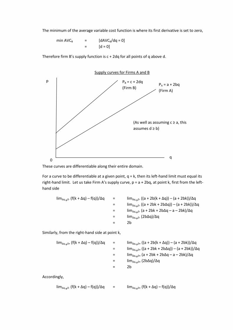
(a) Find the supply functions, defined on q ≥ 0, for each firm and draw them on the same graph. At

which points of their domains are these functions differentiable?

The supply function is that portion of the marginal cost function above the minimum of the

average variable cost function.

Firm A’s cost function is,

CA = aq + bq2

Its marginal cost function is the first derivative of the cost function

MCA = dCA/dq

= a + 2bq

Firm A’s variable cost function is the same as its cost function, because both components

depend on output,

VCA = aq + bq2

Its average variable cost function is,

AVCA = VCA/q

= (aq + bq2)/q

= a + bq

The minimum of the average variable cost function is where its first derivative is set to zero,

min AVCA = [dAVCA/dq = 0]

= [b = 0]

Therefore firm A’s supply function is a + 2bq for all points of q above b.

Firm B’s cost function is,

CB = cq + dq2

Its marginal cost function is the first derivative of the cost function

MCB = dCB/dq

= c + 2dq

Firm B’s variable cost function is the same as its cost function, because both components

depend on output,

VCB = cq + dq2

Its average variable cost function is,

AVCB = VCB/q

= (cq + dq2)/q

= c + dq

The minimum of the average variable cost function is where its first derivative is set to zero,

min AVCB = [dAVCB/dq = 0]

= [d = 0]

Therefore firm B’s supply function is c + 2dq for all points of q above d.

These curves are differentiable along their entire domain.

For a curve to be differentiable at a given point, q = k, then its left-hand limit must equal its

right-hand limit. Let us take Firm A’s supply curve, p = a + 2bq, at point k, first from the left-

hand side

lim∆q

0- (f(k + ∆q) – f(q))/∆q = lim∆q

0- ((a + 2b(k + ∆q)) – (a + 2bk))/∆q

= lim∆q

0- ((a + 2bk + 2b∆q)) – (a + 2bk))/∆q

= lim∆q

0- (a + 2bk + 2b∆q – a – 2bk)/∆q

= lim∆q

0- (2b∆q)/∆q

= 2b

Similarly, from the right-hand side at point k,

lim∆q

0+ (f(k + ∆q) – f(q))/∆q = lim∆q

0+ ((a + 2b(k + ∆q)) – (a + 2bk))/∆q

= lim∆q

0+ ((a + 2bk + 2b∆q)) – (a + 2bk))/∆q

= lim∆q

0+ (a + 2bk + 2b∆q – a – 2bk)/∆q

= lim∆q

0+ (2b∆q)/∆q

= 2b

Accordingly,

lim∆q

0- (f(k + ∆q) – f(q))/∆q = lim∆q

0+ (f(k + ∆q) – f(q))/∆q

0

PB = c + 2dq

(Firm B)

p

q

PA = a + 2bq

(Firm A)

(As well as assuming c ≥ a, this

assumes d ≥ b)

Supply curves for Firms A and B

As such, the function is differentiable along its entire domain, as k may be substituted for

any figure in the function’s domain.

The same analysis applies to Firm B’s supply curve, but with c substituted for a, and d

substituted for b.

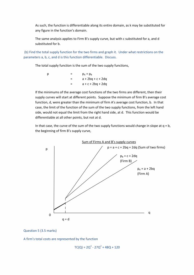
(b) Find the total supply function for the two firms and graph it. Under what restrictions on the

parameters a, b, c, and d is this function differentiable. Discuss.

The total supply function is the sum of the two supply functions,

p = pA + pB

= a + 2bq + c + 2dq

= a + c + 2bq + 2dq

If the minimums of the average cost functions of the two firms are different, then their

supply curves will start at different points. Suppose the minimum of firm B’s average cost

function, d, were greater than the minimum of firm A’s average cost function, b. In that

case, the limit of the function of the sum of the two supply functions, from the left hand

side, would not equal the limit from the right hand side, at d. This function would be

differentiable at all other points, but not at d.

In that case, the curve of the sum of the two supply functions would change in slope at q = b,

the beginning of firm B’s supply curve,

Question 5 (3.5 marks)

A firm’s total costs are represented by the function

TC(Q) = 2Q3 - 27Q2 + 48Q + 120

0

pB = c + 2dq

(Firm B)

p

q

pA = a + 2bq

(Firm A)

Sum of Firms A and B’s supply curves

q = d

p = a + c + 2bq + 2dq (Sum of two firms)

where Q is total output in thousands of units.

(a) Find the firm’s marginal and average cost functions.

Marginal cost is the first derivative of the cost function,

MC = dTC/dQ

= 6Q2 – 54Q + 48

Average cost is the total cost function divided by output,

AC = TC(Q)/Q

= (2Q3 – 27Q2 + 48Q + 120)/Q

= 2Q2 – 27Q +48 + 120/Q

(b) Find the level of output that minimizes the firm’s total cost.

Total cost is minimised where marginal cost is equal to zero and the second derivative of

total cost (the first derivative of marginal cost) is positive,

Set MC = 0

6Q2 – 54Q + 48 = 0

6(Q2 – 9Q + 8) = 0

Q2 – 9Q + 8 = 0

(Q – 1)(Q – 8) = 0

Q = [1, 8]

TC”(Q) = 12Q – 54

TC”(1) = 12(1) – 54

= -42

TC”(8) = 12(8) – 54

= 42

At Q = 8, the second derivative of TC is positive, so Q = 8 is a local minimum of the total cost

function. Accordingly, costs are minimised when the firm produces 8 units of output.

(c) Assume the firm produces this single good in a competitive market in which the price of the good

is $120 per unit. Derive the firm’s profit function and use it to determine the production level that

maximizes profit. Compare your answer to that of (b) and discuss the economic significance of the

two results.

Let R(Q) stand for the firm’s revenue as a function of its output and π(Q) stand for the firm’s

profit as a function of its output.

π(Q) = R(Q) – TC(Q)

= pQ – (2Q3 - 27Q2 + 48Q + 120)

= 120q – 2Q3 + 27Q2 – 48Q – 120

= – 2Q3 + 27Q2 + 72Q – 120

To maximise profit, set the first derivative of the profit function equal to zero,

dπ/dQ = 0

-6Q2 + 54Q + 72 = 0

-6(Q2 – 9Q – 12) = 0

Q2 – 9Q – 12 = 0

Q2 – 9Q = 12

½ x 9 = 4.5

4.52 = 20.25

Q2 – 9Q +20.25 = 32.25

(Q – 4.5)(Q – 4.5) = 32.25

√32.25 = [5.68, -5.68]

Q – 4.5 = 5.68

Q = 10.18

Q – 4.5 = -5.68

Q = 1.18

Then to check the sign of the second derivative of the profit function at each of the output

levels where the first derivative is equal to zero,

π”(Q) = -12Q + 54

π”( 10.18) = -12(10.18) + 54

= -68.16

π”( 1.18) = -12(1.18) + 54

= 39.84

As the second derivative of the profit function is negative at Q = 10.18, the profit function is

maximised at 10,180 units of output.