17 Mourelle y Ezcurra, 1997, diversidad de cactaceas y su relacion a factores ambientales

Copyright Notice This electronic reprint is provided by the author(s) to be consulted by fellow scientists. It is not to be used for any purpose other than private study, scholarship, or research. Further reproduction or distribution of this reprint is restricted by copyright laws. If in doubt about fair use of reprints for research purposes, the user should review the copyright notice contained in the original journal from which this electronic reprint was made.

- Differentiation diversity of Argentine cacti - 547

Sample copy Journal of Vegetation Science Vol. 8, 1997© Opulus Press AB

Journal of Vegetation Science 8: 547-558, 1997© IAVS; Opulus Press Uppsala. Printed in Sweden

Abstract. We studied the differentiation diversity (β-diversityor species turnover) patterns of the three main cactus growthforms (columnar, opuntioid and globose) in 318 (1° × 1°)squares covering Argentina. We analysed the degree ofassociation between species turnover of each growth formwith the spatial variation of a set of 15 environmental variables.

Species turnover was estimated in two ways: (1) bycalculating species turnover along latitudinal and longitudinalgradients and (2) by evaluating the species turnover betweeneach square and its eight surrounding neighbouring grid cells.

For the three growth forms, species turnover in latitudinaltransects was mostly related to the mean within-transect val-ues of certain environmental variables, while in longitudinaltransects it was related to the variation of some environmentalvariables within the transect rather than to their mean values.For columnar species, transect species turnover was mainlyassociated with variation in temperature, confirming the tem-perature-sensivity of this growth form. For opuntioid species,turnover along transects was mainly related to topographicvariables. In the case of globose cacti, transect turnover wasassociated with variation in temperature and rainfall.

For the three growth forms, areas of high turnover coin-cided with marked transitions between different biogeographicprovinces, while the areas with lowest species turnover coin-cide with topographically and climatically uniform plains.Species turnover between individual squares was positivelyassociated with the proportion of summer rainfall in globosecacti, the variation of mean annual temperature in columnarcacti and was negatively related to mean annual temperature inopuntioid cacti. Compared to the other growth forms, globosecacti presented a much larger proportion of squares with a highspecies turnover.

In general, differentiation diversity was lower for theopuntioid and the columnar species, two growth forms withhigher dispersal ability and was highest for the globose cacti,which have the lowest dispersal capacity. Environmentallyheterogeneous areas, where large-scale transitions betweenbiomes occur, have exceptionally high species turnover, andare important target areas for the conservation of biodiversity.

Keywords: Dispersal capacity; Environmental variable;Growth form; Species turnover.

Introduction

The concept of biological diversity has been sub-divided into two main components: (1) local richness orinventory diversity and (2) differentiation or β-diversity,also known as replacement or turnover between speciesassemblages. Both components apply to a wide rangeof scales. The first concept has been commonly labelledas α-diversity, when applied within a community or ahomogeneous habitat, but has also been defined as γ-diversity when applied to the landscape level and as ε-diversity at a regional level (Whittaker 1977). The secondcomponent has received a large array of names frommany authors, such as (1) internal β-diversity or patterndiversity, (2) β-diversity, between-habitat diversity orbetween-site diversity and (3) γ-diversity, geographicdifferentiation or δ-diversity (Whittaker 1960, 1972,1977; MacArthur 1965; Cody 1975, 1986, 1993;Magurran 1988; Cowling et al. 1989; Cornell et al.1992; Colwell & Coddington 1994). This terminologi-cal heterogeneity arises mostly from the application ofessentially the same concept at different scales in whichdifferent biological processes may operate.

Local and regional diversity, or species richness at alocal or regional scale, have long been major topics in theecological and biogeographical literature, focusing ontheir definition and measurements (Pielou 1975; Magurran1988; Begon et al. 1990; Sánchez & López 1988) and onits biological determinants (MacArthur 1965; Pianka 1966;Huston 1979; Brown 1981, 1988; Shmida & Wilson1985; Begon et al. 1990; Rhode 1992; Rosenzweig &Abramsky 1993). Differentiation diversity, usually ap-proached as species turnover, has received less system-atic analysis (for remarkable exceptions see Whittaker1972; Cody 1975, 1986; Routledge 1977; Wilson &Shmida 1984; Shmida & Wilson 1985; Magurran 1988;Harrison et al. 1992). Yet, turnover of species betweenareas is as important as local richness in determiningdiversity at any scale.

In this paper, we will focus on the analysis of differ-entiation diversity for three growth forms of theCactaceae in Argentina: (a) columnar and barrel cacti,

Differentiation diversity of Argentine cacti and its relationshipto environmental factors

Mourelle, Cristina & Ezcurra, Exequiel

Centro de Ecología, UNAM; Apartado Postal 70-275; 04510 - Mexico, D.F.; Mexico;E-mail: [email protected]

548 Mourelle, C. & Ezcurra, E.


(b) globose cacti and (c) opuntioid cacti (Fig. 1). Colum-nar species have cylindrical stems with ribs, formed byan arrangement of the areoles in longitudinal rows. Wealso included the short-stemmed barrel cacti in thiscategory. Globose cacti, the smallest growth form, aremore or less spherical in shape. Opuntioid species arenon-ribbed, with stems formed by flat or cylindricalcladodes (for a detailed description of cactus growthforms see Mourelle & Ezcurra 1996). In Argentina,species of the globose growth form present a high levelof endemism and are restricted in both habitat andrange; opuntioid species are the most widespread andless specific in habitat requirements, and columnar spe-cies are chiefly limited by low temperatures (Mourelle& Ezcurra 1996).

The main purpose of our study was to evaluate thedegree of association between species turnover and a setof environmental variables that were assumed to bepotentially significant determinants of biological varia-tion. We used a pixel resolution of ca. 100 km, assmaller scales cannot be used with the current collectionintensity of the data set (see Mourelle & Ezcurra 1996).This scale is within an order of magnitude of some otherstudies on species turnover (e.g. Harrison et al. 1992). Interms of scale, our measurement of species turnover ordifferentiation diversity is intermediate between theconcept of β-diversity or between-habitat diversity andthe concept of δ-diversity or geographic differentiation(e.g. Cody 1975, 1993; Ricklefs & Schluter 1993).

Few studies have analysed the influence of the dif-ferent environmental factors affecting species turnover.Most of these investigations (Retuerto et al. 1990; Meave

1991; Tueller et al. 1991; Harrison et al. 1992; Cody1993; Kadmon et al. 1993; Wolf 1993; Scheiner & Rey-Benayas 1994) have evaluated the association betweenspecies turnover and direct environmental factors (e.g.mean annual temperature, mean altitude), or a measure oftheir temporal variability (e.g. the standard deviation ofmean monthly temperature, the standard deviation oftotal monthly precipitation). None of the studies mentionedabove related species turnover to the spatial variation ofenvironmental variables; that is, they did not attempt torelate the difference in species composition between twoor more sites (species turnover) with the difference inthe values of the environmental variables between thesame sites (spatial environmental heterogeneity).

Methods

To analyse species turnover, we used a databasecontaining 3395 records from 228 species of theCactaceae occurring in Argentina. Data on the distribu-tion of the species were taken from herbarium labels inseven Argentine herbaria, and supplemented by Kieslingand Ferrari’s unpublished field data and with publishedsources (see Mourelle & Ezcurra 1996). We subdividedthe Cactaceae into three main growth forms: (1) colum-nar cacti, including the shorter-stemmed barrel cacti, (2)globose cacti and (3) opuntioid cacti, with 50, 109 and50 species respectively (for a complete species list, seeMourelle & Ezcurra 1996). All the analyses were car-ried out for each growth form separately. We excludedfrom our analysis the five pereskioid species and the 14

Fig. 1. Schematic representation of the three cactus growth forms studied. The columnar group also includes barrel cacti, which areshort-stemmed but not globose. Columnar and globose growth forms belong to the subfamily Cactoideae; most of the columnargenera belong to the tribes Trichocereeae and Cereeae while the globose genera belong mostly to the tribe Notocacteae. Allopuntioid species belong to the subfamily Opuntioideae (Mourelle & Ezcurra 1996).



epiphytic species known to occur in Argentina, as thelow number of species in these two growth forms doesnot allow for robust statistical tests of hypotheses. Intro-duced species and species with either dubious distribu-tion records or non-valid names (totalling 10 species)were also excluded. The map of Argentina was dividedinto a grid of 318 cells of 1° × 1°. For each species wedigitised the grid squares from where it had been col-lected. These cartographic cells are not equal in area,they range from around 11 000 km2 in the North ofArgentina, to ca. 9000 km2 in the southernmost latitudeswith registered cactus species (an analysis of the poten-tial sources of error introduced by units with variablearea was presented by Mourelle & Ezcurra 1996).

Species richness and species turnover

In this study, species richness is defined as the localnumber of cactus species contained in a square of 1° × 1°.Differentiation diversity was calculated in two differentways: (1) by estimating turnover along geographicalgradients following latitudinal or longitudinal transectsone degree wide and (2) by evaluating, for each indi-vidual square, the turnover between the cell and its eightsurrounding squares.

Species turnover along geographical transectsFor the analysis of transects, we used both Whittaker’s

and Wilson and Shmida’s measures of species turnoveror β-diversity (Magurran 1988). Firstly we calculatedWhittaker’s measure βw = k / ln2, where k is a parameterderived from the negative exponential function S = e–kx,which predicts how between-square similarity (S) de-creases with distance (x) along a transect (Whittaker1972). The negative exponential model is derived fromthe differential equation (1 /S) ( ∂S / ∂x) = – k ; wherethe parameter k is the intrinsic rate of change of biologicalsimilarity per unit distance, which can also be rewritten as( ∂ lnS/ ∂x) = k. Thus, βw (a transform of k) is a turnoverrate in a log2 scale – with ‘octaves’ as intervals; it mea-sures turnover rates in ‘half-changes’ per unit distance.To estimate βw, all possible between-square similaritieswere calculated for each transect, together with the cor-responding between-square distances. The negative ex-ponential parameter (k) was estimated by non-linear re-gression, fitting Whittaker’s model to the set of similarityvs. distance data points. The significance of the fit wasevaluated by an approximate F-test (as variances are notalways additive in non-linear models, an exact ANOVAis not strictly possible, see Draper & Smith 1981).Similarities (S) were calculated using Sørensen’s Co-efficient of Community (Whittaker 1960, 1972; Pielou1979; Wilson et al. 1983; we also tried Jaccard’s Indexand obtained qualitatively similar results, though its fit to

the negative exponential model was somewhat lower).The resulting measure of species turnover is given in half-changes per unit grid cell.

We also used Wilson and Shmida’s index correctedby the size of the transect: βt = (g + l) / [2α (n – 1)],where g is the cumulative number of species that aregained following successive squares from one ex-treme of the transect to the opposite, l is the cumula-tive number of species that are lost, α is the meannumber of species per square (mean species richness)and n is the number of squares in the transect. βtmeasures, for the whole transect, the mean relativeturnover between adjacent squares (Wilson & Shmida1984; Shmida & Wilson 1985). Like Whittaker’s mea-sure, βt is also a turnover rate, estimated in an arith-metic rather than in a logarithmic scale. Additionally,because it only takes into consideration changes be-tween adjacent squares, Wilson and Shmida’s approachemphasises local species turnover and hence betterreflects the effects of short-distance environmentalheterogeneity, while Whittaker’s measure emphasisesspecies turnover along extensive distances and betterreflects the effects of distributional amplitude of thespecies in the group.

For both methods, we estimated turnover rates along15 longitudinal transects (less for some growth forms)and 15 latitudinal transects of different length (bothranging from 3 to 13 squares). We only analyzed thosetransects containing more than three squares with five ormore species. Squares with fewer than three specieswere discarded from the analysis.

Species turnover between individual squaresFor this analysis we calculated the similarity be-

tween each individual square and its eight adjacentneighbouring squares by means of Sørensen’s Coeffi-cient of Community. As similarity decreases exponen-tially with distance (see previous section), we correctedthe similarities of the corner squares (which are fartheraway from the central square and hence are more likelyto show lower similarities) by elevating their values tothe power (1 /√2), where the value √2 is the diagonaldistance between squares one unit in size. This correc-tion can be deduced from Whittaker’s negative expo-nential model described in the previous section. Thus,the species turnover between the central square and anyone of its neighbours is simply βi = 1 – Si , where Si is thecorrected similarity between the central square and theneighbouring square i.

It can be seen that, if Sørensen’s Coefficient ofCommunity is used to measure similarity, then βi = 1 –[2c / (q + si)], where c is the number of species sharedbetween both squares, q is the number of species in thecentral square, and si is the number of species in the



neighbouring square i. This equation can be rewritten asβi = (g + l) / 2 α, where g is the number of species whichare present in the neighbouring square and absent in thecentral square, l is the number of species which arepresent in the central square and absent in the neigh-bouring square and α is the mean species richness inboth squares. This last form is identical to the index ofWilson & Shmida introduced in the previous section.Thus, the mean species turnover between a square andits neighbours (βq) was simply measured as the averageof n values of floristic turnover with the neighbouringsquares, where 0< n ≤ 8 is the number of neighbourswith registered species. Measured in this manner, βq isthe mean turnover rate from a given square with respectto its n neighbours. The resulting values were mappedfor the whole country in three categories: squares withhigh species turnover (0.661 - 1.0), squares with inter-mediate turnover (0.331 - 0.66) and squares with lowturnover (0 - 0.33).

Latitudinal and longitudinal trends in transect speciesturnover

To test if there were spatial trends in species turn-over, we evaluated the relationship between speciesturnover in longitudinal transects and their latitudinalposition by means of time-series analysis of long-termlinear trends; and we also evaluated the relationshipbetween species turnover in latitudinal transects withrespect to their position along the east-west gradient.

Species turnover and environmental predictors

16 environmental variables were digitised for thewhole country on a 1° × 1° scale: two geographic, 11climatic and three topographical – aimed at estimatingsmall-scale environmental heterogeneity as discussed inPalmer & Dixon (1990):

Latitude;Longitude;Mean annual temperature;Mean annual precipitation;Mean annual minimum temperature;Proportion of annual rain falling in summer;Mean number of frost-free days;Mean annual water deficiency measured as the ratio of the net annual

radiation to the heat energy required to evaporate the mean annualprecipitation;

Mean actual evapotranspiration;Mean July temperature;Mean December temperature;Difference between Mean July and Mean December temperature;Annual primary productivity calculated from Lieth’s (1975) index of

evapotranspiration;Altitudinal range calculated as the difference between maximum and

minimum altitude within a square;Topographic variability calculated as the standard deviation of the

altitude of nine points selected systematically within each square;Mean altitude calculated as the average of the nine within-square

points.

To estimate the spatial heterogeneity of the climaticand topographic variables we calculated (1) the meanand the variance of each variable between the squares ofthe latitudinal and longitudinal transects described inthe previous section and (2) the mean squared differencebetween the value of each cartographic cell and thevalues of its eight neighbouring squares (i.e. the vari-ance with respect to the central value). For the analysisof transects, the mean and variance of each environmen-tal variable in that transect were regressed against bothWhittaker’s and Wilson and Shmida’s species turnoverestimates for the transect (βw and βt respectively). Forthe analysis of individual squares, the values of theenvironmental variable in that particular square and ofits spatial variation were regressed against the speciesturnover of the square (βq). Regression analysis wasperformed with the GLIM package, following an addi-tive stepwise procedure (Payne 1986; McCullagh et al.1989; Yee et al. 1991). To increase parsimony in ouranalysis, we previously did a Principal ComponentAnalysis (PCA) of the environmental variables in orderto identify groups of correlated variables. In order todecrease the probability of Type I errors, once a variablehad entered the regression model, we avoided testing theinclusion of new variables showing significant collinear-ity with the first one. We also performed the regressionsdirectly against the PCA axes, but in no case did acomposite axis show a better predictive value than thebest individual variable.

The effect of data collection intensity

The number of species detected in a given area is afunction of the number of herbarium specimens thatwere collected (Soberón & Llorente 1993). Based on theproperties of accumulation functions (Mourelle & Ezcurra1996), we incorporated the logarithm of the number ofvoucher specimens registered per square in our regressionmodels (we previously added one to the number of speci-mens, to avoid the indetermination of log-zero) as anadditional predictor, with the objective of evaluating thepotential effect of undercollection in our study of speciesturnover. Thus, once the final model based on environmen-tal predictors had been fitted, we added the logarithm of thenumber of specimens (our estimation of collection inten-sity), in order to evaluate the proportion of the model’serror that could be attributed to spatial gaps in the collec-tion effort. As with the environmental variables, thepotential effect of undercollection on the estimates ofspecies turnover was evaluated both for transects and forindividual squares, and the effect of spatial variation inthe collection effort was also included as a predictor. Thatis, we evaluated how much of the estimated speciesturnover could be attributable to the fact that some squareswere more collected than others.



Table 2. Best predictors of species turnover in longitudinal transects, for the three cactus growth forms in Argentina. In all growthforms, only one best predictor was found. The variances of the variables estimate the variation between grid-cells within each transect(see Methods).

Growth forms Dependent variable Best predictors r2 Sign P

Columnar βw Variance of number of frost-free days 0.33 + 0.04βt Variance of mean annual temperature 0.18 + 0.15

Opuntioid βw Variance of mean altitude 0.18 + 0.15βt Variance of mean altitude 0.49 + 0.0008

Globose βw Variance of mean annual water deficiency 0.59 + 0.004βt Variance of mean altitude 0.67 + 0.003

Results

Species turnover along transects

In all growth forms and in all transects, the non-linear fit of Whittaker’s exponential model to transectdata was always highly significant, and in all cases theresiduals fitted adequately the required assumptions ofindependence and randomness (Draper & Smith 1981).

Latitudinal transectsDifferent significant predictors resulted from the

regression analysis with species turnover (the depen-dent variable) calculated as Whittaker’s measure (βw) oras Wilson and Shmida’s index (βt). For the columnarspecies, Whittaker’s measure of species turnover wassignificantly higher in N-S transects where actual evapo-transpiration was low, i.e. in arid habitats (Table 1). βt,on the other hand, was higher in transects where mini-mum annual temperature varied considerably betweengrid cells. For opuntioid cacti, βw increased in transectswhere within-square altitudinal variation was high, whileβt was associated with transects with a high number offrost-free days. Finally, for globose cacti, βw was higherin transects where rainfall was concentrated in summer,

while βt was associated with transects where meanminimum annual temperature was high, i.e. transectswith mild winters. For all three growth forms, speciesturnover in transects was unrelated to the mean collec-tion effort, or with its within-transect variation.

Longitudinal transectsIn contrast to latitudinal change, longitudinal turn-

over for the three growth forms was always related to thebetween-squares variation of the environmental factors,rather than to the factors themselves (Table 2). For thecolumnar species, the strongest predictor for βw was thevariance in the number of frost-free days. Transects withhigh variation in the number of frost-free days had, gen-erally, a higher turnover than transects with little varia-tion in this environmental factor. The best predictor of βtwas thermal variation (a variable obviously related to thenumber of frost-free days), but the fit of the regressionmodel was not significant. For the opuntioid species, bothmeasures of species turnover were best predicted byaltitudinal variation between squares, although in thiscase the fit of the model to βw was not significant. Finally,in globose cacti βw was strongly related to variations inthe mean annual water defficiency, an index of aridity;and βt was significantly related to variations in altitude, a

Table 1. Best predictors of species turnover in latitudinal transects for the three cactus growth forms in Argentina. In all growth formsonly one best predictor was found (i.e. once the first stepwise variable entered into the model all other predictors became non-significant). The variances of the variables estimate variation between grid-cells within each transect (see Methods).

Growth forms Dependent variable Best predictors r2 Sign P

Columnar βw Mean actual evapotranspiration 0.60 – 0.001βt Variance of mean minimum annual temperature 0.63 + < 0.001

Opuntioid βw Mean altitudinal range 0.39 + 0.003βt Mean number of frost-free days 0.43 + 0.002

Globose βw Mean percentage of summer rainfall 0.57 + < 0.001βt Mean minimum annual temperature 0.55 + 0.001



complex measure of environmental heterogeneity. Aswith the longitudinal transects, species turnover in latitu-dinal transects was not significantly related for any growthform, neither the mean collection effort, nor with itsbetween-square variation.


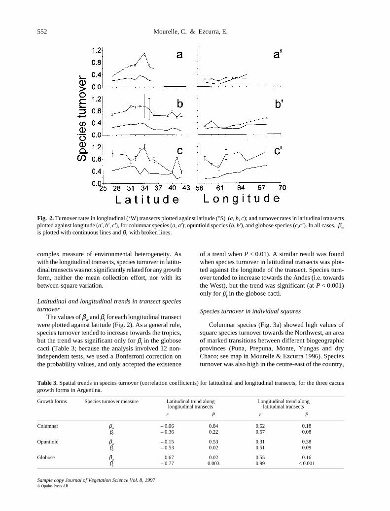
The values of βw and βt for each longitudinal transectwere plotted against latitude (Fig. 2). As a general rule,species turnover tended to increase towards the tropics,but the trend was significant only for βt in the globosecacti (Table 3; because the analysis involved 12 non-independent tests, we used a Bonferroni correction onthe probability values, and only accepted the existence

of a trend when P < 0.01). A similar result was foundwhen species turnover in latitudinal transects was plot-ted against the longitude of the transect. Species turn-over tended to increase towards the Andes (i.e. towardsthe West), but the trend was significant (at P < 0.001)only for βt in the globose cacti.

Species turnover in individual squares

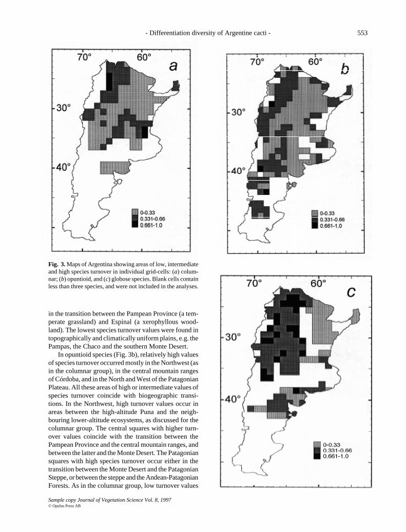
Columnar species (Fig. 3a) showed high values ofsquare species turnover towards the Northwest, an areaof marked transitions between different biogeographicprovinces (Puna, Prepuna, Monte, Yungas and dryChaco; see map in Mourelle & Ezcurra 1996). Speciesturnover was also high in the centre-east of the country,

Table 3. Spatial trends in species turnover (correlation coefficients) for latitudinal and longitudinal transects, for the three cactusgrowth forms in Argentina.

Growth forms Species turnover measure Latitudinal trend along Longitudinal trend alonglongitudinal transects latitudinal transects

r P r P

Columnar βw – 0.06 0.84 0.52 0.18βt – 0.36 0.22 0.57 0.08

Opuntioid βw – 0.15 0.53 0.31 0.38βt – 0.53 0.02 0.51 0.09

Globose βw – 0.67 0.02 0.55 0.16βt – 0.77 0.003 0.99 < 0.001

Fig. 2. Turnover rates in longitudinal (°W) transects plotted against latitude (°S) (a, b, c); and turnover rates in latitudinal transectsplotted against longitude (a', b', c'), for columnar species (a, a'); opuntioid species (b, b'), and globose species (c,c’). In all cases, βwis plotted with continuous lines and βt with broken lines.



in the transition between the Pampean Province (a tem-perate grassland) and Espinal (a xerophyllous wood-land). The lowest species turnover values were found intopographically and climatically uniform plains, e.g. thePampas, the Chaco and the southern Monte Desert.

In opuntioid species (Fig. 3b), relatively high valuesof species turnover occurred mostly in the Northwest (asin the columnar group), in the central mountain rangesof Córdoba, and in the North and West of the PatagonianPlateau. All these areas of high or intermediate values ofspecies turnover coincide with biogeographic transi-tions. In the Northwest, high turnover values occur inareas between the high-altitude Puna and the neigh-bouring lower-altitude ecosystems, as discussed for thecolumnar group. The central squares with higher turn-over values coincide with the transition between thePampean Province and the central mountain ranges, andbetween the latter and the Monte Desert. The Patagoniansquares with high species turnover occur either in thetransition between the Monte Desert and the PatagonianSteppe, or between the steppe and the Andean-PatagonianForests. As in the columnar group, low turnover values

Fig. 3. Maps of Argentina showing areas of low, intermediateand high species turnover in individual grid-cells: (a) colum-nar; (b) opuntioid, and (c) globose species. Blank cells containless than three species, and were not included in the analyses.



occurred in plains with high topographic and climatichomogeneity, e.g. the Pampas, the Chaco, and the south-ern Monte Desert.

The globose species (Fig. 3c) presented a differenttrend compared with the opuntioid and columnar groups.Medium and high turnover squares occupied 75.7% ofall the analysed squares. The high-species-turnover areawas concentrated in the northwestern part of the coun-try, from 62° - 63° W westwards, and northwards from35° - 36° S. It occupied a north-south corridor compris-ing many phytogeographic provinces: in the north, theHigh-Andean, the Puna and the Prepuna and furthersouth, the northern Monte Desert, the Espinal and partof the dry western Chaco. A secondary centre of highturnover was found in northeastern Patagonia, in an areawhere the Monte Desert becomes replaced by thePatagonian Steppe.

Environmental predictors of species turnover in indi-vidual squares

Neither latitude nor species richness showed a sig-nificant association with species turnover between indi-vidual squares for any of the growth forms. The globose

cacti (Fig. 4c) showed the growth form in which thespecies turnover in individual cells was most highlyrelated to environmental factors; 65% of the variance inspecies turnover was explained by the proportion ofannual rain falling in summer (Table 4). That is, speciesturnover increased towards regions where monsoon-type rains are highly concentrated in summer. For co-lumnar cacti (Fig. 4a), the spatial heterogeneity in themean annual temperature explained 63% of the variabil-ity in square species turnover and was positively corre-lated with it. That is, the more different the mean annualtemperature the higher the species turnover. The speciesturnover of opuntioid species was negatively associatedwith the mean annual temperature, i.e., species turnoverincreases towards cooler environments. Opuntioid spe-cies turnover (Fig. 4b) also was significantly associatedwith the spatial heterogeneity in mean annual precipita-tion, i.e., species turnover also tends to increase inregions where the precipitation gradient is steep. For allthree growth forms, a small, but significant, part of theresidual species turnover was attributable to spatial het-erogeneity in the collection effort (Table 4).

Fig. 4. Regressions between species turnover ingrid cells and their best predictors for (a) colum-nar; (b) opuntioid, and (c) globose species (seeTable 4).



Discussion

Species turnover along transects

Differences in turnover rates between longitudinaland latitudinal transects were related to different vari-ables for the same group. Species turnover in latitudinaltransects was mostly related to the mean values ofcertain environmental variables within the transect, whilein longitudinal transects it was always related to thebetween-squares variation of certain environmental vari-ables, rather than to the mean values. The reason for thispossibly lies in the distribution of the environmentalvariables in Argentina, and especially in the subtropicalnorthern part of Argentina where most of the squareswith cacti are found. In this region, there is a markedgradient from the eastern plains, which are more humidand have deep fertile soils, to the western pre-Andeanareas, which are more arid, topographically hetero-geneous, more continental in their temperature regimeand with strict summer-type rains.

The latitudinal transects run parallel to this east-westgradient, while the longitudinal transects intersect it.That is, longitudinal transects cut across widely differ-ent ecosystems, while latitudinal transects run throughmore homogeneous biomes. Thus, the best predictors ofspecies turnover in longitudinal transects are variablesthat measure the intensity of environmental change withinthe transect from east to west (e.g. within-transect varia-tion in mean altitude, in water deficiency, in the numberof frost-free days or in mean annual temperature). Incontrast, the best predictors of species turnover withinlatitudinal transects are mostly variables that measurethe relative position of the north-south transect on theeast-west gradient (e.g. actual evapotranspiration, per-centage of summer rainfall, mean minimum annual tem-perature or number of frost-free days).

In the specific case of columnar cacti, it is interestingto note that, with the exception of βw in latitudinal

transects, species turnover along transects was associ-ated with variations in temperature (e.g. variation in thenumber of frost-free days, variation in mean minimumtemperature). It has been well documented that colum-nar cacti are extremely sensitive to freezing tempera-tures (see Gibson & Nobel 1986 for a review).


There was a feeble trend of increased species turn-over towards the tropics and towards the west, althoughthe trend was significant only for the globose growthform. Whittaker (1977) predicted that species turnovershould increase towards the tropics, and this predictionhas been confirmed for several groups such as birds(MacArthur 1965,1967), insects and the plants they feedon (Janzen & Schoener 1968), bryophytes (Wolf 1993)and mammals (Willig & Sandlin 1991). This prediction,however, did not clearly hold for our cacti.

Species turnover in individual squares

No association was found between species richnessand species turnover. For all growth forms, the squareswith high species turnover tended to occur in areaswhere there are transitions between different biogeo-graphic provinces, or where the physical environmentvaries between squares. In particular, the northwesternpart of Argentina, a topographically and climaticallyheterogeneous region where the boundaries of differentbiogeographic provinces converge, appeared in all casesas an area of high species turnover. In contrast, theenvironmentally uniform large plains of the Pampas, theChaco and the southern Monte Desert appeared in allcases as regions of low species turnover. The behaviourof the columnar and the opuntioid species was quitesimilar. Both showed high values in the northwest, inthe transition between the Pampas grasslands and thesurrounding, more arid ecosystems. The opuntioid spe-

Table 4. Best predictors of species turnover (βq) in individual grid-cells for the three cactus growth forms in Argentina. The variationin environmental variables represents the degree of change of the variables between each grid-cell and its neighbours (i.e. thebetween-cell variation, see Methods).

Growth forms Best predictors r2 Sign P

Columnar Variation in mean annual temperature 0.63 + < 0.001Variation in collection effort 0.08 + 0.01

Opuntioid Mean annual temperature 0.47 – < 0.001Variation in mean annual precipitation 0.16 + 0.0004Variation in collection effort 0.03 + 0.04

Globose Mean percentage of summer rainfall 0.65 + < 0.001Variation in collection effort 0.05 + 0.05



cies also showed high species turnover in the transitionsbetween the different biogeographic provinces of north-ern Patagonia, a geographic trend not shown by themore frost-sensitive columnar group, which does notprosper at these temperate latitudes. The globose spe-cies presented relatively high turnover rates in a muchlarger proportion of the country. This suggests thatregions which are relatively uniform for the species withlarger individuals, are markedly heterogeneous for themore poorly-dispersed globose group. In particular, theglobose species showed high species turnover in all thecentral and northwestern squares, a region occupied byvalleys and pre-Andean ranges with heterogeneous soilsand a more pronounced topography. This trend in indi-vidual squares confirmed the tendency observed in theanalysis of transects, in that species turnover increasedboth towards the tropics and towards the west.

The best predictors of species turnover between gridcells followed the tendency discussed above. The bestpredictor of columnar turnover (variation in mean an-nual temperature) is highest in the pre-Andean ranges ofthe northwest, where the pronounced topography in-duces abrupt changes in mean temperature. The bestpredictor of opuntioid species turnover (mean annualtemperature) is low in the Patagonian squares and in themountainous ranges of the northwest, the two mainareas where opuntioid turnover is high (the relationshipbetween the predictor and opuntioid turnover). The bestpredictor of globose species turnover, percentage ofannual rain falling in summer, is associated with areaswith summer rain. Again, this summer-precipitationpattern is more marked throughout central-northwestArgentina, where both the Andes and the central moun-tain ranges originate rainshadows that impede the ar-rival of winter rains from the Atlantic or the Pacific. It isimportant to note, however, that no causal conclusionsshould be drawn from these regressions. Comparing thespecies-turnover maps with the biogeographic map ofArgentina (see Mourelle & Ezcurra 1996) it seemsobvious that the highest turnover rates coincide withcertain biogeographic boundaries where both biologicaland environmental changes are pronounced.

In the case of columnar species, variation in meantemperature is the best predictor of species turnover. This isin agreement with our previous report (Mourelle & Ezcurra1996), in which we found that a temperature variable (thenumber of frost-free days) was the best predictor of speciesrichness. Although high sensivity to low temperatures hasbeen extensively reported (e.g. Nobel 1981, 1982; Gibson& Nobel 1986) high temperature damage is difficult to findin the field (Gibson & Nobel 1986). We may concludethen, that columnar species turnover is related to tempera-ture change in as much as this variable reflects varyingdegrees of frost risk.

Finally, it is noticeable that the collection effort wasonly weakly related to species turnover. This resultstrongly contrasts with our previous study (Mourelle &Ezcurra 1996) for species richness, where the collectioneffort explained a much higher proportion of the re-sidual variation.

General trends in species turnover

Species turnover is mainly influenced by two groupof factors: the characteristics of the habitat (especiallyenvironmental heterogeneity), and the characteristics ofthe intervening species (chiefly the range of tolerance toenvironmental variation; Whittaker 1972, 1977; Schluter& Ricklefs 1993). In particular, habitat breadth anddispersal capacity have been singled out as importantdeterminants of turnover (e.g. Shmida & Wilson 1985;Westoby 1985; Harrison et al. 1992). With respect tospecialisation in habitat (a measure of niche breadth),the three growth forms may be ranked as: globose >columnar > opuntioid, while their dispersal ability canbe ranked as: opuntioid > columnar > globose (includ-ing both seed-dispersal and cladodes as vegetativepropagules; see Steenbergh & Lowe 1977; Barthlott &Hunt 1993; Mourelle & Ezcurra 1996). It is known thatopuntioid cacti are dispersed by small and large mam-mals (Janzen 1986; Vargas-Mendoza & Gonzalez-Espinosa 1992) and by lizards (Valido & Nogales 1994),columnar cacti are mostly dispersed by birds and mam-mals (Steenbergh & Lowe 1977; Barthlott & Hunt 1993,Valiente-Banuet et al. 1996) and globose cacti are chieflydispersed by insects, lizards and small mammals(Barthlott & Hunt 1993; Figueira et al. 1994). In agree-ment herewith, species turnover in our data set waslower in the opuntioid and columnar groups and it washighest in the globose cacti.

Species turnover in individual squares showed cleargeographical trends in all growth forms: it tended toincrease towards the northwest, and was especially highin squares where different biogeographic provinces con-verge. This yields a somewhat expected but none theless important generalization: the spatial component ofspecies diversity is likely to be higher in heterogeneousregions or in the ecotonal transition between large biomes.

The results presented here have important implica-tions for conservation biology. As a general rule, envi-ronmentally heterogeneous regions, together with re-gions where large-scale transitions between biomes oc-cur, have an exceptionally high species turnover, andcan be targeted for conservation purposes. In the case ofArgentine cacti, such regions occur in the northwest ofthe country, in the transition between the Monte Desert,the Prepuna, the dry western Chaco, and other surround-ing biogeographic provinces.



Acknowledgements. The authors thank the enthusiastic sup-port received from Roberto Kiesling and Omar Ferrari duringC. Mourelle’s travels in Argentina. This paper is part of thefirst author’s doctoral research at UNAM, supported by ascholarship from the Noyes-Smith Sciences Foundation. Theresearch received financial support from the National Councilof Science and Technology (CONACyT).

References

Barthlott, W. & Hunt, D.R. 1993. Cactaceae. In: Kubitzki, K.(ed.) The families and genera of vascular plants, pp. 161-197. Springer-Verlag, Berlin, Heidelberg.

Begon, M., Harper, J.L. & Townsend, C.R. 1990. Ecology:individuals, populations and communities. 2nd ed. Black-well Scientific Publications, Boston, MA.

Brown, J.H. 1981. Two decades of Homage to Santa Rosalia:Toward a general theory of diversity. Am. Zool. 21: 877-888.

Brown, J.H. 1988. Species diversity. In: Myers, A.A. & Giller,P.S. (eds.) Analytical biogeography: An integrated ap-proach to the study of animal and plant distribution, pp.57-89. Chapman and Hall, London.

Cody, M.L. 1975. Toward a theory of continental speciesdiversities: Bird distributions over mediterranean habitatgradients. In: Cody, M.L. & Diamond, J.M. (eds.) Ecologyand evolution of communities, pp. 214-257. Harvard Uni-versity Press, Cambridge, MA.

Cody, M.L. 1986. Diversity, rarity, and conservation inmediterranean-climate regions. In: Soulé, M.E. (ed.) Con-servation biology: The science of scarcity and diversity,pp. 123-152. Sinauer Associates, Sunderland, MA.

Cody, M.L. 1993. Bird diversity components within and be-tween habitats in Australia. In: Ricklefs, R.E. & Schluter,D. (eds.) Species diversity in ecological communities:Historical and geographical perspectives, pp. 147-158.The University of Chicago Press, Chicago and London.

Colwell, R.K. & Coddington, J.A. 1994. Estimating terrestrialbiodiversity through extrapolation. Phil. Trans. R. Soc.Lond. 345: 101-118.

Cornell, H.V. & Lawton, J.H. 1992. Species interactions, localand regional processes, and limits to the richness of eco-logical communities: A theoretical perspective. J. Anim.Ecol. 61: 1-12.

Cowling, R.M., Gibbs Russell, G.E., Hoffman, M.T. & Hilton-Taylor, C. 1989. Patterns of plant species diversity insouthern Africa. In: Huntley, B.J. (ed.) Biotic diversity insouthern Africa, pp. 19-49. Oxford University Press, CapeTown.

Draper, N.R. & Smith, H. 1981. Applied regression analysis,2nd ed. Wiley & Sons, New York, NY.

Figueira, J.E.C., Vasconcellos-Neto, J., Garcia, M.A. & Souza,A.L.T.D. 1994. Saurochory in Melocactus violaceus.Biotropica 26: 295-301.

Gibson, A.C. & Nobel, P.S. 1986. The Cactus primer. HarvardUniversity Press, Cambridge, MA.

Harrison, S., Ross, S.J. & Lawton, J.H. 1992. β-diversity ongeographic gradients in Britain. J. Anim. Ecol. 61: 151-158.

Huston, M. 1979. A general hypothesis of species diversity.Am. Nat. 113: 81-101.

Janzen, D.H. & Schoener, T.W. 1968. Difference in insectabundance and diversity between wetter and drier sitesduring a tropical dry season. Ecology 49: 96-110.

Janzen, D.H. 1986. Chihuahuan desert nopaleras: Defaunatedbig mammal vegetation. Annu. Rev. Ecol. Syst. 17: 595-636

Kadmon, R. & Pulliam, H.R. 1993. Island biogeography:Effect of geographical isolation on species composition.Ecology 74: 977-981.

Lieth, H. 1975. Modeling the primary productivity of theworld. In: Lieth, H. & Whittaker, R.H. (eds.) Primaryproductivity of the biosphere, pp. 237-263. Springer Verlag,Berlin & New York.

MacArthur, R.H. 1965. Patterns of species diversity. Biol.Rev. 40: 510-533.

MacArthur, R.H. 1969. Patterns of communities in the tropics.Biol. J. Linn. Soc. 1: 19-30.

McCullagh, P. & Nelder, J.A. 1989. Generalized linear mod-els, 2nd. ed. Chapman and Hall, London.

Magurran, A.E. 1988. Ecological diversity and its measure-ment. Princeton University Press, Princeton, NJ.

Meave, J.A. 1991. Maintenance of tropical rain forest plantdiversity in riparian forests of tropical savannas. Ph.D.Thesis. York University,Toronto.

Mourelle, C. & Ezcurra, E. 1996. Species richness of Argen-tine cacti: A test of some biogeographic hypotheses. J.Veg. Sci. 7: 667-680.

Nobel, P.S. 1981. Influence of freezing temperatures on a cactus,Coryphanta vivipara. Oecologia (Berl.) 48:194-198.

Nobel, P.S. 1982. Low temperature tolerance and cold harden-ing of cacti. Ecology 63: 1650-1656.

Palmer, M.W. & Dixon, P.M. 1990. Small-scale environmen-tal heterogeneity and the analysis of species distributionsalong gradients. J. Veg. Sci. 1: 57-65.

Payne, C.D. 1986. The Glim System Release 3.77 Manual.Numerical Algorithms Group, Oxford.

Pianka, E.R. 1966. Latitudinal gradients in species diversity:A review of concepts. Am. Nat. 100: 33-45.

Pielou, E.C. 1975. Ecological diversity. John Wiley & Sons,New York, NY.

Pielou, E.C. 1979. Biogeography. John Wiley & Sons, NewYork, NY.

Retuerto, R. & Carballeira, A. 1990. Phytoecological impor-tance, mutual redundancy and phytological threshold val-ues of certain climatic factors. Vegetatio 90: 47-62

Rhode, K. 1992. Latitudinal gradients in species diversity:The search for a primary cause. Oikos 65: 514-527.

Ricklefs, R.E. & Schluter, D. 1993. Species diversity: Re-gional and historical influences. In: Ricklefs, R.E. & Schluter,D. (eds.) Species diversity in ecological communities: His-torical and geographical perspectives, pp. 350-363. TheUniversity of Chicago Press, Chicago and London.

Rosenzweig, M.L. & Abramsky, Z. 1993. How are diversityand productivity related? In: Ricklefs, R.E. & Schluter, D.(eds.) Species diversity in ecological communities: His-torical and geographical perspectives, pp. 52-65. TheUniversity of Chicago Press. Chicago and London.

Routledge, R.D. 1977. On Whittaker’s component of diver-



sity. Ecology 58: 1120-1127.Sánchez, O. & López, G. 1988. A theoretical analysis of some

indices of similarity as applied to biogeography. FoliaEntomol. Mex. 75: 119-145.

Scheiner, S.M. & Rey-Benayas, J.M. 1994. Global patterns ofplant diversity. Evol. Ecol. 8: 1-18.

Schluter, D. & Ricklefs, R.E. 1993. Species diversity, anintroduction to the problem. In: Ricklefs, R. & Schluter,D. (eds.) Species diversity in ecological communities:Historical and geographical perspectives, pp. 1-10. TheUniversity of Chicago Press, Chicago and London.

Shmida, A. & Wilson, M. 1985. Biological determinants ofspecies diversity. J. Biogeogr. 12: 1-20.

Soberón, J. & Llorente, J. 1993. The use of species accumula-tion functions for the prediction of species richness.Conserv. Biol. 7: 480-488.

Steenbergh, W.F. & Lowe, C.H. 1977. Ecology of the saguaro.II: Reproduction, germination, establishment, growth, andsurvival of the young plant. National Park Service Scien-tific Monograph Series, no. 8, U.S. GPO, Washington,DC.

Tueller, P.T., Tausch, R.J. & Bostick, V. 1991. Species andplant community distribution in a Mojave-Great Basindesert transition. Vegetatio 92: 133-150.

Valido, A. & Nogales, M. 1994. Frugivory and seed dispersalby the lizard Gallotia galloti (Lacertidae) in a xeric habitatof the Canary islands. Oikos 70: 403-411.

Valiente-Banuet, A., Arizmendi, M., Rojas-Martínez, A. &Domínguez-Canseco, L. 1996. Ecological relationshipsbetween columnar cacti and nectar-feeding bats in Mexico.

J. Trop. Ecol. 12: 103-119.Vargas-Mendoza, M.C. & Gonzalez-Espinosa, M. 1992. Habi-

tat heterogeneity and seed dispersal of Opuntia strepta-cantha (Cactaceae) in nopaleras of central Mexico. South-west. Nat. 37: 379-385

Westoby, M. 1985. Two main relationships among the com-ponents of species richness. Proc. Ecol. Soc. Aust. 14:103-107.

Whittaker, R.H. 1960. Vegetation of the Siskiyou Mountains,Oregon and California. Ecol. Monogr. 30: 279-338.

Whittaker, R.H. 1972. Evolution and measurement of speciesdiversity. Taxon 21: 213-251.

Whittaker, R.H. 1977. Evolution of species diversity in landcommunities. Evol. Biol. 10: 1-67.

Willig, M.R. & Sandlin, E.A. 1991. Gradients of speciesdensity and species turnover in New World bats: A com-parison of quadrats and band methodologies. In: Mares,M.A. & Shmidly, D.J. (eds.) Latin American mammalogy:History, biodiversity and conservation, pp. 81-96. Univer-sity of Oklahoma Press, Norman, OK.

Wilson, M. & Mohler, C.L. 1983. Measuring compositionalchange along gradients. Vegetatio 54: 129-141.

Wilson, M. & Shmida, A. 1984. Measuring β diversity withpresence-absence data. J. Ecol. 72: 1055-1064.

Wolf, J.H.D. 1993. Diversity patterns and biomass of epi-phytic bryophytes and lichens along an altitudinal gradi-ent in the northern Andes. Ann. MO. Bot. Gard. 80: 928-960

Yee, T.W. & Mitchell, N.D. 1991. Generalized additive mod-els in plant ecology. J. Veg. Sci. 2: 587-602.

Received 22 July 1996;Revision received 25 November 1996;

Accepted 20 February 1997.

17 Mourelle y Ezcurra, 1997, diversidad de cactaceas y su relacion a factores ambientales

Documents

Transcript of 17 Mourelle y Ezcurra, 1997, diversidad de cactaceas y su relacion a factores ambientales