103 - Cepal

Rev

iew

economic commission foR

Latin ameRicaand the caRibbean

Rev

iew

economic commission foR

Latin ameRicaand the caRibbean

Osvaldo SunkelChairman of the Editorial Board

André HofmanDirector

Miguel TorresTechnical Editor

issn 0251-2920

103NO

April • 2011

Alicia BárcenaExecutive Secretary

Antonio pradoDeputy Executive Secretary

The cepal Review was founded in 1976, along with the corresponding Spanish version, Revista de la cepal, and is published three times a year by the United Nations Economic Commission for Latin America and the Caribbean, which has its headquarters in Santiago, Chile. The Review, however, has full editorial independence and follows the usual academic procedures and criteria, including the review of articles by independent external referees. The purpose of the Review is to contribute to the discussion of socio-economic development issues in the region by offering analytical and policy approaches and articles by economists and other social scientists working both within and outside the United Nations. The Review is distributed to universities, research institutes and other international organizations, as well as to individual subscribers.

The opinions expressed in the signed articles are those of the authors and do not necessarily reflect the views of the organization. The designations employed and the way in which data are presented do not imply the expression of any opinion whatsoever on the part of the secretariat concerning the legal status of any country, territory, city or area or its authorities, or concerning the delimitation of its frontiers or boundaries.

A subscription to the cepal Review in Spanish costs US$ 30 for one year (three issues) and US$ 50 for two years. A subscription to the English version costs US$ 35 or US$ 60, respectively. The price of a single issue in either Spanish or English is US$ 15, including postage and handling.

The complete text of the Review can also be downloaded free of charge from the eclac web site (www.cepal.org).

United Nations publicationISSN 0251-2920ISBN 978-92-1-121762-9e-ISBN 978-92-1-054804-5LC/G.2487-PCopyright © United Nations, April 2011. All rights reserved.Printed in Santiago, Chile

Requests for authorization to reproduce this work in whole or in part should be sent to the Secretary of the Publications Board. Member States and their governmental institutions may reproduce this work without prior authorization, but are requested to mention the source and to inform the United Nations of such reproduction. In all cases, the United Nations remains the owner of the copyright and should be identified as such in reproductions with the expression “© United Nations 2008” (or other year as appropriate).

This publication, entitled the cepal Review, is covered in the Social Sciences Citation Index (ssci), published

by Thomson isi, and in the Journal of Economic Literature (jel), published by the American Economic Association

To subscribe, please apply to eclac Publications, Casilla 179-D,Santiago, Chile, by fax to (562) 210-2069 or by e-mail to [email protected]. The subscription form may be requested by mail or e-mail or can be downloaded from the Review’s Web page:http://www.cepal.org/revista/noticias/paginas/5/20365/suscripcion.pdf.

C E P A L r E v i E w 1 0 3

A P r i L 2 0 1 1

A r t i c l e s

The growing and changing middle class in Latin America: an update 7Rolando Franco, Martín Hopenhayn and Arturo León

wage inequality in Latin America: a decade of changes 27Dante Contreras and Sebastián Gallegos

Latin America: financial systems and financing of investment Diagnostics and proposals 45Luis Felipe Jiménez and Sandra Manuelito

The “China effect” on commodity prices and Latin American export earnings 73Rhys Jenkins

Latin America: variability and persistence in commodity prices 89Omar D. Bello, Fernando Cantú and Rodrigo Heresi

Bahamas and Barbados: empirical evidence of interest rate pass-through 115Daniel O. Boamah, Mahalia N. Jackman and Nlandu Mamingi

mercosur as an export platform for the automotive industry 129Valeria Arza

Positional inconsistency: a new concept in social stratification 153Kathya Araujo and Danilo Martuccelli

The Brazilian sugar and alcohol sector: evolution, productive chain and innovations 167Eduardo Strachman and Gustavo Milan Pupin

Brazil: an empirical study on fiscal policy transmission 187Tito Belchior Silva Moreira

Guidelines for contributors to cepal Review 207

Explanatory notesThe following symbols are used in tables in the Review:… Three dots indicate that data are not available or are not separately reported.(–) A dash indicates that the amount is nil or negligible. A blank space in a table means that the item in question is not applicable.(-) A minus sign indicates a deficit or decrease, unless otherwise specified.(.) A point is used to indicate decimals.(/) A slash indicates a crop year or fiscal year; e.g., 2006/2007.(-) Use of a hyphen between years (e.g., 2006-2007) indicates reference to the complete period considered, including the beginning

and end years.The word “tons” means metric tons and the word “dollars” means United States dollars, unless otherwise stated. References to annual rates of growth or variation signify compound annual rates. Individual figures and percentages in tables do not necessarily add up to the corresponding totals because of rounding.

C E P A L R E V I E W 1 0 3 • A P R I L 2 0 1 1

7

The growing and changingmiddle class in Latin America:an update

Rolando Franco, Martín Hopenhayn and Arturo León

This paper employs a two-dimensional definition of the middle class

that combines the occupation of the main household income provider

(manual or non-manual) with family income as a proxy for consumption.

This makes it possible to explore “objective” changes in the Latin American

middle class between 1990 and 2007. “Subjective” changes in class

values, aspirations and identity, among other things, are also analysed.

The most salient findings are the growth of the middle class in both

relative and absolute terms, the increase in education across the board

(overshadowed by the devaluation of its relative importance for income

generation) and the declining relevance of the distinction between manual

and low-level non-manual occupations as an income determinant. The

heterogeneity of the middle strata is brought to light in both vertical and

horizontal sections for different types of risks and levels of well-being

characteristic of households in each segment.

KEYWORDS

Middle class

Economic conditions

Social conditions

Economic indicators

Statistical data

Households

Employment

Income

Latin America

Rolando Franco

ilpes/eclac consultant

✒ [email protected]

Martín Hopenhayn

Director of the eclac Social

Development Division


Arturo León

eclac consultant


8

ThE gRoWIng And ChAngIng mIddLE CLAss In LATIn AmERICA: An uPdATE • RoLAndo FRAnCo, mARTín hoPEnhAyn And ARTuRo LEón


This article analyses the major changes that have occurred over the past two decades in the size of the Latin American middle class and in its composition and profiles. It also seeks to explore how these changes have altered patterns of class values, aspirations and identity in the societies of Latin America.

The growth of the middle strata is not something peculiar to the region but forms part of a global trend. Thus, the World Bank (2006) calculated that there were 1.3 billion middle-class people in the world, many of them in countries such as China and India. Goldman Sachs has highlighted the unprecedented growth in the number of people with middle-class incomes, an expansion that is put at 70 million a year, implying a total of some

2 billion people by 2030, or about 30% of the world’s population (Wilson and Dragusanu, 2008, p. 3).

With the universal character of the phenomenon thus established, this paper will now analyse the specific processes that the expansion of the middle classes has involved in a large group of Latin American countries. The information covers 10 countries accounting for 80% of the region’s population. The book this article is based on (Franco, Hopenhayn and León, 2010) also includes national case studies of five countries containing 65% of the Latin American population. Before going into the data, however, it is necessary to look more closely at what is meant by the middle classes or strata, a concept that can often be elusive.

Iintroduction

IIwhat do we mean when we speak of the middle

classes? Towards a two-dimensional definition

Studying the middle class presents special difficulties, among which mention may be made of the following:(i) The plurality or absence of definitions, resulting

in attributes being ascribed to the wrong groups.(ii) Conceptual hyperbole, i.e., the extension of

observations made on a small and unrepresentative group to a body of people that is difficult to define.

(iii) Amalgamation, i.e., the use of attributes from different groups to create an ideal type of middle class (Escobar and Pedraza, 2010).This study tries to deal with these risks by using

an approach that employs objective dimensions such as occupation, income, education and consumption, while at the same time exploring subjective aspects such as values and aspirations, or people’s adoption of particular lifestyles and mechanisms to establish some “distinction” (in the sense of distinguishing themselves, setting themselves apart) from other social strata. The belief is that using both perspectives permits a fuller and more complete approach to the object of study, namely the middle classes in Latin America today.

In the first instance, a comparative analysis is carried out between countries to capture changes arising over a fairly long period (1990-2007), using information from household surveys that reveals the size and characteristics of these strata. It must be warned that this choice of information source constrains the methodological options available, as will be seen further on.

Occupation has traditionally been viewed as the most vital dimension when it comes to capturing differences within society. It is upon this dimension that the leading studies and theories of social stratification are based. While the highest group is composed of employers and rentiers, the rest of the population is divided between those doing manual jobs and those carrying out non-manual or “white-collar” activities. This implies “intellectual” work, usually with stability of employment and a degree of material prosperity. The link between occupation type and income level is now weaker than formerly, however.

In many studies, consequently, it has been deemed better to use income to identify strata. Thus, the middle

9



class has been defined by identifying it with the intermediate deciles of the distribution or, alternatively, by establishing fixed values around the median. The limitation of this procedure is that it cannot be used to identify differences in the size of the middle class when different countries are analysed.1 This does become possible when occupation (manual, non-manual) is used to differentiate between middle and lower strata. In this case, the relative size of the middle class differs substantially between countries in accordance with their development levels, including the degree of urbanization, productive differentiation, tertiarization of employment and the educational level of the population, among other factors.2 It should also be borne in mind that delimiting social groups on the basis of income alone is complicated by problems of data reliability in the surveys themselves and the great variability of employment situations in a given segment of the income distribution.

Given the advantages and limitations of using these variables on their own to define classes, this study has opted to combine two of them in a construct that has the following characteristics:(i) Occupation is still considered relevant to the

objective sought, but income is believed to be important as well, not just because it can be used to fix the economic level of each stratum, but because it is a proxy for consumption capacity and access to well-being for households.3 Table 1 sets out the terminology and empirical strategy used to delimit the middle social strata (mss) within the population at large.

TABLE 1

income strata

Occupational stratumStratum

High Middle Low

High mssMiddle mss mssLow mss

1 Differences obviously are identified when the strata are delimited using certain fixed limits or values or particular income brackets in the personal or family income distribution.2 The manual stratum encompasses people working in agriculture, forestry and fisheries (Major Group 6 of the International Standard Classification of Occupations (isco 88)).3 The clearest case is access to home mortgages. Banks and financial institutions grant these loans not just by evaluating the financial capacity of the applicant or holder of the loan, but on the basis of family income.

(ii) Family income and occupation are connected by the main household income recipient (mhir), i.e., the family member (not necessarily the household head) receiving the largest monetary income, which may come from wage-paying work or self-employment, capital (rents, profits and dividends) or transfers (retirement and other pensions, social programme transfers, remittances from abroad or from other households). Thus, some mhirs are inactive but receive rents, a pension or income from transfers unrelated to employment.

(iii) Unlike studies of social stratification and mobility, this one takes the “household” and not the individual as the unit of analysis, which makes it possible to address issues such as family size, class “homogamy”, family income composition (according to the number of active members in the household), etc. These issues cannot be studied when stratification is based solely on individuals’ occupation, without reference to the household they are part of. Again by contrast with the usual practice in studies of this type, this one includes all households and not just those whose mhir is in work.4

(iv) The boundaries of the middle class were established from the income distribution among mhirs. The lower limit taken was four times the urban poverty line5 and the upper limit was the value for percentile 95 of this distribution. The middle income stratum was thus composed of households whose mhirs declared income between the values indicated. It should be noted, however, that total family income (the sum of monetary resources brought in by all the members of the household) was taken as a stratification variable.6

4 These studies set out from the definition of occupational strata to analyse people’s working careers during their active lives or compare the occupational position of parents and their active-age children. The unemployed are excluded for lack of information about their last job, as are the inactive (retirees, pensioners, rentiers). Some studies cover only a portion of the employed, such as men or people in work in certain age groups. This is the case when use is made of primary data based on ad hoc questionnaires applied to a sample of the population.5 These poverty lines are estimated by eclac and vary from country to country. See eclac (2008a, Statistical annex, table 6).6 These values were calculated for the latest year available in each country and then applied to the start year. Formerly, current local-currency incomes from the surveys of each country and year were expressed in 2000 dollars at purchasing power parity so that comparisons could be made over time and between countries. Table 1 summarizes the income limits used and compares them with the median of the total household income distribution. Each main income recipient is associated with a family income constituted by the sum of the monetary incomes (from the three sources indicated above) of all the members of the household concerned.

10



(v) The distinction between manual and non-manual occupations was made using the International Standard Classification of Occupations (isco) of the International Labour Organization, disaggregated at a one-digit level (major groups). This requires adjustment to make it consistent with the incorporation of income into the definition of the middle strata.7 Wage-earning and own-account mhirs stating that they work in occupations belonging to Major Groups 1 to 5 of the isco form part of the middle occupational stratum; those working in occupations in Major Groups 6 to 9 (including group 0, the armed forces) are in the low stratum.8 The high stratum is composed of employers and rentiers (when the mhir is inactive). The retired were deemed to be middle-stratum income recipients (see table 2).

(vi) Certain absolute income values were established (in real terms); these need to be maintained over time to ascertain the extent to which changes in income levels and distribution affect the absolute and relative size of the middle strata. We ruled out other alternatives used in recent studies where income is adopted as a criterion for delimiting strata, particularly those that base their structure on certain intermediate deciles of the income distribution (Solimano, 2008) or take some income distribution parameter (the median, for example) and define the middle stratum as all households above and below certain proportions of the value of this parameter, e.g., between 0.75 and 1.25 times the median of the per capita household income distribution (Birdsall, Graham and Pettinato, 2000). Although these approaches do capture changes in the absolute size of the stratum, they cannot record changes in its relative size (based, by definition, on fixed percentiles), or can only record those resulting from changes in income distribution around the median. These variations

7 Many of the classifications used in national surveys in the start year were adapted from isco 68, while those in the end year were generally from isco 88. In some countries, however, the classification of the active population by occupations and trades bears no resemblance to the ilo recommendations, the household survey in Argentina being an example.8 Workers in non-manual occupations include members of the branches of the State; managerial staff in public administration; company directors and managers; professionals, scientists and intellectuals and intermediate-level technical and professional workers; office workers and skilled services workers; and salespeople. Workers in manual occupations include farmers and agricultural and fishery workers; operators, artisans, mechanics and installers; unskilled sales and services workers; and labourers.

are fairly small, since income distribution in the region’s countries has not altered greatly, particularly where the intermediate deciles are concerned. From 1990 to 2006, the income share of households in deciles 5 to 9 registered absolute changes of 1 to 4 percentage points in 9 of the 10 countries selected. The exception is Honduras, where there was a rise of 6 points (see eclac, 2008a, Statistical annex, table 12).

(vii) Total family income was used as a proxy for consumption capacity. This is a departure from the usual practice in poverty studies, most of which go by per capita household income.

(viii) The size of the middle class is not fixed but varies by the level of development in each country. The value of four times the urban poverty line as a proportion of the median of the distribution (see the last column of table 3) is closely related to the level of per capita income,9 to the percentage of

9 The higher per capita income is, the lower the ratio between four poverty lines (PL) and the median of the household income distribution.

TABLE 2

Criteria used to delimit occupational strata

Main income recipientOccupational stratum

High Middle Low

In work

Employers x

Own-account workersin non-manual occupationsa xin manual occupationsb x

Public- and private-sector wage workersin non-manual occupationsa xin manual occupationsb x

Not in work

Rentiers xRetirees xOther inactivec x

Source: prepared by the authors.

a Major Groups 1 to 5 of the International Labour Organization (ilo) International Standard Classification of Occupations (isco 88).

b Major Groups 6 to 9 and Group 0 of the ilo International Standard Classification of Occupations (isco 88).

c Includes main household income recipients (mhirs) with income from remittances, cash transfers from social programmes and other non-work income.

11



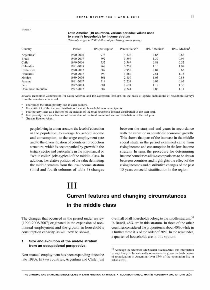
people living in urban areas, to the level of education in the population, to average household income and consumption, to the wage employment rate and to the diversification of countries’ production structure, which is accompanied by growth in the tertiary sector and particularly in the non-manual or “white collar” jobs typical of the middle-class. In addition, the relative position of the value delimiting the middle stratum from the low-income stratum (third and fourth columns of table 3) changes

between the start and end years in accordance with the variation in countries’ economic growth. This shows that part of the increase in the middle social strata in the period examined came from rising income and consumption in the low-income stratum. In sum, the procedure for determining income boundaries allows comparisons to be drawn between countries and highlights the effect of the rising incomes and distributive changes of the past 15 years on social stratification in the region.

TABLE 3

Latin America (10 countries, various periods): values used to classify households by income stratum(Monthly wages in 2000 dollars at purchasing power parity)

Country Period 4PL per capitaa Percentile 95b 4PL / Medianc 4PL / Mediand

Argentinae 1990-2006 976 4 522 0.65 0.62Brazil 1990-2007 792 3 397 1.39 0.96Chile 1990-2006 552 3 569 0.88 0.52Colombia 1991-2005 969 3 259 1.10 1.09Costa Rica 1990-2007 687 2 950 0.84 0.63Honduras 1990-2007 790 1 560 2.51 1.73Mexico 1989-2006 861 2 850 1.05 0.88Panama 1991-2007 514 2 254 0.93 0.65Peru 1997-2003 681 1 674 1.18 1.30Dominican Republic 1997-2007 887 2 241 0.88 1.11

Source: Economic Commission for Latin America and the Caribbean (eclac), on the basis of special tabulations of household surveys from the countries concerned.

a Four times the urban poverty line in each country.b Percentile 95 of the income distribution for main household income recipients.c Four poverty lines as a fraction of the median of the total household income distribution in the start year.d Four poverty lines as a fraction of the median of the total household income distribution in the end year.e Greater Buenos Aires.

IIICurrent features and changing circumstances

in the middle class

The changes that occurred in the period under review (1990-2006/2007) originated in the expansion of non-manual employment and the growth in household’s consumption capacity, as will now be shown.

1. Size and evolution of the middle stratum from an occupational perspective

Non-manual employment has been expanding since the late 1980s. In two countries, Argentina and Chile, just

over half of all households belong to the middle stratum.10 In Brazil, 46% are in this stratum. In three of the other countries considered the proportion is about 40%, while in a further three it is of the order of 30%. In the remainder, a quarter of households are in this stratum.

10 Although the reference is to Greater Buenos Aires, this information is very likely to be nationally representative given the high degree of urbanization in Argentina (over 85% of the population live in urban areas).

12



2. incorporation into the middle stratum via growth in consumption capacity

The countries analysed saw substantial absolute growth in per capita gross domestic product (gdp) within the space of a generation, increasing the income (and thus consumption) of households in the middle and low strata (see table 4).11 The result was an upward shift in the distribution by income bracket of households in the middle and low occupational strata from the under-US$ 5,000 a year bracket (calculated per family at purchasing power parity) towards the intermediate bracket (between US$ 5,000 and US$ 15,000 a year) and even the upper bracket (over US$ 15,000).12 This shift was recorded in almost all the countries (see table 5). There was consequently a large increase in the consumption capacity of households in the middle and low strata, but without significant changes in the (highly concentrated) income distribution.13 Because of this, there

11 Those main household income recipients (mhirs) who were 30 in 1990 are now around 50. Thus, income changes are characterized by mobility within the space of a generation.12 This shift, which is very important from a social stratification perspective, does not show up in analyses of income distribution between household deciles or quintiles.13 In Brazil, Colombia, Costa Rica and Peru, the income share of the 50% of households above the poorest 40% fell by between 1.5 and 4.5

were groups of manual workers who attained to incomes even higher than those of non-manual wage workers, whose remuneration failed to keep pace with theirs or even declined during the period under review.

This favourable change in low-stratum incomes, which was very marked in Brazil, Chile and Panama, was reinforced by the growth of consumer and mortgage lending and by the substantial fall in the relative (and in many cases absolute) prices of the goods consumed by the middle strata. Household purchasing power was also lifted by both the reduction in the number of people per household and the fall in the economic dependency rate, as analysed below.14 At the same time, the decline in the relative prices of mass consumption “durable” goods is partly the effect of comparison with increasingly costly health care and education, which are taking up a growing share of family budgets in the middle strata. This being so, there are limits on the ability of people in the low stratum to attain to middle-stratum consumption patterns, and social divides are often manifested in the affordability or otherwise of private health care and education.

percentage points. In the other countries, the share of this segment rose by between 1.5 and 2.5 percentage points. The increase in Honduras was 6 percentage points (eclac, 2008a, Statistical annex, table 12).14 Treating the household as the unit of analysis provides a better picture of these phenomena than analyses centred on individuals.

TABLE 4

Latin America (10 countries, various periods): level and growth of per capita gdp

(Monthly wages in 2000 dollars at purchasing power parity)

Country Perioda Start year End year Absolute increase Percentage increase Annual growth rate

Argentina 1990-2006 8 781 13 652 4 871 55.5 2.8Brazil 1990-2007 6 480 8 152 1 672 25.8 1.4Chile 1990-2006 5 744 10 939 5 194 90.4 4.1Colombia 1991-2005 5 590 6 536 945 16.9 1.1Costa Rica 1990-2007 6 268 9 067 2 799 44.6 2.2Honduras 1990-2007 2 744 3 312 568 20.7 1.1Mexico 1989-2006 7 517 9 967 2 450 32.6 1.7Panama 1991-2007 4 842 7 917 3 075 63.5 3.1Peru 1997-2003 4 812 4 942 130 2.7 0.4Dominican Republic 1997-2007 5 359 8 149 2 790 52.1 4.3 Argentina 1990-1999 8 781 12 322 3 541 40.3 3.8Argentina 1999-2002 12 322 10 098 -2 224 -18.0 -6.4Argentina 2002-2006 10 098 13 652 3 555 35.2 10.6

Source: prepared by the authors on the basis of information from World Bank databases.

gdp: gross domestic product.a Annual income based on monthly wages in 2000 dollars at purchasing power parity.

13



TABLE 5

Latin America (10 countries, various years): distribution of households by family income bracketa and occupational stratumb

Middle stratum Low stratum(Year)

Total Middle stratum Low stratum(Year)

Total

Argentinac (1990) (2006) Up to 5 000 5 15 11 3 9 6 5 001 to 15 000 33 34 32 31 37 32 Over 15 000 63 51 58 66 54 62

Brazil (1990) (2007) Up to 5 000 30 50 40 14 33 23 5001 to 15 000 35 36 35 43 47 44 Over 15 000 35 14 25 43 20 33

Chile (1990) (2006) Up to 5 000 23 41 32 12 20 15 5 001 to 15 000 43 45 43 36 52 42 Over 15 000 35 14 25 53 28 43

Colombia (1991) (2005) Up to 5 000 16 20 18 10 26 20 5 001 to 15 000 39 52 47 33 51 44 Over 15 000 45 28 35 58 23 36

Costa Rica (1990) (2007) Up to 5 000 10 26 19 9 21 15 5 001 to 15 000 43 54 49 33 51 42 Over 15 000 46 21 33 58 28 43

Honduras (1990) (2007) Up to 5 000 27 69 60 20 58 47 5 001 to 15 000 43 27 30 43 34 36 Over 15 000 30 5 10 37 9 17

Mexico (1989) (2006) Up to 5 000 11 27 21 8 20 14 5 001 to 15 000 47 53 50 40 55 47 Over 15 000 43 20 30 52 25 38

Panama (1991) (2007) Up to 5 000 17 54 39 12 37 26 5 001 to 15 000 45 36 40 44 44 43 Over 15000 38 10 21 43 19 31

Peru (1997) (2003) Up to 5 000 14 48 37 15 52 41 5 001 to 15 000 48 41 43 50 40 43 Over 15 000 38 11 20 36 8 17

Dominican Republic (1997) (2007) Up to 5 000 6 19 15 18 37 30 5 001 to 15 000 36 49 45 39 36 36 Over 15 000 58 32 40 43 27 35


a The income brackets are for annual income based on monthly wages in 2000 dollars at purchasing power parity.b Some columns do not add up to 100% because of rounding.c Greater Buenos Aires.

14



3. The heterogeneity of the middle strata

(a) Segmentation by definitionAccording to the definition adopted for the middle

strata, three subsets of households can be identified. They are: (i) The “consistent” middle class, consisting of middle-

class households whose main income provider (mhir) works in a non-manual occupation and where total family income (the sum of all income provided by all household members whether deriving from work, capital or transfers) ranges between the equivalent of four poverty lines (the lower limit) and the value of percentile 95 of the distribution (the upper limit).15

(ii) The “inconsistent” middle class, comprising households whose mhir works in a manual occupation, even though the family’s total income is of a middle-class level.

(iii) The “precarious” middle class. A large percentage of non-manual wage earners are in unstable employment with very low incomes and often with no contract or social security coverage, and thus are in very much the same situation as manual wage earners and low-skilled own-account workers. Some households in the middle stratum even live in absolute poverty. In the countries with the lowest poverty indices, between 5% and 9% of households in the middle occupational stratum were in this situation in 2006-2007. The proportion was about a sixth in Brazil and Mexico, between 20% and 30% in Colombia, the Dominican Republic and Peru, and as high as 38% in Honduras.16

(b) Hierarchical segmentationClassifying the population by occupation and sector

or category of employment gives an idea of the relative size of the two middle substrata (upper and lower).

15 Total family income is different from per capita household income, i.e., total income divided by the number of household members, which is what poverty studies use. Likewise, the unit of analysis is the household and not one of the individuals composing it, such as the household head, as is the case with social mobility studies (see León, Espíndola and Sembler, 2010).16 On the incidence of poverty, see eclac, Social Panorama of Latin America, various editions. This is an indicator whose calculations take account of the number of people in each household, and it includes the monetary income of all working members and income received by inactive members from non-work sources. However, over two thirds of the total income of households in each occupational stratum (the middle stratum in this case) is brought in by the main income recipient, so that the value of the poverty indicator largely captures the low incomes of working people in the lower middle stratum.

Although it is not possible to completely homogenize the occupational classifications used in 1990 with the current ones, it is possible to estimate what the relative size of these two strata would be now and to highlight the diversity of occupations in the middle occupational stratum.

In 7 of the 10 countries considered, the lower middle stratum contains between two thirds and over three quarters of all households in the whole middle stratum. This is the “gateway” for the middle class, to which a secondary or technical school credential provides access. This lower middle stratum is also the “border zone” with the low stratum, at least in income terms. It is among lower-level non-manual occupations that it is most common to see individual trajectories of upward mobility (by way of employment opportunities) and downward mobility (resulting from recessions and crises or other contingencies) (Kessler and Espinoza, 2007).

(c) Horizontal segmentationThe main types of horizontal segmentation that can

be identified in the middle class are between public- and private-sector employment and between wage and own-account employment.17

— Public- or private-sector employmentA number of authors have argued that the growth

of the middle class in the region took place because of the expansion of the State and the rise in public-sector employment. This particular middle sector is also presented as the embodiment of a culture that has underpinned the outlook of the whole “class”, based on a concern with education and a particular lifestyle, and is said to have been affected by reforms that have reduced the role of the State and thereby diminished public-sector employment (Klein and Tokman, 2000; Torche, 2006).

The present study has not been able to confirm this hypothesis. In only a few of the selected countries, admittedly, has it been possible to compare the scale of public-sector employment in 1990 and a recent year. In four cases (Argentina, Brazil, Chile and Mexico), the information for the base year did not discriminate between public- and private-sector employees. In cases where it was possible to make this comparison for main income recipients and for the employed population as a whole, middle-class public-sector employment was found to have held fairly steady in Honduras, Peru and

17 The self-employed are those not working for a wage or salary. They include both employers and own-account workers who do not have employees of their own. The distinction between wage earners and non-wage earners excludes employers (however many workers they employ), who form part of the high stratum according to the definition of occupational strata used.

15



Colombia, to have fallen in Costa Rica and Panama and to have grown only in the Dominican Republic (see tables 6 and 7).

In the cases of Argentina, Brazil and Chile there are data for the end year of the series used, plus other information indicative of the trend. For Brazil there is information from administrative records indicating that public-sector employment held steady as a share of total employment during the 1990s, although its

distribution changed, since it decreased at the federal and state levels and expanded at the municipal level (Pessoa de Carvalho Filho, Eneuton Dornellas 2002). It can thus be stated with some confidence that public-sector employment in the country continued at around 24% of the total. In Chile, the employment surveys of the National Institute of Statistics (ine) indicate that public-sector employment increased as a share of the total (from 6.9% to 7.4%) between 1990 and 2000,

TABLE 6

Latin America (10 countries): distribution of main household income recipients, by occupational category, around 1990 and 2007

Middle stratumbArgentinaa Brazil Chile Colombia Costa Rica

1990 2006 1990 2007 1990 2006 1991 2005 1990 2007

Public employee ... 20 ... 24 ... 14 16 18 40 31Private employee 74 58 66 53 66 63 39 42 40 58Own-account 26 22 34 24 34 23 44 40 20 11

Total 100 100 100 100 100 100 100 100 100 100

Totalc

Public employee ... 12 ... 13 ... 11 8 8 19 16Private employee 66 62 63 52 69 63 46 42 46 56Own-account 26 21 29 30 27 22 41 42 27 19Employer 8 5 8 6 4 4 4 8 9 10

Total 100 100 100 100 100 100 100 100 100 100

Middle stratumbHonduras Mexico Panama Peru Dominican

Republic

1990 2007 1989 2006 1991 2007 1997 2003 1997 2007

Public employee 24 24 ... ... 47 37 26 29 20 23Private employee 32 44 73 70 39 49 40 40 43 44Own-account 44 32 27 30 14 14 33 31 38 33

Total 100 100 100 100 100 100 100 100 100 100

Totalc Public employee 9 9 ... ... 25 18 10 11 12 12Private employee 36 45 65 69 35 47 33 33 37 34Own-account 53 43 30 25 34 30 47 47 45 48Employer 2 3 5 6 5 5 10 9 6 6

Total 100 100 100 100 100 100 100 100 100 100


a Greater Buenos Aires.b Main income recipients in the middle occupational stratum. Employers belong to the high occupational stratum.c All main income recipients (from the high, middle and low occupational strata)....: The missing data are not separately available. Public-sector employees are included in the private-sector employees category in these

cases.

16



TABLE 7

Latin America (10 countries): distribution of all persons in employment, by occupational category, around 1990 and 2007

Middle stratumbArgentinaa Brazil Chile Colombia Costa Rica

1990 2006 1990 2007 1990 2006 1991 2005 1990 2007

Public employee ... 18 ... 19 ... 13 13 13 32 27Private employee 74 61 71 56 71 65 51 46 46 60Own-account 25 20 28 24 29 21 36 40 21 13Employer 1 1 1 1 0 0 1 1 1 1

Total 100 100 100 100 100 100 100 100 100 100

Totalc Public employee ... 12 ... 12 ... 10 7 6 16 14Private employee 70 65 66 54 73 66 53 45 52 60Own-account 25 19 29 31 24 21 38 44 26 18Employer 5 4 5 4 3 3 3 5 6 7

Total 100 100 100 100 100 100 100 100 100 100

Middle stratumbHonduras Mexico Panama Peru Dominican

Republic

1990 2007 1989 2006 1991 2007 1997 2003 1997 2007

Public employee 19 19 ... ... 40 30 20 20 17 20Private employee 38 44 75 69 46 54 43 42 48 45Own-account 43 36 25 30 14 17 36 37 34 34Employer 0 1 0 1 0 0 1 1 0 1

Total 100 100 100 100 100 100 100 100 100 100

Totalc Public employee 7 7 ... ... 23 15 9 8 11 12Private employee 38 44 67 68 41 50 35 33 45 37Own-account 54 46 30 28 33 31 51 55 40 47Employer 1 2 3 4 3 3 5 5 4 4

Total 100 100 100 100 100 100 100 100 100 100


a Greater Buenos Aires.b All those employed in households in the middle occupational stratum.c All those employed in households in the high, middle and low occupational strata....: The missing data are not separately available. Public-sector employees are included in the private-sector employees category in these cases.

implying a slight drop in its share of middle-sector employment, from 22% to 20% (León and Martínez, 2007; Torche and Wormald, 2007).18 Since the middle of the last decade, however, public-sector employment

18 The data on Chile were obtained from the National Socio-economic Survey (casen 1990 and 2006), which has advantages from the standpoint of income measurement. The employment surveys of the National Institute of Statistics (ine), on the other hand, allow measurements of the level and structure of employment to be compared over time.

has increased by some 35%, outstripping the growth in private-sector wage employment (22%) and own-account employment (20%) (Méndez, 2009).19

In Argentina, the total public-sector share of employment increased slightly from 1999 to 2006 (from 15.5% to 16.2%), after peaking in 2002 (21.7%). This figure includes those employed under government job

19 The percentage increases in the three categories are for the 1996-2006 period. See Méndez (2009, table 5).

17



creation programmes.20 In Mexico, the data for 1994, 1996, 1998 and 2002 show a slight drop and then a recovery, so that the figure ranged between 11% and 12% over the period (eclac, 2008a).21

To sum up, the public-sector share of middle-class employment did not fall substantially in these countries. This tells us nothing about whether the symbolic and socio-economic status of such jobs may have declined. However, the pay of public-sector employees has increased by more than that of private-sector wage earners in most of the countries in recent years (eclac, 2008a).22

— Wage earners and the self-employedThere was a clearer restructuring trend in private-

sector occupations. Wage employment increased and self-employment or own-account working declined. This seems to run counter to the idea of a middle class increasingly composed of professionals and skilled technical workers operating independently on a self-employment basis or as small employers. In all the countries analysed except Mexico and Panama, self-employment lost ground in

20 The Heads of Household Programme began to be operated in early 2002 and created over 2 million jobs for the unemployed (figure published by the Ministry of Labour, Employment and Social Security, http://www.trabajo.gov.ar).21 See eclac (2008a), Statistical annex, table 17.22 See eclac (2008a), Statistical annex, table 21.

the middle sector. This was more marked among mhirs than among the generality of people in employment in this stratum (see tables 6 and 7).23

The rise in female workforce participation was crucial to the growth of the middle stratum. This participation grew substantially between 1990 and 2007. In 7 of the 10 countries, women’s economic activity rate rose by between 6 and 14 percentage points. The increase was greatest in Brazil, Chile, Costa Rica and Mexico, the countries where the middle stratum grew most strongly.24 The growth of female participation was particularly strong among more highly educated women (eclac, 2008a), who went into commerce and services occupations (office workers, secretaries, shop and supermarket employees and health service workers). Participation rates also rose among women with higher education (professionals composing the upper middle stratum), but by less as they were already quite high by the early 1990s.

23 Self-employment declined in the great majority of countries. There is no breakdown of the data by age group. If there were, it would be possible to observe whether the reduction in self-employment is also found among young people entering the labour market. Again, the occupational characteristics recorded are those of people’s main job. People who are wage earners in their main job often work on a self-employed basis in their secondary economic activity.24 See eclac (2008a), Statistical annex, table 16.

IVThe determinants of change

1. Size matters

The real impact of growth on consumption patterns cannot be properly appreciated when the data are analysed in percentage terms. It comes out more clearly when absolute values are considered, together with the size and growth rate of the population, especially in urban centres or in particular areas of large cities.

The number of middle-class households grew by 56 million in the universe of 10 countries taken, representing 80% of the Latin American population. This implies a large expansion of the consumer market. In the region’s largest country, Brazil, the number of people living in middle-stratum households rose from 23 million in 1990 to 61 million in 2007. The number of households in the

middle stratum more than doubled from 9.3 million in 1990 to 20.8 million in 2007, and their share of all households rose from 36% to 46%. In a similar period, the number of middle-class households in Chile grew by some 1.1 million, almost doubling the figure of 1.2 million estimated for the start year. In Argentina, while the proportion of middle-class households fell from 56% to 52%, the absolute number increased by about half a million, which is actually more than the increase in the number of people (440 thousand), owing to the sharp decline in the size of households in this stratum. The large number and spatial concentration of middle-stratum households have created a demonstration effect in society at large, influencing consumption habits and consequently generating a widespread feeling of belonging to this stratum.

18



The decline in the number of people per household was seen everywhere, albeit to varying degrees that depended on the fertility level in each country 15 years ago, socio-economic conditions and the cultural patterns characterizing the different social strata (eclac, 2004). In countries with larger households, the drop in the number of members in the early 1990s is probably explained mostly by falling fertility (Mexico and Honduras), while in those with lower fertility rates the reduction owes more to the rising proportion of single-person households and those consisting of childless couples (Argentina).

The dependency rate, which combines the effects of falling household size and a rising number of members in work, fell both in the middle stratum (from 2.7% to 2.1%) and in the low one (from 2.8% to 2.4%). A crucial role was played in this process both by the drop in fertility and by the rise in female workforce participation (especially among more educated women) and the change in family types. Brazil and Mexico are the two countries that registered the largest increase in the rate of female participation in economic activity during the period reviewed. This rate increased from 44% to 58% in Brazil and from 30% to 48% in Mexico.25

2. The middle sectors are growing

Taking the countries analysed as a whole, the number of middle-class households has been growing, as has the proportion of all households they represent. The exceptions are Argentina, where this share fell from 56% to 52%, and Colombia, where it held steady. The middle stratum is larger in more developed countries. Whereas it only includes 25% of households in Honduras, the proportion in Argentina and Chile is around 50%. In Chile, 40% of households were middle-class in 1990, whereas 52% are now. Another development of note is the increase in family incomes in lower-class households, defined as those whose mhir works in a manual occupation. This has caused incomes in this sector of households to shift to a higher bracket, i.e., from the stratum where family incomes are US$ 5,000 and under to the stratum where they are between US$ 5,000 to US$ 15,000.

There has been a large increase in middle-income households. In Argentina, Chile and Panama this increase has largely come from improvements in households in the lower occupational stratum. In Brazil, Costa Rica, Honduras and Mexico, the increase in these households

25 See eclac (2008a, Statistical annex, table 16).

was smaller but still significant, especially given the expansion in the total number of households in the middle social strata (see the last column of table 8).

It should be emphasized, however, that a fairly large proportion of all middle-stratum households have inadequate incomes. The figure for households in the middle social strata with low incomes is 51% in Brazil,

TABLE 8

Latin America (10 countries): households in the middle social strata, around 1990 and 2007

Country Year

With middle

incomesa

Middle stratum

with low incomesb

Middle social strata

Total households

(percentagesc) (thousands)

Argentinad 1990 25 42 67 2 1812006 54 20 74 3 134

Brazil 1990 24 22 46 15 8252007 26 27 53 33 454

Chile 1990 31 23 54 1 7022006 54 16 70 3 645

Colombia 1991 23 20 43 3 0122005 23 16 39 4 674

Costa Rica 1990 45 13 58 3202007 50 12 62 834

Honduras 1990 9 12 21 1702007 11 17 28 544

Mexico 1989 23 21 44 6 9402006 26 22 48 14 160

Panama 1991 39 12 51 2602007 47 12 59 610

Peru 1997 16 16 32 1 6652003 14 18 32 2 248

Dominican Republic

1997 28 11 39 6332007 20 18 38 1 081


a Households where the income of the mhir is greater than four times the per capita urban poverty line and less than the percentile 95 value.

b Households in the middle occupational stratum where the income of the mhir is four times the per capita urban poverty line or less.

c Percentages of all households in the country. d Greater Buenos Aires.

19



while in Chile it fell from 43% to 23%.26 A similar change occurred in Argentina, although the increase in the proportion of households belonging to the middle social strata was smaller than in Chile. In the other countries, these changes in the composition of the middle social strata were less substantial.

When the middle social strata are delimited using the combination of occupational category and income, the mass of such households is large, accounting for some 50% or even more of the total in Argentina, Brazil, Chile, Costa Rica, Mexico and Panama. These figures support the picture that emerges from different opinion polls and surveys, where a very high proportion of respondents claim to belong to the “middle class”.

3. Educational capital is increasing, but is being devalued

Education levels have increased rapidly in the region over the past two decades. Rising enrolment and graduation rates at all levels have led to a very substantial change in the educational profile of the economically active population. Educational capital remains crucial for incorporation into the middle strata, whether in routine non-manual jobs, which require certification of the second cycle of intermediate or secondary education, or in occupations typical of the upper middle stratum, requiring a professional higher education qualification.

Completion of the secondary cycle is now becoming the rule for the new generations. In 1990, between 30% and 40% of middle-class mhirs had attained this level of education. Now, between 50% and 70% of mhirs have completed it, depending on the country. In Argentina, 31% of mhirs had formerly completed their technical education, whereas the figure now is 47%. Meanwhile, the proportion of mhirs with this level of education has risen from 28% to 48% in Brazil and from 41% to 57% in Chile. Likewise, 83% of middle-class young people have completed at least their secondary studies, and may have gone on to a higher educational level, by the time they enter the labour market.

This increase in education has also occurred among people working in low-stratum occupations, but only those with complete secondary education have a good chance of obtaining non-manual jobs. Those already in the labour market who have not completed secondary

26 Households where the income of the main recipient is less than four times the poverty line per household member. The percentages cited are the ratio between the second and third columns of table 8, multiplied by 100.

education are not paid substantially more even if they have some extra years of schooling. Conversely, incomes increase rapidly for those who have completed the secondary cycle and have some extra years of education on top of this.27

Increasingly widespread completion of the secondary education cycle has led to a relative devaluation of education, manifested in the way the earnings of those who have completed this level have progressively fallen behind those of people who have completed higher education, something that can clearly be seen among the young (eclac, 2008b).28

As increasing numbers of people in the low stratum (manual workers) have achieved higher levels of education and income, and as large segments of the lower middle stratum (non-manual) with complete secondary education have come to be employed for relatively low pay, the incomes of the two strata have tended to converge and earnings have increasingly become dissociated from occupation type.

It is important to realize that, relatively speaking, people completing secondary education now are lower-paid than those who entered the labour market with this level of qualifications in the past. Completion of secondary education was traditionally the educational threshold for the middle class, as it was understood to confer greater appropriation of the cultural codes of modernity and thus to facilitate access to “intellectual” work. Mass completion of this level was to make it less of a mark of distinction.

Considering the large proportion of young people who have completed secondary education, the glass might be seen as “half full”. It might also be seen as “half empty”, however, if what is considered instead is the reduced status, both symbolic and material, associated with this attainment. In addition, the standardized tests now applied to measure effective learning and its quality have systematically revealed widespread shortcomings, hastening the symbolic devaluation of the progress made in terms of years of schooling.

Nonetheless, the educational attainments of these new cohorts and the types of job they go into are still highly segmented. In Chile, for example, despite the rapid expansion of education coverage, differences remain in the educational profiles of young people by social category. Over 83% of those from middle-sector families enter the labour market with 12 years

27 See eclac (2008b, chapter IV, pp. 141-144).28 This has been a factor in widening pay divides and keeping the inequality of income distribution high in the region.

20



of schooling or more, whereas only 43% of those from working-class families do (León and Martínez, 2007). At the same time, the extraordinary expansion of secondary enrolment during the last decade and the mobility it has brought are striking: 70% of Chilean university students are the first generation in their families to have studied at this level.

4. The income divide between manual and non-manual occupations is becoming less clear-cut

There is a tendency towards homogenization of the incomes earned by middle-class and lower-class individuals. This is because there are many low-grade non-manual jobs, at the same time as there are well-paid manual occupations. There are “manual workers [who] possess more knowledge than many middle-class workers, earn more and develop clearer aspirations of social mobility. Generally speaking… manual worker status does not preclude eventual membership of the middle class, depending on the industry, the location and the culture of the occupational and social environment. Competitive workers tend to develop expectations, a world view and political demands different to those developed by uncompetitive workers” (Mora y Araujo, 2008).

5. The penetration of middle-stratum goods and the demonstration effect

The process described has greatly increased the demand for consumer goods (electrical and electronic products, mobile phones, the Internet, cars, etc.), making the penetration of these goods more “visible”. This may have raised their status among people in the low stratum and created a perception that acquiring them is the main route to social integration and not owning them a form of exclusion.

Argentina is a special case. The 2001-2002 crisis resulted in a high level of open unemployment and a decline in family incomes, among other adverse consequences. However, renewed growth from 2003 until well into 2008 meant that, on average, households in the middle and low strata recovered their pre-crisis income levels. In a long-term (point-to-point) comparison, therefore, no marked deterioration is seen in the income of the middle occupational strata. Table 9 summarizes changes in the distribution of households by income

bracket in three periods (1990-1999, 1999-2002 and 2002-2006) in Greater Buenos Aires. Between 1999 and 2002, the percentage of households with annual incomes of less than US$ 5,000 trebled in the middle occupational stratum and quadrupled in the lower stratum.29 The scale of the decline can be seen in the downward shift of all households in the income scale (see the third and sixth columns of table 9). During the recovery, however, income growth benefited low-stratum households more (72%) than middle-stratum ones (39%), markedly reducing the income disparity between the two.30 This appears to indicate that the middle stratum in Argentina too expanded as a result of the rising consumption capacity of low-stratum households, although this is a more recent phenomenon, as it is in Brazil.

6. The competitive and the uncompetitive

Globalization and the interconnectedness of the world economy are affecting the middle classes by giving a crucial role to competitiveness, in the twofold sense of possessing the necessary skills and having the desire to compete and a capacity for risk-taking. The uncompetitive are those whose technological and educational accomplishments are obsolescent and who are therefore ill-prepared for a changing labour market, so that they face the risk of unemployment and a downward drift in wages. Again, insofar as competitiveness involves the incessant renewal of information and knowledge, reskilling and adaptation to new forms of organization, it creates strains and new divisions between losers and winners. All this has undermined a section of the middle class whose specializations or ways of working are less in demand than formerly in the labour market, and particularly those whose age or education level makes it harder for them to adapt. Unionization can help to maintain and even increase pay levels, but its main usefulness is in protecting working conditions and enhancing stability by making it costlier for firms to reduce the number of workers they employ (Mora y Araujo, 2008).

29 It should be recalled that each “occupational stratum” includes all main household income recipients, whether working or inactive.30 The average monthly income figures for households in the middle stratum were US$ 1,855 in 2002 and US$ 2,574 in 2006. The figures for the low stratum were US$ 1,067 and US$ 1,835 a month in 2000 dollars at purchasing power parity.

21



It is worth reflecting on the differences between the size of the middle class as measured by “objective” criteria and the very much larger number of people self-identifying with that class in demoscopic studies.

1. The role of consumption in middle-class identity: the euphoric side

Mass take-up of consumer credit has meant greater access to durable goods and certain services. According to data from eclac, the Inter-American Development Bank (idb) and the World Bank, domestic credit grew from 30% to 55% of gdp in the region between 1990 and 2006, with even stronger growth in mercosur (Matesanz and Palma, 2008), and penetration was particularly strong in the middle and low strata. Credit growth in the high sectors matched output growth. The finding overall is that credit grew far faster than output, suggesting that it reached other parts of the population.

The case of Brazil is revealing. Economic growth contributed to the rise in lending operations, which increased tenfold between 1999 and 2007 even as their cost fell. The interest rate, while still very high, dropped from 90.2% in 1999 to 43.9% in 2007. This easier credit strengthened the large consumer market among the poorer classes, and it expanded beyond so-called “class C” households to those in strata D and E, the lowest in the stratification (Oliveira, 2010).31

All this has coincided with the advent of the low-cost society (Gaggi and Narduzzi, 2007). A combination of factors has brought in an era of mass consumption: the opening up of international trade, the delocalization

31 Groups or strata D and E of the socio-economic classification used in market studies in Brazil comprise the lowest-income households in the stratification scale. The class known as C is normally identified with the lower middle class, according to the Getulio Vargas Foundation. This now appears to have become the largest class in Brazil thanks to the socio-economic rise of people formerly in classes D and E.

TABLE 9

Argentina (Greater Buenos Aires, three periods): distribution of households by family income bracketa and occupational stratumb

(Percentages)

Middle stratum Low stratum Total Middle stratum Low stratum Total

1990 1999

Up to 5 000 5 15 11 5 6 55 001 to 15 000 33 34 32 28 41 32Over 15 000 63 51 58 67 53 62

1999 2002

Up to 5 000 5 6 5 16 26 205 001 to 15 000 28 41 32 39 49 42Over 15 000 67 53 62 46 26 39

2002 2006

Up to 5 000 16 26 20 3 9 65 001 to 15 000 39 49 42 31 37 32Over 15 000 46 26 39 66 54 62

Source: eclac, on the basis of special tabulations of household surveys from the countries concerned.

a The income brackets are for annual income in 2000 dollars at purchasing power parity.b Some columns do not add up to 100% because of rounding.

Vwhat does it mean to be middle class?

22



of product and parts manufacturing in pursuit of lower-cost factors of production, the rapid spread of new mass production technologies, and scaling up as new consumers have emerged. Electronic items, computers, clothing, package travel, different household items, mobile phones, etc., are all part of an ever larger and more dynamic market of avid consumers and financing.

The combination of greater borrowing capacity (via credit cards) and greater consumption plus the development of large firms oriented towards low-cost mass market products have contributed to the emergence of a new middle class.

Collective identities are now defined and groups distinguished by the symbolic content of consumption, which expresses shared meanings and reinforces the marks of identity and social position. In other words, specific consumers’ consumption type provides “signals” that identify them as members of a particular socio-economic stratum. In this context, consumption capacity is central to the formation of middle-class identity and its variability redefines the goods that fulfil the differentiating role associated symbolically with this human activity at any given time (Oliveira, 2010).

Of course, consumption has always played this role as an identifier of lifestyles and as a marker for membership of a social class or group. With the rapid growth of the low-cost society, however, a sophisticated and affluent higher class has tended to be joined by a mass market echelon whose members have medium-low incomes but are able to afford goods and services that were formerly the preserve of higher-income sectors (Gaggi and Narduzzi, 2007). Participation in this new mass consumption tends to be seen and experienced as membership of the middle class.

The fact that everyone is consuming does not mean there is no diversity. There are “consumer profiles” that are mainly associated with age criteria, for example. All this helps to make consumption less homogeneous and create greater freedom for consumers.

This provides an insight into important changes in people’s ways of life. In former times, group pressure tended to pigeonhole them by their family, occupational or class relationships. “Late” modernity has increased individualism, as expressed in a greater concern with the self and the opportunity to take up different material and symbolic consumption options. The result is that consumers have fragmented into differentiated groups in accordance with their tastes and affinities, something that has also been instrumental in expanding the market.

This new functioning of society and of individuals’ self-perception has enlarged the domain of personal choice,

enabling people to mark the differences characteristic of “social closure”: the choice of a place of residence and type of housing, the school their children go to, culinary tastes and the places where they choose to satisfy them, places of entertainment and cultural consumption. Studies by Svampa (2001) on life in the so-called “countries”32 of the upper middle class in Argentina and the later emphasis on the “return to the city” highlighted by Wortman (2010) reveal both this freedom of choice and the way tastes can change in a fairly short space of time. Similarly, Arellano (2008) discusses the emergence in Lima of a new middle class whose origins are in the sierra and which is not “copying” the behaviour of traditional middle-class sectors but is innovating and defining its own lifestyle, in its culinary and musical choices and in other ways.

Of course, not everyone has the same consumption opportunities. There is a sophisticated, affluent higher class with more scope for choice. One might also identify a more established upper middle class with good levels of income and greater opportunities for personalized choices. In contrast, the lower middle class, and its new members in particular, are fulfilling their consumption aspirations in a more standardized way. Nonetheless, a degree of diversity can be found here as well.

2. The aspiration gap

People have goals or desires they hope to be able to realize over their lifetimes. In a society characterized by constant renewal, the distance between expectations and attainments is likely to create frustration. Uncompetitive segments of society are subjected to consumerist stimuli that are heightened by rising education levels, urban life and the mass media, but lack the means to satisfy their aspirations and are thus frustrated in their expectations.

There are fields, such as connectivity and interactive long-distance communication, that are expanding particularly among the young. The same is happening in the cultural industries, especially music and audio-visual production and consumption. Falling product prices in these areas have led to greater individualization of the options available to large sections of society, creating the paradox of “mass individualization” (Hopenhayn, 2005, p. 56).

32 This is the name given in Argentina and elsewhere to gated communities or condominiums that are usually outside the urban area and have heavy security for their residents, generally people with high or medium-high incomes.

23



In this context, membership of the middle class is not necessarily determined by people’s occupational category or even income, but by their status as consumers in a society where they can afford a wide range of goods that are not standardized but can be selected on the basis

of particular preferences. People aspire to participate in this new consumer realm, and this is identified with being middle class. Ergo, there does not necessarily have to be a correlation between objective conditions and subjective perceptions.

VIConclusions

The current situation of the middle strata unquestionably presents some novelties. In the period from 1990 to before the 2008 crisis, the number of middle-class households and their average incomes both grew. This resulted from rising gdp in the countries combined with lower poverty and a small improvement in income distribution. Different factors opened the way to these changes. The “short version”, taking just the first years of the new century, is that macro factors were largely responsible, in the form of improved financing facilities for the region’s countries and strong demand for many of their exportable products. The “long version” is that slow-acting developmental transformations have taken place, such as the decline in the family dependency rate and faster incorporation of women into the labour market, together with the benefits of the “demographic dividend” (i.e., the increase in the number of income recipients per household relative to the number of dependants). This has coincided with the so-called “low-cost society”, characterized by the emergence of industries which set out to bring down the unit cost of many “symbolic” consumer goods formerly affordable only for higher-income strata and by the increased availability of credit at lower interest rates for people on low incomes, contributing to a dynamic of upward social mobility.

The two-dimensional definition of the middle class used in this study brings to light the incorporation into the middle class of households from the manual occupational stratum as their incomes (and thence their consumption) have increased because of the economic growth of the past 16 years. Even without significant improvements in income distribution, the substantial absolute growth in per capita gdp between the beginning of the last decade and the middle of the present one allowed consumption to rise in middle- and lower-stratum households in several countries. There was a “shift” in the household income distribution towards higher income brackets. This was very significant for social stratification, even if it is not perceptible in analyses of income distribution

across household deciles or quintiles. It all helped to increase demand for consumer goods that came into increasingly widespread use (electrical and electronic products, mobile phones, Internet access, cars, etc.) and rendered more “visible” the penetration of such goods among large sections of the population. In these changes lies one of the clues to the greater heterogeneity of the middle strata in terms of occupation type, place of residence and opportunities for different lifestyles, resulting in turn in a greater homogeneity in the goods that can be afforded by those “incorporated” into the middle stratum by way of rising incomes and access to consumption, the latter having been expanded by the remarkable growth in credit.

This study set out by recognizing that the position of individuals in the labour market is no longer sufficient to describe the social structure and delimit its intermediate strata, as the character of occupations has changed and other aspects have become more important, such as consumption and lifestyles. From an occupational perspective, the size of the middle stratum differed substantially by countries’ development level, but increased in all of them except one where it fell slightly and one where it held steady. The rise in the absolute number of middle-stratum households (56 million, taking the total to 128 million households in 16 years) gives a better idea of the remarkable demonstration effect generated by certain increasingly widespread consumption patterns. In the two countries with the largest populations (Brazil and Mexico), the numbers increased by 28 million and 14 million households, respectively.

There were major changes in household size and composition that account for the expansion of the middle strata over the past 15 years. Lower fertility and dependency rates allowed more women to go out to work, and the net result was to increase family incomes and consumption opportunities in the middle and lower strata.

24



In most of the countries, the lower middle sector accounts for between two thirds and over three quarters of all middle-stratum households. Furthermore, a large proportion of wage earners in this sector work under poor conditions, with very low incomes and often without a contract or social security coverage. The analysis of “horizontal” segmentation in the middle stratum does not support either the hypothesis of a diminishing role for the State as an employer or the hypothesis of rising self-employment and a matching reduction in wage employment in the private sector.

Although there are now greater opportunities for educational attainment, a complete secondary education has been devalued in terms of the employment and earning opportunities it commands. The educational attainments of people in the lower stratum have been

rising and large sections of the lower middle stratum have complete secondary education, and this has led to homogenization of incomes between the two strata and to occupation type becoming decoupled from income.

Lastly, it is important to emphasize the structural changes undergone by the region’s societies in the period analysed, especially those deriving from the remarkable development of international trade, including the emergence of new actors with a huge capacity for producing manufactured goods for export while providing a large source of demand for products of every kind. This has led to major changes in social stratification in the countries analysed, and these have been manifested particularly strongly in alterations in the size and characteristics of the middle classes.

(Original: Spanish)

Bibliography

Arellano, Rolando (2008), Valores e ideología: el comportamiento político y económico de las nuevas clases medias en América Latina, Barcelona, Economic Commission for Latin America and the Caribbean (eclac)/Centro de Información y Documentación de Barcelona (cidob).

Birdsall, Nancy, Carol Graham and S. Pettinato (2000), “Stuck in the tunnel: is globalization muddling the middle class?”, Working Paper, No. 14, Washington, D.C., Center on Social and Economic Dynamics, The Brookings Institution, August.

eclac (Economic Commission for Latin America and the Caribbean) (2008a), Social Panorama of Latin America, 2008 (LC/G.2402-P), Santiago, Chile, December. United Nations publication, Sales No. E.08.II.G.89.

(2008b), Juventud y cohesión social en Iberoamérica: un modelo para armar (LC/G.2391), Santiago, Chile, Economic Commission for Latin America and the Caribbean/Spanish Agency for International Cooperation/Ibero-American Secretariat/Ibero-American Youth Organization, Santiago, Chile, October.

(2007), Social Panorama of Latin America, 2007 (LC/G.2351-P), Santiago, Chile. United Nations publication, Sales No. E.07.II.G.124.

(2004), Social Panorama of Latina America, 2004 (LC/G.2259-P), Santiago, Chile. United Nations publication, Sales No. E.04.II.G.148.

eclac/ilo (Economic Commission for Latin America and the Caribbean/International Labour Organization) (2009), “Crisis and the labour market”, eclac/ilo Bulletin, No. 1, Santiago, Chile, June.

Escobar Latapí, Agustín and Laura Pedraza (2010), “Clases medias en México: transformación social, sujetos múltiples”, Clases medias en América Latina. Retrospectiva y cambios recientes, Rolando Franco, Martín Hopenhayn and Arturo León, Mexico City, eclac/Ibero-American Secretariat/Siglo XXI editores.

Espinoza, Vicente (2009), “Entrevista”, ¿Cómo han cambiado la o las clases medias durante los últimos 20 años?, Santiago, Chile, Expansiva, May.

Franco, Rolando and Martín Hopenhayn (2010), “Las clases medias en América Latina: historias cruzadas y miradas diversas”, Clases medias en América Latina. Retrospectiva y cambios recientes, Rolando Franco, Martín Hopenhayn and Arturo León, Mexico City, eclac/Ibero-American Secretariat/Siglo XXI editores.

Franco, Rolando, Martín Hopenhayn and Arturo León (2010), Clases medias en América Latina. Retrospectiva y cambios recientes, Mexico City, eclac/Ibero-American Secretariat/Siglo XXI editores.

Franco, Rolando, Arturo León and Raúl Atria (2007), Estratificación y movilidad social en América Latina. Transformaciones estructurales de un cuarto de siglo, Santiago, Chile, Economic Commission for Latin America and the Caribbean (cepal)/lom ediciones.

Gaggi, Massimo and Edoardo Narduzzi (2007), El fin de la clase media y el nacimiento de la sociedad de bajo coste, Madrid, Editorial Lengua de Trapo.

Hopenhayn, Martín (2005), América Latina desigual y descentrada, Buenos Aires, Editorial Norma.

Kessler, Gabriel and Vicente Espinoza (2007), “Movilidad social y trayectorias ocupacionales en Buenos Aires. Continuidades, rupturas y paradojas”, Estratificación y movilidad social en América Latina. Transformaciones estructurales de un cuarto de siglo, Rolando Franco, Arturo León and Raúl Atria, Santiago, Chile, Economic Commission for Latin America and the Caribbean (eclac)/lom ediciones.

Klein, Emilio and Víctor Tokman (2000), “Social stratification under tension in a globalized era”, cepal Review, No. 72 (LC/G.2120-P), Santiago, Chile, Economic Commission for Latin America and the Caribbean (eclac), December.

León, Arturo, Ernesto Espíndola and Camilo Sembler (2010), “Clases medias en América Latina: una visión de sus cambios en las dos últimas décadas”, Clases medias en América Latina. Retrospectiva y cambios recientes, Rolando Franco, Martín Hopenhayn and Arturo León, Mexico City, eclac/Ibero-American Secretariat/Siglo XXI editores.

25



León, Arturo and Javier Martínez (2007), “La estratificación social en Chile hacia fines del siglo XX”, Estratificación y movilidad social en América Latina. Transformaciones estructurales de un cuarto de siglo, Rolando Franco, Arturo León and Raúl Atria, Santiago, Chile, Economic Commission for Latin America and the Caribbean (eclac)/lom ediciones.

Matesanz, David and Andrés Palma (2008), Las clases medias latinoamericanas y España: oportunidades y desafíos, Madrid, Observatorio de Política Exterior Española (opex)-Fundación Alternativas.

Méndez, María Luisa (2010), “Clases medias en Chile: transformaciones, sentido de pertenencia y tensiones entre proyectos de movilidad”, Clases medias en América Latina. Retrospectiva y cambios recientes, Rolando Franco, Martín Hopenhayn and Arturo León, Mexico City, eclac/Ibero-American Secretariat/Siglo XXI editores.

(2009), “Entrevista”, ¿Cómo han cambiado la o las clases medias durante los últimos 20 años?, Santiago, Chile, Expansiva, May.

Méndez, María Luisa and Modesto Gayo (2007), “El perfil de un debate: movilidad y meritocracia. Contribución al estudio de las sociedades latinoamericanas”, Estratificación y movilidad social en América Latina. Transformaciones estructurales de un cuarto de siglo, Rolando Franco, Arturo León and Raúl Atria, Santiago, Chile, Economic Commission for Latin America and the Caribbean (eclac)/lom ediciones.

Mora y Araujo, Manuel (2008), Vulnerabilidad de las clases medias en América Latina. Competitividad individual y posición social, Barcelona, Economic Commission for Latin America and the Caribbean (eclac)/Centro de Información y Documentación de Barcelona (cidob).

(2007), “La estructura social de la Argentina: evidencias y conjeturas acerca de la estratificación actual”, Estratificación y movilidad social en América Latina. Transformaciones estructurales de un cuarto de siglo, Rolando Franco, Arturo León and Raúl Atria, Santiago, Chile, Economic Commission for Latin America and the Caribbean (eclac)/lom ediciones.

Oliveira, Fabiana Luci de (2010), “Movilidad social y económica en el Brasil. ¿Una nueva clase media?”, Clases medias en América Latina. Retrospectiva y cambios recientes, Rolando Franco, Martín Hopenhayn and Arturo León, Mexico City, eclac/Ibero-American Secretariat/Siglo XXI editores.

Pessoa de Carvalho Filho, Eneuton Dornellas (2002), “Evolução do emprego no Brasil nos anos 60”, thesis, Campinas, State University at Campinas.

Solimano, Andrés (2008), “The middle class and the development process”, Macroeconomía del desarrollo series, No. 65 (LC/L.2892-P), Santiago, Chile, Economic Commission for Latin America and the Caribbean (eclac), April. United Nations publication, Sales No. E.08.II.G.29.

Svampa, Maristella (2001), Los que ganaron, la vida en countries y barrios privados, Buenos Aires, Editorial Biblos.

Toche, Eduardo (2010), “Aproximaciones a la clase media de Lima”, Clases medias en América Latina. Retrospectiva y cambios recientes, Rolando Franco, Martín Hopenhayn and Arturo León, Mexico City, eclac/Ibero-American Secretariat/Siglo XXI editores.

Torche, Florencia (2006), “Una clasificación de clases para la sociedad chilena”, Revista de sociología, No. 20, Santiago, Chile, Faculty of Social Sciences, University of Chile.

Torche, Florencia and Guillermo Wormald (2007), “Chile, entre la adscripción y el logro”, Estratificación y movilidad social en América Latina. Transformaciones estructurales de un cuarto de siglo, Rolando Franco, Arturo León and Raúl Atria, Santiago, Chile, Economic Commission for Latin America and the Caribbean (eclac)/lom ediciones.

Wilson, Dominic and Raluca Dragusanu (2008), The Expanding Middle: the Exploding World Middle Class and Falling Global Inequality, New York, Goldman Sachs, July.

World Bank (2006), World Development Report 2006: Equity and Development, Washington, D.C.

Wortman, Ana (2010), “Las clases medias argentinas”, Clases medias en América Latina. Retrospectiva y cambios recientes, Rolando Franco, Martín Hopenhayn and Arturo León, Mexico City, eclac/Ibero-American Secretariat/Siglo XXI editores.


27

Wage inequality in Latin America:a decade of changes

Dante Contreras and Sebastián Gallegos

This work helps to explain the determinants of wage distribution

in Latin America in the 1990s. The study employs the basic model of

wage variance decomposition developed by Fields (2002), on the basis

of an estimated Mincer wage equation adjusted for selection bias, which

enables quantification of the impacts of the different explanatory variables

of wage inequality. One of the main findings is that education is by far

the most important factor in wage inequality in the region. What is more,

it has become more significant over time, even though the explanatory

power of the model has remained stable.

KEYWORDS

Income distribution

Wages

Equal pay

Education

Gender

Multivariate analysis

Statistical methodology

Latin America

Dante Contreras

Professor, Department of

Economics,

University of Chile


Sebastián Gallegos

PhD candidate in economics

Northwestern University


28

WAgE InEquALITy In LATIn AmERICA: A dECAdE oF ChAngEs • dAnTE ConTRERAs And sEbAsTIán gALLEgos


The authors wish to thank Osvaldo Larrañaga, Claudia Sanhueza, Juan Carlos Feres, Marco Galván, Fernando Medina and the participants at the annual meeting of the Economics Society of Chile (sechi) for their valuable comments. They are also grateful to the Economic Commission for Latin America and the Caribbean (eclac) for providing access to its official databases, which were used as sources of information for this research. Thanks are owed, too, to the Millennium Science Initiative for the funding provided to the Microdata Center through project P07S-023-F. Sole responsibility for the content of this work rests with the authors.

Income distribution in Latin America has been characterized by persistently high levels of inequality. This has been documented in many reports prepared by international agencies, such as the Economic Commission for Latin America and the Caribbean (eclac), the World Bank and the Inter-American Development Bank (idb). The Gini coefficient for Latin America for the period 1970-1990 is, on average, 10 points higher than for Asia, and around 20 points higher than for the countries of Eastern Europe and the Organisation for Economic Co-operation and Development (oecd) (De Ferranti and others, 2003).

eclac (2002a) described the region in the last decade as one of slack economic growth and highly unstable growth rates, largely as a result of the changing international environment. In 2002, Latin America’s per capita gdp was about 2% down on the 1997 level.

The region’s low income levels and high levels of inequality not only have repercussions in terms of well-being and socio-political stability; in a competitive setting, they also conspire against economic efficiency. This occurs, first, because high levels of inequality may be associated with suboptimal decision-making on the part of economic agents, inasmuch as lower-income households will tend to invest less in human capital, which limits opportunities for a large proportion of the population and thereby reduces potential growth rates and constrains development.

Economic efficiency is also compromised because in scenarios of severe, persistent inequality, governments may be induced to devote their efforts entirely to reducing social gaps. Although that is certainly a priority, neglecting economic policies for driving growth and investment will reduce growth possibilities and welfare in the longer term.

Despite the great importance of inequality in Latin America, most studies on the subject take a mainly descriptive approach, although some articles do attempt to account for the causes of changes in income distribution in the region.1 Few studies, however, examine the determinants of inequality using databases that are comparable between countries.

This work contributes to explaining the determinants of wage distribution in Latin America, using databases for a broad sample of countries. The information employed comes from eclac and the study includes 13 countries of the region, for each of which urban data for a starting and a final year were available. Particular care was devoted to the preparation of the data used here, which are compiled from official sources in each country using technically proven sampling and selection criteria. eclac standardizes the definitions and groupings of variables to ensure that the analysis will be comparable.2

The first stage of the analysis is to estimate a wage equation adjusted for selection bias, which yields findings on the returns on education and also on the behaviour of other variables included in the estimate, such as gender and experience.

The gender findings make it possible to examine the wage gap and how it has evolved in Latin America in the past decade. The returns on schooling are also estimated for each cycle of education (primary, secondary and tertiary), which allows examination of how those returns on the different cycles change over time and vary between countries.

Next, following the methodology developed by Fields (2002), the basic model of decomposition of the variance of the labour income logarithm is used to assess the impact on wage dispersion produced by each of the model’s explanatory variables. This procedure was applied for each country for a starting year close to 1990 and a final year close to 2000.

1 An example is the study by Ganuza and others (2001), which presents an analysis based on microsimulations for Latin America. Contreras (1996 and 2002a) uses the wage variance decomposition methodology proposed by Fields (2002) for Chile, as do Contreras and Galván (2003) for the Plurinational State of Bolivia; Gindling and Trejos (2003) for Costa Rica; and De Hoyos (2006) for Mexico.2 The surveys provided by eclac respect the original samples, however, so it is not possible to control for possible changes that may have occurred in their particular characteristics (such as coverage or simple design) during the period analysed.

Iintroduction

29



Following this introduction, this article is organized as follows: section II briefly reviews the literature on the decomposition of income inequality; section III describes the data used; section IV presents the methodology

employed to break down wage variance; section V sets forth the results of the procedure and discusses their interpretation. Lastly, section VI summarizes the key conclusions.

IIDecomposition of income inequality

Several methods of income inequality decomposition have been developed in the literature. Following Morduch and Sicular (2002), these methodologies may be grouped by the structure they impose upon the procedure.

Each of the methods has its advantages and disadvantages. Since income generation by households (individuals) is what ultimately lies behind all decomposition techniques, it would seem reasonable to adopt non-parametric or semi-parametric methods (DiNardo, Fortin and Lemieux, 1996; Deaton, 1997), since these avoid imposing any particular functional form and permit the full distribution of the income function to be examined. They can be extremely complex to calculate, however. Morduch and Sicular (2002) suggest the need to impose more structure, i.e. by parameterizing inequality estimates (rather than conducting parametric estimates) to obtain clearer conclusions. Fields (2002) finds the results of DiNardo, Fortin and Lemieux (1996) highly sensitive to the order in which the adjustments are made.

A very common practice found in the literature is to impose structure and calculate, compare and decompose by subgroups of inequality indexes such as the Gini index, the Theil index or income variance. This procedure allows inequality overall to be calculated as a function of population subgroup inequality. If the inequality index also satisfies an additive decomposition property, then the inequality of the whole population may be expressed as the sum of inequality within subgroups plus the inequality between subgroups. It must be recalled that the more categories of analysis there are, the smaller the number of observations in each subgroup. Accordingly, the inclusion of too many categories may blur the statistical inference.

The main disadvantage of using parametric methods is that they impose a functional form on the income-generation process. However, some of these techniques

are useful in determining whether wage differences or changes in income distribution are attributable to endowment, returns or non-observable effects. Some examples are the decomposition performed by Oaxaca (1973) and the microsimulations of income distribution done at the level of the individual (Juhn, Murphy and Pierce, 1993) and the household (Bourguignon and Ferreira, 2005).

The choice of method depends on the objectives of each investigation and on the data available for it. It is important to ensure that the results are interpreted with the limitations and advantages of the chosen methodology in mind.

This article uses the basic model of wage variance decomposition proposed by Fields (2002), based on an estimation of a Mincer wage equation adjusted for selection bias. This methodology maintains the disadvantages associated with the parametric methods noted earlier. Yet it offers two advantages over other methods. First, the impact of each of the explanatory variables in wage inequality can be isolated and quantified. The decomposition supports dichotomous variables and polynomials in the wage equation; however, the inclusion of interactions precludes ascertainment of the net value of each variable’s contribution to inequality.

Second, the use of a log-linear model and decomposition rules renders irrelevant the measure of inequality to be decomposed, because the same effect is obtained for each explanatory factor across a broad range of inequality measures.3 Consistently with the model developed by Fields (2002), this study uses the wage variance log as a measure of inequality.

3 For example, the Gini coefficient, the Atkinson index, the family of generalized entropy indicators and various centile measures. For a demonstration, see Fields (2002).

30



The information used in this report was provided by eclac and corresponds to official statistics from each of the countries included in the study. The study examined 13 countries of the region, for each of which the data provided referred to urban areas and covered approximately a decade. Since the source data were drawn from official sources, they did not always share a starting or final year. The databases selected therefore corresponded to the starting year closest to 1990, with a final year around 2000.

The criteria used to examine the determinants of wage inequality supported selection of a sample that was homogenous within countries and comparable between them. Observations were selected in order

to permit analysis of the behaviour of labour-market inequality among wage workers. The informal sector, whose magnitude varies from one country to another, was excluded from the selection. The sample comprises wage workers in urban areas working as employees or labourers. Following the definitions most commonly used in Latin America, the workers included were aged between 14 and 65. In order to avoid bias introduced by life-cycle factors, part-time work and other factors, the selection was limited to “full time” workers, i.e. those working between 20 and 80 hours per week.

Figure 1 shows the behaviour of labour income variance. The horizontal axis shows the indicator for the starting year, and the vertical axis shows the measures

IIIData used

FIGURE 1

Latin America (13 countries): wage variance, around 1990 - around 2000 (Percentages)

Source: prepared by the authors on the basis of official data from the Economic Commission for Latin America and the Caribbean (eclac).

bol: Plurinational State of Bolivia; slv: El Salvador; hnd: Honduras; mex: Mexico; gtm: Guatemala; bra: Brazil; ury: Uruguay; nic: Nicaragua; col: Colombia; pan: Panama; chl: Chile; cri: Costa Rica; arg: Argentina.* Countries whose indicators show statistically significant differences over time.

ARG

BOL

BRA*

CHLCOL*

CRI*

SLV*

GTM

HND

NIC

PAN

URY*

MEX

0.35

0.45

0.55

0.65

0.75

0.85

0.95

1.05

0.35 0.45 0.55 0.65 0.75 0.85 0.95 1.05

Starting year

Fina

l yea

r

31



for the final year. Accordingly, inequality indicators in all the countries above (below) the 45º diagonal worsened (improved) over the 10-year period. The indicators of countries marked with an asterisk (*) show statistically significant differences over time.

Colombia and Brazil stand out as countries in which the inequality index improved considerably. Inequality levels have fallen further in Brazil than in any of the other countries. It is interesting that the two countries with the greatest inequality in 1990 achieved significant improvements in income dispersion, while the opposite occurred in countries which have traditionally been more egalitarian, such as Uruguay

and Costa Rica. These results support the hypothesis that the region’s income dispersion levels tended to converge over the decade.

Table 1 provides descriptive statistics for other relevant variables, as well as the number of observations available for the adjusted sample. The levels of schooling rose in all the countries, although only slightly in the overall average.4 After a decade, the average number of complete years of schooling in the region rose from 9 to 10. Substantial progress was made on this front in

4 Measured as years of schooling completed.

TABLE 1

Latin America (13 countries): descriptive statistics and number of observations per country, around 1990 - around 2000 (Percentages)

Country Schooling Experiencea Womenb (Percentages)

Public sectorc (Percentages)

Sized Observationse

Starting year: Argentina 10.6 19.4 36 ... 4.1 2 726 Bolivia (Plurinational State of) 10.8 16.4 28 ... 5.2 3 729 Brazil 6.9 17.7 39 ... 4.8 66 515 Chile 11.2 17.4 32 ... 4.7 14 120 Colombia 9.3 17.1 37 16 5.1 15 361 Costa Rica 9.6 16.9 34 37 4.9 3 119 El Salvador 9.2 16.2 36 ... 5.0 4 137 Guatemala 7.0 17.5 36 22 5.6 4 111 Honduras 7.6 17.0 30 25 5.9 4 117 Mexico 8.5 17.7 31 ... 5.6 8 218 Nicaragua 7.8 17.3 35 ... 6.0 1 814 Panama 11.0 18.2 40 39 5.0 4 029 Uruguay 8.9 22.1 41 31 4.1 7 956

Average 9.1 17.8 35 28 5.1Standard deviation 1.5 1.5 4 9 0.6

Final year: Argentina 11.0 19.6 40 ... 4.0 4 554 Bolivia (Plurinational State of) 10.9 16.5 32 ... 4.9 1 141 Brazil 8.8 17.7 38 ... 4.0 81 851 Chile 12.0 19.1 35 15 4.3 34 672 Colombia 11.2 17.1 43 17 4.6 83 510 Costa Rica 10.3 18.1 37 27 4.5 4 544 El Salvador 9.9 16.7 36 ... 4.7 5 437 Guatemala 9.5 13.7 38 14 5.2 1 588 Honduras 8.6 15.7 39 18 5.3 10 420 Mexico 10.1 18.2 38 ... 4.7 18 373 Nicaragua 7.8 17.3 35 ... 6.0 2 228 Panama 11.9 18.3 39 31 4.5 6 819 Uruguay 10.2 22.3 44 27 3.9 14 109

Average 10.2 17.7 38 21 4.7Standard deviation 1.3 2.1 3 7 0.6


a Refers to potential experience.b Refers to the percentage of women among total employed and among workers in the formal labour market.c Refers to percentage of the total employed and public-sector workers.d Refers to the number of persons residing in the households.e Refers to the number of observations available after adjustment of the sample.

32



Brazil, Colombia and Guatemala, which each gained approximately two full years of schooling.

On average, potential experience —defined by age, years of schooling and age at admission to the first year of primary education— did not change significantly in the 10 years (at 18 years for both the starting and final year).5 Conversely, the number of persons in the household fell in all the countries examined, with the exception of Guatemala. This is consistent with the demographic transition under way in the region.6

The available literature also indicates that women’s participation in the labour market has risen considerably in Latin America. The participation rate of women classified as poor rose by seven percentage points, while the rate for non-poor women rose four points. The male participation rate held relatively steady, regardless of poverty status (eclac, 2003). These figures are consistent with the information shown in table 1. After 10 years, the proportion of women wage-earners rose to almost 40% of all working-age women, with the largest changes in this respect occurring in Honduras and Colombia. Women’s rising participation in the labour market may also be attributed to cultural changes benefitting women and encouraging their integration into economic activities.

5 Age at admission to the first year of primary education varies from 6 to 7, depending on the country.6 According to the classification of the Latin American and Caribbean Demographic Centre (celade) – Population Division of eclac, Brazil, Argentina, Chile and Costa Rica are the countries furthest ahead in the demographic transition.

Lastly, in the countries with information available, public-sector workers decreased from 28% to 21% of the sample. The largest drops in this variable occurred in Costa Rica, Guatemala and Panama. In part, this decline has to do with structural reforms privatizing activities which were previously the domain of the public sector.

Lastly, the annex provides information on the sectors of economic activity, corresponding to manufacturing, construction, commerce, transport, financial establishments, services and public administration and defence.7 Agriculture, mining and electricity, gas and water supply are grouped into a single category. “Other activities” includes teaching, domestic service in private households, and offshore organizations and entities.8 Annex tables A-1 and A-2 show that the share of each branch of activity has remained relatively stable over the 10-year period. There was almost no change in the sectors of agriculture, construction, transport and financial establishments. Among the largest sectors, the share of commerce in total activity rose 5%, while that of manufacturing fell back moderately.

7 These sectors of economic activity were selected because they are homogenous in most of the countries in the sample.8 These two categories are grouped this way because their component activities account for very little weight in the total and are uncommon in the databases.

IVMethodology

The methodology for measuring which variables account for wage inequality is based on the Mincer theoretical model (1974). In this human capital model, a semilogarithmic wage equation is estimated in which the dependent variable is defined as the logarithm of an individual’s hourly wage. The set of explanatory variables comprises years of schooling, work experience and work experience squared. Since there are no measurements of actual experience, this is replaced in the specification by a proxy variable: potential experience.

Dummy variables are also used to control for differences generated by the fact that work is carried out in different sectors of the economy.9 Manufacturing

9 Based on the assumption that the labour market is competitive and workers are paid a wage equal to the value of their marginal output, which depends on their own observable and measurable characteristics. However, the model does not consider other (non-observable) variables which affect people’s wages, such as intelligence, preferences and so forth.

33



is taken as a reference sector, because it absorbs a large number of formal-labour-market workers in all the Latin American countries. Where the data allow, a dichotomous variable was also added for employment in the public sector.10

The equation to be estimated is expressed as follows:

Ln W z b Zj

j

J

j( ) '= ⋅ = ⋅=

+

∑ β1

2

[1]

where βj are parameters and zj correspond to the explanatory variables included in equation [1]. The decomposition for measuring what variables account for wage inequality is performed on the basis of [1]. Hourly wage log variance is then used as a measure of inequality.

Then, according to the theorem of Mood, Graybill and Boes (1974), we obtain:11

Cov z Ln W Cov z Lnj jj

J

jj

J

j( , ( )) ( ,β β⋅ = ⋅=

+

=

+

∑ ∑1

2

1

2

(( ))W

Given that the left side of the above equation corresponds to the covariance of Lnw with itself, this is the variance of Lnw; therefore:

σ β2

1

2

( ( )) ( , ( ))Ln w Cov z Ln wj jj

J

= ⋅=

+

∑ [2]

Division of equation [2] by σ2(Lnw) gives the expression:

100

21

2

1

%( , ( ))

( ( ))=

⋅=

=

+

=∑

Cov Z Ln w

Ln wSj j

j

J

jj

β

σ

JJ +

∑2

where each Sj is given by: Sj = Cov (βj* zj, Lnw) / σ2 (Lnw)

10 This information was available for only 7 of the 13 countries in the sample.11 This theorem is as follows: let Z1... Zj and Y1... Ym be two sets of random variables and a1… aj and b1… bm two sets of constants. Then, cov[Σ aj Zj; Σ bmYm]= Σ Σ aj bm cov[Zj,Ym]. Applying the theorem for a single random variable Y= Σ aj Zj, gives: cov[ Σ aj Zj;Y] = Σ cov[aj Zj;Y] (see demonstration in Mood, Graybill and Boes, 1974).

Using the property that:

Corr (βj* Zj, Lnw) = Cov (βj* Zj, Lnw) / (σβj zj * σLnW)

and combining these expressions, we obtain:

Sj = Cov (βj* Zj, Lnw) / σ2 (Lnw) =

βj * σ(Zj) * Corr (Zj, Lnw)

σ (Lnw)

[3]

Therefore:

100% = Σ Sj (Lnw) [4]

where Sj represents the proportion in which each factor (independent variable in the regression) accounts for the inequality (variance) of the wage logarithm at a given point in time.12

Expression [3] is useful because it shows that each factor can, to some extent, be decomposed intuitively. For example, if years of schooling explain a large proportion of wage inequality, this may be the result of: (i) a high coefficient of education in the log wage regression; (ii) a high standard deviation in years of schooling; or (iii) a high correlation between education and wages.13

Where inequality has risen between two points in time, i.e. where the variance of the wage logarithm has increased, it is necessary to identify the explanatory factors whose contribution to that variance has risen. By

12 In this model, when the variable (Z) is included in linear and quadratic terms, the Sj corresponding to the “generic” variable “Z” is determined by the joint effect of variables Z and Z2, which is obtained from the sum of the Sj of each. In turn, where the wage equation includes a generic variable like “manufacturing”, composed of a sum of dummy variables for the sectors (Ind1, Ind2, etc.), the simple sum of the Sj of each gives a good measure of the relative importance of “manufacturing” in inequality levels.13 In relation to points (i) and (iii), although the correlation between the explanatory variables and the dependent variable (hourly wage logarithm) is known to be closely associated with the coefficient of the estimation for each of the variables, these do not necessarily move in a similar manner. In particular, the definition of the education coefficient in the wage regression depends on the covariance of the variable “years of schooling” with the wage logarithm (which, in turn, has to do with the correlation between these variables) and the variance of “years of schooling”. Accordingly, variation in the education coefficient in the wage regression between two points could result from different combinations of variations in the factors involved. For example, the education coefficient could rise while the correlation between years of schooling and the wage logarithm remains constant and the variance of years of schooling decreases.

34



1. what factors help to explain inequality?

In this section, income equation estimates are used to account for the determinants of wage dispersion.

The results are analysed from the perspective of a simple theoretical model of labour supply and demand at different levels of human capital (Katz and Murphy, 1992), which helps to explain the changes in wage inequality associated with education and other factors. In this model, an increase in schooling can raise inequality levels if it occurs asymmetrically in the population, between target groups or across the income distribution. For example, if the average rise in a country’s schooling levels is concentrated in tertiary education, which offers high economic returns to which only a small fraction of high-income households have access, then average education levels and inequality would both increase. Thus, the asymmetric increase in education would be widening inequality. From the point of view of demand, if demand for the most skilled labour rises and the supply of that category of labour is smaller than other educational groups, the returns associated with this level of education tend to be higher, making this an explanatory factor in the increase in inequality. This conceptual model is used to explain the results for Sj, using data on the returns, levels and dispersion of education to support the explanation in each country.

The evidence shows that, of the variables included in the estimation discussed in the previous section, education plays the greatest role in determining inequality. The following section therefore examines education’s contribution to wage inequality, first by means of a static analysis on the basis of estimations around the year 2000 and, second, by using a dynamic analysis to look at variations in the explanatory capacity of schooling in wage dispersion over the decade. Lastly, the role of other factors in inequality —such as gender, experience and the economic sector in which individuals work— is discussed, looking at how these changed over a decade.

2. Education i: static analysis

Table 2 shows (in decreasing order) the contribution of schooling to wage dispersion for all the countries around 2000. It also includes columns for returns on schooling, the dispersion of years of schooling and the correlation between labour income and years of schooling. As will be recalled, these are the variables which determine the magnitude of education’s contribution to wage inequality (see equation [3]).

The evidence indicates that around the year 2000 education accounted for approximately 38% of wage dispersion in Latin America. Table 2 also shows that, on average, the years of schooling variable has a standard deviation of over four years. This suggests that, despite the increase in years of schooling in the region,14 the distribution of education remains asymmetric.

The contribution of education to inequality (Sj) is closely associated with the return on education. In fact, the correlation between education’s contribution to inequality and the returns on schooling is around 0.68. Table 2 shows that the countries with the highest Sj for schooling are also those that show high returns on education. Schooling makes a particularly significant contribution to inequality in Guatemala, Chile, Brazil and Honduras.

In Guatemala and Honduras, this may be attributed to the still low levels of education in the workforce (around 9 years of schooling on average), which implies that those countries still have high relative demand for workers of average skills levels. In addition, schooling in these countries is more dispersed than the regional average, which suggests an asymmetric distribution of education in the workforce. Schooling is therefore associated with

14 It will be recalled that the average number of completed years of schooling in the region around 2000 was approximately 10 (see table 1).

Vresults

definition, those factors have made a positive contribution to growth in inequality. Where inequality has decreased, the factors whose contribution to wage logarithm variance has declined must be identified. The factors which

show the largest decrease (in absolute terms) and those which have made the largest percentage contribution to inequality are interpreted as those which have had the greatest hand in the retreat of inequality.

35



high average returns (above the regional average), which increases its explanatory power in inequality.

In Chile and Brazil, the data suggest that the reasons for schooling’s high contribution to inequality have to do instead with high returns on tertiary education.15 This fact is also widely documented in the literature (for Chile, see Contreras 1996, 2002a, 2002b; for Brazil, see World Bank, 2004) and speaks of a high demand for skilled workers in relation to the rest of the population, which explains the importance of education in wage dispersion.

Countries such as Argentina and Uruguay show the lowest returns and the smallest Sj in the region. These countries’ workforces have levels of education similar to or higher than the regional average, and low levels of schooling dispersion. Overall, this points to a relatively homogenous workforce, moderate premiums on education and a lower explanatory power for education in wage inequality.

3. Education ii: dynamic analysis

A dynamic analysis serves to ascertain which variables (returns, dispersion and correlation) are linked with changes in the contribution of education to inequality.

15 Returns per cycle of education are given in annex table A-4.

Table 3 shows the contribution of schooling to wage dispersion. The hourly wage logarithm variance is given along with the findings for the contribution of education (Sj) to labour income inequality. In both cases, the table shows the information for the starting and final years, and the variance after a decade.

After a decade, the average contribution of schooling to labour income dispersion in Latin America rose from 35% to 38%. Table 4 shows which factors appear to account for this average increase in education Sj and its unevenness between the countries of the region.

It is worth recalling that the variation in Sj is interpreted differently depending on whether wage income distribution narrowed or broadened over the period. Accordingly, two groups of countries are identified in the analysis, by the direction of the change in the logarithm of wage income.

In countries where inequality increased between two points in time, a proportionally larger contribution of schooling to variance of the wage logarithm means that education has contributed positively to the greater inequality. This first group of countries (in descending order by magnitude of education Sj for the final year) comprises Honduras, Costa Rica,16 Nicaragua, the

16 According to the available literature, wage inequality in Costa Rica rose between 1992 and 1999 (Gindling and Trejos, 2003).

TABLE 2

Latin America (13 countries): wage inequality and contribution of schooling, around 1990 - around 2000 (Percentages)

CountryVariance(LnWa)

Sj final yearb Return on schooling

Deviation schooling

Correlation(LnWa, schooling)

Guatemala 0.71 0.53 0.15 4.76 0.62Chile 0.58 0.48 0.18 3.77 0.55Brazil 0.73 0.46 0.17 4.14 0.55Honduras 0.73 0.45 0.14 4.31 0.62Colombia 0.60 0.42 0.11 4.69 0.62Costa Rica 0.49 0.42 0.13 3.95 0.59Nicaragua 0.60 0.37 0.14 4.23 0.50Bolivia (Plurinational State of) 0.83 0.36 0.14 4.33 0.54Mexico 0.56 0.31 0.14 4.15 0.41Panama 0.73 0.31 0.13 4.22 0.50El Salvador 0.78 0.28 0.10 4.72 0.51Uruguay 0.65 0.27 0.12 3.76 0.48Argentina 0.43 0.24 0.11 3.67 0.40

Average 0.64 0.38 0.14 4.20 0.53Standard deviation 0.11 0.09 0.02 0.36 0.07


a LnW corresponds to the natural logarithm of hourly wages.b Sj refers to the contribution of schooling to inequality.

36



TABLE 3

Latin America (13 countries): wage inequality and contribution of education, around 1990 - around 2000 (Percentages)

CountryVariance of Lnwa Contribution to dispersion

Starting year Final year Variationb Sjc Starting year Sj

c Final year Difd

Honduras 0.72 0.73 Rises 0.46 0.45 -0.01Costa Rica 0.42 0.49 Risese 0.38 0.42 0.03Nicaragua 0.56 0.60 Rises 0.30 0.37 0.07Bolivia (Plurinational State of) 0.76 0.83 Rises 0.27 0.36 0.09Panama 0.52 0.56 Rises 0.39 0.31 -0.08Mexico 0.69 0.73 Rises 0.25 0.31 0.06El Salvador 0.48 0.78 Risese 0.36 0.28 -0.06Uruguay 0.48 0.65 Risesd 0.23 0.27 0.04Guatemala 0.72 0.71 Falls 0.45 0.53 0.08Chile 0.60 0.58 Falls 0.37 0.48 0.11Brazil 1.08 0.73 Fallse 0.48 0.46 -0.02Colombia 0.84 0.6 Fallse 0.33 0.42 0.09Argentina 0.44 0.43 Falls 0.36 0.24 -0.12

Average 0.64 0.64 Constant 0.35 0.38 0.04Standard deviation 0.19 0.11 Falls 0.09 0.09 0


a LnW corresponds to the natural logarithm of hourly wages.b Refers to the sign of the subtraction of the final year from the starting year, to give the variance LnW.c Sj refers to the contribution of schooling to inequality.d Dif refers to the difference between returns in the final and starting years. e The variation between the two years is significant upon application of the bootstrap parameter estimation technique, with 95% confidence

intervals and 100 iterations.

TABLE 4

Latin America (13 countries): contribution of schooling to wage dispersion and its components over time, around 1990 - around 2000 (Percentages)

Country

Contribution to dispersion

Return on education Dispersion of years of education

Correlation between education and income

Starting Final Difa Starting Final Difa Starting Final Difa Starting Final Difa

Honduras 0.46 0.45 -0.01 0.15 0.14 - 4.31 4.31 0 0.61 0.62 +Costa Rica 0.38 0.42 0.03 0.11 0.13 + 4.01 3.95 - 0.57 0.59 +Nicaragua 0.30 0.37 0.07 0.14 0.14 0 4.04 4.23 + 0.41 0.50 +Bolivia (Plurinational State of) 0.27 0.36 0.09 0.12 0.14 + 4.71 4.33 - 0.42 0.54 +Panama 0.39 0.31 -0.08 0.14 0.14 0 4.23 4.15 - 0.49 0.41 -Mexico 0.25 0.31 0.06 0.13 0.13 0 3.96 4.22 + 0.41 0.50 +El Salvador 0.36 0.28 -0.06 0.10 0.10 0 4.78 4.72 - 0.54 0.51 -Uruguay 0.23 0.27 0.04 0.12 0.12 0 3.59 3.76 + 0.39 0.48 +Guatemala 0.45 0.53 0.08 0.13 0.15 + 4.71 4.76 + 0.63 0.62 -Chile 0.37 0.48 0.11 0.16 0.18 + 3.88 3.77 - 0.47 0.55 +Brazil 0.48 0.46 -0.02 0.19 0.17 - 4.19 4.14 - 0.61 0.55 -Colombia 0.33 0.42 0.09 0.15 0.11 - 3.87 4.69 + 0.51 0.62 +Argentina 0.36 0.24 -0.12 0.12 0.11 - 3.71 3.67 - 0.51 0.40 -

Average 0.35 0.38 0.03 0.14 0.14 + 4.16 4.22 + 0.52 0.54 +Standard deviation 0.09 0.09 0.08 0.03 0.02 - 0.38 0.35 - 0.08 0.08 0


a Dif refers to the difference between returns in the final and starting years.

37



Plurinational State of Bolivia, Panama, Mexico, El Salvador and Uruguay.

Of these countries, the contribution of education to inequality increased the most in the Plurinational State of Bolivia. The return on schooling also rose in this country, where it breaks down into a sharp climb in the premium on the last cycle of education and slight drops in the returns on the primary and secondary cycles. As well as these variations in the premium on education, there has been a major shift in the correlation between income and years of schooling completed in the Plurinational State of Bolivia. The higher relative demand for skilled workers (given the increased returns on tertiary education) leads, in this case, to greater wage inequality.

The explanatory power of education increased not only in the Plurinational State of Bolivia, but also in Nicaragua, Mexico17 and Uruguay. Two effects were combined in these three countries: rising returns on higher education and heavily falling premiums in primary and secondary schooling. For example, the return on the secondary cycle fell from 15% to 10% in Nicaragua and from 15% to 11% in Mexico. In Uruguay the primary cycle lost three percentage points of return. In addition, associated with their high DSj is the fact that these three countries are the only ones in this first group to have seen an increase in dispersion in years of education. Here, the higher inequality seems to be driven by changes in the labour force, particularly by expansion in the supply of workers with intermediate skills levels, combined with an asymmetric rise in educational level.

In Costa Rica the variation in education’s contribution to inequality is almost equivalent to that of Uruguay. Here, however, the return on the first two cycles of education remained relatively stable.18 In this case, the greater explanatory power of the schooling factor in inequality lies in the increase in returns on tertiary education, similarly to the Bolivian example.

In Honduras the contribution of education to inequality varied only slightly. This reflected minor changes in the premium on education, a modest variation in the correlation between income and years of schooling completed and no change in the dispersion of years of schooling. These marginal variations suggest minor shifts in the balance between relative supply and demand for different skills levels and, hence, in inequality levels.

17 This is in line with the findings of De Hoyos (2006).18 This is consistent with the findings of Gindling and Trejos (2003), to the effect that the downtrend observed in returns on education in Costa Rica in the 1980s came to a halt in 1990s.

This group is completed by El Salvador and Panama, whose Sj fell considerably. The average returns on education remained constant over time in these countries, however, and schooling’s decline in importance as an explanatory factor in inequality seems to have to do instead with improvements over time in its distribution. Lastly, in both cases education does not account for as much of the variance in income as it did 10 years earlier. Other factors appear to play an important role here, as will be discussed later.

In those countries where inequality decreased, the factors to observe are those whose contribution to wage logarithm variance has declined (i.e. negative ∆Sj). The factors showing the greatest reduction (in absolute terms) and those making the largest percentage contribution to inequality are those with the greatest role in reducing inequality. The group of countries in which inequality declined consists of Guatemala, Chile, Brazil, Colombia and Argentina.

In Argentina the explanatory power of education in inequality fell sharply, by 12 percentage points. This mainly reflects a weakening of the correlation between income and years of schooling completed. Underlying this may be an effect inherent to a change in returns per cycle of education. In fact, the premium on education fell at every level of education in Argentina. This may be correlated with the severe crisis which broke out in the country in 2000, which could have affected the price of the labour factor at different levels of schooling.

Colombia shows an interesting pattern. The average return on schooling in the country fell by four percentage points, which is associated with a major expansion in educational levels (from 9 to 11 years). The augmented explanatory power of education in this case is driven by increased correlation between income and years of schooling, and particularly by a sharp rise in dispersion in years of education. The fact that education has gained explanatory power in wage inequality seems to be due to the steep fall in returns on primary education (from 12% to 5%), unlike the situation in other countries, where the detonator is rising returns on higher education.

Brazil registers a slight drop in the contribution of education to inequality over time. Here almost all the indicators which make up the education Sj have declined. Interestingly enough, Brazil was one of the few countries in which the returns on the first two cycles of education fell, but the premium on the tertiary cycle did not rise (since it was already quite high). Brazil was also the country to see the greatest increase in average years of schooling in the region. Although it remains a highly unequal country, these seem to be the main

38



factors making completed years of schooling work in favour of better distribution of wage income.

Lastly, in Guatemala and Chile education’s contribution to inequality rose substantially (by 8 and 11 percentage points, respectively). The results suggest that this is due to the jump in the returns on education in both countries. Again, when these returns are broken down, it appears that the premium on the tertiary cycle plays an important role. In Guatemala the return on this cycle climbed from 11% to 16%. In Chile, although the increase is smaller (from 22% to 24%), the return remains high. In this case, one percentage point is likely to have a stronger impact on inequality.

Although the Sj are constructed on average respective returns (as well as other relevant variables), these results point to the existence of a close relationship between schooling’s contribution to inequality and the premium per cycle of education. Consistently with the increase in coverage, the returns associated with the first two cycles lose power to account for inequality. Conversely, the returns on tertiary education appear to gain importance over time. According to the theoretical model, this reflects an increase in relative demand for skilled workers which —added to asymmetry in schooling distribution— is associated with higher levels of inequality. In the long term, however, greater coverage of the tertiary education cycle should also reduce its returns, as seems to have occurred with the primary and secondary cycles.

Accordingly, in order to mitigate labour income inequality, education policy should be directed towards

broadening access to tertiary education, with an emphasis on the poorest population segments. This for at least two reasons. First, the fact that this cycle yields high returns indicates that there is great scope for investment in areas in which those returns can be absorbed. This could help to meet the increased demand for workers with tertiary education. And, second, the greater supply of education in the region means that there should be an ever increasing number of individuals with complete secondary education who are potentially apt for tertiary education.

(a) Other causes of wage inequalityTables 5 and 6 summarize the contribution of all

the model’s explanatory factors to inequality for the starting and final years. A final column shows the total percentage of inequality which the model is capable of explaining. The role played by other variables in the model and their explanatory power help to interpret the different results for Sj.

For example, the proportion of inequality explained by education rose in both Chile and the Plurinational State of Bolivia. But inequality fell in the first country and rose in the second. Consequently, in Chile other variables are influencing the drop in inequality, such as the role of women’s labour force participation and the value attributed to work experience, which are more significant than in the Plurinational State of Bolivia.

Another example has to do with El Salvador and Panama, where education does not account for the increase in income variance to the same degree as it did 10 years

TABLE 5

Latin America (13 countries): contribution of explanatory factors to wage inequality, starting year around 1990(Percentages)

Country Schooling Women Experience Experience-2 Public sector Sectors Total

Argentina 35.9 -0.3 9.1 -2.8 ... 2.3 44.2Bolivia (Plurinational State of) 26.6 0.2 10.2 -1.5 ... 0.8 36.3Brazil 47.7 2.6 5.6 1.3 ... 3.3 60.5Chile 37.1 0.4 4.5 1.4 ... 1.0 44.3Colombia 32.9 -0.3 -0.7 1.9 2.6 0.8 37.3Costa Rica 38.4 0.4 6.4 -0.5 4.7 0.6 50.0El Salvador 35.5 0.4 0.2 1.4 ... 8.4 45.9Guatemala 45.0 0.6 -4.2 4.4 12.7 0.8 59.2Honduras 46.0 -0.6 10.0 -2.6 4.8 0.1 57.8Mexico 25.4 1.2 11.8 -1.5 ... 0.5 37.5Nicaragua 30.4 -0.1 4.1 0.5 ... 1.2 36.2Panama 39.0 -0.8 16.7 -4.3 1.6 2.6 54.9Uruguay 23.3 3.1 23.7 -10.4 1.8 1.3 42.8

Average 35.63 0.52 7.49 -0.98 4.70 1.82 46.69Standard deviation 7.83 1.17 7.44 3.68 4.16 2.18 8.98


39



ago. In these cases, the model has less explanatory power and, accordingly, education continues to contribute significantly to explaining inequality.

Around 1990, the model explained, on average, 46.7% of total wage variance. Ten years later, it explained close to 47.1%. In other words, the evidence indicates that the model’s explanatory power is practically the same after a decade.19 Interestingly, although the results show the return on education standing still over the decade (a constant 14%), schooling is precisely the factor to have shown the largest gain in explanatory power (2 percentage points).

This means that, after a decade, education remains the most important factor in explaining income inequality in the region’s formal labour market. The other variables show changes that may indicate tendencies, but are more moderate.

(b) A gender perspectiveThe results of wage equation estimations showed

evidence of a significant gender wage gap in all the countries included in the sample.

The good news, however, is that after 10 years, this wage gap narrowed (in absolute terms) on average for

19 The results are consistent with those obtained by De Hoyos (2006) for Mexico, with 50% of wage variance unexplained by the model around 2006; by Gindling and Trejos (2003) for Costa Rica with 50% for 1990 and 48% for 1999; and by Contreras (2002a) for Chile, with 60% for 1992.

the region. The contribution of the gender gap to wage inequality is presented here. Tables 5 and 6, which show the contribution to inequality of all the explanatory factors for the starting and final years, offer some findings associated with women’s participation in inequality.

Table 5 shows that women’s participation in the labour market contributed to inequality, albeit by a small magnitude (0.52%). In table 6, however, it is apparent that the contribution of gender not only remains small but is almost nil (0.07%) by around 2000.

In other words, women’s participation through the income they generate widens wage dispersion less than it did a decade earlier. That is, the increase in women’s participation in the labour market and the gender shifts in that market have had an equalizing effect on wage distribution. This result may reflect the fact that the greatest increase in women’s labour market participation occurred in lower-income sectors.

(c) Potential experience and economic sectorsAccording to the results set forth in tables 5 and 6,

after education, the variable that contributes most to explaining wage variance is potential experience. This variable’s explanatory power dropped slightly, by around one percentage point.20

20 Since the potential experience variable was included in linear and quadratic terms in the wage estimations, the correspoding Sj is obtained from the sum of the Sj of the two coefficients.

TABLE 6

Latin America (13 countries): contribution of explanatory factors to wage inequality, final year around 2000(Percentages)

Country Schooling Women Experience Experience-2 Public sector Sectors Total

Argentina 23.8 0.7 7.8 -2.8 ... 1.6 31.1Bolivia (Plurinational State of) 35.9 0.5 10.1 -0.8 ... 3.2 48.9Brazil 45.6 -0.6 11.7 -2.2 ... 3.8 58.3Chile 48.3 -0.3 -1.2 3.6 ... 0.9 51.3Colombia 42.0 -0.3 3.1 0.6 4.4 2.5 52.3Costa Rica 41.7 -0.2 5.1 -0.8 2.0 2.2 50.0El Salvador 28.0 -0.2 0.8 1.1 ... 7.4 37.2Guatemala 52.6 0.4 7.1 0.7 3.4 0.4 64.7Honduras 44.6 -0.5 6.0 -1.0 3.5 1.1 53.6Mexico 31.0 0.6 6.9 0.8 ... 0.7 40.0Nicaragua 37.5 0.5 2.0 1.5 ... 0.8 42.3Panama 31.2 0.1 13.3 -5.2 2.5 2.0 43.9Uruguay 26.8 0.2 11.3 -3.7 3.1 1.9 39.6

Average 37.62 0.07 6.46 -0.63 3.15 2.20 47.17Standard deviation 9.01 0.44 4.45 2.39 0.84 1.87 9.25


40



This is consistent with two of the results obtained earlier. First, on average, experience shows almost nil variation in levels for the region. Second, according to the Mincer estimates (1974) shown above, the premium on potential experience did not change either after 10 years.

It may also be ascertained from the results that sector of economic activity accounts for almost two percentage points of labour income variance. Again, this lines up with the fact that the coefficient associated with each of the economic sectors has remained relatively stable for the region. The low incidence of economic sectors as an explanatory variable in inequality suggests that

inequality is fairly stable from one sector to another. In other words, there are factors that cut across sectors which explain inequality to a greater degree than factors within each of the specific sectors.

Lastly, the significance of working in the public sector may also be examined, even though this variable is available for only some of the countries included in the full sample. The relative importance of this variable in explaining wage dispersion seems to have fallen (from 5% to 3%). In reconciling this result with the increased return on work in the public sector as shown in the estimates, it must be recalled that it is heavily influenced by the large drop in Guatemala (from 13% to 3%).

VIConcluding remarks

Latin America shows a markedly unequal income distribution over time. This work aims to help account for the determinants of wage distribution in the region, using comparable databases for a broad sample of countries. Independently of idiosyncratic differences among countries, the results of this study yield information about levels of inequality, changes during the 1990s and their determinants for the region. The main conclusions arising from this study are set forth below.

First, after a decade, the region experienced a phenomenon of convergence between countries. Inequality indicators, such as the return on factors like experience and gender, show more uniform behaviour.

Second, it is interesting to note the unevenness of gender gaps and their evolution over time. Women in the region receive less income than men with similar levels of schooling and experience. Yet this gap narrowed after a decade. In the 1990s women contributed to greater wage inequality, albeit in small magnitude, whereas that contribution was almost nil by the end of the period examined.

Public policies for equity should consider the potential effects of changes in women’s participation in the labour market. It is important to promote female labour-market participation, especially by low-income women, for example through efforts to create more jobs with flexible working hours, child-care services, or both. However, such a policy must also go hand in hand with measures to ensure that jobs satisfy at least threshold levels of social security and protection.

Third, returns on education in Latin America remained relatively stable over a period of 10 years, reflecting two opposing effects. On the one hand, policies implemented in the region to ensure universal access to schooling have lowered the returns on secondary education. On the other, the premium on tertiary education has risen as demand for skilled workers has expanded.

Lastly, on the basis of the methodology used in this study, the explanatory power of the model was found to have remained practically constant over the decade examined. This outcome masks a number of changes, however. Schooling explained around 35% of wage dispersion in Latin America in the 1990s, but this rose to 38% after 10 years. In other words, education has become even more important in accounting for wage inequality in the formal labour market. The other variables show changes which may reflect trends, but are nevertheless small.

In order to achieve a more equitable distribution of labour income in Latin America, it would seem essential to move on from secondary education coverage towards broader access to tertiary education. This should be treated as a long-term strategy. At first, higher levels of tertiary education may be associated with increased inequality, owing to high relative demand for skilled workers and asymmetric distribution of schooling. But as the labour supply becomes more skilled, two effects should materialize. First, the premium on tertiary education should diminish as hitherto rising demand is met. And,

41



second, that premium should be better distributed among the population. Consistently with this, where access to tertiary education remains exclusive, gains in education will broaden inequality, but where tertiary education becomes more widely accessible, the opposite will occur.

ANNEX

TABLE A-1

Latin America (13 countries): economic sectors by country, starting year around 1990 (Percentages)

Country [A] [B] [C] [D] [E] [F] [G] [H] [I] Total

Argentina 1 23 5 18 9 12 13 8 10 100Bolivia (Plurinational State of) 7 16 9 9 9 4 46 ... ... 100Brazil 7 23 6 12 5 4 30 9 4 100Chile 4 26 9 17 10 11 24 ... ... 100Colombia 3 29 6 20 7 9 26 ... ... 100Costa Rica 6 24 5 18 5 7 36 ... ... 100El Salvador 6 27 9 19 6 6 9 10 7 100Guatemala 12 21 7 14 5 4 38 ... ... 100Honduras 11 21 11 16 6 4 32 ... ... 100Mexico 6 24 8 15 4 3 40 ... ... 100Nicaragua 9 17 7 16 7 4 40 ... .. 100Panama 9 14 3 25 6 8 11 15 11 100Uruguay 3 23 6 14 6 5 43 ... ... 100

Average 6.5 22.0 6.9 16.5 6.8 6.5 29.0 10.5 8.0Standard deviation 3.4 4.5 2.2 4.1 1.7 2.9 12.6 3.1 3.2

Source: prepared by the authors on the basis of official data from the Economic Commission for Latin America and the Caribbean (eclac).Notes:[A] Agriculture, mining, and electricity, gas and water supply.[B] Manufacturing.[C] Construction.[D] Commerce.[E] Transport and communications.

[F] Financial establishments.[G] Services.[H] Public administration and defence.[I] Other activities.

Accordingly, future investments in education should aim to raise levels of education beyond secondary school, which will call for a particular emphasis on efforts to facilitate access to tertiary education for the poorest segments of the population.

42



TABLE A-2

Latin America (13 countries): economic sectors by country, final year around 2000 (Percentages)

Country [A] [B] [C] [D] [E] [F] [G] [H] [I] Total

Argentina 2 19 5 21 10 8 13 9 12 100Bolivia (Plurinational State of) 5 20 11 15 9 8 10 8 14 100Brazil 6 20 6 23 6 11 4 10 15 100Chile 10 16 9 19 9 10 27 ... ... 100Colombia 8 21 5 23 6 9 ... 28 ... 100Costa Rica 5 19 6 25 6 11 10 8 11 100El Salvador 4 25 9 22 7 9 9 9 6 100Guatemala 3 24 5 27 4 3 21 12 ... 100Honduras 6 26 9 21 5 7 27 ... ... 100Mexico 3 23 9 17 5 ... 44 ... ... 100Nicaragua 13 17 8 18 5 1 37 ... ... 100Panama 4 12 7 26 8 10 11 12 10 100Uruguay 6 13 5 18 7 9 14 13 17 100

Average 6.0 19.3 7.1 21.5 6.8 8.0 16.6 12.1 12.1Standard deviation 3.1 4.4 2.1 3.6 1.9 3.1 10.0 6.2 3.6

Source: prepared by the authors on the basis of official data from the Economic Commission for Latin America and the Caribbean (eclac).Notes:[A] Agriculture, mining, and electricity, gas and water supply.[B] Manufacturing.[C] Construction.[D] Commerce.[E] Transport and communications.


TABLE A-3

Latin America (13 countries): Mincer equation coefficient corrected for each sector of the economy, around 1990 - around 2000

[A] [C] [D] [E] [F] [G] [H] [I]

Country Year Year Year Year Year Year Year Year

Starting Final Starting Final Starting Final Starting Final Starting Final Starting Final Starting Final Starting Final

Argentina 0.19* 0.01 0.09 -0.04 -0.15 -0.12** 0.04 -0.01 0.08* 0.04 0.04 0.04 0.16 0.13 0.06 0.05Bolivia (Plurinational State of) 0.18* 0.32* 0.00 0.20* 0.03 -0.1 0.17 -0.07 0.29** 0.06 0.06 0.16 ... 0.32 0.17 ...

Brazil -0.26** -0.24** -0.13 -0.14** -0.28 -0.22** -0.03 0.01 0.30** 0.17 -0.32 -0.15 -0.06 0.13 0.03** -0.15Chile 0.06** 0.05* 0.08 0.08** -0.16 -0.13** 0.02 -0.04* 0.21** 0.03 -0.11 0.03 ... ... ... ...Colombia 0.11** 0.32** -0.19 -0.09** -0.05 -0.12** -0.14 -0.03* 0.15** 0.10** -0.04 ... ... 0.04 ... ...Costa Rica 0.11* 0.21** 0.09 -0.05 0.01 -0.12** 0.14 -0.03 0.15** 0.00 0.02 -0.02 ... 0.05 0.02 ...El Salvador -0.37** -0.38** 0.09 -0.18 0.21 -0.16 0.38 0.09 -0.04** -0.03 0.49 0.37 0.72 0.17 0.45** 0.67Guatemala -0.19** 0.02 0.02 0.07 -0.09 -0.07 -0.05 0.13 0.18** 0.45 -0.09 -0.04 ... -0.01 ... ...Honduras -0.23** -0.56** -0.04 -0.05* -0.18 -0.23** -0.08 -0.08* 0.09* -0.01 -0.13 -0.18 ... ... ... ...Mexico -0.03 -0.11 -0.14* -0.05 -0.09* -0.15** 0.10 -0.13** ... ... -0.02 0.00 ... ... ... ...Nicaragua 0.15 0.06 0.06 0.21* -0.06 0 0.34 0.30** 0.33** 0.49** -0.02 -0.01 ... ... ... ...Panama 0.27** 0.14* 0.19 0.22** -0.02 -0.12** 0.29 0.25** 0.26** 0.08* 0.08 -0.06 0.12 -0.04 -0.04 0.20Uruguay -0.01 -0.08* -0.09 0.01 -0.10 -0.04 -0.09 0.12** 0.24** -0.04 -0.13 0.13 ... 0.09 ... ...

Average -0.04 -0.01 -0.04 0.03 -0.11 -0.11 0.04 0.04 0.13 0.10 -0.02 0.03 0.24 0.10 0.09 0.19Standard deviation 0.25 0.25 0.21 0.13 0.18 0.07 0.24 0.13 0.23 0.17 0.18 0.14 0.34 0.10 0.17 0.35


Notes: * Significant at 5%. ** Significant at 1%.

The manufacturing sector was chosen as a reference sector, because it absorbs a large proportion of formal market workers in all the countries in the region.[A] Agriculture, mining, and electricity, gas and water supply.[C] Construction.[D] Commerce.[E] Transport and communications.


43



TABLE A-4

Latin America (13 countries): return on schooling by cycle of education, around 1990 - around 2000 (Percentages)

Country

Primary Secondary Tertiary

Starting year

Final year

Difa Starting year

Final year

Difa Starting year

Final year

Difa

Argentina 0.06 0.05 - 0.12 0.10 - 0.15 0.13 -Bolivia (Plurinational State of) 0.08 0.05 - 0.08 0.05 - 0.13 0.21 +Brazil 0.16 0.11 - 0.21 0.17 - 0.25 0.25 0Chile 0.08 0.09 + 0.15 0.13 - 0.22 0.24 +Colombia 0.12 0.05 - 0.12 0.10 - 0.16 0.13 -Costa Rica 0.07 0.05 - 0.11 0.11 0 0.11 0.16 +El Salvador 0.07 0.07 0 0.15 0.11 - 0.15 0.18 +Guatemala 0.10 0.09 - 0.15 0.16 + 0.11 0.16 +Honduras 0.12 0.10 - 0.16 0.14 - 0.17 0.16 -Mexico 0.07 0.05 - 0.15 0.11 - 0.15 0.17 +Nicaragua 0.09 0.10 + 0.15 0.10 - 0.15 0.18 +Panama 0.06 0.11 + 0.13 0.11 - 0.17 0.18 +Uruguay 0.08 0.05 - 0.12 0.10 - 0.12 0.15 +

Average 0.09 0.08 - 0.14 0.12 - 0.15 0.18 +Standard deviation 0.03 0.03 0 0.03 0.03 0 0.04 0.04 0

Source: prepared by the authors on the basis of official data from the Economic Commission for Latin America and the Caribbean (eclac).Note: All coefficients are significant at 1%.

a Dif refers to the sign (negative, positive or nil) of the difference between the value for the starting year and that for the final year.

(Original: Spanish)

Acemoglu, D. (1997), “Matching, heterogeneity and the evolution of income distribution”, Journal of Economic Growth, vol. 2, No. 1, New York, Springer.

Alesina, A. and D. Rodrik (1994), “Distributive politics and economic growth”, Quarterly Journal of Economics, vol. 109, No. 2, Cambridge, Massachusetts, mit Press.

Atkinson, A. (1970), “On the measurement of inequality”, Journal of Economic Theory, vol. 2, No. 3, Amsterdam, Elsevier.

Bertola, G., F. Blau and L. Kahn (2001), “Comparative analysis of labor market outcomes: lessons for the US from international long-run evidence”, nber Working Papers, No. 8526, Cambridge, Massachusetts, National Bureau of Economic Research.

Bourguignon, F. and F. Ferreira (2005), “Decomposing changes in the distribution of household incomes: methodological aspects”, The Microeconomics of Income Distribution Dynamics in East Asia and Latin America, F. Bourguignon, F. Ferreira and N. Lustig (eds.), Washington, D.C., World Bank/Oxford University Press.

Contreras, D. (2002a), “Explaining Wage Inequality in Chile: Does Education really matter?”, Santiago, Chile, University of Chile, October.

(2002b), “Poverty and Inequality in a Rapid Growth Economy: Chile 1990-1996?”, Santiago, Chile, University of Chile, January.

(1996), “Pobreza y desigualdad en Chile: 1987-1992. Discurso, metodología y evidencia empírica”, Estudios públicos, No. 64, Santiago, Chile, Centro de Estudios Públicos.

Contreras, D. and M. Galván (2003), “Are the Gender and Ethnic Wage Discrimination Decreasing in Bolivia? Evidence of 1994-1999”, April.

Contreras, D. and A. Ruiz Tagle (1997), “Cómo medir la distribución de ingresos en Chile”, Estudios públicos, No. 65, Santiago, Chile, Centro de Estudios Públicos.

De Ferranti, D. and others (2003), Inequality in Latin America and the Caribbean: Breaking with History?, Washington, D.C., World Bank.

De Hoyos, R. (2006), “Accounting for Mexican Income Inequality during the 1990s”, June.

Deaton, Angus (1997), The Analysis of Household Surveys: A Microeconometric Approach to Development Policy, Baltimore, Johns Hopkins University Press.

DiNardo, J., N.M. Fortin and T. Lemieux (1996), “Labor market institutions and the distribution of wages, 1973-1992: a semiparametric approach”, Econometrica, vol. 64, No. 5, New York, Econometric Society.

eclac (Economic Commission for Latin America and the Caribbean) (2004), Social Panorama of Latin America 2004 (LC/L.2220-P), Santiago, Chile. United Nations publication, Sales No. E.04.II.G.148.

Bibliography

44



(2003), Social Panorama of Latin America 2002-2003 (LC/G.2209-P), Santiago, Chile. United Nations publication, Sales No. E.03.II.G.185.

(2002a), Social Panorama of Latin America 2001-2002 (LC/G.2183-P), Santiago, Chile. United Nations publication, Sales No. E.02.II.G.85.

(2002b), Preliminary Overview of the Economies of Latin America and the Caribbean 2002 (LC/G.2196-P), Santiago, Chile. United Nations publication, Sales No. E.02.II.G.126.

Fields, G. (2002), “Accounting income inequality and its change: a new method, with application to the distribution of earnings in the U.S.”, Working Paper, Cornell, Cornell University.

(1996), “Accounting for Differences in Income Inequality”, Cornell, Cornell University, January, unpublished.

Galor, O. and J. Zeira (1993), “Income distribution and macroeconomics”, Review of Economic Studies, vol. 60, No. 1, Blackwell Publishing.

Ganuza, E. and others (eds.) (2001), Liberalización, desigualdad y pobreza: América Latina y el Caribe en los 90, Buenos Aires, Eudeba, June.

Gindling, T.H. and J. Trejos (2003), “Accounting for changing earnings inequality in Costa Rica, 1980-1999”, umbc Economic Department Working Papers, No. 03-108, Baltimore, umbc Department of Economics, April.

Jimeno, J.F. and H. Simón (2001), “Instituciones y estructura salarial: lecciones desde la experiencia española”, unpublished.

Juhn, C., K. Murhpy and B. Pierce (1993), “Wage inequality and the rise in returns to skill”, Journal of Political Economy, vol. 101, No. 3, Chicago, University of Chicago Press.

Katz, L. and K. Murphy (1992), “Changes in relative wages, 1963- 1987: supply and demand factors”, The Quarterly Journal

of Economics, vol. 107, No. 1, Cambridge, Massachusetts, mit Press.Mincer, J. (1996), “Changes in wage inequality, 1970-1990”, nber

Working Papers, No. 5823, Cambridge, Massachusetts, National Bureau of Economic Research, November.

(1974), Schooling, Experience and Earnings, New York, Columbia University Press.

Mood, A., F. Graybill and D. Boes (1974), Introduction to the Theory of Statistics, New York, McGraw-Hill.

Morduch, J. and T. Sicular (2002), “Rethinking inequality decomposition, with evidence from rural China”, Economic Journal, vol. 112, No. 476, London, Royal Economic Society.

Oaxaca, R. (1973), “Male-female wage differentials in urban labor markets”, International Economic Review, vol. 14, No. 3, University of Pennsylvania/ Osaka University Institute of Social and Economic Research Association.

Persson, T. and G. Tabellini (1994), “Is inequality harmful for growth?”, American Economic Review, vol. 84, No. 3, Nashville, Tennessee, American Economic Association.

Robbins, D. (1994), “Relative wage structure in Chile, 1957-1992: changes in the structure of demand for schooling”, Estudios de economía, vol. 21, special number, Santiago, Chile, University of Chile, November.

Shorrocks, A. and G. Wan (2003), “Spatial Decomposition of Inequality”, unu/wider Research Paper, Helsinki, World Institute for Development Economics Research.

World Bank (2004), “Inequality and economic development in Brazil”, A World Bank Country Study, No. 30114, Washington, D.C.


45

Latin America: financial systems and financing of investment.Diagnostics and proposals

Luis Felipe Jiménez and Sandra Manuelito

T his work examines the main characteristics of the financial

systems of Latin America, in order to develop proposals for strengthening

investment finance in the region. First, a diagnostic is given of the

investment-supporting capacities of the region’s banking systems, stock

and bond markets, and flows of external financing. Next, an analysis is

offered of the principal macroeconomic and microeconomic factors and a

number of structural features that have had a hand in the region’s shallow

financial development and the system’s failure to adapt to the needs of

investment financing. Against this background, proposals are made for

expanding the capacity of financial systems to support investment in firms

of all sizes, and guidelines are offered for fostering access to long-term

credit for smaller enterprises.

KEYWORDS

Investments

Financing

Financial services

Financial institutions

Banks

Stocks

Bonds

Capital movements

Capital markets

Business financing

Latin America

Luis Felipe Jiménez

Economic Affairs Officer

Economic Development Division,

eclac


Sandra Manuelito

Economic Affairs Officer

Economic Development Division,

eclac


46

LATIn AmERICA: FInAnCIAL sysTEms And FInAnCIng oF InVEsTmEnT. dIAgnosTICs And PRoPosALs • LuIs FELIPE JIménEz And sAndRA mAnuELITo


Iintroduction

One of the key postulates of the Economic Commission for Latin America and the Caribbean (eclac) is the need to boost investment in Latin America, which is low in comparison both with the developed countries and with other developing regions. In 2008, the region achieved its highest investment rate since 1980, 23.4% of gross domestic product (gdp) measured in current dollars.1 Comparatively speaking, Latin America’s investment rate has been historically lower than that of other emerging regions, particularly developing Asia, whose investment rate rose from 27.8% in 1980 to around 35% in the mid-1990s and over 40% today.

The region has not, moreover, been able to produce sufficient national savings to finance investment nor, on occasion, enough foreign exchange to cover its imported component. The expansion of investment has therefore depended in great measure on external financing and the availability of resources in the international markets. The composition of Latin America’s investment financing by national or external origin is much like that of Sub-Saharan Africa and Central and Eastern Europe. This contrasts with the steadily and fast-growing countries of developing Asia, whose investment has been financed basically from national savings, especially since the Asian crisis of 1997.

This lack of national savings has obliged Latin America to compete with other world regions for access to financial resources and to attract investment. So at times when access has been limited, investment rates have naturally fallen. An exception to this situation was the 2003-2008 period, when investment rose steadily in the region alongside a large increase in national saving. This change was chiefly a result of a sharp rise in national income on the back of high commodity prices and, especially in the case of the Central American countries, higher inflows of remittances.2

In modern economies, savings efforts are expressed as demand for financial assets, whose maturities and

The authors are grateful for comments received from Osvaldo Kacef, Chief of the Economic Development Division of eclac, and from an anonymous cepal Review referee.1 Measured in constant dollars at 2000 prices, gross fixed capital formation in 2008 was 21.9% of gdp, the highest figure since the early 1980s but still lower than the highs of the 1970s (around 25%). 2 See Kacef and Manuelito (2008).

risks depend on savers’ preferences and needs. This demand also extends to a range of services designed to cater for a variety of contingencies (insurance in general, and especially insurance providing for the maintenance of income in retirement) and to meet the needs of increasingly complex economies.

Saving efforts will be frustrated unless the capacity exists to provide the type of instruments and services needed. Where these are lacking, savings are channelled instead into real assets or capital outflows, instead of greater financial saving within the country. Over time, this creates a vicious cycle and gradually erodes the capacity to mobilize savings possibilities, leaving effective saving below potential. At the same time, the absence of instruments for covering contingencies leaves individuals and enterprises open to greater risk than would be desirable, especially people who are not enrolled in formal social protection schemes and firms outside the financial system.

The decision to invest also generates, among other things, demand for resources and services for covering operational and investment-cycle risk. Where the institutional structure is not developed enough to provide these, investment will be constrained by firms’ abilities to generate resources internally. So actual investment will fall short of potential and will be subject to firms’ own capacities to absorb risk, such that they will take forward only the highest-profit or lowest-risk projects. Here, investments —and, as a result, growth— will be lower, and the enterprises with least access to external resources (typically smaller businesses) will face the greatest constraints.

Underdeveloped financial markets have negative systemic impacts and produce exclusions. Where financial intermediation is insufficient, large shares of financial resources remain in the sectors where they are generated; they do not necessarily move to sectors that could make more profitable use of them. When certain segments of the market are underdeveloped and the credit structure is oriented towards the short term, some important needs may not be fully met, especially those associated with housing loans, life insurance and pension schemes. Consequently, only high-income segments can aspire to adequately cover their financing and protection needs. At the same time, shortage of resources and the fact that less sophisticated banking systems demand greater real

47



guarantees lead to the available credit going mainly to firms with privileged access.

This article sets out to analyse the main characteristics of financial systems in Latin America and formulate the groundlines for a strategy to build up their capacity to increase the region’s investment rates, in order to better underpin economic growth.3

Section II examines the characteristics of the region’s financial systems, identifying three main components

3 A highly relevant forerunner to this is the study headed by Barbara Stallings in 2006.

which, although largely present throughout, have reached different levels of development: the banking systems, the stock market and the bonds market. Then, given that no analysis of financing for investment would be complete unless it considered available sources of external financing, the composition of external financial flows is observed, as well.

Section III discusses microeconomic, macroeconomic and structural factors which condition the development of internal financial markets in Latin America. Section IV formulates a number of proposals for a strategy to develop those markets in the region. The article finishes with the study’s main conclusions.

IIGeneral characteristics of financing

sources in Latin America

Latin America’s financial systems are considerably less developed than those of more developed countries, and even those of other countries with similar levels of per capita income. They also lack the complex structure of financing generation and capture seen in the developed countries, although certain components are evident in some cases. Instruments for transferring and covering credit risk and financial risk in general (loan securitization, futures and other derivatives) and their related markets are, with few exceptions, fairly underdeveloped if they exist at all. Only a few countries have seen significant development of institutional investors. Financial markets in the region are dominated by commercial banks, whose portfolios retain much of the risk of their loans and are funded basically by deposits and bond issues; some of them also draw upon resources from the international financial system.

Financial underdevelopment has obvious costs in terms of investment financing, especially for smaller firms. The underdevelopment of institutions and markets able to shift long-term risk to others better prepared to hold them in their portfolios (insurance companies, pension funds and other long-term investment funds) effectively prevents the generation of sufficient longer-term financial resources. Risk is retained within the banks, which —given the short-termist nature of their funding— are at somewhat of a disadvantage and face certain weaknesses vis-à-vis holding risks of a longer horizon. As a result, such long-term financing as there

is has tended to go mainly to large and medium-sized firms which can provide better loan guarantees. Only in a few cases, in which large firms have begun to regularly source funding in the international financial market and therefore need less domestic credit, has an incentive been created for banks to find ways to broaden credit access for smaller firms.

1. Main features of financial systems in Latin America

(a) Banking systemsIn most Latin American countries, the depth of the

banking system —measured as credit as a percentage of gdp— is shallow compared with other countries and regions of the world. Some Latin American countries even have shallower systems than other countries with similar levels of per capita income (see figure 1). Chile and Panama4 are exceptions, with credit to the private sector at 100% of gdp in 2008. In the other countries, this figure is below 60% and, in some cases, even below 20% (Argentina and Haiti).

Although 2003-2008 was one of the longest stretches of growth in Latin America for the last 40 years, access to

4 In the case of Panama, the widespread presence of offshore banks distorts this figure and leads to overestimation of the penetration of the domestic financial system.

48



banking services remained limited or actually narrowed in many countries, as is evident from the comparison between two distant years shown in figure 2.

Broadly speaking, the composition of the loan portfolio, despite some variation between countries, is leaning increasingly towards the short term, reflecting a surge in consumer lending (see table 1). Notwithstanding the jump in this type of lending, however, business lending is still the largest type. Longer-term loans, especially mortgage or housing loans, show very little development, with the exception of Chile.

Another important observation is that very little financial saving is transformed into financing for credit. Several countries have a deposit-to-loan ratio of over 1.5, indicating that a large portion of deposits is not being channelled into total credit (see figure 3).5 The other countries, again with the exception of Chile, have a deposit-to-loan ratio of between 1 and 1.5. This is due to several factors. First, capital markets are not extensively developed, so the money supply is regulated through reserve ratios. Gelos (2006) found that the median reserve requirement on demand deposits in 14 Latin

5 Total credit includes credit to both the public and private sectors.

American countries was 13.8%, well over double the rate of 5% observed in other emerging countries. Second, the region has a history of financing public deficits by issuing domestic debt instruments which, owing either to regulatory factors or to their high yields and low risk, are favoured components of banks’ investment portfolios. This raises no objections from the point of view of financing for investment, providing that these resources are going to public projects with high economic and social returns. If not, growth may be compromised.

With respect to funding, Latin America banks tend to prefer to take deposits on the domestic market, although they also issue bonds in both the domestic and international financial markets. In fact, from 1995 to 2004 deposits rose as a percentage of loans in almost all the countries. The exceptions were the Bolivarian Republic of Venezuela and Costa Rica, where this percentage nevertheless remained high (see figure 3). As will be discussed in more detail later, liabilities held with non-resident financial institutions play a small and decreasing role in funding. Both assets and liabilities are tending to become less dollarized, although dollarization remains very high in certain countries (see table 2).

With regard to the quality of the loan portfolio, and despite the range of definitions, some countries have

FIGURE 1

Selected countries: financial system depth and economic development, 2005(Natural logarithm of per capita gdp in current dollars and credit to the private sector as a percentage of gdp)

Source: prepared by the authors on the basis of International Monetary Fund (imf), International Financial Statistics.

gdp: gross domestic product.

0 50 100 150 200

Credit to the private sector as a percentage of GDP

Per

capi

ta G

DP

(nat

ural

loga

rith

m)

12

6

Mexico

Argentina

Venezuela (Bol. Rep. of)

Costa Rica

BrazilColombia

IndonesiaGuatemala

El Salvador

HondurasParaguay

Australia

Germany

New Zealand

Spain

United States

Japan

PortugalKorea (Rep. of)

China

PanamaMalaysia

Chile

Nicaragua Bolivia (Plur. State of)

EcuadorPeru

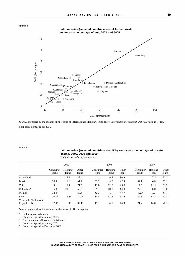
49



Venezuela (Bol. Rep.

of)

Costa RicaBrazil

Colombia

Peru

Argentina

Guatemala

HondurasEl Salvador

Paraguay

Dominican Republic

Haiti

Panama

Uruguay

Chile

Nicaragua

Mexico

Bolivia (Plur. State of)

Ecuador

0 20 40 60 80 100 120

2008

(Pe

rcen

tage

)

2001 (Percentage)

120

100

80

60

40

20

0

FIGURE 2

Latin America (selected countries): credit to the private sector as a percentage of gdp, 2001 and 2008

Source: prepared by the authors on the basis of International Monetary Fund (imf), International Financial Statistic, various issues.


TABLE 1

Latin America (selected countries): credit by sector as a percentage of private lending, 2000, 2005 and 2009 (Data at December of each year)

2000 2005 2009

Consumer loans

Housing loans

Other loans

Consumer loans

Housing loans

Other loans

Consumer loans

Housing loans

Other loans

Argentinaa … 17.4 82.6 … 9.7 90.3 … 7.5 92.5

Brazil 20.3 18.0 61.7 32.2 5.0 62.8 34.1 6.8 59.1

Chile 9.1 19.4 71.5 13.0 22.0 65.0 12.6 25.5 61.9

Colombiab 15.9 21.6 62.5 25.7 10.0 64.3 29.0 8.0 63.0

Mexico 32.4c … 67.6 52.3c … 47.7 42.9c … 57.1

Peru 10.1d 6.8d 89.9d 18.4 12.2 81.6 22.3 11.5 77.7Venezuela (Bolivarian Republic of) 17.9e 6.4e 82.1e 15.1 4.8 84.9 21.7 14.0 78.3

Source: prepared by the authors on the basis of official figures.

a Includes loan advances.b Data correspond to January 2003.c Corresponds to all loans to individuals.d Data correspond to January 2001.e Data correspond to December 2001.

50



FIGURE 3

Latin America (selected countries): deposits taken by the national banking systems as a percentage of credit extended

Source: prepared by the authors on the basis of data from Latin Finance, Latin Banking Guide & Directory, various issues.

TABLE 2

Latin America (selected countries): loans and deposits in foreign currency as a percentage of total loans and deposits, 2000, 2005 and 2009(Percentages)

Loans in foreign currency as a percentage of total loans

Deposits in foreign currency as a percentage of total deposits

2000 2005 2009 2000 2005 2009

Argentina 69.6 14.0 13.0 58.9 9.0 16.1Bolivia (Plurinational State of) … … … … 92.8 63.1Peru 80.4 66.6 46.2 … … …

Source: prepared by the authors on the basis of official figures.

Venezuela (Bol. Rep. of)

Costa Rica

Brazil

Colombia

Argentina Guatemala

Honduras

El Salvador

Paraguay

DominicanRepublic

Mexico

Panama

Uruguay

Chile

Nicaragua

Bolivia (Plur. State of)

Peru

Ecuador

50 70 90 110 130 150 170 190 210 230 250

250

230

210

190

170

150

130

110

90

70

50

2004

(Pe

rcen

tage

)

1995 (Percentage)

a very large non-performing or arrears portfolio (it is commonly assumed that if the non-performing portfolio exceeds 4% of the total portfolio, this is equivalent to over 50% of capital, which poses a high risk for a bank’s financial stability). By this measure, the quality of the loan process is inadequate. The coverage of the arrears portfolio (through reserves and provisions) varies greatly and, in some cases, is less than 100%. Accordingly, if a large part of that portfolio had to be written off, the bank’s capital could be compromised (see table 3). In certain cases, moreover, the criteria for defining arrears and non-recoverable loans are much more lax than those found in more modern portfolio

management practices. Consequently, the actual degree of coverage may be even lower.

Capital adequacy indicators have improved in many cases, thanks to the lessons learned from financial crises in earlier years, which made it advisable to reform the loan process and better match portfolio risk levels to capital. This process was aided by the arrival of foreign banks which were bound by more stringent rules in their home countries; in 2004, most of the countries showed a capital to risk-weighted assets ratio above the 8% required under the New Basel Capital Accord (see figure 4). Nevertheless, capital adequacy may not suffice to cover unexpected losses, given the

51



TABLE 3

Latin America (17 countries): arrears portfolio as a percentage of assets and reserves plus provisions as a percentage of the arrears portfolio in the national banking system, 1998 and 2004

Arrears portfolio as a percentage of assets

Reserves plus provisions as a percentage of the arrears portfolio

1998 2004 1998 2004

Argentina 5.8 4.0 65.2 89.7Bolivia (Plurinational State of) 3.4 0.8 58.0 989.5Brazil 3.5 1.3 113.3 161.9Chile 0.9 0.9 133.9 165.2Colombia 6.4 2.4 38.1 109.8Costa Rica 1.2 4.1 131.4 30.1Ecuador 2.8 3.4 138.5 119.0El Salvador 3.5 1.4 85.8 132.5Guatemala 2.4 3.1 46.6 78.4Honduras 2.9 1.2 48.9 160.7Mexico 7.0 1.3 67.4 203.2Nicaragua 1.3 1.0 121.7 182.7Paraguay 7.1 4.2 34.9 77.4Peru 4.4 1.0 92.0 371.2Dominican Republic 1.3 2.9 143.5 118.3Uruguay 8.2 6.4 68.2 59.6Venezuela (Bolivarian Republic of) 2.1 1.1 150.3 130.2


FIGURE 4

Latin America (18 countries): capital adequacy of the banking system, 1995 and 2004(Capital as a percentage of total risk-weighted assets)


Venez

uela (B

ol. Rep

. of)

Costa R

icaBraz

il

Colombia

Argentin

a

Guatemala

Honduras

El Salv

ador

Ecuad

or

Paraguay

Dominican R

epublic

Mex

ico

Panam

a

UruguayChile

Nicarag

ua

Bolivia

(Plur. S

tate o

f)Peru

1995 2004

Perc

enta

ge

25

20

15

10

5

0

52



incomplete coverage of expected losses associated with the arrears portfolio.

At the same time, as occurs with regulation in other parts of the world, it is possible that not all risks are adequately covered. This is the case of operational risks, which are highly significant in countries which are prone to natural disasters (hurricanes, earthquakes, flooding and other phenomena), risks arising from market concentration6 (higher than in developed countries) and those associated with high macroeconomic variability.

Banking systems in the region also typically have considerable overheads, which a priori lead to high credit costs and, therefore, large spreads. This may be partly to do with their limited activity, which precludes the development of scale economies related, for example, to more intensive use of territorial coverage and the branch network. In several countries spreads are close to 10 percentage points and, in Brazil, over 30%. However, other factors have a hand in this scenario of diminished efficiency. In general, banking systems yield high returns

6 The market concentration indicator considers both public and private banks. Although public banks may play a role as an instrument of monetary policy, leading the authorities to prefer criteria other than profitability, the point emphasized here is the banking system’s lack of competitiveness, which is illustrated by the market’s capture by a small number of institutions.

(see figure 5) amid limited competition, as shown by the market concentration indicators (see figure 6).

(b) The capital marketsThe experience in the developed countries shows

that these markets have great potential to finance investment. An underdeveloped capital market leads to greater dependence on bank lending, which does not necessarily suit the nature of investment projects. By contrast, stock markets offer long-term capital resources at variable cost, and so are better suited to investment projects and reduce the possibilities of bankruptcy.

Debt markets offer broader possibilities for investment financing. First, because they help to materialize and generate long-term financial saving by meeting the needs of institutional investors who seek longer-term financial assets with risk that is different to or lower than stocks. Second, a market for tradable debt improves risk diversification in two ways: institutional investors are better prepared than banks to maintain and absorb long-term risk, because their funding is also long-term; and from the point of view of investment, these markets serve to diversify the liability structure, which helps to reduce risk on the financial side of projects.

Lastly, in modern economies, debt markets are the key channel for the transmission of monetary policy. Where no such market exists, more traditional methods

FIGURE 5

Selected countries: return on assets, 2007 (Net operating balance as a percentage of total assets)

Source: prepared by the authors on the basis of data from International Monetary Fund (imf), Global Financial Stability Report, Washington, D.C., 2009.

Ven

ezue

la (

Bol

. Rep

. of)

Cos

ta R

ica

Bra

zil

Col

ombi

a

Arg

entin

a

Gua

tem

ala

Uni

ted

Stat

es

El S

alva

dor

Ecu

ador

Para

guay

Dom

inic

an R

epub

lic

Mex

ico

Pana

ma

Uru

guay

Chi

le

Spai

n

Ger

man

y

Rep

ublic

of

Kor

ea

Bol

ivia

(Pl

ur. S

tate

of)

Peru

Perc

enta

ge

3.5

3

2.5

2

1.5

1

0.5

0

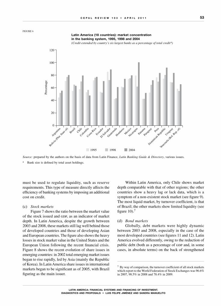
53



must be used to regulate liquidity, such as reserve requirements. This type of measure directly affects the efficiency of banking systems by imposing an additional cost on credit.

(c) Stock marketsFigure 7 shows the ratio between the market value

of the stock issued and gdp, as an indicator of market depth. In Latin America, despite the growth between 2003 and 2008, these markets still lag well behind those of developed countries and those of developing Asian and European countries. The figure also shows the heavy losses in stock market value in the United States and the European Union following the recent financial crisis. Figure 8 shows the recent evolution of share issues in emerging countries: in 2002 total emerging market issues began to rise rapidly, led by Asia (mainly the Republic of Korea). In Latin America share issues in international markets began to be significant as of 2005, with Brazil figuring as the main issuer.

Within Latin America, only Chile shows market depth comparable with that of other regions; the other countries show a heavy lag or lack data, which is a symptom of a non-existent stock market (see figure 9). The most liquid market, by turnover coefficient, is that of Brazil; the other markets show limited liquidity (see figure 10).7

(d) Bond marketsGlobally, debt markets were highly dynamic

between 2003 and 2008, especially in the case of the most developed countries (see figures 11 and 12). Latin America evolved differently, owing to the reduction of public debt (both as a percentage of gdp and, in some cases, in absolute terms) on the back of strengthened

7 By way of comparison, the turnover coefficient of all stock markets which report to the World Federation of Stock Exchanges was 96.6% in 2007, 98.5% in 2008 and 78.4% in 2009.

FIGURE 6

Latin America (18 countries): market concentration in the banking system, 1995, 1998 and 2004(Credit extended by country’s six largest banks as a percentage of total credit a)


a Bank size is defined by total asset holdings.Ve

nezu

ela (B

ol. R

ep. o

f)

Costa

Rica

Brazil

Colombia

Argen

tina

Guatem

alaHon

duras

El Salv

ador

Ecuad

or

Parag

uay

Domini

can R

epub

lic

Mex

ico

Pana

ma

Urugu

ay

Chile

Nicarag

ua

Bolivia

(Plur

. Stat

e of)

Peru

Perc

enta

ge

120

100

80

60

40

20

0

1995 20041998

54



FIGURE 7

Stock market capitalization as a percentage of gdp by world regions, 2003 and 2008

FIGURE 8

Emerging markets: share issues, 1998-2008(Millions of dollars)

Source: prepared by the authors on the basis of data from International Monetary Fund (imf), Global Financial Stability Report, Washington, D.C., several years.



United

Stat

es

Africa

Midd

le Eas

t

Japa

n

Emerging

Eur

ope

Europ

ean U

nion

Asia

Latin A

merica

2003 2008

Perc

enta

ge

140

120

100

80

60

40

20

0

50 000

100 000

150 000

200 000

1998 1999 2000 2001 2002 2003 2004 2005 2006 2007 2008

Emerging Europe Africa Middle East Asia Latin America

55



FIGURE 10

Latin America (selected countries): stock market turnover coefficient, 2007, 2008 and 2009(Percentages of stock market capitalization)

FIGURE 9

Latin America (selected countries): stock market capitalization as a percentage of gdp, 2000 and 2008

Source: prepared by the authors on the basis of data from the World Federation of Exchanges.


Source: prepared by the authors on the basis of data from the World Federation of Exchanges.

2008

Argentina Mexico Peru Colombia Brazil Chile

2000

Perc

enta

ge90

80

70

60

50

40

30

20

10

0

2007

Argentina MexicoPeru Colombia BrazilChile

2008 2009

Perc

enta

ge

70

60

50

40

30

20

10

0

56



FIGURE 11

Global market by world regions: public securities and private debt, 2003 and 2008(Percentages of gdp)

2003

2008


2003 public 2003 private

Perc

enta

ge

250

200

150

100

50

0Latin

AmericaEuropean

UnionAsia Middle

EastEmerging

EuropeJapan United

StatesAfrica

2008 public

LatinAmerica

EuropeanUnion

Asia MiddleEast

EmergingEurope

Japan UnitedStates

Africa

2008 private

Perc

enta

ge

250

200

150

100

50

0

57



fiscal and external positions thanks to improved terms of trade. Latin America showed one of the lowest rates of growth in bond issues, even compared to trends in these instruments in other emerging countries. As is evident in figure 11, public securities account for a large share of instruments in debt markets. In general, public securities are seen as necessary for the development of both local and international debt markets and for affording private issuers broader access to these markets because, as a safe or risk-free asset, they benchmark the cost of funds. They are, moreover, often used as guarantees in interbank and risk-management transactions, which also helps to broaden the market by fostering the development of new segments.

The large proportion of public securities in these markets therefore comes as no surprise. Nevertheless, public securities account for a greater share of the market in Latin America than they do in emerging countries in general or in developed economies (with the exception of Japan and emerging Europe); on average in 2008, public securities accounted for 63.8% of all bond issues in Latin America, much more than in the United States (25.7%), the European Union (30.4%), Asia (56.6%), Africa (46.9%)

and the Middle East (37%).8 This pattern became even more marked with the substitution of external debt with domestic debt in several countries following the upturn in their fiscal and external situations as of 2003.

The weight of public securities in the debt market should draw attention to two aspects of investment financing in the region. First, the degree to which the level of public debt may have exceeded what is necessary to provide a secure asset base for underpinning the development of the private debt market. Public debt could instead be crowding out private bond issues and restricting bank credit through holdings of public securities which are either compulsory or desirable for banks owing to their high returns.

Second, the heavy pressure of public debt in a small market (with, therefore, limited capacity to generate financial resources) may be one of the main factors in explaining high interest rates in certain countries. In markets which are financially integrated to some extent

8 According to figures from the International Monetary Fund, Global Financial Stability Report, various issues.

FIGURE 12

Emerging markets: bond issues, 1998-2008(Millions of dollars)


20 000

40 000

60 000

80 000

100 000

120 000

140 000

160 000

180 000

200 000

1998 1999 2000 2001 2002 2003 2004 2005 2006 2007 2008

Emerging Europe Africa Middle East

Asia Latin America

58



with the rest of the world, this may have boosted capital inflows, sharpening recent tendencies towards currency appreciation.

The problem is not, in either case, excessive public debt as a percentage of gdp as compared with other regions. Neither is it necessarily a problem of debt sustainability in the sense of the State’s ability to fulfil its commitments. The problem is, rather, one of capacity to generate sufficient domestic financial resources in underdeveloped financial systems, and may, in fact, be worsened by the imposition of capital controls.

The evidence also suggests that the composition of bonds issued in the region (not including monetary regulation instruments) is not particularly conducive to investment financing. Compared with other emerging regions and with industrialized countries, Latin America has a disproportionately high percentage of inflation-indexed and floating rate instruments. Around 2009, in countries which had available data, on average 41% of bonds were variable rate and 35% were indexed, while only 31% were fixed rate. By contrast, fixed rate bonds represented 66% and 77%, respectively, of all bonds in emerging and industrialized countries.9 In most cases, this makes it more difficult to finance investment through bond issues, because to the normal risks of an investment project must be added those of interest rate fluctuations and inflation. The relative inexistence of instruments and markets to hedge those risks exacerbates the difficulty.

2. External financing flows

This section discusses separately the main features of external financing flows, given their importance in the financial policy debate. These flows, which mainly take the form of foreign direct investment (fdi), portfolio investment and net other investment assets,10 affect the evolution and characteristics of banking, capital and debt markets in general. A closer examination, however, gives a more precise picture of their contribution to financing in the region.

As the countries of the region gradually gained access to international markets and their bond issues increased, so did their capital inflows. FDI, for example, swelled

9 See bis (2007) and the updated database at www.bis.org. The countries of the region included there are Argentina, Bolivarian Republic of Venezuela, Brazil, Chile, Colombia, Mexico and Peru. 10 “Other investment” forms a residual category that includes all financial transactions not covered in fdi, portfolio investment (shares, bonds and notes) or reserve assets. It therefore includes net external loans and deposits, among others.

considerably in the 1990s, attracted by privatizations, market liberalization (in some cases) and the creation of guarantees for foreign investors.

In the early 2000s, fdi inflows were significantly down on the highs posted in 1999, but still above the levels of the first half of the 1990s. In 2007 and 2008, the region recorded a fresh record for fdi inflows, owing to voluminous flows into Brazil and Mexico (see figure 13).

Portfolio investment climbed strongly in the early 1990s —reflecting privatizations and the further opening of domestic markets to foreign investment— and remained relatively high until 1998, when the fallout of the Asian crisis hit the region. Later, flows of this investment practically disappeared or even turned negative amid defaults on external liabilities on the part of certain countries, the dot.com crisis and turmoil in the United States economy as of 2000. Net flows of portfolio investment did not become significant again for the region until 2007 and 2010, when several countries issued local-currency-denominated public securities, restructured external debt or substituted external with domestic liabilities. Domestic financial markets began to grow rapidly, especially in Brazil, Chile and Peru, and, more recently, improved credit quality led to an upturn in sovereign risk ratings.

Latin American countries began to increase their bond issues on the international market in the first half of the 1990s. This trend was interrupted by the outbreak of the Asian crisis in 1997, then stagnated following defaults by Ecuador (1999) and Argentina (2001)11 and the crisis of 2000-2001 in the United States (see figure 14). Later, as market confidence recovered, issues of external bonds regained some momentum. Nevertheless, the boom in the prices of Latin America’s main exports and improving fiscal situations reduced the need for external resources and led several of the region’s countries to shift their strategies on public debt management towards domestic-market issues.

Several countries have enjoyed access to this form of financing, but Argentina, Brazil and Mexico have issued the largest amounts. Although at first bond issues on international markets consisted mainly of sovereign bonds, the proportion of those issued both by public enterprises and by the private sector has risen (see figures 14 and 15). Only a small group of countries has access to this market, however. In the case of private corporate

11 The amount of new issues by Argentina in 2005 basically reflects efforts to restructure (swap) external debt, more than a return to voluntary external financing.

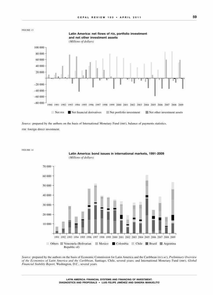
59



FIGURE 13

Latin America: net flows of fdi, portfolio investment and net other investment assets (Millions of dollars)

Source: prepared by the authors on the basis of International Monetary Fund (imf), balance of payments statistics.

fdi: foreign direct investment.

FIGURE 14

Latin America: bond issues in international markets, 1991-2009(Millions of dollars)

Source: prepared by the authors on the basis of Economic Commission for Latin America and the Caribbean (eclac), Preliminary Overview of the Economies of Latin America and the Caribbean, Santiago, Chile, several years; and International Monetary Fund (imf), Global Financial Stability Report, Washington, D.C., several years.

1990 1991 1992 1993 1994 1995 1996 1997 1998 1999 2000 2001 2002 2003 2004 2005 2006 2007 2008 2009–80 000

–60 000

–40 000

–20 000

20 000

40 000

60 000

80 000

100 000

Net FDI Net portfolio investmentNet �nancial derivatives Net other investment assets

10 000

20 000

30 000

40 000

50 000

60 000

70 000

1991 1992 1993 1994 1995 1996 1997 1998 1999 2000 2001 2002 2003 2004 2005 2006 2007 2008 2009

Others Venezuela (Bolivarian Republic of)

Mexico Colombia Chile Brazil Argentina

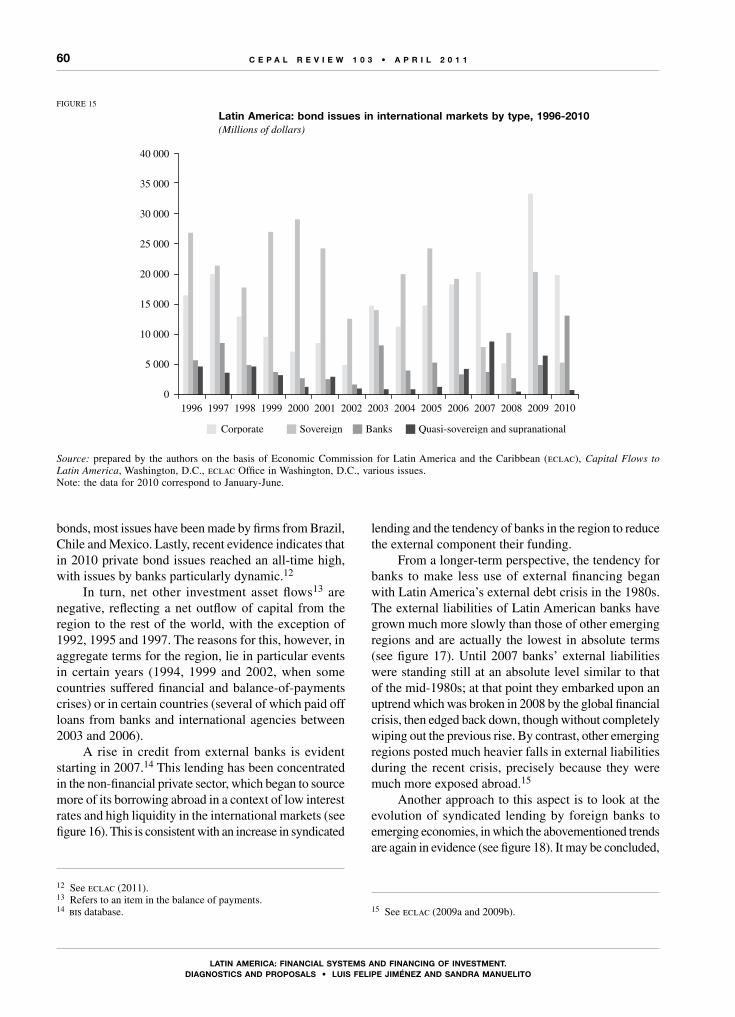
60



bonds, most issues have been made by firms from Brazil, Chile and Mexico. Lastly, recent evidence indicates that in 2010 private bond issues reached an all-time high, with issues by banks particularly dynamic.12

In turn, net other investment asset flows13 are negative, reflecting a net outflow of capital from the region to the rest of the world, with the exception of 1992, 1995 and 1997. The reasons for this, however, in aggregate terms for the region, lie in particular events in certain years (1994, 1999 and 2002, when some countries suffered financial and balance-of-payments crises) or in certain countries (several of which paid off loans from banks and international agencies between 2003 and 2006).

A rise in credit from external banks is evident starting in 2007.14 This lending has been concentrated in the non-financial private sector, which began to source more of its borrowing abroad in a context of low interest rates and high liquidity in the international markets (see figure 16). This is consistent with an increase in syndicated

12 See eclac (2011).13 Refers to an item in the balance of payments.14 bis database.

lending and the tendency of banks in the region to reduce the external component their funding.

From a longer-term perspective, the tendency for banks to make less use of external financing began with Latin America’s external debt crisis in the 1980s. The external liabilities of Latin American banks have grown much more slowly than those of other emerging regions and are actually the lowest in absolute terms (see figure 17). Until 2007 banks’ external liabilities were standing still at an absolute level similar to that of the mid-1980s; at that point they embarked upon an uptrend which was broken in 2008 by the global financial crisis, then edged back down, though without completely wiping out the previous rise. By contrast, other emerging regions posted much heavier falls in external liabilities during the recent crisis, precisely because they were much more exposed abroad.15

Another approach to this aspect is to look at the evolution of syndicated lending by foreign banks to emerging economies, in which the abovementioned trends are again in evidence (see figure 18). It may be concluded,

15 See eclac (2009a and 2009b).

FIGURE 15

Latin America: bond issues in international markets by type, 1996-2010(Millions of dollars)

Source: prepared by the authors on the basis of Economic Commission for Latin America and the Caribbean (eclac), Capital Flows to Latin America, Washington, D.C., eclac Office in Washington, D.C., various issues.Note: the data for 2010 correspond to January-June.

1996 1997 1998 1999 2000 2001 2002 2003 2004 2005 2006 2007 2008 2009 2010

Corporate Sovereign Banks Quasi-sovereign and supranational

5 000

0

10 000

15 000

20 000

25 000

30 000

35 000

40 000

61



FIGURE 16

Latin America: external liabilities with bis reporting banks by sector, December 1983-December 2009 (Millions of dollars)

FIGURE 17

External liabilities of emerging country banks with bis reporting banks by region, June 1985-december 2009(Millions of dollars)

Source: prepared by the authors on the basis of Bank for International Settlements (bis).

Source: prepared by the authors on the basis of Bank for International Settlements (bis).

50 000

100 000

150 000

200 000

250 000

300 000 D

ec. 1

983

Dec

. 198

4D

ec. 1

985

Dec

. 198

6D

ec. 1

987

Dec

. 198

8D

ec. 1

989

Dec

. 199

0D

ec. 1

991

Dec

. 199

2D

ec. 1

993

Dec

. 199

4D

ec. 1

995

Dec

. 199

6D

ec. 1

997

Dec

. 199

8D

ec. 1

999

Jun.

200

0D

ec. 2

000

Jun.

200

1D

ec. 2

001

Jun.

200

2D

ec. 2

002

Jun.

200

3D

ec. 2

003

Jun.

200

4D

ec. 2

004

Jun.

200

5D

ec. 2

005

Jun.

200

6D

ec. 2

006

Jun.

200

7D

ec. 2

007

Jun.

200

8D

ec. 2

008

Jun.

200

9D

ec. 2

009

Public sector Banking sector Non-�nancial private sector

50 000

100 000

150 000

200 000

250 000

300 000

350 000

400 000

Jun.

198

5

Dec

. 198

6

Jun.

198

8

Dec

. 198

9

Jun.

199

1

Dec

. 199

2

Jun.

199

4

Dec

. 199

5

Jun.

199

7

Dec

. 199

8

Mar

. 200

0

Dec

. 200

0

Sep.

200

1

Jun.

200

2

Mar

. 200

3

Dec

. 200

3

Sep.

200

4

Jun.

200

5

Mar

. 200

6

Dec

. 200

6

Sep.

200

7

Jun.

200

8

Mar

. 200

9

Dec

. 200

9

Africa and the Middle East Asia-Paci�c

Europe Latin America and the Caribbean

62



therefore, that Latin America and Caribbean banks show a long-term trend of reducing their indebtedness to non-resident foreign banks.

Another financial flow that has become more significant in the region since the 1990s is that of remittances sent home by migrants, as a result of growing emigration of Latin Americans to the United States, the European Union and even neighbouring countries (see figure 19). In addition, thanks to statistical progress, the

amounts received are more accurately recorded and better facilities —technologically speaking— have become available for sending money between countries. Although in aggregate terms remittances represent a small share of the region’s gdp, at 1.4% in 2008, they have been increasing steadily. As a result, in several countries, especially in Central America, emigrant remittances have become very significant, reaching between 10% and 20% of gdp.

FIGURE 18

Syndicated loans, by region (Millions of dollars)

Source: prepared by the authors on the basis of International Monetary Fund (imf), Global Financial Stability Report, Washington, D.C., several years.

50 000

100 000

150 000

200 000

250 000

300 000

1998 1999 2000 2001 2002 2003 2004 2005 2006 2007 2008

Emerging Europe Africa Middle East

Asia Latin America

63



1. Macroeconomic factors

Macroeconomic volatility is one of the main factors leading to shallow financial development in the region. The Latin American economies have suffered many external and domestic shocks, which have on occasion led to crises in the banking system. Over the past 30 years, with the exception` of the 2003-2008 period, the gdp growth rate has been highly volatile in Latin America. The region has also had historically high

rates of inflation, which dropped to single digits only in 1999. This, together with policies of regulating interest rates, has led to negative real rates and thus discouraged financial saving. At the same time, much of what limited financial saving there was tended to be funnelled into hefty fiscal deficits.

External variability has arisen mainly, though not exclusively, from large swings in the terms of trade. This in addition to the volatility of external financial inflows which, although caused partly by exogenous changes

FIGURE 19

Latin America (19 countries): remittances from emigrant workers, 1995, 2000 and 2008(Millions of dollars, as a percentage of gdp)

Source: prepared by the authors on the basis International Monetary Fund (imf), International Financial Statistics, Washington, D.C.

0

5

10

15

20

25

Argen

tina

Bolivia

(Plur

. Stat

e of)

Brazil

Chile

Colombia

Costa

Rica

Ecuad

or

El Salv

ador

Guatem

alaHait

i

Hondu

ras

Mex

ico

Nicarag

ua

Pana

ma

Paragu

ayPeru

Domini

can R

epub

lic

Urugu

ay

Venez

uela

(Bol.

Rep

. of)

Latin A

merica

Perc

enta

ge

1995 2000 2008

IIIMacroeconomic, microeconomic and

structural factors in the underdevelopment

of Latin America’s financial markets

64



in the external setting, have also led endogenously to internal disequilibria, prompting major shifts in exchange-rate regimes, stance on external liquidity management, or both.

In most of the countries, fiscal, monetary and exchange-rate policies have behaved procyclically, worsening the fallout from external shocks. This is because public revenues are highly correlated with export prices, with the result that volatility in raw material prices has usually been reflected, on the one hand, in public spending variations in the same direction and, on the other, in monetary and exchange-rate policies which —instead of softening international liquidity fluctuations— have passed them directly through to domestic financial flows.

The various crises experienced by the region in recent decades have been expressed in different factors which have dampened support for investment. For example, bouts of high inflation and hyperinflation in a number of countries shortened the maturities of the scarce available savings and increased systemic risk. The external debt crisis and severe devaluations of the 1980s induced the dollarization of much of the limited financial saving. This worsened the shortage of funds for investment and sharpened currency and maturity mismatches between assets and liabilities, exacerbating the risks of long-term financing. To these features is added the large proportion of public debt in domestic markets, as a result of cumulative deficits.

2. Microeconomic factors

(a) In the banking systemLatin American banking underwent significant

changes in the 1990s with the entry of foreign banks to the market. This led to the adoption of modern practices of financing and risk management, but still fell far short of producing levels of uptake of banking services similar to those of countries with similar per capita gdp.

Several studies have identified the problems facing banks in catering for smaller clients, including failings in guarantee schemes and high transaction costs compared with the volume of financial services demanded.

Attention should also be drawn to the banks’ high rates of return. This could indicate the existence of monopoly rents, which discourage the expansion of financing for small, medium-sized and micro-enterprises. The great concentration of the banking industry could be a symptom of insufficient market competition and the prevalence of quasi-monopolies and result in suboptimal service provision. Credit provision by retail

stores has expanded hugely, which is indicative of an unmet demand that could reasonably be covered by banks in terms of cost and loan risk. The experience of developing microcredit in a number of South American countries, such as the Plurinational State of Bolivia, Peru and Chile, and in Central America, also speaks of the potential to expand investment in sectors hitherto inadequately catered for by banks.

(b) In stock marketsSeveral microeconomic factors limit the development

of stock markets. First, a family control structure still persists, along with resistance to allowing external investors to hold equity. Second, the large conglomerates prefer international market finance over local market issues, partly because of the high costs of issuing paper. This is in addition to the limited demand for such instruments, owing to weak protection for minority shareholders, which leaves them exposed to the risk of rent extraction by controlling shareholders: among other factors, there are few independent corporate board members and legislation on the use of privileged information and related-party transactions is weak. The development of these markets also suffers from constraints on the participation of private firms —local or foreign— in certain areas of the economy, accounting and financial disclosure rules that fall short of international standards, a lack of independence of external auditors and the absence of schemes that would foster opening to medium-sized enterprises (such as risk capital).

(c) In bond marketsSome of the factors underlying the shallow

development of this market are also applicable to the stock market, but others are more specific. First, issuing costs are high compared with international markets, owing to higher taxes and the small size of local markets, which prevent the generation of economies of scale or of sufficient infrastructure for trading and securities custody, clearing and settlement.16 Second, bankruptcy processes are more complex and take longer than the international standard. Third, the public sector, notwithstanding its important role as a benchmark, absorbs what is a probably an excessive proportion of the financial savings available in some countries. In addition, the scant development of institutional savers limits both the quantity of resources available and their

16 Zervos (2004), De la Torre and Schmukler (2004).

65



turnover in the local markets, with the exceptions —to some extent— of Brazil and Chile.

3. Structural factors

Lastly, there are factors in the economic structure which lean heavily towards underdevelopment of financial systems and which erode the effectiveness of policies aimed at strengthening investment financing among smaller firms. These factors are:

First, high levels of informality in the economy, which limit access to banking services, since normal financial practices are based on contractual relations and prior records which demonstrate the ability and willingness to pay of potential credit customers. Those lacks also reduce the effectiveness of public policies channelled through support schemes based on formal instruments.

Second, public institutions, including banks and development agencies, are too weak to direct sufficient policy efforts towards market segments in which they could act as pioneers or catalyse later engagement of the private financial sector (for example, support for microenterprises, development of guarantee schemes and financial leasing).

Third, modern practices in financial systems depend heavily on the intensive use of information and communications technologies. Differences in the availability of these technologies and the lag in the communications infrastructure cause, in turn, inequitable access to the financial system’s resources and services, which are uneven across income levels and geographical areas (differences between regions, difficult access from more remote and less populated regions).

IVAspects of a strategy for strengthening

investment financing in the region

Regardless of its particular characteristics, a financial development strategy for boosting investment cannot be successful unless it is preceded by a macroeconomic policy regime that is conducive to stability and can absorb external shocks as well as possible. Although the specific aspects depend on the situation in each country, four general traits warrant mention. First, a fiscal policy which —depending on the needs of the country— promotes sustainable public finances on the basis of a multi-year vision and the creation of countercyclical capacities. Second, a monetary policy that seeks stability and a balance between nominal aspects (inflation) and levels of activity (growth and employment). Third, an exchange-rate policy which, in a framework consistent with the first two aspects, avoids unsustainable real appreciation and the resulting external disequilibria. Exchange-rate policy should also afford a degree of flexibility in order to soften the transmission of external fluctuations. Key factors for this are the degree of integration with international financial markets and the capacity of the domestic financial system to hedge those fluctuations. Fourth, prudential regulation directed at both the solvency of financing institutions and the control of systemic risks.

A strategy for achieving higher growth rates must deal, among other things, with two key challenges: (i) to expand the capacity of the financial system in general and of its various subsystems to finance long-term projects, and (ii) to improve access to capital resources and long-term lending for small and medium-sized enterprises.

These two objectives are complementary and they also need the system to build its capacity to satisfy other development-related needs, such as financing for consumption and housing, working capital, insurance and modern financial services.

In fact, measures for promoting the financial development of smaller firms actually form part of a broader strategy of strengthening capacities to finance investment projects of all sizes, because of two characteristics which are necessary for the development of financial markets: liquidity potential and risk control and diversification. This is why segments with greater liquidity and lower risk are usually those which grow first. In the right conditions, those segments can serve as a platform for the expansion of credit towards segments which have less liquidity, higher risks, or both. So, the strategy here would be to start by consolidating the safer, more liquid segments, then gradually start to

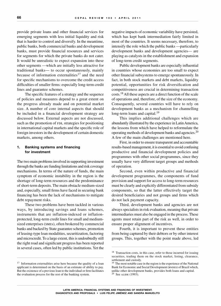
66



provide private loans and other financial services for emerging segments with less initial liquidity and risk that is harder to control and diversify. In the meantime, public banks, both commercial banks and development banks, must provide financial resources and services for segments for which the private banks do not cater. It would be unrealistic to expect expansion into these other segments —which are initially less attractive for traditional banks— to occur spontaneously, mainly because of information externalities17 and the need for specific mechanisms to overcome the credit access difficulties of smaller firms: especially long-term credit lines and guarantee schemes.

The specific features of a strategy and the sequence of policies and measures depend to a great extent on the progress already made and on potential market size. A number of core internal aspects that should be included in a financial development strategy are discussed below. External aspects are not discussed, such as the promotion of fdi, strategies for positioning in international capital markets and the specific role of foreign investors in the development of certain domestic markets, among others.

1. Banking systems and financing for investment

The two main problems involved in supporting investment through the banks are funding limitations and risk coverage mechanisms. In terms of the nature of funds, the main symptom of economic instability in the region is the shortage of long-term resources and the predominance of short-term deposits. The main obstacle medium-sized and, especially, small firms have faced in securing bank financing has been the lack of mechanisms to mitigate debt repayment risks.

These two problems have been tackled in various ways, by introducing savings and loans schemes, instruments that are inflation-indexed or inflation-protected, long-term credit lines for small and medium-sized enterprises (smes), often brokered by commercial banks and backed by State guarantee schemes, promotion of leasing-type loan modalities, securitization, factoring and microcredit. To a large extent, this is undoubtedly still the right road and significant progress has been reported in several cases, often led by public institutions. Yet the

17 Information externalities arise here because the quality of a loan applicant is determined on the basis of an estimate of ability to pay. But the existence of a previous loan to the individual or firm facilitates the evaluation process for the rest of the banking system.

negative impacts of economic variability have persisted, which has kept bank intermediation fairly limited in most of the countries. It seems necessary, therefore, to intensify the role which the public banks —particularly development banks and development agencies— are playing as catalysts in the establishment and expansion of long-term credit segments.

Public development banks are especially influential in countries whose economies are too small to expect other financial subsystems to emerge spontaneously. In fact, in both stock markets and debt markets, liquidity potential, opportunities for risk diversification and competitiveness are crucial in determining transaction costs.18 All these aspects are a direct function of the scale of operations and, therefore, of the size of the economy. Consequently, several countries will have to rely on development banks as a mechanism for channelling long-term loans and capital.19

This implies additional challenges which are abundantly illustrated by the experience in Latin America, the lessons from which have helped to reformulate the operating methods of development banks and agencies.20 A few of the main challenges are mentioned here.

First, in order to ensure transparent and accountable results-based management, it is essential to avoid confusing productive and financial development policies and programmes with other social programmes, since they usually have very different target groups and methods of operation.

Second, even within productive and financial development programmes, the components of fund provision and support for access to long-term resources must be clearly and explicitly differentiated from subsidy components, so that the latter effectively target the desired beneficiaries and not groups and firms which do not lack payment capacity.

Third, development banks and agencies are not always specialists in risk evaluation, meaning that private intermediaries must also be engaged in the process. These agents must retain part of the risk as well, in order to ensure proper alignment of incentives.

Fourth, it is important to prevent these entities from being captured by their debtors or by other interest groups. This, together with the point made above, led

18 Transaction costs, in this case, refer to those incurred for issuing securities, trading them on the stock market, listing, clearance, settlement and custody.19 The most notable case in the region is the experience of the National Bank for Economic and Social Development (bndes) of Brazil which, unlike other development banks, provides both loans and capital.20 See alide (1993).

67



to a major change in the modality of engagement of development banks and agencies in the financial system: instead of providing direct credits, many of them now act as second tier banks.

Fifth, the action of the public sector must not crowd out other, private-sector solutions. This can happen when the provision of financing and guarantees is accompanied by large subsidy components, which ultimately distort relative prices so much that it is not competitive for private agents to enter the market.

2. Stock markets and debt markets

Two conditions which must be met if these markets are to provide long-term resources for investment are the development of institutional investors (pension funds, life insurance companies, mutual funds and investment funds in general), and that their financial saving capacity must not be filled up with public debt securities.

Several countries have institutional investors with long-term financial saving capacity. However, their impact on financing for investment is limited by regulatory provisions which oblige them to buy public debt, or by the high rates of interest these instruments offer.

Progress needs to be made on adequate structuring of the type of instrument offered, especially in the case of public debt. Insofar as economic stability is consolidated, it should be possible to move more towards fixed rate instruments with standard characteristics. These are the type best suited to the financing needs of investment projects and allow the creation of a broad, liquid market, unlike a bond market with different rates and denominations and variable maturities.21

The stock market needs to gradually move away from traditional ownership structures and counteract the disincentives of low market liquidity and high transaction costs. On the demand side, efforts must be made to eliminate the disincentive arising from the scant protection offered to potential minority investors. These risks have been poorly understood in the region and their legal treatment is inadequate.22 Nevertheless, they have become increasingly important as the countries have become more integrated into international financial flows.

One alternative for tackling this array of problems is illustrated by the pioneering experience of Brazil, which

21 See World Bank/ International Monetary Fund (2001) and bis (2002).22 See the reports of the Financial Sector Assessment Program of the International Monetary Fund (imf) at http://www.imf.org/external/np/fsap/fsap.asp.

shows that proper treatment of these risks can lead to stock markets having a more significant role as sources of financing for investment and for innovative firms.

The rules for participating in the market segments of the São Paulo Stock Exchange (bovespa) empower minority shareholders by requiring that all shares carry voting rights and that at least 20% of board members be independent. There are also disincentives to using majority control to extract value from the firm, and minority shareholders have the right to receive the same price for their equities as the controlling investors. Requirements have also been substantially tightened with regard to the presentation of financial statements, disclosure of related-party transactions and the use of privileged information. In order to avoid lengthy legal disputes between firms and their shareholders, such disagreements must be settled in an arbitration forum created especially by bovespa.23

Something which generates intense debate is the impact that certain taxes, particularly capital gains tax, have as a disincentive to demand for financial securities. In the case of shares, a number of approaches suggest that capital gains taxes lead to suboptimal market performance.24 Yet most of these approaches suppose the existence of an unflawed, neutral tax system and a process of share price formation that reflects firms’ true value. The first supposition is —in most of the countries of the region— somewhat unrealistic, and “second best” solutions are often needed to work with a system that allows various forms of evasion and avoidance. At the same time, for shares that are illiquid or seldom quoted, asset price formation is not necessarily accurate. This leaves open opportunities to manipulate prices (for tax purposes or to influence the controlling value). These two factors and the obstacles which commonly stymie tax reform attempts have until now discouraged the elimination of capital gains tax, and in general only securities with a large market presence are exempted.25

Lastly, in several countries of the region, increasing importance has been afforded to investment financing for medium-sized enterprises, especially those engaged in innovative activities. This has taken the form of support for risk capital schemes and policies to facilitate the listing of medium-sized enterprises in stock markets.

23 São Paulo Stock Exchange (bovespa, 2006a, 2006b, 2006c and 2006d) and Santana (2007).24 This is based on the general argument of double taxation of income, particularly in non-integrated tax regimes, i.e. those which do not consolidate all sources of personal income into a single tax.25 Typically gains from public debt securities and those issued by the central bank are tax-exempt.

68



Two key issues to be faced in providing capital for medium-sized enterprises and innovative firms are moral hazard and information asymmetries between investors (or risk capitalists) and the company’s management. The type of organization introduced in the United States, after a number of trials, to provide risk capital to medium-sized and innovative firms has been gradually adopted in several countries, and has become fairly widespread in France, Germany, India, Israel, Taiwan province of China and the United Kingdom, among others. The most developed risk capital schemes in Latin America are seen in Brazil and Chile, but efforts to set up this sort of capital financing have been made in several countries, including Peru, Mexico and Colombia.26

This is a segment of the market in which public development banks and agencies can play a key role, both as providers of funds through intermediaries, in the case of risk capital, or directly as minority shareholders.

With respect to bond markets, recent studies have concluded that 25% of this market’s underdevelopment in Latin America as compared with the developed countries has to do with factors related to economy size (magnitude of gdp) and income level (per capita gdp).27 This would tend to confirm the importance of scale effects. As well, as discussed in the literature on the influence of institutional factors on economic growth, it is possible that the significance of per capita gdp reflects its positive correlation with institutional development.28 In other words, greater institutional development leads, through different channels, to higher per capita gdp and generates better conditions for the expansion of debt markets.

Another 15% of the underdevelopment of the bond market in Latin America is accounted for by the

26 See Jiménez (2008) for a more detailed account of the characteristics and operation of this type of capital. 27 Borensztein, Eichengreen and Panizza (2008).28 Concerning the link between economic growth and institutional development, see Acemoglu and others (2003), and Easterly and Levine (2003).

low rate of access to banking services, which tends to confirm the hypothesis that the two subsystems are complementary, rather than substitutes or competitors as resource providers.29

Historical and geographical factors explain a further 15% of bond market underdevelopment. The only policy variables which are significant are macroeconomic stability, degree of economic openness, protection of creditors’ rights and the costs of contract enforcement. Even so, these variables account for no more than 25% of underdevelopment.30

Concerning the effects of public debt on corporate bond markets, estimates suggest that the crowding-in effects of public bonds —since they help to create a liquid market with a reference yield curve— outweigh the crowding out of private financing. This finding’s applicability to Latin America must be carefully weighed, however, since for much of the period examined, only Brazil, Chile and Mexico registered significant private bond issues, followed at some distance by Argentina.31

Institutional factors leading to deeper bond markets are similar to those that underlie the expansion of stock markets, so the related policies are largely complementary. In these areas, Latin America is similarly placed to the economies of Eastern Europe, but lags behind the emerging Asian countries and the developed economies.32 In most cases,33 institutions and practices which could reduce information asymmetries between debtors and creditors are still incipient.

29 Claessens, Klingenbiel and Schmukler (2003) and Eichengreen and Luengnareumitchai (2004) also report complementary links between the banking system and the bond market.30 Borensztein, Eichengreen and Panizza (2008). Other policy variables are also statistially significant, but make a much smaller contribution to explaining the development of bond markets in Latin America than those mentioned.31 See imf (2005a, table 4.2).32 See imf (2005b, table 4.3).33 Brazil and Chile are usually cited as exceptions, since their institutional frameworks are advanced in comparison with the rest of the countries of the region, yet they are still less developed than those of emerging Asian countries.

69



This paper has examined the characteristics of the main components of financial systems in the region, from the point of view of financing for investment. The analysis was based on three observations: first, the investment rate in the region has been systematically lower than that of other economies which have recently achieved a sustained rise in their growth rates; second, except for the 2003-2008 period, national savings have been insufficient to finance investment, such that growth —and its variations— have been highly dependent on external financing and its variability; third, it is argued that failings in the financial system play a crucial role in determining real levels of saving and investment, and the capacity of individuals and firms to deal with risks. These failings result in tighter constraints on smaller firms, which not only lack access to the resources of the external capital market, but also experience difficulties in accessing the domestic financial system, owing to its shallow development.

The analysis finds that, although the situation is heterogeneous from one country to another and some are further ahead, financial systems in the region are undeveloped and do not serve the needs of investment. Banking services are, with few exceptions, more limited than in other countries with similar per capita gdp and lean towards short-term lending. Conversion of bank deposits into lending is relatively limited, which has to do with outdated monetary regulation practices, combined with banks’ and institutional savers’ strong preference for public securities.

In terms of funding, banks are tending to de-dollarize their net liabilities and rely less on external loans. Portfolio quality varies between countries and in some cases a large non-performing portfolio points to failures in credit processes. Provision for portfolio risk is, in certain cases, insufficient. Capital adequacy indicators seem to indicate a good level of solvency, although doubt remains over the proper measurement of all risks and their inclusion in coverage. What is more, inadequate loan-loss provisions could cast doubt over capital sufficiency.

Interest rate spreads are large in the region, which is associated with large overhead costs and small market size. The combination of high returns and concentration makes for little competition in the banking industry, which has few incentives to expand into segments that are excluded from credit.

Stock markets lag well behind those of other regions, with low capitalization levels and little liquidity. Bond markets, which experienced a global boom in the 2000s, expanded somewhat in the region as well, although to a lesser extent than in faster-growing emerging countries. Unlike in other regions, Latin American bond markets are dominated by public securities, placing strong pressure on domestic interest rates in some cases. This does not reflect public overindebtedness in relation either to gdp or to capacity to serve these debts. On the contrary, several indicators show that public debt declined during the decade and does not represent an excessive burden in comparison with public revenues.

When it comes to the system’s ability to generate financial savings, however, the public sector’s heavy demand for resources seems to lead to high interest rates and constraints on private-sector access to investment finance resources. The crux of the problem is the underdevelopment of the financial system and its limited capacity for mobilizing savings.

The sorts of bonds issued and their maturity structure do not serve the purposes of investment financing. Variable rate and indexed bonds account for a disproportionate percentage of instruments, which poses additional difficulties for investment financing, since there are too few instruments or markets to cover the risks of fluctuations in interest rates and inflation.

External financing flows were also examined, which confirmed the tendency towards a reduction in bank funding from external resources and an increase in issues of bonds —both sovereign and private corporate— in international markets. Access to these resources has been tied to fluctuations in the global economy and affected by specific junctures associated with payment suspensions and renegotiations of external commitments. Nevertheless, after the financial crisis of 2008 external bond issues resumed a brisk upward trend.

Three groups of countries were distinguished in relation to external financing. One group is formed by the countries which have integrated to a greater extent in voluntary markets for external financing and have engaged with the global expansion of these flows. They have a more complex external financing structure and their investment financing is more internationalized than in previous decades. The second group has certain difficulties in gaining access to private financial markets

VConclusions

70



aboard, so their external financing continues to depend mainly on the balance of payments current account and on access to multilateral loans.

Lastly countries in the third group have even greater difficulties in securing voluntary external resources, although fdi may be relatively significant in relation to the small size of their economies. These countries are also subject to greater conditionalities when they seek multilateral support; owing to their internal difficulties they rely largely on remittances and, in some cases, grants.

Correspondingly, the structure of investment financing also differs among those three groups of countries. Generally speaking, notwithstanding their lag, the countries in the first group have more developed domestic financial markets, while the other two groups find it hard to finance growth.

Three factors seem to underlie this situation. First are macroeconomic factors, including, in particular, the lasting impacts on financial saving and real investment of previous episodes of instability and crises. Second are microeconomic factors, such as limited banking sector competency, shallow development of institutional investors, weak protection for minority stakeholders and creditors, high transaction costs associated with small markets and, possibly, demand for resources by the public sector that exceeds the system’s capacity to supply them. Third are structural factors, including very substantial informal sectors and the weakness of public institutions which should be playing a key role in breaking down microeconomic barriers.

On the basis of these observations, consideration was given to the workings of a financial development strategy for boosting investment across the spectrum of firms of different sizes. Two complementary approaches were proposed: – Increase the overall capacity of the system to finance

long-term operations and pursue policies to afford small firms broader access to the system’s resources. These two lines of action are complementary, first, because the nature of the financial markets is such that the first segments to develop are those with greater liquidity and capacity to control and diversify risk. Second, given the information externalities and risk coverage mechanisms available in the

small business segment of lending, it is unrealistic to expect that market to develop spontaneously. But it is also unrealistic to expect any growth in lending to those businesses unless the more liquid markets, which are better able to control, cover and diversify risk, expand first.

– For increasing access to banking services, the main line of action proposed is to make more effective use of public development banks and development agencies to establish sources of long-term financing, develop guarantee schemes and create new financing markets. In light of the experience in the region, proposals are made concerning the way banks participate in the market, with a view to avoiding their capture and boosting lending. As a complement to this public effort, steps need to be taken to increase competition in the banking industry.In relation to capital markets, attention was drawn

to the need to develop institutional investors and improve corporate governance in order to better protect minority shareholders and creditors rights. It is also necessary to examine the role played in development by the domestic public securities market, which has reached such a magnitude that it may be exerting pressure on the system’s limited capacity to generate domestic financial savings. This, in turn, pushes up interest rates and crowds out smes from credit markets. Lastly, the capital markets have the potential to meet the long-term financing needs of medium-sized firms and innovative businesses. Globally speaking, the experience —which, albeit to different extents, is beginning to be replicated in the region— is that risk capital represents these firms’ gateway to markets for other capital resources. Furthermore, the development of stock-market-type institutions has sometimes paved the way for the creation of other markets, such as exchanges for agricultural products, which can finance working capital for small producers.

To sum up, it will take efforts on multiple fronts to strengthen financing for investment in the region. This article has attempted to draw attention to the main domestic problems underlying the financial system’s failure to generate and broker adequate financial resources for investment in businesses of all sizes: small, medium-sized and large.

(Original: Spanish)

71



Acemoglu, Daron and others (2003), “Institutional causes, macroeconomic symptoms: volatility, crises and growth”, Journal of Monetary Economics, vol. 50, No. 1, Amsterdam, Elsevier.

alide (Latin American Association of Development Financing Institutions) (1993), Liberalización financiera y banca de desarrollo, Lima.

bis (Bank for International Settlements) (2007), “Financial stability and local currency bond markets”, cgfs Papers, No. 28, Basel.

(2002), “The development of bond markets in emerging economies”, bis Papers, No. 11, Basel.

, bis statistical database, Basel.Borensztein, Eduardo, Barry Eichengreen and Ugo Panizza (2008),

Bonds Markets in Latin America, Cambridge, Massachusetts, The mit Press.

bovespa (Bolsa de Valores de São Paulo) (2006a), “Novo mercado”, São Paulo.

(2006b), “Nivel 1”, São Paulo. (2006c), “Nivel 2”, São Paulo. (2006d), “Bovespa mais”, São Paulo.

Claessens, Stijn, Daniela Klingenbiel and Sergio Schmukler (2003), “Government bonds in domestic and foreign currency: the role of macroeconomic and institutional factors”, cepr Discussion Papers, No. 3789, London, Centre for Economic Policy Research.

De la Torre, Augusto and Sergio Schmukler (2004), Whither Latin American Capital Markets?, Washington, D.C., World Bank.

Easterly, William and Ross Levine (2003), “Tropics, germs and crops: how endowments influence economic development”, Journal of Monetary Economics, vol. 50, No. 1, Amsterdam, Elsevier.

eclac (Economic Commission for Latin America and the Caribbean) (2011), Preliminary Overview of the Economies of Latin America and the Caribbean 2010 (LC/G.2480-P), Santiago, Chile. United Nations publication, Sales No. E.11.II.G.2.

(2010), Economic Survey of Latin America 2009-2010 (LC/G.2458-P), Santiago, Chile. United Nations publication, Sales No. E.10.II.G.3.

(2009a), Economic Survey of Latin America 2008-2009 (LC/G.2410-P), Santiago, Chile. United Nations publication, Sales No. E.09.II.G.2.

(2009b), Preliminary Overview of the Economies of Latin America and the Caribbean 2009 (LC/G.2424-P), Santiago, Chile. United Nations publication, Sales No. E.09.II.G.149.

Eichengreen, Barry and Pipat Luengnaruemitchai (2004), “Why doesn’t Asia have bigger bonds markets?”, nber Working Papers, No. 10576, Cambridge, Massachusetts, National Bureau of Economic Research.

Gelos, Gaston (2006), “Banking spreads in Latin America”, imf Working Paper, No. 06/44, Washington, D.C., International Monetary Fund.

imf (International Monetary Fund) (2005a), Global Financial Stability Report, Washington, D.C., September.

(2005b), Global Financial Stability Report, Washington, D.C., April.

, International Financial Statistics Database., Balance of Payments Statistics Database.

Jiménez, Luis Felipe (2008), “Venture capital and innovation in Latin America”, cepal Review, No. 96 (LC/G.2396-P), Santiago, Chile.

Kacef, Osvaldo and Sandra Manuelito (2008), “El ingreso nacional bruto disponible en América Latina: una perspectiva de largo plazo”, Macroeconomía del desarrollo series, No. 69 (LC/G.2982-P), Santiago, Chile, Economic Commission for Latin America and the Caribbean (eclac). United Nations publication, Sales No. S.08.II.G.85.

Santana, María Helena (2007), Novo Mercado: the Brazilian Experience, ifc Global Corporate Governance Forum, Washington, D.C.

Stallings, Barbara (2006), Finance for Development: Latin America in a Comparative Perspective, Washington, D.C., Brookings Institution.

World Bank/International Monetary Fund (2001), Developing Government Bond Markets, Washington, D.C.

Zervos, Sara (2004), “The transaction cost of primary markets issuance: the case of Brazil, Chile and Mexico”, World Bank Policy Research Paper, No. 3424, Washington, D.C., World Bank.

Bibliography


73

KEYWORDS

Commodities

International trade

Supply and demand

China

Commodity prices

Exports

Export earnings

Statistical data

Latin America

Rhys Jenkins

Professor, School of International

Development

University of East Anglia, Norwich

United Kingdom


The “China effect” on commodity prices andLatin American export earnings

Rhys Jenkins

The commodity boom between 2002 and 2008 played an important

role in increasing export earnings from Latin America. Growing demand

from China for primary products was one factor stimulating the boom.

While the direct effects of the growth of exports from Latin America

to China have been extensively explored, the indirect impact of higher

Chinese demand for commodities on global commodity prices has

received less attention. This paper estimates the contribution made by

the growth of Chinese demand to the rise in the prices of the 15 main

commodities exported from the region. On the basis of these estimates,

it calculates the total gain for the region as a whole in export revenues

from the “China effect” on world prices. It also provides estimates for

17 Latin American countries of the net effect of Chinese-induced price

increases on their trade balances.

74

ThE “ChInA EFFECT” on CommodITy PRICEs And LATIn AmERICAn ExPoRT EARnIngs • Rhys JEnkIns


The increased economic growth in Latin America since the start of the century has been linked to the commodity boom and the resulting improvement in the region’s terms of trade. A key driver of the substantial increase in global commodity prices between 2002 and 2008, according to many sources, has been rapid economic growth and increased net imports of primary products by China or developing Asia more generally (unctad, 2005, chapter II; imf, 2006, chapter 5; Streifel, 2006; Park and Zhai, 2006; usitc, 2006; Cheung and Morin, 2007). Despite the drop in commodity prices since mid-2008, the fact that China has continued to grow rapidly indicates that it continues to help to maintain commodity prices at higher levels than would otherwise be the case.

Although previous studies have established that the growth of demand from China has been an important factor in recent primary commodity price dynamics, few have sought to estimate the extent to which China has increased the prices of particular commodities, focusing rather on the contribution of China to the growth of global demand, or the increased correlation between commodity prices and Chinese economic activity. The one exception is a study by the United States International Trade Commission (usitc, 2006) which provides estimates of the impact of China on the prices of oil and aluminium. However, this study is restricted to a small number of commodities.

Looked at from the Latin American side, several studies have noted the way in which output movements in China and Latin America have become more closely synchronized in recent years (Lehmann and others,

2007; Cesa-Bianchi and others, 2009; Calderón, 2009). It has been found that the major factor in explaining this increased synchronization has been “demand spillovers”, operating particularly through the impact of China on global commodity prices, rather than increased bilateral trade between Latin America and China (Calderón, 2009). Further exploration of the impact of China on world commodity prices is therefore an important step in understanding the implications of the re-emergence of China as an economic power for the region.

The aim of the present paper is to provide an estimate of the extent to which Latin American export earnings have increased as a result of the impact of China’s economic boom on global commodity prices. In the next section, the major commodities exported from Latin America are identified and the growth of Chinese demand for these commodities and the rise in international prices documented. Section III explains the partial equilibrium approach used to calculate the contribution of China to the increase in prices and the data used. Section IV provides empirical estimates of the impact of demand from China on the prices of the selected commodities between 2002 and 2007. Section V then estimates the total gain in export earnings for Latin America as a result of the increased commodity prices attributable to the rapid growth of demand from China. Section VI takes the analysis further by looking at the impacts on individual countries within the region. A concluding section summarizes the findings and compares them to the impact of direct trade between China and Latin America on the region.

Iintroduction

IILatin American commodity exports

and the “China effect”

Despite active promotion of industrial development by Latin American governments in the second half of the twentieth century, the region as a whole remains heavily dependent on exports of primary commodities, which accounted for just over half of total export earnings in 2007, according to the United Nations Commodity Trade

Database (comtrade). If Mexico is excluded, the share of primary commodities is even more significant, rising to over two thirds of the total. Unsurprisingly, Latin American economic performance is closely associated with movements in commodity prices (Lehmann, Moreno and Jaramillo, 2007).

75



For the purposes of this study, the top 15 primary commodities1 exported from Latin America in 2007 were identified. These commodities can be grouped into six broad product groups with distinct characteristics (see table 1).

Total exports of these 15 products from Latin America came to around US$ 260 billion in 2007, accounting for two thirds of the region’s exports of primary products and around a third of total export earnings.

TABLE 1

Latin America: primary commodity exports, 2007

Product group Commodity

Energy Crude oil

Minerals, ores and metals Copper; iron ore; aluminium; zinc

Feedstuffs Soybeans; soybean oil; fishmeal

Tropical food and beverages Coffee; sugar; bananas

Meat products Beef; poultry

Forest products Timber; wood pulp

Source: prepared by the author on the basis of Standard International Trade Classification (sitc) Rev. 2.

China has become an increasingly important player in the world market for a number of the commodities which Latin America exports (eclac, 2008, chapter I.8; Gallagher and Porzecanski, 2009; Rosales and Kuwayama, 2007, p. 85). It is now the world’s leading consumer of many commodities and accounts for a substantial share of world demand.

Table 2 shows, in common with other studies (e.g., Streifel, 2006; imf, 2006, chapter 5), that the “China effect” on global demand has been most marked in the case of minerals, ores and metals. China has reached a level of income at which metal use relative to gdp tends to rise significantly (unctad, 2005, figure 2.2). This has been a result of the rapid industrialization process in China, which has become increasingly metal-intensive over time as production has shifted from labour-intensive goods (such as clothing) to more capital-intensive sectors (such as electrical and electronics) (Cheung and Morin, 2007). Demand for metals has also been driven by construction and other infrastructure projects (World Bank, 2009, box 2.5).

1 Primary commodities were defined as Standard International Trade Classification (sitc) Rev. 2 classes 0-4 and 68.

TABLE 2

China’s share of global consumption of primary commodities, 2002 and 2007(Percentages)

China’s share of global consumption

Increase in price

2002 2007 2002-2007

Fuels Oil 6.9 9.3 185.1

Minerals, ores and metals Iron ore 22.3 43.9 184.7 Copper 18.2 27.1 356.5 Aluminium 21.1 33.2 95.4 Zinc 22.4 32.4 316.4

Feedstuffs Soybean 18.4 20.9 80.6 Soybean oil 21.2 25.9 85.1 Fishmeal 23.0 27.5 83.6

Tropical food and beverages Coffee 0.3 0.4 125.6 Sugar 7.9 9.3 46.4 Bananas 8.8 9.4 28.6

Meat products Beef 10.6 12.3 22.6 Poultry 16.8 17.2 23.9

Forest products Sawn wood 4.0 8.6 63.6 Chemical pulp 5.7 7.8 55.5

Source: China’s share of consumption calculated by the author on the basis of sources cited in the text, price data taken from United Nations Conference on Trade and Development (unctad) (2008), Trade and Development Report 2008, Geneva, table 2.1, United Nations publication, Sales No. E.08.II.D.21, and International Monetary Fund (imf), World Economic Outlook Database.

Not surprisingly, the contribution to demand has been most striking in the case of iron ore, where China accounts for over 40% of world consumption. Thus, a significant initial share of world consumption in 2002 and a large increase in share between 2002 and 2007 combined to make China a major driver of world demand for iron ore in this period. The demand has been driven by the growth of the Chinese iron and steel industry, with China increasing its share of global steel production from a fifth in 2002 to a third by 2007 and moving from being a net steel importer to a net exporter (iisi, 2008 and 2004). Although not as striking as the case of iron ore, the growth of Chinese consumption of other metals (copper, aluminium and zinc) has also made an important contribution to global demand.

China’s energy use grew more slowly than gdp during the 1980s and 1990s, following the economic reforms of the late 1970s. Since 2000, however, the energy intensity of gdp has begun to rise again (Cheung

76



and Morin, 2007, p. 4). Moreover, the share of coal, which accounts for the bulk of energy use, has been falling, while that of other sources of energy such as oil, natural gas and hydroelectric power has risen (unctad, 2005, pp. 49-50). This has been reflected in China’s increased share of world demand for crude oil since 2002 (see table 2).

After minerals and metals, the next most significant product group in terms of China’s share of global consumption is feedstuffs. This reflects the rapid growth of demand for animal feed (including fish food for aquaculture) in China as living standards rise and consumption patterns change. By the end of the 1990s, China’s level of daily calorie intake per capita was already relatively high and, particularly in urban areas, consumers were shifting towards meat, fish, vegetable oils and fruit (unctad, 2005, p. 45). China is now a leading market for soybeans and fishmeal and its share of world consumption has increased over time.

In this context, it is perhaps surprising that the growth in China’s share of world consumption of meat products in table 1 is not more significant. In the case of poultry, growth in demand in China between 2002 and 2007 was depressed by the impact of the 2004 avian flu outbreak.2 In the case of beef, per capita consumption in China is around a tenth of the level in the United States and a quarter of the average level in the 27 countries of the European Union (Foreign Agricultural Service of the United States Department of Agriculture, Office of Global Analysis), so that although China’s share of global demand is rising, it remains relatively limited.

In the case of forest products, China’s growing share of world chemical pulp consumption has been driven by the growth of capacity in the domestic paper and packaging industry. Local consumption of paper more than doubled between 1995 and 2004 (usitc, 2006, table 4-3). A significant driver of this growth was the demand for packaging from the manufacturing sector. However, part of the increased demand has been met by production using waste paper, which has grown faster in recent years than the use of pulp (usitc, 2006, tables 4-1 and 4-2). As a result, China’s share of global demand for pulp is less than might be expected.

China’s global consumption share has increased more for sawn wood than for pulp since 2002 (see table 2). The pervasiveness of illegal logging, which has been widely commented upon, may have led to Chinese

2 Per capita consumption of poultry fell in China in 2004 and only recovered slowly after that (Foreign Agricultural Service of the United States Department of Agriculture, Office of Global Analysis).

imports being underestimated in official statistics, so that the country’s impact on global demand may be greater than the reported figures suggest (dfid, 2005).

China is not yet an important consumer in the world market for tropical agricultural products. Coffee consumption is still extremely limited in China, and while consumption of bananas and sugar is much more widespread, these are almost entirely produced domestically so that it is unlikely that the growth of Chinese consumption would have had a significant impact on the world market for either product.

Table 2 also shows the substantial price increases that occurred for most primary commodities between 2002 and 2007. The most dramatic rises were in metals, particularly copper and zinc, and in oil. Feedstuffs have also increased significantly in price, although this is largely attributable to dramatic increases in 2007 associated with the demand for land to grow biofuels (World Bank, 2009, pp. 61-63). Other agricultural products have generally had more modest price increases.

Although the Chinese economy has been growing rapidly for three decades, there are several reasons why China only began to have a significant impact on global commodity prices at the start of the twenty-first century. During the 1980s and 1990s, the energy and metal intensity of China’s gdp fell, but this situation was reversed from the late 1990s or early 2000s (Cheung and Morin, 2007; unctad, 2005, pp. 47-49). Increases in industrial efficiency as a result of the economic reforms of the late 1970s led to a fall in energy and metal use at the plant level. At the same time, this was reinforced by changes in the composition of industry as a result of the shift away from the emphasis on heavy industry during the period of central planning towards light industries during the early phase of China’s transition to an export-oriented market economy. More recently, however, as noted above, there has been a shift to capital-intensive and energy-intensive industries, including road building and construction. This has led to an increase in the metal and energy elasticity of Chinese gdp growth since the turn of the millennium.

China has also become much more integrated with global commodity markets over the past decade as the growth of demand for a number of commodities has outstripped domestic supply.3 This has been reflected in significant increases in net imports of commodities such as copper, iron ore, nickel, crude oil and soybeans

3 For example, whereas domestic production of iron ore covered 85% of domestic consumption in 1990, this had fallen to 45% by 2003 (unctad, 2005, p. 74).

77



(unctad, 2005, figure 2.8). Where China has remained largely self-sufficient in terms of supply, on the other hand, its impact on global commodity prices is likely to have been minimal.

Finally, the impact of China on global commodity prices depends not only on the growth rate of Chinese demand but also on its initial share of global consumption, and it was only at the beginning of the twenty-first century that China became a sufficiently important consumer to affect the prices of a number of key commodities. Calderón (2009, p. 54), for instance, suggests that “2002-2003 may represent the turning point in the relationship between Chinese industrial production and world commodity prices”.

Although the focus of this study is the impact of the growth of Chinese demand on commodity prices, it is important to bear in mind that this is by no means the only factor that has affected prices in recent years. On the demand side, other markets for primary commodities have also grown and the contribution of China to global demand growth differs considerably between commodities. Demand may also be affected by movements in the prices of close substitutes.

Supply-side factors also have a significant impact on prices, particularly but by no means exclusively in the case of agricultural products whose supply is affected by climatic factors. All commodities may be affected by changes in the costs of inputs which shift the supply curve, and oil and minerals are affected by new resource discoveries. The supply of oil and minerals may also be disrupted by political conflict or labour unrest in major producing countries.

In addition to the forces of supply and demand in the real economy, commodity prices are also

affected by financial factors. Since commodity prices are normally measured in United States dollar terms, changes in the value of the dollar affect the quoted price. The dollar was at a peak in 2002 and had fallen by around 25% by the end of 2007 (imf, 2008, box 1.4). Commodity prices (excluding oil) rose by 113% in dollar terms between 2002 and 2007 but by only 80% when measured in terms of Special Drawing Rights (SDRs) (unctad, 2008, table 2.1). The International Monetary Fun (imf) estimates that the oil price would have been US$ 25 a barrel lower at the end of 2007 (i.e., over 25% lower than it actually was at the time), and non-fuel commodity prices 12% lower, if the dollar had maintained its 2002 value.

The impact of speculation on commodity prices has been a matter of controversy. There is general agreement that there has been an increase in the significance of financial investment in many commodity markets in recent years (World Bank, 2009, chapter 2; unctad, 2009, chapter 2). A study of five commodities (crude oil, copper, sugar, coffee and cotton) by imf concluded that there was little evidence that speculation affected either long-run price levels or short-run volatility, although this conclusion was subject to a number of caveats (imf, 2006, box 5.1). In contrast, unctad (2008, box 2.1 and 2009, chapter 2) argues that the growth of speculation probably accelerated and amplified price fluctuations.

No attempt will be made here to estimate the impact of these other factors on commodity prices in recent years. Rather, the challenge is to try and separate out the impact of the growth in demand from China. The approach adopted is a partial equilibrium one which only seeks to identify the first round effects of Chinese demand on global prices.

IIIMethodology and data

The first step in the analysis is to identify the contribution of China’s growth to global demand for the primary commodities exported from Latin America. The period covered is from the start of the recent commodity boom in 2002 to 2007. The volatility of prices with the collapse of the boom in 2008 and the fact that trade data were not available for all the Latin American countries for 2008 were the key reasons why the analysis was not extended beyond 2007. Global and Chinese demand for the 15

commodities identified in table 3 (in physical terms) were obtained from various sources.

There are several possible counterfactuals which could be used to estimate the “China effect” on global demand. One possibility would simply be to compare actual global demand for each commodity in 2007 with demand excluding China. This would be the equivalent of a counterfactual in which “China does not exist”. A second approach would be simply to calculate the

78



increase in Chinese consumption of each commodity between 2002 and 2007, and subtract this from global demand. This implies a counterfactual in which Chinese consumption remains unchanged or “China does not grow”. However, since we are interested in the impact of the exceptional growth of Chinese demand on commodity prices, a more appropriate counterfactual is one where Chinese demand grows at the same rate as demand in the rest of the world. Thus, a hypothetical global demand for the 15 commodities in 2007 is estimated on the assumption that China’s demand growth between 2002 and 2007 was the same as the rest of the world’s.4 The difference between this figure and actual demand in 2007 provides an estimate of the extent to which China’s exceptional economic performance increased world demand for the products concerned over the period since 2002. This is the approach adopted in the paper.

One limitation of this approach is that it assumes that the growth of demand in China and in the rest of the world are independent of each other. A first objection to this is that, to the extent that rapid growth in China boosts demand in the rest of the world, a slower rate of growth in China would also lead to a reduction in growth elsewhere. The question then is: how significant is Chinese demand for growth in the rest of the world?5 China’s relatively small share of global demand, averaging 4.6% between 2003 and 2007 (Timmer, 2010, table 1), suggests that its impact on demand in the rest of the world was quite limited during the period.

A second objection, relevant at the level of individual commodities, is that the growth in demand in China may partly be the result of the relocation of certain industries from other countries, rather than a result of increased global demand for commodities. For example, if the rapid growth in demand for iron ore in China is partly a result of the relocation of the global steel industry to China, this may have been at the expense of demand for iron ore in other countries. Thus, the estimated additional growth in demand from China may not represent additional world demand for iron ore, and the implicit assumption that the growth of demand in China and in the rest of the world are independent of each other is not strictly valid.

While the first objection suggests that ignoring the “China effect” on the rest of the world tends to result in

4 This counterfactual could be termed the “China’s share does not increase” scenario.5 This question is key to an ongoing debate about the extent to which China can become the engine for world economic recovery. For contrasting views, see Dollar (2009) and Timmer (2010).

underestimation of its total impact on global demand for commodities, the second suggests the opposite. Although there is no reason to suppose that these two effects necessarily balance each other out, the fact that they operate in opposite directions, and that these indirect effects may be small relative to the direct effects, provides a partial justification for not taking them into account here.

The counterfactual used to calculate the impact of China’s exceptional growth on commodity prices assumes that the other factors affecting prices discussed earlier, such as shifts in supply curves, exchange-rate alterations and speculation, remain unchanged. In other words, we are interested in how much lower commodity prices would have been in 2007 had China’s share of world demand remained at the same level as in 2002, ceteris paribus. Since in effect this means a counterfactual in which the demand curve has shifted downwards, the effect on prices will depend on the elasticity of global supply for each commodity.

Estimates of the global elasticity of supply for the commodities concerned are surprisingly difficult to come by, and when they are available there is often a considerable range of estimates. In the light of this, it was decided that it would be more useful to take a range rather than a single value for the elasticities used to calculate the impact on global prices. These elasticities were then applied to the estimated contribution of China’s rapid growth to global demand for each commodity in order to arrive at the impact on world prices.

Finally, the gains to Latin America from the China effect on global demand were calculated by estimating how much lower in dollar terms Latin America’s exports of each of these commodities would have been in 2007 in the absence of the China-induced price rise. This involved deflating the 2007 value of exports from the region by the price rise attributable to the excess growth of demand from China between 2002 and 2007. At the level of the region as a whole, this was done using gross exports in order to obtain an estimate of the additional export earnings accruing to Latin America as a result of the “China effect” (see table 5 below). However, since different countries within the region may be affected differently depending on whether they are net exporters or net importers of these commodities, the estimates at the individual country level are based on net exports and therefore reflect the influence of price changes on trade balances (table 6). The latter can of course be negative where a country is a net importer of a commodity which has increased significantly in price as a result of Chinese demand.

79



The data on the volume of consumption of the various commodities globally and in China were obtained from a variety of sources. Oil consumption came from the bp publication bp Statistical Review of World Energy, 2008. Consumption of iron ore was from the International Iron and Steel Institute, World Steel in Figures (various issues), and other minerals were from the World Bureau of Metal Statistics, World Metals Statistics. The source for meat products, grains, meals and oil, and sugar was the Foreign Agricultural Service of the United States Department of Agriculture, while figures for forest products, coffee and bananas were based on United Nations Food and Agriculture Organization (fao) data.

The elasticity estimates used in the study were based on a search of a large number of sources which are listed in the appendix. Since the period analysed is only five years and the increase in prices was most

marked in the later years, use was made of short- or medium-run supply elasticities, which tend to be lower than their long-run counterparts. Studies from earlier periods were not necessarily always a good guide to the elasticity of supply in the early twenty-first century, so that an element of judgement had to be applied in determining a plausible range of elasticity estimates, based on recent studies of supply conditions for the commodities concerned.

In order to estimate the “China effect” on the export earnings and trade balances of the Latin American economies, data on exports and imports of each of the 15 commodities in 2007 were obtained for 17 countries from the United Nations Commodity Trade Database. In the case of the Bolivarian Republic of Venezuela, data for exports in 2007 were unavailable and were therefore estimated as the average of the values reported for each commodity in 2006 and 2008.

IVThe “China effect” on commodity prices

1. China’s contribution to increasing global demand

As indicated above, the first step in estimating the “China effect” on global commodity prices is to calculate the addition to global demand resulting from China’s rapid economic growth. In other words, the question being addressed is: how much greater is world demand for a commodity than it would have been if demand in China had grown at the same rate as in the rest of the world between 2002 and 2007?

The first two columns of table 3 compare the increase in consumption in China with that in the rest of the world for the key commodities between 2002 and 2007. In all cases other than poultry, demand grew much faster in China than in the rest of the world, and this was reflected in the increase in China’s share of global consumption of these products, as shown in table 2. The third column of table 3 measures how much higher actual world consumption of these commodities is than it would have been had demand in China grown at the same rate as demand in the rest of the world. In other words, it measures the impact of China’s high growth, relative to the rest of the world, on global demand.

Not surprisingly, table 3 shows that the “China effect” in terms of additional demand has been most

marked in minerals, ores and metals, particularly iron ore. The next most significant group in terms of impact has been feedstuffs. The impact in terms of additional demand for oil and forest products has been relatively limited, while tropical food and beverages and meat products are the categories in which Chinese demand growth in the period had least effect.

2. The “China effect” on world prices

The impact of Chinese demand growth on the world price of different commodities depends not only on the size of the demand effect. It is also affected by the responsiveness of global supply to increased demand and the extent to which an integrated global market exists and China is part of it.

The second and third columns of table 4 present the estimates for the upper and lower bounds of the range of supply elasticities used for the various commodities. Since these relate to the short or medium term, they are all relatively low, reflecting the difficulty of increasing supply in the short term, particularly in the case of crude oil and some minerals. The supply elasticities of tree crops with long gestation periods (e.g., coffee and timber) are also relatively low, while livestock and grains tend to have a more elastic supply.

80



TABLE 3

impact of demand from China on global demand, 2007(Percentages)

Consumption growth 2002-2007China’s demand effecta

China Rest of world

Fuels Oil 48.7 6.6 2.7

Minerals, ores and metals Iron ore 224.9 19.5 38.4 Copper 77.6 6.1 12.3 Aluminium 124.3 20.4 18.2 Zinc 70.7 2.9 14.8

Feedstuffs Soybean 37.2 17.7 3.1 Soybean oil 54.2 18.4 6.4 Fishmeal 24.8 -1.9 6.3

Tropical food and beverages Coffee 32.3 -1.9 0.1 Sugar 30.6 9.2 1.5 Bananas 25.0 17.0 0.6

Meat products Beef 27.1 7.2 2.0 Poultry 21.6 18.7 0.4

Forest products Sawn wood 131.8 2.8 5.0 Chemical pulp 45.0 3.3 2.3

Source: prepared by the author on the basis of the source indicated in table 2.

a This measures how much higher global demand for the commodity was in 2007 than it would have been had demand in China increased at the same rate as in the rest of the world between 2002 and 2007.

TABLE 4

Estimated impact of Chinese demand on world prices, 2007

Effect of Chinese demand (percentages)

Price elasticity of supply “China effect” (percentages)a

Lower Upper Maximum Minimum

Crude oil 2.7 0.1 0.25 27.1 10.8Iron ore 38.4 0.25 0.4 153.6 96.0Copper 12.3 0.1 0.25 122.6 49.1Aluminium 18.2 0.25 0.4 72.8 45.5Zinc 14.8 0.1 0.25 147.6 59.1Soybean 3.1 0.4 0.6 7.7 5.1Soybean oil 6.4 0.4 0.6 16.0 10.7Fishmeal 6.3 0.4 0.6 15.6 10.4Coffee 0.1 0.1 0.4 0.5 0.2Sugar 1.5 0.1 0.5 15.5 3.1Bananas 0.6 0.2 0.4 3.0 1.5Beef 2.0 0.3 0.6 6.6 3.3Poultry 0.4 0.3 0.6 1.4 0.7Sawn wood 5.0 0.2 0.6 25.1 8.4Chemical pulp 2.3 0.2 0.6 11.5 3.8

Source: prepared by the author from table 3 and sources of elasticity estimates cited in the appendix.

a This measures how much higher the world price for the commodity was in 2007 than it would have been had demand in China increased at the same rate as in the rest of the world between 2002 and 2007.

81



In metals, the elasticity of supply in the short run depends on the capacity available to increase output and the level of stocks. In the case of copper, low prices in the 1990s meant that there was very little investment in new capacity so that when demand increased after 2002, supply did not respond and stocks fell sharply from 1.7 million metric tons at the end of 2002 to 0.7 million in 2006 (cochilco, 2008). The low estimated supply elasticity reflects this. A similar situation is apparent in the case of zinc, where demand has outstripped supply in recent years and stocks fell by half between 2003 and 2006 (International Lead and Zinc Study Group). Most zinc comes from underground operations, and it is difficult to increase production from existing mines because of the high capital cost of expansion (Dr. Harlyn Meade quoted in Williams, 2007).

Higher supply elasticities were assumed for iron ore and aluminium. In the case of iron ore, the supply situation appears more favourable than for copper or zinc, with substantial increases in capacity in recent years (Ostensson, 2005). In contrast to other minerals, prices for iron ore are set by negotiation between the main producers and the importers rather than on commodity exchanges, so that it is unlikely that speculation could have affected prices. Finally, capacity expansion in aluminium, particularly in China, has meant that a margin of capacity has been maintained and stocks did not fall significantly between 2002 and 2006 (usgs, Mineral Commodity Summaries: Aluminum).

Supply problems have also been particularly apparent in the case of oil, where high prices have not led to increases in capacity, leading to a drop in the effective spare capacity of the Organization of the Petroleum Exporting Countries (opec) after 2002 (imf, 2008, figure 1.18). The sluggish response of supply in the industry has been attributed to a longer lag between increased prices and new investment being made than in the past. This in turn partly reflects geological and technological factors such as the declining average size of oil fields and the challenges of exploiting non-conventional sources such as deep sea fields or oil sands (imf, 2008, box 1.5). As with copper, this suggests a low estimate for the elasticity of supply.

Agricultural products tend to have a shorter gestation period and therefore a higher short-run elasticity of supply than oil and minerals. The exceptions are tree crops such as coffee and forest products, which take a number of years to mature. Annual crops such as soybeans respond relatively quickly to price increases, as land can be switched from other crops. The soybean acreage in Argentina and Brazil, for example, has doubled

since the mid-1990s in response to the growth in world demand (Ray, 2008).

The fourth and fifth columns of table 4 calculate the impact of the growth of Chinese demand on world prices, given the supply elasticities in the second and third columns. The fourth column provides the upper end of the range based on the low elasticities of supply in the second column, while the fifth column provides the minimum likely impact on prices, based on the higher elasticities in the third column.

The most significant impacts are found for the four metals included. These are of course the commodities for which prices have risen most during the period under consideration, with zinc and copper increasing more than fourfold, iron ore almost threefold and aluminium almost twofold in price since 2002 (see table 2).

The growth of Chinese demand for iron ore above the rate of consumption growth in the rest of the world is estimated to have doubled the world price, although as noted above this is an overestimate to the extent that growth in China has led to a reduction in demand elsewhere. In the case of both copper and zinc, the “China effect” on global price levels was significant because the supply was inelastic, while the estimated effect on the price of aluminium was slightly lower because supply appears to have been more elastic. In all these cases, prices are estimated to have increased by at least 40% as a result of the growth in demand from China.

The “China effect” is estimated to have been in the range of 10% to 25% on the prices of four commodities. In the case of crude oil, despite China’s relatively small share of total world demand, the fact that this share rose over the period plus the low elasticity of supply meant that prices were significantly affected by China’s growth. Since the overall increase in oil prices during this period was more than 180%, however, other factors were clearly far more important than China in driving up prices.6 The other three products are soybean oil, fishmeal and sawn wood. In the case of the first two, this reflects the high share of China in world consumption of these products, while in the case of wood it is the rapid increase in its share over the period that is most striking.

In the case of all the other commodities covered, the estimated effect of Chinese demand on prices over the period was less than 10%. The growth in demand for soybeans from China has largely been met by increases

6 The United States International Trade Commission came to a similar conclusion for the 1995-2004 period, when it estimates that of an oil price increase of 200%, the growth of Chinese demand was responsible for between 12% and 37% (usitc, 2006, p. A.6).

82



in the area harvested in recent years, particularly in Argentina and Brazil, and it is only since 2007, with the increased competition for land (especially in the United States) to produce biofuels, that soybean prices have risen sharply (Ray, 2008).

The impact of Chinese demand on prices for tropical food and beverages is likely to have been very small. Table 4 makes this very clear in the case of coffee, where the estimated price increase attributable to China is negligible, and of bananas, where it is relatively small. The estimate for sugar is much higher, but given the fact that China is not a significant importer and that the global market for sugar is highly fragmented as a result of preferential agreements, it is unlikely that in practice China would have had any real impact on world prices for sugar products.

Meat product prices have also been relatively unaffected by Chinese demand. As noted above, poultry

consumption in China was affected by the avian flu epidemic. Despite the growth in demand for beef in China, this has had a relatively minor effect on pricing. This is the product group for which world prices have increased least in the period since 2002 (see table 2).

In the case of forest products, Chinese demand has had a moderate impact on the price of chemical pulp and a much more significant effect on prices for sawn wood, as noted above. In the latter case, the effect may even be underestimated to the extent that the “China effect” is hidden by the scale of the illegal trade in timber that went unrecorded in the estimates of Chinese timber consumption. On the other hand, transport costs mean that the market for sawn wood tends to be quite regionalized and the main sources of imports to China are the Russian Federation and South-East Asia. Thus, any price impacts of growing Chinese demand are less likely to have affected the Latin American countries.

VThe “China effect” on Latin American

export earnings

The final calculation that needs to be made is the extent to which Latin American export earnings have increased as a result of the rise in prices of primary products attributable to the rapid growth in demand from China. Table 5 provides estimates for each of the 15 commodities. The first column presents the value of exports in 2007. The second and third columns provide high and low estimates for the “China effect” through higher world prices on the value of Latin American exports of these commodities. The fourth column gives a best estimate which in most cases is simply the mid-point of the range indicated by the second and third columns. In the case of sugar and bananas, the best estimate reflects the fact that the most plausible assumption is that China has not affected the price of Latin American exports.

Table 5 shows that two commodities, oil and copper, account for roughly three quarters of the total gain in export revenues resulting from the “China effect” on commodity prices. The two contribute in roughly equal measure, despite the fact that total exports of oil from Latin America are much larger than those of copper. This reflects the greater impact that demand from China has had on copper prices compared to oil, as noted earlier. The

third most important product is iron ore, accounting for a further 10% or so of the total gain in foreign-exchange earnings, followed by aluminium and zinc.

Following behind these in terms of their contribution are soybeans and soybean oil, but these are relatively limited in terms of the additional export earnings created, which totalled between US$ 1.2 billion and US$ 1.7 billion in 2007. The next most significant group of exports after feedstuffs is forest products, with estimates of the total impact ranging from US$ 450 million to US$ 1.2 billion, divided roughly equally between wood and pulp.

The impact on meat exports has been relatively small, with most of the gain being attributed to beef, while there has been virtually no additional revenue from poultry. Finally, as indicated above, China has had little impact on world prices of tropical fruits and beverages, so that it seems reasonable to disregard the estimated effects on bananas and sugar in order to arrive at a more realistic total.

The estimated total effect of Chinese demand on Latin American export earnings from all 15 commodities was between US$ 41 billion and US$ 73 billion, with a best estimate of over US$ 56 billion. This latter figure represents

83



21% of the value of exports of all 15 commodities and 7% of total Latin American exports in 2007.

A number of warnings need to be attached to these estimates. First, they should be taken as orders of magnitude rather than precise values, since the elasticity estimates taken from a variety of sources may not be accurate. A doubling of the assumed elasticity for each commodity would halve the estimated effect. Since the elasticities used for the main commodities that contribute to the overall impact (oil and metals) are low, they are likely if anything to have caused the impact of China on Latin American export earnings to be overestimated.

A second factor that might lead to overestimation of the “China effect” on prices and export earnings is the possibility that the growth of Chinese demand is not entirely a net addition to global demand. It may be that

some of the growth has been offset by a fall in demand in other markets because the industries which use the commodities as inputs have relocated to China. This is most likely to be the case for metals, which are a major contributor to the estimated additional earnings.

A third consideration is that the estimates presented here have been based on the total value of the region’s exports of the 15 commodities in order to calculate the gain in export earnings. However, some countries in the region import some of these commodities, and it might therefore be more appropriate to look at net exports rather than the total value. If this were done, then the estimated gain to the region as a result of the “China effect” on commodity prices would be about 16% lower (between US$ 34 billion and US$ 61 billion, rather than between US$ 41 billion and US$ 73 billion).

TABLE 5

China: estimated impact on Latin American export earnings for 15 commodities, 2007(Millions of dollars)

Exports Estimated effect of China on value of exports

2007 Maximum Minimum Best

Crude oil 129 294 27 580 12 651 20 116Iron ore 11 585 7 016 5 674 6 345Copper 50 494 27 815 16 618 22 217Aluminium 6 587 2 775 2 060 2 418Zinc 4 789 2 856 1 779 2 317Soybean 11 237 799 546 672Soybean oil 6 509 898 627 763Fishmeal 1 970 266 186 226Coffee 8 584 43 17 30Sugar 6 251 838 188 0Bananas 3 273 95 48 0Beef 6 596 407 210 308Poultry 4 708 65 33 49Sawn wood 3 279 657 253 455Chemical pulp 5 422 558 200 379

Total 260 579 72 670 41 090 56 295

Source: prepared by the author on the basis of the United Nations Commodity Trade Database (comtrade).

84



The analysis of the previous section focuses on the aggregate effects of the rapid growth of Chinese commodity demand for Latin America as a whole. It is clear from what has been said about the differential impact of China on different commodities, however, that the effects are unlikely to be uniform across the countries of the region. Specifically, while the impact will have been positive for those countries which are net exporters of these commodities, particularly minerals and oil, some countries which are net importers may well have lost out from the higher commodity prices resulting from rapid Chinese growth. This section extends the analysis to the level of the individual Latin American countries.

The impact on foreign-exchange earnings was estimated by applying the price changes calculated in table 4 to net exports of the 15 commodities in each country. Thus, where a country is a net importer of a commodity whose price has risen as a result of the “China effect”, this will be shown as a loss of foreign exchange, while for commodities where it is a net exporter, there will be a foreign-exchange gain.

Table 6 summarizes the results for 17 Latin American countries in 2007. It shows the percentage by which each country’s trade balance in the 15 commodities is better (worse) than it would have been if China’s share in world demand for these commodities had remained unchanged since 2002. As previously, two estimates are presented, based on lower- and upper-bound values for the price elasticities of each commodity.

The selected countries fall into four broad groups. First, there are those which are substantial beneficiaries of higher commodity prices, with estimated gains of between 20% and 50% as a result of the “China effect”. These are the mineral-exporting economies of the region, Peru, Chile and the Plurinational State of Bolivia. The next group, with gains of between 7% and 20%, is made up of three significant oil exporters (the Bolivarian Republic of Venezuela, Mexico and Ecuador) and the two most diversified economies of the region (Brazil and Argentina). Four other countries have gained slightly on balance from the “China effect”, with increases in foreign-exchange earnings of less than 10%. These include two Central American countries, where the gains are minimal, and Colombia and Paraguay. Finally,

there are five countries where the net impact of Chinese demand on commodity prices has been negative. These are four Central American economies (El Salvador, Nicaragua, Costa Rica and Panama) and Uruguay. In all these cases, the gains from higher export prices for these commodities are more than offset by the increased cost of imports.

Previous analyses of the “China effect” on Latin America have noted the different effects on South America on the one hand and Mexico (and in some cases Central America) on the other (Devlin and others, 2006, chapter 2; Ellis, 2009, chapter 2; González, 2008). Whereas a number of South American countries, most notably Argentina, Brazil, Chile and Peru, have developed significant exports to China and are seen therefore as

VIwinners and losers in the commodity lottery

TABLE 6

China: estimated impact on the net export earnings of Latin American economies, 2007(Percentages)

Country Maximum Minimum

Argentina 11.9 6.9Bolivia (Plurinational State of) 40.0 23.8Brazil 16.0 11.9Chile 47.8 28.8Colombia 9.1 3.3Ecuador 17.4 7.9Mexico 16.2 6.7Paraguay 7.2 4.4Peru 48.2 29.3Uruguay -9.4 -3.9Venezuela (Bolivarian Republic of) 21.4 10.1

Subtotal for Mexico and South America 23.8 13.3

Costa Rica -13.3 -7.5El Salvador -37.0 -19.0Guatemala 3.4 0.1Honduras 3.6 1.6Nicaragua -14.9 -7.5Panama -9.3 -7.6Subtotal for Central America -6.0 -4.0

Total for Latin America 23.3 13.0


85



major beneficiaries of Chinese growth, Mexico is seen as having been disadvantaged because of the increased competition that it has faced from Chinese manufactured goods in the United States market. This is also reflected in the bilateral trade balances between China and the different Latin American countries, with Mexico and Central America having large trade deficits, while the four South American countries have been in surplus. A further group of countries have been relatively unaffected in that they are neither significant exporters to China nor competitors with China in the United States market.

The discussion of commodity prices in this paper provides a further element in the analysis of the differential impacts of Chinese demand on the region. It shows that those countries which are major exporters to China have also benefited from the high world commodity prices induced by the growth of Chinese demand. There are also some countries which have benefited from higher prices even though they are not significant exporters to China, most notably the Plurinational State of Bolivia and the three oil exporters (Ecuador, the Bolivarian Republic of Venezuela and Mexico). The case of Mexico

is particularly interesting since it is usually thought of as having been negatively affected by China.7

On the other hand, the Central American countries as a group have been most negatively affected by the impact of China on commodity prices. With the exception of Costa Rica, these countries continue to recognize Taiwan Province of China and do not have significant exports to mainland China. They are also (along with the Dominican Republic and Mexico) the countries which have suffered most from Chinese competition in the United States market (Jenkins, 2008). The commodities which they export, such as coffee and bananas, have not benefited significantly from the growth of demand, while the cost of imported commodities, particularly oil, has risen. Thus, the “China effect” on commodity prices has reinforced the negative effects on their economies from Chinese competition in export markets.

7 Although Mexico has gained as a result of higher commodity prices, these have not necessarily compensated for the losses which it has suffered from Chinese competition in the United States market and possibly lower prices for its exports of manufactured goods.

VIIConclusion

This paper is a first attempt to estimate one of the major indirect effects of the growth of China on the Latin American economies. While there have been a number of studies which have analysed the (negative) impact of Chinese competition on Latin American (particularly Mexican) exports of manufactures to third markets, and the role of China in the commodity boom is frequently mentioned, there have been no previous studies of the quantitative impact of Chinese demand on the value of the region’s exports of primary commodities.

While it is impossible to arrive at an exact estimate of the gains to Latin America from higher commodity prices attributable to China, the analysis presented here suggests that it is in the range of between US$ 42 billion and US$ 75 billion, most of which is accounted for by oil and minerals. To put this into context, the total value of Latin American exports to China and Hong Kong Special Administrative Region in 2007 came to US$ 41 billion and the increase in exports after 2002 was of US$ 34 billion. Since the increase in the value of Latin American exports to China was partly a result of the increase in commodity prices induced by the growth of

Chinese demand, it is clear that even on a conservative estimate, the indirect impact on world prices was a more significant source of additional export earnings to the region than the direct impact of exports to China.

It follows that any analysis which fails to consider this indirect impact will underestimate the effect of China on the Latin American economies. China’s growth has undoubtedly boosted the export earnings of the region as a whole, both directly and indirectly. When individual countries in the region are considered, however, it becomes clear that, while the majority of countries have gained, there have also been losers from higher commodity prices. The main beneficiaries have been commodity exporters, particularly exporters of non-renewable resources, which raises questions about both the environmental sustainability of this pattern of growth and the implications for economic development of increasing specialization in primary commodities. The main losers in the region have been the Central American countries, and this negative impact has added to the negative effects which have resulted from the increased Chinese competition faced by their manufactured exports.

86



APPENDIX

Sources consulted in arriving at elasticity estimates

Commodity Sources

Fuels Oil Kirchene (2005)Minerals, ores and metals Iron ore Slade (1992); Behrman (1979) Copper Choe (1990); Behrman (1979) Aluminium Choe (1990); United States International Trade Commission (2006) Zinc Choe (1990)Feedstuffs Soybean fapri (n.d.); Williams and Thompson (1984) Soybean oil Valdez and Zietz (1980)Tropical food and beverages Coffee Akiyama and Varangis (1990); Behrman (1979) Sugar fapri (n.d.); Behrman (1979) Bananas Borrell and Hanslow (2004); Behrman (1979)Meat products Beef Sarmiento and Allen (2003); Behrman (1979) Poultry fapri (n.d.)Forest products Sawn wood Solingen and Sedjo (1996) Chemical pulp Bergman and Braunalund (1995)

(Original: English)

Bibliography

Akiyama, T. and P.N. Varangis (1990), “The impact of the International Coffee Agreement on Producing Countries”, World Bank Economic Review, vol. 4, No. 2, Oxford, Oxford University Press.

Behrman, J. (1979), “International commodity agreements: an evaluation of the unctad Integrated Commodity Programme”, Policy Alternatives for a New International Economic Order: an Economic Analysis, W.R. Cline (ed.), New York, Praeger Publishers.

Bergman, M. and R. Braunalund (1995), “Measuring oligopsony power: an application to the Swedish pulp and paper industry”, Review of Industrial Organisation, vol. 10, New York, Springer.

Borrell, B. and K. Hanslow (2004), Banana Supply Elasticities, Canberra, Centre for International Economics.

bp (British Petroleum) (2008), bp Statistical Review of World Energy 2008, London.

Calderón, C. (2009), “Trade, specialisation, and cycle synchronization: explaining output comovement between Latin America, China and India”, China’s and India’s Challenge to Latin America: Opportunity or Threat?, D. Lederman, M. Olarreaga and G. Perry (eds.), Washington, D.C., World Bank.

Cesa-Bianchi, A. and others (2009), “On the Transmission of Global Shocks to Latin America Before and After China’s Emergence in the World Economy”, draft.

Cheung, C. and S. Morin (2007), “The impact of emerging Asia on commodity prices”, Working Paper, No. 07-55, Ottawa, Bank of Canada.

Choe, B.J. (1990), “The metals price boom of 1987-89: the role of supply disruptions and stock changes”, Policy Research Working Paper Series, No. 542, Washington, D.C., World Bank.

cochilco (Chilean Copper Commission) (2008), Anuario de estadísticas del cobre y otros minerales, 1988-2007, Santiago, Chile.

Devlin, R., A. Estevadeordal and A. Rodriguez-Clare (2006), The Emergence of China: Opportunities and Challenges for Latin America and the Caribbean, Washington, D.C., Inter-American Development Bank.

dfid (Department for International Development) (2005), China and Forest Trade in the Asian Pacific Region: Implications for Forests and Livelihoods: Overview, London.

Dollar, D. (2009), “Can China become the engine of world economic growth?”, East Asia & Pacific on the rise [online] http://blogs.worldbank.org/eastpacific/print/2558

eclac (Economic Commission for Latin America and the Caribbean) (2008), Economic and Trade Relations between Latin America and Asia-Pacific: the Link with China, (LC/L.2959), Santiago, Chile, October.

Ellis, R.E. (2009), China in Latin America: The Whats and Wherefores, Boulder, Lynne Reiner.

87



fapri (Food and Agricultural Policy Research Institute) (s/f), Elasticities Database, University of Iowa [online] http://www.fapri.iastate.edu/tools/elasticity.aspx

Gallagher, K. and R. Porzecanski (2009), “China and the Latin America commodities boom: a critical assessment”, Working Paper, No. 192, Amherst, Political Economy Research Institute, University of Massachusetts.

González, F. (2008), “Latin America in the economic equation. Winners and losers: what can losers do?”, China’s Expansion into the Western Hemisphere: Implications for Latin America and the United States, R. Roett and G. Paz (eds.), Washington, D.C., Brookings Institution Press.

iisi (International Iron and Steel Institute) (2008), World Steel in Figures, 2008, Brussels.

(2004), World Steel in Figures, 2004, Brussels.imf (International Monetary Fund) (2008), World Economic Outlook,

Washington, D.C., April. (2006), World Economic Outlook, Washington, D.C.,

September.Jenkins, R. (2008), “China’s global growth and Latin American

exports”, wider Research Paper, No. 2008/104, Helsinki, United Nations University/World Institute for Development Economics Research.

Krichene, N. (2005), “A simultaneous equation model for world crude oil and natural gas markets”, imf Working Papers, No. 05/32, Washington, D.C., International Monetary Fund.

Lehmann, S., D. Moreno and P. Jaramillo (2007), “China, commodity prices and Latin American performance: a few stylized facts”, Working Paper, No. 424, Santiago, Chile, Central Bank of Chile.

Ostensson, O. (2005), The Outlook for Iron Ore Supplies, presentation at the oecd Special Meeting at High Level on Steel (Paris, 12 -13 January 2005).

Park, C-Y. and F. Zhai (2006), “Asia’s imprint on global commodity markets”, erd Working Paper, No. 90, Manila, Asian Development Bank.

Ray, D. (2008), China’s Dramatic Growth in Soybean Imports and Its Commodity Price Impact, Knoxville, University of Tennessee, Agricultural Policy Analysis Center.

Rosales, O. and M. Kuwayama (2007), “Latin America meets China and India: prospects and challenges for trade and investment”, cepal Review, No. 93 (LC/G.2347-P), Santiago, December.

Sarmiento, C. and P.G. Allen (2003), “Dynamics of beef supply in the presence of co-integration: a new test of the backward bending hypothesis”, Review of Agricultural Economics, vol. 22, No. 2, Wisconsin, Agricultural & Applied Economics Association.

Slade, M. (1992), “Environmental costs of natural resource commodities: magnitude and incidence”, Policy Research Working Papers, No. 991, Washington, D.C., World Bank.

Solingen, B. and R. Sedjo (1996), “A comparison of timber models for use in public policy analysis”, Discussion Papers, No. 96-12, Washington, D.C., Resources for the Future.

Streifel, S. (2006), Impact of China and India on Global Commodity Markets: Focus on Metals and Minerals and Petroleum, Washington, D.C., World Bank.

Timmer, H. (2010), “Can China become the engine for world economic growth?”, Prospects for Development [online] http://blogs.worldbank.org/prospects/print/562

unctad (United Nations Conference on Trade and Development) (2009), Trade and Development Report 2009 (unctad/tdr/2009), Geneva.

(2008), Trade and Development Report 2008 (unctad/tdr/2008), Geneva. United Nations publication, Sales No. E.08.II.D.21.

(2005), Trade and Development Report 2005 (unctad/tdr/2005), Geneva. United Nations publication, Sales No. E.05.II.D.13.

United States International Trade Commission (2006), “The effects of increasing Chinese demand on global commodity markets”, Staff Research Study, No. 28, Washington, D.C.

Valdez, A. and J. Zietz (1980), Agricultural Protection in oecd Countries, Washington, D.C., International Food Policy Research Institute.

Williams, L. (2007), Global Capital and the Zinc Market, Global Capital Conference [online] http: //www.mineweb.com/mineweb/view/mineweb/en/page36?oid=37500&sn=Detail

Williams, G. and R.L. Thompson (1984), “Brazilian soybean policy: the international effects of intervention”, American Journal of Agricultural Economics, vol. 66, No. 4, Wisconsin, Agricultural & Applied Economics Association.

World Bank (2009), Global Economic Prospects 2009 , Washington, D.C.


89

Latin America: variability and persistence incommodity prices

Omar D. Bello, Fernando Cantú and Rodrigo Heresi

This article describes variability and persistence in the real prices

of Latin America’s main export commodities. The results of this research

show that real price index series for a large majority of commodities display

high persistence to shocks; and, as they repeatedly suffer both positive

and negative shocks, all commodities display multiple cycles. The rising

price phase that began in the early 2000s differed from previous upswings

in terms of its duration, nature and the number of products involved. As

this is a just one cycle, however, it is impossible to claim that a definitive

change has occurred in the cyclical pattern of commodity price series.

KEYWORDS

Commodities

Exports

Commodity prices

Price indices

Statistical data

Latin America

Omar D. Bello

Economic Affairs Officer, Disaster

Evaluation Unit. Sustainable

Development and Human

Settlements Division, eclac


Fernando Cantú

Economic Affairs Officer. Economic

Development Division, eclac


Rodrigo Heresi

Consultant, Economic Development

Division, eclac


90

LATIn AmERICA: VARIAbILITy And PERsIsTEnCE In CommodITy PRICEs • omAR d. bELLo, FERnAndo CAnTú And RodRIgo hEREsI


The variability of real commodity price series has had significant effects on various dimensions of the Latin American economies. In general, the trade balance, the budget balance, inflation, the real exchange rate and economic growth in the different countries of the region have often been affected by commodity price cycles; and this has posed challenges for the economic policies applied in these countries. This is particularly true in economies whose export basket is highly concentrated on commodities, or whose fiscal accounts rely heavily on revenue obtained from commodities.

Despite efforts to diversify the productive structure and export basket, the region still relies heavily on commodity exports.1 Furthermore, a large proportion of the region’s manufacturing exports are based on natural resources, and, given their low level of value-added, they are also exposed to international commodity-price fluctuations. For example, on average for the period 2000-2006, and for the regional aggregate of Latin America (encompassing 16 countries), 45% of total exports consist of commodities and almost half of the rest (47%) are natural-resource-intensive manufactures.2 The country-by-country picture is quite similar, albeit with certain exceptions, such as Brazil and Mexico, whose export baskets are somewhat more diversified, the corresponding figures being 28.5% and 35% in the case of Brazil, and 14.1% and 7.8% in the case of Mexico. The region’s import basket is heavy in oil and hydrocarbon products: in 2007, oil represented over 20% of total imports in Chile, Honduras, Nicaragua and Uruguay, and over 10% in the case of Brazil, Costa Rica, Ecuador, El Salvador, Guatemala, Panama, Paraguay and Peru. In contrast, oil-producing countries such as the Bolivarian Republic of Venezuela, Colombia, Ecuador and Mexico do not share this problem. The oil price

1 See eclac (2007 and 2008).2 Includes Argentina, the Bolivarian Republic of Venezuela, Brazil, Chile, Colombia, Costa Rica, Ecuador, El Salvador, Guatemala, Honduras, Nicaragua, Panama, Paraguay, Peru, the Plurinational State of Bolivia and Uruguay. Excludes Mexico, because this country accounted for about 40% of the region’s total exports in 2006, a large proportion of which correspond to goods produced by the maquila industry, which are classified as manufactures but contain little value-added. Mexico’s large weight and its low value-added manufactures would obscure the point being made with the aggregate figure, namely the high commodity concentration of the region’s export basket.

also has the potential to affect domestic price indices, as happened in 2008.

Similarly, in some of the region’s countries, fiscal income obtained from commodities (production, taxation or both) accounts for a large share of total income in this sector.3 In the case of the Plurinational State of Bolivia, for example, hydrocarbon taxes accounted for 34% of total fiscal income, or 11% of gross domestic product (gdp). In Chile, copper revenues contributed by the National Copper Corporation (codelco), a State-owned mining company, provided 18% of total central government income (5% of gdp), not counting taxes levied on private mining companies operating in the country. In Mexico, government income obtained from oil is more than a third (35%) of total fiscal income (9% of gdp); and the equivalent figures in Colombia and Ecuador are 14% and 25%, respectively. The Bolivarian Republic of Venezuela is the most extreme case in the region, where over half of fiscal income is obtained from oil.

This paper aims to describe the variability displayed by the prices of the main Latin American commodities in the period 1960-2009, when the real prices of these products have risen and fallen in different episodes.4 Three important aspects of variability are analysed: non-spurious rises and falls in prices, the precise definition of the corresponding cycles and the persistence of price shocks. In the first case, the concepts of net price increases and net price falls are used. Net prices increases (falls) occur when the price quoted in a given quarter is above (below) the maximum (minimum) of the six previous quarters. The length of the window used aims to eliminate spurious price movements. In relation to the second issue, precise dates were determined for real commodity price cycles in Latin America, using a procedure based on the Bry-Boschan algorithm, which makes it possible to determine the local maximum and minimum of the series. A cycle is a period consisting of a rise and subsequent fall in prices, with the rise (fall) defined as a period that starts with a local minimum (maximum) and ends with a local maximum (minimum).

3 The figures quoted correspond to the average for 2003-2007.4 The database used contains 27 real commodity price indices, and seven groupings thereof, with quarterly figures spanning the first quarter of 1960 to the fourth quarter of 2009.

Iintroduction

91



Lastly, the persistence of a price shock is measured by the median-unbiased estimator of auto-regressive models proposed by Andrews and Chen (1994), and an estimator of the “memory” parameter of a fractionally integrated auto-regressive moving average (arma) model.

The key results of the research are as follows: (i) All commodities in the sample display more net

price falls than net increases, although the opposite was true for most commodities in 2000-2009;

(ii) The price-fall phases tend to last longer on average (number of quarters) than the rises, but the upswing

phase in the period 2000-2009 is unprecedented in terms of duration and magnitude; and

(iii) Commodity price shocks are generally highly persistent.The rest of this article is organized as follows:

section II briefly discusses the main stylized facts of commodity price movements. Section III presents the results of non-spurious price variations and estimations of the cycle. Section IV estimates the persistence of the aforementioned shocks, their application, and the results obtained. Lastly, section V, provides an assessment.

IILiterature review and stylized facts

The importance of commodity prices for the world economy has spawned a wide-ranging literature, from which a number of stylized facts can be distilled. Firstly, commodity prices do not display a clear trend (see Grilli and Yang, 1988; Cuddington, 1992; Deaton and Laroque, 1992; Deaton, 1999; Cashin and McDermott, 2002; Cuddington, Ludema and Jayasuriya, 2002; Ocampo and Parra, 2003). According to Cashin and McDermott (2002), even where there is a negative trend, this is usually relatively insignificant in practical terms, since the trend is small in absolute terms and is generally dominated by the variability of the series, as will be analysed in terms of the second stylized fact. All of the above-mentioned authors reached the same conclusion, using databases that include real aggregate and individual commodity-price indices, spanning between 80 and 140 years, and different econometric methods to characterize the trends.

Secondly, primary product prices are characterized by sudden and significant rises and falls, which gives them a high variance. The real price series for oil, copper, coffee and sugar illustrate this idea (see figure 1). The abrupt increases in oil and coffee prices correspond to negative supply shocks. In the case of oil, in the first quarter of 1974, the price rose by 273% from its level in

the last quarter of 1973; and in 1979 it rose again, this time by 102% in relation to its 1978 level. These events reflected political factors that generated a sharp supply constraint (Deaton, 1999). In the case of agricultural goods, a widely quoted example is coffee, for which the price rose by 60% in real terms between mid-1976 and mid-1977, following a period of frosts that substantially depleted the coffee harvest in Brazil with a major impact on world supply.

Thirdly, Deaton and Laroque (1992) detect high autocorrelation in the different series, using an annual database spanning 1900-1987 which includes 11 agricultural and two mineral products. Cuddington (1992), Deaton (1999) and Cashin, Liang and McDermott (2000) also confirm that the series are highly persistent.

Lastly, while Pyndick and Rotemberg (1990) find that the prices of very different commodities are highly correlated, Cashin, McDermott and Scott (1999b) do not detect such correlations using data later than 1970, so they conclude that the earlier authors’ findings reflect the mid-1970s oil shock.

Sections III and IV consider the second stylized fact further in the light of the database, and the third on the basis of the concepts and estimators of persistence used.

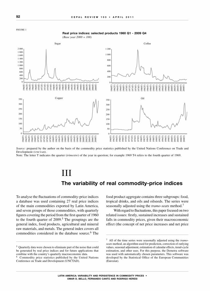
92



To analyse the fluctuations of commodity-price indices a database was used containing 27 real price indices of the main commodities exported by Latin America, and seven groups of those commodities, with quarterly figures covering the period from the first quarter of 1960 to the fourth quarter of 2009.5 The groupings are the general index, food products, agricultural and mineral raw materials, and metals. The general index covers all commodities considered in the database source.6 The

5 Quarterly data were chosen to eliminate part of the noise that could be generated by real price indices and for future applications that combine with the country’s quarterly macroeconomic data.6 Commodity price statistics published by the United Nations Conference on Trade and Development (UNCTAD).

food product aggregate contains three subgroups: food, tropical drinks, and oils and oilseeds. The series were seasonally adjusted using the tramo-seats method.7

With regard to fluctuations, this paper focused on two related issues: firstly, sustained increases and sustained falls in commodity prices, given their macroeconomic effect (the concept of net price increases and net price

7 All of the time series were seasonally adjusted using the tramo-seats method, an algorithm used for prediction, correction of outlying values, seasonal adjustment, estimation of calendar effects, trend-cycle estimation, and other uses. For this purpose, the Demetra software was used with automatically chosen parameters. This software was developed by the Statistical Office of the European Communities (Eurostat).

FIGURE 1

real price indices: selected products 1960 Q1 - 2009 Q4(Base year 2000 = 100)

Source: prepared by the author on the basis of the commodity price statistics published by the United Nations Conference on Trade and Development (unctad).Note: The letter T indicates the quarter (trimestre) of the year in question; for example 1969 T4 refers to the fourth quarter of 1969.

Sugar

0

200

400

600

800

1 000

1 200

1 400

1 600

1 800

2 000

1960

T1

1962

T1

1964

T1

1966

T1

1968

T1

1970

T1

1972

T1

1974

T1

1976

T1

1978

T1

1980

T1

1982

T1

1984

T1

1986

T1

1988

T1

1990

T1

1992

T1

1994

T1

1996

T1

1998

T1

2000

T1

2002

T1

2004

T1

2006

T1

2008

T1

Coffee

0

200

400

600

800

1 000

1 200

1960

T1

1962

T1

1964

T1

1966

T1

1968

T1

1970

T1

1972

T1

1974

T1

1976

T1

1978

T1

1980

T1

1982

T1

1984

T1

1986

T1

1988

T1

1990

T1

1992

T1

1994

T1

1996

T1

1998

T1

2000

T1

2002

T1

2004

T1

2006

T1

2008

T1

Copper

0

50

100

150

200

250

300

350

1960

T1

1962

T1

1964

T1

1966

T1

1968

T1

1970

T1

1972

T1

1974

T1

1976

T1

1978

T1

1980

T1

1982

T1

1984

T1

1986

T1

1988

T1

1990

T1

1992

T1

1994

T1

1996

T1

1998

T1

2000

T1

2002

T1

2004

T1

2006

T1

2008

T1

Oil

0

50

100

150

200

250

300

350

1960

T1

1962

T1

1964

T1

1966

T1

1968

T1

1970

T1

1972

T1

1974

T1

1976

T1

1978

T1

1980

T1

1982

T1

1984

T1

1986

T1

1988

T1

1990

T1

1992

T1

1994

T1

1996

T1

1998

T1

2000

T1

2002

T1

2004

T1

2006

T1

2008

T1

IIIThe variability of real commodity-price indices

93



falls was used for this purpose); and secondly, the sequence of falls and rises in commodity prices, in other words their cycles.

1. Net price increases and falls

This paper records a net price increase in a given quarter t if the current-quarter price Pt is higher than the maximum of the six previous quarters.8 Italso considers that there is a net price fall in a given quarter t if Pt is below the minimum of the six previous quarters.

These concepts and their application extend the work of Hamilton (1996) in two directions. Firstly, a net price fall is defined, because the only purpose of the aforementioned study was to analyse the effect of net increases in the price of oil on economic activity in the United States. The present research is also interested in analysing falls in commodity prices, because, as noted above, downward price movements are recurrent in commodity-price series and have significant macroeconomic consequences for certain Latin American countries.

Secondly, the definition used in this article is stricter, because six quarters are used instead of four as a criterion for deciding whether a net price increase or fall occurred in a given quarter.9 The comparison period is also lengthened to isolate price movements that could have macroeconomic effects, in the belief that such repercussions affect the decisions of economic agents (public and private sector) if they last for at least six quarters. A six-quarter period also makes it possible to filter out spurious price variations.

Using these definitions each period of the time series used can be divided into three categories: net price increases, net price falls, and periods that cannot be characterized by either of these movements.

(a) Results for the entire sampleTable 1 shows the number of net price increases

and net price falls occurring in each decade. The first salient point is that in the period 1960-2009, 20 of the

8 Hamilton (1996) defines a net price increase as a situation in which the price in a given quarter exceeds the maximum price of the four preceding quarters. The author uses this definition to study upswings in the oil market. He does not target his study on price falls, arguing that only oil price increases have a macroeconomic repercussions for the United States economy. Using quarterly data for the period running from the first quarter of 1948 to the second quarter of 1994, he concludes that net increases in the price of oil occurred in the period 1973-1981, and then again in 1989-1992.9 Bello and Heresi (2008) performed this exercise over eight quarters,with very similar results to those presented in this study.

27 real commodity-price indices in the sample reported more net price falls than net increases.10 This was also true for all groupings in the sample; for example, the general price index of all commodities reported 41 net increases and 56 net falls.

The groupings whose real price indices posted net increases most frequently were minerals and metals, and oils and oil seeds, with 49 and 45, respectively. The individual commodity-price indices with the largest number of net increases were lead (54), fish meal (54) and copper (47). The groupings that recorded the largest number of net price-fall periods were agricultural raw materials and minerals and metals, with 58. Iron was the individual commodity whose real price index recorded the largest number of periods with net falls (86), followed by tobacco and rubber, with 67 and 66, respectively.

The difference between the number of net price falls and increases varied by decade. In the 1980s and 1990s, the former outweighed the latter in 30 and 31 of the total of 34 real price indices considered, respectively. In the 1960s, the equivalent figure was 19; and in the 1970s and 2000s, seven and one, respectively. In the period 1970-2009, the net falls or increases in commodity prices seem to be highly correlated; in other words, they experienced net falls or net increases jointly. This is consistent with the fourth stylized fact mentioned in section II, and also with what can be inferred from the database used here.11

(b) Results for the decade of 2000The real commodity-price indices in this decade

had the following features: (i) In this sample, all commodities and their groupings,

except for tobacco, had more net price increases than net price falls.

(ii) There were more net price increases in the 2000s than in any of the four previous decades in all groupings except for oils and oilseeds. The general real price index in that decade accounted for 37% of the net price increases occurring in the entire period; the

10 The real price indices of sugar, bananas, soya meat, fish meal, copper, lead and gold were the only ones that did not fall more often than rise.11 Most of the correlations between aggregate price indices are positive; in other words, commodity prices all tend to move in the same direction. Similarly, as would be expected, the price indices of food products and agricultural raw materials are also highly correlated (0.85 for the whole sample); and each of these groups is highly correlated with the minerals and metals series (roughly 0.72). In contrast, oil displays significantly lower correlations with these three groups, owing to the dissimilar trend of the price of crude oil with respect to other commodities.

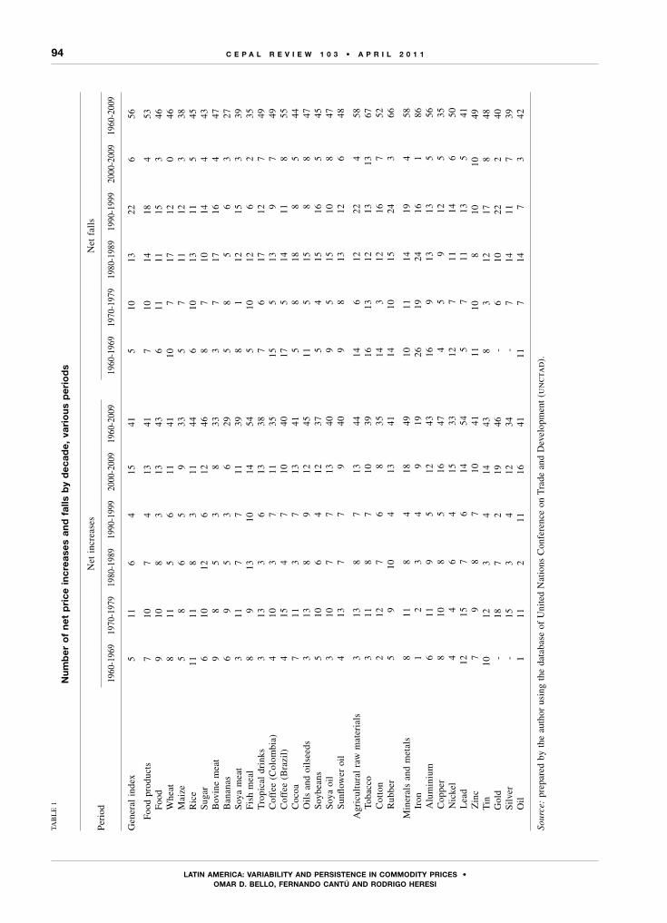
94


C E P A L R E V I E W 1 0 3 • A P R I L 2 0 1 1TA

BL

E 1

Nu

mb

er o

f n

et p

rice

in

crea

ses

and

fal

ls b

y d

ecad

e, v

ario

us

per

iod

s

Per

iod

Net

inc

reas

esN

et f

alls

1960

-196

919

70-1

979

1980

-198

919

90-1

999

2000

-200

919

60-2

009

1960

-196

919

70-1

979

1980

-198

919

90-1

999

2000

-200

919

60-2

009

Gen

eral

ind

ex5

116

415

415

1013

226

56

Fo

od p

rodu

cts

710

74

1341

710

1418

453

Food

910

83

1343

611

1115

346

Whe

at8

115

611

4110

717

120

46

M

aize

58

65

933

57

1112

338

Ric

e11

118

311

446

1013

115

45

S

ugar

610

126

1246

87

1014

443

Bov

ine

mea

t9

85

38

333

717

164

47

B

anan

as6

95

36

295

85

63

27

S

oya

mea

t3

117

711

398

112

153

39

F

ish

mea

l8

913

1014

545

1012

62

35

T

ropi

cal

drin

ks3

133

613

387

617

127

49

C

offe

e (C

olom

bia)

410

37

1135

155

139

749

Cof

fee

(Bra

zil)

415

47

1040

175

1411

855

Coc

oa7

113

713

415

818

85

44

O

ils

and

oils

eeds

313

89

1245

115

158

847

Soy

bean

s5

106

412

375

415

165

45

S

oya

oil

310

77

1340

95

1510

847

Sun

flow

er o

il4

137

79

409

813

126

48

A

gric

ultu

ral

raw

mat

eria

ls3

138

713

4414

612

224

58

To

bacc

o3

118

710

3916

1312

1313

67

C

otto

n2

127

68

3514

312

167

52

R

ubbe

r5

910

413

4114

1015

243

66

M

iner

als

and

met

als

811

84

1849

1011

1419

458

Iron

12

34

919

2619

2416

186

Alu

min

ium

611

95

1243

169

1313

556

Cop

per

810

85

1647

45

912

535

Nic

kel

44

64

1533

127

1114

650

Lea

d12

157

614

545

711

135

41

Z

inc

79

87

1041

1110

810

1049

Tin

10

123

414

438

312

178

48

G

old

-18

72

1946

-6

1022

240

Sil

ver

-15

34

1234

-7

1411

739

Oil

111

211

1641

117

147

342

Sour

ce:

prep

ared

by

the

auth

or u

sing

the

dat

abas

e of

Uni

ted

Nat

ions

Con

fere

nce

on T

rade

and

Dev

elop

men

t (u

nct

ad

).

95



figure for the minerals and metals grouping was similar, whereas the proportion was 30%12 in the case of food and agricultural raw materials, and 39% in the case of oil. Clearly, the rise in commodity prices was led by minerals and metals and oil. From the standpoint of the individual indices, in 2000s, the 27 commodities in the sample recorded more net increases than in the 1980s13 and 1990s, whereas in comparison to the 1960s and 1970s, this was true for 22 and 15 commodities, respectively.

(iii) In keeping with the above, the individual commodity indices and their groupings had fewer net price falls in this decade than in the 1990s, 1980s,14 1970s15 and 1960s16 taken separately. Compared to the 1990s, the number of net falls in the food product price index dropped from 18 to just four in the most recent decade, while the number of net price falls in agricultural raw materials, minerals and metals, and oil dropped from 22, 19, and 7 to just 4, 4 and 3, respectively. In those cases, the net falls in the current decade represented less than 8% of all of those occurring since 1960. The four commodities with the smallest proportion of total net falls were wheat (0), iron (1) and rubber and gold (5).In the past decade, the fact that the general net

increase in real commodity-price indices occurred after two decades dominated by net falls strengthens the perception that this pattern differs significantly from what happened previously, in that there were more net increases in the decade of 2000 than in each of the preceding decades for most real commodity-price indices. Nonetheless, taking the sample as a whole, what stands out most is the variability of prices: a succession of net increases followed by a period of net falls, followed in turn by a new series of net increases. This is consistent with the first stylized fact mentioned above.

2. Commodity price cycles

To date the cycles, this paper used a version of the Bry-Boschan algorithm —one of the most widely used

12 These proportions were 47% for iron, 46% for nickel, 41% for gold, 34% for copper, 33% for tin, and 32% for soybeans.13 Except for sugar.14 Except for tobacco and zinc.15 In this case, the price indices of the groupings (tropical drinks and oils and oilseeds) and of seven individual commodities (soya meat, coffee from Colombia, coffee from Brazil, soybeans, soya oil, cotton and tin) display more net price falls in the decade of 2000 than in the 1970s.16 Except for the general index, bovine meat and copper.

methodologies.17 The same procedure was also used by Cashin, McDermott and Scott (1999a) in the case of commodity prices.18

The Bry-Boschan methodology is based firstly on detecting potential local minima and maxima, for which a three-quarter centred moving window is chosen as comparison horizon. Once the quarters have been chosen, they are subject to two additional rules: minimum duration of phases and cycles, and sequence. An upswing phase is defined as a period that starts with a minimum and ends with a maximum, whereas a fall phase is defined as a period that starts with a maximum and ends with a minimum. The series is thus described by consecutive periods of price rises and falls. A cycle encompasses two phases: rise and fall.

A price index observation for a given commodity was considered as a potential local maximum (minimum) if it represented the highest (lowest) value of the three immediately preceding and subsequent quarters. The minimum duration of a phase was defined as three quarters, which makes the minimum duration of a cycle six quarters. With regard to the sequence rule, if there are two consecutive maxima (minima), the larger (smaller) is used.19

(a) Results for the whole sampleFigure 2 exemplifies the result of applying the

algorithm to the real price indices of four selected commodity groupings. In the case of the general real price index, there are six cycles and one additional upswing; in food products there are seven complete cycles, whereas agricultural raw materials display eight cycles and an upswing; and minerals and metals record seven cycles plus an upswing. For all of these groupings except for food products, the price indices cycles in the figure start

17 For a detailed description of the methodology, see Bry and Boschan (1971). The version used in this article defines potential maxima and minima selection criteria, as described below, and slightly alters the algorithm to include more observations at the start and end of the sample.18 These authors use monthly price series for 36 commodities covering the period January 1957-August 1999, and define a four-month centred moving window, encompassing the two quarters before and after each observation. The results show that during the period analysed there are six complete cycles when the different commodities are averaged, the extremes being banana and fish meal, which recorded three and 10 cycles respectively. Secondly, there is an asymmetry between price upswings and downswings in terms of duration and magnitude, in that the price falls last longer than the booms and are slightly larger in magnitude than the increases that occurred during the upswing phases. 19 This allows for the possibility of minor fall phases during an upswing and vice versa, but imposes a restriction on the length of these reversals.

96



with an upswing.20 Figure A1.1 in annex 1 illustrates the same procedure for several selected commodities. A detailed description of the dates of the cycles and their phases, together with the variation reported in the real price index for selected commodities is shown in table A1.1.21

20 To define the cycles for each of the commodities and their groupings, the sample considered the first complete phase. As a result, for some indices, the cycles are rise-fall, whereas for others they are fall-rise.21 This information for each of the products in the sample is obtainable from the authors on request.

Table 2 shows the results of applying this algorithm to the commodity prices of the sample used. The salient points are as follows:(i) All of the real price indices displayed multiple

complete cycles ranging between three (iron and gold) and 11 (lead). Of the groupings, oils and oilseeds displayed the largest number of cycles: 10. The real price indices of sunflower oil, cotton, copper and zinc recorded 10 cycles, whereas the general index had six complete cycles.

(ii) The average duration of the cycles varied from 16.8 quarters (lead) to 35 (iron). For the general index of prices, the average duration was 26.8 quarters.

FIGURE 2

Cycles of real price indices: selected groupings. 1960 Q1 - 2009 Q4(Base year 2000 = 100)

Source: prepared by the authors on the basis of data obtained from the United Nations Conference on Trade and Development (unctad).Note: In these figures, the number next to the letter T indicates the quarter (trimestre) of the year in question; for example: 1969 T4 corresponds to the fourth quarter of 1969.

General index

2008T21978T3

1963T4

2002T1

1995T4

1993T3

1988T4

1986T41982T4

1983T3

1980T4

1971T31962T1

1974T4

50

150

250

350

450

550

650

750

1960

T1

1962

T1

1964

T1

1966

T1

1968

T1

1970

T1

1972

T1

1974

T1

1976

T1

1978

T1

1980

T1

1982

T1

1984

T1

1986

T1

1988

T1

1990

T1

1992

T1

1994

T1

1996

T1

1998

T1

2000

T1

2002

T1

2004

T1

2006

T1

2008

T1

Food products

1963T4

1965T2

1967T3

1971T3

1974T4

1979T1

1980T4

1982T4

1983T3

1987T3

1988T3

1993T3

1996T2

2002T1

2008T2

50

150

250

350

450

550

650

750

1960

T1

1962

T1

1964

T1

1966

T1

1968

T1

1970

T1

1972

T1

1974

T1

1976

T1

1978

T1

1980

T1

1982

T1

1984

T1

1986

T1

1988

T1

1990

T1

1992

T1

1994

T1

1996

T1

1998

T1

2000

T1

2002

T1

2004

T1

2006

T1

2008

T1

Agricultural raw materials

1964T1

1965T1

1971T1

1973T4

1975T1

1976T4

1978T1

1980T1

1982T4

1983T4

1985T2

1988T2

1989T4

1990T3

1993T4

1995T2

2002T1

2008T3

50

150

250

350

450

550

650

750

1960

T1

1962

T1

1964

T1

1966

T1

1968

T1

1970

T1

1972

T1

1974

T1

1976

T1

1978

T1

1980

T1

1982

T1

1984

T1

1986

T1

1988

T1

1990

T1

1992

T1

1994

T1

1996

T1

1998

T1

2000

T1

2002

T1

2004

T1

2006

T1

2008

T1

Metals and minerals

1963T3

1966T1

1969T11972T4

1974T2

1978T2

1986T3

1989T1

1993T4

1995T1

1999T1

2000T1

10/1/2002

2008T21980T11969T4

50

150

250

350

450

550

650

750

1960

T1

1962

T1

1964

T1

1966

T1

1968

T1

1970

T1

1972

T1

1974

T1

1976

T1

1978

T1

1980

T1

1982

T1

1984

T1

1986

T1

1988

T1

1990

T1

1992

T1

1994

T1

1996

T1

1998

T1

2000

T1

2002

T1

2004

T1

2006

T1

2008

T1

97



(iii) For all of the commodity-price indices in the sample, except for fish meal and food products, the falls tended to last longer than the rises.22 In other words, throughout the five decades covered in the database, commodity prices were falling most of the time. On average, the falls lasted 13.5 quarters whereas the upswings lasted 9.2 quarters. In the case of the general index, the corresponding figures are 19.3 quarters and 10 quarters respectively, whereas the greatest difference in a grouping occurs in tropical drinks, where the corresponding averages with 19.5 quarters and 6.7 quarters, respectively. The real

22 This refers to rises and falls that have concluded, not those currently under way.

commodity-price indices with the largest difference between the duration of falls and rises were coffee (Colombia), bovine meat, tobacco and iron.

(b) Results for the decade of 2000The results show that, for the vast majority of

commodities, the final price upswing in the 2000s is very different from those of previous periods, in terms of both duration and magnitude. All of the aggregate price series display cumulative increases of over 100% in the most important upswing of the decade; for example, the general index of all commodities posted a real increase of 158% over 20 five quarters (2002 Q1-2008 Q2). Some of the largest cumulative increases occurred in the real price indices of oil (381%), copper

TABLE 2

Commodity price cycles, rises and falls: 1960 Q1 - 2009 Q4

Cycles Rises Falls

Number Average duration (number of quarters)



General index 6 26.8 7 10.0 6 19.3Food products 7 25.4 7 10.4 7 15.0 Food 7 25.4 7 12.7 7 12.7 Wheat 8 21.5 9 9.0 8 12.5 Maize 7 20.9 8 9.1 7 11.7 Rice 7 26.3 7 11.7 7 14.6 Sugar 6 30.2 6 14.5 6 15.7 Beef 7 22.9 8 8.1 8 14.8 Bananas 9 18.1 10 7.7 9 10.4 Soya meat 8 22.9 8 8.5 8 14.4 Fish meal 9 18.2 9 10.4 10 7.8 Tropical drinks 6 26.2 6 6.7 6 19.5 Coffee (Colombia) 7 22.9 7 6.0 7 16.9 Coffee (Brazil) 9 17.1 9 5.9 9 11.2 Cocoa 6 26.7 6 11.3 6 15.3 Oils and oilseeds 10 17.3 11 7.7 10 9.7 Soybeans 9 20.9 9 8.4 9 12.6 Soya oil 9 18.7 10 7.4 9 11.2 Sunflower oil 10 18.6 10 8.3 11 10.2 Agricultural raw materials 8 19.0 9 9.2 8 11.9 Tobacco 7 24.4 7 7.1 7 17.3 Cotton 10 16.9 10 8.4 10 8.5 Rubber 7 19.3 8 9.1 7 12.7 Minerals and metals 7 22.0 8 9.1 7 15.3 Iron 3 35.0 3 12.3 3 22.7 Aluminium 9 20.2 10 8.9 9 11.3 Copper 10 17.4 10 8.9 10 9.4 Nickel 8 22.6 8 9.8 8 12.9 Lead 11 16.8 11 8.2 11 8.6 Zinc 10 18.6 10 7.3 10 11.3 Tin 8 21.5 8 9.4 8 12.1 Gold 3 25.3 3 10.3 4 18.3 Silver 5 23.8 6 10.2 5 17.0 Oil 8 23.1 8 10.3 8 12.9

Source: prepared by the authors on the basis of data obtained from the United Nations Conference on Trade and Development (unctad).

98



(266%) and silver (213%), which spanned 26 quarters (2001 Q4-2008 Q2), 16 quarters (2002 Q3-2006 Q3) and 27 quarters (2001 Q3-2008 Q2), respectively. The largest increases occurred in oil and in commodities in the metals and minerals group. The rise in the prices of iron, copper, nickel and oil was so large that they were the only products to attain their maximum between 2007 and 2008, as shown in table 3.

Although these percentage increases are not very different from those observed in the 1970s for certain commodities, the key difference is in the degree of generalization and, particularly, the duration of this price-rise period. Upswings in the four previous decades lasted on average for less than seven quarters, whereas from 2002 onwards, they have averaged 14 consecutive quarters. In all aggregate indices the rising-price periods lasted 20 quarters, more than all previous periods combined. All commodities displayed this result except for the 31-quarter sugar price boom from 1967 Q1 to 1974 Q4. It should be noted that cumulative increases may be affected by the starting point of the upswing,

because 16 of the 27 products recorded their 50-year minimum between 2000 and 2003.

In terms of correlations between the price upswings of the different commodities, there is a significant joint movement encompassing oil, gold, and silver. As would be expected, the uncertainty generated by rising global energy price increases tends to push up the real prices of metals that are used as a store of value. The highest coefficients of correlation with the real oil price index are recorded by gold (0.75) and silver (0.70), whereas the correlation with the other commodities is significantly less (simple average of 0.28). Accordingly, in the 1970s, these metals also experienced two significant positive price shocks. The real price of gold rose by 3.4 times in the 13 previous quarters and up to the first oil shock (1971 Q4-1974 Q4), and then rose again over 14 quarters (1976 Q4-1980 Q1) quadrupling its real value by the end of the decade. The price of silver first rose by 3.2 times over 10 quarters (1972 Q2-1974 Q2), and then by another 5.6 times in another 10 quarter-period (1977 Q4-1980 Q1).

TABLE 3

Commodity price minima and maxima: 1960 Q1 - 2009 Q4

Minimum value Date Maximum value Date

General index 88.7 2001 Q4 503.8 1974 Q4Food products 92.7 2002 Q1 686.1 1974 Q4 Food 93.3 2002 Q1 717.1 1974 Q4 Wheat 91.3 1999 Q4 630.1 1974 Q1 Maize 89.2 2000 Q3 585.6 1974 Q4 Rice 79.0 2001 Q2 1 078.3 1974 Q2 Sugar 58.8 1985 Q2 1 974.3 1974 Q4 Beef 90.3 1998 Q4 437.3 1973 Q3 Bananas 70.5 2003 Q2 258.8 1964 Q2 Soya meat 82.7 1999 Q2 708.2 1973 Q2 Fish meal 90.2 1999 Q2 567.4 1973 Q3 Tropical drinks 72.4 2001 Q4 973.7 1977 Q2 Coffee (Colombia) 49.8 2001 Q4 1 190.8 1977 Q2 Coffee (Brazil) 58.2 2002 Q3 771.7 1977 Q2 Cocoa 89.2 2000 Q4 959.5 1977 Q3 Oils and oilseeds 81.7 2001 Q2 735.7 1974 Q4 Soybeans 84.7 2002 Q1 655.7 1973 Q2 Soya oil 89.2 2000 Q4 959.5 1974 Q4 Sunflower oil 92.3 2000 Q4 984.8 1974 Q4 Agricultural raw materials 83.4 2002 Q1 338.3 1973 Q4 Tobacco 81.1 2006 Q2 245.6 1960 Q1 Cotton 63.0 2001 Q4 491.0 1973 Q4 Rubber 81.7 2001 Q4 1 354.2 1960 Q2 Minerals and metals 80.8 2001 Q4 375.7 1974 Q2 Iron 96.6 2002 Q1 408.7 2008 Q4 Aluminium 71.6 2009 Q1 281.1 1988 Q2 Copper 18.4 1961 Q1 352.4 2008 Q1 Nickel 50.5 1998 Q4 435.4 2007 Q2 Lead 86.0 2003 Q1 484.9 1979 Q2 Zinc 63.3 2003 Q1 509.5 1974 Q2 Tin 68.2 2002 Q1 707.6 1979 Q2 Gold 55.0 1970 Q3 484.6 1980 Q1 Silver 83.8 2001 Q3 1 335.8 1980 Q1 Oil 34.1 1971 Q1 319.2 2008 Q2

Source: prepared by the authors on the basis of data obtained from the United Nations Conference on Trade and Development (unctad).Note: The letter Q indicates the quarter of the year in question; for example 2008 Q4 refers to the fourth quarter of 2008.

99



The analysis of the persistence of the series traditionally starts with a classical unit-root test (the augmented Dickey-Fuller test or the Phillips-Perron test). If the null hypothesis of a unit root is not rejected, the series in question is considered non-stationary and therefore does not have the mean-reversion property, so any disturbance will have permanent effects. If the null hypothesis of a unit root is rejected, the series is deemed to be stationary, and the effect of the shock will be transitory. In this second case, an equation such as (1) is estimated by ordinary least squares (ols). In this equation Pt is the logarithm of the price index in period t, and α is the autoregressive parameter, which is used to construct measures of persistence. The closer the estimation of α is to 1, the more persistent the series is considered to be. The exact configuration of the foregoing equation (in other words, inclusion of the constant term and trend) was chosen for each price series using the Akaike information criteria.

Pt = µ + β ⋅ t + α ⋅ P

t−1 + εt , µ, β ∈ ℜ and α ∈ (−1,1] (1)

This procedure suffers from a number of shortcomings, however. Firstly, the unit root tests only make it possible to characterize the series as stationary or non-stationary, but do not give much information on persistence or any other characteristics. Moreover, these traditional tests of hypothesis are low-power in that they tend not to reject the null hypothesis of a unit root, so a conclusion regarding the persistence of the series might not be statistically reliable.

Secondly, estimation of the parameter α by ols produces estimates that are biased towards 0, especially when the parameter is close to 1, since this estimator has an asymmetric distribution.23 Consequently, the present research uses the unbiased estimate of the mean (uem) for the autoregressive parameter α, as proposed by Andrews and Chen (1994), which makes it possible to mitigate the second problem and obtain a better estimate of the persistence of a series.24

23 See Andrews (1993).24 For further details of the estimation see Andrews and Chen (1994). An application to monthly commodity-price series can be found

Annex 2 shows the results of applying this persistence-evaluation procedure for the individual commodities and groupings studied in this article. To make the analysis more complete, the price indices were analysed in terms of both levels and first differences to measure the effect of a shock on commodity price levels and on their rate of variation (quarterly inflation).

Table A2.1 displays the results of the classical unit-root tests. With a confidence level of 90%, the augmented Dickey-Fuller test does not reject the null hypothesis of a unit root in 20 of the series measured in terms of levels, including the general price index; in other words, the test concludes that the series are not stationary, and any shock will be permanent. For the other series, the levels test does not provide further information. At the same confidence level, the Phillips-Perron test does not reject the null hypothesis of a unit root for 29 series measured in terms of levels, also including the general index and all groupings. Lastly, both tests conclude that the rates of change of all indices are stationary, since they reject the hypothesis for all of the series when measured in terms of first differences.

The first section of table A2.2 reports estimations of the autoregressive parameter both for ols and for uem, for the series in terms of levels, together with two traditional measures of persistence: the cumulative impulse-response function (cirf) and the mean life (ml) of a shock.25 As

in Cashin, Liang and McDermott (2000). The quantiles needed to calculate these coefficients were estimated on the basis of Monte Carlo simulations, which were based on 10,000 replicas of series with the length of the sample required in this study.25 The cirf measures the total cumulative effect of a unit shock over the future horizon of a series; it is calculated as the infinite sum of the impulse-response function (irf),

= =CIRF IRF tt UEM−=

∞

∑ ( )ˆ

.1

1

1 α

The ml indicates how many quarters have to elapse for half of the total effect of a price index shock to dissipate. By providing a time measure of the effect of the shock, this is a good indicator of persistence in a series. It is obtained from the expression

MLUEM

=( )

( )ln ,

ln ˆ.

0 5

α

IVPersistence of real commodity-price indices

100



noted above when considering the results of the unit-root tests, the estimated coefficients of the autoregressive parameter for the equation expressed in terms of levels are very close to 1 for nearly all products. The uem can also be seen to correct the bias of the ols estimator, and presents estimates with higher values. According to this latter method, except for the real index of banana prices (with an estimated α of 0.71), all products have an estimated coefficient of 0.95 or higher. Accordingly, all the series in terms of levels are either stationary with very high persistence, or non-stationary. This is verified in the two persistence measures.

In the first case, the cirf shows that the cumulative effect of a shock will be very large; for example, a shock to the price of wheat will have a total cumulative effect of 54.1 times the magnitude of the shock. With the exception of bananas, this factor has very high values and is actually infinite for many series, including the general price index and most of the groupings. In the second case, the ml shows that a shock will have lasting effects: for example, 37.1 quarters (more than nine years) would have to pass to dissipate half of the effect of the unit shock on the spot price of wheat. Here again, except for the real index of banana prices, this measure displays very high values and even is infinite in many cases.

Moreover, as can be seen from the second section of table A2.2, the estimates of the autoregressive parameter for the series in first-difference terms (rates of change) are significantly lower, although most remain statistically significant. The bias of the ols estimator is smaller, because the values are lower, and so is the difference with respect to the uem. The cirf indicates that the cumulative effect of a disturbance on the rate of variation will be comparatively limited and will seldom double the magnitude of the initial shock. Lastly, the ml of the disturbance is also very low, mostly below 1, which suggests that the effects of a shock on the rate of variation are short-lived.

In brief, the foregoing analysis shows that commodity prices are highly persistent or even non-stationary in nearly all cases; and a disturbance to the price level will have very long-lasting or permanent effects. In contrast, rates of change of prices are not very persistent, and any temporary rise in the price of a good will rapidly dissipate and have a limited impact.

The analysis demonstrated that commodity price levels are highly persistent, or even non-stationary. Nonetheless, it is possible that an autoregressive model such as (1) may fail to fully capture the persistence present in the series, and this could explain the low

level of persistence shown above in the rate of change of prices. To study this feature in greater depth, an autoregressive fractionally integrated moving average (arfima) (0, 1+d, 0) model was estimated for the price the series. This is a fractionally integrated arma model for the rate of change of prices, where d is the integration fraction.26 This model alters equation (1) by introducing a fractional integration factor of the following type

( ) , ,1 1− ⋅ = + ⋅ + ∈ℜ+L P t ddt tµ β ε µ β, (2)

The precise configuration of the foregoing equation (in other words inclusion of the constant term and trend) was chosen for each series using the Akaike information criterion. The aim now is to estimate the parameter d, also known as the memory parameter, which is directly related to the persistence of the series. In an arfima such as (2), if d is equal to 0, the conclusion is that the variable has “short memory” and does not display any persistence. In contrast, if this parameter is within the interval (0, 0.5), then the series will be stationary and have the reversion-to-mean property, but it will also have “long memory”. In the interval [0.5, 1), the variable will also be stationary, but the process no longer reverts to the mean, and the series will be of “very long memory”. Lastly, for values of d that are greater than or equal to 1, the series is not stationary, and any disturbance will have permanent effects. As can be concluded, the higher the value of d, the longer will be the “memory” of the series, and, hence, the more persistent any disturbance.

Estimating the parameters of equation (2) is not a trivial matter, because it involves a non-linear function of the lags of the price series. This paper used several parametric and semi-parametric estimation methods,27 with results as shown in table A2.3. The values estimated by the three parametric methods are generally very similar. The results of the semi-parametric estimates show greater variability, but in most cases the differences are small. To simplify the exposition, the maximum likelihood estimator will be used in the description of

26 The number 1 in parentheses indicates first differences; in other words, as the variables are expressed in logarithms, the first difference is equivalent to the quarterly rate of variation.27 Three parametric estimators (maximum likelihood, modified profile likelihood, and non-linear least squares) and one semiparametric estimator (the Robinson-Henry estimator) were calculated using the arfima 1.04 for Ox package. Two semiparametric methods (the Geweke/Porter-Hudak estimator and the Robinson estimator) were obtained through the gphudak and roblpr extensions in the stata software. For further details of the estimation, see the documentation of these functions.

101



the results, although the values for the other estimators can be consulted in table A2.3.

The estimated value of d for the general price index is around 0.39. This means that, although the effect of a change in the general rate of variation will be transitory, it will take a long time to dissipate because it is a “long-memory” series. In other words, the rate of inflation of the general commodity-price index displays the persistence property. For the food products group, the estimated value is 0.28, and for its food, tropical drinks, and oils and oilseeds components, values of 0.32, 0.26 and 0.22 were obtained, respectively. In the case of agricultural raw materials, d was estimated at 0.40, and for minerals and metals, the estimated value was 0.30. Thus, all rates of change of prices in these groupings are persistent. Oil is the only grouping for which d is not statistically different from 0, and consequently has a “short memory”.

At the individual-product level, the highest persistence is displayed by fish meal (estimated d of 0.45), followed by aluminium (0.41), tobacco (0.34) and a zinc (0.34). In contrast, only seven products display

an estimated d that is not significantly different from 0, and consequently display “short memory” and low persistence: maize, bovine meat, soybeans, cotton, iron, silver and oil.

The banana price index is a special case, since the estimated value of the parameter d is negative, which suggests that the variable is over-differentiated. This was also noted above, because it was the only commodity whose autoregressive coefficient was not close to 1. When the estimation of the arfima model is repeated with the series measured in terms of levels, an estimated coefficient of 0.60 is obtained that is statistically significant.28 Accordingly, the banana price series is stationary in terms of levels, but highly persistent; consequently, the rate of change of the price of this product also does not display very low persistence and could be added to the above listing.

28 In this case, the result of the estimator is reported by non-linear least squares, since it is impossible to use the maximum likelihood estimator for values of d greater than 0.5.

VEvaluation

This study shows that, over the last five decades, the real price indices of all commodities and their groupings:(i) Have displayed significant variability, as shown

both by the presence of multiple cycles in each of the series and by the alternation of non-spurious price increases and falls.

(ii) Commodity price shocks are generally highly persistent; in other words, they take a long time to die out. The most recent upswing period, which encompassed

most commodity prices and ended between the first quarter of 2006 and the fourth quarter of 2009, differs from its predecessors in terms of its generalized nature, duration, and the fact that it was not associated with temporary supply interruptions. Moreover, its abrupt end was followed by a vigorous recovery starting in the second half of 2009. Nonetheless, these differences, in a single cycle, cannot be used to claim that a definitive change has taken place in the cyclical pattern of these series.

The expansionary phase of the latest cycle seems to have been underpinned both by real factors and by

financial ones. The former include burgeoning demand from emerging countries, such as China and India, which have become more important players in commodity markets. The financial factors include an increase in the demand for instruments such as commodity futures. Both of these factors are new on the international scene.

Since 2006, the creation and issuance of instruments indexed to commodity prices have grown significantly, with increasing participation by actors not linked to production, processing, or commercialization (mutual funds, pension funds, investment funds, commodity hedge funds in the futures markets of certain goods). Caballero, Farhi and Gourinchas (2008) argue that this interest stems from the shortage of financial assets available on international markets. Southwood (2008) estimated, for the case of copper, that about 25% of the high price prevailing in the first of 2008 reflected the activity of speculators, and the remaining 75% was underpinned by fundamental factors. This entails additional risks in commodity-price reversion processes which, by being linked to financial factors, were more abrupt and further-

102



reaching than expected. In the fourth quarter of 2008, for example, the real price index of the mineral and metals, agricultural raw materials and oil groupings, posted their largest quarter-on quarter percentage fall of the last five decades: 30.6%, 24.9% and 50.1%, respectively.29 The real price indices of aluminium and nickel fell by 32.8% and 40.7%, respectively, in that quarter; while the copper price index posted its steepest ever fall of 37.5%. All of this is consistent with the bursting of a price bubble.

As this paper has shown, in the latest upswing, the largest price increases were recorded in oil and products in the minerals and metals grouping. Nonetheless, oil was the only commodity to attain its all-time maximum during this upswing. In terms of sequence, the commodities whose prices reflected these increases in demand were oil and minerals and metals. The sustained increase in the price of energy products, together with a growing preference for clean energy sources, triggered growth in the biofuel industry, which meant an increase in demand for soya, wheat, maize and sugar and, hence, in their prices and those of their substitutes.30

The empirical evidence seems to reject conclusions, such as that price increases or falls are secular.31 The study has shown how, since 1960, any upswing period

29 These figures represent the seasonally adjusted quarterly growth rate.30 From the macroeconomic standpoint, rising food prices fuelled higher inflation worldwide from late 2007 to late 2008, particularly in developing countries whose price indices are more heavily weighted in the food category. In 2009, there was a significant fall in inflation, as commodity prices revered their trend. 31 This type of work was popular in the 1980s, because commodity prices were falling in that decade. Studies in that period tended to conclude that the decline was secular; see Reinhart and Wickham (1994).

was followed by a “longer” period of price falls, which can broadly be seen in the behaviour of the different series over decades. This is consistent with the findings of studies that use longer databases; the relevant fact is not the trend of the series but its variability; in other words, price rises and falls are transitory.32 The historical experience of downward adjustments in commodity prices has been mixed in terms of the magnitude and speed of the declines. The fall in product prices in the 1980s was gradual compared to what happened in the fourth quarter of 2008.

With regard to the persistence of commodity price series, the results of this paper show that this would be a relevant factor when designing economic stabilization mechanisms, since these would tend to be unsustainable in that context. Nonetheless, the cyclical characterization of the series presented in section III shows that the series have been affected by shocks of different sign, which suggests there may be substantial room for policy to smooth out the effects of those random changes.

Lastly, the high persistence of commodity-price shocks may be one reason why they have permanent effects on the Latin American economies. Toledo (2008) found that permanent commodity-price disturbances play a significant role in productivity shocks in the Bolivarian Republic of Venezuela, Brazil, Colombia and Peru, whereas highly persistent shocks explain this result in Argentina, Chile and Mexico. One possible source of these findings could be the persistence displayed by the real commodity-price indices, in terms of levels and rates of change, which has been documented in this article.

32 Despite having lasted for several years, the recent surge in commodity prices can be considered transitory, just as, in the light of history, the “long” price declines that occurred in the 1980s also seem transitory.

(Original: Spanish)

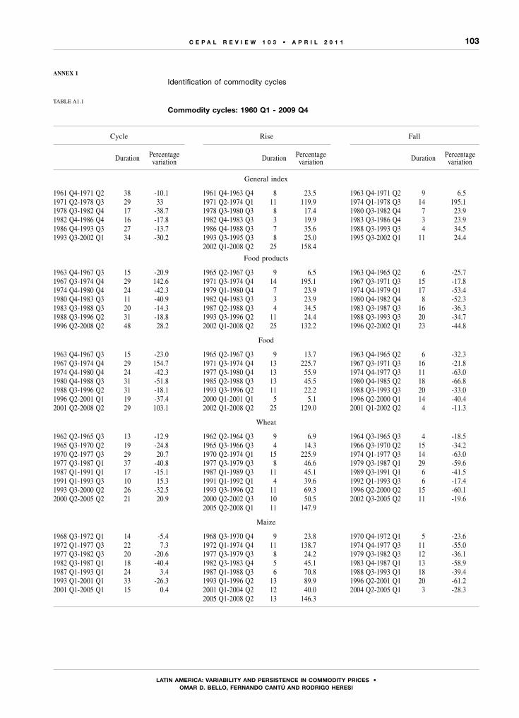
103



ANNEX 1

Identification of commodity cycles

TABLE A1.1

Commodity cycles: 1960 Q1 - 2009 Q4

Cycle Rise Fall

Duration Percentage variation Duration Percentage

variation Duration Percentage variation

General index

1961 Q4-1971 Q2 38 -10.1 1961 Q4-1963 Q4 8 23.5 1963 Q4-1971 Q2 9 6.51971 Q2-1978 Q3 29 33 1971 Q2-1974 Q1 11 119.9 1974 Q1-1978 Q3 14 195.11978 Q3-1982 Q4 17 -38.7 1978 Q3-1980 Q3 8 17.4 1980 Q3-1982 Q4 7 23.91982 Q4-1986 Q4 16 -17.8 1982 Q4-1983 Q3 3 19.9 1983 Q3-1986 Q4 3 23.91986 Q4-1993 Q3 27 -13.7 1986 Q4-1988 Q3 7 35.6 1988 Q3-1993 Q3 4 34.51993 Q3-2002 Q1 34 -30.2 1993 Q3-1995 Q3 8 25.0 1995 Q3-2002 Q1 11 24.4

2002 Q1-2008 Q2 25 158.4

Food products

1963 Q4-1967 Q3 15 -20.9 1965 Q2-1967 Q3 9 6.5 1963 Q4-1965 Q2 6 -25.71967 Q3-1974 Q4 29 142.6 1971 Q3-1974 Q4 14 195.1 1967 Q3-1971 Q3 15 -17.81974 Q4-1980 Q4 24 -42.3 1979 Q1-1980 Q4 7 23.9 1974 Q4-1979 Q1 17 -53.41980 Q4-1983 Q3 11 -40.9 1982 Q4-1983 Q3 3 23.9 1980 Q4-1982 Q4 8 -52.31983 Q3-1988 Q3 20 -14.3 1987 Q2-1988 Q3 4 34.5 1983 Q3-1987 Q3 16 -36.31988 Q3-1996 Q2 31 -18.8 1993 Q3-1996 Q2 11 24.4 1988 Q3-1993 Q3 20 -34.71996 Q2-2008 Q2 48 28.2 2002 Q1-2008 Q2 25 132.2 1996 Q2-2002 Q1 23 -44.8

Food

1963 Q4-1967 Q3 15 -23.0 1965 Q2-1967 Q3 9 13.7 1963 Q4-1965 Q2 6 -32.31967 Q3-1974 Q4 29 154.7 1971 Q3-1974 Q4 13 225.7 1967 Q3-1971 Q3 16 -21.81974 Q4-1980 Q4 24 -42.3 1977 Q3-1980 Q4 13 55.9 1974 Q4-1977 Q3 11 -63.01980 Q4-1988 Q3 31 -51.8 1985 Q2-1988 Q3 13 45.5 1980 Q4-1985 Q2 18 -66.81988 Q3-1996 Q2 31 -18.1 1993 Q3-1996 Q2 11 22.2 1988 Q3-1993 Q3 20 -33.01996 Q2-2001 Q1 19 -37.4 2000 Q1-2001 Q1 5 5.1 1996 Q2-2000 Q1 14 -40.42001 Q2-2008 Q2 29 103.1 2002 Q1-2008 Q2 25 129.0 2001 Q1-2002 Q2 4 -11.3

Wheat

1962 Q2-1965 Q3 13 -12.9 1962 Q2-1964 Q3 9 6.9 1964 Q3-1965 Q3 4 -18.51965 Q3-1970 Q2 19 -24.8 1965 Q3-1966 Q3 4 14.3 1966 Q3-1970 Q2 15 -34.21970 Q2-1977 Q3 29 20.7 1970 Q2-1974 Q1 15 225.9 1974 Q1-1977 Q3 14 -63.01977 Q3-1987 Q1 37 -40.8 1977 Q3-1979 Q3 8 46.6 1979 Q3-1987 Q1 29 -59.61987 Q1-1991 Q1 17 -15.1 1987 Q1-1989 Q3 11 45.1 1989 Q3-1991 Q1 6 -41.51991 Q1-1993 Q3 10 15.3 1991 Q1-1992 Q1 4 39.6 1992 Q1-1993 Q3 6 -17.41993 Q3-2000 Q2 26 -32.5 1993 Q3-1996 Q2 11 69.3 1996 Q2-2000 Q2 15 -60.12000 Q2-2005 Q2 21 20.9 2000 Q2-2002 Q3 10 50.5 2002 Q3-2005 Q2 11 -19.6

2005 Q2-2008 Q1 11 147.9

Maize

1968 Q3-1972 Q1 14 -5.4 1968 Q3-1970 Q4 9 23.8 1970 Q4-1972 Q1 5 -23.61972 Q1-1977 Q3 22 7.3 1972 Q1-1974 Q4 11 138.7 1974 Q4-1977 Q3 11 -55.01977 Q3-1982 Q3 20 -20.6 1977 Q3-1979 Q3 8 24.2 1979 Q3-1982 Q3 12 -36.11982 Q3-1987 Q1 18 -40.4 1982 Q3-1983 Q4 5 45.1 1983 Q4-1987 Q1 13 -58.91987 Q1-1993 Q1 24 3.4 1987 Q1-1988 Q3 6 70.8 1988 Q3-1993 Q1 18 -39.41993 Q1-2001 Q1 33 -26.3 1993 Q1-1996 Q2 13 89.9 1996 Q2-2001 Q1 20 -61.22001 Q1-2005 Q1 15 0.4 2001 Q1-2004 Q2 12 40.0 2004 Q2-2005 Q1 3 -28.3

2005 Q1-2008 Q2 13 146.3

104



(continued)

Cycle Rise Fall



Beef

1963 Q1-1968 Q2 20 59.5 1963 Q1-1966 Q4 15 74.3 1966 Q4-1968 Q2 5 -8.51968 Q2-1971 Q4 15 9.2 1968 Q2-1969 Q3 6 20.7 1969 Q3-1971 Q4 9 -9.51971 Q4-1975 Q1 13 -35.1 1971 Q4-1973 Q3 7 55.1 1973 Q3-1975 Q1 6 -58.21975 Q1-1977 Q2 9 13.5 1975 Q1-1976 Q2 5 39.9 1976 Q2-1977 Q2 4 -18.91977 Q2-1986 Q3 37 -22.6 1977 Q2-1979 Q1 7 70.3 1979 Q1-1986 Q3 30 -54.51986 Q3-1998 Q4 49 -46.2 1986 Q3-1988 Q1 6 17.2 1988 Q1-1998 Q4 43 -54.11998 Q4-2002 Q4 16 6.5 1998 Q4-2001 Q4 12 28.2 2001 Q4-2002 Q4 4 -16.92002 Q4-2008 Q4 24 -8.6 2002 Q4-2004 Q3 7 32.6 2004 Q3-2008 Q4 17 -17.6

Soya meat

1962 Q3-1966 Q3 16 8.1 1964 Q3-1966 Q3 8 24.7 1962 Q3-1964 Q3 8 -13.31966 Q3-1973 Q3 28 152.9 1971 Q4-1973 Q3 7 240.3 1966 Q3-1971 Q4 21 -25.71973 Q3-1977 Q2 15 -43.9 1975 Q1-1977 Q2 9 69.9 1973 Q3-1975 Q1 6 -67.01977 Q2-1988 Q3 45 -48.6 1985 Q2-1988 Q3 13 80.6 1977 Q2-1985 Q2 32 -71.61988 Q3-1997 Q2 35 -22.2 1995 Q1-1997 Q2 9 50.4 1988 Q3-1995 Q1 26 -48.31997 Q2-2000 Q4 14 -35.3 1999 Q3-2000 Q4 6 29.0 1997 Q2-1999 Q3 8 -49.92000 Q4-2004 Q1 13 29.8 2002 Q2-2004 Q1 8 58.1 2000 Q4-2002 Q2 5 -17.92004 Q1-2008 Q2 17 49.7 2006 Q2-2008 Q2 8 133.4 2004 Q1-2006 Q2 9 -35.9

Tropical drinks

1962 Q3-1969 Q2 27 -3.0 1962 Q3-1964 Q3 8 22.8 1964 Q3-1969 Q2 19 -21.01969 Q2-1971 Q4 10 -8.4 1969 Q2-1970 Q3 4 13.2 1970 Q2-1971 Q4 6 -19.11971 Q4-1975 Q2 14 7.4 1971 Q4-1974 Q2 10 53.4 1974 Q2-1975 Q2 4 -30.01975 Q2-1983 Q1 31 9.4 1975 Q2-1977 Q3 8 282.8 1977 Q2-1983 Q1 23 -71.41983 Q1-1993 Q2 41 -65.5 1983 Q1-1984 Q2 5 21.6 1984 Q3-1993 Q2 36 -71.61993 Q2-2001 Q4 34 -24.5 1993 Q2-1994 Q3 5 160.4 1994 Q3-2001 Q4 29 -71.0

Coffee (Colombia)

1963 Q1-1969 Q2 25 -13.6 1963 Q1-1964 Q3 6 27.1 1964 Q3-1969 Q2 19 -32.11969 Q2-1971 Q3 9 4.3 1969 Q2-1970 Q2 4 36.3 1970 Q2-1971 Q3 5 -23.51971 Q3-1975 Q2 15 6.0 1971 Q3-1973 Q1 6 45.2 1973 Q1-1975 Q2 9 -27.01975 Q2-1985 Q1 38 9.3 1975 Q2-1977 Q2 8 278.8 1977 Q2-1985 Q1 30 -71.11985 Q1-1992 Q3 31 -68.8 1985 Q1-1986 Q1 5 69.9 1986 Q1-1992 Q3 26 -81.61992 Q3-1996 Q1 14 95.1 1992 Q3-1994 Q3 8 245.8 1994 Q3-1996 Q1 6 -43.61996 Q1-2002 Q4 28 -57.2 1996 Q1-1997 Q2 5 78.7 1997 Q2-2002 Q4 23 -76.1

Coffee (Brazil)

1963 Q2-1968 Q4 22 -4.0 1963 Q2-1964 Q2 4 40.5 1964 Q2-1968 Q4 18 -31.71968 Q4-1971 Q3 11 -0.1 1968 Q4-1970 Q3 7 42.1 1970 Q3-1971 Q3 4 -29.71971 Q3-1975 Q2 15 30.8 1971 Q3-1973 Q4 9 58.4 1973 Q4-1975 Q2 6 -17.41975 Q2-1979 Q1 15 41.7 1975 Q2-1977 Q2 8 304.7 1977 Q2-1979 Q1 7 -65.01979 Q1-1983 Q1 16 -26.7 1979 Q1-1979 Q4 3 47.2 1979 Q4-1983 Q1 13 -50.21983 Q1-1985 Q2 9 -7.3 1983 Q1-1984 Q3 6 6.0 1984 Q3-1985 Q2 3 -12.51985 Q2-1987 Q3 9 -34.0 1985 Q2-1986 Q1 3 92.7 1986 Q1-1987 Q3 6 -65.81987 Q3-1992 Q3 20 -59.4 1987 Q3-1988 Q4 5 24.1 1988 Q4-1992 Q3 15 -67.31992 Q3-2001 Q4 37 -33.2 1992 Q3-1994 Q3 8 312.3 1994 Q3-2001 Q4 29 -83.8

Oils and oilseeds

1962 Q4-1969 Q2 26 -23.5 1962 Q4-1965 Q2 10 28.3 1965 Q2-1969 Q2 16 -40.41969 Q2-1972 Q3 13 8.4 1969 Q2-1970 Q4 6 38.8 1970 Q4-1972 Q3 7 -21.91972 Q3-1976 Q2 14 20.0 1972 Q3-1974 Q4 9 173.0 1974 Q4-1976 Q2 5 -56.11976 Q2-1982 Q4 27 -39.2 1976 Q2-1979 Q2 13 40.8 1979 Q2-1982 Q4 14 -56.81982 Q4-1986 Q3 15 -35.4 1982 Q4-1984 Q2 6 88.1 1984 Q2-1986 Q3 9 -65.6

105



(continued)

Cycle Rise Fall



Oils and oilseeds

1993 Q2-1997 Q4 17 15.3 1993 Q2-1995 Q1 6 38.7 1995 Q1-1997 Q4 11 -16.81997 Q4-2001 Q1 15 -49.9 1997 Q4-1998 Q2 3 11.8 1998 Q2-2001 Q1 12 -55.22001 Q1-2006 Q2 19 42.7 2001 Q1-2004 Q1 11 95.0 2004 Q1-2006 Q2 8 -26.8

2006 Q2-2008 Q2 9 139.8

Soya

1961 Q2-1966 Q3 21 7.7 1962 Q1-1966 Q3 18 31.4 1961 Q2-1962 Q1 3 -18.11966 Q3-1973 Q2 27 90.2 1969 Q3-1973 Q2 15 195.3 1966 Q3-1969 Q3 12 -35.61973 Q2-1977 Q2 16 -28.9 1976 Q1-1977 Q2 5 65.8 1973 Q2-1976 Q1 11 -57.11977 Q2-1983 Q4 26 -45.0 1982 Q3-1983 Q4 4 38.1 1977 Q2-1982 Q3 22 -60.21983 Q4-1988 Q3 19 -9.5 1987 Q3-1988 Q3 6 61.2 1983 Q4-1987 Q2 13 -43.81988 Q3-1993 Q3 20 -33.8 1992 Q3-1993 Q3 3 18.4 1988 Q3-1992 Q3 17 -44.11993 Q3-1996 Q3 12 7.6 1994 Q4-1996 Q3 7 30.4 1993 Q3-1994 Q4 5 -17.51996 Q3-2004 Q1 30 -5.0 2002 Q1-2004 Q1 8 89.0 1996 Q3-2002 Q1 22 -49.72004 Q1-2008 Q3 17 36.3 2006 Q1-2008 Q3 10 111.7 2004 Q1-2006 Q1 8 -36.2

Soya oil

1964 Q1-1969 Q2 21 -30.3 1964 Q1-1965 Q1 4 41.9 1965 Q1-1969 Q2 17 -50.91969 Q2-1972 Q3 13 15.9 1969 Q2-1971 Q3 9 68.1 1971 Q3-1972 Q3 4 -31.11972 Q3-1976 Q1 14 28.8 1972 Q3-1974 Q4 9 253.9 1974 Q4-1976 Q1 5 -63.61976 Q1-1983 Q1 28 -40.5 1976 Q1-1977 Q2 5 72.7 1977 Q2-1983 Q1 23 -65.51983 Q1-1986 Q3 14 -32.2 1983 Q1-1984 Q2 5 91.2 1984 Q2-1986 Q3 9 -64.51986 Q3-1992 Q4 25 4.4 1986 Q3-1988 Q3 8 63.8 1988 Q3-1992 Q4 17 -36.31992 Q4-1996 Q4 16 11.7 1992 Q4-1994 Q4 8 54.5 1994 Q4-1996 Q4 8 -27.71996 Q4-2001 Q1 16 -46.1 1996 Q4-1998 Q2 6 24.8 1998 Q2-2001 Q1 10 -56.82001 Q1-2006 Q1 21 53.3 2001 Q1-2004 Q1 13 113.0 2004 Q1-2006 Q1 8 -28.0

2006 Q1-2008 Q2 9 150.2

Agricultural raw materials

1964 Q1-1971 Q1 28 -29.9 1964 Q1-1965 Q1 4 6.0 1965 Q1-1971 Q1 24 -33.91971 Q1-1975 Q1 16 32.4 1971 Q1-1973 Q4 11 111.1 1973 Q4-1975 Q1 5 -37.31975 Q1-1978 Q1 12 16.1 1975 Q1-1976 Q4 7 34.4 1976 Q4-1978 Q1 5 -13.71978 Q1-1982 Q4 19 -34.8 1978 Q1-1980 Q1 8 15.3 1980 Q1-1982 Q4 11 -43.51982 Q4-1985 Q2 9 -8.9 1982 Q4-1983 Q4 4 15.9 1983 Q4-1985 Q2 5 -21.41985 Q2-1989 Q4 19 14.2 1985 Q2-1988 Q2 13 24.9 1988 Q2-1989 Q4 6 -8.61989 Q4-1993 Q4 15 -23.1 1989 Q4-1990 Q3 3 3.9 1990 Q3-1993 Q4 12 -26.01993 Q4-2002 Q1 34 -35.4 1993 Q4-1995 Q2 7 41.3 1995 Q2-2002 Q1 27 -54.22002 Q1 2002 Q1-2008 Q3 26 109.7

Tobacco

1963 Q3-1973 Q2 38 -25.5 1963 Q3-1966 Q1 10 26.5 1966 Q1-1973 Q2 28 -41.11973 Q2-1981 Q3 34 1.6 1973 Q2-1976 Q4 15 62.9 1976 Q4-1981 Q3 19 -37.61981 Q3-1984 Q1 10 3.3 1981 Q3-1984 Q2 3 9.9 1984 Q2-1984 Q1 7 -6.01984 Q1-1985 Q4 7 -10.6 1984 Q1-1984 Q4 3 7.2 1984 Q4-1985 Q4 4 -16.61985 Q4-1988 Q2 10 -12.7 1985 Q4-1986 Q4 4 8.3 1986 Q4-1988 Q2 6 -19.41988 Q2-1995 Q2 28 -17.3 1988 Q2-1989 Q4 6 31.6 1989 Q4-1995 Q2 22 -37.11995 Q2-2006 Q2 44 -15.19 1995 Q2-1997 Q3 9 35.5 1997 Q3-2006 Q2 35 -37.4

Minerals and metals

1963 Q3-1969 Q1 22 19.7 1963 Q3-1966 Q1 11 71.9 1966 Q1-1969 Q1 11 -30.41969 Q1-1972 Q4 15 -15.6 1969 Q1-1969 Q4 4 23.1 1964 Q4-1972 Q4 11 -31.41972 Q4-1978 Q2 23 4.9 1972 Q4-1974 Q2 7 104.8 1974 Q2-1978 Q2 16 -48.81978 Q2-1986 Q3 34 -38.9 1978 Q2-1980 Q1 7 38.8 1980 Q1-1986 Q3 27 -56.01986 Q3-1993 Q4 28 -15.5 1986 Q3-1986 Q1 9 88.4 1989 Q1-1993 Q4 19 -55.11993 Q4-1999 Q1 21 -15.7 1993 Q4-1995 Q1 5 48.5 1995 Q1-1999 Q1 16 -43.21999 Q1-2002 Q4 11 -4.4 1999 Q1-2000 Q1 4 18.7 2000 Q1-2002 Q4 7 -19.4

2002 Q4-2008 Q2 26 259.3

106



(continued)

Cycle Rise Fall



Iron

1973 Q3-1988 Q4 60 -11.9 1973 Q3-1975 Q2 6 103.5 1975 Q2-1988 Q4 54 -56.71988 Q4-1994 Q2 21 -13.6 1988 Q4-1991 Q4 12 23.8 1991 Q4-1994 Q2 9 -30.21994 Q2-2000 Q1 24 -6.4 1994 Q2-1998 Q4 19 6.9 1998 Q4-2000 Q1 5 -12.4

Copper

1963 Q2-1967 Q2 16 47.2 1963 Q2-1966 Q1 11 167.6 1966 Q1-1967 Q2 5 -45.01967 Q2-1972 Q2 20 -9.0 1967 Q2-1969 Q4 10 73.6 1969 Q4-1972 Q2 10 -47.51972 Q2-1975 Q2 12 0.9 1972 Q2-1974 Q2 8 136.9 1974 Q2-1975 Q2 4 -57.41975 Q2-1978 Q1 11 4.3 1975 Q2-1976 Q3 5 54.8 1976 Q3-1978 Q1 6 -32.61978 Q1-1982 Q3 17 -17.7 1978 Q1-1980 Q1 8 35.9 1980 Q1-1982 Q3 9 -39.51982 Q3-1987 Q1 19 -6.3 1982 Q3-1985 Q1 11 34.5 1985 Q1-1987 Q1 8 -30.31987 Q1-1993 Q4 27 -0.8 1987 Q1-1989 Q1 8 96.9 1987 Q1-1993 Q4 19 -49.61993 Q4-1999 Q1 21 -33.2 1993 Q4-1995 Q1 5 59.4 1995 Q1-1999 Q1 16 -58.11999 Q1-2002 Q3 14 4.5 1999 Q1-2000 Q4 7 39.6 2000 Q4-2002 Q3 7 -25.22002 Q3-2009 Q1 26 2002 Q3-2006 Q3 16 255.6 2006 Q3-2009 Q1 10 -42.1

Nickel

1962 Q1-1970 Q1 32 23.9 1966 Q1-1970 Q1 16 -8.6 1962 Q1-1966 Q1 16 35.51970 Q1-1974 Q4 18 13.8 1972 Q2-1974 Q4 8 -6.5 1970 Q1-1972 Q2 10 21.71974 Q4-1979 Q4 21 2.4 1978 Q4-1979 Q4 17 -26.1 1974 Q4-1978 Q4 4 38.51979 Q4-1983 Q4 15 -41.6 1983 Q1-1983 Q4 12 -51.0 1979 Q4-1983 Q1 3 19.11983 Q4-1989 Q1 22 204.0 1986 Q4-1989 Q1 13 -29.0 1983 Q4-1986 Q4 9 328.31989 Q1-1995 Q3 26 -60.6 1993 Q4-1995 Q3 18 -77.9 1989 Q1-1993 Q4 8 78.31995 Q3-2000 Q2 19 -9.7 1998 Q4-2000 Q2 13 -57.0 1995 Q3-1998 Q4 6 110.12000 Q2-2007 Q2 28 311.1 2001 Q4-2007 Q2 6 -44.5 2000 Q2-2001 Q4 22 641.1

Zinc

1962 Q3-1968 Q4 25 24.0 1962 Q3-1964 Q3 8 91.2 1964 Q3-1968 Q4 17 -35.11968 Q4-1971 Q1 9 -5.0 1968 Q4-1969 Q4 4 8.4 1969 Q4-1971 Q1 5 -12.31971 Q1-1978 Q1 28 14.7 1971 Q1-1974 Q2 13 375.3 1974 Q2-1978 Q1 15 -75.91978 Q1-1983 Q1 20 -15.8 1978 Q1-1979 Q1 4 38.6 1979 Q1-1983 Q1 16 -39.21983 Q1-1986 Q2 12 -18.4 1983 Q1-1984 Q1 4 43.1 1984 Q1-1986 Q2 8 -42.91986 Q2-1993 Q3 30 11.8 1986 Q2-1989 Q1 12 197.8 1989 Q1-1993 Q3 18 -62.41993 Q3-1996 Q3 12 3.6 1993 Q3-1994 Q4 5 18.8 1994 Q4-1996 Q3 7 -12.81996 Q3-1999 Q1 9 -8.7 1996 Q3-1997 Q3 4 55.8 1997 Q3-1999 Q1 5 -41.41999 Q1-2003 Q1 17 -29.8 1999 Q1-1999 Q4 4 21.4 1999 Q4-2003 Q1 13 -42.22003 Q1-2009 Q1 24 34.7 2003 Q1-2006 Q4 15 424.0 2006 Q4-2009 Q1 9 -74.3

Tin

1965 Q2-1970 Q1 19 -23.4 1968 Q3-1970 Q1 6 12.7 1965 Q2-1968 Q3 13 -32.01970 Q1-1974 Q2 17 86.2 1971 Q3-1974 Q2 11 116.7 1970 Q1-1971 Q3 6 -14.01974 Q2-1979 Q2 20 19.9 1975 Q4-1979 Q2 14 94.8 1974 Q2-1975 Q4 6 -38.41979 Q2-1989 Q2 40 -63.5 1986 Q3-1989 Q2 11 61.5 1979 Q2-1986 Q3 29 -77.41989 Q2-1992 Q3 13 -41.2 1991 Q3-1992 Q3 5 17.6 1989 Q2-1991 Q3 8 -50.11992 Q3-1995 Q3 12 -9.4 1993 Q3-1995 Q3 8 32.2 1992 Q3-1993 Q3 4 -31.41995 Q3-2004 Q3 36 12.7 2002 Q1-2004 Q3 10 127.5 1995 Q3-2002 Q1 26 -50.52004 Q3-2008 Q2 15 106.7 2005 Q4-2008 Q2 10 202.7 2004 Q3-2005 Q4 5 -31.7

Gold

1975 Q1-1980 Q1 22 128.0 1976 Q3-1980 Q1 16 285.2 1975 Q1-1976 Q3 6 -40.81980 Q1-1987 Q4 29 -47.3 1985 Q1-1987 Q4 11 39.3 1980 Q1-1985 Q1 18 -62.21987 Q4-1994 Q1 25 -35.1 1993 Q1-1994 Q1 4 13.9 1987 Q4-1993 Q1 21 -43.01994 Q1 1994 Q1-2001 Q1 28 -44.2

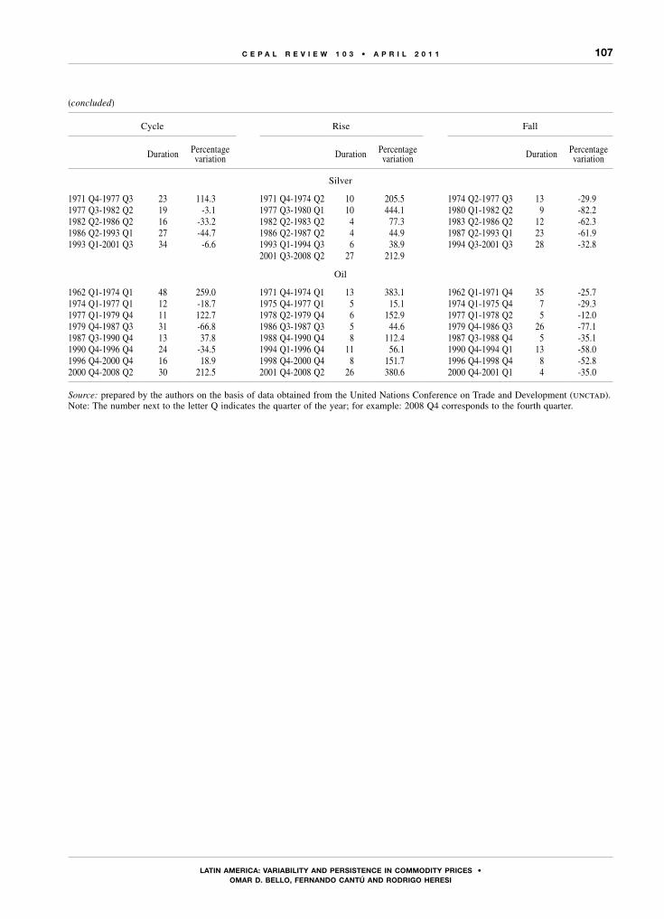
107



(concluded)

Cycle Rise Fall



Silver

1971 Q4-1977 Q3 23 114.3 1971 Q4-1974 Q2 10 205.5 1974 Q2-1977 Q3 13 -29.91977 Q3-1982 Q2 19 -3.1 1977 Q3-1980 Q1 10 444.1 1980 Q1-1982 Q2 9 -82.21982 Q2-1986 Q2 16 -33.2 1982 Q2-1983 Q2 4 77.3 1983 Q2-1986 Q2 12 -62.31986 Q2-1993 Q1 27 -44.7 1986 Q2-1987 Q2 4 44.9 1987 Q2-1993 Q1 23 -61.91993 Q1-2001 Q3 34 -6.6 1993 Q1-1994 Q3 6 38.9 1994 Q3-2001 Q3 28 -32.8

2001 Q3-2008 Q2 27 212.9

Oil

1962 Q1-1974 Q1 48 259.0 1971 Q4-1974 Q1 13 383.1 1962 Q1-1971 Q4 35 -25.71974 Q1-1977 Q1 12 -18.7 1975 Q4-1977 Q1 5 15.1 1974 Q1-1975 Q4 7 -29.31977 Q1-1979 Q4 11 122.7 1978 Q2-1979 Q4 6 152.9 1977 Q1-1978 Q2 5 -12.01979 Q4-1987 Q3 31 -66.8 1986 Q3-1987 Q3 5 44.6 1979 Q4-1986 Q3 26 -77.11987 Q3-1990 Q4 13 37.8 1988 Q4-1990 Q4 8 112.4 1987 Q3-1988 Q4 5 -35.11990 Q4-1996 Q4 24 -34.5 1994 Q1-1996 Q4 11 56.1 1990 Q4-1994 Q1 13 -58.01996 Q4-2000 Q4 16 18.9 1998 Q4-2000 Q4 8 151.7 1996 Q4-1998 Q4 8 -52.82000 Q4-2008 Q2 30 212.5 2001 Q4-2008 Q2 26 380.6 2000 Q4-2001 Q1 4 -35.0

Source: prepared by the authors on the basis of data obtained from the United Nations Conference on Trade and Development (unctad).Note: The number next to the letter Q indicates the quarter of the year; for example: 2008 Q4 corresponds to the fourth quarter.

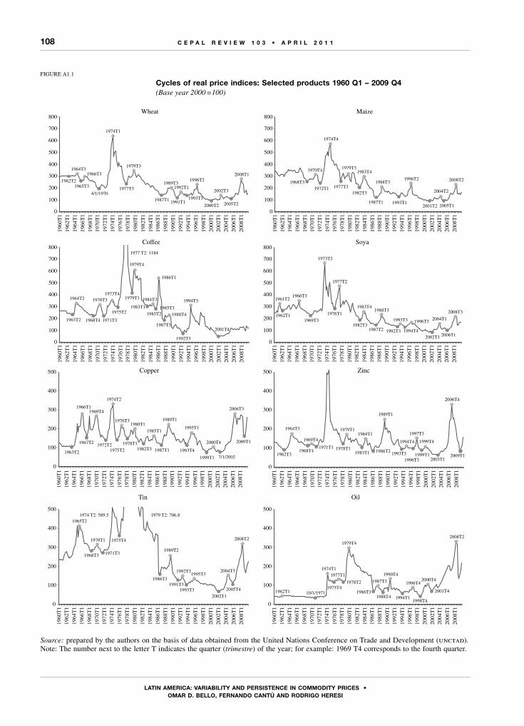
108



FIGURE A1.1

Cycles of real price indices: Selected products 1960 Q1 – 2009 Q4(Base year 2000 =100)

Source: prepared by the authors on the basis of data obtained from the United Nations Conference on Trade and Development (unctad).Note: The number next to the letter T indicates the quarter (trimestre) of the year; for example: 1969 T4 corresponds to the fourth quarter.

Wheat

4/1/1970

1966T3

1965T3

1964T3

1962T2

1974T1

1977T3

1979T3

1987T1

1989T3

1991T1

1992T1

1993T3

1996T2

2000T2

2002T3

2005T2

2008T1

0

100

200

300

400

500

600

700

800

1960

T1

1962

T1

1964

T1

1966

T1

1968

T1

1970

T1

1972

T1

1974

T1

1976

T1

1978

T1

1980

T1

1982

T1

1984

T1

1986

T1

1988

T1

1990

T1

1992

T1

1994

T1

1996

T1

1998

T1

2000

T1

2002

T1

2004

T1

2006

T1

2008

T1

Maize

1968T3

1970T4

1972T1

1974T4

1977T3

1979T3

1982T3

1983T4

1987T1

1988T3

1993T1

1996T2

2001T2

2004T2

2005T1

2008T2

0

100

200

300

400

500

600

700

800

1960

T1

1962

T1

1964

T1

1966

T1

1968

T1

1970

T1

1972

T1

1974

T1

1976

T1

1978

T1

1980

T1

1982

T1

1984

T1

1986

T1

1988

T1

1990

T1

1992

T1

1994

T1

1996

T1

1998

T1

2000

T1

2002

T1

2004

T1

2006

T1

2008

T1

Coffee

1973T4

1971T3

1970T3

1968T4

1964T2

1963T2

1975T2

1979T1

1979T4

1983T1

1984T3

1986T1

1987T3

1988T4

1992T3

1994T3

2001T4

1985T31985T2

0

100

200

300

400

500

600

700

800

1960

T1

1962

T1

1964

T1

1966

T1

1968

T1

1970

T1

1972

T1

1974

T1

1976

T1

1978

T1

1980

T1

1982

T1

1984

T1

1986

T1

1988

T1

1990

T1

1992

T1

1994

T1

1996

T1

1998

T1

2000

T1

2002

T1

2004

T1

2006

T1

2008

T1

Soya

2006T1

2004T1

2002T1

1996T3

1994T4

1993T3

1992T3

1988T3

1987T2

1983T4

1982T3

1977T2

1976T1

1973T2

1969T3

1966T3

1962T1

1961T2

2008T3

0

100

200

300

400

500

600

700

800

1960

T1

1962

T1

1964

T1

1966

T1

1968

T1

1970

T1

1972

T1

1974

T1

1976

T1

1978

T1

1980

T1

1982

T1

1984

T1

1986

T1

1988

T1

1990

T1

1992

T1

1994

T1

1996

T1

1998

T1

2000

T1

2002

T1

2004

T1

2006

T1

2008

T1

1977 T2: 1184

Copper

1963T2

1966T1

1967T2

1969T4

1972T2

1974T2

1975T2

1976T3

1978T1

1980T1

1982T3

1985T1

1987T1

1989T1

1993T4

1995T1

1999T1

2000T4

7/1/2002

2006T3

2009T1

0

100

200

300

400

500

1960

T1

1962

T1

1964

T1

1966

T1

1968

T1

1970

T1

1972

T1

1974

T1

1976

T1

1978

T1

1980

T1

1982

T1

1984

T1

1986

T1

1988

T1

1990

T1

1992

T1

1994

T1

1996

T1

1998

T1

2000

T1

2002

T1

2004

T1

2006

T1

2008

T1

Zinc

1962T3

1964T3

1968T4

1969T4

1971T1 1978T1

1979T1

1983T1

1984T1

1986T2

1989T1

1993T3

1994T4

1996T3

1997T3

1999T1

1999T4

2003T1

2006T4

2009T1

0

100

200

300

400

500

1960

T1

1962

T1

1964

T1

1966

T1

1968

T1

1970

T1

1972

T1

1974

T1

1976

T1

1978

T1

1980

T1

1982

T1

1984

T1

1986

T1

1988

T1

1990

T1

1992

T1

1994

T1

1996

T1

1998

T1

2000

T1

2002

T1

2004

T1

2006

T1

2008

T1

Tin

1965T2

1968T3

1970T1

1971T3

1975T4

1986T3

1989T2

1991T3

1992T3

1993T3

1995T3

2002T1

2004T3

2005T4

2008T2

0

100

200

300

400

500

1960

T1

1962

T1

1964

T1

1966

T1

1968

T1

1970

T1

1972

T1

1974

T1

1976

T1

1978

T1

1980

T1

1982

T1

1984

T1

1986

T1

1988

T1

1990

T1

1992

T1

1994

T1

1996

T1

1998

T1

2000

T1

2002

T1

2004

T1

2006

T1

2008

T1

1979 T2: 706.8 1974 T2: 589.5

Oil

1962T1 10/1/1971

1974T1

1975T4

1977T1

1978T2

1979T4

1986T3

1987T3

1988T4

1990T4

1994T1

1996T4

1998T4

2000T4

2001T4

2008T2

0

100

200

300

400

500

1960

T1

1962

T1

1964

T1

1966

T1

1968

T1

1970

T1

1972

T1

1974

T1

1976

T1

1978

T1

1980

T1

1982

T1

1984

T1

1986

T1

1988

T1

1990

T1

1992

T1

1994

T1

1996

T1

1998

T1

2000

T1

2002

T1

2004

T1

2006

T1

2008

T1

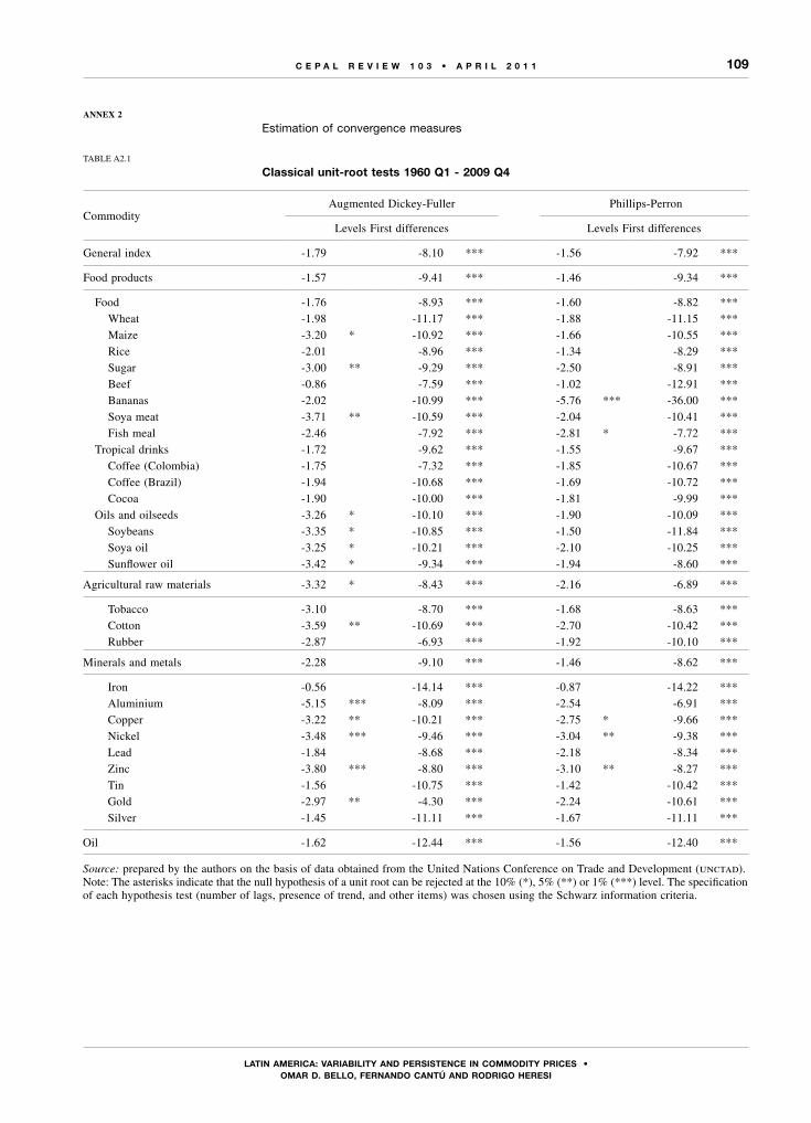
109



ANNEX 2

Estimation of convergence measures

TABLE A2.1

Classical unit-root tests 1960 Q1 - 2009 Q4

CommodityAugmented Dickey-Fuller Phillips-Perron

Levels First differences Levels First differences

General index -1.79 -8.10 *** -1.56 -7.92 ***

Food products -1.57 -9.41 *** -1.46 -9.34 ***

Food -1.76 -8.93 *** -1.60 -8.82 *** Wheat -1.98 -11.17 *** -1.88 -11.15 *** Maize -3.20 * -10.92 *** -1.66 -10.55 *** Rice -2.01 -8.96 *** -1.34 -8.29 *** Sugar -3.00 ** -9.29 *** -2.50 -8.91 *** Beef -0.86 -7.59 *** -1.02 -12.91 *** Bananas -2.02 -10.99 *** -5.76 *** -36.00 *** Soya meat -3.71 ** -10.59 *** -2.04 -10.41 *** Fish meal -2.46 -7.92 *** -2.81 * -7.72 *** Tropical drinks -1.72 -9.62 *** -1.55 -9.67 *** Coffee (Colombia) -1.75 -7.32 *** -1.85 -10.67 *** Coffee (Brazil) -1.94 -10.68 *** -1.69 -10.72 *** Cocoa -1.90 -10.00 *** -1.81 -9.99 *** Oils and oilseeds -3.26 * -10.10 *** -1.90 -10.09 *** Soybeans -3.35 * -10.85 *** -1.50 -11.84 *** Soya oil -3.25 * -10.21 *** -2.10 -10.25 *** Sunflower oil -3.42 * -9.34 *** -1.94 -8.60 ***

Agricultural raw materials -3.32 * -8.43 *** -2.16 -6.89 ***

Tobacco -3.10 -8.70 *** -1.68 -8.63 *** Cotton -3.59 ** -10.69 *** -2.70 -10.42 *** Rubber -2.87 -6.93 *** -1.92 -10.10 ***

Minerals and metals -2.28 -9.10 *** -1.46 -8.62 ***

Iron -0.56 -14.14 *** -0.87 -14.22 *** Aluminium -5.15 *** -8.09 *** -2.54 -6.91 *** Copper -3.22 ** -10.21 *** -2.75 * -9.66 *** Nickel -3.48 *** -9.46 *** -3.04 ** -9.38 *** Lead -1.84 -8.68 *** -2.18 -8.34 *** Zinc -3.80 *** -8.80 *** -3.10 ** -8.27 *** Tin -1.56 -10.75 *** -1.42 -10.42 *** Gold -2.97 ** -4.30 *** -2.24 -10.61 *** Silver -1.45 -11.11 *** -1.67 -11.11 ***

Oil -1.62 -12.44 *** -1.56 -12.40 ***

Source: prepared by the authors on the basis of data obtained from the United Nations Conference on Trade and Development (unctad).Note: The asterisks indicate that the null hypothesis of a unit root can be rejected at the 10% (*), 5% (**) or 1% (***) level. The specification of each hypothesis test (number of lags, presence of trend, and other items) was chosen using the Schwarz information criteria.

110



TABLE A2.2

Estimation of the autoregressive parameter and measures of persistence 1960 Q1 – 2009 Q4

Levels First differences

OLS UEM CIRF ML OLS UEM CIRF ML

General index 0.98 *** 1.00 ∞ ∞ 0.49 *** 0.51 2.03 1.02(0.02) (0.06)

Food products 0.98 *** 1.00 ∞ ∞ 0.38 *** 0.39 1.65 0.74(0.02) (0.07)

Food 0.98 *** 1.00 ∞ ∞ 0.42 *** 0.44 1.77 0.84(0.02) (0.07)

Wheat 0.95 *** 0.98 54.07 37.13 0.22 *** 0.24 1.31 0.48(0.02) (0.07)

Maize 0.94 *** 0.97 34.50 23.56 0.24 *** 0.25 1.34 0.51(0.03) (0.07)

Rice 0.97 *** 1.00 ∞ ∞ 0.42 *** 0.43 1.77 0.83(0.02) (0.07)

Sugar 0.95 *** 0.99 115.03 79.39 0.39 *** 0.40 1.68 0.76(0.02) (0.07)

Beef 0.95 *** 0.99 95.36 65.75 0.08 0.09 1.10 0.29(0.02) (0.07)

Bananas 0.69 *** 0.71 3.48 2.04 -0.32 *** -0.32 - -(0.05) (0.07)

Soya meat 0.93 *** 0.96 25.49 17.32 0.27 *** 0.29 1.40 0.56(0.03) (0.07)

Fish meal 0.96 *** 1.00 ∞ ∞ 0.54 *** 0.56 2.26 1.19(0.02) (0.06)

Tropical drinks 0.97 *** 1.00 ∞ ∞ 0.36 *** 0.37 1.59 0.70(0.02) (0.07)

Coffee (Colombia) 0.96 *** 1.00 ∞ ∞ 0.26 *** 0.28 1.39 0.54(0.02) (0.07)

Coffee (Brazil) 0.96 *** 1.00 ∞ ∞ 0.26 *** 0.28 1.39 0.54(0.02) (0.07)

Cocoa 0.98 *** 1.00 ∞ ∞ 0.32 *** 0.33 1.50 0.63(0.02) (0.07)

Oils and oilseeds 0.95 *** 0.98 58.75 40.37 0.31 *** 0.33 1.49 0.62(0.02) (0.07)

Soya beans 0.93 *** 0.96 23.22 15.74 0.18 ** 0.19 1.24 0.42(0.03) (0.07)

Soya oil 0.94 *** 0.98 46.78 32.08 0.30 *** 0.32 1.47 0.61(0.02) (0.07)

Sunflower oil 0.95 *** 0.99 77.90 53.65 0.38 *** 0.40 1.66 0.75(0.02) (0.07)

Agricultural raw materials 0.96 *** 1.00 ∞ ∞ 0.49 *** 0.50 2.02 1.01(0.02) (0.06)

Tobacco 0.97 *** 1.00 ∞ ∞ 0.44 *** 0.46 1.84 0.88(0.02) (0.06)

Cotton 0.93 *** 0.96 23.84 16.18 0.25 *** 0.27 1.37 0.53(0.03) (0.07)

Rubber 0.95 *** 0.99 73.34 50.49 0.31 *** 0.32 1.48 0.62(0.02) (0.07)

Minerals and metals 0.98 *** 1.00 ∞ ∞ 0.39 *** 0.41 1.69 0.78(0.02) (0.07)

Iron 1.00 *** - - - -0.03 -0.02 - -(0.02) (0.07)

Aluminium 0.92 *** 0.95 19.65 13.27 0.49 *** 0.51 2.04 1.03(0.03) (0.06)

111



(concluded)

Levels First differences

OLS UEM CIRF ML OLS UEM CIRF ML

Copper 0.94 *** 0.98 49.77 34.15 0.30 *** 0.31 1.46 0.60(0.03) (0.07)

Nickel 0.95 *** 0.98 58.68 40.33 0.37 *** 0.39 1.63 0.73(0.02) (0.07)

Lead 0.97 *** 1.00 ∞ ∞ 0.40 *** 0.42 1.72 0.79(0.02) (0.07)

Zinc 0.94 *** 0.98 41.95 28.73 0.42 *** 0.44 1.78 0.84(0.02) (0.07)

Tin 0.97 *** 1.00 ∞ ∞ 0.26 *** 0.27 1.37 0.53(0.02) (0.07)

Gold 0.97 *** 1.00 ∞ ∞ 0.20 ** 0.22 1.28 0.45(0.02) (0.08)

Silver 0.97 *** 1.00 ∞ ∞ 0.11 0.13 1.15 0.34(0.02) (0.08)

Oil 0.96 *** 1.00 ∞ ∞ 0.11 0.13 1.15 0.34(0.02) (0.07)

Source: prepared by the authors on the basis of data obtained from the United Nations Conference on Trade and Development (unctad).Notes: ols = ordinary least squares; uem = unbiased estimate of the mean; cirf = cumulative impulse-response function; ml = half life. The estimated parameter is α of equation (1). The figures in parentheses are the standard deviations of the estimators. The asterisks indicate that the coefficient is significant at the 10% (*), 5% (**) or 1% (***) level.

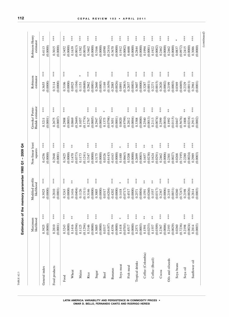
112


C E P A L R E V I E W 1 0 3 • A P R I L 2 0 1 1TA

BL

E A

2.3

Est

imat

ion

of

the

mem

ory

par

amet

er 1

960

Q1

– 20

09 Q

4

Max

imum

li

keli

hood

Mod

ified

pro

file

li

keli

hood

Non

-lin

ear

leas

t sq

uare

sG

ewek

e/ P

orte

r-H

udak

est

imat

orR

obin

son

esti

mat

orR

obin

son-

Hen

ry

esti

mat

or

Gen

eral

ind

ex0.

3925

***

0.39

25**

*0.

4256

***

0.32

11**

*0.

3655

***

0.41

13**

*(0

.000

0)(0

.000

0)(0

.000

0)(0

.000

1)(0

.000

0)(0

.000

0)

Food

pro

duct

s0.

2810

***

0.28

10**

*0.

2948

***

0.26

75**

*0.

3114

***

0.30

15**

*(0

.000

1)(0

.000

1)(0

.000

1)(0

.000

7)(0

.000

0)(0

.000

0)

Foo

d0.

3243

***

0.32

43**

*0.

3425

***

0.29

08**

*0.

3106

***

0.34

52**

*(0

.000

0)(0

.000

0)(0

.000

0)(0

.000

3)(0

.000

0)(0

.000

0) W

heat

0.14

16**

0.14

16**

0.14

70**

0.08

690.

0925

0.16

39**

*(0

.039

4)(0

.040

4)(0

.037

3)(0

.266

9)(0

.110

4)(0

.001

3) M

aize

0.11

250.

1126

0.11

730.

1057

0.11

51*

0.15

82**

*(0

.129

4)(0

.131

1)(0

.124

1)(0

.177

4)(0

.068

0)(0

.001

9) R

ice

0.31

46**

*0.

3146

***

0.33

47**

*0.

2767

***

0.29

62**

*0.

3462

***

(0.0

000)

(0.0

000)

(0.0

000)

(0.0

005)

(0.0

001)

(0.0

000)

Sug

ar0.

3005

***

0.30

05**

*0.

3175

***

0.29

47**

*0.

2660

***

0.31

66**

*(0

.000

0)(0

.000

0)(0

.000

0)(0

.000

2)(0

.000

3)(0

.000

0) B

eef

0.03

170.

0317

0.03

260.

1375

*0.

1169

0.05

90(0

.618

7)(0

.620

4)(0

.614

3)(0

.079

8)(0

.165

9)(0

.241

4)B

anan

as-0

.435

6**

*-0

.420

2**

*-0

.416

3**

*-0

.305

1**

*-0

.208

5**

*-0

.367

0**

*(0

.000

0)(0

.000

0)(0

.000

0)(0

.000

1)(0

.002

6)(0

.000

0) S

oya

mea

t0.

1418

*0.

1418

*0.

1480

*0.

0020

0.08

910.

1912

***

(0.0

703)

(0.0

717)

(0.0

663)

(0.9

799)

(0.2

063)

(0.0

002)

Fis

h m

eal

0.45

17**

*0.

4517

***

0.52

08**

*0.

2812

***

0.28

37**

*0.

4688

***

(0.0

000)

(0.0

000)

(0.0

000)

(0.0

004)

(0.0

003)

(0.0

000)

Tro

pica

l dr

inks

0.25

71**

*0.

2571

***

0.26

99**

*0.

3388

***

0.36

07**

*0.

2844

***

(0.0

003)

(0.0

004)

(0.0

003)

(0.0

000)

(0.0

000)

(0.0

000)

Cof

fee

(Col

ombi

a)0.

1591

**0.

1591

**0.

1657

**0.

2540

***

0.32

87**

*0.

1994

***

(0.0

253)

(0.0

260)

(0.0

238)

(0.0

013)

(0.0

011)

(0.0

001)

Cof

fee

(Bra

zil)

0.15

57**

0.15

57**

0.16

24**

0.21

13**

*0.

2271

***

0.19

22**

*(0

.030

9)(0

.031

7)(0

.029

1)(0

.007

4)(0

.001

5)(0

.000

2) C

ocoa

0.23

67**

*0.

2367

***

0.24

62**

*0.

2599

***

0.28

20**

*0.

2462

***

(0.0

006)

(0.0

006)

(0.0

006)

(0.0

010)

(0.0

002)

(0.0

000)

Oil

s an

d oi

lsee

ds0.

2193

***

0.21

93**

*0.

2301

***

0.19

92**

0.21

99**

*0.

2462

***

(0.0

029)

(0.0

031)

(0.0

027)

(0.0

115)

(0.0

003)

(0.0

000)

Soy

a be

ans

0.02

600.

0260

0.02

68-0

.044

70.

0369

0.08

37*

(0.7

236)

(0.7

247)

(0.7

195)

(0.5

676)

(0.6

069)

(0.0

972)

Soy

a oi

l0.

2198

***

0.21

98**

*0.

2280

***

0.18

08**

0.23

29**

*0.

2415

***

(0.0

024)

(0.0

026)

(0.0

024)

(0.0

216)

(0.0

011)

(0.0

000)

Sun

flow

er o

il0.

2814

***

0.28

14**

*0.

2989

***

0.29

13**

*0.

2961

***

0.30

86**

*(0

.000

3)(0

.000

3)(0

.000

3)(0

.000

2)(0

.000

1)(0

.000

0) (con

tinu

ed)

113



Tabl

e A

2.3

(con

clud

ed)

Max

imum

li

keli

hood

Mod

ified

pro

file

li

keli

hood

Non

-lin

ear

leas

t sq

uare

sG

ewek

e/ P

orte

r-H

udak

est

imat

orR

obin

son

esti

mat

orR

obin

son-

Hen

ry

esti

mat

or

Agr

icul

tura

l ra

w m

ater

ials

0.40

05**

*0.

4005

***

0.44

47**

*0.

3352

***

0.32

80**

*0.

4033

***

(0.0

000)

(0.0

000)

(0.0

000)

(0.0

000)

(0.0

000)

(0.0

000)

Tob

acco

0.34

35**

*0.

3435

***

0.36

48**

*0.

3431

***

0.34

67**

*0.

3676

***

(0.0

000)

(0.0

000)

(0.0

000)

(0.0

000)

(0.0

000)

(0.0

000)

Cot

ton

0.11

930.

1193

0.12

530.

1068

0.14

13**

0.15

92**

*(0

.138

4)(0

.140

4)(0

.131

8)(0

.173

1)(0

.032

2)(0

.001

8) R

ubbe

r0.

2470

***

0.24

70**

*0.

2572

***

0.24

81**

*0.

2352

***

0.24

52**

*(0

.000

4)(0

.000

4)(0

.000

4)(0

.001

8)(0

.000

5)(0

.000

0)

Min

eral

s an

d m

etal

s0.

2987

***

0.29

87**

*0.

3169

***

0.30

11**

*0.

2610

***

0.30

75**

*(0

.000

1)(0

.000

1)(0

.000

1)(0

.000

2)(0

.000

0)(0

.000

0)

Iro

n-0

.004

60.

0323

0.03

270.

0686

0.03

840.

0322

(0.9

309)

(0.5

335)

(0.5

293)

(0.3

807)

(0.5

273)

(0.5

228)

Alu

min

ium

0.40

64**

*0.

4064

***

0.45

62**

*0.

3040

***

0.31

32**

*0.

4433

***

(0.0

000)

(0.0

000)

(0.0

000)

(0.0

001)

(0.0

001)

(0.0

000)

Cop

per

0.18

53**

0.18

53**

0.19

46**

0.19

35**

0.19

42**

*0.

2106

***

(0.0

162)

(0.0

168)

(0.0

151)

(0.0

141)

(0.0

021)

(0.0

000)

Nic

kel

0.28

11**

*0.

2811

***

0.29

73**

*0.

2404

***

0.25

94**

*0.

3026

***

(0.0

002)

(0.0

002)

(0.0

002)

(0.0

024)

(0.0

002)

(0.0

000)

Lea

d0.

3112

***

0.31

12**

*0.

3311

***

0.27

61**

*0.

2668

***

0.32

83**

*(0

.000

0)(0

.000

0)(0

.000

0)(0

.000

5)(0

.000

0)(0

.000

0) Z

inc

0.34

08**

*0.

3408

***

0.36

44**

*0.

1727

**0.

1784

***

0.33

10**

*(0

.000

0)(0

.000

0)(0

.000

0)(0

.028

1)(0

.008

8)(0

.000

0) T

in0.

1522

**0.

1522

**0.

1582

**0.

1524

*0.

1622

***

0.17

90**

*(0

.028

2)(0

.029

0)(0

.027

0)(0

.052

4)(0

.002

3)(0

.000

5) G

old

0.18

27**

*0.

1827

***

0.18

85**

*0.

1482

*0.

1302

**0.

1833

***

(0.0

044)

(0.0

047)

(0.0

043)

(0.0

971)

(0.0

384)

(0.0

014)

Sil

ver

0.06

750.

0675

0.06

950.

1601

*0.

1573

**0.

0839

(0.3

416)

(0.3

447)

(0.3

347)

(0.0

734)

(0.0

371)

(0.1

380)

Oil

0.00

890.

0089

0.00

920.

0308

0.07

420.

0465

(0.8

929)

(0.8

935)

(0.8

913)

(0.6

934)

(0.2

254)

(0.3

562)

Sour

ce:

prep

ared

by

the

auth

ors

on t

he b

asis

of

data

obt

aine

d fr

om t

he U

nite

d N

atio

ns C

onfe

renc

e on

Tra

de a

nd D

evel

opm

ent

(un

cta

d).

Not

es:

The

est

imat

ed p

aram

eter

is

d of

equ

atio

n (2

). T

he fi

gure

s in

par

enth

eses

are

the

p v

alue

s of

the

sig

nifi

canc

e te

st f

or e

ach

esti

mat

or.

The

ast

eris

ks i

ndic

ate

that

the

coe

ffici

ent

is

sign

ifica

nt a

t th

e 10

% (

*),

5% (

**)

or 1

% (

***)

lev

el.

114



Andrews, Donald (1993), “Exactly median-unbiased estimation of first order autoregressive/unit root models”, Econometrica, vol. 61, No. 1, Washington, D.C., Econometric Society.

Andrews, Donald and Hong-Yuan Chen (1994), “Approximately median-unbiased estimation of autoregressive models”, Journal of Business and Economic Statistics, vol. 12, No. 2, Alexandria, American Statistical Association.

Bello, Omar and Rodrigo Heresi (2008), “El auge reciente de precios de los productos básicos en perspectiva histórica”, Macroeconomía del desarrollo series, No. 71 (LC/L.2975-P), Santiago, Chile, Economic Commission for Latin America and the Caribbean (eclac). United Nations publication, Sales No. S.08.II.G.84.

Bello, Omar, Rodrigo Heresi and Omar Zambrano (2008), “The present decade boom of commodity prices in historical perspective and its macroeconomic effects in Latin America”, Santiago, Chile, Economic Commission for Latin America and the Caribbean (eclac), unpublished.

Bry, Gerhard and Charlotte Boschan (1971), Cyclical Analysis of Time Series: Selected Procedures and Computer Programs, Cambridge, Massachusetts, New York, National Bureau of Economic Research.

Caballero, Ricardo, Emmanuel Farhi and Pierre-Olivier Gourinchas (2008), “Financial crash, commodity prices, and global imbalances”, Brookings Papers on Economic Activity, Washington, D.C., Brookings Institution Press.

Cashin, Paul and John McDermott (2002), “The long-run behavior of commodity prices: small trends and big variability”, imf Staff Papers, vol. 49, No. 2, Washington, D.C., International Monetary Fund.

Cashin, Paul, John McDermott and Alasdair Scott (1999a), “Booms and slumps in world commodity prices”, imf Working Papers, No. 155, Washington, D.C., International Monetary Fund (imf).

(1999b), “The myth of co-moving commodity prices”, Discussion Paper Series, No. G99/8, Wellington, Reserve Bank of New Zealand.

Cashin, Paul, Hog Liang and John McDermott (2000), “How persistent are shocks to world commodity prices?”, imf Staff Papers, vol. 47, No. 2, Washington, D.C., International Monetary Fund.

Cuddington, John (1992), “Long-run trends in 26 primary commodities: a disaggregated look at the Prebisch-Singer hypothesis”, Journal of Development Economics, vol. 39, No. 2, Amsterdam, Elsevier.

Cuddington, John and Carlos Urzúa (1989), “Trends and cycles in the net Barter terms of trade: a new approach”, Economic Journal, vol. 99, No. 396, London, Royal Economic Society.

Cuddington, John, Rodney Ludema and Shamila Jayasuriya (2002), “Prebisch-Singer Redux”, Working Paper, No. 140, Santiago, Chile, Central Bank of Chile, February.

Davis, Steven and John Haltiwanger (2001), “Sectoral job creation and destruction responses to oil price changes”, Journal of Monetary Economics, vol. 48, N° 3, Amsterdam, Elsevier.

Bibliography

Deaton, Angus (1999), “Commodity prices and growth in Africa”, Journal of Economic Perspectives, vol. 13, No. 3, Nashville, Tennessee, American Economic Association.

Deaton, Angus and Guy Laroque (1992), “On the behaviour of commodity prices”, Review of Economic Studies, vol. 59, N° 1, Oxford, Blackwell Publishing.

Doornik, Jurgen and Marius Ooms (2004), “Inference and forecasting for arfima models, with an application to US and UK inflation”, Studies in Non-linear Dynamics and Econometrics, vol. 8, No. 2, Berkeley, Berkeley Electronic Press.

eclac (Economic Commission for Latin America and the Caribbean) (2008), Social Panorama of Latin America, 2008 (LC/G.2402-P), Santiago, Chile. United Nations publication, Sales No. E.08.II.G.89.

(2007), Social Panorama of Latin America, 2007 (LC/G.2351-P), Santiago, Chile. United Nations publication, Sales No. E.07.II.G.124.

(various years), Economic Survey of Latin America and the Caribbean, Santiago, Chile.

(various years), Social Panorama of Latin America, Santiago, Chile.

Grilli, Enzo and Maw Yang (1988), “Primary commodity prices, manufactured goods prices, and the terms of trade of developing countries: what the long run shows”, The World Bank Economic Review, vol. 2, Washington, D.C., World Bank.

Hamilton, James (1996), “This is what happened to the oil price-macroeconomy relationship”, Journal of Monetary Economics, vol. 38, No. 2, Amsterdam, Elsevier.

Herrera, Ingrid and Ramón Pineda (2006), “Booms de la cesta petrolera venezolana”, Caracas, Central Bank of Venezuela, unpublished.

Ocampo, José Antonio and María Ángela Parra (2003), “The terms of trade for commodities in the twentieth century”, cepal Review, No. 79 (LC/G.2200), Santiago, Chile, April.

Pyndick, Robert and Julio Rotemberg (1990), “The excess of co-movements of commodity prices”, The Economic Journal, vol. 100, No. 403, London, Royal Economic Society, December.

Reinhart, Carmen and Peter Wickham (1994), “Commodity prices: cyclical weakness or secular decline”, imf Staff Papers, vol. 41, Washington, D.C., International Monetary Fund (imf).

Rodríguez, Francisco (2009), “¿Está América Latina sumida en una trampa de pobreza?”, Macroeconomía del desarrollo series, No. 80 (LC/L.3017-P), Santiago, Chile, Economic Commission for Latin America and the Caribbean (eclac). United Nations publication, Sales No. S.09.II.G.27.

Southwood, Jim (2008), “cru’s new process for managing copper price risk”, presentation at the cru’s 7th World Copper Conference, April.

Toledo, Manuel (2008), “Understanding business cycles in Latin America”, Santiago, Chile, Economic Commission for Latin America and the Caribbean (eclac), unpublished.


115

Bahamas and Barbados: empirical evidence ofinterest rate pass-through

Daniel O. Boamah, Mahalia N. Jackman and Nlandu Mamingi

This paper uses an error correction model to investigate empirically

the effectiveness of central bank interest rate policy in influencing

commercial banks’ lending rate behaviour in Barbados and the Bahamas

using quarterly data for the period January 1995-April 2007. For Barbados,

the study finds that the reaction of commercial bank lending rates to

changes in the central bank’s policy rate is sticky in the short run, but

fully complete in the long run. On average, it takes about four to six

quarters for the full effect of changes in the central bank policy rate to

be transmitted to the economy via adjustments. For the Bahamas, the

reaction of commercial bank lending rates to changes in the central bank

policy rate is fully complete in the short run and the long run, owing to a

low adjustment cost coupled with the use of moral suasion.

KEYWORDS

Interest rates

Bank loans

Commercial banks

Economic analysis

Monetary policy

Central banks

Bahamas

Barbados

Daniel O. Boamah

Deputy Governor,

Central Bank of Barbados


Mahalia N. Jackman

Economist, Research Department,

Central Bank of Barbados


Nlandu Mamingi

Professor of Economics,

Department of Economics,

University of the West Indies,

Bridgetown, Barbados


116

bAhAmAs And bARbAdos: EmPIRICAL EVIdEnCE oF InTEREsT RATE PAss-ThRough • dAnIEL o. boAmAh, mAhALIA n. JACkmAn And nLAndu mAmIngI


Any government can use at the very least fiscal policy or monetary policy, or both, to impact the country’s macroeconomic aggregates such as the inflation rate, unemployment and economic growth. While government taxes and government expenditures are the main tools of fiscal policy, interest rates and the money supply are the key instruments of monetary policy. The choice of one policy over another or the policy mix depends on the characteristics of the country under consideration, i.e. its exchange rate regime, level of development and size of its economy.

This paper addresses the issue of interest rate pass-through in the context of two small open economies with fixed exchange rate regimes, Barbados and the Bahamas. Specifically, it analyses the dynamics of commercial banks’ lending rate reactions to changes in the central bank policy rates of those two countries in the period 1995-2007 with quarterly frequency; hence, it deals with the effectiveness of interest rates in influencing the Barbadian and Bahamian economies. In particular, it focuses on the following questions. First, does the central bank policy rate affect the commercial bank lending rate? Second, if so, how large is the short-term and long-term interest rate pass-through in each country? Third, what is the minimum response time for the central bank’s actions to impact on commercial banks’ average lending rate? Fourth, how do the two countries compare in terms of monetary policy?

As is well documented, central banks’ vital influence on money market conditions, and particularly on money market interest rates, places them at the heart of monetary policy. Changes in money market interest rates affect market interest rates with longer maturities and retail bank interest rates, albeit to varying degrees. Bank decisions regarding the yields paid on their assets and liabilities have an impact on the expenditure and investment behavior of holders and thus real economic activity. In other words, a quicker and fuller pass-through of official and market interest rates to retail bank interest rates strengthens monetary policy transmission and thus may affect price stability. Furthermore, prices set by banks influence their margins and therefore bank profitability and consequently the soundness of the banking system and thus financial stability (De Bondt, 2005, pp. 37-38).

This study focuses on the lending rate mainly because, among the myriad commercial bank interest rates, it is the main channel through which monetary policy action is transmitted to the real economy, since it serves as an important guide to investment decisions.1 This view is supported by the work of Borio and Fritz (1995, p. 3) and Oliner and Rudebusch (1995, p. 3). For instance, the latter study points out that the lending rate channel operates when central bank actions affect the supply of loans from depository institutions (“banks”) and, in turn, the real spending of bank borrowers.

Quite a number of papers have documented various degrees of lending rate stickiness (Moazzami, 1999; Cottarelli and Kourelis, 1994; De Bondt, 2005; Kwapil and Scharler, 2006). The reasons for interest rate pass-through variations may be found, among other things, in different adjustment costs, the demand elasticity of loans, implicit contracts between banks and their customers, switching costs and asymmetric information costs (see, among others, De Bondt, 2005; Kwapil and Scharler, 2006). Put rather differently, the degree of lending rate stickiness depends on the extent to which (i) commercial banks are able to fully insulate their supply of loans in response to changes in reserves; and (ii) borrowers are able to insulate their spending from alterations in the accessibility of bank loans (Oliner and Rudebusch, 1995, p. 3).

At least three considerations justify the present study. First, the concern expressed by the Governor of the Central Bank of Barbados at the apparent slow response of commercial banks’ lending rates to recent reductions in the minimum deposit rate (Barbados Business Authority, 2008, p. 1) suggests a need for a quantitative investigation to shed some light on the problem. Second, an understanding of interest rate pass-through provides useful insight into the transmission mechanism of monetary policy, and should provide policymakers with a general idea as to when a particular policy action can be expected to have an impact on the real economy. Third, a comparative study of countries

1 The lending rate is one of the determinants of foreign direct investment in Barbados, as tested by an error correction model which indicates that the weighted average rate on total loans Granger-causes foreign direct investment in the period 1995-2005. The relationship between the two variables is significant (results are available upon request).

Iintroduction

117



such as Barbados and the Bahamas is more than relevant as it may help reveal the effective role of monetary policy in similar economies.

To answer the different questions of the paper, use is made of an error correction model derived from a partial adjustment model. This popular model is chosen purely and simply to see how effective it is in capturing the pass-through phenomenon in Barbados. The paper makes two contributions to the literature. First, given that most studies focus on developed countries, this paper, by concentrating on small Caribbean economies,

adds to the rather sparse body of knowledge on banking sector behaviour in developing countries. Second, this study is among the very few to compare two small open economies with fixed exchange-rate regimes.

The paper is organized as follows. Section II briefly introduces the Barbadian and Bahamian economies, with emphasis on central bank and commercial bank interest rate paths. Section III reviews the literature. Section IV focuses on modelling. Section V gives the results and interpretations of the exercise, and section VI contains concluding remarks.

IIStylized facts

The Bahamas and Barbados are islands that share similar economic characteristics. Specifically, they are both small open economies whose currencies have been pegged to the United States dollar at parities of BDS$ 2 to US$ 1 (for Barbados) and B$ 1 to US$ 1 (for the Bahamas). In addition, economic growth in both countries is strongly supported by a vibrant tourism sector, accounting for about 60% of gross domestic product (gdp) in the Bahamas and 15% in Barbados, and impressive financial services.

Commercial banks hold a dominant position in both countries’ financial systems. Since they are the main source of finance in the economy, the interest rates set by these banks strongly impact the investment and consumption decisions of individuals and firms and, by extension, economic development in these countries. Hence, the monetary policy of the central banks of the Bahamas and Barbados has, to a large extent, been geared towards influencing interest rate developments in the commercial banking sector. The following subsections discuss the data trends for selected interest rates in both Barbados and the Bahamas over the sample period 1995-2007.

1. Barbados

The Central Bank of Barbados currently uses a combination of direct and indirect instruments to influence interest rates. These include a saving rate floor, a discount rate and reserve requirements. The minimum deposit rate has served as the main monetary policy tool since the 1990s, with changes in the discount rate and reserve requirements playing a secondary role. Prior to 1991, the banking sector was subject to a number of other

restrictions and regulations, including programmes geared towards channelling funds to priority sectors of the economy, with stipulations on saving rate floors as well as ceilings on weighted average lending rates imposed by the Central Bank of Barbados. Accordingly, movements in commercial bank interest rates were generally governed by the central bank.

In the early 1990s, macroeconomic developments in Barbados were characterized by the turmoil in the global economy as a result of the Gulf war and by recessions in Barbados’ main tourism source markets, i.e. North America and the United Kingdom. The Barbados economy experienced a significant fall in real economic activity and persistently high current account deficits resulting in significant losses in foreign exchange reserves. To combat the foreign exchange shortfall, in May 1991 the government entered an 18-month stabilization programme with the International Monetary Fund, prompting financial sector reform. Of particular note, the ceiling on average lending rates was removed.

The financial sector continued to undergo reform throughout the 1990s. The Rate of Interest Order was revoked in June 1992, the residential mortgage rate had been deregulated by September that year and all credit caps and controls had been discontinued by May 1993. Throughout the remainder of the 1990s, there were moderate fluctuations in minimum deposit rates as monetary policy was geared towards managing the level of liquidity in the financial system. Lending rates were fairly stable, however (fluctuating around 11%), suggesting a rather low pass-through of changes in monetary policy to lending rates following liberalization of the latter.

118



From 2000 to 2004, the banking sector was characterized by high levels of liquidity, a consequence of sluggish credit growth. Furthermore, the economy slipped into recession in 2001. In an effort to stem excess liquidity and spur lending to more-productive sectors, the Central Bank of Barbados continuously relaxed its policy stance. Between 2000 and 2001, the Bank cut its minimum deposit rate four times. Nevertheless, commercial banks’ lending rates stagnated. Consequently, the central bank once again sought to regulate lending rates, instructing commercial banks to set a ceiling on the weighted average interest rates charged on loans to productive sectors. The indicative weighted average lending rate was progressively lowered from a maximum of 10% in August 2001 to 8.5% by December, yet lending rates remained relatively high even as the central bank continued to cut its minimum deposit rate, which reached an all-time low of 2.25% in the first quarter of 2004. Consequently, the central bank reintroduced loan rate ceilings in December 2002, setting the maximum average lending rate on selected loans at 8.0%, which quickly translated into a fall in lending rates. However, in 2003 the regulation of loan rates was abolished.

Four years of relatively calm monetary policy spurred strong demand for credit throughout 2005 and 2006, leading to a significant tightening of liquidity in the banking system. In response, the central bank aggressively raised the minimum deposit rate from 2.25% at the beginning of 2005 to 5.25% by the end of 2006, prompting a general upward trend in lending rates. From the fourth quarter of 2006, liquidity began to build up in the banking system, largely reflecting significant foreign capital inflows and a slowdown in credit demand. In an effort to reduce the liquidity build-up, the central bank eased monetary policy, lowering the minimum deposit rate to 4.75% by the end of 2007.

Commercial banks responded slowly on the whole to the actions of the central bank, as changes in lending rates were only a fraction of the cumulative changes in the minimum deposit rate.

2. The Bahamas

As in Barbados, Bahamian monetary policy revolves around the maintenance of a fixed parity between the Bahamian and United States dollars that has existed since 1973. This fixed parity is maintained in practice by keeping external reserves at 50% of the value of total notes and coins and demand liabilities of the central bank (Central Bank of the Bahamas, 1999). Since its establishment, the central bank has used interest rate controls (which include ceilings on deposit rates, a discount rate and stipulations on prime rates) in association with moral suasion to influence domestic interest rates. However, high levels of liquidity meant that the deposit interest rate ceiling could be removed in April 1994.

In the latter part of the 1990s, direct credit controls and moral suasion emerged as the core instruments of monetary policy, with interest rate policy playing a secondary role. In fact, there were only two changes in the discount rate throughout the sample period, associated essentially with shifting bank liquidity and domestic credit conditions.

The most notable characteristic of interest rate policy in the Bahamas is the synchronization between the discount rate and the prime rate. Indeed, during the review period (1995-2007), the difference between the prime rate and the central bank rate was 25 basis points each quarter. In principle, the commercial banks’ prime rate is tied to the central bank discount rate, thus creating scope for it to affect domestic interest rates and economic activity.

IIILiterature review

The literature on interest rate pass-through is vast. Without dismissing the role of commercial bank deposit rates,2 this literature review will focus on lending rates.

2 In the euro area, De Bondt, Mojon and Valla (2005) showed that deposit rates were by and large a non-predictor of lending rates.

Methodologically, most studies are of a time series nature and use an error correction model as a transformation of an autoregressive distributed lag model to study the effectiveness of interest rate transmission mechanisms. More specifically, the typical study starts implicitly with the Cottarelli and Kourelis model (1994) or its variants:

119



LR c LR D R

DR DRt t

t n t

= + + ++ + +

− −

−

α β β1 1 1

2 2 � −− +n tu0 1t tR D

β β (1)

where LRt is the lending rate, DRt is the central bank interest rate, ut is the error term and n stands for the optimal lag.

Equation (1) is an autoregressive distributed lag (ADL) model of order 1 (n: ADL (1,n)). The impact or short-run multiplier is β0 and the long-run multiplier is

β β α=∑ ii

n

011( ).= −

A generalized error correction model corresponding to equation (1) is given by:

∆ ∆ ∆LR c L R

LR

t ii

n

t i ii

n

t i

t

= + +

+ −=

−=

−

−

∑ ∑γ 1( δδ DR ut t− +1)

R Dα β1 0 (2)

where β0 is the short-run multiplier,

δ β= = −ii

n

i

n

i0 0

1( )β α∑ ∑= =

is the long-run multiplier,

γ is the adjustment coefficient and M = (1- β0)/ γ is the mean adjustment lag whereby the official rate is passed on to lending rates. The completeness of the pass-through is tested with either β0 =1 or δ =1.

Tables 1-3 contain the empirical results of the short-run and long-run pass-through for the euro area, the United States and Canada, and other areas, respectively. Most authors have used time series with monthly data. Note that the magnitudes of multipliers are not necessarily comparable, since different time periods and data sources are used.

An examination of these tables reveals that the short-term impact of interest rate pass-through is smaller than the long-term impact in the majority of cases. Put differently, while short-term pass-through is often incomplete, long-term pass-through tends to be more complete. The implication is that monetary policy seems to be potent only in the long run. Short-run impacts are larger than long-run impacts in only 3 out of 44 cases, making unsustainability of interest rate pass-through an issue. Full interest rate pass-through is achieved in the short and long runs in an insignificant number of cases; full interest rate pass-through that is sustainable in this way is of course the ideal.

The only study to use a panel data methodology for the euro area is Sorensen and Werner (2006). As expected, the study uncovers a high degree of fragmentation in the retail banking sector in the euro area. In addition, it finds a great variation in interest rate pass-through at the country level and reveals a degree of stickiness in lending rate reactions to changes in market rates.

Some studies have acknowledged the issue of asymmetric interest rate pass-through; that is, the possibility of lending rates responding differently following an increase or decrease in market interest rates. The results are inconclusive, however, in that some authors have found asymmetry in interest rate pass-through and others have not (see, among others, Mojon, 2000; Borio and Fritz, 1995; Acheampong, 2004).

Where the Bahamas and Barbados are concerned, no work has dealt explicitly with the topic to the best of our knowledge. However, two papers dealing with a related topic are worth mentioning. Moore and Craigwell (2002) showed market power to be the leading determinant of interest rate pass-through in Barbados and the Caribbean. Samuel and Valderama (2006) also found that monetary policy was a key determinant in this area for Barbados.

120



TABLE 1

Euro area: interest rate pass-through by study conducted

Short-term loans to firms Impact Belgium France Germany Euro area

Cottarelli and Kourelis (1994) Short-termLong-term

0.670.87

0.610.83

0.750.90

Mojon (2000) Short-termLong-term

1.001.00

0.711.00

0.611.00

Donnay and Degryse (2001) Short-termLong-term

0.850.92

0.660.72

0.360.42

0.580.74

Toolsema, Sturm and De Haan (2001) Short-termLong-term

0.761.02

0.530.62

0.700.80

Heinemann and Schüller (2002) Short-termLong-term

0.831.00

0.451.00

0.751.00

Angeloni and Ehrmann (2003) Short-termLong-term

0.531.00

De Bondt (2005) Short-termLong-term

0.190.88

Long-term loans to firms Impact Belgium France Germany Euro area

Mojon (2000) Short-termLong-term

0.611.00

0.421.00

0.371.00

Donnay and Degryse (2001) Short-termLong-term

0.210.10

0.230.50

0.250.60

0.540.67

Toolsema, Sturm and De Haan (2001)a Short-termLong-term

0.720.90

0.080.89

0.310.71

Angeloni and Ehrmann (2003) Short-termLong-term

0.741.30

Kwapil and Scharler (2006) Short-termLong-term

0.790.57

Kaufmann and Scharler (2006) Short-termLong-term

0.921.00

De Bondt (2005) Short-termLong-term

0.550.80

Source: prepared by the authors on the basis of the papers cited.

a 2002 version.

TABLE 2

United States and Canada: interest rate pass-through by study conducted

United States Canada

Short-termImpact

Long-termImpact

Short-termImpact

Long-termImpact

Long-term loan ratesCottarelli and Kourelis (1994)a 0.41 0.97 0.78 0.93Moazzami (1999)b 0.34 1.05 0.66 0.95

Short-term loan ratesMoazzami (1999)c 0.42 1.07 0.52 0.80Kwapil and Scharler (2006) 0.79 0.57Kaufmann and Scharler (2006) 0.92 1.00


a There is no clear-cut information on the duration of loans.b Three-month Treasury bill rate.c Overnight rate.

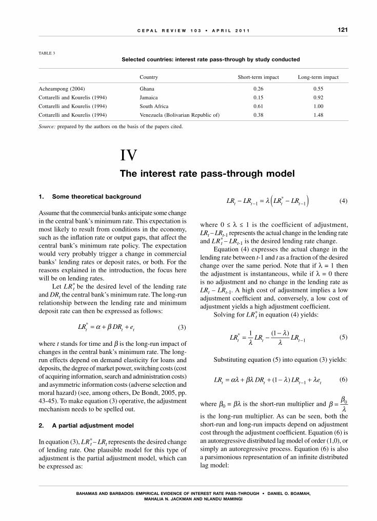
121



1. Some theoretical background

Assume that the commercial banks anticipate some change in the central bank’s minimum rate. This expectation is most likely to result from conditions in the economy, such as the inflation rate or output gaps, that affect the central bank’s minimum rate policy. The expectation would very probably trigger a change in commercial banks’ lending rates or deposit rates, or both. For the reasons explained in the introduction, the focus here will be on lending rates.

Let LR*t be the desired level of the lending rate

and DRt the central bank’s minimum rate. The long-run relationship between the lending rate and minimum deposit rate can then be expressed as follows:

LR DR et t t* = + +α β (3)

where t stands for time and β is the long-run impact of changes in the central bank’s minimum rate. The long-run effects depend on demand elasticity for loans and deposits, the degree of market power, switching costs (cost of acquiring information, search and administration costs) and asymmetric information costs (adverse selection and moral hazard) (see, among others, De Bondt, 2005, pp. 43-45). To make equation (3) operative, the adjustment mechanism needs to be spelled out.

2. A partial adjustment model

In equation (3), LR*t – LRt represents the desired change

of lending rate. One plausible model for this type of adjustment is the partial adjustment model, which can be expressed as:

LR LR LR LRt t− = −( )λ *

1 1− −t t (4)

where 0 ≤ λ ≤ 1 is the coefficient of adjustment, LRt – LRt-1 represents the actual change in the lending rate and LR*

t – LRt-1 is the desired lending rate change. Equation (4) expresses the actual change in the

lending rate between t-1 and t as a fraction of the desired change over the same period. Note that if λ = 1 then the adjustment is instantaneous, while if λ = 0 there is no adjustment and no change in the lending rate as LRt – LRt-1. A high cost of adjustment implies a low adjustment coefficient and, conversely, a low cost of adjustment yields a high adjustment coefficient.

Solving for LR*t in equation (4) yields:

LR LR LRt t t* ( )= − −

−1 1

1λλ

λ (5)

Substituting equation (5) into equation (3) yields:

LR DR LR et t t t= + + − +−αλ βλ ( )1 1λ λ (6)

where β0 = βλ is the short-run multiplier and ββλ

= 0

is the long-run multiplier. As can be seen, both the short-run and long-run impacts depend on adjustment cost through the adjustment coefficient. Equation (6) is an autoregressive distributed lag model of order (1,0), or simply an autoregressive process. Equation (6) is also a parsimonious representation of an infinite distributed lag model:

TABLE 3

Selected countries: interest rate pass-through by study conducted

Country Short-term impact Long-term impact

Acheampong (2004) Ghana 0.26 0.55

Cottarelli and Kourelis (1994) Jamaica 0.15 0.92

Cottarelli and Kourelis (1994) South Africa 0.61 1.00

Cottarelli and Kourelis (1994) Venezuela (Bolivarian Republic of) 0.38 1.48


IVThe interest rate pass-through model

122



LR c Dt ii

t i t= + +=

∞

−∑ β0

R e (7)

3. An error correction model

Equation (6) can alternatively be written, by subtracting LRt-1 on both sides, as

∆LR DR LR et t= + −αλ βλ λ λ1t t− + (8)

where ∆ stands for the first difference operator.Equation (8) can be rewritten, by adding and

subtracting βλ DRt-1, as

∆ ∆LR DR LR DR et t t= + − − +αλ βλ λ β λ( )1 1− −t t (9)

where β0 = βλ is the short-run multiplier, β is the long-run multiplier, λ is the coefficient of adjustment, (1- λ)/ λ is the mean adjustment lag and -log(2(1 - λ)) / log(1 - λ) is the median lag.

Equation (9) is the error correction model (ecm) corresponding to the adl (1.0) captured by equation (6). As can be seen, the theory of cointegration is not introduced for equation (9), since the error correction model precedes the theory of cointegration. Basically, if variables are stationary in levels, then both equation (6) and equation (9) are valid representations of the phenomenon being studied.

4. Method of estimation

Equation (6) and equation (9) are equivalent, as just pointed out. Both are highly non-linear in parameters. Hence, some non-linear algorithms are required to estimate them. In addition, particular attention must be paid to the issue of autocorrelation and heteroskedasticity.

To reprise, the objectives of the model estimation are to derive the short-run interest rate pass-through (β0 = βλ), the long-run interest rate pass-through (β) and the mean lag ((1- λ)/ λ). In addition, for reasons explained in Hendry (1995, pp. 216 and 257), a median lag is also derived.

VEmpirical results

The data of interest are the following: for Barbados, the Central Bank of Barbados minimum deposit rate (mdrate), the weighted average rate on total loans (watloan) and the weighted average rate on selected loans (wasloan); for the Bahamas, the Central Bank of the Bahamas rate (brate) and the weighted average interest rate on loans and overdrafts of commercial bank customers (waverate).

Dealing first with Barbados, the analysis shall start by examining the time series properties of these variables in the period 1995-2007 with quarterly frequency. Figure 1 provides us with the evolution of each series. The quarterly mean stands at 4.029%, 11.55% and 9.87% for mdrate, watloan and wasloan, respectively. The median rate is 4.00%, 11.30% and 10.19% for mdrate, watloan and wasloan, respectively. There is a high degree of synchronization between the series, well captured by the significant correlation between them: 0.659 between mdrate and watloan, 0.791 between mdrate and wasloan and 0.945 between watloan and wasloan. To study the stationarity or non-stationarity of variables, two formal unit root tests are used: the

augmented Dickey-Fuller (adf) test and the Phillips-Perron (pp) test. The ultimate objective of the tests is to rule out any spurious regressions.3 Since both tests are in common use, they are not explained here.

Table 4 reveals that all three variables of interest are non-stationary at a 5% significance level. Indeed, since the adf and pp values are greater than the corresponding critical value for each variable in level and smaller than the critical value for each variable in first difference, it can be concluded that each series is integrated of order 1.

Since the variables are non-stationary, there is the issue of cointegration. In any case, because the adl estimation of equation (6) using mdrate and watloan as variables yields the same results as the error correction model from equation (9), only the ecm results are presented. A non-linear least squares estimation method (see Eviews software for details on the method) using

3 This pre-testing strategy is by and large abandoned in the framework recently initiated by Pesaran, Shin and Smith (2001).

123



Newey-West robust standard errors has been utilized in the exercise to deal with the problems of autocorrelation and heteroskedasticity. Table 5 contains the results of the error correction model (see equation 9) for watloan.

Before interpreting the main results, it is worth noting that while the equation passes the autocorrelation test, as the p value associated with the Lagrange multiplier test indicates, this is not the case for heteroskedasticity and

normality. However, the use of robust standard errors takes care of heteroskedasticity detected at the 10% level. Table 5 indicates that the implied short-run impact (elasticity) is 0.104%. With a p value of 0.0077 associated with a Wald statistic of 7.105, short-run elasticity is statistically different from 0 at the 5% significance level. In addition, short-run elasticity is also statistically different from 1, with a p value of 0.000 associated with

FIGURE 1

barbados: evolution of interest rates, January 1995-April 2007 (quarterly data)(Percentages)

TABLE 4

adf and pp test results for barbados, January 1995-April 2007(Quarterly data)

Variable adf (level) pp (level) adf (first difference) pp (first difference)

mdrate -1.747(c) -1.631(c) -5.382(0)* -6.138(0)*

wasloan -1.182(c) -1.262(c) -3.909(0)* -8.616(0)*

watloan -1.884(c) -1.563(c) -4.105(0)* -4.584(0)*

Source: computation results based on data from Economic and Financial Statistics, Central Bank of Barbados, various issues.Note: adf: augmented Dickey-Fuller t test; pp: Phillips-Perron t test; the null hypothesis for the adf and pp tests is that the data have a unit root; (c): with a constant only in the adf and pp equations in level; critical values are: adf and pp with (c): -3.568, -2.921 and -2.599 at the 1%, 5% and 10% significance levels, respectively; (0): with neither a constant nor a time trend in the first difference equations; critical values are: -2.612, -1.948 and -1.613 at the 1%, 5% and 10% significance levels, respectively; *:significant at the 5% level.

Source: Economic and Financial Statistics, Central Bank of Barbados.

mdrate: Central bank minimum rate.wasloan: Weighted average rate on total loans.watloan: Weighted average rate on selected loans.

2

4

6

8

10

12

14

95 96 97 98 99 00 01 02 03 04 05 06 07

MDRATE WASLOAN WATLOAN

124



a Wald statistic of 530.575. Basically, there does not appear to be full interest rate pass-through in the short run. The long-run impact or elasticity is 0.759%. The latter value is statistically different from 0. However, with a p value of 0.109 associated with a Wald statistic of 2.564, long-run elasticity is not statistically different from 1. The two results combined indicate that while the pass-through impact in the short term appears to be non-existent, in the long run it is fully effective. The key question is the extent of transmission lag. To ascertain this, the mean lag and the median lag are computed. The mean lag is 6.314; that is, it takes six quarters on average for the effect of minimum interest rate changes to be transmitted to lending rates, while 50% of the effect is transmitted in just under four quarters (3.715).

To check whether the results are robust with respect to other types of loans, table 6 presents the results with selected loan rates.

Table 6 indicates that while normality is satisfied, this is not the case for autocorrelation and heteroskedasticity. The use of Newey-West heteroskedasticity- and autocorrelation-consistent (hac) standard errors takes care of the twin problems. The results suggest that the short-run impact (elasticity) is 0.247%. With a p value of 0.0081 associated with a Wald statistic of 7.013, short-run elasticity is statistically different from zero. Moreover, the short-run impact is also statistically different from 1, as indicated by the p value of 0.000 associated with a

Wald statistic of 65.293. Specifically, it is less than 1, i.e. in the short run there is no full interest rate pass-through effect. The table also indicates that long-run elasticity is 1.226%. That value is statistically different from 0. With a p value of 0.324 associated with a Wald statistic of 0.973, long-run elasticity is not statistically different from 1 at the 5% significance level. Summing up, the two results combined indicate that interest rate pass-through is only fully effective in the long run. The mean lag, with a value of 3.965, indicates that on average four quarters are needed for the effect of a change in the minimum deposit rate to be transmitted to the lending rates on selected loans, with 50% of the effect being transmitted in just under two quarters.

As regards the Bahamas, figure 2 shows the central bank rate (brate) and the lending rate, which is the weighted average interest rate on loans and overdrafts (waverate), as decreasing over time. The quarterly mean is 5.88% and 11.60% for brate and waverate, respectively. The median is 5.75% and 11.76% for brate and waverate, respectively. As with Barbados, there is a high degree of correlation (0.85) between the two variables.

Next, the adf and pp tests are used to examine the stationarity or non-stationarity of each variable. Table 7 contains the results of the exercise.

According to the test values, for the Bahamas brate is non-stationary and waverate is stationary. Figure 2 raises some suspicions about the stationarity of the latter

TABLE 5

barbados: error correction results for average total loans, January 1995-April 2007(Quarterly data)

Dependent variable: ∆watloan Method: non-linear least squaresNewey-West hac standard errors and covariance (lag truncation=3)

Parameter Coefficient Standard error t-statistic Probability

α 7.950626 0.699985 11.35829 0.0000

λ 0.136713 0.055639 2.457132 0.0176

β 0.758633 0.150735 5.032896 0.0000

R2 0.164425DW 2.43497

Serial correlation Lagrange multiplier test (χ2

4)a

6.7604(0.1491)

Jarque-Bera normality test

62.221(0.0000)

White heteroskedasticity test (χ25) 9.2490

(0.0995)

Source: econometric results based on data from Economic and Financial Statistics, Central Bank of Barbados, various issues.Note: The model is ∆watloant = αλ + βλmdratet - λ (watloant-1 - βmdratet-1) + λet , where ∆ stands for the first difference operator and other variables are defined as above, λ is the coefficient of adjustment, β is the long-term impact and βλ is the short-term impact. No observation was dropped.

a Figures between parenthesis correspond to p values.

125



TABLE 6

Barbados: error correction results for average selected loans, January 1995-April 2007(Quarterly data)

Dependent variable: ∆wasloan Method: non-linear least squaresNewey-West hac standard errors and covariance (lag truncation=3)


α 4.837868 0.981456 4.929277 0.0000

λ 0.201407 0.075725 2.659700 0.0105

β 1.225545 0.228672 5.359395 0.0000

R2 0.3184DW 1.0308


4)a

13.2112(0.0103)


0.6506(0.7223)


(0.0816)

Source: econometric results based on data from Economic and Financial Statistics, Central Bank of Barbados, various issues.Note: The model is ∆wasloant = αλ + βλmdratet - λ (wasloant-1 - βmdratet-1) + λet , where ∆ stands for the first difference operator and other variables are defined as above, λ is the coefficient of adjustment, β is the long-term impact and βλ is the short-term impact. No observation was dropped.


FIGURE 2

bahamas: evolution of interest rates, January 1995-April 2007 (quarterly data)(Percentages)

Source: prepared by the authors on the basis of data from the Central Bank of the Bahamas.

Brate: Central bank rate.Waverate: Weighted average interest rate on loans and overdrafts.

5

6

7

8

9

10

11

12

13

14

95 96 97 98 99 00 01 02 03 04 05 06 07

BRATE WAVERATE

126



variable, however. Indeed, both the Kwiatkowski-Phillips-Schmidt-Shin (kpss) test and the Elliot-Rothenberg-Stock (ers) test, not presented here, indicate that waverate is non-stationary. That result is accepted.

It is legitimate to examine the relationship between the two variables using the error correction model (see equation 9). Table 8 contains the results of this exercise.

As can be seen, the equation passes the tests of autocorrelation, heteroskedasticity and normality. The short-run impact or elasticity derived from table 8 is 1.193%. With a p value of 0.0000 associated with a Wald statistic of 18.881, the short-run elasticity is statistically different from 0. Short-run elasticity is not statistically different from 1, however, as indicated by a p value of 0.481 associated with a Wald statistic of 0.496, at least at the 5% significance level. That is, in the short run there is a full interest rate pass-through effect. Table 8 also indicates that long-run elasticity is 1.780%. The latter value is statistically different from 0. With a p value of 0.0009 associated with a Wald statistic of 11.025, long-run elasticity is statistically greater than 1 at the 5% significance level. Summing up, the two results combined indicate that interest rate pass-through is fully effective in the short and long run. The mean lag, with a value of 0.507, implies that only about half a quarter is needed on average for the effect of a change in the central bank rate to be transmitted to the lending rate. This may be reflective of the high degree of synchronization between the policy rate and the lending rate.

Overall, there are three major findings. First, interest rate pass-through is fully complete in the long term in both countries. Second, while in Barbados it takes four to six quarters on average for the actions of the central bank to be transmitted to commercial banks, in the Bahamas transmission is almost instantaneous (half a quarter). Third, if the Central Bank of Barbados wishes transmission to be instantaneous, i.e. if it wants to see

the lending rate increase (decrease) by 100 basis points during the quarter in which the change occurs in the minimum deposit rate, then the latter must be increased (decreased) by between 500 and 730 basis points or so. In addition, the reasons for high adjustment costs need to be investigated thoroughly. Although such an investigation is beyond the scope of this paper, such features as market power, switching costs, the demand elasticity of loans and asymmetric information costs can be cited as potential determinants (Moore and Craigwell, 2002).

Two issues that could have some impact on the results presented above merit some discussion. These are omitted variables and asymmetry in the responses of commercial banks to positive and negative monetary shocks. Since lending rates are theoretically influenced by many factors other than the minimum deposit rate (e.g. market power, switching costs, the demand elasticity of loans and asymmetric information costs), the question of interest is whether the model suffers from serious omitted variable misspecification.4 Three considerations among others can be raised. First, the estimated model (6 or 9) is a parsimonious model of a more general infinite distributed lag model (7) which implicitly captures omitted variables through the lagged minimum deposit rate variables, since the latter respond to the states of the economy over the quarters. Second, the impact of most of the so-called missing variables is captured by the adjustment coefficient, which is linked to the adjustment cost. That is, the adjustment coefficient is a kind of summary statistic of all sorts of missing variables. It may therefore be inferred that the model very probably does not suffer from a serious omitted variable misspecification. Third, a formal Ramsey regression equation specification error

4 A model, being an approximation of a certain reality, will always have some degree of misspecification. The question then is how serious the misspecification is.

TABLE 7

Bahamas: adf and pp test results, January 1995=April 2007(Quarterly data)

Variable adf (level) pp (level)adf

(first difference)pp

(first difference)

Brate -2.576(t) -2.675(t) -7.211(c)* -7.352(c)*

waverate -4.610(t)* -4.658(t) -10.656(c)* -18.972(c)*

Source: computation results based on data from the Central Bank of the Bahamas.Note: The null hypothesis for the ADF and PP tests is that the data have a unit root; (t): with a constant and a time trend; critical values for both tests are: -4.148, -3.500 and -3.174 at the 1%, 5% and 10% significance levels, respectively; (c): with a constant; critical values are: -3.568, -2.921 and -2.599 at the 1%, 5% and 10% significance levels, respectively. *:significant at the 5% level.

127



(reset) test for linear regression (lr) seems to confirm that there are no omitted variables. This holds true for Barbados with a Ramsey reset lr test value of 3.180 associated with a p value of 0.365, at least for watloan, and for the Bahamas with a test value of 4.369 associated with a p value of 0.224.

The asymmetry in responses to positive and negative monetary shocks is an important issue. While theoretically an asymmetric model is a valid construct, empirically it does not necessarily hold true, as pointed out in the literature review. This line of research is beyond the realm of the present paper.

TABLE 8

bahamas: error correction results of equation (9) for loans, January 1995-April 2007(Quarterly data)

Dependent variable: ∆waverate

Method: non-linear least squaresNewey-West hac standard errors and covariance (lag truncation=3)


α 0.993616 1.398494 0.710490 0.4808

λ 0.663163 0.114208 5.806640 0.0000

β 1.799594 0.240816 7.472908 0.0000

R2 0.3333DW 2.1254


4)a

6.0062(0.1987)


2.7015(0.2590)


(0.8945)

Source: econometric results based on data fromthe Central Bank of the Bahamas.Note: The model is ∆waveratet = αλ + βλbratet - λ (waveratet-1 - βbratet-1) + λet-1, where ∆ stands for the first difference operator and other variables are defined as above, λ is the coefficient of adjustment, β is the long-term impact and βλ is the short-term impact. No observation was dropped.


VIConcluding remarks

Using an error correction model derived from a partial adjustment model, this paper empirically investigates the effectiveness of central bank interest rate policy as an influence on commercial bank behaviour in Barbados and the Bahamas for the period January 1995-April 2007. A less-than-complete reaction on the part of commercial banks to changes in the central bank policy rate is an impediment to the smooth functioning of the financial system. The study finds that, for Barbados, the reaction of commercial bank lending rates to changes in the central bank minimum rate is sticky in the short run but fully complete or effective in the long run. On average, it takes about four to six quarters for the full effect of changes in the central bank policy rate to be transmitted to the economy via adjustments.

Given the size of the mean adjustment lag for Barbados, the question of interest is how to make the lending rate fully effective in the short term. According to the results of the study, in order to increase (decrease) lending rates by 100 basis points, the minimum deposit rate must be increased (decreased) by between 500 and 730 basis points or so. In addition, the reasons for the high cost of adjustment must be carefully examined. Market power, the demand elasticity of loans, switching costs and asymmetric information costs, among others, could be the elements to look at when it comes to boosting the effectiveness of interest rate policy.

The methods and frequency with which the central bank communicates its policy intentions to the public may also be a possible determinant of the effectiveness

128



of monetary policy. It has been shown elsewhere (Blinder and others, 2008) that the efforts made by central banks to communicate do indeed matter when it comes to smoothing the transmission of monetary shocks. To the extent that more communication helps shape public expectations, frequent communication by a central bank on the future directions it expects its monetary policy action to take should ensure these actions are better signalled.

In the case of the Bahamas, the study finds that the reaction of commercial banks’ lending rates to changes in the central bank policy rate is fully complete or effective in both the short and long run. The presence

of a lower adjustment cost due to a high speed of adjustment combined with the use of moral suasion may well go a long way towards explaining why interest rate responses are fully complete in the short and long run in the Bahamas.

Overall, this comparative study demonstrates that the type of monetary policy applied, in combination with other factors, may well explain why similar economies might respond differently to monetary policy shocks. Indeed, while interest rate controls coupled with moral suasion have resulted in full pass-through of interest rates in the short term in the Bahamas, this is not the case for Barbados with its minimum deposit rate.

(Original: English)

Bibliography

Acheampong, Kwasi (2004), “Bank interest rate channel of monetary policy transmission in Ghana”, Bank of Ghana Working Paper, No. 10, August.

Angeloni, Ignazio and Michael Ehrmann (2003), “Monetary transmission in the euro area: early evidence”, Economic Policy, vol. 18, No. 37, London, Centre for Economic Policy Research (cepr), October.

Barbados Business Authority (2008), Bridgetown, 5 May.Blinder, Alan and others (2008), “Central Bank communication

and monetary policy: a survey of theory and evidence”, Working Paper Series, No. 898, Frankfurt, European Central Bank, May.

Borio, Claudio and Wilhelm Fritz (1995), “The response of short-term bank lending rates to policy rates: a cross-country perspective”, bis Working Papers, No. 27, Basel, Bank for International Settlements, May.

Central Bank of the Bahamas (1999), The Central Bank of the Bahamas: Celebrating 25 Years of Service, 1974-1999, Nassau.

Cottareli, Carlo and Angeliki Kourelis (1994), “Financial structure, bank lending rates and the transmission mechanism of monetary policy”, imf Staff Papers, vol. 41, No. 4, Washington, D.C., International Monetary Fund.

De Bondt, Gabe (2005), “Interest rate pass-through: empirical results for the euro area”, German Economic Review, vol. 6, No.1, Oxford, Blackwell Publishing, February.

De Bondt, Gabe, Benoît Mojon and Natacha Valla (2005), “Term structure and the sluggishness of retail bank interest rates in euro area countries”, European Working Paper Series, No. 518, Frankfurt, European Central Bank, September.

Donnay, Marie and Hans Degryse (2001), “Bank lending rate pass-through and differences in the transmission of a single emu monetary policy”, Center for Economic Studies Discussion Papers, No. 0117, Leuven, Katholieke Universiteit, August.

Heinemann, Friedrich and Martin Schüller (2002), “Integration benefits on EU retail markets: evidence from interest rate pass-through”, zew Discussion Paper, No. 02-26, Mannheim, Zentrum für Europäische Wirtschaftsforschung, April.

Hendry, David (1995), Dynamic Econometrics, Oxford, Oxford University Press.

Kaufmann, Sylvia and Johann Scharler (2006), “Financial systems and the cost of channel transmission of monetary policy shocks”, Working Papers, No. 116, Vienna, Oesterreichische Nationalbank, March.

Kwapil, Claudia and Johann Scharler (2006), “Limited pass-through from policy to retail interest rates: empirical evidence and macroeconomic implications”, Monetary Policy and the Economy, Q4, Vienna, Oesterreichische Nationalbank.

Moazzami, Bakhtiar (1999), “Lending rate stickiness and monetary transmission mechanism: the case of Canada and the United States”, Applied Financial Economics, vol. 9, No. 6, London, Taylor and Francis, December.

Mojon, Benoit (2000), “Financial structure and the interest rate channel of ecb monetary policy”, Working Paper Series, No. 40, Frankfurt, European Central Bank, November.

Moore, Winston and Roland Craigwell (2002), “Market power and interest rate spreads in the Caribbean”, International Review of Applied Economics, vol. 16, No. 4, London, Taylor and Francis.

Oliner, Stephen and Glen Rudebusch (1995), “Is there a bank lending channel for monetary policy?”, Economic Review, San Francisco, Federal Reserve Bank of San Francisco.

Pesaran, M., Y. Shin and R. Smith (2001), “Bounds testing approaches to the analysis of the level relationships”, Journal of Applied Econometrics, vol. 16, No. 3, John Wiley & Sons.

Samuel, Wendell and Laura Valderrama (2006), “The monetary policy regime and banking spreads in Barbados”, imf Working Papers, No. 06/211, Washington, D.C., International Monetary Fund.

Sorensen, Kristopher and Thomas Werner (2006), “Bank interest rate pass-through in the euro area: a cross country comparison”, Working Paper Series, No. 580, Frankfurt, European Central Bank, January.

Toolsema, Linden, Jan-Egbert Sturm and Jakob de Haan (2001), “Convergence of monetary transmission in emu - new evidence”, cesifo Working Paper Series, No. 465, Munich, cesifo Group Munich, April.


129

mercosur as an export platform for theautomotive industry

Valeria Arza

The global automotive industry is dominated by a few multinational

corporations which design global and regional strategies. If regional

strategies prevailed over global ones, the Southern Common Market

(mercosur) could become a competitive export platform. This paper

reviews the extent to which trade agreements covering the automotive

industry in mercosur have helped the region develop into a platform for

exports to the rest of the world. Bilateral trade data from 1991-2005 and

gravity models are used to evaluate trade creation and export market

diversification in the automotive industry. The results show that, as of

2005, mercosur agreements had not turned the region into a platform

for exports to external markets, although they had contributed to trade

creation within the region.

KEYWORDS

Automobile industry

International trade

MERCOSUR

Economic agreements

Exports

Argentina

Brazil

Trade statistics

Valeria Arza

Researcher at the National

Council of Scientific and Technical

Research (conicet)

Research Centre for Industrial

Transformation (cenit)


130

mERCosuR As An ExPoRT PLATFoRm FoR ThE AuTomoTIVE IndusTRy • VALERIA ARzA


Automotive production is dominated by a handful of multinational corporations. In 2005, the leading five (General Motors, DaimlerChrysler, Toyota, Ford and Volkswagen) accounted for 65% of total output. Subsidiaries of some of these firms began producing in Argentina and Brazil in the 1950s, motivated mainly by the growth in these countries’ domestic markets. These markets were highly protected, as the automotive markets of producing countries generally are.

However, new trends in the industry in the 1990s weakened the role of domestic markets and the incentives for multinationals to continue expanding the production capacity of their subsidiaries. The trend now was to increase international competitiveness by internationalizing production, a strategy that was seen as effective both in cutting costs and at the same time in increasing product variety worldwide. In this context, protectionist policies ceased to be the best incentive for creating an internationally competitive automotive industry, as corporate strategies contained strong global elements that perpetuated the need for extensive international trade in both vehicles and parts within the corporation and with suppliers abroad.

The widespread adoption of global strategies by multinationals in the automotive sector ought to have created a “global car”, a car produced globally for global markets. The evidence seems to show, however, that automakers tend to make most of their sales in the regions where their headquarters are based and that they locate their subsidiaries strategically to capture markets in the vicinity of their production sites. These regional strategies are implemented simultaneously with global strategies, and may be said to complement them.

Section II examines these global and regional strategies in greater detail, confirming the findings of many authors (Freyssenet and Lung, 2000; Humphrey and Memedovic, 2003; Rugman and Collinson, 2004) to the effect that regional strategies in the automotive industry are more efficient and profitable than national or global ones. This offers encouraging prospects for

mercosur, as it could potentially be a production and export platform for an internationally competitive industry.

Integration between the mercosur members (Argentina, Brazil, Paraguay and Uruguay) has not yet been fully achieved for the automotive industry. Instead there are a number of bilateral agreements between partners. The most important are those between Argentina and Brazil, which between them account for almost 100% of automotive production in mercosur. These countries signed a special trade agreement for the automotive sector in late 1994. The integration process intensified yet further in consequence of a second agreement signed in 2000. The purpose of the present paper is to ascertain the extent to which the 1994 and 2000 agreements led to genuine trade creation and whether they have facilitated export market diversification.

This paper seeks to answer the following research questions. Is there evidence of trade creation after 1994 and since 2000? Are there patterns of export market diversification after those years? Are these patterns similar for Argentina and Brazil? Is diversification occurring at the expense of trade within the bloc?1

The methodological approach is based on the concept of revealed competitiveness. The paper will analyse the extent to which the intensity of “intra-bloc” trade, the diversification of exports to “extra-bloc” markets, or both, increased in these countries in the years following their agreements. A number of databases were merged to estimate sectoral gravity models and an unbalanced panel of 59,165 worldwide bilateral automotive industry trade flows (isic Rev. 2, No. 341) was prepared for the period from 1991 to 2005.

Section II, as noted, analyses global and regional trends in the industry; section III contextualizes the study by describing the main features of the regulatory framework and also presents the main production and trade statistics for the automotive industry in Argentina and Brazil; section IV presents the research questions and hypotheses. Section V describes the methodology used to test the hypotheses, section VI examines the empirical findings and section VII, lastly, presents the conclusions.

1 The term “bloc” as used in this article refers to the partnership between the two countries.

This study was enhanced by discussions with Andrés López and Gonzalo Varela, and the invaluable assistance of Tim Strawson is acknowledged. The usual disclaimers apply. The research was partially financed by a University of Buenos Aires research grant (ubacyt e601 2008/2010).

Iintroduction

131



From 1961 to 2005, global car output rose by 337%, giving a cumulative annual growth rate of 3%. This process of expansion was accompanied by ever-increasing concentration in the global automotive market which, as already mentioned, is now dominated by a few large multinational corporations.

Despite the concentration of the market, the share of global output accounted for by the United States has been diminishing. The country produced 44% of all vehicles in 1961, but by 2005 the figure had dropped to 18%. Meanwhile, the global share of other regions such as Asia (and China in particular) increased greatly. This relocation of production could be explained by the emergence and intensification of global and regional corporate strategies.

The 1990s saw the appearance of global trends in the industry driven essentially by the goal of enhancing competitiveness by cutting costs and increasing product variety. These trends, which led to a reorganization of the value chain and the internationalization of production, are known as “commonalization”, “modularization” and “global sourcing”.3

“Commonalization” consists in the use of common platforms and other mechanical components globally to concentrate most design activities in few locations.4 It creates new possibilities for increasing scale (especially in design and development) and for economies of scope, since with few alterations different models and versions can be produced on the same platforms. Design activities are usually located in core countries and developing countries thus tend to adopt a “follow design” strategy, meaning that they are rarely involved in the design of their own models, instead adopting models designed centrally by the parent corporation.5 Nonetheless, firms’ regional strategies do create some windows of opportunity

2 This section is largely based on Arza and López (2008a).3 See Humphrey, Lecler and Salerno (2000) for further details on these global strategies.4 The concept of the platform includes the chassis, suspension, transmission and engine compartment, among other elements (Bastos Tigre and others, 1999).5 This marks a clear shift away from the technical and production logic of the 1960s and 1970s, when the different models were produced and sold in national and regional markets with major adaptive innovations introduced by various subsidiaries around the world (Cimoli and Katz, 2001).

for design activities by developing-country subsidiaries, especially when promoted by regional policies (see Ciravegna, 2003, for the case of Fiat-Brazil).

“Modularization” entails a shift in automotive production architecture away from assembly of parts towards assembly of subsystems. The production of subsystems may be outsourced and certain special suppliers (sometimes called mega-suppliers) may produce an individual module for a complete subsystem (instrument panels, seats, gearboxes, doors, etc.). Consequently, modularization also entails greater responsibilities for mega-suppliers, and automakers have increasingly established symbiotic relationships with these as a result. For example, it is now common to see suppliers and automakers participating in joint engineering activities as they cooperate to generate new products, processes or both. This ever-closer dependence on suppliers has led automakers to forge long-term relationships with a smaller number of them, as opposed to encouraging competition between a great many potential suppliers, which was the strategy applied in earlier decades. Again, as suppliers play a greater role in production activities, the automakers themselves are specializing more and more in design.

“Communalization” and “modularization” have to some extent driven the third trend: “global sourcing”. Because common components are used to produce different models and suppliers are becoming key players in automotive production, the automakers usually prefer to buy from the same suppliers, irrespective of where production is carried out. This means that suppliers, especially mega-suppliers and other first-tier suppliers (but not second- and third-tier producers of basic components), need to globalize.6 Likewise, just-in-time technologies sometimes require global suppliers to follow automakers to wherever they are producing, a strategy

6 The term “tier” is used for different groups of vehicle part manufacturers ranked by the sophistication of their output and the type of relationship they establish with automakers. In the first tier are makers of parts incorporating engineering and design processes and often developed on a modular basis. In the second tier are component makers that also supply the first tier. In the third tier, lastly, are makers of standardized components that are inputs for the automotive industry but also for other industries.

IIinternational trends in the automotive industry2

132



known in the trade as “follow sourcing”. This strategy is limited, however, when large economies of scale are required to achieve efficient production.

Broadly speaking, these global trends ought to lead automakers to produce globally in order to sell worldwide. Nonetheless, the empirical evidence seems to show that (i) multinationals concentrate production in the region where their headquarters are located and (ii) multinationals’ subsidiaries tend to locate strategically to supply regional markets in the vicinity of their production facilities.

Figure 1 groups the production activities of multinationals into four regions: Asia, Europe, North America and others. As can be seen, none of them is a true global firm if that is defined as a firm carrying out at least 20% of its production in each of the three main production regions: Asia is still the most important production platform for Toyota (64%) and Europe is the region where psa Peugeot Citroën (83%), Renault (83%), Volkswagen (vw) (71%) and Fiat (65%) do most

of their manufacturing. General Motors (gm) (56%), DaimlerChrysler (54%) and Ford (49%) produce mainly in North America.7

This evidence, which highlights the importance of the regional as opposed to the purely global level, is in accord with a debate being conducted in the specialist literature. A number of studies have argued that regional strategies predominate over global ones in global firms. Regional strategies are said to be more profitable, mainly because they are better at exploiting economies of scale and scope simultaneously (Rugman and Hodgetts, 2001).

7 This evidence is supported by the findings of Rugman and Collinson (2004), who analysed 2001 data for the entire automotive complex. These authors found that none of the 29 automotive companies (including automakers themselves and parts manufacturers) that were among the world’s 500 largest could be called a “global firm”, i.e., a firm that had at least 20% of its market in each of the regions making up the triad (North America, Asia and Europe).

FIGURE 1

internationalization of automotive production, by firm, 2005 (Shares of total output by region)

Source: prepared by the author from the database of the International Organization of Motor Vehicle Manufacturers.

90

75

60

45

30

15

0

Perc

enta

ge

�� Fiat Ford �� Renault Toyota ��

Asi

aO

ther

reg

ions

Nor

th A

mer

ica

Eur

ope

Asi

aO

ther

reg

ions

Nor

th A

mer

ica

Eur

ope

Asi

aO

ther

reg

ions

Nor

th A

mer

ica

Eur

ope

Asi

aO

ther

reg

ions

Nor

th A

mer

ica

Eur

ope

Asi

aO

ther

reg

ions

Nor

th A

mer

ica

Eur

ope

Asi

aO

ther

reg

ions

Nor

th A

mer

ica

Eur

ope

Asi

aO

ther

reg

ions

Nor

th A

mer

ica

Eur

ope

Asi

aO

ther

reg

ions

Nor

th A

mer

ica

Eur

ope

133



Rugman and Collinson (2004) put forward a number of arguments in support of the position that the automotive industry is more likely to try to locate production in regional markets than to turn into a true global industry. In the first place, efficient scale is usually achieved at the regional level (Schlie and Yip, 2000), and this is especially true now that regional trade agreements have become more widespread and comprehensive (Humphrey and Memedovic, 2003). In the second place, demand is often stratified by region because of common cultural and environmental patterns and similar safety regulations and fuel use, among other things. Automakers also prefer their partners in the value chain to operate in the same region they produce in.8 This is because a well-established network of distribution, financial services and after-market services in the region increases automakers’ profitability.

To what extent are these changes in the global automotive industry affecting production in developing countries?

A fundamental point is that, by contrast with the situation in the past, protectionist policies in individual countries will no longer be a pull factor for investment

8 This suggests that there is a limit to global sourcing.

in this sector per se and could even have a negative effect. This is because, as indicated earlier, the current logic of production in the sector has major global and regional components, implying a need for a seamless trade in cars and parts between subsidiaries of the main multinational corporations located around the world and between these and their international suppliers. However, the prevalence of regional strategies at the corporate level does create windows of opportunity for a trade policy based on regional agreements.

Several of these agreements have spread around the globe. mercosur is an interesting case because, other than the Association of South-East Asian Nations (asean), it is the only grouping to contain exclusively developing countries. Although a full agreement among mercosur countries (Argentina, Brazil, Paraguay and Uruguay) has not yet been achieved for the automotive industry, a point that is analysed below, this paper will seek to measure the effect of the agreement on its main partners (Argentina and Brazil) as regards trade creation and export market diversification.

The following section describes changes in the regulations pertaining to trade agreements for the automobile sector between these countries since the 1990s and also discusses the evolution of production and trade in the Argentine and Brazilian automotive industries in the same period.

IIIThe automotive industry in Argentina and Brazil

mercosur is a major area for the global production and sales of the automotive industry. In 2006, this common market of countries produced 3 million vehicles and ranked seventh internationally among vehicle-producing countries, behind Japan (11.5 million), the United States (11.3 million), China (7.2 million), Germany (5.8 million), the Republic of Korea (3.8 million) and France (3.2 million). After the mercosur countries came Spain (2.8 million vehicles), Canada (2.6 million) and Mexico, India and the asean countries (2 million apiece).9 In 2006,

9 Statistics from the International Organization of Motor Vehicle Manufacturers.

2.4 million new vehicles were registered in mercosur, placing the region eighth in the international ranking. Latin America also has a long history of production in this industry, beginning in the late 1950s. In many cases, subsidiaries in mercosur were pioneers in the internationalization strategies of the major firms.

This section will first analyse the evolution of the specific rules governing the integration of the automotive industry in mercosur, from 1994 until 2006. It will provide descriptive statistics to illustrate trade patterns in the industry (chiefly regional trade integration and export market diversification) in Argentina and Brazil during the same period.

134



1. mercosur integration for the automotive industry10

Where the automotive industry is concerned, the integration of the mercosur countries is not yet complete. The member countries have not reached agreement on the common external tariff, intra-bloc trade rules or rules of origin. No common regime has yet been agreed. Instead, there is a long series of bilateral agreements. Brazil and Argentina signed the first agreement in December 1994 and the most recent one in June 2008.

The process of integration between Argentina and Brazil has gone through four stages:

The first stage was one of “no integration”. Until 1994, each national regulatory system gave priority to protecting its own domestic market. The two countries’ industries competed with each other to win new international markets.

The second stage can be termed “towards integration”. This period ran from 1995 to 2000. In late 1994, the two countries signed the Protocol of Ouro Preto, which created the institutional basis for mercosur. With some modifications, the Latin American Integration Association (laia) registered this document as the Twenty-eighth Additional Protocol to Economic Complementation Agreement 14. It allowed Argentina and Brazil to carry on applying national rules pending development of a common policy for the automotive sector in mercosur, planned for 2000. The expectation was that the common policy would establish free trade within mercosur, consensus would be reached on the common external tariff and national incentives that distorted regional competition would be abolished. Consequently, while work on a common policy went on, Argentina and Brazil agreed on the following:(i) Free trade between them in cars and parts, subject

to performance requirements laid down by their respective national regulatory systems (the imports of a partner country had to be offset by exports to any destination).

(ii) Car parts imported from mercosur countries, insofar as they were offset by exports, were considered national for purposes of compliance with the maximum imported content standards.

(iii) Specific rules were agreed on trade quotas (set by firm) for which no compensation was required. The purpose of these quotas was, first, to offset the deficit that arose in Argentina between 1991 and 1994 and,

10 This section is largely based on Arza and López (2008b).

second, to extend tariff preferences exclusively to automakers located in either country.The third stage was one of “deepening integration”

and ran from 2001 to 2005. The new agreement was signed in 2000 and adopted as the Thirty-first Additional Protocol to Economic Complementation Agreement 14, in force from August that year until 31 December 2005.

This agreement established a common external tariff of 35% for motor vehicle imports from third countries which were not subject to quotas. For automobiles and sport utility vehicles the tariff took effect upon the signing of the agreement, while for other automotive products there was a tariff schedule that converged at 35% as indicated in table 1.

Car parts fell into three groups with different tariff levels, converging on rates of 14%, 16% and 18%, respectively, in 2005 as detailed in table 1. Parts not produced locally could be imported by automakers with a tariff of just 2%.

Where intra-bloc trade was concerned, from January 2001 automotive products were subject to 100% tariff preference provided that they complied with rules of origin (as detailed below) and that the proportion of imports and exports in the industry between partners did not exceed the trade ratios approved for the bloc. As table 1 shows, the coefficients of intra-bloc trade (also known as “flex” and defined as the ratio between imports and exports) tended towards an easing of restrictions on trade within the bloc with a view to achieving free trade by 2006.

To benefit from preferential intra-bloc trade, automakers would have to include regional content of 60%. New models were allowed regional content of 40% the first year and 50% the second, but had to reach the 60% figure from the third year of production. One of the concerns of Argentina was that this agreement might damage its parts and components industry, as the Brazilian real was considerably undervalued against the Argentine peso. Consequently, the Government of Argentina succeeded in introducing a special clause that would be applied to subsidiaries located in the country, setting a ceiling of 50% for parts and components imported from any country until 2003, with this share to rise to 60% in 2004 and 65% in 2005.

Lastly, the agreement did away with government incentives, as all production carried out with the benefit of promotional incentives or support from a government body was treated as extra-bloc production (although this provision did not apply retrospectively).

The fourth stage was one of “reversing integration”. By the end of the period covered by the 2000 agreement,

135



it was clear that the new Argentine Government, in office since 2003, did not regard progress towards a regional free trade regime as desirable. Consequently, a new agreement was signed in June 2006 after lengthy negotiations (the Thirty-fifth Additional Protocol to Economic Complementation Agreement 14) and remained in force until June 2008. This agreement established a number of regulations that largely matched those of the earlier agreement; changes were introduced in intra-bloc trade, however. Instead of bringing about free trade, the agreement signed in June 2006 set a more restrictive flex coefficient of 1.95, as compared to the 2.6 applicable in 2005 (see table 1). A new agreement was signed in 2008 (Thirty-eighth Additional Protocol to Economic Complementation Agreement 14) and is valid until 2014. This confirmed that the flex coefficient of 1.95 would be valid whenever Argentina had a deficit in its automotive trade with Brazil, but that it would rise to 2.5 when the opposite occurred (e.g., intra-bloc trade is more restricted when deficits affect Argentina). Free trade within the bloc is not due to be achieved until July 2013.

This study completes the empirical analysis in 2005, i.e., prior to the start of the “reversing integration” stage.

Lastly, the regional influence of the mercosur automotive industry has been expanding thanks to a variety of preferential trade agreements with other countries in Latin America since the late 1990s: Chile (1996 and 2002), Mexico (2003) and the Bolivarian Republic of

Venezuela, Colombia and Ecuador (2005). Argentina and Brazil have also signed a number of agreements with Uruguay since the 1980s; in the context of mercosur integration, however, important steps affecting the automotive sector were taken first in 1994, then in 2002 (Brazil) and 2003 (Argentina).

2. Trade patterns of the Argentine and Brazilian automotive industry

The automotive sector is often considered to be an important pillar of economic and industrial development in Argentina and Brazil. The industry has been systematically supported by governments with opposing views on economic policy. Up to a point, this support has been bound up with issues of political economy (there have been vested interests throughout the long history of production in the sector that make it difficult to remove or reduce government support). Nonetheless, the economic importance of the sector is undeniable. In 2005, the automotive and components industry represented 5.3% of gross industrial production by value in Argentina and 3.5% of industrial employment, while in Brazil the figures were even higher at 10.9% and 6.2%, respectively.

The growth in automotive output in Argentina has been erratic (see figure 2). The industry produced fewer automobiles in 1990 than in 1961. High rates of growth were seen in the 1990s, but in 2002 output dropped back

TABLE 1

Automotive product regulations applying to trade between Argentina and Brazil, 2000-2006

Year

Tariffs for extra-bloc tradea

Flex coefficient for intra-bloca trade between

Argentina and Brazil approved for a 100%

tariff preference

Trailers and semitrailers, trucks, truck tractors and

chassis with engines up to 5 ton load

Buses, car bodies, trucks, truck tractors, chassis with

engines up to 5 ton loadCar parts

I II III

2000 25.0% 18.0% 7.0% 8.0% 9.0% b 2001 26.7% 20.8% 8.2% 9.3% 10.5% 1.62002 28.4% 23.6% 9.3% 10.7% 12.0% 2.02003 30.1% 26.4% 10.9% 12.5% 14.0% 2.22004 31.8% 29.2% 12.5% 14.3% 16.0% 2.42005 33.6% 32.0% 14.0% 16.0% 18.0% 2.62006 35.0% 35.0% c c c Free trade

Source: prepared by the author on the basis of the Thirty-first Additional Protocol to Economic Complementation Agreement No. 14, Latin American Integration Association (laia).

a The terms “intra-bloc” and “extra-bloc” within the table refer to the partnership between Argentina and Brazil.b The Additional Protocol mentioned in the source came into effect on 1 August 2000 for tariffs, but the flex came into effect on 1 January

2001. This provision was operative until 31 December 2005. Consequently, there was no flex in 2000 because intra-bloc trade was not regulated for that year.

c Although the regulations explicitly stated that there would be no flex in 2006 (intra-bloc free trade) and that other vehicles would become subject to the same tariffs as cars that year (35%), the rules for vehicle parts I, II and III applied only as long as the regulations did (up to the end of 2005). Using these regulations as the information source, therefore, it is not possible to complete columns I, II and III for 2006.

136



to levels close to those of 1964. This erratic behaviour in Argentina as compared to Brazil explains why Brazilian car output, similar to Argentina’s until the mid-1960s, was six times as great in 2006.

The two countries also differ greatly in export performance (see figure 3). Not until 2005 did Argentina’s automobile exports catch up with the Brazilian level of the early 1990s (about 180,000 units). Brazilian exports have carried on growing since then, and in 2006 Brazil exported 3.6 times as many cars as Argentina (see figure 3). Argentine exports increased strongly in the 1990s, with a cumulative annual growth rate of 28% between 1992 and 2001, but once again the recession and crisis reversed the industry’s export performance in 2002 and 2003. Only in 2004 did exports begin to grow significantly again.

Brazil has also been more successful than Argentina in penetrating extra-bloc markets. As a comparison of figures 4 and 5 reveals, Brazil has managed to diversify its export markets more widely than Argentina. Argentina began exporting outside mercosur in 2002, but mainly to Latin American markets. Brazil, on the other hand, ventured into more demanding markets such as Europe and North America in the early 1990s. Although these markets still account for only a minor share of Brazil’s total exports (about 16% in 2005), their economic importance should not be downplayed: the number of cars exported by Brazil to Europe and North America in

2005 was only 35% less than Argentina’s total worldwide exports the same year.

Figure 6 shows car exports (isic Rev. 2, No. 341) from Argentina and Brazil to markets with and without preferential trade agreements (i.e., exports to mercosur, Chile, Mexico, Colombia, Ecuador and the Bolivarian Republic of Venezuela compared with exports to other markets). This chart reveals the following:(i) Intra-bloc trade in mercosur increased substantially

in 1995, particularly in the case of Argentina.(ii) The macroeconomic upheaval of 1998-1999

(recessions in Argentina and Brazil) and 2001-2002 (crisis in Argentina) had a negative impact on intra-bloc trade.11

(iii) Mexico and Chile became important markets for Argentina, but even more so for Brazil, around the 2000-2003 period.

(iv) Colombia, Ecuador and the Bolivarian Republic of Venezuela are not major markets for Argentina.

(v) Other markets without preferential trade agreements have always been very important for Brazilian exports and cautiously began to take exports from Argentina in 2004-2005.

11 Intra-bloc trade is actually very elastic relative to gross domestic product (gdp) in Argentina (export elasticity relative to gdp is about 7 for Argentine exports and about 6 for Brazilian exports), but is fairly inelastic relative to gdp in Brazil.

FIGURE 2

Argentina and Brazil: increase in car production, 1959-2006(Thousands of units)

Source: prepared by the author on the basis of data from the Motor Vehicle Manufacturers Association (adefa) and the National Association of Motor Vehicle Manufacturers (anfavea).

2 500

2 000

1 500

1 000

500

0

Tho

usan

ds o

f un

its

1959

1961

1963

1965

1967

1969

1971

1973

1975

1977

1979

1981

1983

1985

1987

1989

1991

1993

1995

1997

1999

2001

2003

2005

Brazil Argentina

137



FIGURE 3

Argentina and Brazil: total exports in the automotive sector, 1990-2006(Units)

Source: prepared by the author on the basis of data from the Motor Vehicle Manufacturers Association (adefa) in Argentina and the National Association of Motor Vehicle Manufacturers (anfavea) in Brazil.

1 000 000

800 000

600 000

400 000

200 000

0

Uni

ts

1990

1991

1992

1993

1994

1995

1996

1997

1998

1999

2000

2001

2002

2003

2004

2005

2006

1990

1991

1992

1993

1994

1995

1996

1997

1998

1999

2000

2001

2002

2003

2004

2005

2006

Argentina Brazil

FIGURE 4

Brazil: total automotive sector exports, by destination, 1991-2005(Millions of 2000 dollars)


3 000

2 000

1 000

0

Mill

ions

of

2000

dol

lars

1991

1992

1993

1994

1995

1996

1997

1998

1999

2000

2001

2002

2003

2004

2005

1991

1992

1993

1994

1995

1996

1997

1998

1999

2000

2001

2002

2003

2004

2005

1991

1992

1993

1994

1995

1996

1997

1998

1999

2000

2001

2002

2003

2004

2005

1991

1992

1993

1994

1995

1996

1997

1998

1999

2000

2001

2002

2003

2004

2005

1991

1992

1993

1994

1995

1996

1997

1998

1999

2000

2001

2002

2003

2004

2005

Asia, Africa and Middle East

Europe and Caucasian countries

North America South and Central America (excluding MERCOSUR countries)

MERCOSUR

138



FIGURE 5

Argentina: total automotive sector exports, by destination, 1991-2005(Millions of 2000 dollars)


2 500

2 000

1 500

1 000

500

0

19

91

19

92

19

93

19

94

19

95

19

96

19

97

19

98

19

99

20

00

20

01

20

02

20

03

20

04

20

05

19

91

19

92

19

93

19

94

19

95

19

96

19

97

19

98

19

99

20

00

20

01

20

02

20

03

20

04

20

05

19

91

19

92

19

93

19

94

19

95

19

96

19

97

19

98

19

99

20

00

20

01

20

02

20

03

20

04

20

05

19

91

19

92

19

93

19

94

19

95

19

96

19

97

19

98

19

99

20

00

20

01

20

02

20

03

20

04

20

05

19

91

19

92

19

93

19

94

19

95

19

96

19

97

19

98

19

99

20

00

20

01

20

02

20

03

20

04

20

05

Mill

ions

of

2000

dol

lars

Asia, Africa and Middle East

Europe and Caucasian countries

North America South and Central America (excluding MERCOSUR countries)

MERCOSUR

FIGURE 6

Argentina and Brazil: exports of automobiles to markets with and without preferential trade agreements, 1991-2005(Millions of 2000 dollars)


2 500

2 000

1 500

1 000

500

0

Mill

ions

of

2000

dol

lars

Colombia, Ecuador or Bol. Rep. of Venezuela

Chile or MexicoMERCOSUROther

19

91

19

92

19

93

19

94

19

95

19

96

19

97

19

98

19

99

20

00

20

01

20

02

20

03

20

04

20

05

19

91

19

92

19

93

19

94

19

95

19

96

19

97

19

98

19

99

20

00

20

01

20

02

20

03

20

04

20

05

19

91

19

92

19

93

19

94

19

95

19

96

19

97

19

98

19

99

20

00

20

01

20

02

20

03

20

04

20

05

19

91

19

92

19

93

19

94

19

95

19

96

19

97

19

98

19

99

20

00

20

01

20

02

20

03

20

04

20

05

Argentina Brazil

139



Figure 7 shows the total number of markets exported to by Argentina and Brazil since 1991. As can be seen, Argentina exported automobiles to just 12 markets in 1991, but by 2005 this figure had quintupled to 64 markets. Brazil was already exporting to many more markets in 1991 (93), and in 2005 the figure reached 130. During the “deepening integration” stage, both countries broke their trends and reached a much larger number of markets than before (Argentina in 2001 and Brazil in 2002).

However, market diversification means not just entering new markets but also exporting at similar levels to all of them. In fact, in 2005 some 40% of Argentine automotive exports went to just one country, Brazil, while 28% of all Brazilian exports went to Argentina that year. In other words, the quantities sold to each market were far from balanced, especially in the case of Argentina. This aspect of diversification is represented by an equivalent index built for each country, defined as:

FFj

j

n=

∑12

where Fj is the share of total Argentine or Brazilian exports going to each market j. The index has a minimum

value of 1 when all the exports of Argentina or Brazil are sold to a single market. Otherwise, the equivalent index evaluates diversification in terms of the number of markets with equal export shares. For example, Figure 8 shows that export diversification for Argentina in 2005 is equivalent to the diversification of a country that exports equal shares of exports to four markets.12

Figure 8 also shows that the level of diversification was roughly stable in Argentina until 2001. In the 1991-1994 period (the “no integration” stage), the index stood at around 1.5. It was somewhat lower (1.2) in the 1995-2000 period (the “towards integration” stage) before climbing to about 3.1 in 2001-2005 (the “deepening integration” stage). In other words, Argentina’s exports were largely confined to Brazil before and after the first agreement; during the “deepening integration” stage, however, the industry reached new markets, especially Chile and Mexico (see figure 6).

12 The absolute number of the equivalent index F is determined by the total number of markets exported to by each country. Thus, as Brazil exports to more markets, it is expected to have a larger equivalent index. The index could have been standardized by the total number of markets, but the idea was to account not only for equal shares across markets but also for the number of markets each country reached.

FIGURE 7

Argentina and Brazil: export markets, 1991-2005(Number of markets)


120

100

80

60

40

20

0

Num

ber

of m

arke

ts

1991 1992 1993 1994 1995 1996 1997 1998 1999 2000 2001 2002 2003 2004 2005

Brazil Argentina

140



In Brazil, conversely, diversification diminished sharply after the first agreement (during the “towards integration” phase). The Argentine market began to be the priority then. In 1991, for example, 12% of Brazilian exports went to Argentina and 12% to Chile. In 1996, exports to Argentina represented almost 41% of the total, while exports to Chile had held steady at about 12%. Beginning in 1997, however, the share of Argentina declined as Brazil penetrated new markets. The diversification index consequently rose. In 2005, Brazil attained an equivalent index value of around 7, which was still below the 1991 value of about 8, even though the country was present in some 25% more markets in 2005 than in 1991.

In sum, Brazil outperformed Argentina in output, exports and export market diversification. The equivalent index suggests that similar proportions of its exports go to more markets than is the case with Argentina, which continues to rely heavily on markets with preferential trade agreements.

There are various factors that account for the different patterns of automotive industry development in Argentina and in Brazil. First, from a macroeconomic point of view, the business climate was more predictable in Brazil than in Argentina during the 1989-2005 period

and Argentine exports (and imports) were much more seriously impacted by macroeconomic cycles than Brazilian ones. Second, the regulatory system was designed and enforced differently, and it involved an asymmetric degree of economic aid in each country. Although the automobile sector was supported by both governments, policy support in Brazil has been much more direct and systematic since the origins of the industry, with subsidies and soft credits offered by federal, provincial and even local government institutions (Laplane and Sarti, 2008; Motta Veiga, 2004; Oman, 2000). In Argentina, conversely, regulations were fairly discretionary and sometimes inconsistent, and this compounded the unpredictability of macroeconomic trends. Furthermore, the government rarely enforced the commitments firms had entered into at various times in relation, for example, to export performance. In addition, there was no concerted political effort to develop the value chain, and there was little motivation for subsidiaries to carry out innovative activities in the country (see Arza and López, 2008c, for further details).

Third, there were structural differences between the Argentine and Brazilian industries. The Brazilian market was at least four times as large and its industrial network was more highly developed. Thus, these locations

FIGURE 8

Argentina and Brazil: diversification as measured by an equivalent index, 1991-2005(Index (1-∞)a of equivalent markets)


a This means that the index can take values between 1 and infinity.

10

8

6

4

2

0

Equ

ival

ent i

ndex

1991 1992 1993 1994 1995 1996 1997 1998 1999 2000 2001 2002 2003 2004 2005

Brazil Argentina

141



might have different strategic importance for the global automakers. Furthermore, the size of the domestic market meant that subsidiaries located in Brazil were historically able to achieve greater production scales (and thus production efficiency) than subsidiaries in Argentina. Humphrey and Oeter (2000, p. 63) argue that a scale in excess of 50,000 units can be considered efficient for light vehicle assembly. In 1999, 27 different models of light vehicles were produced in Argentina, and in no case did volume exceed 35,000 units. In Brazil, on the other hand, 44 models were produced, six of them on an efficient scale. In 2006, 17 models were produced in Argentina, two of them on an efficient scale, while in Brazil 43 models

were produced, 15 on an efficient scale. The better use of scales in Brazil is connected with the size of its market, since an average of 68% of the output of each model was sold in the domestic market in 2006; in Argentina, on the other hand, the domestic market absorbed an average of 44% of the output of each model.

The evidence overall points to differences in the performance of the automotive industry in Argentina and Brazil. However, the purpose of this paper is to ascertain the extent to which efforts by firms and governments at the regional level might yield increases in competitiveness in both countries. Sections IV and V below present the research plan employed for this purpose.

IVresearch questions and hypotheses

The empirical data considered above seem to indicate that intra-bloc trade increased during the period after integration began in 1994. In the case of Brazil, this might have happened at the expense of extra-bloc trade. In the case of Argentina, the descriptive evidence suggests that there was genuine trade creation after the first agreement.

Furthermore, both countries’ export markets seem to have diversified during the “deepening integration” stage (2000-2005). This would support the hypothesis that mercosur became a production and export platform as a consequence of its regional policies. However, while diversification in Argentina began only during this period, Brazil evinced a historical pattern of increasing diversification that was only briefly interrupted after the first agreement (1994). Again, diversification in Argentina was largely due to exports to markets with which the country had preferential trade agreements, whereas this was not the case with Brazil. An alternative explanation for export market diversification is that the macroeconomic recession in both countries drove them to seek new markets for their surplus output.

This paper examines the role of mercosur agreements (in this case, between Argentina and Brazil) in trade creation and export market diversification.

The research questions are:Is there any evidence of trade creation after 1994?

And after 2000? Are there patterns of export market diversification after those years? Are these patterns similar in Argentina and Brazil? Did diversification come at the expense of intra-bloc trade?

The following hypotheses are proposed:— Hypothesis 1: After the first mercosur agreement

for the automotive industry (1994), there was trade creation in Argentina and Brazil.

— Hypothesis 2: After the second mercosur agreement for the automotive industry (2000), there was trade creation in Argentina and Brazil.

— Hypothesis 3.1: Brazil, Argentina or both have diversified their exports to extra-bloc markets since the signing of their second trade agreement in 2000.

— Hypothesis 3.2: Diversification since the 2000 trade agreement has come at the expense of intra-bloc exports (i.e., it has been associated with the contraction of demand from the intra-bloc partners owing to the macroeconomic recessions in those countries).

142



1. The gravity model

This article follows the methodology employed in the integration literature to measure trade creation and diversion resulting from different institutional agreements (Aitken, 1973; Bayoumi and Eichengreen, 1997; Braga, Safadi and Yeats, 1994; Frankel, 1997; Krueger, 1999; Soloaga and Winters, 2001).

Gravity models are inspired by the laws of physics relating to the attraction of objects according to their mass and the distance between them.

force _ of _ gravity GM M

distij

= 2( )i j (1)

In trade theory, physical attraction is replaced by commercial attraction, which is said to be dependent on country size and the distance between countries (G is a constant term). Size is defined according to the market size of the importer and production capacity of the exporter. Distance, in turn, is defined by barriers (institutional and geographical) and distance (geographical and cultural). Thus, basic gravity models are defined as:

X Y N PC N

T T ADij i i

i j i

= + + +

+ + +

α β β β β

β β β1 2

5 6 7 ββ β

β β β β

β

8 9

10 11 12 13

14

I I LL LLij ij

i j i j

+ +

+ + + +

−118CLij ij+ ε

3 4+ +j j

D A (2)

where:i = the importing country.j = the exporting country.Xij = imports (in thousands of dollars at constant

2000 prices) to country i from country j (natural logarithms).

Yi = gdp of the importing country (in dollars at constant 2000 prices) (natural logarithms).

N = population of the importing/exporting country (natural logarithms).

T = land area of the importing/exporting country (natural logarithms).

PCj = production capacity of the exporting country, defined as the maximum production of the

previous five years in dollars at 2000 prices (natural logarithms).

ADi = average distance between country i and all its export partners, weighted by trade flows (measure of remoteness) (natural logarithms).

Dij = distance between country i and country j in kilometres (natural logarithms).

Aij = dichotomous variable for adjoining countries i j.I = dichotomous variable for island countries.LL = dichotomous variable for landlocked countries.CLij = dichotomous variable for common language

between countries i j. This is subdivided into five dichotomous variables for different languages (Arabic, English, French, Spanish and others).

These models have been expanded to cover other aspects, unrelated to size and distance, that affect trade between countries, with the use of dichotomous variables for trade blocs, for example, or indicators of revealed comparative advantage or the evolution of bilateral exchange rates, etc. (Filippini and Molini, 2003; Musila, 2005; Soloaga and Winters, 2001).

The expanded model used in this paper is:

X Y N PC N T

T ADij i i j j i

j i

= + + + + + +

+ +

α β β β

β β1 2 3 4 5

6 7 ββ β β β

β β β8 9 10 11

12 13 14

D A I I

LL LLij ij i j

i j

+ +

+ + −118 19

20 34

CL RCA

BLOCij jj

ij ij

+ +

+−

β

β ε

β β

+ + (3)

where the following variables were added to the basic equation (2):RCAij = revealed comparative advantage, defined as

the ratio between the RCA of country i and the RCA of country j. RCAi is defined as the share of country i in global car exports relative to the share of country i in global exports of all traded products. When the indicator is greater than 1, country i is said to have a comparative advantage in car production. This variable attempts to measure the competitiveness ratio in car production between the importer and the exporter, and is expected to adversely affect the number of vehicles imported.

VMethodology

143



BLOCij = dichotomous variables representing bilateral flows in 15 trade blocs (see annex). These dummy variables can be seen as institutional aids for shortening distances between countries; in other words, countries that are in blocs are expected to trade more between themselves.

To quantify whether trade creation or diversion existed in different circumstances, we employ a set of dichotomous variables to identify trade from, to or between groups of partners. This methodology was originally proposed by Aitken (1973). Since then, a great many empirical studies have employed and improved on the original methodology.

This article employs the methodology proposed by Soloaga and Winters (2001). It will be recalled that the objective is to prove whether trade was created after a particular event (such as the signing of the 1994 and 2000 agreements). Three dichotomous variables are proposed for this method: a first one identifying the bloc when its members import from extra-bloc sources, a second one identifying the bloc when it exports to extra-bloc destinations, and a third identifying intra-bloc trade. To assess whether trade creation took place, the coefficients of these variables before and after the event need to be compared: there will be trade creation when the increase in the third variable is greater than the decrease in the first variable; conversely, there will be trade diversion when the two effects are similar.

2. Data sources and coverage

The United Nations Commodity Trade Database (comtrade) is used. This covers bilateral automotive industry trade flows from 1989 to 2006 (isic Rev. 2, No. 341). To construct the database used in this study, import flows were taken as the first option, with data on export flows being used to complete any missing information. However, comtrade coverage differs over the years, with more missing data in the early years and also in the latest period covered. Consequently, the period was shortened to include only those years in which the data for Argentina and Brazil were reasonably complete (1991-2005).13

The following were employed to meet the information requirements of the gravity models:(i) The World Bank Trade, Production and Protection

Database, which contains information on all the independent variables of equation (2) for 100

13 Trade data produced by the national statistics offices of Argentina and Brazil were used to test the completeness of the comtrade database.

countries during the 1970-2004 period, except for production capacity.

(ii) The World Bank World Development Indicators, to update time-varying information up to 2005.

(iii) The Industrial Statistics Database of the United Nations Industrial Development Organization (unido), to prepare the production capacity indicator.

(iv) World Trade Organization (wto) statistical data sets to identify regional integration agreements.

(v) Legal information from the economic affairs ministries of Argentina and Brazil to identify preferential trade agreements with third countries and other information on regulations affecting the automotive industry in the two countries.Given that information availability differed in

each database used, an unbalanced data panel of 59,165 bilateral flows between 1991 and 2005 (between 3,393 and 4,163 bilateral flows a year) was finally constructed to estimate the equations.

3. Testing the hypotheses

To test the hypotheses set out in section IV, the sample was divided into three periods. The first period runs from 1991 to 1994 and represents the “no integration” stage; the second period runs from 1995 to 2000 and covers the whole of the “towards integration” stage. Lastly, the third period runs from 2001 to 2005 and encompasses all of the “deepening integration” stage.

Two different models were estimated to test the above-mentioned hypotheses.

Model 1This was used to test hypotheses 1 and 2. Three

dichotomous variables were developed, as proposed by Soloaga and Winters (2001), and were added to equation (3).

ARGBRAij is the dichotomous variable identifying trade flows between Argentina and Brazil.

ARGBRAi is the dichotomous variable identifying other imports into Argentina and Brazil.

ARGBRAj is the dichotomous variable identifying exports from Argentina and Brazil to other destinations.

Hypothesis 1 is true if there is a significant increase in the ARGBRAij coefficient between the first and second periods that is not offset by a decrease in the ARGBRAi coefficient.

Hypothesis 2 is true if there is a significant increase in the ARGBRAij coefficient between the second and third periods that is not offset by a decrease in the ARGBRAi coefficient.

144



Model 2This was used to test hypotheses 3.1 and 3.2. The

dichotomous variables included were as follows:ARGBRAij = is the dichotomous variable identifying

trade flows between Argentina and Brazil.ARGCHLij = is the dichotomous variable identifying

trade flows between Argentina and Chile.ARGMEXij = is the dichotomous variable identifying

trade flows between Argentina and Mexico.ARGURYij = is the dichotomous variable identifying

trade flows between Argentina and Uruguay.BRACHLij = is the dichotomous variable identifying

trade flows between Brazil and Chile.BRAMEXij = is the dichotomous variable identifying

trade flows between Brazil and Mexico.BRAURYij = is the dichotomous variable identifying

trade flows between Brazil and Uruguay.ARGBRAi = is the dichotomous variable identifying

all other imports into Argentina and Brazil (excluding those already covered by the variables described above, such as those from Brazil, Argentina, Chile, Mexico and Uruguay).

ARGj = is the dichotomous variable identifying other exports from Argentina (not including those going to Brazil, Chile, Mexico and Uruguay).

BRAj = is the dichotomous variable identifying other exports from Brazil (not including those going to Argentina, Chile, Mexico and Uruguay).

Hypothesis 3.1 will be true if there is a significant increase in Argentine or Brazilian exports or both to any extra-bloc market (ARGj, ARGCHLij, ARGURYij, ARGMEXij, BRAj, BRACHLij, BRAURYij, BRAMEXij) between the second and third periods.

Hypothesis 3.2 is true if there is a decline in intra-bloc trade (ARGBRAij) as large as the combined increase in exports to all other markets between the second and third periods.

In estimating gravity models 1 and 2, the dependent variable was always the natural logarithm of constant import value, and the independent variables were those mentioned in equation (3). As noted above, the difference between models 1 and 2 arises from the different disaggregation of export markets for Argentina and Brazil. Model 1 treats Argentina and Brazil as a bloc and considers not only their intra-bloc trade (ARGBRAij) but also their imports from outside the bloc (ARGBRAi) and exports outside the bloc (ARGBRAj). Model 2 has a twofold purpose. Firstly, it seeks to identify differences between the export patterns of Argentina and Brazil and therefore includes separate dichotomous variables for each of these countries (instead of treating them as a bloc, as

was done in model 1). Secondly, exports to partners with preferential trade agreements are disaggregated, while those to partners without preferential trade agreements are taken together as a category of exports uncovered by such agreements.

The interpretation of the base category (the constant term) is the same in both models. It represents the worldwide bilateral trade that takes place irrespective of the performance of variables included in the models. Since there is no difference in the control variables included in models 1 and 2 (in the latter the dichotomous variable ARGBRAj of model 1 is divided into eight new variables: ARGj, BRAj, ARGURYij, ARGCHLij, ARGMEXij, BRAURYij, BRACHLij, BRAMEXij), none of the coefficients of any of the other variables (the constant term included) ought to differ drastically from the estimates of models 1 and 2.

4. Estimation methods

There are different alternative methods of estimation that could be used to estimate gravity models using panel data. The panel employed in this study includes a maximum of 78 exporting countries and 103 importing countries from all over the world, and covers the 1991-2005 period. Since trade flows relate to a single sector, there could be many bilateral pairs (importing country-exporting country) that have no trade flows in a particular period. This censored characteristic of the database prompted the selection of a Tobit model as a first choice of estimation method.

However, the information gaps in the data set could be due either to a lack of information (nothing is reported when no trade has taken place) or to the absence of bilateral relationships between pairs of countries. To enhance the robustness of the study and avoid listing the value of flows as zero for all missing data, only bilateral relationships in which there was a bilateral flow in at least three years between 1989 and 2006 were retained in the database. Thus, a bilateral relationship could be assumed to exist in all retained cases and a trade flow value of zero was imputed for missing data. In all other cases, it was assumed that no trading relationship existed and they were left out of the analysis. As mentioned, however, the coverage was not distributed in the same way across time. In particular, there were many countries that reported neither imports nor exports in the period before 1994. This implies that the relation imputing zero flows to those first years might have been biased when, in fact, there may have been positive but unreported flows.

145



A basic bootstrapping procedure of data resampling for periods and bilateral flows yielded inconsistent results for Tobit panel estimations. Consistency was only achieved when the pre-mercosur period was excluded (i.e., when data from 1995 were taken). Given the research question posed, centring the analysis on the 1995-2005 period was not an option.

Consequently, the next best alternative was to keep only positive flows for the analysis, thereby avoiding the imputation of zeros. In this way, an ordinary least squares (ols) estimate was carried out for the mean value in the years falling within the three different periods identified in subsection 3 of section V.

VIEmpirical findings

1. robustness of the estimation, goodness of fit and gravity variables

Tables 2 and 3 present the results for models 1 and 2, respectively. As noted, these two models include a different number of dichotomous variables representing extra-bloc trade, and the coefficients for dichotomous variables relating to the export markets of Argentina and Brazil (with subscript j) consequently differ between these two models. However, none of the other variables included in models 1 and 2 changes significantly. This adds to the accuracy of the research design and the robustness of the estimation.

In addition, the goodness of fit of models estimated for different periods is reasonable, with R2 standing in the range of 39% to 51%.

Beginning the analysis with the variables typical of gravity models, most of these are found to be generally significant and show the right signs. Size and distance are the key variables in gravity models. This analysis employs three dichotomous variables for size and six for distance. The results are generally as expected: size affects trade positively and distance does so negatively. The gravity model was also extended to include a dichotomous variable for the competitiveness of the importer’s automotive industry relative to the exporter’s (RCAij) and different dichotomous variables for regulatory tools (trade blocs) that arguably shorten the distance between partners. The results for this group of variables will now be examined:

Size— When the importer’s market size is proxied by

gdp there is a strong positive effect on trade. This effect seems to have increased with time. Market size was also proxied by the importing country’s

population; in this case, however, opposite though much weaker results were obtained (countries with larger populations import fewer automobiles). This may be related to the low purchasing power of highly populated countries, where automobiles generally cannot be afforded as they are goods with a high income elasticity of demand (luxury goods). The size of the importer’s territory is only significant (and positive, although weak) in the last period (2001-2005) analysed here.

— On the exporter’s side, size is proxied by production capacity, and this, as expected, has a strong and significant positive effect on trade. Similarly, the population of the exporting country, another dichotomous variable of the exporter’s size, also shows a significant and positive, albeit weaker, effect on trade. If the exporter’s size is measured by land area, however, the opposite result is seen: smaller exporters trade more. This apparently anomalous finding was to be expected, since automobile producers are largely found in small countries of Europe and Asia. In 2005, in fact, 60% of producer countries, accounting for 53% of global output (not including the production of China and India), were in Asia and Europe.

Distance— The main variables representing geographical distance

are remoteness and the distance in kilometres between partners. The latter is significant and displays a high coefficient with the right sign; a 1% greater distance between partners is associated with 1% less trade. This effect seems to have increased over time. Remoteness (the average distance from all partners) has the opposite effect to the one expected: countries tend to import automobiles from far-off

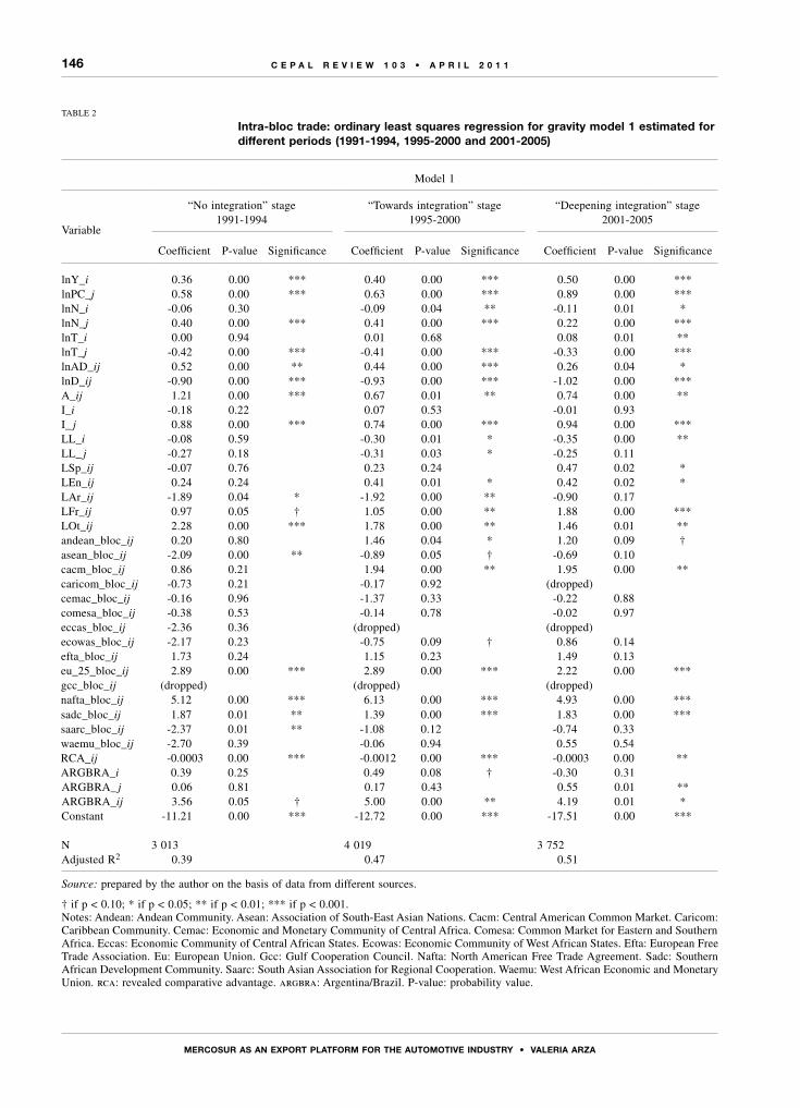
146



TABLE 2

intra-bloc trade: ordinary least squares regression for gravity model 1 estimated for different periods (1991-1994, 1995-2000 and 2001-2005)

Model 1

Variable

“No integration” stage1991-1994

“Towards integration” stage1995-2000

“Deepening integration” stage2001-2005

Coefficient P-value Significance Coefficient P-value Significance Coefficient P-value Significance

lnY_i 0.36 0.00 *** 0.40 0.00 *** 0.50 0.00 ***lnPC_j 0.58 0.00 *** 0.63 0.00 *** 0.89 0.00 ***lnN_i -0.06 0.30 -0.09 0.04 ** -0.11 0.01 *lnN_j 0.40 0.00 *** 0.41 0.00 *** 0.22 0.00 ***lnT_i 0.00 0.94 0.01 0.68 0.08 0.01 **lnT_j -0.42 0.00 *** -0.41 0.00 *** -0.33 0.00 ***lnAD_ij 0.52 0.00 ** 0.44 0.00 *** 0.26 0.04 *lnD_ij -0.90 0.00 *** -0.93 0.00 *** -1.02 0.00 ***A_ij 1.21 0.00 *** 0.67 0.01 ** 0.74 0.00 **I_i -0.18 0.22 0.07 0.53 -0.01 0.93 I_ j 0.88 0.00 *** 0.74 0.00 *** 0.94 0.00 ***LL_i -0.08 0.59 -0.30 0.01 * -0.35 0.00 **LL_ j -0.27 0.18 -0.31 0.03 * -0.25 0.11 LSp_ij -0.07 0.76 0.23 0.24 0.47 0.02 *LEn_ij 0.24 0.24 0.41 0.01 * 0.42 0.02 *LAr_ij -1.89 0.04 * -1.92 0.00 ** -0.90 0.17 LFr_ij 0.97 0.05 † 1.05 0.00 ** 1.88 0.00 ***LOt_ij 2.28 0.00 *** 1.78 0.00 ** 1.46 0.01 **andean_bloc_ij 0.20 0.80 1.46 0.04 * 1.20 0.09 †asean_bloc_ij -2.09 0.00 ** -0.89 0.05 † -0.69 0.10 cacm_bloc_ij 0.86 0.21 1.94 0.00 ** 1.95 0.00 **caricom_bloc_ij -0.73 0.21 -0.17 0.92 (dropped) cemac_bloc_ij -0.16 0.96 -1.37 0.33 -0.22 0.88 comesa_bloc_ij -0.38 0.53 -0.14 0.78 -0.02 0.97 eccas_bloc_ij -2.36 0.36 (dropped) (dropped) ecowas_bloc_ij -2.17 0.23 -0.75 0.09 † 0.86 0.14 efta_bloc_ij 1.73 0.24 1.15 0.23 1.49 0.13 eu_25_bloc_ij 2.89 0.00 *** 2.89 0.00 *** 2.22 0.00 ***gcc_bloc_ij (dropped) (dropped) (dropped) nafta_bloc_ij 5.12 0.00 *** 6.13 0.00 *** 4.93 0.00 ***sadc_bloc_ij 1.87 0.01 ** 1.39 0.00 *** 1.83 0.00 ***saarc_bloc_ij -2.37 0.01 ** -1.08 0.12 -0.74 0.33 waemu_bloc_ij -2.70 0.39 -0.06 0.94 0.55 0.54 RCA_ij -0.0003 0.00 *** -0.0012 0.00 *** -0.0003 0.00 **ARGBRA_i 0.39 0.25 0.49 0.08 † -0.30 0.31 ARGBRA_ j 0.06 0.81 0.17 0.43 0.55 0.01 **ARGBRA_ij 3.56 0.05 † 5.00 0.00 ** 4.19 0.01 *Constant -11.21 0.00 *** -12.72 0.00 *** -17.51 0.00 *** N 3 013 4 019 3 752 Adjusted R2 0.39 0.47 0.51

Source: prepared by the author on the basis of data from different sources.

† if p < 0.10; * if p < 0.05; ** if p < 0.01; *** if p < 0.001.Notes: Andean: Andean Community. Asean: Association of South-East Asian Nations. Cacm: Central American Common Market. Caricom: Caribbean Community. Cemac: Economic and Monetary Community of Central Africa. Comesa: Common Market for Eastern and Southern Africa. Eccas: Economic Community of Central African States. Ecowas: Economic Community of West African States. Efta: European Free Trade Association. Eu: European Union. Gcc: Gulf Cooperation Council. Nafta: North American Free Trade Agreement. Sadc: Southern African Development Community. Saarc: South Asian Association for Regional Cooperation. Waemu: West African Economic and Monetary Union. rca: revealed comparative advantage. argbra: Argentina/Brazil. P-value: probability value.

147



TABLE 3

Market diversification: ordinary least squares regression for gravity model 2 estimated for different periods (1991-1994, 1995-2000 and 2001-2005)

Model 2

Variable

“No integration” stage1991-1994

“Towards integration” stage1995-2000

“Deepening integration” stage2001-2005

Coefficient P-value Significance Coefficient P-value Significance Coefficient P-value Significance

lnY_i 0.36 0.00 *** 0.40 0.00 *** 0.50 0.00 ***lnPC_ j 0.58 0.00 *** 0.63 0.00 *** 0.89 0.00 ***lnN_i -0.05 0.35 -0.09 0.04 ** -0.11 0.01 **lnN_ j 0.40 0.00 *** 0.41 0.00 *** 0.21 0.00 ***lnT_i -0.01 0.81 0.01 0.75 0.08 0.01 ***lnT_ j -0.42 0.00 *** -0.41 0.00 *** -0.33 0.00 ***lnAD_ij 0.47 0.00 *** 0.41 0.00 *** 0.24 0.06 *lnD_ij -0.87 0.00 *** -0.91 0.00 *** -1.01 0.00 ***A_ij 1.08 0.00 *** 0.56 0.02 ** 0.70 0.01 ***I_i -0.17 0.23 0.08 0.51 -0.01 0.95 I_ j 0.87 0.00 *** 0.74 0.00 *** 0.93 0.00 ***LL_i -0.07 0.65 -0.28 0.01 ** -0.35 0.00 ***LL_ j -0.27 0.19 -0.31 0.03 ** -0.25 0.11 LSp_ij 0.05 0.84 0.29 0.15 0.47 0.03 **LEn_ij 0.25 0.22 0.41 0.01 ** 0.42 0.02 **LAr_ij -1.82 0.04 ** -1.88 0.00 *** -0.89 0.18 LFr_ij 0.98 0.05 ** 1.06 0.00 *** 1.88 0.00 ***LOt_ij 2.28 0.00 *** 1.76 0.00 *** 1.47 0.01 ***andean_bloc_ij 0.21 0.79 1.50 0.03 ** 1.24 0.09 *asean_bloc_ij -1.99 0.00 *** -0.83 0.07 * -0.66 0.12 cacm_bloc_ij 0.84 0.22 1.96 0.00 *** 1.98 0.00 ***caricom_bloc_ij -0.73 0.68 -0.17 0.92 (dropped) cemac_bloc_ij -0.02 0.99 -1.22 0.39 -0.17 0.91 comesa_bloc_ij -0.33 0.58 -0.12 0.81 -0.01 0.98 eccas_bloc_ij -2.29 0.37 (dropped) (dropped) ecowas_bloc_ij -2.00 0.27 -0.68 0.12 0.89 0.13 efta_bloc_ij 1.76 0.23 1.15 0.23 1.48 0.13 eu_25_bloc_ij 2.92 0.00 *** 2.91 0.00 *** 2.22 0.00 ***gcc_bloc_ij (dropped) (dropped) (dropped) nafta_bloc_ij 5.25 0.00 *** 6.23 0.00 *** 4.98 0.00 ***sadc_bloc_ij 1.97 0.01 *** 1.47 0.00 *** 1.86 0.00 ***saarc_bloc_ij -2.27 0.00 *** -0.99 0.15 -0.70 0.36 waemu_bloc_ij -2.82 0.37 -0.08 0.92 0.54 0.54 RCA_ij -0.0003 0.00 *** -0.0012 0.00 *** -0.0003 0.00 ***ARGBRA_i 0.31 0.38 0.40 0.17 -0.39 0.19 ARG_ j -1.01 0.02 ** -0.80 0.02 ** 0.12 0.74 BRA_ j 0.43 0.15 0.59 0.03 ** 0.60 0.03 **ARGBRA_ij 3.92 0.03 ** 5.43 0.00 *** 4.91 0.00 ***ARGURY_ij 2.93 0.11 1.76 0.29 0.17 0.92 ARGCHL_ij 1.29 0.48 1.73 0.30 0.79 0.64 ARGMEX_ij -2.05 0.26 1.18 0.48 3.36 0.05 **BRAURY_ij 2.46 0.17 4.08 0.01 ** 2.12 0.21 BRACHL_ij 2.48 0.17 1.39 0.40 1.64 0.33 BRAMEX_ij 3.08 0.09 * 3.92 0.02 ** 4.27 0.01 **Constant -11.03 0.00 *** -12.52 0.00 *** -17.34 0.00 ***

N 3 013 4 019 3 752 Adjusted R2 0.39 0.48 0.51

Source: prepared by the author on the basis of data from different sources.

† if p < 0.10; * if p < 0.05; ** if p < 0.01; *** if p < 0.001.Notes: Andean: Andean Community. Asean: Association of South-East Asian Nations. Cacm: Central American Common Market. Caricom: Caribbean Community. Cemac: Economic and Monetary Community of Central Africa. Comesa: Common Market for Eastern and Southern Africa. Eccas: Economic Community of Central African States. Ecowas: Economic Community of West African States. Efta: European Free Trade Association. Eu: European Union. Gcc: Gulf Cooperation Council. Nafta: North American Free Trade Agreement. Sadc: Southern African Development Community. Saarc: South Asian Association for Regional Cooperation. Waemu: West African Economic and Monetary Union. rca: revealed comparative advantage. argbra: Argentina/Brazil. argury: Argentina/Uruguay. argchl: Argentina/Chile. argmex: Argentina/Mexico. braury: Brazil/Uruguay. brachl: Brazil/Chile. bramex: Brazil/Mexico. P-value: probability value.

148



partners. This could be because the United States and Japan, two countries that are fairly remote from the rest of the world, have highly diversified markets and large shares of global exports.14 The dichotomous variable for cultural distance was language. Sharing the same language became an important factor in trade only during the latest period (countries where Arabic is spoken were an exception, probably because of their very low share of automobile output).

Revealed comparative advantage— These variables have the expected negative signs;

the more competitive the importer is relative to the exporter, the lower the level of trade between them.

Blocs— Most of the significant dichotomous variables have

the expected signs, indicating that the regulations of trade agreements have helped to shorten distances.15

2. Evidence in support of the paper’s main hypotheses

As can be seen in table 2, Argentina and Brazil traded more with each other than predicted by the expanded version of the gravity model (ARGBRAij is significant and positive in all periods). More precisely, in the 1991-1994 period Argentina and Brazil traded 34 times as much as would be expected from the gravity model.16 In the second (“towards integration”) stage, however, after the two countries signed their trade agreement in December 1994, there was 147 times as much trade between them as predicted by the gravity model. In other words, the agreement seems to have had a very large effect on

14 Furthermore, this coefficient changes sign if zero values are included in the Tobit models. Remoteness thus seems to have a negative effect on the creation of new bilateral relationships, but not necessarily on the intensification of trade between established partners.15 The only exception is the bloc of asean countries, which seem to have traded less with one another than predicted by the gravity model, especially in the first two periods. This finding seems to be due to two factors. First, the bloc’s trade deficit in those years was over 100% (between them, the countries imported more than twice as much as they exported), meaning that most imports came from outside the bloc. Second, the main producers in asean (Indonesia, Malaysia and Thailand) exported mainly to destinations outside the bloc.16 Because the model was estimated in logarithms, the effect of the dichotomous variable is given by the formula: =(exp(dichotomous variable coefficient)-1*100 (if expressed as a percentage). In the case above, =(exp(3.56)-1)=34.

intra-bloc trade.17 In the third stage (“deepening integration”), intra-bloc trade was lower than in the previous period; even so, Argentina and Brazil traded 65 times as much as predicted by the gravity model.

Figure 9 shows the evolution of the coefficients of intra-bloc trade between Argentina and Brazil when the gravity model equations are estimated by year. As can be seen, trade between these two countries began to expand in the early 1990s; however, it was not until after the first agreement (in late 1994) that Argentina and Brazil traded a significantly greater volume than would have been expected from the gravity equation. This effect was most pronounced in the 1996-1998 period. In 1999, the Brazilian recession may have diverted Argentine exports to other destinations; a decline in intra-bloc trade was then observed at the time of the Argentine crisis in 2002. These macroeconomic factors may explain which the second agreement signed in 2000, when integration between Argentina and Brazil was deepened, did not increase intra-bloc trade as expected.

Thus, the evidence seems to refute hypothesis 2 but not hypothesis 1. To conclude that there was trade creation after the 1994 agreement, however, it is necessary to determine whether the increase in the intra-bloc trade coefficient offset the decrease in the extra-bloc trade coefficient, as measured by the variable ARGBRAi. Table 2 shows that there was no decline in extra-bloc trade after 1994 and that hypothesis 1 therefore cannot be rejected. In other words, trade was created for Argentina and Brazil after the first agreement in 1994. This did not happen after the agreement signed in 2000 (i.e., the evidence supports hypothesis 1 but not hypothesis 2).

Exports to other destinations during “deepening integration” (stage 3) were 73% (=exp(0.55)-1)*100) higher than anticipated from the gravity model. In stages 1 and 2, these countries exported only about as much to other destinations as would be expected from the gravity model (i.e., the ARGBRAj coefficients were not significant). The significance of the ARGBRAj coefficient in stage 3 seems to indicate that extra-bloc markets were particularly important for the exports of Argentina and Brazil during the “deepening integration” stage. However, the difference between this coefficient and those of stages 1 and 2 is not significant. Although this might be explained statistically by the large standard deviation of the coefficients in the first and second periods, it cannot be categorically stated that Argentina, Brazil or both diversified their export markets after the 2000

17 The difference in the coefficient for ARGBRAij between the first and second periods is significant (p-value of 0.06).

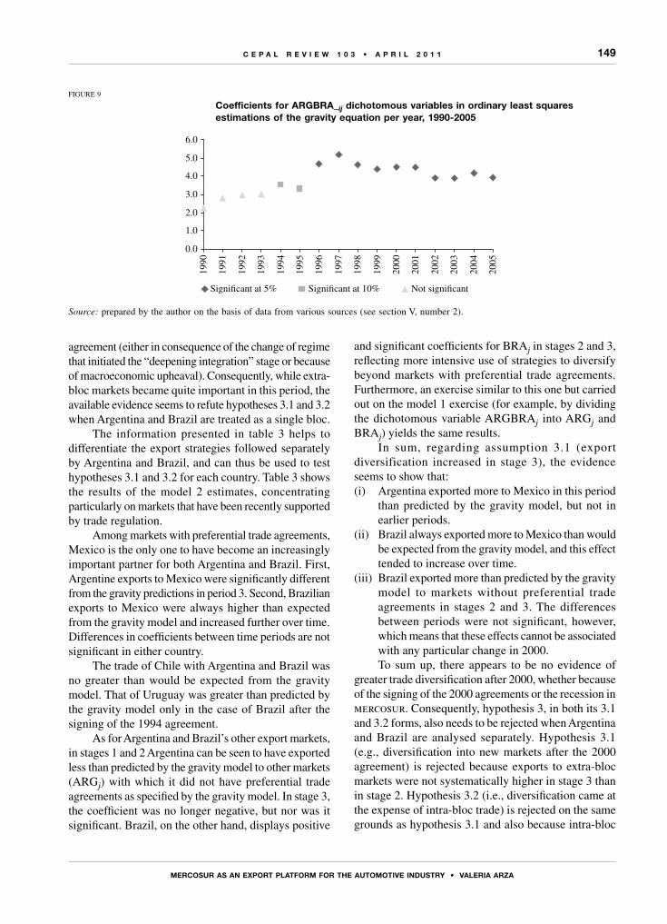
149



agreement (either in consequence of the change of regime that initiated the “deepening integration” stage or because of macroeconomic upheaval). Consequently, while extra-bloc markets became quite important in this period, the available evidence seems to refute hypotheses 3.1 and 3.2 when Argentina and Brazil are treated as a single bloc.

The information presented in table 3 helps to differentiate the export strategies followed separately by Argentina and Brazil, and can thus be used to test hypotheses 3.1 and 3.2 for each country. Table 3 shows the results of the model 2 estimates, concentrating particularly on markets that have been recently supported by trade regulation.

Among markets with preferential trade agreements, Mexico is the only one to have become an increasingly important partner for both Argentina and Brazil. First, Argentine exports to Mexico were significantly different from the gravity predictions in period 3. Second, Brazilian exports to Mexico were always higher than expected from the gravity model and increased further over time. Differences in coefficients between time periods are not significant in either country.

The trade of Chile with Argentina and Brazil was no greater than would be expected from the gravity model. That of Uruguay was greater than predicted by the gravity model only in the case of Brazil after the signing of the 1994 agreement.

As for Argentina and Brazil’s other export markets, in stages 1 and 2 Argentina can be seen to have exported less than predicted by the gravity model to other markets (ARGj) with which it did not have preferential trade agreements as specified by the gravity model. In stage 3, the coefficient was no longer negative, but nor was it significant. Brazil, on the other hand, displays positive

and significant coefficients for BRAj in stages 2 and 3, reflecting more intensive use of strategies to diversify beyond markets with preferential trade agreements. Furthermore, an exercise similar to this one but carried out on the model 1 exercise (for example, by dividing the dichotomous variable ARGBRAj into ARGj and BRAj) yields the same results.

In sum, regarding assumption 3.1 (export diversification increased in stage 3), the evidence seems to show that:(i) Argentina exported more to Mexico in this period

than predicted by the gravity model, but not in earlier periods.

(ii) Brazil always exported more to Mexico than would be expected from the gravity model, and this effect tended to increase over time.

(iii) Brazil exported more than predicted by the gravity model to markets without preferential trade agreements in stages 2 and 3. The differences between periods were not significant, however, which means that these effects cannot be associated with any particular change in 2000.To sum up, there appears to be no evidence of

greater trade diversification after 2000, whether because of the signing of the 2000 agreements or the recession in mercosur. Consequently, hypothesis 3, in both its 3.1 and 3.2 forms, also needs to be rejected when Argentina and Brazil are analysed separately. Hypothesis 3.1 (e.g., diversification into new markets after the 2000 agreement) is rejected because exports to extra-bloc markets were not systematically higher in stage 3 than in stage 2. Hypothesis 3.2 (i.e., diversification came at the expense of intra-bloc trade) is rejected on the same grounds as hypothesis 3.1 and also because intra-bloc

FIGURE 9

Coefficients for ArGBrA_ij dichotomous variables in ordinary least squares estimations of the gravity equation per year, 1990-2005

Source: prepared by the author on the basis of data from various sources (see section V, number 2).

0.0

1.0

2.0

3.0

4.0

5.0

6.0

1990

1991

1992

1993

1994

1995

1996

1997

1998

1999

2000

2001

2002

2003

2004

2005

Not signi�cantSigni�cant at 10%Signi�cant at 5%

150



trade (ARGBRAij) did not change significantly between stages 2 and 3.

Lastly, while hypotheses 3.1 and 3.2 have been rejected, there is some evidence for the growing importance of Mexico vis-à-vis intra-bloc trade. Intra-bloc trade in stage 2 was considerably greater than that between Argentina or Brazil and any other partner with a preferential trade agreement, including Mexico. In stage 3, however, although the intra-bloc trade results

were greater than those for any other partnership, the intra-bloc coefficient is not much different from the trade coefficient between Mexico and Argentina or between Mexico and Brazil. In other words, Mexico seemed to increase in importance (relative to intra-bloc trade) as an export market for Argentina and also for Brazil. This is not the case with Uruguay, a partner whose relative importance declined, or with Chile, whose relative importance was roughly stable over time.

VIIConclusions

The trend towards internationalization of the global automotive industry has intensified since the 1990s and includes global and regional strategies. Regional strategies are said to be more efficient because the trade-off between efficient scale and product differentiation is more balanced.

mercosur has a long history as a location for automotive production. For example, some subsidiaries of multinational corporations began producing earlier in the region than in more developed places. mercosur is now a major area in terms of its share of both global output and exports.

However, the region has not yet achieved full integration for the industry. The main reason for the lack of a full agreement in the automotive industry is that the members of mercosur have not reached a consensus on the common external tariff (Argentina and Brazil prefer higher tariffs, while Uruguay and Paraguay prefer lower tariffs).

This is now one of the few sectors in which Argentine-Brazilian trade is administered by a series of agreements entailing different degrees of intervention. The first of these agreements was reached in 1994 and began what this article has called the “towards integration” stage. The second agreement, signed in 2000, was more committed to regional integration and established the beginning of the “deepening integration” stage. In 2006 and again in 2008, however, agreements were signed that set back intra-bloc integration in one way or another (“reversing integration” stage). Intra-bloc free trade was postponed until 2013, chiefly owing to Argentine concerns about competition from Brazil.

All these agreements tended to favour strategies of complementation within the multinational corporations

located in the two countries. To some extent this was achieved during the “deepening” stage, as discussed by Arza and López (2008b) when studying the Argentine case.

The purpose of this paper was to analyse the extent to which mercosur (defined as Argentina and Brazil only) has been turned into an export platform for automotive production. More specifically, the objective was to examine whether trade was created after the trade agreements of late 1994 and 2000, and whether the two countries diversified their exports to other markets during the “deepening integration” stage (2000-2005).

The methodology proposed (estimation of an expanded gravity equation) required the construction of a large database with information from different sources. Once all the variables needed for the estimation had been assembled, an unbalanced database was created with a maximum of 78 exporting countries and 103 importing countries, with measurements of trade flows in the 1991-2005 period. To meet the research objective, the sample was divided into three periods (before and after the 1994 and 2000 trade agreements) and two different versions of the gravity model were estimated. The difference between the models is that the second disaggregates extra-bloc exports more extensively.

The conclusion from the empirical analysis was that genuine trade creation did take place after the 1994 agreement. Argentina and Brazil traded more with each other than predicted by the gravity model. Furthermore, intra-bloc trade increased significantly after 1994 (i.e., between periods 1 and 2), without harming extra-bloc trade. Possibly as a result of the recession in Brazil (and Argentina) in 1998-1999 and the Argentine crisis of 2001-2002, however, the 2000 agreement did not lead to a large rise in intra-bloc trade.

151



The descriptive evidence shows that after the signing of the second agreement in 2000 (during the “deepening integration” stage), the region apparently exported more than before to other destinations. In Brazil, furthermore, a more aggressive diversification strategy was applied to exports, which expanded beyond the markets covered by preferential trade agreements. This may be because the bloc was turning into an export platform following the enhanced agreement between Argentina and Brazil in 2000, or because both countries suffered macroeconomic upheavals in those years and so had to look for extra-bloc markets. While the econometric estimates show that extra-bloc trade (Argentina’s mainly going to Mexico but Brazil’s also to countries without preferential trade agreements) was greater than predicted by the gravity

model and actually increased in the period, this rise was not statistically significant.

To sum up, there is evidence of trade creation after the 1994 agreement, although the same did not happen after the agreement signed in 2000. Trade creation is accounted for mainly by the rise in intra-bloc trade. Although the export share of countries outside the bloc progressively increased, there is not enough evidence to claim that Argentina or Brazil succeeded in systematically increasing their access to extra-bloc markets after the signing of the integration agreements. In other words, to judge by the evidence gathered up to 2005, the 2000 mercosur agreements were not successful at that time in turning the region into a platform for exports to other extra-bloc markets.

(Original: English)

ANNEX

Selected regional integration agreements

Andean Community: Colombia, Ecuador, Peru and Plurinational State of Bolivia.

asean (Association of South-East Asian Nations):

Brunei Darussalam, Cambodia, Indonesia, Lao People’s Democratic Republic, Malaysia, Myanmar, Philippines, Singapore, Thailand and Viet Nam.

cacm (Central American Common Market):

Costa Rica, El Salvador, Guatemala, Honduras and Nicaragua.

caricom (Caribbean Community): Antigua and Barbuda, Bahamas, Barbados, Belize, Dominica, Grenada, Guyana, Haiti, Jamaica, Montserrat, Saint Kitts and Nevis, Saint Lucia, Saint Vincent and the Grenadines, Suriname and Trinidad and Tobago.

cemac (Economic and Monetary Community of Central Africa):

Cameroon, Central African Republic, Chad, Congo, Equatorial Guinea and Gabon.

comesa (Common Market for Eastern and Southern Africa):

Angola, Burundi, Comoros, Congo, Democratic Republic of the Congo, Djibouti, Egypt, Eritrea, Ethiopia, Kenya, Libya, Madagascar, Malawi, Mauritius, Namibia, Rwanda, Seychelles, Sudan, Swaziland, Uganda, Zambia and Zimbabwe.

eccas (Economic Community of Central African States):

Angola, Burundi, Cameroon, Central African Republic, Chad, Congo, Democratic Republic of the Congo, Equatorial Guinea, Gabon, Rwanda and São Tomé and Príncipe.

ecowas (Economic Community of West African States):

Benin, Burkina Faso, Cape Verde, Côte d’Ivoire, Gambia, Ghana, Guinea, Guinea-Bissau, Liberia, Mali, Niger, Nigeria, Senegal, Sierra Leone and Togo.

efta (European Free Trade Association): Iceland, Liechtenstein, Norway and Switzerland.

eu 15 (European Union (15 countries)): Austria, Belgium, Denmark, Finland, France, Germany, Greece, Ireland, Italy, Luxembourg, Netherlands, Portugal, Spain, Sweden and the United Kingdom.

eu 25 (European Union (25 countries)): Austria, Belgium, Cyprus, Czech Republic, Denmark, Estonia, Finland, France, Germany, Greece, Hungary, Ireland, Italy, Latvia, Lithuania, Luxembourg, Malta, Netherlands, Poland, Portugal, Slovenia, Slovakia, Spain, Sweden and the United Kingdom.

gcc (Gulf Cooperation Council): Bahrain, Kuwait, Oman, Qatar, Saudi Arabia and United Arab Emirates.

mercosur (Southern Common Market): Argentina, Brazil, Paraguay and Uruguay.

nafta (North American Free Trade Agreement):

Canada, Mexico and the United States of America.

Preferential Trade Agreement of the South Asian Association for Regional Cooperation (saarc):

Bangladesh, Bhutan, India, Maldives, Nepal, Pakistan and Sri Lanka.

Sadc (Southern African Development Community):

Angola, Botswana, Democratic Republic of the Congo, Lesotho, Madagascar, Malawi, Mauritius, Mozambique, Namibia, Seychelles, South Africa, Swaziland, United Republic of Tanzania, Zambia and Zimbabwe.

waemu (West African Economic and Monetary Union):

Benin, Burkina Faso, Côte d’Ivoire, Guinea-Bissau, Mali, Niger, Senegal and Togo.

Source: selected by the author on the basis of World Trade Organization (wto) statistical data.

152



Aitken, N.D. (1973), “The effect of the Eec and Eeta on European Trade: a temporal cross-section analysis”, American Economic Review, vol. 63, No. 5, Nashville, Tennessee, American Economic Association.

Arza, V. and A. López (2008a), “Tendencias internacionales en la industria automotriz”, La industria automotriz en el mercosur, A. López (ed.), Montevideo, mercosur Economic Research Network.

(2008b), “El caso argentino”, La industria automotriz en el mercosur, A. López (ed.), Montevideo, mercosur Economic Research Network.

(2008c), “Introducción al libro: la visión regional”, La industria automotriz en el mercosur, A. López (ed.), Montevideo, mercosur Economic Research Network.

Bastos Tigre, P. and others (1999), “Impacto del mercosur en la dinámica del sector automotor”, Impacto sectorial de la integración en el mercosur, J.J. Taccone and L.J. Garay (eds.), Buenos Aires, Institute for the Integration of Latin America and the Caribbean (intal).

Bayoumi, T. and B. Eichengreen (1997), “Is regionalism simply a diversion? Evidence from the evolution of the Ec and Efta”, Regionalism Versus Multilateral Trade Arrangements, T. Ito and A.O. Krueger (eds.), Chicago, University of Chicago Press.

Braga, C.A., R. Safadi and A. Yeats (1994), “Regional integration in the Americas: deja vu all over again?”, World Economy, vol. 17, No. 4, Oxford, Blackwell Publishing.

Cimoli, M. and J. Katz (2001), “Reformas estructurales, brechas tecnológicas y el pensamiento del Dr. Prebisch”, document presented at the Seminar “El desarrollo en el siglo XXI”, Santiago, Chile, Economic Commission for Latin America and the Caribbean (eclac).

Ciravegna, L. (2003), “Global and regional integration of production in the mercosur automotive value chains, the case of Fiat”, eadi Workshop: Clusters and Value Chains in the North and in the Third World, Novara, Università del Piemonte Orientale.

Filippini, C. and V. Molini (2003), “The determinants of East Asian trade flows: a gravity equation approach”, Journal of Asian Economics, vol. 14, No. 5, Amsterdam, Elsevier.

Frankel, J.A. (1997), Regional Trading Blocs in the World Economic System, Washington, D.C., Institute for International Economics.

Freyssenet, M. and Y. Lung (2000), “Between globalisation and regionalisation: what is the future of the motor industry”, Global Strategies and Local Realities: The Auto Industry in Emerging Markets, J. Humphrey, Y. Lecler and M.S. Salerno (eds.), New York, St. Martin’s Press.

Humphrey, J. and O. Memedovic (2003), The Global Automotive Industry Value Chain: What Prospects for Upgrading by Developing Countries, Vienna, United Nations Industrial Development Organization (unido).

Humphrey, J. and A. Oeter (2000), “Motor industry policies in emerging markets: globalisation and the promotion of domestic industry”, Global Strategies and Local Realities: The Auto Industry in Emerging Markets, J. Humphrey, Y. Lecler and M.S. Salerno (eds.), New York, St. Martin’s Press.

Humphrey, J., Y. Lecler and M.S. Salerno (2000), Global Strategies and Local Realities: The Auto Industry in Emerging Markets, J. Humphrey, Y. Lecler and M.S. Salerno (eds.), New York, St. Martin’s Press.

Krueger, A.O. (1999), “Trade creation and trade diversion under nafta”, nber Working Paper, No. 7429, Cambridge, Massachusetts, National Bureau of Economic Research.

Laplane, M. and F. Sarti (2008), “O caso do Brasil”, La industria automotriz en el mercosur, A. López (ed.), Montevideo, mercosur Economic Research Network.

Motta Veiga, P. (2004), Foreign Direct Investment in Brazil: Regulation, Flows and Contribution to Development, Winnipeg, International Institute for Sustainable Development.

Musila, J.W. (2005), “The intensity of trade creation and trade diversion in comesa, eccas and ecowas: a comparative analysis”, Journal of African Economies, vol. 14, No. 1, Oxford, Oxford University Press.

Oman, C. (2000), Policy Competition for Foreign Direct Investment: A Study of Competition among Governments to Attract fdi, Paris, Organisation for Economic Co-operation and Development (oecd).

Rugman, A.M. and S. Collinson (2004), “The regional nature of the world’s automotive sector”, European Management Journal, vol. 22, No. 5, Amsterdam, Elsevier.

Rugman, A. and R. Hodgetts (2001), “The end of global strategy”, European Management Journal, vol. 19, No. 4, Amsterdam, Elsevier.

Schlie, E. and G. Yip (2000), “Regional follows global: strategy mixes in the world automotive industry”, European Management Journal, vol. 18, No. 4, Amsterdam, Elsevier.

Soloaga, I. and A.L. Winters (2001), “Regionalism in the nineties: what effect on Trade? ”, The North American Journal of Economics and Finance, vol. 12, No. 1, Amsterdam, Elsevier.

Bibliography


153

Positional inconsistency:a new concept insocial stratification

Kathya Araujo and Danilo Martuccelli

B ased on empirical research involving some 100 semi-directive

interviews with individuals from different social groups, this article

introduces and discusses the use of a new concept for analysing the

phenomenon of social stratification in contemporary Chilean society,

namely “positional inconsistency”. This describes a more or less permanent

and generalized feeling of positional anxiety in the vast majority of

social strata, which has specific characteristics that distinguish it from

other similar processes (status fear, vulnerability, exclusion, mobility, for

example). It is an experience which, although expressed in similar ways,

is nonetheless fostered by a plurality of factors giving rise to a significant

structural phenomenon.

KEYWORDS

Social classes

Social structure

Social mobility

Economic aspects

Political aspects

Social problems

Urban environment

Chile

Kathya Araujo

Professor, University of the

Academy of Christian Humanism


Danilo Martuccelli

Professor, Paris Descartes University

Centre for the Study of Social

Links (cerlis)

National Centre for Scientific

Research (cnrs)


154

PosITIonAL InConsIsTEnCy: A nEW ConCEPT In soCIAL sTRATIFICATIon • kAThyA ARAuJo And dAnILo mARTuCCELLI


This article reports some of the results of National Scientific and Technological Development Fund (fondecyt) research project No.1085006, on subject individuation and configuration processes in contemporary Chilean society. The authors are grateful for the opinions offered by anonymous referees, and for comments and suggestions that have made it possible to enhance the first version of this article.

This article develops the idea that the study of social stratification in Latin America needs to be extended to take account of an experience which, although not exclusive to the region, has specific and decisive characteristics in it. Based on data from Chile, the article will demonstrate the existence of an experience of “positional inconsistency”, which is commonly occurring and cuts across different social strata.

The thesis is developed in four stages: section II briefly describes the analysis that links the growing complexity of social situations to the study of positional anxiety. Section III stresses the commonality of positional inconsistency in different social strata and then distinguishes it from other similar concepts. Section IV describes the various threats which, paradoxically, reflect both its cross-cutting nature and its diversity in the various sectors studied. Lastly, and by way of conclusion, the article mentions some of the day-to-day challenges that the experience of positional inconsistency poses in the life of most of the individuals interviewed.

This article is based on empirical research carried out in Chile (in the cities of Santiago, Concepción and Valparaíso) between 2007 and 2009, through some

100 semi-directive interviews with men and women of between 30 and 55 years of age, from low-income urban sectors and middle- and high-income groups. In general, the social sciences tend not to use qualitative methods to study social stratification. Most research in this field displays a statistical desire to aggregate individuals into a small number of groups (classes or strata) that define the positional architecture of a society. In Chile, there are numerous essays of this type, which, depending on the theoretical options chosen, emphasize the decisive importance of work, income, consumption, or culture (or a combination of these factors) when defining the boundaries of the major social positions. Statistical techniques are clearly essential when making classifications of this type. Nonetheless, this article aims to highlight a different phenomenon and draw attention to a subjective dimension that is relatively neglected in many studies of social stratification, strictly defined. Without denying the relevance of social divisions, in that dimension it will be necessary to recognize the presence of a common cross-cutting experience of positional inconsistency, underlying the diversity of social positions, as a major feature of social status in today’s Chile.

Iintroduction

IIFrom social stratification to a cross-cutting

positional experience

Although attempts to find a schematic and more or less pyramidal view of major class positionings have not disappeared in Latin America, a more complex view of social positioning is steadily gaining ground. Even in studies that attempt to define the broad class positions in the continent based on the primacy of capitalist-type relations, a variety of other structural factors also need

to be invoked (Portes and Hoffman, 2007). In addition to the traditional coexistence of different modes of production (modern, small enterprise and others), there is a multiplicity of resources that give access to power, prestige or wealth —including both different forms of remuneration and different forms of work contract (and the different levels of social coverage and protection that these imply). The result is a growing awareness that it is essential to draw on a wide variety of factors to more precisely describe social stratification in Latin America. This progressively leads to tension between studies that define class dynamics, and those that adopt a more descriptive approach (Dubet and Martuccelli,

155



2000). This is precisely the meaning of the important contrast between the six major social classes described by Portes and Hoffman (2007) and the 45 social categories distinguished by León and Martínez (2007) in their proposed classification of social actors in Chile.

This reflects a general trend towards increasing complexity of the actual heterogeneity of social situations, which thus far has occurred particularly in Latin America, giving renewed attention to other forms of capital or total assets. The employment-income-education triad has been augmented by a plurality of other factors, such as social capital, the nature of social networks, modes of belonging, different social stereotypes, the capacity to access and control the dominant cultural codes, the importance of places of residence (neighbourhoods), the fact of being a homeowner or not, the effect that personal and family life (separations, deaths and other events) have on social paths. There is also is the primordial role of consumption in the region, not only in the process of breaking down the barriers between social groups, but also in the appearance of new modes of symbolic inclusion among low-income sectors (García Canclini, 1995; Aguilar, 2009), such that, in Chile and elsewhere, a social stratification model generated from market studies has been imposed on public opinion, which classifies Chileans in the categories ABC1 (10% - elite and upper middle class), C2 (20% - middle middle class), C3 (25% - lower middle class), D (35% - poverty) and E (10% - extreme poverty) (Rasse, Salcedo and Pardo, 2009).

Although the idea of a positional pyramid persists in social stratification studies, awareness of the existence of a wide variety of intermediate positions is steadily consolidating. In other words, the multiplicity of the social positioning factors studied makes it increasingly hard to know who is truly “up” or “down”, while hybrid

positionings are increasingly common, and actors may simultaneously and contradictorily experience upward or downward mobility in different social domains. Moreover, this is true in most social strata. The traditional class-based division between groups —although still present in individual mindsets (Araujo, 2009) and evident in terms of income deciles— needs to be supplemented by the view of a continuum of social positions with no abrupt changes between them (aim, 2000). This reality is partly reflected by the fact that between 60% and 80% of Chileans claim to belong to the “middle classes”, which makes this social group predominant when defining the profile of current Chilean society (Torche and Wormald, 2007; León and Martínez, 2007).

Nonetheless, although in Chile the generalization of this sense of belonging to the middle class is important, one should not forget an essential characteristic, namely the marked dispersion and heterogeneity of social experiences observable in a given social group, whether in the low-income sector or in the so-called middle classes (Barozet and Espinoza, 2009), which calls for recognition of the increasing singularity of experiences within different social strata (Espinoza, 2002).

Despite the importance of this type of approach stressing the singularity of social positions, the research reported in this article reveals the existence of a cross-cutting phenomenon in the vast majority of them. Except for a durable and globally protected elite, in a country characterized by high levels of concentration of various forms of power (Molina, 2005), most individuals feel their position is extremely permeable and susceptible to social deterioration. The widespread awareness of this situation defines one of the major positional characteristics of Chileans today: the sense that all positions are liable to suffer active destabilization processes.

IIIwhat is positional inconsistency?

At the heart of this experience of positional inconsistency is the sense that anything can change at any time. It is a permanent positional worry, a daily anxiety that reflects a society wracked by multiple senses of instability. Positional inconsistency is a multiform concern, plural in its sources and generally constant, which gives rise to a climate of positional anxiety shared by many individuals in different social strata. To describe this experience more precisely, it is worth distinguishing it

from other apparently similar notions, such as under-class or marginality; vulnerability or exclusion; status fear or status inconsistency; or social mobility. (i) Despite the greater role accorded to urban or

economic issues in certain testimonies, positional inconsistency is at the opposite extreme of studies of the underclass. The inconsistency in question does not exclusively concern economic change (the shift from an urban and industrial economy to a periurban

156



economy dominated by services), or an essentially urban phenomenon (Wilson, 1987 and 1996). If one considers the experience of the outlying urban areas of Greater Santiago, no specific urban identity has been generated, and the positional inconsistency that its inhabitants complain about cannot be reduced merely to an economic process that has polarized the social structure on new foundations. On the contrary, it is as citizens, generally engaged in the labour market and sharing the mainstream criteria and values of Chilean society, that these inhabitants express their discontent, frustration and positional inconsistency. The problem is not that they are unlike other people, but that by perceiving themselves collectively as others, they feel their positions are particularly unstable. Most of the inhabitants interviewed in these neighbourhoods, whatever their economic status, were formal workers (or had family members working in this sector). Accordingly, they are defined less by their exclusion or economic informality (low overall in Chile) than by their lack of skills and low incomes. The problem is not that they are “out”. The problem is that because they are “in” they feel fragile.

It is in this sense that the notion of positional inconsistency differs from “marginality”. The latter concept stresses a specific structural dimension, namely the limits of the capitalist system in the region, unlike in central countries, to absorb the excess supply of labour from the countryside (Nun, 1969; Quijano, 1971). The major characteristic of positional inconsistency relates not only to a small number of actors (who have been “forgotten” or “left behind” by progress), but to a numerically very large group that perceive their position through a sui generis sense of inconsistency.

(ii) Positional inconsistency denotes a broad social process that cuts across many social strata, although, as discussed below, the sources and its weight vary. Unlike some social stratification studies in which “vulnerability” (generally defined exclusively in relation to poverty) has been confined to the low-income sector and even to an informal proletariat (Contreras and others, 2005; Torche and Wormald, 2007), inconsistency defines a social experience pertaining to many other social strata. Certainly, some studies have shown how the low-income world (sometimes referred to as “sector D”) suffers from both potential and also chronic vulnerability. Despite this distinction, however, the key point, clearly revealed in the studies of the

Socioeconomic Characterization Survey (casen), is that vulnerability always denotes a socially well-defined experience (Ramos and others, 2004). Of course, the reasons for this restricted use of the notion are legitimate, but given the qualitative material that has been produced here, it seems essential to use a broader notion to designate the feeling of positional anxiety expressed by the vast majority of individuals.

A similar distinction applies to “exclusion”. Here, although the term is highly polysemous, one can argue that what underlies this notion is a process of fragilization which increasingly affects social groups that are perfectly adapted to modern society but, nonetheless, are victims of economic circumstances and in particular the employment crisis. In this sense, exclusion is a concept which, without denying the existence of a “fourth world” or an extreme “poverty”, focuses on more integrated social groups. Nonetheless, in this analytical extension, and despite the desire to provide a dynamic and multidimensional definition of exclusion, the core of the analysis prioritizes the thesis of the existence of a crisis of social relations, and relates, sooner or later, essentially to transformation of the modes of integration provided by employment (Castel, 1995; Paugam, 1996). This experience is very far from doing justice to the inherent characteristics of the labour market in Latin America and, in some countries, to the violence of the process through which class divisions are being broken down (Minujín, 1993).

(iii) Positional inconsistency can also not be reduced to mere “status fear” or to “status inconsistency”, although it sometimes includes this process. Although aspects of this type of anxiety are sometimes present in positional inconsistency, the latter is nonetheless different. In the first case, anxiety occurs amidst social positions that are perceived as solid; it is the solidity of the places in question and difficulty in accessing and occupying them that gives rise to status anxiety, the need to fabricate a personality aimed at active and permanent defence of status, as has been magnificently established in relation to the courtesan or organization man (Elias, 1982; Whyte, 1957; Kocka, 1989; Boltanski, 1982). In contrast, in the case of positional inconsistency it is social position itself that is seen as porous and susceptible to deterioration.

In the second case, the notion shares with status inconsistency the characteristic of indicating a

157



loss of status legibility, the fact that contradictions exist between the various (economic or symbolic) registers of a position; that hybrid positionings are increasingly common, and that actors may simultaneously experience contradictory movements up or down in different social domains —in most social strata. Nonetheless, while sharing these aspects, in the case of positional inconsistency, what is stressed is the blurring of positions occupied by actors and the associated sense of anxiety, rather than the contradictions.

The situation of the “middle classes” in Chile makes it possible to specify this distinction more precisely. This social group is characterized by a transition, insufficiently addressed by theory, in terms of its anxiety. For a long time, the specific anxiety of this social group, located in an intermediate position by definition, was considered in theoretical terms more in terms of status than position. Being middle-class meant, first and foremost, possessing and defending a social status (Portocarrero, 1998). In the last few decades a genuine transition has occurred. Without disappearing, the traditional status anxiety pertaining to the middle classes is crystallizing into a fear of “falling” (Ehrenreich, 1989); but above all it is yielding, surreptitiously, to a distinct sense of positional inconsistency. Although the terms used are sometimes similar, since both cases visualize the fear of dropping down the social scale, the essence of the processes are different. In the first case, anxiety originates from a desire to defend “privileges” or “rights”, even access to a status (Lomnitz and Melnick, 1991). In the second case, it is a question of multiplying resources or support (economic, political or relational) to underpin and solidify a social position that is perceived as inconsistent, through a set of relational strategies, (Barozet, 2002; Sánchez, 2009). In the first case, it is the famous “decency” of the Latin American middle classes, and the symbolic frontiers that can be built around that, which defines the status boundary; in the second case, it is not a question of maintaining a given position, but of maintaining position per se. In fact what is involved here is maintaining oneself in a position which, given its unstable nature, needs to be underpinned by individual and collective strategies.

(iv) Lastly, the widespread sense of inconsistency in social positions cannot be reduced only to a direct effect of upward or downward social mobility, or

entry into and exit from poverty. This analytical distinction is particularly important, since Chilean society in recent decades has displayed high rates of social mobility in a context of marked urban segmentation and accentuated income inequality (Torche, 2005; Contreras, D., O. Larrañaga and J. Litchfield, 2001). The mobility rate, measured in terms of the income distribution, is highly eloquent in the short run: between 1996 and 2006, just 18.9% of Chileans included in the study were still in their original income deciles 10 years later (Arzola and Castro, 2009, pp. 70-72). Moreover, this mobility, albeit in different proportions, can be discerned both in the poorest decile (over the 10-year period, just 28.1% remained in this same position, which points to significant upward social mobility), and in the top decile (where just 45.4% remained in the same income decile and decade later). In other words, even if mobility is greater among the poorest sectors than in the wealthiest groups, it is significant in all cases. Without doubt, this reality is consistent with the sense

of positional inconsistency expressed by the interviewees. Nonetheless, the phenomenon here seems broader, not only, as shown below, because of the plurality of sources evoked, but also because members of the middle class, and particularly the upper-class, sectors interviewed here, displayed a profound positional anxiety, even though inter-generational mobility in Chile (the likelihood of moving from the lowest quintiles to the highest and vice versa) is low (Núñez and Miranda, 2009). This means that, although mobility between groups is high, at the upper end of the distribution Chilean society seems particularly closed to the circulation of elites, since various “closed-shop” mechanisms are deployed (Contardo, 2008). Nonetheless, and although at the top of the Chilean social “pyramid” there are barriers that seem unbreachable, this does not remove anxiety in relation to positional inconsistency among the members of this group.

In short, positional inconsistency describes a gradation of situations, because not all actors experience it with the same intensity; and, in particular, not all experience it in terms of the same factors. This inconsistency differs widely according to historical periods and, obviously, between social strata; but it also differs in terms of the factors that are taken into account. The traditional pairing of economy and social relations needs to be augmented by other political, cultural, and urban factors, to restore the complexity of this experience.

158



Positional inconsistency thus denotes a specific experience —a simultaneous mix of status and process. Status: the sense of inconsistency is constant among actors, despite the prosperity they may display in many respects. Process: inconsistency, even when it adopts abrupt forms, is always the result of a series of phases that steadily weaken or deteriorate a given position. To understand this dual reality and its differentiated generalization in current Chilean society, it is useful to distinguish four major factors.

1. Socioeconomic destabilizations

In structural terms, since the 1980s the Chilean economy has gone through a major transformation involving the shrinking of agricultural sectors, the far reaching changes in manual work (accompanied by a substantial reduction in manual labour and a significant internal transformation of this group), and the outsourcing of jobs that has gone hand-in-hand with growth of the private sector and the decline of public employment. This transformation has generally meant that employment has lost its protection capacities, accentuating the trend towards more precarious conditions in the occupational structure, although the phenomenon in Chile is more complex and less uni-directional than often claimed. The transformation process involves both “improvement” and “deterioration” simultaneously —probably not unrelated to the appearance of spurious forms of social mobility, such as individuals who become entrepreneurs and express nostalgia for their former manual worker status, or trades-people who yearn for their former life in agriculture (Kessler and Espinoza, 2007, p. 285). One can thus hypothesize that what underlies these attitudes is a vague awareness of an increase, despite the “objective” mobility experienced, or the feeling of growing positional inconsistency.

This sentiment, as the interviews presented below demonstrate and regardless of how frequently it appears among individuals from different social groups, reflects very different conditions depending on whether the individual in question works in the formal or informal sector of the economy (Infante and Sunkel, 2004), whether

he or she has one or more incomes, and also on the type of employment contract. Nonetheless, there is variety not only in what underlies the anxiety, but also in how it takes the form of chronic worry, or not, and how it is dealt with. Curiously, it is not individuals who display greater “objective” fragility who necessarily express the greatest positional anxiety. What seems to be common and cross-cutting in the interviews, however, is a widespread perception of never definitively or lastingly feeling protected from economic destabilization. This inconsistency can be shown by a large number of factors.

(a) The spectre of job lossIn Chile, unemployment has a huge effect on the

likelihood of being poor or slipping back into poverty (Arzola and Castro, 2009). But, beyond the figures, and even the effective diversity of protection and indemnification mechanisms that different wage-earners enjoy, what needs to be stressed is the type of awareness that individuals express in relation to this eventuality. A perception of more or less acute social exposure, a feeling of more or less pronounced impotence: “It’s a very perverse, very cruel system; the law doesn’t support you, it doesn’t protect you; there’s no safety net. In my case, unemployment insurance lasted three months…” (male, executive). This fear, which is intensified by age and its consequences for job opportunities was often called to mind: “Here, once past 40 you’re too old for work” (male, 49); “In this country, if you’re over 40, you’re old and expensive; so I may now be very expensive for my firm; they could pay two or three people with my wage, and sometimes this worries me…” (male, 51) “As we get older we encounter more competition every day and it’s harder to get ahead, which generates a type of anxiety” (male, 44).

(b) Bankruptcy If wage earners are afraid of losing their jobs,

entrepreneurs and self-employed workers fear bankruptcy. Of course, negative experiences should not eclipse the successful experience of many others (or the same people at different times in their lives). Nonetheless, there is a common anxiety among this group. In fact,

IVThe differentiated generalization

of positional inconsistency

159



their situation is paradoxical. In the last few decades, the income of independent workers in Chile has grown faster than that of wage earners, such that in 1987-1995, average income grew by 90% in the non-wage categories (entrepreneurs and own-account workers), compared to just 45% among wage-earners (León and Martínez, 2007, pp. 316 and 321). In contrast, however, and as a continuation of one of the broad characteristics of this type of work, there is a permanent sense of anxiety and lack of protection. Their position depends, ahead of many other things, on the buoyancy of the market; and any market contraction generally has direct consequences for their income level: “What happens is that you lose your long-term perspective, you get into difficulties and every time you get up in the morning your concern is to get to the end of the day … you let yourself be swept along and you lose objectivity. People talk to you, but you don’t reply, you become emotionally involved…” (male, entrepreneur)

(c) Market fluctuationsThe anxiety of positional inconsistency can be clearly

seen in the awareness displayed by the interviewees in identifying links between global economic changes and their personal situations. In some cases, for example, it is opening up to the international market that clearly marks the change in their life. An example is this woman, who runs a shoe shop and whose life-line was cut “when Chinese shoes started to enter the market”. The experience of another middle-class woman is somewhat different. She had to start working: “When things started to turn bad in my husband’s factory… my husband has an industrial tapestry factory and when the floodgates were opened to allow so many Chinese products in, we were done for.” It is worth considering this point in more detail. The important thing is not the plausibility of the interpretations put forward (an area widely studied by economists through the effective and regional propagation of economic crises, for example (Daher, 2004)); what is important to focus on is the strength of this cultural repertoire in the perception of social position itself.

(d) DebtWhile indebtedness worries many social groups,

this experience was directly mentioned by half of the individuals interviewed; and nearly three times as many people referring to this experience belonged to low-income groups. Clearly, in this difference, one needs to take account of the greater or lesser facility with which members of certain social groups are prepared

to describe their economic difficulties to strangers. Nonetheless, it is reasonable to postulate that this is a particularly significant experience in low-income sectors, because, in those sectors, the threshold of positional disequilibrium is crossed more quickly. On this point, apart from its apparent similarity, two broad mechanisms are described in the testimonies. Firstly, what can be described as “slippage” — the almost permanent feeling that given monetary shortcomings and lack of saving or social protection, it is possible to slip into a situation of overborrowing at any time and in the face of any adversity. Secondly, a mechanism in which the most important aspect of the story is indebtedness resulting from an unstoppable chain of events, as if the wheels of the mechanism, once in motion, are impossible to halt, and the “machine” becomes an implacable schemer: “We were deep in debt because my husband had an accident and was off work for three months. And the bills keep coming in and everything you earn is used to pay the expenses of the house, to have enough to eat, but the bills keep accumulating… Well, you have to try and tighten your belt a bit more to be able to pay, first of all the electricity and water which are basic expenses… but what you owe to the shops also keeps growing…” (female, paper recycler).

(e) Turbulence, slides and switchbacksLastly, although this is not an exhaustive listing,

there is another type of experience which, in its broader version we will discuss below. What does this refer to? As a result of positional inconsistency, regardless of its association with a socioeconomic event (job loss, bankruptcy, current circumstances or indebtedness), a range of social experiences is created through which these events represent a transitory turbulence (“We still live in excellent apartment, but my parents had to bring food to the house because we didn’t have money to buy food…” (male, engineer); a long slide (in other words a marked process of downward social mobility or entry into poverty); or a switchback: a phase of rapid descent followed by a generally slower stage of recovery of social position. In sociological studies, these situations are generally evaluated through statistical techniques, to measure how long it takes people who “fall” to “rise up again”. These analyses are clearly very valuable, because the impact of the fall (into poverty) depends on how long it lasts. But they at least partly minimize an issue that is particularly highlighted in these testimonies: namely, that these “rises” or “falls” are affirmed and articulated in the widespread and constant perception of positional inconsistency.

160



2. Political fears

In terms of the influence of politics on Chilean society, in 1973 and 1989-90, and even the at time of the interviews in 2007-2009, and the possibility of a political change occurring in 2010 (with the victory of the Alliance), seem a source of positional inconsistency, albeit with clearly different intensities and even as an imaginary anxiety. This widespread experience of anxiety has been described, using other theoretical assumptions, as a set of “fears” that are inherent in current Chilean society (undp, 1998 and 2002).

Obviously, this sentiment has deep historical roots. But the fear expressed in relation to politics cannot be seen as a continuity: it is no longer collective, in the historical form of a fear of widespread disorder (although this is not entirely absent); but it is more personalized, the highly individual feeling that politics adds to the long list of factors that can destabilize a situation or social path (Tironi, 2009, p. 92).

This point is crucial. Firstly, because it seems a counterintuitive empirical result, since it calls into question what has been considered as evidence: a society marked by continuity and a weakening of the political factor owing to the adherence by the main government coalitions to common patterns of economic management. This reading echoes the thesis that the impact of political changes in the ordinary social life of people worldwide has decreased significantly. Nonetheless, the results described here emphasize that this thesis needs to be downplayed in the Chilean case. Political change is seen by many individuals as an almost direct source of positional destabilization. An engineer expressed this view clearly: “I believe political change is important because it affects your personal life, your family, work… whatever. For example, a short while ago with all the announcements that were being made, it turns out that company profits were recalculated and share values fell… in that sense it affects you”. Or as a courier says: “I don’t like politics, but we’re involved in politics, you can’t stand aside from it because it’s everywhere”.

This fear of the effects of politics on ordinary life is very strongly rooted in the memory of the dictatorship. “It was very difficult, it was a very very hard time, because you saw things you’d never seen before… bayonets, tanks, soldiers in the street, … low-flying aircraft …All of this marks you, it has an impact on you…” (female, paramedic). In fact, the testimonies and the fear expressed display very similar features, and in fact there is a remarkable narrative standardization: military presence, abuse, rumours, among other things. The vast majority

of those interviewed had very specific memories of that September 11. The feeling of widespread fear even among those who supported the military regime: “My mother told us: ‘Be very careful girls if you ever see a new chevy, there were some cars like that with blacked out windows and men with moustaches, if you see that, keep out of the way because one day they may grab you, bundle you into the car, and we’ll never see you again…’ - ‘But why?’ - ‘Because they are the security forces and just as they grab communists and socialists, they may come across a girl they like the look of and force her…” (female, journalist).

This political fear was clearly an active agent of inconsistency, also expressed through the very practical and material consequences that this event had socially and economically as a factor of family impoverishment, for example. It was also an active agent, but in the opposite direction, among supporters of the dictatorship: “When my father lost his job at Codelco” this lawyer recalls “and the economy started to become more liberalized, you had to be prepared for that, and my father was not prepared… he came from a culture, let’s say, that you had to be employed, and to switch to a way of life that requires other tools, was extremely difficult”. Others, with a similar rationale, recalled how the military coup psychologically destabilized one of their parents or threw them into long-term unemployment: “When I was born, my father was unemployed and marked by the military … my father was eight years at home, eight years unable to find a job…”.

Politics as a factor of positional inconsistency was also invoked by those who describe themselves as supporters of the dictatorship: “The Unidad Popular is what most marked my life because for three years we went to bed with a gun by our side … three years … this was in the countryside. They were always breaking into kill… and they killed all of our neighbours, who were families like us, they killed all of them … they broke in and they killed them … People from the Unidad Popular and the mir they killed them. People have forgotten that, but I saw whole families killed … they took over the property and they killed them”. This lawyer has no hesitation in stating that the Unidad Popular period was “the most horrible, most hateful period, the greatest hate that I have seen in my life was in that period.” In many cases, the impact is such that it recalls the experience evoked in the previous paragraph on the switchback, in which people who lost their job, got it back, or others saw their situation get worse and then improve rapidly.

This effect is not confined to these experiences but is continuous throughout these decades. A producer

161



recalls, for example, that her participation in one of the publicity spots for the NO campaign in 1989, had economic consequences for her, because a client who recognized her changed firm. And during the interviews held between 2008 and 2009, a large percentage of the people interviewed were actively afraid of change in political majority. Our empirical material thus shows a widespread fear, and positional anxiety is one of its most lasting expressions. Something that seems so simple and so profound in its consequences, in the testimonies of the interviewees, is the fact that in Chile, to reuse the words of one of our interviewees, politics affects personal life, the family and work, because politics is everywhere.

3. Dangers and urban threats

The third source of positional inconsistency is one of the main markers of the social distance between individuals in Chile today. While the fear of urban perils is by no means absent among middle-income groups, it is very much in evidence among low-income sectors and particularly among women from those sectors.

Firstly, the city of Santiago has a social morphology marked by pronounced social polarization and residential segregation. The social geography between the classes is well reflected and inscribed in the city: in the three wealthiest boroughs, for example, poverty affects less than 2% of the population, compared to almost 40% among residents of the poorest boroughs (De Mattos, 2004, p. 28). Alternatively, one can point to the fact that the highest-income people live in just 6 of the 34 boroughs of the metropolitan region, and the poorest in just 20 (Rodríguez and Winchester, 2004, p. 116). This division has led to some analysts highlighting the relevance of the “two cities” hypothesis, in which the rich and poor areas of Santiago are mutually independent (41% of the city’s boroughs are socially homogeneous).

Secondly, these statistical conglomerates conceal a high degree of fragmentation of situations and experiences at the local level and within neighbourhoods. In short, the undeniable urban polarization of Santiago conceals a myriad of social micro-fractures, which are particularly visible among the lower-income sectors. In the so-called C strata, but particularly in D, there is a high level of internal heterogeneity. Living standards in some cases approach those of the extreme poverty sectors, whereas others are close to lower middle-class standards (Rasse, Salcedo and Pardo, 2009, p. 21). In other words, low-income housing conceals very heterogeneous realities depending on whether one lives in a residential area (villa) or a shanty town, and whether or not one lives

in a neighbourhood whose reputation, or the value of the house acquired or being acquired, has deteriorated), not forgetting, of course, the insecurity experienced in the urban area.

Nonetheless, it is mainly within the low-income neighbourhoods, in those segregated spaces with high levels of inequality terms of quality of public services, that the feeling is expressed that the city is a major source of positional threat. Four large narrative modes are repeated and overlap in the accounts given.

First mode: “One’s own” neighbourhood, although not great, is not as bad as the others. This attitude is seen also in many other places, and testifies not only to the importance of micro-segregation strategies within population groups or low-income neighbourhoods, but also to one of the key features of the rationale of comparison between urban inhabitants. Here, the reference group with which individuals compare themselves always includes people who live in “worse” neighbourhoods. Why? Because, whatever the state of deterioration, is impossible for individuals not to perceive that their neighbourhood is where they live their lives. The essential effort to maintain dignity leads to this differentiation: “The neighbourhood (Quilicura) is peaceful, where I live it’s very peaceful. Although I live almost at the entry to the barrio, there’s another part which is very bad, but it’s further in, but I found this place here which is more peaceful” (female, cleaner) “Well, our zone is very peaceful, because we’re all working people”, but “yes, there are problems, but on the other side of the neighbourhood, that’s where there are bad people, … there are more juvenile delinquents further in. At least here, it’s very peaceful, it’s really good” (female, paper recycler).

Second mode: The arrival of what many of the people interviewed referred to as the “new folk”, and with them, in a chain of causality that the narration establishes as evidence, an increase in theft and other types of crime that make it always necessary to be on the alert, to be watchful: “Here everyone knows everyone else in the zone, which consists of about 120 apartments, so we know each other, and suddenly people from outside arrive, who we often don’t know, and that’s changed the neighbourhood” (female, cook). Now, who are these “others”? Where do they come from? Does this not reveal an underclass within low-income sectors? In short, is there greater social and cultural difference between one group and the others, or not? Used with caution, the material presented here provides answers to some of these questions. While some of these “other people”, the new arrivals, may be part of the most

162



recent waves of migration to the city of Santiago and, according to some studies, come from rural areas, they are generally very similar socially to the “old” inhabitants. In essence, this is the universe —well analysed by Norbert Elias— of the configuration between the “established” and the “outsiders” (Elias and Scotson, 1965). As in his famous study, here too the existence or otherwise of real differences between one or other group is of little importance. What matters is that the difference in time of residency generates contrary sentiments in the two groups, because inevitably, as the testimonies collected clearly exemplify, the older or “established” inhabitants perceive the new ones, to use the language of Elias, as “outsiders”, as a multiform threat to the urban control they have exercised until then.

Third mode: Drugs as a territorial-exogenous type of alarm. In this register, the repeated reference to drugs in the discourse of the inhabitants, particularly among women from low-income sectors, reveals a positional fear that is expressed in a specifically maternal way: that their children may be tempted into drug use, become involved in drug trafficking, and end up as victims of the violence that this produces in neighbourhoods. Drug trafficking generates a specific form of positional anxiety: “Until about two years ago the borough of La Cisterna was excellent, very peaceful, great to live there, you could go out at night and nothing ever happened, but now everything has gone to ruin because of drugs, gangs … Partly because of the people that came from outside and set up their evil business and start to lead our young astray, so much so that there have been suicides, murders, a horrible situation … Just two months ago we buried a young lad who grew up with my daughters…” (female, market salesperson) .This housewife who lives in another neighbourhood tells a similar story: “The neighbourhood has changed because a lot of drugs are circulating, and children join gangs …violence, there’s a lot of theft, so that’s what’s changed…”.

Fourth mode: Move somewhere else. If “move somewhere else” seems the inevitable conclusion of the foregoing narratives, it is far from being a practical possibility for everyone. Firstly, because even though there maybe an enormous desire, not everyone has the possibility to imagine (still less implement) a solution of this type. Nonetheless, according to a survey, in 2001, 65% of the inhabitants of very low cost housing units in poor boroughs want to leave their social housing (quoted in Dammert and Oviedo, 2004, pp. 281 and 282). Yet the impossibility of doing so, as shown by the interviewees, leads to a feeling of entrapment and urban resignation “I just pray to God to let me sell the house where I live,

move to another neighbourhood that’s a little bit better … All I want now, for example, is to leave the area I live in (the borough of El Bosque), because when I arrived here it wasn’t like this … it has changed…” states this domestic employee. Secondly, because, despite their fears, not everyone can leave the neighbourhood, for urban ties are real and deep rooted in some cases. What remains then is collective action with its possibilities and limitations, the affirmation of the urban space as a way of manifesting their rights in it.

Although this subsection has highlighted the experience of women from low-income sectors, the aim is to underline the specific nature of this modality of positional inconsistency. Naturally, concern for theft and even urban insecurity is present also among the middle- and higher-income groups, but the fear is concentrated in the socioeconomically more vulnerable sectors, as also are complaints of delinquency and crime (Dammert and Oviedo, 2004). When urban insecurity manifests itself among the middle- and high-income groups, this experience is not merely specific but a factor of positional inconsistency in itself. In contrast, in low-income sectors, particularly among women, insecurity, when it appears, immediately generates another experience, which is clearly more anxiety-provoking, namely the fear of seeing one’s social position temporarily or permanently destabilized by socio-urban changes.

4. The unstoppable logic of “accidents”

The final source of destabilization to be mentioned is less homogeneous than the previous ones, yet its heterogeneity is what gives rise to its profound unity. This is a set of dissimilar factors, generally presented and recounted as “accidents of life”, which disturb a path, a life project or a social position. Having said that, clearly all human life is subject to unforeseeable events; contingency, and the events that occur in life, indelibly mark our existence. Nonetheless, not all of them have the capacity perceived by actors, whether real or imagined, to change a life course or put it seriously at risk. What basically defines this logic of accidents is the importance given to them and the narrative role they end up possessing in the description of the paths.

Although different in each case, these “accidents” have been massively recorded by women in low-income sectors (nearly all of them used this narrative form), compared to less than a quarter of men and women from middle- and high-income groups, and nearly half of men interviewed from low-income sectors. Often, accidents are presented as specific experiences that destabilize, but

163



fail to dramatically change the course of life. On other occasions, events of this type ultimately proved highly significant in terms of their positional consequences. The “accident” becomes a “catastrophe”. Theft, for example, will have more or less definitive consequences, such as the case of a woman from a low-income sector who, by losing her papers in the event, will be evicted from her house because she is unable to prove her property title. Undesired pregnancies that precipitate marital or conjugal unions, mostly between men and women from low-income sectors; or falling into drug abuse which compromises the whole family path.

A further point can be made here: life everywhere is marked by tragic accidents; but not only do they have different repercussions according to the social groups in question, they are also more or less absorbed according to the social positions that the individuals in question hold. The more resources available to them, the fewer are the “immediate” repercussions on those positions that suffer existential tragedies. On the contrary, as revealed by the testimonies collected, in Chile today the tragic

vicissitudes of existence often translate into positional destabilization.

The list is long and varied. In some cases it was intra-family sexual violence that triggered a long and fractured process of social deviation or family conflict. In other cases, it was an experience of depression or another illness which, owing to the costs generated, put not only intra-family solidarity to the test, but also its capacity to cope with debts that became chronic: “I’ve got debts from five years back, because of cancer; I took on a debt that I can’t pay; I’ve renegotiated it five times, and from 250,000 pesos it now has grown to a million…” (male, salesperson).

These experiences are really existential, and what draws attention to them are their consequences in terms of positional inconsistency. Does it need to be said? These experiences are never confined to this aspect and, without doubt, it is not necessarily this facet that is emphasized in the stories compiled. Endless pain and interminable grief, the sense of a life brought to an abrupt halt, or a wound that will never heal, form part of this reality.

VFrom positional inconsistency to individuals

In Chilean society, this experience of positional inconsistency, which cuts across many social strata, is all the more significant when the country has experienced high rates of economic growth in recent decades, which have translated, despite the persistence of social inequalities, into a clear sense of improvement and prosperity (Ffrench Davis, 2008). This sentiment is revealed, for example, in the national surveys undertaken for the Human Development Report published by the United Nations Development Programme (undp) between 1998 and 2008, which globally reflect the fact that individuals perceive that their personal situation unequivocally improved over the last few decades (Güell, 2009). In short, Chilean society has experienced a process of collective enrichment which has translated into a perception, held by a majority of Chileans (up to 60%), that their living standards are better or much better than those of their parents (Torche and Wormald, 2007, p. 355).

Without denying this, in conclusion it is worth considering what this multiform anxiety reveals about Chilean society. Schematizing the results, it may be said that positional inconsistency is massive among low-

income sectors and generally relates to economic and urban factors, but also reflects the destabilizing effects of existential “accidents”. It is worth noting that politics is a less important factor in this sector. In contrast, in the medium-high income groups, the main reasons for inconsistency stem from political and economic anxieties, and also, albeit to a lesser extent, from fears related to “accidents”, whereas the urban dimension is particularly absent. Despite these differences, however, this study reaches a key conclusion: as regards social stratification, it needs to be recognized that behind the plurality of places, in Chile today there is a shared paradoxical feeling of positional inconsistency.

In this plural anxiety one can discern the presence of a particular variant of the individualization process (Beck, 1998; Bauman, 2003), in which individuals sense that they have to actively cope with a set of issues, which, in other societies, or even in Chilean society in other times, were the responsibility of institutions or structurally assured by the fact of belonging to a given social stratum (Araujo, 2009). In this sense, this article considers that studies on social stratification should

164



pay special attention to positional inconsistency; not only because this reality, despite the heterogeneity of its sources, introduces a cross-cutting interpretation between strata, but also because it can be found in the origin of many other phenomena present in the country —starting, for example, with the excessive demand for protection that individuals direct towards the family, and which is probably not unrelated to some of their current difficulties (Valenzuela, Tironi and Scully, 2006). There is also a need to develop strategies of favour and reciprocity networks, to alleviate this positional anxiety, generating a sort of “alternative functional system” (Robles, 2000), or setting up strategies within social practices that have an inclusive and structuring function (Barozet, 2006).

For individuals, the reality of positional inconsistency has twin consequences. Firstly, it induces actors to form social networks to protect themselves from risks.

Secondly, given the awareness that these have their limits, owing to the structural, plural and permanent nature of inconsistency, the feeling (in reality the philosophy) that you have to get by in life on your own, gains strength. In Chile, individuals are perceived as being obliged to seek their own responses to a series of structural failures, which inevitably increase insecurities and differences between actors; a feeling that, ultimately, whatever the unequivocal weight of economic processes, life cannot simply be reduced to this single dimension. Positional stability which yesterday was transmitted by ancestry or surname, by middle-class “decency”, and for others by certain forms of wage and community protection, is now increasingly seen as a globally inconsistent reality that constantly requires the deployment of necessarily personal, family and social strategies. Consequently, positional inconsistency is a structural phenomenon of prime importance in contemporary Chilean society.

(Original: Spanish)

Bibliography

Aguilar, O. (2009), “Principios de diferenciación material y simbólica en la estratificación social”, El arte de clasificar a los chilenos, A. Joignant and P. Güell (coords.), Santiago, Chile, Ediciones udp.

aim (Asociación Chilena de Empresas de Investigación de Mercado) (2000), Metodología de medición de niveles socioeconómicos. Método utilizado por aim Chile [online] http://www.aimchile.cl/G1.asp

Araujo, K. (2009), Habitar lo social, Santiago, Chile, lom Ediciones.Arzola, M.E. and R. Castro (2009), “Determinantes de la movilidad

de la pobreza en Chile (1996-2006)”, El arte de clasificar a los chilenos, A. Joignant and P. Güell (coords.), Santiago, Chile, Ediciones udp.

Barozet, E. (2006), “El valor histórico del pituto: clase media, integración y su diferenciación social en Chile”, Revista de sociología, No. 20, Santiago, Chile, Faculty of Social Sciences, University of Chile.

(2002), L’échange de faveurs au sein des couches moyennes chiliennes: de l’entraide informelle à la régulation sociale, thesis, École des hautes études en sciences sociales (ehess).

Barozet, E. and V. Espinoza (2009), “¿De qué hablamos cuando decimos “clase media”? Perspectivas sobre el caso chileno”, El arte de clasificar a los chilenos, A. Joignant and P. Güell (coords.), Santiago, Chile, Ediciones udp.

Bauman, Z. (2003), Modernidad líquida, Buenos Aires, Fondo de Cultura Económica.

Beck, U. (1998), La sociedad del riesgo, Barcelona, Paidós.Boltanski, L. (1982), Les cadres, Paris, Minuit.Castel, R. (1995), Les métamorphoses de la question sociale, Paris,

Fayard.Contardo, O. (2008), Siútico, Santiago, Chile, Vergara.Contreras, D., O. Larrañaga and J. Litchfield (2001), “Poverty and

income distribution in Chile 1987-1998: new evidence”,

Cuadernos de economía, vol. 38, No. 114, Santiago, Chile, Catholic University of Chile.

Contreras, D. and others (2005), “Movilidad y vulnerabilidad en Chile”, Foco, No. 56, Santiago, Chile, Expansiva.

Daher, A. (2004), “Riesgo-país versus riesgo-región: Santiago en el mercosur”, Santiago en la globalización: ¿una nueva ciudad?, C. de Mattos and others, Santiago, Chile, Ediciones Sur.

Dammert, L. and E. Oviedo (2004), “Santiago: delitos y violencia urbana en una ciudad segregada”, Santiago en la globalización: ¿una nueva ciudad?, C. de Mattos and others, Santiago, Chile, Ediciones Sur.

De Mattos, C.A. (2004), “Santiago, Chile: metamorfosis bajo un nuevo impulso de modernización capitalista”, Santiago en la globalización: ¿una nueva ciudad?, C. de Mattos and others, Santiago, Chile, Ediciones Sur-Eure libro.

Dubet, F. and D. Martuccelli (2000), ¿En qué sociedad vivimos?, Buenos Aires, Losada.

Ehrenreich, B. (1989), Fear of Falling, New York, Pantheon Books.Elias, N. (1982), La sociedad cortesana, Mexico City, Fondo de

Cultura Económica.Elias, N. and J. Scotson (1965), The Established and the Outsiders,

London, Sage.Espinoza, V. (2002), “La movilidad ocupacional en el Cono Sur.

Acerca de las raíces estructurales de la desigualdad social”, Proposiciones, No. 34, Santiago, Chile, Ediciones Sur-Eure libro.Ffrench Davis, R. (2008), Chile entre el neoliberalismo y el

crecimiento con equidad, Santiago, Chile, J.C. Sáez Editor.García Canclini, N. (1995), Consumidores y ciudadanos, Mexico

City, Grijalbo.Güell, P. (2009), “En Chile el futuro se hizo pasado: ¿y ahora cuál

futuro?”, El Chile que viene. De dónde venimos, dónde estamos y a dónde vamos, Santiago, Chile, Ediciones udp.

165



Infante, R. and G. Sunkel (2004), Chile: trabajo decente y calidad de vida familiar, 1990-2004, Santiago, Chile, International Labour Organization (ilo).

Kessler, G. and V. Espinoza (2007), “Movilidad social y trayectorias ocupacionales en Buenos Aires. Continuidades, rupturas y paradojas”, Estratificación y movilidad social en América Latina, R. Franco, A. León and R. Atria (coords.), Santiago, Chile, lom Ediciones.

Kocka, J. (1989), Les employés en Allemagne (1860-1980), Paris, École des hautes études en sciences sociales (ehess).

León, A. and J. Martínez (2007), “La estratificación social en Chile hacia fines del siglo XX, Estratificación y movilidad social en América Latina, R. Franco, A. León and R. Atria (coords.), Santiago, Chile, lom Ediciones

Lomnitz, L. and A. Melnick (1991), Chile’s Middle Class. A Struggle in the Face of Neoliberalism, London, Lynne Rienner Publishers.

Minujín, A. (1993), Cuesta abajo, Buenos Aires, unicef/Losada.Molina, S. (2005), Es el tiempo de la equidad, Santiago, Chile,

Academia Chilena de Ciencias Sociales, Políticas y Morales/Instituto de Chile/Banco del Desarrollo.

Nun, J. (1969), “Superpoblación relativa, ejército industrial de reserva y masa marginal”, Revista latinoamericana de sociología, vol. 2, Buenos Aires.

Núñez, J. and L. Miranda (2009), “La movilidad intergeneracional del ingreso y la educación en Chile”, El arte de clasificar a los chilenos, A. Joignant and P. Güell (coords), Santiago, Chile, Ediciones udp.

Paugam, S. (1996), L’exclusion: l’état des savoirs, Paris, La Découverte.Portes, A. and K. Hoffman (2007), “Las estructuras de clase

en América Latina: composición y cambios en la época neoliberal”, Estratificación y movilidad social en América Latina, R. Franco, A. León and R. Atria (coords.), Santiago, Chile, lom Ediciones.

Portocarrero, G. (comp.) (1998), Las clases medias: entre la pretensión y la incertidumbre, Lima, Sur-Oxfam.

Quijano, A. (1971), Redefinición de la dependencia y proceso de marginalización en América Latina, Santiago, Chile, Latin

American and Caribbean Institute for Economic and Social Planning (ilpes).

Ramos, J. and others (2004), Cómo ha cambiado la vida de los chilenos, Santiago, Chile, National Institute of Statistics (ine).

Rasse, A., R. Salcedo and J. Pardo (2009), “Transformaciones económicas y socioculturales: ¿cómo segmentar a los chilenos hoy?”, El arte de clasificar a los chilenos, A. Joignant and P. Güell (coords), Santiago, Chile, Ediciones udp.

Robles, F. (2000), El desaliento inesperado de la modernidad, Santiago, Chile, ril Editores.

Rodríguez, A. and L. Winchester (2004), “Santiago, Chile: una ciudad fragmentada”, Santiago en la globalización: ¿una nueva ciudad?, C. de Mattos and others, Santiago, Chile, Ediciones Sur-Eure libro.

Sánchez, J.F. (2009), Las estrategias relacionales de las clases medias en Cali-Colombia, Brussels, Catholic University of Louvain.

Tironi, E. (2009) “Identidad y relatos nacionales”, El Chile que viene. De dónde venimos, dónde estamos y a dónde vamos, Santiago, Chile, Ediciones udp.

Torche, F. (2005), “Unequal but fluid social mobility in Chile in comparative perspective”, American Sociological Review, vol. 70, No. 3, Nashville, Tennessee, American Sociological Association.

Torche, F. and G. Wormald (2007), “Chile, entre la adscripción y el logro”, Estratificación y movilidad social en América Latina, R. Franco, A. León and R. Atria (coords.), Santiago, Chile, lom Ediciones.

undp (United Nations Development Programme) (2002), Nosotros los chilenos: un desafío cultural, Santiago, Chile.

(1998), Las paradojas de la modernización, Santiago, Chile.Valenzuela, J.S., E. Tironi and T.R. Scully (eds.) (2006), El eslabón

perdido, Santiago, Chile, Taurus Editores.Wilson, W.J. (1996), Jobless Ghetto, New York, Knopf.

(1987), The Truly Disadvantaged, Chicago, University of Chicago Press.

Whyte, W.H. Jr. (1957), The Organization Man, New York, Doubleday Anchor Books.


167

The Brazilian sugar and alcohol sector: evolution, productivechain and innovations

Eduardo Strachman and Gustavo Milan Pupin

T he sugar and alcohol sector is one of the fastest growing and

developing areas of the Brazilian economy, although some specialists

worry unduly that sugarcane cultivation will replace food-crop plantations.

This article analyses how Brazil and the State of São Paulo became

major players in that sector, and expounds a theory on the relevance of

innovations for increasing competitiveness, productivity and the number

of byproducts. The study analyses global value chains to gauge their

importance and gain a better understanding of the sugar and alcohol

sector. It shows that the value chain is under national control, unlike most

other chains in which Brazil participates. Lastly, the article highlights the

most recent innovations in the sector, which reflect a drive to improve

competitiveness.

KEYWORDS

Sugar

Alcohols

Alcohol fuels

Industrial development

Agricultural production

Industrial production

Innovations

Competitiveness

Brazil

Eduardo Strachman

Assistant professor, Economics

Department and Coordinator of

the Postgraduate Programme

in Economics at the “Ciências

e Letras” Faculty Araraquara

Campus, “Julio de Mesquita Filho”

State University of São Paulo

(unesp)


Gustavo Milan Pupin

Holder of a “Licenciado” degree

in Economic Sciences, “Ciências

e Letras” Faculty, Araraquara

Campus, “Julio de Mesquita Filho”

State University of São Paulo

(unesp)


168

ThE bRAzILIAn sugAR And ALCohoL sECToR: EVoLuTIon, PRoduCTIVE ChAIn And InnoVATIons • EduARdo sTRAChmAn And gusTAVo mILAn PuPIn


Although the production of alcohol, and particularly sugar, are not new activities in Brazil, its importance and global dissemination has increased in recent years because fuel alcohol is a renewable resource and it emits virtually no carbon into the atmosphere. The emergence of flex-fuel vehicles has boosted national, and to a lesser extent global, demand, and has also given new impetus to the sector.1 This reflects the increasingly intense search for renewable and less polluting energy sources, to address worldwide environmental problems and promote sustainable growth. The most serious problems include the “greenhouse gas effect”, which requires high levels of investment and research and development (r&d) in this sector and elsewhere.

Against this backdrop, changes have occurred in industrial and technological policy in Brazil and many other countries, which are gradually starting to mix ethanol with gasoline and promote new environmental and labour standards for the sugar sector, with the aim of increasing exports and, if possible, improve its repercussions on the environment and workers.

The price of oil, and hence the price of gasoline, has a direct effect on domestic demand for ethanol, and further adds to the importance of the sector. Moreover, there are strategic issues are regarding the energy potential of sugarcane, only one third of which is exploited owing to a lack of suitable technology for co-generation and separate collection of cane straw. Technological progress in that direction could mitigate problems of energy shortage in periods when Brazil’s water deposits run low (May-December), which is precisely the best time

The authors are grateful for comments by an anonymous referee; any remaining errors are their responsibility.1 Several countries have announced their intention to start (or increase) adding alcohol to gasoline and diesel fuel. These include the countries of the European Community, Angola, Argentina, Australia, Benin, the Bolivarian Republic of Venezuela, Canada, China, Colombia, India, Japan, Mozambique, Nigeria, the Philippines, the Plurinational State of Bolivia, Senegal, South Africa, Thailand, the United States and Zimbabwe (Negrão and Urban, 2005; Souza, 2006; Lima, 2007).

of year for co-generation by burning the residues from the country’s sugar and alcohol industry (Piacente and Piacente, 2004; Vieira, 2003).

Many specialists are worried that sugarcane cultivation may crowd-out plantations that previously provided food products to the Brazilian and world populations. Others fear that cultivation of this crop will spread to the Amazon jungle, thereby aggravating deforestation, and, consequently, the environmental impact of this industry.

Given the growth of the sugar sector and the need to combine it with the socioenvironmental sustainability of the agribusiness, new technologies are needed that, among other things, guarantee higher productivity, the elimination of pre-harvest burning, adequate disposal or use of productive residues, and more efficient energy generation. Investments in r&d, whether by research centres or by public or private enterprises, are essential for maintaining the growth of this activity.

This article is divided into five sections, including the introduction. Section II briefly describes the development of the sugar and alcohol sector in the State of São Paulo, the country’s leading producer, and the problems caused by its deregulation. It also gives details of the main products of that agribusiness and its potential markets; subsequently, it identifies the comparative advantages of Brazilian ethanol compared to that produced in United States and the European Union.

Section III describes the sugar and alcohol value chain, including a brief description of global value chains theories, and it analyses their application to the sugarcane industry. This section also identifies some of the problems faced by globalization of the sector.

Section IV explains the current status of innovations in the sugar and alcohol sector, and how they could contribute to its development. It also discusses a number of factors that are considered strategic for keeping the sector internationally competitive. The fifth and last section presents a number of final thoughts on key areas for improvement or factors that need to be persevered with.

Iintroduction

169



After 1929, a period of large-scale investments in sugarcane production began in the State of São Paulo, in response to the precarious situation of the coffee-growing sector, which accounted for a high percentage of the São Paulo economy at that time. In 1933, following the productive diversification phase, the Vargas government created the Sugar and Alcohol Institute (iaa), whose functions included controlling the production and milling of sugar throughout the country.

The State of São Paulo (Brazil’s wealthiest and best endowed state, and its largest internal market) became Brazil’s most important centre sugar-producing centre, thanks to support from the state government and from technological research centres and institutes (including the Campinas Institute of Agronomy - iac). The priority given to the production of sugarcane in that state was confirmed by the implementation in 1975 of the National Alcohol Programme (Proálcool), as a federal government policy.

Under this programme, alcohol gained importance as a renewable energy source, which gives it a much higher profile today. Until 1975, the production of fuel alcohol was on a small scale, and it lacked a stable market with attractive prices. Through Proálcool, the federal government started to support the market, by providing with incentives for using mixtures of anhydrous alcohol in gasoline and for producing vehicles that fuelled by hydrated alcohol. This led to various changes and triggered the development of the sugar- alcohol sector. Enterprises in industries linked to the sector —Dedini and Zanini— sought new milling technologies for supplying cane to the first stage (using a rake-type metal conveyor) and for preparation of the sugarcane (using pressure rollers or shredding knives that do not require a roller) following the French and Cuban systems, which make better use of the cane than the Brazilian model. This led national research centres, both private and public, to increase investments aimed at improving the cane types (Mariotoni and Furtado, 2004).

Over a 16-year period, the discoveries made by those firms and research centres raised agricultural productivity in the sugar industry by around 56.8% in the State of São Paulo (from an average of 51 tons per hectare before Proálcool (1975) to 80 tons per hectare

in 1991). This contributed directly to lower agricultural production costs, which account for about 60% of the costs of the sector’s productive chain. In addition to increasing productivity, following the implementation of Proálcool, the amount of sugarcane processed by São Paulo sugar refineries also increased. From 1975 to 1985, the amount grew by almost 300%: from 30.4 million tons to 121.7 million tons. Alcohol and sugar production in the state also increased from 362,300 cubic metres to 7.6 million cubic metres (4,767%), and from 2.9 million tons to 3.4 million tons (18%), respectively.

Despite those excellent results, in 1985, the National Alcohol Programme was rendered financially unviable by the fall in the oil price (which dropped to US$ 12 per barrel), the ending of government subsidies following deregulation, and the rise in the international price of sugar (Michellon, Santos and Rodrigues, 2008). Three following periods can be distinguished in the implementation of Proálcool, from its creation until 1990: (i) Moderate growth (1975-1979), characterized by

an increase in production driven by high levels of financing for the assembly and expansion of distilleries attached to existing sugar refineries, promoted also by incentives for using alcohol as a gasoline additive;

(ii) Rapid growth (1980-1985), involving a considerable expansion in the production of hydrated alcohol for direct use in vehicles, and a consequent increase in sugarcane production in Brazil (from 91.5 million tons in 1975-1976 to 225 million tons in 1985-1986); and

(iii) Slowdown and crisis (1986-1990), when alcohol lost the State subsidies granted until then, and the sector faltered in the wake of falling oil prices, resulting in a smaller proportion of alcohol-fuelled vehicles. It should be noted that in 1990 there was a radical change in the State’s participation and mode of action in Brazil, with the short-lived Collor administration (1990-1992) being interrupted by a political trial. That government promoted a wholesale opening up of the Brazilian economy; a privatization process began that would last until the decade of 2000; and the State withdrew from a number of sectors, including sugar and alcohol, and the iaa founded by Vargas in 1933 was closed down.

IIThe State of São Paulo and

the sugar - alcohol sector

170



1. Deregulation of the sugar and alcohol sector and its economic effects

In 1990, the sugar and alcohol sector was drastically deregulated. It was one of the sectors most affected by the changes in the country’s institutional environment, which forced its participants to reorganize without State participation. Following the end of State intervention, economic agents adopted different strategies, involving new competitive structures, mergers and an intensive process of capital migration to “sugarcane frontier” regions, there by losing the relative equity guaranteed by the iaa in the distribution of production and in supply and price guarantees (Vian and Belik, 2003).

The refineries in which investment or the search for new production technologies ended, suffered what Schumpeter (1942) calls the creative destruction process. Over time, this process results in autonomous organization of the industrial economy, in which obsolete technologies, firms and sectors leave the market and are replaced by others that are more innovative. This shows —especially in the long run, when the process becomes inexorable— the importance of investing in innovation to maintain or increase corporate competitiveness in a capitalist economy (Nelson and Winter, 1974, 1977 and 1982).

The changes that occurred in all branches of the sugar and alcohol sector forced agribusiness directors to pursue, among other things, greater product and process flexibility, higher productivity resulting from better use of inputs, and continuity in improving the most productive types in terms of sucrose concentration (also, in this case, with continuous assistance from public and private research centres). Consequently, agribusiness leaders sought factors which, according to Schumpeter (1979), would guarantee the survival and sources of larger profits for firms participating in a competitive market, namely innovation and technological development. This differs from the practice that was widespread until the 1990s, when the most important changes in the sector’s technological regime targeted the rationalization of production costs.

According to Dosi (1988), this search for new products and processes not only reflects training and the incentives generated internally in the firms, but also responds to external causes such as the state of the art in the different sectors, access to external science and technology resources (public research centres and universities, among others), facilities for knowledge dissemination and communication, labour skill development, market conditions and protection

(patents), among others. Possas (2003) states that interaction, training and learning among suppliers and collaborators throughout productive chain could be a major source of incremental innovations, dissemination of new technologies and the appropriation of gains arising from the innovation process. This further increases the importance of suppliers and public and private research centres, not only in the sugar and alcohol sector, but in other segments of the economy also.

Technological and productive progress considerably improved the economic profitability of agribusiness compared to the pre-deregulation period. The discovery of new byproducts (acetic, lactic, and citric acid; biodegradable plastics, papers and pharmaceutical products, among others) emerged from the differentiation and intensification of research and development activities undertaken by the Research Centre of the Sugarcane, Sugar and Alcohol Producers Cooperative of the State of São Paulo (copersucar), and public universities with links to the sector (Assumpção, 2004; Coutinho, 1995). In addition to those new byproducts obtained through diversification and investments in research and development, the sugarcane agribusiness also experienced other innovations, including the production of more finely ground sugars for use in diet foods, sugarcane bagasse for fodder and energy generation, chemical derivatives for cosmetic use, and a new byproduct, electric energy, capable of further expanding income potential in the refineries’ productive process (Fronzaglia and Martins, 2006; Baccarin and Castilho, 2002; Jank, 2008). In addition to helping firms remain in the market by increasing their competitiveness, investments in research and development can also open up new business opportunities. This is possible when the firm succeeds in diversifying its production, enters new markets and becomes less vulnerable to sector crises (Penrose, 1959). According to that author, a firm diversifies when, without completely abandoning its previous lines of production, it starts to make other products, including intermediate goods that are sufficiently different from those that it previously produced, and whose production involves processes of distribution, production and other kinds that are also different. Alcohol and its derivatives, electric energy and diet sugars, among others, are examples of this concept of diversification in the sugar industry.

Some of the technological advances made by the agribusiness analysed in this study are based on more effective reuse of productive residues at several stages of production. Examples include the following: (i) vinasse, a residue obtained from alcohol and sugar production, which is used to irrigate the land where a new crop will

171



be planted; (ii) cane bagasse, which is widely used in the co-generation of electric energy and, to a lesser extent, in the production of fodder; and (iii) straw, which was not exploited until the 1990s, when it was first used to protect the soil after harvesting McCain (since 2006, the viability of using it in co-generation and the production of alcohol through acid or enzymatic hydrolisis has also been analysed).

According to Pavitt (1984, quoted in Dosi, 1988 p. 5), there are four basic ways to invest in r&d: “(i) formalized and economically expensive search process, whose costs are fully borne by the innovating firms; (ii) informal processes of information dissemination and technological training (for example through publications, technical associations, learning by observing, staff transfer); (iii) specific types of externalities in each firm, related to the concept of learning by doing; and (iv) adoption of innovations developed by other industries and incorporated into capital equipment and intermediate inputs.” In the sector under study, the two latter in particular are applied.

The changes, innovations and diversifications that have occurred in the sugar agribusiness between 1975 and 1995 include several examples of paradigm shift, such as the creation of harvesting machines that avoid burning, the use of vinasse as a fertilizer and the discovery of new sugarcane varieties, among others.

2. Main products of the sugar industry

(a) EthanolBrazil is one of the world’s largest ethanol producers,

with output of 17.5 million litres in 2006 (about 34% of the 51 million litres ethanol produced worldwide in that year); and it is ranked second after the United States, which produces 18.5 million litres, equivalent to 36% of global production. Nonetheless, Brazilian ethanol has competitiveness and price advantages over the United States substitute, owing to the energy difference of the raw material used and the technologies applied in the two countries. For that reason, and also because domestic demand is small, Brazil is the world’s largest ethanol exporter. The main destinations for its exports are the European Union (29.3%), the United States (25%), Japan (10.3%) and Jamaica (8.3%) (fiesp, 2008; Neves and Conejero, 2007). Although Brazil has a large share of the world ethanol market, this is a still-developing market that offers many possibilities until it becomes consolidated. In 2005, Brazil exported about 2.5 billion litres of ethanol, exceeding the combined exports of all the other countries (fiesp, 2008). According to Souza

(2006), Brazil does not export more fuel alcohol only because of the current national production constraints, despite being ranked second in the world. Table 1 and Figure 1 show export data for the leading countries in the sector in 2006.

TABLE 1

world ethanol exports, 2006(Billions of litres)

Country Total (% of total)

Brazil 3.40 (64.8%)Costa Rica and Jamaica 0.30 (5.7%)South Africa 0.20 (3.8%)United States 0.20 (3.8%)Saudi Arabia 0.15 (2.9%)China 0.15 (2.9%)European Union 0.10 (1.9%)Other 0.75 (14.3%)

General total 5.25 (100.0%)

Source: Institute of Trade Studies and International Negotiations (icone).

The main drivers of growth in the ethanol market include expansion of the fleet of flex-fuel vehicles, which currently are confined essentially to the domestic market (accounting for 81% of new automobile sales in 2007, according to the National Association of Automobile Manufacturers (anfavea); and the increase or start, depending on the country, of the policy of mixing or adding alcohol to gasoline on the international market (Toneto Jr., 2007). In addition to contributing to the expansion of domestic ethanol consumption, the emergence of flex-fuel vehicles created a new relation between ethanol and gasoline. As these products became perfect substitutes, a close correlation was established between their prices and demands.

Apart from its clear relation with gasoline, ethanol competes with sugar in production decisions, since it increases or decreases depending on the respective market trends. With the breakdown of sugar production in India, for example, the price of the commodity surged on the international market and as a result many refineries adjusted their production proportions to increase the supply of sugar.

Another important factor in the growth of demand for alcohol stems from its potential use in generating new chemical byproducts. This would be possible by turning refineries into by bio-refineries, in other words complexes of equipment, facilities and processes that convert biomass into biofuels, chemical products (ethyl alcohol, butanol, acetone, among others) and electric

172



energy (co-generation) (Bastos, 2007). Unlike sugar, for which there is already a consolidated market, trade in ethanol is still subject to a number of barriers, namely: (i) protectionism; (ii) lack of confidence in the maintenance of supply and the quality and origin of the product; (iii) lack of standardization; and (iv) insufficient distribution channels to reach all of the world’s markets.

The transformation of ethanol into a basic global product would largely eliminate the impact of these barriers and promote its commercialization. Standardization is fundamental for any commodity and involves dissemination and supervision of data on the raw material used, the mode of production, and respect for environmental, labour and quality laws. Although the Brazilian government and various sector and environmental entities have lobbied for the standardization of ethanol and the accompanying data (Negrão and Urban, 2005), that process depends partly on international agreements that will need to be signed with other producers and users of ethanol. As this is an ongoing process, it is not yet possible to predict the outcomes. The term “commodity” is understood as any product,

particularly agricultural or mineral, that is widely traded on the international market by importers and exporters. These products are traded on specific exchanges; in the Brazilian case, the Commodities and Futures Exchange (Bolsa de Mercaderías e Futuros - bm&f).

(b) SugarGlobal demand for sugar is directly related to the

population’s income and growth. Based on the growth of national and international income, and boosted by the expansion of the world market, domestic and international consumption of industrial sugar is expected to increase, mainly for use in the soft drinks, chocolate, food, and ice cream industries (Vieira, 2006).

The demand for sugar is also expected to grow as a result of greater participation in the global market by Asian countries, particularly China, where per capita sugar consumption is still low (7 kg per person per year, compared to 58 kg in Brazil, 18 kg in India, 34 kg in the United States and 38 kg in the European Union). Moreover, the World Trade Organization (wto) has argued against subsidized sugar exports from European

FIGURE 1

Global ethanol exports, 2006(Billions of litres)

Source: Institute of Trade Studies and International Negotiations (icone).

Note: e = Estimates (the data for Brazil and the United States were brought up to date; the figures for South Africa were projected on the basis of preliminary figures for 2006; and exports from other countries were projected on the basis of previous years’ figures). In the case of the European Union, only trade outside the bloc was taken into account.

Others Costa Rica - Jamaica Saudi Arabia China

South Africa United States European Union

6.0

5.5

5.0

4.5

4.0

3.5

3.0

2.5

2.0

1.5

1.0

0.5

0.02001 2002 2003 2004

Brazil

2005 2006e

Bill

ions

of

litre

s

173



countries, reflecting the progress of countries such as Brazil and Australia in that organization. This would guarantee the opening up of new markets for Brazilian sugar (Neves and Conejero, 2007; Toneto Jr., 2007; Vieira, 2006).

Brazil is the world’s largest sugar producer (32.3 million tons, equivalent to 20% of world production); its main direct competitors are the European Union (12%), India (10%) and China (9%). Data from the United States Department of Agriculture show that, despite being world’s leading producer country, Brazil posted the lowest cumulative production growth between 2004 and 2008 (16.5%), compared to India (103.18%) and China (31.79%). The low price of sugar on the world market and growing domestic demand for ethanol could explain this decline.

Although Brazil’s per capita sugar consumption is high, it still exports over 60% of its production —over 20 million tons in 2008, compared to the 5.5 million tons exported by Thailand and 4 million by Australia, its main export competitors (Ministry of Agriculture and Supply, 2009). The European Union grants large subsidies with the aim of exporting part of its output, despite the high barriers it imposes on the entry Brazilian ethanol in the European common market (Mariotoni and Furtado, 2004).

(c) Electric energySelf-sufficiency in electric energy production in

the refineries and efforts to produce a surplus through co-generation led to the emergence of a new market and a new product in the sugar and alcohol sector. In the São Paulo refineries, for example, every ton of sugarcane produces an average of 140 kg of bagasse (dry material), 90% of which is used to produce energy in the refinery. Every ton of cane also produces 140 kg of straw, which represents an unexploited potential, because, although it is currently burnt or left in the field, it could be used to increase energy generation or, in the future, as discussed below, to increase ethanol production (through hydrolysis) (Vieira, 2006).

The growing demand for electric energy in Brazil, driven by economic development and the search for renewable and clean energy sources, has increased the share of co-generation in the Brazilian energy matrix. A relevant feature of that new energy source, which has formed part of the country’s energy matrix since the late 1970s, is the fact that the power generation period coincides with the period in which hydroelectric energy (May-December) is in short supply owing to a reduction in rainfall indices and the emptying of reservoirs.

Nonetheless, co-generation still has to overcome a number of internal barriers, including: (i) the need for wind throughout the year; (ii) efficient integration with transmission lines to reduce dissipation losses; (iii) the price; and (iv) the tendering format (Piacente and Piacente, 2004; Vieira, 2006; Toneto Jr., 2007).

According to Souza (1999), the average investment per kilowatt installed in agribusiness for co-generation varies between US$ 300 and US$ 1,500. Rodrigues (2001, quoted in Piacente and Piacente, 2004) states that, in addition to requiring from 8 to 12 years to construct, a large-scale hydroelectric plant costs about US$ 2,000 per kilowatt, whereas a nuclear plant takes the same time to build and the investment per kilowatt is at least US$ 4,000. Consequently, investing to expand energy generation in the refineries is much more economically viable in the short term, and it does not depend on imported inputs or equipment, as in the case of nuclear energy.

3. Brazil, the United States and the European Union: individual advantages in ethanol production

Although ethanol is also produced in other countries apart from Brazil, the United States and the European Union, only Brazil uses sugar exclusively as the raw material. Whereas in the United States ethanol is produced from maize, which has disrupted the supply of that food product on the domestic and external markets, the European Union primarily uses sugar beet, from which sugar is also produced.

Although in 2006 Brazil lost its position as the world’s largest ethanol supplier to the United States (as shown in figure 2), it has major comparative advantages in terms of the raw material used, the cost of production, productivity, energy potential and the availability of land to expand production. While the cost of producing a litre of ethanol from sugarcane was about US$ 0.20 in Brazil in 2005, a litre of ethanol produced from maize in United States cost US$ 0.45, and a litre produced in the European Union cost US$ 0.65 (fiesp, 2008).

According to Rodrigues (2008), if the Brazilian ethanol production cost is maintained or reduced, it would remain competitive with respect to gasoline, as long as the price of oil does not drop below US$ 40 a barrel.2

2 Roberto Rodrigues, former Agriculture Minister, Coordinator of the Getulio Vargas Foundation Agribusiness Centre, President of the fiesp Supreme Agribusiness Council, and Joint President of the Inter-American Ethanol Commission.

174



Brazil also has productivity advantages: in 2005, the average yield was about 7,000 litres per hectare, much higher than in United States (3,000 litres per hectare) or in the European Union (5,500 litres per hectare (fiesp, 2008; bndes, 2008).

In terms of the energy balance in the raw materials used to produce ethanol in those three countries, when the energy consumed in all stages of manufacture (planting, harvesting, transport, and milling, among others) is compared with the renewable energy generated, it can be seen that the yield of sugarcane is almost 8 times higher than that of maize. Sugarcane ethanol releases about 8.9 units of energy per unit of energy consumed; whereas the proportion is 1 to 1.5 in the case of maize ethanol and roughly 1 to 2 in the case of ethanol made from sugar beet (Macedo, 2007).

Sugarcane energy generation capacity is not confined to ethanol alone, which represents just one third of the energy contained in the cane. As noted above, co-generation is another important source of renewable energy that the residues from sugarcane can provide. This explains the differential energy potential between the raw materials analysed.

By not using a food raw material —as the United States does— and not using the space of food plantations because there are large arable areas available in the country, the Brazilian sugar and alcohol sector has no direct effect on rising food prices, contrary to certain specialists claim. Nor should one fear the advance of sugarcane cultivation to Amazonia, since that region’s

high humidity throughout the year would reduce the productivity of the sugarcane varieties used and known in Brazil. On the contrary, although the increase in maize consumption arising from higher income levels, particularly in the Asian and Eastern European economies, is one of the main factors driving the recent crisis between supply and demand for that product, the growth of ethanol production in the United States could also be partly responsible for the food crisis, since maize is one of the world’s main foods, particularly in America (ipea, 2008).

Given the size of Brazil, there is still ample space for sugarcane cultivation to expand, without encroaching on Amazonia Legal. Figure 3 shows the distribution of the 851 million ha of free land existing in Brazil.

Of the 366 million ha (43%) of arable land in Brazil, sugarcane occupies just 6.2 million ha (1.69%) whereas the pastures and fertile and virgin areas of the agricultural frontier total 300 million ha (81.97%) (Salibe, 2008).

Given that Brazilian livestock production is very extensive, but with some investment could be confined to a smaller land space in Brazil’s vast fertile and virgin areas, there is major potential for the sugar and alcohol sector to continue growing without interfering with the production of other agricultural products. Moreover, thanks to investments in new technologies (cellulosic ethanol for example), the potential for higher sector productivity could allow for greater production without the need to increase the actual amount of sugarcane planted.

FIGURE 2

Global ethanol production(Percentages)

Total production: 51.1 billion litres

Source: prepared by the authors on the basis of data from the Industries Federation of the State of São Paulo (fiesp), Agronegócio brasileiro, São Paulo, 2008.

0.0

5.0

10.0

15.0

20.0

25.0

30.0

35.0

40.0

United States Brazil China India France Germany Russia Others

175



According to Kaplinsky (2000, quoted in Stamer, Maggi and Seibel, 2001, p. 9), a value chain can be understood as “a complete set of activities needed to make a given product or service economically viable, from conception and production through to delivery to the final consumer and its disposal after use”. Thus, the whole of production and even research activities form part of the value chain.

Based on the value chain concept, Sturgeon (1997) analyses a new type of industrial organization, whose chief feature is the division of corporate activities into innovative and productive functions. The abandonment of productive functions by certain firms and sectors can partly be explained by the global value chains concept. When the chains are dominated by large buyers or large enterprises, outsourcing to firms in less developed countries is common —where production is cheaper— to make standardized products using the brand name of those buyers. If the chains are dominated by the producers, the latter will control the most important stages, including, in some cases, marketing operations (brand, publicity and distribution channels, among others).

Global value chains make it possible to analyse the linkages that exist between the various activities, even in a globalised economy. This greater integration of production and trade between firms in different countries is facilitated by the development of new communication and transport technologies (Gereffi and Korzeniewicz, 1994). Humphrey (2006) focuses on world trade in agricultural products, which includes the sugar agribusiness, and identifies three main challenges to be faced by firms and sectors that want to globalize:(i) Produce to satisfy world requirements, given the

increasing importance of agricultural products standards; satisfy the importing countries’ food safety requirements, by providing information on cultivation, harvesting, processing and transport methods.

(ii) Satisfy the demands of global buyers in terms of the speed and reliability of delivery, altering products on request in terms of processing and packaging, as well as product safety guarantees.

(iii) Add value to agricultural export products, particularly in the case of developing countries whose export basket consists mainly of commodities.

FIGURE 3

Division of Brazilian territory(Millions of hectares)

Source: prepared by the authors on the basis of data from the production and Agroenergy Secretariat (spae) of the Ministry of Agriculture and Supply.

405366

80

Protection areas and Amazônia Legal Cities/roads/rivers/lakes Agricultural production areas

IIISugar and alcohol sector value chain

176



Application of the global value chains scheme to an agricultural business makes it possible to analyse the causes and consequences of the organized vertical coordination, implemented in the various sectors of the business. Firstly, the role of subcontracted firms is analysed, along with the position of the producers in those chains, whether in a subordinate or commanding role. Then, the theory concerning the decisive factors in the different forms of vertical coordination is discussed. Lastly, the consequences of the value-chain dynamic is considered in developed and developing countries, and in terms of the distribution of income between firms in the various stages of the chain, and in each of those places (Humphrey, 2006).

The main types of coordination of relations between agents integrated in a value chain are as follows:(i) Relational links: through strategic partnerships.

Participants are mutually dependent and regulated by reputation, social proximity and ethnic links, among other aspects.

(ii) Captive links: Suppliers end up depending on large buyers. These networks often entail a high degree of supervision and control by the contracting enterprise.

(iii) Modular links: Gains in terms of the cost of products and services are obtained without the need for investments specific to the transactions in question. In this case, the suppliers make products and provide services according to a buyer’s specifications (Gereffi and Korzeniewicz, 1994; Sturgeon, 2006; Humphrey, 2006).The analysis of the different links is based on three

explanatory variables: — The complexity of the information to be transferred

between the participants in the chain, to ensure that the transaction is successful;

— The extent to which information can be relied upon, and, consequently, efficiently transferred, without specific investments; and

— The competency of suppliers with respect to the requirements imposed on them (Humphrey, 2006). The key aspects of the sugar sector value chain are the fact that it is controlled by Brazilian domestic enterprises —despite the entry of a number of large transnational enterprises in recent years— and the basically total integration of the chain inside the country. In that sense, it is almost possible to speak of a “Brazilian value chain”.The leading players in the sector analysed in

this article show little desire to develop relations with unknown suppliers of uncertain potential. Nonetheless, there is a clear relationship with cooperatives, which often undertake the sector’s research and development

activities (for example, in the case of the Sugarcane, Sugar and Alcohol Producers Cooperative of the State of São Paulo – copersucar), with large firms that are already consolidated on the market, and with major research centres in universities, either state, federal or private, which also undertake r&d activities for the agriculture sector generally, as explained by Nelson and Winter (1982).

The sugarcane agribusiness chain has undergone far-reaching technological changes over the last few years, owing to its importance to the economy and Brazil’s energy matrix (Ramos and Souza, 2003). The sugar and alcohol productive chain became internationalized in second half of the 1990s, with the aim of expanding sugar production capacity as a result of the influence of transnational food producers (Assumpção, 2004). Recently, a new stage of internationalization has occurred, this time to expand ethanol production capacity, given its increasing environmental and economic importance internationally.

The greatest problem in the global ethanol value chain relates to the market and economies of scale, given the low level of international demand prevailing until 2001-2002, when several countries started to show interest in mixing ethanol and gasoline, and Brazilian exports increased (see table 2). The extent

TABLE 2

Ethanol demand and supply Brazil and worldwide(Billions of litres)

CountriesDemand by country

2003 2005 2010a

Brazil 12.9 14.0 17.4United States 10.6 13.3 18.9Canada 0.4 0.8 1.5European Union 1.5 4.9 12.9Japan 0.8 1.9 7.2Other 1.5 1.5 2.3

Total 27.7 36.4 60.2

BrazilSupply

2003 2005 2010a

12.5 15.8 26.0

Exports(Exports/supply %)

2003 2005 2010a

0.7 2.6 7.2(5.6%) (16.5%) (27.7%)

Source: prepared by the authors on the basis of data from the Sugarcane Industry Union (única) and the Ministry of Agriculture and Supply, Anuário estatístico da agroenergia, Brasilia, 2009.

a Estimates.

177



the domestic market, which still today absorbs most of the sector’s sales. The sugarcane productive chain in Brazil is fully structured. The country dominates the entire productive and distribution process and has the world’s best technologies for producing alcohol and sugar (see figure 4).

to which certain local factors affected demand and production also posed a problem for the globalization of ethanol, because prior to the enormous investments made to expand Brazilian productive capacity (as from 2002-2003, with the aim of increasing exports) production was almost exclusively directed towards

FIGURE 4

Production and concentration of plantations and refineries in Brazil

Source: Sugarcane Industry Union (única).

Map legend: mt (Mato Grosso), go (Goiás), mg (Minas Gerais), ms (Mato Grosso do Sul), pr (Paraná), sp (São Paulo). (Circle): rn (Rio Grande do Norte), pb (Paraíba), pe (Pernambuco), al (Alagoas), se (Sergipe).

Amazone forrest

2 500 km

MT

MS

GO

MG

PB

RN

PEAL

SE

PRSP

2 00

0 km

Sugarcane

178



The sugar and alcohol productive chain is often divided into two types of activities: agricultural and industrial. In this article, the sugar and alcohol sector value chain is divided into four stages: (i) agricultural; (ii) link between the agricultural and industrial sectors; (iii) industrial; and (iv) commercial, as illustrated in figure 5. The analysis did not include technological research processes (research and development) and professional training, since these mostly take place outside the refineries. The main innovations in each stage of the productive chain over the last few years are shown below.

1. Agricultural activity

Despite its simplicity, the productive chain in the agricultural phase is directly responsible for the success

of the remainder of the productive process and accounts for about 60% of costs in the entire sugar and alcohol and chain. Sugarcane cropping has been controlled by satellite by the Brazilian Agricultural Research Enterprise (embrapa), as part of a project for which a series of routines and specific procedures were created to detect, identify, classify and map crop-growing areas. Satellite-use has contributed to the development of precision sugarcane agriculture, which allows for a detailed mapping of soil conditions and rural land plots, which in turn makes it possible to analyse the viability of the plantation and mechanized harvesting methods. It also guarantees the monitoring of soil productivity, which facilitates knowledge of its nutritional needs (Abarca, 1999).

A large proportion of the nutrients needed to prepare land for planting comes from the residues of

IVCurrent status of innovations in the sugar

and alcohol sector

FIGURE 5

value chain of the sugar and alcohol sector, Agricultural and industrial phases

Source: prepared by the authors on the basis of data from the sugarcane industry union (única).

Preparation of soil

Planting

Irrigation

Agricultural/Industrial

linkage

Loading

Cutting

AGRICULTURALPHASE

Transport/weighing

Unloading

INDUSTRIAL

Washing Cane preparation

Supply of mill Milling Treatment

of cane broth

Primary

SUGAR

Chemical

ETHANOL

179



this agribusiness, which are used to fertilize the soil and produce a 30% saving in the process. Use of this organic fertilizer and the cultivation of enhanced varieties of sugarcane have resulted in an increase of about 15% in land productivity. Filter cake, a residue formed by mixing milled bagasse and mud from the pressing, is an organic compound (85% of its composition), rich in calcium, nitrogen and potassium. It is increasingly used instead of traditional potassium-based inputs, mainly in the planting operation. Vinasse, another sector residual, is used in the fertilization and irrigation of the sugarcane crop. Obtained from the distillation and fermentation of sugarcane in the process of making alcohol, vinasse is rich in organic material and mineral nutrients such as potassium (K), calcium (Ca) and sulphur (S), with a pH ranging between 3.7 and 5.0 (Piacente and Piacente, 2004).

Sugarcane genetics is one of the areas in which the greatest progress has been made. It is now possible to choose the best type of cane to plant in a given soil, comparing pest resistance, productivity, sucrose concentration, inclination and size, among other parameters. At the start of the Proálcool programme, there were five or six commercial varieties of sugarcane in Brazil. There are currently over 500, forming a substantial and growing genetic patrimony. The increase in the number of commercial varieties, depending on genetic improvement, is also directly responsible for the growth of sugarcane productivity, which rose from 47 tons per hectare in the 1970s to 82 tons per hectare in 2005 (fapesp, 2006).

Two highly innovative national studies are worth mentioning as an example of the sector’s genetic evolution. The first, undertaken by researchers from the Luiz de Queiroz Agricultural College (esalq)/University of São Paulo, concerns the creation, through genetic modification, of a type of sugarcane that releases proteins that act as an insecticide when attacked by Diatraea saccharalis, an insect that borrows into the interior of the plant and excavates internal galleries, causing major damage to producers. If no attack of this type occurs, the plant remains “conventional” and its phenotype remains unchanged. The second study, undertaken by embrapa Agrobiología, discovered the code of the genetic sequence of Gluconacetobacter Diazotrophicus, one of the bacteria responsible for biological nitrogen fixation in sugarcane. This discovery will make it possible to increase the bacteria’s nitrogen-generating potential, and thus reduce the need for nitrogen base fertilizers for the development of the cane plantation, with consequently lower production costs (JornalCana, 2007; fapesp, 2006).

The greater demand for sugar and ethanol, which is driving the expansion of the sector into new areas, further adds to the importance of investment in genetic varieties of sugarcane for different soil and climate conditions. Research has been undertaken in response to that demand, and much has been learned about improving cane quality.

As the natural composition of the cane includes a high concentration of water, the key challenge is to reduce that proportion and increase the relative concentration of sugars, thereby guaranteeing higher productivity. Many varieties have been created, which differ in terms of precocity, rooting, sucrose concentration, the concentration of fibres and bagasse, and size (which facilitates or impedes mechanized harvesting), among other factors. In addition to better exploitation of sugars for ethanol and sugar production, choosing the most suitable sugarcane for each type of soil and agribusiness need ensures greater efficiency in harvesting (when the specific sizes is chosen) and in electric power generation, given its fibre concentration.

2. Linkage between the agriculture and industrial sectors

This phase, which includes the cutting of the cane, transport, unloading and storage, has caused major controversies both nationally and within the sector. Firstly, the mechanization of harvesting has intensified owing to environmental laws prohibiting burning, which are essential to be able to harvest manually. Secondly, there is a labour problem, since manual harvesting is done under subhuman conditions, for which reason it has attracted criticism both in Brazil and internationally. The pursuit of greater efficiency in mechanized harvesting aims to reduce burning and eliminate manual work in the field. This is one of the requirements to be addressed in the sugar sector, along with respect for environmental, labour and social legislation, the elimination of burning, better working conditions and, as far as possible, the maintenance of rural workers’ jobs. Given those challenges, the leaders of the agribusiness also need to invest in technologies to make mechanized harvesting viable and expand it, provide incentives and professionalization and training courses to enable former farm hands to operate a computerized harvesting machine, so as to keep their current job and eliminate the need for pre-harvesting burning (Bragato and others, 2008).

Although not a very recent development, mechanized harvesting has undergone innovations to make the harvesting machines more efficient, including the following:

180



(i) reduction of soil compacting and consequent root loss, by using lighter machines or those with wheels that are the same distance apart as the sugarcane plantation rows;

(ii) the manufacture of machines capable of harvesting of land with a slope of over 12%, thereby making it possible to increase the mechanization of harvesting; and

(iii) optimization of the process of collecting the cane along with the straw, to subsequently use the latter in industry as an energy source in co-generation or, in the near future, additional generation of alcohol (Manechini, Junior and Donzelli, 2005).The sugarcane transport sector has also played a

major role in the process of modernization and investment in agribusiness research. Studies at this stage are targeted on fuel saving, fleet rationalization, and maintenance of the flow of cane to supply the mills. Cutting, loading and transport represents 30% of cane production cost, with transport alone accounting for 12 percentage points of that figure (Iannoni and Morabito, 2002).

One of the main aims of investments and research in the transport system is to reduce idle time and shorten the truck cycle, in other words the time taken between the truck’s arrival at the refinery for unloading and its return to the field, reloading in the field and return to the refinery again. In other words, the aim is to optimize operations involving those vehicles, whose idle time in the agricultural and industrial phases generates high costs for the refineries. Major investments have been made in logistics and automation of the control process for that purpose (Iannoni and Morabito, 2002).

3. industrial activity as such

In the period 1975-1994, the industrial segment underwent technological progress that helped to expand milling capacity by 100%, and increase the efficiency of the extraction process from 93% to 97%, and of the fermentation process from 80% to 91%. In the same period, it was also possible to reduce steam consumption in distillation by 44% (Abarca, 1999). Nonetheless, those gains were achieved exclusively through incremental innovations, while maintaining the same technological paradigm. The innovations included the installation of several items of peripheral equipment, and the application of new operating procedures in the milling and extraction phases.

With the faster pace of innovations and changes in the sector, there has been greater demand for peripheral and core technologies compatible with the changes in

processes. For example, increasing the mechanization of cane harvesting, without the need for prior burning, caused problems because of the plant and mineral impurities transported to the refineries along with the sugarcane. For that reason, and with a view to developing environmentally correct technologies that help reduce costs and increase productivity, there has been growing interest in dry cleaning the sugarcane.

Dry cleaning uses a blast of air in the opposite direction to the flow of the cane on a conveyor belt. The air gathers the impurities in a chamber, making it easier to separate the straw for use in power generation. In addition, by economizing on water in washing the cane, the process guarantees an increase in the milled product (unlike washing with water, it does not reduce sucrose concentration); it also separates the straw from the cane before it passes through the mill, reduces wear in the mill, improves broth quality, and extends the useful life of the tubular flues of the boilers, among other things (JornalCana, 2008b). To reduce costs and improve the quality of the products and working conditions, the firm Gases e Equipamentos Silton Ltda. (Gasil), based in Recife, Pernambuco, has created a new technology for treating the broth in the sugar and alcohol manufacturing units. The new process purifies the sugar using ozone (O3), instead of sulphur, thereby avoiding harmful effects on workers’ health and the environment. Based on a process in which oxygen (O2) is transformed through a high-tension electric charge, each refinery can produce its own ozone (JornalCana, 2008b). Another important advantage of using ozone to purify the sugar is its greater acceptance on the international market, in view of the restrictions imposed by the World Trade Organization (wto) on products that include sulphur in their productive process (JornalCana, 2008d).

Fermentation, which transforms the sugars contained in the cane broth into alcohol, and is one of the main operations of the distillery, has also been improved. The Brazilian firm Natrontec Estudos e Engenharia de Processos has patented a continuous fermentation process, which uses flocculated yeast. This yeast is obtained by centrifuging the vinasse generated by the fermentation process itself. Continuous fermentation processes do not suffer interruptions. In other words, whereas the full cycle of discontinuous processes includes stages of loading, inoculation, fermentation, unloading and cleaning of the equipment, in continuous processes the “bio-reactor” is constantly supplied with fresh must, which ferments and is also removed constantly. The extraction current matches the feed flow to allow for continuous product flow.

181



It has also been discovered that increasing alcohol concentration in the fermentation process can contribute significantly to reducing the volume of vinasse (residue) in the industrial ethanol production process. Some yeasts allow fermentation with levels of 14% to 16%, which produce a 50% reduction in the volume of vinasse. Fermatec is studying a fermentation process with an alcohol concentration of 18%, which would reduce the volume of residues still further (from 7 litres with an alcohol concentration of 14%, to 5.5 litres with a concentration of 18%). Nonetheless, that process requires higher-skilled labour, without which it could be unviable (JornalCana, 2008c).

A new technology is currently being trialled in a demonstration unit, which promises to double alcohol production without increasing the quantity of sugarcane planted. The new technology —Dedini Hidrólisis Rápida— is being developed jointly between the São Paulo Research Foundation (fapesp) and the Dedini group. If this specific research and development process is successful, the additional production of cellulosic ethanol will generate a new technological paradigm for the sector. The process consists of transforming cane bagasse into sugars formed by six-carbon chains (hexoses). Lignin, the fibre structure of the cane bagasse that protects cellulose, is diluted with a solvent that also makes it possible to form sugars from the process. Subsequently those sugars are fermented and distilled through the processes normally used in the refineries, resulting in higher second-generation production alcohol, based on a residue from the first generation production (bagasse) (Perozzi, 2007).

The fermentation of xylosis (a pentose sugar) is one of the obstacles to producing second-generation ethanol (cellulosic ethanol). As this is more complex than cellulose and hemi-cellulose, fermentation of that sugar requires the use of a fungus, which can increase the cost and possibly make the generation of cellulosic ethanol unviable. Most sugar and alcohol producers produce their own cellular enzymes, which produce savings of up to 12-fold in fermentation costs (Bastos, 2007; JornalCana, 2008c).

The enzymatic hydrolysis process developed by Dedini and fapesp should make it possible to produce two thirds of the sugarcane energy (broth and bagasse) for producing ethanol. Quadex Technology, a firm from Campinas, São Paulo, is investigating alternatives for producing ethanol from any cellulosic material (bagasse and sugarcane straw, paper, tree bark, among other materials), through the acid hydrolysis process. Conclusion of that new technology would ensure 100% exploitation

of the energy potential of sugarcane in ethanol production (JornalCana, 2008c; Perozzi, 2007).

4. Marketing and distribution

Lastly, there is the commercial and distribution phase of this value chain, which is also entirely dominated by the refineries, both in terms of the sale of sugar and alcohol and in terms of the sale of electricity to the distributors. A factor that has a considerable influence on the price of most products sold in Brazil is the cost of the transport used to distribute them. In the vast majority of cases, this is done by road, which apart from being expensive is also slow and of small individual capacity. To reduce both the environmental impact and product prices in the sugar and alcohol industry, the petrobras authorities are considering the construction of alcohol pipelines, which would connect producer regions to consumer centres and export ports. Intensification of rail and water transport is also a potential competitor for the distribution of ethanol and sugar (fapesp, 2008).

The increased production of electric energy through co-generation is also limited by a lack of investment in distribution networks. Many refineries end up wholly or partly discarding the surplus owing to the precarious infrastructure available for energy distribution. Investments are being made in generating capacity and the distribution network of this product to increase sales (Souza, 1999; Castro, Dantas and Leite, 2008). The expansion of energy demand in the Brazilian economy, owing to economic growth (the income-elasticity of electricity consumption is greater than one) has provided an incentive for investments in environmentally correct electricity-generating technologies.

The new technologies and processes that optimize energy can be used both in the older refineries and in the new units, since they have an up-to-date notion of the need to reduce steam consumption and thus increase the production of electric energy. Making this steam saving possible requires investment in high-pressure boilers with adequate generation capacity to exploit the energy surplus (JornalCana, 2008a).

A well-planned investment in co-generation produces significant results compared to investments involving small scale improvements or changes affecting part of capacity. Depending on the technological level, this potential varies from 60 kWh to 80 kWh per ton of sugarcane— a very wide range (30%) which could have decisive repercussions on the results of the agribusiness (Procknor, 2007). Table 3 sets out a number of technological options and their respective productive results.

182



5. innovative strategic agenda

Large-scale technological innovations have not only helped to maintain the sugarcane agribusiness, but have also contributed to its development, participation and international expansion through improved quality standards, respect for environmental regulations, growing price competition and the undeniable energy advantage. Nonetheless, there are a number of aspects that could promote sector growth even further:

Programmes targeting the vertical growth of sugarcane production (more production in the same planted area) and strategic alcohol storage mechanisms, to avoid price fluctuations and supply shortages. Those two programmes would help respond to criticisms regarding the possible advance of sugar cultivation into Amazonia Legal (which, as noted above, are unfounded) and into areas destined for the production of food products, thus improving the sector’s international image. This has also been reported by agro-ecological study of sugarcane approved by the federal government, which proves the existence of over 64 million ha suitable for expanding sugar cropping, excluding Amazonia, the Pantanal, indigenous lands, urban zones, rivers and water sources, among others.

It is important to maintain or increase the sector’s international competitiveness. Achieving this requires guaranteeing and providing incentives for the registration of national and international patents on Brazilian technologies for alcohol production, thereby ensuring the appropriation of any future royalties.

Expansion of ethanol use could also be accelerated. Investments in research and development could provide incentives for using that fuel in heavy transport vehicles, instead of diesel. That would not only help reduce pollution in large cities, but would also lower the price of the fuel used, since refinery managers could use it in their own harvesting machines and trucks. In fact, Brazilian manufacturers have been producing flex-drive motorcycles since early 2009.

Disseminating Brazil’s image as a leading world supplier in agro-energy and environmental solutions (fuel alcohol, biodiesel, carbon credits, clean technologies, among others) would benefit the country and promote its products and services. This effort would ensure that sugarcane ethanol is not confused with ethanol from other agricultural sources that compete with food (such as maize or sugar beet) and would possibly result in lower entry barriers to certain international markets.

Refinery managements could diversify their activities and invest jointly in distribution channels to ensure a larger and more rapid flow of their final product to the domestic and external markets. Joint ventures could be undertaken with independent management, to definitively enter the ethanol distribution market, by purchasing existing distributors or setting up new ones, which could also act in the renewable fuel supply sector. The cosan group, which recently took over Esso’s fuel distribution facility in Brazil, is perhaps an example of this trend (Scaramuzzo, 2008).

TABLE 3

Technological options for co-generation by burning sugarcane: pressure, yield, power and costs(Millions of reais)

Base: Boiler 300 tons/hr steam (66 bar - 480 °C )

Alternatives for the system (bar/°C)

66 / 480 68 / 520 92 / 520 100 / 540 120 / 540

Turbo-reducer (megawatts) 2 x 24.5 2 x 26.0 2 x 27.5 2 x 28.5 2 x 29.0Generator (added margin value) 2 x 30.5 2 x 32.5 2 x 34.0 2 x 35.5 2 x 36.5Fuel (pound steam/pound bagasse) 2.23 2.16 2.18 2.15 2.17Potential generation (megawatts) 48.7 51.9 54.5 56.7 58.1

Investment (millions of reais)

Boiler 39 41 45 46 48Turbogenerators 12 13 14 15 16

Total 51 54 59 61 63

Source: prepared by the authors on the basis of data from C. Procknor, Coogeração de energia a bagaço de cana do Estado de São Paulo, São Paulo, Legislative Assembly of the State of São Paulo, October 2007.

183



Before deregulation, the sugar and alcohol sector did not need or have incentives for larger investments in innovations to help improve its competitive and productive performance. At that time, sector leaders were mainly concerned to lower costs through improvements arising from the learning-by-doing process.

Following the creation of Proálcool in 1975, large-scale production of ethanol supported by government incentives to expand its consumption increased the importance of the sector in the domestic economy. This triggered a process that would consolidate alcohol as a renewable energy source in Brazil. The sugar and alcohol sector was boosted by the production of alcohol-fuelled vehicles, the introduction of imported technologies to increase milling and the emergence of public and private research centres.

The changes that occurred in the Brazilian economy in the late 1990s put an end to the control of sugarcane, sugar and alcohol production quotas and sale prices; and

refinery owners were forced to seek new strategies to keep their products competitive. To meet that new requirement, research centres, both public (universities, embrapa) and private (copersucar), invested increasingly in research and development activities related to the sector.

This paper has analysed the importance of those investments in research and development for the agribusiness, and has identified several barriers that have impeded the globalization of sugarcane and ethanol cultivation, including a lack of knowledge of the composition of ethanol and international quality and sustainability requirements. Sector leaders thus need to continue investing in research and development and in seeking strategies to increase returns, by lowering costs, increasing productivity or discovering new markets —particularly abroad— that guarantee higher incomes, investments and more stringent requirements for sector development.

(Original: Portuguese)

VFinal thoughts

Bibliography

Abarca, C.D.G. (1999), “Inovações tecnológicas na agroindústria da cana de açúcar no Brasil”, Anais da Associação Brasileira de Engenharia de Produção (Engep) [online] http://www.abepro.org.br/biblioteca/enegep1999_A0105.PDF

Assumpção, M.R.P.A. (2004), “Derivados de açúcar: internacionalização na cadeia produtiva do açúcar na segunda metade da década de 1990”, O.R. & A. Revista de administração da ufla, vol. 6, No. 1, Minas Gerais, Federal University of Lavras, January/June.

(1998), “A dinâmica da cadeia de suprimento no setor sucroalcooleiro”, São Carlos, Departamento de Engenharia de Produção (DEP)/Federal University of São Carlos (ufsCar) - Grupo de Estudos e Pesquisas Agroindustriais (gepai) [online] www.agencia.cnptia.embrapa.br/Repositorio/enegep1998_ART189_000fk4291cb02wyiv80sq982yqc2y7l4j.pdf

Baccarin, J.G. and R.C. Castilho (2002), “A geração de energia como opção de diversificação produtiva da agroindústria canavieira”, document presented at the 4º Encontro de Energia no Meio Rural.

Bastos, V.D. (2007), “Etanol, alcoolquímica e biorrefinarias”, bndes setorial, No. 25, Rio de Janeiro, Brazilian Development Bank, March.

bndes (Brazilian Development Bank) (2008), Bioetanol de caña de azúcar: energía para el desarrollo sostenible, Rio de Janeiro, Brazilian Development Bank/Centro de Gestão e Estudos Estratégicos (bndes/cgee).

Bragato, I.R. and others (2008), “Produção de açúcar e álcool versus responsabilidade social corporativa: as ações desenvolvidas pelas usinas de cana-de-açúcar frente às externalidades negativas”, Gestão & produção, vol. 15, No. 1, São Carlos, Federal University of São Carlos, April.

Castro, N.J., G.A. Dantas and A.L.S. Leite (2008), “Instrumentos para compatibilizar o atrito entre remuneração do MWh sucroalcooleiro e a garantia da modicidade tarifária”, Economia y energia, No. 67, April/May.

Coutinho, L. (1995), “A terceira revolução industrial e tecnológica: as grandes tendências de mudança”, Economia e sociedade, No. 1, Campinas, State University at Campinas.

Dosi, G. (1988), “Sources, procedures, and microeconomic effects of innovation”, Journal of Economic Literature, vol. 26, No. 3, Nashville, Tennessee, American Economic Association, September.

Eid, F., K. Chan and S.S. Pinto (1998), “Tecnologia e co-geração de energia na indústria sucroalcooleiroa paulista: uma análise da experiência e dificuldades de difusão”, Informações econômicas, vol. 28, No. 5, São Paulo, Instituto de Economia Agrícola, May.

fapesp (Fundaçao de Amparo à Pesquisa do Estado de São Paulo) (2008), “Nova fronteira”, Pesquisa fapesp, No. 146, São Paulo, April.

(2007), Brasil: líder mundial em conhecimento e tecnologia de cana e etanol, São Paulo.

184



(2006), “Revolução no canavial”, Pesquisa fapesp, No. 122, São Paulo, April.

fiesp (Federation of Industries of the State of São Paulo) (2008), Agronegócio brasileiro, São Paulo.

Fronzaglia, T. and R. Martins (2006), “Coordenação de redes de P&D: o caso de inovação do sistema sucroalcooleiro”, document presented at the International Seminar “Ciência e tecnologia na América Latina”, Campinas, State University at Campinas/Coordenadoria de Relações Institucionais e Internacionais (unicamp/cori).

Gereffi, G., J. Humphrey and T. Surgeon (2005), “The governance of global value chains”, Review of International Political Economy, vol. 12, No. 1, London, Taylor & Francis, February.

Gereffi, G. and M. Korzeniewicz (1994), “Commodity chains and global capitalism”, unpublished.

Humphrey, J. (2006), Global Value Chains in the Agrifood Sector, Vienna, United Nations Industrial Development Organization (unido).

Iannoni, A.P. and R. Morabito (2002), “Análise do sistema logístico de recepção de cana de açúcar: um estudo de caso utilizando simulação discreta”, Gestão & produção, São Carlos, State University of São Carlos.

ipea (Institute of Applied Economic Research) (2008), Carta de conjuntura, Rio de Janeiro.

Jank, M.S. (2008), “A cana de açúcar, de etanol e de eletricidade: uma commodity global” [online] http://www.unica.com.br/opiniao/show.asp?msgCode={E9866ECF-C573-4370-80C5-E0F2E7CF9AF6}

JornalCana (2008a), “Hedge e gestão profissional”, No. 161, May. (2008b), “Etanol pode ser commodity já em 2009”,

No. 174, June. (2008c), “Ações significativas, respostas imediatas”,

No. 175, July. (2008d), “Uma janela se abre para o setor”, No. 176, August. (2007), “Ripalapatrás”, No. 157, January.

Kaplinsky, R. (2000), “Spreading the gains from globalization: what can be learned from value chain analysis?”, ids Working Paper, No. 110, Brighton, Institute of Development Studies.

Lima, S. (2007), “A nova fronteira do etanol”, Exame, September.Macedo, I.C. (2007), “Situação atual e perspectivas do etanol”,

Estudos avançados, vol. 21, No. 59, São Paulo, January/April.Manechini, C., A.R. Junior and J.L. Donzelli (2005), “Benefits

and problems of trash left in the field”, Biomass Power Generation: Sugar Cane Bagasse and Trash, S.J. Hassuani, M.R.L.V. Assuani and I.C. Macedo, Piracicaba, United Nations Development Programme (undp).

Mariotoni, M.A. and A.T. Furtado (2004), “A Organização Mundial do Comércio e as novas oportunidades no mercado internacional para o setor sucroalcooleiro brasileiro” [online] http://www.nipeunicamp.org.br/agrener/anais/2004/Trabalho%20139.pdf

Michellon, E., A.A.L. Santos and J.R.A. Rodrigues (2008), “Breve descrição do Proálcool e perspectivas futuras para o etanol produzido no Brasil”, presentation at the XLVI Congresso da Sociedade Brasileira de Economia, Administração e Sociologia Rural.

Ministry of Agriculture and Supply (2009), Anuário estatístico de agroenergia, Brasilia.

Negrão, L.C.P. and M.L.P. Urban (2005), “Álcool como commodity internacional”, Economia & energia, year 8, No. 47, December/January.

Nelson, R.R. and S.G. Winter (1982), An Evolutionary Theory of Economic Change, Cambridge, Massachusetts, Harvard University Press.

(1977), “In search of a useful theory of innovation”, Research Policy, vol. 6, No. 1, Amsterdam, Elsevier.

(1974), “Neoclassical vs. evolutionary theories of economic growth: critique and prospectus”, Economic Journal, vol. 84, No. 336, London, Royal Economic Society, December.

Neves, M.F. and M.A. Conejero (2007), “Sistema agroindustrial da cana: cenários e agenda estratégica”, Economia aplicada, vol. 11, No. 4, São Paulo, University of São Paulo, October/December.

Pavitt, K. (1984), “Sectoral patterns of technical change: towards a taxonomy and a theory”, Research Policy, vol. 13, No. 6, Amsterdam, Elsevier, December.

Pedro, E.S. (2004), “Gestão tecnológica: um estudo de caso no setor sucroalcooleiro”, São Carlos, Federal University of São Carlos.

Penrose, E. (1959), The Theory of the Growth of the Firm, New York, Wiley.

Perozzi, M. (2007), “O dobro de álcool na mesma área plantada”, Inovação Uniemp, vol. 3, No. 2, Campinas, Uniemp Institute, March/April.

Piacente, E.A. and F.J. Piacente (2004), “Desenvolvimento sustentável na agroindústria canavieira: uma discussão sobre os resíduos” [online] http://www.cori.unicamp.br/IAU/completos/Desenvolvimento%20Sustentavel%20Agroindustria%20Canavieira%20uma%20discussao%20sobre%20os%20residuos.doc

Possas, M.L. (2003), “Ciência, tecnologia e desenvolvimento: referências para debate”, document presented at the Seminar “Brasil em desenvolvimento”, Rio de Janeiro, unpublished.

Possas, S. (2006), “Concorrência e inovação”, Economia da inovação tecnológica, V. Peláez and T. Szmrecsányi (orgs.), São Paulo, Hucitec.

Procknor, C. (2007), Coogeração de energia a bagaço de cana do Estado de São Paulo, São Paulo, Assembléia Legislativa do Estado de São Paulo, October.

Ramos, D.A.R. and J.G. Souza (2003), “As transformações do setor sucroalcooleiro e seus impactos na composição orgânica do capital: uma análise do setor no município de Sertãozinho-SP” [online] www2.prudente.unesp.br/eventos/semana_geo/dulcineiarissattiramos.pdf

rfa (Renewable Fuels Association) (2009), “Ethanol helps vehicles run cleaner” [online] http://www.ethanolrfa.org/index.php

Rodrigues, R. (2008), “Biocombustível”, Cadernos fgv Projetos, year 3, No. 7, Rio de Janeiro, Getulio Vargas Foundation, November.

(2001), “Bagaço e álcool”, Revista agroanalysis, São Paulo, Associação Brasileira de Agribusiness, December.

Salibe, A.C. (2008), “Sustentabilidade ambiental no Brasil sob perspectiva da indústria”, document presented at the International Latin American–European Cooperation Workshop on “Sustainability in Biofuel Production [online] http://cenbio.iee.usp.br/download/eventobiotop/Antonio_Salibe-udop.pdf

Scaramuzzo, M. (2008), “Shell estuda sociedade em usina da Cosan”, Valor econômico, 2 December.

Schumpeter, J.A. (1979), Capitalism, Socialism and Democracy, London, G. Allen & Unwin.

185



Souza, R.R. (2006), “Oportunidades e desafios para o mercado mundial de álcool automotivo”, Rio de Janeiro, Federal University of Rio de Janeiro.

Souza, Z.J. (1999), “Uma avaliação das formas de comercialização da energia co-gerada pelo setor sucroalcooleiro”, Piracicaba.

(n/d), “Um mercado futuro de eletricidade e o setor sucroalcooleiro: oportunidades de negócio” [online] http://www.nuca.ie.ufrj.br/livro/estudos/souzaum.doc

Stamer, J.M., C. Maggi and S. Seibel (2001), “Cadeia de valor global do setor cerâmico: um estudo comparativo dos clusters de Sassuolo, Castellón e Criciúma”, August, unpublished.

Sturgeon, T. (2006), “Conceptualizing integrative trade: the global value chains framework”, document prepared for the ctpl Conference “Integrative Trade between Canada and the United States – Policy Implications”, Ottawa, 6 December.

(1997), “Does manufacturing still matter? The organizational delinking of production from innovation”, Working Paper, No. 92B, Berkeley Roundtable on the International Economy (brie), August.

Sturgeon, T. and J.R. Lee (2005), “Industry co-evolution and the rise of a shared supply-base for electronics manufacturing”, Global

Taiwan: Building Competitive Strengths in a New International Economy, S. Berger and R. Lester (eds.), Armonk, M.E. Sharpe.Toneto, Jr., R. (2007), “Estudo da competitividade da indústria paulista

no setor sucroalcooleiro”, Ribeirão Preto, unpublished. única (Sugarcane Industry Association) (2004), Açúcar e álcool do

Brasil: commodities da energia e do meio ambiente, São Paulo.Vian, C.E.F. and W. Belik (2003), “Os desafios para a reestruturação

do complexo agroindustrial canavieiro do Centro-Sul”, Economia, vol. 4, No. 1, Rio de Janeiro, National Association of Centers for Post-graduation in Economics (anpec).

Vieira, G. (2003), “Avaliação do custo, produtividade e geração de emprego no corte de cana-de-açúcar, manual e mecanizado, com e sem queima prévia”, Botucatu, Julio de Mesquita Filho State University of São Paulo (unesp).

Vieira, M.C.A. (2006), “Setor sucroalcooleiro brasileiro: evolução e perspectivas”, bndes setorial, Rio de Janeiro, Brazilian Development Bank.


187

Brazil: an empirical studyon fiscal policy transmission

Tito Belchior Silva Moreira

T his article sets out to empirically determine whether the ratio

between debt and gross domestic product (gdp) affected real and nominal

variables such as the demand for money, the nominal interest rate,

investment and the output gap, between January 1995 and March 2008.

The specific aim is to identify fiscal-policy transmission channels and decide

whether this policy was active or passive in the period in question. The

study finds empirical evidence that fiscal policy was active and monetary

policy passive —features that characterize a non-Ricardian model.

KEYWORDS

Fiscal policy

Gross domestic product

Investments

Monetary policy

Public debt

Interest rates

Mathematical models

Brazil

Tito Belchior Silva Moreira

Professor and Research Fellow in

the Department of Economics,

Catholic University of Brasilia


188

bRAzIL: An EmPIRICAL sTudy on FIsCAL PoLICy TRAnsmIssIon • TITo bELChIoR sILVA moREIRA


Given the nominal deficits recorded in recent decades, since 1999 the Brazilian authorities have adopted an inflation-targeting regime in a context of fiscal imbalance. Despite the successive primary surpluses achieved in recent years and relative stability in the debt/gdp ratio, the country’s fiscal situation remains worrying, particularly in view of the rising trend of the debt/gdp ratio since the recent global financial crisis (subprime mortgage crisis). In 2009, federal tax revenue fell by 3.05% in real terms, while gdp declined by 0.2%. At the same time, the Union’s expenses increased by 12.51% on the 2008 figure, and its net debt grew from 23.44% of gdp in 2008 to 28.88% in 2009.1

The high interest rates maintained by the Central Bank of Brazil to achieve its inflation targets contributed to the fact that debt service exceeded the primary surplus. Despite the drop in the Special Settlement and Custody System (selic) rate in 2009, Brazil still has one of the highest real interest rates in the world. Constant growth of the nominal deficit and, consequently, public debt, compounded by large short-term liabilities and high interest rates, make the fiscal deficit very worrying.2

The argument that Brazilian fiscal policy affects monetary policy to some extent seems to have foundation and is supported by some economists. It therefore seems sensible to consider fiscal variables when formulating an optimal monetary policy model for the central bank.

Nonetheless, using fiscal variables in the optimal monetary policy rule would mean admitting that the fiscal policy implemented in the Brazilian economy constrains the results and scope of monetary policy, thereby rendering it relatively or wholly ineffective. Assuming that the Central Bank of Brazil has to take account of the fiscal constraint in its monetary policy rule, implies admitting that monetary policy is not active or that fiscal policy is not passive, or both.

Generally speaking, optimal monetary policy models take fiscal policy as given and independent of

1 Data obtained from the government accounts audit for fiscal 2009 performed by the Federal Audit Department (Tribunal de Contas da União). 2 Souza, Moreira and Albuquerque (2007) analyse the long-term solvency of Brazil’s public debt from January 1995 to July 2004, and show that this is not solvent unless seignorage is included as a source of income.

current and future monetary policy. This means that the fiscal policy authority chooses a tax rate to ensure that public debt is inter-temporally solvent.3 The Ricardian equivalence hypothesis is valid and, in that framework, monetary policy is active and fiscal policy passive. In situations of fiscal dominance, monetary policy will be passive and fiscal policy active.

According to Leeper (1991), the distinction between active and passive policy is based on the fact that the former takes into consideration not only the prior or current behaviour of certain variables (passive policy), but also the expected behaviour of certain variables in a given future period. An active policy is not constrained by current conditions, but makes it possible to formulate a decision rule that depends on past, current and future variables. A passive fiscal or monetary policy or authority is constrained by consumer optimizing conditions and the actions of the active authority. For example, if fiscal policy is passive, the fiscal authority’s decision rule will necessarily depend on prior or current public debt.

Blanchard (2004) argues that discussion of the dominance of fiscal over monetary policy is not new, but spans from the modern literature of Sargent and Wallace (1981), as exemplified by “Some unpleasant monetarist arithmetic”, to the fiscal theory of the price level (ftpl) propounded by Woodford (2003).4 In that regard, there has been renewed interest in the discussion on coordination and interaction between monetary and fiscal policies.

The main point of the ftpl line of research is that the present value of the government’s budget constraint and fiscal policy are key factors in determining the price level.5

That argument stands in contrast to the traditional theory of price determination, in which the money supply, and hence the monetary authority, is the only factor determining the price level. Moreover, fiscal policy, either explicitly or implicitly, adjusts the primary

3 This broadly means that fiscal policy is passive.4 See the papers by Loyo (1999) on an application of Woodford’s theory to the case of Brazil, and Sala (2004) on the fiscal theory of the price level. 5 This regime is referred to by Woodford (1995) as “non-Ricardian price determination”.

Iintroduction

189



surplus passively to guarantee the government’s solvency irrespective of the price level.

The main purpose of this article is to use non-Ricardian models to empirically determine whether fiscal policies had effects on real and nominal variables such as the demand for money, the nominal interest rate,

investment and the output gap in the period running from January 1995 to March 2008. Its specific purpose is to evaluate the effects of the debt/gdp ratio on all of the variables mentioned, identify the channels through which fiscal policy is transmitted and decide whether fiscal policy was active or passive in the period analysed.

II Methodological issues

The variables and the respective nomenclature used in this article (in parentheses) are as follows: Means of payment (M); Nominal gdp (Y); Nominal interest rate - percentage (R); Investment or gross fixed capital formation (I); Implicit gdp deflator (P); Nominal exchange rate (E); Real effective exchange rate (e); Primary surplus (SP); Inflation rate (π). The Federal government’s direct income, in other words direct taxes (DT), is obtained from the sum of personal and corporate income taxes and the rural property tax. Federal public bonds and open-market operations (B) were used as a proxy for the public debt. A dummy variable was also used to distinguish the period of managed exchange rates (January 1995 to April 1998) from the “flexible” exchange-rate regime in the following period. Annex table A.8 gives details of the variables used and specifies the sources and units of measurement.

Real gdp was calculated on the basis of the implicit gdp deflator. To calculate the output gap (y) the Hodrick-Prescott filter was used, which is defined as the difference between real gdp and potential gdp (trend). A positive value indicates excess demand. The extended national consumer price index (ipca)6 was used to calculate the real interest rate (r). In all the estimations, the variables were expressed as logarithms.

The time-series models are estimated in detail in section III. Johansen co-integration7 and unit root tests were used in addition to simultaneous equation models —the generalized method of moments with instrumental variables. An analysis was made of the

6 The real interest rate was calculated in the traditional way: (1 + Rt) = (1 + rt) * [1 + Et(πt+1)], assuming that Et(πt+1) = πt+1. 7 The optimal number of lags was chosen on the basis of the following criteria: Modified sequential likelihood ratio test (lr);

long-term equations arising from the co-integration tests, particularly to establish whether the public debt is significant and whether it has the expected sign in accordance with the theoretical model as presented. Other standard time-series techniques, such as weak exogeneity tests, were also used.

It should be noted that use of the generalized method of moments is appropriate when the regressors and error term are correlated, in which case instrumental variables should be used which are not correlated with the residuals, but are correlated with the regressors. The need to add instruments to estimate the coefficients creates an “over -identification” problem; and the J-statistic test was used to verify the existence of that problem. The null hypothesis is that the over-identification constraints are satisfied. The instruments are also used to resolve endogeneity problems.

When the variables are not stationary specific problems are known to arise in conventional inference procedures based on ordinary least squares (ols) regressions. Johnston and DiNardo (1997, p. 317) stress the importance of knowing whether similar problems occur in the context of two-stage ols regressions when faced with those difficulties. Hsiao (1997a and 1997b) analyse that problem and conclude that inference with two-stage least squares estimators using instrumental variables remains valid, even in the case of non-stationary or non-co-integrated series. In that context, Hsiao’s conclusions also hold when the generalized method of moments is applied.

Final prediction error (efp); Akaike information criterion (aic); Schwarz information criterion; Hannan-Quinn information criterion (hq). In cases where these indicators selected different lags, the most moderate model was chosen, in other words the model that indicated the smallest number of lags.

190



This section presents empirical data from fiscal sustainability tests and estimations of various theoretical models that relate the effect of certain fiscal variables on nominal and real variables in the economy. The following subsection considers the effect of the public debt on the demand for money.

1. Effects of the public debt on the demand for money

Kneebone (1989) defines the real demand for money as a negative function of the nominal interest rate and a positive function of output and real wealth.8 Net real wealth is defined as:

W = M / P + β(B / P)] (1)

where W is the net real wealth of private agents; β is the fraction of government bonds that private agents perceive as net wealth (0 ≤ β ≤ 1) and B is the nominal value of government bonds outstanding. Moreover, if Y/P represents real output, R is the nominal interest rate; P is the price level, and M is a nominal money supply, then the real demand for money is given by

M / P = L1(Y / P + L 2R + L3[M / P + β(B / P)] (2)

According to Kneebone (1989), normalizing equation (2), by Y/P gives

m = L1 + L 2R + L3(m - βb) (3)

where L1 > 0, L 2 < 0 and L3 > 0; m = M / Y; b = B / Y.

Equation (3) can also be written as

m = (L1/1 - L3) + (L 2/1 - L3)R + β(L3/1 - L3)b (4)

8 Scarth (1996) works with a similar approach for the real demand for money in a non-Ricardian equivalence setting.

A stochastic equation is then defined from equation (4), such that

mt = β0 + β1Rt + β2bt + ηt (5)

where β0 = (L1/1 - L3); β1 = (L 2/1 - L3) and β2 = (L3/1 - L3). If β2 is statistically equal to zero, then the hypothesis of Ricardian equivalence is imposed.

Table A.1 in the annex shows that m, b, and R are not stationary. As can be seen in annex tables A.4 and A.5, the Johansen co-integration tests indicate a co-integration equation with a 5% significance level. The model as presented also used a dummy variable, as an exogenous variable in the vector autoregression model (var).9 The long-term equation states that

mt = 1.632 - 0.534Rt + 0.438bt (6) (0.125) (0.089) (0.162)

The figures in parentheses represent the standard deviations of the respective estimated coefficients. The long-term equation shows that for every 1% increase in the debt/gdp ratio, there is an increase of 0.438% in the demand for money. There is a positive Pearson correlation of 94.2% between those two variables at a 1% significance level. Based on the Chi-squared distribution, which has a value of 3.869, the null hypothesis of weak endogeneity of the debt/gdp ratio is rejected (probability value = 0.049).

As expected, there is a negative relation between the interest rate and the demand for money. Every 1% increase in the selic rate generates a 0.534% reduction in the demand for money.

— Fiscal sustainability test and effects of the public debt on the demand for moneyLuporini (2006) provides a good review and analysis

of the various ways of testing fiscal sustainability that have been published in the literature. The present paper

9 On the basis of the Schwarz criterion (sic), four lags were chosen.

IIIPresentation of non-ricardian models

and their results

191



specifically uses the Buiter and Patel (1992) approach, which is also described by Luporini (2006).

Based on the article by Wilcox (1989), Buiter and Patel (1992) propose a robust solvency criterion which, in addition to the stationary nature of the debt, assumes that the latter cannot display a positive, stochastic, or deterministic trend. The test consists of estimating the following equation

B trend Bt i ti

= + −=

∞

∑α α β ε0 11

t i+ + (7)

where B is the public debt, trend is the trend term, and ε is the stochastic term. According to Buiter and Patel (1992), insolvency can occur if at least one of the following conditions is fulfilled:(i) The roots of 1 - β(L) are not all outside the unit

circle, in other words, the differential equation is not stable;

(ii) There is a deterministic trend, such that α1 ≠ 0 and the coefficient may be positive;

(iii) The expected mean is not zero, in other words, α0 ≠ 0 , so the process governing the debt may be stationary, but its expected mean is not zero. Also according to Buiter and Patel (1992), where

B trend B t= + −α α0 1 1t tβ ε+ + (8)

the null hypothesis of insolvency is given by β1 = 1 and α1 = 0. In this context, it can be seen that:(i) If the null hypothesis is not rejected, the discounted

debt is not stationary, fiscal policy is unsustainable, and, if the situation persists indefinitely, insolvency will result;

(ii) If the null hypothesis is rejected but there is a positive deterministic trend, fiscal policy is relatively unsustainable because the insolvency problem will eventually arise;

(iii) If the null hypothesis is rejected and it is not possible to reject β1 < 1 and α1 = 0, if there is a positive means such that α0 > 0, the situation once again will eventually lead to insolvency.Buiter and Patel (1992) extend (generalize) the

Wilcox (1989) statistical model, using techniques developed by Phillips and Perron (1988). Those authors show that α0 < 0 and α0 = 0 are conditions that are consistent with the situations of solid solvency and solvency, respectively. Consequently, if α0 > 0, the value of the discounted debt is positive. In that context, conditions for repaying the present value of the debt out of current and future primary surplus, or current and future seignorage, do not exist.

Equation (8) can be normalized through output, such that

b trend b dummy t= + + + +−α α β α ε0 1 1 2t t (9)

where the dummy variable is introduced. It is thus possible to estimate equations (9) and (5) as a system using the generalized method of moments.

The results shown in table 1 indicate that all variables, except the constant and trend terms, are statistically significant at the 1% level. Based on the Wald test, the null hypothesis is not rejected, where the null hypothesis (Ho) is expressed as: β1 = 1 and α1 = 0, the value of the Chi-squared distribution is 1.4286 and the P value is 0.4895. In that context, as the null hypothesis is not rejected, fiscal policy is unsustainable, and if the situation persists indefinitely it will lead to insolvency.

The generalized method of moments with the Bartlett kernel, applied in conjunction with the two equations taken as a system, produces the statistics shown in tables 1 and 2. The model specification is tested through the J-statistic linked to over-identification constraints. The J-statistic of 0.27, together with a P value of 0.975, do not provide evidence to reject the model specification.

TABLE 1

Estimation using the generalized method of moments with the Bartlett kernel, fixed bandwidth(bt = α0 + α1trend + βbt-1 + α2dummy + εt)

Variables Coefficients Standard deviation

Student t-statistic P value

Constant 1.62*10-6 0.0079 0.0002 0.9998Trend -0.0002 0.0003 -0.6881 0.4931Debt/gdp(-1) 1.0269 0.0243 42.3339 <0.0001Dummy 0.0719 0.0107 6.6889 <0.0001R2 0.9769 Adjusted R2 0.9754

Source: prepared by the author.Note: Instruments b(-3,-4,-5,-6), m(-3,-4,-5,-6), R(-3,-4,-5,-6), constant.

gdp: Gross domestic productTrend: TrendDummy: Dummy variableP value: Probability

The results shown in table 2 indicate that all variables are statistically significant at the 1% level. The coefficients have the expected signs, such that for every 1% rise in the interest rate there is a 0.033% reduction in demand for money; and for every 1% increase in the

192



debt/gdp ratio, there is a 0.082% increase in the demand for money. This shows that economic agents view part of the public debt as net wealth, so the model is non-Ricardian. These results agree with those of equation (6) in terms of the significance and signs of the estimated coefficients.

The result shown in tables 1 and 2 are consistent and provide empirical evidence that, in the period analysed, Brazil had an unsustainable fiscal policy corresponding to a non-Ricardian model.

2. Effects of the public debt on the primary surplus

Bohn (1998) attempts to evaluate the sustainability of fiscal policy based on the response of the primary surplus to changes in the debt/gdp ratio. This relation is simplified through a regression of a following type:

SP/Y = 0.004 + 0.031*B/Y (10) (0.002) (0.003)

Table A.1 of the annex shows that both variables are first-order integrated I(1), and table A.2 shows co-integration at a 5% significance level. The figures in parentheses represent the standard deviations of the respective estimated coefficients. The long-term equation shows that for every 1% increase in the debt/gdp ratio there is a 0.031% increase in the primary surplus/gdp

ratio.10 The positive Pearson correlation between the two variables is 74.7% at the 5% significance level. It should also be noted that, based on the Chi-squared distribution, which has a value of 1.168, the null hypothesis of weak endogeneity (probability = 0.279) is not rejected; in other words, the debt/gdp ratio is weakly exogenous.

— Fiscal sustainability test and the effects of the public debt on the primary surplusThe results shown in table 3 indicate that all

variables, except for the constant and trend terms, are statistically significant at the 1% level. In that context, as the null hypothesis is not rejected, fiscal policy is unsustainable, and if the situation persists indefinitely it will lead to insolvency.

The J-statistic of 0.274, together with a P value of 0.90, do not provide evidence to reject the model specification.

TABLE 3

Estimation using the generalized method of moments with the Bartlett kernel, fixed bandwidth(bt = α0 + α1trend + βbt-1 + α2dummy + εt)


Student t- Statistic P value

Constant 0.0009 0.0086 0.1105 0.9122Trend -2.80*10-5 0.0003 -0.0799 0.9365Debt/gdp(-1) 1.0123 0.0201 50.3442 <0.0001Dummy 0.0691 0.0086 8.0382 <0.0001R2 0.9815 Adjusted R2 0.9803

Source: prepared by the author.Note: Instruments b(-2,-3,-4,-5,-6), sp(-2,-3,-4,-5,-6), R(-2,-3,-4, -5,-6), constant.

gdp: Gross domestic productTrend: TrendDummy: Dummy variableP value: Probability

The results shown in table 4 indicate that all variables are statistically significant at the 1% level. The coefficients have the expected signs, such that for every 1% increase

10 Based on the Schwarz (sic) and Hannan-Quinn (hq) information criteria, one lag was chosen.

TABLE 2

Estimation using the generalized method of moments with the Bartlett kernel, fixed bandwidth(mt = β0 + β1Rt + β2bt ηt)


Student t-Statistic P value

Constant 0.1637 0.0027 60.9467 <0.001selic -0.0335 0.0041 -8.1930 <0.001Debt/gdp 0.0818 0.0030 27.0272 <0.001R2 0.8616 Adjusted R2 0.8556

Source: prepared by the author.Note: Instruments b(-3,-4,-5,-6), m(-3,-4,-5,-6), R(-3,-4,-5,-6), constant.

gdp: Gross domestic productselic: Special settlement and custody system rateP value: Probability

193



in the primary surplus cause a reduction in the monetary base, once again ceteris paribus, the interest rate will rise. Although it is well known that the money supply is endogenous in an inflation-targeting regime (because the central bank Brazil controls the selic rate), this is merely an intuitive exercise to evaluate the direction of interest-rate movements in response to an increase in the public debt.

4. Effects of the public debt on the interest rate

— Fiscal sustainability test and effects of the public debt on the interest rateMartins (1980) develops a theory of the determination

of nominal income and the interest rate based on the hypothesis that economic agents can, at different times, hold government bonds and money in their portfolio. Agents take account of the government’s budget constraint, and are not concerned about the future discount rate on liabilities stemming from the issuance of government bonds. Under that theory, the price of bonds is analogous to the price level. Moreover, the nominal interest rate is determined by the relation between the amounts of government bonds and money, and has no relation with the rate of increase in the price level. That result assumes that the Fisher theory (Fisher, 1930, chapters. 2 and 19) on the nominal interest rate is not maintained. Moreira and Souza (2009) test the Martins (1980) model and, on the basis of panel data for the period 1980-2006, show that the ratio between the public debt and the monetary aggregate M1 affects the nominal interest rate.

In keeping with the Martins (1980) model, the fundamental equation can be written as Rt = Bt / Mt, where Rt = (1 + it), t represents time, i represents the nominal interest rate, B is the amount of government bonds, and M the money supply, measured as M1. Expressing both sides of the equation as logarithms, and representing it in stochastic form gives:

log(Rt) = log(Bt) - log(M1t) + et (11)

This section estimates two systems to evaluate the effects of the public debt on the interest rate (selic). The objective of the first consists of evaluating the direct effect according to data presented in tables 5 and 6, whereas the aim of the second is to evaluate the indirect effect of the public debt on the interest rate through the primary surplus, as shown in tables 7, 8, and 9. The direct effect of the primary surplus on the interest rate is thus also tested.

in the debt/gdp ratio, there is a 0.03% increase in the primary surplus/gdp ratio, which means that the primary surplus reacts to variations in the public debt.

TABLE 4

Estimation using the generalized method of moments with the Bartlett kernel, fixed bandwidth(spt = β0 + β1bt + ηt)



Constant 0.0049 0.0006 7.6443 <0.0001Debt/gdp 0.0305 0.0014 21.7183 <0.0001R2 0.6151 Adjusted R2 0.6070

Source: prepared by the author.Note: Instruments b(-2,-3,-4,-5,-6), sp(-2,-3,-4,-5,-6), R(-2,-3,-4, -5,-6), constant.

gdp: Gross domestic productP value: Probability

3. Brief remarks on the relation between the primary surplus, the single national treasury account, and the monetary base

It is worth noting that the federal government’s primary surplus is recorded in the single account of the National Treasury, which in turn forms part of the nonmonetary liability of the central bank. As the variation in the monetary base corresponds to the difference between the variation in central bank’s assets and the variation in its nonmonetary liabilities, an increase in the primary surplus (and hence in the National Treasury single account recorded in the non-monetary liability), with everything else held constant, means the monetary base will shrink. In that context, successive increases in the primary surplus will lead to a contraction in the monetary base ceteris paribus, and consequently a reduction in means of payment. This institutional structure reveals the existence of a direct transmission channel from fiscal policy to monetary policy. In conjunction with this, if the public debt which responds to variations in the primary surplus positively affects the demand for money, both the public debt and the primary surplus can be expected to have repercussions on the interest rate. But, in which direction?

If the interest rate is determined by the supply and demand for money, and if the latter responds positively to variations in the public debt, for a given money supply, the interest rate will rise. Secondly, knowing that increases

194



The results shown in table 5 indicate that all variables, except the trend term, are statistically significant at the 5% level. In that situation, as the null hypothesis is rejected but there is a positive deterministic trend, fiscal policy is relatively unsustainable, and the insolvency problem will eventually arise.

The J-statistic of 0.22 and a P value of 0.99 do not provide evidence to reject the model specification.

The results shown in table 6 indicate that all variables are statistically significant at the 1% level. The coefficient on the public debt shows that for every 1% increase in the debt the interest rate rises by 0.02%. This means that government debt has a positive and significant effect on the interest rate, suggesting a non-Ricardian model and an active fiscal policy. It also shows that when the government increases liquidity in

TABLE 5

Estimation using the generalized method of moments with the Bartlett kernel, fixed bandwidth(Bt = α0 + α1trend + βBt-1 + α2dummy + εt)



Constant 1.9346 0.6172 3.1344 0.0023Trend 0.0033 0.0019 1.7091 0.0908Debt (-1) 0.8522 0.0499 17.0591 <0.0001Dummy -0.1051 0.0409 -2.5648 0.0120R2 0.9957 Adjusted R2 0.9954

Source: prepared by the author.Note: Instruments B(-2,-3,-4,-5,-6), R(-2,-3,-4,-5,-6), constant.

Trend: TrendDummy: Dummy variableP value: Probability

TABLE 6

Estimation using the generalized method of moments with the Bartlett kernel, fixed bandwidth(Rt = β0 + β1Bt + β2M1t ηt)



Constant 0.0553 0.0097 5.6843 <0.0001Debt 0.0245 0.0067 3.6683 0.0004M1 0.0325 0.0073 4.4298 <0.0001R2 0.1225 Adjusted R2 0.0843

Source: prepared by the author.Note: Instruments B(-2,-3,-4,-5,-6), R(-2,-3,-4,-5,-6), constant.

M1: Means of paymentP value: Probability

TABLE 7




Constant 1.7303 0.1425 12.1408 <0.0001Trend 0.0025 0.0004 6.1506 <0.0001Debt (-1) 0.8691 0.0115 75.2616 <0.0001Dummy -0.1086 0.0048 -22.4522 <0.0001R2 0.9955 Adjusted R2 0.9952

Source: prepared by the author.Note: Instruments B(-2,-3,-4,-5,-6), R(-2,-3,-4,-5,-6), SP(-2,-3,-4, -5,-6), constant.

Trend: TrendDummy: Dummy variableP value: Probability

TABLE 8

Estimation using the generalized method of moments with the Bartlett kernel, fixed bandwidth(spt = β0 + β1Bt + ηt)



Constant -2.1326 0.0656 -32.4982 <0.0001Debt 0.8566 0.0048 177.7032 <0.0001R2 0.6431 Adjusted R2 0.6355


P value: Probability

TABLE 9

Estimation using the generalized method of moments with the Bartlett kernel, fixed bandwidth(Rt = β0 + β1SPt - β2M1t ηt)



Constant 0.0778 0.0009 78.0522 <0.0001SP 0.0011 0.0001 6.8915 <0.0001M1 0.0065 0.0002 32.9243 <0.0001R2 0.5067 Adjusted R2 0.4852


SP: Primary surplus.M1: Means of payment P value: Probability

195



K K

K

A B K

At t

t

t t−= −

+−−

−

−1

1

11

1 1 1δ

δ δ/

( )( )+ + (12)

where Kt is the capital stock at the start of period t, Bt is the amount of government bonds at the start of t, A represents technology and the coefficient δ indicates agents’ preferences. Equation (12) shows that the rate of growth of the capital stock is endogenous. In that context, the flow of debt financing as a proportion of the capital stock in the previous period negatively affects the capital accumulation rate. This is due to a crowding-out effect in which productive investment is reduced as a result of an increase in public debt.11

As investment is the difference between the capital stock at times t and t-1 (in other words Kt - Kt-1 = It), and that Yt-1 = AKt-1, equation (12) can be rewritten as follows:

It / Yt-1 = β0 + β1 *(Bt / Yt-1) (13)

where β0 = (δ A - 1) / A(1+ δ) and β1 = -1/[(1 + A)(1 + δ)].Having established this, the equation is estimated

as follows:

It / Yt-1 = β0 + β1 *(Bt / Yt-1) + ut (14)

where the parameter β1 shows the relation between the ratios debt (t)/gdp (t-1) and investment (t)/nominal gdp (t-1), β0 is the intercept parameter, and ut is the (stochastic) error term. Next the parameter β1 is evaluated for statistical significance (different from zero) and sign. If β1 is negative and statistically significant, it can be inferred that the debt/gdp ratio negatively affects the investment (t)/nominal gdp (t-1) ratio. In other words, if β1 = 0, Ricardian equivalence is imposed. Equation (14) can also be empirically tested with the following functional form: It = β0 + β1Yt-1 + β2 *Bt + ut.

Firstly, the aforementioned variables are tested for stationarity, and if no whether they co-integrate. Table A.1 of the annex shows that neither variable is stationary. The Johansen co-integration tests show that there is a

11 Mendonça, Medrano and Sachsida (2009) analyse the effects of fiscal crises on the Brazilian economy between January 1995 and December 2007. The results suggest that following an unexpected increase in government spending: (i) private consumption rises; (ii) gdp decreases (with a probability of 77.1%); and (iii) the interest rate rises. This could indicate a crowding-out effect between public and private investment.

the economy, the interest rate falls. Every 1% increase in the monetary aggregate M1 produces a 0.03% drop in the nominal interest rate.

The results for the second system of equations are shown below, based on three equations, and according to the data shown in table 7, 8, and 9. The results shown in table 7 indicate that all variables are statistically significant at the 1% level. In that context, as the null hypothesis is rejected but there is a positive deterministic trend, fiscal policy is relatively unsustainable, because the insolvency problem will eventually arise. The Wald test does not accept the null hypotheses that β = 1, with a value P < 0,0001.

The value of the J-statistic at 0.20, with a P value of 0.90, does not provide evidence to reject the model specification.

The parameters shown in table 8 are statistically significant at the 1% level. Every 1% increase in the public debt produces a 0.85% increase in the primary surplus.

The results shown in table 9 indicate that all variables are statistically significant at the 1% level. Every 1% increase in the primary surplus produces a 0.001% increase in the nominal interest rate. This shows that the primary surplus has a positive and significant effect on the interest rate, suggesting an active fiscal policy and a passive monetary policy; in other words, a non-Ricardian model. It can also be seen that when the government increases liquidity in the economy, the interest rate falls. For every 1% increase in the monetary aggregate M1, the nominal interest rate drops by 0.006%.

When analysing the repercussions of an increase in the public debt or the primary surplus on the interest rate, it is natural also to examine the effect of those fiscal variables on the level of investment in the economy. This relation is analysed below.

5. Effect of the public debt on investment

Araujo and Martins (1999) show that long-term sustainable growth is possible in a sector overlapping-generations model. They assume a convex technology, no redistribution of income from the previous generation to later ones, with income taxation and without the pure altruism sustained by Barro (1974). Working with a production function of the type Y=AK, and assuming that the agent’s utility function incorporates an absolute inheritance motive, the authors deduce a clear policy repercussion from the model: an increase in government debt has a negative effect on the rate of growth of the capital stock, such that

196



co-integration equation at the 5% significance level, according to the data shown in annex tables A.2 and A.3.12 The model presented here used a dummy variable (as an exogenous variable in the vector autoregression model - var).13

In the resulting long-term equation, the parameter β1 is marginally significant (barely above 5%) as shown below:

It / Yt-1 = -1.621 - 0.220(Bt / Yt-1) (15) (0.073) (0.116)

The figures in parentheses represent the standard deviations of the respective estimated coefficients. According to the long-term equation, for every 1% increase in the debt(t)/gdp (t-1) ratio, there is a 0.22% reduction in the investment(t)/gdp (t-1) ratio. The negative Pearson correlation between the two variables is -27.3% at the 5% significance level. Moreover, based on the Chi-squared distribution, which shows a value of 1.819, the null hypothesis of weak endogeneity (P = 0.177) is not rejected; in other words, the debt(t)/gdp nominal (t-1) ratio is weakly exogenous.

The public debt does not have a neutral role on the real variable of the economy —the ratio of investment to gdp. These empirical tests suggest a clear public policy prescription: the government should set a target for reducing the debt/gdp ratio. This would raise the investment/gdp ratio, leading to higher growth, less unemployment and, hence, an improvement in the population’s living standards.

— Fiscal sustainability test and effects of the public debt on gross fixed capital formationThe results shown in table 10 indicate that all

variables, except the trend term, are statistically significant at the 5% level. In that context, if the null hypothesis is not rejected, the discounted debt is not stationary, fiscal policy is unsustainable; and, if the situation persists indefinitely, it will result in insolvency. The Wald test does not reject the null hypothesis that β1 = 1 and α1 = 0, with the Chi-squared distribution equal to 4.0573 and a P value of 0.1315

12 Based on the sc (Schwarz information criterion) and lr (Likelihood information criterion), one lag was chosen.13 In terms of the specification of the cointegration test, the most usual model was used which is best adapted to the data, namely, the model that includes the intercept in the cointegration equation and in the var, which does not include the trend. This model was used in long-term equations 6, 10, and 15.


TABLE 10




Constant 0.3812 0.1837 2.0750 0.0408Trend 0.0016 0.0010 1.5888 0.1156Real debt (-1) 0.9549 0.0246 38.8315 <0.0001Dummy 0.0378 0.0099 3.8098 0.0003R2 0.9968 Adjusted R2 0.9966

Source: prepared by the author.Note: Instruments B(-2,-3,-4,-5,-6), I(-2,-3,-4,-5,-6), R(-2,-3,-4, -5,-6), constant.

Trend: TendencyDummy: Dummy variableP value: Probability

TABLE 11

Estimation using the generalized method of moments with the Bartlett kernel, fixed bandwidth(It = β0 + β1Yt-1 + β2Bt)



Constant -3.1073 0.1800 -17.2566 <0.0001Real gdp (-1) 1.4357 0.0515 27.8792 <0.0001Real debt -0.2557 0.0301 -8.4955 <0.0001R2 0.9781 Adjusted R2 0.9772

Source: prepared by the author.Note: Instruments B(-2,-3,-4,-5,-6), I(-2,-3,-4,-5,-6), R(-2,-3,-4, -5,-6), constant.

gdp: Gross domestic productP value: Probability

The results shown in table 11 indicate that all variables are statistically significant at the 1% level. For every 1% increase in real debt there is a 0.256% reduction in gross fixed capital formation. This shows that the debt has a negative and significant effect on investment, which suggests an active fiscal policy. There is also a positive effect on investment of lagged real gdp.

Given the negative effect of the public debt on the level of investment, it is natural to test its repercussions on output. The next subsection verifies the effect of the primary surplus and the public debt on the output gap.

197



6. Effects of the primary surplus and public debt on the output gap

This subsection estimates the equations of the fiscal IS curve and the relation between the primary surplus and the public debt. Estimation of the equation that measures the response of the primary surplus as a proportion of gdp (SP/Y), to the levels of the public debt/gdp ratio (B/Y), can be defined as

(SP / Y)t = a0 + a1(SP / Y)t-1+ a2(B / Y)t-1 + ut (16)

where ut is the stochastic term.The fiscal IS curve can be defined as

yt = a3 + a4yt-1 + a5rt-1 + a6(SP / Y)t-1+ a7et-1 + ηt (17)

where yt is the output gap, rt is the real interest rate, (SP/Y)t is the fiscal variable interest (primary surplus/gdp), et is the real exchange rate and ηt+1 is the stochastic term. The name “fiscal IS” reflects the fact that the IS curve includes a fiscal variable. It is possible for the stochastic terms of equations (16) and (17) not to be serially correlated.

This model can be used to verify the direct effects of the public debt on the primary surplus and the indirect effect of that variable (public debt) on the output gap. If the public debt/gdp ratio is statistically significant in equation (16), and the ratio between the primary surplus and gdp is also statistically significant in equation (17), then fiscal policy is active. This means that government debt indirectly affects a real variable, the output gap, through the primary surplus.

The results shown in table 12 indicate that all variables are statistically significant at the 1% level, and that for every 1% increase in the debt/gdp ratio, the primary surplus/gdp ratio increases by 0.023%. These results are consistent with those of equation (10) in terms of the significance and signs of the estimated coefficients. Equation (16) differs from equation (10), because it has the lagged dependent variable as an explanatory variable, in this case the primary surplus/gdp ratio, in t-1.


The results shown in table 13 also indicate that all variables are statistically significant at the 5% level. A 1% increase in the primary surplus/gdp ratio is associated with a 2.963% reduction in the output gap, such that the final effect of the 1% increase in the debt/gdp ratio will

be a reduction of 0.07% in the short-term output gap. In the long term, bearing in mind the autoregressive effect of the coefficient of the lagged output gap, the final effect will be a reduction in the output gap of 0.31%. This result empirically proves that fiscal policy is active.

The other coefficients have the expected signs, such that for every 1% increase in the real interest rate there is a 0.048% reduction in the output; and for every 1% increase in the real exchange rate, the output gap grows by 0.006%.

Although the primary surplus responds to variations in the public debt, which could reflect government concern for the budget constraint, nothing guarantees that this reaction is strong enough to make the debt solvent. If the magnitude of the reaction is appropriate, fiscal policy would be passive; in other words, there would be no effect on real variables, including the output gap.

TABLE 12

Estimation using the generalized method of moments with the Bartlett kernel, fixed bandwidth((SP / Y)t = a0 + a1(SP / Y)t-1+ a2(B / Y)t-1 + ut)



Constant 0.004 <0.001 18.045 <0.001(SP/Y) (-1) 0.221 0.026 8.411 <0.001[B/Y](-1) 0.023 <0.001 27.670 <0.001R2 0.612 Adjusted R2 0.595

Source: prepared by the author.Note: Instruments y(-3,-4,-5,-6), r(-3,-4,-5,-6), SP/Y(-3,-4,-5,-6), e(-3,-4,-5,-6), B/Y(-3,-4,-5,-6), c.

SP: Primary surplusP value: Probability

TABLE 13

Estimation using the generalized method of moments with the Bartlett kernel, fixed bandwidth(yt = a3 + a4yt-1 + a5rt-1 + a6(SP / Y)t-1+ a7et-1 + ηt)


Student t-Statistic

P value

Constant 0.431 0.029 15.047 <0.001Gap (-1) 0.771 0.013 59.371 <0.001Interest -r(-1) -0.048 0.009 -5.316 <0.001[SP/Y](-1) -2.963 0.250 -11.836 <0.001Exchange rate -r(-1) 0.006 0.003 2.091 0.039R2 0.722 Adjusted R2 0.696

Source: prepared by the author.Note: Instruments y(-3,-4,-5,-6), r(-3,-4,-5,-6), SP/Y(-3,-4,-5,-6), e(-3,-4,-5,-6), B/Y(-3,-4, -5,-6),c.

SP: Primary surplus.P value: Probability

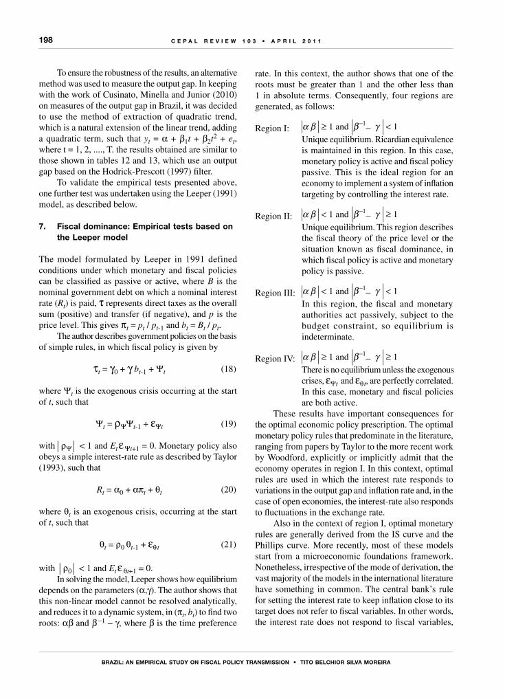
198



To ensure the robustness of the results, an alternative method was used to measure the output gap. In keeping with the work of Cusinato, Minella and Junior (2010) on measures of the output gap in Brazil, it was decided to use the method of extraction of quadratic trend, which is a natural extension of the linear trend, adding a quadratic term, such that yt = α + β1t + β2t2 + et, where t = 1, 2, ...., T. the results obtained are similar to those shown in tables 12 and 13, which use an output gap based on the Hodrick-Prescott (1997) filter.

To validate the empirical tests presented above, one further test was undertaken using the Leeper (1991) model, as described below.

7. Fiscal dominance: Empirical tests based on the Leeper model

The model formulated by Leeper in 1991 defined conditions under which monetary and fiscal policies can be classified as passive or active, where B is the nominal government debt on which a nominal interest rate (Rt) is paid, τ represents direct taxes as the overall sum (positive) and transfer (if negative), and p is the price level. This gives πt = pt / pt-1 and bt = Bt / pt.

The author describes government policies on the basis of simple rules, in which fiscal policy is given by

τt = γ0 + γ bt-1 + Ψt (18)

where Ψt is the exogenous crisis occurring at the start of t, such that

Ψt = ρΨΨt-1 + εΨt (19)

with ρΨ < 1 and Et ε Ψt+1 = 0. Monetary policy also obeys a simple interest-rate rule as described by Taylor (1993), such that

Rt = α0 + απt + θt (20)

where θt is an exogenous crisis, occurring at the start of t, such that

θt = ρ0 θt-1 + εθ t (21)

with ρ0 < 1 and Et ε θt+1 = 0.In solving the model, Leeper shows how equilibrium

depends on the parameters (α,γ). The author shows that this non-linear model cannot be resolved analytically, and reduces it to a dynamic system, in (πt, bt) to find two roots: αβ and β -1 – γ, where β is the time preference

rate. In this context, the author shows that one of the roots must be greater than 1 and the other less than 1 in absolute terms. Consequently, four regions are generated, as follows:

Region I: α β ≥ 1 and β γ < 1−1− Unique equilibrium. Ricardian equivalence

is maintained in this region. In this case, monetary policy is active and fiscal policy passive. This is the ideal region for an economy to implement a system of inflation targeting by controlling the interest rate.

Region II: α β < 1 and β γ ≥ 1−1− Unique equilibrium. This region describes

the fiscal theory of the price level or the situation known as fiscal dominance, in which fiscal policy is active and monetary policy is passive.

Region III: α β < 1 and β γ < 1−1− In this region, the fiscal and monetary

authorities act passively, subject to the budget constraint, so equilibrium is indeterminate.

Region IV: α β ≥ 1 and β γ ≥ 1−1− There is no equilibrium unless the exogenous

crises, εΨt and εθt, are perfectly correlated. In this case, monetary and fiscal policies are both active.

These results have important consequences for the optimal economic policy prescription. The optimal monetary policy rules that predominate in the literature, ranging from papers by Taylor to the more recent work by Woodford, explicitly or implicitly admit that the economy operates in region I. In this context, optimal rules are used in which the interest rate responds to variations in the output gap and inflation rate and, in the case of open economies, the interest-rate also responds to fluctuations in the exchange rate.

Also in the context of region I, optimal monetary rules are generally derived from the IS curve and the Phillips curve. More recently, most of these models start from a microeconomic foundations framework. Nonetheless, irrespective of the mode of derivation, the vast majority of the models in the international literature have something in common. The central bank’s rule for setting the interest rate to keep inflation close to its target does not refer to fiscal variables. In other words, the interest rate does not respond to fiscal variables,

199



whether taxes, primary deficit, or public deficit. As noted above, fiscal policy is passive because this is a Ricardian model. In this context, the debt and fiscal policy have no influence on the price level nor, therefore, on the inflation rate. For that reason, the use of a fiscal IS curve and the formulation of an interest-rate rule that responds to fiscal variables, makes no sense in an active monetary-policy and passive fiscal-policy environment.14

Moreover, taking account of the fact that a given economy operates in region II, in which the fiscal theory of the price level (ftpl) predominates, the application of an optimal monetary policy rule by controlling the interest rate, in the traditional way following Taylor, is questionable. It possibly makes more sense to use an optimal rule such as that proposed by Morais and Andrade (2004), which assumes the monetary authority pursues a flexible inflation targeting regime, which includes the possibility of a target for the debt/gdp ratio. In the proposed model, the public debt directly affects the risk premium and, consequently, the exchange rate. The authors include a target for the debt/gdp ratio based on the loss of monetary authority.

Common sense suggests that if the economy is in regions II, III, or IV, fiscal and monetary policies will need to be coordinated to be able to migrate to region I. Accordingly, the effect of the public debt on real and nominal variables of the economy cannot be neglected. It is therefore necessary to work with targets for reducing the debt/gdp ratio in a clear and transparent fashion.

Estimations are presented below for the coefficients γ and α in equations (18) and (20), where γ represents the reaction of direct taxes to variations in the public debt, and α, which is derived from a simplified Taylor rule, represents the response of the interest rate to variations in inflation. The coefficient γ is determined by estimating two equations as a system through the generalized method of moments, as shown in tables 14 and 15. The coefficient α is also determined by an estimation of two equations as shown in table 16 and 17. As the Taylor rule used in the Leeper model is very simplified, a more common rule was used, in which the interest rate responds to expected inflation and the output gap.

The results shown in table 14 indicate that all variables, except the constant term, are statistically significant at the 5% level. In this context, as the null hypothesis is rejected but there is a positive deterministic trend, fiscal policy is relatively unsustainable, because the problem of insolvency will eventually arise.

14 The term fiscal IS is used by Verdini (2003) as a result of the inclusion of a fiscal variable in the IS, in this case the primary surplus.

TABLE 14

Estimation using the generalized method of moments with the Bartlett kernel, Andrews bandwidth((B /Y)t = a0 + a1Trend + a2(B /Y)t-1 + a4*Dummy + ut)



Constant 0.001 0.021 0.057 0.955Trend 0.001 <0.001 2.064 0.042(B/Y)(-1) 0.717 0.043 16.847 <0.001Dummy 0.146 0.031 4.636 <0.001R2 0.968 Adjusted R2 0.966

Source: prepared by the author.Note: instruments B/Y(-3,-4,-5,-6), I.D.(-3,-4,-5,-6), c.

Trend: TendencyDummy: Dummy variableP value: Probability

TABLE 15

Estimation using the generalized method of moments with the Bartlett kernel, Andrews bandwidth(ID / Yt = a3 + a4*(B /Y)t-1 + ηt)



Constant 0.006 <0.001 27.282 <0.001(B/Y)(-1) 0.005 <0.001 10.035 <0.001R2 0.386 Adjusted R2 0.373

Source: prepared by the author.Note: Instruments B/Y(-3,-4,-5,-6), ID/Y(-3,-4,-5,-6), c.

P value: Probability

TABLE 16

Estimation using the generalized method of moments with the Bartlett kernel, fixed bandwidth (yt = a1 + a2 yt-1 + a3rt-1 + a4et-1 + a5*Dummy + ηt)



Constant 0.8555 0.096 8.947 <0.001Output gap 0.331 0.077 4.312 <0.001Interest-r -0.236 0.031 -7.612 <0.001Exchange rate-r 0.111 0.028 3.971 <0.001Dummy 0.274 0.036 7.659 <0.001R2 0.505 Adjusted R2 0.460

Source: prepared by the author.Note: Instruments R(-2,-3,-4,-5,-6), ipca(-2,-3,-4,-5,-6), B/Y(-2, -3,-4,-5,-6), c.

Dummy: Dummy variableP value: Probability

200



β = 0.98, a unique equilibrium is attained in region II, such that α β < 1 and β γ ≥ 1−1− . It should be noted that α β = < 10.149*0.98 and that β γ− − =1 1 / 0.98 – 0.005 > 1. The same value of β = 0.98 was used estimated by Lima and Issler (2003) and followed by Moreira, Souza and Almeida (2007a and 2007b). These results indicate that the economy is in region II.

Although the output gap is included in equation 20, following Moreira, Souza and Almeida (2007b), the Taylor rule was also tested without the gap, as per the Leeper (1991) model. In this case the result is maintained, in other words, the economy remains in region II.15 To guarantee the robustness of the results, an alternative measure for measuring the output gap was also used. Following the work of Cusinato, Minella and Júnior (2010) on measures of the output gap in Brazil, it was decided to use the quadratic trend extraction method. The results obtained are similar to those shown in tables 16 and 17, which use the output gap estimated with the Hodrick-Prescott filter. Once again, the economy is in region II.

The results also are maintained with respect to the monthly series of the Institute of Applied Economic Research (ipea) for the period from July 2001 to December 2009. The real interest rate was calculated as the difference between the cumulative selic rate for the next 12 months (annual percentage) and the average inflation expectation, according to the Extended National Consumer Price Index. (ipca) —cumulative rate for the next 12 months (annual percentage). The output gap was calculated on the basis of the (general) industrial production index using the Hodrick-Prescott filter. The same monthly variables were used as in the models in tables 14 and 15, and 16 and 17. The estimations gave the same result, namely that in the flexible exchange rate and inflation-targeting period, the economy is operating in region II.

15 Based on the Leeper (1991) model, Moreira, Souza and Almeida (2007a) show that fiscal and monetary policies are both passive in the period 1999-2004. Almeida, Moreira and Souza (2008) show that the fiscal deficit affects the inflation rate indirectly through the output gap, based on the stimation of an IS curve and the Phillips curve for the period January 1996 to January 2007.

TABLE 17

Estimation using the generalized method of moments with the Bartlett kernel, Andrews bandwidth(Rt = a6 + a7*Et(πt+1) + a8*yt + a9*Rt-1 + ηt)



Constant -0.315 0.054 -5.835 <0.001Et(πt+1) 0.149 0.038 3.940 <0.001Output gap 0.177 0.033 5.398 <0.001selic (-1) 0.872 0.026 34.070 <0.001R2 0.789 Adjusted R2 0.775

Source: prepared by the author.Note: Instruments R(-2,-3,-4,-5,-6), ipca(-2,-3,-4,-5,-6), B/Y(-2, -3,-4,-5,-6), c.

selic: Special settlement and custody system rateEt(πt+1) = inflation expectations in period t for the period t+1.P value: Probability


The results shown in table 15 indicate that all variables are statistically significant at the 1% level. For every 1% increase in the debt/gdp ratio, there is a 0.005% increase in the ratio of direct taxes to gdp. That value represents the coefficient γ in the Leeper (1991) model, which shows the reaction of direct taxes to variations in the public debt.

The results shown in table 16 correspond to the estimation of an IS curve in which all variables are statistically significant at the 1% level. All coefficients have the expected sign.


The results shown in table 17 represent the estimation of the Taylor rule in which all variables are statistically significant at the 1% level. All coefficients have the expected sign. It is assumed that Et(πt+1) = πt+1. For every 1% increase in the expected value of inflation, the selic rises by 0.149%. That value represents the coefficient α of the Leeper (1991) model, which shows how the interest rate responds to to variations in inflation.

Based the foregoing results, where the coefficient α = 0.149 (see table 17), and the coefficient γ = 0.005 (see table 15), and bearing in mind that

201



The results presented in subsection 7, based on the Leeper model, show that the Brazilian economy is in a situation of fiscal dominance. This is consistent with the results reported in the earlier subsections. It should be noted that all the fiscal sustainability tests based on Buiter and Patel (1992) showed that Brazil’s fiscal situation in the period analysed is worrying to say the least. The fiscal policy transmission channels can be defined schematically, as shown in tables 18 and 19.

Table 18 shows fiscal policy transmission mechanisms that operate through the money supply. It shows the effects of variations in the public debt on the primary surplus, monetary base, interest rate, investment, and the output gap.

The results described in section III show that the primary surplus reacts positively to variations in the public debt. Nonetheless, the fact that the coefficient of the debt/gdp ratio is positive and statistically significant does not mean it is large enough to guarantee fiscal sustainability. In that case, according to Leeper (1991), the fiscal authority refuses to make a substantial adjustment in direct taxation, thus preventing the repercussion on the deficit from being fully financed by future taxes. As

noted above, the federal government’s primary surplus is recorded in the National Treasury single account, which forms part of the central bank’s non-monetary liabilities. As the variation in the monetary base corresponds to the difference between the variation in central bank assets and the variation in its non-monetary liability, if there is an increase in the primary surplus (and hence in the National Treasury single account recorded in the nonmonetary liability), with everything else held constant, there will be a reduction in the monetary base. In that context, successive increases in the primary surplus will lead to a contraction in the monetary base, ceteris paribus, and consequently a reduction in means of payment. This institutional structure shows the existence of a direct channel for transmitting fiscal policy to monetary policy.

As increases in the primary surplus are known to cause a reduction in the monetary base, once again ceteris paribus, the interest rate is likely to rise. The results show that the public debt has a positive effect on the nominal selic interest rate, and that increases in the public debt cause increases in the primary surplus, which translate into interest-rate hikes. Assuming that higher

IV Final comments

TABLE 18

Transmission of monetary policy through the money supply

↑ (B / Y) ⇒↑ (SP / Y) ⇒↑ (Single Treasury Account) ⇒↑ (Nonmonetary liability) ⇒↓ (Monetary base) ⇒↓ (M) ⇒↑ R ⇒↓ (I) ⇒↓ (y) ↑ (B

_ / Y) ⇒↑ (SP / Y)

.....vicious circle

Source: prepared by the author.

SP: Primary surplus.

TABLE 19

Transmission of fiscal policy through the demand for money

↑ (B / Y) ⇒↑ (demand for money) ⇒↑ R ⇒↓ (I) ⇒↓ (y) ↑ (B_ / Y) ⇒

(demand for money) vicious circle


202



nominal interest rates are accompanied by a higher real interest rates, then increases in the public debt can also be expected to cause lower levels of investment and output. The estimations confirm this negative relation between public debt and levels of investment and the output gap. Having said that, lower levels of output, for a given debt level, result in a higher debt/gdp ratio. This feedback process can generate an undesirable vicious circle.

Similarly to table 18, table 19 shows how fiscal policy is propagated from variations in the debt/gdp ratio, although in this case through the demand for

money. The results show that increases in the debt/gdp ratio increase the demand for money, which means economic agents consider part of the public debt as net wealth, and, consequently, the model is non-Ricardian. A higher demand for money, given the supply of money, suggests a rise in the interest rate.

The results also suggest that increases in the debt/gdp ratio push up the interest rate. The empirical tests show that an interest-rate hike causes reductions in the level of investment and the output gap (see table 19), which can also produce the same undesirable vicious circle.

ANNEX

TABLE A.1

Unit root test

Variables

adf – aic modified adf – sic modified

Critical value 5%

Student t-statistic Value P Critical

value 5%Student

t-statistic Value P

L(m) -2.927 -1.701 0.424 -2.921 -2.196 0.210L(R) -2.919 -2.506 0.120 -2.919 -2.506 0.120L(b) -3.502 -2.145 0.509 -3.495 -2.518 0.319L(I/Y-1) -2.924 -0.723 0.831 -2.924 -0.723 0.831L(B/Y-1) -1.949 -0.916 0.314 -1.947 -0.506 0.821L(SP/Y) -2.919 -0.929 0.771 -2.919 -0.929 0.771


adf: Augmented Dickey-Fuller test.aic: Akaike information criterion.sic: Schwarz criterion.L: logarithm.SP: Primary surplus.P value: Probability.

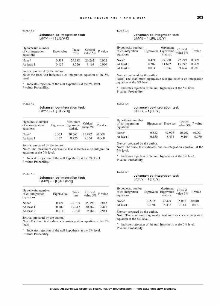
203



TABLE A.2

Johansen co-integration test:L(I/Y-1) = f [ L(B/Y-1)]

Hypothesis: number of co-integration equations

Eigenvalue Tracetests

Critical value 5% P value

Nonea 0.333 29.388 20.262 0.002At least 1 0.157 8.726 9.164 0.060

Source: prepared by the author.Note: the trace test indicates a co-integration equation at the 5% level.

a Indicates rejection of the null hypothesis at the 5% level.P value: Probability.

TABLE A.3

Johansen co-integration test: L(I/Y-1) = F [ L(B/Y-1)]


EigenvalueMaximum Eigenvalue

statistic


Nonea 0.333 20.662 15.892 0.008At least 1 0.157 8.726 9.164 0.060

Source: prepared by the author.Note: The maximum eigenvalue test indicates a co-integration equation at the 5% level.


TABLE A 4

Johansen co-integration test: L(M/Y) = F [L(R), L(B/Y)]


Eigenvalue Trace test


Nonea 0.421 39.705 35.193 0.015At least 1 0.207 12.347 20.262 0.418At least 2 0.014 0.726 9.164 0.981

Source: prepared by the author.Note: The trace test indicates a co-integration equation at the 5% level.


TABLE A.5

Johansen co-integration test: L(M/Y) = f [L(R), L(B/Y)]



statistic


Nonea 0.421 27.358 22.299 0.009At least 1 0.207 11.622 15.892 0.209At least 2 0.014 0.726 9.164 0.981



TABLE A.6

Johansen co-integration test: L(SP/Y) = f [L(B/Y)]


Eigenvalue Trace test Critical value 5% P value

Nonea 0.532 47.908 20.262 <0.001At least 1 0.150 8.434 9.164 0.070

Source: prepared by the author.Note: The trace test indicates one co-integration equation at the 5% level.


TABLE A.7

Johansen co-integration test: L(SP/Y) = f [L(B/Y)]



statistic


Nonea 0.532 39.474 15.892 <0.001At least 1 0.150 8.435 9.164 0.070



204



TABLE A.8

Description of variables

Variables Unit of measurement Source

Means of payment - end period (M) Millions of reais ipea

gdp- market prices (Y) Millions of reais ipea

Interest rate - over/selic (R) Percentages ipea

Gross fixed capital formation - (I) Millions of reais ipea

Implicit gdp deflator (P) Index number ipea

Nominal exchange rate - reais/dollar-commercial -buying - average (E) Percentages ipea

Real effective exchange rate - inpc - exports (e) Percentages ipea

Primary surplus (nfps) -Federal government and central bank -primary - with exchange-rate devaluation (SP)

Millions of reais ipea

Inflation rate - ipca (π) Percentages ipea

Direct taxes = individual and corporate income taxes+ rural property tax (id) Millions of reais ipea

Public debt, federal public bonds and open market operations (B) Millions of reais bacen

Average inflation expectations - ipca - cumulative rate for the next 12 months Et(πt+1) Percentages ipea

Industrial production - general industry Quantum - seasonally adjusted index (average 2002 = 100)

ipea


gdp: Gross domestic productid: Direct taxesipea: Institute of Applied Economic Research bacen: Central Bank of Brazilipca: Extended National Consumer Price Index inpc: National Consumer Price Indexnfsp: Public sector financing needs Quantum: Quantity index over/selic rate: Daily indicator of the interest rate, corresponding to the average adjusted daily rate of financing of federal government bonds, calculated in the Special Settlement and Custody System (selic) and published by the Central Bank of Brazil. This is the basic interest rate in Brazil.

(Original: Portuguese)

Bibliography

Almeida, Ch., T. Moreira and G. Souza (2008), “Optimal monetary rules in a context of fiscal disequilibrium: evidence from Brazil - 1996:I to 2007:I”, Economia e desenvolvimento (Recife), Recife, Universidade Federal de Pernambuco.

Araujo, J.T. and M.A.C. Martins (1999), “Economic growth with finite lifetimes”, Economics Letters, vol. 62, No. 3, Amsterdam, Elsevier.

Barro, R.J. (1974), “Are government bonds net wealth?”, Journal of Political Economy, vol. 82, No. 6, Chicago, University of Chicago Press.

Blanchard, O. (2004), “Fiscal dominance and inflation targeting: lessons from Brazil”, nber Working Paper, No. 10389, Cambridge, Massachusetts, March.

Bohn, H. (1998), “The behavior of U.S. public debt and deficits”, The Quarterly Journal of Economics, vol. 113, No. 3, Cambridge, Massachusetts, The mit Press.

Buiter, W. and R. Patel (1992), “Debt, deficits and inflation: an application to the public finances of India”, Journal of Public Economics, vol. 47, No. 2, Amsterdam, Elsevier.

Cusinato, R., A. Minella and S. Júnior (2010), “Hiato do produto e pib no Brasil: uma análise de dados em tempo real”, Trabalhos para discussão, No. 203, Brasilia, Central Bank of Brazil, April.

Fisher, I. (1930), The Theory of Interest, New York, Macmillan. Hodrick, R.J. and E.C. Prescott (1997), “Postwar U.S. business

cycles: an empirical investigation”, Journal of Money, Credit

205



and Banking, vol. 29, No. 1, New York, Blackwell Publishing, February.

Hsiao, C. (1997a), “Statistical properties of the two-stage least squares estimator under co-integration”, The Review of Economic Studies, vol. 64, No. 3, New York, Blackwell Publishing.

(1997b), “Co-integration and dynamic simultaneous equations models”, Econometrica, vol. 65, No. 3, New York, The Econometric Society.

Johnston, J. and J. DiNardo (1997), Econometric Methods, New York, McGraw-Hill.

Kneebone, R.D. (1989), “On macro-economic instability under a monetarist policy rule in a federal economy”, The Canadian Journal of Economics, vol. 22, No. 3, Quebec, Canadian Economics Association, August.

Leeper, E.M. (1991), “Equilibria under ‘active’ and ‘passive’ monetary and fiscal policies”, Journal of Monetary Economics, vol. 27, No. 1, Amsterdam, Elsevier.

Lima, A.M.C. and J.V. Issler (2003), “A hipótese das expectativas na estrutura a termo de juros no Brasil: uma aplicação de modelos de valor presente”, Revista brasileira de economia, vol. 57, No. 4, Rio de Janeiro, Getulio Vargas Foundation, October/December.

Loyo, E. (1999), “Tight money paradox on the loose: a fiscalist hyperinflation”, jfk School of Government, Harvard University, June, unpublished.

Luporini, V. (2006), “Conceitos de sustentabilidade fiscal”, Textos para discussão, No. 189, Universidade Federal Fluminense, May [online] http:/www.uff.br/econ

Martins, M.A.C. (1980), “A nominal theory of the nominal rate of interest and the price level”, The Journal of Political Economy, vol. 88, No. 1, Chicago, University of Chicago Press, February.

Mendonça, M.J., L.A. Medrano and A. Sachsida (2009), “Avaliando os efeitos da política fiscal no Brasil: resultados de um procedimento de identificação agnóstica”, Textos de discusión, No. 1377, Brasilia, Institute of Applied Economic Research (ipea).

Morais, J.F.M and J.P. de Andrade (2004), “Como a dívida pública afeta a política monetária ótima?”, Finanças Públicas – IX Prêmio Tesouro Nacional, Brasilia, Escola de Administração Fazendária (esaf).

Moreira, T.B.S. and G. da S. Souza (2009), “A nominal theory of the nominal rate of interest and the price level: some empirical evidence”, Economics Bulletin, vol. 29, No. 4.

Moreira, T.B.S., G. da S. Souza and Ch.L. Almeida (2007a), “Política fiscal e monetária: ativa ou passiva? Uma análise empírica e suas implicações sobre as regras ótimas de política monetária”, Cadernos de finanças públicas, Brasilia, Escola de Administração Fazendária (esaf).

(2007b), “The fiscal theory of the price level and the interaction of monetary and fiscal policies: the Brazilian case”, Brazilian Review of Econometrics, vol. 27, No. 1, Rio de Janeiro, Sociedade Brasileira de Econometria, May.

Phillips, P.C.B. (1988), “Regression theory for near–integrated time series”, Econometrica, vol. 56, No. 5, New York, The Econometric Society, September.

Phillips, P.C.B. and P. Perron (1988), “Testing for a unit roots in time series regression”, Biometrika, vol. 75, No. 2, Oxford University Press.

Sala, L. (2004), “The fiscal theory of the price level: identifying restrictions and empirical evidence”, Working Paper, No. 257, Innocenzo Gasparini Institute for Economic Research (igier), Milan, April.

Sargent, T.J. and N. Wallace (1981), “Some unpleasant monetarist arithmetic”, Federal Reserve Bank of Minneapolis Quarterly Review, vol. 5, No. 3, Minneapolis, Federal Reserve Bank of Minneapolis.

Scarth, W.M. (1996), Macroeconomics: An Introduction to Advanced Methods, Canada, Harcourt Brace & Company.

Souza, G., T.B.S. Moreira and J.R. Albuquerque (2007), “Intertemporal solvency and public debt: evidence from Brazil – 1995-2004”, Planejamento e políticas públicas, No. 30, Brasilia, Institute of Applied Economic Research (ipea), June/December.

Taylor, J.B. (1993), “Discretion versus policy rules in practice”, Carnegie-Rochester Conferences Series on Public Policy, vol. 39, No. 1, Amsterdam, Elsevier, December.

Verdini, M. (2003), “Regras monetárias e restrição fiscal: uma análise da política de metas para a inflação no Brasil”, unpublished.

Wilcox, D. (1989), “The sustainability of government deficits: implications of the present-value borrowing constraint”, Journal of Money, Credit and Banking, vol. 21, No. 3, New York, Blackwell Publishing, August.

Woodford, M. (2003), Interest and Prices, Princeton, Princeton University Press.

(1995), “Price level determinacy without control of a monetary aggregate”, nber Working Paper, No. 5204, Cambridge, Massachusetts, National Bureau of Economic Research.

C E P A L r E v i E w 1 0 3

A P r i L 2 0 1 1

207

Guidelinesfor contributorsto cepal Review

In order to facilitate the submission, consideration and publication of articles, the editorial board of the cepal Review has prepared the following information and suggestions to serve as a guide for future contributors.

The submission of an article implies an undertaking by the author not to submit it simultaneously to other publications. The copyright to all articles published in the Review shall be owned by the United Nations.

All articles will be submitted to external referees.

Papers should be submitted in the original language (English, French, Portuguese or Spanish). They will be translated into the appropriate language by the relevant eclac services.

Each article must be accompanied by a summary, no more than 150 words in length, giving a brief description of its subject matter and main conclusions.

Papers should be no longer than 10,000 words, including the summary, notes and bibliography. Shorter papers will also be considered.

Articles should be sent either by e-mail (to [email protected]) or by regular mail, on cd or diskette, to: cepal Review, Casilla 179-D, Santiago, Chile. They should not be submitted in pdf format.

Style guide:

Titles should not be excessively long.

Footnotes

– It is recommended that footnotes be kept to a minimum.

– It is recommended that footnotes not be used to cite bibliographical references; such references should preferably be incorporated into the text.

– Footnotes should be numbered consecutively using superscript Arabic numerals.

Tables and figures

– It is recommended that tables and figures be kept to a minimum, avoiding any redundancy with the text.

– Tables, figures and other elements should be inserted at the end of the text in the format in which they were designed; they should not be inserted as “pictures”. Figures in Excel should include the corresponding worksheets.

– The location of tables and figures in the body of the article should be indicated in the appropriate place as follows:

Insert figure 1Insert table 1

– Tables and figures should include an explicit and complete reference to their sources.

– Tables should indicate the period covered at the end of the title, and should indicate the units in which the data are expressed in a subtitle (in italics and between brackets).

– The symbols referred to in the “Explanatory notes” which appear on the page preceding the table of contents should be taken into account in the preparation of tables and figures.

– Footnotes to tables and figures should be ordered consecutively using superscript lower-case letters.

– Figures should be prepared bearing in mind that they will be printed in black and white.

Acronyms and abbreviations

– Acronyms and abbreviations should not be used unless absolutely necessary, in which case the full name should be written out the first time it occurs in the article.

Bibliography

– Bibliographical references should be directly related to the content of the article and should not be excessively long.

– At the end of the article, under the title “Bibliography”, all the necessary information should be included accurately and in alphabetical order by author: name of author(s), year of publication, full name of article (if any) and publication (including any subtitle), city of publication, publisher and, in the case of a periodical, month of publication.

The editorial board of the Review reserves the right to make any necessary editorial changes in the articles, including their titles.

Authors will receive a one-year courtesy subscription to the Review, plus 30 offprints of their article in Spanish and 30 in English, at the time of publication in each language.

208 C E P A L R E V I E W 1 0 3 • A P R I L 2 0 1 1

Publicaciones de la CEPAL / ECLAC publications Comisión Económica para América Latina y el Caribe / Economic Commission for Latin America and the Caribbean

Casilla 179-D, Santiago de Chile. E-mail: [email protected] Véalas en: www.cepal.org/publicaciones

Publications may be accessed at: www.eclac.org

Revista CEPAL / CEPAL Review La Revista se inició en 1976 como parte del Programa de Publicaciones de la Comisión Económica para América Latina y el Caribe, con el propósito de contribuir al examen de los problemas del desarrollo socioeconómico de la región. Las opiniones expresadas en los artículos firmados, incluidas las colaboraciones de los funcionarios de la Secretaría, son las de los autores y, por lo tanto, no reflejan necesariamente los puntos de vista de la Organización.

La Revista CEPAL se publica en español e inglés tres veces por año. Los precios de suscripción anual vigentes para 2010 son de US$ 30 para ambas versiones. El precio por ejemplar suelto es de US$ 15 para

ambas versiones. Los precios de suscripción por dos años son de US$ 50 para ambas versiones. CEPAL Review first appeared in 1976 as part of the Publications Programme of the Economic Commission for Latin America and the Caribbean, its aim being to make a contribution to the study of the economic and social development problems of the region. The views expressed in signed articles, including those by Secretariat staff members, are those of the authors and therefore do not necessarily reflect the point of view of the Organization.

CEPAL Review is published in Spanish and English versions three times a year. Annual subscription costs for 2010 are US$ 30 for both versions. The price of single issues is US$ 15 in both cases. The cost of a two-year

subscription is US$ 50 for both versions.

Informes periódicos institucionales / Annual reports Todos disponibles para años anteriores / Issues for previous years also available • Balance preliminar de las economías de América Latina y el Caribe, 2009, 184 p. Preliminary Overview of the Economies of Latin America and the Caribbean, 2009, 166 p. • Estudio económico de América Latina y el Caribe 2009-2010, 136 p. Economic Survey of Latin America and the Caribbean 2009-2010, 130 p. • Panorama de la inserción internacional de América Latina y el Caribe, 2009-2010, 176 p. Latin America and the Caribbean in the World Economy, 2009-2010, 168 p. • Panorama social de América Latina, 2009, 218 p. Social Panorama of Latin America, 2009, 208 p. • La inversión extranjera directa en América Latina y el Caribe, 2009, 162 p. Foreign Direct Investment of Latin America and the Caribbean, 2009, 158 p. • Anuario estadístico de América Latina y el Caribe / Statistical Yearbook for Latin America and the Caribbean (bilingüe/bilingual),

2010, 314 p.

Libros de la CEPAL 110 Envejecimiento en América Latina. Sistema de pensiones y protección social integral, Antonio Prado y Ana Sojo (eds.), 304 p. 109 Modeling Public Policies in Latin America and the Caribbean, Carlos de Miguel, José Durán Lima, Paolo Giordiano, Julio Guzmán,

Andrés Schuschny and Masazaku Watanuki (eds.), 322 p. 108 Alianzas público-privadas. Para una nueva visión estratégica del desarrollo, Robert Devlin y Graciela Moguillansky, 2010, 196 p. 107 Políticas de apoyo a las pymes en América Latina. Entre avances innovadores y desafíos institucionales, Carlos Ferraro y Giovanni

Stumpo, 392 p. 106 Temas controversiales en negociaciones comerciales Norte-Sur, Osvaldo Rosales V. y Sebastián Sáez C. (compiladores), 322 p.

209C E P A L R E V I E W 1 0 3 • A P R I L 2 0 1 1

105 Regulation, Worker Protection and Active Labour-Market Policies in Latin America, Jürgen Weller (ed.), 2009, 236 p. 104 La República Dominicana en 2030: hacia una sociedad cohesionada, Víctor Godínez y Jorge Máttar (coords.), 2009, 582 p. 103 L’Amérique latine et les Caraïbes au seuil du troisième millénaire, 2009, 138 p. 102 Migración interna y desarrollo en América Latina entre 1980 y 2005, Jorge Rodríguez y Gustavo Busso, 2009, 272 p. 101 Claves de la innovación social en América Latina y el Caribe, Adolfo Rodríguez Herrera y Hernán Alvarado Ugarte, 2009, 236 p. 100 Envejecimiento, derechos humanos y políticas públicas, Sandra Huenchuan (ed.), 2009, 232 p. 99 Economía y territorio en América Latina y el Caribe. Desigualdades y políticas, 2009, 212 p. 98 La sociedad de la información en América Latina y el Caribe: desarrollo de las tecnologías y tecnologías para el desarrollo, Wilson Peres

y Martin Hilbert (eds.), 2009, 388 p. 97 América Latina y el Caribe: migración internacional, derechos humanos y desarrollo, Jorge Martínez Pizarro (ed.), 2008, 375 p. 96 Familias y políticas públicas en América Latina: una historia de desencuentros, Irma Arriagada (coord.), 2007, 424 p. 95 Centroamérica y México: políticas de competencia a principios del siglo XXI, Eugenio Rivera y Claudia Schatan (coords.), 2008, 304 p. 94 América Latina y el Caribe: La propiedad intelectual después de los tratados de libre comercio, Álvaro Díaz, 2008, 248 p.

Copublicaciones recientes / Recent co-publications Las clases medias en América Latina. Retrospectiva y nuevas tendencias, Rolando Franco, Martín Hopenhayn y Arturo León (eds.) Sesenta años de la CEPAL. Textos seleccionados del decenio 1998-2008, Ricardo Bielschowsky (comp.), CEPAL/Siglo Veintiuno, Argentina, 2010. El nuevo escenario laboral latinoamericano. Regulación, protección y políticas activas en los mercados de trabajo, Jürgen Weller (ed.),

CEPAL/Siglo Veintiuno, Argentina, 2010. Internacionalización y expansión de las empresas eléctricas españolas en América Latina, Patricio Rozas, CEPAL/Lom, Chile, 2009. Gobernanza corporativa y desarrollo de mercados de capitales en América Latina, Georgina Núñez, Andrés Oneto y Germano M. de Paula

(coords.), CEPAL/Mayol, Colombia, 2009. EnREDos. Regulación y estrategias corporativas frente a la convergencia tecnológica, Marcio Wohlers y Martha García-Murillo (eds.),

CEPAL/Mayol, Colombia, 2009. Desafíos y oportunidades de la industria del software en América Latina, Paulo Tigre y Felipe Silveira Marques (eds.), CEPAL/Mayol,

Colombia, 2009. ¿Quo vadis, tecnología de la información y de las comunicaciones?, Martin Hilbert y Osvaldo Cairó (eds.), CEPAL/Mayol, Colombia, 2009. O Estruturalismo latino-americano, Octavio Rodríguez, CEPAL/Civilização Brasileira, 2009. L’avenir de la protection sociale en Amérique latine. Accessibilité, financement et solidarité, CEPALC/Eska, France, 2009. Fortalecer los sistemas de pensiones latinoamericanos. Cuentas individuales por reparto, Robert Holzmann, Edward Palmer y Andras Uthoff (eds.), CEPAL/Mayol, Colombia, 2008. Competition Policies in Emerging Economies. Lessons and Challenges from Central America and Mexico, Claudia Schatan and

Eugenio Rivera Urrutia (eds.), ECLAC/Springer, USA, 2008.

Coediciones recientes / Recent co-editions Clases medias y desarrollo en América Latina, Alicia Bárcena y Narcís Serra (eds.), CEPAL/SEGIB/CIDOB, Chile, 2010. Innovar para crecer. Desafíos y oportunidades para el desarrollo sostenible e inclusivo en Iberoamérica, CEPAL/SEGIB, Chile, 2010. Espacios iberoamericanos. Iberoamérica frente a la crisis, CEPAL/SEGIB, Chile, 2009. Espaços Ibero-Americanos. A Ibero-América em face da crise, CEPAL/SEGIB, Chile, 2009. The United Nations Regional Commissions and the Climate Change Challenges, ECLAC/ECA/ECE/ESCAP/ESCWA, 2009. Hacia un desarrollo inclusivo. El caso de Chile, Osvaldo Sunkel y Ricardo Infante (eds.), CEPAL/OIT/Fundación Chile 21, Chile, 2008. Reformas para la cohesión social en América Latina. Panorama antes de la crisis, Alicia Bárcena y Narcís Serra (eds.),

CEPAL/SEGIB/CIDOB, Chile, 2008. El envejecimiento y las personas de edad. Indicadores sociodemográficos para América Latina y el Caribe, CEPAL/UNFPA, 2009. Espacios iberoamericanos: la economía del conocimiento, CEPAL/SEGIB, Chile, 2008. Hacia la revisión de los paradigmas del desarrollo en América Latina, Oscar Altimir, Enrique V. Iglesias, José Luis Machinea (eds.),

CEPAL/SEGIB, Chile, 2008. Por uma revis o dos paradigmas do desenvolvimento na América Latina, Oscar Altimir, Enrique V. Iglesias, José Luis Machinea (eds.),

CEPAL/SEGIB, Chile, 2008. Hacia un nuevo pacto social. Políticas económicas para un desarrollo integral en América Latina, José Luis Machinea y Narcís Serra (eds.)

CEPAL/CIDOB, España, 2008.

Cuadernos de la CEPAL 94 El cuidado en acción. Entre el derecho y el trabajo, Sonia Montaño Virreira y Coral Calderón Magaña (coords.), 2010, 236 p. 93 Privilegiadas y discriminadas. Las trabajadoras del sector financiero, Flavia Marco Navarro y María Nieves Rico Ibáñez (eds.), 2009, 300 p. 92 Estadísticas para la equidad de género: magnitudes y tendencias en América Latina, Vivian Milosavljevic, 2007, 186 pp.

210 C E P A L R E V I E W 1 0 3 • A P R I L 2 0 1 1

Cuadernos estadísticos de la CEPAL 38 Indicadores ambientales de América Latina y el Caribe, 2009. Solo disponible en CD, 2010. 37 América Latina y el Caribe: Series históricas de estadísticas económicas 1950-2008. Solo disponible en CD, 2009. 36 Clasificaciones estadísticas internacionales incorporadas en el Banco de Datos de Comercio Exterior de América Latina y el Caribe de la

CEPAL (Revisión 3). Solo disponible en CD, 2008. 35 Resultados del Programa de Comparación Internacional para América del Sur. Solo disponible en CD, 2007.

Observatorio demográfico ex Boletín demográfico / Demographic Observatory formerly Demographic Bulletin (bilingüe/bilingual) Edición bilingüe (español e inglés) que proporciona información estadística actualizada, referente a estimaciones y proyecciones de población de los países de América Latina y el Caribe. Incluye también indicadores demográficos de interés, tales como tasas de natalidad, mortalidad, esperanza de vida al nacer, distribución de la población, etc.

El Observatorio aparece dos veces al año, en los meses de enero y julio. Suscripción anual: US$ 20.00. Valor por cada ejemplar: US$ 15.00. Bilingual publication (Spanish and English) proving up-to-date estimates and projections of the populations of the Latin American and Caribbean countries. Also includes various demographic indicators of interest such as fertility and mortality rates, life expectancy, measures of population distribution, etc.

The Observatory appears twice a year in January and July. Annual subscription: US$ 20.00. Per issue: US$ 15.00.

Notas de población Revista especializada que publica artículos e informes acerca de las investigaciones más recientes sobre la dinámica demográfica en la región, en español, con resúmenes en español e inglés. También incluye información sobre actividades científicas y profesionales en el campo de población.

La revista se publica desde 1973 y aparece dos veces al año, en junio y diciembre. Suscripción anual: US$ 20.00. Valor por cada ejemplar: US$ 12.00.

Specialized journal which publishes articles and reports on recent studies of demographic dynamics in the region, in Spanish with abstracts in Spanish and English. Also includes information on scientific and professional activities in the field of population.

Published since 1973, the journal appears twice a year in June and December. Annual subscription: US$ 20.00. Per issue: US$ 12.00.

Series de la CEPAL Comercio internacional / Desarrollo productivo / Desarrollo territorial / Estudios estadísticos y prospectivos / Estudios y perspectivas (Bogotá, Brasilia, Buenos Aires, México, Montevideo) / Studies and Perspectives (The Caribbean, Washington) / Financiamiento del desarrollo / Gestión pública / Informes y estudios especiales / Macroeconomía del desarrollo / Manuales / Medio ambiente y desarrollo / Mujer y desarrollo / Población y desarrollo / Políticas sociales / Recursos naturales e infraestructura / Seminarios y conferencias. Véase el listado completo en: www.cepal.org/publicaciones / A complete listing is available at: www.cepal.org/publicaciones

103 - Cepal

Documents

Transcript of 103 - Cepal