CEPAL Review no. 122
261
122 N O AUGUST • 2017 ISSN 0251-2920 Social protection systems, redistribution and growth in Latin America José Antonio Ocampo and Natalie Gómez-Arteaga 7 The progress and evolution of women’s participation in production and business activities in South America Beatrice E. Avolio and Giovanna F. Di Laura 31 Deindustrialization and economic stagnation in El Salvador Luis René Cáceres 57 Economic growth and gender inequality: an analysis of panel data for five Latin American countries Alison Vásconez Rodríguez 79 Who borrows to accumulate assets? Class, gender and indebtedness in Ecuador’s credit market Carmen Diana Deere and Zachary B. Catanzarite 107 Colombian agricultural product competitiveness under the free trade agreement with the United States: analysis of the comparative advantages Rémi Stellian and Jenny Paola Danna-Buitrago 127 Public transport, well-being and inequality: coverage and affordability in the city of Montevideo Diego Hernández 151 Sectoral breakdown of total factor productivity in Chile, 1996-2010 Patricio Aroca and Nicolás Garrido 171 The impact of the minimum wage on income and employment in Mexico Raymundo M. Campos Vázquez, Gerardo Esquivel and Alma S. Santillán Hernández 189 Spatial distribution of the Brazilian national system of innovation: an analysis for the 2000s Ulisses Pereira dos Santos 217 Analysis of the duration of unemployment and outcomes for unemployed persons in the Bolivarian Republic of Venezuela Josefa Ramoni Perazzi, Giampaolo Orlandoni Merli, Surendra Prasad Sinha, Elizabeth Torres Rivas and Angel Zambrano 235
-
Upload
khangminh22 -
Category
Documents
-
view
0 -
download
0
Transcript of CEPAL Review no. 122

122NO
AUGUST • 2017
ISSN 0251-2920
Social protection systems, redistribution and growth in Latin AmericaJosé Antonio Ocampo and Natalie Gómez-Arteaga 7
The progress and evolution of women’s participation in production and business activities in South AmericaBeatrice E. Avolio and Giovanna F. Di Laura 31
Deindustrialization and economic stagnation in El SalvadorLuis René Cáceres 57
Economic growth and gender inequality: an analysis of panel data for five Latin American countriesAlison Vásconez Rodríguez 79
Who borrows to accumulate assets? Class, gender and indebtedness in Ecuador’s credit marketCarmen Diana Deere and Zachary B. Catanzarite 107
Colombian agricultural product competitiveness under the free trade agreement with the United States: analysis of the comparative advantages Rémi Stellian and Jenny Paola Danna-Buitrago 127
Public transport, well-being and inequality: coverage and affordability in the city of MontevideoDiego Hernández 151
Sectoral breakdown of total factor productivity in Chile, 1996-2010Patricio Aroca and Nicolás Garrido 171
The impact of the minimum wage on income and employment in MexicoRaymundo M. Campos Vázquez, Gerardo Esquivel and Alma S. Santillán Hernández 189
Spatial distribution of the Brazilian national system of innovation: an analysis for the 2000sUlisses Pereira dos Santos 217
Analysis of the duration of unemployment and outcomes for unemployed persons in the Bolivarian Republic of VenezuelaJosefa Ramoni Perazzi, Giampaolo Orlandoni Merli, Surendra Prasad Sinha, Elizabeth Torres Rivas and Angel Zambrano 235
Thank you for your interest in
this ECLAC publication
Please register if you would like to receive information on our editorial
products and activities. When you register, you may specify your particular
areas of interest and you will gain access to our products in other formats.
www.cepal.org/en/suscripciones
ECLACPublications
REV
IEW
ECONOMIC COMMISSION FOR
LATIN AMERICA ANDTHE CARIBBEAN

122NO
AUGUST • 2017
REV
IEW
ECONOMIC COMMISSION FOR
LATIN AMERICA ANDTHE CARIBBEAN
Osvaldo SunkelChairman of the Editorial Board
Miguel TorresTechnical Editor
ISSN 0251-2920
Alicia BárcenaExecutive Secretary
Antonio PradoDeputy Executive Secretary
Alicia BárcenaExecutive Secretary
Antonio PradoDeputy Executive Secretary
Osvaldo SunkelChair of the Editorial Board
Miguel TorresTechnical Editor
The CEPAL Review was founded in 1976, along with the corresponding Spanish version, Revista CEPAL, and it is published three times a year by the Economic Commission for Latin America and the Caribbean (ECLAC), which has its headquarters in Santiago. The Review has full editorial independence and follows the usual academic procedures and criteria, including the review of articles by independent external referees. The purpose of the Review is to contribute to the discussion of socioeconomic development issues in the region by offering analytical and policy approaches and articles by economists and other social scientists working both within and outside the United Nations. The Review is distributed to universities, research institutes and other international organizations, as well as to individual subscribers.
The opinions expressed in the articles are those of the authors and do not necessarily reflect the views of ECLAC.
The designations employed and the way in which data are presented do not imply the expression of any opinion whatsoever on the part of the United Nations concerning the legal status of any country, territory, city or area or its authorities, or concerning the delimitation of its frontiers or boundaries.
To subscribe, please visit the Web page: http://ebiz.turpin-distribution.com/products/197587-cepal-review.aspx
The complete text of the Review can also be downloaded free of charge from the ECLAC website (www.eclac.org).
This publication, entitled CEPAL Review, is covered in theSocial Sciences Citation Index (SSCI), published by Thomson
Reuters, and in the Journal of Economic Literature (JEL),published by the American Economic Association
United Nations publication ISSN: 0251-2920 ISBN: 978-92-1-121957-9 (print) ISBN: 978-92-1-058594-1 (pdf) LC/PUB.2017/10-P Distribution: General Copyright © United Nations, August 2017 All rights reserved Printed at United Nations, Santiago S.17-00174
Requests for authorization to reproduce this work in whole or in part should be sent to the Economic Commission for Latin America and the Caribbean (ECLAC), Publications and Web Services Division, [email protected]. Member States of the United Nations and their governmental institutions may reproduce this work without prior authorization, but are requested to mention the source and to inform ECLAC of such reproduction.

Contents
Social protection systems, redistribution and growth in Latin America
José Antonio Ocampo and Natalie Gómez-Arteaga . . . . . . . . . . . . . . . . . . . . . . . . . . . . . 7
The progress and evolution of women’s participation in production and business activities in South America
Beatrice E . Avolio and Giovanna F . Di Laura . . . . . . . . . . . . . . . . . . . . . . . . . . . . . . . . 31
Deindustrialization and economic stagnation in El Salvador
Luis René Cáceres . . . . . . . . . . . . . . . . . . . . . . . . . . . . . . . . . . . . . . . . . . . . . . . . . . . . . 57
Economic growth and gender inequality: an analysis of panel data for five Latin American countries
Alison Vásconez Rodríguez . . . . . . . . . . . . . . . . . . . . . . . . . . . . . . . . . . . . . . . . . . . . . . 79
Who borrows to accumulate assets? Class, gender and indebtedness in Ecuador’s credit market
Carmen Diana Deere and Zachary B . Catanzarite . . . . . . . . . . . . . . . . . . . . . . . . . . . 107
Colombian agricultural product competitiveness under the free trade agreement with the United States: analysis of the comparative advantages
Rémi Stellian and Jenny Paola Danna-Buitrago . . . . . . . . . . . . . . . . . . . . . . . . . . . . . 127
Public transport, well-being and inequality: coverage and affordability in the city of Montevideo
Diego Hernández . . . . . . . . . . . . . . . . . . . . . . . . . . . . . . . . . . . . . . . . . . . . . . . . . . . . . 151
Sectoral breakdown of total factor productivity in Chile, 1996-2010
Patricio Aroca and Nicolás Garrido . . . . . . . . . . . . . . . . . . . . . . . . . . . . . . . . . . . . . . . 171
The impact of the minimum wage on income and employment in Mexico
Raymundo M . Campos Vázquez, Gerardo Esquivel and Alma S . Santillán Hernández . . . . . . . . . . . . . . . . . . . . . . . . . . . . . . . . . . . . . . . . 189
Spatial distribution of the Brazilian national system of innovation: an analysis for the 2000s
Ulisses Pereira dos Santos . . . . . . . . . . . . . . . . . . . . . . . . . . . . . . . . . . . . . . . . . . . . . . 217
Analysis of the duration of unemployment and outcomes for unemployed persons in the Bolivarian Republic of Venezuela
Josefa Ramoni Perazzi, Giampaolo Orlandoni Merli, Surendra Prasad Sinha, Elizabeth Torres Rivas and Angel Zambrano . . . . . . . . . . . . . . . . . . . . . . . . . . . . . . . 235
Guidelines for contributors to the CEPAL Review . . . . . . . . . . . . . . . . . . . . . . . . 253

Explanatory notes
- Three dots (...) indicate that data are not available or are not separately reported.- A dash (-) indicates that the amount is nil or negligible.- A full stop (.) is used to indicate decimals.- The word “dollars” refers to United States dollars, unless otherwise specified.- A slash (/) between years (e.g. 2013/2014) indicates a 12-month period falling between the two years.- Individual figures and percentages in tables may not always add up to the corresponding total because of rounding.
Social protection systems, redistribution and growth in Latin AmericaJosé Antonio Ocampo and Natalie Gómez-Arteaga
Abstract
After reviewing the debate over the relative merits of universalism and targeting in social policy, this paper assesses the present state of and challenges to social protection systems in Latin America. It shows that these systems expanded broadly but unevenly across the region during the decade from 2003 to 2013. In particular, there are still large inequalities in access to social protection by type of employment and household income. Contributory coverage is low, and while the coverage of non-contributory assistance has increased, benefits are generally small. The impact of social spending in the form of direct transfers is still low by comparison with developed countries. The paper also shows that the expansion of social protection systems has contributed more than GDP growth to poverty reduction.
KeywordsSocial policy, social security, equality, income distribution, public expenditures, poverty mitigation, economic growth, measurement, Latin America
JEL classificationI3, H22, H23
AuthorsJosé Antonio Ocampo is a professor at Columbia University and was formerly United Nations Under-Secretary-General for Economic and Social Affairs, Executive Secretary of the United Nations Economic Commission for Latin America and the Caribbean (ECLAC) and Minister of Finance, Minister of Agriculture and Director of the National Planning Department of Colombia. [email protected]
Natalie Gómez-Arteaga is a staff member with the National Planning Department of Colombia and was formerly a research associate at the Initiative for Policy Dialogue at Columbia University and a consultant to the International Labour Organization and the United Nations Development Programme. [email protected]

8 CEPAL Review N° 122 • August 2017
Social protection systems, redistribution and growth in Latin America
I. Introduction1
Latin America saw significant improvements in its social indicators over the decade from 2003 to 2013, including reductions in income inequality in most countries of the region that contrasted sharply with a global trend towards rising inequality in both developed and developing countries. These improvements were matched by a fair economic performance, particularly in 2003-2008, although with a slowdown in 2008-2013. Improvements in income distribution together with reasonable economic growth resulted in a massive reduction in poverty, the fastest since the 1970s. Besides favourable external conditions (high commodity prices and ample access to external financing), improvements during this “golden social decade” can be attributed to the construction of innovative programmes and stronger welfare States. New forms of social protection have been emerging in the region, including the universal or broad-based pensions of Brazil, Chile and the Plurinational State of Bolivia, the universal health systems of Brazil and Colombia, increasingly attractive cash transfer programmes, and universal transfers such as child benefits in Argentina. Contributory social security has expanded in Ecuador and Uruguay, among other countries of the region, and pension privatizations have been reversed in Argentina and the Plurinational State of Bolivia. These advances have also been matched by progress in other dimensions, such as significant wage growth and rapidly expanding access to education, albeit with significant quality gaps.
With the recent improvements and innovations in its social protection systems, and notwithstanding the diversity that characterizes the region, Latin America can be said to have been gradually moving away from the old focus on targeted State subsidies and towards the conceptions on which the welfare State was built in industrial countries, with the emphasis on universalism and solidarity in social policies based on the principle of social citizenship. Indeed, the expansion of social protection systems in Latin America contrasts heavily with recent experiences in the rest of the world, and particularly in advanced economies, where reforms since the mid-1990s have lessened the generosity of social benefits and reduced the progressivity of income tax systems, making fiscal policy less redistributive (Bastagli, Coady and Gupta, 2012). Retrenchment in several high- and middle-income countries has led to reforms to their social protection systems in which the more costly universal programmes have been scaled back while more targeted and means-tested programmes with more limited benefits have been expanded. In this context, assessing the positive effects that the recent expansion of social protection systems has had in reducing poverty and inequality in Latin America and the way this has tied in with economic development is essential for the formulation of policy recommendations, not only in Latin America but in other middle-income and less developed countries that are building their own welfare States.
This paper reviews the targeting versus universalism debate and assesses recent improvements in 18 Latin American countries on three dimensions of social protection with a view to measuring universality, solidarity and public spending. Between 2002 and 2012, 15 of the 18 Latin American countries improved their scores on the Social Protection Index developed for this paper, indicating that they experienced variable mixes of higher coverage in health care and pensions, smaller coverage gaps between wage earners and non-wage earners, higher social spending and better social assistance coverage in the poorest quintile. However, there are still major inequalities by both type of employment and income level. Non-wage workers are in all cases less likely to be affiliated to health and pension systems, and pension coverage is still highly deficient in terms both of levels of pension scheme membership among the working population and of pension coverage in old age.
1 The authors wish to thank Isabel Ortiz and Christina Behrendt of the International Labour Organization for their contributions to and comments on this paper and Maria José Abud for her outstanding research support.

9CEPAL Review N° 122 • August 2017
José Antonio Ocampo and Natalie Gómez-Arteaga
The impact of social spending on poverty and inequality has been significant. Indirect transfers have had a greater redistributive effect than direct transfers, an indication of the fact that targeted direct transfers, although highly progressive, have low benefits and coverage. Latin America achieves less fiscal redistribution than developed countries because of its relatively unprogressive mix of taxes and transfers and limited benefits.
At a time when economic growth has slowed, some countries are in recession and the immediate outlook is weak, particularly in South America, continuing to expand and strengthen a welfare State with universal benefits would appear to be an essential strategy. This is supported by evidence that there is no trade-off between redistribution and growth. In fact, Latin America countries with greater social protection and higher social spending have grown particularly strongly. However, better protection implies a need to design fiscal systems that generate higher and more progressive taxes.
This paper is divided into six sections aside from this introduction. Section II reviews the universalism versus targeting debate in Latin American social policy from a broad historical perspective. Section III details improvements in social protection systems during the last decade, using a multidimensional index to measure their comprehensiveness and universality. Section IV analyses the present state of social protection systems and shows the persistence of segmentation in access to health care and pensions. Section V assesses their impact on poverty and inequality. Section VI shows the linkages between expanded social protection, economic growth and poverty reduction. Lastly, section VII concludes with some general recommendations.
II. Universalism versus targeting in social policy
Modern conceptions of social policy have their roots in the liberal view that the provision of basic education and health services is inseparable from the progress of modern societies. Beginning in the late nineteenth century, the creation of modern social security systems under the leadership of Bismarck and pressure from the labour and socialist movements led to the development of more comprehensive views of social policy. The development of the welfare State in the major industrial economies from the 1930s onward was a result of this process and of competition with communism in the post-war years. A major corollary of this development was unprecedented growth in the size of the State.
In Latin America, the same views were in evidence but the effects were more limited. The reforms introduced in Uruguay in the 1910s by President Batlle y Ordóñez are perhaps the earliest manifestations of this trend. However, more comprehensive approaches to the welfare State were developed in just a few countries, three in the Southern Cone (Argentina, Chile and Uruguay) and Costa Rica,2 and even these never developed welfare States on the scale of the industrial countries, particularly in terms of the design of comprehensive tax and transfer systems to reduce income inequality. In most Latin American countries, the coverage even of basic educational and health services was low up to the mid-twentieth century, and social security came late and was very restricted in scope, owing to its association with formal employment and its corporatist overtones. The result was a segmented and incomplete welfare State which spread its benefits to some middle sectors of society but tended to marginalize the poor, particularly in rural areas (Bértola and Ocampo, 2012, chaps. I and IV).
The market reforms of the 1980s and 1990s relegated social policy to a subordinate status.3 The new social policy thinking that spread throughout Latin America from the 1980s onward is best
2 Cuba since its 1958 revolution belongs in this list, but the country has been left out of this paper because of its entirely different economic, social and political system.
3 This is reflected, for example, in the absence of any mention of social policy in the 10 principles of the Washington Consensus, as summarized by Williamson (1990), except as a public spending priority.

10 CEPAL Review N° 122 • August 2017
Social protection systems, redistribution and growth in Latin America
summarized in three social policy reform instruments that the World Bank placed at the centre of its agenda for the region: targeting, demand subsidies to facilitate a system with private sector participation, and decentralization. The first of these sought to make social policy consistent with limited fiscal resources while aiding the poor. The other two instruments focused on the need to rationalize the State apparatus. They were supplemented by a proliferation of specific projects aimed at managing the social costs of structural reform, the most important of which were perhaps the social emergency funds.
The new principles were applied unevenly across the region. Targeting was deployed to best effect in conditional cash transfer programmes, which were developed first as an emergency mechanism (Solidaridad in Mexico) or as an instrument to secure fuller take-up of basic educational services (Bolsa Escola in Brazil) but evolved over time into systems with wider coverage whose eventual aim was to reach the entire target population. Renamed Propsera and Bolsa Família, they were copied by other countries and have spearheaded what Ferreira and Robalino (2011) have called the “social assistance revolution”.
The result of the reforms has been that current systems of social policy in Latin America combine three different models, sometimes in the same country. The first is the strictly universal system, essentially run by the public sector with differing degrees of decentralization, that continues to characterize education systems —where it is accompanied by variable levels of private provision, particularly in the university system. The second is the segmented and corporatist system inherited from the past that continues to prevail in several countries’ social security arrangements (health care, pensions and occupational risks). The third is strict targeting, developed to best effect in conditional transfer programmes. Filgueira and others (2006, p. 37) have characterized the resulting systems of social policies as “persistent corporativism mixed with liberal reforms”. These systems lack a pillar of clearly designed entitlements and, most importantly, also lack the coherence and appeal of the old conceptions of the welfare State and thus the capacity to serve as core instruments of social cohesion.
The return of universalism as a social policy paradigm is closely tied to the concepts of social rights and social citizenship. Internationally, this vision was reflected in the rise of the welfare State and the development of the economic, social and cultural rights summarized in articles 22 to 27 of the Universal Declaration of Human Rights and later in the International Covenant on Economic, Social and Cultural Rights, and in similar instruments adopted by the Organization of American States. This new set of rights expresses modern notions of equality, solidarity and non-discrimination that go back to T.H. Marshall’s concept of social citizenship (see Marshall, 1992, which reproduces his original 1950 essay). Furthermore, as stated in the preamble to the United Nations Charter, these rights should be conceived as manifesting the determination of United Nations Member States to “promote social progress and better standards of life in larger freedom”, a concept that of course goes back to Franklin D. Roosevelt’s “freedom from want” and that has most recently been conveyed by Amartya Sen’s “development as freedom” (Sen, 1999). In Latin America, this view has also been expounded in the United Nations Development Programme’s conception of democracy as an extension of the three dimensions of citizenship (civil, political and social) (UNDP, 2004; see also Ocampo, 2007) and in recent ECLAC institutional documents on equality, and particularly the organization’s call for compacts for equality (ECLAC, 2014a).
The most precise formulation of this conception for Latin America is the chapter on the principles of social policy in the ECLAC report Equity, Development and Citizenship (ECLAC, 2000). The four principles are universalism, solidarity, efficiency and integrality. The first expresses the view that the entitlements associated with social policy are more than services or commodities: they are rights and should therefore be guaranteed to all citizens. The second alludes to something that is obvious, particularly in highly unequal societies: that the guarantee of access to these entitlements for the poor should be based on the principle of solidarity, which furthermore expresses the basic objective of
11CEPAL Review N° 122 • August 2017
José Antonio Ocampo and Natalie Gómez-Arteaga
building more inclusive societies. The third indicates that the resources available to society for its social welfare programmes should be optimally used, and the last is a reference to the fact that poverty and inequality have many dimensions, and that these should be tackled simultaneously.
Regarding social protection, in 2008 the International Labour Conference adopted the landmark International Labour Organization Declaration on Social Justice for a Fair Globalization. The Declaration institutionalized the concept of “decent work”, developed by the International Labour Organization (ILO) since 1999 to promote a fair globalization. The concept embodies an integrated approach that recognizes employment, social dialogue, rights at work and social protection as strategic objectives, with the last including “the extension of social security to all” (ILO, 2008, pp. 9-10). As a follow-up to the Declaration, at the hundred and first International Labour Conference in 2012, 184 members unanimously adopted Recommendation No. 202, which provides guidance to members on establishing and maintaining social protection floors as a core element of their national social security systems, guaranteeing universal access to essential health care and a basic income over the life cycle for all (ILO, 2012).
As will be seen in the next section, Latin American countries have made significant progress over the last decade towards more universal and comprehensive social protection systems based on the concepts of social citizenship and decent work.
III. A multidimensional index for measuring social protection systems in Latin America
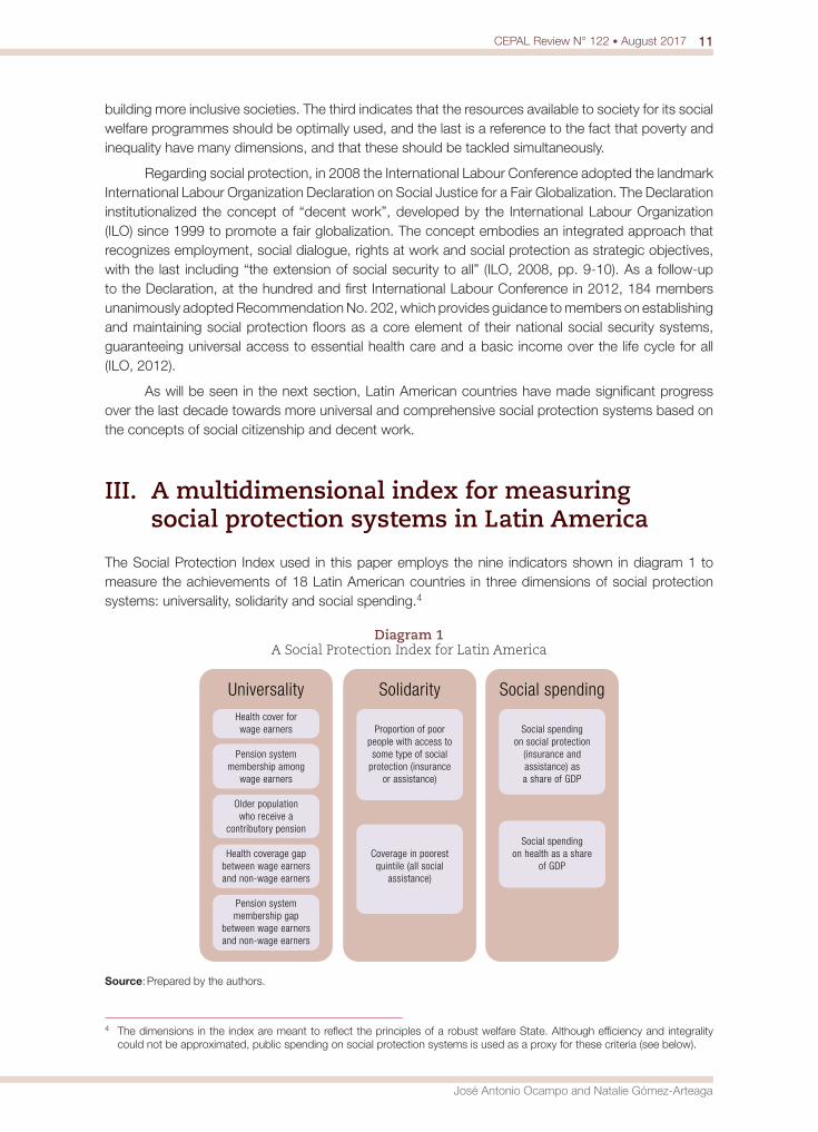
The Social Protection Index used in this paper employs the nine indicators shown in diagram 1 to measure the achievements of 18 Latin American countries in three dimensions of social protection systems: universality, solidarity and social spending.4
Diagram 1 A Social Protection Index for Latin America
Social spending
Social spending on social protection
(insurance and assistance) as a share of GDP
Social spending on health as a share
of GDP
UniversalityHealth cover for wage earners
Pension system membership among
wage earners
Older population who receive a
contributory pension
Health coverage gap between wage earners and non-wage earners
Pension system membership gap
between wage earners and non-wage earners
Solidarity
Proportion of poor people with access to some type of social
protection (insurance or assistance)
Coverage in poorest quintile (all social
assistance)
Source: Prepared by the authors.
4 The dimensions in the index are meant to reflect the principles of a robust welfare State. Although efficiency and integrality could not be approximated, public spending on social protection systems is used as a proxy for these criteria (see below).

12 CEPAL Review N° 122 • August 2017
Social protection systems, redistribution and growth in Latin America
The first dimension, universality, measures the coverage of health-care and pension systems of both types (insurance and assistance) among the working population, and the share of the older population who receive a pension. In view of the historical segmentation of social protection systems in Latin America, a result of their link with formal employment,5 this dimension includes two indicators that measure the coverage gap between wage workers and non-wage workers6 for both health and pensions. The data come from the Social Panorama of Latin America 2013 (ECLAC, 2014b), which had a particular focus on access to health care and pensions in the region.
Although universal coverage should of course apply to other areas of social protection systems and social security more broadly,7 all that is available for most countries at two points in time (around 2002 and around 2012) are data on membership of health-care and pension systems among the working-age population (active labour force), differentiated between wage and non-wage earners, and the share of the older population who receive a contributory pension. Protection for persons with disabilities and work-related risks cannot be measured with the available data, and other programmes such as unemployment benefits are so deficient in the region that only a few countries have them, generally with very low coverage, as they are invariably based on social insurance.8
The second dimension, solidarity, is approximated by two indicators, one that estimates the access of the poorest households to some form of protection and one that measures the efficiency of social assistance at targeting the poor.9 The first is the percentage of multidimensionally poor households that have some kind of social protection, defined as having at least one member with access to health insurance, contributing to any form of social insurance or receiving a pension or retirement income. This indicator is one of the dimensions of the new multidimensional poverty index for Latin America proposed by the Oxford Poverty and Human Development Initiative (OPHI) and included in the Social Panorama of Latin America 2013 (ECLAC, 2014b). Coverage of all social assistance programmes in the poorest quintile of the population measures the targeting efficiency of social assistance, on the basis of World Bank data.
The last dimension measures public sector social spending on both health care and social protection (insurance and assistance) as a percentage of GDP. Cross-country evidence suggests that the larger the social budget, the greater the benefits in terms of poverty and inequality reduction. The size of the budget also reflects the social contract and type of institutions in a given country and the universality of the system. “The hypothesis here is that the size of the budget available for redistribution is not fixed and that the institutional structures of welfare States are likely to affect the definitions of identity and interest among citizens. Thus, an institutional welfare State model based on a universalistic strategy with higher budget intended to maintain normal or accustomed standards of living is likely to result in greater redistribution than a marginal one based on targeting” (Korpi and Palme, 1998, p. 663). Although the index may have some limitations and missing variables, as will be seen in the following sections, it is a very useful measure for the purposes of this study and an interesting proxy for measuring changes in social protection systems.
5 See Barrientos (2011) and Kaplan and Levy (2014).6 Non-wage workers include employers, own-account workers, members of producers’ cooperatives and unpaid family workers.
Because of large information gaps, the coverage indicators measure only wage workers. This indicator and those for coverage gaps between groups approximate the extent to which social protection systems meet the objective of universality.
7 According to ILO, social protection floors include access to essential health care, including maternity care; basic income security for children, providing access to nutrition, education, care and any other necessary goods and services; basic income security for persons in active age who are unable to earn sufficient income, in particular in cases of sickness, unemployment, maternity and disability; and basic income security for older persons. Broader social security encompasses eight areas: sickness benefits, unemployment benefits, old-age benefits, employment injury benefits, family and child benefits, maternity benefits, invalidity and disability benefits and survivors’ benefits.
8 According to ILO data on social protection, the contributory unemployment schemes of Chile and Uruguay have the highest coverage in Latin America and the Caribbean, reaching 27% and 29% of the population, respectively.
9 Social assistance consists of all benefits targeted at vulnerable groups in the population, especially poor households. Most social assistance schemes are means-tested.

13CEPAL Review N° 122 • August 2017
José Antonio Ocampo and Natalie Gómez-Arteaga
Normalized indices were constructed for each of the nine indicators using the maximum (goalpost) and minimum achievements of the pool of countries. 100% coverage was used as the maximum (goalpost) for the coverage indicators, and 0% for the gap indicators. The final index is a summary measure, obtained from the arithmetic mean of the normalized indices of each of the nine indicators (this is a simple average, with all indicators having equal weight).10 It ranges from 0 to 1, where 1 represents the most comprehensive system with closest to universal coverage, the least inequality by type of employment in terms of access to health and pension systems, high social inclusion, well-targeted social assistance and high social spending. Annex A1 gives descriptions and sources for each indicator.
The final Social Protection Index scores for both 2002 and 2012 can be seen in figure 1. On the basis of the 2012 index score, the countries were divided into three groups by the comprehensiveness and universality of their social protection systems: (i) Uruguay, Chile, Costa Rica, Argentina and Brazil, with the highest scores, can be identified as having comprehensive systems; (ii) the Bolivarian Republic of Venezuela, Colombia, Peru, Mexico, Ecuador, the Dominican Republic and Panama have intermediate systems; (iii) El Salvador, Paraguay, the Plurinational State of Bolivia, Nicaragua, Guatemala and Honduras have relatively limited social protection systems. This classification is consistent with different rankings in this area, all concluding that the countries in the Southern Cone, with their higher development, have built more comprehensive welfare States. Costa Rica, for its part, has always stood out as having a fairly universal welfare State despite its much lower GDP per capita (Cecchini and Martínez, 2012).
Figure 1 Latin America (selected countries): Social Protection Index scores, around 2002 and 2012
0
0.1
0.2
0.3
0.4
0.5
0.6
0.7
0.8
0.9
Urug
uay
Chi
le
Cos
ta R
ica
Arge
ntin
a
Braz
il
Vene
zuel
a(B
ol. R
ep. o
f)
Col
ombi
a
Peru
Mex
ico
Ecua
dor
Dom
inic
anRe
p.
Pana
ma
El S
alva
dor
Para
guay
Boliv
ia(P
lur.
Sta
te o
f)
Nic
arag
ua
Gua
tem
ala
Hon
dura
s
Soci
al p
rote
ctio
n in
dex
2002 2012
Comprehensive socialprotection systems
Intermediate socialprotection systems
Limited socialprotection systems
Source: Prepared by the authors, on the basis of data from Economic Commission for Latin America and the Caribbean (ECLAC), Social Panorama of Latin America 2013 (LC/G.2580), Santiago, 2014; Social Panorama of Latin America 2014 (LC/G.2635-P), Santiago, 2014; M.E. Santos and others, “A multidimensional poverty index for Latin America”, OPHI Working Paper, No. 79, University of Oxford, 2015; and the World Bank. “Around 2012” includes years from 2010 to 2013.
Note: The Social Protection Index is the arithmetic mean of the normalized scores of each of the countries on the 9 indicators used to rank them.
10 The arithmetic mean only includes indicators without missing information. Of the 18 countries, 9 have complete information for all 9 indicators (Argentina, Chile, Colombia, Ecuador, El Salvador, Paraguay, Peru, the Plurinational State of Bolivia and Uruguay), 1 has information for 5 indicators (the Bolivarian Republic of Venezuela) and the rest have information for 7 indicators.
14 CEPAL Review N° 122 • August 2017
Social protection systems, redistribution and growth in Latin America
Between 2002 and 2012, 15 of the 18 countries with data available improved their Social Protection Index scores, meaning they made significant improvements on at least one of the social protection dimensions, moving towards a more universal and comprehensive system. In contrast, three did not experience any change in the indicator.
Countries with intermediate social protection systems improved the most (in terms of absolute changes in the index). Colombia had the strongest improvement in its Social Protection Index score, followed by Peru, the Dominican Republic and a country with a limited social protection system, the Plurinational State of Bolivia. In the case of Colombia, the improvement followed efforts to achieve universal health coverage by using a subsidized insurance scheme to reach the poor and self-employed.11 Colombia significantly increased health coverage for both wage and non-wage workers, while reducing the membership gap between the two. Whereas 53% of wage workers had access to health coverage in 2002, by 2012 the proportion was 91%, and the increase in coverage among non-wage workers meant that the coverage gap between the two types of employment narrowed from 75 percentage points in 2002 to 5 points in 2012. Peru, the country with the second-largest improvement in the index, also achieved substantial improvements in access to health care and pensions, with both indicators almost doubling between 2002 and 2012. Furthermore, social assistance coverage in the poorest quintile increased from less than 10% to 70%.
The Plurinational State of Bolivia significantly improved access to pensions among the older population, raising coverage from 13% to 21%. Although this is still comparatively low, the country achieved near-universal coverage among older people (aged 65 and over) with its non-contributory pensions (see section IV). Of the countries with comprehensive systems, Argentina made the greatest improvement, driven mainly by an expansion of pension coverage with the introduction of a mandatory minimum basic pension for all, irrespective of whether beneficiaries had reached the minimum contribution threshold.12
Table 1 shows the average scores on the nine indicators in the index by social protection category for 2012. Unsurprisingly, countries with more comprehensive social protection systems score better on average on eight of the nine indicators. For example, while an average of 82% of the older population in countries with comprehensive social protection systems have access to a pension and thus income security in old age, only 28% and 15% of this population have such security in countries with intermediate and limited social protection systems, respectively. The coverage gap between countries with comprehensive systems and countries with limited systems is large when measured by the coverage of old-age pensions and the percentage of poor households with some kind of protection. The percentage of people aged 65 and older who receive a pension is five times as high in countries with comprehensive systems as in those with limited systems. Similarly, the percentage of poor households with some kind of social protection is three times as great in countries with comprehensive systems as in those with limited systems.
Social assistance coverage in the poorest quintile is the only indicator for which there is no clear difference between categories; indeed, countries with intermediate social protection systems seem to have better targeting efficiency, with higher coverage among the population in the first quintile. Given the scale of some social assistance programmes in the region, mainly conditional cash transfer programmes, it is not surprising that the countries all have similar levels of coverage. Indeed, since low-income countries rely more on means-tested programmes because of their low spending levels and deficient health and pension coverage, it is possible that they might have higher coverage than
11 See the case study on universal health coverage in Colombia conducted for the World Bank by Montenegro, Torres and Acevedo (2013).
12 See Lustig and Pessino (2013). A pension moratorium introduced in 2004-2005 allowed workers of retirement age to receive a pension regardless of whether they had completed the required 30 years of social security contributions in formal employment.

15CEPAL Review N° 122 • August 2017
José Antonio Ocampo and Natalie Gómez-Arteaga
comprehensive social protection systems (Ferreira and Robalino, 2011). In recent years, furthermore, countries like Mexico, Colombia and Peru have continued to improve their targeting mechanisms to reach the poorest households and expand their conditional cash transfer programmes (for Colombia, see Angulo and Gómez, 2015).
Table 1 Latin America (selected countries):a average social protection indicators by category, 2012
Social protection system coverage
Contributory pension coverage (ages 65
and above) (%)
Wage earners in pension
system (%)
Wage earners in health
system (%)
Pension coverage
gap between wage and non-wage workers
Health coverage
gap between wage and non-wage workers
Poor households with access
to some social
protection (%)
Coverage in poorest quintile
(all social assistance)
(%)
Social spending on social protection (% of GDP)
Social spending on health
(% of GDP)
Comprehensive 81.8 77.1 90.0 -52% -12% 92.8 65.0 9.9 5.1
Intermediate 28.4 58.3 75.1 -70% -42% 71.3 68.6 3.7 2.1
Limited 15.3 37.6 41.9 -96% -79% 44.9 63.3 3.3 2.7
Source: Prepared by the authors, on the basis of data from Economic Commission for Latin America and the Caribbean (ECLAC), Social Panorama of Latin America 2013 (LC/G.2580), Santiago, 2014; Social Panorama of Latin America 2014 (LC/G.2635-P), Santiago, 2014; M.E. Santos and others, “A multidimensional poverty index for Latin America”, OPHI Working Paper, No. 79, University of Oxford, 2015; and the World Bank.
a Argentina, Bolivarian Republic of Venezuela, Brazil, Chile, Colombia, Costa Rica, Dominican Republic, Ecuador, El Salvador, Guatemala, Honduras, Mexico, Nicaragua, Panama, Paraguay, Peru, Plurinational State of Bolivia and Uruguay.
The recent improvements in Social Protection Index scores have been due to efforts to develop more universal social protection systems, with specific policies to bring in the traditionally excluded poor and informal population. As will be seen, however, social protection system access and benefits are still highly segmented by type of employment and income level.
IV. Social protection systems in the region are still segmented, although less than formerly
There have been significant improvements in access to health care and pensions13 across the region thanks to recent innovations with flexible contribution mechanisms, basic pensions as in Argentina, non-contributory pensions as in Chile and the Plurinational State of Bolivia, and universal health coverage with a large solidarity component as in Colombia, among others.
Access to pensions and health care increased throughout the region for both wage and non-wage workers and at all income levels between 2002 and 2012. Thanks to efforts to achieve universal health care and to solve the problem of limited coverage when this is linked to formal employment, health-care coverage has improved most among non-wage earners and for the lower quintiles of the income distribution (see figure 2).
13 Access to health care and pensions is a measure of the working-age population (aged 15 and over) that is covered by some kind of health insurance (however financed) and by some pension scheme (public or private). Pension coverage is also measured by the percentage of older people receiving this benefit.
16 CEPAL Review N° 122 • August 2017
Social protection systems, redistribution and growth in Latin America
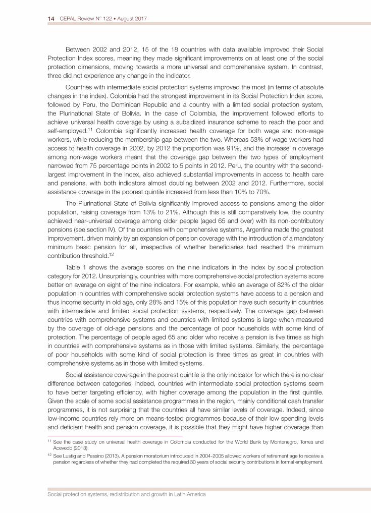
Figure 2 Latin America (selected countries): a health and pension system membership by type
of employment, around 2002 and 2012(Percentages)
Wage earners Non-wage earners
46
54
17
28 28
37 39
48 50 58
65 71
55
66
24
44 38
53 49
61 60
70 73
80
Pens
ions
Heal
th
Pens
ions
Heal
th
Pens
ions
Heal
th
Pens
ions
Heal
th
Pens
ions
Heal
th
Pens
ions
Heal
th
Total Q1 Q2 Q3 Q4 Q5
9
28
2
24
4
23
6
26
10
29
21
39
12
41
3
42
6
39
10
40
14
41
26
48
Pens
ions
Heal
th
Pens
ions
Heal
th
Pens
ions
Heal
th
Pens
ions
Heal
th
Pens
ions
Heal
th
Pens
ions
Heal
th
Total Q1 Q2 Q3 Q4 Q5
2002 2012
Source: Economic Commission for Latin America and the Caribbean (ECLAC), Social Panorama of Latin America 2013 (LC/G.2580), Santiago, 2014.
a Argentina, Bolivarian Republic of Venezuela, Brazil, Chile, Colombia, Costa Rica, Dominican Republic, Ecuador, El Salvador, Guatemala, Honduras, Mexico, Nicaragua, Panama, Paraguay, Peru, Plurinational State of Bolivia and Uruguay.
The percentage of non-wage workers with access to health care almost doubled over a decade, while pension coverage increased by only 3 percentage points. Interestingly, access to health insurance is always more prevalent than pension system membership regardless of type of employment or income quintile, reflecting the greater redistributive impact of health care than of transfers, as will be shown in section V.
The innovations recently introduced to do away with segmentation or “truncation” in access to protection by type of employment are a clear sign of the paradigm shift towards universalism that has overtaken the region in recent years. At the end of the twentieth century, when it became clear that the problem of limited coverage (confined to those in formal employment covered by contributory schemes) was not going to resolve itself as countries developed,14 a wave of innovative mechanisms designed to provide some form of basic protection for all, and especially self-employed workers, spread throughout the region. In addition to the example of Colombia’s subsidized insurance scheme already mentioned, in 2001 Uruguay implemented a monotax system to improve coverage of self-employed workers by unifying different social security contributions and taxes into a single payment under a simplified procedure and granting people covered by the monotax the same social security benefits as wage workers, on the basis of a solidarity principle (ILO, 2014b). Argentina did something similar by subsidizing social security contributions for self-employed workers and microenterprises, while in Brazil a simplified taxation scheme designed for micro and small business known as SIMPLES has significantly reduced employee social security costs for microenterprises.
Despite the improvements since 2002, however, there is still great segmentation in access to social protection by type of employment and income, especially for pensions, as figure 2 also shows. While 66% and 55% and of wage workers are members of a health-care scheme and a pension fund, respectively, only 41% and 12%, respectively, of non-wage workers are. In 2012, less than 5% of non-
14 With economic growth, the informal sector was expected to gradually disappear as workers moved from more traditional (mainly informal) to more modern (formal) sectors. See Kaplan and Levy (2014).
17CEPAL Review N° 122 • August 2017
José Antonio Ocampo and Natalie Gómez-Arteaga
wage workers in the bottom quintile were in pension schemes, as compared to 24% of wage workers in the same quintile. Even in the higher quintiles, non-wage workers have less access to both pensions and health care.
Poor households are also less likely to be covered by both types of protection. This is true in all countries, even those with comprehensive systems, although there the coverage gaps affecting that group are less marked. Interestingly, the health-care coverage gap by type of employment is larger in the second-poorest quintile than in the poorest one. This may partly reflect the success of conditional cash transfer programmes targeted at the poorest population in creating access to universal basic services, leaving people just above the threshold without these benefits, so that the coverage gap in the middle of the distribution is higher.
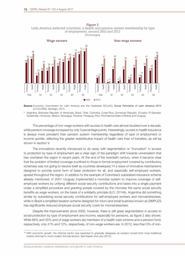
Protection for older people has also increased in recent years. According to household survey data, however, the improvement has been greatest among the wealthier population. While 59% of older people in the top income quintile had access to a pension (whether contributory or non-contributory) in 2012, only 21% of those in the bottom quintile did. It is not only the coverage of old-age pensions that is unequal, but also their amounts. As figure 3 shows, they are significantly higher in the top quintile even than in the fourth quintile.
Figure 3 Latin America: pension coverage and average monthly pension amounts for the population
aged 65 and over, by income quintile, around 2002 and 2012(Dollars at constant 2005 prices and percentages)
0
50
100
150
200
250
300
350
400
450
0
10
20
30
40
50
60
70
1 2 3 4 5
Amou
nt (d
olla
rs in
con
sant
200
5 pr
ices
)
Cove
rage
(per
cent
ages
)
Income quintile
Coverage in 2002 (left scale) Coverage in 2012 (left scale)Amount in 2002 (right scale) Amount in 2012 (right scale)
Source: Economic Commission for Latin America and the Caribbean (ECLAC), Social Panorama of Latin America 2013 (LC/G.2580), Santiago, 2014; and Inclusive Social Development: The Next Generation of Policies for Overcoming Poverty and Reducing Inequality in Latin America and the Caribbean (LC/L.4056/Rev.1), Santiago, 2016.
Given the low coverage of contributory old-age pensions, new non-contributory pension schemes have been emerging in the region, led by Brazil, Chile and, with coverage of 95%, the Plurinational State of Bolivia. In other countries such as Mexico and Panama, non-contributory pensions exist but only as means-tested subsidies that reach less than 30% of the population, although this is still a higher proportion than in 2002 (ECLAC, 2016).
Efforts to expand social protection have come with higher social spending, as this rose by almost 5 percentage points of GDP between 1990 and 2013; 70% of this increase, which was driven mainly by health and social security (insurance and assistance), came between 2002 and 2013 (see figure 4). However, while Latin America ranks second in the emerging and developing world for social

18 CEPAL Review N° 122 • August 2017
Social protection systems, redistribution and growth in Latin America
spending as a share of GDP, it allocates far fewer resources to this than developed countries, whether in the form of direct transfers (including social insurance and assistance, non-contributory pensions and other transfers such as child benefits) or of health and education provision (see figure 5).
Figure 4 Latin America: magnitude and composition of public sector social spending
(Population-weighted averages as percentages of GDP)
3.5 2.9 3.0 3.8 4.0
5.5
3.7
6.2
4.0
6.6
4.2
7.9 8.0
5.0 4.9
0.6 0.7 0.8
1.0 0.8
1990-1991 1996-1997 2002-2003 2008-2009 2012-2013
Weighted averages
Education Health Social protection Housing
Source: Economic Commission for Latin America and the Caribbean (ECLAC), Social Panorama of Latin America 2013 (LC/G.2580), Santiago, 2014.
Figure 5 Selected world regions: public sector social spending
(Percentages of GDP)
0
5
10
15
20
25
30
Advancedeconomies
EmergingEurope
Latin America Middle Eastand North Africa
Asia andthe Pacific
Sub-SaharanAfrica
Education Health Direct transfers
Source: F. Bastagli, D. Coady and S. Gupta, “Income inequality and fiscal policy”, IMF Staff Discussion Note (SDN/12/08), Washington, D.C., International Monetary Fund (IMF).
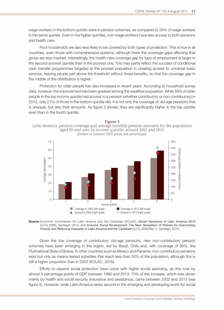
When health and pension system membership is reviewed across the three categories of social protection systems (figure 6), two conclusions emerge. First, countries with comprehensive systems have higher average coverage without major segmentation by income quintile or type of employment
19CEPAL Review N° 122 • August 2017
José Antonio Ocampo and Natalie Gómez-Arteaga
where access to health care is concerned, although gaps remain when it comes to pensions. Second, differences in coverage between the three categories of social protection systems are larger for non-wage workers. In countries with limited systems, the majority of the non-wage working population is excluded from social protection, and social security is only available to the small proportion of workers with formal employment, in contrast to countries with intermediate and comprehensive systems, which have made progress in this regard. For example, whereas 80% and 46% of non-wage workers in countries with comprehensive and intermediate systems, respectively, have access to health-care systems, only 10% do in countries with limited systems. This gap is much larger than the gap for wage workers across all types of social protection systems.
Figure 6 Latin America (selected countries): average health and pension system membership by social
protection category, total and bottom two quintiles, around 2012(Percentages)
Wage workers Non-wage workers
0 10 20 30 40 50 60 70 80 90
100
Pensions Health Pensions Health Pensions Health
Quintile I Quintile II Total
0
10
20
30
40
50
60
70
80
90
Pensions Health Pensions Health Pensions Health
Quintile I Quintile II Total
Comprehensive Intermediate Limited
Source: Prepared by the authors, on the basis of Economic Commission for Latin America and the Caribbean (ECLAC), Social Panorama of Latin America 2013 (LC/G.2580), Santiago, 2014.
Note: The countries with comprehensive systems included in these estimates are Argentina, Chile, Costa Rica and Uruguay, those with intermediate systems are Colombia, the Dominican Republic, Ecuador, Mexico, Panama and Peru, and those with limited systems are El Salvador, Guatemala, Honduras, Nicaragua, Paraguay and the Plurinational State of Bolivia.
In any event, there is still much to be done. Although targeted programmes have successfully brought down poverty, they have been less effective than universal benefits at reducing income inequality (see section V below). The next step has to go beyond narrow targeting mechanisms towards more universal social protection systems, including an expansion of social insurance as countries develop. A universal social protection system that covers people against all types of risks is necessary not only for continuing poverty reduction, but also to increase the resilience of the population above the poverty line, including the middle class (López-Calva and Ortiz-Juárez, 2014; Ferreira and others, 2013), and construct social citizenship. Without universal protection mechanisms, previous gains could be reversed. This implies, of course, that more resources are needed for social spending.
V. The redistributive effectiveness of public spending
The redistributive effect of public spending varies with the characteristics of social protection systems. Higher social spending, universal coverage and progressive transfers are associated with a higher redistributive impact.

20 CEPAL Review N° 122 • August 2017
Social protection systems, redistribution and growth in Latin America
Using the national studies of the 11 countries covered by the Commitment to Equity (CEQ) Project of Tulane University and Inter-American Dialogue15 for which information was available when this study was written, it can be estimated that, on average, countries with comprehensive social protection systems for which information is available reduce inequality by 0.021 points of the Gini coefficient through direct transfers and by 0.085 through in-kind transfers. Intermediate systems do so by 0.010 and 0.037 points, respectively, while in countries with limited systems, direct transfers have almost no impact on inequality (0.006) and in-kind transfers have only a very small redistributive effect (0.030) (figure 7).
Figure 7 Latin America (selected countries): redistributive effects of direct social spending
and in-kind transfers(Absolute changes in Gini coefficient)
-0.04
-0.02 -0.01
-0.02 -0.01
-0.02 0.00 -0.01 -0.01 0.00 -0.01
-0.08
-0.09
-0.10 -0.06
-0.05 -0.04
-0.03
-0.05
-0.02 -0.03 -0.02
-0.14
-0.12
-0.10
-0.08
-0.06
-0.04
-0.02
0 Argentina
(2009)Brazil(2009)
Costa Rica(2010)
Uruguay(2009)
Mexico(2010)
Ecuador(2011-12)
Peru(2009)
Bolivia (Plur. Stateof) (2009)
El Salvador(2010)
Paraguay(2010)
Guatemala(2010)
Comprehensive socialprotection systems
Intermediate socialprotection systems
Limited socialprotection systems
Direct transfers In-kind transfers
Source: Commitment to Equity (CEQ) Project, on the basis of M. Cabrera, N. Lustig and H.E. Morán, “Fiscal policy, inequality, and the ethnic divide in Guatemala”, World Development, vol. 76, Amsterdam, Elsevier, 2015; N. Lustig and others, “The impact of taxes and social spending on inequality and poverty in Argentina, Bolivia, Brazil, Mexico and Peru: a synthesis of results”, CEQ Working Paper, No. 3, CEQ Institute, 2012; N. Lustig, C. Pessino and J. Scott, “The impact of taxes and social spending on inequality and poverty in Argentina, Bolivia, Brazil, Mexico, Peru and Uruguay: an overview”, CEQ Working Paper, No. 13, CEQ Institute, 2013; J. Sauma and D. Trejos, “Gasto público social, impuestos, redistribución del ingreso y pobreza en Costa Rica”, CEQ Working Paper, No. 18, CEQ Institute, 2014; M. Beneke, N. Lustig and J.A. Oliva, “El impacto de los impuestos y el gasto social en la desigualdad y la pobreza en El Salvador”, CEQ Working Paper, No. 26, CEQ Institute, 2015; and F. Llerena and others, “Social spending, taxes and income redistribution in Ecuador”, CEQ Working Paper, No. 28, CEQ Institute, 2015.
Note: In-kind transfers include education and health services, while direct transfers include all monetary transfers such as conditional cash transfers, subsidies and non-contributory pensions. The difference between the Gini coefficients for net market income (which is market income, including contributory pensions, less personal income tax and employee social security contributions) and disposable income (which is net market income plus direct public transfers) is the redistributive effect of direct transfers. The difference between net market income and final income (defined as disposable income plus in-kind transfers minus co-payments and user fees, including pensions) is the outcome of all direct and in-kind transfers. See Lustig and Higgins (2013) for a detailed explanation of the methodology.
15 The Commitment to Equity (CEQ) Assessment uses standard incidence analysis to assess how much redistribution and poverty reduction are being accomplished in each country through social spending, subsidies and taxes and how progressive revenue collection and government spending are. The incidence analysis measures Gini coefficient and poverty indicator changes between different income concepts (before taxes and transfers, after direct taxes, and after direct and in-kind transfers). All CEQ Project working papers are listed in the reference section.
21CEPAL Review N° 122 • August 2017
José Antonio Ocampo and Natalie Gómez-Arteaga
Interestingly, regardless of the type of social protection system, the redistributive effect of in-kind transfers is higher than the effect of direct transfers, reflecting higher budgetary allocations to transfers of this type and, in most cases, their higher coverage. In all countries, the budget allocated to health and education (in-kind transfers) as a percentage of GDP is more than twice that allocated to direct transfers (conditional cash transfers, subsidies and non-contributory pensions), and in several countries much more. The budget for in-kind transfers varies from just under twice the budget for direct transfers in Paraguay (3.5% versus 6.7% of GDP) to 14 times in Peru (0.4% versus 5.9% of GDP). Direct transfers tend to have a larger poverty reduction impact in countries with comprehensive social protection systems. For example, direct transfers reduce the headcount ratio by 7.5 percentage points in Argentina, 3.1 percentage point in Ecuador and less than 1 percentage point in Paraguay.
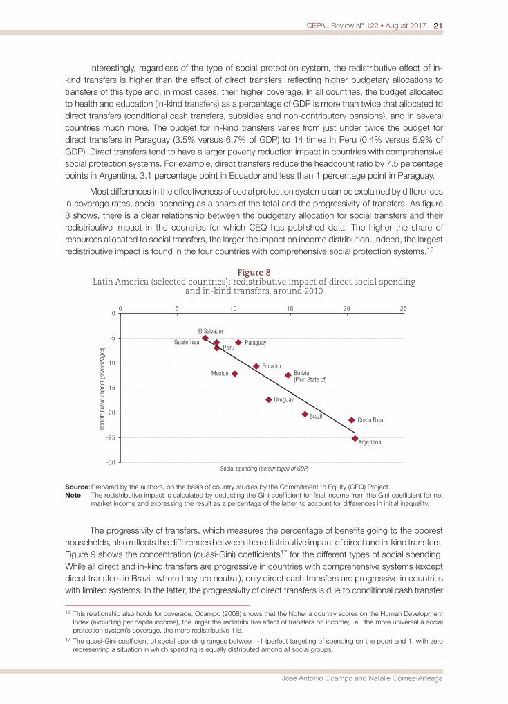
Most differences in the effectiveness of social protection systems can be explained by differences in coverage rates, social spending as a share of the total and the progressivity of transfers. As figure 8 shows, there is a clear relationship between the budgetary allocation for social transfers and their redistributive impact in the countries for which CEQ has published data. The higher the share of resources allocated to social transfers, the larger the impact on income distribution. Indeed, the largest redistributive impact is found in the four countries with comprehensive social protection systems.16
Figure 8 Latin America (selected countries): redistributive impact of direct social spending
and in-kind transfers, around 2010
Argentina
Bolivia(Plur. State of)
Brazil
Mexico
Peru
Uruguay
Paraguay
Ecuador
El Salvador
Guatemala
Costa Rica
-30
-25
-20
-15
-10
-5
00 5 10 15 20 25
Redi
strib
utiv
e im
pact
(per
cent
ages
)
Social spending (percentages of GDP)
Source: Prepared by the authors, on the basis of country studies by the Commitment to Equity (CEQ) Project.Note: The redistributive impact is calculated by deducting the Gini coefficient for final income from the Gini coefficient for net
market income and expressing the result as a percentage of the latter, to account for differences in initial inequality.
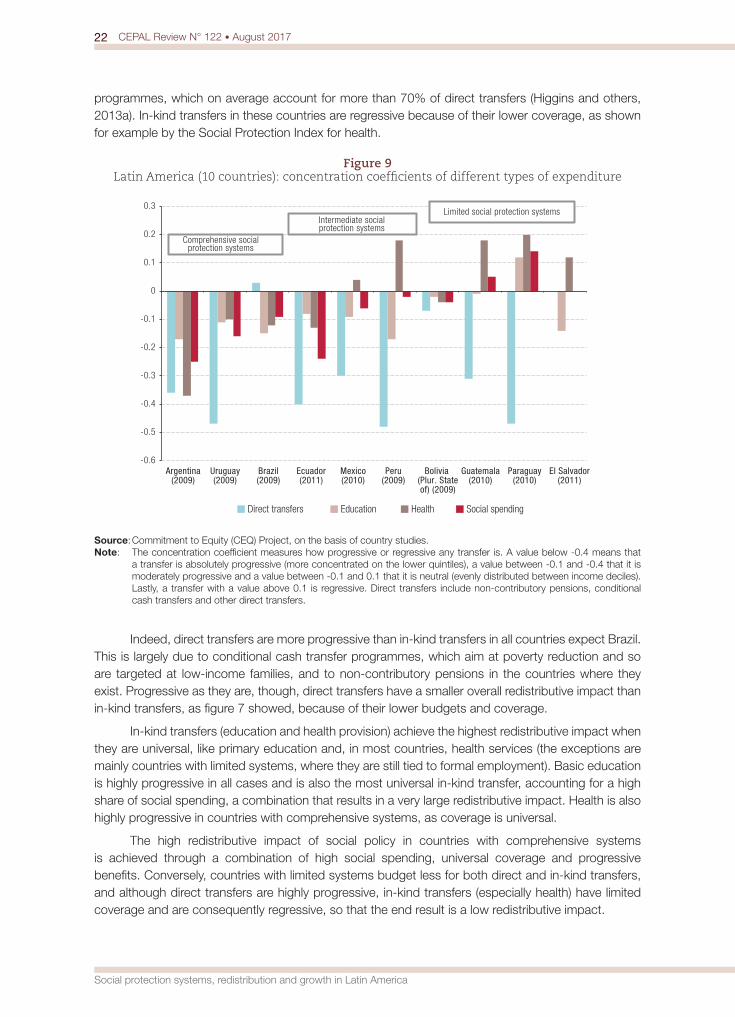
The progressivity of transfers, which measures the percentage of benefits going to the poorest households, also reflects the differences between the redistributive impact of direct and in-kind transfers. Figure 9 shows the concentration (quasi-Gini) coefficients17 for the different types of social spending. While all direct and in-kind transfers are progressive in countries with comprehensive systems (except direct transfers in Brazil, where they are neutral), only direct cash transfers are progressive in countries with limited systems. In the latter, the progressivity of direct transfers is due to conditional cash transfer
16 This relationship also holds for coverage. Ocampo (2008) shows that the higher a country scores on the Human Development Index (excluding per capita income), the larger the redistributive effect of transfers on income; i.e., the more universal a social protection system’s coverage, the more redistributive it is.
17 The quasi-Gini coefficient of social spending ranges between -1 (perfect targeting of spending on the poor) and 1, with zero representing a situation in which spending is equally distributed among all social groups.
22 CEPAL Review N° 122 • August 2017
Social protection systems, redistribution and growth in Latin America
programmes, which on average account for more than 70% of direct transfers (Higgins and others, 2013a). In-kind transfers in these countries are regressive because of their lower coverage, as shown for example by the Social Protection Index for health.
Figure 9 Latin America (10 countries): concentration coefficients of different types of expenditure
-0.6
-0.5
-0.4
-0.3
-0.2
-0.1
0
0.1
0.2
0.3
Argentina(2009)
Uruguay(2009)
Brazil(2009)
Ecuador(2011)
Mexico(2010)
Peru(2009)
Bolivia (Plur. Stateof) (2009)
Guatemala(2010)
Paraguay(2010)
El Salvador(2011)
Direct transfers Education Health Social spending
Comprehensive socialprotection systems
Intermediate socialprotection systems
Limited social protection systems
Source: Commitment to Equity (CEQ) Project, on the basis of country studies.Note: The concentration coefficient measures how progressive or regressive any transfer is. A value below -0.4 means that
a transfer is absolutely progressive (more concentrated on the lower quintiles), a value between -0.1 and -0.4 that it is moderately progressive and a value between -0.1 and 0.1 that it is neutral (evenly distributed between income deciles). Lastly, a transfer with a value above 0.1 is regressive. Direct transfers include non-contributory pensions, conditional cash transfers and other direct transfers.
Indeed, direct transfers are more progressive than in-kind transfers in all countries expect Brazil. This is largely due to conditional cash transfer programmes, which aim at poverty reduction and so are targeted at low-income families, and to non-contributory pensions in the countries where they exist. Progressive as they are, though, direct transfers have a smaller overall redistributive impact than in-kind transfers, as figure 7 showed, because of their lower budgets and coverage.
In-kind transfers (education and health provision) achieve the highest redistributive impact when they are universal, like primary education and, in most countries, health services (the exceptions are mainly countries with limited systems, where they are still tied to formal employment). Basic education is highly progressive in all cases and is also the most universal in-kind transfer, accounting for a high share of social spending, a combination that results in a very large redistributive impact. Health is also highly progressive in countries with comprehensive systems, as coverage is universal.
The high redistributive impact of social policy in countries with comprehensive systems is achieved through a combination of high social spending, universal coverage and progressive benefits. Conversely, countries with limited systems budget less for both direct and in-kind transfers, and although direct transfers are highly progressive, in-kind transfers (especially health) have limited coverage and are consequently regressive, so that the end result is a low redistributive impact.

23CEPAL Review N° 122 • August 2017
José Antonio Ocampo and Natalie Gómez-Arteaga
In any event, the total effect of fiscal policy in the region, including transfers and taxes, is still very small by comparison with more developed countries. While both Organization for Economic Cooperation and Development (OECD) countries and 15 older members of the European Union have an average market income distribution (before taxes and transfers) close to the average for Latin America, they are significantly more effective at reducing the inequality this represents, with the Gini coefficient decreasing by 36% or 17 percentage points in OECD (19 percentage points in the 15 European Union countries) as a result of fiscal policy, while the average reduction in Latin America is only 6% (OECD, 2011; IMF, 2015; Hanni, Martner and Podestá, 2015).18 In addition, and contrary to recent findings by Ostry, Berg and Tsangarides (2014), it is unclear that more unequal countries redistribute more in Latin America, as is the case with OECD countries. Uruguay for example, has relatively low market income inequality and is the country that redistributes the most.
Furthermore, although fiscal spending is progressive and has a large and increasing redistributive impact, taxation across the region is still mildly progressive at best and is actually regressive in some countries, as it relies heavily on revenue from value added tax (VAT) and sales taxes and relatively little on personal income taxes.19 In fact, according to a recent study, the fiscal mix in the region is such that a substantial proportion of the poor may be made poorer (or the non-poor made poor) by the tax and transfer system (Higgins and Lustig, 2015; Lustig and Martínez-Aguilar, 2016). Accordingly, fiscal reform to expand income tax and make taxation more progressive is key to redistribution and the efficiency of fiscal policy.
VI. Myths about the links between economic growth and redistribution
Although national social protection systems around the world have achieved major reductions in poverty and inequality (ILO, 2014a), doubts are often raised as to whether these results are obtained by incurring high opportunity costs in terms of economic growth. There is commonly assumed to be a trade-off between growth and redistribution. However, this trade-off is largely a myth. More broadly, following Cichon and Scholz (2009), there may be said to be three major myths about the relationship between social protection and economic performance, namely:20
(i) At each stage of development, societies can only afford a certain level of social expenditure (the affordability myth);
(ii) There is a trade-off between social expenditure (redistribution) and economic growth (Okun’s trade-off).
(iii) Economic growth will automatically reduce poverty (trickle-down myth).
Going by the recent experience of Latin America, it is possible to refute these myths. First, social protection systems in the region are highly heterogeneous even when per capita GDP differences are taken into account. Second, there is no clear evidence that countries which have expanded their social protection systems have grown by less. Third, there is a stronger correlation between improvements in the Social Protection Index and poverty reduction than between growth and poverty reduction.
18 See also Goñi, López and Servén (2011) and Lustig, Pessino and Scott (2013).19 See the Woodrow Wilson International Center for Scholars project on taxation and equality in Latin America [online] https://
www.wilsoncenter.org/publication/taxation-and-equality-latin-america.20 See Cichon and Scholz (2009) for a review of these myths in the context of the OECD countries.
24 CEPAL Review N° 122 • August 2017
Social protection systems, redistribution and growth in Latin America
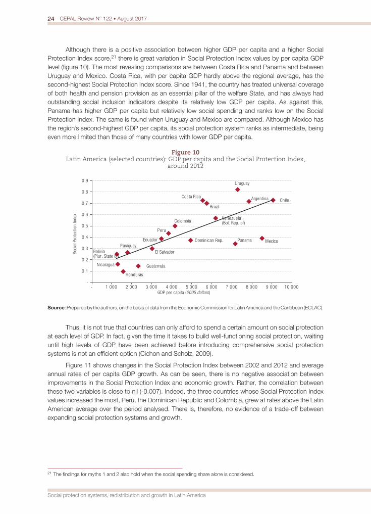
Although there is a positive association between higher GDP per capita and a higher Social Protection Index score,21 there is great variation in Social Protection Index values by per capita GDP level (figure 10). The most revealing comparisons are between Costa Rica and Panama and between Uruguay and Mexico. Costa Rica, with per capita GDP hardly above the regional average, has the second-highest Social Protection Index score. Since 1941, the country has treated universal coverage of both health and pension provision as an essential pillar of the welfare State, and has always had outstanding social inclusion indicators despite its relatively low GDP per capita. As against this, Panama has higher GDP per capita but relatively low social spending and ranks low on the Social Protection Index. The same is found when Uruguay and Mexico are compared. Although Mexico has the region’s second-highest GDP per capita, its social protection system ranks as intermediate, being even more limited than those of many countries with lower GDP per capita.
Figure 10 Latin America (selected countries): GDP per capita and the Social Protection Index,
around 2012
Honduras
GuatemalaNicaragua
Bolivia(Plur. State of)
ParaguayEl Salvador
Panama MexicoEcuador
Peru
Dominican Rep.
ColombiaVenezuela(Bol. Rep. of)
ChileCosta Rica
Brazil
Argentina
Uruguay
-
0.1
0.2
0.3
0.4
0.5
0.6
0.7
0.8
0.9
- 1 000 2 000 3 000 4 000 5 000 6 000 7 000 8 000 9 000 10 000
Soci
al P
rote
ctio
n In
dex
GDP per capita (2005 dollars)
Source: Prepared by the authors, on the basis of data from the Economic Commission for Latin America and the Caribbean (ECLAC).
Thus, it is not true that countries can only afford to spend a certain amount on social protection at each level of GDP. In fact, given the time it takes to build well-functioning social protection, waiting until high levels of GDP have been achieved before introducing comprehensive social protection systems is not an efficient option (Cichon and Scholz, 2009).
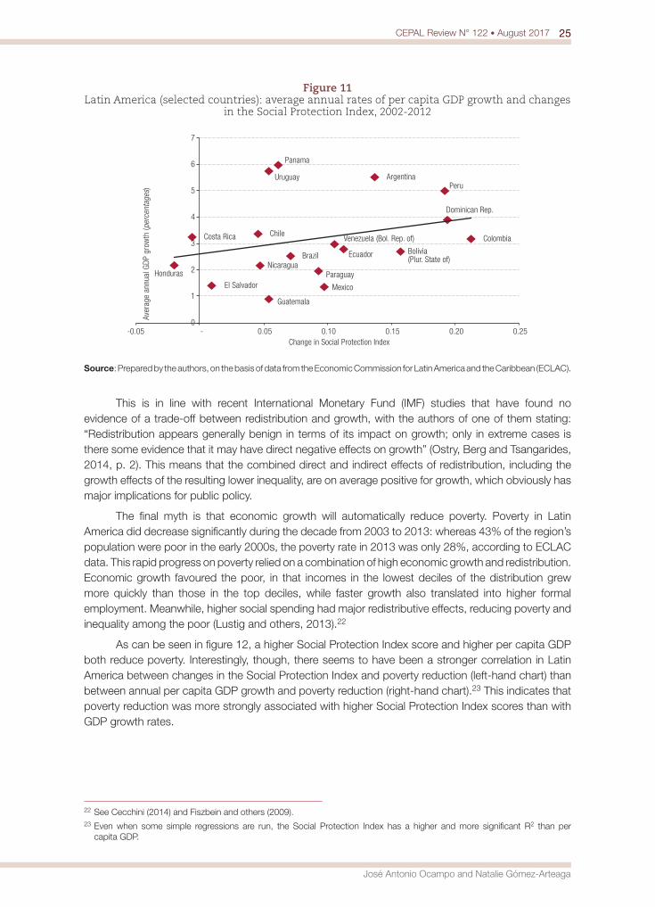
Figure 11 shows changes in the Social Protection Index between 2002 and 2012 and average annual rates of per capita GDP growth. As can be seen, there is no negative association between improvements in the Social Protection Index and economic growth. Rather, the correlation between these two variables is close to nil (-0.007). Indeed, the three countries whose Social Protection Index values increased the most, Peru, the Dominican Republic and Colombia, grew at rates above the Latin American average over the period analysed. There is, therefore, no evidence of a trade-off between expanding social protection systems and growth.
21 The findings for myths 1 and 2 also hold when the social spending share alone is considered.
25CEPAL Review N° 122 • August 2017
José Antonio Ocampo and Natalie Gómez-Arteaga
Figure 11 Latin America (selected countries): average annual rates of per capita GDP growth and changes
in the Social Protection Index, 2002-2012
Honduras
Guatemala
Nicaragua
Bolivia(Plur. State of)
ParaguayEl Salvador
Panama
Mexico
Ecuador
Peru
Dominican Rep.
ColombiaVenezuela (Bol. Rep. of)ChileCosta Rica
Brazil
ArgentinaUruguay
0
1
2
3
4
5
6
7
-0.05 - 0.05 0.10 0.15 0.20 0.25
Aver
age
annu
al G
DP g
row
th (p
erce
ntag
es)
Change in Social Protection Index
Source: Prepared by the authors, on the basis of data from the Economic Commission for Latin America and the Caribbean (ECLAC).
This is in line with recent International Monetary Fund (IMF) studies that have found no evidence of a trade-off between redistribution and growth, with the authors of one of them stating: “Redistribution appears generally benign in terms of its impact on growth; only in extreme cases is there some evidence that it may have direct negative effects on growth” (Ostry, Berg and Tsangarides, 2014, p. 2). This means that the combined direct and indirect effects of redistribution, including the growth effects of the resulting lower inequality, are on average positive for growth, which obviously has major implications for public policy.
The final myth is that economic growth will automatically reduce poverty. Poverty in Latin America did decrease significantly during the decade from 2003 to 2013: whereas 43% of the region’s population were poor in the early 2000s, the poverty rate in 2013 was only 28%, according to ECLAC data. This rapid progress on poverty relied on a combination of high economic growth and redistribution. Economic growth favoured the poor, in that incomes in the lowest deciles of the distribution grew more quickly than those in the top deciles, while faster growth also translated into higher formal employment. Meanwhile, higher social spending had major redistributive effects, reducing poverty and inequality among the poor (Lustig and others, 2013).22
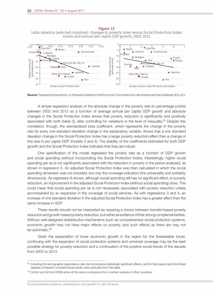
As can be seen in figure 12, a higher Social Protection Index score and higher per capita GDP both reduce poverty. Interestingly, though, there seems to have been a stronger correlation in Latin America between changes in the Social Protection Index and poverty reduction (left-hand chart) than between annual per capita GDP growth and poverty reduction (right-hand chart).23 This indicates that poverty reduction was more strongly associated with higher Social Protection Index scores than with GDP growth rates.
22 See Cecchini (2014) and Fiszbein and others (2009).23 Even when some simple regressions are run, the Social Protection Index has a higher and more significant R2 than per
capita GDP.
26 CEPAL Review N° 122 • August 2017
Social protection systems, redistribution and growth in Latin America
Figure 12 Latin America (selected countries): changes in poverty rates versus Social Protection Index
scores and annual per capita GDP growth, 2002-2012
Bolivia (Plur. State of)
Honduras
Paraguay
Nicaragua
Peru
Dominican Rep.
Ecuador
Colombia
Mexico
El Salvador
PanamaVenezuela (Bol. Rep. of)
Argentina
Brazil
Chile
Costa Rica
Uruguay
-35
-30
-25
-20
-15
-10
-5
0-0.05 0.00 0.05 0.10 0.15 0.20 0.25 0.30
Chan
ge in
pov
erty
rat
e(p
erce
ntag
e po
ints
)
Change in Social Protection Index
Bolivia (Plur. State of)
Honduras
Colombia
Nicaragua
Peru
Dominican Rep.
Ecuador
Paraguay
Mexico
El Salvador
PanamaVenezuela (Bol. Rep. of)
Argentina
Brazil
Chile
Costa Rica
Uruguay
-35
-30
-25
-20
-15
-10
-5
01 2 3 4 5 6 7
Chan
ge in
pov
erty
rat
e(p
erce
ntag
e po
ints
)
Average annual per capita GDP growth (percentages)
Source: Prepared by the authors, on the basis of data from the Economic Commission for Latin America and the Caribbean (ECLAC).
A simple regression analysis of the absolute change in the poverty rate (in percentage points) between 2002 and 2012 as a function of average annual per capita GDP growth and absolute changes in the Social Protection Index shows that poverty reduction is significantly and positively associated with both (table 2), after controlling for variations in the level of inequality.24 Despite this correlation, though, the standardized beta coefficient, which represents the change in the poverty rate for every one standard deviation change in the explanatory variable, shows that a one standard deviation change in the Social Protection Index has a larger poverty reduction effect than a change of this size in per capita GDP (models 3 and 4). The stability of the coefficients estimated for both GDP growth and the Social Protection Index indicates that they are robust.
One specification of the model regressed the poverty rate as a function of GDP growth and social spending (without incorporating the Social Protection Index). Interestingly, higher social spending per se is not significantly associated with the reduction in poverty in the period analysed, as shown in regression 5. An adjusted Social Protection Index was then calculated in which the social spending dimension was not included, but only the coverage indicators (the universality and solidarity dimensions). As regression 6 shows, although social spending still has no significant effect on poverty reduction, an improvement in the adjusted Social Protection Index (without social spending) does. This could mean that social spending per se is not necessarily associated with poverty reduction unless accompanied by an expansion in the coverage of social services. As with regressions 3 and 4, an increase of one standard deviation in the adjusted Social Protection Index has a greater effect than the same increase in GDP.
These results should not be interpreted as requiring a choice between transfer-based poverty reduction and growth-based poverty reduction, but rather as evidence of their strong complementarities. Without well-designed redistributive mechanisms such as comprehensive social protection systems, economic growth may not have major effects on poverty, and such effects as there are may not be automatic.25
Given the expectation of lower economic growth in the region for the foreseeable future, continuing with the expansion of social protection systems and universal coverage may be the best possible strategy for poverty reduction and a continuation of the positive social trends of the decade from 2003 to 2013.
24 Including the demographic dependency ratio did not produce statistically significant effects, and for that reason (and the limited degrees of freedom involved) those results were excluded from the table.
25 Cichon and Scholz (2009) arrive at the same conclusions from a similar analysis of other countries.

27CEPAL Review N° 122 • August 2017
José Antonio Ocampo and Natalie Gómez-Arteaga
Table 2 Regression analysis
Variable(1) (2) (3) (4) (5) (6)
Model 1 Model 2 Model 3 Model 4 Model 5 Model 6
Change in Social Protection Index-1.384** -1.392** -1.196**
(-0.464) (-0.466) (-0.401)
Per capita GDP growth-2.332* -2.353** -1.951** -2.062* -1.213
(-0.372) (-0.375) (-0.311) (-0.329) (-0.193)
Change in Gini coefficient1.022*** 1.178*** 1.039***
(0.555) (0.640) (0.564)
Change in social spending-0.072 -0.014
(-0.229) (-0.045)
Change in adjusted Social Protection Index-0.432***
(-0.463)
Constant -0.081** -0.105*** -0.037 -0.006 0.054 -0.006
Observations 18 18 18 18 18 18
R2 0.138 0.215 0.356 0.655 0.547 0.712
Source: Prepared by the authors.Note: Normalized beta coefficients in parentheses.
*** p<0.01, ** p<0.05, * p<0.1
VII. Conclusions
Given the still high levels of labour market informality in most Latin American countries, as well as low mandatory contributions, the limited coverage of contributory social protection and the small redistributive impact of fiscal policy, the challenges of social policy and social protection in particular in an era of slower economic growth will be large. New solutions are needed for transfers and taxes alike. There should be a move towards universal benefits and expanded non-contributory social protection mechanisms in parallel with labour formalization efforts and flexible mechanisms to increase social insurance contributions and benefits. The rising middle class has new social protection demands, and more of the same will not be enough: fresh resources (from higher contributions but also taxes) and universal coverage (with a mix of contributory and non-contributory schemes) are essential. Targeted social assistance programmes, a strong focus in recent decades, are simply not enough.
Universal coverage of social services should thus be the essential objective of social policy and is the best guarantee that the redistributive impact of social spending will be progressive. Universal benefits will prove more effective at reducing income inequality and creating more equal societies. The causality works both ways: more equal societies demand more universal systems of social policy and social protection, while the latter in turn contribute to equality. A further advantage of universal policies is their political appeal, particularly to the middle classes, which is essential if there is to be political backing for the task of raising the public sector resources necessary to make universal policies effective.
There is thus a major challenge for the fiscal regime, and the crux is the low tax revenue of Latin America, particularly from personal income taxes, in combination with low transfers, as discussed extensively by ECLAC, the World Bank and IMF (see, for example, IMF, 2014 and 2015). The ability to raise taxes, and more redistributive taxes in particular, to create more universal systems of social spending is thus the domain in which the battle for equity can be expected to be fought in years to come.

28 CEPAL Review N° 122 • August 2017
Social protection systems, redistribution and growth in Latin America
BibliographyAngulo, R. and N. Gómez (2015), “Inclusión social e inclusión productiva de los beneficiarios del programa
Más Familias en Acción: estudio de caso de Colombia” [online] http://dds.cepal.org/redesoc/archivos_recursos/4371/Roberto-Angulo_2014_Colombia.pdf.
Barrientos, A. (2011), “On the distributional implications of social protection reforms in Latin America”, Working Paper, No. 2011/69, Helsinki, World Institute for Development Economics Research (UNU-WIDER).
Bastagli, F., D. Coady and S. Gupta (2012), “Income inequality and fiscal policy”, IMF Staff Discussion Note, SDN/12/08, Washington, D.C., International Monetary Fund.
Beneke, M., N. Lustig and J.A. Oliva (2015), “El impacto de los impuestos y el gasto social en la desigualdad y la pobreza en El Salvador”, CEQ Working Paper, No. 26, CEQ Institute.
Bértola, L. and J.A. Ocampo (2012), The Economic Development of Latin America since Independence, Oxford, Oxford University Press.
Cabrera, M., N. Lustig and H.E. Morán (2015), “Fiscal policy, inequality, and the ethnic divide in Guatemala”, World Development, vol. 76, Amsterdam, Elsevier.
Cecchini, S. (2014), “Social protection, poverty and inequality: a comparative perspective”, Journal of Southeast Asian Economies, vol. 31, No. 1.
Cecchini, S. and R. Martínez (2012), “Inclusive social protection in Latin America: a comprehensive, rights-based approach”, ECLAC Books, No. 111, Santiago, Economic Commission for Latin America and the Caribbean (ECLAC).
Cichon, M. and W. Scholz (2009), “Social security social impact and economic performance: a farewell to the three famous myths”, Building Decent Societies: Rethinking the Role of Social Security in State Building, P. Townsend (ed.), London, Palgrave Macmillan.
ECLAC (Economic Commission for Latin America and the Caribbean) (2016), Inclusive Social Development: The Next Generation of Policies for Overcoming Poverty and Reducing Inequality in Latin America and the Caribbean (LC/L.4056/Rev.1), Santiago.(2014a), Compacts for Equality: Towards a Sustainable Future (LC/G.2586(SES.35/3)), Santiago. (2014b), Social Panorama of Latin America 2013 (LC/G.2580), Santiago.(2014c), Social Panorama of Latin America 2014 (LC/G.2635-P), Santiago.(2000), Equity, Development and Citizenship (LC/G.2071(SES.28/3)), Santiago.
Ferreira, F. and others (2013), Economic Mobility and the Rise of the Latin American Middle Class, Washington, D.C., World Bank.
Ferreira, F. and D. Robalino (2011), “Social assistance in Latin America: achievements and limitations”, Handbook of Latin American Economics, J.A. Ocampo and J. Ros (eds.), Oxford, Oxford University Press.
Filgueira, F. and others (2006), “Universalismo básico: una alternativa posible y necesaria para mejorar las condiciones de vida”, Universalismo basico: una nueva política social para America Latina, C. Molina (ed.), Washington, D.C., Inter-American Development Bank.
Fiszbein, A. and others (2009), Conditional Cash Transfers: Reducing Present and Future Poverty”, Washington, D.C., World Bank [online] https://openknowledge.worldbank.org/handle/10986/2597.
Goñi, E., H. López and L. Servén (2011), “Fiscal redistribution and income inequality in Latin America”, World Development, vol. 39, No. 9, Amsterdam, Elsevier.
Hanni, M., R. Martner and A. Podestá (2015), “The redistributive potential of taxation in Latin America”, CEPAL Review, No. 116 (LC/G.2643-P), Santiago, Economic Commission for Latin America and the Caribbean (ECLAC).
Higgins, S. and N. Lustig (2015), “Can a poverty-reducing and progressive tax and transfer system hurt the poor?”, CGD Working Paper, No. 405, Washington, D.C., Center for Global Development [online] http://www.cgdev.org/publication/can-poverty-reducing-and-progressive-tax-and-transfer-systemhurt-poor%03-working-paper.
Higgins, S. and others (2013a), “Social spending, taxes and income redistribution in Paraguay”, CEQ Working Paper, No. 11, CEQ Institute.(2013b), “Comparing the incidence of taxes and social spending in Brazil and the United States”, CEQ Working Paper, No. 16, CEQ Insitute.
ILO (International Labour Organization) (2014a), World Social Protection Report, Geneva.(2014b), “Monotax: promoting formalization and protection of independent workers”, Policy Brief, No. 02/2014.
29CEPAL Review N° 122 • August 2017
José Antonio Ocampo and Natalie Gómez-Arteaga
(2012), Social Security for All: Building Social Protection Floors and Comprehensive Social Security Systems. The Strategy of the International Labour Organization, Geneva.(2008), ILO Declaration on Social Justice for a Fair Globalization, Geneva, International Labour Office.
IMF (International Monetary Fund) (2015), World Economic Outlook: Uneven Growth, Short- and Long-Term Factors, Washington, D.C.(2014), “Fiscal policy and income inequality”, IMF Policy Paper, Washington, D.C.
Kaplan, D. and S. Levy (2014), “The evolution of social security systems in Latin America”, Social Insurance, Informality, and Labor Markets: How to Protect Workers while Creating Good Jobs, M. Frolich and others (eds.), New York, Oxford University Press.
Korpi, W. and J. Palme (1998), “The paradox of redistribution and strategies of equality: welfare state institutions, inequality and poverty in the Western countries”, American Sociological Review, vol. 63, No. 5.
Llerena, F. and others (2015), “Social spending, taxes and income redistribution in Ecuador”, CEQ Working Paper, No. 28, CEQ Institute.
López-Calva, L.F. and E. Ortiz-Juárez (2014), “A vulnerability approach to the definition of the middle class”, Journal of Economic Inequality, vol. 12, No. 1, Springer.
Lustig, N. and S. Higgins (2013), “Commitment to Equity Project: estimating the incidence of social spending, subsidies and taxes. Handbook”, CEQ Working Paper, No. 1, CEQ Institute.
Lustig, N., L.F. López-Calva and E. Ortiz-Juárez (2013), “Deconstructing the decline in inequality in Latin America”, Policy Research Working Paper, No. 6552, Washington, D.C., World Bank.
Lustig, N. and others (2012), “The impact of taxes and social spending on inequality and poverty in Argentina, Bolivia, Brazil, Mexico and Peru: a synthesis of results”, CEQ Working Paper, No. 3, CEQ Institute.
Lustig, N. and C. Pessino (2013), “Social spending and income redistribution in Argentina in the 2000s: the rising role of noncontributory pensions”, CEQ Working Paper, No. 5, CEQ Institute.
Lustig, N., C. Pessino and J. Scott (2013), “The impact of taxes and social spending on inequality and poverty in Argentina, Bolivia, Brazil, Mexico, Peru and Uruguay: an overview”, CEQ Working Paper, No. 13, CEQ Institute.
Lustig, N. and S. Martínez-Aguilar (2016), “Winners and losers: the impact of fiscal policy on the poor and vulnerable in Latin America”, unpublished.
Marshall, T.H. (1992), “Citizenship and social class”, Citizenship and Social Class, T.H. Marshall and T. Bottomore, London, Pluto Press.
Montenegro Torres, F. and O.B. Acevedo (2013), “Colombia case study: the subsidized regime of Colombia’s national health insurance system”, Universal Health Coverage (UNICO) Studies Series, No. 15, Washington, D.C., World Bank.
Ocampo, J.A. (2008), “Las concepciones de la política social: universalismo versus focalización”, Nueva Sociedad, No. 215.(2007), “Market, social cohesion, and democracy”, Policy Matters: Economic and Social Polcies to Sustain Equitable Development, José Antonio Ocampo, Jomo Kwame Sundaram and Sarbuland Khan (eds.), Orient Longman.
Ocampo, J.A. and N. Gómez-Arteaga (2016), “Social protection systems in Latin America: an assessment”, Working Paper, No. 52, Geneva, International Labour Organization (ILO).
OECD (Organization for Economic Cooperation and Development) (2011), Divided We Stand: Why Inequality Keeps Rising, Paris.
Ostry, J., A. Berg and Ch. Tsangarides (2014), “Redistribution, inequality, and growth”, IMF Staff Discussion Note, SDN/14/02, Washington, D.C., International Monetary Fund.
Santos, M.E. and others (2015), “A multidimensional poverty index for Latin America”, OPHI Working Paper, No. 79, University of Oxford.
Sauma, J. and D. Trejos (2014), “Gasto público social, impuestos, redistribución del ingreso y pobreza en Costa Rica”, CEQ Working Paper, No. 18, CEQ Institute.
Sen, A. (1999), Development as Freedom, New York, Alfred A. Knopf.UNDP (United Nations Development Program) (2004), Democracy in Latin America: Toward a Citizens’
Democracy, Buenos Aires, Aguilar, Altea, Taurus, Alfaguara.Williamson, J. (1990), “What Washington means by policy reform”, Latin American Adjustment. How Much
Has Happened?, John Williamson (ed.), Washington, D.C., Institute for International Economics.

30 CEPAL Review N° 122 • August 2017
Social protection systems, redistribution and growth in Latin America
Annex A1Table A1.1
Indicators used to construct the Social Protection Index
Dimension Indicator Measurement Goalpost (maximum) Minimum Data source
Universality Workforce access to health provision
Proportion of wage earners with access to health provision
100% 28.80% Social Panorama of Latin America 2013 (ECLAC, 2014b)
Workforce access to pensions
Proportion of wage earners enrolled in a pension system
100% 26.30% Social Panorama of Latin America 2013 (ECLAC, 2014b)
Older population receiving a pension
Proportion of older population (over 65) receiving a pension
100% 5.70% Social Panorama of Latin America 2013 (ECLAC, 2014b)
Coverage gap in access to health provision by type of employment
Coverage gap in access to health provision (wage workers covered minus non-wage workers covered as a percentage of total workers in each group)
0% -97% Social Panorama of Latin America 2013 (ECLAC, 2014b)
Coverage gap in pension scheme membership by type of employment
Coverage gap in pension scheme membership (wage workers enrolled minus non-wage workers enrolled as a percentage of total workers in each group)
0% -98% Social Panorama of Latin America 2013 (ECLAC, 2014b)
Solidarity Coverage in poorest quintile (all social assistance)
Percentage of population in the poorest quintile covered by any kind of social assistance programme
100% 5% World Bank Atlas of Social Protection Indicators of Resilience and Equity (ASPIRE)
Social protection for the poor
Proportion of multidimensionally poor households with access to at least one of the following types of protection: (i) a member has some form of contributory health insurance; (ii) at least one member is contributing to a social security system; (iii) a member receives a pension or retirement income
100% 22% Santos and others (2015)
Social spending Social spending on health
Social spending on health as a percentage of GDP
6.20% 1.10% Social Panorama of Latin America 2014(ECLAC, 2014c)
Social spending on social protection
Social spending on social security and assistance as a percentage of GDP
13.50% 0.30% Social Panorama of Latin America 2014(ECLAC, 2014c)
Source: Prepared by the authors, on the basis of Economic Commission for Latin America and the Caribbean (ECLAC), Social Panorama of Latin America 2013 (LC/G.2580), Santiago, 2014; Social Panorama of Latin America 2014 (LC/G.2635-P), Santiago, 2014; and M.E. Santos and others, “A multidimensional poverty index for Latin America”, OPHI Working Paper, No. 79, University of Oxford, 2015.
The progress and evolution of women’s participation in production and business activities in South AmericaBeatrice E. Avolio and Giovanna F. Di Laura
Abstract
In 1994, the countries of Latin America and the Caribbean approved the Regional Programme of Action for Women, whose guidelines remain in force thanks to a decision approved at the ninth Regional Conference on Women in Latin America and the Caribbean (Mexico City, 2004), thereby reaffirming their commitment to the goals prescribed for equitable participation by women in economic activities. The present article sets out to analyse the progress and evolution of women’s participation in production and business activities in South America, considering the situation of female employment, its evolution over the past decade and its differences from male employment. The article also analyses men’s and women’s time use, women’s share of employment in jobs with higher average earnings (executive positions) and women’s empowerment and economic autonomy (female entrepreneurs).
KeywordsWomen, women's advancement, businesswomen, women's employment, work study, entrepreneurship, statistical data, South America
JEL classificationJ160, J21, J600, J820
AuthorsBeatrice Avolio is the director of the Women’s Centre, a Senior Professor and Researcher and the Deputy Director-General of CENTRUM Católica Graduate Business School of the Catholic University of Peru. [email protected].
Giovanna Di Laura is a professor and Researcher at CENTRUM Católica Graduate Business School of the Catholic University of Peru. [email protected].
32 CEPAL Review N° 122 • August 2017
The progress and evolution of women’s participation in production and business activities in South America
I. Introduction
The participants in the Fourth World Conference on Women in Beijing (United Nations, 1995) designed a global platform for action on gender equality and women’s empowerment, at the same time reaffirming their commitment to fully developing women’s potential within society. One of the goals laid down at the Conference was equitable participation by women in the economic activities of their respective countries. In 1994, the countries of Latin America and the Caribbean approved the Regional Programme of Action for the Women of Latin America and the Caribbean (1995-2001), whose guidelines remain in force thanks to a decision approved at the eighth Regional Conference on Women in Latin America and the Caribbean (Lima, 2000) and the ninth Regional Conference on Women in Latin America and the Caribbean (Mexico City, 2004) (ECLAC, 2004). The region’s commitment to the goals laid down for equitable participation by women in economic activities has been consolidated in the light of these programmes and platforms for action. Thus, each country has amended its legal framework and created institutions oriented towards the development and promotion of gender equity.
There have been major changes over recent decades in the way women participate in the public world and the labour market in particular, a shift that Kanter (1977) called the most important silent social revolution of the twentieth century. This has brought profound transformations in different areas, including changes in the labour market and educational attainments, declining female fertility rates, alterations in family relationships and improved access to decision-making (ECLAC, 2004). Challenges to the full incorporation of women into the labour market remain, however. Psacharopoulos and Tzannatos (1989) note that, while women make up about half the global population, in much of the world they contribute less than men to the value of production activity, both quantitatively (labour force participation) and qualitatively (educational attainments and skills). This has had a number of repercussions on well-being and economic growth.
Against this background, and more than 20 years on from the Beijing conference, it is important to establish the progress and evolution of indicators relating to women’s participation in economic and production activity in order to appreciate the actual situation of women and contribute to decision-making on policies to bring about gender equity in the world of work. The purpose of this document is to present and analyse the progress and evolution of women’s participation in production and business activities in South America. By reaching a full understanding of women’s participation in the labour market, the aim is to provide information and tools that can support the generation of initiatives in pursuit of gender equity in the world of work.
The article is divided into five sections, including this introduction. The second analyses the situation of female employment in South America, its evolution over the last decade and how it differs from male employment. It presents indicators for women’s participation in economic and production activity and analyses the characteristics of women’s employment. It also includes an analysis of female and male time use in paid and unpaid activities, an issue connected to the sexual division of labour and the reinforcement of traditional gender roles, something that affects the real potential for women to enter and remain in paid employment.
It is important to understand the characteristics and quality of female employment because this information can be used as a tool to promote high-quality employment for women. Accordingly, the third and fourth sections examine, respectively, women’s participation in jobs with higher average pay (executive positions) and women’s empowerment and economic autonomy (female entrepreneurs).
Besides the situation of women in high-level executive positions, the third section of the document presents different initiatives and proposals in various countries for promoting greater
33CEPAL Review N° 122 • August 2017
Beatrice E. Avolio and Giovanna F. Di Laura
participation by women in positions of this kind. It also analyses the main barriers to women taking up these roles, in the hope that an understanding of the factors limiting access can point the way to initiatives for fomenting female participation.
The fourth section presents data on the participation and characteristics of female entrepreneurs. It is important to stress that these women generate employment not only for themselves but also for others, with a direct impact on their countries’ economic development. The fifth and last section formulates some closing reflections.
II. The employment situation and access to jobs
The last few decades have been characterized by a number of changes in the way women participate in economic activity, both globally and in the region. The International Labour Organization (ILO) (2012) has estimated the female labour force at 1.3 billion, or about 39.9% of the total labour force of 3.3 billion.1 Between 1980 and 2008, the female labour force participation rate rose from 50.2% to 51.7%, while the male rate dropped from 82.0% to 77.7% (ILO, 2010). This reflects a progressive narrowing of the gender gap in recent decades. ILO notes that the female participation rate was 50.3% in 2014, while the male rate was 76.7%, a gap of about 26 percentage points (ILO, 2014a). This decline in the participation rate from earlier years (for both men and women) was due to cyclical factors, such as the recession and slow recovery from the recent financial crisis, and to structural factors, such as population ageing and more years of education (ILO, 2016).
Women’s labour market participation in the Latin America and Caribbean region has increased substantially, rising from 43.5% in 1992 to 52.6% in 2012 (ILO, 2012). According to ECLAC (2004), there are still differences between men and women despite this progress. In 2002, about half of all women aged over 15 had no income of their own, while just 20% or so of men were in this situation. This figure still obtains for women at the global level, with about 50% being economically inactive (ILO, 2014a).
This section presents the evolution of indicators reflecting the working situation and access to employment of men and women in South America. Indicators on employment access and quality are used to analyse their working situation. Lastly, indicators of time spent on paid and unpaid work and the differences between men and women are analysed. According to ECLAC (2004), the benefits of gender equality have been paid for mainly by women, who have developed strategies to optimize time use because of men’s low level of participation in domestic tasks.
1. Labour force participation rates2
Women’s participation in the labour market varies from one country to another, reflecting differences in economic development, social norms, education levels and access to childcare services (Verick, 2014). The female labour force participation rate is a driver of growth, so that analysing this indicator can provide clues to a country’s growth potential. Pagés and Piras (2010) argue that promoting female employment has a direct impact on economic growth, not only for women but for their families, by enhancing incomes and financial security.
1 The term “labour force” refers to people of working age who are currently in work and those seeking employment (unemployed) (INSEE, 2016).
2 This is the economically active population (those in or seeking employment) as a share of the working-age population (ILO, 2014a).
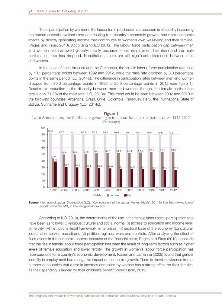
34 CEPAL Review N° 122 • August 2017
The progress and evolution of women’s participation in production and business activities in South America
Thus, participation by women in the labour force produces macroeconomic effects by increasing the human potential available and contributing to a country’s economic growth, and microeconomic effects by directly generating income that contributes to women’s own well-being and their families’ (Pagés and Piras, 2010). According to ILO (2012), the labour force participation gap between men and women has narrowed globally, mainly because female employment has risen and the male participation rate has dropped. Nonetheless, there are still significant differences between men and women.
In the case of Latin America and the Caribbean, the female labour force participation rate rose by 10.1 percentage points between 1992 and 2012, while the male rate dropped by 3.0 percentage points in the same period (ILO, 2014b). The difference in participation rates between men and women dropped from 39.0 percentage points in 1992 to 25.9 percentage points in 2012 (see figure 1). Despite this reduction in the disparity between men and women, though, the female participation rate is only 71.2% of the male rate (ILO, 2013a). This trend could be seen between 2002 and 2010 in the following countries: Argentina, Brazil, Chile, Colombia, Paraguay, Peru, the Plurinational State of Bolivia, Suriname and Uruguay (ILO, 2014c).
Figure 1 Latin America and the Caribbean: gender gap in labour force participation rates, 1992-2012
(Percentages)
82.5 80.3 80 80.2 80.2 80.1 79.9 80 79.7 79.8 79.6 79.5
43.5
49.6 49.8 50.8 51.3 51.5 51.7 52.1 52.6 53.1 53.3 53.6
39
30.7 30.2 29.4 28.9 28.6 28.1 27.9 27.1 26.7 26.3 25.9
0
10
20
30
40
50
60
70
80
90
1992 2002 2003 2004 2005 2006 2007 2008 2009 2010 2011 2012
Male Female Gap
Source: International Labour Organization (ILO), “Key Indicators of the Labour Market (KILM)”, 2014 [online] http://www.ilo.org/empelm/what/WCMS_114240/lang--en/index.htm.
According to ILO (2010), the determinants of the rise in the female labour force participation rate have been as follows: (i) religious, cultural and social norms, (ii) access to education and income level, (iii) fertility, (iv) institutions (legal framework, enterprises), (v) sectoral base of the economy (agricultural, industrial or service-based) and (vi) political regimes, wars and conflicts. After analysing the effect of fluctuations in the economic context because of the financial crisis, Pagés and Piras (2010) conclude that the rise in female labour force participation has been the result of long-term factors such as higher levels of female education and lower fertility. The growth in women’s labour force participation has repercussions for a country’s economic development. Klasen and Lamanna (2009) found that gender inequity in employment had a negative impact on economic growth. There is likewise evidence from a number of countries that a rise in incomes controlled by women has a strong effect on their families, as their spending is largely for their children’s benefit (World Bank, 2012).

35CEPAL Review N° 122 • August 2017
Beatrice E. Avolio and Giovanna F. Di Laura
2. Unemployment
The unemployment rate is the proportion of the working-age population seeking work but unable to find it (Ministry of Labour and Employment Promotion, 2014).3 The global unemployment rate tended to decrease until 2007, but rose in 2008 because of the international financial crisis (ILO, 2014b). This crisis affected the unemployment rate worldwide, but especially in regions where the gender gap in unemployment was almost nil or the rate was actually lower for women. In Latin America and the Caribbean, ILO (2013a) indicates that the female unemployment rate is higher than the male rate by an average factor of 1.35. The female unemployment rate has consistently been higher than the male rate for the last two decades (see figure 2). Although this is a substantial disparity, it has diminished in recent years.
Figure 2 Latin America and the Caribbean (16 countries): ratio between the female and male
unemployment rates, 1990-2012
1990
1991
1992
1993
1994
1995
1996
1997
1998
1999
2000
2001
2002
2003
2004
2005
2006
2007
2008
2009
2010
2011
2012
1.05
1.10
1.15
1.20
1.25
1.30
1.35
1.40
1.45
1.50
Source: International Labour Organization (ILO), 2013 Labour Overview. Latin America and the Caribbean, Lima, ILO Regional Office for Latin America and the Caribbean, 2013.
Between 2002 and 2012, the female unemployment rate in South America fell by more than the male unemployment rate (see table 1). This trend has translated into greater female participation in employment and access to the economic benefits that active participation in paid work entails. Despite this progress, though, the female unemployment rate remains higher than the male rate. According to ILO (2012), the factors that might explain this gap include the greater prevalence of temporary employment among women, differences in education levels, labour market segregation and the tendency for women to leave the workforce for family reasons (such as childcare), which may make them less employable if they then return.
3 The working-age population includes everyone old enough to perform productive functions, covering all those aged over 14 (Ministry of Labour and Employment Promotion, 2014).

36 CEPAL Review N° 122 • August 2017
The progress and evolution of women’s participation in production and business activities in South America
Table 1 South America (selected countries): male and female urban unemployment rates,
2002, 2003, 2011 and 2012(Percentages)
Country Gender 2002 2003 2011 2012
ArgentinaMale 18.0 14.1 6.2 6.1
Female 17.6 18.7 8.5 8.8
Bolivia (Plurinational State of)Male 4.2 ... ... ...
Female 6.8 ... ... ...
BrazilMale 7.3 7.8 ... 4.4
Female 11.5 12.3 ... 6.8
ChileMale 8.6 7.9 6.1 5.4
Female 9.6 9.7 8.7 7.9
ColombiaMale 11.6 9.2 ... 9.4
Female 18.8 15.8 ... 13.2
EcuadorMale 5.8 9.0 ... 4.5
Female 13.9 15.0 ... 5.5
GuyanaMale 20.9 21.2 17.2 ...
Female 29.2 28.5 25.7 ...
ParaguayMale 8.9 6.6 4.4 6.7
Female 13.6 10.0 7.4 9.9
PeruMale 8.3 9.0 5.8 5.4
Female 11.6 11.9 10.1 8.5
SurinameMale 9.9 ... ... ...
Female 20.4 ... ... ...
UruguayMale 13.5 13.5 4.5 5.3
Female 21.2 20.8 7.7 8.1
Venezuela (Bolivarian Republic of)Male 14.4 14.4 7.7 7.4
Female 18.8 20.3 9.3 9.0
Source: International Labour Organization (ILO), “Key Indicators of the Labour Market (KILM)”, 2014 [online] http://www.ilo.org/empelm/what/WCMS_114240/lang--en/index.htm.
3. The employment rate
A higher employment rate means greater participation in paid production activities, which have a greater impact on economic development than unpaid ones (ILO, 2014c).4 However, this indicator does not distinguish the quality of the work done, so the analysis of the distribution of the employed population needs to be extended by considering job characteristics.
The gap between men and women held steady at the global level until 2008, when it widened because of the international financial crisis. This was due to the contraction of the labour market and slower growth in the female employment rate across all regions (ILO, 2012). In South America, the female employment rate stagnated in 2009, probably because of the financial crisis. It began to recover in 2010, however, and there has been a continuing tendency for the gap between men and women to narrow, with the male employment rate growing by less than the female one (ILO, 2013a).
Although a rise in the employment rate signifies improvements in terms of opportunities to obtain work, there needs to be closer analysis of the type and quality of jobs available to women, as many of those newly in work may be underemployed (whether in terms of hours or income) or in jobs deemed vulnerable, a category that includes unpaid family workers and self-employed workers (whose earnings depend directly on their profits from the goods and services produced) (United Nations
4 The employment rate is the proportion of people employed in some economic activity relative to the whole population (Ministry of Labour and Employment Promotion, 2014).

37CEPAL Review N° 122 • August 2017
Beatrice E. Avolio and Giovanna F. Di Laura
Statistics Division/ECLAC, 2001).5 According to ILO (2012), over half of all female employment in 2012 was in vulnerable jobs (self-employment or family work), characterized by long working hours and poor conditions. Again according to ILO (2010), the proportion of workers in wage employment does not differ significantly between men and women at the global level. Female participation is greater in countries such as Argentina, the Bolivarian Republic of Venezuela, Brazil, Colombia, Guyana, Suriname and Uruguay (see figure 3). It is important to stress that the wage employment category includes both the fully employed and those who are underemployed in terms of income, so that this indicator covers all those with a fixed monthly income but does not distinguish whether this income is above or below the minimum living wage.
Figure 3 South America (selected countries): female and male employment rates, 2002 and 2010
(Percentages)
0 10.0 20.0 30.0 40.0 50.0 60.0 70.0 80.0 90.0
2002
2010
2002
2009
2002
2009
2002
2010
2002
2010
2002
2010
2002
2010
2002
2010
2002
2010
2002
2010
2002
2010
Argentina
Bolivia(Plur. State of)
Brazil
Chile
Colombia
Ecuador
Guyana
Paraguay
Peru
Uruguay
Venezuela(Bol. Rep. of)
Female Male
Source: International Labour Organization (ILO), “Key Indicators of the Labour Market (KILM)”, 2014 [online] http://www.ilo.org/empelm/what/WCMS_114240/lang--en/index.htm.
In Ecuador, Paraguay, Peru and the Plurinational State of Bolivia, the female self-employment rate is higher than the male rate. When the composition of self-employment is analysed, most women are found to be in the family worker and own-account worker categories (vulnerable employment). According to Otobe (2011), vulnerable employment is a feature of the informal urban economy and the rural economy and is characterized by low productivity, low pay and a lack of legal and social protection. Again, the ability of people in family jobs to negotiate their working conditions depends on power relations within the family, so that most women are in a subordinate position (ILO, 2012).
Thus, the increase in female labour market participation does not necessarily imply equity in terms of employment quality. Women are found to be more likely to go into jobs classified as vulnerable, as own-account workers or family workers. Workers in vulnerable jobs are less likely than others to have formal employment contracts, meaning they lack access to any social security system.
5 The International Standard Classification of Occupations distinguishes the following categories: employees, self-employed workers and unpaid family workers. The self-employed category includes employers, own-account workers and members of cooperatives. Vulnerable employment encompasses own-account workers and family workers (ILO, 2013b; United Nations Statistics Division/ECLAC, 2001).
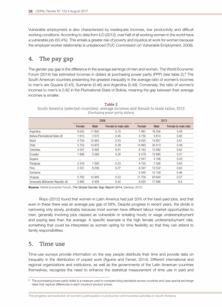
38 CEPAL Review N° 122 • August 2017
The progress and evolution of women’s participation in production and business activities in South America
Vulnerable employment is also characterized by inadequate incomes, low productivity and difficult working conditions. According to data from ILO (2012), over half of all working women in the world have a vulnerable job (50.4%). This entails a greater risk of poverty and injustice at work for women because the employer-worker relationship is unbalanced (TUC Commission on Vulnerable Employment, 2008).
4. The pay gap
The gender pay gap is the difference in the average earnings of men and women. The World Economic Forum (2014) has estimated incomes in dollars at purchasing power parity (PPP) (see table 2).6 The South American countries presenting the greatest inequality in the average ratio of women’s incomes to men’s are Guyana (0.43), Suriname (0.46) and Argentina (0.49). Conversely, the ratio of women’s incomes to men’s is 0.82 in the Plurinational State of Bolivia, meaning the gap between their average incomes is smaller.
Table 2 South America (selected countries): average incomes and female to male ratios, 2013
(Purchasing power parity dollars)
2006 2013
Female Male Female to male ratio Female Male Female to male ratio
Argentina 6 635 17 800 0.70 7 987 16 258 0.49
Bolivia (Plurinational State of) 1 615 3 573 0.45 4 750 5 814 0.82
Brazil 4 704 10 963 0.43 9 055 14 857 0.61
Chile 5 753 14 872 0.39 14 965 30 513 0.49
Colombia 4 557 8 892 0.51 8 163 13 092 0.62
Ecuador 1 696 5 569 0.30 6 579 12 895 0.51
Guyana ... ... ... 2 047 4 708 0.43
Paraguay 2 316 7 000 0.33 4 725 7 526 0.63
Peru 2 231 8 256 0.27 8 337 13 532 0.62
Suriname ... ... ... 5 540 12 159 0.46
Uruguay 5 763 10 950 0.53 11 734 20 644 0.57
Venezuela (Bolivarian Republic of) 2 890 6 929 0.42 9 025 17 896 0.5
Source: World Economic Forum, The Global Gender Gap Report 2014, Geneva, 2013.
Ñopo (2012) found that women in Latin America had just 33% of the best-paid jobs, and that even in these there was an average pay gap of 58%. Despite progress in recent years, the divide is narrowing only slowly, probably because most women have different labour market opportunities to men, generally involving jobs classed as vulnerable or entailing hourly or wage underemployment and paying less than the average. A specific example is the high female underemployment rate, something that could be interpreted as women opting for time flexibility so that they can attend to family responsibilities.
5. Time use
Time-use surveys provide information on the way people distribute their time and provide data on inequality in the distribution of unpaid work (Aguirre and Ferrari, 2014). Different international and regional organizations and institutions, as well as the governments of the Latin American countries themselves, recognize the need to enhance the statistical measurement of time use in paid and
6 The purchasing power parity dollar is a measure used to compare living standards across countries and uses special exchange rates that capture differences in each country’s product prices.
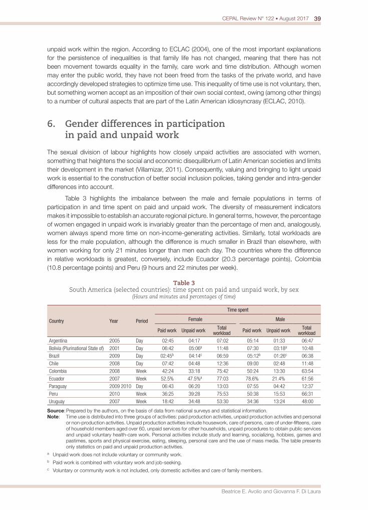
39CEPAL Review N° 122 • August 2017
Beatrice E. Avolio and Giovanna F. Di Laura
unpaid work within the region. According to ECLAC (2004), one of the most important explanations for the persistence of inequalities is that family life has not changed, meaning that there has not been movement towards equality in the family, care work and time distribution. Although women may enter the public world, they have not been freed from the tasks of the private world, and have accordingly developed strategies to optimize time use. This inequality of time use is not voluntary, then, but something women accept as an imposition of their own social context, owing (among other things) to a number of cultural aspects that are part of the Latin American idiosyncrasy (ECLAC, 2010).
6. Gender differences in participation in paid and unpaid work
The sexual division of labour highlights how closely unpaid activities are associated with women, something that heightens the social and economic disequilibrium of Latin American societies and limits their development in the market (Villamizar, 2011). Consequently, valuing and bringing to light unpaid work is essential to the construction of better social inclusion policies, taking gender and intra-gender differences into account.
Table 3 highlights the imbalance between the male and female populations in terms of participation in and time spent on paid and unpaid work. The diversity of measurement indicators makes it impossible to establish an accurate regional picture. In general terms, however, the percentage of women engaged in unpaid work is invariably greater than the percentage of men and, analogously, women always spend more time on non-income-generating activities. Similarly, total workloads are less for the male population, although the difference is much smaller in Brazil than elsewhere, with women working for only 21 minutes longer than men each day. The countries where the difference in relative workloads is greatest, conversely, include Ecuador (20.3 percentage points), Colombia (10.8 percentage points) and Peru (9 hours and 22 minutes per week).
Table 3 South America (selected countries): time spent on paid and unpaid work, by sex
(Hours and minutes and percentages of time)
Country Year Period
Time spent
Female Male
Paid work Unpaid work Total workload Paid work Unpaid work Total
workloadArgentina 2005 Day 02:45 04:17 07:02 05:14 01:33 06:47
Bolivia (Plurinational State of) 2001 Day 06:42 05:06a 11:48 07:30 03:18a 10:48
Brazil 2009 Day 02:45b 04:14c 06:59 05:12b 01:26c 06:38
Chile 2008 Day 07:42 04:48 12:36 09:00 02:48 11:48
Colombia 2008 Week 42:24 33:18 75:42 50:24 13:30 63:54
Ecuador 2007 Week 52.5% 47.5%a 77:03 78.6% 21.4% 61:56
Paraguay 2009 2010 Day 06:43 06:20 13:03 07:55 04:42 12:37
Peru 2010 Week 36:25 39:28 75:53 50:38 15:53 66:31
Uruguay 2007 Week 18:42 34:48 53:30 34:36 13:24 48:00
Source: Prepared by the authors, on the basis of data from national surveys and statistical information.Note: Time use is distributed into three groups of activities: paid production activities, unpaid production activities and personal
or non-production activities. Unpaid production activities include housework, care of persons, care of under-fifteens, care of household members aged over 60, unpaid services for other households, unpaid procedures to obtain public services and unpaid voluntary health-care work. Personal activities include study and learning, socializing, hobbies, games and pastimes, sports and physical exercise, eating, sleeping, personal care and the use of mass media. The table presents only statistics on paid and unpaid production activities.
a Unpaid work does not include voluntary or community work.b Paid work is combined with voluntary work and job-seeking.c Voluntary or community work is not included, only domestic activities and care of family members.

40 CEPAL Review N° 122 • August 2017
The progress and evolution of women’s participation in production and business activities in South America
As regards unpaid activities, the data show that the ones women devote most time to are domestic activities, followed by childcare and care of dependant persons. Considerable time is also spent on voluntary or community work. The most marked difference in time spent on unpaid activities by gender is for domestic activities. The largest gap is in Peru, where women spend 16 hours and 38 minutes longer on these activities every week than men. Nonetheless, men spend more time than women on voluntary or community work in both Chile and Peru (see table 4).
Table 4 South America (selected countries): time spent on activities classified as unpaid work, by sex
(Hours and minutes)
Country Survey periodFemale Male
Childcare Care of dependant persons
Domestic activitiesa Childcare Care of
dependant personsDomestic activitiesa
Argentina Day 00:58 03:03 00:22 01:06
Brazil Day 02:13 04:10 01:39 02:22
Chile Day 02:36 03:54 01:30 02:36
Colombia Week 26:18 22:06 24:00 14:30 13:42 09:30
Paraguay Day 04:29 02:32
Peru Week 12:14 16:47 37:28 05:49 08:55 20:50
Uruguay Week 17:48 28:36 10:06 12:30
Source: Prepared by the authors, on the basis of data from national surveys and statistical information.a By domestic activities is strictly meant work done for the benefit of the household.
III. Women’s participation in managerial and executive positions
Women account for about 1.3 billion of the 3.3 billion people (39.9%) making up the global labour force (ILO, 2012). Global labour force participation rates are 76.7% for men and 50.3% for women (ILO, 2014a). In Latin America and the Caribbean, female participation in the labour force has increased progressively and steadily, rising from 43.5% in 1992 to 49.6% in 2002 and 52.6% in 2012, while male participation dropped from 82.5% in 1992 to 80.3% in 2002 and 79.5% in 2012 (ILO, 2012). This increase in female labour force participation can be explained by the combined effect of economic development, higher levels of education, lower fertility rates, technological development (which means less time has to be spent on housework) and structural shifts that have permitted a reduction in transaction costs and time use (Goldin, 2006). However, time-use inequities are still a critical factor for female labour force participation (ILO, 2012).
Despite this increase in their labour force participation, women are considerably less likely than men to hold upper management jobs and other positions of responsibility. Although statistics are few, information provided by Grant Thornton (2016) indicates that women’s share of managerial posts worldwide is 24%. Regionally, Eastern Europe is in first place (35%), followed by Africa (27%), emerging countries in the Asia and the Pacific region (26%), the European Union (24%), North America (23%) and Latin America (18%).
In Latin America, women’s share of managerial posts ranges from 23% in Mexico down to 16% in Argentina. Furthermore, 53% of firms in the region have no women at all in their management teams, a proportion that is well above the global average of 32% (Grant Thornton, 2015b). The country in the region where the largest share of firms has women in upper management positions is the Bolivarian Republic of Venezuela (31%), while such firms make up just 5% of the total in Chile (World Economic Forum, 2014) (see table 5).
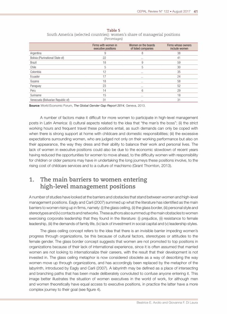
41CEPAL Review N° 122 • August 2017
Beatrice E. Avolio and Giovanna F. Di Laura
Table 5 South America (selected countries): women’s share of managerial positions
(Percentages)
Firms with women in executive positions
Women on the boards of listed companies
Firms whose owners include women
Argentina 9 8 38
Bolivia (Plurinational State of) 22 ... 41
Brazil 18 9 59
Chile 5 5 30
Colombia 12 ... 35
Ecuador 17 ... 24
Guyana 18 ... 58
Paraguay 23 ... 52
Peru 14 6 29
Suriname 15 ... 18
Venezuela (Bolivarian Republic of) 31 ... 31
Source: World Economic Forum, The Global Gender Gap Report 2014, Geneva, 2013.
A number of factors make it difficult for more women to participate in high-level management posts in Latin America: (i) cultural aspects related to the idea that “the man’s the boss”; (ii) the strict working hours and frequent travel these positions entail, as such demands can only be coped with when there is strong support at home with childcare and domestic responsibilities; (iii) the excessive expectations surrounding women, who are judged not only on their working performance but also on their appearance, the way they dress and their ability to balance their work and personal lives. The lack of women in executive positions could also be due to the economic slowdown of recent years having reduced the opportunities for women to move ahead, to the difficulty women with responsibility for children or older persons may have in undertaking the long journeys these positions involve, to the rising cost of childcare services and to a culture of machismo (Grant Thornton, 2013).
1. The main barriers to women entering high-level management positions
A number of studies have looked at the barriers and obstacles that stand between women and high-level management positions. Eagly and Carli (2007) summed up what the literature has identified as the main barriers to women rising up in firms, namely: (i) the glass ceiling, (ii) the glass border, (iii) personal style and stereotypes and (iv) contacts and networks. These authors also summed up the main obstacles to women exercising corporate leadership that they found in the literature: (i) prejudice, (ii) resistance to female leadership, (iii) the demands of family life, (iv) lack of investment in social capital and (v) leadership styles.
The glass ceiling concept refers to the idea that there is an invisible barrier impeding women’s progress through organizations, be this because of cultural factors, stereotypes or attitudes to the female gender. The glass border concept suggests that women are not promoted to top positions in organizations because of their lack of international experience, since it is often assumed that married women are not looking to internationalize their careers, with the result that their development is not invested in. The glass ceiling metaphor is now considered obsolete as a way of describing the way women move up through organizations, and has accordingly been replaced by the metaphor of the labyrinth, introduced by Eagly and Carli (2007). A labyrinth may be defined as a place of intersecting and branching paths that has been made deliberately convoluted to confuse anyone entering it. This image better illustrates the situation of women executives in the world of work, for although men and women theoretically have equal access to executive positions, in practice the latter have a more complex journey to their goal (see figure 4).

42 CEPAL Review N° 122 • August 2017
The progress and evolution of women’s participation in production and business activities in South America
Figure 4 The labyrinth facing female executives
Female executive
Leadership styles
Lack of investment in social capital
Demands offamily life
Resistanceto femaleleadership
Prejudices
Contacts andnetworks
StereotypesGlass borderGlass ceiling
Source: Prepared by the authors.
Where personal style and stereotypes are concerned, it is much harder for women in managerial positions to find a personal management style than it is for men, as women may be perceived as aggressive if they behave like male colleagues but feminine if they take the opposite approach. Contacts and networks are a potential source of employment opportunities. However, women in high-level management positions often feel alone at the top of organizations (because they are the only women), and this makes it difficult for them to forge and maintain contacts.
Prejudices about women playing a leadership role still persist among a section of the population who see this as breaking with the tradition of male leadership. These prejudices directly affect women trying to make their way to executive positions within a firm, as they are paid less or rise up more slowly than male peers at a similar level, despite having equivalent professional qualifications. Resistance to female leadership comes about because of a long-standing tradition that associates the characteristics expected of a leader more with men than with women. The features attributed to women include being friendly, sensitive, kind, charitable and compassionate, while men tend to be considered assertive, ambitious, aggressive and self-assured. Thus, women are associated with communal qualities and men with agentic ones, it being with the latter that people usually associate leaders.
As for the demands of family life, family responsibilities are indeed one of the greatest barriers for most women, as household tasks are not shared out equitably. Because women bear the bulk of family responsibilities, they continue to be the ones who take career breaks, have more days off or work part-time. As a result, they have less experience and accumulate fewer hours of work per year, so that their careers develop more slowly and they earn less. As for the lack of investment in social capital, it has been observed that the managers whose careers progress most rapidly invest more time and effort in socializing, politicking and interacting with others, while those who take longer to rise concentrate on the traditional management activities of planning, organization, direction and oversight. The various statistics on time use in paid and unpaid activities bear this out.
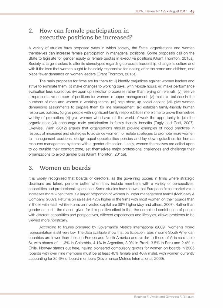
43CEPAL Review N° 122 • August 2017
Beatrice E. Avolio and Giovanna F. Di Laura
2. How can female participation in executive positions be increased?
A variety of studies have proposed ways in which society, the State, organizations and women themselves can increase female participation in managerial positions. Some proposals call on the State to legislate for gender equity or female quotas in executive positions (Grant Thornton, 2015a). Society at large is asked to alter its stereotypes regarding corporate leadership, change its culture and with it the idea that women ought to be solely responsible for looking after the home and children, and place fewer demands on women leaders (Grant Thornton, 2015a).
The main proposals for firms are for them to: (i) identify prejudices against women leaders and strive to eliminate them; (ii) make changes to working days, with flexible hours; (iii) make performance evaluation less subjective; (iv) open up selection processes rather than relying on referrals; (v) reserve a representative number of positions for women in upper management; (vi) maintain balance in the numbers of men and women in working teams; (vii) help shore up social capital; (viii) give women demanding assignments to prepare them for line management; (ix) establish family-friendly human resources policies; (x) give people with significant family responsibilities more time to prove themselves worthy of promotion; (xi) give women who have left the world of work the opportunity to join the organization; (xii) encourage male participation in family-friendly benefits (Eagly and Carli, 2007). Likewise, Wirth (2012) argues that organizations should provide examples of good practices in respect of measures and strategies to advance women, formulate strategies to promote more women to management positions, design equal opportunities policies and lay down guidelines for human resource management systems with a gender dimension. Lastly, women themselves are called upon to go outside their comfort zone, set themselves major professional challenges and challenge their organizations to avoid gender bias (Grant Thornton, 2015a).
3. Women on boards
It is widely recognized that boards of directors, as the governing bodies in firms where strategic decisions are taken, perform better when they include members with a variety of perspectives, capabilities and professional experience. Some studies have shown that European firms’ market value increases more when there is a larger proportion of women in upper management teams (McKinsey & Company, 2007). Returns on sales are 42% higher in the firms with most women on their boards than in those with least, while returns on invested capital are 66% higher (Joy and others, 2007). Rather than gender as such, the reason given for this positive effect is that the combined contribution of people with different capabilities and perspectives, different experiences and lifestyles, allows problems to be viewed more holistically.
According to figures prepared by Governance Metrics International (2009), women’s board representation is still very low. The data available show that participation rates in some South American countries are lower than those in Europe and North America and similar to those of Asia (see table 6), with shares of 11.3% in Colombia, 4.1% in Argentina, 3.9% in Brazil, 3.5% in Peru and 2.4% in Chile. Norway stands out here, having pioneered compulsory quotas for women on boards in 2005 (boards with over nine members must be at least 40% female and 40% male), with women currently accounting for 35.6% of board members (Governance Metrics International, 2009).
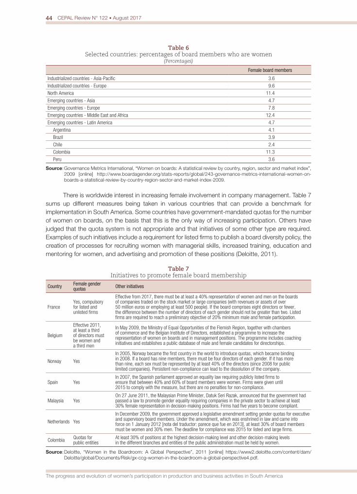
44 CEPAL Review N° 122 • August 2017
The progress and evolution of women’s participation in production and business activities in South America
Table 6 Selected countries: percentages of board members who are women
(Percentages)
Female board members
Industrialized countries - Asia-Pacific 3.6
Industrialized countries - Europe 9.6
North America 11.4
Emerging countries - Asia 4.7
Emerging countries - Europe 7.8
Emerging countries - Middle East and Africa 12.4
Emerging countries - Latin America 4.7
Argentina 4.1
Brazil 3.9
Chile 2.4
Colombia 11.3
Peru 3.6
Source: Governance Metrics International, “Women on boards: A statistical review by country, region, sector and market index”, 2009 [online] http://www.boardagender.org/stats-reports/global/243-governance-metrics-international-women-on-boards-a-statistical-review-by-country-region-sector-and-market-index-2009.
There is worldwide interest in increasing female involvement in company management. Table 7 sums up different measures being taken in various countries that can provide a benchmark for implementation in South America. Some countries have government-mandated quotas for the number of women on boards, on the basis that this is the only way of increasing participation. Others have judged that the quota system is not appropriate and that initiatives of some other type are required. Examples of such initiatives include a requirement for listed firms to publish a board diversity policy, the creation of processes for recruiting women with managerial skills, increased training, education and mentoring for women, and advertising and promotion of these positions (Deloitte, 2011).
Table 7 Initiatives to promote female board membership
Country Female gender quotas Other initiatives
FranceYes, compulsory for listed and unlisted firms
Effective from 2017, there must be at least a 40% representation of women and men on the boards of companies traded on the stock market or large companies (with revenues or assets of over 50 million euros or employing at least 500 people). If the board comprises eight directors or fewer, the difference between the number of directors of each gender should not be greater than two. Listed firms are required to reach a preliminary objective of 20% minimum male and female participation.
Belgium
Effective 2011, at least a third of directors must be women and a third men
In May 2009, the Ministry of Equal Opportunities of the Flemish Region, together with chambers of commerce and the Belgian Institute of Directors, established a programme to increase the representation of women on boards and in management positions. The programme includes coaching initiatives and establishes a public database of male and female candidates for directorships.
Norway Yes
In 2005, Norway became the first country in the world to introduce quotas, which became binding in 2008. If a board has nine members, there must be four directors of each gender. If it has more than nine, each sex must be represented by at least 40% of the directors (since 2008 for public limited companies). Persistent non-compliance can lead to the dissolution of the company.
Spain YesIn 2007, the Spanish parliament approved an equality law requiring publicly listed firms to ensure that between 40% and 60% of board members were women. Firms were given until 2015 to comply with the measure, but there are no penalties for non-compliance.
Malaysia YesOn 27 June 2011, the Malaysian Prime Minister, Datuk Seri Razak, announced that the government had passed a law to promote gender equality requiring companies in the private sector to achieve at least 30% female representation in decision-making positions. Firms had five years to become compliant.
Netherlands Yes
In December 2009, the government approved a legislative amendment setting gender quotas for executive and supervisory board members. Under the amendment, which was enshrined in law and came into force on 1 January 2012 [nota del traductor: parece que fue en 2013], at least 30% of board members must be women and 30% men. The deadline for compliance was 2015 for listed and large firms.
Colombia Quotas for public entities
At least 30% of positions at the highest decision-making level and other decision-making levels in the different branches and entities of the public administration must be held by women.
Source: Deloitte, “Women in the Boardroom: A Global Perspective”, 2011 [online] https://www2.deloitte.com/content/dam/Deloitte/global/Documents/Risk/gx-ccg-women-in-the-boardroom-a-global-perspective4.pdf.
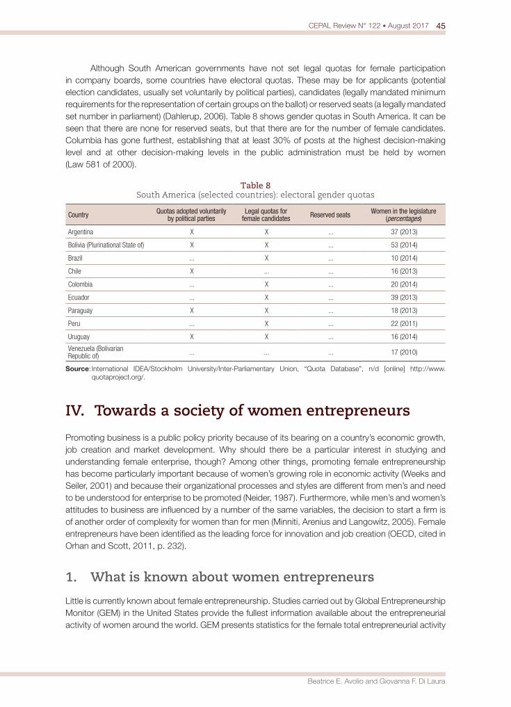
45CEPAL Review N° 122 • August 2017
Beatrice E. Avolio and Giovanna F. Di Laura
Although South American governments have not set legal quotas for female participation in company boards, some countries have electoral quotas. These may be for applicants (potential election candidates, usually set voluntarily by political parties), candidates (legally mandated minimum requirements for the representation of certain groups on the ballot) or reserved seats (a legally mandated set number in parliament) (Dahlerup, 2006). Table 8 shows gender quotas in South America. It can be seen that there are none for reserved seats, but that there are for the number of female candidates. Columbia has gone furthest, establishing that at least 30% of posts at the highest decision-making level and at other decision-making levels in the public administration must be held by women (Law 581 of 2000).
Table 8 South America (selected countries): electoral gender quotas
Country Quotas adopted voluntarily by political parties
Legal quotas for female candidates Reserved seats Women in the legislature
(percentages)
Argentina X X ... 37 (2013)
Bolivia (Plurinational State of) X X ... 53 (2014)
Brazil ... X ... 10 (2014)
Chile X ... ... 16 (2013)
Colombia ... X ... 20 (2014)
Ecuador ... X ... 39 (2013)
Paraguay X X ... 18 (2013)
Peru ... X ... 22 (2011)
Uruguay X X ... 16 (2014)
Venezuela (Bolivarian Republic of) ... ... ... 17 (2010)
Source: International IDEA/Stockholm University/Inter-Parliamentary Union, “Quota Database”, n/d [online] http://www.quotaproject.org/.
IV. Towards a society of women entrepreneurs
Promoting business is a public policy priority because of its bearing on a country’s economic growth, job creation and market development. Why should there be a particular interest in studying and understanding female enterprise, though? Among other things, promoting female entrepreneurship has become particularly important because of women’s growing role in economic activity (Weeks and Seiler, 2001) and because their organizational processes and styles are different from men’s and need to be understood for enterprise to be promoted (Neider, 1987). Furthermore, while men’s and women’s attitudes to business are influenced by a number of the same variables, the decision to start a firm is of another order of complexity for women than for men (Minniti, Arenius and Langowitz, 2005). Female entrepreneurs have been identified as the leading force for innovation and job creation (OECD, cited in Orhan and Scott, 2011, p. 232).
1. What is known about women entrepreneurs
Little is currently known about female entrepreneurship. Studies carried out by Global Entrepreneurship Monitor (GEM) in the United States provide the fullest information available about the entrepreneurial activity of women around the world. GEM presents statistics for the female total entrepreneurial activity

46 CEPAL Review N° 122 • August 2017
The progress and evolution of women’s participation in production and business activities in South America
(TEA) rate and defines enterprise as “any attempt of new businesses or creation of new enterprises, such as self-employment, reorganization of a business, or the expansion of an already existing business by an individual, group of individuals or an already established enterprise” (Serida and others, 2005, p. 13).7 According to the Global Report (Roland, Kelley and Kew, 2012), TEA rates tend to be higher in countries with lower gross output per capita, where more enterprise is driven by economic need. Countries with higher gross output present lower levels of enterprise but a higher proportion of opportunity-driven entrepreneurial initiatives.
The findings indicate that the female TEA rate varies significantly across the 61 countries studied, from 41% in Zambia to 1% in Suriname. In Latin America, the highest female TEA rate is found in Ecuador (33%), followed by Peru, the Plurinational State of Bolivia and Chile (see figure 5). The male TEA rate is higher than the female one in all cases (Kelley and others, 2015).
The same study analyses women’s motives for becoming entrepreneurs. Entrepreneurship is considered opportunity-driven when people decide to start their own venture or firm as a desirable career development option and it reflects a desire to take advantage of a business opportunity. Entrepreneurship is considered necessity-driven when people start ventures or firms because they have no other work options, or the ones they do have are unsatisfactory. The results for Latin America are very interesting, as there prove to be more opportunity-driven than necessity-driven female entrepreneurs in all the countries examined. The opportunity-driven TEA rate is 78% in Uruguay, 71% in Chile and the Plurinational State of Bolivia, 69% in Peru, 68% in Ecuador, 61% in Brazil and 59% in Colombia and Argentina (Kelley and others, 2015).
Figure 5 Entrepreneurial activity rate
(Percentages)
0
5
10
15
20
25
30
35
Arge
ntin
a
Braz
il
Chile
Colo
mbi
a
Ecua
dor
Peru
Urug
uay
Latin
Am
eric
aan
d th
e Ca
ribbe
an
Cent
ral a
ndNo
rther
n As
ia
Sout
hern
Afri
ca
Deve
lopi
ng A
sia
Deve
lope
d As
ia
Deve
lopi
ng E
urop
e
Deve
lope
d Eu
rope
Unite
d St
ates
7 The TEA rate measures the percentage of adults aged between 18 and 64 who are full or part owners of a business that has been in existence for less than 42 months, including both start-ups and new firms. A firm is considered to be a start-up if the women owning all or part of the business state that they have been paying remuneration for less than 3 months or have taken concrete steps to bring a business into operation. A firm is considered new if the women owning all or part of it and actively running it have been paying remuneration for more than 3 but less than 42 months.
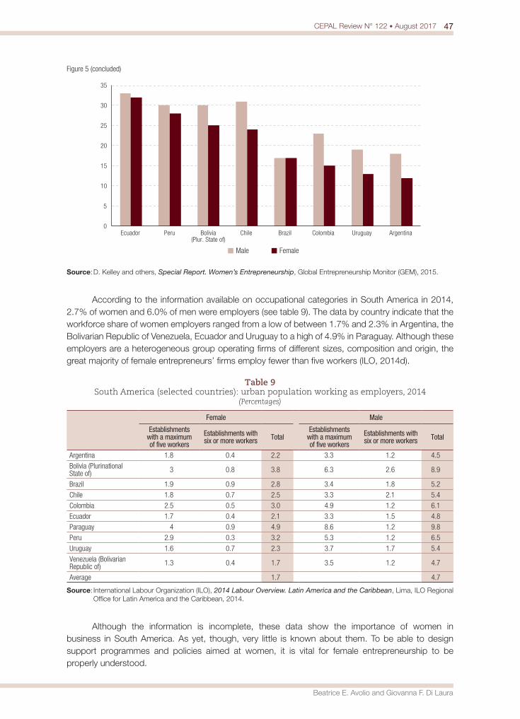
47CEPAL Review N° 122 • August 2017
Beatrice E. Avolio and Giovanna F. Di Laura
0
5
10
15
20
25
30
35
Ecuador Peru Bolivia(Plur. State of)
Chile Brazil Colombia Uruguay Argentina
Male Female
Source: D. Kelley and others, Special Report. Women’s Entrepreneurship, Global Entrepreneurship Monitor (GEM), 2015.
According to the information available on occupational categories in South America in 2014, 2.7% of women and 6.0% of men were employers (see table 9). The data by country indicate that the workforce share of women employers ranged from a low of between 1.7% and 2.3% in Argentina, the Bolivarian Republic of Venezuela, Ecuador and Uruguay to a high of 4.9% in Paraguay. Although these employers are a heterogeneous group operating firms of different sizes, composition and origin, the great majority of female entrepreneurs’ firms employ fewer than five workers (ILO, 2014d).
Table 9 South America (selected countries): urban population working as employers, 2014
(Percentages)
Female Male
Establishments with a maximum of five workers
Establishments with six or more workers Total
Establishments with a maximum of five workers
Establishments with six or more workers Total
Argentina 1.8 0.4 2.2 3.3 1.2 4.5
Bolivia (Plurinational State of) 3 0.8 3.8 6.3 2.6 8.9
Brazil 1.9 0.9 2.8 3.4 1.8 5.2
Chile 1.8 0.7 2.5 3.3 2.1 5.4
Colombia 2.5 0.5 3.0 4.9 1.2 6.1
Ecuador 1.7 0.4 2.1 3.3 1.5 4.8
Paraguay 4 0.9 4.9 8.6 1.2 9.8
Peru 2.9 0.3 3.2 5.3 1.2 6.5
Uruguay 1.6 0.7 2.3 3.7 1.7 5.4
Venezuela (Bolivarian Republic of) 1.3 0.4 1.7 3.5 1.2 4.7
Average 1.7 4.7
Source: International Labour Organization (ILO), 2014 Labour Overview. Latin America and the Caribbean, Lima, ILO Regional Office for Latin America and the Caribbean, 2014.
Although the information is incomplete, these data show the importance of women in business in South America. As yet, though, very little is known about them. To be able to design support programmes and policies aimed at women, it is vital for female entrepreneurship to be properly understood.
Figure 5 (concluded)
48 CEPAL Review N° 122 • August 2017
The progress and evolution of women’s participation in production and business activities in South America
2. The profile of women entrepreneurs
Because entrepreneurship requires people capable of identifying opportunities and willing to take more risks than others, it is very important to analyse the motives and inducements leading them to take this path. These motives have traditionally been characterized using the economic necessity or vocation model. However, Avolio (2008) argues that this model is too simple to characterize women entrepreneurs in Latin America.
In a study of women entrepreneurs in Peru, Avolio (2008) found that they presented a variety of demographic, educational and working profiles and were not a homogeneous group, which meant that they ought not to be treated as a single category, as is usually done in business support programmes aimed at them. According to Avolio (2008), programmes to support female entrepreneurship should start with a diagnosis that recognizes the diversity of their backgrounds. The author puts forward a conceptual framework that explains the profile of women entrepreneurs by the stage of their working and personal lives at which they opt for entrepreneurship (since women start businesses at different points in their lives and this affects the type of business and their particular approach to owning firms) and the factors leading them to do so. Her study identifies six profiles of women entrepreneurs, reflecting the different paths to entrepreneurship, which she calls: young women with working opportunities, rising women with external constraints, consolidated women with curtailed careers, natural young women, developing rising women, and consolidated women in late career.
Avolio (2008) also found that women entrepreneurs had a variety of educational backgrounds and that the type of educational experience they had prior to becoming entrepreneurs did not seem to be a determining factor in the nature of the firm they owned. As regards their employment background, the same study found that women entrepreneurs tended to have had a variety of work experience in different sectors before starting their businesses, and that the decision to set up a firm was apparently influenced by this prior experience or by personal interests. As regards family background, the study indicates that the parents’ work seems to be a factor in the decision to start a business, as women entrepreneurs often come from families in which the parents have been entrepreneurs or self-employed.
The same study establishes that women set store by the financial and emotional support they receive to develop their businesses, mainly from their spouses or partners and from family members. The main obstacles that women generally face are intrinsic to their businesses and not peculiar to their gender. However, the major gender obstacle for women entrepreneurs is the traditional division of roles in the home, which assigns women the main responsibility for childcare and housework even as they carry out economically productive work, owing to the strength of cultural patterns where women’s role in society is concerned. This requires women entrepreneurs to devote themselves more than men to the demands of the home and simultaneously carry out a variety of tasks, something that can create strains in terms of time use or conflicts between their roles as mother and entrepreneur.
Heller (2010) found that women entrepreneurs in Latin America tended to be concentrated in urban areas in most of the region’s countries, were married or cohabiting, and had high levels of education. Almost half (46%) were aged between 30 and 45, while the involvement of young women aged under 30 (16%) suggested a potential for future enterprise. The great majority (70%) were owners or partners of microenterprises (establishments with up to six workers), with a smaller proportion being owners or partners of small and medium-sized enterprises. They were concentrated primarily in service sectors, commerce and the hotel and restaurant trade. The main difficulties they encountered were: lack of experience of business and trading, inadequate specific business training (administration and marketing), barriers in access to credit and financing, obstacles in access to sales networks, and excessive bureaucracy and paperwork when setting up a firm.
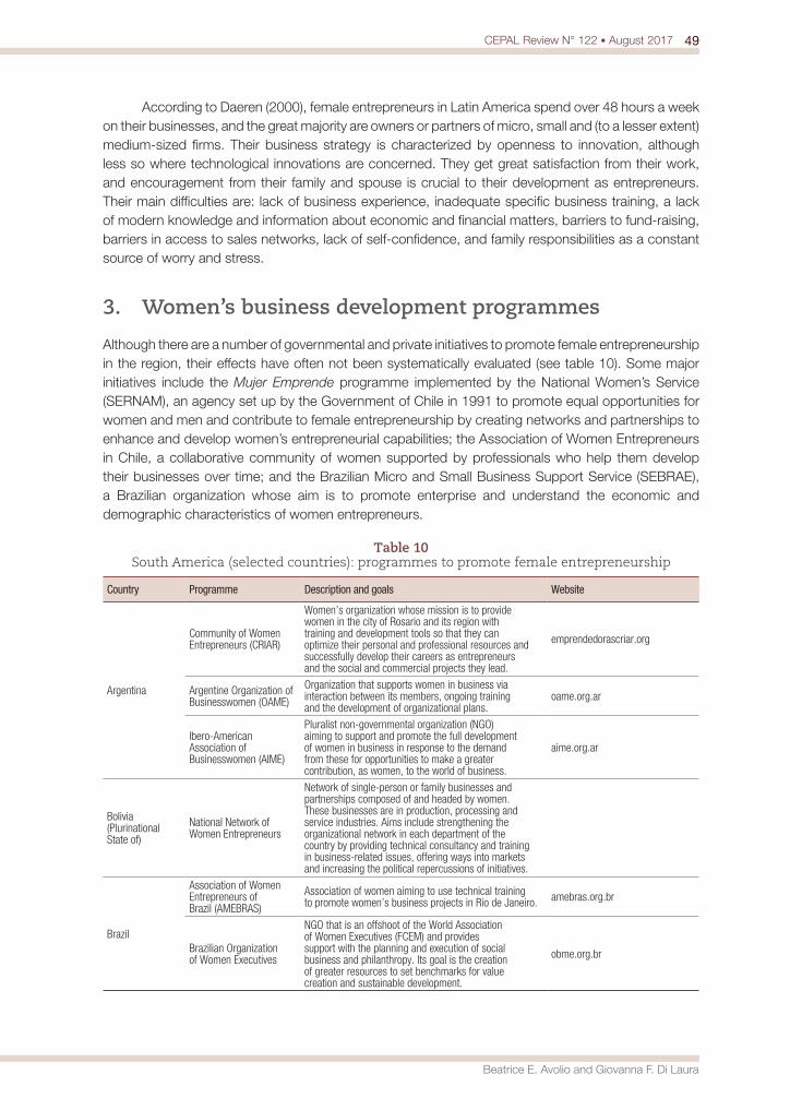
49CEPAL Review N° 122 • August 2017
Beatrice E. Avolio and Giovanna F. Di Laura
According to Daeren (2000), female entrepreneurs in Latin America spend over 48 hours a week on their businesses, and the great majority are owners or partners of micro, small and (to a lesser extent) medium-sized firms. Their business strategy is characterized by openness to innovation, although less so where technological innovations are concerned. They get great satisfaction from their work, and encouragement from their family and spouse is crucial to their development as entrepreneurs. Their main difficulties are: lack of business experience, inadequate specific business training, a lack of modern knowledge and information about economic and financial matters, barriers to fund-raising, barriers in access to sales networks, lack of self-confidence, and family responsibilities as a constant source of worry and stress.
3. Women’s business development programmes
Although there are a number of governmental and private initiatives to promote female entrepreneurship in the region, their effects have often not been systematically evaluated (see table 10). Some major initiatives include the Mujer Emprende programme implemented by the National Women’s Service (SERNAM), an agency set up by the Government of Chile in 1991 to promote equal opportunities for women and men and contribute to female entrepreneurship by creating networks and partnerships to enhance and develop women’s entrepreneurial capabilities; the Association of Women Entrepreneurs in Chile, a collaborative community of women supported by professionals who help them develop their businesses over time; and the Brazilian Micro and Small Business Support Service (SEBRAE), a Brazilian organization whose aim is to promote enterprise and understand the economic and demographic characteristics of women entrepreneurs.
Table 10 South America (selected countries): programmes to promote female entrepreneurship
Country Programme Description and goals Website
Argentina
Community of Women Entrepreneurs (CRIAR)
Women’s organization whose mission is to provide women in the city of Rosario and its region with training and development tools so that they can optimize their personal and professional resources and successfully develop their careers as entrepreneurs and the social and commercial projects they lead.
emprendedorascriar.org
Argentine Organization of Businesswomen (OAME)
Organization that supports women in business via interaction between its members, ongoing training and the development of organizational plans.
oame.org.ar
Ibero-American Association of Businesswomen (AIME)
Pluralist non-governmental organization (NGO) aiming to support and promote the full development of women in business in response to the demand from these for opportunities to make a greater contribution, as women, to the world of business.
aime.org.ar
Bolivia (Plurinational State of)
National Network of Women Entrepreneurs
Network of single-person or family businesses and partnerships composed of and headed by women. These businesses are in production, processing and service industries. Aims include strengthening the organizational network in each department of the country by providing technical consultancy and training in business-related issues, offering ways into markets and increasing the political repercussions of initiatives.
Brazil
Association of Women Entrepreneurs of Brazil (AMEBRAS)
Association of women aiming to use technical training to promote women’s business projects in Rio de Janeiro. amebras.org.br
Brazilian Organization of Women Executives
NGO that is an offshoot of the World Association of Women Executives (FCEM) and provides support with the planning and execution of social business and philanthropy. Its goal is the creation of greater resources to set benchmarks for value creation and sustainable development.
obme.org.br
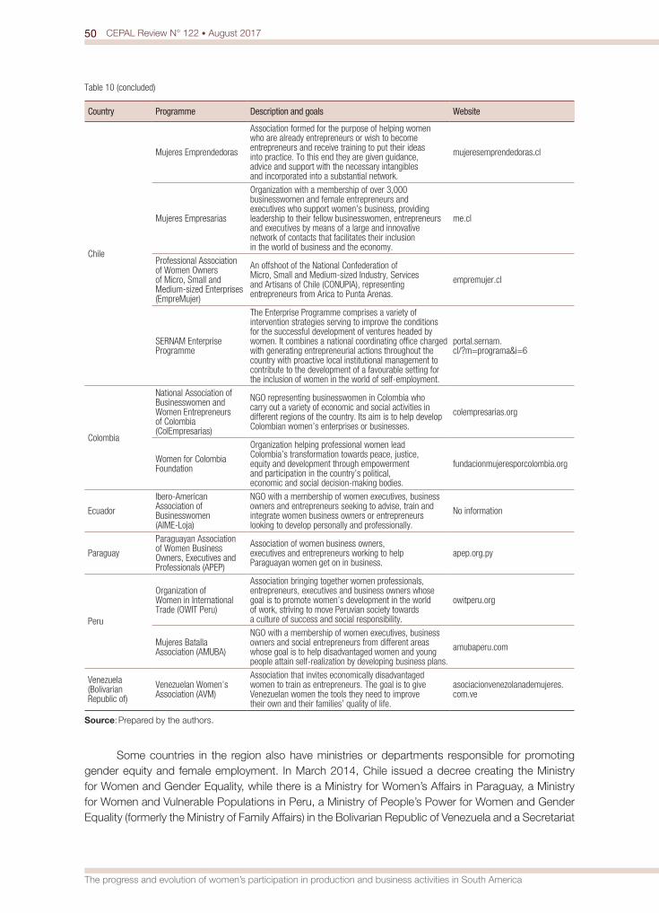
50 CEPAL Review N° 122 • August 2017
The progress and evolution of women’s participation in production and business activities in South America
Country Programme Description and goals Website
Chile
Mujeres Emprendedoras
Association formed for the purpose of helping women who are already entrepreneurs or wish to become entrepreneurs and receive training to put their ideas into practice. To this end they are given guidance, advice and support with the necessary intangibles and incorporated into a substantial network.
mujeresemprendedoras.cl
Mujeres Empresarias
Organization with a membership of over 3,000 businesswomen and female entrepreneurs and executives who support women’s business, providing leadership to their fellow businesswomen, entrepreneurs and executives by means of a large and innovative network of contacts that facilitates their inclusion in the world of business and the economy.
me.cl
Professional Association of Women Owners of Micro, Small and Medium-sized Enterprises (EmpreMujer)
An offshoot of the National Confederation of Micro, Small and Medium-sized Industry, Services and Artisans of Chile (CONUPIA), representing entrepreneurs from Arica to Punta Arenas.
empremujer.cl
SERNAM Enterprise Programme
The Enterprise Programme comprises a variety of intervention strategies serving to improve the conditions for the successful development of ventures headed by women. It combines a national coordinating office charged with generating entrepreneurial actions throughout the country with proactive local institutional management to contribute to the development of a favourable setting for the inclusion of women in the world of self-employment.
portal.sernam.cl/?m=programa&i=6
Colombia
National Association of Businesswomen and Women Entrepreneurs of Colombia (ColEmpresarias)
NGO representing businesswomen in Colombia who carry out a variety of economic and social activities in different regions of the country. Its aim is to help develop Colombian women’s enterprises or businesses.
colempresarias.org
Women for Colombia Foundation
Organization helping professional women lead Colombia’s transformation towards peace, justice, equity and development through empowerment and participation in the country’s political, economic and social decision-making bodies.
fundacionmujeresporcolombia.org
Ecuador
Ibero-American Association of Businesswomen (AIME-Loja)
NGO with a membership of women executives, business owners and entrepreneurs seeking to advise, train and integrate women business owners or entrepreneurs looking to develop personally and professionally.
No information
Paraguay
Paraguayan Association of Women Business Owners, Executives and Professionals (APEP)
Association of women business owners, executives and entrepreneurs working to help Paraguayan women get on in business.
apep.org.py
Peru
Organization of Women in International Trade (OWIT Peru)
Association bringing together women professionals, entrepreneurs, executives and business owners whose goal is to promote women’s development in the world of work, striving to move Peruvian society towards a culture of success and social responsibility.
owitperu.org
Mujeres Batalla Association (AMUBA)
NGO with a membership of women executives, business owners and social entrepreneurs from different areas whose goal is to help disadvantaged women and young people attain self-realization by developing business plans.
amubaperu.com
Venezuela (Bolivarian Republic of)
Venezuelan Women’s Association (AVM)
Association that invites economically disadvantaged women to train as entrepreneurs. The goal is to give Venezuelan women the tools they need to improve their own and their families’ quality of life.
asociacionvenezolanademujeres.com.ve
Source: Prepared by the authors.
Some countries in the region also have ministries or departments responsible for promoting gender equity and female employment. In March 2014, Chile issued a decree creating the Ministry for Women and Gender Equality, while there is a Ministry for Women’s Affairs in Paraguay, a Ministry for Women and Vulnerable Populations in Peru, a Ministry of People’s Power for Women and Gender Equality (formerly the Ministry of Family Affairs) in the Bolivarian Republic of Venezuela and a Secretariat
Table 10 (concluded)
51CEPAL Review N° 122 • August 2017
Beatrice E. Avolio and Giovanna F. Di Laura
on Policies for Women in Brazil, where a Ministry of Women, Racial Equality and Human Rights was also created in October 2015 as a provisional measure. There have not been initiatives of this kind in Argentina, Colombia, Ecuador, the Plurinational State of Bolivia or Uruguay.
4. Some proposals for developing women’s businesses
Following a review of the literature, we can now set out some practical recommendations for stimulating women’s capabilities, reducing the obstacles they face and thus increasing the chances that their business ventures will succeed:
(i) Create national business statistics that include information about gender aspects.
(ii) Develop specific support programmes for businesswomen that take account of their particular needs.
(iii) Develop a formal programme of female business mentors, with businesswomen providing mentoring to women who are just starting out in business.
(iv) Drawing on the experience of programmes implemented in other countries, include the following areas in programmes aimed at encouraging female entrepreneurship: advice and consultancy, training in company management, financing, information access and networking.
(v) Improve women’s business management capabilities by training them in specific subjects and developing their ability to find and attract the human capital they need to advance their businesses.
(vi) Train women to recognize their own shortcomings and recruit the people they need in areas they are unfamiliar with.
(vii) Facilitate access to credit through financing programmes, simplify the system of collateral and, most importantly, reduce the cost of loans for businesswomen.
(viii) Implement specific programmes to facilitate access to information about markets, new products, business development and management with a view to expanding women’s business opportunities.
(ix) Establish networks of contacts that enable women to share experiences with business people and professional organizations and increase their chances of successfully setting up businesses and going on to inspire others in turn. Networks of contacts and access to information expose women to a wider business environment and give them opportunities to increase their own business potential.
V. Final reflections
In recent years, the situation of women’s labour market participation in South America has undergone major shifts that have translated into greater female participation in economic and production activities. There has also been recognition of the importance of supporting women’s participation in the global economy as agents of development, benefiting not just their families but the wider community.
The purpose of this document is to examine the current situation and evolution of South American women’s participation in economic and production activities. Three areas of analysis are distinguished: women in the labour market, i.e., the type and quality of employment available to women; women’s participation in top executive positions, for example as managers or board members; and the characteristics of women business owners and their firms.
52 CEPAL Review N° 122 • August 2017
The progress and evolution of women’s participation in production and business activities in South America
Analysis of the different aspects of female employment, such as participation, supply and quality, is necessary for the design of effective public policies or development programmes in this area. There is general agreement about the importance of job creation, especially for the most vulnerable sections of society, on the grounds that participating in the labour market should help alleviate the vulnerability of poor and extremely poor women.
Progress for women in the labour market has included higher female labour force participation, a rising employment rate and even a drop in unemployment, while the gender gap has narrowed for these indicators. However, women remain disadvantaged in certain areas of economic participation. Although lower, their unemployment rate remains high. They earn less than men on average for the same work and are concentrated in low-paid occupations. Lastly, labour market participation does not necessarily mean women are fully employed, and in fact they are particularly likely to be underemployed, a situation that limits their economic and professional development.
Efforts should be made not only to create and stimulate employment, but to improve its quality and reduce vulnerable employment, for example through the formalization of family workers and the establishment of social and legal protections for people in vulnerable working situations. To reduce the segregation of female employment into lower-paid occupations, efforts are needed to do away with gender stereotypes and roles. This is essential to bring about equity in the labour market, as is investment in early programmes to interest women in science and mathematics and encourage them to participate in sectors such as mining and industry, among other areas traditionally considered male preserves.
Average income is another area in which there is a large divide favouring men. Although this divide has narrowed in recent years, greater efforts are needed to close it completely. One likely cause of this difference in income is the smaller number of hours women spend on paid work as they seek to balance this with family responsibilities and domestic tasks, among other things. Thus, although women engage less in paid work than men, their total workload is greater, mainly because of the time they spend on unpaid activities. There is a need to promote greater equity in the distribution of unpaid activities to increase women’s participation in paid ones. The introduction of care policies and the elimination of the gender stereotypes that facilitate the sexual division of labour are two options for this.
Women’s access to top executive positions is very limited, while they are almost absent from major boards of directors in South America. Proposals for boosting women’s access to these positions include combating prejudices about women leaders, making working hours more flexible, making performance evaluations less subjective, opening up selection processes, guaranteeing women a representative number of top executive positions, maintaining a balance between the numbers of men and women in working teams and establishing family-friendly human resources policies, among other things. Another important aspect for consideration is the need to provide women who have left the labour market with opportunities to rejoin it, as they are at a disadvantage and probably need to refresh their knowledge.
This document presents initiatives undertaken in some countries to promote women’s access to top executive positions, including quotas and the implementation of gender equity policies at private-sector firms. Colombia was the first country in South America to legislate for a system of gender quotas in high-level decision-making positions at public-sector organizations. In view of different countries’ experience, it is proposed that the establishment of quotas should be progressive and be matched by the introduction of high-quality gender policies at private-sector firms.
Lastly, the situation of women employers is analysed. The number of women owning their own firms is small compared to the number of men. Again, women’s firms are mostly small and do less well on average than their male-owned counterparts in profitability and performance terms. Among other factors, this is because women’s greater participation in unpaid activities prevents them from
53CEPAL Review N° 122 • August 2017
Beatrice E. Avolio and Giovanna F. Di Laura
devoting themselves so fully to their businesses. This again shows the need to promote an equitable division of domestic tasks and family care work, so that women can increase their participation in paid activities.
Female labour market participation would make a greater contribution to poverty eradication and the economic empowerment of women were it not for the persistent employment quality differences, wage gap, sexual division of domestic work and barriers to access to top executive positions. Legislation to increase women’s labour market participation worked by bringing about higher levels of education and greater control of fertility. Now it is important to establish policies and initiatives for narrowing the gender gap in employment quality and combating the prejudices and stereotypes that encourage people to assign particular roles to men and women and that limit women’s full participation in economic and production activities.
BibliographyAguirre, R. and F. Ferrari (2014), “Surveys on time use and unpaid work in Latin America and the Caribbean:
experience to date and challenges for the future”, Asuntos de Genero series, No. 122 (LC/L.3678/Rev.1), Santiago, Economic Commission for Latin America and the Caribbean (ECLAC).
Alba, A. (2007), “Uso del tiempo, Ecuador 2007”, presentation.Avolio, B. (2008), “El perfil de las mujeres empresarias en el Perú”, thesis, Lima, Catholic University of Peru.Daeren, L. (2000), “Mujeres empresarias en América Latina: el difícil equilibrio entre dos mundos de trabajo.
Desafíos para el futuro”, paper presented at the Primer Seminario Internacional de la Mujer Empresaria “SIME 2000”.
Dahlerup, D. (2006), Women, Quotas and Politics, New York, Routledge. Deloitte (2011), “Women in the Boardroom: A Global Perspective” [online] https://www2.deloitte.com/content/
dam/Deloitte/global/Documents/Risk/gx-ccg-women-in-the-boardroom-a-global-perspective4.pdf.DGEC (Department of Statistics and Censuses) (2007a), “Encuesta anual de hogares 2005. Uso del tiempo”,
Informe de Resultados, No. 328, Buenos Aires.(2007b), “Encuesta anual de hogares 2005. Uso del tiempo”, Informe de Resultados, No. 329, Buenos Aires.
Eagly, A. and L. Carli (2007), “Women and the labyrinth of leadership”, Harvard Business Review [online] https://hbr.org/2007/09/women-and-the-labyrinth-of-leadership.
ECLAC (Economic Commission for Latin America and the Caribbean) (2010), Time for equality: closing gaps, opening trails (LC/G.2432(SES.33/3)), Santiago.(2004), Roads towards gender equity in Latin America and the Caribbean (LC/L.2114(CRM.9-3)), Mexico City.
Goldin, C. (2006), “The quiet revolution that transformed women’s employment, education, and family”, NBER Working Paper, No. 11953, Cambridge, Massachusetts, National Bureau of Economic Research.
Governance Metric International (2009), “Women on Boards: A Statistical Review by Country, Region, Sector and Market Index” [online] http://www.boardagender.org/stats-reports/global/243-governance-metrics-international-women-on-boards-a-statistical-review-by-country-region-sector-and-market-index-2009.
Grant Thornton (2016), “Women in Business. Turning promise into Practice” [online] http://www.grantthornton.global/globalassets/wib_turning_promise_into_practice.pdf.(2015a), “Women in Business. The Path to Leadership” [online] http://www.grantthornton.global/en/insights/articles/women-in-business-2015/.(2015b), “En América Latina, las mujeres luchan por abrirse paso en el liderazgo empresarial” [online] http://www.grantthornton.com.pe/docs/notas-prensa/ibr-2015-women-in-business.pdf.(2013), Women in Senior Management: Setting the Stage for Growth [online] http://www.grantthornton.ie/db/Attachments/IBR2013_WiB_report_final.pdf.
Heller, L. (2010), “Mujeres emprendedoras en América Latina y el Caribe: realidades, obstáculos y desafíos”, Mujer y Desarrollo series, No. 93 (LC/L.3116-P), Santiago, Economic Commission for Latin America and the Caribbean (ECLAC).
IBGE (Brazilian Geographical and Statistical Institute) (2012), “12º Fórum do Sistema Integrado de Pesquisas Domiciliares”, Pesquisa piloto de uso do tempo 2009: primeiros resultados, Rio de Janeiro.(2010), “Uso del tiempo y trabajo no remunerado”, XII International Meeting on Gender Statistics.
54 CEPAL Review N° 122 • August 2017
The progress and evolution of women’s participation in production and business activities in South America
ILO (International Labour Organization) (2016), World Employment Social Outlook: Trends 2016, Geneva.(2014a), World of Work Report 2014: Developing with Jobs, Geneva.(2014b), “Key Indicators of the Labour Market (KILM)” [online] http://www.ilo.org/empelm/what/WCMS_114240/lang--en/index.htm.(2014c), “Statistics and Databases. Definitions” [online] http://www.ilo.org/ilostat/faces/help_home/conceptsdefinitions?_adf.ctrl-state=agq4okx66_4&clean=true&_afrLoop=713400996779328. (2014d), 2014 Labour Overview. Latin America and the Caribbean, Lima, ILO Regional Office for Latin America and the Caribbean.(2013a), 2013 Labour Overview. Latin America and the Caribbean, Lima, ILO Regional Office for Latin America and the Caribbean.(2013b), Manual de uso e interpretación de las estadísticas laborales, Lima.(2012), Global Employment Trends for Women, Geneva.(2010), Women in Labour Markets: Measuring Progress and Identifying Challenges, Geneva.
INE (National Institute of Statistics) (2008), Encuesta exploratoria de uso del tiempo en el Gran Santiago. ¿Cómo distribuyen el tiempo hombres y mujeres?, Santiago.
INE (National Institute of Statistics) (2011), “Encuesta de empleo del tiempo 2009-2010: resultados definitivos”, Notas de Prensa, Asunción, 14 July.
INE/FCS (National Institute of Statistics/Faculty of Social Sciences) (2008), “Uso del tiempo y trabajo no remunerado en el Uruguay. Módulo de la Encuesta Continua de Hogares. Septiembre, 2007”, Montevideo.
INEC (National Statistics and Census Institute) (2012), “¿En qué utilizamos el tiempo los ecuatorianos? Periodo 2010-2012”, Quito.
INSEE (National Institute of Statistics and Economic Research) (2016), “Definitions, Methods, and Quality” [online] http://www.insee.fr/en/methodes/default.asp?page=definitions/population-active-bit.htm.
International IDEA/Stockholm University/Inter-Parliamentary Union (n/d), “Quota Database” [online] http://www.quotaproject.org/.
Joy, L. and others (2007), “The Bottom Line: Corporate Performance and Women´s Representation on Boards”, Catalyst [online] http://www.catalyst.org/knowledge/bottom-line-corporate-performance-and-womens-representation-boards.
Kanter, R. (1977), Men and Women in Corporations, New York, Basic Books.Kelley, D. and others (2015), Special Report. Women’s Entrepreneurship, Global Entrepreneurship Monitor (GEM).Klasen, S. and F. Lamanna (2009), “The impact of gender inequality in education and employment on economic
growth: new evidence for a panel of countries”, Feminist Economics, vol. 15, No. 3. Ley 581 (2000), “Ley 851 de 2000 (mayo 31)” [online] http://www.hsph.harvard.edu/population/womenrights/
colombia.women.00.pdf. McKinsey & Company (2007), Women Matter: Gender Diversity, a Corporate Performance Driver [online]
http://www.raeng.org.uk/publications/other/women-matter-oct-2007.Ministry for Women and Social Development (2011), Brechas de genero en la distribución del tiempo, Lima.Ministry of Labour and Employment Promotion (2014), “Terminología” [online] http://www.mintra.gob.pe/
mostrarContenido.php?id=165&tip=909. Minniti, M., P. Arenius and N.S. Langowitz (2005), Global Entrepreneurship Monitor: 2004 Report on Women
and Entrepreneurship [online] http://www.gemconsortium.org//download.asp?id=478.Neider, L. (1987), “A preliminary investigation of female entrepreneurs in Florida”, Journal of Small Business
Management, vol. 25, No. 3. Ñopo, H. (2012), New Century, Old Disparities. Gender and Ethnic Earnings Gaps in Latin America and the
Caribbean, New York, Inter-American Development Bank.Orhan, M. and D. Scott (2001), “Why women enter into entrepreneurship: an explanatory model”, Women
in Management Review, vol. 15, No. 5, Emerald. Otobe, N. (2011), “Global economic crisis, gender and employment: the impact and policy response”,
Employment Working Paper, No. 74, International Labour Organization (ILO). Pagés, C. and C. Piras (2010), El dividendo de genero. Cómo capitalizar el trabajo de las mujeres, New York,
Inter-American Development Bank.Psacharopoulos, G. and Z. Tzannatos (1989), “Female labor force participation: an international perspective”,
The World Bank Research Observer, vol. 4, No. 2, Washington, D.C., World Bank.Roland, S., D. Kelley and J. Kew (2012), 2012 Global Report [online] http://www.gemconsortium.org/
report/48545.
55CEPAL Review N° 122 • August 2017
Beatrice E. Avolio and Giovanna F. Di Laura
Serida, J. and others (2005), Global Entrepreneurship Monitor: Peru 2004–2005, Lima, Ediciones ESAN. TUC Commission on Vulnerable Employment (2008), Hard Work, Hidden Lives [online] http://www.
vulnerableworkers.org.uk/files/CoVE_full_report.pdf.United Nations (1995), “Beijing Declaration” [online] http://www.un.org/womenwatch/daw/beijing/platform/
declar.htm.UNSD/ECLAC (United Nations Statistics Division/Economic Commission for Latin America and the Caribbean)
(2011), “Comparación de datos nacionales e internacionales para el indicador 1.7 de los ODM, Proporción de la población ocupada que trabaja por cuenta propia o en una empresa familiar” [online] https://www.google.com/url?sa=t&rct=j&q=&esrc=s&source=web&cd=4&cad=rja&uact=8&ved=0ahUKEwiuqsirv_XLAhWCox4KHZ53CSYQFggqMAM&url=http%3A%2F%2Fmdgs.un.org%2Funsd%2Fmdg%2FResources%2FAttach%2FCapacity%2Fcostarica%2Fcostarica%2FMDG%2520ind%25201-7%2520data%2520summary%2520sheet.doc&usg=AFQjCNGPdjD3FLGyD25IWVtquVd4fVBXFA&sig2=qSPrbDtU63UbBL9z4hWr5A.
Verick, S. (2014), “Female labor force participation in developing countries” [online] http://wol.iza.org/articles/female-labor-force-participation-in-developing-countries.pdf.
Villamizar, M.E. (2011), “Uso del tiempo de mujeres y hombres en Colombia. Midiendo la inequidad”, Asuntos de Genero series, No. 107 (LC/L.3298-P), Santiago, Economic Commission for Latin America and the Caribbean (ECLAC).
Weeks, J. and D. Seiler (2001), “Women’s Entrepreneurship in Latin America: An Exploration of Current Knowledge”, Washington, D.C., Inter-American Development Bank [online] https://publications.iadb.org/bitstream/handle/11319/5065/Women%C2%BFs%20Entrepreneurship%20in%20Latin%20America %3a%20An%20Exploration%20of%20Current%20Knowledge.pdf?sequence=1.
WEF (World Economic Forum) (2014), The Global Gender Gap Report 2014, Geneva. (2013), The Global Gender Gap Report 2014, Geneva.
Wirth, L. (2012), “Las mujeres en la actividad empresarial y en puestos de dirección en América Latina”, Lima.World Bank (2012), World Development Report 2012: Gender Equality and Development, Washington, D.C.

Deindustrialization and economic stagnation in El SalvadorLuis René Cáceres
Abstract
This study will analyse the deindustrialization process in El Salvador. Deindustrialization has been a factor in the Latin American countries since the 1980s and contributes to economic stagnation and quality job loss. The first section reviews selected studies in the literature on this subject and is followed by an exploration of the possible causes of deindustrialization in El Salvador. The idea that remittances may have triggered a bout of Dutch disease is the first possibility to be examined, but it is then ruled out. The focus then turns to the repercussions of economic reforms carried out in the 1990s and, by estimating cointegration equations, evidence is found that the extreme form of trade liberalization that was implemented in El Salvador is the chief reason for the contraction of tradable goods sectors. The study closes with a series of recommendations and conclusions.
KeywordsDeindustrialization, economic conditions, economic growth, trade policy, economic indicators, El Salvador
JEL classificationO11, O18, O54
AuthorLuis René Cáceres holds a doctorate in economics from the University of Utah. [email protected]
58 CEPAL Review N° 122 • August 2017
Deindustrialization and economic stagnation in El Salvador
I. Introduction
The term “deindustrialization” refers to a decline in the manufacturing sector’s share of gross domestic product (GDP) or a decrease in the percentage of total employment represented by that sector. This phenomenon first made its appearance in developed countries in the 1970s and then emerged in developing countries, especially those of Latin America, in the following decade. In the Latin American region, mean manufacturing employment fell from 16.5% of total employment in 1980 to 14.2% in 2003, and the drop in that sector’s share of GDP was even sharper (from 28.1% in 1960 to 16.7% in 2003) (Palma, 2008). As the share of the manufacturing sector has shrunk, the value added by the service sector to GDP has been climbing steadily.
The deindustrialization of developed countries has been interpreted as an intrinsic effect of the economic development process itself, since productivity gains enable manufacturing enterprises to function with fewer and fewer workers. Using a database from 1990, Rowthorn (1994) contends that the manufacturing sector’s share of total employment in developed countries begins to shrink once per capita income reaches the threshold of US$ 12,000. The Latin American countries, however, have begun to witness a deindustrialization process at much lower per capita income levels and without having managed to establish a high-technology industrial base, and this has stunted their development. There is evidence that the manufacturing sector is the main driver of economic growth and productivity. This belief, which dates back to the work of List,1 was later taken up by Kaldor (1967) and is backed up by empirical evidence compiled in a variety of studies (Pieper, 2003; Wells and Thirlwall, 2003). And in fact, the decline in productivity in the Latin American countries seen since the mid-1980s has gone hand in hand with their deindustrialization (Cáceres, 2015; Palma, 2010). It is also noteworthy that deindustrialization in the Latin American economies during this century has been occurring more rapidly than it has in other regions (Rodrik, 2015).
This sector is a source of quality jobs, skill-building opportunities and technology generation and diffusion, and it is also the biggest recipient of research and development (R&D) funding. Manufactured goods also have high income and international price elasticities, which spur export growth. Manufacturing growth correlates positively with social indicators such as life expectancy at birth and literacy rates, among others, and has been a decisive factor in the democratization of developing countries (Rodrik, 2015).
This study seeks to determine the underlying causes of the rapid deindustrialization process witnessed in El Salvador, where the manufacturing sector’s share of total GDP fell from 25% in 2001 to 20% in 2013.2 In tandem with its deindustrialization, the Salvadoran economy has been prone to persistent stagnation ever since the mid-1990s, with a mean annual growth rate for that period of 1.92%. Meanwhile, the agricultural sector’s share of GDP contracted from 14.56% in 1990 to 10.84% in 2013. This contraction in the relative shares of tradable sectors has occurred against the backdrop of the intensive economic reform programmes of the 1990s and the adoption of the United States dollar as legal currency by El Salvador in 2001. Another important macroeconomic factor in the last three decades has been the huge influx of remittances, which amounted to 16.34% of GDP in 2013 and propelled private consumption up to levels of over 90% of GDP. Ironically, all of the country’s economic modernization initiatives and the copious inflow of external resources notwithstanding, the value added by tradables to GDP has been on the decline.
1 According to List (1983), industry is the mother and father of science, literature, the arts, enlightenment, freedom, useful institutions, and national powers and independence (cited by Ho, 2006).
2 Data on workers who pay social security taxes (2014) also attest to the manufacturing sector’s shrinking share of total employment, with a downward trend taking that share from 28.82% in 2003 to 21.75% in 2013.
59CEPAL Review N° 122 • August 2017
Luis René Cáceres
This study is divided into five sections, including this introduction. The second section reviews the most relevant studies in the literature, and the third looks at the data sources that were used. The fourth section examines the possible explanations for the deindustrialization of El Salvador. This analysis shows that imports of consumer goods have increased disproportionately as a result of the reductions made in import duties and have displaced domestic production of tradables. The conclusion that emerges is that deindustrialization has been brought about by the external trade reforms carried out in the 1990s. Cointegration methods are then used to research the possible existence of a relationship between the value added by tradable sectors and trade reform indicators. The fifth and final section of the study offers a number of concluding observations.
II. A selective literature review
Rowthorn and Ramaswamy (1998) studied the cases of 18 developed countries using annual data for 1963-1994 in an effort to determine whether deindustrialization was being brought about by internal factors in those countries’ economies or was an effect of their trade relations with other nations. The results of their estimation of econometric equations indicate that domestic variables, such as the manufacturing sector’s higher productivity levels vis-à-vis the service sector and reductions in the investment rate and price of manufactures, accounted for 80% of the downturn in that sector’s share of total employment, while the remaining 20% was accounted for by external variables, such as imports of manufactures from developing countries. These authors also found that the negative impact of this latter variable had a dampening effect on the sector’s productivity gains. They therefore concluded that deindustrialization was primarily attributable to domestic economic factors in each country. The empirical study done by Lawrence (1987) on Germany, France and Sweden based on data from 1973 to 1985 found that deindustrialization was due to internal variables, as did the study of the United States conducted by Dollar and Wolff (1993). In a more recent study, Lawrence and Edwards (2013) showed that the decline in manufacturing employment in that country was the result of rising productivity coupled with decreasing demand for manufactures relative to services.
Saeger (1997) noted that the reduction in the share of value added by the manufacturing sector to GDP in the countries of the Organization for Economic Cooperation and Development (OECD) was paired with an increase in trade with developing countries. Using data gathered at five-year intervals during the period 1970-1990, Saeger’s estimated equations for a 23-country panel that indicated that imports of manufactures from developing countries had a negative impact on the manufacturing sector’s share of total employment and its value added to GDP, even when the equations included variables for human capital, productivity, per capita income and oil exports (the latter in order to test for the presence of Dutch disease). This negative impact of imports of manufactures represented between 25% and 30% of the variance in the deindustrialization of OECD countries, while productivity and oil exports accounted for around 40%.
Nickell, Redding and Swaffield (2008) estimated equations for each OECD country for the share of the different sectors of the economy in GDP as a function of total factor productivity, level of education, relative prices between sectors and investment. Their results indicate that the effects of these variables differ from one country to the next. In all the countries, the greatest driver of deindustrialization was the relative price of manufactures and non-manufactured goods, whereas total factor productivity and the expansion of human capital reined it in. In addition, changes in the different sectors’ shares of GDP occurred more rapidly in countries where labour laws provided less employment protection.
In the case of Sweden, Lind (2011) found that manufacturing’s share of total employment and value added to GDP began to decline in 1950 and then levelled off in the early 1970s. Later on, the rise in productivity in that sector —which outstripped productivity gains in the service
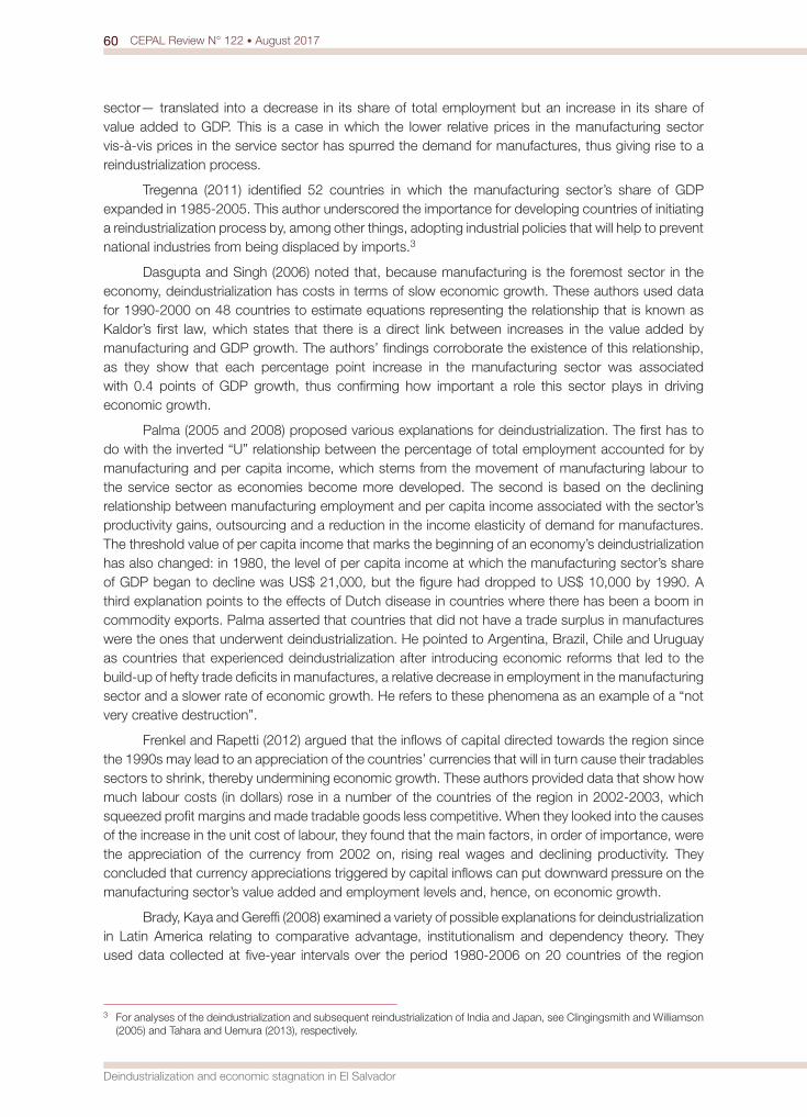
60 CEPAL Review N° 122 • August 2017
Deindustrialization and economic stagnation in El Salvador
sector— translated into a decrease in its share of total employment but an increase in its share of value added to GDP. This is a case in which the lower relative prices in the manufacturing sector vis-à-vis prices in the service sector has spurred the demand for manufactures, thus giving rise to a reindustrialization process.
Tregenna (2011) identified 52 countries in which the manufacturing sector’s share of GDP expanded in 1985-2005. This author underscored the importance for developing countries of initiating a reindustrialization process by, among other things, adopting industrial policies that will help to prevent national industries from being displaced by imports.3
Dasgupta and Singh (2006) noted that, because manufacturing is the foremost sector in the economy, deindustrialization has costs in terms of slow economic growth. These authors used data for 1990-2000 on 48 countries to estimate equations representing the relationship that is known as Kaldor’s first law, which states that there is a direct link between increases in the value added by manufacturing and GDP growth. The authors’ findings corroborate the existence of this relationship, as they show that each percentage point increase in the manufacturing sector was associated with 0.4 points of GDP growth, thus confirming how important a role this sector plays in driving economic growth.
Palma (2005 and 2008) proposed various explanations for deindustrialization. The first has to do with the inverted “U” relationship between the percentage of total employment accounted for by manufacturing and per capita income, which stems from the movement of manufacturing labour to the service sector as economies become more developed. The second is based on the declining relationship between manufacturing employment and per capita income associated with the sector’s productivity gains, outsourcing and a reduction in the income elasticity of demand for manufactures. The threshold value of per capita income that marks the beginning of an economy’s deindustrialization has also changed: in 1980, the level of per capita income at which the manufacturing sector’s share of GDP began to decline was US$ 21,000, but the figure had dropped to US$ 10,000 by 1990. A third explanation points to the effects of Dutch disease in countries where there has been a boom in commodity exports. Palma asserted that countries that did not have a trade surplus in manufactures were the ones that underwent deindustrialization. He pointed to Argentina, Brazil, Chile and Uruguay as countries that experienced deindustrialization after introducing economic reforms that led to the build-up of hefty trade deficits in manufactures, a relative decrease in employment in the manufacturing sector and a slower rate of economic growth. He refers to these phenomena as an example of a “not very creative destruction”.
Frenkel and Rapetti (2012) argued that the inflows of capital directed towards the region since the 1990s may lead to an appreciation of the countries’ currencies that will in turn cause their tradables sectors to shrink, thereby undermining economic growth. These authors provided data that show how much labour costs (in dollars) rose in a number of the countries of the region in 2002-2003, which squeezed profit margins and made tradable goods less competitive. When they looked into the causes of the increase in the unit cost of labour, they found that the main factors, in order of importance, were the appreciation of the currency from 2002 on, rising real wages and declining productivity. They concluded that currency appreciations triggered by capital inflows can put downward pressure on the manufacturing sector’s value added and employment levels and, hence, on economic growth.
Brady, Kaya and Gereffi (2008) examined a variety of possible explanations for deindustrialization in Latin America relating to comparative advantage, institutionalism and dependency theory. They used data collected at five-year intervals over the period 1980-2006 on 20 countries of the region
3 For analyses of the deindustrialization and subsequent reindustrialization of India and Japan, see Clingingsmith and Williamson (2005) and Tahara and Uemura (2013), respectively.
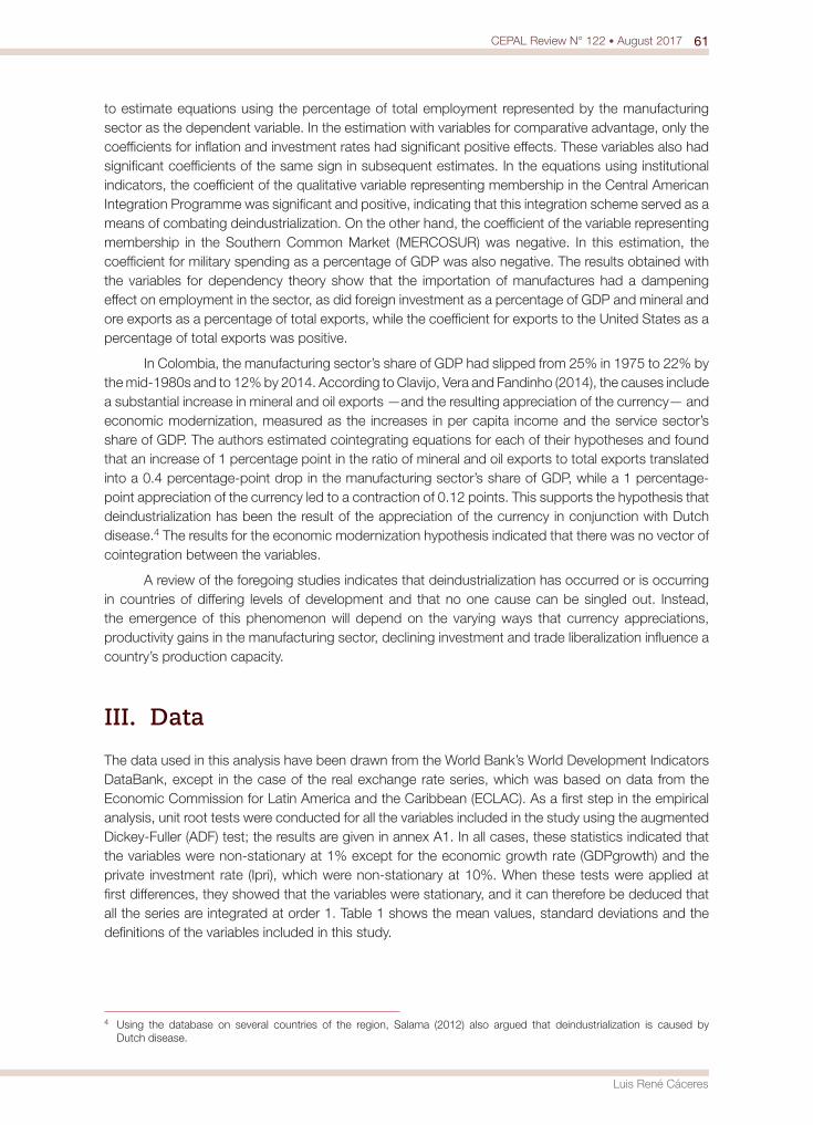
61CEPAL Review N° 122 • August 2017
Luis René Cáceres
to estimate equations using the percentage of total employment represented by the manufacturing sector as the dependent variable. In the estimation with variables for comparative advantage, only the coefficients for inflation and investment rates had significant positive effects. These variables also had significant coefficients of the same sign in subsequent estimates. In the equations using institutional indicators, the coefficient of the qualitative variable representing membership in the Central American Integration Programme was significant and positive, indicating that this integration scheme served as a means of combating deindustrialization. On the other hand, the coefficient of the variable representing membership in the Southern Common Market (MERCOSUR) was negative. In this estimation, the coefficient for military spending as a percentage of GDP was also negative. The results obtained with the variables for dependency theory show that the importation of manufactures had a dampening effect on employment in the sector, as did foreign investment as a percentage of GDP and mineral and ore exports as a percentage of total exports, while the coefficient for exports to the United States as a percentage of total exports was positive.
In Colombia, the manufacturing sector’s share of GDP had slipped from 25% in 1975 to 22% by the mid-1980s and to 12% by 2014. According to Clavijo, Vera and Fandinho (2014), the causes include a substantial increase in mineral and oil exports —and the resulting appreciation of the currency— and economic modernization, measured as the increases in per capita income and the service sector’s share of GDP. The authors estimated cointegrating equations for each of their hypotheses and found that an increase of 1 percentage point in the ratio of mineral and oil exports to total exports translated into a 0.4 percentage-point drop in the manufacturing sector’s share of GDP, while a 1 percentage-point appreciation of the currency led to a contraction of 0.12 points. This supports the hypothesis that deindustrialization has been the result of the appreciation of the currency in conjunction with Dutch disease.4 The results for the economic modernization hypothesis indicated that there was no vector of cointegration between the variables.
A review of the foregoing studies indicates that deindustrialization has occurred or is occurring in countries of differing levels of development and that no one cause can be singled out. Instead, the emergence of this phenomenon will depend on the varying ways that currency appreciations, productivity gains in the manufacturing sector, declining investment and trade liberalization influence a country’s production capacity.
III. Data
The data used in this analysis have been drawn from the World Bank’s World Development Indicators DataBank, except in the case of the real exchange rate series, which was based on data from the Economic Commission for Latin America and the Caribbean (ECLAC). As a first step in the empirical analysis, unit root tests were conducted for all the variables included in the study using the augmented Dickey-Fuller (ADF) test; the results are given in annex A1. In all cases, these statistics indicated that the variables were non-stationary at 1% except for the economic growth rate (GDPgrowth) and the private investment rate (Ipri), which were non-stationary at 10%. When these tests were applied at first differences, they showed that the variables were stationary, and it can therefore be deduced that all the series are integrated at order 1. Table 1 shows the mean values, standard deviations and the definitions of the variables included in this study.
4 Using the database on several countries of the region, Salama (2012) also argued that deindustrialization is caused by Dutch disease.
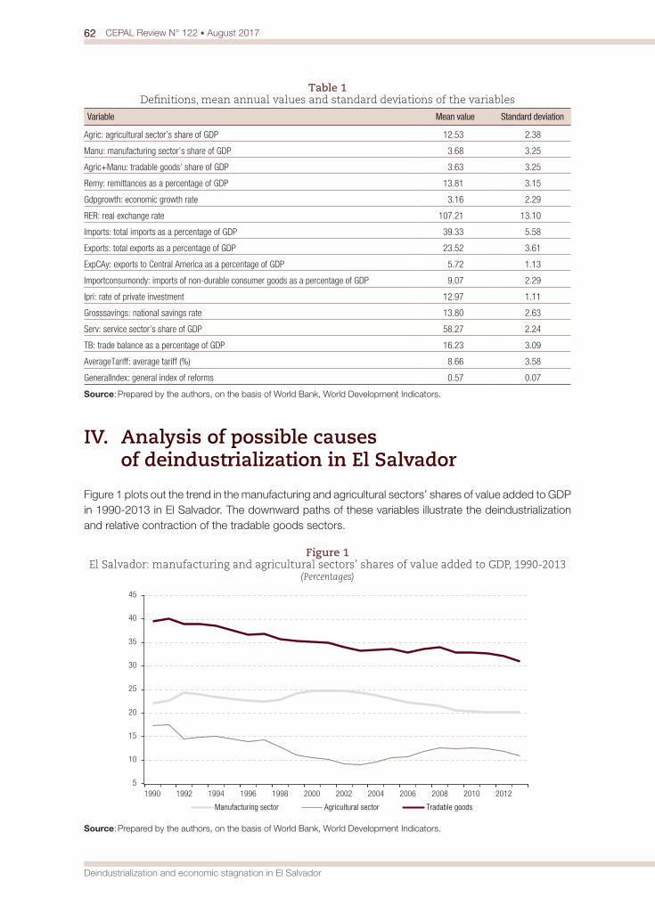
62 CEPAL Review N° 122 • August 2017
Deindustrialization and economic stagnation in El Salvador
Table 1 Definitions, mean annual values and standard deviations of the variables
Variable Mean value Standard deviation
Agric: agricultural sector’s share of GDP 12.53 2.38
Manu: manufacturing sector’s share of GDP 3.68 3.25
Agric+Manu: tradable goods’ share of GDP 3.63 3.25
Remy: remittances as a percentage of GDP 13.81 3.15
Gdpgrowth: economic growth rate 3.16 2.29
RER: real exchange rate 107.21 13.10
Imports: total imports as a percentage of GDP 39.33 5.58
Exports: total exports as a percentage of GDP 23.52 3.61
ExpCAy: exports to Central America as a percentage of GDP 5.72 1.13
Importconsumondy: imports of non-durable consumer goods as a percentage of GDP 9.07 2.29
Ipri: rate of private investment 12.97 1.11
Grosssavings: national savings rate 13.80 2.63
Serv: service sector’s share of GDP 58.27 2.24
TB: trade balance as a percentage of GDP 16.23 3.09
AverageTariff: average tariff (%) 8.66 3.58
GeneralIndex: general index of reforms 0.57 0.07
Source: Prepared by the authors, on the basis of World Bank, World Development Indicators.
IV. Analysis of possible causes of deindustrialization in El Salvador
Figure 1 plots out the trend in the manufacturing and agricultural sectors’ shares of value added to GDP in 1990-2013 in El Salvador. The downward paths of these variables illustrate the deindustrialization and relative contraction of the tradable goods sectors.
Figure 1 El Salvador: manufacturing and agricultural sectors’ shares of value added to GDP, 1990-2013
(Percentages)
5
10
15
20
25
30
35
40
45
1990 1992 1994 1996 1998 2000 2002 2004 2006 2008 2010 2012
Tradable goodsAgricultural sector Manufacturing sector
Source: Prepared by the authors, on the basis of World Bank, World Development Indicators.
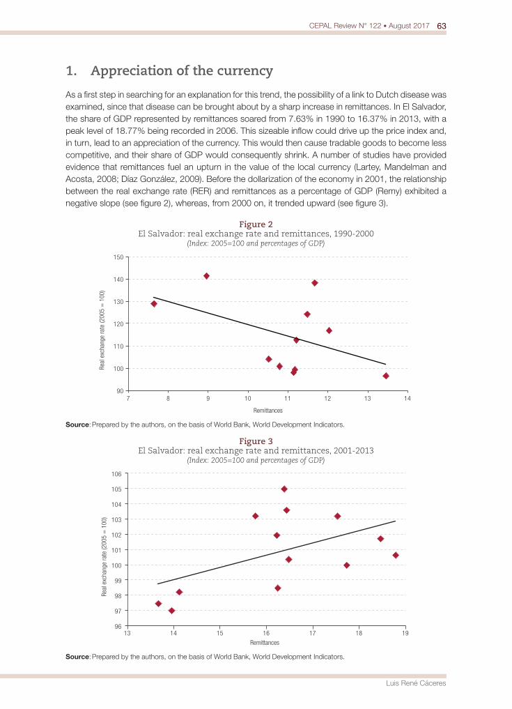
63CEPAL Review N° 122 • August 2017
Luis René Cáceres
1. Appreciation of the currency
As a first step in searching for an explanation for this trend, the possibility of a link to Dutch disease was examined, since that disease can be brought about by a sharp increase in remittances. In El Salvador, the share of GDP represented by remittances soared from 7.63% in 1990 to 16.37% in 2013, with a peak level of 18.77% being recorded in 2006. This sizeable inflow could drive up the price index and, in turn, lead to an appreciation of the currency. This would then cause tradable goods to become less competitive, and their share of GDP would consequently shrink. A number of studies have provided evidence that remittances fuel an upturn in the value of the local currency (Lartey, Mandelman and Acosta, 2008; Díaz González, 2009). Before the dollarization of the economy in 2001, the relationship between the real exchange rate (RER) and remittances as a percentage of GDP (Remy) exhibited a negative slope (see figure 2), whereas, from 2000 on, it trended upward (see figure 3).
Figure 2 El Salvador: real exchange rate and remittances, 1990-2000
(Index: 2005=100 and percentages of GDP)
90
100
110
120
130
140
150
7 8 9 10 11 12 13 14
Real
exc
hang
e ra
te (2
005
= 1
00)
Remittances
Source: Prepared by the authors, on the basis of World Bank, World Development Indicators.
Figure 3 El Salvador: real exchange rate and remittances, 2001-2013
(Index: 2005=100 and percentages of GDP)
96
97
98
99
100
101
102
103
104
105
106
13 14 15 16 17 18 19
Real
exc
hang
e ra
te (2
005
= 1
00)
Remittances
Source: Prepared by the authors, on the basis of World Bank, World Development Indicators.
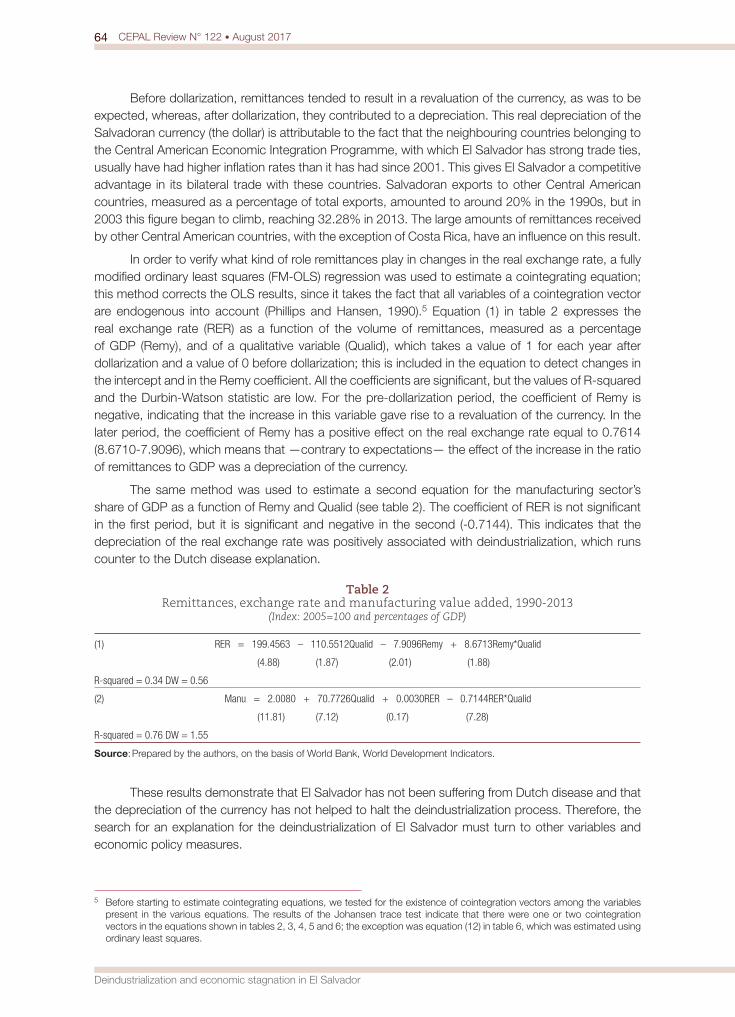
64 CEPAL Review N° 122 • August 2017
Deindustrialization and economic stagnation in El Salvador
Before dollarization, remittances tended to result in a revaluation of the currency, as was to be expected, whereas, after dollarization, they contributed to a depreciation. This real depreciation of the Salvadoran currency (the dollar) is attributable to the fact that the neighbouring countries belonging to the Central American Economic Integration Programme, with which El Salvador has strong trade ties, usually have had higher inflation rates than it has had since 2001. This gives El Salvador a competitive advantage in its bilateral trade with these countries. Salvadoran exports to other Central American countries, measured as a percentage of total exports, amounted to around 20% in the 1990s, but in 2003 this figure began to climb, reaching 32.28% in 2013. The large amounts of remittances received by other Central American countries, with the exception of Costa Rica, have an influence on this result.
In order to verify what kind of role remittances play in changes in the real exchange rate, a fully modified ordinary least squares (FM-OLS) regression was used to estimate a cointegrating equation; this method corrects the OLS results, since it takes the fact that all variables of a cointegration vector are endogenous into account (Phillips and Hansen, 1990).5 Equation (1) in table 2 expresses the real exchange rate (RER) as a function of the volume of remittances, measured as a percentage of GDP (Remy), and of a qualitative variable (Qualid), which takes a value of 1 for each year after dollarization and a value of 0 before dollarization; this is included in the equation to detect changes in the intercept and in the Remy coefficient. All the coefficients are significant, but the values of R-squared and the Durbin-Watson statistic are low. For the pre-dollarization period, the coefficient of Remy is negative, indicating that the increase in this variable gave rise to a revaluation of the currency. In the later period, the coefficient of Remy has a positive effect on the real exchange rate equal to 0.7614 (8.6710-7.9096), which means that —contrary to expectations— the effect of the increase in the ratio of remittances to GDP was a depreciation of the currency.
The same method was used to estimate a second equation for the manufacturing sector’s share of GDP as a function of Remy and Qualid (see table 2). The coefficient of RER is not significant in the first period, but it is significant and negative in the second (-0.7144). This indicates that the depreciation of the real exchange rate was positively associated with deindustrialization, which runs counter to the Dutch disease explanation.
Table 2 Remittances, exchange rate and manufacturing value added, 1990-2013
(Index: 2005=100 and percentages of GDP)
(1) RER = 199.4563 – 110.5512Qualid – 7.9096Remy + 8.6713Remy*Qualid
(4.88) (1.87) (2.01) (1.88)
R-squared = 0.34 DW = 0.56
(2) Manu = 2.0080 + 70.7726Qualid + 0.0030RER – 0.7144RER*Qualid
(11.81) (7.12) (0.17) (7.28)
R-squared = 0.76 DW = 1.55
Source: Prepared by the authors, on the basis of World Bank, World Development Indicators.
These results demonstrate that El Salvador has not been suffering from Dutch disease and that the depreciation of the currency has not helped to halt the deindustrialization process. Therefore, the search for an explanation for the deindustrialization of El Salvador must turn to other variables and economic policy measures.
5 Before starting to estimate cointegrating equations, we tested for the existence of cointegration vectors among the variables present in the various equations. The results of the Johansen trace test indicate that there were one or two cointegration vectors in the equations shown in tables 2, 3, 4, 5 and 6; the exception was equation (12) in table 6, which was estimated using ordinary least squares.

65CEPAL Review N° 122 • August 2017
Luis René Cáceres
2. Trade liberalization
In the mid-1980s, El Salvador began to introduce a series of trade policy measures that did away with quantitative restrictions on imports and, most importantly, lowered import duties. According to data from Lora (2012), the mean import duty was lowered from 22.68% in 1986 to 12.92% by 1993 and to 5.8% by 2009.6 This last value was just half of the mean duty in the Andean countries and MERCOSUR. Other sources, such as the World Bank’s World Development Indicators, give an even lower mean import duty for El Salvador (around 2% in 2013). Other economic liberalization measures in such areas as finance, taxation, labour and privatization were also introduced in the 1990s.
3. Imports and deindustrialization
The increase in imports of non-durable consumer goods (Importconsumondy) from 6% to 12% of GDP between 1990 and 2013 is related to the contraction of the share of GDP represented by tradable goods (Manu+Agric) (see figure 4).
Figure 4 El Salvador: production of tradable goods and imports of non-durable
consumer goods, 1990-2013(Percentages of GDP)
30
32
34
36
38
40
42
5 6 7 8 9 10 11 12 13 14
Trad
able
goo
ds
Imports of non-durable consumer goods
Source: Prepared by the authors, on the basis of World Bank, World Development Indicators.
In order to analyse this point, cointegrating equations were estimated using the FM-OLS methodology that expressed the Manu variable in terms of Importconsumondy and other variables. Equation (3) (see table 3) shows that imports of consumer non-durables, measured as a percentage of GDP, have a negative impact on national manufacturing output, while remittances have a positive effect. This equation explains 77% of the variance of Manu. Equation (4) includes the private investment rate (Ipri), whose coefficient is positive and significant. The coefficient of Remy is significant only at the 14% level. This equation explains 81% of the variance of Manu. El Salvador’s exports to the other Central American countries, measured as a percentage of GDP (ExpCAy), were included as an independent variable in equation (5). The significant and positive coefficient indicates that regional trade flows shield
6 The data series prepared by Lora (2012) covers the period 1985-2009.
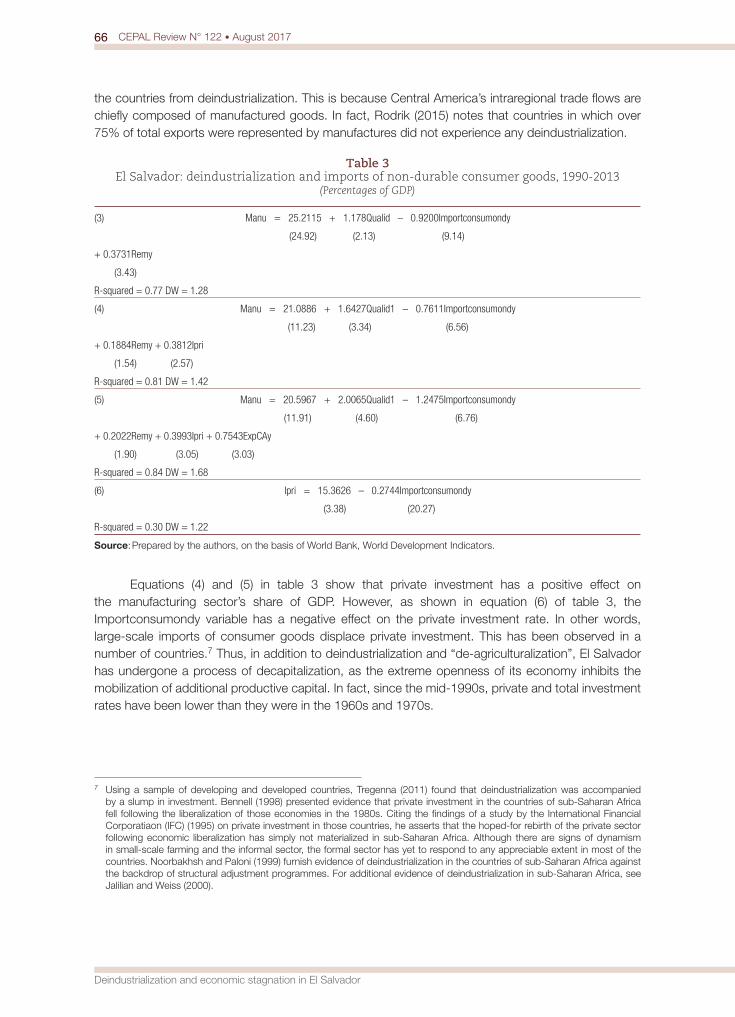
66 CEPAL Review N° 122 • August 2017
Deindustrialization and economic stagnation in El Salvador
the countries from deindustrialization. This is because Central America’s intraregional trade flows are chiefly composed of manufactured goods. In fact, Rodrik (2015) notes that countries in which over 75% of total exports were represented by manufactures did not experience any deindustrialization.
Table 3 El Salvador: deindustrialization and imports of non-durable consumer goods, 1990-2013
(Percentages of GDP)
(3) Manu = 25.2115 + 1.178Qualid – 0.9200Importconsumondy
(24.92) (2.13) (9.14)
+ 0.3731Remy
(3.43)
R-squared = 0.77 DW = 1.28
(4) Manu = 21.0886 + 1.6427Qualid1 – 0.7611Importconsumondy
(11.23) (3.34) (6.56)
+ 0.1884Remy + 0.3812Ipri
(1.54) (2.57)
R-squared = 0.81 DW = 1.42
(5) Manu = 20.5967 + 2.0065Qualid1 – 1.2475Importconsumondy
(11.91) (4.60) (6.76)
+ 0.2022Remy + 0.3993Ipri + 0.7543ExpCAy
(1.90) (3.05) (3.03)
R-squared = 0.84 DW = 1.68
(6) Ipri = 15.3626 – 0.2744Importconsumondy
(3.38) (20.27)
R-squared = 0.30 DW = 1.22
Source: Prepared by the authors, on the basis of World Bank, World Development Indicators.
Equations (4) and (5) in table 3 show that private investment has a positive effect on the manufacturing sector’s share of GDP. However, as shown in equation (6) of table 3, the Importconsumondy variable has a negative effect on the private investment rate. In other words, large-scale imports of consumer goods displace private investment. This has been observed in a number of countries.7 Thus, in addition to deindustrialization and “de-agriculturalization”, El Salvador has undergone a process of decapitalization, as the extreme openness of its economy inhibits the mobilization of additional productive capital. In fact, since the mid-1990s, private and total investment rates have been lower than they were in the 1960s and 1970s.
7 Using a sample of developing and developed countries, Tregenna (2011) found that deindustrialization was accompanied by a slump in investment. Bennell (1998) presented evidence that private investment in the countries of sub-Saharan Africa fell following the liberalization of those economies in the 1980s. Citing the findings of a study by the International Financial Corporatiaon (IFC) (1995) on private investment in those countries, he asserts that the hoped-for rebirth of the private sector following economic liberalization has simply not materialized in sub-Saharan Africa. Although there are signs of dynamism in small-scale farming and the informal sector, the formal sector has yet to respond to any appreciable extent in most of the countries. Noorbakhsh and Paloni (1999) furnish evidence of deindustrialization in the countries of sub-Saharan Africa against the backdrop of structural adjustment programmes. For additional evidence of deindustrialization in sub-Saharan Africa, see Jalilian and Weiss (2000).
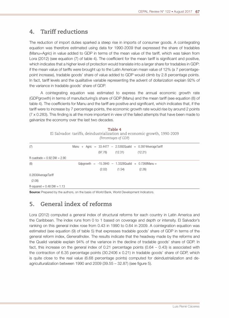
67CEPAL Review N° 122 • August 2017
Luis René Cáceres
4. Tariff reductions
The reduction of import duties sparked a steep rise in imports of consumer goods. A cointegrating equation was therefore estimated using data for 1990-2009 that expressed the share of tradables (Manu+Agric) in value added to GDP in terms of the mean value of the tariff, which was taken from Lora (2012) (see equation (7) of table 4). The coefficient for the mean tariff is significant and positive, which indicates that a higher level of protection would translate into a larger share for tradables in GDP: if the mean value of tariffs were brought up to the Latin American mean value of 12% (a 7 percentage-point increase), tradable goods’ share of value added to GDP would climb by 2.8 percentage points. In fact, tariff levels and the qualitative variable representing the advent of dollarization explain 92% of the variance in tradable goods’ share of GDP.
A cointegrating equation was estimated to express the annual economic growth rate (GDPgrowth) in terms of manufacturing’s share of GDP (Manu) and the mean tariff (see equation (8) of table 4). The coefficients for Manu and the tariff are positive and significant, which indicates that, if the tariff were to increase by 7 percentage points, the economic growth rate would rise by around 2 points (7 x 0.283). This finding is all the more important in view of the failed attempts that have been made to galvanize the economy over the last two decades.
Table 4 El Salvador: tariffs, deindustrialization and economic growth, 1990-2009
(Percentages of GDP)
(7) Manu + Agric = 33.4477 – 2.5392Qualid + 0.3974AverageTariff
(97.78) (12.31) (12.21)
R cuadrado = 0.92 DW = 2.90
(8) Gdpgrowth = -15.3940 – 1.3328Qualid + 0.7268Manu +
(2.02) (1.54) (2.26)
0.2830AverageTariff
(2.08)
R-squared = 0.48 DW = 1.13
Source: Prepared by the authors, on the basis of World Bank, World Development Indicators.
5. General index of reforms
Lora (2012) computed a general index of structural reforms for each country in Latin America and the Caribbean. The index runs from 0 to 1 based on coverage and depth or intensity. El Salvador’s ranking on this general index rose from 0.43 in 1990 to 0.64 in 2009. A cointegration equation was estimated (see equation (9) of table 5) that expresses tradable goods’ share of GDP in terms of the general reform index, GeneralIndex. The results indicate that the headway made by the reforms and the Qualid variable explain 94% of the variance in the decline of tradable goods’ share of GDP. In fact, this increase on the general index of 0.21 percentage points (0.64 – 0.43) is associated with the contraction of 6.35 percentage points (30.2406 x 0.21) in tradable goods’ share of GDP, which is quite close to the real value (6.68 percentage points) computed for deindustrialization and de-agriculturalization between 1990 and 2009 (39.55 – 32.87) (see figure 5).
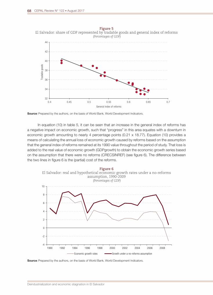
68 CEPAL Review N° 122 • August 2017
Deindustrialization and economic stagnation in El Salvador
Figure 5 El Salvador: share of GDP represented by tradable goods and general index of reforms
(Percentages of GDP)
32
34
36
38
40
42
44
0.4 0.45 0.5 0.55 0.6 0.65 0.7
Trad
able
goo
ds
General index of reforms
Source: Prepared by the authors, on the basis of World Bank, World Development Indicators.
In equation (10) in table 5, it can be seen that an increase in the general index of reforms has a negative impact on economic growth, such that “progress” in this area equates with a downturn in economic growth amounting to nearly 4 percentage points (0.21 x 18.77). Equation (10) provides a means of calculating the annual loss of economic growth caused by reforms based on the assumption that the general index of reforms remained at its 1990 value throughout the period of study. That loss is added to the real value of economic growth (GDPgrowth) to obtain the economic growth series based on the assumption that there were no reforms (CRECSINREF) (see figure 6). The difference between the two lines in figure 6 is the (partial) cost of the reforms.
Figure 6 El Salvador: real and hypothetical economic growth rates under a no-reforms
assumption, 1990-2009 (Percentages of GDP)
-4
-2
0
2
4
6
8
10
1990 1992 1994 1996 1998 2000 2002 2004 2006 2008
Economic growth rates Growth under a no-reforms assumption
Source: Prepared by the authors, on the basis of World Bank, World Development Indicators.
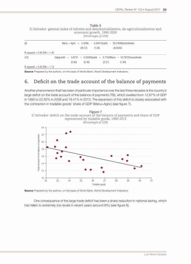
69CEPAL Review N° 122 • August 2017
Luis René Cáceres
Table 5 El Salvador: general index of reforms and deindustrialization, de-agriculturalization and
economic growth, 1990-2009 (Percentages of GDP)
(9) Manu + Agric = 5.4286 – 0.8441Qualid – 30.2406GeneralIndex
(26.57) (1.84) (8.0540)
R-squared = 0.94 DW = 1.40
(10) Gdpgrowth = 3.8731 – 0.5036Qualid + 0.7762Manu – 18.7672GeneralIndex
(0.40) (0.40) (2.31) (1.84)
R-squared = 0.43 DW = 1.13
Source: Prepared by the authors, on the basis of World Bank, World Development Indicators.
6. Deficit on the trade account of the balance of payments
Another phenomenon that has been of particular importance over the last three decades is the country’s large deficit on the trade account of the balance of payments (TB), which swelled from 12.67% of GDP in 1990 to 22.82% in 2008 and 19.41% in 2013. The expansion of this deficit is closely associated with the contraction in tradable goods’ share of GDP (Manu+Agric) (see figure 7).
Figure 7 El Salvador: deficit on the trade account of the balance of payments and share of GDP
represented by tradable goods, 1990-2013 (Percentages of GDP)
10
12
14
16
18
20
22
24
32 33 34 35 36 37 38 39 40 41
Trad
e ac
coun
t of t
he b
alan
ce o
f pay
men
ts
Tradable goods
Source: Prepared by the authors, on the basis of World Bank, World Development Indicators.
One consequence of the large trade deficit has been a sharp reduction in national saving, which has fallen to extremely low levels in recent years (around 8%) (see figure 8).
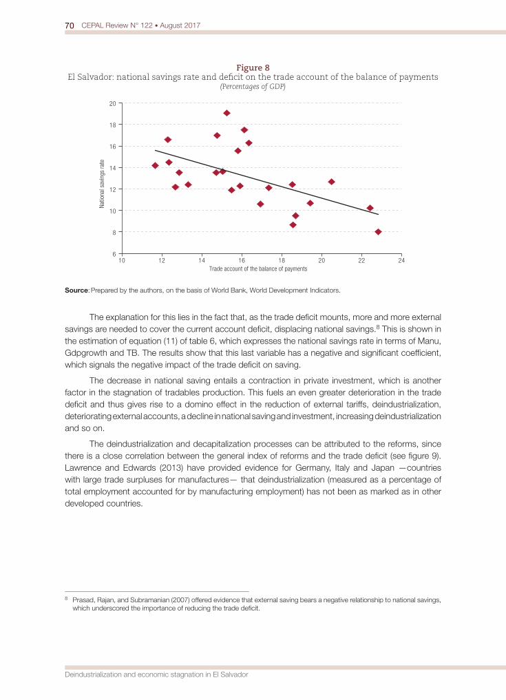
70 CEPAL Review N° 122 • August 2017
Deindustrialization and economic stagnation in El Salvador
Figure 8 El Salvador: national savings rate and deficit on the trade account of the balance of payments
(Percentages of GDP)
6
8
10
12
14
16
18
20
10 12 14 16 18 20 22 24
Natio
nal s
avin
gs ra
te
Trade account of the balance of payments
Source: Prepared by the authors, on the basis of World Bank, World Development Indicators.
The explanation for this lies in the fact that, as the trade deficit mounts, more and more external savings are needed to cover the current account deficit, displacing national savings.8 This is shown in the estimation of equation (11) of table 6, which expresses the national savings rate in terms of Manu, Gdpgrowth and TB. The results show that this last variable has a negative and significant coefficient, which signals the negative impact of the trade deficit on saving.
The decrease in national saving entails a contraction in private investment, which is another factor in the stagnation of tradables production. This fuels an even greater deterioration in the trade deficit and thus gives rise to a domino effect in the reduction of external tariffs, deindustrialization, deteriorating external accounts, a decline in national saving and investment, increasing deindustrialization and so on.
The deindustrialization and decapitalization processes can be attributed to the reforms, since there is a close correlation between the general index of reforms and the trade deficit (see figure 9). Lawrence and Edwards (2013) have provided evidence for Germany, Italy and Japan —countries with large trade surpluses for manufactures— that deindustrialization (measured as a percentage of total employment accounted for by manufacturing employment) has not been as marked as in other developed countries.
8 Prasad, Rajan, and Subramanian (2007) offered evidence that external saving bears a negative relationship to national savings, which underscored the importance of reducing the trade deficit.
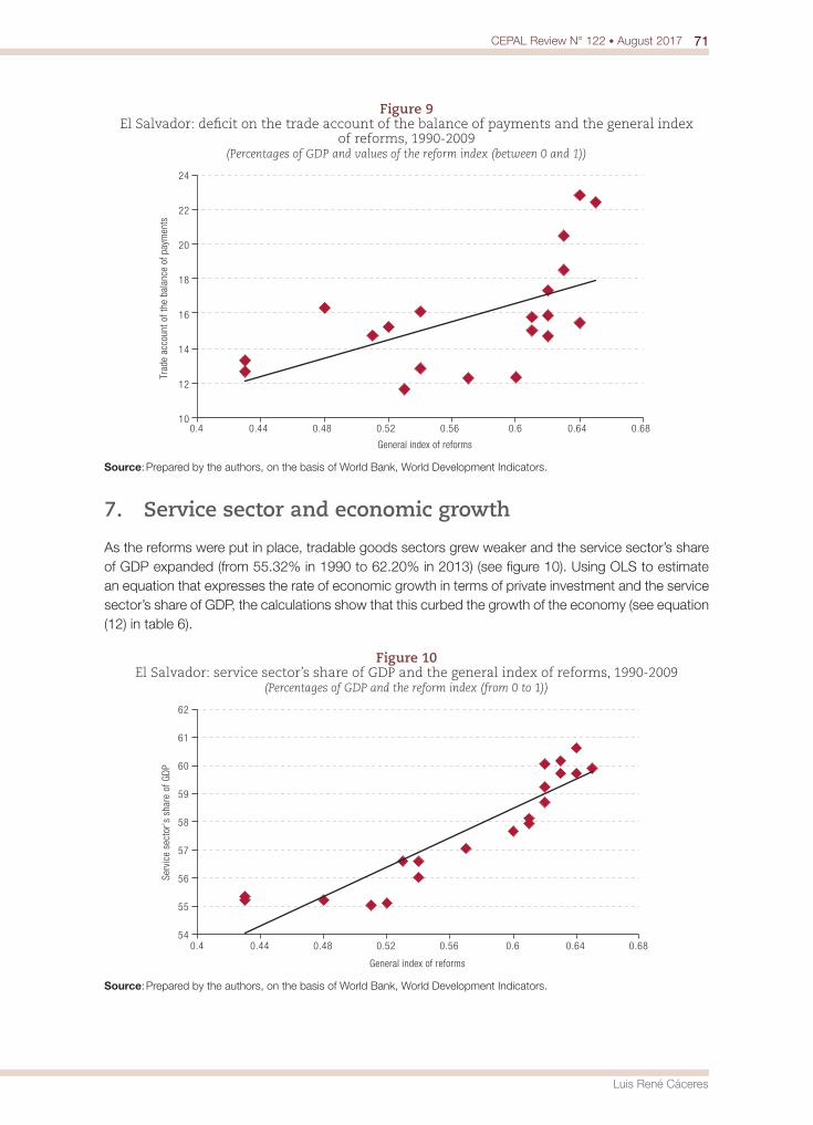
71CEPAL Review N° 122 • August 2017
Luis René Cáceres
Figure 9 El Salvador: deficit on the trade account of the balance of payments and the general index
of reforms, 1990-2009(Percentages of GDP and values of the reform index (between 0 and 1))
10
12
14
16
18
20
22
24
0.4 0.44 0.48 0.52 0.56 0.6 0.64 0.68
Trad
e ac
coun
t of t
he b
alan
ce o
f pay
men
ts
General index of reforms
Source: Prepared by the authors, on the basis of World Bank, World Development Indicators.
7. Service sector and economic growth
As the reforms were put in place, tradable goods sectors grew weaker and the service sector’s share of GDP expanded (from 55.32% in 1990 to 62.20% in 2013) (see figure 10). Using OLS to estimate an equation that expresses the rate of economic growth in terms of private investment and the service sector’s share of GDP, the calculations show that this curbed the growth of the economy (see equation (12) in table 6).
Figure 10 El Salvador: service sector’s share of GDP and the general index of reforms, 1990-2009
(Percentages of GDP and the reform index (from 0 to 1))
54
55
56
57
58
59
60
61
62
0.4 0.44 0.48 0.52 0.56 0.6 0.64 0.68
Serv
ice
sect
or’s
sha
re o
f GDP
General index of reforms
Source: Prepared by the authors, on the basis of World Bank, World Development Indicators.
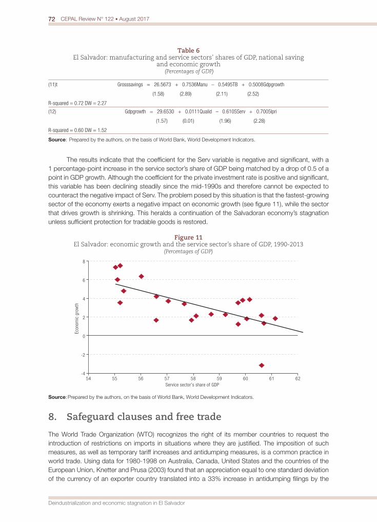
72 CEPAL Review N° 122 • August 2017
Deindustrialization and economic stagnation in El Salvador
Table 6 El Salvador: manufacturing and service sectors’ shares of GDP, national saving
and economic growth (Percentages of GDP)
(11)t Grosssavings = 26.5673 + 0.7536Manu – 0.5495TB + 0.5008Gdpgrowth
(1.58) (2.89) (2.11) (2.52)
R-squared = 0.72 DW = 2.27
(12) Gdpgrowth = 29.6530 + 0.0111Qualid – 0.6105Serv + 0.7005Ipri
(1.57) (0.01) (1.96) (2.28)
R-squared = 0.60 DW = 1.52
Source: Prepared by the authors, on the basis of World Bank, World Development Indicators.
The results indicate that the coefficient for the Serv variable is negative and significant, with a 1 percentage-point increase in the service sector’s share of GDP being matched by a drop of 0.5 of a point in GDP growth. Although the coefficient for the private investment rate is positive and significant, this variable has been declining steadily since the mid-1990s and therefore cannot be expected to counteract the negative impact of Serv. The problem posed by this situation is that the fastest-growing sector of the economy exerts a negative impact on economic growth (see figure 11), while the sector that drives growth is shrinking. This heralds a continuation of the Salvadoran economy’s stagnation unless sufficient protection for tradable goods is restored.
Figure 11 El Salvador: economic growth and the service sector’s share of GDP, 1990-2013
(Percentages of GDP)
-4
-2
0
2
4
6
8
54 55 56 57 58 59 60 61 62
Econ
omic
gro
wth
Service sector’s share of GDP
Source: Prepared by the authors, on the basis of World Bank, World Development Indicators.
8. Safeguard clauses and free trade
The World Trade Organization (WTO) recognizes the right of its member countries to request the introduction of restrictions on imports in situations where they are justified. The imposition of such measures, as well as temporary tariff increases and antidumping measures, is a common practice in world trade. Using data for 1980-1998 on Australia, Canada, United States and the countries of the European Union, Knetter and Prusa (2003) found that an appreciation equal to one standard deviation of the currency of an exporter country translated into a 33% increase in antidumping filings by the

73CEPAL Review N° 122 • August 2017
Luis René Cáceres
importer country, while a contraction equivalent to one standard deviation of the importer country’s real GDP led to a 23% increase in antidumping filings.
Bown and Crowley (2013) estimated equations to identify the variables associated with the adoption of protectionist measures in Australia, Canada, the countries of the European Union, the Republic of Korea and the United States in 1988-2010. They found that around 5% of the goods imported by these countries were subject to temporary trade barriers in 2010. One of the decisive variables influencing the erection of such barriers in all the countries except Australia was a real appreciation in bilateral exchange rates with the importer. A 4% appreciation in the currency of the importing country gave rise to increases of between 60% and 90% in the goods subject to such barriers. A slowdown in economic growth also triggered the erection of barriers to imports in all the countries except Canada. By way of example, a drop in Australia’s economic growth rate from 3.3% to 0.7% was associated with a 40% increase in the antidumping measures that it adopted.
Kee, Neagu and Nicita (2013) examined the trade policies in effect in 2009 in 131 countries in an effort to detect changes made in response to the global crisis. They found that Argentina, Bolivia (Plurinational State of), China, Ecuador, Malawi, the Russian Federation and Turkey had raised their tariffs, whereas the countries of the European Union and the United States had mainly relied on the introduction of antidumping duties.
In May 2015, Ecuador raised its import duties by 45%.9
Given the importance of the balance of payments for national saving and economic growth, El Salvador should follow the lead of developed countries and resort to protectionist measures in economic recessions or when the currency appreciates.
V. Conclusions
This study provides evidence that deindustrialization has various types of negative impacts on the Salvadoran economy, with the most notable of those effects being a slowdown in economic growth, a decline in the national savings rate, the growth of the underground economy and a deterioration in external accounts and investment.
The combination of deindustrialization and the expansion of the service sector has curbed economic growth and has led to an upturn in the trade deficit, which has had an adverse impact on private investment. This engenders a vicious circle in which deindustrialization drives up the external deficit and, in turn, puts downward pressure on private investment, which then fuels further deindustrialization, which boosts the trade deficit even further, and so on and so forth. In other Latin American countries, deindustrialization has not had such adverse effects on economic growth as it has had in El Salvador because of the commodity price boom that was occurring until fairly recently. However, as commodity prices weaken, the negative impact of economic openness will begin to be felt more keenly.
The chief cause of deindustrialization in El Salvador has been the extreme liberalization of the economy carried out in the 1990s under the influence of the Washington Consensus. The empirical evidence presented in this study also points to the adverse repercussions of the wide-ranging reforms introduced during that period.
All of this underscores the urgent need to reinstate protection measures for the national manufacturing and agricultural sectors. Rodrik (1998) has demonstrated that there was nothing
9 Published by the Inter-American Development Bank (IDB) (2015). The Washington Post edition of 26 April 2015 reported that, since 2008, the Group of 20 (G-20) countries had added 1,200 additional export and import restrictions.
74 CEPAL Review N° 122 • August 2017
Deindustrialization and economic stagnation in El Salvador
“inefficient” about the import substitution process and that it had not “run its course”, as was argued during the 1990s in order to justify the reforms that followed.
Studies on the erection of international trade barriers by developed countries show that “free trade” for these countries is discretionary: it prevails when macroeconomic conditions are favourable, but is set aside when given industries’ interests are threatened by, for example, a currency appreciation. Countries like El Salvador should emulate the effective practices of developed countries and introduce import restrictions, not only in response to a slowdown in economic growth or an overvaluation of the currency, but also as a means of helping their manufacturing sectors to develop. In other words, it is important to return to an import substitution model in order to speed economic growth and combat unemployment, underemployment and violence. In addition, as noted by Rodrik (2006), the liberalization model has no historical or conceptual foundation but is instead based on a series of assumptions that are unlikely to be borne out in the real world.
This is particularly important now that the downturn in commodity prices has triggered recessionary trends that will need to be counteracted. Taking the same route as developed countries have in protecting their trading positions is a highly advisable approach.
Tregenna (2014) has argued that deindustrialization will alter the structure and nature of the working class as employment declines in the manufacturing sector —where it is not as arduous to organize labour unions as it is are in other sectors— and rises in the service sector, where organizing the unions is more complicated. The corollary is that the establishment and growth of labour unions in the service sector need to be supported in order to bolster the bargaining power of large segments of the population. Tregenna also contends that deindustrialization prompts the banking system to place its highest priority on serving short-term borrowers in the service sector, which makes national development banks’ provision of long-term financing to production sectors all the more important.
In addition to reintroducing protective measures, productivity levels in the service sector will have to be increased. This has major implications in terms of gender issues because it calls for a substantial increase in the value added by large segments of the female workforce employed in the underground economy.
This study’s findings provide evidence of just how important a role El Salvador’s exports to other Central American countries are playing in countering deindustrialization. It follows that a determined effort should be made to support Central American integration in order to help to sustain the subregion’s industrialization process. The consideration of this issue dates back to the works of Prebisch (1950 and 1951), who argued that Latin American integration was an important means of driving the growth of exports of manufactures, overcoming balance-of-payments constraints, enhancing the use of technology and boosting productivity. Other authors who came after Prebisch advocated economic integration as a tool for promoting industrialization (Balassa, 1961; Reynolds, 1968).
For El Salvador, economic policy needs to be seen as a tool for nation-building. Priority should be given to the restitution of productive power as a vehicle for creating quality jobs, investment, exports, innovation and social cohesion. The term “productive power” was used by List (1991, cited in Ho, 2005) to differentiate his concept of political economy from that of other noted economists (Smith, among others). For List, political economy was not a “science that teaches only how values in exchange are produced by individuals, distributed among them and consumed by them. … a statesman will know and must know, over and above that, how the productive powers of a whole nation can be awakened, increased and protected, and how on the other hand they are weakened, laid to sleep, or utterly destroyed, and how by means of those national productive powers the national resources can be utilised in the wisest and best manner so as to produce national existence, national independence, national prosperity, national strength, national culture, and a national future.”10
10 List as cited by Ho (2005).
75CEPAL Review N° 122 • August 2017
Luis René Cáceres
The objectives of independence, prosperity, culture and a national future, while these may seem elusive today, should be the chief aim of El Salvador’s economic policy, which should be grounded in the protection of the country’s production sectors and the pursuit of equality of opportunity.
BibliographyBalassa, B. (1961), The Theory of Econ Integration, Homewood, Illinois, Irwin.Bennell, P. (1998), “Fighting for survival: manufacturing industry and adjustment in sub-Saharan Africa”,
Journal of International Development, vol. 10, No. 5, Wiley.Bown, Ch. and M.A. Crowley (2013), “Import protection, business cycles, and exchange rates: evidence rom
the Great Recession”, Journal of International Economics, vol. 90, No. 1, Amsterdam, Elsevier.Brady, D., Y. Kaya and G. Gereffi (2008), “Why is Latin America deindustrializing?”, Duke University, unpublished.Cáceres, L.R. (2015), “Labor Productivity in Latin America”, unpublished. Clavijo, S., A. Vera and R.A. Fandinho (2014), “Deindustrialization in Colombia: quantitative analysis of
determinants”, Working Paper, Bogota, National Association of Financial Institutions.Clingingsmith, D. and J.G. Williamson (2005), “India’s deindustrialization in the 18th and 19th centuries”,
Harvard University, unpublished.Dasgupta, S. and A. Singh (2006), “Manufacturing, services and premature de-industrialization in developing
countries: a Kaldorian empirical analysis”, Working Paper, No. 327, Cambridge, Centre for Business Research, University of Cambridge.
Díaz González, E. (2009), “The impact of remittances on macroeconomic stability: the cases of Mexico and Central America”, CEPAL Review, No. 98 (LC/G.2404-P), Santiago, Economic Commission for Latin America and the Caribbean (ECLAC).
Dollar, D. and N. Wolff (1993), Competitiveness, Convergence, and International Specialization, Cambridge, Massachusetts, The MIT Press,
Frenkel, R. and M. Rapetti (2012), “External fragility or deindustrialization: what is the main threat to Latin American countries in the 2010’s?”, World Economic Review, No. 1, Bristol, World Economic Association.
Ho, P. (2006), “Analyzing and arresting uneven development: Friedrich List and Gunnar Myrdal compared”, Journal of Economic Issues, vol. 40, No. 2, Taylor & Francis.(2005), “Distortions in the trade policy for development debate: a re-examination of Friedrich List”, Cambridge Journal of Economics, vol. 29, No. 5, Oxford University Press.
IDB (Inter-American Development Bank) (2015), News, Washington, D.C., 8 June [online] http://www.iadb.org/en/news/news,2359.html.
IFC (International Finance Corporation) (1995), Trends in Private Investment in Developing Countries 1995: Statistics for 1980-93, Discussion Paper, No. 25, Washington, D.C.
Jalilian, H. and J. Weiss (2000), “De-industrialisation in sub-Saharan Africa: myth or crisis?”, Journal of African Economies, vol. 9, No. 1, Oxford University Press.
Kaldor, N. (1967), Strategic Factors in Economic Development, Ithaca, Cornell Univerity Press.Kee, H., C. Neagu and A. Nicita (2013), “Is protectionism on the rise? Assessing national trade policies during
the crisis of 2008-2009”, Review of Economics and Statistics, vol. 95, No. 1, Cambridge, Massachusetts, The MIT Press.
Knetter, M.M. and T.J. Prusa (2003), “Macroeconomic factors and antidumping filings: evidence from four countries”, Journal of International Economics, vol. 61, No. 1, Amsterdam, Elsevier.
Lartey, E., F. Mandelman and P. Acosta (2008), “Remittances, exchange rate regimes and the Dutch disease: a panel data analysis”, Working Paper, Atlanta, Federal Reserve Bank of Atlanta.
Lawrence, R.Z. (1987), “Trade performance as a constraint on European growth”, Barriers to European Growth: A Transatlantic View, R. Lawrence and C. Schultze (eds.), Washington, D.C., The Brookings Institution.
Lawrence, R.Z. and L. Edwards (2013), “US employment deindustrialization: insights from history and the international experience”, Policy Brief, No. 13-27, Washington, D.C., Peterson Institute for International Economics.
Lind, D. (2011), “The myths and reality of deindustrialization in Sweden: the role of productivity”, International Productivity Monitor, vol. 22, Ottawa, Centre for the Study of Living Standards.
List, Friedrich (1991), The National System of Political Economy, Fairfield, Augustus M. Kelley.(1983), The Natural System of Political Economy 1837, London, Frank Cass.

76 CEPAL Review N° 122 • August 2017
Deindustrialization and economic stagnation in El Salvador
Lora, E. (2012), “Las reformas estructurales en América Latina (versión actualizada)”, Working Paper, No. IDB-WP-346, Washington, D.C., Inter-American Development Bank.
Nickell, S., S. Redding and J. Swaffield (2008), “The uneven pace of deindustrialization in the OECD”, The World Economy, vol. 31, No. 9, Wiley.
Noorbakhsh, F. and A. Paloni (1999), “Structural adjustment programs and industry I Sub-Saharan Africa: restructuring or de-industrialization?”, The Journal of Developing Areas, vol. 33, No. 4, Nashville, Tennessee State University.
Palma, G. (2010), “Why has productivity growth stagnated in most Latin American countries since the neo-liberal reforms?”, Cambridge Working Papers in Economics, No. 1030, Cambridge, University of Cambridge. (2008), “De-industrialization, ‘premature’ de-industrialization and the Dutch disease”, The New Palgrave Dictionary of Economics, S.N. Durlauf and L.E. Blume (eds.), London, Palgrave Macmillan.(2005), “Four sources of ‘de-industrialization’ and a new concept of the Dutch-disease”, Beyond Reforms: Structural Dynamic and Macroeconomic Vulnerabilty, J. A. Ocampo (ed.), Santiago, Economic Commission for Latin America and the Caribbean (ECLAC).
Phillips, P. and B. Hansen (1990), “Statistical inference in instrumental variables regressions with I(1) processes”, Review of Economic Studies, vol. 57, No. 1, Oxford University Press.
Pieper, U. (2003), “Sectoral regularities of productivity growth in developing countries – A Kaldorian interpretation”, Cambridge Journal of Economics, vol. 27, Oxford, University Press.
Prasad, E., R. Rajan and A. Subramanian (2007), “Foreign capital and economic growth”, Brookings Papers on Economic Activity, vol. 1, Washington, D.C., Brookings Institution.
Prebisch, R. (1951), Economic Survey of Latin America, 1949 (E/CN.12/164/Rev.1), New York, United Nations.(1949), The Economic Development of Latin America and Its Principal Problems (E/CN.12/89), New York, United Nations.
Reynolds, S.E. (1968), “Custom unions among developing countries”, Malayan Economic Review, Kuala Lumpur, University of Malaya.
Rodrik, D. (2015), “Premature deindustrialization”, Economic Working Papers, No. 107, Princeton, Institute for Advanced Study.(2006), “Good bye Washington Consensus, hello Washington confusion”, Journal of Economic Literature, vol. 44, No. 4, Nashville, American Economic Association. (1998), “Globalization, social conflict and economic growth”, The World Economy, vol. 21, No. 2, New York, Wiley.
Rowthorn, R. (1994), “Korea at the cross roads”, Working Paper, No. 11, Cambridge, Centre for Business Research, University of Cambridge.
Rowthorn, R. and R. Ramaswamy (1998), “Growth, trade and deindustrialization”, IMF Working Paper, No. WP/98/60, Washington, D.C., International Monetary Fund.
Saeger, S. (1997), “Globalization and deindustrialization: myth and reality in the OECD”, Weltwirschaftliches Archiv, vol. 133, Kiel, Springer.
Salama, P. (2012), “Globalización comercial: desindustrialización prematura en América Latina e industrialización en Asia”, Comercio Exterior, vol. 62, No. 6, Mexico City, Banco de Comercio Exterior.
Salvadoran Social Security Institute (2014), Anuario estadístico 2013, San Salvador. Tahara, S. and H. Uemura (2013), “The transformations of growth regime and de-industrialization in Japan”,
Discussion Paper Series, No. 2012-CEGS-02, Yokohama, Yokohama National University.Tregenna, F. (2014), “A new theoretical analysis of deindustrialization”, Cambridge Journal of Economics,
vol. 38, No. 6, Oxford University Press._____ (2011), “Manufacturing productivity, deindustrialization, and reindustrialization”, WIDER Working Paper
Series, No. 57, Helsinki, World Institute for Development Economics Research (UNU-WIDER). Wells, H. and A. Thirlwall (2003), “Testing Kaldor’s growth laws across the countries of Africa”, African
Development Review, vol. 15, No. 2-3, African Development Bank.
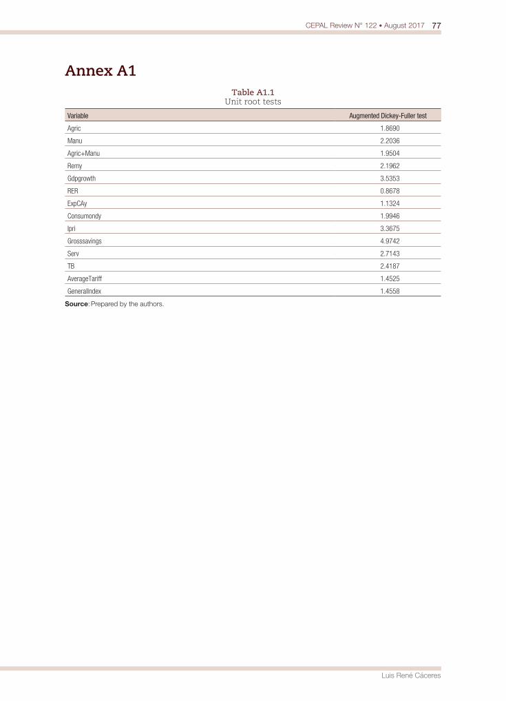
77CEPAL Review N° 122 • August 2017
Luis René Cáceres
Annex A1Table A1.1
Unit root tests
Variable Augmented Dickey-Fuller test
Agric 1.8690
Manu 2.2036
Agric+Manu 1.9504
Remy 2.1962
Gdpgrowth 3.5353
RER 0.8678
ExpCAy 1.1324
Consumondy 1.9946
Ipri 3.3675
Grosssavings 4.9742
Serv 2.7143
TB 2.4187
AverageTariff 1.4525
GeneralIndex 1.4558
Source: Prepared by the authors.

Economic growth and gender inequality: an analysis of panel data for five Latin American countriesAlison Vásconez Rodríguez
Abstract
This study looks at the relationship between the feminization of the labour market —defined as a relative increase in the female labour force participation rate and in the female labour supply as measured in hours— and economic growth in five Latin American countries. On the one hand, these trends are reflected in the potential demand that labour force participation can channel into economic growth. On the other, the conditions under which women enter and remain in the labour market will determine their supply-side (i.e. cost-based) contribution to growth. Labour supply functions are calculated using the supply in terms of hours, feminization rates and estimated wages in dynamic economic growth functions. The results indicate that the feminization of the labour force bears a positive relationship with growth but that increases in the labour supply (as measured in hours) does not.
KeywordsEconomic growth, gender, gender mainstreaming, women, women’s employment, gender equality, econometric models, Latin America
JEL classificationB54, J22, J71, O40
AuthorAlison Vásconez Rodríguez is Associate Professor with the Latin American Faculty of Social Sciences (FLACSO). [email protected]
80 CEPAL Review N° 122 • August 2017
Economic growth and gender inequality: an analysis of panel data for five Latin American countries
I. Gender inequality and economic growth: micro, meso and macro linkages
The conceptualization of the feminist economy raises two issues of interest in the debate concerning the micro/macro linkages between gender inequality and economic growth. The first is the idea that macroeconomic policies and events are linked with people and households, or percolate through to them, via a system of institutions —which include the State, the market and the community— that operates in neither a fully automatic nor a fully organized manner. This system functions within a gender-based framework that is founded upon power relations in which a visible, male-oriented policy approach dominates or influences an invisible, female-oriented one (Carrasco, 2001 and 2003; Elson, 1995a and 1999; Blau, Ferber and Winkler, 2002). The introduction of a gendered framework of considerations and factors sends out biased or skewed signals to the market, where, given the assumption that women workers are “expensive”, employers are reluctant to hire them or, once hired, to continue to employ them.1 Employment decisions therefore entail a process of bargaining and conflict in which both material and immaterial factors wield influence. The end result of that process will permit or prevent those decisions from having a favourable outcome for women candidates in terms of both their participation in the market and the conditions governing their entry and continued participation in the workforce.2
The second issue has to do with the relationships between the market (the economic sphere) and households (the non-economic sphere). In this debate, it is posited that the process of accumulation uses “human energies” as merchandise, while housework reproduces these energies as part of a process that constitutes an integral component of the development of the members of the household. From the external perspective of the household, these energies are diverted from the reproduction of human beings to the production of merchandise. From the internal perspective of households, the production of merchandise is a means to an end, which is reproduction (Picchio, 2003). Viewed in this light, production and reproduction are part of the same continuous process. In fact, the core activity of the economy, according to these postulates, has been diverted from its central objective, which is the reproduction of life, which is in turn founded upon non-mercantile domestic work (Pérez, 2005; Carrasco, 2001).
Consequently, in order to gain an understanding of the characteristics of the labour market, the relationships between the two different spheres in which labour takes place must be considered together with, most importantly, the logic of housework, especially in the case of women, for whom domestic work often represents the sum total of their economic and labour-related activities. Women’s occupational modalities —which may be the outcome of both labour policies and labour relations— reflect the tension that exists between participation in the production process and its organization (Elson, 1995b), which has been “resolved” by resorting to labour flexibility, labour segregation and unequal wages for equal work.3 This leads to the intuition that tensions between the mercantile economy and what is known as the “unpaid care economy” are heightened during crises. Many such crises generate a growing demand for cheap labour that can be employed under flexible conditions in
1 A number of studies have shown this to be a myth based on gender biases in the market. See Berger and Szretter (2002).2 On the subject of intra-household bargaining and conflict, see Agarwal (1997) and Sen (2000).3 A majority of part-time workers are women (although the intensity of labour in the case of both men and women has increased
substantially in recent decades). The women in this segment of the workforce are also employed under more flexible conditions, although not generally under the modality of “on call” workers (as is the case with men), and their employment also exhibits a greater degree of elasticity.
81CEPAL Review N° 122 • August 2017
Alison Vásconez Rodríguez
order to meet the needs of a recovering economy (Todaro and Yáñez, 2004), all of which works to the detriment of the quality of reproduction processes and the “quality” of the workforce.4
This may mean that the so-called “feminization” of the workforce —i.e. the increasing participation of women in the labour force— has an impact on business cycles via its influence on gender relations, in addition to having a beneficial impact both on women’s well-being and economic autonomy and on effective demand and growth.5 The influence of this process is channeled through at least two empirically verified mechanisms: (i) unpaid domestic work, which bears the cost of social reproduction; and (ii) paid work performed by women, who, on average, produce the same amount as men for less pay.6
These two mechanisms may generate differentiated effects during the business cycle via two channels (Darity, 1995; Erturk and Darity, 2000):
• A reproductive channel. Since unpaid domestic work generates a “savings” for the economy, the feminization of the workforce can have a negative effect if that savings is reduced (by paying for domestic work via private services or public services funded out of the government budget, since part of the value that domestic and care work transfers to the economy at no cost will no longer be channeled into the economic circuit but will instead increase the total wage bill).
This may have a positive effect, however, if, during crisis periods, households “substitute” unpaid work for expenditures (i.e. if the saving required in order for the economy to recover is afforded by domestic work, rather than by restrictions on fiscal spending or social benefits or unemployment-generated reductions in labour income) (Cerrutti, 2000).
• A labour market channel. The growing participation of women in the workforce could have a positive effect via a reduction in wage costs (a greater supply of labour at lower wages will cause average wages to decline) owing to gender-based wage inequalities.7
On the other hand, the effect of the pay gap and the downward pressure on average wages may have a negative impact on effective demand. Both of these effects may also occur at one and the same time, with the net effect being determined by the structure of the economy (Blecker and Seguino, 2002).
For Darity (1995), the effects transmitted through the reproductive channel may overshadow those transmitted through the labour market for poorer countries with fewer public caregiving services, while just the opposite would occur in richer countries. Along these same lines, Erturk and Cagatay (1995) have systematized a number of empirical studies on labour-market feminization and, following Rubery (1988), have identified three modalities for women’s entry into the workforce:
• A first modality is a procyclical buffer, in which female labour acts as a flexible reserve army that is drawn on more fully during growth periods and less so during recessions.
4 This detrimental effect could be mitigated by boosting the productivity of the unpaid domestic economy and by transferring (via mercantilization or socialization) some of the activities associated with that economy. The former is a trend that progresses at a faster or slower rate according to an economy’s income levels (and those of its component sectors). The latter is more strongly influenced by the point in the business cycle at which an economy finds itself and by the prevailing welfare regime. Nonetheless, paid care work is primarily performed by women and is generally poorly paid, which reflects the low value placed by society on reproductive activities. Access to these services is also determined by household income levels.
5 For further information on the debate surrounding growth theory as viewed from the standpoint of effective demand, see Dutt (1990), Lo Vuolo (2009) and Bhaduri (2007).
6 There is a wealth of evidence on gender pay gaps in Latin America. A number of these studies will be reviewed in a later section.7 At the global level, the feminization of the workforce and the employment conditions associated with that process have given
rise to structural inequalities in international labour markets and to increasing informalization as a result of the demand for capital (see Benería, 2005 and 2008).

82 CEPAL Review N° 122 • August 2017
Economic growth and gender inequality: an analysis of panel data for five Latin American countries
• A second modality is a segmented one in which there are sectors in which women are overrepresented and the impact of economic recessions or booms on the composition of the workforce (the entry or departure of women) depends on the composition of the sectors and occupations associated with a given stage in the business cycle. This feminized structure “protects” women who are the first to leave the market during recessions. In this sense, this modality entails a countercyclical form of behaviour.
• A third modality is one in which female workers are substituted for male workers during crises, when households’ main breadwinners may be unemployed or underemployed. By the same token, the market may tend to coopt people who have lower salary expectations but who can perform similar work in order to reduce costs during recessions. The existence of gender inequalities may bolster an economic recovery if their effect on costs outweighs the negative implications of inequality in terms of effective demand.
This article is composed of five sections, the first of which is this introduction. The second section contains a review of the literature on the links between growth and gender inequality. The third covers the methodology used in this study, while the fourth presents the results. The fifth and final section concludes.
II. The literature on growth and gender inequality
There are two main types of studies on gender inequality and growth. The first focuses on inequality in terms of human capital, particularly education, while the second focuses on employment and labour income.
There is an extensive collection of research papers which show that gender-based inequalities in education retard long-term growth and that there is therefore a positive relationship between women’s education and economic growth (Dollar and Gatti, 1999; Klasen, 2002). These researchers’ interpretation of their findings indicates that, when men and women have the same endowments and an equal distribution of skills and abilities, the existence of inequality will lead to the exclusion of potentially highly skilled women and to the inclusion of less skilled men. If women are excluded by providing them with less education and if men are given greater access to education, then, in the presence of decreasing returns, educating girls will yield a greater return at the margin. This body of research focuses on one of the foundational principles of the theory of human capital, which holds that there is a direct correlation between investment in education and economic growth. This, in turn, is based on the intuition (which has not been rigorously tested) that (formal) education augments productivity. This theory has been brought into question by those who argue that productivity is not observable and that income levels, as well as employment demand, entail gender biases that are unrelated to educational level. Thus, although these studies’ findings do show that educational inequality may be detrimental in terms of growth (since potentially skilled labour is being lost), they do not necessarily demonstrate that, if women invest in education (or attain a higher level of education), they will have higher levels of income or will gain access to higher-productivity jobs.
Another type of impact of educational inequality for which there is empirical evidence has to do with the externalities that the education of women generates in terms of lower fertility rates, lower infant mortality rates and increased educational opportunities for the next generation (Cavalcanti and Tavares, 2007). High birth rates may also reduce long-term savings rates and levels of investment in education and health (Klasen, 2002; King and Porter, 2010). These conclusions are quite intuitive, since, in most studies, the last of these variables (future education) has not been included and the first variable may be subject to problems of endogeneity that have not been sufficiently controlled for.8 On
8 Aguero and Marks (2008) and Cruces and Galiani (2007), among others, have done research on the relationship between fertility and the female labour supply.
83CEPAL Review N° 122 • August 2017
Alison Vásconez Rodríguez
the other hand, most of these studies use cross-sectional regressions and implicitly assume that the influence exerted by gender inequality is similar in all countries while ignoring their differing structural characteristics. The inclusion of panel studies improves this type of research substantially, and some authors (Klasen and Lamanna, 2009; Klasen, 2006) have therefore introduced panel data in updated versions of their studies. In such cases, their findings remain essentially the same, but their results are more robust.
Another line of research has focused on the impact of gender-related factors on competitiveness. These studies suggest that, in economies specializing in exports that are intensive in female labour, the education of that sector of the workforce is a key factor in boosting competitiveness. And, indeed, a high correlation between the education of women and exports (and, hence, economic growth) has been found (Seguino, 2000). There is little empirical evidence for this line of argument, however, mainly because there is an information problem with regard to competitiveness and domestic productivity. In agricultural economies, the effect of gender-related factors on growth is more closely linked to inequalities in landownership and access to credit than to inequalities in education (Blackden and Bhanu, 1999; Doss and Morris, 2001). In these cases, the most informative indicators for gender inequity are differentials in primary education, access to credit and property rights.
Studies on wage and employment inequalities are fewer in number, and their results have been formulated within differing theoretical frameworks, all of which has given rise to an extensive debate on the subject. Some of these studies focus on long-term determinants of productivity growth and supply, while some of them model the maximization of producers’ profits based on the selection of a suitable level of human capital, whose availability is reduced by the failure of potentially productive people to enter the market (Esteve-Volart, 2004). These studies take the non-inclusion of women in employment as a distortion that reduces the total sum of talent, in the case of employees, and lowers productivity, in the case of unequal access to technology and other production resources (Blackden and others, 2007).
Klasen (2002) and Klasen and Lamanna (2009) have developed economic growth models in which variables representing gaps in participation and education are introduced sequentially in order to measure their indirect effects using equations that trace the links between these gaps and a number of determinants of growth, such as investment. They are unable to determine, however, whether the effect of equity on the distribution of growth stems from the boost given to earnings by the relatively low wages paid to women (whose entry into the workforce may lower average wages and, hence, reduce what is known as the “efficiency wage”). Whether or not increases in women workers’ productivity will actually translate into unbiased wage increases will depend on structural aspects of the economy and its institutions which may reduce or heighten women’s wage bargaining power.
Thus, wage gaps are a plausible source of the relationship between gender inequality in employment and growth. Employment gaps, in the presence of lower wages for women, can reduce growth because the opportunity for using cheaper labour as a competitive advantage is lost (Seguino, 2000). In this case, wage inequality —rather than equality— is efficient. This fits in with the evidence on growth in some countries, including those in Latin America, that have experienced periods of growth coupled with inequality, declines in real wages or unemployment (as in, for example, the Andean countries during the early 2000s). There are not enough empirical studies to provide solid backing for this line of reasoning, however.
Another line of research has centred on the demand-side effects of wage and employment inequality in both the short and long terms (Erturk and Cagatay, 1995; Blecker and Seguino, 2002). These studies focus on the structural traits of economies that influence the interaction between gender relations and macroeconomic aggregates. They indicate that, in semi-industrialized countries, wage differentials may provide a stimulus for two major economic aggregates: investment and exports (Seguino, 2000 and 2010). In developing countries that rely heavily on exports to finance their imports
84 CEPAL Review N° 122 • August 2017
Economic growth and gender inequality: an analysis of panel data for five Latin American countries
of capital goods, female labour has been one of the main sources of exchange rate gains and one of the main reasons for the relaxation of external constraints (thanks to increases in competitiveness).
Some authors have attempted to incorporate gender-based differences into growth models and particularly into differentiated labour supply matrices that reflect the dependence of caregiving activities and the tendency to segregate women workers by diverting them into highly labour-intensive activities in commodity export sectors. Along these lines, Blecker and Seguino (2002) have found that higher wages may spur aggregate consumption (assuming that women workers have a greater propensity to consume than investors do) and aggregate demand. Higher wages can also, however, drive price increases for exports, whereupon export demand will decline. In addition, high wages reduce profits, which may dampen investment. This negative demand effect (on exports and investment) can potentially outweigh the positive effect on consumption, especially if exports are price elastic (as in the case of commodities).
In addition to wage competition, another possible linkage with growth in export-led economies may exist when women are also employed primarily in food production sectors (domestic agriculture), since the lower wages paid in these industries may translate into lower food prices. This will lower average wages in the economy as a whole and boost its competitiveness (Kucera, 2002) and may thus have a positive impact on exports. A more thorough analysis of this and other possible channels for gender-related impacts would require a broad sample of countries and detailed information on their internal demand structures.
Both the evidence and intuitions provided by these studies indicate that growth can have contradictory effects on gender equity: gender inequality may spark upswings in some economic aggregates but may also have a dampening effect on others, such as consumption, if demand effects are strong (Stotsky, 2006; Berik, Rodgers and Seguino, 2008; Braunstein, 2008). Efforts to raise women’s wages in the interests of greater equity may lead to growth in a non-profit-led economy, but they may also spark an economic contraction as a result of their negative effects on investment and exports. These short-term disturbances in demand may not only reduce male employment and output but may also make it difficult to achieve long-term growth. Thus, even though gender equity may have positive supply-side effects on the quality of the labour force over the long run, in the short run gender equity may generate shocks that could push economies off their long-run growth paths. Further analysis of the duration of these departures from the long-term trend is called for (Berik, Rodgers and Seguino, 2009).
In this study an effort will be made to determine the nature of the relationships between economic growth and the feminization of the workforce (as defined by women’s labour force participation rate) in a number of Latin American countries based on the approach devised by Erturk and Cagatay (1995) described in section I. These authors posit that, when activity levels are low (or when an economy is in a recession), the rate of feminization rises and becomes countercyclical. As this trend unfolds, feminization stimulates investment (since wages are low and these workers have limited bargaining power —a situation that generates pay gaps). As investment strengthens, it drives up the initially low equilibrium point. At the same time, the intensity of female household labour will have an impact on household saving as households reduce their expenditures on caregiving services. If, at the base of the cycle, the latter effect overshadows the impact of paid labour, then the feminization of the workforce will put downward pressure on the utilization of production capacity and will deepen the recession. The opposite will occur if, when the economy is contracting, the positive impact of the feminization of the workforce on investment is stronger than the impact that the rising intensity of female household labour has on savings.
These propositions are taken up in the present study. Nevertheless, based on the empirical evidence for Latin America (Contreras, Armas and Vásconez, 2008; Vásconez, 2012; Esquivel, 2005), it is assumed that, although labour force participation is countercyclical and household labour exhibits
85CEPAL Review N° 122 • August 2017
Alison Vásconez Rodríguez
greater intensity among the lower-income population, which has less access to private caregiving services, it is less clear what actually occurs during economic recoveries and what influence the feminization of the workforce actually has on the business cycle. Since the way in which the intensity of household labour responds to economic recessions cannot be empirically verified, it will be assumed, in the absence of historical data, that the feminization of the workforce in terms of intensity (hours worked), within a certain range, is substituted for the time spent on care work, and this may result in the dissaving described earlier. While this study will focus on the relationship between the feminization of the workforce and economic growth, and while it will not make use of data series on the amount of time devoted to household labour, the number of hours worked will be used as a proxy variable for the relationship between work in the labour market and domestic work with a view to arriving at an intuitive conclusion regarding the behaviour of the labour supply in overall terms. The results will provide information on the so-called “market channel” that forms part of this conceptual framework.
III. Methodology
The labour supply, in individual terms, is determined by the offered wage and the reservation wage, which takes into account the time spent providing care and the available time of other earners. In other words, a given person will join the active workforce when the wage offered exceeds that person’s reservation wage. Suppose that, in a nuclear family, the point at which person m will accept paid work is related to the wage received by that person’s partner h.
H si w WR0m m m1= (1)
,H H w WR si w WRm m m m m2= R W (2)
Where , , / ,WR WR p Td y p w T Tdm h h= −S R WX is the reservation wage, which incorporates both the offered working conditions and those of the “other earner” and is the result of a joint decision. Hm is the labour supply as described in (3) and εm is the residual.
Since only the wages of persons who are participating in the labour force can be determined, there is a sample selection bias. Thus, in order to measure the labour supply while correcting for this bias, a three-stage Heckman selection model is used.9 First, the selection bias is calculated using a reduced participation model (i.e. without any wage). Using a general wageless labour supply function in line with Heckman (1976 and 1993), this bias is given by the ratio of the probability density function to the cumulative distribution function for the labour supply in its reduced form. This ratio is also known as the inverse Mills ratio (or lambda, λ), whose mean values are a proxy variable for the existence of labour-market entry barriers. With the inclusion of the bias, the wage can be calculated using the inverse Mills ratio as a regressor:
w Xi i ib im y= + +t (3)
The third step is to use a least squares regression to estimate the labour supply, since the supply is being measured in hours and includes the estimated wage. The formal specification, with separate models for men (m) and women (f) is as follows:
9 For a discussion of the different types of labour supply models, see Berndt (1990), Killingsworth (1983) and Blundell, MaCurdy and Meghir (2007).
86 CEPAL Review N° 122 • August 2017
Economic growth and gender inequality: an analysis of panel data for five Latin American countries
1 2 3 4+ +' ' ' ' 'H X Z D Y w, , , ,� f f i f � f f i f � � f f �b b b b b h f= + + + + (4)
3 41 2' ' ' ' 'H X Z D Y w, , , ,mj m mj m mj m mj m mj m mj m mjb b b b b h f= + + + + + + (4.1)
Where X, Z, D and Y are vectors of human capital, working conditions, demographic factors and income, while w is a wage vector.
For the probability model, it is necessary to calculate the marginal effects given by ∂H/∂lnw, which shows the change in the probability of participation caused by a percentage change in the wage (which is not characterized by direct elasticity). The sum of the estimated probabilities as a proportion of the total working-age population gives the net participation rate, estimated at the aggregate level. The elasticity is the ratio of the percentage change in the wage over the change in this rate.
Once the participation rates have been obtained, the next step is to calculate the feminization indicator, which is the ratio of women’s participation to men’s participation. These variables can then be used to construct three growth models using the GDP growth rate as a dependent variable and including, alternatively, the variables for labour-market feminization and hours of work. Variables for increases in labour intensity, wages and education gaps are also included, in line with other studies covered in the literature review. Given the endogeneity of the relationship between inequality and growth as outlined in the theoretical framework, these problems are corrected for by lagging the explanatory and dependent variables, as well as by using the differences between the values for previous periods in keeping with the generalized method of moments.
This approach to the analysis of the relationship between growth and gender inequality, as well as the causal relationship posited in the conceptual framework, calls for an exploration of the linkage between gender gaps in the labour market and their implications for economic growth (represented, in this case by GDP growth). It is therefore best to include variables that incorporate their previous values, especially in the cases of interest for this analysis. While it is not a question of undertaking a convergence analysis, this study starts off with a dynamic autoregression model in order to shed light on its implications in an econometric panel model and then, starting from there, other lagged variables are incorporated in order to provide an explanation within the framework of the model to be used in this study.
In this study, a non-autoregressive dynamic panel model will be used in which the dependent variable is the quarterly GDP growth rate for each country. Four groups of explanatory variables are proposed:
(i) Growth-related macro variables10
(ii) Labour-market variables
(iii) Gender-gap variables
(iv) Country variables
Three specifications may be proposed. In the first, the macro variables include lagged GDP growth, investment as a percentage of GDP and the expansion of human capital as measured by the mean level of educational attainment of the economically active population (EAP). Labour-market variables include the growth of the labour supply (in hours) and the average wage. Country proxy variables, in combination with the rate of feminization, are also included in order to focus on individual effects. In the second specification, controls are introduced for the macro variables as a group in the form of the lagged levels of economic openness and industrialization; the control for the labour-
10 These variables were selected on the basis of a number of studies on growth estimates (Barro, 2000; Ros, 2004) and some of the studies included in the literature review.
87CEPAL Review N° 122 • August 2017
Alison Vásconez Rodríguez
market variables is the increase in wages, while the control for human capital is the gender gap in educational attainment. Finally, the model is completed with the introduction of two variables specific to the situational context in each country: one corresponding to periods in which there was a change of government (such changes occurred in all the countries except Brazil during the study period (2003-2010), so this variable was not used for that country) and crisis periods, which occurred in 2003 in Argentina and Uruguay and in the second and third quarters of 2009 (the most recent financial crisis) in all the countries.
First, a Hausman test is conducted in order to check the fixed effects. The results yield a statistical value that is quite a bit lower than the chi-squared statistic, and the null hypothesis that there is no significant difference between the two types of models is therefore ruled out (see annex A1). This means that the explanatory values and the effect itself are correlated or, in other words, that cross-country differences are a key factor in accounting for the behaviour of the dependent variable.
Next, in line with the methodology outlined above, the pooled ordinary least squares (OLS) model is run to verify the upper limit of the estimator. The within estimators are then obtained, with variables in differences and without the inclusion of moment instruments for the independent variables.
Finally, the model is run using the generalized method of moments (MGM SYS). The formal specification is:
' ' ' ' 'Y Z G L D Pit it it it i it it1 2 3 4 5b b b b b f= + + + + + (5)
Where Yit is the economic growth rate, Zit is the macro variables vector, Git is the gender variables vector, which includes the variables of interest, Lit is the vector of labour-market conditions, Di is composed of the proxy country variables combined with their feminization rates, and Pit represents the proxy variables for exogenous factors (crises and changes of government). The following considerations with regard to the various instruments should be noted:
• Endogenous variables: Feminization of the labour force and its growth rate (given that a bidirectional relationship exists between growth and inequality), increase in labour-market feminization, wage increases during the preceding period and pay gaps. These variables are instrumentalized by differences and level. The verification of endogeneity is conducted by means of a regression, in reduced form, of these variables for economic growth (see annex A2). In macroeconomics, this specification is used in order to highlight a cause-effect relationship, since the explanatory variables have been lagged and differentiated in order to overcome the endogeneity caused —in this case— by the bidirectionality of the relationship (which has been found to exist in the studies discussed above). The interpretation, after testing for the absence of endogeneity, can be based on the fact that a change in the labour-market feminization variable has a given effect on the rate of economic growth.
• Predetermined variables: Investment rate, level of educational attainment of the EAP and gender gaps in educational attainment. These variables are instrumentalized by differences. In order to select weakly exogenous variables, the same test as in the preceding case is used (see annex A2).
• Lagged exogenous variables: The macro variables of the investment rate, economic openness and the degree of industrialization. These lags are included as their own instruments.
• Current exogenous variables: Proxy variables.
The variable of interest is the indicator of labour-market feminization. The Arellano-Bond test for second-order autocorrelation and the Sargan test for overidentifying restrictions are both performed.
88 CEPAL Review N° 122 • August 2017
Economic growth and gender inequality: an analysis of panel data for five Latin American countries
1. Data sources
The macro data on growth are obtained from two sources: (i) the Penn World Table (PWT 7.0) database; and (ii) CEPALSTAT. Quarterly data for the period from 2003 to 2010 for use in the models were obtained from the statistical compendium entitled “América Latina y el Caribe: series históricas de estadísticas económicas 1950-2008” (ECLAC, 2009b), CEPALSTAT and the countries’ statistical offices (for both constant and current values, which are then used to provide all the information in constant 2000 dollars). The heterogeneity of the countries covered in this study introduces a greater degree of variability, making these sample data an interesting subject for analysis.
In order to derive the estimated wage and labour supply, microdata from household surveys in five countries (Argentina, Brazil, Ecuador, Peru and Uruguay) were cross-checked. These countries were selected to reflect the diversity found in South America: Ecuador and Peru, in the Andean region, have similar social features but quite different economic traits; Argentina, Brazil and Uruguay are all in the Southern Common Market (MERCOSUR) area, and Argentina and Uruguay have economies that are more or less on a par in the sense that they have fairly high income levels, but their poverty rates and distribution patterns are quite different, while Brazil is a middle-income country with a high growth rate, very high poverty levels and a severely skewed distribution pattern. This group of countries was also selected because its members have widely varying feminization/per capita GDP ratios, which sets the stage for interesting inferences at both the group and individual country levels. Microdata from the complete series of monthly employment surveys for 2003-2010 for urban areas were also obtained. However, seasonally adjusted quarterly data were used in order to attain a sufficient degree of variability relative to the macro variables. These results were used to derive a 32-period panel database for each country corresponding to the quarters comprising the period 2003-2010.
IV. Results
Figure 1 gives the labour supply estimates. The trend for 2003-2009 shows a rise of two points, on average, in the female labour force participation rate for Brazil, Ecuador and Uruguay and a comparable decline in Argentina and Peru.
In line with the conceptual framework being used here, the two-stage calculation of labour force participation rates makes it possible to analyse the selection bias using the inverse Mills ratio (lambda), which is related to the non-selection hazard rate. The results make it possible to infer that the values of λ are greater for women than for men (1.5 to 1, on average, for Argentina, 4 to 1 for Ecuador and Uruguay, and 2.5 to 1 for Peru). These ratios are constant throughout the period under study for Argentina, decline in the cases of Ecuador and Peru, and climb in the cases of Brazil and Uruguay, with an increase in the coefficient for women between 2007 and 2010 —a period during which unemployment was also on the rise (see figure 2).
The highest lambda values for women during the period under study were found in Brazil and Peru, but this is not reflected in the labour force participation rates for these countries (since these countries are not the ones with the lowest participation rates). This means that, while the female labour supply is large in proportion to the size of the working-age population, a substantial part of the non-participation rate is accounted for by selection factors, indicating that there is a larger potential labour supply than in other countries. This may be in line with the hypothesis advanced by Erturk and Cagatay (1995), who posit the existence of greater labour force participation intensity in both high- and low-income countries. The lowest lambda values are found in Brazil even though the gap in terms of male selection is the highest. This may have to do with the high value for the labour supply of workers, that has remained at nearly 80% over the last decade.
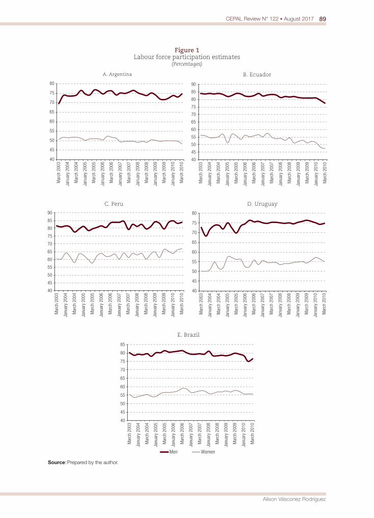
89CEPAL Review N° 122 • August 2017
Alison Vásconez Rodríguez
Figure 1 Labour force participation estimates
(Percentages)
40
45
50
55
60
65
70
75
80
Mar
ch 2
003
Janu
ary
2004
Mar
ch 2
004
Janu
ary
2005
Mar
ch 2
005
Janu
ary
2006
Mar
ch 2
006
Janu
ary
2007
Mar
ch 2
007
Janu
ary
2008
Mar
ch 2
008
Janu
ary
2009
Mar
ch 2
009
Janu
ary
2010
Mar
ch 2
010
A. Argentina
40
45
50
55
60
65
70
75
80
85
90
Mar
ch 2
003
Janu
ary
2004
Mar
ch 2
004
Janu
ary
2005
Mar
ch 2
005
Janu
ary
2006
Mar
ch 2
006
Janu
ary
2007
Mar
ch 2
007
Janu
ary
2008
Mar
ch 2
008
Janu
ary
2009
Mar
ch 2
009
Janu
ary
2010
Mar
ch 2
010
B. Ecuador
40
45
50
55
60
65
70
75
80
85
90
Mar
ch 2
003
Janu
ary
2004
Mar
ch 2
004
Janu
ary
2005
Mar
ch 2
005
Janu
ary
2006
Mar
ch 2
006
Janu
ary
2007
Mar
ch 2
007
Janu
ary
2008
Mar
ch 2
008
Janu
ary
2009
Mar
ch 2
009
Janu
ary
2010
Mar
ch 2
010
C. Peru
40
45
50
55
60
65
70
75
80
Mar
ch 2
003
Janu
ary
2004
Mar
ch 2
004
Janu
ary
2005
Mar
ch 2
005
Janu
ary
2006
Mar
ch 2
006
Janu
ary
2007
Mar
ch 2
007
Janu
ary
2008
Mar
ch 2
008
Janu
ary
2009
Mar
ch 2
009
Janu
ary
2010
Mar
ch 2
010
D. Uruguay
40
45
50
55
60
65
70
75
80
85
Mar
ch 2
003
Janu
ary
2004
Mar
ch 2
004
Janu
ary
2005
Mar
ch 2
005
Janu
ary
2006
Mar
ch 2
006
Janu
ary
2007
Mar
ch 2
007
Janu
ary
2008
Mar
ch 2
008
Janu
ary
2009
Mar
ch 2
009
Janu
ary
2010
Mar
ch 2
010
E. Brazil
Men Women
Source: Prepared by the author.
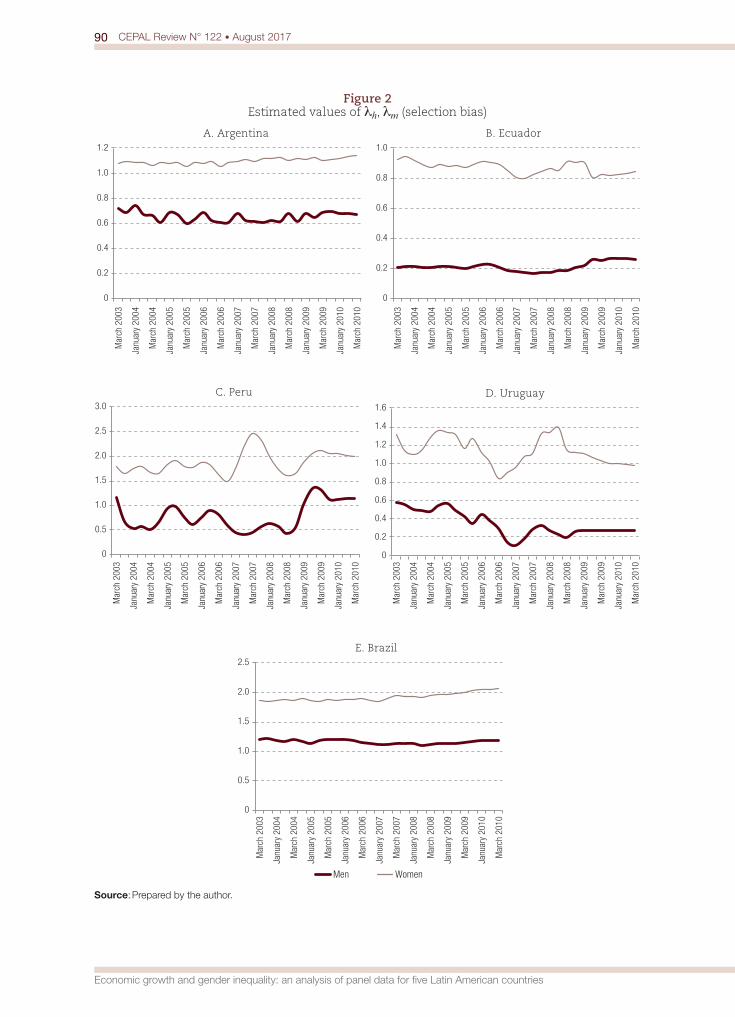
90 CEPAL Review N° 122 • August 2017
Economic growth and gender inequality: an analysis of panel data for five Latin American countries
Figure 2 Estimated values of λh, λm (selection bias)
0
0.2
0.4
0.6
0.8
1.0
1.2
Mar
ch 2
003
Janu
ary
2004
Mar
ch 2
004
Janu
ary
2005
Mar
ch 2
005
Janu
ary
2006
Mar
ch 2
006
Janu
ary
2007
Mar
ch 2
007
Janu
ary
2008
Mar
ch 2
008
Janu
ary
2009
Mar
ch 2
009
Janu
ary
2010
Mar
ch 2
010
A. Argentina
0
0.2
0.4
0.6
0.8
1.0
Mar
ch 2
003
Janu
ary
2004
Mar
ch 2
004
Janu
ary
2005
Mar
ch 2
005
Janu
ary
2006
Mar
ch 2
006
Janu
ary
2007
Mar
ch 2
007
Janu
ary
2008
Mar
ch 2
008
Janu
ary
2009
Mar
ch 2
009
Janu
ary
2010
Mar
ch 2
010
B. Ecuador
0
0.5
1.0
1.5
2.0
2.5
3.0
Mar
ch 2
003
Janu
ary
2004
Mar
ch 2
004
Janu
ary
2005
Mar
ch 2
005
Janu
ary
2006
Mar
ch 2
006
Janu
ary
2007
Mar
ch 2
007
Janu
ary
2008
Mar
ch 2
008
Janu
ary
2009
Mar
ch 2
009
Janu
ary
2010
Mar
ch 2
010
C. Peru
0
0.2
0.4
0.6
0.8
1.0
1.2
1.4
1.6 M
arch
200
3
Janu
ary
2004
Mar
ch 2
004
Janu
ary
2005
Mar
ch 2
005
Janu
ary
2006
Mar
ch 2
006
Janu
ary
2007
Mar
ch 2
007
Janu
ary
2008
Mar
ch 2
008
Janu
ary
2009
Mar
ch 2
009
Janu
ary
2010
Mar
ch 2
010
D. Uruguay
0
0.5
1.0
1.5
2.0
2.5
Mar
ch 2
003
Janu
ary
2004
Mar
ch 2
004
Janu
ary
2005
Mar
ch 2
005
Janu
ary
2006
Mar
ch 2
006
Janu
ary
2007
Mar
ch 2
007
Janu
ary
2008
Mar
ch 2
008
Janu
ary
2009
Mar
ch 2
009
Janu
ary
2010
Mar
ch 2
010
E. Brazil
Men Women
Source: Prepared by the author.
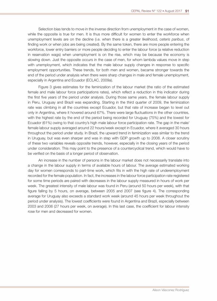
91CEPAL Review N° 122 • August 2017
Alison Vásconez Rodríguez
Selection bias tends to move in the inverse direction from unemployment in the case of women, while the opposite is true for men. It is thus more difficult for women to enter the workforce when unemployment levels are on the decline (i.e. when there is a greater likelihood, ceteris paribus, of finding work or when jobs are being created). By the same token, there are more people entering the workforce, lower entry barriers or more people deciding to enter the labour force (a relative reduction in reservation wags) when unemployment is on the rise, which may be because the economy is slowing down. Just the opposite occurs in the case of men, for whom lambda values move in step with unemployment, which indicates that the male labour supply changes in response to specific employment opportunities. These trends, for both men and women, became stronger towards the end of the period under analysis when there were sharp changes in male and female unemployment, especially in Argentina and Ecuador (ECLAC, 2009a).
Figure 3 gives estimates for the feminization of the labour market (the ratio of the estimated female and male labour force participations rates), which reflect a reduction in this indicator during the first five years of the period under analysis. During those same years, the female labour supply in Peru, Uruguay and Brazil was expanding. Starting in the third quarter of 2009, the feminization rate was climbing in all the countries except Ecuador, but that rate of increase began to level out only in Argentina, where it hovered around 67%. There were large fluctuations in the other countries, with the highest rate by the end of the period being recorded for Uruguay (75%) and the lowest for Ecuador (61%) owing to that country’s high male labour force participation rate. The gap in the male/female labour supply averaged around 22 hours/week except in Ecuador, where it averaged 30 hours throughout the period under study. In Brazil, the upward trend in feminization was similar to the trend in Uruguay, but was even sharper and was in step with GDP growth up to 2008. A closer scrutiny of these two variables reveals opposite trends, however, especially in the closing years of the period under consideration. This may point to the presence of a countercyclical trend, which would have to be verified on the basis of a longer period of observation.
An increase in the number of persons in the labour market does not necessarily translate into a change in the labour supply in terms of available hours of labour. The average estimated working day for women corresponds to part-time work, which fits in with the high rate of underemployment recorded for the female population. In fact, the increases in the labour force participation rate registered for some time periods are paired with decreases in the labour supply measured in hours of work per week. The greatest intensity of male labour was found in Peru (around 50 hours per week), with that figure falling by 5 hours, on average, between 2005 and 2007 (see figure 4). The corresponding average for Uruguay also exceeds a standard work week (around 45 hours per week throughout the period under analysis). The lowest coefficients were found in Argentina and Brazil, especially between 2003 and 2006 (27 hours per week, on average). In this last case, the coefficient for labour intensity rose for men and decreased for women.
92 CEPAL Review N° 122 • August 2017
Economic growth and gender inequality: an analysis of panel data for five Latin American countries
Figure 3 Estimated feminization of the labour market and GDP growth
(Percentages)
-0.04
-0.02
0
0.02
0.04
0.06
0.08
0.10
0.12
0.14
62
63
64
65
66
67
68
69
70
71
72
Janu
ary
2003
Mar
ch 2
003
Janu
ary
2004
Mar
ch 2
004
Janu
ary
2005
Mar
ch 2
005
Janu
ary
2006
Mar
ch 2
006
Janu
ary
2007
Mar
ch 2
007
Janu
ary
2008
Mar
ch 2
008
Janu
ary
2009
Mar
ch 2
009
Janu
ary
2010
Mar
ch 2
010
Fem
ale/
Mal
e pa
rtici
patio
n
Grow
th t/
t-4
A. Argentina
-0.02
0
0.02
0.04
0.06
0.08
0.10
54
56
58
60
62
64
66
68
Janu
ary
2003
Mar
ch 2
003
Janu
ary
2004
Mar
ch 2
004
Janu
ary
2005
Mar
ch 2
005
Janu
ary
2006
Mar
ch 2
006
Janu
ary
2007
Mar
ch 2
007
Janu
ary
2008
Mar
ch 2
008
Janu
ary
2009
Mar
ch 2
009
Janu
ary
2010
Mar
ch 2
010
Fem
ale/
Mal
e pa
rtici
patio
n
Grow
th t/
t-4
B. Ecuador
0
0.02
0.04
0.06
0.08
0.10
0.12
0.14
0.16
0.18
60
62
64
66
68
70
72
74
76
78
80
Janu
ary
2003
Mar
ch 2
003
Janu
ary
2004
Mar
ch 2
004
Janu
ary
2005
Mar
ch 2
005
Janu
ary
2006
Mar
ch 2
006
Janu
ary
2007
Mar
ch 2
007
Janu
ary
2008
Mar
ch 2
008
Janu
ary
2009
Mar
ch 2
009
Janu
ary
2010
Mar
ch 2
010
Fem
ale/
Mal
e pa
rtici
patio
n
Grow
th t/
t-4
C. Peru
0
0.02
0.04
0.06
0.08
0.10
0.12
65
66
67
68
69
70
71
72
73
74
75
Janu
ary
2003
Mar
ch 2
003
Janu
ary
2004
Mar
ch 2
004
Janu
ary
2005
Mar
ch 2
005
Janu
ary
2006
Mar
ch 2
006
Janu
ary
2007
Mar
ch 2
007
Janu
ary
2008
Mar
ch 2
008
Janu
ary
2009
Mar
ch 2
009
Janu
ary
2010
Mar
ch 2
010
Fem
ale/
Mal
e pa
rtici
patio
n
Grow
th t/
t-4
D. Uruguay
-0.02
-0.01 0
0.01
0.02
0.03
0.04
0.05
0.06
0.07
0.08
0.09
58
60
62
64
66
68
70
72
74
Janu
ary
2003
Mar
ch 2
003
Janu
ary
2004
Mar
ch 2
004
Janu
ary
2005
Mar
ch 2
005
Janu
ary
2006
Mar
ch 2
006
Janu
ary
2007
Mar
ch 2
007
Janu
ary
2008
Mar
ch 2
008
Janu
ary
2009
Mar
ch 2
009
Janu
ary
2010
Mar
ch 2
010
Fem
ale/
Mal
e pa
rtici
patio
n
Grow
th t/
t-4
E. Brazil
Feminization Growth
Source: Prepared by the author.
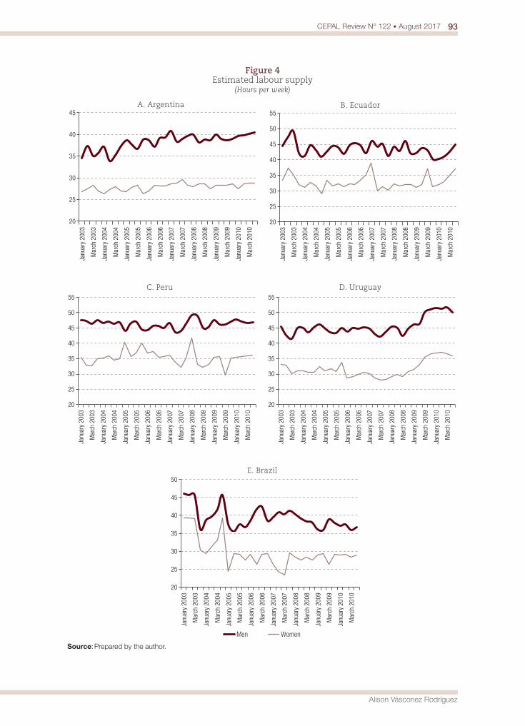
93CEPAL Review N° 122 • August 2017
Alison Vásconez Rodríguez
Figure 4 Estimated labour supply
(Hours per week)
20
25
30
35
40
45
Janu
ary
2003
Mar
ch 2
003
Janu
ary
2004
Mar
ch 2
004
Janu
ary
2005
Mar
ch 2
005
Janu
ary
2006
Mar
ch 2
006
Janu
ary
2007
Mar
ch 2
007
Janu
ary
2008
Mar
ch 2
008
Janu
ary
2009
Mar
ch 2
009
Janu
ary
2010
Mar
ch 2
010
A. Argentina
20
25
30
35
40
45
50
55
Janu
ary
2003
Mar
ch 2
003
Janu
ary
2004
Mar
ch 2
004
Janu
ary
2005
Mar
ch 2
005
Janu
ary
2006
Mar
ch 2
006
Janu
ary
2007
Mar
ch 2
007
Janu
ary
2008
Mar
ch 2
008
Janu
ary
2009
Mar
ch 2
009
Janu
ary
2010
Mar
ch 2
010
B. Ecuador
20
25
30
35
40
45
50
55
Janu
ary
2003
Mar
ch 2
003
Janu
ary
2004
Mar
ch 2
004
Janu
ary
2005
Mar
ch 2
005
Janu
ary
2006
Mar
ch 2
006
Janu
ary
2007
Mar
ch 2
007
Janu
ary
2008
Mar
ch 2
008
Janu
ary
2009
Mar
ch 2
009
Janu
ary
2010
Mar
ch 2
010
C. Peru
20
25
30
35
40
45
50
55
Janu
ary
2003
Mar
ch 2
003
Janu
ary
2004
Mar
ch 2
004
Janu
ary
2005
Mar
ch 2
005
Janu
ary
2006
Mar
ch 2
006
Janu
ary
2007
Mar
ch 2
007
Janu
ary
2008
Mar
ch 2
008
Janu
ary
2009
Mar
ch 2
009
Janu
ary
2010
Mar
ch 2
010
D. Uruguay
20
25
30
35
40
45
50
Janu
ary
2003
Mar
ch 2
003
Janu
ary
2004
Mar
ch 2
004
Janu
ary
2005
Mar
ch 2
005
Janu
ary
2006
Mar
ch 2
006
Janu
ary
2007
Mar
ch 2
007
Janu
ary
2008
Mar
ch 2
008
Janu
ary
2009
Mar
ch 2
009
Janu
ary
2010
Mar
ch 2
010
E. Brazil
Men Women
Source: Prepared by the author.
94 CEPAL Review N° 122 • August 2017
Economic growth and gender inequality: an analysis of panel data for five Latin American countries
The results of the previously described models for the relationship between labour-market feminization and economic growth are presented below, with the third specification of the method of moments (GMM SYS)11 being judged to be the most valid one for correcting for weak exogeneity and endogeneity.12 These estimates confirm the existence of a significant relationship between feminization (measured in terms of the quotient between female and male participation rates) and the economic growth rate. The results are given for all the countries and periods analysed, since this is a panel model. Country-specific variables are also included, however, so that individual effects can be detected.
Table 1 shows that a 1-point increase in the feminization rate is associated with a 5.9% increase in GDP growth. This effect remains and grows stronger over the medium term, since the lagged feminization variable for one period has an effect equivalent to 7.7% on the growth rate. This is considered to be a robust result given the stability of both the coefficient and the standard error in all three specifications. This provides a partial confirmation of the hypothesis that, in the presence of a pre-existing gap in labour force participation, women’s entry into the workforce can help fuel growth or a recovery if an economy is in a recession or when its existing capacity is being underutilized. In other words, a reduction in participation gaps has a positive growth effect over the short and medium terms.
In Ecuador, the trend in feminization during the period under study was confirmed by the result obtained using the model for the group. The fluctuations in this indicator moved in the opposite direction of the fluctuations in the growth rate, however. This leads to the inference that, while women’s participation in the labour force as a whole has a positive impact on the growth rate, their participation increases more rapidly when the economy is slowing down. In addition to the fact that feminization contributes to growth, when there is a sharp slowdown, such as occurred in the second and third quarters of 2009 or the early months of 2010 in some countries, and male unemployment is higher, the response of the female labour supply is positive. If this result is found to hold true over the long term, it could provide corroboration for the theory advanced by Erturk and Cagatay (1995) regarding the relationship between a high rate of feminization and long per capita income levels.
In Uruguay, the recovery that began in the second quarter of 2003 ushered in a steady growth trend that has been less affected by the recent crisis than has been the case in the other countries, and the rise in women’s labour force participation rate has continued to outstrip the increase in the male participation rate (Espino and Azar, 2005; Espino, Leites and Machado, 2009). Thus, the participation gap is narrowing and the feminization rate is climbing, which is in keeping with the result of the model. However, the unemployment gap widened in 2007 and 2008, which means that the rise in participation has not been balanced out by employment.
In Brazil, the overall behaviour of the labour market indicates that, during the recent economic boom, the female labour force participation rate continued to rise, but selection biases remained in place and even increased towards the end of the period. In addition, wage gaps widened and unemployment fell, indicating that opportunities for entering the workforce and for obtaining employment increased, but only in the case of part-time work. Thus, the results in terms of the feminization of the workforce are positive both for women entering the labour market and for economic growth, but entry and employment conditions may not be favourable for women, and widening gaps and shrinking average wages could impact growth in the short run.
11 That is to say, instruments obtained using the generalized method of moments. Foir a detailed explanation of the justification for using this model, see Martín (2008).
12 The Hausman test for fixed or random effects yielded statistical values that indicate that we are dealing with a fixed effects model, so the methodology outlined earlier can be used in this case. Table 1 gives the results for the variables of interest when pooled ordinary least squares and intragroup fixed effect estimator regressions were run. The other variables are given in the detailed model set out in annex A3. The Arellano-Bond test for autocorrelation does not rule out the null hypothesis of the absence of this phenomenon for the second order difference equations, which justifies the use of moment instruments. The Sargan-Hansen test demonstrates the absence of overidentification. Reduced forms were also run to gauge the explanatory power of the additional instruments (lags and differences) for the variables of interest. The F values that were obtained corroborate the instruments’ validity.

95CEPAL Review N° 122 • August 2017
Alison Vásconez Rodríguez
Tab
le 1
La
bou
r-fo
rce
fem
iniz
atio
n p
anel
res
ult
s
Depe
nden
t var
iabl
e:
GDP
grow
th t/
t-4
Pool
ed o
rdin
ary
leas
t squ
ares
Fixe
d ef
fect
s in
tragr
oup
pane
l (1)
GMM
SYS
pan
el (2
)
Spec
if. 1
Spec
if. 2
Spec
if. 3
Spec
if. 1
Spec
if. 2
Spec
if. 3
Spec
if. 1
Spec
if. 2
Spec
if. 3
Fem
iniza
tion
(I)0.
054
0.00
00.
091
0.00
00.
009
0.00
00.
043
***
0.05
4**
*0.
066
*0.
057
**0.
055
**0.
059
**
0.08
00.
072
0.08
80.
015
0.02
10.
037
0.02
40.
025
0.02
6
Fem
iniza
tion
(Q-1
)0.
019
0.
022
0.
020
0.
034
0.00
00.
034
0.00
00.
028
0.00
00.
073
*0.
079
**0.
077
**
0.07
50.
081
0.08
00.
071
0.
065
0.
072
0.
040
0.
039
0.
037
Fem
iniza
tion
(Q-2
)0.
041
0.
041
0.
038
0.
034
0.
034
0.
028
0.
040
0.
039
0.
037
0.
198
0.
231
0.
203
0.
071
0.
065
0.
072
0.
193
0.
224
0.
197
Auto
corr
(1) (
p va
lue)
0.
054
0.03
50.
016
Auto
corr
(2) (
p va
lue)
0.
890
0.72
30.
410
Sarg
an-H
anse
n (p
val
ue)
0.12
60.
503
0.93
7
So
urce
: Pre
pare
d by
the
auth
or.
No
te:
* si
gnifi
cant
at 9
0%; *
* si
gnifi
cant
at 9
5%; *
** s
igni
fican
t at 9
9%.
(1)
Inst
rum
ents
for
equa
tion
in d
iffer
ence
s
Stan
dard
: D
.inve
stm
ent_
gdp
LD.in
vest
men
t_gd
p D
.fem
iniz
atio
n L
D. f
emin
izat
ion
D.in
cr_h
ours
_m L
D. i
ncr_
hour
s _f
D.in
cr_w
age_
Q4
LD. i
ncr_
wag
e_Q
4
D.o
penn
ess
LD
. ope
nnes
s D
.man
ufac
turin
g LD
. man
ufac
turin
g D
.d_r
eces
sion
D.e
duc_
gap
D.e
duc
atta
inm
ent_
eap
(2)
Inst
rum
ents
for
equa
tion
in d
iffer
ence
s
GM
M: L
(2/.)
.L(2
/.). i
nves
tmen
t_gd
p L(
2/.).
fem
iniz
atio
n L(
2/.).
esco
larid
ad_p
ea L
(2/.)
. inc
r_ho
urs
_f L
(2/.)
. inc
r_w
age_
Q4
L(2/
.). e
duc_
gap
St
anda
rd: D
. ope
nnes
s LD
. ope
nnes
s D
. man
ufac
turin
g LD
.man
ufac
turin
g D
.d_
rece
ssio
n
In
stru
men
ts fo
r le
vellin
g eq
uatio
n
GM
M:L
D. i
nves
tmen
t_gd
p LD
. fem
iniz
atio
n LD
.edu
c at
tain
men
t_ea
p L
D.in
cr_h
ours
_f L
D. i
ncr_
wag
e_Q
4 LD
. edu
c_ga
p
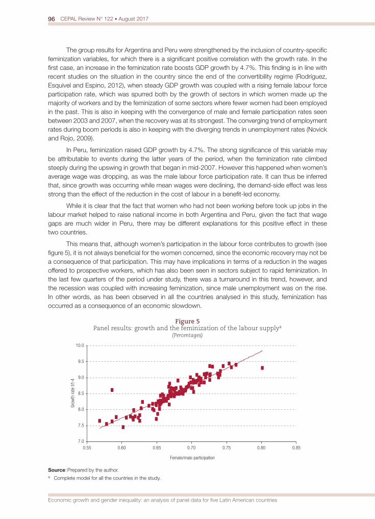
96 CEPAL Review N° 122 • August 2017
Economic growth and gender inequality: an analysis of panel data for five Latin American countries
The group results for Argentina and Peru were strengthened by the inclusion of country-specific feminization variables, for which there is a significant positive correlation with the growth rate. In the first case, an increase in the feminization rate boosts GDP growth by 4.7%. This finding is in line with recent studies on the situation in the country since the end of the convertibility regime (Rodríguez, Esquivel and Espino, 2012), when steady GDP growth was coupled with a rising female labour force participation rate, which was spurred both by the growth of sectors in which women made up the majority of workers and by the feminization of some sectors where fewer women had been employed in the past. This is also in keeping with the convergence of male and female participation rates seen between 2003 and 2007, when the recovery was at its strongest. The converging trend of employment rates during boom periods is also in keeping with the diverging trends in unemployment rates (Novick and Rojo, 2009).
In Peru, feminization raised GDP growth by 4.7%. The strong significance of this variable may be attributable to events during the latter years of the period, when the feminization rate climbed steeply during the upswing in growth that began in mid-2007. However this happened when women’s average wage was dropping, as was the male labour force participation rate. It can thus be inferred that, since growth was occurring while mean wages were declining, the demand-side effect was less strong than the effect of the reduction in the cost of labour in a benefit-led economy.
While it is clear that the fact that women who had not been working before took up jobs in the labour market helped to raise national income in both Argentina and Peru, given the fact that wage gaps are much wider in Peru, there may be different explanations for this positive effect in these two countries.
This means that, although women’s participation in the labour force contributes to growth (see figure 5), it is not always beneficial for the women concerned, since the economic recovery may not be a consequence of that participation. This may have implications in terms of a reduction in the wages offered to prospective workers, which has also been seen in sectors subject to rapid feminization. In the last few quarters of the period under study, there was a turnaround in this trend, however, and the recession was coupled with increasing feminization, since male unemployment was on the rise. In other words, as has been observed in all the countries analysed in this study, feminization has occurred as a consequence of an economic slowdown.
Figure 5 Panel results: growth and the feminization of the labour supplya
(Percentages)
7.0
7.5
8.0
8.5
9.0
9.5
10.0
0.55 0.60 0.65 0.70 0.75 0.80 0.85
Grow
th ra
te t/
t-4
Female/male participation
Source: Prepared by the author.a Complete model for all the countries in the study.
97CEPAL Review N° 122 • August 2017
Alison Vásconez Rodríguez
Yet, given the positive impact of the lagged feminization variable, with a 19% jump in GDP growth for every percentage point rise in the rate of feminization, this phenomenon can be seen to have contributed to subsequent economic recoveries.
The data indicate that, especially in Ecuador, another variable of interest is the growth of the labour supply as measured in hours, which correlates negatively with economic growth. The increase in the number of hours per week is associated with an 8% drop in GDP. On the one hand, the presence of more women (as represented by their participation rate) relative to men has a positive effect on growth, but, on the other, an increase in labour intensity (more hours spent working in the labour market), which can be assumed to reduce the hours devoted to domestic labour, is not. This may also indicate that a gain in productivity (or a greater amount of effort devoted to work, in line with our earlier discussion of the lack of a counterbalance for the labour-income elasticity of supply) may correlate with a reduction in the number of hours of labour supply but may boost production and growth. By the same token, this may be reflecting an “extra-market” effect; in other words, if the feminization rate had been falling during preceding periods (demonstrating that women had been able to leave the labour market and devote themselves to working in the home as a consequence of an earlier recession, for example), the upswing in the growth rate could be spurred by the household “savings” realized by families in that situation.13 The fact that an increase in the female labour supply or in women’s labour intensity is associated with a reduction in GDP may imply that the contribution made by unpaid domestic work to an economic recovery outweighs the contribution made by an increase in hours worked at a low wage (which is biased in this case). This may mean that the gender bias in the labour market is greater than the male/female wage gap that is based on observable characteristic (education or experience, for example) and that the wages of women entering the workforce, on average, should be higher than the wage that the market is currently paying.
The incorporation of other controls into the model does not change the significance of the variables of interest, but it does provide a better explanation for the growth rate. Among factors relating to worker skill levels, the mean level of educational attainment of the EAP correlates positively, although fairly weakly (about 1%), with the growth rate for all the specifications. The level of significance remains the same, but is greater for the lagged variable, exhibiting positive effects in the medium term. In line with this result, the educational attainment gap (the ratio between the educational attainment of the male and female EAP) displays significant negative coefficients for the lagged variable (22%), while the contemporaneous variable is not significant. According to the existing literature on returns to education for men and women in the region, the relationship between educational attainment and wage levels is stronger for women than it is for men. Thus the elimination of these gaps could lead to higher wages and greater participation on the part of women, which could in turn have an impact on demand-led growth in the future.
Along these same lines, an interesting result derived from these models, and one which is corroborated by the data, is that there is a positive correlation between average wage increases and GDP growth, with a 1 percentage point increase in mean wages translating into a 3% upturn in GDP growth.
As for the macrovariables, the level of industrialization is negatively correlated (at nearly 7%) with GDP growth. This may reflect the fact that manufacturing sectors have been sluggish in recent years as the South American countries turn back to the production of commodities (known as “reprimarization”) and the diversification of their production sectors goes into reverse; growth has been driven by other sectors, and production activities have moved forward despite the relative decline,
13 Data on the number of hours devoted to housework are not available for all the countries in time series that can be used for macroeconomic analyses, but the above conclusion may be backed up by data for the particular case of Ecuador. Since 2003, employment surveys in that country have included a battery of questions on time use. The information gathered in these surveys indicates that the growth rates of the female labour supply are inversely related to the growth rates for the number of hours devoted to domestic labour, on average. The latter also exhibit patterns similar to those observed for economic growth.
98 CEPAL Review N° 122 • August 2017
Economic growth and gender inequality: an analysis of panel data for five Latin American countries
on average, of manufacturing output during the period under study. Economic openness, on the other hand, correlates positively with growth in the case of the lagged variable (1.8%), reflecting these economies’ export orientation.
Finally, the two country-specific variables also help to account for the rate of GDP growth. The external crisis variable used for the first two quarters of 2003 in Argentina and Uruguay and from the second quarter of 2009 onward for all the countries had a negative effect equivalent to about 3% on GDP growth. The variable for changes in government during 2003-2010 correlates with increased growth at a significant level, although the coefficient is fairly low (around 1%).14
Based on the conceptual framework used in this study, the hypothesis of a positive relationship between feminization and growth indicates that the feminization of the labour force is associated with greater income-generating opportunities for women and with positive effects on aggregate demand, investment and growth. However, assuming that a pay gap exists whereby women earn lower wages, a second hypothesis is that the entry of women into the workforce lowers average wages and, hence, production costs. This implies that feminization contributes to growth but that this positive effect may be heightened by the existence of gender inequalities that may then remain in place because of the savings that they afford. The above result could be a combination of the effects of these two factors, but the findings discussed above indicate that, during the period under study, the former effect outweighed the latter except in the case of Brazil.
V. Conclusions
These findings provide a basis for a number of basic conclusions. The negative selection effects in the labour supply generated by the exclusion of some people from the labour market who could be participating in it but are not doing so (in this case, women) remained virtually unchanged during this period and, in fact, tended to increase. A more detailed examination of the data shows that these selection effects were stronger in relation to full-time, contractual employment positions, which tend to be more highly paid and are usually more stable, despite the high growth rates experienced by the countries starting in the mid-2000s and continuing on into 2009. It would appear that these economies’ growth modalities have promoted more labour-intensive activities rather than increased job creation, although, in some cases, (e.g. Brazil and Uruguay), average wages have not risen in step with the growth of the economy. In fact, the sectors where more employment opportunities for women have been opened up are service sectors, where the returns to wages are negative.
The labour supply estimates calculated for the countries included in this study point to the existence of three major trends. The first signals a decline in selection bias for both men and women in Ecuador and Peru and only in the case of women in Argentina and Uruguay. In fact, in Ecuador and Uruguay, the bias in the case of the male labour supply was close to zero as of the end of 2009. This overall decrease was coupled with some degree of convergence between the two groups except in Argentina.
The situation in Brazil was somewhat different, where the overall selection coefficients were on the rise owing to the very high theta coefficient registered from 2007 on, which contributed to lambda selection effect similar to what was seen in the other countries. This increase was much the same for men and women, with a converging trend being seen during the last year of the period under study.
The second trend traced an upward swing in the feminization of the labour market in all the countries and a reduction in the male labour supply in Argentina and Ecuador in 2009. In these last
14 During the period under study, a number of more progressive governments were established in Latin America. These governments placed greater emphasis on growth and on State intervention in the economy. For a discussion of some of the features of this period of economic recovery in the region and in the changes in course plotted by these governments, see Machinea and Hopenhayn (2005) and Lustig (2009).
99CEPAL Review N° 122 • August 2017
Alison Vásconez Rodríguez
two cases, the trend may have had something to do with the recent financial crisis, one of whose consequences was a shrinkage of the EAP in those two countries. The rise in feminization was, in most cases, coupled with reductions in labour intensity (number of hours per week), which indicates that underemployment continues to be the main option for women who wish to work.
The third observation was that female labour force participation followed the same trend as economic growth, but fluctuations were countercyclical, as was its rate of increase. A slowdown in the increase of this segment of the labour supply may therefore be signalling a substitution of activities in the home that help to support an economic recovery, although the increasing presence of women (relative to their non-entry) is a positive development that plays an important role in economic growth and in their personal situations.
Consequently, entry into the labour market, while on the rise, is no guarantee that a person will obtain employment, especially employment under suitable conditions. The persistence of unemployment is, generally speaking, attributable to a market’s weak labour absorption capacity, while the presence of underemployment is associated with a limited level of productive job creation. Thus, shortcomings in the employment structure are manifested in persistently high unemployment rates and the continued existence of various forms of underemployment. These findings are in line with those presented in much of the empirical literature dealing with the employment status of women in Latin America, especially in recent years and during the 2008-2009 recession.
Clearly, women’s entry into the labour market brings improvements in their personal and family situation and, according to the results of this study, in the overall economic situation as well. The feminization of the labour force associated with a narrowing of the gap between the male and female labour force participation rates generates growth in GDP as measured both by contemporary and by lagged values, and indications exist of a potentially positive effect over the medium term. However, an increase in the number of hours works (labour intensity) bears an inverse relationship to growth, which could be a sign of a negative impact of a reduction in the time devoted to care work unless the shortfall is made up for by the substitution of public or private caregiving services or by the assumption of some of these tasks by other members of the household. In order to verify this intuition, it would be necessary to undertake an analysis of how household labour and savings are influenced by changes in the female labour supply.
Another variable that acts as a strong incentive for economic growth is the (lagged) growth of mean wages. This is the underlying condition for the feasibility of demand-led growth, but it is also in keeping with the preceding conclusion, since, although low wages in the present may boost growth, wages will have to trend upward if that growth trend is to be sustained.
Therefore, both the negative selection and the pay gaps generated by horizontal inequality can have a positive impact on growth in the short run, with that impact being transmitted via two channels: a reduction in labour costs and household savings (if women devote more time to working in the home or hold less stable jobs).
If the economic policies and export orientation of many of the economies covered here place emphasis on short-term earnings, then pay gaps and gender-based discrimination may continue to buttress this growth modality. It is therefore necessary to devise policies that will bring about changes in the production structure and its orientation so that demand-led factors may open the way for a type of growth that is more solidly based on equity, with equity being a policy goal in its own right, rather than being seen as an “add-on”.
As for the mesoeconomic aspects of the market and labour policy, this study offers a number of key subjects for consideration in the development of public policies designed to improve the labour force participation of women and its potential effects by helping to create a virtuous circle of feminization-expanding demand-growth.

100 CEPAL Review N° 122 • August 2017
Economic growth and gender inequality: an analysis of panel data for five Latin American countries
The first of these subjects has to do with the organization of work (with “work” being defined as all points along the caregiving-market continuum) in such a way that the labour regime will meet the demands of both caregiving and the economic system. This will require breaking down major labour-market entry barriers so that social protection can be combined with labour and economic policies that will provide reliable, ongoing funding for integrated service systems. Labour policy should focus on ensuring that the employment regime incorporates the needs associated with the family life cycle and that employment regulations designed to afford social protection are applied equally to men and women so that women will not be seen as “expensive” workers by potential employers and so that the hours that women work in the labour market are matched by a positive impact on aggregate demand, productivity and growth.
A second subject deals with education, training and preparations for taking part in the workforce, with the types of information and networks regarding labour demand, wage levels and selection and recruitment processes that women can gain access to and the types of labour regulations and inspections needed to help reduce segregation and narrow pay gaps. Means of upholding the equality of men and women, non-discrimination, non-segregation and the co-responsibility of society for the provision of care should be more fully incorporated into regulatory frameworks and in government oversight procedures, as well as into the agendas of workers’ organizations.
Finally, from a methodological standpoint, this research raises some points concerning future analyses of the relationship between growth and gender inequality (and inequality in general) that merit further exploration. While the values transmitted by gender inequalities in the reproductive sphere cannot be measured using the information currently available, an analysis of the visible portions of the economy suffices to show that reproductive matters have an influence on the economic labour regime that this regime, in its turn, has an impact on the wider economy. This type of observation becomes possible when the labour supply is seen as the nexus between the mercantile economy and the household and as the result of a process of conflict between the two that also generates additions to the labour force. This has been the methodological approach used in this study. Better and more complete indicators of development (in addition to growth) and new measurements of gender inequality need to be included in the macro analysis of these phenomena, however. An exploration of other theoretical models that are better matches for the concept of an integrated economy is also called for. There is a need to reframe the endogenization of the labour supply in such a way as to reflect the fact that it is not simply a matter of a choice between different uses of time or between saving and consuming but rather that it entails complex processes that are shaped by social arrangements and conflicts systems as well as by the structure of the economy.
BibliographyAgarwal, B. (1997), “‘Bargaining’ and gender relations: within and beyond the household”, Feminist Economics,
vol. 3, No. 1, Taylor & Francis.Aguero, J. and M. Marks (2008), “Motherhood and female labor participation: evidence from infertility shocks”,
American Economic Review, vol. 98, No. 2, Nashville, Tennessee, American Economic Association.Benería, L. (2008), “The crisis of care, international migration, and public policy”, Feminist Economics, vol. 14,
No. 3, Taylor & Francis.(2005), “Vinculaciones entre lo global y lo local. Patrones de empleo, género e informalización”, Genero, desarrollo y globalización: por una ciencia económica para todas las personas, Barcelona, Hacer.(2003), Gender, Development and Globalization: Economics as if all People Mattered, New York, Routledge.
Berger, S. and H. Szretter (2002), “Costos laborales de hombres y mujeres. El caso de Argentina”, Cuestionando un mito: costos laborales de hombres y mujeres en America Latina, L. Abramo and R. Todaro (eds.), Lima, ILO Regional Office for Latin America and the Caribbean.
Berik, G. and Y. Rodgers (2008), “Engendering development strategies and macroeconomic policies: what’s sound and sensible?”, Social Justice and Gender Equality: Rethinking Development Strategies and Macroeconomic Policies, G. Berik, Y. Rodgers and A. Zammit (eds.), New York, Routledge.

101CEPAL Review N° 122 • August 2017
Alison Vásconez Rodríguez
Berik, G., Y. Rodgers and S. Seguino (2009), “Feminist economics of inequality, development and growth”, Feminist Economics, vol. 15, No. 3, Taylor & Francis.
Berndt, E.R. (1990), The Practice of Econometrics: Classic and Contemporary, Reading, Addison Wesley.Bhaduri, A. (2007), “On the dynamics of profit-led and wage-led growth”, Cambridge Journal of Economics,
vol. 32, No. 1.Blackden, M. and C. Bhanu (1999), “Gender, growth, and poverty reduction: special program of assistance
for Africa, 1998 status report on poverty in Sub-Saharan Africa”, Technical Paper, No. 428, Washington, D.C., World Bank.
Blackden, M. and others (2007), “Gender and growth in Africa: evidence and issues”, Advancing Development: Core Themes in Global Development, G. Mavrotas and A. Shorrocks (eds.), Palgrave Macmillan.
Blau, F., M. Ferber and A. Winkler (2002), The Economics of Women, Men and Work, Upper Saddle River, Prentice Hall.
Blecker, R. and S. Seguino (2002), “Macroeconomic effects of reducing gender wage inequality in an export–oriented semi industrialized economy”, Review of Development Economics, vol. 6, No. 1, Wiley.
Blundell, R., T. Macurdy and C. Meghir (2007), “Labor supply models: unobserved heterogeneity, nonparticipation and dynamics. Specification in Labor Supply and Consumption Models”, London, University College London.
Braunstein, E. (2008), “The feminist political economy of the rent-seeking society: an investigation of gender inequality and economic growth”, Journal of Economic Issues, vol. 42, No. 4, Taylor & Francis.
Carrasco, C. (2003), “Tiempos, trabajos y organización social: reflexiones en torno al mercado laboral femenino”, Mujeres y economía, Barcelona, Icaria.(2001), “La sostenibilidad de la vida humana: ¿un asunto de mujeres?”, Mientras Tanto, No. 82, Barcelona, Icaria Editorial.
Cavalcanti, T. and J. Tavares (2007), “The output cost of gender discrimination: a model-based macroeconomic estimate”, CEPR Discussion Paper, No. 6477, London, Centre for Economic Policy Research.
Cerrutti, M. (2000), “Economic reform, structural adjustment and female labor force participation in Buenos Aires, Argentina”, World Development, vol. 28, No. 5, Amsterdam, Elsevier.
Contreras, J., A. Armas and A. Vásconez (2008), La economía del cuidado, el trabajo no remunerado y remunerado en Ecuador, Quito.
Cruces, G. and S. Galiani (2007), “Fertility and female labor supply in Latin America: new causal evidence”, Labour Economics, vol. 14, No. 3, Amsterdam, Elsevier.
Darity, W. (1995), “The formal structure of a gender-segregated low-income economy”, World Development, vol. 23, No. 11, Amsterdam, Elsevier.
Dollar, D. and R. Gatti (1999), “Gender inequality, income, and growth: are good times good for women?”, Policy Research Report on Gender and Development. Working Paper Series, No. 1, Washington, D.C., World Bank.
Doss, C. and M. Morris (2001), “How does gender affect the adoption of agricultural innovations?: The case of improved maize technology in Ghana”, Agricultural Economics, vol. 25, No. 1, Amsterdam, Elsevier.
Dutt, A.K. (1990), Growth, Distribution and Uneven Development, Cambridge, Cambridge University Press.ECLAC (Economic Commission for Latin America and the Caribbean) (2009a), “Statistical appendix”, Social
Panorama of Latin America, 2009 (LC/G.2423-P), Santiago.(2009b), “América Latina y el Caribe: series históricas de estadísticas económicas 1950-2008”, Cuadernos Estadísticos, No. 37 (LC/G.2415-P), Santiago.
Elson, D. (1999), “Labor markets as gendered institutions: equality, efficiency and empowerment issues”, World Development, vol. 27, No. 3, Amsterdam, Elsevier.(1995a), “Gender awareness in modeling structural adjustment”, World Development, vol. 23, No. 11, Amsterdam, Elsevier.(1995b), Male Bias in the Development Process, New York, Manchester University Press.
Erturk, K. and N. Cagatay (1995), “Macroeconomic consequences of cyclical and secular changes in feminization: an experiment at gendered macromodeling”, World Development, vol. 23, No. 11, Amsterdam, Elsevier.
Erturk, K. and W. Darity (2000), “Secular changes in the gender composition of employment and growth dynamics in the North and the South”, World Development, vol. 28, No. 7, Amsterdam, Elsevier.
Espino, A. and P. Azar (2005), “Changes in economic policy regimes in Uruguay from a gender perspective (1930-2000)”, GEM-IWG Working Paper, No. 06-05, Utah, University of Utah.
Espino, A., M. Leites and A. Machado (2009), “El aumento en la oferta laboral de las mujeres casadas en Uruguay”, Desarrollo y Sociedad, No. 64, Universidad de Los Andes.
102 CEPAL Review N° 122 • August 2017
Economic growth and gender inequality: an analysis of panel data for five Latin American countries
Esquivel, V. (2005), “Antecedentes nacionales e internacionales de estudios sobre diferenciales de ingresos laborales por género”, Buenos Aires, Ministry of Labour, Employment and Social Security.
Esteve-Volart, B. (2004), “Gender discrimination and growth: theory and evidence from India”, Development Economics Papers, No. 42, London, London School of Economics.
Heckman, J. (1993), “What has been learned about labor supply in the past twenty years?”, American Economic Review, vol. 83, No. 1, Nashville, Tennessee, American Economic Association.(1979), “Sample bias as a specification error”, Econometrica, vol. 47, No. 1, New York, The Econometric Society.(1976), “The common structure of statistical models of truncation, sample selection and limited dependent variables and a simple estimator for such models”, Annals of Economic and Social Measurement, vol. 5, No. 4, Cambridge, Massachusetts, National Bureau of Economic Research.
Killingsworth, M. (1983), Labor Supply, New York, Cambridge University Press.King, E. and M. Porter (2010), “Fertility and women’s labour force participation in developing countries”, paper
presented at the Population and Poverty Research Network Conference, Cape Town.Klasen, S. (2006), “Pro-poor growth and gender inequality”, Discussion Paper, No. 151, Ibero-America
Institute for Economic Research.(2002), “Low schooling for girls, slower growth for all? Cross-country evidence on the effect of gender inequality in education on economic development”, World Bank Economic Review, vol. 16, No. 3, Washington, D.C., World Bank.
Klasen, S. and F. Lamanna (2009), “The impact of gender inequality in education and employment on economic growth: new evidence for a panel of countries”, Feminist Economics, vol. 15, No. 3, Taylor & Francis.
Kucera, D. (2002), “The effects of wealth and gender inequality on economic growth: a survey of recent empirical studies, Discussion Paper, No. 136, Geneva, International Institute for Labour Studies.
Lo Vuolo, R. (2009), Distribución y crecimiento, una controversia persistente, Buenos Aires, Miño y Dávila.Lustig, N. (2009), “La pobreza y la desigualdad en América Latina y los gobiernos de izquierda”, Cuaderno,
No. 7, Mexico City, Consejo Mexicano de Asuntos Internacionales. Machinea, J.L. and M. Hopenhayn (2005), “La esquiva equidad en el desarrollo latinoamericano”, Informes
y Estudios Especiales series, No. 14 (LC/L.2414-P), Santiago, Economic Commission for Latin America and the Caribbean (ECLAC).
Martín, F. (2008), Convergencia en renta per capita entre las comunidades autónomas españolas (1955-2004): una aplicación basada en metodos de panel dinamico, Madrid, Fundación de las Cajas de Ahorro.
Novick, M. and S. Rojo (2009), “El trabajo femenino en la post convertibilidad: Argentina 2003-2007”, Santiago.Pérez, A. (2005), “Economía de género y economía feminista: conciliación o ruptura?”, Revista Venezolana
de Estudios de la Mujer, vol. 10, Caracas.Picchio, A. (2003), “A macroeconomic approach to an extended styard of living”, Unpaid Work and the
Economy. A Gender Analysis of the Standards of Living, A. Picchio (ed.), London, Routledge.Rodríguez, C., V. Esquivel and A. Espino (2012), “Crisis, regímenes económicos e impactos de género en
América Latina”, La economía feminista desde America Latina: una hoja de ruta sobre los debates actuales en la región, V. Esquivel (ed.), Santo Domingo.
Ros, J. (2004), La teoría del desarrollo y la economía del crecimiento, Mexico City, Fondo de Cultura Económica.Rubery, J. (1988), Women and Recessions, New York, Routledge.Seguino, S. (2010), “Gender, distribution, and balance of payments constrained growth in developing
countries”, Review of Political Economy, vol. 22, No. 3, Taylor & Francis.(2000), “Gender inequality and economic growth: a cross-country analysis”, World Development, vol. 28, No. 7, Amsterdam, Elsevier.
Sen, A. (2000), “Género y conflictos cooperativos”, Cambios sociales, económicos y culturales: un nuevo saber, los estudios de mujeres, M. Navarro and C. Stimpson (comps.), Mexico City, Fondo de Cultura Económica.
Stotsky, J. (2006), “Gender and its relevance to macroeconomic policy: a survey”, IMF Working Paper, No. 06/233, Washington, D.C., International Monetary Fund.
Todaro, R. and S. Yáñez (2004), El trabajo se transforma. Relaciones de producción y relaciones de genero, Santiago, Ediciones CEM.
Vásconez, A. (2012), “Mujeres, hombres y economías latinoamericanas: un análisis de dimensiones y políticas”, La economía feminista desde America Latina: una hoja de ruta sobre los debates actuales en la región, V. Esquivel (ed.), Santo Domingo.
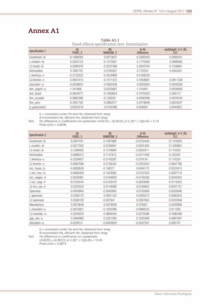
103CEPAL Review N° 122 • August 2017
Alison Vásconez Rodríguez
Annex A1Table A1.1
Fixed effects specification test: feminization
Specification 1 (b)FIXED_2
(B)RANDOM_2
(b-B)Difference
sqrt(diag(V_b-V_B))S.E.
investment~ib -0.1686565 0.0573637 -0.2260203 0.0992541
L.investm~ib 0.0303124 -0.1473261 0.1776385 0.0886562
L2.invest~ib 0.0288376 -0.2557388 0.2845764 0.1338661
feminization 0.7887797 0.0185267 0.770253 0.4044201
L.feminiza~n -0.3723222 -0.3534988 -0.0188234
L2.feminiz~n 0.0647415 -0.1011472 0.1658887 0.0911338
education~a -0.0059632 -0.0063436 0.0003804 0.0040306
fem_argent~a -1.341968 -0.0225667 -1.319401 0.8209595
fem_brazil -0.5604077 -0.1900654 -0.3703423 0.595131
fem_ecuador -0.9882586 -0.129229 -0.8590296 0.4538183
fem_peru -0.3081725 -0.0662077 -0.2419648 0.6024027
d_government 0.0023519 0.0104388 -0.008087 0.0043851
b = consistent under Ho and Ha; obtained from xtreg B inconsistent Ha, efficient Ho; obtained from xtregTest: Ho difference in coefficients not systematic chi2(12) = (b-B)’[(V_b-V_B)^ (-1)](b-B) = 5,13 Prob>chi2 = 0,9536
Specification 2 (b)FIXED_3
(B)RAMDOM_3
(b-B)Difference
sqrt(diag(V_b-V_B))S.E.
investment~ib 0.0947441 0.1097889 -0.0150449 0.1125835
L.investm~ib 0.0577002 0.0185697 0.0391305 0.1330804
L2.invest~ib 0.1269483 0.1319894 -0.0050411 0.110423
feminization 0.0666373 0.1137812 -0.0471439 0.102343
L.feminiza~n -0.3334827 -0.3143287 -0.019154 0.114324
L2.feminiz~n -0.0687099 0.2736242 -0.3423342 0.0847786
incr_hours_m -0.0658539 -0.106271 0.0404172 0.0523413
L.incr_hou~m -0.0926459 -0.1033992 0.0107533 0.0267719
incr_wages~4 0.0039381 0.0184609 -0.0145228 0.0045453
L.incr_wag~4 -0.0105544 -0.0102478 -0.0003066 0.0110023
L2.incr_wa~4 0.0325524 0.0144698 0.0180825 0.0047757
Openness 0.0059945 -0.0042663 0.0102608 0.0035646
L.openness 0.0356175 0.0091102 0.0265073 0.0065033
L2.openness 0.0508193 -0.007941 0.0587603 0.0252948
Manufacture 0.5873649 0.2079639 0.379401 0.2420066
L.manufact~a -0.2910921 -0.1930398 -0.0980523 0.011293
L2.manufac~a 0.3245035 0.0669439 0.2575596 0.1690496
gap_edu~a 0.3946982 0.2321393 0.1625589 0.0861091
education~a -0.025813 -0.0050629 -0.0207501 0.093747
b = consistent under Ho and Ha; obtained from xtreg B inconsistent Ha, efficient Ho; obtained from xtregTest: Ho difference in coefficients no t systematic chi2(20) = (b-B)’[(V_b-V_B)^ (-1)](b-B) = 13,45 Prob>chi2 = 0,2674
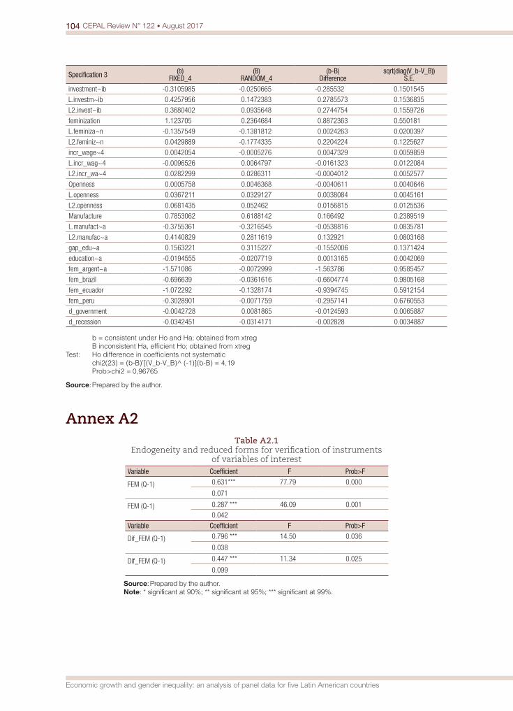
104 CEPAL Review N° 122 • August 2017
Economic growth and gender inequality: an analysis of panel data for five Latin American countries
Specification 3 (b)FIXED_4
(B)RANDOM_4
(b-B)Difference
sqrt(diag(V_b-V_B))S.E.
investment~ib -0.3105985 -0.0250665 -0.285532 0.1501545
L.investm~ib 0.4257956 0.1472383 0.2785573 0.1536835
L2.invest~ib 0.3680402 0.0935648 0.2744754 0.1559726
feminization 1.123705 0.2364684 0.8872363 0.550181
L.feminiza~n -0.1357549 -0.1381812 0.0024263 0.0200397
L2.feminiz~n 0.0429889 -0.1774335 0.2204224 0.1225627
incr_wage~4 0.0042054 -0.0005276 0.0047329 0.0059859
L.incr_wag~4 -0.0096526 0.0064797 -0.0161323 0.0122084
L2.incr_wa~4 0.0282299 0.0286311 -0.0004012 0.0052577
Openness 0.0005758 0.0046368 -0.0040611 0.0040646
L.openness 0.0367211 0.0329127 0.0038084 0.0045161
L2.openness 0.0681435 0.052462 0.0156815 0.0125536
Manufacture 0.7853062 0.6188142 0.166492 0.2389519
L.manufact~a -0.3755361 -0.3216545 -0.0538816 0.0835781
L2.manufac~a 0.4140829 0.2811619 0.132921 0.0803168
gap_edu~a 0.1563221 0.3115227 -0.1552006 0.1371424
education~a -0.0194555 -0.0207719 0.0013165 0.0042069
fem_argent~a -1.571086 -0.0072999 -1.563786 0.9585457
fem_brazil -0.696639 -0.0361616 -0.6604774 0.9805168
fem_ecuador -1.072292 -0.1328174 -0.9394745 0.5912154
fem_peru -0.3028901 -0.0071759 -0.2957141 0.6760553
d_government -0.0042728 0.0081865 -0.0124593 0.0065887
d_recession -0.0342451 -0.0314171 -0.002828 0.0034887
b = consistent under Ho and Ha; obtained from xtreg B inconsistent Ha, efficient Ho; obtained from xtregTest: Ho difference in coefficients not systematic chi2(23) = (b-B)’[(V_b-V_B)^ (-1)](b-B) = 4,19 Prob>chi2 = 0,96765
Source: Prepared by the author.
Annex A2Table A2.1
Endogeneity and reduced forms for verification of instruments of variables of interest
Variable Coefficient F Prob>F
FEM (Q-1)
0.631*** 77.79 0.000
0.071 FEM (Q-1)
0.287 *** 46.09 0.001
0.042
Variable Coefficient F Prob>F
Dif_FEM (Q-1)
0.796 *** 14.50 0.036
0.038 Dif_FEM (Q-1)
0.447 *** 11.34 0.025
0.099 Source: Prepared by the author.Note: * significant at 90%; ** significant at 95%; *** significant at 99%.
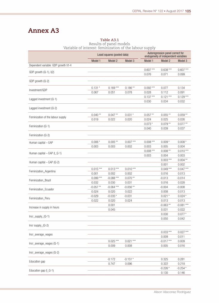
105CEPAL Review N° 122 • August 2017
Alison Vásconez Rodríguez
Annex A3Table A3.1
Results of panel models Variable of interest: feminization of the labour supply
Least squares (pooled data) Autoregression panel correct for endogeneity of independent variables
Model 1 Model 2 Model 3 Model 1 Model 2 Model 3Dependent variable: GDP growth t/t-4
GDP growth (Q-1), I(2) 0.607 *** 0.638 *** 0.607 ***
0.076 0.071 0.099
GDP growth (Q-2)
Investment/GDP0.131 * 0.169 *** 0.186 ** 0.092 *** 0.077 0.134
0.067 0.051 0.078 0.028 0.112 0.091
Lagged investment (Q-1) 0.137 *** 0.121 *** 0.129 ***
0.030 0.034 0.032
Lagged investment (Q-2)
Feminization of the labour supply0.040 ** 0.047 ** 0.031 * 0.057 ** 0.055 ** 0.059 **
0.019 0.022 0.020 0.024 0.025 0.026
Feminization (Q-1) 0.073 * 0.079 ** 0.077 **
0.040 0.039 0.037
Feminization (Q-2)
Human capital – EAP
0.006 * 0.005 ** 0.007 *** 0.008 *** 0.009 * 0.008 *
0.003 0.003 0.002 0.003 0.005 0.004
Human capital – EAP (I_Q-1) 0.008 *** 0.008 ** 0.010 ***
0.003 0.004 0.003
Human capital – EAP (Q-2) 0.003 *** 0.004 **
0.001 0.002
Feminization_Argentina0.015 *** 0.013 *** 0.010 *** 0.049 *** 0.047 ***
0.001 0.002 0.002 0.016 0.013
Feminization_Brazil0.099 *** -0.088 *** 0.070 ** -0.013 -0.014
0.032 0.030 0.031 0.016 0.028
Feminization_Ecuador-0.057 ** -0.064 *** -0.056 ** -0.004 -0.008
0.024 0.020 0.022 0.008 0.013
Feminization_Peru-0.029 -0.035 * -0.031 0.021 * 0.024 *
0.022 0.020 0.024 0.013 0.013
Increase in supply in hours 0.001 -0.063 ** -0.081 ***
0.045 0.031 0.022
Incr_supply_(Q-1) 0.030 0.077 *
0.050 0.042
Incr supply_(Q-2)
Incr_average_wages 0.033 *** 0.027 ***
0.009 0.011
Incr_average_wages (Q-1) 0.025 *** 0.021 *** -0.017 *** 0.009
0.009 0.008 0.005 0.016
Incr_average_wages (Q-2)
Education gap -0.172 -0.151 * 0.325 0.281
0.747 0.096 0.322 0.218
Education gap (I_Q-1) -0.226 * -0.254 *
0.130 0.146

106 CEPAL Review N° 122 • August 2017
Economic growth and gender inequality: an analysis of panel data for five Latin American countries
Least squares (pooled data) Autoregression panel correct for endogeneity of independent variables
Model 1 Model 2 Model 3 Model 1 Model 2 Model 3
Economic openness 0.004 ** 0.005 -0.003 ** 0.003
0.002 0.176 0.001 0.002
Openness (Q-1) 0.018 *** 0.018 ***
0.005 0.004
Openness (Q-2) -0.020 *** -0.007
0.004 0.011
Industrialization -0.065 ** -0.084 -0.233 *** -0.197 ***
0.030 0.285 0.060 0.074
Industrialization (Q-1) -0.048 -0.130 **
0.061 0.052
Industrialization (Q-2) 0.119 *** 0.118 ***
0.032 0.027
Change of government0.007 * 0.007 0.009 * 0.009 *
0.004 0.018 0.005 0.005
External crisis -0.042 *** -0.031 ***
0.007 0.012
Source: Prepared by the author.Note: * significant at 90%; ** significant at 95%; ***significant at 99%.
Table A3.1 (concluded)
Who borrows to accumulate assets? Class, gender and indebtedness in Ecuador’s credit marketCarmen Diana Deere and Zachary B. Catanzarite
Abstract
This article examines the propositions that wealth inequality supports credit market segmentation and that the financial system may reproduce economic inequality. Specifically, we discuss how the sources of credit and the purposes of borrowing may help perpetuate inequality. In Ecuador, the asset-poor are more likely than the asset-rich to borrow from the informal sector for expense purposes and to have higher debt-to-net-wealth ratios. We also investigate the correlates of borrowing by men and women to acquire assets and show that the main factor associated with holding asset debt for both men and women is having a formal savings account.
KeywordsFinancial services, gender, gender mainstreaming, social classes, loans, debt, financial institutions, informal sector, economic indicators, Ecuador
JEL classificationN26, D31, J16
AuthorsCarmen Diana Deere is a Distinguished Professor Emerita of Latin American Studies and Food and Resource Economics with the University of Florida, and Honorary Emerita Professor-Researcher with FLACSO-Ecuador. [email protected]
Zachary B. Catanzarite is a Research Associate with the Center for Latin American Studies at the University of Florida. [email protected]
108 CEPAL Review N° 122 • August 2017
Who borrows to accumulate assets? Class, gender and indebtedness in Ecuador’s credit market
I. Introduction
For the past several decades, financial inclusion —expanding access to credit and other financial services for those who have typically been excluded from formal credit markets— has been a main objective of development policy in Latin America. While the explosion in the number of microfinance institutions (MFIs) throughout the region has undoubtedly increased access to credit, there is concern that the poor may be underrepresented in this expansion, as noted in repeated calls to further deepen outreach efforts (Peck and Miller, 2006; De la Torre, Ize and Schmukler, 2011). At the same time, recent microcredit crises in developing countries have sparked concern that the expansion of microfinance has led to over-indebtedness, particularly among the poor (Schicks, 2013a; Bastiaensen and others, 2013).
Figueroa (2011) argues that as long as wealth inequality in Latin America remains high, the region will continue to be subject to a three-tier financial structure in which the poor pay more for access to credit than the rich. The three-tier financial structure consists of: (i) private banks; (ii) formal, non-banking institutions such as savings and loans (S&L) cooperatives and credit unions; and (iii) the informal sector, comprised primarily of moneylenders but also family and friends. He also demonstrates how wealth inequality predicts market segmentation, with the wealthy relying on formal banks, the less wealthy on formal non-banking institutions and the poor on the informal sector. A hallmark of this financial structure is that credit is more expensive from non-banking institutions than from formal banks, and likewise, more expensive from the informal sector than from non-banking institutions.1
This is primarily due to the role played by collateral in reducing risk —always a requirement of private banks— and the economies of scale in transaction costs associated with large loans. In short, those with sufficient assets (the wealthy) are able to provide collateral and obtain better credit terms in the private banking sector, while the excess demand of the asset-poor is channelled into the more expensive segments.
In this paper, we illustrate this argument in the case of Ecuador and take it a step further by demonstrating how the purpose of borrowing may further exacerbate economic inequality. If the rich and the poor borrow for different purposes, with the rich borrowing to accumulate assets and the poor borrowing primarily to meet current expenses, then the expansion of access to credit through microfinance, for example, might mitigate poverty in the short run while reproducing the concentration of wealth among the asset-rich. Differences in the purpose of borrowing, combined with credit market segmentation, may also explain why the poor might have higher debt-to-net-wealth ratios than the wealthy and a greater likelihood of falling into a debt trap.
We investigate the relationship between household net wealth, sources of credit and the purpose of borrowing by drawing on a unique data set on household wealth for Ecuador. This data set allows us to analyse household and individual borrowing from all sources and for all purposes. In this analysis, we use household net wealth quintiles as a proxy for class, distinguishing between the asset-rich (those who have sufficient assets to provide collateral for loans) and the asset-poor (those who do not).2 Our survey also gathered information on which member of a household is responsible for repayment of a loan. Thus, we combine a class analysis with a gender analysis. We analyse the correlates of borrowing by men and women to acquire assets, as well as individual-level debt-to-net-wealth ratios by gender, topics that have not been explored in much depth.
1 See Banerjee and Duflo (2010) on some of the stylized facts on credit markets in developing countries, such as the difference in interest rates between the formal and informal sector.
2 Our net wealth quintiles likely correspond well to the analytic class structure proposed by Portes and Hoffman (2003) for Latin America, where the wealthiest quintile is made up of capitalists, managers of large and medium-sized firms and public institutions and salaried professionals, and the poorest quintile is comprised of informal sector workers.
109CEPAL Review N° 122 • August 2017
Carmen Diana Deere and Zachary B. Catanzarite
Most quantitative studies tend to focus only on households with businesses (or individual entrepreneurs) or households that engage in agricultural activities, and look at credit access and use only for those specific activities, i.e. what is often termed “productive credit”. Our household finance approach takes into account that households often engage in multiple income-generating activities and may take out loans from various sources for multiple purposes, and moreover that loans are fungible —they can be taken out for one purpose but used in multiple ways (Collins, 2008).
We define asset loans as loans taken out for the purpose of acquiring or enhancing any physical asset. Our definition of an asset loan is broader than the usual focus on “productive” credit because we are interested in the relationship between the distribution of wealth, access to credit and indebtedness. Wealth is conventionally defined as the sum of the value of physical assets (including housing and consumer durables) plus financial assets (Davies, 2008). In a three-tiered financial system, most physical and financial assets potentially serve as collateral for loans. For example, while consumer durables, with the possible exception of vehicles, would hardly suffice as collateral for a private bank loan, a television, stove or refrigerator may be acceptable as collateral at non-banking institutions and in the informal sector, since these can be sold or pawned to meet debt repayments (Vogelgesang, 2003).3 Moreover, even if a stove or refrigerator purchased on installment is not currently used in connection with a business, it may generate the means for a woman’s self-employment (selling cooked food or chilled drinks) if the need arises, much the same way that ownership of a vehicle may constitute a potential means for a man to generate income through transport services.
Expense loans include loans taken out to meet daily expenses such as food, utilities, transportation or clothing; expenses for schooling, health and celebrations; migration expenses; and repayment of previous loans. We thus also depart from conventional analysis by considering education and health as expenses rather than human capital investments, since their financial return may be in the long run as opposed to the short term and does not necessarily accrue to the household that holds the debt.
We demonstrate that those who are asset-rich in Ecuador are not only more likely to borrow from formal sources but also more likely to borrow for the purpose of asset accumulation. In contrast, the asset-poor rely more on informal sources and are more likely to borrow to meet household expenses. Not surprisingly, the poor have higher debt-to-net-wealth ratios than the wealthy. While the great majority of loans taken out in Ecuador are from formal sources, loans taken out individually by either men or women, but particularly women, are more likely to be from informal sources than those for which a couple is responsible. Similarly, while the great majority of loans are taken out for the purpose of asset accumulation, loans for which women are individually responsible are more likely to be expense loans.
Given our primary interest in the relationship between the use of credit and economic inequality, we perform a logistic regression analysis to investigate the correlates of borrowing to acquire assets. Our results suggest that, regardless of gender, the main factor associated with holding asset debt is having a formal savings account. Meanwhile, a major gender difference occurs in the relevance of earning own income, a variable that is significantly associated with women only in terms of borrowing for the purpose of asset accumulation. In the aggregate, those in the poorest wealth quintile, particularly the poorest men, have the most troubling debt-to-net-wealth ratios, but the poorest women may have the highest levels of debt distress as indicated by the need to recycle loans. Taken together, the analysis provides support for Figueroa’s (2011) proposition that under the three-tiered financial system, wealth begets wealth.
3 See CAF (2011, cuadro 4.7) for a detailed breakdown of the types of collateral accepted by a range of formal and informal lending sources in a study of micro-entrepreneurs in Colombia.
110 CEPAL Review N° 122 • August 2017
Who borrows to accumulate assets? Class, gender and indebtedness in Ecuador’s credit market
Following this introduction, the article is organized as followed. Section II describes Ecuador’s financial system and summarizes the available studies on household use of credit and economic inequality. Section III presents the methodology of the 2010 Ecuador national household asset survey and then investigates the sources and purpose of loans by class and gender. In section IV contains the logistic regression analysis of the factors associated with borrowing by individuals for the purpose of asset accumulation. Section V examines the indebtedness of men and women by class and section VI sets out our conclusions.
II. The Ecuadorian context
Ecuador’s financial system has recovered from the 1999-2000 financial crisis that led to the adoption of the United States dollar as the country’s official currency. That crisis was marked by the failure of 22 commercial banks, which held some 60% of the assets of the private financial system, and was the culmination of almost a decade of economic instability. Most analysts attribute that instability to a combination of financial deregulation and liberalization, excessive external debt, sharply fluctuating oil prices (the country’s major export) and political instability (Da Ros, 2003; Jácome, 2007).
The task in the next decade was to restore public confidence and this was done by rebuilding the public banking system that previously had been dismantled, along with State regulation of the private banking system. In 2006, private bank credit as a percentage of gross domestic product (GDP) was 22%, placing Ecuador below the Latin American average but above that of much larger economies such as Peru and Mexico (Fanelli, 2011, table 10.1). By 2010, this share had increased to 28%.4
Two institutions currently regulate the formal, private financial system: the Superintendence of Banking and Insurance (SBS) and the Superintendence of the Popular and Solidarity Economy (SEPS). SBS regulates all private, commercial banks, which numbered 24 in 2013, compared with 96 prior to the financial crisis. Since 2013, SEPS regulates all forms of cooperative financial associations. Prior to 2013, the largest S&L cooperatives (those with assets of more than US$ 1 million and deposits of more than US$ 200,000) were governed by SBS, and those below this threshold by the Ministry of Economic and Social Inclusion.
While many of the S&L cooperatives date back to the 1960s, their numbers expanded rapidly throughout the country following the collapse of the banking sector. A 2002 census of the S&L cooperatives and communal banks and funds revealed that at that time there were 26 regulated cooperatives reporting to SBS and 350 non-regulated institutions reporting to the Ministry; the latter had over half a million members (Jácome and Cordovéz, 2004). By June 2013, 773 S&L cooperatives reported to SEPS. As table 1 shows, these are stratified by size, with the largest cooperatives (segment 4) being the ones that previously reported to SBS.5
The composition of the loan portfolios of the private banks and the S&L cooperatives differ markedly, as table 1 also illustrates. The S&L cooperatives serve microenterprises and households, while the private banks are heavily focused on lending to the commercial sector (corporate firms). Consumer loans (as traditionally defined) make up a relatively large share of the loan portfolios of both the private banks and the S&L cooperative sector, at 36% and 50%, respectively.
4 See World Bank [online] http://econ.worldbank.org/WBSITE/EXTERNAL/EXTDEC/EXTRESEARCH/0,,contentMDK:20696167~pagePK:64214825~piPK:64214943~theSitePK:469382,00.html. Based on World Bank Financial Structure and Economic Development Database, for private credit by deposit money banks and other financial institutions as a share of GDP.
5 Included in the S&L cooperatives (mainly in segments 1 and 2) are what are known as communal banks or funds (often averaging only 25 to 30 members) and other local-level microfinance groups organized by non-governmental organizations (NGOs). A main distinction between these various forms, besides their size and geographical coverage, is that while S&L cooperatives can take deposits from non-cooperative members, the other forms can only hold the savings of their members (SEPS, 2014).

111CEPAL Review N° 122 • August 2017
Carmen Diana Deere and Zachary B. Catanzarite
Table 1 Ecuador: distribution of loans between private banks and savings and loan cooperatives
of different sizes by purpose, June 2013(Percentages)
Institution Number Commercial Consumer Housing Micro-enterprise Totala
Private banks 24 48 35.7 8.5 7.8 100%(US$ 16.3 billion)
Cooperativesb
Segment 4 40 4 51.2 7.3 37.5 100%(US$ 3.3 billion)
Segment 3 78 0.9 49.5 8.8 40.8 100%(US$ 1.2 billion)
Segment 2 296 4.9 39 2 54 100%(US$ 0.5 billion)
Segment 1 359 9.3 37.7 1.5 52.4 100%(US$ 0.1 billion)
Subtotal 773 3.4 49.5 7.1 40 100%US$ 5.0 billion)
Source: Prepared by the authors, on the basis of Superintendence of Banking and Insurances (SBS), Boletín de Series Bancos Privados, 2013 [online] http://www.sbs.gob.ec; and Superintendencia de Economía Popular y Solidaria (SEPS), Boletín Financiero – Sector Financiero Popular y Solidario al 30 de junio de 2013, 2013 [online] http://www.seps.gob.ec.
a The total also includes a fifth category, loans for education, which amount to less than 1% of the total portfolio.b Segments refer to the stratification of savings and loan cooperatives by size, defined by the value of their total assets, number
of members and extent of geographical coverage, with segment 4 representing the largest cooperatives.
Another feature of the Ecuadorian financial system is that the central bank sets the maximum interest rates that can be charged on formal sector loans. As table 2 shows, these vary by the type of institution and the purpose of the loan. As predicted by the Figueroa (2011) model, the lowest interest rates are offered by private banks to corporate clients and the highest rates are for microcredit offered by MFIs. In 2010, the maximum corporate rate was 9.3% per annum, whereas microcredit rates ranged from 25.5% to 30.5% depending on the size of the loan. In our qualitative fieldwork in Ecuador during 2009-2010, moneylenders were reported to charge between 10% and 20% per month.6
Table 2 Ecuador: maximum interest rates, December 2010
(Percentages)
Purpose Interest ratea
Commercial
Corporateb 9.3
Small and medium-sized businessesc 11.8
Housing 11.3
Consumer goods 16.3
Microcreditd
Loans $ 8 500 and more 25.5
Loans between $ 600 and $ 8 500 27.5
Loans less than $ 600 30.5
Source: Prepared by the authors, on the basis of Central Bank of Ecuador, Evolución del volumen de crédito y tasas de interés: análisis del sistema de finanzas públicas y privado del Ecuador, Quito, 2013 [online] http://contenido.bce.fin.ec/documentos/Estadisticas/SectorMonFin/BoletinTasasInteres/ect201312.pdf.
a These same maximum interest rates held through 2014.b Firms with annual sales above $ 5 million.c Firms with annual sales between $ 100,000 and $ 5 million.d Firms with annual sales below $ 100,000.
6 Focus groups in the provinces of Pichincha and Manabí. See also Floro and Messier (2006, p. 239) on the high interest rates charged by moneylenders in Quito and Guayaquil.
112 CEPAL Review N° 122 • August 2017
Who borrows to accumulate assets? Class, gender and indebtedness in Ecuador’s credit market
One of the main drivers of the microfinance movement in Ecuador since 2000 has been the Rural Finance Network (RFR), which brings together private banks working in this subsector,7
S&L cooperatives and NGOs with microfinance programmes. These MFIs, whose mission is financial inclusion, work both in rural areas and among the urban poor. Their combined loan portfolio has steadily increased, growing at around 10% per year during the 2000s (Readout, 2011, p. 30) and more than doubling between 2010 and 2013 (RFR, 2013).
Only a few largescale surveys have been carried out in Ecuador that look at credit use by households, as opposed to firms, and irrespective of source. These surveys point to a recovery of confidence in the private financial system and growing financial inclusion. A representative household survey in the three largest cities (Quito, Guayaquil and Cuenca) in 2003 found that only 12.5% of urban households had taken out a loan in the previous twelve months (Jácome, 2005). An analysis of the nationally representative 2006 Ecuador living standards survey showed that 51.5% of households had taken out a loan for any purpose in the previous year.8 In our nationally representative household assets survey from 2010, described below, we find that 46% of households have an outstanding loan. While the scope and methodology of these surveys differ, they support the conclusion that the financial system both recovered and expanded over the course of the 2000s.
Mideros (2010), utilizing the credit modules in the 2006 living standards survey, analyses the role of income inequality in the use of different types of credit in Ecuador. He finds a much lower incidence of consumer cash loans9 among households in the poorest two income quintiles (22% and 26%, respectively) than among those in the wealthiest two quintiles (31% in each). Installment loans for the acquisition of assets, products and services are the most frequently used form of credit reported in that survey. He finds even greater differentiation for this type of credit, with 24% of households in net wealth quintile I holding such loans as compared to 40% in quintile V (Mideros, 2010, figure 17). In terms of business credit, fewer households in the poorest quintile have a business (31%), and of these, only 9% have a business loan; in contrast, among households in the top quintile, approximately 57% have a business, and 20% of these have a business loan (Mideros, 2010, figure 18).10 Overall, his results suggest considerable differentiation in the use of credit depending on a household’s income quintile.11 We propose that a more robust measure of the role of economic inequality in the use of credit is provided by considering the distribution of wealth rather than income.
III. The Ecuador Household Asset Survey
The Ecuador Household Asset Survey (known as Encuesta Activos FLACSO-Florida (EAFF)) was carried out in 2010 by FLACSO-Ecuador and the University of Florida as part of an international comparative
7 The main banks engaged in microfinance include Banco Solidario, established in 1995 and linked to ACCION International; CREDIFE, established in 1999 as a subsidiary of the largest private bank, Banco Pichincha; and Banco ProCredit, established in 2001. The MIX Market website reports an additional four, all with gross loan portfolios of less than $ 100 million. See [online] http://www.mixmarket.org.
8 Authors’ calculations, based on INEC (2006) and aggregating at the household level all modules that included credit information.9 The possible uses of household consumer credit were for housing, health, food, education, clothing, consumer durables, land
acquisition, debt repayment and special occasions.10 Readout (2011, table 4.2) found similar results analysing the 2004 United States Agency for International Development (USAID)
micro-entrepreneur survey for Ecuador. Only 8% of micro-entrepreneurs in the lowest socioeconomic group had received a loan in the previous 12 months from any source, compared with 25% in the highest group.
11 Mideros (2010) also conducts an econometric analysis of the impact of the different types of credit on the median per capita household income gap. His most important finding is with respect to the potential impact of formal business credit on poverty, which increases the per capita income of households with businesses by 27% compared with those that do not have access to such credit.
113CEPAL Review N° 122 • August 2017
Carmen Diana Deere and Zachary B. Catanzarite
study.12 The survey was based on two-stage, stratified sampling, designed to be representative of the coastal and highland regions of Ecuador, and resulted in a sample of 2,892 households. The primary objective was to measure asset ownership at the household and individual level, and for this purpose we employed two instruments: a household assets inventory and an individual questionnaire. The survey was aimed at the heads of household, and the household inventory of physical assets was completed by the principal couple together, whenever possible.13 For each physical asset —the principal residence, agricultural land, other real estate, livestock, agricultural equipment and installations, businesses and consumer durables— a complete list of owners was obtained as well as information on whether there was an outstanding debt on the asset. The individual questionnaire was then completed by each respondent separately and focused on complementary information on asset ownership, including individual savings, current debt, loans made to third parties and other considerations such as household decision-making.
The individual debt module solicited information on all loans that were obtained by the respondent with current outstanding debt. Thus, the data may underestimate total borrowing activities during a given year due to the exclusion of short-term loans repaid during the previous twelve months. This shortcoming is balanced by the fact that the measure of outstanding debt, which includes loans acquired in previous years, gives a fuller picture of individual indebtedness. Since information on debt was gathered at both the household and individual level, there was a lengthy process of data reconciliation. While this method of data collection produced some duplication and potential misidentification (since husbands and wives sometimes provided contradictory information on the details of the same loan), it had the advantage of maximizing the possibility that information was captured on all outstanding debt. Another shortcoming of our survey was that we did not collect information on the interest rate or terms of these loans.14
Finally, we should note that the survey results are truncated, since we were unable to secure a representative sample of households in the wealthiest socioeconomic group, due primarily to a rejection rate of 100% among this group in Quito. Nonetheless, our estimated Gini coefficient of the concentration of gross wealth is 0.68 —as expected, much greater than the official estimate of the Gini income coefficient for the survey year of 0.52 (Deere and Contreras, 2011).
In the following analysis, the value of individual and household assets is estimated at market value (as reported by respondents for how much they could sell each asset today in its present condition). All results incorporate the sampling design and have been weighted utilizing the sample expansion factors so that the estimates are nationally representative.
1. Formal versus informal sources of loans
Overall, 70% of the 1,791 outstanding loans reported in the survey are from formal sources, and 30% are from informal sources. Figure 1 summarizes the distribution of loans by quintile and source and shows that the majority of loans across all quintile groups are from formal sources. Nonetheless, wealthier quintiles are more likely to have formal loans than poorer quintiles, and poorer quintiles are more likely than wealthier quintiles to rely on informal sources.15
12 See Doss and others (2011) for the comparative results on household wealth in Ecuador, Ghana and Karnataka, India; Deere and Contreras (2011) for more detailed information on the methodology of the Ecuador survey; and Grown and others (2015) for the comparative results on household and individual debt in the three countries.
13 On the rationale for interviewing the couple together for the household asset inventory, see Deere and Catanzarite (2016).14 For examples from Latin America on how interest rates and loan terms vary by formal and informal source in the case of
agricultural loans, see Barham, Boucher and Carter (1996) on Guatemala and Guirkinger (2008) on Peru. 15 Several small-scale surveys of households in urban “popular” neighborhoods in Quito and Guayaquil have found that these
households tend to rely more on informal than formal credit (Jácome and Cordovéz, 2004; Floro and Messier, 2006).

114 CEPAL Review N° 122 • August 2017
Who borrows to accumulate assets? Class, gender and indebtedness in Ecuador’s credit market
Figure 1 Ecuador: proportion of formal and informal loans by household net wealth quintile, 2010
(Percentages)
0
10
20
30
40
50
60
70
80
90
Quintile I Quintile II Quintile III Quintile IV Quintile V
Subtotal formal Subtotal informal
Source: Prepared by the authors, on the basis of Encuesta Activos FLACO-Florida (EAFF), 2010 [online] http://www.flacsoandes.edu.ec/pagina/60759-documentos-de-encuesta-activos-flacso-florida.
Table 3 presents this information at the household level —whether anyone in the household has an outstanding loan— and by net wealth quintile. While households differ as to whether they have a loan at all (53% of households in quintile V as compared to 43% in quintile I), they differ most with respect to the source of their loans. Among households in quintile V, 45% have a formal loan while only 15% have an informal loan; the corresponding figures for quintile I are 29% (formal) and 20% (informal).
Table 3 Ecuador: incidence of household formal and informal loans by net wealth quintile
and credit source, 2010 (Percentages)
SourceQuintile
Total householdsI II III IV V
State bank 2.3 3.9 6.5 4.8 11.4 5.8
Private bank 4.9 6.5 6.9 9.5 16.2 8.8
Cooperative/credit union 6.2 4.2 7.5 14.6 11.7 8.9
Other private/NGO 1.0 2.5 3.3 1.9 2.4 2.2
Business/store 16.2 18.2 14.6 10.7 11.2 14.2
Credit card 0.9 2.8 1.3 1.6 2.7 1.9
Subtotal formal 29.0 34.4 35.4 36.7 45.0 36.1Informal group 0.5 0.7 3.4 0.5 0.2 1.1
Moneylender 2.3 3.2 3.0 1.7 1.7 2.4
Employer 1.3 0.2 0.7 1.2 1.5 1.0
Friend 7.4 6.3 4.6 5.1 6.5 6.0
Family 9.2 7.6 5.3 7.3 5.6 7.0
Other 0.5 0.0 0.5 0.2 0.5 0.3
Subtotal informal 19.9 16.8 16.7 15.7 14.9 16.8Totala 43.2 44.8 46.1 47.9 52.7 46.9
n 575 601 592 540 584 2 892
N 668 995 668 593 669 070 668 756 668 419 3 343 832
Source: Prepared by the authors, on the basis of Encuesta Activos FLACO-Florida (EAFF), 2010 [online] http://www.flacsoandes.edu.ec/pagina/60759-documentos-de-encuesta-activos-flacso-florida.
a The total incidence refers to all households which have a loan irrespective of source and hence is less than the sum of formal and informal sources.
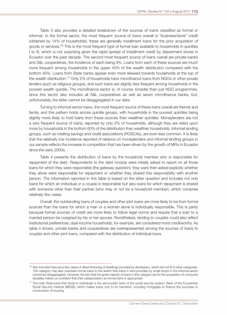
115CEPAL Review N° 122 • August 2017
Carmen Diana Deere and Zachary B. Catanzarite
Table 3 also provides a detailed breakdown of the sources of loans classified as formal or informal. In the formal sector, the most frequent source of loans overall is “business/store” credit (obtained by 14% of households); these are generally installment loans for the prior acquisition of goods or services.16 This is the most frequent type of formal loan available to households in quintiles I to III, which is not surprising given the rapid spread of installment credit by department stores in Ecuador over the past decade. The second most frequent source of loans overall are private banks and S&L cooperatives, the incidence of each being 9%. Loans from each of these sources are much more frequent among households in the upper 40% of the wealth distribution compared with the bottom 40%. Loans from State banks appear even more skewed towards households at the top of the wealth distribution.17 Only 2% of households have microfinance loans from NGOs or other private lenders (such as religious groups), and such loans are slightly less frequent among households in the poorest wealth quintile. The microfinance sector is, of course, broader than just NGO programmes, since this sector also includes all S&L cooperatives as well as seven microfinance banks, but, unfortunately, the latter cannot be disaggregated in our data.
Turning to informal sector loans, the most frequent source of these loans overall are friends and family, and this pattern holds across quintile groups, with households in the poorest quintiles being slightly more likely to hold loans from these sources than wealthier quintiles. Moneylenders are not a very frequent source of loans, reported by only 2% of households, although they are relied upon more by households in the bottom 60% of the distribution than wealthier households. Informal lending groups, such as rotating savings and credit associations (ROSCAs), are even less common. It is likely that the relatively low incidence reported of reliance on moneylenders and informal lending groups in our sample reflects the increase in competition that has been driven by the growth of MFIs in Ecuador since the early 2000s.
Table 4 presents the distribution of loans by the household member who is responsible for repayment of the debt. Respondents to the debt module were initially asked to report on all those loans for which they were responsible (the gateway question); they were then asked explicitly whether they alone were responsible for repayment or whether they shared this responsibility with another person. The information reported in this table is based on the latter question and includes not only loans for which an individual or a couple is responsible but also loans for which repayment is shared with someone other than their partner (who may or not be a household member), which comprise relatively few cases.
Overall, the outstanding loans of couples and other joint loans are more likely to be from formal sources than the loans for which a man or a woman alone is individually responsible. This is partly because formal sources of credit are more likely to follow legal norms and require that a loan to a married person be cosigned by his or her spouse. Nonetheless, lending to couples could also reflect institutional preferences; dual-income households, for example, are considered more creditworthy. As table 4 shows, private banks and cooperatives are overrepresented among the sources of loans to couples and other joint loans, compared with the distribution of individual loans.
16 Also included here are a few cases of direct financing of dwellings provided by developers, which did not fit in other categories. This category may also overstate formal loans to the extent that loans in kind provided by small shops in the informal sector cannot be disaggregated. However, the fact that the great majority of loans in this category are for the acquisition of consumer durables makes us confident that their categorization as formal loans is appropriate.
17 The main State bank that lends to individuals is the semi-public bank of the social security system, Bank of the Ecuadorian Social Security Institute (BIESS), which makes loans only to its members, including mortgages to finance the purchase or construction of housing.

116 CEPAL Review N° 122 • August 2017
Who borrows to accumulate assets? Class, gender and indebtedness in Ecuador’s credit market
Table 4 Ecuador: distribution of loans by who is responsible for debt repayment and source, 2010
(Percentages)
SourceResponsible party
Total loansMale alone Female alone Principal couple Other joint
State bank 11.7 8.7 6.8 9.5 9.4
Private bank 12.1 12.2 21.1 18.2 14.6
Cooperative/credit union 11.5 11.1 25.7 24.3 15.4
Other private/NGO 2.3 5.8 2.1 8.5 3.6
Business/Store 27.6 25.2 18.6 24.8 24.4
Credit card 4.2 3.2 1.3 0.0 3.0
Subtotal formal loans 69.4 66.3 75.6 85.3 70.3
Informal group 0.1 4.3 2.4 0.0 2.1
Moneylender 5.0 3.8 3.8 2.1 4.2
Employer 3.2 0.6 0.8 0.0 1.6
Friend 13.6 9.7 5.9 5.1 10.0
Family 7.6 15.1 11.4 7.5 11.2
Other 1.1 0.4 0.1 0.0 0.6
Subtotal informal loans 30.6 33.7 24.4 14.7 29.7
n 676 612 453 50 1 791
N 807 306 758 834 566 579 55 980 2 188 699
Source: Prepared by the authors, on the basis of Encuesta Activos FLACO-Florida (EAFF), 2010 [online] http://www.flacsoandes.edu.ec/pagina/60759-documentos-de-encuesta-activos-flacso-florida.
Note: F (2.86, 609.89) = 2.97, p = 0.033.
With respect to gender differences (comparing loans for which an individual man or woman is responsible), State banks make up a larger share of the loans for which individual men are responsible, while those from NGOs make up a larger share of the loans to individual women.18 Informal credit group loans are also more common among loans to individual women, while loans from employers are more common among loans to individual men, which reflects the fact that a greater share of men are employed than women. Finally, it is interesting to note that when women borrow alone, they rely more on loans from family members, whereas men in this case rely more on friends as a source of loans.
2. The purpose of borrowing
Of the total 1,821 sole-purpose loans reported, 68% have been taken out for the purpose of asset accumulation and 32% in order to meet expenses.19 As figure 2 shows, there are statistically significant differences by wealth quintile in the distribution of these asset and expense loans. Households in the poorest quintile are much more likely to take out expense loans compared with the other quintiles, whose borrowing activity is geared towards asset accumulation. This is a particularly worrisome finding since it suggests that the loans taken out by the asset poor are less likely to generate a future income stream, making it potentially difficult for them to repay the loan, a factor we will explore.
18 December 2013 data for the 46 MFIs reporting to the Rural Finance Network reveal that 69% of the loan clients of NGOs are women, compared with the overall average for RFN members of 54% (RFN, 2013).
19 Less than 2% of the total loans were reported as dual-purpose expense and asset loans, and these have been excluded from the analysis.

117CEPAL Review N° 122 • August 2017
Carmen Diana Deere and Zachary B. Catanzarite
Figure 2 Ecuador: proportion of asset and expense loans by household net wealth quintile, 2010
(Percentages)
0
10
20
30
40
50
60
70
80
90
Quintile I Quintile II Quintile III Quintile IV Quintile V
Asset Expense
Source: Prepared by the authors, on the basis of Encuesta Activos FLACO-Florida (EAFF), 2010 [online] http://www.flacsoandes.edu.ec/pagina/60759-documentos-de-encuesta-activos-flacso-florida.
Table 5 offers a more detailed breakdown of the incidence of household debt by purpose among those who have loans. This table takes into account that households may have multiple loans and loans for various purposes. It shows that, overall, the most frequent purposes are for the acquisition of consumer durables (28%) and explicitly for a business (27%). This is followed in frequency by loans to acquire a housing lot or dwelling or to improve or expand a dwelling (19%), to meet daily needs (15%) and for health expenses (10%).
Among the most striking class differences is the greater frequency of households in the poorest 40% of the wealth distribution taking out loans to acquire consumer durables (such as a stove, television or refrigerator) and to meet daily needs and health expenses. In contrast, households in the wealthiest 40% borrow most frequently to acquire or upgrade their dwelling or for business purposes. The wealthiest households are also much more likely to borrow to acquire a vehicle, whereas the poorest are more likely to borrow for education expenses. This analysis suggests that wealthier households are more likely than poorer ones to go into debt to acquire assets that will generate income directly and/or serve as collateral for future loans. Worth noting, however, is that households in quintiles I and V are equally like to borrow in order to repay previous loans. The recycling of loans is often noted as a potential signal of over-indebtedness (Schicks, 2013b).
With respect to who is responsible for these loans, figure 3 shows that couples and other joint borrowers are significantly more likely to have loans related to asset acquisition than expenses when compared with individual borrowers. Moreover, lone female borrowers are more likely than any other group to have expense rather than asset debt.
Finally, figure 4 presents the distribution of loans by purpose and source. It shows that while loans intended for asset acquisition are much more likely to be from formal lending sources, expense loans are more likely to be obtained from informal sources.
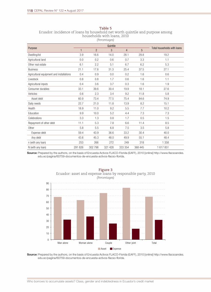
118 CEPAL Review N° 122 • August 2017
Who borrows to accumulate assets? Class, gender and indebtedness in Ecuador’s credit market
Table 5 Ecuador: incidence of loans by household net worth quintile and purpose among
households with loans, 2010 (Percentages)
PurposeQuintile
Total households with loans1 2 3 4 5
Dwelling/lot 3.9 16.6 14.0 28.1 29.8 19.2
Agricultural land 0.0 0.2 0.6 0.7 3.3 1.1
Other real estate 6.1 2.2 5.1 6.7 6.2 5.3
Business 21.1 17.8 31.3 25.4 37.5 27.1
Agricultural equipment and installations 0.4 0.9 0.0 0.2 1.6 0.6
Livestock 0.8 0.8 1.7 0.6 1.6 1.1
Agricultural inputs 0.4 3.6 3.7 0.3 1.6 1.9
Consumer durables 33.1 39.6 30.4 19.9 18.1 27.6
Vehicles 0.6 2.3 3.4 9.2 11.8 5.8
Asset debt 60.9 73.4 77.5 75.4 84.6 74.9
Daily needs 22.7 21.0 11.8 13.9 8.2 15.1
Health 18.9 11.0 9.2 5.5 7.7 10.2
Education 9.9 10.0 5.2 4.4 7.3 7.3
Celebrations 3.3 1.3 0.8 1.7 0.5 1.5
Repayment of other debt 11.1 5.3 7.8 6.6 11.4 8.5
Other 5.8 5.5 6.8 7.5 3.5 5.8
Expense debt 59.4 43.9 36.6 33.2 30.4 40.0
Any debt 43.6 45.3 48.0 49.9 55.1 48.4
n (with any loan) 253 266 272 249 318 1 358
N (with any loan) 291 826 302 798 321 428 333 354 368 445 1 617 851
Source: Prepared by the authors, on the basis of Encuesta Activos FLACO-Florida (EAFF), 2010 [online] http://www.flacsoandes.edu.ec/pagina/60759-documentos-de-encuesta-activos-flacso-florida.
Figure 3 Ecuador: asset and expense loans by responsible party, 2010
(Percentages)
0
10
20
30
40
50
60
70
80
90
Man alone Woman alone Couple Other joint Total
Asset Expense
Source: Prepared by the authors, on the basis of Encuesta Activos FLACO-Florida (EAFF), 2010 [online] http://www.flacsoandes.edu.ec/pagina/60759-documentos-de-encuesta-activos-flacso-florida.

119CEPAL Review N° 122 • August 2017
Carmen Diana Deere and Zachary B. Catanzarite
Figure 4 Ecuador: loans by purpose and source, 2010
(Percentages)
0
10
20
30
40
50
60
70
80
90
Asset Expense
Formal Informal
Source: Prepared by the authors, on the basis of Encuesta Activos FLACO-Florida (EAFF), 2010 [online] http://www.flacsoandes.edu.ec/pagina/60759-documentos-de-encuesta-activos-flacso-florida.
Note: F (1.213), p = 0.000.
IV. The likelihood of borrowing for asset accumulation
We now turn to the likelihood that an individual will acquire an asset loan. In order to conduct a gender analysis, an individual is considered to borrow for asset acquisition whether the loan for which he or she is responsible was obtained individually or jointly. We perform logit regressions for men and women separately. Our variables of interest are as follows: (i) being an income earner, which we define as being in remunerated employment (whether an employer, self-employed or any kind of wage worker) versus being an unpaid family worker, unemployed or not economically active; (ii) having a formal savings account; (iii) being a member of a social network; and (iv) the household net wealth quintile to which the individual belongs.
We hypothesize that individuals who earn income directly are considered more creditworthy than those who do not since they have a verifiable means of making loan repayments. Sometimes proof of employment or of ownership of a business may suffice as collateral, particularly among S&L cooperatives.20 Since obtaining a loan may be tied to having a previous relationship with the lender and having savings may serve as a form of collateral, we expect those who own a formal savings account to be more likely to obtain loans for the purpose of asset accumulation (CAF, 2011). It is common for private banks as well as S&L cooperatives in Ecuador to require potential borrowers to have a savings account and/or to maintain a minimum balance in the account; these conditions may also lower the cost of borrowing. Also, having formal savings might reduce the need for short-term credit, making account holders more likely to seek loans for asset acquisition (Kast and Pomeranz, 2014).
We expect individuals who are members of a social network or group to have greater access to information regarding the availability and conditions of credit and thus to be more likely to have asset loans (Fletschner and Mesbah, 2011). In addition, being a group member may increase the odds of
20 Authors’ review of the websites of the largest of the 39 Ecuadorian savings and loan cooperatives listed on the MIX Market (date of reference: January 2015).
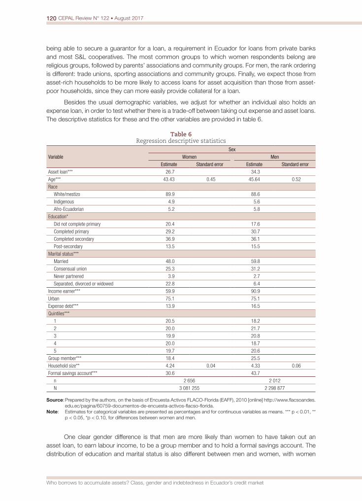
120 CEPAL Review N° 122 • August 2017
Who borrows to accumulate assets? Class, gender and indebtedness in Ecuador’s credit market
being able to secure a guarantor for a loan, a requirement in Ecuador for loans from private banks and most S&L cooperatives. The most common groups to which women respondents belong are religious groups, followed by parents’ associations and community groups. For men, the rank ordering is different: trade unions, sporting associations and community groups. Finally, we expect those from asset-rich households to be more likely to access loans for asset acquisition than those from asset-poor households, since they can more easily provide collateral for a loan.
Besides the usual demographic variables, we adjust for whether an individual also holds an expense loan, in order to test whether there is a trade-off between taking out expense and asset loans. The descriptive statistics for these and the other variables are provided in table 6.
Table 6 Regression descriptive statistics
VariableSex
Women MenEstimate Standard error Estimate Standard error
Asset loan*** 26.7 34.3
Age*** 43.43 0.45 45.64 0.52
Race
White/mestizo 89.9 88.6
Indigenous 4.9 5.6
Afro-Ecuadorian 5.2 5.8
Education*
Did not complete primary 20.4 17.6
Completed primary 29.2 30.7
Completed secondary 36.9 36.1
Post-secondary 13.5 15.5
Marital status***
Married 48.0 59.8
Consensual union 25.3 31.2
Never partnered 3.9 2.7
Separated, divorced or widowed 22.8 6.4
Income earner*** 59.9 90.9
Urban 75.1 75.1
Expense debt*** 13.9 16.5
Quintiles***
1 20.5 18.2
2 20.0 21.7
3 19.9 20.8
4 20.0 18.7
5 19.7 20.6
Group member*** 18.4 25.5
Household size** 4.24 0.04 4.33 0.06
Formal savings account*** 30.6 43.7
n 2 656 2 012
N 3 081 255 2 298 877
Source: Prepared by the authors, on the basis of Encuesta Activos FLACO-Florida (EAFF), 2010 [online] http://www.flacsoandes.edu.ec/pagina/60759-documentos-de-encuesta-activos-flacso-florida.
Note: Estimates for categorical variables are presented as percentages and for continuous variables as means. *** p < 0.01, ** p < 0.05, *p < 0.10, for differences between women and men.
One clear gender difference is that men are more likely than women to have taken out an asset loan, to earn labour income, to be a group member and to hold a formal savings account. The distribution of education and marital status is also different between men and women, with women
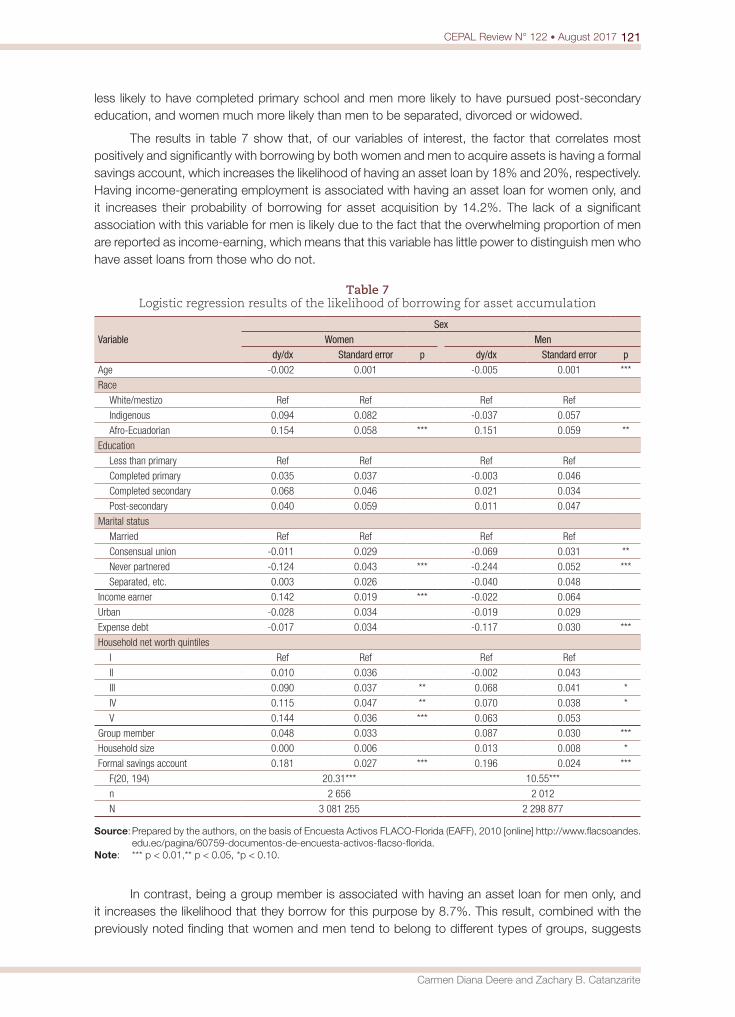
121CEPAL Review N° 122 • August 2017
Carmen Diana Deere and Zachary B. Catanzarite
less likely to have completed primary school and men more likely to have pursued post-secondary education, and women much more likely than men to be separated, divorced or widowed.
The results in table 7 show that, of our variables of interest, the factor that correlates most positively and significantly with borrowing by both women and men to acquire assets is having a formal savings account, which increases the likelihood of having an asset loan by 18% and 20%, respectively. Having income-generating employment is associated with having an asset loan for women only, and it increases their probability of borrowing for asset acquisition by 14.2%. The lack of a significant association with this variable for men is likely due to the fact that the overwhelming proportion of men are reported as income-earning, which means that this variable has little power to distinguish men who have asset loans from those who do not.
Table 7 Logistic regression results of the likelihood of borrowing for asset accumulation
VariableSex
Women Mendy/dx Standard error p dy/dx Standard error p
Age -0.002 0.001 -0.005 0.001 ***
Race
White/mestizo Ref Ref Ref Ref
Indigenous 0.094 0.082 -0.037 0.057
Afro-Ecuadorian 0.154 0.058 *** 0.151 0.059 **
Education
Less than primary Ref Ref Ref Ref
Completed primary 0.035 0.037 -0.003 0.046
Completed secondary 0.068 0.046 0.021 0.034
Post-secondary 0.040 0.059 0.011 0.047
Marital status
Married Ref Ref Ref Ref
Consensual union -0.011 0.029 -0.069 0.031 **
Never partnered -0.124 0.043 *** -0.244 0.052 ***
Separated, etc. 0.003 0.026 -0.040 0.048
Income earner 0.142 0.019 *** -0.022 0.064
Urban -0.028 0.034 -0.019 0.029
Expense debt -0.017 0.034 -0.117 0.030 ***
Household net worth quintiles
I Ref Ref Ref Ref
II 0.010 0.036 -0.002 0.043
III 0.090 0.037 ** 0.068 0.041 *
IV 0.115 0.047 ** 0.070 0.038 *
V 0.144 0.036 *** 0.063 0.053
Group member 0.048 0.033 0.087 0.030 ***
Household size 0.000 0.006 0.013 0.008 *
Formal savings account 0.181 0.027 *** 0.196 0.024 ***
F(20, 194) 20.31*** 10.55***
n 2 656 2 012
N 3 081 255 2 298 877
Source: Prepared by the authors, on the basis of Encuesta Activos FLACO-Florida (EAFF), 2010 [online] http://www.flacsoandes.edu.ec/pagina/60759-documentos-de-encuesta-activos-flacso-florida.
Note: *** p < 0.01,** p < 0.05, *p < 0.10.
In contrast, being a group member is associated with having an asset loan for men only, and it increases the likelihood that they borrow for this purpose by 8.7%. This result, combined with the previously noted finding that women and men tend to belong to different types of groups, suggests
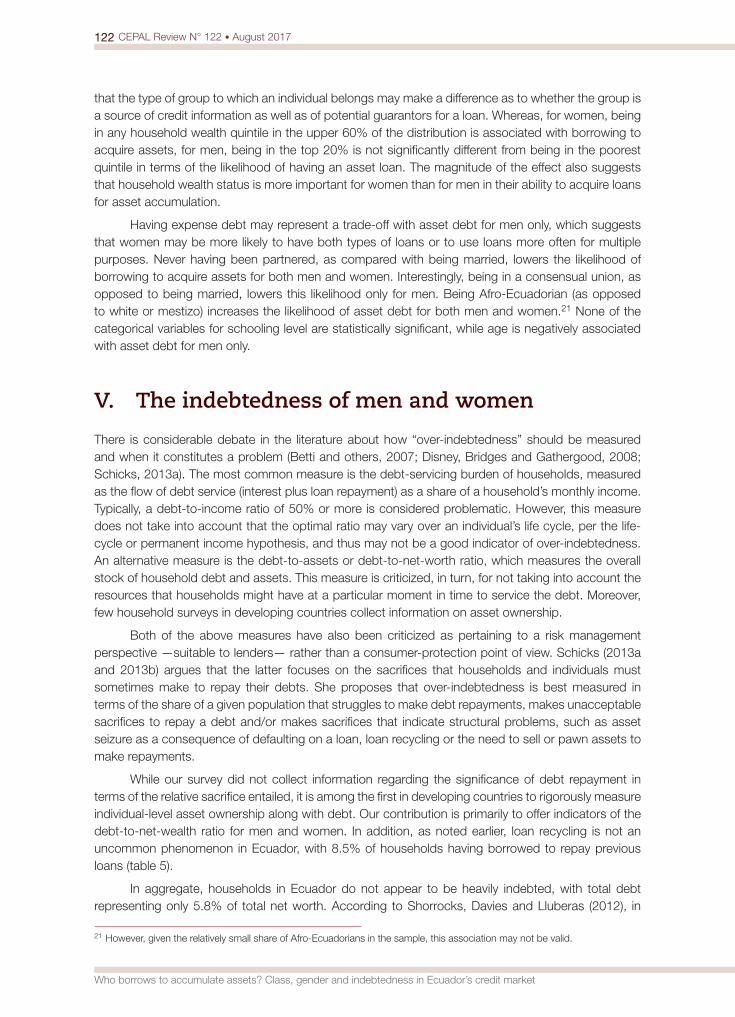
122 CEPAL Review N° 122 • August 2017
Who borrows to accumulate assets? Class, gender and indebtedness in Ecuador’s credit market
that the type of group to which an individual belongs may make a difference as to whether the group is a source of credit information as well as of potential guarantors for a loan. Whereas, for women, being in any household wealth quintile in the upper 60% of the distribution is associated with borrowing to acquire assets, for men, being in the top 20% is not significantly different from being in the poorest quintile in terms of the likelihood of having an asset loan. The magnitude of the effect also suggests that household wealth status is more important for women than for men in their ability to acquire loans for asset accumulation.
Having expense debt may represent a trade-off with asset debt for men only, which suggests that women may be more likely to have both types of loans or to use loans more often for multiple purposes. Never having been partnered, as compared with being married, lowers the likelihood of borrowing to acquire assets for both men and women. Interestingly, being in a consensual union, as opposed to being married, lowers this likelihood only for men. Being Afro-Ecuadorian (as opposed to white or mestizo) increases the likelihood of asset debt for both men and women.21 None of the categorical variables for schooling level are statistically significant, while age is negatively associated with asset debt for men only.
V. The indebtedness of men and women
There is considerable debate in the literature about how “over-indebtedness” should be measured and when it constitutes a problem (Betti and others, 2007; Disney, Bridges and Gathergood, 2008; Schicks, 2013a). The most common measure is the debt-servicing burden of households, measured as the flow of debt service (interest plus loan repayment) as a share of a household’s monthly income. Typically, a debt-to-income ratio of 50% or more is considered problematic. However, this measure does not take into account that the optimal ratio may vary over an individual’s life cycle, per the life-cycle or permanent income hypothesis, and thus may not be a good indicator of over-indebtedness. An alternative measure is the debt-to-assets or debt-to-net-worth ratio, which measures the overall stock of household debt and assets. This measure is criticized, in turn, for not taking into account the resources that households might have at a particular moment in time to service the debt. Moreover, few household surveys in developing countries collect information on asset ownership.
Both of the above measures have also been criticized as pertaining to a risk management perspective —suitable to lenders— rather than a consumer-protection point of view. Schicks (2013a and 2013b) argues that the latter focuses on the sacrifices that households and individuals must sometimes make to repay their debts. She proposes that over-indebtedness is best measured in terms of the share of a given population that struggles to make debt repayments, makes unacceptable sacrifices to repay a debt and/or makes sacrifices that indicate structural problems, such as asset seizure as a consequence of defaulting on a loan, loan recycling or the need to sell or pawn assets to make repayments.
While our survey did not collect information regarding the significance of debt repayment in terms of the relative sacrifice entailed, it is among the first in developing countries to rigorously measure individual-level asset ownership along with debt. Our contribution is primarily to offer indicators of the debt-to-net-wealth ratio for men and women. In addition, as noted earlier, loan recycling is not an uncommon phenomenon in Ecuador, with 8.5% of households having borrowed to repay previous loans (table 5).
In aggregate, households in Ecuador do not appear to be heavily indebted, with total debt representing only 5.8% of total net worth. According to Shorrocks, Davies and Lluberas (2012), in
21 However, given the relatively small share of Afro-Ecuadorians in the sample, this association may not be valid.
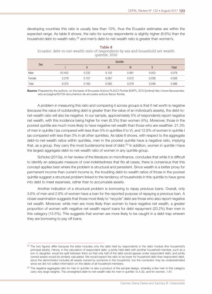
123CEPAL Review N° 122 • August 2017
Carmen Diana Deere and Zachary B. Catanzarite
developing countries this ratio is usually less than 10%, thus the Ecuador estimates are within the expected range. As table 8 shows, the ratio for survey respondents is slightly higher (6.6%) than the household debt-to-wealth ratio,22 and men’s debt-to-net-wealth ratio is greater than women’s.
Table 8 Ecuador: debt-to-net-wealth ratio of respondents by sex and household net wealth
quintile, 2010
SexQuintile
I II III IV V Total
Male -52.452 0.232 0.102 0.091 0.053 0.079
Female 3.279 0.107 0.067 0.072 0.038 0.056
Total 9.375 0.160 0.082 0.079 0.046 0.066
Source: Prepared by the authors, on the basis of Encuesta Activos FLACO-Florida (EAFF), 2010 [online] http://www.flacsoandes.edu.ec/pagina/60759-documentos-de-encuesta-activos-flacso-florida.
A problem in measuring this ratio and comparing it across groups is that if net worth is negative (because the value of outstanding debt is greater than the value of an individual’s assets), the debt-to-net-wealth ratio will also be negative. In our sample, approximately 5% of respondents report negative net wealth, with this incidence being higher for men (6.3%) than women (4%). Moreover, those in the poorest quintile are much more likely to have negative net wealth than those who are wealthier: 21.3% of men in quintile I (as compared with less than 5% in quintiles II to V), and 12.6% of women in quintile I (as compared with less than 3% in all other quintiles). As table 8 shows, with respect to the aggregate debt-to-net-wealth ratios within quintiles, men in the poorest quintile have a negative ratio, implying that, as a group, they carry the most burdensome level of debt.23 In addition, women in quintile I have the largest aggregate debt-to-net-wealth ratio of women in any quintile group.
Schicks (2013a), in her review of the literature on microfinance, concludes that while it is difficult to identify an adequate measure of over-indebtedness that fits all cases, there is consensus that this concept applies best where the problem is structural and persistent. Since wealth is a better proxy for permanent income than current income is, the troubling debt-to-wealth ratios of those in the poorest quintile suggest a structural problem linked to the tendency of households in this quintile to have gone into debt to meet expenses, rather than to accumulate assets.
Another indication of a structural problem is borrowing to repay previous loans. Overall, only 3.6% of men and 2.8% of women have a loan for the reported purpose of repaying a previous loan. A closer examination suggests that those most likely to “recycle” debt are those who also report negative net wealth. Moreover, while men are more likely than women to have negative net wealth, a greater proportion of women with negative net wealth report loans for debt repayment (20.2%) than men in this category (13.5%). This suggests that women are more likely to be caught in a debt trap wherein they are borrowing to pay off loans.
22 The two figures differ because the latter includes only the debt held by respondents in the debt module (the household’s principal adults). Hence, in the calculation of respondent debt, a jointly held debt with another household member, such as a son or daughter, would be split between them so that only half of the debt would appear under respondent debt, and jointly owned assets would be similarly calculated. We would expect the ratio to be lower for household debt than respondent debt, since the denominator includes all assets owned by someone in the household, but the numerator may be underestimated since we did not collect information on the debts of all household members.
23 The negative aggregate ratio for men in quintile I is also a product of the sample design, whereby a few men in this category carry very large weights. The unweighted debt-to-net-wealth ratio for men in quintile I is 4.32, and for women, 1.61.

124 CEPAL Review N° 122 • August 2017
Who borrows to accumulate assets? Class, gender and indebtedness in Ecuador’s credit market
VI. Conclusions
This paper has provided empirical support for Figueroa’s (2011) proposition regarding the segmented structure of credit markets in Latin America. In the case of Ecuador, we have shown that while the formal sector is now the primary source of loans across quintiles, the poor are much more likely to rely on informal sources than the wealthy. Although we do not have primary information on the interest paid on these loans, the greater access of the wealthier quintiles to loans from private and State banks and the lower interest rates that they charge, which are capped by law, illustrates Figueroa’s proposition that asset wealth leads to privileged borrowing conditions and begets wealth.
We have taken this analysis of economic inequality a step further by considering the purposes of borrowing. We have shown that the wealthy are much more likely to borrow for purposes of asset accumulation than the poor. Those in the poorest quintile and individual women are more likely than others to borrow to meet expenses, and their asset acquisition loans are also less likely to generate an income stream in the short term. Not surprisingly, the poorest quintile ends up with the most troubling debt-to-net-wealth ratios, suggesting that their borrowing could lead to an unsustainable debt trap. Moreover, while the poorest men have the most worrisome debt-to-net-wealth ratios, the poorest women among those with negative net wealth may have the highest levels of debt distress given their more frequent practice of borrowing to repay previous loans.
Does this mean that expense loans are always ill advised? We think not since it is well recognized that access to such credit plays an important role in smoothing consumption and managing risks, particularly among those with volatile incomes. As Schicks (2013a) advises, situations of over-indebtedness require a careful analysis of causes, which might include external shocks, lender behaviour (unsuitable products and procedures) and/or borrower behaviour. If the causes are linked to lender behaviour, then the solution, as she suggests, might be “better credit”, not less.
Our regression analysis indicates that the main factor positively associated with the ability of both men and women to access loans for asset accumulation in Ecuador is having a formal savings account. The relationship between having a bank account and access to credit has often been posited in the literature (CAF, 2011). Our analysis provides evidence that this relationship is particularly important for asset accumulation, since lending for this purpose is concentrated in the formal financial sector. A policy implication of our findings is that the trend to “bank the unbanked”, which focuses on promoting savings accounts, might be more broadly successful in the long run than an approach that focuses solely on promoting loans. Moreover, to the extent that formal savings reduces the need for short-term credit, it should facilitate borrowing for the purposes of acquiring assets, as opposed to meeting expenses.
Our analysis confirms the important role of social networks in gaining access to information and credit institutions (Fletschner and Mesbah, 2011). However, in the case of Ecuador, our finding holds for men only. This is likely related to the different types of group to which men and women belong. The most common groups to which men belong are unions and sports associations, and while earning an income is not a point of distinction among men who are able to borrow to acquire assets, belonging to a union does reflect the importance of the type of employment, in this case, formal sector employment and access to the social security system. The Bank of the Ecuadorian Social Security Institute (BIESS) is an important source of State loans (see table 5), though it is only accessible to its members, who, historically, have mostly been male.24 Finally, whether or not women have their own source of income is an important factor in whether they borrow for asset accumulation. This factor alone —women’s independent income— should help reduce gender economic inequality.
24 In 2003, 40% of those enrolled in the social security system were women (ECLAC/CELADE, 2007).

125CEPAL Review N° 122 • August 2017
Carmen Diana Deere and Zachary B. Catanzarite
BibliographyBanerjee, A.V. and E. Duflo (2010), “Giving credit where it is due”, Journal of Economic Perspectives, vol. 24,
No. 3, Nashville, Tennessee, American Economic Association.Barham, B., S. Boucher and M. Carter (1996), “Credit constraints, credit unions, and small-scale producers
in Guatemala”, World Development, vol. 24, No. 5, Amsterdam, Elsevier.Bastiaensen, J. and others (2013), “After the Nicaraguan non-payment crisis: alternatives to microfinance
narcissism”, Development and Change, vol. 44, No. 4, Wiley.BCE (Central Bank of Ecuador) (2013), Evolución del volumen de credito y tasas de interes: analisis del
sistema de finanzas públicas y privado del Ecuador, Quito, 2013 [online] http://contenido.bce.fin.ec/documentos/Estadisticas/SectorMonFin/BoletinTasasInteres/ect201312.pdf.
Betti, G. and others (2007), “Consumer over-indebtedness in the EU: measurement and characteristics”, Journal of Economic Studies, vol. 34, No. 2.
CAF (Andean Development Corporation) (2011), Servicios financieros para el desarrollo: promoviendo el acceso en America Latina, Bogota.
Collins, D. (2008), “Debt and household finance: evidence from the financial diaries”, Development Southern Africa, vol. 25, No. 4, Taylor & Francis.
Da Ros, G. (2003), “El crédito rural y las cooperativas financieras en el Ecuador”, Revista de la UNIRCOOP (Red Universitaria de las Americas en Estudios Cooperativos y Asociativismo), vol. 1, No. 1.
Davies, J. (2008), “An overview of personal wealth”, Personal Wealth from a Global Perspective, J. Davies (ed.), Oxford, Oxford University Press.
De la Torre, A., A. Ize and S. Schmukler (2011), Financial Development in Latin America and the Caribbean: The Road Ahead, Washington, D.C., World Bank.
Deere, C.D. and Z.B. Catanzarite (2016), “Measuring the intra-household distribution of wealth in Ecuador: qualitative insights and quantitative outcomes”, Handbook of Research Methods and Applications in Heterodox Economics, F. Lee and B. Conin (eds.), Cheltenham, Edward Elgar.
Deere, C.D. and J. Contreras (2011), Acumulación de activos: una apuesta por la equidad, Quito, FLACSO-Ecuador [online] http://genderassetgap.org.
Disney, R., S. Bridges and J. Gathergood (2008), “Drivers of over-indebtedness. Report to the Department for Business, Enterprise and Regulatory Reform”, University of Nottingham.
Doss, C. and others (2011), The Gender Asset and Wealth Gaps: Evidence from Ecuador, Ghana and Karnataka, India, Bangalore, Indian Institute of Management [online] http://genderassetgap.org.
EAFF (Encuesta Activos FLACO-Florida) (2010) [online] http://www.flacsoandes.edu.ec/pagina/60759-documentos-de-encuesta-activos-flacso-florida.
ECLAC/CELADE (Economic Commission for Latin America and the Caribbean/Latin American and Caribbean Demographic Centre – Population Division of ECLAC) (2007), “Estudio sobre la protección social de la tercera edad en Ecuador”, Quito.
Fanelli, J.M. (2011), “Domestic financial development in Latin America”, The Oxford Handbook of Latin American Economics, J.A. Ocampo and J. Ros (eds.), Oxford, Oxford University Press.
Figueroa, A. (2011), “Income inequality and credit markets”, CEPAL Review, No. 105 (LC/G.2508-P), Santiago, Economic Commission for Latin America and the Caribbean (ECLAC).
Fletschner, D. and D. Mesbah (2011), “Gender disparity in access to information: do spouses share what they know?”, World Development, vol. 39, No. 8, Amsterdam, Elsevier.
Floro, M. and J. Messier (2006), “Tendencias y patrones de crédito entre hogares urbanos pobres en Ecuador”, La persistencia de la desigualdad: genero, trabajo y pobreza en America Latina, G. Herrera (ed.), Quito, National Women’s Council (CONAMU)/FLACSO-Ecuador.
Grown, C. and others (2015), Who Borrows? An Analysis of Gender, Debt and Assets in Ecuador, Ghana and Karnataka, India, New York, United Nations Entity for Gender Equality and the Empowerment of Women (UN-Women).
Guirkinger, C. (2008), “Understanding the coexistence of formal and informal credit markets in Piura, Peru”, World Development, vol. 36, No. 8, Amsterdam, Elsevier.
INEC (National Statistics and Census Institute) (2006), Bases de datos: Condiciones de vida [online] http://www.ecuadorencifras.gob.ec/condiciones-de-vida-ecv-bases-de-datos/.
Jácome, H. (2007), “El sistema financiero y su papel en el desarrollo económico y social”, La Tendencia. Revista de Analisis Político, No. 4, Quito.
126 CEPAL Review N° 122 • August 2017
Who borrows to accumulate assets? Class, gender and indebtedness in Ecuador’s credit market
(2005), “Alcance de las microfinanzas en las ciudades de Quito, Guayaquil y Cuenca”, Working Paper, No. 05/201, Quito, FLACSO-Ecuador.
Jácome, H. and J. Cordovéz (2004), “Microfinanzas en la economía ecuatoriana: una alternativa para el desarrollo”, Microfinanzas en la economía ecuatoriana: una alternativa para el desarrollo, H. Jácome, E. Ferraro and J. Sánchez (eds.), Quito, FLACSO-Ecuador.
Kast, F. and D. Pomeranz (2014), “Saving more to borrow less: experimental evidence from access to formal savings accounts in Chile”, NBER Working Paper, No. 20239. Cambridge, Massachusettes, National Bureau of Economic Research.
Mideros, A. (2010), Credito y desigualdad. Efecto del acceso a creditos en la brecha de ingreso de los hogares, Quito, FLACSO-Ecuador.
Peck, R. and J. Miller (2006), “Future challenges in Latin American microfinance”, An Insider View of Latin American Microfinance, M. Berger, L. Goldmark and T. Miller-Sanabria (eds.), Washington, D.C., Inter-American Development Bank.
Portes, A. and K. Hoffman (2003), “La estructura de clases en América Latina: composición y cambios durante la era neoliberal”, Desarrollo Económico, vol. 43, No. 171, Buenos Aires, Institute of Economic and Social Development.
Readout, B. (2011), “Balancing Outreach and Sustainability: The Double Bottom Line of Microfinance in Ecuador”, thesis, Gainesville, Florida, University of Florida.
RFR (Rural Finance Network) (2013), Boletín Microfinanciero Trimestral, No. 40, Quito [online] http://www.rfr.org.SBS (Superintendence of Banking and Insurances) (2013), Boletín de Series Bancos Privados [online] http://
www.sbs.gob.ec.Schicks, J. (2013a), “The definition and causes of microfinance over-indebtedness: a customer protection
point of view”, Oxford Development Studies, vol. 41, sup. 1, Taylor & Francis. (2013b), “The sacrifices of micro-borrowers in Ghana – A customer-protection perspective on measuring over-indebtedness”, Journal of Development Studies, vol. 49, No. 9, Taylor & Francis.
SEPS (Superintendencia de Economía Popular y Solidaria) (2014), Ley organica de la economía popular y solidaria y del Sistema Financiero Popular y Solidario de 28 de abril de 2011, Quito.(2013), Boletín Financiero – Sector Financiero Popular y Solidario al 30 de junio de 2013 [online] http://www.seps.gob.ec.
Shorrocks, A., J. Davies and R. Lluberas (2012), Credit Suisse Global Wealth Report 2012, Zurich, Credit Suisse Research Institute [online] https://publications.credit-suisse.com/tasks/render/file/index.cfm?fileid=88EE6EC8-83E8-EB92-9D5F39D5F5CD01F4.
Vogelgesang, U. (2003), “Microfinance in times of crisis: the effects of competition, rising indebtedness and economic crisis on repayment behavior”, World Development, vol. 31, No. 12, Amsterdam, Elsevier.
Colombian agricultural product competitiveness under the free trade agreement with the United States: analysis of the comparative advantages1 Rémi Stellian and Jenny Paola Danna-Buitrago
Abstract
This article studies the competitiveness of Colombian agricultural products relative to those of the United States, with a view to assessing the extent to which the free trade agreement between the two countries represents a risk or an opportunity for Colombia. Colombia’s revealed comparative advantages, in the trade zone it forms with the United States, are calculated for 60 groups of agricultural products and their derivatives, chosen from the Standard Classification for International Trade (SITC), using the method of the Center for International Prospective Studies and Information (CEPII). Most of the product groups display no comparative advantage or comparative disadvantage, so their competitiveness needs to be strengthened to enable trade in agricultural products with the United States to really contribute to the growth of the Colombian economy.
KeywordsAgricultural products, competitiveness, comparative advantage, measurement, free trade, treaties, Colombia, United States
JEL classificationF15, F63, O13
AuthorsRémi Stellian is Assistant Professor at the Faculty of Economics and Management at Pontificia Universidad Javeriana, and also an external co-researcher at the Los Libertadores University Foundation, Bogota, Colombia. [email protected]
Jenny Paola Danna-Buitrago is Director of Institutional Research on Globalization and Sustainable Development at the Los Libertadores University Foundation, Bogota, Colombia. [email protected]
1 The authors gratefully acknowledge the financial support provided by the Los Libertadores University Foundation to the lead author of this research, in his capacity as external co-researcher in the research project “Economic-juridical analysis of the free-trade treaties and trade agreement signed by Colombia: USA, Europe and Asian countries” (International Studies Research Group of the aforementioned institution). They also are grateful for financial support provided by the Colombian Trade Agreements Observatory (OCTC) of the Libertadores University Foundation (Economic and Accounting Thought research group of that institution).
128 CEPAL Review N° 122 • August 2017
Colombian agricultural product competitiveness under the free trade agreement with the United States...
I. Introduction
Colombian foreign policy is founded on a deep alignment with the United States (Londoño, 2011), as manifested in the way Colombia has conducted its international relations with the United States throughout history. Since the end of the First World War, Colombia has viewed the United States as the north star guiding its course, as the main destination for its exports, especially coffee (Iannariello-Monroy, Leon and Oliva, 1999). Successive Colombian governments have viewed that country as a source of foreign exchange and financial aid for development, which has encouraged them to consolidate relations and thus preserve their benefits (Romero, 2006; Londoño, 2011). Since then, Colombia has participated in various United States initiatives such as the Alliance for Progress (1967), the Jumbo, Concorde, Challenger and Hercules support packages (respectively, 1985, 1987, 1989 and 1991), the Andean Trade Preference Act, Plan Colombia (1999) and the Andean Trade Promotion and Drug Eradication Act (ATPDEA, 2002) (Díaz Rivillas, 2002; Swanson, 2006; Toscano, 2012).
The entry into force of the free trade agreement (FTA) between these two historical partners, on 15 May 2012, is the most recent episode and represents a continuation of the aforementioned historical pattern. In general, the FTA is divided into two parts: the first part (chapters 2 to 8, the first chapter being an introduction) deals with merchandise trade; the second (chapters 9-22) addresses a number of considerations related to merchandise trade, such as public procurement, trade in services, foreign direct investment (FDI), intellectual property, labour, and the environment. In the first part, the FTA provides for the immediate or progressive elimination of customs tariffs and non-tariff barriers (such as import restrictions) on a long list of agricultural products and their derivatives (hereinafter referred to as “agricultural products”), namely livestock, fishery, forestry, agriculture and hunting products, along with food and beverages.
The negotiations on those products, which began in 2004, were overshadowed by doubts as to Colombia’s real chances of being able to compete with the United States. Even after the signing of the treaty in 2006 and its approval by the Colombian Congress in 2007, concerns remained over the risks to small-scale farmers and certain products in which the terms agreed upon in the negotiations were considered unfair (Umaña and Caro, 2004; Umaña, 2005; Moncayo, 2006; Pesquera and Rodríguez, 2009). Lack of competitiveness risks triggering a process whereby imports from the United States substitute Colombian agricultural production. This would have an adverse impact on employment and income, particularly in rural areas; and it would also prevent Colombian agricultural products from contributing to economic growth by increasing net exports to the United States (Awokuse, 2008).
Studies evaluating the competitiveness of Colombian agricultural products under the FTA are few. Most of them estimate the effects of the treaty on Colombian agricultural production in terms of trade flows, growth, resource allocation, prices or productivity, among other variables, using either general equilibrium models (DNP, 2003; Martín and Ramírez, 2005; Durán Lima, De Miguel and Schuschny, 2007; Gracia and Zuleta, 2009; Toro and others, 2010; Umaña, 2011; Hernández, 2014); gravity models (Cárdenas and García, 2004 and 2005; Lozano, Castro and Campos, 2005); or econometric models (Cano and others, 2012; Díaz Valencia, 2012). However, regardless of the method used, these studies do not address the competitiveness of Colombian agricultural products explicitly, but instead consider the effects of the treaty.
Against this backdrop, the current study seeks to evaluate the competitiveness of Colombian agricultural products relative to their United States counterparts, using the CEPII indicator (De Saint-Vaulry, 2008). Comparative advantage is defined as the ability to produce a good or service at a lower relative cost (as originally proposed by Ricardo) or by differentiating its characteristics to make it more competitive (Lafay, 1987). The CEPII indicator measures comparative advantages in a standard way,
129CEPAL Review N° 122 • August 2017
Rémi Stellian and Jenny Paola Danna-Buitrago
revealed through an analysis of observed trade patterns, as proposed by Balassa (1965). The use of the CEPII method is justified because it can be seen as the most highly developed means of measuring comparative advantages through trade.
As far as the authors are aware, in the few studies that exist on the competitiveness of Colombian agricultural products, the following two criteria are not applied simultaneously: (i) a study focusing on the bilateral trade zone between Colombia and the United States; and (ii) a study performed using the CEPII revealed comparative advantage (RCA) index. Firstly, studies that measure competitiveness are not referenced on the aforementioned trade zone (first criterion) (World Bank, 2003; Leibovich and Estrada, 2008; Norton and Argüello, 2008; Perfetti, 2011; Danna-Buitrago, 2012; Maldonado and Sánchez, 2012; Reina and others, 2013; Danna-Buitrago and Stellian, 2014). In addition, although Rocha Beltrán (2012) is an exception, this author only measures the comparative advantages of seven agricultural products (wheat, rice, maize, soya, tobacco, potatoes and cotton), rather than a complete nomenclature of products in that sector. So, regardless of their content, the results obtained in these studies do not address the focus of this research. Secondly, although an index similar to an RCA index is used in these studies (albeit not always), it does not take account of the improvements made by CEPII (second criterion).
In short, the present research aims to identify the competitive profile of Colombian agricultural products with respect to those of the United States in an original and systematic way. After calculating the RCA index for 60 groups of agricultural products, as specified in the International Standard Classification for International Trade (SITC), observed trade patterns reveal comparative advantages that are sustainable through time for just three of them, while four others have the potential for such sustainability. The other groups either have no advantage or else have disadvantages. Consequently, Colombia has few opportunities to exploit the benefits of free trade in agricultural products with its historical partner, so it is essential to enhance their competitiveness.
The article is divided into six sections, including this introduction. Section II describes the modalities of liberalization of agricultural trade between the parties. Section III presents the CEPII method to calculate the RCA index, based on other methods considered representative in the literature, with the aim of highlighting the improvements introduced by CEPII. Section IV explains the calculation parameters; and section V presents the calculations and analyses the results. To conclude, section VI summarizes the results and suggests future lines of research.
II. Agricultural trade liberalization within the FTA
Trade in agricultural products is governed by the first part of the FTA, which includes a number of commitments to eliminate import restrictions and export subsidies, and to grant imported goods a treatment that is at least as favourable as that accorded to nationally produced goods (Espinosa and Pasculli, 2013). The key liberalization measure is the total, immediate or progressive elimination of customs tariffs (Article 2.3 of the FTA), such that Colombia and the United States will trade agricultural products tariff-free by 2031 (except for sugar and its derivatives, as will be explained later).
Since the FTA entered into force in 2012, tariffs have already been completely eliminated on most agricultural products, as can be seen from a detailed analysis of the tariff reduction schedules provided for by the FTA in the two existing lists for each country.2 Although the first list is called “Agricultural goods”, the items it includes are not exclusively agricultural, nor does it include all
2 See the lists available [online] http://www.tlc.gov.co/publicaciones.php?id=727.
130 CEPAL Review N° 122 • August 2017
Colombian agricultural product competitiveness under the free trade agreement with the United States...
agricultural products. Some of these are in the second list, called “Non-agricultural goods”, which, despite the name, includes agricultural items such as fishery products and some non-edible raw materials of animal or vegetable origin (natural rubber, wood and natural fibres, among others).
These lists classify products in different groups identified by codes that are not homogeneous across the two countries, but have a common base. Frequently, two or more United States groups correspond to the disaggregation of one Colombian group, or vice versa. For example, Colombia has one group called for aubergines (berenjenas) (07093000), while United States has two aubergine groups: those entering the country between 1 April and 30 November of each year (07093020) and those entering between 1 December and 31 March of the following year (07093040). The United States tariff schedule also has one group for birds’ eggs (04070000), while Colombia has three groups covering this product: hatching eggs (04070010), eggs for the production of vaccines (04070020) and other birds’ eggs (04070090).
Defining the correspondences between the Colombian and United States groups reveals 859 “metagroups”, in other words a set of Colombian groups and an equivalent set of United States groups, without both sets necessarily having an identical level of disaggregation (as in the two foregoing examples). In 644 (75%) of these metagroups, all Colombian groups belong to category “A” (or “AA” in the case of a single group), while all United States groups belong to categories “A” or “F”. The first category (as well as “AA”) indicates an immediate total elimination of tariffs. The “F” category, available only to the United States, represents tariff-free groups prior to signing of the FTA, under ATPDEA; so the FTA allows it to keep some tariff benefits that would otherwise have had to lapse in 2011.
Among the remaining metagroups, there are 102 in which Colombian groups do not belong exclusively to category “A”, but some are in category “B”. This means that, instead of an immediate tariff elimination, a five-year phase-out from a base tariff is introduced; and 2017 is set as the year in which these products will become duty-free. At the same time, the American groups in these 102 metagroups belong to the “A” or “F” categories (as in the 644 metagroups mentioned above). There are also two metagroups in which Colombian groups belong only to category “A”, while some United States groups are in category “B” instead of categories “A” or “F”. In short, in 748 or 87.1% of the 859 metagroups, tariff elimination had already been implemented in 2012, or else it was to be completed no later than 2017.
The last 111 metagroups provide for tariff elimination over five years (8 to 19 years depending on the group). Some metagroups also include a protectionist regime, which is provisional in most cases (see table 1). This regime consists of tariff quotas: there is a limited volume of duty-free imports, and imports in excess of that volume are subject to a tariff. Nonetheless, irrespective of its base level (that is, its level when the FTA entered into force), the tariff in question should be phased out over a period of 10 to 19 years (see table 2), according to the tariff reduction categories mentioned above. Moreover, the duty-free quota increases each year —between 3% and 10% (see Appendix I of the FTA)— until the quota disappears altogether in the year in which the products in question become duty-free. This protectionist regime must therefore be seen as provisional and does not call into question the principle of total liberalization of trade in agricultural products between the two countries.
There is an exception in 19 of the 111 metagroups, namely sugar and its derivatives (including sugar confectionery). In this case, cancellation of the tariff quota applied by the United States in the future is not envisaged. Although the quota increases by 750 metric tons annually (with 50,000 tons as the initial quota in 2012), the United States may impose in-quota tariffs at any time, provided that Colombian exporters receive compensation equivalent to the profits they could have obtained in the absence of any restriction (Article 2.19). Nonetheless, the FTA does not specify who will calculate such compensation, or how it will be calculated, or the value of the applied tariff. Moreover, in maintaining this quota, the out-of-quota tariffs are not phased out, but are set at the most favoured nation level (MFN), which rose to 55% in 2015 (WTO, 2015, p. 74).
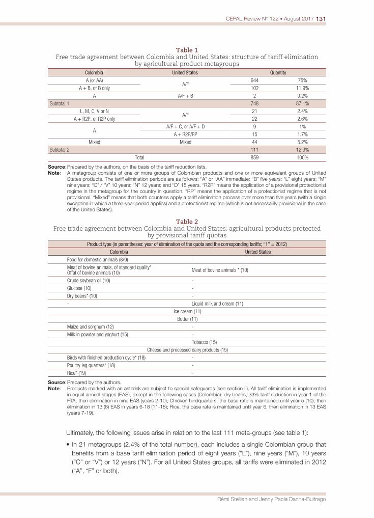
131CEPAL Review N° 122 • August 2017
Rémi Stellian and Jenny Paola Danna-Buitrago
Table 1 Free trade agreement between Colombia and United States: structure of tariff elimination
by agricultural product metagroups Colombia United States QuantityA (or AA)
A/F644 75%
A + B, or B only 102 11.9%
A A/F + B 2 0.2%
Subtotal 1 748 87.1%
L, M, C, V or NA/F
21 2.4%
A + R2P, or R2P only 22 2.6%
AA/F + C, or A/F + D 9 1%
A + R2P/RP 15 1.7%
Mixed Mixed 44 5.2%
Subtotal 2 111 12.9%
Total 859 100%
Source: Prepared by the authors, on the basis of the tariff reduction lists. Note: A metagroup consists of one or more groups of Colombian products and one or more equivalent groups of United
States products. The tariff elimination periods are as follows: “A” or “AA” immediate; “B” five years; “L” eight years; “M” nine years; “C” / “V” 10 years; “N” 12 years; and “D” 15 years. “R2P” means the application of a provisional protectionist regime in the metagroup for the country in question. “RP” means the application of a protectionist regime that is not provisional. “Mixed” means that both countries apply a tariff elimination process over more than five years (with a single exception in which a three-year period applies) and a protectionist regime (which is not necessarily provisional in the case of the United States).
Table 2 Free trade agreement between Colombia and United States: agricultural products protected
by provisional tariff quotasProduct type (in parentheses: year of elimination of the quota and the corresponding tariffs; “1” = 2012)
Colombia United StatesFood for domestic animals (8/9) -
Meat of bovine animals, of standard quality*Offal of bovine animals (10) Meat of bovine animals * (10)
Crude soybean oil (10) -
Glucose (10) -
Dry beans* (10) -
- Liquid milk and cream (11)
Ice cream (11)
Butter (11)
Maize and sorghum (12) -
Milk in powder and yoghurt (15) -
Tobacco (15)
Cheese and processed dairy products (15)
Birds with finished production cycle* (18) -
Poultry leg quarters* (18) -
Rice* (19) -
Source: Prepared by the authors.Note: Products marked with an asterisk are subject to special safeguards (see section II). All tariff elimination is implemented
in equal annual stages (EAS), except in the following cases (Colombia): dry beans, 33% tariff reduction in year 1 of the FTA, then elimination in nine EAS (years 2-10); Chicken hindquarters, the base rate is maintained until year 5 (10), then elimination in 13 (8) EAS in years 6-18 (11-18); Rice, the base rate is maintained until year 6, then elimination in 13 EAS (years 7-19).
Ultimately, the following issues arise in relation to the last 111 meta-groups (see table 1):
• In 21 metagroups (2.4% of the total number), each includes a single Colombian group that benefits from a base tariff elimination period of eight years (“L”), nine years (“M”), 10 years (“C” or “V”) or 12 years (“N”). For all United States groups, all tariffs were eliminated in 2012 (“A”, “F” or both).
132 CEPAL Review N° 122 • August 2017
Colombian agricultural product competitiveness under the free trade agreement with the United States...
• In 22 metagroups (2.6%), each includes at least one Colombian group that benefits from a provisional protectionist regime (tariff quotas). For Colombian groups that do not benefit from this regime, tariff elimination corresponds to category “A”, while all United States groups belong to categories “A” or “F”.
• In nine metagroups (1%) each includes at least one United States group that benefits from a 10- or 15-year tariff-elimination period (respectively “C” and “D”) to phase out the base rate. If a United States group does not benefit from this regime, its tariff elimination occurred either immediately in 2012 (“A”) or else was already duty-free (“F”). In the Colombian groups, tariff elimination was immediate (“A”).
• In 15 metagroups (1.7%), each includes at least one United States group that benefits from a protectionist regime in the form of tariff quotas. This regime is not provisional for two of these metagroups (sugar and its derivatives, as noted above). If a United States group does not benefit from a protectionist regime, its tariff elimination corresponds to categories “A” or “F”, while all Colombian groups are in category “A”.
• The remaining 44 metagroups (5.2%) are “mixed”, since a protectionist regime is applied to one or more groups in both countries or a tariff elimination period longer than five years is granted, or both.3 Some of these metagroups also contain groups comprising sugar and its derivatives, resulting in a non-provisional protectionist regime in the case of the United States.
A “safeguard measure” may also be applied to some Colombian groups that already benefit from a provisional protectionist regime (product type identified by an asterisk in table 2). This measure entails applying an additional tariff if the quantity imported exceeds a certain value (see Annex 2.18 of the FTA for the methods of calculating the additional tariff). Depending on the product, this value varies between 120% and 140% of the corresponding quota. Nonetheless, the safeguard measure should disappear when the quota itself disappears. Here again, the safeguard does not call into question the principle of complete tariff elimination.
In general, agricultural products of Colombian origin have, and will increasingly have, access to the United States market over the next few years. An increase in exports of these products can therefore be expected, which would boost total production and employment. Nonetheless, the United States also has access to the Colombian market, and increasingly so, which means Colombia will need to be as competitive as possible to prevent its agricultural production declining in the face of cheaper or better-quality United States imports. For this reason, a study is made of the competitiveness of Colombian agricultural products relative to those of the United States, through the measure of revealed comparative advantages.
III. Revealed comparative advantage index
The factors that determine the competitiveness of a product or group of products are multidimensional. There are price determinants of competitiveness, in other words, when country A can sell the production of a group at a lower price than country B. The exchange rate is the first factor generating that price difference; other factors relate to the capacity to produce at lower relative costs —wages, intermediate consumption prices, production techniques, transport and marketing costs, taxes and financial costs, among others. There are also determinants of competitiveness that are not linked to prices, such as when the production of country A differs from that of country B in terms of quality, innovations, branding or after-sales service, among other factors (Porter, 1991; Chevassus-Lozza and Gallezot, 1995; Eaton and Kortum, 2002; Costinot, 2009; Chor, 2010; Cuñat and Melitz, 2012).
3 There is one exception, which involves tariff elimination over a three-year period (category “H”, applied to the group comprising natural components of milk not specified or included in another group).
133CEPAL Review N° 122 • August 2017
Rémi Stellian and Jenny Paola Danna-Buitrago
As it is difficult to form a comprehensive view of all the pre-trade factors that determine competitiveness, it is complicated to obtain a single value, based on those factors, that summarizes the competitiveness of a product (or group of products) in one or more countries (Ballance, 1988). The revealed comparative advantage index (RCA) aims to provide a synthetic measure of the ability to produce at lower relative cost by analysing trade, based on the assumption that trade flows (post-trade variables) indirectly reflect these comparative advantages (Balassa, 1977; Lafay, 1987). The RCA index is not intended to identify the determinants of comparative advantage, but to establish the extent to which they exist. The calculation of the RCA index can be understood as a first stage of competitiveness analysis. In the second stage, the main factors explaining the level of comparative advantage achieved by the index should be identified. Although the current study focuses on the first stage, some preliminary observations are also made with respect to the second.
The RCA index is calculated according to a nomenclature of ;K 0 1N =! F I products, or product groups, traded in a specific trade zone consisting of ;n 0 1N =! F I countries in a time period of T N! ) years (or quarters). The zone in question may be the world, the members of the World Trade Organization (WTO), or a group of at least two countries. What need to be remembered is that the index and the variables that enable its calculation refer only to the selected zone. A country belonging to the zone is identified by the letter i, a group of products by the letter k and a time period by the letter t. The variable RCAkit denotes the RCA index of country i with respect to the product (or group of products) k in period t (and within the zone).
To highlight the contributions of the CEPII method, the starting point is the index initially proposed by Balassa (1965). X Rkit ! + represents exports of k (in monetary units) made by country i in time-period t:
:RCA X X X X Rkit kit kitk
K
kiti
n
kiti
n
k
K
1 1 11
!== = ==
+U UZ Z/ / // (1)
This index is based on the relative export structure, from which three terms are extracted:
• Xkitk
K
1=/ denotes total exports by country i in time t, for the K product groups considered in the nomenclature;
• Xkiti
n
1=/ denotes exports of K made in time t by the n countries of the zone;
• Xkiti
n
k
K
11 ==// denotes “global” exports in time t, in other words the total exports of the
n countries of the zone in that period.
Balassa (1965) compares two shares: in the numerator, the share of exports of k in total exports by country i in time t; in the denominator, the same share in the n countries of the zone in question. If RCA 1kit 2 , then country i specializes in the production of k in time t, thereby revealing the existence of comparative advantages; and vice versa, if RCA 1kit 1 , i has no specialization in k (in t), thereby revealing disadvantages.
Nonetheless, the Balassa (1965) indicator does not really allow comparative advantage (or specialization) to be determined, but instead makes a comparison between the structure of a country’s exports and the structure of exports from the area as a whole over a given period (Balassa, 1977), thereby only establishing export potential (Balassa, 1977; Raghurampatruni, 2012; Aytaç and Kiliç, 2014). This is explained by the absence of imports. In fact, by defining M Rkit !
+ as imports of k made by country i in time t, the trade patterns can show that:
; ;m x k i tkit kit72 R W, where:

134 CEPAL Review N° 122 • August 2017
Colombian agricultural product competitiveness under the free trade agreement with the United States...
:
:
x X X X X
m M M M M
kit kit kitk
K
kiti
n
kiti
n
k
K
kit kit kitk
K
kiti
n
kiti
n
k
K
1 1 11
1 1 11
=
=
= = ==
= = ==U
U U
U
Z
Z
Z
Z
/ / //
/ / // (2)
In this case, i displays a greater propensity to export k (in time period t) than the zone as a whole; but, at the same time, i shows an even greater propensity to import k (in t). For this reason, there would be intra-industry trade (trade in different varieties of the same product, Krugman, 1995) which limits the specialization of i and its comparative advantages for k (Lafay, 1990).
To avoid the shortcomings of (1), Balassa (1966) proposes another indicator, which includes imports:
: ;RCA X M
X M1 1kit
kit kit
kit kit!= +
−−" %
(3)
With the indicator specified in this way, if country i records a positive trade balance (numerator) for k in time t, it is assumed that i specializes in the production of k in t and thus has comparative advantages, which is reflected in RCA 0kit 2 . Conversely, if RCA 0kit 1 , then country i does not specialize and reveals disadvantages. Also, RCA 0kit = denotes the absence of (dis)advantages. Thus:
• Specialization is more intense, and the advantages are greater, if the positive trade balance of k recorded by i in t is a larger proportion of the volume of trade in k by country i in period t (denominator), which is reflected in RCA 1kit " .
• In the case of disadvantages (non-specialization), these are more important if the trade deficit of k recorded by country i in t has a greater weight in country i’s trade in k in time t (denominator), which is reflected in RCA 1kit "− .
Another alternative is the RCA index in terms of contribution to the trade balance (Lafay, 1987), which precedes the CEPII indicator:
:RCAW
X M u X M1 Rkitkitk
K kit kit kit kit kiti
n
1 1
!= − − −
= =R W# &/ / where: (4)
:
:
uW
W
W X M
kitkitk
Kkit
kit kit kit
1
=
= +=
/
This RCA index is calculated in two stages:
• First, the difference between the trade balance of k recorded by i in t and a theoretical balance defined as u X Mkit kit kiti
n
1−
= R W/ , is calculated; in other words, the total trade balance recorded by i in t, weighted by the coefficient ukit . This is the ratio of Wkit to Wkitk
K
1=/ ,
or the share of k in country i’s trade in t relative to total trade by that country in the same period. If the balance is higher than its theoretical level, there is a positive difference and hence RCAkit>0, so it is assumed that i displays comparative advantages with respect to k in period t, and vice-versa if it is lower. If RCAkit=0, there are no advantages or disadvantages.

135CEPAL Review N° 122 • August 2017
Rémi Stellian and Jenny Paola Danna-Buitrago
• Second, the difference between the trade balance X Mkit kit− and its theoretical level u X Mkit kit kiti
n
1−
= R W/ is divided by Wkitk
K
1=/ , which represents country i’s total trade in
time period t. Thus:
• When the difference between X Mkit kit− and u X Mkit kit kiti
n
1−
= R W/ is positive, the revealed advantages are less important if i’s total trade in period t is higher.
• When the difference between X Mkit kit− and u X Mkit kit kiti
n
1−
= R W/ is negative, the revealed disadvantages are less important if i’s total trade in period t is higher.
• When X Mkit kit− – u X Mkit kit kiti
n
1−
= R W/ = 0 then RCA 0kit = : the absence of (dis)advantages persists irrespective of country i’s total trade in t.
Nonetheless, despite taking both exports and imports into account, the foregoing indicators (3 and 4) have two weaknesses. First, they do not consider the size of national production. For two different countries, i and j, obtaining RCA RCAkit kjt= using these indicators should not mean that both display the same level of (dis)advantages:
• If RCA RCA 0kit kjt 2= and if i produces less than j, then i has a higher level of specialization, so country i’s advantage must be greater than j’s, rather than identical.
• If RCA RCA 0kit kjt 1= and if i produces less than j, then i has a lower level of specialization, so country i’s disadvantage must be greater than j’s, rather than identical.
Second, neither indicator considers the immediate economic situation surrounding trade. The idea is to reveal comparative (dis)advantages, in other words the structural factors that contribute to competitiveness. However, trade may reflect short-term fluctuations, which by definition should not be used to reveal structural factors. From this standpoint, ignoring the bias introduced by short-term fluctuations when calculating the RCA index can lead to unfounded advantages or disadvantages.
CEPII proposes an indicator of contribution to the trade balance, which, unlike (4), takes account of gross domestic product (GDP) and also corrects the “short-term” bias in trade.4 The indicator not only makes it possible to compare trade in several product groups by several countries, over several periods and on a common basis, but also to correct a number of distortions (Danna-Buitrago and Stellian, 2014). As this is the most complete RCA index since that formulated by Balassa (1965), we chose to use it in the present study. The indicator is calculated according to the following system:
:RCA Y X M v X M1000 Rkitit
kit kit kt kit kitk
K
1
!= − − −=
l l l lR W# &/
where: Yit is the GDP of country i in time t
(5):
: ; :
: ; :
v W W
W X M W W
X X e M M e
e si W
kt kt t
kt kit kiti
n
t ktk
K
kit kit kt kit kit kt
kt kt
1 1
$ $
=
= + =
= == =
l l
R W/ /
otherwise
4 The evolution of the indicators proposed by CEPII before producing this latest version can be consulted in Lafay (1987, 1990 and 1992), De Saint Vaulry (2008) and the CEPII website [online] www.cepii.fr/%5C/anglaisgraph/bdd/chelem/indicators/indicspeit.htm.

136 CEPAL Review N° 122 • August 2017
Colombian agricultural product competitiveness under the free trade agreement with the United States...
Unlike equation (4):
• Equation (5) does not contain the k trade balance X Mkit kit− ; but instead X Mkit kit−l l resulting from the adjustment of Xkit and Mkit by a coefficient ekt , the role of which is explained below. Moreover, the total trade balance X Mkit kiti
n
1−
= R W/ is replaced by the adjusted total balance X Mkit kitk
K
1−
=l lR W/ .
• The (adjusted) total trade balance is not weighted by the share of k in the country’s total trade over the same period ukitR W. Instead, it is weighted by the share of trade in k by the n countries of the zone in time t relative to the total trade of the same countries in the same period vktR W.
• The difference between the (adjusted) balance and its theoretical level is not divided by Wkitk
K
1=/ but by Yit . Thus, where two countries report the same difference, the country with the lowest GDP has greater advantages or less disadvantages. Multiplying the result by 1,000 makes it possible to express RCAkit in thousandths of the GDP of country i in time-period t (‰).
To understand the adjustment of Xkit and Mkit by ekt , the starting point is Wkt , which represents trade in k by all the countries in the zone in period t. Once Wkt has been calculated for each k, it is possible to sum ...W W Wt t Kt1 2+ + and thus calculate Wt , which represents “global” trade defined as the trade in all K product groups in t by all countries in the zone. The coefficient ekt is determined by selecting a “reference period” denoted by the letter r. Thus, W Wkr r is the share of k in global trade in the reference period r. It is assumed that W Wkr r reflects the structural factors of k trade irrespective of short-term fluctuations. From this standpoint:
• If e 1kt = then W W W Wkr r kt t= . This means that the share of k in global trade in time-period t is equal to the equivalent share in period r. In other words, e 1kt = assumes thatXkit and Mkit do not reflect biases due to short-term fluctuations, since k has the same importance in global trade in both periods, r and t. No adjustment is required, since multiplying Xkit and Mkit by e 1kt = gives X Xkit kit=l and M Mkit kit=l .
• If W W 0kt t = , then ekt cannot be calculated, since division by 0 is undefined. In this case, there are no exports or imports of k in period t. Thus, it is assumed that the adjusted exports and imports will also be equal to 0. So, if W W 0kt t = we write e 1kt = , which implies X Xkit kit=l = M Mkit kit=l = 0.
• If, in contrast, W W W Wkt t kr r! with W W 0kt t ! , it is assumed that Xkit and Mkitreflect short-term fluctuations in addition to structural factors. For example, if ,e 1 25kt = , it means that the share of k in global trade in the reference period r is logically 1.25 – 1 = 0.25, in other words 25% higher than the equivalent share in period t. Thus, Xkit and Mkit should be 25% higher to correspond to W Wkr r , that is, to correspond to the structural part of trade in k rather than W Wkt t . Thus, Xkit and Mkit must be 25% larger, or multiplied by 1.25, a coefficient that precisely represents the value of ekt .
Ultimately, after adjusting exports and imports, if the value of the indicator changes from one period to another, this is assumed to exclusively reflect variations in structural factors (for example, productivity) in one country or another. Likewise, after calculating Xkitl for each k and for each t, it is possible to sum X X Xi t i t iKt1 2 g+ + +l l l to obtain the adjusted total exports of country i in period t, denoted by Xitl , and the same applies to the adjusted total imports of i in t, denoted by Mitl .
Lastly, the results of the RCA index calculated according to equation (5) are interpreted in the same way as those of equation (4). RCA 0kit 2 is equivalent to having comparative advantages for i with respect to k in period t; and these advantages are greater or have more influence when the value

137CEPAL Review N° 122 • August 2017
Rémi Stellian and Jenny Paola Danna-Buitrago
of the indicator is higher (more positive). RCA 0kit 1 implies comparative disadvantages for i with respect to k in period t; and these disadvantages are greater or have more influence when the value of the indicator is smaller (more negative).RCA 0kit = indicates the absence of (dis)advantages.
IV. Parameter setting and analysis
As this study seeks to identify Colombia’s comparative (dis)advantages in the bilateral trade zone with the United States, country i is Colombia and n = 2. Data for exports and imports are taken from UNCTADstat (unctadstat.unctad.org), supplied according to the three-digit SITC Rev.3 nomenclature.5 Thus, RCAkit is calculated from the trade of K = 255 product groups k.6 It will then be possible to focus on the results of the 60 groups comprising exclusively agricultural products, including the following7
(see annex A1):
• 36 groups, with codes beginning with 0, consisting of live animals and crude or processed foodstuffs (other than waters, alcoholic beverages and edible oils).
• 4 groups with codes starting with 1, consisting of mineral waters and soft drinks (code 111), alcoholic beverages (112), tobacco (121) and their derivatives (122).
• 16 groups, with codes beginning with 2, composed of crude inedible materials of animal or vegetable origin (except oils).
• 4 groups, with codes beginning with 4, composed of oils of animal or vegetable origin.
The GDP data, Yit for each (i,t), are taken from the World Bank (datos.bancomundial.org), and they are converted from current dollars to thousands of current dollars in order to express them in the same unit as Xkit and Mkit. UNCTADstat provides annual data from 1995 to 2014. It is therefore possible to calculate RCAkit over two decades, so t ∈ {1995; 1996; ...; 2014} and T = 20. This is done to identify a trend in the behavior of the RCA index over time, and thus analyse comparative (dis)advantages from a dynamic vantage point. In fact, calculating a single-year RCA index, or that of the three years available since the implementation of the FTA (2012, 2013 and 2014), does not identify the trend of the indicator over time. Lastly, the reference period r that corrects the short-term bias will be 2014. The last available year is chosen with a retrospective or “backward-looking” approach, assuming that 2014 reflects the structural trends of trade and excludes the bias generated by short-term fluctuations, which makes it possible to adjust Xkit and Mkit from the previous years.8
To analyze the results, six categories K1,K2,…,K6 are are created to identify a time-trend in the behavior of the RCA index for each k product group (Danna-Buitrago and Stellian, 2014). Thus, depending on the vector (VCRki1995;VCRki1996;…; VCRki2014) ∈ R20, k belongs to one category (k ∈ Kx ∃x∈{1;2;...;6}) and not to the others (k ∈ Kx ⇒ k ∉ Ky ∀x,y ∈ {1;2;...;6},y ≠ x). From one category to another, that is, from Kx to Kx+1, k displays increasingly fewer comparative advantages
5 See [online] http://unstats.un.org/unsd/cr/registry/regcst.asp?Cl=14&Top=2&Lg=2.6 The calculations ignore services, because the databases consulted (UN Service Trade, WTO, Organization for Economic
Cooperation and Development (OECD) and International Monetary Fund (IMF)) do not produce statistics that are sufficiently granular to identify this trade between Colombia and the United States. According to UN Service Trade, services accounted for roughly 15.47% of trade between Colombia and the rest of the world between 1995 and 2013. Assuming the same trend is observed in the trade between the two partners, it can be said that roughly 85% of the trade between them was used to calculate the comparative advantages of Colombia with respect to the United States
7 Working with the three-digit SITC nomenclature is a solution to the lack of uniformity in the FTA product lists, as shown in Section II (four lists without uniform coding). It also allows comparative advantages to be calculated at a more aggregate level than the 859 FTA metagroups, thereby affording an overview of these advantages. Future research could go into greater detail using a more granular nomenclature.
8 In contrast, a prospective or “forward-looking” approach is based on the first available period.
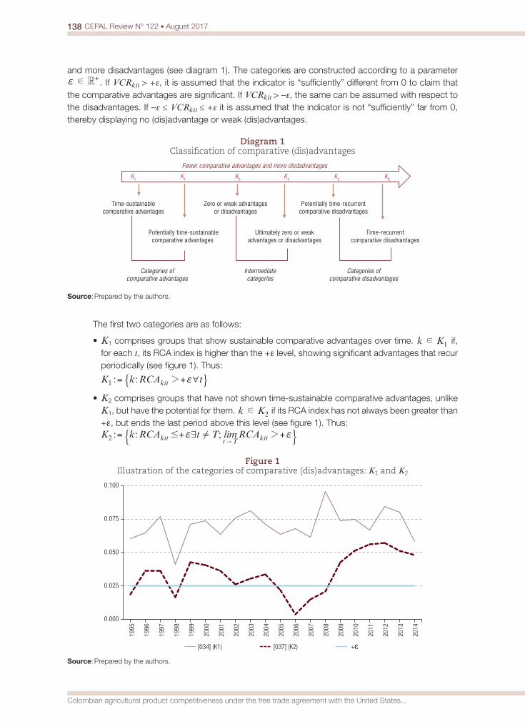
138 CEPAL Review N° 122 • August 2017
Colombian agricultural product competitiveness under the free trade agreement with the United States...
and more disadvantages (see diagram 1). The categories are constructed according to a parameter Rdf +
. If VCRkit > +ε, it is assumed that the indicator is “sufficiently” different from 0 to claim that the comparative advantages are significant. If VCRkit > –ε, the same can be assumed with respect to the disadvantages. If –ε ≤ VCRkit ≤ +ε it is assumed that the indicator is not “sufficiently” far from 0, thereby displaying no (dis)advantage or weak (dis)advantages.
Diagram 1 Classification of comparative (dis)advantages
K1
K1
Potentially time-sustainablecomparative advantages
K3
K4
K5
K6
Fewer comparative advantages and more disdadvantages
Time-sustainablecomparative advantages
Zero or weak advantagesor disadvantages
Potentially time-recurrentcomparative disadvantages
Ultimately zero or weakadvantages or disadvantages
Time-recurrentcomparative disadvantages
Categories ofcomparative advantages
Intermediatecategories
Categories ofcomparative disadvantages
Source: Prepared by the authors.
The first two categories are as follows:
• K1 comprises groups that show sustainable comparative advantages over time. k K1d if, for each t, its RCA index is higher than the +ε level, showing significant advantages that recur periodically (see figure 1). Thus:
= +k: :K RCA tkit1 62 fF I• K2 comprises groups that have not shown time-sustainable comparative advantages, unlike
K1, but have the potential for them. k K2d if its RCA index has not always been greater than +ε, but ends the last period above this level (see figure 1). Thus:
f f= +k: : ; limK RCA t T RCAkit t T kit2 7 2!# +"F I
Figure 1 Illustration of the categories of comparative (dis)advantages: K1 and K2
0.000
0.025
0.050
0.075
0.100
1995
1996
1997
1998
1999
2000
2001
2002
2003
2004
2005
2006
2007
2008
2009
2010
2011
2012
2013
2014
[034] (K1) [037] (K2) +
Source: Prepared by the authors.

139CEPAL Review N° 122 • August 2017
Rémi Stellian and Jenny Paola Danna-Buitrago
The following two categories are referred to as “intermediate”:
• K3 comprises groups that are “neutral” with respect to the (dis)advantages. k K3d if, for each t, its RCA index is within the interval ;f f− +" %, so the (dis)advantages are considered weak from one period to another (see figure 2). Thus:
= −k: : ;K RCA tkit3 d 6f f+" %F I• K4 comprises groups that are “neutral in fine” with respect to the (dis)advantages. k K4d if
its RCA index has not always been in ;f f− +" % but ends in that range (see figure 2). Thus:
= −z !+ −" "% %k: : ; ; ;RCAlimK RCA t T
t T kitkit4 d7f f f f+"
G J
Figure 2 Illustration of the categories of comparative (dis)advantages: K3 and K4
-0.035
-0.025
-0.015
-0.005
0.005
0.015
0.025
0.035
1995
1996
1997
1998
1999
2000
2001
2002
2003
2004
2005
2006
2007
2008
2009
2010
2011
2012
2013
2014
[001] (K3) [011] (K4) - +
Source: Prepared by the authors.
The last two categories are the “negative counterparts” of K1 and K2:
• K5 comprises groups that do not show recurrent comparative disadvantages over time but have the potential to do so. k K5d if its RCA index has not always been below a –ε, but ends the final period below this level (see figure 3). Thus:
k: : ; lim RCAK RCA t T t T kitkit5 f7 1!$ -f= − "F I• K6 comprises groups which show recurrent comparative disadvantages. k K6d if, for each t,
its RCA index is below the –ε level showing significant disadvantages that recur periodically (see figure 3). Thus:
k: : tK RCAkit6 f61-= F I
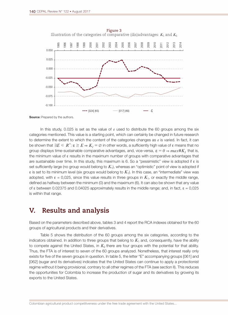
140 CEPAL Review N° 122 • August 2017
Colombian agricultural product competitiveness under the free trade agreement with the United States...
Figure 3 Illustration of the categories of comparative (dis)advantages: K5 and K6
-0.100
-0.075
-0.050
-0.025
0.000
0.025
0.050
1995
1996
1997
1998
1999
2000
2001
2002
2003
2004
2005
2006
2007
2008
2009
2010
2011
2012
2013
2014
[024] (K5) [017] (K6) -
Source: Prepared by the authors.
In this study, 0.025 is set as the value of ε used to distribute the 60 groups among the six categories mentioned. This value is a starting point, which can certainly be changed in future research to determine the extent to which the content of the categories changes as ε is varied. In fact, it can be shown that E R : E K1&d =f7 Q$+ in other words, a sufficiently high value of ε means that no group displays time-sustainable comparative advantages, and, vice-versa, 0 max#K1&=f that is, the minimum value of ε results in the maximum number of groups with comparative advantages that are sustainable over time. In this study, this maximum is 6. So a “pessimistic” view is adopted if ε is set sufficiently large (no group would belong to K1), whereas an “optimistic” point of view is adopted if ε is set to its minimum level (six groups would belong to K1). In this case, an “intermediate” view was adopted, with ε = 0,025, since this value results in three groups in K1, or exactly the middle range, defined as halfway between the minimum (0) and the maximum (6). It can also be shown that any value of ε between 0.02375 and 0.04025 approximately results in the middle range; and, in fact, ε = 0,025 is within that range.
V. Results and analysis
Based on the parameters described above, tables 3 and 4 report the RCA indexes obtained for the 60 groups of agricultural products and their derivatives.
Table 5 shows the distribution of the 60 groups among the six categories, according to the indicators obtained. In addition to three groups that belong to K1 and, consequently, have the ability to compete against the United States, in K2 there are four groups with the potential for that ability. Thus, the FTA is of interest to seven of the 60 groups analyzed. Nonetheless, that interest really only exists for five of the seven groups in question. In table 5, the letter “E” accompanying groups [061] and [062] (sugar and its derivatives) indicates that the United States can continue to apply a protectionist regime without it being provisional, contrary to all other regimes of the FTA (see section II). This reduces the opportunities for Colombia to increase the production of sugar and its derivatives by growing its exports to the United States.

141CEPAL Review N° 122 • August 2017
Rémi Stellian and Jenny Paola Danna-Buitrago
Tab
le 3
C
olom
bia
an
d t
he
Un
ited
Sta
tes:
rev
eale
d c
omp
arat
ive
adva
nta
ge in
dex
(R
CA
) of
sel
ecte
d S
ITC
gro
up
s, 1
995-
2014
(1)
SITC
1995
1996
1997
1998
1999
2000
2001
2002
2003
2004
2005
2006
2007
2008
2009
2010
2011
2012
2013
2014
[001
]-0
.012
-0.0
10-0
.009
-0.0
13-0
.016
-0.0
13-0
.014
-0.0
20-0
.022
-0.0
12-0
.013
-0.0
12-0
.009
-0.0
07-0
.006
0.00
3-0
.001
-0.0
000.
001
-0.0
02
[011
]-0
.032
-0.0
32-0
.026
-0.0
29-0
.034
-0.0
30-0
.026
-0.0
27-0
.033
-0.0
29-0
.028
0.00
0-0
.026
-0.0
30-0
.027
-0.0
29-0
.031
-0.0
29-0
.026
-0.0
23
[012
]-0
.459
-0.4
59-0
.441
-0.4
71-0
.561
-0.5
28-0
.475
-0.4
57-0
.499
-0.4
18-0
.476
-0.4
97-0
.449
-0.5
08-0
.451
-0.4
56-0
.469
-0.4
43-0
.414
-0.3
67
[016
]-0
.009
-0.0
09-0
.007
-0.0
09-0
.011
-0.0
08-0
.008
-0.0
07-0
.008
-0.0
07-0
.008
-0.0
06-0
.006
-0.0
05-0
.006
-0.0
07-0
.008
-0.0
07-0
.007
-0.0
06
[017
]-0
.063
-0.0
63-0
.061
-0.0
66-0
.078
-0.0
72-0
.064
-0.0
65-0
.073
-0.0
67-0
.076
-0.0
79-0
.068
-0.0
71-0
.064
-0.0
65-0
.070
-0.0
65-0
.058
-0.0
51
[022
]-0
.099
-0.0
97-0
.097
-0.1
03-0
.116
-0.1
04-0
.092
-0.0
66-0
.020
-0.0
32-0
.065
-0.0
67-0
.065
-0.1
00-0
.077
-0.0
83-0
.105
-0.1
04-0
.097
-0.0
83
[023
]0.
000
-0.0
00-0
.000
-0.0
00-0
.000
-0.0
000.
000
0.00
00.
000
-0.0
02-0
.000
-0.0
00-0
.000
-0.0
00-0
.000
0.00
00.
000
-0.0
00-0
.000
0.00
0
[024
]-0
.024
-0.0
41-0
.035
-0.0
39-0
.058
-0.0
54-0
.047
0.01
00.
023
0.01
90.
025
-0.0
07-0
.004
0.00
60.
001
-0.0
11-0
.017
-0.0
34-0
.036
-0.0
35
[025
]-0
.013
-0.0
04-0
.005
-0.0
05-0
.004
-0.0
04-0
.007
-0.0
04-0
.003
-0.0
03-0
.004
-0.0
03-0
.003
-0.0
03-0
.002
-0.0
02-0
.002
-0.0
02-0
.002
-0.0
02
[034
]0.
060
0.06
50.
077
0.04
10.
072
0.07
30.
063
0.07
50.
081
0.07
10.
063
0.06
80.
062
0.09
60.
074
0.07
50.
067
0.08
50.
081
0.05
8
[035
]-0
.001
-0.0
01-0
.000
-0.0
00-0
.000
-0.0
00-0
.000
0.00
0-0
.000
-0.0
000.
000
0.00
00.
000
-0.0
000.
000
0.00
0-0
.000
-0.0
00-0
.000
-0.0
00
[036
]-0
.089
-0.0
61-0
.039
-0.0
51-0
.083
-0.0
75-0
.087
-0.0
83-0
.062
-0.0
39-0
.025
-0.0
130.
006
0.01
00.
010
0.01
00.
012
0.01
00.
009
0.01
2
[037
]0.
018
0.03
60.
036
0.01
60.
043
0.04
00.
036
0.02
60.
031
0.03
40.
022
0.00
40.
016
0.02
10.
043
0.05
10.
055
0.05
70.
052
0.04
8
[041
]-0
.693
-0.6
63-0
.572
-0.6
44-0
.896
-0.7
73-0
.712
-0.8
10-0
.922
-0.8
29-0
.785
-0.7
35-0
.754
-0.7
59-0
.601
-0.5
88-0
.635
-0.5
82-0
.505
-0.4
64
[042
]-0
.178
-0.1
94-0
.187
-0.3
25-0
.217
-0.2
06-0
.190
-0.1
76-0
.208
-0.1
87-0
.195
-0.2
04-0
.183
-0.2
10-0
.198
-0.2
01-0
.214
-0.1
96-0
.173
-0.1
58
[043
]-0
.036
0.00
00.
000
-0.0
000.
000
0.00
00.
000
0.00
00.
000
0.00
0-0
.002
0.00
00.
000
-0.0
000.
000
0.00
00.
000
0.00
00.
000
0.00
0
[044
]-2
.546
-2.7
03-2
.495
-2.6
05-3
.281
-3.1
01-2
.783
-2.9
00-3
.238
-3.0
81-2
.936
-3.2
53-2
.947
-3.0
40-2
.576
-2.6
51-2
.832
-2.6
87-2
.516
-2.0
81
[045
]-0
.002
-0.0
03-0
.001
-0.0
01-0
.002
-0.0
02-0
.004
-0.0
03-0
.003
-0.0
02-0
.002
-0.0
02-0
.002
-0.0
04-0
.001
-0.0
01-0
.001
-0.0
01-0
.001
-0.0
01
[046
]-0
.001
-0.0
02-0
.001
-0.0
01-0
.002
-0.0
01-0
.002
-0.0
02-0
.001
-0.0
01-0
.001
-0.0
01-0
.001
-0.0
01-0
.001
-0.0
00-0
.000
-0.0
00-0
.000
-0.0
00
[047
]-0
.013
0.01
1-0
.009
-0.0
04-0
.004
0.01
2-0
.012
-0.0
10-0
.001
-0.0
030.
004
0.00
3-0
.004
0.00
20.
004
0.00
90.
010
0.01
20.
008
0.00
3
[048
]-0
.037
-0.0
34-0
.049
-0.0
32-0
.004
0.00
2-0
.000
0.02
60.
010
0.03
50.
047
0.05
00.
047
0.06
10.
021
0.06
60.
052
0.03
30.
025
-0.0
09
[054
]-0
.023
0.00
6-0
.017
-0.0
19-0
.020
-0.0
28-0
.003
-0.0
020.
019
0.00
50.
013
0.00
9-0
.012
-0.0
21-0
.015
-0.0
22-0
.035
-0.0
19-0
.016
-0.0
24
[056
]0.
004
-0.0
09-0
.031
-0.0
47-0
.021
-0.0
010.
008
0.01
10.
029
0.01
60.
004
-0.0
30-0
.028
-0.0
39-0
.032
-0.0
22-0
.028
-0.0
40-0
.045
-0.0
44
[057
]0.
211
0.33
90.
351
0.22
50.
023
0.12
80.
087
0.03
20.
141
0.21
10.
219
0.25
40.
318
0.49
20.
432
0.53
40.
486
0.51
00.
497
0.34
4
[058
]-0
.028
-0.0
39-0
.009
-0.0
020.
032
0.03
30.
051
0.06
00.
053
0.05
50.
058
0.06
10.
061
0.07
00.
069
0.06
60.
069
0.05
00.
043
0.01
7
[059
]0.
003
-0.0
04-0
.022
-0.0
29-0
.034
-0.0
22-0
.009
-0.0
18-0
.002
0.00
60.
004
0.00
30.
004
0.00
80.
016
0.01
4-0
.012
-0.0
28-0
.023
-0.0
23
[061
]0.
019
0.01
10.
041
-0.0
30-0
.024
0.02
3-0
.010
-0.0
32-0
.027
0.00
60.
007
-0.0
13-0
.047
0.00
30.
056
0.08
30.
072
0.07
90.
054
0.04
6
[062
]0.
001
0.00
30.
018
-0.0
230.
029
0.04
30.
033
0.03
50.
027
0.01
70.
031
0.03
30.
024
0.04
50.
049
0.08
10.
081
0.07
30.
076
0.06
3
[071
]1.
311
1.58
31.
414
0.96
81.
202
1.43
31.
375
1.27
01.
506
1.40
41.
277
1.46
91.
453
2.11
51.
995
2.35
62.
454
2.49
62.
533
2.35
2
[072
]-0
.002
0.00
20.
001
0.00
2-0
.006
0.00
70.
000
-0.0
04-0
.002
-0.0
040.
001
0.00
60.
006
0.00
80.
009
0.00
50.
013
0.01
30.
014
0.01
2
So
urce
: Pre
pare
d by
the
auth
ors.
For
the
cont
ent o
f eac
h S
ITC
gro
up, s
ee a
nnex
A1.
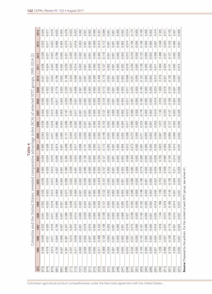
142 CEPAL Review N° 122 • August 2017
Colombian agricultural product competitiveness under the free trade agreement with the United States...
Tab
le 4
C
olom
bia
an
d t
he
Un
ited
Sta
tes:
rev
eale
d c
omp
arat
ive
adva
nta
ge in
dex
(R
CA
) of
sel
ecte
d S
ITC
gro
up
s, 1
995-
2014
(2)
SITC
1995
1996
1997
1998
1999
2000
2001
2002
2003
2004
2005
2006
2007
2008
2009
2010
2011
2012
2013
2014
[073
]-0
.049
-0.0
59-0
.032
-0.0
41-0
.052
-0.0
35-0
.048
-0.0
62-0
.059
-0.0
65-0
.043
-0.0
39-0
.050
-0.0
56-0
.043
-0.0
21-0
.036
-0.0
39-0
.032
-0.0
34
[074
]-0
.019
-0.0
21-0
.020
-0.0
20-0
.025
-0.0
23-0
.018
-0.0
20-0
.024
-0.0
26-0
.023
-0.0
30-0
.025
-0.0
25-0
.022
-0.0
21-0
.024
-0.0
21-0
.017
-0.0
17
[075
]0.
013
0.01
10.
016
0.01
10.
019
0.01
50.
013
0.01
20.
016
0.01
50.
017
0.01
60.
012
0.01
90.
020
0.02
30.
023
0.02
30.
023
0.01
8
[081
]-0
.793
-0.8
40-0
.790
-0.8
45-0
.948
-0.9
04-0
.844
-0.8
37-0
.936
-0.8
74-0
.880
-0.9
60-0
.854
-0.9
17-0
.778
-0.7
86-0
.848
-0.7
86-0
.688
-0.6
25
[091
]-0
.007
-0.0
08-0
.007
-0.0
07-0
.021
-0.0
05-0
.004
-0.0
01-0
.002
0.00
10.
000
-0.0
030.
003
0.00
40.
003
0.00
2-0
.002
-0.0
05-0
.004
-0.0
04
[098
]-0
.361
-0.3
87-0
.357
-0.3
99-0
.450
-0.3
73-0
.298
-0.3
80-0
.365
-0.2
99-0
.131
-0.2
86-0
.167
-0.2
03-0
.230
-0.1
88-0
.239
-0.2
21-0
.275
-0.2
76
[111
]-0
.031
0.01
2-0
.047
-0.0
290.
038
0.02
50.
025
0.03
60.
040
0.04
40.
044
0.04
60.
041
0.04
60.
031
0.03
30.
025
0.00
5-0
.011
-0.0
23
[112
]-0
.011
-0.0
08-0
.010
-0.0
14-0
.015
-0.0
040.
000
-0.0
010.
024
0.01
10.
012
-0.0
02-0
.017
0.00
1-0
.006
-0.0
06-0
.014
-0.0
24-0
.016
-0.0
23
[121
]-0
.002
-0.0
03-0
.001
-0.0
05-0
.002
-0.0
01-0
.002
-0.0
03-0
.006
-0.0
060.
000
-0.0
00-0
.001
0.00
20.
001
0.00
10.
003
0.00
20.
003
0.00
2
[122
]-0
.026
-0.0
30-0
.019
-0.0
39-0
.024
-0.0
02-0
.038
-0.0
90-0
.126
-0.1
41-0
.039
-0.0
37-0
.031
-0.0
02-0
.000
0.00
10.
001
0.00
10.
001
0.00
1
[211
]-0
.009
-0.0
07-0
.010
0.00
0-0
.001
-0.0
01-0
.000
-0.0
00-0
.002
0.00
0-0
.000
0.00
1-0
.000
-0.0
03-0
.003
0.00
2-0
.003
-0.0
01-0
.002
-0.0
02
[212
]-0
.000
-0.0
00-0
.000
-0.0
00-0
.000
-0.0
00-0
.000
-0.0
00-0
.000
0.00
00.
000
0.00
0-0
.000
-0.0
000.
000
-0.0
000.
000
-0.0
00-0
.000
-0.0
00
[222
]-0
.411
-0.4
96-0
.432
-0.4
40-0
.504
-0.5
08-0
.479
-0.5
22-0
.555
-0.5
17-0
.500
-0.5
54-0
.502
-0.5
09-0
.453
-0.4
46-0
.478
-0.4
42-0
.415
-0.3
51
[223
]-0
.069
0.10
9-0
.106
-0.1
08-0
.131
-0.1
22-0
.107
-0.1
07-0
.127
-0.1
72-0
.146
-0.1
43-0
.127
-0.1
34-0
.115
-0.1
19-0
.127
-0.1
19-0
.112
-0.0
94
[231
]-0
.004
-0.0
03-0
.002
-0.0
02-0
.002
-0.0
02-0
.002
-0.0
02-0
.002
-0.0
02-0
.002
-0.0
02-0
.002
-0.0
02-0
.002
-0.0
02-0
.002
-0.0
01-0
.001
-0.0
01
[245
]-0
.001
-0.0
01-0
.001
-0.0
03-0
.003
-0.0
02-0
.001
-0.0
010.
001
0.00
10.
000
0.00
00.
000
0.00
10.
001
0.00
10.
001
0.00
10.
001
0.00
1
[246
]-0
.000
-0.0
00-0
.000
-0.0
00-0
.001
-0.0
000.
000
-0.0
00-0
.000
0.00
0-0
.000
0.00
0-0
.000
-0.0
00-0
.000
-0.0
00-0
.000
-0.0
00-0
.000
-0.0
00
[247
]-0
.003
-0.0
020.
001
-0.0
08-0
.005
-0.0
04-0
.001
-0.0
02-0
.003
-0.0
04-0
.002
-0.0
04-0
.002
-0.0
04-0
.003
-0.0
02-0
.003
-0.0
03-0
.002
-0.0
02
[248
]-0
.010
-0.0
05-0
.016
-0.0
21-0
.019
0.00
2-0
.003
-0.0
090.
006
-0.0
12-0
.006
-0.0
17-0
.013
-0.0
17-0
.011
-0.0
09-0
.016
-0.0
15-0
.014
-0.0
14
[251
]-0
.232
-0.2
27-0
.215
-0.2
36-0
.293
-0.2
90-0
.266
-0.2
82-0
.324
-0.2
73-0
.272
-0.2
90-0
.260
-0.2
61-0
.225
-0.2
21-0
.239
-0.2
16-0
.194
-0.1
74
[261
]-0
.000
-0.0
000.
000
-0.0
00-0
.000
-0.0
00-0
.000
0.00
00.
000
-0.0
000.
000
0.00
00.
000
-0.0
00-0
.000
0.00
00.
000
-0.0
00-0
.000
-0.0
00
[263
]-0
.163
-0.1
42-0
.161
-0.1
80-0
.192
-0.1
98-0
.198
-0.2
19-0
.269
-0.2
61-0
.211
-0.2
34-0
.178
-0.1
60-0
.140
-0.1
25-0
.139
-0.1
22-0
.106
-0.1
00
[265
]-0
.000
0.00
0-0
.000
-0.0
00-0
.000
-0.0
00-0
.001
-0.0
00-0
.000
-0.0
00-0
.000
-0.0
00-0
.000
-0.0
00-0
.000
0.00
00.
000
0.00
00.
000
0.00
0
[268
]-0
.005
-0.0
02-0
.000
-0.0
01-0
.003
-0.0
03-0
.000
-0.0
02-0
.003
-0.0
03-0
.003
0.00
1-0
.002
-0.0
03-0
.002
-0.0
03-0
.003
-0.0
030.
000
-0.0
02
[291
]-0
.021
-0.0
24-0
.016
-0.0
25-0
.019
-0.0
30-0
.023
-0.0
29-0
.039
-0.0
35-0
.034
-0.0
33-0
.019
-0.0
19-0
.023
-0.0
12-0
.011
-0.0
09-0
.007
-0.0
14
[292
]1.
238
1.53
31.
616
1.14
41.
166
1.10
90.
753
0.44
60.
726
0.82
30.
947
1.07
21.
145
2.01
61.
926
2.31
92.
404
2.48
62.
549
2.32
5
[411
]-0
.066
-0.0
57-0
.037
-0.0
72-0
.078
-0.0
39-0
.047
-0.0
59-0
.060
-0.0
55-0
.039
-0.0
33-0
.033
-0.0
32-0
.018
-0.0
21-0
.024
-0.0
21-0
.020
-0.0
17
[421
]-0
.129
-0.1
26-0
.119
-0.1
90-0
.168
-0.1
44-0
.136
-0.1
14-0
.100
-0.0
43-0
.064
-0.1
37-0
.127
-0.1
69-0
.124
-0.1
30-0
.141
-0.1
27-0
.103
-0.1
02
[422
]0.
005
-0.0
16-0
.001
-0.0
14-0
.014
-0.0
010.
004
0.01
10.
014
0.01
30.
009
0.00
30.
003
0.00
3-0
.007
0.00
90.
000
0.00
50.
006
0.00
7
[431
]-0
.030
-0.0
27-0
.025
-0.0
27-0
.037
-0.0
31-0
.024
-0.0
29-0
.032
-0.0
31-0
.030
-0.0
30-0
.028
-0.0
29-0
.026
-0.0
07-0
.015
-0.0
090.
001
-0.0
06
So
urce
: Pre
pare
d by
the
auth
ors.
For
the
cont
ent o
f eac
h S
ITC
gro
up, s
ee a
nnex
A1.
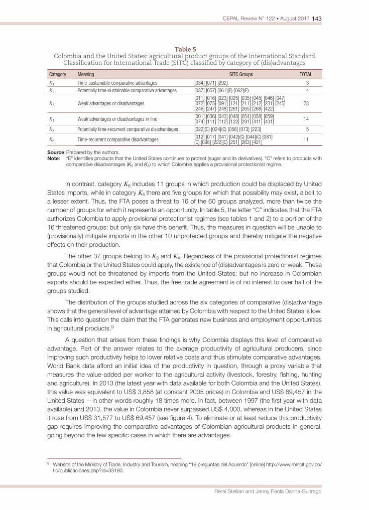
143CEPAL Review N° 122 • August 2017
Rémi Stellian and Jenny Paola Danna-Buitrago
Table 5 Colombia and the United States: agricultural product groups of the International Standard
Classification for International Trade (SITC) classified by category of (dis)advantages
Category Meaning SITC Groups TOTAL
K 1 Time-sustainable comparative advantages [034] [071] [292] 3
K 2 Potentially time-sustainable comparative advantages [037] [057] [061](E) [062](E) 4
K 3 Weak advantages or disadvantages[011] [016] [023] [025] [035] [045] [046] [047] [072] [075] [091] [121] [211] [212] [231] [245] [246] [247] [248] [261] [265] [268] [422]
23
K 4 Weak advantages or disadvantages in fine [001] [036] [043] [048] [054] [058] [059] [074] [111] [112] [122] [291] [411] [431] 14
K 5 Potentially time-recurrent comparative disadvantages [022](C) [024](C) [056] [073] [223] 5
K 6 Time-recurrent comparative disadvantages [012] [017] [041] [042](C) [044](C) [081](C) [098] [222](C) [251] [263] [421] 11
Source: Prepared by the authors.Note: “E” identifies products that the United States continues to protect (sugar and its derivatives). “C” refers to products with
comparative disadvantages (K5 and K6) to which Colombia applies a provisional protectionist regime.
In contrast, category K6 includes 11 groups in which production could be displaced by United States imports, while in category K5 there are five groups for which that possibility may exist, albeit to a lesser extent. Thus, the FTA poses a threat to 16 of the 60 groups analyzed, more than twice the number of groups for which it represents an opportunity. In table 5, the letter “C” indicates that the FTA authorizes Colombia to apply provisional protectionist regimes (see tables 1 and 2) to a portion of the 16 threatened groups; but only six have this benefit. Thus, the measures in question will be unable to (provisionally) mitigate imports in the other 10 unprotected groups and thereby mitigate the negative effects on their production.
The other 37 groups belong to K3 and K4. Regardless of the provisional protectionist regimes that Colombia or the United States could apply, the existence of (dis)advantages is zero or weak. These groups would not be threatened by imports from the United States; but no increase in Colombian exports should be expected either. Thus, the free trade agreement is of no interest to over half of the groups studied.
The distribution of the groups studied across the six categories of comparative (dis)advantage shows that the general level of advantage attained by Colombia with respect to the United States is low. This calls into question the claim that the FTA generates new business and employment opportunities in agricultural products.9
A question that arises from these findings is why Colombia displays this level of comparative advantage. Part of the answer relates to the average productivity of agricultural producers, since improving such productivity helps to lower relative costs and thus stimulate comparative advantages. World Bank data afford an initial idea of the productivity in question, through a proxy variable that measures the value-added per worker to the agricultural activity (livestock, forestry, fishing, hunting and agriculture). In 2013 (the latest year with data available for both Colombia and the United States), this value was equivalent to US$ 3,858 (at constant 2005 prices) in Colombia and US$ 69,457 in the United States —in other words roughly 18 times more. In fact, between 1997 (the first year with data available) and 2013, the value in Colombia never surpassed US$ 4,000, whereas in the United States it rose from US$ 31,577 to US$ 69,457 (see figure 4). To eliminate or at least reduce this productivity gap requires improving the comparative advantages of Colombian agricultural products in general, going beyond the few specific cases in which there are advantages.
9 Website of the Ministry of Trade, Industry and Tourism, heading “19 preguntas del Acuerdo” [online] http://www.mincit.gov.co/tlc/publicaciones.php?id=33180.

144 CEPAL Review N° 122 • August 2017
Colombian agricultural product competitiveness under the free trade agreement with the United States...
Figure 4 Colombia and the United States: value added per worker in the agriculture sector, 1997-2013
(Dollars at 2005 prices)
0
10 000
20 000
30 000
40 000
50 000
60 000
70 000
1997
1998
1999
2000
2001
2002
2003
2004
2005
2006
2007
2008
2009
2010
2011
2012
2013
Colombia United States
Source: World Bank [online] http://datos.bancomundial.org/indicador/EA.PRD.AGRI.KD.
This mainly reflects the use of fertilizers (nitrogenous, phosphate and potassium, among others). According to Wang and others (2015), fertilizer use is the main factor explaining why agricultural productivity in the United States in 2011 was double the 1948 level. In 2013, 649 kg of fertilizer were used per hectare of arable land in the United States compared to 132 kg in Colombia. In fact, fertilizer consumption in both countries has trended up since 2002; but, as figure 5 shows, in 2013 Colombia was still below the United States level of 2002. This helps to explain the productivity differential between the two countries and hence the general level of Colombia’s comparative advantages relative to the United States.
Figure 5 Colombia and the United States: fertilizer consumption, 2002-2013
(Kilograms per hectare of arable land)
0
100
200
300
400
500
600
700
800
2002
2003
2004
2005
2006
2007
2008
2009
2010
2011
2012
2013
Colombia United States
Source: World Bank [online] http://datos.bancomundial.org/indicador/AG.CON.FERT.ZS.
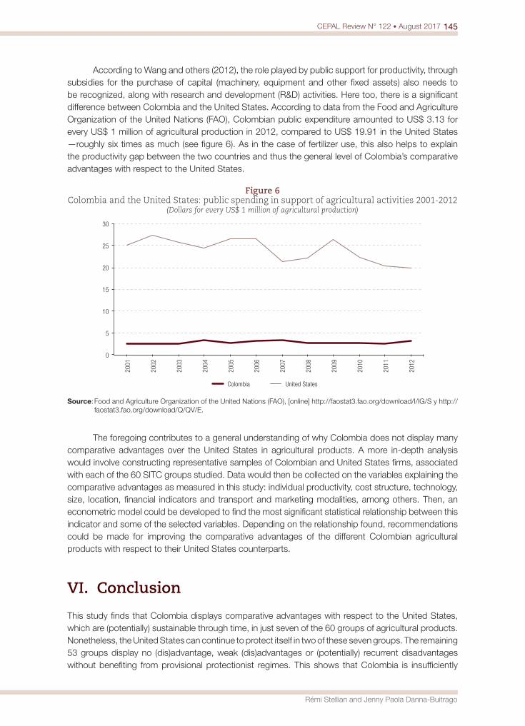
145CEPAL Review N° 122 • August 2017
Rémi Stellian and Jenny Paola Danna-Buitrago
According to Wang and others (2012), the role played by public support for productivity, through subsidies for the purchase of capital (machinery, equipment and other fixed assets) also needs to be recognized, along with research and development (R&D) activities. Here too, there is a significant difference between Colombia and the United States. According to data from the Food and Agriculture Organization of the United Nations (FAO), Colombian public expenditure amounted to US$ 3.13 for every US$ 1 million of agricultural production in 2012, compared to US$ 19.91 in the United States —roughly six times as much (see figure 6). As in the case of fertilizer use, this also helps to explain the productivity gap between the two countries and thus the general level of Colombia’s comparative advantages with respect to the United States.
Figure 6 Colombia and the United States: public spending in support of agricultural activities 2001-2012
(Dollars for every US$ 1 million of agricultural production)
0
5
10
15
20
25
30
2001
2002
2003
2004
2005
2006
2007
2008
2009
2010
2011
2012
Colombia United States
Source: Food and Agriculture Organization of the United Nations (FAO), [online] http://faostat3.fao.org/download/I/IG/S y http://faostat3.fao.org/download/Q/QV/E.
The foregoing contributes to a general understanding of why Colombia does not display many comparative advantages over the United States in agricultural products. A more in-depth analysis would involve constructing representative samples of Colombian and United States firms, associated with each of the 60 SITC groups studied. Data would then be collected on the variables explaining the comparative advantages as measured in this study: individual productivity, cost structure, technology, size, location, financial indicators and transport and marketing modalities, among others. Then, an econometric model could be developed to find the most significant statistical relationship between this indicator and some of the selected variables. Depending on the relationship found, recommendations could be made for improving the comparative advantages of the different Colombian agricultural products with respect to their United States counterparts.
VI. Conclusion
This study finds that Colombia displays comparative advantages with respect to the United States, which are (potentially) sustainable through time, in just seven of the 60 groups of agricultural products. Nonetheless, the United States can continue to protect itself in two of these seven groups. The remaining 53 groups display no (dis)advantage, weak (dis)advantages or (potentially) recurrent disadvantages without benefiting from provisional protectionist regimes. This shows that Colombia is insufficiently

competitive to take advantage of the opportunities offered by the FTA with respect to the products studied. These results are obtained by measuring the comparative advantages revealed through trade, calculated by the CEPII and used in this study to perform this measurement as accurately as possible.
The RCA index allows for a diagnostic of the capacity to produce with lower relative costs or differentiation, or both. Nonetheless, the purpose of the RCA index is not to determine the factors underlying that capability; so, the logical continuation of the present research would be to investigate those factors. As noted above, these generally relate to a productivity gap between Colombia and the United States, which stems, among other things, from a significant differential in fertilizer use and in public-sector support in the two countries. Identifying the underlying factors will make it possible to find various ways of stimulating or consolidating the advantages discussed here. This is essential for avoiding —or at least limiting— the substitution of imports from the United States for Colombian agricultural production, while at the same time promoting growth through exports to the United States. Future research should therefore analyse the economic policy measures that Colombian public entities plan to implement, or have already implemented, to make the FTA a genuine tool for promoting growth in agricultural production and hence the country’s development.
BibliographyAwokuse, T. (2008), “Trade openness and economic growth”, Applied Economics, vol. 40, No. 2, Taylor
& Francis.Aytaç, D. and S. Kiliç (2014), “The short- and long-term effects of trade taxes on vertical specialization”, Asian
Economic and Financial Review, vol. 4, No. 6, Asian Economic and Social Society.Balassa, B. (1977), “Revealed comparative advantage revisited: an analysis of relative export shares of the
industrialized countries, 1953-1971”, The Manchester School, vol. 45, No. 3, Amsterdam, Elsevier.(1966), “Tariff reductions and trade in manufactures among the industrial countries”, American Economic Review, vol. 56, No. 3, Nashville, Tennessee, American Economic Association. (1965), “Trade liberalization and ‘revealed’ comparative advantage”, The Manchester School, vol. 33, No. 2, Amsterdam, Elsevier.
Ballance, H. (1988), “Trade performance as an indicator of comparative advantage”, Economic Development and International Trade, D. Greenaway (ed.), London, Macmillan.
Cano, C. and others (2012), “El mercado mundial del café y su impacto en Colombia”, Borradores de Economía, No. 710, Bogota, Bank of the Republic.
Cárdenas, M. and C. García (2005), “Impacto del TLC con Estados Unidos en el sector agrícola colombiano: más riesgos que oportunidades”, Coyuntura Económica, vol. 35, No. 1.(2004), “El modelo gravitacional y el TLC entre Colombia y Estados Unidos”, Working Paper, No. 27, Bogota, Foundation for Education and Higher Development (Fedesarrollo).
Chevassus-Lozza, E. and J. Gallezot (1995), “La compétitivité hors-prix dans les échanges de produits agricoles et agro-alimentaires français sur le marché communautaire”, Économie et prevision, vol. 117, No. 1, Persée.
Chor, D. (2010), “Unpacking sources of comparative advantage: a quantitative approach”, Journal of International Economics, vol. 82, No. 2, Amsterdam, Elsevier.
Costinot, A. (2009), “On the origins of comparative advantage”, Journal of International Economics, vol. 77, No. 2, Amsterdam, Elsevier.
Cuñat, A. and M. Melitz (2012), “Volatility, labor market flexibility, and comparative advantage”, Journal of the European Economic Association, vol. 10, No. 2, Wiley.
Danna-Buitrago, J.P. (2012), “L’intégration économique internationale de la Colombie (1990-2010): une approche en termes d’économie politique internationale”, thesis, University of Grenoble.
Danna-Buitrago, J.P. and R. Stellian (2014), “Los retos de la integración económica latino-americana: ¿existencia o inexistencia de ventajas comparativas para la agricultura colombiana dentro de la zona ALADI?”, Ágora latinoamericana: logros, obstaculos y retos de la integración regional, vol. 1, Bogota, Association of Universities of Latin America and the Caribbean for Integration (AUALCPI)/University of Applied and Environmental Sciences.
147CEPAL Review N° 122 • August 2017
Rémi Stellian and Jenny Paola Danna-Buitrago
De Saint-Vaulry, A. (2008), “Base de données CHELEM - commerce international du CEPII”, Document de travail CEPII, No. 9, Centre for International Prospective Studies and Information.
Díaz Rivillas, B. (2002), “Política exterior de los EE.UU. hacia Colombia: el paquete de ayuda de 1.300 millones de dólares de apoyo al Plan Colombia y la Región Andina”, America Latina Hoy, vol. 31.
Díaz Valencia, G.A. (2012), “Impacto del TLC con Estados Unidos en el sector agrícola colombiano: más riesgos que oportunidades (caso arroz)”, Revista CIFE, vol. 14, No. 20, Bogota, Santo Tomás University.
DNP (National Planning Department) (2003), “Efectos de un acuerdo bilateral de libre comercio con Estados Unidos”, Archivos de Economía, No. 229, Bogota.
Durán Lima, J., C. De Miguel and A. Schuschny (2007), “Trade agreements by Colombia, Ecuador and Peru with the United States: effects on trade, production and welfare”, CEPAL Review, No. 91 (LC/G.2333-P), Santiago, Economic Commission for Latin America and the Caribbean (ECLAC).
Eaton, J. and S. Kortum (2002), “Technology, geography, and trade”, Econometrica, vol. 70, No. 5, New York, The Econometric Society.
Espinosa, A. and L. Pasculli (2013), “Visión agrícola del TLC entre Colombia y Estados Unidos: preparación, negociación, implementación y aprovechamiento”, Estudios y Perspectivas series, No. 25 (LC/L.3606), Bogota, ECLAC Office in Bogota.
Gracia, O. and H. Zuleta (2009), “Tratado de libre comercio entre Colombia y Estados Unidos: ¿qué impacto puede tener en Colombia?”, Coyuntura Económica, vol. 39, No. 1, Bogota.
Hernández, G. (2014), “Una revisión de los efectos del tratado de libre comercio entre Colombia y Estados Unidos”, Lecturas de Economía, No. 80, University of Antioquia.
Iannariello-Monroy, M., J. León and C. Oliva (1999), El comportamiento de las exportaciones en Colombia: 1962-1996, Washington, D.C., Inter-American Development Bank.
Krugman, P. (1995), “Growing world trade: causes and consequences”, Brookings Papers on Economic Activity, vol. 26, No. 1, The Brookings Institution.
Lafay, G. (1992), “The measurement of revealed comparative advantages”, International Trade Modelling, M.G. Dagenais and P.-A. Muet (eds.), London, Chapman & Hall.(1990), “La mesure des avantages comparatifs révélés”, Économie prospective internationale, No. 42.(1987), “Avantage comparatif et compétitivité”, Économie prospective internationale, No. 29.
Leibovich, J. and L. Estrada (2008), “Competitividad del sector agropecuario colombiano”, Ruta a la prosperidad colectiva, Bogota, Private Competitiveness Council.
Londoño, J. (2011), “Colombia y Estados Unidos: una relación por revisar”, Colombia, una política exterior en transición, D. Cardona (ed.), Bogota, Fundación Fredrich Ebert de Colombia (FESCOL).
Lozano, C., C. Castro and J. Campos (2005), “Un modelo gravitacional para la agenda interna”, Archivos de Economía, No. 296, Bogota, National Planning Department.
Maldonado, N. and E. Sánchez (2012), “Rutas de transformación productiva”, Cuadernos de Economía, vol. 31, No. 57, Bogota, National University of Colombia.
Martín, C. and J. Ramírez (2005), “Impacto económico de un acuerdo parcial de libre comercio entre Colombia y Estados Unidos”, Estudios y Perspectivas series, No. 7 (LC/L.2362-P), Bogota, ECLAC Office in Bogota.
Moncayo, E. (2006), “El TLC de Colombia con Estados Unidos y sus implicaciones en los departamentos colombianos”, Relaciones Internacionales, Estrategia y Seguridad, vol. 1, No. 1, Bogota, Universidad Militar Nueva Granada.
Norton, R. and R. Argüello (2008), “Una perspectiva de la competitividad agrícola de Colombia”, Bogota, United States Agency for International Development (USAID).
Perfetti, J. (2011), “Oferta potencial agrícola de Colombia en un nuevo entorno de mercado”, Cuadernos Fedesarrollo, No. 38, Bogota, Foundation for Education and Higher Development (Fedesarrollo).
Pesquera, A. and A. Rodríguez (2009), “Impactos del actual TLC entre Estados Unidos y Colombia para los pequeños productores rurales”, Deslinde, No. 44.
Porter, M. (1990), The Competitive Advantage of Nations, Harvard Business Review, vol. 68, No. 2.Raghurampatruni, R. (2012), “Revealed comparative advantage: an analysis for India and Asean”, Global
Management Review, vol. 6, No. 4.Reina, M. and others (2013), “Estrategia para lograr el fortalecimiento de la oferta exportable en Colombia”,
Bogota, Foundation for Education and Higher Development (Fedesarrollo).Rocha Beltrán, C. (2012), “El agro colombiano frente al TLC con Estados Unidos: evaluación desde el modelo
de ventajas comparativas”, Econografos, No. 39, Bogota, National University of Colombia.Romero, A. (2006), “El TLC Colombia-USA”, Tendencias, vol. 7, No. 2.

148 CEPAL Review N° 122 • August 2017
Colombian agricultural product competitiveness under the free trade agreement with the United States...
Swanson, J. (2006), “Drug trafficking in the Americas: reforming United States trade policy”, George Washington International Law Review, vol. 38, No. 4.
Toro, J. and others (2010), “El impacto del tratado de libre comercio con Estados Unidos (TLC) en la balanza de pagos hasta 2010”, Borradores de Economía, No. 362, Bogota, Bank of the Republic.
Toscano, O.M. (2012), “Comportamiento y características del endeudamiento público del gobierno nacional central en la década de los noventa (1990-2001)”, Apuntes del CENES, vol. 26, No. 41.
Umaña, C. (2011), “Una evaluación de la estrategia comercial de Colombia a la luz de un modelo de equilibrio general computable basado en la ecuación de gravedad”, Archivos de Economía, No. 379, Bogota, National Planning Department.
Umaña, G. (2005), “Aspectos no comerciales de la negociación del TLC”, Temas no comerciales en la negociación comercial entre Colombia y Estados Unidos, J.C.R. Jaramillo (ed.), Estudios y Perspectivas series, No. 6 (LC/L.2278-P), Bogota, ECLAC Office in Bogota.
Umaña, G. and S. Caro (2004), El juego asimetrico del comercio: el tratado de libre comercio Colombia-Estados Unidos, Bogota, National University of Colombia.
Wang, S.L. and others (2015), “Agricultural productivity growth in the United States: measurement, trends, and drivers”, Economic Research Report, No. 189, United States Department of Agriculture. (2012), “Accounting for the impacts of public research, R&D spill-ins, extension, and roads in U.S. agricultural productivity growth”, Agricultural Productivity: An International Perspective, K.O. Fuglie, V.E. Ball and S.L. Wang (eds.), Cambridge, CAB International (CABI).
World Bank (2003), “Colombia: agricultural and rural competitiveness”, Report, No. 27523-CO, Washington, D.C.WTO (World Trade Organization) (2015), World Tariff Profiles 2015, Geneva.
Annex A1Table A1.1
The 60 groups studied from the Standard International Trade Classification (SITC)
001 Live animals other than animals of division 03
011 Meat of bovine animals, fresh, chilled or frozen
012* Other meat and edible offal of meat, fresh, chilled or frozen
016 Meat and edible meat offal, salted, in brine, dried or smoked; Edible flours of meat or meat offal
017 Prepared or preserved meat and meat offal, n.e.s.
022 Milk, cream and milk products, other than butter or cheese
023 Butter and other fats and oils derived from milk
024 Cheese and curd
025 Eggs, birds’, and egg yolks; egg albumin
034 0Fish, fresh (live or dead), chilled or frozen
035* Fish, dried, salted or in brine; smoked fish
036 Crustaceans, molluscs and aquatic invertebrates, whether in shell or not, fresh (live or dead), chilled, frozen, dried, salted or in brine; Crustaceans, in shell, cooked by steaming or boiling in water
037 Fish, crustaceans, molluscs and other aquatic invertebrates, prepared or preserved, n.e.s.
041 Wheat (including shelled) and meslin, unmilled
042 Rice
043 Barley, unmilled
044 Maize (other than sweet corn), unmilled
045 Cereals, unmilled (other than wheat, rice, barley and maize)
046 Meal and flour of wheat and flour of meslin
047 Other cereal meals and flours
048 Cereals preparations and preparations of flour or starch of fruits or vegetables
054 Vegetables, fresh, chilled, frozen or simply preserved (including dried leguminous vegetables); roots, tubers and other edible vegetable products, n.e.s., fresh or dried
056 Vegetables, roots and tubers, prepared or preserved, n.e.s.

149CEPAL Review N° 122 • August 2017
Rémi Stellian and Jenny Paola Danna-Buitrago
057 Fruit and nuts (not including oil nuts), fresh or dried
058 Fruit, preserved, and fruit preparations (excluding fruit juices)
059* Fruit juices (including grape must) and vegetable juices
061 Sugars, molasses and honey
062 Sugar confectionery
071 Coffee and substitutes for coffee
072 Cocoa
073 Chocolate and other food preparations containing cocoa, n.e.s.
074 Tea and mate
075 Spices
081 Feeding stuff for animals (not including unmilled cereals)
091 Margarine and shortening
098 Edible products and preparations, n.e.s.
111 Non-alcoholic beverages, n.e.s.
112 Alcoholic beverages
121 Tobacco, unmanufactured; tobacco refuse
122* Tobacco, manufactured
211 Hides and skins (except furskins), raw
212 Furskins, raw (including heads, tails, paws and other pieces or cuttings, suitable for furriers’ use), other than hides and skins of group 211
222 Oil-seeds and oleaginous fruits of a kind used for the extraction of “soft” fixed vegetable oils (excluding flours and meals)
223 Oil-seeds and oleaginous fruits, whole or broken, of a kind used for the extraction of other fixed vegetable oils (including flours and meals of oil-seeds or oleaginous fruit, n.e.s.)
231 Natural rubber, balata, gutta-percha, guayule, chicle and similar natural gums, in primary forms (including latex) or in plates, sheets or strip
245 Firewood (other than wood waste) and charcoal
246 Wood in chips or particles and wood waste
247 Wood in rough form or roughly squared
248 Wood, simply worked, and railway sleepers of wood
251 Pulp and waste paper
261 Silk
263 Cotton
265* Vegetable textile fibres (other than cotton and jute)
268 Wool and other animal hair (including wool tops)
291 Crude animal materials, n.e.s.
292 Crude vegetable materials, n.e.s.
411 Animal oils and fats
421* Fixed vegetable fats and oils, “soft”
422* Fixed vegetable fats and oils, other than “soft”
431* Animal or vegetable fats and oils, n.e.s
Source: United Nations Statistics Division, “SITC Rev. 3” [online] https://unstats.un.org/unsd/cr/registry/regcst.asp?Cl=14& Top=2&Lg=1.
Note: The description shown for groups marked with an asterisk has been simplified. Further details can be found at the source.
Table A1.1 (concluded)


Public transport, well-being and inequality: coverage and affordability in the city of MontevideoDiego Hernández
Abstract
Public transport is key to ensuring people’s ability to access the opportunities offered by the city. Unlike other types of transport such as automobiles, public transport is the means that exerts the least monetary pressure on users and most decommodifies mobility. This article analyses the levels of spatial coverage of public transport and the affordability of the service in Montevideo. It also seeks to identify patterns of stratification among diverse socioeconomic groups. The indicators presented show high levels of basic network coverage, coinciding with a growth pattern developed by following spatial and timetable demand. This coverage has a number of stratified differences in access, in particular when affordability is considered. The evidence indicates that household expenditure shows a regressive distribution in relation to access.
KeywordsPublic transport, transport policy, social welfare, equality, household expenditures, cities, Uruguay
JEL classificationR40, R48, Z13, Z18
AuthorDiego Hernández is an assistant professor at the Department of Social and Political Sciences of the Catholic University of Uruguay. [email protected]
152 CEPAL Review N° 122 • August 2017
Public transport, well-being and inequality: coverage and affordability in the city of Montevideo
I. Introduction
Urban mobility facilitates access to other goods and opportunities, and thus has a major impact on people’s quality of life. In fact, it plays an important role in the production and reproduction of social structures which, at the same time, influence the characteristics of daily mobility (Cass, Shove and Urry, 2005; Kaufmann, 2002; Manderscheid, 2009; Ohnmacht, Maksim and Bergman, 2009). Mobility is not a matter of free personal choice and can be subject to very strong structural limitations (Massot and Orfeuil, 2005; Wenglenski and Orfeuil, 2006). It would be naïve to think that mobility reaches all social strata equally; the fact that greater speed of transport and movement are an imperative for modern societies does not mean that the entire population has access to it (Kaufmann, 2002; Urry, 2007). In short, mobility is not equitably distributed: some people have more transport possibilities than others and some can travel much faster than others and in more directions.
The accessibility of goods, services and opportunities is key to people’s well-being and, for that reason, public transport is as much a matter of social policy as other more traditional social policy areas, such as health and education. Public transport is the greatest decommodifier of accessibility, such that someone who has to travel across the city will find public transport the cheapest way of doing so. Aside from the fact that it involves out-of-pocket expenses (payment of a fare), public transport is the means that demands least payment capacity from the individual. This lower demand makes affordability, to an extent, more independent of a person’s performance in the labour market. Decommodification is based on its conception as a social entitlement rather than as a product with monetary value that depends solely on market fluctuations.
Thus, like other social policies, public transport must be analysed on the basis of three fundamental variables: (i) level of coverage, (ii) affordability of the service, and (iii) the existence of specific mechanisms of financial decommodification. This article analyses the three variables for the case of the city of Montevideo, from the perspective of well-being and equity in the provision of a social good.
This article is intended as a contribution to the study of urban mobility in the region from the perspective of welfare State structures and social policies. It also contributes to the analysis of social policies on the continent, insofar as it analyses a sectoral policy that is always mentioned as crucial, but rarely studied systematically to find rationales of provision and stratification.
This article is structured as follows. Section II presents the conceptual framework, with a particular emphasis on the role of accessibility in well-being and the decommodification function of public transport (using the scheme of assets and opportunities structures). Section III conducts a brief analysis of the case of the city of Montevideo and describes the methodology used to build the indicators analysed. Section IV presents the results in terms of coverage and affordability by socioeconomic level. This evidence is complemented with a review of the decommodification mechanisms identified for the Montevidean transport system. The article closes with a discussion of the empirical evidence in section V.
II. Conceptual framework: accessibility, well-being and public transport
1. The concept of accessibility
For Miralles and Cebollada, accessibility refers to the ease with which people can bridge the distance separating two places and thus exercise their autonomy as citizens (Miralles-Guasch and Cebollada,
153CEPAL Review N° 122 • August 2017
Diego Hernández
2003, p. 14).1 An individual can have very little capacity to travel large spatial distances, yet enjoy very good accessibility through proximity. And, conversely, an individual may be able to travel to many different points in the city, but not to the particular one he or she needs to reach, so that, despite having high mobility, that person continues to have poor accessibility. A person may also make many trips —and thus be highly “mobile”— but still have only poor accessibility if he or she has to travel long distances. In this regard, the location of activities is important. In theory, distances can be overcome by the individual moving towards the activity, or by the activity “moving” towards the individual (proximal localization). Problems of accessibility of work, for example, can be resolved in two ways: with a good transport system that takes people to areas with high concentrations of work opportunities or by work opportunities being located near people’s areas of residence.
On the basis of studies on mobility, accessibility and poverty, a set of variables have been identified that facilitate or hinder access (Cass, Shove and Urry, 2005; Church, Frost and Sullivan, 2000; Flamm, Jemelin and Kaufmann, 2008; Titheridge, 2006; Urry, 2007). Focusing on public transport, these can be summarized in the following dimensions:2
(i) Transport opportunities: the road network and its extent, and the extent of the public transport network, travel times, the characteristics of public transport (timetables, regularity, coverage at different times of day), the quality in terms of convenience and safety or rolling stock and static facilities, and the information made available to passengers.
(ii) Institutional configuration: the extent of State participation in the configuration of transport opportunities and the definition of who pays and who is benefited in relation to travel costs. Another question is the priority given to private forms of transport with respect to public transport (or vice versa), driving costs (for example, if there are urban toll roads or highways, payments and so on), the fare structure of public transport and the existence of regulation and subsidy mechanisms.
(iii) Individual characteristics: the extent to which individuals can take advantage of transport opportunities and the place they occupy in relation to the institutional configuration. In this regard, considerations are people’s income, the time available and how they can organize it (in relation to their activities), and their skills and abilities to master the system and its operation (for example, knowing how to drive or being able to understand how public transport works) and being physically able to access transport.
(iv) Urban form: this concerns socioterritorial dynamics such as the location of households and opportunities in the city.
These dimensions cover various structural aspects and various individual characteristics which, combined, define people’s capacity to overcome geographical distances. For example, a person may live in an area with excellent public transport provision, but if that person cannot afford the fare, accessibility will be limited.
In order to capture this interaction between individual and structural aspects, the paradigm of assets and opportunities structures may be used (Hernández, 2012). Under this approach, the analysis centres on the concept of vulnerability as a tool for looking beyond the poor/non-poor dichotomy in examining household and individual well-being.
1 Another concept that, although terminologically different, has much to do with accessibility is that of motility developed by Kaufmann, Bergman and Joye, who define it as “the capacity to be mobile in the social and geographical space or as the way in which entities access and appropriate the capacity for sociospatial mobility” (Kaufmann, Manfred and Joye, 2004, p. 750).
2 Adapted from Hernández (2012).
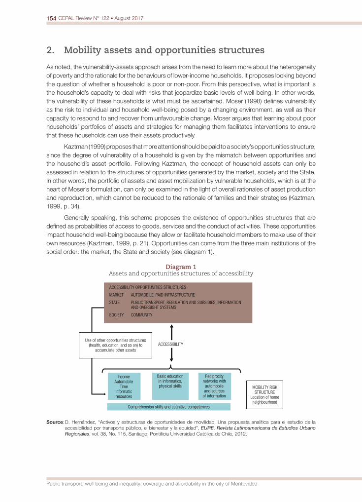
154 CEPAL Review N° 122 • August 2017
Public transport, well-being and inequality: coverage and affordability in the city of Montevideo
2. Mobility assets and opportunities structures
As noted, the vulnerability-assets approach arises from the need to learn more about the heterogeneity of poverty and the rationale for the behaviours of lower-income households. It proposes looking beyond the question of whether a household is poor or non-poor. From this perspective, what is important is the household’s capacity to deal with risks that jeopardize basic levels of well-being. In other words, the vulnerability of these households is what must be ascertained. Moser (1998) defines vulnerability as the risk to individual and household well-being posed by a changing environment, as well as their capacity to respond to and recover from unfavourable change. Moser argues that learning about poor households’ portfolios of assets and strategies for managing them facilitates interventions to ensure that these households can use their assets productively.
Kaztman (1999) proposes that more attention should be paid to a society’s opportunities structure, since the degree of vulnerability of a household is given by the mismatch between opportunities and the household’s asset portfolio. Following Kaztman, the concept of household assets can only be assessed in relation to the structures of opportunities generated by the market, society and the State. In other words, the portfolio of assets and asset mobilization by vulnerable households, which is at the heart of Moser’s formulation, can only be examined in the light of overall rationales of asset production and reproduction, which cannot be reduced to the rationale of families and their strategies (Kaztman, 1999, p. 34).
Generally speaking, this scheme proposes the existence of opportunities structures that are defined as probabilities of access to goods, services and the conduct of activities. These opportunities impact household well-being because they allow or facilitate household members to make use of their own resources (Kaztman, 1999, p. 21). Opportunities can come from the three main institutions of the social order: the market, the State and society (see diagram 1).
Diagram 1 Assets and opportunities structures of accessibility
ACCESSIBILITY
IncomeAutomobile
TimeInformaticresources
Comprehension skills and cognitive competences
ACCESSIBILITY OPPORTUNITIES STRUCTURES
MARKET AUTOMOBILE, PAID INFRASTRUCTURE
STATE PUBLIC TRANSPORT, REGULATION AND SUBSIDIES, INFORMATION AND OVERSIGHT SYSTEMS
SOCIETY COMMUNITY
Use of other opportunities structures (health, education, and so on) to
accumulate other assets
Basic educationin informatics,physical skills
Reciprocitynetworks with
automobileand sources
of information
MOBILITY RISKSTRUCTURE
Location of homeneighbourhood
Source: D. Hernández, “Activos y estructuras de oportunidades de movilidad. Una propuesta analítica para el estudio de la accesibilidad por transporte público, el bienestar y la equidad”, EURE. Revista Latinoamericana de Estudios Urbano Regionales, vol. 38, No. 115, Santiago, Pontificia Universidad Católica de Chile, 2012.
155CEPAL Review N° 122 • August 2017
Diego Hernández
The ability to take advantage of these opportunities structures depends on the resources and assets households have. Resources are all the tangible and intangible goods a household controls, while the idea of asset (the term “capital” could also be used) refers to the subset of those resources whose mobilization allows a household to actually take advantage of the opportunities structures existing at a given time, either to raise its level of well-being or to protect it from situations that could threaten it (Kaztman, 1999, pp. 31-32). This approach may be used to identify tension between resources under the control of households and opportunities structures that reflect the limitations of the context. As the authors of this approach argue, it is meaningless to look at assets but disregard opportunities structures. It is necessary to complement the analysis of asset mobilization strategies with the study of access to opportunities structures and examine possible stratification patterns in this regard. By contrast, adjustment or adaptation is what defines household vulnerability (Kaztman, 1999 and 2009; Kaztman and Filgueira, 2006).
The resources that households can mobilize (and convert into capital) reflect the traditional classification of physical capital (income), human capital (educational level) and social capital (participation in reciprocity networks).
In the rationale of this scheme, accessibility is located at the point of encounter between opportunities structures and the resources households have to make use of them. Vulnerability, or the mismatch between the two variables, could be caused by either of them. For example, a typical high-risk mobility structure could consist of those poor households without private options for motorized transport. Where public transport exists, households that lack sufficient income to pay the fare can hardly make use of it. In this case, the vulnerability could be resolved from the public transport side through compensatory financial mechanisms, or by changing the resources available to households (increasing their income). The possibility of these households making use of market-based opportunities can be completely ruled out, because if they cannot afford public transport, they are unlikely to travel by urban toll roads.
One of the key elements for this article is that the opportunities arising from public transport be treated as part of the State order, owing to the State’s leading role —whether it assumes that role or not— in the regulation and design of the good being provided, including, of course, the fares. The State’s central role in the discussion, however, has mainly to do with the fact that public transport is the motorized transport mechanism that has the greatest potential to decommodify mobility, and this is where the discussion should focus. The notion of decommodification (Esping-Andersen, 1990) is linked to individuals’ capacity to access well-being independently of their market performance.
How is decommodification manifested? In a scenario of maximum decommodification, an individual’s ability to afford something is practically independent of his or her ability to use the system. In a scenario of minimum decommodification, an individual’s capacity to travel from one point of the city to the other depends almost exclusively on affordability, which is associated in turn with labour market performance or inherited physical capital. In a highly commoditized context, the capacity for motorized mobility of an unemployed individual without savings or other income is virtually nil. In fact, at this extreme, if there are no elements of fare regulation, it could be argued that the State provides no opportunities for mobility beyond basic road infrastructure. In the opposite scenario, affordability would be irrelevant because there would be no out-of-pocket spending. In the scenario of maximum decommodification, the delivery of the good is financed out of general revenues, so that the tax regimes, subsidy structures and targeting become important elements. Clearly, neither of these extremes are real and the discussion lies in the definition of situations between the two (see diagram 2).
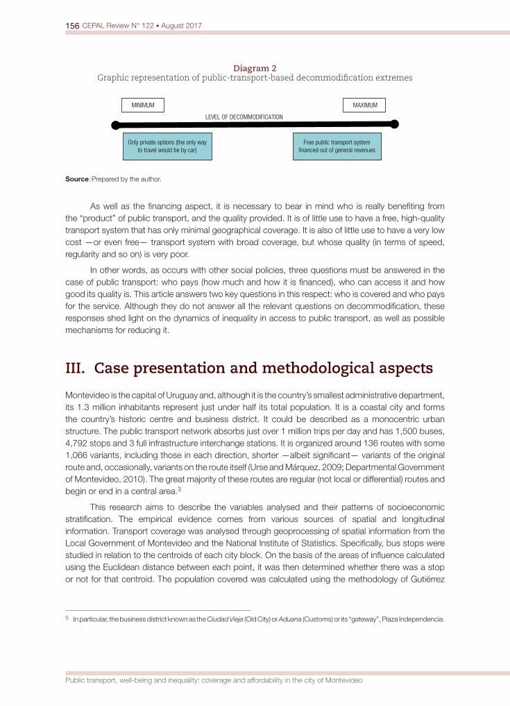
156 CEPAL Review N° 122 • August 2017
Public transport, well-being and inequality: coverage and affordability in the city of Montevideo
Diagram 2 Graphic representation of public-transport-based decommodification extremes
MAXIMUMMINIMUM
LEVEL OF DECOMMODIFICATION
Only private options (the only way to travel would be by car)
Free public transport system financed out of general revenues
Source: Prepared by the author.
As well as the financing aspect, it is necessary to bear in mind who is really benefiting from the “product” of public transport, and the quality provided. It is of little use to have a free, high-quality transport system that has only minimal geographical coverage. It is also of little use to have a very low cost —or even free— transport system with broad coverage, but whose quality (in terms of speed, regularity and so on) is very poor.
In other words, as occurs with other social policies, three questions must be answered in the case of public transport: who pays (how much and how it is financed), who can access it and how good its quality is. This article answers two key questions in this respect: who is covered and who pays for the service. Although they do not answer all the relevant questions on decommodification, these responses shed light on the dynamics of inequality in access to public transport, as well as possible mechanisms for reducing it.
III. Case presentation and methodological aspects
Montevideo is the capital of Uruguay and, although it is the country’s smallest administrative department, its 1.3 million inhabitants represent just under half its total population. It is a coastal city and forms the country’s historic centre and business district. It could be described as a monocentric urban structure. The public transport network absorbs just over 1 million trips per day and has 1,500 buses, 4,792 stops and 3 full infrastructure interchange stations. It is organized around 136 routes with some 1,066 variants, including those in each direction, shorter —albeit significant— variants of the original route and, occasionally, variants on the route itself (Urse and Márquez, 2009; Departmental Government of Montevideo, 2010). The great majority of these routes are regular (not local or differential) routes and begin or end in a central area.3
This research aims to describe the variables analysed and their patterns of socioeconomic stratification. The empirical evidence comes from various sources of spatial and longitudinal information. Transport coverage was analysed through geoprocessing of spatial information from the Local Government of Montevideo and the National Institute of Statistics. Specifically, bus stops were studied in relation to the centroids of each city block. On the basis of the areas of influence calculated using the Euclidean distance between each point, it was then determined whether there was a stop or not for that centroid. The population covered was calculated using the methodology of Gutiérrez
3 In particular, the business district known as the Ciudad Vieja (Old City) or Aduana (Customs) or its “gateway”, Plaza Independencia.

157CEPAL Review N° 122 • August 2017
Diego Hernández
and García (2005), which consists of calculating the proportion of the area covered by the area of influence and applying that to the number of people living in it, assuming that they are covered by that area of influence. For example, if 100 people live in a given census area and the buffer drawn outwards from the bus stop covers 50% of that territory, it is assumed that 50 people are covered by that area of influence. In this case, if the area covered reaches 90%, it will be assumed that all the people in that area are covered. The data on theoretical frequency of the bus service come from information published on the website of the Local Government of Montevideo.
Data on affordability and expenditure on transport were derived from the National Survey of Household Expenditure and Income of the National Statistical Institute. Most of the information came from expenditure on urban transport, which excludes transport for leisure and other purposes (for example, pleasure travel abroad).
Socioeconomic level comes from the division of Montevideo households by income quintile. For the spatial calculations, the levels are the proportion of households in the two poorest income quintiles, which is calculated on the basis of the census segment (approximately six city blocks) and imputed to every block in the segment.
IV. Results
1. Coverage of the public transport network
The network shows considerable density across the city as a whole, leaving few stretches of populated territory uncovered. Generally speaking, the coverage can be said to have developed relatively successfully in relation to demand. The great majority of the most densely populated areas are crossed by a public transport route. Many of the areas that at first sight do not appear to have service belong to the city’s rural areas, which have a very low density. This is a very dense network that appears to reach all areas of the city with potential demand, some with a larger number of services, some with fewer. In this regard, Montevideo can be said to be a city with high public transport connectivity.
It is notable that observation of the areas of influence built around the bus stops within the system shows that the centre and seafront appear uniformly marked by the indicator of 300 m. from a bus stop. There are only a very few interruptions to this pattern, with small portions of the territory in which the distance to a bus stop is between 300 and 500 m. (see map 1). In the other districts of the department, the situation is more uneven, with some areas more than 500 m. or even 750 m. from a stop. On the periphery, the areas of influence are still quite continuous, with the exception of the eastern area. On the suburban periphery, the areas of influence begin to “follow” the rationale of the routes entering in radial form, with much less transversal rationale visible.
As shown in table 1, the number of people without a bus stop within 750 m. is marginal in proportional terms. Looking at the percentage of the city territory at that distance, it is readily discernible that areas with major obstacles to basic access have very low population density. This is a sign of the system’s effectiveness in following demand, and its capacity to avoid extending into areas with low potential demand.
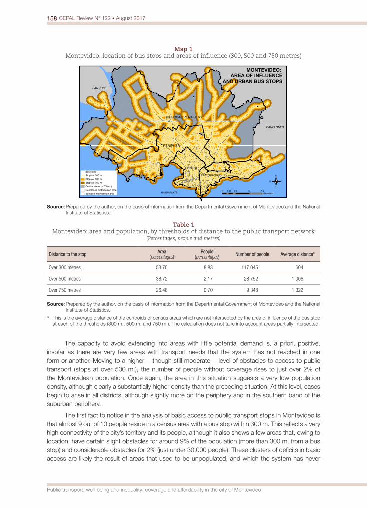
158 CEPAL Review N° 122 • August 2017
Public transport, well-being and inequality: coverage and affordability in the city of Montevideo
Map 1 Montevideo: location of bus stops and areas of influence (300, 500 and 750 metres)
MONTEVIDEO:
0 2,5 5 7,51,25Kilometers
SAN JOSÉ
CANELONES
N
S
W E
AREA OF INFLUENCE AND URBAN BUS STOPS
SUBURBAN PERIPHERY
PERIPHERY
CENTRE
EASTERN COASTBus stopsStops at 300 m.Stops at 500 m.Stops at 750 m.Central areas (+ 750 m.)Canelones metropolitan areaSan josé metropolitan area RIVER PLATE
Source: Prepared by the author, on the basis of information from the Departmental Government of Montevideo and the National Institute of Statistics.
Table 1 Montevideo: area and population, by thresholds of distance to the public transport network
(Percentages, people and metres)
Distance to the stop Area (percentages)
People(percentages) Number of people Average distancea
Over 300 metres 53.70 8.83 117 045 604
Over 500 metres 38.72 2.17 28 752 1 006
Over 750 metres 26.48 0.70 9 348 1 322
Source: Prepared by the author, on the basis of information from the Departmental Government of Montevideo and the National Institute of Statistics.
a This is the average distance of the centroids of census areas which are not intersected by the area of influence of the bus stop at each of the thresholds (300 m., 500 m. and 750 m.). The calculation does not take into account areas partially intersected.
The capacity to avoid extending into areas with little potential demand is, a priori, positive, insofar as there are very few areas with transport needs that the system has not reached in one form or another. Moving to a higher —though still moderate— level of obstacles to access to public transport (stops at over 500 m.), the number of people without coverage rises to just over 2% of the Montevidean population. Once again, the area in this situation suggests a very low population density, although clearly a substantially higher density than the preceding situation. At this level, cases begin to arise in all districts, although slightly more on the periphery and in the southern band of the suburban periphery.
The first fact to notice in the analysis of basic access to public transport stops in Montevideo is that almost 9 out of 10 people reside in a census area with a bus stop within 300 m. This reflects a very high connectivity of the city’s territory and its people, although it also shows a few areas that, owing to location, have certain slight obstacles for around 9% of the population (more than 300 m. from a bus stop) and considerable obstacles for 2% (just under 30,000 people). These clusters of deficits in basic access are likely the result of areas that used to be unpopulated, and which the system has never
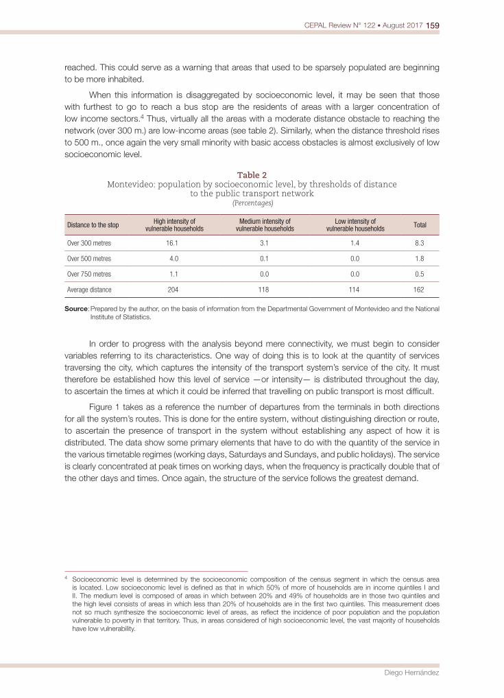
159CEPAL Review N° 122 • August 2017
Diego Hernández
reached. This could serve as a warning that areas that used to be sparsely populated are beginning to be more inhabited.
When this information is disaggregated by socioeconomic level, it may be seen that those with furthest to go to reach a bus stop are the residents of areas with a larger concentration of low income sectors.4 Thus, virtually all the areas with a moderate distance obstacle to reaching the network (over 300 m.) are low-income areas (see table 2). Similarly, when the distance threshold rises to 500 m., once again the very small minority with basic access obstacles is almost exclusively of low socioeconomic level.
Table 2 Montevideo: population by socioeconomic level, by thresholds of distance
to the public transport network (Percentages)
Distance to the stop High intensity of vulnerable households
Medium intensity of vulnerable households
Low intensity of vulnerable households Total
Over 300 metres 16.1 3.1 1.4 8.3
Over 500 metres 4.0 0.1 0.0 1.8
Over 750 metres 1.1 0.0 0.0 0.5
Average distance 204 118 114 162
Source: Prepared by the author, on the basis of information from the Departmental Government of Montevideo and the National Institute of Statistics.
In order to progress with the analysis beyond mere connectivity, we must begin to consider variables referring to its characteristics. One way of doing this is to look at the quantity of services traversing the city, which captures the intensity of the transport system’s service of the city. It must therefore be established how this level of service —or intensity— is distributed throughout the day, to ascertain the times at which it could be inferred that travelling on public transport is most difficult.
Figure 1 takes as a reference the number of departures from the terminals in both directions for all the system’s routes. This is done for the entire system, without distinguishing direction or route, to ascertain the presence of transport in the system without establishing any aspect of how it is distributed. The data show some primary elements that have to do with the quantity of the service in the various timetable regimes (working days, Saturdays and Sundays, and public holidays). The service is clearly concentrated at peak times on working days, when the frequency is practically double that of the other days and times. Once again, the structure of the service follows the greatest demand.
4 Socioeconomic level is determined by the socioeconomic composition of the census segment in which the census area is located. Low socioeconomic level is defined as that in which 50% of more of households are in income quintiles I and II. The medium level is composed of areas in which between 20% and 49% of households are in those two quintiles and the high level consists of areas in which less than 20% of households are in the first two quintiles. This measurement does not so much synthesize the socioeconomic level of areas, as reflect the incidence of poor population and the population vulnerable to poverty in that territory. Thus, in areas considered of high socioeconomic level, the vast majority of households have low vulnerability.
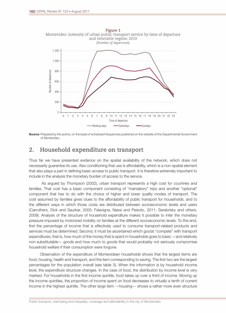
160 CEPAL Review N° 122 • August 2017
Public transport, well-being and inequality: coverage and affordability in the city of Montevideo
Figure 1 Montevideo: intensity of urban public transport service by time of departure
and timetable regime, 2010 (Number of departures)
0
200
400
600
800
1 000
1 200
0 1 2 3 4 5 6 7 8 9 10 11 12 13 14 15 16 17 18 19 20 21 22 23
Num
ber o
f dep
artu
res
Time of departure
Working days Saturdays Sundays
Source: Prepared by the author, on the basis of scheduled frequencies published on the website of the Departmental Government of Montevideo.
2. Household expenditure on transport
Thus far we have presented evidence on the spatial availability of the network, which does not necessarily guarantee its use. Also conditioning that use is affordability, which is a non-spatial element that also plays a part in defining basic access to public transport. It is therefore extremely important to include in the analysis the monetary burden of access to the service.
As argued by Thompson (2002), urban transport represents a high cost for countries and families. That cost has a basic component consisting of “mandatory” trips and another “optional” component that has to do with the choice of higher and lower quality modes of transport. The cost assumed by families gives clues to the affordability of public transport for households, and to the different ways in which those costs are distributed between socioeconomic levels and users (Carruthers, Dick and Saurkar, 2005; Falavigna, Nassi and Peixoto, 2011; Serebrisky and others, 2009). Analysis of the structure of household expenditure makes it possible to infer the monetary pressure imposed by motorized mobility on families at the different socioeconomic levels. To this end, first the percentage of income that is effectively used to consume transport-related products and services must be determined. Second, it must be ascertained which goods “compete” with transport expenditures, that is, how much of the money that is spent in households goes to basic —and relatively non-substitutable— goods and how much to goods that would probably not seriously compromise household welfare if their consumption were forgone.
Observation of the expenditure of Montevidean households shows that the largest items are food, housing, health and transport, and the item corresponding to saving. The first two are the largest percentages for the population overall (see table 3). When the information is by household income level, the expenditure structure changes. In the case of food, the distribution by income level is very marked. For households in the first income quintile, food takes up over a third of income. Moving up the income quintiles, the proportion of income spent on food decreases to virtually a tenth of current income in the highest quintile. The other large item —housing— shows a rather more even structure
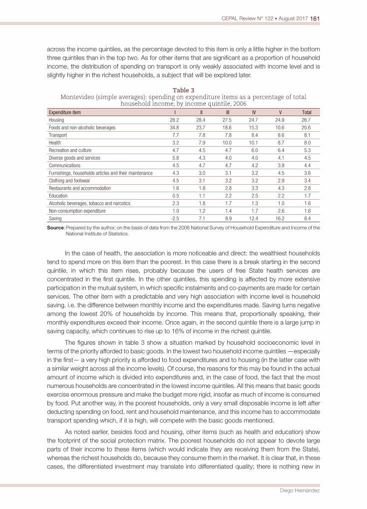
161CEPAL Review N° 122 • August 2017
Diego Hernández
across the income quintiles, as the percentage devoted to this item is only a little higher in the bottom three quintiles than in the top two. As for other items that are significant as a proportion of household income, the distribution of spending on transport is only weakly associated with income level and is slightly higher in the richest households, a subject that will be explored later.
Table 3 Montevideo (simple averages): spending on expenditure items as a percentage of total
household income, by income quintile, 2006Expenditure item I II III IV V TotalHousing 28.2 28.4 27.5 24.7 24.9 26.7
Foods and non-alcoholic beverages 34.8 23.7 18.6 15.3 10.6 20.6
Transport 7.7 7.8 7.8 8.4 8.6 8.1
Health 3.2 7.9 10.0 10.1 8.7 8.0
Recreation and culture 4.7 4.5 4.7 6.0 6.4 5.3
Diverse goods and services 5.8 4.3 4.0 4.0 4.1 4.5
Communications 4.5 4.7 4.7 4.2 3.9 4.4
Furnishings, households articles and their maintenance 4.3 3.0 3.1 3.2 4.5 3.6
Clothing and footwear 4.5 3.1 3.2 3.2 2.9 3.4
Restaurants and accommodation 1.6 1.8 2.8 3.3 4.3 2.8
Education 0.5 1.1 2.2 2.5 2.2 1.7
Alcoholic beverages, tobacco and narcotics 2.3 1.8 1.7 1.3 1.0 1.6
Non-consumption expenditure 1.0 1.2 1.4 1.7 2.6 1.6
Saving -2.5 7.1 8.9 12.4 16.2 8.4
Source: Prepared by the author, on the basis of data from the 2006 National Survey of Household Expenditure and Income of the National Institute of Statistics.
In the case of health, the association is more noticeable and direct: the wealthiest households tend to spend more on this item than the poorest. In this case there is a break starting in the second quintile, in which this item rises, probably because the users of free State health services are concentrated in the first quintile. In the other quintiles, this spending is affected by more extensive participation in the mutual system, in which specific instalments and co-payments are made for certain services. The other item with a predictable and very high association with income level is household saving, i.e. the difference between monthly income and the expenditures made. Saving turns negative among the lowest 20% of households by income. This means that, proportionally speaking, their monthly expenditures exceed their income. Once again, in the second quintile there is a large jump in saving capacity, which continues to rise up to 16% of income in the richest quintile.
The figures shown in table 3 show a situation marked by household socioeconomic level in terms of the priority afforded to basic goods. In the lowest two household income quintiles —especially in the first— a very high priority is afforded to food expenditures and to housing (in the latter case with a similar weight across all the income levels). Of course, the reasons for this may be found in the actual amount of income which is divided into expenditures and, in the case of food, the fact that the most numerous households are concentrated in the lowest income quintiles. All this means that basic goods exercise enormous pressure and make the budget more rigid, insofar as much of income is consumed by food. Put another way, in the poorest households, only a very small disposable income is left after deducting spending on food, rent and household maintenance, and this income has to accommodate transport spending which, if it is high, will compete with the basic goods mentioned.
As noted earlier, besides food and housing, other items (such as health and education) show the footprint of the social protection matrix. The poorest households do not appear to devote large parts of their income to these items (which would indicate they are receiving them from the State), whereas the richest households do, because they consume them in the market. It is clear that, in these cases, the differentiated investment may translate into differentiated quality; there is nothing new in
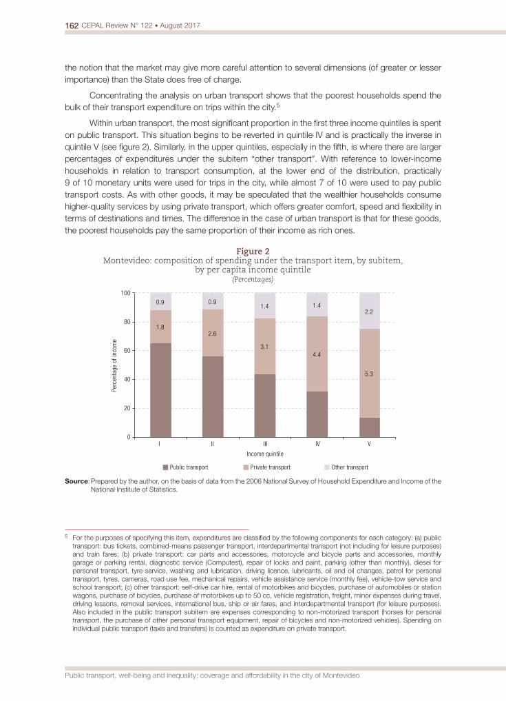
162 CEPAL Review N° 122 • August 2017
Public transport, well-being and inequality: coverage and affordability in the city of Montevideo
the notion that the market may give more careful attention to several dimensions (of greater or lesser importance) than the State does free of charge.
Concentrating the analysis on urban transport shows that the poorest households spend the bulk of their transport expenditure on trips within the city.5
Within urban transport, the most significant proportion in the first three income quintiles is spent on public transport. This situation begins to be reverted in quintile IV and is practically the inverse in quintile V (see figure 2). Similarly, in the upper quintiles, especially in the fifth, is where there are larger percentages of expenditures under the subitem “other transport”. With reference to lower-income households in relation to transport consumption, at the lower end of the distribution, practically 9 of 10 monetary units were used for trips in the city, while almost 7 of 10 were used to pay public transport costs. As with other goods, it may be speculated that the wealthier households consume higher-quality services by using private transport, which offers greater comfort, speed and flexibility in terms of destinations and times. The difference in the case of urban transport is that for these goods, the poorest households pay the same proportion of their income as rich ones.
Figure 2 Montevideo: composition of spending under the transport item, by subitem,
by per capita income quintile(Percentages)
1.8 2.6
3.1 4.4
5.3
0.9 0.9 1.4 1.4
2.2
0
20
40
60
80
100
I II III IV V
Perc
enta
ge o
f inc
ome
Income quintile
Public transport Private transport Other transport
Source: Prepared by the author, on the basis of data from the 2006 National Survey of Household Expenditure and Income of the National Institute of Statistics.
5 For the purposes of specifying this item, expenditures are classified by the following components for each category: (a) public transport: bus tickets, combined-means passenger transport, interdepartmental transport (not including for leisure purposes) and train fares; (b) private transport: car parts and accessories, motorcycle and bicycle parts and accessories, monthly garage or parking rental, diagnostic service (Computest), repair of locks and paint, parking (other than monthly), diesel for personal transport, tyre service, washing and lubrication, driving licence, lubricants, oil and oil changes, petrol for personal transport, tyres, cameras, road use fee, mechanical repairs, vehicle assistance service (monthly fee), vehicle-tow service and school transport; (c) other transport: self-drive car hire, rental of motorbikes and bicycles, purchase of automobiles or station wagons, purchase of bicycles, purchase of motorbikes up to 50 cc, vehicle registration, freight, minor expenses during travel, driving lessons, removal services, international bus, ship or air fares, and interdepartmental transport (for leisure purposes). Also included in the public transport subitem are expenses corresponding to non-motorized transport (horses for personal transport, the purchase of other personal transport equipment, repair of bicycles and non-motorized vehicles). Spending on individual public transport (taxis and transfers) is counted as expenditure on private transport.
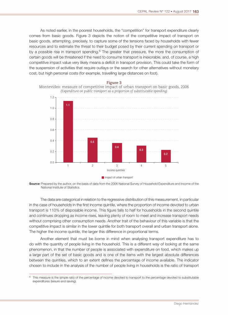
163CEPAL Review N° 122 • August 2017
Diego Hernández
As noted earlier, in the poorest households, the “competition” for transport expenditure clearly comes from basic goods. Figure 3 depicts the notion of the competitive impact of transport on basic goods, attempting, precisely, to capture some of the tensions faced by households with fewer resources and to estimate the threat to their budget posed by their current spending on transport or by a possible rise in transport spending.6 The greater that pressure, the more the consumption of certain goods will be threatened if the need to consume transport is inexorable, and, of course, a high competitive impact value very likely means a deficit in transport provision. This could take the form of the suspension of activities that require outlays or the search for other alternatives without monetary cost, but high personal costs (for example, travelling large distances on foot).
Figure 3 Montevideo: measure of competitive impact of urban transport on basic goods, 2006
(Expenditure on public transport as a proportion of substitutable spending)
1.1
0.5
0.4 0.3
0.2
0.0
0.2
0.4
0.6
0.8
1.0
1.2
1 2 3 4 5
Income quintiles
Impact of urban transport
Source: Prepared by the author, on the basis of data from the 2006 National Survey of Household Expenditure and Income of the National Institute of Statistics.
The data are categorical in relation to the regressive distribution of this measurement, in particular in the case of households in the first income quintile, where the proportion of income devoted to urban transport is 110% of disposable income. This figure falls to half for households in the second quintile and continues dropping as income rises, leaving plenty of room to meet and increase transport needs without comprising other consumption needs. Another trait of the behaviour of this variable is that the competitive impact is similar in the lower quintile for both transport overall and urban transport alone. The higher the income quintile, the larger this difference in proportional terms.
Another element that must be borne in mind when analysing transport expenditure has to do with the quantity of people living in the household. This is a different way of looking at the same phenomenon, in that the number of people is associated with expenditure on food, which makes up a large part of the set of basic goods and is one of the items with the largest absolute differences between the quintiles, which to an extent defines the percentage of income available. The indicator chosen to include in the analysis of the number of people living in households is the ratio of transport
6 This measure is the simple ratio of the percentage of income devoted to transport to the percentage devoted to substitutable expenditures (leisure and saving).
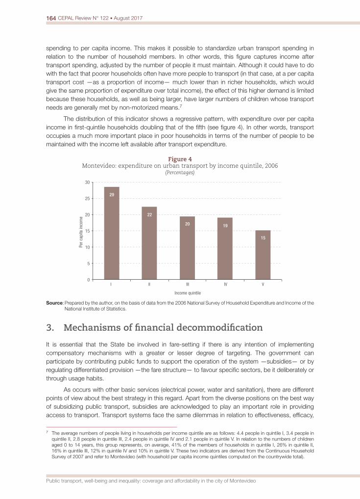
164 CEPAL Review N° 122 • August 2017
Public transport, well-being and inequality: coverage and affordability in the city of Montevideo
spending to per capita income. This makes it possible to standardize urban transport spending in relation to the number of household members. In other words, this figure captures income after transport spending, adjusted by the number of people it must maintain. Although it could have to do with the fact that poorer households often have more people to transport (in that case, at a per capita transport cost —as a proportion of income— much lower than in richer households, which would give the same proportion of expenditure over total income), the effect of this higher demand is limited because these households, as well as being larger, have larger numbers of children whose transport needs are generally met by non-motorized means.7
The distribution of this indicator shows a regressive pattern, with expenditure over per capita income in first-quintile households doubling that of the fifth (see figure 4). In other words, transport occupies a much more important place in poor households in terms of the number of people to be maintained with the income left available after transport expenditure.
Figure 4 Montevideo: expenditure on urban transport by income quintile, 2006
(Percentages)
29
22
20 19
15
0
5
10
15
20
25
30
I II III IV V
Per
capi
ta in
com
e
Income quintile
Source: Prepared by the author, on the basis of data from the 2006 National Survey of Household Expenditure and Income of the National Institute of Statistics.
3. Mechanisms of financial decommodification
It is essential that the State be involved in fare-setting if there is any intention of implementing compensatory mechanisms with a greater or lesser degree of targeting. The government can participate by contributing public funds to support the operation of the system —subsidies— or by regulating differentiated provision —the fare structure— to favour specific sectors, be it deliberately or through usage habits.
As occurs with other basic services (electrical power, water and sanitation), there are different points of view about the best strategy in this regard. Apart from the diverse positions on the best way of subsidizing public transport, subsidies are acknowledged to play an important role in providing access to transport. Transport systems face the same dilemmas in relation to effectiveness, efficacy,
7 The average numbers of people living in households per income quintile are as follows: 4.4 people in quintile I, 3.4 people in quintile II, 2.8 people in quintile III, 2.4 people in quintile IV and 2.1 people in quintile V. In relation to the numbers of children aged 0 to 14 years, this group represents, on average, 41% of the members of households in quintile I, 26% in quintile II, 16% in quintile III, 12% in quintile IV and 10% in quintile V. These two indicators are derived from the Continuous Household Survey of 2007 and refer to Montevideo (with household per capita income quintiles computed on the countrywide total).
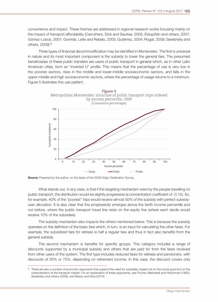
165CEPAL Review N° 122 • August 2017
Diego Hernández
convenience and impact. These themes are addressed in regional research works focusing mainly on the impact of transport affordability (Carruthers, Dick and Saurkar, 2005; Estupiñán and others, 2007; Gómez-Lobos, 2007; Gomide, Leite and Rebelo, 2005; Gutiérrez, 2004; Rogat, 2009; Serebrisky and others, 2009).8
Three types of financial decommodification may be identified in Montevideo. The first is universal in nature and its most important component is the subsidy to lower the general fare. The presumed beneficiaries of these public transfers are users of public transport in general which, as in other Latin American cities, form an “inverted U” profile. This means that the percentage of use is very low in the poorest sectors, rises in the middle and lower-middle socioeconomic sectors, and falls in the upper-middle and high socioeconomic sectors, where the percentage of usage returns to a minimum. Figure 5 illustrates this use pattern.
Figure 5 Metropolitan Montevideo: structure of public transport trips ordered
by income percentile, 2009 (Cumulative percentages)
0
20
40
60
80
100
0 10 20 30 40 50 60 70 80 90 100
Cum
ulat
ive
inve
stm
ent
Income percentile
Equity Public Private
Source: Prepared by the author, on the basis of the 2009 Origin-Destination Survey.
What stands out, in any case, is that if the targeting mechanism were by the people travelling on public transport, the distribution would be slightly progressive (a concentration coefficient of -0.10). So, for example, 40% of the “poorest” trips would receive almost 50% of the subsidy with perfect subsidy-user allocation. It is also clear that the progressivity emerges above the tenth income percentile and not before, where the public transport travel line rests on the equity line (where each decile would receive 10% of the subsidies).
The subsidy mechanism also impacts the others mentioned below. This is because the subsidy operates on the definition of the basic fare which, in turn, is an input for calculating the other fares. For example, the subsidized fare for retirees is half a regular fare and thus in fact also benefits from the general subsidy.
The second mechanism is benefits for specific groups. This category includes a range of discounts supported by a municipal subsidy and others that are paid for from the fares received from other users of the system. The first type includes reduced fares for retirees and pensioners, with discounts of 50% or 75%, depending on retirement income. In this case, the discount covers only
8 There are also a number of economic arguments that support the need for subsidies, based not on the social good but on the characteristics of the transport market. For an explanation of these arguments, see Pucher, Markstedt and Hirschman (1983), Serebrisky and others (2009), and Basso and Silva (2014).

166 CEPAL Review N° 122 • August 2017
Public transport, well-being and inequality: coverage and affordability in the city of Montevideo
those in receipt of a pension or retirement benefit. There are also differentiated fares for students in secondary and tertiary education, consisting of a discount ranging from 50% to 100%, depending on the level of education and the age of the beneficiary.
The total discounts arising from crossed subsidies include free transport for primary school pupils and, on Sundays, for those aged over 70 or under 12. Free transport for schoolchildren has been traditional in Montevidean public transport, and free travel for children and older persons for leisure purposes was instituted after 1990.
Mechanisms based on social groups are affected by self-selection. In the case of students this is obvious: children or young people who are not in the education system are concentrated in the poorest sectors. It is also true that a high proportion of students, especially in primary and lower-secondary school, walk to and from educational establishments. The discount for retirees and pensioners can suffer a similar effect in relation to certain minimum formal requirements —a carnet must be obtained from a social security institute— which can exclude the poorest sectors.
Lastly, the third type of mechanism identified is spatial and time-based, through the diversification of the fares offered to passengers. By purchasing tickets under one of these modalities, passengers can make a trip —or several legs of the same trip— more cheaply than if they bought equivalent tickets at the regular price. This mechanism may be interpreted in two dimensions: time and space. There are two differentiated flat-fare and semi-flat-fare products defined in terms of time: the “2-hour” ticket, which allows the passenger to use the system freely for two hours for the price of roughly 1.4 regular tickets, and the “1-hour” ticket, which allows passengers to take two trips on public transport for the cost of the regular fare.9 So, strictly speaking, the regular fare (known as the “common ticket”) is actually a semi-flat 1-hour fare. This fare structure favours those who, first, use these fares and, second, make most use of the possibilities in relation to the trips taken. Accordingly, those who make two trips on a single ticket are financed by those who make just one. Something similar occurs with those who make several trips on a 2-hour ticket. There is thus a cross-subsidy between those using the 2-hour ticket and those who are not, as there is also between passengers who make more intensive use of the system and those who use it less intensively.10
In the spatial dimension, there are zonal or local routes, which have a 50% discount on the regular fare. These routes include local services, short routes, some circular routes, those that travel to areas not served by the regular network or connect distant points with exchange points in the system. They also include some portions of regular routes which issues zone fares after a certain points. The latest modality incorporated into the system is a peripheral ring which was classified as zonal: all trips beginning and ending within the ring can be taken at the zone fare. This type of fare is particularly progressive because most of the local services are located in peripheral areas where low-income sectors are concentrated. In particular, the zone ticket for the third ring recently mentioned is highly progressively self-selective.
Table 4 summarizes the three mechanisms analysed and each of their components.11
9 This fare allows a third trip when some of the legs are boarded at certain points of the system (generally, terminals or changeover stops).
10 There is a revenue-sharing scheme at the level of the operators, whereby income is divided in equal parts for each leg used and each company receives the equivalent to the number of legs that the passenger used in the system.
11 It bears mentioning that the transport system has other mechanisms that are not included here because their effect is marginal in terms of impact on the purchase of trips or on beneficiaries. These are: the institutional ticket, which gives a discount on the fare for packets of tickets purchased by employees of firms that have an agreement with the Departmental Government of Montevideo, and free transport for some persons with disabilities.

167CEPAL Review N° 122 • August 2017
Diego Hernández
Table 4 Montevideo: compensatory mechanisms in public transport
Type of mechanism Mechanism Description (benefits, targeting, financing)
Universal Subsidy on the regular fare (fare subsidy and transport fund)
Fare stabilization and specific discount (impact of approximately 10%).a Financing from national and departmental government, coordinated by the latter. Targeted on users of public transport and moderately progressive. Sets the base fare for the other mechanisms.
By social group(age and activity)
Primary school pupils Free transport. Cross-financing.
Secondary school pupils
Public system: 50 free tickets during the basic cycle of secondary education (up to age 18) and in the second cycle (up to age 20). Pupils outside the age limit and those in private establishments are entitled to a discount of 50%. National financing for free tickets and municipal financing for discounted tickets. Self-selection effect (attendance at an educational establishment).
Tertiary education studentsPublic system only: discount of 50% (up to age 30) or 25% (over age 30). Regressive self-selection effect. National and municipal financing (in the case of the 25%, the discount is municipally funded).
Tickets for retirees and pensioners Discount of 50% or 70%, depending on income. Municipal financing. Possible effect of exclusion of most vulnerable sectors owing to formal requirements.
Spatial and time-based
Local and zonal offers (local routes, some legs of regular routes, trips within the third ring)
50% of the fare. Cross-financing. Strong concentration in sectors residing in peripheral areas. Spatial self-selection with a progressive effect.
Offer of flat and semi-flat rate, time-based (1-hour and 2-hour tickets)
Second leg at regular rate and unlimited trips within a 2-hour period, at approximately 1.4 times the regular fare. Cross-financing with revenue-sharing between operators. Favours sectors furthest from the centre and implies a lower fare for necessary changes.
Source: Prepared by the author, on the basis of information from the Local Government of Montevideo. The table was formulated using information from around 2012.
a According to consultations with technical staff of the Local Government of Montevideo.
V. Final remarks
The evidence indicates that the public transport network in Montevideo offers high coverage of the geographical area and of the population. Its behaviour shows a high degree of adaptation to demand or, put another way, a supply that is governed spatially and in terms of timetables by the real observed demand. So, in spatial terms, the network is concentrated in sectors with the highest population density and need for travel, while in lower density sectors it tends to form a radial pattern (with relatively unbranched axes leaving broad spaces in between without coverage), although almost a third of the population resides in that broader territory that is the suburban periphery. The time dimension behaves in an identical manner: the peak times and regimes —daytime, working day— have almost double the services of off-peak times (weekends and non-peak-hour). Although marginal in the overall picture, recent processes of peripheral urban expansion mean that the profile of areas with the worst coverage is almost exclusively one of high vulnerability.
This said, the main weakness in terms of stratification occurs in relation to affordability. Household expenditure shows a regressive distribution with respect to access to transport, similarly to the situation in other cities (Falavigna, Nassi and Peixoto, 2011; UNDP, 2008; Thompson, 2002). Households in the lower income quintiles spend a larger proportion of their income on transport, chiefly the consumption of public transport, than higher-income households do. The differences are also more significant in terms of the “competition” with basic goods or the number of people living in these households. In this context, the structure of consumption shows that spending on transport cannot be disregarded, since it puts tension on the ability to obtain other basic goods. In turn, this impacts the quality and quantity of transport consumed, since it becomes an item that can be cut or, where it is indispensable, these cuts can be made in spending on basic goods instead.
If the analysis were in relation to the health system, we would study “out-of-pocket” expenses: the amount of money that households must disburse to access health care. In this field, better-off sectors tend to opt for private, better-quality health care, which is reflected in a higher proportion of
168 CEPAL Review N° 122 • August 2017
Public transport, well-being and inequality: coverage and affordability in the city of Montevideo
spending in relation to income. This does not happen in the case of transport. Although middle and upper sectors also have access to better-quality options —and likely make more trips to different destinations within the city—, proportionally speaking, they use less of their income than other households (or the same amount). This occurs despite efforts by the authorities —quite significant efforts compared with the rest of the region— to keep fares down and maximize affordability.
The research results encourage the adoption of a regional approach to analysing accessibility and public transport policies. First, because transport affordability is a pending issue in the region, and points to the risk of increasing precariousness in low-income sectors, either because they cannot move about the city or because they must do so in inadequate conditions when they cannot afford the service. Second, because, unlike in Montevideo, in several Latin American cities even basic coverage is still an unresolved problem (see, for example, CAF, 2009; Bocarejo and Oviedo, 2012; Vasconcellos, 2012). Third, because the question of quality is central throughout the region. This article has not addressed the quality of transport in Montevideo, but for the future agenda it is essential to ask what level of service and what frequency and regularity would constitute a highly accessible system. This is a key question when analysing the degree of decommodification.
BibliographyBasso, L. and H.S. Silva (2014), “Efficiency and substitutability of transit subsidies and other urban transport
policies”, American Economic Journal: Economic Policy, vol. 6, No. 4, Nashville, Tennessee, American Economic Association.
Bocarejo, J.P. and D.R. Oviedo (2012), “Transport accessibility and social inequities: a tool for identification of mobility needs and evaluation of transport investments”, Journal of Transport Geography, vol. 24, Amsterdam, Elsevier.
CAF (Andean Development Corporation) (2009), Observatorio de Movilidad Urbana para America Latina. Información para mejores políticas y mejores ciudades, Caracas.
Carruthers, R., M. Dick and A. Saurkar (2005), “Affordability of public transport in developing countries”, Transport Papers, No. 3, Washington, D.C., World Bank.
Cass, N., E. Shove and J. Urry (2005), “Social exclusion, mobility and access”, The Sociological Review, vol. 53, No. 3, Wiley.
Church, A., M. Frost and K. Sullivan (2000), “Transport and social exclusion in London”, Transport Policy, vol. 7, No. 3, Amsterdam, Elsevier.
Departmental Government of Montevideo (2010), Plan Montevideo. Memoria de Ordenación, Montevideo.Esping-Andersen, G. (1990), The Three Worlds of Welfare Capitalism, Princeton, Princeton University Press.Estupiñán, N. and others (2007), “Affordability and subsidies in public urban transport: what do we mean,
what can be done?”, Policy Research Working Paper, No. 4440, Washington, D.C., World Bank.Falavigna, C., C.D. Nassi and M. Peixoto (2011), “As despesas em transporte e seu impacto no orcamento
familiar: um indicador para considerar equidade no planejamento de transportes”, paper presented at the XXIV Congresso de Pesquisa e Ensino em Transportes, Salvador de Bahia.
Flamm, M., C. Jemelin and V. Kaufmann (2008), Travel Behaviour Adaptation Processes during Life Course Transitions. A Methodological and Empirical Study using a Person-based GPS Tracking System, Laboratoire de Sociologie Urbaine (LASUR).
Gómez-Lobo, A. (2007), “Affordability of public transport: a methodological clarification”, Documentos de Trabajo, No. 261, Santiago, University of Chile.
Gomide, A., S. Leite and J. Rebelo (2005), “Public transport and urban poverty: a synthetic index of adequate service”, Working Paper, No. 33901, Washington, D.C., World Bank.
Gutiérrez, A. (2004), “Concentración empresaria y eficiencia en el autotransporte urbano de Buenos Aires”, EURE. Revista Latinoamericana de Estudios Urbano Regionales, vol. 30, No. 91, Santiago, Pontificia Universidad Católica de Chile.
Gutiérrez, J. and J.C. García (2005), “Sobreestimaciones del cálculo de distancias en línea recta con respecto al de distancias viarias en el análisis de cobertura de las redes de transporte público”, Madrid, Complutense University of Madrid.

169CEPAL Review N° 122 • August 2017
Diego Hernández
Hernández, D. (2012), “Activos y estructuras de oportunidades de movilidad. Una propuesta analítica para el estudio de la accesibilidad por transporte público, el bienestar y la equidad”, EURE. Revista Latinoamericana de Estudios Urbano Regionales, vol. 38, No. 115, Santiago, Pontificia Universidad Católica de Chile.
Kaufmann, V. (2002), Re-thinking Mobility. Contemporary Sociology, Aldershot, Ashgate.Kaufmann, V., M. Bergman and D. Joye (2004), "Motility: mobility as capital", International Journal of Urban
and Regional Research, vol. 28, No. 4, Wiley.Kaztman, R. (2009), “Territorio y empleo: circuitos de realimentación de las desigualdades en Montevideo”, paper
prepared for the XXVIII International Congress of the Latin American Studies Association, Rio de Janeiro.(1999), Activos y estructuras de oportunidades. Estudios sobre las raíces de la vulnerabilidad social en Uruguay (LC/MVD/R.180/E), Montevideo, United Nations Development Programme (UNDP)/Economic Commission for Latin America and the Caribbean (ECLAC).
Kaztman, R. and F. Filgueira (2006), “Las normas como bien público y como bien privado: reflexiones en las fronteras del enfoque AVEO”, Documentos de Trabajo del IPES – Colección Aportes Conceptuales, No. 4, Montevideo, Catholic University of Uruguay.
Manderscheid, K. (2009), “Unequal mobilities”, Mobilities and Inequality, Surrey, Ashgate.Massot, M.-H. and J.-P. Orfeuil (2005), “La mobilité au quotidien, entre choix individuel et production sociale”,
Cahiers internationaux de sociologie, No. 118.Miralles-Guasch, C. and A. Cebollada (2003), “Movilidad y transporte. Opciones políticas para la ciudad”,
Documentos de Trabajo, No. 25, Barcelona, Laboratorio de Alternativas.Moser, C. (1998), “The asset vulnerability framework: reassessing urban poverty reduction strategies”, World
Development, vol. 26, No. 1, Amsterdam, Elsevier.Ohnmacht, T., H. Maksim and M. Bergman (2009), “Mobilities and inequalities - Making connections”,
Mobilities and Inequality, Surrey, Ashgate.Pucher, J., A. Markstedt and I. Hirschman (1983), “Impacts of subsidies on the costs of urban public transport”,
Journal of Transport Economics and Policy, vol. 17, No. 2.Rogat, J. (2009), Regulación y planificación de buses en America Latina. Resumen orientado a tomadores
de decisiones, UNEP Risø Centre.Serebrisky, T. and others (2009), “Affordability and subsidies in public urban transport: what do we mean,
what can be done?”, Transport Reviews, vol. 29, No. 6, Taylor & Francis.Thompson, I. (2002), “Impacto de las tendencias sociales, económicas y tecnológicas sobre el transporte público:
una investigación preliminar en ciudades de América Latina”, Recursos Naturales e Infraestructura series, No. 41 (LC/L.1717-P), Santiago, Economic Commission for Latin America and the Caribbean (ECLAC).
Titheridge, H. (2006), “Social exclusion and transport policy”, London, University College, unpublished.UNDP (United Nations Development Programme) (2008), “El futuro de la movilidad en Bogotá. Reflexiones
a propósito del Plan Maestro de Movilidad y Estacionamientos”, Cuadernos del Informe de Desarrollo Humano para Bogota, No. 1, Bogota.
Urry, J. (2007), Mobilities, Cambridge, Polity Press.Urse, G. and G. Márquez (2009), “Un modelo de gestión alternativo en el transporte urbano: el caso de
Montevideo”, paper prepared for the Latin American Congress for Public and Urban Transportation (CLATPU), Buenos Aires.
Vasconcellos, E.A. (2012), Transporte urbano y movilidad en los países en desarrollo: reflexiones y propuestas, São Paulo, Instituto Movimiento.
Wenglenski, S. and J.-P. Orfeuil (2006), “The differences in the accessibility to the job market according to the social status and the place of residence in the Paris area”, unpublished.


Sectoral breakdown of total factor productivity in Chile, 1996-20101
Patricio Aroca2 and Nicolás Garrido3
Abstract
This article decomposes total factor productivity (TFP) by economic sector, using data from the Chilean economy’s input-output matrices for 1996, 2003 and 2010. The analysis focuses on the effects of changes in three areas: sectoral demand; the production mix and cross-sectoral transactions; and technological change. It finds that the latter two are the key drivers of productivity variations in the period analysed. Manufacturing industry; electricity, gas and water; and financial intermediation and business services have generated increases in the economy’s overall productivity, while the personal services sector may be acting as a constraint on growth. The article qualifies and contextualizes these conclusions.
KeywordsProductivity, measurement, input-output analysis, factor analysis, Chile
JEL classificationO41, O47, C67
AuthorsPatricio Aroca is a tenured professor at the School of Business of Adolfo Ibáñez University, Chile. [email protected]
Nicolás Garrido is associate professor in the Economics Department at Diego Portales University, Chile. [email protected]
1 The authors are grateful for comments made by those attending presentations of preliminary versions of this article at seminars held at the Adolfo Ibáñez University and at the seminars of Núcleo Intelis, Millennium Scientific Initiative.
2 The author is grateful for financing received from the Fund for the Promotion of Scientific and Technological Development, (FONDEF), as part of the project “Measurement of impact and spillovers from regional projects in Chile” (Code CA13I1006).
3 The author is grateful for financing received from the National Fund for Scientific and Technological Development (FONDECYT), as part of the project “Analysis of regional and sectoral productivity and its influence on the aggregate economy” (No. 1140131).

172 CEPAL Review N° 122 • August 2017
Sectoral breakdown of total factor productivity in Chile, 1996-2010
I. Introduction
Two key assertions are made in the studies by Prescott (1998) and Easterly and Levine (2002). In the first, of an empirical nature, the authors argue that total factor productivity (TFP) (Solow, 1957) is the best construct for differentiating growth rates and gross domestic product (GDP) in different countries. In a second, more theoretical, comment, they note the lack of consensus on the concept of TFP, which makes it impossible to define and measure unambiguously. These two claims have spawned numerous debates and much research in academic circles. The present study contributes to those debates by proposing a new, innovative, way of measuring TFP in the Chilean economy, in which input-output tables are used to break the economy-wide TFP down into contributions made by 12 economic sectors.
The study of TFP in Chile spans different periods and focuses on the macro-, meso- and microeconomic levels, depending on the information available. The greater availability of aggregate information allows more research on TFP at the macroeconomic level. Fuentes, Larraín and Schmidt-Hebbel (2006) show that productivity increases accounted for more than 60% of economic growth in periods of high and moderate expansion (1990-1997 and 1998-2005, respectively).4 These authors argue that TFP is related to structural and cyclical components of the economy: whereas structural factors, including macroeconomic stability, played an important role in pre-1990s periods, the situation has been reversed in the last 20 years when TFP fluctuations have mainly been caused by cyclical effects such as the terms of trade (the price of copper) and the devaluation of the real exchange rate. Chumacero and Fuentes (2006) argue that an exogenous growth model is the best way of interpreting economic data in which there is a steady-state TFP trend and temporary increases arising from improvements in capital quality (calculated by comparing the prices of capital goods and consumer goods); an improvement in the terms of trade; and a reduction in distortions in official measurements, such as government spending. The authors note that when such increases are due to current policies, the change may be long-term, while transitory changes give rise to productivity fluctuations.
Progressively, as the productivity gains from macroeconomic stability began to dwindle, research turned to considering microeconomic influences on TFP and how they complement institutional stability. Studies found links between firms and productivity based on the abundant data from the Annual National Industrial Survey (ENIA). Pavcnik (2002) found evidence that trade liberalization had enhanced enterprise productivity. Several hypotheses to explain the transmission channels of these improvements were also formulated, as follows: (i) greater specialization; (ii) the expansion of potential markets, to take advantage of economies of scale; (iii) dissemination of technological innovations and good management practices; and (iv) reduction of anti-competitive practices at the local level. Bergoeing, Hernando and Repetto (2005) note that TFP growth in firms reflected improvements made within them, rather than the factor relocation that might have been induced by a Schumpeterian process of enterprise “death and birth”. The structure of the labour market and its effect on productivity were studied by Álvarez and Fuentes (2009), who argue that the rise in minimum wages may have undermined TFP in recent years, and mainly affected firms with a larger proportion of low-skilled workers.
The meso-economy5 of the country and its relation to productivity are topics that received later attention, specifically in the studies by Álvarez and Fuentes (2004), Vergara and Rivero (2006)
4 This conclusion is reached with the method used by Fuentes, Larraín and Schmidt-Hebbel (2006), whereby the TFP measurement is estimated from a capital stock that is calculated adjusting for energy consumption and employment through the wage rate and hours worked. The results are not very different when the other measures are used.
5 The term “meso-economy” is used to describe entities that are clearly identifiable, such as the economic sectors and regions of a country, but which do not directly represent the microeconomic behavior of buying and selling in markets, nor do they describe aggregate properties of the macroeconomy as a whole.

173CEPAL Review N° 122 • August 2017
Patricio Aroca and Nicolás Garrido
and Fuentes (2011). The latter author shows that there was a structural break in labour productivity towards the end of the 1990s in many sectors (agriculture, fishing and forestry, mining, commerce, restaurants and hotels, and transport and communications); and that this seems to be related to the macroeconomic productivity effect of structural changes and cyclical components (Fuentes, Larraín and Schmidt-Hebbel, 2006). By decomposing the increase in labour productivity into two categories —sectoral and attributable to labour reallocation between sectors— the authors were able to calculate that over 97% of the increase was sectoral and only 3% arose from reallocation. The tradable goods sectors (mining and manufacturing) display a process of capital deepening that drove labour productivity growth, while TFP had a significant impact on labour productivity in the commerce, restaurants and hotels sectors, and in transport and communications. Álvarez and Fuentes (2004) reach a similar conclusion: the expansion of the mining; manufacturing; and agriculture, forestry, and fisheries sectors in the 1990s was a consequence of capital accumulation and TFP, while growth in the non-tradables sector in the same decade was primarily due to capital accumulation alone. Vergara and Rivero (2006) report conclusions that highlight the heterogeneous performance of tradable goods sectors. In two of these (agriculture-forestry-fishing, and the mining sector) TFP growth outpaced capital accumulation in 1996-2001, while just one sector (manufacturing industry) displays the opposite pattern. According to Fuentes (2011), the construction and financial services sectors may have had a very low TFP growth rate,6 while Vergara and Rivero (2006) report that financial services posted the second highest TFP growth in 1986-2001.
This wide diversity of results warrants three comments. First, the technical criteria and data sources used to measure the country’s productivity vary greatly, even though the conceptual basis of measurement remains the decomposition of growth accounting. Second, Harberger’s (1998) hypothesis that productivity increases are mushroom-like, and cost reductions may be due to “1,001 possible causes” in different sectors, with productivity increase adopting many different guises, seems to apply in the Chilean case. Third, the heterogeneity of results also suggests a relationship between microeconomic, meso-economic and macroeconomic productivity, to enable an integrated reading of the different conclusions from a broad perspective.
This article presents two new approaches to the analysis of sectoral TFP in Chile. First, the information provided by the Central Bank is organized into input-output tables for the years 1996, 2003 and 2010 and made compatible with the relevant data of the National Institute of Statistics (INE). Next, the total TFP of the economy is decomposed into sectoral contributions, the effects of demand and the effect of interaction between sectors. Intersectoral productivity is compared using the Solow growth-accounting model while taking account of the remarks made by Baumol and Wolff (1984).
The results of this research make it possible to construct a taxonomy of sectors, according to their capacity to drive the economy and variations in sectoral productivity. In this taxonomy, the leading sectors are manufacturing industry; electricity, gas and water, and financial intermediation and business services, which led TFP growth in 1996-2010. The productivity growth recorded in these sectors spread throughout the productive fabric.
In this context, the personal services sector could be holding back productivity growth in the economy overall, since its productivity declined in the period analysed, and this had a major impact throughout the production system.
Apart from this introduction, the article is organized in three sections. Section II describes the decomposition method used to analyze productivity, while section III explains the origin of the data and analyses the results of the decomposition; and section IV presents the conclusions. The article concludes with an annex giving details of the calculation methods used.
6 This suggestion is tentative because it is based on Fuentes (2011), which concludes that there was a process of capital intensification coupled with virtually zero labour-productivity growth.

174 CEPAL Review N° 122 • August 2017
Sectoral breakdown of total factor productivity in Chile, 1996-2010
II. Decomposition method
Total factor productivity measures output growth that does not reflect an increase in the primary factors of production, namely capital and labour. Many different measurement techniques are used; and there is an abundant literature on the subject, summarized in several compendia such as Del Gatto, Liberto and Petraglia (2011), and Timmer and others (2010).
In this study, TFP was decomposed and measured using data contained in the Chilean economy’s input-output tables. According to the classification of the main productivity measures developed by the Organization for Economic Cooperation and Development (OECD, 2001), the procedure used can be referred to as multifactor. The measurement used in this study is based on value-added, rather than the gross output used by the OECD measure of productivity of capital (K), labour (L), energy (E), materials (M) and services (S), referred to in the OECD manual as KLEMS. As indicated in table 3 of the 2001 OECD manual, the difference between the two measurements is important. Nonetheless, in order to compare the results presented in this article with those reported in other studies on productivity in Chile, it was decided to base the calculations on value-added.
Input-output tables make it possible to calculate a productivity measure that can be broken down into sectoral contributions, within a consistent analytical framework, as outlined in the aforementioned OECD manual. For the sectoral decomposition of TFP, the method applied by Wolff (1984 and 1985) is used, to describe the changes in production that influenced the fall in productivity growth in the United States after World War II.
In accordance with the formal model, the following variables were defined:
xt: column vector of gross sectoral output in period t
yt: column vector of the final demand of each sector in period t
At: matrix of intersectoral coefficients in period t
lt: row vector of labour coefficients in period t, which indicates the volume of labour needed in each unit of production
kt: row vector of capital coefficients in period t, which indicates the amount of capital needed in each unit of production
pt: row vector of prices in period t, which indicates the price of each unit produced in the different industries.
In addition, the following scalar variables were defined:
wt: average wage rate of all sectors in period t
rt: rate of return on the capital stock in period t
Yt = ptyt: gross national product at current prices in period t
Lt = ltxt: total employment in the economy in period t
Kt = ktxt: total capital stock in the economy in period t.
The application of Solow’s growth accounting technique (1957), which only assumes constant returns to scale and a perfectly competitive environment, makes it possible to define total factor productivity as:
YdY
YwL
LdL
YrK
KdK
t = − −
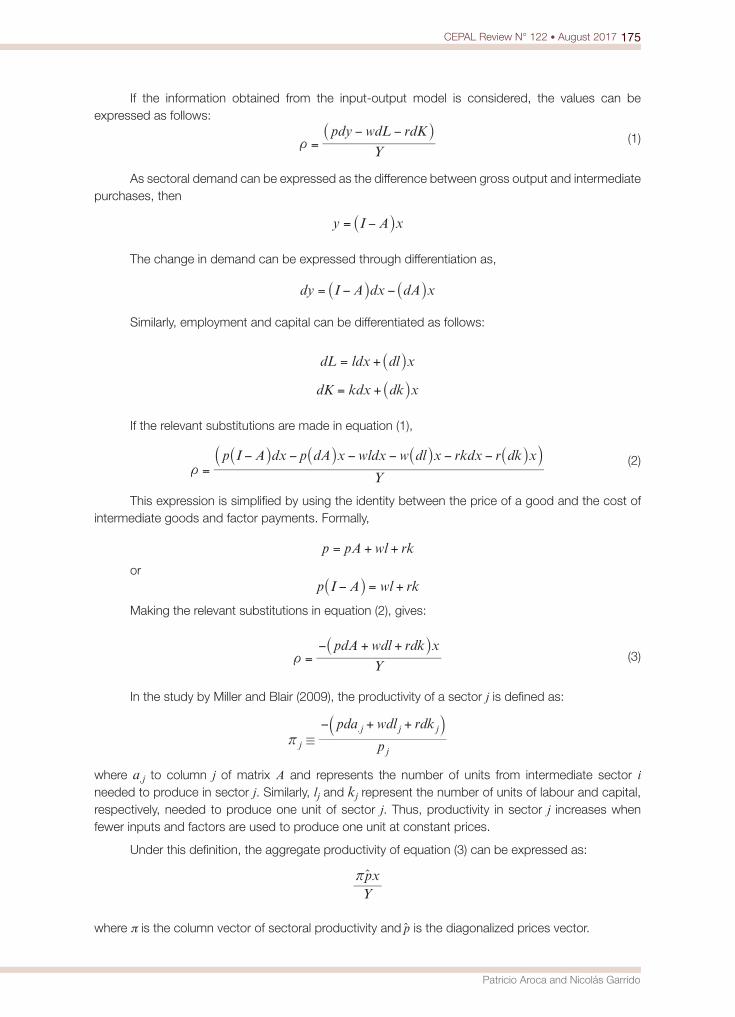
175CEPAL Review N° 122 • August 2017
Patricio Aroca and Nicolás Garrido
If the information obtained from the input-output model is considered, the values can be expressed as follows:
Y
pdy wdL rdKt =
− −R W (1)
As sectoral demand can be expressed as the difference between gross output and intermediate purchases, then
y I A x= −R W
The change in demand can be expressed through differentiation as,
dy I A dx dA x= − −R RW W
Similarly, employment and capital can be differentiated as follows:
dL ldx dl x= + R W dK kdx dk x= + R W
If the relevant substitutions are made in equation (1),
Y
p I A dx p dA x wldx w dl x rkdx r dk xt =
− − − − − −S R R R RW W W W X (2)
This expression is simplified by using the identity between the price of a good and the cost of intermediate goods and factor payments. Formally,
p pA wl rk= + +
or
p I A wl rk− = +R WMaking the relevant substitutions in equation (2), gives:
Y
pdA wdl rdk xt =
− + +R W (3)
In the study by Miller and Blair (2009), the productivity of a sector j is defined as:
p
pda wdl rdk.
jj
j j j/r
− + +S X
where a,j to column j of matrix A and represents the number of units from intermediate sector i needed to produce in sector j. Similarly, lj and kj represent the number of units of labour and capital, respectively, needed to produce one unit of sector j. Thus, productivity in sector j increases when fewer inputs and factors are used to produce one unit at constant prices.
Under this definition, the aggregate productivity of equation (3) can be expressed as:
Ypxrt
where π is the column vector of sectoral productivity and p is the diagonalized prices vector.

176 CEPAL Review N° 122 • August 2017
Sectoral breakdown of total factor productivity in Chile, 1996-2010
Next, applying the relation x I A y1= −
−R W and the identity I p p1= −t t , aggregate productivity can be expressed as
Y
p I A p py1 1
tr
=−
− −t t tR W
To simplify the notation, the foregoing equation can be expressed as:
St r b= (4)
where π is a row vector in which each component j represents the productivity of the corresponding sector. The matrix S p I A p1 1= −
− −t tR W encapsulates the economic effects of transactions between
industries. Each term si,j of matrix S can be expressed as s p
l p,
,i j
j
i j i= , where the technical multiplier,7
li,j represents the direct and indirect increase generated in the physical production of good i as a result of increasing the demand for good j. Consequently, si,j represents the multiplier of good i, derived from an increase in its demand, compared to the price of good j. This could be summarized by saying that if, instead of considering the multiplier li,j, which includes both direct and indirect effects, only the direct effect of technical coefficient ai,j of the technical coefficient matrix A were considered, the economic
effects would be expressed as s p
a p,
,i j
j
i j i=u , where s ,i ju represents the cost of input i relative to that of
good j.
Lastly, Ypy
b =t
is a row vector in which each position j represents the share of sector j in the final demand of the economy. This vector can also be interpreted as the preference for spending in certain sectors as revealed by the country’s demand.
Taking the decomposition expressed in equation (4) and ignoring the second order effects, the change in TFP can be linearly approximated as:
S S St r b r b r bD D D D= + + (5)
While the first term on the right represents the change in productivity arising from the change in demand preferences, the second term refers to the change attributable to the intersectoral effects, and the third represents the intrasectoral changes.
III. Data and results
The calculations described in this article were made using data from the national accounts databases of the Central Bank of Chile for the years 1996, 2003 and 2010. Data from the National Institute of Statistics were also used to calculate the average hourly wage of workers in each year; and the sectoral capital stock data reported by Henríquez (2008) were also considered.
Fuentes, Larraín and Schmidt-Hebbel (2006) provide evidence that the behavior of TFP is linked to the cyclical components of the economy. Thus, to have a timeline reference, figure 1 shows the cyclical component of gross domestic product at constant prices, calculated by applying the Hodrick-Prescott (1981) filter (λ = 1,600). The vertical bars (years 1996, 2003 and 2010) represent the input-output data used in the calculation.
7 In terms of the standard Leontief notation, L = (I–A)-1, so li,j ∈L.
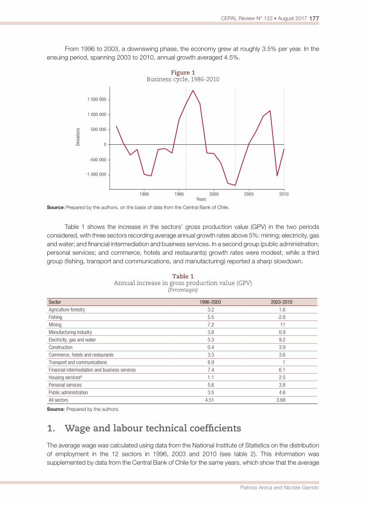
177CEPAL Review N° 122 • August 2017
Patricio Aroca and Nicolás Garrido
From 1996 to 2003, a downswing phase, the economy grew at roughly 3.5% per year. In the ensuing period, spanning 2003 to 2010, annual growth averaged 4.5%.
Figure 1 Business cycle, 1986-2010
1990 1995 2000 2005 2010
-1 000 000
-500 000
0
500 000
1 000 000
1 500 000
Years
Devi
atio
ns
Source: Prepared by the authors, on the basis of data from the Central Bank of Chile.
Table 1 shows the increase in the sectors’ gross production value (GPV) in the two periods considered, with three sectors recording average annual growth rates above 5%: mining; electricity, gas and water; and financial intermediation and business services. In a second group (public administration; personal services; and commerce, hotels and restaurants) growth rates were modest, while a third group (fishing, transport and communications, and manufacturing) reported a sharp slowdown.
Table 1 Annual increase in gross production value (GPV)
(Percentages)
Sector 1996-2003 2003-2010Agriculture-forestry 3.2 1.6
Fishing 5.5 -2.8
Mining 7.2 11
Manufacturing industry 3.8 0.9
Electricity, gas and water 5.3 9.2
Construction 0.4 3.9
Commerce, hotels and restaurants 3.3 3.6
Transport and communications 8.9 1
Financial intermediation and business services 7.4 6.1
Housing servicesa 1.1 2.5
Personal services 5.6 3.8
Public administration 3.5 4.6
All sectors 4.51 3.68
Source: Prepared by the authors.
1. Wage and labour technical coefficients
The average wage was calculated using data from the National Institute of Statistics on the distribution of employment in the 12 sectors in 1996, 2003 and 2010 (see table 2). This information was supplemented by data from the Central Bank of Chile for the same years, which show that the average
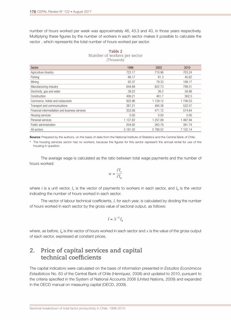
178 CEPAL Review N° 122 • August 2017
Sectoral breakdown of total factor productivity in Chile, 1996-2010
number of hours worked per week was approximately 46, 43.3 and 40, in those years respectively. Multiplying these figures by the number of workers in each sector makes it possible to calculate the vector , which represents the total number of hours worked per sector.
Table 2 Number of workers per sector
(Thousands)
Sector 1996 2003 2010Agriculture-forestry 723.17 710.96 703.24
Fishing 66.17 81.3 45.62
Mining 92.37 79.33 199.17
Manufacturing industry 844.89 822.73 799.31
Electricity, gas and water 39.22 26.2 58.88
Construction 406.21 461.7 562.5
Commerce, hotels and restaurants 925.96 1 129.12 1 746.53
Transport and communications 387.21 484.38 522.57
Financial intermediation and business services 353.08 471.12 574.64
Housing services 0.00 0.00 0.00
Personal services 1 137.82 1 257.89 1 497.94
Public administration 204.92 263.79 391.74
All sectors 5 181.02 5 788.52 7 102.14
Source: Prepared by the authors, on the basis of data from the National Institute of Statistics and the Central Bank of Chile.a The housing services sector has no workers, because the figures for this sector represent the annual rental for use of the
housing in question.
The average wage is calculated as the ratio between total wage payments and the number of hours worked:
ii''
wll
n
v=
where i is a unit vector, lv is the vector of payments to workers in each sector, and ln is the vector indicating the number of hours worked in each sector.
The vector of labour technical coefficients, l, for each year, is calculated by dividing the number of hours worked in each sector by the gross value of sectoral output, as follows:
l x ln1= −t
where, as before, ln is the vector of hours worked in each sector and x is the value of the gross output of each sector, expressed at constant prices.
2. Price of capital services and capital technical coefficients
The capital indicators were calculated on the basis of information presented in Estudios Económicos Estadísticos No. 63 of the Central Bank of Chile (Henríquez, 2008) and updated to 2010, pursuant to the criteria specified in the System of National Accounts 2008 (United Nations, 2009) and expanded in the OECD manual on measuring capital (OECD, 2009).
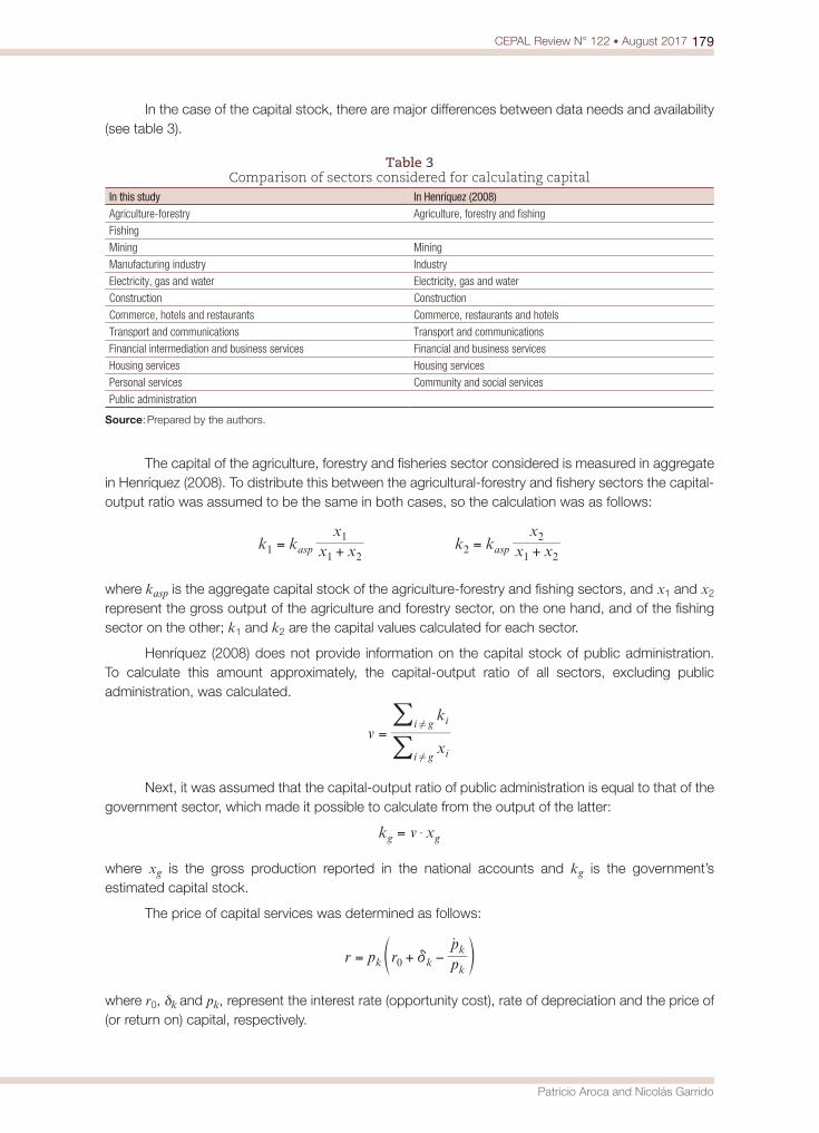
179CEPAL Review N° 122 • August 2017
Patricio Aroca and Nicolás Garrido
In the case of the capital stock, there are major differences between data needs and availability (see table 3).
Table 3 Comparison of sectors considered for calculating capital
In this study In Henríquez (2008)Agriculture-forestry Agriculture, forestry and fishing
Fishing
Mining Mining
Manufacturing industry Industry
Electricity, gas and water Electricity, gas and water
Construction Construction
Commerce, hotels and restaurants Commerce, restaurants and hotels
Transport and communications Transport and communications
Financial intermediation and business services Financial and business services
Housing services Housing services
Personal services Community and social services
Public administration
Source: Prepared by the authors.
The capital of the agriculture, forestry and fisheries sector considered is measured in aggregate in Henríquez (2008). To distribute this between the agricultural-forestry and fishery sectors the capital-output ratio was assumed to be the same in both cases, so the calculation was as follows:
k k x x
xk k x x
xasp asp1
1 2
12
1 2
2= + = +
where kasp is the aggregate capital stock of the agriculture-forestry and fishing sectors, and x1 and x2 represent the gross output of the agriculture and forestry sector, on the one hand, and of the fishing sector on the other; k1 and k2 are the capital values calculated for each sector.
Henríquez (2008) does not provide information on the capital stock of public administration. To calculate this amount approximately, the capital-output ratio of all sectors, excluding public administration, was calculated.
v
x
k
ii g
ii g=
!
!
//
Next, it was assumed that the capital-output ratio of public administration is equal to that of the government sector, which made it possible to calculate from the output of the latter:
k v xg g$=
where xg is the gross production reported in the national accounts and kg is the government’s estimated capital stock.
The price of capital services was determined as follows:
r p r pp
k kk
k0 d= + −
oU Z
where r0, δk and pk, represent the interest rate (opportunity cost), rate of depreciation and the price of (or return on) capital, respectively.
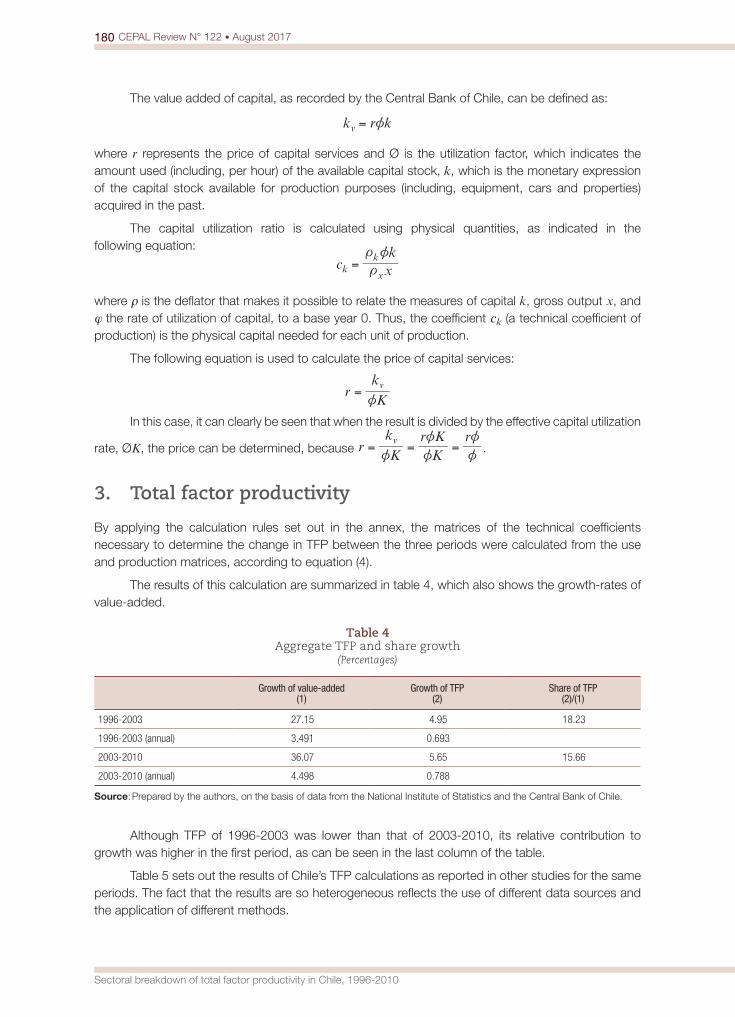
180 CEPAL Review N° 122 • August 2017
Sectoral breakdown of total factor productivity in Chile, 1996-2010
The value added of capital, as recorded by the Central Bank of Chile, can be defined as:
k r kv z=
where r represents the price of capital services and Ø is the utilization factor, which indicates the amount used (including, per hour) of the available capital stock, k, which is the monetary expression of the capital stock available for production purposes (including, equipment, cars and properties) acquired in the past.
The capital utilization ratio is calculated using physical quantities, as indicated in the following equation:
c xk
kx
k
t
t z=
where ρ is the deflator that makes it possible to relate the measures of capital k, gross output x, and ϕ the rate of utilization of capital, to a base year 0. Thus, the coefficient ck (a technical coefficient of production) is the physical capital needed for each unit of production.
The following equation is used to calculate the price of capital services:
r
K
kv
z=
In this case, it can clearly be seen that when the result is divided by the effective capital utilization
rate, ØK, the price can be determined, because r K
k
Kr K rv
z z
z
z
z= = = .
3. Total factor productivity
By applying the calculation rules set out in the annex, the matrices of the technical coefficients necessary to determine the change in TFP between the three periods were calculated from the use and production matrices, according to equation (4).
The results of this calculation are summarized in table 4, which also shows the growth-rates of value-added.
Table 4 Aggregate TFP and share growth
(Percentages)
Growth of value-added (1)
Growth of TFP(2)
Share of TFP (2)/(1)
1996-2003 27.15 4.95 18.23
1996-2003 (annual) 3.491 0.693
2003-2010 36.07 5.65 15.66
2003-2010 (annual) 4.498 0.788
Source: Prepared by the authors, on the basis of data from the National Institute of Statistics and the Central Bank of Chile.
Although TFP of 1996-2003 was lower than that of 2003-2010, its relative contribution to growth was higher in the first period, as can be seen in the last column of the table.
Table 5 sets out the results of Chile’s TFP calculations as reported in other studies for the same periods. The fact that the results are so heterogeneous reflects the use of different data sources and the application of different methods.

181CEPAL Review N° 122 • August 2017
Patricio Aroca and Nicolás Garrido
Table 5 Annual TFP calculated in different studies
(Percentages)
Period Annual TFP1998-2005a 1.89
1990-2005a 3.06
1996-2003a b 0.6
2003-2005a b 1.74
1996-2000c 0.2
2000-2003c -0.1
1998-2005d 1.77
1998-2005e 0.66
2000-2008f 1
Source: Prepared by the authors, on the basis of R. Fuentes, M. Larraín and K. Schmidt-Hebbel, “Sources of growth and behavior of TFP in Chile”, Cuadernos de Economía, vol. 43, No. 127, Santiago, Pontificia Universidad Católica de Chile, 2006; R. Vergara and R. Rivero, “Productividad sectorial en Chile 1986-2001”, Cuadernos de Economía, vol. 43, No. 127, Santiago, Pontificia Universidad Católica de Chile, 2006; R. Fuentes and M. Morales, “On the measurement of total factor productivity: a latent variable approach”, Macroeconomic Dynamics, vol. 15, No. 2, Cambridge University Press, 2011; and I. Magendzo, Evolución de la productividad total de los factores, Santiago, Adolfo Ibáñez University, 2013.
a Fuentes, Larraín and Schmidt-Hebbel (2006).b The authors do not provide information on TFP growth in these periods, but annual TFP indices which were used as a basis for
calculating the data shown in the table. Specifically, the TFP index was used, with capital and employment corrected for hours of work and wages, respectively.
c Vergara and Rivero (2006).d Fuentes R. and M. Morales (2011), on the basis of growth accounting.e Ibid, using a state-space model.f I. Magendzo (2013), Adolfo Ibáñez University.
The figures for 1996-2003 presented in table 4 are similar to the TFP results for those same years calculated by Fuentes, Larraín and Schmidt-Hebbel (2006). This similarity occurs in two dimensions, since the annual growth of TFP in this period was 0.6%, while its contribution to the overall growth of the economy was 18.92%.
To clarify the source of the change in TFP, Table 6 presents the decomposition performed in equation (5). The first row of column 1 shows the difference between productivity in 1996-2003 and in 2003-2010. The value is broken down in the next three columns. The second row reports the share of each component in the change. Most of what occurred between the two periods analysed is due to the variation of intrasectoral and intersectoral productivity, the total of which represents approximately 80% of the change.
Table 6 Decomposition of TFP
Changes in sectoral demand (1)
πSΔß
Changes in the interaction between
sectors (2)πSΔß
Changes in the TFT of each sector (3)
πSΔßTotal
(1)+(2)+(3)
Δρ=0.065-0.0495 0.001344 0.003134 0.002474 0.006949
Percentage 19.34% 45.1% 35.6% 100.06%a
Source: Prepared by the authors.a The amount exceeds 100% owing to second-order approximation errors.
Table 7 shows the decomposition of 35.6% of the observed change in TFP for the economy as a whole. The second column shows the values of w=Sβ, which is a vector of 12 sectors. As the vector β can be interpreted as the distribution of the expenditure of all sectors of the economy expressed in a monetary unit, position i of the vector w(i) represents the increase in economic activity
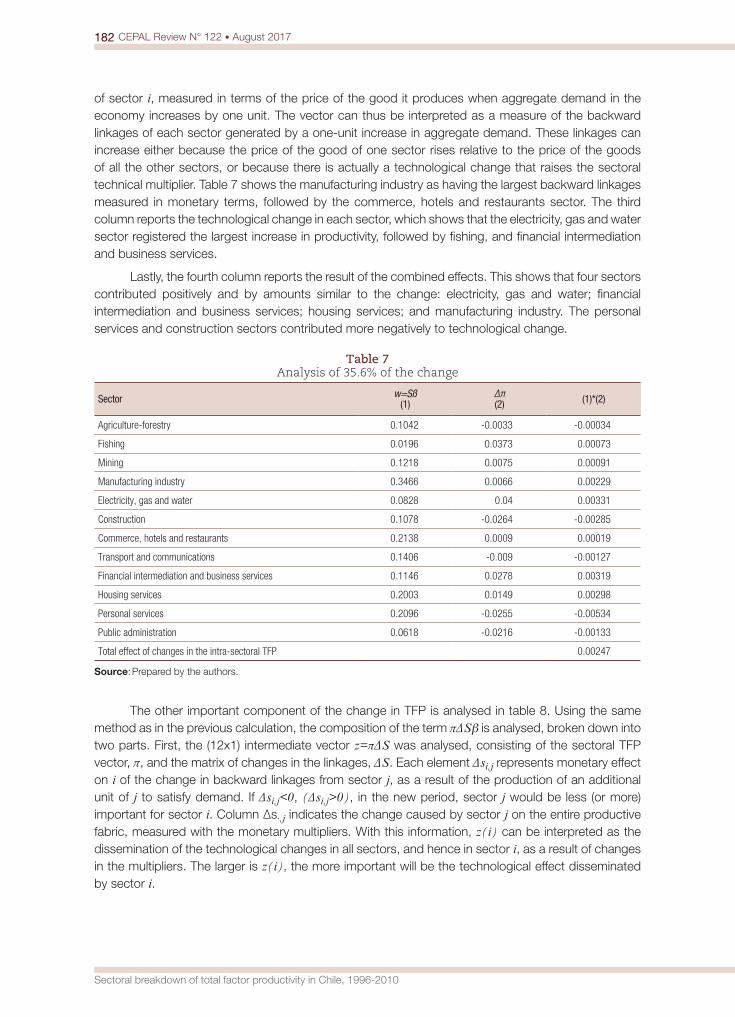
182 CEPAL Review N° 122 • August 2017
Sectoral breakdown of total factor productivity in Chile, 1996-2010
of sector i, measured in terms of the price of the good it produces when aggregate demand in the economy increases by one unit. The vector can thus be interpreted as a measure of the backward linkages of each sector generated by a one-unit increase in aggregate demand. These linkages can increase either because the price of the good of one sector rises relative to the price of the goods of all the other sectors, or because there is actually a technological change that raises the sectoral technical multiplier. Table 7 shows the manufacturing industry as having the largest backward linkages measured in monetary terms, followed by the commerce, hotels and restaurants sector. The third column reports the technological change in each sector, which shows that the electricity, gas and water sector registered the largest increase in productivity, followed by fishing, and financial intermediation and business services.
Lastly, the fourth column reports the result of the combined effects. This shows that four sectors contributed positively and by amounts similar to the change: electricity, gas and water; financial intermediation and business services; housing services; and manufacturing industry. The personal services and construction sectors contributed more negatively to technological change.
Table 7 Analysis of 35 .6% of the change
Sector w=Sß(1)
Δπ(2) (1)*(2)
Agriculture-forestry 0.1042 -0.0033 -0.00034
Fishing 0.0196 0.0373 0.00073
Mining 0.1218 0.0075 0.00091
Manufacturing industry 0.3466 0.0066 0.00229
Electricity, gas and water 0.0828 0.04 0.00331
Construction 0.1078 -0.0264 -0.00285
Commerce, hotels and restaurants 0.2138 0.0009 0.00019
Transport and communications 0.1406 -0.009 -0.00127
Financial intermediation and business services 0.1146 0.0278 0.00319
Housing services 0.2003 0.0149 0.00298
Personal services 0.2096 -0.0255 -0.00534
Public administration 0.0618 -0.0216 -0.00133
Total effect of changes in the intra-sectoral TFP 0.00247
Source: Prepared by the authors.
The other important component of the change in TFP is analysed in table 8. Using the same method as in the previous calculation, the composition of the term πΔSβ is analysed, broken down into two parts. First, the (12x1) intermediate vector z=πΔS was analysed, consisting of the sectoral TFP vector, π, and the matrix of changes in the linkages, ΔS. Each element Δsi,j represents monetary effect on i of the change in backward linkages from sector j, as a result of the production of an additional unit of j to satisfy demand. If Δsi,j<0, (Δsi,j>0), in the new period, sector j would be less (or more) important for sector i. Column Δs∙,j indicates the change caused by sector j on the entire productive fabric, measured with the monetary multipliers. With this information, z(i) can be interpreted as the dissemination of the technological changes in all sectors, and hence in sector i, as a result of changes in the multipliers. The larger is z(i), the more important will be the technological effect disseminated by sector i.
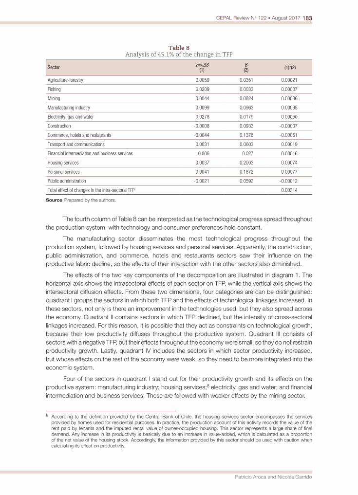
183CEPAL Review N° 122 • August 2017
Patricio Aroca and Nicolás Garrido
Table 8 Analysis of 45 .1% of the change in TFP
Sector z=πΔS(1)
B(2) (1)*(2)
Agriculture-forestry 0.0059 0.0351 0.00021
Fishing 0.0209 0.0033 0.00007
Mining 0.0044 0.0824 0.00036
Manufacturing industry 0.0099 0.0963 0.00095
Electricity, gas and water 0.0278 0.0179 0.00050
Construction -0.0008 0.0933 -0.00007
Commerce, hotels and restaurants -0.0044 0.1376 -0.00061
Transport and communications 0.0031 0.0603 0.00019
Financial intermediation and business services 0.006 0.027 0.00016
Housing services 0.0037 0.2003 0.00074
Personal services 0.0041 0.1872 0.00077
Public administration -0.0021 0.0592 -0.00012
Total effect of changes in the intra-sectoral TFP 0.00314
Source: Prepared by the authors.
The fourth column of Table 8 can be interpreted as the technological progress spread throughout the production system, with technology and consumer preferences held constant.
The manufacturing sector disseminates the most technological progress throughout the production system, followed by housing services and personal services. Apparently, the construction, public administration, and commerce, hotels and restaurants sectors saw their influence on the productive fabric decline, so the effects of their interaction with the other sectors also diminished.
The effects of the two key components of the decomposition are illustrated in diagram 1. The horizontal axis shows the intrasectoral effects of each sector on TFP, while the vertical axis shows the intersectoral diffusion effects. From these two dimensions, four categories are can be distinguished: quadrant I groups the sectors in which both TFP and the effects of technological linkages increased. In these sectors, not only is there an improvement in the technologies used, but they also spread across the economy. Quadrant II contains sectors in which TFP declined, but the intensity of cross-sectoral linkages increased. For this reason, it is possible that they act as constraints on technological growth, because their low productivity diffuses throughout the productive system. Quadrant III consists of sectors with a negative TFP, but their effects throughout the economy were small, so they do not restrain productivity growth. Lastly, quadrant IV includes the sectors in which sector productivity increased, but whose effects on the rest of the economy were weak, so they need to be more integrated into the economic system.
Four of the sectors in quadrant I stand out for their productivity growth and its effects on the productive system: manufacturing industry; housing services;8 electricity, gas and water; and financial intermediation and business services. These are followed with weaker effects by the mining sector.
8 According to the definition provided by the Central Bank of Chile, the housing services sector encompasses the services provided by homes used for residential purposes. In practice, the production account of this activity records the value of the rent paid by tenants and the imputed rental value of owner-occupied housing. This sector represents a large share of final demand. Any increase in its productivity is basically due to an increase in value-added, which is calculated as a proportion of the net value of the housing stock. Accordingly, the information provided by this sector should be used with caution when calculating its effect on productivity.

184 CEPAL Review N° 122 • August 2017
Sectoral breakdown of total factor productivity in Chile, 1996-2010
Diagram 1 TFP: intersectoral and intrasectoral effects
Agriculture-forestry
Fishing
Mining
Manufacturing industry
Electricity, gas and water
Construction
Commerce, hotels and restaurants
Transport and communications Financial intermediationand business services
Housing servicesPersonal services
Public administration
-0,0015
0
0,0015
-0,01 0 0,01
Inte
rsec
tora
l effe
ct
Intrasectoral effects
III
III IV
Source: Prepared by the authors.
Quadrant II is dominated by the personal services sector, which encompasses education, health, social service activities and associations, leisure activities, waste management and a wide range of services, including washing and cleaning of textile and fur products, hairdressing services, funeral services, domestic service and others. These are mainly services provided to households.
Quadrant III contains two sectors: construction and public administration. The change in the effect of the first of these on the productive fabric is small, and it also displays a considerable reduction in TFP.
Quadrant IV comprises the commerce, hotels and restaurants sector, which displays a very small increase in productivity, along with a substantial reduction in its effect on the economy.
IV. Discussion
The results presented so far require two clarifications before offering conclusions. On the one hand, the intensity of the change in productivity should be discussed, and on the other hand a hypothetical analysis of its causes will be presented.
The intensity of change is reflected in the result of the calculation made on the basis of equation (4):
− =t t= − = , , , , %0 0565 0 0495 0 007 0 7, ,03 10 96 03tD =
where ρ03,10 and ρ96,03 represent TFP calculated for the periods 2003-2010 and 1996-2003, respectively. The result shows that productivity grew by 0.7% between the two periods, with the increase in efficiency occurring in 2003-2010, when GDP growth was higher than in 1996-2003 (see table 4). Consequently, the relative share of the increase in efficiency was smaller in the second period than in the first. These conclusions confirm the note of caution expressed by Fuentes, Larraín and Schmidt-Hebbel (2006) concerning the scant economic growth attributable to the “inspiration” factor in their analysis of Chilean growth accounting.
There are two, not necessarily mutually exclusive, hypotheses explaining the reported changes in TFP. According to the first, and given the procyclicality attributed to TFP by Fuentes, Larraín and Schmidt-Hebbel (2006), the years selected for preparing the input-output tables used in this study

185CEPAL Review N° 122 • August 2017
Patricio Aroca and Nicolás Garrido
and the characteristics of the business cycle in Chile (see figure 1), the absolute increase in TFP may have been driven by cyclical factors such as the terms-of-trade improvement induced by the rise in the copper price during the period analyzed (see Fuentes, Larraín and Schmidt-Hebbel, 2006). This first hypothesis, of a macroeconomic type, is complemented by a microeconomic one, relating to a specific transmission channel that may have helped sustain the level of TFP.
The second hypothesis stems from the intersection between the sectoral decomposition performed in this study and summarized in diagram 1, on the one hand, and the results reported by Fernandes and Paunov (2012), on the other. The synthesis presented in this diagram shows the positive influence exerted on productivity growth by the manufacturing; electricity, gas and water; and financial intermediation and business service sectors. In contrast, the Fernandes and Paunov study links these three sectors to the substantial increase in foreign direct investment (FDI) in the services sector during the period analysed. In the 1990s, the services sector absorbed roughly 60% of FDI in Chile, which, through price reduction mechanisms, quality improvements, accentuation of diversification and knowledge dissemination, boosted the TFP of firms in the manufacturing sector.
V. Conclusion
The present study set out to analyse the sectoral composition of changes in TFP occurring in Chile from 1996 to 2010, within the Solow growth accounting framework and taking intrasectoral interaction into account. This exercise made use of input-output tables for the years 1996, 2003 and 2010 provided by the Central Bank of Chile. Part II describes the decomposition method used, while section III and the annex describe the calculations performed to obtain the basic data; and section IV analyses the results obtained.
The decomposition of TFP was performed in three stages, namely intrasectoral productivity, its diffusion effects, and changes in demand that influence productivity. It was found that over 80% of the change in productivity in the period analyzed was due to the first two factors.
The results of this research make it possible to construct a taxonomy of sectors, based on their capacity to drive the economy and changes in sectoral productivity growth. This taxonomy identifies manufacturing industry, and the electricity-gas-water, and financial intermediation and business services sectors, as the drivers of TFP growth in 1996-2010. Productivity growth in these sectors spread throughout the production fabric.
By recording a decline in productivity during the period, which exerted a major influence on the productive system, the personal services sector may have restricted productivity growth in the economy at large.
BibliographyÁlvarez, R. and R. Fuentes (2009), “Labour market regulations and productivity: evidence from Chilean
manufacturing plants”, Working Paper, No. 396, Santiago, Pontificia Universidad Católica de Chile.(2004), “Patrones de especialización y crecimiento sectorial en Chile”, Working Paper, No. 288, Santiago, Central Bank of Chile.
Baumol, W.J. and E.N. Wolff (1984), “On interindustry differences in absolute productivity”, Journal of Political Economy, vol. 92, No. 6, Chicago, The University of Chicago Press.
Bergoeing, R., A. Hernando and A. Repetto (2005), “Market reforms and efficiency gains in Chile”, Working Papers, No. 372, Santiago, Central Bank of Chile.
Chumacero, R.A. and R. Fuentes (2006), “Chilean growth dynamics”, Economic Modelling, vol. 23, No. 2, Amsterdam, Elsevier.

186 CEPAL Review N° 122 • August 2017
Sectoral breakdown of total factor productivity in Chile, 1996-2010
Del Gatto, M., A. Di Liberto and C. Petraglia (2011), “Measuring productivity”, Journal of Economic Surveys, vol. 25, No. 5, Wiley.
Easterly, W. and R. Levine (2002), “It’s not factor accumulation: stylized facts and growth models”, Economic Growth: Sources, Trends, and Cycles, N. Loayza, R. Soto and K. Schmidt-Hebbel (eds.), Santiago, Central Bank of Chile.
Fernandes, A.M. and C. Paunov (2012), “Foreign direct investment in services and manufacturing productivity: evidence for Chile”, Journal of Development Economics, vol. 97, No. 2, Amsterdam, Elsevier.
Fuentes, R. (2011), “Una mirada desagregada del deterioro de la productividad en Chile: ¿existe un cambio estructural?, Working Paper, No. 401, Santiago, Pontificia Universidad Católica de Chile.
Fuentes, R. and M. Morales (2011), “On the measurement of total factor productivity: a latent variable approach”, Macroeconomic Dynamics, vol. 15, No. 2, Cambridge University Press.
Fuentes, R., M. Larraín and K. Schmidt-Hebbel (2006), “Sources of growth and behavior of TFP in Chile”, Cuadernos de Economía, vol. 43, No. 127, Santiago, Pontificia Universidad Católica de Chile.
Harberger, A.C. (1998), “A vision of the growth process”, American Economic Review, vol. 88, No. 1, Nashville, Tennessee, American Economic Association.
Henríquez, C. (2008), “Stock de capital en Chile (1985-2005): metodología y resultados”, Studies in Economic Statistics, No. 63, Santiago, Central Bank of Chile.
Hodrick, R.J. and E.C. Prescott (1981), “Postwar U.S. business cycles: an empirical investigation”, Discussion Papers, No. 451, Northwestern University.
Magendzo, I. (2013), Evolución de la productividad total de los factores, Santiago, Adolfo Ibáñez University.Miller, R. and P.D. Blair (2009), Input-output Analysis: Foundations and Extensions, New York, Cambridge
University Press.OECD (Organization for Economic Cooperation and Development) (2009), Measuring Capital. OECD
Manual, Paris.(2001), Measuring Productivity. Measurement of Aggregate and Industry-level Productivity Growth, Paris.
Pavcnik, N. (2002), “Trade liberalization, exit, and productivity improvements: evidence from Chilean plants”, Review of Economic Studies, vol. 69, No. 1, Oxford University Press.
Prescott, C.E. (1998), “Needed: a theory of total factor productivity”, International Economic Review, vol. 39, No. 3.
Solow, R.M. (1957), “Technical change and the aggregate production function”, Review of Economics and Statistics, vol. 39, No. 3.
Timmer, M.P. and others (2010), Economic Growth in Europe. A Comparative Industry Perspective, Cambridge University Press.
United Nations (2009), System of National Accounts 2008, New York, European Commission/International Monetary Fund/Organization for Economic Cooperation and Development/United Nations.
Vergara, R. and R. Rivero (2006), “Productividad sectorial en Chile 1986-2001”, Cuadernos de Economía, vol. 43, No. 127, Santiago, Pontificia Universidad Católica de Chile.
Wolff, E.N. (1985), “Industrial composition, interindustry effects, and the U.S. productivity slowdown”, The Review of Economics and Statistics, vol. 67, No. 2, Cambridge, Massachusetts, The MIT Press.(1984), “Industrial composition, interindustry effects, and the U.S. productivity slowdown”, Economic Research Reports, No. 84-09, New York, New York University.

187CEPAL Review N° 122 • August 2017
Patricio Aroca and Nicolás Garrido
Annex A1
Data and calculation methods used
This annex describes the calculations performed using the three methods indicated.
Calculation of the technical coefficients
The data provided by the Central Bank of Chile are grouped into production-and-use matrices (see Miller and Blair, 2009), and these were the main source used for calculating the intersectoral transaction matrices.
The Miller and Blair (2009) industry-demand driven model was used, in which technology is determined by the production structure for goods, irrespective of the industry from which they originate, to develop the total requirement matrices. In analytical terms,
U: matrix of uses – 13 products by 12 sectors.
V: matrix of sectoral production – 12 sectors by 13 products
s = V*i: industrial or sectoral production vector (12x1)
Q = V’*i: commodities production vector (13x1)
For simplicity, time subscripts were not used.
On the basis of this information, the intersectoral transactions matrix was calculated as follows:
B U s
D V q
Z D B s
1
1
$
$
$ $
=
=
=
−
−
t
t
t
In this case, a circumflex is placed on the vectors (for example, s) to indicate its diagonalization. The national purchase and import matrices were added together to calculate the coefficients matrix A. Accordingly, the following information, also provided by the Central Bank of Chile, is added to the calculated transaction matrix:
M: matrix of imports by each sector (12x12)
Lv: row vector representing the value added of the wage by sector (12x1)
Kv: row vector representing the value added by capital by sector (12x1)
tv: row vector of indirect taxes (12x1)
The column vector of the total production is calculated as follows:
' 'x i Z i M l k tv v v= + + + +
To calculate the column vector of final demand, the products of each sector are identified and the corresponding intermediate sales are subtracted.
' ' ' 'y x i Z i M= − −

188 CEPAL Review N° 122 • August 2017
Sectoral breakdown of total factor productivity in Chile, 1996-2010
Calculation of the sector productivity vector
Since productivity is calculated for different periods, the approximation proposed by Wolff (1984) is used, as follows:
Yy
v YwL
v YrK
ii
L
k
b =
=
=
The average values of two periods are represented as follows:
2
, ,i
i t i t 1b
b b=
+ +r
The approximate value of aggregate TFP can be calculated by the following equation:
log log logy v L v Kj j L Kj
,t b D D D− −r r r/
The approximate value of TFP in sector j is calculated in a similar way:
log log loga v l v k, , , ,j i j i j L j j K j ji
,r a D D D− − −r r rU S S SX X XZ/
where p
p a,
,i j
j
i i ja = , v p
wl,L j
j
j= , v p
rk,K j
j
j= . The dash placed above the variables signifies that the
Turnquist-Divisia index weights were used for several periods.
The impact of the minimum wage on income and employment in MexicoRaymundo M. Campos Vázquez, Gerardo Esquivel and Alma S. Santillán Hernández1
Abstract
This article analyses the effects of a rise in the minimum wage on wages and employment in Mexico. The source of variation is the equalization in late 2012 of the minimum wage in two areas of the country. Using the National Occupation and Employment Survey (ENOE), econometric analyses are performed of cross-section and individual panel data. The results of the first indicate that, on average, the hourly wage in zone B rose by between 1.6% and 2.6% for workers overall and between 1.8% and 3.3% for wage workers. The panel analysis yields similar results. Although the cross-section analysis does not show an impact in terms of employment, the panel data indicate that the probability of being an informal (formal) worker falls (rises) among those affected by the wage rise policy.
KeywordsMinimum wage, employment, income, economic analysis, econometric models, Mexico
JEL classificationJ31, J38, O15, O54
AuthorsRaymundo M. Campos Vázquez is a research professor at the Centre for Economic Studies at El Colegio de México. [email protected]
Gerardo Esquivel is a research professor at the Centre for Economic Studies at El Colegio de México. [email protected]
Alma S. Santillán Hernández is a full-time professor in the Mathematics and Physics Department of the Autonomous University of the State of Hidalgo. [email protected]
1 The authors are grateful to the Economic Commission for Latin America and the Caribbean (ECLAC) for its support in the preparation of this article and for the excellent comments and suggestions received.
190 CEPAL Review N° 122 • August 2017
The impact of the minimum wage on income and employment in Mexico
I. Introduction
The impact of a rise in the minimum wage on income and employment conditions of workers is an extremely important and controversial topic. Among other things, higher minimum wages can have a significant positive effect on family income levels and, therefore, on the ability to exit poverty. However, a rise in the minimum wage can also have negative impacts, such as job loss —in the case of individuals receiving this level of income— or widespread price rises. In fact, should prices and the minimum wage both rise by similar proportions, the wage rise will produce no real gain. These differentiated effects have been researched extensively worldwide and some of these studies are mentioned later.
This article sets forth evidence regarding the impact of the rise in the minimum wage in Mexico. Up to 2012, Mexico had three minimum wage zones denominated A, B and C. Zone A had the highest minimum wage and zone C, the lowest. At the end of November 2012, the government unexpectedly announced that the minimum wage of zone B would be equalized with that of zone A. Comparison of the figures for January 2012 and January 2013 show that this measure raised zone B’s minimum wage by 3.1% in real terms (a larger rise than in the other two zones). The step affected an area of the country that accounts for roughly 10% of the population. Although the minimum wage rise was relatively small, the fact that it was a completely exogenous and arbitrary decision that affected one zone but not the others makes it possible to analyse its effects on the income and employment conditions of workers in Mexico.
To this end, we use microdata from the National Occupation and Employment Survey (ENOE) of 2012 and 2013. The analysis was limited to those two years to avoid issues of comparison owing to different wage and employment trends in the different geographical areas. The identification strategy used was the difference-in-difference method: the impact of the change in the zone B minimum wage was compared with what was happening in other zones before and after the minimum wage rise. Two types of data were used: cross-section and panel format (where the same individuals were tracked over time). The second strategy eliminates any time invariant individual bias and is thus more robust than the cross-section approach.
The results show that the rise in the minimum wage had no negative effects in employment terms and, on the contrary, produced some positive impacts. The cross-section data showed an increase in labour income in zone B, although there was no increase in the income of low-income workers (defined as those who receive less than three times the minimum wage). In addition, the rise in the minimum wage does not appear to have affected levels of employment in the sample. The panel information yields similar results in terms of hourly wage and, in some cases, positive effects were seen in relation to the total wage. Lastly, the panel data showed that some individuals who had a formal job before the rise in the minimum wage were more likely to keep it afterwards. Similarly, the probabilities of individuals who had an informal job still having that type of work after the rise in the minimum wage decreased, and the probabilities of them securing a formal job increased.
In sum, the increase in the minimum wage produced by the alignment of zones had no negative effects —but did have some positive effects— on employment in Mexico. Nevertheless, the subject still requires more research because the increase in this instance was relatively small. For that reason, it is not advisable to extrapolate these results to a larger minimum wage rise, or to cases or countries in which the minimum wage is substantially higher (relatively speaking) than it was in Mexico at the time when the rise analysed here was decreed.
The article has five sections following this introduction. Section II reviews the literature and section III discusses the data used and presents descriptive statistics on employment and wages in the different geographical zones of Mexico. Section IV describes the methodology employed and the research results, and section V concludes.
191CEPAL Review N° 122 • August 2017
Raymundo M. Campos Vázquez, Gerardo Esquivel and Alma S. Santillán Hernández
II. Literature review
The theory underlying the common notion that a rise in the minimum wage is harmful to employment is quite simple: the rationale is that a higher minimum wage will lower firms’ demand for workers and thus reduce hiring. This argument is so simple that economists did not question is until the early 1990s. The topic came to the fore at that point because the real minimum wage in the United States had dropped by almost 25% in the 1980s (Elwell, 2014), and this led economists to consider the effects that a minimum wage hike might have on employment, poverty levels and income distribution. The great majority of the studies conducted at that time showed that when it starts from relatively low levels, a small rise in the minimum wage has no negative effects on employment.2
Card and Krueger (1994) were pioneers in conducting systematic analysis of the possible consequences of a minimum wage rise in the United States, by means of quasi-experiments to try to capture the marginal effect of such a rise. They examined the effect attributable to the minimum wage rise in New Jersey —from US$ 4.25 to US$ 5.05 per hour— on employment in fast food restaurants such as Burger King and KFC. Card and Krueger chose the fast food business as a subject for analysis because it usually hires unskilled workers at low wages —precisely those who may be expected to be the most affected by minimum wage hikes.
As a control group, Card and Krueger used the fast food business in some cities in the neighbouring state of Pennsylvania, given that the minimum wage there remained constant at US$ 4.25 per hour. The study found no adverse effects on employment and even found some evidence of positive effects. Nevertheless, one of the criticisms of this study was that the trends in employment growth were different in the two states to start with, so that the finding could be an anomaly rather than a universally applicable principle.
Neumark and Wascher (2008) analysed and synthesized the results of over 90 studies subsequent to Card’s and Krueger’s, on the employment effects attributable to minimum wage changes. These studies include empirical evidence for the United States, some countries of the Organization for Economic Cooperation and Development (OECD), Latin America and Indonesia. The authors concludes that, in general, a rise in the minimum wage reduces employment for less skilled workers. In particular, Neumark and Wascher found wage elasticities of employment ranging from -0.1 to -0.3.
Later, Dube, Lester and Reich (2010) generalized the approach used by Card and Krueger (1994) and made use of differences in wage policy between neighbouring states in the United States to estimate minimum wage effects on income and employment in restaurants and other sectors with a predominant proportion of low-income workers. As well as using a larger number of observations (variations in 1,381 counties), one of the advantages of this study was that the information available covered a longer time period (from 1990 to 2006), which enabled the authors to estimate the long-term effects. Dube, Lester and Reich (2010) concluded that the large negative elasticities obtained in the traditional specifications were due mainly to differences (regional and local) in employment trends that were not related to minimum wage policies. These authors nevertheless found similar results to those of Card and Krueger with regard to employment (that is, a zero impact) and notably positive effects on income.
The interest on the effects of the minimum wage on employment are not limited to the United States. Stewart (2004) analysed the impacts of the introduction of a national minimum wage in the United Kingdom in April 1999, and its subsequent increases in 2000 and 2001. Stewart used
2 For a more comprehensive literature review and discussions of the possible impact of the minimum wage on other variables (including price levels) see Campos Vázquez (2015). The discussion of the literature in this section is partly based on that paper.

192 CEPAL Review N° 122 • August 2017
The impact of the minimum wage on income and employment in Mexico
a difference-in-difference estimator and found no evidence of adverse minimum wage impacts on employment in either case. Another more recent analysis for the United Kingdom also found no evidence of a negative impact (Manning, 2012).
Other studies have focused on developing countries, on the basis that they could be affected differently owing to their higher percentage of unskilled workers. Neumark, Cunningham and Siga (2006), for example, analysed the rise in Brazil’s minimum wage, which President Da Silva increased by 20% in 2003 and pledged to double by the end of 2006. These authors found no evidence that the change in the minimum wage had increased income at the lower end of the income distribution, while Lemos (2009) found no effect on employment.
Gindling and Terrell (2009) studied the case of Honduras, analysing the effects of 22 changes in the minimum wage —made between 1990 and 2004— on employment, unemployment and the average wage of workers in different sectors. They found effects only on the income of workers in medium and large firms, where an increase of 1% in the minimum wage led to a rise of 0.29% in the average wage and a relatively large drop (0.46%) in employment. At the same time, the authors found no effects attributable to the minimum wage on the income of workers in small firms or self-employed workers. They did find that a higher minimum wage could create unemployment and transfer employment from large to small firms, which were more likely to disregard the minimum wage rule.
In the case of Mexico, there are no recent studies on the potential impact of minimum wage variations. Bell (1997), whose work focused on the 1980s, when the real minimum wage decreased by 45%, found no significant minimum wage effects on labour income or formal employment. On the basis of data from the National Urban Employment Survey (ENEU) for the period 1989-2001, Bosch and Manacorda (2010) found that wages up to the median of the wage in the formal sector were affected by the minimum wage and that the erosion of their real value with respect to the wage median (37% between 1989 and 1995) increased inequality at the lower end of the distribution in Mexico.
Kaplan and Pérez Arce (2006) analysed the effect of the minimum wage on labour income in Mexico using panel data from the National Urban Employment Survey from 1985 to 2001 and administrative records from the Mexican Social Security Institute (IMSS). They found that changes in the real minimum wage had a positive effect on real labour income, that is, they found evidence supporting the “lighthouse effect” of minimum wages on other income. However, this effect tended to dissipate rapidly further up the distribution and to be smaller than it had been in the 1980s and 1990s. Although there is no evidence for the last decade, if the trend indicated by Kaplan and Pérez Arce (2006) continued, the lighthouse effect may have decreased further still.
III. Data and descriptive statistics
The data used in this work come from the National Occupation and Employment Survey, which contains quarterly data on the labour dynamics of the Mexican population. These are rotating panel data, whereby each quarter 20% of the sample, which has been observed for five consecutive quarters, is replaced. The period studied runs from the first quarter of 2012 to the fourth quarter of 2013. Before progressing further, it is necessary to note a very particular feature of the general minimum wage in Mexico, which is that it fell more than 70% in real terms from its historical peak of the early 1980s.
As noted earlier, until 2012 there were three geographical areas for the minimum wage in Mexico, A, B and C. Zone A had the highest minimum wage and zone C the lowest, while B was an intermediate zone. Figure 1 shows the monthly minimum wage of each of the three geographical areas in the country, deflated by the average national consumer price index for each quarter and converted to June 2014 prices.
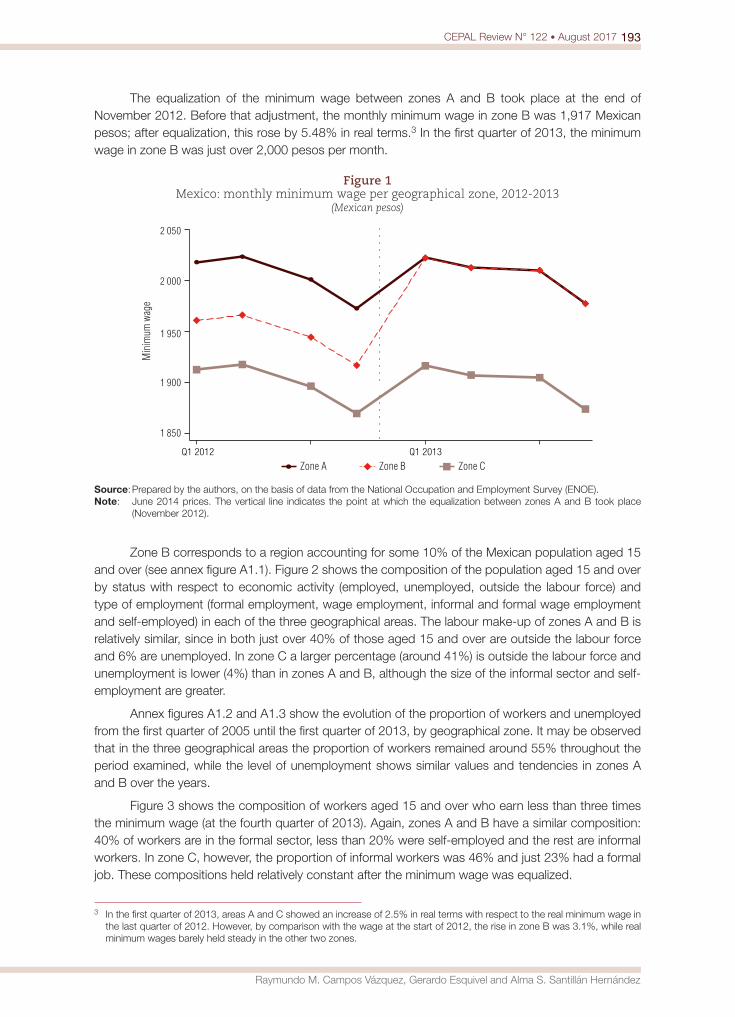
193CEPAL Review N° 122 • August 2017
Raymundo M. Campos Vázquez, Gerardo Esquivel and Alma S. Santillán Hernández
The equalization of the minimum wage between zones A and B took place at the end of November 2012. Before that adjustment, the monthly minimum wage in zone B was 1,917 Mexican pesos; after equalization, this rose by 5.48% in real terms.3 In the first quarter of 2013, the minimum wage in zone B was just over 2,000 pesos per month.
Figure 1 Mexico: monthly minimum wage per geographical zone, 2012-2013
(Mexican pesos)
1 850
1 900
1 950
2 000
2 050
Min
imum
wag
e
Q1 2013Q1 2012
Zone A Zone B Zone C
Source: Prepared by the authors, on the basis of data from the National Occupation and Employment Survey (ENOE).Note: June 2014 prices. The vertical line indicates the point at which the equalization between zones A and B took place
(November 2012).
Zone B corresponds to a region accounting for some 10% of the Mexican population aged 15 and over (see annex figure A1.1). Figure 2 shows the composition of the population aged 15 and over by status with respect to economic activity (employed, unemployed, outside the labour force) and type of employment (formal employment, wage employment, informal and formal wage employment and self-employed) in each of the three geographical areas. The labour make-up of zones A and B is relatively similar, since in both just over 40% of those aged 15 and over are outside the labour force and 6% are unemployed. In zone C a larger percentage (around 41%) is outside the labour force and unemployment is lower (4%) than in zones A and B, although the size of the informal sector and self-employment are greater.
Annex figures A1.2 and A1.3 show the evolution of the proportion of workers and unemployed from the first quarter of 2005 until the first quarter of 2013, by geographical zone. It may be observed that in the three geographical areas the proportion of workers remained around 55% throughout the period examined, while the level of unemployment shows similar values and tendencies in zones A and B over the years.
Figure 3 shows the composition of workers aged 15 and over who earn less than three times the minimum wage (at the fourth quarter of 2013). Again, zones A and B have a similar composition: 40% of workers are in the formal sector, less than 20% were self-employed and the rest are informal workers. In zone C, however, the proportion of informal workers was 46% and just 23% had a formal job. These compositions held relatively constant after the minimum wage was equalized.
3 In the first quarter of 2013, areas A and C showed an increase of 2.5% in real terms with respect to the real minimum wage in the last quarter of 2012. However, by comparison with the wage at the start of 2012, the rise in zone B was 3.1%, while real minimum wages barely held steady in the other two zones.
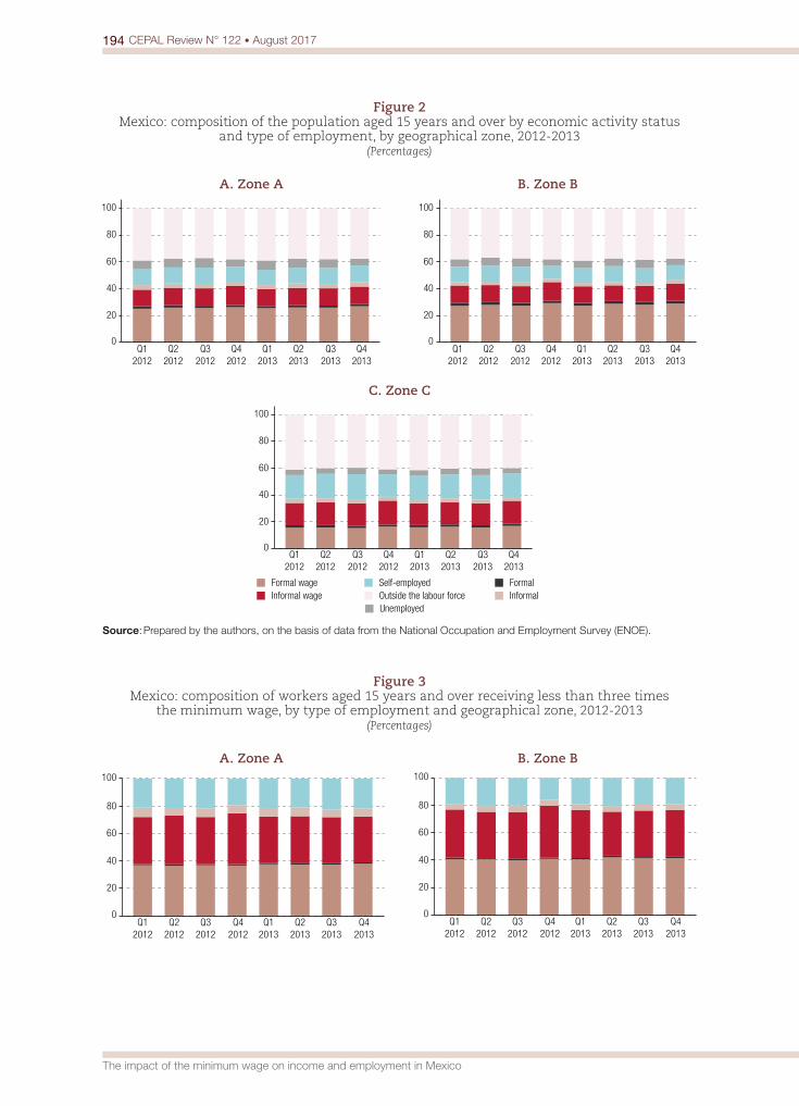
194 CEPAL Review N° 122 • August 2017
The impact of the minimum wage on income and employment in Mexico
Figure 2 Mexico: composition of the population aged 15 years and over by economic activity status
and type of employment, by geographical zone, 2012-2013(Percentages)
A. Zone A B. Zone B
0
20
40
60
80
100
Q12012
Q22012
Q32012
Q42012
Q12013
Q22013
Q32013
Q42013
0
20
40
60
80
100
Q12012
Q22012
Q32012
Q42012
Q12013
Q22013
Q32013
Q42013
C. Zone C
Formal wage FormalInformal wage Informal
Self-employed
UnemployedOutside the labour force
0
20
40
60
80
100
Q12012
Q22012
Q32012
Q42012
Q12013
Q22013
Q32013
Q42013
Source: Prepared by the authors, on the basis of data from the National Occupation and Employment Survey (ENOE).
Figure 3 Mexico: composition of workers aged 15 years and over receiving less than three times
the minimum wage, by type of employment and geographical zone, 2012-2013(Percentages)
A. Zone A B. Zone B
0
20
40
60
80
100
Q12012
Q22012
Q32012
Q42012
Q12013
Q22013
Q32013
Q42013
0
20
40
60
80
100
Q12012
Q22012
Q32012
Q42012
Q12013
Q22013
Q32013
Q42013

195CEPAL Review N° 122 • August 2017
Raymundo M. Campos Vázquez, Gerardo Esquivel and Alma S. Santillán Hernández
C. Zone C
Formal wage Formal
Informal wage InformalSelf-employed
0
20
40
60
80
100
Q12012
Q22012
Q32012
Q42012
Q12013
Q22013
Q32013
Q42013
Source: Prepared by the authors, on the basis of data from the National Occupation and Employment Survey (ENOE).Note: Excludes those not receiving or not specifying income. Minimum wage at fourth quarter of 2013.
Workers’ wages are one of the variables of interest in this work; accordingly, figure 4 shows the evolution of the average wage per geographical zone. It may be seen that the average monthly wage has fallen in real terms in all the geographical areas over time and that it is very similar in zones A and B. At the same time, workers in zone C receive, on average, less income than those in the other two zones.
Figure 4 Mexico: average monthly wage by geographical zone, 2005-2013
(Mexican pesos)
5 000
6 000
7 000
8 000
Zone A Zone B Zone C
Q12005
Q12006
Q12007
Q12008
Q12009
Q12010
Q12011
Q12012
Q12013
Source: Prepared by the authors, on the basis of data from the National Occupation and Employment Survey (ENOE).Note: Persons aged 15 years and over. Excludes those not receiving or not specifying income. June 2014 prices. The vertical
line indicates the point at which the equalization between zones A and B took place.
In order to obtain indications of the possible effects of minimum wage variation in zone B on the wage received in each of the geographical areas, figure 5 presents the evolution of the monthly and hourly average wage received by workers by income level. In principle, it would be expected that those on the lowest income would be the most affected by the rise in the minimum wage in zone B. However, as figure 5 shows, no substantial changes were observed in the average age of those workers receiving less than three times the minimum wage after equalization. In any case, the average monthly wage of those on lower incomes in zone B fell in the third quarter after the change, similarly to the pattern on other parts of the country.
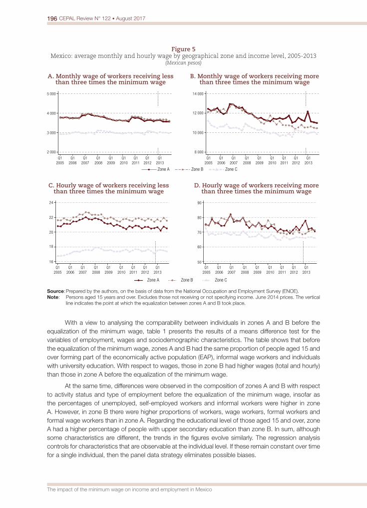
196 CEPAL Review N° 122 • August 2017
The impact of the minimum wage on income and employment in Mexico
Figure 5 Mexico: average monthly and hourly wage by geographical zone and income level, 2005-2013
(Mexican pesos)
A. Monthly wage of workers receiving less than three times the minimum wage
B. Monthly wage of workers receiving more than three times the minimum wage
2 000
3 000
4 000
5 000
8 000
10 000
12 000
14 000
Q12005
Q12006
Q12007
Q12008
Q12009
Q12010
Q12011
Q12012
Q12013
Q12005
Q12006
Q12007
Q12008
Q12009
Q12010
Q12011
Q12012
Q12013
Zone A Zone B Zone C
C. Hourly wage of workers receiving less than three times the minimum wage
D. Hourly wage of workers receiving more than three times the minimum wage
50
60
70
80
90
16
18
20
22
24
Q12005
Q12006
Q12007
Q12008
Q12009
Q12010
Q12011
Q12012
Q12013
Q12005
Q12006
Q12007
Q12008
Q12009
Q12010
Q12011
Q12012
Q12013
Zone A Zone B Zone C
Source: Prepared by the authors, on the basis of data from the National Occupation and Employment Survey (ENOE).Note: Persons aged 15 years and over. Excludes those not receiving or not specifying income. June 2014 prices. The vertical
line indicates the point at which the equalization between zones A and B took place.
With a view to analysing the comparability between individuals in zones A and B before the equalization of the minimum wage, table 1 presents the results of a means difference test for the variables of employment, wages and sociodemographic characteristics. The table shows that before the equalization of the minimum wage, zones A and B had the same proportion of people aged 15 and over forming part of the economically active population (EAP), informal wage workers and individuals with university education. With respect to wages, those in zone B had higher wages (total and hourly) than those in zone A before the equalization of the minimum wage.
At the same time, differences were observed in the composition of zones A and B with respect to activity status and type of employment before the equalization of the minimum wage, insofar as the percentages of unemployed, self-employed workers and informal workers were higher in zone A. However, in zone B there were higher proportions of workers, wage workers, formal workers and formal wage workers than in zone A. Regarding the educational level of those aged 15 and over, zone A had a higher percentage of people with upper secondary education than zone B. In sum, although some characteristics are different, the trends in the figures evolve similarly. The regression analysis controls for characteristics that are observable at the individual level. If these remain constant over time for a single individual, then the panel data strategy eliminates possible biases.

197CEPAL Review N° 122 • August 2017
Raymundo M. Campos Vázquez, Gerardo Esquivel and Alma S. Santillán Hernández
Table 1 Difference in means between zones A and B
Observations Zone A Zone B t-statistic
Logarithm of monthly wagea 99 023 8.4783 8.4876 -1.824*
Logarithm of hourly wagea 99 023 3.3369 3.3876 -10.787***
Economically active population 235 421 0.6204 0.6238 -1.545
Unemployed 235 421 0.0654 0.0576 7.091***
Outside the labour force 235 421 0.3796 0.3762 1.545
Worker 235 421 0.5549 0.5661 -5.091***
Wage workerb 131 464 0.6975 0.7191 -8***
Self-employed or unpaidb 131 464 0.2122 0.1998 5.167***
Formalb 131 464 0.5226 0.5505 -9.3***
Informalb 131 464 0.4774 0.4495 9.3***
Formal wage workerb 131 464 0.4615 0.4865 -8.3***
Informal wage workerb 131 464 0.2359 0.2326 1.320
Age 235 421 39.8438 39.5675 3.561***
Without primary 235 421 0.1031 0.1108 -5.5***
Primary 235 421 0.1974 0.1845 7.167***
Secondary 235 421 0.3075 0.3570 -23.619***
Upper secondary 235 421 0.2404 0.1949 23.947***
University 235 421 0.1516 0.1528 -0.688
Urban 235 421 0.8721 0.8413 20.533***
Man 235 421 0.4743 0.4831 -4***
Source: Prepared by the authors, on the basis of data from the National Occupation and Employment Survey (ENOE).Note: Sample of persons aged 15 years and over observed in 2012. June 2014 prices. Difference significant at *10%, **5%
and ***1%. a Excludes those not receiving or not specifying income.b Limited to those working.
IV. Methodology and results
The aim of this article is to study the possible effects of the increase in the minimum wage in zone B on the employment of workers in that zone. To estimate these effects, the difference-in-difference estimator is used on the basis of cross-section and panel data.
1. Cross-section
To find the difference-in-difference estimator, three econometric specifications are proposed:
Y X zoneB D2013i i i i t i0 1 2 ) )b b b a f= + + + +R W (1)
Y X zoneB D zoneA D2013 2013i i i i i i t i0 1 2 3) ) ) )b b b b a f= + + + + +R RW W (2)
. .
. .
Y X zoneB D zoneB D
zoneB D zoneB D
2013 1 2013 2
2013 3 2013 4i i i i i i
i i i i t i
0 1 2 3
4 3
) ) ) )
) ) ) )
b b b b
b b a f
= + + +
+ + +RR
RR
WW
WW
(3)
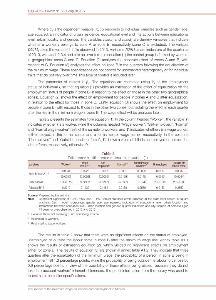
198 CEPAL Review N° 122 • August 2017
The impact of the minimum wage on income and employment in Mexico
Where Yi is the dependent variable, Xi corresponds to individual variables such as gender, age, age squared, an indicator of urban residence, educational level and interactions between educational level, urban locality and gender. The variables zoneAi and zoneBi are dummy variables that indicate whether a worker i belongs to zone A or zone B, respectively (zone C is excluded). The variable D2013i takes the value of 1 if i is observed in 2013. Variables D2013.m are indicators of the quarter m of 2013, with m=1,2,3,4 and ei is an error term. In equation (1) the control group is formed by workers in geographical areas A and C. Equation (2) analyses the separate effect of zones A and B, with respect to C. Equation (3) analyses the effect on zone B in the quarters following the equalization of the minimum wage. These specifications do not control for unobserved heterogeneity or for individual traits that do not vary over time This type of control is included later.
The parameter of interest is β2. The equations are estimated using Yi as the employment status of individual i, so that equation (1) provides an estimation of the effect of equalization on the employment status of people in zone B (in relation to the effect on those in the other two geographical zones). Equation (2) shows the effect on employment for people in zones A and B after equalization, in relation to the effect for those in zone C. Lastly, equation (3) shows the effect on employment for people in zone B, with respect to those in the other two zones, but isolating the effect in each quarter after the rise in the minimum wage in zone B. The wage effect will be analysed later.
Table 2 presents the estimates from equation (1). In the column headed “Worker”, the variable Yi indicates whether i is a worker, while the columns headed “Wage worker”, “Self-employed”, “Formal” and “Formal wage worker” restrict the sample to workers, and Yi indicates whether i is a wage worker, self-employed, in the formal sector and a formal sector wage earner, respectively. In the columns “Unemployed” and “Outside the labour force”, Yi shows a value of 1 if i is unemployed or outside the labour force, respectively, otherwise 0.
Table 2 Difference-in-difference estimator, equation (1)
Variables Workera Wage workera b
Self-employedb Formala b Formal wage
workera c Unemployed Outside the labour force
Zone B*Year 2013-0.0044 -0.0023 -0.0007 0.0081 0.0092 -0.0013 0.0032
[0.0059] [0.0052] [0.0050] [0.0129] [0.0145] [0.0015] [0.0044]
Observations 1 956 622 953 963 953 963 953 963 676 948 2 278 006 2 278 006
Adjusted R^2 0.2212 0.1130 0.1160 0.2158 0.2569 0.0153 0.2650
Source: Prepared by the authors.Note: Coefficient significant at *10%, **5% and ***1%. Robust standard errors adjusted at the state level shown in square
brackets. Each model incorporates gender, age, age squared, indicators of educational level, urban location and interactions between education level, urban location and gender, quarter indicators and city. Sample of persons aged 15 years or over, observed in 2012 and 2013.
a Excludes those not receiving or not specifying income. b Restricted to workers. c Restricted to wage workers.
The results in table 2 show that there were no significant effects on the status of employed, unemployed or outside the labour force in zone B after the minimum wage rise. Annex table A1.1 shows the results of estimating equation (2), which yielded no significant effects on employment either for zone B. The results of equation (3) are shown in annex table A1.2. They indicate that three quarters after the equalization of the minimum wage, the probability of a person in zone B being in employment fell 1.3 percentage points, while the probability of being outside the labour force rose by 0.9 percentage points. In view of the possibility of these effects being biased, because they do not take into account workers’ inherent differences, the panel information from the survey was used to re-estimate the earlier specifications.
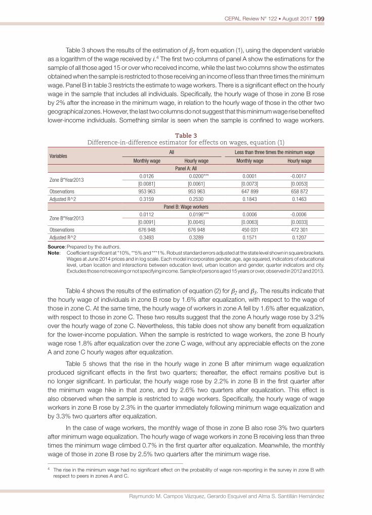
199CEPAL Review N° 122 • August 2017
Raymundo M. Campos Vázquez, Gerardo Esquivel and Alma S. Santillán Hernández
Table 3 shows the results of the estimation of β2 from equation (1), using the dependent variable as a logarithm of the wage received by i.4 The first two columns of panel A show the estimations for the sample of all those aged 15 or over who received income, while the last two columns show the estimates obtained when the sample is restricted to those receiving an income of less than three times the minimum wage. Panel B in table 3 restricts the estimate to wage workers. There is a significant effect on the hourly wage in the sample that includes all individuals. Specifically, the hourly wage of those in zone B rose by 2% after the increase in the minimum wage, in relation to the hourly wage of those in the other two geographical zones. However, the last two columns do not suggest that this minimum wage rise benefited lower-income individuals. Something similar is seen when the sample is confined to wage workers.
Table 3 Difference-in-difference estimator for effects on wages, equation (1)
VariablesAll Less than three times the minimum wage
Monthly wage Hourly wage Monthly wage Hourly wagePanel A: All
Zone B*Year20130.0126 0.0200*** 0.0001 -0.0017
[0.0081] [0.0061] [0.0073] [0.0053]
Observations 953 963 953 963 647 899 658 872
Adjusted R^2 0.3159 0.2530 0.1843 0.1463
Panel B: Wage workers
Zone B*Year20130.0112 0.0196*** 0.0006 -0.0006
[0.0091] [0.0045] [0.0063] [0.0033]
Observations 676 948 676 948 450 031 472 301
Adjusted R^2 0.3493 0.3289 0.1571 0.1207
Source: Prepared by the authors.Note: Coefficient significant at *10%, **5% and ***1%. Robust standard errors adjusted at the state level shown in square brackets.
Wages at June 2014 prices and in log scale. Each model incorporates gender, age, age squared, indicators of educational level, urban location and interactions between education level, urban location and gender, quarter indicators and city. Excludes those not receiving or not specifying income. Sample of persons aged 15 years or over, observed in 2012 and 2013.
Table 4 shows the results of the estimation of equation (2) for β2 and β3. The results indicate that the hourly wage of individuals in zone B rose by 1.6% after equalization, with respect to the wage of those in zone C. At the same time, the hourly wage of workers in zone A fell by 1.6% after equalization, with respect to those in zone C. These two results suggest that the zone A hourly wage rose by 3.2% over the hourly wage of zone C. Nevertheless, this table does not show any benefit from equalization for the lower-income population. When the sample is restricted to wage workers, the zone B hourly wage rose 1.8% after equalization over the zone C wage, without any appreciable effects on the zone A and zone C hourly wages after equalization.
Table 5 shows that the rise in the hourly wage in zone B after minimum wage equalization produced significant effects in the first two quarters; thereafter, the effect remains positive but is no longer significant. In particular, the hourly wage rose by 2.2% in zone B in the first quarter after the minimum wage hike in that zone, and by 2.6% two quarters after equalization. This effect is also observed when the sample is restricted to wage workers. Specifically, the hourly wage of wage workers in zone B rose by 2.3% in the quarter immediately following minimum wage equalization and by 3.3% two quarters after equalization.
In the case of wage workers, the monthly wage of those in zone B also rose 3% two quarters after minimum wage equalization. The hourly wage of wage workers in zone B receiving less than three times the minimum wage climbed 0.7% in the first quarter after equalization. Meanwhile, the monthly wage of those in zone B rose by 2.5% two quarters after the minimum wage rise.
4 The rise in the minimum wage had no significant effect on the probability of wage non-reporting in the survey in zone B with respect to peers in zones A and C.

200 CEPAL Review N° 122 • August 2017
The impact of the minimum wage on income and employment in Mexico
Table 4 Difference-in-difference estimator, equation (2)
VariablesAll Less than three times the minimum wage
Monthly wage Hourly wage Monthly wage Hourly wagePanel A: All
Zone B*Year20130.0082 0.0164** -0.0008 -0.0038
[0.0087] [0.0066] [0.0093] [0.0062]
Zone A*Year2013-0.0194* -0.0158* -0.0046 -0.0099
[0.0097] [0.0086] [0.0139] [0.0089]
Observations 953 963 953 963 647 899 658 872
Adjusted R^2 0.3160 0.2530 0.1843 0.1463
Panel B: Wage workers
Zone B*Year20130.0083 0.0181*** 0.0001 -0.0025
[0.0092] [0.0047] [0.0073] [0.0034]
Zone A*Year2013-0.0121 -0.0064 -0.0026 -0.0086
[0.0072] [0.0047] [0.0096] [0.0063]
Observations 676 948 676 948 450 031 472 301
Adjusted R^2 0.3493 0.3289 0.1571 0.1208
Source: Prepared by the authors.Note: Coefficient significant at *10%, **5% and ***1%. Robust standard errors adjusted at the state level shown in square
brackets. Wages at June 2014 prices and in log scale. Each model incorporates gender, age, age squared, indicators of educational level, urban location and interactions between education level, urban location and gender, quarter indicators and city. Excludes those not receiving or not specifying income. Sample of persons aged 15 years or over, observed in 2012 and 2013.
Table 5 Difference-in-difference estimator, equation (3)
Variables
All Less than three times the minimum wageMonthly wage Hourly wage Monthly wage Hourly wage
Panel A: All
Zone B*Quarter 1 20130.0105 0.0218*** -0.0064 -0.0035
[0.0099] [0.0079] [0.0104] [0.0075]
Zone B*Quarter 2 20130.0248* 0.0262** 0.0138 -0.0057
[0.0137] [0.0127] [0.0128] [0.0108]
Zone B*Quarter 3 20130.0114 0.0196 0.0031 0.0071
[0.0124] [0.0139] [0.0091] [0.0074]
Zone B*Quarter 4 20130.0040 0.0119 -0.0085 -0.0044
[0.0084] [0.0078] [0.0117] [0.0081]
Observations 953 963 953 963 647 899 658 872
Adjusted R^2 0.3159 0.2530 0.1843 0.1463
Panel B: Wage workers
Zone B*Quarter 1 20130.0093 0.0235*** -0.0031 0.0074*
[0.0101] [0.0076] [0.0086] [0.0041]
Zone B*Quarter 2 20130.0304*** 0.0330*** 0.0245** -0.0003
[0.0098] [0.0073] [0.0109] [0.0083]
Zone B*Quarter 3 20130.0037 0.0129 -0.0074 -0.0043
[0.0118] [0.0123] [0.0072] [0.0080]
Zone B*Quarter 4 20130.0017 0.0080 -0.0104 -0.0067
[0.0130] [0.0064] [0.0079] [0.0046]
Observations 676 948 676 948 450 031 472 301
Adjusted R^2 0.3493 0.3289 0.1571 0.1207
Source: Prepared by the authors.Note: Coefficient significant at *10%, **5% and ***1%. Robust standard errors adjusted at the state level shown in square
brackets. Wages at 2014 prices and in log scale. Each model incorporates gender, age, age squared, indicators of educational level, urban location and interactions between education level, urban location and gender, quarter indicators and city. Excludes those not receiving or not specifying income. Sample of persons aged 15 years or over, observed in 2012 and 2013.

201CEPAL Review N° 122 • August 2017
Raymundo M. Campos Vázquez, Gerardo Esquivel and Alma S. Santillán Hernández
2. Robustness
As proof of robustness, equation (1) was estimated with the wage logarithm as the dependent variable, taking only data from 2012, and considering the policy coming into effect after the third quarter of 2012. Table 6 shows the results of the estimation. It will be seen that there are no significant effects in any case. When the date of the new policy is changed, there are no statistically significant results either.
Table 6 Difference-in-difference estimator, equation (1), robustness
VariablesAll Less than three times the minimum wage
Monthly wage Hourly wage Monthly wage Hourly wage
Panel A: All
Zone B*Date0.0018 -0.0017 -0.0009 0.0073
[0.0064] [0.0066] [0.0105] [0.0082]
Observations 482 980 482 980 330 261 330 261
Squared R^2 0.3181 0.2547 0.1874 0.1874
Panel B: Wage earners
Zone B*Date-0.0062 -0.0047 -0.0090 0.0006
[0.0037] [0.0047] [0.0065] [0.0070]
Observations 342 566 342 566 229 467 237 941
Adjusted R^2 0.3526 0.3310 0.1602 0.1223
Source: Prepared by the authors.Note: Coefficient significant at *10%, **5% and ***1%. Robust standard errors adjusted at the state level shown in square
brackets. Wages are at June 2014 prices and log scale. Each model incorporates gender, age, age squared, indicators of educational level, urban location and interactions between education level, urban location and gender, quarter indicators and city. Excludes those not receiving or not specifying income. Sample for individuals aged 15 years and over, observed in 2012. The date indicator takes a value of 1 if it is the third or fourth quarter of 2012, otherwise 0.
3. Uneven effects by gender, age and educational level
In order to determine whether the equalization affected different types of workers in particular, equation (1) was estimated incorporating the variable zoneBi*D2013i, combined with the age, gender and education level of i. Table 7 shows the results of that interaction with the log scale of wage worker i as the dependent variable. After the minimum wage equalization, the wage of workers in zone B without primary schooling rose by 13 percentage points. This was observed both for all wage workers and for those receiving up to three times the minimum wage. The hourly wage for this same group also rose after the minimum wage hike: 13% for all wage workers and 10% for those receiving up to three times the minimum wage.
In the case of wage workers and wage workers receiving up to three times the minimum wage in zone B who had primary education, the hourly wage rose 9.3 and 7 percentage points, respectively, after the minimum wage equalization. The monthly and hourly wage of wage workers in zone B with secondary education rose 7 and 8 percentage points, respectively, after the minimum wage hike, while for wage workers earning less than three times the minimum wage, the monthly wage rose by 8 percentage points and the hourly wage by 7 percentage points.

202 CEPAL Review N° 122 • August 2017
The impact of the minimum wage on income and employment in Mexico
Table 7 Uneven effects on wages by gender, age and educational level
VariablesAll Less than three times the minimum wage
Hourly wage Monthly wage Hourly wage Monthly wage
Zone B*Year 2013*Age-0.0000 -0.0000 -0.0000* -0.0000**
[0.0000] [0.0000] [0.0000] [0.0000]
Zone B*Year 2013*Man0.0087 0.0193 -0.0113 0.0079
[0.0131] [0.0128] [0.0090] [0.0058]
Zone B*Year 2013*No primary0.1371*** 0.1301*** 0.1301*** 0.0999**
[0.0329] [0.0391] [0.0349] [0.0468]
Zone B*Year 2013*Primary0.0620 0.0930*** 0.0637 0.0704*
[0.0394] [0.0309] [0.0420] [0.0395]
Zone B*Year 2013*Secondary0.0695** 0.0822*** 0.0814** 0.0683*
[0.0283] [0.0237] [0.0345] [0.0386]
Zone B*Year 2013*Upper secondary0.0368 0.0609** 0.0547* 0.0576
[0.0319] [0.0249] [0.0303] [0.0372]
Observations 676 948 676 948 450 031 472 301
Adjusted R^2 0.3494 0.3291 0.1572 0.1209
Source: Prepared by the authors.Note: Coefficient significant at *10%, **5% and ***1%. Robust standard errors adjusted at the state level shown in square
brackets. Each model incorporates gender, age, age squared, indicators of educational level, urban location and interactions between education level, urban location and gender, indicators of quarter and city. Excludes those not receiving or not specifying income. Sample for individuals aged 15 years and over, observed in 2012 and 2013.
4. Analysis of panel data
This section uses information from National Occupation and Employment Survey, taking advantage of the panel structure of the data. Three panel databases were built, observing individuals aged 15 and over at two points in time. The first is of individuals observed in the second quarter of 2012 and the second quarter of 2013. The second database is of individuals observed in the fourth quarter of 2012 and the first quarter of 2013. Lastly, the third database groups individuals observed in the fourth quarter of 2012 and the second quarter of 2013. Those observed in December 2012 are excluded from the second two panels, since this was when the minimum wage was equalized between zones A and B. The three panels were built to analyse the sensitivity of the results and to take into account calendar effects that could differ between geographical areas.5
To find the difference-in-difference estimator in panel data, the following equation was calculated:
) )b a+ +Y X zoneB D a2013it it i i t i i0 1 2b b f= + + +R W (4)
where Yit is the dependent variable, Xit corresponds to individual variables that change over time, such as age, age squared and education level, zoneBi indicates whether worker i belongs to zone B, D2013i takes a value of 1 if i is observed in the year 2013, ai is an individual fixed effect variable and εit is an error term. The fixed effect controls for any time invariant differences not observed at the individual level.
5 To analyse the efects of minimum wage equalization on contact rates in the second round of observations, equation (4) was estimated using as a dependent variable the dichotomy whereby 1 means that the individual was observed in the second round of panel data and 0 means otherwise. The effects were analysed for different types of samples restricted by activity status in the first round of observation. The estimations are presented in annex tables A1.12 and A1.13. In the first three panels used, individuals in zone B who were outside the labour force were more likely not to be contacted in the following round than those in zones A and C, after the minimum wage equalization. In comparing zones A and B, it was observed that only in one panel were individuals who participated in the labour market in zone B more likely than those in zone A not to be contacted again after the minimum wage was raised.
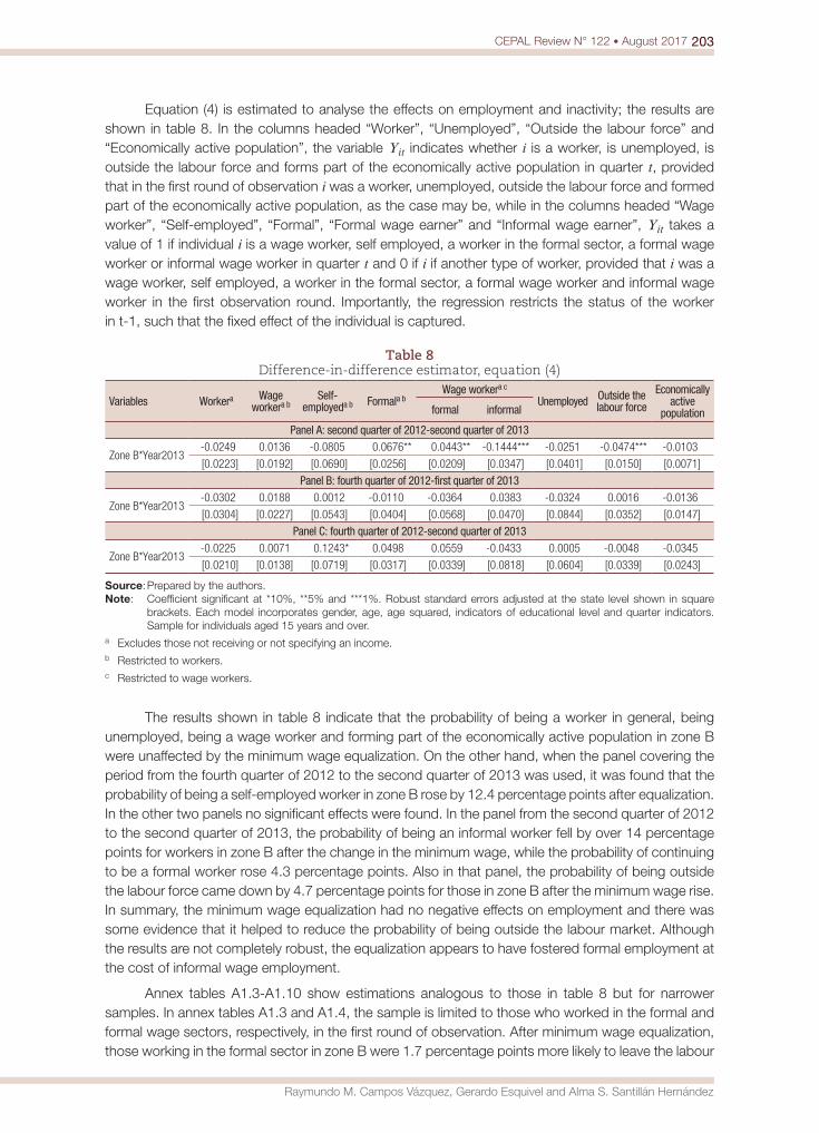
203CEPAL Review N° 122 • August 2017
Raymundo M. Campos Vázquez, Gerardo Esquivel and Alma S. Santillán Hernández
Equation (4) is estimated to analyse the effects on employment and inactivity; the results are shown in table 8. In the columns headed “Worker”, “Unemployed”, “Outside the labour force” and “Economically active population”, the variable Yit indicates whether i is a worker, is unemployed, is outside the labour force and forms part of the economically active population in quarter t, provided that in the first round of observation i was a worker, unemployed, outside the labour force and formed part of the economically active population, as the case may be, while in the columns headed “Wage worker”, “Self-employed”, “Formal”, “Formal wage earner” and “Informal wage earner”, Yit takes a value of 1 if individual i is a wage worker, self employed, a worker in the formal sector, a formal wage worker or informal wage worker in quarter t and 0 if i if another type of worker, provided that i was a wage worker, self employed, a worker in the formal sector, a formal wage worker and informal wage worker in the first observation round. Importantly, the regression restricts the status of the worker in t-1, such that the fixed effect of the individual is captured.
Table 8 Difference-in-difference estimator, equation (4)
Variables Workera Wage workera b
Self-employeda b Formala b
Wage workera c
Unemployed Outside the labour force
Economically active
populationformal informal
Panel A: second quarter of 2012-second quarter of 2013
Zone B*Year2013-0.0249 0.0136 -0.0805 0.0676** 0.0443** -0.1444*** -0.0251 -0.0474*** -0.0103
[0.0223] [0.0192] [0.0690] [0.0256] [0.0209] [0.0347] [0.0401] [0.0150] [0.0071]
Panel B: fourth quarter of 2012-first quarter of 2013
Zone B*Year2013-0.0302 0.0188 0.0012 -0.0110 -0.0364 0.0383 -0.0324 0.0016 -0.0136
[0.0304] [0.0227] [0.0543] [0.0404] [0.0568] [0.0470] [0.0844] [0.0352] [0.0147]
Panel C: fourth quarter of 2012-second quarter of 2013
Zone B*Year2013-0.0225 0.0071 0.1243* 0.0498 0.0559 -0.0433 0.0005 -0.0048 -0.0345
[0.0210] [0.0138] [0.0719] [0.0317] [0.0339] [0.0818] [0.0604] [0.0339] [0.0243]
Source: Prepared by the authors.Note: Coefficient significant at *10%, **5% and ***1%. Robust standard errors adjusted at the state level shown in square
brackets. Each model incorporates gender, age, age squared, indicators of educational level and quarter indicators. Sample for individuals aged 15 years and over.
a Excludes those not receiving or not specifying an income. b Restricted to workers. c Restricted to wage workers.
The results shown in table 8 indicate that the probability of being a worker in general, being unemployed, being a wage worker and forming part of the economically active population in zone B were unaffected by the minimum wage equalization. On the other hand, when the panel covering the period from the fourth quarter of 2012 to the second quarter of 2013 was used, it was found that the probability of being a self-employed worker in zone B rose by 12.4 percentage points after equalization. In the other two panels no significant effects were found. In the panel from the second quarter of 2012 to the second quarter of 2013, the probability of being an informal worker fell by over 14 percentage points for workers in zone B after the change in the minimum wage, while the probability of continuing to be a formal worker rose 4.3 percentage points. Also in that panel, the probability of being outside the labour force came down by 4.7 percentage points for those in zone B after the minimum wage rise. In summary, the minimum wage equalization had no negative effects on employment and there was some evidence that it helped to reduce the probability of being outside the labour market. Although the results are not completely robust, the equalization appears to have fostered formal employment at the cost of informal wage employment.
Annex tables A1.3-A1.10 show estimations analogous to those in table 8 but for narrower samples. In annex tables A1.3 and A1.4, the sample is limited to those who worked in the formal and formal wage sectors, respectively, in the first round of observation. After minimum wage equalization, those working in the formal sector in zone B were 1.7 percentage points more likely to leave the labour
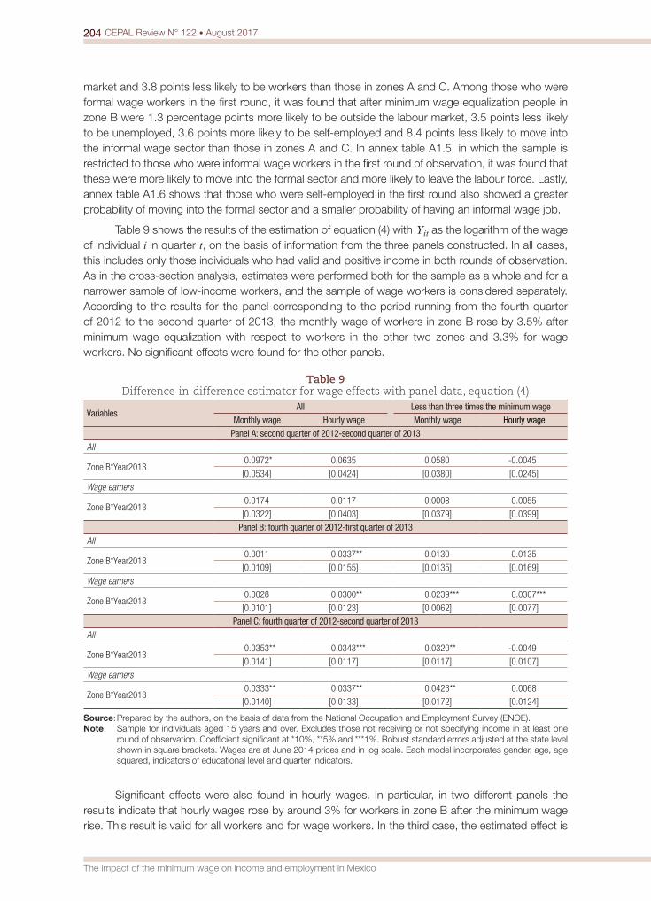
204 CEPAL Review N° 122 • August 2017
The impact of the minimum wage on income and employment in Mexico
market and 3.8 points less likely to be workers than those in zones A and C. Among those who were formal wage workers in the first round, it was found that after minimum wage equalization people in zone B were 1.3 percentage points more likely to be outside the labour market, 3.5 points less likely to be unemployed, 3.6 points more likely to be self-employed and 8.4 points less likely to move into the informal wage sector than those in zones A and C. In annex table A1.5, in which the sample is restricted to those who were informal wage workers in the first round of observation, it was found that these were more likely to move into the formal sector and more likely to leave the labour force. Lastly, annex table A1.6 shows that those who were self-employed in the first round also showed a greater probability of moving into the formal sector and a smaller probability of having an informal wage job.
Table 9 shows the results of the estimation of equation (4) with Yit as the logarithm of the wage of individual i in quarter t, on the basis of information from the three panels constructed. In all cases, this includes only those individuals who had valid and positive income in both rounds of observation. As in the cross-section analysis, estimates were performed both for the sample as a whole and for a narrower sample of low-income workers, and the sample of wage workers is considered separately. According to the results for the panel corresponding to the period running from the fourth quarter of 2012 to the second quarter of 2013, the monthly wage of workers in zone B rose by 3.5% after minimum wage equalization with respect to workers in the other two zones and 3.3% for wage workers. No significant effects were found for the other panels.
Table 9 Difference-in-difference estimator for wage effects with panel data, equation (4)
VariablesAll Less than three times the minimum wage
Monthly wage Hourly wage Monthly wage Hourly wagePanel A: second quarter of 2012-second quarter of 2013
All
Zone B*Year20130.0972* 0.0635 0.0580 -0.0045
[0.0534] [0.0424] [0.0380] [0.0245]
Wage earners
Zone B*Year2013-0.0174 -0.0117 0.0008 0.0055
[0.0322] [0.0403] [0.0379] [0.0399]
Panel B: fourth quarter of 2012-first quarter of 2013All
Zone B*Year20130.0011 0.0337** 0.0130 0.0135
[0.0109] [0.0155] [0.0135] [0.0169]
Wage earners
Zone B*Year20130.0028 0.0300** 0.0239*** 0.0307***
[0.0101] [0.0123] [0.0062] [0.0077]
Panel C: fourth quarter of 2012-second quarter of 2013All
Zone B*Year20130.0353** 0.0343*** 0.0320** -0.0049
[0.0141] [0.0117] [0.0117] [0.0107]
Wage earners
Zone B*Year20130.0333** 0.0337** 0.0423** 0.0068
[0.0140] [0.0133] [0.0172] [0.0124]
Source: Prepared by the authors, on the basis of data from the National Occupation and Employment Survey (ENOE).Note: Sample for individuals aged 15 years and over. Excludes those not receiving or not specifying income in at least one
round of observation. Coefficient significant at *10%, **5% and ***1%. Robust standard errors adjusted at the state level shown in square brackets. Wages are at June 2014 prices and in log scale. Each model incorporates gender, age, age squared, indicators of educational level and quarter indicators.
Significant effects were also found in hourly wages. In particular, in two different panels the results indicate that hourly wages rose by around 3% for workers in zone B after the minimum wage rise. This result is valid for all workers and for wage workers. In the third case, the estimated effect is
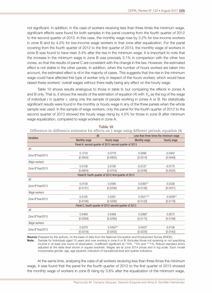
205CEPAL Review N° 122 • August 2017
Raymundo M. Campos Vázquez, Gerardo Esquivel and Alma S. Santillán Hernández
not significant. In addition, in the case of workers receiving less than three times the minimum wage, significant effects were found for both samples in the panel covering from the fourth quarter of 2012 to the second quarter of 2013. In this case, the monthly wage rose by 3.2% for low-income workers in zone B and by 4.2% for low-income wage workers in that zone after equalization. For the panel covering from the fourth quarter of 2012 to the first quarter of 2013, the monthly wage of workers in zone B was found to have risen 3.4% after the rise in the minimum wage. It is important to note that the increase in the minimum wage in zone B was precisely 3.1% in comparison with the other two zones, so that the results of panel C are consistent with the change in the law. However, the estimated effect is not stable in the other panels. In addition, when the number of hours worked are taken into account, the estimated effect is nil in the majority of cases. This suggests that the rise in the minimum wage could have affected this type of worker only in respect of the hours worked, which would have raised these workers’ overall wages without there really being any effect on the hourly wage.
Table 10 shows results analogous to those in table 9, but comparing the effects in zones A and B only. That is, it shows the results of the estimation of equation (4) with Yit as the log of the wage of individual i in quarter t, using only the sample of people working in zones A or B. No statistically significant results were found in the monthly or hourly wage in any of the three panels when the whole sample was used. In the sample of wage workers, only the panel for the fourth quarter of 2012 to the second quarter of 2013 showed the hourly wage rising by 4.5% for those in zone B after minimum wage equalization, compared to wage workers in zone A.
Table 10 Difference-in-difference estimator for effects on 1 wage using different periods, equation (4)
VariablesAll Less than three times the minimum wage
Monthly wage Hourly wage Monthly wage Hourly wagePanel A: second quarter of 2012-second quarter of 2013
All
Zone B*Year20130.1218 0.0779 0.0090 -0.0402
[0.0934] [0.0902] [0.0510] [0.0449]
Wage workers
Zone B*Year20130.0158 0.0195 -0.0127 -0.0175
[0.0604] [0.0754] [0.0546] [0.0525]
Panel B: fourth quarter of 2012-first quarter of 2013All
Zone B*Year20130.0158 0.0390 0.0382** 0.0338
[0.0151] [0.0256] [0.0126] [0.0221]
Wage workers
Zone B*Year20130.0105 0.0261 0.0521*** 0.0439**
[0.0106] [0.0206] [0.0122] [0.0178]
Panel C: fourth quarter of 2012-second quarter of 2013All
Zone B*Year20130.0469 0.0469 0.0366* 0.0073
[0.0269] [0.0280] [0.0172] [0.0199]
Wage workers
Zone B*Year20130.0379 0.0455** 0.0425* 0.0136
[0.0218] [0.0202] [0.0225] [0.0182]
Source: Prepared by the authors, on the basis of data from the National Occupation and Employment Survey (ENOE).Note: Sample for individuals aged 15 years and over working in zone A or B. Excludes those not receiving or not specifying
income in at least one round of observation. Coefficient significant at *10%, **5% and ***1%. Robust standard errors adjusted at the state level shown in square brackets. Wages are at June 2014 prices and in log scale. Each model incorporates gender, age, age squared, indicators of educational level and quarter indicators.
At the same time, analysing the case of all workers receiving less than three times the minimum wage, it was found that the panel for the fourth quarter of 2012 to the first quarter of 2013 showed the monthly wage of workers in zone B rising by 3.8% after the equalization of the minimum wage,
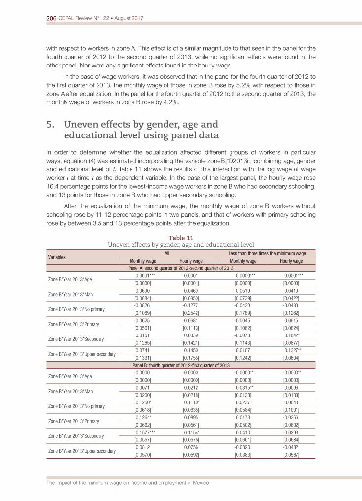
206 CEPAL Review N° 122 • August 2017
The impact of the minimum wage on income and employment in Mexico
with respect to workers in zone A. This effect is of a similar magnitude to that seen in the panel for the fourth quarter of 2012 to the second quarter of 2013, while no significant effects were found in the other panel. Nor were any significant effects found in the hourly wage.
In the case of wage workers, it was observed that in the panel for the fourth quarter of 2012 to the first quarter of 2013, the monthly wage of those in zone B rose by 5.2% with respect to those in zone A after equalization. In the panel for the fourth quarter of 2012 to the second quarter of 2013, the monthly wage of workers in zone B rose by 4.2%.
5. Uneven effects by gender, age and educational level using panel data
In order to determine whether the equalization affected different groups of workers in particular ways, equation (4) was estimated incorporating the variable zoneBit*D2013it, combining age, gender and educational level of i. Table 11 shows the results of this interaction with the log wage of wage worker i at time t as the dependent variable. In the case of the largest panel, the hourly wage rose 16.4 percentage points for the lowest-income wage workers in zone B who had secondary schooling, and 13 points for those in zone B who had upper secondary schooling.
After the equalization of the minimum wage, the monthly wage of zone B workers without schooling rose by 11-12 percentage points in two panels, and that of workers with primary schooling rose by between 3.5 and 13 percentage points after the equalization.
Table 11 Uneven effects by gender, age and educational level
VariablesAll Less than three times the minimum wage
Monthly wage Hourly wage Monthly wage Hourly wagePanel A: second quarter of 2012-second quarter of 2013
Zone B*Year 2013*Age0.0001*** 0.0001 0.0000*** 0.0001***
[0.0000] [0.0001] [0.0000] [0.0000]
Zone B*Year 2013*Man-0.0690 -0.0469 -0.0519 0.0410
[0.0884] [0.0850] [0.0739] [0.0422]
Zone B*Year 2013*No primary-0.0826 -0.1277 -0.0430 -0.0430
[0.1089] [0.2542] [0.1789] [0.1262]
Zone B*Year 2013*Primary-0.0625 -0.0681 -0.0045 0.0615
[0.0561] [0.1113] [0.1062] [0.0824]
Zone B*Year 2013*Secondary0.0151 0.0339 -0.0078 0.1642*
[0.1265] [0.1421] [0.1143] [0.0877]
Zone B*Year 2013*Upper secondary0.0741 0.1450 0.0107 0.1327**
[0.1331] [0.1755] [0.1242] [0.0604]
Panel B: fourth quarter of 2012-first quarter of 2013
Zone B*Year 2013*Age-0.0000 -0.0000 -0.0000** -0.0000**
[0.0000] [0.0000] [0.0000] [0.0000]
Zone B*Year 2013*Man-0.0071 0.0212 -0.0315** -0.0096
[0.0200] [0.0218] [0.0133] [0.0138]
Zone B*Year 2013*No primary0.1250* 0.1110* 0.0237 0.0043
[0.0618] [0.0635] [0.0584] [0.1001]
Zone B*Year 2013*Primary0.1264* 0.0895 0.0173 -0.0366
[0.0662] [0.0561] [0.0502] [0.0602]
Zone B*Year 2013*Secondary0.1577*** 0.1154* 0.0410 -0.0293
[0.0557] [0.0575] [0.0601] [0.0684]
Zone B*Year 2013*Upper secondary0.0812 0.0756 -0.0320 -0.0432
[0.0570] [0.0592] [0.0383] [0.0567]

207CEPAL Review N° 122 • August 2017
Raymundo M. Campos Vázquez, Gerardo Esquivel and Alma S. Santillán Hernández
VariablesAll Less than three times the minimum wage
Monthly wage Hourly wage Monthly wage Hourly wagePanel C: fourth quarter of 2012-second quarter of 2013
Zone B*Year 2013*Age-0.0000 0.0000 -0.0000* -0.0000
[0.0000] [0.0000] [0.0000] [0.0000]
Zone B*Year 2013*Man-0.0073 0.0180 -0.0131** 0.0217
[0.0154] [0.0342] [0.0055] [0.0239]
Zone B*Year 2013*No primary0.1081*** -0.0283 -0.0059 -0.0041
[0.0318] [0.0450] [0.0680] [0.0723]
Zone B*Year 2013*Primary0.0350** -0.0901*** -0.0649 -0.1260**
[0.0159] [0.0264] [0.0773] [0.0609]
Zone B*Year 2013*Secondary0.0598 -0.0180 -0.0727 -0.0581
[0.0356] [0.0449] [0.0728] [0.0682]
Zone B*Year 2013*Upper secondary0.0392 0.0181 -0.0877* -0.0001
[0.0431] [0.0391] [0.0487] [0.0426]
Source: Prepared by the authors.Note: Coefficient significant at *10%, **5% and ***1%. Robust standard errors adjusted at the state level shown in square
brackets. Each model incorporates gender, age, age squared, indicators of educational level, urban location and interactions between educational level, urban location and gender, quarter indicators and city. Excludes those not receiving or not specifying income. Sample for individuals aged 15 years and over.
V. Conclusions
This work has found at least three results worthy of note. First, in no instance was evidence found of negative effects on employment or on income following the decision to increase the minimum wage in geographical zone B. Second, there is evidence that the decision to align minimum wages in zone B with those in zone A led to an increase in workers’ hourly wages and, in some cases, in their total wages. Third and perhaps most important, the rise in the minimum wage in zone B may have shifted the incentives, such that both those who were originally informal wage workers and those who were self-employed showed a greater propensity to move into formal employment. The propensity to remain in formal employment also appears to have increased and, in at least one case, the propensity to be unemployed decreased.
All these results should be treated with caution, however, and they cannot be readily extrapolated to other cases or other economies. There are at least two reasons for this: first, because the increase produced by the wage equalization was relatively small (3.1% in real terms) and, second, because the minimum wage in Mexico has fallen over 70% in real terms in the past three decades, so the slack in Mexican labour markets may very well not apply to other contexts or other economies.
Table 11 (concluded)
208 CEPAL Review N° 122 • August 2017
The impact of the minimum wage on income and employment in Mexico
Bibliography
Bell, L. (1997), “The impact of minimum wages in Mexico and Colombia”, Journal of Labor Economics, vol. 15, No. 3, Chicago, University of Chicago Press.
Bosch, M. and M. Manacorda (2010), “Minimum wages and earnings inequality in urban Mexico”, American Economic Journal: Applied Economics, vol. 2, No. 4, Nashville, Tennessee, American Economic Association.
Campos Vázquez, R.M. (2015), “El minimum wage y el empleo: evidencia internacional y posibles impactos para el caso mexicano”, Economía UNAM, vol. 12, No. 36, National Autonomous University of Mexico.
Card, D. and A. Krueger (1994), “Minimum wages and employment: a case study of the fast-food industry in New Jersey and Pennsylvania”, American Economic Review, vol. 84, No. 4, Nashville, Tennessee, American Economic Association.
Dube, A., W. Lester and M. Reich (2010), “Minimum wage effects across state borders: estimates using contiguous counties”, The Review of Economics and Statistics, vol. 92, No. 4, Cambridge, Massachusetts, The MIT Press.
Elwell, C. (2014), “Inflation and the real minimum wage: a fact sheet”, Congressional Research Service, 8 January [online] https://fas.org/sgp/crs/misc/R42973.pdf.
Gindling, T.H. and K. Terrell (2009), “Minimum wages, wages and employment in various sectors in Honduras”, Labour Economics, vol. 16, No. 3, Amsterdam, Elsevier.
Kaplan, D. and F. Pérez Arce (2006), “El efecto de los salarios mínimos en los ingresos laborales de México”, El Trimestre Económico, vol. 73, No. 289, Fondo de Cultura Económica.
Lemos, S. (2009), “Minimum wage effects in a developing country”, Labour Economics, vol. 16, No. 2, Amsterdam, Elsevier.
Manning, A. (2012), “Minimum wage: maximum impact”, The Resolution Foundation [online] http://www.resolutionfoundation.org/app/uploads/2014/08/Final-Minimum-wage-paper_vFinal.pdf.
Neumark, D. and W.L. Wascher (2008), Minimum Wages, Cambridge, Massachusetts, The MIT Press.Neumark, D., W. Cunningham and L. Siga (2006), “The effects of the minimum wage in Brazil on the distribution
of family incomes: 1996-2001”, Journal of Development Economics, vol. 80, No. 1, Amsterdam, Elsevier.Stewart, M. (2004), “The employment effects of the national minimum wage”, Economic Journal, vol. 114,
No. 494, Wiley.
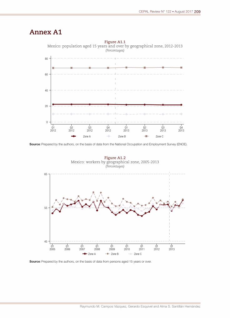
209CEPAL Review N° 122 • August 2017
Raymundo M. Campos Vázquez, Gerardo Esquivel and Alma S. Santillán Hernández
Annex A1Figure A1.1
Mexico: population aged 15 years and over by geographical zone, 2012-2013(Percentages)
0
20
40
60
80
Zone A Zone B Zone C
Q12012
Q22012
Q32012
Q42012
Q12013
Q22013
Q32013
Q42013
Source: Prepared by the authors, on the basis of data from the National Occupation and Employment Survey (ENOE).
Figure A1.2 Mexico: workers by geographical zone, 2005-2013
(Percentages)
45
55
65
Zone A Zone B Zone C
Q12005
Q12006
Q12007
Q12008
Q12009
Q12010
Q12011
Q12012
Q12013
Source: Prepared by the authors, on the basis of data from persons aged 15 years or over.
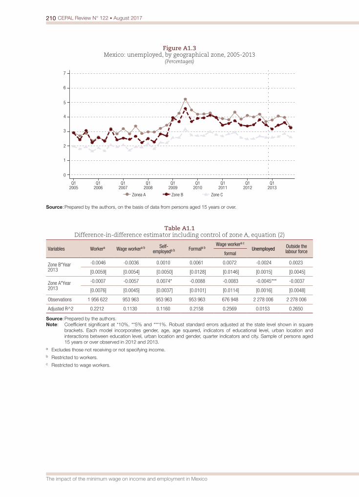
210 CEPAL Review N° 122 • August 2017
The impact of the minimum wage on income and employment in Mexico
Figure A1.3 Mexico: unemployed, by geographical zone, 2005-2013
(Percentages)
0
1
2
3
4
5
6
7
Zonea A Zone B Zone C
Q12005
Q12006
Q12013
Q12007
Q12008
Q12009
Q12010
Q12011
Q12012
Source: Prepared by the authors, on the basis of data from persons aged 15 years or over.
Table A1.1 Difference-in-difference estimator including control of zone A, equation (2)
Variables Workera Wage workera b Self-employeda b Formala b
Wage workera c
Unemployed Outside the labour forceformal
Zone B*Year 2013
-0.0046 -0.0036 0.0010 0.0061 0.0072 -0.0024 0.0023
[0.0059] [0.0054] [0.0050] [0.0128] [0.0146] [0.0015] [0.0045]
Zone A*Year 2013
-0.0007 -0.0057 0.0074* -0.0088 -0.0083 -0.0045*** -0.0037
[0.0076] [0.0045] [0.0037] [0.0101] [0.0114] [0.0016] [0.0048]
Observations 1 956 622 953 963 953 963 953 963 676 948 2 278 006 2 278 006
Adjusted R^2 0.2212 0.1130 0.1160 0.2158 0.2569 0.0153 0.2650
Source: Prepared by the authors.Note: Coefficient significant at *10%, **5% and ***1%. Robust standard errors adjusted at the state level shown in square
brackets. Each model incorporates gender, age, age squared, indicators of educational level, urban location and interactions between education level, urban location and gender, quarter indicators and city. Sample of persons aged 15 years or over observed in 2012 and 2013.
a Excludes those not receiving or not specifying income. b Restricted to workers. c Restricted to wage workers.

211CEPAL Review N° 122 • August 2017
Raymundo M. Campos Vázquez, Gerardo Esquivel and Alma S. Santillán Hernández
Table A1.2 Difference-in-difference estimator with effects for each quarter of 2013, equation (3)
Variables Workera Wage workera b Self-employeda b Formala b
Wage workera c
Unemployed Outside the labour forceformal
Zone B*Quarter 1 2013
0.0016 0.0048 -0.0077 0.0087 0.0072 -0.0034 0.0023
[0.0054] [0.0043] [0.0047] [0.0110] [0.0096] [0.0030] [0.0045]
Zone B*Quarter 2 2013
0.0000 -0.0076 0.0071 0.0116 0.0166 -0.0005 -0.0016
[0.0085] [0.0054] [0.0049] [0.0083] [0.0114] [0.0017] [0.0058]
Zone B*Quarter 3 2013
-0.0127*** -0.0045 -0.0008 0.0032 0.0055 -0.0002 0.0092**
[0.0043] [0.0095] [0.0072] [0.0194] [0.0208] [0.0026] [0.0044]
Zone B*Quarter 4 2013
-0.0082 -0.0035 0.0002 0.0084 0.0079 -0.0007 0.0031
[0.0115] [0.0072] [0.0059] [0.0162] [0.0205] [0.0032] [0.0097]
Observations 1 956 622 953 963 953 963 953 963 676 948 2 278 006 2 278 006
Adjusted R^2 0.2212 0.1130 0.1160 0.2158 0.2569 0.0153 0.2650
Source: Prepared by the authors.Note: Coefficient significant at *10%, **5% and ***1%. Robust standard errors adjusted at the state level shown in square
brackets. Each model incorporates gender, age, age squared, indicators of educational level, urban location and interactions between education level, urban location and gender, quarter indicators and city. Sample of persons aged 15 years or over, observed in 2012 and 2013.
a Excludes those not receiving or not specifying income. b Restricted to workers. c Restricted to wage workers.
Table A1.3 Difference-in-difference estimator for wage workers only, equation (4)
Variables Workera Wage workera b Self-employeda b
Wage workera c
Unemployed Outside the labour forceformal informal
Panel A: second quarter of 2012-second quarter of 2013
Zone B*Year2013-0.0381* 0.0135 -0.0125 0.0352* -0.0217 0.0096 0.0176***
[0.0211] [0.0106] [0.0098] [0.0190] [0.0130] [0.0077] [0.0047]
Panel B: fourth quarter of 2012-first quarter of 2013
Zone B*Year2013-0.0248 -0.0205 0.0034 -0.0407 0.0202 0.0170 0.0050
[0.0387] [0.0164] [0.0064] [0.0609] [0.0471] [0.0155] [0.0284]
Panel C: fourth quarter of 2012-second quarter of 2013
Zone B*Year2013-0.0021 -0.0026 0.0221 0.0519 -0.0545 -0.0312** 0.0199
[0.0445] [0.0107] [0.0192] [0.0334] [0.0326] [0.0149] [0.0198]
Source: Prepared by the authors.Note: Coefficient significant at *10%, **5% and ***1%. Robust standard errors adjusted at the state level shown in square
brackets. Each model incorporates gender, age, age squared, indicators of educational level and quarter indicators. Sample of persons aged 15 years or over.
a Excludes those not receiving or not specifying income. b Restricted to workers. c Restricted to wage workers. Restricted to those figuring as formal workers in the first observation round.
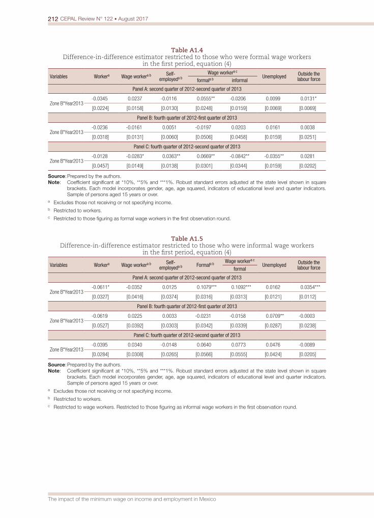
212 CEPAL Review N° 122 • August 2017
The impact of the minimum wage on income and employment in Mexico
Table A1.4 Difference-in-difference estimator restricted to those who were formal wage workers
in the first period, equation (4)
Variables Workera Wage workera b Self-employeda b
Wage workera c
Unemployed Outside the labour forceformala b informal
Panel A: second quarter of 2012-second quarter of 2013
Zone B*Year2013-0.0345 0.0237 -0.0116 0.0555** -0.0206 0.0099 0.0131*
[0.0224] [0.0158] [0.0130] [0.0248] [0.0159] [0.0069] [0.0069]
Panel B: fourth quarter of 2012-first quarter of 2013
Zone B*Year2013-0.0236 -0.0161 0.0051 -0.0197 0.0203 0.0161 0.0038
[0.0318] [0.0131] [0.0060] [0.0506] [0.0458] [0.0159] [0.0251]
Panel C: fourth quarter of 2012-second quarter of 2013
Zone B*Year2013-0.0128 -0.0283* 0.0363** 0.0669** -0.0842** -0.0355** 0.0281
[0.0457] [0.0149] [0.0138] [0.0301] [0.0344] [0.0159] [0.0202]
Source: Prepared by the authors.Note: Coefficient significant at *10%, **5% and ***1%. Robust standard errors adjusted at the state level shown in square
brackets. Each model incorporates gender, age, age squared, indicators of educational level and quarter indicators. Sample of persons aged 15 years or over.
a Excludes those not receiving or not specifying income. b Restricted to workers. c Restricted to those figuring as formal wage workers in the first observation round.
Table A1.5 Difference-in-difference estimator restricted to those who were informal wage workers
in the first period, equation (4)
Variables Workera Wage workera b Self-employeda b Formala b Wage workera c
Unemployed Outside the labour forceformal
Panel A: second quarter of 2012-second quarter of 2013
Zone B*Year2013-0.0611* -0.0352 0.0125 0.1079*** 0.1092*** 0.0162 0.0354***
[0.0327] [0.0416] [0.0374] [0.0316] [0.0313] [0.0121] [0.0112]
Panel B: fourth quarter of 2012-first quarter of 2013
Zone B*Year2013-0.0619 0.0225 0.0033 -0.0231 -0.0158 0.0709** -0.0003
[0.0527] [0.0392] [0.0303] [0.0342] [0.0339] [0.0287] [0.0238]
Panel C: fourth quarter of 2012-second quarter of 2013
Zone B*Year2013-0.0395 0.0340 -0.0148 0.0640 0.0773 0.0476 -0.0089
[0.0284] [0.0308] [0.0265] [0.0566] [0.0555] [0.0424] [0.0205]
Source: Prepared by the authors.Note: Coefficient significant at *10%, **5% and ***1%. Robust standard errors adjusted at the state level shown in square
brackets. Each model incorporates gender, age, age squared, indicators of educational level and quarter indicators. Sample of persons aged 15 years or over.
a Excludes those not receiving or not specifying income. b Restricted to workers. c Restricted to wage workers. Restricted to those figuring as informal wage workers in the first observation round.

213CEPAL Review N° 122 • August 2017
Raymundo M. Campos Vázquez, Gerardo Esquivel and Alma S. Santillán Hernández
Table A1.6 Difference-in-difference estimator restricted to workers who were self-employed
in the first period, equation (4)
Variables Workera Wage workera b Formala b Wage workera c
Unemployed Outside the labour forceformal informal
Panel A: second quarter of 2012-second quarter of 2013
Zone B*Year20130.0038 0.0804 0.1040* 0.0970** -0.0166 -0.0037 0.0063
[0.0337] [0.0618] [0.0610] [0.0430] [0.0299] [0.0086] [0.0224]
Panel B: fourth quarter of 2012-first quarter of 2013
Zone B*Year2013-0.0476 -0.0059 0.2143 -0.0687* 0.0628* 0.0305 0.0082
[0.0688] [0.0432] [0.2032] [0.0373] [0.0345] [0.0517] [0.0742]
Panel C: fourth quarter of 2012-second quarter of 2013
Zone B*Year2013-0.0059 -0.0569 -0.0846 -0.0528* -0.0041 -0.0759*** 0.0816
[0.1071] [0.0657] [0.0655] [0.0287] [0.0557] [0.0234] [0.1110]
Source: Prepared by the authors.Note: Coefficient significant at *10%, **5% and ***1%. Robust standard errors adjusted at the state level shown in square
brackets. Each model incorporates gender, age, age squared, indicators of educational level and quarter indicators. Sample of persons aged 15 years or over.
a Excludes those not receiving or not specifying income. b Restricted to workers. c Restricted to wage workers. Restricted to those figuring as self-employed workers in the first observation round.
Table A1.7 Difference-in-difference estimator for wages restricted to wage workers, equation (4)
Variables Workera Wage workera b
Self-employeda b Formala b Wage workera c
Unemployed Outside the labour force EAP
formal informal
Panel A: second quarter of 2012-second quarter of 2013
Zone B*Year2013-0.0051 0.0204 -0.0209 0.0425 0.0428 -0.1558*** -0.0895 -0.0129 -0.0269**
[0.0345] [0.0275] [0.0881] [0.0272] [0.0295] [0.0306] [0.0701] [0.0189] [0.0092]
Panel B: fourth quarter of 2012-first quarter of 2013
Zone B*Year2013-0.0077 0.0001 0.0028 -0.0473 -0.0624 0.0420 -0.1463 -0.0252 -0.0353
[0.0545] [0.0304] [0.1222] [0.0611] [0.0706] [0.0773] [0.0908] [0.0392] [0.0266]
Panel C: fourth quarter of 2012-second quarter of 2013
Zone B*Year2013-0.0322 -0.0173 0.1577 0.0433 0.0538 0.0652 0.0262 -0.0518 -0.0493
[0.0201] [0.0254] [0.0991] [0.0780] [0.0781] [0.1001] [0.0861] [0.0371] [0.0328]
Source: Prepared by the authors.Note: Coefficient significant at *10%, **5% and ***1%. Robust standard errors adjusted at the state level shown in square
brackets. Each model incorporates gender, age, age squared, indicators of educational level and quarter indicators. Sample of persons aged 15 years or over living in zone A or B
a Excludes those not receiving or not specifying income. b Restricted to workers. c Restricted to wage workers.
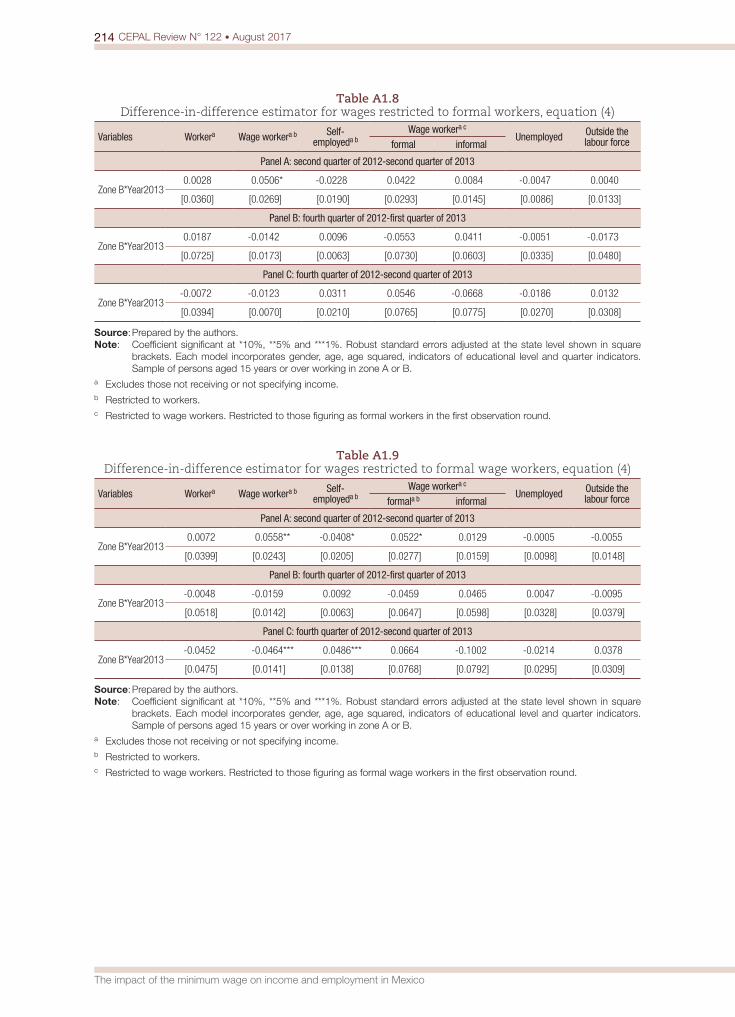
214 CEPAL Review N° 122 • August 2017
The impact of the minimum wage on income and employment in Mexico
Table A1.8 Difference-in-difference estimator for wages restricted to formal workers, equation (4)
Variables Workera Wage workera b Self-employeda b
Wage workera c
Unemployed Outside the labour forceformal informal
Panel A: second quarter of 2012-second quarter of 2013
Zone B*Year20130.0028 0.0506* -0.0228 0.0422 0.0084 -0.0047 0.0040
[0.0360] [0.0269] [0.0190] [0.0293] [0.0145] [0.0086] [0.0133]
Panel B: fourth quarter of 2012-first quarter of 2013
Zone B*Year20130.0187 -0.0142 0.0096 -0.0553 0.0411 -0.0051 -0.0173
[0.0725] [0.0173] [0.0063] [0.0730] [0.0603] [0.0335] [0.0480]
Panel C: fourth quarter of 2012-second quarter of 2013
Zone B*Year2013-0.0072 -0.0123 0.0311 0.0546 -0.0668 -0.0186 0.0132
[0.0394] [0.0070] [0.0210] [0.0765] [0.0775] [0.0270] [0.0308]
Source: Prepared by the authors.Note: Coefficient significant at *10%, **5% and ***1%. Robust standard errors adjusted at the state level shown in square
brackets. Each model incorporates gender, age, age squared, indicators of educational level and quarter indicators. Sample of persons aged 15 years or over working in zone A or B.
a Excludes those not receiving or not specifying income. b Restricted to workers. c Restricted to wage workers. Restricted to those figuring as formal workers in the first observation round.
Table A1.9 Difference-in-difference estimator for wages restricted to formal wage workers, equation (4)
Variables Workera Wage workera b Self-employeda b
Wage workera c
Unemployed Outside the labour forceformala b informal
Panel A: second quarter of 2012-second quarter of 2013
Zone B*Year20130.0072 0.0558** -0.0408* 0.0522* 0.0129 -0.0005 -0.0055
[0.0399] [0.0243] [0.0205] [0.0277] [0.0159] [0.0098] [0.0148]
Panel B: fourth quarter of 2012-first quarter of 2013
Zone B*Year2013-0.0048 -0.0159 0.0092 -0.0459 0.0465 0.0047 -0.0095
[0.0518] [0.0142] [0.0063] [0.0647] [0.0598] [0.0328] [0.0379]
Panel C: fourth quarter of 2012-second quarter of 2013
Zone B*Year2013-0.0452 -0.0464*** 0.0486*** 0.0664 -0.1002 -0.0214 0.0378
[0.0475] [0.0141] [0.0138] [0.0768] [0.0792] [0.0295] [0.0309]
Source: Prepared by the authors.Note: Coefficient significant at *10%, **5% and ***1%. Robust standard errors adjusted at the state level shown in square
brackets. Each model incorporates gender, age, age squared, indicators of educational level and quarter indicators. Sample of persons aged 15 years or over working in zone A or B.
a Excludes those not receiving or not specifying income. b Restricted to workers. c Restricted to wage workers. Restricted to those figuring as formal wage workers in the first observation round.
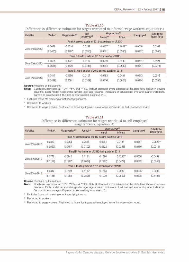
215CEPAL Review N° 122 • August 2017
Raymundo M. Campos Vázquez, Gerardo Esquivel and Alma S. Santillán Hernández
Table A1.10 Difference-in-difference estimator for wages restricted to informal wage workers, equation (4)
Variables Workera Wage workera b Self-employeda b
Wage workera c
Unemployed Outside the labour forceFormala b formal
Panel A: second quarter of 2012-second quarter of 2013
Zone B*Year2013-0.0079 -0.0510 0.0269 0.0937** 0.1048** -0.0010 0.0163
[0.0485] [0.0467] [0.0353] [0.0321] [0.0346] [0.0187] [0.0208]
Panel B: fourth quarter of 2012-first quarter of 2013
Zone B*Year2013-0.0665 0.0221 0.0117 -0.0259 -0.0199 0.0701* 0.0121
[0.0685] [0.0520] [0.0445] [0.0584] [0.0580] [0.0347] [0.0374]
Panel C: fourth quarter of 2012-second quarter of 2013
Zone B*Year2013-0.0417 0.0250 -0.0107 -0.0483 -0.0401 0.0513 0.0043
[0.0429] [0.0591] [0.0369] [0.0816] [0.0824] [0.0424] [0.0286]
Source: Prepared by the authors.Note: Coefficient significant at *10%, **5% and ***1%. Robust standard errors adjusted at the state level shown in square
brackets. Each model incorporates gender, age, age squared, indicators of educational level and quarter indicators. Sample of persons aged 15 years or over working in zone A or B.
a Excludes those not receiving or not specifying income. b Restricted to workers. c Restricted to wage workers. Restricted to those figuring as informal wage workers in the first observation round.
Table A1.11 Difference-in-difference estimator for wages restricted to self-employed
wage workers, equation (4)
Variables Workera Wage workera b Formala b Wage workera c
Unemployed Outside the labour forceformal informal
Panel A: second quarter of 2012-second quarter of 2013
Zone B*Year2013-0.0363 -0.0063 0.0538 0.0384 -0.0447 -0.0267 0.0823**
[0.0523] [0.0757] [0.0702] [0.0523] [0.0338] [0.0160] [0.0315]
Panel B: fourth quarter of 2012-first quarter of 2013
Zone B*Year20130.0776 -0.0142 0.1134 -0.1390 0.1248** -0.0386 -0.0492
[0.1129] [0.1207] [0.2034] [0.1267] [0.0477] [0.0882] [0.0743]
Panel C: fourth quarter of 2012-second quarter of 2013
Zone B*Year20130.0812 -0.1439 -0.1787* -0.1468 0.0030 -0.0695* 0.0288
[0.1146] [0.1059] [0.0895] [0.1030] [0.0552] [0.0328] [0.1185]
Source: Prepared by the authors.Note: Coefficient significant at *10%, **5% and ***1%. Robust standard errors adjusted at the state level shown in square
brackets. Each model incorporates gender, age, age squared, indicators of educational level and quarter indicators. Sample of persons aged 15 years or over working in zone A or B.
a Excludes those not receiving or not specifying income. b Restricted to workers. c Restricted to wage workers. Restricted to those figuring as self-employed in the first observation round.
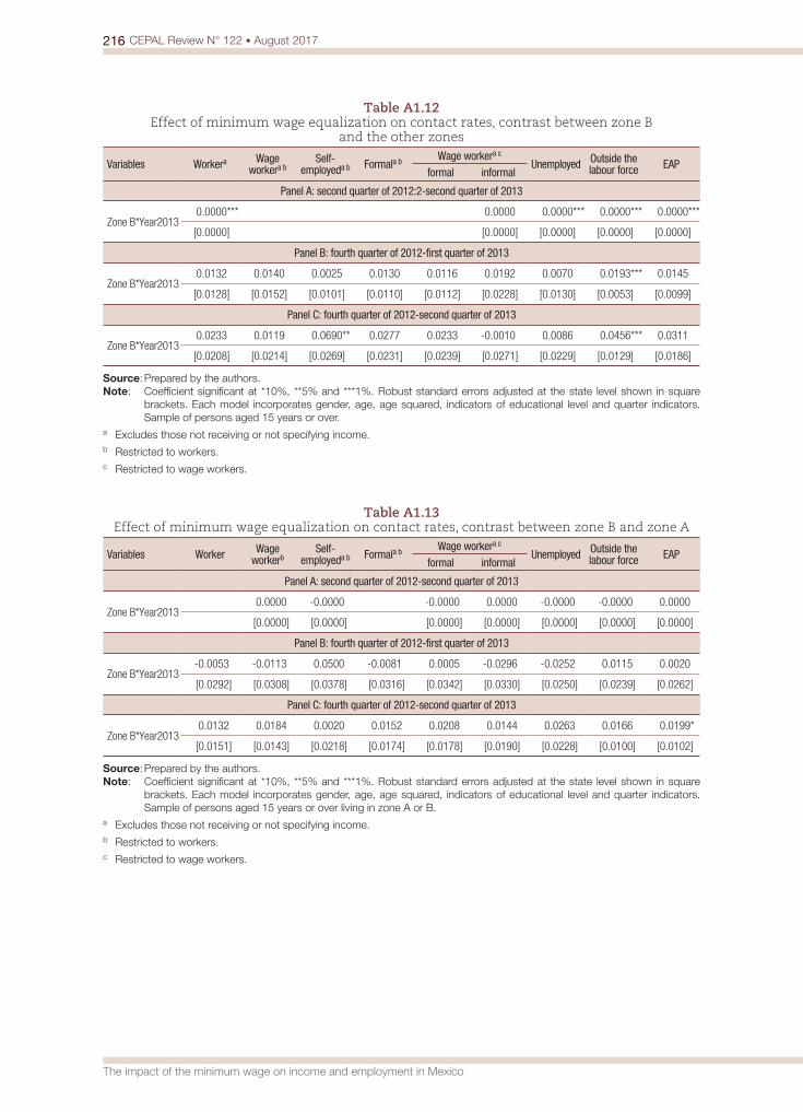
216 CEPAL Review N° 122 • August 2017
The impact of the minimum wage on income and employment in Mexico
Table A1.12 Effect of minimum wage equalization on contact rates, contrast between zone B
and the other zones
Variables Workera Wage workera b
Self-employeda b Formala b Wage workera c
Unemployed Outside the labour force EAP
formal informal
Panel A: second quarter of 2012:2-second quarter of 2013
Zone B*Year20130.0000*** 0.0000 0.0000*** 0.0000*** 0.0000***
[0.0000] [0.0000] [0.0000] [0.0000] [0.0000]
Panel B: fourth quarter of 2012-first quarter of 2013
Zone B*Year20130.0132 0.0140 0.0025 0.0130 0.0116 0.0192 0.0070 0.0193*** 0.0145
[0.0128] [0.0152] [0.0101] [0.0110] [0.0112] [0.0228] [0.0130] [0.0053] [0.0099]
Panel C: fourth quarter of 2012-second quarter of 2013
Zone B*Year20130.0233 0.0119 0.0690** 0.0277 0.0233 -0.0010 0.0086 0.0456*** 0.0311
[0.0208] [0.0214] [0.0269] [0.0231] [0.0239] [0.0271] [0.0229] [0.0129] [0.0186]
Source: Prepared by the authors.Note: Coefficient significant at *10%, **5% and ***1%. Robust standard errors adjusted at the state level shown in square
brackets. Each model incorporates gender, age, age squared, indicators of educational level and quarter indicators. Sample of persons aged 15 years or over.
a Excludes those not receiving or not specifying income. b Restricted to workers. c Restricted to wage workers.
Table A1.13 Effect of minimum wage equalization on contact rates, contrast between zone B and zone A
Variables Worker Wage workerb
Self-employeda b Formala b Wage workera c
Unemployed Outside the labour force EAP
formal informal
Panel A: second quarter of 2012-second quarter of 2013
Zone B*Year20130.0000 -0.0000 -0.0000 0.0000 -0.0000 -0.0000 0.0000
[0.0000] [0.0000] [0.0000] [0.0000] [0.0000] [0.0000] [0.0000]
Panel B: fourth quarter of 2012-first quarter of 2013
Zone B*Year2013-0.0053 -0.0113 0.0500 -0.0081 0.0005 -0.0296 -0.0252 0.0115 0.0020
[0.0292] [0.0308] [0.0378] [0.0316] [0.0342] [0.0330] [0.0250] [0.0239] [0.0262]
Panel C: fourth quarter of 2012-second quarter of 2013
Zone B*Year20130.0132 0.0184 0.0020 0.0152 0.0208 0.0144 0.0263 0.0166 0.0199*
[0.0151] [0.0143] [0.0218] [0.0174] [0.0178] [0.0190] [0.0228] [0.0100] [0.0102]
Source: Prepared by the authors.Note: Coefficient significant at *10%, **5% and ***1%. Robust standard errors adjusted at the state level shown in square
brackets. Each model incorporates gender, age, age squared, indicators of educational level and quarter indicators. Sample of persons aged 15 years or over living in zone A or B.
a Excludes those not receiving or not specifying income. b Restricted to workers. c Restricted to wage workers.

Spatial distribution of the Brazilian national system of innovation: an analysis for the 2000sUlisses Pereira dos Santos
KeywordsEconomic development, regional development, innovations, science and technology, regional disparities, science and technology indicators, Brazil
JEL classificationO10, O30, R58
AuthorUlisses Pereira dos Santos is a professor with the Centre for Regional Development and Planning (CEDEPLAR) of the School of Economics of the Universidade Federal de Minas Gerais, Brazil. [email protected]
Abstract
Regional inequality is an intrinsic characteristic of economic underdevelopment. Some structuralists have attributed this feature to the unequal distribution of the benefits of technical progress among subnational regions. This process is thought to be related to the spatial distribution of the components of the national innovation system, which is such that the available opportunities for taking advantage of the benefits of technical progress differ from one region in Brazil to the next. This study examines the distribution of science, technology and innovation assets among different Brazilian microregions in the years from 2000 to 2010. Its findings indicate that the territorial scope of the national innovation system expanded during the period under study to encompass a larger number of microregions and thus has come to exhibit a greater degree of spatial continuity. This process occurred in parallel with a trend towards a greater regional deconcentration of income in the country.
218 CEPAL Review N° 122 • August 2017
Spatial distribution of the Brazilian national system of innovation: an analysis for the 2000s
I. Introduction
The regional concentration of income is an inherent characteristic of economic underdevelopment. In the course of the debate on development and underdevelopment, a number of renowned authors —such as Furtado (1967a and 1967b), Pinto (2000), Hirshman (1977) and Perroux (1967)— drew attention to the concentration or centralization of income in given locations within different countries. Explicitly or implicitly, these authors saw the regional concentration of income as being linked to the unequal regional distribution of the benefits of technical progress. They therefore thought that a greater incorporation of the benefits of technical progress in some subnational regions than in others would give rise to an unbalanced regional growth process.
Viewed from this perspective, regional income concentration —especially in underdeveloped countries— would appear to be related to the unequal geographic distribution of the components of the national innovation system (NIS). The assumption is that the regional concentration of NIS components leads to a regional concentration of the benefits of technical progress and, consequently, of income. It follows that the spatial concentration of NIS assets within a country would therefore also be linked with economic underdevelopment. By contrast, in developed economies, where the regional concentration of income is less marked, NIS assets are distributed more equally among subnational regions and the division of the benefits of technical progress is therefore more balanced.
In the light of these factors, the objective of this study is to analyse the changes that occurred in the geographic distribution of assets in the fields of science, technology and innovation among Brazilian microregions during the 2000s in order to gauge the extent of the system’s regional expansion. The starting point for this analysis is the observation that the regional concentration of income has in fact been reduced in Brazil in recent years (Silveira Netto and Azzoni, 2013), as attested to by the fact that the richest microregions’ share of the country’s gross domestic product (GDP) shrank during that decade while the share of the poorest 50% of its regions expanded.
This shift reflects the presence of broader regional participation in the national innovation system as a result of the regional redistribution of NIS institutions that occurred during the 2000s. This greater continuity of the system within Brazil is presumably enabling various regions to play a greater role in the national economic circuit, thereby reducing income inequality at the regional level. This, in turn, can be expected to pave the way for the consolidation of the national innovation system and to spur the country’s economic development. Within this framework, data on the different microregions’ scientific and technological activities and on institutions of postgraduate instruction are assessed in order to track the regional performance of the innovation system in 2000-2010. An index that provides a means of gauging the development of local scientific, technological and innovation institutions is therefore proposed for use in measuring each microregion’s involvement in that system.
This article is divided into five sections, the first one of which is this introduction. The second section reviews the literature on regional development and innovation systems, while the third traces the trends in science, technology and innovation indicators in Brazil in 2000-2010. The fourth section outlines the design of an NIS regional development index for use in evaluating the geographic distribution or scope of Brazil’s national innovation system. The fifth and final section presents a number of concluding observations and considerations.
219CEPAL Review N° 122 • August 2017
Ulisses Pereira dos Santos
II. Regional development and innovation systems
Geography has major implications for the technological innovation process. The exchange of information among the various agents in a geographically defined economic system is heightened by physical proximity and the shared social and cultural features of any given locality (Asheim and Gertler, 2005; Cooke, 1998; Jaffe, 1989). Starting with the very first theoretical explorations of the workings of national innovation systems, there was an awareness of the important role played in these systems by institutions and organizations, businesses and learning processes and interactions, but their regional aspects were overlooked (Freeman, 1987 and 1995; Lundvall, 1992; Nelson and Rosenberg, 1993). Thus, the regions’ role in the development of these innovation systems was virtually ignored during the development and consolidation of this concept.
Among all the authors who introduced the concept of national innovation systems, Freeman (1987 and 2002) was the only one to draw attention to the influence exerted by regional policies in helping a country to catch up with more economically developed nations. In his work on the initiatives launched by Japan to promote economic development, he pointed out the patent importance of regional policies in that country and underscored the determined effort that it had put into devising and implementing regional policies in the realms of the sciences, education, communications and infrastructure. He characterized these policies as having played a fundamental part in expanding the coverage of technological training to encompass the entire country and incorporating as many agents as possible into its technological and scientific circles, regardless of their location or economic scale. As noted by Freeman, “regional policies have consistently sought to strengthen technological capability throughout the country, particularly in small and medium-sized firms" (Freeman, 1987, p. 36).
Nonetheless, the regional dimension was virtually ignored in the major studies and research papers on national innovation systems published in the 1990s. Just 15 years later, Freeman (2002) again broke new ground when he introduced the spatial or geographic dimension into this field of study. He thus took the first steps towards identifying the relationship among what he called continental, national and subnational innovation systems based on the assumption that changes in the global economy would trigger changes in those systems. In that study, Freeman highlighted the importance of the subnational scale in research on innovation and asserted that the formation of clusters of industrial activities would have significant development implications. Regional advantages would be influenced, however, by national factors; in other words, they could be leveraged by aspects of the nation’s culture, politics, economy and technological institutions. Freeman (2002) thus saw national and subnational innovation systems as being complementary and felt that theorists needed to gain a better understanding of the changes occurring in innovation systems at all levels of analysis (including everything from a global to a regional scale) and of the relationships between these different scales in terms of the promotion of innovation.
Edquist (2005) also looked at the possible geographical and sectoral scales or boundaries of an innovation system. In his view, the importance of the geographic boundaries of innovation systems is determined by national and regional specificities. He contends that in large, regionally diverse countries, regional innovation systems may be more important than national innovation systems. However, since the legal and political factors that will have an influence on those regional systems are often controlled by national governments, even in big countries, a focus on regional systems is necessarily only one dimension of a broader approach. Like Freeman (2002), Edquist concluded that the different geographical scales on which innovation systems exist are complementary rather than exclusionary.
As for a possible relationship between the geographic distribution of a national innovation system and the regional imbalances inherent in economic underdevelopment, it can be assumed that this relationship is the outcome of an unequal distribution of the benefits of technical progress in
220 CEPAL Review N° 122 • August 2017
Spatial distribution of the Brazilian national system of innovation: an analysis for the 2000s
the national economy (Furtado, 1967b). According to this approach, which is in one way or another present in the work of foundational analysts of regional development such as Perroux (1967) and Hirschman (1977), this relationship is linked to the regional distribution of NIS entities. Thus, a national innovation system, which is the main driver of technological progress in a country, could be linked to the economic imbalances existing among its component regions, since its geographic distribution can exert an influence over the regional distribution of the benefits of technical progress.
The regions in which the main NIS assets interact with one another in ways that enable them to act as drivers of technological innovation would thus tend to develop more quickly than others, since their superior institutional framework for activities in the fields of science, technology and innovation (STI) would give them an advantage over the others in attracting new industries. This, in turn, would fuel the growth of production and boost revenues and tax receipts in those regions. These regions’ greater economic capacity would, in turn, enable them to reinvest profits in their learning and knowledge infrastructure, which would tend to strengthen their regional innovation systems and translate into gains in their internal and external competitiveness (Asheim, 1996; Florida, 1995). This process could perpetuate the regional concentration of income in a country via the concentration of the benefits of technical progress. The regions with weak STI structures would have little chance of garnering the benefits of the technological inroads made in the more developed regions because they would not be in a position to absorb those advances or apply them in their own production activities.
Local STI assets forming part of the same national institutional system may exhibit differing levels of development as a result of the presence of differing technological development trajectories at the regional level and differing local knowledge platforms (Asheim and Gertler, 2005; Oinas and Malecki, 1999). It is therefore assumed that the economic environment influences the actors that exist within it (Cooke, 1998; Isaksen, 2001). In other words, the development and performance of an institutional cluster that is formally linked to a national government and, hence, to the national innovation system, can be determined by the economic and social situation in the region where it is located. This means that similar institutions in a given NIS could start off on an equal footing but could end up moving along differing development paths by virtue of their locations.
It therefore follows that regional development policies should be aligned with national science and technology policies, as was done in Japan (Freeman, 1987). According to this approach, regional development calls for the incorporation of NIS support institutions into the various subnational regions so that they can contribute to the expansion and consolidation of the entire national innovation system. It is important to note, however, that the benefits to be derived from the establishment of a given institution in a specific regional setting will depend on the extent to which that institution is integrated into the social fabric of the region in question (Granovetter, 1985). Such institutions need to be integrated into the social and economic network of the region where they are introduced so that they can help generate and fuel information flows between themselves and local actors involved in the innovation process (Oinas and Malecki, 1999).
In the light of the above, this study will seek to undertake an analysis of national innovation systems from a regional perspective with a view to identifying the determinants and implications of regional systems’ distribution within the national system of which they are a part. It is assumed that the spatial distribution of components of a national innovation system may be linked to a country’s level of economic development and to the regional imbalances that are an inherent feature of underdevelopment. Viewed from this standpoint, a more balanced distribution of STI institutions within a given country’s territory can be expected to be coupled with a spatially broader NIS structure, which would in turn lead to a more equitable distribution of the benefits of technical progress among the various subnational regions. By contrast, the concentration of NIS institutions in just a few regions would be associated with a discontinuous NIS with more limited national coverage, which would in turn be reflected in a regional concentration of the benefits of technical progress and, hence, of income.
221CEPAL Review N° 122 • August 2017
Ulisses Pereira dos Santos
III. The spatial distribution of STI assets in Brazil in the 2000s
1. STI indicators
The following analysis of the spatial development of Brazil’s innovation system during the 2000s is based on three indicators which will serve as proxy variables for three spheres of activity within the innovation system: technological production, scientific production, and educational and research activities. Technological production will be gauged by looking at the number of patent applications filed by residents of the country’s 558 microregions with the National Institute of Industrial Property (INPI). Scientific production will be analysed with reference to the number of articles published in international journals that are indexed in the ISI Web of Science platform. The local education and research network will be quantified in terms of the number of faculty members teaching postgraduate courses in each microregion.
The first of these indicators —the number of patent applications filed by residents of each microregion— was obtained from a special tabulation of the relevant data provided by INPI. The database includes all patent applications filed with INPI between 2000 and 2010, along with detailed information on the applicants (name, National Register of Legal Entities (CNPJ) number or Natural Persons Register (CPF) number, as appropriate, and the state and municipality of residence), as well as the application number and date. The fact that 7,259 patent applications were filed in 2000 and that 8,582 were filed in 2010 points to an increase in the level of technological activity in Brazil during that decade. The data are aggregated at the microregional level for the purposes of the following analysis.
The statistics on scientific articles were drawn from the database maintained by the Institute for Science Information (ISI), which contains references to the articles published in major international journals in all fields of knowledge. Data are available on the fields to which each article is related, its authors, the institutions with which they are associated and their location. For the purposes of this study, the online ISI (Web of Science) database was consulted in the period running from August 2013 to January 2014 in order to obtain read-outs of data on each scientific article published by a resident of Brazil in ISI-indexed journals between the years 2000 and 2010. After checking that the read-outs provided enough information to warrant inclusion in the database used for this study, a total of 10,512 articles published in 2000 and 21,109 articles published in 20101 were entered into the database. The data on articles for which insufficient information was available were not included. The locational data made it possible to compute the number of articles for each municipality and then for each microregion. In the cases where an article had been written by authors located in different microregions, it was attributed to each of those locations. The analysis therefore provides for the existence of double counting, since the total number of articles for the different microregions will exceed the total number of articles published by authors residing in the country.
In order to evaluate microregional education and research networks, data on the number of faculty members teaching postgraduate courses in each microregion were used. These data were obtained from the Georeferenced Information System (GEOCAPES) portal of the Coordinating Office for the Improvement of Higher Education Personnel (CAPES).2 The portal was consulted during the month of April 2014, so all the data used in the study correspond to the information available in the database at that time. The number of teachers in each municipality in 2000 and 2010 was aggregated at the microregional level for use in the analysis to be undertaken here.
1 The articles for which the data were incomplete were not included in the sample, so that information was lost.2 The GEOCAPES data are available online at: http://geocapes.capes.gov.br/geocapesds/.
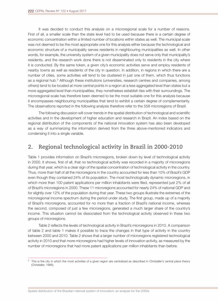
222 CEPAL Review N° 122 • August 2017
Spatial distribution of the Brazilian national system of innovation: an analysis for the 2000s
It was decided to conduct this analysis on a microregional scale for a number of reasons. First of all, a smaller scale than the state level had to be used because there is a certain degree of economic concentration within a limited number of locations within states as well. The municipal scale was not deemed to be the most appropriate one for this analysis either because the technological and economic structure of a municipality serves residents in neighbouring municipalities as well. In other words, for example, the university system of a given municipality does not serve only that municipality’s residents, and the research work done there is not disseminated only to residents in the city where it is conducted. By the same token, a given city’s economic activities serve and employ residents of nearby towns as well as residents of the city in question. In addition, in regions in which there are a number of cities, some activities will tend to be clustered in just one of them, which thus functions as a regional hub.3 Although these institutions (universities, research centres and companies, among others) tend to be located at more central points in a region at a less aggregated level than states but a more aggregated level than municipalities, they nonetheless establish ties with their surroundings. The microregional scale has therefore been deemed to be the most suitable one for this analysis because it encompasses neighbouring municipalities that tend to exhibit a certain degree of complementarity. The observations reported in the following analysis therefore refer to the 558 microregions of Brazil.
The following discussion will cover trends in the spatial distribution of technological and scientific activities and in the development of higher education and research in Brazil. An index based on the regional distribution of the components of the national innovation system has also been developed as a way of summarizing the information derived from the three above-mentioned indicators and condensing it into a single variable.
2. Regional technological activity in Brazil in 2000-2010
Table 1 provides information on Brazil’s microregions, broken down by level of technological activity in 2000. It shows, first of all, that no technological activity was recorded in a majority of microregions during that year, which is a clear sign of the spatial concentration of technological activity in the country. Thus, more than half of all the microregions in the country accounted for less than 10% of Brazil’s GDP even though they contained 24% of its population. The most technologically dynamic microregions, in which more than 100 patent applications per million inhabitants were filed, represented just 2% of all of Brazil’s microregions in 2000. These 11 microregions accounted for nearly 24% of national GDP and for slightly over 12% of the population during that year. These two groups illustrate the extremes of the microregional income spectrum during the period under study. The first group, made up of a majority of Brazil’s microregions, accounted for no more than a fraction of Brazil’s national income, whereas the second, composed of just a few microregions, generated a much larger share of the country’s income. This situation cannot be dissociated from the technological activity observed in these two groups of microregions.
Table 2 reflects the levels of technological activity in Brazil’s microregions in 2010. A comparison of table 2 and table 1 makes it possible to trace the changes in that type of activity in the country between 2000 and 2010. Table 2 shows that a larger number of microregions registered technological activity in 2010 and that more microregions had higher levels of innovation activity, as measured by the number of microregions that had more patent applications per million inhabitants than before.
3 This is the city in which the most activities of a given region are centralized as described in Christaller’s central place theory (Christaller, 1966).

223CEPAL Review N° 122 • August 2017
Ulisses Pereira dos Santos
Table 1 Brazil: microregions, by level of technological activity and percentages of the total number
of microregions, the total population and the country’s gross domestic product, 2000
Patents per million inhabitants Number of microregions Percentage
of microregionsPercentage of the total population Percentage of GDP
0 305 54.7 23.7 9.5
1-30 169 30.3 35.5 27.6
31-60 46 8.2 17.2 23.8
60-100 27 4.8 11.2 15.3
>100 11 2.0 12.4 23.8
Total 558 100.0 100.0 100.0
Source: Prepared by the authors, on the basis of data from the National Institute of Industrial Property (INPI) and Ipeadata.
Table 2 Brazil: microregions, by level of technological activity and percentages of the total number
of microregions, the total population and the country’s gross domestic product, 2010
Patents per million habitants Number of microregions Percentage
of microregionsPercentage of the total population Percentage of total GDP
0 273 48.9 21.2 8.9
1-30 186 33.3 36.0 29.7
31-60 57 10.2 20.0 25.6
60-100 26 4.7 9.7 13.0
>100 16 2.9 13.1 22.8
Total 558 100.0 100.0 100.0
Source: Prepared by the authors, on the basis of data from the National Institute of Industrial Property (INPI) and Ipeadata.
Whereas patent applications were filed by persons or institutions in 253 of Brazil’s microregions in 2000, by 2010 that figure had climbed to 285. In other words, by the second year of reference, more than half of all the microregions were registering technological activity. This means that significant changes occurred in the groups at the two extremes of the spectrum. Although regions in which technological activity was absent remained the largest of the five categories in 2010, that group accounted for smaller percentages of the population and of GDP than it had in 2000. The fact that, although the number of microregions with over 100 patent applications per million inhabitants rose to nearly 3% of the total, their share of GDP shrank may be attributable to an increase in the incomes of the poorer regions. The shares of total income of the groups with 1-30 and 31-60 patent applications per million inhabitants expanded because the number of microregions in those categories rose, as many of the microregions that had previously been in the category displaying an absence of technological activity had moved into one of those two groups.
3. Regional scientific activity in Brazil in 2000-2010
The data on scientific production in Brazil paint a similar picture. In 2000, scientific activity was primarily concentrated in southern and south-eastern Brazil, and the microregions in which it was most intense were in the State of São Paulo. Table 3 shows that the microregions in which scientific activity was taking place in 2000 accounted for just slightly more than 30% of the total.
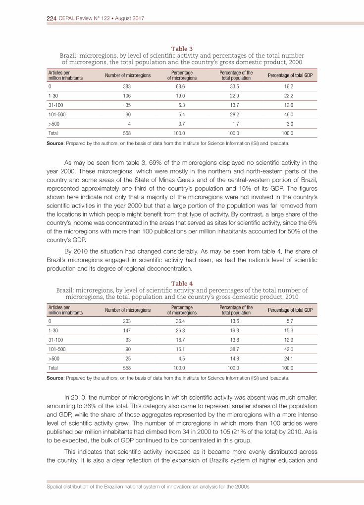
224 CEPAL Review N° 122 • August 2017
Spatial distribution of the Brazilian national system of innovation: an analysis for the 2000s
Table 3 Brazil: microregions, by level of scientific activity and percentages of the total number of microregions, the total population and the country’s gross domestic product, 2000
Articles per million inhabitants Number of microregions Percentage
of microregionsPercentage of the total population Percentage of total GDP
0 383 68.6 33.5 16.2
1-30 106 19.0 22.9 22.2
31-100 35 6.3 13.7 12.6
101-500 30 5.4 28.2 46.0
>500 4 0.7 1.7 3.0
Total 558 100.0 100.0 100.0
Source: Prepared by the authors, on the basis of data from the Institute for Science Information (ISI) and Ipeadata.
As may be seen from table 3, 69% of the microregions displayed no scientific activity in the year 2000. These microregions, which were mostly in the northern and north-eastern parts of the country and some areas of the State of Minas Gerais and of the central-western portion of Brazil, represented approximately one third of the country’s population and 16% of its GDP. The figures shown here indicate not only that a majority of the microregions were not involved in the country’s scientific activities in the year 2000 but that a large portion of the population was far removed from the locations in which people might benefit from that type of activity. By contrast, a large share of the country’s income was concentrated in the areas that served as sites for scientific activity, since the 6% of the microregions with more than 100 publications per million inhabitants accounted for 50% of the country’s GDP.
By 2010 the situation had changed considerably. As may be seen from table 4, the share of Brazil’s microregions engaged in scientific activity had risen, as had the nation’s level of scientific production and its degree of regional deconcentration.
Table 4 Brazil: microregions, by level of scientific activity and percentages of the total number of
microregions, the total population and the country’s gross domestic product, 2010
Articles per million inhabitants Number of microregions Percentage
of microregionsPercentage of the total population Percentage of total GDP
0 203 36.4 13.6 5.7
1-30 147 26.3 19.3 15.3
31-100 93 16.7 13.6 12.9
101-500 90 16.1 38.7 42.0
>500 25 4.5 14.8 24.1
Total 558 100.0 100.0 100.0
Source: Prepared by the authors, on the basis of data from the Institute for Science Information (ISI) and Ipeadata.
In 2010, the number of microregions in which scientific activity was absent was much smaller, amounting to 36% of the total. This category also came to represent smaller shares of the population and GDP, while the share of those aggregates represented by the microregions with a more intense level of scientific activity grew. The number of microregions in which more than 100 articles were published per million inhabitants had climbed from 34 in 2000 to 105 (21% of the total) by 2010. As is to be expected, the bulk of GDP continued to be concentrated in this group.
This indicates that scientific activity increased as it became more evenly distributed across the country. It is also a clear reflection of the expansion of Brazil’s system of higher education and
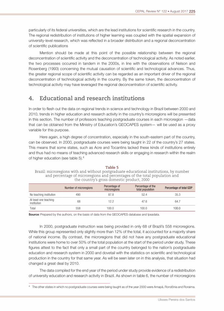
225CEPAL Review N° 122 • August 2017
Ulisses Pereira dos Santos
particularly of its federal universities, which are the lead institutions for scientific research in the country. The regional redistribution of institutions of higher learning was coupled with the spatial expansion of university-level research, which was reflected in a broader distribution and a regional deconcentration of scientific publications
Mention should be made at this point of the possible relationship between the regional deconcentration of scientific activity and the deconcentration of technological activity. As noted earlier, the two processes occurred in tandem in the 2000s, in line with the observations of Nelson and Rosenberg (1993) concerning the mutual causation of scientific and technological advances. Thus, the greater regional scope of scientific activity can be regarded as an important driver of the regional deconcentration of technological activity in the country. By the same token, the deconcentration of technological activity may have leveraged the regional deconcentration of scientific activity.
4. Educational and research institutions
In order to flesh out the data on regional trends in science and technology in Brazil between 2000 and 2010, trends in higher education and research activity in the country’s microregions will be presented in this section. The number of professors teaching postgraduate courses in each microregion —data that can be obtained from the Ministry of Education’s GEOCAPES system— will be used as a proxy variable for this purpose.
Here again, a high degree of concentration, especially in the south-eastern part of the country, can be observed. In 2000, postgraduate courses were being taught in 22 of the country’s 27 states. This means that some states, such as Acre and Tocantins lacked these kinds of institutions entirely and thus had no means of teaching advanced research skills or engaging in research within the realm of higher education (see table 5).4
Table 5 Brazil: microregions with and without postgraduate educational institutions, by number
and percentage of microregions and percentages of the total population and the country’s gross domestic product, 2000
Number of microregions Percentage of microregions
Percentage of the total population Percentage of total GDP
No teaching institution 490 87.8 52.4 35.3
At least one teaching institution 68 12.2 47.6 64.7
Total 558 100.0 100.0 100.0
Source: Prepared by the authors, on the basis of data from the GEOCAPES database and Ipeadata.
In 2000, postgraduate instruction was being provided in only 68 of Brazil’s 558 microregions. While this group represented only slightly more than 12% of the total, it accounted for a majority share of national income. By contrast, the microregions that did not have any postgraduate educational institutions were home to over 50% of the total population at the start of the period under study. These figures attest to the fact that only a small part of the country belonged to the nation’s postgraduate education and research system in 2000 and dovetail with the statistics on scientific and technological production in the country for that same year. As will be seen later on in this analysis, that situation had changed a great deal by 2010.
The data compiled for the end year of the period under study provide evidence of a redistribution of university education and research activity in Brazil. As shown in table 6, the number of microregions
4 The other states in which no postgraduate courses were being taught as of the year 2000 were Amapá, Rondônia and Roraima.

226 CEPAL Review N° 122 • August 2017
Spatial distribution of the Brazilian national system of innovation: an analysis for the 2000s
with professors at the postgraduate level had risen to 115 by 2010, for an increase of more than 70% over the figure for 2000. The average number of professors at the postgraduate level per microregion also jumped from 52 per microregion to 104.5. This increase reflects a rapid expansion of higher education in the 2000s, as nearly 60% of the population was living in microregions in which university-level teaching and research activities were being conducted in 2010. In addition to leading to an increase in the number of professors at the postgraduate level and, consequently, in the number of highly advanced courses that were available, this expansion had the effect of integrating a larger part of the country and of the nation’s population into this field of activity. Nonetheless, these statistics also show that much remains to be done in this regard.
Table 6 Brazil: microregions with and without postgraduate educational institutions, by number
and percentage of microregions and percentages of the total population and the country’s gross domestic product, 2010
Number of microregions Percentage of microregions
Percentage of the total population Percentage of total GDP
No teaching institution 443 79.4 40.2 24.5
At least one teaching institution 115 20.6 59.8 75.5
Total 2010 558 100.0 100.0 100.0
Source: Prepared by the authors, on the basis of data from the GEOCAPES database and Ipeadata.
One important change brought about by this expansion is that, as of 2010, postgraduate courses were being taught in every state of the federation. The fact remains, however, that, although the central-western and north-eastern parts of the country did become more involved in the nation’s scientific systems, the number of professors at the postgraduate level per million inhabitants did rise more sharply in the southern and south-eastern regions.
Scientific production in the country advanced more rapidly than its postgraduate teaching institutions did. In other words, the number of microregions in which scientific articles were published (352) exceeded the number in which postgraduate courses were being taught (115) in 2010. This may be a reflection of spillovers from the creation of an educational and research structure in a given region, since the impact of the establishment of such an institution will be felt beyond the borders of the microregion in question. This is because students and working people who are residing in other microregions may be able to attend courses in the microregion in which a newly created teaching and research institution is located. It is also the case that information flows and the exchange of knowledge will take place between universities, businesses and a wide range of other actors located in different regions.
The same is true of technological production, which was diffused over a greater portion of the country than higher education and research activities were.5
IV. A regional development index for the innovation system in 2000-2010
Indicators of technological activity, scientific activity and higher education and research activity can be used to track the deconcentration of national innovation system assets in Brazil during the 2000s. All the indicators used in this study attest to a quantitative improvement marked by sizeable increases in
5 As was seen earlier, in 2010 patent applications were received by the National Institute of Industrial Property (INPI) from 285 microregions.
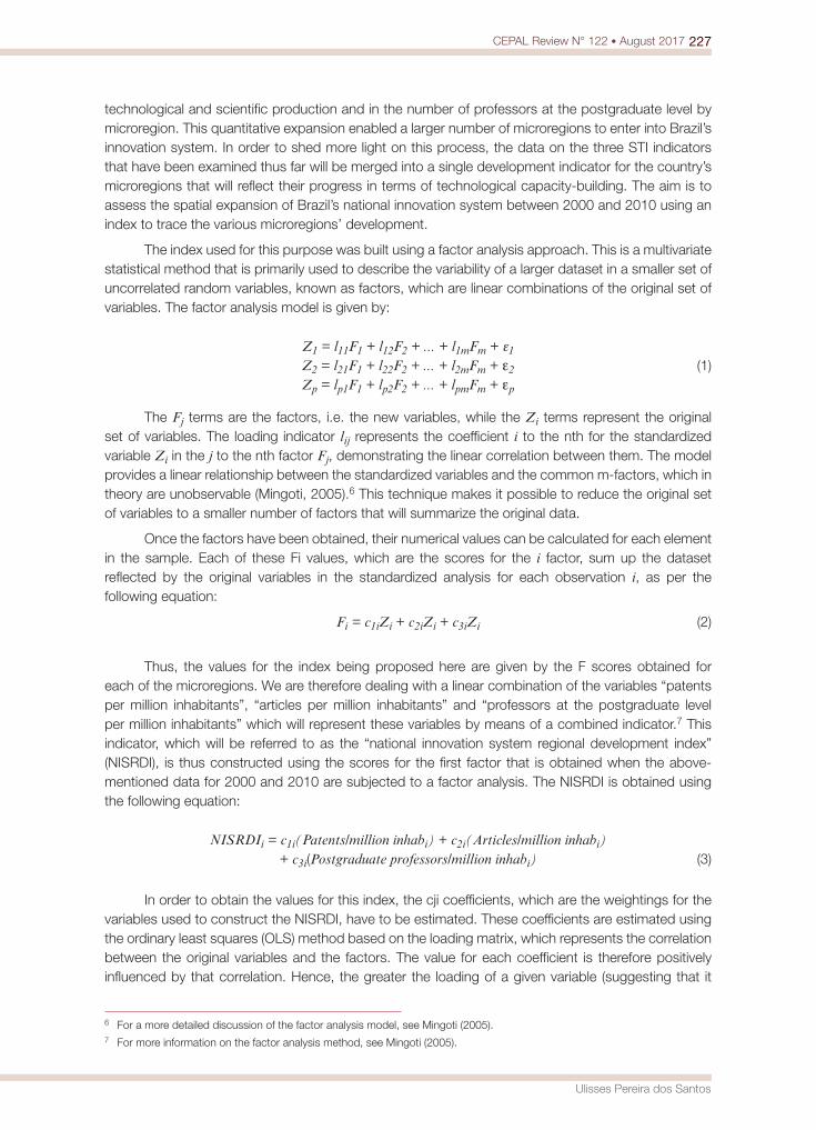
227CEPAL Review N° 122 • August 2017
Ulisses Pereira dos Santos
technological and scientific production and in the number of professors at the postgraduate level by microregion. This quantitative expansion enabled a larger number of microregions to enter into Brazil’s innovation system. In order to shed more light on this process, the data on the three STI indicators that have been examined thus far will be merged into a single development indicator for the country’s microregions that will reflect their progress in terms of technological capacity-building. The aim is to assess the spatial expansion of Brazil’s national innovation system between 2000 and 2010 using an index to trace the various microregions’ development.
The index used for this purpose was built using a factor analysis approach. This is a multivariate statistical method that is primarily used to describe the variability of a larger dataset in a smaller set of uncorrelated random variables, known as factors, which are linear combinations of the original set of variables. The factor analysis model is given by:
Z1 = l11F1 + l12F2 + ... + l1mFm + ε1
Z2 = l21F1 + l22F2 + ... + l2mFm + ε2 (1) Zp = lp1F1 + lp2F2 + ... + lpmFm + εp
The Fj terms are the factors, i.e. the new variables, while the Zi terms represent the original set of variables. The loading indicator lij represents the coefficient i to the nth for the standardized variable Zi in the j to the nth factor Fj, demonstrating the linear correlation between them. The model provides a linear relationship between the standardized variables and the common m-factors, which in theory are unobservable (Mingoti, 2005).6 This technique makes it possible to reduce the original set of variables to a smaller number of factors that will summarize the original data.
Once the factors have been obtained, their numerical values can be calculated for each element in the sample. Each of these Fi values, which are the scores for the i factor, sum up the dataset reflected by the original variables in the standardized analysis for each observation i, as per the following equation:
Fi = c1iZi + c2iZi + c3iZi (2)
Thus, the values for the index being proposed here are given by the F scores obtained for each of the microregions. We are therefore dealing with a linear combination of the variables “patents per million inhabitants”, “articles per million inhabitants” and “professors at the postgraduate level per million inhabitants” which will represent these variables by means of a combined indicator.7 This indicator, which will be referred to as the “national innovation system regional development index” (NISRDI), is thus constructed using the scores for the first factor that is obtained when the above-mentioned data for 2000 and 2010 are subjected to a factor analysis. The NISRDI is obtained using the following equation:
NISRDIi = c1i(Patents/million inhabi) + c2i(Articles/million inhabi) + c3i(Postgraduate professors/million inhabi) (3)
In order to obtain the values for this index, the cji coefficients, which are the weightings for the variables used to construct the NISRDI, have to be estimated. These coefficients are estimated using the ordinary least squares (OLS) method based on the loading matrix, which represents the correlation between the original variables and the factors. The value for each coefficient is therefore positively influenced by that correlation. Hence, the greater the loading of a given variable (suggesting that it
6 For a more detailed discussion of the factor analysis model, see Mingoti (2005).7 For more information on the factor analysis method, see Mingoti (2005).

228 CEPAL Review N° 122 • August 2017
Spatial distribution of the Brazilian national system of innovation: an analysis for the 2000s
correlates more closely with the factor in question), the greater its weighting will be in the calculation of the corresponding score or rating on the index (Mingoti, 2005).
The NISRDI consists, then, of the weighted sum of the values of the standardized variables “patents per million inhabitants”, “articles per million inhabitants” and “professors at the postgraduate level per million inhabitants” obtained using a factor analysis for each of Brazil’s microregions. By convention, the vector of scores for the n observations is normalized so that the mean is equal to 0 and the standard deviation is equal to 1 (Mingoti, 2005; STATACORP, 2009). As a result of this normalization, observations where the result is below the overall mean will be represented by negative values on the NISRDI.
Table 7 shows the characteristics of the factors used to extract the NISRDI index for the years 2000 and 2010.
Table 7 Properties of the factors used to extract the national innovation system regional
development index (NISRDI), 2000 and 2010
Factor 1 (2000) Factor 1 (2010)
Loadings Scores Loadings Scores
Patents per million inhabitants 0.3659 0.07402 0.3834 0.03181
Articles per million inhabitants 0.8494 0.44418 0.9363 0.43059
Postgraduate professors per million inhabitants 0.8575 0.47607 0.9460 0.53734
Autovalue 1.59057 1.91852
Explained variance (percentages) 112 103
KMO test 0.57 0.56
Source: Prepared by the authors, on the basis of data from the National Institute of Industrial Property (INPI), the Institute for Science Information (ISI) and GEOCAPES.
Since the values of the loadings and the coefficients are positive, the NISRDI index exhibits an increasing correlation with technological and scientific activities and with local education and research institutions. Thus, the greater the index values, the greater the level of development of a microregion’s STI structure within the national innovation system. It should be noted that the weighting of the “patents per million inhabitants” variable in the NISRDI is less than those of the other variables. The lower value of its loading, which translates into a lower value for its coefficient, indicates that this variable is less representative in the numerical systematization of the innovation systems being considered here. This may be seen as a reflection of the weak technological performance of the Brazilian innovation system.
Another noteworthy aspect of table 7 is that the only variable whose significance in the make-up of the NISRDI increased between 2000 and 2010 is “postgraduate professors per million inhabitants”, as may be seen from a comparison of the coefficients for those two years. This may be attributable to the government’s policy of focusing on the expansion of the nation’s higher education system in all regions of the country, including the poorest ones. This backs up the evidence discussed in the preceding section.
Table 8 gives descriptive statistics for the NISRDI in 2000 and 2010. In theory, as mentioned earlier, the factor scores obtained using the factor analysis method should have a mean equal to 0 and a standard deviation equal to 1 owing to the normalization of the data. In practice, the values tend towards 0 and 1, respectively, since the theoretical values will be obtained only in the presence of a perfect solution for the factor model (STATACORP, 2009). The mean scores on the NISRDI in 2000 and 2010 are very close to 0, as was to be expected, but the standard deviation is a little further from its theoretical value; nevertheless, it moved closer to that value in the closing year of the period. An analysis of the minimum and maximum values for each year shows that the index scores for microregional science, technology and innovation are widely dispersed.
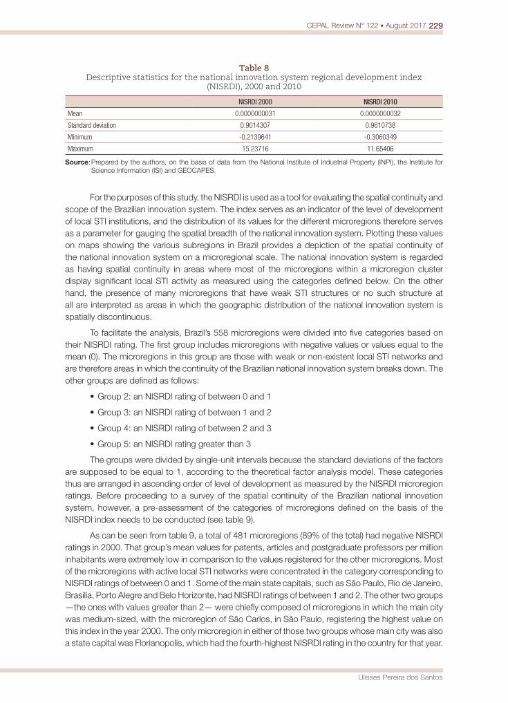
229CEPAL Review N° 122 • August 2017
Ulisses Pereira dos Santos
Table 8 Descriptive statistics for the national innovation system regional development index
(NISRDI), 2000 and 2010
NISRDI 2000 NISRDI 2010
Mean 0.0000000031 0.0000000032
Standard deviation 0.9014307 0.9610738
Minimum -0.2139641 -0.3060349
Maximum 15.23716 11.65406
Source: Prepared by the authors, on the basis of data from the National Institute of Industrial Property (INPI), the Institute for Science Information (ISI) and GEOCAPES.
For the purposes of this study, the NISRDI is used as a tool for evaluating the spatial continuity and scope of the Brazilian innovation system. The index serves as an indicator of the level of development of local STI institutions, and the distribution of its values for the different microregions therefore serves as a parameter for gauging the spatial breadth of the national innovation system. Plotting these values on maps showing the various subregions in Brazil provides a depiction of the spatial continuity of the national innovation system on a microregional scale. The national innovation system is regarded as having spatial continuity in areas where most of the microregions within a microregion cluster display significant local STI activity as measured using the categories defined below. On the other hand, the presence of many microregions that have weak STI structures or no such structure at all are interpreted as areas in which the geographic distribution of the national innovation system is spatially discontinuous.
To facilitate the analysis, Brazil’s 558 microregions were divided into five categories based on their NISRDI rating. The first group includes microregions with negative values or values equal to the mean (0). The microregions in this group are those with weak or non-existent local STI networks and are therefore areas in which the continuity of the Brazilian national innovation system breaks down. The other groups are defined as follows:
• Group 2: an NISRDI rating of between 0 and 1
• Group 3: an NISRDI rating of between 1 and 2
• Group 4: an NISRDI rating of between 2 and 3
• Group 5: an NISRDI rating greater than 3
The groups were divided by single-unit intervals because the standard deviations of the factors are supposed to be equal to 1, according to the theoretical factor analysis model. These categories thus are arranged in ascending order of level of development as measured by the NISRDI microregion ratings. Before proceeding to a survey of the spatial continuity of the Brazilian national innovation system, however, a pre-assessment of the categories of microregions defined on the basis of the NISRDI index needs to be conducted (see table 9).
As can be seen from table 9, a total of 481 microregions (89% of the total) had negative NISRDI ratings in 2000. That group’s mean values for patents, articles and postgraduate professors per million inhabitants were extremely low in comparison to the values registered for the other microregions. Most of the microregions with active local STI networks were concentrated in the category corresponding to NISRDI ratings of between 0 and 1. Some of the main state capitals, such as São Paulo, Rio de Janeiro, Brasilia, Porto Alegre and Belo Horizonte, had NISRDI ratings of between 1 and 2. The other two groups —the ones with values greater than 2— were chiefly composed of microregions in which the main city was medium-sized, with the microregion of São Carlos, in São Paulo, registering the highest value on this index in the year 2000. The only microregion in either of those two groups whose main city was also a state capital was Florianopolis, which had the fourth-highest NISRDI rating in the country for that year.
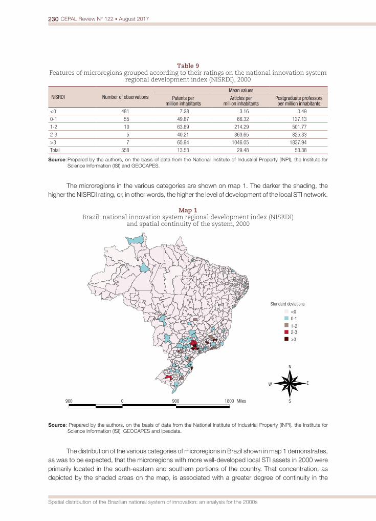
230 CEPAL Review N° 122 • August 2017
Spatial distribution of the Brazilian national system of innovation: an analysis for the 2000s
Table 9 Features of microregions grouped according to their ratings on the national innovation system
regional development index (NISRDI), 2000
NISRDI Number of observationsMean values
Patents per million inhabitants
Articles per million inhabitants
Postgraduate professors per million inhabitants
<0 481 7.28 3.16 0.49
0-1 55 49.87 66.32 137.13
1-2 10 63.89 214.29 501.77
2-3 5 40.21 363.65 825.33
>3 7 65.94 1046.05 1837.94
Total 558 13.53 29.48 53.38
Source: Prepared by the authors, on the basis of data from the National Institute of Industrial Property (INPI), the Institute for Science Information (ISI) and GEOCAPES.
The microregions in the various categories are shown on map 1. The darker the shading, the higher the NISRDI rating, or, in other words, the higher the level of development of the local STI network.
Map 1 Brazil: national innovation system regional development index (NISRDI)
and spatial continuity of the system, 2000
900 0 900 1800 Miles
N
W E
S
Standard deviations
1-2
0-1
<0
2-3
>3
Source: Prepared by the authors, on the basis of data from the National Institute of Industrial Property (INPI), the Institute for Science Information (ISI), GEOCAPES and Ipeadata.
The distribution of the various categories of microregions in Brazil shown in map 1 demonstrates, as was to be expected, that the microregions with more well-developed local STI assets in 2000 were primarily located in the south-eastern and southern portions of the country. That concentration, as depicted by the shaded areas on the map, is associated with a greater degree of continuity in the
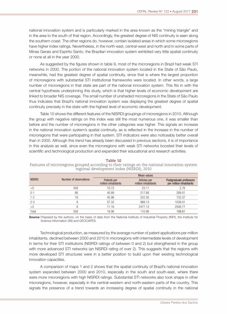
231CEPAL Review N° 122 • August 2017
Ulisses Pereira dos Santos
national innovation system and is particularly marked in the area known as the “mining triangle” and in the area to the south of that region. Accordingly, the greatest degree of NIS continuity is seen along the southern coast. The other regions do, however, contain isolated areas in which some microregions have higher index ratings. Nevertheless, in the north-east, central-west and north and in some parts of Minas Gerais and Espírito Santo, the Brazilian innovation system exhibited very little spatial continuity or none at all in the year 2000.
As suggested by the figures shown in table 9, most of the microregions in Brazil had weak STI networks in 2000. The portion of the national innovation system located in the State of São Paulo, meanwhile, had the greatest degree of spatial continuity, since that is where the largest proportion of microregions with substantial STI institutional frameworks were located. In other words, a large number of microregions in that state are part of the national innovation system. This fits in with the central hypothesis underpinning this study, which is that higher levels of economic development are linked to broader NIS coverage. The small number of unshaded microregions in the State of São Paulo thus indicates that Brazil’s national innovation system was displaying the greatest degree of spatial continuity precisely in the state with the highest level of economic development.
Table 10 shows the different features of the NISRDI groupings of microregions in 2010. Although the group with negative ratings on this index was still the most numerous one, it was smaller than before and the number of microregions in the other categories was higher. This signals an increase in the national innovation system’s spatial continuity, as is reflected in the increase in the number of microregions that were participating in that system. STI indicators were also noticeably better overall than in 2000. Although this trend has already been discussed in previous sections, it is of importance in this analysis as well, since even the microregions with weak STI networks boosted their levels of scientific and technological production and expanded their educational and research activities.
Table 10 Features of microregions grouped according to their ratings on the national innovation system
regional development index (NISRDI), 2010
NISRDI Number of observationsMean values
Patents per million inhabitants
Articles per million inhabitants
Postgraduate professors per million inhabitants
<0 458 10.72 23.11 2.76
0-1 66 40.89 217.68 269.01
1-2 18 45.96 522.35 733.37
2-3 8 57.32 968.13 1039.01
>3 8 71.16 2477.13 2508.77
Total 558 16.96 110.96 108.61
Source: Prepared by the authors, on the basis of data from the National Institute of Industrial Property (INPI), the Institute for Science Information (ISI) and GEOCAPES.
Technological production, as measured by the average number of patent applications per million inhabitants, declined between 2000 and 2010 in microregions with intermediate levels of development in terms for their STI institutions (NISRDI ratings of between 0 and 2) but strengthened in the group with more advanced STI networks (an NISRDI rating of over 2). This suggests that the regions with more developed STI structures were in a better position to build upon their existing technological innovation capacities.
A comparison of maps 1 and 2 shows that the spatial continuity of Brazil’s national innovation system expanded between 2000 and 2010, especially in the south and south-east, where there were more microregions with high NISRDI ratings. Substantial STI networks also took shape in other microregions, however, especially in the central-western and north-eastern parts of the country. This signals the presence of a trend towards an increasing degree of spatial continuity in the national
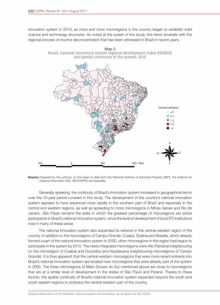
232 CEPAL Review N° 122 • August 2017
Spatial distribution of the Brazilian national system of innovation: an analysis for the 2000s
innovation system in 2010, as more and more microregions in the country began to establish solid science and technology structures. As noted at the outset of this study, this trend dovetails with the regional process of income deconcentration that has been witnessed in Brazil in recent years.
Map 2 Brazil: national innovation system regional development index (NISRDI)
and spatial continuity of the system, 2010
900 0 900 1800 Miles
Standard deviations
N
W E
S
1-2
0-1
<0
2-3
>3
Source: Prepared by the authors, on the basis of data from the National Institute of Industrial Property (INPI), the Institute for Science Information (ISI), GEOCAPES and Ipeadata.
Generally speaking, the continuity of Brazil’s innovation system increased in geographical terms over the 10-year period covered in this study. The development of the country’s national innovation system appears to have advanced more rapidly in the southern part of Brazil and especially in the central and western regions, as well as spreading to more microregions in Minas Gerais and Rio de Janeiro. São Paulo remains the state in which the greatest percentage of microregions are active participants in Brazil’s national innovation system, since the level of development of local STI institutions rose in many of these areas.
The national innovation system also expanded its network in the central-western region of the country. In addition to the microregions of Campo Grande, Cuiabá, Goiânia and Brasilia, which already formed a part of the national innovation system in 2000, other microregions in this region had begun to participate in the system by 2010. The newly integrated microregions were Alto Pantanal (neighbouring on the microregion of Cuiabá) and Dourados and Aquidauana (neighbouring microregions of Campo Grande). It is thus apparent that the central-western microregions that were more recent entrants into Brazil’s national innovation system are located near microregions that were already part of the system in 2000. The three microregions of Mato Grosso do Sul mentioned above are close to microregions that are at a similar level of development in the states of São Paulo and Paraná. Thanks to these factors, the spatial continuity of Brazil’s national innovation system expanded beyond the south and south-eastern regions to embrace the central-western part of the country.
233CEPAL Review N° 122 • August 2017
Ulisses Pereira dos Santos
In the north-east, an inland shift in the trend of the expansion of the national innovation system was observed. The system’s coverage spread out towards the south of Bahia, encompassing the microregions of Vitória da Conquista and Ilhéus-Itabuna. The microregions of Petrolina, Alto Médio Gurgueia and Teresina also became active participants in the national innovation system. Although fewer microregions in the northern part of the country were incorporated into the system, its spatial continuity increased in that region as well. In these two regions and in a large part of the states of Minas Gerais and of Espírito Santo and in the central-western region of the country, map 2 continues to contain many unshaded areas. In other words, in contrast to what has occurred in the wealthier parts of the country, the national innovation system displays almost no continuity at all in the poorer regions. This state of affairs provides further evidence of the relationship between the innovation system’s spatial continuity and economic development. The information provided by maps 1 and 2 and by the data evaluated throughout this study indicate that the southern and south-eastern parts of the country not only have higher levels of scientific and technological production but also have more researchers and a better spatial distribution of STI assets. These findings cannot be considered in isolation from the developmental disparities that separate these regions from the rest of the country.
V. Concluding observations
The analysis conducted for the purposes of this study indicates that Brazil’s national innovation system is undergoing a regional integration process. Between 2000 and 2010, technological, scientific and teaching and research activities began to be undertaken in an increasing number of the country’s microregions. This shift occurred in tandem with the income deconcentration process that has been observed in Brazil in recent years.
The statistics on technological and scientific production show that the Brazilian microregions’ involvement in these activities was much greater in 2010 than it was in 2000. The same is true of teaching and research activities. However, while this does indicate that the spatial continuity of the national innovation system has increased, that continuity is almost wholly confined to the southern and south-eastern regions of the country. As noted earlier, the microregions in those two portions of the country are much more actively involved in the national innovation system than the rest of Brazil’s microregions, which continue to exhibit areas of discontinuity.
The dichotomy between the southern/south-eastern region and the rest of the country cannot be dissociated from the regional economic disparity that has traditionally existed in Brazil. Clearly, the greater level of economic development of the south and south-east is inevitably linked with its stronger STI network, which is not only quantitatively larger than those of the other regions but is also more evenly distributed. This fact allows a larger number of microregions to gain access to the benefits derived from integration into the national innovation system. In other words, the microregions in the southern and south-eastern portions of the country are better able to reap the benefits of technical and scientific information and knowledge flows and of advanced education and research, which have a positive impact on both technologically advanced and more traditional sectors.
The spatial distribution of NIS assets in the State of São Paulo is noteworthy in this respect. Both the STI indicators that were studied in isolation from one another and the NISRDI point to the intensive involvement of that state’s microregions in Brazil’s national innovation system in the two reference years. The fact that this is the most highly developed state in the country establishes a direct link between its NIS performance and the hypothesis being advanced here regarding the need for a better distribution of NIS assets throughout the country. In other words, the regionally balanced distribution of NIS assets in the state with the highest level of economic development in the country indicates that this could be an approach for speeding up the pace of national development.

234 CEPAL Review N° 122 • August 2017
Spatial distribution of the Brazilian national system of innovation: an analysis for the 2000s
In general, the results of this analysis indicate that the expansion of scientific and technological production and of the educational and research activity in Brazil over the 10-year period studied here was fueled by improvements in the regional distribution of these assets. The expansion of the national innovation system also heightened its spatial continuity. Nevertheless, much remains to be done in terms of the innovation system’s regional integration. That integration process will, in turn, help to broaden the regional economic integration process so that more microregions can take part in and benefit from scientific and technological advances, whether in industry, agriculture or specialized service sectors, as the country’s more developed regions are already doing. Thus, economic development and the consolidation of the national innovation system necessarily entail the regional deconcentration of both income and NIS assets.
BibliographyAsheim, B.T. (1996), “Industrial districts as ‘learning regions’: a condition for prosperity”, European Planning
Studies, vol. 4, No. 4, Taylor & Francis. Asheim, B.T. and M. Gertler (2005), “The geography of innovation”, The Oxford Handbook of Innovation,
J. Fagerberg, D. Mowery and R.R. Nelson (eds.), Oxford, Oxford University Press. Christaller, W. (1966), Central Places in Southern Germany, Englewood Cliffs, Prentice-Hall. Cooke, P. (1998), “Introduction: origins of the concept”, Regional Innovation Systems, H. Braczyc, P. Cooke
and M. Heidenreich (eds.), London, UCL Press. Edquist, C. (2005), “Systems of innovation: perspectives and challenges”, The Oxford Handbook of Innovation,
J. Fagerberg, D. Mowery and R.R. Nelson (eds.), Oxford, Oxford University Press. Florida, R. (1995), “Toward the learning region”, Futures, vol. 27, No. 5, Amsterdam, Elsevier. Freeman, C. (2002), “Continental, national and sub-national innovation systems — complementarity and
economic growth”, Research Policy, vol. 31, No. 2, Amsterdam, Elsevier. (1995), “The ‘National System of Innovation’ in historical perspective”, Cambridge Journal of Economics, vol. 19, No. 1, Oxford University Press. (1987), Technology Policy and Economic Performance, London, Pinter Publishers.
Furtado, C. (1967a), Teoria e política do desenvolvimento econômico, São Paulo, Cia. Editora Nacional. (1967b), “Intra-country discontinuities: towards a theory of spatial structures”, Social Science Information, vol. 6, No. 6, SAGE.
Granovetter, M. (1985), “Economic action and social structure: the problem of embeddedness”, American Journal of Sociology, vol. 91, No. 3, Chicago, The University of Chicago Press.
Hirschman, A. (1977), “Transmissão Inter-regional e internacional do crescimento econômico”, Economia regional: textos escolhidos, J. Schwartzman (ed.), Belo Horizonte, Centre for Regional Development and Planning (CEDEPLAR).
Isaksen, A. (2001), “Building regional innovation systems: is endogenous industrial development possible in the global economy?”, Canadian Journal of Regional Science, vol. 24, No. 1.
Jaffe, A. (1989), “Real effects of academic research”, American Economic Review, vol. 79, No. 5, Nashville, Tennessee, American Economic Association.
Lundvall, B.-A. (1992), “Introduction”, National Systems of Innovation: Towards a Theory of Innovation and Interactive Learning, B.-A. Lundvall (ed.), London, Pinter Publishers.
Mingoti, S. (2005), Analise de dados atraves de metodos de estatística multivariada: uma abordagem aplicada, Belo Horizonte, Editora UFMG.
Nelson, R.R. and N. Rosenberg (1993), “Technical innovation and national systems”, National Innovation Systems: A Comparative Analysis, R. Nelson (ed.), New York, Oxford University Press.
Oinas, P. and E. Malecki (1999), “Spatial innovation systems”, Making Connections: Technological Learning and Regional Economic Change, E. Malecki and P. Oinas (eds.), Aldershot, Ashgate.
Perroux, F. (1967), Economia do seculo XX, Lisboa, Herder. Pinto, A. (2000), “A natureza e implicações da heterogeneidade estrutural na América Latina”, Cinquenta
anos de pensamento na CEPAL, R. Bielschowsky (ed.), Rio de Janeiro, Record. Silveira Neto, R. and C. Azzoni (2013), “Os programas sociais e a recente queda na desigualdade regional
da renda no Brazil”, Bolsa Família: uma decada de inclusão e cidadânia. T. Campello and M. Neri (eds.), Brazilia, Institute of Applied Economic Research.
STATACORP (2009), Stata Multivariate Statistics Reference Manual: Release 11, College Station, Stata Press.
Analysis of the duration of unemployment and outcomes for unemployed persons in the Bolivarian Republic of Venezuela1
Josefa Ramoni Perazzi, Giampaolo Orlandoni Merli, Surendra Prasad Sinha, Elizabeth Torres Rivas and Angel Zambrano
1 The Central Bank of Venezuela provided support for this study.
KeywordsUnemployment, economic crisis, employment statistics, informal sector, Venezuela
JEL classificationJ01, J46, J64
AuthorsJosefa Ramoni Perazzi is a Professor with the School of Economic, Administrative and Accounting Sciences of the University of Santander, Colombia. [email protected]
Giampaolo Orlandoni Merli is a Professor with the School of Exact, Physical and Natural Sciences of the University of Santander, Colombia. [email protected]
Surendra Prasad Sinha is a Professor Emeritus of the School of Economic and Social Sciences of the University of Los Andes, Bolivarian Republic of Venezuela. [email protected]
Elizabeth Torres Rivas is a Professor with the School of Economic and Social Sciences of the University of Los Andes, Bolivarian Republic of Venezuela. [email protected]
Angel Zambrano is a Professor with the School of Economic and Social Sciences of the University of Los Andes, Bolivarian Republic of Venezuela. [email protected]
Abstract
Although, at first glance, it would seem to be a contradiction in terms, official statistics indicate that both unemployment and economic activity in the Bolivarian Republic of Venezuela are on a steep downward trend. However, a decline in unemployment can, in fact, occur in the midst of an economic recession if a portion of the actual unemployment rate is concealed by employment in the informal sector and/or by a significant number of people abandoning their job search. Using maximum likelihood estimates for homogeneous Markov matrices applied to household sample survey data for the period starting with the first half of 2012 and ending with the second half of 2013, this study analyses the average duration of unemployment and the outcomes for unemployed persons. The results indicate that long-term unemployment prompts some people to abandon their search for a job (whereupon they cease to be a part of the labour market) and others to move into the informal workforce.
236 CEPAL Review N° 122 • August 2017
Analysis of the duration of unemployment and outcomes for unemployed persons in the Bolivarian Republic of Venezuela
I. Introduction
Unemployment is both a national and a personal problem. At the national level, it represents idle production capacity and a failure to make full use of an important resource, thereby excluding a segment of the population from the creation and enjoyment of wealth. Unlike other macroeconomic problems such as inflation and currency depreciation, unemployment is also such a serious personal problem that, as pointed out by Di Tella, MacCulloch and Oswald (2001), some people would be willing to trade off an increase in the unemployment rate for a larger increase in inflation.
Not all types of unemployment warrant the same degree of response or the adoption of targeted policies, however. What is known as “frictional unemployment” is generated by the time lag between the entry of people into the labour market and their entry into specific jobs. This type of unemployment is self-correcting as job-seekers and employers obtain information about the pool of workers and the pool of available jobs. Mechanisms could be introduced, however, to expedite the process by disseminating information more broadly. Structural unemployment, on the other hand, is, as its name suggests, generated by the very structure of the economy and stems from the inappropriateness of some portion of the available supply of human capital, a technological bias that leads to the uneven development of different sectors of the economy or simply the presence of excess labour supply in a depressed economy.
These two types of unemployment not only have different causes; they also differ in terms of their duration and, consequently, their associated costs. Frictional unemployment is very short-lived, whereas structural unemployment is long-lasting. The former leads to a more efficient assignment of workers to jobs that they are suited for and, while it lasts, job-seekers live off their savings or draw unemployment insurance only for a few weeks. The latter depletes all possible sources of funding, jeopardizes the future of job-seekers’ families and often pushes them into underemployment or employment in the informal sector or may even lead them to abandon their search for employment altogether.
The objective of this study is to provide answers to a number of different questions that have been posed in isolation from one another in various studies. This approach is based on the premise that the complex dynamic of the labour market is not captured by any one indicator. An effort was therefore made to measure how long, on average, people remain unemployed and, when they leave that category, what their status becomes: employed in the formal sector, employed in the informal sector or no longer a part of the workforce at all. In order to do this, maximum likelihood estimates for Markov transition matrices were applied to household sample survey data on the population between 15 and 60 years of age in 2012-2013 compiled by the National Institute of Statistics (INE) of the Bolivarian Republic of Venezuela. The results indicate that the average time spent looking for work is nearly 11 months and that the figure is higher for women and increases as the job-seeker’s level of education rises. It was also found that around two thirds of the unemployed eventually find work —many of them (40%) in the informal sector— while over 30% of them become part of the economically inactive population.
The study is composed of six sections, the first of which is this introduction. The second section outlines the subject under analysis, while the third consists of a brief review of the relevant literature. The fourth and fifth cover the methodology and the results, respectively. Conclusions and recommendations are presented in the final section.
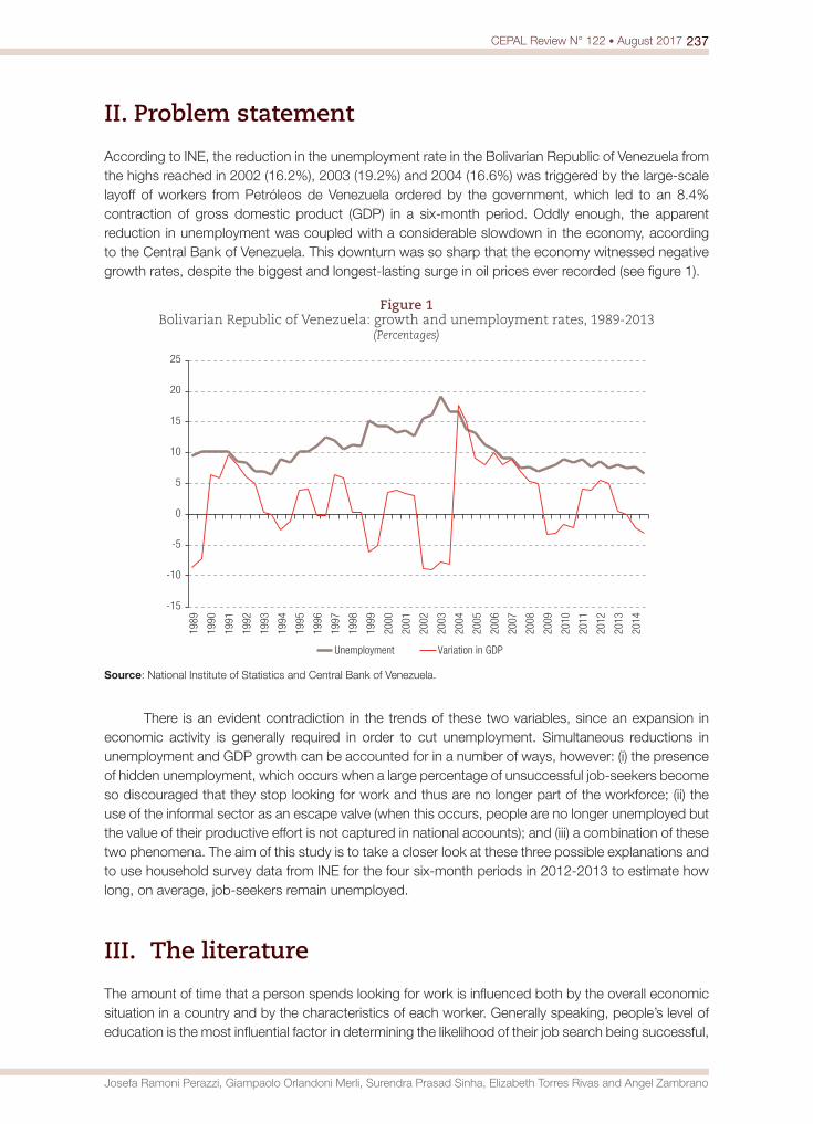
237CEPAL Review N° 122 • August 2017
Josefa Ramoni Perazzi, Giampaolo Orlandoni Merli, Surendra Prasad Sinha, Elizabeth Torres Rivas and Angel Zambrano
II. Problem statement
According to INE, the reduction in the unemployment rate in the Bolivarian Republic of Venezuela from the highs reached in 2002 (16.2%), 2003 (19.2%) and 2004 (16.6%) was triggered by the large-scale layoff of workers from Petróleos de Venezuela ordered by the government, which led to an 8.4% contraction of gross domestic product (GDP) in a six-month period. Oddly enough, the apparent reduction in unemployment was coupled with a considerable slowdown in the economy, according to the Central Bank of Venezuela. This downturn was so sharp that the economy witnessed negative growth rates, despite the biggest and longest-lasting surge in oil prices ever recorded (see figure 1).
Figure 1 Bolivarian Republic of Venezuela: growth and unemployment rates, 1989-2013
(Percentages)
1989
1990
1991
1992
1993
1994
1995
1996
1997
1998
1999
2000
2001
2002
2003
2004
2005
2006
2007
2008
2009
2010
2011
2012
2013
2014
-15
-10
-5
0
5
10
15
20
25
Unemployment Variation in GDP
Source: National Institute of Statistics and Central Bank of Venezuela.
There is an evident contradiction in the trends of these two variables, since an expansion in economic activity is generally required in order to cut unemployment. Simultaneous reductions in unemployment and GDP growth can be accounted for in a number of ways, however: (i) the presence of hidden unemployment, which occurs when a large percentage of unsuccessful job-seekers become so discouraged that they stop looking for work and thus are no longer part of the workforce; (ii) the use of the informal sector as an escape valve (when this occurs, people are no longer unemployed but the value of their productive effort is not captured in national accounts); and (iii) a combination of these two phenomena. The aim of this study is to take a closer look at these three possible explanations and to use household survey data from INE for the four six-month periods in 2012-2013 to estimate how long, on average, job-seekers remain unemployed.
III. The literature
The amount of time that a person spends looking for work is influenced both by the overall economic situation in a country and by the characteristics of each worker. Generally speaking, people’s level of education is the most influential factor in determining the likelihood of their job search being successful,
238 CEPAL Review N° 122 • August 2017
Analysis of the duration of unemployment and outcomes for unemployed persons in the Bolivarian Republic of Venezuela
although the direction and size of its effect may vary. Theoretically, the more educated a job-seeker is, the more likely he or she is to find work, provided that the structure of the production sector is not biased in favour of less skilled workers. There is evidence, however, that, since people with a higher level of education will have a higher reservation wage, their job search will take longer.
Studies conducted by Sum, Harrington and Simpson (1983), Norman (1984) and Stern (1989) in the United States and by Bjorklund and Eriksson (1996) in the Scandinavian countries, on the other hand, indicate that a higher level of education has a positive impact on the probability of a successful job search and reduces the duration of that search. These effects remain but are weaker when comparing the experiences of persons in their own country and their compatriots who seek work abroad (Bruck-Klingberg and others, 2011). The findings of Eckstein and Wolpin (1995) suggest that the amount of time that people remain unemployed is influenced by their aspirations, which rise in tandem with their level of education. The possession of a higher level of education also has a beneficial impact in terms of the subsequent job stability of first-time job seekers (Bratberg and Nilsen, 1998).
Fan and Kong (2011) and Kong (2012) analysed the factors influencing job searches by university graduates in China based on Cox duration models and Kaplan-Meier survival functions. Their results indicate that a university’s reputation and gender are both highly significant factors, with the length of job searches being shorter for women and for graduates of the most prestigious universities. These authors found that the duration of unemployment differs depending on the type of profession, with searches in the fields of engineering and business being shorter than those in the legal field and the sciences. García, Carmona and Gómez (2004) used proportional hazard and log-linear models, while correcting for heterogeneity, to determine the influence exerted by competencies, especially motivation, on the duration of job searches by university graduates in Spain.
These findings do not line up with the results of some other studies, however. Zhou (2003), for example, concluded that a university’s reputation has no more than a marginal effect on the probability of a job search being successful in China, while Bradley and Nguyen (2004) found evidence that this factor has a negative impact that outweighs academic performance among first-time job-seekers in England. It is probable, however, that the effect of the quality of an educational institution is intermingled with the effect of the reservation wage, which rises in step with the quality of the education received (Wolpin, 1987).
Bratberg and Nilsen (1998) also found that job searches are shorter for women than for men in Norway, and they attribute this to the fact that women tend to have a lower reservation wage than men. This finding dovetails with that of Bradley and Nguyen (2004) in England, but is at odds with the results obtained by Zhou (2003) and by Min and others (2006), who found that male university graduates had a greater probability of finding work in China and that their job searches were shorter. Unlike the study done by Kong (2012), most of these studies use logit or probability models to analyse the factors that influence job searches.
Some authors go one step further and look at how other variables, in addition to the traditional components of productivity, may influence the duration of unemployment. Cordón and García (2010) used parametric and non-parametric methods to estimate duration models that could be used to gauge the repercussions of the termination of the fisheries agreement between the European Union and Morocco in 1999. Others have studied the effects of leaving one’s country (Arif, 1996) and of the deep recession that occurred in the United States in the late 2000s (Reich, 2012). Some authors contend that social programmes for the unemployed lengthen their periods of unemployment and that this type of assistance should therefore be more strictly regulated.
Employment in the informal sector is one of the solutions that many workers resort to after a long, unsuccessful job search. Most studies on the subject cover both the formal and informal labour markets. Calderón (2008) used survival functions to estimate the effectiveness of job search
239CEPAL Review N° 122 • August 2017
Josefa Ramoni Perazzi, Giampaolo Orlandoni Merli, Surendra Prasad Sinha, Elizabeth Torres Rivas and Angel Zambrano
mechanisms and the duration of unemployment in Mexico. He considered four possible outcomes: formal employment, informal employment, self-employment and withdrawal from the labour force. Other authors have looked at emigration as another possible outcome for the unemployed (Abellán and Fernández, 1997). Using quarterly data for 2005-2007 on unemployed men between 18 and 65 years of age, these authors found that, as the length of a job search grows, formal-sector workers lower their reservation wages and expand their search to include the informal sector, where one out of three of them end up working. Their study suggests that employment agencies and employment advertisements are of equal effectiveness in job searches.
Márquez and Ruiz-Tagle (2004) analysed the effectiveness of various job-search mechanisms in the Bolivarian Republic of Venezuela, as well as other factors that influence selection and outcomes, including individual characteristics and prior work experience. By applying panel data models to household sample surveys for 1994-2002, these authors concluded that, generally speaking, people who have been working in the informal sector prefer to use non-formal methods to look for jobs, whereas people who have been working in the formal sector are more likely to use more formal, structured job-search approaches. Prior status was found to be a significant factor in determining the probability of success of a given job search.
The Economic and Financial Advisory Office of the National Assembly of Venezuela estimates that, in 2003, the mean duration of unemployment in the country was 18.4 months for women and 8.2 months for men and that the duration increased with age (8.7 months for persons under 30 years of age and 24.9 months for persons over 50 years of age) and level of education (16.8 months for university graduates versus 12.2 months for persons with lower levels of education). In the electricity, natural gas and water sector, a job search may last up to 24 months, but it will last just half as long in the manufacturing sector. Ortega and Martínez (2005) found that the duration of a job search may vary from one region to the next, with job searches being lengthier in the states of Nueva Esparta (16.68 months) and Bolívar (11.75 months) and shorter in the states of Guárico (7.99 months) and Lara (7.15 months).
IV. The methodology
1. Database
INE has carried out household sample surveys regularly ever since 1967 in order to gather information on trends in the labour market, the housing situation and the country’s overall socioeconomic structure. This information can be used to construct national indicators, especially for employment and housing, that can serve as a basis for decision-making.
Information on individuals for the four six-month periods comprising 2012 and 2013 —the most recent data available at the time that the study began— have been used here. The data were organized on the basis of identifiers for the more than 50,000 persons making up the survey cohorts. The next step was to horizontally pair the variables based on those identification codes in order to construct a panel that could be used to track the changes occurring in the employment status of the sample units over time. In order to lessen the amount of dispersion, only the data on people between the ages of 15 and 60 were used, thereby excluding young people who are not yet of working age and most retirees and pensioners.
During the preparation of the database, a series of irregularities were detected that caused a great deal of information loss. These irregularities included the omission of the income levels of many workers in the cohort corresponding to the second half of 2013, the miscoding of the International
240 CEPAL Review N° 122 • August 2017
Analysis of the duration of unemployment and outcomes for unemployed persons in the Bolivarian Republic of Venezuela
Standard Classification of Occupations (ISCO) categories for workers’ occupations (ISCO-88) —even though their job titles and descriptions were available— and distortions of the length of job searches. This made it necessary to adjust the data based on the observed changes in the employment status of the corresponding individuals and in the activities they had carried out in the recent past. There were also many missing pieces of information about the variables needed to determine whether a given job was in the formal or informal sector, what wage and non-wage benefits workers received and what job search strategies were used, among others. As well as making it necessary to adjust the approaches used in this study and to work with a smaller sample, these information gaps give rise to a regrettable loss of information and waste of resources that could be remedied by introducing better data compilation and transcription control mechanisms. Fortunately, some of these variables were not needed for this study, so no observations were lost. Wherever possible, data were imputed from the information provided by other variables. In non-response cases where this could not be done for the variable of interest (less than 7% of all cases), no behaviour pattern could be detected that could be used to associate the variable with any of the covariates.2 The final panel consisted of 30,270 people (51.75% women and 48.25% men). The first panel had a mean age of 34.12 years and a fairly small proportion of people with a higher education (45.11% had completed no more than the basic cycle of schooling (6 years), 28.77% had completed their secondary education (5 additional years), 6.71% had a technical education and 19.41% had a university education); 49.72% of the members of the cohort were married or had a partner and 39.90% were single; 59.91% were employed, 5.80% were looking for work and the rest were part of the economically inactive population (15.53% were studying, 14.29% took care of the home, 4.15% were retired, lived off investment income, had disabilities or marked “other” and 0.33% did not report any type of activity despite the fact that this group was composed of potentially productive persons with an average age of 26.5 years). Although there was some variation, the structure of the other cohorts was more or less the same.
In order to measure the duration of job searches, the amount of time that unemployed persons had been looking for work at the start of the first half of 2012 was recorded. Then the amount of time that passed for the various cohorts was gradually added until such time as the person was no longer unemployed because he or she found a job or joined the economically inactive population. This latter option was determined to have been chosen on the basis of answers to the questions “When did you last look for work?” and “What did you do last week?”. The result was cross-referenced with the amount of time that each person said that he or she had been looking for work (measured by categories). This study thus analyses the paths followed by this group of unemployed persons over the four six-month periods that were covered. It does so by measuring the amount of time that they remained unemployed, identifying their subsequent employment status and examining their job search strategies. The duration of unemployment is defined as the interval between the initial event (the start of a job search as reported by the respondent) and the end point in time (when the person ceases to be unemployed within the period under analysis). In this type of situation, right-hand censorship is inevitable since the event (the end of unemployment) may occur after the study period has ended, as occurred in the case of some people in the last cohort. In these cases, it is advisable to work with percentages and quantiles, as was done here, as well as with life tables and survival analyses. This latter approach will be explored in a forthcoming study.
2 Bethlehem, Cobben and Schouten (2011) identified three different non-response mechanisms. The first is a completely random non-response, which is independent of the target variable (Y) and is not due to factors represented by the covariates either. In this case, non-responses are selective and the results are therefore not biased. The second is a random non-response which is attributable to factors related to one or another covariate but is not related to Y. In this case, the bias that it generates can be corrected for by using X-based techniques. The third mechanism is a non-random response, which is related both to Y and to X. In this case, X-based correction mechanisms are not useful.
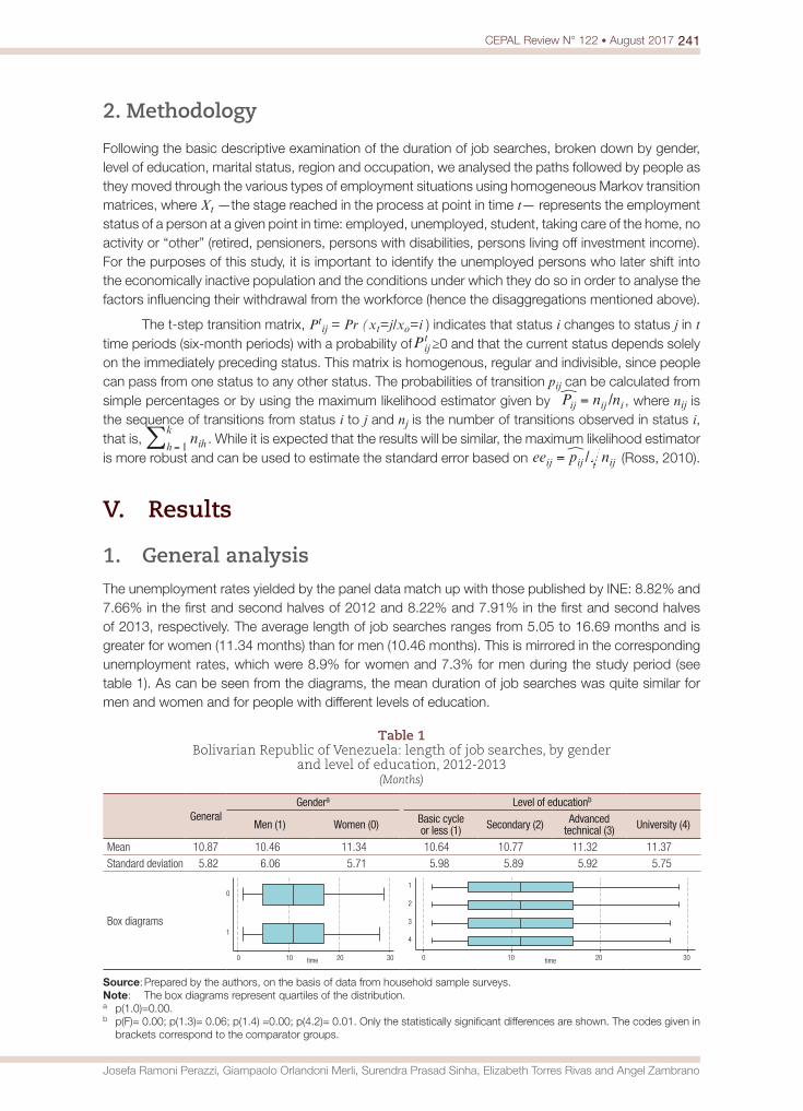
241CEPAL Review N° 122 • August 2017
Josefa Ramoni Perazzi, Giampaolo Orlandoni Merli, Surendra Prasad Sinha, Elizabeth Torres Rivas and Angel Zambrano
2. Methodology
Following the basic descriptive examination of the duration of job searches, broken down by gender, level of education, marital status, region and occupation, we analysed the paths followed by people as they moved through the various types of employment situations using homogeneous Markov transition matrices, where Xt —the stage reached in the process at point in time t— represents the employment status of a person at a given point in time: employed, unemployed, student, taking care of the home, no activity or “other” (retired, pensioners, persons with disabilities, persons living off investment income). For the purposes of this study, it is important to identify the unemployed persons who later shift into the economically inactive population and the conditions under which they do so in order to analyse the factors influencing their withdrawal from the workforce (hence the disaggregations mentioned above).
The t-step transition matrix, Ptij = Pr (xt=j/xo=i ) indicates that status i changes to status j in t
time periods (six-month periods) with a probability ofPijt ≥0 and that the current status depends solely
on the immediately preceding status. This matrix is homogenous, regular and indivisible, since people can pass from one status to any other status. The probabilities of transition pij can be calculated from simple percentages or by using the maximum likelihood estimator given by /P n nij ij i=| , where nij is the sequence of transitions from status i to j and nj is the number of transitions observed in status i, that is, nihh
k
1=/ . While it is expected that the results will be similar, the maximum likelihood estimator
is more robust and can be used to estimate the standard error based on /ee p nij ij ij=} (Ross, 2010).
V. Results
1. General analysis
The unemployment rates yielded by the panel data match up with those published by INE: 8.82% and 7.66% in the first and second halves of 2012 and 8.22% and 7.91% in the first and second halves of 2013, respectively. The average length of job searches ranges from 5.05 to 16.69 months and is greater for women (11.34 months) than for men (10.46 months). This is mirrored in the corresponding unemployment rates, which were 8.9% for women and 7.3% for men during the study period (see table 1). As can be seen from the diagrams, the mean duration of job searches was quite similar for men and women and for people with different levels of education.
Table 1 Bolivarian Republic of Venezuela: length of job searches, by gender
and level of education, 2012-2013(Months)
GeneralGendera Level of educationb
Men (1) Women (0) Basic cycle or less (1) Secondary (2) Advanced
technical (3) University (4)
Mean 10.87 10.46 11.34 10.64 10.77 11.32 11.37
Standard deviation 5.82 6.06 5.71 5.98 5.89 5.92 5.75
Box diagrams
0 10 20 30 time
1
0
0 10 20 30 time
4
3
2
1
Source: Prepared by the authors, on the basis of data from household sample surveys. Note: The box diagrams represent quartiles of the distribution.a p(1.0)=0.00.b p(F)= 0.00; p(1.3)= 0.06; p(1.4) =0.00; p(4.2)= 0.01. Only the statistically significant differences are shown. The codes given in
brackets correspond to the comparator groups.

242 CEPAL Review N° 122 • August 2017
Analysis of the duration of unemployment and outcomes for unemployed persons in the Bolivarian Republic of Venezuela
Job searches take longer as the person’s level of education rises. This could be accounted for either by the fact that more highly trained people have higher reservation wages (which leads them to prolong their search in order to find a job that meets their expectations) or by the possibility that there is not enough demand in the labour market for the available supply of skilled workers. Accordingly, the duration of university graduates’ job searches is significantly greater than it is for workers with a secondary or lower level of education, but is similar to the duration of the job searches of persons with advanced technical training.
The duration of unemployment is also influenced by people’s ages: persons between the ages of 21 and 35 remain unemployed for longer than the members of any other age group, while those over 50 take the least amount of time to leave the category of the unemployed, probably because they are more likely to be able to opt for retirement (see table 2). This result is in keeping with the higher unemployment rates for persons of working age and the lower ones for persons over 50 years of age issued by INE. The box diagram in table 2 depicts the homogenous job search durations found for the first three age groups and what would appear to be the more heterogeneous results for persons over 50. This finding warrants a more specific study on the entry of older adults into the workforce.
Table 2 Bolivarian Republic of Venezuela: length of job searches, by age group,
second half of 2012 and second half of 2013 (Months)
Age groupa
0 10 20 30 time
4
3
2
1
15-20 years (1)
21-35 years (2)
36-50 years (3)
Over 50 years (4)
Mean 10.82 11.52 10.41 9.50
Standard deviation 5.85 5.96 5.89 5.54
Source: Prepared by the authors, on the basis of data from household sample surveys. Note: The box diagram represents quartiles of the distribution.a p(F) = 0.00; p(1.2) = 0.001; p(2.3) = p(1.4) = p(2.4) = p(3.4) = 0. Only the statistically significant differences are shown. The
codes given in brackets correspond to the comparator groups.
The literature indicates that, generally speaking, people who are married or in a civil union are more likely to accept a job offer sooner and to remain in that job longer than single workers without family responsibilities. No significant differences were found, however, between the different categories of marital status included in this study, although it is true that the shortest job searches were recorded for persons who were married or in civil unions (see table 3).
Table 3 Bolivarian Republic of Venezuela: length of job searches, by marital status, 2012-2013
(Months)
Marital statusa Mean Standarddeviation
0 10 20 30 time
3
2
1
Married or in a civil union (1) 10.71 4.91
Divorced, separated or widowed (2) 10.96 5.95
Single (3) 11.01 5.91
Source: Prepared by the authors, on the basis of data from household sample surveys. Note: The box diagram represents quartiles of the distribution.a p(F) = 0.08.
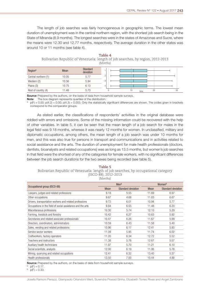
243CEPAL Review N° 122 • August 2017
Josefa Ramoni Perazzi, Giampaolo Orlandoni Merli, Surendra Prasad Sinha, Elizabeth Torres Rivas and Angel Zambrano
The length of job searches was fairly homogeneous in geographic terms. The lowest mean duration of unemployment was in the central northern region, with the shortest job search being in the State of Miranda (8.9 months). The longest searches were in the states of Amazonas and Sucre, where the means were 12.30 and 12.77 months, respectively. The average duration in the other states was around 10 or 11 months (see table 4).
Table 4 Bolivarian Republic of Venezuela: length of job searches, by region, 2012-2013
(Months)
Regiona Mean Standarddeviation
0 10 20 30 time
4
3
2
1
Central northern (1) 10.05 5.77
Western (2) 10.56 5.94
Plains (3) 10.75 6.13
Rest of country (4) 11.48 5.73
Source: Prepared by the authors, on the basis of data from household sample surveys. Note: The box diagram represents quartiles of the distribution.a p(F) = 0.00; p(4.2) = 0.00; p(4.3) = 0.003. Only the statistically significant differences are shown. The codes given in brackets
correspond to the comparator groups.
As stated earlier, the classifications of respondents’ activities in the original database were riddled with errors and omissions. Some of the missing information could be recovered with the help of other variables. In table 5, it can be seen that the mean length of a job search for males in the legal field was 9.18 months, whereas it was nearly 12 months for women. In unclassified, military and diplomatic occupations, among others, the mean length of a job search was under 10 months for men, and this was also true for persons in transport and communications and in activities related to social assistance and the arts. The duration of unemployment for male health professionals (doctors, dentists, bioanalysts and related occupations) was as long as 13.5 months, but women’s job searches in that field were the shortest of any of the categories for female workers, with no significant differences between the job search durations for the two sexes being recorded (see table 5).
Table 5 Bolivarian Republic of Venezuela: length of job searches, by occupational category
(ISCO-88), 2012-2013(Months)
Occupational group (ISCO-88)Mena Womenb
Mean Standard deviation Mean Standard deviationLawyers, judges and related professions 9.18 5.55 11.69 6.97
Other occupations 9.67 4.68 11.83 6.67
Drivers, transportation workers and related professions 9.72 6.01 10.94 5.77
Occupations in the field of social assistance and the arts 9.84 6.55 11.48 6.20
Miscellaneous professions 10.30 5.74 12.10 5.29
Farming, livestock and forestry 10.42 6.27 10.63 5.92
Secretaries and related associate professionals 10.47 6.26 11.67 5.99
Directors, coordinators, administrators 10.59 6.43 11.58 5.40
Sales, vending and related professions 10.96 6.17 12.41 5.85
Service sector workers 11.09 5.95 11.74 6.02
Craftworkers, factory operators 11.20 6.34 12.72 5.52
Teachers and instructors 11.38 5.76 12.67 5.57
Auxiliary health technicians 11.97 5.70 11.21 6.10
Social scientists, analysts 12.00 6.19 11.06 5.78
Mining, quarrying and related occupations 12.41 6.32 13.40 5.37
Health professionals 13.50 7.00 10.44 4.88
Source: Prepared by the authors, on the basis of data from household sample surveys. a p(F) = 0.17.b p(F) = 0.33.
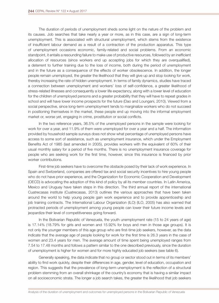
244 CEPAL Review N° 122 • August 2017
Analysis of the duration of unemployment and outcomes for unemployed persons in the Bolivarian Republic of Venezuela
The duration of periods of unemployment sheds some light on the nature of the problem and its causes. Job searches that take nearly a year or more, as in this case, are a sign of long-term unemployment. This is associated with structural unemployment, which stems from the existence of insufficient labour demand as a result of a contraction of the production apparatus. This type of unemployment occasions economic, family-related and social problems. From an economic standpoint, it entails a resounding failure to make use of productive resources, followed by an inefficient allocation of resources (since workers end up accepting jobs for which they are overqualified), a deterrent to further training due to the loss of income, both during the period of unemployment and in the future as a consequence of the effects of worker obsolescence. In addition, the longer people remain unemployed, the greater the likelihood that they will give up and stop looking for work, thereby increasing the rate of hidden unemployment. In terms of family dynamics, studies have traced a connection between unemployment and workers’ loss of self-confidence, a greater likelihood of stress-related illnesses and consequently a lower life expectancy, along with a lower level of education for the children of unemployed persons and a greater probability that they will have to repeat grades in school and will have lower income prospects for the future (Dao and Loungani, 2010). Viewed from a social perspective, since long-term unemployment tends to marginalize workers who do not succeed in positioning themselves in the market, these people end up moving into the informal employment market or, worse yet, engaging in crime, prostitution or social conflicts.
In the two reference years, 36.5% of the unemployed persons in the sample were looking for work for over a year, and 11.9% of them were unemployed for over a year and a half. The information provided by household sample surveys does not show what percentage of unemployed persons have access to some sort of assistance, such as unemployment insurance, which under the Employment Benefits Act of 1985 (last amended in 2005), provides workers with the equivalent of 60% of their usual monthly salary for a period of five months. There is no unemployment insurance coverage for people who are seeking work for the first time, however, since this insurance is financed by prior worker contributions.
First-time job seekers have to overcome the obstacle posed by their lack of work experience. In Spain and Switzerland, companies are offered tax and social security incentives to hire young people who do not have prior experience, and the Organization for Economic Cooperation and Development (OECD) is advocating the adoption of this kind of policy by all its member countries. In Latin America, Mexico and Uruguay have taken steps in this direction. The third annual report of the international Cuatrecasas institute (Cuatrecasas, 2013) outlines the various approaches that have been taken around the world to help young people gain work experience and to provide apprenticeship and job training contracts. The International Labour Organization (ILO) (ILO, 2005) has also warned that protracted periods of unemployment among young people can lower their future income levels and jeopardize their level of competitiveness going forward.
In the Bolivarian Republic of Venezuela, the youth unemployment rate (15 to 24 years of age) is 17.14% (18.79% for girls and women and 15.92% for boys and men in those age groups). It is not only the younger members of this age group who are first-time job seekers, however, as the data indicate that the average age of people looking for work for the first time is 26.3 years in the case of women and 23.4 years for men. The average amount of time spent being unemployed ranges from 7.54 to 17.48 months and follows a pattern similar to the one described previously, since the duration of unemployment is higher for women and for more highly educated job seekers (see table 6).
Generally speaking, the data indicate that no group or sector stood out in terms of its members’ ability to find work quickly, despite their differences in age, gender, level of education, occupation and region. This suggests that the prevalence of long-term unemployment is the reflection of a structural problem stemming from an overall shrinkage of the country’s economy that is having a similar impact on all socioeconomic strata. The longer a job search takes, the greater the likelihood that job seekers

245CEPAL Review N° 122 • August 2017
Josefa Ramoni Perazzi, Giampaolo Orlandoni Merli, Surendra Prasad Sinha, Elizabeth Torres Rivas and Angel Zambrano
will abandon their search, which is why it is important to track the path followed by unemployed persons as they transition from one type of employment status to another.
Table 6 Bolivarian Republic of Venezuela: length of job searches, by gender and level
of education of first-time job seekers, 2012-2013 (Months)
GeneralGendera Level of educationb
Men (1) Women (0) Basic cycle or less (1) Secondary (2) Advanced
technical (3) University (4)
Mean 12.51 11.39 12.79 11.09 11.07 12.58 12.02
Standard deviation 4.97 4.85 4.89 4.79 4.8 4.61 4.75
Box diagrams
5 10 15 20 25 time
1
0
5 10 15 20 25 time
4
3
2
1
Source: Prepared by the authors, on the basis of data from household sample surveys. Note: The box diagrams represent quartiles of the distribution.a p(F)=0.02; (b) p(F) =0.03; p(1.3)=0.03; p(1.4)=0.02; p(2.3)=0.03; p(2.4)=0.02. Only the statistically significant differences are
shown. The codes given in brackets correspond to the comparator groups.
2. Transitions in employment status
As noted earlier, a downward trend in unemployment during economic recessions can be accounted for, in part, by the fact that some job seekers eventually become discouraged and stop looking for work. This phenomenon is known as the “discouraged worker effect”. While 65.11% of the unemployed found work, the other 35% gave up. Some of the people in this latter group (12.75%) went back to school in order to make themselves more competitive and improve their future job prospects; nearly 16% decided to devote themselves to domestic tasks in the home and 5.3% chose neither option and remained idle. A very small percentage (1.19%) continued their search or moved into other categories, such as persons with disabilities or persons who chose to take early retirement or who reached their statutory retirement age (see table 7).
Table 7 Bolivarian Republic of Venezuela: outcomes for unemployed workers, 2012-2013
(Percentages)
Number of periods Found work Stopped searching for work
Returned to school Stayed at home Did not have a job and were not looking for one
Pursuing their job search/ Other
1 79.76 94.19 89.88 86.87 -
2 19.08 5.23 9.08 11.45 -
3 1.16 0.58 1.04 1.68 -
Total 65.11 12.75 15.65 5.30 1.19
Source: Prepared by the authors, on the basis of data from household sample surveys.
The entry of potential workers into the economically inactive population not only translates into an underutilization of the available labour supply but also leads to an underestimation of the actual level of unemployment that delays or distorts the design and adoption of measures for addressing the problem. Workers know that it is not easy to find a job. As shown in figure 2, more than 38% of the unemployed persons in the sample contended that they were tired of looking for work and that they
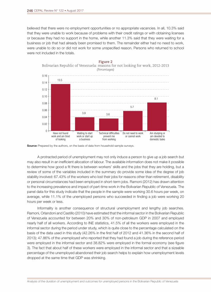
246 CEPAL Review N° 122 • August 2017
Analysis of the duration of unemployment and outcomes for unemployed persons in the Bolivarian Republic of Venezuela
believed that there were no employment opportunities or no appropriate vacancies. In all, 10.3% said that they were unable to work because of problems with their credit ratings or with obtaining licenses or because they had no support in the home, while another 11.3% said that they were waiting for a business or job that had already been promised to them. The remainder either had no need to work, were unable to do so or did not work for some unspecified reason. Persons who returned to school were not included in the totals.
Figure 2 Bolivarian Republic of Venezuela: reasons for not looking for work, 2012-2013
(Percentages)
13.5
3.9 3.6
5.7
8.1
0
0.02
0.04
0.06
0.08
0.10
0.12
0.14
0.16
Have not found work and am tired
of looking
Waiting to start work or start up
a business
Technical difficultiesprevent me
from working
Do not need to workor cannot work
Am studying or am devoted to domestic tasks
Source: Prepared by the authors, on the basis of data from household sample surveys.
A protracted period of unemployment may not only induce a person to give up a job search but may also result in an inefficient allocation of labour. The available information does not make it possible to determine how good a fit there is between workers’ skills and the jobs that they are holding, but a review of some of the variables included in the summary do provide some idea of the degree of job stability involved: 67.43% of the workers who lost their jobs for reasons other than retirement, disability or personal circumstances had been employed in short-term jobs. Ramoni (2012) has drawn attention to the increasing prevalence and impact of part-time work in the Bolivarian Republic of Venezuela. The panel data for this study indicate that the people in the sample were working 30.6 hours per week, on average, while 11.1% of the unemployed persons who succeeded in finding a job were working 20 hours per week or less.
Informality is another consequence of structural unemployment and lengthy job searches. Ramoni, Orlandoni and Castillo (2010) have estimated that the informal sector in the Bolivarian Republic of Venezuela accounted for between 20% and 30% of non-petroleum GDP in 2007 and employed nearly half of all workers. According to INE statistics, 41.5% of all the workers were employed in the informal sector during the period under study, which is quite close to the percentage calculated on the basis of the data used in this study (42.26% in the first half of 2012 and 41.36% in the second half of 2013); 47.86% of the unemployed who reported that they had found a job during the reference period were employed in the informal sector and 38.82% were employed in the formal economy (see figure 3). The fact that about half of these workers were employed in the informal sector and that a sizeable percentage of the unemployed abandoned their job search helps to explain how unemployment levels dropped at the same time that GDP was shrinking.
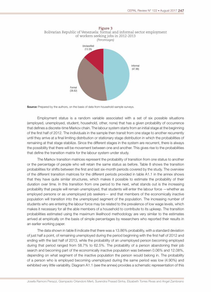
247CEPAL Review N° 122 • August 2017
Josefa Ramoni Perazzi, Giampaolo Orlandoni Merli, Surendra Prasad Sinha, Elizabeth Torres Rivas and Angel Zambrano
Figure 3 Bolivarian Republic of Venezuela: formal and informal sector employment
of workers seeking jobs in 2012-2013(Percentages)
Informal(47.86)
Formal(38.82)
Unclassified(13.35)
Source: Prepared by the authors, on the basis of data from household sample surveys.
Employment status is a random variable associated with a set of six possible situations (employed, unemployed, student, household, other, none) that has a given probability of occurrence that defines a discrete-time Markov chain. The labour system starts from an initial stage at the beginning of the first half of 2012. The individuals in the sample then transit from one stage to another recurrently until they arrive at a final limiting distribution or stationary stage distribution in which the probabilities of remaining at that stage stabilize. Since the different stages in the system are recurrent, there is always the possibility that there will be movement between one and another. This gives rise to the probabilities that define the transition matrix for the labour system under study.
The Markov transition matrices represent the probability of transition from one status to another or the percentage of people who will retain the same status as before. Table 8 shows the transition probabilities for shifts between the first and last six-month periods covered by the study. The overview of the different transition matrices for the different periods provided in table A1.1 in the annex shows that they have quite similar structures, which makes it possible to estimate the probability of their duration over time. In this transition from one period to the next, what stands out is the increasing probability that people will remain unemployed, that students will enter the labour force —whether as employed persons or as unemployed job seekers— and that members of the economically inactive population will transition into the unemployed segment of the population. The increasing number of students who are entering the labour force may be related to the prevalence of low wage levels, which makes it necessary for all the able members of a household to contribute to its upkeep. The transition probabilities estimated using the maximum likelihood methodology are very similar to the estimates arrived at empirically on the basis of simple percentages by researchers who reported their results in an earlier working paper.
The data shown in table 8 indicate that there was a 13.86% probability, with a standard deviation of just half a point, of remaining unemployed during the period beginning with the first half of 2012 and ending with the last half of 2013, while the probability of an unemployed person becoming employed during that period ranged from 58.7% to 62.5%. The probability of a person abandoning their job search and becoming part of the economically inactive population was between 0.06% and 12.08%, depending on what segment of the inactive population the person would belong in. The probability of a person who is employed becoming unemployed during the same period was low (4.90%) and exhibited very little variability. Diagram A1.1 (see the annex) provides a schematic representation of this

248 CEPAL Review N° 122 • August 2017
Analysis of the duration of unemployment and outcomes for unemployed persons in the Bolivarian Republic of Venezuela
transition based on the results obtained in this study. Since this is a regular, indivisible and acyclical matrix, a transition to or from any employment status to any other is possible, but only the most likely shifts are shown here.
Table 8 Bolivarian Republic of Venezuela: employment transition matrix, 2012-2013
(Percentages)
Period 4
Period 1Employed Unemployed Student Household Other None
Employed 73.41 (0.6)
4.90 (0.2)
8.39 (0.3)
9.90(0.3)
3.23(0.2)
0.17 (0.1)
Unemployed 60.60 (1.9)
13.86 (0.5)
9.34 (0.8)
12.08(0.9)
4.07(0.5)
0.06 (0.1)
Student 43.19(1.3)
5.22(0.4)
36.25(0.6)
9.79(0.6)
5.16(0.4)
0.38(0.1)
Household 45.59(1.2)
4.93(0.4)
8.42(0.5)
36.85(0.6)
3.84(0.3)
0.37(0.1)
Other 46.72(2.1)
5.11(0.6)
9.81(0.9)
12.18(1.0)
26.36(0.5)
0.41(0.2)
None 43.12(8.8)
12.84(3.1)
12.84(4.4)
23.85(5.0)
5.50(2.8)
1.83(0.0)
Stationary vector 62.82 5.51 12.86 13.96 4.62 0.24
Source: Prepared by the authors, on the basis of data from household sample surveys. Note: The standard error is shown in parentheses.
The stationary vector obtained from the stochastic matrix is not a projection of what may happen in the future but rather a trend indicator for the distribution based on the behaviour of the variable in question, assuming that the conditions prevailing at the time that the study was conducted remain constant. The process quickly converges towards the stationary probability vector shown in the last row of table 8, which gives the long-term employment profile. This represents the limiting distribution of the system and is independent of its initial state.
The estimated values for the stationary distribution are, in part, similar to those obtained by Márquez and Ruiz-Tagle (2004) for the Bolivarian Republic of Venezuela in 1994-2002. While that study found that the probability of being unemployed was 4.8% (below the 5.51% vector of this study), the probability of remaining employed was much greater (84.9% versus 62.82%). The main difference between these studies’ findings is that, in the former study, the probability of remaining in the economically inactive population was only 10.3% —far below the 31.67%3 estimate of the present study.
3. Job search mechanisms
Workers and employers use various strategies for arriving at the best job/worker match in the least possible amount of time. There is, to some extent, a trade-off between the amount of time spent looking for work and the quality of the job, and this is influenced by factors such as the worker’s reservation wage and his or her ability to cover living expenses while looking for work. Unemployment insurance schemes, which vary from country to country, play a fundamental role in this respect. In the Bolivarian Republic of Venezuela, unemployment insurance coverage is limited to a period of five months.4
3 This is the value yielded by adding up the probabilities for the different categories of economic inactivity: 12.86 + 13.96 + 4.62 + 0.24.4 In the United States, an unemployed person receives up to 50% of his or her salary for 33 weeks. In some European countries,
unemployment insurance coverage lasts for as long as three years. The duration of coverage has a direct impact on the amount of time spent looking for work and, consequently, on the unemployment rate (Brunner and Calarelli, 2004). For a comparative study of unemployment assistance programmes in European countries, see Observatorio de Relaciones Laborales (2012).
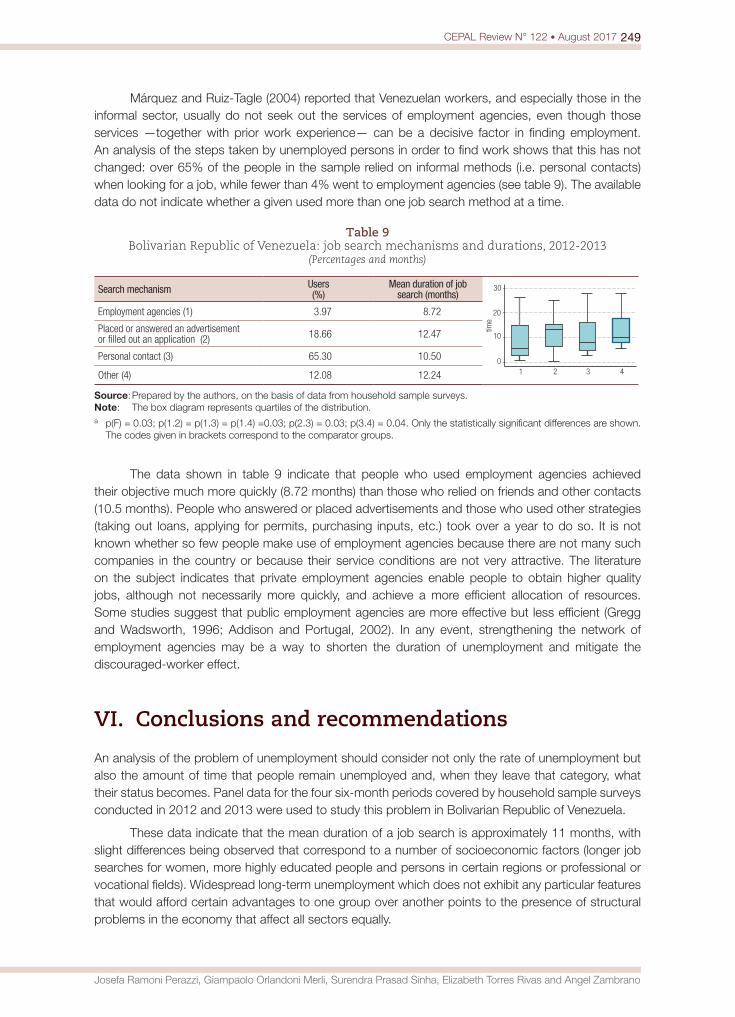
249CEPAL Review N° 122 • August 2017
Josefa Ramoni Perazzi, Giampaolo Orlandoni Merli, Surendra Prasad Sinha, Elizabeth Torres Rivas and Angel Zambrano
Márquez and Ruiz-Tagle (2004) reported that Venezuelan workers, and especially those in the informal sector, usually do not seek out the services of employment agencies, even though those services —together with prior work experience— can be a decisive factor in finding employment. An analysis of the steps taken by unemployed persons in order to find work shows that this has not changed: over 65% of the people in the sample relied on informal methods (i.e. personal contacts) when looking for a job, while fewer than 4% went to employment agencies (see table 9). The available data do not indicate whether a given used more than one job search method at a time.
Table 9 Bolivarian Republic of Venezuela: job search mechanisms and durations, 2012-2013
(Percentages and months)
Search mechanism Users(%)
Mean duration of job search (months)
0
10
20
30
time
1 2 3 4
Employment agencies (1) 3.97 8.72
Placed or answered an advertisement or filled out an application (2) 18.66 12.47
Personal contact (3) 65.30 10.50
Other (4) 12.08 12.24
Source: Prepared by the authors, on the basis of data from household sample surveys. Note: The box diagram represents quartiles of the distribution.a p(F) = 0.03; p(1.2) = p(1.3) = p(1.4) =0.03; p(2.3) = 0.03; p(3.4) = 0.04. Only the statistically significant differences are shown.
The codes given in brackets correspond to the comparator groups.
The data shown in table 9 indicate that people who used employment agencies achieved their objective much more quickly (8.72 months) than those who relied on friends and other contacts (10.5 months). People who answered or placed advertisements and those who used other strategies (taking out loans, applying for permits, purchasing inputs, etc.) took over a year to do so. It is not known whether so few people make use of employment agencies because there are not many such companies in the country or because their service conditions are not very attractive. The literature on the subject indicates that private employment agencies enable people to obtain higher quality jobs, although not necessarily more quickly, and achieve a more efficient allocation of resources. Some studies suggest that public employment agencies are more effective but less efficient (Gregg and Wadsworth, 1996; Addison and Portugal, 2002). In any event, strengthening the network of employment agencies may be a way to shorten the duration of unemployment and mitigate the discouraged-worker effect.
VI. Conclusions and recommendations
An analysis of the problem of unemployment should consider not only the rate of unemployment but also the amount of time that people remain unemployed and, when they leave that category, what their status becomes. Panel data for the four six-month periods covered by household sample surveys conducted in 2012 and 2013 were used to study this problem in Bolivarian Republic of Venezuela.
These data indicate that the mean duration of a job search is approximately 11 months, with slight differences being observed that correspond to a number of socioeconomic factors (longer job searches for women, more highly educated people and persons in certain regions or professional or vocational fields). Widespread long-term unemployment which does not exhibit any particular features that would afford certain advantages to one group over another points to the presence of structural problems in the economy that affect all sectors equally.
250 CEPAL Review N° 122 • August 2017
Analysis of the duration of unemployment and outcomes for unemployed persons in the Bolivarian Republic of Venezuela
Given the fact that people are pursuing lengthy job searches during what official statistics show to be a recession, an explanation for the declining unemployment rate (which had fallen below 8% by the end of the period under analysis) is called for, and the household sample survey results provide one. Over half of the unemployed persons covered by the survey ended up finding work, while the rest withdrew from the labour force and went back to school in an effort to become more competitive or decided to devote their time to caring for the home or engaging in other types of activities. Nearly 48% of the people who did find work ended up being employed in the informal sector. The quality of the jobs obtained by the rest of the people who became employed is unknown. However, information from the sample surveys suggests that a large percentage of the workers have fixed-term contracts or are working part-time. The most commonly used job search mechanisms are not the most suitable ones either, since people usually rely on personal contacts rather than making use of more formal methods.
Given that the transition matrices reflect an upward trend in unemployment, if the economy’s structural problems remain in place, the probability that a worker will be employed in the future is just under 63%, while the probability that a worker will become part of the economically inactive population tops 30%. For the most part, when members of the inactive population decide to rejoin the labour force, they are initially categorized as unemployed. Our findings indicate that the downturn in the unemployment rate should not be interpreted as meaning that the problem is on its way to being resolved but is instead a reflection of the fact that many unsuccessful job seekers are becoming so discouraged that they are withdrawing from the workforce altogether and that many of those who are employed are working in the informal sector.
The work done to prepare the database showed up the presence of a series of gaps or flaws in the compilation and transcription of the survey data. These shortcomings give rise to a loss of information and a waste of valuable resources and point up the need for corrective measures to ensure that full advantage can be taken of the data provided by household sample surveys. They also indicate that INE should restructure its database in order to provide a more complete panel. Extending the analysis to cover other periods would no doubt provide informative results. It would also be of interest to use more refined statistical methods to determine how many older workers are re-entering the labour market, how long job searches are taking, and how much mobility there is between the formal and informal sectors and between different types of employment status.
BibliographyAbellán, C. and A. Fernández (1997), “Relación entre la duración del desempleo y la probabilidad de emigrar”,
Working Paper, No. 141/97, Oviedo, University of Oviedo. Addison, J.T. and P. Portugal (2002), “Job search methods and outcomes”, Oxford Economic Papers, vol. 54,
No. 3, Oxford University Press.Arif, G. (1996), “Period without a job after returning from the Middle East: a survival analysis”, The Pakistan
Development Review, vol. 35, No. 4, Pakistan Institute of Development Economics.Bethlehem, J., F. Cobben and B. Schouten (2011), Handbook of Non-response in Household Survey, Wiley. Bjorklund, A. and T. Eriksson (1996), “Unemployment in the nordic countries”, The Nordic Labour Markets
in the 1990’s, Eskil Wadensjo (ed.), Amsterdam, Elsevier. Bradley, S. and A.N. Nguyen (2004), “The school-to-work transition”, International Handbook of Education
Economics, G. Johnes and J. Johnes (eds.), Cheltenham, Edward Elgar Publishing. Bratberg, E. and O.A. Nilsen (1998), “Transitions from school to work: search time and job duration”, IZA
Discussion Paper, No. 27. Bruck-Klingberg, A. and others (2011), “Does higher education help immigrants find a job?”, Discussion
Paper, No. 6, Institute for Employment Research. Brunner, L. and S.M. Calarelli (2004), “Individual unemployment accounts”, The Independent Review, vol. 8,
No. 4, Independent Institute.
251CEPAL Review N° 122 • August 2017
Josefa Ramoni Perazzi, Giampaolo Orlandoni Merli, Surendra Prasad Sinha, Elizabeth Torres Rivas and Angel Zambrano
Calderón, A. (2008), “Unemployment dynamics in Mexico: can micro-data shed light on the controversy of labor market segmentation in developing countries?”, Morocco, unpublished.
Cordón, E. and F. García (2010), “Evaluación paramétrica y no paramétrica del desempleo pesquero en Marruecos: una aplicación para el caso Andaluz”, Revista de Estudios Regionales, No. 87, Málaga.
Cuatrecasas, Gonçalves Pereira (2013), El fomento del empleo juvenil a traves de la adquisición de experiencia laboral, Manpower Group.
Dao, M.Ch. and P. Loungani (2010), “The tragedy of unemployment”, Finance & Development, vol. 47, No. 4, Washington, D.C., International Monetary Fund.
Di Tella R., R. MacCulloch and A. Oswald (2001), “Preferences over inflation and unemployment: evidence from surveys of happiness”, American Economic Review, vol. 91, No. 1, Nashville, Tennessee, American Economic Association.
Eckstein, Z. and K. Wolpin (1995), “Duration to first job and the return to schooling: Estimates from a search-matching model”, Review of Economic Studies, vol. 62, No. 2, Oxford University Press.
Fan, J. and J. Kong (2011), “Factors affecting job opportunities for university graduates in China. The evidence
from university graduates in Beijing”, Research in World Economy, vol. 2, No. 1, Sciedu Press. García, J., M. Carmona and J. Gómez (2004), “La duración del tiempo de búsqueda del primer empleo”,
Working Paper, Universidad Católica San Antonio. Gregg, P. and J. Wadsworth (1996), “How effective are state employment agencies? Jobcenter use and job
matching in Britain”, Oxford Bulletin of Economics and Statistics, vol. 58, No. 3, Wiley.ILO (International Labour Organization) (2005), El empleo de los jóvenes: vías para acceder a un trabajo
decente, Geneva. Kong, J. (2012), “The analysis of graduate’s job search by nonparametric survival approaches”, Lecture
Notes in Information Technology.Márquez, G. and C. Ruiz-Tagle (2004), “Search methods and outcomes in developing countries: the case of
Venezuela”, Working Paper, No. 519, Washington, D.C., Inter-American Development Bank.Min, W. and others (2006), “The survey on the college graduates in 2005”, Guan Ming Observation, vol. 3. National Assembly of Venezuela (2003), “El desempleo en Venezuela: causas, efectos e implicaciones de
política”, Caracas.Norman, F. (1984), Factors Affecting Job Search Behavior and Employment Outcome for Youth, Princeton,
Educational Testing Service.Observatorio de Relaciones Laborales (2012), “Paro de larga duración y protección por desempleo, ¿algo
más que prestaciones?”, Cauces, No. 21, Madrid. Ortega, D. and I. Martínez (2005), “Morfología del desempleo en Venezuela”, Cambio demografico y desigualdad
social en Venezuela al inicio del Tercer Milenio, A. Freitez and others (eds.), Caracas, Venezuelan Population Studies Association.
Ramoni, J. (2012), “Descripción y análisis de los principales indicadores laborales”, Caracas, Central Bank of Venezuela/Consejo de Publicaciones ULA.
Ramoni, J., G. Orlandoni and L. Castillo (2010), “The size of the informal economy in Venezuela”, El Norte-Finnish Journal of Latin American Studies, No. 5, Helsinki, University of Helsinki.
Reich, M. (2012), “Unemployment after the Great Recession: why so high? What can we do?”, Estudios de Economía Aplicada, vol. 30, No. 1, Spanish Applied Economics Association.
Ross, S. (2010), A First Course in Probability, New Jersey, Prentice Hall.Stern, S. (1989), “Estimating a simultaneous search model”, Journal of Labor Economics, vol. 7, No. 3,
Chicago, The University of Chicago Press. Sum, A., R. Harrington and K. Simpson (1983), “Educational attainment, academic ability, and the employability
and earnings of young persons: implications for the planning and design of JTPA youth programs”, Boston, Northeastern University.
Wolpin, K. (1987), “Estimating a structural search model: the transition from school to work”, Econometrica, vol. 55, No. 4, New York, The Econometric Society.
Zhou, J. (2003), “A study on graduates’ costs in job hunting”, Economics of Education Research, vol. 1, No. 1.
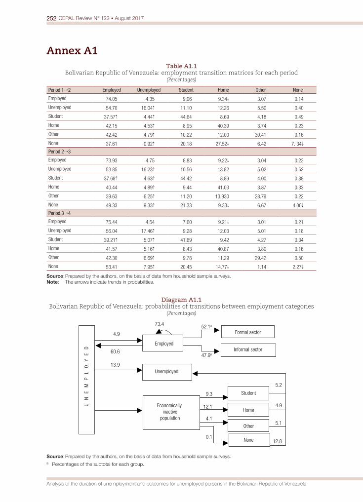
252 CEPAL Review N° 122 • August 2017
Analysis of the duration of unemployment and outcomes for unemployed persons in the Bolivarian Republic of Venezuela
Annex A1Table A1.1
Bolivarian Republic of Venezuela: employment transition matrices for each period(Percentages)
Period 1→2 Employed Unemployed Student Home Other None
Employed 74.05 4.35 9.06 9.34 3.07 0.14
Unemployed 54.70 16.04 11.10 12.26 5.50 0.40
Student 37.57 4.44 44.64 8.69 4.18 0.49
Home 42.15 4.53 8.95 40.39 3.74 0.23
Other 42.42 4.79 10.22 12.00 30.41 0.16
None 37.61 0.92 20.18 27.52 6.42 7. 34
Period 2→3
Employed 73.93 4.75 8.83 9.22 3.04 0.23
Unemployed 53.85 16.23 10.56 13.82 5.02 0.52
Student 37.68 4.63 44.42 8.89 4.00 0.38
Home 40.44 4.89 9.44 41.03 3.87 0.33
Other 39.63 6.25 11.20 13.930 28.79 0.22
None 49.33 9.33 21.33 9.33 6.67 4.00
Period 3→4
Employed 75.44 4.54 7.60 9.21 3.01 0.21
Unemployed 56.04 17.46 9.28 12.03 5.01 0.18
Student 39.21 5.07 41.69 9.42 4.27 0.34
Home 41.57 5.16 8.43 40.87 3.80 0.16
Other 42.30 6.69 9.78 11.29 29.42 0.50
None 53.41 7.95 20.45 14.77 1.14 2.27
Source: Prepared by the authors, on the basis of data from household sample surveys. Note: The arrows indicate trends in probabilities.
Diagram A1.1 Bolivarian Republic of Venezuela: probabilities of transitions between employment categories
(Percentages)
Employed
Unemployed
Student
Home
Other
Formal sector4.9
Informal sector
13.9
9.3
Economically inactive
population
12.1
52.1a
47.9a
4.1
0.1 None
60.6
73.4
5.2
4.9
5.1
12.8
UN
EM
PL
OY
ED
Source: Prepared by the authors, on the basis of data from household sample surveys. a Percentages of the subtotal for each group.

In order to facilitate the submission, consideration and publication of articles, the editorial board of the cepal Review has prepared the following information and suggestions to serve as a guide for future contributors.
The submission of an article implies an undertaking by the author not to submit it simultaneously to other publications. The copyright to all articles published in the Review shall be owned by the United Nations.
Each article will be reviewed by the editorial board, which may decide to submit it to external referees.
Papers should be submitted in the original language (English, French, Portuguese or Spanish). They will be translated into the appropriate language by the relevant eclac services.
Each article must be accompanied by a summary, no more than 150 words in length, giving a brief description of its subject matter and main conclusions.
Each article must also carry three jel (Journal of Economic Literature) classification codes. The JEL Classification Codes Guide is available online at www.aeaweb.org/jel/jel_class_system.php.
Papers should be no longer than 10,000 words, including the summary, notes and bibliography. Shorter papers will also be considered.
Articles should be sent by e-mail to [email protected] in Word format. Papers in pdf format will not be accepted.
Style guide:
Titles should not be excessively long.
Footnotes
— It is recommended that footnotes be kept to a minimum.
— It is recommended that footnotes not be used to cite bibliographical references; such references should preferably be incorporated into the text.
— Footnotes should be numbered consecutively using superscript Arabic numerals.
Tables, figures and equations
— It is recommended that tables and figures be kept to a minimum, avoiding any redundancy with the text.
— Equations should be written using the Office equation editor “MathType”; they should not be inserted as “pictures”.
— Tables, figures and other elements should be inserted at the end of the text in the format in which they were designed; they should not be inserted as “pictures”. Figures in Excel should include the corresponding worksheets.
— The location of tables and figures in the body of the article should be indicated in the appropriate place as follows:
Insert figure 1
Insert table 1
— Tables and figures should include an explicit and complete reference to their sources.
— Tables should indicate the period covered at the end of the title, and should indicate the units in which the data are expressed in a subtitle (in italics and between brackets).
— The symbols referred to in the “Explanatory notes” which appear on the page preceding the table of contents should be taken into account in the preparation of tables and figures.
— Footnotes to tables and figures should be ordered consecutively using superscript lower-case letters.
— Figures should be prepared bearing in mind that they will be printed in black and white.
Acronyms and abbreviations
— Acronyms and abbreviations should not be used unless absolutely necessary, in which case the full name should be written out the first time it occurs in the article.
Bibliography
— Bibliographical references should be directly related to the content of the article and should not be excessively long.
— At the end of the article, under the title “Bibliography”, all the necessary information should be included accurately and in alphabetical order by author: name of author(s), year of publication, full name of article (if any) and publication (including any subtitle), city of publication, publisher and, in the case of a periodical, month of publication.
The editorial board of the Review reserves the right to make any necessary editorial changes in the articles, including their titles.
Authors will receive a one-year courtesy subscription to the Review, plus 30 offprints of their article in Spanish and 30 in English, at the time of publication in each language.
Guidelinesfor contributorsto the CEPAL Review


Publicaciones recientes de la CEPAL ECLAC recent publicationswww.cepal.org/publicaciones
Informes periódicos / Annual reportsTambién disponibles para años anteriores / Issues for previous years also available• Estudio Económico de América Latina y el Caribe 2016, 236 p. Economic Survey of Latin America and the Caribbean 2016, 232 p.
• La Inversión Extranjera Directa en América Latina y el Caribe 2016, 170 p. Foreign Direct Investment in Latin America and the Caribbean 2016, 164 p.
• Anuario Estadístico de América Latina y el Caribe 2016 / Statistical Yearbook for Latin America and the Caribbean 2016, 132 p.
• Balance Preliminar de las Economías de América Latina y el Caribe 2016, 132 p. Preliminary Overview of the Economies of Latin America and the Caribbean 2016, 124 p.
• Panorama Social de América Latina 2015, 226 p. Social Panorama of Latin America 2015, 222 p.
• Panorama de la Inserción Internacional de América Latina y el Caribe 2016, 174 p. Latin America and the Caribbean in the World Economy 2015, 170 p.
Libros y documentos institucionales / Institutional books and documents• Panorama fiscal de América Latina y el Caribe 2017: la movilización de recursos para el financiamiento del desarrollo sostenible, 2017, 115 p. Fiscal Panorama of Latin America and the Caribbean 2017: Mobilizing resources to finance sustainable development, 2017, 108 p.• ECLAC Thinking. Selected Texts (1948-1998), 2016, 520 p.
• La matriz de la desigualdad en América Latina, 2016, 96 p. The social inequality matrix in Latin America, 2016, 94 p.
• Autonomía de las mujeres e igualdad en la agenda de desarrollo sostenible, 2016, 184 p. Equality and women’s autonomy in the sustainable development agenda, 2016, 168 p. Autonomia das mulheres e igualdade na agenda de desenvolvimento sustentável.
Síntese, 2016, 106 p.
• La Unión Europea y América Latina y el Caribe ante la Agenda 2030 para el Desarrollo Sostenible: el gran impulso ambiental, 2016, 112 p. The European Union and Latin America and the Caribbean vis-à-vis the 2030 Agenda for Sustainable Development: The environmental
big push, 2016, 112 p.
• Horizontes 2030: la igualdad en el centro del desarrollo sostenible, 2016, 176 p. Horizons 2030: Equality at the centre of sustainable development, 2016, 174 p. Horizontes 2030: a igualdade no centro do desenvolvimento sustentável, 2016, 176 p.
• 40 años de agenda regional de género, 2016, 130 p. 40 years of the regional gender agenda, 2016,128 p.
• La nueva revolución digital: de la Internet del consumo a la Internet de la producción, 2016, 100 p. The new digital revolution: From the consumer Internet to the industrial Internet, 2016, 100 p.
Libros de la CEPAL / ECLAC books145 Política industrial rural y fortalecimiento de cadenas de valor, Ramón Padilla, (ed.), 2017, 242 p.
144 Desde el gobierno abierto al Estado abierto en América Latina y el Caribe, Alejandra Naser, Álvaro Ramírez-Alujas, Daniela Rosales (eds.), 2017, 466 p.
143 Protección social en América Latina: la desigualdad en el banquillo, Ana Sojo, 2017, 246 p.
142 Consensos y conflictos en la política tributaria de América Latina, Juan Carlos Gómez Sabaini, Juan Pablo Jiménez y Ricardo Martner (eds.), 2017, 446 p.
141 Brechas y transformaciones: la evolución del empleo agropecuario en América Latina, Jürgen Weller (ed.), 2016, 274 p.
140 Protección y formación: instituciones para mejorar la inserción laboral en América Latina y Asia, Alberto Isgut, Jürgen Weller (eds.), 2016, 428 p. Protection and training: Institutions for improving workforce integration in Latin America and Asia, Alberto Isgut, Jürgen Weller (eds.), 2016, 428 p.
139 Hacia una nueva gobernanza de los recursos naturales en América Latina y el Caribe, Hugo Altomonte, Ricardo J. Sánchez, 2016, 256 p.
Páginas Selectas de la CEPAL / ECLAC Select Pages• Planificación y prospectiva para la construcción de futuro en América Latina y el Caribe. Textos seleccionados 2013-2016, Jorge Máttar
y Mauricio Cuervo (comps.), 2016, 222 p.
• Desarrollo inclusivo en América Latina. Textos seleccionados 2009-2016, Ricardo Infante (comp.), 2016, 294 p.
• Globalización, integración y comercio inclusivo en América Latina. Textos seleccionados 2010-2014, Osvaldo Rosales (comp.), 2015, 326 p.
• El desafío de la sostenibilidad ambiental en América Latina y el Caribe. Textos seleccionados 2012-2014, Carlos de Miguel, Marcia Tavares (comps.), 2015, 148 p
Copublicaciones / Co-publications• El imperativo de la igualdad, Alicia Bárcena, Antonio Prado, CEPAL/Siglo Veintiuno, Argentina, 2016, 244 p.
• Gobernanza global y desarrollo: nuevos desafíos y prioridades de la cooperación internacional, José Antonio Ocampo (ed.), CEPAL/Siglo Veintiuno, Argentina, 2015, 286 p.
• Decentralization and Reform in Latin America: Improving Intergovernmental Relations, Giorgio Brosio and Juan Pablo Jiménez (eds.), ECLAC/Edward Elgar Publishing, United Kingdom, 2012, 450 p.
• Sentido de pertenencia en sociedades fragmentadas: América Latina desde una perspectiva global, Martín Hopenhayn y Ana Sojo (comps.), CEPAL/Siglo Veintiuno, Argentina, 2011, 350 p.
Coediciones / Co-editions• Perspectivas económicas de América Latina 2017: Juventud, Competencias y Emprendimiento, 2016, 338 p. Latin American Economic Outlook 2017: Youth, Skills and Entrepreneurship, 2016, 314 p.
• Desarrollo e integración en América Latina, 2016, 314 p.
• Hacia un desarrollo inclusivo: el caso del Uruguay, 2016, 174 p.
• Perspectivas de la agricultura y del desarrollo rural en las Américas: una mirada hacia América Latina y el Caribe 2015-2016, CEPAL/FAO/IICA, 2015, 212 p.
Documentos de proyecto / Project documents• La transversalización del enfoque de género en las políticas públicas frente al cambio climático en América Latina, Marina Casas Varez, 2017, 101 p.
• Financiamiento para el cambio climático en América Latina y el Caribe en 2015, Joseluis Samaniego y Heloísa Schneider, 2017, 76 p.
• El cambio tecnológico y el nuevo contexto del empleo: tendencias generales y en América Latina, Sebastian Krull, 2016, 48 p.
• Cambio climático, políticas públicas y demanda de energía y gasolinas en América Latina: un meta-análisis, Luis Miguel Galindo, Joseluis Samaniego, Jimy Ferrer, José Eduardo Alatorre, Orlando Reyes, 2016, 68 p.
• Estado de la banda ancha en América Latina y el Caribe 2016, 2016, 46 p.
Cuadernos estadísticos de la CEPAL44 Las cuentas de los hogares y el bienestar en América Latina. Más allá del PIB, 2016.
43 Estadísticas económicas de América Latina y el Caribe: Aspectos metodológicos y resultados del cambio de año base de 2005 a 2010
Series de la CEPAL / ECLAC SeriesAsuntos de Género / Comercio Internacional / Desarrollo Productivo / Desarrollo Territorial / Estudios Estadísticos / Estudios y Perspectivas (Bogotá, Brasilia, Buenos Aires, México, Montevideo) / Studies and Perspectives (The Caribbean, Washington) / Financiamiento del Desarrollo / Gestión Pública / Informes y Estudios Especiales / Macroeconomía del Desarrollo / Medio Ambiente y Desarrollo / Población y Desarrollo / Política Fiscal / Políticas Sociales / Recursos Naturales e Infraestructura / Seminarios y Conferencias.
Manuales de la CEPAL5 Estimación de las erogaciones sociales a partir del sistema de cuentas nacionales: una propuesta para las funciones de educación, salud y
protección social, María Paz Colinao, Federico Dorin, Rodrigo Martínez y Varinia Tromben, 2016, 63 p.
4 Territorio e igualdad: planificación del desarrollo con perspectiva de género, 2016, 84 p.
3 Manual de formación regional para la implementación de la resolución 1325 (2000) del Consejo de Seguridad de las Naciones Unidas relativa a las mujeres, la paz y la seguridad, María Cristina Benavente R., Marcela Donadio, Pamela Villalobos, 2016, 126 p.
2 Guía general para la gestión de residuos sólidos domiciliarios, Estefani Rondón Toro, Marcel Szantó Narea, Juan Francisco Pacheco, Eduardo Contreras, Alejandro Gálvez, 2016, 212 p.
Revista CEPAL / CEPAL ReviewLa Revista se inició en 1976, con el propósito de contribuir al examen de los problemas del desarrollo socioeconómico de la región. La Revista CEPAL se publica en español e inglés tres veces por año.
CEPAL Review first appeared in 1976, its aim being to make a contribution to the study of the economic and social development problems of the region. CEPAL Review is published in Spanish and English versions three times a year.
Observatorio demográfico / Demographic Observatory Edición bilingüe (español e inglés) que proporciona información estadística actualizada, referente a estimaciones y proyecciones de población de los países de América Latina y el Caribe. Desde 2013 el Observatorio aparece una vez al año.
Bilingual publication (Spanish and English) proving up-to-date estimates and projections of the populations of the Latin American and Caribbean countries. Since 2013, the Observatory appears once a year.
Notas de poblaciónRevista especializada que publica artículos e informes acerca de las investigaciones más recientes sobre la dinámica demográfica en la región. También incluye información sobre actividades científicas y profesionales en el campo de población. La revista se publica desde 1973 y aparece dos veces al año, en junio y diciembre.
Specialized journal which publishes articles and reports on recent studies of demographic dynamics in the region. Also includes information on scientific and professional activities in the field of population. Published since 1973, the journal appears twice a year in June and December.
Las publicaciones de la CEPAL están disponibles en:ECLAC publications are available at:
www.cepal.org/publicaciones
También se pueden adquirir a través de:They can also be ordered through:
www.un.org/publications
United Nations PublicationsPO Box 960
Herndon, VA 20172USA
Tel. (1-888)254-4286 Fax (1-800)338-4550
Contacto / Contact: [email protected] / Orders: [email protected]


www.eclac.org/revista
United Nations Publication • S.17-00174 • August 2017 • ISSN 0251-2920
Copyright © United Nations • Printed in Santiago
EDITORIAL BOARD
Osvaldo SunkelChairman
José Antonio Alonso
oscAr Altimir
renAto BAumAnn
luis BeccAriA
luis BértolA
luiz cArlos Bresser-PereirA
mArio cimoli
John coAtsworth
roBert Devlin
cArlos De miguel
ricArDo FFrench-DAvis
DAniel heymAnn
mArtín hoPenhAyn
Akio hosono
grAcielA moguillAnsky
JuAn cArlos moreno-BriD
José Antonio ocAmPo
cArlotA Pérez
gert rosenthAl
PAul schreyer
BArBArA stAllings
AnDrAs uthoFF
roB vos
Miguel TorresTechnical Editor
ECONOMIC COMMISSION FOR LATIN AMERICA AND THE CARIBBEAN