1

Partial wavelet coherence analysis for understanding the standalone relationship

between Indian Precipitation and Teleconnection patterns

Maheswaran Rathinasamy1, Ankit Agarwal2, 3,*, VilakshnaParmar4, Rakesh Khosa4 and Arvind Bairwa4

1MVGR College of Engineering, Vizianagaram, India 2 Institute of Earth and Environmental Science, University of Potsdam, Potsdam, Germany

3Potsdam Institute for Climate Impact Research, Telegrafenberg, Potsdam, Germany 4Indian Institute of Technology Delhi, New Delhi

*Corresponding author at: Institute of earth and environmental sciences, University of Potsdam, Germany, Tel: +49 331 977 5433, fax: +49 331 977 2092

Email address: aagarwal@uni-potsdam.de (A. Agarwal)

Abstract

Hydro-meteorological variables, like precipitation, streamflow are significantly influenced by

various climatic factors and large-scale atmospheric circulation patterns. Efficient water

resources management requires an understanding of the effects of climate indices on the

accurate predictability of precipitation. This study aims at understanding the standalone

teleconnection between precipitation across India and the four climate indices, namely, Niño

3.4, PDO, SOI, and IOD using partial wavelet analysis. The analysis considers the cross

correlation between the climate indices while estimating the relationship with precipitation.

Previous studies have overlooked the interdependence between these climate indices while

analysing their effect on precipitation. The results of the study reveal that precipitation is only

affected by Niño 3.4 and IOD and a non-stationary relationship exists between precipitation

and these two climate indices. Further, partial wavelet analysis revealed that SOI and PDO do

not significantly affect precipitation, but seems the other way because of their

interdependence on Niño 3.4. It was observed that partial wavelet analysis strongly revealed

the standalone relationship of climatic factors with precipitation after eliminating other

potential factors.

Keywords: Indian Precipitation, wavelet coherency, partial wavelet coherence,

teleconnections patterns.

Abbreviations

2

ENSO: El Nino Southern Oscillation

PDO: Pacific Decadal Oscillation

SOI: Southern Oscillation Index

IOD: Indian Ocean Dipole

SST: Sea surface temperature

1. Introduction

Efficient water resource management requires an understanding of the effects of natural

climate variability on precipitation, particularly in the context of increasing climate

uncertainties. Analysis of the precipitation records is very important in understanding its

variability and the underlying driving forces of natural systems. The task of quantifying

precipitation variability, particularly as it relates to climate indices through teleconnections,

has been explored in numerous studies (Simpson and Colodner (1999); Bonsal et al. (2001);

Enfield et al. (2001); Gray (2004); Coulibaly and Burn (2004); Soukup et al. (2009);

Rajagopalan et al. (2000); Özger et al. (2009), Valdivia et al. (2012), Malik et al. (2012);

Marwan and Kurths (2015)).

In recent years, wavelet analysis has been increasingly used for analyzing highly irregular,

complex, and intermittent nonstationary time series often encountered in geophysics. Further,

wavelet analysis has been recognized as a useful technique for estimating the teleconnections

between different climate indices and hydro-meteorological variables. Owing to the

advantages of wavelet transforms, techniques such as cross-wavelet analysis (CWT) and

wavelet coherence (WC) have also emerged as powerful tools in testing possible linkages

between two signals (Grinsted et al. (2004)). Labat (2005) has provided a comprehensive

review of wavelet based techniques like wavelet coherence, cross wavelet transform and

wavelet modulus maxima (WMM) for applications in geophysical time series.

Studies such as Gan et al. (2007) investigated the teleconnections between Canadian

precipitation and climate anomalies using wavelet coherence analysis. Mokhov et al. (2011)

3

analysed the relationship between ENSO and Indian precipitation using cross-wavelet

analysis and Granger causality estimation from empirical data for the period of 1871–2003.

Holman et al. (2011) studied the relationship between the groundwater levels in the UK and

North Atlantic Oscillation (NAO) using the cross-wavelet analysis. Zhang et al. (2007)

investigated the possible influence of ENSO on annual maximum streamflow pattern of

Yangtze River, China and concluded that the stream flow observations pertaining to the

middle and lower Yangtze River were dominated by 2- to 8-year periods. Similarly, Schaefli

et al. (2007) presented a comprehensive review of applications of all wavelet methods such as

wavelet spectrum and cross-wavelet spectrum to daily discharge, temperature, and

precipitation.

Aforementioned studies have utilized wavelet coherence analysis in understanding the effect

of teleconnections on hydrological variables. However, It needs to be highlighted that these

studies do not consider the cross correlation between the teleconnections themselves (Gan et

al. (2007) and He et al. (2014)) in estimating their influence on precipitation For example, the

observable of precipitation (P) might be influenced by two variables X1 and X2 such that the

two variables may themselves be correlated. In this situation, analysis of the relationship

between P and X1 using the wavelet coherence analysis inherently considers the effect of X2.

This might result in an erroneous interpretation of the actual relationship between P and X1.

Therefore, it is important to study the standalone effect of every climate index on

precipitation distinctly, for making reliable predictions. However, it is not possible in an

analytical way to study the standalone effect of the climate indices, however in a recent

study, Mihanovic (2009) has presented the concept of partial wavelet coherence (PWC),

providing a statistical way to estimate the standalone dependence of the two variables after

eliminating the effect of other potentially influencing variables.

4

The objective of this paper is to use the concept of partial wavelet coherence analysis in

understanding the standalone dependence between a given climate index and precipitation as

it may shed more light on understanding the underlying natural processes. We hypothesise

that disentangling the effects of the interrelationship of variables will improve the

understanding of the influence of climate indices on Indian precipitation.

The present study utilized linear wavelet analysis to comprehend the dependence between

climatic factors and precipitation. Nonetheless, as the future extension, one can utilize

nonlinear dependence measures based on mutual information theory to investigate the

presence of nonlinear relationships.

The standalone relationship between temporal components of rainfall anomaly and climate

signals at different time scales have not been reported so far in the literature as per author’s

best knowledge.

2. Study Area and data

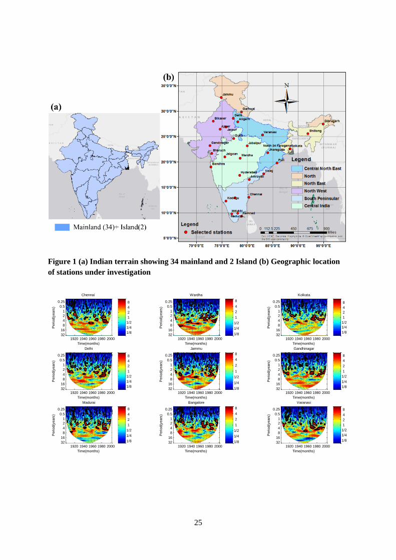
India has been divided into 36 meteorological sub-divisions (34 on the mainland and 2 on

islands) (Figure 1a) out of which 30 meteorological subdivisions were utilized in this study

(Kumar et al. (2010)) based on data availability. Figure 1b demonstrates all the 30 sub-

divisional precipitation stations chosen in this study on the terrain India. Sub-divisional

monthly rainfall data prepared by the Indian Institute of Tropical Meteorology (IITM) is used

for the period of 1901- 2002 (source: http://www.india-wris.nrsc.gov.in/wris.html). Notably,

the quality checks on the data were made to ensure that an error free data is made available

for analysis and design.

Further, on the basis of regional homogeneity, India has been classified into 6 regions

(Southern Peninsular, North East, North West, Central North East, North and Central India)

by IITM is shown in Figure 1b. In this study, five to six stations from each of these

5

homogeneous regions are considered as representative station and a detailed analysis was

done.

Climate index data:

In general, precipitation is tele-connected to several types of climate indices and the

knowledge of teleconnection pattern and strength of the interrelationship gives some amount

of predictability in remote locations (sometimes as long as a few seasons). For instance,

predicting El Niño enables prediction of North American rainfall, snowfall, droughts or

temperature patterns with a few weeks to months’ lead time (Gan et al. (2007)). In the context

of the Indian Precipitation, many different climate indices (SOI, Nino 3.4, NAO, AMO, IOD,

and PDO) have been shown to have teleconnections with precipitation patterns (reference).

The following section provides a brief summary of the climate indices considered in this

study.

a) IOD Index is represented by the by anomalous SST gradient between the western equatorial

Indian Ocean (50°E–70°E and 10°S– 10°N) and the southeastern equatorial Indian Ocean

(90°E–110°E and 10°S–0°N). It has been shown in several studies that IOD plays a key

role in the climate of the Indian subcontinent. The data for IOD was obtained from the

Bureau of Meteorology, Australia.

b) The Niño 3.4 index is one of the different indexes to measure the ENSO effect. Nino 3.4

is estimated as the average sea surface temperature anomaly in the region bounded by

5°N to 5°S, from 170°W to 120°W. Nagesh and Maity(2006) and several other have

shown Nino 3.4 to have some influence on Indian monsoon.

c) Pacific Decadal Oscillation (PDO) is an ocean atmospheric climate index which is

recurring over the mid latitude Pacific. Krishnamurthy and Krishnamurthy (2013) showed

that the Indian monsoon rainfall decadal oscillations were shown to be associated with the

decadal variability of the PDO.

6

d) North Atlantic Oscillation (NAO): It is calculated as the normalized pressure difference

between the Azores and a station in Iceland.

e) American Multi decadal Oscillation (AMO): It is measured as the average anomalies of

sea surface temperatures (SST) in the North Atlantic basin, typically over 0-80N.

f) Southern Oscillation Index (SOI) measures the difference in surface air pressure between

Tahiti and Darwin. It is one of the key climate indices measuring the El Niño and La Niña

events. The data for Niño 3.4, NAO, AMO, PDO, and SOI was downloaded from

http://www.esrl.noaa.gov/psd/data/climateindices website

Although both, SOI and Nino.3.4, measure the same phenomenon of El-Nina and La Nina

events yet there is currently no consensus in the scientific community as to which of these

indices best capture ENSO phases. Therefore, in this study, we have used both the indices for

a detailed analysis.

Homogeneity test

Before embarking on the application of wavelet analysis, the precipitation time series were

tested for homogeneity using Kruskal-Wallis test and Friedman test in Matlab. The p-values

obtained from the tests showed that the precipitation series from the different regions under

investigation are homogeneous at 95% confidence levels. A preliminary correlation analysis

was performed to get a general idea of the relationship between the precipitation and different

climate indices. Table 1 shows the result of correlation analyses. The results suggest that

most of the residual precipitation time series have non-significant (at 95% confidence level)

correlations with the climate indices. The correlation coefficients reveal that correlation

analysis is incapable of revealing the dependence between the precipitation and climate

indices. However, these findings are based on the assumption of stationarity, and therefore a

more appropriate method such as wavelet coherence is used in the following section to get a

better understanding of the relationship.

7

Table 2 shows the interdependence of the climate indices for the different seasons of the year.

It can be observed that some of the climatic factors are significantly (at 95% confidence

levels) interdependent on each other. During the southwest monsoon months (June, July,

Aug, and Sep) the relationship between Niño 3.4 and SOI, PDO are found to be statistically

significant. The correlation between Nino 3.4 and SOI is clear from the fact that they

represent the same ENSO phenomena. The reason for choosing both these indices in the

present roots from the statement from Barnston (2015), who argues that ENSO

is multifaceted, involving different aspects of the ocean and the atmosphere over the tropical

Pacific. Further, one cannot measure one aspect of the entire tropical Pacific perfectly, so we

get a better picture when we consider a few related measures.

Correlation analysis (table 1) also shows that the Niño 3.4 and IOD are not significantly

correlated on the other hand IOD and SOI have significant correlation for some seasons.

Surprisingly, the climate indices from the North Atlantic Ocean such as AMO and NAO are

not correlated with the other indices during any of the seasons.

A simple wavelet coherence analysis between one climate index and precipitation will

certainly carry the effect of other climate indices due to the interdependence. Therefore, it

becomes imperative to independently analyse the effect of one climate index on the

precipitation after removing the effect of other climate indices. Since the focus of the study is

to analyse the interdependent climate indices and then study the standalone effect on

precipitation by each of the climate indices after removing the other’s effect we have

therefore only taken those indices (Niño 3.4, SOI, IOD, and PDO) which share some level of

interdependence with each other.

3. Methods

Wavelet analysis

8

Wavelet method is a multi-resolution analysis used to obtain time-frequency representations

of a continuous signal. Wavelet analysis transforms a signal into scaled and translated

versions of an original (mother) wavelet, instead of decomposing a signal into constituent

harmonic functions as in Fourier analysis. The wavelet transform as defined by Eq. (1)

(Daubechies, 1992) is called the continuous wavelet transform (CWT) because of the scale

and time parameters, a and 𝜏, assume continuous values. (Agarwal et al. (2016 a,b); Giri et al.

(2014)).

1( , ) ( )

tW a f t dt

aa

(1)

It provides a redundant representation of a signal as CWT of a function 𝑓(𝑡) at scale 'a' and

location ' ' can be obtained from the continuous wavelet transform of the same function at

other scales and locations. Here, 𝜓 represents the family of function called wavelets and 𝑡

represents the time. Since the CWT behaves like an orthonormal basis decomposition, it can

be shown that it is also isometric as it preserves the overall energy content of the signal and,

thereby, allows for the recovery of the function f(t) from its transform by using the following

reconstruction formula as provided by Daubechies (1992) in Eq.(2)

2

,

0

1,  af t a W a t dad

C

(2)

where 𝐶𝜓 is a constant and depends on the choice of the wavelet 𝜓 . Clearly, the above

equation suggests that the function f(t) may be seen as a superposition of signals at different

scales and obtained by varying the scale parameter 'a'.

Further, the energy of the signal f(t) can be represented scale wise as given by Daubechies

(1992) in Eq.(3)

9

22

2

0

1( , )

daf t dt W a d

C a

(3)

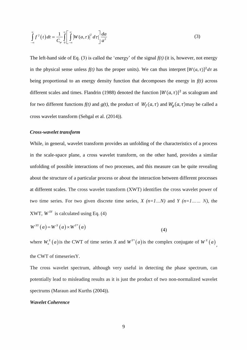
The left-hand side of Eq. (3) is called the ‘energy’ of the signal f(t) (it is, however, not energy

in the physical sense unless f(t) has the proper units). We can thus interpret [𝑊(𝑎, 𝜏)]2𝑑𝜏 as

being proportional to an energy density function that decomposes the energy in f(t) across

different scales and times. Flandrin (1988) denoted the function |𝑊(𝑎, 𝜏)|2 as scalogram and

for two different functions f(t) and g(t), the product of 𝑊𝑓(𝑎, 𝜏) and 𝑊𝑔(𝑎, 𝜏)may be called a

cross wavelet transform (Sehgal et al. (2014)).

Cross-wavelet transform

While, in general, wavelet transform provides an unfolding of the characteristics of a process

in the scale-space plane, a cross wavelet transform, on the other hand, provides a similar

unfolding of possible interactions of two processes, and this measure can be quite revealing

about the structure of a particular process or about the interaction between different processes

at different scales. The cross wavelet transform (XWT) identifies the cross wavelet power of

two time series. For two given discrete time series, X (n=1…N) and Y (n=1…… N), the

XWT, XYW is calculated using Eq. (4)

*XY X YW a W a W a (4)

where X

nW a is the CWT of time series X and *YW a is the complex conjugate of XW a,

the CWT of timeseriesY.

The cross wavelet spectrum, although very useful in detecting the phase spectrum, can

potentially lead to misleading results as it is just the product of two non-normalized wavelet

spectrums (Maraun and Kurths (2004)).

Wavelet Coherence

10

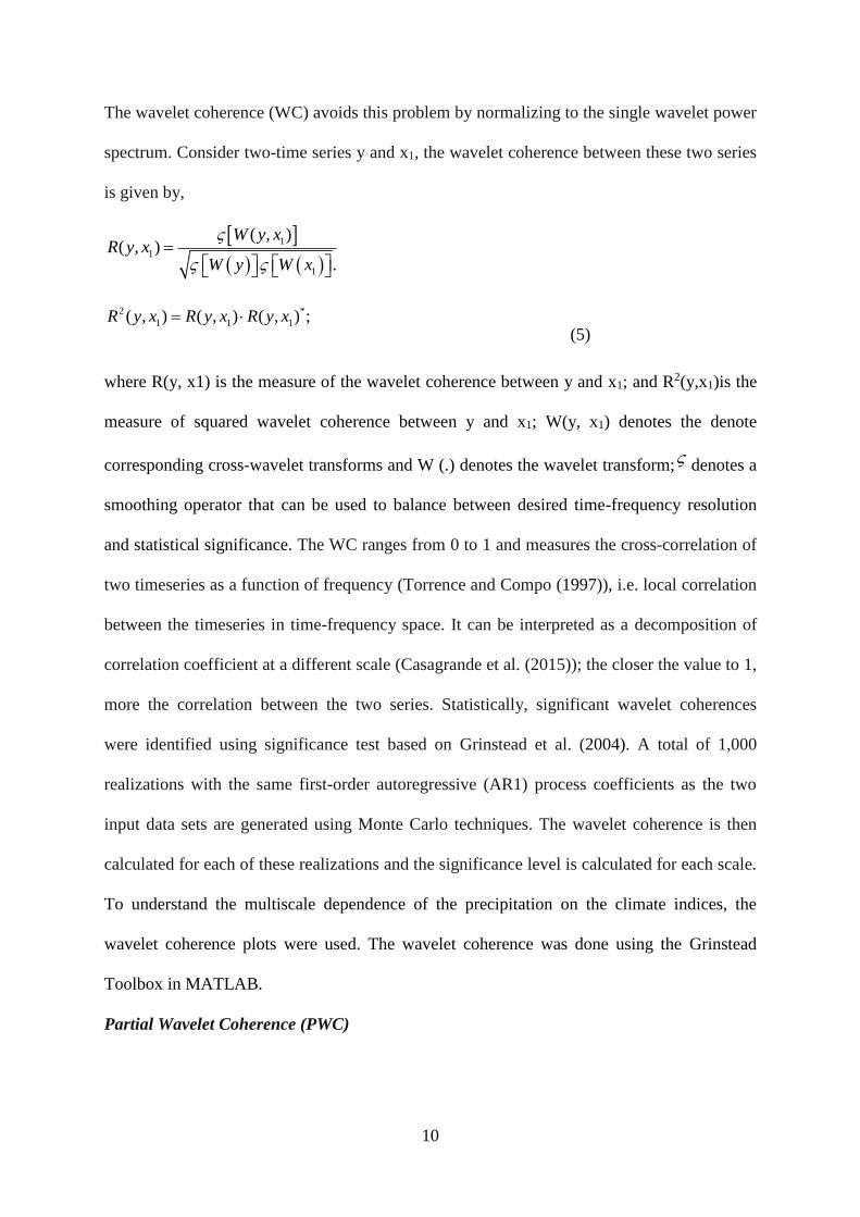
The wavelet coherence (WC) avoids this problem by normalizing to the single wavelet power

spectrum. Consider two-time series y and x1, the wavelet coherence between these two series

is given by,

1

1

1

( , )( , )

.

W y xR y x

W y W x

2 *

1 1 1( , ) ( , ) ( , ) ;R y x R y x R y x (5)

where R(y, x1) is the measure of the wavelet coherence between y and x1; and R2(y,x1)is the

measure of squared wavelet coherence between y and x1; W(y, x1) denotes the denote

corresponding cross-wavelet transforms and W (.) denotes the wavelet transform; denotes a

smoothing operator that can be used to balance between desired time-frequency resolution

and statistical significance. The WC ranges from 0 to 1 and measures the cross-correlation of

two timeseries as a function of frequency (Torrence and Compo (1997)), i.e. local correlation

between the timeseries in time-frequency space. It can be interpreted as a decomposition of

correlation coefficient at a different scale (Casagrande et al. (2015)); the closer the value to 1,

more the correlation between the two series. Statistically, significant wavelet coherences

were identified using significance test based on Grinstead et al. (2004). A total of 1,000

realizations with the same first-order autoregressive (AR1) process coefficients as the two

input data sets are generated using Monte Carlo techniques. The wavelet coherence is then

calculated for each of these realizations and the significance level is calculated for each scale.

To understand the multiscale dependence of the precipitation on the climate indices, the

wavelet coherence plots were used. The wavelet coherence was done using the Grinstead

Toolbox in MATLAB.

Partial Wavelet Coherence (PWC)

11

PWC is a technique similar to the partial correlation that helps to find the resulting WC

between two-time series y and x1 after eliminating the influence of the timeseries

x2.Mihanovic et al. (2009) extended the concept from simple linear correlation and suggested

that the PWC squared (after the removal of the effect of x2) can be defined by an equation

similar to the partial correlation squared, as shown in Eq. (6) which is like the simple WC,

ranging from 0 to 1.

2*

1 2 12

1 2 2 2

2 2 1

2

, , . ,, ,

1 , 1 ,

. 

R y x R y x R y xRP y x x

R y x R x x

where RP denotes the squared partial wavelet coherence

(6)

R (.,.) denotes the wavelet coherence between the two variables and RP2(y, x1, x2) is the

partial wavelet coherence squared between y and x2 when the influence of x1 is excluded. Its

proximity to zero at a certain time-frequency point indicates that the series x2 does not add

significant information to y, i.e. the information that is not already incorporated from x1 at

that point. If partial wavelet coherence squared is high for x1 and not for x2, this would imply

that important covariance exists between x1 and y during that time interval at a designated

wavelet scale (period), and moreover that y was dominantly influenced by x1 and not by x2. If

both RP2(y, x1, x2) and RP2(y, x2, x1) still have significant bands, both x1 and x2 have a

significant influence on y. In this study, the toolbox provided by Ng and Chan (2012) is used

for estimating the partial wavelet coherence.

4. Results

4.1 Wavelet Coherence analyses

To understand the variability of precipitation with reference to time, Continuous Wavelet

Transform (CWT) was performed on the series using 'morlet' wavelet. Morlet wavelet was

chosen because it is widely used complex wavelet having good time-frequency localization

than other real wavelets (Addison (2002)). However, it is to note that Kumar and Foufoula

12

(1994) and Gan et al. (2007) have shown that in this kind of multiscale coherence analysis the

choice of wavelets does not make much difference. The wavelet coefficients obtained from

CWT for the precipitation has been plotted (not shown here) and the significance levels are

calculated according to Grinstead et al. (2004). Using the CWT plot, the dominant periods

and their variability in terms of time were identified. The summary of the results is tabulated

in Table 3. It can be seen that in most of the stations, the long term oscillation exist having a

periodicity of 64-128 months (~5 to 10 years) or even greater in some cases.

To understand the underlying causative factors driving the low-frequency precipitation

process, wavelet coherence analysis was performed between the observed precipitation and

climate indices.

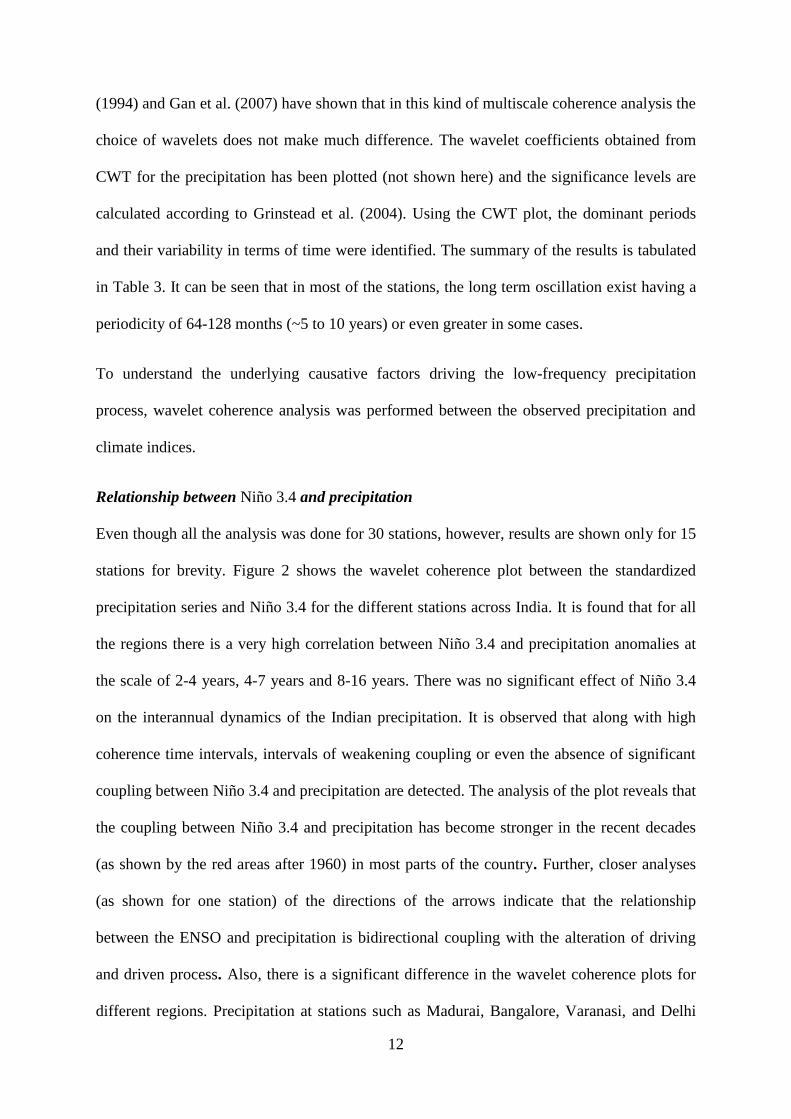
Relationship between Niño 3.4 and precipitation

Even though all the analysis was done for 30 stations, however, results are shown only for 15

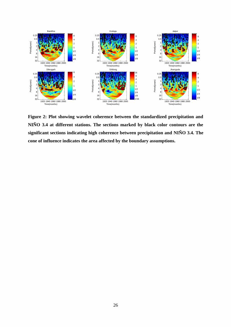
stations for brevity. Figure 2 shows the wavelet coherence plot between the standardized

precipitation series and Niño 3.4 for the different stations across India. It is found that for all

the regions there is a very high correlation between Niño 3.4 and precipitation anomalies at

the scale of 2-4 years, 4-7 years and 8-16 years. There was no significant effect of Niño 3.4

on the interannual dynamics of the Indian precipitation. It is observed that along with high

coherence time intervals, intervals of weakening coupling or even the absence of significant

coupling between Niño 3.4 and precipitation are detected. The analysis of the plot reveals that

the coupling between Niño 3.4 and precipitation has become stronger in the recent decades

(as shown by the red areas after 1960) in most parts of the country. Further, closer analyses

(as shown for one station) of the directions of the arrows indicate that the relationship

between the ENSO and precipitation is bidirectional coupling with the alteration of driving

and driven process. Also, there is a significant difference in the wavelet coherence plots for

different regions. Precipitation at stations such as Madurai, Bangalore, Varanasi, and Delhi

13

Jaipur does not have significant coherence with Niño 3.4 at 16-32 years scale, whereas other

stations such as Chennai, Kolkata, Gandhinagar, Bandhra, Shillong have significant Niño 3.4

influence at that large scale.

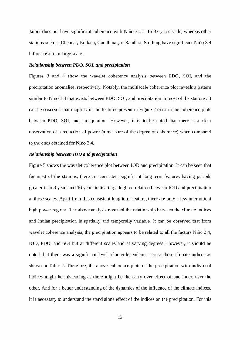
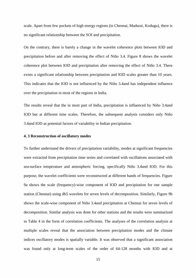
Relationship between PDO, SOI, and precipitation

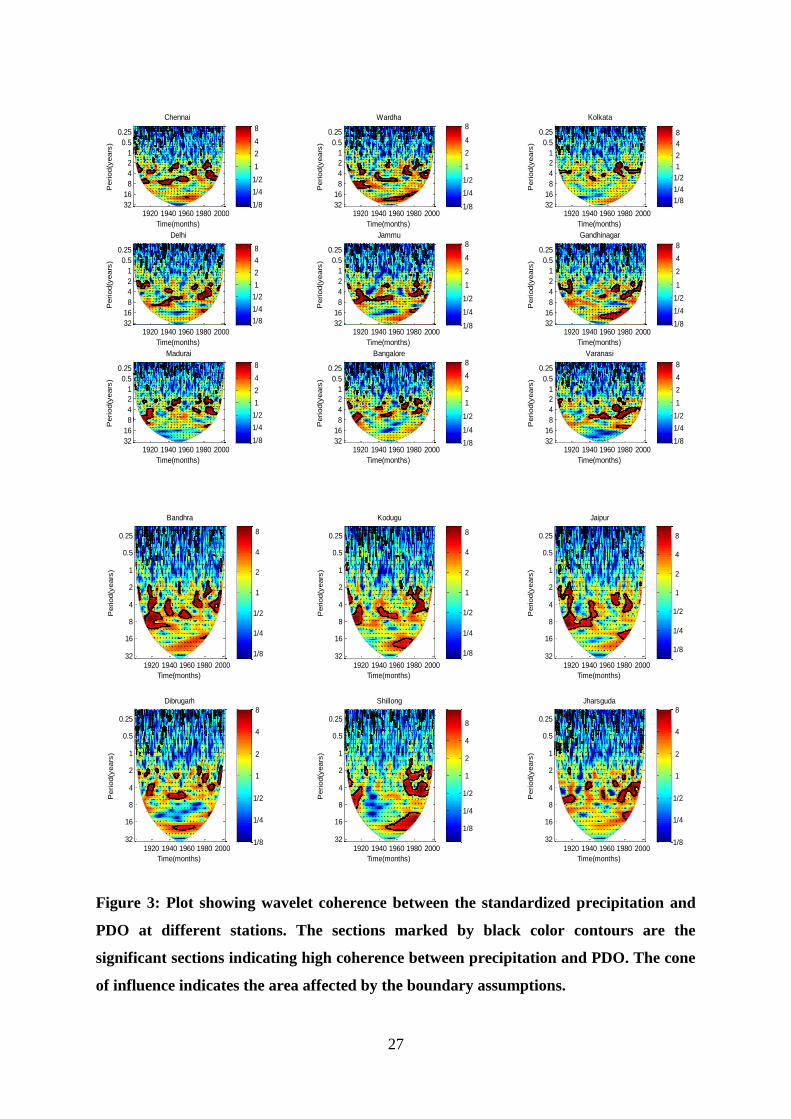
Figures 3 and 4 show the wavelet coherence analysis between PDO, SOI, and the

precipitation anomalies, respectively. Notably, the multiscale coherence plot reveals a pattern

similar to Nino 3.4 that exists between PDO, SOI, and precipitation in most of the stations. It

can be observed that majority of the features present in Figure 2 exist in the coherence plots

between PDO, SOI, and precipitation. However, it is to be noted that there is a clear

observation of a reduction of power (a measure of the degree of coherence) when compared

to the ones obtained for Nino 3.4.

Relationship between IOD and precipitation

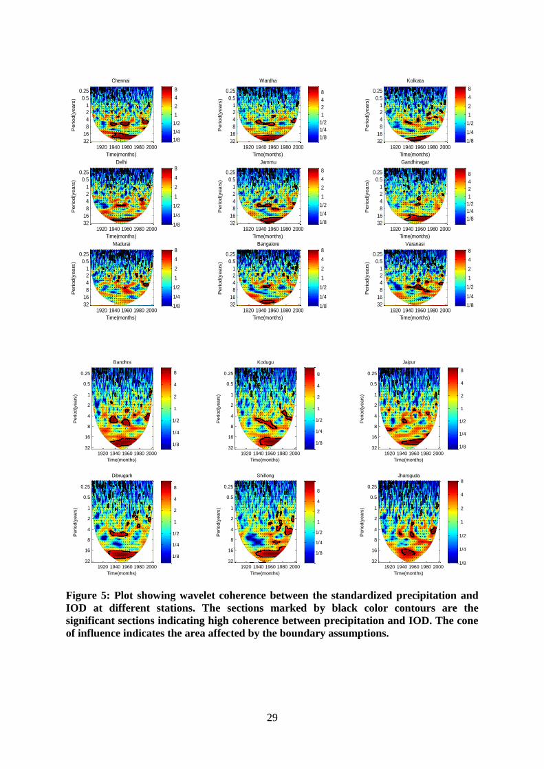
Figure 5 shows the wavelet coherence plot between IOD and precipitation. It can be seen that

for most of the stations, there are consistent significant long-term features having periods

greater than 8 years and 16 years indicating a high correlation between IOD and precipitation

at these scales. Apart from this consistent long-term feature, there are only a few intermittent

high power regions. The above analysis revealed the relationship between the climate indices

and Indian precipitation is spatially and temporally variable. It can be observed that from

wavelet coherence analysis, the precipitation appears to be related to all the factors Niño 3.4,

IOD, PDO, and SOI but at different scales and at varying degrees. However, it should be

noted that there was a significant level of interdependence across these climate indices as

shown in Table 2. Therefore, the above coherence plots of the precipitation with individual

indices might be misleading as there might be the carry over effect of one index over the

other. And for a better understanding of the dynamics of the influence of the climate indices,

it is necessary to understand the stand alone effect of the indices on the precipitation. For this

14

purpose, we have used partial wavelet analysis to study the standalone effect of the climate

indices on precipitation.

In the past, studies such as Newman et al. (2003) showed the dependence of PDO on ENSO

events (Niño 3.4 or SOI) and Ashok et al. (2004) have discussed the relationship between

IOD and ENSO events (Niño 3.4 or SOI). From these studies, it is clear that ENSO events

(Niño 3.4 or SOI) play an influencing role in controlling the other climate indices. Therefore,

the coherence between the standardized precipitation and each of the climate indices (PDO,

SOI, and IOD) after removing the effect of Niño 3.4 is examined. This would help in

understanding the standalone effect of the SOI, IOD, and PDO on Indian precipitation.

4.2 Partial wavelet Coherence Analysis

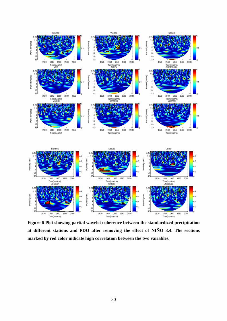
Figures 6, 7, 8 show partial wavelet coherence between the standardized precipitation and

climate indices (PDO, SOI, and IOD) after removing the effect of Niño 3.4. Figure 6 shows

the wavelet coherence analysis between precipitation and PDO after removing the effect of

Niño 3.4. When compared with Figure 3 (which shows the wavelet coherence analysis

between PDO and precipitation) a significant reduction in the high power regions is observed.

Also, the correlation between the precipitation and PDO is found to be zero in most of the

stations. For example, in the case of Chennai, Figure 3 showed a significant relationship

between precipitation and PDO at 4-8 years scale. However, such trend is not observed in

Figure 6.

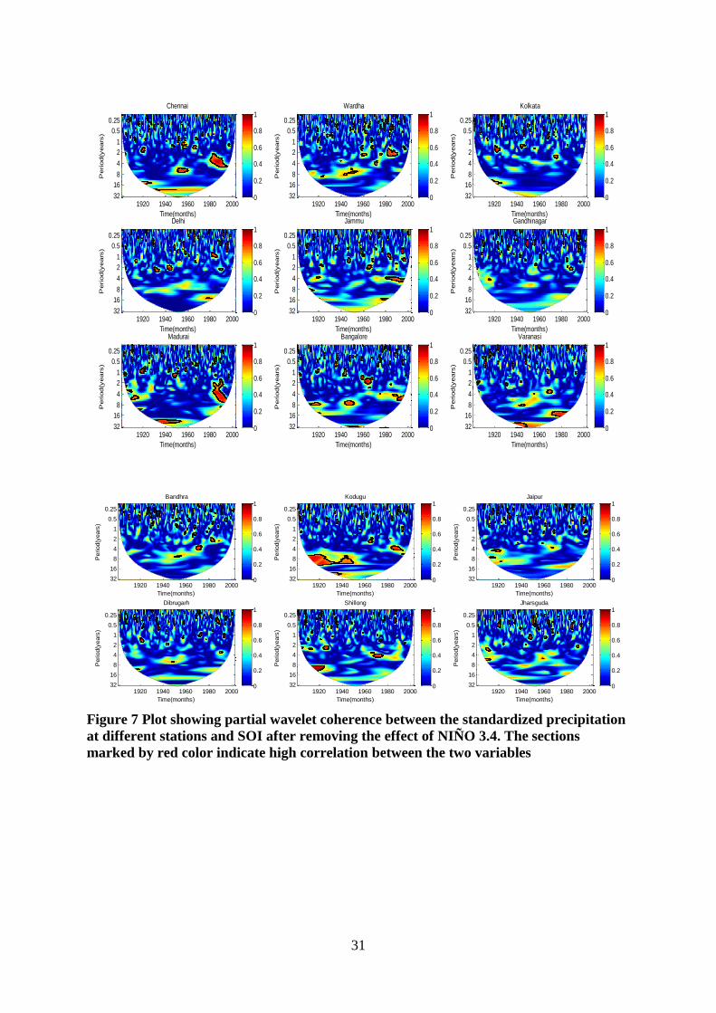
Similarly, Figure 7 shows the standalone relationship between precipitation and SOI after

removing the influence of Niño 3.4. Here, again, a significant difference between Figure 7

and Figure 4 (which shows the wavelet coherence analysis between SOI and precipitation) is

revealed. It is observed that there is not a strong linkage between the SOI and Indian

precipitation except at few places where there is a good degree of correlation at 10 years

15

scale. Apart from few pockets of high energy regions (in Chennai, Madurai, Kodugu), there is

no significant relationship between the SOI and precipitation.

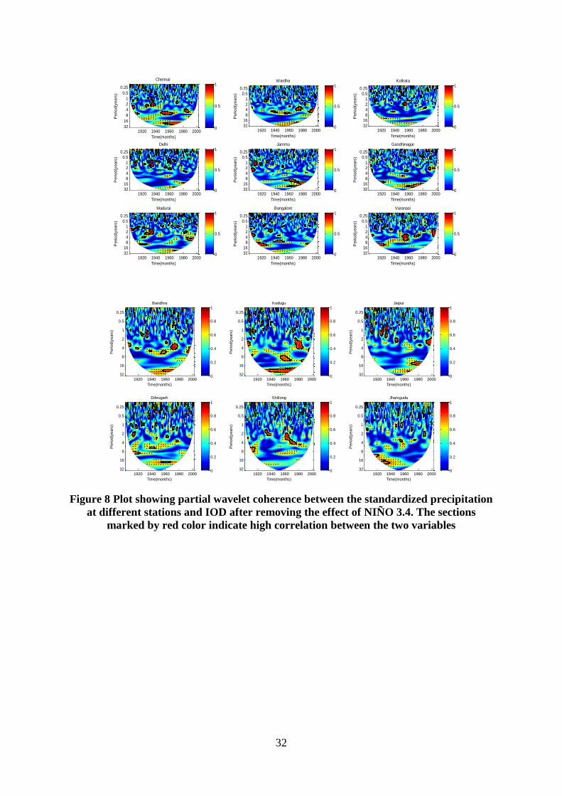
On the contrary, there is barely a change in the wavelet coherence plots between IOD and

precipitation before and after removing the effect of Niño 3.4. Figure 8 shows the wavelet

coherence plot between IOD and precipitation after removing the effect of Niño 3.4. There

exists a significant relationship between precipitation and IOD scales greater than 10 years.

This indicates that the IOD is not influenced by the Niño 3.4and has independent influence

over the precipitation in most of the regions in India.

The results reveal that the in most part of India, precipitation is influenced by Niño 3.4and

IOD but at different time scales. Therefore, the subsequent analysis considers only Niño

3.4and IOD as potential factors of variability in Indian precipitation.

4. 3 Reconstruction of oscillatory modes

To further understand the drivers of precipitation variability, modes at significant frequencies

were extracted from precipitation time series and correlated with oscillations associated with

sea-surface temperature and atmospheric forcing, specifically Niño 3.4and IOD. For this

purpose, the wavelet coefficients were reconstructed at different bands of frequencies. Figure

9a shows the scale (frequency)-wise component of IOD and precipitation for one sample

station (Chennai) using db5 wavelets for seven levels of decomposition. Similarly, Figure 9b

shows the scale-wise component of Niño 3.4and precipitation at Chennai for seven levels of

decomposition. Similar analysis was done for other stations and the results were summarized

in Table 4 in the form of correlation coefficients. The analyses of the correlation analysis at

multiple scales reveal that the association between precipitation modes and the climate

indices oscillatory modes is spatially variable. It was observed that a significant association

was found only at long-term scales of the order of 64-128 months with IOD and at

16

comparatively short-term scales of the order of 16-32 and 32-64 months scales with Niño 3.4.

It was also seen that the association precipitation - IOD and precipitation- Niño 3.4was

complementary to each other. In most of the places, it was observed that when the association

with IOD was strong the association with Niño 3.4was weak and vice-versa. However, at

some of the places like Varanasi, Jabalpur Aligarh, Puri, Jalgaon, and Amravati the

association was significant with both IOD and ENSO.

Figure 10 shows the box plot of the correlation coefficients between Niño 3.4and

precipitation reconstructed modes at different scales. Figure 11 shows the similar plot

between IOD and precipitation. It can be seen that Niño 3.4 has a significant negative

correlation at the scale of 32-64 months (2-5 years) whereas the IOD has a high positive

correlation in the 64 months (10 years) scale. Figure 12 and 13 shows the season-wise split of

the relationship between Niño 3.4, IOD, and precipitation. The analysis of the box plots

reveals that the Niño 3.4affects the precipitation at the scales of 2- 5 years in almost all the

seasons. Particularly during the summer monsoon, the effect of Niño 3.4is found to be

significant at 2 months scales. On the other hand, IOD influences the precipitation at 10 years

scale in all the seasons in a consistent manner. However, it is to be noted that the above

analysis provides only an overall estimate of the relationship of precipitation with Niño

3.4and IOD. Understanding the fact that the relationship evolves with time due to other

physical factors such as solar activity (Narasimha and Bhattacharya (2009)), we attempted to

analyse the temporal evolution of the dependence between Niño 3.4, IOD, and precipitation.

4.4 Temporal evolution of dependence between ENSO, IOD, and precipitation.

The wavelet coherence analysis revealed that the relationship between Niño 3.4, IOD and

precipitation is intermittent and varying with time. Therefore, to further understand the time-

evolution of the relationship between the precipitation and the climate indices at different

scales, the entire time span was split into 4 segments of 25 years each starting with 1901.

17

Figure 14 shows the evolution of the correlation coefficient between Niño 3.4and

precipitation modes with time. Figure 15 shows the correlation coefficient between IOD and

precipitation modes for different time periods. It can be seen that the relationship between the

Niño 3.4and precipitations is clearly evolving with time at all the scales. During the period

1901-1925, it was observed that Niño 3.4-monsoon connection is strong (but negative), while

the IOD-monsoon connection is insignificant; during 1926–1950 where both the Niño 3.4and

IOD influences were weak and insignificant. For the period of 1951-1975, both the

connections strongly influenced the precipitation. And for 1975-2000, the connection was

relatively weak except for the decadal cycles.

5. Discussion

The above study is the first to analyse the stand alone effect of various climatic factors on

precipitation after removing the other potential drivers. Firstly, the basic wavelet coherence

analysis among different climate indicators and Indian precipitation revealed that there is

strong relationship existed between precipitation and all the climatic indices analysed in this

study. However, subsequent analysis using partial wavelet coherence analysis uncovered

some interesting facts about the relationship amongst precipitation and climatic factors. The

PWC analysis showed that effect of PDO and SOI on precipitation is just an artifact of their

dependence on Niño 3.4. Also, it was observed that Niño 3.4 is the primary driver of the

variability of precipitation in most of the stations at scales of the order of 2-4 and 4-7 years

(Narasimha and Bhattacharyya (2009)). It was observed that IOD on the other hand, an

independent driver, acting at the scale of 16 years and complements the Niño 3.4. Further, the

analysis of the direction of the arrows in the coherence plot between Precipitation and Niño

3.4 showed that the Niño 3.4 and precipitation are bidirectional coupling process with the

alteration of driving and driven process. This is in congruence with the observations by

18

Mokhov et al. (2011) where the authors show that the Niño 3.4-Indian precipitation has a

non-symmetric bidirectional coupling using the causality analysis.

Additionally, it can be noticed that partial wavelet analysis can be used as a useful technique

in comprehending the standalone impacts of climatic indices and precipitation and in other

geophysical processes. Further, the IOD events are appeared to happen independently of Niño

3.4 events as the PWC amongst IOD and precipitation is unaffected after removing the Niño

3.4 effect. Likewise, it was clear from the investigation that the scale at which the IOD and

ENSO influence the precipitation are distinctive. Notwithstanding, the strong correlation

amongst IOD and Niño 3.4 amid the autumn as appeared in Table 2 might be because of the

co-occurrence of the Niño 3.4 and the IOD event (Ashok et al. (2004)) which fundamentally

may not be because of the dependence on each other.

We also observed that the coupling between precipitation and Niño 3.4 is becoming stronger

in the latter half of the analysed time (particularly after 1970). Cherchi and Navarra (2013)

obtained similar results using a different approach and explains that this kind of behavior may

be due to the changes occurred in the North Pacific after 1976 (Miller et al. (1994)) and to the

associated differences in the Niño 3.4 teleconnections (Deser and Blackmon (1995)).

With reference to the spatial variation of the association of precipitation with Niño 3.4 and

IOD, it was observed that most parts of India except central India there exists a

complementary relationship of precipitation with Niño 3.4 and IOD. However, it was seen in

some parts of central India (including the east and west parts) the Niño 3.4 and IOD were

simultaneously influencing the precipitation but at different temporal scales. Further, it was

observed that the coastal regions of peninsular and northeast and west regions were more

significantly affected by Niño 3.4 and IOD in comparison with their counterparts in the

inland region. The strength of the relationship between precipitation and climate indices for

19

given period might be driving the degree of spatial variability in Indian precipitation as

observed by Ghosh et al. (2012).

Overall, different climatic indices were analysed and the results show that the effect of PDO

and SOI on precipitation is insignificant, contrary to the results obtained by Krishnamurthy

and Krishnamurthy (2013) where the authors observe a statistically significant influence of

PDO on Indian precipitation. This difference in the results warrants future scope for

understanding the complex dynamics of PDO (Wang et al. (2014)).

The study also reveals the relationship between ENSO, IOD and the monsoon is not constant

in time. In fact, in the record analysed (i.e. 1901-2002) it was possible to distinguish periods

with the strong Niño 3.4-monsoon connection, lack of IOD-monsoon connection and

increasing Niño 3.4-IOD relationship, or with both strong and negative IOD-monsoon and

Niño 3.4-monsoon connections, or with not-significant monsoon- Niño 3.4 and monsoon-

IOD but with strong Niño 3.4-IOD relationships. This temporal variability in the effect of the

influence of IOD and Niño 3.4 on monsoon can be attributed to the changes in the North

Pacific and in the Atlantic sectors.

6. Conclusions

Thirty precipitation time series from different parts of India were examined with the target of

investigating the impacts of climatic factors on Indian precipitation. The conclusion of the

study are as follows:

1) Simple correlation analysis did not demonstrate any evidence of a relationship between the

climate factors and the precipitation. However, multiscale analyses using wavelets suggest

that the precipitation shows a significant relationship with climatic factors such as Niño 3.4,

SOI, PDO, and IOD. Further, the partial wavelet analysis revealed that SOI and PDO do not

significantly affect precipitation, but seems the other way because of their interdependence

on Niño 3.4. It was observed that partial wavelet analysis well-suited to bringing out the

20

standalone relationship of climatic factors with precipitation after removing the other

potential factors.

2) The wavelet coherence plot and the reconstruction of modes at different scales reveal the

Niño 3.4 effects i.e. there is a strong relationship between the Niño 3.4 & precipitation at 2-7

years’ scale also IOD &precipitation shows high coherency at the decadal or higher scale.

3) It was observed that the relationship between IOD, Niño 3.4, and precipitation varies with

time and space.

Therefore, we conclude that the Niño 3.4 and IOD indices show significant linkages with

high- and low-frequency variability in the precipitation, respectively. The results of spectral

analyses coincide with the conclusions of other previous studies, which have detected the

influence of Niño 3.4 and IOD on hydrologic variables in India.

The present study only investigated the linear relationship between the climate indices and

the precipitation. However, it will be interesting to further investigate the presence of

nonlinear dependence between them. Correlation does not imply causation, therefore, another

scope for further study is to investigate the causal relationship between the precipitation and

climate indices at different scales and hence use such information for enhanced precipitation

forecast.

Acknowledgements

This research was funded by Department Science and Technology, India through the

INSPIRE Faculty Fellowship held by Maheswaran Rathinasamy. We are grateful for the two

anonymous reviewers for their valuable suggestion in improving the presentation and

manuscript.

References

Addison P S (2002) The Illustrated Wavelet Transform Handbook: Introductory Theory and Applications in

Science Engineering, Medicine and Finance (Bristol: Institute of Physics Publishing).

21

Agarwal A (2015) Hydrologic regionalization using wavelet-based multiscale entropy technique. Dissertation,

Indian Institute of Technology Delhi

Agarwal, A., Maheswaran, R., Sehgal, V., Khosa, R., Sivakumar, B. and Bernhofer, C. (2016a). Hydrologic

regionalization using wavelet-based multiscale entropy method. Journal of Hydrology, 538, pp.22-32.

Agarwal, A., Maheswaran, R., Kurths, J. and Khosa, R. (2016b). Wavelet Spectrum and self-organizing maps-

based approach for hydrologic regionalization-a case study in the western United States. Water Resources

Management, 30(12), pp.4399-4413.

Ashok, K., Guan, Z., Saji, N. and Yamagata, T. (2004) Individual and combined influences of ENSO and the

Indian Ocean dipole on the Indian summer monsoon. Journal of Climate 17(16), 3141-3155.

Bonsal, B., Zhang, X., Vincent, L. and Hogg, W. (2001) Characteristics of daily and extreme temperatures over

Canada. Journal of Climate 14(9), 1959-1976.

Casagrande, E., B. Mueller, D. G. Miralles, D. Entekhabi, and A. Molini (2015), Wavelet correlations to reveal

multiscale coupling in geophysical systems. J. Geophys. Res. Atmos., 120, 7555–7572.

doi:10.1002/2015JD023265.

Cherchi A, Navarra A. 2013. Influence of ENSO and of the Indian Ocean Dipole on the Indian summer

monsoon variability. Climate Dynamics 41(1): 81–103.

Coulibaly, P. and Burn, D.H. (2004) Wavelet analysis of variability in annual Canadian streamflows. Water

Resources Research 40(3).

Daubechies, I. (1992) Ten lectures on wavelets, SIAM.

Deser, C. and M. L. Blackmon, (1995), On the relationship between Tropical and North Pacific sea surface

temperature variations. J. Climate, 8, 1677-1680.

Enfield, D.B., Mestas-Nunez, A.M. and Trimble, P.J. (2001) The Atlantic multidecadal oscillation and its

relation to rainfall and river flows in the continental U. S. Geophysical Research Letters 28(10), 2077-2080.

Flandrin, P. (1988) A time-frequency formulation of optimum detection. Acoustics, Speech and Signal

Processing, IEEE Transactions on 36(9), 1377-1384.

Foufoula, E. and Kumar, P. (1994) Wavelets in geophysics, San Diego, California, Academic Press.

Gan, T. Y., A. K. Gobena, and Q. Wang (2007) Precipitation of southwestern Canada: Wavelet, scaling,

multifractal analysis, and teleconnection to climate anomalies, J. Geophys. Res., 112, D10110,

doi:10.1029/2006JD007157.

22

Ghosh, S., Das, D, Kao, S-C, Ganguly, A. R. (2012), Lack of uniform trends but increasing spatial variability in

observed Indian rainfall extremes, Nature Climate Change, 2, 86-91

Giri, B. K., Mitra, C., Panigrahi, P. K. Iyengar, A. S. (2014). Multi-scale dynamics of glow discharge plasma

through wavelets: Self-similar behavior to neutral turbulence and dissipation, Chaos: An Interdisciplinary

Journal of Nonlinear Science, 24 (4), 043135.

Gray, S.T., Graumlich, L.J., Betancourt, J.L. and Pederson, G.T. (2004) A tree ring based reconstruction of the

Atlantic Multidecadal Oscillation since 1567 AD. Geophysical Research Letters 31(12).

Grinsted, A., Moore, J.C. and Jevrejeva, S. (2004) Application of the cross wavelet transform and wavelet

coherence to geophysical timeseries. Nonlinear processes in geophysics 11(5/6), 561-566.

He, X., Guan, H., Zhang, X. and Simmons, C. T. (2014), A wavelet-based multiple linear regression model for

forecasting monthly rainfall. Int. J. Climatol., 34: 1898–1912. doi:10.1002/joc.3809

Holman I. P., M. Rivas-Casado, J. P. Bloomfield, and J. J. Gurdak (2011), Identifying non- stationary

groundwater level response to North Atlantic ocean-atmosphere teleconnection patterns using wavelet

coherence, Hydrogeol. J., doi:10.1007/s10040-011-0755-9

Hurrell, J.W. and Van Loon, H. (1997) Climatic Change at High Elevation Sites, pp. 69-94, Springer.

Krishnamurthy L, Krishnamurthy V (2013) Influence of PDO on South Asian summer monsoon and monsoon–

ENSO relation. Clim Dyn 42:2397–2410. doi:10.1007/s00382-013-1856-z

Kumar V , Sharad K. Jain & Yatveer Singh (2010): Analysis of long-term rainfall trends in India, Hydrological

Sciences Journal, 55:4, 484-496

Labat, D. (2005) Recent advances in wavelet analyses: Part 1. A review of concepts. Journal of Hydrology

314(1), 275-288.

Marwan, N., Kurths, J. and Foerster, S. (2015). Analysing spatially extended high-dimensional dynamics by

recurrence plots. Physics Letters A, 379(10), pp.894-900.

Malik, N., Bookhagen, B., Marwan, N. and Kurths, J. (2012). Analysis of spatial and temporal extreme

monsoonal rainfall over South Asia using complex networks. Climate dynamics, 39(3-4), pp.971-987.

Maraun, D. and Kurths, J. (2004) Cross wavelet analysis: significance testing and pitfalls. Nonlinear processes

in geophysics 11(4), 505-514.

Mihanovic, H., Orlie, M. and Pasaria, Z. (2009) Diurnal thermocline oscillations driven by tidal flow around an

island in the Middle Adriatic. Journal of Marine Systems 78, S157-S168.

23

Miller, A. J., Cayan, D. R., Barnett, T. P., Graham, N. E., & Oberhuber, J. M. (1994). The 1976–77 climate shift

of the Pacific Ocean. Oceanography, 7, 21–26

Mokhov II, Smirnov DA, Nakonechny PI, Kozlenko SS, Seleznev EP, Kurths J (2011) Alternating mutual

influence of el-nino southern oscillation and Indian monsoon. Geophys Res Lett 38:L00F04

Narasimha R, Bhattacharyya S (2010) A wavelet cross-spectral analysis of solar–ENSO– rainfall connections in

the Indian monsoons. Appl Comput Harmon Anal 28:285–295

Newman M, Compo G, and Alexander M.A., 2003: ENSO-Forced Variability of the Pacific Decadal

Oscillation. J. Climate,16, 3853–3857.

Ng, E.K. and Chan, J.C. (2012) Geophysical applications of partial wavelet coherence and multiple wavelet

coherence. Journal of Atmospheric and Oceanic Technology 29(12), 1845-1853.

Ozger, M., Mishra, A.K. and Singh, V.P. (2009) Low frequency drought variability associated with climate

indices. Journal of Hydrology 364(1), 152-162.

Valdivia, C., Sauchyn, D. and Vanstone, J. (2012) Groundwater levels and teleconnection patterns in the

Canadian Prairies. Water Resources Research 48(7).

Rajagopalan, B., Cook, E., Lall, U. and Ray, B.K. (2000) Spatiotemporal variability of ENSO and SST

teleconnections to summer drought over the United States during the twentieth century. Journal of Climate

13(24), 4244-4255.

Saji. H. H, B. N. Goswami, P. H. Vinayachandran, T. Yamagata, (1999) A dipole mode in the tropical Indian

Ocean, Nature 401, 360.

Schaefli, B., Maraun, D. and Holschneider, M. (2007) What drives high flow events in the Swiss Alps? Recent

developments in wavelet spectral analysis and their application to hydrology. Advances in Water Resources

30(12), 2511-2525.

Sehgal, Vinit, Mukesh K. Tiwari, and Chandranath Chatterjee. "Wavelet bootstrap multiple linear regression

based hybrid modeling for daily river discharge forecasting." Water resources management 28, no. 10 (2014):

2793-2811.

Simpson, H.J. and Colodner, D.C. (1999) Arizona precipitation response to the Southern Oscillation: A potential

water management tool. Water Resources Research 35(12), 3761-3769.

Soukup, T.L., Aziz, O.A., Tootle, G.A., Piechota, T.C. and Wulff, S.S. (2009) Long lead-time streamflow

forecasting of the North Platte River incorporating oceanic–atmospheric climate variability. Journal of

Hydrology 368(1), 131-142.

24

Torrence, C., Compo, G.P., 1998. A practical guide to wavelet analysis. Bull. Am. Meteorol. Soc. 79, 61–78.

Ummenhofer, C.C., England, M.H., McIntosh, P.C., Meyers, G.A., Pook, M.J., Risbey, J.S., Gupta, A.S. and

Taschetto, A.a.S. (2009) What causes southeast Australia's worst droughts? Geophysical Research Letters 36(4).

Wang L, Chen W, Huang R (2008) Interdecadal modulation of PDO on the impact of ENSO on the east Asian

winter monsoon. Geophys Res Lett 35:L20702. doi:10.1029/2008GL035287

Webster, P.J., Moore, A.M., Loschnigg, J.P. and Leben, R.R. (1999) Coupled ocean atmosphere dynamics in the

Indian Ocean during 1997-98. Nature 401(6751), 356-360.

Zhang, H., Blackburn, T., Phung, B. and Sen, D. (2007) A novel wavelet transform technique for on-line partial

discharge measurements. 1. WT de-noising algorithm. Dielectrics and Electrical Insulation, IEEE Transactions

on 14(1), 3-14.

25

Figure 1 (a) Indian terrain showing 34 mainland and 2 Island (b) Geographic location

of stations under investigation

Time(months)

Period(y

ears

)

Chennai

1920 1940 1960 1980 2000

0.25

0.5

1

2

4

8

16

321/8

1/4

1/2

1

2

4

8

Time(months)

Period(y

ears

)

Wardha

1920 1940 1960 1980 2000

0.25

0.5

1

2

4

8

16

32 1/8

1/4

1/2

1

2

4

8

Time(months)

Period(y

ears

)

Kolkata

1920 1940 1960 1980 2000

0.25

0.5

1

2

4

8

16

321/8

1/4

1/2

1

2

4

8

Time(months)

Period(y

ears

)

Delhi

1920 1940 1960 1980 2000

0.25

0.5

1

2

4

8

16

321/8

1/4

1/2

1

2

4

8

Time(months)

Period(y

ears

)

Jammu

1920 1940 1960 1980 2000

0.25

0.5

1

2

4

8

16

32 1/8

1/4

1/2

1

2

4

8

Time(months)

Period(y

ears

)

Gandhinagar

1920 1940 1960 1980 2000

0.25

0.5

1

2

4

8

16

321/8

1/4

1/2

1

2

4

8

Time(months)

Period(y

ears

)

Madurai

1920 1940 1960 1980 2000

0.25

0.5

1

2

4

8

16

32 1/8

1/4

1/2

1

2

4

8

Time(months)

Period(y

ears

)

Bangalore

1920 1940 1960 1980 2000

0.25

0.5

1

2

4

8

16

32 1/8

1/4

1/2

1

2

4

8

Time(months)

Period(y

ears

)

Varanasi

1920 1940 1960 1980 2000

0.25

0.5

1

2

4

8

16

321/8

1/4

1/2

1

2

4

8

26

Figure 2: Plot showing wavelet coherence between the standardized precipitation and

NIÑO 3.4 at different stations. The sections marked by black color contours are the

significant sections indicating high coherence between precipitation and NIÑO 3.4. The

cone of influence indicates the area affected by the boundary assumptions.

Time(months)

Period(y

ears

)Bandhra

1920 1940 1960 1980 2000

0.25

0.5

1

2

4

8

16

321/8

1/4

1/2

1

2

4

8

Time(months)

Period(y

ears

)

Kodugu

1920 1940 1960 1980 2000

0.25

0.5

1

2

4

8

16

321/8

1/4

1/2

1

2

4

8

Time(months)

Period(y

ears

)

Jaipur

1920 1940 1960 1980 2000

0.25

0.5

1

2

4

8

16

321/8

1/4

1/2

1

2

4

8

Time(months)

Period(y

ears

)

Dibrugarh

1920 1940 1960 1980 2000

0.25

0.5

1

2

4

8

16

32 1/8

1/4

1/2

1

2

4

8

Time(months)

Period(y

ears

)

Shillong

1920 1940 1960 1980 2000

0.25

0.5

1

2

4

8

16

32 1/16

1/8

1/4

1/2

1

2

4

8

16

Time(months)

Period(y

ears

)

Jharsguda

1920 1940 1960 1980 2000

0.25

0.5

1

2

4

8

16

321/8

1/4

1/2

1

2

4

8

27

Figure 3: Plot showing wavelet coherence between the standardized precipitation and

PDO at different stations. The sections marked by black color contours are the

significant sections indicating high coherence between precipitation and PDO. The cone

of influence indicates the area affected by the boundary assumptions.

Time(months)

Period(y

ears

)

Chennai

1920 1940 1960 1980 2000

0.25

0.5

1

2

4

8

16

32 1/8

1/4

1/2

1

2

4

8

Time(months)

Period(y

ears

)

Wardha

1920 1940 1960 1980 2000

0.25

0.5

1

2

4

8

16

32 1/8

1/4

1/2

1

2

4

8

Time(months)

Period(y

ears

)

Kolkata

1920 1940 1960 1980 2000

0.25

0.5

1

2

4

8

16

321/8

1/4

1/2

1

2

4

8

Time(months)

Period(y

ears

)

Delhi

1920 1940 1960 1980 2000

0.25

0.5

1

2

4

8

16

32 1/8

1/4

1/2

1

2

4

8

Time(months)

Period(y

ears

)

Jammu

1920 1940 1960 1980 2000

0.25

0.5

1

2

4

8

16

32 1/8

1/4

1/2

1

2

4

8

Time(months)

Period(y

ears

)

Gandhinagar

1920 1940 1960 1980 2000

0.25

0.5

1

2

4

8

16

32 1/8

1/4

1/2

1

2

4

8

Time(months)

Period(y

ears

)

Madurai

1920 1940 1960 1980 2000

0.25

0.5

1

2

4

8

16

32 1/8

1/4

1/2

1

2

4

8

Time(months)

Period(y

ears

)

Bangalore

1920 1940 1960 1980 2000

0.25

0.5

1

2

4

8

16

32 1/8

1/4

1/2

1

2

4

8

Time(months)

Period(y

ears

)

Varanasi

1920 1940 1960 1980 2000

0.25

0.5

1

2

4

8

16

32 1/8

1/4

1/2

1

2

4

8

Time(months)

Period(y

ears

)

Bandhra

1920 1940 1960 1980 2000

0.25

0.5

1

2

4

8

16

32 1/8

1/4

1/2

1

2

4

8

Time(months)

Period(y

ears

)

Kodugu

1920 1940 1960 1980 2000

0.25

0.5

1

2

4

8

16

32 1/8

1/4

1/2

1

2

4

8

Time(months)

Period(y

ears

)

Jaipur

1920 1940 1960 1980 2000

0.25

0.5

1

2

4

8

16

321/8

1/4

1/2

1

2

4

8

Time(months)

Period(y

ears

)

Dibrugarh

1920 1940 1960 1980 2000

0.25

0.5

1

2

4

8

16

32 1/8

1/4

1/2

1

2

4

8

Time(months)

Period(y

ears

)

Shillong

1920 1940 1960 1980 2000

0.25

0.5

1

2

4

8

16

32

1/8

1/4

1/2

1

2

4

8

Time(months)

Period(y

ears

)

Jharsguda

1920 1940 1960 1980 2000

0.25

0.5

1

2

4

8

16

32 1/8

1/4

1/2

1

2

4

8

28

Figure 4: Plot showing wavelet coherence between the standardized precipitation and

SOI at different stations. The sections marked by black color contours are the

significant sections indicating high coherence between precipitation and SOI. The cone

of influence indicates the area affected by the boundary assumptions.

Time(months)

Period(y

ears

)

Chennai

1920 1940 1960 1980 2000

0.25

0.5

1

2

4

8

16

32 1/8

1/4

1/2

1

2

4

8

Time(months)

Period(y

ears

)

Wardha

1920 1940 1960 1980 2000

0.25

0.5

1

2

4

8

16

321/8

1/4

1/2

1

2

4

8

Time(months)

Period(y

ears

)

Kolkata

1920 1940 1960 1980 2000

0.25

0.5

1

2

4

8

16

321/8

1/4

1/2

1

2

4

8

Time(months)

Period(y

ears

)

Delhi

1920 1940 1960 1980 2000

0.25

0.5

1

2

4

8

16

32 1/8

1/4

1/2

1

2

4

8

Time(months)P

eriod(y

ears

)

Jammu

1920 1940 1960 1980 2000

0.25

0.5

1

2

4

8

16

32 1/8

1/4

1/2

1

2

4

8

Time(months)

Period(y

ears

)

Gandhinagar

1920 1940 1960 1980 2000

0.25

0.5

1

2

4

8

16

321/8

1/4

1/2

1

2

4

8

Time(months)

Period(y

ears

)

Madurai

1920 1940 1960 1980 2000

0.25

0.5

1

2

4

8

16

32 1/8

1/4

1/2

1

2

4

8

Time(months)

Period(y

ears

)

Bangalore

1920 1940 1960 1980 2000

0.25

0.5

1

2

4

8

16

32 1/8

1/4

1/2

1

2

4

8

Time(months)

Period(y

ears

)

Varanasi

1920 1940 1960 1980 2000

0.25

0.5

1

2

4

8

16

32 1/8

1/4

1/2

1

2

4

8

Time(months)

Period(y

ears

)

Bandhra

1920 1940 1960 1980 2000

0.25

0.5

1

2

4

8

16

32

1/8

1/4

1/2

1

2

4

8

Time(months)

Period(y

ears

)

Kodugu

1920 1940 1960 1980 2000

0.25

0.5

1

2

4

8

16

32 1/8

1/4

1/2

1

2

4

8

Time(months)

Period(y

ears

)

Jaipur

1920 1940 1960 1980 2000

0.25

0.5

1

2

4

8

16

32 1/8

1/4

1/2

1

2

4

8

Time(months)

Period(y

ears

)

Dibrugarh

1920 1940 1960 1980 2000

0.25

0.5

1

2

4

8

16

321/8

1/4

1/2

1

2

4

8

Time(months)

Period(y

ears

)

Shillong

1920 1940 1960 1980 2000

0.25

0.5

1

2

4

8

16

321/8

1/4

1/2

1

2

4

8

Time(months)

Period(y

ears

)

Jharsguda

1920 1940 1960 1980 2000

0.25

0.5

1

2

4

8

16

32

1/8

1/4

1/2

1

2

4

8

29

Figure 5: Plot showing wavelet coherence between the standardized precipitation and

IOD at different stations. The sections marked by black color contours are the

significant sections indicating high coherence between precipitation and IOD. The cone

of influence indicates the area affected by the boundary assumptions.

Time(months)

Period(y

ears

)

Chennai

1920 1940 1960 1980 2000

0.25

0.5

1

2

4

8

16

32 1/8

1/4

1/2

1

2

4

8

Time(months)

Period(y

ears

)

Wardha

1920 1940 1960 1980 2000

0.25

0.5

1

2

4

8

16

321/8

1/4

1/2

1

2

4

8

Time(months)

Period(y

ears

)

Kolkata

1920 1940 1960 1980 2000

0.25

0.5

1

2

4

8

16

32 1/8

1/4

1/2

1

2

4

8

Time(months)

Period(y

ears

)

Delhi

1920 1940 1960 1980 2000

0.25

0.5

1

2

4

8

16

32 1/8

1/4

1/2

1

2

4

8

Time(months)

Period(y

ears

)

Jammu

1920 1940 1960 1980 2000

0.25

0.5

1

2

4

8

16

32 1/8

1/4

1/2

1

2

4

8

Time(months)

Period(y

ears

)

Gandhinagar

1920 1940 1960 1980 2000

0.25

0.5

1

2

4

8

16

321/8

1/4

1/2

1

2

4

8

Time(months)

Period(y

ears

)

Madurai

1920 1940 1960 1980 2000

0.25

0.5

1

2

4

8

16

32 1/8

1/4

1/2

1

2

4

8

Time(months)

Period(y

ears

)

Bangalore

1920 1940 1960 1980 2000

0.25

0.5

1

2

4

8

16

32 1/8

1/4

1/2

1

2

4

8

Time(months)

Period(y

ears

)

Varanasi

1920 1940 1960 1980 2000

0.25

0.5

1

2

4

8

16

32 1/8

1/4

1/2

1

2

4

8

Time(months)

Period(y

ears

)

Bandhra

1920 1940 1960 1980 2000

0.25

0.5

1

2

4

8

16

321/8

1/4

1/2

1

2

4

8

Time(months)

Period(y

ears

)

Kodugu

1920 1940 1960 1980 2000

0.25

0.5

1

2

4

8

16

321/8

1/4

1/2

1

2

4

8

Time(months)

Period(y

ears

)Jaipur

1920 1940 1960 1980 2000

0.25

0.5

1

2

4

8

16

32 1/8

1/4

1/2

1

2

4

8

Time(months)

Period(y

ears

)

Dibrugarh

1920 1940 1960 1980 2000

0.25

0.5

1

2

4

8

16

321/8

1/4

1/2

1

2

4

8

Time(months)

Period(y

ears

)

Shillong

1920 1940 1960 1980 2000

0.25

0.5

1

2

4

8

16

32

1/8

1/4

1/2

1

2

4

8

Time(months)

Period(y

ears

)

Jharsguda

1920 1940 1960 1980 2000

0.25

0.5

1

2

4

8

16

32 1/8

1/4

1/2

1

2

4

8

30

Figure 6 Plot showing partial wavelet coherence between the standardized precipitation

at different stations and PDO after removing the effect of NIÑO 3.4. The sections

marked by red color indicate high correlation between the two variables.

Time(months)

Period(y

ears

)

Chennai

1920 1940 1960 1980 2000

0.25

0.5

1

2

4

8

16

32 0

0.5

1

Time(months)

Period(y

ears

)

Wardha

1920 1940 1960 1980 2000

0.25

0.5

1

2

4

8

16

32 0

0.5

1

Time(months)

Period(y

ears

)

Kolkata

1920 1940 1960 1980 2000

0.25

0.5

1

2

4

8

16

32 0

0.5

1

Time(months)

Period(y

ears

)

Delhi

1920 1940 1960 1980 2000

0.25

0.5

1

2

4

8

16

32 0

0.5

1

Time(months)

Period(y

ears

)

Jammu

1920 1940 1960 1980 2000

0.25

0.5

1

2

4

8

16

32 0

0.5

1

Time(months)

Period(y

ears

)

Gandhinagar

1920 1940 1960 1980 2000

0.25

0.5

1

2

4

8

16

32 0

0.5

1

Time(months)

Period(y

ears

)

Madurai

1920 1940 1960 1980 2000

0.25

0.5

1

2

4

8

16

32 0

0.5

1

Time(months)

Period(y

ears

)

Bangalore

1920 1940 1960 1980 2000

0.25

0.5

1

2

4

8

16

32 0

0.5

1

Time(months)

Period(y

ears

)

Varanasi

1920 1940 1960 1980 2000

0.25

0.5

1

2

4

8

16

32 0

0.5

1

Time(months)

Period(y

ears

)

Bandhra

1920 1940 1960 1980 2000

0.25

0.5

1

2

4

8

16

32 0

0.2

0.4

0.6

0.8

1

Time(months)

Period(y

ears

)

Kodugu

1920 1940 1960 1980 2000

0.25

0.5

1

2

4

8

16

32 0

0.2

0.4

0.6

0.8

1

Time(months)

Period(y

ears

)

Jaipur

1920 1940 1960 1980 2000

0.25

0.5

1

2

4

8

16

32 0

0.2

0.4

0.6

0.8

1

Time(months)

Period(y

ears

)

Dibrugarh

1920 1940 1960 1980 2000

0.25

0.5

1

2

4

8

16

32 0

0.2

0.4

0.6

0.8

1

Time(months)

Period(y

ears

)

Shillong

1920 1940 1960 1980 2000

0.25

0.5

1

2

4

8

16

32 0

0.2

0.4

0.6

0.8

1

Time(months)

Period(y

ears

)

Jharsguda

1920 1940 1960 1980 2000

0.25

0.5

1

2

4

8

16

32 0

0.2

0.4

0.6

0.8

1

31

Figure 7 Plot showing partial wavelet coherence between the standardized precipitation

at different stations and SOI after removing the effect of NIÑO 3.4. The sections

marked by red color indicate high correlation between the two variables

Time(months)

Period(y

ears

)Chennai

1920 1940 1960 1980 2000

0.25

0.5

1

2

4

8

16

32 0

0.2

0.4

0.6

0.8

1

Time(months)

Period(y

ears

)

Wardha

1920 1940 1960 1980 2000

0.25

0.5

1

2

4

8

16

32 0

0.2

0.4

0.6

0.8

1

Time(months)

Period(y

ears

)

Kolkata

1920 1940 1960 1980 2000

0.25

0.5

1

2

4

8

16

32 0

0.2

0.4

0.6

0.8

1

Time(months)

Period(y

ears

)

Delhi

1920 1940 1960 1980 2000

0.25

0.5

1

2

4

8

16

32 0

0.2

0.4

0.6

0.8

1

Time(months)

Period(y

ears

)

Jammu

1920 1940 1960 1980 2000

0.25

0.5

1

2

4

8

16

32 0

0.2

0.4

0.6

0.8

1

Time(months)

Period(y

ears

)

Gandhinagar

1920 1940 1960 1980 2000

0.25

0.5

1

2

4

8

16

32 0

0.2

0.4

0.6

0.8

1

Time(months)

Period(y

ears

)

Madurai

1920 1940 1960 1980 2000

0.25

0.5

1

2

4

8

16

32 0

0.2

0.4

0.6

0.8

1

Time(months)

Period(y

ears

)

Bangalore

1920 1940 1960 1980 2000

0.25

0.5

1

2

4

8

16

32 0

0.2

0.4

0.6

0.8

1

Time(months)P

eriod(y

ears

)

Varanasi

1920 1940 1960 1980 2000

0.25

0.5

1

2

4

8

16

32 0

0.2

0.4

0.6

0.8

1

Time(months)

Period(y

ears

)

Bandhra

1920 1940 1960 1980 2000

0.25

0.5

1

2

4

8

16

32 0

0.2

0.4

0.6

0.8

1

Time(months)

Period(y

ears

)

Kodugu

1920 1940 1960 1980 2000

0.25

0.5

1

2

4

8

16

32 0

0.2

0.4

0.6

0.8

1

Time(months)

Period(y

ears

)

Jaipur

1920 1940 1960 1980 2000

0.25

0.5

1

2

4

8

16

32 0

0.2

0.4

0.6

0.8

1

Time(months)

Period(y

ears

)

Dibrugarh

1920 1940 1960 1980 2000

0.25

0.5

1

2

4

8

16

32 0

0.2

0.4

0.6

0.8

1

Time(months)

Period(y

ears

)

Shillong

1920 1940 1960 1980 2000

0.25

0.5

1

2

4

8

16

32 0

0.2

0.4

0.6

0.8

1

Time(months)

Period(y

ears

)

Jharsguda

1920 1940 1960 1980 2000

0.25

0.5

1

2

4

8

16

32 0

0.2

0.4

0.6

0.8

1

32

Figure 8 Plot showing partial wavelet coherence between the standardized precipitation

at different stations and IOD after removing the effect of NIÑO 3.4. The sections

marked by red color indicate high correlation between the two variables

Time(months)

Period(y

ears

)

Chennai

1920 1940 1960 1980 2000

0.25

0.5

1

2

4

8

16

32 0

0.5

1

Time(months)

Period(y

ears

)

Wardha

1920 1940 1960 1980 2000

0.25

0.5

1

2

4

8

16

32 0

0.5

1

Time(months)

Period(y

ears

)

Kolkata

1920 1940 1960 1980 2000

0.25

0.5

1

2

4

8

16

32 0

0.5

1

Time(months)

Period(y

ears

)

Delhi

1920 1940 1960 1980 2000

0.25

0.5

1

2

4

8

16

32 0

0.5

1

Time(months)

Period(y

ears

)

Jammu

1920 1940 1960 1980 2000

0.25

0.5

1

2

4

8

16

32 0

0.5

1

Time(months)

Period(y

ears

)

Gandhinagar

1920 1940 1960 1980 2000

0.25

0.5

1

2

4

8

16

32 0

0.5

1

Time(months)

Period(y

ears

)

Madurai

1920 1940 1960 1980 2000

0.25

0.5

1

2

4

8

16

32 0

0.5

1

Time(months)

Period(y

ears

)

Bangalore

1920 1940 1960 1980 2000

0.25

0.5

1

2

4

8

16

32 0

0.5

1

Time(months)

Period(y

ears

)

Varanasi

1920 1940 1960 1980 2000

0.25

0.5

1

2

4

8

16

32 0

0.5

1

Time(months)

Period(y

ears

)

Bandhra

1920 1940 1960 1980 2000

0.25

0.5

1

2

4

8

16

32 0

0.2

0.4

0.6

0.8

1

Time(months)

Period(y

ears

)

Kodugu

1920 1940 1960 1980 2000

0.25

0.5

1

2

4

8

16

32 0

0.2

0.4

0.6

0.8

1

Time(months)

Period(y

ears

)

Jaipur

1920 1940 1960 1980 2000

0.25

0.5

1

2

4

8

16

32 0

0.2

0.4

0.6

0.8

1

Time(months)

Period(y

ears

)

Dibrugarh

1920 1940 1960 1980 2000

0.25

0.5

1

2

4

8

16

32 0

0.2

0.4

0.6

0.8

1

Time(months)

Period(y

ears

)

Shillong

1920 1940 1960 1980 2000

0.25

0.5

1

2

4

8

16

32 0

0.2

0.4

0.6

0.8

1

Time(months)

Period(y

ears

)

Jharsguda

1920 1940 1960 1980 2000

0.25

0.5

1

2

4

8

16

32 0

0.2

0.4

0.6

0.8

1

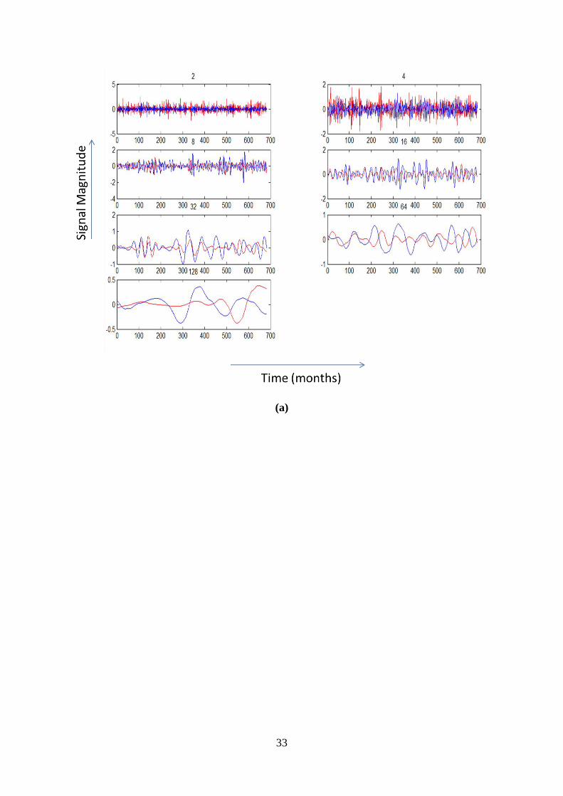
33

(a)

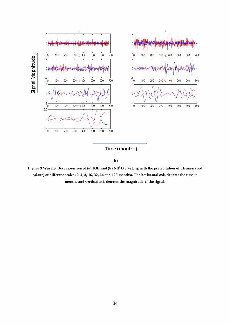
34

(b)

Figure 9 Wavelet Decomposition of (a) IOD and (b) NIÑO 3.4along with the precipitation of Chennai (red

colour) at different scales (2, 4, 8, 16, 32, 64 and 128 months). The horizontal axis denotes the time in

months and vertical axis denotes the magnitude of the signal.

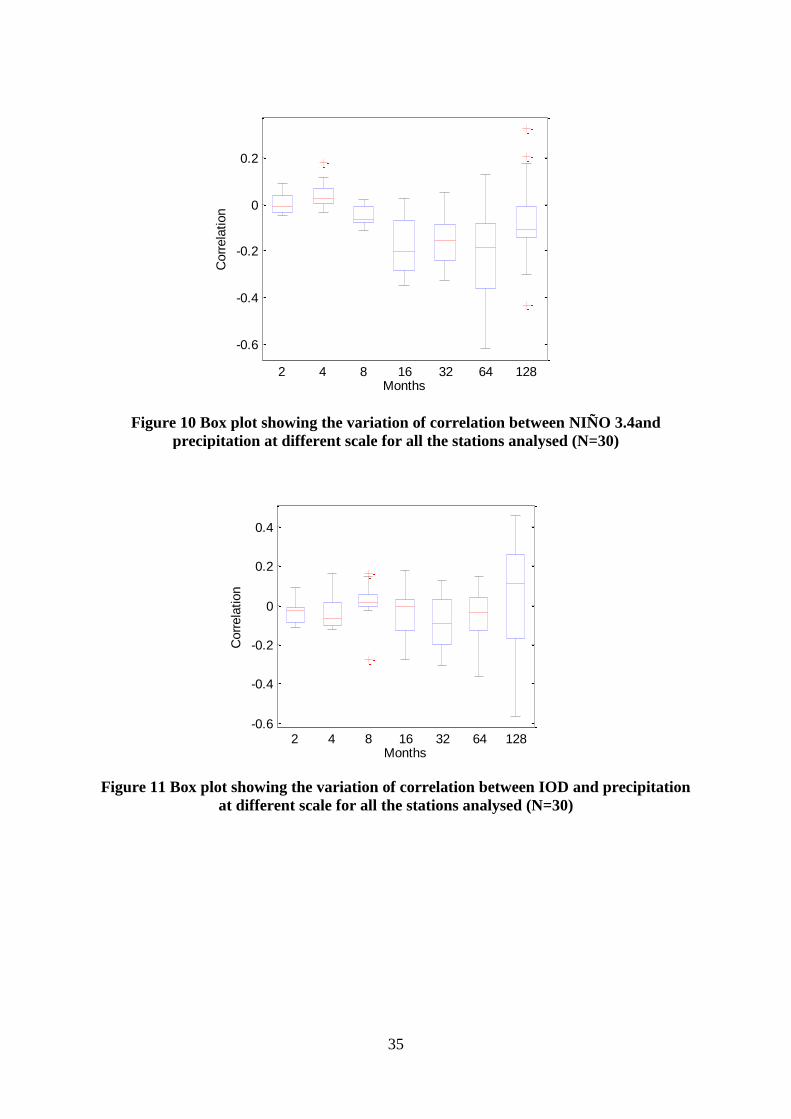
35

Figure 10 Box plot showing the variation of correlation between NIÑO 3.4and

precipitation at different scale for all the stations analysed (N=30)

Figure 11 Box plot showing the variation of correlation between IOD and precipitation

at different scale for all the stations analysed (N=30)

-0.6

-0.4

-0.2

0

0.2

2 4 8 16 32 64 128Months

Corr

ela

tion

-0.6

-0.4

-0.2

0

0.2

0.4

2 4 8 16 32 64 128Months

Corr

ela

tion

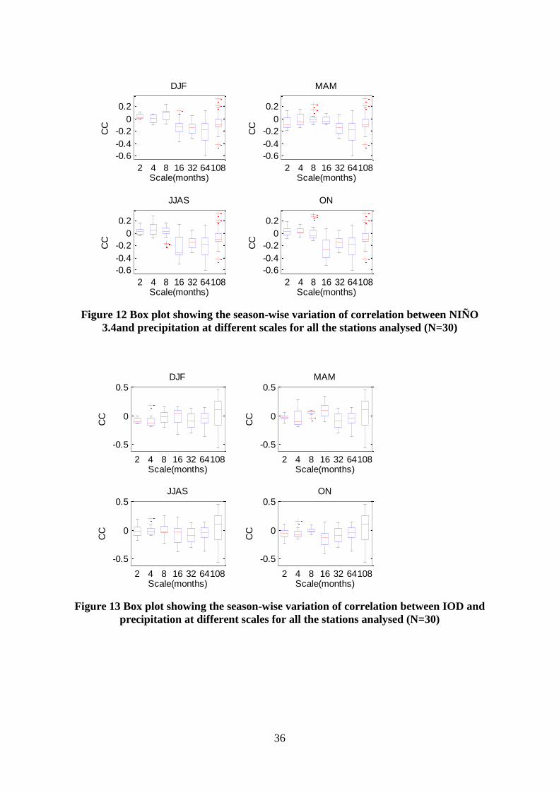
36

Figure 12 Box plot showing the season-wise variation of correlation between NIÑO

3.4and precipitation at different scales for all the stations analysed (N=30)

Figure 13 Box plot showing the season-wise variation of correlation between IOD and

precipitation at different scales for all the stations analysed (N=30)

-0.6

-0.4

-0.2

0

0.2

2 4 8 16 32 64108Scale(months)

CC

DJF

-0.6

-0.4

-0.2

0

0.2

2 4 8 16 32 64108Scale(months)

CC

MAM

-0.6

-0.4

-0.2

0

0.2

2 4 8 16 32 64108Scale(months)

CC

JJAS

-0.6

-0.4

-0.2

0

0.2

2 4 8 16 32 64108Scale(months)

CC

ON

-0.5

0

0.5

2 4 8 16 32 64108Scale(months)

CC

DJF

-0.5

0

0.5

2 4 8 16 32 64108Scale(months)

CC

MAM

-0.5

0

0.5

2 4 8 16 32 64108Scale(months)

CC

JJAS

-0.5

0

0.5

2 4 8 16 32 64108Scale(months)

CC

ON

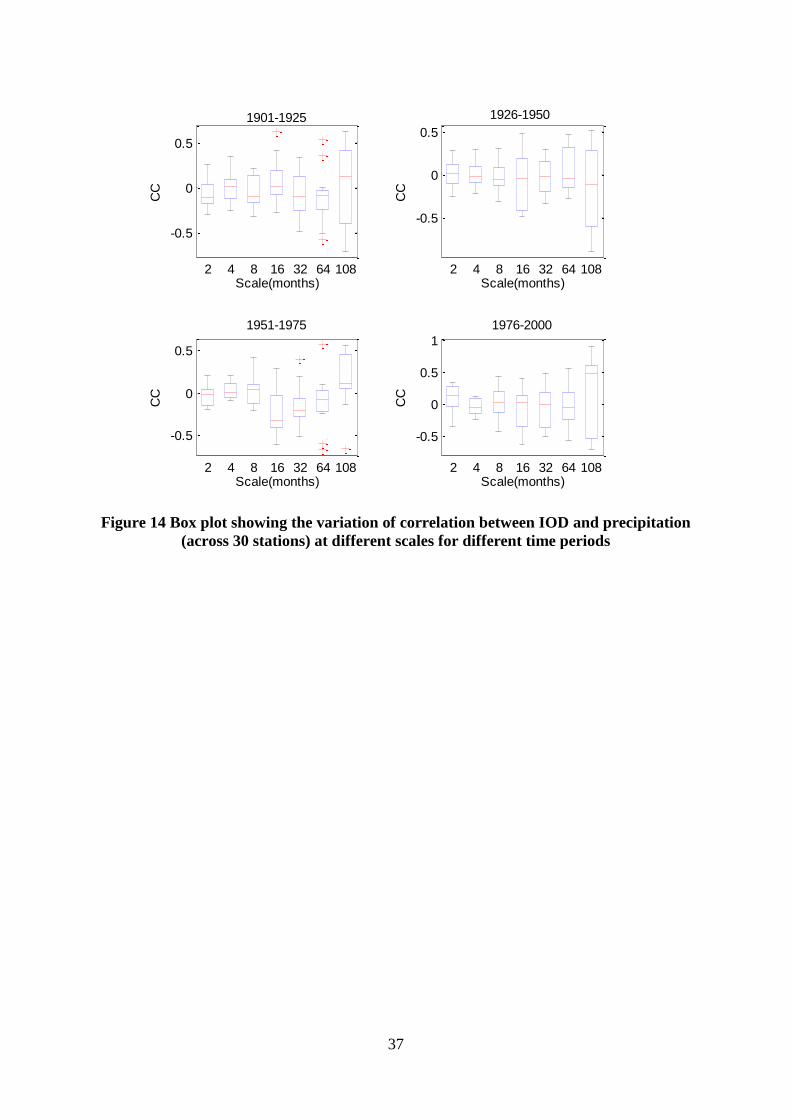
37

Figure 14 Box plot showing the variation of correlation between IOD and precipitation

(across 30 stations) at different scales for different time periods

-0.5

0

0.5

2 4 8 16 32 64 108Scale(months)

CC

1901-1925

-0.5

0

0.5

2 4 8 16 32 64 108Scale(months)

CC

1926-1950

-0.5

0

0.5

2 4 8 16 32 64 108Scale(months)

CC

1951-1975

-0.5

0

0.5

1

2 4 8 16 32 64 108Scale(months)

CC

1976-2000

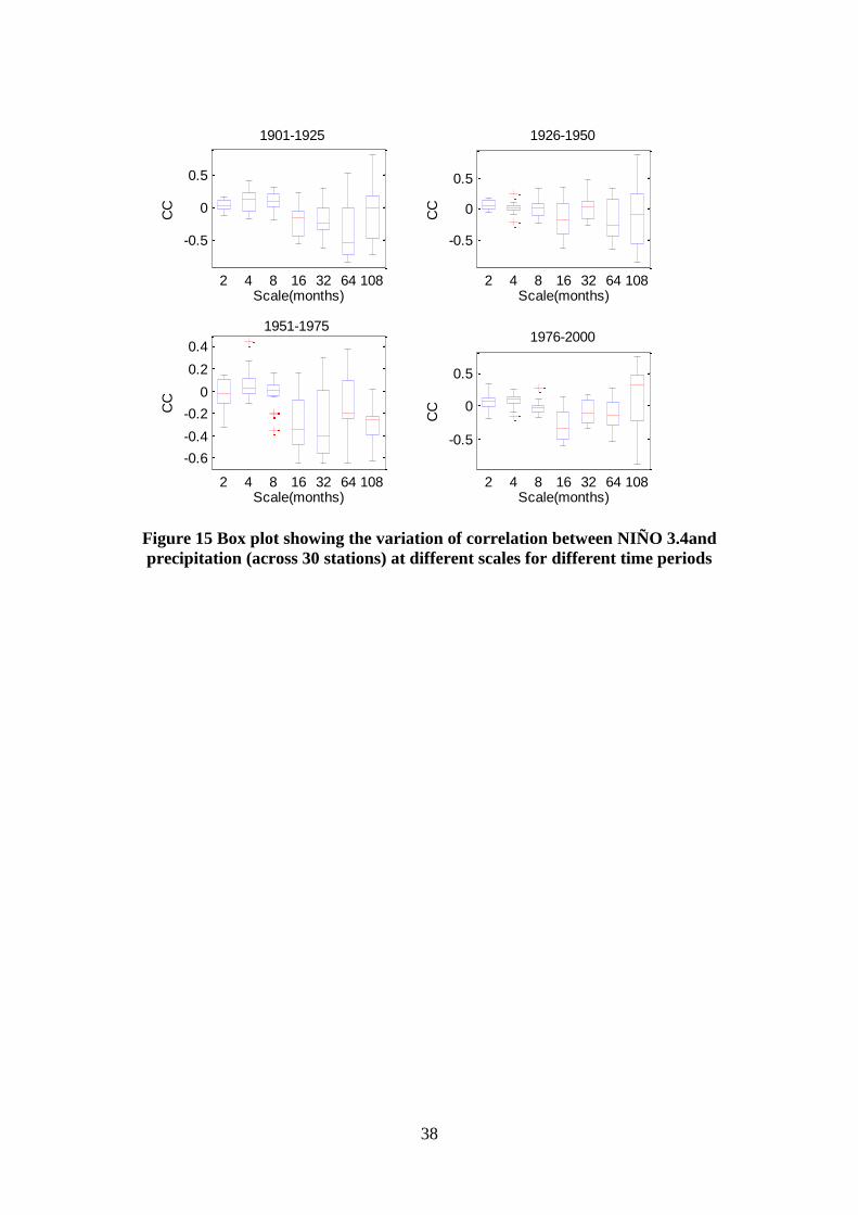
38

Figure 15 Box plot showing the variation of correlation between NIÑO 3.4and

precipitation (across 30 stations) at different scales for different time periods

-0.5

0

0.5

2 4 8 16 32 64 108Scale(months)

CC

1901-1925

-0.5

0

0.5

2 4 8 16 32 64 108Scale(months)

CC

1926-1950

-0.6

-0.4

-0.2

0

0.2

0.4

2 4 8 16 32 64 108Scale(months)

CC

1951-1975

-0.5

0

0.5

2 4 8 16 32 64 108Scale(months)

CC

1976-2000

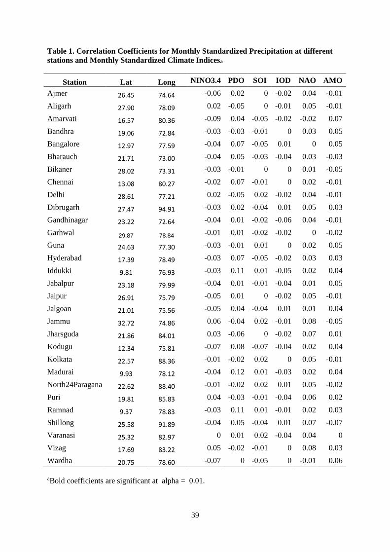
39

Table 1. Correlation Coefficients for Monthly Standardized Precipitation at different

stations and Monthly Standardized Climate Indicesa

Station Lat Long NINO3.4 PDO SOI IOD NAO AMO

Ajmer 26.45 74.64 -0.06 0.02 0 -0.02 0.04 -0.01

Aligarh 27.90 78.09 0.02 -0.05 0 -0.01 0.05 -0.01

Amarvati 16.57 80.36 -0.09 0.04 -0.05 -0.02 -0.02 0.07

Bandhra 19.06 72.84 -0.03 -0.03 -0.01 0 0.03 0.05

Bangalore 12.97 77.59 -0.04 0.07 -0.05 0.01 0 0.05

Bharauch 21.71 73.00 -0.04 0.05 -0.03 -0.04 0.03 -0.03

Bikaner 28.02 73.31 -0.03 -0.01 0 0 0.01 -0.05

Chennai 13.08 80.27 -0.02 0.07 -0.01 0 0.02 -0.01

Delhi 28.61 77.21 0.02 -0.05 0.02 -0.02 0.04 -0.01

Dibrugarh 27.47 94.91 -0.03 0.02 -0.04 0.01 0.05 0.03

Gandhinagar 23.22 72.64 -0.04 0.01 -0.02 -0.06 0.04 -0.01

Garhwal 29.87 78.84 -0.01 0.01 -0.02 -0.02 0 -0.02

Guna 24.63 77.30 -0.03 -0.01 0.01 0 0.02 0.05

Hyderabad 17.39 78.49 -0.03 0.07 -0.05 -0.02 0.03 0.03

Iddukki 9.81 76.93 -0.03 0.11 0.01 -0.05 0.02 0.04

Jabalpur 23.18 79.99 -0.04 0.01 -0.01 -0.04 0.01 0.05

Jaipur 26.91 75.79 -0.05 0.01 0 -0.02 0.05 -0.01

Jalgoan 21.01 75.56 -0.05 0.04 -0.04 0.01 0.01 0.04

Jammu 32.72 74.86 0.06 -0.04 0.02 -0.01 0.08 -0.05

Jharsguda 21.86 84.01 0.03 -0.06 0 -0.02 0.07 0.01

Kodugu 12.34 75.81 -0.07 0.08 -0.07 -0.04 0.02 0.04

Kolkata 22.57 88.36 -0.01 -0.02 0.02 0 0.05 -0.01

Madurai 9.93 78.12 -0.04 0.12 0.01 -0.03 0.02 0.04

North24Paragana 22.62 88.40 -0.01 -0.02 0.02 0.01 0.05 -0.02

Puri 19.81 85.83 0.04 -0.03 -0.01 -0.04 0.06 0.02

Ramnad 9.37 78.83 -0.03 0.11 0.01 -0.01 0.02 0.03

Shillong 25.58 91.89 -0.04 0.05 -0.04 0.01 0.07 -0.07

Varanasi 25.32 82.97 0 0.01 0.02 -0.04 0.04 0

Vizag 17.69 83.22 0.05 -0.02 -0.01 0 0.08 0.03

Wardha 20.75 78.60 -0.07 0 -0.05 0 -0.01 0.06

aBold coefficients are significant at alpha = 0.01.

40

Table 2 Correlation Coefficients between the different climate indices

Months NINO3.4 PDO SOI IOD NAO AMO

NINO3.4 1

PDO 0.39203 1

DJF SOI 0.77582 0.42541 1

IOD 0.127694 0.006052 0.149418 1

NAO -0.0014 -0.001 0.001 -0.0053 1

AMO 0.045 -0.025 0.172 -0.005 -0.116 1.000

NINO3.4 1

PDO 0.382566 1

MAM SOI 0.646109 0.24767 1

IOD 0.129083 0.072002 0.233378 1

NAO 0.025 -0.090 0.015 -0.049 1 AMO 0.266 -0.121 0.002 0.169 -0.100 1

NINO3.4 1

JJAS PDO 0.500945 1

SOI 0.767654 0.33789 1

IOD 0.15391 0.0693 0.193718 1

NAO -0.0148 -0.048 0.072 -0.054 1 -0.125 AMO 0.002 0.028 -0.087 0.077 -0.125 1

NINO3.4 1

PDO 0.375404 1

ON SOI 0.765836 0.318892 1

IOD 0.181336 0.03559 0.110289 1

NAO 0.072 0.021 -0.070 0.056 1 -0.091 AMO -0.081 0.040 0.031 -0.0127 -0.091 1 Bold indicates the correlation values are significantly different from zero at 95% confidence levels.

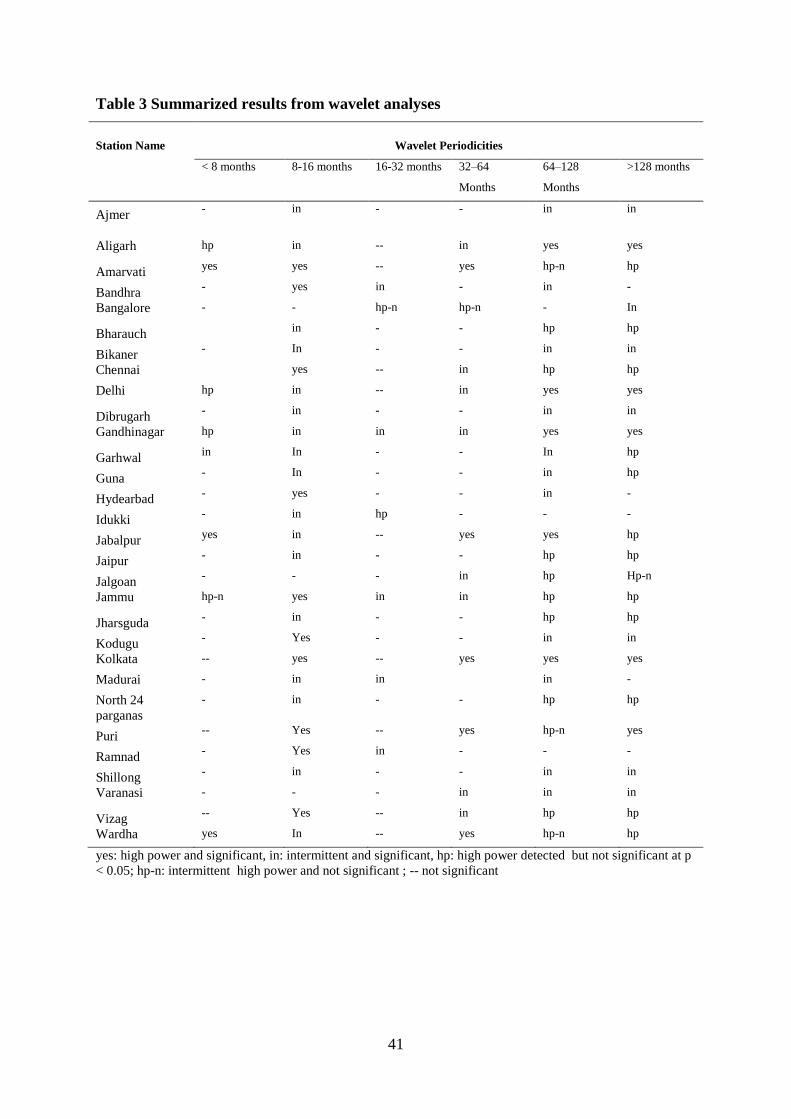
41

Table 3 Summarized results from wavelet analyses

Station Name Wavelet Periodicities

< 8 months 8-16 months 16-32 months 32–64

Months

64–128

Months

>128 months

Ajmer - in - - in in

Aligarh hp in -- in yes yes

Amarvati yes yes -- yes hp-n hp

Bandhra - yes in - in -

Bangalore - - hp-n hp-n - In

Bharauch in - - hp hp

Bikaner - In - - in in

Chennai yes -- in hp hp

Delhi hp in -- in yes yes

Dibrugarh - in - - in in

Gandhinagar hp in in in yes yes

Garhwal in In - - In hp

Guna - In - - in hp

Hydearbad - yes - - in -

Idukki - in hp - - -

Jabalpur yes in -- yes yes hp

Jaipur - in - - hp hp

Jalgoan - - - in hp Hp-n

Jammu hp-n yes in in hp hp

Jharsguda - in - - hp hp

Kodugu - Yes - - in in

Kolkata -- yes -- yes yes yes

Madurai - in in in -

North 24

parganas

- in - - hp hp

Puri -- Yes -- yes hp-n yes

Ramnad - Yes in - - -

Shillong - in - - in in

Varanasi - - - in in in

Vizag -- Yes -- in hp hp

Wardha yes In -- yes hp-n hp

yes: high power and significant, in: intermittent and significant, hp: high power detected but not significant at p

< 0.05; hp-n: intermittent high power and not significant ; -- not significant

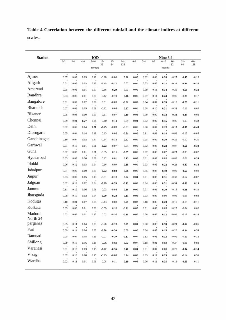
42

Table 4 Correlation between the different rainfall and the climate indices at different

scales.

Station IOD Nino 3.4 0-2 2-4 4-8 8-16 16-

32

32-

64

64-

128

0-2 2-4 4-8 8-16 16-

32

32-

64

64-

128

months months

Ajmer -

0.07

-

0.09 0.05

-

0.12 -0.28 -0.06 0.20

-

0.02

-

0.02

-

0.03

-

0.28 -0.27 -0.45 -0.15

Aligarh -

0.01

-

0.09 0.03

-

0.19 -0.35 -0.12 0.07

-

0.01

-

0.03

-

0.07

-

0.22 -0.29 -0.46 -0.35

Amarvati -

0.05

-

0.08

-

0.01

-

0.07 -0.16 -0.29 -0.03

-

0.06 0.09

-

0.11

-

0.34 -0.29 -0.59 -0.33

Bandhra -

0.03

-

0.09 0.01 0.00 -0.12 -0.10 0.46

-

0.05 0.07

-

0.11

-

0.24 -0.05 -0.31 0.17

Bangalore 0.01 0.02

-

0.02

-

0.06 0.01 -0.03 -0.32 0.09

-

0.04

-

0.07

-

0.33 -0.15 -0.29 -0.11

Bharauch -

0.07

-

0.03 0.05

-

0.09 -0.12 0.04 0.37 0.01 0.08

-

0.10

-

0.31 -0.31 0.11 0.05

Bikaner -

0.05

-

0.08 0.00 0.00 -0.11 -0.07 0.10

-

0.02 0.09

-

0.09

-

0.32 -0.33 -0.49 0.02

Chennai -

0.09 0.01

-

0.27 0.04 0.10 0.14 0.09 0.04 0.02

-

0.02

-

0.15 0.05 0.13 0.32

Delhi -

0.02

-

0.09 0.04

-

0.21 -0.25 -0.03 -0.03 0.01 0.00

-

0.07

-

0.23 -0.13 -0.37 -0.43

Dibrugarh 0.05 0.04 0.14 0.18 0.13 0.06 -0.51

-

0.02 0.11

-

0.01

-

0.18 -0.09 -0.13 -0.05

Gandhinagar -

0.10

-

0.07 0.02

-

0.27 -0.14 -0.12 0.37

-

0.01 0.05

-

0.09

-

0.30 -0.26 -0.10 0.20

Garhwal -

0.01

-

0.10 0.01

-

0.01 -0.22 -0.07 0.04

-

0.01 0.02

-

0.08

-

0.23 -0.07 -0.50 -0.30

Guna -

0.02

-

0.05 0.01 0.01 -0.05 0.15 -0.25

-

0.01 0.02

-

0.08

-

0.07 -0.25 -0.03 -0.07

Hydearbad -

0.03 0.03

-

0.20

-

0.08 0.12 0.01 0.13 0.08

-

0.01 0.02

-

0.05 -0.03 0.01 0.24

Idukki -

0.06

-

0.12 0.03

-

0.04 -0.16 -0.09 0.18

-

0.01

-

0.03

-

0.05

-

0.22 -0.24 -0.47 -0.18

Jabalpur -

0.01

-

0.09 0.00 0.00 -0.22 -0.60 0.28

-

0.06 0.05

-

0.08

-

0.19 -0.09 -0.57 0.02

Jaipur -

0.03

-

0.09 0.05

-

0.13 -0.31 -0.13 0.22

-

0.04 0.01

-

0.05

-

0.31 -0.33 -0.62 -0.07

Jalgoan 0.02

-

0.14

-

0.02

-

0.04 -0.29 -0.33 -0.13 0.00 0.04

-

0.08

-

0.31 -0.39 -0.62 0.19

Jammu -

0.11

-

0.12 0.06 0.01 0.03 -0.04 0.18 0.00 0.01

-

0.01

-

0.20 -0.13 -0.38 -0.19

Jharsguda -

0.08

-

0.10 0.02 0.04 -0.29 -0.22 0.11

-

0.02 0.03

-

0.08 0.00 -0.03 -0.08 -0.03

Kodugu -

0.10 0.01 0.07

-

0.08 -0.13 0.08 0.27 0.02 0.18

-

0.06

-

0.20 -0.19 -0.18 -0.11

Kolkata -

0.03

-

0.06 0.01 0.00 -0.09 0.10 -0.11

-

0.02 0.01

-

0.08

-

0.05 -0.25 -0.04 0.00

Madurai -

0.02 0.02

-

0.01

-

0.12 0.02 -0.16 -0.19 0.07 0.00 0.02

-

0.12 -0.09 -0.18 -0.14

North 24

parganas -

0.05

-

0.11 0.04

-

0.09 -0.20 -0.13 0.21

-

0.04 0.00

-

0.06

-

0.33 -0.29 -0.62 -0.05

Puri -

0.09

-

0.14

-

0.04 0.00 -0.28 -0.30 0.09 0.00 0.04

-

0.09

-

0.15 -0.20 -0.34 0.36

Ramnad -

0.05 0.04 0.05

-

0.16 -0.07 -0.20 -0.17 0.07 0.12

-

0.01

-

0.12 -0.06 -0.21 -0.12

Shillong 0.09 0.16 0.16 0.16 0.06 -0.03 -0.57 0.07 0.18

-

0.01 0.02 -0.27 -0.06 -0.03

Varanasi -

0.01

-

0.13

-

0.03

-

0.19 -0.22 -0.36 0.40

-

0.04

-

0.01

-

0.07 0.00 -0.20 -0.34 -0.14

Vizag -

0.07

-

0.15

-

0.08 0.15 -0.25 -0.08 0.14 0.00 0.05

-

0.11

-

0.23 0.00 -0.14 0.51

Wardha -

0.02

-

0.11 0.01

-

0.01 -0.08 -0.11 0.19

-

0.04 0.06

-

0.11

-

0.35 -0.19 -0.55 -0.11