¿Clase o programa? ¿Academia o divulgación? El ethos y el discurso de la filosofía por televisión
Upload
khangminh22Category
view
2download
0
Surname or Family name: Turner
First name: Alexander
THE UNIVERSITY OF NEW SOUTH WALES Thesis/Project Report Sheet
Other name/s: William Lyttleton
Abbreviation for degree as given in the University calendar: PhD
School: Mechanical and Manufacturing Engineering Faculty: Engineering
Title: A Theoretical and Experimental Investigation of Stress Distribution and Remodelling of a Femur Implanted with a Femoral Prosthesis
Abstract 350 words maximum: Bone loss around uncemented hip replacement stems is associated with stress shielding, with bone resorption occurring in accordance with "Wolff's Law". Extensive bone loss may cause implant or bone failure, and complicate revision procedures. This thesis was concerned with developing a mathematical formulation of "Wolff's Law", which was combined with finite element modelling to simulate time-dependent adaptive bone remodelling.
Experimental and finite element investigations were undertaken to determine the alteration in strain distribution of a femur caused by reconstruction with a cobalt-chrome hip prosthesis (Margron). A site-specific, strain-adaptive bone remodelling theory was developed to predict changes in apparent density due to these changes in strain, based on an equivalent strain stimulus. Time-dependent density changes were compared with radiographic clinical data at the 7 Gruen zones. Remodelling was simulated for 2 additional femora implanted with titanium alloy (Stability) and composite (Epoch) stems. The influences of implant-bone contact conditions, femoral head position, dead zone width, postoperative activity level and prosthesis stiffness on periprosthetic bone remodelling were investigated.
Severe proximal stress shielding medially and laterally was evident for the Margron implant. This was also the case for the Stability and Epoch Stems, although to a lesser extent distally. The finite element model was validated by comparison with experimental strains. Mesh refinement led to adoption of a 5 mm element size, with variable material properties applied to the integration points.
Bone density changes in the Gruen zones were correlated with the radiographic clinical data at 1, 2 and 3 year time points for the Margron model, and at 2 years for the Stability and Epoch models. All correlations were significant (ff > 0.67, p < 0.02), with average errors of less than 5.4% at 2 years. This is the first report of bone density changes measured in Gruen zones correlating with radiographic measurements. Previous studies have overestimated proximal bone loss in the calcar region.
A strain-adaptive bone remodeling theory was developed, which simulated bone density changes in accordance with those seen clinically. This tool could be employed for pre-clinical testing of new implants, investigation of design modifications, and patient-specific implant selection.
Declaration relating to disposition of project report/thesis
I am fully aware of the policy of the University relating to the retention and use of higher degree project reports and theses, namely that the University retains the copies submitted for examination and is free to allow them to be consulted or borrowed. Subject to the provisions of the Copyright Act 1968, the University may issue a project report or thesis in whole or in part, in photostat or microfilm or other copying medium.
I also authorise th publication by University Microfilms of a 350 word abstract in Dissertation Abstracts International (applicable
~ ' '" .# /"'-; 7 _,.., j
to doctoral s o -. . 1. i s;g;~rr;;;;····················· . ~~1...... ············ ~o jjr?Y ........ .
The niversity recognises that there may be exceptional circumstances requiring restrictions on copying or conditions on use. Requests for restriction for a period of up to 2 years must be made in writing to the Registrar. Requests for a longer period of restriction may be considered in exceptional circumstances if accompanied by a letter of support from the Supervisor or Head of School. Such requests must be submitted with the thesis/project report.
FOR OFFICE USE ONLY Date of completion of requirements for Award:
/c~tr
A THEORETICAL AND EXPERIMENTAL INVESTIGATION OF STRESS DISTRIBUTION AND
RElVIODELLING OF A FEMUR IMPLANTED WITH A FEMORAL PROSTHESIS
A THESIS SUBMITTED IN FULFILMENT
OF THE REQUIREMENTS FOR THE DEGREE OF
DOCTOR OF PHILOSOPHY
Alexander W. L. Turner
School of Mechanical and Manufacturing Engineering,
The University of New South Wales.
November 2003
I hereby declare that this submission is my own work and to
the best of my knowledge it contains no materials previously
published or written by another person, nor material which to
a substantial extent has been accepted for the award of any
other degree or diploma at UNSW or any other educational
institution, except where due acknowledgement is made in
the thesis. Any contribution made to the research by others,
with whom I have worked at UNSW or elsewhere, is explicitly
acknowledged in the thesis.
I also declare that the intellectual content of this thesis is the
product of my own work, except to the extent that assistance
from others in the project's design and conception or in style,
presentation and linguistic expression is acknowledged.
""' A. W. L. Turner

"By seeking and blundering we learn."
Johann Wolfgang Von Goethe
ii
Executive Summary
Abstract
Bone loss around uncemented hip replacement stems is associated with stress shield
ing, with bone resorption occurring in accordance with "Wolff's Law". Extensive
bone loss may cause implant or bone failure, and complicate revision procedures.
This thesis was concerned with development of a mathematical formulation of
"\:Volff's Law", which was combined with finite element modelling to simulate time
dependent adaptive bone remodelling changes.
Experimental and finite element investigations were undertaken to determine the
alteration in strain distribution of a femur caused by reconstruction with a cobalt
chrome hip prosthesis (Margron). A site-specific, strain-adaptive bone remodelling
theory was developed to predict changes in apparent density due to these changes in
strain, based on an equivalent strain stimulus equal to the magnitude of the strain
tensor. Time-dependent density changes were compared with radiographic clinical
measurements from the 7 Gruen zones. Remodelling was simulated for 2 additional
femora implanted with titanium alloy (Stability) and composite (Epoch) stems.
The influences of implant-bone contact conditions, femoral head position, dead
zone width, postoperative activity level and prosthesis stiffness on periprosthetic
bone remodelling were investigated.
Severe proximal stress shielding medially and laterally was evident for the Mar
gron implant. This was also the case for the Stability and Epoch stems, although
to a lesser extent distally. The finite element model was validated by comparison
iii
with experimental strains. Mesh refinement led to adoption of a 5 mm element size,
with variable material properties applied to the integration points.
Bone density changes in the Gruen zones correlated with the radiographic find
ings at 1, 2 and 3 year time points for the JVIargron model (R2 > 0.67, p < 0.02),
with an average error of 5.4% at 2 years. Density changes with the Stability and
Epoch models were correlated with radiographic clinical data at 2 years, with good
agreement again (R2 > 0.76, p < 0.02), and with average errors of 3.4% and 3.9%
respectively. This is the first report of bone density changes measured in Gruen
zones correlating with radiographic clinical measurements. Previous studies have
overestimated proximal bone loss in the calcar region.
A strain-adaptive bone remodelling theory was developed, which simulated bone
density changes in accordance with those seen clinically. This tool could be em
ployed for pre-clinical testing of new implants, investigation of design modifications,
and patient-specific implant selection.
Aims
The objective of this study was to evaluate the strain distribution in a femur im
planted with a cobalt-chrome femoral prosthesis, and to simulate bone remodelling
in this femur, consistent with radiographic clinical outcomes. The scope of the
research was to:
• experimentally determine the cortical strain distribution of a femur, before
and after implantation with the Margron hip prosthesis;
• create an anatomical finite element model of a femur;
• validate the finite element model and undertake mesh refinement;
• develop a strain-adaptive remodelling theory, to be coupled with the finite
element model, to predict periprosthetic bone apparent density changes con
sistent with radiographic clinical data;
• investigate the effects of various parameters on remodelling results;
iv
• discuss the limitations of the modelling; and
• suggest further theoretical research.
Recommendations
The results of this study suggest that the proposed computational bone remodelling
theory may be appropriate for determining subject-specific, time-dependent bone
density adaptation around femoral prostheses. The theory could also be applied to
pre-clinical testing of new implant designs, and modifications to existing products.
Further work is proposed to further verify the theory and improve, and the
influence of additional parameters could be investigated. Consideration should be
given to:
• verification of the dead zone width and time-dependence;
• the influence of postoperative rehabilitation and altered musculoskeletal load
ing on remodelling; and
• incorporation of other factors that modulate bone remodelling into the theory.
v
Acknowledgements
By far the greatest thanks must go to my supervisors Bill Walsh, Richard Frost and
Khosrhow Zarrabi for their guidance, support and facilities.
Thanks also to my colleagues at the Orthopaedic Research Laboratories, especially
Mark Gillies, Adam Butler, Richard Harris and Gina O'Reilly, for providing assis
tance, motivation and stress relief.
I would also like to acknowledge Dr. Ron Sekel (St. George Hospital) and A/Prof
Nicholas Pocock (St. Vincent's Hospital) for providing radiographic data, Bill Taylor
for initial modelling help, the medical imaging staff at the Prince of Wales Hospital
for use of their equipment, and my father for his clinical input and proof-reading
skills.
Alex Turner, November 28, 2003.
Vl
Contents
Chapter 1 Introduction
1.1 Objectives . . .
1.2 Thesis Outline .
Chapter 2 Anatomy and Biomechanics of the Hip
2.1 Anatomy of the Hip Joint .....
2.1.1 Proximal Articular Surface .
2.1.2 Distal Articular Surface ..
2.1.3 Joint Capsule and Ligaments
2.1.4 Muscles ....... .
2.2 Biomechanics of the Hip Joint
2.2.1 Stance
2.2.2 Gait .
2.2.3 Stair Climbing
2.2.4 Joint and Muscle Forces
Chapter 3 Hip Arthroplasty
3.1 Indications . . . . . . . . . . . . . . .
3.2 Evolution of Total Hip Arthroplasty .
3.3 Biomaterials .
3.3.1 Metals
3.3.2 Polymers .
3.3.3 Ceramics .
Vll
1
3
4
5
5
5
7
9
11
15
16
18
21
22
29
29
30
34
34
37
39
3.3.4 Biological Response to Biomaterials .
3.4 Femoral Component Design
3.4.1 Material .
3.4.2 Geometry
3.4.3 Surface Finish .
3.5 Performance . . . . .
Chapter 4 Bone 1\Iechanics
4.1 Structure . .
4.2 Composition .
4.3 Development, Growth, Modelling and Remodelling
4.3.1 Bone Formation .....
4.3.2 Mechanical Adaptation .
4.3.3 Mechanotransduction .
4.4 Mechanical Properties . . .
4.4.1 Constitutive Models
4.4.2 Elastic Modulus and Density .
4.4.3 Noninvasive Measurement of Bone Density
Chapter 5 Stress Analysis of the Femur
5.1 Experimental Stress Analysis
5.1.1 Strain Gauges ....
5.1.2 Strain Gauge Studies
5.2 Finite Element Stress Analysis .
5.2.1 Finite Element Modelling
5.2.2 Finite Element Studies
5.3 Remarks . . . . . . . . . . . .
Chapter 6 Bone Adaptation Models
6.1 Site-Specific Models . . . . . .
6.1.1 Adaptive Elasticity Theory.
viii
40
43
43
44
46
48
50
52
55
56
56
60
65
70
71
73
77
81
81
82
84
92
92
95
108
110
113
113
6.1.2 Strain Energy Density Model .
6.1.3 Damage Accumulation Models .
6.2 Non-Site-Specific ]\:1odels ....... .
6.2.1 Self-Optimisation and Bone Maintenance Theories .
6.2.2 Global Models .
6.3 Remodelling Stimulus .
Chapter 7 Materials and Methods
7.1
7.2
Experimental Study .
7.1.1 Specimens
7.1.2 Implant
7.1.3 Mechanical Testing
7.1.4 Data Analysis .
Finite Element Study .
7.2.1 Model Construction .
7.2.2 Model Validation
7.2.3 Mesh Refinement
7.3 Bone Remodelling Study
7.3.1 Margron .....
7.3.2 Comparison with other Implants
7.3.3 Investigation of Parameters
Chapter 8 Results
8.1 Experimental Study.
8.2 Finite Element Study .
8.2.1 Model Validation
8.2.2 Mesh Refinement
8.3 Bone Remodelling Study
8.3.1 Margron .....
8.3.2 Comparison with other Implants
lX
115
117
118
118
126
127
129
131
131
131
133
136
137
137
145
146
146
147
160
165
169
169
175
175
184
188
188
197

8.3.3 Investigation of Parameters
Chapter 9 Discussion
9.1 Experimental Study .
9.2 Finite Element Study .
9.2.1 Model Validation
9.2.2 Mesh Refinement
9.3 Bone Remodelling Study
9.3.1 Margron .....
9.3.2 Comparison with other Implants
9.3.3 Investigation of Parameters
9.3.4 Limitations .........
Chapter 10 Conclusions
10.1 Recommendations .
Appendix A Experimental Strain Gauge Data
Appendix B Strain Distributions
Appendix C Density Changes and Distributions
C.1 Margron ............. .
C.2 Comparison with Other Implants
C.3 Investigation of Parameters ...
C.3.1 Effect of Interface Conditions
C.3.2 Effect of Femoral Head Position
C.3.3 Effect of Dead Zone Width.
C.3.4 Effect of Activity Level . . .
C.3.5 Effect of Prosthesis Stiffness
Appendix D Bone Density Correlations
References
X
203
217
218
221
221
225
227
228
237
247
254
257
259
262
270
274
274
275
282
282
282
285
285
285
287
291

List of Tables
2.1 Range of motion at the hip joint . . . . . . . . . . . . . . . . . 16
2.2 1\iiuscle activity and joint motion during the walking gait cycle 20
2.3 Peak hip joint reaction force for normal walking . 24
2.4 Hip joint and muscle force magnitudes during gait 26
2.5 Joint and muscle force magnitudes acting on the femur during gait . 27
3.1 Typical mechanical properties of implant materials . . . . . . . . . 36
4.1 Mechanical usage windows according to Frost's Mechanostat theory 65
4.2 Experimental values for the elastic modulus of human cortical bone
tissue ............ .
4.3 Experimental values for the elastic modulus of human trabecular
bone tissue . . . . . . . . . . . . . . .
4.4 Apparent density of human bone tissue
73
74
74
4.5 Emperical relationships between elastic modulus and apparent density 76
4.6 Emperical relationships between apparent density and CT data 80
7.1 Joint and muscle force components for the proximal femur
7.2 Margron clinical bone mineral density data .
7.3 Stability clinical bone mineral density data .
7.4 Epoch clinical bone mineral density data ..
7.5 Matrix of femoral head position parameters evaluated
8.1 Statistically significant strains before and after surgery
8.2 Finite element models to investigate convergence .
8.3 Effect of model complexity on computation time .
xi
154
160
163
165
167
171
184
186
8.4 Equivalent strain values and percentages for the Margron, Stability
and Epoch models . . . . . . . . . . . . . . . . . . . 200
A.1 Preoperative minimum principal strains (Load case 1) 262
A.2 Preoperative minimum principal strains (Load case 2) 263
A.3 Preoperative maximum principal strains (Load case 1) 263
A.4 Preoperative maximum principal strains (Load case 2) 264
A.5 Preoperative longitudinal strains (Load case 1) . 264
A.6 Preoperative longitudinal strains (Load case 2) . 265
A. 7 Postoperative minimum principal strains (Load case 1) 265
A.8 Postoperative minimum principal strains (Load case 2) 266
A.9 Postoperative maximum principal strains (Load case 1) 266
A.10 Postoperative maximum principal strains (Load case 2) 267
A.11 Postoperative longitudinal strains (Load case 1) 267
A.12 Postoperative longitudinal strains (Load case 2) 268
A.13 ?-values showing the statistically significant difference between the
strains before and after surgery . . . . . . . . . . . . . . . . . . . . 268
A.14 Postoperative strains as a percentage of preoperative strains (maxi-
mum and minimum principal strains and their corresponding errors) 269
A.15 Postoperative strains as a percentage of preoperative strains (longi
tudinal strains and their corresponding errors) . . . . . . . . . . . . 269
C.1 Predicted bone density changes in the Gruen zones for the Margron
model (dead zone 0.6, no distal contact, version angle 0°, neck length
+4 mm) ................................. 274
C.2 Predicted bone density changes in the Gruen zones for the Stability
model . . . . . . . . . . . . . . . . . . . . . . . . . . . . . . . . . . 275
C.3 Predicted bone density changes in the Gruen zones for the Epoch
model . . . . . . . . . . . . . . . . . . . . . . . . . . . . . . . . . . 275
C.4 Predicted bone density changes in the Gruen zones for the Margron
model (fully bonded contact) . . . . . . . . . . . . . . . . . . . . . . 282
xii
C.5 Predicted bone density changes in the Gruen zones for the lVIargron
model (distal sliding contact) . . . . . . . . . . . . . . . . . . . . . 282
C.6 Predicted bone density changes in the Gruen zones for the Margron
model (version angle 0°, neck length -4 mm) . . . . . . . . . . . . 282
C. 7 Predicted bone density changes in the Gruen zones for the Margron
model (version angle 0°, neck length 0 mm) . . . . . . . . . . . . . 283
C.8 Predicted bone density changes in the Gruen zones for the Margron
model (version angle 0°, neck length +4 mm) . . . . . . . . . . . . 283
C.9 Predicted bone density changes in the Gruen zones for the l\1argron
model (version angle oo, neck length + 7 mm) . . . . . . . . . . . . 283
C.10 Predicted bone density changes in the Gruen zones for the Margron
model (version angle - 20o, neck length +4 mm) . . . . . . . . . . . 283
C.ll Predicted bone density changes in the Gruen zones for the Margron
model (version angle -10°, neck length +4 mm) . . . . . . . . . . . 284
C.12 Predicted bone density changes in the Gruen zones for the Margron
model (version angle +10°, neck length +4 mm) . . . . . . . . . . . 284
C.13 Predicted bone density changes in the Gruen zones for the 1\ifargron
model (version angle + 20°, neck length +4 mm) . . . . . . . . . . . 284
C.14 Predicted bone density changes in the Gruen zones for the Margron
model (dead zone 0.55) . . . . . . . . . . . . . . . . . . . . . . . . . 285
C.15 Predicted bone density changes in the Gruen zones for the Margron
model (dead zone 0.65) . . . . . . . . . . . . . . . . . . . . . . . . . 285
C.16 Predicted bone density changes in the Gruen zones for the Margron
model (90% activity level) . . . . . . . . . . . . . . . . . . . . . . . 285
C.17 Predicted bone density changes in the Gruen zones for the Epoch
model (isoelastic properties) . . . . . . . . . . . . . . . . . . . . . . 286
C.18 Predicted bone density changes in the Gruen zones for the Epoch
model (cobalt-chrome properties) . . . . . . . . . . . . . . . . . . . 286
Xlll
List of Figures
2.1 Osteology of the pelvis and femur .............. .
2.2 The hip bone formed by the ilium, ischium and pubic bones
2.3 Neck-shaft angle of the femur
2.4 Version angle of the femur ..
2.5 Capsule and ligaments of the hip joint
2.6 Muscle attachment points of the pelvis and femur
2. 7 Location of the line of gravity
2.8 A complete gait cycle .....
2.9 Static equilibrium of the pelvis in single-legged stance .
2.10 Components and magnitude of the hip joint reaction force
3.1 The first total hip arthroplasty system
3.2 Early arthroplasty designs ...... .
6
7
8
9
10
12
17
19
23
25
31
32
3.3 Composition of some common orthopaedic biomaterials 35
3.4 Porous coating techniques . . . . . . . . . . . . . . . . 4 7
3.5 Zones around the femoral component for evaluating loosening 49
4.1 Architecture of the proximal femur . . . . . 51
4.2 Architecture of cortical and trabecular bone 53
4.3 Schematic diagram of intramembranous ossification 57
4.4 Schematic diagram of endochondral ossification . . 58
4.5 Endochondral ossification in the epiphyseal growth plate 59
4.6 Adaptation hypothesis for regulation for skeletal mass . . 60
4. 7 Bone remodelling due to the activity of basic multicellular units 63
XIV

408 Specific surface as a function of porosity 0 0 0 0 0 0 0 0 0 0 0 0 0 64
409 Rate of change of bone mass as a function of the strain history 0 66
501 Uniaxial strain gauge grid 82
502 \Vheatstone bridge 0 0 0 0 83
503 A collared implant increases axial compressive loads at the calcar 85
5.4 Load transfer mechanism for an uncemented prosthesis with and
without abductor muscle action present 0 0 0 0 0 0 0 0 0 0 0 0 0 0 0 0 87
505 Set up used for applying the hip joint and abductor forces to the femur 89
506 Representation of the femoral constraints for mechanical testing 0 0 90
50 7 Changed loading if the position of the prosthetic head does not co-
incide with the anatomic one 0 0 0
508 A two-dimensional finite element mesh
509 Nonlinearities in finite element modelling
91
93
95
5010 Two-dimensional side-plate model of the proximal femur 97
5011 Automatic mesh generation methods 98
601 Trilinear curve relating remodelling rate and stimulus 115
602 Graph of the surface area density as a function of apparent density 116
603 Piecewise linear curve relating remodelling rate and stimulus 120
6.4 Checker-board effect in density distribution 0 123
605 Effect of spatial influence function on trabecular morphogenesis 125
701 Flowchart of the study design 0 0 130
702 Anterior-posterior radiograph with 1\ilargron template overlying 132
703 The Margron hip prosthesis 0 0 0 0 0 132
7.4 Strain gauge positions on the femoral cortex 134
705 Mechanical testing of a femur under two load cases 135
706 Femoral geometry for the finite element model 0 0 0 138
70 7 10-noded tetrahedral element showing nodes and integration points 139
708 Finite element meshes for the Margron models 0 0 0 0 0 0 0 140
XV

7.9 Diaphyseal CT slice showing regions of interest to determine Houns-
field units of cortical bone . . . . . . . . . . . . . 142
7.10 "Ringing" phenomenon due to CT-scanning in air 143
7.11 3 and 7 mm finite element meshes used for convergence analysis 147
7.12 Remodelling rate as a function of the remodelling signal. . . . . 150
7.13 Polynomial fit of the bone surface area density-apparent density curve151
7.14 Overview of the bone adaptation simulation . . . . 152
7.15 Load and boundary conditions for the intact femur 155
7.16 Proximal load conditions for the intact femur 156
7.17 Gruen zone analysis of DEXA images . . . . . 159
7.18 Finite element meshes for the Stability models 162
7.19 Finite element meshes for the Epoch models 164
8.1 Medial and lateral principal strains . . 170
8.2 Anterior and posterior principal strains 170
8.3 lVIedial and lateral longitudinal strains 172
8.4 Anterior and posterior longitudinal strains 173
8.5 Medial and lateral percentage strains . . 17 4
8.6 Anterior and posterior percentage strains 174
8. 7 Density distribution of the femur . . . . 176
8.8 Contour plots of preoperative minimum principal strains 177
8.9 Contour plots of postoperative (no distal contact) minimum principal
strains . . . . . . . . . . . . . . . . . . . . . . . . . . . . . . . . . . 178
8.10 Preoperative medial and lateral experimental and finite element prin-
cipal strains for load case 1 . . . . . . . . . . . . . . . . . . . . . . . 179
8.11 Preoperative anterior and posterior experimental and finite element
principal strains for load case 1 . . . . . . . . . . . . . . . . . . . . 179
8.12 Preoperative medial and lateral experimental and finite element prin-
cipal strains for load case 2 . . . . . . . . . . . . . . . . . . . . . . . 180
XVI
8.13 Preoperative anterior and posterior experimental and finite element
principal strains for load case 2 . . . . . . . . . . . . . . . . . . . . 180
8.14 Postperative medial and lateral experimental and finite element prin-
cipal strains for load case 1 . . . . . . . . . . . . . . . . . . . . . . . 182
8.15 Postperative anterior and posterior experimental and finite element
principal strains for load case 1 . . . . . . . . . . . . . . . . . . . . 182
8.16 Postperative medial and lateral experimental and finite element prin-
cipal strains for load case 2 . . . . . . . . . . . . . . . . . . . . . . . 183
8.17 Postperative anterior and posterior experimental and finite element
principal strains for load case 2 183
8.18 Preoperative mesh convergence 185
8.19 Preoperative mesh convergence, distal . 185
8.20 Postoperative mesh convergence . . . . 186
8.21 Mesh convergence and element homogeneity 187
8.22 Minimum principal strain distribution . 189
8.23 Equivalent strain distribution 0 •••• 190
8.24 Density distribution of the remodelled femur 192
8.25 Simulated DEXA images during remodelling of the femur . 193
8.26 Change in bone density in the Gruen zones for increments 10 to 120 193
8.27 Incremental change in bone density in Gruen zone 7 ......... 194
8.28 Comparison of actual and simulated bone density changes for the
first 3 years after surgery . . . . . . . . . . . . . . . . . . . . . . . . 195
8.29 Comparison of actual and simulated bone density changes after 2 years196
8.30 Behaviour of the remodelling error over 120 remodelling increments 196
8.31 Preoperative strains for three femora under 45% gait cycle loading . 197
8.32 Postoperative strains for three femora under 45% gait cycle loading 198
8.33 Effect of implant design on the equivalent strain along the medial
cortex . . . . . . . . . . . . . . . . . . . . . . . . . . . . . . . . . . 199
xvii
8.34 Effect of implant design on the change in bone density in the seven
Gruen zones at 2 years . . . . . . . . . . . . . . . . . . . . . . . . . 202
8.35 Effect of implant design on the change in bone density in the seven
Gruen zones . . . . . . . . . . . . . . . . . . . . . . . . . . . . . . . 203
8.36 Effect of implant contact conditions on the equivalent strain along
the medial cortex . . . . . . . . . . . . . . . . . . . . . . . . . . . . 204
8.37 Effect of contact conditions on the change in bone density in the
seven Gruen zones . . . . . . . . . . . . . . . . . . . . . . . . . . . 205
8.38 Effect of neck length on the equivalent strain along the medial cortex 206
8.39 Effect of neck length on the change in bone density in the seven
Gruen zones . . . . . . . . . . . . . . . . . . . . . . . . . . . . . . . 207
8.40 Effect of version angle on the equivalent strain along the medial cortex208
8.41 Effect of version angle on the change in bone density in the seven
Gruen zones . . . . . . . . . . . . . . . . . . . . . . . . . . . . . . . 209
8.42 Effect of dead zone width on the equivalent strain along the medial
cortex . . . . . . . . . . . . . . . . . . . . . . . . . . . . . . . . . . 210
8.43 Effect of dead zone width on the change in bone density in the seven
Gruen zones . . . . . . . . . . . . . . . . . . . . . . . . . . . . . . . 211
8.44 Effect of postoperative activity level on the equivalent strain along
the medial cortex . . . . . . . . . . . . . . . . . . . . . . . . . . . . 211
8.45 Effect of postoperative activity level on the change in bone density
in the seven Gruen zones . . . . . . . . . . . . . . . . . . . . . . . . 212
8.46 Effect of implant material on the equivalent strain along the medial
cortex . . . . . . . . . . . . . . . . . . . . . . . . . . . . . . . . . . 213
8.47 Effect of implant elastic modulus on the change in bone density in
the seven Gruen zones . . . . . . . . . . . . . . . . . . . . . . . . . 214
8.48 Immediately postoperative interface shear stress ( anteromedial, di
rection 1) . . . . . . . . . . . . . . . . . . . . . . . . . . . . . . . . 215
xviii

8.49 Immediately postoperative interface shear stress (posterolateral, di
rection 1) 0 0 0 0 0 0 0 0 0 0 0 0 0 0 0 0 0 0 0 0 0 0 0 0 0 0 0 0 0 0 0 0 215
8050 Immediately postoperative interface shear stress (anteromedial, di
rection 2) 0 0 0 0 0 0 0 0 0 0 0 0 0 0 0 0 0 0 0 0 0 0 0 0 0 0 0 0 0 0 0 0 216
8051 Immediately postoperative interface shear stress (posterolateral, di
rection 2) 0 0 0 0 0 0 0 0 0 0 0 0 0 0 0 0 0 0 0 0 0 0 0 0 0 0 0 0 0 0 0 0 216
901 Nonlinear mechanoregulation rule including strain and damage me-
diated pathways 0 0 0 0 0 0 0 0 0 0 0 0 0 0 0 0 0 0 0 255
Bo1 Minimum principal strain distribution (Stability)
Bo2 Equivalent strain distribution (Stability) 0 0 0 0
Bo3 Minimum principal strain distribution (Epoch) 0
B.4 Equivalent strain distribution (Epoch) 0 0 0 0 0
270
271
272
273
Co1 Density distribution of the immediately postoperative Stability femur 276
Co2 Density distribution of the remodelled Stability femur 0 0 0 0 0 0 0 0 277
Co3 Simulated DEXA images during remodelling of the Stability femur 0 278
C.4 Density distribution of the immediately postoperative Epoch femur 279
Co5 Density distribution of the remodelled Epoch femur 0 0 0 0 0 0 0 280
Co6 Simulated DEXA images during remodelling of the Epoch femur 281
Do1 Correlation between simulated and clinical BMD changes (Margron,
1 year postop) 0 0 0 0 0 0 0 0 0 0 0 0 0 0 0 0 0 0 0 0 0 0 0 0 0 0 0 0 0 0 287
Do2 Correlation between simulated and clinical BMD changes (Margron,
2 years postop) 0 0 0 0 0 0 0 0 0 0 0 0 0 0 0 0 0 0 0 0 0 0 0 0 0 0 0 0 0 288
Do3 Correlation between simulated and clinical BMD changes (Margron,
3 years postop) 0 0 0 0 0 0 0 0 0 0 0 0 0 0 0 0 0 0 0 0 0 0 0 0 0 0 0 0 0 288
D.4 Correlation between simulated and clinical BMD changes (Stability,
2 years postop) 0 0 0 0 0 0 0 0 0 0 0 0 0 0 0 0 0 0 0 0 0 0 0 0 0 0 0 0 0 289
Do5 Correlation between simulated and clinical Bl\fD changes (Epoch, 2
years postop) 0 0 0 0 0 0 0 0 0 0 0 0 0 0 0 0 0 0 0 0 0 0 0 0 0 0 0 0 0 0 289
Do6 Correlation between simulated and clinical BMD changes (all data) 290
xix

Nomenclature
a
BMD
Cres
Capp
CT
Strain tensor
Poisson's ratio
Remodelling error
Apparent density
Apparent density at integration point i
Convergence criterion
Function for surface area density of bone
Bone mineral density
Constant related to resorption rate
Constant related to apposition rate
Computed tomography
DEXA Dual-energy x-ray absorptiometry
E Elastic modulus
z Superscript indicating ith integration point
HA Hydroxyapatite
HU Hounsfield units
n Total number of integration points
s Dead zone width
S Current remodelling signal
Si Current remodelling signal at integration point i
Bref Reference remodelling signal
s:er Reference remodelling signal at integration point i
XX

t Current time
f::..t Remodelling time step
THA Total hip arthroplasty
N .B. Nomenclature refers to symbols used in the methodology for this thesis.
Within the background sections, terminology consistent with the original publi
cations are used.
xxi

Chapter 1
Introduction
Bone loss around uncemented femoral prostheses is believed to be a mechanically
mediated response to the altered postoperative loading environment, in accordance
with "Wolff's Law". Normally, the hip joint reaction force is carried entirely by
the bone. However, after hip replacement surgery it is shared between the implant
and the bone, with the stiffer component carrying the greater proportion (Huiskes,
1996). This causes bone to be stress-bypassed, or stress-shielded. Stress shielding
is clinically associated with bone resorption-particularly of the proximal-medial
femur-and occurs through adaptive bone remodelling. Although proximal bone
loss may not necessarily be a problem in terms of patient function or clinical scores
(McAuley et al., 1998), it reduces support of the prosthesis which may acceler
ate fatigue failure (Engh et al., 1990), may lead to late loosening, decreases bone
strength and complicates revision due to lack of bone stock (Kerner et al., 1999;
van Rietbergen et al., 1993).
Bone loss around uncemented hip prostheses has been attributed to the implant
design (Bobyn et al., 1990; Engh et al., 1990; McAuley et al., 2000; Sumner and
Galante, 1992; Sychterz et al., 2001) and preoperative bone quality (Engh et al.,
1994, 1992a; Sychterz and Engh, 1996), and has been investigated by radiographic
and dual-energy x-ray absorptiometry studies. Implant-dependent factors that de
termine the degree of stress shielding, and subsequent bone resorption, include elas-
1
1. INTRODUCTION 2
tic modulus, geometry and the characteristics of the implant-bone interface (fit,
surface coating and ingrowth) (Huiskes et al., 1992; Jacobs et al., 1992).
Stress shielding can be evaluated using experimental (e.g., Cristofolini et al.,
1995; Diegel et al., 1989; Finlay et al., 1991; Glisson et al., 2000; Jasty et al., 1994)
and finite element (e.g., Cheal et al., 1992; Huiskes, 1990; Keaveny and Bartel,
1993a; McNamara et al., 1996; Prendergast and Taylor, 1990) methods. Experi
mental methods include strain gauges and photoelasticity, which can only provide
stress information at the periosteal surface. Finite element analysis is able to deter
mine the stress distribution throughout a structure, however the output represents
an approximation of the true results, with accuracy depending on model complexity
and simplifying assumptions. Finite element analysis has been used in orthopaedic
research for over 30 years (Huiskes and Chao, 1983). 1,fodels were highly sim
plified initially, and the results were accordingly imprecise. Computing power has
increased considerably in this time, meaning complex finite element models can now
be analysed on personal computers-previously the domain of expensive worksta
tions. This allows less simplifying assumptions, with the models providing a better
representation of the physiological situation.
Bone remodelling theories have been developed to provide a mathematical for
mulation of "Wolff's Law", which can be combined with finite element analysis to
simulate bone adaptation (e.g., Beaupre et al., 1990a; Carter et al., 1987; Cowin
and Hegedus, 1976; Cowin et al., 1992; Hart et al., 1984a; Huiskes et al., 1992).
These investigations have predicted density distributions and periprosthetic bone
adaptation. Some of the remodelling theories have been compared with in vivo
studies in human (Huiskes, 1993b; Kerner et al., 1999; van Rietbergen and Huiskes,
2001) and canine (van Rietbergen et al., 1993; Weinans et al., 1993) subjects, with
moderate success.
Accurate simulation of strain-adaptive bone remodelling may provide a valuable
tool for selecting the most suitable prosthesis design for an individual patient. This
tool could also be used as one of a suite of pre-clinical tests to assess new implant
1.1 OBJECTIVES 3
designs. This has the potential to save industry vast sums of time and money, and
prevent the almost trial-and-error approach to clinical testing of designs that is
currently taking place.
1.1 Objectives
This study was undertaken to assess the stress distribution and remodelling of
a femur implanted with a femoral prosthesis. Specifically, the following research
questions were asked:
1. does the experimental femoral strain distribution change significantly after
hip replacement surgery with a cobalt-chrome, uncemented hip prosthesis?
2. can the experimental results be reproduced using finite element modelling?
3. is it possible to simulate the adaptive bone remodelling seen clinically, by
using finite element analysis coupled with bone remodelling theory?
The first question was addressed with an experimental strain gauge study in
which four femora were mechanically tested under simplified load conditions to
measure strains before and after reconstruction with a hip prosthesis, in order to
determine the degree of stress shielding. For the second research question, a femur
from the experimental study was used to create an anatomic finite element model.
A postoperative model was also constructed. Using the experimental loading con
figurations, the strain distribution was calculated and compared with the strain
gauge results for validation purposes. Mesh refinement was also examined. Finally,
a bone remodelling rule was developed and coupled with the finite element models
to predict mechanically-mediated adaptation around the hip prosthesis. The pre
dictions were compared with radiographic clinical data. Remodelling simulations
were performed for two other femora with different implant designs and compared
with clinical data to examine the robustness of the method.

1.2 THESIS OUTLINE 4
1.2 Thesis Outline
Before answering the research questions, a thorough literature review of the subjects
pertaining to this research is performed, including:
• Chapter 2-review of the anatomy and biomechanics of the hip joint.
• Chapter 3-review of the history of hip arthroplasty, biomaterials and implant
design.
• Chapter 4-review of bone structure, composition, development, maintenance
and mechanical properties.
• Chapter 5-review of experimental and finite element methods relating to
stress analysis of the femur.
• Chapter 6-review of theoretical bone adaptation theories.
The remainder of the thesis is concerned with addressing the research questions:
• Chapter ?-explanation of the methodology used to answer the research ques-
tions.
• Chapter 8-presentation of results.
• Chapter 9-discussion of the results in the context of previous studies.
• Chapter 10-conclusions and recommendations.

Chapter 2
Anatomy and
Biomechanics of the Hip
2.1 Anatomy of the Hip Joint
The hip joint, or coxofemoral joint, is a synovial, ball and socket joint that transmits
loads between the trunk and the lower limb and allows relative movement between
these segments to take place. Synovial joints have three general features: a joint
cavity, articular cartilage (usually hyaline), and an articular capsule lined with
synovial membrane. The joint capsule is discussed further in Section 2.1.3. The
bones of the hip joint consist of the hip bone, or os coxa, and the femur (Figure 2.1).
Articulation occurs between the femoral head and the acetabulum.
2.1.1 Proximal Articular Surface
The bony pelvis is formed by two hip bones which are joined anteriorly at the pubic
symphysis, and posteriorly to the lateral margins of the sacrum. The hip bone is
formed by the fusion of three bones: the ilium above, the ishcium below and behind,
and the pubis below and in front (Breathnach, 1965). The three parts, which are
joined only by cartilage until just before puberty, meet at the acetabulum on the
lateral side of the hip bone (Figure 2.2). The acetabulum provides a cup-like surface
5

2.1 ANATOMY OF THE HIP JOINT
Tubercle o! crest
lntertrot:hanteric line
Lesser t•ochanter
r----"' IHopub c (p€ct1neal) eminence ,. r-- Supenor ramus ol publs
/ ,~~--Pubic tubercle // Crest o! pubis
/ ~ P~cten PJb:~
U:r•+-1-- Body o! pubis
PublC arch, !eH heY
Ischia> tuberosity
(a) Anterior Aspect
Posterior supe1 or l!iac spine
Postenor inferior iliac spine
Medial supracondylar line--
Adductor tubercle
,.,~,~Iliac crest
\ '' ~ \r-Tubercle of crest
(1 .':J
Greater trochanter
Intertrochanteric crest
Lesser trochanter
Lateral supracondylar line
(b) Posterior Aspect
6
Figure 2.1: Osteology of the pelvis and femur showing common landmarks. Reproduced from 1\Ioore (1992).
2.1 ANATOMY OF THE HIP JOINT
Pubis
Acetabular fossa
Articular ridge
7
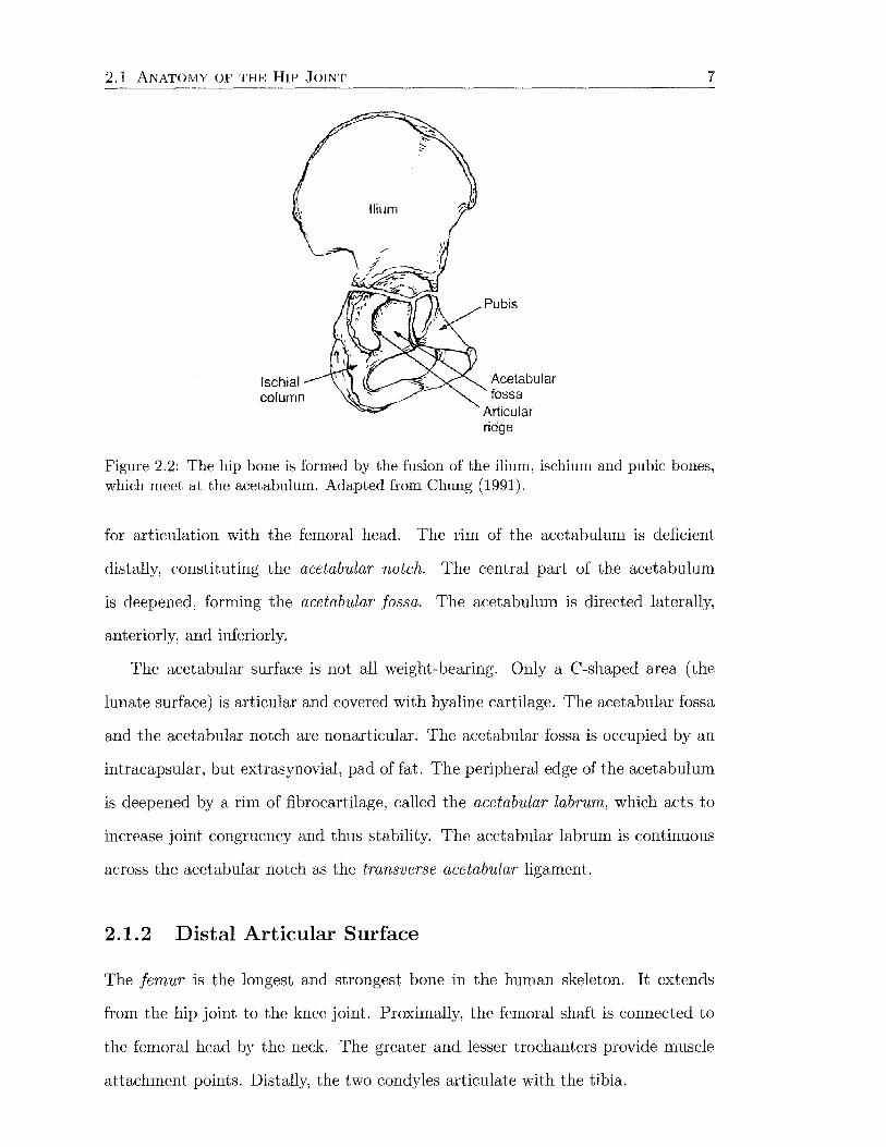
Figure 2.2: The hip bone is formed by the fusion of the ilium, ischium and pubic bones, which meet at the acetabulum. Adapted from Chung (1991).
for articulation with the femoral head. The rim of the acetabulum is deficient
distally, constituting the acetabular notch. The central part of the acetabulum
is deepened, forming the acetabular fossa. The acetabulum is directed laterally,
anteriorly, and inferiorly.
The acetabular surface is not all weight-bearing. Only a C-shaped area (the
lunate surface) is articular and covered with hyaline cartilage. The acetabular fossa
and the acetabular notch are nonarticular. The acetabular fossa is occupied by an
intracapsular, but extrasynovial, pad of fat. The peripheral edge of the acetabulum
is deepened by a rim of fibrocartilage, called the acetabular labrum, which acts to
increase joint congruency and thus stability. The acetabular labrum is continuous
across the acetabular notch as the transverse acetabular ligament.
2.1.2 Distal Articular Surface
The femur is the longest and strongest bone in the human skeleton. It extends
from the hip joint to the knee joint. Proximally, the femoral shaft is connected to
the femoral head by the neck. The greater and lesser trochanters provide muscle
attachment points. Distally, the two condyles articulate with the tibia.
2.1 ANATOMY OF THE HIP JOINT 8
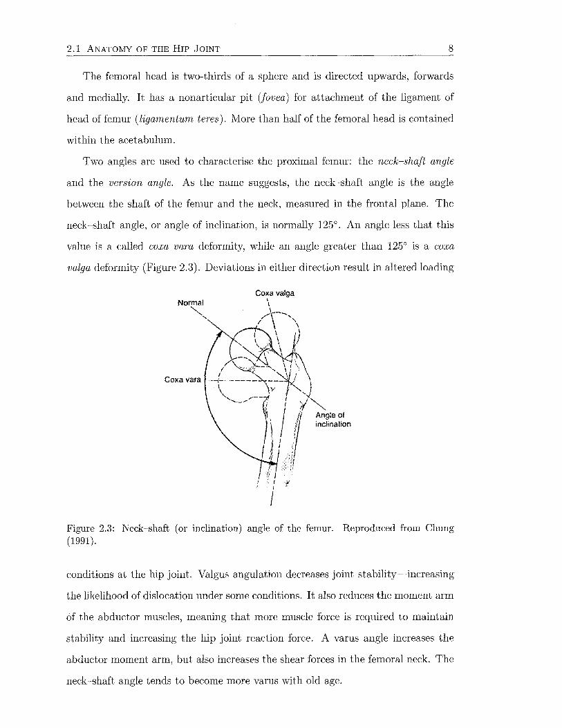
The femoral head is two-thirds of a sphere and is directed upwards, forwards
and medially. It has a nonarticular pit (fovea) for attachment of the ligament of
head of femur (ligamentum teres). More than half of the femoral head is contained
within the acetabulum.
Two angles are used to characterise the proximal femur: the neck-shaft angle
and the version angle. As the name suggests, the neck-shaft angle is the angle
between the shaft of the femur and the neck, measured in the frontal plane. The
neck-shaft angle, or angle of inclination, is normally 125°. An angle less that this
value is a called coxa vara deformity, while an angle greater than 125° is a coxa
valga deformity (Figure 2.3). Deviations in either direction result in altered loading
Normal ""'-,
'
Coxa vara
Angle of inclination
Figure 2.3: Neck-shaft (or inclination) angle of the femur. Reproduced from Chung (1991) 0
conditions at the hip joint. Valgus angulation decreases joint stability-increasing
the likelihood of dislocation under some conditions. It also reduces the moment arm
of the abductor muscles, meaning that more muscle force is required to maintain
stability and increasing the hip joint reaction force. A varus angle increases the
abductor moment arm, but also increases the shear forces in the femoral neck. The
neck-shaft angle tends to become more varus with old age.
2.1 ANATOMY OF THE HIP JOINT 9
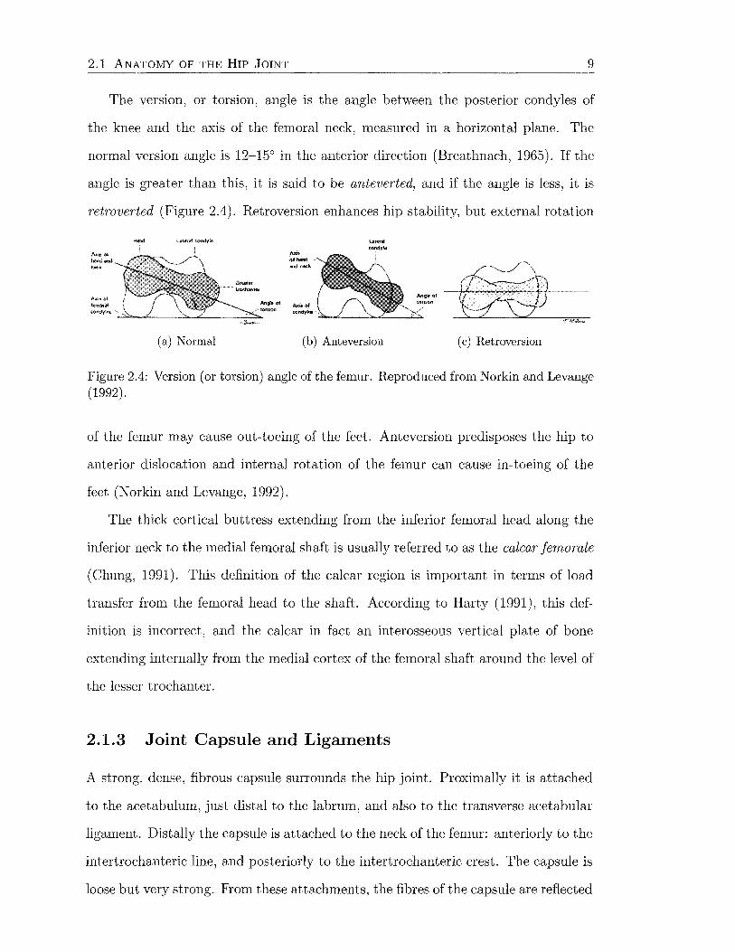
The version, or torsion, angle is the angle between the posterior condyles of
the knee and the axis of the femoral neck, measured in a horizontal plane. The
normal version angle is 12-15° in the anterior direction (Breathnach, 1965). If the
angle is greater than this, it is said to be anteverted, and if the angle is less, it is
retroverted (Figure 2.4). Retroversion enhances hip stability, but external rotation
(a) Normal
Axil: of heod lllfld ne.::k
....... -- ...,_-"-----"'-""'---..;.;::..
(b) Anteversion (c) Retroversion
Figure 2.4: Version (or torsion) angle of the femur. Reproduced from Norkin and Levange (1992).
of the femur may cause out-toeing of the feet. Anteversion predisposes the hip to
anterior dislocation and internal rotation of the femur can cause in-toeing of the
feet (Norkin and Levange, 1992).
The thick cortical buttress extending from the inferior femoral head along the
inferior neck to the medial femoral shaft is usually referred to as the calcar femorale
(Chung, 1991). This definition of the calcar region is important in terms of load
transfer from the femoral head to the shaft. According to Harty ( 1991), this def-
inition is incorrect, and the calcar in fact an interosseous vertical plate of bone
extending internally from the medial cortex of the femoral shaft around the level of
the lesser trochanter.
2.1.3 Joint Capsule and Ligaments
A strong, dense, fibrous capsule surrounds the hip joint. Proximally it is attached
to the acetabulum, just distal to the labrum, and also to the transverse acetabular
ligament. Distally the capsule is attached to the neck of the femur: anteriorly to the
intertrochanteric line, and posteriorly to the intertrochanteric crest. The capsule is
loose but very strong. From these attachments, the fibres of the capsule are reflected
2.1 ANATOMY OF THE HIP JOINT 10
back along the neck to blend with the periosteum. This reflected part forms the
retinacular fibres which bind down the nutrient arteries that supply most of the
head of the femur-primarily the anastomosis of the lateral and medial circumflex
femoral arteries.
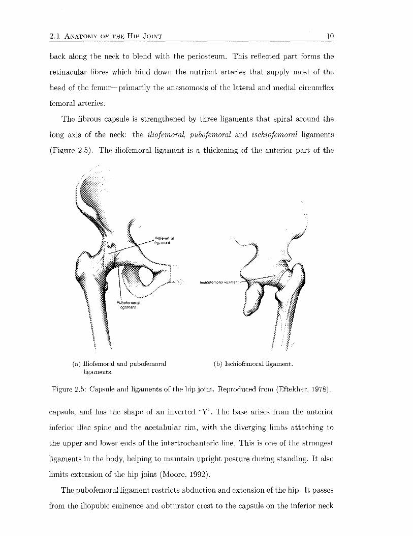
The fibrous capsule is strengthened by three ligaments that spiral around the
long axis of the neck: the iliofemoral, pubofemoral and ischiofemoral ligaments
(Figure 2.5). The iliofemoral ligament is a thickening of the anterior part of the
(a) Iliofemoral and pubofemoral ligaments.
Jschiofemomt H!';p:ment
(b) Ischiofemoral ligament.
Figure 2.5: Capsule and ligaments of the hip joint. Reproduced from (Eftekhar, 1978).
capsule, and has the shape of an inverted "Y". The base arises from the anterior
inferior iliac spine and the acetabular rim, with the diverging limbs attaching to
the upper and lower ends of the intertrochanteric line. This is one of the strongest
ligaments in the body, helping to maintain upright posture during standing. It also
limits extension of the hip joint (Moore, 1992).
The pubofemoral ligament restricts abduction and extension of the hip. It passes
from the iliopubic eminence and obturator crest to the capsule on the inferior neck

2.1 ANATOMY OF THE HIP JOINT 11
of the femur. The ischiofemoral ligament is the weakest of the three, and attaches
to the posteroinferior margin of the acetabulum, passing laterally to the capsule.
The ligament of the head of the femur (ligamentum teres) is an intracapsular
ligament that is weak and appears to contribute little to the strength of the joint. Its
wide end is attached to the acetabular notch and the tranverse acetabular ligament,
and the narrow end is attached to the pit in the femoral head.
Synovial membrane lines the entire joint cavity, with the exception of those
regions covered with articular cartilage. The synovial membrane produces synovial
fluid to lubricate the joint. Bursae are also present around the hip joint to eliminate
friction between tendons and muscles rubbing against other tendons, muscles or
bones. The iliac bursa lies over the hip joint capsule and extends proximally into the
iliac fossa beneath the iliacus muscle. Other bursae in the area are positioned under
gluteus medius and gluteus minimus at their insertions to the greater trochanter,
and three under gluteus maxim us (over the ischial tuberosity, greater trochanter
and the upper part of vast us lateralis).
2.1.4 Muscles
The muscles around the hip joint can be grouped into the thigh muscles and the
gluteal muscles. The thigh muscles may be further subdivided into three groups
(anterior, medial and posterior) based on their locations, actions and innervations.
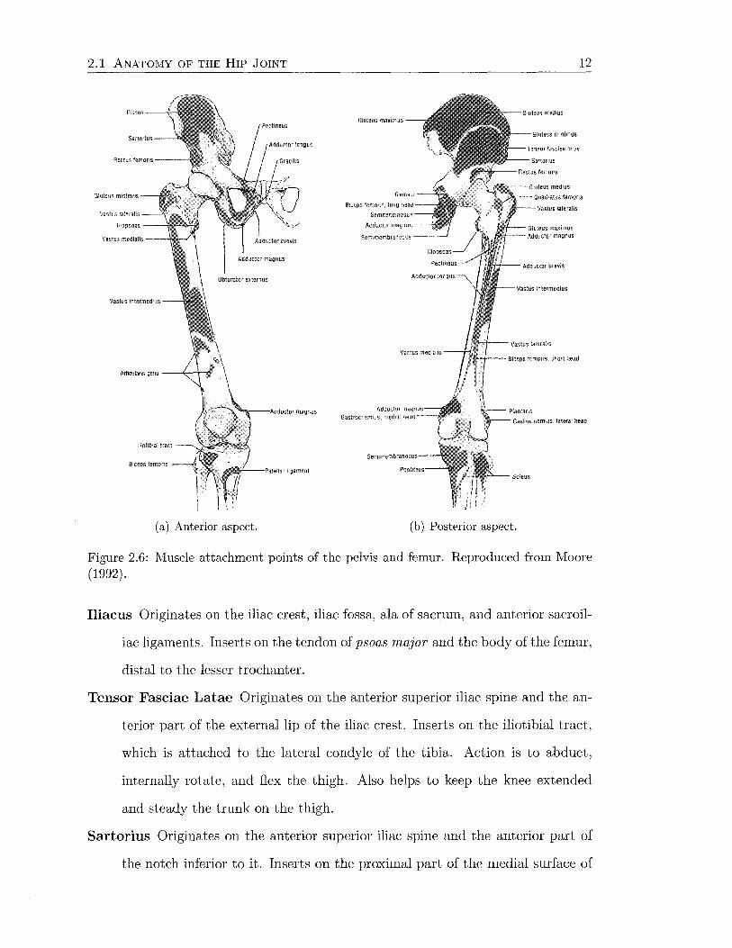
The origin and insertion points, and the actions, of the twenty four muscles crossing
the hip joint are listed according to these groups (Moore, 1992). Pelvic and femoral
attachment points are shown in Figure 2.6.
Muscles of the Anterior Thigh Region
Psoas Major Originates at the sides of the Tl2 to L5 vertebrae and intervertebral
discs between them. Inserts on the lesser trochanter. Acts conjointly with
iliacus to flex the thigh at the hip and to stabilise this joint.
2.1 ANATOMY OF THE HIP JOINT 12
G!u:eus max1nus
Gas1rncnemHJs, lateral head
(a) Anterior aspect. (b) Posterior aspect.
Figure 2.6: Muscle attachment points of the pelvis and femur. Reproduced from Moore (1992).
Iliacus Originates on the iliac crest, iliac fossa, ala of sacrum, and anterior sacroil-
iac ligaments. Inserts on the tendon of psoas major and the body of the femur,
distal to the lesser trochanter.
Tensor Fasciae Latae Originates on the anterior superior iliac spine and the an-
terior part of the external lip of the iliac crest. Inserts on the iliotibial tract,
which is attached to the lateral condyle of the tibia. Action is to abduct,
internally rotate, and flex the thigh. Also helps to keep the knee extended
and steady the trunk on the thigh.
Sartorius Originates on the anterior superior iliac spine and the anterior part of
the notch inferior to it. Inserts on the proximal part of the medial surface of
2.1 ANATOMY OF THE HIP JOINT 13
the tibia. Action is to flex, abduct and externally rotate the thigh at the hip
joint.
Rectus Femoris Originates on the anterior inferior iliac spine and the groove su
perior to the acetabulum. Inserts on the patella and via the patella ligament
to the tibial tuberosity. Action is to extend the leg at the knee joint. Also
steadies the hip joint and helps psoas major and iliacus flex the thigh.
Vastus Lateralis Originates on the greater trochanter and lateral lip of the linea
aspera. Insertion points as for rectus femoris. Action is to extend the leg at
the knee joint.
Vastus Medialis Originates on the intertrochanteric line and the medial lip of the
linea aspera. Insertion points and action as for vastus lateralis.
Vastus Intermedius Originates on the anterior and lateral surfaces of the body
of the femur. Insertion points and action as for vastus lateralis.
Muscles of the Medial Thigh Region
Pectineus Originates on the pectineal line of the pubis and inserts on the pectineal
line of the femur. Action is to adduct and flex the thigh.
Adductor Longus Originates on the body of the pubis, inferior to the pubic crest.
Inserts on the middle third of the linea asp era of the femur. Action is to adduct
the thigh.
Adductor Brevis Originates on the body and inferior ramus of the pubis and
inserts on the pectineal line and proximal part of the linea aspera of the
femur. Action is to adduct the thigh and to some extent flex it.
Adductor Magnus (adductor and hamstring parts) Originates on the infe
rior ramus of the pubis, ramus of ischium (adductor part), and ischial tuberos
ity. Inserts on the gluteal tuberosity, medial linea aspera, supracondylar line
(adductor part) and adductor tubercle of the femur (hamstring part). Ac
tion is to adduct the thigh. The adductor part also flexes the thigh, and the
hamstring part extends the thigh.

2.1 ANATOMY OF THE HIP JOINT 14
Gracilis Originates on the body and inferior ramus of the pubis, and inserts on
the proximal part of the medial surface of the tibia. Action is to adduct the
thigh, flex and help internally rotate the leg.
Obturator Externus Originates on the margins of the obturator foramen and
obturator membrane. Inserts on the trochanteric fossa of the femur. Action is
to externally rotate the thigh and steady the head of femur in the acetabulum.
Muscles of the Posterior Thigh Region
Semitendinosus Originates on the ischial tuberosity and inserts on the medial
surface of the proximal part of the tibia. Action is to extend the thigh, flex
and internally rotate the leg. When thigh and leg are flexed, it can extend
the trunk.
Semimembranosus Originates on the ischial tuberosity and inserts on the pos
terior part of the medial condyle of the tibia. Action is the same as for
semitendinosus.
Biceps Femoris Long head originates on the ischial tuberosity and short head
originates on the lateral lip of the linea aspera and lateral supracondylar line.
Inserts on the lateral side of the head of the fibula; the tendon is split at this
site by the fibular collateral ligament of the knee joint. Action is to flex the
leg and rotate it externally; extends the thigh.
Muscles of the Gluteal Region
Gluteus Maximus Originates on the external surface of the ala of the ilium, in
cluding the iliac crest, dorsal surface of the sacrum and coccyx, and the sacro
tuberous ligament. Most fibres insert in the iliotibial tract; some fibers insert
on the gluteal tuberosity on the femur. Action is to extend the thigh and
assist in its external rotation. Also steadies the thigh and assists in raising
the trunk from a flexed position.
2.2 BIOMECHANICS OF THE HIP JOINT 15
Gluteus Medius Originates on the external surface of the ilium between ante
rior and posterior gluteal lines. Inserts on the lateral surface of the greater
trochanter. Action is to abduct and internally rotate the thigh, and to steady
the pelvis.
Gluteus Minimus Originates on the external surface of the ilium between the
anterior and inferior gluteal lines. Inserts on the anterior surface of the greater
trochanter. Action as for gluteus medius.
Piriformis Originates on the anterior surface of the sacrum and the sacrotuberous
ligament. Inserts on the superior border of the greater trochanter. Action is
to externally rotate the extended thigh and abduct the flexed thigh; steadies
the femoral head in the acetabulum.
Obturator lnternus Originates on the pelvic surface of the obturator membrane
and surrounding bones. Inserts on the medial surface of the greater trochanter.
Action as for piriformis.
Gemelli (superior and inferior) The superior originates on the ischial spme,
and the inferior originates on the ischial tuberosity. Both insert on the medial
surface of the greater trochanter. Action as for piriformis.
Quadratus Femoris Originates ono the lateral border of the ischial tuberosity.
Inserts on the quadrate tubercle on the intertrochanteric crest of the femur
and inferior to it. Action is to externally rotate the thigh and steady the
femoral head in the acetabulum.
2.2 Biomechanics of the Hip Joint
The hip joint is a three degree-of-freedom joint which allows flexion-extension in
the sagittal plane, abduction-adduction in the frontal plane, and internal-external
rotation along the long axis of the femur. The biomechanics of the hip are governed
by the geometry of the joint and the functions of the soft tissues (ligaments and
muscles) surrounding the joint.

2.2 BIOMECHANICS OF THE HIP JOINT 16
The hip is the most mobile joint of the lower limb, enabling correct positioning
of the foot (Table 2.1). A high degree of stability is needed due to significant weight
bearing requirements. The relatively large range of movement results largely from
the femur having a neck that is much narrower in diameter than the equatorial
diameter of the head.
Table 2.1: Range of motion at the hip joint. Reproduced from Norkin and Levange (1992).
Motion Range Comment
Flexion goo with knee extended 120-135° with knee flexed
Extension 10-30° may be reduced by knee flexion Abduction 30-50° Adduction 10-30° Internal Rotation 45-60° measured with knee flexed goo External Rotation 30-45° measured with knee flexed goo
Stability at the hip joint is produced both actively and passively. Passive sta
bility is provided by ligament tension, while active stability is provided by muscle
contraction during activity. The highly conforming articular surfaces also add to
stability. Active stability is generally provided by short muscles located close to the
axis of movement of the hip.
2.2.1 Stance
Bilateral
In erect bilateral, or two-legged, stance, the centre of gravity (COG) is located
around the height of the second lumbar segment-relatively distant from the fairly
small support base provided by the feet-making the body position unstable. De-
spite this, little energy is required to maintain the static erect posture in the form
of muscle contraction since ligaments, bones and joints are able to provide the
forces necessary to overcome the effects of gravity (passive stability). The constant
displacement and correction of the position of the COG within the support base
is called postural sway and the erect stance is maintained through motor control.

2.2 BIOMECHANICS OF THE HIP JOINT 17
Small bursts of muscle activity, particularly in the legs, can be observed in response
to perturbations in the COG position. In bilateral posture each hip joint carries
approximately one-third of the total body weight (Norkin and Levange, 1992).
Under ideal circumstances the line of gravity (LOG), the vertical line between the
COG and the ground, would pass through all joint axes in the lateral view however
this is difficult to achieve because of normal body structures. During relaxed stance,
the ankle joint is in the neutral position and the knee is in full extension. The LOG
passes slightly anterior to the lateral malleolus at the ankle and just anterior to the
midline of the knee (Figure 2.7a). With the hip also in the neutral position, and no
(a) Location of the line of gravity (LOG) in bilateral stance.
(b) Lower limb moments due to the location of the LOG in bilateral stance.
(c) Location of the LOG (vertical line) in unilateral stance.
Figure 2.7: Location of the line of gravity. Reproduced from Norkin and Levange (1992).
deviation in pelvic tilt, the LOG passes slightly posterior to the hip joint axis. The
position of the LOG at the ankle causes a dorsiflexion moment which is corrected
by the soleus muscle (Figure 2. 7b). The extension moment at the knee is opposed
by the posterior joint capsule and associated ligaments-some low level hamstring
activity has also been identified. The extension moment at the hip is opposed by
the iliofemoral ligament and psoas major.
2.2 BIOMECHANICS OF THE HIP JOINT 18
In the frontal plane, the LOG is equidistant from the hip, knee and ankle joints
on each side of the body. Little muscle activity is required to maintain medial
lateral stability since gravitational forces are balanced on each side of the body.
Any postural sway that occurs during normal bilateral stance changes the position
of the LOG relative to the joint axes and consequently, the level of muscle activity
required to maintain that stance.
Unilateral
In unilateral, or single-leg stance, the base of support is much smaller than for
bilateral stance, and hence the position of the centre of gravity is more unstable
(greater postural sway). Consequently, the line of gravity tends to move further
with respect to each of the joints. This results in greater muscle recruitment in
both the frontal and sagittal planes to maintain erect posture. The optimal LOG
in the lateral view remains in the same position as for double stance, however in
the anterior-posterior view, the LOG must pass through the base of support and
in so doing passes closer to the joint axes of the supporting limb (Figure 2. 7 c).
Unilateral stance produces a moment about the supporting hip joint which must
be balanced by abductor muscle forces. The magnitude of the moment depends
on the position of the spine, the position of the nonweight-bearing leg and upper
extremities, and most importantly, the inclination of the pelvis. If the trunk is
tilted over the hip joint, the gravitational moment is minimised by reducing the
distance between the hip joint and the COG. The hip joint supports about five
sixths of the total body weight in unilateral stance, however the additional hip
joint compression caused by abductor muscle action increases the joint load further
(Norkin and Levange, 1992).
2.2.2 Gait
Human locomotion is a translatory progression of the body as a whole, produced by
coordinated movements of the body segments. Normal gait is rhythmic and charac-
2.2 BIOMECHANICS OF THE HIP JOINT 19
terised by alternating propulsive and retropulsive motions of the lower extremities
(Norkin and Levange, 1992). The gait cycle consists of the actions that take place
between initial contact of the reference extremity with the ground and the successive
contact of that extremity. Each limb passes through a stance phase and a swing
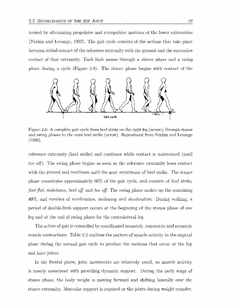
phase during a cycle (Figure 2.8). The stance phase begins with contact of the
Figure 2.8: A complete gait cycle from heel strike on the right leg (arrow), through stance and swing phases to the next heel strike (arrow). Reproduced from Norkin and Levange (1992).
reference extremity (heel strike) and continues while contact is maintained (until
toe off). The swing phase begins as soon as the reference extremity loses contact
with the ground and continues until the next occurrence of heel strike. The stance
phase constitutes approximately 60% of the gait cycle, and consists of heel strike,
foot fiat, midstance, heel off and toe off. The swing phase makes up the remaining
40%, and consists of acceleration, midswing and deceleration. During walking, a
period of double-limb support occurs at the beginning of the stance phase of one
leg and at the end of swing phase for the contralateral leg.
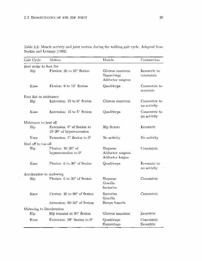
The action of gait is controlled by coordinated isometric, concentric and eccentric
muscle contractions. Table 2.2 outlines the pattern of muscle activity in the sagittal
plane during the normal gait cycle to produce the motions that occur at the hip
and knee joints.
In the frontal plane, joint movements are relatively small, so muscle activity
is mostly associated with providing dynamic support. During the early stage of
stance phase, the body weight is moving forward and shifting laterally over the
stance extremity. Muscular support is required at the joints during weight transfer.
2.2 BIOMECHANICS OF THE HIP JOINT 20
Table 2.2: Muscle activity and joint motion during the walking gait cycle. Adapted from Norkin and Levange (1992)
Gait Cycle Motion
Heel strike to foot fiat Hip Flexion: 30 to 25° flexion
Knee Flexion: 0 to 15° flexion
Foot fiat to midstance Hip Extension: 25 to 0° flexion
Knee Extension: 15 to 5° flexion
Midstance to heel off Hip Extension: 0° of flexion to
10-20° of hyperextension
Knee Extension: 5° flexion to 0°
Heel off to toe off Hip Flexion: 10-20° of
hyperextension to 0°
Knee Flexion: 0 to 30° of flexion
Acceleration to midswing Hip Flexion: 0 to 30° of flexion
Knee Flexion: 30 to 60° of flexion
Extension: 60-30° of flexion
Midswing to Deceleration Hip Hip remains at 30° flexion
Knee Extension: 30° flexion to oo
Muscle
Gluteus maximus Hamstrings Adductor magnus
Quadriceps
Gluteus maximus
Quadriceps
Hip flexors
No activity
Iliopsoas Adductor magnus Adductor longus
Quadriceps
Iliopsoas Gracilis Sartorius
Sartorius Gracilis Biceps femoris
Gluteus maximus
Quadriceps Hamstrings
Contraction
Isometric to concentric
Concentric to eccentric
Concentric to no activity
Concentric to no activity
Eccentric
No activity
Concentric
Eccentric to no activity
Concentric
Concentric
Eccentric
Concentric Eccentric
2. 2 BIOMECHANICS OF THE HIP JOINT 21
The pelvis at the hip is stabilised by gluteus minimus, gluteus medius and tensor
fasciae latae, with gluteus medius resisting lateral dropping of the pelvis to the
contralateral side. The transfer of weight to the supporting limb creates a valgus
thrust at the knee, which is counteracted by vastus medialis, semitendinosis and
gracilis.
In the middle of stance phase, the requirements for medial-lateral stability at
the knee are reduced, however the tensor fasciae latae continues to provide stability
to the pelvis until toe off. Activity of the gluteus medius muscle decreases during
midstance. Adductor magnus and adductor longus begin acting towards toe off,
and work eccentrically during the acceleration part of swing phase to restrain the
lateral weight shift to the opposite extremity (Norkin and Levange, 1992).
2.2.3 Stair Climbing
Climbing stairs is a commonly performed task during normal activities of daily
living. Although similarities exist between level walking gait and stair climbing,
the significant differences are the greater ranges of joint motion, particularly hip
and knee flexion, and larger muscle forces involved. Bergmann et al. (2001) found
torque on the hip joint to be 23% greater during stair climbing than normal gait,
which certainly has strong implications for the stability of hip replacement implants.
Stair gait, like level walking gait, has both swing and stance phases. The stance
phase can be divided into weight acceptance, pull up and forward continuance.
The swing phase is subdivided into foot clearance and foot placement (Norkin and
Levange, 1992). Weight acceptance is comparable to the heel strike to foot flat
phases of walking gait. The pull up portion is a period of single-limb support. The
initial part of pull up is a time of instability at the joints, since all of the body
weight is shifted onto the supporting extremity when the hip, knee and ankle are
flexed. Most of the work during pull up is achieved by the knee extensors, rectus
femoris and vastus lateralis. The foot clearance period corresponds roughly to the
midstance to toe off phases of walking gait.
2.2 BIOMECHANICS OF THE HIP JOINT 22
2.2.4 Joint and Muscle Forces
Both external and internal forces act on the hip. External forces are gravity, inertia,
and the ground reaction force. Internal forces are mainly created by the muscles.
Ligaments, tendons, joint capsule and bones work to resist, transmit, and absorb
forces.
The hip joint reaction force can be roughly estimated by the partial body weight
supported above. Joint compression due to muscle forces should also be taken into
account. Pauwels (1980) (originally published in 1965) used a graphical method to
estimate the joint reaction force during single-legged stance from anterior-posterior
view radiographs. Equilibrium of the pelvis was described in terms of balanced
moments due to the hip joint force and the abductor muscle force (Figure 2.9).
Moment arms and force directions were measured directly from the radiographs.
This method was also applied to the equivalent body position during slow gait. An
approach such as this should be limited to static or quasi-static analyses. Other
investigators have developed similar mathematical models (e.g., Bergmann et al.,
1997; Genda et al., 2001). During activity, inertia and muscle forces dramatically
alter the mechanical situation, and more robust methods are required.
In vivo hip joint reaction forces may be estimated more accurately using either
inverse dynamics or instrumented hip prostheses (Table 2.3). The modern inverse
dynamics approach uses three-dimensional video motion capture systems to measure
joint kinematics. Local coordinate systems are defined for each body segment by
three noncollinear markers. An array of video cameras determines the location of
each marker in global space, thus giving the orientation of each local coordinate
systems in global space. Relative movements between local systems are computed
using Euler/Cardan angles, assuming rigid body mechanics. The ground reaction
force is measured by an in-floor force plate and then used as an input, along with the
kinematic data, in a anthropometric model to determine the moments and forces
from the distal to proximal joints of the lower limb (hence inverse kinematics).
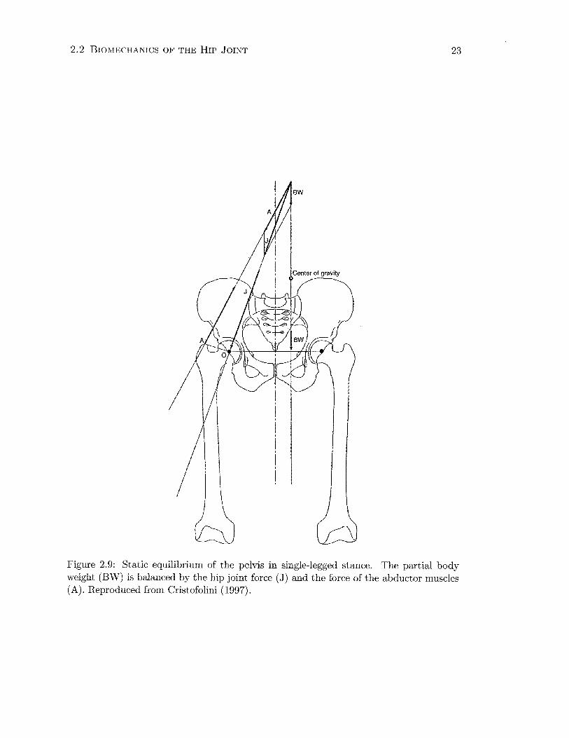
2.2 BIOMECHANICS OF THE HIP JOINT 23
Figure 2.9: Static equilibrium of the pelvis in single-legged stance. The partial body weight (BW) is balanced by the hip joint force ( J) and the force of the abductor muscles (A). Reproduced from Cristofolini (1997).
2.2 BIOMECHANICS OF THE HIP JOINT 24
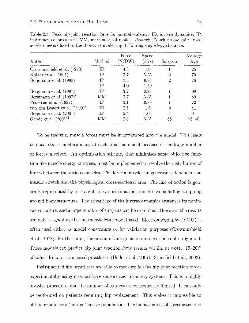
Table 2.3: Peak hip joint reaction force for normal walking. ID, inverse dynamics; IP, instrumented prosthesis; MM, mathematical model. Remarks. *during slow gait; tused accelerometers fixed to the thorax as model input; +during single-legged stance.
Force Speed Average Authur Method (N/BW) (m/s) Subjects Age
Crowninshield et al. (1978) ID 4.3 1.0 1 25 Kotzar et al. (1991) IP 2.7 N/A 2 70 Bergmann et al. ( 1993) IP 3.5 0.83 2 76
IP 4.0 1.39 Bergmann et al. (1997) IP 3.2 0.83 1 89 Bergmann et al. (1997)* lVIM 2.7 N/A 1 89 Pedersen et al. ( 1997) IP 3.1 0.89 1 72 van den Bogert et al. (1999)t ID 2.5 1.5 9 41 Bergmann et al. (2001) IP 2.4 1.09 4 61 Genda et al. (2001)+ MM 2.3 N/A 56 25-6.5
To be realistic, muscle forces must be incorporated into the model. This leads
to quasi-static indeterminacy at each time increment because of the large number
of forces involved. An optimisation scheme, that minimises some objective func-
tion like muscle energy or stress, must be implemented to resolve the distribution of
forces between the various muscles. The force a muscle can generate is dependent on
muscle stretch and the physiological cross-sectional area. The line of action is gen-
erally represented by a straight line approximation, sometimes including wrapping
around bony structures. The advantage of the inverse dynamics system is its nonin-
vasive nature, and a large number of subjects can be examined. However, the results
are only as good as the musculoskeletal model used. Electromyography (EMG) is
often used either as model constraints or for validation purposes ( Crowninshield
et al., 1978). Furthermore, the action of antagonistic muscles is also often ignored.
These models can predict hip joint reaction force results within, at worst, 15-20%
of values from instrumented prostheses (Heller et al., 2001b; Stansfield et al., 2003).
Instrumented hip prostheses are able to measure in vivo hip joint reaction forces
experimentally using internal force sensors and telemetry systems. This is a highly
invasive procedure, and the number of subjects is consequently limited. It can only
be performed on patients requiring hip replacement. This makes it impossible to
obtain results for a "normal" active population. The biomechanics of a reconstructed
2.2 BIOMECHANICS OF THE HIP JOINT 25
hip joint may also differ from a normal hip. This method allows data to be obtained
outside the laboratory environment, and therefore over a wide range of activities.
The large loads on the femoral head have a fairly constant direction regardless
of activity (Bergmann et al., 2001; Kotzar et al., 1991). Large loads are directed
downwards, laterally and posteriorly. Since muscle contractions produce many of
the loads experienced by the femur, it is not surprising that much of the loading is
in line with the femur, as this is the line of action of many of the larger muscles. In
contrast, the direction of loading in the acetabulum varies considerably (Pedersen
et al., 1997). Peak values of hip joint reaction force occur just after heel strike (first
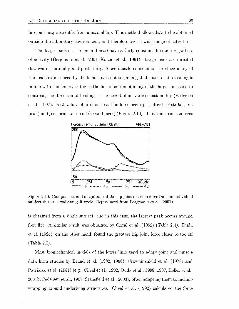
peak) and just prior to toe off (second peak) (Figure 2.10). This joint reaction force
Forces. Femur System [%BW} 250
-50 0 25
F-
PFL\AIN1
%Cycle
Figure 2.10: Components and magnitude of the hip joint reaction force from an individual subject during a walking gait cycle. Reproduced from Bergmann et al. (2001).
is obtained from a single subject, and in this case, the largest peak occurs around
foot flat. A similar result was obtained by Cheal et al. (1992) (Table 2.4). Duda
et al. (1998), on the other hand, found the greatest hip joint force closer to toe off
(Table 2.5).
Most biomechanical models of the lower limb tend to adopt joint and muscle
data from studies by Brand et al. (1982, 1986), Crowninshield et al. (1978) and
Patriarca et al. (1981) (e.g., Cheal et al., 1992; Duda et al., 1998, 1997; Heller et al.,
2001b; Pedersen et al., 1997; Stansfield et al., 2003), often adapting them to include
wrapping around underlying structures. Cheal et al. (1992) calculated the force

2.2 BIOMECHANICS OF THE HIP JOINT 26
components and magnitudes of muscles and the hip joint contact, for three stages
of the stance phase of gait (Table 2.4).
Table 2.4: Joint and muscle force magnitudes ( x BW) of the proximal femur for three phases of gait according to Cheal et al. (1992).
Force Heel Strike Midstance Toe Off
Adductor longus 0.20 0.30 Adductor magnus 0.20 0.30 Gluteus maximus (ant.) 1.28 Gluteus medius 0.72 0.80 1.18 Gluteus minimus 0.54 0.30 0.61 Iliopsoas 1.30 2.60 Piriformis 0.20 Vastus intermedius 0.40 Vastus lateralis 0.40 Vastus medialis 0.33 Joint contact 4.64 3.51 4.33
Duda et al. (1998) incorporated the small rotators of the hip, the short head
of biceps femoris and the ilioibial tract into their model (Table 2.5). The iliotibial
tract was modelled by tensor fasciae latae and a part of gluteus maximus, with
a pseudo-insertion point on the greater trochanter. The magnitudes of each force
are provided for three phases of the gait cycle. These are absolute values of force,
not scaled by body weight. Ten percent of the gait cycle corresponds to the the
instant of maximum abductor and adductor activity, 30% is the first peak in the
ground reaction force and 45% is the second peak, where the axial component of
the hip joint force reaches its maximum. Body weight in this case is 70 kg, which
corresponds to a joint reaction force of 3.19 BW at 45% of the gait cycle. This data
was also used in a study by Stolk et al. (2001).
Even with all of the biomechanical analysis tools available, the actions of some
muscles and soft tissues are not fully understood. The function of the iliotibial tract
is probably the best example of this, with little consensus in the literature. The
tensor fasciae latae muscle and about three-quarters of the fibres of gluteus max
imus insert into the iliotibial tract, which in turn attaches to the lateral condyle
of the tibia. The iliotibial tract is also attached to the linea aspera via the lateral
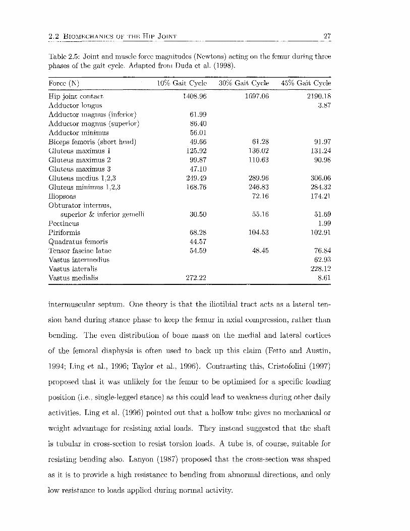
2.2 BIOMECHANICS OF THE HIP JOINT 27
Table 2.5: Joint and muscle force magnitudes (Newtons) acting on the femur during three phases of the gait cycle. Adapted from Duda et al. (1998).
Force (N) 10% Gait Cycle 30% Gait Cycle 45% Gait Cycle
Hip joint contact 1408.96 1697.06 2190.18 Adductor longus 3.87 Adductor magnus (inferior) 61.99 Adductor magnus (superior) 86.40 Adductor minimus 56.01 Biceps femoris (short head) 49.66 61.28 91.97 Gluteus maximus 1 125.92 136.02 131.24 Gluteus maximus 2 99.87 110.63 90.98 Gluteus maximus 3 47.10 Gluteus medius 1,2,3 249.49 289.96 306.06 Gluteus minimus 1,2,3 168.76 246.83 284.32 Iliopsoas 72.16 174.21 Obturator internus,
superior & inferior gemelli 30.50 55.16 51.69 Pectineus 1.99 Piriformis 68.28 104.53 102.91 Quadratus femoris 44.57 Tensor fasciae latae 54.59 48.45 76.84 Vastus intermedius 62.93 Vastus lateralis 228.12 Vastus medialis 272.22 8.61
intermuscular septum. One theory is that the iliotibial tract acts as a lateral ten-
sion band during stance phase to keep the femur in axial compression, rather than
bending. The even distribution of bone mass on the medial and lateral cortices
of the femoral diaphysis is often used to back up this claim (Fetto and Austin,
1994; Ling et al., 1996; Taylor et al., 1996). Contrasting this, Cristofolini (1997)
proposed that it was unlikely for the femur to be optimised for a specific loading
position (i.e., single-legged stance) as this could lead to weakness during other daily
activities. Ling et al. (1996) pointed out that a hollow tube gives no mechanical or
weight advantage for resisting axial loads. They instead suggested that the shaft
is tubular in cross-section to resist torsion loads. A tube is, of course, suitable for
resisting bending also. Lanyon (1987) proposed that the cross-section was shaped
as it is to provide a high resistance to bending from abnormal directions, and only
low resistance to loads applied during normal activity.
2.2 BIOMECHANICS OF THE HIP JOINT 28
Pauwels (1980), who considered the lower extremity in single-legged stance first
as a column, and then introduced joints, musculature, and ligaments one after the
other, proposed that a lateral tension band was needed to reduce large bending
moments in the femur. Under this condition, bending stresses in the femur were
predicted to decrease from proximal to distal, while axial stresses were constant
along the femoral shaft. Ling et al. (1996) likened this tension band effect to the
windward shrouds on a yachts rigging, which keep the mast in tension despite the
bending moment due to the wind on the sails and the righting moment of the keel.
Duda et al. (1997) indicated that at the proximal and distal ends of the femur,
the axial and shear forces showed their highest values. Internal loads were reduced
towards the diaphyseal part, which was mainly under axial compression, with shear
forces close to zero. This studies suggest that the lateral musculature probably does
contribute to the reduction of bending moments in the femur.
Because of these uncertainties, it will not be possible to produce an adequate
representation of the muscles until their forces and actions are reliably established.
Consequently, simplifications are inevitable when modelling the musculoskeletal sys
tem.
Chapter 3
Hip Arthroplasty
3.1 Indications
Total hip arthroplasty is a surgical procedure involving replacement of the bearing
surfaces of the hip with prosthetic devices. An intramedullary stem articulates with
an acetabular cup, via a ball and socket joint. The components may both be fixed in
place using a polymethylmethacrylate grouting agent (cemented), or by biological
fixation relying on direct bone ingrowth/ ongrowth to the material ( uncemented).
Hybrid fixation describes the situation where one component is cemented and the
other is uncemented. The fixation method, particularly when concerned with the
femoral component, strongly influences the transfer of load from the implant to
bone.
Total hip arthroplasty is generally indicated for end-stage arthritic involvement
of the hip in a patient with pain severe enough to cause disability and require med
ication, and is usually associated with loss of joint mobility. The most common ap
plication of total hip replacement is in primary or secondary osteoarthritis, caused
by trauma, congenital dysplasia, or other conditions. Other indications include
osteonecrosis, rheumatoid arthritis, gouty arthroplasty, calcium pyrophosphate de
position, ochronosis, displaced fractures of the femoral neck in elderly individuals,
primary and secondary tumours, and metabolic conditions such as Paget's disease.
29
3.2 EVOLUTION OF TOTAL HIP ARTHROPLASTY 30
Patient factors such as age, physical status, general medical condition, level of pain
and disability, response to conservative therapy, and desired lifestyle must be consid
ered before total hip arthroplasty is proposed (Eftekhar, 1978; Stulberg and Hupfer,
1991).
3.2 Evolution of Total Hip Arthroplasty
Early surgical efforts at alleviating pain from degenerate hip joints involved resection
or osteotomy of the proximal femur. No attempt was made to reform articular
surfaces, and ankylosis of the joint often resulted (McElfresh, 1991).
Interpositional arthroplasty was a procedure developed to restore motion to
ankylosed hip joints in the mid 1800s. The joint was separated, articular surfaces
were refashioned, and an interpositioning substance was placed to prevent subse
quent refusion (Fielding and Stillwell, 1987). Materials such as muscle, fibrous
tissue, celluloid, silver plates, rubber sheets, magnesium, zinc and decalcified bone
were used for interpositioning (Eftekhar, 1978).
In Boston, Smith-Peterson developed the "mould arthroplasty". From 1923, he
employed glass, Bakelite and Pyrex cups. Failure of the cups was a problem until
he experimented with Vitallium, a cobalt-chromium alloy, as an interpositioning
material (McElfresh, 1991). Vitallium was adopted following experimentation by
Venable and Stuck in Texas (Venable et al., 1937). The design was modified by
Otto Aufranc, an assistant to Smith-Peterson, and mould arthroplasty became a
successful procedure. From this concept came hip-socket, or cup arthroplasty, in
which a reshaped femoral head articulated with a polished metal cup fixed in the
acetabulum. This procedure never became popular (Fielding and Stillwell, 1987).
The search for dependable and effective techniques continued. Prosthetic fe
moral head replacement was attempted by Delbet in 1919, who used reinforced
rubber, and by Groves who fashion a hemispherical short stem device from ivory
in 1927. Neither was particularly successful (Fielding and Stillwell, 1987). In 1940,

3.2 EVOLUTION OF TOTAL HIP ARTHROPLASTY 31
Moore and Bohlman implanted a specially made Vitallium prosthesis to replace
the proximal femur. This is the first known metallic replacement hemiarthroplasty
(Eftekhar, 1978). Femoral head replacement, similar to Grove's design, was further
refined by the Judet brothers in 1950 using acrylic material (Figure 3.2A), by and
others. During the 1950s, short stem prostheses were replaced by intramedullary
long stem designs which gave greater stability. The devices proposed by Thompson
in 1950 and Moore in 1952 were the basis for many future designs (Figure 3.2B and
C).
Because of the bipolar nature of joint disease, most devices replacing only one
side of the joint were not successful. Wiles is credited with the first total hip arthro-
plasty (THA) in 1938 (Figure 3.1. This consisted of a ball and cup device fabricated
Figure 3.1: The first total hip arthroplasty is attributed to Phillip Wiles, 1938. Reproduced from Fielding and Stillwell (1987).
from stainless steel. A hemispherical ball was fixed by a bolt through the femoral
neck, and the cup was fixed by screws through a buttressed plate. No other work
with total hip replacement devices was reported until the 1950s. Surgeons tried to
articulate a Thompson or Moore stem with a large Smith-Peterson cup, but found
wear to be a problem. Subsequently IvicKee and Farrar designed a metal cup to
fit over a Thompson prosthesis in 1951, while in 1966, Ring developed a metal
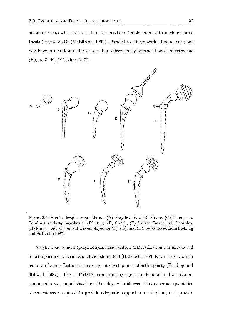
3.2 EVOLUTION OF TOTAL HIP ARTHROPLASTY 32
acetabular cup which screwed into the pelvis and articulated with a Moore pros-
thesis (Figure 3.2D) (McElfresh, 1991). Parallel to Ring's work, Russian surgeons
developed a metal-on-metal system, but subsequently interpositioned polyethylene
(Figure 3.2E) (Eftekhar, 1978).
A a
c
F H
Figure 3.2: Hemiarthroplasty prostheses: (A) Acrylic Judet, (B) Moore, (C) Thompson. Total arthroplasty prostheses: (D) Ring, (E) Sivash, (F) McKee--Farrar, (G) Charnley, (H) Muller. Acrylic cement was employed for (F), (G), and (H). Reproduced from Fielding and Stillwell (1987).
Acrylic bone cement (polymethylmethacrylate, PMMA) fixation was introduced
to orthopaedics by Kiaer and Haboush in 1950 (Haboush, 1953; Kiaer, 1951), which
had a profound effect on the subsequent development of arthroplasty (Fielding and
Stillwell, 1987). Use of PMMA as a grouting agent for femoral and acetabular
components was popularised by Charnley, who showed that generous quantities
of cement were required to provide adequate support to an implant, and provide
3.2 EVOLUTION OF TOTAL HIP ARTHROPLASTY 33
uniform load transfer to the femur. McKee and Farrar redesigned their total hip sys
tem to incorporate cement, with increased success (Figure 3.2F) (Eftekhar, 1978).
The connection between the cement and the bone and between the cement and the
implant is mechanical, without any form of chemical bonding (Kiihn, 2000).
Charnley, who is considered the father of modern hip arthroplasty, also con
cerned himself with wear and lubrication at the joint interface. He initially inves
tigated using thin Teflon® (PTFE) shells on the femoral and acetabular sides to
reduce friction. Failure prompted the use of a small prosthetic head articulating
with a thick Teflon® socket. The small femoral head decreases frictional shear
forces at the bearing interface, theoretically improving socket fixation as well. Ad
verse tissue reaction and wear of the Teflon® led to the adoption of ultra-high
molecular weight polyethylene. The resulting total hip arthroplasty, termed "low
friction arthroplasty", with a cemented intramedullary femoral prosthesis having a
22 mm femoral head, bearing on a low friction polyethylene cup (Figure 3.2G), was
the inspiration for most future developments (Fielding and Stillwell, 1987). Charn
ley also showed the importance of concentrating on the details of surgical technique,
including infection control (Eftekhar, 1978).
Miiller followed Charnley and developed a system with variable neck sizes and
a 32 mm head diameter for greater stability (Figure 3.2H). Other cemented designs
were developed by Ling, Aufranc and Turner, Amstutz, Harris, and others (Fielding
and Stillwell, 1987).
During the first decades with cemented THA, high infection rates were a signifi
cant problem. Improved technique and use of systemic and local antibiotics helped
to reduce this problem. Aseptic loosening became the next major problem. This was
associated with the widening of indications for hip arthroplasty in the 1970s, with
procedures in young and active patients proving less satisfactory. Problems with
osteolysis and bone resorption, caused by "cement disease" (Jones and Hungerford,
1987), led to interest in uncemented implant fixation (Nivbrant, 1999).

3.3 BIOMATERIALS 34
The AML, Harris-Galante and PCA were early porous coated designs that were
widely adopted. Titanium was investigated as a prosthesis material, as bone was
found to grow directly onto its surfaces with certain roughness. Most uncemented
implants were released onto the market without undergoing clinical trials, and there
fore results were often worse than the cemented devices whose problems the implants
were designed to address. Success with cemented femoral stems has been improved
by better cementing techniques, however cemented acetabular components are still
a concern, leading to use of hybrid fixation, with cemented stems and uncemented
cups (Nivbrant, 1999). Aseptic loosening of components still proves to be the most
common cause of revision surgery today (Malchau et al., 2002).
3.3 Biomaterials
Selection of a material for an in vwo application in the body will depend on it
having the appropriate physical properties to perform the task, the ability to be
manufactured and sterilised easily, and biocompatibility.
3.3.1 Metals
The three common alloys used in orthopaedics are stainless steel, cobalt-chromium
alloy and titanium alloy. None of these materials was developed specifically for
biomedical applications, however their strength and corrosion resistance have led to
their use (Wright and Li, 2000).
Stainless Steels
The most frequently used form of stainless steel is 316L (ASTM F138), which is a
low carbon concentration, austenitic stainless steel (Park and Kim, 2000). 316L steel
is an alloy of iron and carbon, also containing chromium, nickel and molybdenum,
with small amounts of manganese, phosphorous, sulphur and silicon (Figure 3.3).
Stainless steel devices are passivated by immersion in a nitric acid bath to create

3.3 BIOMATERIALS
M<>(2·4%)
l(c§§:::::::::!j c {0-03%) ·-Mn,P. S.Sl.H.II"<.totall
Stainless Steel (3!6l)
Titanium {Ti • 6AI· 4V)
Cobalt Alloy (F151
35
Figure 3.3: Composition of some common orthopaedic biomaterials. Reproduced from Wright and Li (2000).
a chromium oxide (Cr20 3 ) layer on the surface. The low carbon concentration in
316L stainless helps maintain corrosion resistance by stopping formation of brittle
carbides. The carbides significantly weaken the material by making it susceptible
to corrosion-related fracture. Stainless steel is generally cold-worked by about 30%
for orthopaedic applications (Table 3.1), however it is prone to crevice and stress
corrosion, and is usually used for relatively short-term load bearing applications
(Wright and Li, 2000).
Cobalt-Chromium Alloys
Cobalt-chrome alloys are available in cast (ASTM F75), forged (ASTM F799) and
cold worked (ASTM F90, F562) compositions. These alloys are all primarily cobalt,
with significant amounts of chromium for corrosion resistance. The F75 and F799
alloys contain about 60% cobalt and 28% chromium (Figure 3.3), while the F90 and
F562 alloys have less cobalt and chromium, but large quantities of tungsten and
nickel. F75 alloy components are usually manufactured using investment casting,
or hot isostatic pressing (HIP) to improve the microstructure. F75 is often used
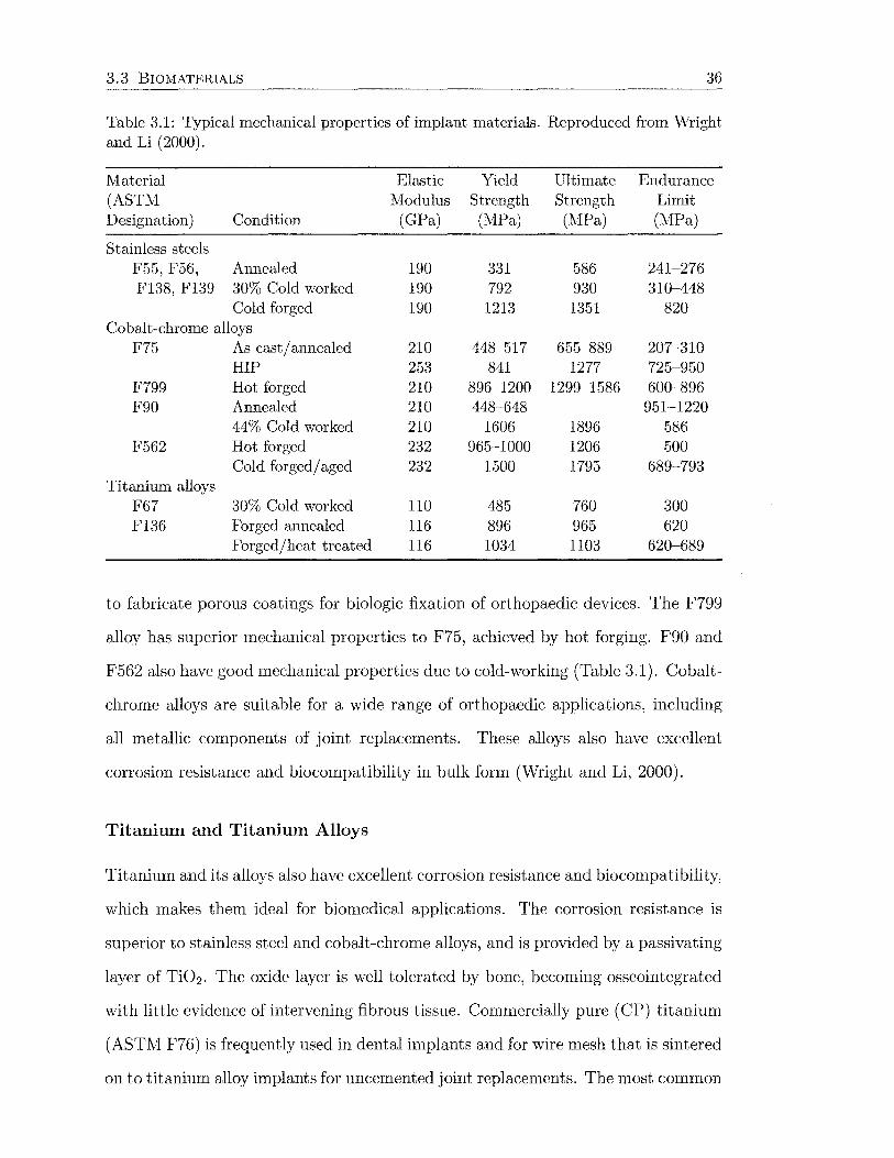
3.3 BIOMATERIALS 36
Table 3.1: Typical mechanical properties of implant materials. Reproduced from Wright and Li (2000).
I\1aterial Elastic Yield Ultimate Endurance (ASTM Modulus Strength Strength Limit Designation) Condition (GPa) (MPa) (l\1Pa) (MPa)
Stainless steels F55, F56, Annealed 190 331 586 241-276 F138, F139 30% Cold worked 190 792 930 310-448
Cold forged 190 1213 1351 820 Cobalt-chrome alloys
F75 As cast/ annealed 210 448-517 655-889 207-310 HIP 253 841 1277 725-950
F799 Hot forged 210 896-1200 1299-1586 600-896 F90 Annealed 210 448-648 951-1220
44% Cold worked 210 1606 1896 586 F562 Hot forged 232 965-1000 1206 500
Cold forged/aged 232 1500 1795 689-793 Titanium alloys
F67 30% Cold worked 110 485 760 300 F136 Forged annealed 116 896 965 620
Forged/heat treated 116 1034 1103 620-689
to fabricate porous coatings for biologic fixation of orthopaedic devices. The F799
alloy has superior mechanical properties to F75, achieved by hot forging. F90 and
F562 also have good mechanical properties due to cold-working (Table 3.1). Cobalt
chrome alloys are suitable for a wide range of orthopaedic applications, including
all metallic components of joint replacements. These alloys also have excellent
corrosion resistance and biocompatibility in bulk form (Wright and Li, 2000).
Titanium and Titanium Alloys
Titanium and its alloys also have excellent corrosion resistance and biocompatibility,
which makes them ideal for biomedical applications. The corrosion resistance is
superior to stainless steel and cobalt-chrome alloys, and is provided by a passivating
layer of Ti02 . The oxide layer is well tolerated by bone, becoming osseointegrated
with little evidence of intervening fibrous tissue. Commercially pure (CP) titanium
(ASTM F76) is frequently used in dental implants and for wire mesh that is sintered
on to titanium alloy implants for uncemented joint replacements. The most common

3.3 BIOMATERIALS 37
titanium alloy for orthopaedic devices is F136 alloy, which consists of aluminium
(about 6%) and vanadium (about 4%) alloying elements (Figure 3.3), so this alloy
is often called Ti-6Al-4V (Park and Kim, 2000). The alloy has excellent fatigue
resistance, and it can be worked to further improve its properties (Table 3.1). Ti-
6Al-4V is often used in joint replacements. Disadvantages associated with titanium
alloy include high notch sensitivity, which can substantially decrease fatigue life, and
low hardness, which give it poor wear resistance and makes the material unsuitable
for bearing surfaces (Wright and Li, 2000).
3.3.2 Polymers
Polyethylene and polymethylmethacrylate are the most commonly used polymers in
orthopaedic applications. Polyethylene is used extensively for load bearing surfaces
in joint replacements (Lee et al., 2000), while PMMA is used for bone cement as
popularised by Charnley.
Polyethylene
Polyethylene is a long-chain polymer consisting of ethylene molecules ( C2H4). The
mechanical properties are dependent on its chemical structure, organisation, molec
ular weight and thermal history. Polyethylene is a two-phase viscoplastic solid con
sisting of crystalline domains within an amorphous matrix. The crystalline regions
are connected by bridging molecules which improve strength. The polyethylene com
monly used in orthopaedic applications is ultra-high molecular weight polyethylene
(UHl\fWPE), with the polymer chains having a molecular weight of 3~6x10⁶ gjmol
(Heisel et al., 2004).
Cross-linking of the polyethylene chains has been proposed to improve the wear
properties (e.g., Chiesa et al., 2000; Muratoglu et al., 2001). Cross-linking occurs
when free radicals located on the amorphous regions react to form a covalent bond
between adjacent molecules. This is thought to resist intermolecular mobility, de
creasing deformation and reducing wear. Unfortunately, cross-linked polyethylene
3.3 BIOMATERIALS 38
exhibits reduced yield strength and increased brittleness, in proportion to the de
gree of cross-linking (Heisel et al., 2004). Cross-linking also produces a large num
ber of submicron and nanometre-sized wear particles, which is thought to provoke
a greater inflammatory response than particles from non-cross-linked polyethylene
(e.g., Endo et al., 2002; Ingram et al., 2002).
Sterilisation methods also influence the mechanical properties of UHlVI\:VPE (Af
fatato et al., 2002; Muratoglu et al., 2003; Reeves et al., 2000). Polyethylene compo
nents are sterilised with gamma irradiation, gas plasma or ethylene oxide. Gamma
irradiation breaks covalent bonds within the polyethylene molecules, producing free
radicals which can react with oxygen. Oxidation causes chain scission which ulti
mately reduces strength and increases brittleness. Gamma irradiation in air and
long shelf life increase exposure of free radicals to oxygen, increasing oxidative ef
fects. Oxidation can be reduced by sterilisation in nitrogen or a vacuum. Remelting
the polymer can drive free radicals to a cross-linking reaction, removing the poten
tial for oxidation, however this induces changes in the crystalline structure which
can reduce some material properties (Heisel et al., 2004).
Polymethylmethacrylate
PMMA is generally available as a two part kit consisting of a liquid and a pow
der. The liquid is predominantly methylmethacrylate monomer, but also contains
hydroquinone which ensures that the monomer does not polymerise due to light
or heat. The liquid also contains N,N-dimethyl-p-toluiodine which helps accelerate
the polymerisation one the reaction has begun. Polymerisation is initiated when
the liquid comes into contact with the initiator, dibenzoyl peroxide, which is mixed
with the powder. In addition to the initiator, the powder mainly contains PMMA,
or a blend of Pl\IMA polymer with a copolymer of PMMA and polystyrene, or
PMMA and methacrylic acid. The copolymers provide toughness to the cement.
To make the cement radiopaque, Ba804 or Zr02 are also present in the powder.
3.3 BIOMATERIALS 39
Polymerisation occurs by an exothermic reaction, although thermal necrosis of tis
sue does not seem to an important factor in cemented prosthesis performance. Third
generation cementing techniques, involving vacuum or centrifuge mixing, pulsatile
lavage to prepare the femoral canal, pressurised cement injection and use of implant
centalisers, have enhanced the performance of cemented fixation (Wright and Li,
2000).
3.3.3 Ceramics
In orthopaedics, ceramics are used for two applications. The first is for bearing sur
faces in total joint replacements, and the second is for bone graft substitutes and as
coatings for metallic implants. Bearing surfaces required ceramics such as alumina
and zirconia that are hard, dense and bioinert, with high wear resistance. Ceramics
used for bone graft substitutes and coatings are generally less dense, bioactive or
bioresorbable materials that provide an osteoconductive surface to which bone will
bond. This type of ceramic includes calcium phosphate and bioglass (Wright and
Li, 2000).
Alumina
Aluminium oxide (Ab03 ) has excellent wear properties due to a very low coefficient
of friction (Park and Lakes, 1992). The alumina surface also has higher wettability
than other polyethylene and metal bearing materials, giving better lubrication.
Refinement of manufacturing techniques has led to a reduction in the incidence of
femoral head fracture (Wright and Li, 2000).
Zirconia
Zirconium oxide (Zr02 ) is also used for femoral heads, but only for articulation
against UHMWPE, because it does not wear well against itself or other ceram
ics (Wright and Li, 2000). Zirconia has low friction and wear resistance against
UHMWPE, and is tougher than alumina. Zirconia, unlike alumina, is unstable in
3.3 BIOMATERIALS 40
its pure form and must be stabilised~usually with yttrium oxide--to prevent it
changing phase. Zirconia implants must be sterilised at room temperature to pre
vent phases change, which can cause surface roughening (Li and Hastings, 1998).
Bioceramics and Glasses
Certain ceramics and glasses have been found to be osteoconductive in nature, with
osteoblasts forming bone in direct contact with the ceramic surface. This results in a
strong chemical bond between the ceramic and bone. Ceramics have therefore been
applied as coatings to uncemented prostheses to improve implant fixation to bone.
Hydroxayapatite (HA) is the most common ceramic coating. The composition of
the coating is not usually pure HA, and may consist of calcium oxide, tricalcium
phosphate, and amorphous calcium phosphate, depending on the manufacturing
process. Bioactive glasses are also being investigated for coating applications, and
include Si02 , CaO, NaO, and P 205 (Wright and Li, 2000).
3.3.4 Biological Response to Biomaterials
A biomaterial is defined as a synthetic material used to replace part of a living
system or to function in intimate contact with living tissue (Park and Lakes, 1992).
The biocompatibility of the material is a function of its ability to perform with an
appropriate reaction of a living system to the presence of the material (Black, 1992).
The biological performance of a material is determined by the interactions be
tween the host and material responses. The host response is the local or systemic
response, other than the intended therapeutic response, of living systems to the ma
terial. The host response may be both local and systemic. The material response
is the response of the biomaterial to living systems, and includes (Black, 1992):
• corrosion (pitting, galvanic, crevice, fretting, stress, microbiological)
• wear (adhesive, abrasive, third-body, corrosive, fatigue)
• dissolution
• degradation
3.3 BIOMATERIALS 41
• swelling
• leaching
• calcification
The host response may be dependent on the physical size of the material. Type I
and type IV hypersensitivity may be associated with biomaterials.
The primary considerations for biocompatibility testing are the type of tissue the
biomaterial contacts, the duration of intended contact, and the nature of contact
(direct or indirect). Biocompatibility is tested according to ISO Standard 19903-1.
The Standard describes a number of in vitro and short- to long-term in vivo tests
to determine a material's biocompatibility, including:
• cytotoxicityt
• sensitisation t
• irritation or intracutaneous reactivity
• systemic toxicity (acute)
• subchronic toxicity (subacute toxicity)
• genotoxicityt
• implantationt
• haemocompatibility
• chronic toxicityt
• carcinogenicityt
Tests marked with t are appropriate for joint replacement devices.
The metals, polymers and ceramics described above have been successfully used
in orthopaedic applications. These materials and their degradation products inter
act with the surrounding physiologic environment and may elicit a host response
that influences the performance of the surgical reconstruction (Jacobs et al., 2000).
Metals
Metals are released from implants in three ways: dissolution, corrosion and wear
(Brown and Merritt, 1991). Dissolution begins early as the implant and the body
3.3 BIOMATERIALS 42
fluid equilibrate, and involves the release of metal ions. Corrosion occurs when there
is a difference in electrochemical potential between two regions in a metal, and can
occur in a number of forms. Metals with a high negative electropotential are prone
to corrosion. However, for some metals corrosion is rapid and results in formation
of a thin passivating oxide layer which prevents further oxidation. \Vear can release
metallic debris as well as metal ions. The host response to metallic debris is initially
the same as that to other debris, however metals are usually eliminated by further
corrosion and dissolution. Metallic debris could migrate to the bearing interface,
causing third-body abrasive wear, and there is also concern about dissemination of
particles beyond the local tissues.
Three metallic elements-calcium, potassium and sodium-are present in large
quantities in the body and play major physiological roles. At least thirteen other
metallic elements are present in trace quantities only. Most of these are present as
non-trace constituents in orthopaedic implants: iron, aluminium, vanadium, man
ganese, nickel, molybdenum, titanium, chromium and cobalt. These trace elements,
with the exception of titanium, play vital physiological roles, and are termed essen
tial trace elements (Black, 1992).
Type IV, delayed-type hypersensitivity has been reported for nickel, cobalt and
chromium. Metal ions are thought to have too low a molecular weight to be capable
of directly activating either humoral or cell-mediated immune responses, however it
is thought that they bind to proteins to form complexes called haptens, which posses
antigenic qualities (Brown and Merritt, 1991). Specific responses to metal sensi
tivity include severe dermatitis, urticaria, and/or vascularitis (Jacobs et al., 2000).
Sensitivity may be related to other clinical symptoms, such as aseptic loosening
(Black, 1992).
Osteolysis
Osteolysis is characterised by destruction of bone and may be present as focal or
diffuse bone loss. Osteolysis has many etiologies, including primary and metastatic
3.4 FEMORAL COMPONENT DESIGN 43
bone tumours, infection, rheumatoid diseases and metabolic abnormalities. In rela
tion to joint prostheses, osteolysis presents as a slowly progressing, thin radiolucent
line surrounding a loose prosthesis, or progressive ballooning and scalloping in the
periprosthetic bony bed. A major cause of osteolysis is particulate wear debris
from articular surfaces, modular interfaces, areas of impingement, and at areas
of abrasion (Jacobs et al., 2000). Metallic, polymeric and ceramic particles have
all been associated with osteolysis, although polyethylene particles generated by
normal articular surface wear is the predominant particle type (Archibeck et al.,
2001). Intra-articular pressure generated during gait may serve to pump particles
throughout the joint and periprosthetic space (Jacobs et al., 2000).
Osteolysis results from increased local synthesis of bone resorbing factors by
macrophages. The cells phagocytose the small particles, but are unable to di
gest them. This stimulates increased macrophage accumulation, proliferation and
synthesis of bone resorbing factors. The reaction is self-sustaining as the indi
gestible particles are egested and recirculated. The cellular response is thought to
be determined by the size, composition and dose of the particulate. Improvements
in design, manufacturing, surgical technique and pharmacological treatments may
limit the amount of wear particles generated and consequently reduce the degree of
osteolysis and related implant loosening (Jacobs et al., 2000).
3.4 Femoral Component Design
3.4.1 Material
The choice of material for a femoral prosthesis will depend on strength, fatigue re
sistance, corrosion resistance, biocompatibility and wear resistance. Consequently,
cobalt-chrome and titanium alloys are frequently used for orthopaedic joint replace
ments. With cemented implants, reducing the elastic modulus has the effect of
increasing cement stress and accordingly the probability of cement failure (Crown
inshield, 1987).
3.4 FEMORAL COMPONENT DESIGN 44
The elastic modulus is particularly important for uncemented hips. Titanium
alloy has approximately half the stiffness of cobalt-chrome alloy, and should theoreti
cally share more load with the bone, reducing stress shielding (Huiskes, 1996). Stress
shielding causes adaptive bone remodelling changes in accordance with "Wolff's
Law". Implant stiffness has been cited as an important factor in determining the
extent of proximal bone loss (Bobyn et al., 1992; Engh et al., 1990; Sumner and
Galante, 1992), although implant-to-bone stiffness ratio has been proposed as a
more significant determinant (Jacobs et al., 1992; l\1cGovern et al., 1994; Sumner
and Galante, 1992; Sychterz et al., 2001). Some researchers have proposed that
there is little clinical benefit of titanium over cobalt-chrome (Jacobs et al., 1993;
Jones and Kelley, 2001; Mont and Hungerford, 1997).
3.4.2 Geometry
Cemented stem geometries can be classified as shape- or force-closed designs. A
shape-closed design implies that fixation is provided by a match of shapes. A force
closed design obtains stability by the action of forces (Huiskes et al., 1998). Shape
closed prostheses include collared designs, while force closed prostheses are tapered
and stability comes from subsidence into the cement as it creeps. Other design
parameters include stem size, stem cross-sectional shape, and stem length. These
factors contribute to the pattern of load transfer in the proximal femur. Cemented
implants are sized to create a circumferential cement mantle between the stem and
the bone, with the cement playing an important role in stress transfer to the femur.
Cement failure is a concern, and high cement stresses associated with sharp edges
and with thin cement mantles should be avoided (Crowninshield, 1987). The stem
should also resist rotation by using a flat or square cross-section, a curved stem, or
by stabilising grooves (Nivbrant, 1999)
Uncemented prostheses rely on intimate contact with bone for fixation. The
exact femoral geometry is impossible to predict, so line-to-line contact cannot be
expected over the implant surface. Implants can be divided into three categories:
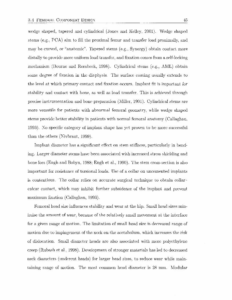
3.4 FEMORAL COMPONENT DESIGN 45
wedge shaped, tapered and cylindrical (Jones and Kelley, 2001). ·wedge shaped
stems (e.g., PCA) aim to fill the proximal femur and transfer load proximally, and
may be curved, or "anatomic". Tapered stems (e.g., Synergy) obtain contact more
distally to provide more uniform load transfer, and fixation comes from a self-locking
mechanism (Bourne and R.orabeck, 1998). Cylindrical stems (e.g., AML) obtain
some degree of fixation in the diaphysis. The surface coating usually extends to
the level at which primary contact and fixation occurs. Implant fit is important for
stability and contact with bone, as well as load transfer. This is achieved through
precise instrumentation and bone preparation (Miller, 1991). Cylindrical stems are
more versatile for patients with abnormal femoral geometry, while wedge shaped
stems provide better stability in patients with normal femoral anatomy (Callaghan,
1993). No specific category of implant shape has yet proven to be more successful
than the others (Nivbrant, 1999).
Implant diameter has a significant effect on stem stiffness, particularly in bend
ing. Larger diameter stems have been associated with increased stress shielding and
bone loss (Engh and Bobyn, 1988; Engh et al., 1990). The stem cross-section is also
important for resistance of torsional loads. Use of a collar on uncemented implants
is contentious. The collar relies on accurate surgical technique to obtain collar
calcar contact, which may inhibit further subsidence of the implant and prevent
maximum fixation (Callaghan, 1993).
Femoral head size influences stability and wear at the hip. Small head sizes min
imise the amount of wear, because of the relatively small movement at the interface
for a given range of motion. The limitation of small head size is decreased range of
motion due to impingement of the neck on the acetabulum, which increases the risk
of dislocation. Small diameter heads are also associated with more polyethylene
creep (R.ubash et al., 1998). Development of stronger materials has led to decreased
neck diameters (undercut heads) for larger head sizes, to reduce wear while main
taining range of motion. The most common head diameter is 28 mm. Modular
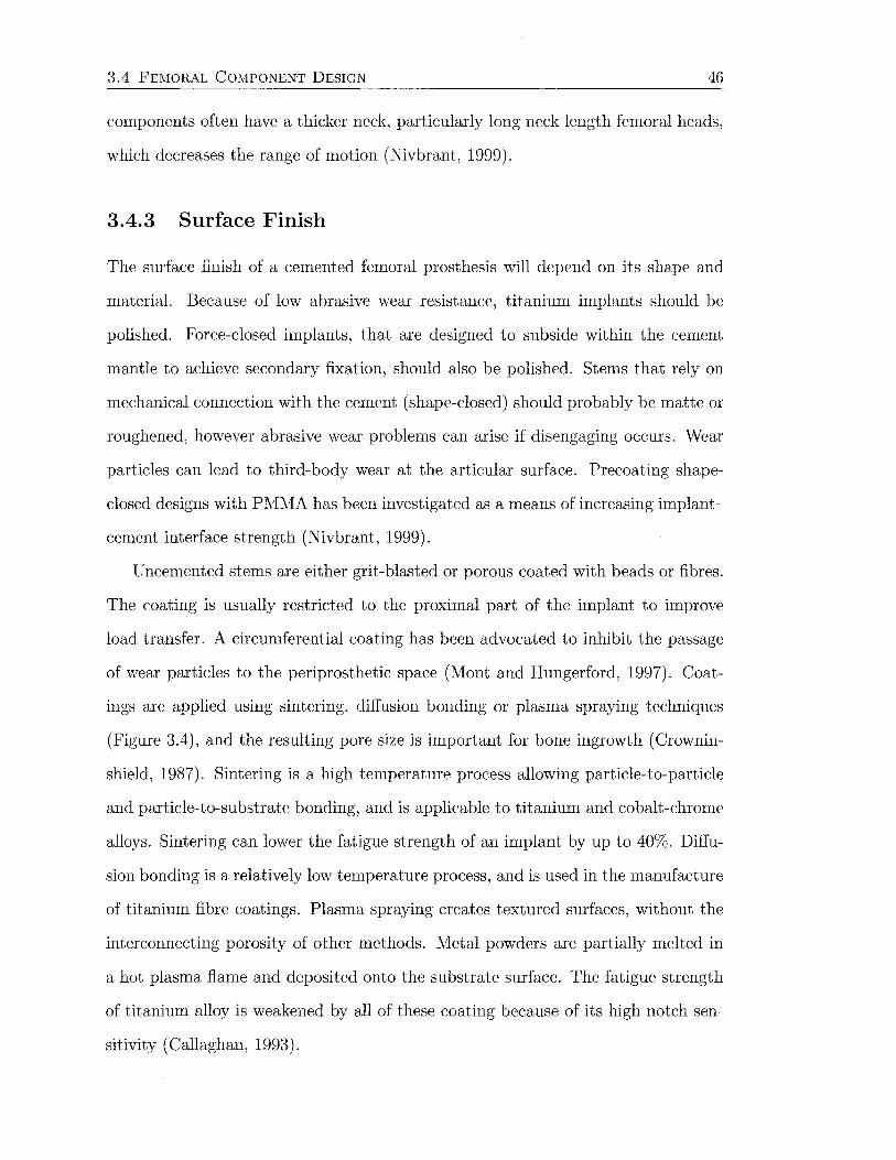
3.4 FEMORAL COMPONENT DESIGN 46
components often have a thicker neck, particularly long neck length femoral heads,
which decreases the range of motion (Nivbrant, 1999).
3.4.3 Surface Finish
The surface finish of a cemented femoral prosthesis will depend on its shape and
material. Because of low abrasive wear resistance, titanium implants should be
polished. Force-closed implants, that are designed to subside within the cement
mantle to achieve secondary fixation, should also be polished. Stems that rely on
mechanical connection with the cement (shape-closed) should probably be matte or
roughened, however abrasive wear problems can arise if disengaging occurs. Wear
particles can lead to third-body wear at the articular surface. Precoating shape
closed designs with Pl\!Hv1A has been investigated as a means of increasing implant
cement interface strength (Nivbrant, 1999).
Uncemented stems are either grit-blasted or porous coated with beads or fibres.
The coating is usually restricted to the proximal part of the implant to improve
load transfer. A circumferential coating has been advocated to inhibit the passage
of wear particles to the periprosthetic space (Mont and Hungerford, 1997). Coat
ings are applied using sintering, diffusion bonding or plasma spraying techniques
(Figure 3.4), and the resulting pore size is important for bone ingrowth (Crownin
shield, 1987). Sintering is a high temperature process allowing particle-to-particle
and particle-to-substrate bonding, and is applicable to titanium and cobalt-chrome
alloys. Sintering can lower the fatigue strength of an implant by up to 40%. Diffu
sion bonding is a relatively low temperature process, and is used in the manufacture
of titanium fibre coatings. Plasma spraying creates textured surfaces, without the
interconnecting porosity of other methods. Metal powders are partially melted in
a hot plasma flame and deposited onto the substrate surface. The fatigue strength
of titanium alloy is weakened by all of these coating because of its high notch sen
sitivity (Callaghan, 1993).

3.4 FEMORAL COMPONENT DESIGN
(a) (A) Surface and (B) cross-sectional views of a cobalt-chrome beaded porous surface.
(b) (A) Surface and (B) cross-sectional views of a titanium plasma-sprayed surface.
(c) (A) Surface and (B) cross-sectional views of a titanium fibre surface.
Figure 3.4: Porous coating techniques. Reproduced from Crowninshield (1987).
47
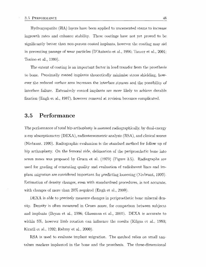
3.5 PERFORMANCE 48
Hydroxyapatite (HA) layers have been applied to uncemented stems to increase
ingrowth rates and enhance stability. These coatings have not yet proved to be
significantly better than non-porous coated implants, however the coating may aid
in preventing passage of wear particles (D'Antonio et al., 1996; Tanzer et al., 2001;
To nino et al., 1999).
The extent of coating is an important factor in load transfer from the prosthesis
to bone. Proximally coated implants theoretically minimise stress shielding, how
ever the reduced surface area increases the interface stresses and the possibility of
interface failure. Extensively coated implants are more likely to achieve durable
fixation (Engh et al., 1987), however removal at revision becomes complicated.
3.5 Performance
The performance of total hip arthoplasty is assessed radiographically, by dual-energy
x-ray absorptiometry (DEXA), radiostereometric analysis (RSA), and clinical scores
(Nivbrant, 1999). Radiographic evaluation is the standard method for follow up of
hip arthroplasty. On the femoral side, delineation of the periprosthetic bone into
seven zones was proposed by Gruen et al. (1979) (Figure 3.5). Radiographs are
used for grading of cementing quality and evaluation of radiolucent lines and im
plant migration are considered important for predicting loosening (Nivbrant, 1999).
Estimation of density changes, even with standardised procedures, is not accurate,
with changes of more than 20% required (Engh et al., 2000).
DEXA is able to precisely measure changes in periprosthetic bone mineral den
sity. Density is often measured in Gruen zones, for comparison between subjects
and implants (Bryan et al., 1996; Glassman et al., 2001). DEXA is accurate to
within 5%, however limb rotation can influence the results (Kilgus et al., 1993;
Kiratli et al., 1992; Rahmy et al., 2000).
RSA is used to evaluate implant migration. The method relies on small tan
talum markers implanted in the bone and the prosthesis. The three-dimensional

3.5 PERFORMANCE 49
1
6 2
5 3
Figure 3.5: Zones around the femoral component delineated by Gruen for evaluating loosening. Reproduced from Gruen et al. (1979).
coordinates of the implant markers can be calculated by using a calibration cage
and two simultaneous x-ray exposures. The radiographs are digitised and relative
movements are calculated using the appropriate software. RSA has an precision of
about 0.1 mm and 0.5° (Nivbrant, 1999).
The performance of total hip arthroplasty can be assessed using clinical scores.
The Harris Hip Score is the most popular, and measures pain, function, activities
of daily living, motion and deformity. Other scores include the WOMAC (West
ern Ontario and McMaster Universities) Osteoarthritis Index and the SF36 (lVIed
ical Outcomes Study 36-Item Short-Form Survey). Although clinical scores give a
measure of patient satisfaction, they are unable to detect early loosening and are
inadequate for identifying poorly performing designs (Nivbrant, 1999).
Chapter 4
Bone Mechanics
Bone is a rigid and hard mineralised tissue. These characteristics allow it to perform
many important biomechanical and metabolic functions. The mechanical properties
of bone allow it to maintain the shape of the body, protect the contents of the
body cavities, transmit muscle and joint forces, and provide a location for bone
marrow. The mineral content of bone serves as a store for ions, particularly calcium.
In addition, bone is a self-repairing material and able to adapt its geometric and
material properties in response to mechanical requirements. Bone is capable of
performing these functions because of its material properties, which are a function
of its composition and structure, and its biological properties.
The ability of bone to adapt to its mechanical environment is often referred to
as Wolff's Law. In 1892, Wolff published his Law of Bone Remodelling (translated
as Wolff (1986)), which stated:
" ... the law of bone remodelling is the law according to which alterations
of the internal architecture clearly observed and following mathemati
cal rules, as well as secondary alterations of the external form of the
bones following the same mathematical rules, occur as a consequence of
primary changes in the shape and stressing or in the stressing of bones."
No mathematical law has yet been derived, and some researchers have questioned
his theories (Cowin, 1997; Lee and Taylor, 1999; Roesler, 1987).
50

4. BONE MECHANICS 51
During the 1860s, the anatomist Meyer sketched the trabecular structure of the
proximal femur in the frontal plane (Figure 4.la). An engineer named Culmann
noticed a similarity between the trabecular architecture and the stress trajectories
produced by his graphical statics method in a crane he was designing (Figure 4.1b).
From Culmann's graphical statics, Wolff presumed that trabeculae in the proximal
(a) tv1eyer's representation of the bone architecture of the proximal femur.
(b) Stress trajectories determined by Culmann's graphical statics method in a Fairbairn crane shaped like the proximal femur.
Figure 4.1: Architecture of the proximal femur. Reproduced from Wolff (1986).
femur followed principal stress trajectories, and that they must therefore cross at
right angles. This hypothesis, however, neglected some fundamental principals of
continuum mechanics. Firstly, there is no correspondence between the stress trajec
tories in a linear elastic, homogeneous, isotropic object in the shape of a bone, and
the architecture of the trabeculae in a real bone of the same shape, loaded in the
4.1 STRUCTURE 52
same manner. Secondly, there is an infinite number of stress trajectories between
two points in the homogeneous object, and a finite number of trabeculae between
two points in cancellous bone. Thirdly, bones are subjected to time-varying, not
static loads (Cowin, 1997). Wolff's concentration on statics led to criticisms of his
"law" in other area also.
The writings of Wolff up until the early 1880s made no reference to bone adap
tation as a dynamic process. Rather, he believed the form of bone to be determined
by static load (Lee and Taylor, 1999). It is Roux that is understood to have in
troduced the dynamic concept of functional adaptation. Roux proposed that bone
was a "quantitative self-regulating mechanism" controlled by a "functional stimulus"
(Lee and Taylor, 1999). Some of Raux's concepts were apparently adopted later by
Wolff. Consequently, some have proposed that the name "Raux's Law" may be more
appropriate for describing the stress-adaptive behaviour of bone (Cowin, 1997).
4.1 Structure
There are two types of bone tissue: trabecular (also called cancellous or spongy) and
cortical (also called compact). Trabecular bone is porous (75-95% porosity) and
found in cuboidal bones, fiat bones and at the ends of long bones. It consists of a
three-dimensional interconnected network of trabecular rods and plates interspersed
with bone marrow (Figure 4.2). The trabecular length scale is approxiately 200 J);m
(Keaveny, 1998).
Cortical bone is dense (5-10% porosity) and found in the shaft of long bones
and enclosing the trabecular tissue in other bones. The cortical bone structure
consists of Haversian systems (secondary osteons) made up of circumferential layers
of fibres with alternating orientations around a central canal carrying blood vessels
(Figure 4.2).
Cortical and trabecular bone contain two main types of bone tissue: woven and
lamellar (Martinet al., 1998). Woven bone is found in the developing embryo, and

4.1 STRUCTURE
lnterstttlaJ lamellae
Trabeculae Osteoclast
Circurnlerenl111! subperiosteal lamettae
53
s:eocy:e
Figure 4.2: Architecture of cortical and trabecular bone. Reproduced from Hayes and Bouxsein (1997).
in new bone formation in postfoetal osteogenesis (e.g., fracture healing). Woven
bone is a fairly disorganised matrix of interwoven collagen fibres with osteocytes
distributed throughout. It is eventually resorbed and replaced by lamellar bone.
Lamellar bone is built up of layers (lamellae), each approximately 3 to 7 pm thick
with parallel fibres. The fibre direction can vary by up to 90° between adjacent layers
(Jee, 2001). In adult cortical bone, lamellae appear in three patterns (Figure 4.2):
1. concentric-circular rings surrounding a longitudinal vascular channel that
together form a structural cone, the osteon or Haversian system;
2. circumferential-several layers of lamellae that extend around part or all of
the circumference of the shaft of a long bone; or
3. interstitial-angular fragments of what were formerly concentric or circum-
ferential lamellae, filling the gaps between Haversian systems.

4.1 STRUCTURE 54
Cortical bone may be further classified as primary or secondary (Martin et al.,
1998). Primary bone refers to tissue that is laid down de novo on an existing
bone surface during growth. The two general types are circumferential lamellar
bone, and plexiform bone, a mixture of lamellar and woven bone tissues. Blood
vessels incorporated in the circumferential lamellar bone are surrounded by several
concentric lamellae, forming a primary osteon with a primary Haversian canal at
its centre.
Secondary bone results from the resorption of existing bone and its replacement
by new lamellar bone. In cortical bone, secondary tissue consists of secondary os
teons. These are about 200 f-Lm in diameter and consist of about sixteen cyclindrical
lamellae surrounding the Haversian canal. Between the Haversian system and the
surrounding bone lies the cement line boundary.
Adult cortical and trabecular bone is almost entirely secondary bone. Most
compact bone is composed of secondary osteons and interstitial lamellae. Secondary
trabecular bone rarely contains osteons, as they do not generally fit within individual
trabeculae; instead containing cresent shaped hemiosteons and interstitial lamellae.
Hemiosteons are also delineated by cement lines.
Small cavities, or lacunae, connected by tubular canals, or canaliculi, are found
throughout woven and lamellar bone. Entrapped cells occupy the lacunae, and
communicate with cells in adjacent lacunae and nearby Haversian canals via cellular
processes within the canaliculi. Osteons are connected by transverse Volkmann's
canals, to form an interconnected network carrying neurovascular and lymphatic
vessels. Blood supply comes from nutrient, metaphyseal and epiphyseal arteries in
adult long bones.
Bone tissue has two major surfaces, periosteal and endosteal. The periosteal
surfaces are external while the endosteal surfaces are internal. The endosteal surface
is further subdivided into the intracortical (Haverian/osteonal), endocortical and
trabecular surfaces (Frost, 1987).
4.2 COMPOSITION 55
4.2 Composition
Bone is made up of 65% mineral and 35% matrix, cells and water (Jee, 2001). The
mineral phase of bone consists mainly of hydroxyapatite crystals, Ca10 (P04 ) 6 (0H)2.
The individual crystals are generally plate-like, measuring about 50 x 50 x 250 A
(Posner, 1985). The mineral is impure, in particular containing 4-6% carbonate
groups replacing the phosphate groups, making the material more realistically a
carbonate apapatite. The major cell types are osteoblasts, osteoclasts, osteocytes and
bone-lining cells. Osteoblasts, osteocytes and bone-lining cells are all descendants of
the osteoblastic cell lineage, representing different stages of maturation. Osteoclasts
represent the final differentiation stage of a line of the monocyte cell family.
Osteoblasts form new bone by secreting most of the components of the organic
matrix, or osteoid. The osteoid is made up primarily of type I collagen (90%) and
other noncollagenous proteins. Osteoblasts regulate the structural organisation of
the collagen matrix and facilitate the precipitation of mineral salts within the os
teoid from ions in the extracellular matrix. Active osteoblasts occur as a contiguous
layer of cuboidal cells 15 to 30 J-lm thick, wherever bone formation takes place. Os
teoblasts are differentiated from mesenchymal cells within the periosteal membrane
or bone marrow in a process taking 2-3 days. Osteoid is laid down at a rate of
about 0.55 [Lm/day (Jee, 2001) to 1 [Lm/day (Martinet al., 1998). This is referred
to as the bone apposition rate.
Bone-lining cells are inactive osteoblasts that are flattened, elongated cells cov
ering quiescent bone surfaces. They cover the majority of the adult bone surfaces.
Bone-lining cells are capable of forming bone without prior bone resorption in re
sponse to anabolic agents. They are also involved in resorption of the surface layer
of osteoid before giving access to osteoclasts. Bone-lining cells are believed to be
involved in mineral homeostasis by forming an ion barrier that regulates the flux of
calcium and phosphate in and out of the bone tissue ( J ee, 2001). Bone-lining cells
are thought to be influenced by strain within the bone, and thus involved with bone
adaptation.
4.3 DEVELOPMENT, GROWTH, MODELLING AND REMODELLING 56
Osteocytes are mature osteoblasts that have become embedded in lacunae within
the bone matrix. They are the most abundant cell type in mature bone, with
about ten times more osteocytes than osteoblasts (Jee, 2001). Osteocytes have little
synthetic activity. They form an extensive network with each other and with cells
at the bone surface, both physically and functionally, via slender cellular processes
which pass through the canaliculi. The cells are connected by gap junctions which
allows direct communication between the cells, through the passage of ions and
small molecules. Osteocytes and bone-lining cells together are believed to form a
sensory network that monitors mechanical load and tissue damage within bone, and
subsequently regulates adaptive responses (Majeska, 2001).
Osteoclasts are large, multinucleated cells that resorb bone by dissolution of
mineral and enzymatic digestion of organic macromolecules (Majeska, 2001). Active
osteoclasts are usually found in cavities on bone surfaces called resorption cavities
or H owship 's lacunae. Cessation of bone resorption is associated with migration of
osteoclasts from endosteal surfaces into adjacent marrow spaces where they undergo
apoptosis (Jee, 2001). Osteoclasts are regulated by numerous factors, including
hormones, growth factors and cytokines.
4.3 Development, Growth, Modelling and
Remodelling
4.3.1 Bone Formation
There are two major modes of primary bone formation, or osteogenesis, and both
involve the transformation of a preexisting mesenchymal tissue into bone tissue.
Mesenchymal tissue contains unspecialised cells that can readily self-proliferate and
differentiate into a number of different cell tissue types via well regulated lineage
cascades. The direct conversion of mesenchymal tissue into bone is called intramem
branous ossification. This process occurs primarily in the bones of the skull. In other
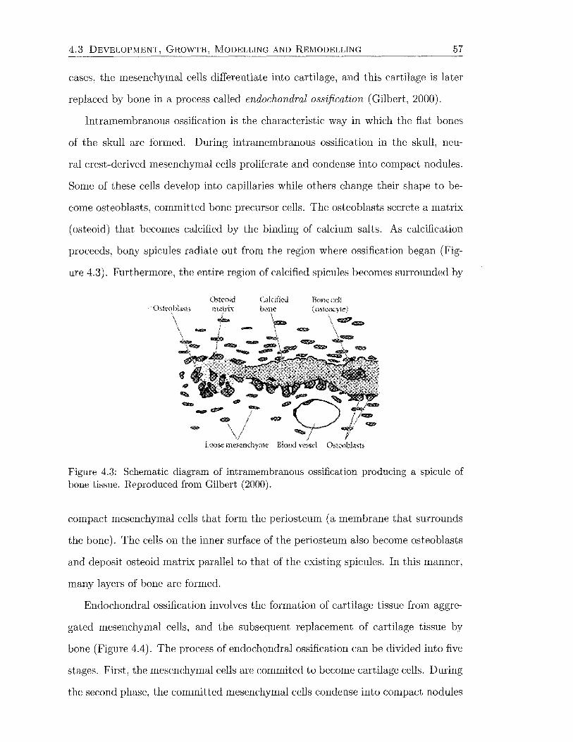
4.3 DEVELOPMENT, GROWTH, MODELLING AND REMODELLING 57
cases, the mesenchymal cells differentiate into cartilage, and this cartilage is later
replaced by bone in a process called endochondral ossification (Gilbert, 2000).
Intramembranous ossification is the characteristic way in which the fiat bones
of the skull are formed. During intramembranous ossification in the skull, neu-
ral crest-derived mesenchymal cells proliferate and condense into compact nodules.
Some of these cells develop into capillaries while others change their shape to be-
come osteoblasts, committed bone precursor cells. The osteoblasts secrete a matrix
(osteoid) that becomes calcified by the binding of calcium salts. As calcification
proceeds, bony spicules radiate out from the region where ossification began (Fig
ure 4.3). Furthermore, the entire region of calcified spicules becomes surrounded by
Calcifietl Rone cd1 (osteoq'le)
9lllf,lll' <JIIll>
Figure 4.3: Schematic diagram of intramembranous ossification producing a spicule of bone tissue. Reproduced from Gilbert (2000).
compact mesenchymal cells that form the periosteum (a membrane that surrounds
the bone). The cells on the inner surface of the periosteum also become osteoblasts
and deposit osteoid matrix parallel to that of the existing spicules. In this manner,
many layers of bone are formed.
Endochondral ossification involves the formation of cartilage tissue from aggre
gated mesenchymal cells, and the subsequent replacement of cartilage tissue by
bone (Figure 4.4). The process of endochondral ossification can be divided into five
stages. First, the mesenchymal cells are commited to become cartilage cells. During
the second phase, the committed mesenchymal cells condense into compact nodules

4.3 DEVELOPMENT, GROWTH, MODELLING AND REMODELLING
(Al (B)
!lyp<mophk d10ndroc-,1es I .
{C)
Ostcob!asts (bom::J
iLl)
.!lkmd
58
Figure 4.4: Schematic diagram of endochondral ossification. (A, B) Mesenchymal cells condense and differentiate into chondrocytes to form the cartilaginous model of the bone. (C) Chondrocytes in the centre of the shaft undergo hypertrophy and apoptosis while they change and mineralise their extracellular matrix. Their deaths allow blood vessels to enter. (D, E) Blood vessels bring in osteoblasts, which bind to the degenerating cartilaginous matrix and deposit bone matrix. (F ~H) Bone formation and growth consist of ordered arrays of proliferating, hypertrophic, and mineralizing chondrocytes. Secondary ossification centres also form as blood vessels enter near the tips of the bone. Reproduced from Gilbert (2000).
and differentiate into chondrocytes, the cartilage cells. In the third phase, the
chondrocytes proliferate rapidly to form the model of the bone. As they divide, the
chondrocytes secrete a cartilage-specific extracellular matrix. In the fourth phase,
the chondrocytes stop dividing and increase their volume dramatically, becoming
hypertrophic chondrocytes. These large chondrocytes alter the matrix they produce
to enable it to become mineralised. The fifth phase involves the invasion of the carti-
lage model by blood vessels. The hypertrophic chondrocytes die by apoptosis. This
space will become bone marrow. As the cartilage cells die, a group of cells that
have surrounded the cartilage model differentiate into osteoblasts. The ostoblasts
begin forming bone matrix on the partially degraded cartilage. Eventually, all the
cartilage is replaced by bone. Thus, the cartilage tissue serves as a model for the
bone that follows. The skeletal components of the vertebral column, the pelvis, and
the limbs are first formed of cartilage and later become bone.
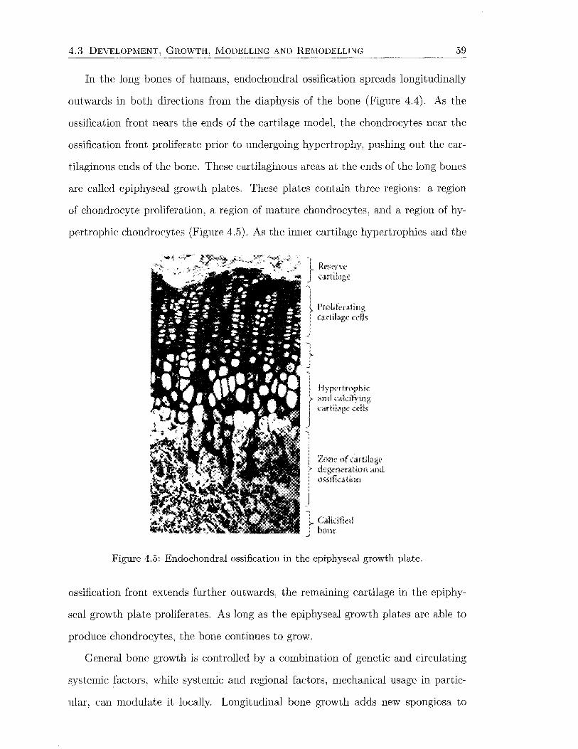
4.3 DEVELOPMENT, GROWTH, MODELLING AND REMODELLING 59
In the long bones of humans, endochondral ossification spreads longitudinally
outwards in both directions from the diaphysis of the bone (Figure 4.4). As the
ossification front nears the ends of the cartilage model, the chondrocytes near the
ossification front proliferate prior to undergoing hypertrophy, pushing out the car
tilaginous ends of the bone. These cartilaginous areas at the ends of the long bones
are called epiphyseal growth plates. These plates contain three regions: a region
of chondrocyte proliferation, a region of mature chondrocytes, and a region of hy-
pertrophic chondrocytes (Figure 4.5). As the inner cartilage hypertrophies and the
'
Pml!ftnling cartilag<: cells
I Hypcrlmphk ' and .;,~akifir·ing f <>H;],g«<lls
Zone of cartila)!,C' degeneration and ossit1,ation
Figure 4.5: Endochondral ossification in the epiphyseal growth plate.
ossification front extends further outwards, the remaining cartilage in the epiphy-
seal growth plate proliferates. As long as the epiphyseal growth plates are able to
produce chondrocytes, the bone continues to grow.
General bone growth is controlled by a combination of genetic and circulating
systemic factors, while systemic and regional factors, mechanical usage in partie-
ular, can modulate it locally. Longitudinal bone growth adds new spongiosa to
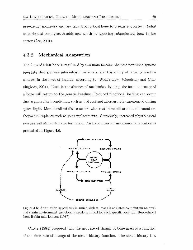
4.3 DEVELOPMENT, GROWTH, MODELLING AND REMODELLING 60
preexisting spongiosa and new length of cortical bone to preexisting cortex. Radial
or periosteal bone growth adds new width by apposing subperiosteal bone to the
cortex (Jee, 2001).
4.3.2 Mechanical Adaptation
The form of adult bone is regulated by two main factors: the predetermined genetic
template that explains intersubject variations, and the ability of bone to react to
changes in the level of loading, according to "Wolff's Law" (Goodship and Cun
ningham, 2001). Thus, in the absence of mechanical loading, the form and mass of
a bone will return to the genetic baseline. Reduced functional loading can occur
due to generalised conditions, such as bed rest and microgravity experienced during
space flight. More localised disuse occurs with cast immobilisation and around or-
thopaedic implants such as joint replacements. Conversely, increased physiological
exercise will stimulate bone formation. An hypothesis for mechanical adaptation is
presented in Figure 4.6.
I BONE DEPOSITION ~
INCREASE ACTIVITY DECREASE STRAINS
1 /,./ ,
/ I I I DECREASE ACTIVITY INCREASE STRAINS
I L. ..... , .... ,,. -t : ' I •
FUNCTION DISUSE
't ) ,, ;~ ' ,, ....._ __ GENETIC BASELINE+--..,..
Figure 4.6: Adaptation hypothesis in which skeletal mass is adjusted to maintain an optimal strain environment, genetically predetermined for each specific location. Reproduced from Rubin and Lanyon (1987).
Carter (1984) proposed that the net rate of change of bone mass is a function
of the time rate of change of the strain history function. The strain history is a

4.3 DEVELOPMENT, GROWTH, MODELLING AND REMODELLING 61
function of the cyclic strain range, mean strain, and the number of loading cycles.
Other potential components of the strain history function include strain rate and
frequency.
Lanyon and Rubin (Lanyon, 1984; Lanyon and Rubin, 1984; Rubin and Lanyon,
1984, 1987) developed the functionally isolated avian ulnar model to investigate the
effects of loading parameters on long bone morphology in vivo. Importantly, this
model isolated the bone from any mechanical loading other than that applied as
part of the experimental protocol. The unknown factor associated with loading from
normal activity between sessions of experimentally applied loading was eliminated.
In contrast, studies such as that by Meade et al. (1984) in which a constantly applied
load was applied to the canine femur via external springs, produced results which
are difficult to interpret, since additional dynamic loads from normal activity were
superimposed.
Lanyon and Rubin's investigations demonstrated that dynamic loading within
the physiological strain range led to an osteogenic response, sensitive to the magni
tude, rate of change, and distribution of the dynamic strain. Static loading within
the physiological range produced similar results to those observed in disuse. The
osteogenic response becomes saturated after as few as 36 consecutive loading cy
cles per day, and only 4 loading cycles per day were needed to prevent resorption.
Turner (1998) termed this the "case of diminishing returns". Turner et al. (1995)
proposed that bone cells responded to stress-generated fluid flow within the bone
matrix proportional to strain rate. In a cylinder, strain rate is proportional to the
amplitude of the applied dynamic load-a stimulus previously proposed by Lanyon
and Rubin. Zernicke et al. (2001) reported an osteogenic response after 3 weeks
of running in mature roosters. This was correlated with the peak circumferential
strain. High impact jump drops with immature roosters showed significant bone
formation which correlated with strain rate. Strain rate increased considerably more
than peak strain during this activity. Mi et al. (2002) reported strain gradients to
be strongly related to bone interstitial fluid flow. In another isolated avian ulna
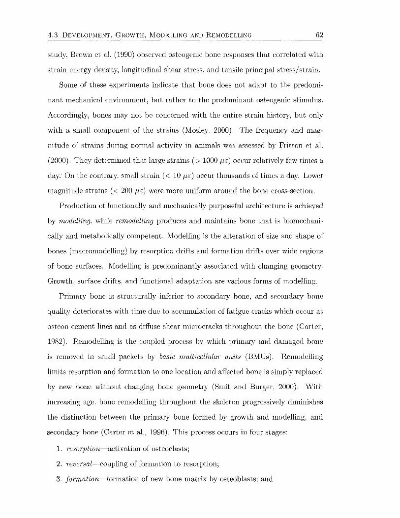
4.3 DEVELOPMENT, GROWTH, MODELLING AND REMODELLING 62
study, Brown et al. (1990) observed osteogenic bone responses that correlated with
strain energy density, longitudinal shear stress, and tensile principal stress/strain.
Some of these experiments indicate that bone does not adapt to the predomi
nant mechanical environment, but rather to the predominant osteogenic stimulus.
Accordingly, bones may not be concerned with the entire strain history, but only
with a small component of the strains (Mosley, 2000). The frequency and mag
nitude of strains during normal activity in animals was assessed by Fritton et al.
(2000). They determined that large strains(> 1000 J-lE) occur relatively few times a
day. On the contrary, small strain ( < 10 J-lE) occur thousands of times a day. Lower
magnitude strains ( < 200 J-lE) were more uniform around the bone cross-section.
Production of functionally and mechanically purposeful architecture is achieved
by modelling, while remodelling produces and maintains bone that is biomechani
cally and metabolically competent. Modelling is the alteration of size and shape of
bones (macromodelling) by resorption drifts and formation drifts over wide regions
of bone surfaces. Modelling is predominantly associated with changing geometry.
Growth, surface drifts, and functional adaptation are various forms of modelling.
Primary bone is structurally inferior to secondary bone, and secondary bone
quality deteriorates with time due to accumulation of fatigue cracks which occur at
osteon cement lines and as diffuse shear microcracks throughout the bone (Carter,
1982). Remodelling is the coupled process by which primary and damaged bone
is removed in small packets by basic multicellular units (BMUs). Remodelling
limits resorption and formation to one location and affected bone is simply replaced
by new bone without changing bone geometry (Smit and Burger, 2000). With
increasing age, bone remodelling throughout the skeleton progressively diminishes
the distinction between the primary bone formed by growth and modelling, and
secondary bone (Carteret al., 1996). This process occurs in four stages:
1. resorption-activation of osteoclasts;
2. reversal-coupling of formation to resorption;
3. formation-formation of new bone matrix by osteoblasts; and

4.3 DEVELOPMENT, GROWTH, MODELLING AND REMODELLING 63
formation resorption
resting reversal
(a) Cortical bone remodelling by EMUs.
~~~ ~a~(7~a
resorption reversal t ~--~
resting formation
(b) Trabecular bone remodelling by B~IUs.
Figure 4.7: Bone remodelling due to the activity of basic multicellular units. Reproduced from Smit and Burger (2000).
4. resting/ quiescence-bone surfaces lined by inactive osteoblasts (bone-lining
cells).
Remodelling takes place on all of the skeletal envelopes/surfaces, although in
adult humans, about 80% of the cancellous and cortical surfaces (periosteal and
endosteal), and about 95% of the intracortical surfaces are inactive with respect
to remodelling at any given time ( J ee, 2001). In cortical bone, remodelling occurs
by osteonal tunnelling in which the osteoclasts of a BMU excavate a canal that is
refilled by osteoblasts. Haversian systems, oriented along the main loading direction,
that are 100-200 p,m wide and up to 10 mm long are the result. Trabecular bone
remodelling results in surface grooves (Howship's lacunae) with a depth of 60-70 p,m
that are refilled by osteoblasts (Figure 4.7). For each BMU, the amount of bone
replaced is generally less than that removed, leading to a net decrease in the amount
of bone. Consequently, increased remodelling leads to greater losses of bone, while
decreased remodelling reduces these losses and conserves bone (Frost, 1987).
The total surface area available for remodelling at any site is dependent on
the local bone porosity. Martin (1984) developed a relationship for this area per
unit volume (specific surface) as a function of the porosity, presented graphically in
Figure 4.8.
According to Burr (2002), bone remodelling achieves three goals:
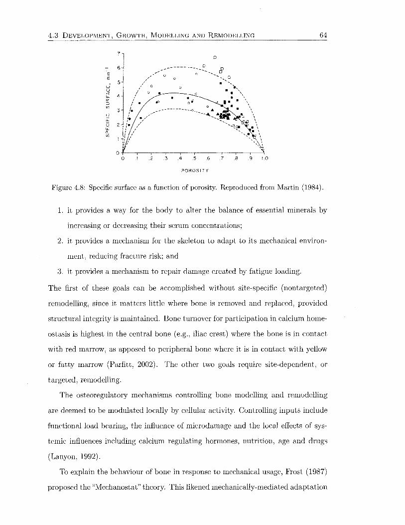
4.3 DEVELOPMENT, GROWTH, MODELLING AND REMODELLING
E E
7
6
. 5 w u ~ 4 a: :::J (f)
u 3
D
-----------:'_ B ,..... 0 -- ........
/', .. ·"' 0 0 ................. 0 ' . ... ....
/ 0 0 ......
' . ' / 0 •!..------- 0 • \ . . . '
(,'. ~ 0~ ••• \ . ' /• ...... ---------..!') A • \'
,' ... - - ... --........... ...... \ lL ,'t ........ ~ .p \ u 2 :• - .... ~ "' . lLJ ... ~ ~ \
~ ................. \ ' ' ' ...... \
.2 .3 .4 .5 6 .7 .8 .9 1.0
POROSITY
64
Figure 4.8: Specific surface as a function of porosity. Reproduced from Martin (1984).
1. it provides a way for the body to alter the balance of essential minerals by
increasing or decreasing their serum concentrations;
2. it provides a mechanism for the skeleton to adapt to its mechanical environ-
ment, reducing fracture risk; and
3. it provides a mechanism to repair damage created by fatigue loading.
The first of these goals can be accomplished without site-specific (nontargeted)
remodelling, since it matters little where bone is removed and replaced, provided
structural integrity is maintained. Bone turnover for participation in calcium home
ostasis is highest in the central bone (e.g., iliac crest) where the bone is in contact
with red marrow, as apposed to peripheral bone where it is in contact with yellow
or fatty marrow (Parfitt, 2002). The other two goals require site-dependent, or
targeted, remodelling.
The osteoregulatory mechanisms controlling bone modelling and remodelling
are deemed to be modulated locally by cellular activity. Controlling inputs include
functional load bearing, the influence of microdamage and the local effects of sys-
temic influences including calcium regulating hormones, nutrition, age and drugs
(Lanyon, 1992).
To explain the behaviour of bone in response to mechanical usage, Frost (1987)
proposed the "Mechanostat" theory. This likened mechanically-mediated adaptation
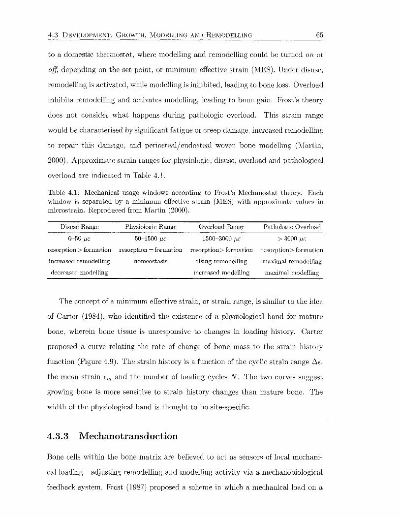
4.3 DEVELOPMENT, GROWTH, MODELLING AND REMODELLING 65
to a domestic thermostat, where modelling and remodelling could be turned on or
off, depending on the set point, or minimum effective strain (MES). Under disuse,
remodelling is activated, while modelling is inhibited, leading to bone loss. Overload
inhibits remodelling and activates modelling, leading to bone gain. Frost's theory
does not consider what happens during pathologic overload. This strain range
would be characterised by significant fatigue or creep damage, increased remodelling
to repair this damage, and periosteal/ endosteal woven bone modelling (Iv1artin,
2000). Approximate strain ranges for physiologic, disuse, overload and pathological
overload are indicated in Table 4.1.
Table 4.1: Mechanical usage windows according to Frost's Mechanostat theory. Each window is separated by a minimum effective strain (MES) with approximate values in microstrain. Reproduced from Martin (2000).
Disuse Range Physiologic Range Overload Range Pathologic Overload
0-50 J1E 50-1500 p,c 1500-3000 p,c > 3000 J1E
resorption > formation resorption = formation resorption> formation resorption> formation
increased remodelling homeostasis rising remodelling maximal remodelling
decreased modelling increased modelling maximal modelling
The concept of a minimum effective strain, or strain range, is similar to the idea
of Carter (1984), who identified the existence of a physiological band for mature
bone, wherein bone tissue is unresponsive to changes in loading history. Carter
proposed a curve relating the rate of change of bone mass to the strain history
function (Figure 4.9). The strain history is a function of the cyclic strain range .6-E,
the mean strain Em and the number of loading cycles N. The two curves suggest
growing bone is more sensitive to strain history changes than mature bone. The
width of the physiological band is thought to be site-specific.
4.3.3 Mechanotransduction
Bone cells within the bone matrix are believed to act as sensors of local mechani-
cal loading~adjusting remodelling and modelling activity via a mechanobiological
feedback system. Frost (1987) proposed a scheme in which a mechanical load on a
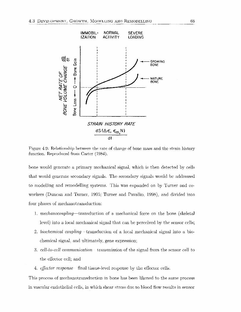
4.3 DEVELOPMENT, GROWTH, MODELLING AND REMODELLING
m1- c "0 '0 0
(,!)
<l.J c 0 m
t 0
' ~ 0 ...J v § m
IMMOBIL- NORMAL IZATION ACTIVITY
SEVERE LOADING
STRAIN HISTORY RATE
dS(l:\E, Em,N)
dt
-GROWING BONE
-MATURE BONE
66
Figure 4.9: Relationship between the rate of change of bone mass and the strain history function. Reproduced from Carter (1984).
bone would generate a primary mechanical signal, which is then detected by cells
that would generate secondary signals. The secondary signals would be addressed
to modelling and remodelling systems. This was expanded on by Turner and co
workers (Duncan and Turner, 1995; Turner and Pavalko, 1998), and divided into
four phases of mechanotransduction:
1. mechanocoupling~transduction of a mechanical force on the bone (skeletal
level) into a local mechanical signal that can be perceived by the sensor cells;
2. biochemical coupling~transduction of a local mechanical signal into a bio-
chemical signal, and ultimately, gene expression;
3. cell-to-cell communication~transmission of the signal from the sensor cell to
the effector cell; and
4. effector response~final tissue-level response by the effector cells.
This process of mechanotransduction in bone has been likened to the same process
in vascular endothelial cells, in which shear stress due to blood flow results in sensor
4.3 DEVELOPMENT, GROWTH, MODELLING AND REMODELLING 67
cells locally producing paracrine factors which act on vascular smooth muscle cells
to alter blood pressure (Duncan and Turner, 1995; Turner et al., 1995).
The first step, mechanocoupling, has been the most thoroughly investigated.
There is general agreement among researchers that cells of the osteoblast lineage
are the most likely transducers of mechanical strain. Osteocytes are the most likely
derivatives of this cell line, due to their distribution within the bone matrix, and
their ability to communicate with other osteocytes and cell lines (Cowin et al.,
1991; Harrigan and Hamilton, 1993a; Lanyon, 1987; Martin, 2000; Turner et al.,
1995; Turner and Pavalko, 1998). Each osteocyte is connected by 50 to 70 gap
junctions at the ends of cellular processes to other osteocytes, bone-lining cells or
osteoblasts on all adjacent bone matrix surfaces. Connection to endothelial cells in
the bone vasculature is also probable (Cowin, 1993). This network of cells forms a
functional syncytium.
The manner in which the local mechanical state of a bone is measured by this cell
population is not fully understood. Some of the possibilities include direct strain,
fluid shear and streaming potentials (Cowin et al., 1991). Tissue level strains, due to
deformation of the osteocytic lacunar walls, cell and cell-process membranes, may be
very small when considered in terms of bone-cell displacement. The physiological
strain range, measured on the periosteal surface, of adult load-bearing bone in
most species is 2000-3000 fJ£ (Rubin and Lanyon, 1984). Some investigators, such
as Turner et al. (1995), have questioned whether bone cells can sense such small
strains, however, it is possible that strain concentrations exist around osteocyte
lacunae (Cowin et al., 1991; Smit and Burger, 2000). Nicolella and Lankford (2002)
estimated strains around lacunae up to 16 000 fJ£, and 30 000 fJ£ within a distance
of one lacunar diameter.
Another possibility is that strain is amplified by stress-generated fluid flow
through the porous bone matrix. Bone cells may be capable of detecting fluid
shear stress. The other effect of fluid flow is streaming potentials. The flow of fluid
containing charged solutes through a solid matrix containing oppositely charged
4.3 DEVELOPMENT, GROWTH, MODELLING AND REMODELLING 68
chemical groups causes charge separation. This results in streaming potentials due
to the balance between electrical forces and fluid density. This creates a poten
tial difference between two sites in the bone tissue of up to 2 m V (Cowin et al.,
1991). The physical quantity cells may sense is the disparity between intra- and
extracellular electric potentials (Harrigan and Hamilton, 1993a). Becket al. (2002),
however, were unable to find a relationship between streaming potential magnitudes
and strain or strain gradients in an experimental study.
It is probable that bone cells react to more than one component of their mechan
ical environment, allowing for a more structurally relevant remodelling response in
different anatomical locations or in bone with different structural properties (Ehrlich
and Lanyon, 2002).
Damage accumulation caused by fatigue loading has also been hypothesised to
influence bone remodelling, particularly under pathological overload conditions. Mi
crodamage accumulates slowly under normal loading conditions, and for this reason
it is unlikely that microcracks trigger increased remodelling due to disuse (Carter,
1984). Microcracks can accrue rapidly when strains exceed 3000 f-1£ (Duncan and
Turner, 1995), and increased remodelling is required to repair the damaged bone
tissue. Due to the low number of osteogenic loading cycles required to induce
modelling, it is improbable that damage accumulation plays a role in this process
(Duncan and Turner, 1995; Lanyon, 1992; Rubin and Lanyon, 1987; Turner et al.,
1995).
The biochemical coupling phase involves measurement of the local mechani
cal signal. Possibilities include force transduction from the extracellular matrix
to the cytoskeleton and nuclear matrix through integrins, stretch-activated cation
(Ca2+) channels within the cell membrane, protein-dependent pathways in the cell
membrane, and linkage between the cytoskeleton and the phospholipase pathways
(Duncan and Turner, 1995). Ingber (1997) proposed a form of cellular architecture
relying on tensional intregrity for stability (tensegrity) as a mechanism for coupling
of the local signal to a cellular response. Compression members within the cell

4.3 DEVELOPJ\1ENT, GROWTH, MODELLING AND REMODELLING 69
resist the contractile pull of the cytoskeleton. This theory predicts that the cells
are hard-wired to respond immediately to mechanical stress transmitted over the
cell surface receptors, that physically couple the cytoskeleton to the extracellular
matrix (integrins) or other cells ( cadherins, selectins).
Candidates for cell-to-cell communication of bone adaptation information in
clude prostaglandin E2 , insulin-like growth factors I and II, and nitric oxide (Bakker
et al., 2001; Blankenhorn et al., 2002; Duncan and Turner, 1995; Turner and Pavalko,
1998; van't Hof and Ralston, 2001). Prostaglandin E2 has important anabolic ac
tions in bone, demonstrated by its ability to promote recruitment of osteoblast
precursor cells and increase osteoblast proliferation. Nitric oxide has been shown
to act as a mediator of mechanically-induced bone formation. Insulin-like growth
factors could couple bone formation to bone resorption (Ehrlich and Lanyon, 2002).
The effector response resulting from the initial local mechanical signal involves
differentiation and recruitment of cells to the bone surface to facilitate an adaptive
response (Duncan and Turner, 1995). Other hormones, particularly calcium regu
lating, may interact with the local mechanical signals to change the sensitivity of
the sensor or effector cells to mechanical load.
The mechanotransduction pathway still requires considerable investigation to
determine how all of these components fit together. According to Martin (2000),
bone-lining cells are restrained from activating remodelling by the strain-generated
signals arriving from the network of osteocytes within the adjacent bone matrix.
Lanyon (1984) also proposed that the osteogenic stimulus in normally loaded bone
prevents high remodelling activity. Martin (2000) went on to suggest that the bone
formation rate of functioning osteoblasts was also inhibited by osteocytic signals.
This seems counterintuitive in terms of loading being conducive to bone formation,
however this leads to creation of new osteocytes, rather than altering osteoblast
differentiation and recruitment to BMUs.
The strain-generated signal produced by osteocytes is most likely interrupted by
fatigue cracks, by direct injury to osteocytes or their processes. According to Martin
4.4 MECHANICAL PROPERTIES 70
(2000), loss of this signal would trigger bone-lining cells to activate remodelling to
repair the bone tissue. Tami et al. (2002) observed a high degree of interconnection
in the osteocyte syncytium of healthy bone. A marked decrease in interconnectivity
was observed under osteoporosis. This situation, in a manner similar to fatigue
damage, decreases the ability of the cells to communicate, subsequently increasing
remodelling and decreasing bone mass.
To account for the fact that bone is not completely resorbed under disuse con
ditions, possible only as far as a genetic baseline level (Figure 4.6), Turner (1998)
introduced a "principle of cellular accommodation". This rule postulated that bone
cells accommodate to an altered mechanical loading environment, making them less
responsive to routing signals over time. Rubin et al. (2002) also proposed that bone
cells are capable of accommodating new loading environment. An osteocyte may be
able to "normalise" the local mechanical environment by modulating its cytoskeletal
architecture, attachment to the matrix, configuration of the periosteocytic space,
and communication channels to surrounding cells. In this manner, the osteocyte
can accommodate most changes in local loading without needing to alter tissue
architecture, except under severe changes in which case site-specific remodelling oc
curs. Cowin et al. (1991) thought it possible for an osteocyte to remodel the shape
of its lacunae, thereby mechanically adjusting its sensitivity to a particular type of
loading.
4.4 Mechanical Properties
The load-bearing capacity of a skeletal structure is dependent on its intrinsic mate
rial properties as well as the size and shape of the bone tissue. From a mechanical
point of view, the allocation of these parameters represents a compromise between
the need for stiffness to make muscle actions efficient, the need for compliance to
absorb energy and avoid fracture, and the need for minimum skeletal weight. The
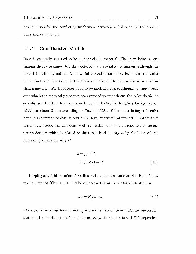
4.4 MECHANICAL PROPERTIES 71
best solution for the conflicting mechanical demands will depend on the specific
bone and its function.
4.4.1 Constitutive Models
Bone is generally assumed to be a linear elastic material. Elasticity, being a con
tinuum theory, assumes that the model of the material is continuous, although the
material itself may not be. No material is continuous to any level, but trabecular
bone is not continuous even at the macroscopic level. Hence it is a structure rather
than a material. For trabecular bone to be modelled as a continuum, a length scale
over which the material properties are averaged to smooth out the holes should be
established. The length scale is about five intertrabecular lengths (Harrigan et al.,
1988), or about 5 mm according to Cowin (1993). When considering trabecular
bone, it is common to discuss continuum level or structural properties, rather than
tissue level properties. The density of trabecular bone is often reported as the ap
parent density, which is related to the tissue level density Pt by the bone volume
fraction Vt or the porosity P
p=ptxVf
= Pt X (1- P) ( 4.1)
Keeping all of this in mind, for a linear elastic continuum material, Hooke's law
may be applied (Chung, 1988). The generalised Hooke's law for small strain is
(4.2)
where O"ij is the stress tensor, and /ij is the small strain tensor. For an anisotropic
material, the fourth order stiffness tensor, Eijkm, is symmetric and 21 independent

4.4 1\ilECHANICAL PROPERTIES
coefficients are needed to characterise it
~1111 ~1122 ~1133 ~1112 ~1123 ~1131
~2222 ~2233 ~2212 ~2223 ~2231
~3333 ~3312 ~3323 ~3331
symm. ~1212 ~1223 ~1231
~2323 ~2331
~3131
72
( 4.3)
For most materials, this number of constants is reduced due to symmetry. A ma
terial that has properties varied along three perpendicular axes (e.g., longitudinal,
radial and circumferential) is said to be orthotropic. Nine independent coefficients
are required to describe orthotropy. Trabecular bone is accepted to be effectively
orthotropic (Yang et al., 1998), with the principal axes governed by the trabecular
orientation.
A special type of orthotropic material, with the properties equal in two of the
three principal directions, is a transverse isotropic material. In this case the number
of independent constants is reduced to five. For cortical bone, the average orienta
tion of the mineralised collagen fibres is approximately parallel to the bone's long
axis. This causes a significant difference in the mechanical properties associated
with the longitudinal direction. The microstructure of primary bone presents a dis
tinct difference in the radial and transverse directions, suggesting that cortical bone
is orthotropic. However, osteonal remodelling tends to convert the bone from an
orthotropic to a transversly isotropic material (Huiskes, 1997; Martinet al., 1998).
An isotropic material is symmetric with respect to every plane and axis, and
has material properties that are identical in all directions. Only two constants are
needed to define an isotropic material-generally expressed as the Young's or elastic
modulus ~ and Poisson's ratio v, or in terms of the the Lame constants f-1 and >..
Isotropic materials have the advantage that the stresses and strains can be de
composed into hydrostatic (dilatational) and deviatoric (distortional) components.
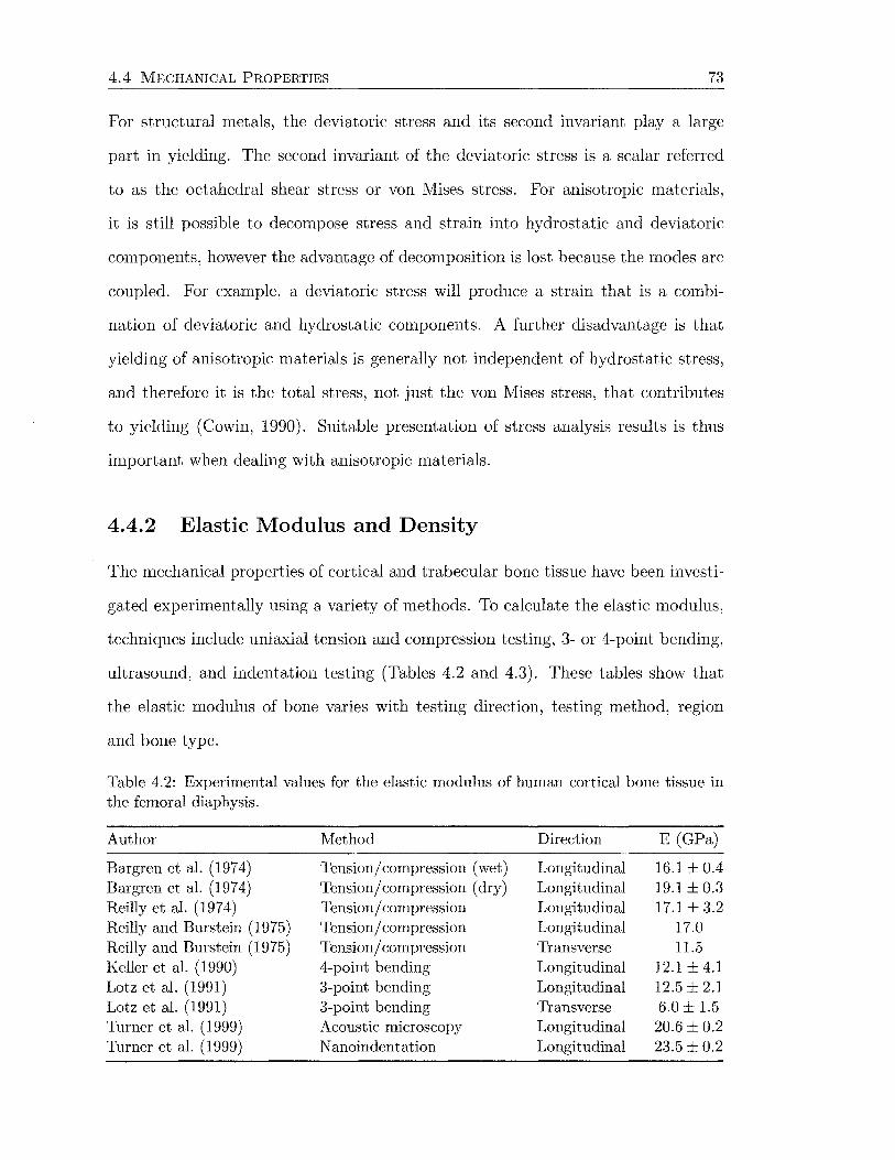
4.4 MECHANICAL PROPERTIES 73
For structural metals, the deviatoric stress and its second invariant play a large
part in yielding. The second invariant of the deviatoric stress is a scalar referred
to as the octahedral shear stress or von Mises stress. For anisotropic materials,
it is still possible to decompose stress and strain into hydrostatic and deviatoric
components, however the advantage of decomposition is lost because the modes are
coupled. For example, a deviatoric stress will produce a strain that is a combi-
nation of deviatoric and hydrostatic components. A further disadvantage is that
yielding of anisotropic materials is generally not independent of hydrostatic stress,
and therefore it is the total stress, not just the von Mises stress, that contributes
to yielding (Cowin, 1990). Suitable presentation of stress analysis results is thus
important when dealing with anisotropic materials.
4.4.2 Elastic Modulus and Density
The mechanical properties of cortical and trabecular bone tissue have been investi-
gated experimentally using a variety of methods. To calculate the elastic modulus,
techniques include uniaxial tension and compression testing, 3- or 4-point bending,
ultrasound, and indentation testing (Tables 4.2 and 4.3). These tables show that
the elastic modulus of bone varies with testing direction, testing method, region
and bone type.
Table 4.2: Experimental values for the elastic modulus of human cortical bone tissue in the femoral diaphysis.
Author Method Direction E (GPa)
Bargren et al. (1974) Tension/ compression (wet) Longitudinal 16.1 ± 0.4 Bargren et al. (1974) Tension/ compression (dry) Longitudinal 19.1 ± 0.3 Reilly et al. (1974) Tension/ compression Longitudinal 17.1±3.2 Reilly and Burstein (1975) Tension/ compression Longitudinal 17.0 Reilly and Burstein (1975) Tension/ compression Transverse 11.5 Keller et al. (1990) 4-point bending Longitudinal 12.1 ± 4.1 Lotz et al. (1991) 3-point bending Longitudinal 12.5 ± 2.1 Lotz et al. (1991) 3-point bending Transverse 6.0 ± 1.5 Turner et al. (1999) Acoustic microscopy Longitudinal 20.6 ± 0.2 Turner et al. (1999) N anoindentation Longitudinal 23.5 ± 0.2
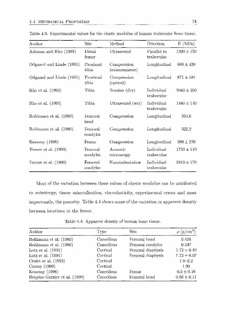
4.4 MECHANICAL PROPERTIES 74
Table 4.3: Experimental values for the elastic modulus of human trabecular bone tissue.
Author Site Method Direction E (MPa)
Ashman and Rho (1988) Distal Ultrasound Parallel to 1300 ± 150 femur trabeculae
Odgaard and Linde (1991) Proximal Compression Longitudinal 689 ± 438 tibia ( extensometer)
Odgaard and Linde (1991) Proximal Compression Longitudinal 871 ± 581 tibia (optical)
Rho et al. (1993) Tibia Tension (dry) Individual 1040 ± 350 trabeculae
Rho et al. (1993) Tibia Ultrasound (wet) Individual 1480 ± 140 trabeculae
Rohlmann et al. (1980) Femoral Compression Longitudinal 394.6 head
Rohlmann et al. ( 1980) Femoral Compression Longitudinal 322.2 condyles
Keaveny (1998) Femur Compression Longitudinal 389 ± 270
Turner et al. (1999) Femoral Acoustic Individual 1750±110 condyles microscopy trabeculae
Thrner et al. (1999) Femoral N anoindentation Individual 1810 ± 170 condyles trabeculae
Most of the variation between these values of elastic modulus can be attributed
to anisotropy, tissue mineralisation, viscoelasticity, experimental errors and most
importantly, the porosity. Table 4.4 shows some of the variation in apparent density
between locations in the femur.
Table 4.4: Apparent density of human bone tissue.
Author Type Site p (g/cm3)
Rohlmann et al. (1980) Cancellous Femoral head 0.426 Rohlmann et al. (1980) Cancellous Femoral condyles 0.347 Lotz et al. (1991) Cortical Femoral diaphysis 1.72 ± 0.10 Lotz et al. (1991) Cortical Femoral diaphysis 1.73 ± 0.07 Crolet et al. (1993) Cortical 1.8-2.2 Currey (1998) Cortical 1.99 Keaveny (1998) Cancellous Femur 0.5 ± 0.16 Bruyere Garnier et al. (1999) Cancellous Femoral head 0.56 ± 0.11

4.4 MECHANICAL PROPERTIES 75
Because of the significant effect of porosity on the mechanical properties of bone,
many empirical relationships have been derived to calculate these properties as a
function of the apparent density. The most frequently cited is the cubic relationship
between compressive elastic modulus and apparent density, published by Carter and
Hayes (1976, 1977), in which
( 4.4)
where Ec is the compressive modulus of cortical bone and Pc is the density of cortical
bone. If Ec = 22 000 MPa and Pc = 1.8 g/ cm3 for bone tested at E- = 0.1 s-1,
Equation 4.4 becomes
( 4.5)
This relationship assumes cortical and trabecular bone are effectively the same ma
terial, differing only in porosity. The strain rate-dependence of the elastic modulus
is due to viscoelasticity. All biological materials display at least some viscoelasticity
(Reilly and Burstein, 1974). Experimental testing has shown that elastic modulus
and ultimate stress increase with strain rate, while strain to failure decreases with
strain rate. Viscoelastic phenomena include creep, stress relaxation and dynamic re
sponse. These properties arise from the combined behaviour of the mineral, organic
and fluid components of bone. Collagen, motion at cement lines between osteons
and between lamellae within osteons, thermoelastic damping from heat flow be
tween osteons and stress-induced fluid flow through the porous bone matrix are all
potential sources of viscoelasticity (Garner et al., 2000). The mineral phase of bone
is effectively elastic (Yamashita et al., 2000).
Researchers have argued that trabecular and cortical bone should have sepa
rate relationships to describe their mechanical properties (e.g., Ashman and Rho,
1988; Evans, 1973; Keller, 1994; Rho et al., 1993; Rice et al., 1988; Schaffier and
Burr, 1988), since cancellous bone is more metabolically active, is remodelled more
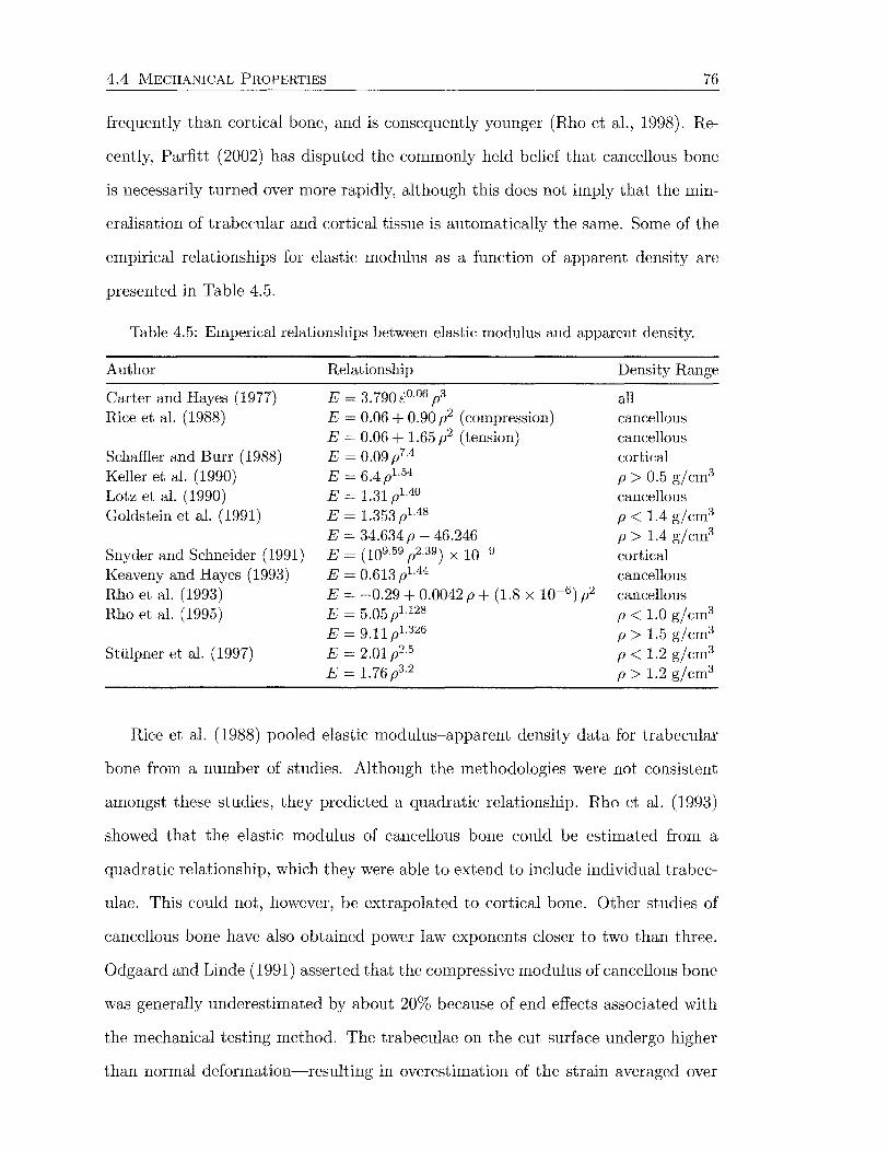
4.4 MECHANICAL PROPERTIES 76
frequently than cortical bone, and is consequently younger (Rho et al., 1998). Re
cently, Parfitt (2002) has disputed the commonly held belief that cancellous bone
is necessarily turned over more rapidly, although this does not imply that the min-
eralisation of trabecular and cortical tissue is automatically the same. Some of the
empirical relationships for elastic modulus as a function of apparent density are
presented in Table 4.5.
Table 4.5: Emperical relationships between elastic modulus and apparent density.
Author
Carter and Hayes ( 1 977) Rice et al. (1988)
Schaffier and Burr (1988) Keller et al. (1990) Lotz et al. (1990) Goldstein et al. (1991)
Snyder and Schneider (1991) Keaveny and Hayes (1993) Rho et al. (1993) Rho et al. (1995)
Sttilpner et al. (1997)
Relationship
E = 3.790i0·06 p3
E = 0.06 + 0.90 p2 (compression) E = 0.06 + 1.65 p2 (tension) E = 0.09p7·4
E = 6.4 Pl. 54
E = 1.31 p1.4o E = 1.353 pl.48
E = 34.634 p - 46.246 E = (109.59 P2.39) x 10-9
E = 0.613 pl.44
E = -0.29 + 0.0042 p + (1.8 X 10⁻⁶ ) p2
E = 5.05 pu28
E = 9.11 Pl.326
E = 2.01p2·5
E = 1.76 p3·2
Density Range
all cancellous cancellous cortical p > 0.5 gjcm3
cancellous p < 1.4 gjcm3
p > 1.4 gjcm3
cortical cancellous cancellous p < 1.0 gjcm3
p > 1.5 g/cm3
p < 1.2 gjcm3
p > 1.2 g/cm3
Rice et al. (1988) pooled elastic modulus-apparent density data. for trabecular
bone from a. number of studies. Although the methodologies were not consistent
amongst these studies, they predicted a. quadratic relationship. Rho et al. (1993)
showed that the elastic modulus of cancellous bone could be estimated from a.
quadratic relationship, which they were able to extend to include individual trabec
ulae. This could not, however, be extrapolated to cortical bone. Other studies of
cancellous bone have also obtained power law exponents closer to two than three.
Odga.a.rd and Linde (1991) asserted that the compressive modulus of cancellous bone
was generally underestimated by about 20% because of end effects associated with
the mechanical testing method. The trabeculae on the cut surface undergo higher
than normal deformation-resulting in overestimation of the strain averaged over
4.4 MECHANICAL PROPERTIES 77
the compression specimen. This may account for some of the variation between the
many modulus~density relationships in Table 4.5.
Empirical relationships based on the apparent density have also been determined
for bone strength (e.g., Carter and Hayes, 1977; Keller et al., 1990; Rice et al., 1988;
Snyder and Schneider, 1991).
4.4.3 Noninvasive Measurement of Bone Density
To determine bone apparent density in the laboratory, the bone tissue weight is
measured and divided by the bulk volume of the sample. Noninvasive methods
for measuring bone apparent density include quantitative computed tomography,
single- and dual-energy absorptiometry, and ultrasonography (Lotz et al., 1990).
Problems with these methods include beam hardening, radiation scattering and
effects of marrow and overlying tissue.
X-ray absorptiometry methods quantify the total bone mineral content (BMC)
contained within a three-dimensional region scanned by an x-ray beam. This is a
projection method, in which all information on bone mass is scanned down to a
two-dimensional plane. The BMC is often normalised by the projected area of the
region scanned, to obtain areal bone mineral density (BMD) (Kaufman and Siffert,
2001).
Dual-energy x-ray absorptiometry (DEXA) provides a measure of the bone min
eral density (BMD) by using two different energy sources and comparing the differ
ence in attenuation. This allows the effects of soft tissue to be separated out. Early
systems used gamma rays rather than x-rays for the photon source, with less accu
rate results. DEXA systems can use either a fan source beam coupled to an array
of detectors, or a pencil beam with a single detector. The fan beam configuration
allows for a straight path scan along the region of interest, whilst the pencil beam
follows a slower two-dimensional raster scan path (Blake et al., 1993). Single-energy
x-ray absorptiometry measures x-ray absorption at a single energy only, and thus
cannot compensate for varying amounts of soft tissue. Consequently, single-energy

4.4 MECHANICAL PROPERTIES 78
methods are useful for anatomical sites where the amount of soft tissue is negli
gible. Unfortunately, x-ray absorptiometry methods do not discriminate between
cortical and trabecular bone, lumping together the bone mass from cortical and
trabecular portions at a particular site. In addition, only areal BMD is measured,
not volumetric density. In vivo studies show DEXA has precision errors of less than
5% (Kilgus et al., 1993; Kiratli et al., 1992; Rahmy et al., 2000). However, Kiratli
et al. (1992) found that rotations of ±5° of the femur has a significant influence on
the area of the scanning region, leading to a variation in BMD of over 5%, while
Rahmy et al. (2000) measured variation up to 20% for femoral rotation of ±15°.
The most significant changes occurred in smaller regions of interest, where the area
measurement is strongly influenced by rotation of the femur.
Computed tomography (CT), like x-ray absorptiometric methods, are available
in single- or dual-energy modes. The single-energy method provides the most re
producible results over the majority of conditions and is most widely used (Mirsky
and Einhorn, 1998). An x-ray source is also employed. CT scanners have developed
considerably over the years to reduce scan times and radiation exposure.
First generation scanners use parallel-beam geometry. Multiple measurements
are obtained using a single x-ray pencil beam and detector. The beam is translated
in a linear motion across the patient to obtain a projection profile. The source
and detector are then rotated by about 1 o around the patient and another projec
tion profile is obtained. This translate-rotate scanning motion is repeated until
the source and detector have been rotated by 180 degrees. The second generation
scanners use a narrow fan beam with multiple detectors to increase scan speed. A
translate-rotate scanning motion is still employed, with a larger rotation increment
(up to 30°). With third generation scanners, a curved detector array consisting
of several hundred independent detectors is mechanically coupled to the fan beam
x-ray source, and both rotate together. The fan beam is larger (30-60°), keeping
the patient in view at all times. For the fourth generation of computed tomography
scanners, the x-ray fan beam rotates while the detector array remains stationary.
4.4 MECHANICAL PROPERTIES 79
The detector array consists of 600 to 4800 (depending on the manufacturer) inde
pendent detectors in a circle that completely surround the patient.
The requirement for faster scan times, and in particular fast multiple scans
for three-dimensional images, has resulted in the development of spiral (helical)
scanning systems. Helical scanners employ continuous rotation of the x-ray source
and/ or detector array, coupled with simultaneous translation along the scanning
axis, to create uninterrupted three-dimensional data. Both third and fourth gener
ation systems achieve this using slip rings to replace cumbersome electrical cables.
Data acquired from all of these scanners are reconstructed using computer soft
ware. Naturally, the reconstruction algorithms become more sophisticated as the
scanner technology improves. A computed tomography scan image consist of many
cells (pixels) each assigned a H ounsfield unit (HU or CT number), which is a di
mensionless number relating the linear attenuation coefficient of the material in the
pixel to the attenuation coefficient of water. A pixel is a two-dimensional represen
tation of a corresponding tissue volume, called a voxel. Voxel size is determined by
the pixel size and the CT slice thickness.
CT measurements can be quantified by scanning alongside calibration phantoms
of known density, such as liquid dipotassium hydrogen phosphate (Esses et al., 1989;
Lotz et al., 1990; Marom and Linden, 1990; Revak, 1980), solid tricalcium phosphate
(Snyder and Schneider, 1991) and solid hydroxyapatite (Cody et al., 1996). One of
the benefits of quantitative CT (QCT) is a linear relationship between attenuation
coefficients and equivalent mineral density. The equivalent mineral density is ex
pressed in terms of mg/mm3 of the calibration material (e.g., mg/mm3 of K2HP04).
Bone apparent density is similarly related to the attenuation coefficients and equiv
alent mineral density (Table 4.6). Other advantages include direct measurement
of a volume of bone, and ability to separately assess trabecular and cortical bone.
Individual bones are usually scanned in water to reduce beam hardening artefacts.

4.4 MECHANICAL PROPERTIES 80
Table 4.6: Emperical relationships between apparent density (g/cm3) and CT data (CT number, HU; equivalent mineral density, QCT). Note. tonly 2 points used.
Author
Esses et al. (1989) Lotz et al. (1990) Snyder and Schneider (1991) Rho et al. (1995) Cody et al. (1996) Couteau et al. (1998) (prox. femur) Couteau et al. (1998) (dist. femur)
Relationship
p = 1.9 X 10⁻³ QCT + 0.105 p = 0.0012 QCT + 0.17 p = 0.701 HU X 10-3
p = (1.076 HU + 131) X 10-3
p = 0.002QCT- 2 p = (1.5 HU + 17.2) X 10-3
p = (1.2HU + 303) X 10-3
Correlation
R 2 = 0.60 R2 = 0.73 R 2 = 0.65 R 2 = 0.84 t
R 2 = 0.80 R 2 = 0.74

Chapter 5
Stress Analysis of the Femur
This chapter reviews the literature on the subject of experimental and finite element
stress analysis of the femur, with respect to the alteration of load transfer pathways
following hip arthroplasty. Both of these techniques have intrinsic advantages and
disadvantages when applied to this subject.
In the natural femur, the joint force is distributed across the entire cross-section
of the femur through a combination of bending and axial loads, with relatively
minor loads. When the femur is implanted with a prosthesis, the applied load
is redistributed in a quite different manner. The bending loads are transmitted
by localised contact stresses between the implant and bone, while axial loads are
transferred by shear at the interface (Joshi et al., 2000b). Experimental and finite
element stress analysis methods are able to evaluate this redistribution of loads to
the femur.
5.1 Experimental Stress Analysis
Experimental methods for stress analysis of the femur include strain gauge (reviewed
here) and photoelastic (e.g., Engh et al., 1992b; Finlay et al., 1989; Glisson et al.,
2000; Hua and \Valker, 1995) techniques. Strain gauge studies are most abundant in
the literature as they give quantitative strain values at discrete locations, although
they have the disadvantage of only measuring site-specific strains, thus giving no
81
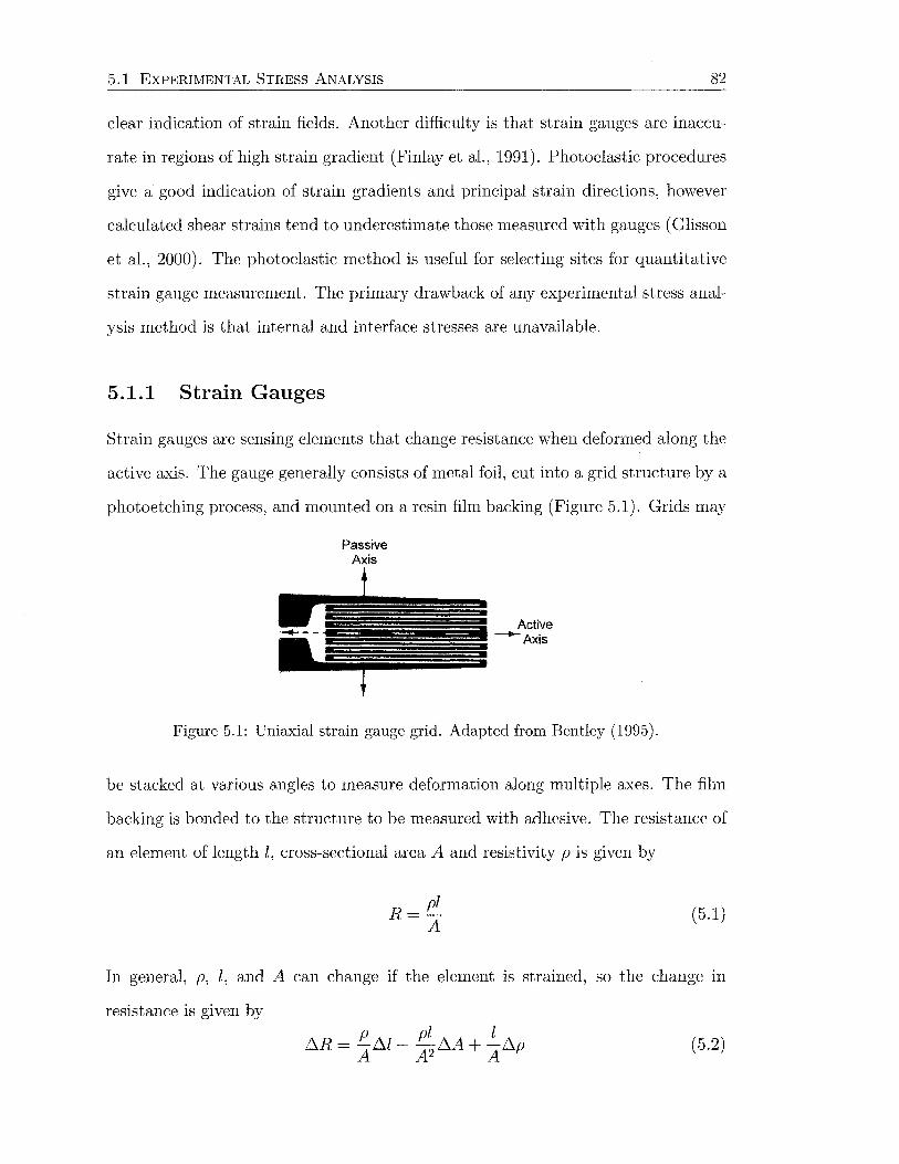
5.1 EXPERIMENTAL STRESS ANALYSIS 82
clear indication of strain fields. Another difficulty is that strain gauges are inaccu
rate in regions of high strain gradient (Finlay et al., 1991). Photoelastic procedures
give a good indication of strain gradients and principal strain directions, however
calculated shear strains tend to underestimate those measured with gauges (Glisson
et al., 2000). The photoelastic method is useful for selecting sites for quantitative
strain gauge measurement. The primary drawback of any experimental stress anal
ysis method is that internal and interface stresses are unavailable.
5.1.1 Strain Gauges
Strain gauges are sensing elements that change resistance when deformed along the
active axis. The gauge generally consists of metal foil, cut into a grid structure by a
photoetching process, and mounted on a resin film backing (Figure 5.1). Grids may
Passive Axis
Figure 5.1: Uniaxial strain gauge grid. Adapted from Bentley (1995).
be stacked at various angles to measure deformation along multiple axes. The film
backing is bonded to the structure to be measured with adhesive. The resistance of
an element of length l, cross-sectional area A and resistivity p is given by
R= pl A
(5.1)
In general, p, l, and A can change if the element 1s strained, so the change in
resistance is given by p pl l
~R = -~l- -~A+ -~p A A2 A
(5.2)

5.1 EXPERIMENTAL STRESS ANALYSIS 83
and dividing through by R = pl /A yields
!:1R !:1l !:1A !:1p -=---+-R l A p
(5.3)
The ratio f1l/l is the longitudinal strain in the element. The strain E is related to
the change in resistance by the gauge factor G
!:1R = Gc: Ro
(5.4)
where R0 is the unstrained resistance of the gauge. Strain gauge elements are
incorporated in resistive, or Wheatstone bridge circuits, to convert the output into
a voltage signal (Figure 5.2). The output voltage Erh is a function offour resistances
~----o~o-----~
Figure 5.2: Wheatstone bridge. Reproduced from Bentley (1995).
R 1 to R4 and the input, or source, voltage Vs
(5.5)
If R 1 is the sensing element (strain gauge), and R 2 to R4 are fixed resistors, it is
required that the fixed resistances are all equal to the unstrained resistance of the
sensing element R0 , for the sensitivity to be as high as possible (Bentley, 1995).
This leads to the linear relationship between output voltage and strain
Vs Erh = 4 cc: (5.6)
5.1 EXPERIMENTAL STRESS ANALYSIS 84
The output voltages are typically amplified and recorded using analogue-to-digital
conversion.
5.1.2 Strain Gauge Studies
Most experimental strain gauge studies in orthopaedic research have investigated
the mechanical response of the femur to hip arthroplasty. The cortical strain dis
tribution of the intact femur is first determined by mechanical testing under a pre
scribed loading, and then tested again after implantation of a hip prosthesis. These
investigations give a measure of the load transfer for the implant-bone system.
The loading employed by most researchers is static and often pseudo-physiological.
The strain distribution for the intact femur usually shows the femur bending in
the coronal plane, with compressive strains medially and tensile strains laterally.
The highest strains are proximal, decreasing distally (e.g., Cristofolini et al., 1995;
Huiskes et al., 1981; McNamara et al., 1997a; Oh and Harris, 1978; Otani et al.,
1993), with this situation reversed following surgery.
Stress Shielding
Significant reductions in strain in the proximal medial femur have been reported
for both cemented (Cristofolini et al., 1997; Finlay et al., 1989; Oh and Harris,
1978; Rohlmann et al., 1987, 1983) and uncemented (Cristofolini et al., 1997; Diegel
et al., 1989; Engh et al., 1992b; Finlay et al., 1991, 1989; Kim et al., 2001; Vanderby
et al., 1990) implant types. Calcar strains are not significantly increased with more
flexible prosthesis materials (Diegel et al., 1989; Oh and Harris, 1978; Simoes and
Vaz, 2002), with all producing significant stress shielding. Stem length (Huiskes
et al., 1981), diameter (Jasty et al., 1994) or surface features (Gillies et al., 2002)
also have little effect. Many authors agree that the congruency between the implant
and the prepared femur is most important for load transfer (Diegel et al., 1989; Jasty
et al., 1994; Simoes and Vaz, 2002), with precise calcar-collar contact (Figure 5.3)
also helpful if present (Jasty et al., 1994; Oh and Harris, 1978; Vander Sloten et al.,
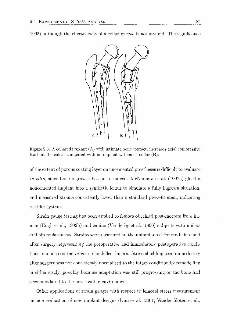
5.1 EXPERIMENTAL STRESS ANALYSIS 85
1993), although the effectiveness of a collar in vivo is not assured. The significance
Figure 5.3: A collared implant (A) with intimate bone contact, increases axial compressive loads at the calcar compared with an implant without a collar (B).
of the extent of porous coating layer on uncemented prostheses is difficult to evaluate
in vitro, since bone ingrowth has not occurred. McNamara et al. (1997a) glued a
noncemented implant into a synthetic femur to simulate a fully ingrown situation,
and measured strains consistently lower than a standard press-fit stem, indicating
a stiffer system.
Strain gauge testing has been applied to femora obtained post-mortem from hu-
man (Engh et al., 1992b) and canine (Vanderby et al., 1990) subjects with unilat-
eral hip replacement. Strains were measured on the unimplanted femora before and
after surgery, representing the preoperative and immediately postoperative condi-
tions, and also on the in vivo remodelled femora. Stress shielding seen immediately
after surgery was not consistently normalised to the intact condition by remodelling
in either study, possibly because adaptation was still progressing or the bone had
accommodated to the new loading environment.
Other applications of strain gauges with respect to femoral stress measurement
include evaluation of new implant designs (Kim et al., 2001; Vander Slaten et al.,
5.1 EXPERIMENTAL STRESS ANALYSIS 86
1993; Viceconti et al., 2001a), measurement of strain during femoral canal prepara
tion and prosthesis insertion (Elias et al., 2000), and verification of finite element
models (McNamara et al., 1994; Rohlmann et al., 1982, 1983; Stolk et al., 2002).
The femora tested in all of these studies are either fresh frozen (Diegel et al.,
1989; Elias et al., 2000; Gillies et al., 2002; Glisson et al., 2000; Kim et al., 2001;
Oh and Harris, 1978; Otani et al., 1993), embalmed (Cristofolini et al., 1995; Hua
and Walker, 1995; Huiskes et al., 1981; Jasty et al., 1994; Sedlacek et al., 1997), dry
(Vander Slaten et al., 1993), or synthetic (Cristofolini et al., 1997; McNamara et al.,
1997a; Simoes and Vaz, 2002; Viceconti et al., 2001a). Synthetic bones are produced
from composite materials to recreate the mechanical properties of cadaveric bone,
without the inter-specimen variability or the difficulty of obtaining specimens.
Loading and Constraints
The systems of forces found in the literature vary widely with different numbers of
muscles and force magnitudes and directions. This is partially due to the differ
ent situations simulated, for example, single-legged stance, two-legged stance, and
various phases of the gait cycle. Some authors tried to make the set up as sim
ple as possible with a single force, while others included a high number of muscle
forces. Some of the common arrangements include a single force on the femoral
head (Diegel et al., 1989; Huiskes et al., 1981; Oh and Harris, 1978; Otani et al.,
1993), the hip joint force and the action of the abductor muscles grouped together
(Cristofolini et al., 1994; Engh et al., 1992b; Finlay et al., 1989; Gillies et al., 2002;
Glisson et al., 2000; Tanner et al., 1988; Vander Slaten et al., 1993), or the hip joint,
abductor and iliotibial tract forces (Finlay et al., 1991; Kim et al., 2001; Rohlmann
et al., 1982). A minority of authors have simulated additional forces such as the
vastus muscles, adductors and rectus femoris (Cristofolini et al., 1995; Munting and
Verhelpen, 1993; Simoes et al., 2000), however Cristofolini et al. (1995) excluded

5.1 EXPERIMENTAL STRESS ANALYSIS 87
the iliotibial tract. Figure 5.4 shows the difference in load transfer when the ab-
ductor muscles are not included, and the potential for overestimating lateral stress
shielding.
(a) Load transfer path with the hip joint reaction force alone.
(b) Load transfer path with the hip joint reaction and abductor muscle forces.
Figure 5.4: Load transfer mechanism for an uncemented prosthesis with and without abductor muscle action present. Reproduced from Cristofolini (1997).
Some methodological studies have been performed to evaluate how the loading
conditions affect the stress distribution of the femur. Rohlmann et al. (1983) found
that a single force applied parallel to the femoral shaft produced strains similar to
loading with hip joint, abductor and iliotibial tract forces. The iliotibial tract force
reduced the bending from hip joint abductor actions. Finlay et al. (1991) concluded
that loading should at least incorporate the abductor muscle force, the iliotibial
tract, or both, in addition to the hip joint force. The iliotibial tract in conjunction
with the joint force increased proximal strains on the medial aspect, while decreasing
tensile strains distally on the lateral aspect, both before and after arthroplasty with
a noncemented hip. The iliotibial tract applied additional compressive loads to the
proximal femur, reducing large tensile bending strains laterally.

5.1 EXPERIMENTAL STRESS ANALYSIS 88
Finlay et al. (1989) found that abductor muscle forces increased medial and
lateral strains while reducing proximal bending. Similarly, McNamara et al. (1997a)
measured strains without abductor simulation that were typically one-third of those
measured with the abductor forces present.
Cristofolini et al. (1995) estimated the importance of simulating various muscle
groups in in vitro mechanical testing of the femur at heel strike. The gluteal mus
cles, adductors, vasti and rectus femoris were investigated. The iliotibial tract was
not included as it was thought to be inactive at heel strike. The gluteal muscles
dominated over all others, with axial strains always at least twice as high as those
generated by other muscles. Rectus femoris was the second most significant muscle,
producing strains 10-50% of those due to the glutei. The vasti were found to be
the least relevant muscle group. This study formed the basis of the development of
a standard heel strike loading test protocol (Cristofolini et al., 1994), in which only
the hip joint and abductor muscles forces were incorporated (Figure 5.5). Rulers
and goniometers were used to ensure force directions and positions were controlled.
A load cell monitored the abducting force.
Aamodt et al. (1997) measured strain on the lateral femur in vivo at a position
35 mm below the lateral eminence of the greater trochanter in two patients. Strains
were measured in single- and two-legged stance, during walking and stair climbing.
Strains during activity were tensile, with maximum principal strains aligned with
the long axis of the femur during stance. These results suggested that the action of
the lateral musculature is not sufficient to overcome the bending moment imposed
by the joint force.
The distal constraints on the femur are also varied. The literature reports the
femur either fixed at the diaphysis (Engh et al., 1992b; Gillies et al., 2002; Hua and
Walker, 1995; Otani et al., 1993; Tanner et al., 1988), or at the condyles (Cristofolini
et al., 1994; Diegel et al., 1989; Finlay et al., 1989; Glisson et al., 2000; Kim et al.,
2001; Munting and Verhelpen, 1993; Oh and Harris, 1978; Vanderby et al., 1990).
Translations are usually fixed distally, however some rotational degrees-of-freedom

5.1 EXPERIMENTAL STRESS ANALYSIS
on lesser trochanter
c
89
®
Figure 5.5: Set up used for applying the hip joint and abductor forces to the femur. (1-5) Rulers and goniometers to measure force directions. (6) Load cell to monitor the abdcutor force. Reproduced from Cristofolini (1997).
may be unconstrained. Proximal constraints are also important to ensure that the
femur is loading isostatically. Figure 5.6 shows how the femur may by constrained
to reproduce physiological loading, even with nonphysiological constraints.
Experimental Errors
Viceconti et al. (1992) examined the effects of some factors not controlled in most
experimental strain gauge studies. They investigated the importance of loading
rate, bone preservation method, strain gauge preservation, bone temperature and
bone hydration on strain measurement. Strain rate was found to be unimportant,
freezing altered mechanical properties less than embalming, moisture penetration
under the gauge could be reduced with a thin layer of polyurethane film, while bone
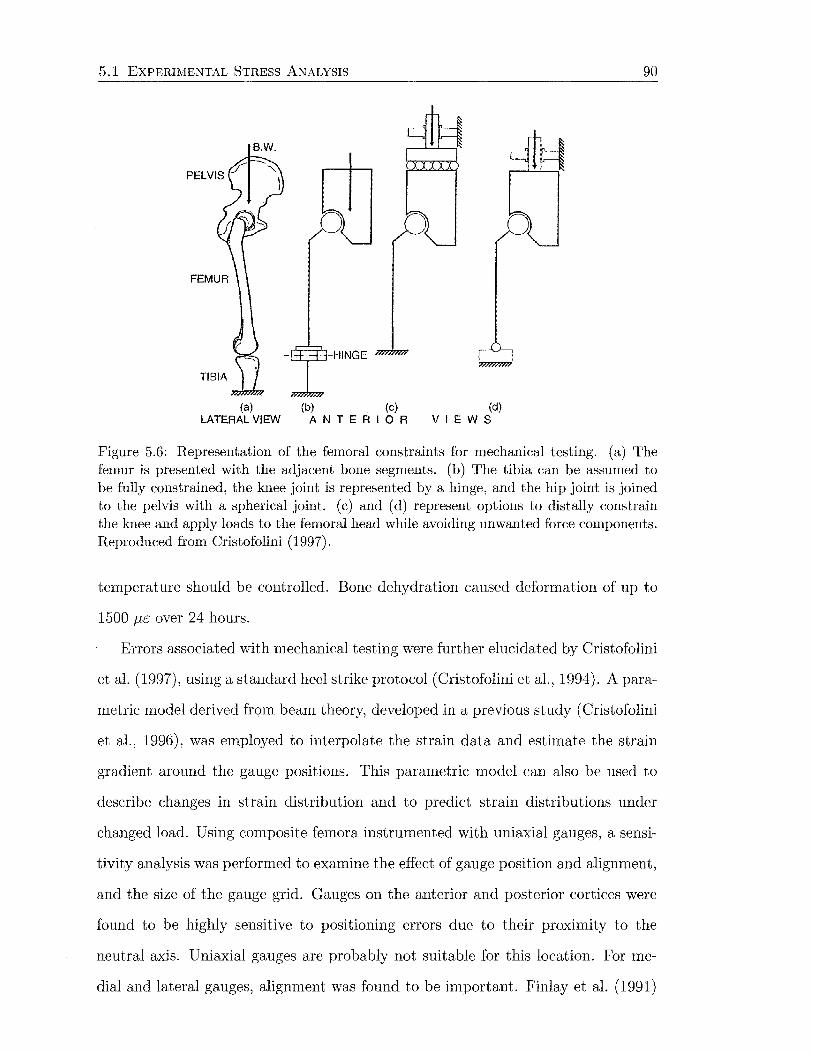
5.1 EXPERIMENTAL STRESS ANALYSIS
B.W.
(a) (b) (c) LATERAL VIEW A N T E A I 0 A
(d) VIEWS
90
Figure 5.6: Representation of the femoral constraints for mechanical testing. (a) The femur is presented with the adjacent bone segments. (b) The tibia can be assumed to be fully constrained, the knee joint is represented by a hinge, and the hip joint is joined to the pelvis with a spherical joint. (c) and (d) represent options to distally constrain the knee and apply loads to the femoral head while avoiding unwanted force components. Reproduced from Cristofolini (1997).
temperature should be controlled. Bone dehydration caused deformation of up to
1500 Jl£ over 24 hours.
Errors associated with mechanical testing were further elucidated by Cristofolini
et al. (1997), using a standard heel strike protocol (Cristofolini et al., 1994). A para
metric model derived from beam theory, developed in a previous study ( Cristofolini
et al., 1996), was employed to interpolate the strain data and estimate the strain
gradient around the gauge positions. This parametric model can also be used to
describe changes in strain distribution and to predict strain distributions under
changed load. Using composite femora instrumented with uniaxial gauges, a sensi
tivity analysis was performed to examine the effect of gauge position and alignment,
and the size of the gauge grid. Gauges on the anterior and posterior cortices were
found to be highly sensitive to positioning errors due to their proximity to the
neutral axis. Uniaxial gauges are probably not suitable for this location. For me-
dial and lateral gauges, alignment was found to be important. Finlay et al. (1991)
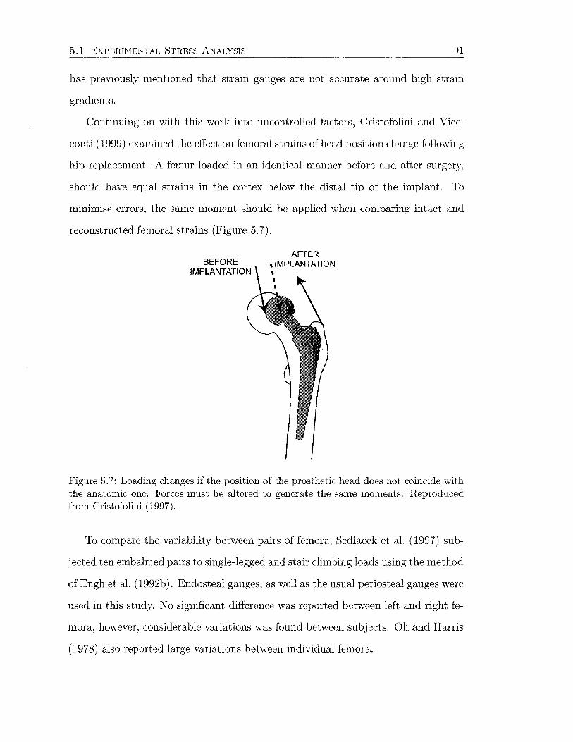
5.1 EXPERIMENTAL STRESS ANALYSIS 91
has previously mentioned that strain gauges are not accurate around high strain
gradients.
Continuing on with this work into uncontrolled factors, Cristofolini and Vice
conti (1999) examined the effect on femoral strains of head position change following
hip replacement. A femur loaded in an identical manner before and after surgery,
should have equal strains in the cortex below the distal tip of the implant. To
minimise errors, the same moment should be applied when comparing intact and
reconstructed femoral strains (Figure 5. 7).
BEFORE IMPLANTATION
AFTER , IMPLANTATION
Figure 5.7: Loading changes if the position of the prosthetic head does not coincide with the anatomic one. Forces must be altered to generate the same moments. Reproduced from Cristofolini (1997).
To compare the variability between pairs of femora, Sedlacek et al. (1997) sub
jected ten embalmed pairs to single-legged and stair climbing loads using the method
of Engh et al. (1992b). Endosteal gauges, as well as the usual periosteal gauges were
used in this study. No significant difference was reported between left and right fe-
mora, however, considerable variations was found between subjects. Oh and Harris
(1978) also reported large variations between individual femora.
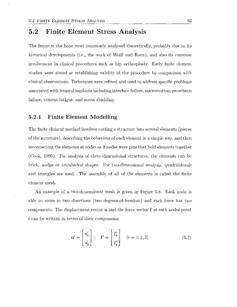
5.2 FINITE ELEMENT STRESS ANALYSIS 92
5.2 Finite Element Stress Analysis
The femur is the bone most commonly analysed theoretically, probably due to its
historical developments (i.e., the work of Wolff and Roux), and also its common
involvement in clinical procedures such as hip arthroplasty. Early finite element
studies were aimed at establishing validity of the procedure by comparison with
clinical observations. Techniques were refined and used to address specific problems
associated with femoral implants including interface failure, micromotion, prosthesis
failure, cement fatigue, and stress shielding.
5.2.1 Finite Element Modelling
The finite element method involves cutting a structure into several elements (pieces
of the structure), describing the behaviour of each element in a simple way, and then
reconnecting the elements at nodes as if nodes were pins that hold elements together
(Cook, 1995). For analysis of three-dimensional structures, the elements can be
brick, wedge or tetrahedral shapes. For two-dimensional analysis, quadrilaterals
and triangles are used. The assembly of all of the elements is called the finite
element mesh.
An example of a two-dimensional mesh is given in Figure 5.8. Each node is
able to move in two directions (two degrees-of-freedom) and each force has two
components. The displacement vector u and the force vector f at each nodal point
i can be written in terms of their components
i [u~] i [ f~] u = ; f = ui fi
y y
(i = 1,2,3) (5.7)
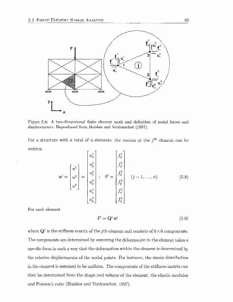
5.2 FINITE ELEMENT STRESS ANALYSIS 93
F
CD 3
3 f. -fJc:- u3 y y
Figure 5.8: A two-dimensional finite element mesh and definition of nodal forces and displacements. Reproduced from Huiskes and Verdonschot (1997).
For a structure with a total of n elements, the vectors at the lh element can be
written ul
X J]; ul f~ ul
y
uJ = u2
fj = J;
u2 X (j = 1, ... , n) (5.8) u2 t;
u3 y
u3 X t:
u3 y Jt
For each element
fJ = QJ uJ (5.9)
where QJ is the stiffness matrix of the jth element and consists of 6 x 6 components.
The components are determined by assuming the deformation in the element takes a
specific form in such a way that the deformation within the element is determined by
the relative displacements of the nodal points. For instance, the strain distribution
in the element is assumed to be uniform. The components of the stiffness matrix can
then be determined from the shape and volume of the element, the elastic modulus
and Poisson's ratio (Huiskes and Verdonschot, 1997).
5.2 FINITE ELEMENT STRESS ANALYSIS 94
The equations for each element (Equation 5.9) can be assembled together, in
the sense that all displacements and forces of the different elements belonging to
the same nodal point are collected. This produces a vector u containing all nodal
point displacement components and a vector f containing all nodal point force
components. For a linear elastic material with small deformations, these two vectors
are related by the m x m stiffness matrix Q, giving
f= Qu (5.10)
where m is the number of degrees-of-freedom in the model (usually 2n for a two
dimensional mesh and 3m for a three-dimensional mesh). The force components
are either zero where no external force is applied, or have a known value equal to
the external force. Displacements are unknown except where boundary constraints
are applied. The nodal displacements are calculated by solving Equation 5.10 for u
(5.11)
The result is usually obtained by some form of Gauss elimination or an iterative
method. The solution is always approximate because of two important simplifi
cations. The deformation of each is limited to a uniform strain field (i.e., linear
displacement), and all load transmission is assumed to occur at the nodal points.
The accuracy of the approximation depends on the element type and the degree of
mesh refinement. The solution converges to the exact solution as the mesh density
approaches infinity.
Different types of elements use different interpolation functions to represent the
coordinates and displacements in the subsequent calculations of stress and strain.
Simple elements with linear displacement fields have a limited number of degrees-of
freedom and therefore low computation time, however they are not able to represent
bending. A larger number of elements can be used, or a more sophisticated element
with a quadratic displacement field, and more nodes per element, may be employed.
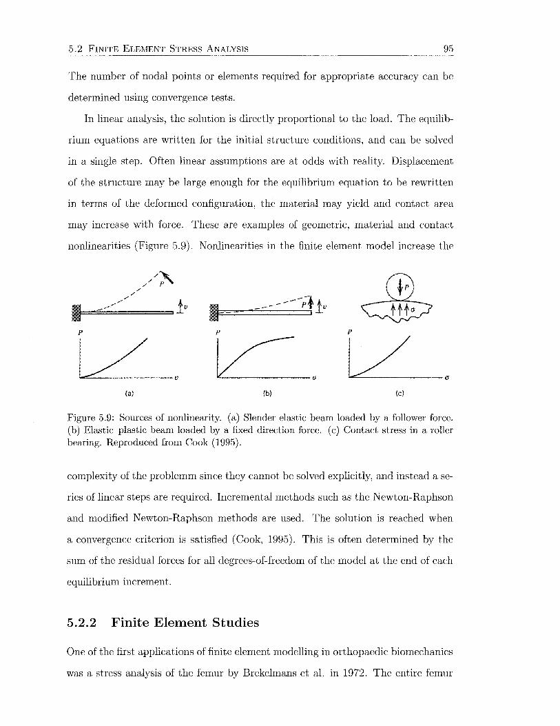
5.2 FINITE ELEMENT STRESS ANALYSIS 95
The number of nodal points or elements required for appropriate accuracy can be
determined using convergence tests.
In linear analysis, the solution is directly proportional to the load. The equilib-
rium equations are written for the initial structure conditions, and can be solved
in a single step. Often linear assumptions are at odds with reality. Displacement
of the structure may be large enough for the equilibrium equation to be rewritten
in terms of the deformed configuration, the material may yield and contact area
may increase with force. These are examples of geometric, material and contact
nonlinearities (Figure 5.9). Nonlinearities in the finite element model increase the
/ /
///~ /
~~=I =-==--=---/==it'
{a)
-------;· !v ,l
p p
L v L/ (b) {c)
Figure 5.9: Sources of nonlinearity. (a) Slender elastic beam loaded by a follower force. (b) Elastic-plastic beam loaded by a fixed direction force. (c) Contact stress in a roller bearing. Reproduced from Cook (1995).
complexity of the problemm since they cannot be solved explicitly, and instead a se
ries of linear steps are required. Incremental methods such as the Newton-Raphson
and modified Newton-Raphson methods are used. The solution is reached when
a convergence criterion is satisfied (Cook, 1995). This is often determined by the
sum of the residual forces for all degrees-of-freedom of the model at the end of each
equilibrium increment.
5.2.2 Finite Element Studies
One of the first applications of finite element modelling in orthopaedic biomechanics
was a stress analysis of the femur by Brekelmans et al. in 1972. The entire femur

5.2 FINITE ELEMENT STRESS ANALYSIS 96
was modelled in two dimensions, with 936 3-noded triangular elements of uniform
thickness (approximately 1074 nodal degrees-of-freedom). A three-dimensional, but
fairly coarse (around 969 degrees-of-freedom), model of the proximal femur was later
published by Valliappan et al. (1977). The three-dimensional model of the femur
developed by Rohlmann et al. (1982) was quite sophisticated by previous standards,
with 7188 degrees-of-freedom. Results from both of these three-dimensional studies
were compared with experimental data, showing conformity in a qualitative sense
only. These method-oriented studies were aimed at demonstrating the possible
applications of finite element modelling to biomechanics, rather than tackling any
specific problems.
Modelling the Femur
Expensive computational demands have meant that the femur is often modelled in
a simplified manner. Although the femur has asymmetric geometry and loading,
two-dimensional models have been created in the plane of the femoral neck. To
account for the structural stiffness of the normal femur, a side-plate is used by some
authors (e.g., Huiskes, 1990; Svensson et al., 1977; Weinans et al., 1992b, 1994).
The thickness of the side-plate is calculated so that the cross-sectional moment of
inertia of the model is equal to that of the three-dimensional femur being approx
imated (Figure 5.10). Further simplified side-plate models of a straight femoral
shaft are also in the literature (Huiskes, 1990; Huiskes et al., 1987; Kuiper and
Huiskes, 1997), along with three-dimensional axisymmetric models of the diaphysis
(Estok and Harris, 2000; Gross and Abel, 2001; Keaveny and Bartel, 1994; Nuno
and Amabili, 2002; Nuno and Avanzolini, 2002).
Anatomic three-dimensional finite element models more accurately represent the
geometry of the femur. The mesh can be created in either a "geometry-based" or
"voxel-based" process. Geometry-based meshing is most common and requires the
extraction of bone contours from CT scans using thresholding and edge-following

5.2 FINITE ELEMENT STRESS ANALYSIS 97
side plate
e-n
Figure 5.10: Two-dimensional side-plate model of the proximal femur accounting for three-dimensional rigidity in the frontal plane. Reproduced from Huiskes (1990).
algorithms (Huiskes et al., 1992; Keaveny and Bartel, 1993a; Mann et al., 1995; Mc
Namara et al., 1994), or by digitising contact radiographs of sectioned femurs (Cheal
et al., 1992; Kerner et al., 1999; Rohlmann et al., 1987; Weinans et al., 1993). The fe-
mur geometry must be reconstructed from the contours using computer-aided draw-
ing (CAD) packages or finite element pre-processors before meshing. This method
requires considerable time investment to perform manually, and consequently many
studies refer to a single bone geometry when, in many cases, anthropometric vari-
ability should not be neglected (Viceconti et al., 1998b).
Automated mesh generation (AMG) methods have been developed, which allow
relatively quick construction of patient-specific finite element models. Voxel-based
meshing is one of these automated procedures that creates nodes to form a cubic lat-
tice along orthogonal axes defined by the CT scanner. Bone contours are extracted
using the method described for geometry-based models, and the structure is created
by converting a voxel (see Section 4.4.3), or several adjacent voxels, directly into

5.2 FINITE ELEMENT STRESS ANALYSIS 98
brick elements if some part of the voxellies within the nearest bone contour. This
method tends to produce somewhat irregular surfaces (Figure 5.11a) and stresses
calculated here tend to oscillate around the theoretical solution (Guldberg et al.,
1998). Nevertheless, voxel-based models have been studied quite extensively by
(a) Voxel-based mesh. Reproduced from Skinner et al. (1994b).
(b) Geometry-based mesh. Reproduced from Viceconti et al. (1998b).
Figure 5.11: Automatic mesh generation methods.
some research groups (Keyak et al., 1993, 1990; Keyak and Skinner, 1992; Lengsfeld
et al., 1998; Weinans et al., 2000). Results from assessment of interface behaviour
when femoral prostheses are introduced (Namba et al., 1998; Skinner et al., 1994a,b)
are somewhat uncertain as the surfaces are not smooth. Cody et al. (1999, 2000a,b)
created subject-specific voxel-based models to predict fractures of the proximal fe-
mur giving reasonable correlation with mechanical testing.
5.2 FINITE ELEMENT STRESS ANALYSIS 99
Geometry-based automated mesh generation procedures have also been estab
lished that create meshes with smooth surfaces and larger element sizes (Fig
ure 5.11 b). These methods tend to alleviate some of the problems associated with
the voxel-based variety (Merz et al., 1996a,b; Viceconti et al., 1998b, 1999).
Material Properties
The majority of finite element models of the femur assume all bone to be a linear
elastic, continuum material. As stated in Section 4.4, some assumptions about the
material behaviour, particularly with respect to trabecular bone, are required for
bone to be modelled in such a manner. The trabecular length scale over which ma
terial properties should be averaged is about five intertrabecular lengths (Harrigan
et al., 1988), or about 5 mm according to Cowin (1993). When considering finite
element modelling of implant-bone systems, a significant issue is that within three
to five intertrabecular lengths of the implant or osteotomy, continuum modelling is
not valid and should be replaced by statistical models for the interface. The results
of continuum level studies around interfaces are correct if the actual compliances
of the region are similar to the continuum model. The continuum limitations do
not limit the degree of refinement necessary for accurate finite element analysis
(Harrigan et al., 1988).
Bone is assumed to be isotropic by most researchers; defined by two indepen
dent constants, the elastic modulus E and Poisson's ratio v. Cortical bone can be
approximated as transversely isotropic (Huiskes, 1997; Martinet al., 1998), and this
constitutive relationship is occasionally applied in finite element models (Pancanti
et al., 2003; Vichnin and Batterman, 1986). Vichnin and Batterman (1986) reported
that transversely isotropic properties in the diaphysis caused higher implant stresses
than isotropic properties. Transverse isotropy is a simplification of orthotropy, and
not as appropriate for describing the material behaviour of trabecular bone. Con
sequently, Wirtz et al. (2003) assigned orthotropic material axes to each element,
based on the trabecular orientation and Haversian system orientations for cortical
5.2 FINITE ELEMENT STRESS ANALYSIS 100
bone. Other researchers who have also applied orthotropic material properties to
their finite element models include Cheal et al. (1992) and Taylor et al. (2002).
Nevertheless, the use of isotropy and transverse isotropy are justified in many sit
uations, as the error due to simplification of the material model is often less than
the error from other sources (Cowin, 1993).
The elastic moduli assigned to the finite element meshes are typically homo
geneous for the bone type (cortical or cancellous), or inhomogeneous, with elastic
modulus dependent on the CT density at each element or integration point. The
elastic modulus-density relationships are empirical relationships, such as presented
earlier in Table 4.5. The relationship derived by Carter and Hayes (1977) (Equa
tion 4.5) is one of the most commonly used. For AMG models, inhomogeneous ma
terial properties are relatively straightforward to implement. Heterogeneity of bone
properties was investigated in a series of papers by Edinin and co-workers (Edinin
and Taylor, 1992; Edinin et al., 1991). The values of Poisson's ratio reported from
finite element studies is invariably constant for both cortical and cancellous bone,
ranging between 0.2 and 0.4, but 0.3 is the most common (Ando et al., 1999; Estok
and Harris, 2000; Harrigan and Harris, 1991; Kang et al., 1993; Keaveny and Bartel,
1993a,b; Mann et al., 1995; Taddei et al., 2003).
Investigators have also implemented homogenisation theory to model the porous
microstructure of trabecular bone (e.g., Bagge, 2000; Fernandes et al., 1999; Ped
ersen, 2002; Pettermann et al., 1997). The aim of homogenisation is to represent a
heterogeneous medium as a homogeneous continuum that has the same macroscopic
behaviour (Prendergast, 1997). The isotropy of the homogenised material depends
on the behaviour of the microstructural building blocks.
The advent of high resolution J.LCT scanners has led to geometry-based AMG
models for small volumes of trabecular bone (Ladd and Kinney, 1998; Ulrich et al.,
1998). Ladd and Kinney (1998) showed that for a small volume of trabecular bone,
variation of Poisson's ratio between 0.15 and 0.35 had negligible effects on stiffness
of the structure. It is unlikely that whole bones will be modelled from J.LCT scans in

5.2 FINITE ELEMENT STRESS ANALYSIS 101
the foreseeable future, due to the massive computational expense linked with mesh
generation and solution solving.
Convergence
Mesh refinement and convergence analysis is rarely reported due to the large amount
of time required to produce a mesh manually (Viceconti et al., 1998b). Some re
searchers that have reported convergence include Valliappan et al. (1977), Vichnin
and Batterman (1986) and Biegler et al. (1995). Others have assumed convergence
by similarity with experimental results. Keyak et al. (1990) and Keyak and Skinner
(1992) examined convergence of a voxel-based model, but the use of strain energy
density as a measure of convergence in this case was disputed by Marks and Gardner
(1993).
Experimental verification
Early studies showed relative agreement with experimental results, but generally
not in an absolute sense (Rohlmann et al., 1982, 1983; Valliappan et al., 1977).
Rohlmann et al. (1983) attributed the difference in results to a number of errors,
due to: extrapolation of stresses from Gauss points, irregular element shapes, bone
geometry, bone properties, contact conditions, geometric linearity, deviations in
strain gauge positions, and ubiquitous experimental errors. The voxel-based model
of Keyak et al. (1993) tended to underestimate experimentally measured strains,
most likely due to imprecise modelling of the bone surface. Finite element models
of synthetic femora have been quite successfully verified at some length. MeN amara
et al. (1994) found better quantitative agreement with experimental results using
synthetic bones as opposed to cadaveric. Experimental testing of synthetic femora,
with and without hip replacement, was done under 4-point bending (McNamara
et al., 1994) and heel strike loading ( Cristofolini et al., 1997; MeN amara et al.,
1997a, 1996; Stalk et al., 2002).
5.2 FINITE ELEMENT STRESS ANALYSIS 102
Stress Shielding
Methods of reducing stress shielding have been studied in detail with finite element
modelling. These include the use of a collar and reduction of implant stiffness, either
by changing elastic modulus or moment of inertia. Rohlmann et al. (1987) stated
that a collar was unimportant for proximal bone stress, although cement stresses
were elevated proximally without it. Contrary to this, Keaveny and Bartel (1993a)
showed that loss of collar support greatly reduced proximal axial forces. Prendergast
and Taylor (1990) also found that a collar on a cemented stem increased stresses in
the calcar region. A low modulus (25 MPa) stem with a collar produced a stress
distribution most like the intact femur.
Unlike the experimental studies described above, elastic modulus of the pros
thesis has been found to have a significant effect on stress in the proximal femur
when modelled numerically. 1v1any researchers have reported a nonlinear inverse
relationship between cortical bone stress and implant modulus (Cheal et al., 1992;
Huiskes et al., 1992; McNamara et al., 1996; Namba et al., 1998; Rohlmann et al.,
1987; Tensi et al., 1989; Weinans et al., 2000) with a greater change in bone stress
for lower prosthesis moduli. The problem of severe stress shielding, however, is
not necessarily resolved (McNamara et al., 1996; Namba et al., 1998). Tensi et al.
(1989) reported that a low modulus (15 GPa) stem is not necessarily ideal for un
cemented hip arthroplasty in terms of stresses in the proximal femur, since high
compressive stresses exist proximally for the low modulus stem, which may exceed
the compressive strength of trabecular bone.
Another issue associated with low modulus implants is the greater interface
stresses and relative motion between the implant and surrounding bone. Optimisa
tion techniques were employed by Kuiper and Huiskes (1997) to obtain an elastic
modulus distribution for an intramedullary stem, in an idealised model, that pro
duced a uniform stress distribution along the implant~bone interface. This was
achieved distally with an elastic modulus that gradually decreased distally. The
5.2 FINITE ELEMENT STRESS ANALYSIS 103
proximal stress peak could not be avoided. Chang et al. (2001) were also inter
ested in minimising interface stresses. They developed a more flexible design with
a reduced mid-stem diameter. A larger diameter distal tip was retained to prevent
instability. Gross and Abel (2001) examined the effect of having a hollow distal
stem on bone and cement stresses. This led to increased proximal bone and cement
stresses relative to a solid stem. By optimising the taper of the hollow section~by
variation of the inner diameter~proximal bone stress could be increased without
overstressing the cement. Cement stresses are important within the context of fa
tigue cracking and release of particulate matter, and have been examined further
in other papers (Estok and Harris, 2000; Kleemann et al., 2003; Mann et al., 1995;
N uno and Amabili, 2002).
The effect of prosthesis stem length appears relatively unimportant with respect
to bone stress, as was found experimentally. Rohlmann et al. (1987) showed that
stem length had little effect on implant, bone or cement stresses, except for stems
shorter than 100 mm. McNamara et al. (1996) found little difference in bone stress
proximally, but a longer stem had greater distal stress shielding. Similarly Toni et al.
(1996) reported that for a proximally bonded implant, stem length had little effect,
however short stems performed better clinically, perhaps due to different bonding
behaviour caused by the level of micromotion. In a remodelling simulation, van
Rietbergen and Huiskes (2001) found no difference in bone adaptation between
a normal implant and the same implant without the distal stem. Vichnin and
Batterman (1986), however, predicted a reduced load bearing capacity for bone
under torsion with the standard version of a cemented stem, as opposed to the
extended.
The fact that finite element models predict increased calcar strains for low mod
ulus materials, where no difference is detected experimentally, underlines the im
portance of the implant-bone and/ or implant-cement interfaces for proximal load
transfer. The method by which they are theoretically modelled is therefore fun
damentally important. Most of the early studies assumed all interfaces to be fully
5.2 FINITE ELEMENT STRESS ANALYSIS 104
bonded, with equal displacements at the nodes across the interface. Subsequently,
many researchers have routinely used springs, gap elements and Coulomb friction
to model interface stress and micromotion. A large range of friction coefficients
have been quoted for implant-cement and implant-bone interfaces. Load transfer
to bone occurs primarily across these interfaces, so any inaccuracies in modelling
the interface characteristics can significantly effect the load transfer (Joshi et al.,
2000b). For example, Mann et al. (1995) found that the largest tensile stresses
in the proximal cement mantle were increased by 95% when Coulomb friction was
used, rather than perfect bonding, to model the cement-implant interface.
Cemented prostheses have two interfaces to be simulated. The cement-bone
interface is predominantly considered bonded, due to the interdigitation of the two
materials in practice. The implant-cement interface is generally modelled as bonded
or with Coulomb friction. Some more complex arrangements have also been investi
gated, for example, Rojek and Telega (1999) developed a contact model accounting
for adhesive forces. This was implemented in a geometrically simplified symmetric
model of a cemented hip in the proximal femur. Shear and tensile stresses could be
transmitted at the interface until separation occurred.
Modelling a porous coated surface poses a few challenges since in reality the
interface behaviour alters with time in vivo. During the immediate postoperative
period, there is no bone ingrowth, so tensile stresses and shear stresses above those
due to friction are not transmitted at the interface. As ingrowth progresses, more
of the coated surface is able to transmit shear and tensile forces. Often the two
extremes are modelled, with frictional contact to represent the immediate postop
erative condition, particularly when initial stability is of interest, or fully bonded
to represent the completely ingrown scenario.
One of the first studies to include nonlinear friction at the implant-bone interface
was published by Tensi et al. (1989). Transverse and normal springs were rigid and
transmitted all forces in regions of porous coating, while only compressive and
Coulomb shear forces were transmitted at smooth surfaces.
5.2 FINITE ELEMENT STRESS ANALYSIS 105
A somewhat elaborate procedure was adopted by Keaveny and Bartel (1994)
to model implant-bone contact. Thin interface elements, 0.25 mm thick, were
defined. A nonlinear constitutive law was applied to each of the 8 Gauss points per
element, allowing debonding (tensile separation) or shear failure to occur at any or
all of the Gauss points. Following separation or shear failure, the modulus at that
point is reduced and the stress distribution is recalculated. An interface element
was considered as being a contact region, transition region (partially debonded) or
separation region depending of the number of debonded Gauss points.
To evaluate interface stress for bonded surfaces, representing porous coated re
gions of noncemented implants, Huiskes and van Rietbergen (1995) employed the
Hoffman criterion. This gives a scalar value that interrelates the roles of differ
ent stress components in the initiation of interface failure. Uncoated regions were
modelled with nonlinear interface elements allowing frictionless sliding and incor
poration a 10 11m gap to simulate a thin fibrous tissue layer. The technique was
later applied by van Rietbergen and Huiskes (2001).
Modelling porous coated surfaces with Coulomb friction and frictionless sliding
elsewhere, Keaveny and Bartel (1993a) showed that axial forces were higher for un
coated implants, when compared with partially and fully coated surface treatments.
Torsional forces are similar for uncoated and partially coated implants, and lower
for fully coated. For a two-thirds coated implant (Keaveny and Bartel, 1995), axial
load transfer was greatest proximally for the no-ingrowth case, compared with typ
ical and ideal interfaces. Micromotion and subsidence was reduced for the typical
and ideal ingrowth cases.
With a simplified three-dimensional model, Keaveny and Bartel (1994) examined
the effect of surface treatment on contact area. The friction coefficient had negligible
effect on the contact region, while the amount of coating and the applied loads had
a small effect. A larger contact area was predicted with the use of a partial coating,
while a combination of axial and bending loads, as opposed to bending alone, caused
greater interface separation. For fully coated stems, axial load were transferred by
5.2 FINITE ELEMENT STRESS ANALYSIS 106
large shear forces at the lateral stem tip, while for partially coated stems, axial load
is transferred by small shear stresses just above the medial aspect of the coating
junction. Tensi et al. (1989), however, detected high shear stresses at the distal
margin of the porous coating for both partially and fully coated prostheses.
Skinner et al. (1994b) used a voxel-based model to asses the extent of porous
coating on an uncemented implant. The length of coating had negligible effect
on femoral stress proximal to the lesser trochanter. A fully coated prosthesis was
recommended based on proximal stresses and reduced distal stress concentration.
Biegler et al. (1995) adopted the same contact method as Keaveny and Bartel
(1994) to study the effect of surface finish on regions of contact. Contact patterns
were similar for the smooth and porous coated versions of an implant, and between
the two designs examined. Stair climbing loading increased interface separation,
which may reduce bone ingrowth.
In a series of papers, the effects of interface conditions around a particular unce
mented hip under heel strike loading in a synthetic femur were reported (McNamara
et al., 1997a, 1996; Toni et al., 1996). Highest bone stresses were obtained with a
proximally bonded stem without any distal contact conditions (representative of an
over-reamed femoral canal). The fully bonded case gave the worst load transfer,
while a proximally bonded implant with sliding distally fell between these two cases.
Further applications of finite element modelling of the femur include measure
ment of prosthesis micromotion (e.g., Ando et al., 1999; Biegler et al., 1995; Vice
conti et al., 2001c, 2000), pre-clinical testing of new implant designs (e.g., Ando
et al., 1999; Joshi et al., 2000a; Viceconti et al., 2001a) and subsequent design
revision (e.g., Viceconti et al., 2001b).
Loading and Constraints
According to a review by Cristofolini (1997), the most common loading arrangement
( 44% of the experimental and finite element literature they reviewed) involved a
single force on the femoral head. The next most common set up (39% of the
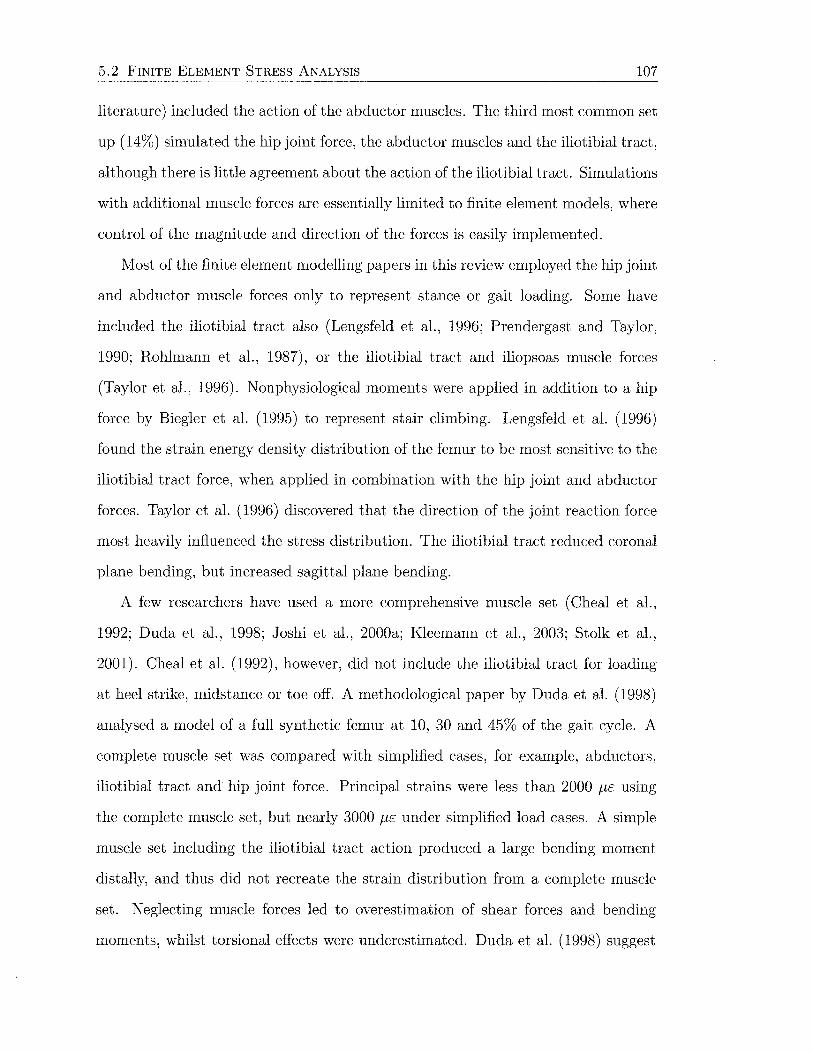
5.2 FINITE ELEMENT STRESS ANALYSIS 107
literature) included the action of the abductor muscles. The third most common set
up (14%) simulated the hip joint force, the abductor muscles and the iliotibial tract,
although there is little agreement about the action of the iliotibial tract. Simulations
with additional muscle forces are essentially limited to finite element models, where
control of the magnitude and direction of the forces is easily implemented.
Most of the finite element modelling papers in this review employed the hip joint
and abductor muscle forces only to represent stance or gait loading. Some have
included the iliotibial tract also (Lengsfeld et al., 1996; Prendergast and Taylor,
1990; Rohlmann et al., 1987), or the iliotibial tract and iliopsoas muscle forces
(Taylor et al., 1996). Nonphysiological moments were applied in addition to a hip
force by Biegler et al. (1995) to represent stair climbing. Lengsfeld et al. (1996)
found the strain energy density distribution of the femur to be most sensitive to the
iliotibial tract force, when applied in combination with the hip joint and abductor
forces. Taylor et al. (1996) discovered that the direction of the joint reaction force
most heavily influenced the stress distribution. The iliotibial tract reduced coronal
plane bending, but increased sagittal plane bending.
A few researchers have used a more comprehensive muscle set (Cheal et al.,
1992; Duda et al., 1998; Joshi et al., 2000a; Kleemann et al., 2003; Stolk et al.,
2001). Cheal et al. (1992), however, did not include the iliotibial tract for loading
at heel strike, midstance or toe off. A methodological paper by Duda et al. (1998)
analysed a model of a full synthetic femur at 10, 30 and 45% of the gait cycle. A
complete muscle set was compared with simplified cases, for example, abductors,
iliotibial tract and hip joint force. Principal strains were less than 2000 JLE using
the complete muscle set, but nearly 3000 JLE under simplified load cases. A simple
muscle set including the iliotibial tract action produced a large bending moment
distally, and thus did not recreate the strain distribution from a complete muscle
set. Neglecting muscle forces led to overestimation of shear forces and bending
moments, whilst torsional effects were underestimated. Duda et al. (1998) suggest

5.3 REMARKS 108
that at the least the abductors, iliotibial tract, adductors and hip joint force should
be included in in vitro studies.
A similar style of investigation by Stolk et al. (2001) set out to determine which
muscle forces should be included in in vitro testing of cemented hip arthroplasty.
The same complete muscle set as Duda et al. (1998), again at 10, 30 and 45% of
the gait cycle, was applied to a model of the proximal femur containing a cemented
implant. Inclusion of the abductor group had the largest effect on deflection of
the model, with further inclusion of the iliotibial tract, vasti and adductors having
relatively small effects. The abductor muscles also had the greatest influence on
the femoral strain distribution. Based on these results, it was concluded that hip
joint and abductor muscle forces were sufficient to adequately reproduce in vivo
bone loading for cemented hip implants. This conclusion was not extrapolated to
loading on the intact femur. It was also suggested that the iliotibial band could be
justifiably excluded on the basis of the lack of consensus on its action and the small
effect it had on load transfer in cemented hip arthroplasty.
In reference to the iliotibial band, Cristofolini (1997) also commented that: "if
a force is unknown or its effect is irrelevant, assigning any value is no less arbitrary
than assigning a value of zero." Cristofolini (1997) further recommended that a
loading set up should begin with a simple starting point, with the hip joint force
only, and other forces should be investigated one by one and retained only if it is
physiological, is shown to affect the results, and its magnitude is known.
5.3 Remarks
Strain gauges and finite element modelling have been used in a large number of
studies concerned with stress shielding following hip arthroplasty. Both methods
have been effective in simulating clinical studies, however it is almost impossible
to quantitatively compare results between studies due to varied loading protocols
and subject-specific models. The conflicting requirements of a flexible stem having

5.3 REMARKS 109
low interface stress, the difficulty of practically implementing a collar, and the
discrepancy between the experimental and theoretical methods when considering
implant stiffness, imply that the mechanism of load transfer to the femur is probably
the most important aspect in the design of a hip prosthesis.
According to Rojek and Telega (1999), the load transfer mechanism and associ
ated stress patterns in prosthetic fixation depend on four aspects: loading charac
teristics, implant geometry, material properties and boundary /interface conditions.
It is the interface conditions that are most difficult to simulate experimentally and
theoretically, especially for porous coated implants. Finite element models, with
few exceptions, assume perfectly congruent surfaces at the implant-bone interface,
whereas in reality, the contact area is highly dependent on difficult to control factors
like surgical technique. This situation with discrete contact points can be repro
duced experimentally, and for this reason has been cited as an important aspect of
load transfer (Diegel et al., 1989; Jasty et al., 1994). Van Rietbergen et al. (1993)
in fact found better agreement with in vivo bone adaptation results when a proxi
mal interface gap was included, while Weinans et al. (1994) showed that proximal
overreaming resulted in dramatic proximal bone loss.
Although pre-clinical evaluation methods for implant designs have progressed
considerably, the importance of in vivo verification is still important. Further stan
dardisation of pre-clinical test protocols, such as ISO 7206 which has considerably
reduced the occurrence of stem fractures (Stolk et al., 2002), will also help improve
the success of hip arthroplasty.
Chapter 6
Bone Adaptation Models
Section 4.3 described the adaptive properties of bone in response to mechanical
load in terms of what has been observed experimentally and possible mechanobi
ological systems that governs that adaptation. Many mathematical models have
been proposed by researchers to simulate these systems theoretically. Since the
exact adaptation process at the cellular/microstructural level is not fully under
stood, most of these mathematical models seek to describe remodelling in terms
of cause-and-effect relationships, essentially with a "black box" in between. Such
models are classified as phenomenological. Optimisation theories have also been
applied to studying the adaptive behaviour of bone, but these models have some
limitations. A mechanistic approach is needed to properly elucidate the interplay
of the biological and mechanical environments. These models should include the
effects of genetics, hormones and drug therapy. Some progress has been made in
this direction, however much more work is needed before reliable results can be
obtained.
This chapter reviews some of the bone adaptation models found in the literature.
The models are either conceptual, or in a form for inclusion in bone adaptation sim
ulations. The adaptation simulations consist of a remodelling theory coupled with
the finite element method in most cases. Boundary element methods have also been
used (e.g., Luo et al., 1995), but are beyond the scope of this review. The advantage
110

6. BONE ADAPTATION ]'v10DELS 111
of finite element modelling is that it provides mechanical quantities, or field vari
ables (e.g., stress, strain), throughout a structure, which can be used to determine
local remodelling stimuli at all of these locations. The finite element model is incre
mentally updated according to the change in material properties and/ or geometry
predicted by the remodelling theory. The theories are quasi-static, i.e., independent
of loading rate, viscoelastic and inertia effects.
In Section 4.3.2, the differences between modelling and remodelling are dis
cussed. Appropriately, computational models tend to simulate these processes sep
arately. Somewhat confusingly though, both modelling and remodelling are often
classified as "remodelling". The alteration of bone geometry brought about by mod
elling is termed surface or external remodelling, while the change of porosity and
ultimately stiffness due to remodelling is called internal remodeling. This distinc
tion was made by Frost (1964). Since all bone remodelling occurs by resorption
and deposition onto surfaces, it would be most precise to use surface remodelling
equations to simulate both modelling and remodelling processes for bone. However,
this would be a massive computational task if applied to all of the envelopes of
the skeleton, particularly the trabecular bone, due to the vast surface area. Most
simulations include only one of the "remodelling" processes.
Mathematically, internal remodelling can be described by a change in apparent
density. The rate of change of apparent density at a particular point can be de
scribed by an objective function F, which is dependent on a particular remodelling
stimulus at location (x, y, z) (Weinans et al., 1992a). The objective function is as
sumed to be related to the local stress tensor a-= a-(x, y, z), the local strain tensor
€ = e(x, y, z), and the local apparent density p = p(x, y, z)
dp dt = F(a-,e,p), 0 < p::::; Pc (6.1)
where the density cannot decrease below 0 (total resorption) or above Pc (density of
cortical bone). Remodelling equilibrium (net rate of change of bone density is zero)
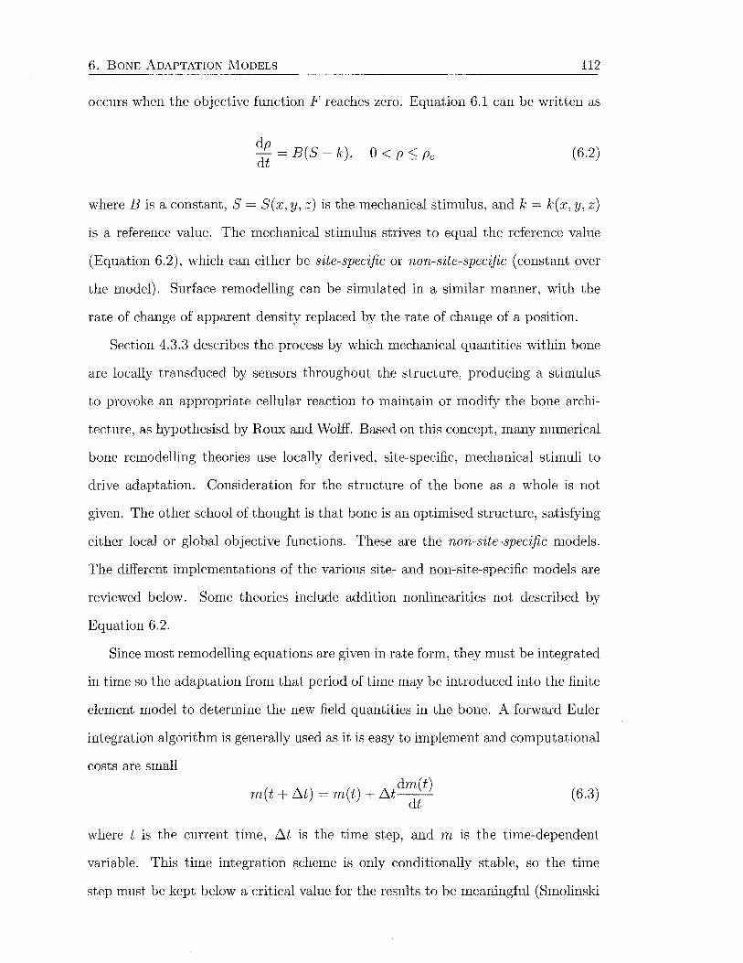
6. BONE ADAPTATION l\10DELS 112
occurs when the objective function F reaches zero. Equation 6.1 can be written as
d: = B(S- k), 0 < p '5. Pc (6.2)
where B is a constant, S = S(x, y, z) is the mechanical stimulus, and k = k(x, y, z)
is a reference value. The mechanical stimulus strives to equal the reference value
(Equation 6.2), which can either be site-specific or non-site-specific (constant over
the model). Surface remodelling can be simulated in a similar manner, with the
rate of change of apparent density replaced by the rate of change of a position.
Section 4.3.3 describes the process by which mechanical quantities within bone
are locally transduced by sensors throughout the structure, producing a stimulus
to provoke an appropriate cellular reaction to maintain or modify the bone archi-
tecture, as hypothesisd by Roux and Wolff. Based on this concept, many numerical
bone remodelling theories use locally derived, site-specific, mechanical stimuli to
drive adaptation. Consideration for the structure of the bone as a whole is not
given. The other school of thought is that bone is an optimised structure, satisfying
either local or global objective functions. These are the non-site-specific models.
The different implementations of the various site- and non-site-specific models are
reviewed below. Some theories include addition nonlinearities not described by
Equation 6.2.
Since most remodelling equations are given in rate form, they must be integrated
in time so the adaptation from that period of time may be introduced into the finite
element model to determine the new field quantities in the bone. A forward Euler
integration algorithm is generally used as it is easy to implement and computational
costs are small dm(t)
m(t + l:lt) = m(t) + l:lt~ (6.3)
where t is the current time, l:lt is the time step, and m is the time-dependent
variable. This time integration scheme is only conditionally stable, so the time
step must be kept below a critical value for the results to be meaningful (Smolinski
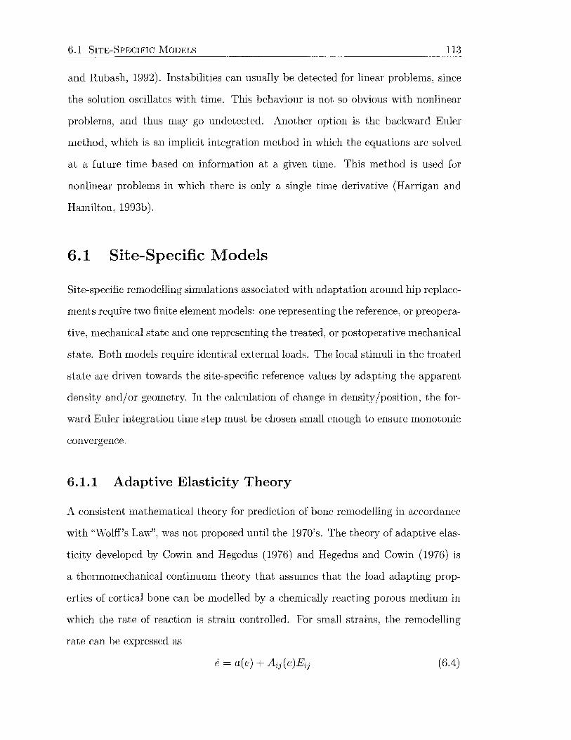
6.1 SITE-SPECIFIC MODELS 113
and Rubash, 1992). Instabilities can usually be detected for linear problems, since
the solution oscillates with time. This behaviour is not so obvious with nonlinear
problems, and thus may go undetected. Another option is the backward Euler
method, which is an implicit integration method in which the equations are solved
at a future time based on information at a given time. This method is used for
nonlinear problems in which there is only a single time derivative (Harrigan and
Hamilton, 1993b).
6.1 Site-Specific Models
Site-specific remodelling simulations associated with adaptation around hip replace
ments require two finite element models: one representing the reference, or preopera
tive, mechanical state and one representing the treated, or postoperative mechanical
state. Both models require identical external loads. The local stimuli in the treated
state are driven towards the site-specific reference values by adapting the apparent
density and/ or geometry. In the calculation of change in density /position, the for
ward Euler integration time step must be chosen small enough to ensure monotonic
convergence.
6.1.1 Adaptive Elasticity Theory
A consistent mathematical theory for prediction of bone remodelling in accordance
with "Wolff's Law", was not proposed until the 1970's. The theory of adaptive elas
ticity developed by Cowin and Hegedus (1976) and Hegedus and Cowin (1976) is
a thermomechanical continuum theory that assumes that the load adapting prop
erties of cortical bone can be modelled by a chemically reacting porous medium in
which the rate of reaction is strain controlled. For small strains, the remodelling
rate can be expressed as
(6.4)
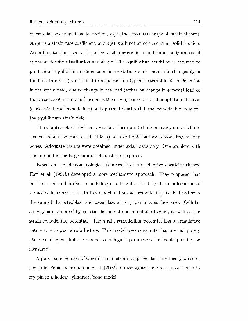
6.1 SITE-SPECIFIC MODELS 114
where e is the change in solid fraction, EiJ is the strain tensor (small strain theory),
AiJ(e) is a strain-rate coefficient, and a( e) is a function of the current solid fraction.
According to this theory, bone has a characteristic equilibrium configuration of
apparent density distribution and shape. The equilibrium condition is assumed to
produce an equilibrium (reference or homeostatic are also used interchangeably in
the literature here) strain field in response to a typical external load. A deviation
in the strain field, due to change in the load (either by change in external load or
the presence of an implant) becomes the driving force for local adaptation of shape
(surface/external remodelling) and apparent density (internal remodelling) towards
the equilibrium strain field.
The adaptive elasticity theory was later incorporated into an axisymmetric finite
element model by Hart et al. (1984a) to investigate surface remodelling of long
bones. Adequate results were obtained under axial loads only. One problem with
this method is the large number of constants required.
Based on the phenomenological framework of the adaptive elasticity theory,
Hart et al. (1984b) developed a more mechanistic approach. They proposed that
both internal and surface remodelling could be described by the manifestation of
surface cellular processes. In this model, net surface remodelling is calculated from
the sum of the osteoblast and osteoclast activity per unit surface area. Cellular
activity is modulated by genetic, hormonal and metabolic factors, as well as the
strain remodelling potential. The strain remodelling potential has a cumulative
nature due to past strain history. This model uses constants that are not purely
phenomenological, but are related to biological parameters that could possibly be
measured.
A poroelastic version of Cowin's small strain adaptive elasticity theory was em
ployed by Papathanasopoulou et al. (2002) to investigate the forced fit of a medull
ary pin in a hollow cylindrical bone model.
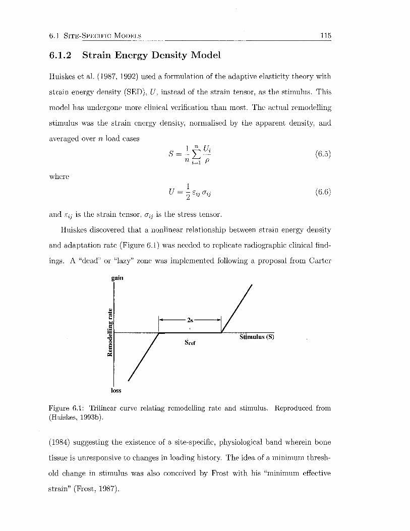
6.1 SITE-SPECIFIC MODELS 115
6.1.2 Strain Energy Density Model
Huiskes et al. (1987, 1992) used a formulation of the adaptive elasticity theory with
strain energy density (SED), U, instead of the strain tensor, as the stimulus. This
model has undergone more clinical verification than most. The actual remodelling
stimulus was the strain energy density, normalised by the apparent density, and
averaged over n load cases
S=]:_tUi n i=l P
(6.5)
where 1
U = 2 Eij rYij (6.6)
and Eij is the strain tensor, rYij is the stress tensor.
Huiskes discovered that a nonlinear relationship between strain energy density
and adaptation rate (Figure 6.1) was needed to replicate radiographic clinical find-
ings. A "dead" or "lazy" zone was implemented following a proposal from Carter
gain
Stimulus (S)
loss
Figure 6.1: Trilinear curve relating remodelling rate and stimulus. Reproduced from (Huiskes, 1993b).
(1984) suggesting the existence of a site-specific, physiological band wherein bone
tissue is unresponsive to changes in loading history. The idea of a minimum thresh
old change in stimulus was also conceived by Frost with his "minimum effective
strain" (Frost, 1987).
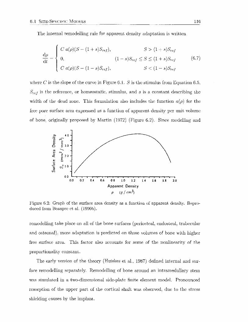
6.1 SITE-SPECIFIC MODELS
The internal remodelling rule for apparent density adaptation is written
dp
dt
C a(p)(S- (I+ s)Sref),
0,
C a(p)(S- (I- s)Sref ),
S > (I+ s)Sref
(I- s)Sref ~ S ~(I+ s)Sref
S <(I- s)Sref
116
(6.7)
where Cis the slope of the curve in Figure 6.1. Sis the stimulus from Equation 6.5,
Sref is the reference, or homeostatic, stimulus, and s is a constant describing the
width of the dead zone. This formulation also includes the function a(p) for the
free pore surface area expressed as a function of apparent density per unit volume
of bone, originally proposed by Martin (I972) (Figure 6.2). Since modelling and
>. 4 0 -·v; M' t: ;:;: <1) s 3 0 0
"' ....__
<1) "' ... ,.. <l: :: 2 0
<1) ~ u
"' r.n 1.0 't: :::s
(.f)
00 0.0 0.2 OA 0.6 0.8 1.0 1.2 1 4 1.6 18 2.0
Apparent Density
p (g / cm3)
Figure 6.2: Graph of the surface area density as a function of apparent density. Reproduced from Beaupre et al. (1990b).
remodelling take place on all of the bone surfaces (periosteal, endosteal, trabecular
and osteonal), more adaptation is predicted on those volumes of bone with higher
free surface area. This factor also accounts for some of the nonlinearity of the
proportionality constant.
The early version of the theory (Huiskes et al., I987) defined internal and sur
face remodelling separately. Remodelling of bone around an intramedullary stem
was simulated in a two-dimensional side-plate finite element model. Pronounced
resorption of the upper part of the cortical shaft was observed, due to the stress
shielding causes by the implant.
6.1 SITE-SPECIFIC MoDELS 117
The model defined by Equation 6.7 has been used by a number of authors with
three-dimensional finite element models to investigate the effect on periprosthetic
remodelling of dead zone width, initial bone quality, stem stiffness (Huiskes, 1993b;
Huiskes et al., 1992; Weinans et al., 1991), and extent of porous coating (Huiskes
and van Rietbergen, 1995). The study by Huiskes (1993b) compared their results
with clinical bone mineral density measurements from Engh et al. (1992a) and
found reasonable agreement. A similar study comparing patient-specific remodelling
results with radiographic data was performed by Kerner et al. (1999). They found
that bone loss in the region of the lesser trochanter was overestimated by the model
in all cases, and that convergence was not reached after 60 increments. Excessive
bone loss in the calcar region was also reported by van Riet bergen and H uiskes
(2001) when comparing a model incorporating the ABG stem with a clinical study.
Weinans et al. (1993) compared theoretical results with two year data from a canine
study, but better results were obtained for press-fit stems when a proximal interface
gap was included (van Rietbergen et al., 1993).
6.1.3 Damage Accumulation Models
A different approach was taken by Prendergast and Taylor (1992), who proposed a
remodelling theory based on the hypothesis that damage accumulation drives bone
remodelling. The remodelling stimulus is the difference between the current damage
rate and the remodelling equilibrium repair rate value. An advantage of this theory
is that it automatically accounts for dynamic loading history as the driving force of
the remodelling process. Surface remodelling of the femoral diaphysis under reduced
torsional loading (Prendergast and Taylor, 1994) and around an intermedullary rod
(Prendergast and Taylor, 1992) was investigated with this model. McNamara et al.
(1997b) showed that the damage stimulus was equivalent to the strain energy density
stimulus used by other researchers, when damage is measured as a function of crack
length.
6.2 NON-SITE-SPECIFIC MODELS 118
Ramtani and Zidi (2001, 2002a,b) explored this topic further, and created a
general continuum thermodynamic framework, along the lines of Cowin and Hege
dus (1976), to describe damage-induced remodelling. This model requires further
identification of constants and understanding of the damage evolution during the
adaptation process (Ramtani and Zidi, 2001).
6.2 Non-Site-Specific Models
Many scientists have assumed that bones are structurally optimised for their me
chanical environment (e.g., Thompson, 1961; Wolff, 1892). It is not clear exactly
what they are optimal for, but possibilities include deformation, strength and
weight. Most non-site-specific remodelling theories involve optimisation, and are
concerned with morphogenesis of the trabecular architecture of the proximal femur,
due to its fairly predictable distribution. These theories are generally coupled with
two-dimensional finite element models.
According to Hart (2001), optimisation studies help to further understanding of
bone as a mechanical structure, but do not provide particularly useful information
about the physiological process of adaptation.
6.2.1 Self-Optimisation and Bone Maintenance Theories
One of the first optimisation approaches was the self-optimisation model of Fyhrie
and Carter (1986), which predicted changes in trabecular orientation and apparent
density resulting from a change in applied stress. The stimulus was either a stress
ratio (a/ a ult) or energy stress ( V2f!E). The bone maintenance theory of Carter
et al. (1987) followed on from this, and proposed that bone in remodelling equilib
rium (i.e., no net bone gain or loss) is exposed to a constant daily stimulus that is
a function of the loading history.
Fyhrie and Carter (1990) applied Carter's model to predicting the apparent
density distribution in a three-dimensional finite element model of the femoral head
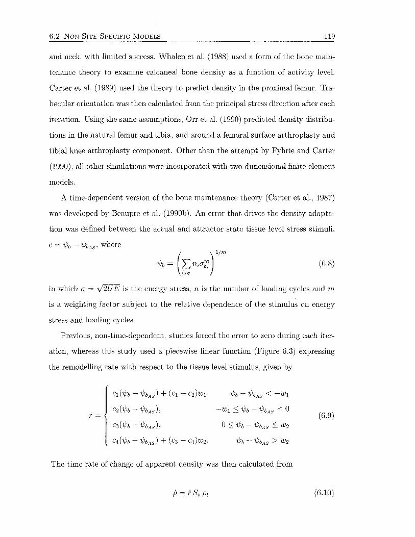
6.2 NON-SITE-SPECIFIC MODELS 119
and neck, with limited success. Whalen et al. (1988) used a form of the bone main-
terrance theory to examine calcaneal bone density as a function of activity level.
Carter et al. (1989) used the theory to predict density in the proximal femur. Tra-
becular orientation was then calculated from the principal stress direction after each
iteration. Using the same assumptions, Orr et al. (1990) predicted density distribu
tions in the natural femur and tibia, and around a femoral surface arthroplasty and
tibial knee arthroplasty component. Other than the attempt by Fyhrie and Carter
(1990), all other simulations were incorporated with two-dimensional finite element
models.
A time-dependent version of the bone maintenance theory (Carteret al., 1987)
was developed by Beaupre et al. (1990b). An error that drives the density adapta-
tion was defined between the actual and attractor state tissue level stress stimuli,
(6.8)
in which CJ = V2U E is the energy stress, n is the number of loading cycles and m
is a weighting factor subject to the relative dependence of the stimulus on energy
stress and loading cycles.
Previous, non-time-dependent, studies forced the error to zero during each iter
ation, whereas this study used a piecewise linear function (Figure 6.3) expressing
the remodelling rate with respect to the tissue level stimulus, given by
c1 ('1/Jb - '1/JbAs) + ( c1 - c2)w1, '1/Jb- '1/JbAs < -w1
C2 ( '1/Jb - '1/Jb AS)' -wl ::; '1/Jb - '1/JbAs < 0 (6.9) r=
c3('1jJb- '1/JbAs), 0 ::; '1/Jb - '1/JbAs ::; W2
c4('1jJb- '1/JbAs) + (c3- c4)w2, '1/Jb- '1/JbAs > W2
The time rate of change of apparent density was then calculated from
p = r Sv Pt (6.10)
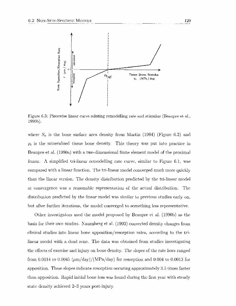
6.2 NON-SITE-SPECIFIC MODELS
Tissue Stress Stimulus -.j,, (MPa /day)
120
Figure 6.3: Piecewise linear curve relating remodelling rate and stimulus (Beaupre et al., 1990b).
where Sv is the bone surface area density from Martin (1984) (Figure 6.2) and
Pt is the mineralised tissue bone density. This theory was put into practice in
Beaupre et al. (1990a) with a two-dimensional finite element model of the proximal
femur. A simplified tri-linear remodelling rate curve, similar to Figure 6.1, was
compared with a linear function. The tri-linear model converged much more quickly
than the linear version. The density distribution predicted by the tri-linear model
at convergence was a reasonable representation of the actual distribution. The
distribution predicted by the linear model was similar to previous studies early on,
but after further iterations, the model converged to something less representative.
Other investigators used the model proposed by Beaupre et al. (1990b) as the
basis for their own studies. Nauenberg et al. (1993) converted density changes from
clinical studies into linear bone apposition/resorption rates, according to the tri
linear model with a dead zone. The data was obtained from studies investigating
the effects of exercise and injury on bone density. The slopes of the rate laws ranged
from 0.0014 to 0.0045 (pm/day)/(MPa/day) for resorption and 0.004 to 0.0013 for
apposition. These slopes indicate resorption occuring approximately 3.5 times faster
than apposition. Rapid initial bone loss was found during the first year with steady
state density achieved 2-3 years post-injury.
6.2 NON-SITE-SPECIFIC MODELS 121
Levenston et al. (1994) modified the daily stimulus to included an exponentially
fading memory of past loading. This model gives the same result as Beaupre et al.
(199Ga) under simplified conditions. Time constants of 5 and 2G days in the remod
elling stimulus also converged to this result. Consideration of previous loading may
be important for short-term implications of use and disuse. Fischer et al. (1996)
implemented the theory of Beaupre et al. (199Gb) to see if a density distribution
could be produced or maintained by more than one set of loads. Similar results
were reported, except near boundaries and high density gradients.
Sti.ilpner et al. (1997) used an equivalent strain E as the stimulus in the theory
of Beaupre et al. (199Gb), defined by E = -JEijEij· This is used to calculate the
remodelling error e, which is the difference between the actual and optimal stimulus
levels
(6.11)
where N is the total number of load cases, i is the ith load case, ni is the number of
load cycles per day of load case i, mi are weighting factors, and Erem is the homeo-
static strain value. The bone apposition rate was determined from a double sigmoid
curve incorporating a dead zone, and also a saturation level. Internal remodelling
proceeds according to Equation 6.10. It was concluded that more complex loading
was required to create a physiological density distribution in three dimensions.
Hernandez et al. (2GGG) expanded the description of Beaupre et al. (199Gb) to
include the influence of biological factors on osteoblasts and osteoclasts. Cellular
activity was then regulated by the both metabolic and mechanical setpoints. A
large number of parameters was required to describe this model, and it is not yet
in a state where it could be used for a whole structure.
Strain Energy-Dependent Model
Huiskes et al. (1987) presented a theory for predicting the density distribution of
bone, as well as an application to stress sheilding as discussed previously. Internal
remodelling, was defined with a relation similar to Equation 6. 7, except that the
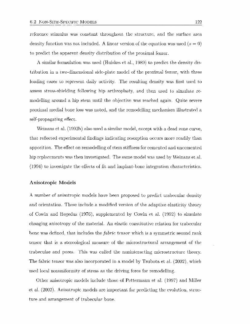
6.2 NON-SITE-SPECIFIC MODELS 122
reference stimulus was constant throughout the structure, and the surface area
density function was not included. A linear version of the equation was used ( s = 0)
to predict the apparent density distribution of the proximal femur.
A similar formulation was used (Huiskes et al., 1989) to predict the density dis
tribution in a two-dimensional side-plate model of the proximal femur, with three
loading cases to represent daily activity. The resulting density was first used to
assess stress-shielding following hip arthroplasty, and then used to simulate re
modelling around a hip stem until the objective was reached again. Quite severe
proximal medial bone loss was noted, and the remodelling mechanism illustrated a
self-propagating effect.
Weinans et al. (1992b) also used a similar model, except with a dead zone curve,
that reflected experimental findings indicating resorption occurs more readily than
apposition. The effect on remodelling of stem stiffness for cemented and uncemented
hip replacements was then investigated. The same model was used by vVeinans et al.
(1994) to investigate the effects of fit and implant-bone integration characteristics.
Anisotropic Models
A number of anisotropic models have been proposed to predict trabecular density
and orientation. These include a modified version of the adaptive elasticity theory
of Cowin and Hegedus (1976), supplemented by Cowin et al. (1992) to simulate
changing anisotropy of the material. An elastic constitutive relation for trabecular
bone was defined, that includes the fabric tensor which is a symmetric second rank
tensor that is a stereological measure of the microstructural arrangement of the
trabeculae and pores. This was called the noninteracting microstructure theory.
The fabric tensor was also incorporated in a model by Tsubota et al. (2002), which
used local nonuniformity of stress as the driving force for remodelling.
Other anisotropic models include those of Pettermann et al. (1997) and Miller
et al. (2002). Anisotropic models are important for predicting the evolution, struc
ture and arrangement of trabecular bone.
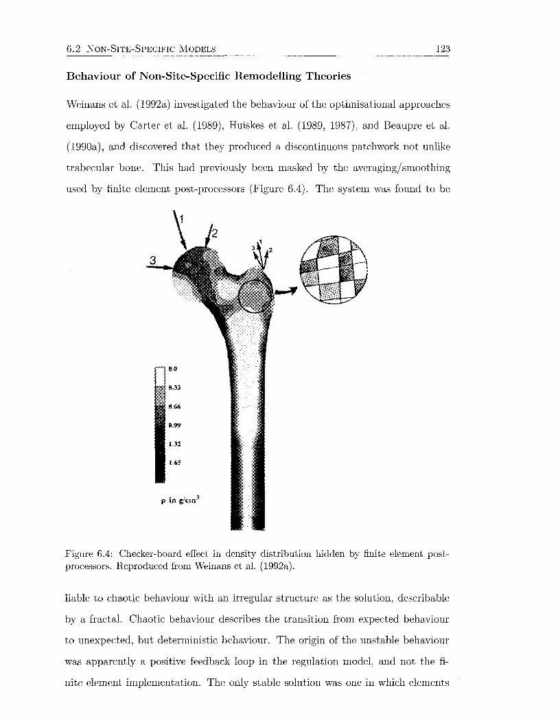
6.2 NON-SITE-SPECIFIC MODELS 123
Behaviour of Non-Site-Specific Remodelling Theories
Weinans et al. (1992a) investigated the behaviour of the optimisational approaches
employed by Carter et al. (1989), Huiskes et al. (1989, 1987), and Beaupre et al.
(1990a), and discovered that they produced a discontinuous patchwork not unlike
trabecular bone. This had previously been masked by the averaging/ smoothing
used by finite element post-processors (Figure 6.4). The system was found to be
Figure 6.4: Checker-board effect in density distribution hidden by finite element postprocessors. Reproduced from Weinans et al. (1992a).
liable to chaotic behaviour with an irregular structure as the solution, describable
by a fractal. Chaotic behaviour describes the transition from expected behaviour
to unexpected, but deterministic behaviour. The origin of the unstable behaviour
was apparently a positive feedback loop in the regulation model, and not the fi
nite element implementation. The only stable solution was one in which elements
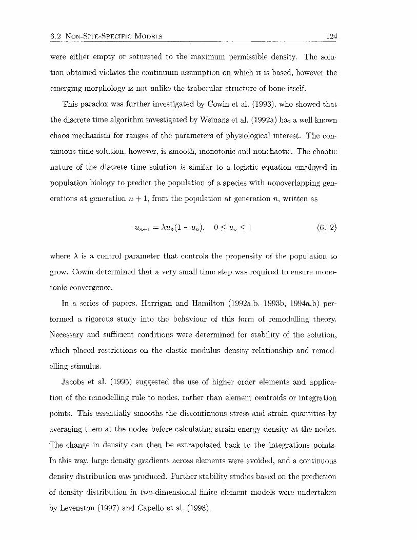
6.2 NON-SITE-SPECIFIC MODELS 124
were either empty or saturated to the maximum permissible density. The solu
tion obtained violates the continuum assumption on which it is based, however the
emerging morphology is not unlike the trabecular structure of bone itself.
This paradox was further investigated by Cowin et al. (1993), who showed that
the discrete time algorithm investigated by Weinans et al. (1992a) has a well known
chaos mechanism for ranges of the parameters of physiological interest. The con
tinuous time solution, however, is smooth, monotonic and nonchaotic. The chaotic
nature of the discrete time solution is similar to a logistic equation employed in
population biology to predict the population of a species with nonoverlapping gen
erations at generation n + 1, from the population at generation n, written as
(6.12)
where A is a control parameter that controls the propensity of the population to
grow. Cowin determined that a very small time step was required to ensure mono
tonic convergence.
In a series of papers, Harrigan and Hamilton (1992a,b, 1993b, 1994a,b) per
formed a rigorous study into the behaviour of this form of remodelling theory.
Necessary and sufficient conditions were determined for stability of the solution,
which placed restrictions on the elastic modulus-density relationship and remod
elling stimulus.
Jacobs et al. (1995) suggested the use of higher order elements and applica
tion of the remodelling rule to nodes, rather than element centroids or integration
points. This essentially smooths the discontinuous stress and strain quantities by
averaging them at the nodes before calculating strain energy density at the nodes.
The change in density can then be extrapolated back to the integrations points.
In this way, large density gradients across elements were avoided, and a continuous
density distribution was produced. Further stability studies based on the prediction
of density distribution in two-dimensional finite element models were undertaken
by Levenston (1997) and Capello et al. (1998).
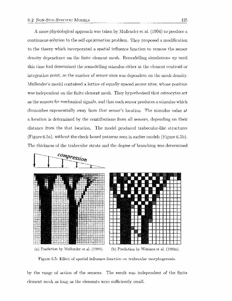
6.2 NoN-SITE-SPECIFIC MODELS 125
A more physiological approach was taken by Mullender et al. (1994) to produce a
continuous solution to the self-optimisation problem. They proposed a modification
to the theory which incorporated a spatial influence function to remove the sensor
density dependence on the finite element mesh. Remodelling simulations up until
this time had determined the remodelling stimulus either at the element centroid or
integration point, so the number of sensor sites was dependent on the mesh density.
Mullender's model contained a lattice of equally spaced sensor sites, whose position
was independent on the finite element mesh. They hypothesised that osteocytes act
as the sensors for mechanical signals, and that each sensor produces a stimulus which
diminishes exponentially away from that sensor's location. The stimulus value at
a location is determined by the contributions from all sensors, depending on their
distance from the that location. The model produced trabecular-like structures
(Figure 6.5a), without the check-board patterns seen in earlier models (Figure 6.5b).
The thickness of the trabecular struts and the degree of branching was determined
(a) Prediction by Mullender et al. (1994). (b) Prediction by Weinans et al. (1992a).
Figure 6.5: Effect of spatial influence function on trabecular morphogenesis.
by the range of action of the sensors. The result was independent of the finite
element mesh as long as the elements were sufficiently small.
6.2 NON-SITE-SPECIFIC MODELS 126
This spatial influence function model was used to demonstrate changes in tra
becular orientation due to varied loading conditions (Mullender and Huiskes, 1995)
including direction and magnitude. Van Rietbergen et al. (1996) applied this theory
to remodelling of a simple 3D lattice structure, while the effect of stimulus on the
resulting equilibrium trabecular structure were examined by Keller (2001). Xinghua
et al. (2002) introduced two nonlinearities into the model, which effectively sped
up convergence of the solution and altered "osteoclast activation", by increasing the
change in density for a change in stimulus. The behaviour of Mullender's model
was the subject of investigation by Zidi and Ramtani (1999, 2000).
Huiskes et al. (2000) reformulated the model of Mullender et al. (1994) in terms
of osteoblast recruitment level relative to a threshold value, and osteoclast activity.
Results were similar to Mullender, except clinical situations could be described in
a more relevant way.
6.2.2 Global Models
Global optimisation models to predict the density distribution and anistotropy of
bone have been assessed in more recent years. These models assume that bone is an
optimal structure, and an optimisation problem (e.g., minimal compliance subject
to a constraint of given mass) is solved to predict bone architecture. The solution
to the problem is generally obtained by utilising Lagrange multipliers to convert
the global problem into a criterion that can be satisfied locally. Local models can
be viewed as a simulation of a local biological process, or a structural "optimality
criterion". The advantage of global models is a clear statement of what bone is
optimal for, although the corresponding local criterion may not be simple for bone
to follow (Miller et al., 2002). Interestingly, some similarities can be found between
the converted local criterion from global models and the criteria from other local
models.
Jacobs et al. (1997) developed an anisotropic model based on density adaptation
and anisotropy reorientation using the principal stress as the external stimulus. The

6.3 REMODELLING STIMULUS 127
adaptive response of bone was proposed to be a globally efficient mechanical struc
ture. The global efficiency function was found to imply a local regulation process.
This theory was applied to a two-dimensional model of the proximal femur. Pan
dorf et al. (1999) looked at adding non-mechanical components to the remodelling
stimulus. These included the effects of parathyroid hormone, calcitonin, calcitriol
and plasma concentrations of calcium and phosphate.
Fernandes et al. (1999) used homogenisation of a porous unit cell in a global
optimisation model for prediction of bone architecture in a three-dimensional prox
imal femur. A cost function accounting for structural stiffness and a biological
constraint associated with metabolic maintenance was optimised. Anisotropy was
accounted for by rotation of the homogenised material properties tensor. The lo
cal formulation of the optimal criterion was shown to be equivalent to the models
used by Beaupre et al. (1990b) and Weinans et al. (1992a). Later, Fernandes et al.
(2002) used the same global optimisation theory to examine bone density around
hip stems. Other models using homogenisation in global optimisation schemes were
proposed by Bagge (2000) and Pedersen (2002).
Subbarayan and Bartel (2000) proposed a global criterion that is a trade off
between the competing costs of metabolic growth and use, represented by mass, and
the cost of failure, represented by total strain energy. This model was not dissimilar
to Fernandes et al. (1999). A local formulation with strain error terms was derived
under the assumption that the shape of the bone is fixed. It was suggested that the
rules of local remodelling models may be thought of as approximations to global
models.
6.3 Remodelling Stimulus
A large number of stimuli have been proposed to regulate bone adaptation. These
include the strain tensor, strain energy density, energy stress, failure stress, von
6.3 REMODELLING STIMULUS 128
Mises stress, average principal strain and equivalent strain. Others are not so spe
cific, proposing as yet unknown functions of mechanical quantities. These stimuli
are all based on continuum mechanics theory. Some are invariant, while others have
direction-dependence.
Stress is usually considered as the force acting over an area, while strain is a non
dimensional measure of change in length. These concepts are not, however, so simple
or intuitive (Humphrey, 2001). Stress, as defined by Cauchy, is a volume-averaged
tensor that transforms outward unit normal vectors, that define orientations of
differential areas about a point of interest, into traction vectors that are a measure
of the intensity of the forces acting on that neighbourhood. Similarly, strain is also
a volume-averaged tensor, defined in terms of a deformation tensor. Consequently,
scalar functions of these quantities will also be volume averaged. Strain energy
density is a popular choice in the literature, however its selection is essentially
based on the fact that it is an easily interpreted scalar function of stress and strain
(Weinans et al., 1992a).
Tensors transform vectors into vectors, and are therefore independent of coordi
nate system. To be computationally useful, components relative to an appropriate
coordinate system are identified. The chosen coordinate system, of which there are
an infinite number, generally depends on convenience of calculation. One of these
possibilities is the principal coordinate system, where the only non-zero components
of the stress or strain tensor are along the diagonal.
Considering these points, it is questionable whether a cell is able to sense a
particular component of a specific volume-averaged tensor that is resolved to a
particular coordinate system that is convenient for computation. It is, nevertheless,
possible that cellular responses may correlate with coordinate-invariant mechanical
quantities. In the case of correlations, there is no need to address causation, and
consequently similar stimuli can be correlated to different responses, and vice versa
(Humphrey, 2001).

Chapter 7
Materials and Methods
This study is divided into three principal sections. The objectives of each section
are to:
1. Experimental Study
• Determine the effect of hip arthroplasty with the ~'largron hip prosthesis,
on the cortical strain distribution of a group of femora.
2. Finite Element Study
• Construct an anatomic finite element model of an intact femur, selected
from the experimental group, and model the femur implanted with the
Margron.
• Validate the finite elerrl'ent models by comparing strain data with exper
imental results.
• Analyse the effects of mesh refinement.
3. Bone Remodelling Study
• Develop a theoretical algorithm to simulate bone adaptation.
• Employ this algorithm to simulate bone adaptation using the finite ele
ment models created in the Finite Element Study.
• Simulate adaptation that is consistent with radiographic clinical data.
129
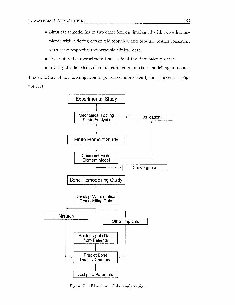
7. MATERIALS AND METHODS 130
• Simulate remodelling in two other femora, implanted with two other im
plants with differing design philosophies, and produce results consistent
with their respective radiographic clinical data.
• Determine the approximate time scale of the simulation process.
• Investigate the effects of some parameters on the remodelling outcome.
The structure of the investigation is presented more clearly in a flowchart (Fig-
ure 7.1).
Experimental Study
Mechanical Testing -I Validation Strain Analysis '--· -------.------J
l Finite Element Study
Construct Finite Element Model
l r--------·._I ___ C_o_n_v_e~~~e_n_ce __ ~
I Bone Remodelling Study I
Margron
-
! Develop Mathematical
Remodelling Rule
l Other Implants
Radiographic Data from Patients
Predict Bone Density Changes
1-
I Investigate Parameters I
Figure 7.1: Flowchart of the study design.
7.1 EXPERIMENTAL STUDY 131
7.1 Experimental Study
The experimental study was concerned with obtaining the cortical strain distribu
tion of four cadaveric femora, before and after hip arthroplasty with a cobalt-chrome
femoral prosthesis. This was undertaken using strain gauges and mechanical test
ing. The change in strain after surgery, caused by stress shielding, may provide a
stimulus for adaptive bone resorption.
7.1.1 Specimens
For the experimental strain gauge study, four fresh-frozen human femora were ob
tained from a tissue bank (mean age: 53 years, range: 34-73 years). The sample
size was limited for a number of reasons. Firstly, it is difficult to obtain fresh human
tissue. Secondly, repeated measures statistics were to be used, so the sample size
could be reduced. Also, the experimental part of the study was essentially aimed
at validating the finite element model.
Each femur was stripped of soft tissue and x-rayed in the medial-lateral and
anterior-posterior planes for the purposes of identifying abnormalities and for im
plant size selection (Figure 7.2).
7.1.2 Implant
The implant investigated was the Margron TM hip prosthesis (Portland Orthopae
dics, Pty. Ltd., Sydney, NS\V, Australia) (Figure 7.3). The Margron hip replace
ment is modular, consisting of separate stem and neck components manufactured
from forged cobalt-chrome alloy, which are joined by a taper. The stem is circular in
cross-section, with a "cone" shape proximally, and a straight cylinder distally (Fig
ure 7.3b ). Two different speed external threads and longitudinal derotation columns
provide immediate resistance to torsional and axial movement (Figure 7.3a). The
proximal part is coated with a 70 J1m hydroxyapatite layer to encourage fixation.
The adjustable neck component allows for selection of the optimum version angle,
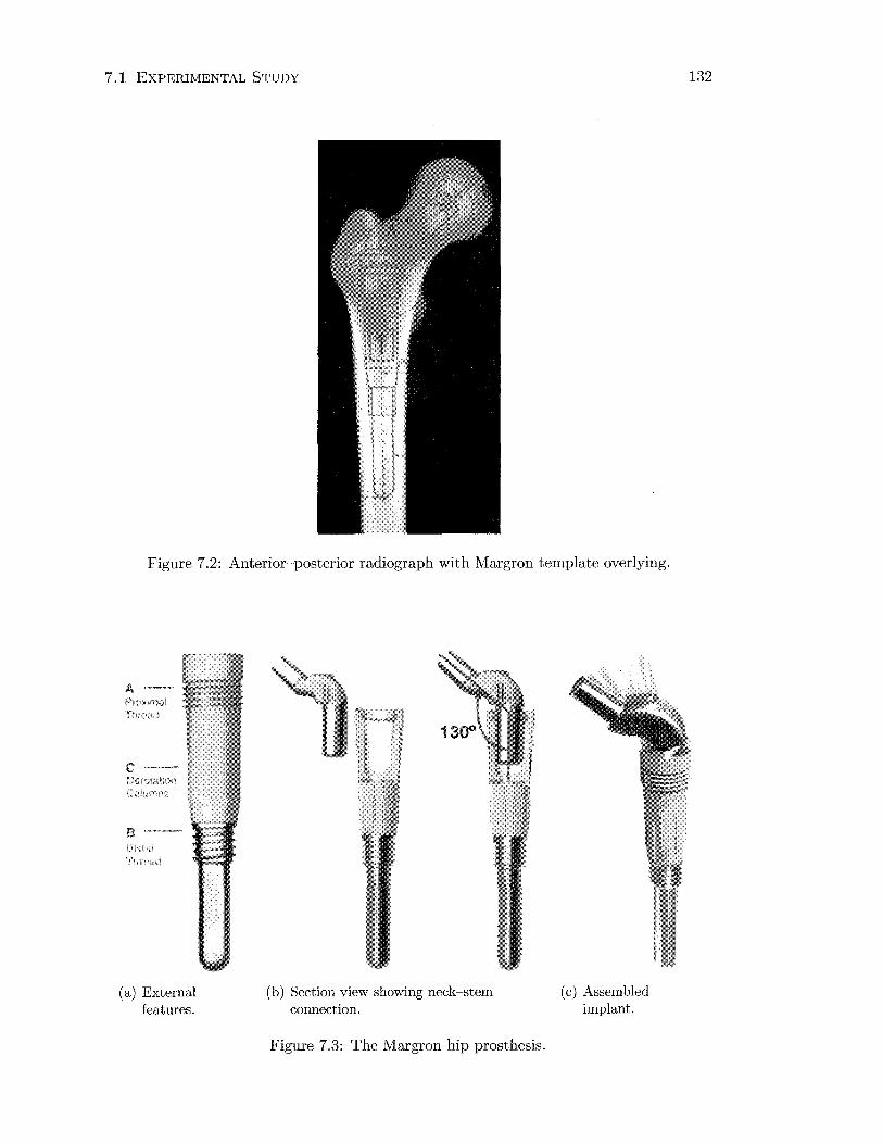
7.1 EXPERIMENTAL STUDY
Figure 7.2: Anterior-posterior radiograph with Margron template overlying.
A-~.~
PrD>>'Tial
c --
8 l\h~d
Tl!r,'<.ul
(a) External features.
(b) Section view showing neck-stem connection.
Figure 7.3: The Margron hip prosthesis.
(c) Assembled implant.
132
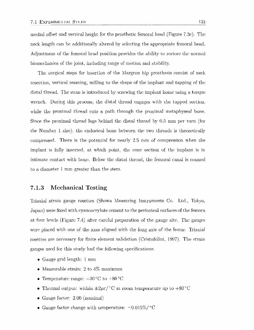
7.1 EXPERIMENTAL STUDY 133
medial offset and vertical height for the prosthetic femoral head (Figure 7.3c). The
neck length can be additionally altered by selecting the appropriate femoral head.
Adjustment of the femoral head position provides the ability to restore the normal
biomechanics of the joint, including range of motion and stability.
The surgical steps for insertion of the Margron hip prosthesis consist of neck
resection, vertical reaming, milling to the shape of the implant and tapping of the
distal thread. The stern is introduced by screwing the implant horne using a torque
wrench. During this process, the distal thread engages with the tapped section,
while the proximal thread cuts a path through the proximal metaphyseal bone.
Since the proximal thread lags behind the distal thread by 0.5 rnrn per turn (for
the Number 1 size), the endosteal bone between the two threads is theoretically
compressed. There is the potential for nearly 2.5 rnrn of compression when the
implant is fully inserted, at which point, the cone section of the implant is in
intimate contact with bone. Below the distal thread, the femoral canal is reamed
to a diameter 1 rnrn greater than the stern.
7.1.3 Mechanical Testing
Triaxial strain gauge rosettes (Showa Measuring Instruments Co. Ltd., Tokyo,
Japan) were fixed with cyanoacrylate cement to the periosteal surfaces of the femora
at four levels (Figure 7.4) after careful preparation of the gauge site. The gauges
were placed with one of the axes aligned with the long axis of the femur. Triaxial
rosettes are necessary for finite element validation (Cristofolini, 1997). The strain
gauges used for this study had the following specifications:
• Gauge grid length: 1 rnrn
• Measurable strain: 2 to 4% maximum
• Temperature range: -30 ac to +80 ac • Thermal output: within ±2f.I£j ac at room temperature up to +80 ac • Gauge factor: 2.00 (nominal)
• Gauge factor change with temperature: ±0.015%/ ac

7.1 EXPERIMENTAL STUDY 134
Figure 7.4: Strain gauge positions on the femoral cortex.
• Gauge factor tolerance: within 81% gauge factor for the respective package of
strain gauges
• Fatigue life: more than 106 reversals at 1000 fJ£
• Excitation: 1 Volt DC
• Strain gauge resistance: 120 n
The strain gauge base material was a polyester, with Cu-Ni alloy for the foil mate
rial, giving the strain gauge up to 10% measurable strain. The strain gauges were
also self-temperature compensating.
The femora were embedded distally in the diaphysis to facilitate fixation for
mechanical testing according to Gillies et al. (2002), with 10° of valgus angulation
and the femoral shaft vertical in the coronal plane ( 0° of flexion). Others have
used a similar form of distal fixation (Hua and Walker, 1995; Otani et al., 1993;
Tanner et al., 1988). The literature reports valgus embedding angles of between
9~12° (Cristofolini et al., 1995; Diegel et al., 1989; Engh et al., 1992b; Finlay et al.,
1991, 1989; Kim et al., 2001; Otani et al., 1993). Two simplified loading conditions
were examined:
(a) LOAD CASE 1, axial force of -820 N, 0° flexion; and
(b) LOAD CASE 2, axial force of -820 N, 10° flexion.
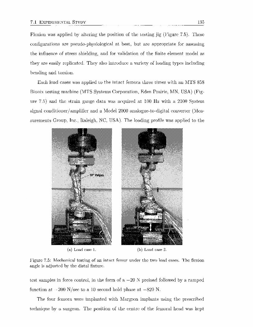
7.1 EXPERI!VIENTAL STUDY 135
Flexion was applied by altering the position of the testing jig (Figure 7.5). These
configurations are pseudo-physiological at best, but are appropriate for assessing
the influence of stress shielding, and for validation of the finite element model as
they are easily replicated. They also introduce a variety of loading types including
bending and torsion.
Each load cases was applied to the intact femora three times with an MTS 858
Bionix testing machine (MTS Systems Corporation, Eden Prairie, MN, USA) (Fig
ure 7.5) and the strain gauge data was acquired at 100 Hz with a 2100 System
signal conditioner/ amplifier and a Model 2000 analogue-to-digital converter (Mea
surements Group, Inc., Raleigh, NC, USA). The loading profile was applied to the
(a) Load case 1. (b) Load case 2.
Figure 7.5: Mechanical testing of an intact femur under the two load cases. The flexion angle is adjusted by the distal fixture.
test samples in force control, in the form of a -20 N preload followed by a ramped
function at -200 N/sec to a 10 second hold phase at -820 N.
The four femora were implanted with Margron implants using the prescribed
technique by a surgeon. The position of the centre of the femoral head was kept
7.1 EXPERIMENTAL STUDY 136
constant by selecting the appropriate neck length and version angle for the pros
thetic femoral head. Mechanical testing was repeated under identical loading.
7.1.4 Data Analysis
Strains were averaged during the hold phase of loading. Maximum and minimum
principal strains were subsequently calculated for each gauge using the formula
(7.1)
where a, b and c are respectively the oo, 45° and 90° grid elements on the triaxial
gauges (Craig, 2000).
Means and standard deviations for the principal and longitudinal strains were
calculated and plotted for each gauge location using Matlab v5.3 (The J\1athworks,
Inc., Natick, MA, USA). The standard deviations included the inter-specimen, but
not the intra-specimen variation. Horizontal bar charts were used, and a Matlab
function was developed to draw the error bars, which was beyond the standard
functionality. Preoperative and postoperative strains were compared using analysis
of variance (ANOVA) with repeated measures (Statistica, Statsoft, Inc., Tulsa, OK,
USA). The extent of stress shielding was assessed by determining the strains after
hip replacement as a percentage of the intact values. To propagate the standard
deviations into the percentages, the following formulae were used
Z =X± y,
z=:E. y'
~z = J~x2 + ~y2
~z = J ( ~x) 2 + ( ~) 2
where ~x, ~y and ~z are the standard deviations of the means x, y and z.
(7.2)

7. 2 FINITE ELEMENT STUDY 137
7.2 Finite Element Study
The primary aim of the finite element study was to produce finite element models
representing the intact and postoperative conditions for one of the femora from the
experimental group. To reproduce the mechanical response of the biological bone
tissue, geometry and material properties of the femur were obtained from computed
tomography ( CT) scanning. By applying loads and boundary conditions identical
to the experimental situation, the finite element model could be validated by the
experimental strain data. l'v1esh refinement was performed to investigate solution
convergence.
7.2.1 Model Construction
A representative cadaveric femur (right, 34 year old female) from the experimental
testing group was selected by a surgeon, and scanned in air using a Toshiba Whole
Body X-Ray CT Scanner (X Series), using a pixel matrix of 512 x 512 and exposure
settings of 120 kV, 100 rnA and 1.0 sec. Slices were taken at 3 mm intervals
proximally and 5 mm intervals distally. A slice thickness of 2 mm was used in all
cases. In-house software was used to extract the periosteal surface contour for each
slice by a thresholding and edge detection process. The contours were exported in
the form of a number of points, along with their corresponding position along the
scanning axis, to MSC.Patran (MSC.Software Corporation, Santa Ana, CA, USA).
Closed loop interpolating B-splines were run through the points from each contour
(Figure 7.6a), and surface sections were subsequently constructed to form the outer
surface of the femur (Figure 7.6c). The surfaces must be created with consideration
to the placement of the implant, particularly with respect to the osteotomy cut.
Creating the geometry of the femoral shaft is a relatively straightforward task of
joining adjacent contours to form surfaces. The geometry of the proximal femur is
not trivial to create, and construction of many new curves is required to regenerate
the shape (Figure 7.6b).

7. 2 FINITE ELEMENT STUDY
(a) CT contours. (b) Reconstruction of proximal geometry.
(c) Intact femur surfaces.
Figure 7.6: Femoral geometry for the finite element model.
138
The surfaces were meshed with two-dimensional, 6-noded, triangular elements
using a global edge length of 5 mm to form a closed volume. This surface mesh was
subsequently used to create a three-dimensional solid mesh with 10-noded, modified,
tetrahedral elements (Figure 7.7). Second order elements were chosen to model the
femur, as they can accurately reproduce bending. The additional computational
cost was considered acceptable considering the more accurate results.
Modified tetrahedral elements were used to address certain problems with the
regular second order tetrahedral elements, mainly related to their use in contact
problems. Regular second order tetrahedral elements usually give accurate results
in problems with no contact, however, in uniform pressure contact situations, the
contact forces are significantly different at the corner and midside nodes (they are
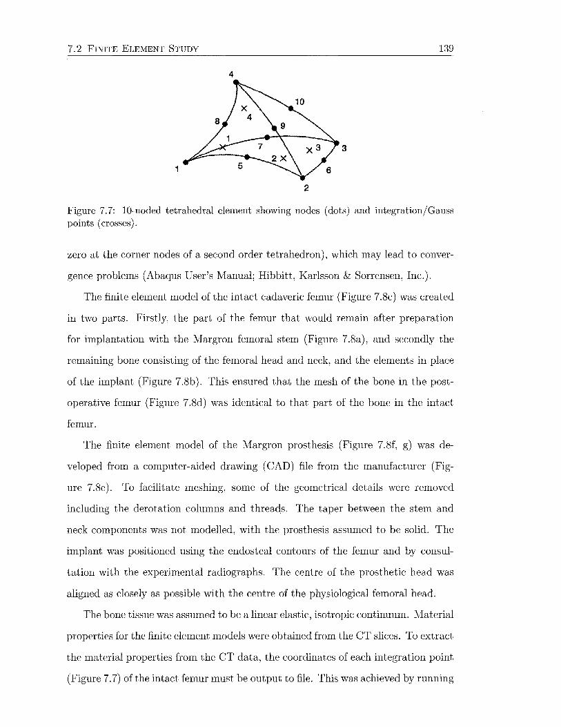
7. 2 FINITE ELEMENT STUDY 139
4
3
1
2
Figure 7.7: 10-noded tetrahedral element showing nodes (dots) and integration/Gauss points (crosses).
zero at the corner nodes of a second order tetrahedron), which may lead to conver
gence problems (Abaqus User's Manual; Hibbitt, Karlsson & Sorrensen, Inc.).
The finite element model of the intact cadaveric femur (Figure 7.8c) was created
in two parts. Firstly, the part of the femur that would remain after preparation
for implantation with the Margron femoral stem (Figure 7.8a), and secondly the
remaining bone consisting of the femoral head and neck, and the elements in place
of the implant (Figure 7 .8b). This ensured that the mesh of the bone in the post
operative femur (Figure 7.8d) was identical to that part of the bone in the intact
femur.
The finite element model of the Margron prosthesis (Figure 7.8f, g) was de
veloped from a computer-aided drawing (CAD) file from the manufacturer (Fig
ure 7.8e). To facilitate meshing, some of the geometrical details were removed
including the derotation columns and threads. The taper between the stem and
neck components was not modelled, with the prosthesis assumed to be solid. The
implant was positioned using the endosteal contours of the femur and by consul
tation with the experimental radiographs. The centre of the prosthetic head was
aligned as closely as possible with the centre of the physiological femoral head.
The bone tissue was assumed to be a linear elastic, isotropic continuum. Material
properties for the finite element models were obtained from the CT slices. To extract
the material properties from the CT data, the coordinates of each integration point
(Figure 7.7) of the intact femur must be output to file. This was achieved by running
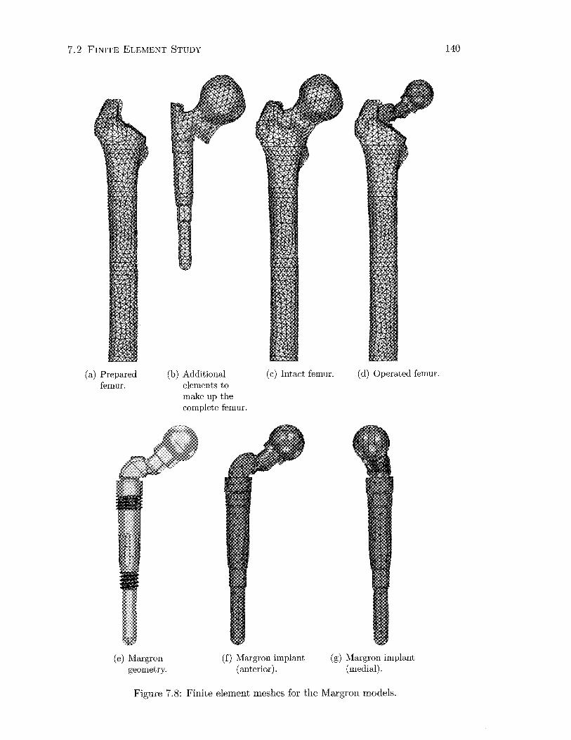
7.2 FINITE ELEMENT STUDY
(a) Prepared femur.
(b) Additional elements to make up the complete femur.
(c) Intact femur. (d) Operated femur.
(e) Margron geometry.
(f) Margron implant (anterior).
(g) Margron implant (medial).
Figure 7.8: Finite element meshes for the Margron models.
140
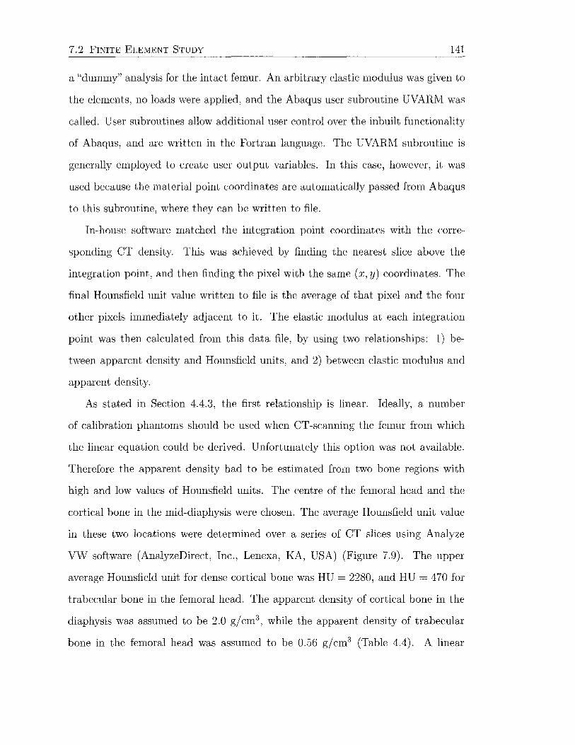
7. 2 FINITE ELEMENT STUDY 141
a "dummy" analysis for the intact femur. An arbitrary elastic modulus was given to
the elements, no loads were applied, and the Abaqus user subroutine UVARM was
called. User subroutines allow additional user control over the inbuilt functionality
of Abaqus, and are written in the Fortran language. The UVARM subroutine is
generally employed to create user output variables. In this case, however, it was
used because the material point coordinates are automatically passed from Abaqus
to this subroutine, where they can be written to file.
In-house software matched the integration point coordinates with the corre
sponding CT density. This was achieved by finding the nearest slice above the
integration point, and then finding the pixel with the same ( x, y) coordinates. The
final Hounsfield unit value written to file is the average of that pixel and the four
other pixels immediately adjacent to it. The elastic modulus at each integration
point was then calculated from this data file, by using two relationships: 1) be
tween apparent density and Hounsfield units, and 2) between elastic modulus and
apparent density.
As stated in Section 4.4.3, the first relationship is linear. Ideally, a number
of calibration phantoms should be used when CT-scanning the femur from which
the linear equation could be derived. Unfortunately this option was not available.
Therefore the apparent density had to be estimated from two bone regions with
high and low values of Hounsfield units. The centre of the femoral head and the
cortical bone in the mid-diaphysis were chosen. The average Hounsfield unit value
in these two locations were determined over a series of CT slices using Analyze
VW software (AnalyzeDirect, Inc., Lenexa, KA, USA) (Figure 7.9). The upper
average Hounsfield unit for dense cortical bone was HU = 2280, and HU = 470 for
trabecular bone in the femoral head. The apparent density of cortical bone in the
diaphysis was assumed to be 2.0 gfcm3 , while the apparent density of trabecular
bone in the femoral head was assumed to be 0.56 gfcm3 (Table 4.4). A linear

7.2 FINITE ELEMENT STUDY 142
Figure 7.9: Diaphyseal CT slice showing 3 regions of interest chosen to determine Hounsfield units of cortical bone.
relationship between apparent density and Hounsfield unit was thus derived
p = 0.801 HU + 173.5 (7.3)
The second relationship was taken from Carter and Hayes (1977).
(7.4)
where i is the strain rate and p is the apparent density of bone. The typical strain
rate for bone during normal activity is i = 0.01 s-1 (Bostrom et al., 2000; Lanyon
and Rubin, 1984), therefore Equation 7.4 becomes
E = 2785l (7.5)
These equations were used to assign the site-dependent elastic moduli to the
bone mesh. To include these relations in the finite element analysis, the *ELAS-
TIC, DEPENDENCIES and *USER DEFINED FIELD Abaqus options were used
in the material definition, in conjunction with the USDFLD user subroutine. The
USDFLD subroutine is used to redefine field variables at a material point (integra
tion point). In this analysis, the elastic modulus field was defined at the integration
points by reading in the file containing the Hounsfield units (data was stored as a
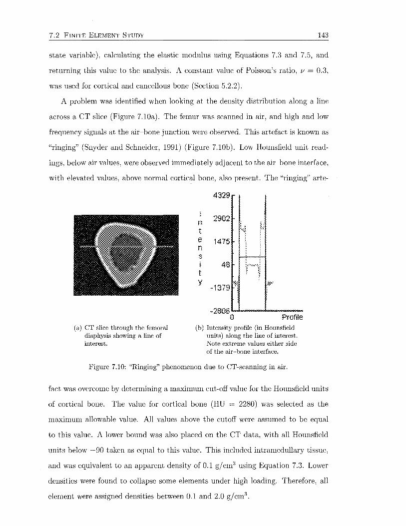
7. 2 FINITE ELEMENT STUDY 143
state variable), calculating the elastic modulus using Equations 7.3 and 7 .5, and
returning this value to the analysis. A constant value of Poisson's ratio, v = 0.3,
was used for cortical and cancellous bone (Section 5.2.2).
A problem was identified when looking at the density distribution along a line
across a CT slice (Figure 7.10a). The femur was scanned in air, and high and low
frequency signals at the air-bone junction were observed. This artefact is known as
"ringing" (Snyder and Schneider, 1991) (Figure 7.10b). Low Hounsfield unit read-
ings, below air values, were observed immediately adjacent to the air-bone interface,
with elevated values, above normal cortical bone, also present. The "ringing" arte-
(a) CT slice through the femoral diaphysis showing a line of interest.
n t e n s i t y
4329
2902
1475
-1379
-2806......,. __ ,.._ __ _ 0 Profile
(b) Intensity profile (in Hounsfield units) along the line of interest. Note extreme values either side of the air-bone interface.
Figure 7.10: "Ringing" phenomenon due to CT-scanning in air.
fact was overcome by determining a maximum cut-off value for the Hounsfield units
of cortical bone. The value for cortical bone (HU = 2280) was selected as the
maximum allowable value. All values above the cutoff were assumed to be equal
to this value. A lower bound was also placed on the CT data, with all Hounsfield
units below -90 taken as equal to this value. This included intramedullary tissue,
and was equivalent to an apparent density of 0.1 gjcm3 using Equation 7.3. Lower
densities were found to collapse some elements under high loading. Therefore, all
element were assigned densities between 0.1 and 2.0 g/cm3.
7.2 FINITE ELEIV1ENT STUDY 144
For the operated femur, the bone properties were applied in exactly the same
way as for the intact femur, given that this part of the mesh is identical. The
Margron elements were assigned the properties of forged cobalt-chrome alloy-an
elastic modulus of E = 210 GPa (Breme and Biehl, 1998) and Poisson's ratio of
v = 0.33. The implant was assumed to be isotropic and linear elastic.
The implant-bone interface was modelled using a combination of fully bonded
and small-sliding contact. In Abaqus, one surface definition provides the master
surface and the other surface definition provides the slave surface. For fully bonded,
or tied contact, each node on the slave surface is constrained to have the same value
of displacement as the point on the master surface that it contacts. This allows
transmission of tensile, compressive and shear forces at the interface. The small
sliding capability of Abaqus allows comparatively small sliding of two bodies relative
to each other. A kinematic constraint ensures that the slave surface nodes do not
penetrate the master surface. The small-sliding contact capability is implemented
by internal contact elements which allow three-dimensional contact between a slave
node and a deformable master surface (Abaqus User's Manual; Hibbitt, Karlsson &
Sorrensen, Inc.). Small-sliding contact does not allow the transfer of tensile forces,
while transfer of shear forces depends on the specified friction coefficient. A friction
coefficient of zero produces frictionless sliding, and thus no transfer of shear at the
interface.
The nonlinear analyses were all run with Abaqus Standard, using the USDLFD
subroutine to define the elastic moduli at the bone integration points, on a personal
computer with parallel1133 MHz Pentium 3 processors and 2GB RAM. The effects
of geometric nonlinearites were included using the Abaqus NLGEOM option. The
output databases (.odb files) were viewed using Abaqus CAE. Field quantities were
plotted with 75% nodal averaging. These were output to a report file by creating a
PATH of nodes and then choosing XY DATA to obtain the field output along the
path. Paths were created along the medial, lateral, anterior and posterior aspects
7. 2 FINITE ELEl'vfENT STUDY 145
of the femur. Python scripting was then used to repeat the extraction of results
from the various finite element models.
7.2.2 Model Validation
The intact and postoperative finite element models were validated by applying loads
and boundary conditions identical to those employed in the experimental study. A
force of 820 N was applied to 3 nodes on the surface of the intact femoral head
to replicate load cases 1 and 2, with the line of action passing through the head
centre. The same procedure was used for the hip joint force on the femoral head of
the hip implant. It was ensured that the hip force was positioned along the same
line of action before and after virtual implantation of the stem. The distal femur
was constrained against all translations at the level the experimental femur was
embedded.
Validation of the reconstructed finite element model was performed with the
implant-bone contact represented as:
(a) no distal~proximal contact surface (between and including the two threads)
bonded, with no contact defined distally (representing an over-reamed med
ullary canal);
(b) fully bonded~all implant surfaces tied to the bone interface; and
(c) distal sliding~the proximal region tied to the bone interface, while the distal
part was allowed to slide and transmit compressive loads.
These conditions were similar to those examined by McNamara et al. (1997a). In
practice, the femoral canal is reamed out to a diameter 1 mm larger than the
distal stem, and therefore condition (c) is most representative, assuming the stem
is inserted straight. A condition with friction at the proximal contact surface was
not analysed as the friction coefficient between the implant and bone was unknown
and would have only introduced additional uncertainties.
Compression of the bone between the proximal and distal threads on the implant,
caused during introduction to the femoral canal, was mentioned in Section 7.1.2.
7.3 BONE REI'v10DELLING STUDY 146
Residual strains, assuming they are appreciable on the periosteal surface and/ or
are not dissipated by viscoelastic effects, are not detected using strain gauges since
the amplifiers must be zeroed before measurement, assuming a state of zero strain.
Therefore, residuals were not incorporated in the finite element model.
Principal strains were obtained along the medial, lateral, anterior and posterior
aspects of the intact and reconstructed models. These were output to file and
plotted using Matlab, alongside the corresponding principal strains for the femur
used to create the finite element models. Comparison of results led to selection of
the contact conditions for use in further studies.
7.2.3 Mesh Refinement
To examine convergence of the finite element solution, two additional models of
the intact femur were created, with 7 and 3 mm element edge lengths, to compare
with the existing 5 mm model (Figure 7.1la, c). After evaluation of convergence
results for the intact femur, only one additional model of the implanted femur was
constructed, with 3 mm element edge lengths (Figure 7.11b). Loads and bound
ary conditions corresponding to load case 1 were applied. The minimum principal
strains along the medial aspect of the femur gave a measure of solution convergence.
The effect of element material homogeneity on solution convergence was also
examined. This was achieved by applying material properties either directly to the
element integration points, or averaging the four integration point values across the
element, and applying the same value to each. This was undertaken for the 3 and
5 mm preoperative models under load case 1.
7.3 Bone Remodelling Study
Adaptive bone remodelling, in accordance with "Wolff's Law", is a phenomenon
observed clinically in response to uncemented hip arthroplasty. The most common
adaptive change is bone resorption over time at the proximal-medial femur, resulting
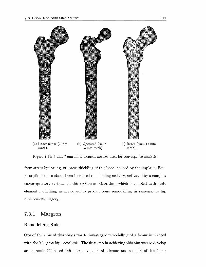
7.3 BONE REMODELLING STUDY
(a) Intact femur (3 mm mesh).
(b) Operated femur (3 mm mesh).
(c) Intact femur (7 mm mesh).
Figure 7.11: 3 and 7 mm finite element meshes used for convergence analysis.
147
from stress bypassing, or stress shielding of this bone, caused by the implant. Bone
resorption comes about from increased remodelling activity, activated by a complex
osteoregulatory system. In this section an algorithm, which is coupled with finite
element modelling, is developed to predict bone remodelling in response to hip
replacement surgery.
7.3.1 Margron
Remodelling Rule
One of the aims of this thesis was to investigate remodelling of a femur implanted
with the l\1argron hip prosthesis. The first step in achieving this aim was to develop
an anatomic CT-based finite element model of a femur, and a model of this femur
7.3 BONE REMODELLING STUDY 148
reconstructed with the Margron hip. This process was discussed in the preceding
section (7.2). Having achieved this, the second step was to conceive an algorithm
to describe the bone adaptive changes seen clinically. This involved development of
a mathematical remodelling rule, and selection of the remodelling signal that will
be the stimulus for adaptation.
The remodelling rule was based on that proposed by Huiskes et al. (1992),
which is a site-specific, strain-adaptive remodelling thoery. This is a phenomeno
logical theory, which is appropriate because there is insufficient understanding of
the mechanobiological processes for a mechanistic model. The majority of three
dimensional models used to simulate bone adaptation in response to stress shielding
have been of this type (Cowin and Hegedus, 1976; Hart et al., 1984a; Huiskes et al.,
1992; Kerner et al., 1999; van Rietbergen and Huiskes, 2001). Details of these
models can be found in Section 6.1.
Huiskes' remodelling theory integrates finite element modelling with a strain
adaptive bone remodelling simulation procedure, which relates local deviations in
the bone mechanical environment from the homeostatic condition (due to inser
tion of a prosthesis), to gradual changes in bone density. Adaptation of the bone
apparent density was defined as "internal" remodelling by Frost (1964).
In Huiskes' model, the remodelling signal was based on the assumption that bone
strives to normalise the strain energy density per unit mass for specified loading
conditions. This choice was initially proposed by Carter et al. (1987). Based on
results using this remodelling signal, from the literature and my own experience,
I decided against using it. Instead, I adopted the equivalent strain proposed by
Sttilpner et al. (1997), similar to TvfikiC and Carter (1995)
(7.6)
where Eij is the strain tensor. This remodelling signal is also a positive, direction
invariant scalar that is easy to interpret. Other signals I considered besides this
one included minimum principal strain (Turner et al., 2003), hydrostatic strain,
7.3 BONE REMODELLING STUDY 149
deviatoric strain and shear strain. The deviation in equivalent strain, S, away from
the physiological value, Sref, is the stimulus for remodelling. A reduction in strain
leads to a decrease in apparent density, while increased strain causes an increased
density, in accordance with "Wolff's Law".
Damage accumulation caused by fatigue loading is another possible stimulus for
remodelling. Fatigue cracking tends to occur when loading is above the physiological
range (Duncan and Turner, 1995). When concerned with periprosthetic adaptation
however, bone resorption caused by underloading is the major problem. Fatigue
cracks accumulate slowly under normal loading conditions, and are therefore not
likely to trigger remodelling due to disuse (Carter, 1984). Hence the influence of
damage accumulation was not considered to be significant for the current applica
tion.
The model accounts for the physiological range of equivalent strains where bone
is unresponsive to load by including a "dead zone" or "lazy zone". This concept was
proposed by Carter (1984) and Frost (1987). This means that a threshold change
in equivalent strain from the reference situation is required before remodelling is
activated. Hsieh et al. (2001) recently showed that the strain threshold increases in
regions of higher peak strains. Others have also assumed the dead zone width to
be site-specific (Beaupre et al., 1990b; Carter, 1984). This suggests that the dead
zone width should be proportional to the reference strain.
The remodelling rate, of either resorption or apposition, is dependent on the
local difference between the equivalent strains before and after reconstruction with a
femoral implant, and the width of the physiological range, or dead zone. This can be
represented with a piecewise linear curve consisting of three sections (Figure 7.12).
To the left of the reference strain, where the actual equivalent strain is less, net
bone resorption occurs. To the right of the reference strain, net bone apposition
takes place. The region with zero slope immediately adjacent to the reference
signal denotes the dead zone, where there is no change in density. The width of the
dead zone at any location depends on the constant parameter s, and also on the

7.3 BONE REMODELLING STUDY
Remodelling Rate
{1-s)Sref Sref 1---------7---+---~--------- Equivalent
I : Strain I I
!- Dead Zone --1
Figure 7.12: Remodelling rate as a function of the remodelling signal.
150
magnitude of the reference equivalent strain Sref· The parameter s is important,
because it can be adjusted to alter the extent of adaptation. In this study, s was
"tuned" to produce simulation results consistent with those found clinically.
Unlike Huiskes' model, the resorption and apposition rates were not assumed to
be the same. Although changes of bone apparent density are all referred to here as
internal remodelling, the biological processes leading to increases and decreases of
density are not the same (Frost, 1987). It is thought that resorption takes place more
quickly than deposition (Beaupre et al., 1990b; Weinans et al., 1992b). Nauenberg
et al. (1993) converted radiographic data relating to use and disuse, into linear
apposition rates and found that resorption occurred approximately 3.5 times faster
than deposition. Thus the slope to the left of the dead zone in Figure 7.12 was
set 3.5 times higher than the slope to the right. The slope of the resorption curve
was limited by the maximum allowable change in density within a remodelling
increment.
Bone remodelling takes place on all of the skeletal surfaces: periosteal, intra
cortical, endocortical and trabecular (Frost, 1987). The potential for remodelling is
therefore related to the amount of free surface area within a given volume. Martin
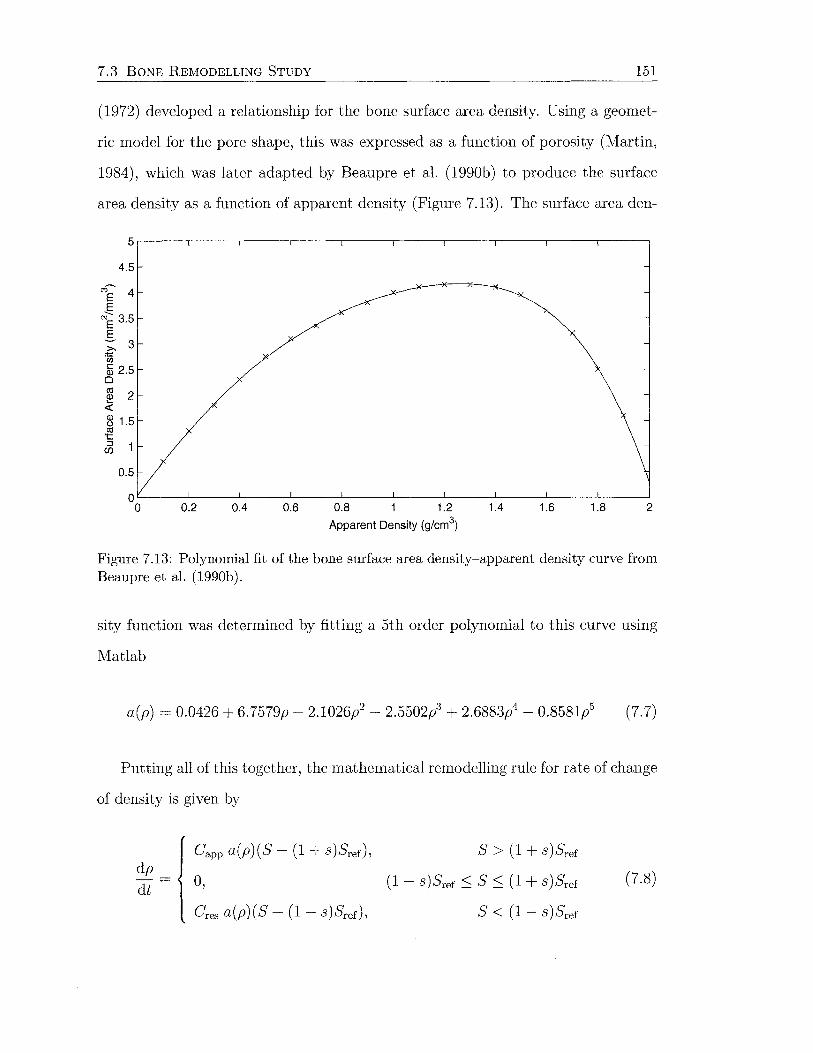
7.3 BONE REMODELLING STUDY 151
(1972) developed a relationship for the bone surface area density. Using a geomet
ric model for the pore shape, this was expressed as a function of porosity (Martin,
1984), which was later adapted by Beaupre et al. (1990b) to produce the surface
area density as a function of apparent density (Figure 7.13). The surface area den-
4.5
""~ 4 E E ~ 3.5 E ~ 3 ~ "iii a5 2.5 0
al 2 ~ 8 1.5 C1l 't:
~ 1
0.5
OL-----L---~----~----~----~----~----~----~----~----~
0 0.2 0.4 0.6 0.8 1 1.2 1.4 1.6 1.8 2
Apparent Density (g/cm3)
Figure 7.13: Polynomial fit of the bone surface area density-apparent density curve from Beaupre et al. (1990b).
sity function was determined by fitting a 5th order polynomial to this curve using
Matlab
a(p) = 0.0426 + 6.7579p- 2.1026/- 2.5502p3 + 2.6883p4- 0.8581l (7.7)
Putting all of this together, the mathematical remodelling rule for rate of change
of density is given by
dp
dt
Capp a(p)(S- (1 + s)Srer),
0,
Cres a(p)(S- (1- s)Srer),
S > (1 + s)Sref
( 1 - S) Sref :::; S :::; ( 1 + S) Sref
S < ( 1 - S) Sref
(7.8)

7.3 BONE REMODELLING STUDY 152
where Capp is the slope of the apposition curve, Cres is the slope of the resorp
tion curve (equal to 3.5 x Capp), and a(p) is the surface area density defined by
Equation 7. 7.
The strain-adaptive bone remodelling procedure is outlined in Figure 7.14. Two
FE MODEL -1 Change in I 1 Postoperative
Femur - Material Properties -. Remodelling Theory I
I Dead Zone I
I Loads/BCs J
I Actual Remodelling I
Signal (S) J
FE MODEL I Reference Remodelling I Preoperative I Signal ( Sref) Femur
l --... 0-----'
_j Figure 7.14: Overview of the bone adaptation simulation.
finite element models are required: one representing the reference, or intact femur,
and one representing the treated, or operated femur. The same mesh is required for
the bone elements remaining after implantation so that site-specific strains can be
directly compared at each integration point. Development of these finite element
models was discussed in Section 7.2. Identical loads and boundary conditions must
also be applied.
The difference between the actual and reference local remodelling signals ( equiv
alent strains), relative to the dead zone width, drives the change in local density,
according to Equation 7.8. The new density distribution in the operated finite
element model is updated using a forward Euler integration algorithm
p(t + ~t) = p(t) + ~t d~~t) (7.9)
where t is the current time and ~t is the analysis time step. This integration scheme
is only conditionally stable, so the time step must be sufficiently small for mean
ingful results (Smolinski and Rubash, 1992). Density changes alter the mechanical
7.3 BONE REMODELLING STUDY 153
properties of bone (Equation 7.5), so new equivalent strains are calculated at the
beginning of the next remodelling iteration. Each remodelling iteration consists of
one pass around the loop represented by the thicker arrows in Figure 7.14. The
simulation continues to pass around this loop until all of the equivalent strains have
reached the dead zone, or the density has reached the maximum (2.0 g/cm3 ) or
minimum (0.1 gjcm3 ) values. This is when a new density distribution is reached
(remodelling equilibrium), and the simulation is terminated.
Implementation
The next part of the remodelling study was to put the adaptation theory into prac
tice. The finite element models had already been created, but it was necessary to
apply new loads and boundary conditions, and to implement the remodelling theory
using Abaqus. The contact conditions for the Margron-bone interface consisted of
fully bonded contact at the proximal surface with no contact defined distally ( condi
tion (c), Section 7.2.2), to represent the slightly over-reamed canal found clinically.
A physiological muscle force configuration was applied to both models. Duda
et al. (1998) proposed that remodelling simulations should include the abductors,
iliotibial band, adductors and hip contact forces. Other researchers have suggested
that site-specific remodelling theories are insensitive to the precise loading condi
tions, as long as the load applied in the model represents a typical loading pattern
that includes axial, bending and torsional components (Huiskes et al., 1987, 1992;
Weinans et al., 1993). For these reasons, a complete muscle set was employed.
The largest hip joint reaction force occurs at 45% of the gait cycle, just prior
to toe off (Duda et al., 1998). The joint and muscle forces at this moment of the
gait cycle were assumed to be representative of the peak loading experienced by
the femur during daily activity (Cristofolini, 1997). The magnitude and direction
of the muscle forces are taken from Duda et al. (1998), assuming a 70 kg subject
(Table 7.1). For a right femur, as used for the current study, the x direction is
anterior, they direction is lateral and the z direction is superior. Only the proximal
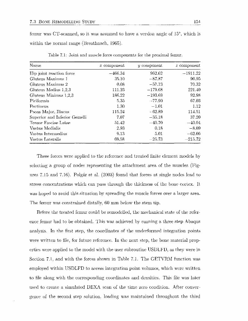
7.3 BONE REMODELLING STUDY 154
femur was CT -scanned, so it was assumed to have a version angle of 15°, which is
within the normal range (Breathnach, 1965).
Table 7.1: Joint and muscle force components for the proximal femur.
Name x component y component z component
Hip joint reaction force -466.34 962.62 -1911.22 Gluteus Maximus 1 35.10 -87.87 90.95 Gluteus Maximus 2 0.08 -57.73 70.32 Gluteus Medius 1,2,3 111.23 -179.68 221.40 Gluteus Minimus 1,2,3 186.22 -193.69 92.98 Piriformis 5.35 -77.90 67.03 Pectineus 1.30 -1.01 1.12 Psoas Iv1ajor, Iliacus 115.24 -62.89 114.51 Superior and Inferior Gemelli 7.07 -35.18 37.20 Tensor Fasciae Latae 51.42 -40.70 -40.04 Vastus Medialis 2.93 0.18 -8.09 Vastus Intermedius 9.13 5.01 -62.06 Vastus Lateralis 69.58 -25.73 -215.72
These forces were applied to the reference and treated finite element models by
selecting a group of nodes representing the attachment area of the muscles (Fig
ures 7.15 and 7.16). Polgar et al. (2003) found that forces at single nodes lead to
stress concentrations which can pass through the thickness of the bone cortex. It
was hoped to avoid this situation by spreading the muscle forces over a larger area.
The femur was constrained distally, 60 mm below the stem tip.
Before the treated femur could be remodelled, the mechanical state of the refer-
ence femur had to be obtained. This was achieved by running a three step Abaqus
analysis. In the first step, the coordinates of the underformed integration points
were written to file, for future reference. In the next step, the bone material prop-
erties were applied to the model with the user subroutine USDLFD, as they were in
Section 7.1, and with the forces shown in Table 7.1. The GETVRM function was
employed within USDLFD to access integration point volumes, which were written
to file along with the corresponding coordinates and densities. This file was later
used to create a simulated DEXA scan of the time zero condition. After conver-
gence of the second step solution, loading was maintained throughout the third
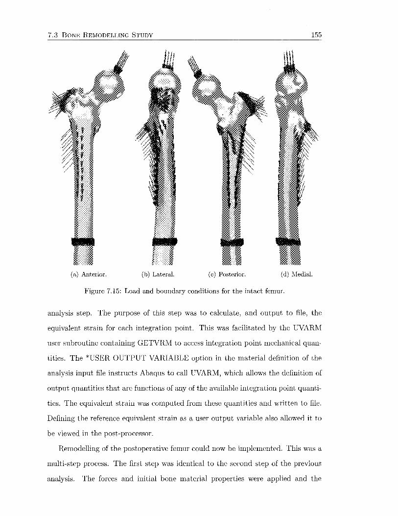
7.3 BONE REl\10DELLING STUDY 155
J
(a) Anterior. (b) Lateral. (c) Posterior. (d) Medial.
Figure 7.15: Load and boundary conditions for the intact femur.
analysis step. The purpose of this step was to calculate, and output to file, the
equivalent strain for each integration point. This was facilitated by the UVARM
user subroutine containing GETVRM to access integration point mechanical quan
tities. The *USER OUTPUT VARIABLE option in the material definition of the
analysis input file instructs Abaqus to call UVARM, which allows the definition of
output quantities that are functions of any of the available integration point quanti
ties. The equivalent strain was computed from these quantities and written to file.
Defining the reference equivalent strain as a user output variable also allowed it to
be viewed in the post-processor.
Remodelling of the postoperative femur could now be implemented. This was a
multi-step process. The first step was identical to the second step of the previous
analysis. The forces and initial bone material properties were applied and the

7.3 BONE REMODELLING STUDY 156
(a) Anterior. (b) Lateral.
(c) Posterior. (d) Medial.
Figure 7.16: Proximal load conditions for the intact femur.
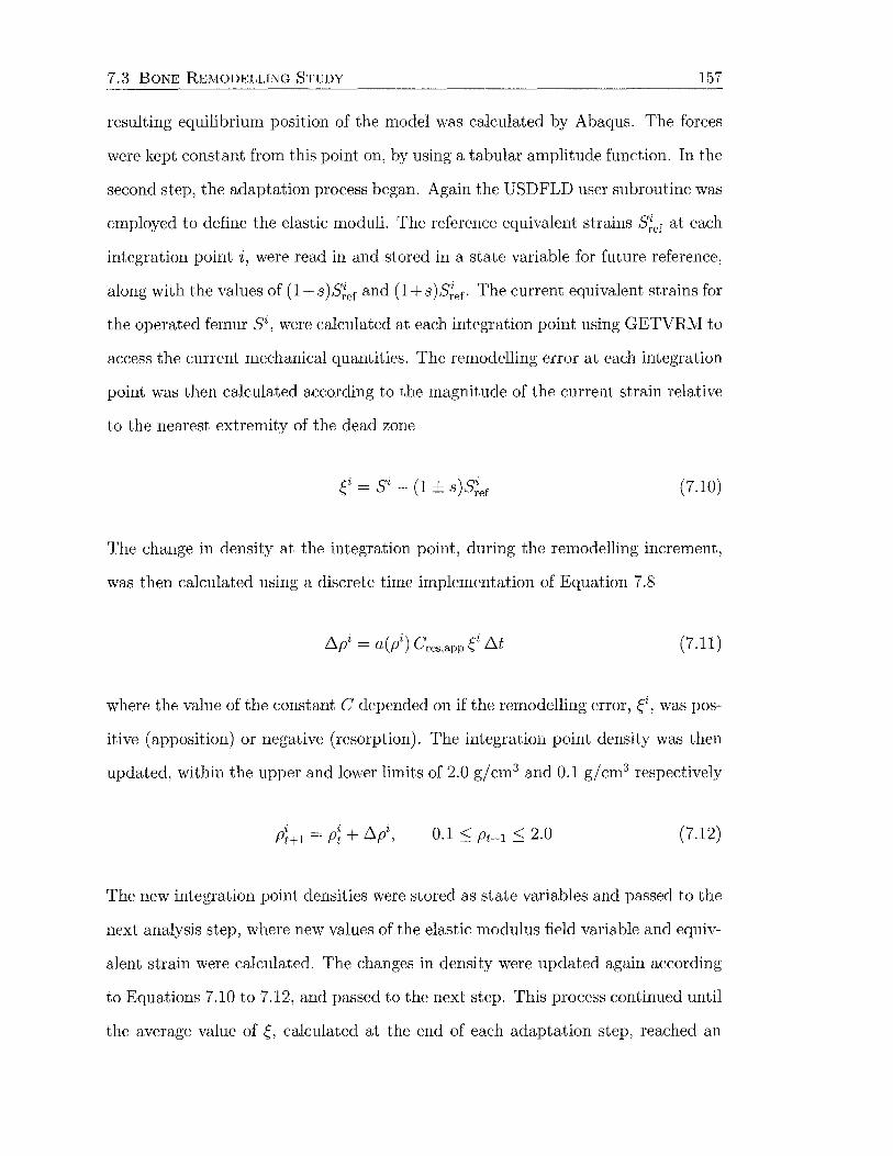
7.3 BONE REMODELLING STUDY 157
resulting equilibrium position of the model was calculated by Abaqus. The forces
were kept constant from this point on, by using a tabular amplitude function. In the
second step, the adaptation process began. Again the USDFLD user subroutine was
employed to define the elastic moduli. The reference equivalent strains s;ef at each
integration point i, were read in and stored in a state variable for future reference,
along with the values of (1- s )s;ef and (1 +s )s;ef· The current equivalent strains for
the operated femur Si, were calculated at each integration point using GETVRM to
access the current mechanical quantities. The remodelling error at each integration
point was then calculated according to the magnitude of the current strain relative
to the nearest extremity of the dead zone
(7.10)
The change in density at the integration point, during the remodelling increment,
was then calculated using a discrete time implementation of Equation 7.8
(7.11)
where the value of the constant C depended on if the remodelling error, ~i, was pos
itive (apposition) or negative (resorption). The integration point density was then
updated, within the upper and lower limits of 2.0 g/cm3 and 0.1 g/cm3 respectively
i i .6.i Pt+l = Pt + P, 0 .1 ::; Pt+l ::; 2. 0 (7.12)
The new integration point densities were stored as state variables and passed to the
next analysis step, where new values of the elastic modulus field variable and equiv
alent strain were calculated. The changes in density were updated again according
to Equations 7.10 to 7.12, and passed to the next step. This process continued until
the average value of~' calculated at the end of each adaptation step, reached an

7.3 BONE REMODELLING STUDY 158
asymptote
(7.13)
where n is the total number of integration points for elements with bone properties.
The closeness of this function to zero indicates how close the remodelling error is
equal to zero throughout the bone.
The value of tlpi (Equation 7.11) for each integration point was monitored dur
ing the first remodelling step to ensure that the changes in density were not greater
than half of the maximum density (~Pmax = 1.0 gjcm3 ) (van Rietbergen et al., 1993;
Weinans et al., 1993). The greatest change in density occurred during the first step,
and if the density change at any integration point was greater than ~Pmax, the
analysis was terminated and the time step, tlt, was reduced accordingly before the
analysis was restarted. This has the effect of decreasing the slope in Figure 7.12.
In this instance, the slope of the resorption curve was equal to 40 gjmm2 for each
remodelling increment.
Data Analysis
Principal strains were obtained along node paths, as explained in Section 7.2.1, on
the femoral cortex preoperatively, postoperatively and at remodelling equilibrium.
Contour plots of these circumstances were also created. The same was done for
the equivalent strains. Contour plots of the density distribution before and after
remodelling were produced, to show the effect of remodelling at the bone surface.
At designated stages throughout the analysis, simulated dual-energy x-ray ab
sorptiometry (DEXA) images were output. The density and volume of each integra-
tion point were written to file and read in, along with the undeformed coordinates,
by in-house software to produce DEXA images in any orientation, with respect to
the coordinate system of the finite element model. Anterior-posterior images were
produced, and quantitatively analysed using Global Lab Image/2 (Data Transla
tion, Inc., Marlboro, MA, USA) to calculate the percent change in bone density,
relative to the preoperative case.

7.3 BONE REMODELLING STUDY 159
Before analysing the DEXA images, an image of the implant, oriented within
Patran in the same manner as the DEXA image, was created. This was scaled
and positioned over the preoperative DEXA image using Adobe Photoshop (Adobe
Systems, Inc., San Jose, CA, USA), to mask out the bone behind. This image was
opened in Global Lab Image and rectangular regions of interest were drawn to rep
resent the seven Gruen zones (Gruen et al., 1979). This image was then thresholded
(Figure 7.17a), and an additional region of interest was created within each rect
angular region, that contained only the bone that would be seen by a conventional
DEXA scanner. These regions were saved and used to analyse subsequent DEXA
(a) Masking of image and thresholding procedure
•;I&U!Iiimml IV~ Tramfer ~&ackSCtt>t
Nll11lbet or
3
(b) Measurement of greyscale value in region of interest
Figure 7.17: Gruen zone analysis of DEXA images.
images, without the need to overlay the implant image or perform thresholding
(Figure 7.17b).
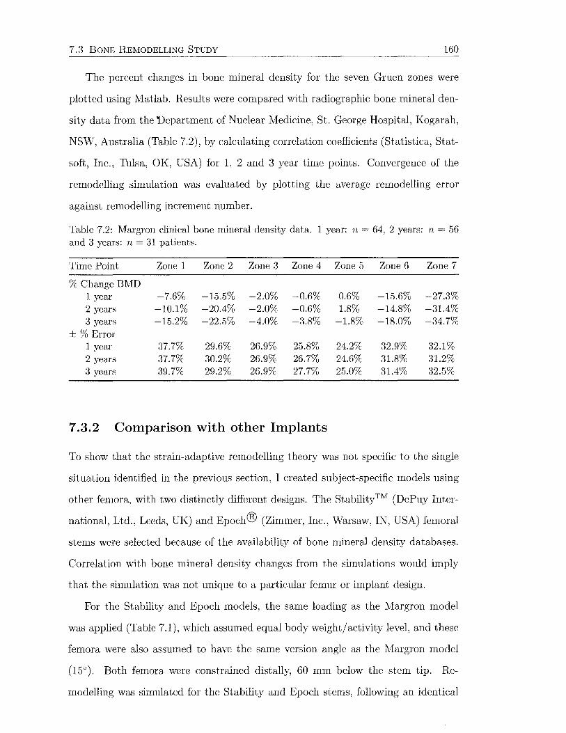
7.3 BONE REI\IODELLING STUDY 160
The percent changes in bone mineral density for the seven Gruen zones were
plotted using Matlab. Results were compared with radiographic bone mineral den
sity data from the Department of Nuclear Medicine, St. George Hospital, Kogarah,
NSW, Australia (Table 7.2), by calculating correlation coefficients (Statistica, Stat
soft, Inc., Tulsa, OK, USA) for 1, 2 and 3 year time points. Convergence of the
remodelling simulation was evaluated by plotting the average remodelling error
against remodelling increment number.
Table 7.2: Margron clinical bone mineral density data. 1 year: n = 64, 2 years: n = 56 and 3 years: n = 31 patients.
Time Point Zone 1 Zone 2 Zone 3 Zone 4 Zone 5 Zone 6 Zone 7
%Change BMD 1 year -7.6% -15.5% -2.0% -0.6% 0.6% -15.6% -27.3% 2 years -10.1% -20.4% -2.0% -0.6% 1.8% -14.8% -31.4% 3 years -15.2% -22.5% -4.0% -3.8% -1.8% -18.0% -34.7%
±%Error 1 year 37.7% 29.6% 26.9% 25.8% 24.2% 32.9% 32.1% 2 years 37.7% 30.2% 26.9% 26.7% 24.6% 31.8% 31.2% 3 years 39.7% 29.2% 26.9% 27.7% 25.0% 31.4% 32.5%
7.3.2 Comparison with other Implants
To show that the strain-adaptive remodelling theory was not specific to the single
situation identified in the previous section, I created subject-specific models using
other femora, with two distinctly different designs. The Stability™ (DePuy Inter
national, Ltd., Leeds, UK) and Epoch® (Zimmer, Inc., Warsaw, IN, USA) femoral
stems were selected because of the availability of bone mineral density databases.
Correlation with bone mineral density changes from the simulations would imply
that the simulation was not unique to a particular femur or implant design.
For the Stability and Epoch models, the same loading as the Margron model
was applied (Table 7.1), which assumed equal body weight/activity level, and these
femora were also assumed to have the same version angle as the Margron model
(15°). Both femora were constrained distally, 60 mm below the stem tip. Re
modelling was simulated for the Stability and Epoch stems, following an identical
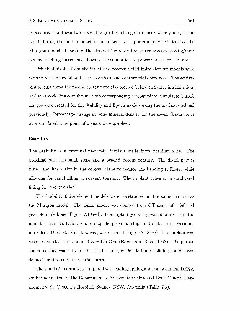
7.3 BONE REMODELLING STUDY 161
procedure. For these two cases, the greatest change in density at any integration
point during the first remodelling increment was approximately half that of the
Margron model. Therefore, the slope of the resorption curve was set at 80 g/mm2
per remodelling increment, allowing the simulation to proceed at twice the rate.
Principal strains from the intact and reconstructed finite element models were
plotted for the medial and lateral cortices, and contour plots produced. The equiva
lent strains along the medial cortex were also plotted before and after implantation,
and at remodelling equilibrium, with corresponding contour plots. Simulated DEXA
images were created for the Stability and Epoch models using the method outlined
previously. Percentage change in bone mineral density for the seven Gruen zones
at a simulated time point of 2 years were graphed.
Stability
The Stability is a proximal fit-and-fill implant made from titanium alloy. The
proximal part has small steps and a beaded porous coating. The distal part is
fluted and has a slot in the coronal plane to reduce the bending stiffness, while
allowing for canal filling to prevent toggling. The implant relies on metaphyseal
filling for load transfer.
The Stability finite element models were constructed in the same manner as
the Margron model. The femur model was created from CT scans of a left, 54
year old male bone (Figure 7.18a-d). The implant geometry was obtained from the
manufacturer. To facilitate meshing, the proximal steps and distal flutes were not
modelled. The distal slot, however, was retained (Figure 7.18e-g). The implant was
assigned an elastic modulus of E = 115 GPa (Breme and Biehl, 1998). The porous
coated surface was fully bonded to the bone, while frictionless sliding contact was
defined for the remaining surface area.
The simulation data was compared with radiographic data from a clinical DEXA
study undertaken at the Department of Nuclear Medicine and Bone Mineral Den
sitometry, St. Vincent's Hospital, Sydney, NSvV, Australia (Table 7.3).
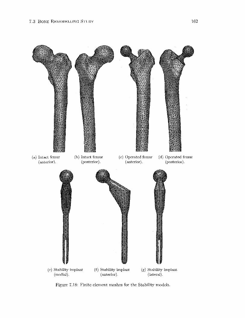
7.3 BONE REMODELLING STUDY 162
(a) Intact femur (anterior).
(b) Intact femur (posterior).
(c) Operated femur (anterior).
(d) Operated femur (posterior).
(e) Stability implant (medial).
(f) Stability implant (anterior).
(g) Stability implant (lateral).
Figure 7.18: Finite element meshes for the Stability models.
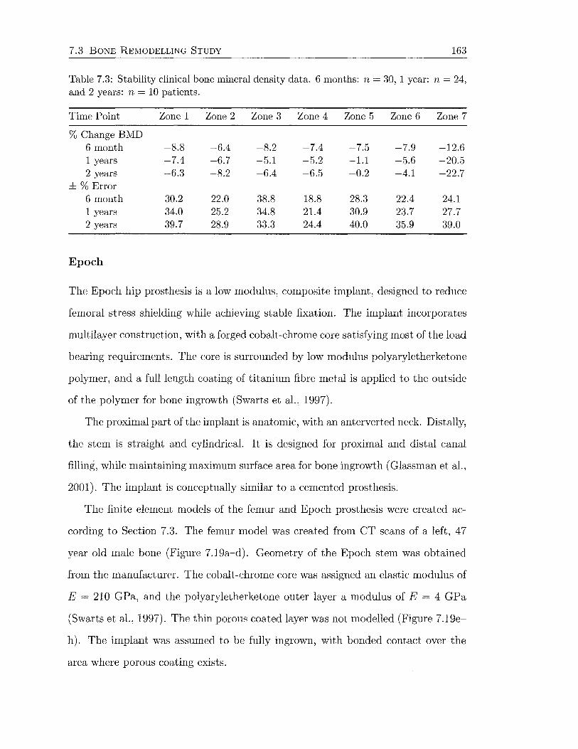
7.3 BONE REMODELLING STUDY 163
Table 7.3: Stability clinical bone mineral density data. 6 months: n = 30, 1 year: n = 24, and 2 years: n = 10 patients.
Time Point Zone 1 Zone 2 Zone 3 Zone 4 Zone 5 Zone 6 Zone 7
%Change BMD 6 month -8.8 -6.4 -8.2 -7.4 -7.5 -7.9 -12.6 1 years -7.4 -6.7 -5.1 -5.2 -1.1 -5.6 -20.5 2 years -6.3 -8.2 -6.4 -6.5 -0.2 -4.1 -22.7
±%Error 6 month 30.2 22.0 38.8 18.8 28.3 22.4 24.1 1 years 34.0 25.2 34.8 21.4 30.9 23.7 27.7 2 years 39.7 28.9 33.3 24.4 40.0 35.9 39.0
Epoch
The Epoch hip prosthesis is a low modulus, composite implant, designed to reduce
femoral stress shielding while achieving stable fixation. The implant incorporates
multilayer construction, with a forged cobalt-chrome core satisfying most of the load
bearing requirements. The core is surrounded by low modulus polyaryletherketone
polymer, and a full length coating of titanium fibre metal is applied to the outside
of the polymer for bone ingrowth (Swarts et al., 1997).
The proximal part of the implant is anatomic, with an anterverted neck. Distally,
the stem is straight and cylindrical. It is designed for proximal and distal canal
filling, while maintaining maximum surface area for bone ingrowth (Glassman et al.,
2001). The implant is conceptually similar to a cemented prosthesis.
The finite element models of the femur and Epoch prosthesis were created ac
cording to Section 7.3. The femur model was created from CT scans of a left, 47
year old male bone (Figure 7.19a-d). Geometry of the Epoch stem was obtained
from the manufacturer. The cobalt-chrome core was assigned an elastic modulus of
E = 210 GPa, and the polyaryletherketone outer layer a modulus of E = 4 GPa
(Swarts et al., 1997). The thin porous coated layer was not modelled (Figure 7.19e
h). The implant was assumed to be fully ingrown, with bonded contact over the
area where porous coating exists.
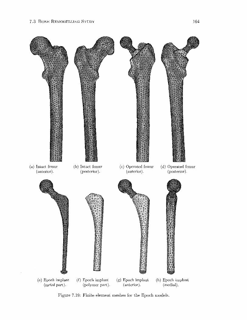
7.3 BONE REMODELLING STUDY
(a) Intact femur (anterior).
(e) Epoch implant (metal part).
(b) Intact femur (posterior).
(f) Epoch implant (polymer part).
(c) Operated femur (anterior).
(g) Epoch implant (anterior).
164
(d) Operated femur (posterior).
(h) Epoch implant (medial).
Figure 7.19: Finite element meshes for the Epoch models.

7.3 BONE REMODELLING STUDY 165
The Epoch model was compared with 2 year radiographic clinical data (Ta
ble 7.4) from a multicentre study of 46 patients (Glassman et al., 2001). The
variation in the data was not available from this paper.
Table 7.4: Epoch clinical bone mineral density data. 2 years: n = 46 patients.
Time Point Zone 1 Zone 2 Zone 3 Zone 4 Zone 5 Zone 6 Zone 7
%Change BMD 2 years -2.4% -3.4% -1.6% -0.1% 1.4% -7.7% -15.8%
7 .3.3 Investigation of Parameters
A mathematical remodelling rule to simulate femoral bone adaptation in response
to hip arthroplasty was developed, and implemented using finite element models.
Remodelling around three different hip replacement stems, inserted in three different
femora was simulated. This technique was then applied to investigate the effects of
varying some of the parameters used to date.
In each case, the influence of the specific parameter was analysed by plotting
the equivalent strains at a series of nodes along the medial cortex for the preopera
tive, immediately postoperative and remodelling equilibrium conditions. The effect
on the simulated density distribution was also examined by comparing percentage
changes in bone mineral density in the seven Gruen zones. The Gruen zone analysis
was performed at a 3 year time point, unless otherwise stated.
Effect of Interface Conditions
The contact condition with a bonded Margron-bone interface proximally and no
contact defined for the distal part implant, representing an over-reamed medullary
canal, produced strains most like the experimental conditions, particularly distally
(Section 8.2.1). This condition was also used for all other simulations involving the
Margron model.

7.3 BONE REJ\WDELLING STUDY 166
To examine the effect of the contact conditions on remodelling, the same contact
conditions were investigated as were used for validation of the postoperative finite
element model (Section 7.2.2):
(a) no distal-proximal surface fully bonded, with no contact defined distally;
(b) fully bonded-all implant surfaces tied to the bone interface; and
(c) distal sliding-the proximal region tied to the bone interface, with frictionless
sliding at the distal cyclindrical part.
No residual stresses or strains from insertion of the Margron stem were included.
This is because static loads do not promote remodelling (Lanyon and Rubin, 1984),
and the variation in strain produced by the external loading is important, rather
than the sum of residual and loading strains (Cristofolini, 1997).
Effect of Femoral Head Position
The Margron is a modular implant that allows for a relatively high degree of vari
ation of the femoral head position. Consequently, remodelling simulations were
performed to evaluate the influence of the femoral head position on bone adapta
tion. The position of the prosthetic femoral head was varied by changing the neck
length and the version angle.
The physiological position of the femoral head was obtained with a +4 mm neck
according to the template. This was varied to the other available neck lengths of
-4, 0 and + 7 mm. The version angle was varied from the physiological position
( +4 mm neck and oo relative angle) by 10° and 20° degrees of anteversion, and the
same quantities of retroversion. The matrix of parameters is shown in Table 7.5.
Effect of Dead Zone Width
The width of the dead zone is an important parameter in the mathematical remod
elling rule, determining the threshold change in strain required to induce adaptation.
This parameter was earlier varied to tune the simulation bone density changes to
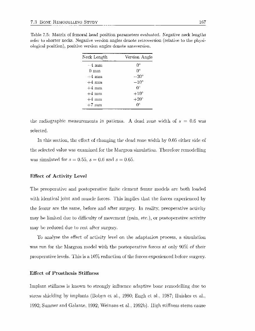
7.3 BONE REMODELLING STUDY 167
Table 7.5: Matrix of femoral head position parameters evaluated. Negative neck lengths refer to shorter necks. Negative version angles denote retroversion (relative to the physiological position), positive version angles denote anteversion.
Neck Length Version Angle
-4mm oo Omm oo
+4mm -20° +4mm -100 +4mm oo +4mm +100 +4mm +20° +7mm oo
the radiographic measurements in patients. A dead zone width of s 0.6 was
selected.
In this section, the effect of changing the dead zone width by 0.05 either side of
the selected value was examined for the Margron simulation. Therefore remodelling
was simulated for s = 0.55, s = 0.6 and s = 0.65.
Effect of Activity Level
The preoperative and postoperative finite element femur models are both loaded
with identical joint and muscle forces. This implies that the forces experienced by
the femur are the same, before and after surgery. In reality, preoperative activity
may be limited due to difficulty of movement (pain, etc.), or postoperative activity
may be reduced due to rest after surgery.
To analyse the effect of activity level on the adaptation process, a simulation
was run for the Margron model with the postoperative forces at only 90% of their
preoperative levels. This is a 10% reduction of the forces experienced before surgery.
Effect of Prosthesis Stiffness
Implant stiffness is known to strongly influence adaptive bone remodelling due to
stress shielding by implants (Bobyn et al., 1990; Engh et al., 1987; Huiskes et al.,
1992; Sumner and Galante, 1992; Weinans et al., 1992b). High stiffness stems cause
7.3 BONE REMODELLING STUDY 168
greater stress shielding than low modulus stems, with a corresponding effect on
bone adaptation.
The Epoch model was used to investigate the effect of prosthesis stiffness on the
amount of bone adaptation, because it has quite unique material properties to begin
with. Remodelling simulations were run with the Epoch entirely fabricated from
cobalt-chrome (CoCr model), and with a material having the elastic modulus of
cortical bone (isoelastic model). For the Epoch, the effect of the prosthesis material
properties on the percentage changes in bone density was evaluated at 2 years.
Flexible stems are likely to induce greater interface stress (with a bonded in
terface) than conventional implant materials, and therefore this result was also
examined. Abaqus gives the interface shear in two perpendicular directions on the
slave contact surface defined by the surface normal. Both components need to be
considered. Contour plots of the shear stresses were produced.
Chapter 8
Results
8.1 Experimental Study
Preoperative and postoperative maximum principal, minimum principal and lon
gitudinal strains were determined under two load cases (load case 1: 0° flexion,
load case 2: 10° flexion) at the sixteen gauge sites on the four femora. Means and
standard deviations were calculated for each strain gauge.
The important results have been plotted in this section. A complete list of the
data, including results for individual femora, can be found in Tables A.1 to A.12
(Appendix A). The two experimental load conditions place the femora in bending
in the coronal plane, while load case 2 introduces additional bending in the sagittal
plane. In most instances, this causes compression medially and posteriorly, and
tension laterally and anteriorly. For this reason, minimum principal strains are
plotted for the aspects of the femur in compression and maximum principal strains
are plotted for those in tension (Figures 8.1 and 8.2). The longitudinal components
of the strains are also presented (Figure 8.3 and 8.4).
The strains before and after surgery were compared for statistical difference at
each gauge using analysis of variance (ANOVA) with repeated measures. Table 8.1
shows the significantly different results for the strains plotted in Figures 8.1 to
8.4. P-values for other strains are given in Table A.13. Comparisons were not
169
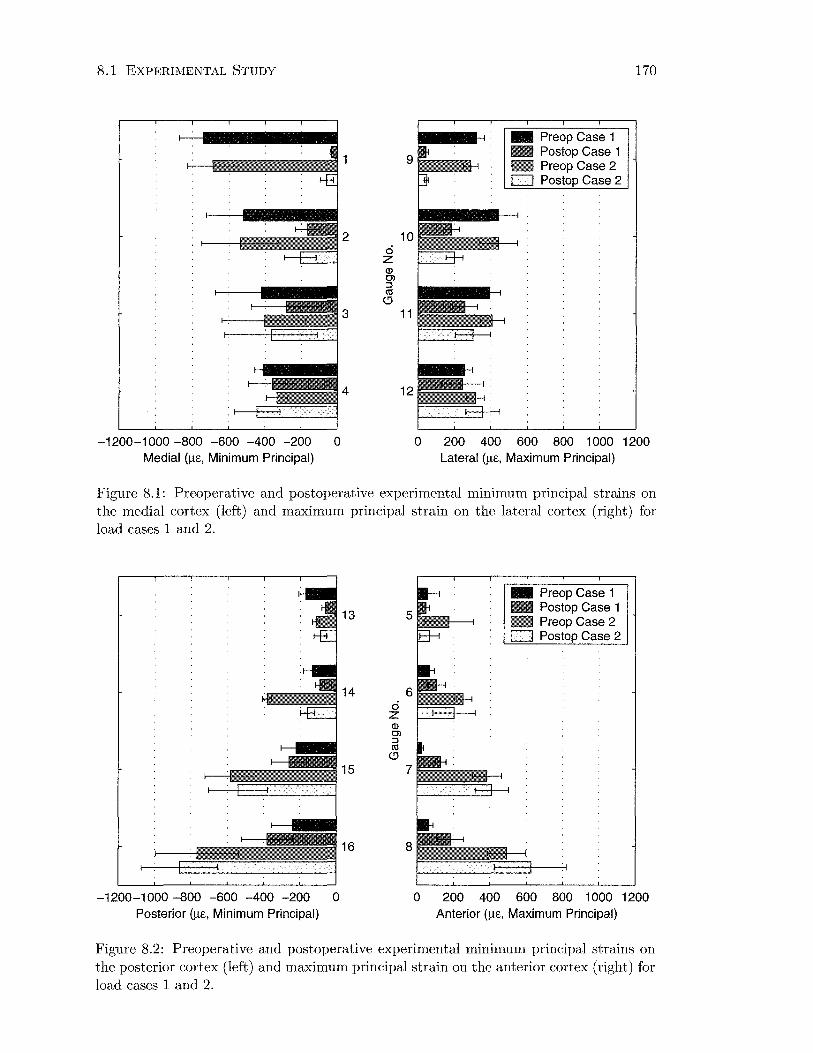
8.1 EXPERIMENTAL STUDY
~---~---··2 ci 10
-1200-1000 -800 -600 -400 -200 0 Medial (!J-E, Minimum Principal)
z Q) C) :J <1l
(!J
3 11
4 12
- Preop Case 1 - Postop Case 1 D Preop Case 2 D Postop Case 2
170
0 200 400 600 800 1 000 1200 Lateral (!J-E, Maximum Principal)
Figure 8.1: Preoperative and postoperative experimental minimum principal strains on the medial cortex (left) and maximum principal strain on the lateral cortex (right) for load cases 1 and 2.
13
14 ci z Q) C) :J <1l
(!J
15
-1200-1000 -800 -600 -400 -200 0 Posterior (!J-E, Minimum Principal)
5
6
7
- Preop Case 1 D Postop Case 1 D Preop Case 2 D Postop Case 2
0 200 400 600 800 1 000 1200 Anterior (!J-E, Maximum Principal)
Figure 8.2: Preoperative and postoperative experimental minimum principal strains on the posterior cortex (left) and maximum principal strain on the anterior cortex (right) for load cases 1 and 2.
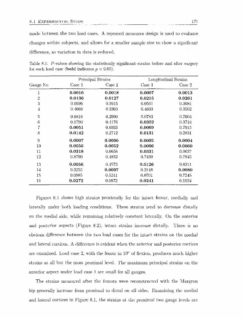
8.1 EXPERIMENTAL STUDY 171
made between the two load cases. A repeated measures design is used to evaluate
changes within subjects, and allows for a smaller sample size to show a significant
difference, as variation in data is reduced.
Table 8.1: P-values showing the statistically significant strains before and after surgery for each load case (bold indicates p < 0.05).
Principal Strains Longitudinal Strains Gauge No Case 1 Case2 Case 1 Case 2
1 0.0016 0.0018 0.0007 0.0013 2 0.0136 0.0127 0.0215 0.0261 3 0.0596 0.5915 0.0561 0.3081 4 0.4068 0.2303 0.4033 0.3502
5 0.8816 0.2990 0.0783 0.7004 6 0.1790 0.4176 0.0302 0.3744 7 0.0051 0.6933 0.0069 0.7915 8 0.0142 0.2712 0.0131 0.2831
9 0.0007 0.0006 0.0005 0.0004 10 0.0056 0.0052 0.0066 0.0060 11 0.0318 0.0658 0.0331 0.0637 12 0.8790 0.4832 0.7430 0.7945
13 0.0056 0.4573 0.0126 0.8311 14 0.3255 0.0007 0.2148 0.0080 15 0.0985 0.5241 0.0701 0.7245 16 0.0272 0.0972 0.0241 0.1024
Figures 8.1 shows high strains proximally for the intact femur, medially and
laterally under both loading conditions. These strains tend to decrease distally
on the medial side, while remaining relatively constant laterally. On the anterior
and posterior aspects (Figure 8.2), intact strains increase distally. There is no
obvious difference between the two load cases for the intact strains on the medial
and lateral cortices. A difference is evident when the anterior and posterior cortices
are examined. Load case 2, with the femur in 10° of flexion, produces much higher
strains at all but the most proximal level. The maximum principal strains on the
anterior aspect under load case 1 are small for all gauges.
The strains measured after the femora were reconstructed with the Margron
hip generally increase from proximal to distal on all sides. Examining the medial
and lateral cortices in Figure 8.1, the strains at the proximal two gauge levels are

8.1 EXPERIMENTAL STUDY 172
significantly lower (p < 0.05) than the intact values for both load cases. Distal to
this, the strains approach the preoperative values, except at gauge 11 under load
case 1, where the postoperative strain continues to be significantly less than before
surgery (p = 0.03).
As with the intact strains, load case 2 causes higher postoperative strains than
load case 1 at the two distal levels anteriorly and posteriorly (Figure 8.2). On these
cortices, significantly different pre- and postoperative strains occur at gauges 7, 8,
13 and 16 for load case 1, and gauge 14 for load case 2 (p < 0.05).
Longitudinal strains (Figures 8.3 and 8.4) are almost identical to the principal
strains on the medial, lateral and posterior cortices, indicating compression medially
and posteriorly, and tension laterally. The anterior longitudinal strains show a
change from small compressive strains proximally to larger tensile strains distally.
2 10 ci z Q) Cl ::::! ell 0
3 11
4 12
-1200-1 000 -800 -600 -400 -200 0 Medial (J.lE, Longitudinal)
- Preop Case 1 - Postop Case 1 - Preop Case 2 - Postop Case 2
0 200 400 600 800 1 000 1200 Lateral (J.lE, Longitudinal)
Figure 8.3: Preoperative and postoperative experimental longitudinal strains on the medial and lateral cortices for load cases 1 and 2.
The similarity between the longitudinal and principal strains is reflected by the
statistically significant results. Of the data plotted in Figures 8.1 to 8.4, the only
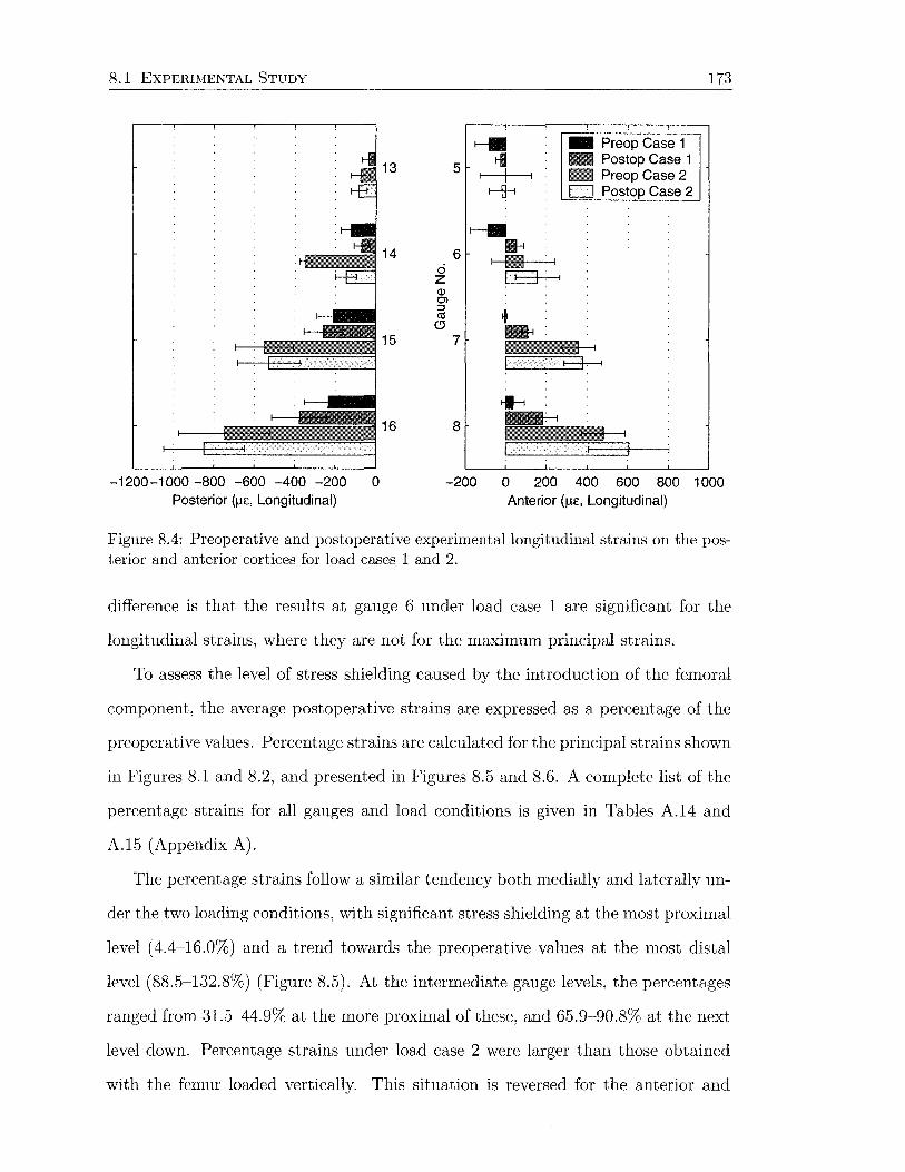
8.1 EXPERIMENTAL STUDY 173
~ - Preop Case 1
13 5 rl - Postop Case 1 I - Preop Case 2
f--{1-i D Postop Case 2
~ 14 6 •
ci I • . I
z ~ Q) O'l :J
+ (1j (.!) -15 7
~
16 8
-1200-1 000 -800 -600 -400 -200 0 -200 0 200 400 600 800 1 000 Posterior (~Jc, Longitudinal) Anterior (Jlc, Longitudinal)
Figure 8.4: Preoperative and postoperative experimental longitudinal strains on the posterior and anterior cortices for load cases 1 and 2.
difference is that the results at gauge 6 under load case 1 are significant for the
longitudinal strains, where they are not for the maximum principal strains.
To assess the level of stress shielding caused by the introduction of the femoral
component, the average postoperative strains are expressed as a percentage of the
preoperative values. Percentage strains are calculated for the principal strains shown
in Figures 8.1 and 8.2, and presented in Figures 8.5 and 8.6. A complete list of the
percentage strains for all gauges and load conditions is given in Tables A.14 and
A.15 (Appendix A).
The percentage strains follow a similar tendency both medially and laterally un
der the two loading conditions, with significant stress shielding at the most proximal
level ( 4.4-16.0%) and a trend towards the preoperative values at the most distal
level (88.5-132.8%) (Figure 8.5). At the intermediate gauge levels, the percentages
ranged from 31.5-44.9% at the more proximal of these, and 65.9-90.8% at the next
level down. Percentage strains under load case 2 were larger than those obtained
with the femur loaded vertically. This situation is reversed for the anterior and
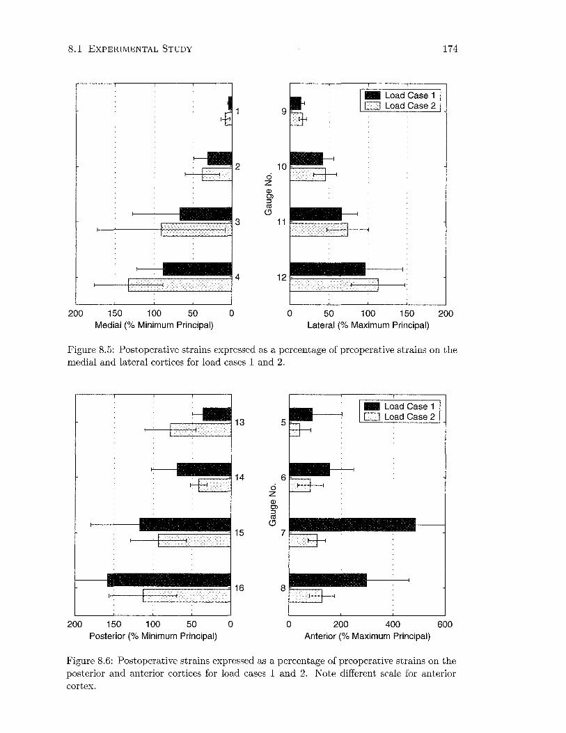
8.1 EXPERIMENTAL STUDY
9
....---=! 2 1 0 F-----, ci z Q) Ol ::J ctS
C)
.---------~3 11r-------~
200 150 100 50 0 0 50
-Load Case 1 D Load Case2
100 150 Medial (% Minimum Principal) Lateral (% Maximum Principal)
174
200
Figure 8.5: Postoperative strains expressed as a percentage of preoperative strains on the medial and lateral cortices for load cases 1 and 2.
14 ci z Q) Ol ::J ctS
C)
15
200 150 100 50 0 Posterior (% Minimum Principal)
5
6
7
0 200
-Load Case 1 D Load Case2
400 Anterior (% Maximum Principal)
600
Figure 8.6: Postoperative strains expressed as a percentage of preoperative strains on the posterior and anterior cortices for load cases 1 and 2. Note different scale for anterior
cortex.
8.2 FINITE ELEMENT STUDY 175
posterior cortices, where percentage strains are higher under loading condition 1
for all gauges except the most proximal on the posterior side (Figure 8.6). The
postoperative strains are considerably larger than their intact values at the distal
two levels anteriorly under load case 1 (note different scale on Figure 8.6 right).
8.2 Finite Element Study
A subject-specific anatomic finite element model of a femur was created, and loads
and boundary conditions were applied as outlined in Chapter 7. This model was
implanted with the Margron hip prosthesis and identical loading was applied.
The intact femur consisted of 17046 elements with 25778 nodes and 77334 nodal
degrees-of-freedom. The operated femur model was comprised of a total of 13695 el
ements with 22364 nodes and 67092 nodal degrees-of-freedom. The operated model
has 9817 bone elements and 3878 implant elements.
Figure 8. 7 shows the density distribution of the femur model, shown in Houns
field units. High density cortical bone (larger Hounsfield unit) is seen along the
femoral diaphysis and up the medial aspect as far as the osteotomy. Proximal to
the level of the lesser trochanter, the cortical shell is thinner, and the density is
reduced, and also appears more variable from the outside. The cortical shell can
also be seen in cross section, where the bone has been prepared to accept the im
plant. Some Hounsfield unit values appear to be outside the specified range of -90
to 2280 HU.
8.2.1 Model Validation
Finite element strains were compared with experimental strains to determine how
effectively the finite element models replicated the experimental situation. Compar
isons were made for the intact femur and the femur reconstructed with the l\hrgron

8.2 FINITE ELEMENT STUDY
SDV2 (Ave . Cr i t . : 75%)
+5 .4 25e+03 +2.800e+03 +2 . 500e+03 +2 .2 00e+03 +1 . 900e+03 +1 .600e+03 +1 . 300e+03 +1 . 000e+03 +7 . 000e+02 +4 . 000e+02 +1 . 000e+02 -2 . 000e+02 -3 . 235e+03
(a) Anteromedial view
• .
•
(b) Posterolateral view
Figure 8.7: Density distribution (Hounsfield units) of the femur .
176
prosthesis under the two simplified load cases used experimentally. The postoper
ative model was investigated with three contact conditions for the implant- bone
interface:
(a) no distal- proximal contact surface (between and including the two threads)
bonded, with no contact defined distally;
(b) fully bonded- all implant surfaces t ied to the bone interface; and
(c) distal sliding- the proximal region tied to the bone interface, while the distal
part was allowed to slide and transmit compressive loads.
From the results it was hoped to ascertain which postoperative condition was most
representative of the experimental situation.
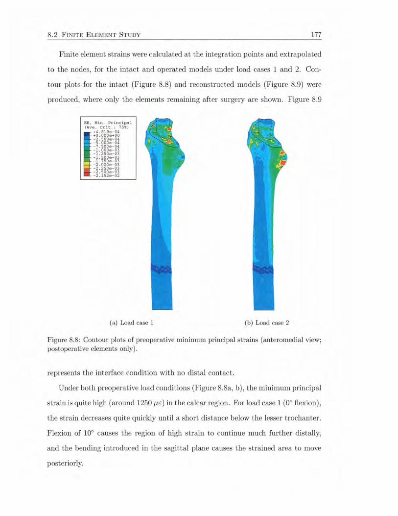
8.2 FINITE ELEMENT STUDY 177
Finite element strains were calculated at the integration points and extrapolated
to the nodes, for the intact and operated models under load cases 1 and 2. Con
tour plots for the intact (Figure 8.8) and reconstructed models (Figure 8.9) were
produced, where only the elements remaining after surgery are shown. Figure 8.9
EE , Min . Pr i ncipal (Ave . Cr it. : 75%)
+4 . 819e-04 +O . OOOe+OO - 2 . 500e-04 -s . oooe-0 4 - 7 . 500e- 04 -l . OOOe-03 -1 . 250e-03 - l. SOOe-03 - 1.750e-03 - 2 . 000e-03 -2 . 250e-03 -2 . 500e-03 - 2 . 152e-02
(a) Load case 1 (b) Load case 2
Figure 8.8: Contour plots of preoperative minimum principal strains (anteromedial view; postoperative elements only).
represents the interface condition with no distal contact.
Under both preoperative load conditions (Figure 8.8a, b), the minimum principal
strain is quite high (around 1250 1-.u::) in the calcar region. For load case 1 (0° flexion),
the strain decreases quite quickly until a short distance below the lesser trochanter.
Flexion of 10° causes the region of high strain to continue much further distally,
and the bending introduced in the sagittal plane causes the strained area to move
posteriorly.

8.2 FINITE ELEMENT STUDY
EE, Min. Princ ipa l (Ave . Cr i t.: 75%)
+2 . 068e- 04 +0 . 00 0e+ 00 -2 .5 00e-0 4 -s . oooe - 04 -7 . 500 e- 04 - l. OOOe-03 -1 . 250e - 03 - l. SOOe-03 - 1.75 0e-03
- -2 . OOOe- 03
i -2 . 250e-03 -2 .500e-03 -l . OSSe-02
(a) Load case 1
178
(b) Load case 2
Figure 8.9: Contour plots of postoperative (no distal contact) minimum principal strains ( anteromedial view).
Postoperatively (Figure 8.8a, b), the minimum principal strains are reduced
significantly. This is especially apparent proximally, although there is a small zone of
high strain adjacent to the implant. Distally, the strains appear similar in magnitude
and distribution to the respective preoperative load cases.
To compare the finite element results with the experimental data, nodal principal
strains were obtained along the anterior, posterior, medial and lateral cortices.
These are plotted as a curve, beside the corresponding experimental data for the
modelled femur, shown as horizontal bars at the gauge locations (Figures 8.10 to
8.17).
For the two preoperative loading conditions, agreement between the experimen-
tal and finite element results is generally good for the medial and lateral principal
strains at the three distal gauge levels (Figures 8. 10 and 8.12). At the level of the
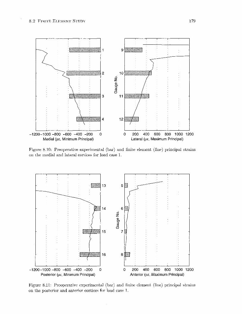
8. 2 FINITE ELEMENT STUDY
-1200-1 000 -800 -600 -400 -200 0 Medial (JlE, Minimum Principal)
179
0 200 400 600 800 1 000 1200 Lateral (JlE, Maximum Principal)
Figure 8.10: Preoperative experimental (bar) and finite element (line) principal strains on the medial and lateral cortices for load case 1.
-1200-1 000 -800 -600 -400 -200 0 Posterior (Jl£, Minimum Principal)
13 5
14 ci z (]) Cl ::J ((!
0 15
6
7 ·.
0 200 400 600 800 1 000 1200 Anterior (JlE, Maximum Principal)
Figure 8.11: Preoperative experimental (bar) and finite element (line) principal strains on the posterior and anterior cortices for load case 1.

8.2 FINITE ELEMENT STUDY 180
1"7"":':~~~~~~ 2 10 F;:;;;;;;;::;:r:;;;;::;:r:;;;;::;:r::;:j
ci z Q) C> :J (1j
c:l fJ!!ilmlm. 3 11
-1200-1 000 -800 -600 -400 -200 0 Medial (J..LE, Minimum Principal)
0 200 400 600 800 1 000 1200 Lateral (J..LE, Maximum Principal)
Figure 8.12: Preoperative experimental (bar) and finite element (line) principal strains on the medial and lateral cortices for load case 2.
14
15
-1200-1000 -800 -600 -400 -200 0 Posterior (j..t£, Minimum Principal)
ci z Q) C> :J (1j
c:l
6
7
0 200 400 600 800 1 000 1200 Anterior (f.l£, Maximum Principal)
Figure 8.13: Preoperative experimental (bar) and finite element (line) principal strains on the posterior and anterior cortices for load case 2.

8.2 FINITE ELEMENT STUDY 181
proximal gauges, there is considerable deviation between the experimental and nu
merical results. This is also a feature of the proximal gauges on the anterior and
posterior cortices (Figures 8.11 and 8.13). Distally on the anterior and posterior
cortices, the finite element results agree well with the experimental data under load
case 2, where the strains are relatively large. Under load case 1 the strains are small
and are underestimated in some instances by the finite element model.
For the two postoperative loading conditions, some of the problems detected
preoperatively are seen. The theoretical strains at the most proximal gauges are
again much larger than those measured experimentally, except at gauge 1 under both
load cases (Figure 8.14 and 8.16) and gauge 5 under load case 1 (Figure 8.15). The
strains produced by load case 1 on the anterior and posterior aspects (Figure 8.15)
underestimate the experimental values also. For the other graphs (Figures 8.14,
8.16 and 8.17), the strains for the middle two gauge levels match up reasonably
with the experimental strains. Distally, the strains are underestimated medially
and laterally under load case 1, and laterally under load case 2, but match well for
the remainder.
The effect of the contact conditions was really only evident at the third level of
gauges (3, 7, 11 and 15). Medially, anteriorly and posteriorly, strains were largest
at this level for the model with no distal contact, with the smallest strains for the
fully bonded interface. On the lateral aspect, the model with no distal contact
again produced the highest strains at this level, however the model with sliding
contact distally produced the smallest strains. Across all of the postoperative graphs
(Figure 8.14 to 8.17), the model with no distal contact, gave results closest to those
achieved experimentally. This model was used for further analysis.
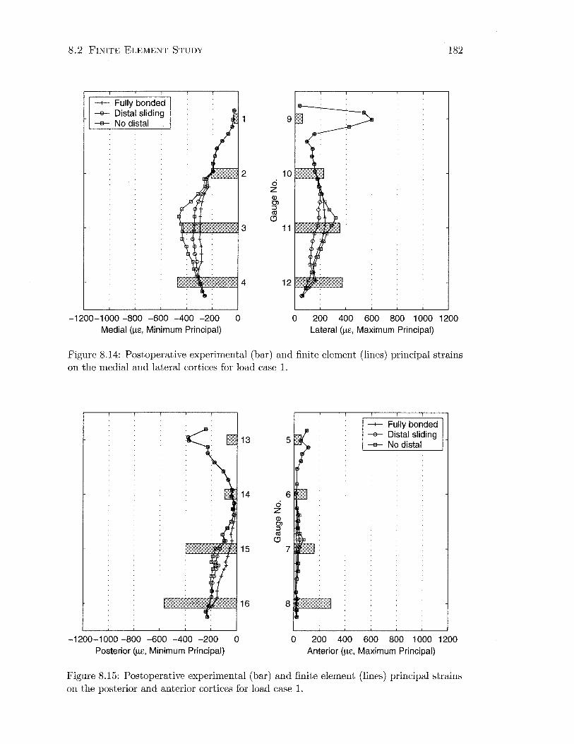
8.2 FINITE ELEMENT STUDY
-1-- Fully bonded -e- Distal sliding -a- No distal
-1200-1000 -800 -600 -400 -200 0 Medial (f.l£, Minimum Principal)
182
0 200 400 600 800 1 000 1200 Lateral (f.l£, Maximum Principal)
Figure 8.14: Postoperative experimental (bar) and finite element (lines) principal strains on the medial and lateral cortices for load case 1.
-1200-1 000 -800 -600 -400 -200 0 Posterior (f.l£, Minimum Principal)
15
ci z Q) 0> ::J cO
<!J
6
7
-1-- Fully bonded -e- Distal sliding -a- No distal
0 200 400 600 800 1 000 1200 Anterior (f.l£, Maximum Principal)
Figure 8.15: Postoperative experimental (bar) and finite element (lines) principal strains on the posterior and anterior cortices for load case 1.
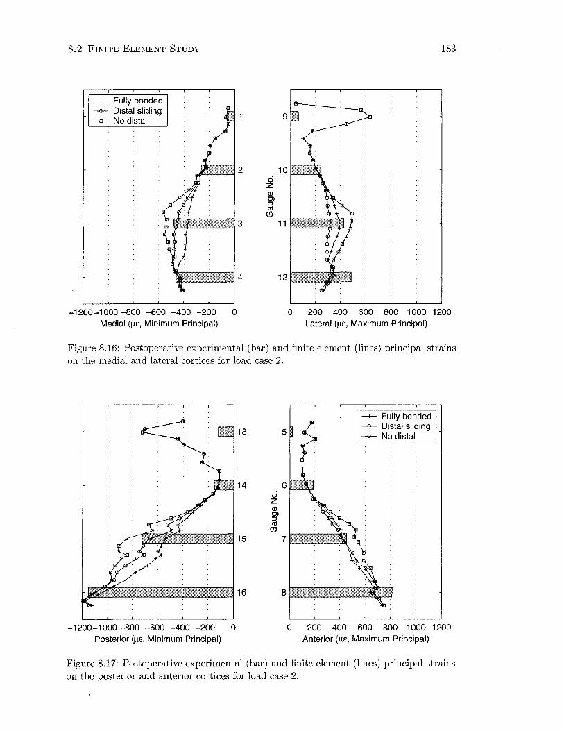
8.2 FINITE ELEMENT STUDY
--+-- Fully bonded -e- Distal sliding -a- No distal
-1200-1000 -800 -600 -400 -200 0 Medial (f.l£, Minimum Principal)
183
0 200 400 600 800 1 000 1200 Lateral (f.l£, Maximum Principal)
Figure 8.16: Postoperative experimental (bar) and finite element (lines) principal strains on the medial and lateral cortices for load case 2.
13
14 ci z (J) C'l ::J ctS
(!)
15
-1200-1000 -800 -600 -400 -200 0 Posterior (f.l£, Minimum Principal)
5
6
7
--+-- Fully bonded -a- Distal sliding -a- No distal
0 200 400 600 800 1 000 1200 Anterior (f.l£, Maximum Principal)
Figure 8.17: Postoperative experimental (bar) and finite element (lines) principal strains on the posterior and anterior cortices for load case 2.

8.2 FINITE ELEMENT STUDY 184
8. 2. 2 Mesh Refinement
Finite element models were prepared and run under the conditions indicated in
Table 8.2. Solution convergence was monitored by plotting minimum principal
strains along the medial aspect of the femur under load case 1 (0° flexion).
Table 8.2: Finite element models to investigate convergence.
Femur Edge Length Material Properties Contact
Intact 3mm integration point NjA 3mm element average NjA 5mm integration point N/A 5mm element average N/A 7mm integration point N/A 7mm element average NjA
Reconstructed 3mm integration point fully bonded 5mm integration point fully bonded
The position of the point of force application was kept constant for all models.
The strain distribution was found to be extremely sensitive to this parameter, with
a load applied only a millimetre or two more medially increasing strains by up to
10% in some cases.
Figure 8.18 shows the minimum principal strain distribution along the medial
aspect of the intact model. The y axis shows the normalised position along the
longitudinal axis of the femur, where zero is located at the level of the osteotomy
and one is the distal prosthesis tip. These results reveal the strain magnitudes
decreasing with mesh refinement from 7 to 5 mm. The data also becomes more
smooth. The difference between the 5 and 3 mm strains is much reduced, indicating
solution convergence. This is particularly evident in the diaphysis, where material
properties are more uniform (Figure 8.19).
Since the 7 mm mesh size was obviously overestimating the strains, postoperative
models were created with 3 and 5 mm mesh densities only. Figure 8.20 shows good
agreement between these mesh sizes again, considering the strains are relatively
small.

8.2 FINITE ELEMENT STUDY 185
r-~--~~~~~~--~--~~~~~0 I -1-- 5 mm Integ Pt
-e- 3 mm Integ Pt -e- 7 mm Integ Pt
0.2
0.4
c g ·u;
0.6 6:
0.8
-2000 -1800 -1600 -1400 -1200 -1 000 -800 -600 -400 -200 0 Medial (f..le, Minimum Principal)
Figure 8.18: Preoperative minimum principal strains on the medial cortex for load case 1, with finite element mesh densities of 3, 5 and 7 mm.
rf---=========::!:=l:S~=-----.---,--..,--?~~~~;1 o.5 -1-- 5 mm Integ Pt -e- 3 mm Integ Pt -e- 7 mm Integ Pt 0.6
0.7
c 0
0.8 ~
0.9
~----~----~------~----~------~----~------~----~----~1.1
-700 -650 -600 -550 -500 -450 -400 -350 -300 -250 Medial (f..le, Minimum Principal)
Figure 8.19: Distal data from Figure 8.18.
0 a.

8. 2 FINITE ELEMENT STUDY 186
rr===~====~-----,-----,-----,-----,~7-10 -+- 5 mm Integ Pt --e- 3 mm Integ Pt
-350 -300 -250 -200 -150 Mediai(JJ£, Minimum Principal)
-100 -50 0
0.2
0.4
c 0
:;:: "iii
0.6 6:..
0.8
Figure 8.20: Postoperative minimum principal strains on the medial cortex for load case 1, with finite element mesh densities of 3 and 5 mm.
Finite element analysis provides only approximate solutions to stress analysis
problems. l\1odel accuracy is generally improved by increasing mesh density, how
ever this is offset by the much larger computation time. Table 8.3 shows the change
in computation time associated with the higher number of degrees-of-freedom of the
more refine models.
Table 8.3: Effect of model complexity on computation time.
Femur
Intact
Reconstructed (fully bonded)
Edge Length
3mm 5mm 7mm
3mm 5mm
Nodal Degrees-of-Freedom
291096 77334 35850
250881 67092
CPU Time
9855.6 sec 864.1 sec 301.8 sec
6555.9 sec 673.7 sec
The effect of homogeneity of element material properties on mesh refinement
is shown in Figure 8.21. The 5 mm mesh with material properties averaged over
the element gives much higher strains than the other material and mesh options,
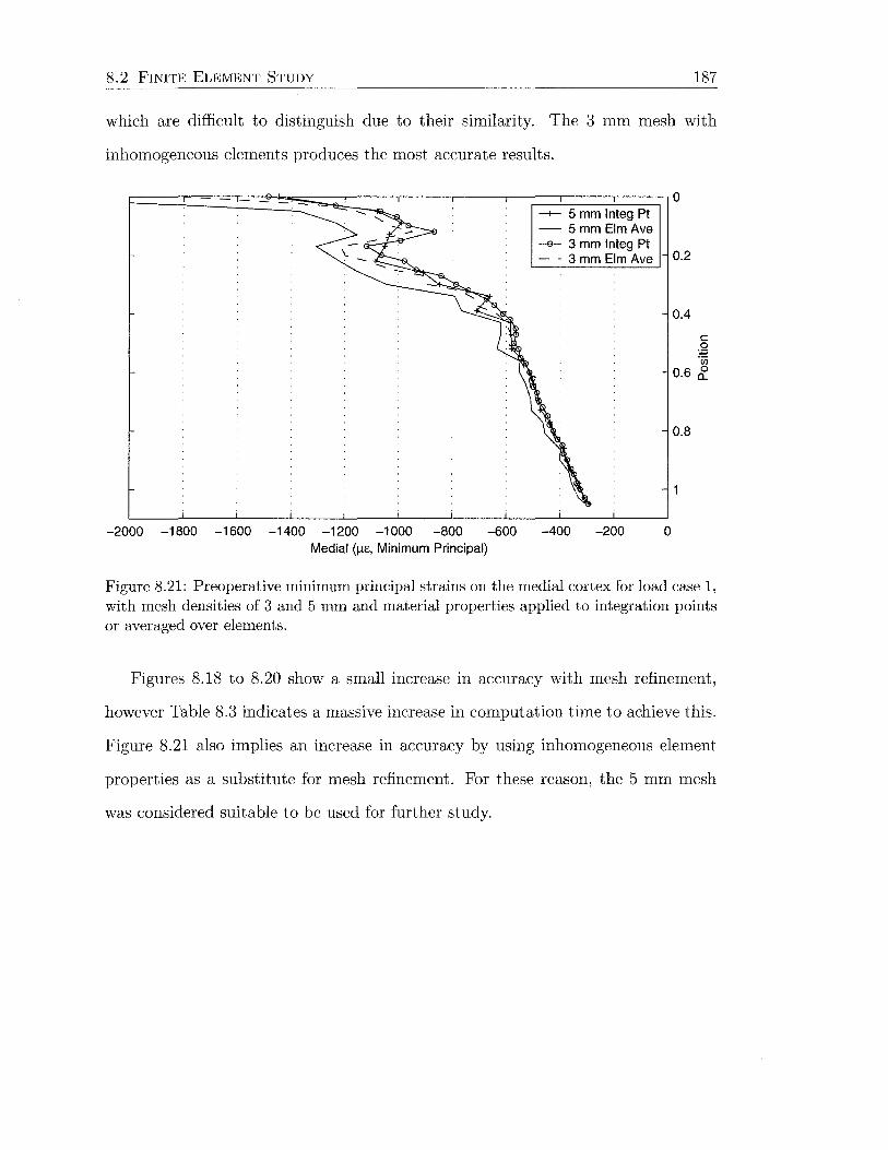
8. 2 FINITE ELEMENT STUDY 187
which are difficult to distinguish due to their similarity. The 3 mm mesh with
inhomogeneous elements produces the most accurate results.
-+- 5 mm Integ Pt - 5mmEimAve -e- 3 mm Integ Pt - · 3 mm Elm Ave
-2000 -1800 -1600 -1400 -1200 -1 000 -800 -600 -400 -200 0 Medial (J.L£, Minimum Principal)
0.2
0.4
c 0
:;::: ·u;
0.6 &.
0.8
Figure 8.21: Preoperative minimum principal strains on the medial cortex for load case 1, with mesh densities of 3 and 5 mm and material properties applied to integration points or averaged over elements.
Figures 8.18 to 8.20 show a small increase in accuracy with mesh refinement,
however Table 8.3 indicates a massive increase in computation time to achieve this.
Figure 8.21 also implies an increase in accuracy by using inhomogeneous element
properties as a substitute for mesh refinement. For these reason, the 5 mm mesh
was considered suitable to be used for further study.
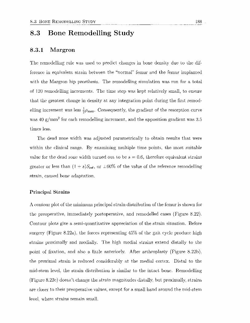
8.3 BONE REMODELLING STUDY 188
8.3 Bone Remodelling Study
8.3.1 Margron
The remodelling rule was used to predict changes in bone density due to the dif
ference in equivalent strain between the "normal" femur and the femur implanted
with the ?vlargron hip prosthesis. The remodelling simulation was run for a total
of 120 remodelling increments. The time step was kept relatively small, to ensure
that the greatest change in density at any integration point during the first remod
elling increment was less ~Pmax· Consequently, the gradient of the resorption curve
was 40 gjmm2 for each remodelling increment, and the apposition gradient was 3.5
times less.
The dead zone width was adjusted parametrically to obtain results that were
within the clinical range. By examining multiple time points, the most suitable
value for the dead zone width turned out to be s = 0.6, therefore equivalent strains
greater or less than (1 ± s )Sref, or ±60% of the value of the reference remodelling
strain, caused bone adaptation.
Principal Strains
A contour plot of the minimum principal strain distribution of the femur is shown for
the preoperative, immediately postoperative, and remodelled cases (Figure 8.22).
Contour plots give a semi-quantitative appreciation of the strain situation. Before
surgery (Figure 8.22a), the forces representing 45% of the gait cycle produce high
strains proximally and medially. The high medial strains extend distally to the
point of fixation, and also a little anteriorly. After arthroplasty (Figure 8.22b),
the proximal strain is reduced considerably at the medial cortex. Distal to the
mid-stem level, the strain distribution is similar to the intact bone. Remodelling
(Figure 8.22c) doesn't change the strain magnitudes distally, but proximally, strains
are closer to their preoperative values, except for a small band around the mid-stem
level, where strains remain small.

8.3 BONE R EMODELLING STUDY
EE, Min . Principal (Ave . Crit .: 75 %)
+2 . 79le - 03 +O . OOOe+OO -2 . 500e-04 -s . oooe-04 -7 . 500e-04 -l . OOOe-03 -1.250e-03 -l . SOOe-03 -1.750e-03 -2.000e - 03 -2.250e-03 - 2 . 500e-03 -1.687e-01
(a) Intact femur
189
(b) Postoperative (c) Remodelled
Figure 8.22: Minimum principal strain distribution (anteromedial view).
Plots of maximum and minimum principal strain values at nodes on the medial
and lateral aspects of the femur, before and after surgery, are also presented in
Figures 8.31 and 8.32. The vertical axis of these graphs is normalised with repect
to the medial intersection of the osteotomy with the cortex (position = 0) and the
distal stem tip (position= 1.0).
Medially at the osteotomy level, the preoperative minimum principal strain is
-2066 fl£, decreasing to less than half of this value at the distal tip of the implant
( -930 p,c). On the lateral side, the maximum principal strains are extreme for
the proximal 20% of the implant , as was seen previously in Figures 8. 10 and 8. 12.
This reduces to about 1300 fl£ at a posit ion of 0.2. The maximum principal strain
decreases further to 512 p,c at the level of the distal stem tip.
Postoperatively, the minimum principal strain on the medial cortex is reduced
to -235 p,c, or 11% of the intact value. The effect of stress shielding is apparent
8.3 BONE R EMODELLI NG STUDY 190
for the proximal 60% of the implant length, whereafter the strain approaches the
preoperative value. At the distal tip, the minimum principal strain is -758 J-LE,
or 83% of the preoperative value. Laterally, stress shielding is also seen along the
proximal 60% of the implant , however extreme values are evident at the proximal
nodes again. Twenty-percent of the distance down the implant , the maximum
principal strain is about 500 J-LE, increasing to 612 J-LE at position equal to 0.6, and
then down to 372 J-LE at position equal to 1.0.
Equivalent Strains
The change in equivalent strain distribution after hip arthroplasty is the stimu
lus for bone adaptation. A situation almost identical to the principal strains is
obtained for the equivalent strain distribution (note different scale, Figure 8.23).
Equivalent strains are high proximally in the preoperative femur (Figure 8.23a).
UVARM3 (Ave . Cri t .: 7 5%)
+2 . 516e- 01 +S . OOOe-03 +4 . 500e-03 +4.000e- 03 +3 . 500e- 0 3 +3 . 000 e-0 3 +2 . 500e- 03 +2 . 000 e-0 3 +l . SOO e-03 +l. OOOe-03 +S . OOOe - 0 4 +O. OO Oe +OO - 1. 2 46e-0 1
(a) Intact femur (b) Postoperative (c) Remodelled
Figure 8.23: Equivalent strain distribution ( anteromedial view).
8.3 BONE R EMODELLING STUDY 191
Surgery reduces the strains, particularly at the medial cortex (Figure 8.23b) , and
then remodelling increases the strain magnitude in this region (Figure 8.23c).
A graph of the equivalent strains along a path of nodes on the medial cortex
of the femur before and after surgery, and after remodelling, is presented in Fig
ure 8.33 (left). The vertical axis is again the normalised position relative to the
osteotomy level and the distal stem tip. Preoperatively, the equivalent strain is
equal to 2111 f-lc at the osteotomy level. This falls away to 1010 f-lc at the distal
tip of the prosthesis. Immediately following implantation with the hip replacement
device, the equivalent strain is reduced to only 45 f-lc at the osteotomy, and 844 f-lc
distally. After 120 remodelling increments, the distal value remains the same, how
ever at the osteotomy level, the strain is now equal to 954 f-lc, which is 45% of the
preoperative value.
Bone Density
The density distribution of the femur after remodelling is shown in Figure 8.24
( c .f. Figure 8. 7). This indicates cortical bone loss around the proximal half of the
Margron stem, particularly medially and anteriorly, however the images do not show
what occurs closer to the implant .
Simulated DEXA images give an appreciation of the density distribution across
the interior of the femur. Figure 8.25a shows the situation before surgery, while
Figure 8.25d gives the result after 120 remodelling increments. Figure 8.25b illus
trates the density distribution after 10 remodelling increments. Bone resorption at
the level of the osteotomy down to the lesser trochanter is the most obvious feature ,
both medially and laterally. This continues , particularly on the medial aspect, until
remodelling increment 60 (Figure 8.25c). Litt le change in density can be detected
visually between the 60 and 120 increment images.
Figure 8.26 shows the percent change in bone density from the preoperative
condition at the seven Gruen zones. Each curve represents the percent change for a
given number of remodelling increments. As the number of increments approaches

8.3 BONE R EMODELLING STUDY
SDV2 (Ave. Crit .: 75%)
•
+5.425e+03 +2.800e+03 +2.500e+03
'- +2. 200e+03 +1 . 900e+03 +1 . 600e+03 +1.300e+03 +1 . 000e+03 +7 . 000e+02 +4.000e+02 +1 . 000e+02 -2 . 000e+02 -3.235e+03
(a) Anteromedial view
• .
•
(b) Posterolateral view
Figure 8.24: Density distribution (Hounsfield units) of the remodelled femur.
192
120, the curves start to overlap as the solution converges. Numerical values for the
bone density changes are provided in Table C.1 (Appendix C).
In zone 1, there is a small increase in bone density (2.4%) during the first 10
increments, but this approaches zero as the remodelling progresses. At remodelling
equilibrium, zone 2 exhibits bone loss of 8.5%. Approximately half of this resorption
( -4.5%) occurs during the first 20 increments. In zones 3, 4 and 5, there is negligible
change in density during the remodelling process. Zone 6 sees a change in bone
density of 26.5%, while maximum bone adaptation of -30.7% occurs in zone 7. In
zone 7, more than half of the density change (-16.6%) takes place within the first
10 remodelling increments.
Figure 8.27 shows how the bone in zone 7 adapts to the postoperative condition,
according to the remodelling theory. The bone density decreases monotonically to
reach a remodelling equilibrium value of -30.7%. This value is approximately
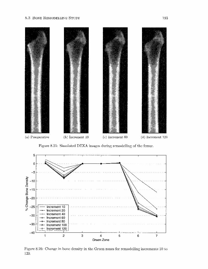
8.3 BONE REMODELLING STUDY 193
(a) Preoperative (b) Increment 10 (c) Increment 60 (d) Increment 120
Figure 8.25: Simulated DEXA images during remodelling of the femur.
5.---.--------,-------,,-------.--------.--------.--------.--~
0
-5
~ -~ -10 Q)
0
~ -15 0 co ~ -20 c co .c () -25 cf?-
-30
-35
- Increment 1 0 Increment 20
-+- Increment 40 -e- Increment 60 -a- Increment 80 -A- Increment 100 ~ Increment 120
-40~--~------~------~~------~------~--------L-------~--~
2 3 4 Gruen Zone
5 6 7
Figure 8.26: Change in bone density in the Gruen zones for remodelling increments 10 to 120.
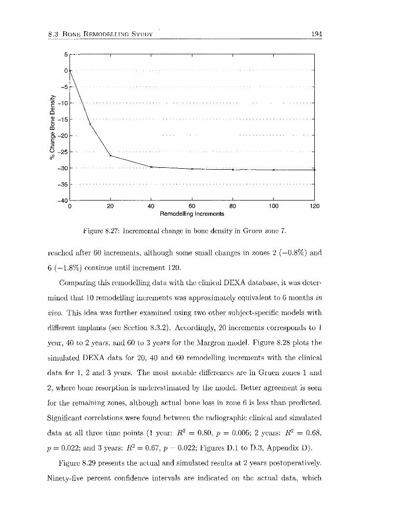
8.3 BONE REMODELLING STUDY
0
-5
~ -~ -10 Q)
0
~ -15 0 Ill
~-20 c ca
.r:. () -25 ~ 0
-30
-35
194
-40~--------~--------~--------~--------~--------~------~
0 20 40 60 Remodelling Increments
80 100
Figure 8.27: Incremental change in bone density in Gruen zone 7.
120
reached after 60 increments, although some small changes in zones 2 ( -0.8%) and
6 ( -1.8%) continue until increment 120.
Comparing this remodelling data with the clinical DEXA database, it was deter
mined that 10 remodelling increments was approximately equivalent to 6 months in
vivo. This idea was further examined using two other subject-specific models with
different implants (see Section 8.3.2). Accordingly, 20 increments corresponds to 1
year, 40 to 2 years, and 60 to 3 years for the Margron model. Figure 8.28 plots the
simulated DEXA data for 20, 40 and 60 remodelling increments with the clinical
data for 1, 2 and 3 years. The most notable differences are in Gruen zones 1 and
2, where bone resorption is underestimated by the model. Better agreement is seen
for the remaining zones, although actual bone loss in zone 6 is less than predicted.
Significant correlations were found between the radiographic clinical and simulated
data at all three time points (1 year: R 2 = 0.80, p = 0.006; 2 years: R 2 = 0.68,
p = 0.022; and 3 years: R 2 = 0.67, p = 0.022; Figures D.1 to D.3, Appendix D).
Figure 8.29 presents the actual and simulated results at 2 years postoperatively.
Ninety-five percent confidence intervals are indicated on the actual data, which
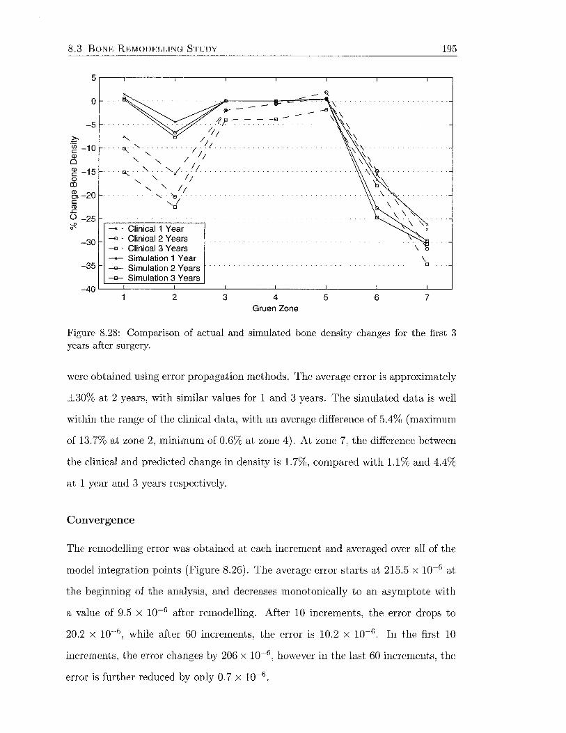
8.3 BONE REMODELLING STUDY 195
5.---.--------.-------,,-------.-------~--------~------~--~
0
-5
-30
-35
-->< • Clinical 1 Year -o · Clinical 2 Years -o · Clinical 3 Years _.,._ Simulation 1 Year -e- Simulation 2 Years --a- Simulation 3 Years
\ D
-40~--~------~--------~------~------~--------L-------~--~
2 3 4 Gruen Zone
5 6 7
Figure 8.28: Comparison of actual and simulated bone density changes for the first 3 years after surgery.
were obtained using error propagation methods. The average error is approximately
±30% at 2 years, with similar values for 1 and 3 years. The simulated data is well
within the range of the clinical data, with an average difference of 5.4% (maximum
of 13.7% at zone 2, minimum of 0.6% at zone 4). At zone 7, the difference between
the clinical and predicted change in density is 1.7%, compared with 1.1% and 4.4%
at 1 year and 3 years respectively.
Convergence
The remodelling error was obtained at each increment and averaged over all of the
model integration points (Figure 8.26). The average error starts at 215.5 x 10⁻⁶ at
the beginning of the analysis, and decreases monotonically to an asymptote with
a value of 9.5 x 10⁻⁶ after remodelling. After 10 increments, the error drops to
20.2 x 10⁻⁶ , while after 60 increments, the error is 10.2 x 10⁻⁶ . In the first 10
increments, the error changes by 206 x 10-6 , however in the last 60 increments, the
error is further reduced by only 0. 7 x 10⁻⁶ .

8.3 BONE REMODELLING STUDY 196
30.---.--------.-------.--------,--------.--------.-------.---~
20
10
.?:- 0 ·c;; c: Q)
0 -10 Q) c: s -20 Q) Ol
ffi -30 .r:. ()
<f- -40
-50
/
-60 - - Clinical2 Years -- Simulation 2 Years
...... '>. ..
"
-70~--~-------L------~~------~------~--------L-------~--~
2 3 4 Gruen Zone
5 6 7
Figure 8.29: Comparison of actual and simulated bone density changes at 2 years (error bars show 95% confidence interval for clinical data).
.... 2 ....
UJ
x10-4 2.5.---------,---------.----------~---------.----------.---------~
2
1.5
0.5
0~--------~--------~--------~--------~~--------~--------~
0 20 40 60 Remodelling Increments
80 100
Figure 8.30: Behaviour of the remodelling error over 120 remodelling increments.
120
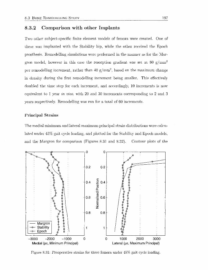
8.3 BONE REMODELLING STUDY 197
8.3.2 Comparison with other Implants
Two other subject-specific finite element models of femora were created. One of
these was implanted with the Stability hip, while the other received the Epoch
prosthesis. Remodelling simulations were performed in the manner as for the Mar
gron model, however in this case the resorption gradient was set at 80 g/mm2
per remodelling increment, rather than 40 gjmm2, based on the maximum change
in density during the first remodelling increment being smaller. This effectively
doubled the time step for each increment, and accordingly, 10 increments is now
equivalent to 1 year in vivo, with 20 and 30 increments corresponding to 2 and 3
years respectively. Remodelling was run for a total of 60 increments.
Principal Strains
The medial minimum and lateral maximum principal strain distributions were calcu-
lated under 45% gait cycle loading, and plotted for the Stability and Epoch models,
and the Margron for comparison (Figures 8.31 and 8.32). Contour plots of the
0.8
- Margron --e-- Stability 1 -a- Epoch
-3000 -2000 -1000 0 Medial (f..L£, Minimum Principal)
0.2
c ~ 0.4 (/) 0
0... "0 Q) (/) :m o.6 E .... 0 z
0.8
0 1000 2000 3000 Lateral (f..L£, Maximum Principal)
Figure 8.31: Preoperative strains for three femora under 45% gait cycle loading.
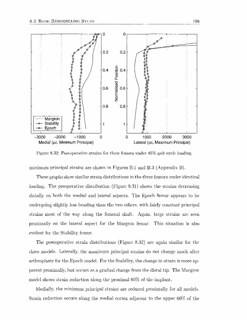
8.3 BONE REMODELLING STUDY 198
- Margron
0.2 0.2
c: 0.4 g 0.4
"(i.j
0 0... "0 Q)
0.6 ~ 0.6 E ..... 0 z
0.8 0.8
-a- Stability 1 -a- Epoch
-3000 -2000 -1000 0 Medial (!1£, Minimum Principal)
0 1000 2000 3000 Lateral (!1£, Maximum Principal)
Figure 8.32: Postoperative strains for three femora under 45% gait cycle loading.
minimum principal strains are shown in Figures B.l and B.3 (Appendix B).
These graphs show similar strain distributions in the three femora under identical
loading. The preoperative distribution (Figure 8.31) shows the strains decreasing
distally on both the medial and lateral aspects. The Epoch femur appears to be
undergoing slightly less bending than the two others, with fairly constant principal
strains most of the way along the femoral shaft. Again, large strains are seen
proximally on the lateral aspect for the Margron femur. This situation is also
evident for the Stability femur.
The postoperative strain distributions (Figure 8.32) are again similar for the
three models. Laterally, the maximum principal strains do not change much after
arthroplasty for the Epoch model. For the Stability, the change in strain is more ap
parent proximally, but occurs as a gradual change from the distal tip. The Margron
model shows strain reduction along the proximal 60% of the implant.
Medially, the minimum principal strains are reduced proximally for all models.
Strain reduction occurs along the medial cortex adjacent to the upper 60% of the
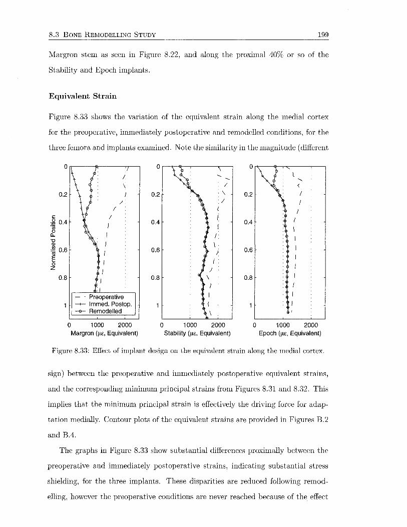
8.3 BONE REMODELLING STUDY 199
Margron stem as seen in Figure 8.22, and along the proximal 40% or so of the
Stability and Epoch implants.
Equivalent Strain
Figure 8.33 shows the variation of the equivalent strain along the medial cortex
for the preoperative, immediately postoperative and remodelled conditions, for the
three femora and implants examined. Note the similarity in the magnitude (different
0 0 0 .....
....... ' / < 0.2 0.2 ·\. 0.2 I
/ .I I ( (
c: I I I 2 0.4 0.4 0.4 ·;n )
I 0 a_ I '0 CD \ ~ 0.6 0.6 / 0.6 E
( . 0 z
0.8 0.8 0.8
- Preoperative -+- lmmed. Postop. -e- Remodelled
0 1000 2000 0 1000 2000 0 1000 2000 Margron (J.L£, Equivalent) Stability (J.L£, Equivalent) Epoch (J.L£, Equivalent)
Figure 8.33: Effect of implant design on the equivalent strain along the medial cortex.
sign) between the preoperative and immediately postoperative equivalent strains,
and the corresponding minimum principal strains from Figures 8.31 and 8.32. This
implies that the minimum principal strain is effectively the driving force for adap
tation medially. Contour plots of the equivalent strains are provided in Figures B.2
and B.4.
The graphs in Figure 8.33 show substantial differences proximally between the
preoperative and immediately postoperative strains, indicating substantial stress
shielding, for the three implants. These disparities are reduced following remod-
elling, however the preoperative conditions are never reached because of the effect

8.3 BONE REMODELLING STUDY 200
of the dead zone. Distally, the changes in equivalent strain are relatively small
following surgery for all models, and therefore the strains remain fairly constant
during the remodelling process.
Table 8.4 presents the equivalent strains from Figure 8.33 as absolute strain
values and as percentages of the preoperative values at the levels of the osteotomy,
the lesser trochanter and the distal stem tip. Stress shielding is apparent for all
implants, with a trend towards normalisation of the equivalent strain due to adap-
tation.
Table 8.4: Preoperative, immediately postoperative and remodelled values of the equiv-alent strain for the Margron, Stability and Epoch models at 3 locations on the medial cortex. The immediately postoperative and remodelled values are given as percentages of the preoperative.
Position Immed Postop Remodelled Preop Immed Postop % Remodelled %
:tvfargron 0 45 fiE 954 fiE 2111 fi£ 2% 45% 0.2 364 J-tf 761 J-tf 1985 f-tc 18% 38% 1.0 844 f-tc 844 J-tf 1010 J-tf 84% 84%
Stability 0 351 f-tc 633 fJ,f 2005 J-tf 18% 32% 0.2 1284 f-tc 1241 J-tf 2254 J-tf 57% 55% 1.0 1489 f-tc 1483 J-tf 1664 J-tf 89% 89%
Epoch 0 81 J-tf 719 f-tc 1096 J-tf 7% 66% 0.2 882 J-tf 878 J-tf 1599 J-tf 55% 55% 1.0 1186 J-tf 1175 J-tf 1315 J-tf 90% 89%
Bone Density
The pre- and post-remodelling contour plots of the Epoch and Stability femora are
shown in Figures C.l, C.2, C.4 and C.5 (Appendix C). Simulated DEXA images
are shown in Figures C.3 and C.6. Appreciable changes in density are evident at the
calcar region, with some densification seen distally. The percent changes in Gruen
zone bone density for the Epoch and Stability models are provided in Tables C.2
and C.3, and were compared with clinical bone mineral data from DEXA studies.
Figure 8.34 plots the simulated change in bone density for the Margron, Stability

8.3 BONE REMODELLING STUDY 201
and Epoch models at 2 years (120, 60 and 60 remodelling increments respectively)
and the corresponding clinical results at 2 years. The Margron model results are
mentioned previously in Section 8.3.1.
The Stability model shows good agreement with the clinical data, with an av
erage difference of 3.4%. The largest discrepancy is at zone 2 (7.4%), while the
smallest is at zone 6 (0%). In zones 1 and 2, there is a tendency for the simula
tion to underestimate the change in bone mineral density. At zone 7, the predicted
decrease in bone density is 20.4%, which is 2.2% less than measured in the clin
ical subjects. At 2 years, the average error on the percentage change in density
measured clinically at each Gruen zone is 34% (Table 7.3). The simulated data
correlated strongly with the clinical (R2 = 0.72, p = 0.016; Figure D.4).
The Epoch simulation predicts a small increase in bone density in zones 1 to
6. This is contrary to the clinical data for zones 1 to 4 and 6, in which a small
decrease in density is found. The bone loss in zone 7 (9.7%) is less than that
expected for the average patient (15.8%) at 2 years. The average difference between
the clinical data and the simulated results is 3.9%, with the largest difference in
zone 6 (7.8%). Confidence intervals were not available for the clinical data with this
implant. Again, agreement between the simulation and clinical data was quantified
by a statistically significant correlation (R2 = 0.76, p = 0.010; Figure D.5). A
significant correlation was present when the 1, 2 and 3 year Margron time points
were combined with the 2 year time points for the Epoch and Stability density
changes (R2 = 0.73, p < 0.00001; Figure D.6).
Convergence
Convergence of the remodelling solutions was monitored using the average sum of
the remodelling errors (Figure 8.35). With the Stability model, the average error
in equivalent strain starts at 163.8 x 10⁻⁶ at the beginning of the analysis, and
decreases to an asymptotic value of 5. 7 x 10⁻⁶ after remodelling. The average error

8.3 BONE REMODELLING STUDY
0 z-. ·u; c (!)
-10 0 (!) c 0 co (!) -20 C> c CIS .c 0 ~ -30 0
z-. ·u; c
-40
0
~ -10 (!) c 0 co (!) -20 C> c CIS .c 0 ~ -30 0
- - -)'
/
... / .,. '- /
'- / '-
'y/.
-->< • Margron Clinical _,._ Margron Simulation
2 3 4
-X--- -X ......... ,._ - -->t----
- · Stability Clinical --- Stability Simulation
202
-'\
" " ·'\. "
"" . . " .
" " ... \; .
5 6 7
-40L---~------~--------~------~---------L--------L--------L--~
2 3 4 5 6 7
X
0 ....... ·x
z-. ,._ - -x- '-- - ,._ '-·u; '-c .,._ ~ -10 ....... ··"'-··
' (!) ' c '-x 0 co (!) -20 C> c CIS .c 0 ~ -30 0
I~ Epoch Clinical I Epoch Simulation
-40 2 3 4 5 6 7
Gruen Zone
Figure 8.34: Effect of implant design on the change in bone density in the seven Gruen zones at 2 years.
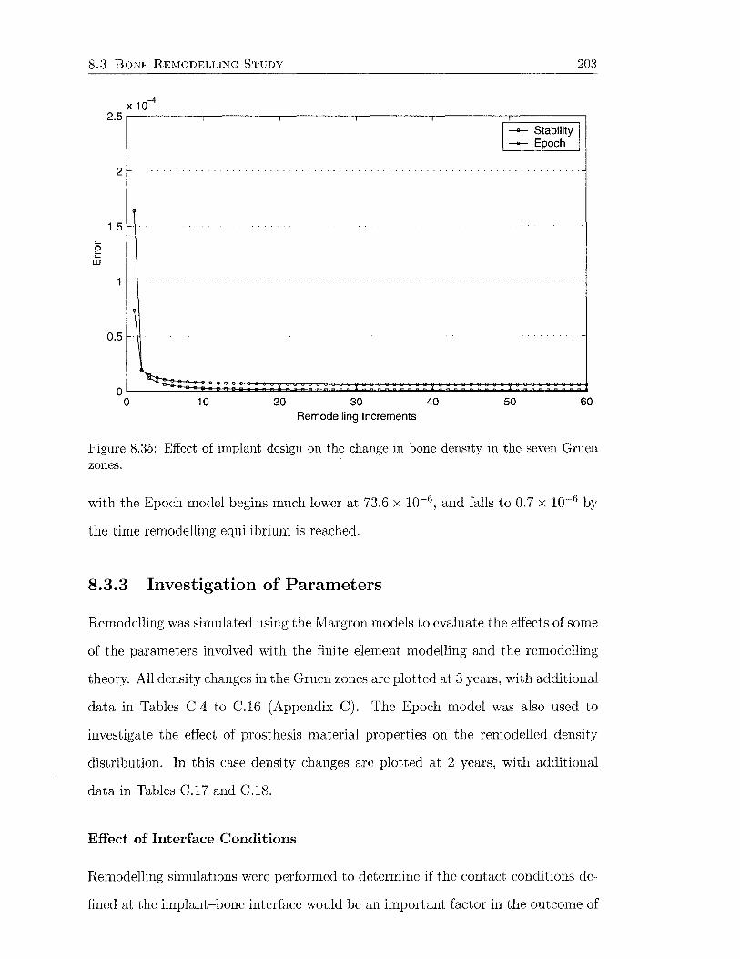
8.3 BONE REMODELLING STUDY 203
X 10-4
2.5,-----,---~-------r----,-----;:c======:::;-1
1
-e--- Stability I ----- Epoch
2
1.5 ..... g w
0.5
10 20 30 Remodelling Increments
40 50 60
Figure 8.35: Effect of implant design on the change in bone density in the seven Gruen zones.
with the Epoch model begins much lower at 73.6 x 10⁻⁶ , and falls to 0.7 x 10⁻⁶ by
the time remodelling equilibrium is reached.
8.3.3 Investigation of Parameters
Remodelling was simulated using the I'viargron models to evaluate the effects of some
of the parameters involved with the finite element modelling and the remodelling
theory. All density changes in the Gruen zones are plotted at 3 years, with additional
data in Tables C.4 to C.16 (Appendix C). The Epoch model was also used to
investigate the effect of prosthesis material properties on the remodelled density
distribution. In this case density changes are plotted at 2 years, with additional
data in Tables C.l7 and C.l8.
Effect of Interface Conditions
Remodelling simulations were performed to determine if the contact conditions de
fined at the implant-bone interface would be an important factor in the outcome of
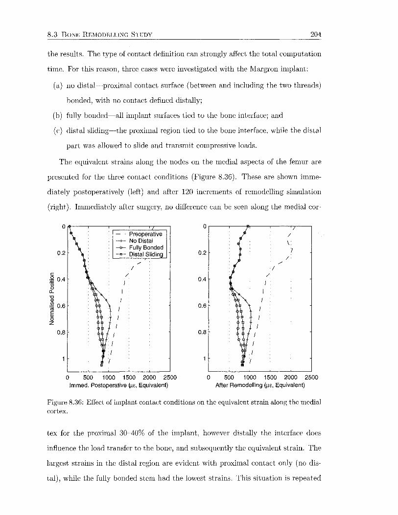
8.3 BONE REMODELLING STUDY 204
the results. The type of contact definition can strongly affect the total computation
time. For this reason, three cases were investigated with the Margron implant:
(a) no distal-proximal contact surface (between and including the two threads)
bonded, with no contact defined distally;
(b) fully bonded-all implant surfaces tied to the bone interface; and
(c) distal sliding-the proximal region tied to the bone interface, while the distal
part was allowed to slide and transmit compressive loads.
The equivalent strains along the nodes on the medial aspects of the femur are
presented for the three contact conditions (Figure 8.36). These are shown imme
diately postoperatively (left) and after 120 increments of remodelling simulation
(right). Immediately after surgery, no difference can be seen along the medial cor-
0.2
c .g 0.4 -~ a.. "'0 Q)
~ 0.6
E 0 z
0.8
0
- - Preoperative -1-- No Distal -e- Fully Bonded -e- Distal Sliding
/
I /
I
I I I
500 1 000 1500 2000 2500 lmmed. Postoperative ~e., Equivalent)
0
/
\
0.2 I /
/
I /
0.4
0.6
0.8
0 500 1 000 1500 2000 2500 After Remodelling (J.lc, Equivalent)
Figure 8.36: Effect of implant contact conditions on the equivalent strain along the medial cortex.
tex for the proximal 30-40% of the implant, however distally the interface does
influence the load transfer to the bone, and subsequently the equivalent strain. The
largest strains in the distal region are evident with proximal contact only (no dis
tal), while the fully bonded stem had the lowest strains. This situation is repeated

8.3 BONE REMODELLING STUDY 205
after remodelling, however remodelling causes the equivalent strain to increase in
the proximal 40% for all models by the same amount.
Figure 8.37 indicates little difference between the three contact conditions in
terms of the degree of bone lost after 3 years. There is a fraction more bone loss
in Gruen zone 6 for the fully bonded model, while all other points on the plot are
approximately coincident.
5.---.--------.-------.--------.--------.--------.-------.---~
0
-5
c -~ -10 Q)
0
~ -15 0 co ~ -20 c: ctl ..c: () -25 rl
..... ,.._. -......1
X
I
I I
-30 1-.-------------, - ·Clinical -1- No Distal Contact
-35 -e-- Fully Bonded -e- Distal Sliding
... /-1
I I
----+:-
\ .. -40L---~------~------~--------~-------L--------L-------~--~
2 3 4 Gruen Zone
5 6 7
Figure 8.37: Effect of contact conditions on the change in bone density in the seven Gruen zones.
For this reason, the fact that the postoperative experimental strain distribution
was best represented (Section 8.2.1), and by taking computation time into account,
the model with the proximal contact surface tied and no contact defined distally
was used for all other remodelling simulations.
Effect of Femoral Head Position
The effects of neck length and version angle on remodelling were analysed. The
physiological neck length was determined as +4 mm from the template. This po
sition was varied to the other available neck lengths, which are -4, 0 and + 7 mm.
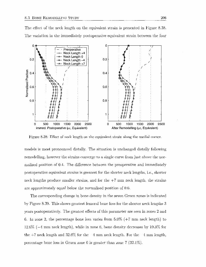
8.3 BONE REMODELLING STUDY 206
The effect of the neck length on the equivalent strain is presented in Figure 8.38.
The variation in the immediately postoperative equivalent strain between the four
0.2
c ,g 0.4 '2 [)_
'0 Q)
~ 0.6
E 0 z
0.8
0
- - Preoperative -+- Neck Length +4 -e- Neck Length 0 -e- Neck Length -4 -A- Neck Length + 7
)
I
I /
500 1 000 1500 2000 2500 lmmed. Postoperative~£, Equivalent)
0
0.2
0.4
0.6
0.8
0
/
\ )
/ /
I /
500 1 000 1500 2000 2500 After Remodelling (!l£, Equivalent)
Figure 8.38: Effect of neck length on the equivalent strain along the medial cortex.
models is most pronounced distally. The situation is unchanged distally following
remodelling, however the strains converge to a single curve from just above the nor-
malised position of 0.4. The difference between the preoperative and immediately
postoperative equivalent strains is greatest for the shorter neck lengths, i.e., shorter
neck lengths produce smaller strains, and for the + 7 mm neck length, the strains
are approximately equal below the normalised position of 0.6.
The corresponding change in bone density in the seven Gruen zones is indicated
by Figure 8.39. This shows greatest femoral bone loss for the shorter neck lengths 3
years postoperatively. The greatest effects of this parameter are seen in zones 2 and
6. In zone 2, the percentage bone loss varies from 5.0% ( + 7 mm neck length) to
12.6% ( -4 mm neck length), while in zone 6, bone density decreases by 19.3% for
the + 7 neck length and 32.6% for the -4 mm neck length. For the -4 mm length,
percentage bone loss in Gruen zone 6 is greater than zone 7 (32.1%).
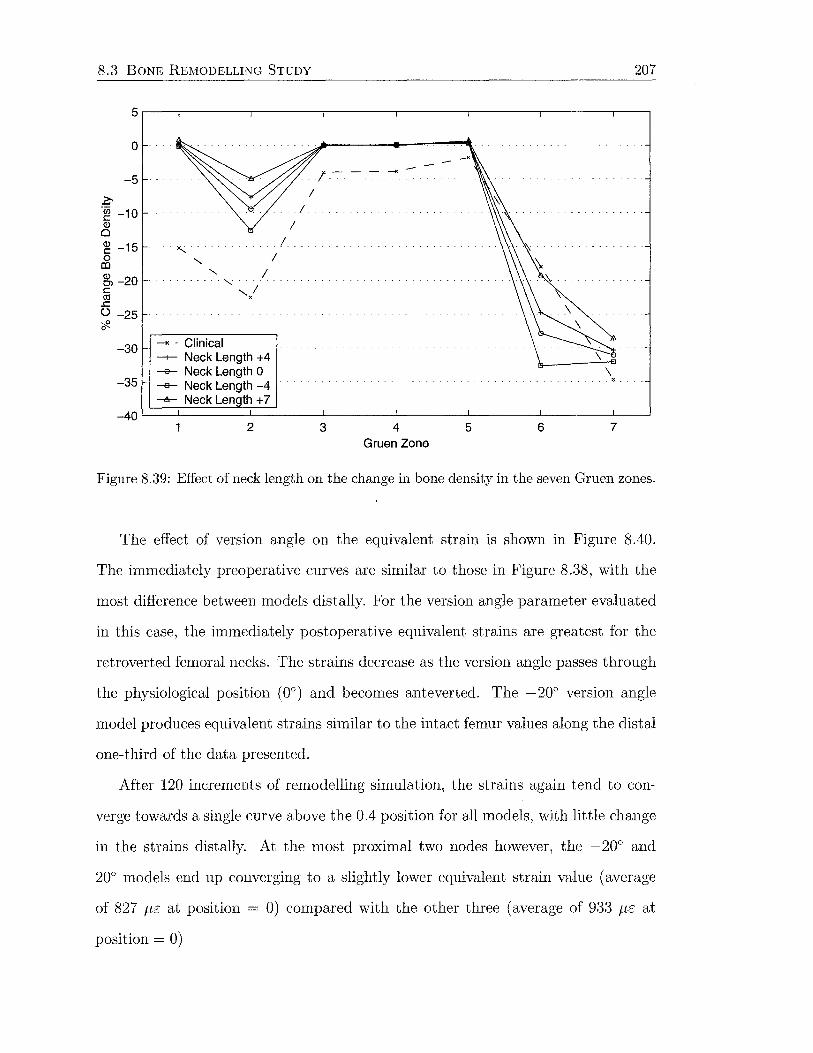
8.3 BONE REMODELLING STUDY 207
5.---.--------.-------.--------.--------.--------,-------.---~
0
-5
c ·~ -10 Q)
0
~ -15 0 co ~-20 c Cll ..c () -25 ;,!!., 0
-30
-35
" I ......... , ,I
X
--Clinical -+- Neck Length +4 --e- Neck Length 0 -e- Neck Length -4
! I
---A- Neck Length + 7 -40~~====~~~--~----_L ______ L_ ____ J_ ____ _L~
2 3 4 Gruen Zone
5 6 7
Figure 8.39: Effect of neck length on the change in bone density in the seven Gruen zones.
The effect of version angle on the equivalent strain is shown in Figure 8.40.
The immediately preoperative curves are similar to those in Figure 8.38, with the
most difference between models distally. For the version angle parameter evaluated
in this case, the immediately postoperative equivalent strains are greatest for the
retroverted femoral necks. The strains decrease as the version angle passes through
the physiological position (0°) and becomes anteverted. The -20° version angle
model produces equivalent strains similar to the intact femur values along the distal
one-third of the data presented.
After 120 increments of remodelling simulation, the strains again tend to con-
verge towards a single curve above the 0.4 position for all models, with little change
in the strains distally. At the most proximal two nodes however, the -20° and
20o models end up converging to a slightly lower equivalent strain value (average
of 827 f.LE at position = 0) compared with the other three (average of 933 J-LE at
position= 0)

8.3 BONE REMODELLING STUDY
o~~~~==~~~~ - · Preoperative
0.2
t:
:2 0.4 ·u; 0 a.. "0 Q)
~ 0.6 § 0 z
0.8
0
-1- Version Angle oo -e- Version Angle +10° -a- Version Angle -1 oo -~>-- Version Angle +20° -+- Version Angle -20°
)
I
/
500 1 000 1500 2000 2500 lmmed. Postoperative Q..t£, Equivalent)
0.2
0.4
0.6
0.8
0
I
I
I
/
)
I
/
\. )
/
208
500 1 000 1500 2000 2500 After Remodelling {/-lE, Equivalent)
Figure 8.40: Effect of version angle on the equivalent strain along the medial cortex.
The plot of bone loss in the seven Gruen zones (Figure 8.41) for the models with
varying version angle, indicates that bone loss generally increases with anteverted
angles at 3 years after surgery. In zone 7, bone loss is proportional to the version
angle. Anteversion increases bone loss ( + 20o, 37.7%), while retroversion decreases
it ( -20°, 24.1 %). This trend is not consistent across the other Gruen zones, with
the 10° anteversion model causing the most bone loss in zones 3-6, while the other
conditions produce similar results. Some densification is apparent for the -20° and
+20° models (3.4% for both). In zone 1, all of the version angles produce similar
results within about 2%. In zone 2, pronounced resorption of 30% and 21.8% occurs
for the +20° and +10° models respectively. Interestingly, the +10° variation gives
results most similar to the clinical mean in four out of the seven zones (2-4 and 7).
Effect of Dead Zone Width
Models were run with dead zone widths of s = 0.55, s = 0.6 and s = 0.65 to
demonstrate the effect of this parameter on the remodelling simulation. Figure 8.42
shows that the dead zone has no effect on the immediately postoperative equivalent

8.3 BONE REMODELLING STUDY
0
-5
Z' -~ -10 Q)
0
~ -15 0 m ~ -20 c co .c () -25 -;!?_ 0
-30
-35
209
--Clinical --+-- Version Angle oo --e- Version Angle +10° -e-- Version Angle -1 oo --A-- Version Angle +20° -+- Version Angle -20°
-40L---~-------L------~--------~-------L--------L-------~--~
2 3 4 Gruen Zone
5 6 7
Figure 8.41: Effect of version angle on the change in bone density in the seven Gruen zones.
strains as expected. After remodelling however, it is the model with the lowest dead
zone width (s = 0.55) that has most approached the preoperative curve, indicating
a greater degree of medial bone resorption. Changes in the equivalent strains occur
mostly over the proximal half of the implant as observed with other models. At the
level of the osteotomy, the equivalent strain equals 816 ILE for the s = 0.55 model,
954 fLE for the s = 0.6 model, and 1095 fLE for the s = 0.65 model, compared with
2111 fLE preoperatively. These values equate to 38.7%, 45.2% and 51.9% of the
preoperative value for the 0.55, 0.6 and 0.65 models respectively. The percentage
of the preoperative values correlate perfectly ( R 2 = 1) with the dead zone width,
indicating a linear relationship between the dead zone width and the remodelled
strain expressed as a percentage of the intact value at remodelling equilibrium, for
the small range of widths considered.
Figure 8.43 indicates what looks like, and is, a linear relationship between dead
zone width and the percent change in bone density in the Gruen zones (R2 > 0.96
in all cases), for the small range of widths. There is close to zero change in density
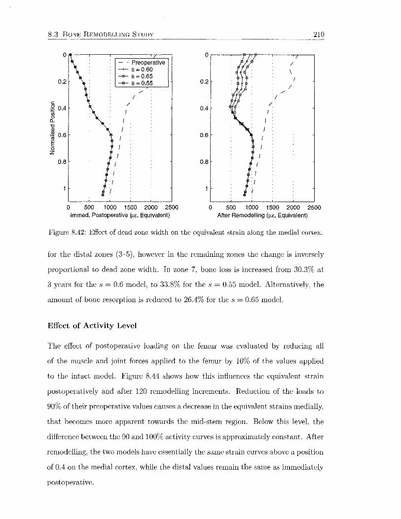
8.3 BONE REMODELLING STUDY
0~---r----r----r----~---.
0.2
c 2 0.4 "Cii 0 a.. "0 Q)
~ 0.6 § 0 z
0.8
0
- - Preoperative -1- s = 0.60 -e- s = 0.65 -e- s = 0.55
I
I
I
)
I /
500 1 000 1500 2000 2500 lmmed. Postoperative ij.te, Equivalent)
0.2
0.4
0.6
0.8
0
I I
)
I
/
I
/
\. l
/
210
500 1 000 1500 2000 2500 After Remodelling (f.le, Equivalent)
Figure 8.42: Effect of dead zone width on the equivalent strain along the medial cortex.
for the distal zones (3-5), however in the remaining zones the change is inversely
proportional to dead zone width. In zone 7, bone loss is increased from 30.3% at
3 years for the s = 0.6 model, to 33.8% for the s = 0.55 model. Alternatively, the
amount of bone resorption is reduced to 26.4% for the s = 0.65 model.
Effect of Activity Level
The effect of postoperative loading on the femur was evaluated by reducing all
of the muscle and joint forces applied to the femur by 10% of the values applied
to the intact model. Figure 8.44 shows how this influences the equivalent strain
postoperatively and after 120 remodelling increments. Reduction of the loads to
90% of their preoperative values causes a decrease in the equivalent strains medially,
that becomes more apparent towards the mid-stem region. Below this level, the
difference between the 90 and 100% activity curves is approximately constant. After
remodelling, the two models have essentially the same strain curves above a position
of 0.4 on the medial cortex, while the distal values remain the same as immediately
postoperative.

8.3 BONE REMODELLING STUDY 211
5.---.--------r--------.-------.--------.--------r-------~--~
0
-5
~ -~ -10 Q)
0 )g -15 0
(l)
gj, -20 c ctl ..c () -25 6'2-
I
.... I I
....._ I
-30 h--------, -- Clinical --t- s = 0.60
-35 ---e--- s = 0.55
-----K-
I
... X •
-e- s = 0.65 -40L=~====~L_ ____ ~ ____ _i ______ L_ ____ ~----~--~
2 3 4 Gruen Zone
5 6 7
Figure 8.43: Effect of dead zone width on the change in bone density in the seven Gruen zones.
0 0 - - Preoperative / --+- 1 00% Activity \. ---e--- 90% Activity
0.2 } 0.2 / /
/ /
I I c / / 2 0.4 0.4
) "iji 0 a.. "0
I I Q)
~ 0.6 I 0.6 I E ..... 0 z
0.8 0.8
0 500 1 000 1500 2000 2500 0 500 1 000 1500 2000 2500 lmmed. Postoperative ()l£, Equivalent) After Remodelling ()l£, Equivalent)
Figure 8.44: Effect of postoperative activity level on the equivalent strain along the medial cortex.
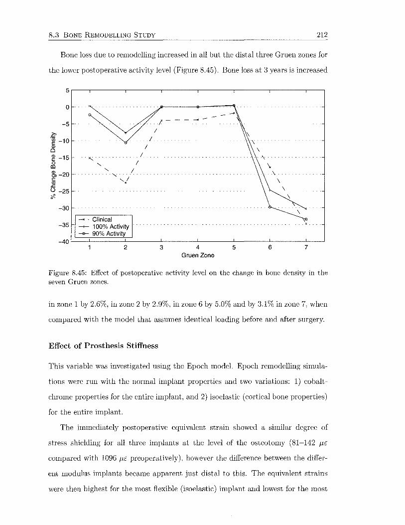
8.3 BONE REMODELLING STUDY 212
Bone loss due to remodelling increased in all but the distal three Gruen zones for
the lower postoperative activity level (Figure 8.45). Bone loss at 3 years is increased
5.---.--------.-------.--------.--------.--------.-------,---~
0
-5
c ·~ -10 Q)
0
~ -15 0 co ~ -20 c: co
..c: () -25 -;12. 0
-30
'- I . , .. ,I
X
_, - Clinical -35 -+- 1 00% Activity
-e- 90% Activity
I
I
I .
-----+<-
... ~.
-40L---~-------L------~--------~------~--------~------~--_J
2 3 4 Gruen Zone
5 6 7
Figure 8.45: Effect of postoperative activity level on the change in bone density in the seven Gruen zones.
in zone 1 by 2.6%, in zone 2 by 2.9%, in zone 6 by 5.0% and by 3.1% in zone 7, when
compared with the model that assumes identical loading before and after surgery.
Effect of Prosthesis Stiffness
This variable was investigated using the Epoch model. Epoch remodelling simula
tions were run with the normal implant properties and two variations: 1) cobalt
chrome properties for the entire implant, and 2) isoelastic (cortical bone properties)
for the entire implant.
The immediately postoperative equivalent strain showed a similar degree of
stress shielding for all three implants at the level of the osteotomy (81-142 J-LE
compared with 1096 J-lE preoperatively), however the difference between the differ
ent modulus implants became apparent just distal to this. The equivalent strains
were then highest for the most flexible (isoelastic) implant and lowest for the most
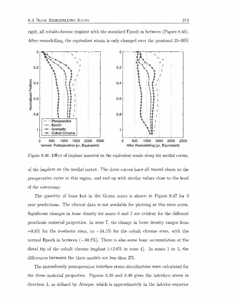
8.3 BONE REMODELLING STUDY 213
rigid, all cobalt-chrome implant with the standard Epoch in between (Figure 8.46).
After remodelling, the equivalent strain is only changed over the proximal 25-30%
0.2
c 2 0.4 -~ a.. -o
CD
~ 0.6 E 0 z
0.8
0
- Preoperative --+-- Epoch --e- lsoelastic
./ /
I
I \
I
I
I
I •
--e- Cobalt Chrome
500 1 000 1500 2000 2500 lmmed. Postoperative (l.t£, Equivalent)
0.2
0.4
0.6
0.8
0
./ /
I \
I
I
I
I
I •
500 1 000 1500 2000 2500 After Remodelling (~-t£, Equivalent)
Figure 8.46: Effect of implant material on the equivalent strain along the medial cortex.
of the implant on the medial cortex. The three curves have all moved closer to the
preoperative curve in this region, and end up with similar values close to the level
of the osteotomy.
The quantity of bone lost in the Gruen zones is shown in Figure 8.4 7 for 3
year predictions. The clinical data is not available for plotting at this time point.
Significant changes in bone density for zones 6 and 7 are evident for the different
prosthesis material properties. In zone 7, the change in bone density ranges from
+0.8% for the isoelastic stem, to -34.5% for the cobalt chrome stem, with the
normal Epoch in between ( -10.2%). There is also some bone accumulation at the
distal tip of the cobalt chrome implant ( +2.6% in zone 4). In zones 1 to 5, the
differences betweent the three models are less than 2%.
The immediately postoperative interface stress distributions were calculated for
the three material properties. Figures 8.48 and 8.49 gives the interface stress in
direction 1, as defined by Abaqus, which is approximately in the inferior-superior
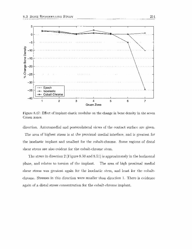
8.3 BONE REMODELLING STUDY 214
5.---.--------.-------,,-------,--------,--------,--------.---,
0
-5
z--~ -10 (])
0
~ -15 0 co ~ -20 c Cll .c () -25 ;{?_ 0
-30
-35 -+- Epoch -e- lsoelastic --a- Cobalt Chrome
-40L---~-------L------~~------~------~--------~-------L--_J
2 3 4 Gruen Zone
5 6 7
Figure 8.47: Effect of implant elastic modulus on the change in bone density in the seven Gruen zones.
direction. Anteromedial and posterolateral views of the contact surface are given.
The area of highest stress is at the proximal-medial interface, and is greatest for
the isoelastic implant and smallest for the cobalt-chrome. Some regions of distal
shear stress are also evident for the cobalt-chrome stem.
The stress in direction 2 (Figure 8.50 and 8.51) is approximately in the horizontal
plane, and relates to torsion of the implant. The area of high proximal-medial
shear stress was greatest again for the isoelastic stem, and least for the cobalt-
chrome. Stresses in this direction were smaller than direction 1. There is evidence
again of a distal stress concentration for the cobalt-chrome implant.

8.3 BONE REMODELLING STUDY
CSHEARl (Ave . Crit . · 75%)
~ +5 . 575e+00 +1. oooe~ oo +8. SOOe-01 +7 . OOOe-01 +5. SOOe-01
I +4 . OOOe-01 -+2. SOOe-01 +1. oooe-ot -5. OOOe-02 -2. OOOe-0 1
I -3 . SOOe-01 -5. OOOe-01 -2. 456e+OO
CSHEARl (Ave . Cri t . · 75%) • +7. 335e+OO
~ =~: ~g~~~g~ +7 . OOOe-01 +5. SOOe-01
-
+4. OOOe-01 +2 . SOOe-01 +1. OOOe-0 1 -5. OOOe-02 -2 . oooe-o1
I -3. SOOe-01 -5 . OOOe-01 -3 . 368e+OO
CSHEARl (Ave. Crit. · 75%)
~ +7. 580e+OO +1. OOOe+OO +8 . SOOe-01 +7 . OOOe-01 +5 . SOOe-01
-
+4. OOOe-01 +2. SOOe-01 +LOOOe-01 -5 . OOOe-02 -2 . OOOe-01
• - 3 . 500e-01 -5 . OOOe-01 -4. 015e+OO
215
Figure 8.48: Immediately postoperative interface shear stress (direction 1) for (left) Epoch, (middle) isoelastic, (right) cobalt-chrome (anteromedial view).
CSHEARl (Ave. Crit .: 75%)
~ +5. 575e+OO +1. OOOe+OO +8 . SOOe-01 +7. OOOe-01 +5 . SOOe-01 +4. OOOe-01 +2 . SOOe-01 +1 . OOOe-01 -5 . OOOe-02 -2. OOOe-01 -3 .SOOe-01 -5 . OOOe-01 -2.456e+OO
CSHEARl (Ave . Crit . · 75%)
~ +7. 335e+OO +1 . OOOe+OO +8 . 500e-01 +7. OOOe-01 +5 .500e-01 +4 . OOOe-01 +2 . 500e-01 +1. OOOe-01 -5 . OOOe-02 -2 . OOOe-0 1
• -3 .500e-01 -5. OOOe-01 -3 . 368e+OO
CSHEAR1 (Ave . Crit. · 75%)
~ +7 . 580e+OO +1 . OOOe+OO +8. 500e-01 +7. OOOe-01 +5. 500e-01 +4. OOOe-01 +2. SOOe-01 +1. OOOe-01 -5 . OOOe-02 -2. OOOe-01 -3 . SOOe-01 -5. OOOe-01 -4 . 015e+OO
Figure 8.49: Immediately postoperative interface shear stress (direction 1) for (left) Epoch, (middle) isoelastic, (right) cobalt-chrome (posterolateral view).
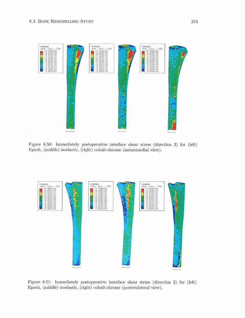
8.3 BONE REMODELLING STUDY
CSHEAR2 (Ave. Crit. · 75%)
~ +6. 608e+OO +1 . OOOe+OO +8. SOOe-01 +7. OOOe-01 +5 . SOOe-01
-
+4. OOOe-01 +2 . SOOe-01 +1. OOOe-01 -5. OOOe-02 -2. OOOe-01
I -3. SOOe-01 -5 . OOOe-01 -2 . 467e+OO
CSHEAR2 (Ave. Crit. · 75%)
111 :i: zgg~:85 +8 . SOOe-01 +7. OOOe-01 +5. SOOe-01 +4. OOOe-01 +2. SOOe-01 +1. OOOe-01 -5 . OOOe-02 -2. OOOe-01 -3. SOOe-01 -5. OOOe-01 -3. 922e+OO
CSHEAR2 (Ave. Crit . · 75%)
~ +5.932e+OO +1 . OOOe+OO +8. SOOe-01 +7. OOOe-01 +5. SOOe-01 +4. OOOe-01 +2 . SOOe-01 +1. OOOe-01 -5. OOOe-02 -2. OOOe-01 -3. SOOe-01 -5. OOOe-01 -4 . 859e+OO
216
Figure 8.50: Immediately postoperative interface shear stress (direction 2) for (left) Epoch, (middle) isoelastic, (right) cobalt-chrome (anteromedial view).
CSHEAR2 (Ave. Crit. · 75%)
~ +6. 608e+OO +1. OOOe+OO +8. SOOe-01 +7. OOOe-01 +5. SOOe-01 +4 . OOOe-01 +2. SOOe-01 +1. OOOe-01 -5. OOOe-02 -2. OOOe-01 -3. 500e-01 -5. OOOe-01 -2 .467e+OO
CSHEAR2 (Ave. Crit. · 75%)
• +1.748e+01 ~ - +1. OOOe+OO
+8. SOOe-01 +7 . OOOe-01 +5. SOOe-01 +4. OOOe-01 +2. 5ooe-01 +1 . OOOe-01 -5. OOOe-02 -2. OOOe-01 -3. SOOe-01 -5. OOOe-01 -3. 922e+OO
CSHEAR2 (Ave. Crit. · 75%)
~ +5. 932e+OO +1. OOOe+OO +8. 500e-01 +7. OOOe-01 +5. 500e-01 +4 . OOOe-01 +2. 500e-01 +1. OOOe-01 -5. OOOe-02
il -2. OOOe-01 -3 . 500e-01 -5. OOOe-01 -4. 859e+OO
Figure 8.51: Immediately postoperative interface shear stress (direction 2) for (left) Epoch, (middle) isoelastic, (right) cobalt-chrome (posterolateral view).
Chapter 9
Discussion
Total hip arthroplasty has one of the highest success rates of contemporary surgeries
(Cristofolini, 1997), relieving pain and immobility. Between July 2001 to June
2002, 26 689 hip replacement procedures were performed in Australia, of which
65% were primary total hips replacements. This represented an increase of 13% in
the primary total hip category from the previous 12 months. Cementless fixation
currently accounts for 41% of primary hip procedures in this country (Graves et al.,
2003). The ageing population and success in younger patients are contributing to
the growing demand.
Implant failure, necessitating revision, can occur for a number of reasons includ
ing aseptic loosening, infection, fracture of the bone or implant, dislocation, wear,
pain and technical error (Graves et al., 2003; Lucht, 2000; Malchau et al., 2002). Of
these, aseptic loosening is the most common. Revision surgery, particularly early
revision, is related to an increased rate of re-revision (Graves et al., 2003; Malchau
et al., 2002). Revision is also associated with higher cost and mortality (Cristofolini,
1997; Graves et al., 2003). Consequently, all measures must be taken to limit the
rate of revision surgery.
A large number of hip prosthesis designs are available on the market, although
many new design aspects have been clinically tested in a somewhat trial-and-error
fashion, with variable results. According to Herberts et al. (1989), to compare two
217
9.1 EXPERIMENTAL STUDY 218
types of prostheses with probabilities of failure of 5% and 3% over 5 years, a series
of almost 3000 patients would have to be followed before one design could be proven
to be significantly better than the other. This does not seem likely, and therefore
pre-clinical tests to predict implant longevity would be advantageous.
Bone resorption around hip replacements due to strain-adaptive remodelling
in accordance with "vVolff's Law" is a common concern. Although clinical failures
associated with bone resorption are infrequent, bone loss reduces bone strength and
increases the risk of fracture. This also reduces the support of the implant which
increases the load it carries, possibly leading to fatigue fracture (Engh et al., 1990).
Sufficient bone stock for revision is a major issue. Development of a in vitro tool
to accurately predict bone remodelling changes around hip prostheses would be a
beneficial design instrument to gain confidence in the performance of an implant,
before moving to in vivo experimentation.
This study first examined the experimental strain distribution of cadaveric fe
mora, before and after hip arthroplasty with the Margron prosthesis, under simple
loading. One of these femora was subsequently taken and used as the basis for an
anatomic finite element model. This finite element model was validated by compar
ison with the strains from the actual femur. Mesh refinement was also examined.
The finite element model was subsequently coupled with a strain-adaptive bone
remodelling theory to investigate changes in periprosthetic bone density.
9.1 Experimental Study
Mechanical testing of four cadaveric femora was undertaken to assess the cortical
strain distribution before and after hip replacement with the Margron prosthesis.
Preoperative strains decreased from proximal to distal on the medial cortex, as seen
by many others, even under different loading conditions (e.g., Cristofolini et al.,
1995; Jasty et al., 1994; Oh and Harris, 1978). This points to bending of the femur
in the coronal plane under the two applied load conditions. Under load case 1 (0°

9.1 EXPERIMENTAL STUDY 219
hip flexion), strains were reasonably constant on the anterior and posterior aspects,
however under load case 2 ( 10° flexion), the strains increased from proximal to distal
due to bending introduced in the sagittal plane. Load case 2 also introduces torque
to the femur.
In the coronal plane (under load cases 1 and 2), bending was highest towards
the metaphysis, while in the sagittal plane (under load case 2), bending was more
significant in the diaphysis. Coronal plane bending can be explained by fixation of
the femur in 10° valgus, where the moment arm for bending in this plane reduces
from proximal to distal. With the femur in 0° flexion, the moment arm for bending
in the sagittal plane remains constant, and consequently the anterior and posterior
strains remain essentially constant along the femur. However, with the femur placed
in 10° flexion, the moment arm for bending in the sagittal plane increases from
proximal to distal, and the strain magnitudes increase accordingly.
Insertion of the cobalt-chrome Margron stem decreased strains from proximal to
distal all around the femur. A statistically significant reduction in proximal strain
was observed medially and laterally at the proximal two gauge levels under both
load conditions, which implies the potential for disuse atrophy of bone in these
regions. Longitudinal strains were generally similar to the principal strains with
compression medially and posteriorly, and tension laterally and mostly anteriorly.
Similar strain magnitudes imply that the principal strains were aligned with the
longitudinal axis of the femur. This is due to loading predominantly in the coronal
plane, a result corroborated by Finlay et al. (1991). Some differences between
the longitudinal and principal strains were evident at the proximal gauges on the
anterior aspect, where strains were compressive rather than tensile. Small strain
magnitudes in these locations could be responsible.
McNamara et al. (1997a) tested a synthetic femora under joint reaction force
alone, with the femur in neutral flexion and constrained at the condyles. They
found compressive strains medially and tensile strains laterally. Anterior strains
were compressive, while posterior strains went from very small compressive at the

9.1 EXPERIMENTAL STUDY 220
most proximal level, to larger tensile strains, and then back to small compressive
strains distally. Using a loading protocol more like load case 1 in the current study,
Oh and Harris (1978) also observed compression medially and tension laterally,
while strains on the anterior aspect were compressive at the proximal two gauges
levels and tensile distally, while posterior strains changed from tensile proximally,
to compressive distally. The trends reported by Oh and Harris (1978) agree very
well with those found in this study.
Expressing the postoperative strains as a percentage of the preoperative values
provides a depiction of the degree of stress shielding. The medial and lateral results
show a high degree of stress shielding proximally, with a trend towards normalisation
of strains distally. There is an additional tendency for stress shielding to be reduced
under load case 2. This tendency is reversed on the anterior and posterior cortices,
where load case 1 appears to produce less stress shielding. At gauges 7 and 8, the
percentage strains are dramatically high (485.9% and 297.4% respectively) under
load case 1. This is due to very small preoperative strains, compared with their
values after surgery. It can be hazardous expressing strains as a percentage of
preoperative values when small values are involved. Finlay et al. (1991) advised
that it was only legitimate for large strains, as insignificant changes in small strain
can translate into large percentage changes.
Direct comparison with the literature is difficult due to the varied testing meth
odologies. The systems of applied forces and constraints differ significantly from
study to study. In the current case, the load conditions are only pseudo-physiological
and the configuration may not give an accurate representation of the degree of
stress shielding expected in vivo. The joint reaction force alone was applied, yet
Cristofolini (1997) advise that excluding the abductor muscle group may lead to
overestimation of lateral stress shielding (see Figure 5.4).
The setup was primarily used for validation of the finite element model, since
the loads and boundary conditions could be easily replicated. More than one femur
was tested to ensure that the results were representative of a group, remembering

9. 2 FINITE ELEMENT STUDY 221
that inter-specimen variation can be significant when dealing with human tissue
(Sedlacek et al., 1997). The femur was fully constrained at the diaphysis in this
study, similar to other investigations (Gillies et al., 2002; Hua and \Valker, 1995; Oh
and Harris, 1978; Otani et al., 1993; Tanner et al., 1988). Proximally, the femoral
head was allowed to translate freely in the horizontal plane, to ensure that the
system was not overconstrained. If the setup is overconstrained, the force applied
by the setup depends on the stiffness of the bone-jig-testing machine ( Cristofolini
and Viceconti, 1999).
9.2 Finite Element Study
An anatomic finite element model of a femur was constructed from CT scans of a
cadaveric femur from the experimental study. CT data files provided the geometry
and apparent density properties for the three-dimensional model (Marom and Lin
den, 1990). A finite element model of the femur reconstructed with the Margron
hip prosthesis was also created.
Under simple load configurations, strains from finite element analysis of these
models were compared with experimental strains for validation purposes. The in
fluence of mesh refinement on the accuracy of the finite element results was also
investigated.
9.2.1 Model Validation
A finite element model should always be validated against experimental strains
measured in the femur from which its geometry has been derived (Cristofolini,
1997). Consequently, the subject-specific finite element model used in this study
was loaded under the same conditions as the experimental femur from which it was
constructed, and principal strains were compared with the experimental strains on
the medial, lateral, anterior, and posterior surfaces.

9.2 FINITE ELEMENT STUDY 222
Preoperatively, discrepancies were seen between the experimental and finite ele
ment results at the proximal level of gauges on all sides of the femur and under both
load cases. This situation was also noted after arthroplasty on the lateral and pos
terior aspects. Part of this problem could be associated with creation of the initial
geometry of the femur. At the level of the proximal gauges, the geometry changes
quite rapidly from the fairly straight shaft to the variable metaphyseal region. This
makes it difficult to accurately reproduce the geometry. The most significant prob
lem resulting from this comes about if the finite element mesh ends up outside the
actual femoral geometry, particularly if integration points are outside the geometry.
If this is the case, the integration point will be assigned the minimum value, and
a high density gradient across the element will ensue. This will also cause a high
strain gradient across the elements (perpendicular to the periosteal surface), with
particularly large deformations at the integration points near the surface. Extrapo
lation of strains from the integration points where they are calculated, to the surface
nodes, will exacerbate the problem in the presence of a strain gradient.
The geometric problem just described is probably what is happening at the most
proximal gauges on the lateral and posterior aspects, as strains at these two locations
are significantly overestimated by the finite element model under all conditions.
Examination of the preoperative surface density distribution (Figure 8. 7) shows an
abrupt decrease in density going from distal to proximal around the level of the
lesser trochanter on the proximal and lateral aspects, lending some weight to this
idea. This problem could be resolved by applying homogeneous properties to each
element, however the mesh would need to be refined (Section 9.2.2), increasing
computation time substantially.
The strain values calculated by the finite element analysis are dependent on the
elastic modulus-apparent density relationship. The Carter and Hayes (1977) rela
tionship (Equation 4.5) is considered to represent an upper bound for the elastic
modulus of bone compared with other relationships in Table 4.5 (Weinans et al.,

9.2 FINITE ELEMENT STUDY 223
2000), and therefore may produce lower strains from the model. However, consis
tently lower finite element strains were not a problem here.
At the medial and anterior proximal gauges, the difference between the experi
mental and finite element results was evident under both load cases preoperatively,
but not after surgery. Strain gauges give only a site-specific measurement of strain,
and give no indication of the strain gradient. Strain gauges are known to be inaccu
rate in regions of high strain gradient (Finlay et al., 1991), which may be the case
at the medial and anterior proximal gauges. The averaging effect in areas of high
strain gradient will depend on the size of the gauge grid (Cristofolini et al., 1997).
Other possible sources of experimental error include bone dehydration or moisture
penetration under the gauge (Viceconti et al., 1992), gauge positioning (Cristofolini
et al., 1997; Rohlmann et al., 1983), ubiquitous experimental errors (Rohlmann
et al., 1983), or gauge calibration, data acquisition, and load cell calibration.
Anterior and posterior strains were underestimated by the finite element model
under load case 1 before and after surgery. Preoperatively, these strains are quite
small to begin with, making differences appear large. The larger experimental
strains suggest more bending of the experimental femur in the sagittal plane, pos
sibly caused by slight misalignment of the femur during testing. Gauges on the
anterior and posterior cortices are also close to the neutral axis of bending in the
frontal plane. Consequently, the strains will be sensitive to measurement location.
It is only when bending is introduced in the sagittal plane that strains are increased
and in better agreement. When using uniaxial strain gauges, Cristofolini et al.
(1997) recommended that anterior and posterior strain gauges be avoided because
of reliability problems related to positioning. The effect may not be as drastic with
triaxial gauges, but could still be important.
Postoperative strains are also sensitive to the position of the prosthetic femoral
head (Cristofolini and Viceconti, 1999) and the characteristics of the implant-bone
interface (Diegel et al., 1989; Huiskes et al., 1992; Jasty et al., 1994; Simoes and Vaz,
2002). Care was taken experimentally and with the finite element model, however
9. 2 FINITE ELEMENT STUDY 224
some positioning errors of the femoral head are possible. Cristofolini and Viceconti
(1999) showed that lateralisation of the prosthetic head by 7 mm can produce strain
errors as high as 50% compared with the physiological position, using heel-strike
loading if the same forces are applied. In terms of congruency, error in preparation
of the femoral canal is minimised with the Margron system since a circular cross
sectioned mill is used for shaping, rather than more difficult to control broaches.
Thus, the likelihood of discrete implant-bone contact points is reduced. In the finite
element model, the interface is assumed to be perfectly congruent.
Strains below the mid-stem region were dependent on the contact conditions
simulated at the interface. Generally, the model with the proximal coated surface
fully bonded to the bone, with no contact defined distally, produced the highest
strains distally, which was also most like the experimental case. Increasing the
contact area tended to decrease the distal strains. This effect was also reported
with finite element modelling of an uncemented hip under heel-strike loading in a
synthetic femur (McNamara et al., 1997a, 1996; Toni et al., 1996). Highest bone
stresses were obtained with a proximally bonded stem without any distal contact
conditions (representative of an over-reamed femoral canal). The fully bonded case
gave the lowest load transfer, while a proximally bonded implant with sliding distally
fell between these two cases. Bonding of the implant-bone interface was simulated
experimentally by gluing the stem into the femoral canal. This produced lower
strains than the standard press-fit stem, but gave better agreement with the finite
element model with a similar interface.
Much of the literature that reports experimental validation of their finite ele
ment models have used homogeneous properties for cortical and cancellous bone.
The studies using composite bones have been able to report good agreement be
tween the strain gauge and finite element results (McNamara et al., 1997a, 1996;
Stolk et al., 2002; Viceconti et al., 1998a, 2001a). Anatomic models with homo
geneous properties based on cadaveric geometry have also been validated. Keyak
9.2 FINITE ELEMENT STUDY 225
et al. (1993) validated a voxel-based model using strain gauges, with loading ap
plied to the femoral head. A significant correlation was shown between experimental
and finite element strains, although the finite element strains tended to underes
timate measured values. Similarly, the automatic mesh generation models created
by Lengsfeld et al. (1998) produced results that correlated well with experimental
data. Certainly, the behaviour of composite bones should be easier to model than
the more complex biological material, while applying homogeneous properties to ca
daveric models represents a significant simplification. There seemed to be a distinct
lack of validated finite element models in the recent literature with inhomogeneous
material properties, either within the material or the element.
Due to the numerous simplifying assumptions made in finite element models,
comparison of the numerical results with experimental strains values can only be
of a qualitative nature (Joshi et al., 2000b). This is partially due to the fact that
the response of bone is difficult to model. In this study, the finite element model of
the femur was made as accurate as possible by using a relatively refined mesh (see
Section 9.2.2) and by applying inhomogeneous material properties to the elements.
Mesh refinement (see next section) ensures that local stress variations are not over
looked, while inhomogeneous elements are capable of reproducing the effects of the
varying elastic modulus field found in bone. Considering these points, and that the
comparisons with strain gauges are limited to a small number of discrete locations,
the finite element model developed here was thought to be sufficiently accurate for
the purpose of determining the stress distribution of the femur, particularly in the
important proximal-medial region.
9.2.2 Mesh Refinement
Solution convergence is an important part of any finite element analysis (Cook,
1995), although it is seldom reported in the biomechanical literature. The finite
element method produces field quantities that are an approximation of the actual
solution. Mesh refinement reduces the error between the approximate and required

9.2 FINITE ELEMENT STUDY 226
results, however model complexity and therefore computation time, are substan
tially increased. Accordingly, a compromise must often be found between these two
competing factors.
In this study, the model of the intact femur was investigated with 3, 5 and
7 mm average element sizes. Solution convergence was monitored by the minimum
principal strain along the medial aspect of the femoral cortex. Model accuracy may
be evaluated using structural displacement (Biegler et al., 1995; Valliappan et al.,
1977; Viceconti et al., 1998b; Vichnin and Batterman, 1986) and/or surface stresses
(Keyak et al., 1990; Keyak and Skinner, 1992; Viceconti et al., 1998a). In this case,
as with Viceconti et al. (1998b), surface strains were employed.
With the material properties applied to each element's integration point, there
sults approached a solution as the mesh was reduced. This was particularly evident
in the diaphysis, where material properties were less variable. The 7 mm mesh was
consistently different from the 3 and 5 mm meshes, and therefore was not examined
for the reconstructed femur model. Good agreement was again seen between the 3
and 5 mm meshes for the postoperative model, especially considering strains were
less than 300 f.l£.
Based on similarity between the 3 and 5 mm mesh results, the 5 mm element
size was accepted for further modelling. This decision was backed up by the com
putation time being 11 times greater for the more refined intact femur mesh. For
the reconstructed model, the time difference was closer to 10, however this would
probably increase further if more complex contact interactions were included.
The effect of applying the material properties to each integration point, or av
eraging them over each element and thereby applying homogeneous properties to
individual elements, was also examined. The results indicate that the least accu
rate solution is produced by the 5 mm mesh with average properties, while the most
accurate solution comes from the 3 mm mesh with distinct properties applied to
the integration points. It is difficult to distinguish between the 5 mm integration
point and 3 mm average strains, which suggests that the use of inhomogeneous
9.3 BONE REivfODELLING STUDY 227
material properties may be used in place of mesh refinement. This finding was also
noted by Edinin and Taylor (1992), where bone stresses were underestimated and
local stress peaks were smoothed out by not using intra-element variation in elastic
modulus. One problem associated with inhomogeneous element properties is that
if the gradient across the element is high, the material properties can be high when
extrapolated to the nodes. This issue was not seen when constant properties were
applied across each element. Extrapolation of strains to the nodes did not appear
to be a problem with variable modulus elements, where in fact some of the local
peak strains found with the average modulus elements were smoothed out.
Another important factor that affects model accuracy is mesh conditioning. Dis
torted elements, or elements with large aspect ratios are sources of ill-conditioning,
which can lead to inaccurate results (Rohlmann et al., 1983; Viceconti et al., 1998b,
1999). Slender elements may possess higher stiffnesses than expected (Cook, 1995).
There were no distorted elements detected in the 5 mm mesh.
9.3 Bone Remodelling Study
A strain-adaptive bone remodelling algorithm was coupled with finite element mod
elling to predict bone density changes in response to reconstruction with a femoral
prosthesis. The optimal strain environment for bone is thought to be genetically
predetermined for each specific location (Carter, 1984; Lanyon, 1987; Rubin and
Lanyon, 1987), which implies the need for a site-specific formulation of the remod
elling rule. Incorporation of a dead zone, as suggested by Carter (1984) and Frost
(1987) is necessary to obtain valid simulation results (Huiskes et al., 1992). There
modelling process has many unknown variables, and the theory is usually simplified
to minimise the number of parameters.
The remodelling rule used in the present study differs from that of Huiskes et al.
(1992) on which it was based, in three key areas: 1) choice of remodelling signal,
2) different rates of resorption and deposition, and 3) use of physiological loading.
9.3 BONE REMODELLING STUDY 228
In this model, equivalent strain, equal to the magnitude of the strain tensor, was
assumed to be the mechanical signal that bone responds to. This may not be
the actual signal that is transduced at the cellular level, however it does produce
results that correlate with the clinical data, which is acceptable considering this is
an empirical model.
The rate of resorption was taken to be 3.5 times greater than the rate of ap
position, based on data from Nauenberg et al. (1993), and general agreement that
resorption occurs more quickly (Beaupre et al., 1990b; Weinans et al., 1992b). In
Huiskes' model, the rates are assumed to be the same, however this simplification
is probably not significant since most of the density changes are reductions.
In the current study, physiological muscle and joint forces from 45% of the gait
cycle were applied. This is in contrast to the simplified loading configurations used
by Huiskes and others, consisting of femoral head and greater trochanter loads only.
9.3.1 Margron
Remodelling of a femur implanted with the Margron hip prosthesis was simulated.
Bone density changes were in accordance with the model theory, with large differ
ences between the pre- and postoperative remodelling signals driving the largest
changes in density. Remodelling did not take place in regions where the difference
in remodelling signals was less than the threshold value, dictated by the dead zone
width.
Literature pertaining to simulation of periprosthetic bone adaptation is primar
ily limited to the model proposed by Huiskes and co-workers (1992). Other pa
pers examining bone adaptation generally refer to trabecular morphogenesis (e.g.,
Beaupre et al., 1990a; Cowin et al., 1992; Mullender et al., 1994) or are mechanistic
models in a form not suitable for implementation due to undetermined biological
parameters (e.g., Fyhrie and Schaffier, 1995; Hart et al., 1984b; Hernandez et al.,
2000).
9.3 BONE REMODELLING STUDY 229
Principal and Equivalent Strains
The physiological load case, representing 45% of the gait cycle, produced bending
of the normal femur in the coronal plane, with minimum principal strains dominat
ing medially, and maximum principal strains laterally. This is primarily due to the
action of the joint reaction force and the muscles inserting on the greater trochanter
(gluteus medius and minimus, piriformis and tensor fasciae latae). There was also
bending in the sagittal plane, with some compression anteriorly, and tension pos
teriorly. In this case, gluteus medius, gluteus maximus and iliopsoas are the major
force components at work. Duda et al. (1998) obtained similar results, with medial
bending and strains below 2000 jJ£. However, bending in the sagittal plane was in
a posterior direction, rather than anterior. This can be attributed to Duda using
an entire femur, a balanced set of forces in static equilibrium, and point loading.
After surgery, minimum principal strains on the medial cortex of the femur were
considerably reduced proximally due to stress shielding (11-22% of the intact val
ues). Remodelling decreased the bone densities, and correspondingly the elastic
moduli in this region, thereby increasing deformations and strains ( 45-54%). Dis
tally, the strains did not change significantly, and remained at about 85% of the
preoperative values during the remodelling simulation. The strains at remodelling
equilibrium were not identical to those found before surgery because of the presence
of the dead zone.
The equivalent strains behaved in a similar manner to the principal strains.
Stress shielding reduced the strains around the region of the lesser trochanter (2-
18% of the reference values), and subsequent remodelling caused the strain to ap
proach the preoperative value (38-45%). After remodelling, the equivalent strains
should all be at least 40% of the reference value, due to a dead zone width of 60%.
Some discrepancies are presumably due to extrapolation of the strains from the
integration points, where the remodelling rule is applied, to the nodes.
Engh et al. (1992b) obtained 5 pairs of femora with unilateral Anatomic Med
ullary Locking (AML) stems (DePuy, Warsaw, IN, USA), obtained at autopsy.
9.3 BONE REMODELLING STUDY 230
Cortical strains were measured in the remodelled femur, the intact femur and the
post-mortem implanted femur. Large strain reductions were observed in the post
mortem implanted femur, which were most pronounced proximally ( 4-10% of intact
strain). Extensive bone adaptation after an average of 7.5 years did not restore
strains to their normal values (4-43% of intact strain), although there was improve
ment similar to that found with the Margron simulation.
In an in vivo canine study, Vanderby et al. (1990) obtained intact, immediately
postoperative, and 4 month remodelled strains. Adaptations were generally con
sistent with the change in strain subsequent to surgery, but this was not strongly
correlated with magnitude. There was no consistent trend identified towards nor
malisation of altered strains. Longer time in vivo may have been required.
Bone Density
This is the first time that changes in bone mineral density predicted by bone re
modelling theory have correlated strongly and significantly with clinical results.
The correlations existed, not only for the seven Gruen zones, but also at three time
points. Up until now, the pattern of density distribution has been qualitatively sim
ilar to clinical observations, or only correlated with change in total bone mineral
content across all regions.
Predictions of BMD changes in this study are on average within 5.4% of the
clinical data at 3 years, with a maximum of 13. 7%. The simulation underestimates
bone loss in zones 1 and 2, while slightly overestimating it in zone 6. The shape
of the curve is the same as that found clinically, and the predictions are within the
range of clinical data. Correlations between the simulated and clinical data were
strong at 1, 2 and 3 years.
Insufficient resorption laterally in zones 1 and 2, and excessive resorption medi
ally in zone 6, could be attributed to a variety of factors. These include the choice of
loading, implant-bone interface conditions, geometric changes, preoperative bone
9.3 BONE REMODELLING STUDY 231
mineral content, or a combination of these. However, it is also important to re
member that the simulation is for a single femur, compared with DEXA data from
a larger population, meaning that the exact pattern of bone resorption should not
necessarily be the same as the group mean.
The somewhat asymmetrical pattern of bone loss predicted by the simulation
may be influenced by the applied loading. One load case is used, representing
physiological muscle forces from 45% of the gait cycle. Some remodelling theories
have used the load history function defined by Carter et al. (1987), where the
remodelling signals were averaged over multiple load cases. This was initially used
for trabecular morphogenesis studies, where one load case was unable to produce
realistic density distributions. Simple configurations were used, with forces applied
to the femoral head and greater trochanter only. Usually three load cases have
been used (e.g., Beaupre et al., 1990a; Huiskes and van Rietbergen, 1995; Huiskes
et al., 1992), although sometimes only one (van Rietbergen et al., 1993; Weinans
et al., 1993). It is possible that additional load cases, e.g., heel strike and stair
climbing, would stress shield a region of bone differently. Nevertheless, it has been
proposed that the actual loading configuration is not important for site-specific
remodelling theories, as long as it represents a typical loading pattern that includes
axial, bending and torsional components (Huiskes et al., 1987, 1992; Weinans et al.,
1993).
Ingrowth is not an immediate process, and therefore only compressive forces
and shear due to friction can be transmitted across the interface until bone in
growth becomes established. After this time, tensile forces can also be transferred
across the interface. It is quite likely that the applied loading in my simulation
causes transmission of tensile loads at the bonded interface of the proximal~lateral
femur, straining the bone and creating an "osteogenic" signal to inhibit bone re
sorption that would not normally be present. Ingrowth occurs via a response to
the trauma created at the time of surgery. Intramembranous formation of woven
bone is followed by creation of lamellar bone. Woven bone is present within 1 week,
9.3 BONE REMODELLING STUDY 232
and mechanical fixation occurs some time thereafter. The exact time in humans is
not certain, however fixation strength plateaus at 2 weeks in canine models, and
clinicians recommend 6~ 12 weeks of protected weight-bearing with humans (Jacobs
et al., 2000). This period of lower usage could stimulate additional resorption not
predicted by the model.
Adaptive changes in the geometry of bone occur in vivo after hip arthroplasty,
such as rounding off of the femoral neck at the osteotomy. This theory does not
account for these changes, although bone resorption is simulated by very low den
sity bone that contributes little to the total density of a region of interest. Since
bone mineral density is a measure of the bone mineral content normalised by the
measurement area, the effect of changing area is hopefully not that significant. The
proximal Gruen zones (1, 2, 6 and 7) are also more liable to measurement errors
in the clinical setting, due to the smaller areas of the regions (Kiratli et al., 1992;
Rahmy et al., 2000). DEXA is accurate to within 5%, however positioning errors
can decrease the precision further (Kilgus et al., 1993; Kiratli et al., 1992; Rahmy
et al., 2000).
Preoperative bone mineral content has been cited as an important predictor of
bone loss following hip arthroplasty (Engh et al., 1994, 1992a; Sychterz and Engh,
1996). This variable is probably not that significant here, as medial bone loss is
overestimated medially at zone 6, but underestimated laterally at zones 1 and 2,
rather than being excessive or too little on both sides of the implant.
Despite small differences between the simulation and clinical percentage density
changes in zones 1, 2 and 6, the predicted values are still well within the 95%
confidence intervals. The error bars are quite large (±30%) because errors can
propagate quickly when numbers are divided. Consider what would happen if a
data point in the high range of one group is divided by a data point in the low
range of the other group, or vice versa. This could lead to large deviations from
the mean when calculating percentage change. The error bars could potentially be
9.3 BONE REMODELLING STUDY 233
reduced by increasing the number of subjects in the study and by stratifying the
data by age. Uncontrolled patient factors are difficult to account for.
The remodelling theory proposed by Huiskes et al. (1992) has been used to sim
ulate apparent density adaptation around hip prostheses. This model predicted
severe proximal bone resorption around an unspecified uncemented titanium pros
thesis, except on the lateral side, when applied to a finite element model of an
"average" femur. Densification was found halfway down the stem laterally, and at
the tip of the stem. The model predicted 68% bone loss at the most proximal
level examined and 35% at the mid-stem level. Twenty increments of remodelling
were simulated, during which convergence was almost reached, althouth the time
scale was not related to a realistic one. This model has been further explored and
compared with in vivo results in human (Huiskes, 1993b; Kerner et al., 1999; van
Rietbergen and Huiskes, 2001) and canine (van Rietbergen et al., 1993; Weinans
et al., 1993) subjects.
Huiskes (1993b) compared the simulation results from Huiskes et al. (1992)
with clinical data from Engh et al. (1992a) and found qualitative agreement, even
though different implants were used in the two studies with respect to both geometry
and materials. Similar trends were noted between the two studies in terms of the
effects of preoperative bone mass. This investigation was a useful first step towards
validation of the simulation model.
Kerner et al. (1999) obtained four pairs of femora with unilateral AML stems
at autopsy. The contralateral femora were used to create intact and postoperative
finite element models for remodelling analysis. The distal parts of the finite ele
ment models were patient-specific, whilst the proximal parts were from the average
femur by Huiskes et al. (1992). Remodelling was simulated on the post-mortem
implanted model and DEXA images were produced for comparison with the in vivo
remodelled femur with the stem. Progressive bone loss in the proximal part of the
bone occurred, with the greatest reductions in the proximal~medial region and lat
erally, distal to the greater trochanter. In all four simulations, bone disappeared
9.3 BONE REMODELLING STUDY 234
completely in the region of the lesser trochanter, while bone densification at the
proximal-lateral region and the distal stem tip was overestimated, compared with
the in vivo remodelled specimens. However, gradual filling of gaps between the
implant and bone was apparent and this was also seen clinically. In this study,
the authors were unable to correlate DEXA measurements in individual scanning
regions from the in vivo remodelled femora with simulations. Instead, total BMC
measured from the lateral direction was compared. This most likely reduced the
influence of the extensive medial bone loss, and suggests that BMC measured from
the anterior direction did not correlate with the clinical results. The simulation was
terminated in all cases after 60 increments, even though the remodelling time in
vivo was different (17, 84, 77 and 72 months) for the specimens. This was before
equilibrium was reached, but gave results closest to the retrievals.
Van Rietbergen and Huiskes (2001) compared simulation data from their aver
age femur model with clinical data for the anatomic, titanium, uncemented ABG
femoral stem (Osteonics, Allendale, NJ, USA). The implant was bonded at the
one-third proximally coated area, with frictionless sliding and a 10 p,m gap distally
to represent a thin fibrous interface. The model was run to equilibrium, with no
mention of real time. The clinical data reported endosteal apposition and densifi
cation in the mid-stem region, and bone resorption in the most proximal sections.
Resorption was predicted by the model in the proximal-medial cortex and in the
proximal greater trochanter. In the calcar region, approximately 40% bone loss was
predicted, compared with the mean of 27.1% for the clinical study. Some densifi
cation occured close to the HA coating on the medial and lateral sides, but not as
much as seen clinically. Distal endosteal apposition seen in the simulation was not
symmetric as found in the clinical study.
In all of these examples, the major problem in my mind, is that bone loss due
to adaptation is overestimated and appears to be self-propagating to some extent.
The degree of bone loss can be lessened by increasing the dead zone width, however
the value of 0. 75 used for the simulations is already a significant proportion of

9.3 BONE REMODELLING STUDY 235
the preoperative mechanical state. In such a case, resorption does not occur until
the remodelling signal is less than one-quarter of the intact value. The problem
can mostly be attributed to the choice of mechanical signal and how it behaves in
response to changes in density. In preliminary studies, I evaluated the signal used
by Huiskes et al. (1992) and found considerably more proximal bone loss for the
Margron model.
Bone remodelling occurs predominantly in the first year and rarely beyond two
years (Bobyn et al., 1992; Bugbee et al., 1997; Engh and Bobyn, 1988; Kroger et al.,
1998). This certainly agrees with the results from the current study, where 86%
of the total change in bone density in zone 7 occurred during the first 2 years ( 40
increments), and 97% by 3 years ( 60 increments). Similar findings were present
in the other Gruen zones. Kilgus et al. (1993) detected small density changes by
DEXA for up to 5~7 years postoperatively, and by Kiratli et al. (1996) up to 8 years
postoperatively. In the present study, very small changes were also present out to
6 years (120 increments), when remodelling equilibrium was reached.
In response to overestimation of proximal bone loss, Kerner et al. (1999) pro
posed that the adaptive process was limited to a finite postoperative period reached
before predicted remodelling equilibrium. They hypothesised that the bone does
not remember its preoperative mechanical state after a certain time and terminates
the remodelling process before the original state is established. This concept has
been explored by others. Turner (1998) hypothesised that bone cells accommodate
to an altered mechanical loading environment, making them less responsive over
time. Cowin et al. (1991) thought it possible for osteocytes to remodel the shape of
their lacunae, thereby mechanically adjusting their sensitivity to a particular type
of loading, while Rubin et al. (2002) proposed that bone cells can accommodate
some degree of change in loading environment, without altering tissue architecture,
by modulating cytoskeletal architecture, attachment to the matrix, configuration of
the periosteocytic space, and communication channels to surrounding cells.
9.3 BONE REMODELLING STUDY 236
The dead zone ensures that the preoperative mechanical environment at a site
consists of a wide range of strains either side of the actual value. This means that
bone need only reach the edge of this range by the time remodelling equilibrium
is reached. This means that the bone has essentially adapted to a new loading
environment, and thus there may be some flaws in Kerner's argument.
Convergence
Remodelling equilibrium was monitored by a function equal to the error between the
actual remodelling signal and the reference value, averaged over all of the integration
points of the bone elements in the model. Some integration points will naturally
begin the simulation with strains within the threshold of no remodelling, and these
will not be changed. Others will have large error values, and therefore the change
in density will be large (within limits). The greatest error is found at the start of
the remodelling simulation, and falls away quickly during the first few remodelling
increments. After this time, only small changes in the error occur as the solution
approaches equilibrium in a monotonic fashion. The convergence function never
reaches zero, as some integration points are unable to reach a state of zero error.
This is because they reach either maximum or minimum density values.
Uniqueness of the solution was not examined closely in this study, however the
greatest change in density during a remodelling increment was limited to half of the
maximum possible value according to Huiskes and co-workers (Huiskes et al., 1992;
van Rietbergen et al., 1993; Weinans et al., 1993). This determined the remodelling
rate, which was kept constant for the remainder of the analysis.
The chaotic behaviour reported with two-dimensional trabecular morphogenesis
studies (Weinans et al., 1992a) was not seen here. This could be related to the
particular remodelling rule, use of higher order elements, and application of the
remodelling rule to the integration points.

9.3 BONE REMODELLING STUDY 237
9.3.2 Comparison with other Implants
The Margron model simulated remodelling results that agreed well with those found
clinically. To demonstrate that the theory was not specific to a particular femur
with a particular implant, remodelling was simulated for two other femora implanted
with two quite distinct implants. This process was also needed to "tune" the dead
zone width. Tuning was performed by comparing the percent change in bone density
predicted by the three models, with the respective 2 year clinical data.
Principal and Equivalent Strains
Preoperative principal strains follow much the same trend for each of the three
prostheses, since all finite element models have the same loading applied. Differences
are probably due to inter-specimen variations in bone density and bone geometry.
Distally, strains are smallest with the 1v1argron femur. This was also the youngest
and smallest femur. Consequently strains could be reduced in this case due to a
small diaphyseal diameter, less femoral head offset and high bone density. The
Epoch femur appears to have fairly constant bending in the coronal plane, rather
than increased bending proximally. This is probably attributable to the geometry
of the femur.
Examining the minimum principal strains along the medial cortex before and
after surgery for the three models, stress shielding is evident proximally in all cases.
The degree of stress shielding can be assessed in terms of the reduction in strain
magnitudes and the distance this effect is propagated distally. All of the implants
caused substantial stress shielding proximally, but this continued for the greatest
distance distally with the Margron implant.
Medial pre- and postoperative equivalent strains were similar to the minimum
principal strains for the Margron, Stability and Epoch models. After remodelling,
the equivalent strains were most changed, compared with the immediately postop
erative situation, for the Margron model, where signals were increased along the
9.3 BONE REr,IODELLING STUDY 238
proximal 40% of the implant. An increase in strain points to a decrease in den
sity, and this was reflected by the Margron losing bone in zones 6 and 7. For the
Epoch and Stability models, the equivalent strains were only altered by remodelling
along the proximal 20% of the respective implants, and accordingly bone loss was
recorded in zone 7, but not significantly in zone 6. Interestingly, the remodelling
signals changed more during the simulation for the Epoch model (7% to 66% of the
preoperative value at the osteotomy) than for the Stability model (18% to 32%),
while the Stability model predicted more bone resorption in zone 7. This implies
that the strain measured at the cortex only gives a partial measure of the internal
strain state of the bone. Higher interface stress with the more flexible Epoch stem
could provoke an osteogenic signal to inhibit resorption.
The different strain distributions for the three implants can be attributed to a
number of factors relating to their material, geometric and interface properties. The
Margron, made from cobalt-chrome, has an elastic modulus around twice that of
the titanium Stability, while the composite Epoch is less stiff again. The Epoch and
Stability both rely on metaphyseal filling with cortical contact medially to provide
some degree of load transfer. Alternatively, the tapered cylindrical Margron stem
initially relies on the two external threads to engage bone for load transfer. Implant
stiffness is related to both material and geometric properties, and is one of the
most significant determinants of stress shielding. The stiffness is dependent on the
elastic modulus and the cross-sectional properties. Axial stiffness is related to the
cross-sectional area (diameter squared), while bending stiffness is proportional to
the moment of inertia, or second moment of area (diameter raised to the fourth
power). While elastic modulus has only a linear effect on stem stiffness, diameter
has a more significant effect, particularly in bending. The distal bending stiffness
of the Stability is decreased by incorporation of a distal slot in the coronal plane
and flutes. The Epoch is more flexible because the rigid cobalt-chrome core has a
relatively small moment of inertia, while the compliant polymer layer has a larger,
but less significant, moment of inertia. Because the Margron does not rely on

9.3 BONE REMODELLING STUDY 239
filling of the metaphysis for load transfer, the proximal cross-sectional area of the
Margron is actually smaller than the Stability and Epoch stems. The Margron
could potentially be more flexible in this region than the Stability.
Increased proximal bone loading associated with flexible uncemented stems has
been studied at length in the finite element literature. Huiskes et al. (1992) eval
uated stress shielding in a three-dimensional model with 110 GPa (titanium) and
20 GPa (isoelastic), as well as 80 and 50 GPa stems. A nonlinear relationship
was evident, with stress shielding increasing with stem stiffness. The influence of
implant stiffness was most significant for lower modulus stems. This scenario was
also encountered by Cheal et al. (1992) who examined three implant materials for a
collared AML implant model (cobalt-chrome, 234.4 GPa; titanium, 110.2 GPa; and
composite, 51.8 GPa), and by Weinans et al. (2000) looking at 200 GPa (cobalt
chrome), 110 GPa (titanium) and 40 GPa (reduced modulus) implants.
Namba et al. (1998) used a voxel-based model to evaluate a collared stem with
cobalt-chrome or titanium material properties. Von Mises stress below the collar
with the titanium implant was twice that found with the cobalt-chrome stem, how
ever this was still only one-tenth of the intact value, indicating stress shielding was
still pronounced. Stress concentration at the distal tip was also reduced using the
titanium stem. McNamara et al. (1996) found reduced stress shielding proximally
for the lower modulus implant when examining 105 and 210 GPa uncemented stems.
This was also associated with lower distal tip stress concentrations.
Looking at cemented stems, Rohlmann et al. (1987) noted reduced bone stress
in the proximal femur for higher modulus implants when comparing 100, 200 and
400 GPa fully bonded and collared stems. Similarly, Prendergast and Taylor (1990)
compared stresses in the medial calcar using high (200 GPa) and low (25 GPa)
modulus cemented implants. The low modulus (collared) stem produced a stress
distribution most like the intact femur. Using a simplified three-dimensional model
of the diaphysis, Gross and Abel (2001) were able to increase proximal bone stress
by tapering the internal diameter of hollow stems.
9.3 BONE REMODELLING STUDY 240
The effect of stem stiffness on results from experimental strain gauge studies
is not so clear cut, with sometimes conflicting conclusions. Examining cemented
implants, Oh and Harris (1978) found no difference in cortical strains for 6 ce
mented stem types with variable stiffness. The work of Diegel et al. (1989) found
no significant difference between strains with uncemented stainless steel (200 GPa)
and composite (72 GPa) stems. Simoes and Vaz (2002) examined 5 modified Free
man uncemented stems, with different materials for the proximal and distal parts,
including steel, aluminium and a composite material. Again little variation was
detected between the stems of differing stiffness. Jasty et al. (1994) found little ef
fect of implant diameter on experimental stress shielding. McNamara et al. (1996),
however, was able to distinguish between 105 and 210 GPa uncemented stems in
the experimental setting. The implants were glued into synthetic femora, to repre
sent the fully-bonded contact situation used in finite element modelling. Likewise,
Bobyn et al. (1992) measured axial strains on the medial cortex of femora retrieved
from dogs implanted bilaterally with uncemented cobalt-chrome and hollow tita
nium implants for 3 years. These were compared with normal femora. Strains for
the flexible side were closer to those on the normal femur ( > 75% of intact values)
compared with the rigid side ( < 50%) for the distal three guages levels. These last
two examples show that ingrowth seems necessary to discriminate between different
modulus stems in the experimental setting.
The experimental studies highlight the importance of the implant~bone interface
in load transfer to bone. In finite element modelling, the interface is generally
perfectly matched to the shape of the prosthesis, with implant~bone contact across
large surface areas. In reality, load transfer probably occurs at discrete points, with
separation at other areas. The characteristics of the implant~bone interface have
justifiably been emphasised by researchers as significantly affecting stress shielding
(Diegel et al., 1989; Huiskes and van Rietbergen, 1995; Huiskes et al., 1992; Jasty
et al., 1994; Simoes and Vaz, 2002; Weinans et al., 1994).
9.3 BONE REMODELLING STUDY 241
Another factor relating to stress shielding is the surface treatment of the implant.
The Margron has an hydroxyapatite (HA) coating over the proximal two-thirds
of its surface, the Stability has a beaded porous coating over the proximal one
third, while the Epoch is fully coated with a titanium fibre mesh. The coatings
are circumferential in all cases. Surface treatment influences the implant-bone
interface, and therefore effects load transfer. The behaviour of these surfaces will
be significantly different in vivo, and will depend on the area available for ingrowth,
and the proportion of this that is actually ingrown.
The effect of extent of coating is quite obvious with the Margron finite element
model when examining the postoperative principal strains. There is a noticeable
increase in medial and lateral strain towards the distal coating junction, at which
point the strains begin to decrease again. The model with the one-third coated Sta
bility stem shows the medial strains increasing more proximally, with peak strains
again around the level of the distal coating interface. A similar situation is evi
dent for the Epoch stem, although the proximal load transfer is probably due to
increased flexibility.
Using an anatomic finite element model, Keaveny and Bartel (1993a) analysed
the influence of the extent of porous coating for fully coated, partially coated (two
thirds), and uncoated AML stems. The interface was modelled with friction in the
region of coating, allowing for separation. Load transfer was influenced by surface
coating, with more transfer of axial loads related to reduced coating area. Using
the two-thirds coated implant, Keaveny and Bartel (1995) showed that ingrowth
substantially decreased proximal load transfer. Axial loading of the proximal bone
decreased from 68% with no ingrowth to 20% for ideal ingrowth. Skinner et al.
(1994b) investigated proximal, five-eigths and fully bonded AML implants with a
voxel-based model. With collar contact, the extent of porous coating had negligible
effect on bone stress proximal to the lesser trochanter, although the distal stress
concentration was reduced with the fully coated implant.
9.3 BONE REMODELLING STUDY 242
Experimental studies investigating the effect of porous coating area on load
transfer are scarce, most likely because strain gauge studies are not sufficiently
sensitive to detect differences. For instance, Gillies et al. (2002) found no significant
difference between cortical strains measured on a femur implanted with the Stability
hip with a the proximal surface smooth, with steps, or steps and porous coating.
Bone Density
Significant correlations were once again found between the percentage changes in
bone density in the Gruen zones predicted by the model and the 2 year clinical
data. The average difference between the bone density changes was 3.4%, with a
maximum of 7.4% for the Stability model, and 3.9%, with a maximum of 7.8%
for the Epoch. These results signify that one consistent theory is able to predict
bone adaptation around three dissimilar femoral prosthesis designs in three different
femora.
The predicted changes in BMD around the Stability and Epoch hip replacements
agreed extremely well with the clinical data. Resorption was underestimated by
the simulation to a small degree laterally for the Stability in zones 1 and 2, and
overestimated slightly in zone 5. With the Epoch, increased bone density was seen
in zones 1 and 2, rather than resorption as detected clinically, while bone loss was
underestimated in the medial Gruen zones. These results would all fall within
the range of clinical data, and differences could be attributed to inter-specimen
variation. Underestimation of bone resorption in the lateral zones could also be due
to the reasons described in relation to the Margron hip prosthesis.
Karrholm et al. (2002) have reported DEXA data for 20 cases of the Epoch stem,
although in this study the proximal two-thirds of the implant was hydroxyapatite
coated. Median, rather than mean changes in bone density are presented, as well as
a range of values. The simulated remodelling changes all fit within the range of data,
as do the results reported by Glassman et al. (2001). In fact Karrholm measured
a median decrease in BMD in zone 7 of 15%, compared with a mean change of
9.3 BONE REMODELLING STUDY 243
15.8% by Glassman. The Epoch DEXA data from Ki:irrholm et al. (2002) was also
compared with the titanium, one-third porous, two-thirds HA coated Anatomic hip
(Zimmer, Warsaw, IN, USA). Significantly less bone resorption took place in zones
1, 2, 6 and 7 with the Epoch at 2 years. No published clinical data is available for
the Margron or Stability hips.
The influence of implant stiffness on bone remodelling has been examined with
in vitro and in vivo studies. Huiskes et al. (1992) simulated remodelling around
110 GPa (titanium) and 20 GPa (isoelastic) stems. The isoelastic stem decreased
total bone loss from 23% to 9%. Weinans et al. (1992b) also found a reduction
in bone loss for more flexible implants when using a two-dimensional side-plate
finite element model and non-site-specific remodelling theory with cobalt-chrome
(210 GPa), titanium (110 GPa) and hypothetical isoelastic (20 GPa) implants. The
cobalt-chrome stem generated severe resorption in the calcar region (76%), com
pared with the titanium (54%) and isoelastic (7%) stems. Bone loss in the proximal
lateral region was also pronounced for the cobalt-chrome (45%) and titanium (38%)
stems.
As with the experimental strain gauge studies, the literature is inconclusive when
considering the in vivo effect of prosthesis flexibility. Engh et al. (1987) considered
stem diameter with the AML implant to be most important factor with respect to
stress shielding, and Engh and Bobyn (1988) noted that stem diameters~ 13.5 mm
led to 5 times the incidence of pronounced resorption sites around AML stems at
2 years, than smaller diameter implants. In a further study, Engh et al. (1990)
detected a statistically significant difference between the occurrence of moderate
and severe stress shielding for stem diameters larger than 13.5 mm.
Bobyn et al. (1990) compared cobalt-chrome and hollow titanium stems in a
bilateral canine study. Consistently increased resorption was found after 2 years
in situ on the stiff stem side, characterised by cortical thinning and reduction in
cortical cross-sectional area. They concluded that stem stiffness strongly influences
resorptive bone remodelling. Bobyn et al. (1992) examined longer term (3 year) data
9.3 BONE REMODELLING STUDY 244
and found larger differences between the femora. Differences obtained by DEXA
measurements were also larger than geometric changes. Sumner and Galante (1992)
reported similar results, with 50% less reduction in proximal cortical area and no
evidence of distal hypertrophy for dogs implanted with porous coated composite
stems for 6 months, compared with titanium alloy stems.
Not all studies have described a reduction in bone mineral content due to more
flexible implants. Initially with 11 (Sychterz and Engh, 1996), and later with 40
(Sychterz et al., 2001) autopsy-retrieved femora with unilateral AivfL implants, no
significant correlation could be found between stem stiffness parameters and bone
loss. It was thought that large variations in femoral bone mineral content between
subjects may have masked this effect. Hughes et al. (1995) compared cobalt-chrome
and titanium stems with similar geometry, and found little effect of stem modulus,
except at Gruen zone 7. Harvey et al. (1999) compared titanium and composite
implants with similar geometry. No clear decrease in stress shielding was associated
with the flexible stem, as determined by changes in cortical area and porosity.
Moreover, some researchers have proposed that there is little clinical advantage of
titanium over cobalt-chrome as an implant material (Jacobs et al., 1993; Jones and
Kelley, 2001; Mont and Hungerford, 1997).
One of the factors reported to contribute significantly to bone resorption sec
ondary to stress shielding is the ratio of implant-to-bone stiffness (Bobyn et al.,
1990; Huiskes et al., 1992; Jacobs et al., 1992; McGovern et al., 1994; Sumner and
Galante, 1992; Sychterz et al., 2001). This ratio applies to both axial and bending
stiffnesses. High stiffness ratios will be associated with low stiffness bone, which is
likely to undergo more bone loss than more rigid tissue implanted with the same
prosthesis. In fact a strong correlation has been identified between bone loss and
bone mineral content in the unoperated femur (Engh et al., 1994, 1992a; Sychterz
and Engh, 1996).
The implant-bone interface is important in load transfer, particularly with re
spect to experimental evaluation of stress shielding. Likewise, the extent of ingrowth
9.3 BONE REMODELLING STUDY 245
will effect the transfer of load to the bone. Remodelling simulations predict bone
density changes consistent with increased proximal load transfer with reduced coat
ing area. Weinans et al. (1994) predicted higher bone loss for a fully coated implant
compared with a reduced coating area, using a two-dimensional side-plate finite
element model, coupled with non-site-specific remodelling theory.
Huiskes and van Rietbergen (1995) investigated the effect of coating area with a
three-dimensional finite element model of a femur implanted with the Omniflex stem
(Osteonics, Allendale, NJ, USA). This was coupled with the remodelling theory from
Huiskes et al. (1992). Fully coated, one-third coated, stripe coated and uncoated
variations were analysed. The uncoated stem reduced bone loss dramatically, but
increased interface motions. The fully and proximally coated stems produced similar
levels of bone loss, although this may be related to the implant design, with a
tapered stem and larger distal tip to prevent toggling. In the fully coated case,
the coating on the distal part of the implant does not come into contact with
the diaphyseal cortex, and therefore this coating does not significantly alter load
transfer. The stripe coated implant produced improved bone retention, but was not
considered as a good clinical option.
Somewhat variable results have been reported in clinical studies when comparing
fully and partially coated implants, making it difficult to draw conclusions. Engh
and Bobyn (1988) examined the influence of extent of porous coating in 411 hip
replacements with the AML stem at 2 years. Radiographic evaluation showed 2~4
times the incidence of pronounced resorption (more than 5 sites) with two-thirds and
fully coated AML stems, compared with one-third coated. However, the number of
proximal resorption sites for the one-third coated stems was higher than for two
thirds, indicating that the gain in bone stock appears to occur in the uncoated
region. Further radiographic examination of 670 primary Al'viL stems (Engh et al.,
1990) showed that the level of porous coating had a significant effect on the incidence
and severity of stress shielding, with approximately three times the incidence of
moderate and severe stress shielding for extensively coated implants compared with
9.3 BONE REMODELLING STUDY 246
proximally coated. However, in a retrospective analysis of 507 unselected patients
with extensively coated AML stems, McAuley et al. (1998) asserted that proximal
bone loss secondary to stress shielding was not associated with a decrease in patient
function or satisfaction, nor related to thigh pain.
Yamaguchi et al. (2000) evaluated the cobalt-chrome Anatomical Hip Endopros
thesis (System Lubeck, S & G Implants, Lubeck, Germany) with full and partial
porous coatings in a total of 61 patients. BMD measurements were made by DEXA,
and significant differences were found in zones 3 and 6 only, with partially coated im
plants losing more bone distally. Results were similar in the proximal regions. This
is in contrast to the AML results, where the partially coated stems were associated
with increased distal bone stock (Engh and Bobyn, 1988).
Sumner and Galante (1992) performed fully and partially coated uncemented
hip arthroplasty in dogs. Proximally coated implants did not decrease cortical bone
loss proximally, and had only a negligible effect distally. At 6 months, proximally
coated stems were associated with less bone loss, however at later time points, bone
loss was similar. Fully coated stems may provoke accelerated bone loss, although
not to a greater extent in the long term.
The influence of hydroxyapatite coatings augmenting implant fixation is yet to
be fully assessed. Clinical success with HA coated implants has been reported by
many (e.g., D'Antonio et al., 1996; Skinner et al., 2003; Tanzer et al., 2001; Yee
et al., 1999). Low failure rates of modern uncemented implant designs will make
it difficult to establish the clinical benefits of HA coating (Mont and Hungerford,
1997), however it has been proposed that although clinical scores and stem sur
vivorship may not be significantly improved by HA coating (Tanzer et al., 2001;
Yee et al., 1999), it may provide a superior barrier to migration of debris particles
(D'Antonio et al., 1996; Skinner et al., 2003; Tanzer et al., 2001; Tonino et al.,
1999). HA coating may also speed up the process of ingrowth in the short term
after surgery, enhancing initial fixation.

9.3 BONE REMODELLING STUDY 247
Interestingly, Aebli et al. (2003) retrieved a proximally HA coated ABG stem
(Howmedica, Staines, UK) after 9.5 years in situ, and discovered that the HA
coating had completely degraded, with bone in direct contact with the titanium
surface in all areas that had been coated. This did not appear to have any negative
effect on ingrowth of the stem, and degradation did not adversely affect the long
term fixation. Tonino et al. (1999) retrieved 5 of the same ABG stems after 3.3-6.2
years in situ. Disintegration of the HA coated was observed again, and the greatest
amount of residual HA was found in the distal metaphyseal region. The coating
was lost proximally, in the region of greatest bone resorption, suggesting that HA
removal may be related to the remodelling process.
Strain-adaptive bone remodelling secondary to stress shielding is influenced by
the implant-bone interface characteristics (fit, bonding, coating area), implant stiff
ness (material and geometric properties) and initial bone stiffness. The differences
in bone density changes seen with the three implants analysed in this study, both
in the clinical and simulation results, can mostly be attributed to a combination of
these factors. Each implant design varied considerably, as did the extent of proximal
bone loss. Although proximal bone loss is a concern, lack of clinical data makes it
difficult to tell if this will influence implant stability in the long term.
9.3.3 Investigation of Parameters
Simulation of bone remodelling changes following hip replacement surgery are de
pendent on a variety of factors including implant stiffness, bone stiffness, interface
characteristics and the remodelling rule itself. The effects of these parameters have
been discussed in some detail already, although some of them are investigated fur
ther here. There are a number of other variables that can be examined, which are
not directly related to the implant design.
9.3 BONE REMODELLING STUDY 248
Effect of Interface Conditions
The three interface conditions that were examined produced very similar remod
elling simulation results. Proximally, the strain distributions were identical for the
three conditions, with all displaying the same degree of stress shielding. Distally, the
contact conditions produced quite different strain distributions, however they were
all within, or close to the dead zone threshold, and therefore very little remodelling
occurred here.
The lack of any significant difference between the contact conditions implies that
either of the three variants can be used for further investigation, and therefore the
choice should come down to other factors like computation time.
The effect of the extent of fixation area has been previously discussed above,
in terms of its effect on bone stress and also clinical outcome. Additional proxi
mal bone loss is reported for extensively coated implants, however proponents of
these prostheses argue that superior initial fixation distally, and lack of any clinical
implications associated with non-progressive bone resorption, make them suitable
(McAuley et al., 1998; Nourbash and Paprosky, 1998). Removal of the implant at
revision is a problem, particularly with well fixed, extensively coated implants.
Effect of Femoral Head Position
Modular hip systems allow for selection of the optimum femoral head position in
cluding medial offset, vertical height and version angle, to restore normal joint
biomechanics and provide stability. The degree of variability depends on the sys
tem in question. Most hip systems allow offset and height to be altered together
by choosing a femoral head with the appropriate neck length. An increased offset
version of the stem is usually available, e.g., Taperloc (Biomet, Warsaw, IN, USA)
( Sakalkale et al., 2001), or in some cases a modular neck to select offset and version
angle, e.g., Margron and ANCA Fit (Cremascoli, Milano, Italy) (Sakai et al., 2002).
Head position can be chosen to modify soft tissue tension, joint stability and leg
9.3 BONE REMODELLING STUDY 249
length. Implant malposition, along with soft tissue imbalance, are the major factors
contributing to hip dislocation (Dorr and Wan, 1998).
In this study, version angle and neck length were varied to study their influence
on periprosthetic bone remodelling. Increased neck length was found to decrease
bone loss in the proximal Gruen zones, with little effect distally. Although the
greatest effect on medial bone strain was seen distally due to the increased moment
arm for bending in the coronal plane, the strains were still within the physiological
range represented by the dead zone, and therefore bone density in zones 3~5 was
unchanged.
Anteversion, relative to the physiological position, generally produced more bone
loss than retroversion. Gill et al. (2002) showed that decreasing the version angle
increases the moment arm (in the horizontal plane) for internally rotating torque.
The moment arm for bending in the coronal plane is also increased for lower version
angles, and is evident from the larger medial strains just after surgery. These larger
moments increase bone strains and lead to a reduction in bone resorption, as was
found in the current study.
The study by Gill et al. (2002) and the current investigation assumed that the
hip joint contact force is unchanged with femoral head position. However muscle
forces, and therefore the joint reaction force, are altered by the change in head
position. Using a biomechanical model, Johnston et al. (1979) showed that increased
neck length reduces the abductor moment arm, which decreases the joint contact
force, but increases the moment on the implant. With gait analysis, Heller et al.
(2001a) reported that the joint force and coronal plane bending moment increase
with increased anteversion after surgery. This was particularly evident for increases
over 20°, relative to the preoperative condition. With 30% of extra anteversion, the
hip contact force was up to 24% greater and the coronal plane bending moment
up to 14% greater in some cases. Decreasing the version angle by 5° was also
investigated, although this had little effect on the hip contact force and bending
moments.
9.3 BONE REMODELLING STUDY 250
Using an equilibrated muscle and joint force set representing 15% of the gait cy
cle, Kleemann et al. (2003) examined the influence of version angle and medial offset
on bone and cement strains using finite element modelling. Increasing prosthesis
anteversion by 20% caused higher muscle and joint contact forces, with surface bone
strains increased up to 16%. Greater offset of +4.8 mm reduced joint and muscle
forces, but increased bone strains by up to 5%, due to the longer moment arm.
The effects of neck length/offset, when the forces are re-calculated for equilib
rium, are essentially cancelled out, because the coronal plane moment arm and joint
reaction force are inversely related. Bone remodelling aspects of offset may be less
important than other clinical factors. Sakalkale et al. (2001) compared standard
and increased offset versions of an uncemented stem. They found that the greater
offset stem had half the polyethylene linear wear rate. The increased offset stem
in fact reproduced the preoperative offset better than the standard stem, which on
average had an smaller offset than the natural state. Increasing offset can tighten
soft tissue and increase stability, without altering leg length. Increased offset also
improves range of abduction and abduction strength (McGrory et al., 1995). Ab
duction strength is enhanced by an increased lever arm for the abductor muscles.
Version angle is also important for stability and range of motion at the hip joint.
Increased anteversion beyond the anatomical position may result in anterior sub
luxation of the femoral head with the hip in extension and external rotation, while
retroversion may cause posterior dislocation when the hip is internally rotation. Ori
entation of the femoral component is however, less critical than orientation of the
acetabular component (McCollum and Gray, 1990). D'Lima et al. (2000) showed
that too little anteversion of the femoral (or acetabular) component decreases the
range of motion in flexion, while too much anteversion reduces extension and ad
duction movements.

9.3 BONE REiviODELLING STUDY 251
Effect of Dead Zone Width
The dead zone width controls the width of the physiological range of strains within
which there is no stimulus for bone adaptation. Altering the dead zone width
provokes a fairly predictable response: increasing the width increases the strain
threshold, meaning a greater deviation in strain away from the normal state to
provoke adaptation, and therefore less remodelling. Decreasing the dead zone width
has the opposite effect.
When the dead zone was altered for the Margron simulations, the changes in
density were proportional to the change in dead zone, for the range of widths ex
amined. This parameter was tuned to obtain the best fit of the simulations to the
clinical data. The dead zone width was also varied with the Epoch and Stability
simulations, to find a single value that matched all three models with their respec
tive clinical density changes. The most suitable quantity for the dead zone width
was s = 0.6, or ±60% of the natural strain. Further investigations with other im
plants and/or femora may reveal a slightly different value, say between 0.55 and
0.6.
The effect of dead zone width on bone loss reported in this study is similar to
that described elsewhere. The model developed by Huiskes et al. (1992) employed a
dead zone width of 0. 75, with strain energy density per unit mass as the remodelling
signal. In canines, a width of 0.35 gave better results (van Rietbergen et al., 1993;
Weinans et al., 1993). The effect of reducing the dead zone width from 0.75 to
0.35, with a human femur, increased total bone loss from 23% to 41% Huiskes et al.
(1992). In the proximal region, bone loss increased from 67% to over 80% for the
smaller dead zone width.
Effect of Activity Level
In previous bone remodelling simulations reported in the literature, it has always
been assumed that postoperative loading was identical to that experienced before
arthroplasty. It is likely that this is not the case, due to pain and difficulty of
9.3 BONE REMODELLING STUDY 252
movement before surgery, or the rehabilitation protocol after surgery. The effect
of reducing the postoperative loads experienced by the femur by 10% after surgery
was to produce additional bone loss in the proximal Gruen zones. The equivalent
strain values obtained along the medial cortex were reduced, with most differences
distally. At remodelling equilibrium, the strains adjacent to the proximal 40% of
the implant were the same as those with 100% of the preoperative loading, however
more bone loss was needed to get there.
This was a simple example to demonstrate the effects of postoperative activity
level on bone density changes in agreement with "Wolff's Law", and have not been
described before. More complex rehabilitation protocols, for example involving
gradually increasing loads during the months after surgery, could be examined in
this manner.
Effect of Prosthesis Stiffness
The effect of prosthesis stiffness was evaluated with the Epoch stem. The standard
Epoch was compared with two other models with identical geometry, but different
material properties. One model was a fully cobalt-chrome version of the Epoch
stem, and the other an isoelastic version with the elastic modulus of cortical bone.
Proximal stress shielding was most pronounced for the higher modulus stem. This
is due to greater load carrying by the more rigid implants, as predicted by simple
composite beam theory (Huiskes, 1996; Silva et al., 1999). Rigid implants were as
sociated with more extensive bone loss in the calcar region, which has been reported
in clinical and theoretical studies.
The influence of prosthesis stiffness on periprosthetic bone remodelling is dis
cussed in some detail above. The results here agree with these studies, indicating
more flexible implants retain more proximal bone. Finite element studies assume
ideal implant-bone interfaces, with fully bonded contact in most cases. In reality,
ingrowth of an uncemented femoral prosthesis depends on the initial stability of the
implant-bone interface. Too much movement at the interface leads to formation of
9.3 BONE REMODELLING STUDY 253
fibrous connective tissue, rather than ingrowth of bone (Callaghan, 1993; Kienapfel
et al., 1999). Micromotions of up to 40 Jtm reportedly allow bone ingrowth (Burke
et al., 1991).
The effect of the prosthesis stiffness on the immediately postoperative interface
stress was examined. The area of high stress was the most important difference,
with the largest area for the isoelastic material properties, and the lowest for the
cobalt-chrome. A distal shear stress concentration was also evident for the cobalt
chrome case. These results were in agreement with the literature, where increased
proximal interface stresses associated with reduced stiffness implants have been
reported in a number of finite element investigations (Cheal et al., 1992; Huiskes,
1990; Huiskes et al., 1992; Weinans et al., 1992b). Although Harrigan et al. (1988)
showed that continuum modelling of bone is not valid at implant interfaces for exact
values of stress, it is probably sufficient for comparisons. Huiskes (1990) found
that for a fully coated Omnifit stem (Osteonics, Allendale, NJ, USA), proximal
interface stress increased by 60% for a titanium stem compared with cobalt-chrome,
while distal interface stresses decreased by 8-21%. Similarly Cheal et al. (1992)
calculated interface stress for fully coated AML stems with cobalt-chrome, titanium
and composite properties. Again, proximal interface stresses increased with the
more flexible implants whilst distal interface stresses decreased.
High shear stress at the implant-bone interface increases the probability of inter
face failure, leading to fibrous tissue formation and accumulation of wear particles
due to abrasion (Huiskes, 1993a). Harvey et al. (1999) compared titanium and com
posite implants with similar geometry. No clear decrease in bone loss was observed,
however bone ingrowth was reduced for the composite implant with three times
more radiopaque lines, indicative of fibrous tissue formation. It is apparent that
stress shielding and interface stress represent conflicting design requirements that
are both dependent on the stem stiffness. Interface stress is also influenced by the
area available for bone ingrowth, however in this case, the area was not examined.
9.3 BONE REMODELLING STUDY 254
9.3.4 Limitations
Limitations with the remodelling simulations presented here can be classified into
those related to the finite element modelling and those related to the remodelling
theory. The results from any finite element analysis depend on the simplifying as
sumptions made. In this case, bone was assumed to be a linear elastic, isotropic
continuum. Cortical and cancellous bone were assumed to be the same material,
differing only by apparent density. Although the elastic modulus-apparent density
relationship may effect exact values, Weinans et al. (2000) showed that for subject
specific finite element models, the difference between subjects was essentially inde
pendent of the elastic modulus-density relationship. Other simplifications relate to
the removal of surface features on the implants and modelling of the implant-bone
interface.
The type of remodelling rule applied here is limited to studies of adaptation
from one equilibrium density distribution to another (Huiskes and Hollister, 1993).
It is not suitable for simulation of bone growth and development, or surface drifts
produced by modelling. The remodelling rule only accounts for internal remodelling,
and does not predict changes in geometry. This may be important when comparing
results with clinical data obtained from DEXA measurements.
Under complete disuse, this remodelling theory would eventually predict total
bone resorption, beyond a genetic baseline value. At the other end of the spectrum,
bone apposition proportional to loading is predicted. Realistically, there is a limit to
the rate at which lamellar bone can be created, with high strains leading to woven
bone formation. In pathalogical overload situations, bone resorption occurs. This
is possibly related to accumulation of fatigue damage leading to impaired cellular
inhibition of remodelling (Martin, 2000).
Prendergast (2002) proposed a remodelling rate curve that includes the effects
of strain and damage mediated remodelling (Figure 9.1). This is similar to the
piecewise linear curve employed in the current study for strains below the threshold
for damage accumulation, E'MDx-thresh, where the slope of the resorption part of the

9.3 BONE REMODELLING STUDY 255
dm dt
tMDx-thresh
! Em in
Figure 9.1: Nonlinear mechanoregulation rule including strain and damage mediated pathways. Adapted from Prendergast (2002).
curve is steeper than the deposition part. The damage threshold is reached when the
remodelling repair process is unable to keep up with the accumulation rate, in which
case bone resorption occurs. This curve represents less of a simplification, however
introduction of more parameters means that the number of assumptions would
rise. A remodelling rule including damage mediated adaptation would certainly
be necessary if a situation with large increases in strains after surgery were to be
simulated.
This theory only considers the mechanical aspects of bone adaptation. Other
metabolic and hormonal factors also influence bone remodelling, while osteolysis due
to wear particles can have a pronounced effect on periprosthestic bone density. It
has been suggested that bone remodelling secondary to stress shielding may actually
make the femur more prone to debris-induced osteolysis (Huiskes, 1993b). Further
modification to the model would be required to include these effects.
There is some degree of uncertainty involved with the finite element modelling
and the adaptation algorithm, due to simplifying assumptions and biological vari
ability. A approach to address these uncertainties would be to employ fuzzy logic.
This has previously been applied to simulation of fracture repair (Ament and Hofer,
2000) and prediction of cancellous bone structure (Luo et al., 2000). With fuzzy

9.3 BONE REMODELLING STUDY 256
rules, it is also possible to include multiple factors in a model. Nevertheless, the cur
rent model has been able to predict clinically relevant density changes in response
to a mechanical stimulus alone.
Chapter 10
Conclusions
This thesis examines the stress distribution and remodelling of a femur implanted
with the Margron hip prosthesis. The femoral stress distribution, pre- and post
operatively, was analysed using experimental strain gauge and finite element meth
ods. The finite element models were subsequently coupled with strain-adaptive
remodelling theory to predict bone density changes due to stress shielding. Density
changes were compared with radiographic data from clinical studies. Additional
finite element models with hip prostheses having different designs (Stability and
Epoch) were also created. Remodelling was simulated in the bone around the
stems, and compared with clinical studies. Some parameters associated with the
finite element models and the remodelling theory were then investigated.
The femoral strain distribution determined experimentally and by finite element
modelling showed severe stress shielding at the proximal-medial cortex for the femur
implanted with the Margron prosthesis. Finite element analysis of the Stability and
Epoch showed similar degrees of stress shielding towards the level of the osteotomy,
however strains distal to this level were observed to increase more quickly with these
two stems.
Remodelling with the l\ilargron prosthesis simulated bone density changes in the
seven Gruen zones that correlated with those found in a clinical DEXA study at 1,
2 and 3 years postoperatively. This has not been reported previously. Simulations
257
10. CONCLUSIONS 258
with the Epoch and Stability were compared with radiographic clinical data at 2
years, and both also correlated strongly and significantly across the Gruen zones.
Small differences between the simulated and clinical results may be attributable to
the choice of loading, representation of the implant-bone interface, bone geometry
changes, DEXA measurement errors, and preoperative bone mineral content. It is
important to remember that subject-specific models are being compared with the
average change in density for a population of patients. Therefore, the percentage
changes in bone mineral density at each Gruen zone should not necessarily be equal
to the mean of the population. Nevertheless, the trends predicted across the Gruen
zones were similar to those found clinically.
The remodelling simulations were based on a purely mechanical stimulus that
was equivalent strain, equal to the magnitude of the strain tensor. The fact that
the simulations agree so well with the clinical data implies that stress shielding
is the major cause of proximal-medial bone loss, and that implant-dependent de
sign factors-such as material, geometric and surface treatment properties-are
extremely important in determining the extent of bone remodelling.
The Margron model was used to examine a number of parameters, with the
following results:
• Of the implant-bone interface contact conditions that were modelled, these
had little effect on the bone density predictions.
• Prosthetic femoral head position had a significant effect on density changes,
however a new equilibrium condition for all of the joint and muscle forces
should be re-calculated for the results to be clincally relevant.
• Dead zone width altered the sensitivity of the bone to the change in the me
chanical environment after surgery. Increasing the dead zone width increased
the range of strains for which no remodelling was stimulated, decreasing the
amount of bone resorption.
• Reducing the postoperative activity level, 1.e., the magnitude of the forces
after surgery, increases bone loss in the proximal Gruen zones.
10.1 RECOMMENDATIONS 259
The influence of prosthesis flexibility was examined with the Epoch femoral
prosthesis. Decreased stiffness enhanced bone retention postoperatively. However,
proximal interface stress was substantially increased for the isoelastic stem, which
could cause interface failure or fibrous tissue formation in vivo. A distal stress
concentration was evident for the cobalt-chrome stem.
The aim of this thesis was not to propose that one implant was superior to
the other. The choice of implant is dependent on many patient-specific factors
including age, bone quality and bone geometry, and therefore an implant that is
successful for one patient may not be appropriate for another. In the future, it
may be possible to predict which implant is better for the individual, in terms of
preserving long term bone stock, by running a number of simulations with different
implants in a patient-specific finite element model created from CT scans of the
subject. This relies to some extent on the continued development of fast automatic
mesh generation method, as this is currently the most labour intensive part of the
process. Although this technology currently requires considerably user input and
would therefore be expensive, it may help select the optimum femoral component for
a patient. Of course implant fixation must be assured and the acetabular component
must also perform for the surgery to be effective.
10.1 Recommendations
Further investigation is warranted for some aspects of the remodelling theory de
veloped in this study, including the reliability of the current method, investigation
of other parameters, and potential modifications to the theory. Aspects relating to
the reliability of the method include:
• Simulating remodelling with other femora containing the three implants ex
amined here. This ensure that the correct value of the dead zone width has
been selected.
10.1 RECOMMENDATIONS 260
• Simulating remodelling with other implants than have clinical DEXA data
available to assess the robustness of the theory.
• Closer examination of the remodelling time frame. In this study, it was com
pared with the radiographic clinical measurements at 1, 2 and 3 years for the
Margron model and 2 years with the others, however only to the nearest 10
remodelling increments. This will only have a small effect for the first few
years, but will become more significant at later time points.
Parameters that would be interesting to investigate further using the current theory
include:
• Examining the influence of rehabilitation protocols on bone adaptation. A
large proportion of bone loss occurs during the first 6 months after surgery.
Patient activity during this time may have a significant effect on bone remod
elling.
• Determining the effect of altered musculoskeletal loading after surgery. For
example, the lateral approach to the hip has the potential for damage to
the superior gluteal nerve, impairing function of the anterior third of gluteus
medius, tensor fasciae latae and gluteus minimus. This outcome could be
investigated using a remodelling simulation.
The remodelling theory could also be expanded to include other modulators of bone
adaptation, such as:
• The local effects of systemic influences including hormones, nutrition, age and
drugs. These factors might alter the dead zone width, the magnitude of the
reference strain (as perceived by the cells) or the remodelling rate.
• The cumulative effects of osteolysis and/ or fatigue microcracks.
These recommendations are beyond the scope and/ or time frame of the current
study.
This research indicates that the proposed bone remodelling theory may be appro
priate for predicting time-dependent, internal bone remodelling changes in subject
specific finite element models. This theory may also provide an implement for

10.1 RECOMl\fENDATIONS 261
pre-clinical assessment of new implant designs and modifications to existing prod
ucts.

Appendix A
Experimental Strain Gauge Data
The following tables contain the minimum and maximum principal strains and the
longitudinal strains for the four experimental femora. Preoperative and postopera-
tive strains are given for load cases 1 and 2. Average and standard deviations are
presented for each gauge location (1-16).
Table A.1: Preoperative minimum principal strains (Load case 1).
Gauge No Femur A Femur B Femur E Femur F Average Std Dev
1 -879.2 -576.4 -714.4 -794.6 -741.2 128.8 2 -632.9 -628.8 -216.2 -604.7 -520.7 203.3 3 -512.9 -578.4 -45.4 -545.8 -420.6 251.6 4 -369.2 -442.5 -456.9 -359.1 -406.9 49.9 5 -239.4 -243.1 -172.7 -176.7 -208.0 38.5 6 -40.5 -180.0 -50.4 -192.3 -115.8 81.5 7 -12.3 -47.4 -12.3 -11.1 -20.8 17.7 8 -27.8 -45.1 -71.1 -20.6 -41.1 22.5 9 -136.4 -172.8 -140.7 -210.9 -165.2 34.5 10 -200.5 -147.8 -147.2 -131.7 -156.8 30.1 11 -160.7 -126.3 -168.3 -97.9 -138.3 32.6 12 -103.1 -95.1 -138.8 -73.4 -102.6 27.2 13 -209.0 -112.7 -103.4 -104.0 -132.3 51.3 15 -231.4 -320.0 -116.3 -222.0 -222.4 83.4 16 -181.4 -374.1 -112.7 -298.5 -241.7 116.9
262

A. EXPERIMENTAL STRAIN GAUGE DATA 263
Table A.2: Preoperative minimum principal strains (Load case 2).
Gauge No Femur A Femur B Femur E Femur F Average Std Dev
1 -850.0 -539.8 -617.0 -749.1 -689.0 137.8 2 -667.3 -689.6 -234.6 -563.8 -538.8 210.1 3 -532.4 -530.4 -56.6 -499.7 -404.8 232.6 4 -343.0 -288.8 -410.1 -293.9 -333.9 56.3 5 -288.3 -296.1 -204.5 -179.0 -242.0 59.0 6 -106.8 -150.1 -81.5 -450.7 -197.3 171.3 7 115.4 -180.5 -171.3 -171.1 -159.6 29.8 8 -154.1 -256.4 -186.9 -247.3 -211.2 49.0 9 -132.8 -131.9 -106.6 -183.3 -138.7 32.1 10 -192.4 -129.1 -119.7 -139.4 -145.2 32.5 11 -140.5 -149.8 -132.1 -126.9 -137.3 10.0 12 -126.8 -132.7 -166.9 -141.1 -141.9 17.7 13 -128.0 -88.8 -125.9 -112.4 -113.8 18.0 14 -410.8 -352.1 -396.8 -376.7 -384.1 25.5 15 -476.1 -779.6 -486.2 -587.1 -582.3 140.8 16 -484.6 -1038.7 -741.6 -798.4 -765.8 227.5
Table A.3: Preoperative maximum principal strains (Load case 1).
Gauge No Femur A Femur B Femur E Femur F Average Std Dev
1 182.7 128.7 163.4 136.8 152.9 24.8 2 209.8 172.3 167.4 174.3 180.9 19.4 3 211.0 200.2 22.8 166.7 150.2 87.0 4 157.4 139.7 164.8 112.1 143.5 23.4 5 125.9 57.1 62.7 -34.2 52.9 65.9 6 80.3 63.7 33.5 93.7 67.8 25.9 7 28.9 37.8 14.5 24.6 26.4 9.7 8 49.2 98.2 49.0 50.7 61.8 24.3 9 377.2 324.8 308.6 265.0 318.9 46.3 10 564.0 494.1 341.9 355.9 439.0 108.0 11 437.0 450.2 349.9 323.5 390.1 62.9 12 300.1 257.8 259.8 194.8 253.1 43.5 13 254.2 164.0 203.4 157.6 194.8 44.5 14 73.0 40.3 83.0 39.5 58.9 22.4 15 98.5 112.9 53.6 109.5 93.6 27.4 16 95.0 143.7 52.2 126.4 104.3 40.2
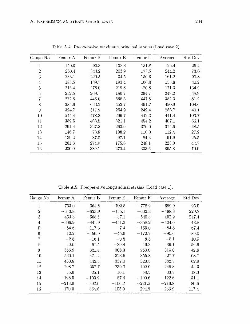
A. EXPERIMENTAL STRAIN GAUGE DATA 264
Table A.4: Preoperative maximum principal strains (Load case 2).
Gauge No Femur A Femur B Femur E Femur F Average Std Dev
1 150.0 90.3 133.3 131.8 126.4 25.4 2 250.4 344.2 203.9 178.5 244.2 73.0 3 233.1 220.5 34.5 156.6 161.2 90.8 4 183.5 139.7 193.4 106.8 155.8 40.2 5 216.4 276.0 219.8 -26.8 171.3 134.9 6 252.5 269.1 180.7 294.7 249.2 48.9 7 272.8 446.0 368.5 441.8 382.3 81.2 8 385.0 633.2 453.7 491.7 490.9 104.6 9 324.7 317.9 254.9 249.4 286.7 40.1 10 545.4 478.3 299.7 442.3 441.4 103.7 11 389.5 463.5 321.1 454.2 407.1 66.1 12 291.4 327.3 263.6 376.0 314.6 48.5 13 146.7 78.8 108.2 116.0 112.4 27.9 14 139.2 87.0 97.1 84.3 101.9 25.5 15 201.3 274.9 175.8 248.1 225.0 44.7 16 230.0 389.1 270.4 333.6 305.8 70.0
Table A.5: Preoperative longitudinal strains (Load case 1).
Gauge No Femur A Femur B Femur E Femur F Average Std Dev
1 -753.0 -564.8 -702.8 -778.9 -699.9 95.5 2 -613.8 -623.9 -155.1 -602.3 -498.8 229.3 3 -463.3 -568.1 -37.1 -540.3 -402.2 247.4 4 -366.9 -441.9 -451.3 -358.2 -404.6 48.8 5 -54.6 -117.3 -7.4 -160.0 -84.8 67.4 6 12.2 -156.9 -45.0 -172.7 -90.6 89.0 7 -2.8 -16.1 -9.8 8.3 -5.1 10.5 8 40.0 97.5 -39.4 46.3 36.1 56.6 9 366.9 321.8 308.3 263.0 315.0 42.8 10 560.1 471.2 323.5 355.8 427.7 108.7 11 430.8 442.5 337.0 320.5 382.7 62.9 12 298.7 257.7 239.0 192.0 246.8 44.3 13 35.0 25.1 16.1 58.5 33.7 18.3 14 -198.5 -103.9 -87.4 -100.6 -122.6 51.1 15 -213.0 -302.6 -106.2 -221.5 -210.8 80.6 16 -170.0 -364.8 -105.9 -294.9 -233.9 117.4

A. EXPERIMENTAL STRAIN GAUGE DATA 265
Table A.6: Preoperative longitudinal strains (Load case 2).
Gauge No Femur A Femur B Femur E Femur F Average Std Dev
1 -791.7 -538.8 -612.5 -739.9 -670.7 115.8 2 -612.3 -603.4 -129.2 -557.7 -475.6 232.2 3 -457.8 -498.2 -41.0 -487.4 -371.1 220.7 4 -322.0 -254.1 -390.1 -284.6 -312.7 58.6 5 -26.6 54.9 133.3 -165.0 -0.9 127.4 6 175.4 185.6 125.0 -145.2 85.2 155.9 7 252.8 445.2 354.6 385.4 359.5 80.5 8 376.1 627.7 453.2 466.5 480.9 105.7 9 298.2 317.9 253.9 249.1 279.8 33.7 10 545.4 467.0 293.7 439.4 436.4 105.2 11 373.0 463.5 320.9 427.2 396.1 62.4 12 264.9 316.2 262.5 361.3 301.2 47.1 13 -9.2 -87.1 -120.1 -84.3 -75.2 46.9 14 -353.1 -304.0 -360.5 -367.4 -346.3 28.8 15 -434.9 -738.6 -441.0 -587.1 -550.4 143.9 16 -466.6 -1017.4 -730.4 -783.0 -749.3 226.0
Table A.7: Postoperative minimum principal strains (Load case 1).
Gauge No Femur A Femur B Femur E Femur F Average Std Dev
1 -34.9 -36.2 -20.2 -39.2 -32.6 8.5 2 -194.0 -210.5 -63.4 -187.7 -163.9 67.7 3 -252.7 -430.1 -15.0 -424.5 -280.6 195.3 4 -180.2 -472.1 -445.1 -343.5 -360.2 132.2 5 -32.1 -127.6 -78.9 -80.9 -79.9 39.0 6 -104.6 -63.3 -37.7 -150.8 -89.1 49.5 7 -52.1 -86.1 -54.1 -67.9 -65.1 15.7 8 -73.0 -127.0 -65.0 -81.0 -86.5 27.8 9 -51.9 -90.5 -43.1 -72.0 -64.4 21.2 10 -75.1 -46.0 -38.8 -41.1 -50.2 16.8 11 -72.0 -104.5 -109.7 -60.6 -86.7 24.1 12 -63.4 -24.4 -127.8 2.0 -53.4 56.4 13 -74.8 -80.3 -42.5 -47.6 -61.3 19.0 14 -71.2 -97.3 -127.0 -72.0 -91.8 26.4 15 -234.4 -398.1 -164.2 -246.0 -260.7 98.5 16 -236.2 -562.9 -316.8 -412.1 -382.0 140.4
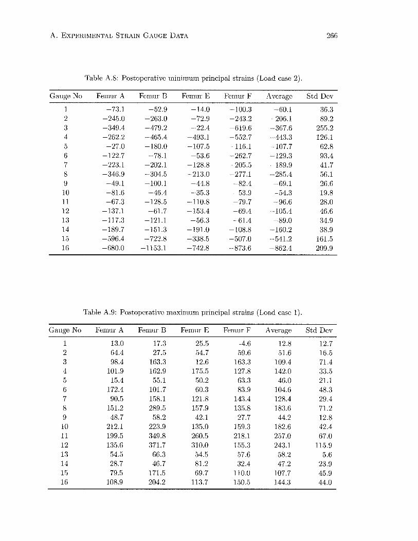
A. EXPERIMENTAL STRAIN GAUGE DATA 266
Table A.8: Postoperative minimum principal strains (Load case 2).
Gauge No Femur A Femur B Femur E Femur F Average Std Dev
1 -73.1 -52.9 -14.0 -100.3 -60.1 36.3 2 -245.0 -263.0 -72.9 -243.2 -206.1 89.2 3 -349.4 -479.2 -22.4 -619.6 -367.6 255.2 4 -262.2 -465.4 -493.1 -552.7 -443.3 126.1 5 -27.0 -180.0 -107.5 -116.1 -107.7 62.8 6 -122.7 -78.1 -53.6 -262.7 -129.3 93.4 7 -223.1 -202.1 -128.8 -205.5 -189.9 41.7 8 -346.9 -304.5 -213.0 -277.1 -285.4 56.1 9 -49.1 -100.1 -44.8 -82.4 -69.1 26.6 10 -81.6 -46.4 -35.3 -53.9 -54.3 19.8 11 -67.3 -128.5 -110.8 -79.7 -96.6 28.0 12 -137.1 -61.7 -153.4 -69.4 -105.4 46.6 13 -117.3 -121.1 -56.3 -61.4 -89.0 34.9 14 -189.7 -151.3 -191.0 -108.8 -160.2 38.9 15 -596.4 -722.8 -338.5 -507.0 -541.2 161.5 16 -680.0 -1153.1 -742.8 -873.6 -862.4 209.9
Table A.9: Postoperative maximum principal strains (Load case 1).
Gauge No Femur A Femur B Femur E Femur F Average Std Dev
1 13.0 17.3 25.5 -4.6 12.8 12.7 2 64.4 27.5 54.7 59.6 51.6 16.5 3 98.4 163.3 12.6 163.3 109.4 71.4 4 101.9 162.9 175.5 127.8 142.0 33.5 5 15.4 55.1 50.2 63.3 46.0 21.1 6 172.4 101.7 60.3 83.9 104.6 48.3 7 90.5 158.1 121.8 143.4 128.4 29.4 8 151.2 289.5 157.9 135.8 183.6 71.2 9 48.7 58.2 42.1 27.7 44.2 12.8 10 212.1 223.9 135.0 159.3 182.6 42.4 11 199.5 349.8 260.5 218.1 257.0 67.0 12 135.6 371.7 310.0 155.3 243.1 115.9 13 54.5 66.3 54.5 57.6 58.2 5.6 14 28.7 46.7 81.2 32.4 47.2 23.9 15 79.5 171.5 69.7 110.0 107.7 45.9 16 108.9 204.2 113.7 150.5 144.3 44.0
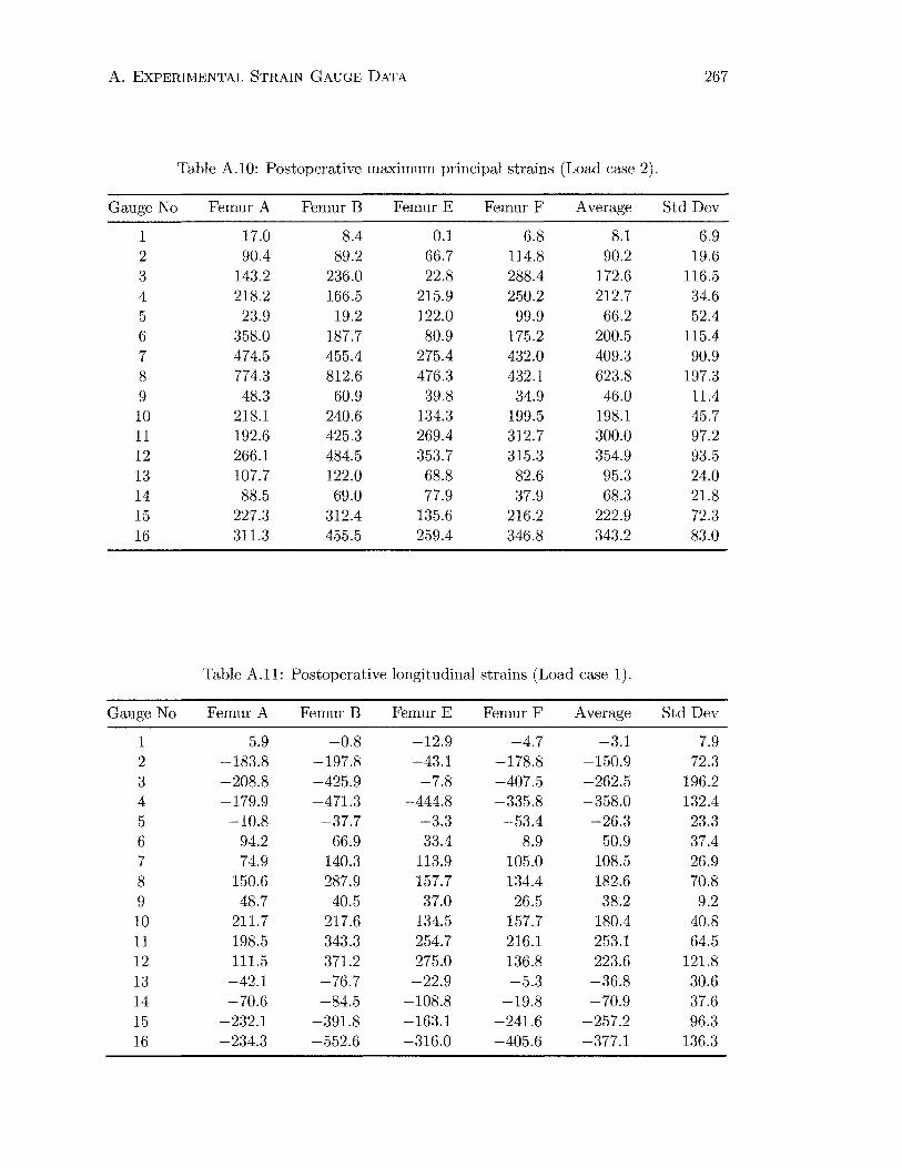
A. EXPERIMENTAL STRAIN GAUGE DATA 267
Table A.10: Postoperative maximum principal strains (Load case 2).
Gauge No Femur A Femur B Femur E Femur F Average Std Dev
1 17.0 8.4 0.1 6.8 8.1 6.9 2 90.4 89.2 66.7 114.8 90.2 19.6 3 143.2 236.0 22.8 288.4 172.6 116.5 4 218.2 166.5 215.9 250.2 212.7 34.6 5 23.9 19.2 122.0 99.9 66.2 52.4 6 358.0 187.7 80.9 175.2 200.5 115.4 7 474.5 455.4 275.4 432.0 409.3 90.9 8 774.3 812.6 476.3 432.1 623.8 197.3 9 48.3 60.9 39.8 34.9 46.0 11.4 10 218.1 240.6 134.3 199.5 198.1 45.7 11 192.6 425.3 269.4 312.7 300.0 97.2 12 266.1 484.5 353.7 315.3 354.9 93.5 13 107.7 122.0 68.8 82.6 95.3 24.0 14 88.5 69.0 77.9 37.9 68.3 21.8 15 227.3 312.4 135.6 216.2 222.9 72.3 16 311.3 455.5 259.4 346.8 343.2 83.0
Table A.11: Postoperative longitudinal strains (Load case 1).
Gauge No Femur A Femur B Femur E Femur F Average Std Dev
1 5.9 -0.8 -12.9 -4.7 -3.1 7.9 2 -183.8 -197.8 -43.1 -178.8 -150.9 72.3 3 -208.8 -425.9 -7.8 -407.5 -262.5 196.2 4 -179.9 -471.3 -444.8 -335.8 -358.0 132.4 5 -10.8 -37.7 -3.3 -53.4 -26.3 23.3 6 94.2 66.9 33.4 8.9 50.9 37.4 7 74.9 140.3 113.9 105.0 108.5 26.9 8 150.6 287.9 157.7 134.4 182.6 70.8 9 48.7 40.5 37.0 26.5 38.2 9.2 10 211.7 217.6 134.5 157.7 180.4 40.8 11 198.5 343.3 254.7 216.1 253.1 64.5 12 111.5 371.2 275.0 136.8 223.6 121.8 13 -42.1 -76.7 -22.9 -5.3 -36.8 30.6 14 -70.6 -84.5 -108.8 -19.8 -70.9 37.6 15 -232.1 -391.8 -163.1 -241.6 -257.2 96.3 16 -234.3 -552.6 -316.0 -405.6 -377.1 136.3
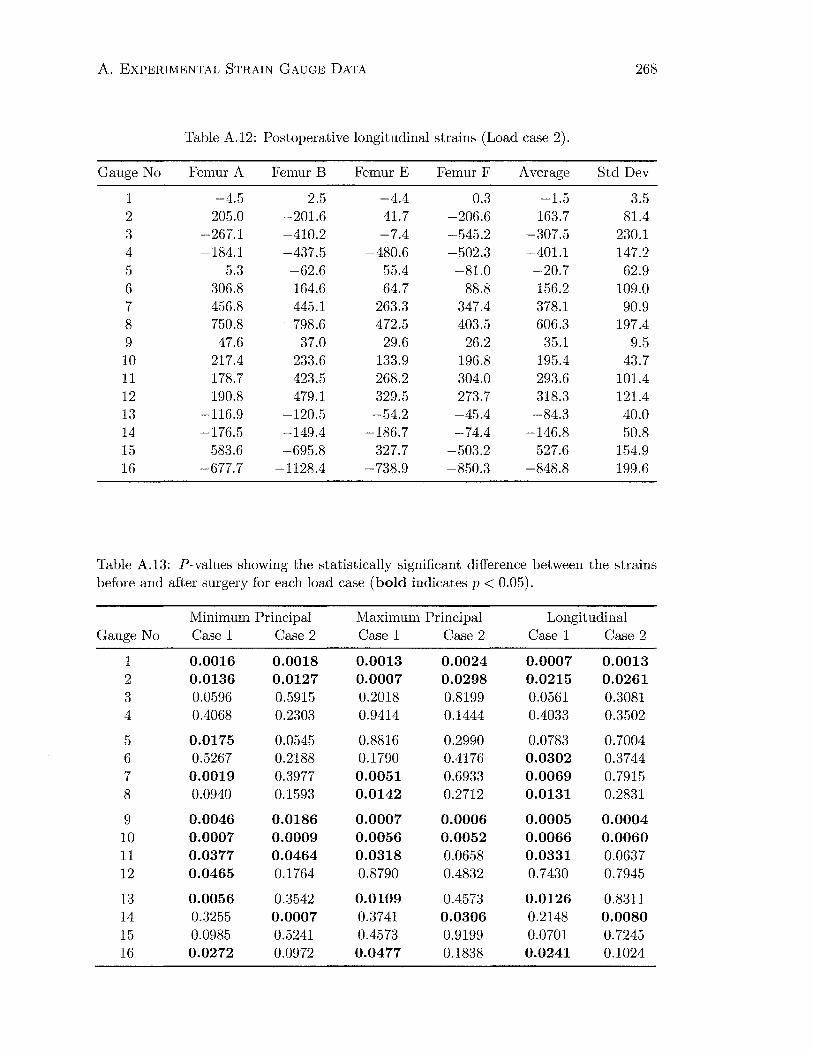
A. EXPERIMENTAL STRAIN GAUGE DATA 268
Table A.12: Postoperative longitudinal strains (Load case 2).
Gauge No Femur A Femur B Femur E Femur F Average Std Dev
1 -4.5 2.5 -4.4 0.3 -1.5 3.5 2 -205.0 -201.6 -41.7 -206.6 -163.7 81.4 3 -267.1 -410.2 -7.4 -545.2 -307.5 230.1 4 -184.1 -437.5 -480.6 -502.3 -401.1 147.2 5 5.3 -62.6 55.4 -81.0 -20.7 62.9 6 306.8 164.6 64.7 88.8 156.2 109.0 7 456.8 445.1 263.3 347.4 378.1 90.9 8 750.8 798.6 472.5 403.5 606.3 197.4 9 47.6 37.0 29.6 26.2 35.1 9.5 10 217.4 233.6 133.9 196.8 195.4 43.7 11 178.7 423.5 268.2 304.0 293.6 101.4 12 190.8 479.1 329.5 273.7 318.3 121.4 13 -116.9 -120.5 -54.2 -45.4 -84.3 40.0 14 -176.5 -149.4 -186.7 -74.4 -146.8 50.8 15 -583.6 -695.8 -327.7 -503.2 -527.6 154.9 16 -677.7 -1128.4 -738.9 -850.3 -848.8 199.6
Table A.13: P-values showing the statistically significant difference between the strains before and after surgery for each load case (bold indicates p < 0.05).
Minimum Principal Maximum Principal Longitudinal Gauge No Case 1 Case 2 Case 1 Case 2 Case1 Case 2
1 0.0016 0.0018 0.0013 0.0024 0.0007 0.0013 2 0.0136 0.0127 0.0007 0.0298 0.0215 0.0261 3 0.0596 0.5915 0.2018 0.8199 0.0561 0.3081 4 0.4068 0.2303 0.9414 0.1444 0.4033 0.3502
5 0.0175 0.0545 0.8816 0.2990 0.0783 0.7004 6 0.5267 0.2188 0.1790 0.4176 0.0302 0.3744 7 0.0019 0.3977 0.0051 0.6933 0.0069 0.7915 8 0.0940 0.1593 0.0142 0.2712 0.0131 0.2831
9 0.0046 0.0186 0.0007 0.0006 0.0005 0.0004 10 0.0007 0.0009 0.0056 0.0052 0.0066 0.0060 11 0.0377 0.0464 0.0318 0.0658 0.0331 0.0637 12 0.0465 0.1764 0.8790 0.4832 0.7430 0.7945
13 0.0056 0.3542 0.0109 0.4573 0.0126 0.8311 14 0.3255 0.0007 0.3741 0.0306 0.2148 0.0080 15 0.0985 0.5241 0.4573 0.9199 0.0701 0.7245 16 0.0272 0.0972 0.0477 0.1838 0.0241 0.1024

A. EXPERIMENTAL STRAIN GAUGE DATA 269
Table A.14: Postoperative strains as a percentage of preoperative strains (maximum and minimum principal strains and their corresponding errors).
Gauge Minimum Principal Strain Maximum Principal Strain No Case 1 Error Case 2 Error Case 1 Error Case 2 Error
1 4.4% 1.4% 8.7% 5.6% 8.4% 8.4% 6.4% 5.6% 2 31.5% 17.9% 38.2% 22.3% 28.5% 9.6% 36.9% 13.7% 3 66.7% 61.2% 90.8% 81.8% 72.9% 63.6% 107.1% 94.2% 4 88.5% 34.2% 132.8% 43.9% 99.0% 28.4% 136.5% 41.6% 5 38.4% 20.1% 44.5% 28.1% 87.0% 115.5% 38.7% 43.2% 6 77.0% 69.0% 65.5% 74.0% 154.2% 92.5% 80.4% 48.9% 7 313.1% 277.6% 119.0% 34.3% 485.9% 209.9% 107.1% 32.9% 8 210.2% 133.2% 135.1% 41.1% 297.4% 164.3% 127.1% 48.5% 9 39.0% 15.2% 49.9% 22.4% 13.9% 4.5% 16.0% 4.6% 10 32.0% 12.4% 37.4% 16.0% 41.6% 14.1% 44.9% 14.8% 11 62.7% 22.8% 70.3% 21.1% 65.9% 20.2% 73.7% 26.7% 12 52.0% 56.7% 74.3% 34.1% 96.0% 48.7% 112.8% 34.5% 13 36.3% 14.1% 78.3% 33.1% 29.9% 7.4% 84.7% 30.0% 14 69.4% 33.5% 41.7% 10.5% 80.2% 50.7% 67.0% 27.2% 15 117.2% 62.4% 92.9% 35.7% 115.0% 59.4% 99.0% 37.7% 16 158.1% 96.0% 112.6% 43.2% 138.3% 67.9% 112.3% 37.4%
Table A.15: Postoperative strains as a percentage of preoperative strains (longitudinal strains and their corresponding errors).
Longitudinal Strain Gauge No Load Case 1 Error Load Case 2 Error
1 0.4% 1.1% 0.2% 0.5% 2 30.3% 20.1% 34.4% 24.0% 3 65.3% 63.2% 82.9% 79.2% 4 88.5% 34.4% 128.3% 52.9% 5 31.0% 36.9% 2382.6% 349096.8% 6 -56.1% -68.9% 183.4% 359.1% 7 -2117.4% -4352.0% 105.2% 34.6% 8 506.0% 816.7% 126.1% 49.5% 9 12.1% 3.3% 12.6% 3.7% 10 42.2% 14.3% 44.8% 14.7% 11 66.1% 20.1% 74.1% 28.1% 12 90.6% 52.0% 105.7% 43.6% 13 -109.1% -108.3% 112.1% 87.8% 14 57.9% 39.0% 42.4% 15.1% 15 122.0% 65.3% 95.9% 37.7% 16 161.2% 99.7% 113.3% 43.3%

Appendix B
Strain Distributions
EE, Min . Principal (Ave. Crit . : 75%)
+6.332e-04 +O.OOOe+OO -2.500e-04 -s . oooe-04 -7 . 500e-04 -l.OOOe-03 -1.250e-03 -l . SOOe-03 -1.750e-03 -2 . 000e-03 -2 . 250e-03 -2 . 500e-03 -5 . 006e-02
(a) Intact femur (b) Postoperative (c) Remodelled
Figure B.l: Minimum principal strain distribution (Stability, anteromedial view).
270
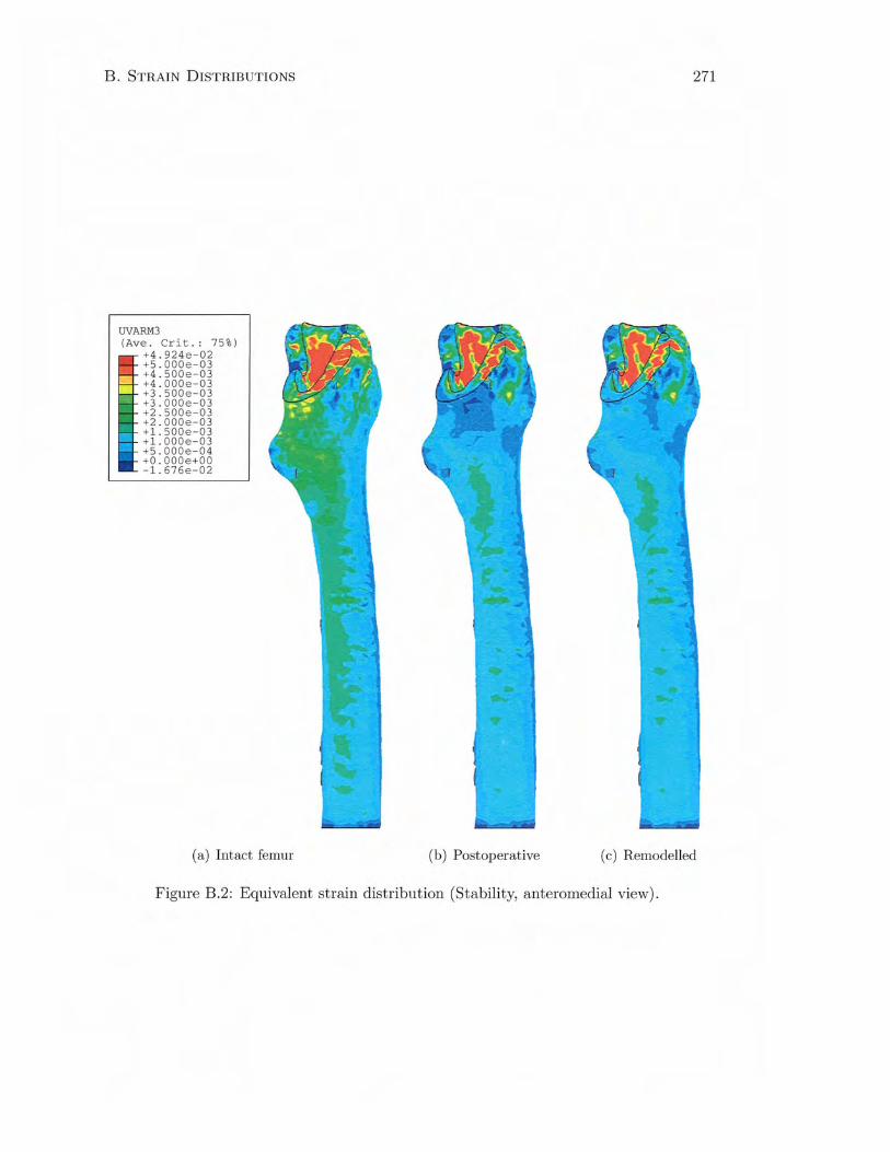
B. STRAIN DISTRIBUTIONS
UVARM3 (Ave . Crit . : 75%)
+4.924e - 02 +S . OOOe-03 +4 . 500e- 03 +4 . 000e-03 +3 . 500e-03 +3 . 000e-03 +2 . 500e-03 +2 . 000e-03 +l . SOOe - 03 +l . OOOe-03 +S . OOOe-04 +O . OOOe+OO -1 . 676e-02
(a) Intact femur
271
(b) Postoperative (c) Remodelled
Figure B.2: Equivalent strain distribution (Stability, anteromedial view) .
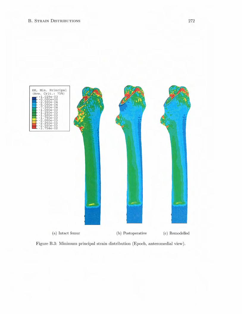
B. STRAIN DISTRIB UTIONS
EE, Min. Principal (Ave. Crit .: 75%)
+1.029e-03 +O.OOOe+OO - 2.500e-04 -s . oooe-04 -7 . 500e-04 - l . OOOe-03 -1 . 250e - 03 -1. SOOe-03 -1.750e - 03 -2.000e-03 -2.250e-03 -2.500e-03 -3.754e- 02
(a) Intact femur
272
(b) Postoperative (c) Remodelled
Figure B.3: Minimum principal strain distribution (Epoch , anteromedial view).
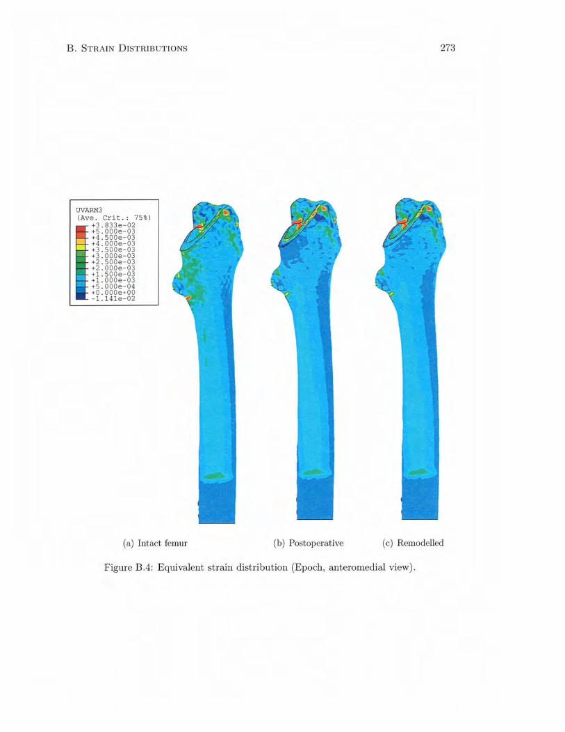
B. STRAIN DISTRIBUTIONS
UVARM3 (Ave . Crit .: 75%)
+3 . 833e-02 +5 . 000e-03 +4 . 500e-03 +4 . 000e-03 +3 . 500e-03 +3.000e- 03 +2.500e-03 +2 . 000e-03 +1.500e-03 +l.OOOe-03 +5.000e-04 +O.OOOe+OO -1.14le-02
(a) Intact femur
273
(b) Postoperative (c) Remodelled
Figure B.4: Equivalent strain distribution (Epoch, anteromedial view) .
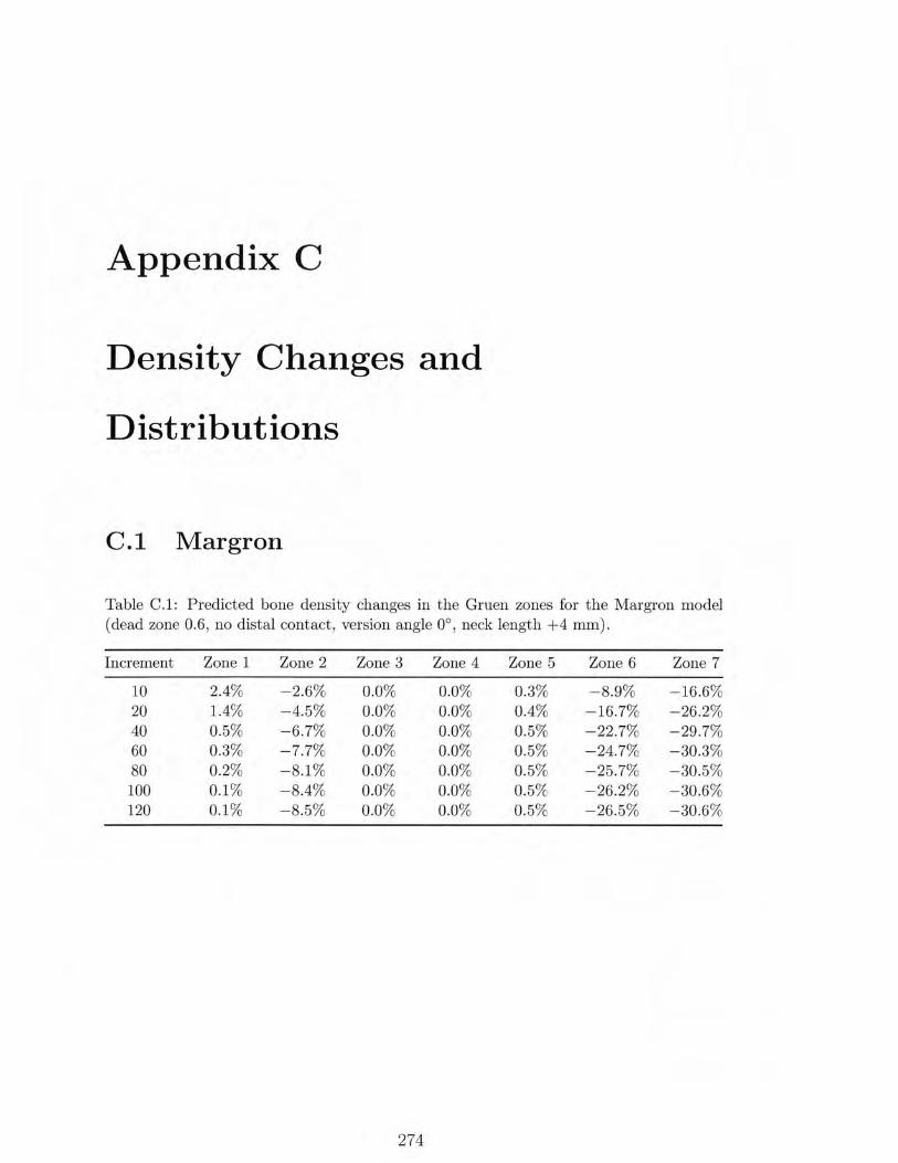
Appendix C
Density Changes and
Distributions
C .l M argron
Table C.1: Predicted bone density changes in the Gruen zones for the Margron model (dead zone 0.6 , no distal contact, version angle 0°, neck length +4 mm).
Increment Zone 1 Zone 2 Zone 3 Zone 4 Zone 5 Zone 6 Zone 7
10 2.4% -2.6% 0.0% 0.0% 0.3% -8.9% -16.6% 20 1.4% -4.5% 0.0% 0.0% 0.4% -16.7% -26.2% 40 0.5% - 6.7% 0.0% 0.0% 0.5% -22.7% -29 .7% 60 0.3% -7.7% 0.0% 0.0% 0.5% -24.7% -30.3% 80 0.2% -8.1% 0.0% 0.0% 0.5% -25.7% - 30.5% 100 0.1% -8.4% 0.0% 0.0% 0.5% -26.2% -30.6% 120 0.1% - 8.5% 0.0% 0.0% 0.5% -26.5% -30.6%
274
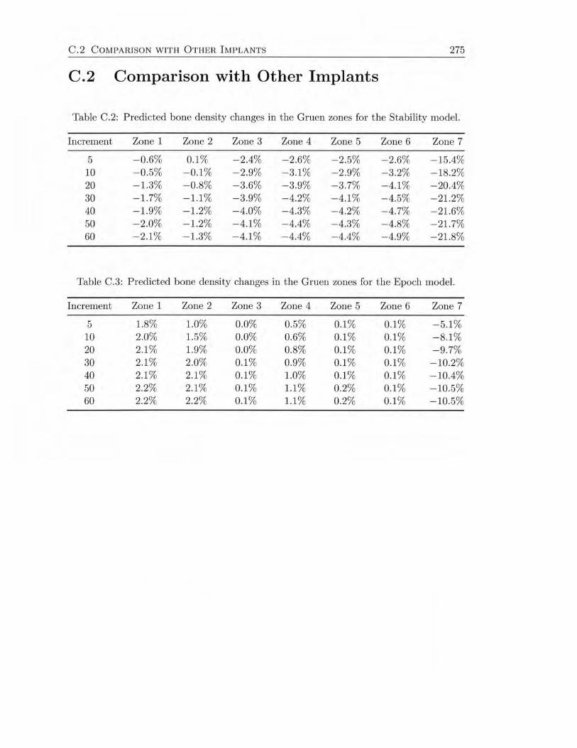
C .2 COMPARISON WITH OTHER I MPLANTS 275
C.2 Comparison with Other Implants
Table C.2: Predicted bone density changes in the Gruen zones for the Stability model.
Increment Zone 1 Zone 2 Zone 3 Zone 4 Zone 5 Zone 6 Zone 7
5 -0.6% 0.1% -2.4% - 2.6% -2.5% -2.6% -15.4% 10 -0.5% -0.1 % -2.9% -3.1% - 2.9% -3.2% -18.2% 20 -1.3% -0.8% -3.6% - 3.9% -3.7% -4.1% - 20.4% 30 -1.7% -1.1% - 3.9% -4.2% - 4.1% -4.5% -21.2% 40 -1.9% -1.2% -4.0% - 4.3% -4.2% -4.7% -21.6% 50 -2.0% -1.2% -4.1% -4.4% -4.3% -4.8% -21.7% 60 -2.1% -1.3% -4.1% -4.4% -4.4% -4.9% -21.8%
Table C.3: Predicted bone density changes in the Gruen zones for the Epoch model.
Increment Zone 1 Zone 2 Zone 3 Zone 4 Zone 5 Zone 6 Zone 7
5 1.8% 1.0% 0.0% 0.5% 0.1% 0.1% -5.1% 10 2.0% 1.5% 0.0% 0.6% 0.1 % 0. 1% - 8. 1% 20 2.1 % 1.9% 0.0% 0.8% 0.1% 0.1% -9.7% 30 2.1 % 2.0% 0.1% 0.9% 0.1 % 0.1% - 10.2% 40 2.1 % 2.1% 0.1 % 1.0% 0.1 % 0.1% -10.4% 50 2.2% 2. 1% 0.1% 1.1% 0.2% 0.1 % -10.5% 60 2.2% 2.2% 0.1% 1.1% 0.2% 0.1 % -10.5%
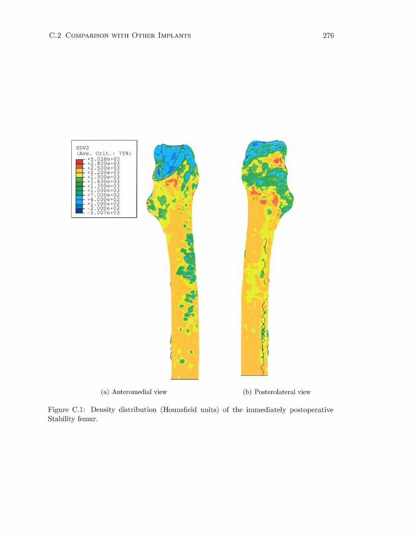
C .2 COMPARISON WITH OTHER IMPLANTS
SDV2 (Ave. Crit. : 75%)
+5.028e+03 +2.800e+03 +2 . 500e+03 +2.200e+03 +1.900e+03 +1 . 600e+03 +1.300e+03 +1.000e+03 +7.000e+02 +4.000e+02 +1.000e+02 -2 . 000e+02 -3.007e+03
(a) Anteromedial view
t •
( (
(b) Posterolateral view
276
Figure C.l: Density distribution (Hounsfield units) of the immediately postoperative Stability femur.
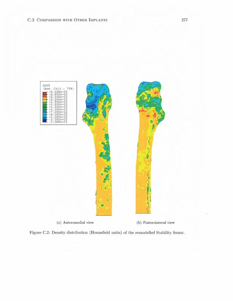
C.2 COMPARISON WITH OTHER IMPLANTS
SDV2 (Ave . Crit .: 75%)
I +5 . 028e+03 +2 . 800e+03 +2 . 500e+03
- +2 . 200e+03 ::': +1 . 900e +03
+1 .600e+03 +1. 300e+03 +1.000e+03 +7.000e+02 +4 .000e+02 +1.0 00e+02 -2 . 000e +02 -3 . 089 e +03
(a) Anteromedial view
t I
' ••
277
(b) Posterolateral view
Figure C.2: Density distribution (Hounsfield units) of the remodelled Stability femur.
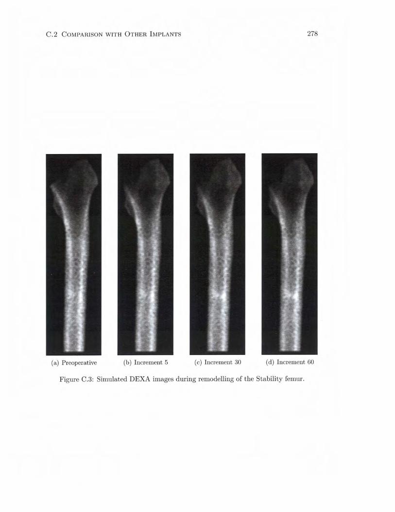
C.2 COMPARISON WITH OTHER IMPLANTS 278
(a) Preoperative (b) Increment 5 (c) Increment 30 (d) Increment 60
Figure C.3: Simulated DEXA images during remodelling of the Stability femur.
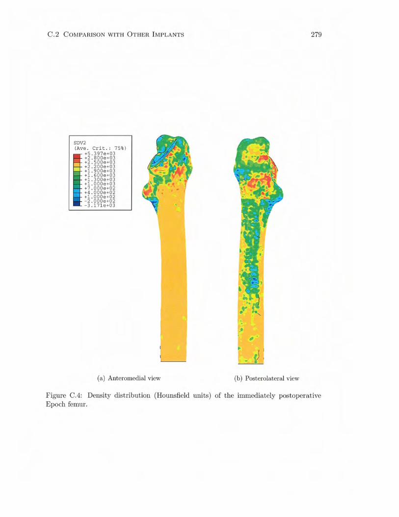
C.2 COMPARISON WITH OTHER IMPLANTS
SDV2 (Ave. Crit.: 75%)
+5.397e+03 +2.800e+03 +2.500e+03 +2.200e+03 +1.900e+03 +1.600e+03 +1. 300e+03 +l . OOOe+03 +7 . 000e+02 +4 . 000e+02 +1.000e+02 -2.000e+02 -3 .1 71e+03
(a) Anteromedial view
279
••
)
(b) Posterolateral view
Figure C.4: Density distribution (Hounsfield units) of the immediately postoperative Epoch femur.

C.2 COMPARISON WITH OTHER IMPLANTS
SDV2 (Ave. Crit . : 75%)
+5.425e+03 +2.800e+03 +2.500e+03 +2.200e+03 +1.900e+03 +1.600e+03 +1 . 300e+03 +1 . 000e+03 +7.000e+02 +4.000e+02 +1.000e+02 -2.000e+02 -3. 1 71e+03
(a) Anteromedial view
280
'.
·'
)
(b) Posterolateral view
Figure C.5: Density distribution (Hounsfield units) of the remodelled Epoch femur.
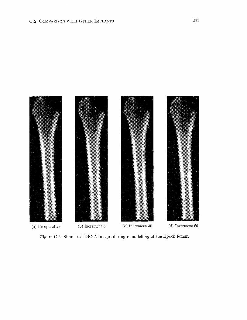
C.2 COMPARISON WITH OTHER IMPLANTS 281
(a) Preoperative (b) Increment 5 (c) Increment 30 (d) Increment 60
Figure C.6: Simulated DEXA images during remodelling of the Epoch femur.
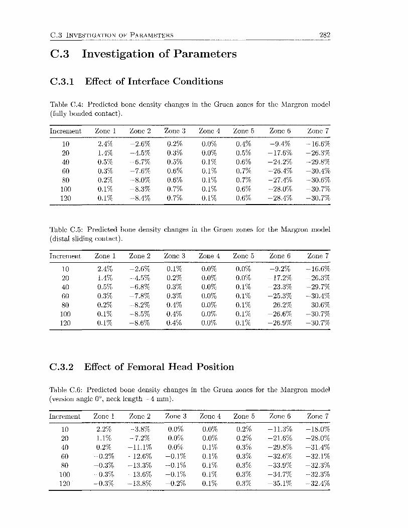
C.3 INVESTIGATION OF PARAMETERS 282
C.3 Investigation of Parameters
C.3.1 Effect of Interface Conditions
Table C.4: Predicted bone density changes in the Gruen zones for the Margron model (fully bonded contact).
Increment Zone 1 Zone 2 Zone 3 Zone 4 Zone 5 Zone 6 Zone 7
10 2.4% -2.6% 0.2% 0.0% 0.4% -9.4% -16.6% 20 1.4% -4.5% 0.3% 0.0% 0.5% -17.6% -26.3% 40 0.5% -6.7% 0.5% 0.1% 0.6% -24.2% -29.8% 60 0.3% -7.6% 0.6% 0.1% 0.7% -26.4% -30.4% 80 0.2% -8.0% 0.6% 0.1% 0.7% -27.4% -30.6% 100 0.1% -8.3% 0.7% 0.1% 0.6% -28.0% -30.7% 120 0.1% -8.4% 0.7% 0.1% 0.6% -28.4% -30.7%
Table C.5: Predicted bone density changes in the Gruen zones for the Margron model (distal sliding contact).
Increment Zone 1 Zone 2 Zone 3 Zone 4 Zone 5 Zone 6 Zone 7
10 2.4% -2.6% 0.1% 0.0% 0.0% -9.2% -16.6% 20 1.4% -4.5% 0.2% 0.0% 0.0% -17.2% -26.3% 40 0.5% -6.8% 0.3% 0.0% 0.1% -23.3% -29.7% 60 0.3% -7.8% 0.3% 0.0% 0.1% -25.3% -30.4% 80 0.2% -8.2% 0.4% 0.0% 0.1% -26.2% -30.6% 100 0.1% -8.5% 0.4% 0.0% 0.1% -26.6% -30.7% 120 0.1% -8.6% 0.4% 0.0% 0.1% -26.9% -30.7%
C.3.2 Effect of Femoral Head Position
Table C.6: Predicted bone density changes in the Gruen zones for the Margron model (version angle 0°, neck length -4 mm).
Increment Zone 1 Zone 2 Zone 3 Zone 4 Zone 5 Zone 6 Zone 7
10 2.2% -3.8% 0.0% 0.0% 0.2% -11.3% -18.0% 20 1.1% -7.2% 0.0% 0.0% 0.2% -21.6% -28.0% 40 0.2% -11.1% 0.0% 0.1% 0.3% -29.8% -31.4% 60 -0.2% -12.6% -0.1% 0.1% 0.3% -32.6% -32.1% 80 -0.3% -13.3% -0.1% 0.1% 0.3% -33.9% -32.3% 100 -0.3% -13.6% -0.1% 0.1% 0.3% -34.7% -32.3% 120 -0.3% -13.8% -0.2% 0.1% 0.3% -35.1% -32.4%
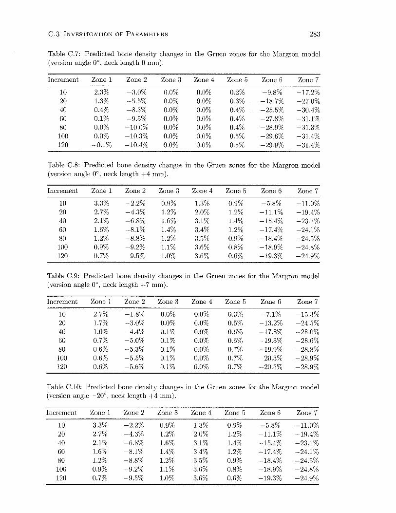
C.3 INVESTIGATION OF PARAMETERS 283
Table C.7: Predicted bone density changes in the Gruen zones for the Margron model (version angle 0°, neck length 0 mm).
Increment Zone 1 Zone 2 Zone 3 Zone 4 Zone 5 Zone 6 Zone 7
10 2.3% -3.0% 0.0% 0.0% 0.2% -9.8% -17.2% 20 1.3% -5.5% 0.0% 0.0% 0.3% -18.7% -27.0% 40 0.4% -8.3% 0.0% 0.0% 0.4% -25.5% -30.4% 60 0.1% -9.5% 0.0% 0.0% 0.4% -27.8% -31.1% 80 0.0% -10.0% 0.0% 0.0% 0.4% -28.9% -31.3% 100 0.0% -10.3% 0.0% 0.0% 0.5% -29.6% -31.4% 120 -0.1% -10.4% 0.0% 0.0% 0.5% -29.9% -31.4%
Table C.8: Predicted bone density changes in the Gruen zones for the Margron model (version angle 0°, neck length +4 mm).
Increment Zone 1 Zone 2 Zone 3 Zone 4 Zone 5 Zone 6 Zone 7
10 3.3% -2.2% 0.9% 1.3% 0.9% -5.8% -11.0% 20 2.7% -4.3% 1.2% 2.0% 1.2% -11.1% -19.4% 40 2.1% -6.8% 1.6% 3.1% 1.4% -15.4% -23.1% 60 1.6% -8.1% 1.4% 3.4% 1.2% -17.4% -24.1% 80 1.2% -8.8% 1.2% 3.5% 0.9% -18.4% -24.5% 100 0.9% -9.2% 1.1% 3.6% 0.8% -18.9% -24.8% 120 0.7% -9.5% 1.0% 3.6% 0.6% -19.3% -24.9%
Table C.9: Predicted bone density changes in the Gruen zones for the Margron model (version angle 0°, neck length +7 mm).
Increment Zone 1 Zone 2 Zone 3 Zone 4 Zone 5 Zone 6 Zone 7
10 2.7% -1.8% 0.0% 0.0% 0.3% -7.1% -15.3% 20 1.7% -3.0% 0.0% 0.0% 0.5% -13.2% -24.5% 40 1.0% -4.4% 0.1% 0.0% 0.6% -17.8% -28.0% 60 0.7% -5.0% 0.1% 0.0% 0.6% -19.3% -28.6% 80 0.6% -5.3% 0.1% 0.0% 0.7% -19.9% -28.8% 100 0.6% -5.5% 0.1% 0.0% 0.7% -20.3% -28.9% 120 0.6% -5.6% 0.1% 0.0% 0.7% -20.5% -28.9%
Table C.10: Predicted bone density changes in the Gruen zones for the Margron model (version angle -20°, neck length +4 mm).
Increment Zone 1 Zone 2 Zone 3 Zone 4 Zone 5 Zone 6 Zone 7
10 3.3% -2.2% 0.9% 1.3% 0.9% -5.8% -11.0% 20 2.7% -4.3% 1.2% 2.0% 1.2% -11.1% -19.4% 40 2.1% -6.8% 1.6% 3.1% 1.4% -15.4% -23.1% 60 1.6% -8.1% 1.4% 3.4% 1.2% -17.4% -24.1% 80 1.2% -8.8% 1.2% 3.5% 0.9% -18.4% -24.5% 100 0.9% -9.2% 1.1% 3.6% 0.8% -18.9% -24.8% 120 0.7% -9.5% 1.0% 3.6% 0.6% -19.3% -24.9%
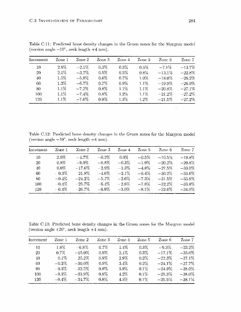
C.3 INVESTIGATION OF PARAMETERS 284
Table C.ll: Predicted bone density changes in the Gruen zones for the Margron model (version angle -10°, neck length +4 mm).
Increment Zone 1 Zone 2 Zone 3 Zone 4 Zone 5 Zone 6 Zone 7
10 2.9% -2.1% 0.3% 0.3% 0.5% -7.1% -13.7% 20 2.1% -3.7% 0.5% 0.5% 0.8% -13.1% -22.8% 40 1.5% -5.8% 0.6% 0.7% 1.0% -18.0% -26.2% 60 1.2% -6.7% 0.7% 0.9% 1.1% -19.9% -26.9% 80 1.1% -7.2% 0.8% 1.1% 1.1% -20.8% -27.1% 100 1.1% -7.4% 0.8% 1.2% 1.1% -21.2% -27.2% 120 1.1% -7.6% 0.9% 1.3% 1.2% -21.5% -27.2%
Table C.12: Predicted bone density changes in the Gruen zones for the Margron model (version angle + 10°, neck length +4 mm).
Increment Zone 1 Zone 2 Zone 3 Zone 4 Zone 5 Zone 6 Zone 7
10 2.0% -4.7% -0.2% 0.0% -0.5% -10.5% -19.8% 20 0.8% -9.9% -0.8% -0.3% -1.9% -20.2% -29.8% 40 0.0% -17.6% -2.9% -1.3% -4.8% -27.5% -33.0% 60 -0.3% -21.8% -4.6% -2.1% -6.4% -30.2% -33.6% 80 -0.4% -24.2% -5.7% -2.6% -7.3% -31.5% -33.8% 100 -0.4% -25.7% -6.4% -2.8% -7.8% -32.2% -33.9% 120 -0.4% -26.7% -6.9% -3.0% -8.1% -32.6% -34.0%
Table C.13: Predicted bone density changes in the Gruen zones for the Margron model (version angle +20°, neck length +4 mm).
Increment Zone 1 Zone 2 Zone 3 Zone 4 Zone 5 Zone 6 Zone 7
10 1.8% -6.8% 0.7% 1.4% 0.3% -9.3% -23.2% 20 0.7% -15.0% 0.9% 2.1% 0.3% -17.1% -33.6% 40 -0.1% -25.2% 0.9% 2.9% 0.2% -22.3% -37.1% 60 -0.3% -30.0% 0.9% 3.4% 0.2% -24.1% -37.7% 80 -0.3% -32.5% 0.8% 3.9% 0.1% -24.9% -38.0% 100 -0.3% -33.9% 0.8% 4.2% 0.1% -25.3% -38.0% 120 -0.4% -34.7% 0.8% 4.5% 0.1% -25.5% -38.1%

C.3 INVESTIGATION OF PARAMETERS 285
C.3.3 Effect of Dead Zone Width
Table C.14: Predicted bone density changes in the Gruen zones for the Margron model ( vdead zone 0.55).
Increment Zone 1 Zone 2 Zone 3 Zone 4 Zone 5 Zone 6 Zone 7
10 1.3% -4.3% 0.0% 0.0% 0.3% -12.2% -21.2% 20 -0.1% -7.7% 0.0% 0.0% 0.4% -21.8% -30.5% 40 -1.1% -10.9% 0.0% 0.0% 0.5% -28.5% -33.3% 60 -1.4% -12.0% 0.0% 0.0% 0.5% -30.7% -33.8% 80 -1.4% -12.4% 0.0% 0.0% 0.6% -31.7% -33.9% 100 -1.5% -12.6% 0.0% 0.0% 0.6% -32.2% -34.0% 120 -1.5% -12.8% 0.0% 0.0% 0.6% -32.6% -34.0%
Table C.15: Predicted bone density changes in the Gruen zones for the Margron model (vdead zone 0.65).
Increment Zone 1 Zone 2 Zone 3 Zone 4 Zone 5 Zone 6 Zone 7
10 3.4% -1.3% 0.0% 0.0% 0.2% -6.0% -12.2% 20 2.7% -2.2% 0.0% 0.0% 0.3% -11.9% -21.5% 40 2.0% -3.4% 0.0% 0.0% 0.4% -17.0% -25.6% 60 1.9% -4.0% 0.0% 0.0% 0.5% -18.8% -26.4% 80 1.8% -4.4% 0.0% 0.0% 0.5% -19.6% -26.7% 100 1.7% -4.6% 0.0% 0.0% 0.5% -20.1% -26.9% 120 1.7% -4.7% 0.0% 0.0% 0.5% -20.4% -26.9%
C.3.4 Effect of Activity Level
Table C.16: Predicted bone density changes in the Gruen zones for the Margron model (90% activity level).
Increment Zone 1 Zone 2 Zone 3 Zone 4 Zone 5 Zone 6 Zone 7
10 0.2% -3.5% 0.0% 0.0% 0.2% -10.7% -19.0% 20 -1.0% -6.3% 0.0% 0.0% 0.3% -20.1% -29.3% 40 -2.0% -9.4% 0.0% 0.0% 0.4% -27.4% -32.8% 60 -2.3% -10.6% 0.0% 0.0% 0.4% -29.7% -33.4% 80 -2.0% -11.1% 0.0% 0.0% 0.4% -30.8% -33.6% 100 -2.5% -11.4% 0.0% 0.0% 0.4% -31.5% -33.7% 120 -2.5% -11.6% 0.0% 0.0% 0.4% -31.8% -33.8%
C.3.5 Effect of Prosthesis Stiffness

C.3 INVESTIGATION OF PARAMETERS 286
Table C.17: Predicted bone density changes in the Gruen zones for the Epoch model ( isoelastic properties).
Increment Zone 1 Zone 2 Zone 3 Zone 4 Zone 5 Zone 6 Zone 7
5 1.9% 0.6% 0.0% 0.4% 0.0% 0.0% 2.2% 10 2.1% 0.8% 0.0% 0.5% 0.1% 0.0% 1.4% 20 2.2% 1.0% 0.0% 0.6% 0.1% 0.0% 0.9% 30 2.2% 1.1% 0.0% 0.7% 0.1% 0.0% 0.8% 40 2.3% 1.1% 0.0% 0.7% 0.1% 0.1% 0.8% 50 2.3% 1.2% 0.0% 0.8% 0.1% 0.1% 0.7% 60 2.3% 1.2% 0.0% 0.8% 0.1% 0.1% 0.7%
Table C.18: Predicted bone density changes in the Gruen zones for the Epoch model (cobalt-chrome properties).
Increment Zone 1 Zone 2 Zone 3 Zone 4 Zone 5 Zone 6 Zone 7
5 1.5% 0.5% 0.1% 0.9% 0.2% -2.2% -19.9% 10 1.4% 0.9% 0.1% 1.4% 0.3% -3.6% -28.8% 20 1.8% 1.3% 0.2% 2.2% 0.5% -4.6% -33.3% 30 1.9% 1.4% 0.3% 2.6% 0.6% -5.1% -34.5% 40 1.9% 1.5% 0.3% 2.8% 0.6% -5.3% -35.0% 50 1.8% 1.5% 0.3% 3.0% 0.6% -5.5% -35.3% 60 1.8% 1.6% 0.3% 3.1% 0.6% -5.6% -35.4%

Appendix D
Bone Density Correlations
6
0
-6
c 0
~ -12 "S E
U5 -18
-24 0
-30 -30
Clinical vs. Simulation DEXA Data (Margron, 1 Year)
SIM = 2.6054 + .93938 * CLIN
Correlation: r = .89701
/ /~oo
0
-24 -18 -12 -6 0
Clinical
6
'R._ Regression 95% confid.
Figure D.l: Correlation between simulated and clinical BMD changes (Margron, 1 year postop).
287

D. BONE DENSITY CORRELATIONS 288
c 0
~ "S E
U5
5
0
-5
-10
-15
-20
-25
-30
Clinical vs. Simulation DEXA Data (Margron, 2 Years)
SIM = 1.3144 + .86789 *GUN
Correlation: r = .82745
-35 '------~~----"~-~~~~~~~~~~-~-~-~----' ~ Regression -35 -30 -25 -20 -15 -1 o -5 o 5 95% confid.
Clinical
Figure D.2: Correlation between simulated and clinical BMD changes (Margron, 2 years postop).
5
0
-5
-10 c 0
~ -15 "S E
U5 -20
-25
-30
-35 -40 -35
Clinical vs. Simulation DEXA Data (Margron, 3 Years)
SIM = 3.9598 + .89638 * GUN
Correlation: r= .81868
0
0
-30 -25 -20 -15 -10 -5
Clinical
0
0 5
-,~ Regression 95% confid.
Figure D.3: Correlation between simulated and clinical BMD changes (Margron, 3 years postop).

D. BONE DENSITY CORRELATIONS
2
-2
-6
c 0
~ -10 :::J E
U5 -14
-18
-22 -26
0
Clinical vs. Simulation DEXA Data (Stability, 2 Years)
Sim = 1 .0708 + .83698 * Clin
Correlation: r = .87306
-22 -18 -14 -10 -6
Clinical
289
~- Regression
-2 2 95% confid.
Figure D.4: Correlation between simulated and clinical BMD changes (Stability, 2 years postop).
c 0 -~
'S E
U5
-10 0
Clinical vs. Simulation DEXA Data (Epoch, 2 Years)
SIM = 1.8451 + .59313 * CLIN
Correlation: r = .84852
-12L-~--~~~~--~--~~~--------~------~~----~
-18 -14 -10 -6 -2 2 6
Clinical
'-c..___ Regression 95% confid.
Figure D.5: Correlation between simulated and clinical BMD changes (Epoch, 2 years postop).
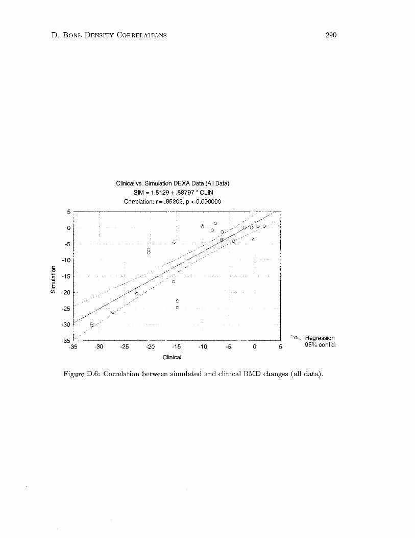
D. BONE DENSITY CORRELATIONS 290
c 0
~ "S E
U5
5
0
-5
-10
-15
-20
-25
-30
Clinical vs. Simulation DEXA Data (All Data)
SIM = 1.5129 + .88797 * CLIN
Correlation: r = .85202, p < 0.000000
-35 "----~-~-~---------~---------_j ~ Regression -35 -30 -25 -20 -15 -10 -5 o 5 95% confid.
Clinical
Figure D.6: Correlation between simulated and clinical BMD changes (all data).

References
Aamodt, A., Lund-Larsen, J., Eine, J., Andersen, E., Benum, P., Husby, 0. S., 1997.
In vivo measurements show tensile axial strain in the proximal lateral aspect of
the human femur. Journal of Orthopaedic Research 15 (6), 927-931.
Aebli, N., Krebs, J., Schwenke, D., Stich, H., Schawalder, P., Theis, J. C., 2003.
Degradation of hydroxyapatite coating on a well-functioning femoral component.
J Bone Joint Burg 85-B ( 4), 499-503.
Affatato, S., Bordini, B., Fagnano, C., Taddei, P., Tinti, A., Toni, A., 2002. Effects
of the sterilisation method on the wear of UHMWPE acetabular cups tested in a
hip joint simulator. Biomaterials 23 (6), 1439-1446.
Ament, C., Hofer, E. P., 2000. A fuzzy logic model of fracture healing. Journal of
Biomechanics 33 (8), 961-968.
Ando, M., Imura, S., Omori, H., Okumura, Y., Bo, A., Baba, H., 1999. Nonlinear
three-dimensional finite element analysis of newly designed cementless total hip
stems. Artificial Organs 23 ( 4), 339-346.
Archibeck, M. J., Jacobs, J. J., Roebuck, K. A., Giant, T. T., 2001. The basic
science of periprosthetic osteolysis. In: Sim, F. H. (Ed.), Instructional Course
Lectures. Vol. 50. American Academy of Orthopaedic Surgeons, Rosemount.
Ashman, R. B., Rho, J. Y., 1988. Elastic modulus of trabecular bone material.
Journal of Biomechanics 21 (3), 177-181.
Bagge, ]'vi., 2000. A model of bone adaptation as an optimization process. Journal
of Biomechanics 33 (11), 1349-1357.
291
REFERENCES 292
Bakker, A. D., Soejima, K., Klein-Nulend, J., Burger, E. H., 2001. The produc
tion of nitric oxide and prostaglandin E(2) by primary bone cells is shear stress
dependent. Journal of Biomechanics 34 (5), 671-677.
Bargren, J. H., Andrew, C., Bassett, L., Gjelsvik, A., 1974. Mechanical properties
of hydrated cortical bone. Journal of Biomechanics 7 (3), 239-245.
Beaupre, G. 8., Orr, T. E., Carter, D. R., 1990a. An approach for time-dependent
bone modeling and remodeling-application: A preliminary remodeling simula
tion. Journal of Orthopaedic Research 8 (5), 662-670.
Beaupre, G. 8., Orr, T. E., Carter, D. R., 1990b. An approach for time-dependent
bone modeling and remodeling-theoretical development. Journal of Orthopaedic
Research 8 (5), 651-661.
Beck, B. R., Qin, Y. X., McLeod, K. J., Otter, M. W., 2002. On the relationship
between streaming potential and strain in an in vivo bone preparation. Calcified
Tissue International 71 ( 4), 335-343.
Bentley, J. P., 1995. Principles of Measurement Systems, 3rd Edition. Longman
Group, Harlow.
Bergmann, G., Deuretzbacher, G., Heller, M. 0., Graichen, F., Rohlmann, A.,
Strauss, J., Duda, G. N., 2001. Hip contact forces and gait patterns from routine
activities. Journal of Biomechanics 34 (7), 859-871.
Bergmann, G., Graichen, F., Rohlmann, A., 1993. Hip joint loading during walking
and running, measured in two patients. Journal of Biomechanics 26 (8), 969-990.
Bergmann, G., Graichen, F., Rohlmann, A., Linke, H., 1997. Hip joint forces during
load carrying. Clinical Orthopaedics and Related Research 335, 190-201.
Biegler, F. B., Reuben, J.D., Harrigan, T. P., Hou, F. J., Akin, J. E., 1995. Effect of
porous coating and loading conditions on total hip femoral stem stability. Journal
of Arthroplasty 10 (6), 839-847.
Black, J., 1992. Biological Performance of Materials. Fundamentals of Biocompati
bility, 2nd Edition. Marel Dekker, New York.
REFERENCES 293
Blake, G. M., Parker, J. C., Buxton, F. M., Fogelman, I., 1993. Dual X-ray ab
sorptiometry: a comparison between fan beam and pencil beam scans. British
Journal of Radiology 66 (790), 902-906.
Blankenhorn, B. D., Donahue, H. J., Jacobs, C. R., 2002. The role fo gap junc
tional intercellular communication in mechanotransduction. In: Transactions of
the Orthopaedic Research Society. Vol. 27. Dallas, TX, p. 575.
Bobyn, J. D., Glassman, A. H., Goto, H., Krygier, J. J., Miller, J. E., Brooks,
C. E., 1990. The effect of stem stiffness on femoral bone resorption after canine
porous-coated total hip arthroplasty. Clinical Orthopaedics and Related Research
261, 196-213.
Bobyn, J. D., Mortimer, E. S., Glassman, A. H., Engh, C. A., Miller, J. E., Brooks,
C. E., 1992. Producing and avoiding stress shielding. Laboratory and clinical
observations of noncemented total hip arthroplasty. Clinical Orthopaedics and
Related Research 27 4, 79-96.
Bostrom, M. P. G., Boskey, A., Kaufman, J. K., Einhorn, T. A., 2000. Form and
Function of Bone. In: Buckwalter, J. A., Einhorn, T. A., Simon, S. R. (Eds.),
Orthopaedic Basic Science: Biology and Biomechanics of the Musculoskeletal Sys
tem, 2nd Edition. American Academy of Orthopaedic Surgeons, Rosemount, pp.
319-369.
Bourne, R. B., Rorabeck, C. H., 1998. A critical look at cementless stems. Taper
designs and when to use alternatives. Clinical Orthopaedics and Related Research
355, 212-223.
Brand, R. A., Crowninshield, R. D., \Vittstock, C. E., Pedersen, D. R., Clark, C. R.,
van Krieken, F. M., 1982. A model of lower extremity muscular anatomy. Journal
of Biomechanical Engineering 104 ( 4), 304-310.
Brand, R. A., Pedersen, D. R., Friederich, J. A., 1986. The sensitivity of muscle
force predictions to changes in physiologic cross-sectional area. Journal of Biome
chanics 19 (8), 589-596.

REFERENCES 294
Breathnach, A. S., 1965. Frazer's Anatomy of the Human Skeleton, 6th Edition. J.
& A. Churchill., London.
Brekelmans, W. A., Poort, H. W., Slooff, T. J., 1972. A new method to analyse the
mechanical behaviour of skeletal parts. Acta Orthopaedica Scandinavica 43 (5),
301-317.
Breme, J., Biehl, V., 1998. l\'1etallic biomaterials. In: Black, J., Hastings, G. (Eds.),
Handbook of Biomaterial Properties. Chapman & Hall, London, pp. 135-213.
Brown, S. A., l\'1erritt, K., 1991. Biocompatibility. In: Petty, W. (Ed.), Total Joint
Replacement. W. B. Saunders, Philadelphia, pp. 51-60.
Brown, T. D., Pedersen, D. R., Gray, M. L., Brand, R. A., Rubin, C. T., 1990. To
ward an identification of mechanical parameters initiating periosteal remodeling:
a combined experimental and analytic approach. Journal of Biomechanics 23 (9),
893-905.
Bruyere Garnier, K., Dumas, R., Rumelhart, C., Arlot, M. E., 1999. Mechanical
characterization in shear of human femoral cancellous bone: torsion and shear
tests. Medical Engineering and Physics 21 (9), 641-649.
Bryan, J. M., Sumner, D. R., Hurwitz, D. E., Tompkins, G. S., Andriacchi, T. P.,
Galante, J. 0., 1996. Altered load history affects periprosthetic bone loss following
cementless total hip arthroplasty. Journal of Orthopaedic Research 14 (5), 762-
768.
Bugbee, W. D., Culpepper, W. J., Engh, C. A., Engh, C. A., 1997. Long-term clin
ical consequences of stress-shielding after total hip arthroplasty without cement.
J Bone Joint Burg 79-A (7), 1007-1012.
Burke, D. W., O'Connor, D. 0., Zalenski, E. B., Jasty, M., Harris, W. H., 1991.
Micromotion of cemented and uncemented femoral components. J Bone Joint
Burg 73-B (1), 33-37.
Burr, D. B., 2002. Targeted and nontargeted remodeling. Bone 30 (1), 2-4.
Callaghan, J. J., 1993. The clinical results and basic science of total hip arthroplasty
with porous-coated prostheses. J Bone Joint Burg 75-A (2), 299-310.
REFERENCES 295
Capello, Vv. N., D'Antonio, J. A., Manley, M. T., Feinberg, J. R., 1998. Hydrox
yapatite in total hip arthroplasty. Clinical results and critical issues. Clinical
Orthopaedics and Related Research 355, 200-211.
Carter, D. R., 1982. The relationship between in vivo strains and cortical bone
remodeling. Critical Reviews in Biomedical Engineering 8 (1), 1-28.
Carter, D. R., 1984. Mechanical loading histories and cortical bone remodeling.
Calcified Tissue International 36 (Suppl 1), 19-24.
Carter, D. R., Fyhrie, D. P., Whalen, R. T., 1987. Trabecular bone density and
loading history: regulation of connective tissue biology by mechanical energy.
Journal of Biomechanics 20 (8), 785-794.
Carter, D. R., Hayes, W. C., 1976. Bone compressive strength: the influence of
density and strain rate. Science 194 (4270), 1174-1176.
Carter, D. R., Hayes, W. C., 1977. The compressive behavior of bone as a two-phase
porous structure. J Bone Joint Surg 59-A (7), 954-962.
Carter, D. R., Orr, T. E., Fyhrie, D.P., 1989. Relationships between loading history
and femoral cancellous bone architecture. Journal of Biomechanics 22 (3), 231-
244.
Carter, D. R., VanDerMeulen, M. C., Beaupre, G. S., 1996. Mechanical factors in
bone growth and development. Bone 18 (1 Suppl), 5-10.
Chang, P. B., Williams, B. J., Bhalla, K. S., Belknap, T. W., Santner, T. J., Notz,
W. I., Bartel, D. L., 2001. Design and analysis of robust total joint replace
ments: finite element model experiments with environmental variables. Journal
of Biomechanical Engineering 123 (3), 239-246.
Cheal, E. J., Spector, M., Hayes, W. C., 1992. Role of loads and prosthesis material
properties on the mechanics of the proximal femur after total hip arthroplasty.
Journal of Orthopaedic Research 10 (3), 405-422.
Chiesa, R., Tanzi, M. C., Alfonsi, S., Paracchini, L., Moscatelli, M., Cigada, A.,
2000. Enhanced wear performance of highly crosslinked UHMWPE for artificial
joints. Journal of Biomedical Materials Research 50 (3), 381-387.
REFERENCES 296
Chung, S.M. K., 1991. Embryology, Growth and Development. In: Steinberg, M. E.
(Ed.), The Hip and its Disorders. W. B. Saunders, Philadelphia, pp. 3-26.
Chung, T. J., 1988. Continuum Mechanics. Prenctice Hall, Englewood Cliffs.
Cody, D. D., Gross, G. J., Hou, F. J., Spencer, H. J., Goldstein, S. A., Fyhrie,
D. P., 1999. Femoral strength is better predicted by finite element models than
QCT and DXA. Journal of Biomechanics 32 (10), 1013-1020.
Cody, D. D., Hou, F. J., Divine, G. W., Fyhrie, D.P., 2000a. Femoral structure and
stiffness in patients with femoral neck fracture. Journal of Orthopaedic Research
18 (3), 443-448.
Cody, D. D., Hou, F. J., Divine, G. W., Fyhrie, D. P., 2000b. Short term in vivo
precision of proximal femoral finite element modeling. Annals of Biomedical En
gineering 28 ( 4), 408-414.
Cody, D. D., McCubbrey, D. A., Divine, G. W., Gross, G. J., Goldstein, S. A.,
1996. Predictive value of proximal femoral bone densitometry in determining
local orthogonal material properties. Journal of Biomechanics 29 (6), 753-761.
Cook, R. D., 1995. Finite Element Modelling for Stress Analysis. John Wiley &
Sons, New York.
Couteau, B., Hobatho, M. C., Darmana, R., Brignola, J. C., Arlaud, J. Y., 1998.
Finite element modelling of the vibrational behaviour of the human femur using
CT-based individualized geometrical and material properties. Journal of Biome
chanics 31 ( 4), 383-386.
Cowin, S. C., 1990. Deviatoric and hydrostatic mode interaction in hard and soft
tissue. Journal of Biomechanics 23 (1), 11-14.
Cowin, S. C., 1993. Bone stress adaptation models. Journal of Biomechanical En
gineering 115 (4B), 528-533.
Cowin, S. C., 1997. The false premise of Wolff's law. Forma 12, 247-262.
Cowin, S. C., Arramon, Y. P., Luo, G. l'vi., Sadegh, A. l\1., 1993. Chaos in the
discrete-time algorithm for bone-density remodeling rate equations. Journal of
Biomechanics 26 (9), 1077-1089.

REFERENCES 297
Cowin, S.C., Hegedus, D. H., 1976. Bone remodeling I: Theory of adaptive elasticity.
Journal of Elasticity 6 (3), 313-326.
Cowin, S.C., Moss-Salentijn, 1., Moss, M. 1., 1991. Candidates for the mechanosen
sory system in bone. Journal of Biomechanical Engineering 113 (2), 191-197.
Cowin, S. C., Sadegh, A. M., 1uo, G. M., 1992. An evolutionary Wolff's law for
trabecular architecture. Journal of Biomechanical Engineering 114 (1), 129-136.
Craig, R. R., 2000. Mechanics of Materials, 2nd Edition. John Wiley & Sons, New
York.
Cristofolini, 1., 1997. A critical analysis of stress shielding evaluation of hip pros
theses. Critical Reviews in Biomedical Engineering 25 ( 4-5), 409-483.
Cristofolini, 1., Cappello, A., McNamara, B. P., Viceconti, M., 1996. A minimal
parametric model of the femur to describe axial elastic strain in response to loads.
Medical Engineering and Physics 18 (6), 502-514.
Cristofolini, 1., McNamara, B. P., Cappello, A., Toni, A., Giunti, A., 1994. A new
protocol for stress shielding tests of hip prostheses. In: Blankervoort, 1., Kooloos,
J. G. M. (Eds.), Abstracts of the 2nd World Congress of Biomechanics. Vol. 2.
Stichting World Biomechanics Publishers, Nijmegen, p. 338.
Cristofolini, 1., McNamara, B. P., Freddi, A., Viceconti, M., 1997. In vitro measured
strains in the loaded femur: quantification of experimental error. Journal of Strain
Analysis for Engineering Design 32 (3), 193-200.
Cristofolini, 1., Viceconti, M., 1999. In vitro stress shielding measurements can be
affected by large errors. Journal of Arthroplasty 14 (2), 215-219.
Cristofolini, 1., Viceconti, M., Toni, A., Giunti, A., 1995. Influence of thigh muscles
on the axial strains in a proximal femur during early stance in gait. Journal of
Biomechanics 28 (5), 617-624.
Crolet, J. M., Aoubiza, B., Meunier, A., 1993. Compact bone: numerical simulation
of mechanical characteristics. Journal of Biomechanics 26 (6), 677-687.
REFERENCES 298
Crowninshield, R. D., 1987. Implant Design in Total Hip Athroplasty. In: Stillwell,
W. T. (Ed.), The Art of Total Hip Arthroplasty. Grune & Stratton, Orlando, pp.
41-50.
Crowninshield, R. D., Johnston, R. C., Andrews, J. G., Brand, R. A., 1978. A
biomechanical investigation of the human hip. Journal of Biomechanics 11 (1-2),
75-85.
Currey, J. D., 1998. Cortical bone. In: Black, J., Hastings, G. (Eds.), Handbook of
Biomaterial Properties. Chapman & Hall, London, pp. 3-14.
D'Antonio, J. A., Capello, W. N., Manley, M. T., 1996. Remodeling of bone around
hydroxyapatite-coated femoral stems. J Bone Joint Surg 78-A (8), 1226-1234.
Diegel, P. D., Daniels, A. U., Dunn, H. K., 1989. Initial effect of collarless stem
stiffness on femoral bone strain. Journal of Arthroplasty 4 (2), 173-178.
D'Lima, D. D., Urquhart, A. G., Buehler, K. 0., Walker, R. H., Colwell, C. W.,
2000. The effect of the orientation of the acetabular and femoral components on
the range of motion of the hip at different head-neck ratios. J Bone Joint Surg
82-A (3), 315-321.
Dorr, L. D., Wan, Z., 1998. Causes of and treatment protocol for instability of total
hip replacement. Clinical Orthopaedics and Related Research 355, 144-151.
Duda, G. N., Heller, .lVI. 0., Albinger, J., Schulz, 0., Schneider, E., Claes, L. E.,
1998. Influence of muscle forces on femoral strain distribution. Journal of Biome
chanics 31 (9), 841-846.
Duda, G. N., Schneider, E., Chao, E. Y. S., 1997. Internal forces and moments in
the femur during walking. Journal of Biomechanics 30 (9), 933-941.
Duncan, R. L., Turner, C. H., 1995. Mechanotransduction and the functional re
sponse of bone to mechanical strain. Calcified Tissue International 57 (5), 344-
358.
Edinin, A. A., Taylor, D. L., 1992. Use of variable stiffness elements is equivalent
to global mesh refinement in a bone-alone proximal femoral finite element model.
REFERENCES 299
In: Transactions of the Orthopaedic Research Society. Vol. 17. Washington, D.
C., p. 309.
Edinin, A. A., Taylor, D. L., Bartel, D. L., 1991. Automatic assignment of bone
moduli from CT data: a 3D finite element study. In: Transactions of the Or
thopaedic Research Society. Vol. 16. Anaheim, CA, p. 491.
Eftekhar, N. S., 1978. Principles of Total Hip Arthroplasty. C. V. Mosby, St Louis.
Ehrlich, P. J., Lanyon, L. E., 2002. Mechanical strain and bone cell function: a
review. Osteoporosis International13 (9), 688-700.
Elias, J. J., Nagao, M., Chu, Y. H., Carbone, J. J., Lennox, D. W., Chao, E. Y. S.,
2000. Medial cortex strain distribution during noncemented total hip arthroplasty.
Clinical Orthopaedics and Related Research 370, 250-258.
Endo, M., Tipper, J. L., Barton, D. C., Stone, M. H., Ingham, E., Fisher, J., 2002.
Comparison of wear, wear debris and functional biological activity of moderately
crosslinked and non-crosslinked polyethylenes in hip prostheses. Proceedings of the
Institution of Mechanical Engineers. Part H, Journal of Engineering in Medicine
216 (2), 111-122.
Engh, C. A., Bobyn, J. D., 1988. The influence of stem size and extent of porous
coating on femoral bone resorption after primary cementless hip arthroplasty.
Clinical Orthopaedics and Related Research 231, 7-28.
Engh, C. A., Bobyn, J. D., Glassman, A. H., 1987. Porous-coated hip replacement.
The factors governing bone ingrowth, stress shielding, and clinical results. J Bone
Joint Burg 69-B (1), 45-55.
Engh, C. A., Glassman, A. H., Suthers, K. E., 1990. The case for porous-coated
hip implants. The femoral side. Clinical Orthopaedics and Related Research 261,
63-81.
Engh, C. A., Hooten, J.P., Zettl-Schaffer, K. F., Ghaffarpour, M., McGovern, T. F.,
Macalino, G. E., Zicat, B. A., 1994. Porous-coated total hip replacement. Clinical
Orthopaedics and Related Research 298, 89-96.

REFERENCES 300
Engh, C. A., McAuley, J. P., Sychterz, C. J., Sacco, M. E., Engh, C. A., 2000.
The accuracy and reproducibility of radiographic assessment of stress-shielding.
A postmortem analysis. J Bone Joint Surg 82-A (10), 1414~1420.
Engh, C. A., McGovern, T. F., Bobyn, J. D., Harris, Vv. H., 1992a. A quantitative
evaluation of periprosthetic bone-remodeling after cementless total hip arthro-
plasty. J Bone Joint Surg 74-A (7), 1009~1020.
Engh, C. A., O'Connor, D., Jasty, l\1., McGovern, T. F., Bobyn, J. D., Harris,
W. H., 1992b. Quantification of implant micromotion, strain shielding, and bone
resorption with porous-coated anatomic medullary locking femoral prostheses.
Clinical Orthopaedics and Related Research 285, 13~29.
Esses, S. I., Lotz, J. C., Hayes, W. C., 1989. Biomechanical properties of the proxi
mal femur determined in vitro by single-energy quantitative computed tomogra
phy. Journal of Bone and Mineral Research 4 (5), 715~722.
Estok, D. M., Harris, W. H., 2000. A stem design change to reduce peak cement
strains at the tip of cemented total hip arthroplasty. Journal of Arthroplasty
15 (5), 584~589.
Evans, F. G., 1973. Mechanical Properties of Bone. C. C. Thomas, Springfield.
Fernandes, P. R., Folgado, J., Jacobs, C. R., Pellegrini, V., 2002. A contact model
with ingrowth control for bone remodelling around cementless stems. Journal of
Biomechanics 35 (2), 167~176.
Fernandes, P. R., Rodrigues, H., Jacobs, C. R., 1999. A model of bone adaptation
using a global optimisation criterion based on the trajectorial theory of Wolff.
Computer Methods in Biomechanics and Biomedical Engineering 2 (2), 125~138.
Fetto, J. F., Austin, K. S., 1994. A missing link in the evolution of THR: "dis
covery" of the lateral femur [published erratum appears in Orthopedics 1994
Jun;17(6):566]. Orthopedics 17 (4), 347~351.
Fielding, J. W., Stillwell, W. T., 1987. The Evolution of Total Hip Arthroplasty.
In: Stillwell, W. T. (Ed.), The Art of Total Hip Arthroplasty. Grune & Stratton,
Orlando, pp. 1~24.

REFERENCES 301
Finlay, J. B., Chess, D. G., Hardie, W. R., Rorabeck, C. H., Bourne, R. B., 1991.
An evaluation of three loading configurations for the in vitro testing of femoral
strains in total hip arthroplasty. Journal of Orthopaedic Research 9 (5), 749-759.
Finlay, J. B., Rorabeck, C. H., Bourne, R. B., Tew, W. M., 1989. In vitro analysis of
proximal femoral strains using PCA femoral implants and a hip-abductor muscle
simulator. Journal of Arthroplasty 4 (4), 335-345.
Fischer, K. J., Jacobs, C. R., Levenston, M. E., Carter, D. R., 1996. Different loads
can produce similar bone density distributions. Bone 19 (2), 127-135.
Fritton, S. P., McLeod, K. J., Rubin, C. T., 2000. Quantifying the strain history of
bone: spatial uniformity and self-similarity of low-magnitude strains. Journal of
Biomechanics 33 (3), 317-325.
Frost, H. M., 1964. The Laws of Bone Structure. C. C. Thomas, Springfield.
Frost, H. M., 1987. Bone "mass" and the "mechanostat": a proposal. Anatomical
Record 219 (1), 1-9.
Fyhrie, D. P., Carter, D. R., 1986. A unifying principle relating stress to trabecular
bone morphology. Journal of Orthopaedic Research 4 (3), 304-317.
Fyhrie, D. P., Carter, D. R., 1990. Femoral head apparent density distribution
predicted from bone stresses. Journal of Biomechanics 23 (1), 1-10.
Fyhrie, D. P., Schaffier, M. B., 1995. The adaptation of bone apparent density to
applied load. Journal of Biomechanics 28 (2), 135-146.
Garner, E., Lakes, R. S., Lee, T., Swan, C., Brand, R. A., 2000. Viscoelastic dissipa
tion in compact bone: implications for stress-induced fluid flow in bone. Journal
of Biomechanical Engineering 122 (2), 166-172.
Genda, E., Iwasaki, N., Li, G., MacvVilliams, B. A., Barrance, P. J., Chao, E. Y. S.,
2001. Normal hip joint contact pressure distribution in single-leg standing-effect
of gender and anatomic parameters. Journal of Biomechanics 34 (7), 895-905.
Gilbert, S. F., 2000. Developmental Biology, 6th Edition. Sinauer Associates, Sun
derland.

REFERENCES 302
Gill, H. 8., Alfaro-Adrian, J., Alfaro-Adrian, C., Mc1ardy-Smith, P., Murray,
D. W., 2002. The effect of anteversion on femoral component stability assessed
by radiostereometric analysis. Journal of Arthroplasty 17 (8), 997-1005.
Gillies, R. M., Morberg, P. H., Bruce, W. J., Turnbull, A., Walsh, \V. R., 2002.
The influence of design parameters on cortical strain distribution of a cementless
titanium femoral stem. Medical Engineering and Physics 24 (2), 109-114.
Glassman, A. H., Crowninshield, R. D., Schenck, R., Herberts, P., 2001. A low
stiffness composite biologically fixed prosthesis. Clinical Orthopaedics and Related
Research 393, 128-136.
Glisson, R. R., Musgrave, D. 8., Graham, R. D., Vail, T. P., 2000. Validity of pho
toelastic strain measurement on cadaveric proximal femora. Journal of Biome
chanical Engineering 122 (4), 423-429.
Goldstein, 8. A., Matthews, 1. 8., Kuhn, J. 1., Hollister, 8. J., 1991. Trabecular
bone remodeling: an experimental model. Journal of Biomechanics 24 (Suppl 1),
135-150.
Goodship, A. E., Cunningham, J. 1., 2001. Pathophysiology of Functional Adap
tation of Bone in Remodeling and Repair in Vivo. In: Cowin, 8. C. (Ed.), Bone
Mechanics Handbook. CRC Press, Boca Raton, p. 26.
Graves, 8., Davidson, D., Ingerson, 1., 2003. Australian Orthopaedic Association
National Joint Replacement Registry. Annual Report. Tech. rep., Australian Or
thopaedic Association.
Gross, 8., Abel, E. \V., 2001. A finite element analysis of hollow stemmed hip pros
theses as a means of reducing stress shielding of the femur. Journal of Biome
chanics 34 (8), 995-1003.
Gruen, T. A., McNeice, G. M., Amstutz, H. C., 1979. ":Modes of failure" of cemented
stem-type femoral components: a radiographic analysis of loosening. Clinical Or
thopaedics and Related Research 141, 17-27.
REFERENCES 303
Guldberg, R. E., Hollister, S. J., Charras, G. T., 1998. The accuracy of digital
image-based finite element models. Journal of Biomechanical Engineering 120 (2),
289-295.
Haboush, E. J., 1953. A new operation for arthroplasty of the hip based on biome
chanics, photoelasticity, fast-setting dental acrylic, and other considerations. Bul
letin Hospital for Joint Disease 14 (2), 242-277.
Harrigan, T. P., Hamilton, J. J., 1992a. An analytical and numerical study of the
stability of bone remodelling theories: dependence on microstructural stimulus.
Journal of Biomechanics 25 (5), 477-488.
Harrigan, T. P., Hamilton, J. J., 1992b. Optimality conditions for finite element sim
ulation of adaptive bone remodeling. International Journal of Solids and Struc
tures 29 (23), 2897-2906.
Harrigan, T. P., Hamilton, J. J., 1993a. Bone strain sensation via transmembrane
potential changes in surface osteoblasts: loading rate and microstructural impli
cations. Journal of Biomechanics 26 (2), 183-200.
Harrigan, T. P., Hamilton, J. J., 1993b. Finite element simulation of adaptive bone
remodeling: a stability criterion and a time stepping method. International Jour
nal for Numerical Methods in Engineering 36 (5), 837-854.
Harrigan, T. P., Hamilton, J. J., 1994a. Bone remodeling and structural optimiza
tion. Journal of Biomechanics 27 (3), 323-328.
Harrigan, T. P., Hamilton, J. J., 1994b. Necessary and sufficient conditions for
global stability and uniqueness in finite element simulations of adaptive bone
remodeling. International Journal of Solids and Structures 31 (1), 97-107.
Harrigan, T. P., Harris, W. H., 1991. A three-dimensional non-linear finite element
study of the effect of cement-prosthesis debonding in cemented femoral total hip
components. Journal of Biomechanics 24 (11), 1047-1058.
Harrigan, T. P., Jasty, M., Mann, R. W., Harris, W. H., 1988. Limitations of the
continuum assumption in cancellous bone. Journal of Biomechanics 21 (4), 269-
275.
REFERENCES 304
Hart, R. T., 2001. Bone Modeling and Remodeling: Theories and Computation. In:
Cowin, S. C. (Ed.), Bone Mechanics Handbook. CRC Press, Boca Raton, p. 31.
Hart, R. T., Davy, D. T., Heiple, K. G., 1984a. A computational method for stress
analysis of adaptive elastic materials with a view toward applications in strain
induced bone remodeling. Journal of Biomechanical Engineering 106 ( 4), 342-350.
Hart, R. T., Davy, D. T., Heiple, K. G., 1984b. Mathematical modeling and nu
merical solutions for functionally dependent bone remodeling. Calcified Tissue
International36 (Suppl 1), 104-109.
Harty, M. H., 1991. Anatomy. In: Steinberg, M. E. (Ed.), The Hip and its Disorders.
W. B. Saunders, Philadelphia, pp. 3-26.
Harvey, E. J., Bobyn, J. D., Tanzer, M., Stackpool, G. J., Krygier, J. J., Hacking,
S. A., 1999. Effect of flexibility of the femoral stem on bone-remodeling and
fixation of the stem in a canine total hip arthroplasty model without cement. J
Bone Joint Surg 81-A (1), 93-107.
Hayes, W. C., Bouxsein, M. 1., 1997. Biomechanics of Cortical and Trabecular
Bone: Implications for Assessment of Fracture Risk. In: Mow, V. C., Hayes,
W. C. (Eds.), Basic Orthopaedic Biomechanics, 2nd Edition. Lippincott-Raven,
Philadelphia, pp. 69-112.
Hegedus, D. H., Cowin, S. C., 1976. Bone remodeling II: Small strain adaptive
elasticity. Journal of Elasticity 6 (4), 337-352.
Heisel, C., Silva, M. J., Schmalzried, T. P., 2004. Bearing surface options for total
hip replacement in young patients. In: Helfet, D. L. (Ed.), Instructional Course
Lectures. Vol. 53. American Academy of Orthopaedic Surgeons, Rosemount.
Heller, M. 0., Bergmann, G., Deuretzbacher, G., Claes, L. E., Haas, N. P., Duda,
G. N., 200la. Influence of femoral anteversion on proximal femoral loading: mea
surement and simulation in four patients. Clinical Biomechanics 16 (8), 644-649.
Heller, M. 0., Bergmann, G., Deuretzbacher, G., Durselen, 1., Pohl, M., Claes,
L. E., Haas, N. P., Duda, G. N., 2001b. Musculo-skeletal loading conditions at

REFERENCES 305
the hip during walking and stair climbing. Journal of Biomechanics 34 (7), 883-
893.
Herberts, P., Ahnfelt, L., Malchau, H., Stromberg, C., Andersson, G. B., 1989.
Multicenter clinical trials and their value in assessing total joint arthroplasty.
Clinical Orthopaedics and Related Research 249, 48-55.
Hernandez, C. J., Beaupre, G. S., Carter, D. R., 2000. A model of mechanobiologic
and metabolic influences on bone adaptation. Journal of Rehabilitation Research
and Development 37 (2), 235-244.
Hsieh, Y. F., Robling, A. G., Ambrosius, W. T., Burr, D. B., Turner, C. H., 2001.
Mechanical loading of diaphyseal bone in vivo: the strain threshold for an os
teogenic response varies with location. Journal of Bone and Mineral Research
16 (12), 2291-2297.
Hua, J., Walker, P. S., 1995. Closeness of fit ofuncemented stems improves the strain
distribution in the femur. Journal of Orthopaedic Research 13 (3), 339-346.
Hughes, S. S., Furia, J.P., Smith, P., Pellegrini, V. D., 1995. Atrophy of the proximal
part of the femur after total hip arthroplasty without cement. A quantitative
comparison of cobalt-chromium and titanium femoral stems with use of dual x
ray absorptiometry. J Bone Joint Surg 77-A (2), 231-239.
Huiskes, R., 1990. The various stress patterns of press-fit, ingrown, and cemented
femoral stems. Clinical Orthopaedics and Related Research 261, 27-38.
Huiskes, R., 1993a. Failed innovation in total hip replacement. Diagnosis and pro
posals for a cure. Acta Orthopaedica Scandinavica 64 (6), 699-716.
Huiskes, R., 1993b. Stress shielding and bone resorption in THA: clinical versus
computer-simulation studies. Acta Orthopaedica Belgica 59 (Suppl 1), 118-129.
Huiskes, R., 1996. Biomechanics of noncemented total hip arthroplasty. Current
Opinion in Orthopaedics 7 (1), 32-38.
Huiskes, R., 1997. Validation of adaptive bone-remodeling simulation models. In:
Lowet, G., Ruegsegger, P., Weinans, H., Meunier, A. (Eds.), Bone Research in

REFERENCES 306
Biomechanics. Vol. 40 of Studies in Health Technology and Informatics. lOS Press,
Amsterdam, pp. 33-48.
Huiskes, R., Chao, E. Y. S., 1983. A survey of finite element analysis in orthopedic
biomechanics: the first decade. Journal of Biomechanics 16 (6), 385-409.
Huiskes, R., Hollister, S. J., 1993. From structure to process, from organ to cell: re
cent developments of FE-analysis in orthopaedic biomechanics. Journal of Biome
chanical Engineering 115 ( 4B), 520-527.
Huiskes, R., Janssen, J. D., Sloof, T. J., 1981. A detailed comparison of experi
mental and theoretical stress analyses of a human femur. In: Cowin, S. C. (Ed.),
Mechanical Properties of Bone. Vol. AMD Vol 45. The American Society of Me
chanical Engineers, New York, pp. 211-234.
Huiskes, R., Ruimerman, R., van Lenthe, G. H., Janssen, J. D., 2000. Effects of
mechanical forces on maintenance and adaptation of form in trabecular bone.
Nature 405 (6787), 704-706.
Huiskes, R., van Rietbergen, B., 1995. Preclinical testing of total hip stems. The
effects of coating placement. Clinical Orthopaedics and Related Research 319, 64-
76.
Huiskes, R., Verdonschot, N., 1997. Biomechanics of Artificial Joints: The Hip. In:
Mow, V. C., Hayes, W. C. (Eds.), Basic Orthopaedic Biomechanics, 2nd Edition.
Lippincott-Raven, Philadelphia, pp. 395-460.
Huiskes, R., Verdonschot, N., Nivbrant, B., 1998. Migration, stem shape, and sur
face finish in cemented total hip arthroplasty. Clinical Orthopaedics and Related
Research 355, 103-112.
Huiskes, R., Weinans, H., Dalstra, M., 1989. Adaptive bone remodeling and biome
chanical design considerations for noncemented total hip arthroplasty. Orthope
dics 12 (9), 1255-1267.
Huiskes, R., Weinans, H., Grootenboer, H. J., Dalstra, M., Fudala, B., Slooff,
T. J., 1987. Adaptive bone-remodeling theory applied to prosthetic-design anal
ysis. Journal of Biomechanics 20 (11-12), 1135-1150.
REFERENCES 307
Huiskes, R., Weinans, H., van Rietbergen, B., 1992. The relationship between stress
shielding and bone resorption around total hip stems and the effects of flexible
materials. Clinical Orthopaedics and Related Research 27 4, 124~ 134.
Humphrey, J. D., 2001. Stress, strain, and mechanotransduction in cells. Journal of
Biomechanical Engineering 123 (6), 638~641.
Ingber, D. E., 1997. Tensegrity: the architectural basis of cellular mechanotrans
duction. Annual Review of Physiology 59, 575~599.
Ingram, J., Matthews, J. B., Tipper, J., Stone, M., Fisher, J., Ingham, E., 2002.
Comparison of the biological activity of grade GUR 1120 and GUR 415HP
UHMWPE wear debris. Bio-Medical Materials and Engineering 12 (2), 177~188.
Jacobs, C. R., Levenston, M. E., Beaupre, G. S., Simo, J. C., Carter, D. R., 1995.
Numerical instabilities in bone remodeling simulations: the advantages of a node
based finite element approach. Journal of Biomechanics 28 ( 4), 449~459.
Jacobs, C. R., Simo, J. C., Beaupre, G. S., Carter, D. R., 1997. Adaptive bone
remodeling incorporating simultaneous density and anisotropy considerations.
Journal of Biomechanics 30 (6), 603~613.
Jacobs, J. J., Galante, J. 0., Sumner, D. R., 1992. Local response to biomaterials:
bone loss in cementless femoral stems. In: Eilert, R. E. (Ed.), Instructional Course
Lectures. Vol. 41. American Academy of Orthopaedic Surgeons, Rosemount, pp.
119~125.
Jacobs, J. J., Goodman, S. B., Sumner, D. R., Hallab, N. J., 2000. Biologic Re
sponse to Orthopaedic Implants. In: Buckwalter, J. A., Einhorn, T. A., Simon,
S. R. (Eds.), Orthopaedic Basic Science: Biology and Biomechanics of the Mus
culoskeletal System, 2nd Edition. American Academy of Orthopaedic Surgeons,
Rosemount, pp. 401 ~426.
Jacobs, J. J., Sumner, D. R., Galante, J. 0., 1993. Mechanisms of bone loss asso
ciated with total hip replacement. Orthopedic Clinics of North America 24 ( 4),
583~590.
REFERENCES 308
Jasty, M., O'Connor, D. 0., Henshaw, R. M., Harrigan, T. P., Harris, Vv. H., 1994.
Fit of the uncemented femoral component and the use of cement influence the
strain transfer the femoral cortex. Journal of Orthopaedic Research 12 (5), 648-
656.
Jee, W. 8. 8., 2001. Integrated Bone Tissue Physiology: Anatomy and Physiology.
In: Cowin, 8. C. (Ed.), Bone Mechanics Handbook. CRC Press, Boca Raton, p. 1.
Johnston, R. C., Brand, R. A., Crowninshield, R. D., 1979. Reconstruction of the
hip. A mathematical approach to determine optimum geometric relationships. J
Bone Joint Surg 61-A (5), 639-652.
Jones, C. P., Kelley, 8. 8., 2001. Cementless fixation of the femoral stem. Current
Opinion in Orthopaedics 12, 52-56.
Jones, L. C., Hungerford, D. 8., 1987. Cement disease. Clinical Orthopaedics and
Related Research 225, 192-206.
Joshi, M. G., Advani, 8. G., Miller, F., Santare, M. H., 2000a. Analysis of a fe
moral hip prosthesis designed to reduce stress shielding. Journal of Biomechanics
33 (12), 1655-1662.
Joshi, M. G., Santare, M. H., Advani, 8. G., 2000b. Survey of stress analyses of the
femoral hip prosthesis. Applied Mechanics Reviews 53 (1 ), 1-18.
Kang, Y. K., Park, H. C., Youm, Y., Lee, I. K., Ahn, l\i1. H., Ihn, J. C., 1993.
Three dimensional shape reconstruction and finite element analysis of femur be
fore and after the cementless type of total hip replacement. Journal of Biomedical
Engineering 15 (6), 497-504.
Karrholm, J., Anderber, C., Snorrason, F., Thanner, J., Langeland, N., Malchau,
H., Herberts, P., 2002. Evaluation of a femoral stem with reduced stiffness. A
randomized study with use of radiostereometry and bone densitometry. J Bone
Joint Surg 84-A (9), 1651-1658.
Kaufman, J. J., Siffert, R. 8., 2001. Noninvasive Measurement of Bone Integrity. In:
Cowin, 8. C. (Ed.), Bone Mechanics Handbook. CRC Press, Boca Raton, p. 34.
REFERENCES 309
Keaveny, T. M., 1998. Cancellous bone. In: Black, J., Hastings, G. (Eds.), Handbook
of Biomaterial Properties. Chapman & Hall, London, pp. 15-23.
Keaveny, T. M., Bartel, D. L., 1993a. Effects of porous coating and collar support
on early load transfer for a cementless hip prosthesis. Journal of Biomechanics
26 (10), 1205-1216.
Keaveny, T. M., Bartel, D. L., 1993b. Load transfer with the Austin l\1oore cement
less hip prosthesis. Journal of Orthopaedic Research 11 (2), 272-284.
Keaveny, T. M., Bartel, D. L., 1994. Fundamental load transfer patterns for press
fit, surface-treated intramedullary fixation stems. Journal of Biomechanics 27 (9),
1147-1157.
Keaveny, T. M., Bartel, D. L., 1995. Mechanical consequences of bone ingrowth in
a hip prosthesis inserted without cement. J Bone Joint Surg 77-A (6), 911-923.
Keaveny, T. M., Hayes, W. C., 1993. A 20-year perspective on the mechanical
properties of trabecular bone. Journal of Biomechanical Engineering 115 ( 4B),
534-542.
Keller, T. S ., 1994. Predicting the compressive mechanical behavior of bone. Journal
of Biomechanics 27 (9), 1159-1168.
Keller, T. 8., 2001. Finite element modeling of bone tissue stress adaptation. Pro
ceedings of SPIE- The International Society for Optical Engineering 4512, 232-
245.
Keller, T. 8., l\1ao, Z., Spengler, D. M., 1990. Young's modulus, bending strength,
and tissue physical properties of human compact bone. Journal of Orthopaedic
Research 8 (4), 592-603.
Kerner, J., Huiskes, R., van Lenthe, G. H., Weinans, H., van Rietbergen, B., Engh,
C. A., Amis, A. A., 1999. Correlation between pre-operative periprosthetic bone
density and post-operative bone loss in THA can be explained by strain-adaptive
remodelling. Journal of Biomechanics 32 (7), 695-703.
REFERENCES 310
Keyak, J. H., Fourkas, M. G., Meagher, J. M., Skinner, H. B., 1993. Validation
of an automated method of three-dimensional finite element modelling of bone.
Journal of Biomedical Engineering 15 (6), 505-509.
Keyak, J. H., Meagher, J. M., Skinner, H. B., Mote, C. D., 1990. Automated
three-dimensional finite element modelling of bone: a new method. Journal of
Biomedical Engineering 12 (5), 389-397.
Keyak, J. H., Skinner, H. B., 1992. Three-dimensional finite element modelling of
bone: effects of element size. Journal of Biomedical Engineering 14 (6), 483-489.
Kiaer, S., 1951. Experimental investigation of the tissue reaction to acrylics plastics.
In: Delchef, M. J. (Ed.), 5th International Congress of Orthopaedic Surgery.
Lielens Imp, Stockolm, pp. 533-536.
Kienapfel, H., Sprey, C., Wilke, A., Griss, P., 1999. Implant fixation by bone in
growth. Journal of Arthroplasty 14 (3), 355-368.
Kilgus, D. J., Shimaoka, E. E., Tipton, J. S., Eberle, R. W., 1993. Dual-energy x
ray absorptiometry measurement of bone mineral density around porous-coated
cementless femoral implants. Methods and preliminary results. J Bone Joint Surg
75-B (2), 279-287.
Kim, Y. H., Kim, J. S., Cho, S. H., 2001. Strain distribution in the proximal human
femur. An in vitro comparison in the intact femur and after insertion of reference
and experimental femoral stems. J Bone Joint Surg 83-B (2), 295-301.
Kiratli, B. J., Checovich, M. M., McBeath, A. A., Wilson, M. A., Heiner, J. P.,
1996. Measurement of bone mineral density by dual-energy x-ray absorptiometry
in patients with the Wisconsin hip, an uncemented femoral stem. Journal of
Arthroplasty 11 (2), 184-193.
Kiratli, B. J., Heiner, J.P., McBeath, A. A., Wilson, M.A., 1992. Determination of
bone mineral density by dual x-ray absorptiometry in patients with uncemented
total hip arthroplasty. Journal of Orthopaedic Research 10 (6), 836-844.

REFERENCES 311
Kleemann, R. U., Heller, M. 0., Stoeckle, U., Taylor, vV. R., Duda, G. N., 2003.
THA loading arising from increased femoral anteversion and offset may lead to
critical cement stresses. Journal of Orthopaedic Research 21 (5), 767-774.
Kotzar, G. M., Davy, D. T., Goldberg, V. M., Heiple, K. G., Berilla, J., Heiple,
K. G., Brown, R. H., Burstein, A. H., 1991. Telemeterized in vivo hip joint force
data: a report on two patients after total hip surgery. Journal of Orthopaedic
Research 9 (5), 621-633.
Kroger, H., Venesmaa, P., Jurvelin, J., Miettinen, H., Suomalainen, 0., Alhava, E.,
1998. Bone density at the proximal femur after total hip arthroplasty. Clinical
Orthopaedics and Related Research 352, 66-7 4.
Kiihn, K.-D., 2000. Bone Cements. Up-to-Date Comparison of Physical and Chem
ical Properties of Commercial Materials. Springer-Verlag, Berlin.
Kuiper, J. H., Huiskes, R., 1997. Mathematical optimization of elastic properties:
application to cementless hip stem design. Journal of Biomechanical Engineering
119 (2), 166-174.
Ladd, A. J. C., Kinney, J. H., 1998. Numerical errors and uncertainties in finite
element modeling of trabecular bone. Journal of Biomechanics 31 (10), 941-945.
Lanyon, L. E., 1984. Functional strain as a determinant for bone remodeling. Cal
cified Tissue International 36 (Suppl 1), 56-61.
Lanyon, L. E., 1987. Functional strain in bone tissue as an objective, and controlling
stimulus for adaptive bone remodelling. Journal of Biomechanics 20 (11/12),
1083-1093.
Lanyon, L. E., 1992. Control of bone architecture by functional load bearing. Journal
of Bone and Mineral Research 7 (Suppl 2), 369-375.
Lanyon, L. E., Rubin, C. T., 1984. Static vs dynamic loads as an influence on bone
remodelling. Journal of Biomechanics 17 (12), 897-905.
Lee, H. B., Khang, G., Lee, J. H., 2000. Polymeric Biomaterials. In: Bronzino,
J. D. (Ed.), The Biomedical Engineering Handbook, 2nd Edition. CRC Press,
Boca Raton.

REFERENCES 312
Lee, T. C., Taylor, D., 1999. Bone remodelling: should we cry Wolff? Irish Journal
of Medical Science 168 (2), 102-105.
Lengsfeld, M., Kaminsky, J., Merz, B., Franke, R. P., 1996. Sensitivity of femoral
strain pattern analyses to resultant and muscle forces at the hip joint. Medical
Engineering and Physics 18 (1), 70-78.
Lengsfeld, M., Schmitt, J., Alter, P., Kaminsky, J., Leppek, R., 1998. Comparison
of geometry-based and CT voxel-based finite element modelling and experimental
validation. Medical Engineering and Physics 20 (7), 515-522.
Levenston, M. E., 1997. Temporal stability of node-based internal bone adaptation
simulations. Journal of Biomechanics 30 ( 4), 403-407.
Levenston, M. E., Beaupre, G. S., Jacobs, C. R., Carter, D. R., 1994. The role of
loading memory in bone adaptation simulations. Bone 15 (2), 177-186.
Li, J., Hastings, G. W., 1998. Oxide bioceramics: inert materials in medicine and
dentistry. In: Black, J., Hastings, G. (Eds.), Handbook of Biomaterial Properties.
Chapman & Hall, London, pp. 340-354.
Ling, R. S. M., O'Connor, J. J., Lu, T. W., Lee, A. J. C., 1996. Muscular activity
and the biomechanics of the hip. Hip International6 (3), 91-105.
Lotz, J. C., Gerhart, T. N., Hayes, W. C., 1990. Mechanical properties of trabecular
bone from the proximal femur: a quantitative CT study. Journal of Computer
Assisted Tomography 14 (1), 107-114.
Lotz, J. C., Gerhart, T. N., Hayes, W. C., 1991. Mechanical properties of metaphy
seal bone in the proximal femur. Journal of Biomechanics 24 (5), 317-329.
Lucht, U., 2000. The Danish Hip Arthroplasty Register. Acta Orthopaedica Scandi
navica 71 (5), 433-439.
Luo, G. M., Cowin, S. C., Sadegh, A. M., Arramon, Y. P., 1995. Implementation of
strain rate as a bone remodeling stimulus. Journal of Biomechanical Engineering
117 (3), 329-338.

REFERENCES 313
Luo, Z. P., Zhang, L., Turner, R. T., An, K. N., 2000. Effects of mechanical
stress/strain and estrogen on cancellous bone structure predicted by fuzzy de
cision. IEEE Transactions on Biomedical Engineering 47 (3), 344-351.
Majeska, R. J., 2001. Cell Biology of Bone. In: Cowin, S.C. (Ed.), Bone Mechanics
Handbook. CRC Press, Boca Raton, p. 2.
lVIalchau, H., Herberts, P., Eisler, T., Garellick, G., Soderman, P., 2002. The
Swedish Total Hip Replacement Register. J Bone Joint Burg 84-A (Suppl 2),
2-20.
Mann, K. A., Bartel, D. L., Wright, T. M., Burstein, A. H., 1995. Coulomb frictional
interfaces in modeling cemented total hip replacements: a more realistic model.
Journal of Biomechanics 28 (9), 1067-1078.
Marks, L. W., Gardner, T. N., 1993. The use of strain energy as a convergence
criterion in the finite element modelling of bone and the effect of model geometry
on stress convergence. Journal of Biomedical Engineering 15 (6), 474-476.
1v1arom, S. A., Linden, M. J., 1990. Computer aided stress analysis of long bones
utilizing computed tomography. Journal of Biomechanics 23 (5), 399-404.
Martin, R. B., 1972. The effects of geometric feedback in the development of osteo
porosis. Journal of Biomechanics 5 (5), 447-455.
Martin, R. B., 1984. Porosity and specific surface of bone. Critical Reviews zn
Biomedical Engineering 10 (3), 179-222.
Martin, R. B., 2000. Toward a unifying theory of bone remodeling. Bone 26 (1),
1-6.
Martin, R. B., Burr, D. B., Sharkey, N. A., 1998. Skeletal Tissue Mechanics.
Springer-Verlag, New York.
McAuley, J. P., Culpepper, W. J., Engh, C. A., 1998. Total hip arthroplasty. Con
cerns with extensively porous coated femoral components. Clinical Orthopaedics
and Related Research 355, 182-188.

REFERENCES 314
McAuley, J. P., Sychterz, C. J., Engh, C. A., 2000. Influence of porous coating level
on proximal femoral remodeling. A postmortem analysis. Clinical Orthopaedics
and Related Research 371, 146-153.
McCollum, D. E., Gray, W. J., 1990. Dislocation after total hip arthroplasty. Causes
and prevention. Clinical Orthopaedics and Related Research 261, 159-170.
:McElfresh, E., 1991. History of Arthroplasty. In: Petty, \V. (Ed.), Total Joint Re
placement. W. B. Saunders, Philadelphia, pp. 3-18.
McGovern, T. F., Engh, C. A., Zettl-Schaffer, K., Hooten, J. P., 1994. Cortical
bone density of the proximal femur following cementless total hip arthroplasty.
Clinical Orthopaedics and Related Research 306, 145-154.
McGrory, B. J., l'viorrey, B. F., Cahalan, T. D., An, K. N., Cabanela, M. E., 1995.
Effect of femoral offset on range of motion and abductor muscle strength after
total hip arthroplasty. J Bone Joint Surg 77-B (6), 865-869.
McNamara, B. P., Cristofolini, L., Toni, A., Taylor, D., 1994. Evaluation of experi
mental and finite element models of synthetic and cadaveric femora for pre-clinical
design-analysis. Clinical Materials 17 (3), 131-140.
McNamara, B. P., Cristofolini, L., Toni, A., Taylor, D., 1997a. Relationship between
bone-prosthesis bonding and load transfer in total hip reconstruction. Journal of
Biomechanics 30 ( 6), 621-630.
McNamara, B. P., Taylor, D., Prendergast, P. J., 1997b. Computer prediction of
adaptive bone remodelling around noncemented femoral prostheses: the relation
ship between damage-based and strain-based algorithms. Medical Engineering
and Physics 19 (5), 454-463.
l\1cNamara, B. P., Viceconti, M., Cristofolini, L., Toni, A., Taylor, D., 1996. Exper
imental and numerical pre-clinical evaluation relating to total hip arthroplasty.
In: Middleton, J., Jones, M. L., Pande, G. N. (Eds.), Computer Methods in
Biomechanics and Biomedical Engineering. Gordon and Breach, Amsterdam, pp.
1-10.

REFERENCES 315
Meade, J. B., Cowin, S. C., Klawitter, J. J., Van Buskirk, W. C., Skinner, H. B.,
1984. Bone remodeling due to continuously applied loads. Calcified Tissue Inter
national 36 (Suppl 1), 25-30.
~:lerz, B., Lengsfeld, M., Miiller, R., Kaminsky, J., Ruegsegger, P., Niederer, P.,
1996a. Automated generation of 3D FE-models of the human femur- comparison
of methods and results. In: Middleton, J., Jones, M. L., Pande, G. N. (Eds.),
Computer Methods in Biomechanics and Biomedical Engineering. Gordon and
Breach, Amsterdam, pp. 125-134.
Merz, B., Niederer, P., Muller, R., Ruegsegger, P., 1996b. Automated finite element
analysis of excised human femora based on precision-QCT. Journal of Biome
chanical Engineering 118 (3), 387-390.
Mi, L. J., Fritton, S. P., Basu, M., Cowin, S. C., 2002. Bone fluid motion induced
by bending and axial loading: analysis of an adaptation study. In: Transactions
of the Orthopaedic Research Society. Vol. 27. Dallas, TX, p. 573.
Mikic, B., Carter, D. R., 1995. Bone strain gage data and theoretical models of
functional adaptation. Journal of Biomechanics 28 ( 4), 465-469.
Miller, G. J., 1991. Biomechanics and Design. In: Petty, W. (Ed.), Total Joint
Replacement. W. B. Saunders, Philadelphia, pp. 189-212.
Miller, Z., Fuchs, M. B., Arcan, M., 2002. Trabecular bone adaptation with an
orthotropic material model. Journal of Biomechanics 35 (2), 247-256.
Mirsky, E. C., Einhorn, T. A., 1998. Bone densitometry in orthopaedic practice. J
Bone Joint Surg 80-A (11), 1687-1698.
Mont, M. A., Hungerford, D. S., 1997. Proximally coated ingrowth prostheses. A
review. Clinical Orthopaedics and Related Research 344, 139-149.
Moore, K. L., 1992. Clinically Oriented Anatomy, 3rd Edition. Williams & Wilkins,
Baltimore.
Mosley, J. R., 2000. Osteoporosis and bone functional adaptation: mechanobiologi
cal regulation of bone architecture in growing and adult bone, a review. Journal
of Rehabilitation Research and Development 37 (2), 189-199.
REFERENCES 316
Mullender, :tv1. G., Huiskes, R., 1995. Proposal for the regulatory mechanism of
Wolff's law. Journal of Orthopaedic Research 13 (4), 503~512.
Mullender, M. G., Huiskes, R., Weinans, H., 1994. A physiological approach to the
simulation of bone remodeling as a self-organizational control process. Journal of
Biomechanics 27 ( 11), 1389~ 1394.
Munting, E., Verhelpen, M., 1993. Mechanical simulator for the upper femur. Acta
Orthopaedica Belgica 59 (2), 123~129.
Muratoglu, 0. K., Bragdon, C. R., O'Connor, D. 0., Jasty, l\1., Harris, W. H.,
2001. A novel method of cross-linking ultra-high-molecular-weight polyethylene
to improve wear, reduce oxidation, and retain mechanical properties. Recipient
of the 1999 HAP Paul Award. Journal of Arthroplasty 16 (2), 149~ 160.
Muratoglu, 0. K., Merrill, E. W., Bragdon, C. R., O'Connor, D., Hoeffel, D.,
Burroughs, B., Jasty, M., Harris, W. H., 2003. Effect of radiation, heat, and aging
on in vitro wear resistance of polyethylene. Clinical Orthopaedics and Related
Research ( 417), 253~262.
Namba, R. S., Keyak, J. H., Kim, A. S., Vu, L. P., Skinner, H. B., 1998. Cement
less implant composition and femoral stress. A finite element analysis. Clinical
Orthopaedics and Related Research 347, 261~267.
Nauenberg, T., Bouxsien, l\1. L., Mikic, B., Carter, D. R., 1993. Using clinical
data to improve computational bone remodeling theory. In: Transactions of the
Orthopaedic Research Society. Vol. 18. San Fransicso, CA, p. 123.
Nicolella, D., Lankford, J., 2002. Strain concentration effects of osteocyte lacunae.
In: Transactions of the Orthopaedic Research Society. Vol. 27. Dallas, TX, p. 88.
Nivbrant, B., 1999. The Femoral Component in Total Hip Arthroplasty. Phd, De
partment of Orthopaedics, Umea University.
Norkin, C., Levange, P., 1992. Joint Structure and Function, 2nd Edition. F.A.
Davis, Philadelphia.

REFERENCES 317
Nourbash, P. S., Paprosky, W. G., 1998. Cementless femoral design concerns. Ra
tionale for extensive porous coating. Clinical Orthopaedics and Related Research
355, 189-199.
Nuiio, N., Amabili, JVI., 2002. Modelling debonded stem-cement interface for hip
implants: effect of residual stresses. Clinical Biomechanics 17 ( 1), 41-48.
Nuiio, N., Avanzolini, G., 2002. Residual stresses at the stem-cement interface of
an idealized cemented hip stem. Journal of Biomechanics 35 (6), 849-852.
Odgaard, A., Linde, F., 1991. The underestimation of Young's modulus in com
pressive testing of cancellous bone specimens. Journal of Biomechanics 24 (8),
691-698.
Oh, I., Harris, W. H., 1978. Proximal strain distribution in the loaded femur. An
in vitro comparison of the distributions in the intact femur and after insertion
of different hip-replacement femoral components. J Bone Joint Surg 60-A (1),
75-85.
Orr, T. E., Beaupre, G. S., Carter, D. R., Schurman, D. J., 1990. Computer predic
tions of bone remodeling around porous-coated implants. Journal of Arthroplasty
5 (3), 191-200.
Otani, T., Whiteside, L. A., White, S. E., 1993. The effect of axial and torsional
loading on strain distribution in the proximal femur as related to cementless total
hip arthroplasty. Clinical Orthopaedics and Related Research 292, 376-383.
Pancanti, A., Bernakiewicz, M., Viceconti, M., 2003. The primary stability of a
cementless stem varies between subjects as much as between activities. Journal
of Biomechanics 36 (6), 777-785.
Pandorf, T., Haddi, A., Wirtz, D. C., Lammerding, J., Forst, R., Weichert, D.,
1999. Numerical simulation of adaptive bone remodeling. Journal of Theoretical
and Applied Mechanics 37 (3), 639-658.
Papathanasopoulou, V. A., Fotiadis, D. I., Foutsitzi, G., Massalas, C. V., 2002. A
poroelastic bone model for internal remodeling. International Journal of Engi
neering Science 40 (5), 511-530.
REFERENCES 318
Parfitt, A. M., 2002. Misconceptions (2): turnover is always higher in cancellous
than in cortical bone. Bone 30 (6), 807-809.
Park, J. B., Kim, Y. K., 2000. l\1etallic Biomaterials. In: Bronzino, J.D. (Ed.), The
Biomedical Engineering Handbook, 2nd Edition. CRC Press, Boca Raton.
Park, J. B., Lakes, R. S., 1992. Biomaterials. An Introduction, 2nd Edition. Plenum
Press, New York.
Patriarco, A. G., Mann, R. W., Simon, S. R., Mansour, J. M., 1981. An evaluation
of the approaches of optimization models in the prediction of muscle forces during
human gait. Journal of Biomechanics 14 (8), 513-525.
Pauwels, F., 1965. Gesammelte Abhandlungen zur Funktionellen Anatomie det Be
wegungsapparates. Springer-Verlag, Berlin.
Pauwels, F., 1980. Biomechanics of the Locomotor Apparatus. Contributions on the
Functional Anatomy of the Locomotor Apparatus. Springer-Verlag, Berlin.
Pedersen, D. R., Brand, R. A., Davy, D. T., 1997. Pelvic muscle and acetabular
contact forces during gait. Journal of Biomechanics 30 (9), 959-965.
Pedersen, P., 2002. On bone mechanics, modelling and optimization. Meccanica
37 (4-5), 335-342.
Pettermann, H. E., Reiter, T. J., Rammerstorfer, F. G., 1997. Computational sim
ulation of internal bone remodeling. Archives of Computational Methods in En
gineering 4 ( 4), 295-323.
Polgar, K., Gill, H. S., Viceconti, M., lVIurray, D. W., O'Connor, J. J., 2003. Strain
distribution within the human femur due to physiological and simplified loading:
finite element analysis using the muscle standardized femur model. Proceedings
of the Institution of Mechanical Engineers. Part H, Journal of Engineering in
Medicine 217 (3), 173-189.
Posner, A. S., 1985. The mineral of bone. Clinical Orthopaedics and Related Re
search 200, 87-99.
Prendergast, P. J., 1997. Review Paper. Finite element models in tissue mechanics
and orthopaedic implant design. Clinical Biomechanics 12 (6), 343-366.
REFERENCES 319
Prendergast, P. J., 2002. Mechanics applied to skeletal ontogeny and phylogeny.
Meccanica 37 (4-5), 317-334.
Prendergast, P. J., Taylor, D., 1990. Stress analysis of the proximo-medial femur
after total hip replacement. Journal of Biomedical Engineering 12 (5), 379-382.
Prendergast, P. J., Taylor, D., 1992. Design of intramedullary prostheses to pre
vent bone loss: predictions based on damage-stimulated remodelling. Journal of
Biomedical Engineering 14 (6), 499-506.
Prendergast, P. J., Taylor, D., 1994. Prediction of bone adaptation using damage
accumulation. Journal of Biomechanics 27 (8), 1067-1076.
Rahmy, A. I. A., Tonino, A. J., Tan, ~r., Ter Riet, G., 2000. Precision of dual
energy X-ray absorptiometry in determining periprosthetic bone mineral density
of the hydroxyapatite coated hip prosthesis. Hip International10 (2), 83-90.
Ramtani, 8., Zidi, M., 2001. A theoretical model of the effect of continuum damage
on a bone adaptation model. Journal of Biomechanics 34 (4), 471-479.
Ramtani, 8., Zidi, M., 2002a. Damage-bone remodelling theory: An extension to
anisotropic damage. Meccanica 37 ( 4-5), 355-363.
Ramtani, 8., Zidi, M., 2002b. Damaged-bone adaptation under steady homogeneous
stress. Journal of Biomechanical Engineering 124 (3), 322-327.
Reeves, E. A., Barton, D. C., FitzPatrick, D. P., Fisher, J., 2000. Comparison of gas
plasma and gamma irradiation in air sterilization on the delamination wear of the
ultra-high molecular weight polyethylene used in knee replacements. Proceedings
of the Institution of Mechanical Engineers. Part H, Journal of Engineering in
Medicine 214 (3), 249-255.
Reilly, D. T., Burstein, A. H., 1974. Review article. The mechanical properties of
cortical bone. J Bone Joint Surg 56-A (5), 1001-1022.
Reilly, D. T., Burstein, A. H., 1975. The elastic and ultimate properties of compact
bone tissue. Journal of Biomechanics 8 (6), 393-405.
Reilly, D. T., Burstein, A. H., Frankel, V. H., 1974. The elastic modulus for bone.
Journal of Biomechanics 7 (3), 271-275.
REFERENCES 320
Revak, C. S., 1980. l'vfineral content of cortical bone measured by computed tomog
raphy. Journal of Computer Assisted Tomography 4 (3), 342~350.
Rho, J. Y., Ashman, R. B., Turner, C. H., 1993. Young's modulus of trabecular
and cortical bone material: ultrasonic and microtensile measurements. Journal
of Biomechanics 26 (2), 111~ 119.
Rho, J. Y., Hobatho, M. C., Ashman, R. B., 1995. Relations of mechanical proper
ties to density and CT numbers in human bone. Medical Engineering and Physics
17 (5), 347~355.
Rho, J. Y., Kuhn-Spearing, 1., Zioupos, P., 1998. Mechanical properties and the
hierarchical structure of bone. Medical Engineering and Physics 20 (2), 92~102.
Rice, J. C., Cowin, S. C., Bowman, J. A., 1988. On the dependence of the elasticity
and strength of cancellous bone on apparent density. Journal of Biomechanics
21 (2), 155~168.
Roesler, H., 1987. The history of some fundamental concepts in bone biomechanics.
Journal of Biomechanics 20 (11-12), 1025~1034.
Rohlmann, A., Mossner, U., Bergmann, G., Hees, G., Kolbel, R., 1987. Effects of
stem design and material properties on stresses in hip endoprostheses. Journal of
Biomedical Engineering 9 (1), 77~83.
Rohlmann, A., Mossner, U., Bergmann, G., Kolbel, R., 1982. Finite-element
analysis and experimental investigation of stresses in a femur. Journal of Biomed
ical Engineering 4 (3), 241~246.
Rohlmann, A., Mossner, U., Bergmann, G., Kolbel, R., 1983. Finite-element
analysis and experimental investigation in a femur with hip endoprosthesis. Jour
nal of Biomechanics 16 (9), 727~742.
Rohlmann, A., Zilch, H., Bergmann, G., Kolbel, R., 1980. Material properties of
femoral cancellous bone in axial loading. Part I: Time independent properties.
Archives of Orthopaedic and Trauma Surgery 97 (2), 95~102.

REFERENCES 321
Rojek, J., Telega, J. J., 1999. Numerical simulation of bone-implant systems us
ing a more realistic model of the contact interfaces with adhesion. Journal of
Theoretical and Applied Mechanics 37 (3), 659-686.
Rubash, H. E., Sinha, R. K., Shanbhag, A. S., Kim, S. Y., 1998. Pathogenesis of
bone loss after total hip arthroplasty. Orthopedic Clinics of North America 29 (2),
173-186.
Rubin, C. T., Judex, S., Hadjiargyrou, M., 2002. Skeletal adaptation to mechanical
stimuli in the absence of formation or resorption of bone. Journal of Musculoskele
tal and Neuronal Interactions 2 (3), 264-267.
Rubin, C. T., Lanyon, L. E., 1984. Regulation of bone formation by applied dynamic
loads. J Bone Joint Burg 66-A (3), 397-402.
Rubin, C. T., Lanyon, L. E., 1987. Kappa Delta Award paper. Osteoregulatory
nature of mechanical stimuli: function as a determinant for adaptive remodeling
in bone. Journal of Orthopaedic Research 5 (2), 300-310.
Sakai, T., Sugano, N., Ohzono, K., Nishii, T., Haraguchi, K., Yoshikawa, H., 2002.
Femoral anteversion, femoral offset, and abductor lever arm after total hip arthro
plasty using a modular femoral neck system. Journal of Orthopaedic Science 7 (1),
62-67.
Sakalkale, D. P., Sharkey, P. F., Eng, K., Hozack, W. J., Rothman, R. H., 2001.
Effect of femoral component offset on polyethylene wear in total hip arthroplasty.
Clinical Orthopaedics and Related Research 388, 125-134.
Schaffler, M. B., Burr, D. B., 1988. Stiffness of compact bone: effects of porosity
and density. Journal of Biomechanics 21 (1), 13-16.
Sedlacek, R. C., O'Connor, D. 0., Lozynsky, A. J., Harris, W. H., 1997. Assessment
of the symmetry of bone strains in the proximal femoral medial cortex under load
in bilateral pairs of cadaver femurs. Journal of Arthroplasty 12 (6), 689-694.
Silva, M. J., Reed, K. L., Robertson, D. D., Bragdon, C. R., Harris, W. H., Maloney,
W. J., 1999. Reduced bone stress as predicted by composite beam theory corre
lates with cortical bone loss following cemented total hip arthroplasty. Journal of
REFERENCES 322
Orthopaedic Research 17 ( 4), 525-531.
Simoes, J. A., Vaz, M. A., 2002. The influence on strain shielding of material stiff-
ness of press-fit femoral components. Proceedings of the Institution of Mechanical
Engineers. Part H, Journal of Engineering in Medicine 216 (5), 341-346.
Simoes, J. A., Vaz, M.A., Blatcher, S., Taylor, M., 2000. Influence of head constraint
and muscle forces on the strain distribution within the intact femur. Medical
Engineering and Physics 22 (7), 453-459.
Skinner, H. B., Kilgus, D. J., Keyak, J. H., Shimaoka, E. E., Kim, A. S., Tipton,
J. S., 1994a. Correlation of computed finite element stresses to bone density
after remodeling around cementless femoral implants. Clinical Orthopaedics and
Related Research 305, 178-189.
Skinner, H. B., Kim, A. S., Keyak, J. H., Mote, C. D., 1994b. Femoral prosthesis
implantation induces changes in bone stress that depend on the extent of porous
coating. Journal of Orthopaedic Research 12 ( 4), 553-563.
Skinner, J. A., Kroon, P. 0., Todo, S., Scott, G., 2003. A femoral component with
proximal HA coating. An analysis of survival and fixation at up to ten years. J
Bone Joint Burg 85-B (3), 366-370.
Smit, T. H., Burger, E. H., 2000. Is EMU-coupling a strain-regulated phenomenon?
A finite element analysis. Journal of Bone and Mineral Research 15 (2), 301-307.
Smolinski, P., Rubash, H. E., 1992. Bone remodeling around total hip implants.
Critical Reviews in Biomedical Engineering 20 (5-6), 461-483.
Snyder, S. M., Schneider, E., 1991. Estimation of mechanical properties of cortical
bone by computed tomography. Journal of Orthopaedic Research 9 (3), 422-431.
Stansfield, B. W., Nicol, A. C., Paul, J.P., Kelly, I. G., Graichen, F., Bergmann, G.,
2003. Direct comparison of calculated hip joint contact forces with those measured
using instrumented implants. An evaluation of a three-dimensional mathematical
model of the lower limb. Journal of Biomechanics 36 (7), 929-936.
Stolk, J., Verdonschot, N., Cristofolini, L., Toni, A., Huiskes, R., 2002. Finite ele
ment and experimental models of cemented hip joint reconstructions can produce
REFERENCES 323
similar bone and cement strains in pre-clinical tests. Journal of Biomechanics
35 ( 4), 499-510.
Stolk, J., Verdonschot, N., Huiskes, R., 2001. Hip-joint and abductor-muscle forces
adequately represent in vivo loading of a cemented total hip reconstruction. Jour
nal of Biomechanics 34 (7), 917-926.
Stulberg, B., Hupfer, T., 1991. Indications and Preoperative Planning for Total
Hip Arthroplasty. In: Petty, W. (Ed.), Total Joint Replacement. W. B. Saunders,
Philadelphia, pp. 189-212.
Sttilpner, M.A., Reddy, B. D., Starke, G. R., Spirakis, A., 1997. A three-dimensional
finite analysis of adaptive remodelling in the proximal femur. Journal of Biome
chanics 30 (10), 1063-1066.
Subbarayan, G., Bartel, D. L., 2000. A reconciliation of local and global models
for bone remodeling through optimization theory. Journal of Biomechanical En
gineering 122 (1), 72-76.
Sumner, D. R., Galante, J. 0., 1992. Determinants of stress shielding: design versus
materials versus interface. Clinical Orthopaedics and Related Research 27 4, 202-
212.
Svensson, N. L., Valliappan, S., Wood, R. D., 1977. Stress analysis of human femur
with implanted Charnley prosthesis. Journal of Biomechanics 10 (9), 581-588.
Swarts, D., Cresser-Brown, J., Devanathan, D., Crowninshield, R. D., 1997. Design
and Development of the Epoch Hip Prosthesis. Tech. rep., Zimmer, Inc.
Sychterz, C. J., Engh, C. A., 1996. The influence of clinical factors on periprosthetic
bone remodeling. Clinical Orthopaedics and Related Research 322, 285-292.
Sychterz, C. J., Topoleski, L. D., Sacco, M., Engh, C. A., 2001. Effect of femoral
stiffness on bone remodeling after uncemented arthroplasty. Clinical Orthopaedics
and Related Research 389, 218-227.
Taddei, F., Viceconti, M., Manfrini, M., Toni, A., 2003. Mechanical strength of a
femoral reconstruction in paediatric oncology: a finite element study. Proceedings

REFERENCES 324
of the Institution of Mechanical Engineers. Part H, Journal of Engineering in
Medicine 217 (2), 111-119.
Tami, A., Netrebko, P., Bauer, T. W., Knothe Tate, M. 1., 2002. The osteocyte
syncytium in healthy and pathalogic human cortical bone. In: Transactions of
the Orthopaedic Research Society. Vol. 27. Dallas, TX, p. 505.
Tanner, K. E., Reed, P. E., Bonfield, W., Rasmussen, G. 1., Freeman, M.A., 1988.
A system for modelling forces on the hip joint in one-legged stance. Journal of
Biomedical Engineering 10 (3), 289-290.
Tanzer, M., Kantor, S., Rosenthall, 1., Bobyn, J. D., 2001. Femoral remodel
ing after porous-coated total hip arthroplasty with and without hydroxyapatite
tricalcium phosphate coating: A prospective randomized trial. Journal of Arthro
plasty 16 (5), 552-558.
Taylor, M. E., Tanner, K. E., Freeman, l'vf. A., Yettram, A. 1., 1996. Stress and
strain distribution within the intact femur: compression or bending? Medical
Engineering and Physics 18 (2), 122-131.
Taylor, W. R., Roland, E., Ploeg, H., Hertig, D., Klabunde, R., Warner, M.D., Ho
batho, M. C., Rakotomanana, 1., Clift, S. E., 2002. Determination of orthotropic
bone elastic constants using FEA and modal analysis. Journal of Biomechanics
35 (6), 767-773.
Tensi, H. M., Gese, H., Ascherl, R., 1989. Non-linear three-dimensional finite ele
ment analysis of a cementless hip endoprosthesis. Proceedings of the Institution
of Mechanical Engineers. Part H, Journal of Engineering in Medicine 203 (H4),
215-222.
Thompson, D. W., 1961. On Growth and Form. Cambridge University Press, Cam
bridge.
Toni, A., McNamara, B. P., Viceconti, M., Sudanese, A., Baruffaldi, F., Giunti, A.,
1996. Bone remodelling after total hip arthroplasty. Journal of Materials Science:
Materials in Medicine 7 (3), 149-152.
REFERENCES 325
Tonino, A. J., Therin, M., Doyle, C., 1999. Hydroxyapatite-coated femoral stems.
Histology and histomorphometry around five components retrieved at post
mortem. J Bone Joint Burg 81-B (1), 148-154.
Tsubota, K., Adachi, T., Tomita, Y., 2002. Functional adaptation of cancellous bone
in human proximal femur predicted by trabecular surface remodeling simulation
toward uniform stress state. Journal of Biomechanics 35 (12), 1541-1551.
Turner, A. W. L., Gillies, R. M., Morris, P., Walsh, W. R., 2003. Effect of implant
material properties on remodelling with a composite hip stem. In: Transactions
of the Orthopaedic Research Society. Vol. 28. New Orleans, LA, p. 1334.
Turner, C. H., 1998. Three rules for bone adaptation to mechanical stimuli. Bone
23 (5), 399-407.
Turner, C. H., Owan, I., Takano, Y., 1995. Mechanotransduction in bone: role of
strain rate. American Journal of Physiology 269 (3 Pt 1), E438-442.
Turner, C. H., Pavalko, F. M., 1998. Mechanotransduction and functional response
of the skeleton to physical stress: the mechanisms and mechanics of bone adap
tation. Journal of Orthopaedic Science 3 (6), 346-355.
Turner, C. H., Rho, J., Takano, Y., Tsui, T. Y., Pharr, G. M., 1999. The elastic
properties of trabecular and cortical bone tissues are similar: results from two
microscopic measurement techniques. Journal of Biomechanics 32 (4), 437-441.
Ulrich, D., van Rietbergen, B., Weinans, H., Ruegsegger, P., 1998. Finite element
analysis of trabecular bone structure: a comparison of image-based meshing tech
niques. Journal of Biomechanics 31 (12), 1187-1192.
Valliappan, S., Svensson, N. L., Wood, R. D., 1977. Three dimensional stress anal
ysis of the human femur. Computers in Biology and Medicine 7 (4), 253-264.
van den Bogert, A. J., Read, L., Nigg, B. M., 1999. An analysis of hip joint loading
during walking, running, and skiing. Medicine and Science in Sports and Exercise
31 (1), 131-142.
REFERENCES 326
van Rietbergen, B., Huiskes, R., 2001. Load transfer and stress shielding of the
hydroxyapatite-ABC hip: A study of stem length and proximal fixation. Journal
of Arthroplasty 16 (8 Suppl 1), 55-63.
van Rietbergen, B., Huiskes, R., Weinans, H., Sumner, D. R., Turner, T. M.,
Galante, J. 0., 1993. ESB Research Award 1992. The mechanism of bone remod
eling and resorption around press-fitted THA stems. Journal of Biomechanics
26 (4-5), 369-382.
van Rietbergen, B., Mullender, M.G., Huiskes, R., 1996. A three dimensional model
for osteocyte-regulated remodeling simulation at the tissue level. In: Middleton,
J., Jones, M. L., Pande, G. N. (Eds.), Computer Methods in Biomechanics and
Biomedical Engineering. Gordon and Breach, Amsterdam, pp. 73-84.
Vander Slaten, J., Labey, L., Van Audekercke, R., Van der Perre, G., 1993. The
development of a physiological hip prosthesis: evaluation of the strains after
implantation of a prototype of hip implant: experiment in a dry femur. Bio
Medical Materials and Engineering 3 (1), 1-13.
Vanderby, R., Manley, P. A., Belloli, D. M., Kohles, S. S., Thielke, R. J., McBeath,
A. A., 1990. Femoral strain adaptation after total hip replacement: a compari
son of cemented and porous ingrowth components in canines. Proceedings of the
Institution of Mechanical Engineers. Part H, Journal of Engineering in Medicine
204 (H2), 97-109.
van't Hof, R. J., Ralston, S. H., 2001. Nitric oxide and bone. Immunology 103 (3),
255-261.
Venable, C. S., Stuck, W. G., Beach, A., 1937. The effects on bone of the presence
of metals; based on electrolysis. An experimental study. Annals of Surgery 105,
917.
Viceconti, M., Baleani, M., De Lollis, A., Toni, A., 1998a. An FEA-based protocol
for the pre-clinical validation of custom-made hip implants. Journal of Medical
Engineering and Technology 22 (6), 257-262.
REFERENCES 327
Viceconti, M., Bellingeri, L., Cristofolini, L., Toni, A., 1998b. A comparative study
on different methods of automatic mesh generation of human femurs. Medical
Engineering and Physics 20 (1), 1-10.
Viceconti, M., Cristofolini, L., Baleani, ]'vi., Toni, A., 2001a. Pre-clinical validation
of a new partially cemented femoral prosthesis by synergetic use of numerical and
experimental methods. Journal of Biomechanics 34 (6), 723-731.
Viceconti, M., Cristofolini, L., Toni, A., 2001b. Design revision of a partially ce
mented hip stem. Proceedings of the Institution of Mechanical Engineers. Part H,
Journal of Engineering in Medicine 215 (5), 471-478.
Viceconti, M., Monti, L., Muccini, R., Bernakiewicz, M., Toni, A., 2001c. Even a
thin layer of soft tissue may compromise the primary stability of cementless hip
stems. Clinical Biomechanics 16 (9), 765-775.
Viceconti, M., Muccini, R., Bernakiewicz, M., Baleani, M., Cristofolini, L., 2000.
Large-sliding contact elements accurately predict levels of bone-implant micro
motion relevant to osseointegration. Journal of Biomechanics 33 (12), 1611-1618.
Viceconti, M., Toni, A., Giunti, A., 1992. Strain gauge analysis of hard tissues:
factors influencing measurements. In: Little, E. G. (Ed.), Experimental Mechanics
- Technology Transfer between High Tech Engineering and Biomechanics. Elsevier
Science Publishers, pp. 177-184.
Viceconti, M., Zannoni, C., Testi, D., Cappello, A., 1999. A new method for the
automatic mesh generation of bone segments from CT data. Journal of Medical
Engineering and Technology 23 (2), 77-81.
Vichnin, H. H., Batterman, S. C., 1986. Stress analysis and failure prediction in the
proximal femur before and after total hip replacement. Journal of Biomechanical
Engineering 108 (1), 33-41.
Weinans, H., Huiskes, R., Grootenboer, H. J., 1992a. The behavior of adaptive bone
remodeling simulation models. Journal of Biomechanics 25 (12), 1425-1441.

REFERENCES 328
Weinans, H., Huiskes, R., Grootenboer, H. J., 1992b. Effects of material properties
of femoral hip components on bone remodeling. Journal of Orthopaedic Research
10 (6), 845-853.
vVeinans, H., Huiskes, R., Grootenboer, H. J., 1994. Effects of fit and bonding
characteristics of femoral stems on adaptive bone remodeling. Journal of Biome
chanical Engineering 116 ( 4), 393-400.
Weinans, H., Huiskes, R., van Rietbergen, B., Sumner, D. R., Turner, T. M.,
Galante, J. 0., 1993. Adaptive bone remodeling around bonded noncemented
total hip arthroplasty: a comparison between animal experiments and computer
simulation. Journal of Orthopaedic Research 11 (4), 500-513.
Weinans, H., Huiskes, R., Verdonschot, N., van Rietbergen, B., 1991. The effect of
adaptive bone remodeling threshold levels on resorption around noncemented hip
stems. Advances in Bioengineering 20, 303-306.
Weinans, H., Sumner, D. R., !gloria, R., Natarajan, R. N., 2000. Sensitivity of
periprosthetic stress-shielding to load and the bone density-modulus relationship
in subject-specific finite element models. Journal of Biomechanics 33 (7), 809-
817.
Whalen, R. T., Carter, D. R., Steele, C. R., 1988. Influence of physical activity on
the regulation of bone density. Journal of Biomechanics 21 (10), 825-837.
Wirtz, D. C., Pandor£, T., Portheine, F., Radermacher, K., Schiffers, N., Prescher,
A., Weichert, D., Niethard, F. U., 2003. Concept and development of an or
thotropic FE model of the proximal femur. Journal of Biomechanics 36 (2), 289-
293.
Wolff, J., 1892. Das Gesetz der Transformation der Knochen. Verlag, Berlin.
Wolff, J., 1986. The Law of Bone Remodelling. Springer-Verlag, Berlin.
Wright, T. M., Li, S., 2000. Biomaterials. In: Buckwalter, J. A., Einhorn, T. A., Si
mon, S. R. (Eds.), Orthopaedic Basic Science: Biology and Biomechanics of the
Musculoskeletal System, 2nd Edition. American Academy of Orthopaedic Sur
geons, Rosemount, pp. 181-215.
REFERENCES 329
Xinghua, Z., He, G., Dong, Z., Bingzhao, G., 2002. A study of the effect of non
linearities in the equation of bone remodeling. Journal of Biomechanics 35 (7),
951-960.
Yamaguchi, K., Masuhara, K., Ohzono, K., Sugano, N., Nishii, T., Ochi, T., 2000.
Evaluation of periprosthetic bone-remodeling after cementless total hip arthro
plasty. The influence of the extent of porous coating. J Bone Joint Burg 82-A (10),
1426-1431.
Yamashita, J., Furman, B. R., Rawls, H. R., Wang, X., Agrawal, C. M., 2000. The
use of dynamic mechanical analysis to assess the viscoelastic properties of human
cortical bone. Journal of Biomedical Materials Research 58 (1), 47-53.
Yang, G., Kabel, J., Cowin, S. C., 1998. The anisotropic Hooke's law for cancellous
bone and wood. Journal of Elasticity 53 (2), 125-146.
Yee, A. J., Kreder, H. K., Bookman, I., Davey, J. R., 1999. A randomized trial of
hydroxyapatite coated prostheses in total hip arthroplasty. Clinical Orthopaedics
and Related Research 366, 120-132.
Zernicke, R. F., Wohl, G. R., Boyd, S. K., Judex, S., 2001. Functional adaptation
of bone. Journal of Medical and Biological Engineering 21 (2), 75-78.
Zidi, M., Ramtani, S., 1999. Bone remodeling theory applied to the study of n
unit-elements model. Journal of Biomechanics 32 (7), 743-747.
Zidi, M., Ramtani, S., 2000. Stability analysis and finite element simulation of bone
remodeling model. Journal of Biomechanical Engineering 122 (6), 677-680.
Copyright © 2022 FDOKUMEN