1

Extratropical Air-Sea Interaction, SST Variability 1

and the Pacific Decadal Oscillation (PDO) 2

3

By Michael Alexander 4

5

Chapter 7 in the AGU Monograph 6 Climate Dynamics: Why Does Climate Vary? 7

8 Submitted September 2008 9

10 11

12

13

14

15

16

17

18

19

Michael Alexander 20 NOAA/Earth System Research Laboratory 21 R/PSD1 22 325 Broadway 23 Boulder, CO 80305-3328 24 USA 25 Michael.Alexander@noaa.gov 26

27

2

AAABBBSSSTTTRRRAAACCCTTT 27 28

We examine processes that influence North Pacific sea surface temperture (SST) 29

anomalies including surface heat fluxes, upper-ocean mixing, thermocline variability, 30

ocean currents and tropical-extratropical interactions via the atmosphere and ocean. The 31

ocean integrates rapidly varying atmospheric heat flux and wind forcing and thus a 32

stochastic model of the climate system, where white noise forcing produces a red 33

spectrum, appears to provide a baseline for SST variability even on decadal time scales. 34

However, additional processes influence Pacific climate variability including the 35

“reemergence mechanism” where seasonal variability in mixed layer depth allows surface 36

temperature anomalies to be stored at depth during summer and return to the surface in 37

the following winter. Wind stress curl anomalies in the central/east Pacific drive 38

thermocline variability that propagates to the west Pacific, via baroclinic Rossby waves 39

and influences SST by vertical mixing and the change in strength and position of the 40

ocean gyres. Atmospheric changes associated with ENSO also influence North Pacific 41

SST anomalies via the “atmospheric bridge”. 42

The dominant pattern of North Pacific SST anomalies, the “Pacific Decadal 43

Oscillation” (PDO), exhibits variability on interannual as well as decadal time scales. 44

Unlike ENSO, the PDO does not appear to be a mode of the climate system but rather it 45

results from several different mechanisms including i) stochastic heat flux forcing 46

associated with random fluctuations in the Aleutian low, ii) the atmospheric bridge 47

augmented by the reemergence mechanism and iii) wind-driven changes in the North 48

Pacific gyres. Recent studies suggest that i) and ii) dominate on interannual time scales 49

while all three contribute about equally to PDO variability on decadal time scales. 50

51

3

1) INTRODUCTION 51

There are several reasons why the oceans play a key role in climate variability at 52

interannual and longer time scales. Due to the high specific heat and density of sea water, 53

the heat capacity of an ocean column ~3.5 m deep is as large as the entire atmosphere 54

above it. In addition, the upper ocean is generally well mixed and sea surface temperature 55

anomalies (SSTAs) extend over the depth of the mixed layer tens to hundreds of meters 56

below the surface. As a result SSTA, the primary means through which the ocean 57

influences that atmosphere, can persist for months or even years. In addition to 58

thermodynamic considerations, many dynamical ocean processes are much slower than 59

their atmospheric counterparts. For example, relatively strong currents such as the Gulf 60

Stream and Kuroshio are on the order of 1 m s-1 roughly two orders of magnitude slower 61

than the jet stream in similar locations. Midlatitude ocean gyres take 5-10 years to fully 62

adjust to the wind forcing that drives them and exchanges with the deeper oceans, via 63

meridional overturning circulations, can take decades to centuries. 64

Beginning with the pioneering work of Namias [e.g. 1959, 1963, 1965, 1969] and 65

Bjerknes [1964], many studies have sought to understand the temporal and spatial 66

structure of midlatitude SSTAs and the extent to which they influence the atmosphere. 67

The dominant pattern of SST variability over the North Pacific exhibited pronounced 68

low-frequency fluctuations during the 20th century and was thus termed the Pacific 69

Decadal Oscillation (PDO) by Mantua et al. [1997]. The fluctuations in the PDO have 70

been linked to many climatic and ecosystem changes and thus has become a focal point 71

for studies of Pacific climate variability. In this chapter, we examine processes that 72

4

influence extratropical SST anomalies and mechanisms for generating Pacific decadal 73

variability including the PDO. 74

This chapter is structured as follows: basic properties of the North Pacific Ocean 75

including the mean SST and its interannual variability, the vertical structure of 76

temperature and the three-dimensional flow are described in section 2; the terms that 77

contribute to the surface heat budget and thus the SST tendency are examined in section 78

3; the processes that generate and maintain North Pacific SST anomalies, including 79

stochastic forcing, upper ocean mixing, ocean currents and Rossby waves, dynamic 80

extratropical air-sea interaction and teleconnections from the tropics are explored in 81

section 4. The PDO and it underlying causes are described in section 5, while section 6 82

examines other potential of variability. 83

84

2) MEAN UPPER OCEAN CLIMATE 85

North Pacific SST variability is strongly shaped by the climate and circulation of the 86

upper ocean. The mean SST field features nearly zonal isotherms across most of the 87

Pacific with a strong gradient near 40ºN, indicative of the subpolar front that separates 88

the two main gyres in the North Pacific (Figure 1a). In the eastern Pacific, the curvature 89

of the isotherms is consistent with the structure of the currents where the sub polar gyre 90

turns north and the subtropical gyre south (Figure 2). The weaker subtropical front, which 91

is more prominent in the SST standard deviation (σ) field (Figure 1b), slopes from the 92

southwest to the northeast between ~20°-30N. The mean isotherms bulge north in the 93

vicinity of Japan associated with the warm water transport by the Kuroshio current, 94

which turns eastward between 35°-40°N as the Kuroshio Extension (KE) and then the 95

5

North Pacific Current. SST anomalies are maximized at the Northern edge of the 96

Kuroshio, with enhanced variability along the subpolar front and the subtropical front in 97

the central-eastern Pacific (Figure 1b). 98

The surface layer over most of the world’s oceans is vertically well mixed and thus, 99

heating/cooling from the atmosphere spreads from the surface down to the base of the 100

mixed layer (h). Due to the large thermal inertia of the surface layer, SSTs reach a 101

maximum in August-September and a minimum in March (Fig. 3), about three months 102

after the respective maximum and minimum in solar forcing, compared to a one month 103

lag for land temperatures. Beneath the warm shallow mixed layer in summer lies the 104

seasonal thermocline where the temperature rapidly decreases with depth. The mixed 105

layer is deepest in late winter, when it ranges from 100 m over much of the North Pacific 106

and 200 m in the KE region but shoals to around 20-30 m in late spring and summer 107

(Figures 3 and 4). Since h is approximately 5–20 times smaller in summer than in winter, 108

less energy is required to heat/cool the mixed layer leading to larger SSTA variability 109

(departures from the seasonal mean) in summer compared with winter but SSTA are 110

larger on decadal timescales during winter [Nakamura and Yamagata, 1999]. 111

In the vertical plane the wind-driven upper ocean circulation consists of a shallow 112

meridional overturning circulation, the subtropical cell (STC, Figure 5a). In midlatitudes, 113

water subducts, i.e. it leaves the mixed layer via downward Ekman pumping and lateral 114

induction and enters the main thermocline. It flows downward and southward along 115

isopycnal surfaces where some of the water: i) returns to midlatitudes via the southern 116

and western branches of the subtropical gyre, ii) reaches the western boundary south of 117

~20°S, and then flows towards the tropics and then eastward along the equator or iii) has 118

6

convoluted pathway in the ocean interior (Figure 5b). Water in ii) and iii) upwells at the 119

equator, and then returns to the subtropics in the thin surface Ekman layer (Figure 5a). 120

Observations [Huang and Russel, 1994; Johnson et al., 1999], modeling studies 121

[McCreary and Lu, 1994; Liu, 1994; Qu et al., 200] and analyses of transient tracers such 122

as tritium from nuclear bomb tests [Fine et al., 1981; Fine et al., 1983], suggest that 123

subduction zones in the North Pacific contribute much of the water within the equatorial 124

undercurrent which then reaches the surface in the eastern equatorial Pacific. Thus, 125

variations in the temperature or strength of this cell could alter conditions in the 126

equatorial Pacific on decadal time scales including modulating ENSO variability. 127

128

3) SST TENDENCY SURFACE HEAT BUDGET 129

Following Frankingoul [1985], the SST tendency equation, derived by integrating the 130

heat budget over the mixed layer, can be written as: 131

132

∂Tm

∂t=

Qnet

ρocph+

w + we

h⎛

⎝⎜⎞

⎠⎟Tb − Tm( )− v ⋅∇Tm −

Qswh

ρocph+ A∇2Tm (1) 133

I II III IV V 134

135

where Tm is the mixed layer temperature, which is equivalent to the SST for a well mixed 136

surface layer, Qnet the net surface heat flux, oρ and pc are the density and specific heat of 137

ocean water, w the mean vertical motion, we the entrainment velocity – the turbulent flux 138

through the base of the mixed layer, Tb the temperature just below the mixed layer, v the 139

horizontal velocity, Qswh the penetrating solar radiation at h and A the horizontal diffusion 140

7

coefficient. The terms in Equation 1 are: I) surface heating/cooling; II) vertical 141

advection/mixing; III) Horizontal advection; IV) sunlight exiting the base of the mixed 142

layer and V) horizontal diffusion due to eddies. 143

The net surface heat exchange has four components: the shortwave (Qsw), longwave 144

(Qlw), sensible (Qsh) and latent (Qlh) heat fluxes. Variability in the sensible and latent heat 145

fluxes, which are functions of the near surface wind speed, air temperature and humidity 146

and the SST, dominate Qnet in winter, since the atmospheric internal variability and mean 147

air-sea temperature difference is much larger during the cold season. Anomalies in Qlh 148

and Qsh are about the same magnitude at high latitudes, while Qlh >> Qsh in the tropics 149

and subtropics, since warm air holds more moisture and small changes in temperature can 150

lead to large changes in specific humidity (the relative humidity is nearly constant at 151

about 75-80% over the ocean). Anomalies in Qsh and Qlh are primarily associated with 152

wind speed anomalies in the tropics and subtropics but are more dependent on 153

temperature and humidity anomalies at mid to high latitudes. In general, Qlw, varies less 154

than the other three components but is generally in phase with the latent and sensible 155

flux. Fluctuations in cloudiness, especially stratiform clouds, have a strong influence on 156

Qsw especially over the North Pacific in spring and summer. 157

In the open ocean, the vertical mass flux into the mixed layer is primarily due to 158

entrainment [Frankignoul, 1985; Alexander, 1992a], i.e. we > w, although the latter is 159

critical for driving the ocean circulation. The entrainment velocity is often estimated from 160

the turbulent kinetic energy equation [e.g. Niller and Kraus, 1977; Gaspar, 1988]. The 161

ML deepens via entrainment; anomalies in we are primarily generated by wind stirring in 162

summer and surface cooling in fall and winter [Alexander et al., 2000]. The mixed layer 163

8

shoals by reforming closer to the surface; there is no entrainment at that time (we = 0) and 164

h is the depth at which there is a balance between surface heating (positive buoyancy 165

flux), wind stirring and dissipation. In general, deepening occurs gradually over the 166

cooling season while the mixed layer shoals fairly abruptly in the spring. Anomalies in h 167

can impact the heat balance of the ML in spring and summer: if the ML shoals earlier 168

than usual, the average net heat flux will heat up the thinner surface layer more rapidly, 169

creating positive SST anomalies [Elsberry and Garwood, 1978]. 170

Horizontal temperature advection is primarily due to Ekman (vek ) and geostrophic 171

( gv ) currents, although ageostrophic currents associated with eddy activity also impact 172

SST in coastal regions and near western boundary currents. The integrated Ekman 173

transport over the mixed layer is given by vek = -k × τ /ρo f , i.e. it is 90º to the right of 174

the surface wind stress in the Northern Hemisphere. The large-scale currents in the North 175

Pacific are in geostrophic balance and are part of the subtropical and sub polar gyres. 176

The contribution of the terms in Equation 1 to SSTA varies as a function of location, 177

season, and time scale. Qnet variability in term 1) is a important component of the heat 178

budget over most of the Northern Hemisphere Oceans from submonthly to decadal 179

timescales and throughout the seasonal cycle. Entrainment impacts SSTA directly via the 180

heat flux through the base of the mixed layer (II) and indirectly through its control of h 181

(in I, II and IV), which have their greatest impact on SSTA in fall and spring 182

respectively. Since Ekman currents respond rapidly to changes in the wind, they have 183

nearly an instantaneous impact on SSTA (in III), but can contribute to interannual and 184

longer time-scale scale variability if the wind or SST gradient anomalies are long lived. 185

Ekman advection contributes to SSTA along the subpolar front and in the central Pacific 186

9

where strong zonal wind anomalies create anomalous meridional Ekman currents 187

perpendicular to the mean SST gradient. Changes in the large-scale wind fields over the 188

North Pacific generate oceanic Rossby waves that slowly propagate westward. The 189

associated changes in vg and the position and strength of the gyres, impact SSTs on 190

decadal time scales especially in the KE region. Penetrating solar radiation (IV) and 191

horizontal diffusion (V) are relatively small and the latter acts to damp SSTA. For more 192

detailed analyses of the terms contributing to North Pacific SSTA see [Frankignoul and 193

Reynolds, 1983; Frankignoul, 1985; Cayan 1992a,b,c; Miller et al., 1994; Alexander et 194

al. 2000; Qiu, 2000, and Seager et al., 2001]. 195

196

4) PROCESSES THAT GENERATE MIDLATIUDE SSTA (PACIFIC FOCUS) 197

Equation 1 can be used to interpret theoretical and numerical models of the upper 198

ocean that increase in complexity as more terms on the right hand side are included. For a 199

motionless ocean with fixed depth h, the temperature (SST) tendency is given by I; the 200

SST behavior in such a slab ocean can be quite complex given the simplicity of the 201

model. Including Term II allows for vertical processes in the ocean, which have been 202

simulated by integral mixed layer models that predict h, or layered models that have 203

vertical diffusion between layers. While the Ekman term in III can be represented via 204

heat flux forcing of the mixed layer, the broader impact of currents have been considered 205

from relatively simple shallow water models to full physics regional and general 206

circulation models (GCMS). 207

208

4.1 Stochastic forcing 209

10

Hasselmann [1976] proposed that some aspects of climate variability could be 210

represented by a slow system that integrates random or stochastic forcing. Like particles 211

undergoing Brownian motion, the slow climate system exhibits random walk behavior, 212

where the variability increases (decreases) with the square of the period (frequency). 213

Frankignoul and Hasselmann [1977] were the first to apply a stochastic model to the real 214

climate system in a study of midlatitude SST variability. The ocean was treated as a 215

motionless slab where the surface heat flux both forces and damps SST anomalies. The 216

forcing represents the passage of atmospheric storms, where the rapid decorrelation time 217

between synoptic events results in a nearly white spectrum (constant as a function of 218

frequency) over the evolution time scale of SST anomalies. The system is damped by a 219

linear negative air-sea feedback, which represents the enhanced (reduced) loss of heat to 220

the atmosphere from anomalously warm (cold) waters and vice-versa. The model may be 221

written as: 222

223 dTm

'

dt=

Fm' − γTm

'

ρch= F ' − λTm

' (2) 224

where a ' denotes a departure from the time mean, F ' (= Fm' ρch , where h is constant) is 225

the stochastic atmospheric forcing (constant for white noise) and the linear damping rate 226

can be represented by γ (Qnet' °C ) or the time scale λ-1. The stochastic model is 227

characterized as a first order autoregressive, AR1, where the predictable part of Tm' 228

depends only on its value at the previous time. The auto correlation (r) of an AR1 process 229

decays exponentially, i.e., 230

r(τ ) = exp−γρch

τ⎡

⎣⎢

⎤

⎦⎥ = exp −λτ[ ], (3) 231

11

where τ is the time lag. 232

The forcing and damping values can be estimated through several different means. If 233

one assumes that the forcing and feedback are entirely through the net heat flux in nature 234

then, F ' can be obtained from the Qnet variance [Czaja, 2003], from simple models of the 235

variables in the bulk formulas [Frankignoul and Hasselmann, 1977; Alexander and 236

Penland, 1996], or indirectly from the SST variance [Reynolds, 1978;]. The damping 237

coefficient can be estimated from the SST autocorrelation (e.g. inverting Equation 3); 238

using typical values in the bulk aerodynamic flux formulas [Lau and Nath, 1996], the 239

flux response in AGGCM experiments to specified SSTAs [Frankignoul, 1985], or from 240

the covariance between Tm and Q after removing the ENSO signal [Frankignoul and 241

Kestnare, 2002; Park et al., 2005]. Typical γ and λ-1 values obtained from these methods 242

are 10-40 Wm-2 ºC-1 and 2-6 months respectively over most of the North Pacific. 243

The variance spectrum of ocean temperature anomalies in the Hasselmann model may 244

be written: 245

Tm' (ω )

2=

F ' 2

ω 2 + λ2 , (4) 246

where ω is the frequency and | |2 indicates the variance or power spectrum. At short time 247

scales or high frequencies (ω >> λ), the ocean temperature variance increases with the 248

square of the period (slope of -2 in a log-log spectral plot, Figure 6). At longer time 249

scales (ω << λ), the damping becomes progressively more important, and the spectrum 250

asymptotes as negative air-sea feedback limits the magnitude of the SST anomalies. This 251

red noise spectrum contains variability on decadal and longer time scales but without 252

spectral peaks. The Hasselmann model has been quite effective at describing the temporal 253

12

variability of mid-latitude SST variability in numerous observational (e.g. Figure 6) and 254

modeling studies, and should be considered as the null hypothesis for extratropical SST 255

variability. 256

Several refinements/extensions have been proposed to the stochastic model for 257

midlatitude SSTs: 258

a) The inclusion of additional processes, such as the rapidly varying portions of the 259

Ekman transport and entrainment in the stochastic forcing [Frankignoul, 1985, 260

Dommenget and Latif, 2002; Lee et al., 2008] 261

b) The forcing and feedback are cyclostationary, i.e. F and λ vary with the seasonal 262

cycle [Frankignoul, 1985: Ortiz and Ruiz de Elvira, 1985; Park et al., 2006]. 263

c) The damping coefficient is given byλ = λ + λ ' , where λ is constant but λ ' 264

varies rapidly and can be approximated by white noise. As a result there is a second, 265

“multiplicative noise” term that depends upon the SST anomaly (λ 'Tm' ). Rapid 266

fluctuations in λ ' , via wind gusts, can significantly contribute to the overall stochastic 267

forcing [Sura et al., 2006]. 268

d) Enabling air-sea feedback by using a second stochastic equation for surface air 269

temperature, which is thermodynamically coupled to the ocean via the air-sea 270

temperature difference [Frankignoul, 1985; Barsugli and Battisti, 1998]. With coupling, 271

the air temperature adjusts to the underlying SSTA reducing the thermal damping, which 272

significantly enhances the decadal SST variability but reduces the surface flux variability 273

(it approaches zero at long time scales) and is apparent when comparing AGCMs with 274

specified SSTs to those coupled to mixed layer ocean models [Bladé, 1997; Bhatt et al., 275

1998; Saravanan, 1998]. 276

13

The primary effect of these extensions to the Hasselmann model is to increase the SSTA 277

variance at annual and longer time scales. 278

279

4.2 Cloud-SST feedbacks 280

Both the insolation and the amount of stratiform clouds are greatest over the North 281

Pacific in summer. Increased clouds cool the ocean, while a colder ocean enhances the 282

static stability, leading to more stratiform clouds that reduce Qsw [Weare, 1994; Klein et 283

al., 1995; Norris and Leovy, 1994]. This positive feedback occurs over the central and 284

western Pacific at 35°N where there are strong gradients in both SST and cloud amount 285

[Norris et al., 1998]. The positive SST-low clouds feedback increases the persistence of 286

North Pacific SST anomalies during the warm season [Park et al., 2006]. 287

288

4.3 “The Reemergence Mechanism” 289

Seasonal variations in entrainment and the mixed layer depth have the potential to 290

influence the evolution of upper ocean thermal anomalies. Namias and Born [1970, 1974] 291

were the first to note a tendency for midlatitude SST anomalies to recur from one winter 292

to the next without persisting through the intervening summer. They speculated that 293

temperature anomalies that form at the surface and spread throughout the deep winter 294

mixed layer remain beneath the mixed layer when it shoals in spring. The thermal 295

anomalies are then incorporated into the summer seasonal thermocline where they are 296

insulated from surface fluxes that damp anomalies in the mixed layer. When the mixed 297

layer deepens again in the following fall, the anomalies are re-entrained into the surface 298

layer and influence the SST. Alexander and Deser [1995] termed this process the 299

14

“reemergence mechanism” (shown schematically in Figure 3) and it has been 300

documented over large portions of the North Atlantic and North Pacific Oceans using 301

subsurface temperature data and mixed layer model simulations [Alexander et al., 1999; 302

2001; Bhatt et al., 1998, Watanabe and Kimoto, 2000 Timlin et al., 2002,; Haniwa and 303

Sugimoto, 2004]. 304

The evolution of upper ocean temperatures in three North Pacific regions is shown by 305

regressing the temperature anomalies as a function of month and depth on SST anomalies 306

in April-May (Figure 7). The regression analyses provides an estimate of how an SST 307

anomaly of 1°C in spring evolves from the previous January through the following April. 308

The regressions indicate the reemergence mechanism occurs in the east, central and west 309

Pacific: the anomalies which extend through out the deep winter mixed layer are 310

maintained beneath the surface in summer and then return to the surface in the following 311

fall and winter. The regional differences in the timing and strength of the reemergence 312

mechanism are partly due variations in the seasonal cycle of mixed layer depth across the 313

North Pacific. The maximum mixed layer depth in the North Pacific, which tends to 314

occur in March, increases from about 80 m along the west coast of North America, to 120 315

m in the central Pacific and 150-250 m in the west Pacific (Figure 4). 316

Combining the Hassleman model with one that includes the seasonal cycle of mixed 317

layer depth significantly enhances the winter-to-winter autocorrelation of SST anomalies 318

via the reemergence mechanism [Alexander and Penland, 1996; Deser et al., 2003]. The 319

lag autocorrelation of North Pacific SSTA starting from March indicates a clear annual 320

cycle with peaks in March of successive years, due to the reemergence mechanism, while 321

the total heat content (including the temperature anomalies in the summer thermocline) 322

15

appears to decay at a constant rate, as expected from the Hasselmann model that uses the 323

winter h to calculate the damping rate. This indicates that the winter mixed layer depth 324

should be used when calculating the feedback parameter λ for studies of the year-to-year 325

persistence of SST anomalies. 326

327

4.4 Dynamic ocean process 328

Ocean dynamics, including advection (Term III), allows for additional mechanisms 329

that contribute to SSTA variability especially on decadal times. In midlatitudes, these 330

mechanisms generally involve the gyre circulations, where the decadal time scale is set 331

by the mean advection of the gyre currents or by the adjustment time of changes in the 332

gyre circulation. 333

Since currents advect ocean temperature anomalies, the reemergence process can be 334

non-local, i.e. SST anomalies created in one winter may return to the surface at a 335

different location in the subsequent winter. Remote reemergence is pronounced in regions 336

of strong currents such as the Gulf Stream [de Coëtlogon and Frankignoul, 2003] and 337

Kuroshio Extension [Sugimoto and Hanawa, 2005]. In the latter, anomalies created near 338

Japan propagate to the central Pacific by the following winter. 339

Saravanan and McWilliams [1998] proposed the “advective resonance” hypothesis 340

where a decadal SSTA peak can be generated based only on the spatial structure of 341

atmospheric forcing and a constant ocean velocity. For interannual and longer periods 342

extratropical atmospheric variability tends to be dominated by fixed spatial patterns that 343

are white in time. Stochastic forcing by these large-scale patterns can lead to low 344

frequency variability if the forcing has a multi-pole structure and the ocean advection 345

16

traverses the centers of the poles. A simple model of such as system devised by 346

Saravanan and McWilliams has two regimes, one where thermal damping dominates 347

ocean advection and the other advection dominates. In the former, the oceanic and 348

atmospheric power spectra are slightly reddened, but do not show any preferred 349

periodicities. While in the latter, the overall variance in the atmosphere and ocean 350

decreases, but a well defined periodicity corresponding to the timescale emerges given by 351

the length scale of the atmospheric forcing divided by the ocean velocity. Wu and Liu 352

[2003] found that advective resonance could generate decadal variability in the eastern 353

North Pacific but the SST anomalies were initiated by Ekman transport rather than the net 354

heat flux. 355

The dynamic adjustment of upper-ocean gyre circulation primarily occurs via 356

westward propagating Rossby waves forced by anomalous wind stress. The relevant 357

equation for wind forced waves forced by can be written as [see Dickinson, 1987; Gill, 358

1982]: 359

360

∂ht

∂t+ c

∂ht

∂x=

1ρ0 f

∇xτ − εht (5) 361

362

where ht is the depth of the thermocline, c is the speed of the 1st baroclinic mode Rossby 363

wave, the constant ρ0 is the sea water density, f is the Coriolis parameter, ∇xτ is the 364

wind stress curl which drives vertical motion, via Ekman pumping and ε is a damping 365

coefficient. ht anomalies are generally compensated by perturbations in the sea surface 366

height (SSH, e.g. Gill 1982), which can be measured from satellite [e.g. Robinson, 2004]. 367

Rossby waves generated by large-scale wind forcing are long and thus non-dispersive, 368

17

i.e. their speeds are independent of wavelength. The Rossby waves propagate nearly due 369

west along a latitude circle (Figure 8), where c decreases rapidly with latitude. The large-370

scale Rossby wave response (Figure 8b) results from the integrated ∇xτ forcing, 371

producing maximum and SSH (ht) variability near the western boundary, while the full 372

SSH field includes small-scale structures associated with eddies in the KE region (Figure 373

8a). The dominant time scale of the large-scale response is set by the basin width, the 374

spatial scale and location (relative to the western edge) of the atmospheric forcing, and 375

the Rossby wave speed. At the latitude of the Kuroshio extension (35ºN) c is ~2.5 cm s−1. 376

For a basin the size of the Pacific, the adjustment timescale is on the order of ~5 (10) 377

years if the Rossby wave was initiated in the central (far eastern) Pacific. 378

The Hasselman model can also be used to understand the dynamical ocean response 379

to wind forcing. Rossby waves excited by stochastic ∇xτ forcing that is zonally uniform 380

produces a ht spectrum that increases with period and flattens out at low frequencies 381

[Frankignoul et al., 1997]. When the forcing has a more complex structure, such as 382

sinusoidal waves in the zonal direction; decadal peaks in the spectra can occur due to 383

resonance with the basin-scale Rossby waves [Jin, 1997]. Decadal peaks may also result 384

from the differential propagation of Rossby waves as a function of latitude: wind forcing 385

at decadal time scales creates Rossby waves that result in ht anomalies of opposite sign 386

on either side of the Kuroshio, which can amplify (damp) the current, since, by 387

geostrophy, the gradient of ht across the jet controls its strength Qiu [2003]. Even for 388

white noise forcing, given the distance between the maximum wind curl forcing in the 389

central basin and the Kuroshio Extension, the portion of the frequency at the decadal time 390

scales will be most effective at generating ht anomalies across the jet axis [Qiu; 2003]. 391

18

The gyre adjustment process impacts SSTs through changes in thermocline depth and 392

the currents. Given the westward deepening of the mixed layer across the basin between 393

30°-50°N in winter (Figure 4), fluctuations in the upper thermocline are well below h in 394

the central Pacific but close to the base of the mixed layer in the western Pacific. Thus, 395

when Rossby waves propagate into the KE region in winter the associated temperature 396

anomalies can then be mixed to the surface via local turbulence. Schneider and Miller 397

(2001) were thereby able to predict winter SSTA in the KE region several years in 398

advance using the Rossby wave model (Eq. 5), forced with the observed ∇xτ , plus a 399

local linear regression between ht and SST in the KE region. Anomalies in ht and SST are 400

relatively independent in summer and over most of the North Pacific in the KE region in 401

all seasons. 402

Once the ht anomalies propagate into the west Pacific, the position and strength of the 403

KE changes [e.g. Qiu, 2000; Kelly, 2004; Qiu and Chen, 2005], which also impacts SSTs 404

along ~40°N due to anomalous geostrophic heat transport [Schneider et al., 2002, Dawe 405

and Thompson 2007; and Kwon and Deser; 2007; Qiu et al., 2007]. Satellite altimetry 406

data and high resolution ocean models indicate that the large scale flow resulting from the 407

arrival of Rossby waves affect the strength of the front and eddy activity in the KE region 408

[Qiu and Chen, 2005; Taguchi et al., 2005; 2007], where the resulting ageostrophic 409

currents influence SSTA [Dawe and Thompson, 2007]. 410

411

4.5 Midlatitude air-sea interaction 412

While atmospheric forcing was crucial in generating low-frequency variability in the 413

aforementioned studies, they did not require an atmospheric response to the developing 414

19

ocean anomalies. Coupled feedbacks could enhance or give rise to new midlatitude 415

modes of decadal variability. Based on analyses of a coupled atmosphere ocean GCM, 416

Latif and Barnett [1994, 1996] proposed a feedback loop between the strength of the 417

Aleutian Low and the subtropical ocean gyre circulation to account for the presence of 418

decadal oscillations. They argued that an intensification of the Aleutian Low would 419

strengthen the subtropical gyre after a delay associated with the Rossby wave adjustment 420

process. An anomalously strong subtropical gyre transports more warm water into the 421

Kuroshio Extension, leading to positive SST anomalies in the western and central North 422

Pacific. In their coupled model experiment and in supplementary AGCM simulations 423

with prescribed SSTA, the atmosphere was very sensitive to SST variations in the KE 424

region, where a strong anomalous high developed over the central Pacific in response to a 425

positive SST anomalies in the KE. The circulation around the high advected warm moist 426

air-over the positive SSTA, which maintained the SST anomalies but reduced the 427

strength of the Aleutian Low, which subsequently weakened the subtropical gyre, 428

switching the phase of the oscillation ~10 years later. 429

While many aspects of the Latif and Barnett hypothesis occur in nature, such as the 430

Rossby wave adjustment to ∇xτ anomalies associated with the strength of the Aleutian 431

low, some are not consistent with data and ocean model simulations driven by observed 432

atmospheric conditions. In particular, when the Aleutian Low strengthens it also shifts 433

southward, as a result, the gyre circulation shifts equatorward and the SST anomalies 434

subsequently cool rather than warm in the KE region [Figure 9; Deser et al., 1999, Miller 435

and Schneider, 2001; Seager et al., 2001] as discussed further in section 4.1.3. In 436

addition, rather than a positive thermal air-sea feedback, surface heat fluxes damps SST 437

20

anomalies in the KE region both in observations and ocean model hindcasts [Seager et 438

al., 2001; Tanimoto et al., 2003; Kelly, 2004]. Finally, the atmospheric response in the 439

AGCM simulations conducted by Latif and Barnett were much larger than in nearly all 440

other AGCM experiments [see Kushnir et al., 2002]. 441

While the original Latif and Barnett mechanism may not be fully realized, 442

midlatitude ocean-to-atmosphere feedbacks still appear to influence decadal variability. 443

Observations, theoretical models and coupled GCMs suggest there is positive air-sea 444

feedback in the North Pacific [Weng and Neelin, 1999; Schneider et al., 2002; Wu et al., 445

2005; Kwon and Deser, 2007; Frankignoul and Sennéchael, 2007; Qiu et al., 2007]. As 446

in the original Latif and Barnett hypothesis wind stress curl anomalies in the central 447

Pacific generates ocean Rossby waves that lead to adjustment of the ocean gyres ~5 years 448

later (Figure 9a), but in contrast to Latif and Barmett, the SST anomalies in the Kuroshio 449

region are maintained by geostrophic currents due to a change in the position of the gyre 450

(Figure 10) and to some extent the Ekman transport, rather than surface fluxes. When the 451

gyres shifts north, KE SSTs increase and the upward directed latent heat fluxes lead to 452

enhanced precipitation over the KE region and a broader atmospheric response that 453

includes ∇xτ anomalies over the central North Pacific that are similar in structure but 454

opposite in sign and somewhat weaker than the curl anomalies reversing the sign of the 455

oscillation forcing pattern (Figure 9b). While this coupled feedback loop explains a small 456

amount of the overall SST variance, it produces a modest spectral peak above the red 457

noise background on decadal time scales [Kwon and Deser, 2007; Qiu et al., 2007]. 458

459

4.6 Tropical-extratropical interactions 460

21

Variability in the North Pacific may not only be generated by extratropical processes 461

but also arise due to fluctuations originating in the tropics that are communicated to 462

midlatitudes by the atmosphere and/or ocean. Furthermore, two-way interactions between 463

the tropical and North Pacific may impact low-frequency variability in both domains. 464

465

4.6.1 “The Atmospheric Bridge” (ENSO Teleconnections) 466

While ENSO-driven atmospheric teleconnections [Trenberth et al., 1998; [Vimont et 467

al., 2002], 2007, chapter 7) alter the near-surface air temperature, humidity, wind and 468

clouds far from the equatorial Pacific. The resulting variations in the surface heat, 469

momentum and fresh water fluxes cause changes in sea surface temperature, salinity, 470

mixed layer depth, and ocean currents. Thus, the atmosphere acts as a bridge spanning 471

from the equatorial Pacific to the North Pacific, South Pacific, the North Atlantic and 472

Indian Oceans [e.g. Alexander, 1990, 1992a; Lau and Nath, 1994, 1996, 2001; Klein et 473

al., 1999; Alexander et al., 2002]. The SST anomalies that develop in response to this 474

“atmospheric bridge” may feed back on the original atmospheric response to ENSO. 475

When El Niño events peak in boreal winter, enhanced cyclonic circulation around the 476

deepened Aleutian low (Figure 11a) results in anomalous northwesterly winds that advect 477

relatively cold dry air over the western/central North Pacific, anomalous southerly winds 478

that advect warm moist air along the west coast of North America and enhanced surface 479

westerlies over the central North Pacific. The resulting anomalous surface heat fluxes and 480

Ekman transport create negative SSTA between 30ºN-50ºN west of ~150ºW and positive 481

SSTA along the west coast of North America (Figure 11a; Alexander et al., 2002; 482

Alexander and Scott, 2008]. In the central North Pacific, the stronger wind stirring and 483

22

negative buoyancy forcing due to surface cooling increases the h through the winter and 484

some of the anomalously cold water returns to the surface in the following fall/winter via 485

the reemergence mechanism [Alexander et al., 2002]. 486

Studies using AGCM-mixed layer ocean model simulations have confirmed the 487

basic bridge hypothesis for forcing North Pacific SST anomalies, but have reached 488

different conclusion on the impact of these anomalies on the atmosphere [Alexander, 489

1992b; Bladé, 1999; Lau and Nath, 1996, 2001]. More recent model experiments suggest 490

that the oceanic feedback on the extratropical response to ENSO is complex, but of 491

modest amplitude, i.e. atmosphere-ocean coupling outside of the tropical Pacific slightly 492

modifies the extratropical atmospheric circulation anomalies but these modifications 493

depend on the seasonal cycle and air-sea interactions both within and beyond the North 494

Pacific Ocean [Alexander et al., 2002; Alexander and Scott, 2008]. 495

Most studies of the atmospheric bridge have focused on boreal winter since 496

ENSO and the associated atmospheric circulation anomalies peak at this time. However, 497

significant bridge-related changes in the climate system also occur in other seasons. Over 498

the western North Pacific, the southward displacement of the jet stream and storm track 499

in the summer prior to when ENSO peaks changes the solar radiation and latent heat flux 500

at the surface, which results in anomalous cooling and deepening of the oceanic mixed 501

layer at ~40ºN [Alexander et al., 2004; Park and Leovy, 2004]. The strong surface flux 502

forcing in conjunction with the relatively thin mixed layer in summer leads to the rapid 503

formation of large-amplitude SST anomalies in the Kuroshio Extension (Figure 11b). 504

While the atmospheric bridge primarily extends from the tropics to the extratropics, 505

variability originating in the North Pacific may also influence the tropical Pacific. Barnett 506

23

et al. [1999] and Pierce et al. [2000] proposed that the atmospheric response to slowly 507

varying SST anomalies in the Kuroshio Extension region, extends into the tropics, 508

thereby affecting the trade winds and decadal variability in the ENSO region. Vimont et 509

al. [2001, 2003] found that the extratropical atmosphere can generate tropical variability 510

via the “seasonal footprinting mechanism”. Large fluctuations in the “North Pacific 511

Oscillation, an intrinsic mode of atmospheric variability, impart an SST footprint onto the 512

ocean during winter via changes in the surface heat fluxes, which persists through 513

summer in the subtropics, and impacts the atmospheric circulation including zonal wind 514

stress anomalies that extend onto and south of the equator. These wind stress anomalies 515

are an important element of the stochastic forcing of interannual and decadal ENSO 516

variability [Vimont et al., 2003; Alexander et al., 2008]. 517

518

4.6.2 Ocean teleconnections 519

The equatorial thermocline variability associated with ENSO excites Kelvin and other 520

coastally trapped ocean waves, which propagate poleward along the eastern boundary in 521

both hemispheres, generating substantial sea level variability [Enfield and Allen, 1980; 522

Chelton and Davis, 1982; Clarke and van Gorder, 1994]. However, these waves impact 523

the ocean only within ~100 km of shore. Energy from the coastal waves can also be 524

refracted as long Rossby waves that propagate westward across the extratropical Pacific 525

[Jacobs et al., 1994; Meyers et al., 1996]. However, wind forcing rather than the eastern 526

boundary waves appears to be the dominant source of Rossby waves across much of the 527

North Pacific [Miller et al., 1997; Chelton and Schlax, 1996; Fu and Qiu, 2002]. 528

Gu and Philander [1997] proposed a mechanism for decadal variability that relies on 529

24

the subduction of surface temperature anomalies in the North Pacific and their subsequent 530

southward propagation in the lower branch of the STC. Upon reaching the equator the 531

thermal anomalies upwell to the surface and amplify via the “Bjerknes feedback” (see 532

chapter 6) and influence the North Pacific via the atmospheric bridge. If warm water is 533

subducted, the subsequent positive anomalies on the equator will act to strengthen the 534

Aleutian Low, which creates cold anomalies in the central North Pacific (Figure 11). This 535

describes one half of the oscillation, the period of which is controlled by the time it takes 536

the water parcels to travel from the surface in the extratropics to the equator. While 537

observations show evidence of thermal anomalies subducting in the main thermocline in 538

the central North Pacific [Deser et al., 1996; Schneider et al., 1999], these anomalies 539

decay away from the subduction region, and the thermocline variability found 540

equatorward of 18° appears to be primarily associated with tropical wind forcing 541

[Schneider et al., 1999; Capotondi et al., 2003]. SSTs in the equatorial Pacific, however, 542

may still be influenced by subduction and transport from the South Pacific [Luo and 543

Yamagata, 2001]. 544

An alternate subduction-related hypothesis is that changes in the subtropical winds 545

alter the speed of the STC, thus changing the rate at which relatively cold water from the 546

surface layer in the extratropics is transported southward and then upwells at the equator. 547

Using an atmosphere-ocean model of intermediate complexity, Kleeman et al. [1999] 548

found that decadal variations of tropical SSTs could be induced by changes in the 549

subtropical winds, while the observational analyses of McPhaden and Zhang [2002] 550

indicated that slowing of the STCs in both hemispheres after 1970 relative to the previous 551

two decades, reduced upwelling along the equator and resulted in substantially warmer 552

25

SSTs in the central equatorial Pacific. 553

554

4.6.3 Two-way connections 555

Liu et al. [2002] and Wu et al. [2003] performed sensitivity experiments using 556

“modeling surgery” in which ocean-atmosphere interaction and can be turned on and off 557

in different regions. These experiments suggest that decadal variability arises in the 558

tropical and North Pacific, via independent mechanisms but variability in both basins can 559

be enhanced by tropical-extratropical interactions. For example, tropical Pacific decadal 560

SST variance is almost doubled when extratropical ocean-atmosphere interaction and 561

oceanic teleconnections are enabled. Observational [Newman, 2007] and modeling 562

studies [Solomon et al., 2003, 2008] support the concept of two-way coupling where 563

variability in the North Pacific influences tropical low-frequency variability and vice-564

versa. 565

566

5) THE PACIFIC DECADAL OSCILLATION 567

5.1 pattern and temporal variability 568

The leading pattern of North Pacific monthly SST variability, as identified by 569

empirical orthogonal function (EOF) analysis and the corresponding principal component 570

(PC 1), the time series of the amplitude and phase of EOF 1 – the Pacific Decadal 571

Oscillation [PDO, Mantua et al., 1997], are shown in Figure 12. The PDO underwent 572

rapid transitions between relatively stable states or “regime changes” around 1925, 1947 573

and 1976, although interannual variability is also apparent in the PDO time series. In the 574

North Pacific, the PDO pattern has anomalies of one sign in the central and western 575

26

North Pacific between approximately 25°-45°N that are ringed by anomalies of the 576

opposite sign. However, the associated SST anomalies extend over the entire basin and 577

are symmetric about the equator [Zhang et al., 1997; Garreaud and Battisti, 1999], 578

leading some to term the phenomenon the Interdecadal Pacific Oscillation (IPO; Power et 579

al., 1999; Folland et al., 2002]. 580

The decadal SST transitions were accompanied by widespread changes in the 581

atmosphere, ocean and marine ecosystems [e.g. Miller et al., 1994; Trenberth and 582

Hurrell, 1994; Benson and Trites, 2002; Deser et al., 2004]. For example, Mantua et al. 583

[1997] found that timing of changes in the PDO closely corresponded to those in salmon 584

production along the west coast of North America. The positive phase of the PDO, with 585

cold water in the central Pacific and warm water along the coast of North America is 586

accompanied by a deeper Aleutian low, with negative SLP anomalies over much of the 587

North Pacific (Figure 12), warm surface air temperature over western North America and 588

enhanced precipitation over Alaska and the southern US and reduced precipitation across 589

the northern US/southern Canada [Mantua et al., 1997; Deser et al., 2004]. 590

591

5.2 Mechanisms for the PDO 592

The PDO could be a critical factor in long-range forecasts given its long time scale 593

and connection to many important climatic and biological variables. However, this 594

depends on whether the mechanism(s) underlying the PDO is (are) predictable and the 595

relationship between PDO SSTA and the associated large-scale atmospheric circulation: 596

is the PDO i) driving, ii) responding to or iii) coupled with the later? We will expand on 597

27

the processes underlying midlatitude SST variability discussed in section 3 as potential 598

mechanisms for the PDO. 599

600

5.2.1 Fluctuations in the Aleutian Low (large-scale stochastic forcing) 601

The Hasselman model for SSTs at a given location can be extended to understand 602

basin-wide SST anomaly patterns. Frankignoul and Reynolds [1983] found that white 603

noise forcing associated with large-scale atmospheric fluctuations could explain much of 604

the variability over the entire North Pacific, while Cayan [1992b] and Iwasaka and 605

Wallace [1995] found that interannual variability in the surface fluxes and SSTs are 606

closely linked to the dominant patterns of atmospheric circulation over the North Pacific 607

and North Atlantic Oceans. We explore SLP/Qnet/SST relationships using an atmospheric 608

general circulation model (AGCM) coupled to a variable depth ocean mixed layer model 609

(MLM), with no ocean currents and hence no ENSO variability or ocean gyre dynamics. 610

As in nature, the leading pattern of SLP variability over the North Pacific is associated 611

with fluctuations in the Aleutian Low (Figure 13a). The near-surface circulation around a 612

stronger low, results in enhanced wind speeds and reduced air temperature and humidity 613

along ~35°N, which cools the underlying ocean via the surface heat fluxes, while the 614

northward advection of warm moist air heats the ocean near North America. The 615

structure of the SLP-related surface flux anomalies (Figure 13b) is very similar to the 616

dominant surface flux and SST patterns (Figure 13c,d). Given that the model has no 617

ocean currents and similar SLP and that similar flux patterns are found in AGCM 618

simulations with climatological SSTs as boundary conditions [Alexander and Scott, 619

1997], indicates that fluctuations in the Aleutian Low can drive PDO-like SST anomalies 620

28

via the surface flux field. 621

The temporal characteristics of the PDO are also consistent with the Hasselman 622

model, i.e. it exhibits a red noise spectrum without significant spectral peaks other than at 623

the annual period (Figure 14). Pierce [2001] generated 100-year synthetic time series 624

using a random number generator and the same lag one autocorrelation coefficient as the 625

observed PDO. The synthetic time series exhibited similar low-frequency variability as 626

the observed PDO with strings of years of the same sign separated by abrupt “regime 627

shifts” and exhibit “significant” (at the 95% level) spectral peaks but at different periods. 628

These findings suggest caution in attributing physical meaning to regime shifts and 629

spectral peaks even in century long data sets. 630

631

5.2.2 Teleconnections from the tropics 632

Mantua et al. [1997] noted that PDO had only a modest correlation with ENSO and 633

that the North Pacific variability was of greater amplitude and lower frequency than that 634

in the tropical Pacific. However, the atmospheric bridge to the North Pacific is complex 635

and is a function of season, lag and location [Newman et al., 2003] and also depends on 636

the ENSO index, data set, etc. [Alexander et al., 2008]. Furthermore, the ENSO-related 637

North Pacific SST anomaly pattern during winter (Figure 11a) clearly resembles the 638

PDO, while the summer ENSO signal (Figure 11b) also projects on the PDO pattern, 639

particularly in the western North Pacific. So, to what extent does ENSO and tropical 640

SSTs in general impact the PDO? 641

Zhang et al. [1997] utilized several analysis techniques to separate interannual ENSO 642

variability from a residual containing the remaining (>7 yr) "interdecadal" variability. 643

29

The SSTA pattern based on low-pass filtered data is similar to the unfiltered ENSO 644

pattern, except it is broader in scale in the eastern equatorial Pacific and has enhanced 645

magnitude in the North Pacific relative to the tropics. The extratropical component 646

closely resembles the PDO. Other statistical methods of decomposing the data indicate 647

that at least a portion of the decadal variability in the PDO region is associated with 648

anomalies in the tropical Pacific [e.g. Nakamura et al., 1997; Mestas Nuñez and Enfield 649

1999; Alexander et al., 2007]. 650

While the broad structure of the 1st EOF of SSTA in observations (Figure 12a) and 651

the AGCM-MLM (Figure 13d) are similar, the anomalies extend along ~40°N in nature 652

but slope southwestward from the central Pacific toward the south China Sea in the 653

model. This bias could be due to several factors, including the absence of ENSO/the 654

atmospheric bridge in the original AGCM-MLM simulations. In AGCM-MLM-TP_OBS 655

experiments, in which the MLM is coupled to the AGCM except in the tropical Pacific 656

where observed SSTs are prescribed for the years 1950-1999, the dominant pattern of 657

North Pacific SSTAs closely resembles the observed PDO [see Fig. 5 Alexander et al., 658

2002]. 659

The observed difference between SSTs averaged over periods 1977-1988 and 1970-660

1976 during winter includes warm ENSO-like conditions in the tropical Pacific and the 661

positive phase of the PDO signal in the North Pacific (Figure 15a). A comparable plot 662

based on an ensemble average of 16 AGCM-MLM-TP_OBS simulations has a similar 663

pattern in the North Pacific (Figure 15b), confirming that the atmospheric bridge can 664

contribute to low-frequency variability in the PDO, although the amplitude of the North 665

Pacific anomalies in the MLM are ~1/3 of their observed counterparts. While there is a 666

30

wide range in epoch differences between ensemble members (not shown), this estimate of 667

ENSO’s impact on low-frequency PDO variability is consistent with that of Schneider 668

and Cornuelle [2005], discussed later in this section. 669

The influence of the tropics on decadal variability in the North Pacific variability via 670

the atmospheric bridge can occur via the teleconnection of decadal signals originating in 671

the ENSO region [Trenberth, 1990; Graham et al., 1994; Deser and Phillips, 2006], 672

decadal forcing from other portions of the tropical Pacific and Indian Oceans [Deser et 673

al., 2004b; Newman, 2007] and/or by ENSO-related forcing on interannual time scales 674

which is integrated, or reddened by ocean processes in the North Pacific, including the 675

reemergence mechanism (Newman et al., 2003; Schneider and Cornuelle, 2005]. 676

Alexander et al. [1999, 2001] showed that the PDO pattern can recur in consecutive 677

winters via the reemergence mechanism. 678

679

5.2.3) Midlatitude ocean dynamics and coupled variability 680

The role of ocean dynamics in PDO variability has been investigated through the 681

change in ocean circulation that occurred in 1976-1977, when the ocean rapidly 682

transitioned from the negative to positive phase of the oscillation (Figure 12a). The 683

strengthening and southward displacement of the Aleutian low beginning in the winter of 684

1976 and in the decade that followed, cooled the central Pacific by enhanced Ekman 685

transport, vertical mixing and upward surface heat flux [Miller et al., 1994]. This cooling 686

projected strongly on the PDO in the center of the basin. In addition, the maximum 687

westerly winds intensified and shifted from about 40°N to 35°N and hence ∇xτ and 688

Ekman pumping shifted southward, with anomalous upward (downward) values south 689

31

(north) of 35°N (Figure 16a,b). Following the Rossby waves adjustment process, the 690

thermocline deepened (shoaled) south (north) of the mean KE axis at ~35°N and the 691

gyres strengthened and shifted southwards over a ~5 yr period (Figure 16c,d). 692

Geostrophic advection associated with southward gyre position, strongly cooled the 693

ocean along 40°N. The SST anomalies in the KE region, also project onto the PDO, 694

helping to maintain the positive phase of the PDO through the 1980s. Model simulations 695

also indicate that the change in the gyres advect the cold water eastward and impact SSTs 696

in the central Pacific but the extent to which this occurs in nature and is important for the 697

PDO is unclear. 698

Given the 20-30 year persistence of anomalies in the PDO record and ~15-25 yr 699

period of PDO variability in paleoclimate reconstructions [Biondi et al., 2001; Gedalof, 700

2002] and in some coupled GCM studies, has lead some to suggest that the PDO is due to 701

positive atmosphere-ocean feedbacks necessary to sustain decadal oscillations. While the 702

North Pacific Ocean appears to have the necessary dynamics to generate low frequency 703

variability, it is unclear whether the atmospheric response to the associated SST 704

anomalies has the correct spatial pattern, phase and amplitude for decadal oscillations. On 705

one hand, recent coupled GCM experiments [Kwon and Deser, 2007] and observationally 706

derived heuristic models [Qiu et al., 2007] suggest that the atmospheric response to SST 707

anomalies in the Kuroshio extension region, while modest, is sufficiently strong to 708

enhance variability at decadal periods. On the other hand, the wind stress curl pattern 709

diagnosed as the response to the KE SST anomalies by Kwon and Deser [2007], was of 710

one sign across the Pacific at ~40°N, while Qiu et al. [2007] found that it switched signs 711

in the center of the basin. There are also conflicting results from AGCM studies with 712

32

either specified SST anomalies [e.g. Peng et al., 1997; Peng and Whitaker, 1999] or 713

where the ocean component is a slab mixed layer and an anomalous heat source, 714

representing geostrophic heat flux convergence, is added in the KE region [Yulaeva et al., 715

2001; Liu and Wu, 2004; Kwon and Deser, 2007]. Some models exhibit a baroclinic 716

response with a surface low that decrease with height downstream over the central 717

Pacific, while others have an equivalent barotropic response with a surface high that 718

increases with height over the central Pacific. The former is in direct response to the low-719

level heating while the latter is stronger and driven by changes in the storm track. In 720

addition, most AGCM studies have found that the response to extratropical SSTs is 721

relatively small compared to internal atmospheric variability [Kushnir et al., 2002], 722

although the current generation of coupled GCMS may not sufficiently resolve all of the 723

oceanic as well as atmospheric processes that could contribute to the PDO. 724

725

5.2.4 The PDO: a multi-process phenomena? 726

How can we reconcile these conflicting findings on the mechanism for the PDO? 727

Several recent studies have used statistical analyses to reconstruct the annually averaged 728

(July-June) PDO and determine the processes that underlie its dynamics. Newman et al. 729

(2003) found that the PDO is well modeled as the sum of atmospheric forcing represented 730

by white noise, forcing due to ENSO, and memory of SST anomalies in the previous year 731

via the reemergence mechanism. Expanding on this concept, Schneider and Cornuelle 732

[2005] found that the annually averaged PDO could be reconstructed based on an AR1 733

model and forcing associated with stochastic variability in the Aleutian low, ENSO 734

teleconnections, and shifts in the North Pacific Ocean gyres; vertical mixing of 735

33

temperature anomalies associated with wind-driven Rossby waves had little impact on 736

the PDO (Figure 17a). On interannual time scales, random Aleutian Low fluctuations and 737

ENSO teleconnections were about equally important in determining the PDO variability 738

with negligible contributions from ocean currents, while on decadal timescales, stochastic 739

forcing, ENSO and changes in the gyre circulations, each contributed approximately 1/3 740

of the PDO variance (Figure 17b). A key implication of these analyses is that, unlike 741

ENSO, the PDO is likely not a single physical mode but rather the sum of several 742

phenomena. Furthermore, random combinations of these and perhaps other processes 743

can give rise to apparent “regime shifts” in the PDO that are not predictable beyond about 744

two years [Barlow et al., 2001; Schenider and Cornuelle, 2005; Alexander et al., 2007; 745

Newman, 2007]. 746

747

6) BEYOND THE PDO 748

The PDO is only one measure of variability in the North Pacific, it is possible that 749

other regions and/or modes of variability may primarily result from North Pacific 750

atmosphere-ocean dynamics. For example, Nakamura et al. [1997] first time filtered the 751

SST anomalies over the Pacific and then computed the first two EOFs for time scales 752

greater than 7 years. The first EOF shows strong variability along 40°-45°N in the west-753

central Pacific along the subarctic front and little signal in the tropics, while the second 754

EOF has a strong loading in the tropical Pacific and along the subtropical front in the 755

central North Pacific. The first three rotated EOFs (where the patterns are no longer 756

required to be orthogonal, e.g. see Richman, 1986; von Storch and Zweirs, 1999] on 757

unfiltered monthly SST anomalies over the Pacific basin are associated with ENSO, the 758

34

PDO and a North Pacific mode that exhibits pronounced decadal variability (Figure 18, 759

Barlow et al., 2001). The latter is similar to the leading pattern of variability identified by 760

Nakamura et al. [1997], although its maximum amplitude is located further east. In 761

addition, variables such as salinity, thermocline depth, and SSH may provide a more 762

direct estimate of dynamically driven ocean variability. Di Lorenzo et al. [2007] recently 763

identified the North Pacific Gyre Oscillation (NPGO) as the dominant mode of SSH 764

variability in the North Pacific that has a dipole structure associated with out-of-phase 765

changes in strength of the subtropical and subpolar gyres in the eastern half of the basin. 766

The NPGO, undergoes decadal variations that appear to be independent of tropical 767

variability. The mechanism(s) behind these extratropical decadal variations and the extent 768

to which they are influenced by global warming requires further study. 769

770

Acknowledgements 771

I thank James Scott for preparing many of the figures and Clara Deser for her 772

insightful comments. The work presented here was supported by grants from the NOAA 773

Office of Global Programs. 774

775

References 776

Alexander, M. A. (1990), Simulation of the response of the North Pacific Ocean to the 777 anomalous atmospheric circulation associated with El Niño., Climate Dyn., 5, 53-65. 778

Alexander, M. A. (1992), Midlatitude atmosphere-ocean interaction during El Niño. Part I: the 779 North Pacific Ocean, J. Climate, 5, 944-958. 780

Alexander, M. A. (1992), Midlatitude atmosphere-ocean interaction during El Niño. Part II: the 781 north hemisphere atmosphere, J. Climate, 5, 959-972. 782

Alexander, M. A., and C. Deser (1995), A mechanism for the recurrence of wintertime 783 midlatitude SST anomalies, J. Phys. Oceanogr., 25, 122-137. 784

35

Alexander, M. A., M. S. Timlin, and J. D. Scott (2001), Winter-to-Winter recurrence of sea 785 surface temperature, salinity and mixed layer depth anomalies, Prog.Oceanogr., 49, 41-61. 786

Alexander, M. A., N.-C. Lau, and J. D. Scott (2004), Broadening the atmospheric bridge 787 paradigm: ENSO teleconnections to the North Pacific in summer and to the tropical west 788 Pacific-Indian oceans over the seasonal cycle, in Earth’s Climate: The Ocean- Atmosphere 789 Interaction, edited by C. Wang, S.-P. Xie, and J. A. Carton, pp. 85-104, AGU, Washington, 790 D. C. . 791

Alexander, M. A., and J. D. Scott (2008), The role of Ekman ocean heat transport in the Northern 792 Hemisphere response to ENSO., J. Climate, in press. 793

Alexander, M. A., L. Matrosova, C. Penland, J. D. Scott, and P. Chang (2008), Forecasting 794 Pacific SSTs: Linear Inverse Model Predictions of the PDO, J. Climate, 21, 385-402. 795

Alexander, M. A., et al. (1999), The re-emergence of SST anomalies in the North Pacific Ocean, 796 J. Climate, 12, 2419-2433. 797

Alexander, M. A., and C. Penland (1996), Variability in a mixed layer model driven by 798 stochastic atmospheric forcing, J. Climate, 9(10), 2424-2442. 799

Alexander, M. A., and J. D. Scott (1997), Surface flux variability over the North Pacific and 800 North Atlantic Oceans, J. Climate, 10(11), 2963-2978. 801

Alexander, M. A., and J. D. Scott (2002), The influence of ENSO on air-sea interaction in the 802 Atlantic. 803

Alexander, M. A., et al. (2000), Processes that influence sea surface temperature and ocean 804 mixed layer depth variability in a coupled model, J. Geophys. Res., 105, 16,823-816,842. 805

Barlow, M., et al. (2001), ENSO, Pacific Decadal Variability, and U.S. Summertime 806 Precipitation, Drought, and Stream Flow, J. Climate, 14, 2105–2128. 807

Barnett, T., D. W. Pierce, M. Latif, D. Dommonget, and R. Saravanan (1999), Interdecadal 808 interactions between the tropics and the midlatitudes in the Pacific basin, Geophys. Res. Lett., 809 26, 615-618. 810

Barsugli, J. J., and D. S. Battisti (1998), The basic effects of atmosphere-ocean thermal coupling 811 on midlatitude variability., J. Atmos. Sci., 55(4), 477-493. 812

Benson, A. J., and A. W. Trites (2002), Ecological effects of regime shifts in the Bering Sea and 813 eastern North Pacific Ocean., Fish and Fisheries, 3, 95-113. 814

Bhatt, U. S., et al. (1998), Atmosphere-ocean interaction in the North Atlantic: near-surface 815 climate variability, J. Climate, 11, 1615-1632. 816

Biondi, F., A. Gershunov, and D. R. Cayan (2001), North Pacific decadal climate variability 817 since 1661, J. Climate, 14, 5–10. 818

36

Bjerknes, J. (1964), Atlantic air-sea interaction, Adv. in Geophys, 20, 1-82. 819

Blade, I. (1997), The influence of midlatitude coupling on the low frequency variability of a 820 GCM. Part I: No tropical SST forcing, J. Climate, 10, 2087-2106. 821

Blade, I. (1999), The influence of midlatitude ocean-atmosphere coupling on the low-frequency 822 variability of a GCM. Part II: Interannual variability induced by tropical SST forcing, J. 823 Climate, 12, 21-45. 824

Capotondi, A., M. A. Alexander, and C. Deser (2003), Why are there Rossby wave maxima at 825 10°S and 13°N in the Pacific?, J. Phys. Oceanogr., 33, 1549-1563. 826

Carton, J. A., G. Chepurin, X. Cao, and B.S. Giese (2000), A Simple Ocean Data Assimilation 827 analysis of the global upper ocean 1950-1995, Part 1: methodology, J. Phys. Oceanogr., 30, 828 294-309. 829

Carton, J. A., and B. S. Giese (2008), A reanalysis of ocean climate using Simple Ocean Data 830 Assimilation (SODA), Mon. Wea. Rev., 136, 2999-3017 831

Cayan, D. R. (1992), Variability of latent and sensible heat fluxes estimated using bulk formulae, 832 Atmos.-Ocean, 30, 1-42. 833

Cayan, D. R. (1992), Latent and sensible heat flux anomalies over the northern oceans: the 834 connection to monthly atmospheric circulation, J. Climate, 5, 354-369. 835

Cayan, D. R. (1992), Latent and sensible heat flux anomalies over the northern oceans: driving 836 the sea surface temperature, J. Phys. Oceanogr., 22, 859-881. 837

Chelton, D. B., and R. E. Davis (1982), Monthly mean sea level variability along the west coast 838 of North America, J. Phys. Oceanogr., 15, 2446 – 2461. 839

Chelton, D. B., and M. G. Schlax (1996), Global observations of oceanic Rossby waves, Science, 840 272, 234-238. 841

Clarke, A. J., and S. van Gorder (1994), On ENSO coastal currents and sea levels, J. Phys. 842 Oceanog., 24, 661–680. 843

Czaja, A. (2003), On the time variability of the net ocean to atmosphere heat flux in midlatitudes, 844 with application to the North Atlantic basin., Quart. J. Roy. Met. Soc., 129, 2867-2878. 845

Dawe, J. T., and L. Thompson (2007), PDO-related heat and temperature budget changes in a 846 model of the North Pacific, J. Climate, 20, 2092–2108. 847

de Coëtlogon, G., and C. Frankignoul (2003), On the persistence of winter sea surface 848 temperature in the North Atlantic., J. Climate, 16, 1364–1377. 849

Deser, C., and A. S. Phillips, (2006), Simulation of the 1976/1977 Climate Transition over the 850 North Pacific: Sensitivity to Tropical Forcing. J. Climate, 19, 6170-6180. 851

37

Deser, C., A. S. Phillips, and J. W. Hurrell (2004), Pacific interdecadal climate variability: 852 Linkages between the Tropics and the North Pacific during boreal winter since 1900, J. 853 Climate, 17, 3109–3124. 854

Deser, C., M. A. Alexander, and M. S. Timlin (1996), Upper ocean thermal variations in the 855 North Pacific during 1970 - 1991, J. Climate, 9(8), 1841-1855. 856

Deser, C., M. A. Alexander, and M. S. Timlin (2003), Understanding the persistence of sea 857 surface temperature anomalies in midlatitudes., J. Climate, 16(1), 57-72. 858

Deser, C., M. A. Alexander, and M. S. Timlin (1999), Evidence for wind-driven intensification 859 of the Kuroshio Current Extension from the 1970s to the 1980s., J. Climate, 12, 1697-1706. 860

Di Lorenzo, E., N. Schneider, K. M. Cobb, K. Chhak, P. J. S. Franks, A. J. Miller, J. C. 861 McWilliams, S. J. Bograd, H. Arango, E. Curchister, T. M. Powell and P. Rivere (2008), 862 North Pacific Gyre Oscillation links ocean climate and ecosystem change., Geophys. Res. 863 Lett., 35(L08607), doi:10.1029/2007GL032838. . 864

Dickinson, R. E. (1978), Rossby waves - long period oscillations of oceans and atmsopheres, 865 Annu. Rev. Fluid Mech., 10, 159-195. 866

Dommenget, D., and M. Latif (2002), Analysis of observed and simulated spectra in the 867 midlatitudes, Climate Dyn., 19(277-288). 868

Elsberry, R., and R. W. Garwood (1978), Sea surface temperature anomaly generation in relation 869 to atmospheric storms, Bull. Amer. Meteor. Soc., 59, 786-789. 870

Enfield, D. B., and J. S. Allen (1980), On the structure and dynamics of monthly mean sea level 871 anomalies along the Pacific coast of North and South America, J. Phys. Oceanogr., 10, 557-872 588. 873

Fine, R. A., et al. (1981), Circulation of tritium in the Pacific Ocean, J. Phys. Oceanogr., 11, 3-874 14. 875

Fine, R. A., et al. (1983), Cross-equatorial tracer transport in the upper waters of the Pacific 876 Ocean, J. Geophys. Res., 88(C1), 763-769. 877

Folland, C. K., J. A. Renwick, M. J. Salinger, and A. B. Mullan (2002), Relative influences of 878 the Interdecadal Pacific Oscillation and ENSO on the South Pacific convergence zone, 879 Geophys. Res. Lett., 29(1643), doi:10.1029/2001GL014201. 880

Frankignoul, C. (1985), Sea surface temperature anomalies, planetary waves, and air-sea 881 feedback in the middle latitudes, Rev. Geophys., 23, 357-390. 882

Frankignoul, C., and E. Kestenare (2002), The surface heat flux feedback. Part I: Estimates from 883 observations in the Atlantic and the North Pacific., Climate Dyn., 19, 633-647. 884

Frankignoul, C., and N. Sennéchael (2007), Observed influence of North Pacific SST anomalies 885

38

on the atmospheric circulation, J. Climate, 20, 592–606. 886

Frankignoul, C., and K. Hasselmann (1977), Stochastic climate models. Part 2. Application to 887 sea-surface temperature variability and thermocline variability, Tellus, 29, 284-305. 888

Frankignoul, C., et al. (1997), A simple model of the decadal response of the ocean to stochastic 889 wind forcing, J. Phys. Oceanogr., 27, 1533-1546. 890

Frankignoul, C., and R. W. Reynolds (1983), Testing a dynamical model for mid-latitude sea 891 surface temperature anomalies, J. Phys. Oceanogr., 13, 1131-1145. 892

Fu, L.-L., and B. Qiu (2002), Low-frequency variability of the North Pacific Ocean: the roles of 893 boundary-driven and wind-driven baroclinic Rossby waves. J. Geophys. Res., 107, 894 doi:10.1029/2001JC001131. 895

Garreaud, R. D., and D. S. Battisti (1999), Interannual (ENSO) and Interdecadal (ENSO-like) 896 variability in the southern hemisphere tropospheric circulation, J. Climate, 12, 2113-2123. 897

Gaspar, P. (1988), Modeling the seasonal cycle of the upper ocean, J. Phys. Ocean, 18, 161-180. 898

Gedalof, Z., N. J. Mantua, and D. L. Peterson (2002), A multi-century perspective of variability 899 in the Pacific Decadal Oscillation: New insights from tree rings and coral, Geophys. Res. 900 Lett., 29(2204), doi:10.1029/2002GL015824. 901

Gill, A. E. (1982), Atmosphere-Ocean Dynamics, 662 pp., Academic Press, New York. 902

Graham, N. E., et al. (1994), On the roles of Tropical and mid-latitude SSTs in forcing 903 interannual to interdecadal variability in the winter northern hemisphere circulation, J. 904 Climate, 7(9), 1416-1441. 905

Gu, D., and S. G. H. Philander (1997), Interdecadal climate fluctuations that depend on 906 exchanges between the tropics and extratropics, Science, 275, 805-807. 907

Hanawa, K., and S. Sugimoto (2004), ‘Reemergence’ areas of winter sea surface temperature 908 anomalies in the world's oceans, Geophys. Res. Lett., 31, doi:10.1029/2004GL019904. 909

Hasselmann, K. (1976), Stochastic climate models., Tellus, 28, 473-485. 910

Huang, R. X., and B. Qiu (1994), Three-dimensional structure of the wind-driven circulation in 911 the subtropical North Pacific., J. Phys. Oceanogr., 24, 1608-1622. 912

Iwasaka, N., and J. M. Wallace (1995), Large scale air sea interaction in the Northern 913 Hemisphere from a view point of variations of surface heat flux by SVD analysis., J. Meteor. 914 Soc. Japan, 73(4), 781-794. 915

Ji, M., A. Leetmaa, and J. Derber (1995), An ocean analyses system for seasonal to 916 interannual climate studies., Mon. Wea. Rev., 123, 460-480. 917

918

39

Jin, F. F. (1997), A theory for interdecadal climate variability of the North Pacific ocean-919 atmosphere system, J. Climate, 10(8), 1821-1835. 920

Johnson, G. C., M. J. McPhaden, and E. Firing. (2001), Equatorial Pacific Ocean horizontal 921 velocity, divergence, and upwelling. , J. Phys. Oceanogr., 31, 839-849. 922

Kalnay, E., and Coauthors (1996), The NCEP/NCAR 40-year reanalysis project., Bull. Amer. 923 Meteor. Soc., 77, 437-471. 924

Kelly, K. A. (2004), The relationship between oceanic heat transport and surface fluxes in the 925 western North Pacific: 1970– 2000 J. Climate, 17, 573-588. 926

Kistler, R., et al. (2001), The NCEP-NCAR 50-year reanalysis: Monthly Means CD-ROM and 927 documentation, Bull. Amer. Met. Soc., 82, 247-267. 928

Kleeman, R., J. P. McCreary, and B. A. Klinger (1999), A mechanism for the decadal variation 929 of ENSO, Geophys. Res. Lett., 26, 1743 – 1747. 930

Klein, S. A., D. L. Hartmann, and J. R. Norris (1995), On the relationships among low-cloud 931 structure, sea surface temperature and atmospheric circulation in the summertime northeast 932 Pacific, J. Climate, 8, 1140-1155. 933

Klein, S. A., B. J. Soden, and N.-C. Lau (1999), Remote sea surface variations during ENSO: 934 evidence for a tropical atmospheric bridge, J. Climate, 12, 917-932. 935

Kushnir, Y., W. A. Robinson, I. Bladé, N. M. J. Hall, S. Peng, and R. Sutton (2002), 936 Atmospheric response to extratropical SST anomalies: Synthesis and evaluation., J. Climate, 937 15, 2205-2231. 938

939 Kwon, Y. O., and C. Deser (2007), North Pacific decadal variability in the Community Climate 940

System Model Version 2, J. Climate, 20, 2416-2433. 941

Latif, M., and T. P. Barnett (1994), Causes of decadal climate variability over the North Pacific 942 and North America, Science, 266, 634-637. 943

Latif, M., and T. P. Barnett (1996), Decadal climate variability over the North Pacific and North 944 America: dynamics and predictability. J. Climate, 9(10), 2407-2423. 945

Lau, N.-C., and M. J. Nath (1996), The role of the 'atmospheric bridge' in linking tropical Pacific 946 ENSO events to extratropical SST anomalies., J. Climate, 9(9), 2036-2057. 947

Lau, N.-C., and M. J. Nath (2001), Impact of ENSO on SST variability in the North Pacific and 948 North Atlantic: seasonal dependence and role of extratropical air-sea coupling., J. Climate, 949 14, 2846-2866. 950

Lau, N. C., and M. J. Nath (1994), A modeling study of the relative roles of tropical and 951 extratropical SST anomalies in the variability of the global atmosphere-ocean system, J. 952 Climate, 7(8), 1184-1207. 953

40

Lee, D. E., Z. Liu, and Y. Liu (2008), Beyond thermal interaction between ocean and 954 atmosphere: On the extratropical climate variability due to the wind-induced SST, J. Climate, 955 21, 2001–2018 956

Liu, Z. (1994), A simple model of the mass exchange between the subtropical and tropical ocean, 957 J. Phys. Oceanogr., 24, 1153-1165. 958

Liu, Z., L. Wu, R. Gallimore, and R. Jacob (2002), Search for the Origins of Pacific Decadal 959 Climate Variability, Geophysical Research Letters, 29(10), doi:1029/2001GL013735. 960

Liu, Z., and L. Wu (2004), Atmospheric Response to North Pacific SST: The role of ocean-961 atmosphere coupling, J. Climate, 17, 1859-1882. 962

Liu, Z., and M. A. Alexander (2007), Atmospheric Bridge, Oceanic Tunnel and Global Climatic 963 Teleconnections, Rev. Geophys., 45, RG2005, doi:2010.1029/2005RG000172. 964

Luo, J. J., and T. Yamagata (2001), Long-term El Niño – Southern Oscillation (ENSO)-like 965 variation with special emphasis on the South Pacific, J. Geophys. Res., 106, 22,211 – 966 222,227. 967

Mantua, N. J., S. R. Hare, Y. Zhang, J. M. Wallace, and R. Francis (1997), A Pacific 968 interdecadal climate oscillation with impacts on salmon production, Bull. Amer. 969 Meteor. Soc., 78(6), 1069-1079. 970

971 McCreary, J. P., and P. Lu (1994), Interaction between the subtropical and equatorial ocean 972

circulations: the subtropical cell, J. Phys. Oceanogr., 24, 466-497. 973

McPhaden, M. J., and D. Zhang (2002), Slowdown of the meridional overturning circulation in 974 the upper Pacific Ocean,, Nature, 415, 603 – 608. 975

Mestas-Nuñez, A. M., and D. B. Enfield (1999), Rotated global modes of non-ENSO sea surface 976 temperature variability, J. Climate, 12, 2734–2746. 977

Meyers, S. D., M. A. Johnson, M. Liu, J. J. O'brien, and J. L. Spiesberger (1996), 978 Interdecadal variability in a numerical model of the northeast Pacific: 1970-89, J. 979 Phys. Oceanogr., 26, 2635-2652. 980

981 Miller, A. J., D. R. Cayan, T. P. Barnett, N. E. Graham, and J. M. Oberhuber (1994), 982

Interdecadal variability of the Pacific Ocean: model response to observed heat flux 983 and wind stress anomalies, Climate Dyn., 10, 287-302. 984

985 Miller, A. J., W. B. White, and D. R. Cayan (1997), North Pacific thermocline variations 986

on ENSO timescales., J. Phys. Oceanogr., 27, 2023-2039. 987 988 Monterey, G. I., and S. Levitus (1997), Climatological Cycle of Mixed Layer Depth in the World 989

Ocean, 5 pp., 87 figs. pp., U.S. Gov. Printing Office, NOAA NESDIS, Wash., D.C. 990

Nakamura, H., H. G. Lin, and T. Yamagata (1997), Decadal climate variability in the North 991

41

Pacific in recent decades, Bull. Amer. Met.Soc., 78, 2215-2226. 992

Namais, J. (1965), Macroscopic association between mean monthly sea surface temperature and 993 the overlying winds, J. Geophys. Res., 70, 2307-2318. 994

Namias, J. (1959), Recent seasonal interactions between North Pacific waters and the overlying 995 atmospheric circulation, J. Geophys. Res., 64, 631-646. 996

Namias, J. (1963), Large-scale air-sea interactions over the North Pacific from summer (1962) 997 through the subsequent winter, J. Geophys. Res., 68, 6171-6186. 998

Namias, J. (1969), Seasonal interactions between the North Pacific Ocean and the atmosphere 999 during the 1960's, Mon. Wea. Rev., 97, 173-192. 1000

Namias, J., and R. M. Born (1970), Temporal coherence in North Pacific sea-surface temperature 1001 patterns, J. Geophys. Res., 75, 5952-5955. 1002

Namias, J., and R. M. Born (1974), Further studies of temporal coherence in North Pacific sea 1003 surface temperatures, J. Geophys. Res., 79, 797-798. 1004

Newman, M. (2007), Interannual to decadal predictability of tropical and North Pacific sea 1005 surface temperatures, J. Climate, 20, 2333-2356. 1006

Newman, M., et al. (2003), ENSO-forced variability of the Pacific Decadal Oscillation. J. 1007 Climate, 16, 3853-3857., J. Climate, 16, 3853-3857. 1008

Niiler, P. P., and E. B. Kraus (Eds.) (1977), One dimension models of the upper ocean, 143-172 1009 pp., Pergamon Press. 1010

Norris, J. R., and C. Leovy (1994), Interannual variability in stratiform cloudiness and sea 1011 surface temperature., J. Climate, 7, 1915-1925. 1012

Norris, J. R., Y. Zhang, and J. M. Wallace (1998), Role of clouds in summertime 1013 atmosphere-ocean interactions over the North Pacific, J. Climate, 11, 2482-2490. 1014

1015 Ortiz, M. J., and A. Ruiz de Elvia (1985), A cyclo-stationary model of sea surface temperature in 1016

the Pacific Ocean, Tellus, 37A, 14-23. 1017

Park, S., and C. B. Leovy (2004), Marine low-cloud anomalies associated with ENSO, J. 1018 Climate, 17, 3448 – 3469. 1019

Park, S., M. A. Alexander and C. Deser (2006), The impact of cloud radiative feedback, remote 1020 ENSO forcing, and entrainment on the persistence of North Pacific sea surface temperature 1021 anomalies., J. Climate, 19, 6243-6261. 1022

Park, S., C. Deser, and M. A. Alexander (2005), Estimation of the surface heat flux response to 1023 sea surface temperature anomalies over the global oceans. J. Climate, 18, 4582–4599. 1024

42

Peng, S., W. A. Robinson, and M. P. Hoerling (1997), The modeled atmospheric response to 1025 midlatitude SST anomalies and its dependence on background circulation states., J. Climate, 1026 10, 971-987. 1027

Peng, S., and J. S. Whitaker (1999), Mechanisms determining the atmospheric response to 1028 midlatitude SST anomalies, J. Climate, 12, 1393-1408. 1029

Pierce, D. W. (2001), Distinguishing coupled ocean-atmosphere interactions from background 1030 noise in the North Pacific, Prog. Oceanogr. , 49, 331-352. 1031

Pierce, D. W., T. P. Barnett, and M. Latif (2000), Connections between the Pacific Ocean tropics 1032 and midlatitudes on decadal timescales, J. Climate, 13, 1173-1194. 1033

Power, S. B., T. Casey, C. Folland, A. Colman, and V. Mehta (1999), Interdecadal modulation of 1034 the impact of ENSO on Australia, Climate Dyn., 15, 319–324. 1035

Qiu, B. (2000), Interannual variability of the Kuroshio Extension system and its impact on the 1036 wintertime SST field. , J. Phys. Oceanogr., 30, 1486-1502. 1037

Qiu, B. (2003), Kuroshio Extension variability and forcing of the Pacific decadal oscillations: 1038 Responses and potential feedback, J. Phys. Oceanog., 33, 2465-2482. 1039

Qiu, B., and S. Chen, 2005 (2005), Variability of the Kuroshio Extension jet, recirculation gyre 1040 and mesoscale eddies on decadal timescales., J. Phys. Oceanog., 35, 2090-2103. 1041

Qiu, B., N. Schneider, and S. Chen (2007), Coupled decadal variability in the North Pacific: An 1042 observationally-constrained idealized model, J. Climate, 20, 3602-3620. 1043

Qu, T., S.-P. Xie, H. Mitsudera, and A. Ishida (2002), Subduction of the North Pacific Mode 1044 Waters in a Global High-Resolution GCM, J. Phys. Oceanogr., 32, 746–763 1045

Rayner, N. A., P. Brohan, D. E. Parker, C .F. Folland, J. J .Kennedy, M. Vanicek, T. Ansell, and 1046 S. F. B. Tett (2006), Improved analyses of changes and uncertainties in sea surface 1047 temperature measured in situ since the mid-nineteenth century: the HadSST2 data set, J. 1048 Climate, 19(3), 446-469. 1049

Reynolds, R. W. (1978), Sea surface temperature anomalies in the North Pacific Ocean., Tellus, 1050 30, 97-103. 1051

Reynolds, R. W., T. M. Smith, C. Liu, D. B. Chelton, K. S. Casey, and M. G. Schlax (2007), 1052 Daily High-Resolution-Blended Analyses for Sea Surface Temperature, J. Climate, 20, 1053 5473–5496 1054

Richman, M. B. (1986), Rotation of principal components, 6, 293–335. 1055

Robinson, I. S. (2004), Measuring the Oceans from Space, 669 pp., Springer, New York. 1056

Saravanan, R. (1998), Atmospheric low frequency variability and its relationship to midlatitude 1057

43

SST variability: studies using the NCAR Climate System Model., J. Climate, 11, 1386-1404. 1058

Saravanan, R., and J. C. McWilliams (1997), Stochasicity and spatial resonance in interdecadal 1059 climate fluctuations, J. Climate, 10, 2299-2320. 1060

Saravanan, R., and J. C. McWilliams (1998), Advective ocean-atmosphere interaction: an 1061 analytical stochastic model with implications for decadal variability., J. Climate, 11, 165–1062 188. 1063

Schneider, N., A. J. Miller, and D. W. Pierce (2002), Anatomy of North Pacific decadal 1064 variability., J. Climate, 15, 586-605. 1065

Schneider, N., et al. (1999), Subduction of decadal north Pacific temperature anomalies: 1066 observations and dynamics, J. Phys. Oceanogr., 29, 1056-1070. 1067

Schneider, N., and B. D. Cornuelle (2005), The forcing of the Pacific Decadal Oscillation., J. 1068 Climate, 18(21), 4355-4373. 1069

Schneider, N., and A. J. Miller (2001), Predicting North Pacific Ocean climate, J. Climate, 14, 1070 3997-4002. 1071

Seager, R., Y. Kushnir, N. H. Naik, M. A. Cane, J. Miller (2001), Wind-Driven Shifts in the 1072 Latitude of the Kuroshio–Oyashio Extension and Generation of SST Anomalies on Decadal 1073 Timescales, J. Climate, 14, 4249–4265 1074

Smith, T. M., et al. (1996), Reconstruction of historical sea surface temperatures using empiracal 1075 orthogonal functions., J. Climate, 9, 1403-1420. 1076

Solomon, A., J.P. McCreary, R. Kleeman, and B.A. Klinger (2003), Interactions between 1077 interannual tropical oscillations and decadal extratropical oscillations in an intermediate 1078 coupled model of the Pacific basin, J. Climate, 16, 2395-2410. 1079

Solomon, A., S.-I. Shin, M.A. Alexander, and J.P. McCreary (2008), The relative importance of 1080 tropical variability forced from the North Pacific through ocean pathways. Climate Dyn. , 31, 1081 doi:10.1007/s00382-00007-00353-00387. 1082

Sugimoto, S., and K. Hanawa (2005), Remote reemergence areas of winter sea surface 1083 temperature anomalies in the North Pacific, Geophys. Res. Lett., 32. 1084

Sura, P., M. Newman, and M. A. Alexander (2006), Daily to decadal sea surface temperature 1085 variability driven by state-dependent stochastic heat fluxes, J. Phys. Oceanogr., 36, 1940-1086 1958. 1087

Taguchi, B., S.-P. Xie, H. Mitsudera, and A. Kubokawa (2005), Response of the Kuroshio 1088 Extension to Rossby waves associated with the 1970s climate regime shift in a high-1089 resolution ocean model. , J. Climate, 18, 2979–2995. 1090

Taguchi, B., S.-P. Xie, N. Schneider, M. Nonaka, H. Sasaki, and Y. Sasai (2007), Decadal 1091

44

variability of the Kuroshio Extension: observations and an eddy-resolving model hindcast, J. 1092 Climate, 20, 2357–2377 1093

Tanimoto, Y., H. Nakamura, T. Kagimoto, and S. Yamane (2003), An active role of extratropical 1094 sea surface temperature anomalies in determining anomalous turbulent heat flux, J. Geophys. 1095 Res., 108(C10), doi:10.1029/2002JC001750. 1096

1097 Timlin, M. S., M. A. Alexander, and C. Deser (2002), On the reemergence of North Atlantic SST 1098

anomalies, J. Climate, 15(9), 2707-2712. 1099

Trenberth, K. E. (1990), Recent observed interdecadal climate changes in the Northern 1100 Hemisphere, Bull. Amer. Meteor. Soc., 71, 988-993. 1101

Trenberth, K. E., G. W. Branstator, D. Karoly, A. Kumar, N-C. Lau, and C. Ropelewski (1998), 1102 Progress during TOGA in understanding and modeling global teleconnections associated 1103 with tropical sea surface temperatures., J. Geophys. Res., 103(C7), 14,291-14324. 1104

1105 Trenberth, K. E., and J. W. Hurrell (1994), Decadal atmosphere-ocean variations in the Pacific, 1106

Climate Dyn., 9, 303-319. 1107

Vimont, D. J., D. S. Battisti, and A. C. Hirst (2001), Footprinting: A seasonal link between the 1108 mid-latitudes and tropics, Geophys. Res. Lett., 28, 3923 – 3926. 1109

Vimont, D. J., J. M. Wallace, and D. S. Battisti (2003), The seasonal footprinting mechanism in 1110 the Pacific: Implications for ENSO, J.Climate, 16, 2668 – 2675. . 1111

von Storch, H., and F. W. Zwiers (1999), Statistical Analysis in Climate Research Cambridge 1112 University Press. 1113

Watanabe, M., and M. Kimoto (2000), On the Persistence of Decadal SST Anomalies in the 1114 North Atlantic, J. Climate, 13(16), 3017-3028. 1115

Weare, B. (1994), Interrelationships between cloud properties and SSTs on seasonal and 1116 interannual timescales., J. Climate, 7, 248-260. 1117

Weng, W., and J. D. Neelin (1999), Analytical prototypes for ocean–atmosphere interaction at 1118 midlatitudes. Part II: mechanisms for coupled gyre modes, J. Climate, 12, 2757–2774 1119

Wu, L., and Z. Liu (2003), Decadal Variability in the North Pacific: the Eastern North Pacific 1120 Mode, J. Climate, 16, 3111-3131. 1121

Wu, L., Z. Liu, R. Gallimore, R. Jacob, D. Lee, and Y. Zhong (2003), A coupled modeling study 1122 of Pacific decadal variability: The Tropical Mode and the North Pacific Mode,, J. Climate, 1123 16, 1101 – 1120. 1124

Wu, L., D. Lee, and Z. Liu (2005), The 1976/77 North Pacific climate regime shift: the role of 1125 subtropical ocean adjustment and coupled ocean-atmosphere feedbacks, J. Climate, 18, 5125-1126 5140. 1127

45

Xie, S.-P., et al. (2000), Interdecadal thermocline variability in the North Pacific for 1958-1997: 1128 A GCM sThermoclineimulation, J. Phys. Oceanogr, 30, 2798–2813 1129

Yulaeva, E., N. Schneider, D. W. Pierce, and T. Barnett (2001), Modeling of North Pacific 1130 climate variability forced by oceanic heat fluxes anomalies, J. Climate, 14, 4027-4046. 1131

Zhang, Y., J. M. Wallace, and D. S. Battisti (1997), ENSO-like interdecadal variability, J. 1132 Climate, 10(5), 1004-1020. 1133

1134

46

1134

1135 1136 Figure 1. a) Annual Mean and b) standard deviation of SST for the years 1985-2007 1137 obtained from the NOAA high resolution (0.25° lat x lon) SST data set [Reynolds et al., 1138 2007]. 1139 1140 1141 1142

47

1143 1144 Figure 2. Annual average near surface (0-500m) ocean currents from the Simple Ocean 1145 Data Assimilation (SODA, Carton and Giese, 2008) for the years 1958-2001. Stronger 1146 (weaker) currents have darker (lighter) streamlines. 1147 1148

1149

48

1149 1150 1151 1152 Figure 3. The mean ocean temperature (°C) and mixed layer depth (h) over the course of 1153 the seasonal cycle in a 5°x5° box centered on 50°N, 145°W (where Weathership P was 1154 located from the 1950s – 1980s) in the northeast Pacific. The temperature values are from 1155 SODA and the h values from Monterey and Levitus [1997]. Arrows denote the 1156 reemergence mechanism where surface heat flux anomalies create temperature anomalies 1157 over the deep winter mixed layer; the anomalies are then sequestered in the summer 1158 seasonal thermocline and return to the surface in the following winter. 1159

1160

49

1160

1161 1162 Figure 4. The long-term mean mixed layer depth (m) during (a) Mar and (b) Sep using a 1163 density difference between the surface and base of the mixed layer of 0.125 kg m-3. Data 1164 obtained from Monterey and Levitus [1997]. 1165 1166

50

1167

1168 1169 1170 Figure 5. The Pacific subtropical cell (STC): (a) Meridional streamfunction computed 1171 from the NCAR OGCM driven by observed atmospheric surface conditions. The flow is 1172 clockwise (counter clockwise) in the Northern (Southern Hemisphere). Contour interval 1173 is 5 Sv. (b) The circulation with in the subsurface portion of the STC and subtropical 1174 gyre. Arrows indicate the averaged upper-ocean velocities, integrated from the base of 1175 the surface Ekman layer (50 m depth) to the depth of the 25 isopycnal; contours denote 1176 the mean potential vorticity (PV) on the 25 isopycnal surface, which outcrops between 1177 30°-40°N. The currents tend to conserve PV, thus the large values along 10 N, act as a 1178 barrier, preventing water subducted in the northern Pacific from reaching the equator 1179 within the interior of the basin. Adapted from Capotondi et al. [2005]. 1180

1181

51

1181 1182 1183 Figure 6. Observed SST variance spectra (black line) in a 5°x5° box centered on 50°N, 1184 145°W using 134 years of month anomalies from the HadSST data set. The gray and 1185 white cures are based on a AR(1) model, fit to the SST data: SSTt+1 = rτ =1SSTt + σεε , 1186

where the noise is given by σε = σ 1− rτ =12( )( )2 , σ is the standard deviation and ε a 1187

random number drawn from a Gaussian distribution. The gray shading represents the 5th 1188 and 95th percentile bounds for 1200 134-yr simulated spectra; the white line is the 1189 average of simulated spectra and overlays the theoretical spectra on an AR(1) model, the 1190 discrete form of Equation 4. 1191

1192

52

Regionsa)

b)

c)

d)

1192 1193 Figure 7. The reemergence mechanism as indicated by lead–lag regressions [°C (1°C)−1] 1194 between temperature anomalies at 5 m in Apr–May, and temperature anomalies from the 1195 previous Jan through the following Apr in the (b) east, (c) central, and (d) west Pacific 1196 regions [shown in (a)]. The contour interval is 0.1 and values greater than (b) 0.55, (c) 1197 0.7, and (d) 0.75 are shaded. Computed using the NCEP ocean assimilation analyses [Ji 1198 et al., 1995]. Adapted from Alexander et al. [1999]. 1199 1200

53

1201 1202 Figure 8. Sea surface height (SSH) anomalies along the zonal band of 32°–34°N from (a) 1203 the satellite altimeter data and (b) the wind-forced baroclinic Rossby wave model; see Eq. 1204 (5). Adapted from Qiu et al. [2007]. 1205

1206

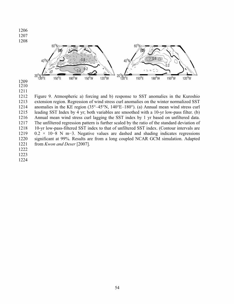
54

1206 1207 1208

1209 1210 1211 Figure 9. Atmospheric a) forcing and b) response to SST anomalies in the Kuroshio 1212 extension region. Regression of wind stress curl anomalies on the winter normalized SST 1213 anomalies in the KE region (35°–45°N, 140°E–180°). (a) Annual mean wind stress curl 1214 leading SST Index by 4 yr; both variables are smoothed with a 10-yr low-pass filter. (b) 1215 Annual mean wind stress curl lagging the SST index by 1 yr based on unfiltered data. 1216 The unfiltered regression pattern is further scaled by the ratio of the standard deviation of 1217 10-yr low-pass-filtered SST index to that of unfiltered SST index. (Contour intervals are 1218 0.2 × 10−8 N m−3. Negative values are dashed and shading indicates regressions 1219 significant at 99%. Results are from a long coupled NCAR GCM simulation. Adapted 1220 from Kwon and Deser [2007]. 1221 1222 1223

1224

55

1224 1225 1226

1227 1228 1229 Figure 10. Relationship between temperature anomalies in the Kuroshio Extension and 1230 Cchanges in the ocean gyres. Simultaneous regression of DJFM subsurface zonal current 1231 velocity along 150°E on the SST anomalies averaged over the KE region. Both variables 1232 have been low-pass filtered to retain periods longer than 10 yr. Contour interval is 0.2 cm 1233 s−1 °C−1, and the shading indicates regressions significant at 99%. Solid (dashed) contours 1234 denote eastward (westward) velocity. Thin contours with boxed labels indicate the 1235 climatological winter (DJFM) mean zonal velocity fields. Contour interval for the mean 1236 zonal velocity is 2 cm s-1 Results are from a long coupled NCAR GCM simulation [Kwon 1237 and Deser, 2007] 1238

1239

56

1239 1240 1241 Figure 11. The ENSO signal including the atmospheric bridge as indicated by the 1242 composite of 10 El Niño minus 10 La Niña events for SLP (contours, interval 0.5 mb) 1243 and SST (shading, interval 0.2 °C) during (a) DJF when ENSO peaks and (b) the 1244 previous JAS. The fields are obtained from NCEP atmospheric reanalysis [Kalnay et al., 1245 1996; Kistler et al., 2001]. 1246

1247

57

1247 1248 1249 1250

1251 1252 Figure 12. The Pacific Decadal Oscillation spatial and temporal structure: the leading 1253 pattern SST and SLP anomalies north of 20°N and normalized time series of monthly 1254 SST anomalies (PDO index, defined by Mantua et al. [2007]. Regressions of the PDO 1255 index on the (a) observed SST (ci 0.1 °C per 1σ PDO value) and (b) SLP (ci 0.25 mb per 1256 1σ PDO value). The SSTs were obtained from the HadSST data set [Rayner et al., 2006], 1257 for the period 1900-2004, and the SLP values from NCEP Reanalysis for the years 1948-1258 2007. (c) The monthly PDO index (gray shading) and 12-month running mean (black 1259 line) during 1900-2007, obtained from [http://jisao.washington.edu/pdo/PDO.latest]. 1260

1261

58

1261 1262

1263 1264 Figure 13. The SLP, flux and SST anomaly patterns associated with the Aleutian low 1265 during winter (DJF). (a) EOF 1 of SLP, regression values of the local (b) Qnet (contour 1266 interval 2.5 W m-2) and (c) SST (CI is 0.05 deg C) anomalies on SLP PC1, (d) EOF 1 of 1267 SST. All fields are obtained from a 50-year simulation of the GFDL AGCM coupled to 1268 an ocean MLM over the ice-free ocean. 1269

1270

59

1270

1271 1272 1273 Figure 14. Power spectrum of the observed PDO index. Dashed indicates the best fit 1274 based on a first-order autoregressive model, thin solid line shows the theoretical slope for 1275 intermediate frequency portion of the spectrum from a stochastic model. Adapted from 1276 Qiu et al. [2007]. 1277

1278

60

1278 1279 Figure 15. The 1977-1988 minus the 1970-1976 average SST during NDJFM from (a) 1280 observations and (b) an ensemble average of 16 model simulations (b). The observations 1281 and model integrations are described in Smith et al. [1996] and Alexander et al. [2002], 1282 respectively. The model consists of an AGCM coupled to an ocean mixed layer ocean 1283 model over the ice-free global oceans except in the central/eastern tropical Pacific (box) 1284 where observed SSTs are specified. Negative values are shaded and the CI is 0.2 °C. 1285

1286

61

1286 1287 Figure 16. The annual a) long-term mean and b) 1977-88 minus 1986-76 wind stress 1288 (vectors) and its curl (contours) from the NCEP reanalysis. The ci is 5×10−8 N m−3 in a) 1289 and 2×10−8 N m−3 in b) where the −1 × 10−8 N m−3 contour is also shown and values < 1290 −2 × 10−8 N m−3 are shaded. The annual c) long-term mean and d) 1977-88 minus 1986-1291 76 geostrophic transport streamfunction, given by the Sverdrup minus Ekman currents: 1292 the adjusted ocean circulation to wind curl forcing. The CI is 10 Sv in c) and 2 Sv in d), 1293 where values > 4 Sv are shaded. 1294

1295

62

1295

1296 1297 Figure 17. (a) The PDO time series and reconstruction (gray) based on contributions to 1298 the PDO from ENSO teleconnections (Niño-3.4*), stochastic fluctuations in the Aleutian 1299 low indicated by the North Pacific Index (NPI*), and the change in the ocean gyres given 1300 by the difference in the zonal average ocean pressure difference (PDEL, indicative of the 1301 slope of the thermocline and hence the strength/position of the ocean gyres) between 38° 1302 and 40°N in the KE region. The index for thermocline depth estimate from 35°-38°N in 1303 the KE region (P*AVG) does not explain a significant fraction of the SSTA variability of 1304 the PDO. Dotted vertical lines mark the winters of 1976/77 and 1998/99. (b) Power 1305 spectrum of the observed and reconstructed PDO, and contributions resulting from the 1306 NPI*, Niño34*, and P*DEL. Spectra have been smoothed by three successive applications 1307 of a five-point running mean. Note the dominance of the NPI* and ENSO* contributions 1308 to the PDO at internal annual time scales and the roughly equal contribution of the three 1309 factors at decadal time scales. From Schenider and Cornulle [2005]. 1310 1311 1312 1313

1314

63

1314

1315 1316 Figure 18. The spatial patterns for the three leading modes of Pacific SST variability 1317 during 1945–93 obtained from rotated principal component analysis: (a) ENSO, (b) 1318 Pacific Decadal Oscillation, and (c) North Pacific. Adapted from Barlow et al. [2001]. 1319