RESEARCH ARTICLE10.1002/2013JC009779

Forcing mechanisms of intraseasonal SST variability off centralPeru in 2000–2008Serena Illig1,2, Boris Dewitte1, Katerina Goubanova1, Gildas Cambon1, Julien Boucharel3,Florian Monetti2, Carlos Romero2, Sara Purca2, and Roberto Flores2

1Laboratoire d’Etudes en G�eophysique et Oc�eanographie Spatiale, CNRS/IRD/UPS/CNES, Toulouse, France, 2Instituto delMar del Peru, Callao, Peru, 3Department of Meteorology, University of Hawaii at Manoa, Honolulu, Hawaii, USA

Abstract The Sea Surface Temperature (SST) intraseasonal variability (40–90 days) along the coast ofPeru is commonly attributed to the efficient oceanic connection with the equatorial variability. Here weinvestigate the respective roles of local and remote equatorial forcing on the intraseasonal SST variabilityoff central Peru (8�S–16�S) during the 2000–2008 period, based on the experimentation with a regionalocean model. We conduct model experiments with different open lateral boundary conditions and/or sur-face atmospheric forcing (i.e., climatological or not). Despite evidence of clear propagations of coastaltrapped waves of equatorial origin and the comparable marked seasonal cycle in intraseasonal Kelvin waveactivity and coastal SST variability (i.e., peak in Austral summer), this remote equatorial forcing only accountsfor �20% of the intraseasonal SST regime, which instead is mainly forced by the local winds and heat fluxes.A heat budget analysis further reveals that during the Austral summer, despite the weak along-shoreupwelling (downwelling) favorable wind stress anomalies, significant cool (warm) SST anomalies along thecoast are to a large extent driven by Ekman-induced advection. This is shown to be due to the shallowmixed layer that increases the efficiency by which wind stress anomalies relates to SST through advection.Diabatic processes also contribute to the SST intraseasonal regime, which tends to shorten the lag betweenpeak SST and wind stress anomalies compared to what is predicted from an advective mixed-layer model.

1. Introduction

The west coast of South-America hosts a very productive oceanic ecosystem [Carr, 2002] that is primarilydue to the upwelling conditions that bring nutrient-enriched waters from the subthermocline to the surface,enabling an intense primary production. The upwelling conditions are driven by Ekman dynamics from theprevailing equatorward along-shore mean winds that generally occur in eastern boundary current systems[Bakun, 1990]. In the Humboldt system, along the coasts of Peru and Chile, the upwelling is highly variabledue to the influence of the large scale circulation of the Pacific Ocean. For instance, at interannual timescales, El Ni~no Southern Oscillation (ENSO) has been shown to influence the upwelling off Peru [Colas et al.,2008; Dewitte et al., 2012] and Chile [Pizarro et al., 2002; Vega et al., 2003] through oceanic teleconnections.ENSO atmospheric teleconnections have also been shown to drive anomalous upwelling conditions off Cen-tral Chile [Montecinos and Gomez, 2010; Goubanova et al., 2011; Rahn, 2012], whereas off Peru, they aremore ubiquitous [Goubanova et al., 2011]. Most studies on upwelling variability in the Humboldt systemand its connection with the equatorial variability have focused on the analysis of coastal sea level and cur-rent (cf. Pizarro et al. [2001, 2002], Ramos et al. [2006], Dewitte et al. [2008b], Vega et al. [2003], and Ramoset al. [2008] for the seasonal to interannual time scales and Brink [1982], Enfield [1987], Spillane et al. [1987],Shaffer et al. [1997], Clarke and Ahmed [1999], Hormazabal et al. [2002], Camayo and Campos [2006], and Bel-madani et al. [2012] for the intraseasonal time scales). Very few studies have investigated the variability ofthe Sea Surface Temperature (SST) although it is often used as a main indicator for upwelling variability[Demarcq and Faure, 2000] and for marine resource management.

Whereas during extreme El Ni~no events, coastal SST warms off Peru and Northern Chile due to the impactof the strong downwelling equatorial Kelvin wave [Dewitte et al., 2012], at intraseasonal time scales, theequatorial connection for SST is more ambiguous due in part to the weaker amplitude of the intraseasonalKelvin wave. The SST intraseasonal variability off Peru may be also forced by local winds that relates to alarge extent with the variability of the South Pacific Anticyclone [Dewitte et al., 2011]. This dual forcing is

Key Points:� Remote equatorial forcing accounts

for �20% of the intraseasonal SSTregime� The wind-SST relationship is

modulated seasonally by the meanstratification� Coastal SST variability results from

advection and mixing processes

Supporting Information:� Supporting text and figures

Correspondence to:Serena Illig,illig@legos.obs-mip.fr

Citation:Illig, S., B. Dewitte, K. Goubanova, G.Cambon, J. Boucharel, F. Monetti, C.Romero, S. Purca, and R. Flores (2014),Forcing mechanisms of intraseasonalSST variability off central Peru in 2000–2008, J. Geophys. Res. Oceans, 119,doi:10.1002/2013JC009779.

Received 31 DEC 2013

Accepted 1 MAY 2014

Accepted article online 10 MAY 2014

ILLIG ET AL. VC 2014. American Geophysical Union. All Rights Reserved. 1

Journal of Geophysical Research: Oceans

PUBLICATIONS

reflected in the spectrum of the SST along the coast. The Figure 1 shows the dominant pattern of variabilityof the subseasonal (namely �2–120 days) SST off central Peru during the 2000–2008 period. The dominantmode of SST subseasonal anomalies off central Peru (Figure 1a) consists in a meridionally extended narrowcoastal fringe of SST anomalies with amplitudes decreasing from the coast to the offshore ocean, with maxi-mum amplitudes of anomalies with absolute values larger than 0.4�C located at 11�S. This SST mode gov-erns the coastal SST variability along the coast of central Peru since the associated SST anomalies averagedwithin the 200 km coastal band between 16�S and 8�S explains �82% of the satellite coastal subseasonalvariability. The dominant time scales of variability of the time series associated with this mode (PC1-SSTA)can be separated into two regimes (Figure 1b), a high-frequency subseasonal regime that corresponds tothe 2–40 day21 frequency band (accounting for 50% of the total power of the PC1-SSTA spectrum) and alow-frequency subseasonal regime (hereafter referred to as intraseasonal regime) that corresponds to the40–90 day21 frequency band and that represents 40% of the total power of the PC1-SSTA spectrum.Whereas the high-frequency regime can be undoubtedly related to synoptically forced winds, particularlyactive in Austral winter, Dewitte et al. [2011] were not able to characterize the forcing mechanism of theintraseasonal regime, although noting a comparable marked seasonal dependence of the IntraseasonalEquatorial Kelvin Wave (IEKW) and the SST along the coast that peaks in Austral summer (from Decemberto May, see the climatological wavelet spectrum in Figure 1c). However, their analysis was limited by theobserved data sets at their disposal. In particular, due to the extended masking of the satellite data near thecoast, the identification of the signature of the Coastal Trapped Waves (CTW) on the SST remains difficult.Also, the scarcity of subsurface observations prevents the investigation of the thermocline variability thatshould reveal the equatorial connection more clearly [Brink, 1982]. Here we extend the study by Dewitteet al. [2011] based on satellite observations with the objective of (1) determining the processes associatedwith the SST variability along the coast of Peru within the intraseasonal regime (namely 40–90 days) and (2)resolving the issue of the forcing of this SST variability by the equatorial Kelvin wave. Besides the societalconcern in relation with marine resource management, the issue of the forcing of the SST variability at intra-seasonal time scales off Peru is also worth tackling in order to better understand the air-sea interactions inupwelling systems (e.g., VOCALS project [Mechoso et al., 2013]).

Our approach is based on the experimentation with a regional ocean model which allows overcoming thelimitations encountered by Dewitte et al. [2011] as well as providing a quantitative evaluation of the mixed-layer processes associated with the upwelling intraseasonal variability. The focus is on the 2000–2008period benefiting from the QuickSCAT winds that have been used previously for regional modeling studiesin this region [Penven et al., 2005; Montes et al., 2010]. Within this model setup, our results indicate that SST

Figure 1. Dominant mode of the Empirical Orthogonal Function (EOF) analysis of the observed satellite TMI-OI daily subseasonal SST anomalies (SSTA, cf. section 2 for data and filteringdescriptions) that captures 33% of the variance. (a) Spatial pattern (color, in �C). (b) Global Normalized Wavelet Power Spectrum (NWPS) of nondimensional PC1-SSTA (period is in days).Dashed line indicates the 95% confidence level and shading underlines significant global NWPS. (c) A 8 year climatology of the NWPS estimated over the period June 2000 to May 2008.White line shows the 95% confidence level.

Journal of Geophysical Research: Oceans 10.1002/2013JC009779

ILLIG ET AL. VC 2014. American Geophysical Union. All Rights Reserved. 2

variability at intraseasonal time scales off central Peru over this period is only marginally influenced by theequatorial Kelvin wave and results mostly from wind forcing despite its very weak variability. The paperthen documents the mixed-layer processes associated with this peculiar SST intraseasonal regime highlight-ing the contribution of mixing processes and its coupling with diabatic forcing.

The paper is structured as follows: section 2 details the observed data sets and the global reanalysis, as wellas the methodology used in this study. Section 3 introduces the regional oceanic model and its validationagainst in situ and satellite data and further describes the various numerical experiments carried out. Sec-tion 4 is devoted to the evaluation of the relative contribution of local wind and remote equatorial Kelvinwave to the intraseasonal SST variability off Peru. In section 5, a heat budget of the mixed-layer documentsthe processes by which local atmospheric forcing triggers intraseasonal SST variability. Finally, a discussionof the results followed by concluding remarks and perspectives to this work are given in section 6.

2. Data and Methods

We use satellite data, along with reanalysis outputs for the forcing of the model simulations. Other data setsare used for the validation, and those are presented in Appendix A.

2.1. Satellite Observations2.1.1. Wind StressThe near-surface atmospheric circulation over the ocean is described through daily zonal and meridionalwind stress components from the NASA satellite QuikSCAT. Homogeneous temporal series of daily meanwind stress fields, on global 0.5� 3 0.5� resolution grids, are generated from L2B product (distributed byJPL/PO.DAAC) by the French ERS Processing and Archiving Facility CERSAT (http://www.ifremer.fr/cersat/en/data/overview/gridded/mwfqscat.html). Note that in near-coastal region due to land contamination QuikS-CAT wind stress data are masked and are not available within 25 km off the coast.

2.1.2. SSTEstimates of SST were obtained from the Tropical Rainfall Measuring Mission (TRMM [Kummerow et al.,2000]) Microwave Imager (TMI) produced by Remote Sensing Systems (RSS, http://www.remss.com). RSSprovides daily 3 day-averaged gridded SST at a 1/4� resolution for latitudes lower than 38� (http://www.ssmi.com/sst/microwave_oi_sst_data_description.html). An important feature of the microwave retrievals isthat they are insensitive to atmospheric water vapor and thus can measure SST through clouds [Wentzet al., 2000]. This is a relevant issue over oceanic eastern boundary regions characterized by extended low-cloud coverage, such as the Humboldt upwelling system. We use the daily Optimally Interpolated (TMI-OI)SST product [Reynolds and Smith, 1994]. In this data set, the aliasing by the diurnal cycle due to the sun-asynchronous orbit of TRMM satellite is corrected by a simple empirical model of diurnal warming [Gente-mann, 2003] and an extensive land-mask is applied to remove land contamination [Gentemann et al., 2010].Although this limits the analysis of near-coastal regions, in particular those dominated by coastal upwellingdynamics, it has been shown that TMI-OI data allow identifying the signature of upwelling variability at sub-seasonal scale further offshore (cf. Goubanova et al. [2013] for the Central Benguela upwelling system).

2.2. Global Reanalysis2.2.1. Atmospheric ReanalysisThe outputs of the European Center for Medium Range Weather (ECMWF) ERA-Interim reanalysis [Uppalaet al., 2005] are used as surface heat and water forcings for our ocean simulations (see section 3.1). We useddaily averages of surface fields (specific humidity, 2 m air temperature, 10 m wind speed, shortwave, long-wave heat fluxes, and precipitations) at the model resolution, i.e., on a T255 horizontal resolution. ERA-Interim product improves upon the ERA-40 reanalysis used in Schweiger et al. [2008], offering enhancedresolution with 60 vertical levels, improved model physics, and radiative transfer model. The data set spans1979 to present (continuing in real time), however this study concentrates on the time period from January2000 to December 2008. This product is considered as our best option for forcing the regional model interms of heat fluxes since it shows improvements over the NCEP reanalysis [Bromwich et al., 2006].

2.2.2. Oceanic ReanalysisOutputs of the Simple Ocean Data Assimilation (SODA) model are used for determining the characteristicsof the long equatorial waves during the 2000–2008 period and are also prescribed as initial and lateral

Journal of Geophysical Research: Oceans 10.1002/2013JC009779

ILLIG ET AL. VC 2014. American Geophysical Union. All Rights Reserved. 3

boundary conditions for our regional model simulations. The SODA reanalysis project, which began in themid-1990s, is an ongoing effort to reconstruct historical ocean climate variability on space and time scalessimilar to those captured by the atmospheric reanalysis projects. SODA 2.1.6 uses a general circulationocean model based on the Parallel Ocean Program numerics [Smith et al., 1992], with an average horizontalresolution of 0.25� 3 0.4� and 40 vertical levels, which have 10 m vertical resolution near the surface.Assimilated data include temperature and salinity profiles from the World Ocean Atlas-01 (Mechanical Bath-ythermograph (MBT), Expendable Bathythermograph (XBT), Conductivity-Temperature-Depth (CTD), andstation data), as well as additional hydrography, SST, and altimeter sea level. The model was forced by dailysurface winds provided by the ECMWF Forecasts ERA40 reanalysis from January 1958 to December 2001and then by QuikSCAT wind stress data. The reader is invited to refer to Carton et al. [2000] and Carton andGiese [2008] for a detailed description of the SODA system.

2.3. Data FilteringData and model monthly climatologies are estimated over the 2000–2008 period. Afterward, they areextrapolated onto a daily time axis using cubic splines.

Subseasonal anomalies are the departure from the monthly mean data. A 1–2-1 filter is previously appliedto the monthly averaged data which are then extrapolated onto the original temporal resolution (daily orweekly) using cubic spline. In order to ensure that no seasonal cycle remains, the monthly seasonal cycleover the period 2000–2008 is also removed. The transfer function (estimated by computing subseasonalanomalies of a daily Gaussian white noise) characterized by its frequencies at 21/23/210 dB attenuation(i.e., 79/50/10% of the input power survives) is 117/168/416 day21.

In order to isolate the variability within the intraseasonal time scales, a band-pass 40–90 days Lanczos filter[Duchon, 1979] is applied to the subseasonal anomalies. The total filter length is 121 days.

2.4. EOF AnalysisIn order to extract the dominant mode of variability of the subseasonal variability along the Peruvian coasts,we apply a classical Empirical Orthogonal Function (EOF) decomposition [Toumazou and Cretaux, 2001] tothe data set over the 2000–2008 period in the central Peru region (17�S–7�S) within 5� wide band off thecoast. We choose to normalize the spatial patterns (hereafter referred to as EOFs) and the associated timeseries (namely, Principal Components or PCs) such as the standard deviation of the time series is equal toone.

2.5. Wavelet AnalysisWavelet analysis is used to detect time-frequency variations within time series data. A detailed descriptionof the wavelet analysis can be found in Torrence and Compo [1998]. In this study, in order to document thetime frequency characteristics of the subseasonal fluctuations, we use the Normalized Wavelet Power Spec-trum (NWPS) described in Goubanova et al. [2013], based on the Morlet function (x0 5 6). It allows for com-paring the magnitude of the wavelet spectrum at different frequencies. In particular, the time average ofNWPS (or Global NWPS) is composed of local variance contributions to the total energy of the time seriesand remains independent of the wavelet spectrum scale resolution. We will estimate global NWPS, i.e.,time-averaged NWPS, and also perform monthly climatology of NWPS.

Following Torrence and Compo [1998], significance levels are determined from v2 distribution (with a num-ber of degree of freedom m) using a background spectrum defined as a first-order autoregressive processhaving the same variance and autocorrelation at lag 21 as our data. For a time-averaged NWPS, m dependson the number of points to average (na) and can be estimated from Torrence and Compo [1998, equation(23)]. In the case of the global NWPS, na corresponds to the total number of days within the consideredperiod, whereas for the 8 year monthly climatological spectrum, we take na equal 240 (8 years 3 30 daysper month).

3. Regional Ocean Model Configuration

Our approach is based on the experimentation with a regional oceanic model of the Peru-Chile region, vali-dated from satellite and in situ observations. Overall, the model is skillful in simulating most aspects of themean state and variability, comparable to former studies using the same model but within different

Journal of Geophysical Research: Oceans 10.1002/2013JC009779

ILLIG ET AL. VC 2014. American Geophysical Union. All Rights Reserved. 4

configurations (domain, resolution, and boundary forcings). The reader is invited to refer to Appendix A forthe detail of the validation.

3.1. ROMS Ocean Model ConfigurationOceanic simulations were performed with the AGRIF version [Penven et al., 2006; Debreu et al., 2012] of theRegional Ocean Modeling System (ROMS [Shchepetkin and Mc Williams, 2005]) version 2.1. ROMS is a splitexplicit, free-surface, topography-following coordinate model that solves the primitive equations based onthe Boussinesq and hydrostatic approximations. Subgrid-scale vertical mixing is parameterized using a K-Profile Parameterization (KPP) boundary layer scheme [Large et al., 1994]. The topography is derived fromthe GEBCO_08 global elevation database at 30 arc-second spatial resolution (http://www.gebco.net).

The ROMS model is used here at an eddy-resolving resolution (1/6� at the equator) in the region extendingfrom 40�S to 15�N, and from the coast to 100�W with 32 sigma-coordinate vertical levels stretched withinthe surface layer. This configuration is the same than the one used in previous recent studies [Echevin et al.,2012; Belmadani et al., 2012; Cambon et al., 2013; Brochier et al., 2013]. The horizontal grid resolution of 1/6�

(�18 km) was selected here as a trade-off between the need to resolve coastal upwelling processes and thecomputational costs associated with the numerous sensitivity experiments. Although mesoscale eddies arewell resolved at 1/6� resolution, especially off Peru (since the wavelength associated with the first baroclinicRossby radius along the coast of the region of interest varies from �600 km near the equator to �200 kmat 35�S), at such resolution the frictional boundary layer along the slope is not. Marchesiello and Estrade[2010] showed in particular that for the Peru coast, the scale of the upwelling is only �5 km, which can onlybe resolved reasonably with a resolution of at least �2 km. Here, like in most of the regional modeling stud-ies of this region that use a lower resolution [Penven et al., 2005; Montes et al., 2010], we will assume thatupwelling dynamics is still well accounted for by our model setup.

At the three lateral open boundaries, mixed active-passive conditions are used [Marchesiello et al., 2001]with forcing data from the SODA reanalysis 2.1.6. For momentum and tracers, a third-order upstream biasedadvection scheme is used [Shchepetkin and McWilliams, 1998]. Explicit lateral viscosity is null everywhere inthe model, except in sponge layers near the open boundaries where it increases smoothly on several grid.Note also that, at lateral open boundaries, a linear adjustment of the model bathymetry to the SODAbathymetry is made within a 2� band. A bulk formulation [Kondo, 1975] is used to compute surface turbu-lent heat, based on ERA-Interim Reanalysis daily mean atmospheric fields (2 m air temperature, relativehumidity, surface wind speed, net shortwave and downwelling longwave fluxes, and precipitations), whilethe wind stress forcing comes from the daily QuikSCAT data. Note that, in order to fill in the QuikSCAT blindzone, an extrapolation of the QuikSCAT momentum fluxes was performed using a simple near-neighborprocedure. For the initialization, SODA potential temperature, salinity, and horizontal current fields wereused.

To diagnose the processes responsible for the surface temperature variability associated with the intrasea-sonal regime, the heat budget within the time varying mixed layer is computed online. The mixed-layerdepth (h) is determined by the KPP vertical mixing scheme. The reader is invited to refer to Menkes et al.[2006] for more details on such heat budget computations.

Hence, the rate of change of the mixed-layer temperature is driven by the advection terms (X-ADV, Y-ADV,Z-ADV), the mixing terms (vertical diffusivity at the mixed-layer base (DIFF) and entrainment/detrainmentterm (ENTR)) and the heat flux term (FORC), such as:

@thTi5 2hu@x Ti|fflfflfflfflffl{zfflfflfflfflffl}X2ADV

2hv@y Ti|fflfflfflfflffl{zfflfflfflfflffl}Y2ADV

2hw@z Ti|fflfflfflfflffl{zfflfflfflfflffl}Z2ADV

21h

kz@z Tð Þz52h|fflfflfflfflfflfflfflfflfflfflfflffl{zfflfflfflfflfflfflfflfflfflfflfflffl}

DIFF

21h@t h3 hTi2Tz52hð Þ

|fflfflfflfflfflfflfflfflfflfflfflfflfflfflfflfflfflffl{zfflfflfflfflfflfflfflfflfflfflfflfflfflfflfflfflfflffl}ENTR

1Q �1Qs2QP

qCPh|fflfflfflfflfflfflfflfflffl{zfflfflfflfflfflfflfflfflffl}FORC

where T is the model potential temperature; (u, v, w) are the components of ocean currents; kz is the verticaldiffusion coefficient; QS the net surface solar heat flux, and QP is the fraction of solar radiation that pene-trate below the base of the mixed-layer depth (h). Q* contains the sum of the other surface heat flux terms,

Journal of Geophysical Research: Oceans 10.1002/2013JC009779

ILLIG ET AL. VC 2014. American Geophysical Union. All Rights Reserved. 5

i.e., longwave radiations, latent and sensible heat fluxes. Brackets denote the vertical average over themixed-layer depth: hTi5 1

h

Ð 02h Tdz.

The simulations were performed over the 2000–2008 period, during which daily averages of all tendencyterms, as well as model state variables (temperature, currents, and sea surface height) were stored. Themodel solution reached a statistical equilibrium (in terms of upper ocean stratification and eddy kineticenergy levels) after 3 year of spin-up performed by repeating the year 2000.

Our confidence in the model configuration results in its realism as evidenced by the detailed validation ofthe model control run experiment (hereafter referred to as ROMSCR) which indicates that it is skillful in simu-lating most aspects of the mean state and variability (see Appendix A). This model configuration provides abenchmark for evaluating sensitivity experiments to surface forcing and open boundary conditions.

3.2. Experiments DescriptionsWe carried out a set of five experiments in order to assess the oceanic response to wind stress, heat fluxesand long equatorial waves at subseasonal time scales in the coastal central region of Peru and thereby inter-pret the observations. All the experiments only differ by their boundary conditions (either climatological or‘‘real time’’). Their setups are summarized in Table 1.

First, the control run experiment (ROMSCR) is performed using the 5 day-mean SODA Ocean Boundary Con-ditions (OBC), the daily QuikSCAT wind stress forcing and with daily bulk formulation input fields for heatfluxes estimations, as described in subsection 3.1. Then, in order to isolate the impact of the distant longequatorial wave signal transmitted as coastal trapped waves along the coast of South-America from thelocal subseasonal atmospheric forcings, the simulation ROMSE uses the 5 day-mean SODA OBC along withprescribed climatologic atmospheric conditions (wind stress and inputs for bulk formulae). The experimentthat has no remote subseasonal equatorial forcing (climatological OBC), while subseasonal local atmos-pheric forcing is included in the surface boundary conditions is called ROMSWQ. Under the hypothesis of lin-earity, these model experiments can be used to infer the respective role of the IEKW and local forcing onthe SST variability along the coast of central Peru.

A complementary experiment was carried out in which the model is forced by prescribed climatologicalOBC and surface heat flux (for bulk formulae), while real-time QuikSCAT wind stress forcing is used. Thisexperiment, ROMSW, when compared to ROMSWQ simulation will allow quantifying the respective role ofthe subseasonal surface heat flux forcing versus the mechanical role of the winds, mixing the surface layerand changing the mixed-layer depth at subseasonal time scale.

At last, in order to quantify the model variability resulting from purely internal dynamics (i.e., nonlinearities),a climatological simulation is performed that used climatologies at boundary conditions (both ocean andatmosphere). This experiment will be referred to as ROMSCLIM.

4. Role of the Remote Equatorial Forcing

In this section, as a first step, we document the time frequency characteristics of the IEKW forcing and itsseasonal modulation. Then, based on the regional oceanic model experiments, we quantify the forcingmechanisms of the intraseasonal SST along the coast of central Peru.

4.1. Spatiotemporal CharacteristicsIn order to derive the IEKW amplitude for the most energetic baroclinic modes, we use a methodology simi-lar to the one described in Dewitte et al. [2003]. It consists in a modal (both vertical and horizontal)

Table 1. Description of ROMS Experiments: Name, Open lateral Boundary Conditions (OBC), QuikSCAT Wind Stress Specifications, andPrescribed Fields for Heat/Water Flux Bulk Formulation

EXP-Name SODA OBC (E) QS Wind Stress (W) HF Bulk Fields (Q)

ROMSCR Total Total TotalROMSE Total Climatology ClimatologyROMSWQ Climatology Total TotalROMSW Climatology Total ClimatologyROMSCLIM Climatology Climatology Climatology

Journal of Geophysical Research: Oceans 10.1002/2013JC009779

ILLIG ET AL. VC 2014. American Geophysical Union. All Rights Reserved. 6

decomposition of the zonal current and pressure variability. This provides estimates of the Kelvin andRossby waves contribution to sea level anomalies according to the most energetic baroclinic modes.Applied to the SODA data over the 2000–2008 period, we find, consistently with the results of Dewitte et al.[2008a], that the first three baroclinic modes are the most energetic, explaining up to 60% of the total SLAintraseasonal variability (correlation with the total SLA> 0.75). A space-time spectral analysis of the IEKW forthe first two baroclinic modes (Figures 2a and 2b) highlights the rich spectrum of energy of long-wavelength (k� 2) intraseasonal Kelvin wave contributions for the gravest baroclinic mode. This analysisshows the propagation of long-wavelength Kelvin wave since the dominant density peaks fits the theoreti-cal dispersion curve (white dashed lines). The latter is derived from the vertical mode decomposition basedon the zonally averaged phase velocity (140�E–80�W). IEKW energy is found between 40260 days and at

Figure 2. Intraseasonal Equatorial Kelvin Wave (IEKW) Sea Level contribution: (top) Space-time power spectral density [see Hayashi, 1982]in the equatorial Pacific for the (a) first and (b) the second baroclinic mode as function of basin split (left scale) and period in days (bottomscale). Units are cm2. White dashed lines indicate theoretical dispersion curves. White plain lines show theoretical critical latitudes curves(right scale). (bottom) Climatology of the NWPS estimated over the period June 2000 to May 2008 for (c) the first and (d) the second baro-clinic modes at 100�W. White line shows the 95% confidence level. For each baroclinic modes, IEKW amplitudes are first normalized bytheir standard deviation averaged along the equator (140�E–80�W), r (indicated in the lower right corner).

Journal of Geophysical Research: Oceans 10.1002/2013JC009779

ILLIG ET AL. VC 2014. American Geophysical Union. All Rights Reserved. 7

�75 days for the first baroclinicmode and between 50–60 daysand at �80 and �100 days for thesecond one. At these frequencies,these waves are trapped along thecoast from 5�S as revealed by thevalues of the theoretical critical lati-tudes [Clarke and Shi, 1991] esti-mated from the model topographyand mean stratification (see plainwhite line, right scale).

Considering the marked seasonaldependence of the intraseasonalSST variance (Figure 1c), it is inter-esting to investigate whether theIEKW activity exhibits comparablecharacteristic. The Figure 2 (bottom)displays the climatology of the Nor-malized Wavelet Power Spectra(NWPS) of the IEKW at the westernboundary of our model configura-tion (100�W). This analysis revealsthat, for the 2000–2008 period, thegravest baroclinic modes experi-ence larger variability during theextended Austral summer season

than during the extended Austral winter, which is comparable to the SSTA spectrum. This suggests a priori alikely influence of the IEKW on SST off central Peru.

The following section is devoted to the analysis of the model simulations, which serves as material for theinterpretation of the above observations.

4.2. Model ResultsIn this section, we analyze the outputs of ROMSE experiment (see Table 1), in which the model is forced by cli-matological surface forcings, and SODA 5 day-mean outputs are prescribed at the three open lateral bounda-ries. In this configuration, the coastal SST variability off Peru and Chile is predominantly under the influence ofthe equatorial variability, but it is also driven by the internal model variability (mesoscale activity). Coastal-Trapped Wave (CTW) propagations are expected in the intraseasonal frequency band [Brink, 1982; Belmadaniet al., 2012], which we observe in ROMSE, based on the analysis of SLA averaged within a 0.5� coastal fringe.The values of the mean phase speed associated to the SLA propagation are estimated based on the linear fitof the scattered plot providing the lag that maximizes the lagged correlation between the SLA at a given lati-tude and the SLA within a centered 7� latitudinal window, as function of the distance (Figure 3a). It indicatesthat the phase speed ranges from 1.7 to 3 m s21 between 5�S and 25�S, which is consistent with observations[Spillane et al., 1987]. Since coastal SLA is the superposition of the contributions of the various baroclinicmodes along the coast, the latitudinal variation in mean phase speed can be interpreted as resulting from thedifferent dissipation rates of the gravest baroclinic modes. In particular, the second baroclinic mode is mostlyinfluential in the northern part but dissipates faster southward than the first mode which thereby dominatesthe SLA variability. This is illustrated by the lagged-correlation analysis between ROMSE coastal SLA and theIEKW at the western boundary of our model domain (100�W) for the first two baroclinic modes (Figure 3b). Itshows that the correlation for the first mode becomes only significant at �7�S and reaches 0.5 only at �12�S,whereas for the second mode, it gradually decreases to become not significant at 13�S. Note that similarresults were obtained when analyzing ROMSCR outputs but with lower correlation values.

The comparison of the model experiments further reveals that the SLA variability within the intraseasonalregimes (40–90 days) can in fact be accounted for by almost the sole equatorial forcing (Figure 4). Forinstance, the ratio of variance between ROMSE (ROMSWQ) and ROMSCR estimated for the 40–90 day21

Figure 3. (top) Propagation velocity of the 0.5� coastal band averaged Sea Level intra-seasonal Anomalies (SLA). At each latitude, the maximum lagged correlation betweenthe coastal SLA at that latitude and the coastal SLA within a centered 7� latitudinalwindow is computed. For each 7�-window, the linear regression coefficient that bestfit the lag estimation is calculated. Shading indicated error in the linear regressioncoefficient estimation. Unit is m s21. (bottom) Maximum lagged correlation betweencoastal (0.5� coastal band averaged) SLA with the first (second) Intraseasonal Equato-rial Kelvin Wave (IEKW) mode at 100�W as a function of latitude in plain (dashed) line.Lag (in days) is specified with color shading. Positive value indicates that equatorialvariability leads.

Journal of Geophysical Research: Oceans 10.1002/2013JC009779

ILLIG ET AL. VC 2014. American Geophysical Union. All Rights Reserved. 8

frequency band for Central Peru Coastal SLA averaged between 16�S and 8�S within the 0.5� width coastalfringe (denoted hereafter as CPC time series) is 95% (24%). Note that the internal model variability asinferred from the analysis of the outputs of ROMSCLIM has a weak signature on the CPC-SLA variability(ratio 5 7%). These results are not surprising and just validate our modeling framework that is able to simu-late the IEKW connection along the coast expected from linear theory.

More interestingly, it is now worth examining how the equatorial variability impacts the intraseasonal SSTvariability along the coast of central Peru. Figure 5 (top) displays the global NWPS of the SST intraseasonalanomalies averaged in the 0.5� coastal band between 16�S and 8�S (CPC-SSTA) for the same three experi-ments (ROMSCR, ROMSE, and ROMSWQ). The results indicate that the IEKW is in fact only marginally influen-tial on the SSTA variability along the coast, since within the intraseasonal frequency band 40–90 day21, only23% of the energy of the SST variability originates from the connection with the equatorial variability. Theclimatological NWPS of the CPC-SSTA (not shown) highlights that the peak season of SST variability inROMSE is in Austral summer, in agreement with ROMSCR and with the IEKW activity. It is worth noting thatROMSCLIM experiment shows that the internal model variability represents 11% of ROMSCR CPC-SSTA vari-ability in the intraseasonal frequency band. In addition, we find that there is little coherency betweenROMSE and ROMSCR off central Peru (Figure 5d). For instance, the maximum lag correlation between theROMSE and ROMSCR CPC-SSTA does not exceed 0.1 over the whole record. Still there are periods when thetime series covary, like in February-March 2002 and April-June 2006, indicating that the IEKW can be influen-tial on SSTA episodically along the coast. The spectrum for the simulation using climatological conditionsfor the open ocean lateral boundaries and daily real-time atmospheric forcing (ROMSWQ) confirms that thelocal atmospheric fluxes are the dominant forcing to explain the SSTA peak in the frequency band 40–90day21 since the spectrum for ROMSCR and ROMSWQ are comparable (ratio 5 93%).

Considering the comparable seasonal variability of the IEKW activity and SST (cf. Figures 2c, 2d and Figure1c), the model results are counterintuitive and calls for investigating the mixed-layer processes associatedwith the local atmospheric forcing.

5. Role of the Local Atmospheric Forcing

Dewitte et al. [2011] showed that the wind stress intraseasonal anomalies along the coast of Peru are charac-terized by a peak variance in Austral winter; especially within the frequency range 2–40 day21. This is illus-trated in Figure 6 that presents the dominant EOF mode of QuikSCAT surface meridional and zonal WindStress Anomalies (WSA) that captures 76% of the total variance of subseasonal anomalies. The spatial pat-tern portrays WSA of the same sign over the entire region with upwelling-favorable south-east (upwellingunfavorable north-west) direction for positive (negative) WSA anomalies (Figure 6a). The maximum

Figure 4. Coastal (0.5� coastal band averaged) SSH averaged between 16�S and 8�S: (top) Global NWPS of subseasonal SSH for (a) ROMSCR

simulation, (b) ROMSE simulation, and (c) ROMSWQ simulation. Unit is cm2. (bottom) Dashed lines indicate the 95% confidence level.

Journal of Geophysical Research: Oceans 10.1002/2013JC009779

ILLIG ET AL. VC 2014. American Geophysical Union. All Rights Reserved. 9

amplitude of anomalies is found 200 km offshore Pisco. The climatological normalized wavelet power spec-trum of the associated time series (Figure 6b) indicates that the largest amount of the wind stress energy isconfined in the 2–40 day21 frequency band, during the Austral winter, from June to September. In contrast,the intraseasonal oscillations (40–90 days) represent only 8.7% of the total variance of the PC1 time series,and are hardly significant in July and August, and not significant in Austral summer. These observationsquestion to which extent, such wind forcing can explain the SST peak variance in Austral summer. Further,which mixed-layer processes are associated with such a weak wind?

5.1. Composite Evolution of an Intraseasonal EventAs a first step, we analyze the evolution of a composite intraseasonal event as simulated by the ROMSWQ

configuration, for which only the surface forcing undergoes subseasonal variations, while oceanic lateralboundary conditions are prescribed using climatologic conditions (see Table 1). The compositing procedureis based on a previous EOF analysis of the SSTA that is used to trace major intraseasonal events along thedominant mode principal component (time series; Figure 7a). The dominant EOF mode of SSTA in ROMSWQ

explains 18% of the subseasonal variability and has a spatial pattern that closely resembles the one of Fig-ure A6a (not shown). The associated time series (PC1-SSTA) has been filtered in order to retain only theintraseasonal time scales using a 40–90 days Lanczos filter. As the local surface forcing is dominant toexplain the coastal intraseasonal SST variability off central Peru, this time series compares very well with theone shown in Figure A6d, with a correlation (RMS differences) larger (smaller) than 0.95 (0.16�C). The com-positing procedure requires the selection of the strongest intraseasonal events (cold and warm), i.e., thathave a local maximum amplitude (in terms of absolute value) larger than 1.25 times the standard deviation.Here it is important to keep in mind that the sign of the PC1-SSTA is defined with respect to the 1st EOF pat-tern which portrays negative anomalies. This implies that positive (negative) values of the time series areassociated with cold (warm) SST events. In this way, we identified 34 events (17 cold events and 17 warmevents, cf. blue and red stars in Figure 7a). Note that most of the peaks occur during the extended Austral

Figure 5. Top plots are the same as Figure 4 but for central Peru coastal SST analysis. Unit is �C2. (bottom) Time series of intraseasonal SST(SSTA, 40–90 days) from ROMSCR (black), ROMSE (red), and ROMSWQ (blue) simulations. Gray vertical bands show the July to October sea-son. Unit is �C.

Journal of Geophysical Research: Oceans 10.1002/2013JC009779

ILLIG ET AL. VC 2014. American Geophysical Union. All Rights Reserved. 10

summer season, consistent with the periods of highest SST variability for the intraseasonal regime as identi-fied from the wavelet analysis (Figures 1c and A6c). As the PC1-SSTA time series is not skewed, the compos-ite represents here the average of any variable for all 34 dates identified (i.e., using both cold and warmevents). Note that we chose to map the negative phase of the variability, i.e., the processes associated withintraseasonal upwelling events. Therefore, the composite corresponds to the mean of the negative eventsfrom which we subtract the mean of the positive ones. The time for this event is denoted as ‘‘day 0.’’ Confi-dence levels are estimated based on a bootstrap method using 10,000 samples and only significant anoma-lies at the 90% level are displayed on Figures 7 and 8.

The results of the composite analysis of the ROMSWQ outputs are presented in Figure 7 for the mixed-layertemperature (TMLD) and the surface wind stress, and temperature and current anomalies along sections per-pendicular to the coast at 11�S at lags 214 days, 27 days, 0 day, and 17 days. This allows us to describe thespatial and temporal evolutions of oceanic conditions and surface wind stress associated with the intraseaso-nal regime. At a lag of 220 days (not shown), upwelling favorable winds start to blow and positive verticalcurrent anomalies can be detected along the shelf. At a lag of 214 days, winds intensify and weak negativeTMLD anomalies (�0.1�C) can be observed in a narrow coastal fringe. They are associated with a shallowercoastal thermocline and a deeper mixed layer (reflecting a change in the vertical stratification). The core ofmaximum upwelling favorable winds undergoes a southward propagation, with the largest amplitudeobserved at 16�S for a lag of 27 days. However, at this date, coastal vertical currents have drastically weak-ened. At this date, the TMLD anomalies have grown and they start to expand offshore, as zonal current anoma-lies within the mixed layer drive them offshore due to the Ekman divergence. Indeed, TMLD anomalies largerthan 0.25�C now occupy a 100 km wide coastal band. In the subsurface, the temperature anomalies can bedetected as deep as 250 m, and the coastal thermocline further rises. Note that a second local significant tem-perature anomaly can be detected �350 km off shore, with amplitudes larger than 0.15�C at the surface. Themature phase of the event (lag 0) corresponds to cold temperature anomalies being well developed over thewhole region, with maximum amplitude along the coast. They continue their offshore propagation as theyare driven offshore by intense zonal current anomalies within the 30 first meters. At this moment, the upwell-ing favorable winds have drastically weakened, and the anomalous coastal vertical currents turn negative.The following week, the wind anomalies change direction and intensify. This leads to downwelling verticalcurrent anomalies along the shelf and shoreward surface zonal current anomalies within the surface mixedlayer. Cold temperature anomalies are still strong but they have weakened at the coast and deepened withinthe mixed layer. At a lag of 114 days, the temperature returns to near normal conditions (not shown).

Figure 7 thus provides a 3-D description of the evolution of a composite intraseasonal event forced by thewinds, which reveals a rather consistent picture with what is expected from Ekman dynamics, although the

Figure 6. First mode of the bivariate EOF analysis of the subseasonal anomalies of the surface wind stress from QuikSCAT data: (a) Spatialpattern (dyn/cm2) showing wind stress vectors (arrows) and wind stress magnitude (color shading). (b) A 8 year climatology of the NWPSfor the wind stress PC1 (PC1-WSA) estimated over the period June 2000 to May 2008. White line shows the 95% confidence level.

Journal of Geophysical Research: Oceans 10.1002/2013JC009779

ILLIG ET AL. VC 2014. American Geophysical Union. All Rights Reserved. 11

phase-lag between peak SST and wind stress anomalies is smaller (�8 days) than a quarter of a period of acycle, suggestive of the contribution of other processes than just Ekman-induced advection to the rate ofSST changes. The latter is devoted to a comprehensive analysis of the processes associated with the SSTfluctuations during the composite event of Figure 7.

5.2. Composite Heat-BudgetThe contributions of the different processes to the rate of change of the mixed-layer temperature (seedetails in section 3.1) were computed online to ensure a perfect closure of the budget. In order to smooththe internal model variability and provide an overview of the time sequence of the main processes at work,we derive intraseasonal anomalies from latitudinal averages (16�S–8�S) as a function of the distance fromthe coast. Figure 8 displays the evolution of the various terms of the heat budget for the intraseasonalregime (bottom, Figures 8f–8l), along with the intraseasonal anomalies of the TMLD (Figure 8a), the mixed-layer depth (Figure 8b), the along-shore wind stress amplitude (Figure 8c), the Ekman pumping velocity(Figure 8d), and the net surface heat fluxes (Figure 8e). In order to ease the interpretation of the time

Figure 7. (top) Intraseasonal band-pass filtered PC1-SSTA (40–90 days) for ROMSWQ. Gray vertical bands show the July to October season. (middle and bottom) Time-lagged compositesof the intraseasonal anomalies of ROMSWQ outputs for the intraseasonal events identified (see text details). (middle) TMLD (color shading, in �C), wind stress vector (arrows, in dyn/cm2),and wind stress amplitude (contour, in 10xdyn/cm2). (bottom) Vertical sections perpendicular to the coast at 11�S in function of depth and distance from the coast (km) of temperature(shading, in �C), cross-shore and vertical currents (arrows, in cm/s). For visualization purposes, mean vertical current amplitude is multiplied by 2000. The plain red (green) line indicatesthe position of the thermocline for the cold-event composite (mixed-layer depth). The dashed red (green) line indicates the mean position of the thermocline as the average betweenwarm-event and cold-event composite (mixed-layer depth). Fields are represented only when significant at 90% confidence level. The time lags are shown at 214, 27, 0, 17 days.

Journal of Geophysical Research: Oceans 10.1002/2013JC009779

ILLIG ET AL. VC 2014. American Geophysical Union. All Rights Reserved. 12

sequence, visual marks as horizontal lines have been drawn as a guide: Black horizontal lines indicate themature phase of the event at a lag of 0 day, i.e., when the rate of change of TMLD is zero. The maximum ofthe upwelling favorable winds are observed 8 days before with values larger than 0.8 dyn cm22 and is high-lighted using green dashed horizontal lines. Green dashed lines indicate the minimum in alongshore windstress at a lag of 222 days and the maximum of the downwelling favorable wind stress 33 days before themature phase of the event.

Figure 8f shows that the region of maximum cooling rate is located near shore 16 days before the maturephase of the event with a heat loss larger than 4.1022 �C � day21. A secondary maximum in the cooling rate isdetected 350 km offshore at a lag of 211 days with absolute values larger than 2.1022 �C �day21. Similar pat-terns are observed for the warming phase between a lag of 0 and a lag of 115 days. The TMLD tendency(RATE, Figure 8f) near the coasts portrays an offshore propagating pattern with velocities estimated at�0.25 m s21.

As a first step, we concentrate on the advection terms that result in a straightforward manner from Ekmandynamics (Figures 8g–8i). During the cooling phase (between a lag of 220 days and a lag of 0 day), bothvertical (Z-ADV, Figure 8i) and zonal advection (X-ADV, Figure 8g) are in phase with the RATE of change ofTMLD, explaining a large amount of its variability. Indeed, the variance explained by the summed-up contri-bution of Z-ADV and X-ADV is 63% of the TMLD tendency over a whole cycle for the average within the first100 km off the coast. Meridional advection (Y-ADV, Figure 8h) opposes vertical advection (i.e., a warmingtendency) near the coast due to the divergent flow at the surface associated with the upwelling, but thiseffect remains rather weak. Zonal advection is partly responsible for the offshore propagation of TMLD

anomalies. Vertical advection presents two local maxima, one located at the coast which corresponds to thecoastal upwelling associated with increased equatorward wind stress, and a secondary maximum located�60 km offshore induced by the rather broad pattern of Ekman pumping (Figure 8d). As mentioned earlier,it is interesting to note the 8 day lag between vertical advection and wind stress anomalies that is largerthan what is expected from Ekman dynamics.

We can interpret the deviation from Ekman theory in the light of the heat budget that provides estimatesof mixing processes. During the developing phase of the event (between a lag of 240 and 215 days)near the coast, the vertical diffusivity at the base of the mixed layer (DIFF, Figure 8j) is a cooling term thatcan be interpreted as resulting from restratification processes [Fox-Kemper and Ferrari, 2008] associatedwith the anomalous conditions of the previous phase. Indeed, the vertical diffusivity term is in quadraturewith the rate of change of TMLD, with a coastal cooling rate larger than 4.5 1022 �C � day21 at a lag of 225days. The entrainment term (ENTR, Figure 8k) contributes only slightly to the cooling near the coast butbecomes one of the main contributors to the cooling tendency in the off-shore region relative to theother terms. ENTR is however smaller than the heat-flux forcing term (FORC, Figure 8l) that has a signifi-cant contribution to RATE. The surface heat-flux forcing can be interpreted as follows (see Figure S1, inSupporting Information): the wind intensification during the developing phase of the event leads to a sig-nificant increase of heat loss through surface latent heat fluxes (>8 W m22). In the first 50 km, small posi-tive anomalies of latent heat fluxes have to be attributed to the colder than normal SST and the weakermean winds. Here the shortwave heat fluxes are enhanced (�11.5 W m22), while 200 km offshore, thedownward longwave heat fluxes are reduced (�21 W/m22). In conclusion, the net surface heat flux is inphase with the wind forcing components and results in an offshore heat loss attributed to evaporationand a small heat gain at the coast. Nevertheless, the heat flux forcing term (FORC, Figure 8l) is not directlycomparable to the surface net heat flux anomaly because the latter is distributed within the mixed layerthat varies during the evolution of an event. To a lesser extent, FORC also integrates the residual of thesolar flux penetration into the mixed layer, which specifically depends on the mixed-layer depth anoma-lies. In particular, the wind intensification tends to deepen the mixed layer through vertical mixing.Indeed, 2 days after the maximum wind intensification (reduction), the MLD is 2 m deeper (shallower)than normal over the whole longitudinal extension (Figure 8b). These variations are negligible offshorewhere the MLD remains relatively deep (MLD >30 m, see Figure 7), but are crucial at the coast, where theMLD rises to a depth of 10 m in Austral summer (see Figures A1c and A3c in Appendix A). Consequently,the surface forcing term, FORC, is in phase with the temporal evolution of the MLD (2 days after the windvariability) and exhibits a variability that is more important at the coast, with absolute values larger than5.1022 �C � day21.

Journal of Geophysical Research: Oceans 10.1002/2013JC009779

ILLIG ET AL. VC 2014. American Geophysical Union. All Rights Reserved. 13

Thus, during the developing phase of the event, mixing and surface forcing are dominant processes, butthey tend to compensate each other near the coast. The summed-up contribution of the mixing terms(DIFF 1 ENTR, warming) and the surface forcing term (FORC, cooling) results in a overall cooling trend inphase with the TMLD tendency with values peaking at 2.21022 �C � day21 at a lag of 216 days at the coast(not shown). The variance explained by DIFF 1 ENTR 1 FORC is 33% of the TMLD tendency over a wholecycle for the average within the first 100 km off the coast, the remaining variance being explained by theadvection terms. This compensation effect is allowed by the shallow mixed layer in Austral summer thattherefore experiences large variations relative to its mean depth and at the same time favors diabatic cool-ing that opposes to the enhanced mixing. The shallow mixed layer is also favorable to the enhancement ofthe influence of Ekman dynamics on SST through anomalous vertical advection of mean vertical tempera-ture [Goubanova et al., 2013].

In order to evaluate the respective role of the surface heat flux forcing versus the mechanical role of thewind, the heat budget was estimated from the ROMSW experiment which considers climatological heat fluxforcing. The results (cf. Figure S2 in Supporting Information) show that the off-shore variability (between300 and 400 km offshore) is drastically reduced in ROMSWQ compared to ROMSW. Indeed, the ratio of varian-ces of the rate of SST change between ROMSW and ROMSWQ for the composite intraseasonal anomalies islower than 30%, revealing that heat flux term is the dominant forcing that triggers offshore SST anomalies.Near the coast, the balance between the tendency terms of ROMSW is qualitatively comparable to ROMSWQ

(cf. Figure 8) although with a weaker amplitude due to smaller variations in the MLD. Indeed, the ratio ofvariances of the TMLD tendency between ROMSW and ROMSWQ and within the first 100 km coastal fringe islarger than 83%. The results of ROMSW thus confirm that the net-heat flux forcing is important in reinforcingSST anomalies through its coupling with vertical mixing variability.

In order to contrast the above results with what happens during the Austral winter when the mixed-layerdepth is deeper (see Figure A3c), the similar composite analysis of the tendency terms is performed, but

Figure 8. Time-lagged composites of the intraseasonal anomalies of ROMSWQ simulation averaged between 16�S and 8�S as a function of the distance from the coast (in 102 km) for theintraseasonal cold events identified based on the 40–90 days band-pass filtered PC1-SSTA from ROMSWQ simulation. (top) The temperature within the mixed layer ((a) TMLD, in �C), themixed-layer depth ((b) h, in m), the along-shore wind stress ((c) 100xdyn/cm2), the Ekman pumping velocity ((d) positive upward, unit is 1027 m s21), and the surface net-heat fluxes ((e)Qnet, W/m2). (bottom) Heat budget results: (f) rate of change, (g) zonal advection, (h) meridional advection, (i) vertical advection, (j) diffusivity at the base of the mixed layer, (k) entrain-ment, and (l) forcing contribution. Unit is 100x �C �day21. Color shading indicates significant composites (90% confidence level).

Journal of Geophysical Research: Oceans 10.1002/2013JC009779

ILLIG ET AL. VC 2014. American Geophysical Union. All Rights Reserved. 14

using the time series associated with the dominant EOF of zonal and meridional wind stress anomalies. The28 events can be selected that mostly take place during the extended winter season, consistently with theperiods of highest WSA variability within the intraseasonal regime (Figure 6b). The heat budget compositereveals that surface heat flux anomalies have a similar amplitude to Austral summer events (cf. Figure S3, inSupporting Information) despite the WSA amplitude being twice as large (cf. Figure 8c). However, the result-ing heat flux forcing term is much weaker due to the relative deep mixed layer in Austral winter (Figure A3cfrom Appendix A). Mixing has also almost no contribution to the rate of SST change. SST intraseasonal vari-ability in Austral winter thus results from Ekman dynamics where zonal and vertical advection terms are themain contributors to the SST changes. These terms remain weak however relative to the intensity of thealong-shore wind stress anomalies because of the significantly reduced surface stratification in Austral win-ter compared to the Austral summer (cf. Figure A3c). In particular, vertical advection is reduced due to thediminished Surface Vertical Temperature Gradient (SVTG) that acts as an efficiency coefficient of the impactof Ekman-driven vertical currents on SST through vertical advection [see Goubanova et al., 2013].

6. Discussion and Conclusions

In this paper, we have investigated the forcing mechanisms of the Sea Surface Temperature variability alongthe coast of Peru based on the experimentation with a regional ocean model that has been previously thor-oughly validated with in situ and satellite observations. Our main focus was on the intraseasonal SST regime(40–90 days) described in Dewitte et al. [2011] because of difficulties to diagnose its forcing mechanismfrom just satellite data and the observation that wind stress anomalies are particularly weak within this fre-quency band, suggesting a privileged role of the intraseasonal equatorial Kelvin wave in forcing this regime.An approach based on sensitivity experiments with a regional ocean model to boundary forcings isadopted. The model experiments, that only differ from either their open lateral ocean boundary conditionsand/or the local atmospheric forcings (i.e., climatological or not), reveal that the intraseasonal SST regime isin fact mostly wind driven. This is counterintuitive considering that the energy of the intraseasonal windstress anomalies is the weakest in Austral summer (i.e., not significant, see Figure 6b), while the equatorialKelvin wave does propagate along the coast as thermocline fluctuations. This suggests that there is a signifi-cant difference in the equatorial oceanic teleconnection for thermocline depth and SST along the coast ofPeru, at least over the 2000–2008 period. This is summarized in Figure 9 that shows the ratio (percentage)of variance for the intraseasonal regime (40–90 days) between the simulation ROMSE, where only the intra-seasonal equatorial Kelvin wave forcing is considered (see Table 1), with respect to the control run simula-tion (ROMSCR), for SST (in red) and thermocline depth (15�C isotherm depth, in blue). It indicates that theequatorial Kelvin wave forcing account for at most �30% of the intraseasonal SST variability along the coast(maximum at �7�S), while the thermocline fluctuations of equatorial origin can easily propagate along thecoast as far South as 20�S since the variance of thermocline anomalies in ROMSE remains larger than 70% ofROMSCR North of 20�S.

Thus, on the one hand, model sensitivity experiments reveal that intraseasonal SST regime is forced by thelocal atmospheric forcing. On the other hand, the wind forcing has a weak variance at intraseasonal timescale, in particular in Austral Summer. This emphasizes the fundamental role of the seasonal variations ofthe surface stratification for controlling the efficiency by which local winds can produce SST changes atintraseasonal time scales along the coast of Peru through vertical advection. Such conceptual advectivemodel, proposed by Dewitte et al. [2011] for interpreting the intraseasonal SST variability off Peru, writes asfollows: dT

dt 52~w : @�T@z , where �T is the mean temperature and ~w denotes the intraseasonal anomalous vertical

velocity. It has been applied by Goubanova et al. [2013] for the central Benguela system considering the sea-sonal evolution of @T

@z to account for climatological changes in surface stratification. They were able to recon-cile similar apparent inconsistency between the seasonal evolution of the wind stress and the intraseasonalSST variability. Here we go beyond this conceptual model by performing an explicit heat budget based onthe regional model. The results confirm that the magnitude of surface stratification (i.e., the vertical temper-ature gradient between the surface and the depth of the base of the mixed layer) determines the efficiencyby which wind stress anomalies can force SST anomalies along the coast of Peru through advection proc-esses. Thus, the SST intraseasonal regime during the Austral summer is mostly wind-driven despite the veryweak wind stress variability (i.e., �6 times weaker than in Austral winter). Still, due to the shallow mixedlayer during this season, diabatic processes have a significant contribution to the rate of SST change

Journal of Geophysical Research: Oceans 10.1002/2013JC009779

ILLIG ET AL. VC 2014. American Geophysical Union. All Rights Reserved. 15

(�30%) which is influential on theevolution of SST anomalies. In partic-ular, they favor a faster response ofSST to wind stress, reducing thequadrature between SST and windstress anomalies expected from theconceptual advective model. As a ver-ification test, the simple advectivemodel is applied here to the centralPeru region. Vertical velocity anoma-lies are derived from Ekman transport(i.e., ~w5 s

qfLU, using an upwelling scale,

LU, �25 km) and the Surface VerticalThermal Gradient is determined

either from observations or ROMSWQ (see Figure A3c). The estimated TMLD tendency at the first coastal pointexhibits comparable variability than when it is calculated from the output of ROMSWQ (not shown). How-ever, a lag of 8 days between both estimates is observed.

Our results provide material for the interpretation of intraseasonal SST variability off Peru, which may beused for improving forecasting strategies. Current approach for short-term prediction within the ENFEN(Estudio Nacional del Fen�omeno El Ni~no) in Peru consists in monitoring the IEKW activity assuming that itcan account for temperature changes along the coast. Our results suggest that at intraseasonal time scale,along-shore winds should be also considered for short-term forecasts of upwelling conditions, which callsfor investigating the source of the intraseasonal winds along the coast of Peru. Dewitte et al. [2011, Figure13] showed that they are related to anomalous conditions of the South Pacific anticyclone and suggestedthat the latter could be related to the Madden-Julian Oscillation (MJO) through atmospheric teleconnec-tions. This issue would deserve further investigation which is beyond the scope of this paper. At this stage,it is interesting to note that a relationship between the MJO and the winds along the coast of Peru wouldimply that the MJO-induced equatorial Kelvin wave be more elusive along the coast of Peru, which mayexplain difficulties in inferring anomalous oceanic conditions along the coast of Peru in recent years fromjust the monitoring of the oceanic equatorial wave (K. Mosquera, personal communication, 2013).

Our results also point out the need to simulate a realistic surface stratification in ocean models for thisregion since, on the one hand, it determines the efficiency by which SST relates to the winds, potentiallyacting as a noise amplifier, and, on the other hand, it determines the balance between diabatic and adia-batic processes. This puts a further stringent test to the oceanic regional model in this region as they arebeing coupled to regional atmospheric models in order to serve as diagnostic tools for understanding thewarm biases in the current generation of global coupled models [Xie et al., 2007]. Whereas recent concernshave been drawn to the sensitivity of the oceanic circulation to mesoscale features of the along-shoreatmospheric circulation (e.g., so-called wind drop-off) [Capet et al., 2004; Renault et al., 2012], it is likely thatcoupled ocean-atmosphere regional models may be as sensitive to the mixing parameterizations used intheir oceanic component. Our results call for evaluating such sensitivity, which goes along with testing theimpact of going toward higher resolution.

At last our study calls for investigating such issue for the coast of Central Chile where an energetic seasonal vary-ing low-level coastal jet is present [Garreaud and Mu~noz, 2005] having a distinct seasonal evolution than theintraseasonal winds off Peru [Renault et al., 2009]. Since intraseasonal Kelvin wave propagation has beenobserved along the coast of Chile [Hormazabal et al., 2002] and that the regional atmospheric circulation is influ-enced by the MJO [Julia et al., 2012], a comparative study would provide interesting material for documentingthe range of thermodynamical regimes associated with intraseasonal variability in upwelling systems.

Overall, our study illustrates the complexity of the processes controlling the intraseasonal SST variability alongthe coast. Attention should thus be paid when using SST for deriving upwelling indexes [Demarcq and Faure,2000], although our findings may not be transposed to all time scales of variability. It also challenges our under-standing of the low-frequency variability and long-term trend in upwelling regions which have been interpretedmostly in the light of the Ekman theory [Bakun, 1990; Gutierrez et al., 2011]. Since mixing appears to contributeto SST changes in the intraseasonal regime, we may speculate that rectification processes could take place

Figure 9. Intraseasonal variability (40-90 days) ratio (%) of variance betweenROMSE simulation and ROMSCR as a function of latitude for the SST (red, left scale)and the depth of the 15�C isotherm (d15, blue, right scale) averaged in a 0.5�

coastal band.

Journal of Geophysical Research: Oceans 10.1002/2013JC009779

ILLIG ET AL. VC 2014. American Geophysical Union. All Rights Reserved. 16

within the mixed layer to explain SST variability at lower frequencies. Dewitte et al. [2012], for instance, suggestthat the long-term cooling trend off Peru observed in their simulation is related to the rectified effect of the ElNi~no variability on the upwelling, which implies a nonlinear mixed-layer process at work. Here as a preliminarystep, our results call for investigating whether the low-frequency changes in mean state could be influential onthe balance of processes explaining the intraseasonal SST regime. In particular, we may wonder if the intraseaso-nal equatorial Kelvin wave activity that exhibits a low-frequency modulation [Dewitte et al., 2008a] may not havebeen more influential on SST at some other periods of time. As mentioned earlier, this has implications for short-term predictions of regional oceanic conditions off Peru useful for fisheries management, since the IEKW-induced SST would be more predictable than Wind-induced SST anomalies. This is the topic of current research.

Appendix A

In this appendix, we evaluate the control run experiment (referred to as ROMSCR, see Table 1), which consistsin running the regional model with the boundary conditions described in section 3.1 (i.e., with the 5 day-meanSODA boundary conditions, the daily QuikSCAT wind stress forcing and with daily bulk formulation input fieldsfor heat fluxes estimations). A special attention is put on the subsurface mean state due to the sensitivity ofthe mixed-layer processes to the characteristics of the vertical stratification. Therefore, we make use of theavailable in situ subsurface observations available at IMARPE and from the CARS2009 climatology. A careful vali-dation of the model is also required considering that an a priori rather low resolution is used to correctlyresolved boundary layer dynamics along the continental slope and therefore the upwelling scale which is ofthe order of�5 km in this region [Marchesiello and Estrade, 2010]. Such limitation applies to most ocean mod-eling studies in this region [Penven et al., 2005; Montes et al., 2010; Belmadani et al., 2012] and is not detrimentalfor achieving a fair realism of most parameters of interest in this study as evidenced from the validation.

A1. In Situ Data

Coastal station SST data, with a monthly resolution, were obtained from five piers of the Peruvian MarineResearch Institute (IMARPE) between 4�S and 14�S (Pa€ıta at (05�0404500S–81�0602100W), Chicama at(07�4102700S–79�2601600W), Chimbote at (9�0402200S–78�3603800W), Callao at (12�0300000S–77�0900000W), andPisco at (13�4800900S–76�1702300W)). For details, the reader is invited to refer to http://www.imarpe.pe/imarpe/index.php?id_seccion5I0108010401000000000000.

15�C isotherm depths data: Flores et al. [2010] provide the average depth of the thermocline along the coastof Peru, defined as the 15�C isotherm, over the 1961–2010 period, on a monthly scale. They have compiledtemperature data from XBT, CTD, Niskin, and Nansen bottle measurements from historical IMARPE andinternational cruises. They derived temperature profiles in 2� 3 1� bins off the Peruvian coast on a 20 mresolution vertical grid (between 0 and 200 m). This method allows deriving monthly averages with a fewgaps, which are filled through linear interpolation [Flores et al., 2010]. The 15�C isotherm depth is thenderived from the temperature profiles.

CARS2009 Temperature Climatology: The 2009 release of the global three-dimensional CSIRO Atlas of RegionalSeas (CARS) climatology is used to validate the model mean stratification off central Peru. This climatologycombines all the available oceanographic data over the last 50 years, along with Array for Real-Time Geo-strophic Oceanography (ARGO) buoy profiles. It is based on rigorous quality controls of input data and anadaptive-length-scale loess mapper to maximize resolution in data-rich regions [Ridgway et al., 2002].CARS2009 covers the global oceans south of 20�N on a 0.5� degree grid.

A2. 2000–2008 Mean StateThe Figure A1 (top map) illustrates the ROMSCR skill in simulating mean SST, compared to the CARS2009

data. Within this configuration, the model simulates a realistic mean SST with spatial correlation betweenmodel and observations larger than 0.99 and absolute differences that do not exceed 0.5�C within thecoastal central Peru region (on average within a 200 km width coastal fringe from 16�S to 8�S). The Peruvianupwelling signature is clearly marked within a 300 km wide coastal strip between 18�S and 5�S, in agree-ment with the observations. The mean SST is improved compared to previous nonclimatological studies[Dewitte et al., 2012; Cambon et al., 2013] because of the use of realistic heat flux forcing combined to thebulk formulation. Differences between model and observations near the coast can be attributed either to

Journal of Geophysical Research: Oceans 10.1002/2013JC009779

ILLIG ET AL. VC 2014. American Geophysical Union. All Rights Reserved. 17

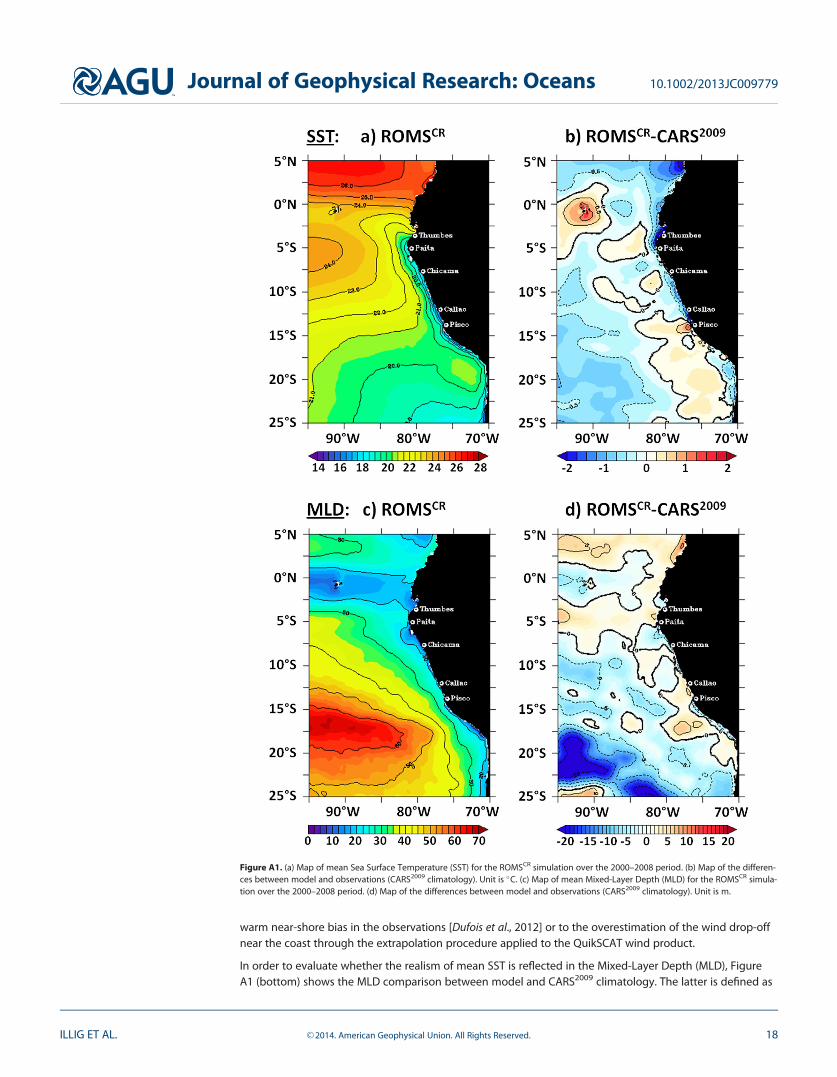
warm near-shore bias in the observations [Dufois et al., 2012] or to the overestimation of the wind drop-offnear the coast through the extrapolation procedure applied to the QuikSCAT wind product.

In order to evaluate whether the realism of mean SST is reflected in the Mixed-Layer Depth (MLD), FigureA1 (bottom) shows the MLD comparison between model and CARS2009 climatology. The latter is defined as

Figure A1. (a) Map of mean Sea Surface Temperature (SST) for the ROMSCR simulation over the 2000–2008 period. (b) Map of the differen-ces between model and observations (CARS2009 climatology). Unit is �C. (c) Map of mean Mixed-Layer Depth (MLD) for the ROMSCR simula-tion over the 2000–2008 period. (d) Map of the differences between model and observations (CARS2009 climatology). Unit is m.

Journal of Geophysical Research: Oceans 10.1002/2013JC009779

ILLIG ET AL. VC 2014. American Geophysical Union. All Rights Reserved. 18

the minimum between an MLD based on a 0.2�C criterion in temperature and an MLD based on a 0.03 crite-rion in salinity, while ROMS MLD is computed online based on the KPP scheme. ROMSCR agrees well withthe observations, with a spatial correlation larger than 0.88. ROMSCR MLD presents a weak mean bias ofless than 5 m along the Peruvian coast. Large scale patterns are also qualitatively similar, with deeper MLDover the South and West of the domain. Note that an offline estimation of the ROMSCR MLD, based on thesame temperature and salinity criteria as the observations, leads to a slight deeper MLD (by less than 10%):�1 m along the coast and �6 m in the South-West corner of the domain. This is due to the erosion of thesurface stratification through entrainment processes.

To further assess the realism of the simulation in terms of the vertical stratification structure, Figures A2aand A2b compare the ROMSCR simulated cross-shore vertical structure of temperature at 12�S in the upper400 m with the CARS2009 climatology temperature data. ROMSCR mean thermal structure is in rather goodagreement with the observations with isotherms tilted upward in the first �50–100 km from the coast andwithin a �100 m thick surface layer. In the surface layer (upper 20 m), the simulation is slightly cooler thanthe observations (�0.5–1�C, as illustrated in Figure 1b) while at deeper depth near the coast (50–150 m)warmer temperatures are found in the observations. Although this may reflect a model deficiency, it is alsolikely related to the different periods over which the climatology was calculated. In particular, the period2000–2008 is characterized by a cooler SST along the coast compared to the period 1976–1999 [Dewitteet al., 2012]. Also, in the core of the Peru-Chile Counter Current (PCCC) at 300 km offshore at 230 m depth,the simulation is slightly cooler than the observations (�0.2�C). Nevertheless, the largest differences arefound in the thermocline, where the simulated temperature is on average warmer by 0.5�C. The maximumdiscrepancies (0.8�C) are found 100 km off shore at 60 m depth. It is associated with a deeper than observedthermocline (�115 m, identified as the depth of the 15�C isotherm), with weaker (25%) vertical gradientsthan in the observations (identified as the thickness of the layer between the 13�C and 17�C isotherms).The rise of the isotherms is associated with a rise of the isopycnals due to the cooler and denser upwelledwaters, which creates a cross-shore density gradient driving the surface geostrophic equatorward PeruCoastal Current (PCC), with velocities larger than 1.5 m s21 near the coast. This is illustrated on Figure A2cthat displays the cross-shore section of mean circulation at 12�S. The poleward Peru Chile Under-Current(PCUC) is found below the PCC, with its core located over the continental shelf and slope at �170 m depth,making it the primary source for the upwelled waters [Huyer et al., 1987]. Mean velocities in the core of thePCUC reach �12 cm s21, consistently with previous model studies [Penven et al., 2005; Montes et al., 2010;Colas et al., 2011; Dewitte et al., 2012] and with the description given in previous observational studies[Huyer et al., 1991; Strub et al., 1998]. The PCCC can also be detected at �200 m depth 300 km offshore,with poleward velocities �0.3 m s21. A realistic simulation of the alongshore current shear is importantsince it controls the baroclinic instabilities and the associated eddy activity [Marchesiello et al., 2003].

Figure A2. Mean (2000–2008) vertical sections perpendicular to the coast at 12�S in function of depth and distance from the coast (km). (a) Mean temperature for the ROMSCR simula-tion. The mean position isotherm 15�C (d15) is underlined using black plain lines, and the 13�C (d13) and 17�C (d17) isotherms are depicted with dashed gray lines. (b) Differencesbetween model and observations (contours are drawn every 0.25�C). Observed mean position of d13, d15, and d17 are indicated as in Figure A2a. (c) ROMSCR regional oceanic circula-tion: mean along shore (color shading, equatorward flows are positive), cross-shore and vertical (arrows) currents. Unit is m s21. For visualization purposes, mean vertical current ampli-tude has been multiplied by 2000.

Journal of Geophysical Research: Oceans 10.1002/2013JC009779

ILLIG ET AL. VC 2014. American Geophysical Union. All Rights Reserved. 19

As a complementary validation of the subsurface mean state, Figure A3a provides a validation of the meanposition of the Peruvian coastal thermocline, identified as the mean position of the 15�C isotherm averagedwithin a 1� coastal band (d15). ROMSCR captures accurately the shallowing of the thermocline while movingsouthward, also in very good agreement with the mean d15 estimations using CARS2009 climatology.Model/observations discrepancies do not exceed 5 m in the northern Peru (0–7�S), and 15 m around 12�S.Similar discrepancies between model and the IMARPE data are found in Dewitte et al. [2012].

The overall comparison of ROMSCR simulated mean state is encouraging to further investigate the intraseaso-nal coastal variability in this model configuration, in particular regarding the mean vertical stratification that isinfluential on the Coastal Trapped Wave characteristics. The following subsection is devoted to this issue.

A3. Variability

First, as an overall estimate of the realism of the ROMSCR simulated variability, Figure A3b provides a Taylordiagram [Taylor, 2001], which includes various indices. The most relevant for the present study are thoseassociated with the coastal variability of temperature and the connection with the linear equatorial dynam-ics, as captured by the sea level variability. In this polar plot, the azimuthal angle provides a measure of thecorrelation (R) between simulated and observed time series. The radial distance from the origin (r) to anypoint is the ratio of the model Root Mean Square (RMS) to that of the observations. The observed point,referred to as OBS and marked with a red strikethrough circle is located at (R 5 1; r 5 1; red circle). The dis-tance from any point to OBF is equal to the normalized error (ratio of the RMS difference between modeland observations to the RMS of the observations).

The model Sea Level Anomalies (SLA, computed with respect to the average value over the 2000–2008period) is evaluated against the AVISO data. The latter are obtained from Ocean Topography ExperimentTOPEX/Poseidon/Jason and European Remote Sensing Satellite ERS-1/2 data sets as weekly maps of Sea

Figure A3. (a) Mean 15�C isotherm depth over the 2000–2008 period averaged within a 1� coastal band as a function of latitude for ROMSCR simulation (black line), IMARPE’s climatology(blue line), IMARPE in situ data (red symbols). (b) Taylor diagram illustrating the ROMSCR skills over the 2000–2008 period. The radial coordinate gives the magnitude of total standarddeviation, normalized by the observed value, and the angular coordinate gives the correlation with observations. It follows that the distance between the observed point (OBS, red strike-through circle) and any model’s point is proportional to the RMS model error. Isolines provide a measure of the skill as defined by equation (4) from Taylor [2001]. Blue squares comparethe 7 day-averaged simulated and observed (AVISO) Sea Level at the equator (86�W), and at several coastal positions (5�S, 15�S, 25�S). Colored circles provide a comparison with themonthly SST measured by IMARPE at five piers (Pa€ıta (5.06�S), Chicama (7.7�S), Chimbote (9.08�S), Callao (12.06�S), and Pisco (13.8�S)). The black star compares PC1-SSTA time seriesfrom the EOF analysis of TMI-OI data and ROMSCR outputs. Note that TMI-OI-PC1 has been shifted forward by 4 days (see Appendix A for details). (c) Coastal (0.5� coastal band averaged)Surface Vertical Thermal Gradient (SVTG, defined as the difference between the SST and the temperature at 50 m depth, blue, left scale in �C/m) and Mixed-Layer Depth (MLD, red, rightscale in meters) averaged between 16�S and 8�S for ROMSCR outputs (plain lines) and the CARS2009 climatology (dashed lines). Gray shading emphasizes the July to October season.

Journal of Geophysical Research: Oceans 10.1002/2013JC009779

ILLIG ET AL. VC 2014. American Geophysical Union. All Rights Reserved. 20

Level Anomalies (SLA) on a 1/3� Mercator grid (Ducet et al. [2000]—http://www.aviso.oceanobs.com). Modeland data are compared at some key locations: at the equator (86�W) and southward along the Peruviancoast at 5�S, 15�S, and 25�S. The results show that ROMSCR SLA is in good agreement with the observations.The agreement between model and observation is high at (0�N, 86�W), and then weakens along with thesouthward propagation and dissipation of the Coastal Trapped Waves. This either traduces model deficien-cies or biases in the satellite observations near the coast due to the contamination of the radar signal bylands and inappropriate tropospheric corrections [Dussurget et al., 2011].

We then compare the monthly SST Anomalies (SSTA computed with respect to the mean over 2000–2008period) from the IMARPE coastal stations located at Pa€ıta (5.06�S), Chicama (7.7�S), Chimbote (9.08�S), Callao(12,06�S), and Pisco (13,8�S), with equivalent ROMSCR simulated time series. As model and in situ data bothexhibit a marked seasonal signal (in phase with each other), with peak values in Austral summer, the resultsindicate a fair agreement with good level of variability and significant linear correlation coefficient in partic-ular at Chicama, Chimbote, and Pisco. Discrepancies can be attributed to the model configuration, in partic-ular to the spatial resolution that is too coarse to resolve the near-shore processes measured at the pierlocations. Concerning the mean bias between model SST and coastal piers observed SST, the overestimatedwind stress forcing near the coast (due to extrapolation of QuikSCAT data) leads to cooler than observedSST, in particular in Boreal winter, in agreement with Figure A1b.

In summary, Figure A3b indicates that over the 2000–2008 period, the model configuration is rather realistic nearthe coast. This suggests that the model has some skills in simulating the surface stratification variability. As a consis-tency check, the seasonal cycle of the Surface Vertical Thermal Gradient (defined as the difference between theSST and the temperature at 50 m depth) and the Mixed-Layer Depth averaged in the 100 km coastal bandbetween 16�S and 8�S are displayed on Figure A3c for the model outputs and the observations. It shows thatboth amplitude and phase of the simulated surface stratification are in very good agreement with the observa-tions. Taylor skills, as estimated from Taylor [2001, equation (4)], are larger than 0.99 (0.96) for SVTG (MLD).

Now we will focus on the evaluation of ROMSCR skill in simulating the variability within the intraseasonal timescales (40–90 days). The Intraseasonal Eddy Kinetic Energy (IEKE) is first diagnosed (Figures A4a and A4b) inorder to estimate the realism of the intraseasonal mesoscale activity in the model. Note that usually the totalmean EKE is considered for validation purpose. Here since our interest is on the intraseasonal variability, we con-sider the IEKE and compare it to estimations based on satellite altimetry (AVISO data). Note also that, since there

Figure A4. Maps of mean surface Intraseasonal (40–90 days) Eddy Kinetic Energy (IEKE) computed from 7 day-averaged intraseasonal sea level pressure gradients over the 2000–2008period for (a) AVISO data and (b) ROMSCR simulation. Unit is cm2 s22. (c) Map of correlation (color shading) and RMS differences (contours) between 7 day-averaged intraseasonal sealevel anomalies from ROMSCR simulation and AVISO data. Blue square patterns denote non-significant correlations (95% confidence level [Sciremammano, 1979]). Unit of RMS is cm.

Journal of Geophysical Research: Oceans 10.1002/2013JC009779

ILLIG ET AL. VC 2014. American Geophysical Union. All Rights Reserved. 21

is no data assimilation in the model, observed and simulated eddies are not expected to agree in their individualfeatures. However, their statistical characteristics (IEKE distribution and intensity) are comparable in both themodel and the observations, which indirectly reflects a realistic vertical current structure variability and associ-ated intraseasonal eddy activity. Although model and altimetry have different spatial resolutions, both productsshow local maxima of EKE near the equator and along the coast of Peru down to 16�S with a similar spatial pat-tern (the spatial correlation is 0.81). A notable discrepancy between the model solution and the observations isthe underestimated IEKE north of 7�S: �15 cm2 s22 in the model versus�30 cm2 s22 based on satellite data.This is likely due to the weaker than observed equatorial variability in the SODA model. Another remarkable dif-ference consists in a significantly smaller IEKE in the first �100 km in the model simulation relative to the obser-vations, a feature that was also mentioned by previous studies [Montes et al., 2010; Colas et al., 2011].

Focusing now on the intraseasonal Sea Level Anomalies (SLA), Figure A4c displays the correlation and RMS dif-ferences between model and observations (weekly altimetric AVISO data). The agreement between model andobservations is statistically significant along the equatorial wave guide and its coastal extension, with correlationvalues larger than 0.5 and RMS differences lower than 1 cm. Note that the agreement between model andobservations decreases southward along the coast (see also Figure A3). Further offshore, the lack of agreementbetween model and observations (correlation is not significant and RMS differences are of the order of the RMS)has to be attributed to the mesoscale activity (see Figures A4a and A4b). Although the model IEKE is realistic(Figure A4), since there is no data assimilation in the model, simulated and observed eddies are not collocated.This results in noisy features at the time and spatial scales of the eddies themselves and explains the low agree-ment of SLA where eddy activity is the largest. In order to filter out the noisy features associated with the meso-scale activity, the data are averaged over a coastal fringe of 100 km width between 16�S and 8�S. In that case,the correlation between observation and model reaches 0.61 (with a RMS difference smaller than 0.9 cm).

We now focus on the comparison between model and observations (TMI-OI) for the intraseasonal SSTAnomalies (SSTA). First, a statistical comparison (Figure A5) indicates that the ROMSCR and daily TMI-OI datashare the same level of intraseasonal variability, with a comparable spatial pattern (spatial correlation ofRMS maps is 0.90), in particular off Peru, the region of interest in this study. However, in this region, the cor-relation between model and observations is not significant, and the RMS difference remains of the order ofthe RMS (Figure A6c). As mentioned above, this discrepancy between model and observations is due to thesignature of eddies on SSTAs: ROMSCR eddies are not necessarily collocated with those observed by TMI-OI.Also TMI-OI is a gridded product with correlation scales of 4 days and 100 km, which tends to smooth themesoscale signature on SST. Such interpolation procedure was not applied to the model outputs. As a

Figure A5. Analysis of daily Sea Surface Temperature intraseasonal (40–90 days) Anomalies (SSTA) over the 2000–2008 period: Map of variability (RMS) for (a) TMI-OI data and (b) ROMSCR

simulation. (c) Map of correlation (color shading) and RMS differences (contours) between observed and simulated SSTA. Blue square patterns denote non-significant correlations (95%confidence level [Sciremammano, 1979]). Unit is �C.

Journal of Geophysical Research: Oceans 10.1002/2013JC009779

ILLIG ET AL. VC 2014. American Geophysical Union. All Rights Reserved. 22

consistency check, we estimated the level of agreement between model and observations of the SSTA aver-aged in the 200 km coastal band between 16�S and 8�S. The correlation then reaches 0.72, while the RMSdifference remains lower than 0.2�C. This indicates that the model has some skills in simulating the SSTintraseasonal variability near the coast.

The agreement between model and observations is further assessed based on an EOF analysis of the modelintraseasonal SSTA within a 5� wide coastal fringe between 17�S and 7�S, which allows extracting the SST vari-ability associated with the upwelling variability. Figure A6 displays the ROMSCR dominant pattern of variability ofthe SSTAs at subseasonal time scales off central Peru. The comparison between Figure A6 and Figure 1 thatshows the results of EOF analysis for the observed SSTA indicates that the model captures the main characteris-tics of the dominant mode of intraseasonal SSTAs off central Peru, that is: maximum variability confined within200 km from the coast (Figure A6a), two regimes of variability peaking at 29 and 60 days and accounting respec-tively for 52% and 44% of the total power of the PC1-SSTA spectrum (Figure A6b), and a marked seasonaldependence of the variability peak variance (Figure A6c). Note that this dominant mode explains 17% of theROMSCR subseasonal variance, against 33% for the TMI-OI data. This has to be attributed to the larger mesoscaleactivity in ROMSCR compared to TMI-OI data that does not project onto the spatial pattern of EOF1. Applying alow-pass spatial filter (binning within a 100 km radius) to the model outputs allows for increasing the averagedexplained variance up to 29.5%, which is in better agreement with the observations. Note that, besides theinherent limitations of the model, differences between model and observations also originate from the consider-ation of the SST data within the coastal masking zone of the TMI-OI data set for the model result (not shown).

Figure A6d displays the PC1-SSTA time series for ROMSCR (black plain line) and TMI-OI (green dashed line) fil-tered at intraseasonal time scales. The time series are lagged in time, ROMSCR PC1-SSTA leading TMI-OI by 4days. This is attributed to the extended masking of the TMI-OI data near the coast, which results in an offshoreextension of the EOF1 spatial pattern more developed for TMI-OI analysis than for the model. Thus, the TMI-OIEOF1 corresponds to a 4 day delayed phase in the upwelling sequence (cf. section 5.2) compared to the EOF

Figure A6. (top) Maps are same as Figure 1 but for ROMSCR SST subseasonal anomalies. (bottom) Intraseasonal band-pass filtered PC1-SSTA (40–90 days) for ROMSCR (black plain line)and TMI-OI (green dashed line). Note that TMI-OI-PC1 has been shifted forward by 4 days (see Appendix A for details). Gray vertical bands show the July to October season.

Journal of Geophysical Research: Oceans 10.1002/2013JC009779

ILLIG ET AL. VC 2014. American Geophysical Union. All Rights Reserved. 23

pattern captured in ROMSCR outputs that is more coastal. Correlation and RMS difference between model andobservations are, respectively, 0.88 and 0.25�C for a lag of 4 days with the model PC1 leading. This correspondsto a high score in the Tailor diagram (black star in Figure A3b in Appendix A) of 0.93 that emphasizes the agree-ment between model and observations in simulating the intraseasonal SST variability off central Peru.

Overall, the comparison between model and observations indicates that the model is skilfull in simulatingmost aspects of the mean state and intraseasonal variability, which provides confidence for using the modelfor diagnostic studies and sensitivity tests to boundary forcings.

ReferencesBakun, A. (1990), Global climate change and intensification of coastal ocean upwelling, Science, 247, 198–201.Belmadani, A., V. Echevin, B. Dewitte, and F. Colas (2012), Equatorially forced intraseasonal propagations along the Peru-Chile coast and

their relation with the nearshore eddy activity in 1992–2000: A modelling study, J. Geophys. Res., 117, C04025, doi:10.1029/2011JC007848.

Brink, K. H. (1982), A comparison of long coastal trapped wave theory with observations off Peru, J. Phys. Oceanogr., 12, 897–913.Brochier, T., V. Echevin, J. Tam, A. Chaigneau, K. Goubanova, and A. Bertrand (2013), Climate change scenarios experiments predict a future

reduction in small pelagic fish recruitment in the Humboldt Current system, Global Change Biology, 19(6), 1841–1853, doi:10.1111/gcb.12184.

Bromwich, D. H., R. L. Fogt, K. E. Hodges, and J. E. Walsh (2006), A tropospheric assessment of the ERA-40, NCEP, and JRA-25 global reanaly-ses in the polar regions, J. Geophys. Res., 112, D10111, doi:10.1029/2006JD007859.

Camayo, R., and E. J. D. Campos (2006), Application of wavelet transform in the study of coastal trapped waves off the west coast of SouthAmerica, Geophys. Res. Lett., 33, L22601, doi:10.1029/2006GL026395.

Cambon, G., K. Goubanova, P. Marchesiello, B. Dewitte, S. Illig, and V. Echevin (2013), Assessing the impact of downscaled winds on aregional ocean model simulation of the Humboldt system, Ocean Modell., 65, 11–24.

Capet, X. J., P. Marchesiello, and J. C. McWilliams (2004), Upwelling response to coastal wind profiles, Geophys. Res. Lett., 31, L13311, doi:10.1029/2004GL020123.

Carr, M.-E. (2002), Estimation of potential productivity in eastern boundary currents using remote sensing, Deep Sea Res., Part II, 49, 59–80.Carton, J. A., and B. S. Giese (2008), A reanalysis of ocean climate using simple ocean data assimilation (SODA), Mon. Weather Rev., 136,

2999–3017, doi:10.1175/2007MWR1978.1.Carton, J. A., G. Chepurin, and X. Cao (2000), A simple ocean data assimilation analysis of the global upper ocean 1950–95. Part I: Methodol-

ogy, J. Phys. Oceanogr., 30, 294–309.Centre ERS d’Archivage, de Traitement (CERSAT) (2002), Mean wind fields (MWF product) user manual, 1, QuikSCAT, Rep. C2-MUT-W-04-IF,

Ifremer, Plouzane, France.Clarke, A., and R. Ahmed (1999), Dynamics of remotely forced intraseasonal oscillations off the western coast of South America, J. Phys.

Oceanogr., 29, 240–258.Clarke, A. J., and C. Shi (1991), Critical frequencies at ocean boundaries, J. Geophys. Res., 96, 10,731–10,738, doi:10.1029/91JC00933.Colas, F., X. Capet, J. C. McWilliams, and A. Shchepetkin (2008), 1997–98 El Ni~no off Peru: A numerical study, Prog. Oceanogr., 79, 138–155,

doi:10.1016/j.pocean.2008.10.015.Colas, F., J. C. McWilliams, X. Capet, and J. Kurian (2011), Heat balance and eddies in the Peru–Chile current system, Clim Dyn, 39, 509–529,

doi:10.1007/s00382-011-1170-6.Debreu, L., P. Marchesiello, P. Penven, and G. Cambon (2012), Two-way nesting in split-explicit ocean models: Algorithms, implementation

and validation, Ocean Modell., 49–50, 1–21.Demarcq, H., and V. Faure (2000), Coastal upwelling and associated retention indices derived from satellite SST. Application to Octopus vul-

garis recruitment, Oceanol. Acta, 23, 391–408.Dewitte, B., S. Illig, L. Parent, Y. duPenhoat, L. Gourdeau, and J. Verron (2003), Tropical Pacific baroclinic mode contribution and associated

long waves for the 1994–1999 period from an assimilation experiment with altimetric data, J. Geophys. Res., 108(C4), 3121, doi:10.1029/2002JC001362.

Dewitte, B., S. Purca, S. Illig, L. Renault, and B. Giese (2008a), Low frequency modulation of the intraseasonal equatorial Kelvin wave activityin the Pacific Ocean from SODA: 1958–2001, J. Clim., 21, 6060–6069.

Dewitte, B., M. Ramos, V. Echevin, O. Pizarro, and Y. duPenhoat (2008b), Vertical structure variability in a seasonal simulation of a medium-resolution regional model simulation of the South Eastern Pacific, Prog. Oceanogr., 79, 120–137.

Dewitte, B., S. Illig, L. Renault, K. Goubanova, K. Takahashi, D. Gushchina, K. Mosquera, and S. Purca (2011), Modes of covariability betweensea surface temperature and wind stress intraseasonal anomalies along the coast of Peru from satellite observations (2000–2008), J.Geophys. Res., 116, C04028, doi:10.1029/2010JC006495.

Dewitte, B., J. Vazquez-Cuervo, K. Goubanova, S. Illig, K. Takahashi, G. Cambon, S. Purca, 1107 D. Correa, D. Gutierrez, A. Sifeddine, and L.Ortlieb (2012), Change in El Ni~no flavours over 1958–2008: Implications for the long-term trend of the upwelling off Peru, Deep Sea Res.,Part II, 77–80, 143–156, doi:10.1016/j.dsr2.2012.04.011.

Ducet, N., P. Y. Le Traon, and G. Reverdin (2000), Global high-resolution mapping of ocean circulation from the combination of T/P andERS-1/2, J. Geophys. Res., 105, 19,477–19,498, doi:10.1029/2000JC900063.

Duchon, C. (1979), Lanczos filtering in one and two dimensions, J. Appl. Meteorol., 18, 1016–1022.Dufois, F., P. Penven, C. P. Whittle, and J. Veitch (2012), On the warm nearshore bias in Pathfinder monthly SST products over Eastern

Boundary Upwelling Systems, Ocean Modelling, 47, 113–118, doi:10.1016/j.ocemod.2012.01.007.Dussurget, R., F. Birol, R. Morrow, and P. De Mey (2011), Fine resolution altimetry data for a regional application in the bay of biscay marine

geodesy, Mar. Geol., 34, 447–476, doi:10.1080/01490419.2011.584835.Echevin, V., K. Goubanova, B. Dewitte, and A. Belmadani (2012), Sensitivity of the Humboldt Current system to global warming: A down-

scaling experiment of the IPSL-CM4 model, Clim. Dyn., 38(3-4), 761–774, doi:10.1007/s00382-011-1085-2.Enfield, D. B. (1987), The intraseasonal oscillation in Eastern Pacific sea levels: How is it forced?, J. Phys. Oceanogr., 17, 1860–1876.Enfield, D. B., M. P. Cornejo-Rodriguez, R. L. Smith, and P. A. Newberger (1987), The equatorial source of propagating variability along the

Peru coast during the 1982–1983 El Ni~no, J. Geophys. Res., 92, 14,335–14,346, doi:10.1029/JC092iC13p14335.

AcknowledgmentsWe would like to thank the CNES (OSTSTproject EBUS-SOUTH, OSTST projectMODOKALT) and ESA (projectOceanFlux) for financial support. TMI-OIdata are produced by Remote SensingSystems and sponsored by the NASAEarth Science MEaSUREs DISCOVERProject. Wind stress data were obtainedfrom the Centre de Recherche etd’Exploitation Satellitaire (CERSAT), atIFREMER, Plouzan�e (France). We aregrateful to B. Giese from Texas A&MUniversity for providing the SODA data.We are thankful to the DSI/IRD forsupporting the SPIRALES projectdedicated to the implementation of acluster at IMARPE (P.I: B. Dewitte) overwhich the model configuration used inthis study was developed and mostsimulations were performed. Some werealso performed on the CALMIPcomputer at University Paul Sabatier(Toulouse, France, CALMIP project 1044).The model grid, forcing, and initialconditions were built using theROMSTOOLS package [Penven et al.,2008]. The authors wish to acknowledgeuse of the Ferret program (NOAA PMEL,http://ferret.pmel.noaa.gov) for analysisand graphics in this paper. The threeanonymous reviewers are thanked fortheir constructive comments.

Journal of Geophysical Research: Oceans 10.1002/2013JC009779

ILLIG ET AL. VC 2014. American Geophysical Union. All Rights Reserved. 24

Flores, R., J. Tenorio, and N. Dominguez (2010), Variaciones de la extensi�on Sur de la Corriente Cromwell frente al Per�u entre los 3�-14�S,Bol. Inst. del Mar del Per�u, 24(1–2), 45–55.

Fox-Kemper, B., and R. Ferrari (2008), Parameterization of mixed layereddies. PartII: Prognosis and impact, J. Phys. Oceanogr., 38, 1166–1179.

Garreaud, R., and R. Mu~noz (2005), The low-level jet off the subtropical west coast of South America: Structure and variability, Mon. WeatherRev., 133, 2246–2261, doi:10.1175/MWR2972.1.

Gentemann, C., C. J. Donlon, A. Stuart-Menteth, and F. J. Wentz (2003), Diurnal signals in satellite sea surface temperature measurements,Geophys. Res. Lett., 30(3), 1140, doi:10.1029/2002GL016291.

Gentemann, C., F. J. Wentz, M. Brewer, K. Hiburn, and D. Smith (2010), Passive microwave remote sensing of the ocean: An overview, inOceanography From Space, Revisited, edited by V. Barale, J. Gower, and L. Alberotanza, pp. 13–33, Springer, Heidelberg, Germany.

Goubanova, K., V. Echevin, B. Dewitte, F. Codron, K. Takahashi, P. Terray, and M. Vrac (2011), Statistical downscaling of sea-surface windover the Peru-Chile upwelling region: diagnosing the impact of climate change from the IPSL-CM4 model, Clim. Dyn., 36(7-8), 1365–1378, doi:10.1007/s00382-010-0824-0.

Goubanova, K., S. Illig, E. Machu, V. Garcon, and B. Dewitte (2013), SST subseasonal variability in the Benguela upwelling system as inferredfrom satellite observations (2000–2008), J. Geophys. Res. Oceans, 118, 4092–4110, doi:10.1002/jgrc.20287.

Guti�errez, D., et al. (2011), Coastal cooling and increased productivity in the main upwelling zone off Peru since the mid-twentieth century,Geophys. Res. Lett., 38, L07603, doi:10.1029/2010GL046324.

Hayashi, Y. (1982), Space-time spectral analysis and its applications to atmospheric waves, J. Meteorol. Soc. Jpn., 60, 156–171.Hormazabal, S., G. Shaffer, and O. Pizarro (2002), Tropical Pacific control of intraseasonal oscillations off Chile by way of oceanic and atmos-

pheric pathways, Geophys. Res. Lett., 29(6), 1081, doi:10.1029/2001GL013481.Huyer, A., R. L. Smith, and T. Paluszkiewicz (1987), Coastal upwelling off Peru during normal and El Ni~no times, J. Geophys. Res., 92, 14,297–

14,307, doi:10.1029/JC092iC13p14297.Huyer, A., M. Knoll, T. Paluszkiewic, and R. L. Smith (1991), The Peru Undercurrent: A study of variability, Deep Sea Res., Part A, 38, S247–

S271.Juli�a, C., D. A. Rahn, and J. A. Rutllant (2012), Assessing the influence of the MJO on strong precipitation events in subtropical, semi-arid

north-central Chile (30�S), J. Clim., 25, 7003–7013.Kondo, J. (1975), Air-sea bulk transfer coefficients in diabatic conditions, Boundary Layer Meteorol., 9, 91–112.Kummerow, C., et al. (2000), The status of the tropical rainfall measuring mission (TRMM) after two years in orbit, J. Appl. Meteorol., 39,

1965–1982.Large, W., J. McWilliams, and S. Doney (1994), Oceanic vertical mixing: A review and a model with a nonlocal boundary layer parameteriza-

tion, Rev. Geophys., 32, 363–403.Marchesiello, P., and P. Estrade (2010), Upwelling limitation by geostrophic onshore flow, J. Mar. Res., 68, 37–62.Marchesiello, P., J. C. McWilliams, and A. Shchepetkin (2001), Open boundary conditions for long-term integration of regional oceanic mod-

els, Ocean Modell., 3, 1–20.Marchesiello, P., J. McWilliams, and A. Shchepetkin (2003), Equilibrium structure and dynamics of the California current system, J. Phys. Oce-

anogr., 33, 753–783.Mechoso, C. R., et al. (2013), Ocean-cloud-atmosphere-land interactions in the Southeastern Pacific: The VOCALS program, Bull. Am. Mete-

orol. Soc., 95, 357–375, doi:10.1175/BAMS-D-11-00246.1.Menkes, C. E. R., J. G. Vialard, S. C. Kennan, J. P. Boulanger, and G. V. Madec (2006), A modeling study of the impact of tropical instability

waves on the heat budget of the eastern equatorial Pacific, J. Phys. Oceanogr., 36, 847–865.Montecinos, A., and F. Gomez (2010), ENSO modulation of the upwelling season off southern-Central Chile, Geophys. Res. Lett., 33, L02708,

doi:10.1029/2009GL041739.Montes, I., F. Colas, X. Capet, and W. Schneider (2010), On the pathways of the equatorial subsurface currents in the eastern equatorial

Pacific and their contributions to the Peru-Chile Undercurrent, J. Geophys. Res., 115, C09003, doi:10.1029/2009JC005710.Penven, P., V. Echevin, J. Pasapera, F. Colas, and J. Tam (2005), Average circulation, seasonal cycle, and mesoscale dynamics of the Peru

Current System: A modeling approach, J. Geophys. Res., 110, C10021, doi:10.1029/2005JC002945.Penven, P., L. Debreu, P. Marchesiello, and J. C. McWilliams (2006), Evaluation and application of the ROMS 1-way embedding procedure to

the central California upwelling system, Ocean Modell., 12, 157–187.Penven, P., P. Marchesiello, L. Debreu, and J. Lefevre (2008), Software tools for pre- and post-processing of oceanic regional simulations,

Environ. Model. Software, 23, 660–662.Pizarro, O., A. J. Clarke, and S. Van Gorder (2001), El Ni~no sea level and currents along the South American coast: Comparison of observa-

tions with theory, J. Phys. Oceanogr., 31(7), 1891–1903.Pizarro, O., G. Shaffer, B. Dewitte, and M. Ramos (2002), Dynamics of seasonal and interannual variability of the Peru–Chile Undercurrent,

Geophys. Res. Lett., 29(12), 1581, doi:10.1029/2002GL014790.Rahn, D. A. (2012), Influence of large scale oscillations on upwelling-favorable coastal wind off central Chile, J. Geophys. Res., 117, D19114,

doi:10.1029/2012JD018016.Ramos, M., O. Pizarro, L. Bravo, and B. Dewitte (2006), Seasonal variability of the permanent thermocline off northern Chile, Geophys. Res.

Lett., 33, L09608, doi:10.1029/2006GL025882.Ramos, M., B. Dewitte, O. Pizarro, and G. Garric (2008), Vertical propagation of extratropical Rossby waves during the 1997–1998 El Ni~no off

the west coast of South America in a medium-resolution OGCM simulation, J. Geophys. Res., 113, C08041, doi:10.1029/2007JC004681.Renault, L., B. Dewitte, M. Falvey, R. Garreaud, V. Echevin, and F. Bonjean (2009), Impact of atmospheric coastal jets on SST off central Chile

from satellite observations (2000–2007), J. Geophys. Res., 114, C08006, doi:10.1029/2008JC005083.Renault, L., B. Dewitte, P. Marchesiello, S. Illig, V. Echevin, G. Cambon, M. Ramos, O. Astudillo, P. Minnis, and J. K. Ayers (2012), Upwelling

response to atmospheric coastal jets off Central Chile: A modeling study of the October 2000 event, J. Geophys. Res., 117, C02030, doi:10.1029/2011JC007446.

Reynolds, R. W., and T. M. Smith (1994), Improved global sea surface temperature analyses using optimum interpolation, J. Clim., 7, 929–948.

Ridgway, K. R., J. R. Dunn, and J. L. Wilkin (2002), Ocean interpolation by four-dimensional least squares—Application to the waters aroundAustralia, J. Atmos. Oceanic Technol., 19(9), 1357–1375.

Schweiger, A. J., R. W. Lindsay, S. Vavrus, and J. Francis (2008), Relationships between Arctic sea ice and clouds during autumn, J. Clim., 21,4799–4810.

Sciremammano, F. (1979), A suggestion for the presentation of correlations and their significance levels, J. Phys. Oceanogr., 9, 1273–1276.

Journal of Geophysical Research: Oceans 10.1002/2013JC009779

ILLIG ET AL. VC 2014. American Geophysical Union. All Rights Reserved. 25

Shaffer, G., O. Pizarro, L. Djurfeldt, S. Salinas, and J. Rutllant (1997), Circulation and low-frequency variability near the Chilean coast:Remotely forced fluctuations during the 1991–1992 El Ni~no, J. Phys. Oceanogr., 27, 217–235.

Shchepetkin, A. F., and J. C. McWilliams (1998), Quasi-monotone advection schemes based on explicit locally adaptive dissipation, Mon.Weather Rev., 126, 1541–1580.

Shchepetkin, A. F., and J. C. McWilliams (2005), The regional oceanic modeling system: A split-explicit, free-surface, topography following-coordinate ocean model, Ocean Modell., 9, 347–404, doi:10.1016/j.ocemod.2004.08.002.

Smith, R., J. Dukowicz, and R. Malone (1992), Parallel ocean general circulation modeling, Physica D., 60, 38–61.Spillane, M. C., D. B. Enfield, and J. S. Allen (1987), Intraseasonal oscillations in sea level along the west coast of the Americas, J. Phys. Ocean-

ogr., 17, 313–325.Strub, P. T., J. M. Mesias, V. Montecino, J. Rutllant, and S. Salinas (1998), Coastal ocean circulation off western South America, in The Sea,

vol. 11, edited by A. R. Robinson and K. H. Brink, pp. 273–314, John Wiley, Hoboken, N. J.Taylor, K. E. (2001), Summarizing multiple aspects of model performance in a single diagram, J. Geophys. Res., 106, 7183–7192.Torrence, C., and G. P. Compo (1998), A practical guide to wavelet analysis, Bull. Am. Meteorol. Soc., 79, 61–78.Toumazou, V., and J.-F. Cretaux (2001), Using a Lanczos Eigensolver in the computation of empirical orthogonal functions, Mon. Weather

Rev., 129, 1243–1250.Uppala, S. M., et al. (2005), The ERA-40 re-analysis, Q. J. R. Meteorol. Soc., 131, 2961–3012.Vega, A., Y. duPenhoat, B. Dewitte, and O. Pizarro (2003), Equatorial forcing of interannual Rossby waves in the South eastern Pacific, Geo-

phys. Res. Lett., 30(5), 1197, doi:10.1029/2002GL015886.Wentz, F. J., C. L. Gentemann, D. K. Smith, and D. B. Chelton (2000), Satellite Measurements of sea surface temperature through clouds, Sci-

ence, 288(5467), 847–850.Xie, S. P., T. Miyama, Y. Q. Wang, H. M. Xu, S. P. de Szoeke, R. J. O. Small, K. J. Richards, T. Mochizuki, and T. Awaji (2007), A regional ocean-

atmosphere model for eastern Pacific climate: Toward reducing tropical biases, J. Clim., 20, 1504–1522.

Journal of Geophysical Research: Oceans 10.1002/2013JC009779

ILLIG ET AL. VC 2014. American Geophysical Union. All Rights Reserved. 26