ADOO? 704 ADVISORY GROUP FOR AEROSPACE RESEARCH AND DEVELOPMENT--ETC F/6 20/it

CRITICAL COMMENTARY ON MEAN FLOW DATA FOR TWO-DIMENSIONAL COM--ETC(U)

MAY 80 H H FERNHOLZ- P J FINLEY

UNCLASSIFIED AGARD-A6-253 NL

._ IIIEEEIIEEE-- Em.'.-'li-I-..'--III-IEEE'.-II-- U'.II

Ul1l 1.o

I Imi11111 2 .4O

MICROCOPY RESOLUTION TEST CHART

AGARDOgraph No.2U3

A C ritical COmWeA onMean Flow Dat for Two-Dimensional

Compressile Turbulent Boundary Layer

DWFRIBUTtON AND AVAILASILITYON SAK COVER

ALGARD.AG-253

NORTH ATLANTIC TREATY ORGANIZATION

ADVISORY GROUP FOR AEROSPACE RESEARCH AND DEVELOPMENT v

(ORGANISATION DU TRAITE DE L'ATLANTIQUE NORD)

AGARDograph No.253

A,9TIA -TMENTRYON)IEANJLOWC ] AT AFORTWO-J JMENSIONALSOMPRESSIBLEI

TURBU LENT BOUNDARY LAYERS

by

10.~erhl P.TJ. inley~uDep et of Aeronautics

ermo-un -ui ynamik Imperial College ofTechnische Universitit Berlin and Science and TechnologyD- 1000 Berlin 12 Prince Consort RoadStrasse des 17. Juni 135 London SW7 2BYBRD Germany Great Britain

4.

This AGARDograph was prepared at the request of the Fluid Dynamics Panel of AGARD.

THE MISSION OF AGARD

The mission of AGARD is to bring together the leading personalities of the NATO nations in the fields of scienceand technology relating to aerospace for the following purposes:

- Exchanging of scientific and technical information;

- Continuously stimulating advances in the aerospace sciences relevant to strengthening the common defenceposture;

- Improving the co-operation among member nations in aerospace research and development;

- Providing scientific and technical advice and assistance to the North Atlantic Military Committee in the fieldof aerospace research and development;

- Rendering scientific and technical assistance, as requested, to other NATO bodies and to member nations inconnection with research and development problems in the aerospace field;

- Providing assistance to member nations for the purpose of increasing their scientific and technical potential;

- Recommending effective ways for the member nations to use their research and development capabilities forthe common benefit of the NATO community.

The highest authority within AGARD is the National Delegates Board consisting of officially appointed seniorrepresentatives from each member nation. The mission of AGARD is carried out through the Panels which arecomposed of experts appointed by the National Delegates, the Consultant and Exchange Programme and the AerospaceApplications Studies Programme. The results of AGARD work are reported to the member nations and the NATOAuthorities through the AGARD series of publications of which this is one.

Participation in AGARD activities is by invitation only and is normally limited to citizens of the NATO nations.

L ess -alFo r The content of this publication has been reproduced

I ==, G irectly from material supplied by AGARD or the authors.

~j. Published May 1980i St Copyright 0 AGARD 1980

All Rights Reserved

ISBN 92-835-1362-2

Printed by Technical Editing and Reproduction Ltdllarford House, 7- 9 Charlotte St. London. WIP I1ID

CONTENTSPage

i PREFACE - THE AGARD-EUROVISC CATALOGUE ivii ACKNOWLEDGEMENTS iviii GRAPHICAL PRESENTATION OF PROFILE DATA v

iv AGARDograph 223 - CORRIGENDA vi

1. INTRODUCTION1.1 Requirement for profile data 11.2 The nature of experimental observations 21.3 Data from short-run facilities (by G.T. Coleman and J.L. Stollery) 5

2. THEORETICAL BASIS FOR THE INTERPRETATION OF NEASUREN4ENTS2.1 Introduction 72.2 Fundamental equations for two-dimensional compressible turbulent boundary layers 112.3 Pripcipal parameters for compressible boundary layers 152.4 Norkovin's hypothesis 182.5 Analytical solutions of the energy equation 192.6 Heat transfer at the wall 49

3. CONCEPTS FRON LOW SPEED STUDIES

3.1 Introduction 513.2 Similarity laws and their description 523.3 Similarity laws and their extension to comressible flow 543.4 Transformation concepts 71

4. INTERPRETATION OF MEAN FLOW MEASUREMENTS FOR ZERO PRESSURE GRADIENT

4.1 General remarks 724.2 Zero pressure gradient adiabatic cases 744.3 Zero pressure gradient isothermal wall cases 874.4 Transition and low Reynolds number effects 974.5 Upstream history effects 1114.6 Wall roughness 118

5. MEAN FLOW DATA FOR PRESSURE GRADIENT CASES5.1 Causes and broad effects 1265.2 Favourable pressure gradient 1365.3 Adverse pressure gradient 1485.4 Conclusions 164

6. NORMAL PRESSURE GRADIENTS

6.1 Normal pressure gradients in ideal flow 1656.2 Modifications to the ideal flow pattern caused by the boundary layer 1716.3 Reynolds stresses 1776.4 Boundary layer Induced pressure gradients - anomalous cases 1846.5 General comment on the interpretation of experimental data 1876.6 Conclusions 189

7. BOUNDARY LAYER LENGTH SCALES

7.1 The 'physical' boundary layer thickness 1907.2 Integral thicknesses 1957.3 The displacement surface 1967.4 Reference flows and improper formulations 1987.5 Defect thicknesses 2017.6 Discussion 2047.7 Conclusions 204

REFERENCES 205

ADDITIONAL REFERENCES 221

i. PREFACE - THE AGARD-EUROVISC CATALOGUE

This is the second of three proposed volumes presenting and discussing two dimensional compressible turbu-lent boundary layer data. The first voluwe, AGARDograph 223, contained tabulated data, in complete form onmicrofiche, and in abbreviated form as printed tables, for 59 experimental boundary layer studies. Theexperiments were also described in a standardised manner, and a certain amount of introductory material wasprovided so as to assist readers wishing to make use of the data. So far as possible, comment and discus-sion was reserved for this second, commentary, volume. We have, in the main, restricted our discussion hereto the time-mean data presented in AGARDograph 223, but have felt free to supplement them with data fromexperimental studies which we have processed since the completion of that volume. Entries in AGARfograph223 are indicated by a reference number such as CAT 7201, while supplementary data to be presented in thethird volume are labeled with a distinguishing "S" - as for example, CAT 7802S. In addition to these supple-mentary entries, about twelve in number, the third volume will contain a discussion of the available fluc-tuation data, and a "source catalogue" which will provide an annotated bibliography of the many papers whichwe have consulted in the course of this enterprise.

The data presented in AGARDograph 223 are also available on magnetic tape. Our original tape output has

been modified, mainly for the greater convenience of FORTRAN users, by P. Bradshaw of Imperial College, andcopies may be obtained from the centres listed in the foreword to AGARDograph 223.

The project arose from a suggestion made to the first author by the late Dietrich Kichemann, and has con-tinued under the auspices of EUROVISC, principally through the assistance of an informal guidance panel.The data collection and computation have throughout been funded by the German Research Council (DFG) and

the Technical University, Berlin (TUB). The Fluid Dynamics Panel of AGARD have supported the editorialwork and arranged publication.

Both for our own correction, and as a reminder to the many workers in the field, we would recall* that"It is a capital mistake to theorise before one has data". We hope that the publication of the firstvolume provides a sufficient justification for the modest level of theoretical appreciation presented here.

* A scandal in Bohemia, Sir Arthur Conan Doyle.

ii. ACKNOWLEDGEMENTS

Preeminence amongst all those to whom we owe thanks must be given to Miss C. Mohr, who has handled allthe computational work associated with the project. We also thank Mrs. H. Geib and Miss J. Barritt forpreparing the text, Miss A. Behlow for collating and typing the references, and Mrs. 1. Gereke for making

all our drawings.

We must thank the DFG and TUB for funding the research work, while the second author must thank the TUB andthe Hermann-Fottinger-Institut for the many occasions on which he has been welcomed as a guest. The publi-cation is funded by AGARD, and we must thank successive executives of the Fluid Dynamics Panel, J. Lawford,M. Fischer and R.H. Rollins for their help and encouragement.

We have throughout benefited from the support and advice of Professors T. Fannellp (Trondheim) andK. Gersten (Ruhr-Universitat Bochum) as successive AGARD editors, and much informal assistance fromProfessor A.D. Young. We have continued to receive help and guidance from the EUROVISC advisory panel,

L.C. Squire (Cambridge), J.L. Stollery (Cranfield) and K.G. Winter (R.A.E. Bedford). We are particularlyindebted to Professors P. Bradshaw and D. Coles for detailed criticism of the text, and much helpfulgeneral advice. Since this last has not always been taken, they and the many other colleagues who haveassisted in this way are not to be blamed for errors of fact or phrasing, which remain our own.

I,

iii. GRAPHICAL PRESENTATION OF PROFILE DATA: LIST OF SOURCES REPRESENTED IN FIGURES

For the sources below a selection of the profile information my be found in the figures listed.

Prof l1es

Source Temperature Velocity"Inner" "Outer"

5301 Coles - 3.3.11.4.2.5 4.2.6

5501 Shutts et al. - 3.3.9,4.2.7 4.2.8

5502 Shutts & Fenter - 4.6.2,4.6.4 4.6.5

5801 Naleid - 5.3.8 -

5802 Stalmach - 3.3.8,4.2.9 4.2.10

5805 Moore (Step) - 4.5.1 4.5.2

5901 Hill 5.1.7 5.2.11 5.2.12

65D2 Moore & Harkness - 4.2.7,4.2.15 4.2.8,4.2.16

6505 Jackson et al. - 3.3.10,4.2.13 4.2.14

6506 Young - 3.3.8.4.3.1,4.6.4,4.6.6 4.3.2,4.6.5

6602 Jeromin 2.5.8 -

6701 Samuels et al. 2.5.15 -

6702 Danberg 2.5.10-13 --

6801 Perry & East 5.1.8 5.2.13,5.2.14 5.2.15

6903 Thomke - 3.3.10,4.2.17 4.2.18

7003 Meier 2.5.9 --

7004 Winter et al. - 5.3.18,5.3.19 5.3.20,5.3.21

7006 Hastings & Sawyer 2.5.5 3.3.8.4.4.12 4.4.11

7007 Zwarts - 5.3.13 5.3.14

7101 Sturek & Danberg 5.1.5 5.3.15,5.3.16 5.3.17

7102 Peake et al. - 3.3.12,5.3.1,5.3.2 5.3.3

7103 Fischer & Maddalon 4.4.7 -

7104 Waltrup & Schetz 5.1.4 5.3.10 5.3.97105 Beckwith et al. 5.1.9 5.2.18 5.2.19

7201 Lewis et al. - 5.1.2,5.2.1,5.3.4 5.1.3,5.2.2,5.3.5

7202 Votslnet & Lee 2.5.17,2.5.18 3.3.13,4.2.19,4.3.9/10/13 4.2.20,4.3.11/12/14

7203 Hopkins & Keener - 4.3.7 4.3.8

7204 Kenner & Hopkins 2.5.14 4.3.1 4.3.2

7205 Horstman & Owen 2.5.13,4.3.6 3.3.0/1,4.3.5 4.3.6

7206 Kemp & Owen 5.1.10 5.2.17 5.2.16

7301 Gates 2.5.6,4.5.6 4.5.4,4.5.5 -

7302 Winter & Gaudet - 3.3.10,4.2.11 4.2.12

7304 Voistnet & Lee 5.1.6 5.2.5,5.2.7,5.2.9 5.2.6,5.2.8,5.2.10

7305 Watson et al. 2.5.7,4.4.3 4.4.4,4.4.5 4.4.6

7401 Thomas 5.2.3,5.3.11 5.2.4

7402 Mabey et al. 2.5.1-4 3.3.0/1/8/9,4.2.1/2 4.2.3,4.2.47601 Vas et al. 4.2.15 4.2.16

6002S Danberg 2.5.21 4.4.8,4.4.10 4.4.97404S Volsinet et al 2.5.19,2.5.20

7701S Mabey 3.3.8 4.4.13-16 4.4.15,4.4.17

7702S Laderman & Demetrlades 2.5.16 4.3.3 4.3.478025 Kussoy et al. - 5.3.6 5.3.7

iv. AMlDolraph 223 - CORRIGENDA

page vi - Abbreviations: STP - stagnation temperature probe.page 13 - 1 3.6, para. 2, last line: p' not pl.page 25 - eqn. 5.13: 8, - -Rz[I - (1+26n/Rz)'J.page 27 - 5.6, para. 2, line 4: "---, so that Pot was set equal to --- ".

5503-A-I: I DATA: 55030101 - 0113.7006-B-2: First profile numbered 70060406 should be 70060405.7105-A-3, Table 1: Table heading; P INF at X-2.083 m.

Last line, X -2.083, -RZ- 197.5.7209-A-1, para. 2, line 3: "--- at X-25 me --- ".

7303-A-1, footnote: "--- values about 10% lower".7305-A-1, Identification panel : 9 < RE/m x 10-6 < 50.7401-A-1, para 2: "--- here. The plates were 0.1 m wide ---.

para 4: Reference to Smith et al. should be "19620.

7402-B-4, run 1702: X =0.623.R-3 References: Fenter (1960) DRL 468 should be Fenter (1959) DRL 437.

1. INTRODUCTION

The quantity of compressible turbulent boundary layer data which is available in the open literature is

very great. In AGARDograph 223 (Fernholz & Finley, 1977), the predecessor of this volume, we presented

a selection of data, restricting our choice' to nominally two dimensional flows for which, with one excep-

tion, mean flow profile data were available'in tabular form. In that data compilation we kept to a

minimum any discussion of the quality or significance of the data, as our primary concern was to make it

available in standard form without, so far as possible, introducing any particular pattern to which it

should be expected to conform. Where we did make comments based on our own ideas or prejudices, we

endeavoured to keep them as distinct as might be from the data proper, and the description of the experi-

ment in which they had been obtained. Individual experiments - "entries" - which are described in

AGARDograph 223 are referred to in this volume by the identification used in the data compilation as, for

example, CAT 7205 (Horstan & Owen, 1972) - where the first two digits (72) refer to the year of publica-

tion of the experiment and the second two (05) were arbitrarily assigned by us during data processing.

Four succeeding digits, as in 7205 0102, refer to the series and the individual boundary layer profile

concerned. We also hope to provide a supplementary volume, and possible entries in this are indicated

by four digits and an S. Some of these data are used in the present volume - e.g. 7802S (Kussoy et al,

1978).

In general we will not discuss practical details of the individual experiments here, presuming that the

published account and our standardised description in AGARDograph 223 or its successor give any informa-

tion which is desired - or at least, which is available. We will however describe and discuss the data

themselves in close detail, for the greater part by comparing the mean velocity profiles to the basic

pattern suggested by the so-called inner and outer 'laws' as used to describe the incompressible zero-

pressure-gradient boundary layer. This procedure is at first sight rather simple minded. The theoreti-

cal background is discussed in §§ 2,3 however, and leads to the expectation that a suitable transformation

of the profiles will allow the data to be compared directly to an accepted 'incompressible norm' (§ 3) for

the zero pressure gradient case (§ 4) and that, as at low speeds, the differences from this standard case

will be informative in pressure gradient flow (§ 5) and in flows which have not achieved equilibrium for

other causes (§ 4.5). The main body of this paper therefore contains, in H 4,5, a graphical presenta-

tion of a great number of transformed velocity profiles in relation to the accepted semi-logarithmic

inaer law and a semi-empirical, also semi-logarithmic, outer law (Fernholz 1969, 1971).

In preparing the data compilation we originally found some difficulty, evidently often shared by the

original experimental worker, in handling data from experiments displaying a significant pressure gradient

normal to the wall. This led us to undertake a thorough investigation of the causes of such normal pres-

sure gradients, the results of which are reported in § 6, while some of the resulting effects are consi-

dered as part of a general assessment of boundary layer thicknesses in 9 7.

Whatever the topic being discussed, the illustrations here used are in every case drawn from experiments

reported in AGARDograph 223 or the proposed supplement. Their validity therefore depends on the general

validity of experimental data and we commence with an assessment of the data needed and the extent to

which it is possible to hope for accurate measurement.

1.1 Requirement for profile data

Aeronautical boundary layer studies have their technological justification in the provision of usable

data or calculation methods for the accurate prediction of skin friction, heat transfer, boundary layer

separation and, to a lesser extent, displacement effect. While, in principle, any prototype situation

could be modelled In an experiment, in practice It is virtually impossible to obtain complete dynamic

similitude, if only because the prototype Reynolds numbers are usually so high that they cannot be

reproduced economically in laboratory experiments. There is therefore a need to develop rational

correlations of data which will allow engineers to predict, or extrapolate, from a limited range of

experimental geometries and governing dimensionless parameters, the likely values of the technically

Important quantities In markedly differing prototype situations.

The practical requirement is for good values of the "wall data" - principally skin friction, and in high

speed flows, heat transfer - but laboratory measurements of these alone do not provide adequate informa-tion as any mode of extrapolation, whether by the use of a refined and complex field calculation method

or by a grossly simplified empirical formula, will depend also on details of the flow field in the

boundary layer. This essentially results from experimental difficulties in modelling transition, as even

flat plate results cannot be properly correlated against values of Rex. while some measure of success has

been achieved when the reference length used is a boundary layer thickness. All rational prediction

methods therefore depend finally on some kind of mean flow, and possibly turbulence, profile information.

The more refined calculation methods attempt to use a limited amount of very generalised fundamental data,

while empirical projections tend to use a very large pool of data from situations which are often morevariously distributed in their original range of application than one would wish when applying the results -

e.g. the 'parametric approach' of § 2.1.2(1). Whatever the approach, profile information is required -rarely for its own sake, since it has no direct technical application - but for use in the development of

prediction methods.

This volume presents a discussion of the mean flow profile data of compressible boundary layers. Anatural approach is to compare the data with, in some way equivalent, incompressible boundary layers, and

this is indeed the general method used in the detailed profile analysis of SS 4,5. The comparison is,however, with the simplest possible case - a 'standard' flat plate boundary layer - and cannot yet be

extended other than in qualitative terms to more general cases. Indeed, it is wise to express cautionabout anyassumption that the low speed layer itself is fully understood. A good, if now slightly dated,appreciation may be obtained by a study of the proceedings of the 1968 Stanford conference on the calcu-

lation of incompressible turbulent boundary layers (Kline et al., 1969, Coles & Hirst, 1969, or briefly,with particular reference to compressible flows, Morkovin & Kline, 1968). A valuable result of this

meeting was that many of the basic problem areas were identified. Recent experimental work aimed at

elucidating some of the individual features of 'complex' two dimensional flows is exemplified by Smitset al. (1979, a,b) while a more general review may be found in Bradshaw (1976, Ed.). Whether the

'incompressible base' can be treated as known or not, it remains difficult to think of incompressibleanalogues for some features of compressible flows. In particular there is the possibility of concentra-

ted pressure changes in distances comparable to the boundary layer thickness, even if shock-wave boundary-layer interactions are excluded. High heat transfer rates are common, and certainly of technical

importance to a greater extent than at low speeds, so that heat transfer enters as a principal variable.The data base required for study is therefore extended by at least two 'dimensions' - heat transfer, and

of course, Mach number.

1.2 The nature of experimental observations

For the reasons stated above, the original data compilation presented as AGARDograph 223 concentrated on

cases for which profile information was available, while this volume discusses the features of the meanflow profiles which were presented there, with some additions. Before embarking on this detailed study

however, we consider some of the general factors which determine the availability of data.

An ideal data set would consist of a series of measurements at successive streamwise stations. The data

presented would include

(a) Wall pressure and temperature at close intervals.

(b) Skin friction and heat transfer at close intervals.

(c) At a number of succeeding profile stations, self-sufficient sets of three independent mean flowproperties.

(d) Turbulence measurements giving, as a minimum, profiles of the mean-square velocity fluctuation coi'-

ponents and of shear stress.

(e) Properly conducted investigations of the experimental environment, such as checks on two-dimensionality,free-stream uniformity and turbulence level as a function of frequency, noise levels, and where

appropriate, the state of tunnel sidewall boundary layers.

3

The length of the list is enough to suggest that the ideal is not readily attainable, but the difficulties

involved in obtaining each item vary widely, and occasionally present conflicting experimental require-

ments.

1.2.1 Long- and short-run facilities

The most significant classification of experimental facilities is into "short-run" and "long-" or"continuous-running" tunnels. In practice this means that "short-run" devices have a typical test

duration of 10 ms or less, while "long-run" tunnels range from about 10 s to the effectively unlimited.The significance of the distinction is that the technically important measurement of heat transfer is very

straightforward in a "short-run" test, and difficult in a "long-run" facility. On the other hand it isvery difficult indeed to measure profile data in a "short-run" tunnel, and relatively straightforward

when given enough time. In compiling data for the development of prediction methods there is therefore a

basic problem in linking heat transfer data simply, and fairly reliably, obtained from short-run tests to

the profile and skin friction data obtained in the very different environment of a continuous, or at least

"long", running wind tunnel. The profile-based nature of our own compilation has therefore led us to

request G.T. Coleman & J.L. Stollery to prepare a short appreciation of data from short-run facilities

which appears as § 1.3 below.

1.2.2 Wall measurements

Of the 'ideal data set' wall measurements, static pressure and wall temperature are easily measured,though

the latter is often not recorded by experimental workers who believe their walls to be adiabatic, or

nearly so. Heat transfer rates are, as stated above, readily determined in short-run facilities, but canpresent considerable problems in continuous run tunnels since most techniques then require some form of

steady state calorimetry, with the associated difficulties of assessing leakage fluxes (mostly due to

lateral conduction) or of arranging a complex set of buffer rings. Many of the techniques require theactual heat flux meter surface, or part of it, to be at a different temperature from the surrounding wall,

and this can cause serious distortion of the results. (See Winter, 1976, for a review of heat transfer

measurement techniques). An interesting hybrid technique, which in principle evades these difficulties,

is the use of an 'isolated mass calorimeter' (Westkaemper, 1959). It is perhaps significant however that

the vast majority of writers on heat transfer techniques for long-run facilities find it necessary todevote a substantial part of their text to techniques for correcting the inherent errors of the method.

Skin friction is perhaps the most difficult quantity of all to measure directly (see the review paper by

Winter, 1977). There is a long history of 'direct' measurement of wall shear stress using floating

element balances, but unless the balance is very large, when, however, the value obtained will not be

truly local (e.g. Winter & Gaudet 1973, CAT 7302) it is very difficult to be certain that various forms of

systematic edge-flow-induced errors are not present (Allen, 1976, 1977a) however repeatable the staticcalibration may have been.

A vital step in the development of experimental techniques is the extension of skin friction measurements

to provide a Preston tube calibration. Balances are expensive, require a relatively large space forinstallation even when the element is small, and are very difficult to use. Further, the edge-induced

errors are likely to become even larger when complicated by inflow and outflow due to pressure gradients,

while "moment sensing" balances are affected directly by the pressure gradient (e.g. the NOL design,

Bruno et al., 1969). Unfortunately, even for adiabatic wall boundary layers, there is as yet no final

agreement on the Preston tube calibration (Fenter & Stalmach, 1957; Hopkins & Keener 1966; Allen, 1973,

1974 revised, Allen 1977b; Bradshaw & Unsworth, 1974, and revised, Bradshaw 1977b), so that research

workers often present several different values and leave it to the reader to choose (e.g. Peake et al.,

1971, CAT 7102). It may or may not be possible to extend the calibration to severe heat transfer cases

(it is not uncommon to find a 30%-50% difference in values depending on the calibration chosen - Bartlett

et al., 1979a), but if this is done it is most important that calibrations are made against balanceswhich have the floating element at the same temperature as the surrounding test surface. This is clearly

a formidable design problem, but an uncooled floating element in a cooled wall may give unrealistically

low shear stress values (Westkaemper, 1963). A difference of order 20% was found by Voisinet & Lee with

4

Tw/Tr = 0.22 (CAT 7202, and corrected data, private communication). We would however encourage experi-

mental workers to take Preston tube readings whenever possible, since it is relatively straightforward and

cheap to do so, while disregarding the apparent discouragements above, as if the raw Preston data are

presented it will always be possible to reduce the data using the calibration of the reader's choice - or

the final definitive calibration if that is ever achieved.

1.2.3 Mean flow profile data

Mean flow data in the boundary layer are with very rare exceptions (LDV, Electron beam, hot-wire probes

in use for turbulence measurements) deduced from measured Pitot (Pt2) profiles and measured or assumed

total temperature(To) and static pressure (p) profiles. The question of static pressure variation is

fully discussed in § 6 below, and so will not be considered further here, other than by remarking that on

a straight wall with not too severe longtiudinal pressure gradients it is usually reasonable to assume

that p is a function of x only. The measurements, if made, are likely to prove difficult, especially at

high Mach numbers (see Beckwith et al., 1971).

Usually total temperature profiles are, in practice, measured nowadays, and in severe heat transfer cases

this is absolutely necessary. A general appreciation of the extent to which available theories predict

the temperature profile may be found in § 2.5.6 below, and may serve as a guide to the requirement for a

measured profile. Three basic types of probe can be distinguished, each with its own advantages and

disadvantages. Historically the first of these, and conceptually the simplest, is the vented Pitot

type referred to in AGARDograph 223 as a stagnation temperature probe (STP). The earlier designs

(Winkler 1954) appeared successful, but later users sometimes obtained anomalous results. This was

almost certainly a consequence of insufficient attention to the details of the flow within the probe and

inadequate care in designing the vents (Bartlett et al., 1979). The advantage of a probe of this

type is that it is relatively robust and, when properly designed, the calibration factor is very close to

one. The disadvantage is that the probes are comparatively large, because of relatively complex construc-

tion, and that the good calibration characteristics begin to fail below probe Reynolds numbers based on

outside diameter of about 50.

Dissatisfaction with the STP led to the development of the equilibrium cone probe (ECP) by Danberg (1961).

The aim here is to achieve, as closely as possible, the laminar flow recovery temperature on a cone which

is in principle thermally isolated from its support. In use the probe seems very satisfactory, but it

requires a relatively long settling time. It also appears to be difficult to construct a very small

probe with satisfactory characteristics (see Fig. 2.1.3 below, from Meier, 1976, and Figs. 2.5.17,18)

as the achievement of a constant calibration factor implies a requirement for effectively conical flow,

so that there is again a minimum Reynolds number limit. Effective thermal isolation is also difficultto achieve.

Unshielded fine wire probes (FWP), whether thermocouple probes or resistance wires, can be mde very

small (Fig. 2.1.3) but usually have very variable calibration characteristics. They operete in a sensi-

tive low Reynolds number regime and, since they are not shielded, cannot have very long supports. Since

the supports are the electrical leads themselves, there are usually also large conduction corrections.

They obviously have an advantage in high resolution and the possibility of getting close to the wall,

though wall proximity corrections might be significant, but because of the fundamentally unattractive

calibration characteristics should perhaps be avoided unless small size and rapid response are the

dominating requirements.

Finally, there is the possibility of constructing a combined Pitot/total temperature probe (Meier, 1968).

Considered as a To probe, this is a vented STP with the vents outside the wind tunnel. An advantage is

that the flow rate in the probe can be controlled, which however introduces a further variable into the

calibration procedure. The combined probe does give a 'single point' Pt2,To determination at the

expense of relatively complicated calibration equipment and procedures. The construction isalsodifficult,

and may give rise to unrepeatable conduction errors (Mabey & Sawyer, 1976).

5

The pitot profile is the fundamental boundary layer measurement, and is, by comparison with total tempera-

ture or static pressure measurement, relatively straightforward. The probes theilselves are very simple

and so can be made, in flattened form, with a very small vertical dimension. The limits are set by

settlinqc time and at high Mach numbers, by low Reynolds number and rarefaction effects on the calibration

(e.g. Beckwith et al., 1971, at M = 20 where the probe height Reynolds number was about 3 at the innermostmeasuring points, and the associated calibration factor about 2:1). At more modest Mach numbers (less

than about 10) the restriction is however more a matter of difficulty of construction and settling time.

Probe size limitations and calibration procedures do not significantly affect the quality of data in the

greater part of the boundary layer, but result in serious restrictions as the wall is approached. There

are virtually no experiments for which it is possible to place confidence in wall shear stress and heat

flux values obtained from the slope of the velocity and total temperature profiles, and except in hyper-

sonic flows with very thick sublayers it is unusual for observations to extend into the sublayer (say

yuT/v < 20) without extrapolation of total temperature data. It is therefore not possible to check wall

measurements against profile data unless it can be assumed that the profile as a whole obeys a general

similarity relationship as discussed in §§ 3, 4 below, when a curve-fitting procedure as suggested by

Coles (1964), Coles & Hirst (1968) will give a statistically determined shear stress value.

1.2.4 Turbulence profile measurements

We hope in a succeeding volume, to consider the available turbulence profile data, and so will be examin-

ing the possibilities of measuring various quantities there. There are three main approaches. The

classic route is to use hot-wire (or hot-wire related) devices, much as for low speed flow, which with the

separation of variables achieved by mode analysis (Kovasznay, 1950, 1953a, Morkovin, 1956, 1967) providevelocity and total temperature fluctuation profiles. Cross-wires (Laderman, 1976) or analogous devices

(Mikulla & Horstman, 1976) may be used to give shear stress values. Reduction of data must however remain

problematic for the immediate future (see the effects of 'response restoration' and changes in modal

analysis in Laderman & Demetriades, 1979). Spatial resolution is good, but accuracy not very high.Recently the non-intrusive techniques have started to give usable data. These, the laser-doppler-

velocimeter and the electron beam fluorescent technique (for p') are of the highest importance as they

give both mean and fluctuation data by means which are quite unrelated to the hot-wire techniques, and so

in principle may provide a direct check on the calibration and reduction procedures of the classic tech-

nique. (See the comparisons between hot-wire and laser derived values in Johnson& Rose 1975, 1976).

For optical reasons it can be difficult to make measurements very close to the wall, and the results,

particularly from the electron beam technique, may not be very precise. It does seem likely, however,

that well established turbulence profiles may become available in the near future when all three techniques

are combined.

1.2.5 Availability of data from 'long run' facilities - a summary

The greater part of the 'complete data set' specified at the start of§ 1.2 can be measured with reasonable

success. The principal areas of difficulty in mean flow measurements remain the determination of the

shear stress and heat transfer at the wall, the static pressure profiles and of all profile data very close

to the wall. Values found from measurements in the wall itself are probably more reliable than values

deduced from profile measurements, but even so not of sufficient accuracy to allow confident prediction at

the 10% level. This is particularly the case with shear stress measurements in flows with pressure

gradients, or in any flow with substantial heat transfer. Mean profile data outside the sublayer are

reasonably reliable, but are not, unfortunately, good enough near the wall to allow a proper comparison

with wall measurements. The available turbulence data are valuable but as yet relatively imprecise,

with some uncertainty remaining in the accuracy of data reduction procedures.

1.3 Data from short-run facilities (by G.T. Coleman* & J.L. Stolleryt)

The use of short duration (intermittent) facilities for hypersonic research is relatively common for two

reasons. Firstly such facilities, which are often derivatives of shock tubes (e.g. Shock Tunnel,

Longshot Tunnel) can be built at a relatively low cost, and secondly the energy released in the running

* Aerodynamics Department, RAE Farnborough - tAerodynamics Division, College of Aeronautics,Cranfieldjedford

l6

time (usually measured in tens of milliseconds) is stored up over a longer period (usually measured in

minutes) so that the required power input is low. The Reynolds numbers obtainable in tunnels of this

type are now high enough for flat plate turbulent layers to be studied under both natural and forced

transition conditions if long models are used. A problem is that such tunnels are frequently of an open-

jet configuration with a fairly small nozzle, necessitating the use of low aspect ratio models which

immediately throws some doubt on the two-dimensionality of the results.

The great advantage of short duration facilities is the ability to measure easily the heat transfer rate

to the wall using well-developed transient techniques (for reviews see Schultz & Jones, 1973, Winter,

1976). The measurements are made at constant wall temperature, without any requirement for control, and

most frequently under cold wall conditions. In this context of heat transfer measurement it is worth

making a brief mention of other facilities which, although not strictly short duration, do share both some

of the problems and some features of techniques and analysis. They usually run at lower Mach numbers

with relatively long running times (seconds), and use transient techniques (either injection of the model

into the established free-stream or fast removal of a shroud from the model) for measurement of heat

transfer. Examples are given in the work of Eaton et al. (1968) and Hughes (1973).

In short-run facilities pressure measurements are invariably more difficult to make because the filling

time of tubes is a parameter to be considered by the experimenter. This response time becomes longer as

the pressure to be measured becomes lower. Wall static pressure, although low, is usually measured

easily and accurately because the orifice itself can be of a relatively large diameter. However, the

ability to measure pitot pressure profiles is limited, thick boundary layers can be generated but the

probes themselves are, of necessity, large. The comments in the report by Allen (1974a) are particularly

relevant here. He shows that small probes (d/6 < 0.05) are needed to avoid distorting as well as dis-

displacing the true profile. He also shows that the displacement correction increases strongly with Mach

number rising from the low speed value of 0.15 d to around 1.0 d at M = 4. This leads to difficulty of

interpretation, particularly close to the wall where the probe records some average value in a region where

large gradients are present. Combined with this problem is the present inability, not restricted solely

to this type of facility, to measure the boundary layer temperature profile. Numerous attempts have been

and are currently being made to develop a reliable fast response temperature probe (East & Perry, 1967;

Bartlettetal., 1979) but the fact is that no definitive temperature profile data exist. Calculation of

velocity profiles invariably depends on an assumed temperature relation (usually Crocco, § 2.5). This

combination of problems encountered with profile measurements results in the inability to reliably estimate

the skin friction coefficient from profile data in short duration facilities (see for example Coleman et al,

1973, or Coleman, 1973a,b).

Most theoretical approaches te compressible turbulent boundary layers predict Cf as a function of a Reynolds

number, a Mach number and a heat transfer parameter and this has to be related to Stanton number by the

use of an assumed Reynolds analogy factor. The large amount of heat transfer data available from the

short duration facilities would provide a good test of any theory if the theories themselves could predict

the relevant quantities. The measurement of skin friction coefficient is arguably the most difficult

task at present. The use of surface pitot tubes, in particular the Preston tube, is feasible but the

validity of the interpretation formulae at high Mach numbers and cold wall conditions is not yet satis-

factorily established (Coleman et al., 1973) despite the recent findings of Allen (1974, 1977b). There

have been attents to develop new techniques for measuring wall shear stress under such conditions; for

example Green and Coleman (1973) tried to relate small pressure differences across inclined surface slots

to Tw. Unfortunately the experiments showed that geometric considerations and pressure gradient effects

dominated the results, and hence these tests further emphasised the difficulty of cf measurement. The

data of Holden (1972), taken from the Calspan Shock Tunnel are unique in this field since he measured cf

uslnI a floating surface element balance. He was also able to make simultaneous measurements of heat

transfer and hence could evaluate the Reynolds analogy factor directly. Even so the values varied between

0.95 and 1.2. To summarise the situation with respect to measurements from short duration facilities,

they are characterised by a reliance on wall pressure and heat transfer data, with only rare profile surveys

and wall shear stress measurements. Such tunnels have the unique ability of providing accurate hea+

transfer measurements under isothermal, cold-wall conditions.

7

2. THEORETICAL BASIS FOR THE INTERPRETATION OF MEASUREMENTS

2.1 Introduction

2.1.1 State of the art

In forming their analysis for boundary layers in compressible fluids Kaman & Tsien (1938) were compelledto assume that the greater part of the boundary layer was laminar. Such a restriction was necessary "be-cause of the lamentable state of knowledge concerning the laws of turbulent flow of compressible fluidsat high speeds". This statement is still true as far as analytical and numerical solutions are concerned.On the other hand one must concede that over the years a considerable measure of success has been achievedby those who set out to provide a description of the two-dimensional incompressible turbulent boundarylayer. It remains true, however, that what has been accomplished is a description rather than a theoryand it is certainly not possible, as yet, to predict the behaviour of a boundary layer beginning from a

general descriptive theory of turbulence as such. To round off the picture, one should add to thisWillmarth's statement (1975) that our basic experimental knowledge of the structure of turbulence in low

speed flow is only rudimentary at present. Knowing that the state of the art is even worse for compressibleturbulent boundary layers, one can only admire the ingenuity and audacity of scientists and engineers whohave sent men to the moon and space probes to other planets. There is no doubt that it is the wish andthe need to fly at supersonic speeds which started and has kept going research on high speed boundarylayers. We have attempted to collect and present some of the experimental data gained in many windtunnelsand on many geometrical configurations in AGAROOgraph 223, and we hope to discuss, briefly, an even greaternumber of experiments in a "source catalogue" as part of a succeeding volume. The availability of this

bulk of data has been too tempting for us not to at least attempt an interpretative survey of some aspectsof the two-dimensional compressible turbulent boundary layer. Theoretical results with a sound physicalbasis will be used wherever possible so to impose some order on the vast amount of'experimental data.

2.1.2 Classification of calculation methods

We shall not try to discuss calculation methods here, nor evaluate their underlying semi-empirical input,nor shall we compare their success or failure with respect to experiments. This, we hope, will be done by

others in connection with or after a "Stanford type" conference on compressible turbulent boundary layers(see Kline et al. 1968). It seems useful, however, to point out connections between the experimental resultsand physical concepts discussed below on the one hand and the different types of prediction methods on theother hand by referring to a classification given by Laufer (1969):

(1) Parametric approach. This technique does not tackle the complete boundary layer problem; that is, thequestion of the velocity and temperature distributions, but concentrates on the technologically importantquestion of prediction of the skin friction and of the heat-transfer coefficient. It introduces new para-meters (such as the wall-to-freestream temperature ratio, Mach number and Reynolds number), with the helpof which it seeks an empirical correlation of the experimental data.

(2) Direct approach. Here the flow parameters such as the mean velocity and the mean temperature arecomputed from the equations for compressible boundary layers after some necessary assumptions have beenmade concerning the turbulent transport and correlation terms.

(3) Transformation method. Here a mathematical transformation is sought that would reduce the compressibleequations to their incompressible form. It is then possible to use the extensive and well documentedempirical information available for the incompressible case and apply it to the compressible case by means

of the transformation. Obviously, such a scheme can work only if the transformation correctly reflectsall of the differences exhibited by the turbulent mechanism in a compressible flow as contrasted with one

In an incompressible flow.

All three approaches need boundary conditions both at the free-stream edge of the boundary layer and at

the wall. These are readily available for the cases collected in AGARfograph 223.The parametric approach needs in addition a Reynolds number formed with a characteristic length of theboundary layer, e.g. the momentum loss thickness 62 (eqn. 2.3.4) for the determination of which densityand velocity profiles at a position x in the boundary layer must be known. The direct approach makes use

8

of starting profiles for temperature and velocity but needs measured profiles for comparison with the

theoretical results at various stations x downstream, since closure assumptions known so far are tentativeonly. Lastly the transformation method needs both measurements in the domain of the compressible boundarylayer and in the transformed domain where the latter can - in the most favourable case - be a boundary

layer comparable with the one in the subsonic case (Coles 1964). Though we do not deal in this investiga-

tion with calculation methods for compressible turbulent boundary layers, we thought it to be convenient

to give a few references, especially for those readers who are new to the field. Apart from an early

survey by Hornung (1966) the conference at Langley Research Center in 1968 (Compressible turbulent

boundary layers, NASA SP-216, 1968) gave the first general review on compressible turbulent boundary layersboth from a theoretical and from an experimental point of View. Some of the knowledge available at NASALangley was presented at a Von Karman Institute Short Course in 1976 by Bushnell et al. (1976). This was

followed by three investigations: On compressible turbulent shear layers (Bradshaw 1977), a critique of

some recent second order closure models for compressible boundary layers (Rubesin et al. 1977), and by

turbulence modeling for compressible flows (Marvin 1977). rinally it way suffice to show the bold aim ofthose who intend to calculate compressible boundary layers by quoting the title of an investigation byAdams & Hodge (1977) - "The calculation of compressible, transitional, turbulent, and relaminarizational

boundary layers over smooth and rough surfaces using an extended mixing length hypothesis" - which con-

tains a large number of further references. We agree with Marvin's (1977) statement that "if progressIn modeling for compressible flows is to be made, it will come through combining a broad experimentaleffort with developments in computational techniques and modeling ideas".

2.1.3 Restrictions for the present discussion

Before we set out, we should state - as was done in AGARDograph 223 - what flows we have considered andunder what conditions:

We have restricted ourselves to the study of nominally two-dimensional turbulent boundary layers (some ofthem transitional) formed on rigid impermeable walls, and have excluded cases in which it would be

necessary to take account of chemical reactions or ionization. In fact we have assumed throughout thatthe test gas was a perfect gas, with constant specific heats, although in a few cases the temperature

range is such that the relationship between reservoir conditions and test station conditions is detectably

falsified as a result of vibrational excitation. Boundary layers with suction or injection through thewall we-e excluded. In the region of interest flows had to be free of discontinuities (e.g. shockwaves),and the boundary layers under investigation had to be steady. No viscous-inviscid interaction at thefree-stream boundary of the boundary layer is considered here.

With these assumptions the equations for compressible laminar boundary layers can be solved by computersof the size available in most universities, aerospace companies, and government establishments. In the

case of a turbulent boundary layer, however, the problem is not solely a numerical one: Calculation methodsstill depend on some form of empirical correlation or a simplified model of turbulence which again requiresan empirical - mostly experimental - input in order to cope with the closure problem. When the turbulentfields to be considered are further complicated by three-dimensionality and/or property variation the

problems of calculation or rational description become so complex that successful predictions - in contrast

to "postdlctions" (Saffman 1978)-are still extremely rare. As stated above, the mean flow is assumed two-dimensional with mean velocities denoted by u and v in the x and y directions respectively, where x is the

coordinate parallel to and y normal to the wall. Fluctuating quantities are indicated by a dash as u', v',

p', p' and T.

2.1.4 Characteristics of compressible boundary layers

The flow in a compressible boundary layer is characterized by large changes in density and temperature

(Fig. 2.1.1) which again influence such transport properties as the viscosity U and the heat conductivityA. The density and temperature changes are a result of compressibility, viscous dissipation and/or heat

transfer at the wall. In turbulent flows the transport mechanisms associated with fluctuation quantitiessuch as velocity, temperature, and pressure increase the exchange of momentum and heat considerably as

compared to that in a laminar boundary layer. Fig. 2.1.1 shows two sets of boundary layer profiles at

9

Profile M6 T./T R62 ROO] - m9 -

1801 4.51 1.02 2310 9522 1

30C CAT 74.02Profile M6 T/T Re62 Reg 7 C

m 0102 72 0498 2101 9261 925 ----- - I_

I CAT 7205 ykV0 t/T8 6 ~ u20 -- -- --- ..- -.. 5

T/T6A. 415

y ------------- -- /u 6 3

0 -

050

0.2 0.4 0.6 0 02 04 1.0P0/p 6u6, Q/u6 00/%,a; 0/u8

0 1 2 3 4 5 6 0 1 2 3 4 ST/T8 -- T/T6 -

Fig. 2.1.1 Velocity-, temperature-, and mass flow profiles in a zero pressuregradient boundary layer along an isothermal and adiabatic wall (air).

mI I __ CAT 7305.5 Profile M T,./Tr R% R%

3010504 1031 1.0 1S19 14606 helium30

25

y10 - - __ !_

5 - --

- -(0 02 0.4 0.6 0.8 1.0 DO/pu u6

0 1 2 3 4 5 6 7 8 9 10 11 12 13 32 33T/7r

Fig. 2.1.2 Velocity-, temperature-, and mass flow profiles in a zero pressure gradientboundary layer along an adiabatic wall (Watson et al. 1973),

. .,

10

24- () Equilibrium probe

(2) Combined pressure - temperature probe(3) Fine wire probe

20 Q Flattened Pitot probe?,1.6 M 2

o 1.2

0015

i 0.8

0.4-

07 ,surface0 0.4 0.8 1.2 1.6 2.0 2.4

Fig. 2.1.3 Typical dimensions of temperature and pressure boundary layer probes(courtesy H.U. Meier 1976).

about the same Reynolds number (Re62 2200), one set measured on an adiabatic wall, the other on an iso-thermal wall. Though the boundary conditions, Mach number and heat transfer parameter, differ considerably,the respective velocity, temperature, and mass flow profiles look very much the same. The reader shouldnote that neither of the measured profiles can prcvide such information as the velocity and temperaturegradient at the wall, necessary to determine skin friction and heat flux. What is evident, however, is thefact that the bulk of the mass flow is increasingly found toward the outer edge of the boundary layer withrising Mach number. This effect is emphasised even more in Fig. 2.1.2, where the Mach number was 10 in ahelium flow on an adiabatic wall. Here the temperature ratio between the wall and the boundary layer edgeis about 30! In this context it is also of interest to note the size of total temperature and pressure

probes in comparison with a typical boundary layer (Fig. 2.1.3).

11

2.2 Fundamental equations for two-dimensional compressible turbulent boundary layers

2.2.1 Background

As far as the authors are aware, these equations were first derived in detail in 1951 Independently byYoung - published by Nowarth (1953) - and by Van Driest (1951). A later version was given by Schubauer &Tchen - published by C.C. Lin (1959). We sha'l follow here those versions of the basic equations containing

time averaged variables and not Favre's suggestion (1965), (1971) to use "mass-weighted" variables, wherebydensity fluctuations are removed from the equations of motion, continuity and energy. For a further dis-

cussion of these equations the reader is referred to Laufer (1969), Rubesin & Rose (1973) and Cebeci &Smith (1974), for example.

It appears necessary to state explicitly which assumptions for the derivation of the conservation equationfor compressible turbulent boundary layers were made, so that the order of magnitude of the terms neglected

can be re-assessed as new data - mainly fluctuation measurements - become available. This is even moreimportant for compressible than for incompressible boundary layers, since supersonic flows offer more

opportunities than subsonic ones for violent changes in pressure gradient or geometry (Bradshaw, 1974a).Turbulence intensity, shear stress and heat transfer rate rise through a shock wave and fall through an

expansion. This can diminish the reliability of estimates for the order of magnitude of turbulence termsin the conservation equations for compressible flow as compared with those for incompressible flow.Furthermore we find additional turbulence terms in compressible boundary layers due to density and tempe-rature fluctuation. In addition the pressure fluctuations - this holds mainly for the transport equations

where they appear explicitly - become thermodynamic variables and could, in fact, attain the same order

of magnitude as the other fluctuating quantities. Clearly, this is the situation in a random sound field

(Laufer, 1969).

We shall not consider here terms containing viscosity fluctuations, since it is reasonable to assume thatthese terms are negligibly small (Laufer, 1969).

For steady, two-dimensional boundary layers the usual assumptions are: (6/x) = 0 (E), where e - 1 and 6is the boundary layer thickness, x/L = 0 (1); (u/u6) - 0 (1); T/T6 = 0 (1); p/p6 - 0 (1) where L is a

characteristic length of a body in x-direction and 6 denotes the edge of the boundary layer.For a discussion of 6 see § 7.

Double correlationsof fluctuating quantities are at most of the order of E, while triple correlationswill be at most of the order of c2 (Schubauer & Tchen, 1959).

2.2.2 The conservation equations

For the sake of simplicity we shall write the conservation equations in a cartesian coordinate system

where x denotes the main flow direction parallel to the wall and where y is the coordinate normal to thewall. We have also assumed throughout this chapter that the effects of normal pressure gradients due to

curvature are negligible. This is not always the case. The conditions under which normal pressure gradients

are significant will be discussed in § 6. we thought it helpful to deal with this question separatelysince the more general question of the effects of compressibility on turbulence can then be dealt with

here with the equations retaining a general likeness to those with which readers are accustomed when

dealing with low-speed flow.

12

The continuity equation then reads

a ) + - (Fv + p77) + -L (j"u T ) a 0. (2.2.1)aX ay ax

The last term in eqn. (2.2.1) will be considered as of order c, i.e. small, being the derivative in thedirection parallel to the wall and in addition that of a double correlation which in itself is assumedto be of order c. The *quation of motion In x-direction can be written:

u + ( +'"") .- + (; - V r"" upv¢"ax ay ax ay up

VaW3 aw' -2!-]a2 "" (P." (2!L +,-

7a az ax (2.2.2)

Assuming that the terms

a o -0u~v) 2 T au-u - u7 - axoy ax 5y

a 2g aul avl awlTX--- -- + z 2-)-

are one order of magnitude smaller than the remaining ones, that is, of order e, eqn. (2.2.2) becomes

u a u a~ a -au - =-P;T-+ (-P ; + y- .. + T- (G T - P ')y y' (2.2.3)

We cannot rule out the possibility that the equation of motion normal to the wall (y-direction) may becomeimportant in a reduced form

+ a~ (v ) 0 (2.2.4)

resulting in a variation of the mean static pressure across the boundary layer due to the increasingImportance of the Reynolds stress contribution as the Mach number rises (e.g. Finley 1977). The magnitudeof the normal pressure variation can be evaluated from eqn. (2.2.4) which yields after integration:

=P - . (2.2.5)

Beckwith (1970) relates 7 and - p v by relations holding for incompressible turbulent boundary layersand obtains

5w - (2.2.6)

If one integrates eqn. (2.2.4) from y to the boundary layer edge one gets

;7 (2.2.7)

and by substituting for p, by p, u26/(y 426)

L(- ) M). (2.2.7a)

•a U7. . . . . . . .. . . ] . . . . . . . .. . . . rLl l . .. .... . . . .. . . l I 1 . . . . . . . .. . I I ]

13

This relationship is given incorrectly by Schubauer & Tchen (Lin 1959 p.90)The energy equation reads:

I~~~h, ,(u.;.

a ( ay1 - (2.2.8)

Here we have assumed that the terms

[C (T _ ' + ; P T "+ u'T' + p'u'T')] ; L [c p (0 1X pPP

can be neglected as at most of order E compared with the remaining terms in eqn. (2.2.8). Here h - cTIs the mean specific enthalpy.

A further necessary relationship is the equation of state which becomes, after the introduction of mean

and fluctuating quantities,

= R (P T + p-T) (2.2.9)

where in many cases p'T' is assumed small compared with p T.

The equation of state provides a relationship which is needed below in connection with Morkovin's hypothesisbetween the fluctuating components of pressure, density and temperature:

P =p' + T_ + P T' (2.2.10)

P T pT

Under the conditions set above the system of conservation equations has the following boundary conditions:

Aty= 0:

0 (where ; is the relative mean velocity between the wall and the fluid)

= 0 (impermeable wall)

u, V' -W, 0

Tw

0) -PW

Aty 6:

- P6

U17 - v'T' 0 (alternatively, for high free-stream turbulence these values must be known).

2.2.3 Momentum and energy transport terms

The system of conservation equations and state equations (which include those for the transport properties

1, A etc.) contains more unknowns than equations. The essential difficulty is that described as the closureproblem, in which one attempts to relate turbulence quantities, such as the double correlations Vrv andv-'Tr to the mean flow field.

Such a closure can in principle be achieved by using the transport equations for turbulence quantities suchas Reynolds stresses, turbulent kinetic energy or heat flow kc V-r' but again we need a much wider know-ledge of the behaviour of turbulence under the influence of compressibility and heat transfer before sucha general closure of the system of conservation equations will be possible. Nevertheless, attempts in this

, . . . . .. . . .Li

14

direction have been undertaken (see references in section 2.1.2).A second way of coping with the closure problem consists of using empirical correlations for the eddyviscosity cu defined by

C - - V -- r/(au/ay) (2.2.11)

and for the eddy coefficient of heat transfer cV where

CA - C p v'T'/(aT/ay) (2.2.12)

It is obvious that a transfer of knowledge from incompressible to compressible flow is attempted here whichappears to be reasonable at first sight but may contain serious danger when one considers the differentturbulence structure in subsonic and supersonic flows. Also, c and CA being relations between turbulenceand mean field quantities, may in principle be affected by the influence of density changes on the meanfields of ; and T. Indeed, this turns out to be the main complication in practice. A relationship betweenthe two eddy coefficients is given by the definition of the turbulent Prandtl number Prt

* *cPrt 1 = V' au/ay

vT aT/ay (2.2.13)

which has the advantage of being free from the direct influence of the mean densitiy p. The Prandtl numberwill be discussed below in more detail. For laminar flow the Prandtl number is defined by

Pr, - 1.I (2.2.14)

and the ratio y of the specific heats cp and cv is a further necessary quantity specifying the propertiesof the fluid. For practical purposes these quantities can be treated as virtually invariant for the diatomicgases in which we are most interested.There were only three gases used in the experiments described in AGARDograph 223 - air, nitrogen and helium.Unless specifically stated we have treated the working fluid as a perfect gas with constant specific heats.The perfect gas properties assumed are:

Gas air nitrogen heliumGas constant R in m2/s2 K: 287.1387 296.50 2078.739Ratio of specific heats : 1.40 1.40 1.667

The transport properties were calculated after Keyes (1952) for the diatomic gases (minor constituents ofair being ignored) and Neubert (1974) for helium.

For the diatomic gases the expression

106 a 0 T I2 Ns/m 2 (2.2.15)

I + a T 1 10-al/T

was used, where the constants and the range of validity are given as

ao a aI range of validity

air: 1.488 122.1 5 79 < T/K < 1845

nitrogen: 1.418 116.4 5 81 < T/K < 1695.

15

These relations were used also at lower temperatures down to 50 K for lack of better information. For

helium the expression

50.23 T 0.64752 T 0 7 + e"T (61.2730T3 - 199.1754T2 + 179.1353T - 59.05466)

1+ T0 5 (T-0.3) eT/ (T-0.3)

x 10-8 Ns/m 2 (2.2.16)

was used, and the range of validity is 0.4 < T/K < 400.

2.3 Principal parameters for compressible boundary layers

2.3.1 Identification of parameters

The relevant dimensionless quantities for compressible turbulent boundary layers can be obtained by a

formal scaling of the equation of motion (2.2.3) and the energy equation (2.2.8). Scaling is done by

using quantities of the undisturbed free stream, such as velocity, density, temperature and transport

coefficients. Here we have used

x = L u= Uo p . U = h. y= L

v = U . = P .P, = P= cp cap cP .

If the dimensionless quantities are denoted by ^ the equations read:

Pu + -- 4 + - ;-- + - (: -) .- (X -- ) (2.3.1)3R ay ax 3y ay ay

( v + TV) A , (Pr Re z . (. .) - w ( v'T')

ax ay ay cp ay ay

+ ~) 2 -2 -2 A a(y-1) M + (y-l) M [ Re- - p -- (2.3.2)

ax ay ay

(note that as a result of assuming the fluid to be a perfect gas, cp equals one).

The Reynolds number appears explicitly in those terms which denote viscous effects or heat conduction. The

Mach number Is found in combination with both "pressure work" and viscous dissipation, I. e. with terms

indicating the changes in the mean flow which result from compressibility and dissipation effects which

are of much greater importance in supersonic than in subsonic boundary layer flow.

Taking into account variable transport properties causes a further difficulty, in that it is no longer

obvious at which position in the boundary layer the transport properties should be defined. Values are

required for the formation of the characteristic parameters of the boundary layer problem, mainly in the

Reynolds and Prandtl numbers. One rather unscientific way out of this difficulty is the definition of a"reference temperature", at which the transport properties are determined. For the purposes of this

discussion we will assume that experimental results may be treated as though the test wall is either

adiabatic or isothermal. Under these circumstances the recovery temperature Tr, at which there would be

no heat transfer, can be reasonably defined (see eqn. 2.5.38) and a simple heat transfer parameter is

obtained as the ratio Tw/Tr- For a discussion of other possibilities see Walz (1966).

A constant pressure compressible boundary layer will therefore be specified by the following parameters

Reynolds number Re (specification still open), heat transfer parameter Tw/Tr, and

Mach number M6 u/l 6

16

(where 6 denotes the free-stream edge of the boundary layer) as variables of the first importance, and byPrandtl number and the ratio of the specific heats as specific properties of the fluid.

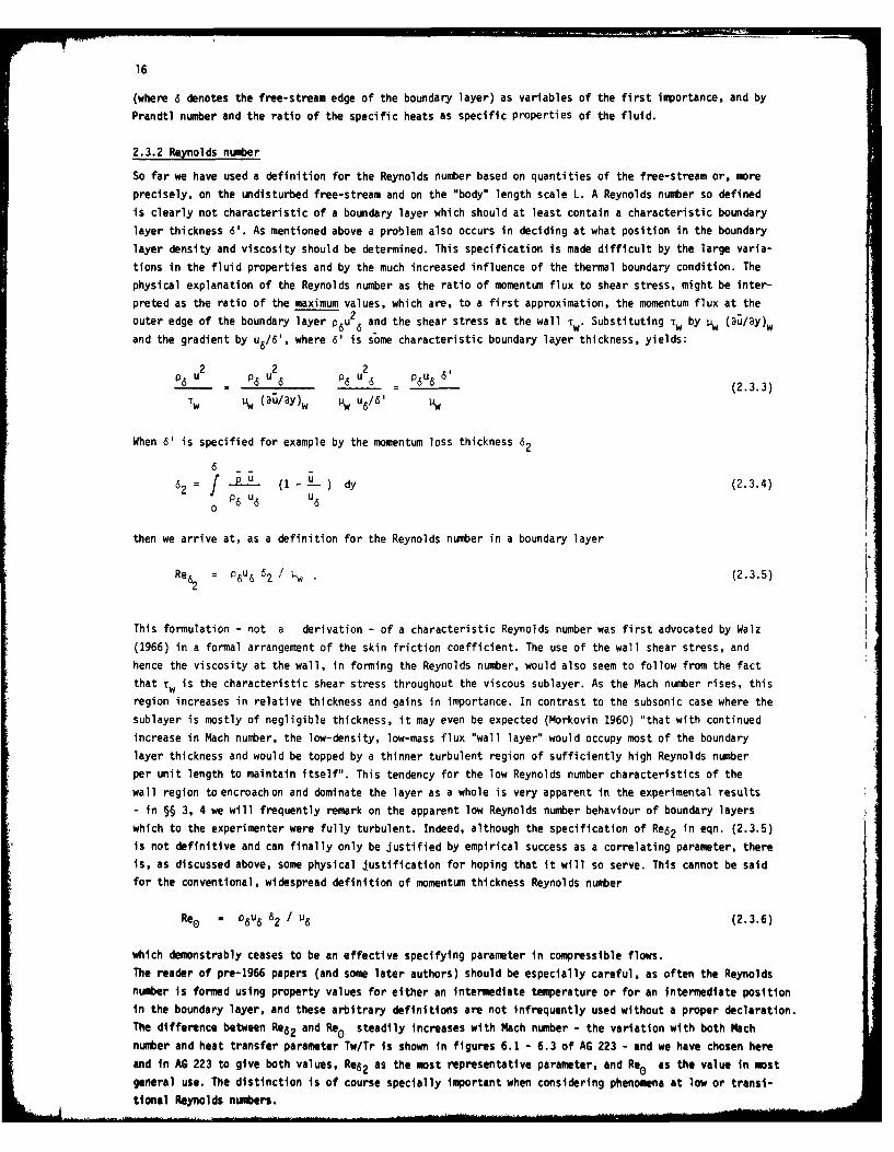
2.3.2 Reynolds number

So far we have used a definition for the Reynolds number based on quantities of the free-stream or, more

precisely, on the undisturbed free-stream and on the "body" length scale L. A Reynolds number so definedis clearly not characteristic of a boundary layer which should at least contain a characteristic boundary

layer thickness 6'. As mentioned above a problem also occurs in deciding at what position in the boundarylayer density and viscosity should be determined. This specification is made difficult by the large varia-

tions in the fluid properties and by the much increased influence of the thermal boundary condition. Thephysical explanation of the Reynolds number as the ratio of momentum flux to shear stress, might be inter-

preted as the ratio of the maximum values, which are, to a first approximation, the momentum flux at theouter edge of the boundary layer p~u2. and the shear stress at the wall 'w* Substituting Tw by pw (au/ay)wand the gradient by u6/6', where 6' is some characteristic boundary layer thickness, yields:

p6 -2 u 2 = 6 6 6' (2.3.3)Tw 1, (a ;l aY )w 1w u 6 ' 61w

When 6' is specified for example by the momentum loss thickness 62

662u dy (2.3.4)

0 P6 u6 6

then we arrive at, as a definition for the Reynolds number in a boundary layer

Re 2 : 06 62 / 1w• (2.3.5)

This formulation - not a derivation - of a characteristic Reynolds number was first advocated by Walz

(1966) in a formal arrangement of the skin friction coefficient. The use of the wall shear stress, andhence the viscosity at the wall, in forming the Reynolds number, would also seem to follow from the factthat Tw is the characteristic shear stress throughout the viscous sublayer. As the Mach number rises, thisregion increases in relative thickness and gains in importance. In contrast to the subsonic case where thesublayer is mostly of negligible thickness, it may even be expected (Morkovin 1960) "that with continuedincrease in Mach number, the low-density, low-mass flux "wall layer" would occupy most of the boundarylayer thickness and would be topped by a thinner turbulent region of sufficiently high Reynolds numberper unit length to maintain itself". This tendency for the low Reynolds number characteristics of thewall region to encroachon and dominate the layer as a whole is very apparent in the experimental results- in §§ 3, 4 we will frequently remark on the apparent low Reynolds number behaviour of boundary layerswhich to the experimenter were fully turbulent. Indeed, although the specification of Re62 in eqn. (2.3.5)is not definitive and can finally only be justified by empirical success as a correlating parameter, thereis, as discussed above, some physical justification for hoping that it will so serve. This cannot be saidfor the conventional, widespread definition of momentum thickness Reynolds number

Reo - P6u6 62 / V6 (2.3.6)

which demonstrably ceases to be an effective specifying parameter in compressible flows.The reader of pre-1966 papers (and some later authors) should be especially careful, as often the Reynoldsnumber is formed using property values for either an intermediate temperature or for an intermediate positionin the boundary layer, and these arbitrary definitions are not infrequently used without a proper declaration.The difference between Re62 and Re0 steadily increases with Mach number - the variation with both Mach

number and heat transfer parameter Tw/Tr is shown in figures 6.1 - 6.3 of AG 223 - and we have chosen here

and in AG 223 to give both values, Re62 as the most representative parameter, and Re0 as the value in mostgeneral use. The distinction Is of course specially important when considering phenomena at low or transi-

tional Reynolds numbers.

17

2.3.3 Pressure gradient

We also require some for of a pressure gradient parameter. This does not emerge explicitly from the

conservation equations. Such a parameter can, however, be derived in several ways. One form is obtained

by comparing the pressure gradient to the shear stress times a characteristic boundary layer thickness:

dp/dx 6' = u u du6 6' = P U6 6' d -du/dx

- _ !___ 6./.x = Re 6 u6/dx"w .rw dx 1w (Da/ay)w u 616,

When the characteristic thickness 6' is taken as 62 one obtains the pressure gradient parameter which has

for a long time been used for Incompressible turbulent boundary layers,

P 6 u 6 62 du6 =62 dp (2.3.7)Tw dx Tw dx

In a few catalogue entries 1l2 was calculated but very often the distances between the free-stream velocity

measurements were too large to permit an accurate determination of the gradient du6 /dx.

Clauser (1956) in his work on constant density equilibrium boundary layers was possibly the first to show

that a parameter of this type, HI. using 6i, as the characteristic length, provided an adequate pressure

gradient parameter for this restricted class of flows. l1 is also suggested by the raw form of the boundary

layer integral equation

d (P6 u 6 62) = Tw + 61 X

though the strict conditions for similarity cannot be satisfied. In a variable density flow where

6

= 6 f (I - 0 u ) dy (2.3.8)

0 p6 6

we doubt that a general correlation can be achieved with II, as parameter since cases can occur for which

61 becomes negative. As an example, see the flow with strong acceleration and wall cooling studied by

Back & Cuffel (1972 - CAT 7207 series 01).

I2 has one disadvantage which it shares with n 1 in that it tends toward infinity in the case of flow separa-

tion. This can be avoided by using the alternative second definition

*l du6 /dx*Re6 (2.3.9)u62/62

In supersonic flow, the pressure field is not adequately described by its streamwise derivative alone.

Principally as a result of the large ratio between dynamic head and static pressure, substantial pressure

variations may occur normal to the wall on which a boundary layer grows. An outline of the factors involved

is given in § 5, while a detailed consideration of the pressure field in the boundary layer is given in § 6.

Here we note that a parameter is required to express the likely importance of the normal pressure gradient

and we propose the quantity

SW - (ao/ax) / (av/ax) (2.3.10)

which represents the degree to which a change in Prandtl-Meyer angle (v), and so Mach number, is associated

with a change in flow direction (0), or streamwise curvature.

2.3.4 The hypersonic regime

We have not, in this section, made any attempt to draw a distinction between the "supersonic" and the

*hypersonic" regime - and consider any such attempt unrewarding. As M6 increases, there is no possible

simplification of the equation of motion in the boundary layer as a result of being able to assume

18

M> 1 - as in many gasdynamic applications. If any such distinction is to be made, it would for this

purpose, be related to some basic change in the relative importance of the turbulent terms, for example

by defining a "hypersonic turbulent flow" as one for which Morkovin's hypothesis (§ 2.4) has demonstrably

broken down,or where chemical reactions have to be taken into account due to the high total enthalpy of

the high Mach number flow. It is not possible to say that this occurs for M larger than any particular

value.

2.4 Morkovin's hypothesis

It is difficult to perceive how strongly the terms u'v', v'T', and P'v' are influenced by compressibili-

ty by direct inspection of eqns. (2.3.1) and (2.3.2). The Mach number appears explicitly only in the dissi-

pation term of the energy equation which contains v I 9u/y. As au/3y tends to zero in the outer layer

and Uv' towards the wall, the product of the two may be smaller than the first term containing (au/3y)2

only. The term T'v' need not be considered here since it can be eliminated by means of the continuity

equation (2.2.1).

In order to obtain an estimate of the importance of the fluctuating quantities we examine the definition

of total enthalpy H in a boundary layer. For instantaneous quantities H is defined:

H = cpTo =c pT + 1/2 (u2 + v2 + w2 ) . (2.4.1)

After the introduction of mean and fluctuating quantities this equation can be written for a two-dimensional

flow as

-2 u 1 1 [u,2 + -2 v,2 2To' T' + u + [ + 2 v +v +v +w ]. (2.4.2)

T 0 T cpTo u cp T0

When fluctuation terms are sufficiently small for second order terms to be neglected (a condition which

embraces the region of validity of the hnt-wi~e anemometer at high speeds) one can write with some re-

arrangement (Morkovin 1960)

o -' y-l 2) -1 u' (Y-1) M2 (2.4.3)(1+__ - M) +(24)

T 2 + M2

Under the additional assumption that To/To is an order smaller than the two remaining terms (confirmed bymeasurements e.g. Kistler (1959) in boundary layers along adiabatic walls) - this is called the "strong

Reynolds analogy" statement by Morkovin (1960) - we can write

T'- (y-1) M2 - . (2.4.4)

T u

Using eqn. (2.2.10) yields for T/T

. + (2.4.5)

T 0 oT P

and neglecting pressure fluctuations and second order terms one obtains

T' = .p' = .(Y-1) M2 =._ - (2.4.6)

T Pu

Eqn. (2.4.6) was given by Morkovin (1960, eqn. 8). Bradshaw & Ferris (1971) deduced from this equation that

if P'15 is small the turbulence structure is not affected by compressibility effects and called thisMorkovin's hypothesis.

Ig .

As in the outer region of a boundary layer the velocity fluctuations are usually small and the Mach number

large, (T) 2 /T is nowhere larger than 0.1 even at a Mach number 5. Under the above assumptions temperature

and density fluctuations do not influence the turbulence field significantly up to at least a Mach number

of 5. This means that the knowledge of the turbulence structure gained in subsonic flow can be extended to

supersonic flow.

2.5 Analytical solutions of the energy equation

2.5.1 The total enthalpy equation

Further insight into the relation between the mean velocity and the mean temperature field can be gained

by deriving an equation for the mean total enthalpy. This can be achieved by multiplying eqn. (2.2.3) by

u and adding this equation for the mechanical energy to the thermal energy equation (2.2.8). After some

rearrangement and writing

H u + 2/2 (mean total enthalpy per unit mass) (2.5.1)

one obtains

+ p v H ._ = 3H + a Pr-1 - ;upY U ;y F -5Y) y -[ u - I ]Y

- - 4 T p + Cp p v'T' ] (2.5.2)ay

This equation is identical with eqn. (155) of Howarth (1953) if due account is taken of eqn. (2.4.2),

ignoring the terms in square brackets in the latter equation. Eqn. (2.5.2) has the following boundary

conditions:

y = 0:

u= v =0; v7-= v'T' = -v = 0; H = cpTw;

y 6:

u u6; ' : vT' = 0; H = cpT6 + u2 6/2.

Under the special conditions Pr = 1 and (u p- rr+ cp p v'T') independent of y or zero, eqn. (2.5.2) has

a particular solution, H = constant, which was first published by Busemann (1931) for laminar boundary

layers. This solution will be discussed and extended for values of the Prandtl number smaller but close

to one in § 2.5.4. While the assumption Pr = I needs little justification for the technically important

gases, it is less obvious under which conditions (u p-G -v + Cp p v'T') may be assumed to be independent

of the coordinate y or even be zero. Neglecting second order terms in eqn. (2.4.2), multiplying the re-

maining terms by p v' and taking the temporal mean, yields

Scp v'T P : cp v'T' + p . (2.5.3)

Now for adiabatic flow Morkovin (1960) has shown thdt

(V7r)/77r) << 1 which, inserted into eqn. (2.5.3)

leaves us with

PC v'T' + u V 0. (2.5.4)

Eqn. (2.5.4) shows further that subject to the above condition cp v'T' must be of the same order as ;-77.

Another possible line of argument starts from the energy equation for instantaneous quantities. Comparing

this equation for H with the equation for H, in which the temporal mean was taken, allows the conclusion

that if AH/ay - 0, for the particular solution giving H z constant, then 3H/ay is very likely to be zero,

20

implying that aH'/ay must be zero also. This reasoning leads to

(p c v'T' + _ 'UV r) = 0. (2.5.5)

The case for accepting this result is further developed in Howarth (1953).

2.5.2 The total enthalpy integral

The special case of adiabatic flow is clearly of the greatest interest both experimentally and theoretically.

It is difficult to ensure that a test wall is in fact truly adiabatic, and one of the most important

experimental criteria available is that there be a zero streamwise growth rate of the total enthalpy integral

across the boundary layer. If we integrate eqn. (2.5.2) with respect to y from zero to a "D-state" well

outside the boundary layer, we obtain

D D Df 1 +dP+ [_ Uv + c IvT' = 0 . (2.5.6)

0 ax ay 7y 7rU y p

An evaluation of the second and third term in connection with the boundary conditions of eqn. (2.5.2) yields

D

f L + (P v + Trv-r) - ] dy + X w (-)W 0 . (2.5.7)

0

It should be noted here that a number of the "conventional" assumptions at the boundary layer edge have been

made. For instance, assuming that (Du/3y)D = 0 and (at/ay)D = 0 implies, probably correctly, that moleculartransfer terms at the boundary layer edge are negligible. Less satisfactory in a windtunnel flow is the

assumption that the term ( u p U'rV)D does not contribute to the energy balance as although =v does fall

off, many experimental facilities have a strongly turbulent freestream flow, and ; p is a large term at the

D-point.

Generally, particularly in high Mach number facilities, both the choice of the D-point (see § 7 below) and

the free-stream turbulence rate require a carcfu' assessment. Otherwise one is easily led to erroneous

estimates of the total energy content of the boundary layer and to wrong conclusions about the existence

and/or magnitude of the so-called overshoot (see § 2.5.6 below).

After differentiation, rearrangement and taking account of the continuity equation (2.2.1), eqn. (2.5.7)

yields:

D

-r f u (H- H) d y + Xw () 0

0

and after integration between two streamwise positions x, and x2

D x2 x2

EfPU( H D)dy I f I ( dx (25.o xI x1

On the left-hand side we have the difference in the rate of flux of total enthalpy, integrated across the

boundary layer, between the fixed positions x, and x2 and on the right-hand side the heat flux at the wall

between the same fixed positions x, and x2 .

For an adiabatic wall the right-hand side of eqn. (2.5.8) Is zero and, by assuming that at x - 0 H = HD,

one obtainsD D

HD P dy)/~J P ; dy). (2.5.9)

0 0

21

This latter equation is often used as a check as to whether a flow is truly adiabatic when both total

pressure and total temperature profiles across the boundary layer are available.

Equations (2.5.8) and (2.5.9) are formally the same as those for compressible laminar boundary layers

which can be found in Howarth (1953 p. 397).

2.5.3 The mean temperature distribution

Since it is impossible to determine the mean velocity profile in a compressible turbulent boundary layerwithout knowing the temperature distribution across the boundary layer, Morkovin (1960) is certainly

correct in stating that "the second cornerstone of analytical and empirical evaluations of skin frictionand heat transfer lies in the correct determination of the mean static or stagnation temperature profiles".It is therefore extremely fortunate that we know of two exact solutions giving relations between the mean

static enthalpy 5 or the mean static temperature T and the mean velocity ; in which the parameters are theMach number, the ratio of the specific heats, and a heat transfer parameter. We shall first discuss these

particular solutions of the energy equation for Prandtl number equal to one and then extend the discussion

to a Prandtl number range 0.70 < Pr < 1.

2.5.3.1 The mean temperature distribution for Pr = 1 in a boundary layer along an adiabatic wall

As already mentioned in § 2.5.1 the equation for the mean total enthalpy (2.5.2) has the particularsolution H equals constant under the conditions that the Prandtl number is unity and that the term

(u p + p cp v'T') is zero or independent of y. A justification for this latter condition was givenin § 2.5.1. The solution H = constant satisfies the boundary conditions of eqn. (2.5.2) only if one

requires that (AH/ay)w = 0, i.e. according to eqn. (2.5.1) that ( T/ay)w be zero. This implies that theheat transfer between the fluid and the wall must be zero. Now if R is constant across the boundary layer,then the following relationship holds

c T + u/ p T 2 6/p u/2=c T + u2 /2 (2.5.10)

and noting that (e.g. Busemann in Wien, Harms 1931)

(u2 /2)/c T, = (y-1) M2 12 (2.5.11)

one obtains

T = 1 + _-1 M2 [1 2 (2.5.12)

T6 2 U6

Eqn. (2.5.12) holds for both laminar and turbulent boundary layers for all pressure gradients dp/dx underthe condition Prandtl number unity and zero heat transfer at the wall.

The reader should note that this solution cannot describe correctly the temperature distribution at the

outer edge of an adiabatic boundary layer due to the limitation that the Prandtl number has been assumedto be unity (see § 2.5.4.1).

For the boundary condition y - 0 and u -0 eqn. (2.5.12) yields a relationship for the so called adiabaticwall temperature (again for Pr = 1),

(Tw)ad = 16 (1+ - " (2.5.13)2

The temperature difference (Tw)ad - T6 denotes the temperature increase of an adiabatic wall due to

compressibility effects.

If eqn. (2.5.12) is re-written in terms of the total temperature It reduces to

T6 To6 -1 (2.5.14)(Tad To

The temperature-velocity relationship expressed by eqn. (2.5.12) was given for laminar boundary layers by

Busemann (1935) and Crocco (1932).

22

2.5.3.2 The mean temperature distribution for a boundary layer with zero pressure gradient along an

isothermal wall. In this paragraph we discuss the second analytical solution of the energy equation.For this purpose we need the assumptions that the pressure gradient dp/dx is zero and that the temperature

of the wall is constant. Furthermore the Prandtl number range will be restricted.

The following equations were derived in principle by van Driest (in Lin 1959) who, however, used the

concepts of the eddy coefficients of friction e and heat transfer cX resulting in a mixed Prandtl number

Prm Cp ( +c

PrM = (2.5.15)X + C

We think it more advantageous to keep the molecular Prandtl number Pr = Vc pcA and the turbulent Prandtl

number Prt (cf. eqn. 2.5.18) apart in the terms of the following equations and present therefore a slightlydifferent derivation for the T - ; relationship. For this it is convenient to substitute the term

(P v + Iv) in the energy equation (2.2.5) by means of the equation of motion (2.2.3) and to introduce

= pau/ay resulting in

; - -h.~ I ~~)-~~ .P u h a rl . .. (P = vd;-a

3x T ay ay By ax dx dx

2

= (---) -- (p cp v'T') + - - iT . (2.5.16)ay Pray ay p a

The independent variables x and y are now replaced by E and u using the Crocco transformation u - u ( , y)

and x = (. Hence eqn. (2.5.16) becomes

2i [1 + ( -- ] + - (1-Pr) - u -

au Pr au Pr au au a d& au

+ ah a ( v)] (Prt - 1) - p I [i +L (1_ at)] -0 (2.5.17)Prt Au au au Prt au

where the Prandtl number for turbulent flows is defined as

Prt = 'v aT/ay =ir'- ah/ay (2.5.18)=V a-/ay -iWr a/ay

So far we do not have an analytical solution for eqn. (2.5.17) and it is necessary to introduce furthersimplifications. One possible assumption is that the pressure gradient in the streamwise direction,

dp/d& = dp/dx, be zero which implies that ah/a = 0. Eqn. (2.5.17) then reduces to

TI [1l+i (i. --)] + L- [ --P -Tl ( -Pa)]au Pr au au Pr a Prt au

=a 1+ L _( h = 0 (2.5.19)

au Prt au

A simple solution for eqn. (2.5.19) can be given for laminar boundary layers where = is zero and if it

is further assumed that the Prandtl number is unity. The resulting relationship was - though derived in a

different manner - published independently by Crocco (1932)+) and Busemann (1935).

+) This date is given by Schlichting (1965). The original source has not been consulted..

23

Under these assumptions eqn. (2.5.19) yields

2= 1 (2.5.20)

3u2

which with eqn. (2.5.11) and the boundary conditions

y 0 = ; Tw =constant (Y = : = 6; T= T 1\(2.5.21)

y=6:u u 6T ~Tgives

Tw (1 W) u M 1 (2.5.22)

T T T1-)~ '66 u 6 u 6 .26 6 T6If the adiabatic wall temperature, eqn. (2.5.13), is introduced one obtains the alternative form.

T- = Tw + (Twad T _ 1 ( )2 (2.5.22a)

T6 T6 T6 u6 2 6 u6

Eqn. (2.5.22) is strictly valid only for laminar boundary layers with zero pressure gradient, constant walltemperature and Prandtl number unity. It is commonly referred to as the Crocco-relationship (e.g. Rotta

1964).

For a discussion of the solutions which are obtained from eqn. (2.5.20) when boundary conditions, different

from (2.5.21) are used, the reader is referred to Rotta (1964).

In the case of an adiabatic wall, when (Tw)ad = Tw, eqn. (2.5.22a) becomes identical with eqn. (2.5.12).

Another form of eqn. (2.5.22) which is often used for comparison with measurements follows after some re-

arrangement

T' " TW HO -Hw -

0 - ___0__ =u (2.5.22b)

T06 Tw Ho6 Hw u6

and is sometimes called the "linear" temperature-velocity relationship.

The range of validity of these two equations can be extended to turbulent boundary layers if one assumesthat both Prandtl numbers, Pr and Prt , are one. The pressure gradient dp/dx must, of course, be zero andthe wall temperature constant. Under these conditions eqn. (2.5.19) yields formally the same solution, i.e.

eqn. (2.5.22). The difference in the temperature profile for laminar and turbulent flows with the sameboundary conditions will then be caused only by the different velocity profiles.

Before we proceed to further analytical solutions of the energy equation which hold also for a Prandtlnumber in the range 0.70 < Pr < 1, van Driest's (1955) form of the energy equation will be given which is

essentially identical with eqn. (2.5.19).

[@ 1 h)IPr M a; aT

T 1 -ah +1] + r= 0 (2.5.23)au PrM au PrM au au

where T = i au/ay - _p =v and the mixed Prandtl number PrM is defined by eqn. (2.5.15).Eqn. (2.5.23) is easier to handle than eqn. (2.5.19) though one cannot distinguish any longer between the

development of the molecular and the turbulent Prandtl number across the boundary layer. For ease of

handling we shall henceforth use eqn. (2.5.23) while retaining eqn. (2.5.19) briefly for discussion in§ 2.5.4.2 below.

24

2.5.4 A semi-empirical temperature distribution for Pr 0 1

Van Driest extended Crocco's (1946) analysis for an arbitrary but constant Prandtl number to a "variable

Prandtl number theory" for both laminar (1954) and turbulent (1955) compressible boundary layers. The aim

of van Driest's investigation was largely to determine theoretically the Reynolds analogy and recovery

factors for compressible boundary layers with zero pressure and wall temperature gradients in streamwise

direction (dp/dx = 0 and Tw = constant). Walz (1956, 1959) has further developed van Driest's work to

arrive at an extended form of the Crocco temperature velocity relationship (2.5.22). His version (eqn.

2.5.37) allows for constant Prandtl numbers in the range 0.7 < Pr < 1 which covers all technically important

gases. The modification becomes the more significant as the Mach number of the flow is increased. The

van Driest-Walz approach is outlined below.

2.5.4.1 Solutions of equation (2.5.23). Following Crocco, or, for a turbulent boundary layer, Van Driest

(1955) a rearrangement of eqn. (2.5.23) leads to the following dimensionless equation

-) + (l-PrM) - M2 (2.5.24)PrM T PrM

which is a linear, first-order differential equation in (h'/PrM) as a function of u,, at constant x. The

symbols h and u. denote h/h and /u6 respectively, and the primes indicate differentiation with respect

to u. alone.

After integration - for details see van Driest (in Lin 1959) - eqn. (2.5.24) becomes

u.1u. . R*I)M

h. (-*) = A.(0) + [1-5 (0)] + (y-l) t E- -u -) R (1) - (u)] (2.5.25)S (1) S*(1)

Eqn. (2.5.25) gives the enthalpy distribution for a turbulent boundary layer from the wall to the outer

edge under the conditions dp/dx = 0 and constant wall temperature and was first given in this form by

van Driest (1955).

The integrals S*(-u) and R*(u*) are defined by

* T (l-PrM)S*(u.) PrM exp (2.5.26

and

R*(*) 1 . -Pr~ dTuM 1-PrR*(u.) f PrM exp I - I d T f! exp (f dT) du] du. (2.5.27)

TT0 Tw 0 rw

S (1) Is a general expression for the Reynolds-analogy factor

1 T

S*(1) -s = f PrM exp (- f (1-PrM) .T) du. (2.5.28)0 T w

T

and R (1) a general expression for the recovery factor

1 T

2 R(1) E r - 2 PrM exp f - (l-PrM) LTf T-o r

1

f exp [f (1-PrM) dr ;d. d;, (2.5.29)

oi , T

25

Now, eqn. (2.5.25) can only be solved if the Prandtl number and the shear stress distributions are knownin order to evaluate Integrals (2.5.26) to (2.5.29). Under the assumption that thcPrandtl number is con-stant but may assume values different from unity eqns. (2.5.26) to (2.5.29) can be written (for laminarflows these equations were originally given by Crocco):

Z. PrM-l-Pr 6.)- Prd E- . = PrM •S(), (2.5.30)

No0

- urPr Pr"-1 u. ~ -PrMRPr} PrM Z. [IT) du*1 d = PrM R (.) (2.5.31)

o o

1 P r _ 1I

SprM (1) = PrM 1 I du* = s, (2.5.32)N00

and

2R* () 2 1 1 du.}d = r. (2.5.33)p (I) = I dI

P

0 0

For a constant mixed Prandtl number PrM eqn. (2.5.25) then yields

Pr M ( PrM 1 2 PrM S(i) 2 PrM R(-,)

=h(O) + [1-h.(O)] s + r M s r (2.5.34)

Eqn. (2.5.34) was first given by Walz (1956, published 1959) who introduced a further assumption, namely

PrM S (U*) 2 PrM R (u*) -2- u. and r u* (2.5.35)

As an inspection of eqns. (2.5.30) and (2.5.31) shows, these relationships can hold only if the Prandtlnumber is close to unity, say in the range 0.7 < PrM < 1, which is the case for technically important gases.Introducing the relationships (2.5.35) into eqn. (2.5.34) yields

h( i) (0) + [1-f*(0)] -. + r 6[M - U2 (2.5.36)

or for constant specific heat cp

T/T6 -- (Tw/T6) + [1+ r I M6 - Tw/T6] (u/ud) - r ''M (u/u6 ) (2.5.37)

Differentiating eqn. (2.5.36) with respect to y and assuming zero heat transfer at the wall, which resultsin (af/ay)y_0 = 0, one obtains for the temperature at the wall, now called the recovery temperature Tr

T M2

Tr = T, (1+r i M ). (2.5.38)

Eqn. (2.5.38) was originally derived by van Driest (1955) using eqn. (2.5.25) and given empirically byAckermann (1942) and H.B. Squire (1942). Both authors, however, used a function dependent on the Prandtlnumber instead of the recovery factor as defined by eqn. (2.5.33) (see Schubauer& Tchen in Lin 1959).Since all the quantities in eqn. (2.5.38) can be determined from measurements when the wall is adiabatic,this equation is often used for an experimental determination of the recovery factor as

Tr - T

Tr IS (2.5.38a)To r T6ea

If the recovery temperature is introduced into eqn. (2.5.37). the temperature velocity relationship reads

26

_ I Tr -Tw (-

- 6 21 _ _ ;l - ( 2 .5 .3 7 a )T6 T6 u6 2

or

L-w +Tr -Tw r Y- 7 ( )-(2.5.37b)

T6 T6 T6 u 6

When r = 1 eqn. (2.5.37b) is identical with eqn. (2.5.22a), as derived for Pr = 1.The equations listed under (2.5.37) have been called Walz's equations (e.g. Voisinet & Lee 1973).

Likewise, after some rearrangement, another form of eqn. (2.5.37) is

To - Tw Tr Tw (u)2 (2.5.37c)

TO6- Tw T06 Tw To6 -T- -

which may again be compared with eqn. (2.5.22b) derived for Pr = 1.

Eqn. (2.5.37c) may also be written

TO - Tw u ( -)2= B U + (1-0) (U (2.5.37d)

T06 Tw U6

where a = Tr Tw (see Danberg 1971).T06 Tw

Danberg calls eqn. (2.5.37d) "a well known modification of the Crocco temperature velocity relationship".

Still another form of eqn. (2.5.37) is mentioned by Rotta (1965) and called case I or Crocco's solution:

TO Tw Tr -Tw + Tr ] (u) 2 (2.5.37e)To To To5 6 To U

T06 T06 T06 u 06 6

For Prandtl number unity equation (2.5.37e)becomes identical with eqn. (2.5.22b) since Tr + T06.

A special case of this temperature-velocity relationship is obtained for zero heat transfer at the wall,

i.e. for an adiabatic wall. Then eqn. (2.5.37a) for example reduces to

-T2)(qw=O) = I + r i2 M6 (1- ( )2] (2.5.39)

which again is equivalent to eqn. (2.5.12) for Prandtl number unity. Another form of eqn. (2.5.39) - some-

times called the modified Crocco equation - follows immediately from eqn. (2.5.37c) for TW = Tr, i.e. for

zero heat transfer:

T0 T r = u_ 2 (2 .5 .4 0 )

T06 Tr u6

Probably because of the similar form of eqn. (2.5.39) and (2.5.12) the validity range of the former equations

is sometimes extended to flows with pressure gradients in the rain stream direction along adiabatic walls.

Since no analytical solution for these boundary conditions is known, eqn. (2.5.39) may represent a reasonablefirst order approximation for the temperature distribution where the Prandtl number differs from unity and

lies in the range 0.7 < PrM < 1. Eqn. (2.5.40) is recommended as being especially suitable for boundarylayers in wind tunnel nozzles by many authors, irrespective of upstream and local temperature conditions at

the wall or upstream and local pressure gradients in the main stream direction or normal to the wall.

Eqn. (2.5.40) is sometimes called the "quadratic" temperature velocity relationship in comparison to the

27

"linear" temperature-velocity relationship eqn. (2.5.22b) derived for Prandtl number unity.

If *linear" and "quadratic" relationships are used in the same figure for a comparison with measured data,then the pairs of comparable equations (2.5.14 & 2.5.22b) and (2.5.40 & 2.5.37c) should be taken. Unfortu-

nately this simple rule is neglected by many authors.

Table (2.5.1) gives a sumary of the temperature velocity relationships derived so far and their status

and restrictions.

Table 2.5.1 Temperature-velocity relationships for compressible turbulent boundary layers

Number Equation Status Restrictions

(2.5.12) T/T5 I + ((y-I)/22 M2 [1- (5/u6)2 exact f Pr = 1; adiabatic wall{ - _

(2.5.14) H /Hw = 1 exact { (u puv-+ pcp v'T') 0 f(y)

(2.5.22) T/T6 = (Tw/T6) + [1-(Tw/T6)] (u/u6)

+ [(2J M [(u/u 6) - (u/u6)2] exact { Pr = 1; Prt = 0; dp/dx = 0;

{

(2.5.22b) (To-Tw)/(ToD-Tw) = (Ro-Hw)/(Ho;Hw) = u/u5 exact { Tw = constant

(2.5.39) T/T6 - 1 + r [(y-1)/2] M2 [1-(u/u6)2] based on { PrM = constant and 0.7<Pr, 1 ;

eqn. {

(2.5.40) (To-Tr)/To6-Tr) = (u/u.)2 (2.5.25) { dp/dx = 0; adiabatic wall

(2.5.39) 1 These equations are used for flows with semi- { PrM = constant and 0.7<PrMi1 ;} pressure gradients in mainstream direction

(2.5.40) 1 along adiabatic walls because of their empirical { adiabatic wall} form which is similar to eqns. (2.5.12)

and (2.5.14).

(2.5.37a) T/T6= (Tw/T6) + [1+r[(y-I)/2]M2 - (Tw/T6)]

(u/u6 ) - r [(y-1)/21 M2 (-u/u6) 2 based on {Pr = constant and O.7<PrM

(2.5.37d) (To-Tw)/TogTw) - [(Tr-Tw)/(j,6-Tw)](i/u6 ) eqn. { dp/dx = 0; Tw = constant

- 2+ [(To 6-Tr)/(To6-Tw)l (u/u6) (2.5.25)

(2.5.37e) To/To6 = (Tw/To6) + [(Tr-Tw)/To6] (u/u6 )

+ [1- (Tr/To6)] (;/u6)2

2.5.4.2 A discussion of equation (2.5.19). If the boundary layer is divided into a viscous sublayer where

the influence of viscosity dominates over that of the turbulence terms and into an outer region where the

turbulence terms dominate over the viscous shear stress, then eqn. (2.5.19) can be simplified and reduces to

I R 1 hr-Pr 3TIa[ + 1- ( a 7)+a -V'F --Pr z 0 (2.5.41)

au au au au

and

+aDR)J+au I-Prt ..-. ( -7r)= 0 (2.5.42)au t au au Pr t au

respectively.

For constant but non-unity Prandtl number the respective solution for eqns. (2.5.41) and (2.5.42) is formally

given by eqn. (2.5.34) where the mixed Prandtl number PrM must be substituted by the molecular Prandtl

number Pr or the turbulent Prandtl number Prt respectively. Since Pr z 0.72 and Prt = 0.90 (e.g. Lin 1959),

it remains to match the two solutions somehow in the buffer layer. This could be achieved by a straight

line to a first order approximation. We shall comment again on Prandtl number distributions in § 2.6.4.

I..

28

2.5.5 Other semi-empirical temperature distributions

Numerous attempts have been made to find analytical expressions for temperature distributions In turbulent

boundary layers. Among those which have come to our attention we have chosen a few, none of which appears

to us in any way better than the relations derived in § 2.5.4. This may be due to the fact that the authors

of these semi-empirical relationships were short of measurements which could be used for a comparison or

did not care to present comparisons over a wider range of data. For a survey of pre-1958 attempts to find

relationships between the static temperature and the mean velocity u the reader is referred to Schubauer

& Tchen in Lin (1959).

2.5.5.1 Zero pressure gradient and adiabatic wall. Schubauer & Tchen (Lin 1959) suggested a semi-empirical

temperature-velocity relation with "variable recovery factor", starting from the following equation written

in a form similar to eqn. (2.5.10)

cpT +1 r (y) u2 =c T6 + r6 u6 =(cT)

p 7 6 T6 6 p w q =0.

This yields

w+ ) (2.5.43)T 06 T 6 6

where

r (y) - 1

r (6) - 1

If the distribution of the recovery factor is chosen suitably, eqn. (2.5.43) can represent a total temper-

ature distribution with an overshoot.

A further analytical expression for the temperature as a function of the velocity was given by Whitfield

& High (1977) in adiabatic or constant wall temperature boundary layers with constant but non-unity Prandtl

numbers. Here the Reynolds stress was assumed to be proportional to the local turbulent kinetic energy in

the boundary layer

2T p exp (-4n5/2)

where n = y/6 was approximated by (u/u6)m and inserted into eqn. (2.5.23).

This results in a second-order, non-linear ordinary differential equation for which zeroth and first-order

perturbation solutions were obtained in terms of the small parameter c = 1 - PrM. For the adiabatic wall

case the solution permits the calculation of the total temperature overshoot and is apparently used at

AEDC for data reduction. Comparisons with measurements were performed for data given by Gates (1973),

Danberg (1964), Hopkins & Keener (1972), and Bertram & Neal (1965). Some of these data, however, do not

show an overshoo.t (the reader is also referred to Laderman (1977) who found good agreement with the

theoretical prediction suggested by Whitfield & High). Finally Hopkins & Keener (1972) presented an

empirical relation

TO - Tw 1.660 (u/u)

T06 - Tw

which was found to fit their data and was used to determine total temperatures in the region between the

innermost probe measurement and the wall. This relationship comes close to eqn. (2.5.40) which is valid

for zero heat transfer.

2.5.5.2 Zero pressure gradient and isothermal wall. Rotta (1960) presented a more sophisticated model for

the temperature distribution. In our notation this semi-empirical relationship reads for the log-law region

29

T =Prt [rq M u 2 ( .. 4T.... (-u)2] q Cu (2.5.44)Tw uT 2 UT

where H and aq are defined by eqns. (3.2.8) and (3.2.9) respectively and the "constant" of integration

C1 is determined from experiments as

C1 = 1 - 3.4 aq - 0.2 M . (2.5.45a)

Bradshaw (1976, 1977b) gives another relationship for C1

C1 = 5.2 + 95 M2 - 30.7 Bq - 226B2 (2.5.45b)

Bradshaw states "that the trends of the two equations (2.5.45 a and b) are quite different except for therise in C1 with M" but he concludes "the present evidence, though inconclusive, suggests that changes in

C1 need be considered only if accuracies better than 5 to 10 % are being aimed at".

For the outer region of the boundary layer Rotta found

2_ Pr 2 (2.5.46)

weeT 6 T 2 6 u6 U6

where

u* = (urBq)/-(y-l) M2] and

62 2 (y-1) M2 - + cR q T Prt 1T

u and TR are here the velocity and temperature at "a point of virtual maximum temperature".

The data used for comparison by Rotta were those of Lobb et al. (1955) and Winkler & Cha (1959) for which

the important skin friction values were deduced from the slope of the velocity profile. Therefore such a

comparison cannot be conclusive.

Without giving any proof, Danberg (1971) states that "for the high heat transfer or high Mach numiber situ-

ation, the deviation of experimental data from the Crocco relationship is known to be significant". Hetherefore suggests a better method of correlating temperature profile data by introducing a length scale Lbeing a characteristic thermal boundary layer thickness and a characteristic enthalpy scale Hs. The non-

dimensional total enthalpy H++ is then expressed as

++ 1 H12H = (P_) 1 12 d (H-Hw) = In y + C + 2n"H (2.5.47)0 aw

where w. - sin t

Hs , A and the two profile constants CH and 7H are obtained from measured temperature data by a least square

method. This suggestion of an improved temperature relation cannot be regarded as established since theauthor has provided too little experimental evidence for comparison. Beyond this it is well known thatfour adjustable constants allow almost any curve fit. Since a comparison with measurements was performed in

one case only (Sturek 1970) it is too early to judge how this correlation will appear when applied to othercases.

2.5.5.3 Variable pressure gradient and variable wall-temperature. KUster (1972) extended a suggestion by

Cohen (1959) and Walz (in Favre 1964) to introduce the influence of the pressure and the temperature

gradients, dp/dx and dTw/dx, via two free functions cj - with J 1 and 2 - in a sami-empirical relation-ship which contains the exact solutions derived In § 2.5.4. The following relationship was suggested

A L. . . . . . . . . . . . - - I I . . .. . . 1 . . l . . . . . . . . . I '

30

n.+Hm(1-r) (.)1] (2 .5 .4 8-" + (I- T-6- [-U c ;

c. (2.. -1)] ____ 1+ 2

where m6 = (y-l) M6/2.The difficulty lies In the problem of how one should determine the functions cI nd c2. KUster used tie

first and second compatibility conditions but agreement with measurements was not satisfactory, judced from

the few comparisons with measurements pohlished in KUster's thesis. Nevertheless, we feel that ther,: may be

a possibility of improvement.

2.5.6 Comparison with measurements and conclusions

There exist two major comparisons between measured and theoretically predicted temperature profiles, one by

Walz (Favre 1964) and the other by Rotta (1964) and both investigations share the same problems. Firstly

very few reliable data were available at the time - Walz used the measurements by Lobb et al. (1955) and

by Winkler & Cha (1959), Rotta those by Lobb et al., Winkler & Cha, Hill (1959), and Nothwang (1957) - and

secondly neither Walz nor Rotta were aware of possible transition effects on the boundary layer profiles

they had investigated. Rotta's paper (1964) - better known as Rotta (1965) - has had a widespread effect

on the literature up to the present and so it seems worthwhile to repeat his main conclusions:

"(a) The measured temperature distributions in turbulent boundary layers with zero heat transfer

satisfy the requirement of vanishing energy loss thickness with sufficient accuracy.

The Crocco relation (eqn. 2.5.37) provides a good approximation to the actual temperature

distribution.

(b) The temperature distributions of boundary layers on nozzle walls are not representative of

those on flat plates. Obviously the temperature distributions on nozzle walls are severely

affected by the upstream history. The measured temperature distributions differ greatly from

the Crocco-relation.

(c) The available temperature distributions of flat plate boundary layers with heat transfer are

found to be only in moderate or poor agreement with the modified Reynolds analogy. ... The

measured temperature distributions display unexpected deviations from the Crocco solution.

(d) There is no evidence that the Crocco relation provides a satisfactory approximation to the

temperature distribution in supersonic turbulent boundary layers with heat transfer.

(e) Obvious shortcomings of the available experimental results shed doubts on the reliability

of the conclusions drawn."

Unfortunately many later authors have overlooked Rotta's important statement (e) and have happily copied

(a) to (d) only.

In the meantime Rotta's plea for more experiments has been fulfilled and the survey which follows,

accompanied by figures (2.5.1) to (2.5.19) and further ones in section 5 should allow a check and possibly

an extension of Rotta's conclusions.

The comparison between measured temperature distributions and theoretical predictions is confined to the

following boundary conditions:

Zero pressure gradient, adiabatic or isothermal wall, while the Prandtl number of the flow is assumed

constant and must lie in the range 0.7 _ PrM < 1. If the origin of the boundary layer is defined, for

instance by the known position of the leading edge of a flat plate, equations (2.5.37) to (2.5.40) can

be applied and suggest three different plots: 0/T06 , 1/T6 , n'd (I'o-Tw)/(To-Tw) versus u/u . Though

Rotta chose t'o/To 6 versus U/u, we prefer the latter two combinations. In a few cases we have also plotted

f0/To6 for comparison.

Since there follows a rather extensive discussion of mean temperature profiles we wish to define our aims

clearly. Firstly, we want to find out whether eqn. (2.5.37) provides a correct description of the tempera-

ture profile T/T, as a function of u/u,, y, r, and M6 ; secondly, many investigators have chosen to plot

31.

(oTw)/(To6-Tw) versus u/u6, a version of the temperature profile plot which requires very accurate wall

temperature and total temperature measurements, especially in the vicinity of the wall. Such accurate

measurements do not seem to be feasible in the inner region of the boundary layer at present, and for this

reason such a plot can lead to conclusions about physical effects which are - to put it mildly - at least

dubious. We also wish to issue a warning here to those readers who intend to compare their theories with

temperature measurements close to a wall. There are several cases where experimentalists - probably because

their temperature probes were much larger than their pressure probes - extrapolated their temperature

distributions towards the wall by assuming a priori the validity of certain relationships 1=T(u). Such aprocedure can easily be detected if the wall distance of a measuring station is compared with the dimensions

of the temperature probe in the y-direction. We have commented on such extrapolations in the "Editors'

Comment" of the entries in AGARDograph 223, e.g. Jeromin (6602), Samuels et al. (CAT 6701), Voisinet & Lee

(CAT 7202), Gates (CAT 7301), and Laderman & Demetriades (CAT 7403). For a comment on the latter measure-

ments the reader is referred to Meier (1977, p. 20). In this context we should also mention that total

temperature probes have been much improved over the past fifteen years. The reader is referred to the

investigations of Winkler (1954), Danberg (1961), Meier (1968, 1969b), Meier et al. (1974a), Voisinet et al.

(1974), Maurer & Petersen (1975), Meier (1977) and Hovstadius (1977b).

The comparisons presented here are intended to show that only the version T/T6 versus u/u, presents a

readily assessable picture from which conclusions about the validity of eqn. (2.5.37) may be drawn.

The investigation is divided into two parts, the first deals with boundary layers along adiabatic walls

and the second with boundary layers along isothermal walls. In both sections we shall distinguish between

flows with and without upstream effects. Further details of the cases discussed are given in table 2.5.2.

Table 2.5.2 Selected temperature profile measurements

CAT M Tw/Tr Re62 x 10-3 Type of probe

(i) Adiabatic wall, defined origin

7006 4 1 0.7 - 2 ECP +

7301 4.9 0.9-1 2.6 - 7 ECP

7305 10 1 0.2 - 1.6 STP ++ )

7402 2.5-4.5 1 1.1 - 9.1 STP

(ii) Adiabatic wall, origin not defined

6602 2.5-3.5 1 4.3 - 9.6 ECP

7003 1.7-3.0 0.9-1 1.9 - 7.2 STP

(iii) Isothermal wall, defined origin

6701 6 0.4-0.5 0.9 - 3.5 STP

6702 6.5 0.5-0.9 0.3 - 1.9 ECP

7204 6.3 0.3-0.5 1.1 - 2.3 STP

7205 7.2 0.5 1.4 - 3.0 STP+FWP ++++)

7702S 3.0 0.57-1 1.4 - 2.8 BWP ...

(iv) Isothermal wall, origin not defined

7202 4.9 0.2-1 1.6 - 38 ECP+FWP

+) ECP - equilibrium cone probe

++) STP - shielded temperature probe

-.+) BWP - bare wire probe

+++) FWP - fine wire probe

32

2.5.6.1 Temperature profiles (zero-pressure gradient, adiabatic wall). Among the measurements in compressible

turbulent boundary layers with zero pressure gradient along an adiabatic wall with a defined origin thoseof Mabey et al. (1974) seem to us very reliable, and we shall therefore make extensive use of them (see

also sections 3 and 4).

Profile M6 T/; Re82 T, K Tr K o from measured u/U 674.020100, 2.47 1.01 3515 295.3 293.2 - (T-T)/(T6-T):(6

- theoretical a. from measured To/To6

1.2

2 10 10

0.6.1 m -_- 00- 0

090.4 T.6

u/u8 /u0 1i 0

0 06 0.7 08 0.9 1.0 0 02 0. 06 0.8 10

Fig. 2.5.1 Comparison between measured and theoretical temperature profiles in aboundary layer (zero pressure gradient, adiabatic wall, defined origin)Mabey et al. (1974)

Figure 2.5.1 shows a sample from their data and will be used as an example for the method of discussion

of all data in this connection. The left hand graph shows a comparison of T/T6 as measured with the pre-

diction of eqn. (2.5.37a). The curve shown is obtained by using as input the measured values of u/u,Tw, T6 and M6. y was assumed to be 1.40, and the recovery factor r was taken to be 0.896. The measuredtemperature values are shown as filled diamonds, and it can be seen that agreement with the prediction

of eqn. (2.5.37a) is good - the maximum deviation is less than 5 %.

The right hand graph displays firstly the data plotted in a manner designed to show how well it fits the"quadratic" relationship of eqn. (2.5.40). This relation is shown as the lower solid line. Adjacent toT*-

this are open circles which represent values of T = (To-TwY(ToTw) calculated from eqn. (2.5.37d) using

as input the experimental values of u/u6. As might be expected, the two theoretical' values agree veryclosely, as any difference between them arises only from uncertainties in the selection of the recovery

factor r and from lack of confidence that the wall is truly adiabatic - eqn. (2.5.40) of course here

assumes that w = Tr while eqn. (2.5.37d) does not. The directly measured data, shown as solid diamonds,

apparently differ radically from the predicted curve, but as seen below, this difference is in factillusory. A more profitable comparison is between the predicted relationship of To/To to u/u, shown by

the upper line [here calculated from eqn. (2.5.37e)] and the measured values of T /T and 6/u, shown as

open diamonds. The differences in T do not exceed 1 % and it becomes apparent that tge seemingly large

differences observed in the plot of T against u/u6 arise from the fact that the ordinate represents adifference of two comparable relatively large and uncertainly determined quantities. The differences ob-

served, in other words, arise from the sensitivity of the plotting method chosen rather than from any realphysical phenomenon. This sensitivity is not necessarily undesirable - what is to be regretted is the

tendency of workers in the field to emphasize differences observed in this presentation as being technically

significant.

The sensitivity of the plot is further underlined in Fio.2.5.2 which shows data from two other profiles in

Mabey et al. (CAT 7402). The left hand graph shows that on the T/T, against u/u, axes there are only very

small differences between the profiles and that they are in good agreement with the theoretical curve of

33

4 - Profile M6 T./T R 2 Re0 (yu1 /.). 2949 2913 T. K1701 450 102 1528 6243 185 . . from measured u/ub

, -- 1701 4.49 1,00 3839 15372 165 - - /(To-6 ) = (/u6)L theoretical o o from measured T0/T06

03 - 10

I 1 08 --.-- -

T0

T6 062--- 04 T0 -Tw :A 00 O T

to T.6 -To

040

1': 0i O/ua 002 ... 4- .oO

05 06 07 08 09 1.0 0 02 04 06 08 10

Fig. 2.5.2 Comparison between measured and theoretical temperature profiles in aboundary layer (zero pressure gradient, adiabatic wall, defined origin).Mabey et al. (1974)

eqn. (2.5.37a). For the right hand graph the data for profile 74021704 are plotted twice, using two slightly

differing values for the wall temperature, both of which were given by the authors as experimental values

in different stages of their work. The only difference between the experimental values (open symbols) is

the small difference in Tw, but the plot apparently shows large systematic differences between the two

sets, especially in the vicinity of the well. Also shown adjacent to the line representing eqn. (2.5.40)

are T values (filled circles) calculated from eqn. (2.5.37d) with the experimental u/us and the different

values for Tw as input. The differences are again small.

The sensitivity of the plot is greatest when the flow is near-adiabatic, and we are of the opinion that

those who conclude, on the basis of the popular T* agains 5/u6 plot, that agreement between theory and

experiment is bad, have been misled by the particular characteristics of the plotting method. It is also

probable that the apparent increase in T (and so TO) near the wall is not very important and could indeedbe related to small systematic imperfections in the experimental measurement techniques.

Confidence in the theoretical relations based on eqn. (2.5.37) is of great importance, as without some

temperature-velocity correlation a very great part of the data available, for which there are no temperature

measurements (see AGARDograph 223, table 7.1), must be regarded as of very restricted use. We therefore

propose to examine further the extent to which relations such as eqn. (2.5.37) predict the temperature

satisfactorily. In the figures which follow, measured data points are indexed to their profile number in

AGARDograph 223 and compared to the predictions of eqns. (2.5.37a) and (2.5.40).

Fig. (2.5.3) shows T -data for which we have calculated the recovery temperature Tr and have evaluated

T with both Tr and the measured wall temperature Tw. Again the differences between the T data are of

a magnitude which cannot have been caused by a physical effect, especially since agreement between theo-

retical and measured T/T6 -profiles is good (left hand graph). But since the increase of T* after the sharp

fall in the wall region was found to be smaller than in the measurements shown in Fig. (2.5.2), we looked

for data which do not show such an increase at all (Fig. 2.5.4). For a comparison with Fig. (2.5.1) we have

also plotted the To/To6-profile which shows the same small deviation from the theoretical curve. The ex-

periments described so far cover a Mach number range 2.5 < M6 < 4.5 and a Reynolds number range 1500 <

Re6 2 < 7600. Earlier measurements, on the same flat plate but with an equilibrium cone probe instead of a

combined temperature-pressure probe, were performed by Hastings & Sawyer (1970). These data show a very

similar behaviour - good agreement for the T/T6-profiles and deviation in the T -profiles in the near wall

region - however, they lack the increase of T near the wall, though data were taken at y+ values as low

as 18 (Fig. 2.5.5).

34

Tw MeasuredProfile M6 Re62 Ree T, K T. K (yu,/Vw}n,,

0 1.7021701 4.50 1528 621.3 288 72 259 50 185S---o m 7.021805 4.49 6813 26837 2942. 29856 252

-theoretical

- 12

3 10~--~T - --- T- 1" .56 008

00~00506 10 0s

-01 05 06 07 08 09 10

Fig. 2.5.3 Comparisn between measured and theoretical temperature profiles in aboundary layer (zero pressure gradient, adiabatic wall, defined origin).Mabey et al. (1974)

T. =T,

Profile M6 Re62 Reo T, K T, K (yu,/v.)_,3 -o * 7.020101 2 .9 3099 5888 291 19 295 19 47

o 7.02120. 3 50 7609 21153 29209 29582 39 6theoretical

el,12 10

2 2 To6 - ,

T ° 10 0 95To

T, 6 08 T I a. ThI 9

06

'0-.o-T, .U2 / oT, 6 / ,

02 %6 U6 0u/u6. -. " o-

Cr 0 ---0 05 06 07 08 09 10 oil 9!2 u/U 6

0 02 01. 06 08 10

Fig. 2.5.4 Comparison between measured and theoretical temperature profiles in aboundary layer (zero pressure gradient, adiabatic wall, defined origin).Mabey et al. (1974)

35

12

Profile M6 T/T Re62 (YUt/w*m m 10

- o 70060401 397 1.003 2615 18.470060403 3.96 0.99. 3882 17.9 08theoretical3 -1. ' -- 06t

T.-T 08 °°04

060

0.6 -- 02

0 05 06 07 08 09 10 O0 02 01. 06 08 10

Fig. 2.5.5 Comparison between measured and theoretical temperature profiles in aboundary layer (zero pressure gradient, adiabatic wall, defined origin).Hastings & Sawyer (1970)

_. As with the "Mabey data" some profiles

10 - -L __ show an overshoot of the total temperature

1 H Z - - - " profile (see § 2.5.2) but some do not.08 'T .. Mabey et al. (1974) investigated their

IT -** I I i I .,' " ( Itemperature probe very carefully and

041 -I / J profiles were slightly in error (appendix C60 I ; o of their paper) and that an increase in

00

02 - - - ]---- total temperature of only 30C towards the

0 .3.4. 0./6' ' t~ospe~et: edge of .he boundary layer would be0 00- to correct the enthalpy balance".

4 Profile M8 Tw.,/T Re62 Re0 A very pronounced overshoot occurs in

S - o 73010901 406 1022 2649 9149 profile 7702 S 0103 (Fig. 2.5.16 , Laderman--- 73010903 1.11 0981 6778 23121 & Demetriade 197)inpole 7300/

F -- 73011003 411 0959 7140 2380 003 ( ig. 2.5.6 Gates), and in the profile

theoretical plotted in Fig. (2.5.15) where we show

boudarlaer(zeopessregraien, meaasuets onll aefne iothrmal all). t

icooling (Samuels et al. 1967). For these

10 - s-- a .rofiles the temperature overshoot is large

F-- -€-- - - with different upstream histories the

Ieffect of which will be discussed later.1o- lue In Fig. (2.5.6) we have plotted three

03 04 05 06 07 08 09 0 temperature profie in an a m

adiabatic boundary layer with defined

origin. The leading edge region of theFig. 2.5.6 Comparison between measured and theoretical temper-te asu ed er

ature profiles (zero pressure gradient, adiabatic e or eand isothermal wall, defined origin). Gates (1973) and cooled for series 10.

0A

36

Since no discrepancies are discernible which go beyond the normal measuring inaccuracies, one may conclude

that the upstream temperature effect was either too small to affect the downstream velocity profiles orthat the temperature profiles are already back to equilibrium as they agree well with the temperature-

velocity relationship (see also section 4.5). The overshoot apparently decreases with decreasing heat

transfer parameter Tw/Tr . Areement between measured and theoretical values for T/T6 is very good but less

satisfactory for T*, with measurements lying above and below the theoretical curve - the measurements shown

so far lay all below the theoretical curve.

In Fig. (2.5.6) we draw the reader's attention to extrapolated temperature data. Such data occur in several

publications but the authors' remark that some wall data were in fact extrapolated has sometimes been over-looked by theoreticians who happily compare their theoretical results with "imaginary" measurements (e.g.

Shang 1973 brought to our attention by H.U. Meier). Watson et al. (1973) extended the Mach number range

for boundary layers along adiabatic walls to M, = 10 by performing measurements in helium. Agreement between

measured and theoretical temperature profiles T/T6 is very good (Fig. 2.5.7) whereas deviations between

the T*-profiles are again large.

4-0

CAT M6 TW/T, Re2 Ree- o 73050104 9.20 1.0 41./ 3453

20 73050204 9.74 1.0 662 5948 x= 2 11m--- 73050504 10.31 1.0 1550 15074 J

10 T 10

TT6 08

04.

2 2

L; L ,U/Ut.1 00

0 04 J 06 Y.' Oq 10 003 01. 05 06 07 08 09 10

Fig. 2.5.7 Comparison betwieen measured and theoretical temperature profiles in a

Loundiry layer (zero pressure nradient,adiabatic wall, defined origin,helium).',3tson et .al. (1973)

So far we have exarined only those temperature profiles where the origin of the boundary layer was clearly

defined, in most cases by the leading edge of the flat plate. Apart from Winter & Gaudet (1973) who measured

boundary layers with Mach numbers smaller than 3 there are only two further cases where the temperature

distribution was actually measured in a boundary layer along an adiabatic wall. Jeromin (1966) measured

temperature profiles on a nozzle wall at Mach numbers 2.55 and 3.58, two of which are plotted in Fig. (2.5.8).

The temperature profile T/T6 confirms Jeromin's statement that "the Crocco-van Driest temperature-velocity

relationship - here eqn. (2.5.37a) - with a recovery factor r a 0.89 was indistinguishable from the

experimental temperature data". We find, however, a discrepancy between eqn. (2.5.40) on the one hand and

37

Profile M6 T/1T Re6,o 66020103 2.55 1.028 8276

A 66020203 3.58 1.042 4782theoretical3 1.0,.,.l

f60.8 - -

2 f. " Text rapolated _ 0.6 l

\ 0 (/u6)2

'00.2

0 0.4 0.5 0.6 07 08 0.9 1.0 0*0 02 0.4 06 0.8 10

Fig. 2.5.8 Comparison between measured and theoretical temperature profiles(zero pressure gradient, adiabatic wall, origin not defined). Jeromin (1966)

Profile M6 Tw/T1 Re62 T. K (YUt/Vw)mn 12o 70030201 196 1015 3683 284 6 56

-4 70030601 292 1016 1872 2811. 206--- 70031202 286 0.896 2163 2779 1415 0

L theoretical - 0

-T - C 0

3- - 10- 0 06

0H - - 02a 30 0

2 1.

, 0

U/u ' K dIference in T. JuI6 .I05 02 1 05 0

' 05 0.6 0.7 08 09 1.0 05 06 07 08 09 10

Fig. 2.5.9 Comparison between measured and theoretical temperature profiles(zero pressure gradient, adiabatic and slightly cooled wall, origin: not defined). Meier (1970)

eqn. (2.5.37d) and the measured data on the other hand. This could again have been caused by small

ihnaccuracier os intemperature measurements or because the wall is slightly heated. The measurements

show no overshoot. It is interesting to compare Jeromin's measurements with those of Meier (1970) which

were also performed on a flat nozzle wall (Fig. 2.5.9). From the large nwit er of measurements two

profiles were selected with zero heat transfer at the wall and one with slight cooling. For all threetemperature profiles agreement between measured and theoretical 7/T 6 profiles is good but again

38T*

disagreement between the T data occurs. One of the measured T*- profiles with zero heat transfer shows an

increase of T in the wall region whereas the other does not. Both have, however, an overshoot which then

disappears for the profile with slight cooling, as one might expect.

2.5.6.2 Temperature profiles (zero pressure gradient, isothermal wall). Among the measurements along iso-

thermal walls with defined origin we have chosen those by Danberg (1967) for a detailed discussion because

they seem to have been very carefully performed and exploit technique and knowledge gained in the earlier

investigations by Lobb et al. (1955) and Winkler & Cha (1959). Beginning with a near-adiabatic flat plate

case (Fig. 2.5.10) we find good agreement between the measured and the theoretical temperature distribution

"/T6 and again differences in the T*

10 0c profiles, with the measurements lying

this time above the theoretical curve

08 . . . . U (cf. Figs. 2.5.6 and 2.5.7). Since theTO-- Danberg temperature probe was an equi-To- T.

06 C librium cone probe (ECP) we will discuss

later (Fig. 2.5.19) measurements performed0 T with both types of probes (ECP and STP),

02 0O in order to investigate whether probe

effects could have caused these dis-

03 0.4 05 0 0 .8 1 0 crepancies. Fig. (2.5.11) shows tempera-8 ture profiles with a heat transfer para-

Profile M6 T*/T Re62 Re. meter Tw/T r - 0.55 which agree well with7_ - 67020601 631 0936 275 1603 the theoretical curves, both for static

67020701 643 0928 532 3187, -theoretical temperature T and total temperature,

6---- i'i.e. T*-profiles. The same investigation

T .contains also measurements where agree-ment between measured and theoretical

profiles in the near wall region is less

good (Fig. 2.5.12). These discrepancies4 t become even more marked in the tempera-

ture profiles 67020104 and 0201 (Danberg)

3 i which are plotted in Fig. (2.5.13). Since

0 ,the Reynolds numbers Re 2 are rather low

2 (< 2000) we first thought of Reynolds

number effects - though difficult tou/u6 account for - but this argument had tU

0 03 04 05 06 07 08 09 10 be discarded when we remembered tlat

good agreement between measurements andFig. 2.5.10 Comparison between measured and theoretical tempe- theory had been found for temperature

rature profiles in a boundary layer (zero pressure profiles at much lower Reynolds numbers,qradient isothermal wall, defined oriain)Danberg ,1967) such as in Fig. (2.5.10) than those

presented in Fig. (2.5.12). There was,of course, the possibility that these discrepancies were specific to this experiment and other measurements

in a comparable parameter range would show better agreement between measured and theoretical data. Fortu-

nately the measurements of Horstman & Owen (1972) lie in the same parameter range though the Reynolds numbers

were slightly higher (profiles 72050102 and 0103 in Fig. 2.5.13). These measurements confirm the trend of

the temperature distribution predicted by the theory though deviations exist of up to 8 ' between measured

and theoretical data as the wall is approached. A further set of measurements, again in the same parameter

range (Keener & Hopkins 1972) is shown in Fig. (2.5.14) and gives good agreement with the theoretical data

though the y+ values are bigger than those of the profiles shown in Fig. (2.5.13).

We may conclude therefore that the deviations in the vicinity of the wall are specific for Danberg's

measurements only.

39

Profile M6 T./1; Re Reg-. 67020901 650 0544 956 3929

o 67020903 637 0568 1858 7620- theoretical

3 1.0

IS12

3 1 L!i____- 01 -...I T o-T.

I2 ',

4-.

06

C 1 0/ui/u 6

00.4 05 06 0.7 0.8 0.9 10 002 064 0.6 08 10

Fig. 2.5.11 Comparison between measured and theoretical temperature profiles in aboundary layer (zero pressure gradient, isothermal wall, defined origin).Danberg (1967)

-o602016.40.216969

108

T - .~ __ hoeiai

Ti

06- -- -T - -

02 -/u

0 04 0.5 0.6 0.7 0.8 09 1.0 1.1, _.,Profile M6 T/T Re6, Reg

N, Nx--- o 67020301 6.41 0.49 1218 4498

o67021001 6-34 0.52 1669 6395

Sb theoreticao l

T ,33de o

2I

0 04 0 5 06 07 08 09 10 11

Fig. 2.5.12 Comparison between measured and theoretical tempe-rature profiles (zero pressure gradient, tsothermlwall, defined origin. Ianberg (1967)

40

CAT Mb T,/T, Reb Rea (yu,/v,,,o 6702010. 61.9 0525 82. 3288 -

-e 67020201 668 0.87 77. 305. -

1.i .o72050102 720 0.98 2101 9261 264\7 72050103 7 20 01.76 3042 12950 2441

\ - -theoretical

T ' 12

3-4 _ --,, . - 1.0

S 0!0 0

2 1 -0 ... . . . o'r r 'a i 01. - I ----

. .. . L..-...-u/ /o oI ' i % ~02 -, - -- -

00. 05 0.6 07 0.8 09 1.0 0 02 0.4 06 08 10

Fig. 2.5.13 Comparison between measured and theoretical temperature profiles in aboundary layer (zero pressure gradient, isothermal wall, defined origin).Danberg (1967), Horstman & Owen (1972)

Profile M6 T/T r Re62 Re@ (yu,/Vw)mn

-o 0201 6.39 0314 2281 5116 98

- 01.01 6.42 0.419 1247 3766 49.4

-- theoretical

1theoreticalI ~1.2

3 1 0 -- . . itheory- 4 08 _--T r , -- T- T w.

I 06 ..6 .

04

I - 02U/u 6 U/U

06 07 0.8 09 10 0 02 0.4 06 0.8 1.0

Fig. 2.5.14 Comparison between measured and theoretical temperature profiles in aboundary layer (zero pressure gradient, isothermal wall, defined origin).Keener & Hopkins (1972)

41

4 __ _ __ Profile M6 Tw/Tr Re 62

- o 67010204 604 0.426 3493--- *67010102 5.94 0487 1752--- a 67010105 5.97 0.489 3548L theoretical--O10\\ lt 1.o-- -

SO. 8 -4 10 Th-Tt __-o

T6 0.6

20 - -

Fig ~U/U 6 j ___ j/U602o

04 05 06 07 08 09 10 0 02 04 06 08 10

Fig. 2.5.15 Comparison between measured and theoretical temperature profiles (zero

pressure gradient, isothermal wall, defined origin). Samuels et al. (1967).

In Fig. (2.5.15) we present measurements

10 .which were performed by Samuels et al.(1967) in a boundary layer on the exterior

08 --- of a hollow cylinder. They found an unex-0E -T __ _ pectedly large overshoot in the To-profiles

I; which causes an apparent associated over-

01. -. -4 .. .. shoot in the velocity profiles. These-. - - temperature measurements must therefore

02 _. be treated with reserve. Furthermore the

0 /u6 8 0 innermost To values (sometimes up to 5-V 0.2 0.3 01 05 6 07 08 09 10 points) are extrapolations. The position

Profile MO T/T R% iyu/vj) from which extrapolations were used is25 -e7702S0103 30 10 1634 26.6

---07702S0203 2.99 0767 2086 41 Indicated in Fig. (2.5.15) for each tempera-7702S0303 298 0578 2826 62 ture profile. Apart from the differences

T L i between the measured and theoretical tempe-

16 o 0 . rature profiles in the vicinity of the wall

20 " t. the trend of the theory is, however, con--- ".firmed also by these measurements.

* , l Finally, recent measurements on a flat plate

15. .carried out by Laderman & Demetriades (1977)__-_ are shown in Fig. (2.5.16). The heat transfer

parameter Is varied In a range 0.58 - Tw/Tw r< 1, and agreement between both types of

0 02 03 04 05 06 07 08 09 10 profiles, /T, and T , and the theoreticalvalues is good if some measured data close

Fig. 2.5.16 Comparison between measured and theoretical to the wall of profile 7702S0303 are nottemperature profiles (zero pressure gradient, considered. It is interesting to note thatadiabatic and isothermal wall, defined origin). Laderman (1978) comes to the same conclusionLadernmn & Demetriades (1977) Ldre 17)cmst h aecnlso

about the use of the T* versus ;/u, plot aswe are trying to bring to our readers' attention. Laderman states "that in the adiabatic case the Croccoparameter T* is extremely sensitive to uncertainties in the total temperature and that the Crocco relation,

cast in its usual form T*versus ;/u,, cannot be used to judge the quality of the boundary layer flow".

42

Experiments in a boundary layer along an isothermal nozzle wall with no defined origin have been performedby Voisinet & Lee (1972). These measurements are shown in Fig. (2.5.17) and (2.5.18) for a Mach number 4.80

and a range of the heat transfer parameter 0.22 < Tw/Tr < 0.91. The measured T/T -profiles agree very wellwith the theoretical profiles though the large amount of extrapolated data is noteworthy. The T*-data dis-agree with the theoretical curves - except for profiles 1103 and 1203 - and the measured data lie below

the theoretical ones. In the same test section Voisinet et al. (1974) undertook a comparative experiment

with an equilibrium cone probe (ECP) and a shielded temperature-pressure probe (STP) which had also beenpreviously used by Meier (1970) and by Mabey et al. (1974). As can be seen from Fig. (2.5.19) agreement

between the two temperature probes is very good except for the region close to the wall where the ST-probegives higher temperatures than the EC-probe (about 2 % according to the authors). In Fig. (2.5.21) we finallyshow a comparison between theory and measurements performed with the original "Danberg probe" (1961). Thiscomparison agrees well with the results obtained so far and shows no shortcomings in the temperature

measurements as sometimes suggested. A further comparison between velocity profile data obtained by anST-probe (Meier 1970) and by a Laser-Doppler technique was performed by Maurer et al. (1975) who found dis-crepancies betveen the two measuring techniques both at the outer edge and in the wall region of theboundary layer. The explanation of the differences between the measurements is not yet conclusive but thephenomena are of sufficient interest to need further clarification. In Fig. (2.5.20) we plotted some

velocity profiles given by Voisihet et al. (1974) where skin friction was determined according to Fernholz(1971). No differences between the velocity profiles occur which could be due to the different temperatureprofiles used for the determination of the transformed velocity profiles.

10

08- - > * 0

060

,T -T.ol

04 measurements> a s0 _ " _- - *0- --

0.2 ..0.2 Q -t --4--

S" I Cu6 /U60 01 0.2 0.3 04 0.5 06 07 08 09 10

TO extropo!oted

3

2 Profile M6 T./T r Re62 00o 7202010S 480 092 2105

e 72020204 481 091 6801-- a 72020305 480 091 13252

theoreticalu/u6 0

0 01 02 03 04 05 06 07 08 09 10

Fig. 2.5.17 Comparison between measured and theoreticaltemperature profiles (zero pressure gradient,slightly cooled wall, origin not defined)Voisinet & Lee (1972)

43

Prolfe W* T./T, R%, (yu,/v.)o 0601 1,77 0785 165 3514

--. 1001 490 0767 6083 1 1.-- 0 1103 482 0216 8720 27

- 1203 .86 0228 33761. 10a - theoretical 10

0T + 08

08 10 T 06*O8

06 02

0 01.6- 022

00

O/60 es i "ff"J" °"Izj'" 6 u/u

0 02 04 06 08 10 0 02 04 06 08 10

Fig. 2.5.18 Comparison between measured and theoretical temperature profilesin a boundary layer along an isothermal wall with probable upstreameffects. Voisinet & Lee (1972)

Prof ile M6 T / T, Re 6 2

1 i_: ,o 7404S0101 A 4 79 0964 1457.4 -' - . 7404S01018 4.79 0958 1497

, 7404S0501A 488 0777 6637_ 7404SO501B 488 0780 6657

-combined temperature pressure probe (STP)N ,-conicai equilibrium temperature probe !ECPl

,--hretVcl

3 10

6 0 08 0 08 06 07 08 09" 10

T hermal-- wal o not d Ind V. 197 4 )

i -4o ---' . : .., 02 -- _ • o •

U'6 0 I , , o U,:4 05 06 0 7 0 8 09 10 0 4 0 5 0 6 0 7 08 09 1

Fig. 2.5.19 Comparison between measured - two different probes - and theoreticaltemperature profiles in a boundary layer (zero pressure grdent. iso-thermal wall, orgn not defined). Vosnet et al. (1974)

44

34.Profile M6 T. T Re Cue.10"T

o740450101A .79 0.964 1457 1.171

e 7404S0101B 479 0.958 1497 1.1607404S0202A 491 0.968 5776 0.*809I

26 a 7404S0202B 4 91 0.967 6039 0.803 1 t

n 7404S0501 A 4.88 0,777 6637 0.84322 & 7404S0501B 488 0.780 6623 0.843 . *

L n.Cac equihbrium temperature probe IECP) 40combinel temperature-pressure probe (STP 0

14: I

10 o +

16

1002 46 101 2 4 6 102 2 4 6 10' 2 4 6 10'

Fig. 2.5.20 Law of the wall for a compressible turbulent boundary layer (adiabaticand isothermal wall, zero pressure gradient, origin not defined).Voisinet et al. (1974)

Profile M6 T./ii Re62o 6002S0102 518 090 969

4 ik - 6002S0201 509 081 725

O -- 6002S0202 520 079 910

theoretical 1 10

T8

TTo

2 w

20

02- +

U/U6 0 1 u/u6

0 05 06 07 08 09 10 0 05 06 07 08 09 10

Fig. 2.5.21 Comparison between measured and theoretical temperature profiles in atransitional compressible boundary layer (isothermal wall, zero pressuregradient, defined origin). Danberg (1960)

45

2.5.6.3 Conclusions. After this survey of measured and theoretical temperature profiles, based on a wide

variety of measurements in compressible turbulent boundary layers with zero pressure gradient along adiabatic

and isothermal walls where (a) the origin is defined and where (b) upstream effects cannot absolutely be

excluded, the following conclusions may be drawn. They hold for the parameter range investigated which is

approximately: M& < 10, 0.2 < Tw/Tr < 1, 275 < Re6 2 < 33000.

(1) Eqns. (2.5.37a) with Tr=Tw and (2.5.40) hold for compressible turbulent boundary layers along adiabatic

walls. It need not be repeated that these temperature-velocity relationships cannot describe the

temperature overshoot at the boundary layer edge. This overshoot is consistent and essentially implied

by the total enthalpy integral presented in eqn. (2.5.9). Though this deficiency may be deplorable, it

appears to be of little importance if only the mean temperature distribution is needed. The plot

(TO/Tw)(TO4 - Tw) = T* versus u/u 6 is so sensitive to small errors in To or Tw that it should

not be used as a test for the validity of eqn. (2.5.40). An increase of T* in the wall region is

physically not plausible and is due to small measuring errors and does not represent a physical effect

of any importance. It is highly improbable that there exists any such strong relationship betwetn the

T*-distribution and the Prandtl number distribution which mightbe used to explain the temperature

increase (see section 2.5.8) as claimed by Meier & Rotta (1971).

(2) Eqns. (2.5.37a), (2.5.37d) and (2.5.37e) hold for compressible turbulent boundary layers along iso-

thermal walls with moderate and high cooling rates. There are so few measurements in the viscous sub-

layer that it is impossible to judge whether these equations can predict the wall slope of the tempe-

rature profile (:4T/-y)w which would be desirable in order to determine the heat transfer rate at the

wall. Eqn. (2.5.37a) can predict the mean temperature profile in a boundary layer within an accuracy

range of 10 %.

(3) Failure of the equations derived in § 2.5.4 to agree with measurements is probably due to their

application to flow cases which go beyond their range of validity or because local equilibrium of

the boundary layer had not been reached or there were unresolved measuring problems in the wall regions.

(4) We still lack relations for the mean temperature profile when the wall temperature varies with x and/or

if there exists a pressure gradient dp/dx in streamwise direction. Boundary layers along isothermal

walls with pressure gradients in the strearhise direction are dealt with in secticto 5.

(5) This survey should end once and for all speculations that the Crocco parameter T* is adequately

represented by a linear relationship between T* and the velocity profile, such as eqn. (2.5.22b),

for boundary layers of the "flat-plate" type and that it follows a quadratic relation, such as eqn.

(2.5.40), for boundary layers in nozzle flows. For flows with pressure gradients the reader is

referred to § 5.

2.5.7 Recovery factor and Reynolds analogy factor

2.5.7.1 General remarks. In § 2.5.4 we presented an analysis largely due to Van Driest (1955) which

permits a prediction of the temperature-velocity relationship restricted to flows with zero pressure

gradient along isothermal walls. The solution used also required the assumption of constant laminar and

turbulent Prandtl numbers close to one and as pre ted implied a knowledge of the recovery factor, defined

within these restrictions by eqn. (2.5.33).

In general the recovery factor is t-nated as an L constant (we have used the valuo 0.896 throughout)

but the Van Driest analysis does allow of an asses., the sensitivity of the recovery factor to changes

in the laminar and turbulent Prandtl nu~mbers. This ; a matter of r--iderable potential importance, as with

46

the same restrictions the analysis predicts a value for the Reynolds analogy factor s (eqn. (2.5.32) which

relates skin friction to wall heat flux.

The relationships of eqns. (2.5.32) and (2.5.33) give r and s as functions of the velocity and shear stress

distributions through the layer with the "combined Prandtl number" PrM (eqn. 2.5.15) as parameter and are

special cases of the more general relations of eqns. (2.5.28) and (2.5.29) in which this also varies through

the layer. To evaluate the integrals it is necessary to provide as input either a theoretical or empirical

relationship. Van Driest in fact used the imcompressible pipe flow data of Nikuradse (1932) so that in

principle the results should apply to incompressible flow.

The empirical input consists firstly of a velocity profile the key features of which are the velocity at

the outer edges of the viscous sublayer us,, and the buffer layer, Ubl. These are taken to be given by

1/2 1/2(Usl/U6) = 5 (cf/2) and (ubl/ud) = 5 (1+1n6) (cf/2 ) (2.5.48)

The shear-stress / velocity relationship assumes that T = Tw in the sublayer and buffer layer and that

elsewhere it is adequately described by

K 1(t/tw) = 1 - exp 1- (1- u)] (2.5.49)

(cf/2)"/2 u6

which is effectively the semi-log law. After much numerical work, eqns. (2.5.32) and (2.5.33) then give

1/2 _ 2 3s = Prt {1 + 2.50 (cf/2 ) (1 -Pr) [1- + -7 (1-Prt) ]

1c/"2 Pr1 Pr, (2.5.50)+ 5 (cf/2)1 [(1r- 1) + In [1 + ' 6lt- 1)](

t t

2r Prt {1 + 5 (cf/2)1/2 (1-Prt) It + y (1-Prt)] + 25 (cf/2)

PrI Pr1 7 Pr1(r, ( ) + 2 n [ tr + 1)] + In 6 • In (1 + *9 ( F7t 1))t t t

In 6 • In [I + 1. ( Pr1 I) (2.5.51)

as accurate representations of the result.

The effects of compressibility and temperature changes on these expressions are represented by replacing

cf/2 in the above expressions by the product (cf/2 )(Tw/T6 ) which for an adiabatic wall implies an iterative

approach as (Tw/T6 ) then equals (1 + r yl M 2 ), though Van Driest also used Coles'(1953) experimental

values for some of the analysis. The very large number of arbitrary assumptions required is unfortunate,

but the analysis is instructive as the results are very insensitive to variations in the input. For a wide

range of cf corresponding to Rex values from 3 x 105 to 108 at M6 = 0,

with Prt = 0.86, Pr1 = 0.71 r = const = 0.88; 0.82 < s < 0.83 while

with Prt = 1.0, Pr1 = 0.71 0.88 < s < 0.92.

For a fixed Rex of 107 on an adiabatic wall as the Mach number varies from 0 to 3, with Prt - 0.86,

PrI - 0.71

r - 0.88 ± 0.005, 0.828 < s < 0.829.

The influence of the temperature upstream-history on the recovery factor was investigated by Gates (i9 73)

- see also § 4.5 where the effects are summarized.

47

2.5.7.2 Recovery factor. The analytic expression of eqn. (2.5.51) requires as input a value of Prt ,assumed constant through the layer. Van Driest adopted a circular argument, choosing a value of Prt (= 0.86)

which leads to a constant value of r (= 0.88) which was in agreement with the experimental data available

to him (data from BRL, NACA and MITthe last probably Shoulberg et al. (1953/54)). Experimental determination

of the recovery factor is in principle fairly straight-forward, residual uncertainties arising from the

fact that no experimental boundary layer can be turbulent from the leading edge and heat transfer from one

face of a model to the other. The early values cited by Van Driest were close to 0.88, and were supported

by the results of Mack (1954) at M6 = 4.4. More recent measurements at Mach numbers up to 6.9 in helium are

reported by Rudy & Weinstein (197)). In contrast to the early results they found an increase in the recovery

factor from 0.88 to approximately 0.91 at M6 = 7. In the transitional regime Shoulberg et al. (1954) found

that the recovery factor in a laminar boundary layer decreased slightly with Reynolds number from 0.885 to

0.866 and increased to 0.90 during transition falling sharply to the constant value 0.88 in the turbulent

boundary layer.

The experimental 4nd theoretical values are discussed here as a constant value of r should at least give a

reasonable hope that the range of values for s should not be too great.

2.5.7.3 Reynolds analogy factor. The quantity s, in principle determined from eqn. (2.5.32) or, more

generally, eqn. (2.5.28), is within the assumptions leading to eqn. (2.5.25) the "Reynolds analogy factor"

relating skin friction and heat transfer by

s = cf / (2 St) (2.5.52).

Since, especially in short duration facilities, heat transfer measurements are relatively easily performed,

while skin friction measurements are always difficult, it would be of great value to have a reliable value

for s.

Analyses of the available experimental information have been given by, among others, Wilson (1969), Cary

(1970),and Cary & Bertram (1974). No calculation method fur s may be considered as established, so that we

must rely on experiments in which both Tw and qw were measured. Cary (1970) evaluated measurements by

Fallis (1952),Heronimus (1966), Neal (1966), Bertram et al. (1968),and Wallace (1967) for which there was

little or no associated profile data, and by YcJng (1965), Lee et al. (1968) and Hopkins et al. (1969).

These last three sets of data, or later updated "ersions, are in AGARDograph 223 as CAT 6505, 7202, 7203,

and 7204 and include full profile tabulations. Over the ranges 2 < M6 12 and 0.1 < Hw/Ho Cary found a

scatter

0.9 c s < 1.3

in s-values on flat plates, for which Reynolds analogy should be applicable, and gave as his conclusions:

"For Mach numbers less than 4 or 5 with other than near-adiabatic wall conditions and for Mach numbers

greater than 4 or 5, there are insufficient data and too much scatter in the available data to empirically

define the Reynolds analogy factor within desirable accuracy limits".

A more recent survey by Bradshaw (1977) suggests that in constant pressure flows 0.75 < s < 1.0.

Keener & Polek (1972) performed measurements of both skin friction and heat transfer in a zero-pressure

gradient boundary layer for the parameter range 5.9 <M 6 < 7.7, 0.3 <Tw/Tr <0.5, and 2 x 10 < Re

2 x 104. They did not find any distinct Mach number effect on the Reynolds analogy factor, and most of

their results fall within 4 % of s = 1 with a maximum scatter of 1 9 %.

Results from experiments with pressure gradients need careful interpretation as Reynolds analogy does not

strictly apply, so that variations may be observed as a result either of the effect of pressure gradient

or as a change in the circumstances of some ill defined equivalent zero pressure value. This does not,

however, prevent workers In the field from presenting so called Reynolds analogy factors even without

proper measurements of CF or CQ. For instance Pasiuk et al. (1965) made some measurements in a mild

favourable pressure gradient on a straight wall and found s-values well described by the empirical relation

s = Pr1 2/3 suggested by Colburn (1933). The authors deduce these values by comparison with mean CF values

estimated from the momentum integral equation so that they cannot be assumed to be in any way accurate.

48

The only pressure gradient cases in AGARDograph 223 for which both CF and CQ were directly measured are

those of Voisinet & Lee (CAT 7304) and of Kemp & Owen (CAT 7206). The Voisinet & Lee measurements weremade on a flat tunnel wall. The Mach number rose steadily from 3.8 to 4.5 and for the cases with both

CF and CQ values Tw/Tr was about 0.75. The apparent s-values range from 1.19 to 1.66 with a mean of 1.45

if Tr is calculated assuming a flat plate value for r = 0.896. As remarked elsewhere, it is difficult to

assign a meaning or value to "recovery temperature" in a flow affected by upstream history, and theauthors found "true experimental adiabatic wall temperatures" for which Tw/Tr was about 0.93. If these

temperatures were used instead of the "flat plate" Tr when defining the Stanton number the mean valueof s would be about 1.03. Such a finding is, however, superseded if one considers the corrected CF values

published recently by Voisinet (1977). The influence of the correction on the logarithmic law of thewall is shown in Fig. (4.3.13). It would also be very unwise to draw precise conclusions from the

measurements of Kemp & Owen (1972) who measured Tw and qw on a curved nozzle wall in a favourable pressure

gradient. The range covered was 20 < M6 < 50, 0.35 <Tw/Tr < 0.85, and 9 x 102 < Re0 < 6 x 103, givingapparent s-values from 1.06 to 1.8 with a mean of about 1.4 (even higher values up to 2.5 appear not tohave been presented explicitly in the report). These results are also, possibly, uncharacteristic as a

consequence of low Reynolds number effects (see also the discussion in context with Figs. (5.2.13 and

5.2.14)).

The available experimental data, then, do not permit any conclusion which might be relied upon to agree

with new experimental evidence. Any new data must be based on skin friction and heat transfer measure-ments of a very high standard associated with a careful - and honest - error analysis so that genuinephysical changes in the value of s can be distinguished fromthe unavoidably large scatter of the skin

friction and heat transfer measurements.

!1

49

2.6 Heat transfer at the wall

2.6.1 General remarks

This paragraph is suitably begun with the statement made by Van Driest (see Lin 1959): "Any discussion of

convective heat transfer in gases is essentially a discussion of the characteristics of the boundary layer

in a compressible real fluid subjected to arbitrary wall temperature .... The heat transfer to or from

the boundary layer takes place by molecular conduction at the wall, whether the flow is laminar or turbu-lent; thus the transfer of heat per unit area from a wall to a flowing fluid, or vice versa, is the product

of the thermal conductivity and temperature gradient in the fluid at the surface of contact of fluid and

wall".

This is a reiteration of Fourier's law of heat conduction, here

qw = - A (3T/3y)w (2.6.1)

The principal objects of boundary layer theory must be to predict firstly skin friction and secondly - and

perhaps the more important at very high speeds - the heat transfer at the wall, or the temperature profile

gradient at the wall. This requires, in general, the solution of the coupled system of momentum and energy

equations, which, for turbulent boundary layers, can be achieved for only a few special cases. There is

a double closure problem in that Ti-v and v'T' must somehow be related to the mean velocity and temperature

field. The problem is of such complexity that no full solution for boundary layers in a pressure gradient

and flowing over a wall with arbitrary temperature distribution can be expected in the near future.

There are a few numerical solutions for selected boundary conditions, and even fewer analytical solutions.

In fact it is probably proper to describe as such only one - the form of "Reynolds Analogy" based on the

Van Driest solution for isothermal wall boundary layers in zero pressure gradient. It is only fair to

remark that there is very little experimental information for the more complex cases which could be used

to check any theoretical or numerical solution. The experiment of Gran et al. (1974) includes an account of

the constant pressure flow over a wall with a step change in temperature, and a varied pressure gradient flow

including quite strong adverse gradients over a cooled wall of roughly constant temperature. Unfortunately

detailed data were not available to us. Voisinet & Lee (1973) describe an accelerated flow over a cooled

wall, the data for which is available as CAT 7304, but some caution is called for interpretation as there

are probably substantial upstream history effects present (see the discussion of Figs. (4.2.19/20) and

(4.3.9-14) below, where the favourable pressure gradient case and the "control" zero pressure gradient

case (CAT 7202) is described). Further results from properly instrumented test cases of this type wouldbe highly desirable.

2.6.2 Reynolds analogy

Reynolds, in 1874, remarked on the close analogy which exists between heat transfer and momentum transfer.

Since that time a very wide range of analytical expressions relating the wall shear stress to the heat

flux have been developed for a variety of boundary conditions by a multitude of authors. These relations

are commonly referred toas "Reynolds analogy".

Because of this variety, it is always needful to enquire what an author in fact means by Reynolds analogy

in a given context, and to determine what expression he is using, and what may be its range of validity.

For surveys of "ordinary", "modified", "weak" and "strong" Reynolds analogies, the reader is referred to

Schubauer & Tchen (in Lin 1959), Morkovin (in Favre 1964) and Rotta (1964).

As discussed in § 2.5.7.3 above, there are relatively few fully documented sets of data available whichwould allow a check on the various, mostly semi-empirical, relationships which go by the name of "Reynolds

analogy". We do not consider it useful therefore, at present. to list thesevaried relationships and attempt

a comparison with experiment.. Rather we will briefly discuss a single relationship based on eqn. (2.5.25)

which is due to Van Driest (1955). If the Crocco transformation is applied to eqn. (2.6.1) and qw is made

dimensionless by 36u6 eqn. (2.6.1) yields

qw 2 7w 1 h a(-h) (2.6.2).

P6u6 pu 6 w 2u a(u/u6) w

so

Apart from T the only unknown of the problem is the dimensionless derivative at the wall. A value can be

obtained if'one differentiates eqn. (2.5.25) and inserts the boundary conditions at the wall to give

q1h6 hr hw ' C r _ h (2.6.3)

6 62u 6 6 6

where,for constant specific heat, hr = cpTr and s is the Reynolds analogy factor as defined by eqn. (2.5.32)

with (PrM)w = Pr w . Substitution of the Stanton number

St = (2.6.4)p~u6 (hr-hw)

into eqn. (2.6.3) then gives

St = cf/( 2s) . (2.6.5)

In the text below the name "Reynolds analogy" implies eqn. (2.6.5).

The range of validity of this definition is determined by that of eqn. (2.5.25) and thus it holds for

boundary layers with zero pressure gradient (dp/dx = 0) and with constant wall temperature where the

Prandtl number lies in the range 0.7 < Pr < 1.

Eqn. (2.6.5) offers, in principle, an elegant means for determining the skin friction coefficient from

heat transfer measurements with of course the necessary precondition that the Reynolds analogy factor s

is known. It seems wisest to accept Cary's comment (1970) that - so far - heat transfer data cannot in

general be used to validate cf formulas because of the uncertainty in the Reynolds analogy factor (see

also § 2.5.7.3).

2.6.3 Stanton number and recovery factor

Partly as a consequence of the common use of Reynolds analogy, and partly as, often, the most convenient

form in which boundary layer calculations predict heat transfer, the Stanton number is perhaps the

usually preferred form of presentation for heat transfer data. Data in this form implies that the wall

temperature and recovery temperature are known. If measurements are made in near adiabatic conditions, the

Stanton number, if not the heat flux measurement, becomes unduly sensitive to errors in the measurement of

Tw , and more importantly in the estimation of Tr' This can lead to considerable difficulty in processing

data, as authors are not always punctilious in stating what values of the recovery factor or directly,

Tr, they have used. The possible importance of the selection of Tr or Tad is well shown in the discussion

of possible s-values deduced from the data of Voisinet & Lee (CAT 7304) in § 2.5.7.3. For this reason we

follow a suggestion by J.E. Green (private communication) and recommend that data be presented as values of

CQ = qw/p6 H6 u, (2.6.6)

and have done so in AGARDograph 223. Workers using the data can then convert them into values of St

according to their own ideas as to what Tr is, so long as Tw is also stated.

r w . . . .

51

3. CONCEPTS FROM LOW-SPEED STUDIES

3.1 Introduction

Over the years a considerable measure of success has been attained by those who set out to provide a des-

cription of the two-dimensional incompressible turbulent boundary layer. The complications in the com-

pressible case are such that rather than make a direct attack on the actual compressible flow field, a great

part of the effort has been,and probably will be,devoted to the relation of observations in compressible

flow to those in incompressible flow. Before we attempt this, at least for some asp., z of compressible

turbulent boundary layer behaviour, it seems reasonable to discuss briefly the basis for & ch a comparison.

The discussion will of itself make clear why any such framework for description cannot be generally valid,

and, indeed, we must hope that the procedure will eventually be superseded by a more complete theoretical

treatment. The probable reason why it is possible to transfer knowledge from the incompressible to the

compressible case is the validity of the Morkovin hypothesis (see § 2.4) which can be interpreted as

stating that the turbulence structure in boundary layers at M, < 5 - possibly < 7 - is virtually the same

as at low speeds. This is good luck for the fluid dynamicist but cannot yet be proved rigorously in the

mathematical sense. If a mathematical justification were possible then a compressibility transformation

should exist which transforms the conservation equations for a compressible flow into those for a flow

of constant density but variable transport coefficients. We do not wish to discuss the topic of the general

validity of a transformation for the conservation equations here and refer the reader to a brief review

in § 3.4. We will only remark here that it seems impossible to transform the turbulence characteristics

pointwise.

There are more obvious gross physical phenomena present in compressible flows which have no direct analogue

in the incompressible case, so we can only be surprised by the success of a description based on the "laws"

of the wall and the wake. To what low speed flow, for instance, should one compare a case such as that of

Sturek & Danberg (1971 - CAT 7101) in which a boundary layer is compressed on a curved "isentropic" ramp?

There are strong normal pressure gradients present (;p/ay 0.4 p/6) and the boundary layer is rapidly

compressed so as to become thinner C - in an adverse pressure gradient! - ) while the shear stress both atthe wall and in the body of the flow rises again. As an extreme example of a flow differing radically from

any low speed analogue, we may cite the shock-boundary layer interaction (e.g. Rose, 1973 - CAT 7306 S)

in which a near step change in pressure occurs, often leading to immediate separation (see also Bradshaw

1974a).

Nevertheless, low speed ideas developed for "modest" pressure gradients still provide a useful starting

point for compressible flows (see § 5). Thus it is convenient to carry over certain of the concepts which

have proved successful in incompressible flows, and apply them to compressible cases. This is permissable

so long as the underlying assumptions are borne in mind and their essentially semi-empirical basis is

recognised. It is very unlikely that there will be any substantial theoretical (as opposed to computational)

advance in the near future, so that the extension of these concepts to compressible flow can only be

justified by experimental evidence of their success. At low speeds, for a given geometry, the behaviour

of the turbulent boundary layer is specified by the value of the Reynolds number which in a constant

transport property fluid is fixed by a representative velocity and length and the kinematic viscosity.

Any attempt to extend the principle of similarity to boundary layers on bodies of different shapes rapidly

founders, except for some cases of affine transformations (almost exclusively in laminar boundary layers)

or for certain very restricted ranges of.self-similar flows. A large measure of success has, however, been

achieved qualitatively, and within limits, quantitatively,by appeal to the concept of "local similarity".

The presumption is that the features of a boundary layer at a point will at least primarily, if not

completely, be determined by the mean flow boundary conditions at that point. We shall deal with modi-

fications of this concept in § 4.3.3 where upstream influences or history effects will be discussed. Thus

the velocity profile in a turbulent boundary layer at a point may be expected to depend on the values ofa locally defined Reynolds number and pressure gradient parameter, together with a sufficient number of

streamwise derivatives of these quantities. The derivatives effectively define the upstream history of theboundary layer, which physically is of very great importance.

52

3.2 Similarity laws and their description

Leaving aside history effects at present, the similarity concept assumes that there is local equilibrium

as between the production and dissipation of turbulent energy (Townsend 1960). The further assumption of

dual "wall" and "wake" similarity, confirmed for large enough Reynolds number by experiment, leads to the

well known statement of a "wall" law for the inner region of a turbulent boundary layer

u fl (y u /v) (3.2.1)

and a "wake" law for the outer region

(u/u ) - (U/U) = f2 (Y/6') (3.2.2)

which are individually independent of Reynolds number and where 6' is some characteristic length of the

boundary layer, such as, though not necessarily, a boundary layer thickness 6.

Eqn. (3.2.2) has been found to depend heavily on some as yet unexpressed pressure gradient parameter,

whereas f1 in eqn. (3.2.1) is effectively invariant also for boundary layers with adverse and slightly

favourable pressure gradients (see Patel 1965), though the extent of the region within which the relationholds may be found to shrink considerably. Since we have not defined what we mean by "large enough

Reynolds number" low Reynolds number effects will be dealt with in § 4.4. Functional arguments, or appeal

to dimensional analysis of the turbulent structure in the inner region of the boundary layer lead to the

so called universal logarithmic wall law which forms a part of both f, and

u/u = K I In (y uT/vw) + C1 (3.2.3)

while a useful description of the outer region, for zero pressure gradient, has been given by Rotta (1962)

as

(u 6/u) - (u/u) = K2 In (y/V) + f3 (uT/u) (3.2.4).

This description is essentially empirical, and the choice of any one expression for f2 rather than another

must be based on a balance between convenience and accuracy of description.

A relation of this general type will be shown below (eqn. 3.2.25 and Fernholz 1971) to provide with certain

conditions, a good description for the compressible zero pressure gradient boundary layer also.

An alternative method of describing the log-law region (i.e. the larger part of the inner region) and the

outer region is to adopt the principle of Coles (1956) and to use a combination of eqns. (3.2.3) and (3.2.4)

where the influence of an adverse pressure gradient is included by adding a function of (y/6') to fl to give

u/uT = K1 - In (y uT/vw) + C1 + K_ 1F (x) w (y/) (3.2.5)

w (y/6') is the wake function which is assumed to be effectively universal. Changes in the pressure gradient,

and to a lesser extent in Reynolds number, make themselves felt by changes in the value of the parameter :,

found experimentally by inserting the boundary conditions at the outer edge of the boundary layer - the

conventionally used description of w being chosen so that w (1) = 2. Hinze (1959) suggested that the wake

function could be adequately described by

w (n) = 1 + sin-7 (2n - 1). (3.2.6a)

and it is this simple form which was chosen for the data description at the Stanford Conference (Coles &

Hirst 1969). There have been various attempts at increasing the accuracy of description, typical of which

Is the polynominal form proposed by Rotta (1964a)

w = 39n 2 - 125n4 + 138n5 -133n6 + 38n7 (3.2.6b)

where n = y/6. The apparent increased precision of any of these descriptions is probably not justified by

53

the accuracy of the experimental data. The various expressions usually used for w also have in common the

defect that they are formulated not only to give w (1) = 2 but also (Dw/an)1 = 0. In consequence they cannot

satisfy (au/ay)6 = 0. This does not introduce significant falsification except at low values of 11 - the

effect on results for zero pressure gradient is discussed in some detail by Finley (1966) and Bull (1969).The difficulty can be circumvented, at the cost of losing a "universal shape" for the wake profile by

replacing the whole wake term in eqn. (3.2.5) by a divergence function g expressing the difference between

the mean velocity and the wall law

U/uT = K11 ln (yuT/vW) + C1 + g (y/6'). (3.2.5a)

The function g is then constrained to satisfy the wall law at low values of y and

U = u61 U/ay = 0

at y = 6'. A simple form satisfying the minimum number of constraints is that proposed by Finley (1966):

g = g6 n (3-2n) + nI 2 (1-n) (3.2.6c)

where g, is the value of g at n = 1 and corresponds closely to the "wake strength" A (/u) discussed in

3.3.3 below. This description, in common with the "wake law" descriptions, suffers from the defect that

the characteristic thickness 6' must either be left as a free variable in a curve fitting procedure or

identified with a boundary layer thickness which, experimentally, is very ill defined (§ 7).

The question then arises as to how this low speed concept may be transferred to supersonic boundary layers.

Coles (1953 pt. I) gives an extensive survey (table III of his report) of the generalizations of Prandtl's

mixing length-theory, of von KSrman's similarity theory to the compressible case, and of various other

generalizations of incompressible flow models for the log-law and for skin-friction laws. Part of thisinvestigation resulted in the now "classic" graph by Chapman & Kester (1953) showing skin friction versus

Mach number and revealing differences up to 140 9.

Among the later attempts to extend the logarithmic law of the wall to compressible turbulent boundary layers

we mention onl, Rotta's (1959, 1960) suggestion that one should write the "law of the wall" in the following

form

u/uT = f3 Ly UT/V w ; MT ; B ; ,Pr] , (3.2.7)

where M is a Mach number parameterT

Tw 1/2 1/32.8M (-) a M6 (cf/2)

1 2 (3.2.8)YPw w

Bq a dimensionless heat flux parameter

qw

Bq = (3.2.9)

and aw and qw are the speed of sound and the rate of heat transfer at the wall.

For a detailed discussion and the complete formulation of the logarithmic law (3.2.3), the outer law (3.2.4),

and Coles' combined law (3.2.5) the reader is referred to the original paper (Rotta 1959). Unfortunately

no comparison with reliable measurements was or could be made then in order to test this model. It has

recently been taken up again by Bradshaw (1977b) In a slightly modified version.

54

3.3 Similarity laws and their extension to compressible flow

If we transfer the similarity concept to supersonic turbulent boundary layers, it is only reasonable to

continue using the same multilayer concept of the boundary layer since it successfully provided a reasonable

account of the structure of the mean velocity profile in the subsonic case. The boundary layer is therefore

again divided into an "inner region" formed successively by the viscous sublayer, the buffer layer, and thelog-law region, and an "outer region" formed by the outer layer and a superlayer.

3.3.1 The inner region

The usual derivation of the velocity distribution in the inner region is based on the assumptions (1) that

the convection term 3/9x in the equation of motion is small compared with the viscous term, (2) that the

pressure gradient term can be ignored so as to simplify the discussion and (3) that Ttotal where

Ttotal = P u/3y - p (3.3.1)

is constant in the inner region and equals Tw. This model as taken from the theory of incompressible

turbulent boundary layers is complemented by Morkovin's hypothesis that the structure of the turbulencedoes not change significantly due to compressibility effects up to about a Mach number M6 5 in the outer

flow. "The dominating factor in the compressible turbulent-boundary-layer problem is apparently then the

effect of high temperature on the velocity profile near the wall and therefore on the shear stress. This

latter observation was first advanced by von Khrman in 1935 but has been somewhat neglected in favour of

interpolation formulae or of elaborate generalizations of the mixing length hypothesis" (Coles 1953 part I).

The increased dissipation rate in the viscous sublayer has the effect that with increasing Mach number at a

fixed Reynolds number the sublayer thickness increases. The same effect is of course responsible for the

observed increase in the thickness of the laminar boundary layer at high Mach numbers (see for example

Van Driest 1951).

The viscous sublayer

If one assumes that in the viscous sublayer the molecular shear stress pau/Dy is large compared with the

Reynolds shear stress P u - and equal to the skin friction Tw, then one obtains for the velocity gradient

3uU 2 T w w= - , (3.3.2)y Vw T

in which the variation of the viscosity with temperature is taken to be given adequately by

= uw (T/Tw)w (3.3.3).

Using eqn. (2.5.37) for the temperature distribution (valid under the assumptions dp/dx = 0 and Tw = constant)

eqn. (3.3.2) yields, with w = 1

u_'_" uY (3.3.4)

UT V w

where the transformed mean velocity in the sublayer Usl is defined by6 6

usj = u-. L ia (3.3.5)

in which

T, Y- 2a= = t (1+r - M,)- land (3.3.6)

*2 T

b *2 r I2 M~ 2 (3.3.7)Tw

55

When the transformed velocity ;s.1. is used, eqn. (3.3.4) is formally identical with the linear velocity

distribution in the Incompressible turbulent boundary layer to which it reduces for ) = Tw and M6 ' 0.

The log-law region

Between the viscobs sublayer and the outer layer there exists a region where the Reynolds shear stress

=-v-7r is dominant and is assumed equal to the skin friction Trw . If one assumes further that Prandtl's

mixing length theory is also valid for compressible turbulent boundary layers, one obtains from- = (/y)

ST 1/2

-- K Y u, ( ) (3.3.8)

where K1 = 0.40 is von K&rm&n's constant and z Prandtl's mixing length.

Again one can use eqn. (2.5.37) to substitute for the temperature ratio and obtain (Fernholz 1969)

* 1 y u ,U - ln W + C (3.3.9)

where

u 2b2 a*uu - sin (3.3.10)b* = u si"

b L[(a*2 + 4b-2) I/2

a* and b.2 are given by eqns. (3.3.6) and (3.3.7) and

21 ,sin ir~ 2 -

C1 = lIn uT +u -L(a . 2 + 4b2) /

VW uTI e2+W21'

The suffix I - except for K - here denotes a boundary condition at the lower end of the validity range of

the log-law which can in principle only be found by experiment.

For an adiabatic wall Tw becomes the recovery temperature Tr (eqn. 2.5.38) and a* = 0. In this case

experiments show that u1/u 6 lies in the range 0.3 ul/u 6 < 0.6. With a value for Ul/u, z 0.5 one can show

that arc sin [] can be replaced by the expression in the square bracket for Mach numbers up to 8 with a

relative error of - 4 % or less only. Then C* reduces to

C; YlUl . 5.10 (3.3.11)ad uT In .1W

which is the same value as for the incompressible case This result was also confirmed by the measurementsdiscussed in this report and by general computational experience (Bushnell et al. 1976).

A comparison of measurements with the logarithmic law of the wall and the determination of the wake strength

A(U*/uT)(see section 3.3.3) are obviously affected by the choice of the "log-law constants" (KI = 0.40 and

C1 = 5.10). One of our (otherwise exceedingly helpful) commentators has remarked that it is a pity we are

using these "relatively old fashioned" values. Since the constants are experimentally determined we feel

that it is not possible to state that one set of values is correct and have stayed with the values used

here. Firstlybecause we relied on Coles' (1956) thorough investigation and secondly, because a visual

comparison of this log-law with a large quantity of the data presented in raw form, in AGARDograph 223,

suggests that it provides a good description which would not be materially improved by changing to any of

the other pairs of values given in table (3.3.1), which presents a selection taken from four of the most

thorough investigations.

- continued next page

56

The first approach to this type of transformation was suggested by Van Driest (1951) who derived a relation-

ship similar to eqn. (3.3.9) also using the mixing length concept. He assumed Prandtl number unity and so a

recovery factor equal to one and determined the constant C1 so that for the limit M - 0 and (Tw/T) I 1the well established relationship for the incompressible case should result. Van Driest's equation for the

logarithmic law then reads:

u 1 ln + F1 (3.3.12)

u T

where

u u 2A2 u - B u6 B2

= '- sin-1 + - sin ( ) (3.3.13a)(B2+4A2)1/2 (B2+4A2)1/2

where

A2 -I1 M2 T B = ( + Y1 2 T (3.3. 13b)- A 7-) 7-1w w

and where F1 is a constant.

Comparisons between measurements and the logarithmic law of the wall are made in this survey only with the

relationship given by eqn. (3.3.9). Without attempting a true statistical survey, routine plotting of most

of the profiles in AGARDograph 223 has convinced us that velocity profiles in compressible turbulent

boundary layers are well represented by eqn. (3.3.9) within the limits set by the assumptions. A comparison

between measurements in transformed and ur-transforred coordinates is given in Fig. (3.3.0). There is

little need to make any further comment about the necessity to take into account the effects caused by

Mach number and heat transfer on the velocity profile.

The differences likely to appear if the alternative transformation is used can be seen in Fig. (3.3.1).

Here three sets of profile data are plotted using firstly eqn. (3.3.10) with r = 0.896 and secondly

eqn. (3.3.10) with r = 1.0 which then reduces to eqn. (3.3.13a).The differences, although systematic,

are small when compared to experimental error, particularly in the determination of cf. (These data are

further discussed in connection with figures 4.2.1 - 4.2.4,4.3.5 and 4.3.6.)

Table 3.3.1

Author KI C1

Coles (1956) 0.40 5.10

Coles (1962) 0.41 5.0

Patel (1965, 1969) 0.418 5.45

Huffmann & Bradshaw 0.41 5.0(1972)

Bradshaw (1976) 0.41 5.20

For a discussion of the various experiments considered by these authors when recommending particular values,

the reader is referred to the original papers.

57

28 - - - - - - - - ___

00

24 - -

22__ __

Ut

20 __.

18 T __

16 ___

Profile M6 Tw/Tr Re62 ReO14 94-oe 74021203 3.50 0.997 6250 17333

~. 74021805 4.49 0.983 6813 2683712__ 72050103 7.20 0.76 3042 12950

10 yut/v" with transformed velocities . U

10' 2 14 6 10 2 2 4 6 103 2 4 6 10'

Fig. 3.3.0 Law of the wall for a compressible turbulent boundary layer with zeropressure gradient. Natural and transformed velocities. CAT 7205 & 7402.

26- CAT M6 T./1, Reb2

o * 74021701 150 102 152824 -o* 74021705 4.47 099 4318

22 n, 72050102 720 050 2101&22 r 0 896 4"

20 8

18 - 7--

UT16f

14

12

10 IU 1 v101 2 4 6 102 2 4 6 103 2

Fig. 3.3.1 Comparison of velocity profiles transformed by using recovery factors1 and 0.896. Mabey et al. (1974), Horstman & Owen (1972).

58

3.3.2 The outer region

The existence of the postulated similarity of the velocity profile in the outer region of a compressible

turbulent boundary layer can be verified by plotting the velocity defect (u* - u*)/uT over yl' where

the transformation of the velocities u*6, u* and the characteristic length ' have yet to be determined.

Since the mean velocity approaches the velocity u6 in the free-stream asymptotically the boundary layer

thickness is an ill-defined quantity, and it is sensible to use instead an integral length . as suggested

by Rotta (1950) for incompressible boundary layers:

: u dy 6 1K (3,3,14)

61K is defined by setting the density constant in eqn. (2.3.8). The only difficulty in using the reference

length A is that both the velocity profile and the skin friction must be known which, unfortunately, is

not always the case for the published measurements. If both are available then both the velocity defect

distribution and the integral length scale can be transformed and applied to compressible turbulent

boundary layers. It is then hoped that the dimensionless velocity defect will be described by a function

u

- -= f 4 (& some pressure gradient parameter) (3.3.15)uT (.

where1 * - *

u I d (y/6) . (3.3.16)

0

The transformed velocities u and u* are defined by eqn. (3.3.10). There is no justification for the simple

relationship of eqn. (3.3.15) other than verification by experiment. An evaluation of a large number of

experiments in zero-pressure gradient boundary layers, mainly along adiabatic walls has led to the following

semi-empirical relation (Fernholz 1971)

:-M In Y-- - N (3.3.17)U T A*

with M = 4.70 and N = 6.74 (1.5 x 103 < Re6 2 < 4 x 104).

While eqn. (3.3.17) may well represent an oversimplification, it will be found that this semilogarithmic

defect law serves as an effective benchmark when we examine various secondary influences on the boundary

layer (e.g. low Reynolds number effects in § 4.4 and pressure gradient effects in § 5).

More elaborate semi-empirical relationships of the type

+ +

6 -u 1 + K f5 (-) (3.3.18)

u IT

were suggested by Coles (1953), by Stalmach (1958) and by Maise & McDonald (1968), the latter two authors

using Van Driest's velocity transformation according to eqn. (3.3.12), i.e. with Prandtl number one.

Due to the different methods applied in specifying the boundary layer thickness , the authors of the

semi-empirical relations mentioned above do not agree with each other nor do they agree with measurements

if these are plotted using values as given by the experimentalists.

Fig. (3.3.2) shows this comparison. Since the figure is meant only to illustrate the problem, the reader

is referred to an earlier paper (Fernholz 1969) for the identification of the experimental data.

Libby & Vlsich (1959), Mathews & Childs (1970) and Sun & Childs (1973) extended Coles' (1956) wall-wake

velocity profile (eqn. 3.2.5) to compressible turbulent boundary layers (a) for adiabatic flows with

pressure gradient and (b) for isothermal wall and zero pressure gradient, using in the 1973 paper the

transformed velocity u* as given by eqn. (3.3.12). Sun & Childs (1976) modified Coles' relationship to

avoid the shortcoming basic to this formulation that the velocity gradient at the boundary edge has a

59

___ __ - -- Stalmach (1958)--

_ 1u- Y Yu;-" , -, -k In 522512-w(B)l

u_ 8r___ Maise and Mc Donald (1968)

t

0 01 05 y/6 10

Fig. 3.3.2 Velocity distribution in a compressible turbulent boundary layer withzero pressure gradient. (For legend see Fernholz 1969)

non-zero value. Though the basic elements of this "amalgamated" velocity profile look promising, no

sufficient comparisons with experiments are available as yet. We do not see, however, how the authors

can solve the problem of determining the boundary layer thickness 6 in a generally valid way other than

by leaving it as a free variable in a curve-fitting operation and so essentially begging the question.

Transforted velocities according to Van Driest (eqn. 3.3.12) were also used by Lewis, Gran & Kubota (1972)

for a semi-empirical description of the velocity distribution in the inner and outer region.

3.3.3 The strength of the wake component

The velocity profile in the outer region generally departs quite noticeably from the semi-logarithmic

profile of the inner region. Coles (1964) denoted the maximum difference between the profile and the

logarithmic law

u 1 ln Ty + c (3.3.19)

for subsonic boundary layers (K = 0.40 and C1 5.10) by A (u/u T) and referred to it as the strength of the

wake component for boundary layer flow. The quantity A (-u/uT) was found by Coles "to be distinguished by an

almost exquisite sensitivity to the history and environment of a particular flow' It can thus be of

assistance in assessing boundary layer data more precisely and achieve the tentative identification of a

normal state for tne turbulent boundary layer at constant pressure .

As can be seen from Fig. (3.3.3) - for the references see Coles' paper - the strength of the wake component

of a subsonic zero-pressure-gradient turbulent velocity profile is a function of the Reynolds number Re62,

ranging from a constant value of approximately 2.75 in the range 4 < Re 2 x 10-

_3 15 to zero at about

Re6 2 = 500. For Reynolds numbers in the range 25 x 103 _ Re6 2 < 60 x 10 Coles noticed that measurements

disagree both with each other and with experimental data at lower Reynolds numbers. He left the issue open,noting only that it seems to be necessary to choose between two alternatives: (1) either some of the

experimental data at large Reynolds numbers must be questioned on grounds that are at present obscure;(2) or the similarity laws for the mean profile, particularly the defect law, are not valid at the high

level of precision attempted in Coles' survey. He estimated the accuracy with which A (u/u T) can be

determined as being no better than 5 to 10 %, given a typical uncertainty of perhaps 0.01 in U/u5 . This

seems to be an optimistic estimate for compressible boundary layers, because skin friction measurements

60

o Ashkenas and Riddell I 7 Landweber and Siao (49)x Dutton (221 0 Mickley and Davis (53)v Grant (38) A Peters 155)

6 + Hama i:g} 0 Wieghardt (17 8 m/s) 167)

* Klebanoff(4 ) * Wieghardt (330 m/s) 1671

Au)

Re.

0 2500 5000 7500 10000 12500 15000

Fig. 3.3.3 Strength of the wake component in equilibrium subsonic turbulent flow(zero pressure gradient). From Coles (1962).

alone show a greater range of uncertainty than in the subsonic case.Nevertheless it seems to be worthwhile to transfer the evaluation of such a wake-strength model tocompressible boundary layers. First attempts were presented by Squire and Fernholz (Euromech 21, Toulouse1970) and published in 1971 and 1972, respectively. In both cases the strength of the wake componentA (a/uT) was evaluated from transformed velocities with eqn. (3.3.9) as the base line. For the determin-ation of u* Squire (1971) used the original Van Driest transformation with recovery factor unity and Re-as the abscissa whereas Fernholz (1972) used eqn.(3.3.10) with recovery factor 0.896 and Re,, (eqn.2.3.5)as correlation parameter (see also Mabey 1977).In the subsonic case the choice of the Reynolds number - defined as 62K P u6/u6 - does not pose a problem.This is not so in supersonic boundary layers where there exist many more possible combinations of

c"" 9w'' K' w' 62 and 62K"

This is well illustrated by a comparison of Figs. (3.3.4 a & b). For this initial discussion of the wake-

strength we have restricted the test cases to those where the boundary layer on an adiabatic wall hasgrown from a well defined origin - the leading edge of a flat plate, for example, - under constant

pressure conditions throughout.

Fig. (3.3.4a) shows the development of the strength of the wake component with Reynolds number Re62 .There is a decrease of the wake component similar to that observed in the subsonic case, with [(*/u*1)

tending towards zero as Re62 becomes smaller than about 500; furthermore there is an overshoot beyondthe subsonic line (taken from Coles (1962) Rand Report) with a peak at about Re62 = 6 x 10 , and perhapsa subsequent decay to the subsonic line. Overshoot and peak are, however, almost entirely formed bymeasurements carried out in a single experimental facility by Hastings & Sawyer (1970) and Mabey et al.

(1974). It would therefore be unwise to place too much emphasis on this group alone without furtherevidence from other experiments. Compared with this group of high data, recent measurements of velocityprofiles at low Reynolds numbers by Mabey (1977) reveal a much smaller wake strength. They are in factlower than Coles' (1953) velocity profiles in about the same Mach number range.The scatter of the data is such that we could not discover any explicit influence of the Mach number on

the strength of the wake component (see also Squire 1971). Any attempt to do so would have to be in

statistical terms.

61

4 CAT 46 -ronge &5301 25-45 0 £

3 v 5501 17-2.5 - - -

v 6502 27 o-02 6506 49 - i Ax7Q / . 00

7006 4"1 o 7305 98-103--' 0

a 7402 25 - 4 5 3 o p0 o 7701 25- 45 Re=P6 u 6 6/ 6

3 -- (Coles 1962)

2 ° L subsonic

010

0 02 214_ _ -@_ _

10 - 2 4 6 103 2 4 6 10" 2 4 6 105

Fig. 3.3.4 Strength of the wake component in a compressible turbulent boundary layer(adiabatic wall, zero pressure gradient, defined origin)

As will be evident from the log-law plots below, measurements did not always agree with eqn. (3.3.9).In these cases the wake strength A (u*/uT) was determined as the maximum vertical distance between themeasurements in the outer region and a line with the same slope as eqn. (3.3.9) but with a constant CIadapted to the measurements of the specific velocity profile, sometimes larger and sometimes smaller than5.10. Such a procedure inevitably introduces a personal factor and thus contains a further uncertainty.

In Fig. (3.3.4b) the wake strength is plotted versus Re0 = 1,6u6 62/6. One might argue that a quantity

characteristic of the outer region of a boundary layer such as the strength of the wake component shouldbe a function of outer-edge quantities only and should therefore be a function of Re rather than ReC2.An empirical reason for not accepting this argument is that the decay of the wake component to zero atReynolds numbers at about 500 would not then be transformed correctly on to the subsonic data collected

by Coles (1962).

Fig. (3.3.3) leads to the suggestion that the strength of the wake component and the wake parameter ' ineqn. (3.2.5) of Coleq wall-wake law are correlated for at least a subsonic boundary layer with zero

pressure gradient byKI11T- 1.(u/u (3.3.19).

This relation can be extended to compressible boundary layers when A (U/uT) is replaced by A(U*/UTIf such a correlation exists then it should be possible to transform eqr. (3.2.5) by using u* and theintegral length ,'.* defined by eqn. (3.3.16) and to calculate r.* from a suitably transformed relationship,

such as eqn. (3.3.20).

i n ( - w (3.3.20 ).T 1

It is interesting to note thdt for zero pressure gradient boundary layers on adiabatic walls the expression(uT IN Ivw) is to a good approximation a function of the Reynolds number Rek 2 only (Fernholz 1969) and thatthis statement can be extended to boundary layers along isothermal walls as can be seen in Fig. (3.3.5).

62

10z

8 1 Lwv.,0.J °' with heat transfer -Af -

In(u! ) without heat transfer4 8 v w-h

2 6

0 -- aIn Re 2 + b

0_ . . Re6

102 2 4 6 103 2 46 104 2 4 6 10' 2 4 6 106

Fig. 3.3.5 Relationship between the characteristic Reynolds numbers UTZ /lw

and u6p 662/Ow for compressible turbulent boundary layers (iso-

thermal and adiabatic walls, zero pressure gradient)

The symbols in Fig.(3.3.5)are explained in Table 3.3.2.

CAT Mb Re,2 x 10- 3

TW/Tr

O 7701 S Mabey 2.5 - 4.5 0.4 - 4.3 1

* 7305 Watson 9.0 - 10 0.5 - 1.5 1

a 5301 Coles 2.0 - 4.5 0.7 - 5.8 1

o 5802 Stalmach 1.7 - 3.7 0.9 - 5.8

* 7402 Mabey et al. 2.5 - 4.5 2.2 - 9.1 1

0 7006 Hastings & Sawyer 4 0.8 - 6.7 1

Y 5501 Shutts 1.7 - 2.5 3.5 - 14.3 1

1 6505 Jackson 1.6 - 2.2 8.9 - 71.1 1

O 7601 Vas 3 9.1 - 121 1

v 7302 Winter & Gaudet 0.2 - 2.2 10.8 - 196 1

a 6502 Moore & Harkness 2.7 - 2.9 21.6 - 359.3 19 6903 Thomke 3.0 - 4.4 62.0 - 115 1

W 6002 S Danberg 5.2 0.7 - 1.0 0.80 - 0.90

Of 7204 Keener & Hopkins 2.0 - 6.5 1.0 - 2.3 0.33 - 0.50

Or 7205 Horstman & Owen 7.2 1.4 - 3.0 0.50

V 7702 S Laderman & Demetriades 3 1.3 - 2.8 0.57 - 1.006 6506 Young 4.9 2.0 0.50- 1.00

Of

7303 Hopkins & Keener 7.5 4.5 - 15.5 0.31 - 0.46

' 7202 Voisinet & Lee 4.9 6.9 - 33.0 0.22

Table 3.3.2

63

Furthermore one can easily verify that the following identity holds

uTA* _U 6 (3.3.21)

w w

where

6

1= f (1 - -- )dy (3.3.22)

0 u6

Eqn. (3.3.21) reduces to the equivalent relation for incompressible flow surinested by Rotta (1962).

The measurements plotted in Fig. (3.3.5) can be approximated by

In (u A*/vW) 0.964 In Re,2 + 0.04 (3.3.23)

The strength of the wake component at higher Reynolds numbers - up to 3.6 x 105 - can be investigated only

if one is prepared to evaluate measurements where the origin of the boundary layer is not defined

(Fig. 3.3.6) such as on wind tunnel wall or a wall forming a continuation of a wind tunnel nozzle.

The scatter of the data in relation to the line for subsonic equilibrium flat nlate data is ever, lar'er4than in Fig. (3.2.4). A second peak, formed by noticeably "hinh" data at about Re, 2 = 7 x 10 , is anain

formed by measurements from a single experiment (Thomke 1969).

The measurements of Jackson et al. (CAT 6505) contain both profiles with larqe and with small wake

strength, the latter at Re62> 6 x 103 supported by the measurements of Vas et al. (CAT 7601). Two velocity

profiles with a similarly small wake strength at moderately high Reynolds numbers were measured by

Moore & Harkness (CAT 6502) but the majority of their velocity profiles showed the almost "normal" scatter

about the line A(u*/u ) = 2.75.

4

CAT M-range ,, 0& 5802 17-37 4 0

3 - 5 8 0 5 2 .0 - 3 .5 * - * w - oo 6502 2.8 0

2 - 6505 1.6-2.2 3 - 0 - o

* 6601 2.4-3.4 &3

1 -o 6903 2.0-5.0 -

a 7302 0.2-0.8 Re6 p6u6 20 o 7601 2.94 0

0l. I I ___" - -°<~ ' --

0,

A(U)l Cotes (196212 'subsonic 0, a C o

f/ A •

0 ' L..0 . 1.i Re%:P6 u66 2/P'

10 2 4 6 10 2 4 62 4 6 2 4 6106

Fig. 3.3.6 Strength of the wake component in a compressible turbulent boundarylayer (adiabatic wall, zero pressure qradient, origin not defined)

64

If one allows scatter of the wake strength within a band of + 15% then one can conclude that similarity

exists even for high Reynolds numbers, but we have no explanation yet for the consistent lower or higher

data from CAT 6505 and 7601 or 6903 (Thomke), respectively.

An even less satisfactory picture is obtained from a plot of the wake strength in boundary layers with

heat transfer (Fig. 3.3.7). There are very few measurements available and no trend can be recognised.

An exceptionally largie value of the wake strength (of about 7) occurs in a velocity profile measured

by Laderman & Demetriades (1)74) (see § 4.3) and some similarly hinh values in measurements of Voisinet& Lee (1972) (see Fig. 4.3.)). leither of these data was plotted in Fig. (3.3.7), however.

CAT M6 - range T/1-range3 0 6506 4.90 0 52-0.971

1 7204 6 20-6.50 0.31-0.51" C 0112 0 7205 720 0.47- 0501 o--

1 7203 750 0.31-0.46 0

1 e o="defined origin Ree= P6 U 62/46

0 -

( ) -.

Coles (1962) / ___

/0

subsonic -- x_____I

i Re = p u6 62 /4.

0102 2 4 6 10 2 4 6 10' 2 . 6 1?

Fig. 3.3.7 Strength of the wake component in a compressible turbulent boundarylayer (isothermal wall, zero pressure gradient)

Since this riore reneral discussion of the development of the wake strength in a compressible turbulent

boiindary l yer does not lead to a clear conclusion, velocity profiles with approximately the same Reynolds

r.u ber I.rer selected from among the large number of measurements and plotted- as u*/u versus yu_/v, in

'7rou .with arnroximately common Reynolds numbers Re6 2 of 2 x 10 3; 2.7 x 103; 8 x 103; 71 x 10 and

Y' x 11 3 .

3 einninr at the low Reynolds numbers (Fig. 3.3.8) we find velocity profiles with little scatter about

the lonarithr'ic law - note the scale - but with a variation in wake strength in the range 1.60 < A(u*/u)

< 3.70. For the uoper groun all measurements were taken from one experiment (CAT 5302), while for the

lower the data were selected from four different experiments. No systematic differences are found though

hinher values of the wake strength seem to be linked more often to the higher Mach numbers. Fig. (3.3.9)

shows measurements with different upstream conditions (CAT 5501) on a flat plate: Transition trip upstream

of profile 0102, no transition trip (profile 0401) and extra screens in the settling chamber upstream of

profile 0603 (skin friction was measured, however, without the extra screens). Also shown is profile

74021505, for which transition was forced. Apart from the disturbed lower part of profile 0401 the behaviour

of the other profiles is normal and it is not possible - taking into account Fig. (3.3.8) - to say whether

the variation in wake strength 2.20 < A(u*/uT)<3.20 is due to the changed upstream conditions or due to

"normal" scatter.

65

26CAT M6 Re62 Re0 +4

2 024 y 58020101 1.74 2582 3680 T 0

o 58020204273 2967 6154 S a

22 * 58020304 367 2714 8135 -- - 0

20 - T- .. _18__ __

U.16 __ __-- I-

11. 0

14 80 CAT M Re 2 Re.

0 o7701S0201 2/49 2169 411612 v " 58020202 273 1833 3808

9 .7701S0303 349 1953 548410 -- ---

- - 70060206 3.92 1978 6426

u,/vw o 74021401 4 0 2093 70948 a 65060101 490 2005 8859

I 2 4 6 102 2 4 6 0 2 10"

6 10 2 4 6 102 2 4 6 103

Fig. 3.3.8 Variable wake strength in a compressible boundary layer at constantReynolds number Re62 (adiabatic wall, zero oressure gradient)

30CAT x~m] M6 Re62 ReO0

28 o 55010102 040 180 8707 12554 1 trip " --. - i

* 55010401 0.40 200 8181 12672 no trip .%

26 a 55010603 060 2.42 8886 160331sc r eensw 74021505 - 3.98 8089 26500 "b

24 _

22- ____

20 , i77

18 .-1o I

1 6 . . .. -- - - - -

14 10 2

10 2 4 6 10 2 1. 6 10 2 4 6 rt

Fig. 3.3.9 Variable wake strength in a compressible boundary layer with variableupstream conditions (adiabatic wall, zero pressure gradient)

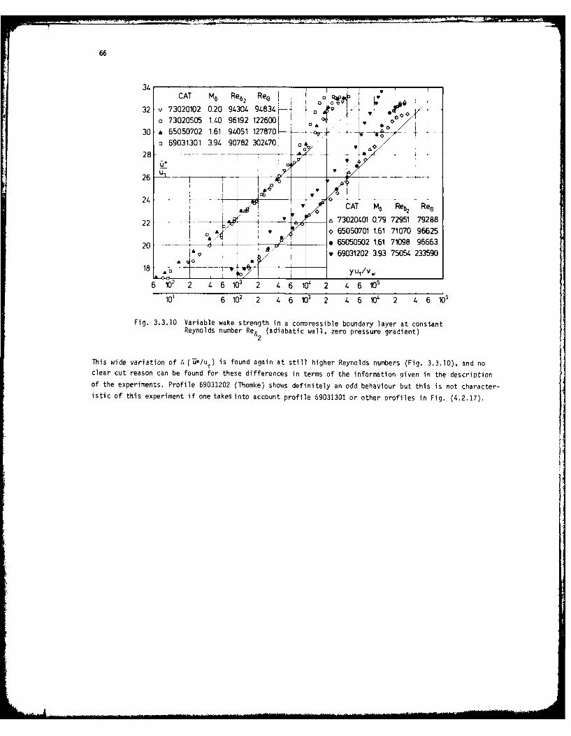
66

34 . . . .-CAT M6 Re 2 Ree

,

32 73020102 0.20 94304 94834 -7 ,-73020505 1.40 96192 122600 - "

30 £ 65050702 1.61 94051 127870 --- -: - - j - --- -

o 69031301 3.94 90782 302470 -

28 -0.0

26 T ___ _

24r A CAT M6 Re~ Ree

22_ a_ 73020401 0.79 72951 79288o 65050701 1.61 71070 96625

20 -~-- _ __ - ~65050502 1.61 71098 9666369031202 3.93 75054. 233590

6 12 2 4 10 2 4 6 104 2 4 6105

10' 6 102 2 4 6103 2 46 10' 2 4 6105

Fig. 3.3.10 Variable wake strength in a compressible boundary layer at constantReynolds number Re,6 (adiabatic wall, zero pressure gradient)

This wide variation of A (11*/u T) is found again at still higher Reynolds numbers (Fig. 3.3.10), and noclear cut reason can be found for these differences in terms of the information given in the descriptionof the experiments. Profile 69031202 (Thomke) shows definitely an odd behaviour but this is not character-istic of this experiment if one takes into account profile 69031301 or other profiles in Fig. (4.2.17).

67

3.3.4 Factors influencing the wake component

In an attempt to account for the observed discrepancies in supersonic boundary layers we should perhaps

look first at the main effects which were considered to be the cause of anomalies in the wake strength

in subsonic boundary layers. Coles (1962) found that three-dimensionality in the mean flow, free-stream

turbulence level and tripping devices were such causes. "Except possibly at very low Reynolds numbers,

the effect of increased free-stream turbulence is to decrease the strength of the wake component. The

amount of the decrease may also depend on Reynolds number and on the scale of the turbulence. As for

boundary layers with tripping devices it was found that the strength of the wake component sometimes

dropped below the normal or equilibrium value following a strong disturbance". We now comment on each

factor in turn:

Three-dimensionality of the flow

In principle all measurements in boundary layers are likely to be influenced by three-dimensional effects

if they were obtained in the downstream part of a wind tunnel the width to length ratio of which is small.

Unfortunately it is impossible to prove or qualify such a deficiency since in general we do not have

enough information about the-flow field, and sufficiently closely spaced velocity profiles are not avail-

able to allow a check of the momentum integral equation. We can only accept - or not - the authors' word

that all is well. A first attempt to estimate the effects of convergence or divergence of the flow for

center-line velocity profiles in square-duct type wind tunnels was made by Brederode & Bradshaw (1978)

for subsonic flow. They suggest a ratio of 6/b = 0.25 as an upper limit for the boundary layer along the

center-line to be still two-dimensional.

Free-stream turbulence level

We know of only one case where an attempt was made to influence the free-stream turbulence level deliber-

ately (CAT 5501) and the velocity profiles are plotted in Fig. (3.3.9). If the extra screens in the

settling chamber have reduced the turbulence level - which was not explicitly stated by Shutts et al.

(1955)- then the increase of the wake strength from A (U*/uT) = 2.70 for no extra screens (profile 55010102)

to 3.20 would agree with the finding of Coles for subsonic boundary layers. But even this rather weak

conclusion must be treated with caution since only the Reynolds numbers have a common value, the Mach

number was changed from 1.80 to 2.42, and the skin friction was measured only without the extra screens.

This is a good example of how difficult it can be to draw definite conclusions from the measurements in

AGARD.graph 223.

There is no experiment where the free-stream turbulence level is explicitly stated in any of our documented

entries. If its influence on the wake strength and on the skin friction were to be strong then this lack

of information would be extremely unfortunate. Systematic experiments are urgently required and could well

explain some of the scatter found in the wake strength of velocity profiles in supersonic boundary layers.

Tripping devices

Tripping devices are used for several purposes in boundary layer investigations, mainly for promoting

transition and for artificially thickening the boundary layer. Tripping the boundary layer automatically

introduces disturbances and this must be done with great care since a boundary layer may recover very

slowly from the effects of such a disturbance. Though a tripped boundary layer is thicker and so more

convenient for the insertion of measuring probes, it may exhibit features which are by no means character-

istic of the equilibrium or normal boundary layer which was the original aim of an investigation. As can

be seen from tables 4.2.1, 4.3.1 and 4.3.2 most of the boundary layers which are well documented have

undergone forced transition and have thus been disturbed in one way or another.

Coles (CAT 1953) investigated the effect of different types of tripping devices on a boundary layer

(Fig. 3.3.11) - fence trip (53011101), sand strip (53011201) and air-jet trip (53011302) - at the same

Mach number (4.54) and about the same Reynolds number Re62 (1288 to 1603). The small differences between

the velocity profiles - measured about 0.5 m downstream from the trips - cannot be attributed to the

tripping devices but more probably to values of the skin friction which, for example, seem to be too

high for velocity profiles 0801 and 1101 as is suggested by the visible discrepancies in the semi-log region.

ALJ

68

24

22 -

20 _ __... . . .

U,

18 41

16 -

4 i Profile M6 Re8 2 Re. transition device14 o 1201 4.55 1288 5274 sand-trip

* 1302 4.54 1353 5532 air-jet trip12 - A - -- , 0801 3.70 1484 4461 fence trip

& 1101 4.55 1603 6601 fence trip10

y 4v8, YUr/vw

10, 2 4 6 102 2 4 6 10 2 4 6 10'

Fig. 3.3.11 Law of the wall for a compressible boundary layer (adiabatic wall,zero pressure gradient, different transition devices). Coles (CAT 5301)

Investigations into the effectiveness of air jets were extended by Korkegi (1954, 1956) but unfortunately

no tabulated data are available. Stone & Cary (1972) present profiles downstream of very violent trips

- airjets and rows of relatively large balls near the leading edge of a flat plate. We find less distortion

introduced by the trips than is reported by the authors, and in general the interesting result is that the

trips, at least at the downstream station of the two, do not seem to leave any special mark on the mean

profile characteristics. On a transformed log-law plot, no effect can be seen which could not be accounted

for by the general experimental scatter. Peake et al. (1971) investigated a boundary layer recovering in

nearly constant pressure from the disturbance of flowing up and down a step (height 3.8 and length 12.3 mm

at a station for which 6 would have been 4 - 6 mm with no trip). The velocity profiles are shown in

Fig. (3.3.12). Except for the first velocity profile (71020301), measured 36 mm behind the ring, the

velocity profiles further downstream seem to have recovered completely from the disturbance if one accepts

that the scatter may well not be due to physical effects but to uncertainties in the skin friction measure-

ments. Scatter larger than normal is found in the measurements as a whole. In Fig. (3.3.12) we have also

plotted for comparison profile 71020101 measured at the same position as profile 71020301 but without the

ring. If one assumes the boundary layer thickness of this undisturbed velocity profile as a scale then

the last measured velocity profile (0305) is about 63 boundary layer thicknesses downstream, and the

normal behaviour of the velocity profiles downstream of a step with a height of about 60 % of the undis-

turbed boundary layer thickress is almost surprising.As can be seen from Fig. (3.3.12) the measurements - except for 71020303 - do not agree well with eqn.

(3.3.9), both grad4ent and constant being different. Such profiles are rare among the data presented in

AGARDograph 223. If the wale strength is evaluated on the basis of individual straight lines through

the data, one finds that .' (u*/u) varies with the distance downstream falling to a value of 1.55 at

x = 0 66 m (data not given in Fig. 3.3.12).

Upstream history effects

To the three physical effects discussed by Coles (1962) we would like to add at least one more, i.e. the

Influence of the upstream history on the strength of the wake component other than by tripping devices.

Since there is no full systematic investigation of upstream history effects on the boundary layer -

the experiment of Gates (CAT 7301) lacks skin friction information - we would like to draw attention to

an experiment where there is a probable downstream heat-transfer history effect in addition to a downstream

69

Profile x [in] M6 Re62 Ree

28 * 0101 029 392 3109 10225

o 0301 029 379 4000 124701 126 x 0302 0.2 362 7358 215601 1 .o-I - -

6 0303 052 3.60 8560 249601 0 o

2 o 0 0305 066 361 8411 246001 ---- ,-

")with upstream disturbance

00022o- 1 __

20 " --- -- -- --

Ut18 0 0

cl is x

16 41 B yu 1 /v.

1411- x 2 310 2 4 6 10 2 4 6 10 2 4

Fig. 3.3.12 Development of a compressible turbulent boundary layer downstream froma disturbance (adiabatic wall, zero pressure gradient). Peake et al.(CAT 7102).

effect of the nozzle pressure gradient (CAT 7202). These experiments,which cover the adiabatic wall and

the isothermal wall cases,contain velocity profiles showing a different behaviour from any we have observed

before. The wake strength in the adiabatic wall zero pressure gradient boundary layer reaches values of

A (u*/u T) ranging from 5.4 to 8.0 (Fig. 3.3.13). Other velocity profiles in the same Reynolds number range

show a transitional behaviour (not plotted here) and velocity profiles with very high cooling rates show a

behaviour which differs completely from the normal logarithmic law (Fig. 4.3.10) and which is due to

uncorrected skin friction measurements (Voisinet 1977).

35Profile x[m] Mt Re62 Re. U

o 0101 145 4.75 1556 6261 *30 o 0105 2 21 1.80 2105 8575 .

* 0301 145 . 80 9530 39008 g oo

25 a 0305 221 480 13252 53799 *,

~o ,*,,

U ,

0.

10 O- :, : ' o I ,

:~ ~ u- /V ,I ;o~

_____________ lyu/ _______

100 2 46 10' 2 4.610 2 4 610' 6 i

Fig. 3.3.13 Law of the wall for a compressible boundary layer (adiabatic wall, zeropressure gradient, origin not defined). Vosinet & Lee (CAT 7202).

10 0 2 46 ! 2 2 I.6 ! 3 6 'Y

70

3.3.5 Conclusions as to the strength of the wake component

Tentatively one could draw the following conclusions:

1) More systematic measurements with well defined boundary conditions and a well known wind tunnel

environment are necessary.

2) The strength of the wake component decays at low Reynolds numbers both in subsonic and supersonic

boundary layers tending to zero below a Reynolds number Re62 < 500. This behaviour appears to be

Independent of Mach number and heat transfer in the parameter range discussed in this report.

3) The apparent maxima of the wake strength at Reynolds numbers Red2 = 6 x 103 and 7 x 104 must be

treated with caution since they are in each case formed by measurements from a single experiment.

4) If a scatter of about ± 20 % of the wake strength is accepted then an average value of the wake

strength of 2.75 can be assumed to exist for supersonic boundary layers at Re6 > 6 x 103. This

agrees with the wake strength for subsonic flow found by Coles (1962) in the range 6 x 10 <

Red2 < 15 x 103.

5) A determination of the wake strength cannot be very precise, but the amount of scatter found is

too great to be accounted for by simple random error. No definite explanation can be given yet.

Discrepancies in the wake strength could be due to the three-dimensionality of the flow, free-stream

turbulence, upstream history effects or other as yet unknown environmental conditions. This

deficiency prevents us as yet from using the wake strength as a means of classification for

compressible turbulent boundary layers as suggested by Coles (1962) for subsonic zero-pressure

gradient boundary layers.

71

3.4 Transformation concepts

We have just advocated rather strongly var Driest's transformation and this will be used throughout the

remainder of sections 4 and 5, where we compare measurements with each other and with semi-empirical

relations. Therefore it seems necessary to make a few more general remarks about transformation concepts

in boundary layer theory. The motivation behind all transformations is to convert the mathematically

difficult coupled system of partial differential equations describing compressible boundary layers into

a form which can be solved more easily, for example into a system which is mathematically similar to the

equations for boundary layers with constant density. A mathematically correct transformation then makes

it possible to transform the solutions of the "simpler" system to the complex system in order to predict

the behaviour of the compressible flow. The Stewartson-Illingworth transformation provides such a relation-

ship between a high Mach number laminar boundary layer and a subsonic flow (see for example Stewartson

1964). The difference in the turbulent case has been stated by Crocco (1963) as follows: "since the

mechanism determining the distribution of the turbulent shearing stress is unknown, one cannot be assured

of the physical validity of the transformation, even if this correctly transforms the inertia and pressure

terms of the equations". On this point Crocco differs from Coles (1962) who points out that: "if a trans-

formation can be found to treat the acceleration and pressure terms in the equations, and if this trans-

formation is required to be physically realistic, then it must follow without reference to any special

definition of the shearing stresses that these stresses can also be treated by the transformation".

There have been many attempts to take into account the arguments given by Coles and Crocco for their

respective views, but the problem of a point to point transformation of a high speed turbulence fieid to

a low speed one remains unsolved. All transformation concepts for turbulent flows need assumptions based

on experimental input. We hope it will suffice here to say that Coles' transformation connects the full

set of equations in both planes of the transformation, considers the physics of the turbulent motion via

three functions and needs a minimum of semi-empirical information. For a survey of empirical relations

used in transformation concepts the reader is referred to Economos (1970), Economos & Boccio (1970) and

KUster (1972). Van Driest's transformation as applied in this investigation circumvents the problem inherent

in transformations for turbulent flows by shifting the difficulties into the acceptance of a mixing length

hypothesis used to connect the turbulent shear stress and the mean velocity. Before considering any further

development of transformation concepts for compressible turbulent boundary layers the reader should take

note of the argument brought forward by Beckwith (1970) to illustrate the lack of correspondence in the

transformed incompressible flow:"(1) When streamwise pressure gradients are large in a hypersonic boundary layer, then the normal pressure

gradients are also large because of the inherent Mach wave structure of the flow (see §6 where itwill be seen that this is not necessarily the case).

(2) When the heat transfer is large in the compressible flow, aT/ay is large both in the compressible flow

and in the corresponding incompressible flow which is, however, restricted by the condition that

Wa/y = 0 and that o is constant. Hence, for any reasonable equation of state for gases, the require-

ments for correspondence between the two flows cannot be satisfied.

(3) If the turbulent correlation terms containing p' are significant (e.g. in low-density compressible

flows), then the transformation again breaks down because of the constant-density limitation in the

low-speed flow."

Two further remarks concern the energy equation which must be retained in full also in the case of the

low-speed flow. Terms which can usually be omitted if the Mach number tends to zero - as the last two

terms in square brackets of eqn. (2.3.2) - may become important near the wall where the temperature and

viscosity on the one hand and the turbulent dissipation term u p v on the other hand are large.

72

4. INTERPRETATION OF MEAN FLOW MEASUREMENTS FOR ZERO PRESSURE GRADIENT

4.1 General remarks

4.1.1 Basis of presentation

Since this section will consist of a discussion of mean flow measurements in compressible turbulent boundary

layers and a comparison of the measured data with theoretically or semi-empirically derived solutions, we

start by quoting a remark of Coles' (1953): "In the area of compressible turbulent boundary layers a

comparison of experimental results does not involve the measurements so much as their interpretation".

We have presented here only "raw" data or at most measurements corrected by the experimentalist whom we

have assumed to be the person who is most familiar with the peculiarities of his equipment and his specific

experimental conditions. We decided therefore not to follow Coles (1962) or Coles & Hirst (1968) who fitted

the profiles to the logarithmic law of the wall before discussing them any further, since we could notbe sure that by such a procedure some information inherent in the measurements - though possibly not yet

recognizable - might get lost. Sometimes the "obviously" erroneous data point has indicated the direction

to future progress.

Unfortunately, we do not know the-environmental conditions, such as the noise level or the freestream-

turbulence level in the tunnel, for any of the experiments documented in AGARDograph 223 (Fernholz & Finley

1977), and for only a few are we fortunate enough to know something about the upstream history.

We also point out here that we do not think that the boundary layer thickness 6 should be used in the

interpretation of compressible boundary layer data but a better defined integral length, such as 62 or A*.

Here we recognize that we are prejudiced and discuss the reasons in § 7.

4.1.2 Classification of experiments

The experiments available for comparison suggest an order of presentation which was given in § 6 and 7 of

AGARDograph 223 and which will also be used here.

More than half of the available data describe tests made in nominally constant-pressure boundary layers

(group I) which we have subdivided firstly into cases in which the boundary layer has grown from a well

defined origin under constant pressure conditions throughout (IA) and secondly into cases (IB) where the

boundary layer is formed on a tunnel wall or the continuation of the nozzle wall after having passed

through the nozzle expansion upstream. In two cases (CAT 7202 and 7301) this history is in some measure

described and in one (CAT 7302) the development is so long and gradual that the boundary layer is probably

fully "relaxed" so as to have the same characteristics as a fully developed flat plate boundary layer.

Cases with substantial heat transfer are relatively rare. There is in addition a small group (IC) of cases

describing the recovery of a severely disturbed layer, under local zero-pressure-gradient conditions.

Unless otherwise stated, we have chosen for comparison only those measurements for which at least both

the velocity profile and the skin friction were measured.

4.1.3 The standard case

A discussion of the different velocity profiles belonging to one of these categories would be more logical

and informative if a standard velocity profile could be defined. One result of the investigation described

in § 3.3.5 has been to show that in compressible boundary layers a criterion based on the wake strength

is not definite enough "to make possible not only a precise classification of boundary layer flows but a

refinement and rationalization of the similarity laws" (Coles 1962). We are forced therefore to retreat

one step and to demand only that the transformed standard velocity profile for a zero pressure gradient

compressible turbulent boundary layer along an adiabatic wall obeys the law of the wall (eqn. 3.3.9) and

the outer law (eqn. 3.3.17) in their van Driest transformed form. How far both relationships may be

extended to hold for boundary layers along isothermal walls with severe heat transfer must be checked

by comparison with experiment. As will be shown the law of the wall can also be applied to boundary layers

with moderate adverse and favourable pressure gradients for which the outer law in the form of eqn. (3.3.17)

does not hold.

73

The outer profile is, on the contrary, a very sensitive indicator of the presence of pressure gradients

or their downstream effects in a relaxing boundary layer.

The "standard" boundary layer (normal, equilibrium, ideal, fully developed, asymptotic are some other

possible adjectives proposed by Coles 1962) must be free of upstream history effects and will develop

with constant local boundary conditions only. This state can be achieved in practice if the Reynolds

number is high and when upstream disturbances have completely abated. Such flows are probably generated

best in two ways: (1) On a flat plate positioned in the zero pressure gradient region of the test section

with a sharp leading edge, i.e. with a defined origin. Disturbances caused by a leading edge or a tripping

device must have died out completely at the measuring station. (2) On a wind-tunnel wall so far downstream

from the nozzle that equilibrium has been reached again. The latter set-up which is the only one by which

boundary layers with very high Reynolds numbers can be generated has the inherent disadvantage that it is

difficult to keep the boundary layer free of flow convergence or divergence, i.e. of three-dimensional

effects over a long running distance.

We shall discuss first the "standard" boundary layer velocity profiles and the effects of perturbations

on velocity profiles which are due to boundary or upstream conditions. The procedure for each group of

the zero-pressure gradient boundary layers is the same, complemented only by necessary amendments which

are specific to a particular case.

We have first plotted the velocity profiles in the law of the wall coordinates as specified by eqns.

(3.3.9) and (3.3.10) and compared them with the logarithmic law of the wall using the von Karman constant

K1 = 0.40 and CI = 5.10.The next step has been to plot the velocity measurements in the outer region in coordinates as specified

by eqn. (3.3.17). Though this is a relatively simple way to perform a comparison we will see that a

number of conclusions can be drawn from such a plot demonstrating effects due to low Reynolds number flow,

transition, pressure gradient or upstream history.

74

4.2 Zero pressure gradient adiabatic cases

4.2.1 Supposedly "standard" cases (class IA)

Specification of zero pressure gradient and adiabatic wall gives boundary conditions which reduce the

number of parameters to a bare minimum, i.e. to Reynolds number and Mach number, and minimize the

dependence on stagnation temperature information.

For the following discussion we have chosen the investigations classified as I A 1, i.e. flows with a

defined leading edge or origin, developed under zero pressure gradient conditions, with an adiabatic and

smooth wall, where both velocity profiles and skin friction were measured. The relevant overall information

is given in table 4.2.1.

Table 4.2.1

CAT Author M6 Re62 x 10-3 Transition

5301 Coles 2 - 4.5 0.7 - 5.7 Forced

5501 Shutts et al. 2 - 2.2 3.5 - 12 Forced

6502 Moore & Harkness 2.9 21.6 Natural

6506 Young 4.9 2.0 Probably natural7006 Hastings & Sawyer 3.9 0.7 - 7.4 Natural

7305 Watson et al. 10 0.4 - 1.5 Natural

7402 Mabey et al. 2.5 - 4.5 1 - 9 Forced (glass spheres)

After looking at a very large number of data which were compared with the law of the wall and the law of

the wake - a by-product of AGARDograph 223 - we feel that the velocity profiles measured by Mabey et al.

(1974) are probably the most reliable ones, performed with a great amount of care and professional skill.

From among the large number of velocity profiles a few were chosen which are thought to be representative

of this experiment and which are shown in Figs. 4.2.1 to 4.2.4.

28 6

Profile M6 Re62 Reo 6 ,26 A 0303 250 9095 17172 4 *

o 1001 348 2278 6342 0oo 24 * 1204 349 7609 21153 0. = v

a 1601 4 50 1079 4403 6

22 o 1703 450 2941 11805 -

1805 449 6813 26837

18 -- a-1

Uo "

16 - -- Profile M6 Re Reo

" 0100 247 3515 658214 0_ o 0101 249 3099 5889

12 1701 450 1528 6243

U 1801 452 2310 952210 , u/v. _ 1804 450 5831 235291100 2 10.. . .

1 2 4 6 10 2 4 6 03

101 2 4 6 102 2 4 6 1V 2

Fig. 4.2.1 Law of the wall for a compressible boundary layer (adiabatic wall, zeropressure gradient, defined origin). Mabey et al. (1974)

75

In Fig. (4.2.1) velocity profiles are presented which agree very well with the law of the wall (group a)

in a Reynolds number range 1500 < Re62 < 6000. Mark the large differences between the two definitions of

the Reynolds number Re6 and ReG. The velocity profiles plotted in Fig. (4.2.1b) show what is thought to

be the normal scatter agout the log-law line due to a measuring error in the skin friction Tw of about

t 4 %. In principle there need not be differences between velocity profiles at low (Re62 < 2000) and

moderate to high Reynolds numbers (Re62 > 4500) measured at two positions on the plate if the boundary

layer is fully turbulent (Fig. 4.2.2a). All velocity profiles discussed so far exhibit the slope given by

the von K&rmhn constant K = 0.40, only one profile (74020301) having a slightly steeper slope than the

others (Fig. 4.2.2b). Similar velocity profiles were measured by Coles (1953) and are presented in Fig.

(4.2.5a). Neither of the authors comments on these "odd" profiles, and no explanation could be found from

the description of the experiments.

28

Profile xl[m] M6 Re6226 . 1601 037 .49 1079 T.,1701 037 450 1528 o

24 170 138 49 3839 T

*1805 138 449 6813 022 - - -

20 u. IU,

18.Profile M6 Re6 , Re0

16 - . ., __. 0603 279 7813 16470

Ol __- • 0803 299 5902 13411514 -__-_ 1203 350 6250 17333

1505 398 8089 26500

12 %. . .. 0301 250 .774 9050

yu IV.

1010. 2 I. 6 102 2 1 6 10' 2

10i 2 1. 6 10 2 4 6 10 2 4-

Fig. 4.2.2 Law of the wall for a compressible boundary layer (adiabatic wall, zeropressure gradient, defined origin). Mabey et al. (1974)cf. fig. 4.2.4

Figs. (4.2.3) and (4.2.4) show that the measurements agree well with the outer law in the form of eqn.

(3.3.17). The good agreement with both the logarithmic law and the outer law proves that the boundary layer

is fully developed in this experiment, even at the low Reynolds numbers. For a discussion of velocity pro-

files at very low and transition Reynolds numbers, measured in the same test boundary layer by Hastings &

Sawyer (1970) and Mabey (1977), the reader is referred to § 4.4.

Coles' (1953) velocity profiles (Fig. 4.2.5) can be divided into two groups, (a) one with a steeper slope

than given by the von K&rman constant in eqn. (3.3.11) and the other (group b) where the measurements

follow the logarithmic law very well (the two groups of measurements are plotted with a shift by one decade

in the abscissa). Different transition devices can not possibly answer for these discrepancies as was shownin Fig. (3.3.11). In the outer law plot this difference in slope does not appear, and here the velocity

profiles are preferably grouped according to the Reynolds number range with a rough division at about

Re62 = 2000 (Fig. 4.2.6). For Re62 < 2000 low Reynolds number effects are clearly visible resulting in a

departure of the velocity profile from the straight line - at much smaller values of - In (y/A* ) than

at higher Reynolds numbers.

Velocity profiles at higher Reynolds numbers were measured by Shutts et al.(1955) and Moore & Harkness

(1965). The log-law plot is shown in Fig. (4.2.7) and the outer law in Fig. (4.2.8). Whereas the measure-

ments of Moore & Harkness agree very well with the inner and the outer law (note the small wake strength),

those of Shutts et al., while showing the usual amount of scatter for the inner law, agree very well with

the outer law.

76

8-800

7 Profile 7 - Profile& 0303 . 0100

6 =1001 0101

e 1204 e 02015 a 1601 5 170

o 1703 o 180'

4a 1805 4u-0".v 1804

UT U,

33

1 1In (y/l7in 0,/A-

0 Lq?4-04-3 -2 -3 -2

Fig. 4.2.3 Outer law for a compressible boundary layer; Mabey et al. (1974)cf. fig. 4.2.1

017 i 7

Profile I Profile

6 o 1601 6 , 0603

I 1701 £ 0803

5 o 1704 5 1203

. 1805 o 15054 u - - 4 u *030us-U uI, U6 0301

3 - 3 U

2 -- 2

1 1 k--1

In (y/&') In (y/")0 1 I 9 Q 0 ! -

-3 -2 -1 -3 -2

Fig. 4.2.4 Outer law for a compressible boundary layer (adiabatic wall, zeropressure gradient, defined origin). Mabey et al. (1974) cf.fig. 4.2.2

77

26 Profile M6 Re6 -- ----.--- 9

o 0301 1.98 578524 * 0501 2.57 3502 _yY90 _ __

v0601 2.58 5463 1~ - ©22 v 0901 3.70 2730U

a 1301 4.50 776

18 ~ -- _

16 UT

V6

14 lbProfile M6 Re62

12 a~- 0701 3.69 760

Y I£V 1001 4.51 880

10,L aI lI101 2 4 6 10 2 2 4 6 103 2 4 6 1&

Fig. 4.2.5 Law of the wall for a compressible boundary layer (adiabatic wall, zeropressure gradient, defined origin). Coles (1953)

8 8Prof ile 3Prof ile

7 0 0301 7- w 0401o 0501 L\ o 0701

v 0601 6 10019 0901 AAA1301

5- 5 - -

U; -Q* Re 2> 2000 ;Q*Re 62 <2000

3 3

2 2 - ___

0

4

In (yAI 0, In, (y/V ~ IA-3 -2 -i-3 -2 -

Fig. 4.2.6 Outer law for a compressible boundary layer (adiabatic wall, zeropressure gradient, defined origin). Coles (1953)

78

30

28 CAT M6 Re 82 Ree L _ -

o 65020501 2.90 21687 50298 , -P'I j

-65020601 2.90 21657 480792 /1 1

22

1__ CAT M6 Re62 Re0 o 55010103 1.73 14.276 20055

*55010202 2.041071620* , ' 55010501 2.25 3573 6053

16 55010504 2.24 12299 20797Y ut/v, 55010604 2.45 10348 18920

14 '2 2 01

10 2 4 6 102 2 4 6 10' 2 4 6 1V

Fig. 4.2.7 Law of the wall fora compressible boundary layer (adiabatic wall, zero

pressure gradient, defined origin). Shutts et al. (1955);Moore & Harkness (1965)

88

7 Profile 7 . \ Profile77

o 0501 o 0103

6 0506 6 0202" ~ ~~ u O_" 00501

CAT 6502 & 05045 v 0604*

____ 4 UCAT 5501

3 3

2 2

1 1

In (y/A') In (y/A)0 - 0 ' a ..

-3 -2 -1 -3 -2

Fig. 4.2.8 Outer law for a compressible boundary layer (adiabatic wall, zeropressure gradient, defined origin). Shutts et al. (1955);Moore & Harkness (1965)

79

The data of Hastings & Sawyer (1970) were obtained on the same flat plate as those of Mabey et al. (1974).

They are superseded by the latter measurements except for the data obtained in the transition region which

are discussed in § 4.4 together with the velocity profiles measured oy Watson et al. (1973) which also have

very low Reynolds numbers.

It is interesting to note that no measurements were taken in the viscous sublayer in any of the experiments

*presented so far.

4.2.2 Conclusion (class IA)

Unless new and convincing evidence appears it is claimed that the standard turbulent velocity profile in a

compressible boundary layer with zero pressure gradient along an adiabatic wall is described satisfactorily

by the law of the wall (eqn. 3.3.9) with the constantsK I = 0.40 and C = 5.10 and by an outer law given by

eqn. (3.3.17). All "constants" are truly independent of Mach number, heat transfer parameter and Reynolds

number. The range of the validity of the outer law shrinks considerably for Re5 2 < 2000 and finally vanishes

completely (see § 4.4).

Assuming this as a basis for a diagnosis of velocity profiles in compressible boundary layers, departures

from this standard behaviour must be due to different upstream or boundary conditions, i.e. a departure

from local equilibrium in the inner and outer region of the boundary layer respectively.

4.2.3 Other cases with no defined origin (class IB)

We now discuss measurements in boundary layers with zero pressure gradient alorg adiabatic walls with no

defined origin (group IB). These cases are listed in table 4.9.2.

Table 4.2.2

CAT Author M6 Re 2 x 10- 3 Transition

5802 Stalmach 1.7 - 3.7 0.7 - 8.8 Forced (grit type)

5805 Moore 2 - 3.5 3.4 - 8.5 No information

6502 Moore & Harkness 2.8 70 - 359 Natural

6505 Jackson et al. 1.6 - 2.2 '5.8 - 94 No information

6601 Hopkins & Keener 2.4 - 3.4 21 - 34 Natural

6903 Thomke 2 - 5 20 - 150 Natural

7202 Voisinet & Lee 4.9 1.6 - 13 Natural

7302 Winter & Gaudet 0.2 - 2.8 5.4 - 142 Natural

7601 Vas et al. 3 9.1 - 159 Natural

Stalmach's (1958) velocity profiles were measured in a 51 mm wide tunnel with a floating element width of

25.4 nn. It is therefore surprising that the data agree so well with the logarithmic law, at least those

of series 02 (Fig. 4.2.9), showing very clearly the increase in wake strength A(Ub/u ) from 0.95 to 3.25

with increasing Reynolds number at constant Mach number. The same velocity profiles are compared with the

outer law in Fig. (4.2.10) showing the normal behaviour of a fully turbulent boundary layer.

The experiments presented by Moore (1958) do not show anything especially significant except that the skin

friction appears to be slightly too high, and they will be discussed in connection with a relaxing boundary

layer downstream of a step in § 4.5.

The medium and high Reynolds number range is covered by measurements performed by Winter & Gaudet (Fig.

4.2.11). Velocity profiles at Mach numbers below 2 agree very well with the logarithmic law whereas those

at M 6 = 2.20 lie consistently above this line. In the Reynolds number range 11 x 103 < Re6 < 14 x 104

presented here, the strength of the wake component is almost constant at 2.70 t 0.30-whicA is well within

the scatter band mentioned In § 3.3.3. The outer law representation for these measurements is giien in

Fig. (4.2.12).

80

28

Profile M5 Reb A Q! Ree _ A26 2 U

o 0201 274 959 0.95 1996 £

24 - 0202 2.73 1504 1.55 3124.o 0203 273 1833 1.60 3808

22 " 0201. 273 2967 2.40 6154 _°___

A 0207 2.74 5853 3.25 121540

20 -.U U

18 T

16 A

UTVo b ° " y u Ivw

2 10 2 6 102 2 4 6 103 2

Fig. 4.2.9 Law of the wall for a compressible boundary layer (adiabatic wall, zeropressure gradient, no defined origin). Stalmach (1958)

8

Profile Re627 o o 0201 959

, z 0202 15046 0 o 0203 1833

0 n 0204 29675 --- A 0207 5853

U6 -u

3 _

'0

2 _1 - - ________ . . ..... - ______

10 In (y iA69\

-3 -2 -1

Fig. 4.2.10 Outer law for a compressible boundary layer (adiabatic wall, zeropressure gradient). Stalmach (1958)

381

Profile M6 Re62 9f32 o 04.02 0.79 108790 -*

8 0403 0.79 14182030 a 0503 1.40 45658----

n 0504 1.39 87352 128 v 0505 1.40 96076 e

v 0801 2.00 31338 0.026 -- - -- TT -- - ---

0 Proilke Mb, Re62

o0905 2.20 10864

18e 0906 2.20 1414218-4 *0908 2.20 18926

*0910 2.20 2549516, o- i 0913 2.20 40203

14 Y u1 /v.10? 2 4 6 103 2 4 6 10' 2 4. 6 10'l0d 2 4 6 102 2 4 6 103 2 4 6 10,

Fig. 4.2.11 Law of the wall for a compressible boundary layer (adiabatic wall,zero pressure gradient). Winter & Gaudet (1973)

8 18-Profilie 0Profile

0 o 0402 o 0905

OL003 e 09066 e0503 6- * 0908

. 0504. * 09105 0505 5o 0913

v 0801-4 4__-

3 3 -_________

2 2_

0 4!-1 1 I iV_ -

-3 -- 1-3 -2

Fig. 4.2.12 Outer law for a compressible boundary layer (adiabatic wall, zeropressure gradient, origin not defined). Winter & Gaudet (1973)

82

Compared with the velocity profiles of Winter & Gaudet those of Jackson et al. (1965) which are in the

same Mach- and Reynolds number range show either a much smaller wake strength A (u*/uT) 1.60 or a much

bigger one, about 3.80 (Fig. 4.2.13). The range overlaps that of the study by Shutts et al. (1955). who

used the same balances (cf. dat3 in Fig. 4.2.7). A momentum balance using the experimental cf-values

indicated that the layer was not strictly two-dimensional (authors' comment). It is interesting to note

that the velocity profiles which have the larger wake strength agree with the outer law for a much larger

distance (Fig. 4.2.14) than those with the smaller wake strength.

34Profile M5 Re62 Re(). ,

30 v 0801 2.20 5852 9829 -i-V 1001 2.20 15602 26207 o _ °o_ ,26 a 1201 2.20 27686 46505 0

a 1402 2.20 53072 89145

22 8_

10 - 0 0502 1.61 71098 9666310 A U/V 0701 1.61 71070 96625

6, . i 0702 1.61 94051, 127870

10' 2 4 6 102 2 4 6 103 2 4 6 10' 2

101 2 4 6 102 2 4 6 10' 2 4 6 10' 2 4

Fig. 4.2.13 Law of the wall for a compressible boundary layer (adiabatic wall, zeropressure gradient, no defined origin). Jackson et al. (1965)

o Profile Profile

7 976 o V 0801

0 0301 V 1001

6 - - 0501 6 0 1201

0 & 0701 # 1402

56 -5

4. 4 -

3 3

2 2

1 1

In iy/A1) In (y/")00 *-3 -2 -1 -3 -2

Fig. 4.2.14 Outer law for a compressible boundary layer (adiabatic wall, zeropressure gradient). Jackson et al. (1965)

83

32 Profile M6 Re2 Re, - 38v 0101 296 9152 23198

30 1 0107 287 23712 57543 36

o 0209 280 47141 11160028 a 0306 287 92577 225720 34

o 0406 2.90 121670 300250 C a

26- - , -_o_ _ -T -32

06

2 - Prfl M 30

22 U,: 28

20 . . . . 2601CAT 650218< 24

1 :a Profile M6 Re2 Reo

161 0101 Z83 190390 424070 2j oo •0103 267 359310 733680

o 0201 2.84 159050 36305014 * 0203 2.69 287250 599440

A ,yu!/v , a 0401 290 70161 165240

102 2 4 6 10' 2 4 6 10' 2 4 6 1o5

Fig. 4.2.15 Law of the wall for a compressible boundary layer (adiabatic wall, zeropressure gradient). Vas (1976), Moore & Harkness (1965).

Fig. (4.2.15) shows measurements by Vas et al. (1976) and by Moore & Harkness (1965) which were performed

at a Mach number 2.90 in a Reynolds number range 9 x 103 < Re6 < 3.6 x 105. The velocity profiles pre-- -

sented by Vas et al. again have a rather small wake strength 1.40 < A (U*/u ) <2.20 (see also Fig. 2.7.5)

compared with those measured by Moore & Harkness where the strength of the wake component lies in the

range 2 to 3. Both cases show the normal amount of scatter below and above the logarithmic law. Apart from

the fact that the latter boundary layers reach the highest Reynolds numbers Re6 known to the editors of

AGARDograph 223, the only obvious difference between the measurements lies in t~e different size of the

test-section, with W = H = 0.232 and L = 2.56 m (CAT 7601) and W = H = 1.22 and L > 14.63 m (CAT 6502)

respectively. The outer law shows good agreement with the measurements of both experiments 'Fig. 4.2.16).

8 - '-CAT 8 -- -CAT

£ o 65020101 o 76010101

7 -- -* * 65020103 7 .... - 76010107

65020201 o 760102096 .65020203 6 76010306

- 65020401 o 760104065 5 A7--

0 owl'4U;-6"~ -JU

U1 0A UT

3 3 -

2 +2 Y

1 . -- 1

In (y/A') In (y/A)0-41 0 4

-3 -2 -1 -3 -2 A

Fig. 4.2.16 Outer law for a compressible boundary layer (adiabatic wall, zeropressure gradient) Moore & Harkness (1965); Vas (1976).

84

The measurements performed by Thomke (1969) contain velocity profiles in approximately the same Reynolds

number range as those of Vas et al. (1976) but at Mach numbers of both 3 and 4. The physical scale of

Thomke's experiments is also much greater than that of Vas. For the majority of the data skin friction

appears to be slightly low so that the measurements lie above the logarithmic law of the wall (Fig. 4.2.17)

but, however assessed, the wake strength is large.In the legend of Fig. (4.2.17) the second additive

number in the column with the heading A (u*/u T) denotes the correction due to the shift above or below

the standard logarithmic law. Agreement between outer law and measurements is again very good (Fig. 4.2.18).

34 Profile M6 Re62 AMO'/u,) Ree0 AL o

o 0701 2.98 111500 2.25+0.5 259420 , ,= 8o 0 0

32 * 0702 2.95 150690 3.05 346710 ----

, 1201 394 62496 340 194120 06 "Zo0

30 £ 1202 393 75054 5,10-15 233590o 1301 394 90782 3.60 302470 0

28 a 1302 393 110330 4.70-0.7 366810 , 0 S

* 1501 444 53791 360-02 206290* 1502 4.40 66532 4.75-0.8 252540 " _

24 ________ _____

26 - A9

2 4S0

22

20- - _,

8 Y l

102 2 4 6 1033 2 4 6 10 2 4 6

Fig. 4.2.17 Law of the wall for a compressible boundary layer (adiabatic wall,zero pressure gradient). Thomke (1969).

Ab I

8Profile Profile

o 0 0701 1301

* 0702 - 1302

6 -. \A A 1201 6._1501& 1202 v 1502

5 o .... -.. .. 5 . .-6 -- 5---,U

4. 4 u_-_

Ut0 0 t "Y=-

3 4-3

-3 -2 2 -3 -

F;g. 4.2.18 Outer law for a compressible boundary layer (adiabatic wall, zeropressure gradient, origin not defined). Thomke (1969).

. .. . ' ... ... .. .. .. .. . . . . . . .. . .. . .. .. . . .. . . .. . ... .. . .l li ill.. ... . .. . I ... ... .. .... ..

85

The three velocity profiles presented by Hopkins & Keener (1966) in the range 21 < Re6 x 103 < 34 show- 2 -

a difference in the wake strength between 2.30 and 3.20, and skin friction measured by a balance appears

to be low despite the importance given to skin friction measurements in this experiment. Since both Mach

number and Reynolds number range are covered by the experiments shown above, the Hopkins & Keener data

are not given here in graphical form.

Having discussed measurements over a Mach number range 0.8 < M6 < 4.5 and a Reynolds number range

1x 103 < Re62 < 3.5 x 105 where the law of the wall and the outer law did agree with the bulk of the

data and where discrepancies were very probably due to the normal error which cannot be avoided with skin

friction measurements, we have been puzzled all the more by the velocity profiles obtained by Voisinet & Lee

(1972) (c.f. Fig. 4.2.19). They lie consistently above the logarithmic law according to eqn. (3.3.9)

requiring a constant C1 = 6.1 and they exhibit a wake strength - after correction for disagreement with

the standard wall law - in the range 6.30 < A (u*/u ) < 7.70. Since otherwise such high values of the

wake strength are observed only in boundary layers with high rates of heat transfer (see § 4.3) we can

only assume that the upstream thermal history effects have not yet abated at the profile measuring stations.

In general there was, for this experiment, substantial heat transfer in the nozzle region, so that there

is a downstream history effect in addition to any downstream effect of the nozzle pressure-gradient.

After these discrepancies in the log-law plot it is not surprising to find also considerable deviations

from the standard outer law (Fig. 4.2.20) which is similar to cases found in boundary layers with adverse

pressure gradients (see § 5).

As for a conclusion there is little to add to those given at the end of § 4.2.2 except that the Reynolds

number range of the validity of both the law of the wall and the outer law can be extended safely to

Reynolds numbers up to 3.5 x 105 for boundary layers with zero pressure gradient along adiabatic walls.

36 . iProfile M6 Re% Re0 a.

32 o 0404 480 2058 8259 D

v 0503 4.86 5959 24912 *,, £

28 e 0505 490 6639 28122 .. .. 4i J7* --- --

0205 4.82 6962 2876424 £ 0301 480 9530 39008 [ o ,

o 0303 486 10371 42808 -a 0305 4.80 13252 53799 0

U-

12 - __---- - -1--

0_8

o4o p" "y ut/vw-j

10 2 4 6 101 2 4 6 102 2 4 6 103 2 4 6 10'

Fig. 4.2.19 Law of the wall for a compressible boundary layer (very slight cooling,zero pressure gradient, upstream history effect). Voisinet & Lee (1972).

86

Profile 0Profile

7 0 0404. 7 _A\ & 0301v 0 503 £o 0303

6 9 0505 6 a 0305& 0205

5 5

00

0

1 --- ~- 0 1

aw &In (y/Y) In (y/hl

0 -2 -1 -~* 3 -2 -

Fig. 4.2.20 Outer law for a compressible boundary layer (adiabatic wall, zeropressure gradient, upstream history effect). Voisinet & Lee (1972).

87

4.3 Zero-pressure-gradient isothermal wall cases

4.3.1 General remarks

As with compressible turbulent boundary layers along adiabatic walls the validity of the transformed

similarity laws for the viscous sublayer, the log-law region, and the outer region rests on the correct

representation of the temperature distribution for boundary layers on isothermal walls - here we have

used eqn. (2.5.37a) - and on a comparison with measurements.

Experiments in flows with heat transfer are even more laborious and difficult to perform than those on

adiabatic walls described above. It is not astonishing therefore to find that the number of cases in-

vestigated is small indeed. Since the wall is heated by viscous dissipation in compressible boundary

layers, and wall cooling is often essential for the survival of high-speed aircraft, high-speed experiments

with heated walls, i.e. Tw > T r , are of little technical interest (little work is available on strongly

heated walls even at low speeds, one exception being the investigation by Kelnhofer 1970 who measured

velocity and temperature profiles in a turbulent boundary layer with zero pressure gradient). All of the

experiments discussed below will therefore belong to the group of the "cooled wall" cases. As experiments

in boundary layers with adiabatic walls are limited by the recovery temperature which according to eqn.(2.5.38) is mainly determined by the Mach number, only cooled wall boundary layer experiments permit

experiments at higher Mach numbers at all. This extended Mach number range - 5 <M6 < 10 - is of special

interest for experiments concerned with boundary layer flow on the space-shuttle. Another problem which

accompanies all high Mach number experiments are low Reynolds number effects. Though a Reynolds number

increase is obtained by a decreasing wall temperature reducing the viscosity at the wall, high Mach numberflow can only be achieved at bearable costs in small test facilities which have small test sections and can

thus only produce flows at relatively low Reynolds numbers. For example at a Mach number M6 = 7.2 the highest

Reyiolds number obtained in a published experiment was Re62 = 3.0 x 10

As was mentioned in § 2.2.3 a convenient definition of a heat transfer parameter makes use of the recovery

temperature which can be defined for a boundary layer along an isothermal wall. The independent heat trans-

fer parameter used in this investigation is therefore the ratio of the wall temperature Tw to the recovery

temperature Tr*The heat flux is most usually presented in the form of a Stanton number see eqn. (2.6.4), though the

difficulty of giving a sensible value to the recovery 'or adiabatic wall) temperature when the wall is

not isothermal leads us to use cq = qw/pcpU 6To6 (see § 2.6.3).In the experiments discussed below, the heat transfer parameter lies in the range 0.2 < Tw/Tr 1.1, with

Tw/Tr = 1 characterizing zero heat transfer or the "adiabatic wall" case. TW/T r < 0.50 will be called high

or severe cooling. Tw/Tr < 0.80 moderate cooling but this classification was chosen for convenience only.

Since we need the shear stress velocity u. for the comparison between the semi-empirical relationships and

the measured data, table 4.3.1 contains only experiments where the skin friction was measured. Skin frictionwas therefore considered a more important quantity than the heat transfer qw at the wall. This is only due

to the poor state of our knowledge concerning the Reynolds analogy factor. Otherwise a version of eqn.

(2.6.5) could be used to determine the skin friction for all cases where the Stanton number is known, i. e.

where qw and Tw are available from measurements.

Table 4.3.1

CAT Author M Tw/Tr Re 2 x 10-3 Transition

6506 Young 5.0 0.6 - 1.0 1.7 - 2.5 forced

6702 Danberg 6.5 0.5 - 0.9 0.3 - 1.9 natural

7204 Keener & Hopkins 6.3 0.3 - 0.5 1 - 2.3 natural & forced

7205 Horstman & Owen 7.2 0.5 1.4 - 3.0 natural

7702 S Laderman & 3.0 0.6 - 1.0 1.4 - 2.8Demetriades

88

Table 4.3.2 presents measurements where the origin of the boundary layer is not known (nozzle wall) and

where upstream history effects cannot be excluded.

Table 4.3.2

CAT Author M6 Tw/Tr Re62 x 10-3 Transition

7202 Voisinet & Lee 4.9 0.25 - 1 1.8 - 38 natural

7203 Hopkins & Keener 7.2 0.3 - 0.5 4.5 - 15.5 natural

7403 Laderman & 9.4 0.42 6.5 naturalDemetri ades

AGARDograph 223 Fig. (6.3) shows clearly that there exists a great need for more experiments in compressible

turbulent boundary layers with heat transfer.

4.3.2 Zero pressure gradient cases with no upstream history effects

Table 4.3.1 lists only five experiments with skin friction measurements where the origin of the zero-pressure-

gradient boundary layer was defined by a leading edge and where the wall temperature was constant, so that

no upstream history effects should occur. In all cases the wall temperature was below the recovery temper-

ature, i.e. the wall was cooled. Thus all the assumptions were fulfilled which underliethe temperature-

velocity relationship given by eqn. (2.5.37a) and which are needed for the transformation of the velocities

u* and u* . Unfortunately these prerequisites are often forgotten when comparisons between theory and

experiments are carried out. Except for the Danberg case, where the skin friction was determined from the

slope of the velocity profile, the wall shear stress was measured by a floating element balance (CAT 6506,

7204, 7205) or by a Preston tube (CAT 7702 S). Therefore only three sets of data in this group (1 A) can

properly be compared directly with the log-law and the outer law plot. It is convenient to begin the dis-

cussion with an experiment where the heat transfer parameter Tw/Tr was varied moderately, i.e. with an

almost adiabatic case Tw/Tr = 0.97 progressing to a value Tw/Tr r 0.52 (Young 1965). Some profiles of

CAT 6506 are shown in Figs. (4.3.1a) and (4.3.2). Young did not measure temperature profiles, so that the

velocities were evaluated from the total pressure distribution by assuming that the temperature distribution

was given by eqn. (2.5.37a).

26Profile M6 Re62 Ree T,/T,

24 o 0101 4.88 2005 8860 0.972 +a 0102 4.91 1904 6220 0.711

22 o 0103 4.90 1926 5813 0.659 0

n 0104 4.89 1914 5214 0.600 , 0

20 & 0105 4.86 1946 1 4619 0.523 °.4

CAT 6506 K 0* C

u. CAT 7204

u, -a with tronsition trip16 . Profile M6 Re: Ree T./T

de' o 0101 621 1066 2416 033314 ' A " . - . + 02011639 2281 5116 0 314

. 0301 642 1421 4457 043812 v 04011642 1247 3767 0419

1 0501 650 1793 6633 0508yu1 /v, o 06011650 2344 8554 0501

10 2 4 6 102 2 4 6 101 10,

100 101 2 4 6 102 2 4 6 10 2

Fig. 4.3.1 Law of the wall for a compressible boundary layer (isothermal wall,zero pressure gradient, defined origin). Young (1965) andKeener & Hopkins (1972).

89

This assumption is reasonable (see § 2.5.6) if data points close to the temperature peak in the immediate

vicinity of the wall are not considered. Fortunately this experiment can be supplemented and extended to

higher cooling rates (0.51 > Tw/T r > 0.31) in about the same Reynolds number range (106? < Re62 < 2347)

with measured temperature profiles by Keener & Hopkins (1972). These velocity profiles are presented in

Figs. (4.3.1b) and (4.3.2). Agreement between the log-law (eqn. 3.3.9) and the measurements is very good

in the first case and good in the second, if one considers the likely measuring accuracy of a floating

element balance in a cooled wall. This comparison suggests that the value of the constant Cin eqn. (3.3.9)

remains unchanged from the adiabatic wall case if the wall is cooled and kept isothermal. Three measured

temperature profiles are presented in CAT 7204 (0101, 0201, 0401) (see Fig. 2.5.14), so that the uncertainty

inherent in Young's experiment is eliminated (see also the comparison between the measured and the calcu-

lated temperature profiles in Fig. 4.3.6). In addition the downstream effect of transition on the boundary

layer profiles was investigated by introducing a boundary layer trip near the leading edge for profiles

0201, 0401 and 0601, and allowing natural transition to develop for profiles 0101, 0301 and 0501. The

profiles with forced transition appear to show a larger strength of the wake component but no generally

valid conclusion can be drawn.

The outer law shows good agreement with the measurements (Fig. 4.3.2) for Reynolds numbers Re62 > 2000,

but deviations occur for profiles with lower Reynolds numbers as already observed in Fig. (4.2.6).

8 8CAT CAT

7 - __ o 65060101 - - - _ - a 720401017 65600 o 72040301e 65060102

o 65060103 a 720403016-.65060104 6 9 72040401

0 \ ,

0 . 65060105 v 72040501

55 Y

o 72040201

4 -u 0 o 72040601 u ;-O .

Re 62 > 1900 Re62 < 1900

0\

2 1

In (y/6') In (y/i*)0 -41 0 1 ._ 1 •

-3 -2 -1 -3 -2

Fig. 4.3.2 Outer law for a compressible boundary layer (isothermal wall, zeropressure gradieit, defined origin). Young (1965) and Keener & Hopkir "

More recent measurements by Laderman & Demetriades (1977) show good agreement both i-' t* ,.

4.3.3) and with the outer law (Fig. 4.3.4). Since their skin friction values were deter..

a Preston tube and by using the evaluation method of Hopkins & Inouye (1971)which "..

by balance measurements in a satisfactory manner, the wall shear stress has as, ,-

present authors using a semi-empirical method (Fernholz 1971). In both cases mea .-.

tatively with the logarithmic law, eqn. (3.3.9). Moreover, while (Tw)re e 7e-

ment, (Tw)H&I provides the better correlation. The skin friction value , .

(4.3.3) and show differences of up to 20 ). Laderman & Demetriaues caic ,

wake correlation (Coles) and found that the (T,)H& i values we_, ,,

dure was applied to the outer law and there are hardly any dlfer,.There exist so few measurements in boundary layers with defined . ...

also discuss in this context the axisymmetric boundary layer stud'e -

boundary layer may have been affected by a slightly favourable re.,,

ADAOS? 70 ADVISORY GROUP FOR AEROSPACE RESEARCH AND DEVELOPMENT--ETC F/S 20/4

CRITICAL COMMENTARY ON MEAN FLOW DATA FOR TWO-DIMENSIONAL COM-ETC(U)MAY 80 H H FERNHOLZ, P J FINLEY

UNCLASSIFIED AGARO-A6-253 NL,flnl******l*,-EIEEEEEEEII-IEIhIIIIIEEE-IEEEEIIEEEE-u-El.--ii-- El.'U

11w1 1 1.2 % L 2_- I

.11111L5 1. 4OICROCOPYREO ION TST

MICROCOPY RESOLUTION TEST CHART

9O

28 VProfie M T.g/; R% F.c,.

26 o7702S0101 3.0/, 1.0 1362 1.96 1.99 -•

-

*7702S0103 3.0 1.0 163/, 1.85 1.92 a

2/. o7702S0203 2.99 0.77 2086 18. 2.10 a

*7702S0303 2.98 0.58 2826 182 2.24 10

22 -

20a) with t F* adoJ

18o

16 _ _,t

12

,o 0 i yuv,

10' 2 1. 6 102 2 4. 6 0 i101 2 4 6 102 2 4 6 103

Fig. 4.3.3 Law of the wall for a compressible turbulent boundary layer (zero pressuregradient, Isothermal wall, defined origin). Laderman & Demetriades (1977).

16* 0 Profile 16o 7702S0101 a:

7702S0103 1 ___14 " 7702S0203 14

12 X m 7702S0303 12So I I

1 , 1 -

U ith u-0" a withy8 UT Fe 8 U1 "IH-1

8 -6- 5 -l - - 0,

2 * -2-

0Lt In (y/A" 04in (y/h')

6 -5 -4 -3 -2 -1 - -5 -4 -3 -2 1

Fig. 4.3.4 Outer law for a compressible turbulent boundary layer (adiabatic wall,zero pressure gradient, defined origin). Laderman & Demetriades (1977).

angle cone-ogive which formed the front part of the 3.30 m long cylinder. It is, however, highly probable

that the boundary layer has reached equilibrium at the measuring stations which were in the region 1.15 to

2.37 m downstream. Agreement between measurements and the law of the wall is very good (Fig. 4.3.5). and

it is a pity that only three profiles were measured in this carefully designed experiment. Measurements

included also skin friction, heat transfer and velocity fluctuations. As can be seen on Fig. (4.3.6) there

is good agreement with the outer law, and agreement between measured and theoretical temperature profiles

-.. 2.6.3Ta) is satisfactory.

91

26

24 Profile M Re T Rego 0101 72 1395 0.503 6198 v

22 * 0102 72 2101 0.498 9261 a _ ____

0103 72 3042 0.476 12950 0

18

16 vIV2

14-

12yu1/vW

Vo 2 4 6 2 4 6

Fig. 4.3.5 Law of the wall for a compressible boundary layer (isothermal wall, zeropressure gradient, axisyametrlc). Horstman & Owen (1972).

7-77 "Profile

" a 72050101

6- 72050102 yu/.25v 72050103 51 z 7

1'"

U-C 4

3---2-

3

2

01 - In WeAIi)I-3 -2 0.6 08 10

Fig. 4.3.6 Outer law for a Comparison of temperaturecompressible boundary measurements with theorylayer

(isothermal wall, zero pressure gradient, axisymmetric)Horstman & Owen (1972).

92

4.3.3 Zero pressure gradient cases with upstream history effects

The next two cases which we deal with are boundary layers along tunnel walls, i.e. with no defined origin,

which could be subject to upstream history effects both due to pressure gradient and wall temperature

variations. The measurements by Hopkins & Keener (1972) extended the Reynolds number range of the flat

plate experiment (CAT 7204) to Re62 - 15.5 x 103 at a Mach number M6 = 7.5 (CAT 7203). The measuring stationwas 10.13 m downstream of the throat and - as the authors state - the test section flow "was not entirely

uniform but relatively so for this type of facility". It would therefore not be too surprising to find more

scatter around the law of the wall line than in the cases discussed above (Fig. 4.3.7). All measurements

lie consistently low, however, which could be due to a systematic error in the skin friction measurement.As will be seen below in the discussion of the Voisinet et al. (CAT 7202) data, the fact that the floating

element of the balance was not cooled could easily have caused the skin friction values to be overestimated.

A reduction of around 20 % as in the case of CAT 7202 would bring most of the data into much better agree-

ment with the log-law.

28 - - - - -Profile MG Re% Ree T./T

26 o 1201 739 .533 19.86 0.4.63 - . -___* 0501 7.10 1.783 18131 0a110

2 e.0 1301 75. 730. 31283 0450 *_v 0601 7.59 783. 2901. 0.383S0701 7..7 8809 29363 0.355 922 ____

20-

UU

o Profile M6 Re62 Re% T./T,16 o W 71.8 U077 61222 0.464

1a. 1101 79. 1.605 53472 0389M 1001 7.7 15.67 527.1. 0.363

YU,/V 0301 746 14.504. 42759 0.311.12 216 1' .

2 1. 6 02 2 4 6 V

V0 2 1. 6 102 2 1. 6 V0 2 4 6

Fig. 4.3.7 Law of the wall for a compressible boundary layer (isothermsal wall, zeropressure gradient, no defined origin). Hopkins & Keener (1972).

As for the outer law, the velocity profiles as measured by Hopkins & Keener agree well with eqn. (3.3.17)

(see Fig. 4.3.8).In the nozzle-wall experiment of Voisinet & Lee (CAT 7202) a comparison of the measured data with thelogarithmic law of the wall gives a rather confusing result. For moderate wall cooling (Tw/Tr -0.78)measurements follow the same slope as the log-law curve but indicate that the constant C1 is 6.10 insteadof 5.10 (Fig. 4.3.9). whereas with severe wall cooling (Tw/Tr 20.22) the data do not exhibit a linearbehaviour in the log-law region at all and lie consistently lower (Fig. 4.3.10). The velocity profiles inthe moderate heat transfer case thus agree qualitatively with the adiabatic wall case both for the log-lawregion (Figs. 4.3.9 and 4.2.19) and for the outer law (Figs. 4.3.11 and 4.2.20). Compared with the*standard profile" consistent discrepancies occur which seem to be characteristic of the NOL data,however. These deviations from the typical outer law behaviour could be due to upstream history effects.The velocity distribution in the outer layer resemb~les one in a boundary layer which has been exposed toa slight adverse pressure gradient (Figs. 4.3.11 and 4.3.12).One reason for faulty skin friction measurements could be the so called "hot-spot-effect" (Westkaemper 1963)which results from an uncooled floating element in an otherwise cooled wall. Experiments with a floatingelement, the temperature of which was up to 150 K above that, of the surrounding wll, revealed that con~-siderable corrections must be applied to the skin friction data (Voisinet 1977). They amo~t to a reductionof Cf by 20 % according to Reynolds number, Mach number, and the temperature difference between thefloating elamant and the wll.

93

Profile a Profileo0201 7 o 1501o 0501 a 1101

6 .1301 '.10010601 40301

U;

I -7

5 •0701_ _ _

3 S

In (y/A)0 In (y/A)W3 -2 -3 -2 -1

Fig. 4.3.8 Outer law for a compressible boundary layer (isothermal wall, zeropressure gradient). Hopkins & Keener (1972).

36

Profile xlm] M. Re82 ReG V

32 o 0601 1..5 1.77 1865 61.16 ga ,,

* 1001 1.45 4.90 6083 21413 1 a e

28 0801 1..5 4.81 12025 42388a 0605 2.21 4.81 1974 6959

24 . 1005 2.21 4.91 7562 26816v 0805 2.21 4.85 12724 45414 o20 o L

U__ o

16- -0

121

i 8 -

4 /..............100 2 . 6 10 2 4 6 i 4T 6 10 2 46 6

Fig. 4.3.9 Law of the wall for a compressible boundary layer (Isothermal wall,Tw/Tr * 0.78, zero pressure gradient). Voisinet & Lee (1972).

94

32 -

Profile xmI M6 Re% Re a-o14011.454 7 9 6963 7498

* 1101 1.90 4.82 7905 8935

24 v 1103 2.21 4.82 8720 9733 -

S15011.45 493 21288 2549420 1 21 1.90 492 23652 28139 0 P

1203 2.21 1.86 3376. 40140

12U-

8-0

YU,/v,

100 2 4 6 10 4 6 1 2 6 10 2 4 6 10'

Fig. 4.3.10 Law of the wall for a compressible boundary layer (isothermal wall(TW/Tr) 0.22; zero pressure gradient, origin not defined).

Voisinet & Lee (1972).

Profile Profile

7 - o 0601 7 ,0801o 0605 0805

6 6 - .1001a 1005

5 5

4 R% < 2000 Re0 > 2000

3 , 3\ONa

2- 2-- .

01 _____-

In (y/AI) a In (y/Alj 520 - , 1 q-

-3 -2 -1 -3 -2 -1

Fig. 4.3.11 Outer law for a compressible boundary layer (isothermal wall,TW/Tr * 0.78, zero pressure gradient). Voisinet & Lee (1972).

96

Profile Profile

7 - 1101 7 . 1201v 1103 1203

6 0 1.01 601501

5 5

*.-

3 3 \v

2 2a __ __

In (y/) In (y/A')

3 -2 -3 -2

Fig. 4.3.12 Outer law for a compressible boundary layer (isothermal wall(Tw/Tr) 0.22; zero pressure gradient; origin not defined).Votsinet & Lee (1972).

36

Profile M62 R% Cf (1972) cf (1977) CfF%32 o 72021.01 4.79 6963 1.72.10"3 1.31.1 1.05'10-3 - -.-

V 72021103 4.82 8720 1.62.10 "3 1.26.10-3 1.00 "10-3 ac28 a 72021501 4.93 21288 1.30.10-1 1.08.10 " 0.84 -10-3 -

, 72021203 4.86 3376. 1.11 10-3 0.90"10-3 0.81" 10-3 A24. -- 0

0

20

014

12

yut/v,

10o /2 6 101 2 . 6 102 2 1. 6 10 2 . 6 10

Fig. 4.3.13 Law of the wall for a compressible boundary layer (isothemal wall,Tw/Tr 0 0.22, zero pressure gradient, origin not defined).

Votsinet & Lee (1972). cf from Voistnet (1977).

96

Since the skin friction measurements In

boundary layers with severe cooling9 (CAT 7203) are affected most by such a

Profile correction, we have re-plotted the velocityprofiles, shown in Figs. (4.3.10) and

8 o 72021401 (4.3.12) as originally reported.v 72021103 Figs. (4.3.13) and (4.3.14) present the

7 - a 72021501 equivalent plots using the revised skin

& 72021203 friction values reported by Voislnet (1977).The measurements agree much better with the

6 - cf from standard logarithmic wall, though the

u 8-u^Voisinet (1977) "velocity dip" below the log-law is stillU., 5 - visible. It can be seen that the change in

0 cf value has.little effect on the agreement4 with the outer law. This is generally the

case since changes in uT which is containedimplicitly in both quantities plotted

3 tend to cancel out.aV0 \ The velocity and temperature profile

2 u measured by Laderman & Demetriades (1974)will not be discussed in detail here

though the heat transfer parameter Tw/Tr =1 0.42 and Mach number M, = 9.37 emphasize

In1 (Y/In) 0the importance and interest of the experiment.

I ... I Unfortunately skin friction was not measured-3 -2 - so that our usual control plots could not

be drawn. Measurements furthermore showeda rise in the static pressure of nearly

50 % from the boundary layer edge to the

Fig. 4.3.14 Outer law for a compressible boundary layer wall which still lacks a satisfactory(isotherval wall, Tw/Tr = 0.22, zero pressure physical explanation (see § 6.4.2).gradient, origin not defined). Voisinet & Lee Probe effects by which an apparent normal

(1972). pressure distribution could have been

caused must be excluded since measurements

with a similar static pressure probe (Owen et al. 1975) did not show a static pressure variation in acomparable boundary layer. In any case there is relatively little difficulty in measuring the overall

pressure difference across the boundary layer, however difficult it may be to obtain readings within it.

4.3.4 Conclusions

From the evidence presented in § 4.3 we conclude that both the logarithmic law of the wall (eqn. 3.3.9)

and the outer law (eqn. 3.3.17) agree satisfactorily with measurements in boundary layers with zero

pressure gradient along Isothermal walls. The Mach number range investigated is 3 < M6 < 7.2 and theheat transfer parameter range 0.31 < Tw/Tr < 1. Deviations between both the logarithmic law of the walland the outer law and measurements which occur in the experiments of Voisinet & Lee (1972) are probably

due to upstream history effects.

97

4.4 Transition and low Reynolds number effects

4.4.1 General remarks

We have no intention of adding another and - due to the present state of the art - necessarily inconclusive

chapter to the history of transition in compressible boundary layers. For "a critical evaluation of tran-

sition from laminar to turbulent shear layers with emphasis on hypersonically traveling bodies" the reader

is referred to Morkovin (1969), for more recent basic papers to Kendall (1971 and 1975), Mack (1971 and

1975), Ichel (1977) and finally to AGARD CP 224 (1977) (see especially Morkovin's advisory report) on

laminar-turbulent transition. In the latter report Reshotko remarks that one of the reasons why the whole

picture is so confused is that we have too little information about the disturbance environment (nature

and spectrum) in experimental facilities. Though the main sources of the disturbances causing transition

have been known for some time, reports of experiments at present do not provide sufficient information

about the test conditions, information which would have to encompass both disturbance spectra and amplitudes

as well as obliqueness distributions (Morkovin CP 224, Kendall 1975). Since some time must be expected to

elapse before a documentation of any experiment will contain all the information necessary for a calculation

of the disturbance growth in a boundary layer up to the end of the transition region, it would be helpfulif one were able to judge whether the transition process has begun in a boundary layer and how far down-

stream it has progressed, especially when only mean flow data are available. This is of importance for test

models in wind tunnels with flows at high Mach and low Reynolds numbers, a case occurring quite frequently.

In this parameter range - especially in pre-1960 investigations - boundary layers were often taken as

being turbulent while in fact they were transitional or even still laminar. The Reynolds numbers attained

in these boundary layers were necessarily small, and the following discussion will therefore be confined

to the phenomena in these low Reynolds number boundary layers and not consider the manifold causes which

lead to transition.

As will be shown below, a comparison of measured velocity profiles with the law of the wall and the outer

law provides a simple criterion which allows us to distinguish between low-Reynolds number "transitional"

and "turbulent" boundary layers. This criterion is so far limited in its range of validity to zero pressure

gradient boundary layers along adiabatic or isothermal walls. Accepting these boundary conditions, one can

postulate that a compressible boundary layer is considered fully turbulent only when the velocity profile

agrees both with the law of the wall in the respective part of the inner layer and with the outer law in

the outer region of the boundary layer. The extent of agreement with the outer law, as shown in the many

outer region plots (e.g. figures 4.2.3, 4.2.4, 4.2.5 etc.) presented in the preceding sections, increases

as the Reynolds number rises. The Reynolds number range within which transitional velocity profiles may

be observed is as wide as 300 < Re62 < 6000 but equally one may find fully turbulent velocity profiles in

this range. The problem which has to be overcome before we can say with certainty that there exists a

unique relationship n = ]1 (Re6 ) is, however, not so much the exclusion of transitional cases but that ofprofiles strongly influenced b upstream history effects.

Before we look at a few cases andapply the above criterion to transitional boundary layers, some fundamentalsof the transition process in compressible boundary layers should be recalled.

The main effect of compressibility on phenomena connected with boundary layer stability is an increase inthe wave velocity of the disturbance of self-excited oscillations with Mach number. This has the consequence

that the disturbances, although possessing the same dimensionless amplification coefficient as in the in-

compressible case, have less time (per, unit distance) to grow in amplitude. Thus, the adiabatic compressible

boundary layer is more stable than the incompressible one (Laufer & Vrebalovich 1960) leading to higher

transition Reynolde numbers (Potter & Whitfield 1962).

For boundary layers at Mach numbers of approximately 4.5 and larger, according to the "forcing theory"

incoming sound waves are, however, the dominating mechanism which causes transition by inducing fluctuations

of all frequencies to grow instead of only selected frequencies as predicted by "simple" stability theory

(Mack 1971 and Kendall 1975).As far as the length of the transition region Is concerned, Potter & Whitfield (1962) have found experi-

mentally at Mach numbers from zero to eight that the extent of the transition region increases with in-creasing transition Reynolds numbers for boundary layers over adiabatic walls. It Increases with Machnumber if the transition Reynolds number Is constant. Thus it is established that we will find higher

98

transition Reynolds numbers (however defined) and larger transition regions in comressible than inincompressible boundary layers. We must now also consider the local spreading of disturbances through thelaminar boundary layer which leads finally to the fully turbulent state. In agreement with other experi-mental data (Klebanoff & Tldstrom, 1959), Laufer & Vrebalovich (1960), Demetriades (1960) and confirmedby LaGraff (1970) and Owen (1970b) and with theory (Dunn & Lin 1955), Potter & Whitfield found a criticallayer of intense fluctuation-energy concentration (mass flow and total temperature) at all Mach numbers.The distance of this layer from the surface increases with Mach number in the case of adiabatic and cooledisothermal walls (e.g. LaGraff 1970). This fluctuation peak is the result of a strong vorticity concen-tration at points where the local mean velocity is equal to the propagation velocity of the oscillations.The variation of the critical layer height yc with Mach number is shown in Fig. (4.4.1)

1.0

Faired to cold wall datao.S._mesuret

Yc0.6 •/ "sonic point\Y.J (cold wall) -

U 1- 1 Adiabatic flot plate Cold wall Tw/T05

"L Potter £ Wh'tield (1962) o Nagamatsu et al. (1966) 0.210& Demetriodes (1960) a SoftleY et d. 11968) 0.210

sonic point. * Laufer & Vrebolovich (1960) o La Graff (1970) 0.4160.2 insulated wall . Owen (1969)

van Driest * Maddolon & Henderson (1967)(1952 a) (cone, helium)

0 2 6 8 10 12 1. 16M6

Fig. 4.4.1 Peak fluctuation height in laminar boundary layers from LaGraff (1970).Flagged symbols transitional.

Measurements for both adiabatic and cooled wall boundary layers present a picture of a gradual spreadingof fluctuations from this rather narrow critical layer in the outer region of the boundary layer towardsthe wall with increasing Reynolds number (e.g. LaGraff 1970, 1972) indicating a very gradual growth ratenormal to the surface compared to the rapid stretching which must take place in the streamwtse direction.Fischer (1972) and Fischer & Weinstein (1972) discussed this spreading of a "turbulent disturbance" and

found that the wall spreading angle (m 10) was insensitive to local Mach number. Since, however, thelocation of the critical layer moves towards the boundary layer edge with increasing Mach number, the

relatively constant wall spreading angle (for Mach numbers larger than six) implies a greater downstreamlag of w ll boundary layer transition as Mach number increases. So it is not surprising to find a highfluctuation level in the outer region of the boundary layer when the Reynolds number is still a factor oftwo smeller than that which is associated with the onset of transition based on heat transfer measurementsat the all. It thus seems that the wall measurements only detect a change in the laminar conditions when

the disturbances have spread to the immediate proximity of the wall. Then transient phenomena becomeapparent in a surface thin-film gauge output although the mean value is still indicative of a laminarboundary layer (LaGraff 1970). Skin friction measurements performed with a floating element balance seemto be a more reliable means of indicating transition. According to Watson et al. (1973) skin frictionvalues show a departure from the value appropriate for a laminar boundary layer before measured heattransfer coefficients depart from the appropriate laminar coefficient. This finding favours a criterionwhich uses skin friction as a means of transition detection. Since mean flow profiles deviate also fromlaminer profiles well upstream of the point where the heat transfer at the wall changes its character fromlaminar to turbulent (Watson et al. 1973) we have a sound physical background for choosing the law of thewall and the outer law plots as criteria for the state of the velocity profile in a boundary layer in a

99

compressible fluid. This is certainly a better substantiated procedure than the method which uses thevelocity power law exponent n, mentioned for example by Martellucci & Laganelli (1974).

In this context we note an observation related to natural and forced transition made by (en (1970a),"namely that the fluctuation level in the turbulent boundary layer resulting from forced transition does

not approach that of the natural turbulent boundary until some time after complete transition (Fig. 4.4.2).

30

x x natural

tripped /20 x

x x

15 M =4.0 x

VRMS x\X

(mV) o10 /

x I

xx

0 50 100 150 200

P lin Hg)

Fig. 4.4.2 Comparison of natural and controlled transition at t=4.!.

Reproduced r,%.n (1970).

This fact suggests that boundary layer measurements should only be made in a region well away from theroughness element if it is desired to simulate turbulent flow due to natural transition. However, sincethe fluctuation levels in ooth cases are the same well downstream, it would appear that, in the wallregion, no additional disturbances were introduced by the trip although this will not necessarily be the

case for the greater roughness heights which would be required to bring transition up close to the tripposition". This last remark may lead to an explanation of the slope in the velocity profiles of Fig.3.3.11 - Coles 1953) which is steeper than the one given by the law of the wall (eqn. 3.3.9) and which

is best seen in the velocity profiles downstream of the "fence trip" which seems to have been of a rather"fierce" nature (see also Korkegi 1956).

4.4.2 Analysis of measured velocity profiles

After having discussed some basic features of the transition process it is appropriate to discuss experi-

ments where velocity and temperature profiles as well as wall data have been measured. From among the largenumber of cases a few are listed here (Table 4.4.1). They were selected because they describe measurementsin laminar and transitional boundary layers which were extended into the fully turbulent regime, or becausethey were thought of as being interesting measurements despite the fact that tabulated data were not always

available.

Only of one the listed experiments (Watson et al. 1973), where laminar, transitional and turbulent velocityprofiles were measured in sequence, contains skin friction measurements made by a flcating element balance.It is therefore appropriate to begin a discussion with these data. In Fig. (4.4.3) typical Mach number,static temperature, and mass flow profiles were plotted for three successive stations, ranging from aprofile at the most forward station (which the authors state to be far from laminar by comparison with aprofile obtained by a self-similar solution) to a turbulent but not yet fully developed profile at station 4.

100

;m -r *li kn r- .-E r,

oC esC. CL) E- a aI L - -

V- La Ij Ef41. n 4n (A (n n

ub 91- a. a. . a. a. a. a. c- C.

o CL CL a. a . es a. 1 a. CL . c- a>a. U-~ LaC) U- C) C.C. C-) La.

a. P N La LA.. r rJN4

0c 04 0 0 (b 0 0) o0 0 0 4

U- ;Z -

En0!

cr~~ 004nL

I- C> 0

%D 0)

NC - CN En Nn 0% EU N n

E E I LO t --. 6 -W En1 EL P4 -w a',N E

Ix CC

En qr4) 0~ * n Nl

-C E~i -Ln

M. co a, 6 )

0o co - W -

0a .4I E a

N= Wt) (4

-0 .~ * M0 0 0ED En E

0)c

-2 N N!r_-

u w 44.u

EU 4. 41 4 N E 4) N, 41 41

0 C lio

4.. 1%0 0 0 -- .I--

EU - . 'a r-. U . -to P0i4A iv at zU E 0L3 4n EU; :7

EU EA-. 4) 3G 0%U ~ . 4) 6CE- . 0, 4.- E. _ _En U-

S. 04k L. a; . I) t- :E ' Co -Z4 .) 4L 4) 4 U- v 0'.- 41

C! I WUC .aLC4a ) Va 41N4. ImIA . 4-) L -

to) mUEC.) _

'101

CL Cfl

t-4f-

w 0

0

AL,

00

LAJCI

m

-0

II 0c

410

T a, 40.Q

aCU

oo

041

0 C 04 0

. 00 0 Qc A CI

0 toc'J ~3 C'I \J

102

44

IPr ofile M6 Re"- x [mlIo 0301 9.85 343 0.74

0304 9.83 1 1047 2.11

Ir2 from trapezoidalImi 1y~O [l I rule CAT 7305

2 2 _ -

OK /(p 6 U6 ) 01

0 0.2 04 0.6 0.8 1.0 0 0.2 0.4 0.6 0.8 1.0 M/M6

0 10 20 T/T6 30

Fig. 4.4.3. Iach num'ber-, tem'perature- and mass-flow profiles in a transitional/turbulent co-.pressible boundary layer (adiabatic wall, zero pressuregradient). !tson Pt al. (1973).

35 ___

30 Profile x [ml M6 l 2 K Re6;" Re6J 0o 0301 0.74 9.85 2.38 352 3213 -0

0302 0.99 9.73 2.18 270 2421. 0

25 0303 1.25 9.80 1.54 444 4020 c, - - _

o0304 2.11 9.83 1.44 1078 9807

20~ calculated according to INTVAR 0

amlinear sublayr 0 *60,Q

15 UT relation - 6 0

10

Fig. 4.4.4. Deovelopme'nt of transitional velocity profile (adiahAtic wall, zeropressure r radient, helium). Iatson ot al. (1973).

103

Inspection of Fig. (4.4.4) where the same data are presented in log-law coordinates shows the transitionalbehaviour of profiles 0301 and 0302 whereas the last two profiles follow the law of the wall as far as the

slope is concerned, lying however slightly above the straight line given by eqn. (3.3.9). This latterbehaviour is confirmed by the measurements at higher Reynolds numbers given in Fig. (4.4.5). If it isassumed that the parallel shift is not caused by a systematic error in the skin friction measurement(approximately - 10 %), the low value of cf indicates that the mean skin friction has not reached the valueappropriate to the turbulent velocity profile, i.e. the inner region is not yet fully turbulent.

22

200

0" o. Calculated according

18 A___%t ITA

06 Calculated according

16 (a to trapezoidal rule

Profile M6 R ) Hl2" ) Re7) H 1 ") x[ml14 0403 10.0 548 1.81 525 2.55 1.25

* . . 0503 10.3 678 1.58 629 2.00 1.2512 o -A 0204 9.7 662 4.42 826 2.24 2.11o 0404 10.0 1301 1.57 1265 1.89 2.11

10, o 0505 10.3 1550 1.56 1471 1.81 2.11y U-/V, CAT 7305

81 2 4 6 10 2 2 4 2

Fig. 4.4.5 Law of the wall for a compressible boundary layer (adiabatic wall,zero pressure gradient, low Peynolds number ). Watson et al. (1973).

8- 8Profile Profile

7 o 0301 7 04030 * 0302 * 0503

6- 4 0303 6- 0204o 030. 0 o 0404

50O n 5 , • o 05040) - 000_o_4.____

SU, o ^ ( Ut0 b)

3 " 3 A

00

202

1 &01 .

In (y/1W) o In (y/ ff 00 A3

-3 -2 -3 -2 -

Fig. 4.4.6 Outer law for a compressible boundary layer (adiabatic wall, zeropressure gradient, low Reynolds number). Watson et al. (1973)

104

The outer law plot in Fig. (4.4.6) shows no agreement with eqn. (3.3.17) for the two clearly transitional

velocity profiles (0301, 0302) as is to be expected. Compared with the fully developed velocity profiles

described In § 4.2 the low Reynolds number profiles have only short regions where they agree with eqn.

(3.3.17), except for profile 0504. but their overall behaviour is clearly distinct from both the tran-

sitional and the fully developed velocity profiles.

We now draw attention to the development of the kinematic shape parameter H12K - defined as the ratio of

displacement and momentum loss thickness with density set constant - which starts at H12 K = 2.36 (Fig. 4.4.4)

and ends at 1.44. The former value lies not far from 2.60 which corresponds to the appropriate value of

the Blasius solution describing the velocity profile in a laminar subsonic boundary layer with zero pressure

gradient. H12 K which is given in Fig. (4.4.5) for all velocity profiles serves apparently as an excellent

indicator for velocity profiles in the laminar or transitional state, as can also be seen from the measure-

ments of Fischer & Maddalon (CAT 7103) plotted in Fig. (4.4.7).

2.0 2.0Profile M6 i R% l 2K xlml

a 71030101 6.1 ( 88 2.45 0.099o 71030104 6.2 o 223 2.06 0.432o 71030107 6.. 332 1.81 0.599 1

1.5 i 1.5

IM I

1.0 1.0

0 02 0.4 0.6 0.8 1.0 ,0 i 0.2 0.4 0.6 0.8 100 1 2 4 6 8 10 12 4

Fig. 4.4.7 Mach number, temperature, and mass-flow profiles in a transitionalcompressible boundary layer (adiabatic wall, zero pressure gradient,defined origin). Fischer & Maddalon (CAT 7103).

Returning to Figs. (4.4.5) and (4.4.6) one can conclude that the transition process begins and therefore

ends first in the outer region of a compressible boundary layer. Due to the very small spreading angle of

the disturbances originating in the crittical layer the transition process is felt in the inner region

further downstream than in the outer region. This phenomenon can be observed (Fernholz 1972) in the

measurements performed by Winkler & Cha (1959) and by Danberg (1960) the latter being plotted in Figs.

(4.4.8) and (4.4.9). In these experiments the wall was cooled and the skin friction was deduced from the

wall slope of the velocity profile. They are less cogent therefore than the data of Watson et al. but

show nevertheless the same tendency. It is interesting to note that the outer law is satisfied more

closely for Danberg's velocity profiles (Fig. 4.4.9) than for those in Fig. (4.4.6), probably due to the

higher Reynolds number and lower Mach number in Danberg's experiment. Since Danberg determined skin

friction from the wall slope of the velocity profile, a method which does not guarantee very accurate

results, we have calculated cf from a semi-empirical relationship (Fernholz 1971) assuming that the

velocity profiletis fully turbulent. The resulting logarithmic-law plot is shown in Fig. (4.4.10) with the

respective values of the skin friction coefficient cf given in the legend. Two groups of velocity profilescan be clearly distinguished differing from each other at the low and the high end of y+. Even with the

higher values of cf profiles 6002S0101 and 0201 do not behave as fully turbulent velocity~ profiles should d,

0.50.

105

24 - 0

20 - 0

2. - -- __ ___ -

0 &22 -, _ __ _ _

0 €

14 0 0

18 - ___ --

16- o

" " Profile M6 TA/ R%2 1 x [m12 - - o 6002S0101 5.05 0.91 7/.5 1.616 0.29

o 6002S0102 5.18 0.90 969 1.423 0.3710 "* 6002S0201 5.09 0.81 725 1.606 0.29

L & yut/v. I a 6002S0202 5.20 0.79 910 1.4.33 0.,78100 2 . 6 2 6 10 2 1 6 0

Fig. 4.4.8 Law of the wall for a compressible boundary layer (isothermal wall, zero-pressure gradient, defined origin). Danberg (1960).

whereas it would be impossible to dis-

8 - tinguish profiles 6002S0102 and 0202 from

fully turbulent velocity profiles at lowProfile Reynolds numbers. Thus ambiguities arising

7 o 6002S0101 from an uncertain determination of cf

o 6002S0102 cannot be wholly excluded.

6 o- * 6002S0201 Hastings & Sawyer (1970) measured turbu-0 0 6002S0202 lent velocity profiles on a flat plate, and

__C3 a the outer law shows very good agreement withU* 0.0 the measurements (Fig. 4.4.11), i.e. the

U0 outer part of the velocity profile is fully

Ur 4. * turbulent. The comparison between the law

0 of tne wall and profiles 0202, 0203 and

3 0204 (Fig. 4.4.12) reveals discrepancies

which must be attributed to the transitional

*state of the inner layer and are not

necessarily a consequence of difficulties

In measuring skin friction at low total

In pressures in the tunnel.Mabey (1977) extended earlier measurements

In (y/91) A(Mabey et al. 1974) to much lower Reynolds

"L numbers (370 < Re6 < 4300). These tests

-3 -2 -1 were performed on ihe same flat plate as

those of Hastings & Sawyer (1970). Theboundary layer was tripped by means of

Fig. 4.4.9 Outer law for a compressible boundary layer

isothermal wall, zero pressure gradient, defined small glass spheres (ballotini) attachedorigin). Danberg (1960). by a thin layer of Araldite in a narrow

band (Mabey 1965). "At the low Reynolds

106

22 10 1Profile Ma " R% FWE*x A~ut,

20 o 6002S0101 5.05 0.91 745 1.56 (1936 - o

o 6002S0102 5.18 0.90 969 1.337 1.290* 6002S0201 5.09 0.81 725 1.610 0.783 -

£ 6002S0202 5.20 0.79 910 1.,23 1.068

12 u- A- -ooh

100

100

6 L0 2 6 10' 2 4 6 102 2 4 6

Fig. 4.4.10 Law of the wall for a compressible boundary layer (isothermal wall, zero-pressure gradient, defined origin). Danberg (1960). cf from Fernholz (1971).

8Profile Profile

o0 o o00 0o

0 .0203 I0o036 - A 0 2 0 4

- 0405

5 £0206 0" '06

0Re 62< 2000 Re _ - Re2> 2000

U4 Y - --J ---- .. ... I--- --- -__ _

UT1 UT1

3-

2-I0

1-

in (y/A') 0 in (y/-)0 - •0 ... .- I. -

-3 -2 - -3 -2

Fig. 4.4.11 Outer law for a compressible boundary layer (adiabatic wall, zeropressure gradient). Hastings & Sawyer (1970).

107

21. Profile ON M6 Re82 2o 0202 0.66 3.9. 875 4b

22 e 0203 0.81 3.92 1325 L6a020. 0.91 3.9. 1.6 06 11

2o & 0206 1.17 3.92 178 & - - - -- • -/

a 0401 0.41 3.97 2615 -24• :,

a 0,.03 0.66 396 3882 . S ,18 v 0,05 0.91 3.96 5357 -., 22

9 01.06 1.07 3.91, 6751 0, u

SL CAT 7006

U1 ~~

-- --

1 8

12 47 16,, I ,

y u v . /

__12

10 2 4 6 2 4 16 V2 2 4 6 10' 2 4 6 10' 2

100 2 . 6 10 2 4 6 V 2 4 6 10 2

Fig. 4.4.12 Law of the wall for a compressible boundary layer (adiabatic wall, zeropressure gradient, transition effects). Hastings & Sawyer (1970).

numbers the boundary layer state was assessed by an examination of the measurements of local skin friction,

velocity profiles and surface hot film signals" (Mabey 1977). A comparison of the measurements at moderate

Reynolds numbers with earlier ones (cf. Figs. 4.2.1 and 4.2.2) shows that all velocity profiles lie below

the log-law line for y+ < 200 (Fig. 4.4.13). This is possibly due to the skin friction measurements the

accuracy of which was estimated to be only 7 % (Mabey, appendix E). The values of the form parameter

H12Klie in the range which Is characteristic of moderate to low Reynclds number boundary layers

(Rotta 1962).

26 *

24

22

20U,18 ' -

Profile M5 Re62 H,2 K X ImM]

16 ' - o 7701S0201 2..9 2192 1.53 368

9 7701S0202 2.4.9 3211 1.1.6 62311, e 7701S0203 2.49 .326 1.42 873

a 7701S0301 3.48 100. 1.42 876

12 -a - 7701S0302 3.49 1269 1.18 623lnYU/v a 7701S0303 3.19 1951 1.12 876

101 2 4 6 102 2 1 6 1 2 1 6 0'

Fig. 4.4.13 Law of the wall for a compressible boundary layer (adiabatic wall, zeropressure gradient, defined origin). Kabey (1977).

108

A further decrease in Reynolds number - 800 < Re6 < 1500 - reveals that the he lelocityprofiles (Fig. 4.4.14) almost vanisheswhich is to be expected. Furthermore. , .Vhe measurementsdo not follow the logarithmic law any longer, at least quantitatively. The author does not commnt onthese discrepancies but hints at probe problem due to a rather thin boundary layer. The only comparable

velocity profiles were measured by Coles (1953) and Stalmach (1gS8), and are presented as profiles

53010401/0701/1001/1301 in Fig. (4.2.5) and Fig. (4.2.10), respectively.

22

20

18 - -~ -" --

16U,

12 At"

10. 0 9 Profile M6 Re62 H12 X x ImmI10o 7701S01.01 3.96 825 1.41 876

__ o_ 7701S0/.02 3.99 927 1.1.9 6238 1 . 7701S01.03 3.96 1/.89 1.41 8760

a 7701S0501 4.46 613 1./.5 8766 & 7701S0502 4.47 1089 1.41. 876

1 2 . 6 10' 2 1. 6 102 2 1. 6 1&

Fig. 4.4.14 Law of the wall for a compressible boundary layer (adiabatic wall, zeropressure gradient, defined origin). Mabey (1977).

Profile 53011301 especially shows a slope which differs from that of the logarithmic law, but the overall

behaviour of the velocity profile fits into the framework given in § 4.2. A comparison between the outer

law (eqn. 3.3.17) and the velocity measurements (Fig. 4.4.15) shows good agreement - though necessarily

within a small range expected at these low Reynolds numbers (see also figures 4.2.6 and 4.3.2).

80

7 Profile 7 Profile

o 77010201 o 770101.016 e77010203 6 9 . 77010403

o 77010301 0 0 a 770105015 - a 77010302 5- 0 & 77010502

a

4. -O ___ __ -

3 U1 3 UA __ _ _

,000

0 -2In (y/X) 0 , In (y/"l

-3 -2- -3 -2 -I

Fig. 4.4.15 Outer law for a compressible boundary layer (adiabatic wall, zeropressure gradient, defined origin). Mabey (1977).

109

Judging from the velocity measurements presented so far, it is easy to distinguish low Reynolds number

turbulent velocity profiles from low Reynolds number transitional ones by comparing measurements with the

semi-empirical relationships in the log-law region and in the outer region. Fully turbulent velocity

profiles should agree both with the logarithmic law and at least - within a small range - with the outer

law. Transitional velocity profiles can agree with the outer law (Fig. 4.4.11) but do not agree with the

logarithmic law (Fig. 4.4.12) if the transition process has not reached the wall. Furthermore the value

of H12K provides a useful indicator of the state of the boundary layer - at least for boundary layers with

zero pressure gradient.

It was therefore surprising to find a further category of low Reynolds number velocity profiles

- 370 < Re62 < 640 - shown in Figs. (4.4.16) and (4.4.17). We cannot account for profiles 7701S0601/0701

which we simply think must result from experimental error. The remaining three velocity profiles shown

appear to be strongly transitional (note also the H12K values), judging by a comparison with the logarithmic

law (Fig. 4.4.16); but except for profile 0702 they show an outer law behaviour which resembles much more

that of velocity profiles in a severe pressure gradient (see § 5). Unless a plausible explanation can be

found for discrepancies as these we think it futile to look for possible low-Reynolds number effects on

the constants in the logarithmic law (see § 3.3).

22 Profile M6 Re62 H12K xImmrn) 0

20 a 7701S0601 2.49 539 2.79 368 0 0__

* 7701S0701 3.51 524 2.39 3680 oo

o 7701S0702 3.51 526 1.65 623___ ° -I

18 a 7701S0801 4.00 410 1.78 623 "0 I =

16 o 7701S0901 4.51 592 1.55 623

j"

B -- ! ~ -- $12

10 0

8 - 06 10' 2 4 6 102 yu/v

Fig. 4.4.16 Law of the wall for a compressible boundary layer at low Reynoldsnumbers (adiabatic vall, zero pressure pradient, defined orlriin). lGhey (1977)

There is a last group of low Reynolds number data which should perhaps be mentioned here. Because of con-

fusing secondary effects they have not been introduced earlier. In general, very high Mach number boundary

layers are characterised by a large value of jw/q , so that exceptionally low values of Re62 are observed

in flows which nevertheless have some turbulent characteristics. The extreme example is the contoured nozzle

wall boundary layer studied by Kemp and Owen (CAT 7206) with Mach numbers from 19 to 45 (Figs. 5.2.13 and

5.2.14).Re6 2 lies in the range 60-300, and in transformed axes the greatest value of (y u,/v) is about 50,

while H12 K takes values between 2.40 and 3.10. The outer region is indeed turbulent, as was confirmed by hot-

wire measurements, but the inner region is certainly still transitional (Figs. 5.2.13, 5.2.14). In view of

the low values of (y ut/vw) it is not surprising that there is no discernable log law. The lack of any

agreement either quantitatively or qualitatively cannot be asigned solely to low Reynolds number effects

however, as the layer has experienced a very strong upstream expansion in the nozzle throat, possibly

even passing through a region of re-laminarisation. The local streamwise pressure gradients, and even more

so, the local normal pressure gradients, are also substantial.

A somewhat similar, though not so extreme, case is described by Hill (CAT 5901). The boundary layer was

110

formed in a conical nozzle, and is not subject to significant pressure gradients in the region of study.

The Reynolds number range (Re 2 from 130-470, Re0 1000-3000) is such that re-laminarisation in the throat

region is not improbable, though there is Insufficient information on transition for any conclusion to

be drawn. Here again the H12K values (1.8-2.5) are more characteristic of a laminar layer. The inner

region has not become fully turbulent (Fig. 5.2.7) whereas the outer region shows pressure gradient

effects, i.e. deviations from the outer law (Fig. 5.2.8) which conceal possible low Reynolds number

effects. On the whole the outer region appears to be turbulent.'

Profile Profile

7 o 7701S0702 7 7701S0601

a 7701S0801 e 7701S0701

6 a 7701S0901 -

0 \0

; -" 5 -U3 3- 2

In (y/I. W) on I Ily/W). a, 0-3 -2 21 -3 -2

Fig. 4.4.17 Outer law for a compressible boundary layer at low Reynolds numbers(adiabatic wall, zero pressure gradient, defined origin). Mabey (1977).

111

4.5 Upstream history effects

A shortcoming of many of the older boundary layer calculation methods, both for subsonic and supersonic

flow, lies in their inability to account for the upstream history of the boundary layer and relaxation of

upstream effects downstream. One reason for this failure is the assumption that the development of a

boundary layer, and here especially the distributions of turbulent shear stress U and temperature trans-

port v'T', is determined by local conditions only, via eddy coefficients of momentum and heat transfer or

otherwise.

Relaxation is not used here in the strict sense of the word as it is defined, for examplein thermodynamics,

but is meant to describe the transition process between two well-defined, possibly equilibrium states of

the turbulence structure.

In supersonic flow these upstream effects influence the velocity and the temperature fields in different

ways even for a Prandtl number of unity since their features are not similar across the layer unless there

is a sufficiently long history of similar "input" conditions at the wall and in the free stream (which

includes pressure gradients) (Morkovin 1960). The mode of propagation of relevant quantities in both fields

is parabolic, i.e. corresponds to nearly parabolic spreading of changes in time or space from the source

of a point disturbance. Local features of the temperature and velocity field depend therefore on the

boundary conditions and on the upstream history unless there is a sufficiently long relaxation region.

As was shown for subsonic flow, upstream history and relaxation effects may influence the inner and the

outer region of a boundary layer more or less strongly and for a different length of time. In Klebanoff &

Diehl's (1952) experiment, where the boundary layer had been disturbed by a spanwise rod lying on the wall

(with diameter, d, about equal to the undisturbed boundary layer thickness o at the trip position), a

downstream distance of 26 80 was not sufficient for the velocity profile to regain similarity. Clauser

(1956) placed a much smaller trip rod with d/6o = 0.055 parallel to the wall and across the boundary layer,

but now at distances y/o = 0.15 and 0.55 from the wall. He found that the inner layer returns much more

quickly to the universal inner law than the outer layer to its own equilibrium state, confirming the strong

influence of upstream history and relaxation on the large eddies. One reason for this behaviour lies in the

rather long lifetime of these eddies.

An experiment similar to the one by Klebanoff & Diehl but in supersonic flow was performed by Peake et al.

(1971). These measurements unfortunately show a scatter larger than normal but the discrepancies between

the log-law and the velocity profiles (Fig. 3.3.12) show at least qualitatively the downstream effect of

the disturbance. For a more detailed discussion the reader is referred to section 3.3.4 where the effect

of tripping devices on the boundary layer has already been discussed.

A further example of a supersonic boundary layer developing after a change in wall roughness will be dis-

cussed in section 4.6 (Kubota & Berg 1977).

Two further experiments which belong to this group of experiments in principle are characterized by relative-

ly large local disturbances of the wall geometry:

Firstly the investigation of Clutter & Kaups (CAT 6401) - though an interesting and useful experiment - pro-

vides no skin friction data. This renders it impossible to compare the velocity profiles with the log-law

or the outer law. Furthermore the profile measurements do not extend within the momentum deficit peak in

about half the cases, so that the integral values, and Reynolds numbers based on 620 should be treated

with reserve. The boundary layer was formed, in each case, under essentially constant pressure conditions

on the nose extension which finished as a parallel cylinder of 70 mm diameter. For model (a) - for details

see CAT 6401 or thz original paper - the profiles were measured on the parallel section downstream of an

abrupt increase in diameter which was of circular meridional section. The boundary layer was relaxing

after traversing the strong shock-induced separation ahead of the junction, and reattachment to the

shoulder of the center-body (series 01-0d). Since hoth oressure and temperature measurements were performed,

a comparison with the results of calculation methods of large enough sophistication should at least be

possible.

The second investigation (Moore CAT 5805) dealt with the turbulent boundary layer behind a forward facing

step. A further test configuration which continued the nozzle contour as a flat plate allowed a direct com-

parison between a "normal" tunnel wall boundary layer, and the "same boundary layer" subjected to an abrupt

disturbance. Unfortunately no attempt was made to check on cross-flow effects, which are likely to be marked

112

in the region of the step. The data throughout do not appear to be very accurate althouyi skin friction

was ,easured with a miniaturized floating element balance. Iiith the step originatinC at X = J approxirately25 m downstream of the nozzle exit plate we have shown the development of the velocity profiles downstrear,

from this position for both the undisturbed and the disturbed case in Fig. (4.5.1).

26 . . . .

Profile x[mmJ M6 Re62 S.

24 o 0301 7 2954129 V-- -9 0302 20 3.06 356.

22 v 030. .5 3.06 3979 V --O

o 0306 58 3.00 4.86 v20 :- i

18 - - -'-/_% .Downstream of step

16 _ DA Profile xlmm] M6 Re820701 20 3.02 4.92

. 0702 32 3.01 .6..11 -~0703 45 2.981.969

12 2 yu,/v w 1& 0704 58 300 .. 902 4 6 102 2 . 6 109 2 1. 6 10'

112 1.6 102 2 46 103 2 1.610'

Fig. 4.5.1 Law of the wall for a compressible boundary layer (adiabatic wall,zero pressure gradient) Moore (1958).

There appears to be hardly any difference between the two series of velocity profiles (the 1, ach and Reynolds

numbers are approximately the sare in both cases). This may be due to the rather small step height, h = 2.03

nm, as compared to the displacennt thickness 7 mm downstream in the undisturbed flow of 1.46 r. The "rough-ness Reynolds number" h ut/vw equals 67 with data from profile 0101 (see ? 4.6).A comparison with other smooth

wall measurements, e.g. those of Stalmach (CAT 5802), which were performed in the same tunnel and which are

shown in Fig.(4.2.9), does not give an indication why Moore's velocity profiles should lie below the standard

log-law curve. Agreement between the neasurements and the outer law is very good as can be seen from Fig.

(4.5.2).

8 -- 8 -.

O VV Profile Profile

7 :0301 7 o 07010302 0702030% 6 07030305 - 070.5 5 1

3 ,. 3

2 2

1 1

In (y/") In (y/')-3 -2 -3-2 -1

Fig. 4.5.2 Outer law for a compressible boundary layer (adiabatic wall,zero pressure gradient) Moore (1958).

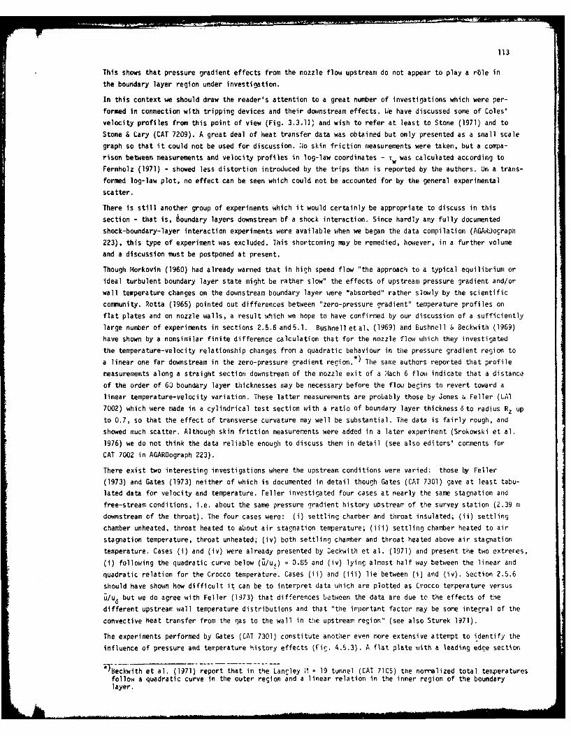
113

This shows that pressure gradient effects from the nozzle flow upstream do not appear to play a role in

the boundary layer region under investigation.

In this context we should draw the reader's attention to a great number of investigations which were per-

formed in connection with tripping devices and their downstream effects. lie have discussed some of Coles'

velocity profiles from this point of view (Fig. 3.3,13 and wish to refer at least to Stone (1971) and to

Stone & Lary (CAT 7209). A great deal of heat transfer data was obtained but only presented as a small scale

graph so that it could not be used for discussion. ;o skin friction measurements were taken, but a compa-

rison between measurements and velocity profiles in log-law coordinates - Tw was calculated according to

Fernholz (1971) - showed less distortion introduced by the trips than is reported by the authors. On a trans-

formed log-law plot, no effect can be seen which could not be accounted for by the general experimental

scatter.

There is still another group of experiments which it would certainly be appropriate to discuss in this

section - that is, 6oundary layers downstream of a shock interaction. Since hardly any fully documented

shock-boundary-layer interaction experiments were available when we began the data compilation (AGARograph

223), this type of experiment was excluded. This shortcoming may be remedied, however, in a further volume

and a discussion must be postponed at present.

Though Morkovin (1960) had already warned that in high speed flow "the approach to a typical equilibrium or

ideal turbulent boundary layer state might be rather slow" the effects of upstream pressure gradient and/or

wall temperature changes on the downstream boundary layer were "absorbed" rather slowly by the scientific

community. Rotta (1965) pointed out differences between "zero-pressure gradient" temperature profiles on

flat plates and on nozzle walls, a result which we hope to have confirmed by our discussion of a sufficiently

large number of experiments in sections 2.5.6 and5.1. Bushnell etal, (1969) and Bushnell & Beckwith (1969)

have shown by a nonsimilar finite difference calculation that for the nozzle flow which they investigated

the temperature-velocity relationship changes from a quadratic behaviour in tie pressure gradient region to*)

a linear one far downstream in the zero-pressure gradient region. The same authors reported that profile

measurements along a straight section downstream of the nozzle exit of a Mach 6 flow indicate that a distance

of the order of 6U boundary layer thicknesses may be necessary before the flow begins to revert toward a

linear temperature-velocity variation. These latter measurements are probably those by Jones 6 Feller (LA1

7002) which were made in a cylindrical test section with a ratio of boundary layer thickness 6 to radius Rz up

to 0.7, so that the effect of transverse curvature may well be substantial. The data is fairly rough, and

showed much scatter. Although skin friction measurements were added in a later experiment (Srokowski et al.

1976) we do not think the data reliable enough to discuss them in detail (see also editors' comments for

CAT 7002 in AGARDograph 223).

There exist two interesting investigations where the upstream conditions were varied: those by Feller

(1973) and Gates (1973) neither of which is documented in detail though Gates (CAT 7301) gave at least tabu-

lated data for velocity and temperature. Feller investigated four cases at nearly the same stagnation and

free-stream conditions, i.e. about the same pressure gradient history upstrearr of the survey station (2.39 m

downstream of the throat). The four cases were: (i) settling chamber and throat insulated; (ii) settling

chamber unheated, throat heated to about air stagnation temperature; (iii) settling chamber heated to air

stagnation temperature, throat unheated; (iv) both settling chamber and throat heated above air stagnation

temperature. Cases (i) and (iv) were already presented by 3eckwith et al. (1971) and present the two extreres,

(i) following the quadratic curve below (Ulu,) = 0.85 and (iv) lying almost half way between the linear and

quadratic relation for the Crocco temperature. Cases (ii) and (iii) lie between (i) and (iv). Section 2.5.6

should have shown how difficult it can be to interpret data which are plotted as Crocco temperature versus

u/u6 but we do agree with Feller (1973) that differences between the data are due to the effects of the

different upstream wall temperature distributions and that "the irrportant factor may be some integral of the

convective heat transfer from the gas to the wall in thie upstrear region" (see also Sturek 1971).

The experiments performed by Gates (CAT 7301) constitute another even more extensive attempt to identify the

influence of pressure and temperature history effects (Fig. 4.5.3). A flat plate with a leading edge section

-)Beckwith et al. (1971) report that in the Langley 11 19 tunnel (CAT 71C5) the normalized total temperaturesfollow a quadratic curve in the outer region and a linear relation in the inner region of the boundarylayer.

114

a bC

Fig. 4.5.3 Flow configurations. Gites (1W73).

(a half-wedgeof 100 included angle) wnich could be cooled was fixed along the tunnel centre line in that

part of the test section where the pressure gradient was zero (configuration (c), series 09 and I). The

temperature distribution on the wall which provided the temperature upstream history was designed such that

the wall temperature fell from 233 K at the leading edge to 91 K at X = 0.427 m, rose to 296 K at X = 1.45 m

and remained constant up to 3.28 m (velocity and temperature profiles series 10). In the case which was used

for comparison the wall temperature was nearly adiabatic with slight heat transfer to or from the plate

(profile series 09). Since the pressure distribution was identical in both experiments any differences

between the cooled and uncooled leading edge cases must therefore be ascribed to the temperature history

alone. It is, however, extremely unfortunate that no skin friction measurements were provided so that upstream

effects on the skin friction at the measuring stations could not be observed. A comparison between the velocity

profiles and the log-law - where Tw was calculated according to Fernholz (1971) - does not show differences

between the two groups of velocity profiles (Fig. 4.5.4). Leaving aside the possible uncertainty in the

28 _

26 .. .... . .030

24 //.0

22 __ 0_.U200

18 ____

I j CAT 7301

16 . __-__ ___

..- Profile M6 Re62 Tw/.T leoding edge

14 - o 0901 4.06 2649 1.02

0 e 0903 4,11 6778 098 cooled

12 " . 1001 405 2565 0.98 cooed

10 yu/v 1003 411 7140 096

10' 2 4 6 102 2 6 103 2 4 6 104

Fig. 4.5.4 Law of the wall for a compressible boundary layer (upstream temperaturehistory, zero pressure gradient, defined origin). Gates (1973). cf fromFernholz (1971).

determination of the skin friction which could of course change te picture, no differences between tne

velocity profiles can be observed whicn ro beyond the normal scatter. As so often in ,OL neasurements the

wake strength is larger (profiles j903 and 1J03) than in comparable cases (cf. section 3.3.3). The equi-

valent temperature profiles are shown in Fig. (2.5.6) and do not show upstream effects either.

An obvious gross effect of upstream heating as reported by Gates is to modify the downstream adiabatic wall

temperature. For example, in the absence of any leading edge cooling the "experimental recovery factor" was

about 0.88. The corresponding value with a cooled leading edge was 0.78 at the first measuring station

(X = 0.914 m) relaxing to 0.86 at the most downstream station (X = 2.743 m). Similar effects were reported

by Voisinet & Lee (CAT 7202).

i r115

In configuration (b) the test plate in the tunnel was extended upstream by a plate of similar construction

where the leading edoe was formed by a half wedge of 190 included angle and was 153 rmr upstream of the throat

(X = 0). Again the leading edge section could be cooled by liquid nitrogen. In this expe'iment the wall

temperature fell from 277 K at X = -0.08 m to 251 K at X = -0.015 m and rose to the adiabatic wall tempera-

ture 299 K at X = 0.305 m (profile series 08). In the second experiment on this plate the wall temperature

fell from 321 K at X = 0.061 m to 298 K at X = 1.14 m remaining constant from thereon (series 07). Some

velocity profiles characteristic of these cases are plotted in Fig. (4.5.5). The measurements lie slightly

28 DOD{ m

26 _._ _

2/. __ - __ -- _

20 - j800 6

08 4 0

16 - "Profile M6 Re62 Tw/T r

0 0 0701 3.96 2766 0.91314/- e 0702 4.01 3435 0.922

0 o •0704 3.93 5651 0.936

12 o P'i o 0804 3.99 6318 0.926<0

10 2 1 y 3 ,

101 2 . 6 102 2 4 6 10 2 4 6 10'

Fig. 4.5.5 Law of the wall for a compressible boundary layer with upstreamtemperature history (isothermal wall, zero pressure gradient,defined origin). Gates (1973).

above the log-law but they are so consistent in themselves that it is impossible to discern upstream-history

effects. cf was determined in the same way as for series 09 and 10. It is interesting to note that the severe

upstream pressure history in this case does not show at all on the ,og-law plot.

The equivalent temperature profiles are shown in Fig. (4.5.6) and agreement with the prediction is good both

for the static and for the total temperature profiles. However, attention should be drawn to the data extra-

polated in the inner region by Gates himself. It is a pity that this discussion must necessarily be inconclu-

sive because no skin friction information was provided for an investigation on this large scale.

Before we close this discussion of measurements where the boundary layer had deliberately been subjected to

upstream history effects we wish to draw attention to two other large projects. Both investigations were

performed in watercooled conical supersonic nozzles (Boldman et al. CAT 6901 and Back et al. CAT 7207) and

had apparently clearly defined practical objectives. Although their authors provide a large amount of data,

it is not sufficient to describe the upstream history effects on the downstream boundary layer, especially

as no reliable skin friction data were available. The experiments were included as entries in AGARDograph

223 principally as a challenge for calculation methods.

This discussion of upstream history effects in supersonic boundary layers is not very satisfactory. This

may partly be due to the fact that the "systematic" investigations performed so far do not give sufficient

information or because the upstream effects were too weak, partly because these effects are hidden - and there-

fore not enough magnified - in experiments which had other objectives such as that of Lewis et al.(1972) (cf.Fig. 5.5.1.1 and 5.1.2) and especially those carried out in boundary layers with favourable pressure gra-

dients (see section 5.2). In these latter cases "upstream effects" were, however, often confused with

116

1.0 of

TI

0.8

0.7!

0.6 _ u /u6

0.2 0.3 0.4 0.5 0.6 0.7 0.8 0.9 1.0leading

Profile M6 Re62 T/T, x[mj edge4 -- o 0701 3.96 2766 0.91. 1.45 Iod

- 070. 3.93 5651 0.936 3 .8 9 c ° ° e-& 0801 4.03 3058 0,933 1.5,-- 080. 3.99 6318 0926 3.89

te rea theoretical

T6 CAT 7301

2 polated

I I I U/U60.2 0.13 0,4. 0.5 0.6 07 0.8 0.9 1.0

Fig. 4.5.6 Comparison between measured and theoretical

temperature profiles in a boundary layer(upstream temperature history, zero pressuregradient, origin defined). Gates (1973).

cGiibined pressure gradient and cooling effects on the temperature profiles. Jeviations, for example, between

n.easured temperatures and predictions according to the equations of table (2.5.1) probably occur simply

because the validity range of these equations was exceeded (see section 5.2).

Since there exist hardly any reliable calculation methods for compressible turbulent boundary layers which

can take account of the variety of upstream histories discussed above, we briefly resort to laminar bounda-

ry layer calculations to throw some light on upstream effects in a controlled manner. It is well understood

that transport phenomena are radically different in laminar and turbulent flows but laminar flow calculations

ray at least serve as a guideline for the engineer until we have good experimental evidence for turbulent

boundary layers.

Lack (1970) found that favourable pressure gradient and wall cooling strongly influenced both temperature

and velocity profiles over a wide range of flow velocities; this was noted for similarity solutions of the

equations for laminar boundary layers. Since similarity solutions can only give a crude approxintion for

physically realistic compressible larinar boundary layers, Moser (1979) used a pseudo Tschebyscheff-spectral-

rethod to calculate the development of a compressible laminar boundary layer with a wall-temperature dis-

tribution decreasin c monotonically to a constant value. The numerical results are compared with the tenmpe-

rature-velocity relationship (eqn. 2.5.37a) using a recovery factor r = 0.85 (Walz 1966) and the velocity

distribution calculated by the numerical method. Fig. 4.5.7 shows that good agreement is achieved for profiles

(3.2.A) and(3.2.J), the former having hardly been influenced by the wall-temperature Cradient and the latter

having recovered from such a gradient. Larger discrepancies occur for profiles (3.2.B) and (3.2.C). here

eqn. (2.5.37a) does not hold since the wall is not isothermal. It is astonishing, however, that the dis-

crepancies do not exceed 20 % in the outer region of the boundary layer and that all temperature profiles

117

agree in the near wall region. Note that the recovery factor as calculated by Moser was 0.787, i.e.

smaller than that given above by Walz. In Fig.(4.5.7)we show therefore temperature profiles calculated

according to eqn. (2.5.37a) with r = 0.787 (broken line). In this case the discrepancies are larger.

Both Moser and Gates found a variable recovery factor, i .e. a function of upstream history and Mach number,

but we do not think that the evidence provided for such a variation is sufficient yet.

Profile M6 T./T R62 Ae x mlo 3.A 12 0 747 8 76 0006e 32B 12 0.25 61 295 0.080o 3.2C 12 0,10 185 421 0.153. 32D 12 010 265 605 0.300

18"lOQ von Driest (isothermal wali, zero pressure gradient)

recovery factor r - 0.85; --- r 0.787

16

T T0.0 T

0.4

0 0'10 .1 0.2 0Qa -Pr'ofile i 2A i.2 l2 30d

0 0.2 0 406 o.8 to o 0,2 q4 o,6 0.8 1.0

Fig. 4.5.7 Comparison between numerically calculated temperature profiles andvan Driest's analytical solution (laminar boundary layer, zeropressure gradient, variable wall temperature, defined origin).

Further investigations using various other wall-temperature distributions are necessary before final con-

clusions can be drawn about the influence of variable wall temperature in the upstream region.

Fig. 4.2.17 Law of the wall for a compressible boundary layer (adiabatic wall,zero pressure gradient). Thomke (1969).

8 -= ",Profile Profile7'o 0701 7-- .- .. . 1301

* 0702 a 1302

6 , 1201 6 v 1501& 1202 [ 1502

5!

SU*-U *6-

33

2 2- '

32 -1

Ft. , I r jad 0tc wull, ue

118

4.6 Wall roughness

Since skin friction drag contributes a laroe proportion of the total drac' of aerodynamic bodies cruising

at supersonic speeds, the influence of surface roughness on the skin friction of a compressible turbulent

boundary layer must be known. The same holds for wall heat transfer which is larer for a rough surface

than for one which is aerodynamically smooth. As well as effects on the data, changes of the turbulence

structure due to wall roughness are to be expected. Unfortunately there are so many possible types of

roughness that even for incompressible boundary layers only a few have been investigated (for references

see Schlichting 1965 and Fernholz in Bradshaw 1976). It is necessary to distinruish between two- and three-

dimensional roughnesses. V-9rooves and ridges such as square bars (cf. Perry et al. 1969, Antonia t LLxton

1971 for incompressible flow, and Kubota & BerC 1977 for compressible flow) are typical of the first type

and sand orain roughness of the second. Such uniformly distributed roughnesses may avain be divided into"closely spaced", of which sand grain roughness is typical or "widely spaced" which may in the limit be

regarded as a set of more or less independent protuberances. In the first case, a single roughness scale

may be sufficient to relate different sizes of sand grain roughness, for example, whereas in the second

both roughness height and spacing must be taken into account. Such protuberances, single circular holes

and various forward and backward facing steps were investigated as to their effect on a supersonic boundary

layer by Gaudet & Winter (1973). Developments in re-entry technolony and supersonic flight vehicle desion

have suggested the importance of two further kinds of surface rouchness. One is the phenomenon of cross-

hatching on heat-shield materials (e.g. Langanelli & Nestler 1969) and the other is the pattern of surface

ridges or grooves with longer scale surface undulations created during the fabrication process of fiberglass

wound material (Reda 1974 and Reda et al. 1975). This latter type of rouchness needs,for a physical model,

one or more roughness scales and at least one short and one long wavelength scale.

In contrast to the extent and complexity of the problems there is a dearth of available data, as can be seen

from Table 4.6.1. Only three of the investigations listed there contain tabulated data which could be used

for the data compilation (CAT 5502, 5804 and 6506), two of which deal with sand-grain roughness and one with

a two-dimensional V-groove type roughness. Since Fenter & Lyons (CAT 5804) did not measure skin friction

their data could not be used for a comparison with the inner or outer law of a turbulent boundary layer.

Closely spaced three-dimensional roughness

It is not astonishing to find that it is the boundary layer over the sand grain roughness coverin' a surface

uniformly which has been investigated most thoroughly, both in low and high speed flow. Prandtl (1932) and

Schlichting (1936) showed that the result of experiments by Nikuradse (1933) in which both the skin friction

and the development of mean velocity profiles in a sand-roughened pipe flow had been measured also hold for

incompressible boundary layers (confirmed by Hama 1954). If the roughness length scale kr (related to the

mean height of the sand grains) is made dimensionless by v/ut one can distinnuish between three regires in]T

incompressible flow. The argument holds for nominally zero pressure oradient flow, for if the shear stress

in the wall region changes with y (aT/Dy # 0) a parameter (k r/Tw) T/3y must appear but its effects are

unknown. According to the value of a roughness Reynolds number krUT/Vw one can distinruish according to

Clauser (1956):

(1) Aerodynamically smooth walls (0 < kruT/v < 5).

The roughness elements are submerged in the viscous sublayer and do not affect the boundary layer

significantly. The upper limit establishes the critical permissible roughness of a surface below which the

skin friction drag is the same as that for a smooth surface.

(2) An intermediate condition (often referrd to as transient or transitional roughness)

(5 < kruT/v < 70). The velocity profile is affected by the roughness of the wall, and this effect is takeninto account by a function f which is substituted into the law of the wall instead of the constant C in

eqn. (3.2.3) where

f (krUT/V) = C - A (;k/u,). (4.6.1)

Eqn. (4.6.1) is sometimes called the Clauser form of the roughness function and is universal for the

conventional sand grain roughness in pipe, duct and zero-pressure boundary layer flows.

119

u Uo C') U. - 0- N

4-1in

o 0 0 .. 0. CL -

0. 0. 0. 0. 0. 0.oa a.0. 0. 0. L 9-L

0. ~ ~ ~ C . U A U L. 3

j, C)

9 -

C. C) C C C: .

IL'c

.4 0 A- w .

0 =C4A

@300

o0 CW C @33 4

o9 cc C) 03)0 @

2: e C4 (v C Ln 0'0. 0 l

@. 1')

I N W

U.UI-o

N 01

@3 C D a C, I

4O C 0

120

A (a /U T) in eqn. (4. '6.1), the roughness induced "shift" of the outer velocity profile'can be expressedaccording to Kara (1954) for natural roughnesses such as wrought or cast iron by

A (ak/u) = (I/K) In [(kru /v) + 3.30] - 2.92. (4.6.2)

It is zero for smooth walls and depends only on the roughness Reynolds number.

The logarithmic law then reads

u/uT = (I/K) In (u.y/v) + f (kruT/v). (4.6.3)

(3) Fully developed roughness (70 < kruT/V).

The velocity distribution in the log-law region is now independent of the viscosity because the characteris-

tic Reynolds number is large. The logarithmic law of the wall simplifies tou/uT = (1/K) In (y/k) + Ck (4.6.4)

where Nikuradse (1933) found Ck to be 8.5. Another form of eqn. (4.6.4) - often adopted for velocity profiles

in atmospheric boundary layers - is given as

u/u = (1/K) In (y/zo) (4.6.5)

z0 beina chosen so as to absorb the constant Ck. The serniloCartthric relationship between u/u and (y/k)

holds only for the region close to the wall. If the reference point from which y is to be measured is not

chosen correctly the region that should be linear on a semi-loo plot becomes curved, and this may be used

to find the origin of y (Schubauer & Tchen 1959).

Similarly, for roughness distributions other than the conventionally agreed "sand grain roughness" there

may be difficulty in choosing the characteristic height k. In effect, for any repeatable roughness form,the value of k must be found experimentally as a proportion of a definable physical roughness dimension,

so giving an "equivalent sand grain roughness height" ks -The knowledge gained in incompressible boundary layers along walls with uniformly distributed sand-grain

roughness can be transferred to compressible boundary layers if the following modifications are taken into

account (Goddard 1959):

(a) The kinematic viscosity v in the roughness Reynolds number and in equations

(4.6.1 to 4.6.3) must be taken as the wall value vw.

(b) The mean velocity 5 must be transformed to u++ according to van Driest (1951),

i.e. eqn. (3.3.13.a) or as we shall do here according to eqn. (3.3.10).

(c) The upper limit for the rouahness Reynolds number should be raised from 5 to 10

for an aerodynamically smooth wall.

These modifications were seen to be necessary if a velocity profile in a compressible turbulent boundary

were to agree with its incompressible equivalent both in the log-law and the outer law form (see sections

3 and 4).

Goddard found for zero-pressure gradient flow along an adiabatic wall that the upper limit for an aero-

dynamically smooth surface was independent of Mach number for a Mach number range 0.70 < M6 < 4.50. The

ratio of the skin friction coefficients cf /cf measured on a rough and a smooth wall and plotted against

kru /vw remained unity up to a value of of the roughness Reynolds number and followed a quadratic

relationship - as given by Nikuradse for the incompressible case - from there on (Goddard Fig. 27). This

result was confirmed by Reda (1974), and we present his comparison with published data in Fig. (4.6.1).

Bradshaw (1977)has observed that for large enough values of Mach and Reynolds number the flow near the top

of the roughness elements must exceed M = 1 and explicit dependence on the Mach number is then to be expected.

The only tabulated data measured in a boundary layer over sand grain roughness (Shutts & Fenter 1955) are

shown in Fig. (4.6.2). It is seen that the effect of roughness is to displace the velocity profile curve

downward to a position essentially parallel to its original position (as had already been remarked by

flkuradse 1933). As can be seen from several evaluations of boundary layer velocity profiles over rough

walls with various kinds of roughness this shift of the velocity profile & (u/u) is a function only of

the roughness Reynolds number (kuT/Vw) (Goddard Fig. 40, Reda Fi. 19 and Kubota & Berg Fig. 18).

Kubota A Berg (1977) give a semi-empirical relationship between the velocity shift - using the velocity

ratio A (5 k/uT) of eqn. (4.6.1):

121

a (i-) .3.28 -5.70 In ks + 2.83 (In k+l- 0.29 (In k )3 (4.6.6)

which holds for "several roughness configurations (sand grain, V-groove square bar) and Mach numb~ers

(0 < M8 ! 6)" if the roughness height ks is chosen as the equivalent experimentally determined sand grain

roughness.

Whereas eqn. (4.6,6) holds for transient and fully rough regimes a simple relationship can be derived forthe fully rough regime alone. If the velocity in eqn. (4.6.4) is substituted by a* and if one then sub-tracts eqn. (4.6.4)* so obtained from eqn. (3.3.9), which holds for flow along a smooth wall, one obtains

- r * i .C~(4.6.7)

If this relationship is to be used for flows over walls other than covered with sand grain roughness then

k must be substituted by the equivalent sand grain roughness k s. The latter is determined from the shift

of the velocity profile over the unknown roughness which is then inserted into eqns. (4.6.6) or (4.6.7).

C** was found by Nikuradse to be - 3.

3.5 - !MR- mew 11 ft/F TINE WUSS MRl

0 INK 4.5 _1-W7

16186 ~ fl

&0 M 43 l' a 46 Is -O LA PLAI[

0. 0.04qs

2.0-6i i.12

ALL DATA F01 AIA1C fiB

0.5- #6, FO f=

I is 108U

Fig. 4.6.1 Smooth-to-rough wall skin friction coefficient ratio v. roughnessReynolds number; a comparison with published data. Taken from Reda (1974)

Profile R% ximl FRI VIOP'1C%i- V. th

o 0101 10533 0.22 11102 3.21 1.91 S1.2 71.0* 0103 16691 0.50 0.109 267 1.65 A.9.2 7.50* 0105 22 104. 0.70 0.109 2.70 1.62 41.1.8 750* 0201 6737 0.19 0.162 1.16 2.36 67.1. 920* 0202 11.g21 0.0 0.162 3.4.2 2.15 60.2 6.1.0

21 0201. 26225 0600 0.162 2.67 1.85 69.9 750

.) from authors22 . c, for a smooth wall

from Fernholz 11971)20 -04 VW_

CAT 5502

1112.50 in (yu,A. .i

12r - -

--- __

g10 = 0

I0 - - 0 1 1 - _____I I

10 2 1. 6 V0 2 1. 6 103 2 & 6 10

Fig. 4.6.2 Law of the wall for a compressible0 boundary layer (adiabatic wall, zero pressure gradient,M8 2, defined origin, sand-grain roughness). Shutts & Venter (1955).

122

Since only a few tabulated data were available for a comparison with the above semei-empirical relation-

ships, we have used Pedals (1974) figure 19 as our Fig. (4.6.3).

SlUM SOURCI 0. IM , FTi 6AMMESS cONiaISUiTMiUIMADE 0 SAi sam iN PIE FLOWIFSi OMiUI

S GODDARD 25 -41 •it SA Mm COE*-CIuY mlOS 43 135 I' V.4 FLAT IPATE

14- MANA - [UV FAT SURFACEIFMm cIAUKM'I

C CLEAM - - SAW m -MEIFM CLAUSEWI

12 0 PUNITSAIA 2 2 3 . 10 6 S FLAT.U MUMWAL

M PRESENT ATA 21 23 106 MUEL j FLAT. NOZZL WALL* POESENT OTA 29 2 3 -10 MODEL .12 FLAT, NZZLE WALL

10

S.U,

6 # ALL DATA FO AOIAUATIC FLOW

4-

#9, #9. *2 It SIR\ * FULLY ROUGH

10 100 1000ROe

Fig. 4.6.3 Rouahness induced law-of-the-wall velocity shift v. roughness Reynoldsnumber; a comparison with published data. Taken from Reda (1974).

Fig. (4.6.4) shows the Shutts & Fenter data of Fig. (4.6.2) plotted versus the abscissa y/k. Neither thesedata nor those by Young (1965) agree satisfactorily with eqn. (4.6.4) if the transformed velocity u* is

used instead of u. This may partly be due to the fact that the flow is still within the transient regime,

partly that the skin friction measurements have larger errors than for boundary layers along a smooth wall.

This contradicts the results found by Goddard (1959, Fig. 38).

24 Profile M Re2 t/,- 0- __

o 0201 4.97 1817 0.944 a0 AN22 0205 487 1709 0,555 O II 1 -

2 0301 4.94 2059 0.962 0 _ _ oe_2 0305 4.84 1845 0.542 6 0

18 0401 4.97 2536 0.966 A' 250 In (y/ k) 8. So

A 0405 4.93 2168 0.541. 1

16-- CAT 6506 A, N~~0.~u2 0 (b) L CAT 5502

14 . A -m -.-

6 I( 1o Profile M6 Re62

12 0 - o_ o0101 2.02 10533* 0105 2.01 22104

10 0- _ , o 0201 2.01 8737- _ y0204 2.02 26225

8 T y/kI II

10O 2 4 6 lo' 2 4 6 10O10o 2 4 6 10' 2 4 6 102 2

Fig. 4.6.4 Law of the wall for compressible turbulent boundary layers over rough walls(adiabatic and isothermal wall, zero pressure gradient, defined origin).Shutta & Fenter (1955) and Young (1965).

123

As is well known from subsonic flow measurements there is no influence of the wall roughness on the outer

law as can be seen from Fig.(4.6.5).

8 0 8e 0 0103 o 0201

@ 0105 .0205o 0202 0301

6.a0205 6 a 0305

50 _ 0401U;-u"CAT 5502 U;U * " 04054l l : °U oo

3 -1 3CAT 6506

2 12

(adiabatic and isothermal wall, zero pressure gradient, deined origin).Shutts & Fenter (1955); Young (1965).

Fenter & Lyons (CAT 5804) describe a further systematic DRL attempt to investigate the effects of distributed

roughness. In these tests the boundary layer was formed on a flat plate, with an initial smooth section on

which was mounted a trip. Profile measurements were then made at the downstream end of a variety of rough

inserts. The absence of any shear stress measurements unfortunately reduces the value of the data greatly.

(They also include one series of measurements with uniform roughness where the entire plate surface was coated

with spherical beads of 0.105 mm diameter).

Two-dimensional roughness

An obvious choice for a two-dimensional roughness is the transverse V-Sroove or thread roughness. The chief

advantage of this roughness lies in its application to bodies of revolution and several investigations have

been made using such surfaces (Wade 1955, James 1959, Fenter 1960). Also, there is evidence that this type

of roughness compares closely with sand grain roughness as mntioned above (Young 1965). The only experimn-

tal investigation for which tabulated data were orovided in sufficient detail for a comparison with smooth

wall data is that of Young (CAT 6506) who did not measure TO profiles but used the van Driest velocity

transformation. The roughness pattern had a regular 90 0 saw tooth (V-groove) section aligned across the

plate, with wave lengths of 0.127, 0.254 or 0.762 mm, and corresponding peak to trough heights of one half

the wavelength. Young's measurements are distinguished in so far as both skin friction (the floating element

balance was duly cooled) and heat transfer were measured and as smooth wall Oata were available for compari-

son. The latter agree very well with the logarithmic law (Fig. 4.3.1) and with the outer law (Fig. 4.3.2),

irrespective of the heat transfer rate. Agreement between the rough wall data and the outer law is good as

can be seen from Fig. (4.6.5.b).

The skin friction measurements show that for the smallest roughness height the increase above the smooth

plate results are small. This explains the small deviation of the velocity profiles from the log-law in

Fig. (4.6.6) if one takes into account additionally that measuring errors for the skin friction are likely

to increase if wll roughness and heat transfer are involved. From these results one may also deduce that

the smallest surface roughness used in this experiment was below the limit for the critical roughness

Reynolds number. In this case the result is not affected by heat transfer - u. k/vw rises from 5.2 for the

F1II

124

adiabatic wall to 6.6 for the cooled wall.

roughness Ukhe~ght k U " AIUN

Profile M6 T. / T, Re62 mm V, UT

o 0201 497 0.944 1817 0.0635 5 2 -* 0205 487 0555 1907 00635 6.6 -

0301 494 0.962 2059 0127 11 5 150

• 0305 4.84 0542 1845 0127 149 150

o 0401 4.97 0967 2535 0.381 388 490

* 0405 4.93 0.541 2168 0381 45.6 4.90

24 00

CAT 650622 -. _

20 - CL.17 -0 a __£

UT

182.50 In (yu,/v.)#5 10 0 * l

16 . . o --- ,

14 712 I a -U, !i10E L _101 2 4 6 102 2 4 6 10'

Fig. 4.6.6 Law of the wall for a compressible turbulent boundary layer (isothermalwall, zero pressure gradient, aefined origin, V-groove rouglnoss).Yount (1965).

As for the larger roughness heights the expected downward shift in the velocity profiles occurs but there

is hardly any difference between the cases with and without wall cooline. This means that the transformation

accounts for the heat transfer as for smooth wall boundary layers described in section 4.3.

In order to com.plete the discussion we have also plotted some of Younr's velocity profiles versus y/k (Fio.

4.6.4.b). Here we find the opposite trend to that of the Shutts & Fenter data as the measurements now lie

above the Nikuradse relationship (eqn. 4.6.4), arain contradicting conclusions of Goddard (1959).Since both

heat transfer and skin friction were measured in this experiment we would like to qunte the conclusions

drawn by Young:

"With increasing roughness, heat transfer to the rounh surface is increased, as is the skin friction, but

to a different degree which depends on the roughness rerime of the flow.The Peynolds aralogy factor, which is relatively insensitive to chanres in the flow parameters, appears to

remain valid as long as the rounhness height is less than twice the lamipar sublayer thickness. For rough-

ness in excess of this value, the analogy factor increases directly with the rouchness height until the

fully rough regime is reached, after which it is protable that it increases approximately with cf. that is,

it appears that ch may reach a relatively constant value for larme rouehness heirhts".

Pnother two-dimensional roughness configuration which has been studied extensively in low speed flow (e.g.

Perry et al. 1969, Antonia & Luxton 1971) is the square bar type which is characterized hy a heinht and awavelength. If the wavelength to heinht ratio X remains below a certain level quasi-stable vortices are

found in the cavity in between. This type of roughness is called "d-type" (e.r. V'ood t Antonia 1975). For

a d-type roughness in subsonic flow little direct interactlnn seems to occur hetween the roughness and the

125

mean flow in the boundary layer, so that there are features similar to those of a smooth-wall boundary

layer. Kubota & Berg (1977) present measurements in a compressible boundary layer over a d-type roughness

(X = 4) where the crests of the roughness elements were aligned with the smooth surface upstream. Roughness

heights of 0.318, 0.635 and 1.27 mm were used corresponding - according to the authors - with equivalent

roughness Reynolds numbers of 18, 40 and 85. Both mean flow and fluctuating flow data were acquired for

several snooth-to-rough surface step changes and a single rough-to-sooth surface step change.

Since no tabulated data were available from the authors of the report we can only quote three of their

conclusions:

(1) "The establishment of new equilibrium mean and fluctuating flow profiles downstream of a step change

in surface roughness is accomplished in nearly the same distance (in term of boundary layer thicknesses)

as in the incompressible case. The step change smooth-to-rough configuration boundary layer attains new

mean flow selfsimilar profiles over some 10 8 or 20 61 downstream of the step, while the fluctuation pro-

files reach this state some 14-16 6 or 28-32 61 downstream of the step. These distances are independent of

roughness height for roughnesses in the transitionally rough regirre - (ks uT/vw) < 70.

The step roughness change rough-to-smooth configuration produced a somewhat slower adjustment of the boundary

layer sore 14 6 or 28 61 for mean flow equilibrium and some 20-25 6 or 40-50 61 for fluctuation equilibrium.

(2) The hypersonic smooth and rough wall equilibrium profile velocity data, subsequent to a modified Van

Driest transformation - modified in the sense that the T/T, = f (U/u,) relationship was substituted by a

least squares quadratic curve fit to the measured data - to "equivalent incompressible" form are well corre-

lated by the incompressible composite law of the wall.

(3) The investigation of the rough-to-smooth step change configuration revealed the existence of very signi-

ficant pressure and temperature history effects throughout the boundary layer. . . The presence of the rough

surface on the nozzle wall within the expansion region was sufficient to alter the history effects but was

not able to eliminate them. . . . Considerably more research is needed in this area to delineate the extent

of these history effects and investigate the possibility of destroying them."

For further references on rough wall boundary layer flows the reader is referred to Fernholz (see Bradshaw

"Turbulence" 1976), to Dvorak (1969) for a calculation method for incompressible flow and to Chen (1972) for

a calculation method for compressible boundary layers.

126

5. INTERPRETATION OF MEAN FLOW DATA FOR PRESSURE GRADIENT CASES

5.1 Causes and broad effects

In section 4 it was shown that the general behaviour of a constant pressure boundary layer was, when con-

sidered as a transformed profile in relation to the wall and wake law , very similar to that of a low speed

boundary layer. Departures from eqns.(3.3.9) and (3.3.17) were not generally large, and when observed

could usually be ascribed to a known, if often unquantifiable, secondary factor (§§ 3.3.4, 4.2.3) or to

experimental uncertainty, particularly in the determination of skin friction. This means that the van

Driest transformation can cope very well with mean density gradients 3 /ay perpendicular to a wall which

may be isothermal or adiabatic if at least the pressure gradient 21/ax is zero.

It therefore seems sensible to continue a discussion of mean flow profiles on the same basis though the

transformation should now take into account .4/9x besides 3 /3y . From subsonic experience we would ex-

pect the "constant pressure" wall law (eqn. 3.3.9) to be observed over a wide range of pressure gradients -

see the figures in sections 5.2 and 5.3 - so long as the flow does not approach separation, in adversepressure gradients, or moderate favourable pressure gradients even if far from relaminarization. We would

also expect the wake function to be increased in an adverse pressure gradient and vice versa.

There are, however, distinctive features of the compressible flow. At supersonic Mach numbers the pressure

changes are comparable with the total pressure, and as a result of the hyperbolic nature of the inviscidflow field, these pressure changes may be concentrated into relatively small regions. The dynamic pressure

may well become very large as compared to the static pressure, so that quite small changes in flow direc-

tion may require relatively large pressure differences normal to the flow. This possibility (p<< 1/2 p U2)

also leads to the possibility of turbulent Reynolds stresses in a boundary layer becoming comparable with

the static pressure (Finley 1977). Finally the large proportional changes in pressure, and consequently

density, lead to some features of boundary layer behaviour which appear to run counter to low speed ex-

perience - for instance a boundary layer in a strong adverse pressure gradient becomes thinner and exerts

an increased shear stress on the wall (Sturek & Danberg, CAT 7101, Lewis et al. CAT 7201, Rose 1973, CAT

7306S and others). Such an effect results from the difference in the flow/unit area - velocity relationship

between sub- and supersonic flow. The general tendency is for a stream tube to decrease in cross-sectional

area as -t slows down rather than to increase. Consequently, in an adverse pressure gradient, a boundarylayer will decrease in thickness, at least until the greater part of the flow becomes subsonic, and as aresult the vorticity and turbulent intensity tend to increase. The general level of Reynolds stresses

7000

Re 8 2 M6 c X10" ' Re62T T c, (measured)

5000 4 20_~,~

4000-

100 _Q M6C, (calculated)

x [mini

2 10 0

30 0 46 5o 600 700

Fig. 5.1.1 Distribution of skin friction, Mach and Reynolds number in a compressibleturbulent boundary layer with variable pressure gradient. Lewis et al.(1972).

127

therefore rises, leading to an increase in wall shear. This effect can be masked by dimensionless presen-

tation, as the scaling quantity P6u2 /2 for the skin friction coefficient also increases as the flow is

decelerated. The distribution of skin friction, Mach number and Reynolds number Re62 in a boundary layer

with varied streanwise pressure gradient (Lewis et al. 1972) is shown in Fig.(5.1.1), and the effects

described above can be seen distinctly. The pressure gradients in this experiment are not severe, however,

and therefore the skin friction distribution can be fairly well predicted even by a calculation method

which does not hold for boundary layers with pressure gradients (Fernholz 1971).

The relevant features of the pressure fields are considered in detail in § 6 so that we here present onlya brief summary. In relation to natural axes along and normal to the flow streamlines, pressure (or more

strictly, normal stress) gradients along the normal can only occur as a result of streamline curvature:

;p/3n = - pu2/R = - y M2 p/R (5.1.1)

where R is the radius of curvature and n and R take the same sign for concave curvature. The pressure

change in a small distance such as the boundary layer thickness,6 , normal to the flow,

A p = 6 (;p/an) = y M2 (6/R) p (5.1.2)

may therefore be proportionally quite large even for modest values of (6/R) if the Mach number is high

enough.

Normal pressure differences of this type, that is, associated with streamline curvature, propagate along

the Mach lines of the flow and are therefore linked to the streamwise pressure gradient by

(ap/an) = ; coti (ap/as) (5.1.3)

where p is the Mach angle sin - (I/M).

The rate of change of flow direction 9 is linked to the rate of change of pressure and Mach number being

(a@G/Bs) = t (av/a s) (5.1.4)

where v (M) is the Prandtl-Meyer angle. As a first estimate for the pressure variation on a curved wall,

it is reasonable to replace s and n by x along the wall and y normal to it, and we refer to a flow in which

the pressure gradient is associated with wall curvature as a SIMPLE WAVE FLOW. There is no rate of change

of pressure along one of the families of characteristics in the free stream flow.

A flow in which equal rates of change of p, M, voccur along both sets of characteristics has straight

streamlines. In natural coordinates therefore, 3p/Bn = o. In inviscid flow, the flow along any straight

wall has ap/an = o, and any wave pattern will be reflected at the wall in such a way as to ensure that

g/as = o. We refer to such a flow, with essentially straight streamlines (at least locally) as a

REFLECTED WAVE FLOW. If the natural coordinates s, n are replaced by the boundary layer coordinates x, y

however, an apparent normal pressure gradient will appear, as except in the trivial case of parallel flow

for which ap/ax = o, the divergence of the streamlines (although they are straight) causes the isobar

through the point (x, o) to curve away from the profile normal. For purely radial flow at a distance Rv

from the vertex, the resulting apparent pressure gradient is

-i Y YM2.? p (5.1.5)

Rv M -1

where i is I for planar and 2 for conical flow, so that the pressure difference across a small distance 6,

normal to the wall, is

p=- 6i ( )2 yM2

A (R ; p (5.1.6)

This can be seen to be fairly small for M not of order 1, A p/p being of order (6/Rv)2 or less than 0.01.

We therefore expect that in reflected wave flows, ap/ay will be negligible. However, although the wall on

which a boundary layer is growing may be straight, the concentrated nature possible for conressible wave

structures allows streamlines at quite small distances from the wall to have significant curvature

128

(e.g. Kussoy et al. 1978, Rose 1973, Zakkay & Wang 1972). and consequently achieve the large values of

A p/p associated with simple wave flows. We have, in AG 223, provided an indicator of the relative impor-

tance of the simple wave element in a flow in the quantity

SW = (ao/av) (5.1.7)

which should in principle be evaluated along a streamline just outside the boundary layer. This has not

been found as helpful as was hoped, and it has been necessary at this stage to assign arbitrary values as

SW = 1 - flows with wall curvature and simple wave structure

(Class 118)

SW = 0 - straight wall flows with no significant concentrated disturbances

(Class IIA)

SW = 0.5 - straight wall flows in which it is believed that the pressure gradients

(Classified are strong enough to cause significant streamline curvature inside thewith 1iB) boundary layer.

We would also point out the extreme case represented by the "normal pressure gradient" flows studied by

Thomann (CAT 6800, series 06-09). There are no profiles available for flows of this type, but they de-

monstrate the existence of a class for which

SW = - - curved wall flows with superposed wave structures causing circular

(Class IIC) streamlines with no streamwise property gradients, but large normal

gradients.

The mean flow wall heat transfer measurements of Thomann (CAT 6800) are especially interesting as he used

the identical measuring equipment for a series of flows in which all possible types of pressure gradient

were observed. Of particular interest is the difference of 20 % in heat transfer rate observed for two

flows on a convex surface (which is therefore not likely to be strongly affected by longitudinal vortex

structures) with different strengths of pure normal pressure gradient (SW =® ), suggesting that the strength

of the normal pressure gradient element must have a significant effect on the turbulence structure. This

effect has no analogue in low speed flow, since it is only on very sharp corners for which the boundary

layers assumptions break down that significant normal property gradients will be observed.

Reference will be made to these various effects in the consideration of mean flow profiles and wall data

below.

In accounting for large discrepancies between an experimental skin friction distribution (Zwarts 1970) and

the results predicted by the Bradshaw & Ferris (1971) calculation method, Bradshaw (1974) concluded "that

the mean dilatational rate of strain, div U , directly affects the turbulence structure to an extent much

greater than expected from the terms (in say, the Reynolds-stress transport equations) that contain the

extra rate of strain explicitly. The main a priori reason for believing that compression or dilatation

may have large effects on the structure of turbulent shear layers was that other extra rates of strain have

been found to change the Reynolds stresses by an order of magnitude more than expected from the size of

the explicit extra terms in the Reynolds-stress transport equations." Bradshaw then introduced this addi-

tional effect by modifying the transport equation in his system of equations accordingly.

As is well known from experience with calculation methods for subsonic boundary layers, every calculation

procedure can be made to agree with a limited number of experiments, and so it was only a question of time

before other calculation methods followed suit (e.g. Horstman 1976, 1977). Once more comparisons between

calculation methods and experiments, especially in adverse pressure gradients, had been performed

(Rubesin et al. 1977 and Acharya et al. 1978),it was not surprising to find that other methods could

describe the experiments well even without extra compression or dilatation terms. So this effect must be

considered questionable unless further evidence for its existence is brought forward.

Before we continue the analysis of mean velocity and temperature measurements, the validity range of the

theoretical assumptions should be stated again and attention should be drawn to the determination of the

wall shear stress and the changes of the turbulence level due to pressure gradients.

As was shown in section 2.5 the temperature-velocity relations hold for boundary layers with pressure

129

gradients only under the condition that the wall is adiabatic. Since the temperature distribution accord-

ing to eqn.(2.5.37a) is used for the deviation of the transformed velocity u* in the logarithmic-law and

in the outer law, these relations are strictly confined to flows along an adiabatic wall if a pressure

gradient is present.

Any investigation of turbulent boundary layers with pressure gradients has to deal with the basic problem

of how to determine the skin friction. Floating element balances which are very reliable for zero pressure

gradient flows (Winter 1977) are sensitive to pressure gradients in the streamwise direction, and the Preston

tube encounters problems related to the validity of its calibration curve in pressure gradient flows,

besides the problems which arise from the different calibration curves as such (a good demonstration of

this dilemma is given in CAT 7102) if the flow is compressible.

Most research workers seem to have forgotten that the validity of the logarithmic law becomes at least

doubtful in favourable pressure gradients if we can transfer knowledge from subsonic (Patel 1965) to super-

sonic flow. For a further discussion of error sources the reader is referred to Rubesin et al.(1977).

Finally attention should be drawn to the increased level of turbulence in boundary layers with adverse

pressure gradients (Gootzait & Childs 1976 and Acharya et al. 1978). Again it is known from measurements

in subsonic turbulent boundary layers that hot-wire signals must be corrected if the turbulence level ex-

ceeds 20 % or so, a value which will be easily exceeded in boundary layers close to separation, even in

incompressible flow. Correction methods are still controversial in subsonic flows, let alone in supersonic

boundary layers.

If these precautions are heeded it should be possible to discuss, and even explain, some of the discrepan-

cies which will occur when measurements in flows with pressure gradients are compared with the logarithmic

law of the wall, the outer law, and the temperature-velocity relationships whi-h may serve as indicators

of the influence or the strength of the pressure gradient.

In the following we shall discuss boundary layer measurements in flows with pressure gradients, firstly

those in a favourable pressure gradient divided into (a) reflected wave - straight wall and (b) simple

wave - curved wall, secondly those in an adverse pressure gradient divided in the same way.

Since the experiment of Lewis et al.(1972) includes the three cases of zero-, adverse- and favourable-

pressure gradient (Fig.5.1.1), it is very well suited to serve as an example of the behaviour of velocity

profiles in various pressure gradients. Sample velocity profiles are shown in log-law coordinates in

Fig.(5.1.2) and in outer-law coordinates in Fig.(5.1.3). As suggested above, the strength of the wake

a (u*/u ) increases considerably in an adverse pressure gradient compared with that in a zero pressure

X 1

24 I22 a i, , i x

20I , . ... -

18- & :CAT 7201

16' Profile M6 Re62 Reo PGrad x [m]16 o 0105 3.98 1514 5035 ZPG 0.342

14 a 0109 3.22 2975 7368 APG 0.40614 0115 2.55 6707 12661 FPG 0.482

12 0119 3.63 4474 13032 FPG 0672

10Z1 2 4 6 8102 2 4 6 8101 2 4 6 80

Fig. 5.1.2 Law of the wall for a compressible axisymmetric boundary layer (adiabaticwall, variable pressure gradient). Lewis et al. (1972).

i kW=UN

130

157a

-and ZPG y X 1 3 [m6 _ APG 12.5 1

F FPG

5 CT a FPG 10uCAT 7201

3 -

a 0

2 - 0 - O -

0a P U

3.5 -3.0 -2.5 -2.0 -1.5 -1.0 0 0.2 0.4 0.6 0.8 1.0

Fig. 5.1.3 Comparison of outer-law with measurements Mass flow profiles (CAT 7201)

gradient - here from approximately 2.6 to 6 - and falls to "negative" values in a favourable pressure gra-dient. The outer law plot shows similarly strongly characterized tendencies. The zero-pressure gradientprofile (0105) agrees with the "outer law" very well. The adverse-pressure gradient profile (0109) shows

a markedly steeper slope than the zero pressure gradient profile while the favourable-pressure gradient

profile (0119) which is downstream of the change from adverse to favourable pressure gradient shows the re-verse tendency. The other favourable-pressure gradient profile (0115) is the first profile after the

change of pressure gradient, and shows by its intermediate character (as also for the wall law in Fig.5.1.2)

that the nature of the profile does not depend only on the local values of the boundary conditions but alsoon the recent history of the boundary layer - particularly for the outer region.

In general, this behaviour of the velocity profiles is confirmed by several other cases in sections 5.2 and

5.3. This experiment may therefore serve as example of all those following except that some caution should

be expressed about the determination of skin friction. Lewis et al. did not measure the wall shear stressdirectly but used the curve-fitting procedure of Coles & Hirst (1969) applied to equivalent incompressiblevelocity profiles transformed as suggested by van Driest (1951). In order to justify this procedure a ca-

libration function for Stanton tubes was presented as evidence of consistency. Since both calibrationsassume a priori the validity of the law of the wall, the good agreement of the velocity profiles with thelaw of the wall (Fig.5.1.2) is no independent proof of its validity,which can only be established by

measuring skin friction directly, for example by a floating element balance, or, possibly, by using a rangeof Preston tubes down to a size small enough to qualify as a sublayer device. For compressible boundary

layers the law of the wall and the outer law depend on the transformation rule for the velocity u whichagain needs a temperature - velocity relationship as given in section 2.5.4. We remarked there that

eqn.(2.5.37) should only be valid for boundary layers with pressure gradients different from zero if the

wall is adiabatic. It is therefore an open question how strongly the temperature profile is affected by

a pressure gradient.

An inspection of Table 7.1 in VARDograph 223 shows that there are few cases where both temperature and ve-

locity profiles and skin friction were measured in the same experiment. Investigations which fulfill this

condition and which can in principle provide evidence of the validity range of the temperature - velocity

relationship are presented in Table 5.1.1 and will be discussed first.

I 131

Table 5.1.1

CAT PG T0 Cf M- Re62 xIO 3 Tw/Tr

7104 APG STP FEB 2.4- 1.9 11 - 26 1

7101 APG CCP,FPTP P 3.5- 2.8 6.5 - 18.8 1

7304 FPG ECP,FWP FEB 3.8- 4.6 2 - 47 0.25 - 1

5901 FPG STP V 8 -10 0.15- 0.47 0.5

6801 FPG STP V 8 -11.5 0.9 - 6.8 0.3 - 0.4

7105 FPG FWP FEB 19.5 0.2 - 0.3 0.2

7206 FPG STP FEB 19 - 45 0.06- 0.13 0.35 - 0.85

A discussion of the validity of the temperature-velocity relationship in boundary layers with streamwise

pressure gradients is more complicated than for the zero-pressure gradient case (cf.section 2.5.6), since

none of the boundary layers hasa defined origin. Therefore we cannot exclude upstream history effects.

In what follows we shall adhere to the pattern of discussion already established in section 2.5.6.

Fig.(5.1.4) - Waltrup & Schetz (1971) - shows a comparison of T/T6 as measured with the prediction of

eqn.(2.5.39). Agreement between measurements and the theoretical curve is good. The right hand graph

shows a comparison between the relationship To/Tod to u/u6 as here calculated from eqn.(2.5.37e) with

Tw=Tr and the measured values of To/To6 . As compared with zero pressure gradient profiles, deviations

between measurements and predictions are relatively large (up to 2.5 %). There is a small overshoot as

is to be expected for profiles on an adiabatic wall, with a relatively more extended overshoot region as

compared to the profiles in Fig.(5.1.5) for example. The measurements lie above the predicted values

contrary to our findings in Figs.(2.5.1 and 2.5.4).

Profile M6 Re62 T/Tr

-o 71040102 2.10 17391 1.04

--- a 71040104 1.88 26107 0.98theoretical

2.0 -

1.8'

1.6 ... 09

1.42 090

12T

120 0o I5~ I

05 06 0.7 0.8 09 10 05 0.6 07 08 09 10

Fig. 5.1.4 Comparison between measured and theoretical temperature profiles(adverse pressure gradient, adiabatic wall, origin not defined).Waltrup & Schetz (1971).

132

Profile M6 Re62 52

- o 71010202 3.54 8041 0 10 To

---- 671010205 3.16 13762 1.41 0 6

'11010307 2.97 17702 1.2. 0

3--{'- :theoretical

08~T -T.

-~ 02 /0

10 u,,,00li/u6- - 0/uo

0 01. 0.5 0.6 0.7 0.8 09 10 01 &. /u610 0.2 0.4. 0.6 0.8 1.0

Fig. 5.1.5 Comparison between measured and theoretical temperature profiles (zeroand adverse pressure gradient, adiabatic wall, origin not defined)Sturek & Danberg (1971).

The left hand graph of Fig.(5.1.5) - Sturek & Oanberg (1971) - again shows good agreement between measure-

ments and predictions, whereas large deviations again occur between the Crocco temperature function

T* = (To-Tw)/(To6 -Tw) calculated from eqn.(2.5.40), using as input the experimental values of u/u6 . The

theoretical curves, all represented in the right hand figure by the dashed line, cannot be distinguished

from each other but they differ from the relation T* =(u/u6 )2. As we have seen already in section 2.5.6

(e.g. Fig.2.5.1), the directly measured data, shown as open symbols, apparently differ considerably from

the predicted curves. We have noted above that these differences are in fact illusory.

Finally agreement between the T /To 6 data and the prediction is excellent, predictions and measurements

being indistinguishable.

Both boundary layer experiments were performed in adverse pressure gradients (the first a reflected wave -

straight wall case, the second a simple wave - curved wall case) on adiabatic walls. The following discus-

sion is concerned with boundary layers in favourable pressure gradients on straight walls only. The first

experiment is that by Voisinet & Lee (1973) and, although the cooling rate is extremely high, agreement

between predictions and measurements is very good (Fig. 5.1.6). The equivalent zero-pressure gradient case

Profile M6 Re 62 Tw/T,- 1203 4.50 28058 0.232

- 1304 4.51 41822 0.259

- 1501 4.37 29503 0.23922 _7- theoretical

T extrapolated EC-Probe CAT 7304

16 ,- - FW-Probe .' T0

12 - 04 - - ,

1.6 n-- 02

0.2 03 0.4 05 0.6 0.7 08 09 10 02 0,4 06 08 10

Fig. 5.1.6 Comparison between measured and theoretical temperature profiles in aboundariy layer (favourable pressure gradient, isothermal wall, originnot defined) Voisinet & Lee (1973).

133

is shown in Fig.(2.5.18) and the resemblance to the graphs for profiles 72021103 and 1203 in Fig.(2.5.18)

is striking. Again we have indicated the region where temperature measurements "had to be extrapolated

due to the size of the equilibrium cone probe (ECP)". Measurements performed with a fine-wire probe (FWP)

extended much more closely towards the wall but they show a dip in the temperature distribution which is

probably caused by "probe-problems". The reader should note the Crocco temperature T* follows a linear

relationship with u/u6 as in the case for a boundary layer with zero pressure gradient. It is possible

that - apart from the pecularities of the NOL-tunnel - the high cooling rate has such a dominant influence

that the rather moderate favourable pressure gradient is in fact too weak to affect the temperature dis-

tribution.

The next two experiments (Hill CAT 5901 and Perry & East CAT 6801) have similar geometrical arrangements

since they were performed on the wall of a conical nozzle. The temperature profiles have in common that

measurements and predictions differ radically from each other as far as the static temperatures are con-

cerned (Figs. 5.1.7 and 5.1.8). Hill's boundary layer had very low Reynolds numbers and values of the

10 Profile M6 Tw/T r Re62 H12 K x m]

o 59010401 8.29 0.542 471 1.88 0.199 - . 59010402 9.10 0.546 317 2.04 0.24

\ 59010701 10.0 0.469 188 2.46 0.19

8 -theoretical

7. 1-2. . ,6 T T

0 0

, I o5 08 0

3 040

0 A'

0 0.2 0.4 0.6 08 10 0 0.2 04 0.6 08 10

Fig. 5.1.7 Comparison between measured and theoretical temperature profiles(favourable pressure gradient, isothermal wall, origin not defined).Hill(1959)

8 - - - Profile M6 Re 62 TV/T, x [m]

7' . .. -- o 0901 10.20 2309 0288 05647. _ -- e 0902 10.65 2137 0288 0.665

* 0903 11.60 1935 0288 0767

-CAT 6801, -- L_ - -", theoreticol cvon 1Driest

5 \

2Ju 0"- ' u/ud

6~ 0.

01 0

1 - 0. 6 -

0 4'. I

03 0.4 0.5 06 0.7 0.8 0.9 1.0 05 06 07 08 09 10

Fig. 5.1.8 Comparison between measured and theoretical temperature profiles in a boun-dary layer (isothermal wall, favourable pressure gradient, origin not de-fined). Perry & East (1968).

134

form parameter H12k which indicate that the boundary layer may not have been far from laminar. This does

not explain, however, the deviations from the predictions in Fig.(5.1.7). Since we cannot distinguish in

this experiment between the influence of pressure gradient, wall cooling, and low Reynolds number, we can

only accept that for one or more of these causes, the temperature-velocity relationships as given in

section 2.5 do not hold any longer(see also Figs. 5.2.11 and 5.2.12).

The right hand graph of Fig.(5.1.8) reveals a most interesting phenomenon in that the measured Crocco tem-

perature T* agrees very well with the relationship T* = (u/u6 )2 but not with T* as evaluated from the

measured values of u/u6 . For this behaviour we cannot offer an explanation but must wait for further ex-

perimental evidence in similar boundary layers (cf.Figs. 5.2.13 and 5.2.14 and the associated discussion).

The final two investigations are distinguished by extremely high Mach numbers and extremely low Reynoldsnumbers (Beckwith et al. CAT 7105 and Kemp & OwenCAT 7206). Beckwith et al. used a fine-wire probe and a

great many data points were taken. Corrections to the To data are perhaps more properly described as a

calibration procedure. They may be summarized as amounting to finding a probe recovery factor of about0.7 to 0.75 when the probe and its support are in a flow region where the total temperature is reasonably

uniform. Conduction and radiation corrections were applied to all data, and close to the wall where the

probe was at a markedly lower temperature than the support, these were large and resulted in an effective

recovery factor near one.

Profile M6 Ret, Tw/T7, ]| i

o1 0101 19.3 214 0.199 4 1~~

*0201 1914 356 0.188'

0 2 0301 19.7 323 0.182 01-

2 2

/66 - -.- ~~-----

0 0.3 0.4 0.5 0 6 0.7 0.8 0.9 1.0 Z

28 A

"'_oProfile M6 T/T r20 _ _ ' i ... " -- -,101 7 2060404Z 42.2 0.671 _

16 ,

Profile12 [ 0101 • ',k*4 - .. .

*- 0201

8. - 0301IItheoretical 2

4 CAT 7105 -0u/u 6 i q U/u 6 fU, 0 1001/6

0'2 0'3 01. 0 5 06 07 08 0g 10 0 02 01. 06 08 10 12

Fig. 5.1.9 Comparison between measured and theoreticil Fig. 5.1.10 Comparison between measured andtemperature profiles in a boundary layer theoretical temperature profiles(favourable pressure gradient, isothermal (favourable pressure gradient,wall, origin not defined). Beckwith et al. isothermal wall, origin not de-(1971). fined) Kemp & Owen (1972).

Fig.(5.1.9) shows fair general agreement between the measured static temperature and prediction except in

the outer region. This is unusual if compared with the temperature distributions shown in section 2.5.6.The same discrepancies appear on the upper graph where T* is plotted versus u/u6 . Again the relation-

shipofT* to (u 6) is approximately linear as opposed to quadratic and there are discrepancies in the

135

outer region corresponding to those in the static temperature distribution.

Fig.(5.1.10) shows the static temperature variation in a boundary layer with a Mach number M6 = 42.2. at a

moderate cooling rate. Since discrepancies are difficult to recognize on this graph in view of the axes

chosen, we point out here that the apparent agreement is illusory. Actual spot values (see AGARDograph

223) depart from the curve by up to 700 %. The experiment is unique in its range so that whatever reser-

vations we may have, we feel that the results should be presented even if the most that can be hoped for

is a qualitative discussion.

Conclusions:

No experimental investigation is available for which upstream history effects on the boundary layers in a

pressure gradient as discussed here can definitely be excluded. All conclusions must necessarily be

tentative therefore.

The temperature-velocity relationships (2.5.39) and (2.5.40) hold for compressible boundary layers with mo-

derate favourable and adverse pressure gradients if the wall is adiabatic. There are not enough experi-

ments to define exactly what is meant by "moderate". In some cases the validity range may even be extended

to flows with heat transfer if the wall is isothermal. There are often cases of boundary layers on iso-

thermal walls, however, where discrepancies between measured temperature profiles and predictions are large.

More experimental investigations are necessary in boundary layers with favourable and adverse pressure

gradients on isothermal walls under controlled conditions. We do not at present have any good quality

data for experiments with significant streamwise wall temperature variation, let alone with a superimposed

pressure gradient.

136

5.2 Favourable pressure gradient

5.2.1 Reflected wave - straight wall

This group (II A in AGARDograph 223) covers those flows in which a wave structure is generated somewhere

else in the flow and imposed on a boundary layer flowing along a straight wall. The test layer thus passes

through a "reflectedwave", without significant streamline curvature.

All boundary layers discussed in this section - they are listed in Table 5.2.1 - were subject to a favour-

able pressure gradient in the test region. Though, particularly for the nozzle flows (CAT 5901/6801) there

may have been a measure of re-laminarization in the throat, in the test region they at least show some

turbulent characteristics, and are not locally in pressure gradients which might cause re-laminarization.

In many cases the transition process appears imcomplete.

Table 5.2.1

CAT M6 Tw/Tr Re62 x 10-3 Cf Origin

2F

7201 2.4 -3.7 1.0 4.5 - 6.7 V/S defined

7401 2.5 -3.0 1.05 6.4 - 7.8 S not defined

7304 3.8 -4.6 0.23-1.0 2.0 -47 F not defined

5901 8 - 10 0.5 0.15- 0.47 V not defined

6801 8 - 11.5 0.3 -0.4 0.9 - 6.8 V not defined

Apart from Naleid (CAT 5801) - where only one profile was measured (see Fig.5.3.8) - and Voisinet & Lee

(CAT 7304) skin friction was not determined by a floating element balance (F) but only from Stanton tubes,

surface fences (S) or from the velocity profiles (V). In all cases but one discussed in this section the

upstream pressure gradient and/or wall temperature history could have affected the boundary layer in the

text section. There was only one experiment (Lewis et al. CAT 7201) where the origin of the axisymmetric

boundary layer was defined, and where the pressure-gradient distribution was known, leading from a zero

via an adverse to a favourable pressure gradient.

26- --

Profile M6 Re62 n2 xIM ,24 v 72010115 255 6707 -047 048 -. ,

* 72010116 2 65 6346 -041 0'.9 00 -

22 e 72010117 300 5465 -032 054 k_ ,®0

2 72010118 3.53 4745 -024 065 020

18 U i.

12i

10 yut/v

101 2 . 6 102 2 4 6 103 2 4 6 10"

Fig. 5.2.1 Law of the wall for a compressible boundary layer (adiabatic wall, favourable pres-sure gradient, defined origin) Lewis et al.(1972). cf from transformed log-law.

Transition was believed to be complete upstream of x = 0.204 m. The authors state further that heat trans-

fer at the wall was zero within experimental accuracy. This investigation was repeated with a strongly

cooled wall (Gran et al. 1974, Hahn &Lutz 1971) but the numerical data is not at present available.

Fig.(5.2.1) shows a comparison of the experimental data with the logarithmic law, revealing upstream

137

history effects by showing a positive wake strength for the most upstream velocity profile in the favour-able pressure region (0115) and a negative wake strength further downstream as is to be expected from amildly accelerated subsonic boundary layer (Patel 1965). Exept for profile 72010116 there is still aregion where agreement with the logarithmic law is fairly good. This is not true for the outer law(Fig.5.2.2) where measurements and eqn.(3.3.17) disagree considerably because of the strong pressure gra-

dient and history effects on the outer region of the boundary layer.

8

7 Profile

v 72010115

6 v 72010116e 72010117

5 0 o 72010118

U1 40

0000

0

2--S00

1 Uv. mV

00 0

In (y,/A) 00 - -2 -1 0

Fig. 5.2.2 Outer law for a compressible turbulent boundary layer ina favourable pressure gradient (adiabatic wall, definedorigin) Lewis et al. (1972).

Thomas (CAT 7401) performed his experiment in a test boundary layer on a flat surface extending upstreaminto the settling chamber and facing one of a number of contoured nozzle blocks. The evidence of earliertests (Jeromin 1966, Squire 1970) was that transition occurred well upstream, and that the velocity profileswere fully developed after experiencing the throat region expansion. The principal uncertainty here mustbe the question of three-dimensionality, as the length/width ration of the experimental surface is morethan 5:1. Fig.(5.2.3) shows velocity profiles measured under test condition C with cf as determined fromthe velocity profile slope by Thomas.

Agreement with the logarithmic law is good and there still exists a small but positive wake strength exceptfor the most downstream profile (74010318). One explanation for this behaviour of the velocity profilescould be the small pressure gradient and the relatively short development of the boundary layer. Againthere is little agreement between the measurements and the outer law (Fig. 5.2.4) though, again, there isa trend to decreasing negative slope as the boundary layer develops. As can be seen from the legend ofFig.(5.2.3) the Reynolds number R6 falls with increasing distance downstream if the pressure gradient isfavourable. It is interesting to gompare the results of Thomas' experiment with a similar one in the sameReynolds number range but at higher Mach numbers by Voisinet & Lee (CAT 7304) where skin friction wasdetermined by means of a floating element balance. The wall temoerature history was carefully recordedin this experiment (TD 15 CAT 7304-A-3) showing that heat-transfer from the flow occurred in the nozzleregion. As we have seen while discussing the ZPG cases of this experiment (Voisinet & Lee 1972, section4.2, Fig.4.2.19) the measured velocity profiles (Fig. 5.2.5) lie consistenty above the logarithmic lawresembling the low Reynolds number profiles of Hasting & Sawyer (1970) and Watson et al.(1973) shownin Figs.(4.4.12) and (4.4.5). We therefore conclude that the transition process - delayed in any caseby the favourable pressure gradient - is not complete in the inner layer. This conclusion is strengthened

138

28 -

26

-,=

0 0

2 2 U .

20 U10

18

,

Profile M6 Re2 x Imi

16 0.o 74010304 261 7718 00381 74010307 2.72 7505 0.076

14 , -.s 74010309 2.84 7285 0102

&£ 74010311 296 6936 0127

12 " _ 74010314 3.10 6673 0165

1Z 74010318 324 7575 0216101- 2 . 6 102 2 . 6 103 2 1. 6 10'

Fig. 5.2.3 Law of the wall for a compressible turbulent boundary layer (adiaba-tic wall, favourable pressure gradient, origin not defined).Thomas (1974). cf from razor blade technique.

8 8 -'0 Profile 0 Profile

7 - o 74010304 FPG 7 o 74010204 APGe 74010307 * 74010208

6 &b - 74010309 6 a 74010210£ 74010311 o 74010213

5 - 74010314 5 a 74010215

"o% a 740103184

e 1' 4

LU8-U 1. U6U

q0'

U V2

2 0

0

In (y/A*) 0 a, In (y/A') 100

,f 1

ao

-3 -2 -1 -3 -2 -1

Fig. 5.2.4 Outer law for a compressible turbulent boundary layer in an adverse andfavourable pressure gradient (adiabatic wall, origin not defined)

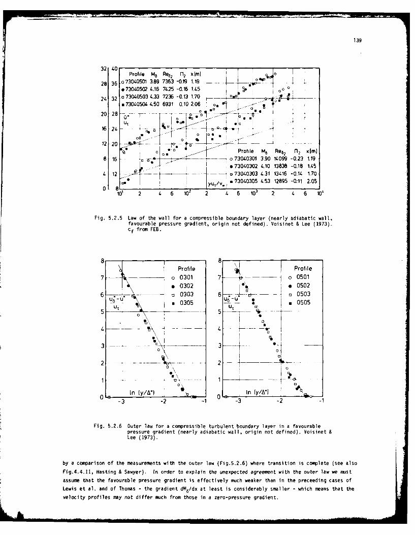
139

32C Prof fle M6 Re62 n2~ XI . 0

28 36 o73040501 3.89 7363 -0.19 1.19

7304.05W2 4.16 71.25 -0.16 1.4.50

24 32 073040503 4.33 7236 -0.13 1.70 tr +_ _-_- -

S73040504 4.50 6931 0.10 2.06 O* . "-°--

20 28 T0 o af- .

C •*~~ - t i ' O • . - .v12 20 . - o %--000

02 20 -ail .01 0 Profile M6 Re62 n2 xlmJ8 16 1 o ....-- o73040301 3.90 14099 -0.23 1.19

- I .73040302 4.10 13838 -0.18 1.45

. 12 - - - o 73040303 4.31 13416 -0.14 1.704 12 o7304v " 0305 4.53 12895 -0:11 2.05

0 8L101 2 4 6 102 2 4 6 103 2 46 10'

Fig. 5.2.5 Law of the wall for a compressible boundary layer (nearly adiabatic wall,favourable pressure gradient, origin not defined). Voisinet & Lee (1973).cf from FEB.

8 8Profile Proftile

7 o 0301 7 11,o 0501

* 0302 * 0502

6 0 0303 6 ,, o 0503u; - U6 -u -

_-U % • 0305 .- • 0505

00

0

0,

0In (y/A*) 4 in (/" ._

+A_.- 0 -- t--- -"

-3 -2 . -3 -2 -1

Fig. 5.2.6 Outer law for a compressible turbulent boundary layer in a favourablepressure gradient (nearly adiabatic wall, origin not defined). Voisinet &Lee (1973).

by a comparison of the measurements with the outer law (Fig.5.2.6) where transition is complete (see also

Fig.4.4.11, Hasting & Sawyer). In order to explain the unexpected agreement with the outer law we must

assume that the favourable pressure gradient is effectively much weaker than in the preceeding cases of

Lewis et al. and of Thomas - the gradient dM6/dx at least is considerably smaller - which means that the

velocity profiles may not differ much from those in a zero-pressure gradient.

140

Fig.(5.2.7) shows velocity profiles in the same boundary layer but with severe wall cooling. Although

transition should be delayed even more by wall cooling, profile 73041403 lies below the logarithmic law

at about the same Mach and Reynolds number as the velocity profiles in Fig.(5.2.5) along an adiabatic wall.

The skin friction data for the highly cooled boundary layer were corrected by Voisinet (1977) and both the

old and the corrected values are given in the legend of Fig.(5.2.7). Nevertheless the scatter in the data

is rather large. The only clear tendency is that the downstream velocity profiles lie in general below

the upstream ones. There is good agreement between the velocity profiles and the outer law (Fig.5.2.8),

irrespective of the change in cf. Agreement with the log law (Fig.5.2.9) and the outer law (Fig.5.2.10)

is good, as would be expected ir view of the low values of 112 .

36 1

02 - -0- Y o

20i II

0i2o. -t :__

U correctel

16 ,c Profile M6 T /Tr Re6 2 c .103 c-103

12 - _.. ._ o 7304.1202 1439 0 2.3 26339 135 10908 u 7304.120. 461 0233 28328 135 1230

SC - 730.1302 438 0256 4.527 112 09658 -ao 730.130. 4.51 0259 .1822 112 1050

4- - YU1/V, 730414,03 4.55 0218 9756 1.81 168101 2 .6 102 2 4 6 103 2 4 6 10' 2 4 6 10 '

Fig. 5.2.7 Law of the wall for a compressible boundary layer (isothermal wall, favourablepressure gradient, origin not defined) Voisinet & Lee (1973). cf fromVoisinet (1977) corrected.

8-@ Profile Profile

7 o 730.1202 o 1202 So 7301201o 1204 S

6 . s 73041304 a 1304 Sa 730.14.03 a 1403 S

5 C-c from Voisinet u-u C, fromU6 Uu- U o" fcrrce-u , 0 & Lee (1973) u ,o 0 1 Vo s inet (1977)

4 0 . ... ____ 1

0

--In (y/0 o In (y/W)0 ,-3 -2 -1 -3 -2 -1

Fig. 5.2.8 Outer law for a compressible boundary layer in a favourable pressure gradient(isothermal wall, origin not defined) Voisinet & Lee (1973).

141

36 I . -! "

32 Profile M6 Tw./Tr Re62 nl2 xm X _M

o1202 439 024 26339 -0.15 170 0

28 34 o 1203 450 023 28058 -012 1.90 _ -

e 1204 461 023 28328 010 206 0

24 30 0- -_ _ --

20 26 - P on

16 224_ - .

12 18 - uo4-n--Profile M6 T/T, Re 62 f 2 x (m]

8 14 Q - -+ 1. 1501 437 0.24 29503 -0.17 1.70

0 01 P, o1502 4.51 0.29 21995 -013 1.91

4 10 -1503 4.62 0.25 25870 011 2.06

0 6

1) 2 46 102 2 4610' 2 4610' 2 46105

Fig. 5.2.9 Law of the wall for a compressible boundary layer (isothermal wall,favourable pressure gradient, origin not defined) Voisinet & LeeCAT 7304. cf from Voisinet (1977) FEB.

e 8,

Profile Profile

e 73041202 1 73041501

0 o 73041203 730415026 o" 73041204 6 -- -- ...... 73041503

5.° c, from 5l . ¢

° Voisinet (1977)1 °e' c c1from

004 * 0, 1 4 -

T UT

3• 3

1 "g 21 "

CIO

In (y/6") o in (y1*) ,,0~- 01 -,,,--341 -2 -1 3 -2 -

Fig. 5.2.10 Outer law for a compressible turbulent boundary layer in a favourablepressure gradient (isothermal wall, origin not defined) Voisinet &Lee (1973).

142

There are two further investigations of accelerated boundary layers in conical nozzles with nominally

isothermal walls where the favourable pressure gradient was stronger than in the case of CAT 7304 butwhere the skin friction was determined from the wall slope of the velocity profile. However, the Reynoldsnumbers Re6 were smaller by almost a factor 100 and the Mach number larger by a factor of 2. The veloci-

ty profiles 2plotted in Fig.(5.2.11) show a typical laminar/transitional behaviour (Hill CAT 5901). i.e.the inner region has in no case become fully turbulent. Comparisons should be made with Figs.(4.4.5) and

22 0 _

20 Z-- 1 i -

0 a:

16 _ -- ,tUt

14 _.- _

12 -- _____

1-Profile M6 Tw/'r, Re2 H12K x [m]1o 59010101 8.25 0.53 332 1.97 0.19

8- 59010102 9.04 0.52 250 2.17 0.24. 59010401 8.29 0.54 471 1.88 0.19

6 - 59010402 9.10 0.55 317 2.04 0.24o " y 59010701 10.0 047 188 245 0.24

10 2 4 6 10' 2 4 6 102 2 4 6 103

Fig. 5.2.11 Law of the wall for a compressible boundary layer (isothermal wall,favourable pressure gradient, origin not defined) Hill (1959).cf from velocity gradient.

Profile (4.4.8). Here again the shape parameter

7 -__- o 59010101 H12k is a good indicator of the transitio-7 nal behaviour of the boundary layer. The* 59010102 outer region (Fig. 5.2.12) reflects a low

6 o 59010401 Reynolds number behaviour similar to that6U

• 590104.02 shown in Fig.(4.4.6) for the measurements0 ... 59010402 of Watson et al.(CAT 7305) or for a boun-

5 V 0 v 59010701 dary layer in an adverse pressure gradient

U;- . 10 and not the behaviour of a boundary layerU_ - - in a favourable pressure gradient (e.g.

UFig. 5.2.2).

3 ..........U 0 Perry & East (CAT 6801) also made measure-

2 ... ments in the boundary layer on the wall of\0 a conical nozzle. An obvious practical

difference from the Hill (CAT 5901) measure-

I ... .ments is that the running time, in a given

tunnel, was very short of order 10-20 ms.In (y/&*) The instrumental difficulties were there-

-3 -2 fore more pronounced, and in fact it was

only possible to obtain one datum pointFig. 5.2.12 Outer law for a compressible boundary layer from each run. Velocity profiles in inner

in a favourable pressure gradient (isother-mal wall, origin not defined) Hill (1959). region coordinates are presented in

143

Figs.(5.2.13 and 14), with the author's skin friction values as deduced from the slope of the velocityprofile. The Mach number range is much the same as for Hill (CAT 5901; Fig.5.2.11) and the heat transfer

parameter not too disimilar. The Reynolds numbers are, however, an order of magnitude greater. The lack

of agreement with the wall law is therefore surprising and superficially suggests that the boundary layer,

at least in the inner region, is not yet fully turbulent. It is not even possible to discern a definite

trend towards the wall law at the higher Reynolds numbers - compare series 03/09. The outer law plots

(Fig. 5.2.15) als show little consistency - series 06/09 behaving much as zero pressure gradient profiles,

while series 01/03 appear, if anything, to show a pattern more characteristic of adverse pressure gradient

profiles (see Fig.5.3.5). Data reduction for this experiment assumes small normal pressure gradients,

Profile M6 T /Tr Re62 Re. H12 K x [M]

o 68010101 8.0 0.39 3265 13558 1.48 0.548

o 68010102 8.50 0.39 2648 12309 1.49 0.650

, 68010103 8.87 0.39 2969 14949 1.49 0.752

e 68010301 8.05 0.35 7085 26350 1.46 0.548

a 68010302 8.50 0.35 6575 27047 1.45 0.650

a 68010303 9.05 0.35 6716 31073 1.49 0.752

4238 1 A-

34 __

30--- -.U t

26 - - -- _& 0

22 - - &_-

18S 0

14 o a _ _ "

Syut/v w10101 2 4 6 102 2 4 6 103

Fig. 5.2.13 Law of the wall for a compressible boundarylayer in a favourable pressure gradient (iso-thermal wall, origin not defined. Perry &East (1968). cf from velocity profile.

which is reasonable, and uses experimental temperature values (Fig.5.1.8) which differ markedly from the"van Driest" predicted values. It is tempting to ascribe the log law disagreement to the uncertainty in

skin friction values as determined from the velocity gradient, but the variation is excessive, and there

is no pattern to it. We cannot therefore draw any definite conclusions from this experiment, and must

leave interpretation to wait on further knowledge while retaining a suspicion that we are once more ob-

serving the consequences of the gradual progression of transition inwards fron the critical layer towards

the wall - possibly retarded by the (not very strong) favourable pressure gradient. This not very strong

pressure gradient and the comparison with the Hill data render it unlikely that the combination "pressure

gradient and wall cooling" invalidates the temperature-velocity relationship and consequently the trans-

formation for the velocity u

144

Profile M6 T./T, Re62 Re. H12K x [M]

o 68010601 9.90 0.316 1068 5340 162 0.564o 68010602 10.50 0.316 888 4950 1.62 0.665

68010603 11.20 0.316 731 4624 1.66 0.767

68010901 10.20 0.288 2309 11130 1.55 0.56468010902 1065 0288 2137 11191 153 0.66568010903 1160 0.288 1935 11927 155 0767

28 . .. .' -

26----l0

24-- 9I A

22 - -UI ,

so A

18 -- +l0 0

A IU

16 - -o00 0

o % -,

14 -]_

00

1A yu/V ,101' 2 4 6 102 2 4 6 103

Fig. 5.2.14 Law of the wall for a compressible boundarylayer in a favourable pressure gradient (iso-thermal wall, origin not defined. Perry &East (1968). cf from velocity profile.

8 - 8 -- *

i Profile Profile7 o 68010101 7- . o 68010601

o 68010102 9"°. n 680106026 . . - A", 68010103 6 . A 68010603

9 68010301 * 68010901

U6 1 A £680109035 68010302 5 u 68010902U6 68010303 6000

In (y/A') 4ro ' } In (y/A') o ,,

U N;-3 -2 -3 -2

Fig. 5.2.15 Outer law for a compressible boundary layer (isothermal wall, favourablepressure gradient, origin not defined). Perry & East (1968).

145

5.2.2 Simple wave - curved wall

In these flows the curved streamlines require, in principle, normal pressure gradients, the significance of

which increases with Mach number.

The only boundary layer experiment with a favourable pressure gradient along a curved wall (contoured

nozzle) including skin friction measurements, was performed by Kemp & Owen (CAT 7206). There are two

further unique features, the extremely high Mach numbers and the as extremely low Reynolds numbers. It is

probably impossible at present to interpret these measurements in terms of correlations drawn directly from

flat plate experience. These measurements were made in a Mach number range unmatched by any other reported

experiment, and the instrumental and conceptual difficulties are such that no great emphasis should be

placed ony any precise iumerical value. We suppose that there were strong thermal and pressure history

effects as can be ;-en -rom Fig.(5.2.16, see legend of 5.2.17). The velocity profiles are not typical

_ £Profile

7 72060402

6 \O 0__ 720604036 72060404

5& 72060405

Ut o3 0

0

In (y/91)0 ~ -2

Fig. 5.2.16 Outer law for a compressible boundary layer

with a favourable pressure gradient along anisothermal wall. Kemp & Owen (1972).

of those found in a favourable pressure gradient boundary layer (e.g. Figs.5.2.2 and 5.2.4). They can be

compared qualitatively, however, with those of Hill (Fig.5.2.12) - except very close to the outer edge of

the layer - where we also think that upstream history effects were present. As was mentioned in the

editors' comment of CAT 7206 (AGARDograph 223), some scatter was introduced in the outer region of the

profiles by using the authors' T/T6 data as an input for the profiles, so that for the outermost profile

points the pressures may be up to 5 % in error from this cause alone.

The inner law plot shows a most unusual behaviour also (Fig.5.2.17). In inner region coordinates the

maximum value of yuT/Vw is of the order 40 and the H12 k value which has been shown to be a good indicator

of the state of the boundary layer is characteristic of a laminar boundary layer (the Blasius profile is

characterized by H12 k = 2.60).

The thickness of the viscous sublayer is very large (approximately 25 %) compared to the thickness of the

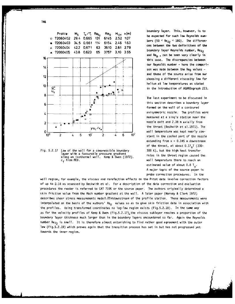
146

Profile M6 T,/ T, Re~ Ree Hl boundary layer. This, however, is to62 12 XIM)be expected for such low Reynolds num-

o 72060402 29.4 0.665 131 6145 2.52 1.07

* 72060403 34.5 0.661 114 6154 2.46 1.63 bers (50 < Re62 < 180). The differen-

a~ 72060404 42.2 0.671 63 3610 2.61 2.79 ces between the two definitions of the

& 72060405 43.8 0.623 65 3757 3.10 3.55 boundary layer Reynolds number, Re62and Re. , can be seen very clearly in

16 -- this case. The discrepancies between

1our Reynolds number - here the compari-14 ___

son was made between the Re0 values -

and those of the source arise from our12 _____ __

choosing a different viscosity law for

10 _helium at low temperatures as stated

0" in the introduction of AGARDograph 223.UT £

4%90 The last experiment to be discussed in

6 _ __ . _ this section describes a boundary layer

I I formed on the wall of a contoured

4 • _ _ axisymmetric nozzle. The profiles were0 measured at a single station near the

2 , ___,_ __ nozzle exit and 2.08 m axially from

SUI I the throat (Beckwith et al.1971). The0 1/ wall temperature was kept nearly con-

100 2 4 5 101 2 4 6 102 stant in the cooled part of the nozzle

extending from x = 0.145 m downstream

of the throat, at about 0.170 T (330-Fig. 5.2.17 Law of the wall for a compressible boundary 300 K), but the high heat transfer

layer with a favourable pressure gradientalong an isothermal wall. Kemp & Owen (1972). rates in the throat region caused thecf from FEB. wall temperature there to reach an

estimated value of about 0.8 TO.A major topic of the source paper is

probe correction procedures. In the

wall region, for example, the viscous and rarefaction effects on the Pitot data involve correction factors

of up to 2.14 as assessed by Beckwith et al. For a description of the data correction and evaluation

procedures the reader is referred to CAT 7105 or the source paper. The authors originally determined a

skin friction value from the Mach number gradient at the wall. A later paper (Harvey & Clark 1972)

describes shear stress measurements madeO.20mdownstream of the profile station. These measurements were

interpolated on the basis of the authors' Re0 values so as to give skin friction data in association with

the profiles. Using transformed coordinates no log-law region exists (Fig.5.2.18). In the same way

as for the velocity profiles of Kemp-& Owen (Fig.5.2.17),the viscous sublayer reaches a proportion of theboundary layer thickness much larger than in the boundary layers encountered so far. Again the Reynolds

number Re62 is small. It is therefore almost astonishing to find rather good agreement with the outer

law (Fig.5.2.19) which proves again that the transition process has set in but has not progressed yet

towards the inner region.

I

147

18

16

14___

12 __..

10

.... %CAT 7105

6 Profile M6 T/T, Re6 Ree

o 0101 19.26 0.199 214 23444 o 0201 19.42 0.188 356 3770

o , 0301 19.65 0.182 323 33982 _1

100 2 4 6 101 2 4 6 102 2 4 6 101

Fig. 5.2.18 Law of the wall for a compressible boundary layer (favourable pressuregradient, isothermal wall, origin not defined). Beckwith et al. (1971).cf from FEB.

8

o 01017, * 0201

6 s \ 0301

5 CAT 7105

04 U

3 0o

2 0

In (y/A-) o

-3 -2

Fig. 5.2.19 Outer law for a compressible boundary layer(favourable pressure gradient, isothermal wall,origin not defined). Beckwith et al. (1971).

148

5.3 Adverse pressure gradient

5.3.1 Reflected wave - straight wall

We have discussed the features of the reflected wave - straight wall flow in a favourable pressure gradient

in section 5.2.1. They remain unchanged in principle in an adverse pressure gradient flow. The relevant

boundary layer experiments are listed in table 5.3.1 and discussed below.

None of these boundary layers approached separation, however, and only three experiments (Sturek & Danberg

1971, Kussoy et al. 1978 and Gootzait & Childs 1977) contain shear stress and/or fluctuating velocity

measurements which are of great importance for the discussion of this type of flow.

Table 5.3.1

CAT M6 Tw/Tr Re62x1O-3 cf Origin

7102 4 - 2 1.0 3 - 39 P defined

7201 4 - 2.4 1.0 1.5 - 6.8 V/S defined

7802 S 2.3 - 1.9 1.0 11 - 34 *) not defined

5801 2 1.0 7.1 - 8.2 F/P not defined

7104 2.4 - 1.9 1.0 11 - 26 F not defined

7401 2.5 - 2.2 1.0 7 - 13 S not defined

7007 4 - 3 1.0 10 - 32 P not defined

* embedded hot-wire

As in earlier sections we begin by a discussion of results from experiments for which the boundary layer

had a defined origin, the flow was adiabatic and three-dimensionality was nominally eliminated by an

axisymmetric configuration. Peake et al. (CAT 7102) made measurements on the inner surface of a hollow

cylinder, with a retractable centre body on the axis which was used to impose a pressure gradient on thetest layer. Preston tubes were employed to determine the wall shear stress, using a number of compressible

calibration procedures, of which we have arbitrarily chosen the Hopkins & Keener (1966) TR-method. As a

control check, we first present a set of zero pressure gradient profiles (series 01, Fig.5.3.1). Agreement

with the log law is fairly good, but some scatter is shown in both slope and position. The outer-law-

profiles are self consistent and agree fairly well with the outer law (Fig.5.3.3.b).

Series 02 (Fig.5.3.2) covers the adverse pressure gradient results, but neither the boundary conditions

for the profiles nor the results, are easy to interpret. Profiles 0201, 0203 were respectively at the

start and end of the adverse-pressure gradient, with 0202 in the middle. Profiles 0204-6 are in a zero-

pressure gradient relaxation-flow downstream of the pressure rise. Profile 0201 is therefore, except at

the wall, in an adverse longitudinal and a normal pressure gradient, and the upstream distance over which

the pressure gradient has acted increases as we move out from the wall. The pressure field is as shown in

the sketch, where the arrows indicate the direction of the pressure gradient, much as shown in Fig.(6.1.2)

with the pressure gradient reversed. Both the departure of profile 0201 from the log law and its

difference from 0101 (to which if the longitudinal wall pressure distribution alone is considered, it

should be identical) may therefore be caused by adverse streamwise pressure gradients, by the pressure

increase in the normal direction, or by both. Discrepancies may also, in part, spring from the resulting

errors in data reduction, since the normal pressure gradient will result in the Mach number in the outer

region being less than that calculated assuming constant pressure. Profile 0202 is in a region where nor-

mal pressure gradients should be negligible. For this, and the succeeding profiles, the slope of the inner

region suggests that there may be errors in the skin friction values. It seems that the wake region is

more pronounced than for a typical zero-pressure gradient case, if not very different from series 01 in the

same experiment. Profile 03 is again subject to both longitudinal and normal pressure gradients, this 4

time of a sense to cause the Mach numbers in the outer region to be greater than assumed. The appearance

on the log law plot is again much as would be expected of a subsonic adverse pressure gradient layer.

149

26-

22.

20 -U

18

Profile M6 Re82 A(G*/U 1)16 - - -~ o 71020101 3108 3.4.0

*71020102 46527 4..0

14IC 71020103 395603 4.15o71020104. 6282 4.0

12_ __- __ 71020105 7187 3.70

Y £ /, 71020106 7759 3.4.5

10' 2 4 6 10' 2 4. 6 10 2 4. 6 10'

Fig. 5.3.1 Law of the wall for a compressible boundary layer (adiabatic wall,zero pressure gradient, defined origin). Peake et al. (1971).

300

26--0- -

U-

0

20 ___* Profile M6 Re620 o 71020201 3.93 3003

18 --- - - - o- .71020202 2.90 10088o71020203 2.08 25701

16 71020204 2.00 35972

/ 0 YU/V 71020205 1.99 3911.6

:01aw4 6 10 2 4 6 1 2 1.6 10V 1. 65

Fig.5.3. Lawof the wall for a comipressible boundary layer (adiabatic wall,advese resure radent defnedoriin)Peake et al.(1971).

150

Walpesue 01 02 03 04 05 06Wall pressure

C21 Wove structure

Profile 0 2 0 / 5 0

Peake et al. recalculated profile 0203 (also 0202 for which it was inappropriate) with a normal pressure

gradient of double the magnitude which would be predicted by § 6.1.3 eqn. (6.1.14b) below. The calculations

contain discrepancies, but would seem to indicate that Mach number and velocity values taking account ofthe normal pressure gradient should not differ detectably from those assuming constant pressure on the ve-

locity profile plots. The succeeding profiles 0204, 0205, in a zero pressure gradient region, appear if

anything more as expected of a favourable pressure gradient flow on the log law plot. In the outer law

plot (Fig.5.3.3) 0201 shows a steeper slope and lower values in the outermost region, and this typical

behaviour spreads inwards, becoming very pronounced for 0202, less so for 0203 while 0204 and 0205 in

contrast to their log-law behaviour return towards the zero pressure gradient law.

88

Profile AProfile7 o 71020201 7- o 71020101

r 71020202 e 710201026- o 71020203 6 - - -t " 71020103

. 71020204 o 71020104

5 6 71020205 5 a 71020105

/ i -4 -. I&r- - - - 71020106

U, "U,,o..s3 - _ -

al 0 adverse bi zero 0

o pressure gradient gradient o-2 pressure adelo

In (y/A1) ' ,X In (y/-)

-3 -2 -1 -3 -2 -1

Fig. 5.3.3 Outer law for an axisynetric compressible turbulent boundary layer(adiabatic wall, defined origin). Peake et al. (1971).

151

We should perhaps note here that for any flow in which the boundary layer edge lies in a simple wave

region (whether in a wholly simple wave flow or as an incoming or outgoing simple wave forming part of a

structure as shown in the sketch above), it may not be possible to define u6 precisely. This should be

borne in mind when inspecting any outer law plot such as Fig.(5.3.3) and its successors throughout § 5.

The dependence of u on p in a free-stream flow is not very strong at high Mach numbers, so that the pro-

blem is not likely to become serious unless the normal pressure gradients are very strong, or the Mach

number relatively low(see § 7).

Lewis et al.(CAT 7201) also performed tests on the inner surface of a cylinder, thus eliminating end

effects, and a pressure gradient was again imposed by a centre body. There are no upstream pressure gra-dient effects as for the accelerated flow region of the same experiment (Fig.5.2.1), and it is astonishing

how well the inner law plot (Fig.5.3.4) resembles that of velocity profiles in a moderate adverse

pressure gradient boundary layer in subsonic flow. For the compressible boundary layer the skin friction

values were obtained by the curve-fitting procedure of Coles & Hirst (1969) applied to equivalent

incompressible velocity profiles transformed as suggested by van Driest (1951). Again the velocity

profiles hardly extend into the inner region.

UU

28 - -- -+ --f- -

26 ,, I I -

u, 00

22 -

18 I - "io __

Profile M6 Re62 fn216 o - 072010106 383 1700 030

e 72010108 3 38 2821 05114 -j -j o 72010110 307 3562 065

s 72010112 277 4466 07712 . -1 a 72010113 262 5703 074

Syu,/v.I a 72010114 247 6784 077

10, 2 4 6 101 2 1 6 102 2 6 10'

Fig. 5.3.4 Law of the wall for a compressible boundary layer (adiabatic wall,adverse pressure gradient, defined origin) Lewis et al. (1972).cf from transformed log-law.

The development of the layer near stations 13 and 14 is particularly interesting. Here the wall pressure

gradient is adverse with quite high values of R 2 . However, profiles 0113 and 0114 are moving towards the

log law, after profiles 0108-0112 have shown what might be termed classic low-speed adverse-pressuregradient behaviour (Fig.5.3.4). The adverse pressure gradient stops at or just downstream of station 14,

to be followed by a favourable pressure gradient, consequently the whole of profile 0114 and probably most

of the outer part of 0113 are in fact in a simple wave favourable pressure gradient region. The same

behaviour is visible in the outer law plot (Fig.5.3.5). Profile 0106, the first shown here and the first

in the adverse pressure gradient region shows a rather weak influence of the pressure gradient, as might

be expected.

152

Profileo 72010106

o 72010108

7 o 72010110S72010112

6- 72010113

72010114

5U - ci

U., 4

2UZU

In (y/ }0 'aI" -3 -2 -1

Fig. 5.3.5 Outer law for a compressible turbulent boundarylayer in an adverse pressure gradient (adiaba-tic wall, defined origin) Lewis et al.(1972).

All other cases considered here describe boundary layers in adverse, or more complex pressure gradients

for which the upstream history is not defined other than by the provision of one or more profiles in a

zero pressure gradient region ahead of the imposition of the pressure gradient.A particularly fully instrumented study is that made by Kussoy et al.(CAT 7802 S). The test boundary

layer is formed on the inner surface of a cylindrical extension to an axisymmetric nozzle, and four

different centre-bodies were used to impose a reflected wave pressure gradient. Two of these cases in-clude full profile measurements, at close streamwise intervals. The wave structures produced in both casesconsist of a compression followed by an expansion. In the first, more "moderate", pressure gradient ofseries 01, the wall pressure is initially constant, then rises as the compression reaches the wall and isreflected before continuing at a constant level to the end of the test zone. The expansion wave does notreach the wall, although the outer part of the downstream profiles (0110-0113) is affected. For the more

abrupt pressure gradient of series 02 the wall pressure, after an initial constant pressure portion (0202),rises to a plateau (0210-0212) as for series 01, but the expansion wave then reaches the wall and thepressure falls markedly In the region described by the last two profiles (0213, 0214). There is evidence

of a strong compression wave entering the test-region in the outer part of the last profile.

The wave structures are relatively concentrated, in that the streamwise extent - at any given value of y -is of the same order as the boundary layer thickness, so that in terms of the general flow structureillustrated in Fig.(6.1.2) and the sketch above (Peake et al., CAT 7102), the "reflected wave" region

153

(indicated by stippling in Fig.6.1.2) is entirely submerged in the boundary layer. The static pressure

field is easily explained in terms of the wave structure, and will be discussed in § 6.2 below.

Wall law profiles are shown for series 01 and 02 in Figs.(5.3.6.a and 6b) respectively. Profiles 0102,

0104 and 0203 are only slightly, if at all, affected by the incoming wave structure and appear as typical

zero-pressure gradienc profiles in both shape and position in the log-law plot. 0107 is at the start of

the adverse pressure gradient as observed at the wall and 0109 at the end. The wake component is observed

to increase as expected (Fig.5.3.6.a) and then decrease again for 0111 and 0113.

Numerical agreement with the log-law is, however, very poor. It is possible that the flush-mounted hot-

wire skin friction gauges are influenced by the pressure gradient effects, though as sublayer devices they

should be relatively unaffected. Series 02(Fig.5.3.6.b) shows the same general behaviour. The initial

zero-pressure gradient profile of 0203 develops an increased wake component by 0207, at the start of the

adverse-pressure gradient at the wall, which becomes increasingly exaggerated in profiles 0209 and 0210

before decreasing in 0212 and 0214, where the wall pressure gradient is favourable. Again there seems to

be a strong pressure-linked effect on the skin friction values, and this discussion has been based on an

inspection of the profiles individually, disregarding the downward displacement of the log law.

32

Profile M8 Tw/Tr Re6 px10 -3 N/rn2 4

30 o 0102 229 106 15870 8.19 e4 o"

a 0104 228 106 15520 805 0 13 &

28 o 0107 2.19 105 - 9.09 0- -

e 0109 219 105 - 11.8 0026 6 0111 220 105 - 11.2. __

& 0113 223 105 - 11.6 0 £

u, CAT 7802 S22

20 .. ... . .- £

18 .... ""

16_____

101 2 4 6 102 2 4 6 101 2 1. 6 10

Fig. 5.3.6.a Law of the wall for an axisymmetric compressible turbulent bounda-ry layer (adiabatic wall, variable pressure gradient, origin notdefined). Kussoy et al.(1978). cf from heated-wire gauge.

154

4oGProfile M6 T./T Re62 pwx10-3 N/m2

36 o 0203 2.20 1.05 14852 9.18s 0207 2.05 1.05 13454 9.19 0

32 o 0209 2.03 1.05 28930 11.6 -

* 0210 2,00 1.05 - 14.4 .428 4 0212 2.08 1.05 - 14.5

A 0214 2.08 105 18394 11.7 0 11124 -2 , CAT 7802 S

200 A20 -T

8101 2 4 6 102 2 4 6 103 2 4 6 104

Fig. 5.3.6.b Law of the wall for an axisymmetric compressible turbulent boun-dary layer (adiabatic wall, variable pressure gradient, originnot defined). Kussoy et a1.(1978). cf from heated-wire gauge.

o 0102 o 0203

8 _ 0104 8 .0207o 0107 o 0209

7 -- - - 0109 7 . * * 021000111 0 a 21A~lil 0212

6 A • 0113 6 -' p- - & 0214

CAT 7802 S CAT 7802 Su-"5 + " :u6-u -- e6

4 4

3 3 . .4€, A

2 i 2 --0

AA

In(y/A') n I(Y/ 0

-3 -2 -3 -2 -1

Fig. 5.3.7 Outer law for an axisymmetric compressible turbulent boundarylayer (adiabatic wall, variable pressure gradient, origin notdefined). Kussoy et al.(1978). cf from heated-wire gauge.

In the outer region plots (Fig.5.3.7) there seems to be a slightly greater delay before the influence of

the pressure gradient is made apparent. For series 01, profiles 01, 04 and 07 agree well with the zero-pressure gradient law. Profile 0109, however, shows very strong adverse pressure gradient characteristics,

which are progressively relaxed in profiles 0111 and 0113, though with a very peculiar kink in the inner

law plot (Fig.5.3.6.a). This may possibly be a result of the penetration of the outgoing compression wave

by the incoming expansion wave.

155

For series 02, profiTes 03 and 07 agree with the zero-pressure gradient law though 07 is not fully typical

in the inner region - in the log-law plot, Fig.(5.3.6.b) the shape of this profile is also a little odd.

Profiles 0209 and 0210, respectively in the middle and towards the end of the adverse-pressure region as

measured at the wall, show a very strong adverse-pressure gradient behaviour, with 0210 tending very slight-

ly to return towards the zero-pressure gradient line. Profile 0212, at the end of the wall zero-pressure

gradient region, and affected in its outer region by the incoming expansion wave - it shows a point of in-

flection which it is tempting to compare with the kink in 0113 - is well back towards the zero-pressure

gradient line while 0214 is tending to lie on the other side as it begins to develop favourable-pressure

gradient characteristics (cf. Fig.5.2.4) .

The picture generally is confused by the uncertainty in the skin friction measurements, which should notaffect the outer law plot very strongly, and by the inevitable complexity of a flow field with superposed

wave structures.

In the remaining cases, either static pressure was not measured, or the pressure gradients were not strong

enough for it to become necessary to analyze the flow in such detail.

Naleid's experiment (1958) represents an early attempt to determine the influence of pressure gradients on

skin friction and on the Preston tube calibration. The profiles presented were measured at the same

station on the floor of a wind tunnel in different mild pressure gradients with approximately the same

edge state. The skin friction values associated with these velocity profiles were measured directly with

a floating element balance. We only show a comparison of the measurements with the logarithmic law

(Fig.5.3.8), since the pressure gradient has little effect either in the log-law region or in the outer

region in this case.

Waltrup & Schetz (1971) performed their investigation on the bottom nozzle block and test section wall of

a wind tunnel. Pressure gradients were imposed by three ramps of the full tunnel width which were mounted

in the centre of the tunnel. The test boundary layer had undergone a largely two-dimensional expansion in

the nozzle . Spark schlieren photographs clearly established, however, that the boundary layer was turbulent.

30Profile M6 Re62 Reo l2

28 o 0701 1.883 8198 12288 0.232 o _ _

* 0501 1.918 8019 12171 0.115

26 o 0801 1.837 8236 12288 0.386 -ti.

* 0301 1.936 7782 11879 0.029

24 , 0201 1.997 7151 11165 0.020 '50

2 0101 1.947 7588 11633 -0.083

20 U. CAT 5801 _

20. ..,

18 -.-- __ .

161

14101 2 4 6 102 2 4 6 103 2 4 6 10'

Fig. 5.3.8 Law of the wall for a compressible boundary layer (adiabatic wall,adverse pressure gradient, origin not defined). Naleid(1958).cf from FEB.

156

8 F8

7-Profile 0i Profile7 o 71040102 o' i 71040202

6 - * 71040103 6n- u 71040203

e 71040104 1 0 71040204

0'

5 ------ 5U6 - U u6 -u

4 4,U

~0

3 3

2 200o 0

1 --a-t1 p

In (y/A*) 9 In (y/A") 00 L4 - O 0 4 1 1 - - ' -

-3 -2 -3 -2

Fig. 5.3.9 Outer law for a compressible turbulent boundary layer in an aoversepressure gradient (adiabatic wall, origin not defined) Waltrup &Schetz (1971).

32 , °S0

30 Profile M6 Re5 2 xjnm . - -"71040102 2 10 17391 0076 0 *o 0

28 * 71040103 193 21823 0127 o"

71040104 188 26107 0178 0 7

24 o1U 0

U,

22 0 .

200 0

1 -" Profile M6 Re62 x Im]

0 a 71040202 228 12090 007616 Cb a

a 0 • 71040203 211 16805 01270 yu 1 /v o 71040204 195 21577 0178

14102 2 4 6 103 2 4 6 101

6 1 4 6 10 2 4 6 10'

Fig. 5.3.10 Law of the wall for a compressible boundary layer (adiabatic wall,adverse pressure gradient, origin not defined) Waltrup & Schetz(1971). cf from FEB. Two different pressure gradient developments.

The profiles presented consist of three sets - two of which are shown in Figs.(5.3.9 and 5.3.10) - each

representing the development of the layer under a different pressure gradient. The outer law plot shows

the adverse pressure gradient behaviour of the velocity profiles (Fig.5.3.9) whereas the velocity profiles

do not apparently exhibit a log-law region in Fig.(5.3.10). It is possible that this is a consequence of

using a moment sensitive (i.e. pivoted) balance in a relatively strong pressure gradient so that a moment

is produced by the pressure field on the face of the balance element (parallel-flexure balances are not

157

sensitive to pressure gradient induced error - see Winter 1977). The pressure gradient was not strong

enough to cause separation in the boundary layer, so that a distinguishable log-law region sh-,ii exist.

Thomas(1974) has investigated boundary 1-yers in favourable (Figs.5.2.3 and 5.2.4) and adverse pressure

gradients on a flat surface facing one of d number of contoured nozzle blocks. For the zero pressure

gradient experiment in the same test section Liie reader is referred to Jeromin(1966). As mentioned in

section 5.2 the principal uncertainty here nust be the question of three-dimensionality, as the length to

width ratio of the experimental surface is over 5:1. The profiles are given in fine detail as can be seen

from Fig.(5.3.11) where agreement betwee' -dasurerents ano the logarithmic law is very good. The profiles

30

28 Profile M6 Re62 x mlo 74010204 2 52 6811 0038 41

* 74010208 2 41 8471 0089 .26

* 74010210 234 9987 0114

24 o 74010213 2 28 11267 0152

* 74010215 2 21 13467 0178

200

U.

18 f

16

14£14- .----

121101 2 4 6 102 2 4 6 101 2 4 6 10"

Fig. 5.3.11 Law of the wall for a compressible turbulent boundary layer (adiaba-tic wall, adverse pressure gradient, origin not defined) Thomas(1974). cf from razor blade technique.

show a long linear region and values for the wake strength (A (u*/u ) ' 5.5) which are considerably higher

than most results for zero-pressure gradient boundary layers in the same Reynolds number range (cf.

Figs. 3.3.4 and 3.3.6). This is in agreement with results obtained in subsonic boundary layers. The wall

shear stress was estimated using the razor-blade technique after Smith et al.(1962) and the sensors were

calibrated against thi Spalding & Chi (1964) skin friction correlation for boundary layers in zero

pressure gradient flows. Although one may have reservations about this calibration method, the results

as seen in Fig.(5.3.11) are convincing. Fig.(5.3.12) shows a comparison between the outer law and the

measurements, which cross the theoretical curve with a greater negative slope - as expected for velocity

profiles in an adverse pressure gradient.

158

The last experiment in this groupis that of Zwarts (1970). The test

o 0204 boundary layer was formed on the

8 * 0208 floor of the 0.127 m square wind

02 tunnel and the test section started1 0210 about 0.75 m downstream of the nozzle

07 o 0213 throat. A contoured splitter plate

• 02 15 was designed by the method of charac-

teristics to give a Mach number

6 distribution on the tunnel floor such6 u \ that the initial flow at M 4 passed

5 U__ __O through a constant Mach number gra-

dient falling to M6 = 3 over a

distance of 0.15 m, followed by a

4 second region of constant Mach number

flow. Surface flow visualization

tests showed that there was consider-

3 able flow convergence in the adverse

o3 pressure gradient region due to inflow

from the tunnel sidewalls. Preston

2 I tube measurements at stations 38.1 men

to either side of the centre lineoshowed differences in skin friction

of up to 10 % from the centre line

In (y /Al) value. The author offers skin fric-

I , z tion values deduced from several

calibration functions (data evaluated

from the Hopkins & Keener method

(1966) which gives the smallest cf

Fig. 5.3.12 Outer law for a compressible boundary layer values were selected here). Agree-(adiabatic wall, adverse pressure gradient, ment of the velocity profiles withorigin not defined). Thomas (1974).cf from razor blade technique.

38

Profile M 6 Re62 x Im]

34 o 70070103 402 10773 0019 -, o* . '

* 70070106 372 14189 0.057 I

30 * 70070109 3.46 17939 0095 ,

o 70070112 326 22101 0133

26 a 70070115 299 30651 0171 - , ra 70070117 296 32099 0197 ,

22 * 0

14 o !18 r '

!yut/v,1 0 ff j10 2 4 6 102 2 4 6 103 2 . 6 10 4

Fig. 5.3.13 Law of the wall for a compressible boundary layer (adiabatic wall,adverse pressure gradient, origin not defined) Zwarts (1970).cf from Preston tube.

159

the logarithmic law is fair, all pro-

files lying low which means that the

skin friction velocity is still too

8 high (Fig.5.3.13) if agreement with

Profile the log-law should be reached.

The outer law plot (Fig.5.3.14) is7a 70070103 typical, if more pronounced than

* 70070106 Fig.(5.3.12) of an adverse pressure

6 n 70070109 gradient boundary layer. Profile

c3 70070112 0117 is in a near zero-pressuregradient but shows adverse-pressure

5 a 70070115 gradient characteristics inherited

6- & 70070117 from the upstream flow, though it is

U1 4 relaxing towards the zero-pressure

gradient curve.

3 1

2A Fig. 5.3.14 Outer law for a compres-

sible turbulent boundaryI •layer in an adverse

pressure gradient (adia-r 0 A 0 Xfebatic wall, origin not

2defined) Zwarts (1970).

-3 -2 -

5.3.2. Simple wave - curved wall

This section deals with pressure gradient cases in which the pressure gradient is the result of streamline

curvature. This is associated with a "simple wave" which may either be generated in the test-zone itself,

and propagate downstream, or may be generated elsewhere and be propagated downstream so as to strike the

test-zone. The curved mean flow of the simple wave cases is associated with normal pressure gradients,

which at high Mach numbers become very large. There is very little available information on what effect

this may have on the turbulent structure (CAT 7101 contains the only measurements of fluctuating quantities),

but the effects are unlikely to be negligible. There are relatively few available accounts of simple wave

flows, and this is especially unfortunate as the boundary layers on a hypervelocity vehicle will always

experience locally-generated simple wave structures. The typical adverse pressure gradient case is the

flow approaching an inlet where a concave surface gives rise to a generated simple compression wave.

From among the three reported simple wave compression tests, Clutter & Kaups (CAT 6401), Stroud & Miller

(CAT 6503) and Sturek & Danberg (CAT 7101) only the last one provides sufficient data to allow it to be

used in our normal scheme of comparisons.

The boundary layer experiment performed by Sturek & Danberg (1971) took place on a ramp forming a continua-

tion of the flat test wall opposite a flexible plate nozzle. The test section extended 0.56 m downstream

from the nozzle exit plane and the curved ramp started with a faired step at x = 0.305 m. The test zone

included a zero pressure gradient region before the ramp followed by a simple wave isentropic compression.

Oil flow visualisation did not show appreciable divergence of the streamlines near the centre line, but

streamlines near the side walls diverged considerably. The main portion of the data consists of three

160

sets of eight profiles, each set for a different reservoir pressure. In each case (series 02 and 03 are

discussed here) three zero pressure gradient stations were followed by five on the curved ramp. The wall

shear stress was determined using a Preston tube and the Yanta et al.(1969) calibration curve. The velo-

city profiles are plotted in inner law coordinates in Figs.(5.3.15) and (5.3.16) with the adverse pressure

4C Profile M6 Re6, n2 x [m]

36 o 71010202 354 8041 0 0.20e 71010204 3.24 12718 1.39 0.43

32 A 71010205 316 13762 141 0.46o 71010207 3.00 15429 129 0.51 -

28 a 71010208 2.91 15908 112 054

U,1 o

20 •-

16-------..---

12 --

101 2 4 6 102 2 4 6 103 2 4 6 104

Fig. 5.3.15 Law of the wall for a compressible boundary layer (adiabatic wall,adverse pressure gradient, origin not defined). Sturek & Danberg(1971). cf from Preston tube.

38 -

34 Profile M6 Re62 n2 x[mJ Q40

o 71010303 3.50 9700 0 0.25

30 71010304 3,23 14577 1.43 0.43 •

71010306 3.06 16567 1.28 0.48 0

26 c 71010307 2.97 17702 124 0.51 _^__I

a 71010308 2.90 18800 1.11 0.54

22 .- --- -- - - -

18 .. ..

0: yu'/v w

10 102101 2 4 6 10 2 4 6 10' 2 4 6 10'

Fig. 5.3.16 Law of the wall for a compressible boundary layer (adiabatic wall,adverse pressure gradient, origin not defined). Sturek & Danberg(1971). cf from Preston tube.

161

88

Profile oProfile7 0 71010202 7 o 71010303

e 71010204 * 710103046 0 6 71010205 6 7 o 71010306

S71010207 o 710103075 -- . * * 71010208 u 71010308

1 -

3 4_ ---___- 3-------00

2 O2 0

1 1

in (y/A") -2 -1 in (yJ--3 -2 -3 -2 -

Fig. 5.3.17 Outer law for a compressible turbulent boundary layer in an adversepressure gradient (adiabatic wall, origin not defined). Sturek &Danberg (1971).

gradient profiles lying above the logarithmic law (although within the normal scatter band) whereas the

zero pressure gradient profile lies slightly below the log law. The wake strength is much larger than for

the profiles in Fig.(5.3.11) but so is the pressure gradient parameter 12 This behaviour of the veloci-ty profiles in a moderate adverse pressure gradient is confirmed by the outer law plot shown in Fig.(5.3,17).

Finally we show two sets of profiles measured on a waisted body by Winter et al.(CAT 7004). In addition

to the simple wave pressure gradient induced by longitudinal curvature there are probably strong conver-gence and divergence effects resulting from the large proportional change in transverse curvature (thevalue of 6/R is not so high as to make transverse curvature itself a dominating feature).Skin friction was determined by the razor blade technique. The profiles appear to have little or nosystematic relationship to the wall law (Figs.5.3.18 and 19) and it is only possible to say that the flow

is so complex, with history effects, simple wave pressure gradient, and convergence - divergence all super-

imposed, that it would not be profitable to assign the large differences observed to any one of these.We have the same difficulty in arriving at any conclusions when inspecting the outer region profiles(Figs.5.3.20 and 21) but nevertheless present them for information.

162

32

Profile M6 Re62 61/R Rzu /Iv 0 c x 10'

30 e 0101 1.77 2516 0.015 13575 2.72 e. .* 0102 1.63 4159 0.027 10386 1.92

28 o 0103 1.45 7742 0.058 8105 1.43 e4c A A

e 0104 1,29 17730 0.089 8244 0.83 e

26 e 0105 1.25 12428 0.049 12972 1.71 i -

a 0106 1.22 9288 0.031 15922 2.17 ! ,

JCAT 7001.4022 e ID4

20 * 0

18-. . . .000

o[16 -

1210 2 4 6 10 2 4 6 10 2 4 6 0 L

Fig. 5.3.18 Law of the wall for an axisymmetric compressible boundary layer(adiabatic wall, variable pressure gradient, defined origin).Winter et al.(1970).

30 - - - __ - -

Profile M6 Re 61/R1Rzu,/v, I *

28 o 0601 3.33 605 0.020 2780 _".- o -000 -ee 0602 3.05 1579 0.047 2438 1

26 0603 2.76 2448 0.040 3386 _ --- _ .... .

e 0604 2.47 3403 0.034 7138 0 o e

24 * 0605 2.43 2900 0.027 8101 _____ *

CAT 7004 e

22 - 0 • -U

20 -

18 _ _

16 0 * - ____ o 1.57 1.130 1.32 1.13

0 1.26 0.831- e 1.25 1.68

1v, 1 yu./V. * 1.22 1.88

100 2 4 6 10' 2 1 610t 2 2 4 6 10

Fig. 5.3.19 Law of the wall for an axisymmetric boundary layer (adiabaticwall, variable pressure gradient, defined origin). Winter et

163

8 8Profile * Profile

7 * 0 0101 7 e 010.0 9 0102 . 0105

o 0103 6 -0106

CAT 7004 * CAT 70045 5

U6 - U 4 -U eU, 4 U, 4

3- 3 -w A

2 - 2 e

1 0 1

In (y/a) o o' e In(y/0*) A

0-3 -2 -1 -3 -2

Fig. 5.3.20 Outer law for an axisymmetric compressible boundary layer (adiabaticwall, variable pressure gradient, defined origin). Winter et al.(1970).

8Profile

7 o 0601. 0602

6 V 0603

e 0601.

5 0605u6 -U 0CAT 7004

UT 4

%0

0

2- 30

2 0

- 0

-3 -2 -1 0

Fig. 5.3.21 Outer law for an axisymmetric compressibleboundary layer (adiabatic wall, variablepressure gradient, defined origin). Winteret al.(1970).

A W - - -'- .. . . .. . .. j 1fr. . . "11il

164

5.4 Conclusions

a) We have discussed the results of about fourteen experiments in pressure gradients and compared theprofiles to the inner and outer laws for the zero-pressure gradient case. The picture which results issomewhat confusing, so that any conclusions here are only tentative.

b) The law of the wall in transformed coordinates does hold for flows with moderate favourable and ad-verse pressure gradients on adiabatic walls. We have not examined flows close to separation or re-lamina-

rization.

c) The law of the wall in transformed coordinates would seem to apply erratically to flows on cooledisothermal walls in moderate pressure gradients. The cases with substantial disagreement appear to beassociated with Reynolds numbers Re62 below 2000,in some cases ranging below 400. The experiment ofPerry & East iseven among these casesof a special kind.

d) For all experiments with Mach numbers above about 5 in accelerated flows, the nozzle wall studies,the Re62 values were low, in some cases very low indeed. The boundary layers studied were not fullyturbulent and displayed transitional characteristics.

e) The outer law as specified by eqn.(3.3.17) provides a useful indicator of pressure gradient effects.In a favourable pressure gradient the negative slope on our usual plot becomes less, giving values wnichlie above the zero pressure gradient curve in the outer region. In contrast, the data for an adversepressure gradient show a greater negative slope with values below the zero pressure gradient law in theouter region.

f) Wall shear stress values should be regarded with suspicion, as the extent to which zero pressure gra-dient Preston tube calibrations may be used has yet to be established, and floating element balancesoperating on the moment principle are subject to errors which are not in general allowed for (Winter 1977).

g) Measurements are needed in adverse pressure gradients with heat transferfora cooled isothermal wall,and for all pressure gradients with wall temperature varied in a controlled manner.

165

6. NORMAL PRESSURE GRADIENTS

We have, at various points above (H 2.3, 5.1) remarked that in compressible flows quite large pressure

gradients may be observed normal to the wall on which a boundary layer has formed. In this section we

attempt to predict the likely occurrence and magnitude of such pressure variations by an examination of

the root causes. We will first consider the pressure field in various types of ideal flow, and then see

in what way 'inviscid' flow features are modified by the presence of the boundary layer. At hypersonic

speeds we will further note that Reynolds stresses may become significant compared to the mean static

pressure, while the boundary layer itself may well induce relatively large changes in the free stream

flow. Together, the various normal pressure gradient effects can cause serious difficulties in the

interpretation of results, both directly by their effect on pressure and density values, and less

obviously through the difficulty found in specifying reference qualities.

6.1 Normal Pressure gradients in ideal flow

In this section, and elsewhere throughout this report excepting § 6.3,distinction will be made between"pressure" and "normal stress". (In all cases, what is referred to as a pressure gradient should actually

be more strictly called a normal stress gradient.) Outside the boundary layer, the "pressure gradients"

are uniquely related to the local fluid accelerations. In natural coordinates for a steady flow

(a I3s) : - i(3t13s) (6.1 .1)

and

(a/an) = - '0i2/R (6.1.2)

where U is the velocity and s the distance along the streamline, n is distance measured normal to the

streamline, and R is the radius of curvature (n and R taking the same sign for concave curvature).

thigh speeds the static pressure becomes small compared to u2 or the total pressure p, and (a/n)

(eqn. 6.1.2) may become relatively large even for large values of R. If (3p/an) is taken as constant

over a small distance, such as the boundary layer thickness 6, in the n direction, the pressure difference

is given approximately by

y M (6.1.3)p an

and it is easy to see how, even at modest Mach numbers, significant changes in pressure can occur across a

boundary layer on a curved wall. As an example, consider the ramp flow studied by Sturek & Danberg

(CAT 7101) where a 20% static pressure variation is found across the boundary layer with an edge Mach

number of about 3.

In natural coordinates a transverse pressure gradient occurs only in a curved flow. The quantities

required to determine it are, however, not generally available - for instance it is difficult to imagine a

simple way of measuring R - while the direct measurement of p in the flow field is often extremely diffi-

cult. It is particularly helpful therefore to relate the transverse pressure gradients to the longitu-

dinal gradients, as on the wall streamline it is relatively simple to measure the latter. It is also

helpful to generalize this relation in attempting to account for - or exclude - certain secondary effects.

In all sections below, we define the "normal pressure gradient" in local cartesian coordinates as the

variation of pressure along the local, straight, normal y to the surface on which the boundary layer is

growing, x being the coordinate along the surface in the stream direction. Then since T is a function

of x and y only

S .Lx -1 (6.1.4)

ay x ax to n

and any attempt to link the normal pressure gradient (aT/ay) to the streamwise pressure gradient (as/ax)

166

may be reduced to an attempt to trace the isobars (ay/ax)-.

6.1.1 The simple wave

Any flow in which changes of property are found along only one of the two families of characteristics

(Mach lines) will be described as a simple wave flow. Such a wave structure is generated when a flow,

hitherto uniform, flows over a cruved wall and the isobars are then formed by the downstream running

family of characteristics (we assume here that these do not coalesce to form a shock). A streamline of

such a "generated" simple wave can in principle be replaced by a solid wall, and its curvature will then

be such as to cancel the wave structure which approaches it from upstream. The isobars are thus the

family of characteristics approaching from upstream. For a simple wave flow, therefore, close to the

wall along which x is measured,

(aP/ay) = + cotI (ax) (6.J.5)

where V is the Mach angle and the -sign refers to a generated wave, the + sign to be cancelled wave

(Fig. 6.1.1).

.Generated" Cancelled"

/// / I' -"

.\\,,\./ . ax/ //

/ /

ax/ I / .

\\ \\ \ "\\

Fig. 6.1.1 Relationship between pressure gradient and curvature for "generated" and "cancelled"simple waves. Boundary layer effects not represented.

A generated wave is formed, for example, by the first curved ramp or centre body of a supersonic engine

intake, while the designer of the "bell" or downstream divergent portion of a contoured nozzle will aim to

exactly cancel the wave structure generated in the throat region.

Equation 6.1.5 may be rearranged to give the "ideal flow" normal pressure gradient as

(0/ay) = (M2-1) (wa-x) + M (6.1.6)ax

or

1 2 1 2 3M +y2 DMay 1+ jiM, - 617

167

where the high Mach number limit is indicated by the arrow. If it is assumed that the flow direction and

curvature near the wall do not vary too rapidly, eqns. (6.1.5 - 6) allow (a /3y) to be estimated from the

pressure variation along the wall.

We emphasize that eqns. (6.1.5 - 7) apply only to a simple wave flow characterised by streamline curvature.

The direction of flow changes in accordance with

l ae = ± (6.1.8)

where a is the flow direction and v is the Prandtl-Meyer angle. Strearmvise property gradients may also

occur without change of direction, as described in the next section, and eqns. (6.1.5 - 8) do not apply

to these "reflected wave" structures.

6.1.2 The reflected wave

If the rates of change of properties are equal along both sets of characteristics, the streamline deflec-

tion e in eqn. (6.1.8) due to one set exactly opposes that resulting from the other end and the stream-

line remains a straight line. This streamline could be replaced by a straight wall, when the two sets of

characteristics are represented by the approaching wave structure together with its reflection at the wall.

We will refer to such a region of superposed wave structures as a "reflected wave". As an example,

consider the simple wave structure and its reflection shown in Fig.(6.1.2). Within the region ABC the

transverse components of the two simple waves oppose each other, and to the first order cancel out.

Reflected simple

Approaching B j wove

ZPG A

Fig. 6.1.2 Reflection of a simple wave structure at a straight wall. The boundary of the regiondefined here as a "reflected wave" is indicated by stippling. Boundary layer effectsnot represented.

A "pure" reflected wave as defined in these terms would be produced in a radial "source flow", for which

the streamlines are straight and all originate from the vertex, or virtual origin of the flow (Fig. 6.1.3).

The isobars are circles centred on the vertex so that

168

Normal to wallCircular isobar N

centred on vertex

Streamlines

Vertex - -

Fig. 6.1.3 Departure of the isobar from the profile normal in a region of local radial flow.Boundary layer effects not represented.

(ax/ay)-i - y/Rv (6.1.9)

where Rv is the distance from the vertex. Thus for such a flow

(ap/ay) = v (wp/ax) (6.1 .10)

and substituting the isentropic flow relations

2- :-- -p (6.1.11)

ay Rv M- Rv

where i is I for planar and 2 for conical flow, while the arrow again indicates the high Mach number limit.

Other forms in which the distance from the vertex is eliminated, so as to give (Dp/ay) in terms of local

quantities only, are

I M2 - ( _)2 , (- (6.1.12)

ay il- ax pax

oro2) T M ( WaM 2 (6.1.13)

ay (I +ILmiY

This apparent pressure gradient arises essentially from the increasing divergence of the isobar from the

"straight" profile normal, as y increases (Fig. 6.1.3). In a true radial flow of the type leading to

eqn. 6.1.11, it can be seen that only small pressure differences across a boundary layer could result.

A typical layer growth rate is of the order of 10-1 radian so that from eqn. (6.1.11) the proportional

169

change in pressure (p) is about 10-2. It is however, possible to impose a concentrated wave structure

on to a thick boundary layer in such a way that the local virtual Rv is very much less in relation to 6

than for the true source flow. An estimate of the "reflected wave" contribution can then be made from

eqns. (6.1.12) or (6.1.13). In general the detailed distribution of pressure in the imposed wave struc-

ture will not produce an exact cancellation of the simple wave element throughout the region of inter-

action - exact cancellation is imposed only at the wall - so that such a concentrated wave structure may

well induce substantial streamline curvature quite close to the wall (e.g. Zakkay & Wang, CAT 7208, Rose,

CAT 7306S, Kussoy et al., CAT 7802S). Where curvature is pronounced, the pressure changes associated

with it will always dominate the "apparent" gradients associated with a fully cancelled structure.

(a) (b) (c) (d)

X,:,.QV I: / I

(a) A b)(c) C (d)

PW

A C x

Fig. 6.1.4 Streamline and isobars for the reflection of a simple wave expansion at a straight wall:-(a)-(d), representative profile normals-.- ;a-y, characteristics, and their reflections

''-- ; isobars -- and streamlines . Boundary layer effects not represented.

6.1.3 Changes in pressure gradient

Figure (6.1.4) shows the characteristics of Fig. (6.1.2) together with the associated streamline pattern.

It is assumed that the wave structure is such that within ABC cancellation is complete, In the simple

wave regions the characteristics are straight and the streamlines corved, while in the reflected wave

region the opposite is true. The inclination of the isobars to the normal is low in ABC, changing

abruptly at the boundary to take up the inclination of the characteristics in the simple wave region.

Any traverse which is completed within ABC will show only the relatively small normal pressure changes

associated with the local radial flow, while any traverse penetrating the simple wave regions will show

the much greater gradients associated with curvature. It is therefore possible to make a traverse in a

region where both (ap/ax) and (p/ y) are zero near the wall - such as traverse (a) - which will at quite

small values of y start to show a large normal pressure gradient. Reference to Fig. (6.1.2) shows how

within ABC the streamwise components of the pressure gradient reinforce while the transverse components

cancel. It can be seen therefore, that the normal pressure gradient on the profile normal (a),

associated with the change from zero pressure gradient to the reflected oressure gradient from A to C, has

one half of the magnitude of a simple wave producing the streamwise pressure gradient which is found along

the wall just after A. That is, where SW denotes a simple wave and RW a reflected wave.

170

SZPG

Y

OL SWSW

y yRW

0.

ZPG

1.0 (b) 10

ZPG . ZPG

y SW y SW

RW Y.

C) 1.0 (d) 1.0P/P. P/P"

Fig. 6.1.5 Schematic static pressure profiles at various streamline stations for a simple wave expansion.Not to scale. Profile normals (a)-(d) and characteristics a-y,'-y' as in Fig. (6.1.4). Boundarylayer effects not represented.

1 cot V (Along AC, RW) (6.1.14a)

'y(a),SW a A

while the corresponding relationship at the downstream end, profile normal (d), is

- cot lic (Along AC, RW) (6.1.14b)'Y(d),SW ax g co C '

Figure (6.1.5) shows, qualitatively, the variation of static pressure on the foisr profile normals (a)- (d)

of Fig. (6.1.4), in relation to the leading (a) and trailing (y) characteristic; of the incoming wave

pattern and the outgoing wave (a', y').

6.1.4 Concentrated disturbances

The discussion in § 6.1.3 above is based on the behaviour of wave structures which are large compared with

a transverse characteristic dimension such as the boundary layer thickness. In test facilities

concentrated disturbances of small scale are often present, caused by minor imperfections in the construc-

tion of the apparatus. Figure 6.1.6 shows how such changes of characteristic dimension very much less

than the transverse dimension 6 may give rise to pressure differences across the boundary layer up to

double the size of the original disturbance. Special care should be taken in interpreting data from

sources in which flow uniformity is specified in terms of Mach number, as for isentropic flow and an

unreflected disturbance

r2

o ta a (6.1.15)(+ -y IM2) Y f

2

so that a 1% discrepancy in M might give rise to a pressure difference of up to 14% across the boundary

171

, 'wall _

P -P P6 -P

Ap AP

00,

-2

Fig. 6.1.6 Normal pressure d fferences across a 'boundary layer' (viscous effects not represented)caused by concentrated disturbances

layer at high M.

6.1.5 The "pure" normal pressure gradient

In 9 6.1.1 we examined the normal pressure changes associated with a curved flow such that the streamwise

rate of variation of Prandtl Meyer angle v was equal to the rate of change of direction S (eqn. 6.1.8).

In 5 6.1.2 the gradients associated with a compound wave structure such that the changes in - cancelled

while those in v reinforced were assessed. It is also possible to superpose two wave structures in

such a way that the changes in v oppose while those in ,' reinforce. The result is a "pure" normal pres-

sure gradient flow with streamlines along which properties are invariant - as for instance at a free-jet

boundary. It is important to recognise therefore that the absence of a longitudinal pressure gradient

does not guarantee the absence of a normal pressure gradient. A special case of this tyne, for which an

exact solution is possible (Bickley, in Howarth 1953, p. 158), is the "compressible free vortex", with

circular streamlines. Equation 6.1.2, with the isentropic flow relations, gives the result

(r/r*) 2 = 2(1 + -- M2 )/(Y+I)M (6.1.16)

where r* is the radius at which M . [As M tends to infinity, there is a minimum oossible radius at

which (r/r*)2 = (y-l/(y+l).] Some of the flows studied by Thomann (CAT 6800) have domains of this type,

and such investigations are potentially of great value in that they should allow the isolation of the

effects of curvature and of normal pressure gradients. Attempts to set up and study such boundary layers

have been made or are projected by MUller (1973 - Fig. 6.1.7) and Horton (1978).

6.2 Modifications to the ideal flow pattern caused by the boundary layer

The estimates of normal pressure gradients and differences in § 6.1 above assume that the flow is acted on

by normal stresses only. If the isobars are to be traced through a boundary layer, it is necessary to

examine the influence of shear stresses. We may then predict the resulting changes in the wave pattern

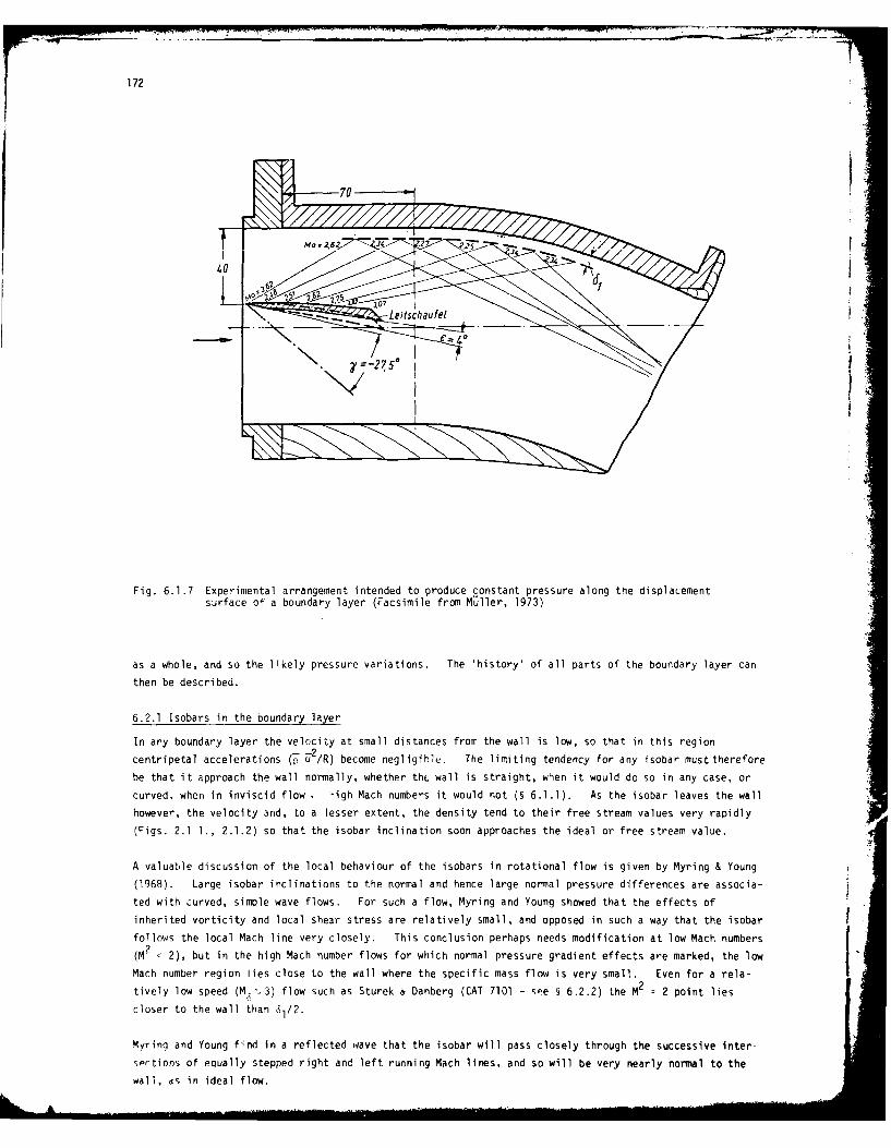
172

\17 / I:

2750

Fig. 6.1.7 Experimental arrangement intended to produce constant pressure along the displacementsurface of a boundary layer (Facsimile from Muller, 1973)

as a whole, and so the likely pressure variations. The 'history' of all parts of the boundary layer can

then be described.

6.2.1 Isobars in the boundary layer

In ary boundary layer the velocity at small distances from the wall is low, so that in this region

centripetal accelerations ( U2/R) become negligibhl. The limiting tendency for any isobar must therefore

be that it approach the wall normally, whether thL wall is straight, wien it would do so in any case, or

curved, when in inviscid flow , -igh Mach numbers it would not (§ 6.1.1). As the isobar leaves the wall

however, the velocity and, to a lesser extent, the density tend to their free stream values very rapidly

(Figs. 2.1 1., 2.1.2) so that the isobar inclination soon approaches the ideal or free stream value.

A valuable discussion of the local behaviour of the isobars in rotational flow is given by Myring & Young

(1968). Large isobar inclinations to the normal and hence large normal pressure differences are associa-

ted with curved, simple wave flows. For such a flow, Myring and Young showed that the effects of

inherited vorticity and local shear stress are relatively small, and opposed in such a way that the isobar

follows the local Mach line very closely. This conclusion perhaps needs modification at low Mach numbers

(M2

< 2), but in the high Mach number flows for which normal pressure gradient effects are marked, the low

Mach number region lies close to the wall where the specific mass flow is very small. Even for a rela-

tively low speed (M "13) flow such as Sturek & Danberg (CAT 7101 - -Pe 9 6.2.2) the M2

2 point lies

closer to the wall than 61/2.

Myring and Young find in a reflected wave that the isobar will pass closely through the successive inter-

sertions of equally stepped right and left running Mach lines, and so will be very nearly normal to the

wali, ds in ideal flow.

173

Since the local Mach lines curve towards the wall the effect of the boundary layer is to shift the

effective generation, cancellation or reflection of any wave structure slightly upstream, and toreduce the pressure differences expected across the region occupied by the boundary layer from the values

which would be predicted from ideal flow considerations alone. In this respect the effect is much the

same as would be observed if the actual wall and boundary layer were to be replaced by an extension of the

free stream flow into the outer part of the space occupied by the boundary layer with generation, cancel-

lation or reflection of any wave structure at a stream surface corresponding to the displacement surface

of the boundary layer.

The displacement surface here is to be interpreted as a stream surface of the free stream extended into

the space in reality occupied by the boundary layer. The extension should take into account all wave

structures in the free stream up- and down-stream of the station under consideration, and all such

stream surfaces are in principle determinate if sufficient details of the free stream flow are known.

The displacement surface then marks the inner boundary of an ideal mass flow equal to that of the original

free stream and boundary layer. In general it will not be possible to determine the displacement surface

directly, and practical approximations are discussed in§ 7 below.

The isobars of a simple wave flow, therefore, are Mach lines of the free stream outside the boundary

layer. As an isobar is followed into the boundary layer its inclination to the wall increases as the

Mach number falls. If it is assumed to follow the local Mach line throughout the boundary layer, it will

eventually become normal to a surface on which M = 1. This surface will, for modest to hiqh free stream

Mach numbers, lie very close to the wall - for the Sturek & Danberq (CAT 7101) flow described below, at y-

values less than 61/20. The subsonic flow between this Vi = 1 surface and the wall is relatively slow and

of low densiLy (the specific momentum flux for the Sturek & Danberq case at M = 1 is 10% of the boundary

laver edqe value, while at hiqher Mach numbers it is an even lower orooortion) so that this portion of the

curved flow can suoport only very small pressure differences and the isobar continues to the wall effec-

tively normally.

6.2.2 Mei.surements of the static pressure field in a simple-wave flow

The behatiour described at the end of the previous section is best illustrated by a practical numerical

example. There are very few flows for which static pressure measurements have been made at sufficiently

cise intervals for the pressure field to be properly described. The only fully documented simple wave

case is the flow on a two dimensional ramp described by Sturek & Danberg (CAT 7101 - Fig. 6.2.1). A full

description is given in AGARDograph 223, the essential feature being that a relatively thick boundary

layer was grown under ZPG conditions (profiles 01-03- the original flow direction is shown by the arrow

marked Uo) before passing on to a curved concave ramp (profiles 04-08). The static pressure field on

the ramp, shown to scale in Fig. (6.2.1), is deduced entirely from measurements on the profile normals

marked 04 - 08, and so depends partly on subjective factors introduced when cross-plotting and interpola-

ting. The original data are however smooth and provided at close intervals, so that it is unlikely that

substantial error has been introduced. The isobars are shown as the right-running set of curved Mach

lines. The separation between the M=l surface and the wall is of order 1', of the boundary layer thick-

ness and could scarcely be shown at this scale. Also shown is a single left-running Mach line, while

extrapolations of this and the right running Mach line or isobar which meets it at the wall are shown as

reflectc at the displacement surface. In the following section (§ 7) it will be shown that the 61 sur-

face can not in fact be determined precisely. The surface shown here is a smoothed curve sketched

through the "D STAR" values which represent the best estimate we can make. The essential difficulty lies

in the requirement for values corresponding to an extension of the free stream flow into the boundary layer

region as far as the 61 surface. The figure can not therefore show more than the plausibility of the

general mechanism discussed above. It would however be very difficult to introduce a substantial change

in the pattern shown while using the original data, and in succeeding sections we will describe the flow in

terms of wave structures interacting with the displacement surface - which inevitably they affect as a

result of the bulk compression and expansion resulting from their associated pressure changes.

174

Sturek & Danberg 087101 02 04 - 08 06 07

Isobars 05P,-of ie 0,.4

Fig. 6.2.1 Isobars for the flow on a curved planar ramp (Sturek & Danberg 1971). The pressuredata are interpolated from the static pressure profiles CAT 7101 0104-8. Theleft running lines are a local incoming Mach Line (-) and an extrapolation of acorresponding free stream characteristic C--).

6.2.3 Static pressure field measurement in a reflected wave flow

Kussoy et al (1978-CAT 7802S) provide detailed measurements in a reflected wave adverse pressure

gradient flow. For the fully instrumented studies, two contoured centre-bodies were successively

mounted on the axis of a cylindrical test section and traversed along the axis so as to permit

measurements at up to 14 stations relative to the wave structure, using a single station traverse

gear mounted in the test surface. In consequence there is some slight but systematic variation of

the boundary layer entering the wave structure, and the 'reference', or 'first-' profiles of each

set, which were measured with the centre bodies retracted, are not strictly part of each series.

The pressure gradients were not so great as to cause positive pressure waves to coalesce into

shock waves anywhere in the test zone, nor did separation occur. The data have already been

discussed briefly above (Figs. 5.3.6, 5.3.7).

• 00 m ........

175

0.6

0.4 'h a A , An78 CAT !I A& 02 3) p. (PROF)

0 int a p. (TAB 2)

0 INF 0 0 A A 0 p oy=6emm)

02 03 04 05 06 07 08 09 10 11 1312Profile No 7802 S 0102 -13

02 030 .0 05 06f07l 0 s8h09 1011 12 13 . (max)

60 6 (AUT)50i~ D1 x0(AUT)

(mm) V40 J -,Mach lines

30 + (Approximate)

20 P -PINF

10 IHI-100 mm---

Fig. 6.2.2 Static pressure profiles for a straight wall adverse pressure gradient flow.(Kussoy et al., 1978 CAT 780S 0102-0113). Lower: profiles with (x), authors' 61point; (- - ), 6 (9 7) displacement surfaceTel ), authors' boundary layeredge; ( 0 ), position of Po peak. Uppr: longitudinal static pressure variation,(x), at wall from profile data; ( ae at wall from pressure runs (authors table 2);y 6 a )at y = 60 me, outside the boundary edge.

The static pressure fields are shown in the form of profile measurements in Figs. (6.2.2, 6.2.3). In

each case the static pressure distribution in the flow direction at the wall (y 0) is shown, as

also are values for y 60 mm corresponding to a traverse well outside the boundary layer. There

are two values for p e depending on whether data are taken from wall pressure runs (labelled "Tab. 2)

or frem the profile runs. The differ ces are not great. In each case the wave structure produced

by the centre body consists of a compression wave followed by an expansion. An incoming wave at

y =60 mm leads the wall pressure change that it causes by about 120 mm.

For series 01 the start and finish of the incomiing compression can be detected in the staticpressure profiles, as can thp outgoing reflected wave which, however, initially appears more concentrated

and stronger than might be expected (see the "bulge" in the inner part of profiles 0108 and 0109).

For the later profiles tne general shape of the static pressure distribution is as expected ifallowance is made for the arrival of the incoming expansion wave in the outer part of the layer

176

from profile 0109 on. A light grid has been sketched in to show the approximate direction of the

Mach lines, along which changes will propagate. Two values for the displacement surface are shown,

one for 0 STAR calculated allowing for varying static pressure as suggested in § 7 below, the

other representing the authors' 61 values calculated as for a zero pressure gradient case. It

is interesting that for both series 01 and 02, the conventional expression suggests a marked

dip in the displacement surface in the zone where the incoming pressure wave approached the wall.

If this were in fact present, an expansion - compression - expansion wave would propagate outwards

from the affected area. There is little sign of any such structureeither in the static pressure

profiles, or in the wall pressure variation.

0.6AA AAA

0.4 o A pw(PROF)PPINF O A p,, (TAB 2)

0PINF 0 0 A o p (y=6Omm)

02 03 04 05 06 07 08 09 10 11 1'2 o 14

Profile No 7802S 0202-14

02 03 04 05 06 07 08 09 10 11 12 13 14

60 /o p (mox)

. "a 6 (AUT)50 y(mm D1 (AUT)

40 (mam). -7 Mach lines

30, , . (Approximate)

2 0 \ \

20 PINF

10 .. . . .- 6"

0

100 mm

Fig. 6.2.3 Static pressure profiles for a straight-wall adverse pressure gradient flow.(Kussoy et al., 1978, CAT 7802S 0202 - 0214). Legend - as for Fig. 6.2.2.

177

It is evident from the foregoing that any attempt at accounting for pressure history effects in the

velocity profiles, as in § 5, must taken into consideration the history of the particular part of the

layer under discussion. In a wave structure whose dimensions are comparable with the boundary layer

thickness, the past history of the inner and outer layers may be very different.

An inspection of the pressure field of series 02 (Fig. 6.2.3) makes this point even more clearly. Here

the compression wave is stronger than in series 01, and is followed more raDidly by a stronger expansion

wave. Consequently the pressure at a point in the boundary layer may be either above or below the wall

pressure, while the local upstream history will consist first of a pressure rise, corresponding to the

incoming compression wave, on which is superposed in any order, and with any degree of overlap, compres-

sion by the outgoing reflected wave and expansion to the incoming rarefaction wave. The pressure changes

can again be seen to follow the (approximate) Mach line grid, and there is again a localised dip in the

authors' 6, value where the compression wave reaches the wall. The D STAR (§ 7) value if anything shows

the reverse tendency. Both here and to a lesser extent for series 01 (Fig. 6.2.2) the wall pressure

seems a little low in relation to the general pressure level in the inner part of the boundary layer in a

way which is not explained easily in terms of the wave structure. The observed pressure variation

suggests that there is a weak outgoing expansion wave in this region, or alternatively that the probes

are affected by the wall and the wave structure so as to give a slightly high reading when close to the

wall.

The static pressure distributions shown in Figs (6.2.2) and (6.2.3) demonstrate how comolicatel the local

pressure history may become, even with a relatively simple applied wave structure.

6.3 Reynolds stresses

The turbulent kinetic energy level in the boundary layer is closely related to the level of the Reynolds

stresses. Of these, the shear stress in the inner fully turbulent region is approximately equal to the

wall shear stress. As the Mach number rises, the skin friction coefficient cf at a given value of Re6 2and Tw/Tr falls, by a factor of about 5 as M goes from 0.5 to 7 in a zero pressure gradient layer

without heat transfer. The typical Reynolds stresses -T _0 etc. are therefore falling in

relation to the free stream dynamic pressure puOe2 . The static pressure, however, falls even more

rapidly since

-e = T-e = Me2 6e (6.3.1)

(the ratio Pe/qe falls from M = 0.5 to M = 7 by a factor of 200) so that at high Mach numbers the Reynolds

stresses may become of the same order as the mean static pressure.

6.3.1 Normal stresses in hypersonic nozzle boundary layers

The normal stress acting in the y direction is composed essentially of contributions from the mean static

pressure and from the normal Reynolds stress o v7 , viscous normal stresses being negligible. Equation

(6.1.2) should therefore be modified, in general, to read, writing o for the total normal stress

a = (a/an)(p + V 7) = - u2/R (6.3.2)

from which 't may be seen that a significant Reynolds stress will cause a local dip in the static pressure

as compared to the value which would be predicted from a momentum balance for the mean flow alone.

In zero-pressure-gradient cases the Mach number has not generally been sufficiently high for the Reynolds

stress contribution to be significant, and in any case exoerimentalists tend to assume that there is no

pressure variation in the normal direction. Apparently anomalous observations in hypersonic nozzle wall

boundary layers can be explained if the Reynolds stress is assumed to play a significant part (Finley,

1977 and below). A nozzle wall boundary layer experiences strong normal oressure gradients as a result

of wall curvature, so that it can become difficult to differentiate between the various contributiors to

the static pressure field.

A 6ll Ii *II I

178

2X

r

PUA

2

r 8y

AXIS WALL

Fig. 6.3.1 Variation of normal stress a in a contoured hypersonic nozzle.Curve A: Normal stress as it would be determined for inviscid flow by a characteristics

calculation starting from the pressure distribution on the axisCurve B: Normal stress distribution as modified by retardation in the boundary layer.urv'e-C: Specific momentum flux distribution showing the fall which occurs in the boundary

layer

Figure (6.3.1) shows the normal stress (-) variation in a hypersonic nozzle. Curve A represents the'ideal flow' distribution which would be determined by a characteristics calculation proceeding from the

pressure distribution on the axis. In the absence of retardation by the boundary layer, the specificmomentum flux p u 2 would vary in a similar manner, but, as discussed in § 6.2 above, not only does thevelocity fall as the wall is approached but also, especially in a hypersonic layer, the density fallsvery rapidly, so that the actual specific momentum flux is distributed more as shown in curve C. The rate

of change of normal stress as predicted by eqn. (6.3.2) therefore falls off as the wall is approachedgiving a variation of the form shown as curve B, which has zero slope at the wall.

Static pressure measurement at very high Mach numbers is formidably difficult, so that no great emphasisshould be placed on exact numerical values. However, Figs. (6.3.2) and (6.3.3), drawn from measurements

In nozzle wall boundary layers at Mach numbers of order 20, show measured static pressure distributionswhich dip noticeably below normal stress distributions predicted from eqn. (6.3.2). The stress values

(curves 81, B2, B) were determined using the tabulated values of , u for Beckwith et al., CAT 7105, andFischer et al., CAT 7001, with the assumption that R could be treated as constant through the boundary

179

layer, and requiring the curve to pass through the reported pressure values at the wall and the boundary

layer edge. In Fig. (6.3.2) curve D2 represents values obtained from corrected static probe measure-

ments. Curve D in Fig. (6.3.3) is the authors' representation of measured values as used for convenience

in data reduction. There are inevitable inconsistencies in any analysis of this data resulting from the

variety of assumptions which may be incorporated. The figures show however that in both these cases

there is a dip in the static pressure distribution of order 0.4 - 0.5 Pw, the dip being greatest in the

zone where turbulent mixing is very intense. We therefore presume that this is a Reynolds stress effect.

P/PW \ D1 .

D2

0.5 " -. .. . .

(pU2)(pUZo -- 0201 0201P-(P u2)/(pu 2), c1 . ~ o ~

-0.5 C- " 2/'Yrr

0-1

Fig. 6.3.2 Normal stress and static pressure observed in a M = 20 nozzle boundary layer (Beckwit, -t al.1971, CAT 7105 0201, 0201P).Curve A: o/pw as calculated for inviscid flow by Beckwith et al.Curves Bl, B2: a/pw as modified by the boundary layer. Calculated from eqn. (6.3.2)

assuming constant R and using the data as tabulated for: (81, 0201), thelinear static pressure distribution assumed by the authors (Dl) and (B2,0201P)the authors' measured static pressure distribution (D2).

Curves Cl, C2: Specific momentum flux distributions used to calculate Bl(Cl) and B2(C2).Curves U1, U2: Static pressure distributions as assumed by the authors for data reduction (Dl)

and as obtained from corrected static probe measurements (D2).A : Assumed boundary layer edge points.

6.3.2 Scalino of Reynolds stresses

If we assume that the peak values of the various Reynolds stresses will to the first order bear a fixed

relationship, we may use these results to estimate the likely magnitude of a Reynolds-stress-induced

static-pressure dip in other flow cases. We take the wall shear stress as typical of turbulent stresses

and write, ignoring any dependence on pressure gradient for the time being,

Ap(max.) = (_i - )max. = ( rv-)max. = 2kTw = ky PMe Cf (6.3.3)

180

D A

1.0

(PU2)/(pU2)8

Y(m)

0 .1

Fig. 6.3.3 Normal stress and static pressure observed in a M = 22 nozzle boundary layer. (Fischer et al.1970, CAT 7001 0104).Curve A : o/pw for inviscid flow (D.M. Bushnell, private communication)C-ur-v-e- B,C,D: as for (Fig. 6.3.2), all referring to the authors' representation of the static

pressure distribution (D).

There are no fully measured profiles of the type that we require to evaluate k, but static pressure was

measured in the two cases shown above in Figs.(6.3.2, 6.3.3). A wall shear stress value in the same

facility used by Beckwith et al. and under closely matched conditions was measured by Harvey & Clark (1972).

With the profile 0201P shown in Fig. (6.3.2) this gives a value of 3.14 for k as defined in eqn. (6.3.3).

There is no corresponding wall stress value for the profile measured by Fischer et al. (1970, Fig. 6.3.3),

though they do provide an estimate for cf based on the limiting slope of the velocity profile. This

'ives a value for k of 3.8. It is extremely difficult either to measure a shear stress value, or to

estimate it from the profile at these Mach numbers (M \ 20) so that these results only permit us to

estimate k as roughly 3, preference being given to the Beckwith et al. (1971) result since it uses a

measured cf value, while the set of straight lines used by Fischer et al. (1970) unduly emphasizes the

peak difference (see Fig. 6.3.4 below). The numerical values given here differ slightly from those

given in Finley (1977) due to differences in the choice of scaling values for p, and cf. Those presented

here are consistent internally with the tables in AGARDograph 223.

It is tempting to go further and attempt to deduce the distribution of the Reynolds stress contribution

through the boundary layer. In Fig. (6.3.4), (Ap/yp6M62cf) as suggested by eqn. 6.3.3 is plotted

against y/6. The 6 value is inevitably very imprecise (see 9 7) since we are here dealing with flows

strongly affected by normal pressure gradients. The peak value of (Ap/yp 6M62 cf) is the value of k as

defined in eqn. 6.3.3, and the speakiness of the Fischer et al. representation of the static pressure

distribution obviously gives rise to a misleading value. With these reservations the two distributions

181

are in surprisingly good agreement.

TI \ _ O~-7001

3 \ - 7105

-YM" P, \

2

/ \/

I / / \\

0 5 10

Fig. 6.3.4 Pressure drop due to Reynolds stress scaled according to eqn. (6.3.3).Values from Beckwith et al., CAT 7105, ( 6 = 112 mm) Representation 01-values from Fischer et al., CAT 7001, C- ,6 = 152 mm).

If there is in fact an element of universality in this Reynolds stress distribution, then it may be used

to predict the static pressure variation in cases where measurements were incomplete. As an example, we

show in Fig. (6.3.5) a possible reconstruction of the static pressure profile at M, = 44.6 for a case

studied by Kemp & Owen (CAT 7206). This is an extreme example and has been chosen to illustrate a number

of secondary points. If the difference (a - p) is dependent on the intensity of turbulent fluctuations,

then it should take a peak value at or near the y-position corresponding to peak fluctuations. Accordingly

this figure has been constructed by using the authors' data, reduced assuming a linear static variation

between a Pitot-derived value at the boundary layer edge and the wall value (curve Dl), to construct thenormal stress variation (curve B) as for Figures (6,3.2, 6.3.3). The Ap variation has then been applied

taking account of the turbulent fluctuations measured with a hot film and shown in Fig. 28 of Kemp & Owen

(1972). These show the peak as occurring at y/6 = 0.8, and also show a significant fluctuation level

in the free stream. The inner part of the distribution, again guided by Fig. 28 of CAT 7206, has been

assumed to start at the point at which the specific momentum flux becomes significant (curve C). The

uncertainties are numerous, beginning perhaps with some question as to the meaning of static pressureunder these circumstances. If static pressure readings were to be taken in such a flow, there would be

in addition to all the calibration uncertainties relating to steady flow mentioned by Beckwith et al.

(CAT 7105), the question of the likely response of a nrobe in a flow with such high implied fluctuation

levels. It seems probable that the original results used to construct Fig. (6.3.4) are also so

affected.

6.3.3 Reynolds stresses in stragh-wl flows

The effect of Reynolds stresses is most pronounced at high Mach number. The data based used for §6.3.2

consists therefore of the two nozzle wall boundary layer cases available with more or less full profile

information. The influence of wall curvature on the static pressure field is thus comparable in

magnitude, if different in form, to that of Reynolds stresses. We therefore look at the Reynolds stress

182

3

D1 \0 2 102

0 /P PU2/(pu2)b

1i6 05/ \

/

0 0 01 0 2

Fig. 6.3.5 Reconstruction of static pressure profile (02) for a hypersonic nozzle wall boundary layer.(Kemp & Owen CAT 7206 0604, M = 44.6, Re = 81, Re@ = 4800, TW/TR = 0.65). Dl, staticpressure assumed by authors; B, normal strss distribution; C, specific momentum flux.Compare Figs. (6.3.2) & (6.3.3).

effects likely to be associated with straight wall flows. Eqn. (6.3.2) shows that for a straight wall

zero longitudinal pressure gradient flow, no difference in static pressure should be observed across

the boundary layer as a whole, and for moderate reflected wave flows the argument of § 6.1.2 would also

suggest only small pressure differences. In table (6.3.1) an estimate is given of the likely pressure

dip which might be found in a range of typical straight wall boundary layers if the quantitative estimate

of § 6.3.2 is assumed to hold over the full Mach number range. Unfortunately there are very few cases

in which a static pressure distribution was measured - usually experimentalists who took account of

possible static pressure variations were satisfied if a Pitot-derived free stream pressure matched the

wall pressure. The (Ap/p6 ) values predicted are in many cases substantial, though the significance of

the variation, and its susceptibility to measuremert, remain uncartln. The key experiments would

appear to be the NOL boundary 1 jer chhnnel studies of Voisinet & Lee (CAT 7202/7304) for which static

pressure profiles were detailed and precise enough, if the Prcbes used response appropriately, to detect

the pressure dips of 5-8% predicted. No such dip is apparent in the repnrted results. It remains

difficult however to account for the observations of Beckwith et al. (CAT 7105) and Fischer et al,

(CAT 7001) other than by invoking the Reynolds stress mechanism. In § 6.4.2 we discuss the straight wall

measurements of Lademan & Demetriades (1974, CAT 7403). It is suggested there that there is a boundary-

layer-induced simple wave generated at the displacement surface which accounts for the overall pressure

difference (Pw " P,) observed. If this is accepted, a normal stress distribution may be sketched in on

the same basis as for the curves B above, and a Reynolds stress dip of about 0.13 p6 becomes apparent

(source Fig. 5). The prediction in table (6.3.1) is 0.15 p6 . This result would seem to give very good

agreement with the above, but does depend on the basic wave structure being as assumed.

L,. ... ... _.... ..' ' ..... ..... .. I I f. .... ... .ii .... , " " -

183

Table 6.3.1. Possible Reynolds stress induced pressure dips in straight-wall boundary layers.

CAT Author M Re 2 xl'30 Tw/Tr CfxlO4 (Pp/p6 )max Comment

5301 0201 Coles 1.98 4.36 1.0 21.8 0.036 ZPG. See remarks on0901 3.70 2.73 1.0 13.8 0.079 longitudinal pressure1201 4.54 1.29 1.0 13.1 0.114 variations in para. 6.4.1.

6502 0103 Moore/ 2.67 360 1.0 8.62 0.026 ZPGHarkness

6702 0401 Danberg 6.46 0.38 0.64 15.6 0.273 ZPG. Static pressure data0801 6.34 1.07 0.86 9.92 0.167 were measured but discarded.

See para. 6.4.1.

7102 0106 Peake et al 3.90 7.76 1.0 10.3 0.066 ZPG case, series 01.

7104 0102 Waltrup/ 2.10 17.4 1.0 13.4 0.025 Reflected wave APG. StaticSchetz pressure profile measured.

See para. 6.4.4. small dipfound.

7202 0101 Voisinet/ 4.75 1.56 0.93 8.90 0.084 ZPG. Static pressure0305 Lee 4.80 13.3 0.91 5.55 0.054 profile measured. No dip

found.

7203 1001 Hopkins/ 7.47 15.5 0.36 7.33 0.172 ZPG.1201 Keener 7.39 4.53 0.46 7.14 0.164

7205 0102 Horstman/ 7.20 2.10 0.50 8.50 0.185 ZPG. Hotwire data availableOwen at M=6.7.

7302 0914 Winter/ 2.21 46.5 1.0 12.9 0.026 ZPG.Gaudet

7304 0101 Voisinet/ 3.85 2.28 0.94 12.4 0.077 Reflected wave, FPG. Static0305 Lee 4.53 65.8 0.95 6.58 0.057 pressure profile measured.

No dip found.

7305 0303 Watson et al 9.80 0.44 1.0 3.78 0.182 ZPG. See para. 6.4.2.0504 10.3 1.55 1.0 2.40 0.028

7402 0101 Mabey et al 2.49 3.10 1.0 18.5 0.048 ZPG.0303 2.50 9.09 1.0 15.6 0.0411601 4.50 1.08 1.0 13.7 0.1161805 4.49 6.81 1.0 8.8 0.075

7403 0101 Laderman/ 9.37 6.52 0.42 4.06 0.150 Nominal ZPG. See para.Demetriades 6.3.4, 6.4.2. Static pressure

measured, large difference

found. Hotwire dataavailable.

6.3.4 Inferences drawn from fluctuation measurements

Any attempt at estimating the effect of Reynolds stresses more directly is inhibited by the general

uncertainty as to flucutation levels in hypersonic boundary layers. As the Mach number rises there is a

general tendency for the turbulent intensity in terms of local mean flow quantities to rise. This must

imply an element of doubt in the interpretation of any hot wire/hot film results. For modest Mach

numbers there is some evidence (if much disputed) that the application of Morkovin's hypothesis in the

form of the "coordinate stretching density factor" (see Owen et al ., 1975, Figure 10; Laderman &

Demetriades, 1974, Figure 16) may correlate the data. In essence this amounts to the assumption that

stress distributions, as opoosed to fluctuation velocity components, will remain substantially invariate

with Mach number. To apply this argument to a Mach number range beyond M = 5 is perhaps a little rash,

but information as to the individual components of turbulent intensity is not available so that one has

little option. The hot wire is presumed to respond to specific mass flow and to total temnerature

fluctuations, and the reduction of such data from cross wires to yield Reynolds stresses in flows with

significant pressure and density fluctuations is essentially controversial.

184

Direct observation of the v r7 component is limited to the laser observations of Johnson & Rose (1975) at

M = 2.9. At this Mach number, Morkovin's hypothesis might be expected to apply, so that the results

should perhaps be expected to scale to low speed results. On the whole (source, Figures 1,2) this is

the case. This implies a peak value for the y-component normal stress of about double the wall shear

stress. The values incidentially agree quite well with hot-wire derived values, with the hot wire

values on the whole lying higher.

We are here attempting to compare results obtained at Mach 20 with results obtained at "modest" Mach

numbers, so that intermediate results are of crucial importance. Owen et al. (1975) report hot-wire-

derived results at M = 6.7 (source, figure 10) which suggest - T' values of order Tw as compared with

values reported by Kistler (1958) and Morkovin & Phinney (1958) of roughly twice Tvw (CAT 5803).

values Pre possibly, at high Mach number, rather greater than _ - values. Laderman & Demetriades

(1973, 1974, CAT 7403) originally reported substantially lower fluctuation levels at M : 9.4. They

have since reappraised their data in the light of relatively low speed experiments (M 3, CAT 7702S)

so that the shear stress profiles achieve better agreement with the limiting value at the wall (Laderman

& Demetriades, 1979). As part of this reappraisal, requiring substantial changes in modal analysis,

they note that V7' values are "quite a bit" higher than UTT values. The crucial point is the degree of

correlation between u' and v', as the normal stresses may be substantially greater than the shear stresses

if the correlation level is low. The valueof71 V"/rw predicted by eqn. (6.3.3) using the data of

CAT 7105 and CAT 7001 is about 6. If "quite a bit" (see above) encompasses a ratio of about 1.5, this is

feasible. More precisely, they include data for [(VT7)/u62 0 at (y/6) = 0.5 over the whole Mach number

range 0 to 10. The graph (source Figure 14) suggests a near constant value of 0.04. If this is used

directly in eqn. (6.3.3), it gives a value for !G-/pSofabout0.18,in good agreement with the estimates

above.

Any approach other than a simplistic correlation must bea little hoDeful, as the local turbulence levels

(as opposed to turbulence levels referenced to free stream mean quantities) may be very high indeed.

Hot wire or hot film derived values therefore need to be evaluated with extreme caution. Extreme

hypersonic results are few, but Fischer et al. (1971, CAT 7001) report mass flow fluctuations of 50>

referred to local mean values at M 20, while Kemp & Owen (CAT 7206) report peak values at M = 38 of 80>.

Referred to freestream mean flow quantities, the fluctuation levels, respectively 10> and 5',, do not seem

too large. It would be a brave man however who placed too much credence in any numerical hot-wire/hot-

film result obtained in such flows.

6.4 Boundary layer induced pressure gradients - anomalous cases

Setting aside the question of possible Reynolds stress induced local pressure drops, the main proposition

of §§ 6.1, 6.2 is that significant normal pressure gradients will only be observed in connection with

streamline curvature. At high speeds the curvature required is not great, and may therefore be associa-

ted as much with the curvature of the boundary layer displacement surface as with the curvature, if not

great, of the wall on which the boundary layer is growing.

6.4.1 Normal pressure gradients in straight walls

A boundary layer growing on a straight wall will not in general develop so as to have a displacement

thickness which increases linearly with distance from the leadin, edge. In general it will not even

increase monotonically in a zero pressure gradient flow, since the change in shape factor at transition

implies that with a momentum thickness which of necessity increases monotonically, there is very likely

to be a local reduction in displacement thickness. The tendency for flows which have not developed

the very thick sublayers (and so displacement thicknesses) characteristic of hyptrsonic boundary layers

will be for the displacement surface to be initially convex with an increasing radius of curvature as

the laminar layfr develops,as for a low speed layer, to pass through a concave region associated with

transition, and then to develop into a very slightly convex surface in the full turbulent region. The

radii of curvature involved are very large, so that at low speeds pressure variations associated with

displacement surface curvature will be negligible. However, as the Mach number rises there may come a

stage at which the simple wave structure generated at the displacement surface causes detectable longi-

185

tudinal and normal static pressure gradients. The linkage between longitudinal and normal pressuregradients haracteristic of simple wave flows (eqns. 6.1.5 - 6.1.7) implies that the resulting normal

gradient is likely to be noticeably greater than the longitudinal gradient.

Coles (1953 - CAT 5301) found static pressure variations along his flat plate of about 5%. The plate

was very carefully constructed, and so effectively flat, and the empty tunnel static pressure variations

did not exceed 1%. He therefore attributed this variation to boundary layer induced effects. Since

any incoming disturbance is relatively small, this conclusion implies a simple wave structure originating

from the displacement surface with a radius of curvature in the range 1006to 600 6. Danberg (1964,

Figure 10) noted differences between freestream static and wall static pressure of up to 10% at low

values of x, falling downstream. His boundary layer measurements covered an Re6 2 range of about

300 - 1700, and so covered the transitional region. The curvature of the displacement surface requirea

is about 500 6. In the case of Danberg (tabulated as CAT 6702) there are four successive stations so

that overtly it should be possible to look for the appropriate displacement surface curvature. The

precision of 61 determination called for would however be several orders of magnitude greater than can

in fact be accomplished in an experiment, so that the mechanism cannot be confirmed. For fully developed

turbulent layers on straight walls in nominally zero pressure gradient conditions, boundary layer induced

pressure gradients should be very small so long as the boundary layer growth follows the general pattern of

a low speed layer. Where a static pressure determination has been made for high Reynolds number cases,

the authors have in general remarked that no significant difference between wall and free stream pressure

was found (Stalmach, 1958, Pitot determination; Sturek & Danberg, 1972, Pitot and static determination;

Voisinet & Lee, 1972, Pitot and static, everywhere except station 1 which was, away from the wall, in the

last part of the nozzle expansion - as profiled in Fig. 6.1.4, Fig. 6.1.5; Horstmann & Owen, 1972, Pitot;

Watson et al., 1973, Pitot - but see below). This is also the general observation in flows with not-too-

strong reflected wave pressure gradients. (Lobb et al., 1955, Pitot; Naleid, 1958, Pitot; Hill, 1959,

Pitot; Pasiuk et al., 1965, Pitot; Waltrup & Schetz, 1971, Pitot and static - but with a dip - see below;

Voisinet & Lee, 1973, Pitot and static; Thomas, 1974, Pitot and static).

The references cited here are those in which some specific comment was made. For the majority of straight

wall cases, the authors have assumed that the static p-essure was constant, usually not even considering

it necessary to say so.

Significant static pressure differences across boundary layers on straight walls are noted by experimenters

working with strong pressure gradients (Zakkay & Wang, 1972, Kussoy et al., 1978; Gopinath & East 1975:

various of those working with siiock-boundary layer interactions) but there remain anomalous cases.

6.4.2 Anomalous cases

While numerical agreement may be somewhat vague, the great majority of observed normal pressure gradients

can be explained by appeal to one or other of the mechanisms discussed in § 6.1, with some reference to

6.3. There remain however a few cases which do not overtly fall into any of the groups suggested

above. Of these the most important are the measurements made by Laderman & Demetriades (1972b, 1974,

CAT 7403). A single profile was studied in detail (PT2, TO, P profiles) on a flat tunnel wall at

M = 9.37, Tw/Tr = 0.4, Re 2 6500. As a straight wall, high Reynolds number (Re, = 37,000) zero longi-

tudinal pressure gradient case therefore we would expect no static pressure differences across the layer,

while there might possibly be (Table 6.3.1) a 15", pressure dip in the layer as a result of the action of

Reynolds stresses. The actual observation is of a 40' pressure difference across the layer, as established

by Pitot measurements, the detailed static distribution, after -orrections applied to cive agreement in

the free stream, being of the general type sketched in Figs (6.3.2, 6.3.5) above, with a '"eynolds stress

dip" of about 0.13p, occurring in the range 0 .- y/ < 0.4. This suggests that the displacement surface

is locally concave to the free stream. The authors do however report a longitudinal wall pressure qradient

of 25 per metre. Further detail of the wall pressure distribution, which is strongly Reynolds number

dependent, is reported in McRonald (1975). There is a minimum in wall pressure upstream of the survey

station, which moves further upstream as the total pressure and so characteristic Reynolds number falls.

,de tunnel calibration reports (Laufer et al. 1967) however show no corresponding longitudinal pressure

gradients on the centre line. Consequently the pressure gradient developing along the tunnel wall cannot

0-AO87 704 ADVISORY GROUP FOR AEROSPACE RESEARCH AND DEVELOPMENT--ETC FIG 20/4A CRITICAL COMMENTARY ON MEAN FLOW DATA FOR TWO-DIMENSIONAL CO-ETC(U)MAY 80 H H FERNHOLZ. P j FINLEY

UNCLASSIFIED AGARDAG-253

3 3fllllfff.f lA Go"E [ D r-EEEEEEEEEE

inuuLm. 8

1 1 111 11 2 -211111 11112- . 0

I11tII25141LA.

MICROCOPY RESOLUTION TEST CHART

186

be the result of an incoming pressure gradient reflected at the wall, and must be a simple wave structure

originating at the wall as a result of boundary layer growth.

If we assume that there is a simple wave structure, then the transverse and longitudinal pressure

gradients are linked by eqn. (6.1.6)

Ap(y)/p = -4(6/Ax)Ap(x)/p (6.4.1)

which with the values 6 = 0.15 m, Ax = 1 m and (ap/ax) = 25%/m gives an estimate for the pressure difference

across the layer of 35%, as compared with the 40% reported.

This explanation implies that the displacement surface is concave, with a radius of about 300 6, in

contrast to the very slightly convex displacement surface which would be expected for a low speed layer.

In turn this implies that the boundary layers on a parallel sided duct will compress the free stream flow

well before the boundary layer itself has reached the axis, and this in turn implies a more rapid axial

compression than would be predicted from any crude one-dimensional Fanno line approach. There is insuf-

fient experimental information from long parallel sided ducts at high Mach number to allow us to say at

what Mach number this hypothetical displacement surface concavity becomes significant, how soon it follows

on from transition, or if there is generally a convex displacement region soon after transition. The

only apparently comparable measurements are those of Watson et al CAT 7305, which were made at M = 10, but

at much lower Reynolds number on a flat plate. For any flat plate, however sharp edged, at this Mach

number, there is a strong leading edge shock-boundary-layer interaction giving a shock wave of noticeable

curvature near x = 0. In consequence the 'free stream flow' or more properly the boundary layer exterior

flow has noticeable vorticity. It is therefore very difficult to decide, from Pitot measurements,

whether there is or is not a static pressure difference across the boundary layer. If the greater total

pressure loss associated with the more steeply inclined part of the leading edge shock is not sufficiently

allowed for - and it is difficult to predict the details of the viscous interaction - a straight applica-

tion of the normal shock relation to the Pitot reading will give an over-estimate of the static pressure,

and vice-versa. Watson (1978) presents (source pp 13/14, Fig. 9) details of the flow field calculated

assuming that static pressure variation across the boundary layer could be neglected. The calculated

flow field implies a 'low speed' type of 61 variation - initially convex, concave in the transitionregion, and convex in the fully turbulent region. The associated static pressure variations would be

ap/ay > 0, < 0, > 0, and clearly an iterative calculation would be possible. Combined with the

uncertainty of the influence of significant exterior flow vorticity, it is unlikely that quantitative

results would be particularly helpful - it is only possible to say that the assumption Pw/Pd = 1 is a

convenient first approximation which is certainly incorrect.

The results of Watson (1978) and Watson et al. (1973, CAT 7305) are not so much anomalous as uncertain.

There remain however a number of experiments displaying, to a greater or lesser extent, inexplicable

features. The most significant of these is the conical nozzle flow studied by Backx (1975) reported

also as Backx & Richards (1976). For this straight wall flow at M = 15 and 20, Tw/Tr = 0.15 and Rex l0-

= 35 and 25, the wall static pressure was observed to be up to 80% greater than the free stream pressure

as determined from Pitot measurements. This difference is very much greater than can be accounted for

by the basic reflected wave mechanism (§ 6.1.2). While experimental error is always possible at these

Mach numbers, it is very unlikely that Pitot and wall static measurements could be in error by this

amount, so that an alternative explanation must be sought. Backx (1975) considered the question at

some length in the light of estimated values of various terms in the y-momentum equation, without beingable to account for a pressure difference of more than 20%. In common with many discussions of the time,

the possible Reynolds stress contribution is confused with the possible effects of streamline curvature.

If the latter is the cause of the observed pressure difference, the flow must, in the boundary layer, be

of simple wave character. Any such argument can only be very tentative, since it amounts to the sugges-

tion that a displacement surface concavity of the type suggested in connection with the Laderman &Demetriades case (CAT 7403) is developing, and causing a compression at the wall which outweighs the

source flow expansion of the conical nozzle. The observation of conical flow in the core of the nozzle

(Slechten, quoted by Backx, 1975) does not eliminate this possibility, as a wave structure developing at

187

the wall at Mach 15-20 would require about 10 diameters to reach the centre line. The displacement

surface curvature required is of order 5006 and so would not be likely to be detected by any boundarylayer calculation, which would be more concerned with the growth of 61 and unlikely to give a precision

which would allow of a curvature estimate.

Peterson (1974) and Peterson & George (1975) report hypersonic (M = 14) contoured nozzle wall measurements,which as expected show Pw greater than p6. The original measurements were made with a calibrated"cone-static" probe with static holes on the face of a 100 half angle cone. The measurements have been

repeated using a conventional low-speed type of static probe (CCP, static holes, 16d downstream of shoulderof conical nose, Peterson, private communication, 1978, and CAT 7405S). There are substantial differencesin the detail static pressure distributions recorded. The arguments for accepting one set of results

rather than the other will not be rehearsed here, but both sets of data include points near the wall for

which p > pw, the original data showing more scatter. This feature cannot be accounted for by the mechanismsdiscussed here, except possibly by a localised disturbance, and must be attributed to uncertainty ininstrumental response to highly turbulent flows or to possible wall interactions. In other respects a

curved-wall nomal stress distribution with a 'Reynolds-stress dip' accounts well for the observedpressure variation.

Pfeiffer & Will (1973, CAT 73075) give profiles measured on an extension to a conical nozzle. This was

either 'unheated' when the wall temperature remained substantially constant and equal to that in thenozzle (Tw/Tr = 0.5), or 'heated' to a temperature of the same order as the free stream total temperature.The general tendency is for the pressure to rise from the wall to the freestream, with a localised rise

near the wall. These results appear to contradict every suggestion made above. The difference (p, - Pw)

increases downstream, reaching a maximum of about 0.5 p6 in both cases if the wall static value is taken

(the probe data do not reach quite such low values). The overall difference is small for the first sta-tion, but the localised rise close to the wall is about 0.2 - 0.3 p6. This can only be accounted for, ifreal, by a localised disturbance. Otherwise it implies a negative (!) value of 5 -0V or, more realisti-

cally, instrumental error. Details of the probe configuration and correction procedure are not available,

and it may be that the data are in fact uncorrected. The overall difference is much less likely to be in

error, but implies a convex displacement surface with a radius of order 400 6.

Finally, we remark the static pressure dip of about 4-6% observed by Waltrup & Schetz (CAT 7104) in the

outer part of the boundary layer in straight wall flows at M - 2. This is 2-3 times the dip which would

be predicted from the Reynolds stress estimate of § 6.3 above; and raises the question of possible

pressure gradient effects, as the data base used in § 6.3 was obtained in favourable pressure gradient

flows, while Waltrup & Schetz (1971) were studying adverse pressure gradients. Since the first

station in each case corresponds to a zero pressure gradient flow and there is no trend with downstreamdistance as the adverse pressure gradient takes effect, it seems more likely that any discrepancy is the

result of the general uncertainty of probe response in highly turbulent flows.

6.5 General comment on the interpretation of experimental data

Taken at face value, the correlations of static pressure difference across boundary layers as presentedby Fischer et al. (1970, 71) and Kemp & Owen (1972) should have as independent variable not the Machnumber but a group of the general nature (yM6

2/R), where R is an appropriate mean streamline radius

of curvature. Since they report the overall difference across the layer the Reynolds stress dip shouldnot affect the correlation. We reproduce figure 9 of Kemp & Owen (1972) as Fig. (6.5.1), with some

additions. The legend is as in the original, but several of the sources may be found in AGARDograph 223.We have not ourselves obtained data for some of the cases quoted. The level of correlation obtained

implies a 4:1 range in the value of (y6/R) which seems not Improbable for hypersonic contoured nozzledata. The 'anomalous case' data however also fall broadly within this band, implying that displacement

surface curvature may be of the same order even on a straight surface. For instance, the value ofR(wall)/6 for CAT 7105 (Figure 6.3.2 above) is about 300, which may be compared with the straight-wall(R/6) values of 100-600 deduced in 1 6.4. The wall geometry ceases therefore to be the obvious con-

trolling feature in hypersonic flows, with the associated low local unit Reynolds numbers, and it is

188

le 10.509

: ::.06? I* £*I.65 I d"L a .51 N U N wall de

A 110,. o .f a Cla k oS ) .o r..- .,,-0 iI-.i.

0 Seall"p oo Speake 4 A#~".A CAl (W L Nit. Lii,.o c.-.' n ,, pieJ# Wallow 691.'0 edge()o Cm lmpah.I o "Ot

•P -'-W+

~~!I~0 0~I6kI-d

6* :00

0 0a

0 / ' Laderman a Oemetroades(1974)

( Paterson 17)

) Backx (19751

. 0I I n I I I I10 Ibo

Fig. 6.5.1 Overall static pressure differences across boundary layers. Facsimile from Kemp & Owen

(1972) with additions.

easy to visualise, for example, a nozzle running in an off-design condition such that the displacement

surface corresponded to the boundary of a free jet. There would then be only a very small, possibly

zero, gradient of pw while ap/ay in the boundary layer could be quite large. An observer whose interest

lay in the quality of the flow in the test core would however consider the flow reasonably uniform, since

he would be observing a domain covering stationary (minimum) values of p as a function of both x and y.

It may be possible (see for instance Beckwith et al., 1971) to make and calibrate static probes which

can be used accurately in the Mach and Reynolds number ranges in question in steady flow, and away from

solid walls. The effect of a solid wall, or at least the point at which static pressure results should

be discarded because of wall proximity, can in part be inferred by observing any change in wall pressure

caused by the approach of the probe. It seems unlikely however that the steady flow calibrations can be

expected to hold very closely in regions of very high turbulent intensity. The calibration corrections

are often very large (of order 2:1) so that the possibility of non-linear interaction between various

factors needs to be taken very seriously.

The analysis of the sections above provides a number of flow models which separately or together allow

static pressure data which, at high Mach numbers, are likely to be rather dubious, to be fitted to a

curve of the right type. The static pressure data on their own will always be Inadequate. To provide

a proper outer limit, Pitot data should always be taken for a substantial distance outside the boundary

layer. Unless there are significant entropy gradients in the outside flow, this will allow a fit, not

only to the static pressure level at the boundary layer edge, but also to the likely level of normal stress

gradients to be expected. A streanwise Pitot survey is also very valuable as it will reveal the presence

of any concentrated disturbances. The wall pressure should be measured not only at the profile station,

but at fairly close intervals for a region upstream and downstream. The wall pressure gradient is a

189

significant datum in any attempt at constructing the wave pattern, and is one of the easiest and

cheapest sets of data to obtain. The normal stress gradient at the wall is zero, and the distribution

between Pw with zero gradient and p, with a known gradient is then fairly closely constrained. The

detail distribution may be refined by using the profile data to determine the distribution of specific

momentum flux as in § 6.3.1, and is not very sensitive to small changes in the profile input. The static

pressure distribution as measured may then be compared to the normal stress distribution in the light of

the probable effect of Reynolds stresses as predicted in § 6.3.2 and the consistency of the whole assessed.At high Mach numbers it is not wise to predict from the wall curvature as such, since, as remarked above,

the contribution to (ya/R) from displacement effects may well be the same order as that from the wallcurvature, so that it is better to work from the profile information itself where possible.

A boundary layer calculation may give the value of 61 within a few percent without giving any precision

in a value of 3261/ax2 , so that it is as yet not reasonable to expect calculation methods to give any

reliable prediction for boundary layer induced normal pressure gradient effects.

6.6 Conclusions

(a) Normal pressure gradients are primarily associated with streamline curvature.

(b) At high Mach numbers the minimum radii of curvature required to give significant normal pressure

gradients may well be very large - of order 500 6.

(c) Significant streamline curvature may occur within the boundary layer as the result of the reflection

of an incoming wave structure even though the wall be straight.

(d) Significant streamline curvature may well be induced by the variation of boundary layer displacement

thickness in the absence of any incoming wave structure and of any wall curvature.

(e) A pressure dip will be superposed on the normal stress distribution associated with streamline curva-

ture because the normal stress is the sum of a static pressure contribution and a Reynolds stress contri-

bution which may well, at hypersonic Mach numbers, be of the same order.(f) The presence or absence of significant normal pressure gradients cannot be inferred from the

longitudinal (wall) static pressure distribution alone. The link between longitudinal and normal

pressure variations depends strongly on the wave structure involved.(g) The above conclusions are with few exceptions qualitatively supported by the available experimental

evidence. Some of the arguments put forward in connection with boundary layer induced pressure gradients

are however speculative, and would be clarified by experiments in which the flow outside the boundary layerwas studied in rather greater detail than is usual.(h) Exact quantitative results at hypersonic Mach numbers probably cannot be hoped for, as the response

of available static probes in the intensely turbulent part of the boundary layer is problematic even

when they have been calibrated in steady flow over an appropriate Mach and Reynolds number range.

" I

190

7. BOUNDARY LAYER LENGTH SCALES

7.1 The 'physical' boundary layer thickness

The flow on any surface supporting a tubulent boundary layer is, in principle, easily divided into that

region affected by vorticity and turbulence, the boundary layer itself, and the region further out whichis in most laboratory cases Irrotational, the free stream or exterior flow. Unfortunately, even in the

simplest possible case with a uniform free stream, there is no clear practical boundary between the tworegions since the flow properties in the boundary layer approach their free stream values asymptotically.The majority of practical boundary layer thickness definitions are based on a small measured differencebetween flow in the outer part of the boundary layer and the free stream (the simolest being 6995, thedistance from the surface at which the velocity reaches 0.995 of the free stream value). The combination

of a small property decrement (e.g. 0.005 ue) and the very small gradients causes the resulting boundarylayer thickness value to be very sensitive to the accuracy of measurement. At high Mach numbers, the

approach of properties to their free stream values becomes even more gradual, and the difficulty is com-pounded by the likely presence of normal pressure gradients, so that the limiting tendency is not to a

set of constant values, but for most properties to a free stream value which itself has a variation in the

y-di recti on.

The determination of a boundary layer thickness 6 is of importance for two main purposes. Firstly, a

scaling length is required when property distributions in different cases are to be compared, particularly

for the variation of turbulence quantities. Secondly, there is need to know where the boundary layer

edge is - or at least when a position may safely be assumed to be outside it. Experimentally we wish toknow how far out a traverse needs to continue, and for various practical applications it is very important

to know when boundary layers growing on opposed surfaces will begin to interact directly. The second

factor is also of importance since for many purposes, both in the theoretical treatment and in the documen-

tation of experimental work, scaling values of the flow properties are required, and these are usually

taken, in principle, to correspond to the flow just outside the boundary layer.

7.1.1 The boundary layer edge state or 'D-state'

We have throughout the earlier sections of this volume, and its predecessor AGARDograph 223, referred to

the boundary layer 'delta' properties p6,u6 etc. and used them in theoretical sections and for the

formation of Reynolds numbers, integral thicknesses etc. without so far enquiring too closely how they

might be determined. A formal approach follows defining terms used in the rest of this section.

The reservoir or R-state In an experimental facility the R-state is the state of fluid from the settling

chamber brought reversibly and adiabatically to rest. In flight it is the state of fluid unaffected by

the presence of the vehicle brought reversibly and adiabatically to rest relative to the vehicle. The

R-state is therefore not a function of position.

The exterior flow or E-state The state of fluid at any point outside the boundary layer is referred to

as an E-state. In general the E-state is a function of position, being dependent on the static pressure

field in the test zone or generated by the vehicle. Many laboratory flows are shock-free so that the

stagnation properties of an E-state are those of the R-state, and so not functions of position. In free

flight and in laboratory tests with shock waves in the free stream there will generally be free-stream

entropy or total pressure gradients which will cause the stagnation E-state to be a function of position

also.

The boundary layer edge or 0-state The D-state at a particular station is defined as a state in the

outer part of the boundary layer which is specified by some artibrary criterion of departure from a

neighbouring E-state.

The R-, E-, and 0- states are all actual physically observable states and in principle directly measurable.

The R-state is easily, accurately and precisely measured with very simple probes. For the majority of

experimental cases In which free stream entropy gradients are negligible, R-state measurements thereforealso provide good values for the stagnation properties of the E-states. In such cases a Pitot survey

will straightforwardly determine the Mach number and static pressure distribution for all points know to

lie outside the boundary layer, with some possible difficulties arising from real gas effects at very high

- o M0 01

191

Mach numbers. Where entropy gradients are present in the free stream, a static property must be measured

directly. While troublesome, this will usually be possible with for example a static probe, as the

influence of fluctuations should be negligible, so that a probe can be calibrated directly in an appropriate

Mach and Reynolds number range.

The D-state however is arbitrarily defined, and usually not too carefully. The D-state lies inside the

boundary layer, but is intended to occur 'at the outer edge' of the layer, so that the D-state properties

are representative of the local E-state while differing from them slightly as a result of the application

of the chosen criterion of difference. If a specification of the D-state is to be at all precise, it is

clearly necessary to have available accurate, precise, values for both the outer region 'profile data' and

for the local E-state. The most common criteria applied are of the type u = 0.995 ue in which the chosen

difference is usually much smaller than accuracy of measurement and often less than experimental scatter.

Since the boundary layer thickness is then defined as the y-value at which the D-state occurs, and since

the property gradients in this region may be very small, it is apparent that even if the precision with

which the states in question are estimated is much increased by some averaging or curve fitting procedure,

no very precise value for 6 can be hoped for on this basis.

7.1.2 Property based boundary layer edge criteria for zero normal pressure gradient cases

If the velocity variation along a profile normal is the result of boundary layer action alone, then a

criterion based on a property decrement such as the 0.995 ue one cited above is in principle straightforward

to apply, since ue and other exterior flow properties are constant. Because it is perhaps the most

familiar from low speed studies, the 0.995 ue criterion initially appears very attractive. However as theMach number rises, the velocity gradient in the outer part of the layer becomes progressively less and less,

so that although the 0.995 ue criterion will give a usable set of values for the D-state, any estimate of

the value of 6 becomes increasingly imprecise and indeed unrepeatable. Other properties, such as p, MPt2and possibly in very strong heat transfer cases, TO may approach their free stream values more abruptly

and at greater y-values, and so provide decrement criteria which are more suitable, or at least more precise

in the value for 6 which they yield. There is some evidence that values so derived also bear a relation-

ship to the point at which turbulence levels reach the free stream value (Laderman & Demetriades, 1979,

measurements on a cone at M = 7.1. Revision of Laderman, 1976). The abruptness with which the various

flow properties approach the free stream values is perhaps best assessed by an examination of the isentropic

and normal shock equations in small difference or error form. For small departures from a local prevail-

ing level

dPo d yM'- dM y_ dM ( l.Po P 1 + M Y W (7.1 .1)

dpt2 ( -. dM (7.1.2)

Pt2 p Z-YM, - (--I W

and, eliminating (dM/M),

dPt2 2(2M2-1)(+Yl 2 dp 2(M2-1)2 dpPt- M(Y "(-)] P '[y (0-) Y-1 0P + (7.1.3)

where the arrows indicate the high Mach number limit, and the static pressure terms are retained for later

use.

If the velocity is to be related to the pressure changes it is necessary to incorporate the energy

equation to allow for possible changes in the total temperature:

!°o dp IM dT ° )LO- - u (7.1.4)

0 p"

192

The total temperature term is usually smaller than the velocity term, though not always negligible, and

may take either sign. We will Initially assume that the flow may be treated, at least in this region, as

isoenergetic - i.e. To is taken as constant, partly for simplicity, and partly because we have not found a

case in which the general conclusions which follow are affected.

For a layer with no normal pressure gradient in isoenergetic flow of a diatomic gas, eqns. (7.1.1 - 7.1.4)

give the ratios shown in table (7.1.1).

Table 7.1.1 Relationships between small property changes (y = 1.4,p, To, constant)

Mach number 2 4 6 10Ratio:

(dpo/po)/(dM/M) 3.11 5.33 6.15 6.67 7

(dPt2/Pt2)/ (dM/M) 1.81 1.95 1.98 1.99 2

(dpo/po)/(dPt2/Pt2) 1.72 2.73 3.11 3.35 3.5

(dpo/po)/(du/u) 5.6 22.4 50.4 140

(dPt2/Pt2)/(du/u) 3.26 8.21 16.2 41.8

It can be seen the relationships between small changes in po Pt2 and M are not strongly dependent on Mach

number, while the small velocity changes become less and less sensitive to changes in these variables as

the Mach number rises. The 0.995 ue criterion would correspond to Pt2 values ranging from 0.984 Pt2e at

M = 2 to about 0.79 pt2e at M = 10 (though precise numerical values should no longer be taken from smalldifference equations when the decrement in question is of the order of 20%).

In Fig. (7.1.1) we show experimental values of various flow properties near the boundary layer edge for aprofile measured by Horstman & Owen (CAT 7205) with Me = 7.2. The authors' D-state was defined as the

point at which po/Por = 0.99, and property values are normalised to this state. The very gradual limiting

tendency of u/u6 , in comparison to the rapid change in Pt2 and po derived from the Pitot measurements, is

very marked, and suggests that the most readily applied criterion will be based directly on pt2 measurements,

or, as the authors have done here and as is recommended below, on a derived po value.

Fig. (7.1.1) shows that this case, for which Tw/Tr was about 0.5. the variation of T0 was also very

gradual, and for this reason alone would therefore not be likely to provide a useful decrement criterion.

In addition since To values are frequently observed to "overshoot" the free stream value, and so display

a very gradual fall from values To > To6 to TO = T06 , we reject any further serious consideration of a Tocriterion.

7.1.3 Other criteria for zero normal pressure gradient cases

The property decrement criteria are the most commonly employed, but many others have been proposed. The

most obvious is the use of the photographic image in a schlieren or shadowgraph picture. If not signifi-

cantly affected by refraction (and a properly focused schlieren system should not be while shadowgraph pic-

tures inherently are) this approach will lead to high values of 6, as the image will show the peaks or

outermost movements of the eddies present averaged in some manner along the light path and over the time

of exposure.

A variety of plotting methods have been put forward, the general aim being to obtain a 6 value from a

reasonably well conditioned intersection of curves or lines rather than from the almost "grazing" inter-

section implicit in the use of a small property decrement. These all rely on the free stream properties

being accurately known and truly constant. Kistler (CAT 5803) used for 6 the y-value at which an extra-

polation of the semi-logarithmic portion of his velocity profile reached the free stream velocity. This

procedure yields a relatively precise value for 6 if the E-states are accurately known, but in common with

many other methods requires a fairly complete data reduction before it can be applied. A number of

193

o Pt2 Authors 8

a M 72050103A TO 8(polpoft0-9 9 )V Po M=7.2 cv

0-30

v co

~y(m)

000

~0-25

Oo -

0.9 1.0u/ u. etc.

Fig. 7.1.1 Variation of boundary layer flow properties near the boundary layeredge (Horstman & Owen, CAT 7205 0103)

authors (Peterson, 1969; Winter et al., 1970, inter alia) have noted that in many profiles there is a

substantial region in which Pt2 appears to vary linearly with distance from the wall. An extrapolation

of this linear variation to meet the free stream value then provides a well conditioned intersection and

a precise 6-value. A study of the application of this criterion (Hill, 1976) showed that the6 value was

typically a little greater than the value using a 0.995 ue criterion, but less than the "Kistler" valueobtained from the semi-log plot. However, as the Mach number rises the linear portion found up to about

Mach 4 increasingly becomes curved, so that the method can no longer be used. Peterson (1969) alsogives examples of the application of a method due originally to Schlichting. The outer region is assumed

to behave generally as a wake and leads to a prediction (Schlichting, 1968) that

( - (u/u6)] /2 El - (y/6) 3/ 2] (7.1.5)

The intercept on the y-axis of a plot of [l - (u/u6)]1/2 should then yield a value for 6312. In practice

the variation is not linear over the whole outer region so that an element of subjective judgement is

required in deciding the range to be treated as linear. Again, it is not a convenient procedure unlessdata reduction is already complete. Peterson (1969) discusses the question generally, and a further

examination has been made by Hill (1976).

194

Selection of an explicit criterion may be avoided if it is assumed that the relevant portion of theprofile is properly described by a wall-and-wake law (eqns. 3.2.5, 3.2.6), so that the value of 6 may beobtained from a statistical fit to the experimental data points, either in the original physical variables

or after transformation to "equivalent incompressible form" (eqn. 3.3.10). The validity of this proce-

dure must depend on how closely the profile does in fact follow the wall-and-wake law, and on the form of

the wake law assumed. It has the advantage of removing subjective judgement as a factor except in theneed for a decision as to how near to the (as yet unknown) 6-value one should include data points, since

most wake laws do not properly represent the outermost part of the layer. This difficulty may be overcome

by using a more complex wake- or divergence-function (see the various for-is of eqn. 3.2.6 and Bull, 1969)

but the additional complication is probably not worthwhile

If fluctuation measurements are available, a boundary layer edge or characteristic thickness may be defined

in relation to these. Definition 'by approach to the free stream fluctuation level' cannot be very

precise, as the fluctuation level measurements can never be very accurate. The availability of conditional

sampling techniques however makes possible a definition in terms of the 50% intermittency point, as sugges-

ted and initially applied by Laderman & Demetriades (CAT 7403). This proposal is attractive as it provides

a well conditioned intersection and should be universally applicable. It should also relate properly to

the physical process of turbulent mixing in the boundary layer. The 50% intermittency point lies well

within the 6-value as defined by the other criteria discussed above, but this is not of itself a disadvan-

tage if the 6-value is defined as a suitable multiple of they-value at 50% intermittency.

Finally, the problems of choosing an edge criterion may be avoided by using a suitable integral thickness.

If there is in fact any universal similarity in the inner and outer regions of the transformed velocity

profiles of zero pressure gradient boundary layers, then the defect-integral thickness A* defined in

eqn. (3.3.16) should bear a nearly fixed proportion to the physical boundary layer thickness 6, however

that may be defined. Acceptance of eqn. (3.3.17) as a description of the outer region gives A*/6 = 4.18.This corresponds to taking 6 as defined by the intersection of eqn. (3.3.17) with the (y/A*) axis in the

outer region plots presented in § 4 above, and the validity of the procedure depends on the quality of the

fit near the point of intersection. The intersection itself is well conditioned, and, as an integral

thickness, A* is precisely determined.

7.1.4 Boundary layer thickness in the presence of normal pressure gradients

When the free stream wave structure is such as to imply significant normal pressure gradients, properties

such as M, T, p. p, u vary as a result of the free stream pressure field as well as the action of turbulent

mixing in the boundary layer. Almost any criterion based on these 'static' properties therefore becomes

unworkable, as the gradients in the free stream are finite, while the gradients due to the boundary layer

alone are tending to zero. The pressure field induced variation will always therefore become greater

than the shear-induced variation at sufficiently large y. Criteria based on a property decrement are

particularly difficult to apply, since the decrement is a difference from a quantity which is itself a

function of position, and probably experimentally, and so imprecisely, defined.

In a normal pressure gradient case it is always possible to find at least one property which reaches a

maxinum near the boundary layer edge, and the position of this maximum may be used to define a 6-value.As an example, consider the Pitot pressure profile for a flow with negative (3p/ay) such as Sturek &

Danberg, CAT 7101. As the wall is approached from the free stream, pt2 initially rises as the Mach num-

ber falls at constant po. With a further approach to the wall, po begins to fall rapidly as a result

of viscous action and the rise in pt2 associated with rising static pressure is outweighed by the fall

due to the drop in p0. This approach is not to be encouraged, as it is evident that, other things

being equal, a 6-value obtained from a property maximum will occur relatively closer to the wall in a

strong normal pressure gradient than in a weak one. The requirement is for comparison with a property

which does not vary in the free stream.

In the majority of laboratory cases the free stream total pressure pne and total temperature Toe may be

treated as constant, so that in principle these properties provide a proper base for a boundary edge

criterion. The total temperature, however, is not suitable in practice, firstly because it shows a very

195

gradual approach to the free stream value, and secondly because of the possibility of a 'total temperature

overshoot' (see I 7.1.2and Fig. 7.1.1). A criterion based on pd, on the other hand, is very attractive.

Of the various possible properties it approaches the free stream value the most abruptly (eqns. 7.1.1 -

7.1.4, table 7.1.1 and Fig. 7.1.1) so that a po criterion is overtly the most distinct possible.

Unfortunately, po cannot be measured directly and must instead be found as a combination of experimental

Pitot and static tube measurements. The appropriate combination of errors, using eqn. (7.1.3) would seem,

at first sight, to counter the advantage of rapid approach to the free stream value exactly. This is not

in fact the case, since experimentally one is, or should be, looking for differences between sets of

readings taken with the same instruments, so that systematic error should cancel, while random error can

be reduced to any desired degree by increasing the number of readings. In principle, the edge criterion

should be made by comparison of poe and por but at high Mach numbers when for systematic error

dp0 dpt 2 1 dp(7.1.3)P--: - Pt2 Y -F P

the error in (dp/p) is likely to be so large that such an approach will be unhelpful. Instead, the Pitot

and static measurements should extend into the exterior flow until there is no systematic trend visible in

the po value, which may then be usefully compared to the value of Por to give a check on the static

pressure value rather than an edge criterion.

Where, in AGARDograph 223 and its successor, we have received profile data which allow us to calculate po

at points well out into the free stream, we have in general observed that readings are sufficiently

precise and repeatable to allow the use of a 1% p0 decrement as a sensible edge criterion. Scatter in p0

is usually small - so small in fact that we have not infrequently avoided making a judgement of the D-state

by taking the highest recorded po value as the boundary layer edge, at least for initial numerical

processing (e.g. Figs. 6.2.2, 6.2.3).

Our experience therefore leads us to recommend that the boundary layer edge state, and the boundary layer

edge, be taken at a point where

(Poe - Pod ) = 0 .01 (Poe - Pw) (7.1.6)

which at high Mach numbers corresponds very closely to (pod/Poe) = 0.99, and at low speeds reduces to the

common 0.995 ue criterion.

This criterion should also be applied in zero-normal-pressure-gradient cases, when if the normal pressure

gradient is truly negligible, it may be replaced by a directly measured Pt2 criterion calculated from

eqn. (7.1.3) - or, approximately, following table 7.1.1, a 1/3% Pt2 decrement. To eliminate systematic

error the measurements should always extend into the free stream and to allow other workers to apply theirown criteria when they wish, the experimental values obtained outside the D-point should be included in

any data presentation.

7.2. Intetral thicknesses

In the previous section we emphasised the arbitrary nature of the definition of the physical boundary layer

thickness 6, and the consequent lack of precision in any numerical value which may be obtained. Suitably

defined 'integral thicknesses' do not suffer this disadvantage, since with proper formulation such as thatdiscussed below, the integrands In the defining equations all tend to zero at large y so that the values

of the integrals are not sensitive to the choice of 6. A precisely determined length scale is desirable,

the object being to use it both as a scaling length for property distributions through the boundary layerand also in the formation of Reynolds numbers when looking for overall similarity rules and empirical

projections of data. With the exception of the Rotta-Clauser outer law defect thickness A (eqn. 3.3.16),

the defining integrals for the usual 'thicknesses' 6I 62, 63 etc., include velocities measured relative

to the wall, so that the ratio of any one thickness to any other is Reynolds number dependent. None of

these integral thicknesses therefore serves as a scaling length for property distributions even in incom-

pressible flow, so that there is even less reason to attempt any such scaling in compressible cases. The

196

usual choice of scaling length for Reynolds number formation, 62 , foilows principally from the importance

of the momentum defect in the momentum integral equation, and has no special justification in similarity

terms. The choice is in essence arbitrary,and if Red 2 or Ree (see eqns. 2.3.5, 2.3.6) are used as the

specifying variable in a data presentation, the ratios of 61, 63 etc. to 62 are implicitly a part of thatpresentation - as in principle, though not usually in practice, should be the technically desirablerelationship to the length of boundary layer development x.

The integral thicknesses are notionally defined so as to represent in convenient form 'deficits' of mass

flow, momentum, kinetic energy etc., in the real boundary layer as compared to a reference flow which is

representative of the exterior flow extending inwards to the wall for the displacement thickness, and,

for the others, to the displacement surface. The integral thicknesses therefore have, in principle,

straightforward physical interpretations. When a boundary layer does not experience a significant

normal pressure gradient, the E-states are functions of x only and the calculation and interpretation of

61, 62 etc., present no complications. We see below however that if the physical significance of the

quantities called 'displacement thickness', 'momentum thickness' etc. is to be retained in flows with

normal pressure gradients, it is necessary to change the usual 'constant E-state' formulation of the

integrals to take account of the fact that the E-states are functions of y. As an obvious pcint, if 62

were to be calculated for planar flow from the usual equation6

6 f- -- (1- 2) (7.2.1,2.3.8)

it is apparent that the value of 62 so determined is a function of 6, since p, and u, depend on the choice

of D-state. We will see below that eqn. (7.2.1) can only give a value of 62 representing the supposed

momentum deficit p6u6262 by chance. A proper formulation of the integral thicknesses will be seen to

require inconvenient procedures, so that in addition to a correct presentation we will consider various

possible approximations.

7.3 The displacement surface

A technically important result of the growth of the boundary layer is the change induced in the free stream

flow, by comparison with some equivalent ideal flow in which viscous effects do not develop. At high Mach

numbers the 'displacement effect' may be very large - consider for instance the boundary layer induced

pressure gradients discussed in § 6.4, above, or, more directly, the large values of displacement thickness

found in hypersonic nozzles (6, is about 0.25Rz for CAT 70010104, examined below) so that it is of some

importance to assess the effect correctly. Here we require that the comparison be made with an ideal

inviscid flow which has the same free stream as that actually observed outside the boundary layer for all

y> 6. The ideal flow must extend into the space in fact occupied by the real, viscous, boundary layer flow,and we require, in principle, that this reference flow should be in every particular an extension of the

actual free stream flow. If the free stream is supersonic the reference flow is determinate, and could be

calculated by the method of characteristics from experimental information describing a sufficient extent of

the free stream up- and downstream of the profile normal (Fig. 7.3.1). The displacement surface is thena stream-surface of the reference flow such that the mass flow between the displacement surface and any

chosen surface in the free-stream is the same as that in the real viscous flow between the wall and the

chosen free-stream stream-surface. The wall is not in general a stream-surface of the reference flow,

since the displacement surface is not in general a stream-surface of the real flow. The reference flow

is not uniquely determined when the free stream is subsonic, or when an extension of a supersonic free

stream indicates that the Mach number in the reference flow will locally become subsonic for y > 6*

(see below).

7.3.1 Displacement thickness in flows with normal pressure gradients

In this section we will denote a 'properly defined' displacement thickness by 6*, in contrast to a'usually defined' thickness 61 (eqns. 7.2.1, 2.3.8) or various improperly defined quantities specified by

eqns. (7.4.1 - 3). A mass balance between the real flow (p,u etc.) and the reference flow (p',u' etc.)

then requires

197

N6

Fig. 7.3.1 Uniqueness of the reference flow. AB is a line in the free stream along whichproperties are known. AC and BC are right- and left-running characteristics ofthe free stream flow. All properties in the domain of determinancy ABC are thenknown so that values along the profile normal NN may be calculated.

h hf pu(R z + ycosc)dy = P'u'(R z + ycos)dy, (7.3.1)o 6*

where h is a value of y greater than 6, Rz is the transverse curvature of the wall, defined positive for

boundary layers on the exterior of an axisymmetric body and a is the inclination of the wall to the axis.

The form of eqn. (7.3.1) shows that values of p', u', for y < 6* do not affect the result, so that a

calculation of the reference flow does not need to extend to the wall. By the same token, approximate

reference flows discussed below need only be accurate representations for y > 6*. We will in general

assume that cosa may be taken as one, and rewrite eqn. (7.3.1) for convenience in processing data as

6" 6

f Pul'i + )dy f (pu - Pu)(l + - )dy (7.3.2)0 z 0 z

Since, in a flow with normal pressure gradients, p' and u' are functions of y, it is necessary to

solve for 6* as a limit in the full form of eqn. (7.3.2).

7.3.2 Displacement thickness in flows with no normal pressure gradient - importance of transverse

curvature

If normal pressure gradients are negligible, p',u' are constant and may be set equal to p6 ,u6 . Eqn

(7.3.2) then reduces to

+ ( - U))(l + >-)dy (7.3.3)2Rz 0 P6 U6 "z

which is the proper form of the defining equation for 61, now equal to 6*, for axisymmetric flow. Data

sources by no means always make it clear how far the defining equations for integral thicknesses have taken

account of transverse curvature, so that it is advisable to assess its importance. A thorough general

treatment for zero normal pressure gradient cases (though this condition is not explicitly stated) is

given by Hokenson (1977). We therefore restrict comment here to some general observations. It is

apparent that the evaluation of the integral will be inaccurate if (y/Rz) is omitted when (6/R.) is signi-

ficant compared to one at the desired level of accuracy. In general, though not always, source papers

have recognized this. In hypersonic flows especially, (e*/Rz) may take relatively Hgh values (e.g. 0.25

for CAT 7001), and it is then important to include the (6*2/2Rz) term. This is usually not done, the only

case in AG223 for which full account of transverse curvature was taken by the oriyinal authors being Kemp

& Owen (CAT 7206), who however did not in this allow for the very strong normal pressure gradients in

198

their experiment (see Fig. 6.3.5). In all except the most exceptional circumstances (Richmond 1957,CAT 5701S) the other integral thicknesses 62, 63 etc. are small compared to Rz so that the quadratic

term on the left of equations su h as (7.3.3) - see eqns. (7.5.4) below - may be ignored safely. It

will usually only be significant for the determination of the displacement thickness.

7.4 Reference flows, and improper formulations

The reference flow as defined in § 7.3 above is in principle determinate and straight-forwardly, if

laboriously, calculable. It is unusual in practice to have a set of values which have been calculatedas an extension of the neighbouring experimental free stream flow field. Values are sometimes given for

nozzle flows (corresponding to the curves labelled A in Figs. 6.3.1 - 6.3.3) but not necessarily for theexact flow conditions at which the boundary layer measurements were taken. Often the 'theoretical'curves are also calculated in advance, using a predicted displacement surface before the measurements arein fact obtained. This is perhaps the cause of the failure of curves A and B or D to agree at theboundary layer edge in Fig. (6.3.2), and to a lesser extent in Fig. (6.3.3).

7.4.1 Choice of reference flow

To solve eqn. (7.3.2) the reference flow properties p',u' must be known. We examine below the effect of

three levels of representation of the reference flow:(a) "Characteristics based". For a profile measured in a nozzle by Fischer et al. (CAT 70010104) we havea characteristics determination of the inviscid flow field, starting from the pressure distribution on the

axis (D.M. Bushnell, private communication). This is in reasonably good agreement with experimentalvalues at the boundary layer edge (Fig. 6.3.3), and extends in as far as y =

(b) "Linear extention". The reference flow is approximated by a linear projection of the free streamproperties into the boundary layer space. This was done graphically as a best eye-estimate. The proce-dure is relatively convenient, as all the integrands which result are simple polynomials. The linear

extension is clearly the obvious first approximation, and in the outer part of the layer will only departgradually from the 'correct' characteristics values.(c) "Pressure based". Both the characteristics-based and the linear extension reference flow require thata separate input of reference flow data be made, in addition to the boundary layer measurements. A devicewhich has been commonly employed, and which we adopted in AGARDograph 223, is to calculate a referenceflow assumed to be given by an isentropic extension from the free stream total pressure Poe (or failingthat, po6) to the local experimental value of the static pressure.

The requirement is for good prediction of the reference flow for y > 6* (which has yet to be determined).

The extent to which the estimates based on linear extension and the local static pressure are likely to pro-vide a good estimate may be assessed from Fig. (7.4.1), based on Figs. (6.3.2, 6.3.3). The linearextension of pressure, as a typical property, will evidently be a good approximation to the characteristicsolution. The local measured static pressure is however markedly lower throughout, in particular forhypersonic nozzle flows as a consequence of the "Reynolds stress dip". Regrettably it is apparent, for aflow of the type chosen as an example here, as also for the additional case considered in the numericalexperiment below, that the difference between the local static pressure as measured and any static pressurededuced. as a reasonable extension of the exterior flow field is large enough to suggest that serious errorwill result if the pressure based reference flcw is adopted for calculation purposes. Therefore, despite

its convenience, this approach should probably be abandoned.

(P. Bradshaw, private communication, points out that a boundary layer calculation which did not allow forap/ay would probably use as a boundary condition a 'pseudo-velocity' calculated from poe and Pw - that ispressure, velocity and density used as 'free stream values' would in fact be the wall states of the pressure

based reference flow. Figs. (6.3.2, 6.3.3) perhaps indicate that this would be imprudent for a flow with

strong ap/ay though the approach provides a very useful starting point for the calculation of flows such asshock-boundary-layer interactions).

199

Pp Betc.

ICl

, I6 Y

Fig. 7.4.1 Sketch to illustrate different levels of approximation to the reference flow.A - 'characteristics' or exact value,B - 'linear extension',C - 'pressure based',D - 'constant reference flow'.The experimental variation shown as C1 is typical of flow at modest supersonic Machnumbers. -In a hypersonic nozzle the'Reynolds stress dip' (§ 6.3) will give avariation such as the broken line of C2 .

7.4.2 Effect of reference flow variations: Improper formulations

In table (7.4.1) we compare values of 6* for two profiles (Fischer et al., 7001 0104, the nozzle flow dis-

cussed above, and, as representative of flows at lower Mach number, Sturek & Danberg, 7101 0205, mea;ured

Table 7.4.1 Values of displacement thickness (6*) and related integral quantities

Quantity Reference flow qn. Values

Profile no. 7001 0104 7101 0205

M6 21.6 3.16

pup 1.35 1.21

1 6*(m) Characteristics (7.3.2) 7.7310-2 -

2 6*(m) Linear extension (7.3.2) 7.57 " 8.31.10-3

3 6*(m) Pressure based (7.3.2) 6.91 " 7.68

4 6 lp(m) Pressure based (7.4.1) 7.00 " 7.77

5 6 1(pw)(m) Pressure based (7.4.2) 7.67 " 8.68

6 6 1(p6)(m) Pressure based (7.4.3) 6.22 " 7.61

7 61 (m) Constant,d values (7.3.3) 7.31 " 6.80"

Rows I - 3: "properly defined" with differing estimates of the reference flow.

3 - 5: comparison between "properly defined" 6*(row 3) and improperly defined quantities(rows 4 -6) with the same reference flow.

7: conventional definition.

on a planar ramp). The first three rows give properly defined values of 6*, with differing estimates

of the reference flow. These are succeeded by three improperly defined quantities which have been sugges-

ted by various authors attempting to handle the problem of a non-constant reference flow. (As examples,

200

see McLafferty & Barber. 1959, 1962; Kepler & O'Brien, 1962; Voisinet & Lee, 1972, CAT 7202, 1973,

CAT 7304. These authors used a pressure based reference flow and 61(pw) as defined in eqn. 7.4.2.Hoydysh & Zakkay, 1969, give complicated definitions which are equivalent to 6l(1 ) and 6l(p6)' eqns. 7.4.2,

7.4.3. The definitions adopted by Stroud & Miller, 1966, CAT 6503 are similar. Clutter & Kaups, 1964.CAT 6401, used an 'inviscid' reference flow calculated from the model wall pressure distribution which was

then shifted into agreement at the boundary layer edge, with 61(p6) as defined in eqn.(7.4.3). Finally,

in row 7 we give the usual 61 value, which may be regarded either as incorrectly formulated, or as an

extreme example of a badly estimated reference flow (p',u' equal to p6,u6, which are functions of 6). The

comparisons form two groups. Variations between row 1, 2, 3 and possibly 7 show the effect of inaccurate

estimation of the reference flow. Variations between rows 3, 4, 5 and 6 result from different formula-

tions all using the same (pressure based) reference flow, indicated by writing p',u' as ppUp, Theimproperly defined quantities are given by eqns.(7.4.1-7.4.3):

2

61P + 1 (l +J-)dy (7.4.1)0 o pp z

This quantity was proposed because of its similarity to the conventional 61 and is attractive since no

scaling quantities are required, while it is independent of 6 if the D-ooint is taken sufficiently far out.

2

[6+() z I (pu)pw = o Ippu - pu)( + -)dy. (7.4.2)z0 p z

This quantity, as used for instance by Voisinet & Lee (1972, 1973), has the advantage that the scaling

quantities ppw" upw do not depend on the choice of D point, so that the value of 61(pw) is again indepen-

dent of 6 if 6 is sufficiently large. In contrast 61(p,) below is, through the influence of changes inthe D-state, dependent on the choice of D point. It is included as more directly comparable with the

conventional 61, definition of eqns. (7.2.1, 7.3.3)2 616

[6( )+ - ]-lu6 = f (ppUp - pu)(l + !-)dy (7.4.3)z0Z

The three 6* values of rows 1-3 clearly demonstrate the influence of the reference flow assumption. (The

first row is blank for 7101 0205 as we do not have details of a characteristics calculation). Both flowsare on concave walls so that the pressure, and so density and specific mass flow values, fall progressively

from the characteristics solution to the pressure based assumption. Row 7, for 7001 0104, gives a higher

value again, as would be expected since the Reynolds stress dip causes the static pressure over most of the

range 6* < y<6 to be less than the boundary layer edge value, p6. For 7101 0205, the row 7 value is thelowest as at the (relatively) low Mach number, the Reynolds stress dip is small or negligible (and was notdetected) so that the experimental static pressure distribution is of the form of curve B in Figs. (6.3.2,

6.3.3) and so everywhere above p6. (Excepting the Reynolds stress dip, these trends would be reversed

for flow over a convex surface).

We cannot claim that the value given in row 1 is accurate in absolute terms, but the differences between

rows should be representative. Numerically, at 10% from row 1 to row 3 for 7001 0104 and 22% from row 2

to row 7 for 7101 0205 the differences are appreciable. The technical significance depends on the actualdisplacement thickness values. For 7001 0104 6*/Rz is 0.25 and the difference in 6* values is, at 7 mm,

greater than any conceivable fabrication error. The difference suggests that very refined characteristic

calculations for nozzles may well not be justified. For 7101 0205, the difference, at 1.5 mm, is also

large compared with likely fabrication errors or the precision of inviscid flow field calculations.

Errors resulting from the improper calculation of the reference flow are therefore significant.

As compared with a 'usual' 61 determination with constant reference flow, or the pressure-based value,

the linear extension appears to give a reasonable approximation (within 2%). It would obviously be

fairly straightforward to use a higher order polynomial extrapolation of the free stream propery variationso as to refine this approach, and in the absence of a characteristic calculation and possibly for any

extension of these ideas to lower speed flows for which the reference flow is not in principle uniquely

determined, this would appear to be the most promising method of estimating a proper 6* value, if high

201

accuracy is required. A curve fitting procedure would also eliminate the element of subjective judgement

present in the calculations of table 7.4.1.

The improperly defined quantities of rows 4-6 should be compared to the correctly defined but inaccurately

determined 6* value of row 3, as all use the same reference flow. The quantities 6lp and 61(pw) are

insensitive to choice of 6 and the agreement between 6* (row 3) and 6lp appears to be good. This must be

regarded as an empirical agreement which may exist for concave wall flows, as we do not have any convex

wall data with sufficient detail for a useful comparison. Any general analytical estimate of the diffe-

rence between 6*and 61p or an equivalent quantity usinga better reference flow is intractable since 6* is found

by solution of eqn. (7.3.2) for 6*as the limitofa definite integral. The difference between 61(pw) and 6*with

the same reference flow is unacceptably large - 10% or more -so that this formulation is unlikely to be useful.

The row 6 quantity 6 1(p6) takesanarbitrary value depending on the choice ofa6value,and like the 'usual' 61

of row 7 should be discarded for this reason alone. In a concave wall flow such as the two examples treated

here, as the chosen value of 6 increased 61 would fall continuously while 61(p6) would rise. The arbitrary

nature of 61( p6) is particularly clearly ill ustrated by the values obtained for the nozzle flow reported byKemp& Owen (CAT 7206). For 10 cases out of 29,61 (ps) as defined by eqn.(7.4.3) is found to takea complex value

(shown as NOT REAL in the print-out in AGARDograph 223).

In conclusion, the error resulting from an inaccurately assessed reference flow would seem, on an empirical

basis, to be much greater than the error resulting from a choice of certain improperly defined quantities,

such as 6lp with a better reference flow, which may be more straightforwardly determined.

7.5 Defect thicknesses

The displacement thickness 6* is a quantity which has direct physical significance in its own right.

Particularly at hypersonic speeds, when it may achieve relatively large values and so modify the exterior

flow to a substantial extent, there is a need to evaluate it properly and as accurately as possible. The

momentum thickness, whether in its 'usual' formulation as 62 (eqn. 2.3.4), or properly defined as e below(eqn. 7.5.5) has no such direct physical significance, but rather provides (at least in flows without

normal pressure gradients) a convenient way of describing the accumulated friction effect of the boundary

layer. It appears in the momentum integral equation in just this way - the integral equation itself

being a convenient shorthand for a control surface momentum balance. If only because of its importance

in the momentum integral equation, the momentum defect thickness is also, conventionally, the most favoured

reference length for the formation of Reynolds numbers intended to correlate experimental data. The

factors which affect a proper definition of the momentum thickness apply equally to the other defect thick-

nesses, such as 63, 64 etc., each integral quantity having value only in so far as it actually describes

the defect of the flow property (specific momentum, kinetic energy, total enthalpy etc.) resulting from the

presence of the boundary layer. Our initial development is therefore in general terms.

7.5.1 General formulation for a property defect

We require a value for the defect of a convected property q (specific momentum, kinetic energy, total

enthalpy as appropriate) in the real boundary layer as compared with the value for the same mass flow of

fluid in the ideal or reference flow, which must therefore be evaluated from the displacement thickness

outwards. The defect should be described accurately, and a proper formulation will be insensitive to

the choice of D-state or 6-point. A proper defining equation for the deficit of the property q is then,

following the arguments of § 7.3,

h h= p'u'q'(l + -s )dy - f puq(l + Ycosod)dy (7.5.1)

z * 0 Z

in which it can again be seen that reference flow values for y < 6* do not influence the result. In

calculation it is again convenient to rearrange eqn. (7.5.1) as (once more setting cose - 1):

6 6*-e i f (p'u'q' - puq)(l + z)dy - f p'u'q'(l + I)dy (7.5.2)

z 0 Z 0 Z

202

The subsequent definition of a defect thickness in terms of the property deficit is essentially

arbitrary, as it is necessary to choose representative scaling values for p, u and q. The natural

extension of low speed practice is to define a deficit annulus adjacent to the wall and 6q in depth,

where 6q is the desired defect thickness. Then

= 1q (p'uq')scale(1 + z)dy (7.5.3)(deficit of q) a( -d 753

z 0 Z

where (p'u'q')scale is the chosen scaling flux per unit area of the convected property q. and is essentially

defined in terms of an arbitrary chosen state of the reference flow.

For flows with no normal pressure gradient in which p',u',q' are constant and may be evaluated at the D-

state, eqns. (7.5.1 - 7.5.3) then give6 2

6 j Pu ( - -)(l + J-)dy (7.5.4)

q 2 fo P6u6 q6

which can be seen to reduce to the 'usual' definition for a planar flow. As remarked in S 7.3.2 above,

the defect thicknesses are nearly always very small compared toRz so that the quadratic term (6q 2/2R ) mayusually be dropped safely.

7.5.2 Momentum defect thickness

We take the momentum defect thickness as a typical integral quantity of this class, and will not discuss

the other possibilities further. If it is desired to describe the momentum defect as a thickness, a

scaling value for (pu2) must be chosen, and the value of the thickness which results will be in inverse

proportion to this scaling value. Ideally the scaling value should be taken at a fixed state with

physical significance in the reference flow, but the only value which suggests itself on this basis is a

value calculated at y = 6*, which would in practice be inconvenient. A fixed value may be obtained by

choosing (pU2) pW, the value for the pressure-based reference flow at the wall. This state however is not

a state of a reasonable extension of the free stream flow field, and so not attractive, although it is in

fact numerically not too different from the values of a characteristic based or linear extended reference

flow at y = 6* (see Figs. 6.3.2, 6.3.3). The choice is arbitraryand for our convenience. since many ofthe necessary integral quantities are tabulated in AGARDograph 223, the scaling quantity used here is (pu2)6.

Recognising that the value of a properly defined momentum defect thickness will then depend on the choice

of D-state we may then recast eqns. (7.5.1)-(7.5.3) to give

(momentum deficit) 6 2 612 612 62e .(1 +-)dy+6 2 +7-+6 1 + N-6- 6 (7.5.5)

where 61,62 are the 'usual' displacement and momentum defect thicknesses evaluated with a constant referenceflow corresponding to the D-state. The formulation for the momentum deficit (as opposed to the value of

9) is not sensitive to the choice of D-point so long as the same value of 6 is used for all the integrals.

7.5.3 Choice of reference flow

It is apparent that the value of the momentum deficit and of e as found from eqn. (7.5.5) will depend on

the reference flow values used. Once 6 has been chosen, the only term affected is the integral at the

start of the right hand side of (7.5.5). Unfortunately, the (positive) value of this integral is verynearly the same as the (negative) su of the remaining terms, so that the value of 0, and so the momentum

deficit, is found as the difference of two large quantities of nearly the same magnitude. The value is

therefore very sensitive to the determination of the reference flow, so much so that in any flow withsignificant normal pressure gradients, it may be wise to say that the momentum deficit cannot be sensibly

determined unless unusually precise and accurate information for the reference flow is available. In

table (7.5.1) we give, in rows 1-3, values for e calculated using the same data as for the 6" comparison of

table (7.4.1).

In row 2, calculated using the linear extension reference flow, the integral term in eqn. (7.5.5) is about

203

Table 7.5.1 Values of momentum thickness e and related integral quantities

Quantity Reference flow ScaIin Eqn. Values

Profile no. 7001 0104 7101 0205

N - - 21.6 3.16

Pw/P6 1.35 1.21

Defect thicknesses (in):

1 e Characteristics (Pu)6 (7.5.5) 2.46

2 e Linear extension (Pu)6 (7.5.5) 2.33 1.50

3 e Pressure based (P,u)6 (7.5.5) 0.18 1.51

4 62p Pressure based (0,u)6 (7.5.6) 0.23 1.37

5 12(pw ) Pressure based (p,U)pw (7.5.7) 0.21 1.35

6 62(p6) Pressure based (,u) 6 (7.5.8) 0.25 1.52

7 62 Constant,6 values (p,u)6 (7.5.4) 0.24 1.62

Rows 1 - 3: "properly defined" with differing estimates of the reference flow.

3 - 5: comparison between 'properly defined' e (row 3) and improperly definedquantities (rows 4 - 6) with the same reference flow.

7: conventional definition.

20 times e for 7001 0104, and 8 times e for 7101 0205, so that the absolute values of e given here shouldnot be expected to be very accurate even within the framework of the assumptions' used to calculate them.

The trends however should be representative, and consequently the fact that a properly determined 8 valueusing a reasonable extension of the free stream (rows 1, 2) can, as for 7001 0104, be 10 times as large as

a value using the customary constant reference flow (row 7) or the convenient pressure based variable

reference flow which has been much used fn the past (row 3) is very disturbing. The difference is not so

marked for the relatively low Mach number case 7101 0205, though it would not be safe to assume that

reasonable agreement is ensured by lower Mach numbers.

It is evidently important that any 'proper' scheme for calculating the integral thicknesses should be

self consistent. The 6" value used in determining 8 must be calculated using the same reference flow -

the general sensitivity of the calculation is further displayed by a fall in q (row 2) for 7001 0104 from

2.33 m to 0.82 - if the 6* value obtained from the characteristics calculation is used in eqn. (7.5.5)

instead of the self-consistent linear extension value. The corresponding change in S* values is 2j%.

Thus a 6" value may well be found with acceptable accuracy for the specification of displacement effect

while a higher order of accuracy in S* is required if a proper e value is to be calculated.

7.5.4 Improper formulations

In rows 4, 5, 6 of table (7.5.1) we also present various integral quantities related to the momentum thick-

ness. These are 62-type quantities related to the 61-type quantities defined in eqns. (7.4.1 - 7.4.3)

with the same supposed advantages and disadvantages in formulation. They originate in the works cited

at the start of 5 7.4.2.

6 - (I - -!!-)(I + 1-)dy (7.5.6)0 p u pu z

2 I(0u) f u(u u)(l + J-)dy (7.5.7)[210w1 + z 11 u ) z

+ 2 (Piu2)6 - f Pu(up -u)(1 + I-)dy (7.5.8)

- z 0 z

204

The deficit value appearing in eqns. (7.5.7, 7.5.8) is the same, the differen: hbtoen 62(1w) and 62(p6)merely reflecting the difference between the scaling values used. Rows is' w same reference flow,and except for row 5, the sam scaling quantities. The results of ov ition again suggest that thechoice of a proper reference flow is far more important than the choicr jrmulation. though the modestlevel of agreement in rows 3, 4 and 6 should be considered to contain a measure of coincidence. The final

row, 7, again provides the 'usual' value for comparison, either with rows 1-3, as an example of a badlyestimated reference flow, or as a further case of improper formulation. For this case alone is theactual deficit obtained dependent on the choice of D-point.

7.6 Discussion

The analysis above shows that the momentum defect thickness is, as by the same token, would be the otherproperty defect thicknesses, very sensitive to the accuracy of determination of the reference flow. In

tables (7.4.1) and (7.5.1), row 1 represents a best estimate of the appropriate reference flow and row 2 asensible first approximation. In rows 3 to 6 a convenient but inaccurate method of calculation is used,while a 'conventional' value is given in row 7 (this 'conventional' value is in a sense properly defined,

but with an exceedingly inaccurate reference flow). The results show that while acceptable estimates

can be made for the displacement thickness, a properly defined momentum thickness can only be determined inthe presence of normal pressure gradients if enough measurements are made in the free stream to allow arefined estimate, or a proper characteristics calculation, of an appropriate reference flow as discussed in

9 7.2.1 above.

Any agreement between a properly defined value of 6 using a good estimate for the reference flow and one or

more of the improperly defined quantities in rows 4-7 must be regarded as coincidental. This leaves the

question of whether the very large difference between the best estimate of row 1 for 7001 0104 and rows 4-7is significant. The characteristics solution used does not agree exactly at the boundary layer edge, so

that there is some systematic error. The reference flows used for row 1 and 2 do however differ quitenoticeably, while row 2 appears as quite a good approximation when plotted out. It seems likely then that

the difference is real, and numerically, with a factor of 10, it is most marked. Whether it is exactlycalculated or not, the mere fact that so large a variation can result from choosing a proper as opposed toan improper definition must, for flows with significant normal pressure gradients, throw in doubt any

correlations based on Reynolds numbers using e as a reference length. In the absence of firm referenceflow values which agree with experimental data at the edge of the boundary layer, the numerical results

are inevitably erratic. Agreement at the D-state for profile 7001 0104 was quite good for both the

characteristics solution and the eye-estimated linear extension. For profile 7101 0205, the linearextension was based on the free stream measurements, but did not agree at the D-point which was retained

at the (Pu)max point as for AGARDograph 223. This introduces yet a further variable requiring exploration.The range of variation is not however so marked in this case.

7.7 Conclusions

(a) Special care is required in arriving at values for all boundary layer thickness scales

in flows with significant normal pressure gradients.(b) The physical boundary layer thickness is best defined in terms of a total pressure criterion, orpossibly in relation to percentage intermittency.

(c) The integral thicknesses cannot be evaluated properly without information which allows a precisedetermination of a reference flow which is in all particulars a reasonable extension of the potential flow

outside the boundary layer.(d) The displacement thickness 6* can probably be determined with reasonable accuracy even with an approxi-

mate reference flow.

(e) The value of the momentum defect thickness 8, as properly representative of the momentum deficit of the

boundary layer, is exceedingly sensitive to accuracy in the reference flow.(f) Reference flow information is generally inadequate for the determination of a proper O-value.

(g) Consequently correlations of data, for flows with normal pressure gradients, which are based on Re.

should be examined closely.(h) The arguments above once more emphasise a requirement for experimental observations to extend well intothe free stream.

205

REFERENCES

Acharya M. 1977 Effects of compressibility on boundary layer turbulence. AIAA J. 15, 303-305 and AIAA

Paper 76-334.

Acharya M. 1978 On the measurement of turbulent fluctuations in high speed flows using hot wires and

hot films. NASA TM 78535.

Acharya M., Kussoy M.I., Horstman C.C. 1978 Reynolds number and pressure gradient effects on compressible

turbulent boundary layers. AIAA Paper 78-199. See also Kussoy, Horstman, Acharya. Finally AIAA J. 16,

1217-1218.

Ackermann G. 1942 Plattenthermometer in Stromung mit groBer Geschwindigkeit und turbulenter Grenzschicht.

Forschung auf dem Gebiit des Ingenieurwesens 13, 226-234.

Adams J.C., Hodge B.K. 1977 The calculation of compressible, transitional, turbulent and relaminariza-

tional boundary layers over smooth and rough surfaces using an extended mixing length hypothesis.

AIAA Paper 77-682.

Adcock J.B., Peterson J.B., McRee D.J. 1965 Experimental investigation of a turbulent boundary layer at

Mach 6, high Reynolds numbers and zero heat transfer. NASA TN D-2907, (CAT 6501).

Allen J.M. 1970 Experimental Preston tube and law-of-the-wall study of turbulent skin friction on axi-

symmetric bodies at supersonic speeds. NASA TN D-5660, (CAT 7005).

Allen J.M. 1972 Pitot probe displacement in a supersonic turbulent boundary layer. NASA TN 0-6759,

(CAT 7303).

Allen J.M. 1973a Evaluation of compressible flow Preston tube evaluations. NASA TN D-7190, (CAT 7303).

Allen J.M. 1973b Evaluation of Preston tube calibration equations in supersonic flow. AIAA J. 11,

1461-1463.

Allen V3.M. 1974a Effects of Mach number on Pitot probe displacement in a turbulent boundary layer. NASA

TN D-7466.

Allen J.MI. 1974b Reply by author to P. Bradshaw and K. Unsworth (Evaluation of Preston tube calibration

equations in supersonic flow). AIAA J. 12, 1295-1296.

Allen J.M. 1975 Influence of probe geometry on Pitot probe displacement in supersonic turbulent flow.

AIAA J. 13, 949-950.

Allen J.M. 1976 Systematic study of error sources in supersonic skin friction balance measurements.

NASA TN D-8291.

Allen J.M. 1977a Experimental study of error sources in skin friction balance measurements. Trans AS14E

Ser. I 99, 197-204.

Allen J.M. 1977b Re-evaluation of compressible flow Preston tube calibrations. NASA TM X-3488.

Allen J.M. 1977c Re-evaluation of compressible flow Preston tube calibrations. J. Fluids Engrg. 99, 197.

Antonia, R.A., Luxton R.E. 1971 The response of a turbulent boundary layer to a step change in surface

roughness. Pt. 1 Smooth to rough. J. Fluid Mech. 48, 721-761.

Back L.H. 1970 Accelerstion and cooling effects in laminar boundary layers - subsonic, transonic and

supersonic speeds. AIM J. 8, 794-802.

Back L.H., Massier P.F., Cuffel R.F. 1967 Flow phenorena and convective heat transfer in a conical

supersonic nozzle. J. Spacecraft & Rockets 4, 1040-1047.

Back L.H., Cuffel R.F., Massier P.F. 1969a Laninarization of a turbulent boundary Tayer in nozzle flow.

AIAA J. 7, 730-733.

Back L.N., Cuffel R.F., Massier P.F. 1969b Laminar, transition and turbulent boundary layer heattransfer measurements with wall cooling in turbulent airflow through a tube. Trans. Am. Soc.

Mech. Engrs. Ser. C, 91, 477-487.

206

Back L.H., Cuffel R.F., Messier P.F. 1970a Laminarization of a turbulent boundary layer in nozzle

flow - boundary layer and heat transfer measurements with wall cooling. Trans. Am. Soc. Mech.

Lngrs.Ser. C, 92, 333-344.

Back L.H., Cuffel R.F., Messier P.F. 1970b Experimental convective heat transfer and pressure

distributions and boundary layer thicknesses through a variable cross sectional area channel.

4th Int. Hea-t Transfer Conf. Versailles, 2.

Back L.H., Cuffel R.F. 1970 Relationship between temperature and velocity profiles in a turbulent

boundary layer along a supersonic nozzle with heat transfer. AIAA J. 8, 2067-2069.

Back L.H., Cuffel R.F. 1971 Turbulent boundary layer and heat transfer measurements along aconvergent-divergent nozzle. Trans. Am. Soc. tiech. Engrs., Ser. C, 93, 397-407.

Back L.H., Cuffel R.F. 1972 Turbulent boundary layer measurements along a supersonic nozzle with

and without wall cooling. Trans. Am. Soc. Mech. Engrs., Ser. C, 94, 242-243, (CAT 7207).

Gackx E. 1973 Measurements in the Mach 15 turbulent boundary layer on the wall of the longshot

conical nozzle. Von Karman Institute. Preprint 73-01.

Backx E. 1975 A study of the turbulent boundary layer at Mach 15 and 19.8 on the wall of a conicalnozzle. Ph. D. thesis Catholic Univ. Leuven.

Backx E., Richards B.E. 1976 A high Mach number turbulent boundary layer study. AIAA J. 14, 1159-1161.

Bartlett R.P., Edwards A.J., Harvey J.K., Hillier R. 1979a Pitot pressure and total temperature profilemeasurements in a hypersonic, turbulent boundary layer at M = 9. I.C. Aero Rep. 79-01.

Bartlett R.P., Edwards A.J., Hillier R. 1979b Development and calibration of a total temperature

probe for the Imperial College Aeronautics Dept. Gun Tunnel. I.C. Aero Rep. 79-02.

i3eckwith I.E. 1970 Recent advances in research on compressible turbulent boundary layers. In Analytical

Methods in Aircraft Aerodynamics. NASA SP 228, 355-416.

Beckwith I.E., Harvey W.D., Clark F.L. 1971 Comparisons of turbulent boundary layer measurements atMach number 19.5 with theory and an assessment of probe errors. NASA TN D-6192, (CAT 7105).

Berg D.E. 1977 Surface roughness effects on the hypersonic turbulent boundary layer. CALTECH PasadenaPh. U. thesis. Univ. Microfilms 77-17260. See also Kubota & Berg.

Bertrair I.H., Neal L. 1965 Recent experiments in hypersonic turbulent boundary layers. NASA TM X-56335.

Bertram M.H., Cary A.M., Whitehead A.H. 1968 Experiments with hypersonic turbulent boundary layerson flat plates and delta wings. AGARD Hypersonic Boundary Layers and Flow Fields. Conf. Proc. 30.

Boldman O.R., Schmidt J.F., Fortini A. 1966 Turbulence, heat transfer and boundary layer measurements

in a conical nozzle with a controlled inlet velocity profile. NASA TN D-3221.

Boldman D.R., Schmidt J.F., Ehlers R.C. 1967 Effect of uncooled inlet length and nozzle convergence

angle on the turbulent boundary layer and heat transfer in conical nozzles operating with air.

Trans. Am. Soc. 4ech. Engrs. Ser. G 89, 341-350.

Ooldman, D.R., Neumann H.E., Schmidt J.F. 1967b Heat transfer in 300 and 600 half-angle of convergence

nozzles with various diameter uncooled pipe inlets. NASA TN 0-4177.

Boldman D.R., Schmidt J.F., Gallagher A.K. 1968 Laminarization of a turbulent boundary layer as

observed from heat-transfer and boundary layer measurements in conical nozzles. NASA TU 0-4788.

Boldman D.R., Schmidt J.F., Ehlers R.C. 1969 Experimental and theoretical turbulent boundary layerdevelopment in a Mach 4.4 water cooled conical nozzle. NASA TN D-5377, (CAT 6901).

Boldman D.R., .Aeumenn H.E., Ehlers R.C. 1970 Velocity, intermittency and turbulence intensity

measurements in the boundary layer of an accelerated flow. iASA TN D-6043.

Boldmmn D.R., Graham R.W. 1972 Heat transfer and boundary layers in conical nozzles. NASA TN D-6594.

[radshaw P. 1974a The effect of mean compression or dilatation on the turbulence structure of

supersonic boundary layers. J. Fluid 14ech. 63, 449-464.

207

Bradshaw P. (Editor) 1976 Topics in Applied Physics, Turbulence. Springer V. Berlin.

Bradshaw P. 1977a Compressible turbulent shear layers. Ann. Rev. Fluid Mech. 9, 33-54.

Bradshaw P. 1977b An improved van Vriest skin-friction formula for compressible turbulent boundary

layers. AIAA J. 15, 212-214.

Bradshaw P., Ferris D.H. 1971 Calculation of boundary layer development using the turbulent energy

equation: compressible flow or adiabatic walls. J.Fluid Mech. 46, 83-110.

Bradshaw P., Unsworth K. 1973 A note on Preston tube calibrations in compressible flow. I.C. Aero.

Rep. 73-07.

Bradshaw P., Unsworth, K. 1974 Comment on "Evaluation of Preston tube calibration equations in

supersonic flow". AIAA J. 12, 1293-1295.

Brederode de V., Bradshaw P. 1978 Influence of side walls on the turbulent center-plane boundary

layer in a square duct. J. Fluids Engrg. 100, 91-96.

Bruno J.R., Yanta I.I.J., Risher D.B. 1969 Balance for measuring skin friction In the presence

of heat transfer. dOL TR 69-56.

Bull ;.K. 1969 Velocity profiles of turbulent boundary layers. J. Roy. Aeronaut. Soc. 73, 143-147.

Busemann A. 1931 Gasdynamik in Handbuch der Experimentalphysik. Bd IV, 1. Eds. Wien-Haris.

Akad. Verlagsgesellschaft, Leipzig.

Busenann A. 1935 Gasstrbmung mit laminarer Grenzschicht entlang einer Platte. ZAMM 15, 23-25.

Bushnell D.M., Johnson C.B., Harvey W.D., Feller W.V. 1969 Comparison of prediction methods

and studies of relaxation in hypersonic turbulent nozzle-wall boundary layers. NASA Td D-5433.

Bushnell L).M., Beckwith I.E. 1969 Calculation of nonequilibrium hypersonic turbulent boundary

layers and comparisons with experimental data. AIAA Paper 69-684.

Bushnell D.M., Cary A.M..Jr., Harris J.E. 1976 Calculation methods for compressible turbulent

boundary layers.State-of-the-art 1976. NASA SP 422.

Cary A.Y. 1970a Turbulent boundary layer heat transfer and transition measurements with

surface cooling at Mach 6. NASA TN D-5863.

Cary A.M. 1970b Summary of available information on Reynolds analogy for zero-pressure-gradient,

compressible turbulent boundary layer flow. NASA TN D-5560.

Cary A.M., Bertram M.H. 1974 Engineering prediction of turbulent skin friction and heat transferin high-speed flow. NASA TH D-7507.

Cebeci T., Smith A.M.O. 1974 Analysis of turbulent boundary layers. Academic Press, New York.

Chapman D.R., Kester R.H. 1953 ,Measurements of turbulent skin friction on cylinders in

axial flow at subsonic and supersonic velocities. J. Aero. Sci. 20, 441-448.

Chen K.K. 1972 Compressible turbulent boundary layer heat transfer to rough surfaces under

arbitrary pressure gradient. AIAA J. 10, 623-629 (1972) and AIAA Paper 71-166, 1-10.

Chew Y.T., Squire L.C. 1979 The boundary layer development downstream of a shock interaction

at an expansion corner. J.F.M. (io be published).

Chew Y.T. 1979 Shock wave and boundary layer interaction in the presence of an expansion corner.

Aero. Quart. XXX, 506-527.

Clauser F.H. 1956 The turbulent boundary layer. Advances in Applied Mechanics Vol. IV,

New York 1-56.

Clutter D.W., Kaups K. 1964 Wind-tunnel investigation of turbulent boundary layers on axially

symmetric bodies at supersonic speeds. Douglas Aircraft Rept. LB 31425, AD 435111, (CAT 6401).

Cohen N.B. 1959 A method for computing turbulent heat transfer in the presence of a streamwise

pressure gradient for bodies in high-speed flow. NASA Memo. 1-2-59L.

208

Colburn A.P. 1933 A method of correlating forced convection heat transfer data and a comparison

with fluid friction. Trans. AICh. Engrs. 29, 174-210.

Coleman G.T. 1973a A study of hypersonic boundary layers over a family of axisymmetric

bodies at zero incidence: Preliminary report and data tabulation. Imp. Col. Aero. Rep. 73-06.

Coleman G.T. 1973b Hypersonic turbulent boundary layer studies. Ph.D. thesis, Univ. of London.

Coleman G.T., Osborne C.. Stollery J.L. 1973 Heat transfer from a hypersonic turbulent

boundary layer on a flat plate. J. Fluid. 4ech. 60, 257-272.

Coles D. 1953 Measurements in the boundary layer on a smooth flat plate in supersonic flow.

I. The problem of the turbulent boundary layer.

II. Instrumentation and experimental techniques at the Jet Propulsion Laboratory.

III. Measurements in a flat plate boundary layer at the Jet Propulsion Laboratory.

J.P.L. Cal. Inst. Tech. Rep.Nos. 20-69, 20-70, 20-71, (CAT 5301).

Coles D. 1954 Measurement of turbulent friction on a smooth flat plate in supersonic flow.

J. Aeronaut. Sci. 21, 433-448, (CAT 5301).

Coles D. 1956 The law of the wake in the turbulent boundary layer. J. Fluid Mech. 1, 191-226.

Coles D. 1964 The turbulent boundary layer in a compressible fluid. Phys. Fluids 7, 1403-1423.

Coles D.E., Hirst E.A. 1969 Proceedings Computation of Turbulent Boundary Layers - 1968 AFOSR-IFP

Stanford Conference. Volume II Compiled Data. Stanford Univ., Stanford, USA.

Crocco L. 1932 Sulla trasmissione del calore da una lar'ina piana a un fluido scorrente ad

alta velocitA. L'Aerotecnica 12, 181-197.

Crocco L. 1946 Lo strato laminare nei gas. Ministero della Difesa-Aeronautica,Roma.Monografie

Scientifiche di Acronautica 3. Transl. in Aerophys. Lat.. North Amer. Aviation Rept.AL-684; 1948

Crocco L. 1963 Transformations of the compressible turbulent boundary layer with heat exchange.

AIAA J. 1, 2723-2731.

Danberg J.E. 1960 Measurements of the ,characteristics of the compressible turbulent boundary

layer with air injection. NAVORD Rep. 6683.

Danberg J.E. 1961 The equlilibrium temperature probe, a device for measuring temperatures

in hypersonic layers NOLTR 61-2.

Danberg J.E. 1964 Characteristics of the turbulent boundary layer with heat and mass transfer

at M = 6.7. NOLTR 64-99.

Danberg J.E. 1967 Characteristics of the turbulent boundary layer with heat and mass transfer:

Data tabulation. NOLTR 67-6, (CAT 6702).

Danberg J.E. 1971 A re-evaluation of zero pressure gradient compressible turbulent boundary

layer measurements. CPP 93-71 (AGARD)

Demetriades A. 1960 An experiment on the stability of hypersonic laminar boundary layers.

J. Fluid Mech. 7, 385-396.

Dhawan S. 1953 Direct measureent of skin friction. NACA Rep. 1121.

van Driest E.R. 1951 Turbulent boundary layer in compressible fluids. J. Aeronaut. Sci.18, 145-160.

van Driest E.R. 1954 The laminar boundary layer with variable fluid properties. Presented at the

1954 feeting of the Heat Transfer and Fluid ?lechanics Institute, Berkeley.

van Driest E.R. 1955 The turbulent boundary layer with variable Prandtl number in "50 Jahre

Grenzschichtforschung". Ed. H. Gbrtler, VieweC Verlag Braunschweig.

van Driest E.R. 1956 The problem of aerodynamic heating. Aeronaut. Eng. Review 15, 26-41.

Junn O.W., Lin C.C. 1955 On the stability of the laminar boundary layer in a compressible fluid.

J. Aero. Sci. 22, 455.

209

Dvorak F.A. 1969 Calculation of turbulent boundary layers on rough surfaces in pressure

gradients. AIAA J. 7, 1752-1759.

East R.A., Perry J.H. 1967 A short time response stagnation temperature probe. Aeronaut. Res.

Council C.P. 909.

Eaton C.J. et al. 1968 Experimental studies at Mach numbers of 3.4 and 5 of turbulent boundary

layer heat transfer in two-dimensional flow with pressure gradient. BAC GW Div. Rep. ST 2310.

Economos C. 1970 A modified form of the Coles-compressibility transformation. AIAA J. 8, 2284-2286.

Economos C., Boccio J. 1970 An investigation of the high speed turbulent boundary layer with

heat transfer and arbitrary pressure gradient. ASA CR 1679 and 1680.

Fallis W.B. 1952 Heat transfer in the transitional and turbulent boundary layers of a flat plate

at supersonic speeds. UTIA Rep. 19. Inst. Aerophys. Univ. Toronto.

Favre A. 1964 The Mechanics of Turbulence. Gordon & Breach, New York.

Favre A. 1965 Equation des gaz turbulents compressibles. J. Ifcanique 4, 361-421.

Favre A. 1971 Equations statistiques aux fluctuations turbulents dans les ecoulements

compressibles, cas des vitesses et des temperatures. Compt. Rend. Acad. Sci. Paris,

Ser. A 273, 1087.

Feller W.V. 1973 Effects of upstream wall temperatures on hypersonic tunnel wall boundary-

layer profile measurements. AIAA J. 11, 556-558.

Fenter F.W. 1958 An investigation of the threshold value of surface roughness at supersonic speeds.Rep. No. DRL-416, CM-919.

Fenter F.W. 1959 The turbulent boundary layer on uniformly rough surfaces at supersonic speeds.

Rep. DRL-437.

Fenter F.W. 1960 The turbulent boundary layer on uniformly rough surfaces at supersonic speeds.

Rep. No. DRL-468, CM-941 (this reference given in Young (1965) and in AG 223 is probably

incorrect and should read Fenter (1959) as above. See source catalogue in Vol. III).

Fenter F.., Stalmach D.J. 1957 The measurement of local turbulent skin friction at supersonic

speeds by means of surface impact pressure probes. Rep. ;1o. DRL-392, CM-878.

Fenter F.W.., Lyons 1!.C. 1958 An experimental investigation of the effects of several types

of surface roughness on turbulent boundary layer characteristics at supersonic speeds.Rep. No. DRL-411, AD 657 134, (CAT 5804).

FernholT H. 1964 Three-dimensional disturbances in a two-dimensional incompressible

turbulent boundary layer. Aero. Res. Council R + M 3368 (London).

Fernholz H. 1969 Geschwindigkeitsprofile, Teirperaturprofile und halbempirische Gesetze

in korpressiblen turbulenten Grenzschichten bei konstantem Druck. Ing. Arch. 38, 311-328.

Fernholz H. 1971 Ein halbempirisches Gesetz fUr die Uandreibung in kompressiblen turbulenten

Grenzschichten bei isothermer und adiabater Wand. ZAI1 51, T 148-149.

Fernholz H. 1972 Departures from a fully developed turbulent velocity profile on a flat plate

in compressible boundary layers. Fluid Dynamics Transactions Vol. 6, Pt. II, 151-177.

Fernholz H.H., Finley P.J. 1976 A critical compilation of compressible turbulent boundary

layer data. Von Karman Institute for Fluid Dynamics, Lecture Series 86.

Fernholz H.1., Finley P.J. 1977 A critical corpilation of compressible turbulent boundary

layer data. AGARD AG-223.

Finley P.J. 1966 Velocity measurements in a thin turbulent water layer.La Houille Blanche 6, 713-721.

Fitley P.J. 1977 Static pressure in hypersonic nozzle boundary layers.

AIAA J. 15, 878-881.

210-- , - -

Fischer M.C. 1972 Spreading of a turbulent disturbance. AIM J. 10, 957-959.

Fischer M.C., Maddalon D.V., Weinstein L.M., Wagner R.D. 1970 Boundary layer surveys on a nozzle wall

at M= 20, including hot-wire fluctuation measurements. AIAA Paper 70-746, (CAT 7001).

Fischer M.C., Maddalon D.V., Weinstein L.M., Waaner R.D. 1971 Boundary layer Pitot and hot-wire

surveys at M= 20. AIAA J. 9, 826-834.

Fischer M.C., Maddalon D.V. 1971 Experimental laminar, transitional and turbulent boundary layer

profiles on a wedge at local Mach number 6.5 and comparison with theory. NASA TN D-6462, (CAT 7103).

Fischer M.C., Weinstein L.M. 1972 Cone transitional boundary layer structure at Me = 14.

AIAA J. 10, 699-701.

Gates D.F. 1973a Measurements of upstream history effects in compressible turbulent boundary layers.

NOL TR 73-152, (CAT 7301).

Gates D.F. 1973b An experimental investigation of the effect of upstream conditions on the

downstream characteristics of compressible turbulent boundary layers - using supersonic

half nozzle and conventional flat plate. Ph.D. thesis Univ. Maryland, Univ. Microfilms 73-23731.

Gates D.F., Allen R.W. 1974 Experimental measurements of upstream history effects in supersonic

turbulent flow. Proc. 1974 Heat Transfer and Fluid Mechanics Institute, 330-347.

Gaudet L., Winter K.G. 1973 Measurements of the drag of some characteristic aircraft excrescences

immersed in turbulent boundary layers. RAE Tech. Memo Aero. 1538.

Goddard F.E. 1959 Effect of uniformly distributed roughness on turbulent skin friction drag

at supersonic speeds. J. Aeronaut. Sci. 26, 1-15 and J.P.L. Rep. 20-113 (1957).

Gootzait E., Childs M.E. 1974 Mean and fluctuating flow measurements in axisymmetric supersonic

boundary layer flow subjected to distributed adverse pressure gradients. NASA-CR-139435.

Gootzait E., Childs M.E. 1977 Turbulence measurements in axisymmetric supersonic boundary layer

flow in adverse pressure gradients. AIAA Paper 77-129.

Gopinath R., East R.A. 1971 The effect of adverse pressure gradient on the hypersonic

turbulent bound'ry layer on a nozzle wall at high rates of heat transfer. A.A.S.U.

Report 326. Univ. Southampton.

Gran R.L., Lewis J.E., Kubota T. 1974 The effect of wall cooling on a compressible turbulent

boundary layer. J. Fluid Mech. 66, 507-528.

Green J.E., Coleman G.T. 1973 An exploratory study of shear stress induced pressures in

inclined surface slots beneath a turbulent boundary layer. RAE Tech. Memo Aero. 1513.

Haase W., Gauler H.F., Thiele F. 1973 Ein Vergleich nuerischer Integrationsverfahren bei

konstanter und variabler Schrittweite. Interner Bericht No. 13, Lehrstuhl f. Oberschall-

technik, Techn. Univ. Berlin.

Hahn J.S. 1970 Experimental investigation of adiabatic wall turbulent boundary layers with

pressure gradient at Mach number 4. USA AEDC TR 70-31.

Hahn J.S., Lutz R.G. 1971 Turbulent boundary layers with pressure gradient and heat transfer

at lach number 4. AEDC TR 71-3 (AD 8791364).

kama F.R. 1954 Boundary layer characteristics for smooth and rough surfaces. Trans. Soc. Nay.

Architects Marine Engrs. 62, 333-358.

Harvey W.O., Clark F.L. 1972 Measurement of skin friction on the wall of a hypersonic nozzle.

AIAA J. 10, 1256-1258.

Hastings R.C., Sawyer W.G. 1970 Turbulent boundary layers on a large flat plate at M - 4.

RAE Techn. Rep. 70040 and R + M 3678, (CAT 7006).

,eronirus G.A. 1966 Hypersonic shock tunnel experiments on the W7 flat plate model-expansion

side, turbulent flow and leading edge transpiration data. Cornell Aeronaut.Lab.Inc. Cal Rep.

AA-1952-Y2.

211

Hill F.K. 1956 Boundary layer measurements in hypersonic flow. J. Aeron. Sci. 23, 35-42

Hill F.K. 1959a Turbulent boundary layer measurements at Mach numbers from 8 to 10.

Phys. Fluids 2, 778-680, (CAT 5901).

Hill F.K. 1959b Skin friction and heat transfer measurements at Mach numbers from 8 to 10 in

turbulent boundary layers. Appendix II, Bumblebee Aerodyn. Panel T.G.-14-37, Vol. I.

Phys. Lab. Johns Hopkins Univ. p. 15-26.

Hill M. 1976 Examination of boundary layer edge criteria. Project report, Jept. Aeronaut.

Imperial College London.

Hinze J.0. 1959 Turbulence. McGraw Hill, New York.

Hodge B.K., Adams J.C. 1978 The calculation of compressible transitional, turbulent and

relaminarizational boundary layers over smooth and rough surfaces using an extended

mixing length hypothesis. AEDC pp. 1-103. See also Adams & Hodge.

Hokenson G.J. 1977 Consistent integral thickness utilization for boundary layers with

transverse curvature. AIAA J. 15, 597-600.

Holden M.S. 1972 An experimental investigation of turbulent boundary layers at high Mach number.

NASA CR-112147.

Hopkins E.J., Keener E.R. 1966 Study of surface Pitots for measuring turbulent skin friction

at supersonic Mach numbers - adiabatic wall. NASA TN D 3478, (CAT 6601).

Hopkins E.J., Rubesin M.W., Inouye M., Keener E.R., Mateer G.C., Polek T.E. 1969 Summary and

correlation of skin friction and heat transfer data for a hypersonic turbulent boundary

layer on simple shapes. dASA TN D-5089.

Hopkins E.J., Keener E.R., Dwyer H.A. 1971 Turbulent skin friction and boundary layer profiles

measured on nonadiabatic flat plates at hypersonic Mach numbers. AIAA Paper 71-167.

Hopkins E.J., Inouye M. 1971 An evaluation of theories for predicting turbulent skin friction

and heat transfer on flat plates at supersonic and hypersonic Mach numbers. AIA J. 9, 993-1003.

Hopkins E.J., Keener E.R., Polek T.E., Dwyer H.A. 1972 Hypersonic turbulent skin friction

and boundary layer profiles on nonadiabatic flat plates. AIAA J. 10, 40-48.

Hopkins E.J., Keener E.R. 1972 Pressure gradient effects on hypersonic turbulent skin friction

and boundary layer profiles. AIAA J. 10, 1141-1142 and AIAA Paper 72-215, (CAT 7203).

Hornung H.G. 1966 A survey of compressible flow boundary layers - theory and experiment.

Australian ARC Rep. ACA 67.

Horstman C.C. 1977 A turbulence model for nonequilibrium adverse pressure gradient flows.

AIAA J. 15, 131-132 and AIAA Paper 76-412.

Horstman C.C., Owen F.K. 1972 Turbulent properties of a compressible boundary layer. AIAA J. 10,

1418-1424, (CAT 7205).

Horstman C.C., Kussoy M.I., Lanfranco M.J. 1978 An evaluation of several compressible turbulent

boundary layer models; Effect of pressure gridient and Reynolds number. AIAA Paper 78-1160.

Hovstadius G. 1977a A mass flow probe for measurement in high enthalpy supersonic boundary

layers. Sweden FFA-128.

Hovstadius G. 1977b A combined probe for measurement of mass flow, stagnation temperature,

and stagnation pressure in supersonic boundary layers. Sweden FFA-129.

Howarth L. (Ed.) 1953Modern Developments in Fluid Dynamics. Oxford, Clarendon Press.

Huffman G.D., Bradshaw P. 1972 A note on von Khrmhn's constant in low Reynolds number

turbulent flow. J. Fluid flech. 53, 45-60.

Hughes T. 1973 Some heat transfer measurements in compressible turbulent boundary layers.

Aeronaut. J. 77, 94-98.

212

Jackson M.W., Czarnecki K.R., Monta W.J. 1965 Turbulent skin friction at high Reynolds

numbers and low supersonic velocities. NASA TN D-2687, (CAT 6505).

James C.S. 1959 Boundary layer transition on hollow cylinders in supersonic free flight

as affected by Mach number and a screwthread type of surface roughness. NASA Memo 1-20-59A.

Jeromin L.O.F. 1966 Conressible turbulent boundary layer with fluid injection. Ph. D. thesis

Cambridge, (CAT 6602).

Jerorin L.O.F. 1968 An experimental investigation of the compressible turbulent boundary

layer with air injection. Aeronaut. Res. Council, R. + M. No. 3526.

Johnson D.A., Rose W.C. 1975 Laser velocimeter and hot-wire anemometer comparisons

in a supersonic boundary layer. AIAA J. 13, 512-515.

Johnson D.A., Rose W.C. 1976 Turbulence measurements in a transonic boundary layer

and free-shear layer using laser velocimetry and hot-wire anemometry techniques.

AIAA Paper 76-399.

Jones R.A., Feller W.V. 1970 Preliminary surveys of the wall boundary layer in a 11ach 6

axisymmetric tunnel. NASA TN D-5620, (CAT 7002).

Karm~n Th.v. 1935 The problem of resistance in compressible fluids. Reale Accademia d'Italia,

V Convegno della Fondazione Allessandro Volta, Rome, p. 226-290.

Khrman Th.v., Tsien H.S. 1938 Boundary layer in compressible fluids. J. Aeronaut. Sci.5,227-232.

Keener E.R., Hopkins E.J. 1969 Use of Preston tubes for measuring hypersonic turbulent

skin friction. AIAA Paper 69-345.

Keener E.R., Hopkins E.J. 1971 Accuracy of Pitot pressure rakes for turbulent boundary

layer measurements in supersonic flow. NASA TN D-6229.

Keener E.R., Hopkins E.J. 1972 Turbulent boundary layer velocity profiles on a nonadiabatic

flat plate at Mach number 6.5. dIASA TN D-6907, (CAT 7204).

Keener E.R., Polek T.E. 1972 Measurements of Reynolds analogy for a hypersonic turbulent

boundary layer on a nonadiabatic flat plate. AIAA J. 10, 845-846.

Kelnhofer Wm.J. 1970 Wall temperature effects on subsonic gas flows. DLR-FB 70-66.

Kemp J.H., Owen F.K. 1972 Experimental study of nozzle wall boundary layers at Mach

numbers 20 to 47. NASA TN D-6965, (CAT 7206).

Kendall J.M. 1971 JPL Experimental investigations. Proceedings Boundary Layer Transition

Workshop Vol. IV Aerospace Corp. San Bernardino, Calif.

Kendall J.M. 1975 Wind tunnel experiments relating to supersonic and hypersonic boundarylayer transition. AIAA J. 13, 290-299.

Keyes F.G. 1952 The heat conductivity, viscosity, specific heat and Prandtl numbers

for thirteen gases. Project Squid TR No. 37. M.I.T. Cambridge, Mass.

Kistler A.L. 1958 Fluctuation measurements in supersonic turLilent boundary layers.

Ballistic Research Laboratories, Rep. 1052 and Phys. Fluids 2, 1959, (CAT 5803).

Klebanoff P.S., Diehl Z.W. 1952 Some features of artificially thickened fully developed

turbulent boundary layers with zero pressure gradient. NACA R-lll0.

Klebanoff P.S., Tidstrom K.D. 1959 Evolution of amplified waves leading to transition

in a boundary layer with zero pressure gradient. NASA TN D-195.

Kline S.J. et al. (Editors) 1968 Proceedings Computation of turbulent boundary layers - 1968AFOSR-IFP-Stanford Conference, Vol I.

Korkegi R.H. 1954 Transition studies and skin friction measurements on an insulated flat plate

at a hypersonic Mach number. GALCIT Memo. No. 17.

213

Korkegi R.H. 1956 Transition studies and skin friction measurements on an insulated flatplate at a hypersonic Mach number. J. Aeronaut. Sci. 23, 97-107 and 192.

Kovasznay L.S.G. 1950 The hot-wire anemometer in supersonic flow. J. Aeronaut. Sci. 17, 565.

Kovasznay L.S.G. 1953a Development of turbulence measuring equipment. NACA TN 2839.

Kovasznay L.S.G. 1953b Turbulence in supersonic'flow. J. Aeronaut. Sci. 20, 657-674, 682.

Kubota T., Berg D.E. 1977 Surface roughness effects on the hypersonic turbulent boundary layer.

CALTECH AD A 042141. See also Berg (1977).

KUster H.J. 1972 Ein Integralverfahren zur Berechnung zweidimensionaler kompressibler turbulenterGrenzschichten mit Druckgradient und WdrmeUbergang auf der Basis einer Kompressibilit ts-

transformation. Dissertation T.U. Berlin.

Kussoy M.I., Horstman C.C., Acharya M. 1978 An experimental documentation of pressure gradient

and Reynolds number effects on compressible turbulent boundary layers. NASA TM 78488.

Laderman A.J. 1976 New measurements of turbulent shear stresses in hypersonic boundary layers.AIAA J. 14, 1286-1292..

Laderman A.J. 1978a Effect of wall temperature on a supersonic turbulent boundary layer.AIAA J. 16, 723-730.

Laderman A.J. 1978b Pressure gradient effects on supersonic boundary layer turbulence.

Ford Aerospace & Communications Corp. Aeronautics Div. Rep. No. U-6467. Newport Beach, Calif.

Laderman A.J. 1979 Adverse pressure gradient effects un supersonic boundary layer turbulence.

AIAA Paper 79-1563.

Laderman A.J., Demetriades A. 1972a Turbulence measurements in the hypersonic boundary layer

over a cooled wall. Philco Ford. Corp. Publ. U-5079.

Laderman A.J., Demetriades A. 1972b Measurements of the mean and turbulent flow in a

cooled-wall boundary layer at Mach 9.37. AIAA Paper 72-73.

Laderman A.J., Demetriades A. 1974 Mean and fluctuating flow measurements in the hypersonic

boundary layer over a cooled wall. J. Fluid Mech. 63, 121-144, (CAT 7403).

Laderman A.J., Demetriades A. 1977 Investigation of the structure of a cooled wall turbulent

supersonic boundary layer. Aeronutronics Publ. No. U-6370.

Laderman A.J.. Demetriades A. 1979 Turbulent shear stresses in compressible boundary layers.AIAA J. 17, 736-744.

LaGraff J.E. 1972 Observations of hypersonic boundary layer transitior using hot wire anemometry.AIAA J. 10, 762-769. And Ph.D. thesis Oxford University 1970.

Langanelli A.L., Nestler D.E. 1969 Surface ablation patterns: A phenomenological study.

AIAA J. 7, 1319-1325.

Laufer J., Vrebalovich T. 1960 Stability and transition of a supersonic laminar boundary layer

on an insulated flat plate. J. Fluid ech. 9, 257-299.

Laufer J. 1969 Thoughts on compressible turbulent boundary layers. Rand Corporation

RM-5946-PR, Santa Monica.

Lee R.E., Yanta W.J., Leonas A,C. 1968 Velocity profile, skin friction balance andheat transfer measurements of the turbulent boundary layer at Mach 5. Proc. 1968

Heat Transfer and Fluid Mechanics Institute *

Lewis J.E., Gran R.L., Kubota T. 1972 An experiment on the adiabatic compressible turbulent

boundary layer in adverse and favourable pressure gradients. J. Fluid Mech. 51, 657-672,

(CAT 7201).

Lewis C.H., Miner E.W., Anderson E.C. 1972 Effects of strong axial pressure gradients onturbulent boundary layer flows. Virginia Polytech. Blacksburg Va., AGARO CP 93/R 21.

214

Libby P.A., Visich M. 1959 The law of the wake in compressible turbulent boundary layers.

J. Aero/Space Sci. 26, 541-542.

Lin C.C. (Editor) 1959 Turbulent Flows and Heat Transfer. Vol. V. High speed aerodynamicsand jet propulsion. Princeton University Press. Princeton, New Jersey.

Lobb R.K., Winkler E.M., Persh J. 1955 Experimental investigation of turbulent boundarylayers in hypersonic flow. NOL NAVORD Report 3880, (CAT 5503).

Mabey D.G. 1965 Boundary layer transition measurements using a surface hot film downstreamof distributed roughness at Mach numbers from 1.3 to 4. J. Roy. Aeronaut. Soc. 69, 96-100.

tlabey D.G. 1977 Some observations on the wake component of the velocity profiles of turbulentboundary layers at subsonic and supersonic speeds. RAE TR 77-004.

Mabey D.G., Meier H.U., Sawyer W.G. 1974 Experimental and theoretical studies of the boundarylayer on a flat plate at Mach numbers from 2.5 to 4.5. RAE TR 74127, (CAT 7402).

Mabey D.G., Gaudet L. 1975 Performance of small skin friction balances at supersonic speeds.J. Aircraft 12, 819-825.

Mabey D.G., Sawyer W.G. 1976 Experimental studies of the boundary layer on a flat plate

at Mach numbers from 2.5 to 4.5. ARC R+. 3784.

Mack L.M. 1954 An experimental investigation of the temperature recovery factor. Rept. 20-80

Jet Propulsion Lab., Pasadena.

Fack L.M. 1971 Progress in compressible boundary layer stability computations. Proc. BoundaryLayer Transition Workshop. Vol. IV Aerospace Corp., San Bernardino, Calif.

Mack L.M. 1975 Linear stability theory and the problem of supersonic boundary layer transition.

AIAA J. 13, 278-289.

Mc Ronald A.D. 1975 Measurements of density and temperature in a hypersonic turbulentboundary layer using the electron beam fluorescence technique. Ph.D. thesis Univ. S.California.

Maise G., McDonald H. 1968 Mixing length and kinematic eddy viscosity in a compressible

boundary layer. AIAA J. 6, 73-80.

Martellucci A., Langanelli A.L., Hahn J. 1974 Hypersonic turbulent boundary layer characteristicswith mass transfer. SAMSO TR 74 112 also as GE RSD Doc. 74 SD 2039.

Marvin J.G. 1977 Turbulence modeling for compressible flows. NASA TM X-73, 188.

Mathews D.C., Childs M.E. 1970 Use of Coles' universal wake function for compressibleturbulent boundary layers. J.Aircraft 7, 137-140.

Maurer F., Petersen J.C., Pfeifer H.J., Haertig J. 1975 Messung von Geschwindigkeitsprofilenin einem Oberschallwindkanal mittels Laser-Doppler-Verfahren. BMFT-FB W 75-15.

Maurer F., Petersen J.C. 1975 Messungen der Geschwindigkeitsprofile turbulenter Oberschall-grenzschichten mit dem Laser-Doppler-Velocimeter im Vergleich zu Ergebnissen mit einerkoinbinierten Druck-Tem.peratur-Sonde. Abhandl. Aerodyn. Inst. der RWTH Aachen, H.22, 254-259.

Meier H.U. 1968 Eine kombinierte Sonde fUr Temperatur- und Druckmessungen in Grenzschichtenbei kompressiblen Stromungen. AVA Gbttlngen 68 G 03.

Meier H.U. 1969b A combined probe for temperature and pressure measurements in boundary

layers in compressible flow. AIAA J. 7, 529-530.

Meier H.U. 1970a Experimentelle und theoretische Untersuchungen von turbulenten Grenzschichtenbel Oberschallstrbmung. M.P.I. Mitteilungen Nr. 49, (CAT 7003).

Meler H.U. 1977 Measuring techniques for compressible turbulent boundary layers.

DLR-FB 77-49.

Meier H.U., Rotta J.C. 1970 Experimental and theoretical investigations of temperaturedistributions in supersonic boundary layers. AIAA Paper 70-744.

Meier H.U., Rotta J.C. 1971 Temperature distributions in supersonic turbulent boundary

layers. AIAA J. 9, 2149-2156.

Meier H.U., Lee R.E., Voisinet R.L. 1974 Vergleichsmessungen mit einer Danberg-Temperatur-

sonde und einer kombinierten Druck-Temperatur-Sonde in turbulenten Grenzschichten bei

Oberschallanstrbmung. ZfW 22, 1-10 and ICIASF (1973).

Michel R. 1977 Prediction of the onset and development of boundary layer transition. ESA TT-414.

Mikulla V., Horstman C.C. 1976 Turbulence measurements in hypersonic shock-wave boundary layer

interaction flows. AIM J. 14, 568-575.

Monta W.J., Czarnecki K.R., Deveikis W.D. 1968 Drag due to two-dimensional roughness in a

turbulent boundary layer at Mach 3 with and without heat transfer. NASA TN D-4746.

Moore D.R. 1958 An experimental investigation of the turbulent boundary layer behind a forward-

facing step in supersonic flow. Rep. DRL-425 , CF-2707, AD 655 462, (CAT 5805).

Moore D.R., Harkness J. 1965 Experimental investigations of the compressible turbulent

boundary layer at very high Reynolds numbers. AIAA J. 3, 631-638, (CAT 6502).

Morkovin M.V. 1956 Fluctuations and hot-wire anemometry in compressible flows.

AGAR'oCraph No. 24.

Morkovin M.V. 1960 The structure of supersonic turbulent boundary layers. AGARD Wind Tunnel and

Model Testing Panel.

Morkovin M.V. 1962 Effects of compressibility on turbulent flows. In: Mechanique de la Turbulence.

Editions du Centre Nat. de la Rech. Sci.(See also Favre).

Morkovin M.V. 1967 Signal interpretation in high speed anemometry. Proc. Int. Symp. Hot-Wire

Anemometry, Univ. Maryland, 38-51

Morkovin M.V. 1969 Critical evaluation of transition from laminar to turbulent shear layers

with emphasis on hypersonically traveling bodies. Tech. Rep. AFFDL-TR-68-149.

Morkovin M.V., Phinney R.E. 1958 Extended applications of hot-wire anemometry to high speed

turbulent boundary layers. Dept. Aeronaut. The Johns Hopkins Univ. ASTIA AD-158-279.

Morkovin M.V., Kline S.J. 1968 Calculation of incompressible turbulent boundary layers.

A review of the AFOSR-IFP Stanford 1968 Conference. NASA SP 216 pp. 2.1-2.13.

Moser H.A. 1979 Berechnung der kompressiblen laminaren Grenzschichtstrbmung mit Druckgradient und

ver~nderlicher Wandtemperatur mit einem Pseudo-Tschebyscheff-Spektralverfahren. Dissertation

T.U. Berlin.

Myring D.E., Young A.D. 1968 The isobars in boundary layers at supersonic speeds.

Aeronaut. Quart. 19, 105-126.

Naleid J.F. 1958 Experimental investigation of the impact pressure probe method of measuring

local skin friction at supersonic speeds in the presence of an adverse pressure gradient.

Report No. DRL-432, CF-2739, (CAT 5801).

Neal L. 1966 A study of the pressure, heat transfer, and skin friction on sharp and blunt

flat plates at Mach 6.8. NASA TN D-3312.

Neubert W. 1974 Zahigkeit und Recovery-Faktor von Helium fur Temperaturen von 0,40 bis 4000 K.

Studienarbeit Hermann-Fdttinger-Institut fUr Thermo- und Fluiddynamik,T.U. Berlin.

Nikuradse J. 1932 GesetzagBigkeit der turbulenten Stromung in glatten Rohren. Forsch. Arb.

Ingenieurwesen, Heft 356.

Nikuradse J. 1933 Strdmungsgesetze In rauhen Rohren. Forsch. Arb. Ingenieurwesen, Heft 361

and NACA TM 1292 (1950)

Nothwang G.J. 1957 An evaluation of four experimental methods for measuring mean properties

of a supersonic turbulent boundary layer. MACA Rep. 1320.

216

Owen F.K. 1969 Fluctuation measurements in compressible boundary layers. Ph.D. thesis Oxford

Univ. and ARC 31228.

Owen F.K. 1970a Transition experiments on a flat plate at subsonic and supersonic speeds.

AIM J. 8, 518-523.

Owen F.K. 1970b Fluctuation and transition measurements in compressible boundary layers.

AIAA Paper 70-745.

Owen F.K., Horstman C.C. 1972a Hypersonic transitional boundary layers. AIAA J. 10, 769-775.

Owen F.K., Horstmn C.C. 1972b On the structure of hypersonic turbulent boundary layers.

J. Fluid Mech., 53, 611-636.

Owen F.K., Horstman C.C., Kussoy M.I. 1975 Mean and fluctuating flow measurements of a fully

developed, non-adiabatic hypersonic boundary layer. J. Fluid Mech. 70, 393-413.

Pasiuk L., Hastings G.M., Chatham R. 1965 Experimental Reynolds analogy factor for a compressible

turbulent boundary layer with a pressure gradient. NOL TR 64-200, (CAT 6504).

Patel V.C. 1965 Calibration of the Preston tube and limitations on its use in pressure gradients.

J. Fluid Mech. 23, 185-208.

Patel V.C., Head M.R. 1969 Some observations on skin friction and velocity profiles in fully

developed pipe and channel flows. J. Fluid Mech. 38, 181-201.

Peake D.J., Brakmann G., Romeskie J.M. 1971 Comparisons between some high Reynolds number

turbulent boundary layer experiments at Mach 4 and various recent calculation procedures.

Nat. Res. Council of Canada and AGARD CP-93-71 Paper 11, (CAT 7102).

Perry A.E., Schofield W.H., Joubert P.N. 1969 Rough wall turbulent boundary layers.

J. Fluid Mech. 37, 383-413.

Perry J.H., East R.A. 1968 Experimental measurements of cold wall turbulent hypersonic

boundary layers. AGARD CP No. 30, (CAT 6801).

Perry J.H. 1968 An experimental study of the turbulent boundary layer at high Mach number and

high wall heat transfer. Ph.D. thesis Univ. Southampton.

Peterson C.W. 1974 Pressure and temperature measurements in a cold wall hypersonic turbulent

boundary layer. Proc. 1974 Heat Transfer and Fluid Mech. Inst., 105-121.

Peterson C.W., George O.L. 1974 Wind tunnel pressure probes: New calibrations for new

geometries and flow environments. AIAA Paper 74-635 and AIAA J. 13, 1263-1264 (1975).

Peterson J.B. 1969 Boundary layer velocity profiles downstream of three-dimensional transition

trips on a flat plate at Mach 3 and 4. NASA TN D 5523.

Pfeiffer H., Will H. 1973 Profile measurement in hypersonic turbulent boundary layers with

heat transfer. Euromech Colloquium 43, Gbttingen.

Potter J.L., Whitfield J.D. 1962 Effects of slight nose bluntness and roughness on boundary

layer transition in supersonic flows. J. Fluid Mech. 12, 501-532.

Prandtl L. 1932 Zur turbulenten Strbmung in Rohren und 1angs Platten. Ergebnisse der AVA

G&ttingen (Oldenbourg Verlag, MIdnchen) 4, 18-29.

Reda D.C. 1974 Compressible turbulent skin friction on rough and rough/wavy walls in

adiabatic flow. NOL TR 74-34.

Reda D.C., Ketter F.C., Fan C. 1975 Compressible turbulent skin friction on rough and rough

wavy walls in adiabatic flow. AIM J. 13, 553-555.

Rose W.C. 1973 The behaviour of a compressible turbulent boundary layer in a shock-wave induced

adverse pressure gradient. NASA TN D-7092 (and Ph.D. thesis Univ. Washington 1972).

Rotta J.C. 1950 Ober die Theorie der turbulenten Grenzschichten. Mitt. M.P.I. f. Strdmungs-

forschung, Gdttingen Ber. I and NACA TM 1344 (1953).

217

Rotta J.C. 1959 Ober den EinfluB der Machschen Zahl und des WrmeUberganges auf das

Wandgesetz turbulenter Strmung. Z.F.W. 7, 264-274.

Rotta J.C. 1960 Turbulent boundary layers with heat transfer in compressible flow. AGARD Rep. 281.

Rotta J.C. 1962 Turbulent boundary layers in* incompressible flow. In Progress in Aeronautical

Sciences, Vol. 2, Pergamon Press.

Rotta J.C. 1964a Temperaturverteilungen in der turbulenten Grenzschicht an der ebenen Platte.

Int. J. Heat Mass Transfer 7, 215-228.

Rotta J.C. 1964b A review of experimental temperature distribution in supersonic and hypersonic

turbulent boundary layers with heat transfer. AVA 64 A 10, Gbttingen.

Rotta J.C. 1965 Heat transfer and temperature distribution in turbulent boundary layers at

supersonic and hypersonic flow. AGARDograph 97, 35-63.

Rubesin M.W., Rose W.C. 1973 The turbulent mean flow, Reynolds stress and heat flux equations

in mass-averaged dependent variables. NASA Tech. Memo X-62248.

Rubesin M.W., Crisalli A.J., Horstman C.C., Acharya M. 1977 A critique of some recent second

order closure models for compressible boundary layers. AIAA Paper 77-128.

Rudy D.H., Weinstein L.M. 1970 Investigation of turbulent recovery factor in hypersonic

Helium flow. AIAA J. 8, 2286-2287.

Saffman P.G. 1977 Problems and progress in the theory of turbulence. Structure and Mechanisms

of Turbulence Vol. I, p. 273. Ed. H. Fiedler, Springer Verlag Berlin.

Samuels R.D., Peterson J.B., Adcock J.B. 1967 Experimental investigation of the turbulent

boundary layer at a Mach number of 6 with heat transfer at high Reynolds numbers.

NASA TN D-3858, (CAT 6701).

Schlichting H. 1936 Experimentelle Untersuchungen zum Rauhigkeitsproblem. Ing. Archiv 7,1 and

NACA TM 823.

Schlichting H. 1965 Grenzschichttheorie. Braun Verlag Karlsruhe,and Boundary Layer Theory,

6th English Edition 1968.

Schubauer G.B., Tchen C.M. 1959 In Turbulent Flows and Heat Transfer . Ed. C.C.Lin.

Princeton University Press, Princeton New Jersey.

Schultz D.L., Jones T.V. 1973 Heat transfer measurements in short duration hypersonic facilities.

AGARDograph 165.

Shang J.S. 1973 Computations of hypersonic turbulent boundary layers with heat transfer.

AIAA Paper 73-699.

Shoulberg, R.H., Hill J.A.F., Rivas M.R. 1952 An experimental determination of flat plate recovery

factors for Mach numbers between 1.90 and 3.14. M.I.T. Naval Supersonic Lab.,1952, Rep.36.

Shoulberg R.H., Hill, J.A.F., Rivas M.R. 1954 An experimental determination of flat pl.ce recovery

factors for Mach numbers between 1,90 and 3,14. J. Aeronaut. Sci. 21, 763-771.

Shoulberg R.H., Kendal R.E. et al. 1953 An experimental investigation of flat plate heat transfer

coefficients at Mach numbers of 2; 2,5; and 3,0 for a surface temperature to stream total

temperature ratio of 1,18. M.I.T. Naval Supersonic Lab. Rep. No. 39.

Shutts W.H., Hartwig W.H., Weller J.E. 1955 Final report on turbulent boundary layer and skin

friction measurements on a smooth thermally Insulated flat plate at supersonic speeds.

Report No. DRL-364, CM-823, (CAT 5501).

Shutts W.H., Fenter F.W. 1955 Turbulent boundary layer and skin friction measurements on an

artificially roughened thermally Insulated flat plat at supersonic speeds. Report No. DRL-366,CM-837. AD 409935, (CAT 5502).

Smith K.G., Gaudet L., Winter K.G. 1962 The use of surface Pitot tubes as skin friction meters

at supersonic speeds. Aeronaut. Res. Council R + M 3351.

218

Smits, A.J., Young S.T.B., Bradshaw P. 1979a The effects of short regions of high surface

curvature on turbulent boundary layers. J. Fluid Mech. 94, 209-242.

Smits, A.J., Eaton J.A., Bradshaw P. 1979b The response of a turbulent boundary layer to

lateral divergence. J. Fluid Mach. 94, 243-268.

Spalding D.B., Chi S.W. 1964 The drag of a compressible turbulent boundary layer on a

smooth flat plate with and without heat transfer. J. Fluid Mech. 18, 117-143.

Squire H.B. 1942 Heat transfer calculation for aerofoils. Brit. Aeronaut. Res. Council Rept.

and Mem. 1986.

Squire L.C. 1970 Further experimental investigation of compressible turbulent boundary layers

with air injection. ARC R + M 3627.

Squire L.C. 1971 Eddy viscosity distributions in compressible turbulent boundary layers with

injection. Aeronaut. Quart. XXIII, 169-182.

Squire L.C., Thomas G.D., Marriott P.G. 1977 Compressible turbulent boundary layers with injection.

AIAA J. 15, 425-427.

Srokowski A.J., Howard F.G., Feller W.V. 1976 Direct measurements at Mach 6 of turbulent skin

friction reduction by injection from single and multiple flush slots. AIAA Paper 76-178.

Stalmach C.J. 1958 Experimental investigation of the surface impact probe method of measuring

local skin friction at supersonic speeds. Univ. of Texas, DRL-410, CF 2675, (CAT 5802).

Stewartson K. 1964 The Theory of Laminar Boundary Layers In Compressible Fluids. Oxford Univ. Press.

Stone D.R. 1971 The effect of discrete jets used as a boundary layer trip on transition, heat

transfer and the downstream flow field at Mach numbers of 6.0 and 8.5. T l.Sc. thesis North

Carolina State Univ.

Stone D.R., Cary A.M. 1972 Discrete sonic jets used as boundary layer trips at Mach numbers of

6 and 8.5.N4ASA Td D-6802, (CAT 7209).

Stroud J.F., Miller L.D. 1965 An experimental and analytical investigation of hypersonic inlet

boundary layers. Lockheed-California Co. Burbank LR-18803 and AFFDL-TR-65-123 Vol. I and II,

(CAT 6503).

Stroud J.F., Miller L.D. 1966 Hypersonic inlet boundary layer research. J. Aircraft 3, 548-554.

Sturek W.B. 1970 An experirental investieation of the supersonic turbulent boundary layer in a

moderate adverse pressure gradient Pt. 1. A detailed description of the experiment and

tabulation. 3allistic Research Labs. Aberdeen Proving Grounds, Id. BRL Report 1543.

Sturek !'.B. 1971 Pi.D. thesis Univ. of Delaware, :Iewark, Del.

Sturek U.B. 1973a Calculation of turbulent shear stress in supersonic turbulent boundary layer

zero and adverse pressure gradient flow. AIAA Paper 73-166.

Sturek W.B. 1973b Wall heat transfer effects on supersonic nozzle wall boundary layer temperature

profiles. Ballistic Res. Lab. !Ierorandum Rep. rIo. 2328.

Sturek VW.B. 1374 Turbulent boundary layer shear stress distribution for compressible adverse

pressure gradient flow. AIAA J. 12, 375-376.

Sturek ti.B., DanberC J.L. 1971a Experimental measurements of the supersonic turbulent boundary

layer in a region of moderate adverse pressure gradient. AIAA Paper 71-162.

Sturek 6:.b., Danberg J.r. 1971b Supersonic turbulent boundary layer in an adverse pressure gradient.

Univ. Delaware I.R. No. 141, (CAT 71C1).

Sturek V.B., Danberg J.L. 1971c The supersonic turbulent boundary layer in an adverse pressure

Cradient - experirment and data analysis. AGARD CCP-93-71.

Sturek '.3., Danberg J.E. 1372a Supersonic turhulent boundary layer in adverse pressure gradient.

Pt. I: The experient. AIAP. J. IC, 475-480.

219

Sturek W.B., Danberg J.E. 1972b Supersonic turbulent boundary layer in adverse pressure gradient.

Pt. II: Data analysis. AIAA J. 10, 630-636.

Sun C.C., Childs If.E. 1973 A modified wall-wake velocity profile for turbulent compressible

boundary layers. J. Aircraft 10, 381-383.

Sun C.C.. Childs 'I.E. 1976 A wall-wake velocity profile for compressible nonadiabatic flows.

AIMA J. 14, 820-822.

Thcmann H. 1967a Heat transfer reasurements at M - 7.17 - first step of a comparison between

tunnel test and free flight. FFA Rep. 110.

Thomann H. 1967b heat transfer in a turbulent boundary layer with a pressure gradient normal

to the flow. FFA - 113.

Thomann H. 1968 Effect of strearise wall curvature on heat transfer in a turbulent boundary

layer. J. Fluid Mech. 33, 282-292, (CtT 6800).

Thomann H. 1969 See Drougge G, Thomann H.: Measurements of heat transfer in a highly cooled

turbulent boundary layer at M = 4.6 and 7. FFA AU-12C-4.

Thomas G.O. 1974 Compressible turbulent boundary layers with combined air injection

and pressure gradient. ARC R + MI 3779 and Ph. 3. thesis Cambridge 1973, (CAT 7401).

Thomke G.J. 1969 Boundary layer skin friction characteristics in the supersonic test section

of the douglas Aerophysics Laboratory 4 ft Trisonic Wind Tunnel. M.Donnell-Douclas

Astronautics Co. Santa 3onlca, (CAT 6903). (Unpublished private communication).

Townsend A.A. 1960 Equilibrium layers and wall turbulence. J. Fluid Mlech. 11, 97-120

Vas I.E., Settles G.S., Bogdonoff S.M4. 1976 An experimental study of the compressible turbulent

boundary layer over a wide range of Reynolds number. Princeton University report (CAT 7601).

Voisinet R.L.P. 1977 Temperature-step effects on direct measurement of skin-friction drag.

NSWC NOL TR 77-7.

Voisinet R.L.P. 1978 Influence of surface roughness and mass transfer on turbulent boundary

layer flow. DEA-Meettng 1978.

Voisinet R.L.P. 1979 Combined influence of roughness and mass transfer on turbulent skin friction

at Mach 2.9. AIAA Paper 79-0003.

Voisinet L.P., Lee R.E. 1972 Measurements of a Mach 4.9 zero pressure gradient turbulent boundary

layer with heat transfer. NOL TR 72-232, (CAT 7202).

Voisinet L.P., Lee R.E. 1973 Measurements of a supersonic favourable-pressure-gradient turbulent

boundary layer with heat transfer - Part 1 - Data compilation. NOL TR 73-224, (CAT 7304).

Voisinet R.L.P., Lee R.E., Meier H.U. 1974 Comparative measurements of total temperature in a

supersonic turbulent boundary layer using a conical equilibrium and combined temperature-

pressure probe. NOL TR 74-10.

Wade J.H.T. 1955 An experimental investigation of the effects of surface roughness on the drag

of a cone-cylinder model at a Fach number of 2.48. Univ. Toronto. UTIAS Rep. 34.

Wallace J.E. 1967 Hypersonic turbulent boundary layer studies at cold wall conditions.

Proc. 1967 Heat Transfer and Fluid Mech. Inst., 427-451.

Waltrup P.J., Schetz J.A. 1971 An experimental investigation of a compressible turbulent

boundary layer subjected to a systematic variation of adverse pressure gradients. Virginia

Polytechnic Institute VPI-E-71-18, (CAT 7104).

Waltrup P.J., Schetz J.A. 1973 Supersonic turbulent boundary layer subjected to adverse pressure

gradients. AIM J. 11, 50-58.

Walz A. 1956 Theorle und Praxis der Berechnung von StrUmun2sgrenzschichten. Habilltationsschrlft

T.H. Karlsruhe.

220

Walz A. 1959 Compressible turbulent boundary layers with heat transfer and pressure gradient

in flow direction. J. Research Nat. Bureau of Standards. Vol. 63B, 53-70.

Walz A. 1966 Stromungs- und Temperaturgrenzschichten. Verlag G. Braun Karlsruhe.

Watson R.D., Harris J.E., Anders J.B. 1973 Measuremnts in a transitional/turbulent Mach 10

boundary layer at high Reynolds numbers. AIAA Paper 73-165, (CAT 7305).

Weller J.E., Hartwig W.H. 1952 The direct measurement of local skin friction coefficient.

DRL Report 295 CF-1747.

Westkaemper J.C. 1959 An experimental evaluation of the insulated mass technique of measuring

heat transfer at high velocities. Report No. DRL-439, CF-2765.

Westkaemper J.C. 1963 Step temperature effects on direct measurements of drag. AIM J. 1, 1708-1710.

Whitfield D.L., High M.D. 1977 Velocity-temperature relations in turbulent boundary layers with

non-unity Prandtl numbers. AIAA J. 15, 431-434 and AIAA Paper 76-411.

Willmarth W.W. 1975 Structure of turbulence in boundary layers.in*Advances in Applied liechanics:

Academic Press, ,New York, pp. 159-254.

Wilson D.M. 1969 A correlation of heat-transfer and skin friction data and an experimentalReynolds analogy factor for highly cooled turbulent boundary layers at Mach 5.0. NOLTR-69-51.

Winkler E.M. 1954 Stagnation temperature probes for use at high supersonic speeds and evaluated

temperatures. NAVORD Rep. 3834.

Winkler E.M. 1961 Investigation of flat plate hypersonic turbulent boundary layer with heat transfer.

Trans. Am. Soc. Nech. Engrs. Ser. E, 83, 323-329, (CAT 5902).

Winkler E.M., Cha M.H. 1959 Investigation of flat plate hypersonic turbulent boundary layer with

heat transfer at a Mach number of 5.2. IOL !1AVORD Rep. 6631, (CAT 5902).

Winter K.G. 1976 Notes on the measurement of aerodynamic heat transfer in model testine facilities.PJ.E T!M Aero 1657.

Winter K.G. 1977 An outline of the techniques available for the reasurerent of skin friction in

turbulent boundary layers. Progr. Aerospace Sci. 18, 1-57.

Winter K.G., Smith K.G., Rotta J.C. 1965 Turbulent boundary layer studies on a waisted body ofrevolution in subsonic and supersonic flow. AGARDorraph 97, 1, 933-962.

Winter K.G., Smith K.G., Gaudet L. 1965 Measurements of turbulent skin friction at high Reynoldsnumbers at flach numbers of 0.2 and 2.2. AGARDoraph 97, 1, )7-124.

Winter K.G., Gaudet L. 1968 Some recent work on compressible turbulent boundary layers and

excrescence drag. NASA SP 216, 15.1 - 15.25.

Winter K.G., Gaudet L. 1970 Turbulent boundary-layer studies at high Reynolds numbers at 'Iachnurbers between 3.2 and 2.8. RAE TR 70251.

Winter K.G., Rotta J.C., Srith K.G. 1970 Studies of the turbulent boundary layer on a waisted body

of revolution in subsonic and supersonic flow. ARC R + Ni 3633 (supersedes RU* TR 6815 (1968)),(CAT 7004).

Winter K.G., Gaudet L. 1973 Turbulent boundary-layer studies at hieh .Reynolds numbers at :1ach

numbers between 0.2 and 2.8. ARC P + " 3712, (CAT 73C2). Supersedes RAE Rep. 7C251 (197C).

Wood 0.11. , Antonia P.H. 1975 ,4easurements in a turbulent boundary layer over a d-type surface

roughness. Aeronaut. Quart. 26, 2C2.

Yanta W.J., Grott D.L., Lee R.L. 1969 An experimental investigation of the Prestor probe including

effects of heat transfer, compressibility and favourable pressure gradient. AIAA Paper 9-648.

Young A.D. 1951 The equations of motion and energy and the velocity profile of a turbulent boundarylayer in a compressible fluid. The College of Aeronautics Cranfield Rep. 42. (See also"Aodern

uevelopents in Fluid Jynarics", Ed. L. Howarth (1953), Oxford Clarendon Press.

221

Young F.L. 1965 Experimental investigation of the effects of surface roughness on cowpressible

turbulent boundary layer skin friction and heat transfer. Univ. Texas Report ORL-532, AD 621 0.5,

(CAT 6506).

Zakkay V., Wang C.R. 1972 Turbulent boundary layer in an adverse pressure gradient without effect

of wall curvature. NASA CR-112247, (CAT 7208).

Zwarts F. 1970 Compressible turbulent boundary layers. Ph.D. thesis, t. Gill Univ. Dept. Mech. Eng.,

(CAT 7007).

Additional references

Horton A.P. 1978 Reported as CC 767 in the CAARC yearbook 1978, ARC, London.

Hoydysh W.G., Zakkay V. 1969 An experimental investigation of hypersonic turbulent boundary layersin adverse pressure gradient. AIM J. 7, 105-116.

Kepler C.E., O'Brien R.L. 1962 Supersonic turbulent boundary layer growth over cooled walls inadverse pressure gradients. United Aircraft Corp. Aero. Syst. Div. ASD-TDR-62-87.

NcLafferty G.H., Barber R.E. 1959 Turbulent boundary layer characteristics in supersonic stream havingadverse pressure gradients. United Aircraft Co., East Hartford Rep. R 1285, I, 1-124.

cLafferty G.H., Barber R.E. 1962 The effect of adverse pressure gradients on the characteristics ofturbulent boundary layers in supersonic streams. J. Aerospace Sct. 29, 1-10.

Muller J. 1973 Untersuchungen der turbulenten Grenzschicht an etner Konkav gekr;nmten Wand bei

Uberschallstromung. AVA-Bericht IB 251-73 A21.

Richmond R.L. 1957 Experimental Investigation of thick axially symetric boundary layers on cylindersat subsonic and supersonic speeds. Guggenheim Aeronaut. Lab. CALTECH. Hyp. Res. Prog. Nemo. 39.

REPORT DOCUMENTATION PAGE

1. Recipient's Reference 2.Originator's Reference 3. Further Reference 4. Security Classificationof Document

AGARD-AG-253 ISBN 92-835-1362-2 UNCLASSIFIED

S.Originator Advisory Group for Aerospace Research and DevelopmentNorth Atlantic Treaty Organization7 rue Ancelle, 92200 Neuilly sur Seine, France

6.TitleA CRITICAL COMMENTARY ON MEAN FLOW DATA FOR TWO-DIMENSIONAL COMPRESSIBLE TURBULENT BOUNDARY LAYERS

7. Presented at

8. Author(s)/Editor(s) 9. Date

H.H.Fernholz and P.J.Finley May 1980

10. Author's/Editor's Address 11. Pages

See Flyleaf 228

12. Distribution Statement This document is distributed in accordance with AGARDpolicies and regulations, which are outlined on theOutside Back Covers of all AGARD publications.

13. Keywords/Descriptors

Turbulent boundary layer Two dimensional flowBoundary layer flow Turbulent flowCompressible flow Flow distribution

lfbstractThis volume presents a discussion of mean flow proffle data for compressible boundary layers.In AGARDograph 223, (Fernholz and Finley, 1977) the predecessor of this volume, data werepresented for nominally two-dimensional flows for which mean flow profile data wereavailable in tabular form. Data for 59 experimental boundary layer studies were given, with abrief introduction. Comment and discussion were reserved for this volume, AGARDograph253. Suitable cross-references are given to relate the discussion in this volume to the earlierpublication.

The commentary in this volume includes discussion of the theoretical basis for interpretationof measurements, concepts from low-speed studies, interpretation of mean flow data with andwithout pressure gradient. The causes of normal pressure gradients are described, so as toallow an estimation of their magnitude, and their influence on boundary layer scale lengths.A third volume is planned in this series, which will include additional data, some of which isdiscussed here.

This work was sponsored by the Fluid Dynamics Panel of AGARD.

>.~0 0m~

5, o .0 0 :

0 'oL E..2

c- . 0 t - !

t.- , e-

a m. -0 LW.

ad -) < 0 - -

E E- E E

2 .2 -; 0 U, o =~~~or 0 o20 < ~ ~ 0

r i- -U~

r- r I E 0 E5- 0 C 00-E

ri~~ cZ-r. -

U- -1 'L'- 0 E ~ 0

>~ LL. ~ U~

U: C

C.~ 0

= , P

z0 5 0

LL. f -... /

5 Z CU * .U .

E -E

0- U. 0C.0 .7.7

r- Z

= 0 z0r'~. 2

-3 FS__________

- ,0 -.

-g , r_ :E- - e a

90 0 t

= .g 0 C -kA ebo0 Co=c A 1

0< Q

w CD CL 0 CD CD

CU

ca. w .

CD C: a oj w0

0U 00.;5

CD 0~ (0-o 0 =

0~o C 00t0 o

CD >

0a r- :; 0-c, = ,0 0 '

to = -

(4 0 00

0. o~ E2 -. w , ~~- q.=~ U CD.

0 'D 2.

(jqCO w =0 2,

R. E F. >0..C

> ~ -D 0, 0DDa 0 n,

0. CD 0, (D.- -.

n" 0.' 02 wE-C

.0

n CD

CD co -= - -- ,

D C.V -. FD' C

9.0 0 LA0 to _____________